Post Syndicated from Takeshi Nakatani original https://aws.amazon.com/blogs/big-data/optimize-data-layout-by-bucketing-with-amazon-athena-and-aws-glue-to-accelerate-downstream-queries/
In the era of data, organizations are increasingly using data lakes to store and analyze vast amounts of structured and unstructured data. Data lakes provide a centralized repository for data from various sources, enabling organizations to unlock valuable insights and drive data-driven decision-making. However, as data volumes continue to grow, optimizing data layout and organization becomes crucial for efficient querying and analysis.
One of the key challenges in data lakes is the potential for slow query performance, especially when dealing with large datasets. This can be attributed to factors such as inefficient data layout, resulting in excessive data scanning and inefficient use of compute resources. To address this challenge, common practices like partitioning and bucketing can significantly improve query performance and reduce computation costs.
Partitioning is a technique that divides a large dataset into smaller, more manageable parts based on specific criteria, such as date, region, or product category. By partitioning data, downstream analytical queries can skip irrelevant partitions, reducing the amount of data that needs to be scanned and processed. You can use partition columns in the WHERE clause in queries to scan only the specific partitions that your query needs. This can lead to faster query runtimes and more efficient resource utilization. It especially works well when columns with low cardinality are chosen as the key.
What if you have a high cardinality column that you sometimes need to filter by VIP customers? Each customer is usually identified with an ID, which can be millions. Partitioning isn’t suitable for such high cardinality columns because you end up with small files, slow partition filtering, and high Amazon Simple Storage Service (Amazon S3) API cost (one S3 prefix is created per value of partition column). Although you can use partitioning with a natural key such as city or state to narrow down your dataset to some degree, it is still necessary to query across date-based partitions if your data is time series.
This is where bucketing comes into play. Bucketing makes sure that all rows with the same values of one or more columns end up in the same file. Instead of one file per value, like partitioning, a hash function is used to distribute values evenly across a fixed number of files. By organizing data this way, you can perform efficient filtering, because only the relevant buckets need to be processed, further reducing computational overhead.
There are multiple options for implementing bucketing on AWS. One approach is to use the Amazon Athena CREATE TABLE AS SELECT (CTAS) statement, which allows you to create a bucketed table directly from a query. Alternatively, you can use AWS Glue for Apache Spark, which provides built-in support for bucketing configurations during the data transformation process. AWS Glue allows you to define bucketing parameters, such as the number of buckets and the columns to bucket on, providing an optimized data layout for efficient querying with Athena.
In this post, we discuss how to implement bucketing on AWS data lakes, including using Athena CTAS statement and AWS Glue for Apache Spark. We also cover bucketing for Apache Iceberg tables.
Example use case
In this post, you use a public dataset, the NOAA Integrated Surface Database. Data analysts run one-time queries for data during the past 5 years through Athena. Most of the queries are for specific stations with specific report types. The queries need to complete in 10 seconds, and the cost needs to be optimized carefully. In this scenario, you’re a data engineer responsible for optimizing query performance and cost.
For example, if an analyst wants to retrieve data for a specific station (for example, station ID 123456) with a particular report type (for example, CRN01), the query might look like the following query:
In the case of the NOAA Integrated Surface Database, the station_id column is likely to have a high cardinality, with numerous unique station identifiers. On the other hand, the report_type column may have a relatively low cardinality, with a limited set of report types. Given this scenario, it would be a good idea to partition the data by report_type and bucket it by station_id.
With this partitioning and bucketing strategy, Athena can first eliminate partitions for irrelevant report types, and then scan only the buckets within the relevant partition that match the specified station ID, significantly reducing the amount of data processed and accelerating query runtimes. This approach not only meets the query performance requirement, but also helps optimize costs by minimizing the amount of data scanned and billed for each query.
In this post, we examine how query performance is affected by data layout, in particular, bucketing. We also compare three different ways to achieve bucketing. The following table represents conditions for the tables to be created.
| . | noaa_remote_original | athena_non_bucketed | athena_bucketed | glue_bucketed | athena_bucketed_iceberg |
| Format | CSV | Parquet | Parquet | Parquet | Parquet |
| Compression | n/a | Snappy | Snappy | Snappy | Snappy |
| Created via | n/a | Athena CTAS | Athena CTAS | Glue ETL | Athena CTAS with Iceberg |
| Engine | n/a | Trino | Trino | Apache Spark | Apache Iceberg |
| Is partitioned? | Yes but with different way | Yes | Yes | Yes | Yes |
| Is bucketed? | No | No | Yes | Yes | Yes |
noaa_remote_original is partitioned by the year column, but not by the report_type column. This row represents if the table is partitioned by the actual columns that are used in the queries.
Baseline table
For this post, you create several tables with different conditions: some without bucketing and some with bucketing, to showcase the performance characteristics of bucketing. First, let’s create an original table using the NOAA data. In subsequent steps, you ingest data from this table to create test tables.
There are multiple ways to define a table definition: running DDL, an AWS Glue crawler, the AWS Glue Data Catalog API, and so on. In this step, you run DDL via the Athena console.
Complete the following steps to create the "bucketing_blog"."noaa_remote_original" table in the Data Catalog:
- Open the Athena console.
- In the query editor, run the following DDL to create a new AWS Glue database:
- For Database under Data, choose
bucketing_blogto set the current database. - Run the following DDL to create the original table:
Because the source data has quoted fields, we use OpenCSVSerde instead of the default LazySimpleSerde.
These CSV files have a header row, which we tell Athena to skip by adding skip.header.line.count and setting the value to 1.
For more details, refer to OpenCSVSerDe for processing CSV.
- Run the following DDL to add partitions. We add partitions only for 5 years out of 124 years based on the use case requirement:
- Run the following DML to verify if you can successfully query the data:
Now you’re ready to start querying the original table to examine the baseline performance.
- Run a query against the original table to evaluate the query performance as a baseline. The following query selects records for five specific stations with report type
CRN05:


We ran this query 10 times. The average query runtime for 10 queries is 27.6 seconds, which is far longer than our target of 10 seconds, and 155.75 GB data is scanned to return 1.65 million records. This is the baseline performance of the original raw table. It’s time to start optimizing data layout from this baseline.
Next, you create tables with different conditions from the original: one without bucketing and one with bucketing, and compare them.
Optimize data layout using Athena CTAS
In this section, we use an Athena CTAS query to optimize data layout and its format.
First, let’s create a table with partitioning but without bucketing. The new table is partitioned by the column report_type because most of expected queries use this column in the WHERE clause, and objects are stored as Parquet with Snappy compression.
- Open the Athena query editor.
- Run the following query, providing your own S3 bucket and prefix:
Your data should look like the following screenshots.


There are 30 files under the partition.
Next, you create a table with Hive style bucketing. The number of buckets needs to be carefully tuned through experiments for your own use case. Generally speaking, the more buckets you have, the smaller the granularity, which might result in better performance. On the other hand, too many small files may introduce inefficiency in query planning and processing. Also, bucketing only works if you are querying a few values of the bucketing key. The more values you add to your query, the more likely that you will end up reading all buckets.
The following is the baseline query to optimize:
In this example, the table is going to be bucketed into 16 buckets by a high-cardinality column (station), which is supposed to be used for the WHERE clause in the query. All other conditions remain the same. The baseline query has five values in the station ID, and you expect queries to have around that number at most, which is less enough than the number of buckets, so 16 should work well. It is possible to specify a larger number of buckets, but CTAS can’t be used if the total number of partitions exceeds 100.
- Run the following query:
The query creates S3 objects organized as shown in the following screenshots.


The table-level layout looks exactly the same between athena_non_bucketed and athena_bucketed: there are 13 partitions in each table. The difference is the number of objects under the partitions. There are 16 objects (buckets) per partition, of roughly 10–25 MB each in this case. The number of buckets is constant at the specified value regardless of the amount of data, but the bucket size depends on the amount of data.
Now you’re ready to query against each table to evaluate query performance. The query will select records with five specific stations and report type CRN05 for the past 5 years. Although you can’t see which data of a specific station is located in which bucket, it has been calculated and located correctly by Athena.
- Query the non-bucketed table with the following statement:


We ran this query 10 times. The average runtime of the 10 queries is 10.95 seconds, and 358 MB of data is scanned to return 2.21 million records. Both the runtime and scan size have been significantly decreased because you’ve partitioned the data, and can now read only one partition where 12 partitions of 13 are skipped. In addition, the amount of data scanned has gone down from 206 GB to 360 MB, which is a reduction of 99.8%. This is not just due to the partitioning, but also due to the change of its format to Parquet and compression with Snappy.
- Query the bucketed table with the following statement:


We ran this query 10 times. The average runtime of the 10 queries is 7.82 seconds, and 69 MB of data is scanned to return 2.21 million records. This means a reduction of average runtime from 10.95 to 7.82 seconds (-29%), and a dramatic reduction of data scanned from 358 MB to 69 MB (-81%) to return the same number of records compared with the non-bucketed table. In this case, both runtime and data scanned were improved by bucketing. This means bucketing contributed not only to performance but also to cost reduction.
Considerations
As stated earlier, size your bucket carefully to maximize performance of your query. Bucketing only works if you are querying a few values of the bucketing key. Consider creating more buckets than the number of values expected in the actual query.
Additionally, an Athena CTAS query is limited to create up to 100 partitions at one time. If you need a large number of partitions, you may want to use AWS Glue extract, transform, and load (ETL), although there is a workaround to split into multiple SQL statements.
Optimize data layout using AWS Glue ETL
Apache Spark is an open source distributed processing framework that enables flexible ETL with PySpark, Scala, and Spark SQL. It allows you to partition and bucket your data based on your requirements. Spark has several tuning options to accelerate jobs. You can effortlessly automate and monitor Spark jobs. In this section, we use AWS Glue ETL jobs to run Spark code to optimize data layout.
Unlike Athena bucketing, AWS Glue ETL uses Spark-based bucketing as a bucketing algorithm. All you need to do is add the following table property onto the table: bucketing_format = 'spark'. For details about this table property, see Partitioning and bucketing in Athena.
Complete the following steps to create a table with bucketing through AWS Glue ETL:
- On the AWS Glue console, choose ETL jobs in the navigation pane.
- Choose Create job and choose Visual ETL.
- Under Add nodes, choose AWS Glue Data Catalog for Sources.
- For Database, choose
bucketing_blog. - For Table, choose
noaa_remote_original. - Under Add nodes, choose Change Schema for Transforms.
- Under Add nodes, choose Custom Transform for Transforms.
- For Name, enter
ToS3WithBucketing. - For Node parents, choose Change Schema.
- For Code block, enter the following code snippet:
The following screenshot shows the job created using AWS Glue Studio to generate a table and data.

Each node represents the following:
- The AWS Glue Data Catalog node loads the
noaa_remote_originaltable from the Data Catalog - The Change Schema node makes sure that it loads columns registered in the Data Catalog
- The ToS3WithBucketing node writes data to Amazon S3 with both partitioning and Spark-based bucketing
The job has been successfully authored in the visual editor.
- Under Job details, for IAM Role, choose your AWS Identity and Access Management (IAM) role for this job.
- For Worker type, choose G.8X.
- For Requested number of workers, enter 5.
- Choose Save, then choose Run.
After these steps, the table glue_bucketed. has been created.
- Choose Tables in the navigation pane, and choose the table
glue_bucketed. - On the Actions menu, choose Edit table under Manage.
- In the Table properties section, choose Add.
- Add a key pair with key
bucketing_formatand value spark.

- Choose Save.

Now it’s time to query the tables.
- Query the bucketed table with the following statement:


We ran the query 10 times. The average runtime of the 10 queries is 7.09 seconds, and 88 MB of data is scanned to return 2.21 million records. In this case, both the runtime and data scanned were improved by bucketing. This means bucketing contributed not only to performance but also to cost reduction.
The reason for the larger bytes scanned compared to the Athena CTAS example is that the values were distributed differently in this table. In the AWS Glue bucketed table, the values were distributed over five files. In the Athena CTAS bucketed table, the values were distributed over four files. Remember that rows are distributed into buckets using a hash function. The Spark bucketing algorithm uses a different hash function than Hive, and in this case, it resulted in a different distribution across the files.
Considerations
Glue DynamicFrame does not support bucketing natively. You need to use Spark DataFrame instead of DynamicFrame to bucket tables.
For information about fine-tuning AWS Glue ETL performance, refer to Best practices for performance tuning AWS Glue for Apache Spark jobs.
Optimize Iceberg data layout with hidden partitioning
Apache Iceberg is a high-performance open table format for huge analytic tables, bringing the reliability and simplicity of SQL tables to big data. Recently, there has been a huge demand to use Apache Iceberg tables to achieve advanced capabilities like ACID transaction, time travel query, and more.
In Iceberg, bucketing works differently than the Hive table method we’ve seen so far. In Iceberg, bucketing is a subset of partitioning, and can be applied using the bucket partition transform. The way you use it and the end result is similar to bucketing in Hive tables. For more details about Iceberg bucket transforms, refer to Bucket Transform Details.
Complete the following steps:
- Open the Athena query editor.
- Run the following query to create an Iceberg table with hidden partitioning along with bucketing:
Your data should look like the following screenshot.

There are two folders: data and metadata. Drill down to data.

You see random prefixes under the data folder. Choose the first one to view its details.

You see the top-level partition based on the report_type column. Drill down to the next level.

You see the second-level partition, bucketed with the station column.

The Parquet data files exist under these folders.
- Query the bucketed table with the following statement:


With the Iceberg-bucketed table, the average runtime of the 10 queries is 8.03 seconds, and 148 MB of data is scanned to return 2.21 million records. This is less efficient than bucketing with AWS Glue or Athena, but considering the benefits of Iceberg’s various features, it is within an acceptable range.
Results
The following table summarizes all the results.
| . | noaa_remote_original | athena_non_bucketed | athena_bucketed | glue_bucketed | athena_bucketed_iceberg |
| Format | CSV | Parquet | Parquet | Parquet | Iceberg (Parquet) |
| Compression | n/a | Snappy | Snappy | Snappy | Snappy |
| Created via | n/a | Athena CTAS | Athena CTAS | Glue ETL | Athena CTAS with Iceberg |
| Engine | n/a | Trino | Trino | Apache Spark | Apache Iceberg |
| Table size (GB) | 155.8 | 5.0 | 5.0 | 5.8 | 5.0 |
| The number of S3 Objects | 53360 | 376 | 192 | 192 | 195 |
| Is partitioned? | Yes but with different way | Yes | Yes | Yes | Yes |
| Is bucketed? | No | No | Yes | Yes | Yes |
| Bucketing format | n/a | n/a | Hive | Spark | Iceberg |
| Number of buckets | n/a | n/a | 16 | 16 | 16 |
| Average runtime (sec) | 29.178 | 10.950 | 7.815 | 7.089 | 8.030 |
| Scanned size (MB) | 206640.0 | 358.6 | 69.1 | 87.8 | 147.7 |
With athena_bucketed, glue_bucketed, and athena_bucketed_iceberg, you were able to meet the latency goal of 10 seconds. With bucketing, you saw a 25–40% reduction in runtime and a 60–85% reduction in scan size, which can contribute to both latency and cost optimization.
As you can see from the result, although partitioning contributes significantly to reduce both runtime and scan size, bucketing can also contribute to reduce them further.
Athena CTAS is straightforward and fast enough to complete the bucketing process. AWS Glue ETL is more flexible and scalable to achieve advanced use cases. You can choose either method based on your requirement and use case, because you can take advantage of bucketing through either option.
Conclusion
In this post, we demonstrated how to optimize your table data layout with partitioning and bucketing through Athena CTAS and AWS Glue ETL. We showed that bucketing contributes to accelerating query latency and reducing scan size to further optimize costs. We also discussed bucketing for Iceberg tables through hidden partitioning.
Bucketing just one technique to optimize data layout by reducing data scan. For optimizing your entire data layout, we recommend considering other options like partitioning, using columnar file format, and compression in conjunction with bucketing. This can enable your data to further enhance query performance.
Happy bucketing!
About the Authors
 Takeshi Nakatani is a Principal Big Data Consultant on the Professional Services team in Tokyo. He has 26 years of experience in the IT industry, with expertise in architecting data infrastructure. On his days off, he can be a rock drummer or a motorcyclist.
 Noritaka Sekiyama is a Principal Big Data Architect on the AWS Glue team. He is responsible for building software artifacts to help customers. In his spare time, he enjoys cycling with his road bike.


 Shoukat Ghouse is a Senior Big Data Specialist Solutions Architect at AWS. He helps customers around the world build robust, efficient and scalable data platforms on AWS leveraging AWS analytics services like AWS Glue, AWS Lake Formation, Amazon Athena and Amazon EMR.


 Alan Peaty is a Senior Partner Solutions Architect at AWS. Alan helps Global Systems Integrators (GSIs) and Global Independent Software Vendors (GISVs) solve complex customer challenges using AWS services. Prior to joining AWS, Alan worked as an architect at systems integrators to translate business requirements into technical solutions. Outside of work, Alan is an IoT enthusiast and a keen runner who loves to hit the muddy trails of the English countryside.
 Parag Srivastava is a Solutions Architect at AWS, helping enterprise customers with successful cloud adoption and migration. During his professional career, he has been extensively involved in complex digital transformation projects. He is also passionate about building innovative solutions around geospatial aspects of addresses.


 Manjit Chakraborty is a Senior Solutions Architect at AWS. He is a Seasoned & Result driven professional with extensive experience in Financial domain having worked with customers on advising, designing, leading, and implementing core-business enterprise solutions across the globe. In his spare time, Manjit enjoys fishing, practicing martial arts and playing with his daughter.
 Neeraj Roy is a Principal Solutions Architect at AWS based out of London. He works with Global Financial Services customers to accelerate their AWS journey. In his spare time, he enjoys reading and spending time with his family.


 Satya Adimula is a Senior Data Architect at AWS based in Boston. With over two decades of experience in data and analytics, Satya helps organizations derive business insights from their data at scale.
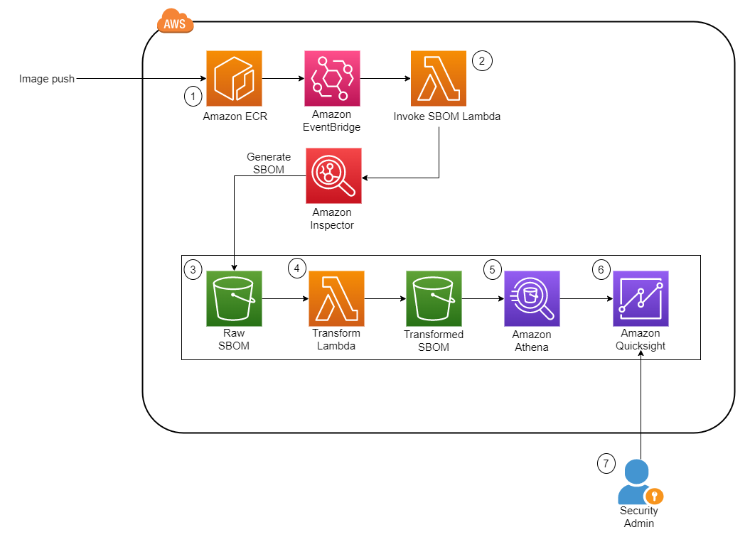


 Venkata Kampana is a Senior Solutions Architect in the AWS Health and Human Services team and is based in Sacramento, CA. In that role, he helps public sector customers achieve their mission objectives with well-architected solutions on AWS.
 Jim Daniel is the Public Health lead at Amazon Web Services. Previously, he held positions with the United States Department of Health and Human Services for nearly a decade, including Director of Public Health Innovation and Public Health Coordinator. Before his government service, Jim served as the Chief Information Officer for the Massachusetts Department of Public Health.


 Pramod Nayak is the Director of Product Management of the Low Latency Group at LSEG. Pramod has over 10 years of experience in the financial technology industry, focusing on software development, analytics, and data management. Pramod is a former software engineer and passionate about market data and quantitative trading.
 LakshmiKanth Mannem is a Product Manager in the Low Latency Group of LSEG. He focuses on data and platform products for the low-latency market data industry. LakshmiKanth helps customers build the most optimal solutions for their market data needs.
 Vivek Aggarwal is a Senior Data Engineer in the Low Latency Group of LSEG. Vivek works on developing and maintaining data pipelines for processing and delivery of captured market data feeds and reference data feeds.
 Alket Memushaj is a Principal Architect in the Financial Services Market Development team at AWS. Alket is responsible for technical strategy, working with partners and customers to deploy even the most demanding capital markets workloads to the AWS Cloud.


 Pathik Shah is a Sr. Analytics Architect on Amazon Athena. He joined AWS in 2015 and has been focusing in the big data analytics space since then, helping customers build scalable and robust solutions using AWS analytics services.
 Raj Devnath is a Product Manager at AWS on Amazon Athena. He is passionate about building products customers love and helping customers extract value from their data. His background is in delivering solutions for multiple end markets, such as finance, retail, smart buildings, home automation, and data communication systems.


 Claudia Chitu is a Data strategist and an influential leader in the Analytics space. Focused on aligning data initiatives with the overall strategic goals of the organization, she employs data as a guiding force for long-term planning and sustainable growth.
 Spyridon Dosis is an Information Security Professional in Acast. Spyridon supports the organization in designing, implementing and operating its services in a secure manner protecting the company and users’ data.
 Srikant Das is an Acceleration Lab Solutions Architect at Amazon Web Services. He has over 13 years of experience in Big Data analytics and Data Engineering, where he enjoys building reliable, scalable, and efficient solutions. Outside of work, he enjoys traveling and blogging his experiences in social media.


 Rahul Sonawane is a Principal Analytics Solutions Architect at AWS with AI/ML and Analytics as his area of specialty.
 Gaurav Parekh is a Solutions Architect helping AWS customers build large scale modern architecture. He specializes in data analytics and networking. Outside of work, Gaurav enjoys playing cricket, soccer and volleyball.


 Sandeep Adwankar is a Senior Technical Product Manager at AWS. Based in the California Bay Area, he works with customers around the globe to translate business and technical requirements into products that enable customers to improve how they manage, secure, and access data.
 Navnit Shukla serves as an AWS Specialist Solution Architect with a focus on Analytics. He possesses a strong enthusiasm for assisting clients in discovering valuable insights from their data. Through his expertise, he constructs innovative solutions that empower businesses to arrive at informed, data-driven choices. Notably, Navnit Shukla is the accomplished author of the book titled Data Wrangling on AWS. He can be reached via


 Darshit Thakkar is a Technical Product Manager with AWS and works with the Amazon Athena team based out of Boston, Massachusetts.
 Wei Zheng is a Sr. Software Development Engineer with Amazon Athena. He joined AWS in 2021 and has been working on multiple performance improvements on Athena.
 Chuho Chang is a Software Development Engineer with Amazon Athena. He has been working on query optimizers for over a decade.
 Pathik Shah is a Sr. Analytics Architect on Amazon Athena. He joined AWS in 2015 and has been focusing in the big data analytics space since then, helping customers build scalable and robust solutions using AWS analytics services.


 Let’s go through each numbered step as outlined in the architecture:
 Philipp Karg is Lead FinOps Engineer at BMW Group and founder of the CLEA platform. He focus on boosting cloud efficiency initiatives and establishing a cost-aware culture within the company to ultimately leverage the cloud in a sustainable way.
 Alex Gutfreund is Head of Product and Technology Integration at the BMW Group. He spearheads the digital transformation with a particular focus on platforms ecosystems and efficiencies. With extensive experience at the interface of business and IT, he drives change and makes an impact in various organizations. His industry knowledge spans from automotive, semiconductor, public transportation, and renewable energies.
 Cizer Pereira is a Senior DevOps Architect at AWS Professional Services. He works closely with AWS customers to accelerate their journey to the cloud. He has a deep passion for Cloud Native and DevOps, and in his free time, he also enjoys contributing to open-source projects.
 Selman Ay is a Data Architect in the AWS Professional Services team. He has worked with customers from various industries such as e-commerce, pharma, automotive and finance to build scalable data architectures and generate insights from the data. Outside of work, he enjoys playing tennis and engaging in outdoor activities.
 Nick McCarthy is a Senior Machine Learning Engineer in the AWS Professional Services team. He has worked with AWS clients across various industries including healthcare, finance, sports, telecoms and energy to accelerate their business outcomes through the use of AI/ML. Outside of work Nick loves to travel, exploring new cuisines and cultures in the process.
 Miguel Henriques is a Cloud Application Architect in the AWS Professional Services team with 4 years of experience in the automotive industry delivering cloud native solutions. In his free time, he is constantly looking for advancements in the web development space and searching for the next great pastel de nata.


 Michael Hamilton is a Sr Analytics Solutions Architect focusing on helping enterprise customers in the south east modernize and simplify their analytics workloads on AWS. He enjoys mountain biking and spending time with his wife and three children when not working.
 Cody Penta is a Solutions Architect at Amazon Web Services and is based out of Charlotte, NC. He has a focus in security and CDK, and enjoys solving the really difficult problems in the technology world. Off the clock, he loves relaxing in the mountains, coding personal projects, and gaming.
 Angus Ferguson is a Solutions Architect at AWS who is passionate about meeting customers across the world, helping them solve their technical challenges. Angus specializes in Data & Analytics with a focus on customers in the financial services industry.


 Anirban Sinha is a Senior Technical Account Manager at AWS. He is passionate about building scalable data warehouses and big data solutions working closely with customers. He works with large ISVs customers, in helping them build and operate secure, resilient, scalable, and high-performance SaaS applications in the cloud.
 Phil Bates is a Senior Analytics Specialist Solutions Architect at AWS. He has more than 25 years of experience implementing large-scale data warehouse solutions. He is passionate about helping customers through their cloud journey and using the power of ML within their data warehouse.
 Gaurav Singh is a Senior Solutions Architect at AWS, specializing in AI/ML and Generative AI. Based in Pune, India, he focuses on helping customers build, deploy, and migrate ML production workloads to SageMaker at scale. In his spare time, Gaurav loves to explore nature, read, and run.