Tag Archives: Amazon Athena

How ANZ Institutional Division built a federated data platform to enable their domain teams to build data products to support business outcomes

Post Syndicated from Leo Ramsamy original https://aws.amazon.com/blogs/big-data/how-anz-institutional-division-built-a-federated-data-platform-to-enable-their-domain-teams-to-build-data-products-to-support-business-outcomes/

In today’s rapidly evolving financial landscape, data is the bedrock of innovation, enhancing customer and employee experiences and securing a competitive edge. Recognizing this paradigm shift, ANZ Institutional Division has embarked on a transformative journey to redefine its approach to data management, utilization, and extracting significant business value from data insights.

Like many large financial institutions, ANZ Institutional Division operated with siloed data practices and centralized data management teams. As time went on, the limitations of this approach became apparent due to rising data complexity, larger volumes, and the growing demand for swift, business-driven insights. Consequently, the bank encountered several challenges and needed to take the following actions:

  • Create business insights from untapped data potential, estimated to be approximately $150 million in the Institutional Division alone
  • Improve operational efficiency by removing manual data handling, the use of spreadsheets, and duplicate data entries
  • Increase agility by making data expertise more readily available, thereby improving time to market and overall customer experience
  • Address data quality
  • Standardize tooling and remove the Shadow IT culture, driving scalability, reducing risk, and minimizing overall operational inefficiencies

These challenges are not unique to ANZ Institutional Division. Globally, financial institutions have been experiencing similar issues, prompting a widespread reassessment of traditional data management approaches.

One major trend, embraced by many financial institutions, has been the adoption of the data mesh architecture and the shift towards treating data as a product. This paradigm, pioneered by thought leaders like Zhamak Dehghani, introduces a decentralized approach to data management that aligns closely with modern organizational structures and agile methodologies.

Some notable global examples of leading companies embracing and implementing this trend are JPMorgan Chase, Capital One, and Saxo Bank.

Inspired by these global trends and driven by its own unique challenges, ANZ’s Institutional Division decided to pivot from viewing data as a byproduct of projects to treating it as a valuable product in its own right.

This shift promises several business benefits:

  • Empowered domain expertise – By decentralizing data ownership to domain-based teams, ANZ can use the deep business knowledge within each unit to create more relevant and valuable data products
  • Increased agility – Domain teams can now respond more quickly to business needs, creating and iterating on data products without relying on a centralized bottleneck
  • Improved data quality – With domain experts overseeing their own data, there’s a greater likelihood of catching and correcting quality issues at the source
  • Scalability – The federated approach allows for greater scalability, enabling ANZ to handle increasing data volumes and complexity more effectively
  • Innovation catalyst – By democratizing data access and empowering teams to create data products, ANZ is fostering a culture of innovation and data-driven decision-making across the organization

This transition is not just about technology; it represents a fundamental shift in how ANZ views and values its data assets. By treating data as a product, the bank is positioned to not only overcome current challenges, but to unlock new opportunities for growth, customer service, and competitive advantage.

This post explores how the shift to a data product mindset is being implemented, the challenges faced, and the early wins that are shaping the future of data management in the Institutional Division.

ANZ’s federated data strategy

In response to the challenges, ANZ Group formulated a data strategy that focuses on empowering employees to securely use data to improve the sustainability and financial well-being of their customers. At its core are the following pillars:

  • Introducing new ways of working that focus on generating customer value first
  • New technology platforms and tooling that allow the bank to collect, share, archive, and dispose data in a secure and controlled way
  • Achieving consistency in how data is produced and consumed across the entire bank through data products and better-connected systems
  • Supporting the bank’s risk and regulatory obligations by providing a secure and resilient data platform that provides fine-grained, controlled access to quality data products

ANZ has made the strategic decision to adopt an architectural and operational model aligned with the data mesh paradigm, which revolves around four key principles: domain ownership, data as a product, a self-serve data platform, and federated computational governance.

Domain ownership recognizes that the teams generating the data have the deepest understanding of it and are therefore best suited to manage, govern, and share it effectively. This principle makes sure data accountability remains close to the source, fostering higher data quality and relevance.

Treating data as a product instils a product-centric mindset, emphasizing that data must be secure, discoverable, understandable, interoperable, reusable, and managed throughout its lifecycle. This principle makes sure data consumers, both internal and external, derive consistent value from well-designed data products.

A self-serve data platform empowers domains to create, discover, and consume data products independently. It abstracts technical complexities and provides user-friendly tools, enabling a scalable, repeatable, and automated approach to producing high-quality data products.

Under the federated mesh architecture, each divisional mesh functions as a node within the broader enterprise data mesh, maintaining a degree of autonomy in managing its data products. To effectively coordinate these autonomous nodes and facilitate seamless integration, enterprise-wide standards, such as those related to data governance, interoperability, and security, are essential to maintain alignment and consistency across all nodes and domains and teams within.

With this approach, each node in ANZ maintains its divisional alignment and adherence to data risk and governance standards and policies to manage local data products and data assets. This enables global discoverability and collaboration without centralizing ownership or operations.

As a result, governance resides with the data products themselves, making sure standards and policies, such as access control, data quality, and compliance, are enforced where the data lives. In this regard, the enterprise data product catalog acts as a federated portal, facilitating cross-domain access and interoperability while maintaining alignment with governance principles. This model balances node or domain-level autonomy with enterprise-level oversight, creating a scalable and consistent framework across ANZ.

Within the ANZ enterprise data mesh strategy, aligning data mesh nodes with the ANZ Group’s divisional structure provides optimal alignment between data mesh principles and organizational structure, as shown in the following diagram.

Central to the success of this strategy is its support for each division’s autonomy and freedom to choose their own domain structure, which is closely aligned to their business needs. Divisions decide how many domains to have within their node; some may have one, others many. These nodes can implement analytical platforms like data lake houses, data warehouses, or data marts, all united by producing data products. Nodes and domains serve business needs and are not technology mandated.

Under the federated computational governance model, the ANZ Group strategy defines guardrails that treat a node as a logical data container suitable for the following:

  • Ingestion and metadata management
  • Creating source-aligned data products complying with ANZ’s Data Product Specification (DPS)
  • Integrating source-aligned data products from other nodes
  • Producing consumer-aligned data products for specific business purposes
  • Publishing conforming data products to ANZ’s Data Product Catalog (DPC)

Following on from this strategy is organizing its domain structure to provide autonomy to various functional teams while preserving the core values of data mesh. The following diagram depicts an example of the possible structure.

For instance, Domain A will have the flexibility to create data products that can be published to the divisional catalog, while also maintaining the autonomy to develop data products that are exclusively accessible to teams within the domain. These products will not be available to others until they are deemed ready for broader enterprise use.

This strategy supports each division’s autonomy to implement their own data catalogs and decide which data products to publish to the group-level catalog. This flexibility extends to divisional domains, which can choose which data products to publish to the divisional catalog or keep visible only to domain consumers.

Institutional Data & AI Platform architecture

The Institutional Division has implemented a self-service data platform to enable the domain teams to build and manage data products autonomously. The Institutional Data & AI platform adopts a federated approach to data while centralizing the metadata to facilitate simpler discovery and sharing of data products. The following diagram illustrates the building blocks of the Institutional Data & AI Platform.

The building blocks are as follows:

  1. Foundational Data & AI Platform capabilities – A dedicated data platform team provides domain-agnostic tools, systems, and capabilities to enable autonomous data product development across domains. This self-serve infrastructure allows domain teams to manage the full data lifecycle without relying on a centralized data team. Key capabilities include data storage, data onboarding and transformation, and data utilities that facilitate data sharing with interoperability between domains. These capabilities abstract the technical complexities associated with data management infrastructure, allowing domain experts to focus on creating valuable data products rather than infrastructure management.
  2. Domain-owned data assets – The domain-oriented data ownership approach distributes responsibility for data across the business units within the Institutional Division. Domain teams are responsible for developing, deploying, and managing their own analytical data products alongside operational data services. Data contracts authored by data product owners automate data product creation and provide a standard to access data products. By treating the data as a product, the outcome is a reusable asset that outlives a project and meets the needs of the enterprise consumer. Consumer feedback and demand drives creation and maintenance of the data product.
  3. Division-level metadata management and data governance – A centrally hosted service provides domain teams with the capability to publish their data products along with relevant metadata, like business definitions and lineage. Some of the key features implemented are:
    1. Metadata management that centralizes metadata and presents it within the context of data products, such as data quality scores and data product lineage.
    2. A data portal for consumers to discover data products and access associated metadata.
    3. Subscription workflows that simplify access management to the data products.
    4. Computational governance that enforces divisional and enterprise data policies and standards, such as data classification and business data models for aligning terminology.

The following diagram is a high-level example of the technical architecture approach towards the Institutional Data & AI Platform. The solution uses a building block approach, on a cloud-centered platform comprised of AWS services, with partner solutions and open standards like OpenLineage and Apache Iceberg.

Let’s look at the key services that enable the federated platform to operate at scale:

  • Data storage and processing:
    • Apache Iceberg on Amazon Simple Storage Service (Amazon S3) offers an optimized way to store data assets and products and promotes interoperability across other services
    • Amazon Redshift allows domain teams to create and manage fit-for-purpose data marts
    • AWS Lambda and AWS Glue are used for data onboarding and processing, and data utilities created in Python and PySpark promote reusability and quality across the data processing pipelines
    • dbt simplifies data transformation rules and allows sub-domain data analysts to build modeling logic as SQL statements
    • Amazon Managed Workflows for Apache Airflow (Amazon MWAA) enables efficient management of workflows and data pipeline orchestration using out-of-the-box integrations with AWS services
  • Metadata management and data governance:
    • To maintain data reliability and accuracy, a robust data quality framework using Soda core is used that automates data quality using checks defined in a data contract
    • Amazon DataZone enables data product cataloging, discovery, metadata management, and implementing computational governance
    • OpenLineage simplifies harvesting and collection of data and process-level lineage, which are then published to Amazon DataZone
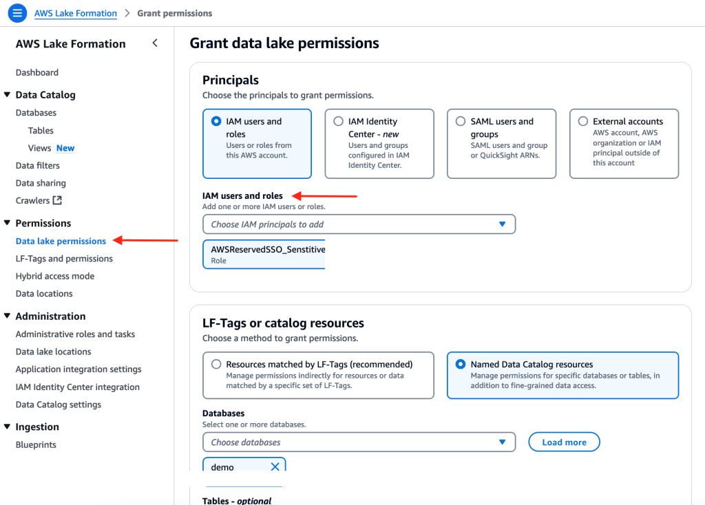
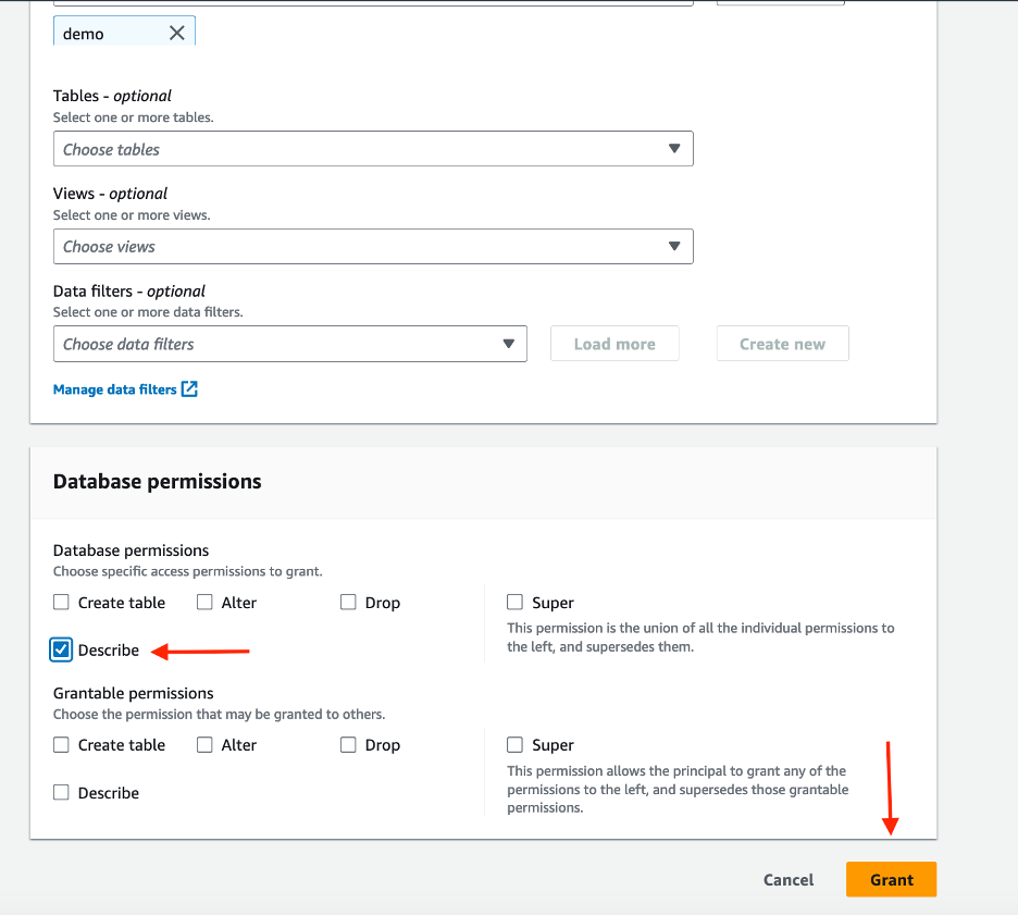
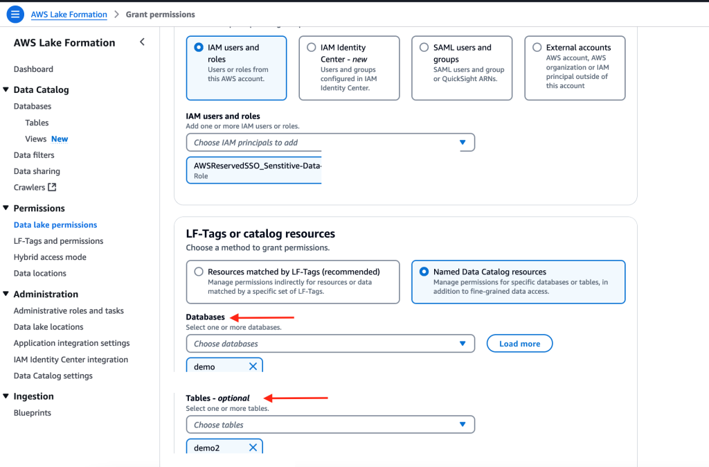
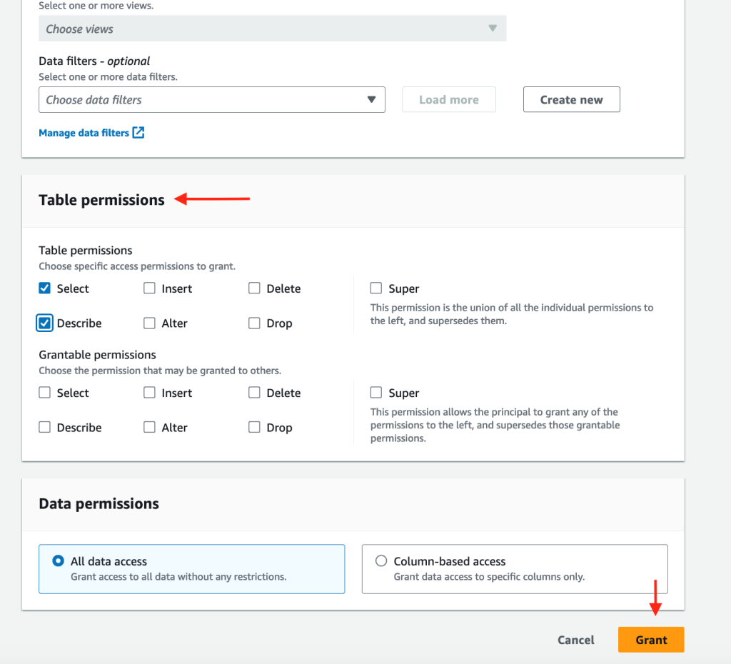
    • AWS Lake Formation, combined with AWS Glue Data Catalog, provides data governance and access management to data products that reside within sub-domains
  • Analytics:
    • Tableau offers capabilities for sub-domains with data visualization and business intelligence capabilities
  • Observability and security:
    • Observability needs of the platform are built into all the processes using monitoring, with logging functionality provided by Amazon CloudWatch and AWS CloudTrail
    • AWS Secrets Manager makes sure secrets are stored and made available for data pipelines to access services in a secure manner

The technical implementation actualizes the data product strategy at ANZ Institutional Division. Amazon DataZone plays an essential role in facilitating data product management for the domain teams. The service addresses several critical aspects of the Institutional Division’s data product strategy, including:

  • Data cataloging and metadata management – Amazon DataZone provides comprehensive data cataloging and metadata management capabilities
  • Data governance and compliance – Effective data governance is essential for scaling data products
  • Self-service capabilities – Amazon DataZone empowers domain teams with self-service capabilities, enabling them to create, manage, and deploy data products independently
  • Integration and interoperability – One of the challenges in scaling data products is providing seamless integration across various data sources and systems
  • Collaboration and sharing – Amazon DataZone provides a platform for sharing data and metadata across teams and domains

Institutional Division’s delivery model to achieve scale

The Institutional Division has successfully used the federated architecture, and key to this delivery model is the implementation of Foundational Data & AI Platform capabilities that serve all domains within the division. This model promotes self-service and accelerates the delivery of subsequent initiatives by using the capabilities built for previous use cases.

To evaluate the success of the delivery model, ANZ has implemented key metrics, such as cost transparency and domain adoption, to guide the data mesh governance team in refining the delivery approach. For instance, one enhancement involves integrating cross-functional squads to support data literacy.

The key to scaling the Institutional Division operating model are the following considerations:

  • Data as a product approach – Use techniques like event storming and domain-driven design to capture business events and their meanings.
  • Education and enablement – Conduct learning interventions to upskill teams on understanding and using the data as a product approach.
  • Iterative data platform delivery – Work backward from business initiative to iteratively deliver self-service data platform infrastructure capabilities.
  • Managing demand efficiently – Implement a feedback mechanism to manage demand on data products. Track and manage data debt using standard data contract specifications. Most importantly, adopt governance and standards to make sure data products are built and maintained with a long-term perspective, minimizing technical debt.

“The Institutional Data & Analytics Platform (IDAP) has allowed the Institutional team to establish a base foundation to allow various teams to aggregate and consume the wealth of data across the division. This self-service platform enables business leaders to both create and consume reusable data products, unlocking value across this division. It’s also an excellent proof point for our broader data mesh architecture, allowing us to connect this divisional data to broader enterprise data stores—further positioning us to put the customer at the center of everything we do.”

– Tim Hogarth, CTO ANZ

“AWS believes that democratizing data, while not compromising on security and fine-grained access, is a key component of any future-proof, scalable data platform, so we are pleased to be enabling ANZ bank’s IDAP metadata management and data governance capabilities through Amazon DataZone. This allows the diverse business functions at ANZ the autonomy to self-serve on their data needs with built-in governance.”

– Shikha Verma, Head of Product, Amazon DataZone

Conclusion

ANZ’s journey to move towards a data product approach has improved the organization’s approach to manage data and reduce data silos, and has positioned it to become a data-driven, customer-centric organization. By combining federated platform practices and adopting AWS services and open standards, ANZ Institutional Division is achieving its objectives in decentralization with a scalable data platform that enables its domain teams to make informed decisions, drive innovation, and maintain a competitive edge.

Special thanks: This implementation success is a result of close collaboration between ANZ Institutional Division, AWS ProServe, and the AWS account team. We want to thank ANZ Institutional Executives and the Leadership Team for the strong sponsorship and direction.


About the Authors

Leo Ramsamy is a Platform Architect specializing in data and analytics for ANZ’s Institutional division. He focuses on modern data practices, including Data Mesh architecture, data governance, quality management, and observability. His work aligns data strategies with business goals, improving accessibility and enabling better decision-making across ANZ.

Srinivasan Kuppusamy is a Senior Cloud Architect – Data at AWS ProServe, where he helps customers solve their business problems using the power of AWS Cloud technology. His areas of interests are data and analytics, data governance, and AI/ML.

Rada Stanic is a Chief Technologist at Amazon Web Services, where she helps ANZ customers across different segments solve their business problems using AWS Cloud technologies. Her special areas of interest are data analytics, machine learning/AI, and application modernization.

Amazon SageMaker Lakehouse integrated access controls now available in Amazon Athena federated queries

Post Syndicated from Esra Kayabali original https://aws.amazon.com/blogs/aws/amazon-sagemaker-lakehouse-integrated-access-controls-now-available-in-amazon-athena-federated-queries/

Today, we announced the next generation of Amazon SageMaker, which is a unified platform for data, analytics, and AI, bringing together widely-adopted AWS machine learning and analytics capabilities. At its core is SageMaker Unified Studio (preview), a single data and AI development environment for data exploration, preparation and integration, big data processing, fast SQL analytics, model development and training, and generative AI application development. This announcement includes Amazon SageMaker Lakehouse, a capability that unifies data across data lakes and data warehouses, helping you build powerful analytics and artificial intelligence and machine learning (AI/ML) applications on a single copy of data.

In addition to these launches, I’m happy to announce data catalog and permissions capabilities in Amazon SageMaker Lakehouse, helping you connect, discover, and manage permissions to data sources centrally.

Organizations today store data across various systems to optimize for specific use cases and scale requirements. This often results in data siloed across data lakes, data warehouses, databases, and streaming services. Analysts and data scientists face challenges when trying to connect to and analyze data from these diverse sources. They must set up specialized connectors for each data source, manage multiple access policies, and often resort to copying data, leading to increased costs and potential data inconsistencies.

The new capability addresses these challenges by simplifying the process of connecting to popular data sources, cataloging them, applying permissions, and making the data available for analysis through SageMaker Lakehouse and Amazon Athena. You can use the AWS Glue Data Catalog as a single metadata store for all data sources, regardless of location. This provides a centralized view of all available data.

Data source connections are created once and can be reused, so you don’t need to set up connections repeatedly. As you connect to the data sources, databases and tables are automatically cataloged and registered with AWS Lake Formation. Once cataloged, you grant access to those databases and tables to data analysts, so they don’t have to go through separate steps of connecting to each data source and don’t have to know built-in data source secrets. Lake Formation permissions can be used to define fine-grained access control (FGAC) policies across data lakes, data warehouses, and online transaction processing (OLTP) data sources, providing consistent enforcement when querying with Athena. Data remains in its original location, eliminating the need for costly and time-consuming data transfers or duplications. You can create or reuse existing data source connections in Data Catalog and configure built-in connectors to multiple data sources, including Amazon Simple Storage Service (Amazon S3), Amazon Redshift, Amazon Aurora, Amazon DynamoDB (preview), Google BigQuery, and more.

Getting started with the integration between Athena and Lake Formation
To showcase this capability, I use a preconfigured environment that incorporates Amazon DynamoDB as a data source. The environment is set up with appropriate tables and data to effectively demonstrate the capability. I use the SageMaker Unified Studio (preview) interface for this demonstration.

To begin, I go to SageMaker Unified Studio (preview) through the Amazon SageMaker domain. This is where you can create and manage projects, which serve as shared workspaces. These projects allow team members to collaborate, work with data, and develop ML models together. Creating a project automatically sets up AWS Glue Data Catalog databases, establishes a catalog for Redshift Managed Storage (RMS) data, and provisions necessary permissions.

To manage projects, you can either view a comprehensive list of existing projects by selecting Browse all projects, or you can create a new project by choosing Create project. I use two existing projects: sales-group, where administrators have full access privileges to all data, and marketing-project, where analysts operate under restricted data access permissions. This setup effectively illustrates the contrast between administrative and limited user access levels.

In this step, I set up a federated catalog for the target data source, which is Amazon DynamoDB. I go to Data in the left navigation pane and choose the + (plus) sign to Add data. I choose Add connection and then I choose Next.

I choose Amazon DynamoDB and choose Next.

I enter the details and choose Add data. Now, I have the Amazon DynamoDB federated catalog created in SageMaker Lakehouse. This is where your administrator gives you access using resource policies. I’ve already configured the resource policies in this environment. Now, I’ll show you how fine-grained access controls work in SageMaker Unified Studio (preview).

I begin by selecting the sales-group project, which is where administrators maintain and have full access to customer data. This dataset contains fields such as zip codes, customer IDs, and phone numbers. To analyze this data, I can execute queries using Query with Athena.

Upon selecting Query with Athena, the Query Editor launches automatically, providing a workspace where I can compose and execute SQL queries against the lakehouse. This integrated query environment offers a seamless experience for data exploration and analysis.

In the second part, I switch to marketing-project to show what an analyst experiences when they run their queries and observe that the fine-grained access control permissions are in place and working.

In the second part, I demonstrate the perspective of an analyst by switching to the marketing-project environment. This helps us verify that the fine-grained access control permissions are properly implemented and effectively restricting data access as intended. Through example queries, we can observe how analysts interact with the data while being subject to the established security controls.

Using the Query with Athena option, I execute a SELECT statement on the table to verify the access controls. The results confirm that, as expected, I can only view the zipcode and cust_id columns, while the phone column remains restricted based on the configured permissions.

With these new data catalog and permissions capabilities in Amazon SageMaker Lakehouse, you can now streamline your data operations, enhance security governance, and accelerate AI/ML development while maintaining data integrity and compliance across your entire data ecosystem.

Now available
Data catalog and permissions in Amazon SageMaker Lakehouse simplifies interactive analytics through federated query when connecting to a unified catalog and permissions with Data Catalog across multiple data sources, providing a single place to define and enforce fine-grained security policies across data lakes, data warehouses, and OLTP data sources for a high-performing query experience.

You can use this capability in US East (N. Virginia), US West (Oregon), US East (Ohio), Europe (Ireland), and Asia Pacific (Tokyo) AWS Regions.

To get started with this new capability, visit the Amazon SageMaker Lakehouse documentation.

— Esra

From data lakes to insights: dbt adapter for Amazon Athena now supported in dbt Cloud

Post Syndicated from Darshit Thakkar original https://aws.amazon.com/blogs/big-data/from-data-lakes-to-insights-dbt-adapter-for-amazon-athena-now-supported-in-dbt-cloud/

At AWS, we are committed to empowering organizations with tools that streamline data analytics and transformation processes. We are excited to announce that the dbt adapter for Amazon Athena is now officially supported in dbt Cloud. This integration enables data teams to efficiently transform and manage data using Athena with dbt Cloud’s robust features, enhancing the overall data workflow experience.

In this post, we discuss the advantages of dbt Cloud over dbt Core, common use cases, and how to get started with Amazon Athena using the dbt adapter.

The need for streamlined data transformations

As organizations increasingly adopt cloud-based data lakes and warehouses, the demand for efficient data transformation tools has grown. Athena plays a critical role in this ecosystem by providing a serverless, interactive query service that simplifies analyzing vast amounts of data stored in Amazon Simple Storage Service (Amazon S3) using standard SQL. This enables you to extract insights from your data without the complexity of managing infrastructure.

dbt has emerged as a leading framework, allowing data teams to transform and manage data pipelines effectively. With the dbt adapter for Athena adapter now supported in dbt Cloud, you can seamlessly integrate your AWS data architecture with dbt Cloud, taking advantage of the scalability and performance of Athena to simplify and scale your data workflows efficiently.

Benefits of the dbt adapter for Athena

We have collaborated with dbt Labs and the open source community on an adapter for dbt that enables dbt to interface directly with Athena. Previously, the dbt adapter for Athena was only compatible with dbt Core, requiring teams to manually manage configurations and execute transformations locally or through custom setups. Now, with support for dbt Cloud, you can access a managed, cloud-based environment that automates and enhances your data transformation workflows. This upgrade allows you to build, test, and deploy data models in dbt with greater ease and efficiency, using all the features that dbt Cloud provides.

The support of the dbt adapter for Athena in dbt Cloud offers several advantages over using it with dbt Core:

  • Managed infrastructure – dbt Cloud provides a fully managed environment for running dbt projects, eliminating the need for local setup, maintenance, and configuration. This saves time and effort, especially for teams looking to minimize infrastructure management and focus solely on data modeling.
  • Scheduling and automation – dbt Cloud comes with a job scheduler, allowing you to automate the execution of dbt models. This feature makes sure your datasets are always up to date without needing to set up and maintain external scheduling systems like Apache Airflow. You can also set up dependencies between jobs easily within dbt Cloud, making sure that transformations run in the correct sequence without manual oversight.
  • Enhanced collaboration and version control – You can use a web-based interface for editing and reviewing dbt models, enabling collaboration among data teams. You can review code changes directly on the platform, facilitating efficient teamwork. Additionally, dbt Cloud integrates with Git providers, making version control and code collaboration more streamlined. This makes sure your data models are well-documented, versioned, and straightforward to manage within a collaborative environment.
  • Monitoring and alerting – You get built-in tools for monitoring job executions and performance to set up alerts and notifications for job failures, providing quick response times and minimizing disruptions. Furthermore, you can gain insights into the performance of your data transformations with detailed execution logs and metrics, all accessible through the dbt Cloud interface.

Common use cases for using the dbt adapter with Athena

The following are common use cases for using the dbt adapter with Athena:

  • Building a data warehouse – Many organizations are moving towards a data warehouse architecture, combining the flexibility of data lakes with the performance and structure of data warehouses. Using Athena and the dbt adapter, you can transform raw data in Amazon S3 into well-structured tables suitable for analytics. This setup allows businesses to build a scalable and efficient data lakehouse where they can perform SQL-based transformations and make sure data is clean and ready for analytics without investing heavily in data warehouse infrastructure.
  • Incremental data processing – The adapter allows for incremental data processing, where only new or updated data is transformed and processed. This feature reduces the amount of data scanned by Athena, resulting in faster query performance and lower costs. For example, instead of processing an entire dataset daily, dbt can be configured to transform only the data ingested in the last 24 hours, making data operations more efficient and cost-effective.
  • Cost management and optimization – Because Athena charges based on the amount of data scanned by each query, cost optimization is critical. The adapter enables data teams to optimize transformations by creating efficient data models, such as partitioning and compressing data to minimize scan costs. Additionally, dbt’s automated scheduling in dbt Cloud can be used to manage the frequency of data transformations, making sure queries are run only when necessary, helping to control costs effectively.
  • Data archiving and tiered storage – Organizations with a large amount of historical data can use Athena to query archived data stored in the lower-cost storage classes of Amazon S3 (such as Amazon S3 Glacier). With the adapter, data teams can build models that segment and process data based on usage patterns, making sure frequently accessed data is optimized for quick queries while older data remains accessible but cost-efficient. Alternatively, you can use Amazon S3 Intelligent-Tiering to optimize storage costs by moving data between two access tiers when access patterns change. This approach helps in managing storage costs while maintaining the flexibility to analyze historical trends when needed.
  • Event-driven data transformations – In scenarios where organizations need to process data in near real time, such as for streaming event logs or Internet of Things (IoT) data, you can integrate the adapter into an event-driven architecture. For example, event data can be continuously loaded into Amazon S3, and dbt models can be configured to run incrementally, transforming the new data into structured formats for immediate analysis. This setup supports agile data processing while taking advantage of the serverless architecture of Athena to keep operational costs low.
  • Compliance and data governance – For organizations managing sensitive or regulated data, you can use Athena and the adapter to enforce data governance rules. With dbt, teams can define data quality checks and access controls as part of their transformation workflow. This makes sure that only compliant, high-quality data is made available for analytics, and costs are optimized by processing only the data that meets governance standards. Additionally, dbt’s documentation features help maintain a clear record of data transformations, supporting audit and compliance efforts.

How to use the dbt adapter for Athena

To get started, create a project and set up a connection with Athena in dbt Cloud. The following figure shows the steps to create a project using dbt Cloud and configure the Athena connection.

Next, use the dbt Cloud interactive development environment (IDE) to deploy your project. The following figure demonstrates how to build dbt runs and deploy changes to Athena using the dbt Cloud interface.

Conclusion

At AWS, we are committed to providing you with the best possible tools and services to help you succeed in the cloud. dbt has emerged as a leading data transformation platform, trusted by thousands of organizations worldwide. By partnering with dbt Labs, we are able to bring the power of dbt directly to the AWS Cloud, empowering you to seamlessly integrate your data transformation workflows into the broader cloud infrastructure. This partnership is a testament to our shared vision of making data more accessible, reliable, and valuable for organizations of all sizes.

We are excited to see how you will use the dbt Cloud compatible dbt adapter for Athena to drive your data-driven initiatives forward. The combination of dbt and Athena creates a powerful and efficient environment for transforming and analyzing data in a serverless architecture. This synergy allows you to take advantage of the strengths of both tools, making it straightforward to manage complex data pipelines, reduce costs, and scale your operations.


About the Authors

Darshit Thakkar is a Technical Product Manager with AWS and works with the Amazon Athena team.

Selman Ay is a Data Architect in the AWS Professional Services team.

BP Yau is a Sr Partner Solutions Architect at AWS helping customers architect big data solutions to process data at scale

Streamline AI-driven analytics with governance: Integrating Tableau with Amazon DataZone

Post Syndicated from Ramesh H Singh original https://aws.amazon.com/blogs/big-data/streamline-ai-driven-analytics-with-governance-integrating-tableau-with-amazon-datazone/

Amazon DataZone is a data management service that makes it faster and easier for customers to catalog, discover, share, and govern data stored across AWS, on premises, and from third-party sources. Amazon DataZone recently announced the expansion of data analysis and visualization options for your project-subscribed data within Amazon DataZone using the Amazon Athena JDBC driver.

Collaborating closely with our partners, we have tested and validated Amazon DataZone authentication via the Athena JDBC connection, providing an intuitive and secure connection experience for users. With this integration, you can now seamlessly query your governed data lake assets in Amazon DataZone using popular business intelligence (BI) and analytics tools, including partner solutions like Tableau.

Ali Tore, Senior Vice President of Advanced Analytics at Salesforce, highlighting the value of this integration, says

“We’re excited to partner with Amazon to bring Tableau’s powerful data exploration and AI-driven analytics capabilities to customers managing data across organizational boundaries with Amazon DataZone. This integration enables our customers to seamlessly explore data with AI in Tableau, build visualizations, and uncover insights hidden in their governed data, all while leveraging Amazon DataZone to catalog, discover, share, and govern data across AWS, on premises, and from third-party sources—enhancing both governance and decision-making.”

With this launch, Amazon DataZone strengthens its commitment to empowering enterprise customers with secure, governed access to data across the tools and platforms they rely on. For example, Guardant Health uses Amazon DataZone to democratize data access across its organization, enabling diverse teams to efficiently access, query, and analyze data tailored to their specific needs.

Rajesh Kucharlapati, Senior Director of Data, CRM, and Analytics at Guardant Health, says

“By harmonizing data across multiple business domains, we foster a culture of data sharing. Using Amazon DataZone lets us avoid building and maintaining an in-house platform, allowing our developers to focus on tailored solutions. Leveraging AWS’s managed service was crucial for us to access business insights faster, apply standardized data definitions, and tap into generative AI potential. We also needed an easy connection process for widely-used analytics tools like Tableau, DBeaver, and Domino, directly within Amazon DataZone projects. This new JDBC connectivity feature enables our governed data to flow seamlessly into these tools, supporting productivity across our teams.”

Use case

Amazon DataZone addresses your data sharing challenges and optimizes data availability. Here’s how:

  • Data product creation – As a data producer, you can create and catalog data products while enforcing governance, making your data findable, accessible, interoperable, and reusable (FAIR).
  • Streamlined access – As a data consumer, you can easily locate and subscribe to data from multiple sources within a single project. You can analyze this data using a variety of tools, including built-in AWS options such as Amazon Athena, Amazon Redshift, and Amazon SageMaker.
  • Integration with partner tools – The addition of support for partner analytics tools offers you greater flexibility and efficiency in your workflows. You can now use your tool of choice, including Tableau, to quickly derive business insights from your data while using standardized definitions and decentralized ownership. Refer to the detailed blog post on how you can use this to connect through various other tools.

Prerequisites

To get started, complete these steps:

  1. Download and install the latest Athena JDBC driver for Tableau.
  2. Copy the JDBC connection string from the Amazon DataZone portal into the JDBC connection configuration to establish a connection from Tableau. This will direct you to authenticate using single sign-on with your corporate credentials.

When you’re connected, you can query, visualize, and share data—governed by Amazon DataZone—within Tableau.

The following diagram shows the high-level architecture of the Tableau integration.

Solution walkthrough: Configure Tableau to access project-subscribed data assets

To configure Tableau to access project-subscribed data assets, follow these detailed steps:

  1. Download the latest Athena driver. If Tableau has the Athena driver preinstalled, it could be the older (v2) version. To confirm compatibility with Amazon DataZone, you’ll need the latest (v3) driver that includes the necessary authentication features. To download the latest JDBC driver version x, visit Athena JDBC 3.x driver.
  2. Install the driver. Copy the JDBC driver file to the appropriate folder for your operating system:
    • For macOS: ~/Library/Tableau/Drivers
    • For Windows: C:\Program Files\Tableau\Drivers
  3. On the Amazon DataZone console, select your project, as shown in the following screenshot of DataZone Console.
  4. To capture the JDBC connection parameters, follow these steps:
    1. On the project page, review the connection options under ANALYTICS TOOLS. Choose Connect with JDBC.
    2. In the JDBC parameters dialog box, select Using IDC auth and copy the JDBC URL. Optionally, you can use Using IAM auth to connect with your Amazon DataZone project as an AWS Identity and Access Management (IAM) role (from a server), provided that you are added as a project member within that project. The following screenshot shows the dialog box.
  5. To configure the Tableau desktop for connection, follow these steps:
    1. On the To a Server connection menu, select Other Databases (JDBC).
    2. Paste the copied JDBC URL into the URL field, leaving the other fields (Dialect, Username, Password) unchanged.
  6. To sign in with single sign-on, choose Sign in, as shown in the following screenshot. You’ll be redirected to authenticate with AWS IAM Identity Center. Use the credentials for your AWS single sign-on account.
  7. After you’re signed in, you’ll be prompted to authorize the DataZoneAuthPlugin. Choose Allow access to authorize access to Amazon DataZone from Tableau, as shown in the following screenshot.
  8. After the connection is established, a success message will appear, as shown in the following screenshot.

You can now view your project’s subscribed data directly within Tableau and build dashboards.

Conclusion

Amazon DataZone continues to expand its offerings, providing you with more flexibility in how you access, analyze, and visualize your subscribed data. With support for the Athena JDBC driver, you can now use a wide range of popular BI and analytics tools including Tableau, making governed data within Amazon DataZone more accessible than ever before.

In this post, you learned how the recent enhancements in Amazon DataZone facilitate a seamless connection with Tableau. By integrating Tableau with the comprehensive data governance capabilities of Amazon DataZone, we’re empowering data consumers to quickly and seamlessly explore and analyze their governed data. This integration helps organizations break down silos, foster collaboration, and make informed decisions, all while maintaining the security and control needed in today’s complex, distributed data landscape.

The feature is supported in all AWS commercial Regions where Amazon DataZone is currently available. Check out the video below and the detailed blog post to learn how to connect Amazon DataZone to external analytics tools via JDBC. Get started with our technical documentation.

Related blog posts


About the Authors

Ramesh H Singh is a Senior Product Manager Technical (External Services) at AWS in Seattle, Washington, currently with the Amazon DataZone team. He is passionate about building high-performance ML/AI and analytics products that enable enterprise customers to achieve their critical goals using cutting-edge technology. Connect with him on LinkedIn.

Adiascar Cisneros is a Tableau Senior Product Manager based in Atlanta, GA. He focuses on the integration of the Tableau Platform with AWS services to amplify the value users get from our products and accelerate their journey to valuable, actionable insights. His background includes analytics, infrastructure, network security, and migrations. Follow him on LinkedIn.

Joel Farvault is Principal Specialist SA Analytics for AWS with 25 years’ experience working on enterprise architecture, data governance and analytics, mainly in the financial services industry. Joel has led data transformation projects on fraud analytics, claims automation, and Master Data Management. He leverages his experience to advise customers on their data strategy and technology foundations.

Yogesh Dhimate is a Sr. Partner Solutions Architect at AWS, leading technology partnership with Tableau. Prior to joining AWS, Yogesh worked with leading companies including Salesforce driving their industry solution initiatives. With over 20 years of experience in product management and solutions architecture Yogesh brings unique perspective in cloud computing and artificial intelligence.

Ariana Rahgozar is a Sr. Senior Solutions Architect at AWS, leading customers design and implement technical solutions as part of their cloud journey.

Expanding data analysis and visualization options: Amazon DataZone now integrates with Tableau, Power BI, and more

Post Syndicated from Ramesh H Singh original https://aws.amazon.com/blogs/big-data/expanding-data-analysis-and-visualization-options-amazon-datazone-now-integrates-with-tableau-power-bi-and-more/

Amazon DataZone  now launched authentication supports through the  Amazon Athena JDBC driver, allowing data users to seamlessly query their subscribed data lake assets via popular business intelligence (BI) and analytics tools like Tableau, Power BI, Excel, SQL Workbench, DBeaver, and more. This integration empowers data users to access and analyze governed data within Amazon DataZone using familiar tools, boosting both productivity and flexibility.

Customers use Amazon DataZone to streamline data access and governance by enabling data users to locate and subscribe to data from multiple sources within a single project. Amazon DataZone natively integrates with Amazon-specific options like Amazon Athena, Amazon Redshift, and Amazon SageMaker, allowing users to analyze their project governed data. With this launch of JDBC connectivity, Amazon DataZone expands its support for data users, including analysts and scientists, allowing them to work in their preferred environments—whether it’s SQL Workbench, Domino, or Amazon-native solutions—while ensuring secure, governed access within Amazon DataZone.

Collaborating closely with our partners, we have tested and validated Amazon DataZone authentication via the Athena JDBC connection, providing an intuitive and secure connection experience for users. With this integration, you can now seamlessly query your governed data lake assets in Amazon DataZone using popular business intelligence (BI) and analytics tools, including partner solutions like Tableau.

Ali Tore, Senior Vice President of Advanced Analytics at Salesforce, highlighting the value of this integration, says

“We’re excited to partner with Amazon to bring Tableau’s powerful data exploration and AI-driven analytics capabilities to customers managing data across organizational boundaries with Amazon DataZone. This integration enables our customers to seamlessly explore data with AI in Tableau, build visualizations, and uncover insights hidden in their governed data, all while leveraging Amazon DataZone to catalog, discover, share, and govern data across AWS, on premises, and from third-party sources—enhancing both governance and decision-making.”

With this launch, Amazon DataZone strengthens its commitment to empowering enterprise customers with secure, governed access to data across the tools and platforms they rely on. For example, Guardant Health uses Amazon DataZone to democratize data access across its organization, enabling diverse teams to efficiently access, query, and analyze data tailored to their specific needs.

Rajesh Kucharlapati, Senior Director of Data, CRM, and Analytics at Guardant Health, says

“By harmonizing data across multiple business domains, we foster a culture of data sharing. Using Amazon DataZone lets us avoid building and maintaining an in-house platform, allowing our developers to focus on tailored solutions. Leveraging AWS’s managed service was crucial for us to access business insights faster, apply standardized data definitions, and tap into generative AI potential. We also needed an easy connection process for widely-used analytics tools like Tableau, DBeaver, and Domino, directly within Amazon DataZone projects. This new JDBC connectivity feature enables our governed data to flow seamlessly into these tools, supporting productivity across our teams.”

Getting started

To get started, download and install the latest Athena JDBC driver for your tool of choice. After installation, copy the JDBC connection string from the Amazon DataZone portal into the JDBC connection configuration to establish a connection from your tool. This will direct you to authenticate using single sign-on (SSO) with your corporate credentials. After connecting, you can query, visualize, and share data—governed by Amazon DataZone—within the tools you already know and trust.

In this post, we’ll guide you through connecting various analytics tools to Amazon DataZone using the Athena JDBC driver, enabling seamless access to your subscribed data within your Amazon DataZone projects.

Solution overview

To demonstrate these capabilities, consider a use case where your marketing team wants to drive a campaign that’s focused on product adoption. To achieve this, you need access to sales orders, shipment details, and customer data owned by the retail team. The retail team, acting as the data producer, publishes the necessary data assets to Amazon DataZone, allowing you, as a consumer, to discover and subscribe to these assets.

After the subscription is approved, the data assets become available within your marketing team’s project environment in Amazon DataZone. You can then use your preferred tool (for example, DBeaver, as shown in the following diagram) to perform data exploration.

Prerequisites

To follow along with this post, you need to have the following prerequisites in place:

  1. AWS account – You must have an active AWS account. If you don’t have one, see How do I create and activate a new AWS account?.
  2. Amazon DataZone resources – You need a domain for Amazon DataZone, an Amazon DataZone project, and a new Amazon DataZone project environment (DefaultDataLake environment with a DataLakeProfile).
  3. Publish data assets – As the data producer from the retail team, you must ingest individual data assets into Amazon DataZone. For this use case, create a data source and import the technical metadata of four data assets—customers, order_items, orders, products, reviews, and shipments—from AWS Glue Data Catalog. Ensure the data assets are enriched with business descriptions and published to the catalog.
  4. Subscribe data assets – As a data analyst from the marketing team, you must discover and subscribe to the data assets. The data producer from the retail team will review and approve your subscription. Upon successful fulfillment, the data assets will be added to your data lake environment. For detailed subscription instructions, see the Amazon DataZone User Guide.

The following figure shows the subscribed assets added to the data lake environment in your marketing project.

In the following sections, we will walk you through the steps to configure DBeaver to consume the subscribed assets from Amazon DataZone.

Configuring DBeaver to access subscribed data assets

In this section, you configure DBeaver to access the subscribed assets from the Marketing project

To configure DBeaver:

  1. Connect with JDBC: In the Amazon DataZone portal, navigate to the Marketing project, select the Environments tab and select Connect with JDBC.
    1. Select Marketing from the list in the top navigation are.
    2. Choose Environments
    3. Select Connect with JDBC.

  1. A new screen will display the JDBC connection parameters. Make sure to capture these details for configuring the database connection in DBeaver, including the JDBC URL, Domain ID, Environment ID, Region, and IDC Issuer URL.
  2. Download and install the latest Athena driver:
    • If DBeaver has the Athena driver pre-installed, it might be the older (v2) version. To ensure compatibility with Amazon DataZone, you need the latest driver (v3), which includes the necessary authentication features.
    • Download the latest JDBC driver—version 3.x.
    • To install the latest driver:
      • Go to Database and then to Driver Manager in DBeaver.
      • Select the Athena driver and choose Edit.
      • Choose Download to fetch the latest driver version.
      • If prompted, select the appropriate version and confirm the download.
  1. In the DBeaver SQL client, create a new database connection and select the Athena driver.
  2. In the Driver Properties section, enter the parameters that you captured from Amazon DataZone:
    • CredentialsProvider: The credentials provider to authenticate requests to AWS
    • DataZoneDomainId: The ID of your Amazon DataZone domain
    • DataZoneDomainRegion: The AWS Region where your domain is hosted.
    • DataZoneEnvironmentId: The ID of your DefaultDataLake environment.
    • IdentityCenterIssuerUrl: The issuer URL used by AWS IAM Identity Center for token issuance.
    • OutputLocation: Amazon S3 path for storing query results.
    • Region: The Region where the environment is created.
    • Workgroup: Amazon Athena workgroup of the environment.

  1. Choose Test connection.
  2. You will be redirected to the IAM Identity Center sign-in portal. Sign in with your credentials. If you’re already signed in through single sign-on (SSO), this step will be skipped.
  3. After you sign in, you will be prompted to authorize the DataZoneAuthPlugin. Choose Allow access to authorize access to Amazon DataZone from DBeaver.
  4. After the connection is established, a success message will appear as shown in the screenshot
  5. You can now view and query all subscribed assets directly within DBeaver.

These steps might also apply to other analytics tools and clients that support JDBC connections. If you’re using a different tool, you might need to adapt these instructions accordingly to ensure proper configuration and access to Amazon DataZone data assets.

Integration with other applications

You can use similar steps for other BI and analytics tools that support standard database connections.

Connect to Tableau Desktop

Use the Athena JDBC driver to connect Tableau to Amazon DataZone and visualize your subscribed data.

To connect to Tableau Desktop:

  1. Make sure that you’re using the latest Athena JDBC 3.x driver.
  2. Copy the JDBC driver file and place it in the appropriate folders for your operating system
    • For Mac OS: ~/Library/Tableau/Drivers
    • For Windows: C:\Program Files\Tableau\Drivers 
  3. Open Tableau Desktop. From the To a Server connection menu, select Other Databases (JDBC) to connect to Amazon DataZone.
  4. Paste the JDBC connection string you copied from the DataZone portal into the URL Leave other fields such as Dialect, Username, and Password blank and choose Sign in.
  5. This will redirect you to authenticate with IAM Identity Center. Enter the credentials of the Identity Center user that you used to sign in to the DataZone portal. Authorize the DataZoneAuthPlugin to access Amazon DataZone from Tableau. Once the connection is established with the success message, you now view your project’s subscribed data directly within Tableau and build dashboards.

See the Amazon DataZone and Tableau blog post for step-by-step instructions.

Connect to Microsoft Power BI

Now, let’s look at connecting Amazon DataZone with Microsoft Power BI on Windows.

While Amazon Athena provides a native ODBC driver for connecting to ODBC-compatible tools like Microsoft Power BI, it currently doesn’t support Amazon DataZone authentication. Therefore, in this post, we will use an ODBC-JDBC bridge to connect Amazon DataZone with Microsoft Power BI using the Athena JDBC driver, which supports DataZone authentication.

In this post, we’re using the ZappySys driver as the ODBC-JDBC bridge. This is a third-party solution that requires a separate licensing fee, which isn’t included in the AWS solution. You can choose to use any other solution for ODBC-JDBC bridge.

To connect to Power BI:

  1. Make sure that you have administrator privileges to run the ODBC Data Source Administrator.
  2. From the Windows Start menu, run the ODBC Data Source Administrator (the 64-bit version) using run as Administrator.
  3. Create a New Data Source with the ZappySys JDBC Bridge Driver. You will be prompted to enter your connection details.
  4. Paste the JDBC URL you copied from the DataZone portal in the Connection String, along with the driver class and JDBC driver file. Make sure that you’re using the latest Athena JDBC 3.x driver.
  5. Choose Test Connection. A new dialog window will pop up after the connection is successful.
  6. After configuring the data source, launch Power BI. Create a blank report or use an existing report to integrate the new visuals. Choose Get Data and select the name of the data source you created. This will open a new browser window to authenticate your credentials. Allow access to authorize the DataZone plugin. After authorization is complete, you can build your reports in Microsoft Power BI with the subscribed data assets.

Connect to SQL Workbench

Discover how SQL Workbench can connect to Amazon DataZone for users who prefer a SQL interface to query data lake tables and views subscribed through projects in Amazon DataZone.

To connect to SQL Workbench

  1. Make sure that you’re using the latest Athena JDBC 3.x driver.
  2. Open SQL Workbench/J and choose Manage Drivers.
  3. Select the option to add a new driver. Enter a name for it, such as DatazoneAthenaJDBC, and import the driver you downloaded in the previous steps.
  4. Create a new connection and enter a name it, such as datazone-profile. In the Driver option, select the driver you configured.
  5. For the URL, enter the string jdbc:athena://region=us-east-1; (In the example, the Virginia Region is being used). Choose Extended Properties.
  6. Under Extended Properties, add the following parameters that you copied from the DataZone portal and choose OK. You can also include these parameters in the JDBC (URL) connection string.

    1. The parameters to add are:
      • Workgroup
      • DataZoneEndpointOverride
      • OutputLocation
      • DataZoneDomainId
      • IdentityCenterIssuerURL
      • CredentialsProvider
      • DatazoneEnvironmentId
      • DataZoneDomainRegain

  1. You will be prompted to sign in and authenticate. Allow access and authorization to Amazon DataZone.
  2. After successful connection, in SQL Workbench/J, under Database Explorer, select the desired database. For example, select the database that has access to the subscribed data asset orders. Select the data asset and execute the query.

Cleanup

To ensure no additional charges are incurred after testing, be sure to delete the Amazon DataZone domain. See Delete Amazon DataZone domains for instructions.

Conclusion

Amazon DataZone continues to expand its offerings, providing you with more flexibility to access, analyze, and visualize your subscribed data. With support for the Athena JDBC driver, you can now use a wide range of popular BI and analytics tools, making data accessed through Amazon DataZone more accessible than ever before. Whether you’re using Tableau, Power BI, or other familiar tools, the integration with Amazon DataZone ensures that your data remains secure and accessible to authorized users.

The feature is supported in all AWS commercial Regions where Amazon DataZone is currently available. Watch the video below to learn how to connect Amazon DataZone to external analytics tools via JDBC. Get started with our technical documentation.


About the Authors

Ramesh H Singh is a Senior Product Manager Technical (External Services) at AWS in Seattle, Washington, currently with the Amazon DataZone team. He is passionate about building high-performance ML/AI and analytics products that enable enterprise customers to achieve their critical goals using cutting-edge technology. Connect with him on LinkedIn.

Eric Fleishman is a software engineer at AWS in Seattle. He loves diving into cloud technology and solving complex problems to build impactful solutions. Outside of work, he is all about staying active—whether its snowboarding down the slopes or working out. He enjoys pushing his limits and embracing new challenges.

Theo Tolv is a Senior Analytics Architect based in Stockholm, Sweden. He’s worked with small and big data for most of his career, and has built applications running on AWS since 2008. In his spare time he likes to tinker with electronics and read space opera.

Joel Farvault is Principal Specialist SA Analytics for AWS with 25 years’ experience working on enterprise architecture, data governance and analytics, mainly in the financial services industry. Joel has led data transformation projects on fraud analytics, claims automation, and Master Data Management. He leverages his experience to advise customers on their data strategy and technology foundations.

Lakshmi Nair is a Senior Analytics Specialist Solutions Architect at AWS. She specializes in designing advanced analytics systems across industries. She focuses on crafting cloud-based data platforms, enabling real-time streaming, big data processing, and robust data governance.

Fabricio Hamada is a Senior Data Strategy Solutions Architect at AWS.

Lionel Pulickal is Sr. Solutions Architect at AWS

Analyze Amazon EMR on Amazon EC2 cluster usage with Amazon Athena and Amazon QuickSight

Post Syndicated from Boon Lee Eu original https://aws.amazon.com/blogs/big-data/analyze-amazon-emr-on-amazon-ec2-cluster-usage-with-amazon-athena-and-amazon-quicksight/

Gaining granular visibility into application-level costs on Amazon EMR on Amazon Elastic Compute Cloud (Amazon EC2) clusters presents an opportunity for customers looking for ways to further optimize resource utilization and implement fair cost allocation and chargeback models. By breaking down the usage of individual applications running in your EMR cluster, you can unlock several benefits:

  • Informed workload management – Application-level cost insights empower organizations to prioritize and schedule workloads effectively. Resource allocation decisions can be made with a better understanding of cost implications, potentially improving overall cluster performance and cost-efficiency.
  • Cost optimization – With granular cost attribution, organizations can identify cost-saving opportunities for individual applications. They can right-size underutilized resources or prioritize optimization efforts for applications that are driving high usage and costs.
  • Transparent billing – In multi-tenant environments, organizations can implement fair and transparent cost allocation models based on individual application resource consumption and associated costs. This fosters accountability and enables accurate chargebacks to tenants.

In this post, we guide you through deploying a comprehensive solution in your Amazon Web Services (AWS) environment to analyze Amazon EMR on EC2 cluster usage. By using this solution, you will gain a deep understanding of resource consumption and associated costs of individual applications running on your EMR cluster. This will help you optimize costs, implement fair billing practices, and make informed decisions about workload management, ultimately enhancing the overall efficiency and cost-effectiveness of your Amazon EMR environment. This solution has been only tested on Spark workloads running on EMR on EC2 that uses YARN as its resource manager. It hasn’t been tested on workloads from other frameworks that run on YARN, such as HIVE or TEZ.

Solution overview

The solution works by running a Python script on the EMR cluster’s primary node to collect metrics from the YARN resource manager and correlate them with cost usage details from the AWS Cost and Usage Reports (AWS CUR). The script activated by a cronjob makes HTTP requests to the YARN resource manager to collect two types of metrics from paths /ws/v1/cluster/metrics for cluster metrics and /ws/v1/cluster/apps for application metrics. The cluster metrics contain utilization information of cluster resources, and the application metrics contain utilization information of an application or job. These metrics are stored in an Amazon Simple Storage Service (Amazon S3) bucket.

There are two YARN metrics that capture the resource utilization information of an application or job.

  • memorySeconds – This is the memory (in MB) allocated to an application times the number of seconds the application ran
  • vcoreSeconds – This is the number of YARN vcores allocated to an application times the number of seconds application ran

The solution uses memorySeconds to derive the cost of running the application or job. It can be modified to use vcoreSeconds instead if necessary.

The metadata of the YARN metrics collected in Amazon S3 is created, stored, and represented as database and tables in AWS Glue Data Catalog, which is in turn available to Amazon Athena for further processing. You can now write SQL queries in Athena to correlate the YARN metrics with the cost usage information from AWS CUR to derive the detailed cost breakdown of your EMR cluster by infrastructure and application. This solution creates two corresponding Athena views of the respective cost breakdown that will become the data source to Amazon QuickSight for visualization.

The following diagram shows the solution architecture.

EMR Cluster Usage Utility Solution Architecture

Prerequisites

To perform the solution, you need the following prerequisites:

  1. Confirm that a CUR is created in your AWS account. It needs an S3 bucket to store the report files. Follow the steps described in Creating Cost and Usage Reports to create the CUR on the AWS Management Console. When creating the report, make sure the following settings are enabled:
    • Include resource IDs
    • Time granularity is set to hourly
    • Report data integration to Athena

It can take up to 24 hours for AWS to start delivering reports to your S3 bucket. Thereafter, your CUR gets updated at least one time a day.

  1. The solution needs Athena to run queries against the data from the CUR using standard SQL. To automate and streamline the integration of Athena with CUR, AWS provides an AWS CloudFormation template, crawler-cfn.yml, which is automatically generated in the same S3 bucket during CUR creation. Follow the instructions in Setting up Athena using AWS CloudFormation templates to integrate Athena with the CUR. This template will create an AWS Glue database that references to the CUR, an AWS Lambda event and an AWS Glue crawler that gets invoked by S3 event notification to update the AWS Glue database whenever the CUR gets updated.
  2. Make sure to activate the AWS generated cost allocation tag, aws:elasticmapreduce:job-flow-id. This enables the field, resource_tags_aws_elasticmapreduce_job_flow_id, in the CUR to be populated with the EMR cluster ID and is used by the SQL queries in the solution. To activate the cost allocation tag from the management console, follow these steps:
    • Sign in to the payer account’s AWS Management Console and open the AWS Billing and Cost Management console
    • In the navigation pane, choose Cost Allocation Tags
    • Under AWS generated cost allocation tags, choose the aws:elasticmapreduce:job-flow-id tag
    • Choose Activate. It can take up to 24 hours for tags to activate.

The following screenshot shows an example of the aws:elasticmapreduce:job-flow-id tag being activated.

CostAllocationTag

You can now test out this solution on an EMR cluster in a lab environment. If you’re not already familiar with EMR, follow the detailed instructions provided in Tutorial: Getting started with Amazon EMR to launch a new EMR cluster and run a sample Spark job.

Deploying the solution

To deploy the solution, follow the steps in the next sections.

Installing scripts to the EMR cluster

Download two scripts from the GitHub repository and save them into an S3 bucket:

  • emr_usage_report.py – Python script that makes the HTTP requests to YARN Resource Manager
  • emr_install_report.sh  – Bash script that creates a cronjob to run the python script every minute

To install the scripts, add a step to the EMR cluster through the console or AWS Command Line Interface (AWS CLI) using aws emr add-step command.

Replace:

  • REGION with the AWS Regions where the cluster is running (for example, Europe (Ireland) eu-west-1)
  • MY-BUCKET with the name of the bucket where the script is stored (for example, my.artifact.bucket)
  • MY_REPORT_BUCKET with the bucket name where you want to collect YARN metrics (for example, my.report.bucket)
aws emr add-steps \
--cluster-id j-XXXXXXXXXXXXX \
--steps Type=CUSTOM_JAR,Name="Install YARN reporter",Jar=s3://REGION.elasticmapreduce/libs/script-runner/script-runner.jar,Args=[s3://<MY-BUCKET>/emr-install_reporter.sh,s3://<MY-BUCKET>/emr_usage_reporter.py,MY_REPORT_BUCKET]

You can now run some Spark jobs on your EMR cluster to start generating application usage metrics.

Launching the CloudFormation stack

When the prerequisites are met and you have the scripts deployed so that your EMR clusters are sending YARN metrics to an S3 bucket, the rest of the solution can be deployed using CloudFormation.

Before launching the stack, upload a copy of this QuickSight definition file into an S3 bucket required by the CloudFormation template to build the initial analysis in QuickSight. When ready, proceed to launch your stack to provision the remaining resources of the solution.

  1. Choose

This automatically launches AWS CloudFormation in your AWS account with a template. It prompts you to sign in as needed and make sure you create the stack in your intended Region.

The CloudFormation stack requires a few parameters, as shown in the following screenshot.

CloudFormationStack

The following table describes the parameters.

Parameter Description
Stack name A meaningful name for the stack; for example, EMRUsageReport
S3 configuration
YARNS3BucketName Name of S3 bucket where YARN metrics are stored
Cost Usage Report configuration
CURDatabaseName Name of Cost Usage Report database in AWS Glue
CURTableName Name of Cost Usage Report table in AWS Glue
AWS Glue Database configuration
EMRUsageDBName Name of AWS Glue database to be created for the EMR Cost Usage Report
EMRInfraTableName Name of AWS Glue table to be created for infrastructure usage metrics
EMRAppTableName Name of AWS Glue table to be created for application usage metrics
QuickSight configuration
QSUserName Name of QuickSight user in default namespace to manage the EMR Usage Report resources in QuickSight.
QSDefinitionsFile S3 URI of the definition JSON file for the EMR Usage Report.
  1. Enter the parameter values from the preceding table.
  2. Choose Next.
  3. On the next screen, enter any necessary tags, an AWS Identity and Access Management (IAM) role, stack failure, or advanced options if necessary. Otherwise, you can leave them as default.
  4. Choose Next.
  5. Review the details on the final screen and select the check boxes confirming AWS CloudFormation might create IAM resources with custom names or require CAPABILITY_AUTO_EXPAND.
    CloudFormationCheckbox
  6. Choose Create.

The stack will take a couple of minutes to create the remaining resources for the solution. After the CloudFormation stack is created, on the Outputs tab, you can find the details of the resources created.

Reviewing the correlation results

The CloudFormation template creates two Athena views containing the correlated cost breakdown details of the YARN cluster and application metrics with the CUR. The CUR aggregates cost hourly and therefore correlation to derive the cost of running an application is prorated based on the hourly running cost of the EMR cluster.

The following screenshot shows the Athena view for the correlated cost breakdown details of YARN cluster metrics.

CorrelationResults

The following table describes the fields in the Athena view for YARN cluster metrics.

Field Type Description
cluster_id string ID of the cluster.
family string Resource type of the cluster. Possible values are compute instance, elastic map reduce instance, storage and data transfer.
billing_start timestamp Start billing hour of the resource.
usage_type string A specific type or unit of the resource such as BoxUsage:m5.xlarge of compute instance.
cost string Cost associated with the resource.

The following screenshot shows the Athena view for the correlated cost breakdown details of YARN application metrics.

CostBreakdownYARNAppMetrics

The following table describes the fields in the Athena view for YARN application metrics.

Field Type Description
cluster_id string ID of the cluster
id string Unique identifier of the application run
user string User name
name string Name of the application
queue string Queue name from YARN resource manager
finalstatus string Final status of application
applicationtype string Type of the application
startedtime timestamp Start time of the application
finishedtime timestamp End time of the application
elapsed_sec double Time taken to run the application
memoryseconds bigint The memory (in MB) allocated to an application times the number of seconds the application ran
vcoreseconds int The number of YARN vcores allocated to an application times the number of seconds application ran
total_memory_mb_avg double Total amount of memory (in MB) available to the cluster in the hour
memory_sec_cost double Derived unit cost of memoryseconds
application_cost double Derived cost associated with the application based on memoryseconds
total_cost double Total cost of resources associated with the cluster for the hour

Building your own visualization

In QuickSight, the CloudFormation template creates two datasets that reference Athena views as data sources and a sample analysis. The sample analysis has two sheets, EMR Infra Spend and EMR App Spend. They have a prepopulated bar chart and pivot tables to demonstrate how you can use the datasets to build your own visualization to present the cost breakdown details of your EMR clusters.

EMR Infra Spend sheet references to the YARN cluster metrics dataset. There is a filter for date range selection and a filter for cluster ID selection. The sample bar chart shows the consolidated cost breakdown of the resources for each cluster during the period. The pivot table breaks them down further to show their daily expenditure.

The following screenshot shows the EMR Infra Spend sheet from sample analysis created by the CloudFormation template.

EMR App Spend sheet references to the YARN application metrics. There is a filter for date range selection and a filter for cluster ID selection. The pivot table in this sheet shows how you can use the fields in the dataset to present the cost breakdown details of the cluster by users to observe the applications that were run, whether they were completed successfully or not, the time and duration of each run, and the derived cost of the run.

The following screenshot shows the EMR App Spend sheet from sample analysis created by the CloudFormation template.

Cleanup

If you no longer need the resources you created during this walkthrough, delete them to prevent incurring additional charges. To clean up your resources, complete the following steps:

  1. On the CloudFormation console, delete the stack that you created using the template
  2. Terminate the EMR cluster
  3. Empty or delete the S3 bucket used for YARN metrics

Conclusion

In this post, we discussed how to implement a comprehensive cluster usage reporting solution that provides granular visibility into the resource consumption and associated costs of individual applications running on your Amazon EMR on EC2 cluster. By using the power of Athena and QuickSight to correlate YARN metrics with cost usage details from your Cost and Usage Report, this solution empowers organizations to make informed decisions. With these insights, you can optimize resource allocation, implement fair and transparent billing models based on actual application usage, and ultimately achieve greater cost-efficiency in your EMR environments. This solution will help you unlock the full potential of your EMR cluster, driving continuous improvement in your data processing and analytics workflows while maximizing return on investment.


About the authors

Boon Lee Eu is a Senior Technical Account Manager at Amazon Web Services (AWS). He works closely and proactively with Enterprise Support customers to provide advocacy and strategic technical guidance to help plan and achieve operational excellence in AWS environment based on best practices. Based in Singapore, Boon Lee has over 20 years of experience in IT & Telecom industries.

Kyara Labrador is a Sr. Analytics Specialist Solutions Architect at Amazon Web Services (AWS) Philippines, specializing in big data and analytics. She helps customers in designing and implementing scalable, secure, and cost-effective data solutions, as well as migrating and modernizing their big data and analytics workloads to AWS. She is passionate about empowering organizations to unlock the full potential of their data.

Vikas Omer is the Head of Data & AI Solution Architecture for ASEAN at Amazon Web Services (AWS). With over 15 years of experience in the data and AI space, he is a seasoned leader who leverages his expertise to drive innovation and expansion in the region. Vikas is passionate about helping customers and partners succeed in their digital transformation journeys, focusing on cloud-based solutions and emerging technologies.

Lorenzo Ripani is a Big Data Solution Architect at AWS. He is passionate about distributed systems, open source technologies and security. He spends most of his time working with customers around the world to design, evaluate and optimize scalable and secure data pipelines with Amazon EMR.

Demystify data sharing and collaboration patterns on AWS: Choosing the right tool for the job

Post Syndicated from Ramakant Joshi original https://aws.amazon.com/blogs/big-data/demystify-data-sharing-and-collaboration-patterns-on-aws-choosing-the-right-tool-for-the-job/

Data is the most significant asset of any organization. However, enterprises often encounter challenges with data silos, insufficient access controls, poor governance, and quality issues. Embracing data as a product is the key to address these challenges and foster a data-driven culture.

In this context, the adoption of data lakes and the data mesh framework emerges as a powerful approach. By decentralizing data ownership and distribution, enterprises can break down silos and enable seamless data sharing. Cataloging data, making the data searchable, implementing robust security and governance, and establishing effective data sharing processes are essential to this transformation. AWS offers services like AWS Data Exchange, AWS Glue, AWS Clean Rooms and Amazon DataZone to help organizations unlock the full potential of their data.

Personas

Let’s identify the various roles involved in the data sharing process.

First of all, there are data producers, which might include internal teams/systems, third-party producers, and partners. The data consumers include internal stakeholders/systems, external partners, and end-customers. At the core of this ecosystem lies the enterprise data platform. When considering enterprises, numerous personas come into play:

  • Line of business users – These personas need to classify data, add business context, collaborate effectively with other lines of business, gain enhanced visibility into business key performance indicators (KPIs) for improved outcomes, and explore opportunities for monetizing data
  • Partners – Partners should be able to share data, collaborate with other partners and customers.
  • Data scientists and business analysts – These personas should be able to access the data, analyze it and generate actionable business insights
  • Data engineers – Data engineers are tasked with building the proper data pipeline and cataloging the data that meets the diverse needs of stakeholders, including business analysts, data scientists, partners, and line of business users
  • Data security and governance officers – Data security involves making sure producers and consumers have appropriate access to the data, implementing right access permissions, and maintaining compliance with industry regulations, particularly in highly regulated sectors like healthcare, life sciences, and financial services. This persona is also responsible for enhancing data governance by tracking lineage, and establishing data mesh policies

Choosing the right tool for the job

Now that you have identified the various personas, it’s important to select the appropriate tools for each role:

  • Starting with the producers, if your data source includes a software as a service (SaaS) platform, AWS Glue offers options to automate data flows between software service providers and AWS services.
  • For producers seeking collaboration with partners, AWS Clean Rooms facilitates secure collaboration and analysis of collective datasets without the need to share or duplicate underlying data.
  • When dealing with third-party data sources, AWS Data Exchange simplifies the discovery, subscription, and utilization of third-party data from a diverse range of producers or providers. As a producer, you can also monetize your data through the subscription model using AWS Data Exchange.
  • Within your organization, you can democratize data with governance, using Amazon DataZone, which offers built-in governance features.
  • For SaaS consumers, AWS Glue supports bidirectional transfer and serves both as a producer and consumer tool for various SaaS providers.

Let’s briefly describe the capabilities of the AWS services we referred above:

AWS Glue is a fully managed, serverless, and scalable extract, transform, and load (ETL) service that simplifies the process of discovering, preparing, and loading data for analytics. It provides data catalog, automated crawlers, and visual job creation to streamline data integration across various data sources and targets.

AWS Data Exchange enables you to find, subscribe to, and use third-party datasets in the AWS Cloud. It also provides a platform through which a data producer can make their data available for consumption for subscribers. It is a data marketplace featuring over 300 providers offering thousands of datasets accessible through files, Amazon Redshift tables, and APIs. This service supports consolidated billing and subscription management, offering you the flexibility to explore 1,000 free datasets and samples. You don’t need to set up a separate billing mechanism or payment method specifically for AWS Data Exchange subscriptions.

AWS Clean Rooms is designed to assist companies and their partners in securely analyzing and collaborating on collective datasets without revealing or sharing underlying data. You can swiftly create a secure data clean room, fostering collaboration with other entities on the AWS Cloud to derive unique insights for initiatives such as advertising campaigns or research and development. This service protects underlying data through a comprehensive set of privacy-enhancing controls and flexible analysis rules tailored to specific business needs.

Amazon DataZone is a data management service that makes it fast and straightforward to catalog, discover, share, and govern data stored across AWS, on-premises, and third-party sources. With Amazon DataZone, administrators and data stewards who oversee an organization’s data assets can manage and govern access to data using fine-grained controls. These controls are designed to grant access with the right level of privileges and context. Amazon DataZone makes it straightforward for engineers, data scientists, product managers, analysts, and business users to access data throughout an organization so they can discover, use, and collaborate to derive data-driven insights.

Use cases

Let’s review some example use cases to understand how these diverse services can be effectively applied within a business context to achieve the desired outcomes. In this particular scenario, we focus on a company named AnyHealth, which operates in the healthcare and life sciences sector. This company encompasses multiple lines of businesses, specializing in the sale of various scientific equipment. Three key requirements have been identified:

  • Sales and customer visibility by line of business – AnyHealth wants to gain insights into the sales performance and customer demands specific to each line of business. This necessitates a comprehensive view of sales activities and customer requirements tailored to individual lines of business.
  • Cross-organization supply chain and inventory visibility – The company faces challenges related to supply chain and inventory management, especially in global crisis situations like a pandemic. They want to address instances where inventory items are idle in one line of business while there is demand for the same items in another. To overcome this, they want to establish cross-organizational visibility of supply chain and inventory data, breaking down silos and achieving prompt responses to business demands.
  • Cross-sell and up-sell opportunities – AnyHealth intends to boost sales by implementing cross-selling and up-selling strategies. To achieve this, they plan to use machine learning (ML) models to extract insights from data. These insights will then be provided to sales representatives and resellers, enabling them to identify and capitalize on opportunities effectively.

In the following sections, we discuss how to address each requirement in more detail and the AWS services that best fit each solution.

Sales and customer visibility by line of business

The first requirement involves obtaining visibility into sales and customer demand by line of business. The key consumers of this data include line of business leaders, business analysts, and various other business stakeholders.

The initial step is to ingest sales and order data into the platform. Currently, this data is centralized in the ERP system, specifically SAP. The objective is to regularly retrieve this data and capture any changes that occur. The data engineers are instrumental in building this pipeline. Given that we are dealing with a SaaS integration, AWS Glue is the logical choice for seamless data ingestion.

Next, we focus on building the enterprise data platform where the accumulated data will be hosted. This platform will incorporate robust cataloging, making sure the data is easily searchable, and will enforce the necessary security and governance measures for selective sharing among business stakeholders, data engineers, analysts, security and governance officers. In this context, Amazon DataZone is the optimal choice for managing the enterprise data platform.

As stated earlier, the first step involves data ingestion. Data is ingested from a third-party vendor SaaS solution (SAP), and the data engineer uses AWS Glue. Utilizing the SAP data connector, the data engineer establishes a connection with the SAP environment, running scheduled jobs.

The data lands in Amazon Simple Storage Service (Amazon S3). Additional AWS Glue jobs are created to transform and curate the data. The curated data is placed in a designated bucket and AWS Glue crawlers are run to catalog the data. This cataloged data is then managed through Amazon DataZone.

In Amazon DataZone, the data security officer creates the corporate domain. She/he creates producer projects and enables access to data engineers, and business analysts. Data engineers ensure sales and customer data is available from the source into the Amazon DataZone project. Business analysts enhance the data with business metadata/glossaries and publish the same as data assets or data products. The data security officer sets permissions in Amazon DataZone to allow users to access the data portal. Users can search for assets in the Amazon DataZone catalog, view the metadata assigned to them, and access the assets.

Amazon Athena is used to query, and explore the data. Amazon QuickSight is used to read from Amazon Athena and generate reports that is consumed by the line of business users and other stakeholders.

The following diagram illustrates the solution architecture using AWS services.

Cross-organization supply chain and inventory visibility

For the second requirement, the objective is to achieve visibility of supply chain and inventory across the organization. The key stakeholders remain line of business users. They would like to get a cross-organization visibility of supply chain and inventory data. The aim is to ingest supply chain and inventory information in a scheduled manner from the ERP system (SAP), and also capture any changes in the supply chain and inventory data. The persona involved in setting up the data ingestion pipeline is a data engineer. Given that we are extracting data from SAP, AWS Glue is the suitable choice for this requirement.

The next step involves obtaining economic indicators and weather information from third-party sources. AnyHealth, with its diverse lines of business, including one that manufactures medical equipment such as inhalers for asthma treatment, recognizes the significance of collecting weather information, particularly data about pollen, because it directly impacts the patient population. Additionally, socioeconomic conditions play a crucial role in government-assisted programs related to out-of-hospital care. To incorporate this third-party data, AWS Data Exchange is the logical choice.

Finally, all the accumulated data needs to be hosted on the enterprise data platform, with cataloging, and robust security and governance measures. In this context, Amazon DataZone is the preferred solution.

The pipeline begins with the ingestion of data from SAP, facilitated by AWS Glue. The data lands in Amazon S3, where AWS Glue jobs are used to curate the data, generate curated tables, and then AWS Glue crawlers are used to catalog the data.

AWS Data Exchange serves as the platform for collecting economic trends and weather information. The business analyst leverages AWS Data Exchange to retrieve data from various sources. In the AWS Data Exchange marketplace, they identify the data set, subscribe to the data, and subsequently consume it. Any changes in the source data invokes events, which updates the data object in the Amazon S3 bucket.

Amazon DataZone is used to manage and govern the datalake. Similar to the first use case, the data security officer creates a producer project. The data owner from LoB creates supply chain and inventory data assets in the producer project and publishes the same. From the consumer perspective, the data security officer also creates a consumer project, which allows the sales and marketing teams from different LoBs to search for the supply chain and inventory data published by the producer. Consumers request access to the published supply chain and inventory data, and the producer grants the necessary access. Amazon Athena is used to query, and explore the data. Amazon QuickSight is used to read from Amazon Athena and generate reports.

The following diagram illustrates this architecture.

Cross-sell and up-sell opportunities

The third requirement involves identifying cross-sell and up-sell opportunities. The key business consumers in this context are the sales representatives and resellers. AnyHealth operates globally, selling products in Europe, America, and Asia. Direct business transactions with consumers occur in America and Europe, and resellers facilitate sales in Asia, where AnyHealth lacks a direct relationship with the consumers.

The enterprise data platform is used to host and analyze the sales data and identify the customer demand. This data platform is managed by Amazon Data Zone. Cross-sell and up-sell opportunities, derived through ML models, are integrated into the customer relationship management (CRM) system, which in this case is Salesforce. Sales representatives access this data from Salesforce to engage with the market and collaborate with customers. AWS Glue is used for this integration.

Typically, resellers don’t provide their partners direct access to their customer data. Although AnyHealth doesn’t have direct access, understanding customer personas and profile information is essential to equip resellers with right offers to cross-sell and up-sell products. AWS Clean Rooms enables collaboration on collective datasets with stringent security controls, enabling insights without sharing the underlying data.

By addressing these requirements, AnyHealth can effectively identify and capitalize on cross-sell and up-sell opportunities, tailoring their approach based on the distinct dynamics of direct and reseller-based business models across various regions.

The initial step in the architecture involves a pipeline where SAP data is ingested into Amazon S3 and curated using AWS Glue job. The curated data is cataloged, governed and managed using Amazon DataZone.

In this scenario, where sales and customer information are acquired, data scientists build ML models to identify cross-sell and upsell opportunities. Using Amazon DataZone, these opportunities are shared with line of business users, providing transparency regarding the opportunities presented to sales reps and resellers. The cross-sell and upsell insights are pushed to Salesforce through AWS Glue, with an event-driven workflow for timely communication to sales reps. However, for resellers, a different pipeline is needed as AnyHealth doesn’t have direct access to the customer sales data. AnyHealth uses AWS Clean Rooms for this purpose.

With AWS Clean Rooms, the collaboration is started by AnyHealth (the collaboration initiator) who invites resellers to join. Resellers participate in the collaboration, and share the customer profile and segment information, while maintaining privacy by excluding customer names and contact details. AnyHealth uses the customer profile information and order trends to identify cross-sell and upsell opportunities. These opportunities are shared with the reseller to pursue further and position products in the market.

The following diagram illustrates this architecture.

Final architecture

Let’s now examine the complete architecture which covers all three use cases. In this architecture, purpose-built services like AWS Data Exchange, AWS Glue, AWS Clean Rooms and Amazon DataZone, have been used. The seamless integration of these services works cohesively to achieve end-to-end business objectives.

The following diagram illustrates this architecture.

To strengthen the security posture of your cloud infrastructure, we recommend using AWS Identity and Access Management (IAM), which allows you to manage access to AWS resources by creating users, groups, and roles with specific permissions. Additionally, you can use AWS Key Management Service (AWS KMS), which enables you to create, manage, and control encryption keys used to protect your data, so only authorized entities can access sensitive information. To provide an audit trail for compliance, you can use AWS CloudTrail, which records API calls made within your AWS account.

Conclusion

In this post, we discussed how to choose right tool for building an enterprise data platform and enabling data sharing, collaboration and access within your organization and with third-party providers. We addressed three business use cases using AWS Glue, AWS Data Exchange, AWS Clean Rooms, and Amazon DataZone through three different use cases.

To learn more about these services, check out the AWS Blogs for Amazon DataZone, AWS Glue, AWS Clean Rooms, and AWS Data Exchange.


About the authors

Ramakant Joshi is an AWS Solutions Architect, specializing in the analytics and serverless domain. He has a background in software development and hybrid architectures, and is passionate about helping customers modernize their cloud architecture.

Debaprasun Chakraborty is an AWS Solutions Architect, specializing in the analytics domain. He has around 20 years of software development and architecture experience. He is passionate about helping customers in cloud adoption, migration and strategy.

Enriching metadata for accurate text-to-SQL generation for Amazon Athena

Post Syndicated from Naidu Rongali original https://aws.amazon.com/blogs/big-data/enriching-metadata-for-accurate-text-to-sql-generation-for-amazon-athena/

Extracting valuable insights from massive datasets is essential for businesses striving to gain a competitive edge. Enterprise data is brought into data lakes and data warehouses to carry out analytical, reporting, and data science use cases using AWS analytical services like Amazon Athena, Amazon Redshift, Amazon EMR, and so on. Amazon Athena provides interactive analytics service for analyzing the data in Amazon Simple Storage Service (Amazon S3). Amazon Redshift is used to analyze structured and semi-structured data across data warehouses, operational databases, and data lakes. Amazon EMR provides a big data environment for data processing, interactive analysis, and machine learning using open source frameworks such as Apache Spark, Apache Hive, and Presto. These data processing and analytical services support Structured Query Language (SQL) to interact with the data.

Writing SQL queries requires not just remembering the SQL syntax rules, but also knowledge of the tables metadata, which is data about table schemas, relationships among the tables, and possible column values. Large language model (LLM)-based generative AI is a new technology trend for comprehending a large corpora of information and assisting with complex tasks. Can it also help write SQL queries? The answer is yes.

Generative AI models can translate natural language questions into valid SQL queries, a capability known as text-to-SQL generation. Although LLMs can generate syntactically correct SQL queries, they still need the table metadata for writing accurate SQL query. In this post, we demonstrate the critical role of metadata in text-to-SQL generation through an example implemented for Amazon Athena using Amazon Bedrock. We discuss the challenges in maintaining the metadata as well as ways to overcome those challenges and enrich the metadata.

Solution overview

This post demonstrates text-to-SQL generation for Athena using an example implemented using Amazon Bedrock. We use Anthropic’s Claude 2.1 foundation model (FM) in Amazon Bedrock as the LLM. Amazon Bedrock models are invoked using Amazon SageMaker. Working examples are designed to demonstrate how various details included in the metadata influences the SQL generated by the model. These examples use synthetic datasets created in AWS Glue and Amazon S3. After we review the significance of these metadata details, we’ll delve into the challenges encountered in gathering the required level of metadata. Subsequently, we’ll explore strategies for overcoming these challenges.

The examples implemented in the workflow are illustrated in the following diagram.

the solution architecture and workflow

Figure 1. The solution architecture and workflow.

The workflow follows the following sequence:

  1. A user asks a text-based question which can be answered by querying relevant AWS Glue tables through Athena.
  2. Table metadata is fetched from AWS Glue.
  3. The tables’ metadata and SQL generating instructions are added to the prompt template. The Claude AI model is invoked by passing the prompt and the model parameters.
  4. The Claude AI model translates the user intent (question) to SQL based on the instructions and tables’ metadata.
  5. The generated Athena SQL query is run.
  6. The generated Athena SQL query and the SQL query results are returned to the user.

Prerequisites

These prerequisites are given If you want to try this example yourself. You can skip this prerequisites section if you want to understand the example without implementing it. The example centers on invoking Amazon Bedrock models using SageMaker, so we need to set up a few resources in an AWS Account. The relevant CloudFormation template, Jupyter Notebooks, and details of launching the necessary AWS services are covered in this section. The CloudFormation template creates the SageMaker instance with the necessary S3 bucket and IAM role permissions to run AWS Glue commands, Athena SQL, and invoke Amazon Bedrock AI models. The two Jupyter Notebooks (0_create_tables_with_metadata.ipynb and 1_text-to-sql-for-athena.ipynb) provide working code snippets to create the necessary tables and generate the SQL using the Claude AI model on Amazon Bedrock.

Granting Anthropic’s Claude permissions on Amazon Bedrock 

  • Have an AWS account and sign in using the AWS Management Console.
  • Change the AWS Region to US West (Oregon).
  • Navigate to the AWS Service Catalog console and choose Amazon Bedrock.
  • On the Amazon Bedrock console, choose Model Access in the navigation pane.
  • Choose Manage model access.
  • Select the Claude
  • Choose Request model access if you’re requesting the model access for the first time. Otherwise choose Save Changes.

Deploying the CloudFormation stack

BDB-4100-CFN-Launch-Stack

After launching the CloudFormation stack:

  • On the Create stack page, choose Next
  • On the Specify stack details page, choose Next
  • On the Configure stack options page, choose Next
  • On the Review and create page, select I acknowledge that AWS CloudFormation might create IAM resources
  • Choose Submit

Downloading Jupyter Notebooks to  SageMaker 

  • In the AWS Management Console, choose the name of the currently displayed Region and change it to US West (Oregon).
  • Navigate to the AWS Service Catalog console and choose Amazon SageMaker.
  • On the Amazon SageMaker console, choose Notebook in the navigation pane.
  • Choose Notebook instances.
  • Select the SageMakerNotebookInstance created by the texttosqlmetadata CloudFormation stack.
  • Under Actions, choose Open Jupyter
  • Navigate to Jupyter console, select New, and then choose Console.
  • Run the following Shell script commands in the console to copy the Jupyter Notebooks.
    cd /home/ec2-user/SageMaker
    BASE_S3_PATH="s3://aws-blogs-artifacts-public/artifacts/BDB-4265"
    aws s3 cp "${BASE_S3_PATH}/0_create_tables_with_metadata.ipynb" ./
    aws s3 cp "${BASE_S3_PATH}/1_text_to_sql_for_athena.ipynb" ./
    

  • Open each downloaded Notebook and update the values of the athena_results_bucket, aws_region, and athena_workgroup variables based on the outputs from the texttosqlmetadata CloudFormation

Solution implementation

If you want to try this example yourself, try the CloudFormation template provided in the previous section. In the subsequent sections, we will illustrate how each element of the metadata included in the prompt influences the SQL query generated by the model.

  1. The steps in the 0_create_tables_with_metadata.ipynb Jupyter Notebook create Amazon S3 files with synthetic data for employee and department datasets, creates employee_dtls and department_dtls Glue tables pointing to those S3 buckets, and extracts the following metadata for these two tables.
    CREATE EXTERNAL TABLE employee_dtls (
    	id int COMMENT 'Employee id',
    	name string COMMENT 'Employee name',
    	age int COMMENT 'Employee age',
    	dept_id int COMMENT 'Employee Departments ID',
    	emp_category string COMMENT 'Employee category. Contains TEMP For temporary, PERM for permanent, CONTR for contractors ',
    	location_id int COMMENT 'Location identifier of the Employee',
    	joining_date date COMMENT 'Joining date of the Employee',
    	CONSTRAINT pk_1 PRIMARY KEY  (id) ,
    	CONSTRAINT FK_1 FOREIGN KEY (dept_id) REFERENCES department_dtls(id)
    ) 
    PARTITIONED BY (
    	region_id string COMMENT 'Region identifier. Contains AMER for Americas, EMEA for Europe, the Middle East, and Africa, APAC for Asia Pacific countries'
    );
    
    CREATE EXTERNAL TABLE department_dtls (
    	id int COMMENT 'Department id',
    	name string COMMENT 'Department name',
    	location_id int COMMENT 'Location identifier of the Department'
    )

  2. The metadata extracted in the previous step provides column descriptions. For the region_id partition column and emp_category column, the description provides possible values along with their meaning. The metadata also has foreign key constraint details. AWS Glue doesn’t provide a way to specify the primary key and foreign key constraints, so use custom keys in the AWS Glue table-level parameters as an alternative to gather primary key and foreign keys while creating the AWS Glue table.
    # Define the table schema
    employee_table_input = {
        'Name': employee_table_name,
        'PartitionKeys': [
            {'Name': 'region_id', 'Type': 'string', 'Comment': 'Region identifier. Contains AMER for Americas, EMEA for Europe, the Middle East, and Africa, APAC for Asia Pacific countries'}
        ],
        'StorageDescriptor': {
            'Columns': [
                {'Name': 'id', 'Type': 'int', 'Comment': 'Employee id'},
           …
            ],
            'Location': employee_s3_path,
         …
        'TableType': 'EXTERNAL_TABLE',
        'Parameters': {
            'classification': 'csv',
            'primary_key': 'CONSTRAINT pk_1 PRIMARY KEY  (id)',
            'foreign_key_1': 'CONSTRAINT FK_1 FOREIGN KEY (dept_id) REFERENCES department_dtls(id)'          
        }
    }
    
    # Create the table
    response = glue_client.create_table(DatabaseName=database_name, TableInput=employee_table_input)
    

  3. The steps in the 1_text-to-sql-for-athena.ipynb Jupyter notebook create the following wrapper function to interact with Claude FM on Amazon Bedrock to generate SQL based on user-provided text wrapped up in a prompt. This function hard codes the model’s parameters and model ID for demonstrating the basic functionality.
    def interactWithClaude(prompt):
    
        body = json.dumps(
            {
                "prompt": prompt,
                "max_tokens_to_sample": 2048,
                "temperature": 1,
                "top_k": 250,
                "top_p": 0.999,
                "stop_sequences": [],
            }
        )
        modelId = "anthropic.claude-v2"  
        accept = "application/json"
        contentType = "application/json"
        response = bedrock_client.invoke_model(
            body=body, modelId=modelId, accept=accept, contentType=contentType
        )
        response_body = json.loads(response.get("body").read())
        response_text_claude = response_body.get("completion")
        return response_text_claude

  4. Define the following set of instructions for generating Athena SQL query. These SQL generating instructions specify which compute engine the SQL query should run on and other instructions to guide the model in generating the SQL query. These instructions are included in the prompt sent to the Bedrock model.
    athena_sql_generating_instructions = """
    Read database schema inside the <database_schema></database_schema> tags which contains a list of table names and their schemas to do the following:
        1. Create a syntactically correct AWS Athena query to answer the question.
        2. For tables with partitions, include the filters on the relevant partition columns.
        3. Include only relevant columns for the given question.
        4. Use only the column names that are listed in the schema description. 
        5. Qualify column names with the table name.
        6. Avoid joins to a table if there is no column required from the table.
        7. Convert Strings to Date type while filtering on Date type columns
        8. Return the sql query inside the <SQL></SQL> tab.
    """

  5. Define different prompt templates for demonstrating the importance of metadata in text-to-SQL generation. These templates have placeholders for SQL query generating instructions and tables metadata.
    athena_prompt1 = """
    Human:  You are an AWS Athena query expert whose output is a valid sql query. You are given the following Instructions for building the AWS Athena query.
    <Instructions>
    {instruction_dtls}
    </Instructions>
            
    Only use the following tables defined within the database_schema and table_schema XML-style tags:
    
    <database_schema>
    <table_schema>
    CREATE EXTERNAL TABLE employee_dtls (
      id int,
      name string,
      age int ,
      dept_id int,
      emp_category string ,
      location_id int ,
      joining_date date
    ) PARTITIONED BY (
      region_id string
      )
    </table_schema>
    
    <table_schema>
    CREATE EXTERNAL TABLE department_dtls (
      id int,
      name string ,
      location_id int 
    )
    </table_schema>
    </database_schema>
    
    Question: {question}
    
    Assistant: 
    """

  6. Generate the final prompt by passing the question and instruction details as arguments to the prompt template. Then, invoke the model.
    question_asked = "List of permanent employees who work in North America and  joined after Jan 1 2024"
    prompt_template_for_query_generate = PromptTemplate.from_template(athena_prompt1)
    prompt_data_for_query_generate = prompt_template_for_query_generate.format(question=question_asked,instruction_dtls=athena_sql_generating_instructions)
    llm_generated_response = interactWithClaude(prompt_data_for_query_generate)
    print(llm_generated_response.replace("<sql>", "").replace("</sql>", " ")  )
    

  7. The model generates the SQL query for the user question by using the instructions and table details provided in the prompt.
    SELECT employee_dtls.id, employee_dtls.name, employee_dtls.age, employee_dtls.dept_id, employee_dtls.emp_category
    FROM employee_dtls 
    WHERE employee_dtls.region_id = 'NA' 
      AND employee_dtls.emp_category = 'permanent'
      AND employee_dtls.joining_date > CAST('2024-01-01' AS DATE)
    

Significance of prompts and metadata in text-to-SQL generation

Understanding the details of tables and the data they contain is essential for both human SQL experts and generative AI-based text-to-SQL generation. These details, collectively known as metadata, provide crucial context for writing SQL queries. For the text-to-SQL example implemented in the previous section, we used prompts to convey specific instructions and table metadata to the model, enabling it to perform user tasks effectively. A question arises on what level of details we need to include in the table metadata. To clarify this point, we asked the model to generate SQL query for the same question three times with different prompts each time.

Prompt with no metadata

For the first test, we used a basic prompt containing just the SQL generating instructions and no table metadata. The basic prompt helped the model generate a SQL query for the given question, but it’s not helpful because the model made assumptions about table names, column names, and literal values used in the filter expressions.

Question: List of permanent employees who work in North America and joined after January 1, 2024.

Prompt definition:

Human: You are an Amazon Athena query expert whose output is a valid sql query. You are given the following Instructions for building the Amazon Athena query.
<Instructions>
{instruction_dtls}
</Instructions>

Question: {question}
Assistant:

SQL query generated:

SELECT emp.employee_id, emp.first_name, emp.last_name, emp.department_id
FROM employee emp
WHERE emp.contract = 'Permanent'
AND emp.region = 'North America'
AND CAST(emp.start_date AS  DATE) > CAST('2024-01-01' AS DATE)

Prompt with basic metadata

For solving the problem of assumed table names and column names, we added table metadata in DDL format in the second prompt. As a result, the model used the correct column names and data types and restricted the DATE casting to a literal string value. It got the SQL query syntactically correct, but one issue remains: the model assumed the literal values used in the filter expressions.

Question: List of permanent employees who work in North America and joined after January 1, 2024.

Prompt definition:

Human: You are an Amazon Athena query expert whose output is a valid sql query. You are given the following Instructions for building the Amazon Athena query.
<Instructions>
{instruction_dtls}
</Instructions>

Only use the following tables defined within the database_schema and table_schema XML-style tags:

<database_schema>
<table_schema>
CREATE EXTERNAL TABLE employee_dtls (
  id int,
  name string,
  age int ,
  dept_id int,
  emp_category string ,
  location_id int ,
  joining_date date
) PARTITIONED BY (
  region_id string
  )
</table_schema>

<table_schema>
CREATE EXTERNAL TABLE department_dtls (
  id int,
  name string ,
  location_id int 
)
</table_schema>
</database_schema>

Question: {question}
Assistant:

SQL query generated:

SELECT employee_dtls.id, employee_dtls.name, employee_dtls.age, employee_dtls.dept_id, employee_dtls.emp_category
FROM employee_dtls 
WHERE employee_dtls.region_id = 'NA' 
  AND employee_dtls.emp_category = 'permanent'
  AND employee_dtls.joining_date > CAST('2024-01-01' AS DATE)

Prompt with enriched metadata

Now we need to figure out how to provide the possible values of a column to the model. One way could be including metadata in the column for low cardinality columns. So we added column descriptions along with possible values in the third prompt. As a result, the model included the correct literal values in the filter expressions and gave accurate SQL query.

Question: List of permanent employees who work in North America and joined after Jan 1, 2024.

Prompt definition:

Human: You are an Amazon Athena query expert whose output is a valid sql query. You are given the following Instructions for building the Amazon Athena query.
<Instructions>
{instruction_dtls}
</Instructions>

Only use the following tables defined within the database_schema and table_schema XML-style tags:

<database_schema>
<table_schema>
CREATE EXTERNAL TABLE employee_dtls (
id int COMMENT 'Employee id',
name string COMMENT 'Employee name',
age int COMMENT 'Employee age',
dept_id int COMMENT 'Employee Departments ID',
emp_category string COMMENT 'Employee category. Contains TEMP For temporary, PERM for permanent, CONTR for contractors ',
location_id int COMMENT 'Location identifier of the Employee',
joining_date date  COMMENT 'Employee joining date',
CONSTRAINT pk_1 PRIMARY KEY  (id) ,
CONSTRAINT FK_1 FOREIGN KEY (dept_id) REFERENCES department_dtls(id)
) PARTITIONED BY (
region_id string COMMENT 'Region identifier. Contains AMER for Americas, EMEA for Europe, the Middle East, and Africa, APAC for Asia Pacific countries'
)
</table_schema>

<table_schema>
CREATE EXTERNAL TABLE department_dtls (
id int COMMENT 'Department id',
name string COMMENT 'Department name',
location_id int COMMENT 'Location identifier of the Department'
)
</table_schema>
</database_schema>

Question: {question}
Assistant:

SQL query generated:

SELECT employee_dtls.id, 
employee_dtls.name
FROM employee_dtls 
WHERE employee_dtls.emp_category = 'PERM'
  AND employee_dtls.region_id = 'AMER' 
  AND employee_dtls.joining_date > CAST('2024-01-01' AS DATE)

Prompt with foreign key constraints in the Metadata

Note that when we added the finer details to the metadata of the third prompt, we included foreign key constraints as well. This is done to help the model generate SQL for advanced queries that require joins. Adding foreign key constraints to the metadata helps the model identify the correct columns to be used in the join conditions. To demonstrate this point, we asked the model to write SQL for showing department details along with the employee details. For showing the department details, we need the department_dtls table. The model added department_dtls table to the SQL query and identified the right columns for the join condition based on foreign key constraint details included in the metadata.

Question: List of permanent employees who work in North America and joined after Jan 1, 2024.

SQL query generated:

SELECT
  employee_dtls.name AS employee_name,
  employee_dtls.age,
  department_dtls.name AS department_name
FROM employee_dtls 
JOIN department_dtls 
  ON employee_dtls.dept_id = department_dtls.id
WHERE 
  employee_dtls.emp_category = 'PERM'
  AND employee_dtls.region_id = 'AMER' 
  AND employee_dtls.joining_date > CAST('2024-01-01' AS DATE)

Additional observations

Though the model included relevant employee attributes in the SELECT clause, the exact list of attributes it included varied each time. Even for the same prompt definition, the model provided a varying list of attributes. The model randomly used one of the two approaches for casting the string literal value to date type. The first approach uses CAST('2024-01-01' AS DATE) and the second approach uses DATE '2024-01-01'.

Challenges in maintaining the metadata

Now that you understand how maintaining detailed metadata along with foreign key constraints helps the model in generating accurate SQL queries, let’s discuss how you can gather the necessary details of table metadata. The data lake and database catalogs support gathering and querying metadata, including table and column descriptions. However, making sure that these descriptions are accurate and up-to-date poses several practical challenges, such as:

  1. Creating database objects with useful descriptions requires collaboration between technical and business teams to write detailed and meaningful descriptions. As tables undergo schema changes, updating metadata for each change can be time-consuming and requires effort.
  2. Maintaining lists of possible values for the columns requires continuous updates.
  3. Adding data transformation details to metadata can be challenging because of the dispersed nature of this information across data processing pipelines, making it difficult to extract and incorporate into table-level metadata.
  4. Adding data lineage details to metadata faces challenges because of the fragmented nature of this information across data processing pipelines, making extraction and integration into table-level metadata complex.

Specific to the AWS Glue Data Catalog, more challenges arise, such as the following:

  1. Creating AWS Glue tables through crawlers doesn’t automatically generate table or column descriptions, requiring manual updates to table definitions from the AWS Glue console.
  2. Unlike traditional relational databases, AWS Glue tables don’t explicitly define or enforce primary keys or foreign keys. AWS Glue tables operate on a schema-on-read basis, where the schema is inferred from the data when querying. Therefore, there’s no direct support for specifying primary keys, foreign keys, or column descriptions in AWS Glue tables like there is in traditional databases.

Enriching the metadata

Listed here some ways that you can overcome the previously mentioned challenges in maintaining the metadata.

  • Enhance the table and column descriptions: Documenting table and column descriptions requires a good understanding of the business process, terminology, acronyms, and domain knowledge. The following are the different methods you can use to get these table and column descriptions into the AWS Glue Data Catalog.
    • Use generative AI to generate better documentation: Enterprises often document their business processes, terminologies, and acronyms and make them accessible through company-specific portals. By following naming conventions for tables and columns, consistency in object names can be achieved, making them more relatable to business terminology and acronyms. Using generative AI models on Amazon Bedrock, you can enhance table and column descriptions by feeding the models with business terminology and acronym definitions along with the database schema objects. This approach reduces the time and effort required to generate detailed descriptions. The recently released metadata feature in Amazon DataZoneAI recommendations for descriptions in Amazon DataZone, is along these principles. After you generate the descriptions, you can update the column descriptions using any of the following options.
      • From the AWS Glue catalog UI
      • Using the AWS Glue SDK similar to Step 3a : Create employee_dtls Glue table for querying from Athena in the 0_create_tables_with_metadata.ipynb Jupyter Notebook
      • Add the COMMENTS in the DDL script of the table.
        CREATE EXTERNAL TABLE <table_name> 
        ( column1 string COMMENT '<column_description>' ) 
        PARTITIONED BY ( column2 string COMMENT '<column_description>' )

  • For AWS Glue tables cataloged from other databases:
    • You can add table and column descriptions from the source databases using the crawler in AWS Glue.
    • You can configure the EnableAdditionalMetadata Crawler option to crawl metadata such as comments and raw data types from the underlying data sources. The AWS Glue crawler will then populate the additional metadata in AWS Glue Data Catalog. This provides a way to document your tables and columns directly from the metadata defined in the underlying database.
  • Enhance the metadata with data profiling: As demonstrated in the previous section, providing the list of values in the employee category column and their meaning helped in generating the SQL query with more accurate filter conditions. We can provide such a list of values or data characteristics in the column descriptions with the help of data profiling. Data profiling is the process of analyzing and understanding the data and its characteristics as distinct values. By using data profiling insights, we can enhance column descriptions.
  • Enhance the metadata with details of partitions and a range of partition values: As demonstrated in the previous section, providing the list of partition values and their meaning in the partition column description helped in generating the SQL with more accurate filter conditions. For list partitions, we can add the list of the partition values and their meanings to the partition column description. For range partitions, we can add more context on the grain of the values like daily, monthly, and a specific range of values to the column description.

Enriching the prompt

You can enhance the prompts with query optimization rules like partition pruning. In the athena_sql_generating_instructions, defined as part of the 1_text-to-sql-for-athena.ipynb Jupyter Notebook, we added an instruction “For tables with partitions, include the filters on the relevant partition columns”. This instruction guides the model on how to handle partition pruning. In the example, we observed that the model added the relevant partition filter on the region_id partition column. These partition filters will speed up the SQL query execution and is one of the top query optimization techniques. You can add more such query optimization rules to the instructions. You can enhance these instructions with relevant SQL examples.

Cleanup

To clean up the resources, start by cleaning up the S3 bucket that was created by the CloudFormation stack. Then delete the CloudFormation stack using the following steps.

  • In the AWS Management Console, choose the name of the currently displayed Region and change it to US West (Oregon).
  • Navigate to AWS CloudFormation.
  • Choose Stacks.
  • Select texttosqlmetadata
  • Choose Delete.

Conclusion

The example presented in the post highlights the importance of enriched metadata in generating accurate SQL query using the text-to-SQL capabilities of  Anthropic’s Claude model on Amazon Bedrock and discusses multiple ways to enrich the metadata. Amazon Bedrock is at the center of this text-to-SQL generation. Amazon Bedrock can help you build various generative AI applications including the metadata generation use case mentioned in the previous section. To get started with Amazon Bedrock, we recommend following the quick start in the GitHub repo and familiarizing yourself with building generative AI applications. After getting familiar with generative AI applications, see the GitHub Text-to-SQL workshop to learn more text-to-SQL techniques. See Build a robust Text-to-SQL solution and Best practices for Text-to-SQL for the recommended architecture and best practices to follow while implementing text-to-SQL generation.


About the author

Naidu Rongali is a Big Data and ML engineer at Amazon. He designs and develops data processing solutions for data intensive analytical systems supporting Amazon retail business. He has been working on integrating generative AI capabilities into the data lake and data warehouse systems using Amazon Bedrock AI models. Naidu has a PG diploma in Applied Statistics from the Indian Statistical Institute, Calcutta and BTech in Electrical and Electronics from NIT, Warangal. Outside of his work, Naidu practices yoga and goes trekking often.

How AppsFlyer modernized their interactive workload by moving to Amazon Athena and saved 80% of costs

Post Syndicated from Michael Pelts original https://aws.amazon.com/blogs/big-data/how-appsflyer-modernized-their-interactive-workload-by-moving-to-amazon-athena-and-saved-80-of-costs/

This post is co-written with Nofar Diamant and Matan Safri from AppsFlyer. 

AppsFlyer develops a leading measurement solution focused on privacy, which enables marketers to gauge the effectiveness of their marketing activities and integrates them with the broader marketing world, managing a vast volume of 100 billion events every day. AppsFlyer empowers digital marketers to precisely identify and allocate credit to the various consumer interactions that lead up to an app installation, utilizing in-depth analytics.

Part of AppsFlyer’s offering is the Audiences Segmentation product, which allows app owners to precisely target and reengage users based on their behavior and demographics. This includes a feature that provides real-time estimation of audience sizes within specific user segments, referred to as the Estimation feature.

To provide users with real-time estimation of audience size, the AppsFlyer team originally used Apache HBase, an open-source distributed database. However, as the workload grew to 23 TB, the HBase architecture needed to be revisited to meet service level agreements (SLAs) for response time and reliability.

This post explores how AppsFlyer modernized their Audiences Segmentation product by using Amazon Athena. Athena is a powerful and versatile serverless query service provided by AWS. It’s designed to make it straightforward for users to analyze data stored in Amazon Simple Storage Service (Amazon S3) using standard SQL queries.

We dive into the various optimization techniques AppsFlyer employed, such as partition projection, sorting, parallel query runs, and the use of query result reuse. We share the challenges the team faced and the strategies they adopted to unlock the true potential of Athena in a use case with low-latency requirements. Additionally, we discuss the thorough testing, monitoring, and rollout process that resulted in a successful transition to the new Athena architecture.

Audiences Segmentation legacy architecture and modernization drivers

Audience segmentation involves defining targeted audiences in AppsFlyer’s UI, represented by a directed tree structure with set operations and atomic criteria as nodes and leaves, respectively.

The following diagram shows an example of audience segmentation on the AppsFlyer Audiences management console and its translation to the tree structure described, with the two atomic criteria as the leaves and the set operation between them as the node.

Audience segmentation tool and its translation to a tree structure

To provide users with real-time estimation of audience size, the AppsFlyer team used a framework called Theta Sketches, which is an efficient data structure for counting distinct elements. These sketches enhance scalability and analytical capabilities. These sketches were originally stored in the HBase database.

HBase is an open source, distributed, columnar database, designed to handle large volumes of data across commodity hardware with horizontal scalability.

Original data structure

In this post, we focus on the events table, the largest table initially stored in HBase. The table had the schema date | app-id | event-name | event-value | sketch and was partitioned by date and app-id.

The following diagram showcases the high-level original architecture of the AppsFlyer Estimations system.

High level architecture of the Estimations system

The architecture featured an Airflow ETL process that initiates jobs to create sketch files from the source dataset, followed by the importation of these files into HBase. Users could then use an API service to query HBase and retrieve estimations of user counts according to the audience segment criteria set up in the UI.

To learn more about the previous HBase architecture, see Applied Probability – Counting Large Set of Unstructured Events with Theta Sketches.

Over time, the workload exceeded the size for which HBase implementation was originally designed, reaching a storage size of 23 TB. It became apparent that in order to meet AppsFlyer’s SLA for response time and reliability, the HBase architecture needed to be revisited.

As previously mentioned, the focus of the use case entailed daily interactions by customers with the UI, necessitating adherence to a UI standard SLA that provides quick response times and the capability to handle a substantial number of daily requests, while accommodating the current data volume and potential future expansion.

Furthermore, due to the high cost associated with operating and maintaining HBase, the aim was to find an alternative that is managed, straightforward, and cost-effective, that wouldn’t significantly complicate the existing system architecture.

Following thorough team discussions and consultations with the AWS experts, the team concluded that a solution using Amazon S3 and Athena stood out as the most cost-effective and straightforward choice. The primary concern was related to query latency, and the team was particularly cautious to avoid any adverse effects on the overall customer experience.

The following diagram illustrates the new architecture using Athena. Notice that import-..-sketches-to-hbase and HBase were omitted, and Athena was added to query data in Amazon S3.

High level architecture of the Estimations system using Athena

Schema design and partition projection for performance enhancement

In this section, we discuss the process of schema design in the new architecture and different performance optimization methods that the team used including partition projection.

Merging data for partition reduction

In order to evaluate if Athena can be used to support Audiences Segmentation, an initial proof of concept was conducted. The scope was limited to events arriving from three app-ids (approximated 3 GB of data) partitioned by app-id and by date, using the same partitioning schema that was used in the HBase implementation. As the team scaled up to include the entire dataset with 10,000 app-ids for a 1-month time range (reaching an approximated 150 GB of data), the team started to see more slow queries, especially for queries that spanned over significant time ranges. The team dived deep and discovered that Athena spent significant time at the query planning stage due to a large number of partitions (7.3 million) that it loaded from the AWS Glue Data Catalog (for more information about using Athena with AWS Glue, see Integration with AWS Glue).

This led the team to examine partition indexing. Athena partition indexes provide a way to create metadata indexes on partition columns, allowing Athena to prune the data scan at the partition level, which can reduce the amount of data that needs to be read from Amazon S3. Partition indexing shortened the time of partition discovery in the query planning stage, but the improvement wasn’t substantial enough to meet the required query latency SLA.

As an alternative to partition indexing, the team evaluated a strategy to reduce partition number by reducing data granularity from daily to monthly. This method consolidated daily data into monthly aggregates by merging day-level sketches into monthly composite sketches using the Theta Sketches union capability. For example, taking a data of a month range, instead of having 30 rows of data per month, the team united those rows into a single row, effectively slashing the row count by 97%.

This method greatly decreased the time needed for the partition discovery phase by 30%, which initially required approximately 10–15 seconds, and it also reduced the amount of data that had to be scanned. However, the expected latency goals based on the UI’s responsiveness standards were still not ideal.

Furthermore, the merging process inadvertently compromised the precision of the data, leading to the exploration of other solutions.

Partition projection as an enhancement multiplier

At this point, the team decided to explore partition projection in Athena.

Partition projection in Athena allows you to improve query efficiency by projecting the metadata of your partitions. It virtually generates and discovers partitions as needed without the need for the partitions to be explicitly defined in the database catalog beforehand.

This feature is particularly useful when dealing with large numbers of partitions, or when partitions are created rapidly, as in the case of streaming data.

As we explained earlier, in this particular use case, each leaf is an access pattern being translated into a query that must contain date range, app-id, and event-name. This led the team to define the projection columns by using date type for the date range and injected type for app-id and event-name.

Rather than scanning and loading all partition metadata from the catalog, Athena can generate the partitions to query using configured rules and values from the query. This avoids the need to load and filter partitions from the catalog by generating them in the moment.

The projection process helped avoid performance issues caused by a high number of partitions, eliminating the latency from partition discovery during query runs.

Because partition projection eliminated the dependency between number of partitions and query runtime, the team could experiment with an additional partition: event-name. Partitioning by three columns (date, app-id, and event-name) reduced the amount of scanned data, resulting in a 10% improvement in query performance compared to the performance using partition projection with data partitioned only by date and app-id.

The following diagram illustrates the high-level data flow of sketch file creation. Focusing on the sketch writing process (write-events-estimation-sketches) into Amazon S3 with three partition fields caused the process to run twice as long compared to the original architecture, due to an increased number of sketch files (writing 20 times more sketch files to Amazon S3).

High level data flow of Sketch file creation

This prompted the team to drop the event-name partition and compromise on two partitions: date and app-id, resulting in the following partition structure:

s3://bucket/table_root/date=${day}/app_id=${app_id}

Using Parquet file format

In the new architecture, the team used Parquet file format. Apache Parquet is an open source, column-oriented data file format designed for efficient data storage and retrieval. Each Parquet file contains metadata such as minimum and maximum value of columns that allows the query engine to skip loading unneeded data. This optimization reduces the amount of data that needs to be scanned, because Athena can skip or quickly navigate through sections of the Parquet file that are irrelevant to the query. As a result, query performance improves significantly.

Parquet is particularly effective when querying sorted fields, because it allows Athena to facilitate predicate pushdown optimization and quickly identify and access the relevant data segments. To learn more about this capability in Parquet file format, see Understanding columnar storage formats.

Recognizing this advantage, the team decided to sort by event-name to enhance query performance, achieving a 10% improvement compared to non-sorted data. Initially, they tried partitioning by event-name to optimize performance, but this approach increased writing time to Amazon S3. Sorting demonstrated query time improvement without the ingestion overhead.

Query optimization and parallel queries

The team discovered that performance could be improved further by running parallel queries. Instead of a single query over a long window of time, multiple queries were run over shorter windows. Even though this increased the complexity of the solution, it improved performance by about 20% on average.

For instance, consider a scenario where a user requests the estimated size of app com.demo and event af_purchase between April 2024 and end of June 2024 (as illustrated earlier, the segmentation is defined by the user and then translated to an atomic leaf, which is then broken down to multiple queries depending on the date range). The following diagram illustrates the process of breaking down the initial 3-month query into two separate up to 60-day queries, running them simultaneously and then merging the results.

Splitting query by date range

Reducing results set size

In analyzing performance bottlenecks, examining the different types and properties of the queries, and analyzing the different stages of the query run, it became clear that specific queries were slow in fetching query results. This problem wasn’t rooted in the actual query run, but in data transfer from Amazon S3 at the GetQueryResults phase, due to query results containing a large number of rows (a single result can contain millions of rows).

The initial approach of handling multiple key-value permutations in a single sketch inflated the number of rows considerably. To overcome this, the team introduced a new event-attr-key field to separate sketches into distinct key-value pairs.

The final schema looked as follows:

date | app-id | event-name | event-attr-key | event-attr-value | sketch

This refactoring resulted in a drastic reduction of result rows, which significantly expedited the GetQueryResults process, markedly improving overall query runtime by 90%.

Athena query results reuse

To address a common use case in the Audiences Segmentation GUI where users often make subtle adjustments to their queries, such as adjusting filters or slightly altering time windows, the team used the Athena query results reuse feature. This feature improves query performance and reduces costs by caching and reusing the results of previous queries. This feature plays a pivotal role, particularly when taking into account the recent improvements involving the splitting of date ranges. The ability to reuse and swiftly retrieve results means that these minor—yet frequent—modifications no longer require a full query reprocessing.

As a result, the latency of repeated query runs was reduced by up to 80%, enhancing the user experience by providing faster insights. This optimization not only accelerates data retrieval but also significantly reduces costs because there’s no need to rescan data for every minor change.

Solution rollout: Testing and monitoring

In this section, we discuss the process of rolling out the new architecture, including testing and monitoring.

Solving Amazon S3 slowdown errors

During the solution testing phase, the team developed an automation process designed to assess the different audiences within the system, using the data organized within the newly implemented schema. The methodology involved a comparative analysis of results obtained from HBase against those derived from Athena.

While running these tests, the team examined the accuracy of the estimations retrieved and also the latency change.

In this testing phase, the team encountered some failures when running many concurrent queries at once. These failures were caused by Amazon S3 throttling due to too many GET requests to the same prefix produced by concurrent Athena queries.

In order to handle the throttling (slowdown errors), the team added a retry mechanism for query runs with an exponential back-off strategy (wait time increases exponentially with a random offset to prevent concurrent retries).

Rollout preparations

At first, the team initiated a 1-month backfilling process as a cost-conscious approach, prioritizing accuracy validation before committing to a comprehensive 2-year backfill.

The backfilling process included running the Spark job (write-events-estimation-sketches) in the desired time range. The job read from the data warehouse, created sketches from the data, and wrote them to files in the specific schema that the team defined. Additionally, because the team used partition projection, they could skip the process of updating the Data Catalog with every partition being added.

This step-by-step approach allowed them to confirm the correctness of their solution before proceeding with the entire historical dataset.

With confidence in the accuracy achieved during the initial phase, the team systematically expanded the backfilling process to encompass the full 2-year timeframe, assuring a thorough and reliable implementation.

Before the official release of the updated solution, a robust monitoring strategy was implemented to safeguard stability. Key monitors were configured to assess critical aspects, such as query and API latency, error rates, API availability.

After the data was stored in Amazon S3 as Parquet files, the following rollout process was designed:

  1. Keep both HBase and Athena writing processes running, stop reading from HBase, and start reading from Athena.
  2. Stop writing to HBase.
  3. Sunset HBase.

Improvements and optimizations with Athena

The migration from HBase to Athena, using partition projection and optimized data structures, has not only resulted in a 10% improvement in query performance, but has also significantly boosted overall system stability by scanning only the necessary data partitions. In addition, the transition to a serverless model with Athena has achieved an impressive 80% reduction in monthly costs compared to the previous setup. This is due to eliminating infrastructure management expenses and aligning costs directly with usage, thereby positioning the organization for more efficient operations, improved data analysis, and superior business outcomes.

The following table summarizes the improvements and the optimizations implemented by the team.

Area of Improvement Action Taken Measured Improvement
Athena partition projection Partition projection over the large number of partitions, avoiding limiting the number of partitions; partition by event_name and app_id Hundreds of percent improvement in query performance. This was the most significant improvement, which allowed the solution to be feasible.
Partitioning and sorting Partitioning by app_id and sorting event_name with daily granularity 100% improvement in jobs calculating the sketches. 5% latency in query performance.
Time range queries Splitting long time range queries into multiple queries running in parallel 20% improvement in query performance.
Reducing results set size Schema refactoring 90% improvement in overall query time.
Query result reuse Supporting Athena query results reuse 80% improvement in queries ran more than once in the given time.

Conclusion

In this post, we showed how Athena became the main component of the AppsFlyer Audiences Segmentation offering. We explored various optimization techniques such as data merging, partition projection, schema redesign, parallel queries, Parquet file format, and the use of the query result reuse.

We hope our experience provides valuable insights to enhance the performance of your Athena-based applications. Additionally, we recommend checking out Athena performance best practices for further guidance.


About the Authors

Nofar DiamantNofar Diamant is a software team lead at AppsFlyer with a current focus on fraud protection. Before diving into this realm, she led the Retargeting team at AppsFlyer, which is the subject of this post. In her spare time, Nofar enjoys sports and is passionate about mentoring women in technology. She is dedicated to shifting the industry’s gender demographics by increasing the presence of women in engineering roles and encouraging them to succeed.

Matan Safri Matan Safri is a backend developer focusing on big data in the Retargeting team at AppsFlyer. Before joining AppsFlyer, Matan was a backend developer in IDF and completed an MSC in electrical engineering, majoring in computers at BGU university. In his spare time, he enjoys wave surfing, yoga, traveling, and playing the guitar.

Michael PeltsMichael Pelts is a Principal Solutions Architect at AWS. In this position, he works with major AWS customers, assisting them in developing innovative cloud-based solutions. Michael enjoys the creativity and problem-solving involved in building effective cloud architectures. He also likes sharing his extensive experience in SaaS, analytics, and other domains, empowering customers to elevate their cloud expertise.

Orgad Kimchi Orgad Kimchi is a Senior Technical Account Manager at Amazon Web Services. He serves as the customer’s advocate and assists his customers in achieving cloud operational excellence focusing on architecture, AI/ML in alignment with their business goals.

Query AWS Glue Data Catalog views using Amazon Athena and Amazon Redshift

Post Syndicated from Pathik Shah original https://aws.amazon.com/blogs/big-data/query-aws-glue-data-catalog-views-using-amazon-athena-and-amazon-redshift/

Today’s data lakes are expanding across lines of business operating in diverse landscapes and using various engines to process and analyze data. Traditionally, SQL views have been used to define and share filtered data sets that meet the requirements of these lines of business for easier consumption. However, with customers using different processing engines in their data lakes, each with its own version of views, they’re creating separate views per engine, adding to maintenance overhead. Furthermore, accessing these engine-defined views requires customers to have elevated access levels, granting them access to both the SQL view itself and the underlying databases and tables referenced in the view’s SQL definition. This approach impedes granting consistent access to a subset of data using SQL views, hampering productivity and increasing management overhead.

Glue Data Catalog views is a new feature of the AWS Glue Data Catalog that customers can use to create a common view schema and single metadata container that can hold view-definitions in different dialects that can be used across engines such as Amazon Redshift and Amazon Athena. By defining a single view object that can be queried from multiple engines, Data Catalog views enable customers to manage permissions on a single view schema consistently using AWS Lake Formation. A view can be shared across different AWS accounts as well. For querying these views, users need access to the view object only and don’t need access to the referenced databases and tables in the view definition. Further, all requests against the Data Catalog views, such as requests for access credentials on underlying resources, will be logged as AWS CloudTrail management events for auditing purposes.

In this blog post, we will show how you can define and query a Data Catalog view on top of open source table formats such as Iceberg across Athena and Amazon Redshift. We will also show you the configurations needed to restrict access to the underlying database and tables. To follow along, we have provided an AWS CloudFormation template.

Use case

An Example Corp has two business units: Sales and Marketing. The Sales business unit owns customer datasets, including customer details and customer addresses. The Marketing business unit wants to conduct a targeted marketing campaign based on a preferred customer list and has requested data from the Sales business unit. The Sales business unit’s data steward (AWS Identity and Access Management (IAM) role: product_owner_role), who owns the customer and customer address datasets, plans to create and share non-sensitive details of preferred customers with the Marketing unit’s data analyst (business_analyst_role) for their campaign use case. The Marketing team analyst plans to use Athena for interactive analysis for the marketing campaign and later, use Amazon Redshift to generate the campaign report.

In this solution, we demonstrate how you can use Data Catalog views to share a subset of customer details stored in Iceberg format filtered by the preferred flag. This view can be seamlessly queried using Athena and Amazon Redshift Spectrum, with data access centrally managed through AWS Lake Formation.

Prerequisites

For the solution in this blog post, you need the following:

  • An AWS account. If you don’t have an account, you can create one.
  • You have created a data lake administrator Take note of this role’s Amazon Resource Name (ARN) to use later. For simplicity’s sake, this post will use IAM Admin role as the Datalake Admin and Redshift Admin but make sure that in your environment you follow the principle of least privilege.
  • Under Data Catalog settings, have the default settings in place. Both of the following options should be selected:
    • Use only IAM access control for new databases
    • Use only IAM access control for new tables in new databases

Get started

To follow the steps in this post, sign in to the AWS Management Console as the IAM Admin and deploy the following CloudFormation stack to create the necessary resources:

  1. Choose to deploy the CloudFormation template.
    Launch Cloudformation Stack
  2. Provide an IAM role that you have already configured as a Lake Formation administrator.
  3. Complete the steps to deploy the template. Leave all settings as default.
  4. Select I acknowledge that AWS CloudFormation might create IAM resources, then choose Submit.

The CloudFormation stack creates the following resources. Make a note of these values—you will use them later.

  • Amazon Simple Storage Service (Amazon S3) buckets that store the table data and Athena query result
  • IAM roles: product_owner_role and business_analyst_role
  • Virtual private cloud (VPC) with the required network configuration, which will be used for compute
  • AWS Glue database: customerdb, which contains the customer and customer_address tables in Iceberg format
  • Glue database: customerviewdb, which will contain the Data Catalog views
  • Redshift Serverless cluster

The CloudFormation stack also registers the data lake bucket with Lake Formation in Lake Formation access mode. You can verify this by navigating to the Lake Formation console and selecting Data lake locations under Administration.

Solution overview

The following figure shows the architecture of the solution.

As a requirement to create a Data Catalog view, the data lake S3 locations for the tables (customer and customer_address) need to be registered with Lake Formation and granted full permission to product_owner_role.

The Sales product owner: product_owner_role is also granted permission to create views under customerviewdb using Lake Formation.

After the Glue Data Catalog View (customer_view) is created on the customer dataset with the required subset of customer information, the view is shared with the Marketing analyst (business_analyst_role), who can then query the preferred customer’s non sensitive information as defined by the view without having access to underlying customer tables.

  1. Enable Lake Formation permission mode on the customerdbdatabase and its tables.
  2. Grant the database (customerdb) and tables (customer and customer_address) full permission to product_owner_role using Lake Formation.
  3. Enable Lake Formation permission mode on the database (customerviewdb) where the multiple dialect Data Catalog view will be created.
  4. Grant full database permission to product_owner_role using Lake Formation.
  5. Create Data Catalog views as product_owner_role using Athena and Amazon Redshift to add engine dialects.
  6. Share the database and Data Catalog views read permission to business_analyst_role using Lake Formation.
  7. Query the Data Catalog view using business_analyst_role from Athena and Amazon Redshift engine.

With the prerequisites in place and an understanding of the overall solution, you’re ready to set up the solution.

Set up Lake Formation permissions for product_owner_role

Sign in to the LakeFormation console as a data lake administrator. For the examples in this post, we use the IAM Admin role, Admin as the data lake admin.

Enable Lake Formation permission mode on customerdb and its tables

  1. In the Lake Formation console, under Data Catalog in the navigation pane, choose Databases.
  2. Choose customerdb and choose Edit.
  3. Under Default permissions for newly created tables, clear Use only IAM access control for new tables in this database.
  4. Choose Save.
  5. Under Data Catalog in the navigation pane, choose Databases.
  6. Select customerdb and under Action, select View
  7. Select the IAMAllowedPrincipal from the list and choose Revoke.
  8. Repeat the same for all tables under the database customerdb.

Grant the product_owner_role access to customerdb and its tables

Grant product_owner_role all permissions to the customerdb database.

  1. On the Lake Formation console, under Permissions in the navigation pane, choose Data lake permissions.
  2. Choose Grant.
  3. Under Principals, select IAM users and roles.
  4. Select product_owner_role.
  5. Under LF-Tags or catalog resources, select Named Data Catalog resourcesand select customerdb for Databases.
  6. Select SUPER for Database permissions.
  7. Choose Grant to apply the permissions.

Grant product_owner_role all permissions to the customer and customer_address tables.

  1. On the Lake Formation console, under Permissions in the navigation pane, choose Data lake permission
  2. Choose Grant.
  3. Under Principals, select IAM users and roles.
  4. Choose the product_owner_role.
  5. Under LF-Tags or catalog resources, choose Named Data Catalog resourcesand select customerdb for databases and customer and customer_address for tables.
  6. Choose SUPER for Table permissions.
  7. Choose Grant to apply the permissions.

Enable Lake Formation permission mode

Enable Lake Formation permission mode on the database where the Data Catalog view will be created.

  1. In the Lake Formation console, under Data Catalog in the navigation pane, choose Databases.
  2. Select customerviewdb and choose Edit.
  3. Under Default permissions for newly created tables, clear Use only IAM access control for new tables in this database.
  4. Choose Save.
  5. Choose Databases from Data Catalog in the navigation pane.
  6. Select customerviewdb and under Action select View.
  7. Select the IAMAllowedPrincipal from the list and choose Revoke.

Grant the product_owner_role access to customerviewdb using Lake Formation mode

Grant product_owner_role all permissions to the customerviewdb database.

  1. On the Lake Formation console, under Permissions in the navigation pane, choose Data lake permissions.
  2. Choose Grant
  3. Under Principals, select IAM users and roles.
  4. Choose product_owner_role
  5. Under LF-Tags or catalog resources, choose Named Data Catalog resourcesand select customerviewdb for Databases.
  6. Select SUPER for Database permissions.
  7. Choose Grant to apply the permissions.

Create Glue Data Catalog views as product_owner_role

Now that you have Lake Formation permissions set on the databases and tables, you will use the product_owner_role to create Data Catalog views using Athena and Amazon Redshift. This will also add the engine dialects for Athena and Amazon Redshift.

Add the Athena dialect

  1. In the AWS console, either sign in using product_owner_role or, if you’re already signed in as an Admin, switch to product_owner_role.
  2. Launch query editor and select the workgroup athena_glueview from the upper right side of the console. You will create a view that combines data from the customer and customer_address tables, specifically for customers who are marked as preferred. The tables include personal information about the customer, such as their name, date of birth, country of birth, and email address.
  3. Run the following in the query editor to create the customer_view view under the customerviewdb database.
    create protected multi dialect view customerviewdb.customer_view
    security definer
    as
    select c_customer_id, c_first_name, c_last_name, c_birth_day, c_birth_month,
    c_birth_year, c_birth_country, c_email_address,
    ca_country,ca_zip
    from customerdb.customer, customerdb.customer_address
    where c_current_addr_sk = ca_address_sk and c_preferred_cust_flag='Y';

  4. Run the following query to preview the view you just created.
    select * from customerviewdb.customer_view limit 10;

  5. Run following query to find the top three birth years with the highest customer counts from the customer_view view and display the birth year and corresponding customer count for each.
    select c_birth_year,
    	count(*) as count
    from "customerviewdb"."customer_view"
    group by c_birth_year
    order by count desc
    limit 3

Output:

  1. To validate that the view is created, go to the navigation pane and choose Views under Data catalog on the Lake Formation console
  2. Select customer_view and go to the SQL definition section to validate the Athena engine dialect.

When you created the view in Athena, it added the dialect for Athena engine. Next, to support the use case described earlier, the marketing campaign report needs to be generated using Amazon Redshift. For this, you need to add the Redshift dialect to the view so you can query it using Amazon Redshift as an engine.

Add the Amazon Redshift dialect

  1. Sign in to the AWS console as an Admin, navigate to Amazon Redshift console and sign in to Redshift Qurey editor v2.
  2. Connect to the Serverless cluster as Admin (federated user) and run the following statements to grant permission on the Glue automount database (awsdatacatalog) access to product_owner_role and business_analyst_role.
    create user  "IAMR:product_owner_role" password disable;
    create user  "IAMR:business_analyst_role" password disable;
    
    grant usage on database awsdatacatalog to "IAMR:product_owner_role";
    grant usage on database awsdatacatalog to "IAMR:business_analyst_role";

  3. Sign in to the Amazon Redshift console as product_owner_role and sign in to the QEv2 editor using product_owner_role (as a federated user). You will use the following ALTER VIEW query to add the Amazon Redshift engine dialect to the view created previously using Athena.
  4. Run the following in the query editor:
    alter external view awsdatacatalog.customerviewdb.customer_view AS
    select c_customer_id, c_first_name, c_last_name, c_birth_day, c_birth_month,
    c_birth_year, c_birth_country, c_email_address,
    ca_country, ca_zip
    from awsdatacatalog.customerdb.customer, awsdatacatalog.customerdb.customer_address
    where c_current_addr_sk = ca_address_sk and c_preferred_cust_flag='Y'

  5. Run following query to preview the view.
    select * from awsdatacatalog.customerviewdb.customer_view limit 10;

  6. Run the same query that you ran in Athena to find the top three birth years with the highest customer counts from the customer_view view and display the birth year and corresponding customer count for each.
    select c_birth_year,
    	count(*) as count
    from awsdatacatalog.customerviewdb.customer_view
    group by c_birth_year
    order by count desc
    limit 3

By querying the same view and running the same query in Redshift, you obtained the same result set as you observed in Athena.

Validate the dialects added

Now that you have added all the dialects, navigate to the Lake Formation console to see how the dialects are stored.

  1. On the Lake Formation console, under Data catalog in the navigation pane, choose Views.
  2. Select customer_view and go to SQL definitions section to validate that the Athena and Amazon Redshift dialects have been added.

Alternatively, you can also create the view using Redshift to add Redshift dialect and update in Athena to add the Athena dialect.

Next, you will see how the business_analyst_role can query the view without having access to query the underlying tables and the Amazon S3 location where the data exists.

Set up Lake Formation permissions for business_analyst_role

Sign in to the Lake Formation console as the DataLake administrator (For this blog, we use the IAM Admin role, Admin, as the Datalake admin).

Grant business_analyst_role access to the database and view using Lake Formation

  1. On the Lake Formation console, under Permissions in the navigation pane, choose Data lake permissions.
  2. Choose Grant
  3. Under Principals, select IAM users and roles.
  4. Select business_analyst_role.
  5. Under LF-Tags or catalog resources, select Named Data Catalog resources and select customerviewdb for Databases.
  6. Select DESCRIBE for Database permissions.
  7. Choose Grant to apply the permissions.

Grant the business_analyst_role SELECT and DESCRIBE permissions to customer_view

  1. On the Lake Formation console, under Permissions in the navigation pane, choose Data lake permission.
  2. Choose Grant.
  3. Under Principals, select IAM users and roles.
  4. Select  business_analyst_role.
  5. Under LF-Tags or catalog resources, choose Named Data Catalog resources and select customerviewdb for Databases and customer_view for Views.
  6. Choose SELECT and DESCRIBE for View permissions.
  7. Choose Grant to apply the permissions.

Query the Data Catalog views using business_analyst_role

Now that you have set up the solution, test it by querying the data using Athena and Amazon Redshift.

Using Athena

  1. Sign in to the Athena console as business_analyst_role.
  2. Launch query editor and select the workgroup athena_glueview. Select database customerviewdb from the dropdown on the left and you should be able to see the view created previously using product_owner_role. Also, notice that no tables are shown because business_analyst_role doesn’t have access granted for the base tables.
  3. Run the following in the query editor to query the view query.
    select * from customerviewdb.customer_view limit 10

As you can see in the preceding figure, business_analyst_role can query the view without having access to the underlying tables.

  1. Next, query the table customer on which the view is created. It should give an error.
    SELECT * FROM customerdb.customer limit 10

Using Amazon Redshift

  1. Navigate to the Amazon Redshift console and sign in to Amazon Redshift query editor v2. Connect to the Serverless cluster as business_analyst_role (federated user) and run the following in the query editor to query the view.
  2. Select the customerviewdb on the left side of the console. You should see the view customer_view. Also, note that you cannot see the tables from which the view is created. Run the following in the query editor to query the view.
    SELECT * FROM "awsdatacatalog"."customerviewdb"."customer_view";

The business analyst user can run the analysis on the Data Catalog view without needing access to the underlying databases and tables on from which the view is created.

Glue Data Catalog views offer solutions for various data access and governance scenarios. Organizations can use this feature to define granular access controls on sensitive data—such as personally identifiable information (PII) or financial records—to help them comply with data privacy regulations. Additionally, you can use Data Catalog views to implement row-level, column-level, or even cell-level filtering based on the specific privileges assigned to different user roles or personas, allowing for fine-grained data access control. Furthermore, Data Catalog views can be used in data mesh patterns, enabling secure, domain-specific data sharing across the organization for self-service analytics, while allowing users to use preferred analytics engines like Athena or Amazon Redshift on the same views for governance and consistent data access.

Clean up

To avoid incurring future charges, delete the CloudFormation stack. For instructions, see Deleting a stack on the AWS CloudFormation console. Ensure that the following resources created for this blog post are removed:

  • S3 buckets
  • IAM roles
  • VPC with network components
  • Data Catalog database, tables and views
  • Amazon Redshift Serverless cluster
  • Athena workgroup

Conclusion

In this post, we demonstrated how to use AWS Glue Data Catalog views across multiple engines such as Athena and Redshift. You can share Data Catalog views so that different personas can query them. For more information about this new feature, see Using AWS Glue Data Catalog views.


About the Authors

Pathik Shah is a Sr. Analytics Architect on Amazon Athena. He joined AWS in 2015 and has been focusing in the big data analytics space since then, helping customers build scalable and robust solutions using AWS analytics services.

Srividya Parthasarathy is a Senior Big Data Architect on the AWS Lake Formation team. She enjoys building data mesh solutions and sharing them with the community.

Paul Villena is a Senior Analytics Solutions Architect in AWS with expertise in building modern data and analytics solutions to drive business value. He works with customers to help them harness the power of the cloud. His areas of interests are infrastructure as code, serverless technologies, and coding in Python.

Derek Liu is a Senior Solutions Architect based out of Vancouver, BC. He enjoys helping customers solve big data challenges through AWS analytic services.

Federated access to Amazon Athena using AWS IAM Identity Center

Post Syndicated from Ajay Rawat original https://aws.amazon.com/blogs/security/federated-access-to-amazon-athena-using-aws-iam-identity-center/

Managing Amazon Athena through identity federation allows you to manage authentication and authorization procedures centrally. Athena is a serverless, interactive analytics service that provides a simplified and flexible way to analyze petabytes of data.

In this blog post, we show you how you can use the Athena JDBC driver (which includes a browser Security Assertion Markup Language (SAML) plugin) to connect to Athena from third-party SQL client tools, which helps you quickly implement identity federation capabilities and multi-factor authentication (MFA). This enables automation and enforcement of data access policies across your organization.

You can use AWS IAM Identity Center to federate access to users to AWS accounts. IAM Identity Center integrates with AWS Organizations to manage access to the AWS accounts under your organization. In this post, you will learn how to configure the Athena driver to use the AWS configuration profile credentials. This will allow you to resolve credentials from IAM Identity Center and use the MFA capability of your federation identity provider (IdP).In this post, you will learn how you can integrate the Athena browser-based SAML plugin to add single sign-on (SSO) and MFA capability with your federation identity provider (IdP).

Prerequisites

To implement this solution, you must have the follow prerequisites:

Note: Lake Formation only supports a single role in the SAML assertion. Multiple roles cannot be used.

Solution overview

Figure 1: Solution architecture

Figure 1: Solution architecture

To implement the solution, complete the steps below as shown in Figure 1:

  1. An IAM Identity Center delegated administrator creates two custom permission sets within Identity Center.
  2. An IAM Identity Center delegated administrator assign permission sets to AWS accounts and users and groups. The user has permissions to single sign-on roles that are provisioned in the data lake account. The role created by Identity Center has a name that begins with AWSReservedSSO.
  3. A Lake Formation administrator grants single sign-on roles permissions to the corresponding database and tables.

The solution workflow consists of the following high-level steps as shown in Figure 1:

  1. The user configures IAM Identity Center authentication using the AWS CLI.
  2. The AWS CLI redirects the user to the AWS access portal URL. The user enters workforce identity credentials (username and password). Then chooses Sign in.
  3. The AWS access portal verifies the user’s identity. IAM Identity Center redirects the request to the Identity Center authentication service to validate the user’s credentials.
  4. If MFA is enabled for the user, then they are prompted to authenticate their MFA device.
  5. The user enters or approves the MFA details. The user’s MFA is successfully completed.
  6. The user selects the AWS account to use from the displayed list. Then select the IAM single sign-on role to use from the displayed list.
  7. The user tests the SQL client connection and then uses the client to run a SQL query.
  8. The client makes a call to Athena to retrieve the table and associated metadata from the Data Catalog.
  9. Athena requests access to the data from Lake Formation. Lake Formation invokes the AWS Security Token Service (AWS STS).
  10. Lake Formation invokes AWS STS.
    1. Lake Formation obtains temporary AWS credentials with the permissions of the defined IAM role (sensitive or non-sensitive) associated with the data lake location.
    2. Lake Formation returns temporary credentials to Athena.
  11. Athena uses the temporary credentials to retrieve data objects from Amazon S3.
  12. The Athena engine successfully runs the query and returns the results to the client.

Solution walkthrough

The walkthrough includes five sections that will guide you through the process of creating permission sets, assigning permission sets to AWS Accounts, managing permission sets access using Lake Formation, and setting up third-party SQL clients such as SQL Workbench to connect to your data store and query your data through Athena.

Step 1: Federate onboarding

Federating onboarding is done within the IAM Identity Center account. As part of federated onboarding, you need to create IAM Identity Center users and groups. Groups are a collection of people who have the same security rights and permissions. You can create groups and add users to the groups. Create one IAM Identity Center group for sensitive data and another for non-sensitive data to provide distinct access to different classes of data sets. You can assign access to IAM Identity Center permission sets to a user or group.

To federate onboarding:

  1. Open the AWS Management Console using the IAM Identity Center account and go to IAM Identity Center.
  2. Choose Groups.
  3. Choose Create group.
  4. Enter a Group name and Description .
  5. Choose Create group.

To add a user as a member of a group:

  1. Open the IAM Identity Center console.
  2. Choose Groups.
  3. Select the group name that you want to update.
  4. On the group details page, under Users in this group, choose Add users to group.
  5. On the Add users to group page, under Other users, locate the users you want to add as members and select the check box next to each of them.
  6. Choose Add users to group.

Figure 2: Assigning users to a group

Figure 2: Assigning users to a group

Step 2: Create permission sets

For this step, create two permission sets (sensitive-iam-role and non-sensitive-iam-role). These permission sets can be assigned to users or groups in IAM Identity Center, granting them specific access to AWS account resources.

To create custom permission sets:

  1. In the IAM Identity Center administrator account, under Multi-Account permissions, choose Permission sets.
  2. Choose Create permission set.
  3. On the Select permission set type page, under Permission set type, choose Custom permission set.

    Figure 3: Selecting a permission set

    Figure 3: Selecting a permission set

  4. Choose Next.
  5. On the Specify policies and permission boundary page, expand Inline policy to add custom JSON-formatted policy text.
  6. Insert the following policy and update the S3 bucket name (<s3-bucket-name>), AWS Region (<region>) account ID (<account-id>), CloudWatch alarm name (<AlarmName>), Athena workgroup name (sensitive or non-sensitive) (<WorkGroupName>), KMS key alias name (<KMS-key-alias-name>), and organization ID (<aws-PrincipalOrgID>).
    {
      "Statement": [
        {
          "Action": [
            "lakeformation:SearchTablesByLFTags",
            "lakeformation:SearchDatabasesByLFTags",
            "lakeformation:ListLFTags",
            "lakeformation:GetResourceLFTags",
            "lakeformation:GetLFTag",
            "lakeformation:GetDataAccess",
            "glue:SearchTables",
            "glue:GetTables",
            "glue:GetTable",
            "glue:GetPartitions",
            "glue:GetDatabases",
            "glue:GetDatabase"
          ],
          "Effect": "Allow",
          "Resource": "*",
          "Sid": "LakeformationAccess"
        },
        {
          "Action": [
            "s3:PutObject",
            "s3:ListMultipartUploadParts",
            "s3:ListBucketMultipartUploads",
            "s3:ListBucket",
            "s3:GetObject",
            "s3:GetBucketLocation",
            "s3:CreateBucket",
            "s3:AbortMultipartUpload"
          ],
          "Effect": "Allow",
          "Resource": [
            "arn:aws:s3:::<s3-bucket-name>/*",
            "arn:aws:s3:::<s3-bucket-name>"
          ],
          "Sid": "S3Access"
        },
        {
          "Action": "s3:ListAllMyBuckets",
          "Effect": "Allow",
          "Resource": "*",
          "Sid": "AthenaS3ListAllBucket"
        },
        {
          "Action": [
            "cloudwatch:PutMetricAlarm",
            "cloudwatch:DescribeAlarms"
          ],
          "Effect": "Allow",
          "Resource": [
            "arn:aws:cloudwatch:<region>:<account-id>:alarm:<AlarmName>"
          ],
          "Sid": "CloudWatchLogs"
        },
        {
          "Action": [
            "athena:UpdatePreparedStatement",
            "athena:StopQueryExecution",
            "athena:StartQueryExecution",
            "athena:ListWorkGroups",
            "athena:ListTableMetadata",
            "athena:ListQueryExecutions",
            "athena:ListPreparedStatements",
            "athena:ListNamedQueries",
            "athena:ListEngineVersions",
            "athena:ListDatabases",
            "athena:ListDataCatalogs",
            "athena:GetWorkGroup",
            "athena:GetTableMetadata",
            "athena:GetQueryResultsStream",
            "athena:GetQueryResults",
            "athena:GetQueryExecution",
            "athena:GetPreparedStatement",
            "athena:GetNamedQuery",
            "athena:GetDatabase",
            "athena:GetDataCatalog",
            "athena:DeletePreparedStatement",
            "athena:DeleteNamedQuery",
            "athena:CreatePreparedStatement",
            "athena:CreateNamedQuery",
            "athena:BatchGetQueryExecution",
            "athena:BatchGetNamedQuery"
          ],
          "Effect": "Allow",
          "Resource": [
            "arn:aws:athena:<region>:<account-id>:workgroup/<WorkGroupName>",
            "arn:aws:athena:{Region}:{Account}:datacatalog/{DataCatalogName}"
          ],
          "Sid": "AthenaAllow"
        },
        {
          "Action": [
            "kms:GenerateDataKey",
            "kms:DescribeKey",
            "kms:Decrypt"
          ],
          "Condition": {
            "ForAnyValue:StringLike": {
              "kms:ResourceAliases": "<KMS-key-alias-name>"
            }
          },
          "Effect": "Allow",
          "Resource": "*",
          "Sid": "kms"
        },
        {
          "Action": "*",
          "Condition": {
            "StringNotEquals": {
              "aws:PrincipalOrgID": "<aws-PrincipalOrgID>"
            }
          },
          "Effect": "Deny",
          "Resource": "*",
          "Sid": "denyRule"
        }
      ],
      "Version": "2012-10-17"
    }

  7. Update the custom policy to add the corresponding Athena workgroup ARN for the sensitive and non-sensitive IAM roles.

    Note: See the documentation for information about AWS global condition context keys.

  8. Choose Next.
  9. On the Specify permission set details page, enter a name to identify this permission set in IAM Identity Center. The name that you specify for this permission set appears in the AWS access portal as an available role. Users sign in to the AWS access portal, choose an AWS account, and then choose the role.
  10. Choose Next.
  11. On the Review and create page, review the selections that you made, and then choose Create.

Step 3: Assign permission sets to AWS accounts

You can add and remove permissions sets for an IAM user or group by attaching and detaching permission sets. Permission sets define what actions an identity can perform on which AWS resources.

To assign permission sets to AWS accounts:

  1. In the IAM Identity Center administrator account, under Multi-account permissions, choose AWS accounts.
  2. On the AWS accounts page, select one or more AWS accounts that you want to assign single sign-on access to.
  3. Choose Assign users or groups.

    Figure 4: Selecting users and groups

    Figure 4: Selecting users and groups

  4. On the Assign users and groups to “<AWS account name>”, for Selected users and groups, choose the users that you want to create the permission set for. Choose Next.
  5. Select permission sets: On the Assign permission sets to “AWS-account-name” page, select one or more permission sets.
  6. On the Review and submit assignments to AWS-account-name page, for Review and submit, choose Submit.

Step 4. Grant permissions to IAM (single sign-on) roles

A data lake administrator has the broad ability to grant a principal (including themselves) permissions on Data Catalog resources. This includes the ability to manage access controls and permissions for the data lake. When you grant Lake Formation permissions on a specific Data Catalog table, you can also include data filtering specifications. This allows you to further restrict access to certain data within the table, limiting what users can see in their query results based on those filtering rules.

To grant permissions to IAM roles:

In the Lake Formation console, under Permissions in the navigation pane, select Data Lake permissions, and then choose Grant.

To grant Database permissions to IAM roles:

  1. Under Principals, select the IAM role name (for example, Sensitive-IAM-Role).
  2. Under Named Data Catalog resources, go to Databases and select a database (for example, demo).

    Figure 5: Select an IAM role and database

    Figure 5: Select an IAM role and database

  3. Under Database permissions, select Describe and then choose Grant.

    Figure 6: Grant database permissions to an IAM role

    Figure 6: Grant database permissions to an IAM role

To grant tables permissions to IAM roles:

  1. Repeat steps 1 and 2 of the preceding procedure.
  2. Under Tables – optional, select a table name (for example, demo2).

    Figure 7: Select tables within a database to grant access

    Figure 7: Select tables within a database to grant access

  3. Select the desired Table Permissions (for example, select and describe), and then choose Grant.

    Figure 8: Grant access to tables within the database

    Figure 8: Grant access to tables within the database

  4. Repeat steps 1 through 4 to grant access for the respective database and tables for the non-sensitive IAM role.

Step 5: Client-side setup using JDBC

You can use a JDBC connection to connect Athena and SQL client applications (for example, PyCharm or SQL Workbench) to enable analytics and reporting on the data that Athena returns from Amazon S3 databases. To use the Athena JDBC driver, you must specify the driver class from the JAR file. Additionally, you must pass in some parameters to change the authentication mechanism so the athena-sts-auth libraries are used:

  • S3 output location – Where in S3 the Athena service can write its output. For example, s3://path/to/query/bucket/.
  • The IAM Identity Center administrator can configure the session duration for the AWS access portal. The session duration can be set from a minimum of 15 minutes to a maximum of 90 days.

To set up PyCharm

  1. Install Athena JDBC 3.x driver from Athena JDBC 3.x driver.
    1. In the left navigation pane, select JDBC 3.x and then Getting started. Select Uber jar to download a .jar file, which contains the driver and its dependencies.

      Figure 9: Download Athena JDBC jar

      Figure 9: Download Athena JDBC jar

  2. Open PyCharm and create a new project.
    1. Enter a Name for your project
    2. Select the desired project Location
    3. Choose Create

    Figure 10: Create a new project in PyCharm

    Figure 10: Create a new project in PyCharm

  3. Configure Data Source and drivers. Select Data Source, and then choose the plus sign or New to configure new data sources and drivers.

    Figure 11: Add database source properties

    Figure 11: Add database source properties

  4. Configure the Athena driver by selecting the Drivers tab, and then choose the plus sign to add a new driver.

    Figure 12: Add database drivers

    Figure 12: Add database drivers

  5. Under Driver Files, upload the custom JAR file that you downloaded in the Step 1. Select the Athena class dropdown. Enter the driver’s name (for example Athena JDBC Driver). Then choose Apply.

    Figure 13: Add database driver files

    Figure 13: Add database driver files

  6. Configure a new data source. Choose the plus sign and select your driver’s name from the driver dropdown.
  7. Enter the data source name (for example, Athena Demo). For the authentication method, select User & Password. Then choose Apply.

    Figure 14: Create a project data source profile

    Figure 14: Create a project data source profile

  8. Select the SSH/SSL tab and select Use SSL. Verify that the Use truststore options for IDE, JAVA, and system are all selected. Then choose Apply.

    Figure 15: Enable data source profile SSL

    Figure 15: Enable data source profile SSL

  9. Select the Options tab and then select Single Session Mode. Then choose Apply.

    Figure 16: Configure single session mode in PyCharm

    Figure 16: Configure single session mode in PyCharm

  10. Select the General tab and enter the JDBC and single sign-on URL. The following is a sample JDBC URL based on the SAML application:
    jdbc:athena://;CredentialsProvider= ProfileCredentials; ProfileName=<name-of-the-profile>;WorkGroup=<name-of-the-WorkGroup>; 

    1. Choose Apply.
    2. Choose Test Connection. If the profile has expired, refresh the single sign-on session by running aws sso login --profile <profile-name> with the corresponding profile.

    Figure 17: Test the data source connection

    Figure 17: Test the data source connection

  11. After the connection is successful, select the Schemas tab and select All databases and All schemas.

    Figure 18: Select data source databases and schemas

    Figure 18: Select data source databases and schemas

  12. Run a sample test query: SELECT <table-names> FROM <database-name> limit 10;
  13. Verify that the credentials and permissions are working as expected.

To set up SQL Workbench

  1. Open SQL Workbench.
  2. Configure an Athena driver by selecting File and then Manage Drivers.
  3. Enter the Athena JDBC Driver as the name and set the library to browse the path for the location where you downloaded the driver. Enter amazonaws.athena.jdbc.AthenaDriver as the Classname.
  4. Enter the following URL, replacing <name-of-the-WorkGroup> with your workgroup name.
    jdbc:athena://;CredentialsProvider=ProfileCredentials;ProfileName=<name-of-the-profile>;WorkGroup=<name-of-the-WorkGroup>;

  5. Choose OK.
  6. Run a test query, replacing <table-names> and <database-name> with your table and database names:
    SELECT <table-names> FROM <database-name> limit 10;

  7. Verify that the credentials and permissions are working as expected.

Conclusion

In this post, we covered how to use JDBC drivers to connect to Athena from third-party SQL client tools. You were able to set this up without creating IAM users or any type of long-lived credentials that would need to be stored on your developers’ workstations. You learned how to configure IAM Identity Center users and groups, create permission sets, and assign permission sets to AWS Accounts. You also learned how to grant permissions to single sign-on roles using Lake Formation to create distinct access to different classes of data sets and connect to Athena through an SQL client tool (such as PyCharm). This setup can also work with other supported identity sources such as IAM Identity Centerself-managed or on-premises Active Directory, or an external IdP.

 
If you have feedback about this post, submit comments in the Comments section below. If you have questions about this post, contact AWS Support.
 

Ajay Rawat
Ajay Rawat

Ajay is a Senior Security Consultant, focusing on AWS Identity and Access Management (IAM), data protection, incident response, and operationalizing AWS security services to increase security effectiveness and reduce risk. Ajay is a technology enthusiast and enjoys working with customers to solve their technical challenges and to improve their security posture in the cloud.
Mihir Borkar
Mihir Borkar

Mihir is an AWS Data Architect who excels at simplifying customer challenges with innovative cloud data solutions. Specializing in AWS Lake Formation and AWS Glue, he designs scalable data lakes and analytics platforms, demonstrating expertise in crafting efficient solutions within the AWS Cloud.

Synchronize data lakes with CDC-based UPSERT using open table format, AWS Glue, and Amazon MSK

Post Syndicated from Shubham Purwar original https://aws.amazon.com/blogs/big-data/synchronize-data-lakes-with-cdc-based-upsert-using-open-table-format-aws-glue-and-amazon-msk/

In the current industry landscape, data lakes have become a cornerstone of modern data architecture, serving as repositories for vast amounts of structured and unstructured data. Change data capture (CDC) refers to the process of identifying and capturing changes made to data in a database and then delivering those changes in a downstream system. Capturing every change from transactions in a source database and moving them to the target keeps the systems synchronized, and helps with analytics use cases and zero-downtime database migrations.

However, efficiently managing and synchronizing data within these lakes presents a significant challenge. Maintaining data consistency and integrity across distributed data lakes is crucial for decision-making and analytics. Inaccurate or outdated data can lead to flawed insights and business decisions. Businesses require synchronized data to gain actionable insights and respond swiftly to changing market conditions. Scalability is a critical concern for data lakes, because they need to accommodate growing volumes of data without compromising performance or incurring exorbitant costs.

To address these issues effectively, we propose using Amazon Managed Streaming for Apache Kafka (Amazon MSK), a fully managed Apache Kafka service that offers a seamless way to ingest and process streaming data. We use MSK connect—an AWS managed service to deploy and run Kafka Connect to build an end-to-end CDC application that uses Debezium MySQL connector to process, insert, update, and delete records from MySQL and a confluent Amazon Simple Storage Service (Amazon S3) sink connector to write to Amazon S3 as raw data that can be consumed by other downstream application for further use cases. To process batch data effectively, we use AWS Glue, a serverless data integration service that uses the Spark framework to process the data from S3 and copies the data to the open table format layer. Open table format manages large collections of files as tables and supports modern analytical data lake operations such as record-level insert, update, delete, and time travel queries. We chose Delta Lake as an example open table format, but you can achieve the same results using Apache Iceberg or Apache Hudi.

The post illustrates the construction of a comprehensive CDC system, enabling the processing of CDC data sourced from Amazon Relational Database Service (Amazon RDS) for MySQL. Initially, we’re creating a raw data lake of all modified records in the database in near real time using Amazon MSK and writing to Amazon S3 as raw data. This raw data can then be used to build a data warehouse or even a special type of data storage that’s optimized for analytics, such as a Delta Lake on S3. Later, we use an AWS Glue exchange, transform, and load (ETL) job for batch processing of CDC data from the S3 raw data lake. A key advantage of this setup is that you have complete control over the entire process, from capturing the changes in your database to transforming the data for your specific needs. This flexibility allows you to adapt the system to different use cases.

This is achieved through integration with MSK Connect using the Debezium MySQL connector, followed by writing data to Amazon S3 facilitated by the Confluent S3 Sink Connector. Subsequently, the data is processed from S3 using an AWS Glue ETL job, and then stored in the data lake layer. Finally, the Delta Lake table is queried using Amazon Athena.

Note: If you require real-time data processing of the CDC data, you can bypass the batch approach and use an AWS Glue streaming job instead. This job would directly connect to the Kafka topic in MSK, grabbing the data as soon as changes occur. It can then process and transform the data as needed, creating a Delta Lake on Amazon S3 that reflects the latest updates according to your business needs. This approach ensures you have the most up-to-date data available for real-time analytics.

Solution overview

The following diagram illustrates the architecture that you implement through this blog post. Each number represents a major component of the solution.

The workflow consists of the following:

  1. Near real-time data capture from MySQL and streaming to Amazon S3
    1. The process starts with data originating from Amazon RDS for
    2. A Debezium connector is used to capture changes to the data in the RDS instance in near real time. Debezium is a distributed platform that converts information from your existing databases into event streams, enabling applications to detect and immediately respond to row-level changes in the databases. Debezium is built on top of Apache Kafka and provides a set of Kafka Connect compatible connectors.
    3. The captured data changes are then streamed to an Amazon MSK topic. MSK is a managed service that simplifies running Apache Kafka on AWS.
    4. The processed data stream (topic) is streamed from MSK to Amazon S3 in JSON format. The Confluent S3 Sink Connector allows near real-time data transfer from an MSK cluster to an S3 bucket.
  2. Batch processing the CDC raw data and writing it into the data lake
    1. Set up an AWS Glue ETL job to process the raw CDC
    2. This job reads bookmarked data from an S3 raw bucket and writes into the data lake in open file format (Delta). The job also creates the Delta Lake table in AWS Glue Data Catalog.
    3. Delta Lake is an open-source storage layer built on top of existing data lakes. It adds functionalities like ACID transactions and versioning to improve data reliability and manageability.
  3. Analyze the data using serverless interactive query service
    1. Athena, a serverless interactive query service, can be used to query the Delta Lake table created in Glue Data Catalog. This allows for interactive data analysis without managing infrastructure.

For this post, we create the solution resources in the us-east-1 AWS Region using AWS CloudFormation templates. In the following sections, we show you how to configure your resources and implement the solution.

Configure resources with AWS CloudFormation

In this post, you use the following two CloudFormation templates. The advantage of using two different templates is that you can decouple the resource creation of the CDC pipeline and AWS Glue processing according to your use case, and if you have requirements to create specific process resources only.

  1. vpc-msk-mskconnect-rds-client.yaml – This template sets up the CDC pipeline resources such as a virtual private cloud (VPC), subnet, security group, AWS Identity and Access Management (IAM) roles, NAT, internet gateway, Amazon Elastic Compute Cloud (Amazon EC2) client, Amazon MSK, MSKConnect, RDS, and S3
  2. gluejob-setup.yaml – This template sets up the data processing resources such as the AWS Glue table, database and ETL

Configure MSK and MSK connect

To start, you’ll configure MKS and MSK connect using Debezium connector to capture incremental changes in table and write into Amazon S3 using an S3 sink connector. The vpc-msk-mskconnect-rds-client.yaml stack creates a VPC, private and public subnets, security groups, S3 buckets, Amazon MSK cluster, EC2 instance with Kafka client, RDS database, and MSK connectors, and its worker configurations.

  1. Launch the stack vpc-msk-mskconnect-rds-client using the CloudFormation template:
    BDB-4100-CFN-Launch-Stack
  2. Provide the parameter values as listed in the following
. A B C
1 Parameters Description Sample value
2 EnvironmentName An environment name that is prefixed to resource names. msk-delta-cdc-pipeline
3 DatabasePassword Database admin account password. S3cretPwd99
4 InstanceType MSK client EC2 instance type. t2.micro
5 LatestAmiId Latest AMI ID of Amazon Linux 2023 for EC2 instance. You can use the default value. /aws/service/ami-amazon-linux- latest/al2023-ami-kernel-6.1-x86_64
6 VpcCIDR IP range (CIDR notation) for this VPC. 10.192.0.0/16
7 PublicSubnet1CIDR IP range (CIDR notation) for the public subnet in the first Availability Zone. 10.192.10.0/24
8 PublicSubnet2CIDR IP range (CIDR notation) for the public subnet in the second Availability Zone. 10.192.11.0/24
9 PrivateSubnet1CIDR IP range (CIDR notation) for the private subnet in the first Availability Zone. 10.192.20.0/24
10 PrivateSubnet2CIDR IP range (CIDR notation) for the private subnet in the second Availability Zone. 10.192.21.0/24
11 PrivateSubnet3CIDR IP range (CIDR notation) for the private subnet in the third Availability Zone. 10.192.22.0/24
  1. The stack creation process can take approximately one hour to complete. Check the Outputs tab for the stack after the stack is created.

Next, you set up the AWS Glue data processing resources such as the AWS Glue database, table, and ETL job.

Implement UPSERT on an S3 data lake with Delta Lake using AWS Glue

The gluejob-setup.yaml CloudFormation template creates a database, IAM role, and AWS Glue ETL job. Retrieve the values for S3BucketNameForOutput, and S3BucketNameForScript from the vpc-msk-mskconnect-rds-client stack’s Outputs tab to use in this template. Complete the following steps:

  1. Launch the stack gluejob-setup.
    Launch Cloudformation Stack
  2. Provide parameter values as listed in the following
. A B C
1 Parameters Description Sample value
2 EnvironmentName Environment name that is prefixed to resource names. gluejob-setup
3 GlueDataBaseName Name of the Data Catalog database. glue_cdc_blog_db
4 GlueTableName Name of the Data Catalog table. blog_cdc_tbl
5 S3BucketForGlueScript Bucket name for the AWS Glue ETL script. Use the S3 bucket name from the previous stack. For example, aws- gluescript-${AWS::AccountId}-${AWS::Region}-${EnvironmentNam e
6 GlueWorkerType Worker type for AWS Glue job. For example, G.1X G.1X
7 NumberOfWorkers Number of workers in the AWS Glue job. 3
8 S3BucketForOutput Bucket name for writing data from the AWS Glue job. aws-glueoutput-${AWS::AccountId}-${AWS::Region}-${EnvironmentName}
9 S3ConnectorTargetBucketname Bucket name where the Amazon MSK S3 sink connector writes the data from the Kafka topic. msk-lab-${AWS::AccountId}- target-bucket
  1. The stack creation process can take approximately 2 minutes to complete. Check the Outputs tab for the stack after the stack is created.

In the gluejob-setup stack, we created an AWS Glue database and AWS Glue job. For further clarity, you can examine the AWS Glue database and job generated using the CloudFormation template.

After successfully creating the CloudFormation stack, you can proceed with processing data using the AWS Glue ETL job.

Run the AWS Glue ETL job

To process the data created in the S3 bucket from Amazon MSK using the AWS Glue ETL job that you set up in the previous section, complete the following steps:

  1. On the CloudFormation console, choose the stack gluejob-setup.
  2. On the Outputs tab, retrieve the name of the AWS Glue ETL job from the GlueJobName In the following screenshot, the name is GlueCDCJob-glue-delta-cdc.

  1. On the AWS Glue console, choose ETL jobs in the navigation pane.
  2. Search for the AWS Glue ETL job named GlueCDCJob-glue-delta-cdc.
  3. Choose the job name to open its details page.
  4. Choose Run to start the On the Runs tab, confirm if the job ran without failure.

  1. Retrieve the OutputBucketName from the gluejob-setup template output.
  2. On the Amazon S3 console, navigate to the S3 bucket to verify the data.

Note: We have enabled AWS Glue job bookmark, which will make sure job will process the new data in each job run.

Query the Delta Lake table using Athena

After the AWS Glue ETL job has successfully created the Delta Lake table for the processed data in the Data Catalog, follow these steps to validate the data using Athena:

  1. On the Athena console, navigate to the query editor.
  2. Choose the Data Catalog as the data source.
  3. Choose the database glue_cdc_blog_db created using gluejob-setup stack.
  4. To validate the data, run the following query to preview the data and find the total count.
SELECT * FROM "glue_cdc_blog_db"."blog_cdc_tbl" ORDER BY cust_id DESC LIMIT 40;
SELECT COUNT(*) FROM "glue_cdc_blog_db"."blog_cdc_tbl";

The following screenshot shows the output of our example query.

Upload incremental (CDC) data for further processing

After we process the initial full load, let’s perform insert, update, and delete records in MySQL, which will be processed by the Debezium mysql connector and written to Amazon S3 using a confluent S3 sink connector.

  1. On the Amazon EC2 console, go to the EC2 instance named KafkaClientInstance that you created using the CloudFormation template.

  1. Sign in to the EC2 instance using SSM. Select KafkaClientInstance and then choose Connect.

  1. Run the following commands to insert the data into the RDS table. Use the database password from the CloudFormation stack parameter tab.
sudo su - ec2-user
RDS_AURORA_ENDPOINT=`aws rds describe-db-instances --region us-east-1 | jq -r '.DBInstances[] | select(.DBName == "salesdb") | .Endpoint.Address'`
mysql -f -u master -h $RDS_AURORA_ENDPOINT  --password
  1. Now perform the insert into the CUSTOMER table.
use salesdb;
INSERT into CUSTOMER values(8887,'Customer Name 8887','Market segment 8887');
INSERT into CUSTOMER values(8888,'Customer Name 8888','Market segment 8888');
INSERT into CUSTOMER values(8889,'Customer Name 8889','Market segment 8889');

  1. Run the AWS Glue job again to update the Delta Lake table with new records.
  2. Use the Athena console to validate the data.
  3. Perform the insert, update, and delete in the CUSTOMER table.
    UPDATE CUSTOMER SET NAME='Customer Name update 8888',MKTSEGMENT='Market segment update 8888' where CUST_ID = 8888;
    UPDATE CUSTOMER SET NAME='Customer Name update 8889',MKTSEGMENT='Market segment update 8889' where CUST_ID = 8889;
    DELETE FROM CUSTOMER where CUST_ID = 8887;
    INSERT into CUSTOMER values(9000,'Customer Name 9000','Market segment 9000');
    

  4. Run the AWS Glue job again to update the Delta Lake table with the insert, update, and delete records.
  5. Use the Athena console to validate the data to verify the update and delete records in the Delta Lake table.

Clean up

To clean up your resources, complete the following steps:

  1. Delete the CloudFormation stack gluejob-setup.
  2. Delete the CloudFormation stack vpc-msk-mskconnect-rds-client.

Conclusion

Organizations continually seek high-performance, cost-effective, and scalable analytical solutions to extract value from their operational data sources in near real time. The analytical platform must be capable of receiving updates to operational data as they happen. Traditional data lake solutions often struggle with managing changes in source data, but the Delta Lake framework addresses this challenge. This post illustrates the process of constructing an end-to-end change data capture (CDC) application using Amazon MSK, MSK Connect, AWS Glue, and native Delta Lake tables, alongside guidance on querying Delta Lake tables from Amazon Athena. This architectural pattern can be adapted to other data sources employing various Kafka connectors, enabling the creation of data lakes supporting UPSERT operations using AWS Glue and native Delta Lake tables. For further insights, see the MSK Connect examples.


About the authors

Shubham Purwar is a Cloud Engineer (ETL) at AWS Bengaluru specializing in AWS Glue and Athena. He is passionate about helping customers solve issues related to their ETL workload and implement scalable data processing and analytics pipelines on AWS. In his free time, Shubham loves to spend time with his family and travel around the world.

Nitin Kumar is a Cloud Engineer (ETL) at AWS, specializing in AWS Glue. With a decade of experience, he excels in aiding customers with their big data workloads, focusing on data processing and analytics. He is committed to helping customers overcome ETL challenges and develop scalable data processing and analytics pipelines on AWS. In his free time, he likes to watch movies and spend time with his family.

How Zurich Insurance Group built a log management solution on AWS

Post Syndicated from Jake Obi original https://aws.amazon.com/blogs/big-data/how-zurich-insurance-group-built-a-log-management-solution-on-aws/

This post is written in collaboration with Clarisa Tavolieri, Austin Rappeport and Samantha Gignac from Zurich Insurance Group.

The growth in volume and number of logging sources has been increasing exponentially over the last few years, and will continue to increase in the coming years. As a result, customers across all industries are facing multiple challenges such as:

  • Balancing storage costs against meeting long-term log retention requirements
  • Bandwidth issues when moving logs between the cloud and on premises
  • Resource scaling and performance issues when trying to analyze massive amounts of log data
  • Keeping pace with the growing storage requirements, while also being able to provide insights from the data
  • Aligning license costs for Security Information and Event Management (SIEM) vendors with log processing, storage, and performance requirements. SIEM solutions help you implement real-time reporting by monitoring your environment for security threats and alerting on threats once detected.

Zurich Insurance Group (Zurich) is a leading multi-line insurer providing property, casualty, and life insurance solutions globally. In 2022, Zurich began a multi-year program to accelerate their digital transformation and innovation through the migration of 1,000 applications to AWS, including core insurance and SAP workloads.

The Zurich Cyber Fusion Center management team faced similar challenges, such as balancing licensing costs to ingest and long-term retention requirements for both business application log and security log data within the existing SIEM architecture. Zurich wanted to identify a log management solution to work in conjunction with their existing SIEM solution. The new approach would need to offer the flexibility to integrate new technologies such as machine learning (ML), scalability to handle long-term retention at forecasted growth levels, and provide options for cost optimization. In this post, we discuss how Zurich built a hybrid architecture on AWS incorporating AWS services to satisfy their requirements.

Solution overview

Zurich and AWS Professional Services collaborated to build an architecture that addressed decoupling long-term storage of logs, distributing analytics and alerting capabilities, and optimizing storage costs for log data. The solution was based on categorizing and prioritizing log data into priority levels between 1–3, and routing logs to different destinations based on priority. The following diagram illustrates the solution architecture.

Flow of logs from source to destination. All logs are sent to Cribl which routes portions of logs to the SIEM, portions to Amazon OpenSearch, and copies of logs to Amazon S3.

The workflow steps are as follows:

  1. All of the logs (P1, P2, and P3) are collected and ingested into an extract, transform, and load (ETL) service, AWS Partner Cribl’s Stream product, in real time. Capturing and streaming of logs is configured per use case based on the capabilities of the source, such as using built-in forwarders, installing agents, using Cribl Streams, and using AWS services like Amazon Data Firehose. This ETL service performs two functions before data reaches the analytics layer:
    1. Data normalization and aggregation – The raw log data is normalized and aggregated in the required format to perform analytics. The process consists of normalizing log field names, standardizing on JSON, removing unused or duplicate fields, and compressing to reduce storage requirements.
    2. Routing mechanism – Upon completing data normalization, the ETL service will apply necessary routing mechanisms to ingest log data to respective downstream systems based on category and priority.
  2. Priority 1 logs, such as network detection & response (NDR), endpoint detection and response (EDR), and cloud threat detection services (for example, Amazon GuardDuty), are ingested directly to the existing on-premises SIEM solution for real-time analytics and alerting.
  3. Priority 2 logs, such as operating system security logs, firewall, identity provider (IdP), email metadata, and AWS CloudTrail, are ingested into Amazon OpenSearch Service to enable the following capabilities. Previously, P2 logs were ingested into the SIEM.
    1. Systematically detect potential threats and react to a system’s state through alerting, and integrating those alerts back into Zurich’s SIEM for larger correlation, reducing by approximately 85% the amount of data ingestion into Zurich’s SIEM. Eventually, Zurich plans to use ML plugins such as anomaly detection to enhance analysis.
    2. Develop log and trace analytics solutions with interactive queries and visualize results with high adaptability and speed.
    3. Reduce the average time to ingest and average time to search that accommodates the increasing scale of log data.
    4. In the future, Zurich plans to use OpenSearch’s security analytics plugin, which can help security teams quickly detect potential security threats by using over 2,200 pre-built, publicly available Sigma security rules or create custom rules.
  4. Priority 3 logs, such as logs from enterprise applications and vulnerability scanning tools, are not ingested into the SIEM or OpenSearch Service, but are forwarded to Amazon Simple Storage Service (Amazon S3) for storage. These can be queried as needed using one-time queries.
  5. Copies of all log data (P1, P2, P3) are sent in real time to Amazon S3 for highly durable, long-term storage to satisfy the following:
    1. Long-term data retentionS3 Object Lock is used to enforce data retention per Zurich’s compliance and regulatory requirements.
    2. Cost-optimized storageLifecycle policies automatically transition data with less frequent access patterns to lower-cost Amazon S3 storage classes. Zurich also uses lifecycle policies to automatically expire objects after a predefined period. Lifecycle policies provide a mechanism to balance the cost of storing data and meeting retention requirements.
    3. Historic data analysis – Data stored in Amazon S3 can be queried to satisfy one-time audit or analysis tasks. Eventually, this data could be used to train ML models to support better anomaly detection. Zurich has done testing with Amazon SageMaker and has plans to add this capability in the near future.
  6. One-time query analysis – Simple audit use cases require historical data to be queried based on different time intervals, which can be performed using Amazon Athena and AWS Glue analytic services. By using Athena and AWS Glue, both serverless services, Zurich can perform simple queries without the heavy lifting of running and maintaining servers. Athena supports a variety of compression formats for reading and writing data. Therefore, Zurich is able to store compressed logs in Amazon S3 to achieve cost-optimized storage while still being able to perform one-time queries on the data.

As a future capability, supporting on-demand, complex query, analysis, and reporting on large historical datasets could be performed using Amazon OpenSearch Serverless. Also, OpenSearch Service supports zero-ETL integration with Amazon S3, where users can query their data stored in Amazon S3 using OpenSearch Service query capabilities.

The solution outlined in this post provides Zurich an architecture that supports scalability, resilience, cost optimization, and flexibility. We discuss these key benefits in the following sections.

Scalability

Given the volume of data currently being ingested, Zurich needed a solution that could satisfy existing requirements and provide room for growth. In this section, we discuss how Amazon S3 and OpenSearch Service help Zurich achieve scalability.

Amazon S3 is an object storage service that offers industry-leading scalability, data availability, security, and performance. The total volume of data and number of objects you can store in Amazon S3 are virtually unlimited. Based on its unique architecture, Amazon S3 is designed to exceed 99.999999999% (11 nines) of data durability. Additionally, Amazon S3 stores data redundantly across a minimum of three Availability Zones (AZs) by default, providing built-in resilience against widespread disaster. For example, the S3 Standard storage class is designed for 99.99% availability. For more information, check out the Amazon S3 FAQs.

Zurich uses AWS Partner Cribl’s Stream solution to route copies of all log information to Amazon S3 for long-term storage and retention, enabling Zurich to decouple log storage from their SIEM solution, a common challenge facing SIEM solutions today.

OpenSearch Service is a managed service that makes it straightforward to run OpenSearch without having to manage the underlying infrastructure. Zurich’s current on-premises SIEM infrastructure is comprised of more than 100 servers, all of which have to be operated and maintained. Zurich hopes to reduce this infrastructure footprint by 75% by offloading priority 2 and 3 logs from their existing SIEM solution.

To support geographies with restrictions on cross-border data transfer and to meet availability requirements, AWS and Zurich worked together to define an Amazon OpenSearch Service configuration that would support 99.9% availability using multiple AZs in a single region.

OpenSearch Service supports cross-region and cross-cluster queries, which helps with distributing analysis and processing of logs without moving data, and provides the ability to aggregate information across clusters. Since Zurich plans to deploy multiple OpenSearch domains in different regions, they will use cross-cluster search functionality to query data seamlessly across different regional domains without moving data. Zurich also configured a connector for their existing SIEM to query OpenSearch, which further allows distributed processing from on premises, and enables aggregation of data across data sources. As a result, Zurich is able to distribute processing, decouple storage, and publish key information in the form of alerts and queries to their SIEM solution without having to ship log data.

In addition, many of Zurich’s business units have logging requirements that could also be satisfied using the same AWS services (OpenSearch Service, Amazon S3, AWS Glue, and Amazon Athena). As such, the AWS components of the architecture were templatized using Infrastructure as Code (IaC) for consistent, repeatable deployment. These components are already being used across Zurich’s business units.

Cost optimization

In thinking about optimizing costs, Zurich had to consider how they would continue to ingest 5 TB per day of security log information just for their centralized security logs. In addition, lines of businesses needed similar capabilities to meet requirements, which could include processing 500 GB per day.

With this solution, Zurich can control (by offloading P2 and P3 log sources) the portion of logs that are ingested into their primary SIEM solution. As a result, Zurich has a mechanism to manage licensing costs, as well as improve the efficiency of queries by reducing the amount of information the SIEM needs to parse on search.

Because copies of all log data are going to Amazon S3, Zurich is able to take advantage of the different Amazon S3 storage tiers, such as using S3 Intelligent-Tiering to automatically move data among Infrequent Access and Archive Access tiers, to optimize the cost of retaining multiple years’ worth of log data. When data is moved to the Infrequent Access tier, costs are reduced by up to 40%. Similarly, when data is moved to the Archive Instant Access tier, storage costs are reduced by up to 68%.

Refer to Amazon S3 pricing for current pricing, as well as for information by region. Moving data to S3 Infrequent Access and Archive Access tiers provides a significant cost savings opportunity while meeting long-term retention requirements.

The team at Zurich analyzed priority 2 log sources, and based on historical analytics and query patterns, determined that only the most recent 7 days of logs are typically required. Therefore, OpenSearch Service was right-sized for retaining 7 days of logs in a hot tier. Rather than configuring UltraWarm and cold storage tiers for OpenSearch Service, copies of the remaining logs were simultaneously being sent to Amazon S3 for long-term retention and could be queried using Athena.

The combination of cost-optimization options is projected to reduce by 53% the cost of per GB of log data ingested and stored for 13 months when compared to the previous approach.

Flexibility

Another key consideration for the architecture was the flexibility to integrate with existing alerting systems and data pipelines, as well as the ability to incorporate new technology into Zurich’s log management approach. For example, Zurich also configured a connector for their existing SIEM to query OpenSearch, which further allows distributed processing from on premises and enables aggregation of data across data sources.

Within the OpenSearch Service software, there are options to expand log analysis using security analytics with predefined indicators of compromise across common log types. OpenSearch Service also offers the capability to integrate with ML capabilities such as anomaly detection and alert correlation to enhance log analysis.

With the introduction of Amazon Security Lake, there is another opportunity to expand the solution to more efficiently manage AWS logging sources and add to this architecture. For example, you can use Amazon OpenSearch Ingestion to generate security insights on security data from Amazon Security Lake.

Summary

In this post, we reviewed how Zurich was able to build a log data management architecture that provided the scalability, flexibility, performance, and cost-optimization mechanisms needed to meet their requirements.

To learn more about components of this solution, visit the Centralized Logging with OpenSearch implementation guide, review Querying AWS service logs, or run through the SIEM on Amazon OpenSearch Service workshop.


About the Authors

Clarisa Tavolieri is a Software Engineering graduate with qualifications in Business, Audit, and Strategy Consulting. With an extensive career in the financial and tech industries, she specializes in data management and has been involved in initiatives ranging from reporting to data architecture. She currently serves as the Global Head of Cyber Data Management at Zurich Group. In her role, she leads the data strategy to support the protection of company assets and implements advanced analytics to enhance and monitor cybersecurity tools.

Austin RappeportAustin Rappeport is a Computer Engineer who graduated from the University of Illinois Urbana/Champaign in 2011 with a focus in Computer Security. After graduation, he worked for the Federal Energy Regulatory Commission in the Office of Electric Reliability, working with the North American Electric Reliability Corporation’s Critical Infrastructure Protection Standards on both the audit and enforcement side, as well as standards development. Austin currently works for Zurich Insurance as the Global Head of Detection Engineering and Automation, where he leads the team responsible for using Zurich’s security tools to detect suspicious and malicious activity and improve internal processes through automation.

Samantha Gignac is a Global Security Architect at Zurich Insurance. She graduated from Ferris State University in 2014 with a Bachelor’s degree in Computer Systems & Network Engineering. With experience in the insurance, healthcare, and supply chain industries, she has held roles such as Storage Engineer, Risk Management Engineer, Vulnerability Management Engineer, and SOC Engineer. As a Cybersecurity Architect, she designs and implements secure network systems to protect organizational data and infrastructure from cyber threats.

Claire Sheridan is a Principal Solutions Architect with Amazon Web Services working with global financial services customers. She holds a PhD in Informatics and has more than 15 years of industry experience in tech. She loves traveling and visiting art galleries.

Jake Obi is a Principal Security Consultant with Amazon Web Services based in South Carolina, US, with over 20 years’ experience in information technology. He helps financial services customers improve their security posture in the cloud. Prior to joining Amazon, Jake was an Information Assurance Manager for the US Navy, where he worked on a large satellite communications program as well as hosting government websites using the public cloud.

Srikanth Daggumalli is an Analytics Specialist Solutions Architect in AWS. Out of 18 years of experience, he has over a decade of experience in architecting cost-effective, performant, and secure enterprise applications that improve customer reachability and experience, using big data, AI/ML, cloud, and security technologies. He has built high-performing data platforms for major financial institutions, enabling improved customer reach and exceptional experiences. He is specialized in services like cross-border transactions and architecting robust analytics platforms.

Freddy Kasprzykowski is a Senior Security Consultant with Amazon Web Services based in Florida, US, with over 20 years’ experience in information technology. He helps customers adopt AWS services securely according to industry best practices, standards, and compliance regulations. He is a member of the Customer Incident Response Team (CIRT), helping customers during security events, a seasoned speaker at AWS re:Invent and AWS re:Inforce conferences, and a contributor to open source projects related to AWS security.

How Cloudinary transformed their petabyte scale streaming data lake with Apache Iceberg and AWS Analytics

Post Syndicated from Yonatan Dolan original https://aws.amazon.com/blogs/big-data/how-cloudinary-transformed-their-petabyte-scale-streaming-data-lake-with-apache-iceberg-and-aws-analytics/

This post is co-written with Amit Gilad, Alex Dickman and Itay Takersman from Cloudinary. 

Enterprises and organizations across the globe want to harness the power of data to make better decisions by putting data at the center of every decision-making process. Data-driven decisions lead to more effective responses to unexpected events, increase innovation and allow organizations to create better experiences for their customers. However, throughout history, data services have held dominion over their customers’ data. Despite the potential separation of storage and compute in terms of architecture, they are often effectively fused together. This amalgamation empowers vendors with authority over a diverse range of workloads by virtue of owning the data. This authority extends across realms such as business intelligence, data engineering, and machine learning thus limiting the tools and capabilities that can be used.

The landscape of data technology is swiftly advancing, driven frequently by projects led by the open source community in general and the Apache foundation specifically. This evolving open source landscape allows customers complete control over data storage, processing engines and permissions expanding the array of available options significantly. This approach also encourages vendors to compete based on the value they provide to businesses, rather than relying on potential fusing of storage and compute. This fosters a competitive environment that prioritizes customer acquisition and prompts vendors to differentiate themselves through unique features and offerings that cater directly to the specific needs and preferences of their clientele.

A modern data strategy redefines and enables sharing data across the enterprise and allows for both reading and writing of a singular instance of the data using an open table format. The open table format accelerates companies’ adoption of a modern data strategy because it allows them to use various tools on top of a single copy of the data.

Cloudinary is a cloud-based media management platform that provides a comprehensive set of tools and services for managing, optimizing, and delivering images, videos, and other media assets on websites and mobile applications. It’s widely used by developers, content creators, and businesses to streamline their media workflows, enhance user experiences, and optimize content delivery.

In this blog post, we dive into different data aspects and how Cloudinary breaks the two concerns of vendor locking and cost efficient data analytics by using Apache Iceberg, Amazon Simple Storage Service (Amazon S3), Amazon Athena, Amazon EMR, and AWS Glue.

Short overview of Cloudinary’s infrastructure

Cloudinary infrastructure handles over 20 billion requests daily with every request generating event logs. Various data pipelines process these logs, storing petabytes (PBs) of data per month, which after processing data stored on Amazon S3, are then stored in Snowflake Data Cloud. These datasets serve as a critical resource for Cloudinary internal teams and data science groups to allow detailed analytics and advanced use cases.

Until recently, this data was mostly prepared by automated processes and aggregated into results tables, used by only a few internal teams. Cloudinary struggled to use this data for additional teams who had more online, real time, lower-granularity, dynamic usage requirements. Making petabytes of data accessible for ad-hoc reports became a challenge as query time increased and costs skyrocketed along with growing compute resource requirements. Cloudinary data retention for the specific analytical data discussed in this post was defined as 30 days. However, new use cases drove the need for increased retention, which would have led to significantly higher cost.

The data is flowing from Cloudinary log providers into files written into Amazon S3 and notified through events pushed to Amazon Simple Queue Service (Amazon SQS). Those SQS events are ingested by a Spark application running in Amazon EMR Spark, which parses and enriches the data. The processed logs are written in Apache Parquet format back to Amazon S3 and then automatically loaded to a Snowflake table using Snowpipe.

Why Cloudinary chose Apache Iceberg

Apache Iceberg is a high-performance table format for huge analytic workloads. Apache Iceberg brings the reliability and simplicity of SQL tables to big data, while making it possible for processing engines such as Apache Spark, Trino, Apache Flink, Presto, Apache Hive, and Impala to safely work with the same tables at the same time.

A solution based on Apache Iceberg encompasses complete data management, featuring simple built-in table optimization capabilities within an existing storage solution. These capabilities, along with the ability to use multiple engines on top of a singular instance of data, helps avoid the need for data movement between various solutions.

While exploring the various controls and options in configuring Apache Iceberg, Cloudinary had to adapt its data to use AWS Glue Data Catalog, as well as move a significant volume of data to Apache Iceberg on Amazon S3. At this point it became clear that costs would be significantly reduced, and while it had been a key factor since the planning phase, it was now possible to get concrete numbers. One example is that Cloudinary was now able to store 6 months of data for the same storage price that was previously paid for storing 1 month of data. This cost saving was achieved by using Amazon S3 storage tiers as well as improved compression (Zstandard), further enhanced by the fact that Parquet files were sorted.

Since Apache Iceberg is well supported by AWS data services and Cloudinary was already using Spark on Amazon EMR, they could integrate writing to Data Catalog and start an additional Spark cluster to handle data maintenance and compaction. As exploration continued with Apache Iceberg, some interesting performance metrics were found. For example, for certain queries, Athena runtime was 2x–4x faster than Snowflake.

Integration of Apache Iceberg

The integration of Apache Iceberg was done before loading data to Snowflake. The data is written to an Iceberg table using Apache Parquet data format and AWS Glue as the data catalog. In addition, a Spark application on Amazon EMR runs in the background handling compaction of the Parquet files to optimal size for querying through various tools such as Athena, Trino running on top of EMR, and Snowflake.

Challenges faced

Cloudinary faced several challenges while building its petabyte-scale data lake, including:

  • Determining optimal table partitioning
  • Optimizing ingestion
  • Solving the small files problem to improve query performance
  • Cost effectively maintaining Apache Iceberg tables
  • Choosing the right query engine

In this section, we describe each of these challenges and the solutions implemented to address them. Many of the tests to check performance and volumes of data scanned have used Athena because it provides a simple to use, fully serverless, cost effective, interface without the need to setup infrastructure.

Determining optimal table partitioning

Apache Iceberg makes partitioning easier for the user by implementing hidden partitioning. Rather than forcing the user to supply a separate partition filter at query time, Iceberg tables can be configured to map regular columns to the partition keys. Users don’t need to maintain partition columns or even understand the physical table layout to get fast and accurate query results.

Iceberg has several partitioning options. One example is when partitioning timestamps, which can be done by year, month, day, and hour. Iceberg keeps track of the relationship between a column value and its partition without requiring additional columns. Iceberg can also partition categorical column values by identity, hash buckets, or truncation. In addition, Iceberg partitioning is user-friendly because it also allows partition layouts to evolve over time without breaking pre-written queries. For example, when using daily partitions and the query pattern changes over time to be based on hours, it’s possible to evolve the partitions to hourly ones, thus making queries more efficient. When evolving such a partition definition, the data in the table prior to the change is unaffected, as is its metadata. Only data that is written to the table after the evolution is partitioned with the new definition, and the metadata for this new set of data is kept separately. When querying, each partition layout’s respective metadata is used to identify the files that need to be accessed; this is called split-planning. Split-planning is one of many Iceberg features that are made possible due to the table metadata, which creates a separation between the physical and the logical storage. This concept makes Iceberg extremely versatile.

Determining the correct partitioning is key when working with large data sets because it affects query performance and the amount of data being scanned. Because this migration was from existing tables from Snowflake native storage to Iceberg, it was crucial to test and provide a solution with the same or better performance for the existing workload and types of queries.

These tests were possible due to Apache Iceberg’s:

  1. Hidden partitions
  2. Partition transformations
  3. Partition evolution

These allowed altering table partitions and testing which strategy works best without data rewrite.

Here are a few partitioning strategies that were tested:

  1. PARTITIONED BY (days(day), customer_id)
  2. PARTITIONED BY (days(day), hour(timestamp))
  3. PARTITIONED BY (days(day), bucket(N, customer_id))
  4. PARTITIONED BY (days(day))

Each partitioning strategy that was reviewed generated significantly different results both during writing as well as during query time. After careful results analysis, Cloudinary decided to partition the data by day and combine it with sorting, which allows them to sort data within partitions as would be elaborated in the compaction section.

Optimizing ingestion

Cloudinary receives billions of events in files from its providers in various formats and sizes and stores those on Amazon S3, resulting in terabytes of data processed and stored every day.

Because the data doesn’t come in a consistent manner and it’s not possible to predict the incoming rate and file size of the data, it was necessary to find a way of keeping cost down while maintaining high throughput.

This was achieved by using EventBridge to push each file received into Amazon SQS, where it was processed using Spark running on Amazon EMR in batches. This allowed processing the incoming data at high throughput and scale clusters according to queue size while keeping costs down.

Example of fetching 100 messages (files) from Amazon SQS with Spark:

var client = AmazonSQSClientBuilder.standard().withRegion("us-east-1").build()
var getMessageBatch: Iterable[Message] = DistributedSQSReceiver.client.receiveMessage(new ReceiveMessageRequest().withQueueUrl(queueUrl).withMaxNumberOfMessages(10)).getMessages.asScala
sparkSession.sparkContext.parallelize(10) .map(_ => getMessageBatch) .collect().flatMap(_.toList) .toList

When dealing with a high data ingestion rate for a specific partition prefix, Amazon S3 might potentially throttle requests and return a 503 status code (service unavailable). To address this scenario, Cloudinary used an Iceberg table property called write.object-storage.enabled, which incorporates a hash prefix into the stored Amazon S3 object path. This approach was deemed efficient and effectively mitigated Amazon S3 throttling problems.

Solving the small file problem and improving query performance

In modern data architectures, stream processing engines such as Amazon EMR are often used to ingest continuous streams of data into data lakes using Apache Iceberg. Streaming ingestion to Iceberg tables can suffer from two problems:

  • It generates many small files that lead to longer query planning, which in turn can impact read performance.
  • Poor data clustering, which can make file pruning less effective. This typically occurs in the streaming process when there is insufficient new data to generate optimal file sizes for reading, such as 512 MB.

Because partition is a key factor in the number of files produced and Cloudinary’s data is time based and most queries use a time filter, it was decided to address the optimization of our data lake in multiple ways.

First, Cloudinary set all the necessary configurations that helped reduce the number of files while appending data in the table by setting write.target-file-size-bytes, which allows defining the default target file size. Setting spark.sql.shuffle.partitions in Spark can reduce the number of output files by controlling the number of partitions used during shuffle operations, which affects how data is distributed across tasks, consequently minimizing the number of output files generated after transformations or aggregations.

Because the above approach only addressed the small file problem but didn’t eliminate it entirely, Cloudinary used another capability of Apache Iceberg that can compact data files in parallel using Spark with the rewriteDataFiles action. This action combines small files into larger files to reduce metadata overhead and minimize the amount of Amazon S3 GetObject API operation usage.

Here is where it can get complicated. When running compaction, Cloudinary needed to choose which strategy to apply out of the three that Apache Iceberg offers; each one having its own advantages and disadvantages:

  1. Binpack – simply rewrites smaller files to a target size
  2. Sort – data sorting based on different columns
  3. Z-order – a technique to colocate related data in the same set of files

At first, the Binpack compaction strategy was evaluated. This strategy works fastest and combines small files together to reach the target file size defined and after running it a significant improvement in query performance was observed.

As mentioned previously, data was partitioned by day and most queries ran on a specific time range. Because data comes from external vendors and sometimes arrives late, it was noticed that when running queries on compacted days, a lot of data was being scanned, because the specific time range could reside across many files. The query engine (Athena, Snowflake, and Trino with Amazon EMR) needed to scan the entire partition to fetch only the relevant rows.

To increase query performance even further, Cloudinary decided to change the compaction process to use sort, so now data is partitioned by day and sorted by requested_at (timestamp when the action occurred) and customer ID.

This strategy is costlier for compaction because it needs to shuffle the data in order to sort it. However, after adopting this sort strategy, two things were noticeable: the same queries that ran before now scanned around 50 percent less data, and query run time was improved by 30 percent to 50 percent.

Cost effectively maintaining Apache Iceberg tables

Maintaining Apache Iceberg tables is crucial for optimizing performance, reducing storage costs, and ensuring data integrity. Iceberg provides several maintenance operations to keep your tables in good shape. By incorporating these operations Cloudinary were able to cost-effectively manage their Iceberg tables.

Expire snapshots

Each write to an Iceberg table creates a new snapshot, or version, of a table. Snapshots can be used for time-travel queries, or the table can be rolled back to any valid snapshot.

Regularly expiring snapshots is recommended to delete data files that are no longer needed and to keep the size of table metadata small. Cloudinary decided to retain snapshots for up to 7 days to allow easier troubleshooting and handling of corrupted data which sometimes arrives from external sources and aren’t identified upon arrival. SparkActions.get().expireSnapshots(iceTable).expireOlderThan(TimeUnit.DAYS.toMillis(7)).execute()

Remove old metadata files

Iceberg keeps track of table metadata using JSON files. Each change to a table produces a new metadata file to provide atomicity.

Old metadata files are kept for history by default. Tables with frequent commits, like those written by streaming jobs, might need to regularly clean metadata files.

Configuring the following properties will make sure that only the latest ten metadata files are kept and anything older is deleted.

write.metadata.delete-after-commit.enabled=true 
write.metadata.previous-versions-max=10

Delete orphan files

In Spark and other distributed processing engines, when tasks or jobs fail, they might leave behind files that aren’t accounted for in the table metadata. Moreover, in certain instances, the standard snapshot expiration process might fail to identify files that are no longer necessary and not delete them.

Apache Iceberg offers a deleteOrphanFiles action that will take care of unreferenced files. This action might take a long time to complete if there are a large number of files in the data and metadata directories. A metadata or data file is considered orphan if it isn’t reachable by any valid snapshot. The set of actual files is built by listing the underlying storage using the Amazon S3 ListObjects operation, which makes this operation expensive. It’s recommended to run this operation periodically to avoid increased storage usage; however, too frequent runs can potentially offset this cost benefit.

A good example of how critical it is to run this procedure is to look at the following diagram, which shows how this procedure removed 112 TB of storage.

Rewriting manifest files

Apache Iceberg uses metadata in its manifest list and manifest files to speed up query planning and to prune unnecessary data files. Manifests in the metadata tree are automatically compacted in the order that they’re added, which makes queries faster when the write pattern aligns with read filters.

If a table’s write pattern doesn’t align with the query read filter pattern, metadata can be rewritten to re-group data files into manifests using rewriteManifests.

While Cloudinary already had a compaction process that optimized data files, they noticed that manifest files also required optimization. It turned out that in certain cases, Cloudinary reached over 300 manifest files—which were small, often under 8Mb in size—and due to late arriving data, manifest files were pointing to data in different partitions. This caused query planning to run for 12 seconds for each query.

Cloudinary initiated a separate scheduled process of rewriteManifests, and after it ran, the number of manifest files was reduced to approximately 170 files and as a result of more alignment between manifests and query filters (based on partitions), query planning was improved by three times to approximately 4 seconds.

Choosing the right query engine

As part of Cloudinary exploration aimed at testing various query engines, they initially outlined several key performance indicators (KPIs) to guide their search, including support for Apache Iceberg alongside integration with existing data sources such as MySQL and Snowflake, the availability of a web interface for effortless one-time queries, and cost optimization. In line with these criteria, they opted to evaluate various solutions including Trino on Amazon EMR, Athena, and Snowflake with Apache Iceberg support (at that time it was available as a Private Preview). This approach allowed for the assessment of each solution against defined KPIs, facilitating a comprehensive understanding of their capabilities and suitability for Cloudinary’s requirements.

Two of the more quantifiable KPIs that Cloudinary was planning to evaluate were cost and performance. Cloudinary realized early in the process that different queries and usage types can potentially benefit from different runtime engines. They decided to focus on four runtime engines.

Engine Details
Snowflake native XL data warehouse on top of data stored within Snowflake
Snowflake with Apache Iceberg support XL data warehouse on top of data stored in S3 in Apache Iceberg tables
Athena On-demand mode
Amazon EMR Trino Opensource Trino on top of eight nodes (m6g.12xl) cluster

The test included four types of queries that represent different production workloads that Cloudinary is running. They’re ordered by size and complexity from the simplest one to the most heavy and complex.

Query Description Data scanned Returned results set
Q1 Multi-day aggregation on a single tenant Single digit GBs <10 rows
Q2 Single-day aggregation by tenant across multiple tenant Dozens of GBs 100 thousand rows
Q3 Multi-day aggregation across multiple tenants Hundreds of GBs <10 rows
Q4 Heavy series of aggregations and transformations on a multi-tenant dataset to derive access metrics Single digit TBs >1 billion rows

The following graphs show the cost and performance of the four engines across the different queries. To avoid chart scaling issues, all costs and query durations were normalized based on Trino running on Amazon EMR. Cloudinary considered Query 4 to be less suitable for Athena because it involved processing and transforming extremely large volumes of complex data.

Some important aspects to consider are:

  • Cost for EMR running Trino was derived based on query duration only, without considering cluster set up, which on average launches in just under 5 minutes.
  • Cost for Snowflake (both options) was derived based on query duration only, without considering cold start (more than 10 seconds on average) and a Snowflake warehouse minimum charge of 1 minute.
  • Cost for Athena was based on the amount of data scanned; Athena doesn’t require cluster set up and the query queue time is less than 1 second.
  • All costs are based on list on-demand (OD) prices.
  • Snowflake prices are based on Standard edition.

The above chart shows that, from a cost perspective, Amazon EMR running Trino on top of Apache Iceberg tables was superior to other engines, in certain cases up to ten times less expensive. However, Amazon EMR setup requires additional expertise and skills compared to the no-code, no infrastructure management offered by Snowflake and Athena.

In terms of query duration, it’s noticeable that there’s no clear engine of choice for all types of queries. In fact, Amazon EMR, which was the most cost-effective option, was only fastest in two out of the four query types. Another interesting point is that Snowflake’s performance on top of Apache Iceberg is almost on-par with data stored within Snowflake, which adds another great option for querying their Apache Iceberg data-lake. The following table shows the cost and time for each query and product.

. Amazon EMR Trino Snowflake (XL) Snowflake (XL) Iceberg Athena
Query1 $0.01
5 seconds
$0.08
8 seconds
$0.07
8 seconds
$0.02
11 seconds
Query2 $0.12
107 seconds
$0.25
28 seconds
$0.35
39 seconds
$0.18
94 seconds
Query3 $0.17
147 seconds
$1.07
120 seconds
$1.88
211 seconds
$1.22
26 seconds
Query4 $6.43
1,237 seconds
$11.73
1,324 seconds
$12.71
1,430 seconds
N/A

Benchmarking conclusions

While every solution presents its own set of advantages and drawbacks—whether in terms of pricing, scalability, optimizing for Apache Iceberg, or the contrast between open source versus closed source—the beauty lies in not being constrained to a single choice. Embracing Apache Iceberg frees you from relying solely on a single solution. In certain scenarios where queries must be run frequently while scanning up to hundreds of gigabytes of data with an aim to evade warm-up periods and keep costs down, Athena emerged as the best choice. Conversely, when tackling hefty aggregations that demanded significant memory allocation while being mindful of cost, the preference leaned towards using Trino on Amazon EMR. Amazon EMR was significantly more cost efficient when running longer queries, because boot time cost could be discarded. Snowflake stood out as a great option when queries could be joined with other tables already residing within Snowflake. This flexibility allowed harnessing the strengths of each service, strategically applying them to suit the specific needs of various tasks without being confined to a singular solution.

In essence, the true power lies in the ability to tailor solutions to diverse requirements, using the strengths of different environments to optimize performance, cost, and efficiency.

Conclusion

Data lakes built on Amazon S3 and analytics services such as Amazon EMR and Amazon Athena, along with the open source Apache Iceberg framework, provide a scalable, cost-effective foundation for modern data architectures. It enables organizations to quickly construct robust, high-performance data lakes that support ACID transactions and analytics workloads. This combination is the most refined way to have an enterprise-grade open data environment. The availability of managed services and open source software helps companies to implement data lakes that meet their needs.

Since building a data lake solution on top of Apache Iceberg, Cloudinary has seen major enhancements. The data lake infrastructure enables Cloudinary to extend their data retention by six times while lowering the cost of storage by over 25 percent. Furthermore, query costs dropped by more than 25–40 percent thanks to the efficient querying capabilities of Apache Iceberg and the query optimizations provided in the Athena version 3, which is now based on Trino as its engine. The ability to retain data for longer as well as providing it to various stakeholders while reducing cost is a key component in allowing Cloudinary to be more data driven in their operation and decision-making processes.

Using a transactional data lake architecture that uses Amazon S3, Apache Iceberg, and AWS Analytics services can greatly enhance an organization’s data infrastructure. This allows for sophisticated analytics and machine learning, fueling innovation while keeping costs down and allowing the use of a plethora of tools and services without limits.


About the Authors

Yonatan Dolan is a Principal Analytics Specialist at Amazon Web Services. He is located in Israel and helps customers harness AWS analytical services to leverage data, gain insights, and derive value. Yonatan is an Apache Iceberg evangelist.

Amit Gilad is a Senior Data Engineer on the Data Infrastructure team at Cloudinar. He is currently leading the strategic transition from traditional data warehouses to a modern data lakehouse architecture, utilizing Apache Iceberg to enhance scalability and flexibility.

Alex Dickman is a Staff Data Engineer on the Data Infrastructure team at Cloudinary. He focuses on engaging with various internal teams to consolidate the team’s data infrastructure and create new opportunities for data applications, ensuring robust and scalable data solutions for Cloudinary’s diverse requirements.

Itay Takersman is a Senior Data Engineer at Cloudinary data infrastructure team. Focused on building resilient data flows and aggregation pipelines to support Cloudinary’s data requirements.

Simplify custom contact center insights with Amazon Connect analytics data lake

Post Syndicated from Donnie Prakoso original https://aws.amazon.com/blogs/aws/simplify-custom-contact-center-insights-with-amazon-connect-analytics-data-lake/

Analytics are vital to the success of a contact center. Having insights into each touchpoint of the customer experience allows you to accurately measure performance and adapt to shifting business demands. While you can find common metrics in the Amazon Connect console, sometimes you need to have more details and custom requirements for reporting based on the unique needs of your business. 

Starting today, the Amazon Connect analytics data lake is generally available. As announced last year as preview, this new capability helps you to eliminate the need to build and maintain complex data pipelines. Amazon Connect data lake is zero-ETL capable, so no extract, transform, or load (ETL) is needed.

Here’s a quick look at the Amazon Connect analytics data lake:

Improving your customer experience with Amazon Connect
Amazon Connect analytics data lake helps you to unify disparate data sources, including customer contact records and agent activity, into a single location. By having your data in a centralized location, you now have access to analyze contact center performance and gain insights while reducing the costs associated with implementing complex data pipelines.

With Amazon Connect analytics data lake, you can access and analyze contact center data, such as contact trace records and Amazon Connect Contact Lens data. This provides you the flexibility to prepare and analyze data with Amazon Athena and use the business intelligence (BI) tools of your choice, such as, Amazon QuickSight and Tableau

Get started with the Amazon Connect analytics data lake
To get started with the Amazon Connect analytics data lake, you’ll first need to have an Amazon Connect instance setup. You can follow the steps in the Create an Amazon Connect instance page to create a new Amazon Connect instance. Because I’ve already created my Amazon Connect instance, I will go straight to showing you how you can get started with Amazon Connect analytics data lake.

First, I navigate to the Amazon Connect console and select my instance.

Then, on the next page, I can set up my analytics data lake by navigating to Analytics tools and selecting Add data share.

This brings up a pop-up dialog, and I first need to define the target AWS account ID. With this option, I can set up a centralized account to receive all data from Amazon Connect instances running in multiple accounts. Then, under Data types, I can select the types I need to share with the target AWS account. To learn more about the data types that you can share in the Amazon Connect analytics data lake, please visit Associate tables for Analytics data lake.

Once it’s done, I can see the list of all the target AWS account IDs with which I have shared all the data types.

Besides using the AWS Management Console, I can also use the AWS Command Line Interface (AWS CLI) to associate my tables with the analytics data lake. The following is a sample command:

$> aws connect batch-associate-analytics-data-set --cli-input-json file:///input_batch_association.json

Where input_batch_association.json is a JSON file that contains association details. Here’s a sample:

{
	"InstanceId": YOUR_INSTANCE_ID,
	"DataSetIds": [
		"<DATA_SET_ID>"
		],
	"TargetAccountId": YOUR_ACCOUNT_ID
} 

Next, I need to approve (or reject) the request in the AWS Resource Access Manager (RAM) console in the target account. RAM is a service to help you securely share resources across AWS accounts. I navigate to AWS RAM and select Resource shares in the Shared with me section.

Then, I select the resource and select Accept resource share

At this stage, I can access shared resources from Amazon Connect. Now, I can start creating linked tables from shared tables in AWS Lake Formation. In the Lake Formation console, I navigate to the Tables page and select Create table.

I need to create a Resource link to a shared table. Then, I fill in the details and select the available Database and the Shared table’s region.

Then, when I select Shared table, it will list all the available shared tables that I can access.

Once I select the shared table, it will automatically populate Shared table’s database and Shared table’s owner ID. Once I’m happy with the configuration, I select Create.

To run some queries for the data, I go to the Amazon Athena console.The following is an example of a query that I ran:

With this configuration, I have access to certain Amazon Connect data types. I can even visualize the data by integrating with Amazon QuickSight. The following screenshot show some visuals in the Amazon QuickSight dashboard with data from Amazon Connect.

Customer voice
During the preview period, we heard lots of feedback from our customers about Amazon Connect analytics data lake. Here’s what our customer say:

Joulica is an analytics platform supporting insights for software like Amazon Connect and Salesforce. Tony McCormack, founder and CEO of Joulica, said, “Our core business is providing real-time and historical contact center analytics to Amazon Connect customers of all sizes. In the past, we frequently had to set up complex data pipelines, and so we are excited about using Amazon Connect analytics data lake to simplify the process of delivering actionable intelligence to our shared customers.”

Things you need to know

  • Pricing — Amazon Connect analytics data lake is available for you to use up to 2 years of data without any additional charges in Amazon Connect. You only need to pay for any services you use to interact with the data.
  • Availability — Amazon Connect analytics data lake is generally available in the following AWS Regions: US East (N. Virginia), US West (Oregon), Africa (Cape Town), Asia Pacific (Mumbai, Seoul, Singapore, Sydney, Tokyo), Canada (Central), and Europe (Frankfurt, London)
  • Learn more — For more information, please visit Analytics data lake documentation page.

Happy building,
Donnie

Simplify data lake access control for your enterprise users with trusted identity propagation in AWS IAM Identity Center, AWS Lake Formation, and Amazon S3 Access Grants

Post Syndicated from Shoukat Ghouse original https://aws.amazon.com/blogs/big-data/simplify-data-lake-access-control-for-your-enterprise-users-with-trusted-identity-propagation-in-aws-iam-identity-center-aws-lake-formation-and-amazon-s3-access-grants/

Many organizations use external identity providers (IdPs) such as Okta or Microsoft Azure Active Directory to manage their enterprise user identities. These users interact with and run analytical queries across AWS analytics services. To enable them to use the AWS services, their identities from the external IdP are mapped to AWS Identity and Access Management (IAM) roles within AWS, and access policies are applied to these IAM roles by data administrators.

Given the diverse range of services involved, different IAM roles may be required for accessing the data. Consequently, administrators need to manage permissions across multiple roles, a task that can become cumbersome at scale.

To address this challenge, you need a unified solution to simplify data access management using your corporate user identities instead of relying solely on IAM roles. AWS IAM Identity Center offers a solution through its trusted identity propagation feature, which is built upon the OAuth 2.0 authorization framework.

With trusted identity propagation, data access management is anchored to a user’s identity, which can be synchronized to IAM Identity Center from external IdPs using the System for Cross-domain Identity Management (SCIM) protocol. Integrated applications exchange OAuth tokens, and these tokens are propagated across services. This approach empowers administrators to grant access directly based on existing user and group memberships federated from external IdPs, rather than relying on IAM users or roles.

In this post, we showcase the seamless integration of AWS analytics services with trusted identity propagation by presenting an end-to-end architecture for data access flows.

Solution overview

Let’s consider a fictional company, OkTank. OkTank has multiple user personas that use a variety of AWS Analytics services. The user identities are managed externally in an external IdP: Okta. User1 is a Data Analyst and uses the Amazon Athena query editor to query AWS Glue Data Catalog tables with data stored in Amazon Simple Storage Service (Amazon S3). User2 is a Data Engineer and uses Amazon EMR Studio notebooks to query Data Catalog tables and also query raw data stored in Amazon S3 that is not yet cataloged to the Data Catalog. User3 is a Business Analyst who needs to query data stored in Amazon Redshift tables using the Amazon Redshift Query Editor v2. Additionally, this user builds Amazon QuickSight visualizations for the data in Redshift tables.

OkTank wants to simplify governance by centralizing data access control for their variety of data sources, user identities, and tools. They also want to define permissions directly on their corporate user or group identities from Okta instead of creating IAM roles for each user and group and managing access on the IAM role. In addition, for their audit requirements, they need the capability to map data access to the corporate identity of users within Okta for enhanced tracking and accountability.

To achieve these goals, we use trusted identity propagation with the aforementioned services and use AWS Lake Formation and Amazon S3 Access Grants for access controls. We use Lake Formation to centrally manage permissions to the Data Catalog tables and Redshift tables shared with Redshift datashares. In our scenario, we use S3 Access Grants for granting permission for the Athena query result location. Additionally, we show how to access a raw data bucket governed by S3 Access Grants with an EMR notebook.

Data access is audited with AWS CloudTrail and can be queried with AWS CloudTrail Lake. This architecture showcases the versatility and effectiveness of AWS analytics services in enabling efficient and secure data analysis workflows across different use cases and user personas.

We use Okta as the external IdP, but you can also use other IdPs like Microsoft Azure Active Directory. Users and groups from Okta are synced to IAM Identity Center. In this post, we have three groups, as shown in the following diagram.

User1 needs to query a Data Catalog table with data stored in Amazon S3. The S3 location is secured and managed by Lake Formation. The user connects to an IAM Identity Center enabled Athena workgroup using the Athena query editor with EMR Studio. The IAM Identity Center enabled Athena workgroups need to be secured with S3 Access Grants permissions for the Athena query results location. With this feature, you can also enable the creation of identity-based query result locations that are governed by S3 Access Grants. These user identity-based S3 prefixes let users in an Athena workgroup keep their query results isolated from other users in the same workgroup. The following diagram illustrates this architecture.

User2 needs to query the same Data Catalog table as User1. This table is governed using Lake Formation permissions. Additionally, the user needs to access raw data in another S3 bucket that isn’t cataloged to the Data Catalog and is controlled using S3 Access Grants; in the following diagram, this is shown as S3 Data Location-2.

The user uses an EMR Studio notebook to run Spark queries on an EMR cluster. The EMR cluster uses a security configuration that integrates with IAM Identity Center for authentication and uses Lake Formation for authorization. The EMR cluster is also enabled for S3 Access Grants. With this kind of hybrid access management, you can use Lake Formation to centrally manage permissions for your datasets cataloged to the Data Catalog and use S3 Access Grants to centrally manage access to your raw data that is not yet cataloged to the Data Catalog. This gives you flexibility to access data managed by either of the access control mechanisms from the same notebook.

User3 uses the Redshift Query Editor V2 to query a Redshift table. The user also accesses the same table with QuickSight. For our demo, we use a single user persona for simplicity, but in reality, these could be completely different user personas. To enable access control with Lake Formation for Redshift tables, we use data sharing in Lake Formation.

Data access requests by the specific users are logged to CloudTrail. Later in this post, we also briefly touch upon using CloudTrail Lake to query the data access events.

In the following sections, we demonstrate how to build this architecture. We use AWS CloudFormation to provision the resources. AWS CloudFormation lets you model, provision, and manage AWS and third-party resources by treating infrastructure as code. We also use the AWS Command Line Interface (AWS CLI) and AWS Management Console to complete some steps.

The following diagram shows the end-to-end architecture.

Prerequisites

Complete the following prerequisite steps:

  1. Have an AWS account. If you don’t have an account, you can create one.
  2. Have IAM Identity Center set up in a specific AWS Region.
  3. Make sure you use the same Region where you have IAM Identity Center set up throughout the setup and verification steps. In this post, we use the us-east-1 Region.
  4. Have Okta set up with three different groups and users, and enable sync to IAM Identity Center. Refer to Configure SAML and SCIM with Okta and IAM Identity Center for instructions.

After the Okta groups are pushed to IAM Identity Center, you can see the users and groups on the IAM Identity Center console, as shown in the following screenshot. You need the group IDs of the three groups to be passed in the CloudFormation template.

  1. For enabling User2 access using the EMR cluster, you need have an SSL certificate .zip file available in your S3 bucket. You can download the following sample certificate to use in this post. In production use cases, you should create and use your own certificates. You need to reference the bucket name and the certificate bundle .zip file in AWS CloudFormation. The CloudFormation template lets you choose the components you want to provision. If you do not intend to deploy the EMR cluster, you can ignore this step.
  2. Have an administrator user or role to run the CloudFormation stack. The user or role should also be a Lake Formation administrator to grant permissions.

Deploy the CloudFormation stack

The CloudFormation template provided in the post lets you choose the components you want to provision from the solution architecture. In this post, we enable all components, as shown in the following screenshot.

Run the provided CloudFormation stack to create the solution resources. Refer to the following table for a list of important parameters.

Parameter Group Description Parameter Name Expected Value
Choose components to provision. Choose the components you want to be provisioned. DeployAthenaFlow Yes/No. If you choose No, you can ignore the parameters in the “Athena Configuration” group.
DeployEMRFlow Yes/No. If you choose No, you can ignore the parameters in the “EMR Configuration” group.
DeployRedshiftQEV2Flow Yes/No. If you choose No, you can ignore the parameters in the “Redshift Configuration” group.
CreateS3AGInstance Yes/No. If you already have an S3 Access Grants instance, choose No. Otherwise, choose Yes to allow the stack create a new S3 Access Grants instance. The S3 Access Grants instance is needed for User1 and User2.
Identity Center Configuration IAM Identity Center parameters. IDCGroup1Id Group ID corresponding to Group1 from IAM Identity Center.
IDCGroup2Id Group ID corresponding to Group2 from IAM Identity Center.
IDCGroup3Id Group ID corresponding to Group3 from IAM Identity Center.
IAMIDCInstanceArn IAM Identity Center instance ARN. You can get this from the Settings section of IAM Identity Center.
Redshift Configuration

Redshift parameters.

Ignore if you chose DeployRedshiftQEV2Flow as No.

RedshiftServerlessAdminUserName Redshift admin user name.
RedshiftServerlessAdminPassword Redshift admin password.
RedshiftServerlessDatabase Redshift database to create the tables.
EMR Configuration

EMR parameters.

Ignore if you chose parameter DeployEMRFlow as No.

SSlCertsS3BucketName Bucket name where you copied the SSL certificates.
SSlCertsZip Name of SSL certificates file (my-certs.zip) to use the sample certificate provided in the post.
Athena Configuration

Athena parameters.

Ignore if you chose parameter DeployAthenaFlow as No.

IDCUser1Id User ID corresponding to User1 from IAM Identity Center.

The CloudFormation stack provisions the following resources:

  • A VPC with a public and private subnet.
  • If you chose the Redshift components, it also creates three additional subnets.
  • S3 buckets for data and Athena query results location storage. It also copies some sample data to the buckets.
  • EMR Studio with IAM Identity Center integration.
  • Amazon EMR security configuration with IAM Identity Center integration.
  • An EMR cluster that uses the EMR security group.
  • Registers the source S3 bucket with Lake Formation.
  • An AWS Glue database named oktank_tipblog_temp and a table named customer under the database. The table points to the Amazon S3 location governed by Lake Formation.
  • Allows external engines to access data in Amazon S3 locations with full table access. This is required for Amazon EMR integration with Lake Formation for trusted identity propagation. As of this writing, Amazon EMR supports table-level access with IAM Identity Center enabled clusters.
  • An S3 Access Grants instance.
  • S3 Access Grants for Group1 to the User1 prefix under the Athena query results location bucket.
  • S3 Access Grants for Group2 to the S3 bucket input and output prefixes. The user has read access to the input prefix and write access to the output prefix under the bucket.
  • An Amazon Redshift Serverless namespace and workgroup. This workgroup is not integrated with IAM Identity Center; we complete subsequent steps to enable IAM Identity Center for the workgroup.
  • An AWS Cloud9 integrated development environment (IDE), which we use to run AWS CLI commands during the setup.

Note the stack outputs on the AWS CloudFormation console. You use these values in later steps.

Choose the link for Cloud9URL in the stack output to open the AWS Cloud9 IDE. In AWS Cloud9, go to the Window tab and choose New Terminal to start a new bash terminal.

Set up Lake Formation

You need to enable Lake Formation with IAM Identity Center and enable an EMR application with Lake Formation integration. Complete the following steps:

  1. In the AWS Cloud9 bash terminal, enter the following command to get the Amazon EMR security configuration created by the stack:
aws emr describe-security-configuration --name TIP-EMRSecurityConfig | jq -r '.SecurityConfiguration | fromjson | .AuthenticationConfiguration.IdentityCenterConfiguration.IdCApplicationARN'
  1. Note the value for IdcApplicationARN from the output.
  2. Enter the following command in AWS Cloud9 to enable the Lake Formation integration with IAM Identity Center and add the Amazon EMR security configuration application as a trusted application in Lake Formation. If you already have the IAM Identity Center integration with Lake Formation, sign in to Lake Formation and add the preceding value to the list of applications instead of running the following command and proceed to next step.
aws lakeformation create-lake-formation-identity-center-configuration --catalog-id <Replace with CatalogId value from Cloudformation output> --instance-arn <Replace with IDCInstanceARN value from CloudFormation stack output> --external-filtering Status=ENABLED,AuthorizedTargets=<Replace with IdcApplicationARN value copied in previous step>

After this step, you should see the application on the Lake Formation console.

This completes the initial setup. In subsequent steps, we apply some additional configurations for specific user personas.

Validate user personas

To review the S3 Access Grants created by AWS CloudFormation, open the Amazon S3 console and Access Grants in the navigation pane. Choose the access grant you created to view its details.

The CloudFormation stack created the S3 Access Grants for Group1 for the User1 prefix under the Athena query results location bucket. This allows User1 to access the prefix under in the query results bucket. The stack also created the grants for Group2 for User2 to access the raw data bucket input and output prefixes.

Set up User1 access

Complete the steps in this section to set up User1 access.

Create an IAM Identity Center enabled Athena workgroup

Let’s create the Athena workgroup that will be used by User1.

Enter the following command in the AWS Cloud9 terminal. The command creates an IAM Identity Center integrated Athena workgroup and enables S3 Access Grants for the user-level prefix. These user identity-based S3 prefixes let users in an Athena workgroup keep their query results isolated from other users in the same workgroup. The prefix is automatically created by Athena when the CreateUserLevelPrefix option is enabled. Access to the prefix was granted by the CloudFormation stack.

aws athena create-work-group --cli-input-json '{
"Name": "AthenaIDCWG",
"Configuration": {
"ResultConfiguration": {
"OutputLocation": "<Replace with AthenaResultLocation from CloudFormation stack>"
},
"ExecutionRole": "<Replace with TIPStudioRoleArn from CloudFormation stack>",
"IdentityCenterConfiguration": {
"EnableIdentityCenter": true,
"IdentityCenterInstanceArn": "<Replace with IDCInstanceARN from CloudFormation stack>"
},
"QueryResultsS3AccessGrantsConfiguration": {
"EnableS3AccessGrants": true,
"CreateUserLevelPrefix": true,
"AuthenticationType": "DIRECTORY_IDENTITY"
},
"EnforceWorkGroupConfiguration":true
},
"Description": "Athena Workgroup with IDC integration"
}'

Grant access to User1 on the Athena workgroup

Sign in to the Athena console and grant access to Group1 to the workgroup as shown in the following screenshot. You can grant access to the user (User1) or to the group (Group1). In this post, we grant access to Group1.

Grant access to User1 in Lake Formation

Sign in to the Lake Formation console, choose Data lake permissions in the navigation pane, and grant access to the user group on the database oktank_tipblog_temp and table customer.

With Athena, you can grant access to specific columns and for specific rows with row-level filtering. For this post, we grant column-level access and restrict access to only selected columns for the table.

This completes the access permission setup for User1.

Verify access

Let’s see how User1 uses Athena to analyze the data.

  1. Copy the URL for EMRStudioURL from the CloudFormation stack output.
  2. Open a new browser window and connect to the URL.

You will be redirected to the Okta login page.

  1. Log in with User1.
  2. In the EMR Studio query editor, change the workgroup to AthenaIDCWG and choose Acknowledge.
  3. Run the following query in the query editor:
SELECT * FROM "oktank_tipblog_temp"."customer" limit 10;


You can see that the user is only able to access the columns for which permissions were previously granted in Lake Formation. This completes the access flow verification for User1.

Set up User2 access

User2 accesses the table using an EMR Studio notebook. Note the current considerations for EMR with IAM Identity Center integrations.

Complete the steps in this section to set up User2 access.

Grant Lake Formation permissions to User2

Sign in to the Lake Formation console and grant access to Group2 on the table, similar to the steps you followed earlier for User1. Also grant Describe permission on the default database to Group2, as shown in the following screenshot.

Create an EMR Studio Workspace

Next, User2 creates an EMR Studio Workspace.

  1. Copy the URL for EMR Studio from the EMRStudioURL value from the CloudFormation stack output.
  2. Log in to EMR Studio as User2 on the Okta login page.
  3. Create a Workspace, giving it a name and leaving all other options as default.

This will open a JupyterLab notebook in a new window.

Connect to the EMR Studio notebook

In the Compute pane of the notebook, select the EMR cluster (named EMRWithTIP) created by the CloudFormation stack to attach to it. After the notebook is attached to the cluster, choose the PySpark kernel to run Spark queries.

Verify access

Enter the following query in the notebook to read from the customer table:

spark.sql("select * from oktank_tipblog_temp.customer").show()


The user access works as expected based on the Lake Formation grants you provided earlier.

Run the following Spark query in the notebook to read data from the raw bucket. Access to this bucket is controlled by S3 Access Grants.

spark.read.option("header",True).csv("s3://tip-blog-s3-s3ag/input/*").show()

Let’s write this data to the same bucket and input prefix. This should fail because you only granted read access to the input prefix with S3 Access Grants.

spark.read.option("header",True).csv("s3://tip-blog-s3-s3ag/input/*").write.mode("overwrite").parquet("s3://tip-blog-s3-s3ag/input/")

The user has access to the output prefix under the bucket. Change the query to write to the output prefix:

spark.read.option("header",True).csv("s3://tip-blog-s3-s3ag/input/*").write.mode("overwrite").parquet("s3://tip-blog-s3-s3ag/output/test.part")

The write should now be successful.

We have now seen the data access controls and access flows for User1 and User2.

Set up User3 access

Following the target architecture in our post, Group3 users use the Redshift Query Editor v2 to query the Redshift tables.

Complete the steps in this section to set up access for User3.

Enable Redshift Query Editor v2 console access for User3

Complete the following steps:

  1. On the IAM Identity Center console, create a custom permission set and attach the following policies:
    1. AWS managed policy AmazonRedshiftQueryEditorV2ReadSharing.
    2. Customer managed policy redshift-idc-policy-tip. This policy is already created by the CloudFormation stack, so you don’t have to create it.
  2. Provide a name (tip-blog-qe-v2-permission-set) to the permission set.
  3. Set the relay state as https://<region-id>.console.aws.amazon.com/sqlworkbench/home (for example, https://us-east-1.console.aws.amazon.com/sqlworkbench/home).
  4. Choose Create.
  5. Assign Group3 to the account in IAM Identity Center, select the permission set you created, and choose Submit.

Create the Redshift IAM Identity Center application

Enter the following in the AWS Cloud9 terminal:

aws redshift create-redshift-idc-application \
--idc-instance-arn '<Replace with IDCInstanceARN value from CloudFormation Output>' \
--redshift-idc-application-name 'redshift-iad-<Replace with CatalogId value from CloudFormation output>-tip-blog-1' \
--identity-namespace 'tipblogawsidc' \
--idc-display-name 'TIPBlog_AWSIDC' \
--iam-role-arn '<Replace with TIPRedshiftRoleArn value from CloudFormation output>' \
--service-integrations '[
  {
    "LakeFormation": [
    {
     "LakeFormationQuery": {
     "Authorization": "Enabled"
    }
   }
  ]
 }
]'

Enter the following command to get the application details:

aws redshift describe-redshift-idc-applications --output json

Keep a note of the IdcManagedApplicationArn, IdcDisplayName, and IdentityNamespace values in the output for the application with IdcDisplayName TIPBlog_AWSIDC. You need these values in the next step.

Enable the Redshift Query Editor v2 for the Redshift IAM Identity Center application

Complete the following steps:

  1. On the Amazon Redshift console, choose IAM Identity Center connections in the navigation pane.
  2. Choose the application you created.
  3. Choose Edit.
  4. Select Enable Query Editor v2 application and choose Save changes.
  5. On the Groups tab, choose Add or assign groups.
  6. Assign Group3 to the application.

The Redshift IAM Identity Center connection is now set up.

Enable the Redshift Serverless namespace and workgroup with IAM Identity Center

The CloudFormation stack you deployed created a serverless namespace and workgroup. However, they’re not enabled with IAM Identity Center. To enable with IAM Identity Center, complete the following steps. You can get the namespace name from the RedshiftNamespace value of the CloudFormation stack output.

  1. On the Amazon Redshift Serverless dashboard console, navigate to the namespace you created.
  2. Choose Query Data to open Query Editor v2.
  3. Choose the options menu (three dots) and choose Create connections for the workgroup redshift-idc-wg-tipblog.
  4. Choose Other ways to connect and then Database user name and password.
  5. Use the credentials you provided for the Redshift admin user name and password parameters when deploying the CloudFormation stack and create the connection.

Create resources using the Redshift Query Editor v2

You now enter a series of commands in the query editor with the database admin user.

  1. Create an IdP for the Redshift IAM Identity Center application:
CREATE IDENTITY PROVIDER "TIPBlog_AWSIDC" TYPE AWSIDC
NAMESPACE 'tipblogawsidc'
APPLICATION_ARN '<Replace with IdcManagedApplicationArn value you copied earlier in Cloud9>'
IAM_ROLE '<Replace with TIPRedshiftRoleArn value from CloudFormation output>';
  1. Enter the following command to check the IdP you added previously:
SELECT * FROM svv_identity_providers;

Next, you grant permissions to the IAM Identity Center user.

  1. Create a role in Redshift. This role should correspond to the group in IAM Identity Center to which you intend to provide the permissions (Group3 in this post). The role should follow the format <namespace>:<GroupNameinIDC>.
Create role "tipblogawsidc:Group3";
  1. Run the following command to see role you created. The external_id corresponds to the group ID value for Group3 in IAM Identity Center.
Select * from svv_roles where role_name = 'tipblogawsidc:Group3';

  1. Create a sample table to use to verify access for the Group3 user:
CREATE TABLE IF NOT EXISTS revenue
(
account INTEGER ENCODE az64
,customer VARCHAR(20) ENCODE lzo
,salesamt NUMERIC(18,0) ENCODE az64
)
DISTSTYLE AUTO
;

insert into revenue values (10001, 'ABC Company', 12000);
insert into revenue values (10002, 'Tech Logistics', 175400);
  1. Grant access to the user on the schema:
-- Grant usage on schema
grant usage on schema public to role "tipblogawsidc:Group3";
  1. To create a datashare and add the preceding table to the datashare, enter the following statements:
CREATE DATASHARE demo_datashare;
ALTER DATASHARE demo_datashare ADD SCHEMA public;
ALTER DATASHARE demo_datashare ADD TABLE revenue;
  1. Grant usage on the datashare to the account using the Data Catalog:
GRANT USAGE ON DATASHARE demo_datashare TO ACCOUNT '<Replace with CatalogId from Cloud Formation Output>' via DATA CATALOG;

Authorize the datashare

For this post, we use the AWS CLI to authorize the datashare. You can also do it from the Amazon Redshift console.

Enter the following command in the AWS Cloud9 IDE to describe the datashare you created and note the value of DataShareArn and ConsumerIdentifier to use in subsequent steps:

aws redshift describe-data-shares

Enter the following command in the AWS Cloud9 IDE to the authorize the datashare:

aws redshift authorize-data-share --data-share-arn <Replace with DataShareArn value copied from earlier command’s output> --consumer-identifier <Replace with ConsumerIdentifier value copied from earlier command’s output >

Accept the datashare in Lake Formation

Next, accept the datashare in Lake Formation.

  1. On the Lake Formation console, choose Data sharing in the navigation pane.
  2. In the Invitations section, select the datashare invitation that is pending acceptance.
  3. Choose Review invitation and accept the datashare.
  4. Provide a database name (tip-blog-redshift-ds-db), which will be created in the Data Catalog by Lake Formation.
  5. Choose Skip to Review and Create and create the database.

Grant permissions in Lake Formation

Complete the following steps:

  1. On the Lake Formation console, choose Data lake permissions in the navigation pane.
  2. Choose Grant and in the Principals section, choose User3 to grant permissions with the IAM Identity Center-new option. Refer to the Lake Formation access grants steps performed for User1 and User2 if needed.
  3. Choose the database (tip-blog-redshift-ds-db) you created earlier and the table public.revenue, which you created in the Redshift Query Editor v2.
  4. For Table permissions¸ select Select.
  5. For Data permissions¸ select Column-based access and select the account and salesamt columns.
  6. Choose Grant.

Mount the AWS Glue database to Amazon Redshift

As the last step in the setup, mount the AWS Glue database to Amazon Redshift. In the Query Editor v2, enter the following statements:

create external schema if not exists tipblog_datashare_idc_schema from DATA CATALOG DATABASE 'tip-blog-redshift-ds-db' catalog_id '<Replace with CatalogId from CloudFormation output>';

grant usage on schema tipblog_datashare_idc_schema to role "tipblogawsidc:Group3";

grant select on all tables in schema tipblog_datashare_idc_schema to role "tipblogawsidc:Group3";

You are now done with the required setup and permissions for User3 on the Redshift table.

Verify access

To verify access, complete the following steps:

  1. Get the AWS access portal URL from the IAM Identity Center Settings section.
  2. Open a different browser and enter the access portal URL.

This will redirect you to your Okta login page.

  1. Sign in, select the account, and choose the tip-blog-qe-v2-permission-set link to open the Query Editor v2.

If you’re using private or incognito mode for testing this, you may need to enable third-party cookies.

  1. Choose the options menu (three dots) and choose Edit connection for the redshift-idc-wg-tipblog workgroup.
  2. Use IAM Identity Center in the pop-up window and choose Continue.

If you get an error with the message “Redshift serverless cluster is auto paused,” switch to the other browser with admin credentials and run any sample queries to un-pause the cluster. Then switch back to this browser and continue the next steps.

  1. Run the following query to access the table:
SELECT * FROM "dev"."tipblog_datashare_idc_schema"."public.revenue";

You can only see the two columns due to the access grants you provided in Lake Formation earlier.

This completes configuring User3 access to the Redshift table.

Set up QuickSight for User3

Let’s now set up QuickSight and verify access for User3. We already granted access to User3 to the Redshift table in earlier steps.

  1. Create a new IAM Identity Center enabled QuickSight account. Refer to Simplify business intelligence identity management with Amazon QuickSight and AWS IAM Identity Center for guidance.
  2. Choose Group3 for the author and reader for this post.
  3. For IAM Role, choose the IAM role matching the RoleQuickSight value from the CloudFormation stack output.

Next, you add a VPC connection to QuickSight to access the Redshift Serverless namespace you created earlier.

  1. On the QuickSight console, manage your VPC connections.
  2. Choose Add VPC connection.
  3. For VPC connection name, enter a name.
  4. For VPC ID, enter the value for VPCId from the CloudFormation stack output.
  5. For Execution role, choose the value for RoleQuickSight from the CloudFormation stack output.
  6. For Security Group IDs, choose the security group for QSSecurityGroup from the CloudFormation stack output.

  1. Wait for the VPC connection to be AVAILABLE.
  2. Enter the following command in AWS Cloud9 to enable QuickSight with Amazon Redshift for trusted identity propagation:
aws quicksight update-identity-propagation-config --aws-account-id "<Replace with CatalogId from CloudFormation output>" --service "REDSHIFT" --authorized-targets "< Replace with IdcManagedApplicationArn value from output of aws redshift describe-redshift-idc-applications --output json which you copied earlier>"

Verify User3 access with QuickSight

Complete the following steps:

  1. Sign in to the QuickSight console as User3 in a different browser.
  2. On the Okta sign-in page, sign in as User 3.
  3. Create a new dataset with Amazon Redshift as the data source.
  4. Choose the VPC connection you created above for Connection Type.
  5. Provide the Redshift server (the RedshiftSrverlessWorkgroup value from the CloudFormation stack output), port (5439 in this post), and database name (dev in this post).
  6. Under Authentication method, select Single sign-on.
  7. Choose Validate, then choose Create data source.

If you encounter an issue with validating using single sign-on, switch to Database username and password for Authentication method, validate with any dummy user and password, and then switch back to validate using single sign-on and proceed to the next step. Also check that the Redshift serverless cluster is not auto-paused as mentioned earlier in Redshift access verification.

  1. Choose the schema you created earlier (tipblog_datashare_idc_schema) and the table public.revenue
  2. Choose Select to create your dataset.

You should now be able to visualize the data in QuickSight. You are only able to only see the account and salesamt columns from the table because of the access permissions you granted earlier with Lake Formation.

This finishes all the steps for setting up trusted identity propagation.

Audit data access

Let’s see how we can audit the data access with the different users.

Access requests are logged to CloudTrail. The IAM Identity Center user ID is logged under the onBehalfOf tag in the CloudTrail event. The following screenshot shows the GetDataAccess event generated by Lake Formation. You can view the CloudTrail event history and filter by event name GetDataAccess to view similar events in your account.

You can see the userId corresponds to User2.

You can run the following commands in AWS Cloud9 to confirm this.

Get the identity store ID:

aws sso-admin describe-instance --instance-arn <Replace with your instance arn value> | jq -r '.IdentityStoreId'

Describe the user in the identity store:

aws identitystore describe-user --identity-store-id <Replace with output of above command> --user-id <User Id from above screenshot>

One way to query the CloudTrail log events is by using CloudTrail Lake. Set up the event data store (refer to the following instructions) and rerun the queries for User1, User2, and User3. You can query the access events using CloudTrail Lake with the following sample query:

SELECT eventTime,userIdentity.onBehalfOf.userid AS idcUserId,requestParameters as accessInfo, serviceEventDetails
FROM 04d81d04-753f-42e0-a31f-2810659d9c27
WHERE userIdentity.arn IS NOT NULL AND eventName='BatchGetTable' or eventName='GetDataAccess' or eventName='CreateDataSet'
order by eventTime DESC

The following screenshot shows an example of the detailed results with audit explanations.

Clean up

To avoid incurring further charges, delete the CloudFormation stack. Before you delete the CloudFormation stack, delete all the resources you created using the console or AWS CLI:

  1. Manually delete any EMR Studio Workspaces you created with User2.
  2. Delete the Athena workgroup created as part of the User1 setup.
  3. Delete the QuickSight VPC connection you created.
  4. Delete the Redshift IAM Identity Center connection.
  5. Deregister IAM Identity Center from S3 Access Grants.
  6. Delete the CloudFormation stack.
  7. Manually delete the VPC created by AWS CloudFormation.

Conclusion

In this post, we delved into the trusted identity propagation feature of AWS Identity Center alongside various AWS Analytics services, demonstrating its utility in managing permissions using corporate user or group identities rather than IAM roles. We examined diverse user personas utilizing interactive tools like Athena, EMR Studio notebooks, Redshift Query Editor V2, and QuickSight, all centralized under Lake Formation for streamlined permission management. Additionally, we explored S3 Access Grants for S3 bucket access management, and concluded with insights into auditing through CloudTrail events and CloudTrail Lake for a comprehensive overview of user data access.

For further reading, refer to the following resources:


About the Author

Shoukat Ghouse is a Senior Big Data Specialist Solutions Architect at AWS. He helps customers around the world build robust, efficient and scalable data platforms on AWS leveraging AWS analytics services like AWS Glue, AWS Lake Formation, Amazon Athena and Amazon EMR.

Use AWS Data Exchange to seamlessly share Apache Hudi datasets

Post Syndicated from Saurabh Bhutyani original https://aws.amazon.com/blogs/big-data/use-aws-data-exchange-to-seamlessly-share-apache-hudi-datasets/

Apache Hudi was originally developed by Uber in 2016 to bring to life a transactional data lake that could quickly and reliably absorb updates to support the massive growth of the company’s ride-sharing platform. Apache Hudi is now widely used to build very large-scale data lakes by many across the industry. Today, Hudi is the most active and high-performing open source data lakehouse project, known for fast incremental updates and a robust services layer.

Apache Hudi serves as an important data management tool because it allows you to bring full online transaction processing (OLTP) database functionality to data stored in your data lake. As a result, Hudi users can store massive amounts of data with the data scaling costs of a cloud object store, rather than the more expensive scaling costs of a data warehouse or database. It also provides data lineage, integration with leading access control and governance mechanisms, and incremental ingestion of data for near real-time performance. AWS, along with its partners in the open source community, has embraced Apache Hudi in several services, offering Hudi compatibility in Amazon EMR, Amazon Athena, Amazon Redshift, and more.

AWS Data Exchange is a service provided by AWS that enables you to find, subscribe to, and use third-party datasets in the AWS Cloud. A dataset in AWS Data Exchange is a collection of data that can be changed or updated over time. It also provides a platform through which a data producer can make their data available for consumption for subscribers.

In this post, we show how you can take advantage of the data sharing capabilities in AWS Data Exchange on top of Apache Hudi.

Benefits of AWS Data Exchange

AWS Data Exchange offers a series of benefits to both parties. For subscribers, it provides a convenient way to access and use third-party data without the need to build and maintain data delivery, entitlement, or billing technology. Subscribers can find and subscribe to thousands of products from qualified AWS Data Exchange providers and use them with AWS services. For providers, AWS Data Exchange offers a secure, transparent, and reliable channel to reach AWS customers. It eliminates the need to build and maintain data delivery, entitlement, and billing technology, allowing providers to focus on creating and managing their datasets.

To become a provider on AWS Data Exchange, there are a few steps to determine eligibility. Providers need to register to be a provider, make sure their data meets the legal eligibility requirements, and create datasets, revisions, and import assets. Providers can define public offers for their data products, including prices, durations, data subscription agreements, refund policies, and custom offers. The AWS Data Exchange API and AWS Data Exchange console can be used for managing datasets and assets.

Overall, AWS Data Exchange simplifies the process of data sharing in the AWS Cloud by providing a platform for customers to find and subscribe to third-party data, and for providers to publish and manage their data products. It offers benefits for both subscribers and providers by eliminating the need for complex data delivery and entitlement technology and providing a secure and reliable channel for data exchange.

Solution overview

Combining the scale and operational capabilities of Apache Hudi with the secure data sharing features of AWS Data Exchange enables you to maintain a single source of truth for your transactional data. Simultaneously, it enables automatic business value generation by allowing other stakeholders to use the insights that the data can provide. This post shows how to set up such a system in your AWS environment using Amazon Simple Storage Service (Amazon S3), Amazon EMR, Amazon Athena, and AWS Data Exchange. The following diagram illustrates the solution architecture.

Set up your environment for data sharing

You need to register as a data producer before you create datasets and list them in AWS Data Exchange as data products. Complete the following steps to register as a data provider:

  1. Sign in to the AWS account that you want to use to list and manage products on AWS Data Exchange.
    As a provider, you are responsible for complying with these guidelines and the Terms and Conditions for AWS Marketplace Sellers and the AWS Customer Agreement. AWS may update these guidelines. AWS removes any product that breaches these guidelines and may suspend the provider from future use of the service. AWS Data Exchange may have some AWS Regional requirements; refer to Service endpoints for more information.
  2.  Open the AWS Marketplace Management Portal registration page and enter the relevant information about how you will use AWS Data Exchange.
  3. For Legal business name, enter the name that your customers see when subscribing to your data.
  4. Review the terms and conditions and select I have read and agree to the AWS Marketplace Seller Terms and Conditions.
  5. Select the information related to the types of products you will be creating as a data provider.
  6. Choose Register & Sign into Management Portal.

If you want to submit paid products to AWS Marketplace or AWS Data Exchange, you must provide your tax and banking information. You can add this information on the Settings page:

  1. Choose the Payment information tab.
  2. Choose Complete tax information and complete the form.
  3. Choose Complete banking information and complete the form.
  4. Choose the Public profile tab and update your public profile.
  5. Choose the Notifications tab and configure an additional email address to receive notifications.

You’re now ready to configure seamless data sharing with AWS Data Exchange.

Upload Apache Hudi datasets to AWS Data Exchange

After you create your Hudi datasets and register as a data provider, complete the following steps to create the datasets in AWS Data Exchange:

  1. Sign in to the AWS account that you want to use to list and manage products on AWS Data Exchange.
  2. On the AWS Data Exchange console, choose Owned data sets in the navigation pane.
  3. Choose Create data set.
  4. Select the dataset type you want to create (for this post, we select Amazon S3 data access).
  5. Choose Choose Amazon S3 locations.
  6. Choose the Amazon S3 location where you have your Hudi datasets.

After you add the Amazon S3 location to register in AWS Data Exchange, a bucket policy is generated.

  1. Copy the JSON file and update the bucket policy in Amazon S3.
  2. After you update the bucket policy, choose Next.
  3. Wait for the CREATE_S3_DATA_ACCESS_FROM_S3_BUCKET job to show as Completed, then choose Finalize data set.

Publish a product using the registered Hudi dataset

Complete the following steps to publish a product using the Hudi dataset:

  1. On the AWS Data Exchange console, choose Products in the navigation pane.
    Make sure you’re in the Region where you want to create the product.
  2. Choose Publish new product to start the workflow to create a new product.
  3. Choose which product visibility you want to have: public (it will be publicly available in AWS Data Exchange catalog as well as the AWS Marketplace websites) or private (only the AWS accounts you share with will have access to it).
  4. Select the sensitive information category of the data you are publishing.
  5. Choose Next.
  6. Select the dataset that you want to add to the product, then choose Add selected to add the dataset to the new product.
  7. Define access to your dataset revisions based on time. For more information, see Revision access rules.
  8. Choose Next.
  9. Provide the information for a new product, including a short description.
    One of the required fields is the product logo, which must be in a supported image format (PNG, JPG, or JPEG) and the file size must be 100 KB or less.
  10. Optionally, in the Define product section, under Data dictionaries and samples, select a dataset and choose Edit to upload a data dictionary to the product.
  11. For Long description, enter the description to display to your customers when they look at your product. Markdown formatting is supported.
  12. Choose Next.
  13. Based on your choice of product visibility, configure the offer, renewal, and data subscription agreement.
  14. Choose Next.
  15. Review all the products and offer information, then choose Publish to create the new private product.

Manage permissions and access controls for shared datasets

Datasets that are published on AWS Data Exchange can only be used when customers are subscribed to the products. Complete the following steps to subscribe to the data:

  1. On the AWS Data Exchange console, choose Browse catalog in the navigation pane.
  2. In the search bar, enter the name of the product you want to subscribe to and press Enter.
  3. Choose the product to view its detail page.
  4. On the product detail page, choose Continue to Subscribe.
  5. Choose your preferred price and duration combination, choose whether to enable auto-renewal for the subscription, and review the offer details, including the data subscription agreement (DSA).
    The dataset is available in the US East (N. Virginia) Region.
  6. Review the pricing information, choose the pricing offer and, if you and your organization agree to the DSA, pricing, and support information, choose Subscribe.

After the subscription has gone through, you will be able to see the product on the Subscriptions page.

Create a table in Athena using an Amazon S3 access point

Complete the following steps to create a table in Athena:

  1. Open the Athena console.
  2. If this is the first time using Athena, choose Explore Query Editor and set up the S3 bucket where query results will be written:
    Athena will display the results of your query on the Athena console, or send them through your ODBC/JDBC driver if that is what you are using. Additionally, the results are written to the result S3 bucket.

    1. Choose View settings.
    2. Choose Manage.
    3. Under Query result location and encryption, choose Browse Amazon S3 to choose the location where query results will be written.
    4. Choose Save.
    5. Choose a bucket and folder you want to automatically write the query results to.
      Athena will display the results of your query on the Athena console, or send them through your ODBC/JDBC driver if that is what you are using. Additionally, the results are written to the result S3 bucket.
  3. Complete the following steps to create a workgroup:
    1. In the navigation pane, choose Workgroups.
    2. Choose Create workgroup.
    3. Enter a name for your workgroup (for this post, data_exchange), select your analytics engine (Athena SQL), and select Turn on queries on requester pay buckets in Amazon S3.
      This is important to access third-party datasets.
    4. In the Athena query editor, choose the workgroup you created.
    5. Run the following DDL to create the table:

Now you can run your analytical queries using Athena SQL statements. The following screenshot shows an example of the query results.

Enhanced customer collaboration and experience with AWS Data Exchange and Apache Hudi

AWS Data Exchange provides a secure and simple interface to access high-quality data. By providing access to over 3,500 datasets, you can use leading high-quality data in your analytics and data science. Additionally, the ability to add Hudi datasets as shown in this post allows you to enable deeper integration with lakehouse use cases. There are several potential use cases where having Apache Hudi datasets integrated into AWS Data Exchange can accelerate business outcomes, such as the following:

  • Near real-time updated datasets – One of Apache Hudi’s defining features is the ability to provide near real-time incremental data processing. As new data flows in, Hudi allows that data to be ingested in real time, providing a central source of up-to-date truth. AWS Data Exchange supports dynamically updated datasets, which can keep up with these incremental updates. For downstream customers that rely on the most up-to-date information for their use cases, the combination of Apache Hudi and AWS Data Exchange means that they can subscribe to a dataset in AWS Data Exchange and know that they’re getting incrementally updated data.
  • Incremental pipelines and processing – Hudi supports incremental processing and updates to data in the data lake. This is especially valuable because it enables you to only update or process any data that has changed and materialized views that are valuable for your business use case.

Best practices and recommendations

We recommend the following best practices for security and compliance:

  • Enable AWS Lake Formation or other data governance systems as part of creating the source data lake
  • To maintain compliance, you can use the guides provided by AWS Artifact

For monitoring and management, you can enable Amazon CloudWatch logs on your EMR clusters along with CloudWatch alerts to maintain pipeline health.

Conclusion

Apache Hudi enables you to bring to life massive amounts of data stored in Amazon S3 for analytics. It provides full OLAP capabilities, enables incremental processing and querying, along with maintaining the ability to run deletes to remain GDPR compliant. Combining this with the secure, reliable, and user-friendly data sharing capabilities of AWS Data Exchange means that the business value unlocked by a Hudi lakehouse doesn’t need to remain limited to the producer that generates this data.

For more use cases about using AWS Data Exchange, see Learning Resources for Using Third-Party Data in the Cloud. To learn more about creating Apache Hudi data lakes, refer to Build your Apache Hudi data lake on AWS using Amazon EMR – Part 1. You can also consider using a fully managed lakehouse product such as Onehouse.


About the Authors

Saurabh Bhutyani is a Principal Analytics Specialist Solutions Architect at AWS. He is passionate about new technologies. He joined AWS in 2019 and works with customers to provide architectural guidance for running generative AI use cases, scalable analytics solutions and data mesh architectures using AWS services like Amazon Bedrock, Amazon SageMaker, Amazon EMR, Amazon Athena, AWS Glue, AWS Lake Formation, and Amazon DataZone.

Ankith Ede is a Data & Machine Learning Engineer at Amazon Web Services, based in New York City. He has years of experience building Machine Learning, Artificial Intelligence, and Analytics based solutions for large enterprise clients across various industries. He is passionate about helping customers build scalable and secure cloud based solutions at the cutting edge of technology innovation.

Chandra Krishnan is a Solutions Engineer at Onehouse, based in New York City. He works on helping Onehouse customers build business value from their data lakehouse deployments and enjoys solving exciting challenges on behalf of his customers. Prior to Onehouse, Chandra worked at AWS as a Data and ML Engineer, helping large enterprise clients build cutting edge systems to drive innovation in their organizations.

Understanding Apache Iceberg on AWS with the new technical guide

Post Syndicated from Carlos Rodrigues original https://aws.amazon.com/blogs/big-data/understanding-apache-iceberg-on-aws-with-the-new-technical-guide/

We’re excited to announce the launch of the Apache Iceberg on AWS technical guide. Whether you are new to Apache Iceberg on AWS or already running production workloads on AWS, this comprehensive technical guide offers detailed guidance on foundational concepts to advanced optimizations to build your transactional data lake with Apache Iceberg on AWS.

Apache Iceberg is an open source table format that simplifies data processing on large datasets stored in data lakes. It does so by bringing the familiarity of SQL tables to big data and capabilities such as ACID transactions, row-level operations (merge, update, delete), partition evolution, data versioning, incremental processing, and advanced query scanning. Apache Iceberg seamlessly integrates with popular open source big data processing frameworks like Apache Spark, Apache Hive, Apache Flink, Presto, and Trino. It is natively supported by AWS analytics services such as AWS Glue, Amazon EMR, Amazon Athena, and Amazon Redshift.

The following diagram illustrates a reference architecture of a transactional data lake with Apache Iceberg on AWS.

AWS customers and data engineers use the Apache Iceberg table format for its many benefits, as well as for its high performance and reliability at scale to build transactional data lakes and write-optimized solutions with Amazon EMR, AWS Glue, Athena, and Amazon Redshift on Amazon Simple Storage Service (Amazon S3).

We believe Apache Iceberg adoption on AWS will continue to grow rapidly, and you can benefit from this technical guide that delivers productive guidance on working with Apache Iceberg on supported AWS services, best practices on cost-optimization and performance, and effective monitoring and maintenance policies.

Related resources


About the Authors

Carlos Rodrigues is a Big Data Specialist Solutions Architect at AWS. He helps customers worldwide build transactional data lakes on AWS using open table formats like Apache Iceberg and Apache Hudi. He can be reached via LinkedIn.

Imtiaz (Taz) Sayed is the WW Tech Leader for Analytics at AWS. He is an expert on data engineering and enjoys engaging with the community on all things data and analytics. He can be reached via LinkedIn.

Shana Schipers is an Analytics Specialist Solutions Architect at AWS, focusing on big data. She supports customers worldwide in building transactional data lakes using open table formats like Apache Hudi, Apache Iceberg, and Delta Lake on AWS.

Analyze Elastic IP usage history using Amazon Athena and AWS CloudTrail

Post Syndicated from Aidin Khosrowshahi original https://aws.amazon.com/blogs/big-data/analyze-elastic-ip-usage-history-using-amazon-athena-and-aws-cloudtrail/

An AWS Elastic IP (EIP) address is a static, public, and unique IPv4 address. Allocated exclusively to your AWS account, the EIP remains under your control until you decide to release it. It can be allocated to your Amazon Elastic Compute Cloud (Amazon EC2) instance or other AWS resources such as load balancers.

EIP addresses are designed for dynamic cloud computing because they can be re-mapped to another instance to mask any disruptions. These EIPs are also used for applications that must make external requests to services that require a consistent address for allow listed inbound connections. As your application usage varies, these EIPs might see sporadic use over weeks or even months, leading to potential accumulation of unused EIPs that may inadvertently inflate your AWS expenditure.

In this post, we show you how to analyze EIP usage history using AWS CloudTrail and Amazon Athena to have a better insight of your EIP usage pattern in your AWS account. You can use this solution regularly as part of your cost-optimization efforts to safely remove unused EIPs to reduce your costs.

Solution overview

This solution uses activity logs from CloudTrail and the power of Athena to conduct a comprehensive analysis of historical EIP attachment activity within your AWS account. CloudTrail, a critical AWS service, meticulously logs API activity within an AWS account.

Athena is an interactive query service that simplifies data analysis in Amazon Simple Storage Service (Amazon S3) using standard SQL. It is a serverless service, eliminating the need for infrastructure management and costing you only for the queries you run.

By extracting detailed information from CloudTrail and querying it using Athena, this solution streamlines the process of data collection, analysis, and reporting of EIP usage within an AWS account.

To gather EIP usage reporting, this solution compares snapshots of the current EIPs, focusing on their most recent attachment within a customizable 3-month period. It then determines the frequency of EIP attachments to resources. An attachment count greater than zero suggests that the EIPs are actively in use. In contrast, an attachment count of zero indicates that these EIPs are idle and can be released, aiding in identifying potential areas for cost reduction.

In the following sections, we show you how to deploy the solution using AWS CloudFormation and then run an analysis.

Prerequisites

Complete the following prerequisite steps:

  1. If your account doesn’t have CloudTrail enabled, create a trail, then capture the S3 bucket name to use later in the implementation steps.
  2. Download the CloudFormation template from the repository. You need this template.yaml file for the implementation steps.

Deploy the solution

In this section, you use AWS CloudFormation to create the required resources. AWS CloudFormation is a service that helps you model and set up your AWS resources so that you can spend less time managing those resources and more time focusing on your applications that run in AWS.

The CloudFormation template creates Athena views and a table to search past AssociateAddress events in CloudTrail, an AWS Lambda function to collect snapshots of existing EIPs, and an S3 bucket to store the analysis results.

Complete the following steps:

  1. On the AWS CloudFormation console, choose on Create stack and choose With new resources (standard).
  2. In the Specify Template section, choose an existing template and upload the template.yaml file downloaded from the prerequisites.
  3. In the Specify stack details section, enter your preferred stack name and the existing CloudTrail S3 location, and maintain the default settings for the other parameters.
  4. At the bottom of the Review and create page, select the acknowledgement check box, then choose Submit.

Wait for the stack to be created. It should take a few minutes to complete. You can open the AWS CloudFormation console to view the stack creation process.

Run an analysis

You have configured the solution to run your EIP attachments analysis. Complete the following steps to analyze your EIP attachment history. If you’re using Athena for the first time in your account, you need to set up a query result location in Amazon S3.

  1. On the Athena console, navigate to the query editor.
  2. For Database, choose default.
  3. Enter the following query and choose Run query:
select 
eip.publicip,
eip.allocationid,
eip.region,
eip.accountid,
eip.associationid, 
eip.PublicIpv4Pool,
max(associate_ip_event.eventtime) as latest_attachment,
count(associate_ip_event.associationid) as attachmentCount
from eip LEFT JOIN associate_ip_event on associate_ip_event.allocationid = eip.allocationid 
group by 1,2,3,4,5,6

All the required tables are created under the default database.

You can now run a query on the CloudTrail logs to look back in time for the EIP attachment. This query provides you with better insight to safely release idle EIPs in order to reduce costs by displaying how frequently each specific EIP was previously attached to any resources.

This report will provide the following information:

  • Public IP
  • Allocation ID (the ID that AWS assigns to represent the allocation of the EIP address for use with instances in a VPC)
  • Region
  • Account ID
  • latest_attachment date (the last time EIP was attached to a resource)
  • attachmentCount (number of attachments)
  • The association ID for the address (if this field is empty, the EIP is idle and not attached to any resources)

The following screenshot shows the query results.

Clean up

To optimize cost, clean up the resources you deployed for this post by completing the following steps:

  1. Delete the contents in your S3 buckets (eip-analyzer-eipsnapshot-* and eip-analyzer-athenaresulteipanalyzer-*).
  2. Delete the S3 buckets.
  3. On the AWS CloudFormation console, delete the stack you created.

Conclusion

This post demonstrated how you can analyze Elastic IP usage history to have a better insight of EIP attachment patterns using Athena and CloudTrail. Check out the GitHub repo to regularly run this analysis as part of your cost-optimization strategy to identify and release inactive EIPs to reduce costs.

You can also use Athena to analyze logs from other AWS services; for more information, see Querying AWS service logs.

Additionally, you can analyze activity logs with AWS CloudTrail Lake and Amazon Athena. AWS CloudTrail Lake is a managed data lake that enables organizations to aggregate, immutably store, and query events recorded by CloudTrail for auditing, security investigation, and operational troubleshooting. AWS CloudTrail Lake supports the collection of events from multiple AWS regions and AWS accounts. For CloudTrail Lake, you pay for data ingestion, retention, and analysis. Refer to AWS CloudTrail Lake pricing page for pricing details.


About the Author

Aidin Khosrowshahi is a Senior Technical Account Manager with Amazon Web Services based out of San Francisco. He focuses on reliability, optimization, and improving operational mechanisms with his customers.

How Fujitsu implemented a global data mesh architecture and democratized data

Post Syndicated from Kanehito Miyake original https://aws.amazon.com/blogs/big-data/how-fujitsu-implemented-a-global-data-mesh-architecture-and-democratized-data/

This is a guest post co-authored with Kanehito Miyake, Engineer at Fujitsu Japan. 

Fujitsu Limited was established in Japan in 1935. Currently, we have approximately 120,000 employees worldwide (as of March 2023), including group companies. We develop business in various regions around the world, starting with Japan, and provide digital services globally. To provide a variety of products, services, and solutions that are better suited to customers and society in each region, we have built business processes and systems that are optimized for each region and its market.

However, in recent years, the IT market environment has changed drastically, and it has become difficult for the entire group to respond flexibly to the individual market situation. Moreover, we are challenged not only to revisit individual products, services, and solutions, but also to reinvent entire business processes and operations.

To transform Fujitsu from an IT company to a digital transformation (DX) company, and to become a world-leading DX partner, Fujitsu has declared a shift to data-driven management. We built the OneFujitsu program, which standardizes business projects and systems throughout the company, including the domestic and overseas group companies, and tackles the major transformation of the entire company under the program.

To achieve data-driven management, we built OneData, a data utilization platform used in the four global AWS Regions, which started operation in April 2022. As of November 2023, more than 200 projects and 37,000 users were onboarded. The platform consists of approximately 370 dashboards, 360 tables registered in the data catalog, and 40 linked systems. The data size stored in Amazon Simple Storage Service (Amazon S3) exceeds 100 TB, including data processed for use in each project.

In this post, we introduce our OneData initiative. We explain how Fujitsu worked to solve the aforementioned issues and introduce an overview of the OneData design concept and its implementation. We hope this post will provide some guidance for architects and engineers.

Challenges

Like many other companies struggling with data utilization, Fujitsu faced some challenges, which we discuss in this section.

Siloed data

In Fujitsu’s long history, we restructured organizations by merging affiliated companies into Fujitsu. Although organizational integration has progressed, there are still many systems and mechanisms customized for individual context. There are also many systems and mechanisms overlapping across different organizations. For this reason, it takes a lot of time and effort to discover, search, and integrate data when analyzing the entire company using a common standard. This situation makes it difficult for management to grasp business trends and make decisions in a timely manner.

Under these circumstances, the OneFujitsu program is designed have one system per one business globally. Core systems such as ERP and CRM are being integrated and unified in order to not have silos. It will make it easier for users to utilize data across different organizations for specific business areas.

However, to spread a culture of data-driven decision-making not only in management but also in every organization, it is necessary to have a mechanism that enables users to easily discover various types of data in organizations, and then analyze the data quickly and flexibly when needed.

Excel-based data utilization

Microsoft Excel is available on almost everyone’s PC in the company, and it helps lower the hurdles when starting to utilize data. However, Excel is mainly designed for spreadsheets; it’s not designed for large-scale data analytics and automation. Excel files tend to contain a mixture of data and procedures (functions, macros), and many users casually copy files for one-time use cases. It introduces complexity to keep both data and procedures up to date. Furthermore, it tends to require domain-specific knowledge to manage the Excel files for individual context.

For those reasons, it was extremely difficult for Fujitsu to manage and utilize data at scale with Excel.

Solution overview

OneData defines three personas:

  • Publisher – This role includes the organizational and management team of systems that serve as data sources. Responsibilities include:
    • Load raw data from the data source system at the appropriate frequency.
    • Provide and keep up to date with technical metadata for loaded data.
    • Perform the cleansing process and format conversion of raw data as needed.
    • Grant access permissions to data based on the requests from data users.
  • Consumer – Consumers are organizations and projects that use the data. Responsibilities include:
    • Look for the data to be used from the technical data catalog and request access to the data.
    • Handle the process and conversion of data into a format suitable for their own use (such as fact-dimension) with granted referencing permissions.
    • Configure business intelligence (BI) dashboards to provide data-driven insights to end-users targeted by the consumer’s project.
    • Use the latest data published by the publisher to update data as needed.
    • Promote and expand the use of databases.
  • Foundation – This role encompasses the data steward and governance team. Responsibilities include:
    • Provide a preprocessed, generic dataset of data commonly used by many consumers.
    • Manage and guide metrics for the quality of data published by each publisher.

Each role has sub-roles. For example, the consumer role has the following sub-roles with different responsibilities:

  • Data engineer – Create data process for analysis
  • Dashboard developer – Create a BI dashboard
  • Dashboard viewer – Monitor the BI dashboard

The following diagram describes how OneData platform works with those roles.

Let’s look at the key components of this architecture in more detail.

Publisher and consumer

In the OneData platform, the publisher is per each data source system, and the consumer is defined per each data utilization project. OneData provides an AWS account for each.

This enables the publisher to cleanse data and the consumer to process and analyze data at scale. In addition, by properly separating data and processing, it becomes effortless for the teams and organizations to share, manage, and inherit processes that were traditionally confined to individual PCs.

Foundation

When the teams don’t have a robust enough skillset, it can require more time to model and process data, and cause longer latency and lower data quality. It can also contribute to lower utilization by end-users. To address this, the foundation role provides an already processed dataset as a generic data model for data commonly use cases used by many consumers. This enables high-quality data available to each consumer. Here, the foundation role takes the lead in compiling the knowledge of domain experts and making data suitable for analysis. It is also an effective approach that eliminates duplicates for consumers. In addition, the foundation role monitors the state of the metadata, data quality indicators, data permissions, information classification labels, and so on. It is crucial in data governance and data management.

BI and visualization

Individual consumers have a dedicated space in a BI tool. In the past, if users wanted to go beyond simple data visualization using Excel, they had to build and maintain their own BI tools, which caused silos. By unifying these BI tools, OneData lowers the difficulty for consumers to use BI tools, and centralizes operation and maintenance, achieving optimization on a company-wide scale.

Additionally, to keep portability between BI tools, OneData recommends users transform data within the consumer AWS account instead of transforming data in the BI tool. With this approach, BI tool loads data from AWS Glue Data Catalog tables through an Amazon Athena JDBC/ODBC driver without any further transformations.

Deployment and operational excellence

To provide OneData as a common service for Fujitsu and group companies around the world, Regional OneData has been deployed in several locations. Regional OneData represents a unit of system configurations, and is designed to provide lower network latency for platform users, and be optimized for local languages, working hours for system operations and support, and region-specific legal restrictions, such as data residency and personal information protection.

The Regional Operations Unit (ROU), a virtual organization that brings together members from each region, is responsible for operating regional OneData in each of these regions. OneData HQ is responsible for supervising these ROUs, as well as planning and managing the entire OneData.

In addition, we have a specially positioned OneData called Global OneData, where global data utilization spans each region. Only the properly cleansed and sanitized data is transferred between each Regional OneData and Global OneData.

Systems such as ERP and CRM are accumulating data as a publisher for Global OneData, and the dashboards for executives in various regions to monitor business conditions with global metrics are also acting as a consumer for Global OneData.

Technical concepts

In this section, we discuss some of the technical concepts of the solution.

Large scale multi-account

We have adopted a multi-account strategy to provide AWS accounts for each project. Many publishers and consumers are already onboarded into OneData, and the number is expected to increase in the future. With this strategy, future usage expansion at scale can be achieved without affecting the users.

Also, this strategy allowed us to have clear boundaries in security, costs, and service quotas for each AWS service.

All the AWS accounts are deployed and managed through AWS Organizations and AWS Control Tower.

Serverless

Although we provide independent AWS accounts for each publisher and consumer, both operational costs and resource costs would be enormous if we accommodated individual user requests, such as, “I want a virtual machine or RDBMS to run specific tools for data processing.” To avoid such continuous operational and resource costs, we have adopted AWS serverless services for all the computing resources necessary for our activities as a publisher and consumer.

We use AWS Glue to preprocess, cleanse, and enrich data. Optionally, AWS Lambda or Amazon Elastic Container Service (Amazon ECS) with AWS Fargate can also be used based on preferences. We allow users to set up AWS Step Functions for orchestration and Amazon CloudWatch for monitoring. In addition, we provide Amazon Aurora Serverless PostgreSQL as standard for consumers, to meet their needs for data processing with extract, load, and transform (ELT) jobs. With this approach, only the consumer who requires those services will incur charges based on usage. We are able to take advantage of lower operational and resource costs thanks to the unique benefit of serverless (or more accurately, pay-as-you-go) services.

AWS provides many serverless services, and OneData has integrated them to provide scalability that allows active users to quickly provide the required capability as needed, while minimizing the cost for non-frequent users.

Data ownership and access control

In OneData, we have adopted a data mesh architecture where each publisher maintains ownership of data in a distributed and decentralized manner. When the consumer discovers the data they want to use, they request access from the publisher. The publisher accepts the request and grants permissions only when the request meets their own criteria. With the AWS Glue Data Catalog and AWS Lake Formation, there is no need to update S3 bucket policies or AWS Identity and Access Management (IAM) policies every time we allow access for individual data on an S3 data lake, and we can effortlessly grant the necessary permissions for the databases, tables, columns, and rows when needed.

Conclusion

Since the launch of OneData in April 2022, we have been persistently carrying out educational activities to expand the number of users and introducing success stories on our portal site. As a result, we have been promoting change management within the company and are actively utilizing data in each department. Regional OneData is being rolled out gradually, and we plan to further expand the scale of use in the future.

With its global expansion, the development of basic functions as a data utilization platform will reach a milestone. As we move forward, it will be important to make sure that OneData platform is used effectively throughout Fujitsu, while incorporating new technologies related to data analysis as appropriate. For example, we are preparing to provide more advanced machine learning functions using Amazon SageMaker Studio with OneData users and investigating the applicability of AWS Glue Data Quality to reduce the manual quality monitoring efforts. Furthermore, we are currently in the process of implementing Amazon DataZone through various initiatives and efforts, such as verifying its functionality and examining how it can operate while bridging the gap between OneData’s existing processes and to the ideal process we are aiming for ideals.

We have had the opportunity to discuss data utilization with various partners and customers and although individual challenges may differ in size and its context, the issues that we are currently trying to solve with OneData are common to many of them.

This post describes only a small portion of how Fujitsu tackled challenges using the AWS Cloud, but we hope the post will give you some inspiration to solve your own challenges.


About the Author


Kanehito Miyake is an engineer at Fujitsu Japan and in charge of OneData’s solution and cloud architecture. He spearheaded the architectural study of the OneData project and contributed greatly to promoting data utilization at Fujitsu with his expertise. He loves rockfish fishing.

Junpei Ozono is a Go-to-market Data & AI solutions architect at AWS in Japan. Junpei supports customers’ journeys on the AWS Cloud from Data & AI aspects and guides them to design and develop data-driven architectures powered by AWS services.