Post Syndicated from Richard Perez original https://aws.amazon.com/blogs/messaging-and-targeting/enhance-event-experiences-with-a-generative-ai-powered-whatsapp-assistant-using-aws-end-user-messaging/
Technology conferences and events serve as vital opportunities for innovation, knowledge sharing, and networking in the rapidly evolving technology industry. These gatherings range from large international conventions attracting tens of thousands of attendees, or more specialized conferences focused on specific sectors such as AI, cybersecurity, or a particular industry.
In this post, we share how the AWS Communication Developer Services (CDS) team integrated an AWS End User Messaging Social WhatsApp channel with Amazon Bedrock to launch the AWS Summit Assistant Bot at the AWS Dubai Summit 2025, enhancing the experience of attendees in real-world applications.
AWS Global Summits
AWS Global Summits have become an important event in the technology community, offering invaluable opportunities for professionals to explore the latest cloud computing innovations and best practices. These summits, held in major cities worldwide, bring together developers, engineers, and business leaders to share knowledge, network, and gain hands-on experience with AWS technologies. The events typically feature keynote speeches from AWS executives and industry leaders, providing insights into future trends and strategic directions in cloud computing. Attendees can participate in technical sessions, workshops, and demos that cover a wide range of topics, from artificial intelligence and machine learning (AI/ML) to serverless computing. The impact of these summits extends beyond the events themselves, fostering a global community of cloud practitioners and driving innovation across various industries that rely on cloud technologies.
Attendee experience
Despite the valuable experience these events create, attendees often find navigating their way around these events challenging. Participants frequently find themselves uncertain about which sessions align best with their interests and expertise levels. Locating specific sessions within the venue can be time-consuming, and finding essential venue-specific areas such as quiet rooms or lost property offices has been a persistent pain point.
Users are increasingly reluctant to download single-use mobile apps due to friction like account creation, logins, storage, and app fatigue. Storyly notes that users spend 80% of their app time in their top three apps, with most others abandoned quickly. For event apps specifically, this reluctance stems from the same factors: app fatigue, privacy concerns about sharing personal information, and the time and effort required to set up and navigate yet another platform. Unless the value is immediate and clear, many attendees simply opt out, mirroring the broader trend where users avoid the hassle of downloading apps unless they offer sustained, high-value utility.
These challenges can detract from the overall event experience and can lead to missed opportunities for learning and networking.
How we enhanced the attendee experience
The AWS Summit Assistant Bot, launched at the AWS Dubai Summit (May 2025), offered a seamless solution to these attendee challenges. Attendees simply scanned QR codes that were strategically placed throughout the venue to initiate a WhatsApp chat with the AI-powered assistant. This innovative assistant uses advanced natural language processing to understand attendees’ interests and provide tailored session recommendations. Moreover, it offered real-time guidance on session locations and can direct users to various venue-specific areas, providing a smooth and efficient summit experience.
Solution overview
Let’s examine how the AWS Summit Assistant Bot architecture enables seamless interaction between attendees and summit information systems. The AWS Summit Assistant Bot design allows for real-time processing of attendee messages and response generation using Amazon Bedrock Knowledge Bases for helpful and relevant answers. The following diagram illustrates how various AWS services work together to process attendee messages.
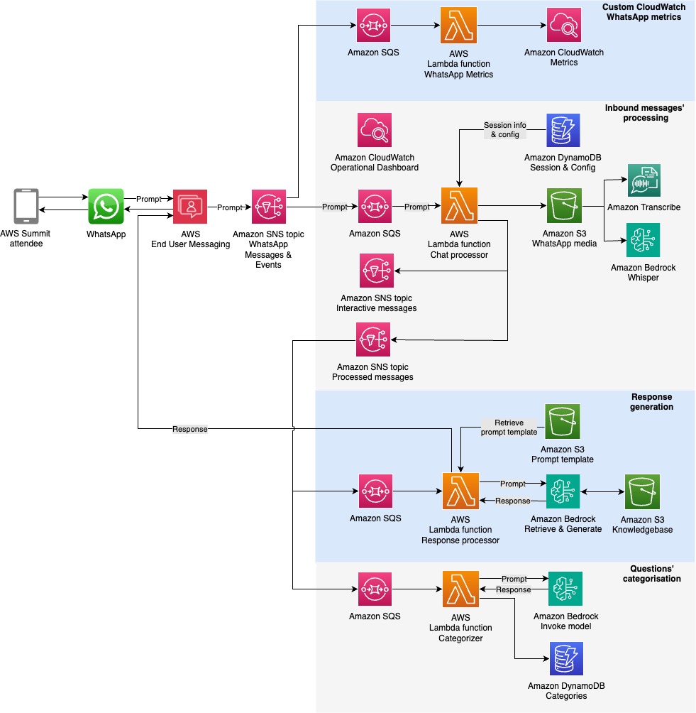
The architecture follows a modular pattern with four key components that enable efficient message processing and analytics capabilities:
- Custom metrics – Custom Amazon CloudWatch WhatsApp metrics enable real-time monitoring of engagement events through Amazon Simple Notification Service (Amazon SNS) topic integration. These metrics track message delivery status and read receipts, providing crucial operational and performance insights.
- Inbound message processing – This pipeline forms the core functionality, implementing message validation filters for length and message type constraints, managing session state, and handling audio transcription workflows. Validated messages are published to a dedicated SNS topic for downstream consumption.
- Response generation – This component uses Amazon Bedrock Knowledge Bases for intelligent message handling, with architecture designed for flexible integration of alternative processing engines. Future iterations of the AWS Summit Assistant Bot will use the Strands Agents SDK and tools.
- Questions categorization – This framework provides contextual analytics beyond standard CloudWatch and AWS Lambda insights. This component implements an Amazon DynamoDB based categorization system that works in conjunction with Amazon Bedrock to dynamically classify and track inquiry patterns while maintaining user privacy through personally identifiable information (PII)-free analytics.
Technical implementation
Our serverless, event-driven architecture efficiently handles WhatsApp message processing through a seamless multi-stage workflow. When a WhatsApp message arrives, AWS End User Messaging receives it and immediately publishes it to an SNS topic. From there, the messages are written to Amazon Simple Queue Service (Amazon SQS) queues, which enables controlled and systematic processing. Lambda functions then handle the core business logic, processing these messages and managing interactions with DynamoDB. To generate responses, the system uses Amazon Bedrock Knowledge Bases to create personalized content for each user. Finally, these tailored responses are routed back to users through AWS End User Messaging, completing the WhatsApp communication cycle.
The system implements two parallel processes alongside the main message processing pipeline. The first is a categorization service that processes messages through Amazon SNS and Amazon SQS before using Lambda functions to analyze content against existing DynamoDB category records. This function either increments existing category counters or creates new categories as needed. The second parallel process handles custom CloudWatch metrics, following a similar initial flow through Amazon SNS and Amazon SQS, but employs specialized Lambda functions to extract and record engagement metrics for operational monitoring.
Generative AI integration
The Amazon Bedrock implementation encompasses two core AI capabilities:
- A knowledge base retrieval system using OpenSearch vector embeddings and Anthropic’s Claude 3.7 Sonnet model for accurate information retrieval
- A real-time message categorization engine that dynamically classifies incoming messages into existing categories or creates new ones based on content analysis
Voice message processing
The voice message handling system implements a sophisticated processing chain. WhatsApp voice messages in OGG format are processed through a Lambda based conversion pipeline using the ffmpeg library. The converted audio is then transcribed using Whisper through Amazon Bedrock Marketplace, chosen for its fast processing and robust multi-language support capabilities.
Security and privacy considerations
Our security-first approach implements multiple layers of protection:
- Customer managed key encryption for data at rest and in transit across Amazon SNS, Amazon SQS, and DynamoDB
- Minimized PII CloudWatch logging and automatic data cleanup through DynamoDB TTL settings
- Amazon Bedrock Guardrails to prevent inappropriate content generation and protect against data loss
- Custom logic to prevent resource draining by preventing the ingestion of unreasonably large messages and keeping a short conversation context window
Monitoring and analytics
Monitoring is important for operational purposes but also for understanding what questions users are asking. The solution uses the following components:
- A Real-time CloudWatch dashboard for tracking operational metrics such as messages published on SNS topics; WhatsApp messages sent, delivered, and read, Lambda invocations; failures; and Amazon Bedrock metrics
- CloudWatch logs for granular analytics using CloudWatch insights such as unique users and number of conversations
- Generative AI-powered categorization of users’ questions
Conclusion
The AWS Summit Assistant Bot demonstrates how AWS services can be combined to create practical, generative AI-powered solutions that enhance real-world experiences. This framework can be adapted for various event types and scales, such as tech conferences, trade shows, festivals, campus orientations, and shopping centers.
To learn more about building similar solutions:
- Explore the AWS End User Messaging documentation
- Review Amazon Bedrock capabilities for natural language processing
- Visit the AWS Communication Developer Services blog for more insights
- Deploy your own communications hub
By using these AWS services and resources, you can create innovative, AI-powered communication solutions for a wide range of applications.