Tag Archives: Technical How-to

Stream mainframe data to AWS in near real time with Precisely and Amazon MSK

2025-10-16 Supreet Padhi

Post Syndicated from Supreet Padhi original https://aws.amazon.com/blogs/big-data/stream-mainframe-data-to-aws-in-near-real-time-with-precisely-and-amazon-msk/

This is a guest post by Supreet Padhi, Technology Architect, and Manasa Ramesh, Technology Architect at Precisely in partnership with AWS.

Enterprises rely on mainframes to run mission-critical applications and store essential data, enabling real-time operations that help achieve business objectives. These organizations face a common challenge: how to unlock the value of their mainframe data in today’s cloud-first world while maintaining system stability and data quality. Modernizing these systems is critical for competitiveness and innovation.

The digital transformation imperative has made mainframe data integration with cloud services a strategic priority for enterprises worldwide. Organizations that can seamlessly bridge their mainframe environments with modern cloud platforms gain significant competitive advantages through improved agility, reduced operational costs, and enhanced analytics capabilities. However, implementing such integrations presents unique technical challenges that require specialized solutions. Some of the challenges include converting EBCDIC data to ASCII, where the handling of data types is unique to the mainframe, such as binary data and COMP data. Data stored in Virtual Storage Access Method (VSAM) files can be quite complex due to practices to store multiple different record types in a single file. To address these challenges, Precisely—a global leader in data integrity, serving over 12,000 customers—has partnered with Amazon Web Services (AWS) to enable real-time synchronization between mainframe systems and Amazon Relational Database Service (Amazon RDS). For more on this collaboration, check out our previous blog post: Unlock Mainframe Data with Precisely Connect and Amazon Aurora.

In this post, we introduce an alternative architecture to synchronize mainframe data to the cloud using Amazon Managed Streaming for Apache Kafka (Amazon MSK) for greater flexibility and scalability. This event-driven approach provides additional possibilities for mainframe data integration and modernization strategies.

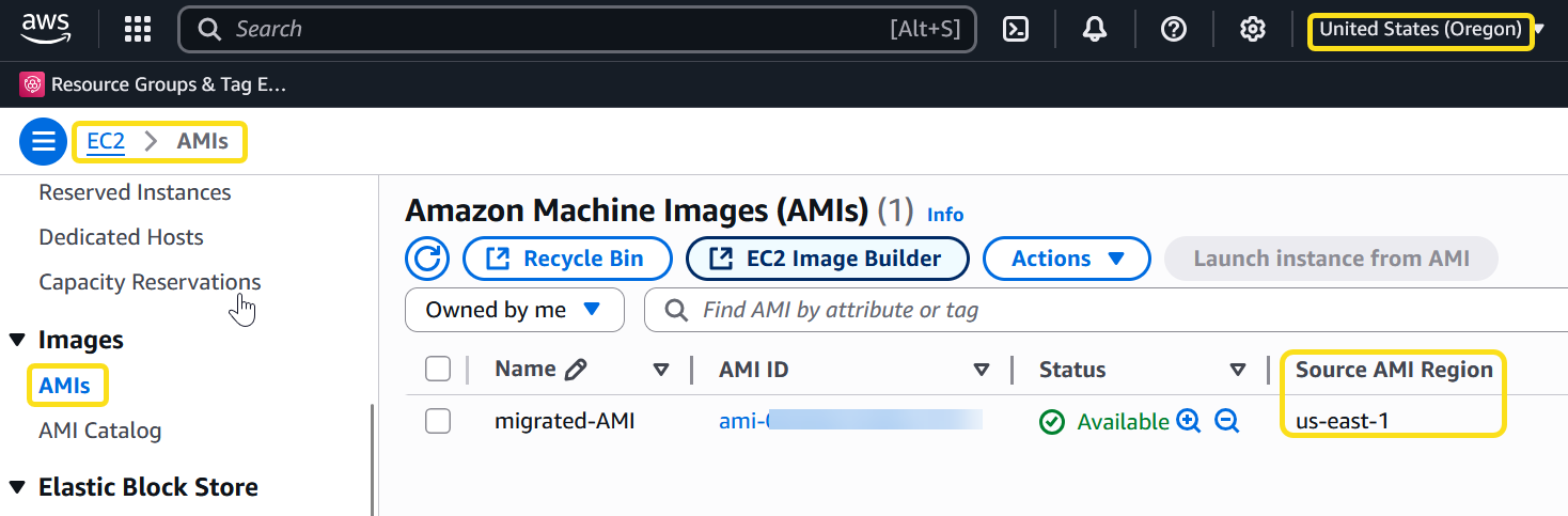
A key enhancement in this solution is the use of the AWS Mainframe Modernization – Data Replication for IBM z/OS Amazon Machine Image (AMI) available in AWS Marketplace, which simplifies deployment and reduces implementation time.

Real-time processing and event-driven architecture benefits

Real-time processing makes data actionable within seconds rather than waiting for batch processing cycles. For example, financial institutions such as Global Payments have leveraged this solution to modernize mission-critical banking operations, including payments processing. By migrating these operations to the AWS Cloud, they enhanced user experience, improved scalability and maintainability, while enabling advanced fraud detection – all without impacting the performance of existing mainframe systems. Change data capture (CDC) enables this by identifying database changes and delivering them in real time to cloud environments.

CDC offers two key advantages for mainframe modernization:

Incremental data movement – Eliminates disruptive bulk extracts by streaming only changed data to cloud targets, minimizing system impact and ensuring data currency
Real-time synchronization – Keeps cloud applications in sync with mainframe systems, enabling immediate insights and responsive operations

Solution overview

In this post, we provide a detailed implementation guide for streaming mainframe data changes from DB2z through AWS Mainframe Modernization – Data Replication for IBM z/OS AMI to Amazon MSK and then applying those changes to Amazon Relational Database Service (Amazon RDS) for PostgreSQL using MSK Connect with the Confluent JDBC Sink Connector.

By introducing Amazon MSK into architecture and streamlining deployment through the AWS Marketplace AMI, we create new possibilities for data distribution, transformation, and consumption that expand upon our previously demonstrated direct replication approach. This streaming-based architecture offers several additional benefits:

Simplified deployment – Accelerate implementation using the preconfigured AWS Marketplace AMI
Decoupled systems – Separate the concern of data extraction from data consumption, allowing both sides to scale independently
Multi-consumer support – Enable multiple downstream applications and services to consume the same data stream according to their own requirements
Extensibility – Create a foundation that can be extended to support additional mainframe data sources such as IMS and VSAM, as well as additional AWS targets using MSK Connect sink connectors

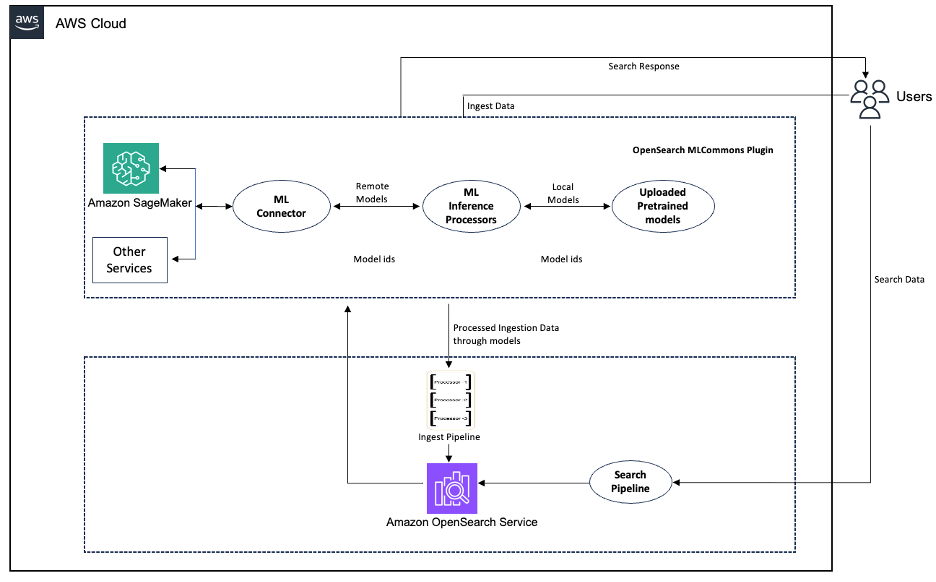
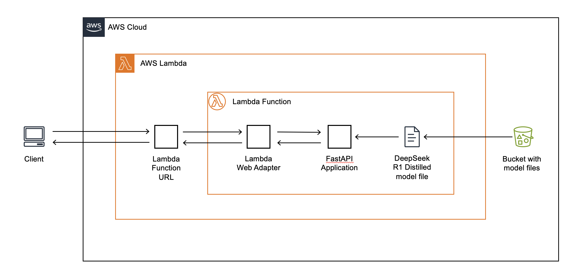
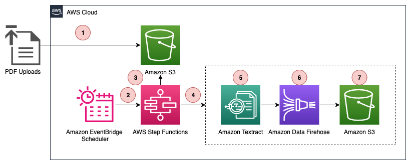
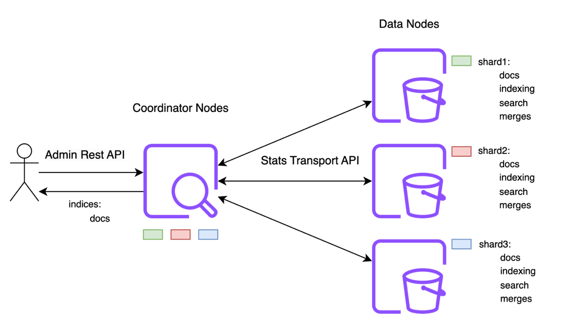
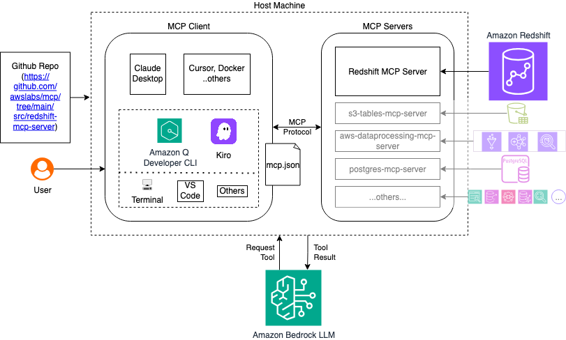
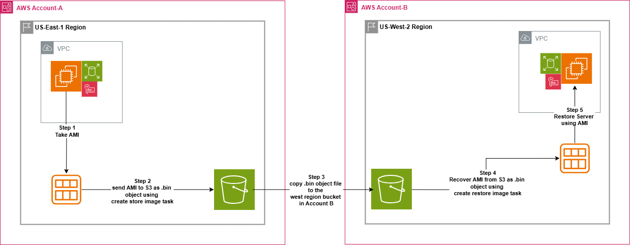
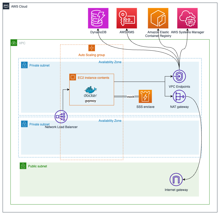
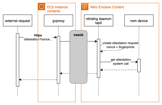
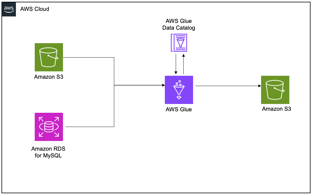
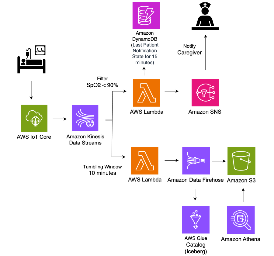
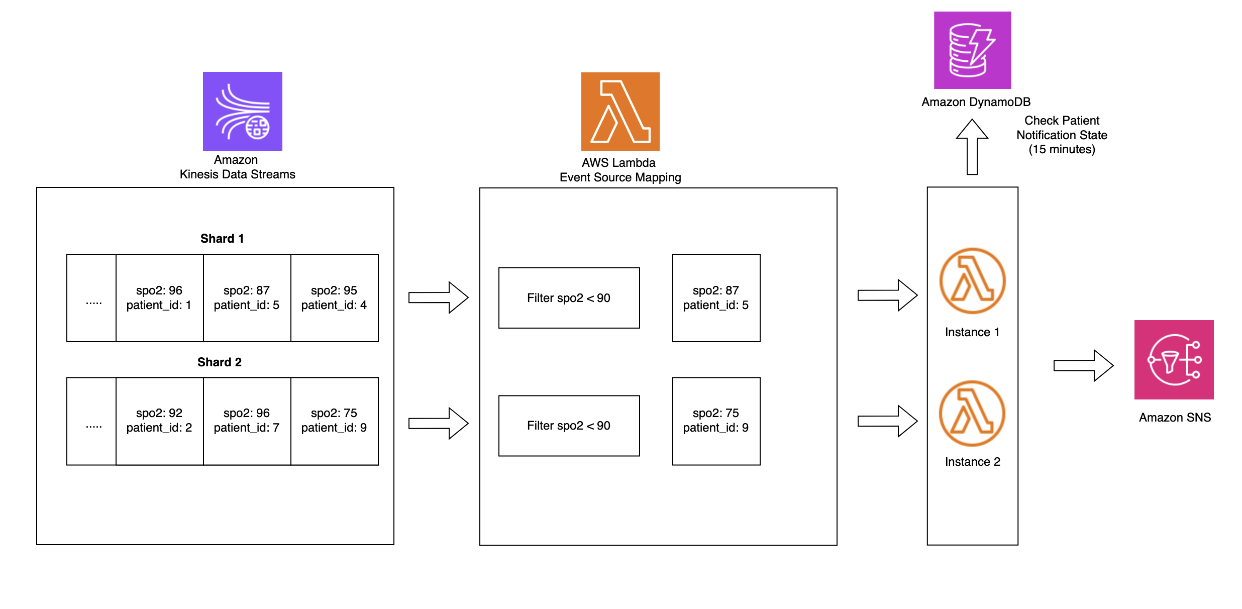
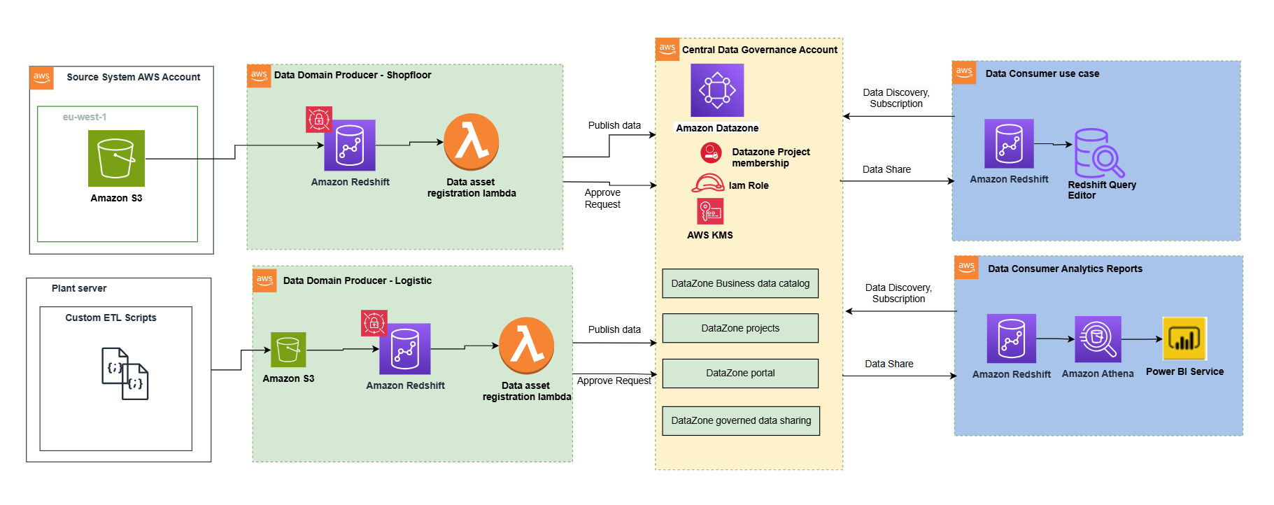
The following diagram illustrates the solution architecture.

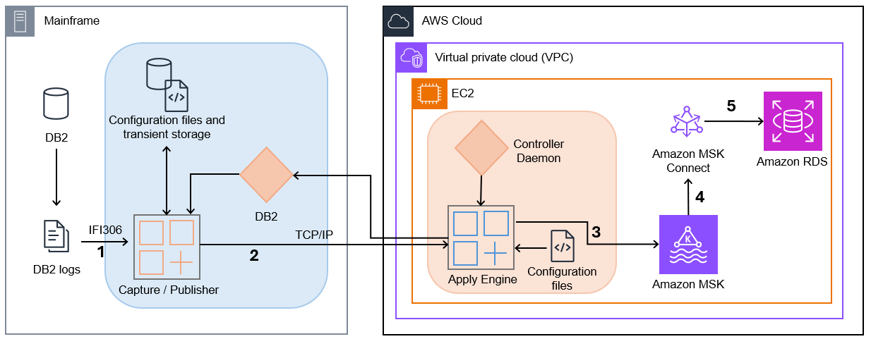
Capture/Publisher – Connect CDC Capture/Publisher captures Db2 changes from Db2 logs using IFI 306 Read and communicates captured data changes to a target engine through TCP/IP.
Controller Daemon – The Controller Daemon authenticates all connection requests, managing secure communication between the source and target environments.
Apply Engine – The Apply Engine is a multifaceted and multifunctional component in the target environment. It receives the changes from the Publisher agent and applies the changed data to the target Amazon MSK.
Connect CDC Single Message Transform (SMT) – Performs all necessary data filtering, transformation, and augmentation required by the sink connector.
JDBC Sink Connector – As data arrives, an instance of the JDBC Sink Connector along with Apache Kafka writes the data to target tables in Amazon RDS.

This architecture provides a clean separation between the data capture process and the data consumption process, allowing each to scale independently. The use of MSK as an intermediary enables multiple systems to consume the same data stream, opening possibilities for complex event processing, real-time analytics, and integration with other AWS services.

Prerequisites

To complete the solution, you need the following prerequisites:

Install AWS Mainframe Modernization – Data Replication for IBM z/OS
Have access to Db2z on mainframe from AWS using your approved connectivity between AWS and your mainframe

Solution walkthrough

The following code content shouldn’t be deployed to production environments without additional security testing.

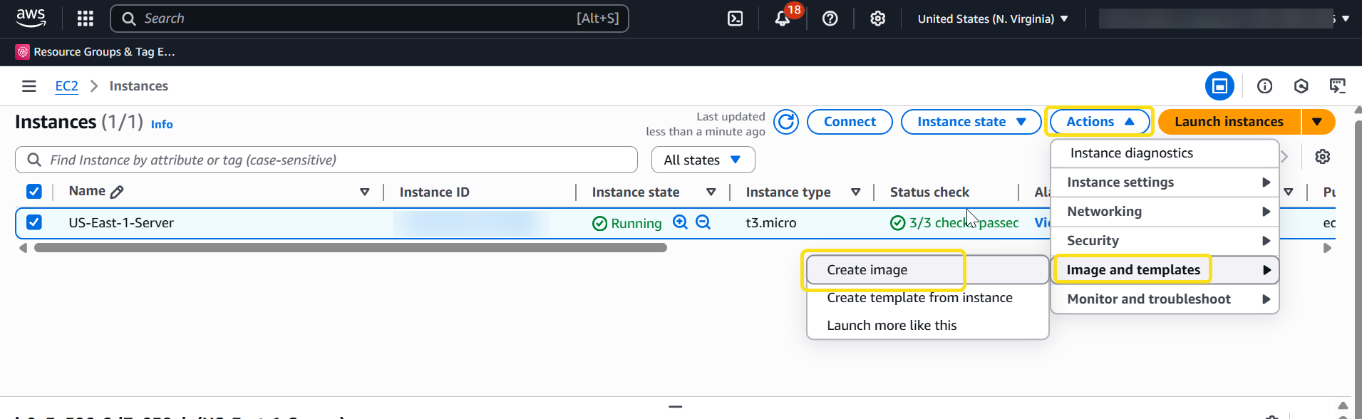
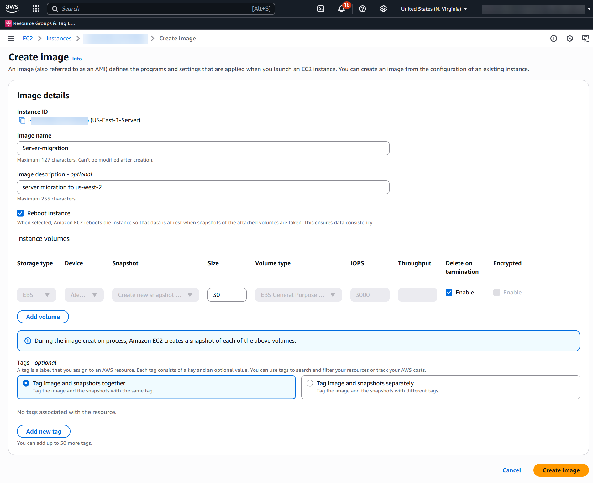
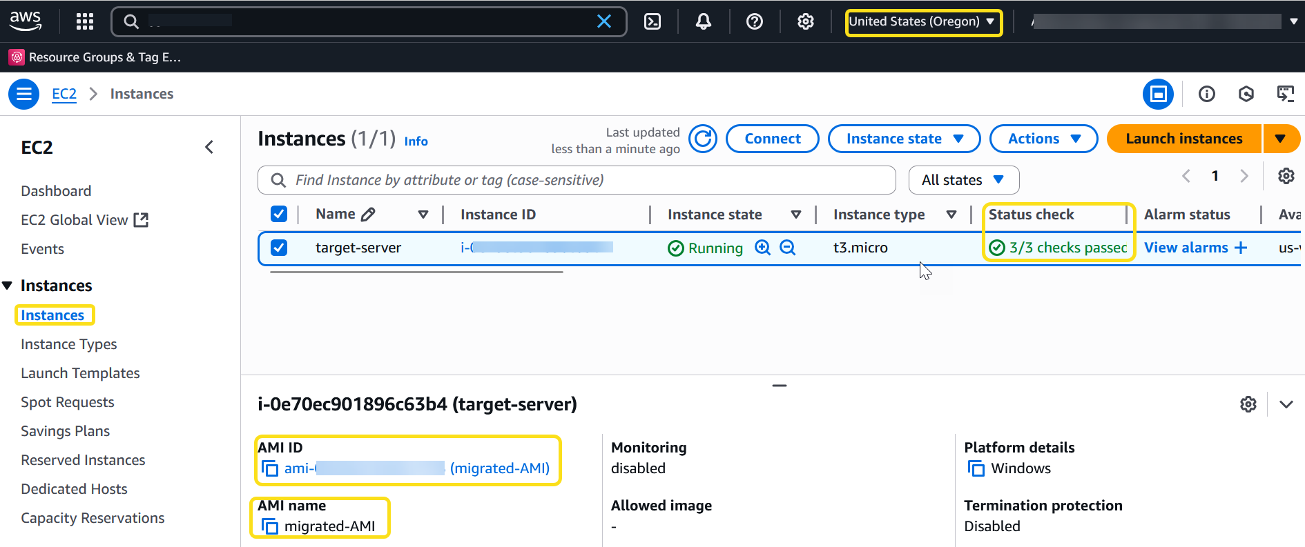
Configure the AWS Mainframe Modernization Data Replication with Precisely AMI on Amazon EC2

Follow the steps defined at Precisely AWS Mainframe Modernization Data Replication. Upon the initial launch of the AMI, use the following command to connect to the Amazon Elastic Compute Cloud (Amazon EC2) instance:

ssh -i ami-ec2-user.pem ec2-user@$AWS_AMI_HOST

Configure the serverless cluster

To create an Amazon Aurora PostgreSQL-Compatible Edition Serverless v2 cluster, complete the following steps:

Create a DB cluster by using the following AWS Command Line Interface (AWS CLI) command. Replace the placeholder strings with values that correspond to your cluster’s subnet and subnet group IDs.

aws rds create-db-cluster \
   --db-cluster-identifier cdc-serverless-pg-cluster \
   --engine aurora-postgresql \
   --serverless-v2-scaling-configuration MinCapacity=1,MaxCapacity=2 \
   --master-username connectcdcuser \
   --manage-master-user-password \
   --db-subnet-group-name "<subnet-security-group-id>" \
   --vpc-security-group-ids "<cluster-security-group-id>"

Verify the status of the cluster by using the following command:

aws rds describe-db-clusters --db-cluster-identifier cdc-serverless-pg-cluster

Add a writer DB instance to the Aurora cluster:

aws rds create-db-instance \
   --db-cluster-identifier cdc-serverless-pg-cluster \
   --db-instance-identifier cdc-serverless-pg-instance \
   --db-instance-class db.serverless \
   --engine aurora-postgresql

Verify the status of the writer instance:

aws rds describe-db-instances --db-instance-identifier cdc-serverless-pg-instance

Create a database in the PostgreSQL cluster

After your Aurora Serverless v2 cluster is running, you need to create a database for your replicated mainframe data. Follow these steps:

Install the psql client:
```
sudo yum install postgresql16
```

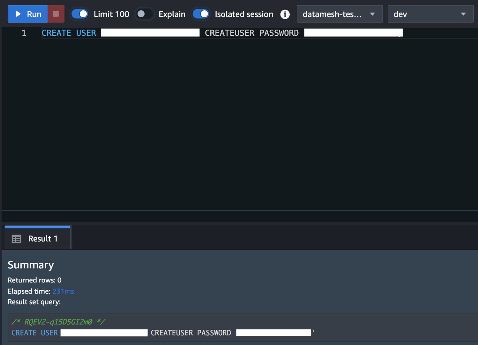
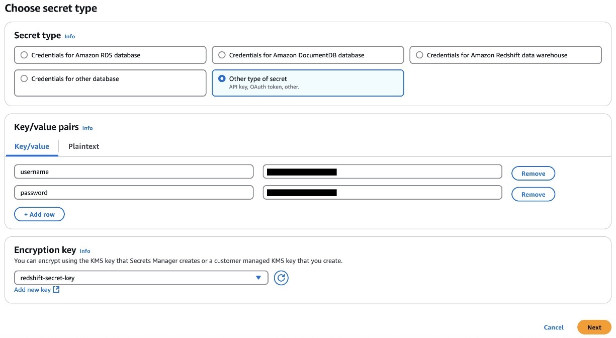
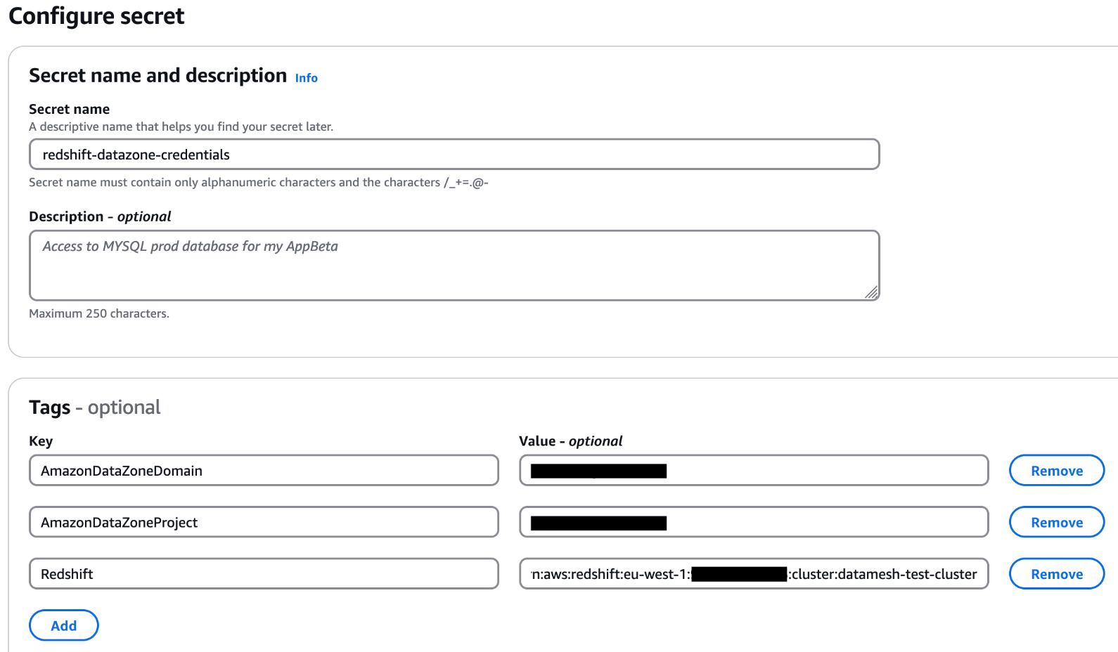
Retrieve the password from secret manager:

aws secretsmanager get-secret-value --secret-id '<cdc-serverless-pg-cluster-secret ARN>' --query 'SecretString' --output text

Create a new database in PostgreSQL:

PGPASSWORD="password" psql --host=<DATABASE-HOST> --username=connectcdcuser --dbname=postgres -c "CREATE DATABASE dbcdc"

Configure the serverless MSK cluster

To create a serverless MSK cluster, complete the following steps:

Copy the following JSON and paste it into a new file create-msk-serverless-cluster.json. Replace the placeholder strings with values that correspond to your cluster’s subnet and security group IDs.

   {
     "VpcConfigs": [
       {
         "subnets": [
           "<cluster-subnet-1>",
           "<cluster-subnet-2>",
           "<cluster-subnet-3>"
         ],
         "securityGroups": ["<cluster-security-group-id>"]
       }
     ],
     "ClientAuthentication": {
       "Sasl": {
         "Iam": {
           "Enabled": true
         }
       }
     }
   }

Invoke the following AWS CLI command in the folder where you saved the JSON file in the previous step:

aws kafka create-cluster-v2 --cluster-name pgsqlmsk --serverless file://create-msk-serverless-cluster.json

Verify cluster status by invoking the following AWS CLI command:
```
aws kafka list-clusters-v2 --cluster-type-filter SERVERLESS
```

Get the bootstrap broker address by invoking the following AWS CLI command:

aws kafka get-bootstrap-brokers --cluster-arn "<msk-serverless-cluster-arn>"

Define the environment variable to store the bootstrap servers of the MSK cluster and locally install Kafka in the path environment variable:
```
export BOOTSTRAP_SERVERS=<kafka_bootstrap_servers_with_ports>
```

Create a topic on the MSK cluster

To create a Kafka topic, you need to install the Kafka CLI first. Follow these steps:

Download the binary distribution of Apache Kafka and extract the archive in folder kafka:

wget https://dlcdn.apache.org/kafka/3.9.0/kafka_2.13-3.9.0.tgz
   tar -xzf kafka_2.13-3.9.0.tgz
   ln -sfn kafka_2.13-3.9.0 kafka

To use IAM to authenticate with the MSK cluster, download the Amazon MSK Library for IAM and copy to the local Kafka library directory as shown in the following code. For complete instructions, refer to Configure clients for IAM access control.
```
wget https://github.com/aws/aws-msk-iam-auth/releases/download/v2.3.1/aws-msk-iam-auth-2.3.1-all.jar
cp aws-msk-iam-auth-2.3.1-all.jar kafka/libs
```

In the directory, create a file to configure a Kafka client to use IAM authentication for the Kafka console producer and consumers:

security.protocol=SASL_SSL
   sasl.mechanism=AWS_MSK_IAM
   sasl.jaas.config=software.amazon.msk.auth.iam.IAMLoginModule required; sasl.client.callback.handler.class=software.amazon.msk.auth.iam.IAMClientCallbackHandler

Create the Kafka topic, which you defined in the connector config:

kafka/bin/kafka-topics.sh --create --bootstrap-server $BOOTSTRAP_SERVERS --command-config kafka/config/client-config.properties --partitions 1 --topic pgsql-sink-topic

Configure the MSK Connect plugin

Next, create a custom plugin available in the AMI at /opt/precisely/di/packages/sqdata-msk_connect_1.0.1.zip which contains the following:

JDBC Sink Connector from Confluent
MSK Config provider
AWS Mainframe Modernization – Data Repication for IBM z/OS Custom SMT

Follow these steps:

Invoke the following to upload the .zip file to an S3 bucket to which you have access:
```
aws s3 cp /opt/precisely/di/packages/sqdata-msk_connect_1.0.1.zip s3://<bucket>/
```

Copy the following JSON and paste it into a new file create-custom-plugin.json. Replace the placeholder strings with values that correspond to your bucket.

{
     "contentType": "ZIP",
     "description": "jdbc sink connector",
     "location": {
       "s3Location": {
         "bucketArn": "arn:aws:s3:::<bucket>",
         "fileKey": "sqdata-msk_connect_1.0.1.zip"
       }
     },
     "name": "jdbc-sink-connector"
   }

Invoke the following AWS CLI command in the folder where you saved the JSON file in the previous step:
```
aws kafkaconnect create-custom-plugin --cli-input-json file://create-custom-plugin.json
```
Verify plugin status by invoking the following AWS CLI command:
```
aws kafkaconnect list-custom-plugins
```

Configure the JDBC Sink Connector

To configure the JDBC Sink Connector, follow these steps:

Copy the following JSON and paste it into a new file create-connector.json. Replace the placeholder strings with appropriate values:

{
     "connectorConfiguration": {
       "connector.class": "io.confluent.connect.jdbc.JdbcSinkConnector",
       "connection.url": "jdbc:postgresql://<postgresql-endpoint>
/dbcdc?currentSchema=public",
       "config.providers": "secretsmanager",
       "config.providers.secretsmanager.class": "com.amazonaws.kafka.config.providers.SecretsManagerConfigProvider",
       "connection.user": "${secretsmanager:MySecret-1234:username}",
       "connection.password": "${secretsmanager:MySecret-1234:password}",
       "config.providers.secretsmanager.param.region": "<region>",
       "tasks.max": "1",
       "topics": "pgsql-sink-topic",
       "insert.mode": "upsert",
       "delete.enabled": "true",
       "pk.mode": "record_key",
       "auto.evolve": "true",
       "auto.create": "true",
       "value.converter": "org.apache.kafka.connect.storage.StringConverter",
       "key.converter": "org.apache.kafka.connect.storage.StringConverter",
       "transforms": "ConnectCDCConverter",
       "transforms.ConnectCDCConverter.type": "com.precisely.kafkaconnect.ConnectCDCConverter",
       "transforms.ConnectCDCConverter.cdc.multiple.tables.enabled": "true",
       "transforms.ConnectCDCConverter.cdc.source.table.name.ignore.schema": "true"
     },
     "connectorName": "pssql-sink-connector",
     "kafkaCluster": {
       "apacheKafkaCluster": {
         "bootstrapServers": "<msk-bootstrap-servers-string>",
         "vpc": {
           "subnets": [
             "<cluster-subnet-1>",
             "<cluster-subnet-2>",
             "<cluster-subnet-3>"
           ],
           "securityGroups": ["<cluster-security-group-id>"]
         }
       }
     },
     "capacity": {
       "provisionedCapacity": {
         "mcuCount": 1,
         "workerCount": 1
       }
     },
     "kafkaConnectVersion": "3.7.x",
     "serviceExecutionRoleArn": "<arn-of-a-role-that-msk-connect-can-assume>",
     "plugins": [
       {
         "customPlugin": {
           "customPluginArn": "<arn-of-custom-plugin-that-contains-connector-code>",
           "revision": 1
         }
       }
     ],
     "kafkaClusterEncryptionInTransit": {"encryptionType": "TLS"},
     "kafkaClusterClientAuthentication": {"authenticationType": "IAM"},
     "logDelivery": {
       "workerLogDelivery": {
         "cloudWatchLogs": {
           "enabled": true,
           "logGroup": "<loggroup>"
         }
       }
     }
   }

Invoke the following AWS CLI command in the folder where you saved the JSON file in the previous step:
```
aws kafkaconnect create-connector --cli-input-json file://create-connector.json
```
Verify connector status by invoking the following AWS CLI command:
```
aws kafkaconnect list-connectors
```

Set up Db2 Capture/Publisher on Mainframe

To establish the Db2 Capture/Publisher on the mainframe for capturing changes to the DEPT table, follow these structured steps that build upon our previous blog post, Unlock Mainframe Data with Precisely Connect and Amazon Aurora:

Prepare the source table. Before configuring the Capture/Publisher, ensure the DEPT source table exists on your mainframe Db2 system. The table definition should match the structure defined at \$SQDATA_VAR_DIR/templates/dept.ddl. If you need to create this table on your mainframe, use the DDL from this file as a reference to ensure compatibility with the replication process.
Access the Interactive System Productivity Facility (ISPF) interface. Sign in to your mainframe system and access the AWS Mainframe Modernization – Data Repication for IBM z/OS ISPF panels through the supplied ISPF application menu. Select option 3 (CDC) to access the CDC configuration panels, as demonstrated in our previous blog post.
Add source tables for capture:
1. From the CDC Primary Option Menu, choose option 2 (Define Subscriptions).
2. Choose option 1 (Define Db2 Tables) to add source tables.
3. On the (Add DB2 Source Table to CAB File panel), enter a wildcard value (%) or the specific table name DEPT in the (Table Name) field.
4. Press Enter to display the list of available tables.
5. Type S next to the DEPT table to select it for replication, then press Enter to confirm.

This process is like the table selection process shown in figure 3 and figure 4 of our previous post but now focuses specifically on the DEPT table structure.

With the completion of both the Db2 Capture/Publisher setup on the mainframe and the AWS environment configuration (Amazon MSK, Apply Engine, and MSK Connect JDBC Sink Connector), you now have a fully functional pipeline ready to capture data changes from the mainframe and stream them to the MSK topic. Inserts, updates, or deletions to the DEPT table on the mainframe will be automatically captured and pushed to the MSK topic in near real time. From there, the MSK Connect JDBC Sink Connector and the custom SMT will process these messages and apply the changes to the PostgreSQL database on Amazon RDS, completing the end-to-end replication flow.

Configure Apply Engine for Amazon MSK integration

Configure the AWS side components to receive data from the mainframe and forward it to Amazon MSK. Follow these steps to define and manage a new CDC pipeline from DB2 z/OS to Amazon MSK:

Use the following command to switch to the connect user:
```
sudo su connect
```

Create the apply engine directories:

mkdir -p \$SQDATA_VAR_DIR/apply/DB2ZTOMSK/ddl
     connect> mkdir -p \$SQDATA_VAR_DIR/apply/DB2ZTOMSK/scripts

Copy the sample script from dept.ddl:

cp \$SQDATA_VAR_DIR/templates/dept.ddl \$SQDATA_VAR_DIR/apply/DB2ZTOMSK/ddl/

Copy the following content and paste it in a new file $SQDATA_VAR_DIR/apply/DB2ZTOMSK/scripts/DB2ZTOMSK.sqd. Replace the placeholder strings with values that correspond to the DB2z endpoint:

-----------------------------------------------------------------------
   Name: DB2TOKAF: Z/OS DB2 To Kafka
   -----------------------------------------------------------------------
   SUBSTITUTION PARMS USED IN THIS SCRIPT:
   ---------------------------------------------------------------------
   JOBNAME DB2TOKAFKA;
   -----------------------------
   TABLE DESCRIPTIONS
   ---------------------------
   BEGIN GROUP SOURCE_TABLES;
   DESCRIPTION Db2SQL /var/precisely/di/sqdata/apply/DB2ZTOMSK/ddl/dept.ddl AS DEPT KEY IS DEPTNO;
   END GROUP;
   -------------------------------------------------------------
   DATASTORE SECTION
   -------------------------------------------------------------
   SOURCE DATASTORE
   DATASTORE cdc://<DB2z endpoint with port>/dbcg/DBCG_TBTSS388T6 OF UTSCDC AS CDCIN DESCRIBED BY GROUP SOURCE_TABLES;
   -- TARGET DATASTORE
   DATASTORE kafka:///pgsql-sink-topic/table_key OF JSON AS TARGET KEY IS DEPTNO DESCRIBED BY GROUP SOURCE_TABLES;
   ---------------------------------
   PROCESS INTO TARGET
   SELECT { REPLICATE(TARGET) } FROM CDCIN;

Create the working directory:

mkdir -p /var/precisely/di/sqdata_logs/apply/DB2ZTOMSK

Add the following to $SQDATA_DAEMON_DIR/cfg/sqdagents.cfg:

[DB2ZTOMSK]
   type=engine
   program=sqdata
   args=/var/precisely/di/sqdata/apply/DB2ZTOMSK/scripts/DB2ZTOMSK.prc --log-level=8
   working_directory=/var/precisely/di/sqdata_logs/apply/DB2ZTOMSK
   stdout_file=stdout.txt
   stderr_file=stderr.txt
   auto_start=0
   comment=Apply Engine for MSK from Db2z

After the preceding code is added to the sqdagents.cfg section, reload for the changes to take effect:
```
sqdmon reload
```

Validate the apply engine job script by using the SQData parse command to create the compiled file expected by the SQData engine:

sqdparse $SQDATA_VAR_DIR/apply/DB2ZTOMSK/scripts/DB2ZTOMSK.sqd $SQDATA_VAR_DIR/apply/DB2ZTOMSK/scripts/DB2ZTOMSK.prc

The following is an example of the output that you get when you invoke the command successfully:

SQDC042I mounting/running sqdparse with arguments:
SQDC041I args[0]:sqdparse
SQDC041I args[1]:/var/precisely/di/sqdata/apply/DB2ZTOMSK/scripts/DB2ZTOMSK.sqd
SQDC041I args[2]:/var/precisely/di/sqdata/apply/DB2ZTOMSK/scripts/DB2ZTOMSK.prc
SQDC000I *******************************************************
SQDC021I sqdparse Version 5.0.1-rel (Linux-x86_64)
SQDC022I Build-id 4f2d7c16728aa2e40c610db7d5a6e373476a9889
SQDC023I (c) 2001, 2025 Syncsort Incorporated. All rights reserved.
SQDC000I *******************************************************
SQDC000I
SQD0000I 2025-03-31 00:59:10
>>> Start Preprocessed /var/precisely/di/sqdata/apply/DB2ZTOMSK/scripts/DB2ZTOMSK.sqd
000001 ----------------------------------------------------------------------
000002 -- Name: DB2TOKAF:  Z/OS DB2 To Kafka
000003 ----------------------------------------------------------------------
000004 --  SUBSTITUTION PARMS USED IN THIS SCRIPT:
000005 ----------------------------------------------------------------------
000006
000007 JOBNAME DB2TOKAFKA;
000008
000009 ----------------------------
000010 -- TABLE DESCRIPTIONS
000011 ----------------------------
000012 BEGIN GROUP SOURCE_TABLES;
000013 DESCRIPTION Db2SQL /var/precisely/di/sqdata/apply/DB2ZTOMSK/ddl/dept.ddl  AS DEPT
000014 KEY IS DEPTNO;
000015 END GROUP;
000016
000017 ------------------------------------------------------------
000018 --       DATASTORE SECTION
000019 ------------------------------------------------------------
000020
000021 -- SOURCE DATASTORE
000022 DATASTORE /var/precisely/di/sqdata/apply/DB2ZTOMSK/scripts/DB0A.ENGINE3.DEPT.COPY
000023           OF UTSCDC
000024           AS CDCIN
000025           DESCRIBED BY GROUP SOURCE_TABLES;
000026
000027 -- TARGET DATASTORE
000028 DATASTORE 
000029           OF JSON
000030           AS TARGET
000031           KEY IS DEPTNO
000032           DESCRIBED BY GROUP SOURCE_TABLES;
000033
000034 ----------------------------------
000035
000036 PROCESS INTO TARGET
000037 SELECT
000038 {
000039     REPLICATE(TARGET)
000040 }
000041 FROM CDCIN;
<<< End Preprocessed /var/precisely/di/sqdata/apply/DB2ZTOMSK/scripts/DB2ZTOMSK.sqd
>>> Start Preprocessed /var/precisely/di/sqdata/apply/DB2ZTOMSK/ddl/dept.ddl
000001 CREATE TABLE DEPARTMENT
000002 (
000003    DEPTNO char(3) NOT NULL,
000004    DEPTNAME varchar(36) NOT NULL,
000005    MGRNO char(6),
000006    ADMRDEPT char(3) NOT NULL,
000007    LOCATION char(16),
000008    CONSTRAINT PK_DEPTNO PRIMARY KEY (DEPTNO)
000009 ) ;
<<< End Preprocessed /var/precisely/di/sqdata/apply/DB2ZTOMSK/ddl/dept.ddl
Number of Data Stores...................: 2
Data Store..............................: /var/precisely/di/sqdata/apply/DB2ZTOMSK/scripts/DB0A.ENGINE3.DEPT.COPY
  Alias.................................: CDCIN
  Type..................................: UTS Change Data Capture
  Number of Records.....................: 1
    Record Name.........................: DEPARTMENT
    Record Description Alias............: DEPT
    Record Description Length...........: 72
    Number of Fields....................: 5
      ................................... TYPE            OFF   LEN   XLEN  EXT
      ................................... ---------- ----- ----- ----- -----
      DEPTNO............................: CHAR(3)             0     3     3
      DEPTNAME..........................: VARCHAR(36)         3    38    38
      MGRNO.............................: CHAR(6)             7     6     6
      ADMRDEPT..........................: CHAR(3)            14     3     3
      LOCATION..........................: CHAR(16)           17    16    16
Data Store..............................: 
  Alias.................................: TARGET
  Type..................................: JSON
  Number of Records.....................: 1
    Record Name.........................: DEPARTMENT
    Record Description Alias............: DEPT
    Record Description Length...........: 70
    Number of Fields....................: 5
      ................................... TYPE            OFF   LEN   XLEN  EXT
      ................................... ---------- ----- ----- ----- -----
      DEPTNO............................: CHAR(3)             0     3     3
      DEPTNAME..........................: VARCHAR(36)         3    38    38
      MGRNO.............................: CHAR(6)            41     6     6
      ADMRDEPT..........................: CHAR(3)            47     3     3
      LOCATION..........................: CHAR(16)           50    16    16
Section.................................: SQDSTP000
  Number of steps.......................: 1
SQDC017I sqdparse(pid=4023) terminated successfully

Copy the following content and paste it in a new file /var/precisely/di/sqdata_logs/apply/DB2ZTOMSK/sqdata_kafka_producer.conf. Replace the placeholder strings with values that correspond to your bootstrap server and AWS Region.

metadata.broker.list=<kafka_bootstrap_servers_with_ports>
     security.protocol=SASL_SSL
     sasl.mechanism=OAUTHBEARER
     sasl.oauthbearer.config="extension_AWSMSKCB=python3,/usr/lib64/python3.9/site-packages/aws_msk_iam_sasl_signer/cli.py,--region,<region>"
     sasl.oauthbearer.method="default"

Start the apply engine using the controller daemon by using the following command:
```
sqdmon start ///DB2ZTOMSK
```

Monitor the apply engine through the controller daemon by using the following command:

sqdmon display ///DB2ZTOMSK --format=details

The following is an example of the output that you get when you invoke the command successfully:

Engine..................................: DB2ZTOMSK
version.................................: 5.0.1-rel (Linux-x86_64)
git.....................................: f021c29a84c1a99f59144288aeeb2cb8fa494485
jobname.................................: DB2TOKAFKA
parsed..................................: 20250320172610278108
started.................................: 2025-03-20.17.47.23.444474
started (UTC)...........................: 2025-03-20.17.47.23.444474 (1742492843444)
updated (UTC)...........................: 2025-03-20.17.47.25.901018 (1742492845901)
Input Datastore.........................: /var/precisely/di/sqdata/apply/DB2ZTOMSK/scripts/DB0A.ENGINE3.DEPT.COPY
Alias...................................: CDCIN
Type....................................: UTS Change Data Capture
  Records Read..........................: 14
  Records Selected......................: 14
  Bytes Read............................: 2892
Output Datastore........................: kafka:///pgsql-sink-topic/table_key
Alias...................................: TARGET
Type....................................: JSON
  Records Inserted......................: 14
  Records Updated.......................: 0
  Records Deleted.......................: 0
  Formatted bytes.......................: 3458
  Unformatted bytes.....................: 448
Total Output Formatted bytes............: 3458
Total Output Unformatted bytes..........: 448
SQDC017I sqdmon(pid=123540) terminated successfully

Logs can also be found at /var/precisely/di/sqdata_logs/apply/DB2ZTOMSK.

Verify data in the MSK topic

Invoke the Kafka CLI command to verify the JSON data in the MSK topic:

kafka/bin/kafka-console-consumer.sh --bootstrap-server $BOOTSTRAP_SERVERS --consumer.config kafka/config/client-config.properties --topic pgsql-sink-topic --from-beginning --property print.key=true

Verify data in the PostgreSQL database

Invoke the following command to verify the data in the PostgreSQL database:

PGPASSWORD="password" psql --host=<DATABASE-HOST> --username=<user> --dbname=<database> -c "select * from \"DEPT\""

With these steps completed, you’ve successfully set up end-to-end data replication from DB2z to RDS for PostgreSQL, using AWS Mainframe Modernization – Data Replication for IBM z/OS AMI, Amazon MSK, MSK Connect, and the Confluent JDBC Sink Connector.

Cleanup

When you’re finished testing this solution, you can clean up the resources to avoid incurring additional charges. Follow these steps in sequence to ensure proper cleanup.

Step 1: Delete the MSK Connect components

Follow these steps:

List existing connectors:
```
aws kafkaconnect list-connectors
```

Delete the sink connector:

aws kafkaconnect delete-connector --connector-arn "<arn-of-connector>"

List custom plugins:
```
aws kafkaconnect list-custom-plugins
```

Delete the custom plugin:

aws kafkaconnect delete-custom-plugin --custom-plugin-arn "<arn-of-custom-plugin>"

Step 2: Delete the MSK cluster

Follow these steps:

List MSK clusters:

aws kafka list-clusters-v2 --cluster-type-filter SERVERLESS

Delete the MSK serverless cluster:

aws kafka delete-cluster --cluster-arn "<arn-of-msk-serverless-cluster>"

Step 3: Delete the Aurora resources

Follow these steps:

Delete the Aurora DB instance:

aws rds delete-db-instance --db-instance-identifier cdc-serverless-pg-instance --skip-final-snapshot

Delete the Aurora DB cluster:

aws rds delete-db-cluster --db-cluster-identifier cdc-serverless-pg-cluster --skip-final-snapshot.

Conclusion

By capturing changed data from DB2z and streaming it to AWS targets, organizations can modernize their legacy mainframe data stores, enabling operational insights and AI initiatives. Businesses can use this solution to take advantage of cloud-based applications with mainframe data to provide scalability, cost-efficiency, and enhanced performance.

The integration of AWS Mainframe Modernization – Data Replication for IBM z/OS AMI with Amazon MSK and RDS for PostgreSQL provides an enhanced framework for real-time data synchronization that maintains data integrity. This architecture can be extended to support additional mainframe data sources such as VSAM and IMS, as well as other AWS targets. Organizations can then tailor their data integration strategy to specific business needs. Data consistency and latency challenges can be effectively managed through AWS and Precisely’s monitoring capabilities. By adopting this architecture, organizations keep their mainframe data continually available for analytics, machine learning (ML), and other advanced applications.Streaming mainframe data to AWS in near real time represents a strategic step toward modernizing legacy systems while unlocking new opportunities for innovation, with data transfers occurring in subseconds. With Precisely and AWS, organizations can effectively navigate their modernization journey and maintain their competitive advantage.

Learn more about AWS Mainframe Modernization – Data Replication for IBM z/OS AMI in the Precisely documentation. AWS Mainframe Modernization Data Replication is available for purchase in AWS Marketplace. For more information about the solution or to see a demonstration, contact Precisely.

About the authors

Migrate encrypted Amazon EC2 instances across AWS Regions without sharing AWS KMS keys

2025-10-16 Rakesh Mannepalli

Post Syndicated from Rakesh Mannepalli original https://aws.amazon.com/blogs/compute/migrate-encrypted-amazon-ec2-instances-across-aws-regions-without-sharing-aws-kms-keys/

At AWS, we’ve designed our global infrastructure with isolated AWS Regions to help you achieve high fault tolerance and stability for your applications. These AWS Regions are organized into partitions, each with distinct network and security boundaries.

As your business evolves, you might need to migrate workloads between AWS Regions. Perhaps you’re looking to reduce latency for users in new geographic areas, meet Region-specific compliance requirements, or you’re an ISV expanding your product’s availability. Whatever your motivation, cross-Region migration needs careful planning, especially when dealing with encrypted resources.

When migrating Amazon Elastic Compute Cloud (Amazon EC2) instances with encrypted Amazon Elastic Block Storage (Amazon EBS) volumes across AWS Regions with in the same account or a different account, you face a particular challenge: AWS Key Management Service (AWS KMS) keys are AWS Region-specific and cannot be shared across AWS Regions. This post provides a step-by-step approach to successfully migrate your encrypted EC2 instances without compromising your security posture by sharing your KMS keys.

Solution overview

The following diagram and steps are an overview of how an EC2 instance can be migrated to a different Region in a different account without sharing the KMS keys.

Figure 1:Design to migrate EC2 between two accounts

Prerequisites

The following prerequisites are necessary to complete this solution:

Create an S3 bucket in both the source and target Region.
Configure the target account Amazon S3 bucket with the following policy to copy the Amazon Machine Image (AMI) file between two accounts:

{
    "Version": "2012-10-17",
    "Statement": [
        {
            "Sid": "Statement1",
            "Effect": "Allow",
            "Principal": {
                "AWS": "arn:aws:sts::1234567891:assumed-role/<rolename>"
            },
            "Action": [
                "s3:GetObject",
                "s3:PutObject",
                "s3:PutObjectAcl"
            ],
            "Resource": "arn:aws:s3:::<target-bucket-name>/*"
        }
    ]
}

Implementation steps

Now based on the above architecture, you are implementing the follow steps to move your EC2 instance from the source account to the target account

Create an AMI of the server that you want to move to a different Region in the same account or different account.
1. Choose the server
2. Choose Actions, Image and templates, and Create image.
  
  Figure 2: steps to create an AMI
3. Fill the details and choose Create Image.
  
  Figure 3: Confirming AMI creation attributes
Check the status of the AMI by choosing AMI ID or under AMI on your left-hand side menu, wait until the status shows as Available.

Figure 4: AMI availability status

Run the following command using AWS CloudShell from the AWS console.

aws ec2 create-store-image-task --image-id ami-xxxxxxxxx –bucket <bucket_name>

You can check the status of the job using the following command to make sure it is completed.
```
aws ec2 describe-store-image-tasks
```
Figure 5: CloudShell command execution
Now you can see your AMI bin file in the S3 bucket.

Figure 6: .bin file in the source S3 bucket
Copy the AMI bin to the target S3 bucket using the following command from the CloudShell in the source account.
```
aws s3 cp s3://<source_bucket>/ami-000xxxxxxxxx.bin s3://<target_bucket>/
```
When the copy job is completed, validate the AMI’s availability in .bin format in the target AWS account S3 bucket.

Figure 7: .bin file in the target S3 bucket
Now restore the .bin file as an AMI in the target account by running the following command in the target account CloudShell.
```
aws ec2 create-restore-image-task --object-key ami-xxxx.bin --bucket <target_bucket> --name "<AMI_name>"
```
Figure 8: CloudShell command execution
Check the availability of the AMI under the EC2 section in the target. You should find a new AMI ID along with the source Region information.

Figure 9: AMI created in the target account
Launch the instance using the migrated AMI in the target Region.

Figure 10: Launched EC2 instance in the target account

Limitations

Following are the limitations with this process:

To store an AMI, your AWS account must either own the AMI and its snapshots, or the AMI and its snapshots must be shared directly with your account. You can’t store an AMI if it is only publicly shared.
Only Amazon EBS-backed AMIs can be stored using these APIs.
Paravirtual (PV) AMIs are not supported.
The size of an AMI (before compression) that can be stored is limited to 5,000 GB.
Quota on store image requests: 1,200 GB of storage work (snapshot data) in progress.
Quota on restore image requests: 600 GB of restore work (snapshot data) in progress.
For the duration of the store task, the snapshots must not be deleted and the AWS Identity and Access Management (IAM) principal doing the store must have access to the snapshots, otherwise the store process fails.
You can’t create multiple copies of an AMI in the same S3 bucket.
An AMI that is stored in an S3 bucket can’t be restored with its original AMI ID. You can mitigate this by using AMI aliasing.
Currently the store and restore APIs are only supported by using the AWS Command Line Interface (AWS CLI), AWS SDKs, and Amazon EC2 API. You can’t store and restore an AMI using the Amazon EC2 console.

Clean up resources

When you have successfully deployed the server in the target Region you can delete the S3 buckets that were created for this migration. You can also terminate EC2 and delete associated EBS volumes and snapshots if you do not need them to avoid additional cost.

Conclusion

In this post, we showed you how to migrate an Amazon EC2 instances into another Region in a different account without sharing any AWS KMS keys in a secured manner.

Securing applications with AWS Nitro Enclaves: TLS termination, TAP networking, and IMDSv2

2025-10-14 David-Paul Dornseifer

Post Syndicated from David-Paul Dornseifer original https://aws.amazon.com/blogs/compute/securing-applications-with-aws-nitro-enclaves-tls-termination-tap-networking-and-imdsv2/

AWS Nitro Enclaves provide isolated environments that keep critical operations such as decryption and cryptographic key management secure from both from root user and external threats.

Many customers have applications that require end-to-end authentication using Transport Layer Security (TLS) and requiring control over TLS termination.

TLS termination refers to the process where encrypted TLS traffic is decrypted using the server’s private key, converting the secure encrypted communication back to plaintext for processing. TLS termination can be done directly within an enclave, helping to ensure that encrypted traffic is not exposed outside the trusted boundary.

This is particularly valuable for public-facing services such as anonymization proxies and Model Context Protocol (MCP) servers, where clients demand assurance that their communications are protected and the application’s integrity can be independently verified using cryptographic attestation in a remote fashion.

This post covers critical design and implementation decisions from the Build multi-party crypto wallets with AWS Nitro Enclaves workshop and the associated public GitHub repository.

Specifically, in this blog we explore patterns on how:

you can build applications that are remotely verifiable by clients, including enclave-based TLS termination using Nitriding, an open-source framework built by Brave and AWS Nitro Enclaves.
you can configure TAP networking devices for AWS Nitro Enclaves using gvproxy.
your enclaves can access EC2 instance metadata service (IMDSv2) and fetch temporary AWS credentials.
you can decrypt secrets via AWS Key Management Service (KMS) using cryptographic attestation and the Python Boto3 SDK.

Prerequisites and Deployment

This post builds on our workshop “Build multi-party crypto wallets with AWS Nitro Enclaves” which demonstrates a Shamir Secret Sharing (SSS) application. The SSS app securely splits cryptographic private keys into multiple shards, requiring a threshold number to reconstruct the original key, ideal for Nitro Enclaves as it prevents any single party from accessing the complete key while maintaining operational functionality.

To follow along hands-on, you’ll need to deploy the provided AWS Cloud Development Kit (CDK) stack from the workshop repository on GitHub. However, you can understand the concepts and architecture discussed in this post without deploying the solution yourself.

Solution architecture

The following diagram depicts the high-level architecture of the solution.

Before we dive deep into the application design, lets introduce the high-level components enclosed in the AWS Cloud Development Kit (AWS CDK) stack:

A dedicated virtual private cloud (VPC) and private subnets are created. Internet access is only possible through a NAT gateway, avoiding public exposure of the Amazon Elastic Compute Cloud (EC2) instances.
EC2 instances are placed in several private subnets and in different Availability Zones (AZ) using the auto-scaling group (ASG) to provide high availability. Network Load Balancer (NLB) is used to distribute the requests between different EC2 instances in the ASG. Each EC2 instance has one AWS Nitro enclave associated.
AWS Key Management Service (AWS KMS) manages the symmetric key required for secure private key management using AWS Nitro Enclaves.
Amazon DynamoDB is used to store the key shards for the Shamir Secret Sharing (SSS) solution.

Application design

During the AWS CDK deployment process (shown in the following figure), the following application will be built and deployed to the EC2 instance and the associated enclave. You can review the Python source code for the different components in the public GitHub repository.

EC2 instance (left side)

gvproxy: Proxy component that manages outbound and inbound TCP to vsock connections.
watchdog: Systemd service that starts the enclave and makes sure it stays up and healthy.
imds proxy: Systemd service that forwards Instance Metadata calls originating from vsock to 169.254.169.254. This allows the enclave to request fresh IMDSv2 credentials.

Enclave (right side)

TAP interface: gvproxy counterpart. A fully routed network interface created by nitriding-daemon that allows inbound and outbound traffic routing in the enclave.
imds proxy: IMDS proxy counterpart that allows the enclave to request credentials from its parent instance metadata service.
nitriding-daemon: HTTPS service that terminates incoming HTTPS connections, responds to attestation requests, and forwards all /app* HTTP requests to the sss app HTTP listener.
SSS application: An SSS application that interacts with all AWS services such as AWS KMS or DynamoDB through Boto3 and provides key management and signing capabilities.
Nitro Secure Module: Enclave internal /dev/nsm device that provides attestation and random number generator capabilities. Attestation private/public keys are managed by AWS.

Enclave based TLS termination and Remote Validation

Let’s now see how we can achieve TLS termination inside the enclave and allow remote clients to verify the enclaves code.

To do so, we are using Nitriding, a Go toolkit that simplifies running web applications inside AWS Nitro Enclaves without requiring networking stack changes. It uses gvproxy to create a tap0 interface, enabling controlled inbound and outbound traffic for the application inside the enclave.

Let’s have a look at the most important features nitriding offers.

TLS Termination: Nitriding generates an ephemeral private/public key pair on first launch, issuing a self-signed certificate for TLS. Furthermore, it supports Let’s Encrypt certificates for production use.

Application integration: Nitriding terminates TLS and forwards all /app* HTTP requests to the HTTP listener of the configured application. In the workshop these requests are forwarded to the SSS application.

Attestation endpoint: By default, nitriding exposes an /attestation endpoint that accepts a nonce value and returns a signed cryptographic attestation document.

This cryptographic attestation document includes hash measurements, also referred to as platform configuration registers (PCR), such as the hash of the enclave images (PCR0) or details about the parent EC2 instance (PCR4). For details on these measurements, refer to Where to get an enclave’s measurements.

The attestation document supports optional, customizable fields, namely nonce, public-key and user_data, which can be set individually for every attestation doc. For more information on the Nitro Enclaves attestation process and document structure, refer to Nitro Enclaves Attestation Process or check out the workshop sections about Customizing Attestation or document Validation.

Nitriding adds the nonce to the attestation document as a measure of freshness. Furthermore, the fingerprint (hash) of TLS certificate used by the enclave, is being added to the user_data field, as shown in the following sequence diagram.

This binds the certificate to the specific enclave instance.

By comparing the TLS certificate fingerprint presented during the HTTPs connection and the fingerprint in the attestation document, you can prove the following aspects:

The private key for TLS termination resides securely inside the enclave (in a trusted AWS environment).
The enclave is running trusted code, as verified by the attestation’s PCR (Platform Configuration Register) measurements.
The identity of the enclave is validated, whether the code is open source (allowing deterministic measurement through reproducible builds) or closed source (with measurements distributed by the provider). For more information on deterministic and reproducible builds, refer to Establishing verifiable security: Reproducible builds and AWS Nitro Enclaves.

Horizontal scaling

Let’s now have look into the scaling properties of a AWS Nitro Enclave based nitriding application and learn how we can improve the processing capacities of our application by scaling out horizontally.The provided CDK, by default, provisions a single EC2 instance with its associated enclave. As depicted in the preceding sequence diagram, nitriding generates a self-signed certificate at the start and uses it to terminate TLS connections. This approach is limited to a single worker because load balancing requests over several workers would introduce non-identical TLS certificates. Non-identical TLS certificates behind NLB can cause certificate mismatch errors and TLS handshake failures when clients are routed to different backend servers with certificates that don’t match (the expected domain name) or have different validation properties.There are different ways you can address this issue besides implementing your own cryptographic attestation-based method:

Create a symmetric KMS key and associate it with your enclaves using AWS KMS condition keys for AWS Nitro Enclaves. Use AWS Certificate Manager (ACM) to create an exportable TLS certificate. Alternatively, generate a custom TLS certificate in a trusted environment. Encrypt all sensitive key material via AWS KMS and store the ciphertext in a database such as DynamoDB. Provide the encrypted TLS certificate to each enclave that requires access and use cryptographic attestation to decrypt the TLS certificate or key.
Nitriding provides an enclave key synchronization mechanism based on AWS Nitro Enclaves cryptographic attestation. This mechanism supports Let’s Encrypt certificates out of the box so organizations can avoid all the operational and security challenges associated with self-signed certificates, particularly in context of web browsers.

Virtual Networking for Enclaves with Tap Interface

Now let’s deep dive into how nitriding provides tap0based networking (to the enclave) and learn how we can use tap0 networking without nitriding.

As mentioned previously, nitriding uses gvisor-tap-vsock package to provide tap0 based networking to the enclave.

gvisor-tap-vsock delivers a user-mode network stack for virtual machines (VMs) and containers, enabling secure, flexible connectivity between AWS Nitro Enclaves and external networks.

You can use gvisor-tap-vsock independently from nitriding if you only require tap0 networking without TLS termination and http forwarding capabilities. The setup remains the same as in the workshop; however instead of nitriding binary, you need to include the gvforwarder binary in the enclave Dockerfile. The build instructions can be found in Makefile.

After copying the binary into your Docker file, use a similar command in your enclave start.sh file to activate DNS resolution and start gvforwarder:

echo "nameserver 192.168.127.1" > /run/resolvconf/resolv.conf
./app/gvforwarder -url vsock://3:1024/connect &

After you have started your enclave with gvforwarder you can manage port forwarding using the gvproxy process running on EC2 parent instances as done in the workshop.

IMDSv2 access from inside Enclaves

This section explores the requirement of accessing EC2 Instance Metadata Service Version 2 (IMDSv2) from inside an enclave and discusses different ways on how access can be provided.

Applications inside AWS Nitro Enclaves often need access to IMDSv2 to obtain temporary AWS credentials to interact with AWS services such as AWS KMS for decrypt operations. IMDSv2 is only accessible from within the associated EC2 instance and can be accessed at 169.254.169.254.You can enable IMDSv2 access for enclaves using one of the following two approaches:

Dedicated vsock proxy route (as done in the workshop)

Run a vsock proxy on the EC2 parent instance and one inside the enclave to provide access to IMDSv2 from inside the enclave. Apply the following configuration to your enclave to map 169.254.169.254 from inside the enclave to the endpoint on the parent instance:

ip addr add 169.254.169.254/16 dev lo
IN_ADDRS=169.254.169.254:80 OUT_ADDRS=3:8002 ./app/proxy &

This method is suitable if you do not need a tap interface in the enclave and want to tightly control outbound communication.

TAP interface with gvisor-tap-vsock

If your enclave uses a tap interface via gvisor, pass the -ec2-instance-metadata flag in the gvisor start command on the parent EC2 instance. This allows the host process to forward IMDSv2 traffic from the enclave (via tap0) to the metadata service. Ensure you are using gvisor-tap-vsock version v0.8.7 or newer for this feature.

Any of the EC2 parent instance or enclave related changes described in this section can be applied to an existing workshop CDK stack by rerunning the cdk deploy command as described here: Deploy the CDK application.

Encrypting and decrypting secrets inside AWS Nitro Enclaves using Python and Cryptographic Attestation

In this section we will go in depth on how KMS based decryption can be implemented inside enclaves in Python using AWS SDK for Python (Boto3).

Decryption, leverages the enclave’s unique cryptographic attestation feature unavailable directly on standard EC2 instances – ensuring enhanced security by verifying the enclave’s integrity.Encryption inside an enclave using the Boto3 SDK however mirrors the process outside the enclave, so it’s not detailed here.

High-Level Decryption Flow

The process for decrypting content inside a Nitro Enclave follows these streamlined steps:

Ensure that the enclave has outbound networking configured.
Generate an ephemeral RSA key pair.
Request an attestation document that includes the public key.
Create a KMS decrypt request with the ciphertext and attached attestation document.
Receive and parse the resulting ciphertext_for_recipient in Cryptographic Message Syntax (CMS) format.

This flow enables secure decryption in Python, aligning with workshop examples for practical implementation.

Make sure that the tap0 network Interface is up and running and DNS has been configured

The Python code example discussed uses Boto3 SDK. Boto3 requires a fully routed network interface such as tap0 as described previously and access to AWS credentials. The credentials can be managed manually as done in the workshop or managed automatically by the SDK. See the previous section about managing AWS credentials.

Generate an ephemeral RSA key pair inside the enclave

Generate a fresh RSA private/public key pair for each session. This key is just used for the re-encryption schema and does not need persisted.

from cryptography.hazmat.primitives.asymmetric import rsa
private_key = rsa.generate_private_key(
    public_exponent=65537,
    key_size=2048,
)
public_key = private_key.public_key()

Request an attestation document included the public key

Use the Nitro Secure Module (NSM) to generate an attestation document that cryptographically proves enclave identity and includes the ephemeral public key.

import base64
import aws_nsm_interface_verifiably
file_desc = aws_nsm_interface_verifiably.open_nsm_device()
attestation_doc = aws_nsm_interface_verifiably.get_attestation_doc(
    file_desc, public_key=public_key_raw)["document"]
attestation_doc_b64 = base64.b64encode(attestation_doc).decode("utf-8")

AWS Nitro Enclaves SDK for C can be used along with Python to interact with the NSM device as done in the Validate a Nitro Enclave Attestation Document sample code repository.

Create an AWS KMS decrypt request including the ciphertext and attestation document

Send the attestation document as part of the Recipient parameter in the AWS KMS decrypt API call. AWS KMS will verify the attestation and encrypt the response for your enclave’s public key.

response = kms_client.decrypt(
    KeyId=ssm_params["KMSKeyID"],
    CiphertextBlob=base64.standard_b64decode(ciphertext_blob_b64),
    Recipient={
        "KeyEncryptionAlgorithm": "RSAES_OAEP_SHA_256",
        "AttestationDocument": base64.standard_b64decode(attestation_doc_b64),
    },
)

Receive and parse the ciphertext_for_recipient CMS document

AWS KMS returns a Cryptographic Message Syntax (CMS) structure containing the encrypted symmetric key and ciphertext. To decrypt, use the following steps:

Load the private key from Step 2

from cryptography.hazmat.primitives import serialization
with open(private_key_file, "rb") as f:
    private_key_raw = f.read()
private_key = serialization.load_der_private_key(private_key_raw, 
                                   password=None)

Parse the CMS structure

Use a library such as asn1crypto to extract the encrypted key, initialization vector (IV), and encrypted content.

from asn1crypto import cms
content_info = cms.ContentInfo.load(ciphertext_for_recipient)
enveloped_data = content_info["content"]
recipient_infos = enveloped_data["recipient_infos"][0].chosenencrypted_key = recipient_infos["encrypted_key"].native
encrypted_content_info = enveloped_data["encrypted_content_info"]
content_encryption_algorithm = encrypted_content_info["content_encryption_algorithm"]
iv = content_encryption_algorithm["parameters"].native
encrypted_content = encrypted_content_info["encrypted_content"].native

Decrypt the symmetric key

CMS uses private/public key cryptography to encrypt a symmetric key that is used for the payload. Use the enclave’s RSA private key to decrypt the symmetric key with OAEP padding.

from cryptography.hazmat.primitives.asymmetric import padding
from cryptography.hazmat.primitives import hashes
decrypted_sym_key = private_key.decrypt(
    encrypted_key,
    padding.OAEP(
        mgf=padding.MGF1(algorithm=hashes.SHA256()),
        algorithm=hashes.SHA256(),
        label=None,
    ),
)

Decrypt the content with Advanced Encryption Standard (AES)

Use the decrypted symmetric key and IV to decrypt the content (typically using AES-CBC).

from cryptography.hazmat.primitives.ciphers import Cipher, algorithms, modes
from cryptography.hazmat.backends import default_backend
from cryptography.hazmat.primitives import padding as sym_padding
cipher = Cipher(
    algorithms.AES(decrypted_sym_key), modes.CBC(iv), backend=default_backend()
)
decryptor = cipher.decryptor()
decrypted_padded = decryptor.update(encrypted_content) + decryptor.finalize()
unpadder = sym_padding.PKCS7(128).unpadder()
decrypted_content = unpadder.update(decrypted_padded) + unpadder.finalize()

Encode the content for transport

Encode the decrypted content as base64 for safe transport or further processing.

import base64
result = base64.b64encode(decrypted_content).decode("utf-8")

Cleanup

To avoid incurring future charges, delete the resources following the steps described in the workshop Cleanup section.

Conclusion

In this post, you learned how to use AWS Nitro Enclaves for building secure (public) applications using TLS termination, cryptographic attestation and TAP networking. The implementation includes practical examples using gvisor-tap-vsock tap networking, secure IMDSv2 access patterns and Python based CMS decrypt..

Ready to enhance your application security? Visit our GitHub repository and workshop to start building with AWS Nitro Enclaves today.

Integrate Amazon CloudWatch alarms with WhatsApp using AWS End User Messaging

2025-10-13 Ruchikka Chaudhary

Post Syndicated from Ruchikka Chaudhary original https://aws.amazon.com/blogs/messaging-and-targeting/integrate-amazon-cloudwatch-alarms-with-whatsapp-using-aws-end-user-messaging/

Timely and accessible alert notifications are crucial for maintaining operational excellence, but traditional alerting mechanisms often fall short. Email notifications can get buried in crowded inboxes, SMS messages might incur high costs for international teams, and pager systems lack the rich context modern teams need for rapid incident response. WhatsApp, with over 2 billion users worldwide, offers several advantages:

Universal accessibility – Available on virtually every smartphone
Rich media support – Sends formatted messages, images, and links
Global reach – No international SMS fees
High engagement – Messages are typically delivered within seconds
Familiar interface – Many teams already use WhatsApp for daily communication

This post walks through a solution to build a serverless alerting system that delivers Amazon CloudWatch alarms to WhatsApp using AWS End User Messaging.

Overview of solution

The solution uses AWS End User Messaging Social to create a seamless bridge between CloudWatch alarms and WhatsApp notifications. This serverless architecture provides real-time infrastructure alerts through WhatsApp messaging platform teams already know and use.

The architecture consists of four main AWS services working together. The data flow begins when CloudWatch alarms detect breaches of predefined thresholds and publish notifications to an Amazon Simple Notification Service (Amazon SNS) topic. The SNS topic triggers an AWS Lambda function that processes the alarm data, formats contextual WhatsApp messages, and uses AWS End User Messaging Social to deliver notifications to specified recipients.

The following diagram illustrates the solution architecture.

Prerequisites

Implementation requires an AWS account with appropriate permissions for AWS CloudFormation, Lambda, Amazon SNS, and CloudWatch. You must also have a WhatsApp Business Account integrated with AWS End User Messaging and the WhatsApp phone number ID from the AWS End User Messaging console. (For instructions to locate this information, see View a phone number’s ID in AWS End User Messaging Social).

For more information about how to set up WhatsApp using AWS End User Messaging Social, refer to Automate workflows with WhatsApp using AWS End User Messaging Social.

Before you deploy this solution, create an approved template in your Meta account named cw_alarm_notification. Alternatively, use your preferred template name and modify the Lambda function code accordingly (as shown in the following screenshot).

Lambda function code

The solution uses a Python-based Lambda function that processes CloudWatch alarm notifications and formats them for WhatsApp delivery. The function receives SNS events containing CloudWatch alarm data, extracts relevant information, formats contextual messages, and delivers notifications through AWS End User Messaging Social.

The following function code shows an example to parse the SNS message content and extract key alarm information, including alarm name, state value, and reason for state change:

def process_alarm_notification(record):
    # Parse SNS message
    sns_message = json.loads(record['Sns']['Message'])
    
    # Extract alarm details
    alarm_name = sns_message.get('AlarmName', 'Unknown Alarm')
    alarm_description = sns_message.get('AlarmDescription', '')
    new_state = sns_message.get('NewStateValue', 'UNKNOWN')
    old_state = sns_message.get('OldStateValue', 'UNKNOWN')
    reason = sns_message.get('NewStateReason', '')
    timestamp = sns_message.get('StateChangeTime', '')
    region = sns_message.get('Region', '')
    
    # Format WhatsApp message
    message = format_alarm_message(
        alarm_name, alarm_description, new_state, 
        old_state, reason, timestamp, region
    )
    
    # Send WhatsApp message
    send_whatsapp_message(message)

The following code shows an example to create a template message for WhatsApp (you can change the template name if required):

              # Build message
              template_name = 'cw_alarm_notification'
              template_message = {
                      "name": template_name,
                      "language": {
                          "code": "en"
                      },
                      "components": [
                          {
                              "type": "header",
                              "parameters": [{
                                  "type": "text",
                                  "parameter_name": "emoji",
                                  "text": state_emoji
                                  }
                              ]
                          },
                          {
                              "type": "body",
                              "parameters": [
                                  {
                                      "type": "text",
                                      "parameter_name": "alarm_name",
                                      "text": alarm_name
                                  },
                                  {
                                      "type": "text",
                                      "parameter_name": "status",
                                      "text": old_state + " → " + new_state
                                  },
                                  {
                                      "type": "text",
                                      "parameter_name": "region_account",
                                      "text": region + " - " + account_id
                                  },
                                  {
                                      "type": "text",
                                      "parameter_name": "time",
                                      "text": formatted_time
                                  },
                                  {
                                      "type": "text",
                                      "parameter_name": "description",
                                      "text": alarm_description + reason
                                  }
                              ]
                          }

                      ]
                  }
              
              return template_message

The send_whatsapp_message function uses AWS End User Messaging Social to deliver formatted messages through the socialmessaging client:

def send_whatsapp_message(message):
    """Send message via AWS End User Messaging"""
    client = boto3.client('socialmessaging')
    
    response = client.send_whats_app_message(
        originationPhoneNumberId=os.environ['WHATSAPP_PHONE_NUMBER_ID'],
        destinationPhoneNumber=os.environ['ALERT_RECIPIENT'],
        messageBody={'text': message}
    )

Deploy the solution

The solution uses AWS CloudFormation for infrastructure as code (IaC) deployment. The main template creates an SNS topic for alarm notifications, a Lambda function for message processing, and required AWS Identity and Access Management (IAM) roles with least-privilege permissions.

The CloudFormation template requires a recipient number with an active WhatsApp account to receive alarm notifications as messages. The template also requires the WhatsApp phone number ID retrieved from the AWS End User Messaging Social console, as noted in the prerequisites. The template must be deployed in the same AWS Region as AWS End User Messaging Social. See the following code:

aws cloudformation deploy \
  --template-file <cloudwatch-eum-whatsapp-alerts.yaml> \
  --stack-name cloudwatch-eum-whatsapp-alerts \
  --parameter-overrides \
    WhatsAppPhoneNumberId=<your-phone-number-id-from-eum> \
    AlertRecipient=<+1234567890> \
    Environment=dev \
  --capabilities CAPABILITY_IAM \
  --region <EUM-region>

The preceding template deploys an alarm called SampleHighCPUAlarm that triggers an SNS topic. The SNS topic triggers the WhatsApp alarm notifier Lambda function, which processes and sends the message using AWS End User Messaging Social.

Test the solution

You can test the solution using the sample alarm created by the CloudFormation stack. The following screenshot shows an example alarm configuration and its CloudWatch metrics, currently in the OK state.

You can use the following code to trigger the alarm by updating this metric:

 aws cloudwatch put-metric-data --namespace "Custom/EC2" --metric-data MetricName=CPUUtilization,Value=85,Unit=Percent

As the alarm switches from OK to ALARM state, a WhatsApp Message is delivered.

Conclusion

Integrating CloudWatch with WhatsApp notifications represents a significant step forward in modern infrastructure monitoring. By using AWS End User Messaging, teams can receive critical alerts through their preferred communication channel while maintaining the reliability and scalability of AWS services.

The solution’s modular architecture, simple yet effective security model, and cost-effective design make it suitable for organizations of various sizes.

About the author

Visualize data lineage using Amazon SageMaker Catalog for Amazon EMR, AWS Glue, and Amazon Redshift

2025-10-13 Shubham Purwar

Post Syndicated from Shubham Purwar original https://aws.amazon.com/blogs/big-data/visualize-data-lineage-using-amazon-sagemaker-catalog-for-amazon-emr-aws-glue-and-amazon-redshift/

Amazon SageMaker offers a comprehensive hub that integrates data, analytics, and AI capabilities, providing a unified experience for users to access and work with their data. Through Amazon SageMaker Unified Studio, a single and unified environment, you can use a wide range of tools and features to support your data and AI development needs, including data processing, SQL analytics, model development, training, inference, and generative AI development. This offering is further enhanced by the integration of Amazon Q and Amazon SageMaker Catalog, which provide an embedded generative AI and governance experience, helping users work efficiently and effectively across the entire data and AI lifecycle, from data preparation to model deployment and monitoring.

With the SageMaker Catalog data lineage feature, you can visually track and understand the flow of your data across different systems and teams, gaining a complete picture of your data assets and how they’re connected. As an OpenLineage-compatible feature, it helps you trace data origins, track transformations, and view cross-organizational data consumption, giving you insights into cataloged assets, subscribers, and external activities. By capturing lineage events from OpenLineage-enabled systems or through APIs, you can gain a deeper understanding of your data’s journey, including activities within SageMaker Catalog and beyond, ultimately driving better data governance, quality, and collaboration across your organization.

Additionally, the SageMaker Catalog data lineage feature versions each event, so you can track changes, visualize historical lineage, and compare transformations over time. This provides valuable insights into data evolution, facilitating troubleshooting, auditing, and data integrity by showing exactly how data assets have evolved, and generates trust in data.

In this post, we discuss the visualization of data lineage in SageMaker Catalog and how capture lineage from different AWS analytics services such as AWS Glue, Amazon Redshift, and Amazon EMR Serverless automatically, and visualize it with SageMaker Unified Studio.

Solution overview

The generation of data lineage in SageMaker Catalog operates through an automated system that captures metadata and relationships between different data artifacts for AWS Glue, Amazon EMR, and Amazon Redshift. When data moves through various AWS services, SageMaker automatically tracks these movements, transformations, and dependencies, creating a detailed map of the data’s journey. This tracking includes information about data sources, transformations, processing steps, and final outputs, providing a complete audit trail of data movement and transformation.

The implementation of data lineage in SageMaker Catalog offers several key benefits:

Compliance and audit support – Organizations can demonstrate compliance with regulatory requirements by showing complete data provenance and transformation history
Impact analysis – Teams can assess the potential impact of changes to data sources or transformations by understanding dependencies and relationships in the data pipeline
Troubleshooting and debugging – When issues arise, the lineage system helps identify the root cause by showing the complete path of data transformation and processing
Data quality management – By tracking transformations and dependencies, organizations can better maintain data quality and understand how data quality issues might propagate through their systems

Lineage capture is automated using several tools in SageMaker Unified Studio. To learn more, refer to Data lineage support matrix.

In the following sections, we show you how to configure your resources and implement the solution. For this post, we create the solution resources in the us-west-2 AWS Region using an AWS CloudFormation template.

Prerequisites

Before getting started, make sure you have the following:

An active AWS account with billing enabled.
An AWS Identity and Access Management (IAM) user with administrator access (AdministratorAccess policy) or specific permissions to create and manage resources such as a virtual private cloud (VPC), subnet, security group, IAM roles, NAT gateway, internet gateway, SageMaker Unified Studio, and Amazon Simple Storage Service (Amazon S3) buckets.
An S3 bucket (for this post, datazone-{account_id}).
Sufficient VPC capacity in your chosen Region.
AWS IAM Identity Center set up. For instructions, refer to Enable IAM Identity Center and Add users to your Identity Center directory.

Configure SageMaker Unified Studio with AWS CloudFormation

The vpc-analytics-lineage-sus.yaml stack creates a VPC, subnet, security group, IAM roles, NAT gateway, internet gateway, Amazon Elastic Compute Cloud (Amazon EC2) client, S3 buckets, SageMaker Unified Studio domain, and SageMaker Unified Studio project. To create the solution resources, complete the following steps:

Launch the stack vpc-analytics-lineage-sus using the CloudFormation template:

Provide the parameter values as listed in the following table.

Parameters	Sample value
DatazoneS3Bucket	s3://datazone-{account_id}/
DomainName	dz-studio
EnvironmentName	sm-unifiedstudio
PrivateSubnet1CIDR	10.192.20.0/24
PrivateSubnet2CIDR	10.192.21.0/24
PrivateSubnet3CIDR	10.192.22.0/24
ProjectName	sidproject
PublicSubnet1CIDR	10.192.10.0/24
PublicSubnet2CIDR	10.192.11.0/24
PublicSubnet3CIDR	10.192.12.0/24
UsersList	analyst
VpcCIDR	10.192.0.0/16

The stack creation process can take approximately 20 minutes to complete. You can check the Outputs tab for the stack after the stack is created.

Next, we prepare source data, setup the AWS Glue ETL Job, Amazon EMR Serverless Spark Job and Amazon Redshift Job to generate the lineage and capture lineage from Amazon SageMaker Unified Studio

Prepare data

The following is example data from our CSV files:

attendance.csv

EmployeeID,Date,ShiftStart,ShiftEnd,Absent,OvertimeHours
E1000,2024-01-01,2024-01-01 08:00:00,2024-01-01 16:22:00,False,3
E1001,2024-01-08,2024-01-08 08:00:00,2024-01-08 16:38:00,False,2
E1002,2024-01-23,2024-01-23 08:00:00,2024-01-23 16:24:00,False,3
E1003,2024-01-09,2024-01-09 10:00:00,2024-01-09 18:31:00,False,0
E1004,2024-01-15,2024-01-15 09:00:00,2024-01-15 17:48:00,False,1

employees.csv

EmployeeID,Name,Department,Role,HireDate,Salary,PerformanceRating,Shift,Location
E1000,Employee_0,Quality Control,Operator,2021-08-08,33002.0,1,Night,Plant C
E1001,Employee_1,Maintenance,Supervisor,2015-12-31,69813.76,5,Evening,Plant B
E1002,Employee_2,Production,Technician,2015-06-18,46753.32,1,Evening,Plant A
E1003,Employee_3,Admin,Supervisor,2020-10-13,52853.4,5,Night,Plant A
E1004,Employee_4,Quality Control,Manager,2023-09-21,55645.27,5,Evening,Plant A

Upload the sample data from attendance.csv and employees.csv to the S3 bucket specified in the previous CloudFormation stack (s3://datazone-{account_id}/csv/).

Ingest employee data in Amazon Relational Database Dervice (Amazon RDS) for MySQL table

On the CloudFormation console, open the stack vpc-analytics-lineage-sus and collect the Amazon RDS for MySQL database endpoint to use in the following commands to create a default employeedb database.

Connect to Amazon EC2 instance with mysql package installation

Run the following command to connect to the database

>MySQL -u admin -h database-1.cuqd06l5efvw.us-west-2.rds.amazonaws.com -p

Run the following command to create an employee table

Use employeedb;

CREATE TABLE employee (
  EmployeeID longtext,
  Name longtext,
  Department longtext,
  Role longtext,
  HireDate longtext,
  Salary longtext,
  PerformanceRating longtext,
  Shift longtext,
  Location longtext
);

Running the following command to insert rows.

INSERT INTO employee (EmployeeID, Name, Department, Role, HireDate, Salary, PerformanceRating, Shift, Location) VALUES ('E1000', 'Employee_0', 'Quality Control', 'Operator', '2021-08-08', 33002.00, 1, 'Night', 'Plant C'), ('E1001', 'Employee_1', 'Maintenance', 'Supervisor', '2015-12-31', 69813.76, 5, 'Evening', 'Plant B'), ('E1002', 'Employee_2', 'Production', 'Technician', '2015-06-18', 46753.32, 1, 'Evening', 'Plant A'), ('E1003', 'Employee_3', 'Admin', 'Supervisor', '2020-10-13', 52853.40, 5, 'Night', 'Plant A'), ('E1004', 'Employee_4', 'Quality Control', 'Manager', '2023-09-21', 55645.27, 5, 'Evening', 'Plant A');

Capture lineage from AWS Glue ETL job and notebook

To demonstrate the lineage, we set up an AWS Glue extract, transform, and load (ETL) job to read the employee data from an Amazon RDS for MySQL table and the employee attendance data from Amazon S3, and join both datasets. Finally, we write the data to Amazon S3 and create the attendance_with_emp1 table in the AWS Glue Data Catalog.

Create and configure AWS Glue job for lineage generation

Complete the following steps to create your AWS Glue ETL job:

On the AWS Glue console, create a new ETL job with AWS Glue version 5.0.
Enable Generate lineage events and provide the domain ID (retrieve from the CloudFormation template output for DataZoneDomainid; it will have the format dzd_xxxxxxxx)

Use the following code snippet in the AWS Glue ETL job script. Provide the S3 bucket (bucketname-{account_id}) used in the preceding CloudFormation stack.

from pyspark.sql import SparkSession
from pyspark.sql import SparkSession, DataFrame
from pyspark.sql.functions import *
from pyspark.sql.types import *
from pyspark import SparkContext
from pyspark.sql import SparkSession
import sys
import logging


spark = SparkSession.builder.appName("lineageglue").enableHiveSupport().getOrCreate()
 
connection_details = glueContext.extract_jdbc_conf(connection_name="connectionname")

employee_df = spark.read.format("jdbc").option("url", "jdbc:MySQL://dbhost:3306/database_name").option("dbtable", "employee").option("user", connection_details['user']).option("password", connection_details['password']).load()

s3_paths = {
'absent_data': 's3://bucketname-{account_id}/csv/attendance.csv'
}
absent_df = spark.read.csv(s3_paths['absent_data'], header=True, inferSchema=True)

joined_df = employee_df.join(absent_df, on="EmployeeID", how="inner")

joined_df.write.mode("overwrite").format("parquet").option("path", "s3://datazone-{account_id}/attendanceparquet/").saveAsTable("gluedbname.tablename")

Choose Run to start the job.
On the Runs tab, confirm the job ran without failure.
After the job has executed successfully, navigate to the SageMaker Unified Studio domain.
Choose Project and under Overview, choose Data Sources.
Select the Data Catalog source (accountid-AwsDataCatalog-glue_db_suffix-default-datasource).
On the Actions dropdown menu, choose Edit.
Under Connection, enable Import data lineage.
In the Data Selection section, under Table Selection Criteria, provide a table name or use * to generate lineage.
Update the data source and choose Run to create an asset called attendance_with_emp1 in SageMaker Catalog.
Navigate to Assets, choose the attendance_with_emp1 asset, and navigate to the LINEAGE section.

The following lineage diagram shows an AWS Glue job that integrates data from two sources: employee information stored in Amazon RDS for MySQL and employee absence records stored in Amazon S3. The AWS Glue job combines these datasets through a join operation, then creates a table in the Data Catalog and registers it as an asset in SageMaker Catalog, making the unified data available for further analysis or machine learning purposes.

Create and configure AWS Glue notebook for lineage generation

Complete the following steps to create the AWS Glue notebook:

On the AWS Glue console, choose Author using an interactive code notebook.
Under Options, choose Start fresh and choose Create notebook.
In the notebook, use the following code to generate lineage.
In the following code, we add the required Spark configuration to generate lineage and then read CSV data from Amazon S3 and write in Parquet format to the Data Catalog table. The Spark configuration includes the following parameters:
- spark.extraListeners=io.openlineage.spark.agent.OpenLineageSparkListener – Registers the OpenLineage listener to capture Spark job execution events and metadata for lineage tracking
- spark.openlineage.transport.type=amazon_datazone_api – Specifies Amazon DataZone as the destination service where the lineage data will be sent and stored
- spark.openlineage.transport.domainId=dzd_xxxxxxx – Defines the unique identifier of your Amazon DataZone domain where the lineage data will be associated
- spark.glue.accountId={account_id} – Specifies the AWS account ID where the AWS Glue job is running for proper resource identification and access
- spark.openlineage.facets.custom_environment_variables – Lists the specific environment variables to capture in the lineage data for context about the AWS and AWS Glue environment
- spark.glue.JOB_NAME=lineagenotebook – Sets a unique identifier name for the AWS Glue job that will appear in lineage tracking and logs
See the following code:
```
%%configure —name project.spark -f
{
"—conf":"spark.extraListeners=io.openlineage.spark.agent.OpenLineageSparkListener \
--conf spark.openlineage.transport.type=amazon_datazone_api \
--conf spark.openlineage.transport.domainId=dzd_xxxxxxxx \
--conf spark.glue.accountId={account_id} \
--conf spark.openlineage.facets.custom_environment_variables=[AWS_DEFAULT_REGION;GLUE_VERSION;GLUE_COMMAND_CRITERIA;GLUE_PYTHON_VERSION;] \
--conf spark.glue.JOB_NAME=lineagenotebook"
}

from pyspark.sql import SparkSession
from pyspark.sql import SparkSession, DataFrame
from pyspark.sql.functions import *
from pyspark.sql.types import *
from pyspark import SparkContext
from pyspark.sql import SparkSession
import sys
import logging


spark = SparkSession.builder.appName("lineagegluenotebook").enableHiveSupport().getOrCreate()

s3_paths = {
'absent_data': 's3://datazone-{account_id}/csv/attendance.csv'
}
absent_df = spark.read.csv(s3_paths['absent_data'], header=True, inferSchema=True)

absent_df.write.mode("overwrite").format("parquet").option("path", "s3://datazone-{account_id}/attendanceparquet2/").saveAsTable("gluedbname.tablename")
```
After the notebook has executed successfully, navigate to the SageMaker Unified Studio domain.
Choose Project and under Overview, choose Data Sources.
Choose the Data Catalog source ({account_id}-AwsDataCatalog-glue_db_suffix-default-datasource).
Choose Run to create the asset attendance_with_empnote in SageMaker Catalog.
Navigate to Assets, choose the attendance_with_empnote asset, and navigate to the LINEAGE section.

The following lineage diagram shows an AWS Glue job that reads data from the employee absence records stored in Amazon S3. The AWS Glue job transform CSV data into Parquet format, then creates a table in the Data Catalog and registers it as an asset in SageMaker Catalog.

Capture lineage from Amazon Redshift

To demonstrate the lineage, we are creating an employee table and an attendance table and join both datasets. Finally, we create a new table called employeewithabsent in Amazon Redshift. Complete the following steps to create and configure lineage for Amazon Redshift tables:

In SageMaker Unified Studio, open your domain.
Under Compute, choose Data warehouse.
Open project.redshift and copy the endpoint name (redshift-serverless-workgroup-xxxxxxx).
On the Amazon Redshift console, open the Query Editor v2, and connect to the Redshift Serverless workgroup with a secret. Use the AWS Secrets Manager option and choose the secret redshift-serverless-namespace-xxxxxxxx.

Use the following code to create tables in Amazon Redshift and load data from Amazon S3 using the COPY command. Make sure the IAM role has GetObject permission on the S3 files attendance.csv and employees.csv.

Create Redshift table absent

CREATE TABLE public.absent (
    employeeid character varying(65535),
    date date,
    shiftstart timestamp without time zone ,
    shiftend timestamp without time zone,
    absent boolean,
    overtimehours integer
);

Load data into absent table.

COPY absent
FROM 's3://datazone-{account_id}/csv/attendance.csv' 
IAM_ROLE 'arn:aws:iam::accountid:role/RedshiftAdmin'
csv
IGNOREHEADER 1;

Create Redshift table employee

CREATE TABLE public.employee (
    employeeid character varying(65535),
    name character varying(65535),
    department character varying(65535),
    role character varying(65535),
    hiredate date,
    salary double precision,
    performancerating integer,
    shift character varying(65535),
    location character varying(65535)
);

Load data into employee table.

COPY employee
FROM 's3://datazone-{account_id}/csv/employees.csv' 
IAM_ROLE 'arn:aws:iam::account-id:role/RedshiftAdmin'
csv
IGNOREHEADER 1;

After the tables are created and the data is loaded, perform the join between the tables and create a new table with a CTAS query:

CREATE TABLE public.employeewithabsent AS
SELECT 
  e.*,
  a.absent,
  a.overtimehours
FROM public.employee e
INNER JOIN public.absent a
ON e.EmployeeID = a.EmployeeID;

Navigate to the SageMaker Unified Studio domain.
Choose Project and under Overview, choose Data Sources.
Select the Amazon Redshift source (RedshiftServerless-default-redshift-datasource).
On the Actions dropdown menu, choose Edit.
Under Connection, Enable Import data lineage.
In the Data Selection section, under Table Selection Criteria, provide a table name or use * to generate lineage.
Update the data source and choose Run to create an asset called employeewithabsent in SageMaker Catalog.
Navigate to Assets, choose the employeewithabsent asset, and navigate to the LINEAGE section.

The following lineage diagram shows joining two redshift tables and creating a new redshift table and registers it as an asset in SageMaker Catalog.

Capture lineage from EMR Serverless job

To demonstrate the lineage, we read employee data from an RDS for MySQL table and an attendance dataset from Amazon Redshift, and join both datasets. Finally, we write the data to Amazon S3 and create the attendance_with_employee table in the Data Catalog. Complete the following steps:

On the Amazon EMR console, choose EMR Serverless in the navigation pane.
To create or manage EMR Serverless applications, you need the EMR Studio UI.
1. If you already have an EMR Studio in the Region where you want to create an application, choose Manage applications to navigate to your EMR Studio, or select the EMR Studio that you want to use.
2. If you don’t have an EMR Studio in the Region where you want to create an application, choose Get started and then choose Create and launch Studio. EMR Serverless creates an EMR Studio for you so you can create and manage applications.
In the Create studio UI that opens in a new tab, enter the name, type, and release version for your application.
Choose Create application.
Create an EMR Spark serverless application with the following configuration:
1. For Type, choose Spark.
2. For Release version, choose emr-7.8.0.
3. For Architecture, choose x86_64.
4. For Application setup options, select Use custom settings.
5. For Interactive endpoint, enable the endpoint for EMR Studio.
6. For Application configuration, use the following configuration:
```
[{
    "Classification": "iceberg-defaults",
    "Properties": {
        "iceberg.enabled": "true"
    }
}]
```
Choose Create and Start application.

After application has started, submit the Spark application to generate lineage events. Copy the following script and upload it to the S3 bucket (s3://datazone-{account_id}/script/). Upload the MySQL-connector-java JAR file to the S3 bucket (s3://datazone-{account_id}/jars/) to read the data from MySQL.

from pyspark.sql import SparkSession
from pyspark.sql import SparkSession, DataFrame
from pyspark.sql.functions import *
from pyspark.sql.types import *
from pyspark import SparkContext
from pyspark.sql import SparkSession
import sys
import logging


spark = SparkSession.builder.appName("lineageglue").enableHiveSupport().getOrCreate()

employee_df = spark.read.format("jdbc").option("driver","com.MySQL.cj.jdbc.Driver").option("url", "jdbc:MySQL://dbhostname:3306/databasename").option("dbtable", "employee").option("user", "admin").option("password", "xxxxxxx").load()

absent_df = spark.read.format("jdbc").option("url", "jdbc:redshift://redshiftserverlessendpoint:5439/dev").option("dbtable", "public.absent").option("user", "admin").option("password", "xxxxxxxxxx").load()

joined_df = employee_df.join(absent_df, on="EmployeeID", how="inner")

joined_df.write.mode("overwrite").format("parquet").option("path", "s3://datazone-{account_id}/emrparquetnew/").saveAsTable("gluedname.tablename")

After you upload the script, use the following command to submit the Spark application. Change the following parameters according to your environment details:

application-id: Provide the Spark application ID you generated.
execution-role-arn: Provide the EMR execution role.
entryPoint: Provide the Spark script S3 path.
domainID: Provide the domain ID (from the CloudFormation template output for DataZoneDomainid: dzd_xxxxxxxx).

accountID: Provide your AWS account ID.

aws emr-serverless start-job-run --application-id 00frv81tsqe0ok0l --execution-role-arn arn:aws:iam::{account_id}:role/service-role/AmazonEMR-ExecutionRole-1717662744320 --name "Spark-Lineage" --job-driver '{
        "sparkSubmit": {
            "entryPoint": "s3://datazone-{account_id}/script/emrspark2.py",
            "sparkSubmitParameters": "--conf spark.executor.cores=1 --conf spark.executor.memory=4g --conf spark.driver.cores=1 --conf spark.driver.memory=4g --conf spark.executor.instances=2 --conf spark.hadoop.hive.metastore.client.factory.class=com.amazonaws.glue.catalog.metastore.AWSGlueDataCatalogHiveClientFactory --conf spark.jars=/usr/share/aws/datazone-openlineage-spark/lib/DataZoneOpenLineageSpark-1.0.jar,s3://datazone-{account_id}/jars/MySQL-connector-java-8.0.20.jar --conf spark.extraListeners=io.openlineage.spark.agent.OpenLineageSparkListener --conf spark.openlineage.transport.type=amazon_datazone_api --conf spark.openlineage.transport.domainId=dzd_xxxxxxxx --conf spark.glue.accountId={account_id}"
        }
    }'

After the job has executed successfully, navigate to the SageMaker Unified Studio domain.
Choose Project and under Overview, choose Data Sources.
Select the Data Catalog source ({account_id}-AwsDataCatalog-glue_db_xxxxxxxxxx-default-datasource).
On the Actions dropdown menu, choose Edit.
Under Connection, enable Import data lineage.
In the Data Selection section, under Table Selection Criteria, provide a table name or use * to generate lineage.
Update the data source and choose Run to create an asset called attendancewithempnew in SageMaker Catalog.
Navigate to Assets, choose the attendancewithempnew asset, and navigate to the LINEAGE section.

The following lineage diagram shows an AWS Glue job that integrates employee information stored in Amazon RDS for MySQL and employee absence records stored in Amazon Redshift. The AWS Glue job combines these datasets through a join operation, then creates a table in the Data Catalog and registers it as an asset in SageMaker Catalog.

Clean up

To clean up your resources, complete the following steps:

On the AWS Glue console, delete the AWS Glue job.
On the Amazon EMR console, delete the EMR Serverless Spark application and EMR Studio.
On the AWS CloudFormation console, delete the CloudFormation stack vpc-analytics-lineage-sus.

Conclusion

In this post, we showed how data lineage in SageMaker Catalog helps you track and understand the complete lifecycle of your data across various AWS analytics services. This comprehensive tracking system provides visibility into how data flows through different processing stages, transformations, and analytical workflows, making it an essential tool for data governance, compliance, and operational efficiency.

Try out these lineage visualization methods for your own use cases, and share your questions and feedback in the comments section.

About the Authors

Building a real-time ICU patient analytics pipeline with AWS Lambda event source mapping

2025-10-11 Priyanka Chaudhary

Post Syndicated from Priyanka Chaudhary original https://aws.amazon.com/blogs/big-data/building-a-real-time-icu-patient-analytics-pipeline-with-aws-lambda-event-source-mapping/

In hospital intensive care units (ICUs), continuous patient monitoring is critical. Medical devices generate vast amounts of real-time data on vital signs such as heart rate, blood pressure, and oxygen saturation. The key challenge lies in early detection of patient deterioration through vital sign trending. Healthcare teams must process thousands of data points daily per patient to identify concerning patterns, a task crucial for timely intervention and potentially life-saving care.

AWS Lambda event source mapping can help in this scenario by automatically polling data streams and triggering functions in real-time without additional infrastructure management. By using AWS Lambda for real-time processing of sensor data and storing aggregated results in secure data structures designed for large analytic datasets called Iceberg tables in Amazon Simple Storage Service (Amazon S3) buckets, medical teams can achieve both immediate alerting capabilities and gain long-term analytical insights, enhancing their ability to provide timely and effective care.

In this post, we demonstrate how to build a serverless architecture that processes real-time ICU patient monitoring data using Lambda event source mapping for immediate alert generation and data aggregation, followed by persistent storage in Amazon S3 with an Iceberg catalog for comprehensive healthcare analytics. The solution demonstrates how to handle high-frequency vital sign data, implement critical threshold monitoring, and create a scalable analytics platform that can grow with your healthcare organization’s needs and help monitor sensor alert fatigue in the ICU.

Architecture

The following architecture diagram illustrates a real-time ICU patient analytics system.

Arch diagram

In this architecture, real-time patient monitoring data from hospital ICU sensors is ingested into AWS IoT Core, which then streams the data into Amazon Kinesis Data Streams. Two Lambda functions consume this streaming data concurrently for different purposes, both using Lambda event source mapping integration with Kinesis Data Streams. The first Lambda function uses the filtering feature of event source mapping to detect critical health events where SpO2(blood oxygen saturation) levels fall below 90%, immediately triggering notifications to caregivers through Amazon Simple Notification Service (Amazon SNS) for rapid response. The second Lambda function employs the tumbling window feature of event source mapping to aggregate sensor data over 10-minute time intervals. This aggregated data is then systematically stored in S3 buckets in Apache Iceberg format for historical analysis and reporting. The entire pipeline operates in a serverless manner, providing scalable, real-time processing of critical healthcare data while maintaining both immediate alerting capabilities and long-term data storage for analytics.

Amazon S3 data, with its support for Apache Iceberg table format, enables healthcare organizations to efficiently store and query large volumes of time-series patient data. This solution allows for complex analytical queries across historical patient data while maintaining high performance and cost efficiency.

Prerequisites

To implement the solution provided in this post, you should have the following:

An active AWS account
IAM permissions to deploy CloudFormation templates and provision AWS resources
Python installed on your machine to run the ICU patient sensor data simulator code

Deploy a real-time ICU patient analytics pipeline using CloudFormation

You use AWS CloudFormation templates to create the resources for a real-time data analytics pipeline.

To get started, Sign in to the console as Account user and select the appropriate Region.
Download and launch CloudFormation template where you want to host the Lambda functions.
Choose Next.
On the Specify stack details page, enter a Stack name (for example, IoTHealthMonitoring).
For Parameters, enter the following:
1. IoTTopic: Enter the MQTT topic for your IoT devices (for example, icu/sensors).
2. EmailAddress: Enter an email address for receiving notifications.
Wait for the stack creation to complete. This process might take 5-10 minutes.
After the CloudFormation stack completes, it creates following resources:
1. An AWS IoT Core rule to capture data from the specified IoTTopic topic and routes it to Kinesis data stream.
2. A Kinesis data stream for ingesting IoT sensor data.
3. Two Lambda functions:
  - FilterSensorData: Monitors critical health metrics and sends alerts.
  - AggregateSensorData: Aggregates sensor data in 10 minutes window.
4. An Amazon DynamoDB table (NotificationTimestamps) to store notification timestamps for rate limiting alerts.
5. An Amazon SNS topic and subscription to send email notifications for critical patient conditions.
6. An Amazon Data Firehose delivery stream to deliver processed data to Amazon S3 using Iceberg format.
7. Amazon S3 buckets to store sensor data.
8. Amazon Athena and AWS Glue resources for the database and an Iceberg table for querying aggregated data.
9. AWS Identity and Access Management (IAM) roles and policies to support required permissions for Amazon IoT rules, Lambda functions, and Data Firehose streams.
10. Amazon CloudWatch log groups to record for Kinesis Firehose activity and Lambda functions.

Solution walkthrough

Now that you’ve deployed the solution, let’s review a functional walkthrough. First, simulate patient vital signs data and send it to AWS IoT Core using the following Python code on your local machine. To run this code successfully, ensure you have the necessary IAM permissions to publish messages to the IoT topic in the AWS account where the solution is deployed.

import boto3
import json
import random
import time
# AWS IoT Data client
iot_data_client = boto3.client(
    'iot-data',
    region_name='us-west-2'
)
# IOT Topic to publish
topic = 'icu/sensors'
# Fixed set of patient IDs
patient_ids = [1, 2, 3, 4, 5, 6, 7, 8, 9, 10]
print("Infinite sensor data simulation...")
try:
    while True:
        for patient_id in patient_ids:
            # Generate sensor data
            message = {
                "patient_id": patient_id,
                "timestamp": int(time.time()),
                "spo2": random.randint(91, 99),
                "heart_rate": random.randint(60, 100),
                "temperature_f": round(random.uniform(97.0, 100.0), 1)
            }
            # Publish to topic
            response = iot_data_client.publish(
                topic=topic,
                qos=1,
                payload=json.dumps(message)
            )
            print(f"Published: {message}")
        # Wait 30 seconds before next round
        print("Sleeping for 30 seconds...\n")
        time.sleep(30)
except KeyboardInterrupt:
    print("\nSimulation stopped by user.")

The following is the format of a sample ICU sensor message produced by the simulator.

{
    "patient_id": 1,
    "timestamp": 1683000000,
    "spo2": 85,
    "heart_rate": 75,
    "temperature_f": 98.6
}

Data is published to the icu/sensors IoT topic every 30 seconds for 10 different patients, creating a continuous stream of ICU patient monitoring data. Messages published to AWS IoT Core are passed to Kinesis Data Streams using the following message routing rule deployed by our solution.

Two Lambda functions consume data from Data Streams concurrently, both using the Lambda event source mapping integration with Kinesis Data Streams.

Event source mapping

Lambda event source mapping automatically triggers Lambda functions in response to data changes from supported event sources like Amazon DynamoDB Streams, Amazon Kinesis Data Streams, Amazon Simple Queue Service (Amazon SQS), Amazon MQ, and Amazon Managed Streaming for Apache Kafka. This serverless integration works by having Lambda poll these sources for new records, which are then processed in configurable batch sizes ranging from 1 to 10,000 records. When new data is detected, Lambda automatically invokes the function synchronously, handling the scaling automatically based on the workload. The service supports at-least-once delivery and provides robust error handling through retry policies and dead-letter queues for failed events. Event source mappings can be fine-tuned through various parameters such as batch windows, maximum record age, and retry attempts, making them highly adaptable to different use cases. This feature is particularly valuable in event-driven architectures, so that customers can focus on business logic while AWS manages the complexities of event processing, scaling, and reliability.

Event source mapping uses tumbling windows and filtering to process and analyze data.

Tumbling windows

Tumbling windows in Lambda event processing enable data aggregation in fixed, non-overlapping time intervals, where each event belongs to exactly one window. This is ideal for time-based analytics and periodic reporting. When combined with event source mapping, this approach allows efficient batch processing of events within defined time periods (for example, 10-minute windows), enabling calculations such as average vital signs or cumulative fluid intake and output while optimizing function invocations and resource usage.

When you configure an event source mapping between Kinesis Data Streams and a Lambda function, use the Tumbling Window Duration setting, which appears in the trigger configuration in the Lambda console. The solution you deployed using the CloudFormation template includes the AggregateSensorData Lambda function, which uses a 10-minute tumbling window configuration. Depending on the volume of messages flowing through the Amazon Kinesis stream, the AggregateSensorData function can be invoked multiple times for each 10-minute window, sequentially, with the following attributes in the event supplied to the function.

Window start and end: The beginning and ending timestamps for the current tumbling window.
State: An object containing the state returned from the previous window, which is initially empty. The state object can contain up to 1 MB of data.
isFinalInvokeForWindow: Indicates if this is the last invocation for the tumbling window. This only occurs once per window period.
isWindowTerminatedEarly: A window ends early only if the state exceeds the maximum allowed size of 1 MB.

In a tumbling window, there is a series of Lambda invocations in the following pattern:

AggregateSensorData Lambda code snippet:

def handler(event, context):
    
    state_across_window = event['state']
    # Iterate through each record and decode the base64 data
    for record in event['Records']:
        encoded_data = record['kinesis']['data']
        partition_key = record['kinesis']['partitionKey']
        decoded_bytes = base64.b64decode(encoded_data)
        decoded_str = decoded_bytes.decode('utf-8')
        decoded_json = json.loads(decoded_str)
        # create partition_key attribute if it do not exists in state
        if partition_key not in state_across_window:
            state_across_window[partition_key] = {"min_spo2": decoded_json['spo2'], "max_spo2": decoded_json['spo2'], "avg_spo2": decoded_json['spo2'], "sum_spo2": decoded_json['spo2'], "min_heart_rate": decoded_json['heart_rate'], "max_heart_rate": decoded_json['heart_rate'], "avg_heart_rate": decoded_json['heart_rate'], "sum_heart_rate": decoded_json['heart_rate'], "min_temperature_f": decoded_json['temperature_f'], "max_temperature_f": decoded_json['temperature_f'], "avg_temperature_f": decoded_json['temperature_f'], "sum_temperature_f": decoded_json['temperature_f'], "record_count": 1}
        else:
            min_spo2 = state_across_window[partition_key]['min_spo2'] if state_across_window[partition_key]['min_spo2'] < decoded_json['spo2'] else decoded_json['spo2']
            max_spo2 = state_across_window[partition_key]['max_spo2'] if state_across_window[partition_key]['max_spo2'] > decoded_json['spo2'] else decoded_json['spo2']
            sum_spo2 = state_across_window[partition_key]['sum_spo2'] + decoded_json['spo2']
            min_heart_rate = state_across_window[partition_key]['min_heart_rate'] if state_across_window[partition_key]['min_heart_rate'] < decoded_json['heart_rate'] else decoded_json['heart_rate']
            max_heart_rate = state_across_window[partition_key]['max_heart_rate'] if state_across_window[partition_key]['max_heart_rate'] > decoded_json['heart_rate'] else decoded_json['heart_rate']
            sum_heart_rate = state_across_window[partition_key]['sum_heart_rate'] + decoded_json['heart_rate']
            
            min_temperature_f = state_across_window[partition_key]['min_temperature_f'] if state_across_window[partition_key]['min_temperature_f'] < decoded_json['temperature_f'] else decoded_json['temperature_f']
            max_temperature_f = state_across_window[partition_key]['max_temperature_f'] if state_across_window[partition_key]['max_temperature_f'] > decoded_json['temperature_f'] else decoded_json['temperature_f']
            sum_temperature_f = state_across_window[partition_key]['sum_temperature_f'] + decoded_json['temperature_f']
            
            record_count = state_across_window[partition_key]['record_count'] + 1
            avg_spo2 = sum_spo2/record_count
            avg_heart_rate = sum_heart_rate/record_count
            avg_temperature_f = sum_temperature_f/record_count
            
            state_across_window[partition_key] = {"min_spo2": min_spo2, "max_spo2": max_spo2, "avg_spo2": avg_spo2, "sum_spo2": sum_spo2, "min_heart_rate": min_heart_rate, "max_heart_rate": max_heart_rate, "avg_heart_rate": avg_heart_rate, "sum_heart_rate": sum_heart_rate, "min_temperature_f": min_temperature_f, "max_temperature_f": max_temperature_f, "avg_temperature_f": avg_temperature_f, "sum_temperature_f": sum_temperature_f, "record_count": record_count}
        
    # Determine if the window is final (window end)
    is_final_window = event.get('isFinalInvokeForWindow', False)
    # Determine if the window is terminated (window ended early)
    is_terminated_window = event.get('isWindowTerminatedEarly', False)
    window_start = event['window']['start']
    window_end = event['window']['end']
    if is_final_window or is_terminated_window:
        firehose_client = boto3.client('firehose')
        firehose_stream = os.environ['FIREHOSE_STREAM_NAME']
        for key, value in state_across_window.items():
            value['patient_id'] = key
            value['window_start'] = window_start
            value['window_end'] = window_end
            
            firehose_client.put_record(
                DeliveryStreamName= firehose_stream,
                Record={'Data': json.dumps(value) }
            )
        
        return {
            "state": {},
            "batchItemFailures": []
        }
    else:
        print(f"interim call for window: ws: {window_start} we: {window_end}")
        return {
            "state": state_across_window,
            "batchItemFailures": []
        }

The first invocation contains an empty state object in the event. The function returns a state object containing custom attributes that are specific to the custom logic in the aggregation.
The second invocation contains the state object provided by the first Lambda invocation. This function returns an updated state object with new aggregated values. Subsequent invocations follow this same sequence. Following is a sample of the aggregated state, which can be supplied to subsequent Lambda invocations within the same 10-minute tumbling window.

{
    "min_spo2": 88,
    "max_spo2": 90,
    "avg_spo2": 89.2,
    "sum_spo2": 625,
    "min_heart_rate": 21,
    "max_heart_rate": 22,
    "avg_heart_rate": 21.1,
    "sum_heart_rate": 148,
    "min_temperature_f": 90,
    "max_temperature_f": 91,
    "avg_temperature_f": 90.1,
    "sum_temperature_f": 631,
    "record_count": 7,
    "patient_id": "44",
    "window_start": "2025-05-29T20:51:00Z",
    "window_end": "2025-05-29T20:52:00Z"
}

The final invocation in the tumbling window has the isFinalInvokeForWindow flag set to the true. This contains the state returned by the most recent Lambda invocation. This invocation is responsible for passing aggregated state messages to the Data Firehose stream, which delivers data to the Amazon S3 bucket using Iceberg data format.
After the aggregated data is sent to Amazon S3, you can query the data using Athena.

Query: SELECT * FROM "cfdb_<<Database>>"."table_<<Table>>"

Sample result of the preceding Athena query:

Event source mapping with filtering

Lambda event source mapping with filtering optimizes data processing from sources like Amazon Kinesis by applying JSON pattern filtering before function invocation. This is demonstrated in the ICU patient monitoring solution, where the system filters for SpO2 readings from Kinesis Data Streams that are below 90%. Instead of processing all incoming data, the filtering capability is used to selectively processes only critical readings, significantly reducing costs and processing overhead. The solution uses DynamoDB for sophisticated state management, tracking low SpO2 events through a schema combining PatientID and timestamp-based keys within defined monitoring windows.

This state-aware implementation balances clinical urgency with operational efficiency by sending immediate Amazon SNS notifications when critical conditions are first detected while implementing a 15-minute alert suppression window to prevent alert fatigue among healthcare providers. By maintaining state across multiple Lambda invocations, the system helps ensure rapid response to potentially life-threatening situations while minimizing unnecessary notifications for the same patient condition. The integration of Lambda’event filtering, DynamoDB state management, and reliable alert delivery provided by Amazon SNS creates a robust, scalable healthcare monitoring solution that exemplifies how AWS services can be strategically combined to address complex requirements while balancing technical efficiency with clinical effectiveness.

Filter sensor data Lambda code snippet:

sns_client = boto3.client('sns')
dynamodb = boto3.resource('dynamodb')
table_name = os.environ['DYNAMODB_TABLE']
sns_topic_arn = os.environ['SNS_TOPIC_ARN']
table = dynamodb.Table(table_name)
FIFTEEN_MINUTES = 15 * 60  # 15 minutes in seconds
def handler(event, context):
    for record in event['Records']:
        print(f"Aggregated event: {record}")
        encoded_data = record['kinesis']['data']
        partition_key = record['kinesis']['partitionKey']
        decoded_bytes = base64.b64decode(encoded_data)
        decoded_str = decoded_bytes.decode('utf-8')
        # Check last notification timestamp from DynamoDB
        try:
            response = table.get_item(Key={'partition_key': partition_key})
            item = response.get('Item')
            now = int(time.time())
            if item:
                last_sent = item.get('timestamp', 0)
                if now - last_sent < FIFTEEN_MINUTES:
                    print(f"Notification for {partition_key} skipped (sent recently)")
                    continue
            # Send SNS Notification
            sns_response = sns_client.publish(
                TopicArn=sns_topic_arn,
                Message=f"Patient SpO2 below 90 percentage event information: {decoded_str}",
                Subject=f"Low SpO2 detected for patient ID {partition_key}"
            )
            print("Message sent to SNS! MessageId:", sns_response['MessageId'])
            # Update DynamoDB with current timestamp and TTL
            table.put_item(Item={
                'partition_key': partition_key,
                'timestamp': now,
                'ttl': now + FIFTEEN_MINUTES + 60  # Add extra buffer to TTL
            })
        except Exception as e:
            print("Error processing event:", e)
            return {
                'statusCode': 500,
                'body': json.dumps('Error processing event')
            }
    return {
        'statusCode': 200,
        'body': {}
    }

To generate an alert notification through the deployed solution, update the preceding simulator code by setting the SpO2 value to less than 90 and run it again. Within 1 minute, you should receive an alert notification at the email address you provided during stack creation. The following image is an example of an alert notification generated by the deployed solution.

Clean up

To avoid ongoing costs after completing this tutorial, delete the CloudFormation stack that you deployed earlier in this post. This will remove most of the AWS resources created for this solution. You might need to manually delete objects created in Amazon S3, because CloudFormation won’t remove non-empty buckets during stack deletion.

Conclusion

As demonstrated in this post, you can build a serverless real-time analytics pipeline for healthcare monitoring by using AWS IoT Core, Amazon S3 buckets with iceberg format, and Amazon Kinesis Data Streams integration with AWS Lambda event source mapping. This architectural approach eliminates the need for complex code while enabling rapid critical patient care alerts and data aggregation for analysis using Lambda. The solution is particularly valuable for healthcare organizations looking to modernize their patient monitoring systems with real-time capabilities. The architecture can be extended to handle various medical devices and sensor data streams, making it adaptable for different healthcare monitoring scenarios. This post presents one implementation approach, and organizations adopting this solution should ensure the architecture and code meets their specific application performance, security, privacy, and regulatory compliance needs.

If this post helps you or inspires you to solve a problem, we would love to hear about it!

About the authors

Set up custom domains in Amazon Connect hosted with M365 Exchange Online or Google Workspace

2025-10-10 Zip Zieper

Post Syndicated from Zip Zieper original https://aws.amazon.com/blogs/messaging-and-targeting/set-up-custom-domains-in-amazon-connect-hosted-with-m365-exchange-online-or-google-workspace/

Amazon Connect Email provides built-in capabilities that make it straightforward to prioritize, assign, and automate the resolution of customer service emails, improving customer satisfaction and agent productivity. With Amazon Connect Email, you can receive and respond to emails sent by customers to business addresses or submitted through web forms on your website or mobile app. You can configure auto-responses, prioritize emails, create or update cases, and route emails to the best available agent when agent assistance is required. Additionally, these capabilities work seamlessly with Amazon Connect outbound campaigns, helping you deliver proactive and personalized email communications.

Amazon Connect Email integrates with Amazon Simple Email Service to send, receive, and monitor emails for content marked as spam or containing viruses, delivery success rates, and sender reputation results.

This post guides you through setting up email in Amazon Connect by routing emails from your email server (Microsoft 365 or Google Workspace) to Amazon Simple Email Service (Amazon SES) SMTP endpoints using a custom email domain onboarded to Amazon SES. By configuring Amazon Connect with your custom email domain in Amazon SES, you can create a unified communication hub that enhances customer experience while simplifying agent workflows. The result is a more responsive, efficient contact center that meets customers where they are, whether they prefer speaking, chatting, or sending emails.

Use case overview

AnyCompany has invested heavily in its email infrastructure over the years, developing a robust and centralized email server that manages both internal and external email traffic. This unified system has become an integral part of their operations, streamlining communication across departments and with customers. AnyCompany has also established a public support email address that has gained significant recognition and trust among their customer base. This email address, featured prominently in all their product documentation, marketing materials, and customer communications, has become a cornerstone of their brand identity in customer support.

Now, AnyCompany faces the challenge of enhancing their customer support process by implementing an automated acknowledgment system for incoming support emails. However, they want to maintain their existing email setup due to its deep integration with internal workflows and the substantial investment it represents. Additionally, preserving their well-known support email address is crucial to protect the brand equity they’ve built over years of customer interactions.

By integrating Amazon Connect with their current email server, AnyCompany can create a seamless solution that addresses these complex requirements. With this integration, customers can continue sending emails to the familiar public support address (for example, [email protected]), maintaining consistency in their customer experience. When new emails are received, Amazon Connect can trigger automated acknowledgment messages, providing immediate assurance to customers that their inquiries have been received and are being processed.

This approach offers multiple benefits. It improves customer satisfaction by providing prompt responses and reduces the volume of follow-up emails. It also preserves AnyCompany’s significant investment in their existing email infrastructure, so they can continue using the centralized system for both internal and external communications. Perhaps most importantly, it maintains the brand recognition associated with their long-standing support email address, so customers can continue to use the contact point they’ve grown to trust over the years.

Solution overview

This post provides a contact center email solution with the following benefits:

Customers continue to send emails to your custom domain
Emails are routed through your primary email server to Amazon Connect (via Amazon SES)
Agents receive and respond to emails within the Amazon Connect agent workspace
Customers receive agent responses from your custom domain (via Amazon SES)

This solution involves three main steps:

Configure Microsoft 365 or Google Workspace to route emails to Amazon Connect
Verify your custom domain in Amazon SES to enable sending emails
Onboard your email address in Amazon Connect to handle customer communications

Prerequisites

Before you begin, make sure you have the following prerequisites:

Administrative access to modify your custom email domain’s DNS settings.
- Note – modifying MX records can impact email receiving for your primary domain (example.com). It is highly recommended to create a subdomain (for example, testing.example.com) for testing to avoid impacting any email receiving on your primary domain or use the provided email domain that comes with the Amazon Connect instance (for example, @<instance-alias>.email.connect.aws).
Administrative access to modify your Microsoft 365 Exchange Online or Google Workspace Gmail configuration.
AWS Identity and Access Management (IAM) access to Amazon SES and Amazon Connect on your AWS Management Console.
An existing user in Amazon Connect with access to managing email flows, channels, and routing. For example, CallCenterManager can be used to perform actions related to user management, metrics, and routing. Or you can create a user with a custom scoped-down security profile.
When setting up Amazon Simple Email Service for use with Amazon Connect your SES account will be in the sandbox mode, which works well for testing. You will need to request Amazon SES production access before you can fully utilize Amazon SES with Amazon Connect.

Configure Amazon SES

Part of creating a domain identity is configuring its DKIM-based verification. DomainKeys Identified Mail (DKIM) is an email authentication method that Amazon SES uses to verify domain ownership, and receiving mail servers use to validate email authenticity. To learn more, refer to Creating a domain identity.

Complete the following steps to configure your domain identity in Amazon SES:

Open your AWS console and choose the AWS Region where your Amazon Connect instance is deployed.
On the Amazon SES console, choose Identities under Configuration in the navigation pane.
Choose Create identity and provide the following information:
1. Choose Domain as the identity type.
2. Enter your custom email domain name.
3. Enable Use a custom MAIL FROM domain.
4. Set MAIL FROM domain to feedback.
5. Set Behavior on MX failure to Use default MAIL FROM domain.
For DKIM verification, provide the following information (unless instructed otherwise):
1. Choose Easy DKIM under Advanced DKIM settings.
2. Choose RSA_2048_BIT for DKIM signing key length.
3. Enable Publish DNS records to Route53 if applicable.
4. Enable DKIM signatures.
Choose Create identity.

Amazon SES will generate DNS records needed to verify the domain, including:

DKIM CNAME records
Custom MAIL FROM domain MX and TXT records
DMARC TXT records

If the domain is hosted in Route 53, Amazon SES provides an option to automatically Publish DNS records to Route53. When your domain is hosted with Route 53, SES domain verification typically completes within a few minutes. You will see the status Verification pending, followed by Verified.

If the domain is not hosted in Route53, Amazon SES will present individual copy buttons per record as well as a CSV file download option. These records must be added to your DNS so Amazon SES can verify the domain.

After your externally managed DNS has been updated, return to the Amazon SES console and confirm that the identity status has changed to Verified. The time to complete this step is highly variable. You can choose to configure DKIM by using either Easy DKIM or Bring Your Own DKIM (BYODKIM), and depending on your choice, you will have to configure the signing key length of the private key. For detailed steps, refer to Creating a domain identity.

When you first setup Amazon SES, your account is placed in the SES sandbox which we use to prevent unauthorized or unintended sending. While in sandbox mode, you can only send mail to email addresses and domains you verify. After you receive Amazon SES production access for your custom domain, you can send and receive email to and from a valid email address without verification. For more information about the Amazon SES sandbox, refer to Request production access (Moving out of the Amazon SES sandbox).

For setup and testing purposes, complete the following steps to configure an email identity in Amazon SES:

On the Amazon SES console, choose Identities under Configuration in the navigation pane.
Choose Create identity and choose Email Address.
Enter your work email address (you will need access to the inbox to verify ownership). This is the email address that Amazon Connect and Amazon SES will use to send and receive email while your SES account is in the sandbox.
Click Create identity.
Check your email inbox and click the link to verify this is an email address you control.

Configure Amazon Connect

Complete the following steps to configure Amazon Connect:

On the Amazon Connect console, open your instance by clicking on Instance alias.
Under Channels and communications, choose Email.
Choose Add domain.
Choose the domain you verified in Amazon SES.
In your instance, choose Email addresses under Channels.
Choose Create email address and provide the following information:
1. Create an email address with the same name and domain as the inbound address your customers will use ([email protected]).
2. Provide a friendly sender name that will appear in customer inboxes.
3. Create a new flow or attach an existing flow to the custom domain email address (this flow will route inbound emails).
4. Choose Save.
Configure Outbound email configuration in your outbound queue:
1. For Default email address, provide the email address you created earlier.
2. For Outbound email flow, provide the email flow for outbound emails (this flow will route outbound emails).
3. Choose Save.

Configure Microsoft 365 Exchange or Google Workspace

In this section, we provide step-by-step guidance to configure your primary email service with a rule (Microsoft) or route (Google) that sends inbound email addressed to a specific address(s) to Amazon Connect.

Option A: Microsoft 365 Exchange configuration

Complete the following steps to configure Microsoft 365 Exchange:

Find the email receiving endpoint for your Region. For example, inbound-smtp.us-west-2.amazonaws.com.
Create a connector in Exchange:
1. Navigate to the Exchange admin center.
2. Under Mail flow, choose Connectors.
3. Choose Add a connector.
4. Set Connection from to Office 365
5. Set Connection to to Your organization’s email server.
6. Choose Next.
7. Name the connector to identify the Region.
8. Choose Next.
9. For Use of connector, select Only when I have a transport rule set up that redirects messages to this connector.
10. For Routing, enter the SES email receiving endpoint.
11. Choose the plus sign, then choose Next.
12. For Security restrictions, select Always use Transport Layer Security (TLS) to secure the connection.
13. Follow your internal process for this step. In this example, we select Any digital certificate, including self-signed certificates.
14. Choose Next.
15. For Validation email, enter a valid email address currently used in your Amazon Connect instance.
16. Choose the plus sign, then choose Next.
  This will send a test email address to that email address. No action needs to be taken with the test email. You should see the email validated and receive the validation test email in the agent workspace.
17. Review your connector configuration and choose Create connector.

Validate that the connector status is set to On, then proceed to the next steps.

Create a mail flow rule to send your inbound email to Amazon Connect:
1. Under Mail flow, choose Rules.
2. Choose Add a rule¸ then choose Create a new rule.
3. Name the rule.
4. Set conditions to apply if the recipient is this person and choose the email address for Amazon Connect.
5. Set the action to Redirect the message to and the following connector and choose your new connector.
6. Choose Next.
7. Set Rule mode to Enforce.
8. Activate the rule immediately by specifying the current time.
9. Set Match sender address in message to Header or envelope.
10. Choose Next.
11. Review your rule configuration and choose Finish.

After you confirm your rule is enabled, you can test your configuration.

Option B: Google Workspace Gmail configuration

Complete the following steps to configure with Google Workspace:

Log into your Google Workspace admin account.
Navigate to Gmail.
Choose Hosts and choose Add Route.
Configure the mail route:
1. Provide a name indicating the Region.
2. Enter the SES email receiving endpoint and port 25.
3. Enable security options:
  1. Select Require mail to be transmitted via a secure (TLS) connection.
  2. Select Require CA signed certificate.
  3. Select Validate certificate hostname.
4. Choose Test TLS connection.
5. If the connection is successful, choose SAVE.
Configure default routing:
1. Navigate to Default routing and choose Configure.
2. Enter the email address that should route to Amazon Connect.
3. Change the route to the mail route you created.
4. Select Perform this action on non-recognized and recognized addresses.
5. Save and confirm the route is enabled.

Test your configuration

After you have completed the appropriate steps above, test both inbound (to Amazon Connect) and outbound (from Amazon Connect) message-flows.

Test inbound (to Amazon Connect)

Test your inbound configuration:

Open your email application.
Send a test email to the email address you configured to be sent to Amazon Connect.
In the Amazon Connect agent workspace, accept the incoming email.
Confirm the email received in your agent workspace matches the email address you configured to be sent to Amazon Connect.

Test outbound (to external recipient from Amazon Connect)

Test your outbound configuration:

Log in to your Amazon Connect instance.
Choose New email.
Enter To address (use your work email address), Subject & Body.
1. Alternatively, To address (use your work email address) and choose a Template.
Click Send.
Check your work email inbox for the message. Verify the email’s From address is the email address you configured to be sent from Amazon Connect.

Request Amazon SES production access

Once you have successfully tested email receiving and sending within Amazon Connect, request Amazon SES production access (see Moving out of the Amazon SES sandbox) in the Amazon SES Developer Guide. Importantly, you will not be able to send email from your domain via Amazon Connect until your account is removed from the SES sandbox.

Conclusion

In this post, we showed how to configure Amazon Connect to handle emails using your custom domain through Microsoft 365 or Google Workspace. This setup provides a seamless email experience for your customers while giving your agents the powerful tools available in the Amazon Connect agent workspace.

To get started with Amazon Connect Email, refer to the Amazon Connect Administrator Guide. For hands-on learners, the Amazon Connect Email Enablement Workshop provides guidance and exercises to configure Amazon Connect Email, set up email queues and routing rules, and discusses best practices for delivering exceptional email-based customer service.

Additional resources

For additional guidance and information, refer to the following resources:

About the authors

How to configure and verify ACM certificates with trust stores

2025-10-09 Chris Morris

Post Syndicated from Chris Morris original https://aws.amazon.com/blogs/security/how-to-configure-and-verify-acm-certificates-with-trust-stores/

In this post, we show how to configure customer trust stores to work with public certificates issued through AWS Certificate Manager (ACM). Organizations can encounter challenges when configuring trust stores for ACM certificates and incorrect trust store configuration can lead to SSL/TLS errors and application downtime. While most modern web browsers and operating systems trust ACM certificates by default, understanding how this trust is established and verifying proper configuration is important for IT professionals and developers. We also describe the relationship between public certificates issued through ACM and Amazon Trust Services. Whether you’re developing applications that connect to endpoints using ACM certificates or managing systems with customer trust stores that need to trust ACM certificates, this guide will provide you with insight regarding ACM certificate trust.

Background

ACM is a managed service that you can use to provision, manage, and deploy public and private SSL/TLS certificates. When you visit a website over HTTPS that has an ACM certificate, most modern web browsers will show a Connection is secure message in the address bar. This indicates that the web browser trusted the certificate. ACM certificates are trusted by popular browsers such as Chrome, Firefox, and Safari because they are issued by Amazon Trust Services, a public certificate authority (CA) managed by Amazon, whose root CA certificates are included by default in most web browsers’ and operating systems’ trust stores.

What is a trust store?

Web browsers, devices, and applications trust a collection of certificates known as CA certificates. These collections of CA certificates are called trust stores. Most often, the CA certificates in a trust store are root CA certificates. Root CA certificates are CA certificates that act as the foundation of trust. It’s best practice that root CAs issue intermediate CA certificates, which then issue end-entity certificates to minimize interaction with the root CA. When navigating to a website protected with HTTPS using a web browser, the website will present the end-entity certificate and the certificate chain. The certificate chain is a series of certificates, each issued by the next, leading back to a root CA certificate. The web browser will then check the end-entity certificate. It will make sure it’s derived from a root certificate that is in its trust store. It is important to note that trust store configurations can vary depending on the web browser, device or application.

Amazon Trust Services

Amazon Trust Services is a publicly trusted CA that is managed by Amazon. Amazon Trust Services root CA certificates are included in the trust stores of most web browsers and operating systems. As shown in Figure 1, when you request a public ACM certificate through DNS, Email, or HTTP validation, it will be issued by one of the multiple intermediate CAs that Amazon manages. These intermediate CAs are issued by one of the five Amazon Trust Services root CAs. Therefore, by trusting the Amazon Trust Services root CAs, you will be trusting ACM certificates. It’s important to note that ACM uses a dynamic intermediate CA model. This means you cannot predict which specific intermediate CA will issue an ACM certificate. The issuing intermediate CA is selected dynamically from a group of intermediate CAs at the time of certificate issuance. This means that the intermediate CA that issues ACM certificates is non-deterministic. In summary, we recommend customer trust stores include the five Amazon Trust Services root CA certificates. This includes Amazon Root CA 1, Amazon Root CA 2, Amazon Root CA 3, Amazon Root CA 4 and Starfield Services Root Certificate Authority – G2.

Figure 1 – ACM certificate chain

Best practices

To help establish reliable HTTPS connections to endpoints using ACM certificates, we recommend that your trust stores include the five Amazon root CAs.

Distinguished name of Amazon root CA	SHA-256 hash of subject public key information	URL to root CA certificate in DER or PEM format
CN=Amazon Root CA 1,O=Amazon,C=US	fbe3018031f9586bcbf41727e417b7d1c45c2f47f93be372a17b96b50757d5a2	DER, PEM
CN=Amazon Root CA 2,O=Amazon,C=US	7f4296fc5b6a4e3b35d3c369623e364ab1af381d8fa7121533c9d6c633ea2461	DER, PEM
CN=Amazon Root CA 3,O=Amazon,C=US	36abc32656acfc645c61b71613c4bf21c787f5cabbee48348d58597803d7abc9	DER, PEM
CN=Amazon Root CA 4,O=Amazon,C=US	f7ecded5c66047d28ed6466b543c40e0743abe81d109254dcf845d4c2c7853c5	DER, PEM
CN=Starfield Services Root Certificate Authority – G2,O=Starfield Technologies\, Inc.,L=Scottsdale,ST=Arizona,C=US	2b071c59a0a0ae76b0eadb2bad23bad4580b69c3601b630c2eaf0613afa83f92	DER, PEM

Adding the five Amazon root CAs provide maximum compatibility for trusting ACM certificates. If you must use certificate pinning in your application, we recommend that you pin to the public key of the mentioned root CAs.

While addressing the best practices, it is important to review how trust stores should not be configured.

Don’t limit your trust stores to only the intermediate CA certificates that issue ACM certificates. Examples of such intermediate CAs include Amazon RSA 2048 M01, Amazon RSA 2048 M02, Amazon RSA 2048 M03. Adding only these intermediate CA certificates to your trust store will introduce risk to your application. This is because of the dynamic intermediate CA (ICA) model. When an ACM certificate is issued or when it’s renewed, it will be from one of the many intermediate CAs. Furthermore, they are non-deterministic. If an ACM certificate was first issued by Amazon RSA 2048 M01, there is no guarantee that it will renew from that same intermediate CA.

In summary, here are the best practices for trusting ACM certificates.

Add the five Amazon root CAs listed in Amazon Trust Services to your trust stores: Amazon Root CA 1 through 4 and Starfield Services Root Certificate Authority – G2.
You should only add Amazon root CAs to your trust store, not their intermediate CAs or end-entity certificates. Because of the dynamic intermediate CA (ICA) model, installing only intermediate CAs or end-entity certificates will introduce risk to your trust store and application.
Do not pin an ACM certificate (end-entity) or its intermediate CA certificate.
- If you require pinning, we recommend that you pin to the public key of the Amazon root CAs.
- For more information, see Trust Store and Pinning Recommendations and Certificate pinning problems.
- For OWASP guidance on certificate pinning, see Certificate and Public Key Pinning and Pinning Cheat Sheet.
Do not modify Amazon root CA information in popular browsers and systems. By default, Amazon root CAs are already configured in most modern browsers, operating systems, and mobile devices.
Additional best practices can be found in the ACM documentation.

How do I verify that the Amazon root CAs are in my trust store?

As mentioned in the previous section, most modern web browsers and operating systems already include the five Amazon root CAs in their respective trust stores by default. It’s still recommended to verify that the Amazon root CAs are installed correctly. It’s important to note that many applications have different trust store locations. For example, an application might use the Windows trust store location—Trusted Root Certification Authorities—as its trust store or it might use a PEM trust store in a custom directory. This is why we recommend that you review your application’s trust store documentation.

To verify, check your system’s trust store for existing Amazon root CA certificates. If they are not present, you can proceed with adding the five Amazon root CA certificates.

Windows: Check for the Amazon root CAs in Windows operating systems (GUI)

Press Windows + R, enter certmgr.msc , then press Enter.
Go to Trusted Root Certification Authorities and choose Certificates.

Figure 2: Windows certificate store: Trusted Root Certification Authorities

Check for the Amazon root CAs in Windows operating systems (CLI)

You can use Powershell to check for the Amazon root CAs. Use the certutil command.

Open Windows Powershell and use the following certutil commands. These will search for the five Amazon root CAs.

> certutil -store AuthRoot | findstr /i "Amazon" 
Issuer: CN=Amazon Root CA 4, O=Amazon, C=US 
Subject: CN=Amazon Root CA 4, O=Amazon, C=US 
Issuer: CN=Amazon Root CA 1, O=Amazon, C=US 
Subject: CN=Amazon Root CA 1, O=Amazon, C=US 
Issuer: CN=Amazon Root CA 2, O=Amazon, C=US 
Subject: CN=Amazon Root CA 2, O=Amazon, C=US 
Issuer: CN=Amazon Root CA 3, O=Amazon, C=US 
Subject: CN=Amazon Root CA 3, O=Amazon, C=US

> certutil -store AuthRoot | findstr /i "Starfield Services Root Certificate Authority - G2" 
Issuer: CN=Starfield Services Root Certificate Authority - G2, O=Starfield Technologies, Inc., L=Scottsdale, S=Arizona, C=US
Subject: CN=Starfield Services Root Certificate Authority - G2, O=Starfield Technologies, Inc., L=Scottsdale, S=Arizona, C=US

Add Amazon root CAs to the default trust store using the UI

Download each Amazon Trust Services root CA. You can select the DER or PEM versions.

Open Certmgr: Press Windows + R, enter certmgr.msc, and press Enter.
Add to the trusted root:
1. Choose Trusted Root Certification Authorities.
2. Right-click Certificates.
3. Select All Tasks and choose Import.
4. Follow the Certificate Import Wizard:
  1. Choose Next.
  2. Browse to the root CA certificate file location. You might need to select All Files(*.*) to view the root CA certificate files.
  3. Select Place all certificates in the following store.
  4. Verify Trusted Root Certification Authorities is selected and choose Next.
  5. Choose Finish.

Add Amazon root CAs to the default trust store using the CLI

Download each Amazon Trust Services root CA. You can select the DER or PEM versions.
In Powershell, add a CA certificate to AuthRoot using certutil.
> certutil -addstore AuthRoot AmazonRootCA1.cer
In Powershell, verify that the certificate has been added.
> certutil -store AuthRoot | findstr /i "Amazon"

Amazon Linux 2023: Check for the Amazon root CAs in default trust store

The following is the default location for the system trust store in Amazon Linux 2023:

/etc/pki/tls/certs/ca-bundle.crt

1. Using OpenSSL, search for Amazon root CA certificates in the ca-bundle.crt bundle:

openssl crl2pkcs7 -nocrl -certfile /etc/pki/tls/certs/ca-bundle.crt | openssl pkcs7 -print_certs -noout | grep -i "Amazon\|Starfield Services" 

subject=C=US, O=Amazon, CN=Amazon Root CA 1 
issuer=C=US, O=Amazon, CN=Amazon Root CA 1 
subject=C=US, O=Amazon, CN=Amazon Root CA 2 
issuer=C=US, O=Amazon, CN=Amazon Root CA 2 
subject=C=US, O=Amazon, CN=Amazon Root CA 3 
issuer=C=US, O=Amazon, CN=Amazon Root CA 3 
subject=C=US, O=Amazon, CN=Amazon Root CA 4 
issuer=C=US, O=Amazon, CN=Amazon Root CA 4 
subject=C=US, ST=Arizona, L=Scottsdale, O=Starfield Technologies, Inc., CN=Starfield Services Root Certificate Authority - G2 
issuer=C=US, ST=Arizona, L=Scottsdale, O=Starfield Technologies, Inc., CN=Starfield Services Root Certificate Authority - G2

To add the Amazon root CAs to the default trust store

1. Navigate to the following directory for adding CA certificates
$ cd /etc/pki/ca-trust/source/anchors/

2. Using cURL, download each Amazon Trust Services root CA in the preceding folder. Do this for each of the Amazon root CAs replacing the name of the PEM file as needed.

$ sudo curl -O https://www.amazontrust.com/repository/AmazonRootCA1.pem

3. Add the root CAs by updating the system trust store.
$ sudo update-ca-trust extract

4. Verify that the bundle has been updated with OpenSSL.
$ openssl crl2pkcs7 -nocrl -certfile /etc/pki/tls/certs/ca-bundle.crt | openssl pkcs7 -print_certs -noout | grep -i "Amazon\|Starfield Services"

Java: Check for the Amazon root CAs in a Java trust store (Java Keystore)

Many custom Java applications use Java Keystore (JKS) as a trust store. You can use the keytool CLI tool to verify if the Amazon root CAs exist in your JKS trust store.

keytool -list -keystore custom_truststore.jks -storepass mypassword

Keystore type: PKCS12
Keystore provider: SUN

Your keystore contains 5 entries

amazonrootca1, Jun 27, 2025, trustedCertEntry, Certificate fingerprint (SHA-256): 8E:CD:E6:88:4F:3D:87:B1:12:5B:A3:1A:C3:FC:B1:3D:70:16:DE:7F:57:CC:90:4F:E1:CB:97:C6:AE:98:19:6E 
amazonrootca2, Jun 27, 2025, trustedCertEntry, Certificate fingerprint (SHA-256): 1B:A5:B2:AA:8C:65:40:1A:82:96:01:18:F8:0B:EC:4F:62:30:4D:83:CE:C4:71:3A:19:C3:9C:01:1E:A4:6D:B4 
amazonrootca3, Jun 27, 2025, trustedCertEntry, Certificate fingerprint (SHA-256): 18:CE:6C:FE:7B:F1:4E:60:B2:E3:47:B8:DF:E8:68:CB:31:D0:2E:BB:3A:DA:27:15:69:F5:03:43:B4:6D:B3:A4 
amazonrootca4, Jun 27, 2025, trustedCertEntry, Certificate fingerprint (SHA-256): E3:5D:28:41:9E:D0:20:25:CF:A6:90:38:CD:62:39:62:45:8D:A5:C6:95:FB:DE:A3:C2:2B:0B:FB:25:89:70:92 
starfieldg2, Jun 27, 2025, trustedCertEntry, Certificate fingerprint (SHA-256): 56:8D:69:05:A2:C8:87:08:A4:B3:02:51:90:ED:CF:ED:B1:97:4A:60:6A:13:C6:E5:29:0F:CB:2A:E6:3E:DA:B5

The output should show the Amazon root CAs listed as “trustedCertEntry” with those exact certificate fingerprints.

To add the Amazon root CAs to a Java trust store (Java Keytool)

1. Download each Amazon Trust Services root CA in PEM or DER format. Use the PowerShell command Invoke-WebRequest if you’re using Windows, or use cURL if you’re using a Linux-based operating system or MacOS.

> Invoke-WebRequest -Uri "https://www.amazontrust.com/repository/AmazonRootCA1.pem" -OutFile "AmazonRootCA1.pem"

$ curl -O https://www.amazontrust.com/repository/AmazonRootCA1.pem

2. Import the Amazon root CAs to the trust store—custom_truststore.jks. Replace changeit with your JKS password. Do this command for each of the Amazon root CAs, replacing the name of the root CA as needed.

$ keytool -importcert -alias "AmazonRootCA1" -file "AmazonRootCA1.pem" -keystore custom_truststore.jks -storepass changeit -trustcacerts -noprompt

Test your trust store configuration

After you have set up your trust store with the five Amazon root CA certificates, you can perform tests to confirm that the installed root CAs are correctly providing trust. Remember that your custom application might be sourcing its trust from a store other than the stores mentioned in this article. For custom applications, we recommend checking your testing documentation.

PEM

For operating systems or applications that use PEM certificate bundles, such as Amazon Linux 2023, you can use OpenSSL or cURL to test. For additional test URLs, see the Amazon Trust Services website. Replace CAbundle.pem with your certificate bundle.

$ openssl s_client -connect valid.rootca1.demo.amazontrust.com:443 -CAfile CAbundle.pem

$ curl -iv --cacert CAbundle.pem https://valid.rootca1.demo.amazontrust.com

Windows

Because Windows doesn’t use PEM certificate bundles, but a trust store in certmgr called Trusted Root Certification Authorities, you can use PowerShell to test.

1. Copy the following PowerShell script and save it in a file named ssl-connect.ps1.


param (
[string]$url = "https://valid.rootca1.demo.amazontrust.com"
)

$sslStream = $null
$tcpClient = $null

try {
$uri = [System.Uri]$url
$hostname = $uri.Host
$port = if ($uri.Port -eq -1) { 443 } else { $uri.Port }

# Connect to the server
$tcpClient = New-Object System.Net.Sockets.TcpClient
$tcpClient.Connect($hostname, $port)

# Define the certificate validation callback
$callback = {
param($sender, $certificate, $chain, $sslPolicyErrors)

Write-Host "Server Certificate:`nSubject : $($certificate.Subject)`nIssuer : $($certificate.Issuer)`n"

Write-Host "Certificate Chain:"
foreach ($c in $chain.ChainElements) {
Write-Host ("Subject : {0}`nIssuer : {1}`nThumbprint : {2}`n" -f
$c.Certificate.Subject,
$c.Certificate.Issuer,
$c.Certificate.Thumbprint)
}


if ($sslPolicyErrors -eq 'None') {
Write-Host "Certificate is valid and trusted."
} else {
Write-Host "Certificate error(s): $sslPolicyErrors"
}

return $true
}

# Create the SSL stream using the callback
$sslStream = New-Object System.Net.Security.SslStream($tcpClient.GetStream(), $false, $callback)

# Initiate TLS handshake
$sslStream.AuthenticateAsClient($hostname)
}
catch {
Write-Host "ERROR: $($_.Exception.Message)"
}
finally {
if ($sslStream) { $sslStream.Dispose() }
if ($tcpClient) { $tcpClient.Close() }
}

2. Run the PowerShell script with the following command:

> .\ssl-connect.ps1

You can test with the other test URLs by passing them in -url:

> .\ssl-connect.ps1 -url https://s3.amazonaws.com

3. After running the command, you should see the subject and issuer of the end-entity certificate and the full trust chain, including the intermediate CA and root CA. If the command returns Certificate is valid and trusted, the certificate is trusted. If it returns an error with Certificate error, the error should tell you what went wrong.

Java

To test your Java applications that use JKS as a trust store, you can make HTTPS connections to endpoints that use Amazon Trust Services certificates.

1. Copy the Java code and name the file SSLTester.java.

In the code, you can replace the urls variable with additional URLs to test HTTPS. See the Amazon Trust Services website for additional test URLs.
Update your_keystore.jks and your password with your JKS file path and password.

import javax.net.ssl.SSLContext; 
import javax.net.ssl.TrustManagerFactory; 
import java.io.FileInputStream; 
import java.net.URL; 
import java.security.KeyStore;
import java.security.cert.Certificate; 
import java.security.cert.X509Certificate; 

public class SSLTester {
     public static void main(String[] args) {
         // Enable revocation checking
         System.setProperty("com.sun.net.ssl.checkRevocation", "true");
         System.setProperty("com.sun.security.enableCRLDP", "true");   
         System.setProperty("com.sun.security.enableAIAcaIssuer", "true");
         // Define your HTTPS URLs here
         String[] urls = {
              "https://valid.rootca1.demo.amazontrust.com/",  // Use an Amazon Trust Services Valid test URL (Example: https://valid.rootca1.demo.amazontrust.com/)
              "https://revoked.rootca1.demo.amazontrust.com/", // Use an Amazon Trust Services Revoked test URL (Example: https://revoked.rootca1.demo.amazontrust.com/)
              "https://expired.rootca1.demo.amazontrust.com/", // Use an Amazon Trust Services Expired test URL (Example: https://expired.rootca1.demo.amazontrust.com/)
              "https://ec2.amazonaws.com" // AWS Service Endpoint
		  };
          String keystorePath = "your_keystore.jks"; // Define your .jks file
          String keystorePassword = "your password"; // Pass your keystore password

          try {
             // Load the JKS
             KeyStore trustStore = KeyStore.getInstance("JKS");
             FileInputStream fis = new FileInputStream(keystorePath);
             trustStore.load(fis, keystorePassword.toCharArray());
             fis.close();

             // Initialize TrustManagerFactory with JKS
             TrustManagerFactory tmf = 
TrustManagerFactory.getInstance(TrustManagerFactory.getDefaultAlgorithm());
             tmf.init(trustStore);
            // Initialize SSLContext
            SSLContext sslContext =
SSLContext.getInstance("TLS");
             sslContext.init(null, tmf.getTrustManagers(), null);

             // Test SSL connections to URLs
             for (String urlStr : urls) {
                 System.out.println("Testing URL: " + urlStr);
                 try {
                     URL url = new URL(urlStr);
                     javax.net.ssl.HttpsURLConnection conn = (javax.net.ssl.HttpsURLConnection) url.openConnection();                    conn.setSSLSocketFactory(sslContext.getSocketFactory());
                     conn.connect();

                     // Get server certificate
                     Certificate[] certs = 
conn.getServerCertificates();
                     for (Certificate cert : certs) {
                         if (cert instanceof X509Certificate) {
                             X509Certificate x509Cert = (X509Certificate) cert;
                             System.out.println("Certificate: " + x509Cert.getSubjectDN());
                         }
                     }
                     System.out.println("Connection successful for " + urlStr);
                     conn.disconnect();
                 } catch (Exception e) {
                     System.err.println("Failed for " + urlStr + ": " + e.getMessage());
                 }
             }
         } catch (Exception e) {
             e.printStackTrace();
         }
     }
 }

2. After you save the file, compile it and run.

javac SSLTester.java
java SSLTester.java

3. Check the output after it’s finished running.

For Valid URLs, you should see Connection successful:

Connection successful for https://valid.rootca1.demo.amazontrust.com/

For Revoked URLs, you should see Certificate has been revoked:

failed: java.security.cert.CertPathValidatorException: Certificate has been revoked, reason: UNSPECIFIED

For Expired URLs, you should see Validity check failed:

Failed for https://expired.rootca1.demo.amazontrust.com/: PKIX path validation failed: java.security.cert.CertPathValidatorException: validity check failed

Conclusion

When your web browser, device, or application performs HTTPS connections, it validates the certificate presented by the server using its trust store. A trust store is a collection of trusted CA certificates, primarily consisting of root CA certificates. When trusting endpoints using public certificates issued through ACM, best practice recommends installing the five Amazon Trust Services root CA certificates into your trust store. Be aware that trusting only the Amazon Trust Services intermediate CA certificates, such as Amazon RSA 2048 M01 and Amazon RSA 2048 M02, increases your application’s risk for outages. This is because of the non-deterministic nature of the dynamic intermediate CA (ICA) model. It’s worth noting that trust store configurations can vary across different applications. Furthermore, applications can also source their trust store from different locations. For example, you can have a Java application hosted on a Windows-based operating system that sources its trust store from a Java Keystore (JKS) file rather than the default Windows trust store location Trusted Root Certification Authorities. This means that you should thoroughly test your application after installing the Amazon Trust Services root CA certificates in your trust store. This will help to sustain reliable HTTPS connections to endpoints using ACM certificates.

If you have feedback about this post, submit comments in the Comments section below. If you have questions about this post, contact AWS Support.

Breaking down data silos: Volkswagen’s approach with Amazon DataZone

2025-10-07 Bandana Das

Post Syndicated from Bandana Das original https://aws.amazon.com/blogs/big-data/breaking-down-data-silos-volkswagens-approach-with-amazon-datazone/

Over the years, organizations have invested in building purpose-built cloud-based data warehouses that are siloed from one another. One of the major challenges these organizations encounter today is enabling cross-organization discovery and access to data across these siloed data warehouses built using different technology stacks. The data mesh pattern addresses these issues, founded in four principles: domain-oriented decentralized data ownership and architecture, treating data as a product, providing self-serve data infrastructure as a platform, and implementing federated governance. The data mesh pattern helps organizations mimic their organizational structure into data domains and makes it possible to share the data across the organization and beyond to improve their business models.

In 2019, Volkswagen AG and Amazon Web Services (AWS) started their collaboration to co-develop the Digital Production Platform (DPP), with the goal of enhancing production and logistics efficiency by 30% while reducing production costs by the same margin. The DPP was developed to streamline access to data from shop floor devices and manufacturing systems by handling integrations and providing a range of standardized interfaces. However, as applications and use cases evolved on the platform, a significant challenge emerged: the ability to share data across applications stored in isolated data warehouses (within Amazon Redshift in isolated AWS accounts designated for specific use cases), without the need to consolidate data into a central data warehouse. Another challenge was discovering all the available data stored across multiple data warehouses and facilitating a workflow to request access to data across business domains within each plant. The common method used was largely manual, relying on emails and general communication (through tickets and emails). The manual approach not only increased the overhead but also varied from one use case to another in terms of data governance.

In this post, we introduce Amazon DataZone and explore how Volkswagen used Amazon DataZone to build their data mesh, tackle the challenges encountered, and break the data silos. A key aspect of the solution was enabling data providers to automatically publish their data products to Amazon DataZone, serving as a central data mesh for enhanced data discoverability. Additionally, we provide code to guide you through the deployment and implementation process.

Introduction to Amazon DataZone

Amazon DataZone is a data management service that makes it faster and straightforward to catalog, discover, share, and govern data stored across AWS, on-premises, and third-party sources. Key features of Amazon DataZone include the business data catalog, with which users can search for published data, request access, and start working on data in days instead of weeks. In addition, the service facilitates collaboration across teams and helps them manage and monitor data assets across different organizational units. The service also includes the Amazon DataZone portal, which offers a personalized analytics experience for data assets through a web-based application or API. Lastly, Amazon DataZone offers governed data sharing, which makes sure the right data is accessed by the right user for the right purpose with a governed workflow.

Solution overview

The following architecture diagram represents a high-level design that is built on top of the data mesh pattern. It separates source systems, data domain producers (data publishers), data domain subscribers (data consumers), and central governance to highlight the key aspects. This data mesh architecture is specially tailored for cross-AWS account usage. The objective of this approach is to create a foundation for building data governance on a scale, supporting the objectives of data producers and consumers with strong and consistent governance.

This architecture allows for the integration of multiple data warehouses into a centralized governance account that stores all the metadata from each environment.

A data domain producer uses Amazon Redshift as their analytical data warehouse to store, process, and manage structured and semi-structured data. The data domain producers load data into their respective Amazon Redshift clusters through extract, transform, and load (ETL) pipelines they manage, own, and operate. The producers maintain control over their data through Amazon Redshift security features, including column-level access controls and dynamic data masking, supporting data governance at the source. A data domain producer uses Amazon Redshift ETL and Amazon Redshift Spectrum to process and transform raw data into consumable data products. The data products could be Amazon Redshift tables, views, or materialized views.

Data domain producers expose datasets to the rest of the organization by registering them to Amazon DataZone service, which acts as a central data catalog. They can choose what data assets to share, for how long, and how consumers can interact with these. They’re also responsible for maintaining the data and making sure it’s accurate and current.

The data assets from the producers are then published using the data source run to Amazon DataZone in the central governance account. This process populates the technical metadata into the business data catalog for each data asset. The business metadata can be added by business users (data analysts) to provide business context, tags, and data classification for the datasets. This approach provides the required features to allow producers to create catalog entries with Amazon Redshift from all their data warehouses built in with Redshift clusters. In addition, the central data governance account is used to share datasets securely between producers and consumers. It’s important to note that sharing is done through metadata linking alone. No data (except logs) exists in the governance account. The data isn’t copied to the central account; just a reference to the data is used, so that the data ownership remains with the producer.

Amazon DataZone provides a streamlined way to search for data. The Amazon DataZone data portal provides a personalized view for users to discover and search data assets. An Amazon DataZone user (consumer) with permissions to access the data portal can search for assets and submit requests for subscription of data assets using a web-based application. An approver can then approve or reject the subscription request.

When a data domain consumer has access to an asset in the catalog, they can consume it (query and analyze) using the Amazon Redshift query editor. Each consumer runs their own workload based on their use case. In this way, the team can choose the tools for the job to perform analytics and machine learning activities in its AWS consumer environment.

Publishing and registering data assets to Amazon DataZone

To publish a data asset from the producer account, each asset must be registered in Amazon DataZone for consumer subscription. For more information, refer to Create and run an Amazon DataZone data source for Amazon Redshift. In the absence of an automated registration process, required tasks must be completed manually for each data asset.

Using the automated registration workflow, the manual steps can be automated for the Amazon Redshift data asset (Redshift table or view) that needs to be published in an Amazon DataZone domain or when there’s a schema change in an already published data asset.

The following architecture diagram represents how data assets from Amazon Redshift data warehouses have been automatically published to the data mesh created with Amazon DataZone.

The process consists of the following steps:

In the producer account (Account B), the data to be shared resides in a Redshift cluster.
The producer account (Account B) uses a mechanism to trigger the dataset registration AWS Lambda function with a specific payload containing the information and name of the database, schema, table, or view that has a change in metadata.
The Lambda function performs the steps to automatically register and publish the dataset in Amazon DataZone:
1. Get the Amazon Redshift clusterName, dbName, schemas, and tables from the JSON payload, which is used as the event to trigger the Lambda function.
2. Get the Amazon DataZone data warehouse blueprint ID.
3. Enable the blueprint in the data producer account.
4. Identify the Amazon DataZone Domain ID and project ID for the producer via assuming role in Amazon DataZone account (Account A).
5. Check if an environment already exists in the project. If not, create an environment.
6. Create a new Redshift data source by providing the correct Redshift database information in the newly created environment.
7. Initiate a data source run request in the data source to make the Redshift tables or views available in Amazon DataZone.
8. Publish the tables or views in the Amazon DataZone catalog.

Prerequisites

The following prerequisites are required before starting:

Two AWS accounts to implement the solution have been described in this post. However, you can also use Amazon DataZone to publish data within a single account or across multiple accounts.
- Amazon DataZone account (Account A) – This is the central data governance account, which will have the Amazon DataZone domain and project.
- Data domain producer account (Account B) – This account acts as the data domain producer. It has been added as an associated account to Account A.

Prerequisites in data domain producer account (Account B)

As part of this post, we want to publish assets and subscribe to assets from a Redshift cluster that already exists. Complete the following prerequisite steps to set up Account B:

Set up the Redshift cluster, including database, schema, tables, and views (optional). The node type must be from the RA3 family. For more information, see Amazon Redshift provisioned clusters.
Create a superuser in Amazon Redshift for Amazon DataZone. For the Redshift cluster, the database user you provide in AWS Secrets Manager must have superuser permissions. For reference please see the note section in this QuickStart guide with sample Amazon Redshift data
Store the user’s credentials in Secrets Manager. Select the credential type, enter the credential values, and choose the AWS Key Management Service (AWS KMS) key with which to encrypt the secret.
Add the tags to the Secret Manager secret to allow Amazon DataZone to find this secret and limit the access to a particular Amazon DataZone domain and Amazon DataZone project. The Redshift cluster Amazon Resource Name (ARN) must be added as a tag so it can be used by Amazon Redshift as a valid credential. For reference please see the note section in this QuickStart guide with sample Amazon Redshift data

Add an Amazon DataZone provisioning IAM role and Amazon Redshift manage access IAM role in the secret’s resource policy. The AWS Identity and Access Management (IAM) roles are created as part of the AWS Cloud Development Kit (AWS CDK) deployment (discussed later in this post). The following code shows an example of the Secrets Manager secret’s resource policy. Store the secret ARN in an AWS Systems Manager parameter.

{
  "Version" : "2012-10-17",
  "Statement" : [ {
    "Effect" : "Allow",
    "Principal" : "*",
    "Action" : "secretsmanager:GetSecretValue",
    "Resource" : "*",
    "Condition" : {
      "ArnEquals" : {
        "aws:PrincipalArn" : [ 
          "arn:aws:iam::<<Data_Producer_Acct_Id(Account B)>>:role/DzRedshiftAccess-<<AWS_Region>>-<< Amazon_DataZone _Domain_Name>>",
          "arn:aws:iam::<<Data_Producer_Acct_Id(Account B)>>:role/DataZoneProvisioning-<< Amazon_DataZone_Account_id(Account A)>>"
        ]
      }
    }
  } ]
}

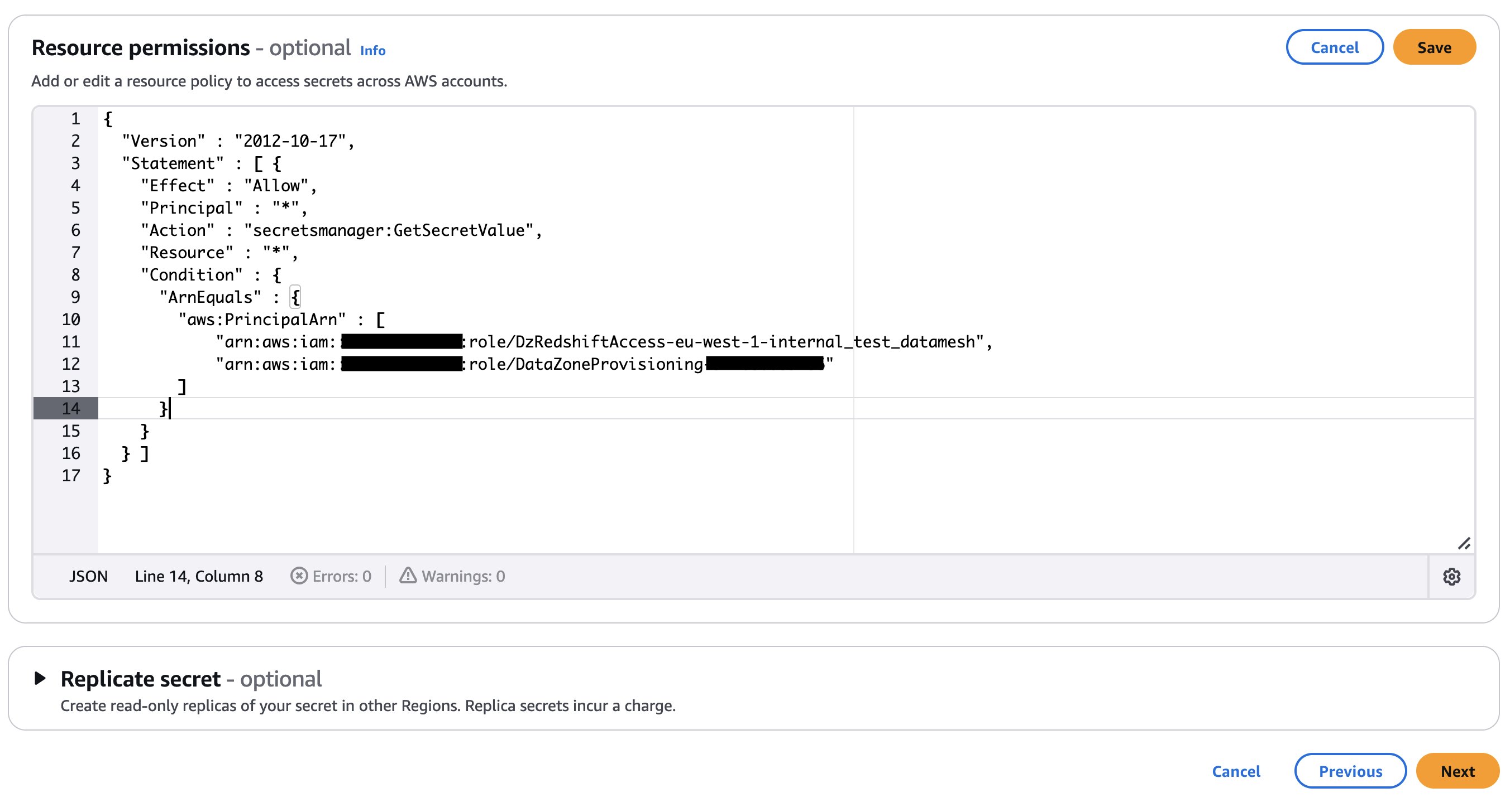If your secret is encrypted with a custom KMS key, append the key policy with the following statement and add a tag to the key: AmazonDatazoneEnvironment = All. You can skip this step if you’re using an AWS managed KMS key.

{
    "Effect": "Allow",
    "Principal": {
        "Service": "logs.<<AWS_Region>>.amazonaws.com",
        "AWS": "arn:aws:iam::<<Data_Producer_Acct_Id(Account B)>>:root"
    },
    "Action": [
        "kms:Decrypt",
        "kms:Encrypt",
        "kms:GenerateDataKey*",
        "kms:ReEncrypt*"
    ],
    "Resource": "*"
 },
 {
    "Sid": "AllowDatazoneRoles-DEV",
    "Effect": "Allow",
    "Principal": {
        "AWS": "*"
    },
    "Action": [
        "kms:Decrypt",
        "kms:Describe*",
        "kms:Get*",
        "kms:Encrypt",
        "kms:GenerateDataKey",
        "kms:ReEncrypt*",
        "kms:CreateGrant"
    ],
    "Resource": "*",
    "Condition": {
        "StringLike": {
            "aws:PrincipalArn": [
                "arn:aws:iam::<<Data_Producer_Acct_Id(Account B)>>:role/aws-service-role/redshift.amazonaws.com/AWSServiceRoleForRedshift",
                "arn:aws:iam::<<Data_Producer_Acct_Id(Account B)>>:role/datazone_*",
                "arn:aws:iam::<<Data_Producer_Acct_Id(Account B)>>:role/<<Redshift_Cluster_IAM_Role>>",
                "arn:aws:iam::<<Data_Producer_Acct_Id(Account B)>>:role/service-role/AmazonDataZoneRedshiftAccess-<<AWS_Region>>-*"
            ]
         }
     }
 }

Place a mechanism to generate the following payload to trigger the dataset registration Lambda function. The payload must contain the relevant Redshift database, schema, and table or view that you want to publish in the Amazon DataZone domain. The following example code assumes you have three databases in your Redshift cluster and within those databases you have different schemas, tables, and views. You should adjust the payload based on your use case.

{
    "source": "redshift-user-initiated",
    "detail-type": "Amazon Redshift dataset registration in Amazon DataZone",
    "datasets": [
        {
            "clusterName": "<<YOUR_REDSHIFT_CLUSTER_NAME>>",
            "dbName":"<<YOUR_REDSHIFT_DATABASE_NAME_1>>",
            "schemas": [
                {
                    "schemaName":"<<YOUR_REDSHIFT_SCHEMA_NAME>>",
                    "addAllTables":false,
                    "addAllViews":false,
                    "tables":[
                        "<<YOUR_REDSHIFT_TABLE_NAME>>",
                        "<<YOUR_REDSHIFT_TABLE_NAME>>"
                    ],
                    "views":[
                        "<<YOUR_REDSHIFT_VIEW_NAME>>"
                    ]
                }
            ]
        },
        {
            "clusterName": "<<YOUR_REDSHIFT_CLUSTER_NAME>>",
            "dbName":"<<YOUR_REDSHIFT_DATABASE_NAME_2>>",
            "schemas": [
                {
                    "schemaName":"<<YOUR_REDSHIFT_SCHEMA_NAME>>",
                    "addAllTables":true,
                    "addAllViews":true,
                    "tables":[],
                    "views":[]
                }
            ]
        },
        {
            "clusterName": "<<YOUR_REDSHIFT_CLUSTER_NAME>>",
            "dbName":"<<YOUR_REDSHIFT_DATABASE_NAME_3>>",
            "schemas": [
                {
                    "schemaName":"<<YOUR_REDSHIFT_SCHEMA_NAME>>",
                    "addAllTables":true,
                    "addAllViews":false,
                    "tables":[],
                    "views":[
                        "<<YOUR_REDSHIFT_VIEW_NAME>>"
                    ]
                }
            ]
        }
    ]
}

Prerequisites in Amazon DataZone account (Account A)

Complete the following steps to set up your Amazon DataZone account (Account A):

Sign in to Account A and make sure you have already deployed an Amazon DataZone domain and a project within that domain. Refer to Create Amazon DataZone domains for instructions to create a domain.
If your Amazon DataZone domain is encrypted with a KMS key, add the data domain account (Account B) to the KMS key policy with the following actions:
```
"Action": [
    "kms:Encrypt",
    "kms:Decrypt",
    "kms:ReEncrypt*",
    "kms:GenerateDataKey*",
    "kms:DescribeKey"
]
```

Create an IAM role that is assumable by Account B and make sure the role has a following policy attached and is a member (as contributor) of your Amazon DataZone project. For this post, we call the role dz-assumable-env-dataset-registration-role. By adding this role, you can successfully run the registration Lambda function.

In the following policy, provide the AWS Region and account ID corresponding to where your Amazon DataZone domain is created, and the KMS key ARN used to encrypt the domain:

  {
    "Version": "2012-10-17",
    "Statement": [
        {
            "Action": [
                "datazone:CreateDataSource",
                "datazone:CreateEnvironment",
                "datazone:CreateEnvironmentProfile",
                "datazone:GetDataSource",
                "datazone:GetDataSourceRun",
                "datazone:GetEnvironment",
                "datazone:GetEnvironmentProfile",
                "datazone:GetIamPortalLoginUrl",
                "datazone:ListDataSources",
                "datazone:ListDomains",
                "datazone:ListEnvironmentProfiles",
                "datazone:ListEnvironments",
                "datazone:ListProjectMemberships",
                "datazone:ListProjects",
                "datazone:StartDataSourceRun",
                "datazone:UpdateDataSource",
                "datazone:SearchUserProfiles"
            ],
            "Resource": "*",
            "Effect": "Allow"
        },
        {
            "Action": [
                "kms:Decrypt",
                "kms:DescribeKey",
                "kms:GenerateDataKey"
            ],
            "Resource": "arn:aws:kms:<<account_region>>:<<Datazone_Account_id(Account A)>>


}:key/${DataZonekmsKey}",
            "Effect": "Allow"
        }
    ]
}

Add Account B in the trust relationship of this role with the following trust relationship:

{
    "Version": "2012-10-17",
    "Statement": [
        {
            "Effect": "Allow",
            "Principal": {
                "AWS": [
                    "arn:aws:iam::<<Data_Producer_Acct_Id(Account B)>>:root",
                    "arn:aws:iam::<<Datazone_Account_id(Account A)>>:root",
                ]
            },
            "Action": "sts:AssumeRole"
        }
    ]
}

Add the role as a member of the Amazon DataZone project in which you want to register your data sources. For more information, see Add members to a project.

Additional tools

The following tools are needed to deploy the solution using the AWS CDK:

Either Bash/ or ZSH terminal
Node and NPM using Node Version Manager:
- Install Node Version Manager (NVM)
- Install Node version 18.12.0 using the following command (node and npm binaries should now be available):
```
$ nvm install 18.12.0
```
Python
AWS Command Line Interface (AWS CLI); see Installing or updating to the latest version of the AWS CLI
AWS CDK for Python (Boto3); see Installation
AWS CDK

Deploy the solution

After you complete the prerequisites, use the AWS CDK stack provided on the GitHub repo to deploy the solution for automatic registration of data assets into the Amazon DataZone domain. Complete the following steps:

Clone the repository from GitHub to your preferred integrated development environment (IDE) using the following commands:

git clone https://github.com/aws-samples/sample-how-to-automate-amazon-redshift-cluster-data-asset-publish-to-amazon-datazone

$ cd sample-how-to-automate-amazon-redshift-cluster-data-asset-publish-to-amazon-datazone

At the base of the repository folder, run the following commands to build and deploy resources to AWS:
```
$ npm install
```
```
$ npm run lint
```
Sign in to Account B (the data domain producer account) using the AWS CLI with your profile name.
Make sure you have configured the Region in your credential’s configuration file.
Bootstrap the AWS CDK environment with the following commands at the base of the repository folder. Provide the profile name of your deployment account (Account B). Bootstrapping is a one-time activity and is not needed if your AWS account is already bootstrapped.
```
$ export AWS_PROFILE=<<PROFILE_NAME>>
```
```
$ npm run cdk bootstrap
```
Replace the placeholder parameters (marked with the suffix _PLACEHOLDER) in the file config/DataZoneConfig.ts:
1. Amazon DataZone domain and project name of your Amazon DataZone instance. Make sure all names are in lowercase.
2. The AWS account ID of the Amazon DataZone account (Account A).
3. The assumable IAM role from the prerequisites.
4. The AWS Systems Manager parameter name containing the Secrets Manager secret ARN of the Amazon Redshift credentials.
Use the following command in the base folder to deploy the AWS CDK solution. During deployment, enter y if you want to deploy the changes for some stacks when you see the prompt Do you wish to deploy these changes (y/n)?
```
npm run cdk deploy --all
```
After the deployment is complete, sign in to Account B and open the AWS CloudFormation console to verify that the infrastructure was deployed.

Test automatic data registration to Amazon DataZone

Complete the following steps to test the solution:

Sign in to Account B (producer account).
On the Lambda console, open the datazone-redshift-dataset-registration function.
Under TEST EVENTS, choose Create new test event.

For Event name, enter Redshift, and for Event JSON, enter the following JSON structure (change the cluster, schema, database, and table names according to your environment):

{
  "source": "redshift-user-initiated",
  "detail-type": "Amazon Redshift dataset registration in Amazon DataZone",
  "datasets": [
    {
      "clusterName": "YOUR_REDSHIFT_CLUSTER_NAME",
      "dbName": "DATABASE_NAME",
      "schemas": [
        {
          "schemaName": "SCHEMA_NAME_1",
          "addAllTables": false,
          "addAllViews": false,
          "tables": [
            "TABLE_NAME"
          ],
          "views": []
        },
        {
          "schemaName": "SCHEMA_NAME_2",
          "addAllTables": false,
          "addAllViews": false,
          "tables": [],
          "views": [
            "VIEW_NAME"
          ]
        }
      ]
    }
  ]
}

Choose Save.
Choose Invoke.
Open the Amazon DataZone console in Account A where you deployed the resources.
Choose Domains in the navigation pane, then open your domain.
On the domain details page, locate the Amazon DataZone data portal URL in the Summary section. Choose the link to the data portal.
For more details about accessing Amazon DataZone, refer to How can I access Amazon DataZone?
In the data portal, open your project and choose the Data tab.
In the navigation pane, choose Data sources and find the newly created data source for Amazon Redshift.
Verify that the data source has been successfully published.

After the data sources are published, users can discover the published data and submit a subscription request. The data producer can approve or reject requests. Upon approval, users can consume the data by querying the data in the Amazon Redshift query editor. The following screenshot illustrates data discovery in the Amazon DataZone data portal.

Clean up

Complete the following steps to clean up the resources deployed through the AWS CDK:

Sign in to Account B, go to the Amazon DataZone domain portal, and check there is no subscription for your published data asset. If there is a subscription, either ask the subscriber to unsubscribe or revoke the subscription request.
Delete the published data assets that were created in the Amazon DataZone project by the dataset registration Lambda function.
Delete the remaining resources created using the following command in the base folder:
```
npm run cdk destroy –all
```

Conclusion

Amazon DataZone offers a seamless integration with AWS services, providing a powerful solution for organizations like Volkswagen to break down their data silos and implement effective data mesh architectures through a straightforward implementation highlighted in this post. By using Amazon DataZone, Volkswagen addressed its immediate data sharing hurdles and laid the groundwork for a more agile, data-driven future in automotive manufacturing. The automated data publishing from various warehouses, coupled with standardized governance workflows, has significantly reduced the manual overhead that once slowed down Volkswagen’s data engineering teams. Now, instead of navigating a labyrinth of emails, tickets, and communication, Volkswagen’s data engineers and data scientists can quickly discover and access the data they need, all while maintaining their security and compliance standards.

By using Amazon DataZone, organizations can bring their isolated data together in ways that make it simpler for teams to collaborate while maintaining security and compliance at scale. This approach not only addresses current data governance challenges but also creates a highly scalable foundation for future data-driven innovations. For guidance on establishing your organization’s data mesh with Amazon DataZone, contact your AWS team today.

About the Authors

Seamlessly Integrate Data on Google BigQuery and ClickHouse Cloud with AWS Glue

2025-10-07 Ray Wang

Post Syndicated from Ray Wang original https://aws.amazon.com/blogs/big-data/seamlessly-integrate-data-on-google-bigquery-and-clickhouse-cloud-with-aws-glue/

Migrating from Google Cloud’s BigQuery to ClickHouse Cloud on AWS allows businesses to leverage the speed and efficiency of ClickHouse for real-time analytics while benefiting from AWS’s scalable and secure environment. This article provides a comprehensive guide to executing a direct data migration using AWS Glue ETL, highlighting the advantages and best practices for a seamless transition.

AWS Glue ETL enables organizations to discover, prepare, and integrate data at scale without the burden of managing infrastructure. With its built-in connectivity, Glue can seamlessly read data from Google Cloud’s BigQuery and write it to ClickHouse Cloud on AWS, removing the need for custom connectors or complex integration scripts. Beyond connectivity, Glue also provides advanced capabilities such as a visual ETL authoring interface, automated job scheduling, and serverless scaling, allowing teams to design, monitor, and manage their pipelines more efficiently. Together, these features simplify data integration, reduce latency, and deliver significant cost savings, enabling faster and more reliable migrations.

Prerequisites

Before using AWS Glue to integrate data into ClickHouse Cloud, you must first set up the ClickHouse environment on AWS. This includes creating and configuring your ClickHouse Cloud on AWS, making sure network access and security groups are properly defined, and verifying that the cluster endpoint is accessible. Once the ClickHouse environment is ready, you can leverage the AWS Glue built-in connector to seamlessly write data into ClickHouse Cloud from sources such as Google Cloud BigQuery. You can follow the next section to complete the setup.

Set up ClickHouse Cloud on AWS
1. Follow the ClickHouse official website to set up environment (remember to allow remote access in the config file if using Clickhouse OSS)
  https://clickhouse.com/docs/get-started/quick-start
Subscribe the ClickHouse Glue marketplace connector
1. Open Glue Connectors and choose Go to AWS Marketplace
2. On the list of AWS Glue marketplace connectors, enter ClickHouse in the search bar. Then choose ClickHouse Connector for AWS Glue
3. Choose View purchase options on the right top of the view
4. Review Terms and Conditions and choose Accept Terms
5. Choose Continue to Configuration once it’s enabled
6. On Follow the vendor’s instructions part in the connector instructions as below, choose the connector enabling link at step 3

Configure AWS Glue ETL Job for ClickHouse Integration

AWS Glue enables direct migration by connecting with ClickHouse Cloud on AWS through built-in connectors, allowing for seamless ETL operations. Within the Glue console, users can configure jobs to read data from S3 and write it directly to ClickHouse Cloud. Using AWS Glue Data Catalog, data in S3 can be indexed for efficient processing, while Glue’s PySpark support allows for complex data transformations, including data type conversions, to support compatibility with ClickHouse’s schema.

Open AWS Glue in the AWS Management Console
1. Navigate to Data Catalog and Connections
2. Create a new connection
Configure BigQuery Connection in Glue
1. Prepare a Google Cloud BigQuery Environment
2. Create and Store Google Cloud Service Account Key (JSON format) in AWS Secret Manager, you can find the details in BigQuery connections.
3. The JSON Format content example is as following:
```
{
  "type": "service_account",
  "project_id": "h*********g0",
  "private_key_id": "cc***************81",
  "private_key": "-----BEGIN PRIVATE KEY-----\nMI***zEc=\n-----END PRIVATE KEY-----\n",
  "client_email": "clickhouse-sa@h*********g0.iam.gserviceaccount.com",
  "client_id": "1*********8",
  "auth_uri": "https://accounts.google.com/o/oauth2/auth",
  "token_uri": "https://oauth2.googleapis.com/token",
  "auth_provider_x509_cert_url": "https://www.googleapis.com/oauth2/v1/certs",
  "client_x509_cert_url": "https://www.googleapis.com/robot/v1/metadata/x509/clickhouse-sa%40h*********g0.iam.gserviceaccount.com",
  "universe_domain": "googleapis.com"
}
```
  - type: service_account.
  - project_id: The ID of the GCP project.
  - private_key_id: A unique ID for the private key within the file.
  - private_key: The actual private key.
  - client_email: The email address of the service account.
  - client_id: A unique client ID associated with the service account.
  - auth_uri, token_uri, auth_provider_x509_cert_url
  - client_x509_cert_url: URLs for authentication and token exchange with Google’s identity and access management systems.
  - universe_domain: The domain name of GCP, googleapis.com
4. Create Google BigQuery Connection in AWS Glue
5. Grant the IAM role associated with your AWS Glue job permission for S3, Secret Manager, Glue services, and AmazonEC2ContainerRegistryReadOnly for accessing connectors purchased from AWS Marketplace (reference doc)
Create ClickHouse connection in AWS Glue
1. Enter clickhouse-connection as its connection name
2. Choose Create connection and activate connector

Create a Glue job

On the Connectors view as below, select clickhouse-connection and choose Create job
Enter bq_to_clickhouse as its job name and configure gc_connector_role as its IAM Role
Configure BigQuery connection and clickhouse-connection to the Connection property
Choose the Script tab and Edit script. Then choose Confirm on the Edit script popup view.
Copy and paste the following code onto the script editor which can be referred from clickhouse official doc

The source code is as following:

import sys
from pyspark.sql import SparkSession
from awsglue.context import GlueContext
from awsglue.job import Job
from awsglue.utils import getResolvedOptions

args = getResolvedOptions(sys.argv, ['JOB_NAME'])
spark = SparkSession.builder.getOrCreate()
glueContext = GlueContext(spark.sparkContext)
job = Job(glueContext)
job.init(args['JOB_NAME'], args)

connection_options = {
    "connectionName": "Bigquery connection",
    "parentProject": "YOUR_GCP_PROJECT_ID",
    "query": "SELECT * FROM `YOUR_GCP_PROJECT_ID.bq_test_dataset.bq_test_table`",
    "viewsEnabled": "true",
    "materializationDataset": "bq_test_dataset"
}
jdbc_url = " jdbc:clickhouse://YOUR_CLICKHOUSE_CONNECTION.us-east-1.aws.clickhouse.cloud:8443/clickhouse_database?ssl=true "
username = "default"
password = "YOUR_PASSWORD"
query = "select * from clickhouse_database.clickhouse_test_table"
# Add this before writing to test connection
try:
    # Read from BigQuery with Glue Connection
    print("Reading data from BigQuery...")
    GoogleBigQuery_node1742453400261 = glueContext.create_dynamic_frame.from_options(
        connection_type="bigquery",
        connection_options=connection_options,
        transformation_ctx="GoogleBigQuery_node1742453400261"
    )
    # Convert to DataFrame
    bq_df = GoogleBigQuery_node1742453400261.toDF()
    print("Show data from BigQuery:")
    bq_df.show()
    
    # Write BigQuery Data to Clickhouse with JDBC
    bq_df.write \
    .format("jdbc") \
    .option("driver", 'com.clickhouse.jdbc.ClickHouseDriver') \
    .option("url", jdbc_url) \
    .option("user", username) \
    .option("password", password) \
    .option("dbtable", "clickhouse_test_table") \
    .mode("append") \
    .save()
    
    print("Write BigQuery Data to ClickHouse successfully")
    
    # Read from Clickhouse with JDBC
    reaf_df = (spark.read.format("jdbc")
    .option("driver", 'com.clickhouse.jdbc.ClickHouseDriver')
    .option("url", jdbc_url)
    .option("user", username)
    .option("password", password)
    .option("query", query)
    .option("ssl", "true")
    .load())
    
    print("Show Data from ClickHouse:")
    reaf_df.show()
    
except Exception as e:
    print(f"ClickHouse connection test failed: {str(e)}")
    raise e
finally:
    job.commit()

Choose Save and Run on the right top of the current view

Testing and Validation

Testing is crucial to verify data accuracy and performance in the new environment. After the migration completes, run data integrity checks to confirm record counts and data quality in ClickHouse Cloud. Schema validation is essential, as each data field must align correctly with ClickHouse’s format. Running performance benchmarks, such as sample queries, will help verify that ClickHouse’s setup delivers the desired speed and efficiency gains.

The Schema and Data in source BigQuery and destination Clickhouse
AWS Glue output logs

Clean Up

After completing the migration, it’s important to clean up unused resources—such as BigQuery for sample data import and database resources in ClickHouse Cloud—to avoid unnecessary costs. Regarding IAM permissions, adhering to the principle of least privilege is advisable. This involves granting users and roles only the permissions necessary for their tasks and removing unnecessary permissions when they are no longer required. This approach enhances security by minimizing potential threat surfaces. Additionally, reviewing AWS Glue job costs and configurations can help identify optimization opportunities for future migrations. Monitoring overall costs and analyzing usage can reveal areas where code or configuration improvements may lead to cost savings.

Conclusion

AWS Glue ETL offers a robust and user-friendly solution for migrating data from BigQuery to ClickHouse Cloud on AWS. By utilizing Glue’s serverless architecture, organizations can perform data migrations that are efficient, secure, and cost-effective. The direct integration with ClickHouse streamlines data transfer, supporting high performance and flexibility. This migration approach is particularly well-suited for companies looking to enhance their real-time analytics capabilities on AWS.

About the Authors

Optimize efficiency with language analyzers using scalable multilingual search in Amazon OpenSearch Service

2025-10-03 Sunil Ramachandra

Post Syndicated from Sunil Ramachandra original https://aws.amazon.com/blogs/big-data/optimize-efficiency-with-language-analyzers-using-scalable-multilingual-search-in-amazon-opensearch-service/

Organizations manage content across multiple languages as they expand globally. Ecommerce platforms, customer support systems, and knowledge bases require efficient multilingual search capabilities to serve diverse user bases effectively. This unified search approach helps multinational organizations maintain centralized content repositories while making sure users, regardless of their preferred language, can effectively find and access relevant information.

Building multi-language applications using language analyzers with OpenSearch commonly involves a significant challenge: multi-language documents require manual preprocessing. This means that in your application, for every document, you must first identify each field’s language, then categorize and label it, storing content in separate, pre-defined language fields (for example, name_en, name_es, and so on) in order to use language analyzers in search to improve search relevancy. This client-side effort is complex, adding workload for language detection, potentially slowing data ingestion, and risking accuracy issues if languages are misidentified. It’s a labor-intensive approach. However, Amazon OpenSearch Service 2.15+ introduces an AI-based ML inference processor. This new feature automatically identifies and tags document languages during ingestion, streamlining the process and removing the burden from your application.

By harnessing the power of AI and using context-aware data modeling and intelligent analyzer selection, this automated solution streamlines document processing by minimizing manual language tagging, and enables automatic language detection during ingestion, providing organizations sophisticated multilingual search capabilities.

Using language identification in OpenSearch Service offers the following benefits:

Enhanced user experience – Users can now find relevant content regardless of the language they search in
Increased content discovery – The service can surface valuable content across language silos
Improved search accuracy – Language-specific analyzers provide better search relevance
Automated processing – You can reduce manual language tagging and classification

In this post, we share how to implement a scalable multilingual search solution using OpenSearch Service.

Solution overview

The solution eliminates manual language preprocessing by automatically detecting and handling multilingual content during document ingestion. Instead of manually creating separate language fields (en_notes, es_notes, and so on) or implementing custom language detection systems, the ML inference processor identifies languages and creates appropriate field mappings.

This automated approach improves accuracy compared to traditional manual methods and reduces development complexity and processing overhead, allowing organizations to focus on delivering better search experiences to their global users.

The solution comprises the following key components:

ML inference processor – Invokes ML models during document ingestion to enrich content with language metadata
Amazon SageMaker integration – Hosts pre-trained language identification models that analyze text fields and return language predictions
Language-specific indexing – Applies appropriate analyzers based on detected languages, providing proper handling of stemming, stop words, and character normalization
Connector framework – Enables secure communication between OpenSearch Service and Amazon SageMaker endpoints through AWS Identity and Access Management (IAM) role-based authentication.

The following diagram illustrates the workflow of the language detection pipeline.

Workflow of the language detection pipeline

Figure 1: Workflow of the language detection pipeline

This example demonstrates text classification using XLM-RoBERTa-base for language detection on Amazon SageMaker. You have flexibility in choosing your models and can alternatively use the built-in language detection capabilities of Amazon Comprehend.

In the following sections, we walk through the steps to deploy the solution. For detailed implementation instructions, including code examples and configuration templates, refer to the comprehensive tutorial in the OpenSearch ML Commons GitHub repository.

Prerequisites

You must have the following prerequisites:

An OpenSearch Service domain running version 2.15 or later
Amazon SageMaker access for model deployment
Appropriate IAM roles and policies for service integration
Fine-grained access control enabled on the OpenSearch Service domain

Deploy the model

Deploy a pre-trained language identification model on Amazon SageMaker. The XLM-RoBERTa model provides robust multilingual language detection capabilities suitable for most use cases.

Configure the connector

Create an ML connector to establish a secure connection between OpenSearch Service and Amazon SageMaker endpoints, primarily for language detection tasks. The process begins with setting up authentication through IAM roles and policies, applying proper permissions for both services to communicate securely.

After you configure the connector with the appropriate endpoint URLs and credentials, the model is registered and deployed in OpenSearch Service and its modelID is used in subsequent steps.

POST /_plugins/_ml/models/_register
{
  "name": "sagemaker-language-identification",
  "version": "1",
  "function_name": "remote",
  "description": "Remote model for language identification",
  "connector_id": "your_connector_id"
}

Sample response:

{
  "task_id": "hbYheJEBXV92Z6oda7Xb",
  "status": "CREATED",
  "model_id": "hrYheJEBXV92Z6oda7X7"
}

After you configure the connector, you can test is by sending text to the model through OpenSearch Service, and it will return the detected language (for example, sending “Say this is a test” returns en for English).

POST /_plugins/_ml/models/your_model_id/_predict
{
  "parameters": {
    "inputs": "Say this is a test"
  }
}
{
  "inference_results": [
    {
      "output": [
        {
          "name": "response",
          "dataAsMap": {
            "response": [
              {
                "label": "en",
                "score": 0.9411176443099976
              }
            ]
          }
        }
      ]
    }
  ]
}

Set up the ingest pipeline

Configure the ingest pipeline, which uses ML inference processors to automatically detect the language of the content in the name and notes fields of incoming documents. After language detection, the pipeline creates new language-specific fields by copying the original content to new fields with language suffixes (for example, name_en for English content).

The pipeline uses an ml_inference processor to perform the language detection and copy processors to create the new language-specific fields, making it straightforward to handle multilingual content in your OpenSearch Service index.

PUT _ingest/pipeline/language_classification_pipeline{
  "description": "ingest task details and classify languages",
  "processors": [
    {
      "ml_inference": {
        "": "6s71PJQBPmWsJ5TTUQmc",
        "input_map": [
          {
            "inputs": "name"
          },
          {
            "inputs": "notes"
          }
        ],
        "output_map": [
          {
            "predicted_name_language": "response[0].label"
          },
          {
            "predicted_notes_language": "response[0].label"
          }
        ]
      }
    },
    {
      "copy": {
        "source_field": "name",
        "target_field": "name_{{predicted_name_language}}",
        "ignore_missing": true,
        "override_target": false,
        "remove_source": false
      }
    }
  ]
}
{
  "acknowledged": true
}

Configure the index and ingest documents

Create an index with the ingest pipeline that automatically detects the language of incoming documents and applies appropriate language-specific analysis. When documents are ingested, the system identifies the language of key fields, creates language-specific versions of those fields, and indexes them using the correct language analyzer. This allows for efficient and accurate searching across documents in multiple languages without requiring manual language specification for each document.

Here’s a sample index creation API call demonstrating different language mappings.

PUT /task_index
{
  "settings": {
    "index": {
      "default_pipeline": "language_classification_pipeline"
    }
  },
  "mappings": {
    "properties": {
      "name_en": { "type": "text", "analyzer": "english" },
      "name_es": { "type": "text", "analyzer": "spanish" },
      "name_de": { "type": "text", "analyzer": "german" },
      "notes_en": { "type": "text", "analyzer": "english" },
      "notes_es": { "type": "text", "analyzer": "spanish" },
      "notes_de": { "type": "text", "analyzer": "german" }
    }
  }
}

Next, ingest this input document in German

{
  "name": "Kaufen Sie Katzenminze",
  "notes": "Mittens mag die Sachen von Humboldt wirklich."
}

The German text used in the preceding code will be processed using a German-specific analyzer, supporting proper handling of language-specific characteristics such as compound words and special characters.

After successful ingestion into OpenSearch Service, the resulting document appears as follows:

{
  "_source": {
    "predicted_notes_language": "en",
    "name_en": "Buy catnip",
    "notes": "Mittens really likes the stuff from Humboldt.",
    "predicted_name_language": "en",
    "name": "Buy catnip",
    "notes_en": "Mittens really likes the stuff from Humboldt."
  }
}

Search documents

This step demonstrates the search capability after the multilingual setup. By using a multi_match query with name_* fields, it searches across all language-specific name fields (name_en, name_es, name_de) and successfully finds the Spanish document when searching for “comprar” because the content was properly analyzed using the Spanish analyzer. This example shows how the language-specific indexing enables accurate search results in the correct language without needing to specify which language you’re searching in.

GET /task_index/_search
{
  "query": {
    "multi_match": {
      "query": "comprar",
      "fields": ["name_*"]
    }
  }
}

This search correctly finds the Spanish document because the name_es field is analyzed using the Spanish analyzer:

{
  "hits": {
    "total": { "value": 1, "relation": "eq" },
    "max_score": 0.9331132,
    "hits": [
      {
        "_index": "task_index",
        "_id": "3",
        "_score": 0.9331132,
        "_source": {
          "name_es": "comprar hierba gatera",
          "notes": "A Mittens le gustan mucho las cosas de Humboldt.",
          "predicted_notes_language": "es",
          "predicted_name_language": "es",
          "name": "comprar hierba gatera",
          "notes_es": "A Mittens le gustan mucho las cosas de Humboldt."
        }
      }
    ]
  }
}

Cleanup

To avoid ongoing charges and delete the resources created in this tutorial, perform the following cleanup steps

Delete the Opensearch service domain. This stops both storage costs for your vectorized data and any associated compute charges.
Delete the ML connector that links your OpenSearch service to your machine learning model.
Finally, delete your Amazon SageMaker endpoints and resources.

Conclusion

Implementing multilingual search with OpenSearch Service can help organizations break down language barriers and unlock the full value of their global content. The ML inference processor provides a scalable, automated approach to language detection that improves search accuracy and user experience.

This solution addresses the growing need for multilingual content management as organizations expand globally. By automatically detecting document languages and applying appropriate linguistic processing, businesses can deliver comprehensive search experiences that serve diverse user bases effectively.

About the authors

Deploying AI models for inference with AWS Lambda using zip packaging

2025-10-03 Ayush Kulkarni

Post Syndicated from Ayush Kulkarni original https://aws.amazon.com/blogs/compute/deploying-ai-models-for-inference-with-aws-lambda-using-zip-packaging/

AWS Lambda provides an event-driven programming model, scale-to-zero capability, and integrations with over 200 AWS services. This can make it a good fit for CPU-based inference applications that use customized, lightweight models and complete within 15 minutes.

Users usually package their function code as container images when using machine learning (ML) models that are larger than 250 MB, which is the Lambda deployment package size limit for zip files. In this post, we demonstrate an approach that downloads ML models directly from Amazon S3 into your function’s memory so that you can continue packaging your function code using zip files. To optimize startup latency without implementing application-level performance optimizations, we use Lambda SnapStart. SnapStart is an opt-in capability available for Java, Python, and .NET functions that optimizes startup latency—from 16.5s down to 1.6s for the application used in this post.

Application architecture

In this post, we demonstrate how to build a chatbot, using a 4-bit quantized version of the DeepSeek-R1-Distill-Qwen-1.5B-GGUF model for inference along with Lambda Function URL (FURL) and Lambda Web Adapter (LWA) to stream text responses. A FURL is a dedicated HTTP(s) endpoint for your Lambda function, and you can use LWA, an open-source project available on AWS Labs, for familiar web application frameworks (such as FastAPI, Next.JS, or Spring Boot) with Lambda. For a detailed explanation of how this response streaming architecture works, refer to this AWS Compute post.

Today, Lambda functions are run on CPU-based Amazon Elastic Compute Cloud (Amazon EC2) instances that use x86 and ARM64 architectures. For this reason, you must use SDKs that enable large language model (LLM) inference on CPUs. In this post, we also demonstrate how to use the llama.cpp project (through the llama-cpp-python library) and the FastAPI web framework to handle web requests. To use models that exceed the 250 MB zip package size limit of Lambda, you can download them from an S3 bucket during function initialization. The following figure describes this architecture in detail.

Architecture diagram demonstrating an AI inference workload with AWS Lambda FURLs and AWS Lambda Web Adapter

Figure 1: Application architecture

You can refer to this GitHub repository for the application code used in this example.

Downloading ML models during function initialization

As an alternative to packaging ML models using OCI container images, you can download them from durable storage, such as Amazon S3, during initialization. Initialization (or INIT) refers to the phase when Lambda downloads your function code, starts the language runtime and runs your function initialization code, which is code outside the handler. Loading large files directly into memory can be faster than first downloading them to disk and then loading them into memory. To do so, you can use a Linux capability called memfd, to directly download the ML model from Amazon S3 directly into memory, while referencing it using a standard file descriptor. Referencing the model using a file descriptor is necessary for llama.cpp to successfully import the model. This is comprised of two steps.

First, create a memory-only file descriptor:


    libc = ctypes.CDLL("libc.so.6", use_errno=True)
    MFD_CLOEXEC = 1
    
    memfd_create = libc.memfd_create
    memfd_create.argtypes = [ctypes.c_char_p, ctypes.c_uint]
    memfd_create.restype = ctypes.c_int
    
    fd = memfd_create(b"model", MFD_CLOEXEC)
    if fd == -1:
        errno = ctypes.get_errno()
    raise OSError(errno, f"memfd_create failed: {os.strerror(errno)}")
    
    return fd

Then, download the model into the memory-mapped file referenced by the previously created file descriptor.

def download_model_to_memfd(bucket, key, chunk_size=100*1024*1024):  # 100MB chunks

    s3 = boto3.client('s3')
    
    # Get file size
    response = s3.head_object(Bucket=bucket, Key=key)
    file_size = response['ContentLength']
    
    # Create memory file
    fd = create_memfd()
    
    # Pre-allocate the full file size
    try:
        os.ftruncate(fd, file_size)
    except OSError as e:
        logger.error(f"Failed to allocate {file_size/1024/1024:.2f}MB in memory: {e}")
        cleanup_fd(fd)
        raise RuntimeError(f"Not enough memory to load model of size {file_size/1024/1024:.2f}MB")
    
    # Calculate parts
    parts = []
    for start in range(0, file_size, chunk_size):
        end = min(start + chunk_size - 1, file_size - 1)
        parts.append({'start': start, 'end': end})
    
    logger.info(f"Downloading {file_size/1024/1024:.2f}MB in {len(parts)} parts")
    
    # Download parts concurrently
    download_func = partial(download_part, s3, bucket, key, fd)
    with ThreadPoolExecutor(max_workers=multiprocessing.cpu_count()) as executor:
        executor.map(download_func, parts)
    
    fd_path = f"/proc/self/fd/{fd}"
    return fd, fd_path

Querying the chatbot

After deploying our sample chatbot application, we begin interacting with it.

The first query to the chatbot results in a new execution environment being initialized. When Lambda runs the initialization code described in the previous section, your ML model is directly downloaded from Amazon S3 into the function’s memory. After this, Lambda runs the function’s handler method. Looking at the X-Ray trace segment in the following figure, we observe that the first Init times out after 10 s. The second Init completes in 16.68 s. Furthermore, the first Init times out because Lambda limits the duration of this phase to 10s. If Init takes longer than this, then Lambda retries it during function invocation applying the function’s configured execution duration timeout.

Screenshot of AWS X-Ray Segments demonstrating INIT duration of 16.68 s

Figure 2: Init duration, indicated by AWS X-Ray trace segment

Optimizing startup performance with SnapStart

To optimize function startup latency, you can use Lambda SnapStart. SnapStart is designed to optimize startup latency stemming from long-running function initialization code. Lambda uses SnapStart to initialize your function when you publish a function version, as shown in the following figure. Then, Lambda takes a Firecracker microVM snapshot of the memory and disk state of the initialized execution environment, encrypts the snapshot, and intelligently caches it to optimize retrieval latency.

Screenshot of AWS Lambda Console showing how to enable SnapStart for your Lambda function

Figure 3: Enabling SnapStart

Querying the chatbot again shows a significant speed-up in initialization latency. You can verify this by viewing your function’s Amazon CloudWatch Logs, and searching for the “RESTORE_REPORT” log line, as shown in the following figure. For the sample application used, restore duration is 1.39 s. This is a considerable improvement over the Init duration of 16.68 s. Performance results may vary. But best of all, you don’t need to change a single line of code to achieve this improvement!

Screenshot of Amazon CloudWatch Logs demonstrating RESTORE duration of 1.39 s

Figure 4: Achieving faster startup latency with SnapStart

Tuning inference performance

Inference performance depends on the CPU resources allocated to your function. Lambda allocates CPU power in proportion to the amount of memory configured for your function. Allocating more memory results in faster inference results, measured by the rate at which prompt tokens are evaluated (tokens evaluated per second), and the rate at which output tokens are produced (tokens generated per second). For this example, we allocate the maximum—in other words 10 GB memory—to maximize performance. Performance results obtained at other memory size configurations are included in the following table. As the table shows, doubling the memory allocated from 5 GB to 10 GB results in an 83% improvement in tokens evaluated and generated (per second), with only a 24% increase in billed GB-seconds. Performance results may vary. Refer to the sample code to instrument performance at different memory sizes.

Memory Size (MB)	Tokens evaluated per second	Tokens generated per second	Billed Duration (ms)	Billed GB-seconds
10240	44.68	29.53	36,660	366.60
9216	41.67	26.77	37,690	339.21
8192	37.17	22.05	44,298	354.38
7168	33.67	21.78	44,818	313.73
6144	28.89	18.43	52,579	315.47
5120	24.41	16.07	59,036	295.18
4096	19.07	12.94	72,648	290.59
3072	13.39	9.20	101,468	304.40
2048	10.01	6.77	135,862	271.72

Table 1: Inference performance at different memory sizes

Understanding how application costs scale with usage

To estimate the cost of running this workload, we begin by making some assumptions about our traffic patterns. We estimate about 30,000 inference calls per month to our Lambda function, with each inference call averaging 10s in duration. We set function memory to 10 GB, because it represents the ideal price-performance for our use case. We deploy our application in the US-West-2 (Oregon) AWS Region. Initially, because our number of invokes is low, we assume a 5% cold-start rate. In other words, 5% of invokes result in a cold-start when a new execution environment is created. When using SnapStart with the Lambda managed Python runtime, you are charged for caching your function’s snapshot and for restoring execution from your function’s snapshot.

With these parameters, the monthly Lambda bill is $91.1, calculated as shown in the following table. The monthly costs shown in the table are only illustrative.

Charge	Calculation	Monthly Cost
Compute	30,000 inferences * 10 seconds per inference * 10 GB (configured memory) * $0.00001667 per GB-second	$50.01
Requests	$0.2 per million requests * 30,000 inferences	$0.006
SnapStart – Cache	10 GB function memory * 2.59M GB-seconds per month * $0.0000015046 per GB-second	$38.99
SnapStart – Restore	10 GB function memory * $0.0001397998 per GB restore * 1500 cold-starts	$2.09
Total	Compute + Requests + SnapStart Cache + SnapStart Restore	$91.1

At low invocation volume, the added charges for the SnapStart account for approximately 50% of total monthly cost. For this added charge, cold-start latency reduces from 16.68 s to1.39 s, without having to implement complex optimizations ourselves. We can demonstrate how these costs scale with usage. We assume that our chatbot grows in popularity with traffic increasing 10 times to 300,000 monthly inference calls. Although cold-start rates for individual Lambda functions can vary due to several factors, Lambda’s re-use of execution environments generally results in cold-start rates decreasing with higher traffic volume. For the purposes of this example, we assume that our cold-start rate drops to 1% of all invokes with the 10 times growth in traffic.With these assumptions, our monthly Lambda bill at 10 times higher traffic volume is $543.3. Added charges for SnapStart now constitute less than 10% of our total bill, as shown in the following table. Monthly costs shown in this table are only illustrative.

Charge	Calculation	Monthly Cost
Compute	300,000 inferences * 10 seconds per inference * 10 GB (configured memory) * $0.00001667 per GB-second	$500.01
Requests	$0.2 per million requests * 300,000 inferences	$0.06
SnapStart – Cache	10 GB function memory * 2.59M GB-seconds per month * $0.0000015046 per GB-second	$38.99
SnapStart – Restore	10 GB function memory * $0.0001397998 per GB restore * 3000 cold-starts	$4.18
Total	Compute + Requests + SnapStart Cache + SnapStart Restore	$543.24

Considerations

Lambda functions are run on CPU-based EC2 instances. If your ML models need GPU-based inference, foundational LLMs, or exceed the Lambda limits on execution duration (15 minutes) and function memory (10 GB), then you can use AWS Machine Learning, AWS Generative AI, or AWS Compute services.

Moreover, you should know the following things about Lambda SnapStart:

Handling uniqueness: If your initialization code generates unique content that is included in the snapshot, then the content isn’t unique when it’s reused across execution environments. To maintain uniqueness when using SnapStart, you must generate unique content after initialization, such as if your code uses custom random number generation that doesn’t rely on built-in-libraries or caches any information such as DNS entries that might expire during initialization. To learn how to restore uniqueness, visit Handling uniqueness with Lambda SnapStart in the Lambda Developer Guide.

Performance tuning: To maximize performance, we recommend that you preload dependencies and initialize resources that contribute to startup latency in your initialization code instead of in the function handler. This moves the latency associated with these operations during version publish, rather than during function invocation and can yield faster startup performance. To learn more, visit Performance tuning for Lambda SnapStart in the Lambda Developer Guide.

Networking best practices: The state of connections that your function establishes during the initialization phase isn’t guaranteed when Lambda resumes your function from a snapshot. In most cases, network connections that an AWS SDK establishes automatically resume. For other connections, review the Networking best practices for Lambda SnapStart in the Lambda Developer Guide.

Conclusion

In this post, we demonstrated how you can download ML models directly from Amazon S3 into your function’s memory, enabling you to deploy your AWS Lambda functions using zip packages. To optimize startup latency without implementing application-level performance optimizations, we also demonstrated the use of Lambda SnapStart, an opt-in capability available for Java, Python, and .NET. For the application used in this post, SnapStart reduced startup latency from 16.68 s down to 1.39 s.

To learn more about Lambda, refer to our documentation. For details about Lambda SnapStart, refer to our launch posts for Java, Python and .Net, and the documentation.

You can refer to this GitHub repository for the application code used in this example.

How Laravel Nightwatch handles billions of observability events in real time with Amazon MSK and ClickHouse Cloud

2025-10-01 Masudur Rahaman Sayem

Post Syndicated from Masudur Rahaman Sayem original https://aws.amazon.com/blogs/big-data/how-laravel-nightwatch-handles-billions-of-observability-events-in-real-time-with-amazon-msk-and-clickhouse-cloud/

Laravel, one of the world’s most popular web frameworks, launched its first-party observability platform, Laravel Nightwatch, to provide developers with real-time insights into application performance. Built entirely on AWS managed services and ClickHouse Cloud, the service already processes over one billion events per day while maintaining sub-second query latency, giving developers instant visibility into the health of their applications.

By combining Amazon Managed Streaming for Apache Kafka (Amazon MSK) with ClickHouse Cloud and AWS Lambda, Laravel Nightwatch delivers high-volume, low-latency monitoring at scale, while maintaining the simplicity and developer experience Laravel is known for.

The challenge: Delivering real-time monitoring for a global developer community

The Laravel framework powers millions of applications worldwide, serving billions of requests each month. Each request can generate potentially hundreds of observability events, such as database queries, queued jobs, cache lookups, emails, notifications, and exceptions. For Nightwatch’s launch, Laravel anticipated instant adoption from its global community, with tens of thousands of applications sending events around the clock from day one.

Laravel Nightwatch needed an architecture that could:

Ingest millions of JSON events per second from customer applications reliably.
Provide sub-second analytical queries for real-time dashboards.
Scale horizontally to handle unpredictable traffic spikes.
Deliver all of this in a cost-effective, low-maintenance manner.

The challenge was to process data on a global scale and provide deep insights into application health without compromising on a straightforward setup experience for developers.

The solution: A decoupled streaming and analytics pipeline

Laravel Nightwatch implemented a dual-database, streaming-first architecture, shown in the preceding figure, that separates transactional and analytical workloads.

Transactional workloads – user accounts, organization settings, billing, and similar workloads run on Amazon RDS for PostgreSQL.
Analytical workloads – telemetry events, metrics, query logs, and request traces are handled by ClickHouse Cloud.

Key components

The key components of the solution include the following:

Ingestion layer
- Amazon API Gateway receives telemetry from Laravel agents embedded in customer applications
- Lambda validates and enriches events. Validated and enriched events are published to Amazon MSK, partitioned for scalability
Streaming to analytics
- ClickPipes in ClickHouse Cloud subscribe directly to MSK topics, reducing the need to build and manage extract, transform, and load (ETL) pipelines
- Materialized views in ClickHouse pre-aggregate and transform raw JSON into query-ready formats
Dashboards and delivery
- The Nightwatch dashboard, built with Laravel, Inertia, and React, runs on AWS Fargate for Amazon ECS
- Amazon ElastiCache for Redis accelerates session and cache lookups
- Cloudflare CDN provides low-latency delivery to global users

Why Amazon MSK and ClickHouse Cloud?

Nightwatch requires a durable, horizontally scalable, and low maintenance streaming backbone.

With Amazon MSK Express brokers, we have achieved over 1 million events per second during load testing, benefiting from low-latency, elastic scaling, and simplified operations. MSK Express brokers require no storage sizing or provisioning, scale up to 20 times faster, and recover 90% quicker than standard Apache Kafka brokers—all while enforcing best-practice defaults and client quotas for reliable performance. Its seamless integration with other AWS services—such as Lambda, Amazon Simple Storage Service (Amazon S3), and Amazon CloudWatch—made it straightforward to build a resilient, end-to-end streaming architecture.

To ingest and transform these events in real time, Nightwatch uses ClickHouse Cloud and its managed integration platform, ClickPipes. ClickHouse Cloud excels at analytical workloads by delivering up to 100 times faster query performance for analytics compared to traditional row-based databases. Its advanced compression algorithms provide up to 90% storage savings, significantly reducing infrastructure costs while maintaining high performance. With its columnar architecture and optimized execution engine, ClickHouse Cloud can query billions of rows in under 1 second, enabling Laravel Nightwatch to serve real-time dashboards and analytics at global scale.

By integrating Amazon MSK and ClickHouse using ClickPipes, Laravel also reduced the operational burden of building and managing ETL pipelines, reducing latency and complexity.

Overcoming challenges

Testing complexity

While synthetic benchmarking and test datasets yield useful results, a more realistic workload is required to rigorously test infrastructure and code before deployment to production. The team used Terraform to manage infrastructure alongside application code, creating multiple dev and test environments, and allowing them to test the platform internally with their own applications before each release.

Multi-region infrastructure

The need to cater to multiple data storage regions also brought challenges—with latency, complexity, and cost the foremost concerns. However, the AWS, ClickHouse Cloud, and Cloudflare stack made available a powerful set of networking tools and scaling options. While VPC peering, RDS replication, and global server load balancing did the heavy lifting on the networking side, the ability to scale and right-size each resource kept costs to a minimum.

Query performance at scale

Materialized views, intelligent time-series partitioning, and specialized ClickHouse codecs helped ensure that queries remained sub-second even as data volumes grew into the billions. Meanwhile, compute separation allowed distinct workloads to scale separately while accessing the same data, with clusters right-sized horizontally and vertically depending on the requirements of each load.

Results

Laravel Nightwatch’s launch exceeded expectations:

5,300 users registered in the first 24 hours
500 million events processed on day one
97 ms average dashboard request latency
760,000 exceptions logged and analyzed in real time

By building on Amazon MSK and ClickHouse Cloud, we were able to scale from zero to billions of events without sacrificing performance or developer experience.

What’s next

Laravel plans to expand Nightwatch with:

More regions to cater to customers with data sovereignty requirements outside the US and EU
Broader data collection to provide even deeper insight into customers’ applications
SOC 2 certification to cater to customers with tighter compliance requirements
More advanced monitoring and analysis to identify issues before they affect users

The current architecture comfortably supports applications of all sizes, from hobby to enterprise (including a generous free tier), and is designed to handle over one trillion monthly events without performance degradation.

Conclusion

Laravel Nightwatch demonstrates how Amazon MSK, ClickHouse Cloud, and AWS serverless technologies can be combined to build a cost-effective, real-time monitoring platform at global scale. By designing for scale from day one, Laravel delivered sub-second analytics across billions of events, while maintaining the developer-friendly experience their community expects.

About the authors

How to export to Amazon S3 Tables by using AWS Step Functions Distributed Map

2025-10-01 Chetan Makvana

Post Syndicated from Chetan Makvana original https://aws.amazon.com/blogs/compute/how-to-export-to-amazon-s3-tables-by-using-aws-step-functions-distributed-map/

Companies running serverless workloads often need to perform extract, transform, and load (ETL) operations on data files stored in Amazon Simple Storage Service (Amazon S3) buckets. Though traditional approaches such as an AWS Lambda trigger for Amazon S3 or Amazon S3 Event Notifications can handle these operations, they might fall short when workflows require enhanced visibility, control, or human intervention. For example, some processes might need manual review of failed records or explicit approval before proceeding to subsequent stages. Customer orchestration solutions to these issues can prove to be complex and error prone.

AWS Step Functions address these challenges by providing built-in workflow management and monitoring capabilities. The Step Functions Distributed Map feature is designed for high-throughput, parallel data processing workflows so that companies can handle complex ETL jobs, fan-out processing, and data visualization at scale. Distributed Map handles each dataset item as an independent child workflow, processing millions of records while maintaining built-in concurrency controls, fault tolerance, and progress tracking. The processed data can be seamlessly exported to various destinations, including Amazon S3 Tables with Apache Iceberg support.

In this post, we show how to use Step Functions Distributed Map to process Amazon S3 objects and export results to Amazon S3 Tables, creating a scalable and maintainable data processing pipeline.

See the associated GitHub repository for detailed instructions about deploying this solution as well as sample code.

Solution overview

Consider a consumer electronics company that regularly participates in industry trade shows and conferences. During these events, interested attendees fill out paper sign-up forms to request product demos, receive newsletters, or join early access programs. After the events, the company’s team scans hundreds of thousands of these forms and uploads them to Amazon S3.Rather than manually reviewing each form, the company wants to automate the extraction of key customer details such as name, email address, mailing address, and interest areas. They’d like to store this structured data in S3 Tables with Apache Iceberg format for downstream analytics and marketing campaign targeting.

Let’s look at how this post’s solution uses Distributed Map to process PDFs in parallel, extract data using Amazon Textract, and write the cleaned output directly to S3 Tables. The result is scalable, serverless post-event data onboarding, as shown in the following figure.

The data processing workflow as shown in the preceding diagram includes the following steps:

A user uploads customer interest forms as scanned PDFs to an Amazon S3 bucket.
An Amazon EventBridge Scheduler rule triggers at regular intervals, initiating a Step Functions workflow execution.
The workflow execution activates a Step Functions Distributed Map state, which lists all PDF files uploaded to Amazon S3 since the previous run.
The Distributed Map iterates over the list of objects and passes each object’s metadata (bucket, key, size, entity tag [ETag]) to a child workflow execution.
For each object, the child workflow calls Amazon Textract with the provided bucket and key to extract raw text and relevant fields (name, email address, mailing address, interest area) from the PDF.
The child workflow sends the extracted data to Amazon Data Firehose, which is configured to forward data to S3 Tables.
Firehose batches the incoming data from the child workflow and writes it to S3 Tables at a preconfigured time interval of your choosing.

With data now structured and accessible in S3 Tables, users can easily analyze them using standard SQL queries with Amazon Athena or business intelligence like Amazon QuickSight.

The data-processing workflow

EventBridge Scheduler starts new Step Functions workflows at regular intervals. The timeline for this schedule is flexible. However, When setting up your schedule, make sure the frequency aligns with how far back your state machine is configured to look for PDFs. For example, if your state machine checks for PDFs from the past week, you’d want to schedule it to run weekly. The Step Functions workflow subsequently performs the following three steps (note that these steps are steps 4, 5, 6, and 7 in the preceding workflow diagram:

Extract relevant user data from the PDFs.
Send the extracted user data to Firehose.
Write the data to S3 Tables in Apache Iceberg table format.

The following diagram illustrates this workflow.

Let’s look at each step of the preceding workflow in more detail.

Extract relevant user data from PDF documents

Step Functions uses Distributed Map to process PDFs concurrently in parallel child workflows. It accepts input from JSON, JSONL, CSV, Parquet files, Amazon S3 manifest files stored in Amazon S3 (used to specify particular files for processing), or an Amazon S3 bucket prefix (allows iteration over file metadata for all objects under that prefix). The Step Functions automatically handles parallelization by splitting the dataset and running child workflows for each item, with the ItemBatcher field allowing to group multiple PDFs into a single child workflow execution (e.g., 10 PDFs per batch) to optimize performance and cost.

The following screenshot of the Step Functions console shows the configuration for Distributed Map. For example, we have configured Distributed Map to process 10 customer interest PDFs in a single child workflow.

The following image shows one example of these scanned PDFs, which includes the customer information that this post’s solution processes.

Each child workflow then calls the Amazon Textract AnalyzeDocument API with specific queries to extract customer information.

{
  "Document": {
    "S3Object": {
      "Bucket": "<input PDFs bucket>",
      "Name": "{% $states.input.Key %}"
    }
  },
  "FeatureTypes": [
    "QUERIES"
  ],
  "QueriesConfig": {
    "Queries": [
      {
        "Alias": "full_name",
        "Text": "What is the customer's name?"
      },
      {
        "Alias": "phone_number",
        "Text": "What is the customer’s phone number?"
      },
      {
        "Alias": "mailing_address",
        "Text": "What is the customer’s mailing address?"
      },
      {
        "Alias": "interest",
        "Text": "What is the customer’s interest?"
      }
    ]
  }
}

The API analyzes each scanned PDF and returns a JSON structure containing the extracted customer information.

Send the extracted user data to Firehose

The child workflow then uses a Firehose PutRecordBatch API action with service integrations to queue the extracted customer information for further processing. The PutRecordBatch action request includes the Firehose stream name and the data records. The data records include a data blob from step 1 that contains extracted customer information, as shown in the following example.

{
  "DeliveryStreamName": "put_raw_form_data_100",
  "Records": [
    {
      "Data": "{\"full_name\":\"Anthony Ayala\",\"phone_number\":\"001-384-925-0701\",\"mailing_address\":\"38548 Joshua Wall Suite 974, East Heatherfort, OH 32669\",\"interest\":\"Fitness Trackers\",\"processed_date\":\"2025-05-01\"}"
    },
    {
      "Data": "{\"full_name\":\"Becky Williams\",\"phone_number\":\"+1-283-499-2466\",\"mailing_address\":\"227 King Forge Suite 241, East Nathanland, PR 05687\",\"interest\":\"Al Assistants\",\"processed_date\":\"2025-05-01\"}"
    }
  ]
}

Write the data to S3 Tables in Apache Iceberg table format

Firehose efficiently manages data buffering, format conversion, and reliable delivery to various destinations, including Apache Iceberg, raw files in Amazon S3, Amazon OpenSearch Service, or any of the other supported destinations. Apache Iceberg tables can be either self-managed in Amazon S3 or hosted in S3 Tables. Though self-managed Iceberg tables require manual optimization—such as compaction and snapshot expiration—S3 Tables automatically optimize storage for large-scale analytics workloads, improving query performance and reducing storage costs.

Firehose simplifies the process of streaming data by configuring a delivery stream, selecting a data source, and setting an Iceberg table as the destination. After you’ve set it up, the Firehose stream is ready to deliver data. The delivered data can be queried from S3 Tables by using Athena, as shown in the following screenshot of the Athena console.

The query results include all processed customer data from the PDFs, as shown in the following screenshot.

This integration demonstrates a powerful, code-free solution for transforming raw PDF forms into enriched, queryable data in an Iceberg table. You can use these data for further analysis.

Conclusion

In this post, we showed how to build a scalable, serverless solution for processing PDF documents and exporting the extracted data to S3 Tables by using Step Functions Distributed Map. This architecture offers several key benefits such as reliability, cost-effectiveness, visibility, and maintainability. By leveraging AWS services such as Step Functions, Amazon Textract, Firehose, and S3 Tables, companies can automate their document processing workflows while ensuring optimal performance and operational excellence. This solution can be adapted for various use cases beyond customer interest forms, such as invoice processing, application forms, or any scenario requiring structured data extraction from documents at scale.

Though this example focuses on processing PDF data and writing to S3 Tables, Distributed Map can handle various input sources including JSON, JSONL, CSV, and Parquet files in Amazon S3; items in Amazon DynamoDB tables; Athena query results; and all paginated AWS List APIs. Similarly, through Step Functions service integrations, you can write results to multiple destinations such as DynamoDB tables by using the PutItem service integration.

To get started with this solution, see the associated GitHub repository for deployment instructions and sample code.

Scaling cluster manager and admin APIs in Amazon OpenSearch Service

2025-09-26 Rajiv Kumar Vaidyanathan

Post Syndicated from Rajiv Kumar Vaidyanathan original https://aws.amazon.com/blogs/big-data/scaling-cluster-manager-and-admin-apis-in-amazon-opensearch-service/

Amazon OpenSearch Service is a managed service that makes it simple to deploy, secure, and operate OpenSearch clusters at scale in the AWS Cloud. A typical OpenSearch cluster is comprised of cluster manager, data, and coordinator nodes. It is recommended to have three cluster manager nodes, and one of them will be elected as a leader node.

Amazon OpenSearch Service introduced support for 1,000-node OpenSearch Service clusters capable of handling 500,000 shards with OpenSearch Service version 2.17. For large clusters, we have identified bottlenecks in admin API interactions (with the leader) and introduced improvements in OpenSearch Service version 2.17. These improvements have helped OpenSearch Service to publish cluster metrics and monitor at same frequency for large clusters while maintaining the optimal resource usage (less than 10% CPU and less than 75% JVM usage) on the leader node (16 core CPU with 64 GB JVM heap). It has also ensured that metadata management can be performed on large clusters with predictable latency without destabilizing the leader node.

General monitoring of an OpenSearch node using health check and statistics API endpoints doesn’t cause visible load to the leader. But as the number of nodes increase in the cluster, the volume of these monitoring calls also increases proportionally. The increase in the call volume coupled with the less optimal implementation of these endpoints overwhelms the leader node, resulting in stability issues. In this post, we demonstrate the different bottlenecks that were identified and the corresponding solutions that were implemented in OpenSearch Service to scale cluster manager for large cluster deployments. These optimizations are available to all new domains or existing domains upgraded to OpenSearch Service versions 2.17 or above.

Cluster state

To understand the various bottlenecks with the cluster manager, let’s examine the cluster state, whose management is the core operation of the leader. The cluster state contains the following key metadata information:

Cluster settings
Index metadata, which includes index settings, mappings, and alias
Routing table and shard metadata, which contains details of shard allocation to nodes
Node information and attributes
Snapshot information, custom metadata, and so on

Node, index, and shard are managed as first-class entities by the cluster manager and contain information such as identifier, name, and attributes for each of their instances.

The following screenshots are from a sample cluster state for a cluster with three cluster manager and three data nodes. The cluster has a single index (sample-index1) with one primary and two replicas.

Cluster metadata showing index and shard configuration

Nodes metadata

As shown in the screenshots, the number of entries in the cluster state is as follows:

IndexMetadata (metadata#indices) has entries equal to the total number of indexes
RoutingTable (routing_table) has entries equal to the number of indexes multiplied by the number of shards per index
NodeInfo (nodes) has entries equal to the number of nodes in the cluster

The size of a sample cluster state with six nodes, one index, and three shards is around 15 KB (size of JSON response from the API). Consider a cluster with 1,000 nodes, which has 10,000 indexes with an average of 50 shards per index. The cluster state would have 10,000 entries for IndexMetadata, 500,000 entries for RoutingTable, and 1,000 entries for NodeInfo.

Bottleneck 1: Cluster state communication

OpenSearch provides admin APIs as a REST endpoint for users to manage and configure the cluster metadata. Admin API requests are handled by either coordinator node (or) by data node if the cluster does not have dedicated coordinator node provisioned. You can use admin APIs to check cluster health, modify settings, retrieve statistics, and more. Some of the examples are the CAT, Cluster Settings, and Node Stats APIs.

The following diagram illustrates the admin API control flow.

Admin API Request Flow

Let’s consider a Read API request to fetch information about the cluster settings.

The user makes the call to the HTTP endpoint backed by the coordinator node.
The coordinator node initiates an internal transport call to the leader of the cluster.
The transport handler in the leader node performs a filter and selection of metadata based on the input request from the latest cluster state.
The processed cluster state is then returned back to the coordinating node, which then generates the response and finishes the request processing.

The cluster state processing on the nodes is shown in the following diagram.

Request Processing using Cluster State

As discussed earlier, most of the admin read requests require the latest cluster state and the node which processes the API request and makes a _cluster/state call to the leader. In a cluster setup of 1,000 nodes and 500,000 shards, the size of the cluster state would be around 250 MB. This can overload leader and cause the following issues:

CPU usage increases on the leader due to simultaneous admin calls because the leader has to vend the latest state to many coordinating nodes in the cluster simultaneously.
The heap memory consumption of the cluster state can grow to multiples of 100 MB depending upon the number of index mappings and settings configured by the user. It causes JVM memory pressure to build on the leader, causing frequent garbage collection pauses.
Repeated serialization and transfer of the large cluster state causes transport worker threads to be busy on the leader node, potentially causing delays and timeouts of further requests.

The leader node sends periodic ping requests to follower nodes and requires transport threads to process the responses. Because the number of threads serving the transport channel is limited (defaults to the number of processor cores), the responses are not processed in a timely fashion. The leader-follower health checks in the cluster get timed out, thereby causing a spiral effect of nodes leaving the cluster and more shard recoveries being initiated by the leader.

Solution: Latest local cluster state

Cluster state is versioned using two long fields: term and version. The term number is incremented whenever a new leader is elected, and the version number is incremented with every metadata update. Given that the latest cluster state is cached on all the nodes, it can be used to serve the admin API request if it is up-to-date with the leader. To check the freshness of the cached copy, a light-weight transport API is introduced, which fetches only the term and version corresponding to the latest cluster state from leader. The request-coordinating node matches it with the local term and version, and if they’re the same, it uses the local cluster sate to serve the admin API read request. If the cached cluster state is out of sync, the node makes a subsequent transport call to fetch the latest cluster state and then serves the incoming API request. This offloads the responsibility of serving read requests to the coordinating node, thereby reducing the load on the leader node.

Cluster state processing on the nodes after the optimization is shown in the following diagram.

Optimized Request Processing

Term-version checks for cluster state processing are now used by 17 read APIs across the _cat and _cluster APIs in OpenSearch.

Impact: Less CPU resource usage on leader

From our load tests, we observed at least 50% reduction in CPU usage without a change in the API latency due to the aforementioned improvement. The load test was performed on an OpenSearch cluster consisting of 3 cluster manager nodes (8 cores each), 5 data nodes (64 cores each), and 25,000 shards with a cluster state size of around 50 MB. The workload consists of the following admin APIs invoked, with periodicity mentioned in the following table:

/_cluster/state
/_cat/indices
/_cat/shards
/_cat/allocation

Request Count / 5 minutes	CPU (max)
	Existing Setup	With Optimization
3000	14%	7%
6000	20%	10%
9000	28%	12%

Bottleneck 2: Scatter-gather nature of statistics admin APIs

The next group of admin APIs are used to fetch the statistics information of the cluster. These APIs include _cat/indices, _cat/shards, _cat/segments, _cat/nodes, _cluster/stats, and _nodes/stats, to name a few. Unlike metadata, which is managed by the leader, the statistics information is distributed across the data nodes in the cluster.

For example, consider the response to the _cat/indices API for the index sample-index1:

[
  {
    "health": "green",
    "status": "open",
    "index": "sample-index1",
    "uuid": "QrWpe7aDTRGklmSp5joKyg",
    "pri": "1",
    "rep": "2",
    "docs.count": "30",
    "docs.deleted": "0",
    "store.size": "624b",
    "pri.store.size": "208b"
  }
]

The values for fields docs.count, docs.deleted , store.size, and pri.store.size are fetched from the data nodes, which have the corresponding shards, and are then aggregated by the coordinating node. To compute the preceding response for sample-index1, the coordinator node collects the statistics responses from three data nodes hosting one primary and two replica shards, respectively.

Every data node in the cluster collects statistics related to operations such as indexing, search, merges, and flushes for the shards it manages. Every shard in the cluster has about 150 indices metrics tracked across 20 metric groups.

The response from the data node to coordinator contains all the shard statistics of the index and not just the ones (docs and store stats) requested by the user. The response size of stats returned from data node for a single shard is around 4 KB. The following diagram illustrates the stats data flow among nodes in a cluster.

Stats API Request Flow

For a cluster with 500,000 shards, the coordinator node needs to retrieve stats responses from different nodes whose sizes sum to around 2.5 GB. The retrieval of such large response sizes can cause the following issues:

High network throughput volume between nodes.
Increased memory pressure because statistics responses returned by data nodes are accumulated in memory of the coordinator node before constructing the user-facing response.

The memory pressure can cause a circuit breaker of the coordinator node to trip, resulting in 429 TOO MANY REQUEST responses. It also results in an increase in CPU utilization on the coordinator node due to garbage collection cycles being triggered to reclaim the heap used for stats requests. The overloading of the coordinator node to fetch statistics information for admin requests can potentially result in rejecting critical API requests such as health check, search, and indexing, resulting in a spiral effect of failures.

Solution: Local aggregation and filtering

Because the admin API returns only the user-requested stats in the response, it is not required by data nodes to send the entire shard-level stats because it’s not requested by the user. We have now introduced stats aggregation at transport action so each data node aggregates the stats locally and then responds back to the coordinator node. Additionally, data nodes support filtering of statistics so only specific shard stats, as requested by the user, can be returned to the coordinator. This results in reduced compute and memory on coordinator nodes because they now work with responses that are far smaller.

The following output is the shard stats returned by a data node to the coordinator node after local aggregation by index. The response is also filtered based on user-requested statistics. The response contains only docs and store metrics aggregated by index for shards present on the node.

Stats Received on Coordinator after Optimization

Impact: Faster response time

The following table shows the latency for health and stats API endpoints in a large cluster. These results are for a cluster size of 3 cluster manager nodes, 1,000 data nodes, and 500,000 shards. As explained in the following pull request, the optimization to pre-compute statistics prior to sending response helps reduce response size and improve latency.

API	Response Latency
	Existing Setup	With Optimization
_cluster/stats	15s	0.65s
_nodes/stats	13.74s	1.69s
_cluster/health	0.56s	0.15s

Bottleneck 3: Long-running stats request

With admin APIs, users can specify the timeout parameter as part of the request. This helps the client fail fast if requests are taking more time to be processed due to an overloaded leader or data node. However, the coordinator node continues to process the request and initiate internal transport requests to data nodes even after the user’s request gets disconnected. This is wasteful work and causes unnecessary load on the cluster because the response from the data node is discarded by the coordinator after the request has timed out. No mechanism exists for the coordinator to track that the request has been cancelled by the user and further downstream transport calls don’t need to be attempted.

Solution: Cancellation at transport layer

To prevent long-running transport requests for admin APIs and reduce the overhead on the already overwhelmed data nodes, cancellation has been implemented at the transport layer. This is now used by the coordinator to cancel the transport requests to data nodes after the user-specified timeout expires.

Impact: Fail fast without cascading failures

The _cat/shards API fails gracefully if the leader is overloaded in case of large clusters. The API returns a timeout response to the user without issuing broadcast calls to data nodes.

Bottleneck 4: Huge response size

Let’s now look at challenges with the popular _cat APIs. Historically, CAT APIs didn’t support pagination because the metadata wasn’t expected to grow to tens of thousands in size when it was designed. This assumption no longer holds for large clusters and can cause compute and memory spikes while serving these APIs.

Solution: Paginated APIs

After careful deliberations with the community, we introduced a new set of paginated list APIs for metadata retrieval. The APIs _list/indices and _list/shards are pagination counterparts to _cat/indices and _cat/shards. The _list APIs maintain pagination stability, so that a paginated dataset maintains order and consistency even when a new index is added or an existing index is removed. This is achieved by using a combination of index creation timestamps and index names as page tokens.

Impact: Bounded response time

_list/shards can now successfully return paginated responses for a cluster with 500,000 shards without getting timed out. Fixed response sizes facilitate faster data retrieval without overwhelming the cluster for large datasets.

Conclusion

Admin API’s are critical for observability and metadata management of OpenSearch domains. Admin APIs, if not designed properly, introduce bottlenecks in the system and impacts the performance of OpenSearch domains. The improvements made for these APIs in version 2.17 have performance gains for all customers of OpenSearch service irrespective of whether it is large-sized (1,000 nodes), mid-sized (200 nodes), or small-sized (20 nodes). It ensures that elected cluster manager node is stable even when the API’s are exercised for domains with large metadata size. OpenSearch is an open source, community-driven software. The foundational pieces of APIs such as pagination, cancellation, and local aggregation are extensible and can be used for other APIs.

If you would like to contribute to OpenSearch, open up a GitHub issue and let us know your thoughts. You could get started with these open PR’s in Github [PR1] [PR2] [PR3] [PR4].

About the authors

How to develop an AWS Security Hub POC

2025-09-26 Shahna Campbell

Post Syndicated from Shahna Campbell original https://aws.amazon.com/blogs/security/how-to-develop-an-aws-security-hub-poc/

The enhanced AWS Security Hub (currently in public preview) prioritizes your critical security issues and helps you respond at scale to protect your environment. It detects critical issues by correlating and enriching signals into actionable insights, enabling streamlined response. You can use these capabilities to gain visibility across your cloud environment through centralized management in a unified cloud security solution. During the preview period, these enhanced Security Hub capabilities are available at no additional cost. While the integrated services—Amazon GuardDuty, Amazon Inspector, Amazon Macie, and AWS Security Hub Cloud Security Posture Management (CSPM)—will continue to incur standard charges, new customers can use the trial periods available at no additional cost for each of these underlying security services. By combining these trials with the Security Hub preview, organizations can conduct comprehensive proof of concept (POC) evaluations without significant upfront investment.

In this blog post, we guide you through how to plan and implement a proof of concept (POC) for Security Hub to assess the implementation, functionality, and value of Security Hub in your environment. We walk you through the following steps:

Understand the value of Security Hub
Determine success criteria for the POC
Define Security Hub configuration
Prepare for deployment
Enable Security Hub
Validate deployment

Understand the value of Security Hub

Figure1: AWS Security Hub overview

Figure 1 provides a visualization of how Security Hub unifies signals from multiple AWS security services and capabilities. The signals, which are ingested by Security Hub from multiple AWS security services and capabilities, include:

Threats: Amazon GuardDuty findings
Vulnerabilities: Amazon Inspector vulnerability findings
Controls: AWS Security Hub CSPM findings
Configurations: Resource inventory
Network exposures: Amazon Inspector network reachability findings
Sensitive data: Amazon Macie findings

At its core, Security Hub provides four key capabilities in one unified solution:

Unified security operations: Security Hub delivers a unified security operations experience, bringing your security signals into a single consolidated view and avoiding the need to switch between multiple security tools. This provides comprehensive visibility across your AWS environment, empowering your security teams to efficiently detect, prioritize, and respond to potential security risks.
Intelligent prioritization helps focus on what matters most: AWS Security Hub helps you identify and prioritize critical security risks that might be missed when viewing findings in isolation. Security findings are correlated by analyzing resource relationships and signals from AWS security services and capabilities.
Actionable insights guide security teams on next steps: Gain actionable insights through advanced analytics to transform correlated findings into clear, prioritized insights that highlight the most critical security risks in your environment. You can quickly understand potential impacts, visualize relationships, and identify which security issues pose the greatest risk to critical resources
Streamlined security response and automation capabilities: Security Hub enhances your security operations by enabling streamlined response capabilities. It seamlessly integrates with your existing ticketing systems to help facilitate efficient incident management.

With this integrated approach your security team can:

Investigate critical risks that need immediate attention
Monitor security trends across cloud environment
Automate responses to streamline remediation

Understand the Open Cybersecurity Schema Framework

Security Hub uses the Open Cybersecurity Schema Framework (OCSF) to help standardize security data and analysis and enable better integration between security tools. This standardization helps simplify how security findings are structured and analyzed across your environment. This standardized data model enables seamless integration and data exchange across your security tooling, providing normalized and consistent data formats. When implementing your Security Hub POC, make sure that you’re familiar with the OCSF specifications. The OCSF schema has eight categories to organize event classes, and each of them are aligned with a specific domain or area of focus. Security Hub uses the Findings category and the classes in the following list.

Compliance: describes results of evaluations performed against resources, to check compliance with various industry frameworks or security standards.
Data Security: describes detections or alerts generated by various data security processes such as data loss prevention (DLP), data classification, secrets management, digit rights management (DRM), and data security posture management (DSPM).
Detection: describes detections or alerts generated by security products using correlation engines, detection engines or other methodologies.
Vulnerability: notifications about weakness in an information system, system security procedures, internal controls, or implementation that could be exploited or triggered by a threat source.

Additionally, confirm that any analytics or security information and event management (SIEM) tools you plan to integrate with support the OCSF data format to maximize the value of the consolidated security insights provided by Security Hub.

Determine success criteria

Establishing clear, measurable objectives is fundamental to a successful POC. Begin by defining success metrics that will demonstrate the effectiveness of Security Hub, and whether Security Hub has helped address challenges that you’re facing. Some examples of success criteria include:

Alert consolidation metrics: I use multiple security services and need a solution that I can use to correlate signals from each service to help me prioritize risks in my environment.
- o Reduced time spent correlating alerts across different services.
- o Fewer duplicate alerts across services.
Response time improvements: I need to visualize potential attack paths that adversaries could use to exploit resources and assess the potential blast radius.
- Reduced mean time to detect (MTTD) security incidents.
- Reduced mean time to response (MTTR) for critical findings.
- Reduced time to identify potentially affected resources in blast radius.
- Increased accuracy of attack path analysis.
- Number of controls implemented based on attack path insights.
Automation capabilities: I want to automate and reduce the time my team takes to implement response and remediation actions and want to integrate more automated workflows, including a ticketing system.
- Increased percentage of security findings automatically routed to correct teams using Jira Cloud or ServiceNow.
- Reduced average time from detection to ticket creation.
Risk visibility improvements: I want to collect an inventory of my assets within my environment, understand which resources have security coverage by AWS security services, and identify which are the most critical and have the most risk.
- Reduced time to identify critical resources affected by new vulnerabilities, threats, and misconfigurations.
- Faster identification and remediation of security coverage gaps across my AWS Organizations.

After establishing your success criteria, it’s essential to evaluate organizational readiness and potential constraints that might impact your POC implementation. Begin by conducting a comprehensive assessment of your current environment: Are the foundational security services (GuardDuty, Amazon Inspector, Security Hub CSPM, and Macie) enabled across your accounts?

Review your administrative capabilities within AWS Organizations to verify that you have the necessary permissions and control over service deployment. Consider your team’s capacity—do you have dedicated people who can focus on implementation and testing? Additionally, verify that the timing aligns with stakeholder availability for proper evaluation and feedback.

Maximize your POC value through service activation

To get the most comprehensive evaluation of the capabilities of Security Hub, carefully plan your service activation timeline to optimize the trial periods available at no additional cost. Here’s how to strategically enable services:

Coordinate the activation of foundational security services to maximize their overlapping trial periods available at no additional cost:

GuardDuty: 30–day trial (covers most protection plans except GuardDuty Malware Protection)
Security Hub CSPM: 30–day trial
Macie: 30–day trial
Amazon Inspector: 15–day trial

Consider enabling these services simultaneously so that you have at least two weeks of overlapping coverage to evaluate the full correlation and risk prioritization capabilities of Security Hub across each service. Optionally, if you want to conduct a POC with minimal configuration because of limitations, you can enable Security Hub CSPM and Amazon Inspector during the initial POC phase to properly assess the results and data.

Note: Document your activation dates and trial expiration dates carefully. Create calendar reminders for trial end dates and schedule your key POC evaluation milestones to occur while services are active. This will help make sure that you can thoroughly assess the unified security operations capabilities of Security Hub when services are running at full capacity.

If you already have one or more of these underlying services enabled, you can proceed to enable the new Security Hub. To fully use the new Security Hub capabilities, particularly the exposure findings feature, specific service dependencies must be met, both Security Hub CSPM and Amazon Inspector are essential because they provide the foundational data needed for the Security Hub correlation engine and exposure findings features. The combination enables Security Hub to deliver comprehensive risk analysis and prioritization by correlating configuration risks with runtime vulnerabilities. If you have other security services already enabled (such as GuardDuty or Macie), you can maintain these existing services while enabling Security Hub, and it will automatically begin incorporating their findings into its consolidated view, enhancing your overall security posture visualization.

Resources

To maximize the value of your Security Hub POC you can use this GuardDuty findings tester repository hosted in the AWS Labs GitHub account and discussed in the Testing and evaluating GuardDuty detections. This repository contains scripts and guidance that you can use as a POC to generate GuardDuty findings related to real AWS resources. There are multiple tests that can be run independently or together depending on the findings you want to generate.

These findings are correlated with Security Hub CSPM control checks to detect misconfigurations and Inspector for vulnerabilities as shown in Figure 2. The example shows the finding page for a Potential Remote Execution finding: Lambda function has network-exploitable software vulnerabilities with a high likelihood of exploitation. The Potential attack path shows that the Lambda function can be exploited remotely over the network with no user interaction or special privileges.

Figure 2: Potential remote execution exposure finding

Note: It’s recommended that you deploy these tests in a non-production account to help make sure that findings generated by these tests can be clearly identified.

Define your Security Hub configuration

After your success criteria have been established, you’re ready to plan your configuration. Some important decisions include:

Determine AWS service integrations: In addition to the core security capabilities of posture management through Security Hub CSPM and vulnerability management through Amazon Inspector, Security Hub integrates signals from other AWS security services such as GuardDuty and Macie.
Define third-party integrations:
- For ticketing, Security Hub has native integrations with popular service management systems such as Atlassian’s Jira Service Management Cloud and ServiceNow.
- Partners who already support or intend to support the OCSF schema to receive findings from Security Hub include companies such as Arctic Wolf, CrowdStrike, DataBee, Datadog, DTEX Systems, Dynatrace, Fortinet, IBM, Netskope, Orca Security, Palo Alto Neworks, Rapid7, Securonix, SentinelOne, Sophos, Splunk, Sumo Logic, Tines, Trellix, Wiz, and Zscaler.
- Service partners such as Accenture, Caylent, Deloitte, IBM, and Optiv can help you adopt Security Hub and the OCSF schema.
Select a delegated administrator: From the AWS Organizations management account, you can set a delegated administrator for your organization. As a best practice, we recommend using the same delegated administrator across security services for consistent governance.
Select accounts in scope: Define accounts you want to have Security Hub enabled for.
Define regions: Determine regional restrictions or considerations.

Prepare for deployment

After you determine your success criteria and your Security Hub configuration, you should have an idea of your stakeholders, desired state, and timeframe. Now, you need to prepare for deployment. In this step, you should complete as much as possible before you deploy Security Hub. The following are some steps to take:

Create a project plan and timeline so that everyone involved understands what success look like and what the scope and timeline is.
Define the relevant stakeholders and consumers of the Security Hub data. Some common stakeholders include security operations center (SOC) analysts, incident responders, security engineers, cloud engineers, and finance.
Define who is responsible, accountable, consulted, and informed during the deployment. Make sure that team members understand their roles.
Make sure that you have access through your AWS Organizations management account to enable Security Hub for your organization and delegate an administrator.
Determine which accounts and AWS Regions you want to enable Security Hub in.

Enable Security Hub

AWS security services integrate with AWS Organizations to help you centrally manage Security Hub.

If you haven’t already done so, enable at least Security Hub CSPM and Amazon Inspector. Also enable any other AWS security services that you want to integrate with Security Hub.
Enable Security Hub for your organization from the organization management account.
If setting a delegated administrator for Security Hub, see Setting a delegated administrator account in Security Hub from the management account.

Note: As a best practice, we recommend using the same delegated administrator across security services for consistent governance.
Sign into the delegated administrator with an IAM policy that gives you permission to enable and disable member accounts. With this policy, you will have granular control to decide what Regions you want enabled.
Configure third-party integrations to create incidents or issues for Security Hub findings.

Note: After you enable Security Hub, exposure findings in your environment are created and analyzed immediately. However, it can take up to 6 hours to receive an exposure finding for a resource.

Validate deployment

The final step is to confirm that Security Hub is configured correctly and evaluate the solution against your success criteria.

Validate policy: Verify that you have the correct permissions to manage member accounts and regional restrictions are configured correctly.
Validate integrations: Verify that tickets with ServiceNow or Jira Cloud are working correctly by signing in to the AWS Management Console for Security hub and choosing Inventory in the navigation pane. Select Findings and verify there is a ticket ID in your finding.
Assess success criteria: Determine if you achieved the success criteria that you defined at the beginning of the project.

Clean up

You might want to remove Security Hub if you do not plan to move forward with deploying into production or need to gain approvals before continuing to use Security Hub. To properly clean up your test environment make sure you address each item below:

Before completing the cleanup, document your evaluation results, findings, and recommendations for production implementation.
If you used the GuardDuty findings tester or other testing tools, remove these resources first to stop generating test findings.
If you enabled services specifically for the POC and don’t plan to continue using them, disable them:
- Disable third-party integrations (such as Jira Cloud or ServiceNow connections)
- Disable Security Hub
- Disable Amazon Inspector, GuardDuty, and Macie if they were enabled only for testing
Remove any test resources that were created specifically for the POC such as IAM roles, and policies.

Conclusion

In this post, we showed you how to plan and implement a Security Hub POC. You learned how to do so through phases, including defining success criteria, configuring Security Hub, and validating that Security Hub meets your business needs. Remember to use the trial periods to maximize your testing window without incurring significant costs. Throughout the POC, maintain focus on your predefined success criteria while remaining open to unexpected benefits or challenges that may arise. Maintain open communication with your AWS account team to address any questions or concerns to help you get the most out of your Security Hub POC experience.

Additional resources

If you have feedback about this post, submit comments in the Comments section below. If you have questions about this post, contact AWS Support.

Controlling AWS API Calls from Amazon Q Developer: Enterprise Governance with Built-in User Agent Markers

2025-09-25 Kirankumar Chandrashekar

Post Syndicated from Kirankumar Chandrashekar original https://aws.amazon.com/blogs/devops/controlling-aws-api-calls-from-amazon-q-developer-enterprise-governance-with-built-in-user-agent-markers/

As organizations increasingly adopt AI-powered development tools, a critical challenge emerges: how do you maintain security governance when AI assistants execute AWS operations on behalf of users? Organizations want to leverage AI assistance for development and read operations while maintaining strict controls over write operations that impact production systems and auditing calls made via AI assistants. Consider this scenario: A developer asks Amazon Q Developer “List my S3 buckets”, Q Developer suggests aws s3 ls, the developer approves, and Q Developer executes the command via AWS CLI. From an AWS perspective, this looks identical to the developer manually running the aws s3 ls command on the terminal outside of Amazon Q Developer. But what if your organization needs to distinguish between AI-assisted operations and manual commands for governance or compliance?

Amazon Q Developer, the most capable generative AI–powered assistant for software development, generates AWS CLI commands in response to user requests and executes them using its use_aws and execute_bash built-in tools. The challenge of distinguishing AI-assisted operations from manual commands is a key consideration for Amazon Q Developer adoption in enterprise environments. To address this governance challenge, Amazon Q Developer includes a built-in solution: user-agent markers that automatically identify AWS CLI calls made through Q Developer in CloudTrail logs, enabling precise IAM policy controls.

This blog post explores how Amazon Q Developer’s built-in user agent markers set for AWS CLI calls enable precise IAM policy controls, allowing organizations to distinguish and govern AI-assisted AWS operations while maintaining the productivity benefits of AI-powered development. The following sections demonstrate how these user agent markers work, how to implement IAM policies that leverage them, and how to monitor their effectiveness in your environment.

Understanding Amazon Q Developer User Agent Markers

Prerequisites

This section builds on your knowledge of these concepts and assumes you have the necessary setup in place. These foundational elements are essential for understanding how user agent markers work and for implementing the governance controls discussed later in this post. If you need guidance on any of these topics, please refer to the linked documentation:

AWS CLI v2.x installation and configuration with credential setup – Required to execute AWS commands and observe user agent behavior
Amazon Q Developer setup for CLI and/or IDE extensions – Needed to generate the user agent markers this post examines
AWS CloudTrail concepts and API logging – Essential for monitoring and verifying user agent markers in practice
IAM policies and permissions management – Critical for implementing the governance controls that leverage these markers

Amazon Q Developer automatically includes identifiable markers in the user agent string of all AWS API calls it makes via AWS CLI. These markers appear in two primary contexts: CLI tool operations and IDE integration operations.

Q Developer CLI Tool

When using Amazon Q Developer CLI (both use_aws and execute_bash tools), all AWS CLI calls include:

exec-env/AmazonQ-For-CLI-Version-<QCLI-VersionNo>

How It Works: Amazon Q Developer CLI automatically sets:

AWS_EXECUTION_ENV=AmazonQ-For-CLI-Version-<QCLI-VersionNo>

This means all AWS CLI commands executed through Q Developer CLI – whether via the use_aws tool or execute_bash commands – automatically include this marker.

Q Developer IDE Integration

When using Amazon Q Developer from IDE integrations, AWS CLI calls include:

exec-env/AmazonQ-For-IDE-Version-<QIDE-Plugin-VersionNo>

How It Works: Amazon Q Developer IDE plugin automatically sets:

AWS_EXECUTION_ENV=AmazonQ-For-IDE-Version-<QIDE-Plugin-VersionNo>

This applies when Q Developer makes AWS API calls through IDE integrations, such as when analyzing your codebase or suggesting AWS resource configurations. The IDE marker enables you to distinguish between CLI-based and IDE-based Q Developer operations.

Complete User Agent Example

Here’s how a complete user agent string appears in CloudTrail:

From Q Developer CLI:

"userAgent": "aws-cli/2.27.17 md/awscrt#0.26.1 ua/2.1 os/macos#24.6.0 md/arch#x86_64 lang/python#3.13.3 md/pyimpl#CPython exec-env/AmazonQ-For-CLI-Version-1.15.0 
cfg/retry-mode#standard md/installer#exe md/prompt#off md/command#sts.get-caller-identity"

From Q Developer IDE Integration:

"user-agent": "aws-cli/2.27.17 md/awscrt#0.26.1 ua/2.1 os/macos#24.6.0 md/arch#x86_64 lang/python#3.13.3 md/pyimpl#CPython exec-env/AmazonQ-For-IDE-Version-1.93.0 
cfgretry-mode#standard md/installer#exe md/prompt#off md/command#sts.get-caller-identity"

The key identifiers are exec-env/AmazonQ-For-CLI-Version-* and exec-env/AmazonQ-For-IDE-Version-*, which clearly distinguish Amazon Q Developer operations from regular AWS CLI/SDK usage executed outside of Q Developer.

Architecture Diagram

┌─────────────────────────────────────────────────────────────────────────────┐
│                           Amazon Q Developer Flow                           │
└─────────────────────────────────────────────────────────────────────────────┘

┌──────────────────┐    ┌──────────────────┐    ┌──────────────────┐
│   Developer      │    │   Amazon Q       │    │   AWS APIs       │
│                  │    │   Developer      │    │                  │
│ ┌──────────────┐ │    │                  │    │                  │
│ │ Q CLI        │ │    │ ┌──────────────┐ │    │ ┌──────────────┐ │
│ │ use_aws tool │ │────┼─│ Adds marker: │ │────┼─│ CloudTrail   │ │
│ └──────────────┘ │    │ │ exec-env/    │ │    │ │ Event with   │ │
│                  │    │ │ AmazonQ-For- │ │    │ │ User Agent   │ │
│ ┌──────────────┐ │    │ │ CLI-Version  │ │    │ │ Marker       │ │
│ │ IDE          │ │    │ └──────────────┘ │    │ └──────────────┘ │
│ │ Integration  │ │────┼─│ Adds marker: │ │    │                  │
│ └──────────────┘ │    │ │ exec-env/    │ │    │                  │
│                  │    │ │ AmazonQ-For- │ │    │                  │
│ ┌──────────────┐ │    │ │ IDE-Version  │ │    │                  │
│ │ execute_bash │ │────┼─└──────────────┘ │    │                  │
│ │ commands     │ │    │                  │    │                  │
│ └──────────────┘ │    │                  │    │                  │
└──────────────────┘    └──────────────────┘    └──────────────────┘
         │                        │                        │
         │                        │                        │
         ▼                        ▼                        ▼
┌──────────────────────────────────────────────────────────────────────────────┐
│                              IAM Policy Engine                               │
│                                                                              │
│  ┌─────────────────────────────────────────────────────────────────────────┐ │
│  │ Condition: StringLike                                                   │ │
│  │ "aws:userAgent": "*exec-env/AmazonQ-For-*"                              │ │
│  │                                                                         │ │
│  │ ┌─────────────────┐              ┌─────────────────┐                    │ │
│  │ │ Q Developer     │              │ Regular AWS     │                    │ │
│  │ │ Operations      │              │ CLI Operations  │                    │ │
│  │ │                 │              │                 │                    │ │
│  │ │ • Block writes  │              │ • Allow writes  │                    │ │
│  │ │ • Allow reads   │              │ • Allow reads   │                    │ │
│  │ └─────────────────┘              └─────────────────┘                    │ │
│  └─────────────────────────────────────────────────────────────────────────┘ │
└──────────────────────────────────────────────────────────────────────────────┘

IAM Policy Implementation

Use the aws:userAgent condition in IAM policies to control Amazon Q Developer operations through two approaches:

IAM Policies: Deploy in each AWS account where developers have access for deploying workloads or performing AWS operations. Q Developer operates using the developer’s existing AWS credentials and permissions – it doesn’t have additional access beyond what the user already possesses. Attach these policies to the same IAM users, groups, or roles that developers use for their regular AWS work.

Service Control Policies (SCPs): Deploy once at the AWS Organizations level for organization-wide governance. SCPs apply to all member accounts automatically and cannot be overridden by account-level policies.

The following policy allows read operations from Q Developer, blocks write operations from Q Developer, and allows write operations from regular AWS CLI executed outside Q Developer:

Note: This IAM policy example is for illustration purposes only. Follow least privilege principles in production environments. For more details refer prepare for least previlege permissions.

{
  "Version": "2012-10-17",
  "Statement": [
    {
      "Sid": "AllowReadOperationsFromQDeveloper",
      "Effect": "Allow",
      "Action": [
        "s3:GetObject*",
        "s3:ListBucket*",
        "ec2:Describe*"
      ],
      "Resource": "*",
      "Condition": {
        "StringLike": {
          "aws:userAgent": "*exec-env/AmazonQ-For-*"
        }
      }
    },
    {
      "Sid": "BlockWriteOperationsFromQDeveloper",
      "Effect": "Deny",
      "Action": [
        "s3:DeleteObject*",
        "ec2:TerminateInstances",
        "iam:DeleteUser"
      ],
      "Resource": "*",
      "Condition": {
        "StringLike": {
          "aws:userAgent": "*exec-env/AmazonQ-For-*"
        }
      }
    },
    {
      "Sid": "AllowWriteOperationsFromRegularCLI",
      "Effect": "Allow",
      "Action": [
        "s3:DeleteObject*",
        "ec2:TerminateInstances",
        "iam:DeleteUser"
      ],
      "Resource": "*",
      "Condition": {
        "StringNotLike": {
          "aws:userAgent": "*exec-env/AmazonQ-For-*"
        }
      }
    }
  ]
}

Note on User Agent Reliability: While AWS warns that user agents can be “spoofed,” this concern is reduced for Q Developer governance use cases. The user agent is automatically set by Q Developer’s tools, not manually controlled by users. Any spoofing would require deliberate effort and would be detectable through usage pattern analysis. This approach is designed for operational governance and policy differentiation, not as a sole security control.

Additional Control Layer: Custom Agent Configuration

For an additional layer of control, you can create a custom agent configuration that restricts which AWS services Amazon Q Developer can access using allowedServices and deniedServices parameters for the use_aws tool:

{
  "toolsSettings": {
    "use_aws": {
      "allowedServices": ["s3", "lambda", "ec2"],
      "deniedServices": ["eks", "rds"]
    }
  }
}

This custom agent configuration works in conjunction with IAM policies to provide defense-in-depth governance of AI-assisted AWS operations. For more details, refer to the agent configuration documentation.

Verification and Monitoring

CloudTrail Event Analysis

To verify that your policies are working correctly, examine CloudTrail events. Here’s what to look for:

Amazon Q Developer Event

{
  "eventTime": "2025-01-15T10:30:00Z",
  "eventName": "GetCallerIdentity",
  "userAgent": "aws-cli/2.27.17 md/awscrt#0.26.1 ua/2.1 os/macos#24.6.0 md/arch#x86_64 lang/python#3.13.3 md/pyimpl#CPython exec-env/AmazonQ-For-CLI-Version-1.15.0 cfg/retry-mode#standard md/installer#exe md/prompt#off md/command#sts.get-caller-identity",
  "sourceIPAddress": "203.0.113.12",
  "userIdentity": {
    "type": "IAMUser",
    "principalId": "AIDACKCEVSQ6C2EXAMPLE",
    "arn": "arn:aws:iam::123456789012:user/developer"
  }
}

Regular AWS CLI Event

{
  "eventTime": "2025-01-15T10:35:00Z",
  "eventName": "GetCallerIdentity", 
  "userAgent": "aws-cli/2.27.17 md/awscrt#0.26.1 ua/2.1 os/macos#24.6.0 md/arch#x86_64 lang/python#3.13.3 md/pyimpl#CPython cfg/retry-mode#standard md/installer#exe md/prompt#off md/command#sts.get-caller-identity",
  "sourceIPAddress": "203.0.113.12",
  "userIdentity": {
    "type": "IAMUser",
    "principalId": "AIDACKCEVSQ6C2EXAMPLE", 
    "arn": "arn:aws:iam::123456789012:user/developer"
  }
}

Monitoring Script Example

Create a simple monitoring script to track Amazon Q Developer usage:

#!/bin/bash
# Monitor Amazon Q Developer AWS API usage
# Get events from last 24 hours and filter for Q Developer user agents
aws cloudtrail lookup-events \
  --start-time $(date -u -v-24H '+%Y-%m-%dT%H:%M:%SZ') \
  --lookup-attributes AttributeKey=EventName,AttributeValue=GetCallerIdentity \
  --query 'Events[?contains(CloudTrailEvent, `AmazonQ-For-CLI`)].[EventTime,EventName,UserIdentity.userName]' \
  --output table

Conclusion

Amazon Q Developer’s built-in user agent markers provide a powerful foundation for implementing enterprise-grade security controls around AI-assisted AWS operations. By leveraging these markers in IAM policies, organizations can:

Distinguish between AI-assisted and manual AWS operations
Implement differentiated security policies based on operation source
Maintain detailed audit trails for compliance requirements
Enable secure Amazon Q Developer adoption in enterprise environments while maintaining strict controls over write operations that could impact production systems

For organizations currently evaluating Amazon Q Developer adoption, implementing user agent marker-based controls is a key component of your deployment strategy. This approach enables you to realize the productivity benefits of AI-assisted development while maintaining the governance and security controls your organization requires.

Experience the power of Amazon Q Developer as your AI-powered coding assistant, and implement the governance controls outlined in this post to ensure secure adoption in your enterprise environment. These built-in user agent markers enable you to maintain enterprise-grade security while unlocking the productivity benefits of AI-assisted development.

To learn more about Amazon Q Developer’s features and capabilities, visit the Amazon Q Developer product page.

About the Author

Kirankumar Chandrashekar is a Generative AI Specialist Solutions Architect at AWS, focusing on Amazon Q Developer/Kiro and developer productivity. Bringing deep expertise in AWS cloud services, DevOps, modernization, and infrastructure as code, he helps customers accelerate their development cycles and elevate developer productivity through innovative AI-powered solutions. By leveraging Amazon Q Developer and Kiro, he enables teams to build applications faster, automate routine tasks, and streamline development workflows. Kirankumar is dedicated to enhancing developer efficiency while solving complex customer challenges, and enjoys music, cooking, and traveling.

Amazon OpenSearch Serverless monitoring: A CloudWatch setup guide

2025-09-24 Urmila Iyer

Post Syndicated from Urmila Iyer original https://aws.amazon.com/blogs/big-data/amazon-opensearch-serverless-monitoring-a-cloudwatch-setup-guide/

Amazon OpenSearch Serverless simplifies the deployment and management of OpenSearch workloads by automatically scaling based on your usage patterns. The service considers key metrics such as shard utilization, storage consumption, and CPU usage while maintaining millisecond-level response times, with the simplicity of a serverless environment.

While OpenSearch Serverless handles scaling automatically, implementing robust monitoring remains crucial for understanding usage patterns, optimizing costs, helping to ensure performance, and maintaining reliability. Proactive monitoring helps organizations detect critical issues with the applications or infrastructure in real time and identify root causes quickly.

This post is part of our Amazon OpenSearch service monitoring series, focusing on OpenSearch Serverless workloads and deployments. In this post, we explore commonly used Amazon CloudWatch metrics and alarms for OpenSearch Serverless, walking through the process of selecting relevant metrics, setting appropriate thresholds, and configuring alerts. This guide will provide you with a comprehensive monitoring strategy that complements the serverless nature of your OpenSearch deployment while maintaining full operational visibility.

Key benefits of CloudWatch monitoring for OpenSearch Serverless

Implementing CloudWatch monitoring for your OpenSearch Serverless collections offers several key advantages:

Near real-time performance monitoring – CloudWatch provides near real-time monitoring, enabling you to track your OpenSearch Serverless collections’ performance as they operate. This immediate visibility allows for swift detection of anomalies or performance issues, enabling prompt response to potential problems.
Efficient error diagnosis – You can quickly identify and address common errors without extensive log analysis. For instance, by monitoring ingestion request errors, you can preemptively mitigate bulk indexing request failures.
Proactive alerting system – Use the CloudWatch alarm functionality in conjunction with Amazon Simple Notification Service (SNS) to set up custom alerts. By defining specific thresholds for critical metrics, you can receive instant notifications through email or SMS when your OpenSearch Serverless collections approach or exceed these limits.
Comprehensive historical analysis – The data retention capabilities of CloudWatch allow for in-depth historical analysis. This helps you to identify long-term performance trends, recognize recurring patterns in resource utilization and optimize workload distribution based on historical insights.

Solution overview

Understanding which metrics to monitor in OpenSearch Serverless helps optimize your system’s performance and reliability. This guide explains the key metrics to monitor, their significance, how to determine appropriate thresholds, and the step-by-step process for setting up alarms. Understanding these fundamentals will help you establish effective monitoring for your OpenSearch Serverless collections and help maintain optimal performance and reliability.

Prerequisites

Before getting started, you must have the following prerequisites:

An AWS account that provides access to AWS services.
An OpenSearch Serverless collection.

CloudWatch metrics and recommended alarms for OpenSearch Serverless

The following table summarizes key CloudWatch metrics for OpenSearch Serverless, including recommended alarm thresholds, metric descriptions, and applicable workload types.

Alarm	Metric Level	Metric Description	Alarm Description	Use case
IndexingOCU maximum is >= 10 for 5 minutes, three consecutive times	Account Level	Serverless compute capacity is measured in OpenSearch Compute Units (OCUs). Each OCU is a combination of 6 GiB of memory and corresponding virtual CPU (vCPU), in addition to data transfer to Amazon Simple Storage Service (Amazon S3). The IndexingOCU metric reports the number of OCUs used for data ingestion across all collections.	This alarm will alert you when Indexing OCUs scale upto / beyond 10 for more than 15 minutes.	Monitor and Optimize Costs
SearchOCU maximum is >= 10 for 5 minutes, three consecutive times	Account Level	Serverless compute capacity is measured in OCUs. Each OCU is a combination of 6 GiB of memory and corresponding virtual CPU (vCPU), in addition to data transfer to Amazon S3. The SearchOCU metric reports the number of OCUs used to search collection data across all collections.	This alarm will alert you when Search OCUs scale upto / beyond 10 for more than 15 minutes.	Monitor and Optimize Costs
IngestionRequestLatency maximum is >= 3 secs for 1 minutes, five consecutive times.	Collection Level	The IngestionRequestLatency metric reports the latency, in seconds, for bulk write operations to a collection.	This alarm monitors the maximum latency of bulk write operations to a collection. It triggers when the maximum IngestionRequestLatency exceeds 3 seconds for five consecutive 1-minute intervals (for a total of 5 minutes). This indicates a sustained performance degradation in data ingestion operations, which could impact application performance and data availability.	This metric might be crucial to monitor for log-based workloads, where indexing time is critical.
SearchRequestLatency maximum is >= 2 secs for 1 minutes, five consecutive times.	Collection Level	The SearchRequestLatency metric reports the latency, in seconds, that it takes to complete a search operation against a collection.	This alarm monitors the maximum latency of search operations against a collection. It triggers when the maximum SearchRequestLatency exceeds 2 seconds for five consecutive 1-minute intervals (for a total of 5 minutes). Consistently high search latency indicates performance issues that could degrade user experience and application responsiveness.	This metric might be crucial to monitor for vector and search-based workloads, where search time is critical.
IngestionRequestErrors sum is >= 100 errors for 1 minute, five consecutive times	Collection Level	The IngestionRequestErrors metric reports the total number of bulk indexing request errors to a collection. OpenSearch Serverless emits this metric when there are bulk indexing request failures, such as an authentication or availability issue.	This alarm monitors the total count of failed bulk indexing operations to a collection. It triggers when the number of IngestionRequestErrors equals or exceeds 100 errors for five consecutive 1-minute intervals (for a total of 5 minutes).	Persistent ingestion errors indicate systemic issues that could lead to data loss or inconsistency.
SearchRequestErrors sum is >= 50 errors for 1 minute, five consecutive times	Collection Level	The SearchRequestErrors metric reports the total number of query errors per minute for a collection.	This alarm monitors the total count of failed search query operations in a collection. It triggers when the number of SearchRequestErrors equals or exceeds 50 errors for five consecutive 1-minute intervals (for a total of 5 minutes).	Persistent search errors indicate potential issues that could impact application functionality and user experience.
ActiveCollection minimum is 0 for 1 minutes, three consecutive times.	Collection Level	This metric indicates whether a collection is active. A value of 1 means that the collection is in an ACTIVE state. This value is emitted upon successful creation of a collection and remains 1 until you delete the collection. The metric can’t have a value of 0.	The alarm triggers when the metric is missing for three consecutive 1-minute intervals (for a total of 3 minutes). Because an active collection always emits a value of 1, missing data indicates the collection has been deleted or is experiencing serious issues. Note: Make sure to setup the CloudWatch alarm so that it will treat missing data as breaching.	Monitor Availability of Collection

The specific threshold values mentioned are examples. However, you may need to adjust these thresholds based on the unique requirements and SLAs of your own applications and workloads running on OpenSearch Serverless.

To decide when to raise the global OCU limits, you should regularly review the IndexingOCU and SearchOCU metrics at the account level. If you notice the metrics consistently approaching the set threshold, it’s a good indication that you should consider increasing the overall account limits to accommodate your growing usage.

Additionally, monitor the collection-level metrics like IngestionRequestLatency and SearchRequestLatency. If you notice certain collections have consistently high latency, it might be a sign that the OCU allocation for those specific collections is insufficient. In such cases, you could consider increasing the OCU limits for those high-usage collections, rather than raising the global account limits.

By closely monitoring both the account-level and collection-level metrics, you can make informed decisions about when and how to adjust your OCU limits to maintain optimal performance and cost efficiency for your OpenSearch Serverless deployment.

Steps to create a CloudWatch alarm

CloudWatch Alarms can be created using any of the following methods:

AWS Management Console
AWS Command Line Interface (AWS CLI)
CloudFormation template (JSON or / YAML)

Detailed steps and a / sample code snippet for each method are provided in the following sections.

Using the console

The AWS Management Console provides a user-friendly, visual interface for creating CloudWatch alarms. Follow these step-by-step instructions to set up your alarm through the console.

Navigate to the CloudWatch console
In the navigation pane, choose Alarms and then, All alarms.
Choose Create alarm.

Choose Select Metric.
Select the namespace AOSS

To setup alerting on IndexingOCU across all collections, navigate to ClientId and select the metric.
Under Conditions:
1. For Statistic: Select Maximum.
2. For Period: Select 5 minutes.
3. For Threshold type: Choose Static and Greater.

Choose Next. Under Notification, select an SNS topic to notify when the alarm is in ALARM state, OK state, or INSUFFICIENT_DATA state.

When finished, choose Next. Enter a name and description for the alarm. The name must contain only UTF-8 characters, and can’t contain ASCII control characters. The description can include markdown formatting, which is displayed only in the alarm Details tab in the CloudWatch console. The markdown can be useful to add links to runbooks or other internal resources. Then choose Next.
Under Preview and create, confirm that the information and conditions are what you want, then choose Create alarm.

For detailed documentation, refer to Create a CloudWatch alarm based on a static threshold.

Using the AWS CLI

For those who prefer command-line interfaces or need to automate alarm creation, the AWS CLI offers an efficient alternative. This section demonstrates how to create a CloudWatch alarm using a single CLI command.

To set up a CloudWatch alarm using the AWS CLI, you can use the put-metric-alarm command. The following example demonstrates how to create an alarm that sends an Amazon SNS email when the IndexingOCU exceeds 2 for 15 minutes at the account level. Replace [region] and [account-id] with your AWS Region and account ID.

aws cloudwatch put-metric-alarm \
--alarm-description '# IndexingOCU scaling out' \
--actions-enabled \
--alarm-actions 'arn:aws:sns:[region]:[account-id]:SecurityHubRecurringSummary' \
--metric-name 'IndexingOCU' \
--namespace 'AWS/AOSS' \
--statistic 'Maximum' \
--dimensions '[{"Name":"ClientId","Value":"[account-id]"}]' \
--period 300 \
--evaluation-periods 3 \
--datapoints-to-alarm 3 \
--threshold 2 \
--comparison-operator 'GreaterThanThreshold' \
--treat-missing-data 'ignore'

CloudFormation JSON

Infrastructure as Code (IaC) enables version-controlled, repeatable deployments. This JSON template shows how to define a CloudWatch alarm using AWS CloudFormation, suitable for those who prefer JSON syntax for their IaC implementations.

Replace [region] and [account-id] with your AWS Region and account ID.

{
    "Type": "AWS::CloudWatch::Alarm",
    "Properties": {
        "AlarmDescription": "# IndexingOCU scaling out",
        "ActionsEnabled": true,
        "OKActions": [],
        "AlarmActions": [
            "arn:aws:sns:[region]:[account-id]:SecurityHubRecurringSummary"
        ],
        "InsufficientDataActions": [],
        "MetricName": "IndexingOCU",
        "Namespace": "AWS/AOSS",
        "Statistic": "Maximum",
        "Dimensions": [
            {
                "Name": "ClientId",
                "Value": "[account-id]"
            }
        ],
        "Period": 300,
        "EvaluationPeriods": 3,
        "DatapointsToAlarm": 3,
        "Threshold": 2,
        "ComparisonOperator": "GreaterThanThreshold",
        "TreatMissingData": "ignore"
    }
}

CloudFormation YAML

For teams that prefer YAML’s more readable format, this section provides the equivalent CloudFormation template in YAML. The template creates the same CloudWatch alarm with identical configurations as the JSON version.

Replace [region] and [account-id] with your AWS Region and account ID.

Type: AWS::CloudWatch::Alarm
Properties:
    AlarmDescription: "# IndexingOCU scaling out"
    ActionsEnabled: true
    OKActions: []
    AlarmActions:
        - arn:aws:sns:[region]:[account-id]:SecurityHubRecurringSummary
    InsufficientDataActions: []
    MetricName: IndexingOCU
    Namespace: AWS/AOSS
    Statistic: Maximum
    Dimensions:
        - Name: ClientId
          Value: "[account-id]"
    Period: 300
    EvaluationPeriods: 3
    DatapointsToAlarm: 3
    Threshold: 2
    ComparisonOperator: GreaterThanThreshold
    TreatMissingData: ignore

CloudWatch dashboards

You can use Amazon CloudWatch dashboards to monitor multiple resources in a unified view. For example, the following dashboard provides a consolidated view of OpenSearch Serverless OCU usage, helping you track and manage costs.

Clean up

To avoid incurring unintended future charges, delete the following resources that were created as part of solution walk-through of this post:

CloudWatch alarms
CloudFormation stacks
SNS topics

Conclusion

Effective monitoring helps maintain optimal performance and reliability of your OpenSearch Serverless collections. By implementing the CloudWatch alarms and monitoring strategies outlined in this post, you can work towards proactively identifying and responding to performance issues before they impact your applications, optimize costs by tracking OCU usage patterns, support high availability objectives by monitoring collection health and error rates, and help maintain consistent performance through latency monitoring. Remember that the thresholds suggested in this guide serve as a starting point, you should adjust them based on your specific use cases, performance requirements, and budget constraints. Regular review and refinement of these alarms will help you maintain an efficient and cost-effective OpenSearch Serverless deployment.

Optimize security operations with AWS Security Incident Response

2025-09-24 Kyle Shields

Post Syndicated from Kyle Shields original https://aws.amazon.com/blogs/security/optimize-security-operations-with-aws-security-incident-response/

Security threats demand swift action, which is why AWS Security Incident Response delivers AWS-native protection that can immediately strengthen your security posture. This comprehensive solution combines automated triage and evaluation logic with your security perimeter metadata to identify critical issues, seamlessly bringing in human expertise when needed. When Security Incident Response is integrated with Amazon GuardDuty and AWS Security Hub within a unified security environment, organizations gain 24/7 access to the AWS Customer Incident Response Team (CIRT) for rapid detection, expert analysis, and efficient threat containment—managed through one intuitive console. Security Incident Response is included with Amazon Managed Services (AMS), which helps organizations adopt and operate AWS at scale efficiently and securely.

In this post, we guide you through enabling Security Incident Response and executing a proof of concept (POC) to quickly enhance your security capabilities while realizing immediate benefits. We explore the service’s functionality, establish POC success criteria, define your configuration, prepare for deployment, enable the service, and optimize effectiveness from day one, helping your organization build confidence throughout the incident response lifecycle while improving recovery time.

Understanding the functionality of Security Incident Response

AWS Security Incident Response service provides comprehensive threat detection and response capabilities through a streamlined four-step process. It begins by ingesting security findings from GuardDuty and select Security Hub integrations with third-party tools. The service then automatically triages these findings using customer metadata and threat intelligence to identify anomalous behavior and suspicious activities. When potential threats are detected, CIRT members proactively investigate cases through the customer portal to determine whether they are true or false positives. For confirmed threats, the service escalates findings for immediate action, while false positives trigger updates to the auto-triage system and suppression rules for GuardDuty and Security Hub, continuously improving detection accuracy.

Comprehensive protection with minimal prerequisites

Security Incident Response delivers powerful security capabilities through seamless integration with both the AWS threat detection and incident response (TDIR) system and third-party security services such as CrowdStrike, Lacework, and TrendMicro. This solution provides a unified command center for end-to-end incident management—from planning and communication to resolution—while ingesting GuardDuty findings and integrating with external providers through Security Hub. With secure case management and an immutable activity timeline, it significantly enhances your security operations by augmenting your security operations center (SOC) and incident response (IR) teams with improved visibility and access to AWS-proven tools and personnel. The AWS CIRT works collaboratively with your responders during investigations and recovery, freeing your valuable resources for other priorities.

The service delivers continuous value through proactive monitoring and response capabilities. It constantly monitors your environment using GuardDuty and Security Hub findings, with service automation, triage, and analysis working diligently in the background to alert you only for genuine security concerns. This protection provides immediate value during potential incidents without demanding your constant attention.

Getting started is straightforward—the only prerequisite is having AWS Organizations enabled and making sure that you have established Organizations with a fundamental organizational unit (OU) structure encompassing member accounts. This foundation not only enables Security Incident Response deployment but also serves as the cornerstone for implementing a robust TDIR strategy across your organization.

Determine success criteria

Establishing success criteria helps benchmark the outcomes of the POC with the goals of the business. Some example criteria include:

Designate an incident response team: Identity and document internal team members and external resources responsible for incident response. As highlighted in AWS Well-Architected Security Pillar, having designated personnel reduces triage and response times during security incidents.
Develop a formal incident response framework: Develop a comprehensive incident response plan with detailed playbooks and regular table-top exercise protocols. AWS provides a reference library of playbooks on GitHub.
Run tabletop exercises: Consider implementing regular simulations that test incident response plans, identify gaps, and build muscle memory across security teams before a real crisis occurs. AWS provides context on various types of tabletop exercises.
Identify existing third-party security providers: Identify third-party security providers with Security Hub integrations that feed into Security Incident Response. AWS partners provide findings as documented at Detect and Analyze.
Implement GuardDuty: Configure GuardDuty according to best practices to monitor and detect threats across critical services. AWS maintains GuardDuty best practices in AWS Security Services Best Practices for GuardDuty.

Review your success criteria to make sure that your goals are realistic given your timeframe and potential constraints that are specific to your organization. For example, do you have full control over the configuration of AWS services that are deployed in an organization? Do you have resources that can dedicate time to implement and test? Is this time convenient for relevant stakeholders to evaluate the service?

Define your Security Incident Response configuration

After establishing your success criteria and timeline, it’s best practice to define your Security Incident Response configuration. Some important decisions include the following:

Select a delegated administrator account: Identify which account will serve as delegated administrator (DA) for Security Incident Response. This account and the AWS Region you select will host the Security Incident Response service and portal. AWS Security Reference Architecture (SRA) recommends using dedicated security tooling account. Review Important considerations and recommendations documentation before finalizing the DA.
Define the account scope: Security Incident Response is considered an organization-level service. Every account in every Region within your organization is entitled to coverage under a single subscription. Service coverage automatically adjusts as accounts are added or removed, providing complete protection across your entire AWS footprint.
Configure findings sources: Determine which security findings meet your organization’s needs. The service automatically ingests GuardDuty findings organization-wide and select Security Hub finding types from third-party partners. Evaluate which GuardDuty protection plans and Security Hub findings provide the most value for your security posture and incident response capabilities.
Develop an escalation framework: Establish clear escalation thresholds for different case types: self-managed, AWS-supported, and proactive cases. Define who has authority to determine case submission and type based on severity, impact, and resource requirements.
Implement analytics strategy: Determine whether to use native AWS analytics tools (such as Amazon Athena, Amazon OpenSearch, and Amazon Detective) or integrate with existing security information and event management (SIEM) solutions. These capabilities can enrich incident response with contextual data and deeper insights.

Prepare for deployment

After determining success criteria and Security Incident Response configuration, identify stakeholders, desired state, and timeframe. Prepare for deployment by completing:

Project plan and timeline: Develop a project plan with defined success criteria, scope boundaries, key milestones, and realistic implementation timelines. Suggested timeline of events:
- Before enablement:
  - Configure GuardDuty and Security Hub third parties, perform resource planning
  - Request approvals for POC trial from the AWS account team or Service team
- Day 0 – Enable the service
- Week 1 – Open reactive CIRT cases
- Week 2 – Connect to IT service management (ITSM) tools
- Week 3 – Execute a tabletop exercise
- Week 4 – Review the reporting provided by CIRT
Identify stakeholders: Identify CISO, information security teams, SOC personnel, incident response teams, security engineers, finance, legal, compliance, external MSSPs, and business unit representatives.
Develop a RACI matric: Create detailed RACI chart defining roles and responsibilities across incident response lifecycle, facilitating accountability and proper communication channels.
Configure management account access: Secure authorization to delegate administrative access. For more information, see Permissions required to designate a delegated Security Incident Response administrator account.
Set up IAM roles and permissions: Use AWS Identity and Access Management (IAM) roles to implement role-based access controls aligned with the RACI chart, including case management, escalation, and read-only roles using AWS managed policies. For more information, see AWS Managed Policies

Enable Security Incident Response

With preparations in place, you are ready to enable the service.

Access Security Incident Response in the management account:

Within the organization’s management account, go to the AWS Management Console and search for Security Incident Response in the console search bar.
Choose Sign Up.
Verify that Use delegated administrator account – Recommended is selected, enter the delegated administrator account number in the Account ID field, and choose Next.
Sign in to the delegated administrator account configured in step 3, search for Security Incident Response, and choose Sign up.

Complete setup in the delegated administrator account:

Define membership details:
1. Select your home region under Region selection.
2. For Membership name, enter a suitable name that follows your organization’s naming standards.
3. Under Membership contacts, enter the Primary and Secondary contact information.
Add Membership tags according to your organization’s tagging strategy.
Choose Next.
Configure permissions for proactive response:
1. Service permissions for proactive response is already enabled, but you can disable this feature if needed.
2. Select By choosing this option… and choose Next.
3. Review service permissions and choose Next.
Review the membership configuration and details, then choose Sign up.
The service-linked role created with proactive response cannot be created in the management account through this on-boarding process. See the AWS Security Incident Response User Guide for deploying the service-linked role to the management account.

Detailed instructions can be found in the YouTube setup video.

Many organizations have well-established processes and application suites for IR and security threat management. To accommodate these pre-existing setups, AWS has developed integrations with popular ITSM and case management applications. Our initial releases enable complete bi-directional integration with both Jira and ServiceNow, with more on the way.

We have provided comprehensive instructions to guide you through the setup process in GitHub.

Optimize value on day one

Immediately after enabling the service, Security Incident Response begins to ingest your GuardDuty and Security Hub findings (from security partners). Your findings are automatically triaged and monitored using deterministic evaluation logic; based on your organization’s unique metadata and security perimeter, high-priority threats are escalated to your Security Incident Response command center for immediate investigation. While your organization receives 24/7 coverage from the start, implementing these recommended optimizations will significantly enhance threat detection accuracy, reduce false positives, accelerate response times, and strengthen your overall security posture through customized protection aligned with your specific business risks and compliance requirements.

To maximize immediate value from Security Incident Response, we suggest using its reactive capabilities beginning at day one. When your team encounters suspicious activities or requires expert investigation, you can create an AWS-supported case through the service portal to engage AWS CIRT specialists directly. These security experts effectively extend your team’s capabilities, providing specialized knowledge and guidance to help you quickly understand, contain, and remediate potential security concerns. This on-demand access to AWS CIRT can reduce your mean time to resolution, minimize potential impact, and make sure you have professional support even for complex security scenarios that might otherwise overwhelm internal resources.

Examples of reactive support queries include:

We noticed a suspicious IP address in our environment, performing various API calls. Can you help us investigate?
A new account was created two days ago, we were notified through an Amazon EventBridge rule and our endpoint detection and response (EDR) integrations, can you help us scope it and find out who created it? How was it created?
An AWS Identity and Access Management (IAM) user is making cross-Region API calls and creating resources in an unused Region.
Our EDR solution detected unusual behavior on our production website, indicating a potential breach.
Our EDR detected a suspicious web-shell upload and activity. We need help investigating and isolating this.
An unauthorized user generated API activity above their authorization level, help us find privilege escalations.
We need help analyzing security logs from our AWS WAF and Amazon Elastic Compute Cloud (Amazon EC2) instances. Are there any Indicators of compromise or suspicious patterns?

Next steps

If you decide to move forward with AWS Security Incident Response and deploy a POC, we recommend the following action items:

Determine if you have the approval and budget to use Security Incident Response. Preferred pricing agreements, discounts, and performance-based trials are available.
Configure and deploy GuardDuty to help maintain comprehensive and relevant coverage across your management and member accounts, critical services, and workloads.
Verify that third-party security tools (such as CrowdStrike, Lacework, or Trend Micro) are properly integrated with Security Hub.
Communicate the security incident response tooling changes to the relevant organizational teams.

Conclusion

In this post, we showed you how to plan and implement an AWS Security Incident Response POC. You learned how to do so through phases, including defining success criteria, configuring Security Incident Response, and validating that Security Incident Response meets your business needs.

As a customer, this guide will help you run a successful POC with Security Incident Response. It guides you in assessing the value and factors to consider when deciding to implement the current features.

Additional resources

Security Incident Response – Getting Started Guide
Configuring security tool integrations through Security Hub
Managing Security Incident Response events with Amazon EventBridge
Amazon GuardDuty best practices
AWS Security Hub best practices
AWS Security Incident Response Technical Guide (best practices)
AWS Managed Services Offering
AWS Security Incident Response Blog: The customer’s journey to accelerating the incident Response lifecycle

If you have feedback about this post, submit comments in the Comments section below. If you have questions about this post, contact AWS Support.

Accelerating SQL analytics with Amazon Redshift MCP server

2025-09-24 Ramkumar Nottath

Post Syndicated from Ramkumar Nottath original https://aws.amazon.com/blogs/big-data/accelerating-sql-analytics-with-amazon-redshift-mcp-server/

As data analysts and engineers, we often find ourselves switching between multiple tools to explore database schemas, understand table structures, and execute queries across different Amazon Redshift data warehouses. Using natural language to explore metadata and data can simplify this process, but an AI agent often needs the additional context of your Redshift cluster configurations and schemas to successfully discover and build the best execution path.

This is where the Model Context Protocol (MCP) can act as a bridge between the AI agent and your Redshift clusters to provide the necessary information to better support natural language interfaces to your data. MCP is an open standard that enables AI applications to securely connect to external data sources and tools, providing them with rich, real-time context about your specific environment. Unlike static tools, MCP allows AI agents to dynamically discover database structures, understand table relationships, and execute queries with full awareness of your Amazon Redshift setup.

To address these challenges and unlock the full potential of conversational data analysis, Amazon Web Services (AWS) released the Amazon Redshift MCP server, an open source solution that innovates how you interact with Amazon Redshift data warehouses. The Amazon Redshift MCP server integrates seamlessly with Amazon Q Developer command line interface (CLI), Claude Desktop, Kiro, and other MCP-compatible tools. It can enable discover, explore, and analyze your Amazon Redshift metadata and data through natural language conversations with an AI assistant that truly understands your database environment.

In this post, we walk through setting up the Amazon Redshift MCP server and demonstrate how a data analyst can efficiently explore Redshift data warehouses and perform data analysis using natural language queries.

What is the Amazon Redshift MCP Server?

The Amazon Redshift MCP server is a MCP implementation that provides AI agents with safe, structured access to Amazon Redshift resources. It enables:

Cluster discovery – Automatically discover both provisioned Redshift clusters and serverless workgroups
Metadata exploration – Browse databases, schemas, tables, and columns through natural language
Safe query execution – Execute SQL queries in READ ONLY mode with built-in safety protections
Multi-cluster support – Work with multiple clusters and workgroups simultaneously for data reconciliation tasks

The MCP server acts as a bridge between Amazon Q CLI and your Amazon Redshift infrastructure, translating natural language requests into appropriate API calls and SQL queries. The following diagram illustrates the high-level architecture.

Figure 1 - High level architecture diagram

The following video demonstrates the solution outlined in this post.

Prerequisites

Before you begin, ensure you have the following:

System requirements

Python 3.10 or newer
uv package manager (installation guide)
Amazon Q CLI or other tools such as Claude Desktop installed and configured

AWS requirements

AWS credentials configured using AWS Command Line Interface (AWS CLI), environment variables, or AWS Identity and Access Management (IAM) roles
Appropriate IAM permissions for Amazon Redshift access
At least one Redshift cluster or serverless workgroup

Required IAM permissions

The user identity needs the following IAM permissions in your access policies:

{
  "Version": "2012-10-17",
  "Statement": [
    {
      "Effect": "Allow",
      "Action": [
        "redshift:DescribeClusters",
        "redshift-serverless:ListWorkgroups",
        "redshift-serverless:GetWorkgroup",
        "redshift-data:ExecuteStatement",
        "redshift-data:BatchExecuteStatement",
        "redshift-data:DescribeStatement",
        "redshift-data:GetStatementResult"
      ],
      "Resource": "*"
    }
  ]
}

Installation and configuration

The following section covers the steps required to install and configure Amazon Redshift MCP server.

Install required dependencies

Complete the following steps to install required dependencies:

Install the uv package manager if you haven’t already:

# macOS/Linux
curl -LsSf https://astral.sh/uv/install.sh | sh

# Windows
powershell -c "irm https://astral.sh/uv/install.ps1 | iex"

Install Python 3.10 or newer:

uv python install 3.10

Configure the MCP server

The MCP server can be configured using several MCP supported clients. In this post we discuss the steps using Amazon Q Developer CLI and Claude Desktop.Complete the following instructions to set up Amazon Q Developer CLI on your host machine and access the Amazon Redshift MCP Server:

Install the Amazon Q Developer CLI.
Configure the Amazon Redshift MCP server in your Amazon Q CLI configuration. Edit the MCP configuration file at ~/.aws/amazonq/mcp.json:

{
  "mcpServers": {
    "awslabs.redshift-mcp-server": {
      "command": "uvx",
      "args": ["awslabs.redshift-mcp-server@latest"],
      "env": {
        "AWS_PROFILE": "default",
        "AWS_REGION": "us-east-1",
        "FASTMCP_LOG_LEVEL": "INFO"
      },
      "disabled": false,
      "autoApprove": []
    }
  }
}

For further details on installation, refer to the Installation section in the Amazon Redshift MCP server README.md.

Start Amazon Q CLI to verify the MCP server is properly configured:

q chat

/tools

You should notice the Amazon Redshift MCP server initialize successfully in the startup logs.To set up Amazon Q Developer CLI on your host machine and access the Amazon Redshift MCP Server using Claude Desktop, complete the following steps:

Download and install Claude Desktop for your operating system
Open Claude Desktop and in the bottom left, choose the gear icon to navigate to Settings
Choose the Developer tab and configure your MCP server by adding the same configuration as step 3 in the Amazon Q CLI setup
Restart Claude Desktop to activate the MCP server connection
Test the integration by starting a new conversation and asking: Show me all available Redshift clusters

Use case: Customer purchase analysis

Imagine a practical scenario where a data analyst needs to explore customer purchase data across multiple Redshift clusters. The following walkthrough demonstrates how the MCP server simplifies this workflow.As a data analyst at an ecommerce company, you need to:

Discover available Redshift clusters
Explore the database structure to find customer and sales data
Analyze customer purchase patterns
Generate insights for the business team

To accomplish these tasks, you follow these steps:

Ask Amazon Q to show you available Amazon Redshift resources:

Show me all available Redshift clusters

Amazon Q will use the MCP server to discover your clusters and provide details such as cluster identifiers and types (provisioned or serverless), current status and availability, connection endpoints and configuration, and node types and capacity information.

Explore the database structure to understand your data organization:

What databases and tables are available in the analytics-cluster?

Amazon Q will use the MCP server to systematically explore the objects in the cluster:

Before analyzing data, understand the table schemas:

Show me the structure of the customers and orders tables in analytics-cluster

Amazon Q will use the MCP server to will examine the table columns and provide detailed schema information.

Analyze customer purchase patterns using natural language queries:

Analyze customer purchase pattern from analytics cluster. Show me the top 10 customers by total purchase amount and their buying frequency

Amazon Q will use the MCP server to run the appropriate SQL queries and provide insights.

The MCP server supports analyzing data across multiple clusters:

Compare customer acquisition costs between the analytics-cluster and marketing-cluster data.

Amazon Q will use the MCP server to run the appropriate SQL queries compare the data across analytics-cluster and marketing-cluster.

Best Practices

The MCP server comes equipped with several essential safety protections designed to safeguard your data and system performance. The READ ONLY mode serves as a critical safeguard against unintended data modifications, and we recommend enabling this feature when applicable to your use case. To further enhance security, the server implements query validation mechanisms that scrutinize operations for potential harmful impacts, with user-in-loop validation being recommended for optimal safety. For resource management, the server enforces resource limits to prevent performance-impacting runaway queries, again benefiting from user-in-loop validation for best results. In terms of accessibility, the MCP capability maintains broad availability across all AWS Regions where Amazon Redshift Data API is supported, with throttling limits aligned to existing Amazon Redshift Data API service quotas to ensure consistent performance and reliability.For best results, follow these recommendations:

Start with discovery – Begin by exploring cluster and database structure and tables
Use natural language – Describe what you want to analyze rather than writing SQL directly
Iterate gradually – Build complex analyses step by step
Verify results – Cross-check important findings with business stakeholders
Document insights – Save important queries and results for future reference

Conclusion

The Amazon Redshift MCP server transforms how data analysts interact with Redshift clusters by enabling natural language data exploration and analysis through agentic tooling like Kiro and Amazon Q CLI. By eliminating the need to manually write SQL queries and navigate complex database structures, analysts can focus on generating insights rather than wrestling with syntax and schema discovery.Whether you’re performing a one-time analysis, generating regular reports, or exploring new datasets, the Amazon Redshift MCP server provides a powerful, intuitive interface for your data analysis workflows.Ready to get started? Here’s what to do next:

Install the MCP server following the configuration steps in this post
Explore your Amazon Redshift environment using natural language queries
Start with simple analyses and gradually build complexity
Share insights with your team using the natural language summaries
Provide feedback to help improve the MCP server capabilities

Check out these blog posts to help you navigate using natural language with your use cases: