How SOCAR built a streaming data pipeline to process IoT data for real-time analytics and control

Post Syndicated from DoYeun Kim original https://aws.amazon.com/blogs/big-data/how-socar-built-a-streaming-data-pipeline-to-process-iot-data-for-real-time-analytics-and-control/

SOCAR is the leading Korean mobility company with strong competitiveness in car-sharing. SOCAR has become a comprehensive mobility platform in collaboration with Nine2One, an e-bike sharing service, and Modu Company, an online parking platform. Backed by advanced technology and data, SOCAR solves mobility-related social problems, such as parking difficulties and traffic congestion, and changes the car ownership-oriented mobility habits in Korea.

SOCAR is building a new fleet management system to manage the many actions and processes that must occur in order for fleet vehicles to run on time, within budget, and at maximum efficiency. To achieve this, SOCAR is looking to build a highly scalable data platform using AWS services to collect, process, store, and analyze internet of things (IoT) streaming data from various vehicle devices and historical operational data.

This in-car device data, combined with operational data such as car details and reservation details, will provide a foundation for analytics use cases. For example, SOCAR will be able to notify customers if they have forgotten to turn their headlights off or to schedule a service if a battery is running low. Unfortunately, the previous architecture didn’t enable the enrichment of IoT data with operational data and couldn’t support streaming analytics use cases.

AWS Data Lab offers accelerated, joint-engineering engagements between customers and AWS technical resources to create tangible deliverables that accelerate data and analytics modernization initiatives. The Build Lab is a 2–5-day intensive build with a technical customer team.

In this post, we share how SOCAR engaged the Data Lab program to assist them in building a prototype solution to overcome these challenges, and to build the basis for accelerating their data project.

Use case 1: Streaming data analytics and real-time control

SOCAR wanted to utilize IoT data for a new business initiative. A fleet management system, where data comes from IoT devices in the vehicles, is a key input to drive business decisions and derive insights. This data is captured by AWS IoT and sent to Amazon Managed Streaming for Apache Kafka (Amazon MSK). By joining the IoT data to other operational datasets, including reservations, car information, device information, and others, the solution can support a number of functions across SOCAR’s business.

An example of real-time monitoring is when a customer turns off the car engine and closes the car door, but the headlights are still on. By using IoT data related to the car light, door, and engine, a notification is sent to the customer to inform them that the car headlights should be turned off.

Although this real-time control is important, they also want to collect historical data—both raw and curated data—in Amazon Simple Storage Service (Amazon S3) to support historical analytics and visualizations by using Amazon QuickSight.

Use case 2: Detect table schema change

The first challenge SOCAR faced was existing batch ingestion pipelines that were prone to breaking when schema changes occurred in the source systems. Additionally, these pipelines didn’t deliver data in a way that was easy for business analysts to consume. In order to meet the future data volumes and business requirements, they needed a pattern for the automated monitoring of batch pipelines with notification of schema changes and the ability to continue processing.

The second challenge was related to the complexity of the JSON files being ingested. The existing batch pipelines weren’t flattening the five-level nested structure, which made it difficult for business users and analysts to gain business insights without any effort on their end.

Overview of solution

In this solution, we followed the serverless data architecture to establish a data platform for SOCAR. This serverless architecture allowed SOCAR to run data pipelines continuously and scale automatically with no setup cost and without managing servers.

AWS Glue is used for both the streaming and batch data pipelines. Amazon Kinesis Data Analytics is used to deliver streaming data with subsecond latencies. In terms of storage, data is stored in Amazon S3 for historical data analysis, auditing, and backup. However, when frequent reading of the latest snapshot data is required by multiple users and applications concurrently, the data is stored and read from Amazon DynamoDB tables. DynamoDB is a key-value and document database that can support tables of virtually any size with horizontal scaling.

Let’s discuss the components of the solution in detail before walking through the steps of the entire data flow.

Component 1: Processing IoT streaming data with business data

The first data pipeline (see the following diagram) processes IoT streaming data with business data from an Amazon Aurora MySQL-Compatible Edition database.

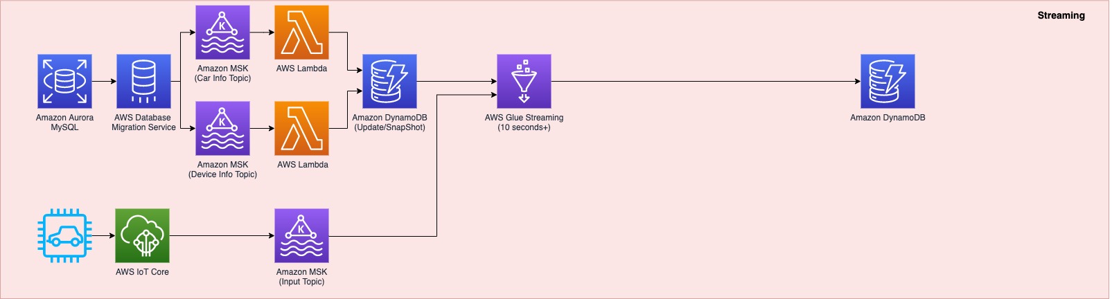
Whenever a transaction occurs in two tables in the Aurora MySQL database, this transaction is captured as data and then loaded into two MSK topics via AWS Database Management (AWS DMS) tasks. One topic conveys the car information table, and the other topic is for the device information table. This data is loaded into a single DynamoDB table that contains all the attributes (or columns) that exist in the two tables in the Aurora MySQL database, along with a primary key. This single DynamoDB table contains the latest snapshot data from the two DB tables, and is important because it contains the latest information of all the cars and devices for the lookup against the streaming IoT data. If the lookup were done on the database directly with the streaming data, it would impact the production database performance.

When the snapshot is available in DynamoDB, an AWS Glue streaming job runs continuously to collect the IoT data and join it with the latest snapshot data in the DynamoDB table to produce the up-to-date output, which is written into another DynamoDB table.

The up-to-date data in DynamoDB is used for real-time monitoring and control that SOCAR’s Data Analytics team performs for safety maintenance and fleet management. This data is ultimately consumed by a number of apps to perform various business activities, including route optimization, real-time monitoring for oil consumption and temperature, and to identify a driver’s driving pattern, tire wear and defect detection, and real-time car crash notifications.

Component 2: Processing IoT data and visualizing the data in dashboards

The second data pipeline (see the following diagram) batch processes the IoT data and visualizes it in QuickSight dashboards.

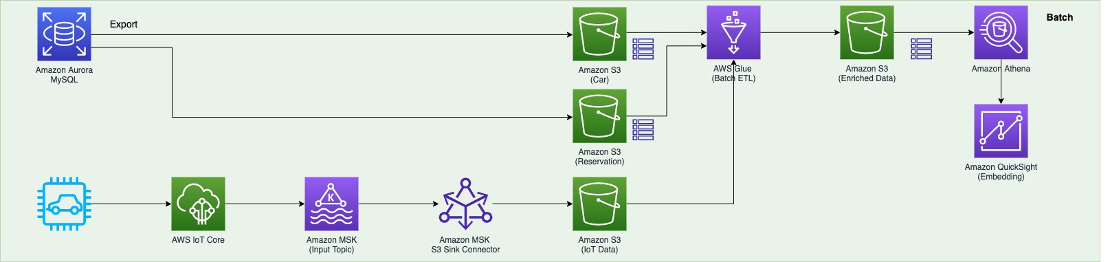
There are two data sources. The first is the Aurora MySQL database. The two database tables are exported into Amazon S3 from the Aurora MySQL cluster and registered in the AWS Glue Data Catalog as tables. The second data source is Amazon MSK, which receives streaming data from AWS IoT Core. This requires you to create a secure AWS Glue connection for an Apache Kafka data stream. SOCAR’s MSK cluster requires SASL_SSL as a security protocol (for more information, refer to Authentication and authorization for Apache Kafka APIs). To create an MSK connection in AWS Glue and set up connectivity, we use the following CLI command:

aws glue create-connection —connection-input
'{"Name":"kafka-connection","Description":"kafka connection example",
"ConnectionType":"KAFKA",
"ConnectionProperties":{
"KAFKA_BOOTSTRAP_SERVERS":"<server-ip-addresses>",
"KAFKA_SSL_ENABLED":"true",
// "KAFKA_CUSTOM_CERT": "s3://bucket/prefix/cert.pem",
"KAFKA_SECURITY_PROTOCOL" : "SASL_SSL",
"KAFKA_SKIP_CUSTOM_CERT_VALIDATION":"false",
"KAFKA_SASL_MECHANISM": "SCRAM-SHA-512",
"KAFKA_SASL_SCRAM_USERNAME": "<username>",
"KAFKA_SASL_SCRAM_PASSWORD: "<password>"
},
"PhysicalConnectionRequirements":
{"SubnetId":"subnet-xxx","SecurityGroupIdList":["sg-xxx"],"AvailabilityZone":"us-east-1a"}}'

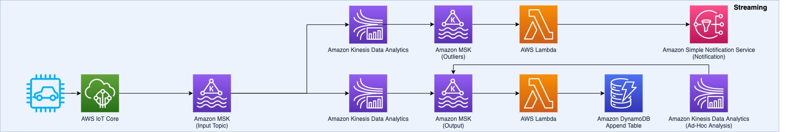
Component 3: Real-time control

The third data pipeline processes the streaming IoT data in millisecond latency from Amazon MSK to produce the output in DynamoDB, and sends a notification in real time if any records are identified as an outlier based on business rules.

AWS IoT Core provides integrations with Amazon MSK to set up real-time streaming data pipelines. To do so, complete the following steps:

  1. On the AWS IoT Core console, choose Act in the navigation pane.
  2. Choose Rules, and create a new rule.
  3. For Actions, choose Add action and choose Kafka.
  4. Choose the VPC destination if required.
  5. Specify the Kafka topic.
  6. Specify the TLS bootstrap servers of your Amazon MSK cluster.

You can view the bootstrap server URLs in the client information of your MSK cluster details. The AWS IoT rule was created with the Kafka topic as an action to provide data from AWS IoT Core to Kafka topics.

SOCAR used Amazon Kinesis Data Analytics Studio to analyze streaming data in real time and build stream-processing applications using standard SQL and Python. We created one table from the Kafka topic using the following code:

CREATE TABLE table_name (
column_name1 VARCHAR,
column_name2 VARCHAR(100),
column_name3 VARCHAR,
column_name4 as TO_TIMESTAMP (`time_column`, 'EEE MMM dd HH:mm:ss z yyyy'),
 WATERMARK FOR column AS column -INTERVAL '5' SECOND
)
PARTITIONED BY (column_name5)
WITH (
'connector'= 'kafka',
'topic' = 'topic_name',
'properties.bootstrap.servers' = '<bootstrap servers shown in the MSK client info dialog>',
'format' = 'json',
'properties.group.id' = 'testGroup1',
'scan.startup.mode'= 'earliest-offset'
);

Then we applied a query with business logic to identify a particular set of records that need to be alerted. When this data is loaded back into another Kafka topic, AWS Lambda functions trigger the downstream action: either load the data into a DynamoDB table or send an email notification.

Component 4: Flattening the nested structure JSON and monitoring schema changes

The final data pipeline (see the following diagram) processes complex, semi-structured, and nested JSON files.

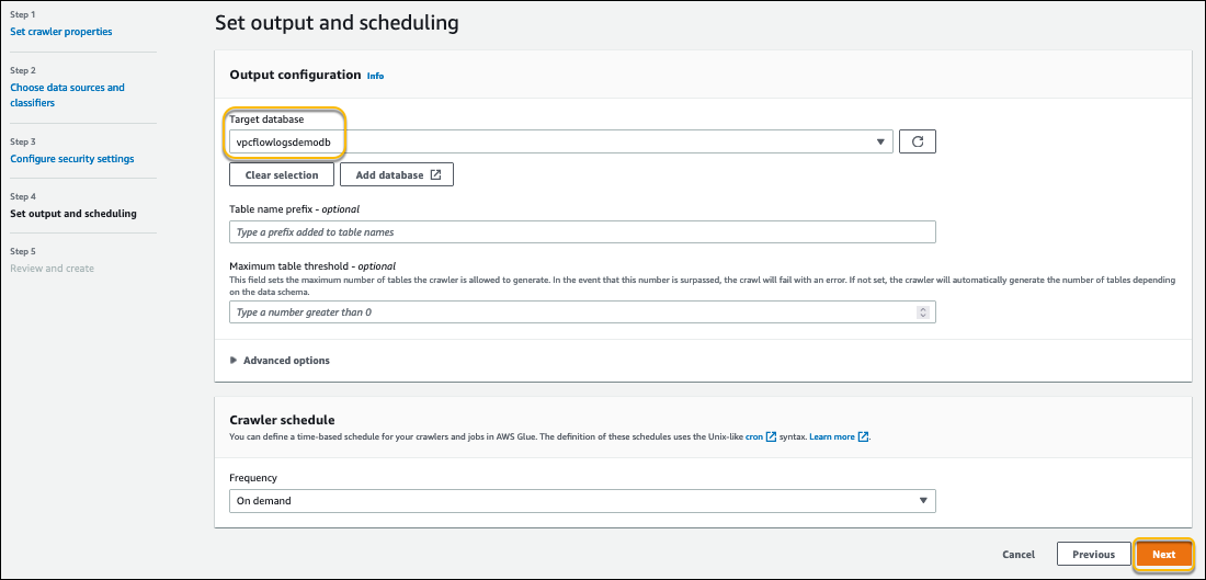
This step uses an AWS Glue DynamicFrame to flatten the nested structure and then land the output in Amazon S3. After the data is loaded, it’s scanned by an AWS Glue crawler to update the Data Catalog table and detect any changes in the schema.

Data flow: Putting it all together

The following diagram illustrates our complete data flow with each component.

Let’s walk through the steps of each pipeline.

The first data pipeline (in red) processes the IoT streaming data with the Aurora MySQL business data:

  1. AWS DMS is used for ongoing replication to continuously apply source changes to the target with minimal latency. The source includes two tables in the Aurora MySQL database tables (carinfo and deviceinfo), and each is linked to two MSK topics via AWS DMS tasks.
  2. Amazon MSK triggers a Lambda function, so whenever a topic receives data, a Lambda function runs to load data into DynamoDB table.
  3. There is a single DynamoDB table with columns that exist from the carinfo table and the deviceinfo table of the Aurora MySQL database. This table consists of all the data from two tables and stores the latest data by performing an upsert operation.
  4. An AWS Glue job continuously receives the IoT data and joins it with data in the DynamoDB table to produce the output into another DynamoDB target table.
  5. This target table contains the final data, which includes all the device and car status information from the IoT devices as well as metadata from the Aurora MySQL table.

The second data pipeline (in green) batch processes IoT data to use in dashboards and for visualization:

  1. The car and reservation data (in two DB tables) is exported via a SQL command from the Aurora MySQL database with the output data available in an S3 bucket. The folders that contain data are registered as an S3 location for the AWS Glue crawler and become available via the AWS Glue Data Catalog.
  2. The MSK input topic continuously receives data from AWS IoT. Each car has a number of IoT devices, and each device captures data and sends it to an MSK input topic. The Amazon MSK S3 sink connector is configured to export data from Kafka topics to Amazon S3 in JSON formats. In addition, the S3 connector exports data by guaranteeing exactly-once delivery semantics to consumers of the S3 objects it produces.
  3. The AWS Glue job runs in a daily batch to load the historical IoT data into Amazon S3 and into two tables (refer to step 1) to produce the output data in an Enriched folder in Amazon S3.
  4. Amazon Athena is used to query data from Amazon S3 and make it available as a dataset in QuickSight for visualizing historical data.

The third data pipeline (in blue) processes streaming IoT data from Amazon MSK with millisecond latency to produce the output in DynamoDB and send a notification:

  1. An Amazon Kinesis Data Analytics Studio notebook powered by Apache Zeppelin and Apache Flink is used to build and deploy its output as a Kinesis Data Analytics application. This application loads data from Amazon MSK in real time, and users can apply business logic to select particular events coming from the IoT real-time data, for example, the car engine is off and the doors are closed, but the headlights are still on. The particular event that users want to capture can be sent to another MSK topic (Outlier) via the Kinesis Data Analytics application.
  2. Amazon MSK triggers a Lambda function, so whenever a topic receives data, a Lambda function runs to send an email notification to users that are subscribed to an Amazon Simple Notification Service (Amazon SNS) topic. An email is published using an SNS notification.
  3. The Kinesis Data Analytics application loads data from AWS IoT, applies business logic, and then loads it into another MSK topic (output). Amazon MSK triggers a Lambda function when data is received, which loads data into a DynamoDB Append table.
  4. Amazon Kinesis Data Analytics Studio is used to run SQL commands for ad hoc interactive analysis on streaming data.

The final data pipeline (in yellow) processes complex, semi-structured, and nested JSON files, and sends a notification when a schema evolves.

  1. An AWS Glue job runs and reads the JSON data from Amazon S3 (as a source), applies logic to flatten the nested schema using a DynamicFrame, and pivots out array columns from the flattened frame.
  2. The output is stored in Amazon S3 and is automatically registered to the AWS Glue Data Catalog table.
  3. Whenever there is a new attribute or change in the JSON input data at any level in the nested structure, the new attribute and change are captured in Amazon EventBridge as an event from the AWS Glue Data Catalog. An email notification is published using Amazon SNS.

Conclusion

As a result of the four-day Build Lab, the SOCAR team left with a working prototype that is custom fit to their needs, gaining a clear path to production. The Data Lab allowed the SOCAR team to build a new streaming data pipeline, enrich IoT data with operational data, and enhance the existing data pipeline to process complex nested JSON data. This establishes a baseline architecture to support the new fleet management system beyond the car-sharing business.


About the Authors

DoYeun Kim is the Head of Data Engineering at SOCAR. He is a passionate software engineering professional with 19+ years experience. He leads a team of 10+ engineers who are responsible for the data platform, data warehouse and MLOps engineering, as well as building in-house data products.

SangSu Park is a Lead Data Architect in SOCAR’s cloud DB team. His passion is to keep learning, embrace challenges, and strive for mutual growth through communication. He loves to travel in search of new cities and places.

YoungMin Park is a Lead Architect in SOCAR’s cloud infrastructure team. His philosophy in life is-whatever it may be-to challenge, fail, learn, and share such experiences to build a better tomorrow for the world. He enjoys building expertise in various fields and basketball.

Younggu Yun is a Senior Data Lab Architect at AWS. He works with customers around the APAC region to help them achieve business goals and solve technical problems by providing prescriptive architectural guidance, sharing best practices, and building innovative solutions together. In his free time, his son and he are obsessed with Lego blocks to build creative models.

Vicky Falconer leads the AWS Data Lab program across APAC, offering accelerated joint engineering engagements between teams of customer builders and AWS technical resources to create tangible deliverables that accelerate data analytics modernization and machine learning initiatives.

Introducing the AWS Lambda Telemetry API

Post Syndicated from Julian Wood original https://aws.amazon.com/blogs/compute/introducing-the-aws-lambda-telemetry-api/

This blog post is written by Anton Aleksandrov, Principal Solution Architect and Shridhar Pandey, Senior Product Manager

Today AWS is announcing the AWS Lambda Telemetry API. This provides an easier way to receive enhanced function telemetry directly from the Lambda service and send it to custom destinations. Developers and operators can now more easily monitor and observe their Lambda functions using Lambda extensions from their preferred observability tool providers.

Extensions can use the Lambda Logs API to collect logs generated by the Lambda service and code running in their Lambda function. While the Logs API provides extensions with access to logs, it does not provide a way to collect additional telemetry, such as traces and metrics, which the Lambda service generates during initialization and invocation of your Lambda function.

Previously, observability tools retrieved traces from AWS X-Ray using the AWS X-Ray API or built their own custom tracing libraries to generate traces during Lambda function invocation. Tools required customers to modify AWS Identity and Access Management (IAM) policies to grant access to the traces from X-Ray. This caused additional complexity for tools to collect traces and metrics from multiple sources and introduced latency in seeing Lambda function traces in observability tool dashboards.

The Lambda Telemetry API is a new API that enhances the existing Lambda Logs API functionality. With the new Telemetry API, observability tools can receive function and extension logs, and also events, traces, and metrics directly from within the Lambda service. You do not need to install additional tracing libraries. This reduces latency and simplifies access permissions, as the extension does not require additional access to X-Ray.

Today you can use Telemetry API-enabled extensions to send telemetry data to Coralogix, Datadog, Dynatrace, Lumigo, New Relic, Sedai, Site24x7, Serverless.com, Sumo Logic, Sysdig, Thundra, or your own custom destinations.

Overview

To receive logs, extensions subscribe using the new Lambda Telemetry API.

Lambda Telemetry API

Lambda Telemetry API

The Lambda service then streams the telemetry events directly to the extension. The events include platform events, trace spans, function and extension logs, and additional Lambda platform metrics. The extension can then process, filter, and route them to any preferred destination.

You can add an extension from the tooling provider of your choice to your Lambda function. You can deploy extensions, including ones that use the Telemetry API, as Lambda layers, with the AWS Management Console and AWS Command Line Interface (AWS CLI). You can also use infrastructure as code tools such as AWS CloudFormation, the AWS Serverless Application Model (AWS SAM), Serverless Framework, and Terraform.

Lambda Extensions from the AWS Partner Network (APN) available at launch

Today, you can use Lambda extensions that use Telemetry API from the following Lambda partners:

  • The Coralogix AWS Lambda Telemetry Exporter extension now offers improved monitoring and alerting for Lambda functions by further streamlining collection and correlation of logs, metrics, and traces.
  • The Datadog extension further simplifies how you visualize the impact of cold starts, and monitor and alert on latency, duration, and payload size of your Lambda functions by collecting logs, traces, and real-time metrics from your function in a simple and cost-effective way.
  • Dynatrace now provides a simplified observability configuration for AWS Lambda through a seamless integration. The new solution delivers low-latency telemetry, enables monitoring at scale, and helps reduce monitoring costs for your serverless workloads.
  • The Lumigo lambda-log-shipper extension simplifies aggregating and forwarding Lambda logs to third-party tools. It now also makes it easy for you to detect Lambda function timeouts.
  • The New Relic extension now provides a unified observability view for your Lambda functions with insights that help you better understand and optimize the performance of your functions.
  • Sedai now uses the Telemetry API to help you improve the performance and availability of your Lambda functions by gathering insights about your function and providing recommendations for manual and autonomous remediation in a cost-effective manner.
  • The Site24x7 extension now offers new metrics, which enable you to get deeper insights into the different phases of the Lambda function lifecycle, such as initialization and invocation.
  • Serverless.com now uses the Telemetry API to provide real-time performance details for your Lambda function through the Dev Mode feature of their new Serverless Console V.2 offering, which simplifies debugging in the AWS Cloud.
  • Sumo Logic now makes it easier, faster, and more cost-effective for you to get your mission-critical Lambda function telemetry sent directly to Sumo Logic so you could quickly analyze and remediate errors and exceptions.
  • The Sysdig Monitor extension generates and collects real-time metrics directly from the Lambda platform. The simplified instrumentation offers lower latency, reduced MTTR (mean time to resolution) for critical issues, and cost benefits while monitoring your serverless applications.
  • The Thundra extension enables you to export logs, metrics, and events for Lambda execution environment lifecycle events emitted by the Telemetry API to a destination of your choice such as an S3 bucket, a database, or a monitoring backend.

Seeing example Telemetry API extensions in action

This demo shows an example of using a telemetry extension to receive telemetry, batch, and send it to a desired destination.

To set up the example, visit the GitHub repo for the extension implemented in the language of your choice and follow the instructions in the README.md file.

To configure the batching behavior, which controls when the extension sends the data, set the Lambda environment variable DISPATCH_MIN_BATCH_SIZE. When the extension receives the batch threshold, it POSTs the telemetry events batch to the destination specified in the DISPATCH_POST_URI environment variable.

You can configure an example DISPATCH_POST_URL for the extension to deliver the telemetry data using https://webhook.site/.

Lambda environment variables

Lambda environment variables

Telemetry events for one invoke may be received and processed during the next invocation. Events for the last invoke may be processed during the SHUTDOWN event.

Test and invoke the function from the Lambda console, or AWS CLI. You can see that the webhook receives the telemetry data.

Webhook receiving telemetry data

Webhook receiving telemetry data

You can also view the function and extension logs in CloudWatch Logs. The example extension includes verbose logging to understand the extension lifecycle.

CloudWatch Logs showing extension verbose logging

Sample Telemetry API events

When the extension receives telemetry data, each event contains a JSON dictionary with additional information, such as related metrics or trace spans. The following example shows a function initialization event. You can see that the function initializes with on-demand concurrency. The runtime version is Node.js 14, the initialization is successful, and the initialization duration is 123 milliseconds.

{
  "time": "2022-08-02T12:01:23.521Z",
  "type": "platform.initStart",
  "record": {
    "initializationType": "on-demand",
    "phase":"init",
    "runtimeVersion": "nodejs-14.v3",
    "runtimeVersionArn": "arn"
  }
}

{
  "time": "2022-08-02T12:01:23.521Z",
  "type": "platform.initRuntimeDone",
  "record": {
    "initializationType": "on-demand",
    "status": "success"
  }
}

{
  "time": "2022-08-02T12:01:23.521Z",
  "type": "platform.initReport",
  "record": {
    "initializationType": "on-demand",
    "phase":"init",
    "metrics": {
      "durationMs": 123.0,
    }
  }
}

Function invocation events include the associated requestId and tracing information connecting this invocation with the X-Ray tracing context, and platform spans showing response latency and response duration as well as invocation metrics such as duration in milliseconds.

{
    "time": "2022-08-02T12:01:23.521Z",
    "type": "platform.start",
    "record": {
      "requestId": "e6b761a9-c52d-415d-b040-7ba94b9452f3",
      "version": "$LATEST",
      "tracing": {
        "spanId": "54565fb41ac79632",
        "type": "X-Amzn-Trace-Id",
        "value": "Root=1-62e900b2-710d76f009d6e7785905449a;Parent=0efbd19962d95b05;Sampled=1"
      }
    }
  }
  
  {
    "time": "2022-08-02T12:01:23.521Z",
    "type": "platform.runtimeDone",
    "record": {
      "requestId": "e6b761a9-c52d-415d-b040-7ba94b9452f3",
      "status": "success",
      "tracing": {
        "spanId": "54565fb41ac79632",
        "type": "X-Amzn-Trace-Id",
        "value": "Root=1-62e900b2-710d76f009d6e7785905449a;Parent=0efbd19962d95b05;Sampled=1"
      },
      "spans": [
        {
          "name": "responseLatency", 
          "start": "2022-08-02T12:01:23.521Z",
          "durationMs": 23.02
        },
        {
          "name": "responseDuration", 
          "start": "2022-08-02T12:01:23.521Z",
          "durationMs": 20
        }
      ],
      "metrics": {
        "durationMs": 200.0,
        "producedBytes": 15
      }
    }
  }
  
  {
    "time": "2022-08-02T12:01:23.521Z",
    "type": "platform.report",
    "record": {
      "requestId": "e6b761a9-c52d-415d-b040-7ba94b9452f3",
      "metrics": {
        "durationMs": 220.0,
        "billedDurationMs": 300,
        "memorySizeMB": 128,
        "maxMemoryUsedMB": 90,
        "initDurationMs": 200.0
      },
      "tracing": {
        "spanId": "54565fb41ac79632",
        "type": "X-Amzn-Trace-Id",
        "value": "Root=1-62e900b2-710d76f009d6e7785905449a;Parent=0efbd19962d95b05;Sampled=1"
      }
    }
  }

Building a Telemetry API extension

Lambda extensions run as independent processes in the execution environment and continue to run after the function invocation is fully processed. Because extensions run as separate processes, you can write them in a language different from the function code. We recommend implementing extensions using a compiled language as a self-contained binary. This makes the extension compatible with all the supported runtimes.

Extensions that use the Telemetry API have the following lifecycle.

Telemetry API lifecycle

Telemetry API lifecycle

  1. The extension registers itself using the Lambda Extension API and subscribes to receive INVOKE and SHUTDOWN events. With the Telemetry API, the registration response body contains additional information, such as function name, function version, and account ID.
  2. The extensions start a telemetry listener. This is a local HTTP or TCP endpoint. We recommend using HTTP rather than TCP.
  3. The extensions use the Telemetry API to subscribe to desired telemetry event streams.
  4. The Lambda service POSTs telemetry stream data to your telemetry listener. We recommend batching the telemetry data as it arrives to the listener. You can perform any custom processing on this data and send it on to an S3 bucket, other custom destination, or an external observability service.

See the Telemetry API documentation and sample extensions for additional details.

The Lambda Telemetry API supersedes the Lambda Logs API. While the Logs API remains fully functional, AWS recommends using the Telemetry API. New functionality is only available with the Extensions API. Extensions can only subscribe to either the Logs or Telemetry API. After subscribing to one of them, any attempt to subscribe to the other returns an error.

Mapping Telemetry API schema to OpenTelemetry spans

The Lambda Telemetry API schema is semantically compatible with OpenTelemetry (OTEL). You can use events received from the Telemetry API to build and report OTEL spans. Three Telemetry API lifecycle events represent a single function invocation: start, runtimeDone, and runtimeReport. You should represent this as a single OTEL span. You can add additional details to your spans using information available in runtimeDone events under the event.spans property.

Mapping of Telemetry API events to OTEL spans is described in the Telemetry API documentation.

Metrics and pricing

The Telemetry API introduces new per-invoke metrics to help you understand the impact of extensions on your function’s performance. The metrics are available within the report.runtimeDone event.

  • platform.runtime measures the time taken by the Lambda Runtime to run your function handler code.
  • producedBytes measures the number of bytes returned during the invoke phase.

There are also two new trace spans available within the report.runtimeDone event:

  • responseLatencyMs measures the time taken by the Runtime to send a response.
  • responseDurationMs measures the time taken by the Runtime to finish sending the response from when it starts streaming it.

Extensions using Telemetry API, like other extensions, share the same billing model as Lambda functions. When using Lambda functions with extensions, you pay for requests served, and the combined compute time used to run your code and all extensions, in 1-ms increments. To learn more about the billing for extensions, visit the Lambda pricing page.

Useful links

Conclusion

The Lambda Telemetry API allows you to receive enhanced telemetry data more easily using your preferred monitoring and observability tools. The Telemetry API enhances the functionality of the Logs API to receive logs, metrics, and traces directly from the Lambda service. Developers and operators can send telemetry to destinations without custom libraries, with reduced latency, and simplified permissions.

To see how the Telemetry API works, try the demos in the GitHub repository.

Build your own extensions using the Telemetry API today, or use extensions provided by the Lambda observability partners.

For more serverless learning resources, visit Serverless Land.

An Untrustworthy TLS Certificate in Browsers

Post Syndicated from Bruce Schneier original https://www.schneier.com/blog/archives/2022/11/an-untrustworthy-tls-certificate-in-browsers.html

The major browsers natively trust a whole bunch of certificate authorities, and some of them are really sketchy:

Google’s Chrome, Apple’s Safari, nonprofit Firefox and others allow the company, TrustCor Systems, to act as what’s known as a root certificate authority, a powerful spot in the internet’s infrastructure that guarantees websites are not fake, guiding users to them seamlessly.

The company’s Panamanian registration records show that it has the identical slate of officers, agents and partners as a spyware maker identified this year as an affiliate of Arizona-based Packet Forensics, which public contracting records and company documents show has sold communication interception services to U.S. government agencies for more than a decade.

[…]

In the earlier spyware matter, researchers Joel Reardon of the University of Calgary and Serge Egelman of the University of California at Berkeley found that a Panamanian company, Measurement Systems, had been paying developers to include code in a variety of innocuous apps to record and transmit users’ phone numbers, email addresses and exact locations. They estimated that those apps were downloaded more than 60 million times, including 10 million downloads of Muslim prayer apps.

Measurement Systems’ website was registered by Vostrom Holdings, according to historic domain name records. Vostrom filed papers in 2007 to do business as Packet Forensics, according to Virginia state records. Measurement Systems was registered in Virginia by Saulino, according to another state filing.

More details by Reardon.

Cory Doctorow does a great job explaining the context and the general security issues.

EDITED TO ADD (11/10): Slashdot thread.

[$] Class action against GitHub Copilot

Post Syndicated from original https://lwn.net/Articles/914150/

The GitHub Copilot
offering claims to assist software developers through the application of
machine-learning techniques. Since its inception, Copilot has been
followed by controversies, mostly based on
the extensive use of free software to train the machine-learning engine. The announcement of a
class-action lawsuit against Copilot was thus unsurprising. The lawsuit
raises all of the expected licensing questions and more;
while some in our
community have welcomed this attack against Copilot,
it is not clear that this action will lead to good results.

Cloud Security: Buyer Be Critical

Post Syndicated from Aaron Wells original https://blog.rapid7.com/2022/11/10/cloud-security-buyer-be-critical/

Tailoring solutions to challenges

Cloud Security: Buyer Be Critical

It takes a toolbox with different, well, tools to secure an ever-expanding operational perimeter in the cloud. Think about what’s under the general daily purview of cloud security teams: preventing misconfigurations, taming threats and vulnerabilities, and so much more. Now, apply that to different high-risk industries around the globe that must build and tailor cloud security solutions to their unique challenges. For instance:

  • Financial Services: It can be difficult trying to leverage the benefits of digital transformation while attempting to modernize decades of tradition in an old-school industry. Mobile banking/financial services, for instance, has been the one of the largest industry shifts over the past decade and has accelerated cloud adoption in the sector. Thus, security must keep pace with the service’s rapid growth. The desire to operationalize on-premises and cloud practices is typically strong in this industry, but must also take into account client trust in a financial-services partner to protect that client’s bottom line.    
  • Healthcare: With the growing normalization of telehealth services across the spectrum of medical providers, it’s more critical than ever to secure patient health information (PHI) while adhering to regulatory standards like HIPAA. The need for speed and innovation in medicine is critical, so scaling communication and technology operations into the cloud can be incredibly beneficial. However, providers are also continually challenged with securing PHI within new technologies at speed and scale without slowing innovation.    
  • Automotive: With the modernization of engines, software, and connectivity, the need for passenger safety is more important than ever. As more automobile controls are conveniently accessible through cloud-based controls, cyberattacks have correspondingly increased. Ensuring security checks are implemented in the production and design of a new vehicle while also pushing software updates throughout the ownership lifecycle of that vehicle is critical to manufacturer integrity and passenger safety.

Expansive perimeters

Within and throughout these different use cases and industries are specific budgetary constraints that have prompted organizations to scale cloud operations at unprecedented speeds – no doubt accelerated in large part by the pandemic as it was in its early stages a couple of years ago. Do companies want to go back to not saving money? Certainly not. That means attackers are as ready as they’ll ever be to try and break expanding cloud perimeters.

With your company’s reputation at risk, it’s more critical than ever that security keeps pace with those expanding perimeters, particularly at a time of global financial crisis for many companies as they emerge from the pandemic. Whether a company is looking for a partner to alleviate financial strain in a potential merger situation or seeking an outright buyer, the security of the merged or acquired company’s cloud-hosted operations – particularly vulnerable to attackers during a time of change – is paramount.

High-profile recent examples of the above include Discovery, Inc.’s purchase of WarnerMedia, Elon Musk’s acquisition of Twitter, and Microsoft’s acquisition of Activision Blizzard. These are tectonic shifts for all companies involved, of a sort that can leave cloud security extremely vulnerable at certain points in the process. And the higher-profile the company, the more attractive it can be to an attacker.

Evaluating solutions at speed and scale

So, you’re seeking a strongly effective solution. But, the cloud security vendor space can be confusing. One provider defines cloud security a certain way and another defines it a separate way, and their offerings differ accordingly. Between CASB, SaaS Security, CSPM, and CWPP solutions, there’s a lot to learn. Are any of these right for your cloud operations? There is no one-size-fits-all solution, but you may find a suite of tools that can best work for your specific use case(s).

There are any number of cloud security guides, whitepapers, research, and more that can help you evaluate solutions available from reputable providers. The latest edition of The Complete Cloud Security Buyer’s Guide is a timely and discerning dive into different types of cloud security and the use cases to which they align. Get help with the process of evaluating vendors, while taking into account the need for speed in deploying effective security that protects ever-expanding operational perimeters in the cloud.

Explore how to make the best case for more – or any – cloud security at your company, plus get a handy checklist to use when looking into a potential solution. Get started now with the 2022 edition of The Complete Cloud Security Buyer’s Guide from Rapid7.

Handy Tips #40: Simplify metric pattern matching by creating global regular expressions

Post Syndicated from Arturs Lontons original https://blog.zabbix.com/simplify-metric-pattern-matching-by-creating-global-regular-expressions/24225/

Streamline your data collection, problem detection and low-level discovery by defining global regular expressions. 

Pattern matching within unstructured data is mostly done by using regular expressions. Defining a regular expression can be a lengthy task, that can be simplified by predefining a set of regular expressions which can be quickly referenced down the line.  

Simplify pattern matching by defining global regular expressions:

  • Reference global regular expressions in log monitoring and snmp trap items
  • Simplify pattern matching in trigger functions and calculated items
  • Global regular expressions can be referenced in low-level discovery filters
  •  Combine multiple subexpressions into a single global regular expression
Check out the video to learn how to define and use global regular expressions.
Define and use global regular expressions: 
  1. Navigate to Administration General Regular expressions
  2. Type in your global regular expression name
  3. Select the regular expression type and provide subexpressions
  4. Press Add and provide multiple subexpressions
  5. Navigate to the Test tab and enter the test string
  6. Click on Test expressions and observe the result
  7. Press Add to save and add the global regular expression
  8. Navigate to Configuration Hosts
  9. Find the host on which you will test the global regular expression
  10. Click on either the Items, Triggers or Discovery button to open the corresponding section
  11. Find your item, trigger or LLD rule and open it
  12. Insert the global regular expression
  13. Use the @ symbol to reference a global regular expression by its name
  14. Update the element to save the changes
Tips and best practices
  • Each subexpressions and the total combined result can be tested in Zabbix frontend 
  • Zabbix uses AND logic if several subexpressions are defined 
  • Global regular expressions can be referenced by referring to their name, prefixed with the @ symbol 
  • Zabbix documentation contains the list of locations supporting the usage of global regular expression. 

Sign up for the official Zabbix Certified Specialist course and learn how to optimize your data collection, enrich your alerts with useful information, and minimize the amount of noise and false alarms. During the course, you will perform a variety of practical tasks under the guidance of a Zabbix certified trainer, where you will get the chance to discuss how the current use cases apply to your own unique infrastructure. 

The post Handy Tips #40: Simplify metric pattern matching by creating global regular expressions appeared first on Zabbix Blog.

Out now: Hello World’s special edition on Computing content

Post Syndicated from Gemma Coleman original https://www.raspberrypi.org/blog/hello-world-special-edition-computing-content/

Hello World, our free magazine for computing and digital making educators, has just published its second special edition: The Big Book of Computing Content.

Cover of The Big Book of Computing Content.

A special edition on the content we teach in the Computing classroom

While Hello World‘s first special edition, The Big Book of Computing Pedagogy, focused on how we can teach Computing, this new book is about what we mean by Computing. It aims to demonstrate the breadth of knowledge and skills contained within this constantly evolving subject.

We have structured the new special edition around our taxonomy for formal Computing education, to which we map all our formal education resources. Originally we developed the taxonomy when we started work in the consortium setting up and delivering England’s National Centre for Computing Education, and specifically when we designed the 500 hours of classroom materials in the Teach Computing Curriculum.

The Raspberry Pi Foundation's computing content taxonomy, made of 11 strands: effective use of tools, safety and security, design and development, impact of technology, computing systems, networks, creating media, algorithms and data structures, programming, data and information, artificial intelligence.
The 11 strands of Computing content in our taxonomy.

Our Computing taxonomy comprises eleven strands and aims to categorise Computing conceptual knowledge and skills to both demonstrate the breadth of Computing as a discipline, and to provide a common language to describe the different areas of study and competencies.

The Big Book of Computing Content complements our first Hello World special edition and follows the same principle of introducing readers to up-to-date research, followed by our favourite stories from past Hello World issues by educators who put that content into practice. For each of the eleven strands in our taxonomy, we also present a table of learning outcomes, which provides examples of knowledge and skills that learners from ages 5 to 19 could develop at each stage of their formal computing education. 

Your thoughts on The Big Book of Computing Content

Hello World’s first special edition was very popular around the world, with educators setting up Big Book of Computing Pedagogy reading groups, leaders using the book to support pre-service teachers, and even of an upcoming translation into Thai.

We’ve already started to hear similar stories about The Big Book of Computing Content from Hello World readers, including CSEdResearch dedicating their Computer Science Education Discussion Group to all things Big Book of Computing Content in its first week of publication.

A tweet about Hello World's special edition The Big Book of Computing Content.

We’d love to hear from more educators about how you are using this new special edition, and how it complements your reading of the first Big Book.

You can also subscribe now to get each new Hello World — whether regular issue or special edition — straight to your digital inbox, for free! And if you’re based in the UK and do paid or voluntary work in education, you can subscribe for free print issues.

PS Have you listened to our Hello World podcast yet? Listen and subscribe wherever you get your podcasts.

The post Out now: Hello World’s special edition on Computing content appeared first on Raspberry Pi.

Seeing through hardware counters: a journey to threefold performance increase

Post Syndicated from Netflix Technology Blog original https://netflixtechblog.com/seeing-through-hardware-counters-a-journey-to-threefold-performance-increase-2721924a2822

By Vadim Filanovsky and Harshad Sane

In one of our previous blogposts, A Microscope on Microservices we outlined three broad domains of observability (or “levels of magnification,” as we referred to them) — Fleet-wide, Microservice and Instance. We described the tools and techniques we use to gain insight within each domain. There is, however, a class of problems that requires an even stronger level of magnification going deeper down the stack to introspect CPU microarchitecture. In this blogpost we describe one such problem and the tools we used to solve it.

The problem

It started off as a routine migration. At Netflix, we periodically reevaluate our workloads to optimize utilization of available capacity. We decided to move one of our Java microservices — let’s call it GS2 — to a larger AWS instance size, from m5.4xl (16 vCPUs) to m5.12xl (48 vCPUs). The workload of GS2 is computationally heavy where CPU is the limiting resource. While we understand it’s virtually impossible to achieve a linear increase in throughput as the number of vCPUs grow, a near-linear increase is attainable. Consolidating on the larger instances reduces the amortized cost of background tasks, freeing up additional resources for serving requests and potentially offsetting the sub-linear scaling. Thus, we expected to roughly triple throughput per instance from this migration, as 12xl instances have three times the number of vCPUs compared to 4xl instances. A quick canary test was free of errors and showed lower latency, which is expected given that our standard canary setup routes an equal amount of traffic to both the baseline running on 4xl and the canary on 12xl. As GS2 relies on AWS EC2 Auto Scaling to target-track CPU utilization, we thought we just had to redeploy the service on the larger instance type and wait for the ASG (Auto Scaling Group) to settle on the CPU target. Unfortunately, the initial results were far from our expectations:

The first graph above represents average per-node throughput overlaid with average CPU utilization, while the second graph shows average request latency. We can see that as we reached roughly the same CPU target of 55%, the throughput increased only by ~25% on average, falling far short of our desired goal. What’s worse, average latency degraded by more than 50%, with both CPU and latency patterns becoming more “choppy.” GS2 is a stateless service that receives traffic through a flavor of round-robin load balancer, so all nodes should receive nearly equal amounts of traffic. Indeed, the RPS (Requests Per Second) data shows very little variation in throughput between nodes:

But as we started looking at the breakdown of CPU and latency by node, a strange pattern emerged:

Although we confirmed fairly equal traffic distribution between nodes, CPU and latency metrics surprisingly demonstrated a very different, bimodal distribution pattern. There is a “lower band” of nodes exhibiting much lower CPU and latency with hardly any variation; and there is an “upper band” of nodes with significantly higher CPU/latency and wide variation. We noticed only ~12% of the nodes fall into the lower band, a figure that was suspiciously consistent over time. In both bands, performance characteristics remain consistent for the entire uptime of the JVM on the node, i.e. nodes never jumped the bands. This was our starting point for troubleshooting.

First attempt at solving it

Our first (and rather obvious) step at solving the problem was to compare flame graphs for the “slow” and “fast” nodes. While flame graphs clearly reflected the difference in CPU utilization as the number of collected samples, the distribution across the stacks remained the same, thus leaving us with no additional insight. We turned to JVM-specific profiling, starting with the basic hotspot stats, and then switching to more detailed JFR (Java Flight Recorder) captures to compare the distribution of the events. Again, we came away empty-handed as there was no noticeable difference in the amount or the distribution of the events between the “slow” and “fast” nodes. Still suspecting something might be off with JIT behavior, we ran some basic stats against symbol maps obtained by perf-map-agent only to hit another dead end.

False Sharing

Convinced we’re not missing anything on the app-, OS- and JVM- levels, we felt the answer might be hidden at a lower level. Luckily, the m5.12xl instance type exposes a set of core PMCs (Performance Monitoring Counters, a.k.a. PMU counters), so we started by collecting a baseline set of counters using PerfSpect:

In the table above, the nodes showing low CPU and low latency represent a “fast node”, while the nodes with higher CPU/latency represent a “slow node”. Aside from obvious CPU differences, we can see that the slow node has almost 3x CPI (Cycles Per Instruction) of the fast node. We also see much higher L1 cache activity combined with 4x higher count of MACHINE_CLEARS. One common cause of these symptoms is so-called “false sharing” — a usage pattern occurring when 2 cores reading from / writing to unrelated variables that happen to share the same L1 cache line. Cache line is a concept similar to memory page — a contiguous chunk of data (typically 64 bytes on x86 systems) transferred to and from the cache. This diagram illustrates it:

Each core in this diagram has its own private cache. Since both cores are accessing the same memory space, caches have to be consistent. This consistency is ensured with so-called “cache coherency protocol.” As Thread 0 writes to the “red” variable, coherency protocol marks the whole cache line as “modified” in Thread 0’s cache and as “invalidated” in Thread 1’s cache. Later, when Thread 1 reads the “blue” variable, even though the “blue” variable is not modified, coherency protocol forces the entire cache line to be reloaded from the cache that had the last modification — Thread 0’s cache in this example. Resolving coherency across private caches takes time and causes CPU stalls. Additionally, ping-ponging coherency traffic has to be monitored through the last level shared cache’s controller, which leads to even more stalls. We take CPU cache consistency for granted, but this “false sharing” pattern illustrates there’s a huge performance penalty for simply reading a variable that is neighboring with some other unrelated data.

Armed with this knowledge, we used Intel vTune to run microarchitecture profiling. Drilling down into “hot” methods and further into the assembly code showed us blocks of code with some instructions exceeding 100 CPI, which is extremely slow. This is the summary of our findings:

Numbered markers from 1 to 6 denote the same code/variables across the sources and vTune assembly view. The red arrow indicates that the CPI value likely belongs to the previous instruction — this is due to the profiling skid in absence of PEBS (Processor Event-Based Sampling), and usually it’s off by a single instruction. Based on the fact that (5) “repne scan” is a rather rare operation in the JVM codebase, we were able to link this snippet to the routine for subclass checking (the same code exists in JDK mainline as of the writing of this blogpost). Going into the details of subtype checking in HotSpot is far beyond the scope of this blogpost, but curious readers can learn more about it from the 2002 publication Fast Subtype Checking in the HotSpot JVM. Due to the nature of the class hierarchy used in this particular workload, we keep hitting the code path that keeps updating (6) the “_secondary_super_cache” field, which is a single-element cache for the last-found secondary superclass. Note how this field is adjacent to the “_secondary_supers”, which is a list of all superclasses and is being read (1) in the beginning of the scan. Multiple threads do these read-write operations, and if fields (1) and (6) fall into the same cache line, then we hit a false sharing use case. We highlighted these fields with red and blue colors to connect to the false sharing diagram above.

Note that since the cache line size is 64 bytes and the pointer size is 8 bytes, we have a 1 in 8 chance of these fields falling on separate cache lines, and a 7 in 8 chance of them sharing a cache line. This 1-in-8 chance is 12.5%, matching our previous observation on the proportion of the “fast” nodes. Fascinating!

Although the fix involved patching the JDK, it was a simple change. We inserted padding between “_secondary_super_cache” and “_secondary_supers” fields to ensure they never fall into the same cache line. Note that we did not change the functional aspect of JDK behavior, but rather the data layout:

The results of deploying the patch were immediately noticeable. The graph below is a breakdown of CPU by node. Here we can see a red-black deployment happening at noon, and the new ASG with the patched JDK taking over by 12:15:

Both CPU and latency (graph omitted for brevity) showed a similar picture — the “slow” band of nodes was gone!

True Sharing

We didn’t have much time to marvel at these results, however. As the autoscaling reached our CPU target, we noticed that we still couldn’t push more than ~150 RPS per node — well short of our goal of ~250 RPS. Another round of vTune profiling on the patched JDK version showed the same bottleneck around secondary superclass cache lookup. It was puzzling at first to see seemingly the same problem coming back right after we put in a fix, but upon closer inspection we realized we’re dealing with “true sharing” now. Unlike “false sharing,” where 2 independent variables share a cache line, “true sharing” refers to the same variable being read and written by multiple threads/cores. In this case, CPU-enforced memory ordering is the cause of slowdown. We reasoned that removing the obstacle of false sharing and increasing the overall throughput resulted in increased execution of the same JVM superclass caching code path. Essentially, we have higher execution concurrency, causing excessive pressure on the superclass cache due to CPU-enforced memory ordering protocols. The common way to resolve this is to avoid writing to the shared variable altogether, effectively bypassing the JVM’s secondary superclass cache. Since this change altered the behavior of the JDK, we gated it behind a command line flag. This is the entirety of our patch:

And here are the results of running with disabled superclass cache writes:

Our fix pushed the throughput to ~350 RPS at the same CPU autoscaling target of 55%. To put this in perspective, that’s a 3.5x improvement over the throughput we initially reached on m5.12xl, along with a reduction in both average and tail latency.

Future work

Disabling writes to the secondary superclass cache worked well in our case, and even though this might not be a desirable solution in all cases, we wanted to share our methodology, toolset and the fix in the hope that it would help others encountering similar symptoms. While working through this problem, we came across JDK-8180450 — a bug that’s been dormant for more than five years that describes exactly the problem we were facing. It seems ironic that we could not find this bug until we actually figured out the answer. We believe our findings complement the great work that has been done in diagnosing and remediating it.

Conclusion

We tend to think of modern JVMs as highly optimized runtime environments, in many cases rivaling more “performance-oriented” languages like C++. While it holds true for the majority of workloads, we were reminded that performance of certain workloads running within JVMs can be affected not only by the design and implementation of the application code, but also by the implementation of the JVM itself. In this blogpost we described how we were able to leverage PMCs in order to find a bottleneck in the JVM’s native code, patch it, and subsequently realize better than a threefold increase in throughput for the workload in question. When it comes to this class of performance issues, the ability to introspect the execution at the level of CPU microarchitecture proved to be the only solution. Intel vTune provides valuable insight even with the core set of PMCs, such as those exposed by m5.12xl instance type. Exposing a more comprehensive set of PMCs along with PEBS across all instance types and sizes in the cloud environment would pave the way for deeper performance analysis and potentially even larger performance gains.

Special thanks to Sandhya Viswanathan, Jennifer Dimatteo, Brendan Gregg, Susie Xia, Jason Koch, Mike Huang, Amer Ather, Chris Berry, Chris Sanden, and Guy Cirino


Seeing through hardware counters: a journey to threefold performance increase was originally published in Netflix TechBlog on Medium, where people are continuing the conversation by highlighting and responding to this story.

[$] Moving past TCP in the data center, part 2

Post Syndicated from original https://lwn.net/Articles/914030/

At the end of our earlier article on John
Ousterhout’s talk at Netdev 0x16, he had concluded
that TCP was unsuitable for data-center environments for a variety of
reasons. He also argued that there was no way to repair TCP so that it
could serve the needs of data-center networking. In order for software to
be able
to use the full potential of today’s networking hardware, TCP needs to be
replaced with a protocol that is different in almost every way, he said.
The second
half of the talk covered the Homa
transport protocol
that he and others at Stanford have been working on
as a possible replacement for TCP in the data center.

Learn more about Apache Flink and Amazon Kinesis Data Analytics with three new videos

Post Syndicated from Deepthi Mohan original https://aws.amazon.com/blogs/big-data/learn-more-about-apache-flink-and-amazon-kinesis-data-analytics-with-three-new-videos/

Amazon Kinesis Data Analytics is a fully managed service for Apache Flink that reduces the complexity of building, managing, and integrating Apache Flink applications with other AWS services. Apache Flink is an open-source framework and engine for stateful processing of data streams. It’s highly available and scalable, delivering high throughput and low latency for the most demanding stream-processing applications.

In this post, we highlight three new videos for you to learn more about Apache Flink and Kinesis Data Analytics, including open-source contributions to Apache Flink, our learnings from running thousands of Flink jobs on a managed service, and how we use Kinesis Data Analytics and Apache Flink to enable machine learning (ML) in Alexa.

In Introducing the new Async Sink, we present the new Async Sink framework, an open-source contribution to make it easier than ever to build sink connectors for Apache Flink. You can learn about the need for the Async Sink framework and how we built it, followed by a demo of building a new sink to Amazon CloudWatch to deliver CloudWatch metrics, in under 20 minutes! The Async Sink framework bootstraps development of Flink sinks, is compatible with Apache Flink 1.15 and above, and has already seen usage by the community beyond building new sinks to AWS services.

The video Practical learnings from running thousands of Flink jobs shares insight from running Kinesis Data Analytics, a managed service for Apache Flink that runs tens of thousands of Flink jobs. You can learn lessons based on our experience of operating Apache Flink at very large scale, touching on issues such as out-of-memory errors, timeouts, and stability challenges. The video also covers improving application performance with memory tuning and configuration changes and the approaches to automating job health monitoring and management of Flink jobs at scale.

“Alexa, be quiet!” End-to-end near-real time model building and evaluation in Amazon Alexa discusses how Alexa has built an automated end-to-end solution for incremental model building or fine-tuning ML models through continuous learning, continual learning, or semi-supervised active learning. Alexa uses Apache Flink to transform and discover metrics in real time. In this video, you learn about how Alexa scales infrastructure to meet the needs of ML teams across Alexa, and explore specific use cases that use Apache Flink and Kinesis Data Analytics to improve Alexa experiences to delight customers.

To learn more about Kinesis Data Analytics for Apache Flink, visit our product page.


About the author

Deepthi Mohan is a Principal Product Manager on the Kinesis Data Analytics team.

Enrich VPC Flow Logs with resource tags and deliver data to Amazon S3 using Amazon Kinesis Data Firehose

Post Syndicated from Chaitanya Shah original https://aws.amazon.com/blogs/big-data/enrich-vpc-flow-logs-with-resource-tags-and-deliver-data-to-amazon-s3-using-amazon-kinesis-data-firehose/

VPC Flow Logs is an AWS feature that captures information about the network traffic flows going to and from network interfaces in Amazon Virtual Private Cloud (Amazon VPC). Visibility to the network traffic flows of your application can help you troubleshoot connectivity issues, architect your application and network for improved performance, and improve security of your application.

Each VPC flow log record contains the source and destination IP address fields for the traffic flows. The records also contain the Amazon Elastic Compute Cloud (Amazon EC2) instance ID that generated the traffic flow, which makes it easier to identify the EC2 instance and its associated VPC, subnet, and Availability Zone from where the traffic originated. However, when you have a large number of EC2 instances running in your environment, it may not be obvious where the traffic is coming from or going to simply based on the EC2 instance IDs or IP addresses contained in the VPC flow log records.

By enriching flow log records with additional metadata such as resource tags associated with the source and destination resources, you can more easily understand and analyze traffic patterns in your environment. For example, customers often tag their resources with resource names and project names. By enriching flow log records with resource tags, you can easily query and view flow log records based on an EC2 instance name, or identify all traffic for a certain project.

In addition, you can add resource context and metadata about the destination resource such as the destination EC2 instance ID and its associated VPC, subnet, and Availability Zone based on the destination IP in the flow logs. This way, you can easily query your flow logs to identify traffic crossing Availability Zones or VPCs.

In this post, you will learn how to enrich flow logs with tags associated with resources from VPC flow logs in a completely serverless model using Amazon Kinesis Data Firehose and the recently launched Amazon VPC IP Address Manager (IPAM), and also analyze and visualize the flow logs using Amazon Athena and Amazon QuickSight.

Solution overview

In this solution, you enable VPC flow logs and stream them to Kinesis Data Firehose. This solution enriches log records using an AWS Lambda function on Kinesis Data Firehose in a completely serverless manner. The Lambda function fetches resource tags for the instance ID. It also looks up the destination resource from the destination IP using the Amazon EC2 API and IPAM, and adds the associated VPC network context and metadata for the destination resource. It then stores the enriched log records in an Amazon Simple Storage Service (Amazon S3) bucket. After you have enriched your flow logs, you can query, view, and analyze them in a wide variety of services, such as AWS Glue, Athena, QuickSight, Amazon OpenSearch Service, as well as solutions from the AWS Partner Network such as Splunk and Datadog.

The following diagram illustrates the solution architecture.

Architecture

The workflow contains the following steps:

  1. Amazon VPC sends the VPC flow logs to the Kinesis Data Firehose delivery stream.
  2. The delivery stream uses a Lambda function to fetch resource tags for instance IDs from the flow log record and add it to the record. You can also fetch tags for the source and destination IP address and enrich the flow log record.
  3. When the Lambda function finishes processing all the records from the Kinesis Data Firehose buffer with enriched information like resource tags, Kinesis Data Firehose stores the result file in the destination S3 bucket. Any failed records that Kinesis Data Firehose couldn’t process are stored in the destination S3 bucket under the prefix you specify during delivery stream setup.
  4. All the logs for the delivery stream and Lambda function are stored in Amazon CloudWatch log groups.

Prerequisites

As a prerequisite, you need to create the target S3 bucket before creating the Kinesis Data Firehose delivery stream.

If using a Windows computer, you need PowerShell; if using a Mac, you need Terminal to run AWS Command Line Interface (AWS CLI) commands. To install the latest version of the AWS CLI, refer to Installing or updating the latest version of the AWS CLI.

Create a Lambda function

You can download the Lambda function code from the GitHub repo used in this solution. The example in this post assumes you are enabling all the available fields in the VPC flow logs. You can use it as is or customize per your needs. For example, if you intend to use the default fields when enabling the VPC flow logs, you need to modify the Lambda function with the respective fields. Creating this function creates an AWS Identity and Access Management (IAM) Lambda execution role.

To create your Lambda function, complete the following steps:

  1. On the Lambda console, choose Functions in the navigation pane.
  2. Choose Create function.
  3. Select Author from scratch.
  4. For Function name, enter a name.
  5. For Runtime, choose Python 3.8.
  6. For Architecture, select x86_64.
  7. For Execution role, select Create a new role with basic Lambda permissions.
  8. Choose Create function.

Create Lambda Function

You can then see code source page, as shown in the following screenshot, with the default code in the lambda_function.py file.

  1. Delete the default code and enter the code from the GitHub Lambda function aws-vpc-flowlogs-enricher.py.
  2. Choose Deploy.

VPC Flow Logs Enricher function

To enrich the flow logs with additional tag information, you need to create an additional IAM policy to give Lambda permission to describe tags on resources from the VPC flow logs.

  1. On the IAM console, choose Policies in the navigation pane.
  2. Choose Create policy.
  3. On the JSON tab, enter the JSON code as shown in the following screenshot.

This policy gives the Lambda function permission to retrieve tags for the source and destination IP and retrieve the VPC ID, subnet ID, and other relevant metadata for the destination IP from your VPC flow log record.

  1. Choose Next: Tags.

Tags

  1. Add any tags and choose Next: Review.

  1. For Name, enter vpcfl-describe-tag-policy.
  2. For Description, enter a description.
  3. Choose Create policy.

Create IAM Policy

  1. Navigate to the previously created Lambda function and choose Permissions in the navigation pane.
  2. Choose the role that was created by Lambda function.

A page opens in a new tab.

  1. On the Add permissions menu, choose Attach policies.

Add Permissions

  1. Search for the vpcfl-describe-tag-policy you just created.
  2. Select the vpcfl-describe-tag-policy and choose Attach policies.

Create the Kinesis Data Firehose delivery stream

To create your delivery stream, complete the following steps:

  1. On the Kinesis Data Firehose console, choose Create delivery stream.
  2. For Source, choose Direct PUT.
  3. For Destination, choose Amazon S3.

Kinesis Firehose Stream Source and Destination

After you choose Amazon S3 for Destination, the Transform and convert records section appears.

  1. For Data transformation, select Enable.
  2. Browse and choose the Lambda function you created earlier.
  3. You can customize the buffer size as needed.

This impacts on how many records the delivery stream will buffer before it flushes it to Amazon S3.

  1. You can also customize the buffer interval as needed.

This impacts how long (in seconds) the delivery stream will buffer the incoming records from the VPC.

  1. Optionally, you can enable Record format conversion.

If you want to query from Athena, it’s recommended to convert it to Apache Parquet or ORC and compress the files with available compression algorithms, such as gzip and snappy. For more performance tips, refer to Top 10 Performance Tuning Tips for Amazon Athena. In this post, record format conversion is disabled.

Transform and Conver records

  1. For S3 bucket, choose Browse and choose the S3 bucket you created as a prerequisite to store the flow logs.
  2. Optionally, you can specify the S3 bucket prefix. The following expression creates a Hive-style partition for year, month, and day:

AWSLogs/year=!{timestamp:YYYY}/month=!{timestamp:MM}/day=!{timestamp:dd}/

  1. Optionally, you can enable dynamic partitioning.

Dynamic partitioning enables you to create targeted datasets by partitioning streaming S3 data based on partitioning keys. The right partitioning can help you to save costs related to the amount of data that is scanned by analytics services like Athena. For more information, see Kinesis Data Firehose now supports dynamic partitioning to Amazon S3.

Note that you can enable dynamic partitioning only when you create a new delivery stream. You can’t enable dynamic partitioning for an existing delivery stream.

Destination Settings

  1. Expand Buffer hints, compression and encryption.
  2. Set the buffer size to 128 and buffer interval to 900 for best performance.
  3. For Compression for data records, select GZIP.

S3 Buffer settings

Create a VPC flow log subscription

Now you create a VPC flow log subscription for the Kinesis Data Firehose delivery stream you created.

Navigate to AWS CloudShell or Terminal/PowerShell for a Mac or Windows computer and run the following AWS CLI command to enable the subscription. Provide your VPC ID for the parameter --resource-ids and delivery stream ARN for the parameter --log-destination.

aws ec2 create-flow-logs \ 
--resource-type VPC \ 
--resource-ids vpc-0000012345f123400d \ 
--traffic-type ALL \ 
--log-destination-type kinesis-data-firehose \ 
--log-destination arn:aws:firehose:us-east-1:123456789101:deliverystream/PUT-Kinesis-Demo-Stream \ 
--max-aggregation-interval 60 \ 
--log-format '${account-id} ${action} ${az-id} ${bytes} ${dstaddr} ${dstport} ${end} ${flow-direction} ${instance-id} ${interface-id} ${log-status} ${packets} ${pkt-dst-aws-service} ${pkt-dstaddr} ${pkt-src-aws-service} ${pkt-srcaddr} ${protocol} ${region} ${srcaddr} ${srcport} ${start} ${sublocation-id} ${sublocation-type} ${subnet-id} ${tcp-flags} ${traffic-path} ${type} ${version} ${vpc-id}'

If you’re running CloudShell for the first time, it will take a few seconds to prepare the environment to run.

After you successfully enable the subscription for your VPC flow logs, it takes a few minutes depending on the intervals mentioned in the setup to create the log record files in the destination S3 folder.

To view those files, navigate to the Amazon S3 console and choose the bucket storing the flow logs. You should see the compressed interval logs, as shown in the following screenshot.

S3 destination bucket

You can download any file from the destination S3 bucket on your computer. Then extract the gzip file and view it in your favorite text editor.

The following is a sample enriched flow log record, with the new fields in bold providing added context and metadata of the source and destination IP addresses:

{'account-id': '123456789101',
 'action': 'ACCEPT',
 'az-id': 'use1-az2',
 'bytes': '7251',
 'dstaddr': '10.10.10.10',
 'dstport': '52942',
 'end': '1661285182',
 'flow-direction': 'ingress',
 'instance-id': 'i-123456789',
 'interface-id': 'eni-0123a456b789d',
 'log-status': 'OK',
 'packets': '25',
 'pkt-dst-aws-service': '-',
 'pkt-dstaddr': '10.10.10.11',
 'pkt-src-aws-service': 'AMAZON',
 'pkt-srcaddr': '52.52.52.152',
 'protocol': '6',
 'region': 'us-east-1',
 'srcaddr': '52.52.52.152',
 'srcport': '443',
 'start': '1661285124',
 'sublocation-id': '-',
 'sublocation-type': '-',
 'subnet-id': 'subnet-01eb23eb4fe5c6bd7',
 'tcp-flags': '19',
 'traffic-path': '-',
 'type': 'IPv4',
 'version': '5',
 'vpc-id': 'vpc-0123a456b789d',
 'src-tag-Name': 'test-traffic-ec2-1', 'src-tag-project': ‘Log Analytics’, 'src-tag-team': 'Engineering', 'dst-tag-Name': 'test-traffic-ec2-1', 'dst-tag-project': ‘Log Analytics’, 'dst-tag-team': 'Engineering', 'dst-vpc-id': 'vpc-0bf974690f763100d', 'dst-az-id': 'us-east-1a', 'dst-subnet-id': 'subnet-01eb23eb4fe5c6bd7', 'dst-interface-id': 'eni-01eb23eb4fe5c6bd7', 'dst-instance-id': 'i-06be6f86af0353293'}

Create an Athena database and AWS Glue crawler

Now that you have enriched the VPC flow logs and stored them in Amazon S3, the next step is to create the Athena database and table to query the data. You first create an AWS Glue crawler to infer the schema from the log files in Amazon S3.

  1. On the AWS Glue console, choose Crawlers in the navigation pane.
  2. Choose Create crawler.

Glue Crawler

  1. For Name¸ enter a name for the crawler.
  2. For Description, enter an optional description.
  3. Choose Next.

Glue Crawler properties

  1. Choose Add a data source.
  2. For Data source¸ choose S3.
  3. For S3 path, provide the path of the flow logs bucket.
  4. Select Crawl all sub-folders.
  5. Choose Add an S3 data source.

Add Data source

  1. Choose Next.

Data source classifiers

  1. Choose Create new IAM role.
  2. Enter a role name.
  3. Choose Next.

Configure security settings

  1. Choose Add database.
  2. For Name, enter a database name.
  3. For Description, enter an optional description.
  4. Choose Create database.

Create Database

  1. On the previous tab for the AWS Glue crawler setup, for Target database, choose the newly created database.
  2. Choose Next.

Set output and scheduling

  1. Review the configuration and choose Create crawler.

Create crawler

  1. On the Crawlers page, select the crawler you created and choose Run.

Run crawler

You can rerun this crawler when new tags are added to your AWS resources, so that they’re available for you to query from the Athena database.

Run Athena queries

Now you’re ready to query the enriched VPC flow logs from Athena.

  1. On the Athena console, open the query editor.
  2. For Database, choose the database you created.
  3. Enter the query as shown in the following screenshot and choose Run.

Athena query

The following code shows some of the sample queries you can run:

Select * from awslogs where "dst-az-id"='us-east-1a'
Select * from awslogs where "src-tag-project"='Log Analytics' or "dst-tag-team"='Engineering' 
Select "srcaddr", "srcport", "dstaddr", "dstport", "region", "az-id", "dst-az-id", "flow-direction" from awslogs where "az-id"='use1-az2' and "dst-az-id"='us-east-1a'

The following screenshot shows an example query result of the source Availability Zone to the destination Availability Zone traffic.

Athena query result

You can also visualize various charts for the flow logs stored in the S3 bucket via QuickSight. For more information, refer to Analyzing VPC Flow Logs using Amazon Athena, and Amazon QuickSight.

Pricing

For pricing details, refer to Amazon Kinesis Data Firehose pricing.

Clean up

To clean up your resources, complete the following steps:

  1. Delete the Kinesis Data Firehose delivery stream and associated IAM role and policies.
  2. Delete the target S3 bucket.
  3. Delete the VPC flow log subscription.
  4. Delete the Lambda function and associated IAM role and policy.

Conclusion

This post provided a complete serverless solution architecture for enriching VPC flow log records with additional information like resource tags using a Kinesis Data Firehose delivery stream and Lambda function to process logs to enrich with metadata and store in a target S3 file. This solution can help you query, analyze, and visualize VPC flow logs with relevant application metadata because resource tags have been assigned to resources that are available in the logs. This meaningful information associated with each log record wherever the tags are available makes it easy to associate log information to your application.

We encourage you to follow the steps provided in this post to create a delivery stream, integrate with your VPC flow logs, and create a Lambda function to enrich the flow log records with additional metadata to more easily understand and analyze traffic patterns in your environment.


About the Authors

Chaitanya Shah is a Sr. Technical Account Manager with AWS, based out of New York. He has over 22 years of experience working with enterprise customers. He loves to code and actively contributes to AWS solutions labs to help customers solve complex problems. He provides guidance to AWS customers on best practices for their AWS Cloud migrations. He is also specialized in AWS data transfer and in the data and analytics domain.

Vaibhav Katkade is a Senior Product Manager in the Amazon VPC team. He is interested in areas of network security and cloud networking operations. Outside of work, he enjoys cooking and the outdoors.

Simplifying Amazon EC2 instance type flexibility with new attribute-based instance type selection features

Post Syndicated from Sheila Busser original https://aws.amazon.com/blogs/compute/simplifying-amazon-ec2-instance-type-flexibility-with-new-attribute-based-instance-type-selection-features/

This blog is written by Rajesh Kesaraju, Sr. Solution Architect, EC2-Flexible Compute and Peter Manastyrny, Sr. Product Manager, EC2.

Today AWS is adding two new attributes for the attribute-based instance type selection (ABS) feature to make it even easier to create and manage instance type flexible configurations on Amazon EC2. The new network bandwidth attribute allows customers to request instances based on the network requirements of their workload. The new allowed instance types attribute is useful for workloads that have some instance type flexibility but still need more granular control over which instance types to run on.

The two new attributes are supported in EC2 Auto Scaling Groups (ASG), EC2 Fleet, Spot Fleet, and Spot Placement Score.

Before exploring the new attributes in detail, let us review the core ABS capability.

ABS refresher

ABS lets you express your instance type requirements as a set of attributes, such as vCPU, memory, and storage when provisioning EC2 instances with ASG, EC2 Fleet, or Spot Fleet. Your requirements are translated by ABS to all matching EC2 instance types, simplifying the creation and maintenance of instance type flexible configurations. ABS identifies the instance types based on attributes that you set in ASG, EC2 Fleet, or Spot Fleet configurations. When Amazon EC2 releases new instance types, ABS will automatically consider them for provisioning if they match the selected attributes, removing the need to update configurations to include new instance types.

ABS helps you to shift from an infrastructure-first to an application-first paradigm. ABS is ideal for workloads that need generic compute resources and do not necessarily require the hardware differentiation that the Amazon EC2 instance type portfolio delivers. By defining a set of compute attributes instead of specific instance types, you allow ABS to always consider the broadest and newest set of instance types that qualify for your workload. When you use EC2 Spot Instances to optimize your costs and save up to 90% compared to On-Demand prices, instance type diversification is the key to access the highest amount of Spot capacity. ABS provides an easy way to configure and maintain instance type flexible configurations to run fault-tolerant workloads on Spot Instances.

We recommend ABS as the default compute provisioning method for instance type flexible workloads including containerized apps, microservices, web applications, big data, and CI/CD.

Now, let us dive deep on the two new attributes: network bandwidth and allowed instance types.

How network bandwidth attribute for ABS works

Network bandwidth attribute allows customers with network-sensitive workloads to specify their network bandwidth requirements for compute infrastructure. Some of the workloads that depend on network bandwidth include video streaming, networking appliances (e.g., firewalls), and data processing workloads that require faster inter-node communication and high-volume data handling.

The network bandwidth attribute uses the same min/max format as other ABS attributes (e.g., vCPU count or memory) that assume a numeric value or range (e.g., min: ‘10’ or min: ‘15’; max: ‘40’). Note that setting the minimum network bandwidth does not guarantee that your instance will achieve that network bandwidth. ABS will identify instance types that support the specified minimum bandwidth, but the actual bandwidth of your instance might go below the specified minimum at times.

Two important things to remember when using the network bandwidth attribute are:

  • ABS will only take burst bandwidth values into account when evaluating maximum values. When evaluating minimum values, only the baseline bandwidth will be considered.
    • For example, if you specify the minimum bandwidth as 10 Gbps, instances that have burst bandwidth of “up to 10 Gbps” will not be considered, as their baseline bandwidth is lower than the minimum requested value (e.g., m5.4xlarge is burstable up to 10 Gbps with a baseline bandwidth of 5 Gbps).
    • Alternatively, c5n.2xlarge, which is burstable up to 25 Gbps with a baseline bandwidth of 10 Gbps will be considered because its baseline bandwidth meets the minimum requested value.
  • Our recommendation is to only set a value for maximum network bandwidth if you have specific requirements to restrict instances with higher bandwidth. That would help to ensure that ABS considers the broadest possible set of instance types to choose from.

Using the network bandwidth attribute in ASG

In this example, let us look at a high-performance computing (HPC) workload or similar network bandwidth sensitive workload that requires a high volume of inter-node communications. We use ABS to select instances that have at minimum 10 Gpbs of network bandwidth and at least 32 vCPUs and 64 GiB of memory.

To get started, you can create or update an ASG or EC2 Fleet set up with ABS configuration and specify the network bandwidth attribute.

The following example shows an ABS configuration with network bandwidth attribute set to a minimum of 10 Gbps. In this example, we do not set a maximum limit for network bandwidth. This is done to remain flexible and avoid restricting available instance type choices that meet our minimum network bandwidth requirement.

Create the following configuration file and name it: my_asg_network_bandwidth_configuration.json

{
    "AutoScalingGroupName": "network-bandwidth-based-instances-asg",
    "DesiredCapacityType": "units",
    "MixedInstancesPolicy": {
        "LaunchTemplate": {
            "LaunchTemplateSpecification": {
                "LaunchTemplateName": "LaunchTemplate-x86",
                "Version": "$Latest"
            },
            "Overrides": [
                {
                "InstanceRequirements": {
                    "VCpuCount": {"Min": 32},
                    "MemoryMiB": {"Min": 65536},
                    "NetworkBandwidthGbps": {"Min": 10} }
                 }
            ]
        },
        "InstancesDistribution": {
            "OnDemandPercentageAboveBaseCapacity": 30,
            "SpotAllocationStrategy": "capacity-optimized"
        }
    },
    "MinSize": 1,
    "MaxSize": 10,
    "DesiredCapacity":10,
    "VPCZoneIdentifier": "subnet-f76e208a, subnet-f76e208b, subnet-f76e208c"
}

Next, let us create an ASG using the following command:

my_asg_network_bandwidth_configuration.json file

aws autoscaling create-auto-scaling-group --cli-input-json file://my_asg_network_bandwidth_configuration.json

As a result, you have created an ASG that may include instance types m5.8xlarge, m5.12xlarge, m5.16xlarge, m5n.8xlarge, and c5.9xlarge, among others. The actual selection at the time of the request is made by capacity optimized Spot allocation strategy. If EC2 releases an instance type in the future that would satisfy the attributes provided in the request, that instance will also be automatically considered for provisioning.

Considered Instances (not an exhaustive list)


Instance Type        Network Bandwidth
m5.8xlarge             “10 Gbps”

m5.12xlarge           “12 Gbps”

m5.16xlarge           “20 Gbps”

m5n.8xlarge          “25 Gbps”

c5.9xlarge               “10 Gbps”

c5.12xlarge             “12 Gbps”

c5.18xlarge             “25 Gbps”

c5n.9xlarge            “50 Gbps”

c5n.18xlarge          “100 Gbps”

Now let us focus our attention on another new attribute – allowed instance types.

How allowed instance types attribute works in ABS

As discussed earlier, ABS lets us provision compute infrastructure based on our application requirements instead of selecting specific EC2 instance types. Although this infrastructure agnostic approach is suitable for many workloads, some workloads, while having some instance type flexibility, still need to limit the selection to specific instance families, and/or generations due to reasons like licensing or compliance requirements, application performance benchmarking, and others. Furthermore, customers have asked us to provide the ability to restrict the auto-consideration of newly released instances types in their ABS configurations to meet their specific hardware qualification requirements before considering them for their workload. To provide this functionality, we added a new allowed instance types attribute to ABS.

The allowed instance types attribute allows ABS customers to narrow down the list of instance types that ABS considers for selection to a specific list of instances, families, or generations. It takes a comma separated list of specific instance types, instance families, and wildcard (*) patterns. Please note, that it does not use the full regular expression syntax.

For example, consider container-based web application that can only run on any 5th generation instances from compute optimized (c), general purpose (m), or memory optimized (r) families. It can be specified as “AllowedInstanceTypes”: [“c5*”, “m5*”,”r5*”].

Another example could be to limit the ABS selection to only memory-optimized instances for big data Spark workloads. It can be specified as “AllowedInstanceTypes”: [“r6*”, “r5*”, “r4*”].

Note that you cannot use both the existing exclude instance types and the new allowed instance types attributes together, because it would lead to a validation error.

Using allowed instance types attribute in ASG

Let us look at the InstanceRequirements section of an ASG configuration file for a sample web application. The AllowedInstanceTypes attribute is configured as [“c5.*”, “m5.*”,”c4.*”, “m4.*”] which means that ABS will limit the instance type consideration set to any instance from 4th and 5th generation of c or m families. Additional attributes are defined to a minimum of 4 vCPUs and 16 GiB RAM and allow both Intel and AMD processors.

Create the following configuration file and name it: my_asg_allow_instance_types_configuration.json

{
    "AutoScalingGroupName": "allow-instance-types-based-instances-asg",
    "DesiredCapacityType": "units",
    "MixedInstancesPolicy": {
        "LaunchTemplate": {
            "LaunchTemplateSpecification": {
                "LaunchTemplateName": "LaunchTemplate-x86",
                "Version": "$Latest"
            },
            "Overrides": [
                {
                "InstanceRequirements": {
                    "VCpuCount": {"Min": 4},
                    "MemoryMiB": {"Min": 16384},
                    "CpuManufacturers": ["intel","amd"],
                    "AllowedInstanceTypes": ["c5.*", "m5.*","c4.*", "m4.*"] }
            }
            ]
        },
        "InstancesDistribution": {
            "OnDemandPercentageAboveBaseCapacity": 30,
            "SpotAllocationStrategy": "capacity-optimized"
        }
    },
    "MinSize": 1,
    "MaxSize": 10,
    "DesiredCapacity":10,
    "VPCZoneIdentifier": "subnet-f76e208a, subnet-f76e208b, subnet-f76e208c"
}

As a result, you have created an ASG that may include instance types like m5.xlarge, m5.2xlarge, c5.xlarge, and c5.2xlarge, among others. The actual selection at the time of the request is made by capacity optimized Spot allocation strategy. Please note that if EC2 will in the future release a new instance type which will satisfy the other attributes provided in the request, but will not be a member of 4th or 5th generation of m or c families specified in the allowed instance types attribute, the instance type will not be considered for provisioning.

Selected Instances (not an exhaustive list)

m5.xlarge

m5.2xlarge

m5.4xlarge

c5.xlarge

c5.2xlarge

m4.xlarge

m4.2xlarge

m4.4xlarge

c4.xlarge

c4.2xlarge

As you can see, ABS considers a broad set of instance types for provisioning, however they all meet the compute attributes that are required for your workload.

Cleanup

To delete both ASGs and terminate all the instances, execute the following commands:

aws autoscaling delete-auto-scaling-group --auto-scaling-group-name network-bandwidth-based-instances-asg --force-delete

aws autoscaling delete-auto-scaling-group --auto-scaling-group-name allow-instance-types-based-instances-asg --force-delete

Conclusion

In this post, we explored the two new ABS attributes – network bandwidth and allowed instance types. Customers can use these attributes to select instances based on network bandwidth and to limit the set of instances that ABS selects from. The two new attributes, as well as the existing set of ABS attributes enable you to save time on creating and maintaining instance type flexible configurations and make it even easier to express the compute requirements of your workload.

ABS represents the paradigm shift in the way that our customers interact with compute, making it easier than ever to request diversified compute resources at scale. We recommend ABS as a tool to help you identify and access the largest amount of EC2 compute capacity for your instance type flexible workloads.

How Kyligence Cloud uses Amazon EMR Serverless to simplify OLAP

Post Syndicated from Daniel Gu original https://aws.amazon.com/blogs/big-data/how-kyligence-cloud-uses-amazon-emr-serverless-to-simplify-olap/

This post was co-written with Daniel Gu and Yolanda Wang, from Kyligence.

Today, more than ever, organizations realize that modern business runs on data—almost all our interactions with business are based on data, and organizations must use analytics to understand, plan, and improve their operations. That is where Online Analytical Processing (OLAP) comes in. OLAP is designed to manage and analyze big data, enabling organizations to use their data to extract business insights in multiple dimensions.

Kyligence Cloud OLAP solution offers an Intelligent OLAP Platform to simplify multi-dimensional analytics for cloud data lakes. In the past, Kyligence used to deploy and maintain its own Spark clusters based on Amazon Elastic Compute Cloud (Amazon EC2) to handle the multi-dimensional model pre-computing process that required users to build their monitoring and alerting systems to improve the observability and reliability of the Spark cluster. In this post, we present how Kyligence built and end-to-end Kyligence Cloud OLAP solution with Amazon EMR Serverless to simplify deployment and operations, reduce costs, and accelerate time-to-value over the data lake.

What is Amazon EMR Serverless?

Amazon EMR Serverless is a big data cloud platform for running large-scale distributed data processing jobs, and machine learning (ML) applications using open-source analytics frameworks like Apache Spark and Apache Hive. Amazon EMR Serverless makes it easy and cost-effective for data engineers and analysts to run applications without having to tune, operate, optimize, secure, or manage clusters.

What is OLAP?

OLAP is an approach to quickly answer analytics queries at high speeds on large volumes of data, providing capabilities for precomputation, sophisticated data modeling, and multi-dimensional analytics by rolling up large, sometimes separate datasets into a multi-dimensional database known as an OLAP Cube that enables “slicing and dicing” of data from different viewpoints for a streamlined query experience. Apache Kylin, Apache Druid, and ClickHouse are some of the popular OLAP tools.

Although OLAP tools have been successfully used in various industries, they still face many challenges:

  • Dependence on IT organizations – Traditional OLAP tools require complex infrastructure to run large-scale data computing. It requires a large team of IT professionals to operate and maintain this infrastructure, resulting in high costs.
  • Need for large compute resources – Traditional OLAP tools need huge amount of computing resources for processing, and transforming data through a series of specific steps toward a concrete goal. Lack of computational capabilities leads to longer response times, limits the amount of data that can be processed, and impedes the flexibility of the OLAP tool greatly . As a result, data analysts are often confined to narrow datasets, incapable of analyzing all the data freely.
  • Inefficient usage of resources in the cloud – When a large-scale data modeling calculation is performed in the cloud, the cost estimation tools estimate and deploy the corresponding computing resources. However, the utilization rate of resources is often not very high, resulting in inefficient usage of resources.

With OLAP integrated with Amazon EMR Serverless, OLAP tools can use Amazon EMR Serverless as a serverless computing resource pool to complete data processing jobs, which simplifies and enhances user experience.

Kyligence approach to OLAP using Amazon EMR Serverless

Kyligence is an AWS ISV partner that offers an Intelligent OLAP Platform to simplify multi-dimensional analytics for cloud data lakes. As a cloud-native OLAP platform, Kyligence Cloud now integrates with Amazon EMR Serverless to automatically provision Spark to run indexing and building jobs. This empowers you to use all the features and benefits of Kyligence’s OLAP with Amazon EMR Serverless.

Kyligence seamlessly connects to major AWS-native data sources including Amazon Simple Storage Service (Amazon S3), Amazon Redshift, and Amazon Relational Database Service (Amazon RDS) to get the most out of your data on AWS, building a comprehensive AWS big data solution. During data modeling, Kyligence uses Amazon S3 to store the pre-computed data, and serves it for high concurrency queries. Kyligence also seamlessly interfaces with popular business intelligence (BI) tools such as Tableau, Microsoft Power BI, and Microsoft Excel to provide rich, built-in data visualization and self-service tools.

The following diagram illustrates the Kyligence Cloud architecture on AWS.

What you can expect from Kyligence Cloud on AWS

This solution offers the following benefits:

  • High performance – With AWS’s global infrastructure and the distributed computing capabilities of Amazon EMR, Kyligence offers a scalable, cost-effective, high-performance OLAP engine for multi-dimensional analytics. It enables critical data applications and large-scale interactive analytics, and helps you achieve sub-second query response times and high concurrency on PB-scale data.
  • Auto-scaling – Kyligence Cloud’s computing resources can be expanded with one click, and as load decreases, cluster size can be automatically reduced. This auto-scaling capability provides optimized costs with service stability.
  • High compatibility – Kyligence Cloud provides a rich set of APIs (ODBC, JDBC, Rest API, Python Client) and standard ANSI-SQL and XMLA/MDX interface, which can be easily integrated with popular analytics tools like Tableau, Microsoft Excel, Microsoft Power BI, and data science tools like Python.
  • Security and reliability – With Amazon S3, Amazon RDS, Kyligence enterprise-level security features, and AWS Identity and Access Management (IAM) support, Kyligence Cloud safely manages access to the services and resources deployed on AWS while supporting multi-level access control of data models, tables, and cells to ensure data security and privacy protection.
  • One-click deployment on AWS – Kyligence Cloud is available in AWS Marketplace. The deployment is completed automatically based on an AWS CloudFormation template and parameter settings. Kyligence performs automated cluster operation and maintenance, and elastic rule-based cluster scaling, which lightens the workload for IT administrators and cloud infrastructure teams. Kyligence also offers a quick deployment method in the Kyligence Cloud Portal.

How Amazon EMR Serverless integrates with OLAP

With Amazon EMR Serverless, Kyligence Cloud provides out-of-the-box managed Apache Spark services. The Kyligence engine can distribute the compute job to Apache Spark in Amazon EMR Serverless. With the automatic on-demand provisioning and scaling capabilities of Amazon EMR Serverless, Kyligence can quickly meet changing processing requirements at any data volume.

The following diagram illustrates Kyligence Cloud integrated with Amazon EMR Serverless.

Benefits of using Kyligence Cloud with Amazon EMR Serverless

In the past, Kyligence used to deploy and maintain its own Spark clusters based on Amazon Elastic Compute Cloud (Amazon EC2) to handle the multi-dimensional model pre-computing process that required Kyligence users to build their monitoring and alerting systems to improve the observability and reliability of the Spark clusters.

Now, running Kyligence on Amazon EMR Serverless offers a more cost-effective, and high-performance way to run cloud analytics on AWS:

  • Simplified deployment on the cloud – With managed services, you don’t need to consider the lifecycle of the underlying infrastructure and resources. This greatly reduces application complexity and simplifies the deployment of Kyligence Cloud.
  • Improve performance on the cloud – With the help of Amazon EMR Serverless, it provides a refined scaling strategy, which can help Kyligence Cloud spin up and recycle resources faster. In Kyligence performance benchmark testing, we observed 15–20% faster performance compared to open-source Spark cluster for index building.
  • Reduce the difficulty of operation and maintenance – With the help of Amazon EMR Serverless capabilities, operation and maintenance personnel can easily maintain the capacity and running status of computing resources without having to understand the underlying analysis framework.
  • Cost-optimization on the cloud – Amazon EMR Serverless provides a refined scaling strategy that can automatically determine the resources that the application needs, acquires these resources to process your jobs, and releases the resources when the jobs complete. You only pay for the resources used by the application, which helps reduce the Total Cost of Operations (TCO) on the cloud.

Get started with Kyligence Cloud on Amazon EMR Serverless

You can get started with the full potential of Kyligence Cloud on the AWS Marketplace or quickly test drive Kyligence.

To use Amazon EMR Serverless, you just need to select Serverless Spark on the Build Cluster tab during deployment.

Conclusion

Using managed and scalable services like Amazon EMR Serverless allows Kyligence users to speed up self-service analytics on large volumes of data, and maintain a relatively simplified architecture. With this solution, you can now concentrate on business demands instead of technical issues.

About Kyligence

Kyligence was founded in 2016 by the original creators of Apache Kylin™, the leading open-source OLAP for big data. Kyligence offers an Intelligent OLAP Platform to simplify multi-dimensional analytics for cloud data lakes.

For more information, visit Kyligence.


About the authors

Daniel Gu is a senior product manager on the Kyligence Cloud Team, who manages products and services and conducts research to determine the viability of products in the cloud.

Yolanda Wang is a senior product marketing manager at Kyligence, who owns the positioning, messaging, and branding of Kyligence products and works with various teams to drive go-to-market strategies.

Kiran Guduguntla is a WW Go-to-Market Specialist for Amazon EMR at AWS. He works with AWS customers across the globe to strategize, build, develop, and deploy modern data analytics solutions.

Protecting election groups during the 2022 US midterm elections

Post Syndicated from Andie Goodwin original https://blog.cloudflare.com/protecting-election-groups-during-the-2022-us-midterm-elections/

Protecting election groups during the 2022 US midterm elections

Protecting election groups during the 2022 US midterm elections

On Tuesday, November 8, 2022, constituents cast their ballots for the 2022 US midterm elections, which included races for all 435 seats in the House of Representatives, 35 of the 100 seats in the Senate, and many gubernatorial races in states including Florida, Michigan, and Pennsylvania. Preparing for elections is a giant task, and states and localities have their work cut out for them with corralling poll workers, setting up polling places, and managing the physical security of ballots and voting machines.

We at Cloudflare are proud to be able to play a role in helping safeguard the integrity of the electoral process. Through our Impact programs, we provide cyber security products to help protect access to authoritative voting information and the security of sensitive voter data.

We have reported on our work in the election space with the Athenian Project, dedicated to protecting state and local governments that run elections; Cloudflare for Campaigns, a project with a suite of Cloudflare products to secure political campaigns’ and state parties’ websites and internal teams; and Project Galileo, in which we have helped voting rights organizations and election results sites stay online during traffic spikes.

Since our reporting in 2020, we have expanded our relationships with government agencies and worked with project participants across the United States in a range of election roles to support free and fair elections. For the midterm elections, we continued to support election entities with the tools and expertise on how to secure their web infrastructure to promote trust in the voting process.

Overall, we were ready for the unexpected, as we had experience supporting those in the election community in 2020 during a time of uncertainty around COVID-19 and increased political polarization. But for the midterms, the Cybersecurity and Infrastructure Security Agency (CISA), the key agency tasked with protecting election infrastructure against cyber threats, reported the morning of November 8 that they “continue to see no specific or credible threat to disrupt election infrastructure” for the day of the election.

At Cloudflare, although we did see reports of a few smaller attacks and outages, we are pleased that the robust cyber security preparations by governments, nonprofits, local municipalities, campaigns, and state parties appeared to be successful, as we did not identify large-scale attacks on November 8, 2022.

Below are highlights on the activity we saw as we approached midterms and how we worked together with all of these groups to secure election resources.

Key takeaways from the 2022 midterm elections

For state and local governments protected under the Athenian Project

  • We protect 361 election websites in 31 states. This is a 31% increase since our reporting during the 2020 election.
  • Average daily application-layer attack volume against Athenian sites was only 3.4% higher in November through Election Day than it was in October.
  • From October 1 through November 8, 2022, government election sites experienced an average of 16,170,728 threats per day.
  • A majority of the threats to government election sites that Cloudflare mitigated in October 2022 were classified as HTTP anomaly, SQL injection, and software specific CVEs.

For political campaigns and state parties protected under Cloudflare for Campaigns

  • With our partnership with Defending Digital Campaigns, we protected 56 House campaigns, 15 political parties, and 34 Senate campaigns during the midterm elections.
  • Average daily application-layer attack volume against campaign sites was over 3x higher in November through Election Day than it was in October.
  • From October 1 through November 8, 2022, political campaign and state party sites saw an average of 149,949 threats per day.
  • HTTP anomaly, SQL injection, and directory traversal were the most active categories for mitigated requests against campaign sites in October.

Risks to online election groups as we approached the midterms

In preparation for the midterms, the Federal Bureau of Investigation (FBI) and CISA put out a variety of public service announcements calling attention to cyber election risks, like DDoS attacks, and providing reassurance that cyber attacks were “unlikely to result in large-scale disruptions or prevent voting.” Earlier this year, the FBI issued a warning on phishing attempts, with details about a seemingly organized plot to steal election officials’ credentials via an email with a fake invoice attached.

We also saw some threat actors announce plans to target the midterm elections. Killnet, a pro-Russia hacking group, targeted US state websites, successfully taking the public-facing websites of a number of states temporarily offline. Hacking groups will target public-facing government websites to promote mistrust in the democratic process.

Voting authorities face challenges unrelated to malicious activity, too. Without the proper tools in place, traffic spikes during election season can impede voters’ ability to access information about polling places, registration, and results. During the 2020 US election, we saw 4x traffic spikes to government elections sites.

On the political organizing side, political campaigns and state parties increasingly rely on the Internet and their web presence to issue policy stances, raise donations, and organize their campaign operations. In October 2022, the FBI notified Republican and Democratic state parties that Chinese hackers were scanning party websites for vulnerabilities.

So, what happened during the 2022 US midterm elections?

Protecting election groups during the 2022 US midterm elections

As we prepared for the midterms, we had a team of engineers ready to assist state and local governments, campaigns, political parties, and voting rights organizations looking for help to protect their websites from cyber attacks. A majority of the threats that we saw and directly assisted on were before the election, especially in the wake of many advisories from federal agencies on Killnet’s targeting of US government sites.

During this time, we worked with CISA’s Joint Cyber Defense Collaborative (JCDC) to provide security briefings to state and local election officials and to make sure our free Enterprise services for state and local governments under the Athenian Project were part of JCDC’s Cybersecurity Toolkit to Protect Elections. We provided additional support in terms of webinars, security recommendations, and best practices to better prepare these groups for the midterms.

A week before the election, we worked with partners such as Defending Digital Campaigns to onboard many political campaigns and state parties to Cloudflare for Campaigns after seeing a number of campaigns come under DDoS attack. With this, we were able to accept 21 of the Senate Campaigns up for re-election, with an overall total of 34 Senate campaigns protected under the project.

Preparing for the next election

Being in the election space means working with local government, campaigns, state parties, and voting rights organizations to build trust. Democracies rely on access to information and trusted election results.

We accept applications to the Athenian Project all year long, not just during election season — learn how to apply. We look forward to providing more information on threats to these actors in the election space in the next few months to support their valuable work.

New Research: Optimizing DAST Vulnerability Triage with Deep Learning

Post Syndicated from Tom Caiazza original https://blog.rapid7.com/2022/11/09/new-research-optimizing-dast-vulnerability-triage-with-deep-learning/

New Research: Optimizing DAST Vulnerability Triage with Deep Learning

On November 11th 2022, Rapid7 will for the first time publish and present state-of-the-art machine learning (ML) research at AISec, the leading venue for AI/ML cybersecurity innovations. Led by Dr. Stuart Millar, Senior Data Scientist, Rapid7’s multi-disciplinary ML group has designed a novel deep learning model to automatically prioritize application security vulnerabilities and reduce false positive friction. Partnering with The Centre for Secure Information Technologies (CSIT) at Queen’s University Belfast, this is the first deep learning system to optimize DAST vulnerability triage in application security. CSIT is the UK’s Innovation and Knowledge Centre for cybersecurity, recognised by GCHQ and EPSRC as a Centre of Excellence for cybersecurity research.

Security teams struggle tremendously with prioritizing risk and managing a high level of false positive alerts, while the rise of the cloud post-Covid means web application security is more crucial than ever. Web attacks continue to be the most common type of compromise; however, high levels of false positives generated by vulnerability scanners have become an industry-wide challenge. To combat this, Rapid7’s innovative ML architecture optimizes vulnerability triage by utilizing the structure of traffic exchanges between a DAST scanner and a given web application. Leveraging convolutional neural networks and natural language processing, we designed a deep learning system that encapsulates internal representations of request and response HTTP traffic before fusing them together to make a prediction of a verified vulnerability or a false positive. This system learns from historical triage carried out by our industry-leading SMEs in Rapid7’s Managed Services division.

Given the skillset, time, and cognitive effort required to review high volumes of DAST results by hand, the addition of this deep learning capability to a scanner creates a hybrid system that enables application security analysts to rank scan results, deprioritise false positives, and concentrate on likely real vulnerabilities. With the system able to make hundreds of predictions per second, productivity is improved and remediation time reduced, resulting in stronger customer security postures. A rigorous evaluation of this machine learning architecture across multiple customers shows that 96% of false positives on average can automatically be detected and filtered out.

Rapid7’s deep learning model uses convolutional neural networks and natural language processing to represent the structure of client-server web traffic. Neither the model nor the scanner require source code access — with this hybrid approach first finding potential vulnerabilities using a scan engine, followed by the model predicting those findings as real vulnerabilities or false positives. The resultant solution enables the augmentation of triage decisions by deprioritizing false positives. These time savings are essential to reduce exposure and harden security postures — considering the average time to detect a web breach can be several months, the sooner a vulnerability can be discovered, verified and remediated, the smaller the window of opportunity for an attacker.

Now recognized as state-of-the-art research after expert peer review, Rapid7 will introduce the work at AISec on Nov 11th 2022 at the Omni Los Angeles Hotel at California Plaza. Watch this space for further developments, and download a copy of the pre-print publication here.

New MITRE Engenuity ATT&CK® Evaluation: Rapid7 MDR Excels

Post Syndicated from Warwick Webb original https://blog.rapid7.com/2022/11/09/new-mitre-engenuity-att-ck-r-evaluation-rapid7-mdr-excels/

New MITRE Engenuity ATT&CK® Evaluation: Rapid7 MDR Excels

Every Managed Services organization claims they have the expertise and technology to effectively detect and respond to threats. But can they prove it?

Assessing these services and how they’d perform in a real-world scenario just got easier with results from the first ever MITRE ATT&CK Evaluations for Managed Services.

Rapid7 MDR was excited to participate in this inaugural evaluation, along with 16 other Managed Service providers. We battle adversaries on behalf of our customers every single day, but most of this work goes largely unseen. This evaluation was an opportunity to show a wider audience the early detection, accelerated action, and deep partnership engagement that Rapid7 MDR delivers to customers across the globe every day.

And the results speak for themselves.

Rapid7 reported malicious activity across all 10 ATT&CK Evaluation steps

Rapid7 MDR reported 63 of the 74 total attacker ‘techniques’ within these steps, accurately describing the full scope and impact of the breach while maintaining the strong signal-to-noise ratio that everyone expects of Rapid7.

This evaluation offers visibility into a real-world engagement with Rapid7. What our team delivered to MITRE Engenuity wasn’t ‘special’ treatment, but rather a demonstration of the resources, experience, and technology we bring to bear for all customers as part of the unlimited incident response service included with Rapid7 MDR.

Here are other highlights:

Reliable, early detection: we stopped OilRig (a.k.a. APT34) at the starting line

The attack began in a familiar way: a phishing email was used to drop a malicious payload and establish persistence on the workstation of an unsuspecting user. With a foothold in the environment, the attacker performed discovery actions and dumped user credentials, before moving laterally across the organization and eventually collecting and exfiltrating sensitive data.

Rapid7 MDR identified the very first step in the attack, notifying MITRE about the download and execution of the initial malicious payload and providing recommended actions to contain the threat. Had this been a ‘real world’ customer incident, the attack would have stopped here.

Comprehensive coverage across kill chain

As the attack was allowed to continue, our team went on to identify and report to MITRE Engenuity all major steps of the compromise – from discovery and credential dumping to Web shell installation, data staging, data exfiltration, and cleanup.

Robust, actionable reporting

The evaluation also highlights the comprehensive reporting, robust communications, detailed timelines, and deep forensic investigation that Rapid7 MDR customers receive. At the conclusion of the engagement, we delivered a comprehensive 40 page incident report describing in detail the full scope and impact of the breach and attributed the activity to APT group OilRig, an Iran-linked hacking group known to target critical infrastructure.

MDR left the environment better than we found it

While containment was out of scope for this evaluation, you’ll see that Rapid7 provided detailed response and mitigation recommendations along the way. While other Managed Services put work back on the customer to figure out how to resolve incidents and harden their security to prevent similar incidents in the future, Rapid7 provides this guidance and partners with customers to ensure these recommendations are implemented. We provide an end-to-end detection and response program.

Finally, what the MITRE ATT&CK Evaluation doesn’t show you

What’s reported out here is just a slice of what’s possible with Rapid7 MDR.

While this evaluation was largely endpoint-focused, our customers get complete coverage: endpoints, network, users, cloud, and more. As the attack surface grows in complexity, you need a real MDR partner, scaling with your business, driving the end-to-end results, staying ahead of the most advanced attacks, working as a seamless extension of your team.

Our many differences, including integrated DFIR, add up.

To learn more about our evaluation, join our webcast.

The collective thoughts of the interwebz