Пластмасата представлява верига от молекули (полимер), която се получава при свързването на малки молекули (мономери), извлечени от петрол или газ. Макропластмасата са големи (над 20 мм) пластмасови отпадъци (например пластмасовите бутилки). Мезопластмасата представлява големи пластмасови частици, които се получават от пелети от необработена пластмаса (без съдържание на рециклирани материали) и обикновено са с размер между 5 и 10 мм.
Микропластмасата са малки частици (под 5 мм), получени при разграждането на макропластмасата. Микроперлите, които също са вид микропластмаса, са малки гранули, част от състава на продуктите за лична хигиена, като паста за зъби и гелове за почистване (ексфолианти/скраб). От прането също се получава микропластмаса, когато синтетичните дрехи отделят малки нишки (микровлакна). Нанопластмасата представлява малки частици от микропластмаса с размер от 0,2 до 2 мм.
Какво точно е микропластмаса?
Микропластмасата е смятана за замърсител на околната среда, защото пластмасата се разгражда между 20 и 500 години в зависимост от състава си и се открива в огромни количества в морската среда. Пластмасовите частици се категоризират като първична и вторична микропластмаса. Първичната се произвежда в сурова форма за целите на пластмасовата индустрия. Тя е под формата на пелети или се преработва, за да се добави към фармацевтични и козметични продукти (микроперли). Първичната микропластмаса се използва и като абразивен компонент за почистване на промишлени машини с въздух под налягане.
Вторичната микропластмаса е резултат от разграждането на по-големи продукти. Отпадъците на плажа допринасят за получаването на микропластмасата, тъй като по-големи пластмасови части се разграждат под влиянието на слънцето и морските вълни. Микровлакната от дрехите попадат в отпадъчната вода и достигат до океана, ако не успеят да се филтрират.
Типовете микропластмаса са: полипропилен (PP), полиетилен (PE), полиетилентерефталат (PET), поливинилхлорид (PVC), полиметилметакрилат (PMMA), полиетилен с висока плътност (HDPE), полиетилен с ниска плътност (LDPE), поливинилацетат (PVA).
Микропластмасата е навсякъде?!
Още преди 20 годиниучените започват да разсъждават какви са потенциалните рискове, които микропластмасата крие. Първоначално фокусът на изследванията е насочен предимно към рисковете за морския живот. Оттогава е установено, че микропластмаса се открива не само в дълбокия океан, но и в aрктическия сняг и aнтарктическия лед, в миди, трапезна сол, във водата за пиене и бирата. Микропластмасата циркулира и във въздуха или пада заедно с дъжда над планините и градовете. През 2015 г. океанографите установяват, че микропластмасовите частици на повърхността на водните източници по целия свят са между 15 и 51 трилиона.
През 2017 г. австралийски учени съобщават, че зоопланктон, който е изложен на замърсяване с микровлакна, произвежда наполовина по-малко ларви, а възрастните са значително по-малки по размер. Микровлакната не са били погълнати от зоопланктона, но учените са установили, че те възпрепятстват плуването му и водят до деформации. В друго изследване от 2019 г. става ясно, че възрастни индивиди от тихоокеански вид раци (Emerita analoga), които са изложени на замърсяване с микровлакна, живеят по-кратко.
Един от най-сериозните проблеми за океанския свят е натрупаната в седимента микропластмаса, която няма как да се почисти, тъй като не изплува на повърхността. Тези места са известни като „горещи точки“, където нивата на замърсяване са по-сериозни и крият рискове за здравето на рибите и останалите морски обитатели.
Опасности за човешкото здраве
Доказателство, че сме изложени на замърсяване с микропластмаса, откриваме в изследване, установило наличието на микропластмаса в човешки проби от фецес. Микропластмаса се открива и в проби от слюнка на пациенти с различни белодробни заболявания. Тя е установена и в белите дробове на хора, които работят в текстилната индустрия, като съществува връзка с редица респираторни и белодробни заболявания.
Поради етични ограничения, стриктните правила за работа с човешки проби и ограничения брой лабораторни техники изследванията върху влиянието на микро- и нанопластмасата върху човешкото здраве са трудноизпълними. Поради тази причина учените работят с in vitro модели – клетъчни линии с човешки произход. Посредством такива изследвания е установено, че нанопластмасата може да бъде погълната от нашите клетки чрез различни механизми в зависимост от вида на клетката, големината и химичната структура на частиците.
Най-силно изложен на микро- и нанопластмаса е гастроинтестиналният тракт. In vitro изследване с използването на клетки от чревен епител сочи, че в рамките на 4 часа при част от клетките настъпва т.нар. апоптоза (програмирана клетъчна смърт). В in vitro изследване на Ву и сътрудници от 2020 г. е установено че микропластмасата възпрепятства размножаването на клетките от клетъчната линия Caco-2, съставена от клетки от чревния епител. Но доста фактори не могат да се вземат предвид – pH в червата, наличието на йони, органични вещества и ензими. Освен това изследваният полистирен e модифициран и не е известно да има същите ефекти в немодифицирано състояние.
Редица in vitro изследвания са насочени и към влиянието на микро- и нанопластмасата върху белодробните клетки, клетките на имунната система, нервните клетки, червените кръвни клетки. Въпреки установените клетъчни отговори към пластмасовите частици и цитотоксичността, която предизвикват, тези проучвания са противоречиви, тъй като не могат напълно да пресъздадат всички условия на реалната среда, а именно човешкото тяло.
Други фактори, от които зависят резултатите от тези изследвания, са концентрацията, големината и химичната структура на повърхността на пластмасовите частици. В in vitro условия токсичността на микро- и нанопластмасата се изразява в нарушение на структурата на клетъчната мембрана, предизвикване на оксидативен стрес (излагане на увеличено количество свободни радикали), индуциране на възпалителни процеси, генотоксичност (повреда на ДНК), апоптоза и автофагия (поглъщане на увредени органели, грешно нагънати белтъци и други клетъчни структури, наречени автофагозоми), нарушения в енергийната хомеостаза и метаболитни нарушения на клетките.
Интегрираната система за управление на отпадъците, известна като „четирите R“ (reduce, reuse, recycle, recover – намаляване, повторно използване, рециклиране и възстановяване), предлага списък с 10 препоръки към страните, които биха искали да намалят замърсяването с пластмаса:
(1) регулиране на производството и потреблението на пластмаса; (2) екодизайн; (3) увеличаване на търсенето на рециклирана пластмаса; (4) намаляване на употребата на пластмаси; (5) използване на възобновяема енергия за рециклиране; (6) увеличена отговорност на производителя по отношение на отпадъците; (7) подобрения в системите за събиране на отпадъци; (8) приоритизиране на рециклирането; (9) използване на биоразградими пластмаси; (10) подобряване на рециклируемостта на отпадъците от електроника.
Какво лично всеки от нас може да предприеме, за да намали всекидневното излагане на микропластмасово замърсяване? На първо място, се препоръчва да проветряваме редовно помещенията, в които се намираме. Заедно с това е необходимо да почистваме редовно с прахосмукачка и да пречистваме въздуха. По този начин се отстранява прахта, която често съдържа микропластмаса. Добре е да избягваме козметични продукти, съдържащи микроперли, както и дрехи от синтетични материали (акрил и полиестер). Загряването на пластмасови кутии за храна в микровълнова фурна също не е препоръчително, както и излагането на пластмасови бутилки с вода на слънчевите лъчи.
Най-трудната стъпка за разрешаване на този проблем е човечеството да започне да разчита по-малко на пластмасата и по възможност да я замени с алтернативни и по-здравословни продукти.
Заглавно изображение: Микропластмаса в петриева паничка. Източник: sciencedirect.com
Global organizations have always strived to provide a consistent app experience for their Internet users all over the world. Cloudflare has helped in this endeavor with our mission to help build a better Internet. In 2021, we announced an upgraded Cloudflare China Network, in partnership with JD Cloud to help improve performance for users in China. With this option, Cloudflare customers can serve cached content locally within China without all requests having to go to a data center outside of China. This results in significant performance benefits for end users, but requests to the origin still need to travel overseas.
We wanted to go a step further to solve this problem. In early 2023, we launched China Express, a suite of connectivity and performance offerings in partnership with China Mobile International (CMI), CBC Tech and Niaoyun. One of the services available through China Express is Private Link, which is an optimized, high-quality circuit for overseas connectivity. Offered by our local partners, a more reliable and high performance connection from China to the global internet.
A real world example
“Acme Corp” is a global Online Shopping Platform business that serves lots of direct to consumer brands, transacting primarily over e-commerce channels. Web performance for them directly translates to customer engagement and suppliers and revenue. With 90% of their suppliers in mainland China and online stores serving the consumers out of China, Acme Corp had enabled the Cloudflare China Network to help accelerate performance and improve suppliers’ experience of Store Backend systems with the suppliers. While their suppliers had a great experience with static content, they still had challenges with dynamic content. They experienced performance bottlenecks and high packet loss on their origin requests. This manifested as an intermittent timeout issue on their origin pull requests.
This is an expected issue with cross-border network congestion and the vagaries of ISP routing in and out of China. Coming out of the pandemic, the business needed to rapidly evolve and direct suppliers’ dynamic content to global consumers, which meant they couldn’t cache as much content statically within the country. This led to increasing user experience issues and increased the administrative burden on the IT teams.
China Express to the rescue
The organization wanted a solution that would improve cross-border performance and reduce the number of timeouts experienced during origin pull requests. They wanted to avoid the administrative complexity of using a private line through a third-party vendor which had the potential to increase the chance for human error.
The organization chose a private link service through Cloudflare’s local partner CMI. The preliminary design looked like this.
Eyeballs in mainland China land on a Cloudflare China Network data center within mainland China.
Statically cached content is delivered directly out of one of the 30 data centers within China
Origin pull requests for dynamic content are routed through tunnel to the partner data center in Hong Kong
From the partner data center, these requests arrive at the origin server
Workers in China Data Center fall back to user through China Express while required, otherwise go through the public Internet
China Express removes the timeout issue, and the performance doubles in peak time!
When we dive into the peak hour data analysis during 20:00 – 02:00 +1 CST (China Standard Time) by 5 Mins
China express shows fairly stable Avg. Download Throughput over peak hour, while due to congestion with public internet the Avg. Download Throughput has a big impactBar chart view of Avg. Load Time over peak hour, China express shows 54% performance improvement than public line over peak hour.
Test Name
Number of Runs
% Availability
Average Response (ms)
Average Load (ms)
Test w/China Express (CMI AAS)
144
100
2293
1001
Test w/o China Express (CMI AAS) (Public line ONLY)
144
78.61
4159
2186
% of performance increase
81%
118%
Conclusion
China Express is a great solution for global organizations looking to improve stability and performance for users in mainland China. In conjunction with our in-country China Network data centers, this can make measurable improvements in app stability and performance and reduce the administrative burden for IT teams. If you’d like to learn more, talk to one of our experts who can discuss your specific needs and propose a tailored solution.
Между 4 и 5 часа обсъждане потрябва на Комисията по правни въпроси в Народното събрание, за да приеме на първо четене промени в Наказателно-процесуалния кодекс (НПК), с които се предвижда…
With Amazon Detective, you can analyze and visualize security data to investigate potential security issues. Detective collects and analyzes events that describe IP traffic, AWS management operations, and malicious or unauthorized activity from AWS CloudTrail logs, Amazon Virtual Private Cloud (Amazon VPC)Flow Logs, Amazon GuardDuty findings, and, since last year, Amazon Elastic Kubernetes Service (EKS) audit logs. Using this data, Detective constructs a graph model that distills log data using machine learning, statistical analysis, and graph theory to build a linked set of data for your security investigations.
Starting today, Detective offers investigation support for findings in AWS Security Hub in addition to those detected by GuardDuty. Security Hub is a service that provides you with a view of your security state in AWS and helps you check your environment against security industry standards and best practices. If you’ve turned on Security Hub and another integrated AWS security services, those services will begin sending findings to Security Hub.
Enabling AWS Security Findings in the Amazon Detective Console When you enable Detective for the first time, Detective now identifies findings coming from both GuardDuty and Security Hub, and automatically starts ingesting them along with other data sources. Note that you don’t need to enable or publish these log sources for Detective to start its analysis because this is managed directly by Detective.
If you are an existing Detective customer, you can enable investigation of AWS Security Findings as a data source with one click in the Detective Management Console. I already have Detective enabled, so I add the source package.
In the Detective console, in the Settings section of the navigation pane, I choose General. There, I choose Edit in the Optional source packages section to enable Detective for AWS Security Findings.
Once enabled, Detective starts analyzing all the relevant data to identify connections between disparate events and activities. To start your investigation process, you can get a visualization of these connections, including resource behavior and activities. Historical baselines, which you can use to provide comparisons against recent activity, are established after two weeks.
Investigating AWS Security Findings in the Amazon Detective Console I start in the Security Hub console and choose Findings in the navigation pane. There, I filter findings to only see those where the Product name is Inspector and Severity label is HIGH.
The first one looks suspicious, so I choose its Title (CVE-2020-36223 – openldap). The Security Hub console provides me with information about the corresponding Common Vulnerabilities and Exposures (CVE) ID and where and how it was found. At the bottom, I have the option to Investigate in Amazon Detective. I follow the Investigate finding link, and the Detective console opens in another browser tab.
Here, I see the entities related to this Inspector finding. First, I open the profile of the AWS account to see all the findings associated with this resource, the overall API call volume issued by this resource, and the container clusters in this account.
For example, I look at the successful and failed API calls to have a better understanding of the impact of this finding.
Then, I open the profile for the container image. There, I see the images that are related to this image (because they have the same repository or registry as this image), the containers running from this image during the scope time (managed by Amazon EKS), and the findings associated with this resource.
Depending on the finding, Detective helps me correlate information from different sources such as CloudTrail logs, VPC Flow Logs, and EKS audit logs. This information makes it easier to understand the impact of the finding and if the risk has become an incident. For Security Hub, Detective only ingests findings for configuration checks that failed. Because configuration checks that passed have little security value, we’re filtering these outs.
Availability and Pricing Amazon Detective investigation support for AWS Security Findings is available today for all existing and new Detective customers in all AWS Regions where Detective is available, including the AWS GovCloud (US) Regions. For more information, see the AWS Regional Services List.
Amazon Detective is priced based on the volume of data ingested. By enabling investigation of AWS Security Findings, you can increase the volume of ingested data. For more information, see Amazon Detective pricing.
When GuardDuty and Security Hub provide a finding, they also suggest the remediation. On top of that, Detective helps me investigate if the vulnerability has been exploited, for example, using logs and network traffic as proof.
Currently, findings coming from Security Hub are not included in the Finding groups section of the Detective console. Our plan is to expand Finding groups to cover the newly integrated AWS security services. Stay tuned!
Joel Fernandes introduced himself to the memory-management track at the
2023 Linux Storage, Filesystem,
Memory-Management and BPF Summit as a co-maintainer of the
read-copy-update (RCU) subsystem and an implementer of the “lazy RCU”
functionality. Lazy RCU can improve performance, especially on systems
that are not heavily utilized, but it also has some implications for memory
management that he wanted to discuss with the group.
A full conference pass is $1,099. Register today with the code secure150off to receive a limited time $150 discount, while supplies last.
AWS re:Inforce is back, and we can’t wait to welcome security builders to Anaheim, CA, on June 13 and 14. AWS re:Inforce is a security learning conference where you can gain skills and confidence in cloud security, compliance, identity, and privacy. As an attendee, you will have access to hundreds of technical and non-technical sessions, an Expo featuring AWS experts and security partners with AWS Security Competencies, and keynote and leadership sessions featuring Security leadership. re:Inforce 2023 features content across the following six areas:
Data protection
Governance, risk, and compliance
Identity and access management
Network and infrastructure security
Threat detection and incident response
Application security
The threat detection and incident response track is designed to showcase how AWS, customers, and partners can intelligently detect potential security risks, centralize and streamline security management at scale, investigate and respond quickly to security incidents across their environment, and unlock security innovation across hybrid cloud environments.
Breakout sessions, chalk talks, and lightning talks
TDR201 | Breakout session | How Citi advanced their containment capabilities through automation Incident response is critical for maintaining the reliability and security of AWS environments. To support the 28 AWS services in their cloud environment, Citi implemented a highly scalable cloud incident response framework specifically designed for their workloads on AWS. Using AWS Step Functions and AWS Lambda, Citi’s automated and orchestrated incident response plan follows NIST guidelines and has significantly improved its response time to security events. In this session, learn from real-world scenarios and examples on how to use AWS Step Functions and other core AWS services to effectively build and design scalable incident response solutions.
TDR202 | Breakout session | Wix’s layered security strategy to discover and protect sensitive data Wix is a leading cloud-based development platform that empowers users to get online with a personalized, professional web presence. In this session, learn how the Wix security team layers AWS security services including Amazon Macie, AWS Security Hub, and AWS Identity and Access Management Access Analyzer to maintain continuous visibility into proper handling and usage of sensitive data. Using AWS security services, Wix can discover, classify, and protect sensitive information across terabytes of data stored on AWS and in public clouds as well as SaaS applications, while empowering hundreds of internal developers to drive innovation on the Wix platform.
TDR203 | Breakout session | Vulnerability management at scale drives enterprise transformation Automating vulnerability management at scale can help speed up mean time to remediation and identify potential business-impacting issues sooner. In this session, explore key challenges that organizations face when approaching vulnerability management across large and complex environments, and consider the innovative solutions that AWS provides to help overcome them. Learn how customers use AWS services such as Amazon Inspector to automate vulnerability detection, streamline remediation efforts, and improve compliance posture. Whether you’re just getting started with vulnerability management or looking to optimize your existing approach, gain valuable insights and inspiration to help you drive innovation and enhance your security posture with AWS.
TDR204 | Breakout session | Continuous innovation in AWS detection and response services Join this session to learn about the latest advancements and most recent AWS launches in detection and response. This session focuses on use cases such as automated threat detection, continual vulnerability management, continuous cloud security posture management, and unified security data management. Through these examples, gain a deeper understanding of how you can seamlessly integrate AWS services into your existing security framework to gain greater control and insight, quickly address security risks, and maintain the security of your AWS environment.
TDR205 | Breakout session | Build your security data lake with Amazon Security Lake, featuring Interpublic Group Security teams want greater visibility into security activity across their entire organizations to proactively identify potential threats and vulnerabilities. Amazon Security Lake automatically centralizes security data from cloud, on-premises, and custom sources into a purpose-built data lake stored in your account and allows you to use industry-leading AWS and third-party analytics and ML tools to gain insights from your data and identify security risks that require immediate attention. Discover how Security Lake can help you consolidate and streamline security logging at scale and speed, and hear from an AWS customer, Interpublic Group (IPG), on their experience.
TDR209 | Breakout session | Centralizing security at scale with Security Hub & Intuit’s experience As organizations move their workloads to the cloud, it becomes increasingly important to have a centralized view of security across their cloud resources. AWS Security Hub is a powerful tool that allows organizations to gain visibility into their security posture and compliance status across their AWS accounts and Regions. In this session, learn about Security Hub’s new capabilities that help simplify centralizing and operationalizing security. Then, hear from Intuit, a leading financial software company, as they share their experience and best practices for setting up and using Security Hub to centralize security management.
TDR210 | Breakout session | Streamline security analysis with Amazon Detective Join us to discover how to streamline security investigations and perform root-cause analysis with Amazon Detective. Learn how to leverage the graph analysis techniques in Detective to identify related findings and resources and investigate them together to accelerate incident analysis. Also hear a customer story about their experience using Detective to analyze findings automatically ingested from Amazon GuardDuty, and walk through a sample security investigation.
TDR310 | Breakout session | Developing new findings using machine learning in Amazon GuardDuty Amazon GuardDuty provides threat detection at scale, helping you quickly identify and remediate security issues with actionable insights and context. In this session, learn how GuardDuty continuously enhances its intelligent threat detection capabilities using purpose-built machine learning models. Discover how new findings are developed for new data sources using novel machine learning techniques and how they are rigorously evaluated. Get a behind-the-scenes look at GuardDuty findings from ideation to production, and learn how this service can help you strengthen your security posture.
TDR311 | Breakout session | Securing data and democratizing the alert landscape with an event-driven architecture Security event monitoring is a unique challenge for businesses operating at scale and seeking to integrate detections into their existing security monitoring systems while using multiple detection tools. Learn how organizations can triage and raise relevant cloud security findings across a breadth of detection tools and provide results to downstream security teams in a serverless manner at scale. We discuss how to apply a layered security approach to evaluate the security posture of your data, protect your data from potential threats, and automate response and remediation to help with compliance requirements.
TDR231 | Chalk talk | Operationalizing security findings at scale You enabled AWS Security Hub standards and checks across your AWS organization and in all AWS Regions. What should you do next? Should you expect zero critical and high findings? What is your ideal state? Is achieving zero findings possible? In this chalk talk, learn about a framework you can implement to triage Security Hub findings. Explore how this framework can be applied to several common critical and high findings, and take away mechanisms to prioritize and respond to security findings at scale.
TDR232 | Chalk talk | Act on security findings using Security Hub’s automation capabilities Alert fatigue, a shortage of skilled staff, and keeping up with dynamic cloud resources are all challenges that exist when it comes to customers successfully achieving their security goals in AWS. In order to achieve their goals, customers need to act on security findings associated with cloud-based resources. In this session, learn how to automatically, or semi-automatically, act on security findings aggregated in AWS Security Hub to help you secure your organization’s cloud assets across a diverse set of accounts and Regions.
TDR233 | Chalk talk | How LLA reduces incident response time with AWS Systems Manager Liberty Latin America (LLA) is a leading telecommunications company operating in over 20 countries across Latin America and the Caribbean. LLA offers communications and entertainment services, including video, broadband internet, telephony, and mobile services. In this chalk talk, discover how LLA implemented a security framework to detect security issues and automate incident response in more than 180 AWS accounts accessed by internal stakeholders and third-party partners using AWS Systems Manager Incident Manager, AWS Organizations, Amazon GuardDuty, and AWS Security Hub.
TDR432 | Chalk talk | Deep dive into exposed credentials and how to investigate them In this chalk talk, sharpen your detection and investigation skills to spot and explore common security events like unauthorized access with exposed credentials. Learn how to recognize the indicators of such events, as well as logs and techniques that unauthorized users use to evade detection. The talk provides knowledge and resources to help you immediately prepare for your own security investigations.
TDR332 | Chalk talk | Speed up zero-day vulnerability response In this chalk talk, learn how to scale vulnerability management for Amazon EC2 across multiple accounts and AWS Regions. Explore how to use Amazon Inspector, AWS Systems Manager, and AWS Security Hub to respond to zero-day vulnerabilities, and leave knowing how to plan, perform, and report on proactive and reactive remediations.
TDR333 | Chalk talk | Gaining insights from Amazon Security Lake You’ve created a security data lake, and you’re ingesting data. Now what? How do you use that data to gain insights into what is happening within your organization or assist with investigations and incident response? Join this chalk talk to learn how analytics services and security information and event management (SIEM) solutions can connect to and use data stored within Amazon Security Lake to investigate security events and identify trends across your organization. Leave with a better understanding of how you can integrate Amazon Security Lake with other business intelligence and analytics tools to gain valuable insights from your security data and respond more effectively to security events.
TDR431 | Chalk talk | The anatomy of a ransomware event Ransomware events can cost governments, nonprofits, and businesses billions of dollars and interrupt operations. Early detection and automated responses are important steps that can limit your organization’s exposure. In this chalk talk, examine the anatomy of a ransomware event that targets data residing in Amazon RDS and get detailed best practices for detection, response, recovery, and protection.
TDR221 | Lightning talk | Streamline security operations and improve threat detection with OCSF Security operations centers (SOCs) face significant challenges in monitoring and analyzing security telemetry data from a diverse set of sources. This can result in a fragmented and siloed approach to security operations that makes it difficult to identify and investigate incidents. In this lightning talk, get an introduction to the Open Cybersecurity Schema Framework (OCSF) and its taxonomy constructs, and see a quick demo on how this normalized framework can help SOCs improve the efficiency and effectiveness of their security operations.
TDR222 | Lightning talk | Security monitoring for connected devices across OT, IoT, edge & cloud With the responsibility to stay ahead of cybersecurity threats, CIOs and CISOs are increasingly tasked with managing cybersecurity risks for their connected devices including devices on the operational technology (OT) side of the company. In this lightning talk, learn how AWS makes it simpler to monitor, detect, and respond to threats across the entire threat surface, which includes OT, IoT, edge, and cloud, while protecting your security investments in existing third-party security tools.
TDR223 | Lightning talk | Bolstering incident response with AWS Wickr enterprise integrations Every second counts during a security event. AWS Wickr provides end-to-end encrypted communications to help incident responders collaborate safely during a security event, even on a compromised network. Join this lightning talk to learn how to integrate AWS Wickr with AWS security services such as Amazon GuardDuty and AWS WAF. Learn how you can strengthen your incident response capabilities by creating an integrated workflow that incorporates GuardDuty findings into a secure, out-of-band communication channel for dedicated teams.
TDR224 | Lightning talk | Securing the future of mobility: Automotive threat modeling Many existing automotive industry cybersecurity threat intelligence offerings lack the connected mobility insights required for today’s automotive cybersecurity threat landscape. Join this lightning talk to learn about AWS’s approach to developing an automotive industry in-vehicle, domain-specific threat intelligence solution using AWS AI/ML services that proactively collect, analyze, and deduce threat intelligence insights for use and adoption across automotive value chains.
Hands-on sessions (builders’ sessions and workshops)
TDR251 | Builders’ session | Streamline and centralize security operations with AWS Security Hub AWS Security Hub provides you with a comprehensive view of the security state of your AWS resources by collecting security data from across AWS accounts, Regions, and services. In this builders’ session, explore best practices for using Security Hub to manage security posture, prioritize security alerts, generate insights, automate response, and enrich findings. Come away with a better understanding of how to use Security Hub features and practical tips for getting the most out of this powerful service.
TDR351 | Builders’ session | Broaden your scope: Analyze and investigate potential security issues In this builders’ session, learn how you can more efficiently triage potential security issues with a dynamic visual representation of the relationship between security findings and associated entities such as accounts, IAM principals, IP addresses, Amazon S3 buckets, and Amazon EC2 instances. With Amazon Detective finding groups, you can group related Amazon GuardDuty findings to help reduce time spent in security investigations and in understanding the scope of a potential issue. Leave this hands-on session knowing how to quickly investigate and discover the root cause of an incident.
TDR352 | Builders’ session | How to automate containment and forensics for Amazon EC2 In this builders’ session, learn how to deploy and scale the self-service Automated Forensics Orchestrator for Amazon EC2 solution, which gives you a standardized and automated forensics orchestration workflow capability to help you respond to Amazon EC2 security events. Explore the prerequisites and ways to customize the solution to your environment.
TDR353 | Builders’ session | Detecting suspicious activity in Amazon S3 Have you ever wondered how to uncover evidence of unauthorized activity in your AWS account? In this builders’ session, join the AWS Customer Incident Response Team (CIRT) for a guided simulation of suspicious activity within an AWS account involving unauthorized data exfiltration and Amazon S3 bucket and object data deletion. Learn how to detect and respond to this malicious activity using AWS services like AWS CloudTrail, Amazon Athena, Amazon GuardDuty, Amazon CloudWatch, and nontraditional threat detection services like AWS Billing to uncover evidence of unauthorized use.
TDR354 | Builders’ session | Simulate and detect unwanted IMDS access due to SSRF Using appropriate security controls can greatly reduce the risk of unauthorized use of web applications. In this builders’ session, find out how the server-side request forgery (SSRF) vulnerability works, how unauthorized users may try to use it, and most importantly, how to detect it and prevent it from being used to access the instance metadata service (IMDS). Also, learn some of the detection activities that the AWS Customer Incident Response Team (CIRT) performs when responding to security events of this nature.
TDR341 | Code talk | Investigating incidents with Amazon Security Lake & Jupyter notebooks In this code talk, watch as experts live code and build an incident response playbook for your AWS environment using Jupyter notebooks, Amazon Security Lake, and Python code. Leave with a better understanding of how to investigate and respond to a security event and how to use these technologies to more effectively and quickly respond to disruptions.
TDR441 | Code talk | How to run security incident response in your Amazon EKS environment Join this Code Talk to get both an adversary’s and a defender’s point of view as AWS experts perform live exploitation of an application running on multiple Amazon EKS clusters, invoking an alert in Amazon GuardDuty. Experts then walk through incident response procedures to detect, contain, and recover from the incident in near real-time. Gain an understanding of how to respond and recover to Amazon EKS-specific incidents as you watch the events unfold.
TDR271-R | Workshop | Chaos Kitty: Gamifying incident response with chaos engineering When was the last time you simulated an incident? In this workshop, learn to build a sandbox environment to gamify incident response with chaos engineering. You can use this sandbox to test out detection capabilities, play with incident response runbooks, and illustrate how to integrate AWS resources with physical devices. Walk away understanding how to get started with incident response and how you can use chaos engineering principles to create mechanisms that can improve your incident response processes.
TDR371-R | Workshop | Threat detection and response on AWS Join AWS experts for a hands-on threat detection and response workshop using Amazon GuardDuty, AWS Security Hub, and Amazon Detective. This workshop simulates security events for different types of resources and behaviors and illustrates both manual and automated responses with AWS Lambda. Dive in and learn how to improve your security posture by operationalizing threat detection and response on AWS.
TDR372-R | Workshop | Container threat detection with AWS security services Join AWS experts for a hands-on container security workshop using AWS threat detection and response services. This workshop simulates scenarios and security events while using Amazon EKS and demonstrates how to use different AWS security services to detect and respond to events and improve your security practices. Dive in and learn how to improve your security posture when running workloads on Amazon EKS.
Browse the full re:Inforce catalog to get details on additional sessions and content at the event, including gamified learning, leadership sessions, partner sessions, and labs.
If you want to learn the latest threat detection and incident response best practices and updates, join us in California by registering for re:Inforce 2023. We look forward to seeing you there!
If you have feedback about this post, submit comments in the Comments section below. If you have questions about this post, contact AWS Support.
Want more AWS Security news? Follow us on Twitter.
Amazon Managed Workflow for Apache Airflow (Amazon MWAA) is a managed service for Apache Airflow that lets you use the same familiar Apache Airflow environment to orchestrate your workflows and enjoy improved scalability, availability, and security without the operational burden of having to manage the underlying infrastructure.
In April 2023, Amazon MWAA added support for shell launch scripts for environment versions Apache Airflow 2.x and later. With this feature, you can customize the Apache Airflow environment by launching a custom shell launch script at startup to work better with existing integration infrastructure and help with your compliance needs. You can use this shell launch script to install custom Linux runtimes, set environment variables, and update configuration files. Amazon MWAA runs this script during startup on every individual Apache Airflow component (worker, scheduler, and web server) before installing requirements and initializing the Apache Airflow process.
In this post, we provide an overview of the features, explore applicable use cases, detail the steps to use it, and provide additional facts on the capabilities of this shell launch script.
Solution overview
To run Apache Airflow, Amazon MWAA builds Amazon Elastic Container Registry (Amazon ECR) images that bundle Apache Airflow releases with other common binaries and Python libraries. These images then get used by the AWS Fargate containers in the Amazon MWAA environment. You can bring in additional libraries through the requirements.txt and plugins.zip files and pass the Amazon Simple Storage Service (Amazon S3) paths as a parameter during environment creation or update.
However, this method to install packages didn’t cover all of your use cases to tailor your Apache Airflow environments. Customers asked us for a way to customize the Apache Airflow container images by specifying custom libraries, runtimes, and supported files.
Applicable use cases
The new feature adds the ability to customize your Apache Airflow image by launching a custom specified shell launch script at startup. You can use the shell launch script to perform actions such as the following:
Install runtimes – Install or update Linux runtimes required by your workflows and connections. For example, you can installlibaio as a custom library for Oracle.
Configure environment variables – Set environment variables for the Apache Airflow scheduler, web server, and worker components. You can overwrite common variables such as PATH, PYTHONPATH, and LD_LIBRARY_PATH. For example, you can set LD_LIBRARY_PATH to instruct Python to look for binaries in the paths that you specify.
Manage keys and tokens – Pass access tokens for your private PyPI/PEP-503 compliant custom repositories to requirements.txt and configure security keys.
How it works
The shell script runs Bash commands at startup, so you can install using yum and other tools similar to how Amazon Elastic Cloud Compute Cloud (Amazon EC2) offers user data and shell scripts support. You can define a custom shell script with the .sh extension and place it in the same S3 bucket as requirements.txt and plugins.zip. You can define an S3 file version of the shell script during the environment creation or update via the Amazon MWAA console, API, or AWS Command Line Interface (AWS CLI). For details on how to configure the startup script, refer to Using a startup script with Amazon MWAA.
During the environment creation or update process, Amazon MWAA copies the plugins.zip, requirements.txt, shell script, and your Apache Airflow Directed Acrylic Graphs (DAGs) to the container images on the underlying Amazon Elastic Container Service (Amazon ECS) Fargate clusters. The Amazon MWAA instance extracts these contents and runs the startup script file that you specified. The startup script is run from the /usr/local/airflow/startup Apache Airflow directory as the airflow user. When it’s complete, the setup process will install the requirements.txt and plugins.zip files, followed by the Apache Airflow process associated with the container.
The following screenshot shows you the new optional Startup script file field on the Amazon MWAA console.
For monitoring and observability, you can view the output of the script in your Amazon MWAA environment’s Amazon CloudWatch log groups. To view the logs, you need to enable logging for the log group. If enabled, Amazon MWAA creates a new log stream starting with the prefix startup_script_exection_ip. You can retrieve log events to verify that the script is working as expected.
You can also use Amazon MWAA local-runner to test this feature on your local development environments. You can now specify your custom startup script in the startup_script directory in the local-runner. It’s recommended that you locally test your script before applying changes to your Amazon MWAA setup.
You can reference files that you package within plugins.zip or your DAGs folder from your startup script. This can be beneficial if you require installing Linux runtimes on a private web server from a local package. It’s also useful to be able to skip installation of Python libraries on a web server that doesn’t have access, either due to private web server mode or for libraries hosted on a private repository accessible only from your VPC, such as in the following example:
#!/bin/sh
export ENVIRONMENT_STAGE=”development”
echo “$ENVIRONMENT_STAGE”

if [“${MWAA_AIRFLOW_COMPONENT} != “webserver”
then
pip3 install -r /usr/local/airflow/dags/requirements.txt
fi
The MWAA_AIRFLOW_COMPONENT variable used in the script identifies each Apache Airflow scheduler, web server, and worker component that the script runs on.
Additional considerations
Keep in mind the following additional information of this feature:
Specifying a startup shell script file is optional. You can pick a specific S3 file version of your script.
Updating the startup script to an existing Amazon MWAA environment will lead to a restart of the environment. Amazon MWAA runs the startup script as each component in your environment restarts. Environment updates can take 10–30 minutes. We suggest using the Amazon MWAA local-runner to test and reduce the feedback loop.
You can make several changes to the Apache Airflow environment, such as setting non-reserved AIRFLOW__ environment variables and installing custom Python libraries. For a detailed list of reserved and unreserved environment variables that you can set or update, refer to Set environment variables using a startup script.
Upgrading Apache Airflow core libraries and dependencies or Python versions is not supported. This is because there are constraints used for the base Apache Airflow configuration in Amazon MWAA that will lead to version incompatibility with different installs of the Python runtime and dependent library versions. Amazon MWAA runs validations prior to your custom startup script run to prevent Python or Apache Airflow installs from including triggering workflows.
A failure during the startup script run results in an unsuccessful task stabilization of the underlying Amazon ECS Fargate containers. This can impact your Amazon MWAA environment’s ability to successfully create or update.
The startup script runtime is limited to 5 minutes, after which it will automatically time out.
To revert a startup script that is failing or is no longer required, edit your Amazon MWAA environment to reference a blank .sh file.
Conclusion
In this post, we talked about the new feature of Amazon MWAA that allows you to configure a startup shell launch script. This feature is supported on new and existing Amazon MWAA environments running Apache Airflow 2.x and above. Use this feature to install Linux runtimes, configure environment variables, and manage keys and tokens. You now have an additional option to customize your base Apache Airflow image to meet your specific needs.
Parnab Basak is a Solutions Architect and a Serverless Specialist at AWS. He specializes in creating new solutions that are cloud native using modern software development practices like serverless, DevOps, and analytics. Parnab works closely in the analytics and integration services space helping customers adopt AWS services for their workflow orchestration needs.
Vishal Vijayvargiya is a Software Engineer working on Amazon MWAA at Amazon Web Services. He is passionate about building distributed and scalable software systems. Vishal also enjoys playing badminton and cricket.
Deriving insight from data is hard. It’s even harder when your organization is dealing with silos that impede data access across different data stores. Seamless data integration is a key requirement in a modern data architecture to break down data silos. AWS Glue is a serverless data integration service that makes data preparation simpler, faster, and cheaper. You can discover and connect to over 70 diverse data sources, manage your data in a centralized data catalog, and create, run, and monitor data integration pipelines to load data into your data lakes and your data warehouses. AWS Glue for Apache Spark takes advantage of Apache Spark’s powerful engine to process large data integration jobs at scale.
In this post, we discuss the main benefits that this new AWS Glue version brings and how it can help you build better data integration pipelines.
Spark upgrade highlights
The new version of Spark included in AWS Glue 4.0 brings a number of valuable features, which we highlight in this section. For more details, refer to Spark Release 3.3.0 and Spark Release 3.2.0.
Support for the pandas API
Support for the pandas API allows users familiar with the popular Python library to start writing distributed extract, transform, and load (ETL) jobs without having to learn a new framework API. We discuss this in more detail later in this post.
Python UDF profiling
With Python UDF profiling, now you can profile regular and pandas user-defined functions (UDFs). Calling show_profiles() on the SparkContext to get details about the Python run was added on Spark 1 for RDD; now it also works for DataFrame Python UDFs and provides valuable information about how many calls to the UDF are made and how much time is spent on it.
For instance, to illustrate how the profiler measures time, the following example is the profile of a pandas UDF that processes over a million rows (but the pandas UDF only needs 112 calls) and sleeps for 1 second. We can use the command spark.sparkContext.show_profiles(), as shown in the following screenshot.
Pushdown filters
Pushdown filters are used in more scenarios, such as aggregations or limits. The upgrade also offers support for Bloom filters and skew optimization. These improvements allow for handling larger datasets by reading less data and processing it more efficiently. For more information, refer to Spark Release 3.3.0.
ANSI SQL
Now you can ask SparkSQL to follow the ANSI behavior on those points that it traditionally differed from the standard. This helps users bring their existing SQL skills and start producing value on AWS Glue faster. For more information, refer to ANSI Compliance.
Adaptive query execution by default
Adaptive query execution (AQE) by default helps optimize Spark SQL performance. You can turn AQE on and off by using spark.sql.adaptive.enabled as an umbrella configuration. Since AWS Glue 4.0, it’s enabled by default, so you no longer need to enable this explicitly.
Improved error messages
Improved error messages provide better context and easy resolution. For instance, if you have a division by zero in a SQL statement on ANSI mode, previously you would get just a Java exception: java.lang.ArithmeticException: divide by zero. Depending on the complexity and number of queries, the cause might not be obvious and might require some reruns with trial and error until it’s identified.
On the new version, you get a much more revealing error:
Caused by: org.apache.spark.SparkArithmeticException: Division by zero.
Use `try_divide` to tolerate divisor being 0 and return NULL instead.
If necessary set "spark.sql.ansi.enabled" to "false" (except for ANSI interval type) to bypass this error.
== SQL(line 1, position 8) ==
select sum(cost)/(select count(1) from items where cost > 100) from items
       ^^^^^^^^^^^^^^^^^^^^^^^^^^^^^^^^^^^^^^^^^^^^^^^
Not only does it show the query that caused the issue, but it also indicates the specific operation where the error occurred (the division in this case). In addition, it provides some guidance on resolving the issue.
New pandas API on Spark
The Spark upgrade brings a new, exciting feature, which is the chance to use your existing Python pandas framework knowledge in a distributed and scalable runtime. This lowers the barrier of entry for teams without previous Spark experience, so they can start delivering value quickly and make the most of the AWS Glue for Spark runtime.
The new API provides a pandas DataFrame-compatible API, so you can use existing pandas code and migrate it to AWS Glue for Spark changing the imports, although it’s not 100% compatible.
If you just want to migrate existing pandas code to run on pandas on Spark, you could replace the import and test:
# Replace pure pandas
import pandas as pd
# With pandas API on Spark
import pyspark.pandas as pd
In some cases, you might want to use multiple implementations on the same script, for instance because a feature is still not available on the pandas API for Spark or the data is so small that some operations are more efficient if done locally rather than distributed. In that situation, to avoid confusion, it’s better to use a different alias for the pandas and the pandas on Spark module imports, and to follow a convention to name the different types of DataFrames, because it has implications in performance and features, for instance, pandas DataFrame variables starting with pdf_, pandas on Spark as psdf_, and standard Spark as sdf_ or just df_.
You can also convert to a standard Spark DataFrame calling to_spark(). This allows you to use features not available on pandas such as writing directly to catalog tables or using some Spark connectors.
The following code shows an example of combining the different types of APIs:
# The job has the parameter "--additional-python-modules":"openpyxl",
#  the Excel library is not provided by default

import pandas as pd
# pdf is a pure pandas DF which resides in the driver memory only
pdf = pd.read_excel('s3://mybucket/mypath/MyExcel.xlsx', index_col=0)

import pyspark.pandas as ps
# psdf behaves like a pandas df but operations on it will be distributed among nodes
psdf = ps.from_pandas(pdf)
means_series = psdf.mean()

# Convert to a dataframe of column names and means
#  pandas on Spark series don't allow iteration so we convert to pure pandas
#  on a big dataset this could cause the driver to be overwhelmed but not here
# We reset to have the index labels as a columns to use them later
pdf_means = pd.DataFrame(means_series.to_pandas()).reset_index(level=0)
# Set meaningful column names
pdf_means.columns = ["excel_column", "excel_average"]

# We want to use this to enrich a Spark DF representing a huge table
#  convert to standard Spark DF so we can use the start API
sdf_means = ps.from_pandas(pdf_means).to_spark()

sdf_bigtable = spark.table("somecatalog.sometable")
sdf_bigtable.join(sdf_means, sdf_bigtable.category == sdf_means.excel_column)
Writing allowed based on column names instead of position
An optimized serializer to increase performance when reading from Amazon Redshift
Other minor improvements like trimming pre- and post-actions and handling numeric time zone formats
This new Amazon Redshift connector is built on top of an existing open-source connector project and offers further enhancements for performance and security, helping you gain up to 10 times faster application performance. It accelerates AWS Glue jobs when reading from Amazon Redshift, and also enables you to run data-intensive workloads more reliably. For more details, see Moving data to and from Amazon Redshift. To learn more about how to use it, refer to New – Amazon Redshift Integration with Apache Spark.
When you use the new Amazon Redshift connector on an AWS Glue DynamicFrame, use the existing methods: GlueContext.create_data_frame and GlueContext.write_data_frame.
When you use the new Amazon Redshift connector on a Spark DataFrame, use the format io.github.spark_redshift_community.spark.redshift, as shown in the following code snippet:
In addition to all the new features, AWS Glue 4.0 brings performance improvements at lower cost. In summary, AWS Glue 4.0 with Amazon Simple Storage Service (Amazon S3) is 2.7 times faster than AWS Glue 3.0, and AWS Glue 4.0 with Amazon Redshift is 7.1 times faster than AWS Glue 3.0. In the following sections, we provide details about AWS Glue 4.0 performance results with Amazon S3 and Amazon Redshift.
Amazon S3
The following chart shows the total job runtime for all queries (in seconds) in the 3 TB query dataset between AWS Glue 3.0 and AWS Glue 4.0. The TPC-DS dataset is located in an S3 bucket in Parquet format, and we used 30 G.2X workers in AWS Glue. We observed that our TPC-DS tests on Amazon S3 had a total job runtime on AWS Glue 4.0 that was 2.7 times faster than that on AWS Glue 3.0. Detailed instructions are explained in the appendix of this post.
.
AWS Glue 3.0
AWS Glue 4.0
Total Query Time
5084.94274
1896.1904
Geometric Mean
14.00217
10.09472
Amazon Redshift
The following chart shows the total job runtime for all queries (in seconds) in the 1 TB query dataset between AWS Glue 3.0 and AWS Glue 4.0. The TPC-DS dataset is located in a five-node ra3.4xlarge Amazon Redshift cluster, and we used 150 G.2X workers in AWS Glue. We observed that our TPC-DS tests on Amazon Redshift had a total job runtime on AWS Glue 4.0 that was 7.1 times faster than that on AWS Glue 3.0.
.
AWS Glue 3.0
AWS Glue 4.0
Total Query Time
22020.58
3075.96633
Geometric Mean
142.38525
8.69973
Get started with AWS Glue 4.0
You can start using AWS Glue 4.0 via AWS Glue Studio, the AWS Glue console, the latest AWS SDK, and the AWS Command Line Interface (AWS CLI).
To start using AWS Glue 4.0 in AWS Glue Studio, open the AWS Glue job and on the Job details tab, choose the version Glue 4.0 – Supports spark 3.3, Scala 2, Python 3.
In this post, we discussed the main upgrades provided by the new 4.0 version of AWS Glue. You can already start writing new jobs on that version and benefit from all the improvements, as well as migrate your existing jobs.
About the authors
Gonzalo Herreros is a Senior Big Data Architect on the AWS Glue team. He’s been an Apache Spark enthusiast since version 0.8. In his spare time, he likes playing board games.
Noritaka Sekiyama is a Principal Big Data Architect on the AWS Glue team. He works based in Tokyo, Japan. He is responsible for building software artifacts to help customers. In his spare time, he enjoys cycling with his road bike.
Bo Li is a Senior Software Development Engineer on the AWS Glue team. He is devoted to designing and building end-to-end solutions to address customer’s data analytic and processing needs with cloud-based data-intensive technologies.
Rajendra Gujja is a Senior Software Development Engineer on the AWS Glue team. He is passionate about distributed computing and everything and anything about the data.
Savio Dsouza is a Software Development Manager on the AWS Glue team. His team works on solving challenging distributed systems problems for data integration on Glue platform for customers using Apache Spark.
Mohit Saxena is a Senior Software Development Manager on the AWS Glue team. His team works on distributed systems for building data lakes on AWS and simplifying integration with data warehouses for customers using Apache Spark.
Appendix: TPC-DS benchmark on AWS Glue against a dataset on Amazon S3
To perform a TPC-DS benchmark on AWS Glue against a dataset in an S3 bucket, you need to copy the TPC-DS dataset into your S3 bucket. These instructions are based on emr-spark-benchmark:
Create a new S3 bucket in your test account if needed. In the following code, replace $YOUR_S3_BUCKET with your S3 bucket name. We suggest you export YOUR_S3_BUCKET as an environment variable:
Copy the TPC-DS source data as input to your S3 bucket. If it’s not exported as an environment variable, replace $YOUR_S3_BUCKET with your S3 bucket name:
If your business is looking into cyber insurance to protect your bottom line against security incidents, you’re in good company. The global market for cybersecurity insurance is projected to grow from 11.9 billion in 2022 to 29.2 billion by 2027.
But you don’t want to go into buying cyber security insurance blind. We put together this cyber insurance readiness checklist to help you strengthen your cyber resilience stance in order to better secure a policy and possibly a lower premium. (And even if you decide not to pursue cyber insurance, simply following some of these best practices will help you secure your company’s data.)
What is Cyber Insurance?
Cyber insurance is a specialty insurance product that is useful for any size business, but especially those dealing with large amounts of data. Before you buy cyber insurance, it helps to understand some fundamentals. Check out our post on cyber insurance basics to get up to speed.
Once you understand the basic choices available to you when securing a policy, or if you’re already familiar with how cyber insurance works, read on for the checklist.
Cyber Insurance Readiness Checklist
Cybersecurity insurance providers use their questionnaire and assessment period to understand how well-situated your business is to detect, limit, or prevent a cyber attack. They have requirements, and you want to meet those specific criteria to be covered at the most reasonable cost.
Your business is more likely to receive a lower premium if your security infrastructure is sound and you have disaster recovery processes and procedures in place. Though each provider has their own requirements, use the checklist below to familiarize yourself with the kinds of criteria a cyber insurance provider might look for. Any given provider may not ask about or require all these precautions; these are examples of common criteria. Note: Checking these off means your cyber resilience score is attractive to providers, though not a guarantee of coverage or a lower premium.
You encrypt data at rest and in transit. Note: Backblaze B2 provides server-side encryption (encryption at rest), and many of our partner integration tools, like Veeam, MSP360, and Archiware, offer encryption in transit.
You follow the 3-2-1 or 3-2-1-1-0 backup strategies and keep an air-gapped copy of your backup data (that is, a copy that’s not connected to your network).
You run backups frequently. You might consider implementing grandfather-father-son strategy for your cloud backups to meet this requirement.
You store backups off-site and in a geographically separate location. Note: Even if you keep a backup off-site, your cyber insurance provider may not consider this secure enough if your off-site copy is in the same geographic region or held at your own data center.
Your backups are protected from ransomware with object lock for data immutability.
AcenTek Adopts Cloud for Cyber Insurance Requirement
Learn how Backblaze customer AcenTek secured their data with B2 Cloud Storage to meet their cyber insurance provider’s requirement that backups be secured in a geographically distanced location.
By adding features like SSE, 2FA, and object lock to your backup security, insurance companies know you take data security seriously.
Cyber insurance provides the peace of mind that, when your company is faced with a digital incident, you will have access to resources with which to recover. And there is no question that by increasing your cybersecurity resilience, you’re more likely to find an insurer with the best coverage at the right price.
Ultimately, it’s up to you to ensure you have a robust backup strategy and security protocols in place. Even if you hope to never have to access your backups (because that might mean a security breach), it’s always smart to consider how fast you can restore your data should you need to, keeping in mind that hot storage is going to give you a faster recovery time objective (RTO) without any delays like those seen with cold storage like Amazon Glacier. And, with Backblaze B2 Cloud Storage offering hot cloud storage at cold storage prices, you can afford to store all your data for as long as you need—at one-fifth the price of AWS.
Get Started With Backblaze
Get started today with pay-as-you-go pricing, or contact our Sales Team to learn more about B2 Reserve, our all-inclusive, capacity-based bundles starting at 20TB.
The memory-management subsystem has the unenviable task of trying to
predict which pages of memory will be needed in the near future. Since
predictions tend to be difficult, the code relies heavily on the heuristic
that memory used in the recent past is likely to be used again in the near
future. However, even knowing which memory has been recently used can be a
challenge. At the 2023 Linux Storage,
Filesystem, Memory-Management and BPF Summit, Aneesh Kumar and Wei Xu,
both presenting remotely,
discussed some ways to use the increasingly capable hardware counters that
are provided by current and upcoming CPUs.
When setting up your email sending infrastructure and connections to APIs it is necessary to ensure proper setup. It is also important to ensure that after making changes to your sending pipeline that you verify that your application is working as expected. Not only is it important to test your sending processes, but it’s also important to test your monitoring to ensure that sending event tracking is working as intended. A common pitfall for email senders is that when they attempt to test their email sending infrastructure or event monitoring they send to invalid addresses and/or test accounts that generate no, or negative, reputation as a result of these sends.
The Amazon Simple Email Service (SES) provides you with an easy-to-use mechanism to accomplish these tests. Amazon SES offers the mailbox simulator feature which enables a sender the ability to test different sending events to ensure your service is working as expected. Using the mailbox simulator you can test: delivery success, bounces, complaints, automated responses (like out of office messages), and when a recipient address is on the suppression list.
In this blog we will outline some information about the mailbox simulator and how to interact with the feature to test your email sending services.
What is the mailbox simulator?
The mailbox simulator is a feature offered to help Amazon SES senders test their sending services to verify normal operation. It provides mechanisms to test their monitoring and event notification services. This feature gives a sender the ability to test their service and email monitoring to verify that it is working as expected without the risk of negatively impacting their sending reputation. The mailbox simulator is an MTA operated by SES that is set to receive mail and to simulate different sending events based on the recipient address used.
Why use the mailbox simulator?
The mailbox simulator provides an easy-to-use mechanism to test your integration with Amazon SES. This gives senders the ability to test their sending environment without triggering actual bounces or complaints, which negatively impact their account sending reputation, as well as not counting against a sender’s email sending quotas. It is important to test these events to ensure that event monitoring is properly setup and function. A gap in monitoring these events could lead to a decrease in sender reputation from bounces or complaint events going unnoticed. The mailbox simulator gives a sender the ability to programmatically evaluate whether their event monitoring process has been set up properly without the negative impact to their sending reputation that would occur if sending test emails to differing mailbox providers or invalid email addresses.
How do I use the mailbox simulator?
Your first step is setting up a destination for your event notifications. This can be done using Amazon Simple Notification Service (SNS) or by using event publishing depending on your use-case. Once you have set up an event destination and configured it for your sending identity (either an email address or domain) you are ready to proceed to testing the configuration.
Using the Amazon SES mailbox simulator is simple. In practice, you will be sending an email to an Amazon SES owned mailbox. This mailbox will respond based on the event-type you want to test. Below is a map of the event types and the corresponding email addresses to test the events:
If you are using the Amazon SES console to test these events, SES has already included the addresses to simplify the testing experience and you can find these under the ‘Scenario’ dropdown.
After sending an email to one of the five destinations, you should soon receive a notification, or event, to your publishing destination. This is an example of a success event.
If you have not received confirmation of the event, it is likely there is a problem with your monitoring configuration. We recommend reviewing the documentation on SNS topic setup and/or event publishing to uncover if an error was made during initial setup.
Note: A sender may have verified an email address and a domain to use for testing. The domain may have the appropriate configuration while the email address does not. When sending an email from SES, SES will use the most specific identity (email address is used before the domain) and will use the configuration associated with that identity. This means that in this instance you can either remove the email address verification for that domain and re-test or set up the same configuration for that email address that is verified.
What next?
Now that your initial setup of event publishing is complete and you have tested your first event through the mailbox simulator, it is time to set up automated testing using the mailbox simulator. Testing email events after a successful update to your application is recommended to confirm that updates have not caused bugs in your event ingestion mechanisms.
Choosing the Right Domain for Optimal Deliverability with Amazon SES
As a sender, selecting the right domain for the visible From header of your outbound messages is crucial for optimal deliverability. In this blog post, we will guide you through the process of choosing the best domain to use with Amazon Simple Email Service (SES)
Understanding domain selection and its impact on deliverability
With SES, you can create an identity at the domain level or you can create an email address identity. Both types of verified identities permit SES to use the email address in the From header of your outbound messages. You should only use email address identities for testing purposes, and you should use a domain identity to achieve optimal deliverability.
Choosing the right email domain is important for deliverability for the following reasons:
The domain carries a connotation to the brand associated with the content and purpose of the message.
Mail receiving organizations are moving towards domain-based reputational models; away from IP-based reputation.
Because the email address is a common target for forgery, domain owners are increasingly publishing policies to control who can and cannot use their domains.
The key takeaway from this blog is that you must be aware of the domain owner’s preference when choosing an identity to use with SES. If you do not have a relationship with the domain owner then you should plan on using your own domain for any email you send from SES.
Let’s dive deep into the technical reasons behind these recommendations.
What is DMARC?
Domain-based Message Authentication, Reporting, and Conformance (DMARC) is a domain-based protocol for authenticating outbound email and for controlling how unauthenticated outbound email should be handled by the mail receiving organization. DMARC has been around for over a decade and has been covered by this blog in the past.
DMARC permits the owner of an email author’s domain name to enable verification of the domain’s use. Mail receiving organizations can use this information when evaluating handling choices for incoming mail. You, as a sender, authenticate your email using DKIM and SPF.
DKIM works by applying a cryptographic signature to outbound messages. Mail receiving organizations will use the public key associated with the signing key that was used to verify the signature. The public key is stored in the DNS.
SPF works by defining the IP addresses permitted to send email as the MAIL FROM domain. The record of IP addresses is stored in the DNS. The MAIL FROM domain is not the same domain as the domain in the From header of messages sent via SES. It is either domain within amazonses.com or it is a custom MAIL FROM domain that is a subdomain of the verified domain identity. Read more about SPF and Amazon SES.
A message passes the domain’s DMARC policy when the evaluation DKIM or SPF indicate that the message is authenticated with an identifier that matches (or is a subdomain of) the domain in the visible From header.
How can I look up the domain’s DMARC policy?
You must be aware of the DMARC policy of the domain in which your SES identities reside. The domain owner may be using DMARC to protect the domain from forgery by unauthenticated sources. If you are the domain owner, you can use this method to confirm your domain’s current DMARC policy.
You can look up the domain’s DMARC policy in the following ways:
Perform a DNS query of type TXT against the hostname called _dmarc.<domain>. For example, you can use the ‘dig’ or ‘nslookup’ command on your computer, or make the same query using a web-based public DNS resolver, such as https://dns.google/
The “p” tag in the DMARC record indicates the domain’s policy.
How does the domain’s policy affect how I can use it with SES?
This section will cover each policy scenario and provide guidance to your usage of the domain with SES.
Policy
How to Interpret
You have verified the domain identity with EasyDKIM
You have only email address identities with the domain
No DMARC record
The domain owner has not published a DMARC policy. They may not yet be aware of DMARC
There is no DMARC policy for mail receiving organizations to apply. Your messages are authenticated with DKIM, so mail receiving organization may leverage a domain-based reputational model for your email.
There is no DMARC policy for mail receiving organizations to apply. Your messages are not authenticated, so reputation remains solely based on IP.
none
The domain owner is evaluating the DMARC reports that the mail receiving organizations send to the domain owner, but has requested the mail receiving organizations not use DMARC policy logic to evaluate incoming email.
There is no DMARC policy for mail receiving organizations to apply. Your messages are authenticated with DKIM, so mail receiving organization may leverage a domain-based reputational model for your email.
There is no DMARC policy for mail receiving organizations to apply. Your messages are not authenticated, so reputation remains solely based on IP.
quarantine
The domain owner has instructed mail receiving organizations to send any non-authenticated email to a quarantine or to the Junk Mail folders of the recipients.
Your messages are authenticated with DKIM and will not be subjected to the domain’s DMARC policy.
Mail receiving organizations may not deliver your messages to the inboxes of your intended recipients.
reject
The domain owner has instructed mail receiving organizations to reject any non-authenticated email sending from the domain.
Your messages are authenticated with DKIM and will not be subjected to the domain’s DMARC policy.
Mail receiving organizations may reject these messages which will result in ‘bounce’ events within SES.
Other considerations
If the domain has a none or quarantine policy, you must be aware that the domain owner may have a plan to migrate to a more restrictive policy without consulting with you. This will affect your deliverability in the form of low inboxing/open rates, or high bounce rates. You should consult with the domain owner to determine if they recommend an alternative domain for your email use case.
Not all mail receiving organizations enforce DMARC policies. Some may use their own logic, such as quarantining messages that fail a reject policy. Some may use DMARC logic to build a domain-based reputational model based on your sending patterns even if you do not publish a policy. For example, here is a blueprint showing how you can set up custom filtering logic with SES Inbound.
If you have verified the domain identity with the legacy TXT record method, you must sign your email using a DKIM signature. The DKIM records in the DNS must be within the same domain as the domain in the From header of the messages you are signing.
If you have the domain identity verified with EasyDKIM and you also have email address identities verified within the same domain, then the email address identities will inherit the DKIM settings from the domain identity. Your email will be authenticated with DKIM and will not be subjected to the domain’s DMARC policy.
Can I use SPF instead of DKIM to align to the domain’s DMARC policy?
Messages can also pass a DMARC policy using SPF in addition to DKIM. This is enabled through the use of a custom MAIL FROM domain. The custom MAIL FROM domain needs to be a subdomain of the SES identity and the SES domain identity’s DMARC policy must not be set to strict domain alignment due to the way SES handles feedback forwarding. The domain owner enables a custom MAIL FROM domain by publishing records in the DNS. There is no way to authenticate email without publishing records in the DNS. Read Choosing a MAIL FROM domain to learn more.
The recommended approach is to use EasyDKIM primarily, and optionally enable a custom MAIL FROM domain as an additive form of authentication.
What should I do if I am not the domain owner?
The process of enabling DKIM and SPF authentication involves publishing DNS records within the domain. Only the domain owner may modify DNS for their domain. If you are not the domain owner, here are some alternative solutions.
Option 1: Segregate your email sending programs into subdomains.
This option is best for people within large or complex organizations, or vendors who are contracted to send email on behalf of an organization.
Ask the domain owner to delegate a subdomain for your use case (e.g. marketing.domain.example). Many domain owners are willing to delegate use of a subdomain because allowing for multiple use cases on a single domain becomes a very difficult management and governance challenge.
Through the use of subdomains they can segregate your email sending program from the email sent by normal mailbox users and other email sending programs. This also gives mail receiving organizations the ability to create a reputational model that is specific to your sending patterns, which means that you do not need to inherit any negative reputation incurred by others.
Option 2: Use a domain in which you are the domain owner.
This option is best if you have end-customers (or tenants) who have email addresses within domains which have domain owners that will not allow any form of delegation to you.
Use your own domain as the domain identity, and use subdomains within your domain to distinguish your end-customers from each other (e.g. tenant1.yourdomain.example, tenant2.yourdomain.example, tenant3.yourdomain.example, …). Amazon WorkMail uses this strategy for the awsapps.com domain.
This gives you complete control over the domain as well as your reputation. Use subdomains to segregate reputation between your end-customers if you have a multi-tenant business model.
Here are some additional suggestions to make your email more personable while remaining aligned to the domains’ DMARC policies.
You may format the From header of your outgoing messages so that the display name clearly reflects the name of the message author.
What should I do if the domain is already being used for a different email sending program?
From a deliverability perspective, it is beneficial to compartmentalize your sending into different domains, or subdomains, for different email sending programs. That will limit the reputational blast radius if something were to go wrong with one campaign. Consider using different subdomains for each sending program. For example:
marketing.domain.example
receipts.domain.example
DMARC was designed for marketing and transactional email use cases, so it is good practice to publish ‘reject’ DMARC policies for those subdomains. Having a strong policy doesn’t give a free pass into recipient inboxes, but it allows the mail receiving organization to know what to do with messages that aren’t authenticated, which can lead to better trust. Building trust is the best way to gain a positive reputation.
If the domain is used by normal users for day-to-day correspondences, the domain owner should be very careful about publishing a DMARC policy because it is known to create interoperability issues with mailing lists and other email providers. Many of these email domains may never publish a ‘reject’ DMARC policy. For new email sending programs, you should strongly consider using a subdomain rather than any domain that is being used for user correspondences.
Conclusion
To ensure optimal deliverability with Amazon SES, it’s essential to be aware of the domain owner’s preferences and use a domain identity for outbound messages. Keep in mind that email address identities should only be used for testing purposes or with domains without DMARC policies. Domain owners can use subdomains to segregate email sending programs, making management and governance easier while allowing mail receiving organizations to build isolated reputational models.
By following the recommendations in this blog, you’ll be better prepared to align with the domain owner’s preferences, achieve higher deliverability rates for your authenticated outbound email, and be compatible with future DMARC developments.
The collective thoughts of the interwebz
Manage Consent
To provide the best experiences, we use technologies like cookies to store and/or access device information. Consenting to these technologies will allow us to process data such as browsing behavior or unique IDs on this site. Not consenting or withdrawing consent, may adversely affect certain features and functions.
Functional
Always active
The technical storage or access is strictly necessary for the legitimate purpose of enabling the use of a specific service explicitly requested by the subscriber or user, or for the sole purpose of carrying out the transmission of a communication over an electronic communications network.
Preferences
The technical storage or access is necessary for the legitimate purpose of storing preferences that are not requested by the subscriber or user.
Statistics
The technical storage or access that is used exclusively for statistical purposes.The technical storage or access that is used exclusively for anonymous statistical purposes. Without a subpoena, voluntary compliance on the part of your Internet Service Provider, or additional records from a third party, information stored or retrieved for this purpose alone cannot usually be used to identify you.
Marketing
The technical storage or access is required to create user profiles to send advertising, or to track the user on a website or across several websites for similar marketing purposes.


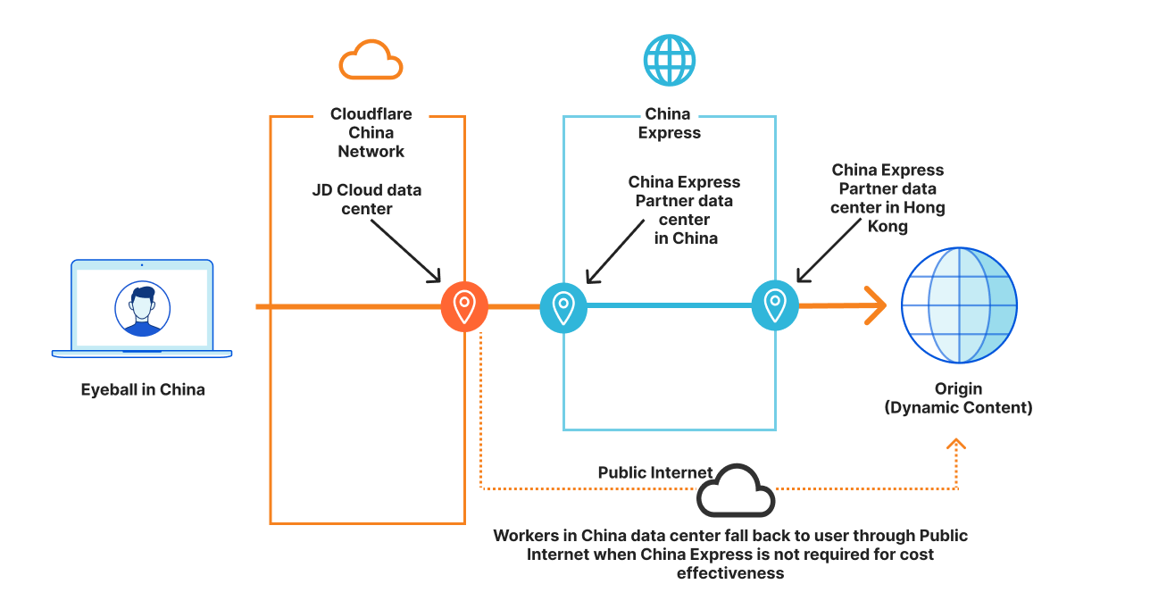
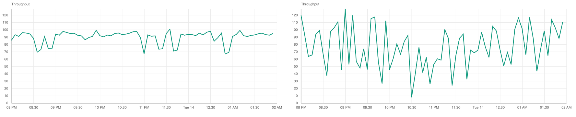
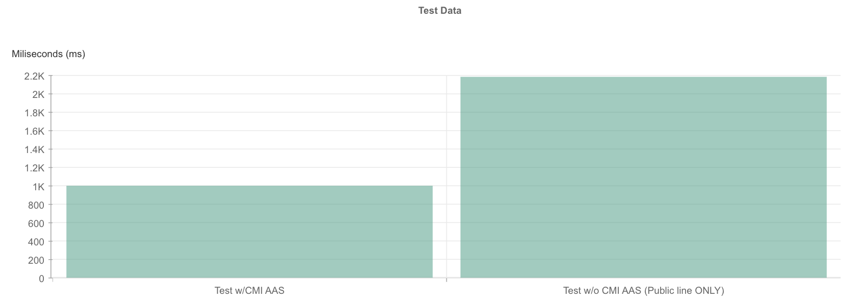


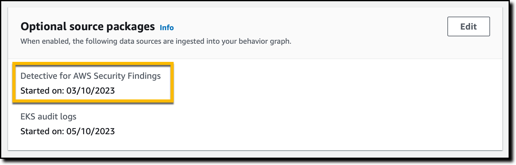


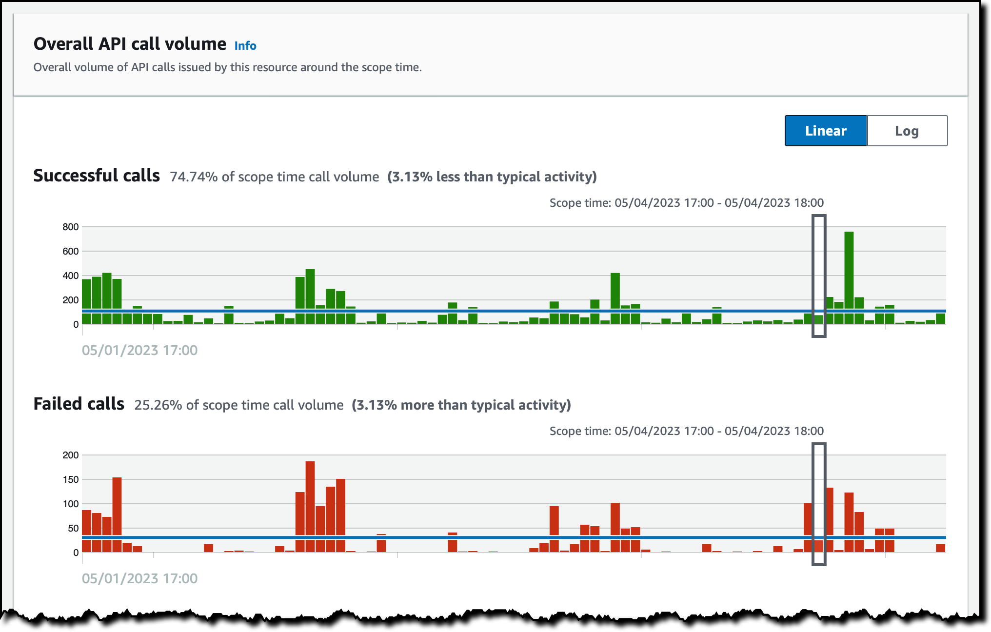


 Vishal Vijayvargiya is a Software Engineer working on Amazon MWAA at Amazon Web Services. He is passionate about building distributed and scalable software systems. Vishal also enjoys playing badminton and cricket.
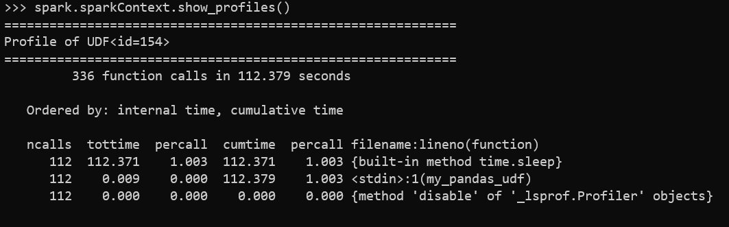
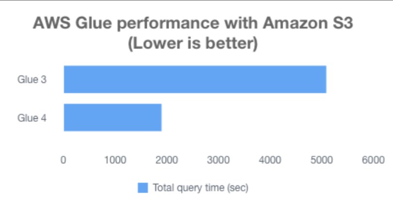


 Gonzalo Herreros is a Senior Big Data Architect on the AWS Glue team. He’s been an Apache Spark enthusiast since version 0.8. In his spare time, he likes playing board games.
 Noritaka Sekiyama is a Principal Big Data Architect on the AWS Glue team. He works based in Tokyo, Japan. He is responsible for building software artifacts to help customers. In his spare time, he enjoys cycling with his road bike.
 Bo Li is a Senior Software Development Engineer on the AWS Glue team. He is devoted to designing and building end-to-end solutions to address customer’s data analytic and processing needs with cloud-based data-intensive technologies.
 Rajendra Gujja is a Senior Software Development Engineer on the AWS Glue team. He is passionate about distributed computing and everything and anything about the data.
 Savio Dsouza is a Software Development Manager on the AWS Glue team. His team works on solving challenging distributed systems problems for data integration on Glue platform for customers using Apache Spark.
 Mohit Saxena is a Senior Software Development Manager on the AWS Glue team. His team works on distributed systems for building data lakes on AWS and simplifying integration with data warehouses for customers using Apache Spark.