The betting and gaming industry has grown into a data-rich landscape that presents an enticing target for sophisticated bots. The sensitive personally identifiable information (PII) that is collected and the financial data involved in betting and in-game economies is especially valuable. Microtransactions and in-game purchases are frequently targeted, making them an ideal case for safeguarding with AWS WAF.
In this blog post, we’ll explore some of these threats in more detail and explain how a layered bot mitigation strategy that uses AWS WAF can minimize the risk and impact of bot activity.
Understanding common automated threats
Automations deployed by threat actors can perform web scraping, perform betting arbitrage to gain an unfair advantage, and use automated techniques to undermine fair competition. Aggressive web scraping can also lead to application overload, service disruptions, and degraded user experience. At AWS, we routinely identify and mitigate automated threats for betting and gaming customers. Some of the common tactics we see in this space include the following:
Scraping tactics
Scraper bots often use fake accounts or compromised credentials to systematically harvest betting odds and other competitive data from multiple sites. A common example of scraping is arbitrage betting, where the scraped data is used to place simultaneous bets in different venues in order to make profits from tiny differences in the asset’s listed price. There are also competitive scraper bots that use this data to improve their betting applications.
Account-related tactics
Account creation fraud aims at claiming sign-up bonuses or other incentives at scale by using bot-generated accounts. Account takeover fraud aims at logging into user accounts to change account details, make purchases, withdraw funds, steal personal information or loyalty points, or use this data to access other accounts on different websites. A common form of this tactic is automated brute force login techniques, such as credential stuffing.
Denial-of-service tactics
Volumetric floods can cause betting and gaming sites to experience slow page-loads, downtime, and damaged brand reputation. DDoS attacks are another common security concern for many customers.
In-game tactics
In-game bots can use automated cheating or expediting techniques to manipulate resources and gain unfair advantages. These bots typically manipulate client applications and make malicious API requests.
AWS WAF intelligent threat mitigation features
To help protect customers from such automated tactics, AWS WAF offers the following intelligent threat mitigation features.
AWS WAF Common Bot Control managed rule group
The AWS WAF Common Bot Control managed rule group uses static analysis to identify web requests and header information that is correlated with known good bots and bad bots. These techniques are helpful in detecting a variety of self-identifying bots, such as web scraping frameworks, search engines, and automated browsers. Using these predetermined patterns and signatures can help gaming customers to identify and block known bot behaviors.
CAPTCHA and challenge rule actions
CAPTCHA rule action – Configured rules in AWS WAF can have a CAPTCHA action. When a rule is configured with a CAPTCHA action, users are required to solve a puzzle to prove that a human being is sending the request. When a user successfully solves a CAPTCHA challenge, a token is placed on their browser so it won’t challenge future requests, using a configurable immunity time. Learn about best practices for configuring CAPTCHA.
Challenge rule action – Challenge scripts run a silent challenge that requires the client session to verify that it’s a browser and not a bot. The verification runs in the background without involving the end user. Challenge-based bot detection can check each visitor’s ability to run JavaScript and store cookies. When a challenge is solved correctly, AWS WAF vends out an AWS WAF token, as seen in Figure 1, which allows bot control to track user activity across sessions. A reduced ability to process these challenges is a sign of bot traffic. The challenge action is a good option for verifying clients that you suspect of being invalid. You can use this feature by setting a selected AWS WAF rule action to CHALLENGE or by using a targeted bot control managed rule group. To learn more about protecting against bots with the AWS WAF challenge and CAPTCHA actions, see this blog post.
Figure 1: A sequence diagram explaining the flow of requests when Challenge is set as a rule action for an AWS WAF rule
Client application integration
AWS WAF provides the following levels of integration.
Intelligent threat integration
To improve the user experience and reduce latency for mobile and API-driven applications, AWS WAF provides client-side application APIs to integrate with your application. These integrations help verify that the client applications that send web requests to your protected resources are the intended clients and that your end users are human beings. This functionality is available for JavaScript and for Android and iOS mobile applications. As shown in Figure 2, the token acquisition process is similar to a challenge action, but slightly different. The basic approach for using the SDK is to create a token provider by using a configuration object, then to use the token provider to retrieve tokens from AWS WAF. By default, the token provider includes the retrieved tokens in your web requests to your protected resource. The intelligent threat integration APIs work with web access control lists (ACLs) that use the intelligent threat rule groups to enable the full functionality of these advanced managed rule groups. You can use the AWS WAF mobile SDKs to implement AWS WAF intelligent threat integration SDKs for Android and iOS mobile applications.
Figure 2: A sequence diagram explaining the flow of requests when AWS WAF intelligent threat mitigation SDKs are configured
CAPTCHA JavaScript integration
You can also verify end users by making them solve customized CAPTCHA puzzles that you manage in your application. This is similar to the functionality provided by the AWS WAF CAPTCHA rule action, but with added control over the puzzle placement and behavior. This integration uses the JavaScript intelligent threat integration to run silent challenges and provide AWS WAF tokens to the customer’s page.
AWS WAF Targeted Bot Control
The AWS WAF Targeted Bot Control tier includes the common-level protections described earlier and adds targeted detection for sophisticated bots that don’t self-identify. Targeted protections mitigate bot activity by using a combination of rate limiting and CAPTCHA and background browser challenges. Targeted protections use detection techniques such as the following:
Implementing browser fingerprinting – Browser fingerprinting is a powerful tracking and identification technique employed by online gaming sites to gain deep insights into their players’ computing setups. This technique involves probing the unique characteristics and configuration of each gamer’s browser. By collecting dozens of browser data points, a fingerprint can be generated that allows the requests coming from that specific browser to be identified and tracked across gaming sessions. Even if players try to randomize or spoof some browser attributes, perhaps in an attempt to bypass certain restrictions or gain an unfair advantage, the overall fingerprint still allows detection of such attempts. For example, if the user agent claims to be Chrome on Windows but other fingerprint attributes indicate Linux and Firefox, that suggests an attempted spoofing by the player, which can then be flagged by the gaming site’s security measures.
By using browser fingerprinting and looking for discrepancies, gaming and betting sites gain tools to help detect and block sophisticated bots even when the bots try to mask their true identity and intent. AWS WAF uses tokens for detecting browser inconsistencies, such as when the characteristics of a browser do not match the user agent. The AWS Targeted Bot Control rule group offers this functionality by emitting labels like TGT_SignalBrowserInconsistency, and the recommended mitigation action for inconsistent browsers is to serve a CAPTCHA puzzle.
Detecting browser automation – Many threat actors who operate automated programs use scripting languages to carry out their tasks, such as data scraping or launching exploits. They often employ tools that mimic the behavior of a web browser to bypass security measures. To address these challenges, AWS WAF Bot Control offers solutions to help detect and block automated software that simulates browser activity. It uses specific rules like TGT_SignalAutomatedBrowser to examine requests for signs that suggest the browser is not operated by a human, helping to identify and mitigate potential threats from automated systems.
Understand normal volumetric activity with unique browser ID tracking – AWS WAF Targeted Bot Control monitors application visitors by assigning each one a unique browser ID (UBID) embedded in a token. It establishes baselines for the number of requests a client sends within a five-minute session and sets three thresholds per device: high, medium, and low. The system identifies clients that exceed normal request rates and challenges them with a CAPTCHA puzzle using the TGT_VolumetricSession rule. For verified bots, the rule group takes no action but labels the traffic with awswaf:managed:aws:bot-control:bot:verified.
Using real-time machine learning models for clustering and behavior analysis – Traditional solutions to fight advanced bots faced limitations: handling massive amounts of player traffic, accurately identifying bots without labeling every request (ground truth), and staying cost-effective. To address these challenges, the AWS WAF team created a machine learning model. This model finds hidden bot networks by analyzing patterns in website traffic. It automatically analyzes traffic statistics to identify suspicious activity that suggests coordinated bot activity.
The model aggregates data at different levels, including the client, session, and behavioral cluster levels. It uses features like session statistics, behavioral cluster information (derived from clustering), and relative entropy to identify suspicious behavior. This feature analyzes web traffic every few minutes and optimizes the analysis for the detection of low intensity, long-duration bots that are distributed across many IP addresses. AWS WAF emits the labels TGT_ML_CoordinatedActivityMedium and TGT_ML_CoordinatedActivityHigh, based on the confidence level of the detection.
This machine learning capability is included by default in the AWS WAF Targeted Bot Control rules, but you can choose to disable it if needed.
Fraudulent account creation involves the creation of fake accounts for activities such as bonus abuse, impersonation, and phishing. These fake accounts can damage your reputation and expose you to financial fraud. To help prevent account creation fraud, we recommend using the AWS WAF Fraud Control account creation fraud prevention (ACFP) feature. This feature is available in the AWS Managed Rules rule group AWSManagedRulesACFPRuleSet, along with companion application integration SDKs. By integrating this feature into your system, you can effectively monitor and control account creation attempts, helping to provide a safer and more secure environment for your customers.
Threat actors might try to gain unauthorized access to a player’s account by using stolen credentials, guessing passwords through brute-force exploits, or other means. After they gain access, they can steal money, information, or services, or even pose as the victim to gain access to other accounts. This can lead to financial loss and damage to your reputation. To help prevent account takeovers, we recommend using the AWS WAF Fraud Control account takeover prevention (ATP) feature. This feature is available in the AWS Managed Rules rule group AWSManagedRulesATPRuleSet, along with companion application integration SDKs.
Conclusion
Bot management involves choosing controls to identify traffic coming from bots, and then blocking undesired traffic. The more threat actors are motivated to target a web application, the more they will invest in detection evasion techniques, requiring more advanced mitigation capabilities. We recommend that you adopt a layered approach to managing bots, with differentiated tooling that is adapted to specific bot tactics.
Ready to start putting the tools in place to protect your gaming or betting application from sophisticated bot threats? Check out our solution overview guide for AWS WAF and the Implementing a bot control strategy on AWS whitepaper to learn more about deploying a layered bot mitigation strategy on AWS. You can also sign up for an AWS Activation Day to work directly with our experts on implementing capabilities like AWS WAF, AWS WAF Bot Control, and AWS Shield for your specific use case. For hands-on experience, try our bot mitigation workshops—you can enable managed rule groups like Bot Control in just a few steps. Start your proof-of-concept by contacting your AWS account representative today.
If you have feedback about this post, submit comments in the Comments section below. If you have questions about this post, contact AWS Support.
Website defacement occurs when threat actors gain unauthorized access to a website, most commonly a public website, and replace content on the site with their own messages. In this blog post, we show you how to detect website defacement, and then automate both defacement verification and your defacement response by using Amazon CloudWatch Synthetics visual monitoring canaries. Canaries are configurable scripts that run on a schedule and compare screenshots taken during a canary run with screenshots taken during a baseline canary run. If the discrepancy between the two screenshots exceeds a threshold percentage, the canary fails. We will show you how to quickly deploy a maintenance page through AWS WAF after you verify the defacement.
Common causes of defacement include unauthorized access, SQL injection, cross-site scripting (XSS), or malware. You can use AWS services such as AWS WAF, Amazon Route 53, and Amazon GuardDuty to put additional mechanisms in place to help improve your security posture.
Solution overview
The architectural diagram in Figure 1 shows a typical web application where users access the application by using Amazon CloudFront protected by AWS WAF.
Figure 1: Defacement detection and response with CloudWatch Synthetics
As shown in the diagram, the solution consists of two parts: 1) visual monitoring for defacement detection, and 2) automation of the verification and defacement response.
Part 1: Visual monitoring for defacement detection
Defacement detection uses CloudWatch Synthetics visual monitoring canaries to perform visual monitoring. You can create canaries in CloudWatch Synthetics that periodically take a screenshot of the monitored URLs. Because the canaries only need network access to the monitored URLs, you can implement this solution without affecting the application or modifying its code. For more details on how to create CloudWatch Synthetics visual monitoring canaries, see Visual monitoring of applications with Amazon CloudWatch Synthetics.
You can use the CloudWatch Synthetics visual monitoring blueprint to compare screenshots taken during a canary run with screenshots taken during a baseline canary run. This solution is suitable for static a target=”_blank” hrefs where a discrepancy between the two screenshots that exceeds a threshold percentage could indicate a possible defacement attempt, causing the canary to trigger a failure event.
The threshold percentage is defined by the visual variance that occurs when the current screenshot differs from the baseline screenshot that was captured during the first run of the canary. To reduce false positives, you can adjust the threshold for detecting visual variance.
# Setting Threshold to 5%
syntheticsConfiguration.withVisualVarianceThresholdPercentage(5);
Figure 2 shows the first baseline screenshot of a webpage with visual variance set to 5%.
Figure 2: Image taken during a baseline canary run
Figure 3 shows the visual variance of a defaced webpage. In this case, the visual variance was set to 5% in the script, and the visual variance detected was 30.92%.
Figure 3: Failed canary run due to differences from the baseline screenshot
Figure 4 shows a webpage with dynamic content that triggered a false positive because the visual monitoring canary was unable to differentiate between real dynamic content and variation from the baseline. In this case, the visual variance was set to 5% in the script, and the visual variance detected was 5.25%.
Figure 4: Dynamic content in Feedback form that triggered canary failure
You can select the dynamic content to exclude it from the visual comparison for subsequent canary runs. To exclude the dynamic content, edit the baseline screenshot in CloudWatch Synthetics. Using a simple click-drag, you can select the area to exclude from visual comparison for subsequent canary runs, as shown in Figure 5.
Figure 5: Exclusion of dynamic content
If your applications have additional areas with dynamic content, you can select more than one area to exclude from comparison.
Figure 6 shows a successful canary run after exclusion of the area that contains the dynamic content.
Figure 6: Canary succeeded after the exclusion of dynamic content
The following shows the event pattern script in EventBridge. Make sure to update the canary name with the name of the CloudWatch Synthetics visual monitoring canary that you created earlier to serve as the event source.
 // Event patterns in EventBridge to get event source from canary

{
  "source": ["aws.synthetics"],
  "detail-type": ["Synthetics Canary TestRun Failure"],
  "detail": {
    "canary-name": ["<replace-with-canary-name>"]
  }
}
When the event pattern matches the rules that you configured in EventBridge, the Amazon SNS topic triggers the approval flow, as shown in Figure 7. This begins automation of the verification and defacement response, which we describe in the next section.
Figure 7: Amazon SNS topic triggered when the event pattern matches
Part 2: Automation of the verification and defacement response
Figure 8 outlines how to automate the verification and defacement response. When alerts are received upon detection of defacement, the notified team can choose to verify the defacement. This defacement monitor uses CloudWatch Synthetics while maintaining the flexibility to configure and verify threshold settings through manual verification. If you are confident in your thresholds, you can bypass the approval flow and directly block site traffic by using an AWS WAF rule during a defacement attempt.
Figure 8: Defacement detection and response with CloudWatch Synthetics
As shown in the diagram, this is what the traffic flow looks like during a defacement:
The canary from the CloudWatch Synthetics visual monitor identifies defacement through visual variance against the baseline screenshot taken during the first canary run and emits an event.
If the emitted event matches the rules configured in EventBridge, Amazon SNS is triggered. This triggers the subscribed AWS Lambda function that sends a Slack notification with the event details asking for approval.
The notified team receives a Slack message about the defacement and makes an approval decision.
If approval is granted, an AWS WAF rule is added to block traffic and a maintenance page is served to users.
The user that accessed the origin is shown a maintenance page served by AWS WAF.
Although this example shows the use of Slack as an approval mechanism, you can use the communication mechanism of your choice.
Conclusion
In this post, you learned how to use CloudWatch Synthetics to monitor for defacement and display a maintenance page through AWS WAF and CloudFront while you work on recovering the service. You also learned how to use manual approval to identify the optimal threshold and exclude the area that contains dynamic content to reduce false positives.
Although most web applications already use CloudFront and AWS WAF, you can integrate this solution to your existing environment without affecting the application or modifying its code. This solution helps detect potential defacement, providing you with an additional layer of protection for your environment.
We recommend that you explore the capabilities of CloudWatch Synthetics monitoring to detect and use the capabilities of the cloud through services such as EventBridge, Amazon SNS, and Lambda to enable automation. This can help you proactively protect your application against defacement attempts.
If you have feedback about this post, submit comments in the Comments section below. If you have questions about this post, contact AWS Support.
Amazon OpenSearch Service is a managed service that makes it easy to deploy, operate, and scale OpenSearch domains in AWS to perform interactive log analytics, real-time application monitoring, website search, and more. Understanding OpenSearch service spend per domain is crucial for effective cost management, optimization, and informed decision-making. Amazon OpenSearch Service Pricing is based on three dimensions: instances, storage, and data transfer. Storage pricing depends on the chosen storage type and also the storage tier. Visibility into domain-level charges enables accurate budgeting, efficient resource allocation, fair cost attribution across projects, and overall cost transparency.
In this post, we show you how to view the OpenSearch Service domain-level cost using AWS Cost Explorer. For example, the account in the following screenshot has five OpenSearch Service domains deployed.
Using AWS Cost Explorer, you can see the cost at the service level by default but not at an individual domain level. However, users can still breakdown the cost using a dimension like Usage type. The simplest approach to gain domain level visibility is by enabling resource-level data in AWS Cost Explorer. There are no additional charges for enabling resource-level data at daily granularity in AWS Cost Explorer. If you need domain-level cost data beyond 14 days then either you can setup a Data Export/CUR or you can use user-defined cost allocation tags. User-defined cost allocation tags offer benefits such as cost categorization and cost allocation to categorize and group your AWS costs across cost centers and based on criteria that are meaningful to your organization, such as projects, departments, environments, or applications. This provides better visibility and granularity into your cost breakdown compared to just looking at resource-level costs.
Overview
This post demonstrates how to use user-defined cost allocation tags attached to a cluster using these high-level steps:
Add a user-defined cost allocation tag to an OpenSearch Service domain
Activate the user-defined cost allocation tag
Analyze OpenSearch Service domain costs using AWS Cost Explorer and tags
Prerequisites
For this walkthrough, you should have the following prerequisites:
1. Add a user-defined cost allocation tag to an OpenSearch Service domain
The user-defined cost allocation tags are key-value pairs and user will need to define both a key and a value to an OpenSearch Service domain using one of the following methods:
To add a user-defined cost allocation tag using the AWS Management Console, follow these steps:
In the AWS Management Console, under Analytics, choose Amazon OpenSearch Service.
Select the domain you want to add tags to and go to the Tags
Choose Add tags and then Add new tag.
Enter a tag and an optional value.
Choose Save.
The following screenshot shows the Add tags window.
AWS CLI
To add a user-defined cost allocation tag using the AWS CLI, you can use the aws opensearch add-tags command to add tags to an OpenSearch Service domain. The command requires the domain Amazon Resource Name (ARN) and a list of tags to be added. Use the following syntax.
You can use the Amazon OpenSearch Service configuration API to create, configure, and manage OpenSearch Service domains. Use the following AddTags command to tag an OpenSearch Service domain.
You can programmatically add tags to an OpenSearch Service domain using the AWS OpenSearch SDK. The SDK provides methods to interact with Amazon OpenSearch Service API and manage tags. For example, Python client can use the client.add_tags command to tag a domain. You must provide values for domain_arn, tag_key, and tag_value.
When provisioning an OpenSearch Service domain using CloudFormation or Terraform, you can define the tags as part of the resource configuration by using AWS::OpenSearchService::Domain Tag.
The add-tags command can fail in the following scenarios, so make sure all the values are entered correctly:
Invalid resource ARN – The command will fail if the provided ARN for the OpenSearch Service domain is invalid or does not exist.
Insufficient permissions – Verify that the IAM user or role you’re using to run the OpenSearch Service commands has the necessary permissions to access the OpenSearch Service domain and perform the desired actions, such as adding tags.
Exceeded tag limit – The OpenSearch Service domain has limit of up to 10 tags, so if the number of tags you are trying to add exceeds this limit, the command will fail.
For ease of use and best results, use the Tag Editor to create and apply user-defined tags. The Tag Editor provides a central, unified way to create and manage your user-defined tags. For more information, refer to Working with Tag Editor in the AWS Resource Groups User Guide.
2. Activate the user-defined cost allocation tag
User-defined cost allocation tags are tags that you define, create, and apply to resources, and it may take up to 24 hours for the tag keys to appear on your cost allocation tags page for activation in the Billing and Cost Management console. After you select your tags for activation, it can take an additional 24 hours for tags to activate and be available for use in Cost Explorer. Use the following steps to activate the user-defined cost allocation tags you created in previous steps.
As shown in the following screenshot, on the Billing and Cost Management dashboard, in the navigation pane, select Cost Allocation Tags.
To activate the tag, under User-defined cost allocation tags, enter opensearchdomain to search for your tag name, select it, and choose Activate. This confirms that Cost Explorer and your AWS Cost and Usage Reports (CUR) will include these tags.
In general, cost allocation tags cannot be deleted and can only be deactivated. However, you can exclude the tag that you do not want in the CUR report or in AWS Cost Explorer and only include tags that are needed.
3. Analyze OpenSearch Service domain cost using AWS Cost Explorer and tags
AWS Cost Explorer only displays tags starting from the date when you have enabled user-defined cost allocation tags and not from when the resource was tagged. Therefore, even if your resources had tags for a long time, AWS Cost Explorer will show “No tag key” for all of the previous days until the date when tag was enabled, but users can request to backfill tags. To analyze OpenSearch Service domain costs using AWS Cost Explorer and tags, follow these steps:
On the Billing and Cost Management console, in the navigation pane, under Cost analysis, choose Cost Explorer.
In the Report parameters help panel on the right, under Group by, for Dimension, select Tag. Under Tag, choose the opensearchtestdomain tag key that you created.
Under Applied filters, choose OpenSearch Service.
The following screenshot shows the CUR dashboard.
Costs
There is no additional fee or charge for using the user-defined cost allocation tags in AWS Cost Explorer. However, an excessive number of tags can increase the size of your CUR file. Your CUR file contains your usage and cost data, including tags you apply, so more tags mean more data in the file. CUR data is stored in Amazon Simple Storage Service (Amazon S3), so larger CUR file could increase storage cost.
The best practice is to be selective about which tags you enable and how many you use. Start with tags that provide the most value for attributes such as cost allocation and analytics. Monitor your CUR file size over time and add and remove tags thoughtfully.
Conclusion
This post outlines a solution for AWS customers to gain visibility into their OpenSearch Service workload costs on a per-domain basis using AWS Cost Explorer and user-defined cost allocation tags. This approach enables greater cost transparency and control, making it easier to allocate costs accurately and make informed decisions about Amazon OpenSearch service workload usage. The process involves adding a cost allocation tag to each OpenSearch Service domain, activating the user-defined tag, and then analyzing the costs in AWS Cost Explorer based on the tag. By implementing this solution, customers can obtain granular insights into OpenSearch Service workload costs at the domain level, facilitating precise cost attribution and better alignment of costs with business requirements.
Nikhil Agarwal is a Sr. Technical Manager with Amazon Web Services. He is passionate about helping customers achieve operational excellence in their cloud journey and actively working on technical solutions. He is an artificial intelligence (AI/ML) and analytics enthusiastic, he deep dives into customer’s ML and OpenSearch service specific use cases. Outside of work, he enjoys traveling with family and exploring different gadgets.
Rick Balwani is an Enterprise Support Manager responsible for leading a team of Technical Account Mangers (TAMs) supporting AWS independent software vendor (ISV) customers. He works to ensure customers are successful on AWS and can build cutting-edge solutions. Rick has a background in DevOps and system engineering.
Ashwin Barve is a Sr. Technical Manager with Amazon Web Services. In his role, Ashwin leverages his experience to help customers align their workloads with AWS best practices and optimize resources for maximum cost savings. Ashwin is dedicated to assisting customers through every phase of their cloud adoption, from accelerating migrations to modernizing workloads.
Generative artificial intelligence (AI) is now a household topic and popular across various public applications. Users enter prompts to get answers to questions, write code, create images, improve their writing, and synthesize information. As people become familiar with generative AI, businesses are looking for ways to apply these concepts to their enterprise use cases in a simple, scalable, and cost-effective way. These same needs are shared by a variety of security stakeholders. For example, if security directors want to summarize their security posture in natural language, a security architect will need to triage alerts or findings and investigate AWS CloudTrail logs to identify high priority remediation actions or detect potential threat actors by identifying potentially malicious activity. There are many ways to deploy solutions for these use cases.
In this blog post, we review a fully serverless solution for querying data stored in Amazon Security Lake using natural language (human language) with Amazon Q in QuickSight. This solution has multiple use cases, such as generating visualizations and querying vulnerability information for vulnerability management using tools such as Amazon Inspector that feed into AWS Security Hub. The solution helps reduce the time from detection to investigation by using natural language to query CloudTrail logs and Amazon Virtual Private Cloud (VPC) Flow Logs, resulting in quicker response to threats in your environment.
Amazon Security Lake is a fully managed security data lake service that automatically centralizes security data from AWS environments, software as a service (SaaS) providers, and on-premises and cloud sources into a purpose-built data lake that’s stored in your AWS account. The data lake is backed by Amazon Simple Storage Service (Amazon S3) buckets, and you retain ownership over your data. Security Lake converts ingested data into Apache Parquet format and a standard open source schema called the Open Cybersecurity Schema Framework (OCSF). With OCSF support, Security Lake normalizes and combines security data from AWS and a broad range of enterprise security data sources.
Amazon QuickSight is a cloud-scale business intelligence (BI) service that delivers insights to stakeholders, wherever they are. QuickSight connects to your data in the cloud and combines data from a variety of different sources. With QuickSight, users can meet varying analytic needs from the same source of truth through interactive dashboards, reports, natural language queries, and embedded analytics. With Amazon Q in QuickSight, business analysts and users can use natural language to build, discover, and share meaningful insights.
The recent announcements for Amazon Q in QuickSight, Security Lake, and the OCSF present a unique opportunity to apply generative AI to fully managed hybrid multi-cloud security related logs and findings from over 100 independent software vendors and partners.
Solution overview
The solution uses Security Lake as the data lake which has native ingestion for CloudTrail, VPC Flow Logs, and Security Hub findings as shown in Figure 1. Logs from these sources are sent to S3 buckets in your AWS account and are maintained by Security Lake. We then create Amazon Athena views from tables created by Security Lake for Security Hub findings, CloudTrail logs, and VPC Flow Logs to define the interesting fields from each of the log sources. Each of these views are ingested into a QuickSight dataset. From these datasets, we generate analyses and dashboards. We use Amazon Q topics to label columns in the dataset that are human-readable and create a named entity to present contextual and multi-visual answers in response to questions. After the topics are created, users can perform their analysis using Q topics, QuickSight analyses, or QuickSight dashboards.
Figure 1: Solution architecture
You can use the rollup AWS Region feature in Security Lake to aggregate logs from multiple Regions into a single Region. Specifying a rollup Region can help you adhere to regional compliance requirements. If you use rollup Regions, you must set up the solution described in this post for datasets only in rollup Regions. If you don’t use a rollup Region, you must deploy this solution for each Region you that want to collect data from.
Prerequisites
To implement the solution described in this post, you must meet the following requirements:
Basic understanding of Security Lake, Athena, and QuickSight.
Security Lake is already deployed and accepting CloudTrail management events, VPC Flow Logs, and Security Hub findings as sources. If you haven’t deployed Security Lake yet, we recommend following the best practices established in the security reference architecture.
This solution uses Security Lake data source version 2 to create the dashboards and visualizations. If you aren’t already using data source version 2, you will see a banner in your Security Lake console with instructions to update.
An existing QuickSight deployment that will be used to visualize Security Lake data or an account that is able to sign up for QuickSight to create visualizations.
QuickSight Author Pro and Reader Pro licenses are needed for using Amazon Q features in QuickSight. Non-pro Authors and Readers can still access Q topics if an Author Pro or Admin Pro user shares the topic with them. Non-pro Authors and Readers can also access data stories if a Reader Pro, Author Pro, or Admin Pro shares one with them. Review Generative AI features supported by each QuickSight licensing tiers.
In the following section, we walk through the steps to ingest Security Lake data into QuickSight using Athena views and then using Amazon Q in QuickSight to create visualizations and query data using natural language.
Provide cross-account query access
In alignment with our security reference architecture, it’s a best practice to isolate the Security Lake account from the accounts that are running the visualization and querying workloads. It’s recommended that QuickSight for security use cases be deployed in the security tooling account. See How to visualize Amazon Security Lake findings with Amazon QuickSight for information on how to set up cross-account query access. Follow the steps in the Configure a Security Lake subscriber section and configure Athena to visualize your data section.
When you get to the create resource link steps, create a resource link for data source version 2 for Security Hub, CloudTrail, and VPC flow log tables for a total of three resource links. The way to identify data source version 2 tables is by their name; it ends in _2_0. For example:
For the remainder of this post, we will be referencing the database name security_lake_visualization and the resource link names for Security Hub findings, CloudTrail logs, and VPC Flow Logs respectively, as shown in Figure 2:
We will call the QuickSight account the visualization account. If you plan to use same account as the Security Lake delegated administrator and QuickSight, then skip this step and go to the next section where you will create views in Athena.
Create views in Athena
A view in Athena is a logical table that helps simplify your queries by working with only a subset of the relevant data. Follow these steps to create three views in Athena, one each for Security Hub findings, CloudTrail logs, and the VPC Flow Logs in the visualization account.
These queries default to the previous week’s data starting from the previous day, but you can change the time frame by modifying the last line in the query from 8 to the number of days you prefer. Keep in mind that there is a limitation on the size of each SPICE table of 1 TB. If you want to limit the volume of data, you can delete the rows that you find unnecessary. We included the fields customers have identified as relevant to reduce the burden of writing the parsing details yourself.
To create views:
Sign in to the AWS Management Console in the visualization account and navigate to the Athena console.
If a Security Lake rollup Region is used, select the rollup Region.
Choose Launch Query Editor.
If this is the first time you’re using Athena, you will need to choose a bucket to store your query results.
Choose Edit Settings.
Choose Browse S3.
Search for your bucket name.
Select the radio button next to the name of your bucket.
Select Choose.
For Data Source, select AWSDataCatalog.
Select Database as security_lake_visualization. If you used a different name for the database for cross account query access, then select that database.
Figure 3: Athena database selection
Copy the query for the security_hub_view from the GitHub repo for this post. If you’re using a different name for the database and table resource link than the one specified in this post, edit the FROM statement at the bottom of the query to reflect the correct names.
Paste the query in the query editor and then choose Run. The name of the view is set in the first line of the query which is security_insights_security_hub_vw2.
To confirm this view was created correctly, choose the three dots next to the view that was created and select Preview View.
Figure 4: Previewing the view
Repeat steps 5–9 to create the CloudTrail and VPC Flow Logs views. The queries for each can be found in the GitHub repo.
Figure 5: Athena views
Create QuickSight dataset
Now that you’ve created the views, use Athena as the data source to create a dataset in QuickSight. Repeat these steps for the Security Hub findings, CloudTrail logs, and VPC Flow Logs. Start by creating a dataset for the Security Hub findings.
To configure permissions on tables:
Sign in to the QuickSight console in the visualization account. If a Security Lake rollup Region is used, select the rollup Region.
Although there are multiple ways to sign in to QuickSight, we used IAM based access to build the dashboards. To use QuickSight with Athena and Lake Formation, you first need to authorize connections through Lake Formation.
When using a cross-account configuration with AWS Glue Data Catalog, you need to configure permissions on tables that are shared through Lake Formation. For the use case in this post, use the following steps to grant access on the cross-account tables in the Glue Catalog. You must perform these steps for each of the Security Hub, CloudTrail, and VPC Flow Logs tables that you created in the preceding cross-account query access section. Because granting permissions on a resource link doesn’t grant permissions on the target (linked) database or table, you will grant permission twice, once to the target (linked table) and then to the resource link.
In the Lake Formation console, navigate to the Tables section and select the resource link for the Security Hub table. For example:
Select Actions. Under Permissions, select Grant on target.
For the next step, you need the Amazon Resource Name (ARN) of the QuickSight users or groups that need access to the table. To obtain the ARN through the AWS Command Line Interface (AWS CLI), run following commands (replacing account ID and Region with that of the visualization account.) You can use AWS CloudShell for this purpose.
After you have the ARN of the user or group, copy it and go back to the LakeFormation console Grant on Target page. For Principals, select SAML users and groups, and then add the QuickSight user’s ARN.
Figure 6: Selecting principals
For LF-Tags or catalog resources, keep the default settings.
Figure 7: Table grant on target permissions
For Table permissions, select Select for both Table Permissions and Grantable Permissions, and then choose Grant.
Figure 8: Selecting table permissions
Navigate back to the Tables section and select the resource link for the Security Hub table. For example:
Select Actions. This time under Permissions, and then choose Grant.
For Principals, select SAML users and groups, and then add the QuickSight user’s ARN captured earlier.
For the LF-Tags or catalog resources section, use the default settings.
For Resource link permissions choose Describe for both Table Permissions and Grantable Permissions.
Repeat steps a–k for the CloudTrail and VPC Flow Logs resource links.
To create datasets from views:
After permissions are in place, you create three datasets from the views created earlier. Because both Quicksight and Lake Formation are Regional services, verify that you’re using QuickSight in the same Region where Lake Formation is sharing the data. The simplest way to determine your Region is to check the QuickSight URL in your web browser. The Region will be at the beginning of the URL, such as us-east-1. To change the Region, select the settings icon in the top right of the QuickSight screen and select the correct Region from the list of available Regions in the drop-down menu.
Navigate back to the QuickSight console.
Select Datasets, and then choose New dataset.
Select Athena from the list of available data sources.
Enter a Data source name, for example security_lake_securityhub_dataset and leave the Athena workgroup as [primary]. Choose Create data source.
At the Choose your table prompt, for Catalog, select AwsDataCatalog. For Database, select security_lake_visualization. If you used a different name for the database for cross-account query access, then select that database. For Tables, select the view name security_insights_security_hub_vw2 to build your dashboards for Security Hub findings. Then choose Select.
Figure 9: Choose a table during QuickSight dataset creation
At the Finish dataset creation prompt, select Import to SPICE for quicker analytics. Choose Visualize. This will create a new dataset in QuickSight using the name of the Athena view, which is security_insights_security_hub_vw2. You will be taken to the Analysis page, exit out of it.
Go back to the QuickSight console and repeat steps 3–8 for the CloudTrail and VPC Flow Log datasets.
Create a topic
Now that you have created a dataset, you can create a topic. Q topics are collections of one or more datasets that represent a subject area for your business users to ask questions. Topics allow users to ask questions in natural language and to build visualizations using natural language.
To create a Q topic:
Navigate to the QuickSight console.
Choose Topics in the left navigation pane.
Figure 10: QuickSight navigation pane
Choose New topic. Create one topic each for the Security Hub findings, CloudTrail logs, and VPC Flow Logs
Figure 11: QuickSight topic creation
On the New topic page, do the following:
For Topic name, enter a descriptive name for the topic. Name the first one SecurityHubTopic. Your business users will identify the topic by this name and use it to ask questions.
For Description, enter a description for the topic. Your users can use this description to get more details about the topic.
Choose Continue.
On the Add data to topic page, choose the dataset you created in the Create a QuickSight dataset section. Start with the Security Hub dataset security_insights_security_hub_vw2.
Choose Continue. It will take a few minutes to create the topic.
Now that your topic has been created, navigate to the Data tab of the topic.
Your Data Fields sub-tab should be selected already. If not, choose Data Fields.
Figure 12: Topics data fields
For each of the fields in the list, turn on Include to make sure that all fields are included. For this example, we selected all fields, but you can adjust the included columns as needed for your use case. Note, you might see a banner at the top of the page indicating that the indexing is in progress. Depending on the size of your data, it might take some time for Q to make those fields available for querying. Most of the time, indexing is complete in less than 15 minutes.
Review the Synonyms column. These alternate representations of your column name are automatically generated by Amazon Q. You can add and remove synonyms as needed for your use case.
At this point, you’re ready to ask questions about your data using Amazon Q in QuickSight. Choose Ask a question about SecurityHubTopic at the top of the page.
Figure 13: Ask questions using Q
You can now ask questions about Security Hub findings in the prompt. Enter Show me findings with compliance status failed along with control id.
Figure 14: Q answers
Under the question, you will see how it was interpreted by QuickSight.
Repeat steps 1–13 to create CloudTrail and VPC Flow Log QuickSight topics.
Create named entities for your topics
Now that you’ve created your topics, you will now add named entities. Named entities are optional, but we’re using them in the solution to help make queries more effective. The information contained in named entities, the ordering of fields, and their ranking make it possible to present contextual, multi-visual answers in response to even vague questions.
To create a named entity:
In the QuickSight console, navigate to Topics.
Select the Security Hub topic that you created in the previous section.
Under the Data tab, select the Named Entity subtab, and choose Add Named Entity.
Figure 15: Named entity subtab
Enter Security Findings as the entity name.
Select the following datafields: Status, Metadata Product Name, Finding Info Title, Region, Severity, Cloud Account Uid, Time Dt, Compliance Status, and AccountId. The order of the fields helps Q to prioritize the data, so rearrange your data fields as needed.
Choose Save in the top right corner to save your results.
Repeat steps 1–6 with the CloudTrail dataset using the following datafields: API operation, Time Dt, Region, Status, AccountId, API Response Error, Actor User Credential Uid, Actor User Name, Actor User Type, Api Service Name, Actor Idp Name, Cloud Provider, Session Issuer, and Unmapped.
Figure 17: CloudTrail named entity creation
Repeat steps 1–6 with the VPC Flow Log dataset using the following datafields: Src Endpoint IP, Src Endpoint Port, Dst Endpoint IP, Dst Endpoint Port, Connection Info Direction, Traffic Bytes, Action, Accountid, Time Dt, and Region.
Figure 18: VPC Flow log named entity creation
Create visualizations using natural language
After your topic is done indexing, you can start creating visualizations using natural language. In QuickSight, an analysis is the same thing as a dashboard, but is only accessible by the authors. You can keep it private and make it as robust and detailed as you want. When you decide to publish it, the shared version is called a dashboard.
To create visualizations:
Open the QuickSight console and navigate to the Analysis tab.
In the top right, select New analysis.
Select the dataset you created previously, it will have the same naming convention as the Athena view. For reference, the Athena view query created a Security Hub dataset called security_insights_security_hub_vw2.
Validate the information about the data set you’re going to use in the analysis and choose USE IN ANALYSIS.
On the pop up, select the interactive sheet option and choose Create.
For datasets that have a corresponding Q topic, which you created in a previous step, choose Build visual at the top of the screen.
Figure 19: Build visual using natural language
Enter your prompt and choose BUILD. For example, enter findings with product security hub group by control id include count. Q automatically generates a visualization.
Figure 20: Q response
To add to your dashboard, choose ADD TO ANALYSIS to see your new visualization module in your current analysis.
The supplied questions are targeted towards a Security Hub findings topic, where you can ask questions about your security hub findings data. For example, show all Security Hub findings for critical severity for a specific resource or ARN.
If you use Amazon Inspector for software vulnerability management and you want to monitor top common vulnerabilities and exposures (CVEs) affecting your organization, choose Build visual and enter show all ACTIVE findings with product inspector group by Title add count in the prompt. We used the keyword ACTIVE because ACTIVE is a finding state in Security Hub that indicates the finding is still active as per the finding source and Amazon Inspector has not closed the finding yet. If Amazon Inspector has closed the finding, the finding will have a state of ARCHIVED.
Figure 21: Q Response for an Amazon Inspector findings question
To add the remaining datasets, which allows you to visualize data from multiple datasets in a single view, select the dropdown in the left navigation under Dataset.
Select Add a new dataset.
Search the name of the remaining datasets you created previously.
Select anywhere on the name of the dataset to make the radial button blue for the single dataset you want to add. Choose Select.
Repeat steps 7–12 in this section to add all the corresponding datasets you created previously.
Note: When you add additional datasets to the same Analysis and use Build visual to generate visualizations using natural language, the corresponding datasets with Q Topics are populated in the drop down under the prompt. Be sure to choose the correct dataset when asking questions.
Figure 22: Choosing a QuickSight dataset
To create dashboards:
After you’ve created the visual and are ready to publish the analysis as a dashboard, select PUBLISH in the top right corner.
Enter a name for your dashboard.
Choose Publish Dashboard.
After your dashboard is published, your users can ask questions about the data through the dashboard as well. This dashboard can be shared with other users. Users with QuickSight Reader Pro licenses can ask questions using Amazon Q.
To ask questions using the dashboard:
Navigate to the Dashboards section on the left navigation.
Select the dashboard you previously published.
Select Ask a question about [Topic Name] at the top of the screen. A module will open from the side of your screen. Questions can only be addressed to a single topic. To change the topic, select the name of the topic and a drop-down will appear. Select the name of the current topic to see other options and select the topic you want to ask a question about. For this example, select CloudTrailTopic.
Figure 23: Selecting a topic
Enter a question in the prompt. For this example, enter show top API operations in the last 24 hours with accessdenied.
Figure 24: CloudTrail question 1
Enter show all activity by user johndoe in the last 3 days.
Figure 25: CloudTrail question 2
Q will automatically build a small dashboard based on the questions provided.
Now change the topic to VPCFlowTopic as described in step 3.
Enter show me the top 5 dst ip by bytes for outbound traffic with dst port 443.
Figure 26: VPC Flow Log question
You can build executive summaries using QuickSight data stories, which also use generative AI. Data stories use Amazon Q prompts and visuals to produce a draft that incorporates the details that you provide. For example, you can create a data story about how a specific CVE affects your organization by asking Q questions, then add visuals from analyses you already created.
Conclusion
In this blog post, you learned how to use generative AI for your security use cases. We showed you how to use cross-account query access to allow a QuickSight visualization account to subscribe to Security Lake data for Security Hub findings, CloudTrail logs, and VPC Flow Logs. We then provided instructions for creating, Athena views, QuickSight datasets, Q topics, named entities, and for using natural language to build dashboards and query your data. You can customize the Athena views to create, update, or delete columns and column names as needed for your use case. You can also customize the Q topics and named entities to use naming conventions and structure responses based on your organization’s needs.
If you have feedback about this post, submit comments in the Comments section below. If you have questions about this post, contact AWS Support.
If you have a customer facing application, you might want to enable self-service sign-up, which allows potential customers on the internet to create an account and gain access to your applications. While it’s necessary to allow valid users to sign up to your application, self-service options can open the door to unintended use or sign-ups. Bad actors might leverage the user sign-up process for unintended purposes, launching large-scale distributed denial of service (DDoS) attacks to disrupt access for legitimate users or committing a form of telecommunications fraud known as SMS pumping. SMS pumping is when bad actors purchase a block of high-rate phone numbers from a telecom provider and then coerces unsuspecting services into sending SMS messages to those numbers.
Amazon Cognito is a managed OpenID Connect (OIDC) identity provider (IdP) that you can use to add self-service sign-up, sign-in, and control access features to your web and mobile applications. AWS customers who use Cognito might encounter SMS pumping if SMS functions are enabled to send SMS messages, for example, perform user phone number verification during the registration process, to facilitate SMS multi-factor authentication (MFA) flows, or to support account recovery using SMS. In this blog post, we explore how SMS pumping may be perpetrated and options to reduce risks, including blocking unexpected user registration, detecting anomalies, and responding to risk events with your Cognito user pool.
Cognito user sign-up process
After a user has signed up in your application with an Amazon Cognito user pool, their account is placed in the Registered (unconfirmed) state in your user pool and the user won’t be able to sign in yet. You can use the Cognito-assisted verification and confirmation process to verify user-provided attributes (such as email or phone number) and then confirm the user’s status. This verified attribute is also used for MFA and account recovery purposes. If you choose to verify the user’s phone number, Cognito sends SMS messages with a one-time password (OTP). After a user has provided the correct OTP, their email or phone number is marked as verified and the user can sign in to your application.
Figure 1: Amazon Cognito sign-up process
If the sign-up process isn’t protected, bad actors can create scripts or deploy bots to sign up a large number of accounts, resulting in a significant volume of SMS messages sent in a short period of time. We dive deep into prevention, detection, and remediation mechanisms and strategies that you can apply to help protect against SMS pumping based on your use case.
Protect the sign-up flow
In this section, we review several prevention strategies to help protect against SMS sign-up frauds and help reduce the amount of SMS messages sent to bad actors.
Implement bot mitigation
Implementing bot mitigation techniques, such as CAPTCHA, can be very effective in preventing simple bots from pumping user creation flows. You can integrate a CAPTCHA framework on your application’s frontend and validate that the client initiating the sign-up request is operated by a human user. If the user has passed the verification, you then pass the CAPTCHA user response token in ClientMetadata together with user attributes to an Amazon Cognito SignUp API call. As part of the sign-up process, Cognito invokes an AWS Lambda function called pre sign-up Lambda trigger, which you can use to reject sign-up requests if there isn’t a valid CAPTCHA token presented. This will slow down bots and help reduce unintended account creation in your Cognito user pool.
Validate phone number before user sign-up
Another layer of mitigation is to identify the actor’s phone number early in your application’s sign-up process. You can validate the user provided phone number in the backend to catch incorrectly formatted phone numbers and add logic to help filter out unwanted phone numbers prior to sending text messages. Amazon Pinpoint offers a Phone Number Validate feature that can help you determine if a user-provided phone number is valid, determine phone number type (such as mobile, landline, or VoIP), and identify the country and service provider the phone number is associated with. The returned phone number metadata can be used to decide whether the user will continue the sign-up process and send an SMS message to that user. Note that there’s an additional charge for using the phone number validation service. For more information, see Amazon Pinpoint pricing.
To build this validation check into the Amazon Cognito sign-up process, you can customize the pre sign-up Lambda trigger, which Cognito uses to invoke your code before allowing users to sign-up and sending out an SMS OTP. The Lambda trigger invokes the Amazon Pinpoint phone number validate API, and based on the validation response, you can build a custom pattern that fits your application to continue or reject the user sign-up. For example, you can reject user sign-ups with VoIP numbers or reject users who provide a phone number that’s associated with countries that you don’t operate in, or even reject certain cellular service providers. After you reject a user sign-up using the Lambda trigger, Cognito will deny the user sign-up request and will not invoke user confirmation flow nor send out an SMS message.
When you send a request to the Amazon Pinpoint phone number validation service, it returns the following metadata about the phone number. The following example represents a valid mobile phone number data set:
Note that PhoneType includes type MOBILE, LANDLINE, VOIP, INVALID, or OTHER. INVALID phone numbers don’t include information about the carrier or location associated with the phone number and are unlikely to belong to actual recipients. This helps you decide when to reject user sign-ups and reduces SMS messages to undesired phone numbers. You can see details about other responses in the Amazon Pinpoint developer guide.
Example pre sign-up Lambda function to block user sign-up except with a valid MOBILE number
The following pre sign-up Lambda function example invokes the Amazon Pinpoint phone number validation service and rejects user sign-ups unless the validation service returns a valid mobile phone number.
import { PinpointClient, PhoneNumberValidateCommand } from "@aws-sdk/client-pinpoint"; // ES Modules import

const validatePhoneNumber = async (phoneNumber) => {
  const pinpoint = new PinpointClient();
  const input = { // PhoneNumberValidateRequest
    NumberValidateRequest: { // NumberValidateRequest
      PhoneNumber: phoneNumber,
    },
  };
  const command = new PhoneNumberValidateCommand(input);
  const response = await pinpoint.send(command);

  return response;
};

const handler = async (event, context, callback) => {

  const phoneNumber = event.request.userAttributes.phone_number;
  const validationResponse = await validatePhoneNumber(phoneNumber);

  if (validationResponse.NumberValidateResponse.PhoneType != "MOBILE") {
    var error = new Error("Cannot register users without a mobile number");
    // Return error to Amazon Cognito
    callback(error, event);
  }
  // Return to Amazon Cognito
  callback(null, event);
};

export { handler };
Use a custom user-initiated confirmation flow or alternative OTP delivery method
In your user pool configurations, you can opt out of using Amazon Cognito-assisted verification and confirmation to send SMS messages to confirm users. Instead, you can build a custom reverse OTP flow to ask your users to initiate the user confirmation process. For example, instead of automatically sending SMS messages to a user when they sign up, your application can display an OTP and direct the user to initiate the SMS conversation by texting the OTP to your service number. After your application has received the SMS message and confirmed the correct OTP is provided, invoke a service such as a Lambda function to call the AdminConfirmSignUp administrative API operation to confirm user, then call AdminUpdateUserAttributes to set the phone_number_verified attribute as true to indicate that the user phone number is verified.
You can also choose to deliver an OTP using other methods, such as email, especially if your application doesn’t require the user’s phone number. During the user sign-up process, you can configure a custom SMS sender Lambda trigger in Amazon Cognito to send a user verification code through email or another method. Additionally, you can use the Cognito email MFA feature to send MFA codes through email.
Detect SMS pumping
When you’re considering the various prevention options, it’s important to set up detection mechanisms to identify SMS pumping as they arise. In this section, we show you how to use AWS CloudTrail and Amazon CloudWatch to monitor your Amazon Cognito user pool and detect anomalies that could lead to SMS pumping. Note that building detection mechanism based on anomalies requires knowing your average or baseline traffic and the difference in metrics that represent regular activity and metrics that can indicate unauthorized or unintended activity.
Service quotas dashboard and CloudWatch alarms
Bad actors may attempt to leverage either the sign-up confirmation or the reset password functionality of Amazon Cognito. As shown previously in Figure 1, when a new user signs up to your Cognito user pool, the SignUp API operation is invoked. When the user provides the OTP confirmation code, the ConfirmSignUp API operation is invoked. The call rate of both APIs is tracked collectively under Rate of UserCreation requests under Amazon Cognito service in the service quotas dashboard.
You can set up Amazon CloudWatch alarms to monitor and issue notifications when you’re close to a quota value threshold. These alarms could be an early indication of a sudden usage increase, and you can use them to triage potential incidents.
Additionally, when your services are sending SMS messages, those transactions count towards the Amazon Simple Notification Service (Amazon SNS) service quota. You should set up alarms to monitor the Transactional SMS Message Delivery Rate per Second quota and the SMS Message Spending in USD quota.
CloudTrail event history
When bad actors plan SMS pumping, they are likely attempting to trick you to send as many SMS messages as possible rather than completing the user confirmation process. Under the context of a user sign-up event, you might notice in the CloudTrail event history that there are more SignUp and ResendConfirmationCode events—which send out SMS messages—than ConfirmSignUp operations; indicating a user has initiated but not completed the sign-up process. You can use Amazon Athena or CloudWatch Logs Insights to search and analyze your Amazon Cognito CloudTrail events and identify if there’s a significant reduction in finishing the user sign-up process.
Figure 2: SignUp API logged in CloudTrail event history
Similarly, you can apply this observability towards the user password reset flow by analyzing the ForgotPassword API and ConfirmForgotPassword API operations for deviations.
Note that the slight deviations in user completion flow in the CloudTrail event history alone might not be an indication of unauthorized activity, however a substantial deviation above the regular baseline might be a signal of unintended use.
Monitor excessive billing
Another opportunity for detecting and identifying unauthorized Amazon Cognito activity is by using AWS Cost Explorer. You can use this interface to visualize, understand, and manage your AWS costs and usage over time, which might assist by highlighting the source of excessive billing in your AWS account. Be aware that charges in your account can take up to 24 hours to be displayed, so while this method can help provide some assistance in identifying SMS pumping activity, it should only be used as a supplement to other detection methods.
In the navigation pane, under Cost Analysis, choose Cost Explorer.
In the Cost and Usage Report, under Report Parameters, select Date Range to include the start and end date of the time period that you want to apply a filter to. In Figure 3 that follows, we use an example date range between 2024-07-03 and 2024-07-17.
In the same Report Parameter area, under Filters, for Service, select SNS (Simple Notification Service). Because Amazon Cognito uses Amazon SNS for delivery of SMS messages, filtering on SNS can help you identify excessive billing.
Figure 3: Reviewing billing charges by service
Apply AWS WAF rules as mitigation approaches
It’s recommended that you apply AWS WAF with your Amazon Cognito user pool to protect against common threats. In this section, we show you a few advanced options using AWS WAF rules to block or throttle specific bad actor’s traffic when you have observed irregular sign-up attempts and suspect they were part of fraudulent activities.
Target a specific bad actor’s IP address
When building AWS WAF remediation strategies, you can start by building an IP deny list to block traffic from known malicious IP addresses. This method is straightforward and can be highly effective in preventing unwanted access. For detailed instructions on how to set up an IP deny list, see Creating an IP set.
Target a specific phone number area code regex pattern
In an SMS pumping scheme, bad actors often purchase blocks of cell phone numbers from a wireless service provider and use phone numbers with the same area code. If you observe a pattern and identify that these attempts use the same area code, you can apply an AWS WAF rule to block that specific traffic.
To configure an AWS WAF web ACL to block using an area code regex pattern:
Open the AWS WAF console.
In the navigation pane, under AWS WAF, choose WAF ACLs.
Choose Create web ACL. Under Web ACL details, select Regional resources, and select the AWS Region as your Amazon Cognito user pool. Under Associated AWS resources, select Add AWS resources, and choose your Cognito user pool. Choose Next.
On the Add rules and rule groups page, choose Add rules, Add my own rules and rule groups, and Rule builder.
Create a rule in Rule builder.
For If a request, select matches the statement.
For Inspect, select Body.
For Match type, select Matches regular expression.
For Regular expression, enter a match for the observed pattern. For example, the regular expression ^303|^\+1303|^001303 will match requests that include the digits 303, +1303, or 001303 at the beginning of any string in the body of a request:
Figure 4: Creating a web ACL
Under Action, choose Block. Then, choose Add rule.
Continue with Set rule priority and Configure metrics, then choose Create web ACL.
Be aware that this method will block all user sign-up requests that contain phone numbers matching the regex pattern for the target area code and could prevent legitimate users whose numbers match the defined pattern from signing up. For example, the rule above will apply to all users with phone numbers starting with 303, +1303, or 001303. You should consider implementing this method as an as-needed solution to address an ongoing SMS pumping attack.
Target a specific bad actor’s client fingerprint
Another method is to examine an actor’s TLS traffic. If your application UI is hosted using Amazon CloudFront or Application Load Balancer (ALB), you can build AWS WAF rules to match the client’s JA3 fingerprint. The JA3 fingerprint is a 32-character MD5 hash derived from the TLS three-way handshake when the client sends a ClientHello packet to the server. It serves as a unique identifier for the client’s TLS configuration because various attributes such as TLS version, cipher suites, and extensions are derived to calculate the fingerprint, allowing for the unique detection of clients even when the source IP and other commonly used identification information might have changed.
Fraudulent activities, such as SMS pumping, are typically carried out using automated tools and scripts. These tools often have a consistent SSL/TLS handshake pattern, resulting in a unique JA3 fingerprint. By configuring an AWS WAF web ACL rule to match the JA3 fingerprint associated with this traffic, you can identify clients with a high degree of accuracy, even if they change other attributes, such as IP addresses.
AWS WAF has introduced support for JA3 fingerprint matching, which you can use to identify and differentiate clients based on the way they initiate TLS connections, enabling you to inspect incoming requests for their JA3 fingerprints. You can build the remediation strategy by first evaluating AWS WAF logs to extract JA3 fingerprints for potential malicious hosts, then proceed with creating rules to block requests where the fingerprint matches the malicious JA3 fingerprint associated with previous attacks.
To configure an AWS WAF web ACL to block using JA3 fingerprint matching for CloudFront resources:
Open the AWS WAF console.
In the navigation pane, under AWS WAF, choose WAF ACLs.
Choose Create web ACL. Under Web ACL details, select Amazon CloudFront distributions. Under Associated AWS resources, select Add AWS resources, and select your CloudFront distribution. Choose Next.
On the Add rules and rule groups page, choose Add rules, Add my own rules and rule groups, and Rule builder.
In Rule builder:
For If a request, select matches the statement.
For Inspect, select JA3 fingerprint.
For Match type, keep Exactly matches string.
For String to match, enter the JA3 fingerprint that you want to block.
For Text transformation, choose None.
For Fallback for missing JA3 fingerprint, select a fallback match status for cases where no JA3 fingerprint is detected. We recommend choosing No match to prevent unintended traffic blocking.
If you need to block multiple JA3 fingerprints, include each one in the rule and for If a request select matches at least one of the statements (OR).
Figure 5: Creating an AWS WAF statement for a JA3 fingerprint
Under Action, select Block, and choose Add rule. You can choose other actions such as COUNT or CAPTCHA that suit your use case.
Continue with Set rule priority and Configure metrics, then choose Create web ACL.
Note that JA3 fingerprints can change over time due to the randomization of TLS ClientHello messages by modern browsers. It’s important to dynamically update your web ACL rules or manually review logs to update the JA3 fingerprint search string in your match rule when applicable.
AWS WAF remediation considerations
These AWS WAF remediation approaches help to block potential threats by providing mechanisms to filter out malicious traffic. It’s essential to continually review the effectiveness of these rules to minimize the risk of blocking legitimate sources and make dynamic adjustments to the rules when you detect new bad actors and patterns.
Summary
In this blog post, we introduced mechanisms that you can use to detect and protect your Amazon Cognito user pool against unintended user sign-up and SMS pumping. By implementing these strategies, you can enhance the security of your web and mobile applications and help to safeguard your services from potential abuse and financial loss. We suggest that you apply a combination of these prevention, detection, and mitigation approaches to protect your Cognito user pools.
If you have feedback about this post, submit comments in the Comments section below. If you have questions about this post, contact AWS Support.
Organizations are increasingly using a multi-cloud strategy to run their production workloads. We often see requests from customers who have started their data journey by building data lakes on Microsoft Azure, to extend access to the data to AWS services. Customers want to use a variety of AWS analytics, data, AI, and machine learning (ML) services like AWS Glue, Amazon Redshift, and Amazon SageMaker to build more cost-efficient, performant data solutions harnessing the strength of individual cloud service providers for their business use cases.
In such scenarios, data engineers face challenges in connecting and extracting data from storage containers on Microsoft Azure. Customers typically use Azure Data Lake Storage Gen2 (ADLS Gen2) as their data lake storage medium and store the data in open table formats like Delta tables, and want to use AWS analytics services like AWS Glue to read the delta tables. AWS Glue, with its ability to process data using Apache Spark and connect to various data sources, is a suitable solution for addressing the challenges of accessing data across multiple cloud environments.
AWS Glue is a serverless data integration service that makes it straightforward to discover, prepare, and combine data for analytics, ML, and application development. AWS Glue custom connectors allow you to discover and integrate additional data sources, such as software as a service (SaaS) applications and your custom data sources. With just a few clicks, you can search for and subscribe to connectors from AWS Marketplace and begin your data preparation workflow in minutes.
In this post, we explain how you can extract data from ADLS Gen2 using the Azure Data Lake Storage Connector for AWS Glue. We specifically demonstrate how to import data stored in Delta tables in ADLS Gen2. We provide step-by-step guidance on how to configure the connector, author an AWS Glue ETL (extract, transform, and load) script, and load the extracted data into Amazon Simple Storage Service (Amazon S3).
Azure Data Lake Storage Connector for AWS Glue
The Azure Data Lake Storage Connector for AWS Glue simplifies the process of connecting AWS Glue jobs to extract data from ADLS Gen2. It uses the Hadoop’s FileSystem interface and the ADLS Gen2 connector for Hadoop. The Azure Data Lake Storage Connector for AWS Glue also includes the hadoop-azure module, which lets you run Apache Hadoop or Apache Spark jobs directly with data in ADLS. When the connector is added to the AWS Glue environment, AWS Glue loads the library from the Amazon Elastic Container Registry (Amazon ECR) repository during initialization (as a connector). When AWS Glue has internet access, the Spark job in AWS Glue can read from and write to ADLS.
With the availability of the Azure Data Lake Storage Connector for AWS Glue in AWS Marketplace, an AWS Glue connection makes sure you have the required packages to use in your AWS Glue job.
For this post, we use the Shared Key authentication method.
Solution overview
In this post, our objective is to migrate a product table named sample_delta_table, which currently resides in ADLS Gen2, to Amazon S3. To accomplish this, we use AWS Glue, the Azure Data Lake Storage Connector for AWS Glue, and AWS Secrets Manager to securely store the Azure shared key. We employed an AWS Glue serverless ETL job, configured with the connector, to establish a connection to ADLS using shared key authentication over the public internet. After the table is migrated to Amazon S3, we use Amazon Athena to query Delta Lake tables.
The following architecture diagram illustrates how AWS Glue facilitates data ingestion from ADLS.
AWSGlueServiceRole, which allows the AWS Glue service role access to related services.
AmazonEC2ContainerRegistryReadOnly, which provides read-only access to Amazon EC2 Container Registry repositories. This policy is for using AWS Marketplace connector libraries.
An S3 bucket policy for the S3 bucket that you need to load ETL data from Data Lake.
Configure your ADLS Gen2 account in Secrets Manager
Complete the following steps to create a secret in Secrets Manager to store the ADLS credentials:
On the Secrets Manager console, choose Store a new secret.
For Secret type, select Other type of secret.
Enter the key accountName for the ADLS Gen2 storage account name.
Enter the key accountKey for the ADLS Gen2 storage account key.
Enter the key container for the ADLS Gen2 container.
Leave the rest of the options as default and choose Next.
Enter a name for the secret (for example, adlstorage_credentials).
Choose Next.
Complete the rest of the steps to store the secret.
Subscribe to the Azure Data Lake Storage Connector for AWS Glue
The Azure Data Lake Storage Connector for AWS Glue simplifies the process of connecting AWS Glue jobs to extract data from ADLS Gen2. The connector is available as an AWS Marketplace offering.
Complete the following steps to subscribe to the connector:
Log in to your AWS account with the necessary permissions.
Navigate to the AWS Marketplace page for the Azure Data Lake Storage Connector for AWS Glue.
Choose Continue to Subscribe.
Choose Continue to Configuration after reading the EULA.
For Fulfilment option, choose Glue 4.0.
For Software version, choose the latest software version.
Choose Continue to Launch.
Create a custom connection in AWS Glue
After you’re subscribed to the connector, complete the following steps to create an AWS Glue connection based on it. This connection will be added to the AWS Glue job to make sure the connector is available and the data store connection information is accessible to establish a network pathway.
To create the AWS Glue connection, you need to activate the Azure Data Lake Storage Connector for AWS Glue on the AWS Glue Studio console. After you choose Continue to Launch in the previous steps, you’re redirected to the connector landing page.
In the Configuration details section, choose Usage instructions.
Choose Activate the Glue connector from AWS Glue Studio.
The AWS Glue Studio console allows the option to either activate the connector or activate it and create the connection in one step. For this post, we choose the second option.
For Connector, confirm Azure ADLS Connector for AWS Glue 4.0 is selected.
For Name, enter a name for the connection (for example, AzureADLSStorageGen2Connection).
Enter an optional description.
Choose Create connection and activate connector.
The connection is now ready for use. The connector and connection information is visible on the Data connections page of the AWS Glue console.
Read Delta tables from ADLS Gen2 using the connector in an AWS Glue ETL job
Complete the following steps to create an AWS Glue job and configure the AWS Glue connection and job parameter options:
On the AWS Glue console, choose ETL jobs in the navigation pane.
Choose Author code with a script editor and choose Script editor.
Choose Create script and go to the Job details section.
Update the settings for Name and IAM role.
Under Advanced properties, add the AWS Glue connection AzureADLSStorageGen2Connection created in previous steps.
For Job parameters, add the key --datalake-formats with the value as delta.
Use the following script to read the Delta table from ADLS. Provide the path to where you have Delta table files in your Azure storage account container and the S3 bucket for writing delta files to the output S3 location.
On the Runs tab, confirm the job ran successfully.
On the Amazon S3 console, verify the delta files in the S3 bucket (Delta table path).
Create a database and table in Athena to query the migrated Delta table in Amazon S3.
You can accomplish this step using an AWS Glue crawler. The crawler can automatically crawl your Delta table stored in Amazon S3 and create the necessary metadata in the AWS Glue Data Catalog. Athena can then use this metadata to query and analyze the Delta table seamlessly. For more information, see Crawl Delta Lake tables using AWS Glue crawlers.
SELECT * FROM "deltadb"."sample_delta_table" limit 10;
By following the steps outlined in the post, you have successfully migrated a Delta table from ADLS Gen2 to Amazon S3 using an AWS Glue ETL job.
Read the Delta table in an AWS Glue notebook
The following are optional steps if you want to read the Delta table from ADLS Gen2 in an AWS Glue notebook:
Create a notebook and run the following code in the first notebook cell to configure the AWS Glue connection and --datalake-formats in an interactive session:
Run the following code in a new cell to read the Delta table stored in ADLS Gen 2. Provide the path to where you have delta files in an Azure storage account container and the S3 bucket for writing delta files to Amazon S3.
To clean up your resources, complete the following steps:
Remove the AWS Glue job, database, table, and connection:
On the AWS Glue console, choose Tables in the navigation pane, select sample_delta_table, and choose Delete.
Choose Databases in the navigation pane, select deltadb, and choose Delete.
Choose Connections in the navigation pane, select AzureADLSStorageGen2Connection, and on the Actions menu, choose Delete.
On the Secrets Manager console, choose Secrets in the navigation pane, select adlstorage_credentials, and on the Actions menu, choose Delete secret.
If you are no longer going to use this connector, you can cancel the subscription to the connector:
On the AWS Marketplace console, choose Manage subscriptions.
Select the subscription for the product that you want to cancel, and on the Actions menu, choose Cancel subscription.
Read the information provided and select the acknowledgement check box.
Choose Yes, cancel subscription.
On the Amazon S3 console, delete the data in the S3 bucket that you used in the previous steps.
You can also use the AWS Command Line Interface (AWS CLI) to remove the AWS Glue and Secrets Manager resources. Remove the AWS Glue job, database, table, connection, and Secrets Manager secret with the following command:
In this post, we demonstrated a real-world example of migrating a Delta table from Azure Delta Lake Storage Gen2 to Amazon S3 using AWS Glue. We used an AWS Glue serverless ETL job, configured with an AWS Marketplace connector, to establish a connection to ADLS using shared key authentication over the public internet. Additionally, we used Secrets Manager to securely store the shared key and seamlessly integrate it within the AWS Glue ETL job, providing a secure and efficient migration process. Lastly, we provided guidance on querying the Delta Lake table from Athena.
Try out the solution for your own use case, and let us know your feedback and questions in the comments.
About the Authors
Nitin Kumar is a Cloud Engineer (ETL) at Amazon Web Services, specialized in AWS Glue. With a decade of experience, he excels in aiding customers with their big data workloads, focusing on data processing and analytics. He is committed to helping customers overcome ETL challenges and develop scalable data processing and analytics pipelines on AWS. In his free time, he likes to watch movies and spend time with his family.
Shubham Purwar is a Cloud Engineer (ETL) at AWS Bengaluru, specialized in AWS Glue and Amazon Athena. He is passionate about helping customers solve issues related to their ETL workload and implement scalable data processing and analytics pipelines on AWS. In his free time, Shubham loves to spend time with his family and travel around the world.
Pramod Kumar P is a Solutions Architect at Amazon Web Services. With 19 years of technology experience and close to a decade of designing and architecting connectivity solutions (IoT) on AWS, he guides customers to build solutions with the right architectural tenets to meet their business outcomes.
Madhavi Watve is a Senior Solutions Architect at Amazon Web Services, providing help and guidance to a broad range of customers to build highly secure, scalable, reliable, and cost-efficient applications on the cloud. She brings over 20 years of technology experience in software development and architecture and is data analytics specialist.
Swathi S is a Technical Account Manager with the Enterprise Support team in Amazon Web Services. She has over 6 years of experience with AWS on big data technologies and specializes in analytics frameworks. She is passionate about helping AWS customers navigate the cloud space and enjoys assisting with design and optimization of analytics workloads on AWS.
Amazon Redshift is a widely used, fully managed, petabyte-scale data warehouse service. Tens of thousands of customers use Amazon Redshift to process exabytes of data every day to power their analytics workloads.
Redshift Test Drive is a tool hosted on the GitHub repository that let customers evaluate which data warehouse configurations options are best suited for their workload. The Test Drive Workload Replicator utility consists of scripts that can be used to extract the workload queries from your source warehouse audit logs and replay them on a target warehouse you launched. The Test Drive Configuration Comparison utility automates this process by deploying target Amazon Redshift warehouses and orchestrating the replay of the source workload through a combination of AWS CloudFormation and AWS StepFunctions.
Both utilities unload the performance metrics from the replay of the source workload on the target configuration(s) to Amazon Simple Storage Service (Amazon S3), which is used as a storage to store the performance metrics. Although the Replay Analysis UI and Configuration Comparison utility can provide a preliminary performance comparison, many customers want to dig deeper by analyzing the raw data themselves.
The walkthrough illustrates an example workload replayed on a single Amazon Redshift data warehouse and data sharing architecture using the Workload Replicator utility, the output of which will be used to evaluate the performance of the workload.
Use case overview
For the sample use case, we assumed we have an existing 2 x ra3.4xlarge provisioned data warehouse that currently runs extract, transform, and load (ETL), ad hoc, and business intelligence (BI) queries. We’re interested in breaking these workloads apart using data sharing into a 32 base Redshift Processing Unit (RPU) Serverless producer running ETL and a 64 base RPU Serverless consumer running the BI workload. We used Workload Replicator to replay the workload on a replica baseline of the source and target data sharing configuration as specified in the tutorial. The following image shows the process flow.
Generating and accessing Test Drive metrics
The results of Amazon Redshift Test Drive can be accessed using an external schema for analysis of a replay. Refer to the Workload Replicator README and the Configuration Comparison README for more detailed instructions to execute a replay using the respective tool.
The external schema for analysis is automatically created with the Configuration Comparison utility, in which case you can proceed directly to the SQL analysis in the Deploy the QEv2 SQL Notebook and analyze workload section. If you use Workload Replicator, however, the external schema is not created automatically, and therefore needs to be configured as a prerequisite to the SQL analysis. We demonstrate in the following walkthrough how the external schema can be set up, using sample analysis of the Data Sharing use case.
Executing Test Drive Workload Replicator for data sharing
To execute Workload Replicator, use Amazon Elastic Compute Cloud (Amazon EC2) to run the automation scripts used to extract the workload from the source.
Configure Amazon Redshift Data Warehouse
Create a snapshot following the guidance in the Amazon Redshift Management Guide.
Enable audit logging following the guidance in Amazon Redshift Management Guide.
Enable the user activity logging of the source cluster following the guidance Amazon Redshift Management Guide.
Enabling logging requires a change of the parameter group. Audit logging needs to be enabled prior to the workload that will be replayed because this is where the connections and SQL queries of the workload will be extracted from.
Launch the baseline replica from the snapshot by restoring a 2 node ra3.4xlargeprovisioned cluster from the snapshot.
Launch the producer warehouse by restoring the snapshot to a 32 RPU serverless namespace.
The consumer should not contain the schema and tables that will be shared from the producer. You can launch the 64 RPU Serverless consumer either from the snapshot and then drop the relevant objects, or you can create a new 64 RPU Serverless consumer warehouse and recreate consumer users.
Create a datashare from the producer to the consumer and add the relevant objects.
Data share objects can be read using two mechanisms: using three-part notation (database.schema.table), or by creating an external schema pointing to a shared schema and querying that using two-part notation (external_schema.table). Because we want to seamlessly run the source workload, which uses two-part notation on the local objects, this post demonstrates the latter approach. For each schema shared from the producer, run the following command on the consumer:
CREATE EXTERNAL SCHEMA schema_name
FROM REDSHIFT DATABASE ‘datashare_database_name’ SCHEMA ‘schema_name’;
Make sure to use the same schema name as the source for the external schema. Also, if any queries are run on the public schema, drop the local public schema first before creating the external equivalent.
Grant usage on the schema for any relevant users.
Configure Redshift Test Drive Workload Replicator
Create an S3 bucket to store the artifacts required by the utility (such as the metrics, extracted workload, and output data from running UNLOAD commands).
Launch the following three types of EC2 instances using the recommended configuration of m5.8xlarge, 32GB of SSD storage, and Amazon Linux AMI:
Baseline instance
Target-producer instance
Target-consumer instance
Make sure you can connect to the EC2 instance to run the utility.
For each instance, install the required libraries by completing the following steps from the GitHub repository: a. 2.i b. 2.ii (if an ODBC driver should be used—the default is the Amazon Redshift Python driver) c. 2.iii d. 2.iv e. 2.v
Create an AWS Identity and Access Management (IAM) role for the EC2 instances to access the Amazon Redshift warehouses, to read from the S3 audit logging bucket, and with both read and write access to the new S3 bucket created for storing replay artifacts.
If you are going to run COPY and UNLOAD commands, create an IAM role with access to the S3 buckets required, and attach it to the Amazon Redshift warehouses that will execute the load and unload.
In this example, the IAM role is attached to the baseline replica and producer warehouses because these will be executing the ETL processes. The utility will update UNLOAD commands to unload data to a bucket you define, which as a best practice should be the bucket created for S3 artifacts. Write permissions need to be granted to the Amazon Redshift warehouse for this location.
Run Redshift Test Drive Workload Replicator
Run aws configure on the EC2 instances and populate the default Region with the Region the utility is being executed in.
Extract only needs to be run once, so connect to the baseline EC2 instance and run vi config/extract.yaml to open the extract.yaml file and configure the extraction details (select i to begin configuring elements, then use escape to leave edit mode and :wq! to leave vi). For more details on the parameters, see Configure parameters.
The following code is an example of a configured extract that unloads the logs for a half hour window to the Test Drive artifacts bucket and updates COPY commands to run with the POC Amazon Redshift role.
Run make extract to extract the workload. When completed, make note of the folder created at the path specified for the workload_location parameter in the extract (s3://testdriveartifacts/myworkload/Extraction_xxxx-xx-xxTxx:xx:xx.xxxxxx+00:00).
On the same baseline EC2 instance that will run the full workload on the source replica, run vi config/replay.yaml and configure the details with the workload location copied in the previous step 3 and the baseline warehouse endpoint. (See additional details on the parameters Configure parameters to run an extract job. The values after the analysis_iam_role parameter can be left as the default).
The following code is an example for the beginning of a replay configuration for the source replica.
On the EC2 instance that will run the target-producer workload, run vi config/replay.yaml. Configure the details with the workload location copied in the previous step 3, the producer warehouse endpoint and other configuration as in step 4. In order to replay only the producer workload, add the appropriate users to include or exclude for the filters parameter.
The following code is an example of the filters used to exclude the BI workload from the producer.
On the EC2 instance that will run the target-consumer workload, run vi config/replay.yaml and configure the details with the workload location copied in the previous step 3, the consumer warehouse endpoint, and appropriate filters as for step 5. The same users that were excluded on the producer workload replay should be included in the consumer workload replay.
The following is an example of the filters used to only run the BI workload from the consumer.
Run make replay on the baseline instance, target-producer instance, and target-consumer instance simultaneously to run the workload on the target warehouses.
Analyze the Workload Replicator output
Create the folder structure in the S3 bucket that was created in the previous step.
For comparison_stats_s3_path, enter the S3 bucket and path name. For what_if_timestamp, enter the replay start time. For cluster_identifier, enter the target cluster name for easy identification.
The following screenshot shows
Use the following script to unload system table data for each target cluster to a corresponding Amazon S3 target path that was created previously in the baseline Redshift cluster using QEv2.
UNLOAD ($$
SELECT a.*,Trim(u.usename) as username FROM sys_query_history a , pg_user u
WHERE a.user_id = u.usesysid
and a.start_time > to_timestamp('{what_if_timestamp}','YYYY-MM- DD-HH24-MI-SS')
$$) TO '{comparison_stats_s3_path}/{what_if_timestamp}/{cluster_identifier}/'
FORMAT AS PARQUET PARALLEL OFF ALLOWOVERWRITE
IAM_ROLE '{redshift_iam_role}';
For what_if_timestamp, enter the replay start time. For comparison_stats_s3_path, enter the S3 bucket and path name. For cluster_identifier, enter the target cluster name for easy identification. For redshift_iam_role, enter the Amazon Resource Name (ARN) of the Redshift IAM role for the target cluster.
Create an external schema in Amazon Redshift with the name comparison_stats.
CREATE EXTERNAL SCHEMA comparison_stats from DATA CATALOG
DATABASE 'redshift_config_comparison'
IAM_ROLE '{redshift-iam-role}'
CREATE EXTERNAL DATABASE IF NOT EXISTS;
Create an external table in Amazon Redshift with the name redshift_config_comparision_aggregate based on the Amazon S3 file location.
After creating a partitioned table, alter the table using the following statement to register partitions to the external catalog.
When you add a partition, you define the location of the subfolder on Amazon S3 that contains the partition data. Run that statement for each cluster identifier.
ALTER TABLE comparison_stats.redshift_config_comparision_aggregate
ADD PARTITION (cluster_identifier='{cluster_identifier}')
LOCATION '{comparison_stats_s3_path}/{what_if_timestamp}/{cluster_identifier}/';
Example:
ALTER TABLE comparison_stats.redshift_config_comparision_aggregate
ADD PARTITION (cluster_identifier='baseline-ra3-4xlarge-2')
LOCATION 's3://workload-replicator-redshift/2024-03-05-21-00-00/baseline-ra3-4xlarge-2/';
ALTER TABLE comparison_stats.redshift_config_comparision_aggregate
ADD PARTITION (cluster_identifier='producer-serverless32RPU')
LOCATION 's3://workload-replicator-redshift/2024-03-05-21-00-00/producer-serverless32RPU/';
ALTER TABLE comparison_stats.redshift_config_comparision_aggregate
ADD PARTITION (cluster_identifier='consumer-serverless64RPU')
LOCATION 's3://workload-replicator-redshift/2024-03-05-21-00-00/consumer-serverless64RPU/';
Deploy the QEv2 SQL Notebook and analyze workload
In this section, we analyze the queries that were replayed in both the baseline and target clusters. We analyze the workload based on the common queries that are executed in the baseline and target clusters.
Import the notebook into the baseline Redshift clusters using QEv2. For guidance, refer to the Authoring and running notebooks.
Create the stored procedure common_queries_sp in the same database that was used to create the external schema.
The stored procedure will create a view called common_queries by querying the external table redshift_config_comparison_aggregate that was created in previous steps.
The view will identify the queries common to both the baseline and target clusters as mentioned in the notebook.
Execute the stored procedure by passing the cluster identifiers for the baseline and target clusters as parameters to the stored procedure.
For this post, we passed the baseline and producer cluster identifier as the parameters. Passing the cluster identifiers as parameters will retrieve the data only for those specific clusters.
Once the common_queries view is created, you can perform further analysis using subsequent queries that are available in the notebook. If you have more than one target cluster, you can follow the same analysis process for each one. For this post, we have two target clusters: producer and consumer. We first performed the analysis between the baseline and producer clusters, then repeated the same process to analyze the data for the baseline versus consumer clusters.
To analyze our workload, we will use the sys_query_history view. We frequently use several columns from this view, including the following:
elapsed_time: The end-to-end time of the query run
execution_time: The time the query spent running. In the case of a SELECT query, this also includes the return time.
compile_time: The time the query spent compiling
For more information on sys_query_history, refer to SYS_QUERY_HISTORY in the Amazon Redshift Database Developer Guide. The following table shows the descriptions of the analysis queries.
Name of the query
Description
1
Overall workload by user
Count of common queries between baseline and target clusters based on user
2
Overall workload by query type
Count of common queries between baseline and target clusters based on query type
3
Overall workload comparison (in seconds)
Compare the overall workload between the baseline and target clusters by analyzing the execution time, compile time, and elapsed time
4
Percentile workload comparison
The percentage of queries that perform at or below that runtime (for example, p50_s having the value of 5 seconds means 50% of queries in that workload were 5 seconds or faster)
5
Number of improve/degrade/stay same queries
The number of queries degraded/stayed the same/improved when comparing the elapsed time between the baseline and target clusters
6
Degree of query-level performance change (proportion)
The degree of change of the query from the baseline to target relative to the baseline performance
7
Comparison by query type (in seconds)
Compare the elapsed time of different query types such as SELECT, INSERT, and COPY commands between the baseline cluster and target cluster
8
Top 10 slowest running queries (in seconds)
Top 10 slowest queries between the baseline and target cluster by comparing the elapsed time of both clusters
9
Top 10 improved queries (in seconds)
The top 10 queries with the most improved elapsed time when comparing the baseline cluster to the target cluster
Sample Results analysis
In our example, the overall workload improvement for workload isolation architecture using data sharing for ETL workload between baseline and producer is 858 seconds (baseline_elapsed_time – target_elapsed_time) for the sample TPC data, as shown in the following screenshots.
The overall workload improvement for workload isolation architecture using data sharing for BI workload between baseline and consumer is 1148 seconds (baseline_elapsed_time – target_elapsed_time) for sample TPC data, as shown in the following screenshots.
Cleanup
Complete the following steps to clean up your resources:
Delete the Redshift provisioned replica cluster and the two Redshift serverless endpoints (32 RPU and 64 RPU)
Delete the S3 bucket used to store the artifacts
Delete the baseline, target-producer, and target-consumer EC2 instances
Delete the IAM role created for the EC2 instances to access Redshift clusters and S3 buckets
Delete the IAM roles created for Amazon Redshift warehouses to access S3 buckets for COPY and UNLOAD commands
Conclusion
In this post, we walked you through the process of testing workload isolation architecture using Amazon Redshift Data Sharing and Test Drive utility. We demonstrated how you can use SQL for advanced price performance analysis and compare different workloads on different target Redshift cluster configurations. We encourage you to evaluate your Amazon Redshift data sharing architecture using the Redshift Test Drive tool. Use the provided SQL script to analyze the price-performance of your Amazon Redshift cluster.
About the Authors
Ayan Majumder is an Analytics Specialist Solutions Architect at AWS. His expertise lies in designing robust, scalable, and efficient cloud solutions for customers. Beyond his professional life, he derives joy from traveling, photography, and outdoor activities.
Ekta Ahuja is an Amazon Redshift Specialist Solutions Architect at AWS. She is passionate about helping customers build scalable and robust data and analytics solutions. Before AWS, she worked in several different data engineering and analytics roles. Outside of work, she enjoys landscape photography, traveling, and board games.
Julia Beck is an Analytics Specialist Solutions Architect at AWS. She is passionate about supporting customers in validating and optimizing analytics solutions by architecting proof of concept workloads designed to meet their specific needs.
A mobile driver’s license (mDL) is a digital representation of a physical driver’s license that’s stored on a mobile device. An mDL is a significant improvement over physical credentials, which can be lost, stolen, counterfeited, damaged, or contain outdated information, and can expose unconsented personally identifiable information (PII). Organizations are working together to use mDLs across various situations, ranging from validating identity during airplane boarding to sharing information for age-restricted activities.
The trust in the mDL system is based on public-private key cryptography where mDLs are signed by issuing authorities using their private key and verified using the issuing authority’s public key. In this blog post, we show you how to build an mDL issuing authority in Amazon Web Services (AWS) using AWS Private Certificate Authority and AWS Key Management Service (AWS KMS) according to mDL specification ISO/IEC 18013-5:2021. These AWS services align with the cryptographic requirements placed on the issuing authorities by ISO/IEC 18013-5. While we have tailored this post to an mDL use case, the sign and verify mechanism using AWS Private CA and AWS KMS can be used for multiple kinds of digital identity verification.
Solution overview
AWS Private CA provides you with a highly available private certificate authority (CA) service without the initial investment and ongoing maintenance costs of operating your own private CA. CA administrators can use AWS Private CA to create a complete CA hierarchy, including online root and subordinate CAs, without needing external CAs. You can issue, rotate, and revoke certificates that are trusted within your organization using AWS Private CA.
AWS Private CA can issue certificates formatted as required by ISO/IEC 18013-5. You can build a certificate authority (CA) in AWS Private CA—referred to as the issuing authority certificate authority (IACA) in ISO/IEC 18013-5. We create an IACA self-signed root certificate and an mDL document signing certificate in AWS Private CA.
AWS KMS is a managed service that you can use to create and control the cryptographic keys that are used to protect your data. AWS KMS uses FIPS 140-2 Level 3 validated hardware security modules (HSMs) to protect AWS KMS keys, which is a requirement for building an issuing authority as described in ISO/IEC 18013-5. We create an asymmetric key pair in AWS KMS for signing and verification of the mDL document. We programmatically create a certificate signing request (CSR) that’s signed by the asymmetric key pair stored in AWS KMS. The CSR is sent to the AWS Private CA service for issuing the mDL document signing certificate that matches the certificate profile requirement specified for the document signing certificate in ISO/IEC 18013-5.
We sign an mDL document using the private key of the asymmetric key pair created in AWS KMS with a KeyUsage value of SIGN_VERIFY. The signed mDL document is delivered to a mobile device where it’s stored in a digital wallet and produced for verification by mDL readers. The mDL readers are configured with IACA certificates from various issuing authorities that allow them to verify the mDL documents signed by respective issuing authorities. An example of an issuing authority could be a state government agency that issues driver’s licenses.
Least privilege
The solution in this post uses AWS KMS and AWS Private CA services. Before you implement the process described in this post, ensure that the AWS Identity and Access Management (IAM) principal you choose follows the principle of least privilege and that permissions are scoped to the minimum required permissions required. See Security best practices in IAM to learn more.
Solution architecture
A sample solution architecture for building an mDL issuing authority in AWS is shown in Figure 1. The figure shows the step-by-step process starting from setting up a private CA and issuing an mDL document signing certificate to mDL issuance and verification. The infrastructure that’s built using this architecture includes a root certificate authority, which issues a document signer certificate. You can find the certificate requirements in section B.1 Certificate Profile of ISO/IEC 18013-5.
Figure 1: mDL issuing authority architecture and process flow in AWS
In this post, we use AWS Command Line Interface (AWS CLI) commands, but these can be replaced by AWS SDK API calls if needed. Along with the AWS CLI steps, a GitHub sample is provided that’s used to programmatically create and sign an mDL document signing CSR using AWS KMS.
See the AWS CLI commands documentation for AWS Private CA and AWS KMS for detailed information on the commands used in this solution.
Solution walkthrough
Use the following steps to create the infrastructure needed for mDL signing and verification.
Step 1: Create IACA CA in AWS Private CA
In this step, the root of trust IACA (issuing authority CA) will be created. The IACA root CA is the root of trust that will be used for verification of the mDL.
Create a local ca_config.txt file with the following content. The contents of this file are derived from the Certificate profiles section (Annex B) within ISO/IEC 18013-5. You can change the Country and CommonName values in the file as needed for your requirements.
The IACA root certificate will be paired with a certificate revocation list (CRL). See Planning a certificate revocation list (CRL) for information about configuring CRLs. Create a local file called revocation_config.txt with the following information to configure a CRL. The values for CustomCname and S3BucketName are examples, update them with the values that you have created within your AWS account. Update ExpirationInDays to fit your requirements. We recommend configuring encryption on the Amazon Simple Storage Service (Amazon S3) bucket containing your CRLs.
Invoke an AWS CLI command to create a private certificate authority. Replace the region parameter as needed. Update the file:// paths in the following command to the locations where you’ve stored the ca_config.txt and revocation_config.txt files.
The command should produce the following output. The output contains the Amazon Resource Name (ARN) of the created CA. You will need this ARN in subsequent steps.
Step 2: Retrieve the CSR for IACA root certificate
You’ll create an IACA root certificate, which starts with retrieving a CSR. This step retrieves the CSR for the IACA root certificate. The certificate-authority-arn parameter carries the CA ARN that was generated in Step 1.
This step issues the IACA root certificate. Create a file named extensions.txt using the following contents, which are derived from the Certificate profiles section of ISO/IEC 18013-5.
The KeyUsage extension with KeyCertSign and CRLSign should be set to true. A custom extension for the CRL distribution point is set and the validity of the certificate should be set to 9 years or 3285 days (set in the next step). Because the IACA root certificate is only used to issued mDLs, a maximum validity period of 9 years is sufficient, as indicated in Table B.1 of ISO/IEC 18013-5. Additionally, a CRL distribution point extension must be present. In the following example, the CRL URL encoded in the CDP extension is http://example.com/crl/0116z123-dv7a-59b1-x7be-1231v72571136.crl, aligning with both the CA CRL configuration applied to the CA at creation and to the CA ID. For base-64 encoding of the CDP extension, you can refer to this java sample.
Note that the IACA root CA created with AWS Private CA currently doesn’t have a CRL distribution point (CDP) extension by default. However, that is a mandatory extension according to the IACA root certificate profile in ISO/IEC 18013-5. To implement this, we use a custom extension passed in using API passthrough, which embeds the CDP extension. The distribution point specified in that extension must be based on the CA ID, which is 0116z123-dv7a-59b1-x7be-1231v7257113 derived from the CA ARN that was created in Step 1.
Step 4: Retrieve root certificate
This step retrieves the IACA root certificate in PEM format.
Use the following code to retrieve the IACA root certificate:
Copy the output and store it in a file named document-signing-kms.csr. You will use the file in Step 8 to create the mDL document signing certificate based on this CSR.
Step 8: Generate an mDL document signing certificate
Create a file named extensionSigner.txt with the following contents. The contents of this file are derived from the Certificate profiles section of ISO/IEC 18013-5. The JSON snippet that follows shows the extension structure containing the KeyUsage extension with DigitalSignature field set to true.
Store the output text in document_signing_cert.pem.
You now have the mDL document signing certificate for packaging later with the Concise Binary Object Representation (CBOR) structure required by ISO/IEC 18013-5.
An mDL reader can trust the mDL presented by a user after cryptographically verifying the mDL. This verification requires the reader to possess the mDL signing certificate chain of the issuing authority that issued the user the mDL. As required by the decentralized public key infrastructure (PKI) trust model specified in ISO/IEC 18013-5, the mDL reader will ingest the mDL signing certificate chain of the issuing authority.
Step 11: User makes an mDL signing request to the issuing authority
The user makes a request to the issuing authority to sign the mDL.
Step 12: Issuing authority issues signed mDL to the user
The issuing authority will authenticate the user’s identity and issue a signed mDL. The issuing authority provisions mDL data to the user’s device along with a CBOR encoded object known as a mobile security object (MSO). MSOs contain a digest algorithm, individual digests of mDL data elements, and a validity period. After this MSO has been generated and encoded as required by ISO/IEC 18013-5:2021 section 9.1.2.4, the MSO can be signed by the issuing authority. This signature can be generated in AWS KMS as shown in the following command. Generating the encoded MSO is out of scope for this post.
Use the following command to produce the SHA-256 digest of encoded MSO object using the sha256sum utility.
sha256sum < EncodedMSO > EncodedMSODigest
Sign the digest using the AWS KMS asymmetric key created in Step 6.
This signature will be combined with the issuing authority certificate and the MSO to form a CBOR Object Signing and Encryption (COSE) signed message and will be presented with the mDL data elements to readers. Readers can validate this signature to confirm the integrity of the MSO.
Step 13: User presents their mDL to an mDL reader
The user presents their mDL to the mDL reader for identity verification, such as at an airport. This process is called mDL Initialization in ISO/IEC 18013-5:2021 section 6.3.2.2. The mDL is activated during this initialization step.
Step 14: An mDL reader requests mDL data from a user’s mobile device
The mDL reader issues an mDL retrieval request to the user’s mobile device. A key feature of mDLs is that they allow mDL holders to present a subset of their PII. An mDL reader will request specific attributes such as name and date of birth, requiring the mDL holder to consent to the release of this information. The mDL reader’s request contains the list of PII data element identifiers that it is requesting the mDL holder to share.
Step 15: User consents to share their mDL data
The user receives a prompt notifying them of mDL sharing request. This prompt shows the user the list of PII data elements that are being requested. The user consents to the request and the mDL data that includes the MSO is shared with the reader.
Step 16: Reader validates mDL integrity
The reader receives the mDL data and validates it for integrity. The inclusion of the MSO with the mDL data elements provides mDL readers with a mechanism for validating the integrity of the data they’ve received. The mDL reader can then hash and verify individual mDL data elements presented by the device. If all data elements match their corresponding entries in the MSO, the mDL device reader can attest that the data hasn’t been tampered with.
As an example, assume that the mDL contains the following data elements:
The MSO’s integrity would first confirm that the validity period of the MSO (not shown) has not expired. It can then verify the signature (not shown) with the issuing authority’s public key. After this has been established, both data elements need to be verified. The CBOR representation of each element (digestID, random, elementIdentifier, and elementValue) is encoded as bytes and then hashed using SHA-256. For example, the following should equal D6AA81E454036313A9A681809151DDDBDF702289094F18286DDC591C41C6434E.
If all data elements pass this hash verification check, then the presented mDL contents can be trusted by the mDL reader.
Summary
As you saw in this solution, mobile driver’s licenses (mDLs) provide increased security and flexible consent management to preserve privacy for individuals. The principles of cryptographic signing and verification aren’t new and both AWS KMS and AWS Private CA are well suited for supporting digital identity applications, whether it’s a driver’s license or some other kind of identification. To learn more about AWS KMS asymmetric keys and AWS Private CA, see Digital signing with the new asymmetric keys feature of AWS KMS and How to host and manage an entire private certificate infrastructure in AWS.
The rapid adoption of software as a service (SaaS) solutions has led to data silos across various platforms, presenting challenges in consolidating insights from diverse sources. Effective data analytics relies on seamlessly integrating data from disparate systems through identifying, gathering, cleansing, and combining relevant data into a unified format. AWS Glue, a serverless data integration service, has simplified this process by offering scalable, efficient, and cost-effective solutions for integrating data from various sources. With AWS Glue, you can streamline data integration, reduce data silos and complexities, and gain agility in managing data pipelines, ultimately unlocking the true potential of your data assets for analytics, data-driven decision-making, and innovation.
This post explores the new Salesforce connector for AWS Glue and demonstrates how to build a modern extract, transform, and load (ETL) pipeline with AWS Glue ETL scripts.
Introducing the Salesforce connector for AWS Glue
To meet the demands of diverse data integration use cases, AWS Glue now supports SaaS connectivity for Salesforce. This enables users to quickly preview and transfer their customer relationship management (CRM) data, fetch the schema dynamically on request, and query the data. With the AWS Glue Salesforce connector, you can ingest and transform your CRM data to any of the AWS Glue supported destinations, including Amazon Simple Storage Service (Amazon S3), in your preferred format, including Apache Iceberg, Apache Hudi, and Linux Foundation Delta Lake; data warehouses such as Amazon Redshift and Snowflake; and many more. Reverse ETL use cases are also supported, allowing you to write data back to Salesforce.
The following are key benefits of the Salesforce connector for AWS Glue:
You can use AWS Glue native capabilities
It is well tested with AWS Glue capabilities and is production ready for any data integration workload
It works seamlessly on top of AWS Glue and Apache Spark in a distributed fashion for efficient data processing
Solution overview
For our use case, we want to retrieve the full load of a Salesforce account object in a data lake on Amazon S3 and capture the incremental changes. This solution also allows you to update certain fields of the account object in the data lake and push it back to Salesforce. To achieve this, you create two ETL jobs using AWS Glue with the Salesforce connector, and create a transactional data lake on Amazon S3 using Apache Iceberg.
In the first job, you configure AWS Glue to ingest the account object from Salesforce and save it into a transactional data lake on Amazon S3 in Apache Iceberg format. Then you update the account object data that is extracted from the first job in the transactional data lake in Amazon S3. Lastly, you run the second job to send that change back to Salesforce.
Prerequisites
Complete the following prerequisite steps:
Create an S3 bucket to store the results.
Sign up for a Salesforce account, if you don’t already have one.
Create an AWS Identity and Access Management (IAM) role for the AWS Glue ETL job to use. The role must grant access to all resources used by the job, including Amazon S3 and AWS Secrets Manager. For this post, we name the role AWSGlueServiceRole-SalesforceConnectorJob. Use the following policies:
The Salesforce connector supports two OAuth2 grant types: JWT_BEARER and AUTHORIZATION_CODE. For this post, we use the AUTHORIZATION_CODE grant type.
On the Secrets Manager console, create a new secret. Add two keys, ACCESS_TOKEN and REFRESH_TOKEN, and keep their values blank. These will be populated after you enter your Salesforce credentials.
Configure the Salesforce connection in AWS Glue. Use AWSGlueServiceRole-SalesforceConnectorJob while creating the Salesforce connection. For this post, we name the connection Salesforce_Connection.
In the Authorization section, choose Authorization Code and the secret you created in the previous step.
Provide your Salesforce credentials when prompted. The ACCESS_TOKEN and REFRESH_TOKEN keys will be populated after you enter your Salesforce credentials.
Create an AWS Glue database. For this post, we name it glue_etl_salesforce_db.
Create an ETL job to ingest the account object from Salesforce
Complete the following steps to create a new ETL job in AWS Glue Studio to transfer data from Salesforce to Amazon S3:
On the AWS Glue console, create a new job (with the Script editor option). For this post, we name the job Salesforce_to_S3_Account_Ingestion.
Make sure that the name, which you used to create the Salesforce connection, is passed as the connectionName parameter value in the script, as shown in the following code example:
The script fetches records from the Salesforce account object. Then it checks if the account table exists in the transactional data lake. If the table doesn’t exist, it creates a new table and inserts the records. If the table exists, it performs an upsert operation.
On the Job details tab, for IAM role, choose AWSGlueServiceRole-SalesforceConnectorJob.
Under Advanced properties, for Additional network connection, choose the Salesforce connection.
Depending on the size of the data in your account object in Salesforce, the job will take a few minutes to complete. After a successful job run, a new table called account is created and populated with Salesforce account information.
SELECT id, name, type, active__c, upsellopportunity__c, lastmodifieddate

FROM "glue_etl_salesforce_db"."account"
Validate transactional capabilities
You can validate the transactional capabilities supported by Apache Iceberg. For testing, try three operations: insert, update, and delete:
Create a new account object in Salesforce, rerun the AWS Glue job, then run the query in Athena to validate the new account is created.
Delete an account in Salesforce, rerun the AWS Glue job, and validate the deletion using Athena.
Update an account in Salesforce, rerun the AWS Glue job, and validate the update operation using Athena.
Create an ETL job to send updates back to Salesforce
AWS Glue also allows you to write data back to Salesforce. Complete the following steps to create an ETL job in AWS Glue to get updates from the transactional data lake and write them to Salesforce. In this scenario, you update an account record and push it back to Salesforce.
On the AWS Glue console, create a new job (with the Script editor option). For this post, we name the job S3_to_Salesforce_Account_Writeback.
Run the update query in Athena to change the value of UpsellOpportunity__c for a Salesforce account to “Yes”:
update “glue_etl_salesforce_db”.”account”
set upsellopportunity__c = ‘Yes’
where name = ‘<SF Account>’
Run the S3_to_Salesforce_Account_Writeback AWS Glue job.
Depending on the size of the data in your account object in Salesforce, the job will take a few minutes to complete.
Validate the object in Salesforce. The value of UpsellOpportunity should change.
You have now successfully validated the Salesforce connector.
Considerations
You can set up AWS Glue job triggers to run the ETL jobs on a schedule, so that the data is regularly synchronized between Salesforce and Amazon S3. You can also integrate the ETL jobs with other AWS services, such as AWS Step Functions, Amazon Managed Workflows for Apache Airflow (Amazon MWAA), AWS Lambda, or Amazon EventBridge, to create a more advanced data processing pipeline.
By default, the Salesforce connector doesn’t import deleted records from Salesforce objects. However, you can set the IMPORT_DELETED_RECORDS option to “true” to import all records, including the deleted ones. Refer to Salesforce connection options for different Salesforce connection options.
To avoid incurring charges, clean up the resources used in this post from your AWS account, including the AWS Glue jobs, Salesforce connection, Secrets Manager secret, IAM role, and S3 bucket.
Conclusion
The AWS Glue connector for Salesforce simplifies the analytics pipeline, reduces time to insights, and facilitates data-driven decision-making. It empowers organizations to streamline data integration and analytics. The serverless nature of AWS Glue means there is no infrastructure management, and you pay only for the resources consumed while your jobs are running. As organizations increasingly rely on data for decision-making, this Salesforce connector provides an efficient, cost-effective, and agile solution to swiftly meet data analytics needs.
To learn more about the AWS Glue connector for Salesforce, refer to Connecting to Salesforce in AWS Glue Studio. In this user guide, we walk through the entire process, from setting up the connection to running the data transfer flow. For more information on AWS Glue, visit AWS Glue.
About the authors
Ramakant Joshi is an AWS Solutions Architect, specializing in the analytics and serverless domain. He has a background in software development and hybrid architectures, and is passionate about helping customers modernize their cloud architecture.
Kamen Sharlandjiev is a Sr. Big Data and ETL Solutions Architect, Amazon MWAA and AWS Glue ETL expert. He’s on a mission to make life easier for customers who are facing complex data integration and orchestration challenges. His secret weapon? Fully managed AWS services that can get the job done with minimal effort. Follow Kamen on LinkedIn to keep up to date with the latest Amazon MWAA and AWS Glue features and news!
Debaprasun Chakraborty is an AWS Solutions Architect, specializing in the analytics domain. He has around 20 years of software development and architecture experience. He is passionate about helping customers in cloud adoption, migration and strategy.
In this blog post, I dive into a cross-Region replication (CRR) solution for card payment keys, with a specific focus on the powerful capabilities of AWS Payment Cryptography, showing how your card payment keys can be securely transported and stored.
In today’s digital landscape, where online transactions have become an integral part of our daily lives, ensuring the seamless operation and security of card payment transactions is of utmost importance. As customer expectations for uninterrupted service and data protection continue to rise, organizations are faced with the challenge of implementing robust security measures and disaster recovery strategies that can withstand even the most severe disruptions.
For large enterprises dealing with card payments, the stakes are even higher. These organizations often have stringent requirements related to disaster recovery (DR), resilience, and availability, where even a 99.99 percent uptime isn’t enough. Additionally, because these enterprises deliver their services globally, they need to ensure that their payment applications and the associated card payment keys, which are crucial for securing card data and payment transactions, are securely replicated and stored across AWS Regions.
Furthermore, I explore an event-driven, serverless architecture and the use of AWS PrivateLink to securely move keys through the AWS backbone, providing additional layers of security and efficiency. Overall, this blog post offers valuable insights into using AWS services for secure and resilient data management across AWS Regions.
Card payment key management
If you examine key management, you will notice that card payment keys are shared between devices and third parties today the same as they were around 40 years ago.
A key ceremony is the process held when parties want to securely exchange keys. It involves key custodians responsible for transporting and entering, key components that have been printed on pieces of paper into a hardware security module (HSM). This is necessary to share initial key encryption keys.
Let’s look at the main issues with the current key ceremony process:
It requires a secure room with a network-disconnected Payment HSM
The logistics are difficult: Three key custodians in the same place at the same time
Timewise, it usually takes weeks to have all custodians available, which can interfere with a project release
The cost of the operation which includes maintaining a secure room and the travel of the key custodians
Lost or stolen key components
Now, let’s consider the working keys used to encrypt sensitive card data. They rely on those initial keys to protect them. If the initial keys are compromised, their associated working keys are also considered compromised. I also see companies using key management standards from the 1990s, such as ANSI X9.17 / FIPS 171, to share working keys. NIST withdrew the FIPS 171 standard in 2005.
Analyzing the current scenario, you’ll notice security risks because of the way keys are shared today and sometimes because organizations are using deprecated standards.
So, let’s get card payment security into the twenty-first century!
Solution overview
AWS Payment Cryptography is a highly available and scalable service that currently operates within the scope of an individual Region. This means that the encryption keys and associated metadata are replicated across multiple Availability Zones within that Region, providing redundancy and minimizing the risk of downtime caused by failures within a single Region.
While this regional replication across multiple Availability Zones provides a higher level of availability and fault tolerance compared to traditional on-premises HSM solutions, some customers with stringent business continuity requirements have requested support for multi-Region replication.
By spanning multiple Regions, organizations can achieve a higher level of resilience and disaster recovery capabilities because data and services can be replicated and failover mechanisms can be implemented across geographically dispersed locations.
This Payment Cryptography CRR solution addresses the critical requirements of high availability, resilience, and disaster recovery for card payment transactions. By replicating encryption keys and associated metadata across multiple Regions, you can maintain uninterrupted access to payment services, even in the event of a regional outage or disaster.
Primary Region: Encryption keys are generated and managed in a primary Region using Payment Cryptography.
Replication: The generated encryption keys are securely replicated to a secondary Region, creating redundant copies for failover purposes.
Failover: In the event of a regional outage or disaster in the primary Region, payment operations can seamlessly failover to a secondary Region, using the replicated encryption keys to continue processing transactions without interruption.
This cross-Region replication approach enhances availability and resilience and facilitates robust disaster recovery strategies, allowing organizations to quickly restore payment services in a new Region if necessary.
When one of the events is detected, a Lambda function is launched to start key replication.
The Lambda function performs key export and import processes in a secure way using TR-31, which uses an initial key securely generated and shared using TR-34. This initial key is generated when the solution is enabled.
The CRR solution is deployed in several steps, and it’s essential to understand the underlying processes involved, particularly TR-34 (ANSI X9.24-2) and TR-31 (ANSI X9.143-2022), which play crucial roles in ensuring the secure replication of card payment keys across Regions.
Define which Region the AWS Cloud Development Kit (AWS CDK) stack will be deployed in. This is the primary Region that Payment Cryptography keys will be replicated from.
Enable CRR. This step involves the TR-34 process, which is a widely adopted standard for the secure distribution of symmetric keys using asymmetric techniques. In the context of this solution, TR-34 is used to securely exchange the initial key-encrypting key (KEK) between the primary and secondary Regions. This KEK is then used to encrypt and securely transmit the card payment keys (also called working keys) during the replication process. TR-34 uses asymmetric cryptographic algorithms, such as RSA, to maintain the confidentiality, integrity and authenticity of the exchanged keys.
Figure 2: TR-34 import key process
Create, import, and delete keys in the primary Region to check that keys will be automatically replicated. This step uses the TR-31 process, which is a standard for the secure exchange of cryptographic keys and related data. In this solution, TR-31 is employed to securely replicate the card payment keys from the primary Region to the secondary Region, using the previously established KEK for encryption. TR-31 incorporates various cryptographic algorithms, such as AES and HMAC, to protect the confidentiality and integrity of the replicated keys during transit
Figure 3: TR-31 import key process
Clean up when needed.
Detailed information about key blocks can be found on the related ANSI documentation. To summarize, the TR-31 key block specification and the TR-34 key block specification, which is based on the TR-31 key block specification, consists of three parts:
Key block header (KBH) – Contains attribute information about the key and the key block.
Encrypted data – This is the key (initial key encryption key for TR-34 and working key for TR-31) being exchanged.
Signature (MAC) – Calculated over the KBH and encrypted data.
Figure 4 presents the entire TR-31 and TR-34 key block parts. It is also called key binding method, which is the technique used to protect the key block secrecy and integrity. On both key blocks, the key, its length, and padding fields are encrypted, maintaining the key block secrecy. Signing of the entire key block fields verifies its integrity and authenticity. The signed result is appended to the end of the block.
Figure 4: TR-31 and TR-34 key block formats
By adhering to industry-standard protocols like TR-34 and TR-31, this solution helps to ensure that the replication of card payment keys across Regions is performed in a secure manner that delivers confidentiality, integrity, and authenticity. It’s worth mentioning that Payment Cryptography fully supports and implements these standards, providing a solution that adheres to PCI standards for secure key management and replication.
If you want to dive deep into this key management processes, see the service documentation page on import and export keys.
Prerequisites
The Payment Cryptography CRR solution will be deployed through the AWS CDK. The code was developed in Python and assumes that there is a python3 executable in your path. It’s also assumed that the AWS Command Line Interface (AWS CLI) and AWS CDK executables exist in the path system variable of your local computer.
Note: Tests and commands in the following sections where run on a MacOS operating system.
Deploy the primary resources
The solution is deployed in two main parts:
Primary Region resources deployment
CRR setup, where a secondary Region is defined for deployment of the necessary resources
This section will cover the first part:
Figure 5: Primary Region resources
Figure 5 shows the resources that will be deployed in the primary Region:
A CloudTrail trail for write-only log events.
CloudWatch Logs log group associated with the CloudTrail trail. An Amazon Simple Storage Service (Amazon S3) bucket is also created to store this trail’s log events.
A VPC, private subnets, a security group, Lambda functions, and VPC endpoint resources to address private communication inside the AWS backbone.
DynamoDB tables and DynamoDB Streams to manage key replication and orchestrate the solution deployment to the secondary Region.
Lambda functions responsible for managing and orchestrating the solution deployment and setup.
Some parameters can be configured before deployment. They’re located in the cdk.json file (part of the GitHub solution to be downloaded) inside the solution base directory.
The parameters reside inside the context.ENVIRONMENTS.dev key:
Note: You can change the parameters origin_vpc_cidr, origin_vpc_name and origin_subnets_prefix_name.
Validate that there aren’t VPCs already created with the same CIDR range as the one defined in this file. Currently, the solution is set to be deployed in only two Availability Zones, so the suggestion is to keep the origin_subnet_mask value as is.
To deploy the primary resources:
Download the solution folder from GitHub:
$ git clone https://github.com/aws-samples/automatically-replicate-your-card-payment-keys.git && cd automatically-replicate-your-card-payment-keys
Inside the solution directory, create a python virtual environment:
$ python3 -m venv .venv
Activate the python virtual environment:
$ source .venv/bin/activate
Install the dependencies:
$ pip install -r requirements.txt
If this is the first time deploying resources with the AWS CDK to your account in the selected AWS Region, run:
$ cdk bootstrap
Deploy the solution using the AWS CDK:
$ cdk deploy
Expected output:
Do you wish to deploy these changes (y/n)? y
apc-crr: deploying... [1/1]
apc-crr: creating CloudFormation changeset...
   apc-crr
  Deployment time: 307.88s
Stack ARN:
arn:aws:cloudformation:<aws_region>:<aws_account>:stack/apc-crr/<stack_id>
  Total time: 316.06s
If the solution is correctly deployed, an AWS CloudFormation stack with the name apc-crr will have a status of CREATE_COMPLETE status. You can check that by running the following command:
You can change the dest_region, dest_vpc_name, dest_vpc_cidr, dest_subnet1_cidr, dest_subnet2_cidr, dest_subnets_prefix_name and dest_rt_prefix_name parameters.
Validate that there are no VPCs or subnets already created with the same CIDR ranges as are defined in this file.
To enable CRR and monitor its deployment process
Enable CRR.
From the solution base folder, navigate to the application directory:
$ cd application
Run the enable script.
$ ./enable-crr.sh
Expected output:
START RequestId: 8aad062a-ff0b-4963-8ca0-f8078346854f Version: $LATEST
Setup has initiated. A CloudFormation template will be deployed in us-west-2.
Please check the apcStackMonitor log to follow the deployment status.
You can do that by checking the CloudWatch Logs Log group /aws/apc-crr/apcStackMonitor in the Management Console,
or by typing on a shell terminal: aws logs tail "/aws/lambda/apcStackMonitor" --follow
You can also check the CloudFormation Stack in the Management Console: Account 111122223333, Region us-west-2
END RequestId: 8aad062a-ff0b-4963-8ca0-f8078346854f
REPORT RequestId: 8aad062a-ff0b-4963-8ca0-f8078346854f  Duration: 1484.53 ms  Billed Duration: 1485 ms  Memory Size: 128 MB Max Memory Used: 79 MB  Init Duration: 400.95 ms
This will launch a CloudFormation stack to be deployed in the AWS Region that the keys will be replicated to (secondary Region). Logs will be presented in the /aws/lambda/apcStackMonitor log (terminal from step 2).
If the stack is successfully deployed (CREATE_COMPLETE state), then the KEK setup will be invoked. Logs will be presented in the /aws/lambda/apcKekSetup log (terminal from step 3).
If the following message is displayed in the apcKekSetup log, then it means that the setup was concluded and new working keys created, deleted, or imported will be replicated.
Keys Generated, Imported and Deleted in <Primary (Origin) Region> are now being automatically replicated to <Secondary (Destination) Region>
There should be two keys created in the Region where CRR is deployed and two keys created where the working keys will be replicated. Use the following commands to check the keys:
Monitor the resources deployment in the secondary Region. Open a terminal to tail the apcStackMonitor Lambda log and check the deployment of the resources in the secondary Region.
2024-03-05T15:18:17.870000+00:00 2024/03/05/apcStackMonitor[$LATEST]6e6762b029cb4f7d8963c3206226deac INIT_START Runtime Version: python:3.11.v29  Runtime Version ARN: arn:aws:lambda:us-east-1::runtime:2fb93380dac14772d30092f109b1784b517398458eef71a3f757425231fe6769
2024-03-05T15:18:18.321000+00:00 2024/03/05/apcStackMonitor[$LATEST]6e6762b029cb4f7d8963c3206226deac START RequestId: 1bdd37b4-e95b-43bd-a49b-9da55e603845 Version: $LATEST
2024-03-05T15:18:18.933000+00:00 2024/03/05/apcStackMonitor[$LATEST]6e6762b029cb4f7d8963c3206226deac Stack creation in progress. Status: CREATE_IN_PROGRESS
2024-03-05T15:18:24.017000+00:00 2024/03/05/apcStackMonitor[$LATEST]6e6762b029cb4f7d8963c3206226deac Stack creation in progress. Status: CREATE_IN_PROGRESS
2024-03-05T15:18:29.108000+00:00 2024/03/05/apcStackMonitor[$LATEST]6e6762b029cb4f7d8963c3206226deac Stack creation in progress. Status: CREATE_IN_PROGRESS
...
2024-03-05T15:21:32.302000+00:00 2024/03/05/apcStackMonitor[$LATEST]6e6762b029cb4f7d8963c3206226deac Stack creation in progress. Status: CREATE_IN_PROGRESS
2024-03-05T15:21:37.390000+00:00 2024/03/05/apcStackMonitor[$LATEST]6e6762b029cb4f7d8963c3206226deac Stack creation completed. Status: CREATE_COMPLETE
2024-03-05T15:21:38.258000+00:00 2024/03/05/apcStackMonitor[$LATEST]6e6762b029cb4f7d8963c3206226deac Stack successfully deployed. Status: CREATE_COMPLETE
2024-03-05T15:21:38.354000+00:00 2024/03/05/apcStackMonitor[$LATEST]6e6762b029cb4f7d8963c3206226deac END RequestId: 1bdd37b4-e95b-43bd-a49b-9da55e603845
2024-03-05T15:21:38.354000+00:00 2024/03/05/apcStackMonitor[$LATEST]6e6762b029cb4f7d8963c3206226deac REPORT RequestId: 1bdd37b4-e95b-43bd-a49b-9da55e603845Duration: 200032.11 ms Billed Duration: 200033 ms  Memory Size: 128 MB Max Memory Used: 93 MB  Init Duration: 450.87 ms
Monitor the setup of the KEKs between the primary and secondary Regions. Open another terminal to tail the apcKekSetup Lambda log and check the setup of the KEK between the key distribution host (Payment Cryptography in the primary Region) and the key receiving devices (Payment Cryptography in the secondary Region).
2024-03-12T14:58:18.954000+00:00 2024/03/12/apcKekSetup[$LATEST]ea4c6a7c85ac42da8a043aa8626d2897 INIT_START Runtime Version: python:3.11.v29  Runtime Version ARN: arn:aws:lambda:us-west-2::runtime:2fb93380dac14772d30092f109b1784b517398458eef71a3f757425231fe6769
2024-03-12T14:58:19.399000+00:00 2024/03/12/apcKekSetup[$LATEST]ea4c6a7c85ac42da8a043aa8626d2897 START RequestId: a9b60171-dfaf-433a-954c-b0a332d22f50 Version: $LATEST
2024-03-12T14:58:19.596000+00:00 2024/03/12/apcKekSetup[$LATEST]ea4c6a7c85ac42da8a043aa8626d2897 ##### Step 1. Generating Key Encryption Key (KEK) - Key that will be used to encrypt the Working Keys
2024-03-12T14:58:19.850000+00:00 2024/03/12/apcKekSetup[$LATEST]ea4c6a7c85ac42da8a043aa8626d2897 ##### Step 2. Getting APC Import Parameters from us-east-1
2024-03-12T14:58:21.680000+00:00 2024/03/12/apcKekSetup[$LATEST]ea4c6a7c85ac42da8a043aa8626d2897 ##### Step 3. Importing the Root Wrapping Certificates in us-west-2
2024-03-12T14:58:21.826000+00:00 2024/03/12/apcKekSetup[$LATEST]ea4c6a7c85ac42da8a043aa8626d2897 ##### Step 4. Getting APC Export Parameters from us-west-2
2024-03-12T14:58:23.193000+00:00 2024/03/12/apcKekSetup[$LATEST]ea4c6a7c85ac42da8a043aa8626d2897 ##### Step 5. Importing the Root Signing Certificates in us-east-1
2024-03-12T14:58:23.439000+00:00 2024/03/12/apcKekSetup[$LATEST]ea4c6a7c85ac42da8a043aa8626d2897 ##### Step 6. Exporting the KEK from us-west-2
2024-03-12T14:58:23.555000+00:00 2024/03/12/apcKekSetup[$LATEST]ea4c6a7c85ac42da8a043aa8626d2897 ##### Step 7. Importing the Wrapped KEK to us-east-1
2024-03-12T14:58:23.840000+00:00 2024/03/12/apcKekSetup[$LATEST]ea4c6a7c85ac42da8a043aa8626d2897 ##### Initial Key Exchange Successfully Completed.
2024-03-12T14:58:23.840000+00:00 2024/03/12/apcKekSetup[$LATEST]ea4c6a7c85ac42da8a043aa8626d2897 Keys Generated, Imported and Deleted in us-west-2 are now being automatically replicated to us-east-1
2024-03-12T14:58:23.840000+00:00 2024/03/12/apcKekSetup[$LATEST]ea4c6a7c85ac42da8a043aa8626d2897 Keys already present in APC won't be replicated. If you want to, it must be done manually.
2024-03-12T14:58:23.844000+00:00 2024/03/12/apcKekSetup[$LATEST]ea4c6a7c85ac42da8a043aa8626d2897 END RequestId: a9b60171-dfaf-433a-954c-b0a332d22f50
2024-03-12T14:58:23.844000+00:00 2024/03/12/apcKekSetup[$LATEST]ea4c6a7c85ac42da8a043aa8626d2897 REPORT RequestId: a9b60171-dfaf-433a-954c-b0a332d22f50 Duration: 4444.78 ms  Billed Duration: 4445 ms  Memory Size: 5120 MB  Max Memory Used: 95 MB  Init Duration: 444.73 ms
Testing
Now it’s time to test the solution. The idea is to simulate an application that manages keys in the service. You will use AWS CLI to send commands directly from a local computer to the Payment Cryptography public endpoints.
Check if the user or role being used has the necessary permissions to manage keys in the service. The following AWS Identity and Access Management (IAM) policy example shows an IAM policy that can be attached to the user or role that will run the commands in the service.
Prepare to monitor the replication processes. Open a new terminal to monitor the apcReplicateWk log and verify that keys are being replicated from one Region to the other.
Create, import, and delete working keys. Start creating and deleting keys in the account and Region where the CRR solution was deployed (primary Region).
Currently, the solution only listens to the CreateKey, ImportKey and DeleteKey commands. CreateAlias and DeleteAlias commands aren’t yet implemented, so the aliases won’t replicate.
It takes some time for the replication function to be invoked because it relies on the following steps:
A Payment Cryptography (CreateKey, ImportKey, or DeleteKey) log event is delivered to a CloudTrail trail.
The log event is sent to the CloudWatch Logs log group, which invokes the subscription filter and the Lambda function associated with it is run.
CloudTrail typically delivers logs within about 5 minutes of an API call. This time isn’t guaranteed. See the AWS CloudTrail Service Level Agreement for more information.
You can disable the solution (keys will stop being replicated, but the resources from the primary Region will remain deployed) or destroy the resources that were deployed.
Note: Completing only Step 3, destroying the stack, won’t delete the resources deployed in the secondary Region or the keys that have been generated.
Disable the CRR solution.
The KEKs created during the enablement process will be disabled and marked for deletion in both the primary and secondary Regions. The waiting period before deletion is 3 days.
From the base directory where the solution is deployed, run the following commands:
$ source .venv/bin/activate
$ cd application
$ ./disable-crr.sh
Expected output:
START RequestId: bc96659c-3063-460a-8b29-2aa21b967c9a Version: $LATEST
Deletion has initiated...
Please check the apcKekSetup log to check if the solution has been successfully disabled.
You can do that by checking the CloudWatch Logs Log group /aws/apc-crr/apcKekSetup in the Management Console,
or by typing on a shell terminal: aws logs tail "/aws/lambda/apcKekSetup" --follow

Please check the apcStackMonitor log to follow the stack deletion status.
You can do that by checking the CloudWatch Logs Log group /aws/apc-crr/apcStackMonitor in the Management Console,
or by typing on a shell terminal: aws logs tail "/aws/lambda/apcStackMonitor" --follow
END RequestId: bc96659c-3063-460a-8b29-2aa21b967c9a
REPORT RequestId: bc96659c-3063-460a-8b29-2aa21b967c9a  Duration: 341.94 ms Billed Duration: 342 ms Memory Size: 128 MB Max Memory Used: 76 MB  Init Duration: 429.87 ms
Keys created during the exchange of the KEK will be deleted and the logs will be presented in the /aws/lambda/apcKekSetup log group.
Expected output:
2024-03-05T16:40:23.510000+00:00 2024/03/05/apcKekSetup[$LATEST]1c97946d8bc747b19cc35d9b1472ff8d INIT_START Runtime Version: python:3.11.v28  Runtime Version ARN: arn:aws:lambda:us-east-1::runtime:7893bafe1f7e5c0681bc8da889edf656777a53c2a26e3f73436bdcbc87ccfbe8
2024-03-05T16:40:23.971000+00:00 2024/03/05/apcKekSetup[$LATEST]1c97946d8bc747b19cc35d9b1472ff8d START RequestId: fc10b303-f028-4a94-a2cf-b8c0a762ea16 Version: $LATEST
2024-03-05T16:40:23.971000+00:00 2024/03/05/apcKekSetup[$LATEST]1c97946d8bc747b19cc35d9b1472ff8d Disabling CRR and Deleting KEKs
2024-03-05T16:40:25.276000+00:00 2024/03/05/apcKekSetup[$LATEST]1c97946d8bc747b19cc35d9b1472ff8d Keys and aliases deleted from APC.
2024-03-05T16:40:25.294000+00:00 2024/03/05/apcKekSetup[$LATEST]1c97946d8bc747b19cc35d9b1472ff8d DB status updated.
2024-03-05T16:40:25.297000+00:00 2024/03/05/apcKekSetup[$LATEST]1c97946d8bc747b19cc35d9b1472ff8d END RequestId: fc10b303-f028-4a94-a2cf-b8c0a762ea16
2024-03-05T16:40:25.297000+00:00 2024/03/05/apcKekSetup[$LATEST]1c97946d8bc747b19cc35d9b1472ff8d REPORT RequestId: fc10b303-f028-4a94-a2cf-b8c0a762ea16 Duration: 1326.39 ms  Billed Duration: 1327 ms  Memory Size: 5120 MB  Max Memory Used: 94 MB  Init Duration: 460.29 ms
Second, the CloudFormation stack will be deleted with its associated resources. Logs will be presented in the /aws/lambda/apcStackMonitor Log group.
Expected output:
2024-03-05T16:40:25.854000+00:00 2024/03/05/apcStackMonitor[$LATEST]2cb4c9044a08474894ff5fa81940dbec START RequestId: 6b0b8207-19ae-40a1-b889-c92f8a5c243c Version: $LATEST
2024-03-05T16:40:26.486000+00:00 2024/03/05/apcStackMonitor[$LATEST]2cb4c9044a08474894ff5fa81940dbec De-provisioning Resources in the Destination Region. StackName: apc-setup-orchestrator-77aecbcf-1e4f-4e2a-8faa-6e3606a32690
2024-03-05T16:40:26.805000+00:00 2024/03/05/apcStackMonitor[$LATEST]2cb4c9044a08474894ff5fa81940dbec Stack deletion in progress. Status: DELETE_IN_PROGRESS
2024-03-05T16:40:31.889000+00:00 2024/03/05/apcStackMonitor[$LATEST]2cb4c9044a08474894ff5fa81940dbec Stack deletion in progress. Status: DELETE_IN_PROGRESS
2024-03-05T16:40:36.977000+00:00 2024/03/05/apcStackMonitor[$LATEST]2cb4c9044a08474894ff5fa81940dbec Stack deletion in progress. Status: DELETE_IN_PROGRESS
2024-03-05T16:40:42.065000+00:00 2024/03/05/apcStackMonitor[$LATEST]2cb4c9044a08474894ff5fa81940dbec Stack deletion in progress. Status: DELETE_IN_PROGRESS
2024-03-05T16:40:47.152000+00:00 2024/03/05/apcStackMonitor[$LATEST]2cb4c9044a08474894ff5fa81940dbec Stack deletion in progress. Status: DELETE_IN_PROGRESS
...
2024-03-05T16:44:10.598000+00:00 2024/03/05/apcStackMonitor[$LATEST]2cb4c9044a08474894ff5fa81940dbec Stack deletion in progress. Status: DELETE_IN_PROGRESS
2024-03-05T16:44:15.683000+00:00 2024/03/05/apcStackMonitor[$LATEST]2cb4c9044a08474894ff5fa81940dbec Stack deletion in progress. Status: DELETE_IN_PROGRESS
2024-03-05T16:44:20.847000+00:00 2024/03/05/apcStackMonitor[$LATEST]2cb4c9044a08474894ff5fa81940dbec Stack deletion completed. Status: DELETE_COMPLETE
2024-03-05T16:44:21.043000+00:00 2024/03/05/apcStackMonitor[$LATEST]2cb4c9044a08474894ff5fa81940dbec Resources successfully deleted. Status: DELETE_COMPLETE
2024-03-05T16:44:21.601000+00:00 2024/03/05/apcStackMonitor[$LATEST]2cb4c9044a08474894ff5fa81940dbec END RequestId: 6b0b8207-19ae-40a1-b889-c92f8a5c243c
2024-03-05T16:44:21.601000+00:00 2024/03/05/apcStackMonitor[$LATEST]2cb4c9044a08474894ff5fa81940dbec REPORT RequestId: 6b0b8207-19ae-40a1-b889-c92f8a5c243cDuration: 235746.42 ms Billed Duration: 235747 ms  Memory Size: 128 MB Max Memory Used: 94 MB
Destroy the CDK stack.
$ cd ..
$ cdk destroy
Expected output:
Are you sure you want to delete: apc-crr (y/n)? y
apc-crr: destroying... [1/1]
   apc-crr: destroyed
Delete all remaining working keys from the primary Region. If keys generated in the primary Region weren’t deleted before disabling the solution, then they’ll also exist in the secondary Region. To clean up keys in both Regions, get the key ARNS that have a status of CREATE_COMPLETE and delete them.
While using this Payment Cryptography CRR solution, it is crucial that you follow security best practices to maintain the highest level of protection for sensitive payment data:
Least privilege access: Implement strict access controls and follow the principle of least privilege, granting access to payment cryptography resources only to authorized personnel and services.
Encryption in transit and at rest: Make sure that sensitive data, including encryption keys and payment card data, is encrypted both in transit and at rest using industry-standard encryption algorithms.
Audit logging and monitoring: Activate audit logging and continuously monitor activity logs for suspicious or unauthorized access attempts.
Regular key rotation: Implement a key rotation strategy to periodically rotate encryption keys, reducing the risk of key compromise and minimizing potential exposure.
Incident response plan: Develop and regularly test an incident response plan to promote efficient and coordinated actions in the event of a security breach or data compromise.
Conclusion
In the rapidly evolving world of card payment transactions, maintaining high availability, resilience, robust security, and disaster recovery capabilities is crucial for maintaining customer trust and business continuity. AWS Payment Cryptography offers a solution that is tailored specifically for protecting sensitive payment card data.
By using the CRR solution, organizations can confidently address the stringent requirements of the payment industry, safeguarding sensitive data while providing continued access to payment services, even in the face of regional outages or disasters. With Payment Cryptography, organizations are empowered to deliver seamless and secure payment experiences to their customers.
To go further with this solution, you can modify it to fit your organization architecture by, for example, adding replication for the CreateAlias command. This will allow the Payment Cryptography keys alias to also be replicated between the primary and secondary Regions.
Amazon CodeCatalyst is a unified software development service for development teams to quickly build, deliver and scale applications on AWS while adhering to organization-specific best practices. Developers can automate development tasks and innovate faster with generative AI capabilities, and spend less time setting up project tools, managing CI/CD pipelines, provisioning and configuring various development environments or coordinating with team members.
It can integrate with services like AWS CodeArtifact, which is a managed artifact repository service that lets you securely store, publish, and share software packages. In this blog post we will show you how to use Publish to AWS CodeArtifact action in a CodeCatalyst workflow to publish packages to AWS Code Artifact.
In Amazon CodeCatalyst, an action is the main building block of a workflow, and defines a logical unit of work to perform during a workflow run. Typically, a workflow includes multiple actions that run sequentially or in parallel depending on how you’ve configured them. Amazon CodeCatalyst provides a library of pre-built actions that you can use in your workflows, such as for building, testing, deploying applications, as well as the ability to create custom actions for specific tasks not covered by the pre-built options.
Following are the instructions on using Publish to AWS CodeArtifact action in Amazon CodeCatalyst workflow.
Prerequisites
To follow along with this walkthrough, you will need:
A domain and repository created in AWS CodeArtifact for publishing your package. See Create a repository.
An AWS account associated with your space and have the IAM role in that account that has permissions to publish our package to AWS Code Artifact. For more information about the role and role policy, see Creating a CodeCatalyst service role. Make sure that the role includes the following permissions policy:
In the trust policy, we have specified two AWS services in the Principal element. Service principals are defined by the service. The following service principals are defined for CodeCatalyst:
amazonaws.com – This service principal is used for a role that will grant CodeCatalyst access to AWS.
codecatalyst-runner.amazonaws.com – This service principal is used for a role that will grant CodeCatalyst access to AWS resources in deployments for CodeCatalyst workflows.
Walkthrough
In this example, we are going to publish a npm package to a CodeArtifact repository called ‘myapp-frontend in the domain ‘myapp-artifacts. Amazon CodeCatalyst is available in two regions at the moment i.e. Europe (Ireland) and US West (Oregon). We will use ‘us-west-2’ for all the resources in this walkthrough.
Here are the steps to create your workflow.
In the navigation pane, choose CI/CD, and then choose Workflows.
Choose Create workflow.
The workflow definition file appears in the CodeCatalyst console’s YAML editor.
To configure your workflow
You can configure your workflow in the Visual editor, or the YAML editor. Let’s start with the YAML editor and then switch to the visual editor.
Choose + Actions to see a list of workflow actions that you can add to your workflow.
In the Build action, choose + to add the action’s YAML to your workflow definition file. Your workflow now looks similar to the following. You can follow the below code by editing in YAML editor.
The following code shows the newly created workflow.
Name: CodeArtifactWorkflow
SchemaVersion: "1.0"

# Optional - Set automatic triggers.
Triggers:
  - Type: Push
    Branches:
      - main

# Required - Define action configurations.
Actions:
  Build:
    # Identifies the action. Do not modify this value.
    Identifier: aws/[email protected]
    # Specifies the source and/or artifacts to pass to the action as input.
    Inputs:
      # Optional
      Sources:
        - WorkflowSource # This specifies that the action requires this Workflow as a source
    Outputs:
      Artifacts:
        - Name: ARTIFACT
          Files:
            - "**/*"
    # Defines the action's properties.
    Configuration:
      # Required - Steps are sequential instructions that run shell commands
      Steps:
        - Run: cd integration/npm/npm-package-example-main
        - Run: npm pack
        - Run: ls
    Compute:
      Type: EC2
    Environment:
      Connections:
        - Role: CodeCatalystWorkflowDevelopmentRole-action-workshop
          Name: codecatalystconnection
      Name: action-builder
In this build action, we are using ‘npm pack’ command to create a compressed tarball (.tgz) file of our package’s source code and configuration files. We are creating an output artifact named ‘ARTIFACT’ and our files are in this directory integration/npm/npm-package-example-master.
Now, we are going to select publish-to-code-artifact action from the action’s dropdown list.
The following code shows the newly added action in the workflow file.
If you chose ‘Visual’ option to view the workflow definition file in the visual editor. This is going to look as shown in the image below. The fields in the visual editor let you configure the YAML properties shown in the YAML editor.
How the “Publish to AWS CodeArtifact” action works:
The “Publish to AWS CodeArtifact” action works as follows at runtime:
Checks if the PackageFormat, PackagePath, RepositoryName, DomainNameand AWSRegionis specified, validates the configuration, and configures AWS credentials based on the Environment, Connection, and Role specified.
Looks for package files to publish in the path configured in the PackagePathfield in the WorkflowSource If no source is configured in Sources, but an artifact is configured in Arifacts, then the action looks for the files in the configured artifact folder.
Publishes the package to AWS CodeArtifact.
Cleanup
If you have been following along with this workflow, you should delete the resources you deployed so that you do not continue to incur charges.
Delete the published package in AWS CodeArtifact by following these instructions.
Delete the repository in AWS CodeArtifact by following these instructions.
Delete the domain in AWS CodeArtifact by following these instructions.
For Amazon CodeCatalyst, if you created a new project for this tutorial, delete it. For instructions, see Deleting a project. Deleting the project also deletes the source repository and workflow.
Conclusion
In this post, we demonstrated how to use an Amazon CodeCatalyst workflow to publish packages to AWS CodeArtifact by utilizing the Publish to AWS CodeArtifact action. By following the steps outlined in this blog post, you can ensure that your packages are readily available for your projects while maintaining version control and security.
For further reading, see Working with actions in the CodeCatalyst documentation.
About the Authors
Muhammad Shahzad is a Solutions Architect at AWS. He is passionate about helping customers achieve success on their cloud journeys, enjoys designing solutions and helping them implement DevSecOps by explaining principles, creating automated solutions and integrating best practices in their journey to the cloud. Outside of work, Muhammad plays badminton regularly, enjoys various other sports, and has a passion for hiking scenic trails.
Alexander Schueren is a Senior Specialist Solutions Architect at AWS, dedicated to modernizing legacy applications and building event-driven serverless solutions. With a focus on simplifying complexity and bringing clarity to technical challenges, Alexander is on a mission to empower developers with the tools they need for success. As the maintainer of the open-source project “Powertools for AWS Lambda (TypeScript),” he is committed to driving innovation in serverless technologies. In his free time, Alexander channels his creativity through street photography, capturing decisive moments in the urban landscape.
This post is co-written with Hemant Aggarwal and Naveen Kambhoji from Kaplan.
Kaplan, Inc. provides individuals, educational institutions, and businesses with a broad array of services, supporting our students and partners to meet their diverse and evolving needs throughout their educational and professional journeys. Our Kaplan culture empowers people to achieve their goals. Committed to fostering a learning culture, Kaplan is changing the face of education.
Kaplan data engineers empower data analytics using Amazon Redshift and Tableau. The infrastructure provides an analytics experience to hundreds of in-house analysts, data scientists, and student-facing frontend specialists. The data engineering team is on a mission to modernize its data integration platform to be agile, adaptive, and straightforward to use. To achieve this, they chose the AWS Cloud and its services. There are various types of pipelines that need to be migrated from the existing integration platform to the AWS Cloud, and the pipelines have different types of sources like Oracle, Microsoft SQL Server, MongoDB, Amazon DocumentDB (with MongoDB compatibility), APIs, software as a service (SaaS) applications, and Google Sheets. In terms of scale, at the time of writing over 250 objects are being pulled from three different Salesforce instances.
In this post, we discuss how the Kaplan data engineering team implemented data integration from the Salesforce application to Amazon Redshift. The solution uses Amazon Simple Storage Service as a data lake, Amazon Redshift as a data warehouse, Amazon Managed Workflows for Apache Airflow (Amazon MWAA) as an orchestrator, and Tableau as the presentation layer.
Solution overview
The high-level data flow starts with the source data stored in Amazon S3 and then integrated into Amazon Redshift using various AWS services. The following diagram illustrates this architecture.
Amazon MWAA is our main tool for data pipeline orchestration and is integrated with other tools for data migration. While searching for a tool to migrate data from a SaaS application like Salesforce to Amazon Redshift, we came across Amazon AppFlow. After some research, we found Amazon AppFlow to be well-suited for our requirement to pull data from Salesforce. Amazon AppFlow provides the ability to directly migrate data from Salesforce to Amazon Redshift. However, in our architecture, we chose to separate the data ingestion and storage processes for the following reasons:
We needed to store data in Amazon S3 (data lake) as an archive and a centralized location for our data infrastructure.
From a future perspective, there might be scenarios where we need to transform the data before storing it in Amazon Redshift. By storing the data in Amazon S3 as an intermediate step, we can integrate transformation logic as a separate module without impacting the overall data flow significantly.
Apache Airflow is the central point in our data infrastructure, and other pipelines are being built using various tools like AWS Glue. Amazon AppFlow is one part of our overall infrastructure, and we wanted to maintain a consistent approach across different data sources and targets.
To accommodate these requirements, we divided the pipeline into two parts:
Migrate data from Salesforce to Amazon S3 using Amazon AppFlow
Load data from Amazon S3 to Amazon Redshift using Amazon MWAA
This approach allows us to take advantage of the strengths of each service while maintaining flexibility and scalability in our data infrastructure. Amazon AppFlow can handle the first part of the pipeline without the need for any other tool, because Amazon AppFlow provides functionalities like creating a connection to source and target, scheduling the data flow, and creating filters, and we can choose the type of flow (incremental and full load). With this, we were able to migrate the data from Salesforce to an S3 bucket. Afterwards, we created a DAG in Amazon MWAA that runs an Amazon Redshift COPY command on the data stored in Amazon S3 and moves the data into Amazon Redshift.
We faced the following challenges with this approach:
To do incremental data, we have to manually change the filter dates in the Amazon AppFlow flows, which isn’t elegant. We wanted to automate that date filter change.
Both parts of the pipeline were not in sync because there was no way to know if the first part of the pipeline was complete so that the second part of the pipeline could start. We wanted to automate these steps as well.
Implementing the solution
To automate and resolve the aforementioned challenges, we used Amazon MWAA. We created a DAG that acts as the control center for Amazon AppFlow. We developed an Airflow operator that can perform various Amazon AppFlow functions using Amazon AppFlow APIs like creating, updating, deleting, and starting flows, and this operator is used in the DAG. Amazon AppFlow stores the connection data in an AWS Secrets Managermanaged secret with the prefix appflow. The cost of storing the secret is included with the charge for Amazon AppFlow. With this, we were able to run the complete data flow using a single DAG.
The complete data flow consists of the following steps:
Create the flow in the Amazon AppFlow using a DAG.
Update the flow with the new filter dates using the DAG.
After updating the flow, the DAG starts the flow.
The DAG waits for the flow complete by checking the flow’s status repeatedly.
A success status indicates that the data has been migrated from Salesforce to Amazon S3.
After the data flow is complete, the DAG calls the COPY command to copy data from Amazon S3 to Amazon Redshift.
This approach helped us resolve the aforementioned issues, and the data pipelines have become more robust, simple to understand, straightforward to use with no manual intervention, and less prone to error because we are controlling everything from a single point (Amazon MWAA). Amazon AppFlow, Amazon S3, and Amazon Redshift are all configured to use encryption to protect the data. We also performed logging and monitoring, and implemented auditing mechanisms to track the data flow and access using AWS CloudTrail and Amazon CloudWatch. The following figure shows a high-level diagram of the final approach we took.
Conclusion
In this post, we shared how Kaplan’s data engineering team successfully implemented a robust and automated data integration pipeline from Salesforce to Amazon Redshift, using AWS services like Amazon AppFlow, Amazon S3, Amazon Redshift, and Amazon MWAA. By creating a custom Airflow operator to control Amazon AppFlow functionalities, we orchestrated the entire data flow seamlessly within a single DAG. This approach has not only resolved the challenges of incremental data loading and synchronization between different pipeline stages, but has also made the data pipelines more resilient, straightforward to maintain, and less error-prone. We reduced the time for creating a pipeline for a new object from an existing instance and a new pipeline for a new source by 50%. This also helped remove the complexity of using a delta column to get the incremental data, which also helped reduce the cost per table by 80–90% compared to a full load of objects every time.
With this modern data integration platform in place, Kaplan is well-positioned to provide its analysts, data scientists, and student-facing teams with timely and reliable data, empowering them to drive informed decisions and foster a culture of learning and growth.
Try out Airflow with Amazon MWAA and other enhancements to improve your data orchestration pipelines.
Hemant Aggarwal is a senior Data Engineer at Kaplan India Pvt Ltd, helping in developing and managing ETL pipelines leveraging AWS and process/strategy development for the team.
Naveen Kambhoji is a Senior Manager at Kaplan Inc. He works with Data Engineers at Kaplan for building data lakes using AWS Services. He is the facilitator for the entire migration process. His passion is building scalable distributed systems for efficiently managing data on cloud.Outside work, he enjoys travelling with his family and exploring new places.
Jimy Matthews is an AWS Solutions Architect, with expertise in AI/ML tech. Jimy is based out of Boston and works with enterprise customers as they transform their business by adopting the cloud and helps them build efficient and sustainable solutions. He is passionate about his family, cars and Mixed martial arts.
Amazon Managed Workflows for Apache Airflow (Amazon MWAA) is a managed service for Apache Airflow that allows you to orchestrate data pipelines and workflows at scale. With Amazon MWAA, you can design Directed Acyclic Graphs (DAGs) that describe your workflows without managing the operational burden of scaling the infrastructure. In this post, we provide guidance on how you can optimize performance and save cost by following best practices.
Amazon MWAA environments include four Airflow components hosted on groups of AWS compute resources: the scheduler that schedules the work, the workers that implement the work, the web server that provides the UI, and the metadata database that keeps track of state. For intermittent or varying workloads, optimizing costs while maintaining price and performance is crucial. This post outlines best practices to achieve cost optimization and efficient performance in Amazon MWAA environments, with detailed explanations and examples. It may not be necessary to apply all of these best practices for a given Amazon MWAA workload; you can selectively choose and implement relevant and applicable principles for your specific workloads.
Right-sizing your Amazon MWAA environment
Right-sizing your Amazon MWAA environment makes sure you have an environment that is able to concurrently scale across your different workloads to provide the best price-performance. The environment class you choose for your Amazon MWAA environment determines the size and the number of concurrent tasks supported by the worker nodes. In Amazon MWAA, you can choose from five different environment classes. In this section, we discuss the steps you can follow to right-size your Amazon MWAA environment.
Monitor resource utilization
The first step in right-sizing your Amazon MWAA environment is to monitor the resource utilization of your existing setup. You can monitor the underlying components of your environments using Amazon CloudWatch, which collects raw data and processes data into readable, near real-time metrics. With these environment metrics, you have greater visibility into key performance indicators to help you appropriately size your environments and debug issues with your workflows. Based on the concurrent tasks needed for your workload, you can adjust the environment size as well as the maximum and minimum workers needed. CloudWatch will provide CPU and memory utilization for all the underlying AWS services utilize by Amazon MWAA. Refer to Container, queue, and database metrics for Amazon MWAA for additional details on available metrics for Amazon MWAA. These metrics also include the number of base workers, additional workers, schedulers, and web servers.
Analyze your workload patterns
Next, take a deep dive into your workflow patterns. Examine DAG schedules, task concurrency, and task runtimes. Monitor CPU/memory usage during peak periods. Query CloudWatch metrics and Airflow logs. Identify long-running tasks, bottlenecks, and resource-intensive operations for optimal environment sizing. Understanding the resource demands of your workload will help you make informed decisions about the appropriate Amazon MWAA environment class to use.
Choose the right environment class
Match requirements to Amazon MWAA environment class specifications (mw1.small to mw1.2xlarge) that can handle your workload efficiently. You can vertically scale up or scale down an existing environment through an API, the AWS Command Line Interface (AWS CLI), or the AWS Management Console. Be aware that a change in the environment class requires a scheduled downtime.
Fine tune configuration parameters
Fine-tuning configuration parameters in Apache Airflow is crucial for optimizing workflow performance and cost reductions. It allows you to tune settings such as Auto scaling, parallelism, logging, and DAG code optimizations.
Auto scaling
Amazon MWAA supports worker auto scaling, which automatically adjusts the number of running worker and web server nodes based on your workload demands. You can specify the minimum and maximum number of Airflow workers that run in your environment. For worker node auto scaling, Amazon MWAA uses RunningTasks and QueuedTasks metrics, where (tasks running + tasks queued) / (tasks per worker) = (required workers). If the required number of workers is greater than the current number of running workers, Amazon MWAA will add additional worker instances using AWS Fargate, up to the maximum value specified by the maximum worker configuration.
Auto scaling in Amazon MWAA will gracefully downscale when there are more additional workers than required. For example, let’s assume a large Amazon MWAA environment with a minimum of 1 worker and a maximum of 10, where each large Amazon MWAA worker can support up to 20 tasks. Let’s say, each day at 8:00 AM, DAGs start up that use 190 concurrent tasks. Amazon MWAA will automatically scale to 10 workers, because the required workers = 190 requested tasks (some running, some queued) / 20 (tasks per worker) = 9.5 workers, rounded up to 10. At 10:00 AM, half of the tasks complete, leaving 85 running. Amazon MWAA will then downscale to 6 workers (95 tasks/20 tasks per worker = 5.25 workers, rounded up to 6). Any workers that are still running tasks remain protected during downscaling until they’re complete, and no tasks will be interrupted. As the queued and running tasks decrease, Amazon MWAA will remove workers without affecting running tasks, down to the minimum specified worker count.
Web server auto scaling in Amazon MWAA allows you to automatically scale the number of web servers based on CPU utilization and active connection count. Amazon MWAA makes sure your Airflow environment can seamlessly accommodate increased demand, whether from REST API requests, AWS CLI usage, or more concurrent Airflow UI users. You can specify the maximum and minimum web server count while configuring your Amazon MWAA environment.
Logging and metrics
In this section, we discuss the steps to select and set the appropriate log configurations and CloudWatch metrics.
Choose the right log levels
If enabled, Amazon MWAA will send Airflow logs to CloudWatch. You can view the logs to determine Airflow task delays or workflow errors without the need for additional third-party tools. You need to enable logging to view Airflow DAG processing, tasks, scheduler, web server, and worker logs. You can enable Airflow logs at the INFO, WARNING, ERROR, or CRITICAL level. When you choose a log level, Amazon MWAA sends logs for that level and higher levels of severity. Standard CloudWatch logs charges apply, so reducing log levels where possible can reduce overall costs. Use the most appropriate log level based on environment, such as INFO for dev and UAT, and ERROR for production.
You can choose which Airflow metrics are sent to CloudWatch by using the Amazon MWAA configuration option metrics.statsd_allow_list. Refer to the complete list of available metrics. Some metrics such as schedule_delay and duration_success are published per DAG, whereas others such as ti.finish are published per task per DAG.
Therefore, the cumulative number of DAGs and tasks directly influence your CloudWatch metric ingestion costs. To control CloudWatch costs, choose to publish selective metrics. For example, the following will only publish metrics that start with scheduler and executor:
An effective practice is to utilize regular expression (regex) pattern matching against the entire metric name instead of only matching the prefix at the beginning of the name.
Monitor CloudWatch dashboards and set up alarms
Create a custom dashboard in CloudWatch and add alarms for a particular metric to monitor the health status of your Amazon MWAA environment. Configuring alarms allows you to proactively monitor the health of the environment.
Optimize AWS Secrets Manager invocations
Airflow has a mechanism to store secrets such as variables and connection information. By default, these secrets are stored in the Airflow meta database. Airflow users can optionally configure a centrally managed location for secrets, such as AWS Secrets Manager. When specified, Airflow will first check this alternate secrets backend when a connection or variable is requested. If the alternate backend contains the needed value, it is returned; if not, Airflow will check the meta database for the value and return that instead. One of the factors affecting the cost to use Secrets Manager is the number of API calls made to it.
On the Amazon MWAA console, you can configure the backend Secrets Manager path for the connections and variables that will be used by Airflow. By default, Airflow searches for all connections and variables in the configured backend. To reduce the number of API calls Amazon MWAA makes to Secrets Manager on your behalf, configure it to use a lookup pattern. By specifying a pattern, you narrow the possible paths that Airflow will look at. This will help in lowering your costs when using Secrets Manager with Amazon MWAA.
To use a secrets cache, enable AIRFLOW_SECRETS_USE_CACHE with TTL to help to reduce the Secrets Manager API calls.
For example, if you want to only look up a specific subset of connections, variables, or config in Secrets Manager, set the relevant *_lookup_pattern parameter. This parameter takes a regex as a string as value. To lookup connections starting with m in Secrets Manager, your configuration file should look like the following code:
Schedulers and workers are two components that are involved in parsing the DAG. After the scheduler parses the DAG and places it in a queue, the worker picks up the DAG from the queue. At the point, all the worker knows is the DAG_id and the Python file, along with some other info. The worker has to parse the Python file in order to run the task.
DAG parsing is run twice, once by the scheduler and then by the worker. Because the workers are also parsing the DAG, the amount of time it takes for the code to parse dictates the number of workers needed, which adds cost of running those workers.
For example, for a total of 200 DAGs having 10 tasks each, taking 60 seconds per task to parse, we can calculate the following:
Total tasks across all DAGs = 2,000
Time per task = 60 seconds + 20 seconds (parse DAG)
Total time = 2000 * 80 = 160,000 seconds
Total time per worker = 72,000 seconds
Number of workers needs = Total time/Total time per worker = 160,000/72,000 = ~3
Now, let’s increase the time taken to parse the DAGs to 100 seconds:
Total tasks across all DAGs = 2,000
Time per task = 60 seconds + 100 seconds
Total time = 2,000 *160 = 320,000 seconds
Total time per worker = 72,000 seconds
Number of workers needs = Total time/Total time per worker = 320,000/72,000 = ~5
As you can see, when the DAG parsing time increased from 20 seconds to 100 seconds, the number of worker nodes needed increased from 3 to 5, thereby adding compute cost.
To reduce the time it takes for parsing the code, follow the best practices in the subsequent sections.
Remove top-level imports
Code imports will run every time the DAG is parsed. If you don’t need the libraries being imported to create the DAG objects, move the import to the task level instead of defining it at the top. After it’s defined in the task, the import will be called only when the task is run.
Avoid multiple calls to databases like the meta database or external system database. Variables are used within the DAG that are defined in the meta database or a backend system like Secrets Manager. Use templating (Jinja) wherein calls to populate the variables are only made at task runtime and not at task parsing time.
For example, see the following code:
import pendulum
from airflow import DAG
from airflow.decorators import task
import numpy as np  # <-- DON'T DO THAT!

with DAG(
    dag_id="example_python_operator",
    schedule=None,
    start_date=pendulum.datetime(2021, 1, 1, tz="UTC"),
    catchup=False,
    tags=["example"],
) as dag:

    @task()
    def print_array():
        """Print Numpy array."""
        import numpy as np  # <-- INSTEAD DO THIS!
        a = np.arange(15).reshape(3, 5)
        print(a)
        return a
    print_array()
The following code is another example:
# Bad example
from airflow.models import Variable

foo_var = Variable.get("foo")  # DON'T DO THAT

bash_use_variable_bad_1 = BashOperator(
    task_id="bash_use_variable_bad_1", bash_command="echo variable foo=${foo_env}", env={"foo_env": foo_var}
)

bash_use_variable_bad_2 = BashOperator(
    task_id="bash_use_variable_bad_2",
    bash_command=f"echo variable foo=${Variable.get('foo')}",  # DON'T DO THAT
)

bash_use_variable_bad_3 = BashOperator(
    task_id="bash_use_variable_bad_3",
    bash_command="echo variable foo=${foo_env}",
    env={"foo_env": Variable.get("foo")},  # DON'T DO THAT
)

# Good example
bash_use_variable_good = BashOperator(
    task_id="bash_use_variable_good",
    bash_command="echo variable foo=${foo_env}",
    env={"foo_env": "{{ var.value.get('foo') }}"},
)

@task
def my_task():
    var = Variable.get("foo")  # this is fine, because func my_task called only run task, not scan DAGs.
print(var)
Writing DAGs
Complex DAGs with a large number of tasks and dependencies between them can impact performance of scheduling. One way to keep your Airflow instance performant and well utilized is to simplify and optimize your DAGs.
For example, a DAG that has simple linear structure A → B → C will experience less delays in task scheduling than a DAG that has a deeply nested tree structure with an exponentially growing number of dependent tasks.
Dynamic DAGs
In the following example, a DAG is defined with hardcoded table names from a database. A developer has to define N number of DAGs for N number of tables in a database.
# Bad example
dag_params = getData()
no_of_dags = int(dag_params["no_of_dags"]['N'])
# build a dag for each number in no_of_dags
for n in range(no_of_dags):
    dag_id = 'dynperf_t1_{}'.format(str(n))
default_args = {'owner': 'airflow','start_date': datetime(2022, 2, 2, 12, n)}
To reduce verbose and error-prone work, use dynamic DAGs. The following definition of the DAG is created after querying a database catalog, and creates as many DAGs dynamically as there are tables in the database. This achieves the same objective with less code.
Running all DAGs simultaneously or within a short interval in your environment can result in a higher number of worker nodes required to process the tasks, thereby increasing compute costs. For business scenarios where the workload is not time-sensitive, consider spreading the schedule of DAG runs in a way that maximizes the utilization of available worker resources.
DAG folder parsing
Simpler DAGs are usually only in a single Python file; more complex DAGs might be spread across multiple files and have dependencies that should be shipped with them. You can either do this all inside of the DAG_FOLDER , with a standard filesystem layout, or you can package the DAG and all of its Python files up as a single .zip file. Airflow will look into all the directories and files in the DAG_FOLDER. Using the .airflowignore file specifies which directories or files Airflow should intentionally ignore. This will increase the efficiency of finding a DAG within a directory, improving parsing times.
Deferrable operators
You can run deferrable operators on Amazon MWAA. Deferrable operators have the ability to suspend themselves and free up the worker slot. No tasks in the worker means fewer required worker resources, which can lower the worker cost.
For example, let’s assume you’re using a large number of sensors that wait for something to occur and occupy worker node slots. By making the sensors deferrable and using worker auto scaling improvements to aggressively downscale workers, you will immediately see an impact where fewer worker nodes are needed, saving on worker node costs.
Dynamic Task Mapping
Dynamic Task Mapping allows a way for a workflow to create a number of tasks at runtime based on current data, rather than the DAG author having to know in advance how many tasks would be needed. This is similar to defining your tasks in a for loop, but instead of having the DAG file fetch the data and do that itself, the scheduler can do this based on the output of a previous task. Right before a mapped task is run, the scheduler will create N copies of the task, one for each input.
Stop and start the environment
You can stop and start your Amazon MWAA environment based on your workload requirements, which will result in cost savings. You can perform the action manually or automate stopping and starting Amazon MWAA environments. Refer to Automating stopping and starting Amazon MWAA environments to reduce cost to learn how to automate the stop and start of your Amazon MWAA environment retaining metadata.
Conclusion
In conclusion, implementing performance optimization best practices for Amazon MWAA can significantly reduce overall costs while maintaining optimal performance and reliability. Key strategies include right-sizing environment classes based on CloudWatch metrics, managing logging and monitoring costs, using lookup patterns with Secrets Manager, optimizing DAG code, and selectively stopping and starting environments based on workload demands. Continuously monitoring and adjusting these settings as workloads evolve can maximize your cost-efficiency.
About the Authors
Sriharsh Adari is a Senior Solutions Architect at AWS, where he helps customers work backward from business outcomes to develop innovative solutions on AWS. Over the years, he has helped multiple customers on data platform transformations across industry verticals. His core area of expertise includes technology strategy, data analytics, and data science. In his spare time, he enjoys playing sports, binge-watching TV shows, and playing Tabla.
Retina Satish is a Solutions Architect at AWS, bringing her expertise in data analytics and generative AI. She collaborates with customers to understand business challenges and architect innovative, data-driven solutions using cutting-edge technologies. She is dedicated to delivering secure, scalable, and cost-effective solutions that drive digital transformation.
Jeetendra Vaidya is a Senior Solutions Architect at AWS, bringing his expertise to the realms of AI/ML, serverless, and data analytics domains. He is passionate about assisting customers in architecting secure, scalable, reliable, and cost-effective solutions.
AWS offers regulated customers tools, guidance and third-party audit reports to help meet compliance requirements. Regulated industry customers often require a service-by-service approval process when adopting cloud services to make sure that each adopted service aligns with their regulatory obligations and risk tolerance. How financial institutions can approve AWS services for highly confidential data walks through the key considerations that customers should focus on to help streamline the approval of cloud services. In this post we cover how regulated customers, especially FSI customers, can approach secrets management on Amazon Elastic Kubernetes Service (Amazon EKS) to help meet data protection and operational security requirements. Amazon EKS gives you the flexibility to start, run, and scale Kubernetes applications in the AWS Cloud or on-premises.
Applications often require sensitive information such as passwords, API keys, and tokens to connect to external services or systems. Kubernetes has secrets objects for managing these types of sensitive information. Additional tools and approaches have evolved to supplement the Kubernetes Secrets to help meet the compliance requirements of regulated organizations. One of the driving forces behind the evolution of these tools for regulated customers is that the native Kubernetes Secrets values aren’t encrypted but encoded as base64 strings; meaning that their values can be decoded by a threat actor with either API access or authorization to create a pod in a namespace containing the secret. There are options such as GoDaddy Kubernetes External Secrets, AWS Secrets and Configuration Provider (ASCP) for the Kubernetes Secrets Store CSI Driver, Hashicorp Vault, and Bitnami Sealed secrets that you can use to can help to improve the security, management, and audibility of your secrets usage.
Security and compliance is a shared responsibility between AWS and the customer. The AWS Shared Responsibility Model describes this as security of the cloud and security in the cloud:
AWS responsibility – Security of the cloud: AWS is responsible for protecting the infrastructure that runs the services offered in the AWS Cloud. For Amazon EKS, AWS is responsible for the Kubernetes control plane, which includes the control plane nodes and etcd database. Amazon EKS is certified by multiple compliance programs for regulated and sensitive applications. The effectiveness of the security controls are regularly tested and verified by third-party auditors as part of the AWS compliance programs.
Customer responsibility – Security in the cloud: Customers are responsible for the security and compliance of customer configured systems and services deployed on AWS. This includes responsibility for securely deploying, configuring and managing ESO within their Amazon EKS cluster. For Amazon EKS, the customer responsibility depends upon the worker nodes you pick to run your workloads and cluster configuration as shown in Figure 1. In the case of Amazon EKS deployment using Amazon Elastic Compute Cloud (Amazon EC2) hosts, the customer responsibility includes the following areas:
The security configuration of the data plane, including the configuration of the security groups that allow traffic to pass from the Amazon EKS control plane into the customer virtual private cloud (VPC).
The configuration of the nodes and the containers themselves.
The nodes’ operating system, including updates and security patches.
Other associated application software:
Setting up and managing network controls, such as firewall rules.
The sensitivity of your data, such as personally identifiable information (PII), keys, passwords, and tokens
Customers are responsible for enforcing access controls to protect their data and secrets.
Customers are responsible for monitoring and logging activities related to secrets management including auditing access, detecting anomalies and responding to security incidents.
Your company’s requirements, applicable laws and regulations
When using AWS Fargate, the operational overhead for customers is reduced in the following areas:
The customer is not responsible for updating or patching the host system.
Fargate manages the placement and scaling of containers.
Figure 1: AWS Shared Responsibility Model with Fargate and Amazon EC2 based workflows
As an example of the Shared Responsibility Model in action, consider a typical FSI workload accepting or processing payments cards and subject to PCI DSS requirements. PCI DSS v4.0 requirement 3 focuses on guidelines to secure cardholder data while at rest and in transit:
Control ID
Control description
3.6
Cryptographic keys used to protect stored account data are secured.
3.6.1.2
Store secret and private keys used to encrypt and decrypt cardholder data in one (or more) of the following forms:
Encrypted with a key-encrypting key that is at least as strong as the data-encrypting key, and that is stored separately from the data-encrypting key.
Stored within a secure cryptographic device (SCD), such as a hardware security module (HSM) or PTS-approved point-of-interaction device.
Has at least two full-length key components or key shares, in accordance with an industry-accepted method. Note: It is not required that public keys be stored in one of these forms.
3.6.1.3
Access to cleartext cryptographic key components is restricted to the fewest number of custodians necessary.
NIST frameworks and controls are also broadly adopted by FSI customers. NIST Cyber Security Framework (NIST CSF) and NIST SP 800-53 (Security and Privacy Controls for Information Systems and Organizations) include the following controls that apply to secrets:
Regulation or framework
Control ID
Control description
NIST CSF
PR.AC-1
Identities and credentials are issued, managed, verified, revoked, and audited for authorized devices, users and processes.
NIST CSF
PR.DS-1
Data-at-rest is protected.
NIST 800-53.r5
AC-2(1) AC-3(15)
Secrets should have automatic rotation enabled. Delete unused secrets.
Based on the preceding objectives, the management of secrets can be categorized into two broad areas:
Identity and access management ensures separation of duties and least privileged access.
Strong encryption, using a dedicated cryptographic device, introduces a secure boundary between the secrets data and keys, while maintaining appropriate management over the cryptographic keys.
Choosing your secrets management provider
To help choose a secrets management provider and apply compensating controls effectively, in this section we evaluate three different options based on the key objectives derived from the PCI DSS and NIST controls described above and other considerations such as operational overhead, high availability, resiliency, and developer or operator experience.
Architecture and workflow
The following architecture and component descriptions highlight the different architectural approaches and responsibilities of each solution’s components, ranging from controllers and operators, command-line interface (CLI) tools, custom resources, and CSI drivers working together to facilitate secure secrets management within Kubernetes environments.
External Secrets Operator (ESO) extends the Kubernetes API using a custom resource definition (CRD) for secret retrieval. ESO enables integration with external secrets management systems such as AWS Secrets Manager, HashiCorp Vault, Google Secrets Manager, Azure Key Vault, IBM Cloud Secrets Manager, and various other systems. ESO watches for changes to an external secret store and keeps Kubernetes secrets in sync. These services offer features that aren’t available with native Kubernetes Secrets, such as fine-grained access controls, strong encryption, and automatic rotation of secrets. By using these purpose-built tools outside of a Kubernetes cluster, you can better manage risk and benefit from central management of secrets across multiple Amazon EKS clusters. For more information, see the detailed walkthrough of using ESO to synchronize secrets from Secrets Manager to your Amazon EKS Fargate cluster.
ESO is comprised of a cluster-side controller that automatically reconciles the state within the Kubernetes cluster and updates the related secrets anytime the external API’s secret undergoes a change.
Figure 2: ESO workflow
Sealed Secrets is an open source project by Bitnami comprised of a Kubernetes controller coupled with a client-side CLI tool with the objective to store secrets in Git in a secure fashion. Sealed Secrets encrypts your Kubernetes secret into a SealedSecret, which can also be deployed to a Kubernetes cluster using kubectl. For more information, see the detailed walkthough of using tools from the Sealed Secrets open source project to manage secrets in your Amazon EKS clusters.
Sealed Secrets comprises of three main components: First, there is an operator or a controller which is deployed onto a Kubernetes cluster. The controller is responsible for decrypting your secrets. Second, you have a CLI tool called Kubeseal that takes your secret and encrypts it. Third, you have a CRD. Instead of creating regular secrets, you create SealedSecrets, which is a CRD defined within Kubernetes. That is how the operator knows when to perform the decryption process within your Kubernetes cluster.
Upon startup, the controller looks for a cluster-wide private-public key pair and generates a new 4096-bit RSA public-private key pair if one doesn’t exist. The private key is persisted in a secret object in the same namespace as the controller. The public key portion of this is made publicly available to anyone wanting to use Sealed Secrets with this cluster.
Figure 3: Sealed Secrets workflow
The AWS Secrets Manager and Config Provider (ASCP) for Secret Store CSI driver is an open source tool from AWS that allows secrets from Secrets Manager and Parameter Store, a capability of AWS Systems Manager, to be mounted as files inside Amazon EKS pods. It uses a CRD called SecretProviderClass to specify which secrets or parameters to mount. Upon a pod start or restart, the CSI driver retrieves the secrets or parameters from AWS and writes them to a tmpfs volume mounted in the pod. The volume is automatically cleaned up when the pod is deleted, making sure that secrets aren’t persisted. For more information, see the detailed walkthrough on how to set up and configure the ASCP to work with Amazon EKS.
ASCP comprises of a cluster-side controller acting as the provider, allowing secrets from Secrets Manager, and parameters from Parameter Store to appear as files mounted in Kubernetes pods. Secrets Store CSI Driver is a DaemonSet with three containers: node-driver-registrar, which registers the CSI driver with Kubelet; secrets-store, which implements the CSI Node service gRPC services for mounting and unmounting volumes during pod creation and deletion; and liveness-probe, which monitors the health of the CSI driver and reports to Kubernetes for automatic issue detection and pod restart.
Figure 4: AWS Secrets Manager and configuration provider
In the next section, we cover some of the key decisions involved in choosing whether to use ESO, Sealed Secrets, or ASCP for regulated customers to help meet their regulatory and compliance needs.
Comparing ESO, Sealed Secrets, and ASCP objectives
All three solutions address different aspects of secure secrets management and aim to help FSI customers meet their regulatory compliance requirements while upholding the protection of sensitive data in Kubernetes environments.
ESO synchronizes secrets from external APIs into Kubernetes, targeting the cluster operator and application developer personas. The cluster operator is responsible for setting up ESO and managing access policies. The application developer is responsible for defining external secrets and the application configuration.
Sealed Secrets encrypts your Kubernetes secrets before storing them in version control systems such as public Git repositories. This is the case if you decide to check in your Kubernetes manifest to a Git repository granting access to your sensitive secrets to anyone who has access to the Git repository. This is ultimately the reason why Sealed Secrets was created and the sealed secret can be decrypted only by the controller running in the target cluster.
Using ASCP, you can securely store and manage your secrets in Secrets Manager and retrieve them through your applications running on Kubernetes without having to write custom code. Secrets Manager provides features such as rotation, auditing, and access control that can help FSI customers meet regulatory compliance requirements and maintain a robust security posture.
Installation
The deployment and configuration details that follow highlight the different approaches and resources used by each solution to integrate with Kubernetes and external secret stores, catering to the specific requirements of secure secrets management in containerized environments.
ESO provides Helm charts for ease of operator deployment. External Secrets provides custom resources like SecretStore and ExternalSecret for configuring the required operator functionality to synchronize external secrets to your cluster. For instance, SecretStore can be used by the cluster operator to be able to connect to AWS Secrets Manager using appropriate credentials to pull in the secrets.
To install Sealed Secrets, you can deploy the Sealed Secrets Controller onto the Kubernetes cluster. You can deploy the manifest by itself or you can use a Helm chart to deploy the Sealed Secrets Controller for you. After the controller is installed, you use the Kubeseal client-side utility to encrypt secrets using asymmetric cryptography. If you don’t already have the Kubeseal CLI installed, see the installation instructions.
ASCP provides Helm charts to assist in operator deployment. The ASCP operator provides custom resources such as SecretProviderClass to provide provider-specific parameters to the CSI driver. During pod start and restart, the CSI driver will communicate with the provider using gRPC to retrieve the secret content from the external secret store you specified in the SecretProviderClass custom resource. Then the volume is mounted in the pod as tmpfs and the secret contents are written to the volume.
Encryption and key management
These solutions use robust encryption mechanisms and key management practices provided by external secret stores and AWS services such as AWS Key Management Service (AWS KMS) and Secrets Manager. However, additional considerations and configurations might be required to meet specific regulatory requirements, such as PCI DSS compliance for handling sensitive data.
ESO relies on encryption features within the external secrets management system. For instance, Secrets Manager supports envelope encryption with AWS KMS which is FIPS 140-2 Level 3 certified. Secrets Manager has several compliance certifications making it a great fit for regulated workloads. FIPS 140-2 Level 3 ensures only strong encryption algorithms approved by NIST can be used to protect data. It also defines security requirements for the cryptographic module, creating logical and physical boundaries.
Both AWS KMS and Secrets Manager help you to manage key lifecycle and to integrate with other AWS Services. In terms of key rotation, both provide automatic rotation of secrets that runs on a schedule (which you define), and abstract the complexity of managing different versions of keys. For AWS managed keys, the key rotation happens automatically once every year by default. With customer managed keys (CMKs), automatic key rotation is available but not enabled by default.
When using SealedSecrets, you use the Kubeseal tool to convert a standard Kubernetes Secret into a Sealed Secrets resource. The contents of the Sealed Secrets are encrypted with the public key served by the Sealed Secrets Controller as described in the Sealed Secrets project homepage.
In the absence of cloud native secrets management integration, you might have to add compensating controls to achieve the regulatory standards required by your organization. In cases where the underlying SealedSecrets data is sensitive in nature, such as cardholder PII, PCI requires that you store sensitive secrets in a cryptographic device such as a hardware security module (HSM). You can use Secrets Manager to store the master key generated to seal the secrets. However, this you will have to enable additional integration with Amazon EKS APIs to fetch the master key securely from the EKS cluster. You will also have to modify your deployment process to use a master key from Secrets Manager. The applications running in the EKS cluster must have permissions to fetch the SealedSecret and master key from Secrets Manager. This might involve configuring the application to interact with Amazon EKS APIs and Secrets Manager. For non-sensitive data, Kubeseal can be used directly within the EKS cluster to manage secrets and sealing keys.
For key rotation, you can store the controller generated private key in Parameter Store as a SecureString. You can use the advanced tier in Parameter Store if the file containing the private keys exceeds the Standard tier limit of up to 4,096 characters. In addition, if you want to add key rotation, you can use AWS KMS.
The ASCP relies on encryption features within the chosen secret store, such as Secrets Manager. Secrets Manager supports integration with AWS KMS for an additional layer of security by storing encryption keys separately. The Secrets Store CSI Driver facilitates secure interaction with the secret store, but doesn’t directly encrypt secrets. Encrypting mounted content can provide further protection, but introduces operational overhead related to key management.
ASCP relies on Secrets Manager and AWS KMS for encryption and decryption capabilities. As a recommendation, you can encrypt mounted content to further protect the secrets. However, this introduces the additional operational overhead of managing encryption keys and addressing key rotation.
Additional considerations
These solutions address various aspects of secure secrets management, ranging from centralized management, compliance, high availability, performance, developer experience, and integration with existing investments, catering to the specific needs of FSI customers in their Kubernetes environments.
ESO can be particularly useful when you need to manage an identical set of secrets across multiple Kubernetes clusters. Instead of configuring, managing, and rotating secrets at each cluster level individually, you can synchronize your secrets across your clusters. This simplifies secrets management by providing a single interface to manage secrets across multiple clusters and environments.
External secrets management systems typically offer advanced security features such as encryption at rest, access controls, audit logs, and integration with identity providers. This helps FSI customers ensure that sensitive information is stored and managed securely in accordance with regulatory requirements.
FSI customers usually have existing investments in their on-premises or cloud infrastructure, including secrets management solutions. ESO integrates seamlessly with existing secrets management systems and infrastructure, allowing FSI customers to use their investment in these systems without requiring significant changes to their workflow or tooling. This makes it easier for FSI customers to adopt and integrate ESO into their existing Kubernetes environments.
ESO provides capabilities for enforcing policies and governance controls around secrets management such as access control, rotation policies, and audit logging when using services like Secrets Manager. For FSI customers, audits and compliance are critical and ESO verifies that access to secrets is tracked and audit trails are maintained, thereby simplifying the process of demonstrating adherence to regulatory standards. For instance, secrets stored inside Secrets Manager can be audited for compliance with AWS Config and AWS Audit Manager. Additionally, ESO uses role-based access control (RBAC) to help prevent unauthorized access to Kubernetes secrets as documented in the ESO security best practices guide.
High availability and resilience are critical considerations for mission critical FSI applications such as online banking, payment processing, and trading services. By using external secrets management systems designed for high availability and disaster recovery, ESO helps FSI customers ensure secrets are available and accessible in the event of infrastructure failure or outages, thereby minimizing service disruption and downtime.
FSI workloads often experience spikes in transaction volumes, especially during peak days or hours. ESO is designed to efficiently managed a large volume of secrets by using external secrets management that’s optimized for performance and scalability.
In terms of monitoring, ESO provides Prometheus metrics to enable fine-grained monitoring of access to secrets. Amazon EKS pods offer diverse methods to grant access to secrets present on external secrets management solutions. For example, in non-production environments, access can be granted through IAM instance profiles assigned to the Amazon EKS worker nodes. For production, using IAM roles for service accounts (IRSA) is recommended. Furthermore, you can achieve namespace level fine-grained access control by using annotations.
ESO also provides options to configure operators to use a VPC endpoint to comply with FIPS requirements.
Additional developer productivity benefits provided by ESO include support for JSON objects (Secret key/value in the AWS Management console) or strings (Plaintext in the console). With JSON objects, developers can programmatically update multiple values atomically when rotating a client certificate and private key.
The benefit of Sealed Secrets, as discussed previously, is when you upload your manifest to a Git repository. The manifest will contain the encrypted SealedSecrets and not the regular secrets. This assures that no one has access to your sensitive secrets even when they have access to your Git repository. Sealed Secrets offer a few benefits to developers in terms of developer experience. Sealed Secrets gives you access to manage your secrets, making them more readily available to developers. Sealed Secrets offers VSCode extension to assist in integrating it into the software development lifecycle (SDLC). Using Sealed Secrets, you can store the encrypted secrets in the version control systems such as Gitlab and GitHub. Sealed Secrets can reduce operational overhead related to updating dependent objects because whenever a secret resource is updated, the same update is applied to the dependent objects.
ASCP integration with the Kubernetes Secrets Store CSI Driver on Amazon EKS offers enhanced security through seamless integration with Secrets Manager and Parameter Store, ensuring encryption, access control, and auditing. It centralizes management of sensitive data, simplifying operations and reducing the risk of exposure. The dynamic secrets injection capability facilitates secure retrieval and injection of secrets into Kubernetes pods, while automatic rotation provides up-to-date credentials without manual intervention. This combined solution streamlines deployment and management, providing a secure, scalable, and efficient approach to handling secrets and configuration settings in Kubernetes applications.
Consolidated threat model
We created a threat model based on the architecture of the three solution offerings. The threat model provides a comprehensive view of the potential threats and corresponding mitigations for each solution, allowing organizations to proactively address security risks and ensure the secure management of secrets in their Kubernetes environments.
X = Mitigations applicable to the solution
Threat
Mitigations
ESO
Sealed Secrets
ASCP
Unauthorized access or modification of secrets
Implement least privilege access principles
Rotate and manage credentials securely
Enable RBAC and auditing in Kubernetes
X
X
X
Insider threat (for example, a rogue administrator who has legitimate access)
Implement least privilege access principles
Enable auditing and monitoring
Enforce separation of duties and job rotation
X
X
Compromise of the deployment process
Secure and harden the deployment pipeline
Implement secure coding practices
Enable auditing and monitoring
X
Unauthorized access or tampering of secrets during transit
Enable encryption in transit using TLS
Implement mutual TLS authentication between components
Use private networking or VPN for secure communication
X
X
X
Compromise of the Kubernetes API server because of vulnerabilities or misconfiguration
Secure and harden the Kubernetes API server
Enable authentication and authorization mechanisms (for example, mutual TLS and RBAC)
Keep Kubernetes components up-to-date and patched
Enable Kubernetes audit logging and monitoring
X
Vulnerability in the external secrets controller leading to privilege escalation or data exposure
Keep the external secrets controller up-to-date and patched
Regularly monitor for and apply security updates
Implement least privilege access principles
Enable auditing and monitoring
X
Compromise of the Secrets Store CSI Driver, node-driver-registrar, Secrets Store CSI Provider, kubelet, or Pod could lead to unauthorized access or exposure of secrets
Implement least privilege principles and role-based access controls
Regularly patch and update the components
Monitor and audit the component activities
X
Unauthorized access or data breach in Secrets Manager could expose sensitive secrets
Implement strong access controls and access logging for Secrets Manager
Encrypt secrets at rest and in transit
Regularly rotate and update secrets
X
X
Shortcomings and limitations
The following limitations and drawbacks highlight the importance of carefully evaluating the specific requirements and constraints of your organization before adopting any of these solutions. You should consider factors such as team expertise, deployment environments, integration needs, and compliance requirements to promote a secure and efficient secrets management solution that aligns with your organization’s needs.
ESO doesn’t include a default way to restrict network traffic to and from ESO using network policies or similar network or firewall mechanisms. The application team is responsible for properly configuring network policies to improve the overall security posture of ESO within your Kubernetes cluster.
Any time an external secret associated with ESO is rotated, you must restart the deployment that uses that particular external secret. Given the inherent risks associated with integrating an external entity or third-party solution into your system, including ESO, it’s crucial to implement a comprehensive threat model similar to the Kubernetes Admission Control Threat Model.
Also, ESO set up is complicated and the controller must be installed on the Kubernetes cluster.
SealedSecrets cannot be reused across namespaces unless they’re re-encrypted or made cluster-wide, which makes it challenging to manage secrets across multiple namespaces consistently. The need to manually rotate and re-encrypt SealedSecrets with new keys can introduce operational overhead, especially in large-scale environments with numerous secrets. The old sealing keys pose a potential risk of misuse by unauthorized users, which increases the risk. To mitigate both risks (high overhead and old secrets), you should implement additional controls such as deleting older keys as part of the key rotation process or periodically rotate sealing keys and make sure that old sealed secret resources are re-encrypted with the new keys. Sealed Secrets doesn’t support external secret stores such as HashiCorp Vault, or cloud provider services such as Secrets Manager, Parameter Store, or Azure Key Vault. Sealed Secrets requires a Kubeseal client-side binary to encrypt secrets. This can be a concern in FSI environments where client-side tools are restricted by security policies.
While ASCP provides seamless integration with Secrets Manager and Parameter Store, teams unfamiliar with these AWS services might need to invest some additional effort to fully realize the benefits. This additional effort is justified by the long-term benefits of centralized secrets management and access control provided by these services. Additionally, relying primarily on AWS services for secrets management can potentially limit flexibility in deploying to alternative cloud providers or on-premises environments in the future. These factors should be carefully evaluated based on the specific needs and constraints of the application and deployment environment.
Conclusion
We have provided a summary of three options for managing secrets in Amazon EKS, ESO, Sealed Secrets, and AWS Secrets and Configuration Provider (ASCP), and the key considerations for FSI customers when choosing between them. The choice depends on several factors including existing investments in secrets management systems, specific security needs and compliance requirements, preference for a Kubernetes native solution or willingness to accept vendor lock-in.
The guidance provided here covers the strengths, limitations, and trade-offs of each option, allowing regulated institutions to make an informed decision based on their unique requirements and constraints. This guidance can be adapted and tailored to fit the specific needs of an organization, providing a secure and efficient secrets management solution for their Amazon EKS workloads, while aligning with the stringent security and compliance standards of the regulated institutions.
If you have feedback about this post, submit comments in the Comments section below. If you have questions about this post, contact AWS Support.
Customers across diverse industries rely on Amazon OpenSearch Service for interactive log analytics, real-time application monitoring, website search, vector database, deriving meaningful insights from data, and visualizing these insights using OpenSearch Dashboards. Additionally, customers often seek out capabilities that enable effortless sharing of visual dashboards and seamless embedding of these dashboards within their applications, further enhancing user experience and streamlining workflows.
In this post, we show how to embed a live Amazon Opensearch dashboard in your application, allowing your end customers to access a consolidated, real-time view without ever leaving your website.
Solution overview
We demonstrate how to deploy a sample flight data dashboard using OpenSearch Dashboards and embed it into your application through an iFrame. The following diagram provides a high-level overview of the end-to-end solution.
The workflow includes the following steps:
The user requests for the embedded dashboard by opening the static web server’s endpoint in a browser.
The request reaches the NGINX endpoint. The NGINX endpoint routes the traffic to the self-managed OpenSearch Dashboards server. The OpenSearch Dashboards server acts as the UI layer that connects to the OpenSearch Service domain as the server.
The self-managed OpenSearch Dashboards server interacts with the Amazon managed OpenSearch Service domain to fetch the required data.
The requested data is sent to the OpenSearch Dashboards server.
The requested data is sent from the self-managed OpenSearch Dashboards server to the web server using the NGINX proxy.
The dashboard renders the visualization with the data and displays it on the website.
Prerequisites
You will launch a self-managed OpenSearch Dashboards server on an Amazon Elastic Compute Cloud (Amazon EC2) instance and link it to the managed OpenSearch Service domain to create your visualization. The self-managed OpenSearch Dashboards server acts as the UI layer that connects to the OpenSearch Service domain as the server. The post assumes the presence of a VPC with public as well as private subnets.
Create an OpenSearch Service domain
If you already have an OpenSearch Service domain set up, you can skip this step.
For instructions to create an OpenSearch Service domain, refer to Getting started with Amazon OpenSearch Service. The domain creation takes around 15–20 minutes. When the domain is in Active status, note the domain endpoint, which you will need to set up a proxy in subsequent steps.
Deploy an EC2 instance to act as the NGINX proxy to the OpenSearch Service domain and OpenSearch Dashboards
In this step, you launch an AWS CloudFormation stack that deploys the following resources:
A security group for the EC2 instance
An ingress rule for the security group attached to the OpenSearch Service domain that allows the traffic on port 443 from the proxy instance
An EC2 instance with the NGINX proxy and self-managed OpenSearch Dashboards set up
Complete the following steps to create the stack:
Choose Launch Stack to launch the CloudFormation stack with some preconfigured values in us-east-1. You can change the AWS Region as required.
Provide the parameters for your OpenSearch Service domain.
Choose Create stack. The process may take 3–4 minutes to complete as it sets up an EC2 instance and the required stack. Wait until the status of the stack changes to CREATE_COMPLETE.
On the Outputs tab of the stack, note the value for DashboardURL.
Access OpenSearch Dashboards using the NGINX proxy and set it up for embedding
In this step, you create a new dashboard in OpenSearch Dashboards, which will be used for embedding. Because you launched the OpenSearch Service domain within the VPC, you don’t have direct access to it. To establish a connection with the domain, you use the NGINX proxy setup that you configured in the previous steps.
Navigate to the link for DashboardURL (as demonstrated in the previous step) in your web browser.
Enter the user name and password you configured while creating the OpenSearch Service domain.
You will use a sample dataset for ease of demonstration, which has some preconfigured visualizations and dashboards.
Import the sample dataset by choosing Add data.
Choose the Sample flight data dataset and choose Add data.
To open the newly imported dashboard and get the iFrame code, choose Embed Code on the Share menu.
Under Generate the link as, select Snapshot and choose Copy iFrame code.
The iFrame code will look similar to the following code:
Copy the code to your preferred text editor, remove the /_dashboards part, and change the frame height and width from height="600" width="800" to height="800" width="100%".
Wrap the iFrame code with HTML code as shown in the following example and save it as an index.html file on your local system:
The next step is to host the index.html file. The index.html file can be served from any local laptop or desktop with Firefox or Chrome browser for a quick test.
There are different options available to host the web server, such as Amazon EC2 or Amazon S3. For instructions to host the web server on Amazon S3, refer to Tutorial: Configuring a static website on Amazon S3.
The following screenshot shows our embedded dashboard.
Clean up
If you no longer need the resources you created, delete the CloudFormation stack and the OpenSearch Service domain (if you created a new one) to prevent incurring additional charges.
Vibhu Pareek is a Sr. Solutions Architect at AWS. Since 2016, he has guided customers in cloud adoption using well-architected, repeatable patterns. With his specialization in databases, data analytics, and AI, he thrives on transforming complex challenges into innovative solutions. Outside work, he enjoys short treks and sports like badminton, football, and swimming.
Kamal Manchanda is a Senior Solutions Architect at AWS, specializing in building and designing data solutions with focus on lake house architectures, data governance, search platforms, log analytics solutions as well as generative AI solutions. In his spare time, Kamal loves to travel and spend time with family.
Adesh Jaiswal is a Cloud Support Engineer in the Support Engineering team at Amazon Web Services. He specializes in Amazon OpenSearch Service. He provides guidance and technical assistance to customers thus enabling them to build scalable, highly available, and secure solutions in the AWS Cloud. In his free time, he enjoys watching movies, TV series, and of course, football.
When using cryptography to protect data, protocol designers often prefer symmetric keys and algorithms for their speed and efficiency. However, when data is exchanged across an untrusted network such as the internet, it becomes difficult to ensure that only the exchanging parties can know the same key. Asymmetric key pairs and algorithms help to solve this problem by allowing a public key to be shared over an untrusted network. And by using a key agreement scheme, two parties can use each other’s public key in combination with their own private key to each derive the same shared secret.
In this blog post we provide an overview of the new API action and explain how it can help you establish secure communications by exchanging only public keys to obtain a derived shared secret. We then show example commands to demonstrate how AWS KMS and OpenSSL can be used by two parties to derive a shared secret.
With this new DeriveSharedSecret API action, customers can take an external party’s public key and, in combination with a private key that resides within AWS KMS, derive a shared secret which can be used to derive a symmetric encryption key with a key derivation function (KDF). Customers can then use this symmetric encryption key to encrypt data locally within their application.
The same external party can combine their own related private key with the customer’s corresponding public key from AWS KMS to derive the same shared secret.
Now that both parties have the same shared secret, they can generate a symmetric encryption key that can be used to encrypt and decrypt the data they exchange.
DeriveSharedSecret offers a simple and secure way for customers to use their private key from within their application, enabling new asymmetric cryptography use cases for keys protected by AWS KMS, such as elliptic curve integrated encryption scheme (ECIES) or end-to-end encryption (E2EE) schemes.
AWS KMS DeriveSharedSecret overview
The AWS KMS API Reference documentation covers the DeriveSharedSecret API action in more detail than we include in this post. We broadly describe how to interact with the API action, using the following steps:
Create an elliptic curve (ECC) KMS key, selecting that the key be used for KEY_AGREEMENT and choosing one of the supported key specs. You will not be able to modify existing ECC keys to be used for key agreement.
Have another party create an elliptic curve key that matches the key spec you defined for your KMS key.
Retrieve the public key associated with your KMS key by using the existing GetPublicKey API action.
Exchange public keys through a trusted means of exchange with the other party. Note that DeriveSharedSecret expects a base64-encoded DER-formatted public key.
Use the other party’s public key as an input, along with your specified KEY_AGREEMENT key. The only key agreement algorithm supported by AWS KMS at launch is ECDH.
The other party should use the public key retrieved from AWS KMS and the private key associated with their generated ECC key pair to derive a shared secret.
The result of the preceding steps is that both parties have the same output without exchanging secret information. Only public keys were exchanged between the two parties. The output of DeriveSharedSecret is the raw shared secret. This shared secret is the multiplication of points on the elliptic curves and can result in many more bytes than are needed for an encryption key. We recommend that customers use a KDF, following the National Institute of Standards and Technology (NIST) SP800-56A Rev. 3 section 5.8 guidance, to derive encryption keys from this shared secret.
For the purposes of this post, we will demonstrate the steps by using the AWS CLI and OpenSSL command line. AWS has incorporated best practices for customers within the AWS Encryption SDK. You can find more details at AWS KMS ECDH keyrings.
Example use case
An example use case where you might wish to use ECDH key agreement is for end-to-end encryption. Although protocols exist that provide a secure framework for secure communications (for example, within AWS Wickr), we will highlight the simplified high-level steps behind some of these protocols. In our example use case, Alice and Bob are both part of a messaging network. This network is managed by a centralized service, and this service must not be able to access Alice or Bob’s unencrypted messages.
Figure 1: High-level architecture for the service described in the example use case
As shown in Figure 1, Alice and Bob each have an ECC key pair and participate in the secret derivation by using ECDH, through the following steps:
Alice registers her public key in the centralized key storage service. A detailed discussion of the key storage service is beyond the scope of this post.
Bob, an AWS KMS user, calls the AWS KMS GetPublicKey action to obtain the public key for the ECC KMS key pair.
Bob registers his public key in the same centralized key storage service.
Alice, who wants to exchange encrypted messages with Bob, retrieves Bob’s public key from the centralized key storage service.
Bob gets a notification that Alice wants to communicate with him, and he retrieves Alice’s public key from the centralized key storage service.
Using Bob’s public key and her private key, Alice derives a shared secret by using her cryptography provider.
Using Alice’s public key and his private key, Bob derives a shared secret by using DeriveSharedSecret.
Alice and Bob now have an identical shared secret. From this shared secret, she can create a symmetric encryption key by using a suitable KDF. The symmetric encryption key can be used to create ciphertext that can be sent to Bob.
Example use case walkthrough
You can use the following steps to create a KMS key for ECDH use and derive a shared secret by using AWS KMS. For our demonstration purposes, the user Alice (from our example use case) is using OpenSSL as the cryptography tool. We will show how the AWS KMS user Bob and OpenSSL user Alice can derive a shared secret by using each other’s public key.
General prerequisites
You must have the following prerequisites in place in order to implement the solution:
AWS CLI — The latest version is recommended. The example here uses aws-cli/2.15.40 and aws-cli/1.32.110.
Both parties (Alice and Bob, from our example use case) have an ECC key on the same curve. The steps in the next section, Key creation prerequisite, explain how these keys can be created.
Key creation prerequisite
Alice and Bob must use the same ECC curve during key creation. The DeriveSharedSecret API action supports curves ECC_NIST_P256, ECC_NIST_P384, and ECC_NIST_P521, which map to P-256, P-384, and P-521 respectively in OpenSSL. The curves that AWS KMS supports are the curves approved by the U.S. National Institute of Standards and Technology (NIST). Additionally, AWS KMS supports the SM2 key spec only in Amazon Web Services China Regions.
Bob creates an asymmetric KMS key for key agreement purposes
Bob creates a key pair in AWS KMS by using the CreateKey API action. In the following example, Bob creates an ECC key pair with ECC_NIST_P256 for the KeySpec parameter and KEY_AGREEMENT for the KeyUsage parameter.
You can follow the Creating asymmetric KMS keys documentation to see how to use the AWS Management Console to create a KMS key pair with the same properties as shown here. This example creates a KMS key with a default KMS key policy. You should review and configure your key policy according to the principle of least privilege, as appropriate for your environment.
Note: When a KMS key is created, it will be logged by AWS CloudTrail, a service that monitors and records activity within your account. API calls to the AWS KMS service are logged in CloudTrail, which you can use to audit access to KMS keys.
To allow your KMS key to be identified by a human-readable string rather than by the KeyId value, you can create an alias for the KMS key (replace the target-key-id value of a1b2c3d4-5678-90ab-cdef-EXAMPLE11111 with your KeyId value). This makes it easier to use and manage your KMS keys.
Bob creates an alias for his KMS key by using the CLI with the following command:
The following sections outline the steps that Alice and Bob will follow to share their public keys, retrieve one another’s public key, and then derive the same shared secret using AWS KMS and OpenSSL. The shared secrets derived by Alice and Bob respectively are then compared to show that they both derived the same shared secret.
Step 1: Alice generates and registers her OpenSSL public key with a central service
AWS KMS expects the public key in DER format. Therefore, in this example Alice creates a DER-format public key by using her ECC private key. Alice runs the following command to produce a DER-format file that contains her public key:
The file openssl_ecc_public_key.bin.der will have the public key in DER format, which Alice can store in the centralized key storage service (or send to anyone she would like to communicate with). Details about the centralized key storage service are beyond the scope of this post.
Step 2: Bob obtains the public key for his ECC KMS Key
To retrieve a copy of the public key for his ECC KMS key, Bob uses the GetPublicKey API action. Bob calls this API by using the AWS CLI command get-public-key, as follows:
The returned PublicKey value is a DER-encoded X.509 public key. Because the AWS CLI is being used, the public key output is base64-encoded for readability purposes. This base64-encoded value is decoded by using the base64 command, and the decoded value is stored in the output file. The file kms_ecdh_public_key.der contains the DER-encoded public key.
Note: If you call this API by using one of the AWS SDKs, such as Boto3, then the returned PublicKey value is not base64-encoded.
In our example use case, Alice is using OpenSSL, which expects the public key in PEM format. Bob converts his DER-format public key into PEM format by using the following command:
The file kms_ecdh_public_key.pem contains the public key in PEM format.
Step 3: Bob registers his public key with the centralized key storage service
Bob saves his public key in PEM format, obtained in Step 2, in the centralized key storage service.
Step 4: Alice retrieves Bob’s public key to derive a shared secret
To perform ECDH key agreement, the two parties involved (Alice and Bob, in our example use case) need to exchange their public key with each other. Alice, who wants to send encrypted messages to Bob, retrieves Bob’s public key from the centralized key storage service.
Bob’s public key, kms_ecdh_public_key.pem, is already in PEM format as expected by OpenSSL.
Step 5: Bob retrieves Alice’s public key to derive a shared secret
To perform ECDH key agreement, the two parties involved, Alice and Bob, need to exchange their public key with each other. Bob gets a notification that Alice wants to communicate with him, and he retrieves Alice’s public key from the centralized key storage service.
Alice’s public key, openssl_ecc_public_key.bin.der, is already in DER format as expected by AWS KMS.
Step 6: Alice uses OpenSSL to derive the shared secret
Alice, using her private key and Bob’s public key, can derive the shared secret by using OpenSSL. Alice derives the shared secret by using the OpenSSL pkeyutl command with the derive option, as follows:
The file openssl.ss will have the shared secret in binary format.
Step 7: Bob uses AWS KMS to derive the shared secret
Bob, using his private key (which remains securely within AWS KMS) and Alice’s public key, can derive the shared secret by using AWS KMS. The following example shows how Bob uses the DeriveSharedSecret API action with the AWS CLI command derive-shared-secret. At launch, the only supported key agreement algorithm is ECDH. Bob passes Alice’s public key for the PublicKey parameter.
Because the AWS CLI is being used, the returned SharedSecret value is base64-encoded for readability purposes. Using the base64 --decode command, the decoded binary format is stored to the file.
Note: If you call this API by using one of the AWS SDKs, such as Boto3, then the returned SharedSecret value is not base64-encoded.
The file kms.ss will have the shared secret in binary format.
Step 8: Using the shared secret and a suitable KDF, Alice derives an encryption key to encrypt her communication to Bob
You can use the following command to compare the two files containing the derived shared secrets that were obtained in Steps 6 and 7 and verify that they are identical:
diff -qs openssl.ss kms.ss
Because these files are identical, we can see that the same secret was derived using both AWS KMS and OpenSSL.
Using the shared secret, Alice should then derive a symmetric encryption key by using a suitable KDF. She can use this symmetric encryption key to encrypt data and send the ciphertext to Bob.
This blog post does not cover the steps to derive that symmetric encryption key, because that can be a complex topic depending on your use case. However, we note that you should not use the raw shared secret as an encryption key because it is not uniform. In other words, the shared secret has a lot of entropy, but the byte string itself is not random.
NIST recommends that you use a KDF function over the raw shared secret (value Z as described in section 5.8 of NIST SP800-56A Rev. 3). The KDFs that are recommended are described in more detail in NIST SP800-56C Rev. 2. One such example is OpenSSL Single Step KDF (SSKDF) EVP_KDF-SS, but using this KDF involves choosing the other values, such as FixedInfo, carefully.
To help customers make the right choice for the resulting KDF to use on the shared secret, the AWS Encryption SDK now includes AWS KMS ECDH keyrings. The keyring is a construct within the AWS Encryption SDK that you implement within your code. The keyring handles the management of encryption keys while applying best practices to protect your data. You can use the keyring to reference your KMS keys for key agreement, and then call a function to encrypt data. Data will be encrypted by using a derived shared wrapping key following NIST recommendations, and the Encryption SDK applies key commitment to the ciphertext.
Summary
In this blog post, we highlighted how you can use the recently launched DeriveSharedSecret API action to securely derive a shared secret. You’ve seen how ECDH can be used between two parties without having to share secret information across untrusted networks. We explained how you can audit your AWS KMS key usage through AWS CloudTrail logs. We highlighted that you would need to use a KDF to generate a symmetric encryption key from the shared secret. We strongly recommend that you use the AWS Encryption SDK to encrypt your data, which helps make sure that the recommended NIST key derivation functions are used for generating symmetric encryption keys.
If you have feedback about this post, submit comments in the Comments section below. If you have questions about this post, contact AWS Support.
Data quality is crucial in data pipelines because it directly impacts the validity of the business insights derived from the data. Today, many organizations use AWS Glue Data Quality to define and enforce data quality rules on their data at rest and in transit. However, one of the most pressing challenges faced by organizations is providing users with visibility into the health and reliability of their data assets. This is particularly crucial in the context of business data catalogs using Amazon DataZone, where users rely on the trustworthiness of the data for informed decision-making. As the data gets updated and refreshed, there is a risk of quality degradation due to upstream processes.
Amazon DataZone is a data management service designed to streamline data discovery, data cataloging, data sharing, and governance. It allows your organization to have a single secure data hub where everyone in the organization can find, access, and collaborate on data across AWS, on premises, and even third-party sources. It simplifies the data access for analysts, engineers, and business users, allowing them to discover, use, and share data seamlessly. Data producers (data owners) can add context and control access through predefined approvals, providing secure and governed data sharing. The following diagram illustrates the Amazon DataZone high-level architecture. To learn more about the core components of Amazon DataZone, refer to Amazon DataZone terminology and concepts.
To address the issue of data quality, Amazon DataZone now integrates directly with AWS Glue Data Quality, allowing you to visualize data quality scores for AWS Glue Data Catalog assets directly within the Amazon DataZone web portal. You can access the insights about data quality scores on various key performance indicators (KPIs) such as data completeness, uniqueness, and accuracy.
By providing a comprehensive view of the data quality validation rules applied on the data asset, you can make informed decisions about the suitability of the specific data assets for their intended use. Amazon DataZone also integrates historical trends of the data quality runs of the asset, giving full visibility and indicating if the quality of the asset improved or degraded over time. With the Amazon DataZone APIs, data owners can integrate data quality rules from third-party systems into a specific data asset. The following screenshot shows an example of data quality insights embedded in the Amazon DataZone business catalog. To learn more, see Amazon DataZone now integrates with AWS Glue Data Quality and external data quality solutions.
In this post, we show how to capture the data quality metrics for data assets produced in Amazon Redshift.
Amazon Redshift is a fast, scalable, and fully managed cloud data warehouse that allows you to process and run your complex SQL analytics workloads on structured and semi-structured data. Amazon DataZone natively supports data sharing for Amazon Redshift data assets.
With Amazon DataZone, the data owner can directly import the technical metadata of a Redshift database table and views to the Amazon DataZone project’s inventory. As these data assets gets imported into Amazon DataZone, it bypasses the AWS Glue Data Catalog, creating a gap in data quality integration. This post proposes a solution to enrich the Amazon Redshift data asset with data quality scores and KPI metrics.
Solution overview
The proposed solution uses AWS Glue Studio to create a visual extract, transform, and load (ETL) pipeline for data quality validation and a custom visual transform to post the data quality results to Amazon DataZone. The following screenshot illustrates this pipeline.
The pipeline starts by establishing a connection directly to Amazon Redshift and then applies necessary data quality rules defined in AWS Glue based on the organization’s business needs. After applying the rules, the pipeline validates the data against those rules. The outcome of the rules is then pushed to Amazon DataZone using a custom visual transform that implements Amazon DataZone APIs.
The custom visual transform in the data pipeline makes the complex logic of Python code reusable so that data engineers can encapsulate this module in their own data pipelines to post the data quality results. The transform can be used independently of the source data being analyzed.
Each business unit can use this solution by retaining complete autonomy in defining and applying their own data quality rules tailored to their specific domain. These rules maintain the accuracy and integrity of their data. The prebuilt custom transform acts as a central component for each of these business units, where they can reuse this module in their domain-specific pipelines, thereby simplifying the integration. To post the domain-specific data quality results using a custom visual transform, each business unit can simply reuse the code libraries and configure parameters such as Amazon DataZone domain, role to assume, and name of the table and schema in Amazon DataZone where the data quality results need to be posted.
In the following sections, we walk through the steps to post the AWS Glue Data Quality score and results for your Redshift table to Amazon DataZone.
IAM role – If you want to follow in your own environment and your Amazon DataZone domain has associated additional producer accounts, make sure that you have an AWS Identity and Access Management (IAM) role in the Amazon DataZone domain account with Amazon DataZone write privileges that your AWS Glue role can assume.
A custom visual transform lets you define, reuse, and share business-specific ETL logic with your teams. Each business unit can apply their own data quality checks relevant to their domain and reuse the custom visual transform to push the data quality result to Amazon DataZone and integrate the data quality metrics with their data assets. This eliminates the risk of inconsistencies that might arise when writing similar logic in different code bases and helps achieve a faster development cycle and improved efficiency.
For the custom transform to work, you need to upload two files to an Amazon Simple Storage Service (Amazon S3) bucket in the same AWS account where you intend to run AWS Glue. Download the following files:
Copy these downloaded files to your AWS Glue assets S3 bucket in the folder transforms (s3://aws-glue-assets–<account id>-<region>/transforms). By default, AWS Glue Studio will read all JSON files from the transforms folder in the same S3 bucket.
In the following sections, we walk you through the steps of building an ETL pipeline for data quality validation using AWS Glue Studio.
Create a new AWS Glue visual ETL job
You can use AWS Glue for Spark to read from and write to tables in Redshift databases. AWS Glue provides built-in support for Amazon Redshift. On the AWS Glue console, choose Author and edit ETL jobs to create a new visual ETL job.
Establish an Amazon Redshift connection
In the job pane, choose Amazon Redshift as the source. For Redshift connection, choose the connection created as prerequisite, then specify the relevant schema and table on which the data quality checks need to be applied.
Apply data quality rules and validation checks on the source
The next step is to add the Evaluate Data Quality node to your visual job editor. This node allows you to define and apply domain-specific data quality rules relevant to your data. After the rules are defined, you can choose to output the data quality results. The outcomes of these rules can be stored in an Amazon S3 location. You can additionally choose to publish the data quality results to Amazon CloudWatch and set alert notifications based on the thresholds.
Preview data quality results
Choosing the data quality results automatically adds the new node ruleOutcomes. The preview of the data quality results from the ruleOutcomes node is illustrated in the following screenshot. The node outputs the data quality results, including the outcomes of each rule and its failure reason.
Post the data quality results to Amazon DataZone
The output of the ruleOutcomes node is then passed to the custom visual transform. After both files are uploaded, the AWS Glue Studio visual editor automatically lists the transform as mentioned in post_dq_results_to_datazone.json (in this case, Datazone DQ Result Sink) among the other transforms. Additionally, AWS Glue Studio will parse the JSON definition file to display the transform metadata such as name, description, and list of parameters. In this case, it lists parameters such as the role to assume, domain ID of the Amazon DataZone domain, and table and schema name of the data asset.
Fill in the parameters:
Role to assume is optional and can be left empty; it’s only needed when your AWS Glue job runs in an associated account
For Domain ID, the ID for your Amazon DataZone domain can be found in the Amazon DataZone portal by choosing the user profile name
Table name and Schema name are the same ones you used when creating the Redshift source transform
Data quality ruleset name is the name you want to give to the ruleset in Amazon DataZone; you could have multiple rulesets for the same table
Max results is the maximum number of Amazon DataZone assets you want the script to return in case multiple matches are available for the same table and schema name
Edit the job details and in the job parameters, add the following key-value pair to import the right version of Boto3 containing the latest Amazon DataZone APIs:
--additional-python-modules
boto3>=1.34.105
Finally, save and run the job.
The implementation logic of inserting the data quality values in Amazon DataZone is mentioned in the post Amazon DataZone now integrates with AWS Glue Data Quality and external data quality solutions . In the post_dq_results_to_datazone.py script, we only adapted the code to extract the metadata from the AWS Glue Evaluate Data Quality transform results, and added methods to find the right DataZone asset based on the table information. You can review the code in the script if you are curious.
After the AWS Glue ETL job run is complete, you can navigate to the Amazon DataZone console and confirm that the data quality information is now displayed on the relevant asset page.
Conclusion
In this post, we demonstrated how you can use the power of AWS Glue Data Quality and Amazon DataZone to implement comprehensive data quality monitoring on your Amazon Redshift data assets. By integrating these two services, you can provide data consumers with valuable insights into the quality and reliability of the data, fostering trust and enabling self-service data discovery and more informed decision-making across your organization.
If you’re looking to enhance the data quality of your Amazon Redshift environment and improve data-driven decision-making, we encourage you to explore the integration of AWS Glue Data Quality and Amazon DataZone, and the new preview for OpenLineage-compatible data lineage visualization in Amazon DataZone. For more information and detailed implementation guidance, refer to the following resources:
Fabrizio Napolitano is a Principal Specialist Solutions Architect for DB and Analytics. He has worked in the analytics space for the last 20 years, and has recently and quite by surprise become a Hockey Dad after moving to Canada.
Lakshmi Nair is a Senior Analytics Specialist Solutions Architect at AWS. She specializes in designing advanced analytics systems across industries. She focuses on crafting cloud-based data platforms, enabling real-time streaming, big data processing, and robust data governance.
Varsha Velagapudi is a Senior Technical Product Manager with Amazon DataZone at AWS. She focuses on improving data discovery and curation required for data analytics. She is passionate about simplifying customers’ AI/ML and analytics journey to help them succeed in their day-to-day tasks. Outside of work, she enjoys nature and outdoor activities, reading, and traveling.
In today’s digital landscape, managing secrets, such as passwords, API keys, tokens, and other credentials, has become a critical task for organizations. For some Amazon Web Services (AWS) customers, centralized management of secrets can be a robust and efficient solution to address this challenge. In this post, we delve into using AWS data protection services such as AWS Secrets Manager and AWS Key Management Service (AWS KMS) to help make secrets management easier in your environment by centrally managing them from a designated AWS account.
Centralized secrets management involves the consolidation of sensitive information into a single, secure repository. This repository acts as a centralized vault where secrets are stored, accessed, and managed with strict security controls. Centralizing secrets can help organizations enforce uniform security policies, streamline access control, and mitigate the risk of unauthorized access or leakage.
This approach offers several key benefits. First, it can enhance security by reducing the threat surface and providing a single point of control for managing access to sensitive information. Additionally, centralized secrets management can facilitate compliance with regulatory requirements by enforcing strict access controls and audit trails.
Furthermore, centralization promotes efficiency and scalability by enabling automated workflows for secret rotation, provisioning, and revocation. This automation reduces administrative tasks and minimizes the risk of human error, enhancing overall operational excellence.
Overview
In this post, we’ll walk you through how to set up a centralized account for managing your secrets and their lifecycle by using AWS Lambda rotation functions. Furthermore, to facilitate efficient access and management across multiple member accounts, we’ll discuss how to establish tunnelling through VPC peering to enable seamless communication between the Centralized Security Account in this architecture and the associated member accounts.
Notably, applications within the member accounts will directly access the secrets stored in the Centralized Security Account through the use of resource policies, streamlining the retrieval process. Additionally, using AWS provided DNS within the Centralized Security Account’s virtual private cloud (VPC) will automate the resolution of database host addresses to their respective control plane IP addresses. This functionality allows AWS Lambda function traffic to efficiently traverse the peering connection, enhancing overall system performance and reliability.
Figure 1 shows the solution architecture. The architecture has four accounts that are managed through AWS Organizations. Out of these four accounts, there are three workload accounts designated as Account A, Account B, and Account C that host the application and database for serving user requests, and a Centralized Security Account from which the secrets will be maintained and managed. VPC 1 from every workload account (Account A, Account B, and Account C) is peered with VPC 1 (part of the Centralized Security Account) to allow communication between workload accounts and the secrets management account. For high availability, secrets are also replicated to a different AWS Region.
Figure 1: Sample solution architecture for centrally managing secrets
Deploy the solution
Follow the steps in this section to deploy the solution.
Step 1: Create secrets, including database secrets, in your Centralized Security Account
First, create the secrets you want to use for this walkthrough. For example, the database secrets will have a following parameters:
Important: Make sure that you do NOT use aws/secretsmanager, because it is an AWS managed key for Secrets Manager and you cannot modify the key policy.
Figure 3: Select the encryption key to encrypt the secret created
AWS Secrets Manager makes it possible for you to replicate secrets across multiple AWS Regions to provide regional access and low-latency requirements. If you turn on rotation for your primary secret, Secrets Manager rotates the secret in the primary Region, and the new secret value propagates to the associated Regions. Rotation of replicated secrets does not have to be individually managed.
Note: When replicating a secret in Secrets Manager, you have the option to choose between using a multi-Region key (MRK) or an independent KMS key in the Region where the secrets are replicated. Your choice depends on your specific requirements such as operational preferences, regulatory compliance, and ease of management.
For Database, select the database from the list of supported database types displayed and provide the host URL in the server address field, the database name, and the port number. Choose Next.
Figure 4: Selecting the database and providing the database details
For Configure secret, provide a secret name (for example, PostgresAppUser) and optionally add a description and tags. The resource permissions required to access the secret from across accounts will be explained later in this post.
(Optional) Under Replicate secret, select other Regions and customer managed KMS keys from respective Regions to replicate this secret for high availability purposes, and then choose Next.
The next screen will ask you to configure automatic rotation, but you can skip this step for now because you will create the rotation Lambda function in Step 2. Choose Next and then Store to finish saving the secret.
Note: Secrets Manager rotation uses a Lambda function to update the secret and the database or service. After the secret is created, you must create a rotation Lambda function separately and attach it to the secret for rotating it. This detailed process is covered in the following steps.
Step 2: Deploy the rotation Lambda function where needed
For secrets that require automatic rotation to be turned on, deploy the rotation Lambda function from the serverless application list.
In the left navigation menu, choose Applications, and then choose Create application.
Choose Serverless Application and then choose the Public Applications tab.
Make sure you have selected the checkbox for Show apps that create custom IAM roles or resource policies.
Figure 5: Create a rotation Lambda function in the centralized security account for secret rotation
In the search field under Serverless application, search for SecretsManager, and the available functions for rotation will be displayed. Choose the Lambda function based on your DB engine type. For example, if the DB engine type is Postgres SQL, select SecretsManagerRDSPostgreSQLRotationSingleUser from the list by choosing the application name.
Figure 6: Choosing the AWS provided PostgreSQL rotation function (optionally you may choose a different rotation Lambda function)
On the next page, under Application settings, provide the requested details for the following settings:
functionName (for example, PostgresDBUserRotationLambda)
endpoint – For the SecretsManagerRDSPostgreSQLRotationSingleUser option, in the endpoint field, add https://secretsmanager.us-east-1.amazonaws.com. (Choose the Secrets Manager service endpoint based on the Region where the rotation Lambda is created.)
kmsKeyArn – Used by the secret for encryption.
vpcSecurityGroupIds Provide the security group ID for the rotation Lambda function. Under the outbound rules tab of the security group attached to the rotation Lambda, add the required rules for the Lambda function to communicate with the Secrets Manager service endpoint and database. Also, make sure that the security groups attached to your database or service allow inbound connections from the Lambda rotation function.
vpcSubnetIds – When you provide vpcSubnetIDs, provide subnets of a VPC from the Centralized Security Account where you are planning to deploy your rotation Lambda functions.
Figure 7: Set up rotation Lambda configuration
Select the checkbox next to I acknowledge that this app creates custom IAM roles and resource policies, and then choose Deploy. This will create the required Lambda function to rotate your secret.
Navigate to the Secrets Manager console and edit the secret to turn on automatic rotation (for instructions, see the Secrets Manager documentation).
Figure 8: Editing the rotation in the Secrets Manager console
Set a rotation schedule according to your organization’s data security strategy.
For Lambda rotation function, select the new Lambda function PostgresDbUserRotationLambda that you created in the previous step to associate it with the secret.
Figure 9: The rotation configuration settings in the Secrets Manager console
Step 3: Set up networking for Lambda to reach the Secrets Manager service endpoint
To provide connectivity to the Lambda function, you can either deploy a VPC endpoint with Private DNS enabled or a NAT gateway.
Deploy a VPC endpoint with Private DNS enabled
To create an Amazon VPC endpoint for AWS Secrets Manager (recommended)
Open the Amazon VPC console, choose Endpoints, and then choose Create endpoint.
For Service category, select AWS services. In the Service Name list, select the Secrets Manager endpoint service named com.amazonaws.<Region>.secretsmanager.
Figure 10: Create a VPC endpoint for Secrets Manager
For VPC, specify the VPC you want to create the endpoint in. This should be the VPC that you selected for hosting centralized secret rotation using the AWS Lambda function.
To create a VPC endpoint, you need to specify the private IP address range in which the endpoint will be accessible. To do this, select the subnet for each Availability Zone (AZ). This restricts the VPC endpoint to the private IP address range specific to each AZ and also creates an AZ-specific VPC endpoint. Specifying more than one subnet-AZ combination helps improve fault tolerance and make the endpoint accessible from a different AZ in case of an AZ failure.
Select the Enable DNS name checkbox for the VPC endpoint. Private DNS resolves the standard Secrets Manager DNS hostname https://secretsmanager.<Region>.amazonaws.com. to the private IP addresses associated with the VPC endpoint specific DNS hostname.
Figure 11: Set up VPC endpoint configurations
Associate a security group with this endpoint (for instructions, see the AWS PrivateLink documentation). The security group enables you to control the traffic to the endpoint from resources in your VPC. The attached security group should accept inbound connections from the Lambda function for rotation on port 443.
Figure 12: Attaching the security group to the VPC endpoint
Create a NAT gateway
Alternatively, you can give your function internet access. Place the function in private subnets and route the outbound traffic to a NAT gateway in a public subnet. The NAT gateway has a public IP address and connects to the internet through the VPC’s internet gateway. To create a NAT gateway, follow the steps described in this AWS re:post article.
Step 4: Deploy VPC peering
Next, deploy VPC peering between the Centralized Security Account and the member accounts that hold the database.
In the left navigation pane, choose Peering connections, and then choose Create peering connection.
Configure the following information, and choose Create peering connection when you are done:
Name – You can optionally name your VPC peering connection, for example central_secret_management_vpc_peer.
VPC ID (Requester) – Select the centralized secret management AWS Lambda VPC in your account with which you want to create the VPC peering connection.
Account – Choose Another account.
Account ID – Enter the ID of the AWS account that owns the database.
Figure 13: Create VPC peering connection
VPC ID (Accepter) – Enter the ID of the database VPC with which to create the VPC peering connection.
Figure 14: Create VPC peering connection – Entering the VPC ID
From the database account, navigate to the Amazon VPC console. Choose Peering connections and then choose Accept request.
Figure 15: Accepting the VPC peering request from the database account (Accounts A, B, and C)
Add a route to the route tables in both VPCs so that you can send and receive traffic across the peering connection. Each table has a local route and a route that sends traffic for the peer VPC to the VPC peering connection.
Figure 16: Sample table to show VPC peering connections between the Centralized Security Account and application/database accounts
Perform the following steps in the Centralized Security Account:
Select the Centralized Security Account Lambda VPC. Under Details, choose Main route table.
Choose Edit routes, and then choose Add routes. Under Destination, add the database VPC CIDR (172.31.0.0/16) in an empty field. Under Target, select the peering connection you created in Step 3.
Perform the following steps in Account 2, where the application/database is hosted:
Select the Centralized Security Account Lambda VPC and then, under Details, choose Main route table.
Choose Edit routes, and then choose Add routes. Under Destination, add the rotation Lambda VPC CIDR (10.0.0.0/16) in an empty field. Under Target, select the peering connection you created in Step 3.
Step 5: Set up resource-based policies on each secret
After the secrets are deployed into the Centralized Security Account, to allow application roles or users in other accounts to access the secrets (known as cross-account access), you must allow access in both a resource policy and in an identity policy. This is different than granting access to identities in the same account rather than the secret.
To set up resource-based policies on each secret
Attach a resource policy to the secret in the Centralized Security Account by using the following steps:
Attach an identity policy to the identity in the accounts where you hosted your applications to provide access to the secret and the KMS key used to encrypt the secret.
The access policies mentioned here are just for the example in this post. In a production environment, only provide the needed granular permissions by exercising least privilege principles.
What challenges does this solution present, and how can you overcome them?
Along with the advantages discussed in this post, there are a few challenges you should anticipate while deploying this solution:
Currently there is a maximum of 20,480 characters allowed in a resource-based permissions policy attached to a secret. For organizations where a large number of external accounts need to be given access to a secret, you will need to keep this quota in mind.
There is also a limit on the total number of active VPC peering connections per VPC. By default, the limit is 50 connections, but this is adjustable up to 125. If you require more connections across VPCs, you can use other solutions, like a transit gateway, as an alternative.
As the number of applications that require access to secrets from the Centralized Security Account increases, the number of external accesses will also increase, and access control might become difficult over time. To reduce the number of external accounts that have access to the Centralized Security Account, you may choose to use AWS IAM Access Analyzer.
Conclusion
In this post, we provided you with a step-by-step solution to establish a Centralized Security Account that uses the AWS Secrets Manager service for securely storing your secrets in a central place. The post outlined the process of deploying AWS Lambda functions to facilitate automatic rotation of necessary secrets. Furthermore, we delved into the implementation of VPC peering to provide uninterrupted connectivity between the rotation function and your databases or applications housed in different AWS accounts, helping to ensure smooth rotation.
Finally, we discussed the essential policies that are needed to enable applications to use these secrets through resource-based policies. This implementation provides a way for you to conveniently monitor and audit your secrets.
If you have feedback about this post, submit comments in the Comments section below. If you have questions about this post, contact AWS Support.
Poor data quality can lead to a variety of problems, including pipeline failures, incorrect reporting, and poor business decisions. For example, if data ingested from one of the systems contains a high number of duplicates, it can result in skewed data in the reporting system. To prevent such issues, data quality checks are integrated into data pipelines, which assess the accuracy and reliability of the data. These checks in the data pipelines send alerts if the data quality standards are not met, enabling data engineers and data stewards to take appropriate actions. Example of these checks include counting records, detecting duplicate data, and checking for null values.
To address these issues, Amazon built an open source framework called Deequ, which performs data quality at scale. In 2023, AWS launched AWS Glue Data Quality, which offers a complete solution to measure and monitor data quality. AWS Glue uses the power of Deequ to run data quality checks, identify records that are bad, provide a data quality score, and detect anomalies using machine learning (ML). However, you may have very small datasets and require faster startup times. In such instances, an effective solution is running Deequ on AWS Lambda.
In this post, we show how to run Deequ on Lambda. Using a sample application as reference, we demonstrate how to build a data pipeline to check and improve the quality of data using AWS Step Functions. The pipeline uses PyDeequ, a Python API for Deequ and a library built on top of Apache Spark to perform data quality checks. We show how to implement data quality checks using the PyDeequ library, deploy an example that showcases how to run PyDeequ in Lambda, and discuss the considerations using Lambda for running PyDeequ.
To help you get started, we’ve set up a GitHub repository with a sample application that you can use to practice running and deploying the application.
Since you are reading this post you may also be interested in the following:
In this use case, the data pipeline checks the quality of Airbnb accommodation data, which includes ratings, reviews, and prices, by neighborhood. Your objective is to perform the data quality check of the input file. If the data quality check passes, then you aggregate the price and reviews by neighborhood. If the data quality check fails, then you fail the pipeline and send a notification to the user. The pipeline is built using Step Functions and comprises three primary steps:
Data quality check – This step uses a Lambda function to verify the accuracy and reliability of the data. The Lambda function uses PyDeequ, a library for data quality checks. As PyDeequ runs on Spark, the example employs the Spark Runtime for AWS Lambda (SoAL) framework, which makes it straightforward to run a standalone installation of Spark in Lambda. The Lambda function performs data quality checks and stores the results in an Amazon Simple Storage Service (Amazon S3) bucket.
Data aggregation – If the data quality check passes, the pipeline moves to the data aggregation step. This step performs some calculations on the data using a Lambda function that uses Polars, a DataFrames library. The aggregated results are stored in Amazon S3 for further processing.
Notification – After the data quality check or data aggregation, the pipeline sends a notification to the user using Amazon Simple Notification Service (Amazon SNS). The notification includes a link to the data quality validation results or the aggregated data.
The following diagram illustrates the solution architecture.
Implement quality checks
The following is an example of data from the sample accommodations CSV file.
id
name
host_name
neighbourhood_group
neighbourhood
room_type
price
minimum_nights
number_of_reviews
7071
BrightRoom with sunny greenview!
Bright
Pankow
Helmholtzplatz
Private room
42
2
197
28268
Cozy Berlin Friedrichshain for1/6 p
Elena
Friedrichshain-Kreuzberg
Frankfurter Allee Sued FK
Entire home/apt
90
5
30
42742
Spacious 35m2 in Central Apartment
Desiree
Friedrichshain-Kreuzberg
suedliche Luisenstadt
Private room
36
1
25
57792
Bungalow mit Garten in Berlin Zehlendorf
Jo
Steglitz – Zehlendorf
Ostpreußendamm
Entire home/apt
49
2
3
81081
Beautiful Prenzlauer Berg Apt
Bernd+Katja 🙂
Pankow
Prenzlauer Berg Nord
Entire home/apt
66
3
238
114763
In the heart of Berlin!
Julia
Tempelhof – Schoeneberg
Schoeneberg-Sued
Entire home/apt
130
3
53
153015
Central Artist Appartement Prenzlauer Berg
Marc
Pankow
Helmholtzplatz
Private room
52
3
127
In a semi-structured data format such as CSV, there is no inherent data validation and integrity checks. You need to verify the data against accuracy, completeness, consistency, uniqueness, timeliness, and validity, which are commonly referred as the six data quality dimensions. For instance, if you want to display the name of the host for a particular property on a dashboard, but the host’s name is missing in the CSV file, this would be an issue of incomplete data. Completeness checks can include looking for missing records, missing attributes, or truncated data, among other things.
As part of the GitHub repository sample application, we provide a PyDeequ script that will perform the quality validation checks on the input file.
The following code is an example of performing the completeness check from the validation script:
Use the AWS SAM CLI to build and deploy the rest of the data pipeline to your AWS account.
For detailed deployment steps, refer to the GitHub repository Readme.md.
When you deploy the sample application, you’ll find that the DataQuality function is in a container packaging format. This is because the SoAL library required for this function is larger than the 250 MB limit for zip archive packaging. During the AWS Serverless Application Model (AWS SAM) deployment process, a Step Functions workflow is also created, along with the necessary data required to run the pipeline.
Run the workflow
After the application has been successfully deployed to your AWS account, complete the following steps to run the workflow:
Go to the S3 bucket that was created earlier.
You will notice a new bucket with the prefix as your stack name.
Follow the instructions in the GitHub repository to upload the Spark script to this S3 bucket. This script is used to perform data quality checks.
Subscribe to the SNS topic created to receive success or failure email notifications as explained in the GitHub repository.
Open the Step Functions console and run the workflow prefixed DataQualityUsingLambdaStateMachine with default inputs.
You can test both success and failure scenarios as explained in the instructions in the GitHub repository.
The following figure illustrates the workflow of the Step Functions state machine.
Review the quality check results and metrics
To review the quality check results, you can navigate to the same S3 bucket. Navigate to the OUTPUT/verification-results folder to see the quality check verification results. Open the file name starting with the prefix part. The following table is a snapshot of the file.
Check_status suggests if the quality check was successful or a failure. The Constraint column suggests the different quality checks that were done by the Deequ engine. Constraint_status suggests the success or failure for each of the constraint.
You can also review the quality check metrics generated by Deequ by navigating to the folder OUTPUT/verification-results-metrics. Open the file name starting with the prefix part. The following table is a snapshot of the file.
entity
instance
name
value
Column
price is non-negative
Compliance
1
Column
neighbourhood
Completeness
1
Column
price
Completeness
1
Column
id
Uniqueness
1
Column
host_name
Completeness
0.998831356
Column
name
Completeness
0.997348076
For the columns with a value of 1, all the records of the input file satisfy the specific constraint. For the columns with a value of 0.99, 99% of the records satisfy the specific constraint.
Considerations for running PyDeequ in Lambda
Consider the following when deploying this solution:
Running SoAL on Lambda is a single-node deployment, but is not limited to a single core; a node can have multiple cores in Lambda, which allows for distributed data processing. Adding more memory in Lambda proportionally increases the amount of CPU, increasing the overall computational power available. Multiple CPU with single-node deployment and the quick startup time of Lambda results in faster job processing when it comes to Spark jobs. Additionally, the consolidation of cores within a single node enables faster shuffle operations, enhanced communication between cores, and improved I/O performance.
For Spark jobs that run longer than 15 minutes or larger files (more than 1 GB) or complex joins that require more memory and compute resource, we recommend AWS Glue Data Quality. SoAL can also be deployed in Amazon ECS.
Choosing the right memory setting for Lambda functions can help balance the speed and cost. You can automate the process of selecting different memory allocations and measuring the time taken using Lambda power tuning.
Workloads using multi-threading and multi-processing can benefit from Lambda functions powered by an AWS Graviton processor, which offers better price-performance. You can use Lambda power tuning to run with both x86 and ARM architecture and compare results to choose the optimal architecture for your workload.
Clean up
Complete the following steps to clean up the solution resources:
On the Amazon S3 console, empty the contents of your S3 bucket.
Because this S3 bucket was created as part of the AWS SAM deployment, the next step will delete the S3 bucket.
To delete the sample application that you created, use the AWS CLI. Assuming you used your project name for the stack name, you can run the following code:
sam delete --stack-name "<your stack name>"
To delete the ECR image you created using CloudFormation, delete the stack from the AWS CloudFormation console.
For detailed instructions, refer to the GitHub repository Readme.md file.
Conclusion
Data is crucial for modern enterprises, influencing decision-making, demand forecasting, delivery scheduling, and overall business processes. Poor quality data can negatively impact business decisions and efficiency of the organization.
In this post, we demonstrated how to implement data quality checks and incorporate them in the data pipeline. In the process, we discussed how to use the PyDeequ library, how to deploy it in Lambda, and considerations when running it in Lambda.
You can refer to Data quality prescriptive guidance for learning about best practices for implementing data quality checks. Please refer to Spark on AWS Lambda blog to learn about running analytics workloads using AWS Lambda.
About the Authors
Vivek Mittal is a Solution Architect at Amazon Web Services. He is passionate about serverless and machine learning technologies. Vivek takes great joy in assisting customers with building innovative solutions on the AWS cloud platform.
John Cherian is Senior Solutions Architect at Amazon Web Services helps customers with strategy and architecture for building solutions on AWS.
Uma Ramadoss is a Principal Solutions Architect at Amazon Web Services, focused on the Serverless and Integration Services. She is responsible for helping customers design and operate event-driven cloud-native applications using services like Lambda, API Gateway, EventBridge, Step Functions, and SQS. Uma has a hands on experience leading enterprise-scale serverless delivery projects and possesses strong working knowledge of event-driven, micro service and cloud architecture.
“Everything fails all the time” – Werner Vogels, CTO Amazon
Although customers always take precautionary measures when they build applications, application code and configuration errors can still happen, causing application downtime. To mitigate this, Amazon Managed Service for Apache Flink has built a new layer of resilience by allowing customers to opt for the system-rollback feature that will seamlessly revert the application to a previous running version, thereby improving application stability and high availability.
Apache Flink is an open source distributed processing engine that offers powerful programming interfaces for stream and batch processing. It also offers first-class support for stateful processing and event time semantics. Apache Flink supports multiple programming languages, including Java, Python, Scala, SQL, and multiple APIs with different levels of abstraction. These APIs can be used interchangeably in the same application.
Managed Service for Apache Flink is a fully managed, serverless experience in running Apache Flink applications, and it now supports Apache Flink 1.19.1, the latest released version of Apache Flink at the time of this writing.
This post explores how to use the system-rollback feature in Managed Service for Apache Flink.We discuss how this functionality improves your application’s resilience by providing a highly available Flink application. Through an example, you will also learn how to use the APIs to have more visibility of the application’s operations. This would help in troubleshooting application and configuration issues.
Error scenarios for system-rollback
Managed Service for Apache Flink operates under a shared responsibility model. This means the service owns the infrastructure to run Flink applications that are secure, durable, and highly available. Customers are responsible for making sure application code and configurations are correct. There have been cases where updating the Flink application failed due to code bugs, incorrect configuration, or insufficient permissions. Here are a few examples of common error scenarios:
Code bugs, including any runtime errors encountered. For example, null values are not appropriately handled in the code, resulting in NullPointerException
The Flink application is updated with parallelism higher than the max parallelism configured for the application.
The application is updated to run with incorrect subnets for a virtual private cloud (VPC) application which results in failure at Flink job startup.
As of this writing, the Managed Service for Apache Flink application still shows a RUNNING status when such errors occur, despite the fact that the underlying Flink application cannot process the incoming events and recover from the errors.
Errors can also happen during application auto scaling. For example, when the application scales up but runs into issues restoring from a savepoint due to operator mismatch between the snapshot and the Flink job graph. This can happen if you failed to set the operator ID using the uid method or changed it in a new application.
You may also receive a snapshot compatibility error when upgrading to a new Apache Flink version. Although stateful version upgrades of Apache Flink runtime are generally compatible with very few exceptions, you can refer to the Apache Flink state compatibility table and Managed Service for Apache Flink documentation for more details.
In such scenarios, you can either perform a force-stop operation, which stops the application without taking a snapshot, or you can roll back the application to the previous version using the RollbackApplication API. Both processes need customer intervention to recover from the issue.
Automatic rollback to the previous application version
With the system-rollback feature, Managed Service for Apache Flink will perform an automatic RollbackApplication operation to restore the application to the previous version when an update operation or a scaling operation fails and you encounter the error scenarios discussed previously.
If the rollback is successful, the Flink application is restored to the previous application version with the latest snapshot. The Flink application is put into a RUNNING state and continues processing events. This process results in high availability of the Flink application with improved resilience under minimal downtime. If the system-rollback fails, the Flink application will be in a READY state. If this is the case, you need to fix the error and restart the application.
However, if a Managed Service for Apache Flink application is started with application or configuration issues, the service will not start the application. Instead, it will return in the READY state. This is a default behavior regardless of whether system-rollback is enabled or not.
System-rollback is performed before the application transitions to RUNNING status. Automatic rollback will not be performed if a Managed Service for Apache Flink application has already successfully transitioned to RUNNING status and later faces runtime issues such as checkpoint failures or job failures. However, customers can trigger the RollbackApplication API themselves if they want to roll back on runtime errors.
Here is the state transition flowchart of system-rollback.
System-rollback is an opt-in feature that needs you to enable it using the console or the API. To enable it using the API, invoke the UpdateApplication API with the following configuration. This feature is available to all Apache Flink versions supported by Managed Service for Apache Flink.
Each Managed Service for Apache Flink application has a version ID, which tracks the application code and configuration for that specific version. You can get the current application version ID from the AWS console of the Managed Service for Apache Flink application.
Observability of the application versions change is of utmost importance because Flink applications can be rolled back seamlessly from newly upgraded versions to previous versions in the event of application and configuration errors. First, visibility of the version history will provide chronological information about the operations performed on the application. Second, it will help with debugging because it shows the underlying error and why the application was rolled back. This is so that the issues can be fixed and retried.
ListApplicationOperations – This API will list all the operations, such as UpdateApplication, ApplicationMaintenance, and RollbackApplication, performed on the application in a reverse chronological order.
DescribeApplicationOperation – This API will provide details of a specific operation listed by the ListApplicationOperations API including the failure details.
Although these two new APIs can help you understand the error, you should also refer to the AWS CloudWatch logs for your Flink application for troubleshooting help. In the logs, you can find additional details, including the stack trace. Once you identify the issue, fix it and update the Flink application.
For troubleshooting information, refer to documentation .
System-rollback process flow
The following image shows a Managed Service for Apache Flink application in RUNNING state with Version ID: 3. The application is consuming data successfully from the Amazon Kinesis Data Stream source, processing it, and writing it into another Kinesis Data Stream sink.
Also, from the Apache Flink Dashboard, you can see the Status of the Flink application is RUNNING.
To demonstrate the system-rollback, we updated the application code to intentionally introduce an error. From the application main method, an exception is thrown, as shown in the following code.
throw new Exception("Exception thrown to demonstrate system-rollback");
While updating the application with the latest jar, the Version ID is incremented to 4, and the application Status shows it is UPDATING, as shown in the following screenshot.
After some time, the application rolls back to the previous version, Version ID: 3, as shown in the following screenshot.
The application now has successfully gone back to version 3 and continues to process events, as shown by StatusRUNNING in the following screenshot.
To troubleshoot what went wrong in version 4, list all the application versions for the Managed Service for Apache Flink application: sample-app-system-rollback-test.
Review the details of the UpdateApplication operation and note the OperationId. If you use the AWS CLI and APIs to update the application, then the OperationId can be obtained from the UpdateApplication API response. To investigate what went wrong, you can use OperationId to invoke describe-application-operation.
Use the following command to invoke describe-application-operation.
Review the CloudWatch logs for the actual error information. The following code shows the same error with the complete stack trace, which demonstrates the underlying problem.
Amazon Managed Service for Apache Flink failed to transition the application to the desired state. The application is being rolled-back to the previous state. Please investigate the following error. org.apache.flink.runtime.rest.handler.RestHandlerException: Could not execute application.
at org.apache.flink.runtime.webmonitor.handlers.JarRunOverrideHandler.lambda$handleRequest$4(JarRunOverrideHandler.java:248)
at java.base/java.util.concurrent.CompletableFuture.uniHandle(CompletableFuture.java:930)
at java.base/java.util.concurrent.CompletableFuture$UniHandle.tryFire(CompletableFuture.java:907)
...
...
...
Caused by: java.lang.Exception: Exception thrown to demonstrate system-rollback
at com.amazonaws.services.msf.StreamingJob.main(StreamingJob.java:101)
at java.base/jdk.internal.reflect.NativeMethodAccessorImpl.invoke0(Native Method)
at java.base/jdk.internal.reflect.NativeMethodAccessorImpl.invoke(NativeMethodAccessorImpl.java:62)
at java.base/jdk.internal.reflect.DelegatingMethodAccessorImpl.invoke(DelegatingMethodAccessorImpl.java:43)
at java.base/java.lang.reflect.Method.invoke(Method.java:566)
at org.apache.flink.client.program.PackagedProgram.callMainMethod(PackagedProgram.java:355)
... 12 more
Finally, you need to fix the issue and redeploy the Flink application.
Conclusion
This post has explained how to enable the system-rollback feature and how it helps to minimize application downtime in bad deployment scenarios. Moreover, we have explained how this feature will work, as well as how to troubleshoot underlying problems. We hope you found this post helpful and that it provided insight into how to improve the resilience and availability of your Flink application. We encourage you to enable the feature to improve resilience of your Managed Service for Apache Flink application.
To learn more about system-rollback, refer to the AWS documentation.
About the author
Subham Rakshit is a Senior Streaming Solutions Architect for Analytics at AWS based in the UK. He works with customers to design and build streaming architectures so they can get value from analyzing their streaming data. His two little daughters keep him occupied most of the time outside work, and he loves solving jigsaw puzzles with them. Connect with him on LinkedIn.
The collective thoughts of the interwebz
Manage Consent
To provide the best experiences, we use technologies like cookies to store and/or access device information. Consenting to these technologies will allow us to process data such as browsing behavior or unique IDs on this site. Not consenting or withdrawing consent, may adversely affect certain features and functions.
Functional
Always active
The technical storage or access is strictly necessary for the legitimate purpose of enabling the use of a specific service explicitly requested by the subscriber or user, or for the sole purpose of carrying out the transmission of a communication over an electronic communications network.
Preferences
The technical storage or access is necessary for the legitimate purpose of storing preferences that are not requested by the subscriber or user.
Statistics
The technical storage or access that is used exclusively for statistical purposes.The technical storage or access that is used exclusively for anonymous statistical purposes. Without a subpoena, voluntary compliance on the part of your Internet Service Provider, or additional records from a third party, information stored or retrieved for this purpose alone cannot usually be used to identify you.
Marketing
The technical storage or access is required to create user profiles to send advertising, or to track the user on a website or across several websites for similar marketing purposes.


 Nikhil Agarwal is a Sr. Technical Manager with Amazon Web Services. He is passionate about helping customers achieve operational excellence in their cloud journey and actively working on technical solutions. He is an artificial intelligence (AI/ML) and analytics enthusiastic, he deep dives into customer’s ML and OpenSearch service specific use cases. Outside of work, he enjoys traveling with family and exploring different gadgets.
 Rick Balwani is an Enterprise Support Manager responsible for leading a team of Technical Account Mangers (TAMs) supporting AWS independent software vendor (ISV) customers. He works to ensure customers are successful on AWS and can build cutting-edge solutions. Rick has a background in DevOps and system engineering.
 Ashwin Barve is a Sr. Technical Manager with Amazon Web Services. In his role, Ashwin leverages his experience to help customers align their workloads with AWS best practices and optimize resources for maximum cost savings. Ashwin is dedicated to assisting customers through every phase of their cloud adoption, from accelerating migrations to modernizing workloads.
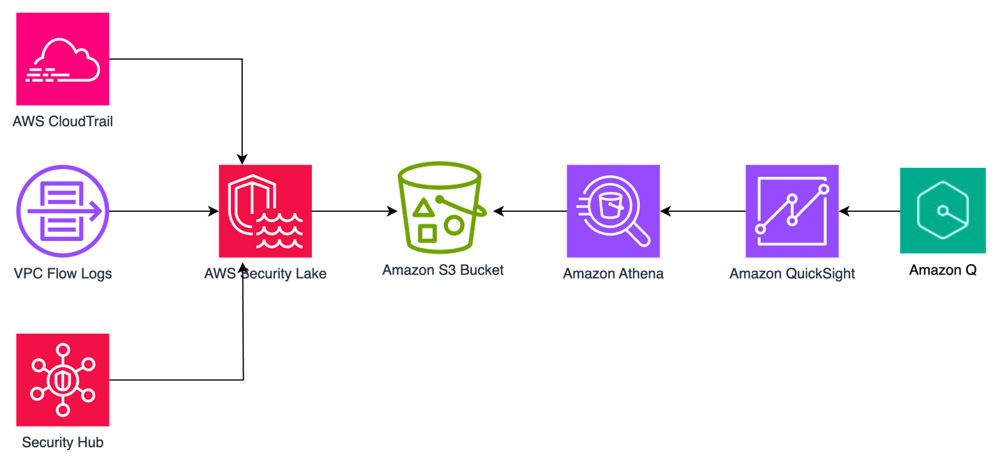
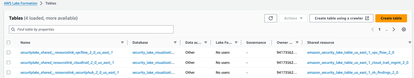


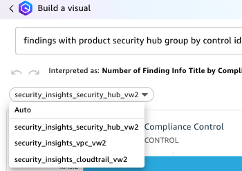


 Nitin Kumar is a Cloud Engineer (ETL) at Amazon Web Services, specialized in AWS Glue. With a decade of experience, he excels in aiding customers with their big data workloads, focusing on data processing and analytics. He is committed to helping customers overcome ETL challenges and develop scalable data processing and analytics pipelines on AWS. In his free time, he likes to watch movies and spend time with his family.
 Shubham Purwar is a Cloud Engineer (ETL) at AWS Bengaluru, specialized in AWS Glue and Amazon Athena. He is passionate about helping customers solve issues related to their ETL workload and implement scalable data processing and analytics pipelines on AWS. In his free time, Shubham loves to spend time with his family and travel around the world.
 Pramod Kumar P is a Solutions Architect at Amazon Web Services. With 19 years of technology experience and close to a decade of designing and architecting connectivity solutions (IoT) on AWS, he guides customers to build solutions with the right architectural tenets to meet their business outcomes.
 Madhavi Watve is a Senior Solutions Architect at Amazon Web Services, providing help and guidance to a broad range of customers to build highly secure, scalable, reliable, and cost-efficient applications on the cloud. She brings over 20 years of technology experience in software development and architecture and is data analytics specialist.
 Swathi S is a Technical Account Manager with the Enterprise Support team in Amazon Web Services. She has over 6 years of experience with AWS on big data technologies and specializes in analytics frameworks. She is passionate about helping AWS customers navigate the cloud space and enjoys assisting with design and optimization of analytics workloads on AWS.


 Kamen Sharlandjiev is a Sr. Big Data and ETL Solutions Architect, Amazon MWAA and AWS Glue ETL expert. He’s on a mission to make life easier for customers who are facing complex data integration and orchestration challenges. His secret weapon? Fully managed AWS services that can get the job done with minimal effort. Follow Kamen on
  Debaprasun Chakraborty is an AWS Solutions Architect, specializing in the analytics domain. He has around 20 years of software development and architecture experience. He is passionate about helping customers in cloud adoption, migration and strategy.


 apc-crr
 Deployment time: 307.88s
Stack ARN:
arn:aws:cloudformation:<aws_region>:<aws_account>:stack/apc-crr/<stack_id>
Deployment time: 307.88s
Stack ARN:
arn:aws:cloudformation:<aws_region>:<aws_account>:stack/apc-crr/<stack_id>


 Alexander Schueren is a Senior Specialist Solutions Architect at AWS, dedicated to modernizing legacy applications and building event-driven serverless solutions. With a focus on simplifying complexity and bringing clarity to technical challenges, Alexander is on a mission to empower developers with the tools they need for success. As the maintainer of the open-source project “Powertools for AWS Lambda (TypeScript),” he is committed to driving innovation in serverless technologies. In his free time, Alexander channels his creativity through street photography, capturing decisive moments in the urban landscape.

 Hemant Aggarwal is a senior Data Engineer at Kaplan India Pvt Ltd, helping in developing and managing ETL pipelines leveraging AWS and process/strategy development for the team.
 Naveen Kambhoji is a Senior Manager at Kaplan Inc. He works with Data Engineers at Kaplan for building data lakes using AWS Services. He is the facilitator for the entire migration process. His passion is building scalable distributed systems for efficiently managing data on cloud.Outside work, he enjoys travelling with his family and exploring new places.
 Jimy Matthews is an AWS Solutions Architect, with expertise in AI/ML tech. Jimy is based out of Boston and works with enterprise customers as they transform their business by adopting the cloud and helps them build efficient and sustainable solutions. He is passionate about his family, cars and Mixed martial arts.
 Sriharsh Adari is a Senior Solutions Architect at AWS, where he helps customers work backward from business outcomes to develop innovative solutions on AWS. Over the years, he has helped multiple customers on data platform transformations across industry verticals. His core area of expertise includes technology strategy, data analytics, and data science. In his spare time, he enjoys playing sports, binge-watching TV shows, and playing Tabla.
 Retina Satish is a Solutions Architect at AWS, bringing her expertise in data analytics and generative AI. She collaborates with customers to understand business challenges and architect innovative, data-driven solutions using cutting-edge technologies. She is dedicated to delivering secure, scalable, and cost-effective solutions that drive digital transformation.
 Jeetendra Vaidya is a Senior Solutions Architect at AWS, bringing his expertise to the realms of AI/ML, serverless, and data analytics domains. He is passionate about assisting customers in architecting secure, scalable, reliable, and cost-effective solutions.


 Vibhu Pareek is a Sr. Solutions Architect at AWS. Since 2016, he has guided customers in cloud adoption using well-architected, repeatable patterns. With his specialization in databases, data analytics, and AI, he thrives on transforming complex challenges into innovative solutions. Outside work, he enjoys short treks and sports like badminton, football, and swimming.
 Kamal Manchanda is a Senior Solutions Architect at AWS, specializing in building and designing data solutions with focus on lake house architectures, data governance, search platforms, log analytics solutions as well as generative AI solutions. In his spare time, Kamal loves to travel and spend time with family.
 Adesh Jaiswal is a Cloud Support Engineer in the Support Engineering team at Amazon Web Services. He specializes in Amazon OpenSearch Service. He provides guidance and technical assistance to customers thus enabling them to build scalable, highly available, and secure solutions in the AWS Cloud. In his free time, he enjoys watching movies, TV series, and of course, football.


 Fabrizio Napolitano is a Principal Specialist Solutions Architect for DB and Analytics. He has worked in the analytics space for the last 20 years, and has recently and quite by surprise become a Hockey Dad after moving to Canada.
 Lakshmi Nair is a Senior Analytics Specialist Solutions Architect at AWS. She specializes in designing advanced analytics systems across industries. She focuses on crafting cloud-based data platforms, enabling real-time streaming, big data processing, and robust data governance.
 Varsha Velagapudi is a Senior Technical Product Manager with Amazon DataZone at AWS. She focuses on improving data discovery and curation required for data analytics. She is passionate about simplifying customers’ AI/ML and analytics journey to help them succeed in their day-to-day tasks. Outside of work, she enjoys nature and outdoor activities, reading, and traveling.


 Vivek Mittal is a Solution Architect at Amazon Web Services. He is passionate about serverless and machine learning technologies. Vivek takes great joy in assisting customers with building innovative solutions on the AWS cloud platform.
 John Cherian is Senior Solutions Architect at Amazon Web Services helps customers with strategy and architecture for building solutions on AWS.
 Uma Ramadoss is a Principal Solutions Architect at Amazon Web Services, focused on the Serverless and Integration Services. She is responsible for helping customers design and operate event-driven cloud-native applications using services like Lambda, API Gateway, EventBridge, Step Functions, and SQS. Uma has a hands on experience leading enterprise-scale serverless delivery projects and possesses strong working knowledge of event-driven, micro service and cloud architecture.


 Subham Rakshit is a Senior Streaming Solutions Architect for Analytics at AWS based in the UK. He works with customers to design and build streaming architectures so they can get value from analyzing their streaming data. His two little daughters keep him occupied most of the time outside work, and he loves solving jigsaw puzzles with them. Connect with him on