Tag Archives: Advanced (300)

Reference guide for building a self-service analytics solution with Amazon SageMaker

Post Syndicated from Navnit Shukla original https://aws.amazon.com/blogs/big-data/reference-guide-for-building-a-self-service-analytics-solution-with-amazon-sagemaker/

Organizations today face a critical challenge with fragmented data scattered across multiple silos, including data lakes, warehouses, SaaS applications, and legacy systems. This disconnect prevents businesses from gaining a holistic view of their customers, optimizing operations, and making real-time data-driven decisions. To stay competitive, companies are turning to self-service analytics, enabling both business and technical users to quickly access, explore, and analyze data without dependency on IT teams.

However, implementing self-service analytics comes with significant challenges. Organizations must address integrating data from diverse sources for seamless access, creating business and technical catalogs to improve data discoverability, enabling data lineage and quality to build trust and reliability, implementing fine-grained access controls to ensure security and compliance, providing role-specific tools for data engineers, analysts, and artificial intelligence (AI)/machine learning (ML) teams, and establishing governance frameworks to enforce policies and regulatory requirements.

In this post, we show how to use Amazon SageMaker Catalog to publish data from multiple sources, including Amazon S3, Amazon Redshift, and Snowflake. This approach enables self-service access while ensuring robust data governance and metadata management. By centralizing metadata, users can improve data discoverability, lineage tracking, and compliance while empowering analysts, data engineers, and data scientists to derive AI-driven insights efficiently and securely. We use a sample retail use case to demonstrate the solution, making it easier to understand how these capabilities can be applied to real-world scenarios.

Amazon SageMaker: Enabling self-service analytics

Amazon SageMaker brings together AWS AI/ML and analytics capabilities, delivering an integrated experience for analytics and AI with unified data access, enabling teams to:

  • Discover and access data stored across Amazon S3, Amazon Redshift, and other third-party sources through the Lakehouse architecture.
  • Perform complete AI and analytics workflows using familiar AWS services for data analysis, processing, model training, and generative AI app development.
  • Use Amazon Q Developer, an advanced generative AI assistant to accelerate software development.
  • Ensure enterprise-grade security with built-in governance, fine-grained access controls, and secure artifact sharing with Amazon SageMaker Catalog.
  • Collaborate in shared projects, allowing teams to work together efficiently while maintaining compliance and governance.

Retail use case overview

In our example, a retail organization operates across multiple business units, each storing data in different platforms, creating challenges in data access, consistency, and governance.


Figure 1: High-level architecture of our retail use case showing data flow across multiple systems

Our retail organization faces data fragmentation across its business units:

  • The Wholesale Sales business unit stores its data in Amazon S3.
  • The Store Sales business unit maintains its transactional data in Amazon Redshift.
  • Online Sales Data is stored in Snowflake.

These disparate data sources result in data silos, inconsistent schemas, duplication, and missing values, making it difficult for analysts and AI-driven solutions to derive meaningful insights.

Data model

The following Entity-Relationship (ER) Diagram represents the dataset structure and relationships between different entities in Wholesale, Retail, and Online Sales Data:


Figure 2: Entity-Relationship Diagram showing the relationships between different data entities

Key entities in our data model

Our sample dataset models a multi-channel retail business with interconnected entities representing products, sales channels, customers, and locations.

  1. PRODUCTS is a central entity that links to WHOLESALE_SALES, RETAIL_SALES, and ONLINE_SALES, representing product transactions across different sales channels.
  2. WHOLESALE_SALES records bulk transactions where WAREHOUSES distribute products to retailers. Each sale is associated with a PRODUCT and a WAREHOUSE.
  3. RETAIL_SALES captures individual purchases made in physical STORES. Each transaction involves a PRODUCT and a STORE, along with details like quantity sold, discount applied, and revenue.
  4. ONLINE_SALES tracks e-commerce transactions where customers buy products online. Each record links to a CUSTOMER and a PRODUCT, along with details like quantity, price, and shipping information.
  5. CUSTOMERS represent buyers in the system and are linked to ONLINE_SALES (for purchasing) and CUSTOMER_REVIEWS (for leaving product reviews).
  6. CUSTOMER_REVIEWS stores feedback provided by customers for products they purchased online. Each review is linked to an ONLINE_SALES order, a CUSTOMER, and a PRODUCT.
  7. STORES represent physical retail locations where products are sold. They are associated with RETAIL_SALES, indicating that products are purchased in-store.
  8. WAREHOUSES are responsible for stocking and distributing products through WHOLESALE_SALES transactions. They manage stock levels and facilitate bulk sales to retailers.

Data distribution across systems

To simulate a real-world enterprise scenario, our data is distributed across multiple systems and AWS accounts as follows:

Accounts Location Tables
Wholesale Amazon S3 WHOLESALE_SALES, PRODUCT, WAREHOUSE
Store Amazon Redshift RETAIL_SALES, STORE, PRODUCT
Online Sales Snowflake ONLINE_SALES, CUSTOMER, CUSTOMER_REVIEWS, PRODUCT

Assumptions

We are making the following assumptions for this implementation.

Building the SageMaker Catalog

In this section, we walk through the process of creating the SageMaker Catalog from multiple sources using Amazon SageMaker Unified Studio.

Step 1: Setting up your SageMaker Unified Studio environment

Before we begin building our data catalog, we cover some terminology for SageMaker Unified Studio.

Domain: A domain in Amazon SageMaker Unified Studio is a logical boundary that serves as the primary container for all your data assets, users, and resources, allowing efficient data organization and management.
Domain Units: Domain units are subcomponents within a domain that help organize related projects and resources together, enabling hierarchical structuring of your data management activities.
Blueprint: A blueprint in Amazon SageMaker Unified Studio is a template that defines standardized configurations for projects, including what resources are provisioned, and what tools, and parameters are applied.
Project Profile: A project profile is a collection of blueprints which are configurations used to create projects. A project profile can define if a particular blueprint is enabled during the creation of the project, or available later for the project users to enable on-demand.
Project: A project in Amazon SageMaker Unified Studio is a boundary within a domain where users can collaborate with others to work on a business use case. In projects, users can create and share data and resources.

Now, we can set up our Amazon SageMaker Unified Studio environment.

Create a SageMaker domain

  1. Open the Amazon SageMaker management console in the Centralized Processing account and use the region selector in the top navigation bar to choose the appropriate AWS Region.
  2. Choose Create a Unified Studio domain.
  3. Choose Quick setup as explained in Create an Amazon SageMaker Unified Studio domain – quick setup.
  4. For Create IAM Identity Center User, search for SSO users through email addresses.
    If there is no Amazon Identity Access Manager (IAM) Identity Center instance, a prompt appears to enter your name after your email address. This creates a new local IAM Identity Center instance.
  5. Choose Create domain.

Log in to SageMaker Unified Studio

Now that we have created a new SageMaker Unified Studio domain, complete the following steps to visit the Amazon SageMaker Unified Studio.

  1. On the SageMaker platform console, open the details page of your domain.
  2. Choose the link for Amazon SageMaker Unified Studio URL.
  3. Log in with your SSO credentials.

Now you signed in to the SageMaker Unified Studio.

Create a project

The next step is to create a project. Complete the following steps:

  1. On the SageMaker Unified Studio, choose Select a project on the top menu, and choose Create project.
  2. For Project name, enter a name (such as AnyCompanyDataPlatform).
  3. For Project profile, choose All capabilities.
  4. Choose Continue.
  5. Review the input and choose Create project. This project serves as a collaborative workspace for our data integration efforts.

Wait for the project to be created. Project creation can take about five minutes. Then The SageMaker Unified Studio console goes to the project’s home page.

Step 2: Connecting to data sources

Now, we connect to our various data sources to bring them into our data catalog.

Importing existing AWS Glue Data Catalog (Wholesale Sales Data)

We first import the wholesale sales data from Amazon S3 in the Wholesale account into Amazon SageMaker Unified Studio.

Set up cross-account access

  1. Log in to Centralized Processing account and create a Glue Crawler role named glue-cross-s3-access with the AWSGlueServiceRole and cross account S3 access policy for Wholesale account.
    Sample cross account S3 access policy:

    { "Version": "2012-10-17", "Statement": [ { "Effect": "Allow", "Action": [ "s3:GetObject" ], "Resource": [ "arn:aws:s3:::<wholesale-account-bucket>/*" ] } ]}

  2. Log in to the Wholesale account and create an S3 bucket policy that grants access to S3 data files for the previously created glue-cross-s3-access role of the Centralized Processing account.
  3. Log in to the Centralized Processing account and create a database named anycompanydatacatlog from the AWS Glue.
  4. Grant permissions to the glue-cross-s3-access role for the anycompanydatacatalog database in AWS Lake Formation.
  5. Run the Glue Crawler using the glue-cross-s3-access role to scan the S3 bucket in the Wholesale account. For more information, refer to the tutorial explaining how to catalog S3 data using the Glue crawler.
  6. Verify the anycompanydatacatlog database and its corresponding tables.

Configure the Glue data catalog assets

  1. Download the provided scripts from the Bring Your Own Glue Data Catalog Assets repository.
  2. Copy the Amazon SageMaker Unified Studio project role ARN from project overview section.
  3. Add the same Amazon SageMaker Unified Studio project role as LakeFormation Data Lake Administrator.

Import the assets into Amazon SageMaker Unified Studio

  1. Open AWS CloudShell in the Centralized Processing account console.
  2. Upload the previously downloaded bring_your_own_gdc_assets.py file to AWS CloudShell.
  3. Run the import script in AWS CloudShell with following parameters.
    1. project-role-arn: Enter the project role ARN of SageMaker Unified Studio.
    2. database-name: Enter the database name of Glue Catalog (such as anycompanydatacatalog).
    3. region: Enter the region of SageMaker Unified Studio (such as us-east-1).
    python3 bring_your_own_gdc_assets.py \
    --project-role-arn <Project role ARN> \
    --database-name <Glue Database name to import> \
    --region <region-code>

Verify the imported wholesale sales data

  1. In the Centralized Processing account, go to the SageMaker Unified Studio console, choose your project.
  2. Choose Data in the navigation pane.
  3. Confirm that the wholesale_db database and its tables (WHOLESALE_SALES, PRODUCT, WAREHOUSE) are now available under anycompanydatacatalog.

Connecting to Amazon Redshift (Stores sales data)

In this step, we bring stores sales data from Amazon Redshift in the Store account into Amazon SageMaker Unified Studio.

Set up cross-account access

  1. Login to the Store account, create a virtual private cloud (VPC) peering connection between the Store account and the Centralized Processing account, which hosts the Amazon SageMaker Unified Studio, and configure route tables following the documentation.
  2. Update your Redshift VPC security group’s rule to include the Centralized Processing account’s IPv4 CIDR range, enabling network connectivity and allowing incoming requests from the Centralized Processing account to access the Store account resources.

Create a federated connection for Amazon Redshift

  1. In the Centralized Processing account, go to the SageMaker Unified Studio console, choose your project.
  2. Choose Data in the navigation pane.
  3. In the data explorer, choose the plus sign to add a data source.
  4. Under add a data source, choose Add connection, then choose Amazon Redshift.
  5. Enter the following parameters in the connection details, and choose Add data.
    1. Name: Enter the connection name (such as anycompanyredshift).
    2. Host: Enter the Amazon Redshift cluster endpoint.
    3. Port: Enter the port number (Amazon Redshift uses 5439 as the default port).
    4. Database: Enter the database name
    5. Authentication: Choose either the database username and password credentials or AWS Secrets Manager. We recommend using AWS Secrets Manager.

After the connection is established, the federated catalog is created, as shown in the following screenshot. This catalog uses the AWS Glue connection to Amazon Redshift. The databases, tables, and views are automatically cataloged in the catalog section and registered with Lake Formation.

Verify the stores sales data

  1. Visit the Catalog section in SageMaker Unified Studio.
  2. Confirm that the retails sales public database and its tables (RETAIL_SALES, STORE, PRODUCT) are now available.

Connecting to Snowflake (online sales data)

In this step, we bring online sales data from Snowflake into Amazon SageMaker Unified Studio.

Create a federated connection for Snowflake

  1. In the Centralized Processing account, go to the SageMaker Unified Studio console, choose your project.
  2. Choose Data in the Navigation Pane.
  3. In the data explorer, choose the plus sign (+) to add a data source.
  4. Under Add a data source, choose Add connection, then choose Snowflake.
  5. Enter the following parameters in the connection details, and choose Add data.
    1. Name: Enter the connection name (such as anycompanysnowflake).
    2. Host: Enter the Snowflake cluster endpoint.
    3. Port: Enter the port number (Snowflake uses 443 as the default port).
    4. Database: Enter the database name (such as anycompanyonlinesales).
    5. Warehouse: Enter the warehouse name (such as COMPUTE_WH).
    6. Authentication: Choose either the database username and password credentials or Secrets Manager.

After the connection is established, the federated catalog is created for Snowflake. This catalog uses the AWS Glue connection to Snowflake. The databases, tables, and views are automatically cataloged in the Data Catalog and registered with Lake Formation.

Verify the online sales data

  1. Go to the Catalog section in SageMaker Unified Studio.
  2. Confirm that the Online sales public database and its tables (CUSTOMER_REVIEWS, CUSTOMER, ONLINE_SALES, PRODUCT) are now available.

Step 3: Analyze the data together

Once all the data from different data sources has been cataloged, we can analyze it using Amazon Athena query engine from Amazon SageMaker Unified Studio.

  1. In the Centralized Processing account, go to the SageMaker Unified Studio console, choose your project.
  2. Choose Query Editor from the Build section.
  3. Select Athena (Lakehouse) as a connection.
  4. Run queries joining multiple data source catalogs to analyze the data.

Example: What is the total revenue generated from wholesale, retail, and online sales for each product?

SELECT p.product_id, p.product_name, COALESCE(SUM(ws.total_revenue), 0) AS wholesale_revenue, COALESCE(SUM(rs.revenue), 0) AS retail_revenue, COALESCE(SUM(os.sale_price * os.quantity_sold), 0) AS online_revenue, (COALESCE(SUM(ws.total_revenue), 0) + COALESCE(SUM(rs.revenue), 0) + COALESCE(SUM(os.sale_price * os.quantity_sold), 0)) AS total_revenueFROM awsdatacatalog.anycompanydatacatalog.anycompany_products pLEFT JOIN awsdatacatalog.anycompanydatacatalog.anycompany_wholessale_sales ws ON p.product_id = ws.product_idLEFT JOIN anycompanyredshift.public.retail_sales rs ON p.product_id = rs.product_idLEFT JOIN anycompanysnowflake.sales.online_sales os ON p.product_id = os.product_idGROUP BY p.product_id, p.product_nameORDER BY total_revenue DESC;

Similarly, users can derive valuable business insights by querying across catalogs for different analytical questions.

Step 4: Creating a Business Glossary

A business glossary helps standardize terminology across the organization and makes data more discoverable. Now we create a business glossary for Wholesale data PRODUCT.

  1. In the Navigation Pane, choose Data and select Publish to Catalog for the Wholesale data PRODUCT table.
  2. Choose Assets and choose the products table.
  3. Create a Glossary named ‘Product‘ and a Term named ‘Sales‘ from Metadata entities.
  4. Choose Generate Descriptions to automatically generate summary of your data using AI. Choose Add Terms.
  5. Choose ACCEPT ALL for Automated Metadata Generation.
  6. Choose sales term and choose Add Terms.
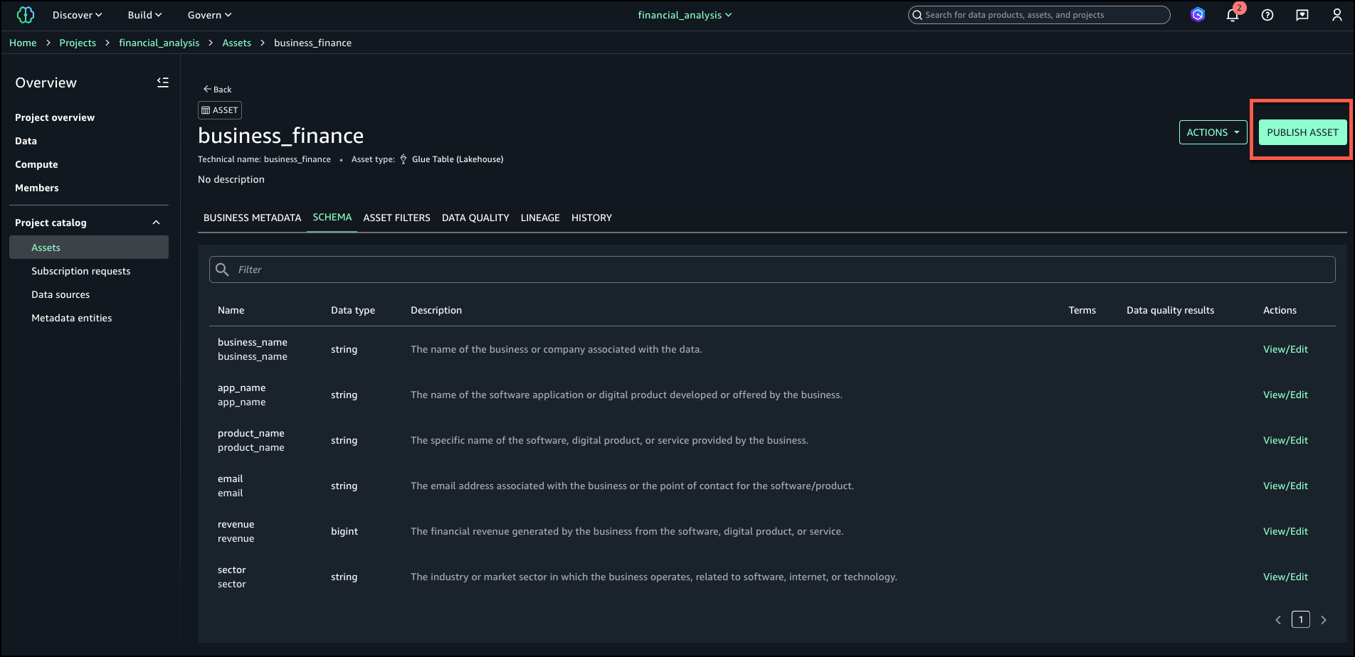
  7. Choose Publish Asset.
  8. Choose Assets and then Published. We can now see a published asset that is searchable and available to request for subscription.

Similarly, you can create business glossaries for other data products by following the above steps.

Step 5: Setting up access controls

To ensure proper governance, set up fine-grained access controls.

  1. For each user create a new single sign-on (SSO) user
  2. Create the following roles and permissions to attach to the SSO user:
Role Description Access Level
Data Steward Manages the data catalog and glossary Full access to catalog and glossary
ETL Developer Develops data integration pipelines Read/write access to data sources and AWS Glue
Data Analyst Analyzes sales data Read-only access to all sales data
AI Engineer Builds forecasting models Read access to sales data, full access to SageMaker features

Benefits of SageMaker Catalog

By implementing a self-service business data catalog using Amazon SageMaker Unified Studio, our retail organization achieves several key benefits:

  1. Unified data access: Users can discover and access data from Amazon S3, Redshift, and Snowflake through a single interface.
  2. Standardized metadata: The business glossary ensures consistent terminology across the organization.
  3. Governance and compliance: Fine-grained access controls ensure that users only access data they’re authorized to see.
  4. Collaboration: Different teams (ETL developers, data analysts, AI engineers) can collaborate within a shared environment.

Cleanup

To avoid incurring additional charges associated with the resources created in this post, make sure to delete the following items from your AWS account:

  1. The Amazon SageMaker domain.
  2. The Amazon S3 bucket associated with the Amazon SageMaker domain.
  3. Cross-account resources such as VPC peering connections, security groups, route tables, AWS Glue Data Catalog entries, and associated IAM roles4. The tables and databases created in this post.

Conclusion

In this post, we demonstrated how Amazon SageMaker Catalog provides a unified approach to data publishing, discovery, and analysis across multiple data sources. Using a retail scenario, we showed how to import data from Amazon S3, Amazon Redshift, and Snowflake into Amazon SageMaker Unified Studio, and how to join and analyze data from these multiple sources to derive meaningful business insights.

By centralizing metadata and enabling cross-source data integration, data is easily discovered across an organization, multiple data sources can be joined and comprehensive analysis performed without moving or duplicating data. This unified approach maintains strong governance with consistent policies, security, and compliance across all data sources while enabling self-service analytics that reduce time-to-insight for your teams.

To learn more about Amazon SageMaker and how to get started, refer to the Amazon SageMaker User Guide.

About the authors

Navnit Shukla

Navnit Shukla

Navnit is an AWS Specialist Solutions Architect at AWS with a focus on Data and AI. He possesses a strong enthusiasm for assisting clients in discovering valuable insights from their data. Through his expertise, he constructs innovative solutions that empower businesses to arrive at informed, data-driven choices. Notably, he is the lead author of Data Wrangling on AWS and AI-Ready Data Blueprints with O’Reilly.

Ayan Majumder

Ayan Majumder

Ayan is an Analytics Specialist Solutions Architect at AWS. His expertise lies in designing robust, scalable, and efficient cloud solutions for customers. Beyond his professional life, he derives joy from traveling, photography, and outdoor activities.

Karan Edikala

Karan Edikala

Karan is a Solutions Architect at AWS who helps small businesses unlock value through cloud technology. He specializes in Generative AI, guiding customers to build AI-powered solutions that deliver measurable ROI and optimize their data strategies on AWS. Outside of work, Karan enjoys piloting general aviation aircraft, golfing, and skiing.

Introducing the Apache Spark troubleshooting agent for Amazon EMR and AWS Glue

Post Syndicated from Jake Zych original https://aws.amazon.com/blogs/big-data/introducing-the-apache-spark-troubleshooting-agent-for-amazon-emr-and-aws-glue/

The newly launched Apache Spark troubleshooting agent can eliminate hours of manual investigation for data engineers and scientists working with Amazon EMR or AWS Glue. Instead of navigating multiple consoles, sifting through extensive log files, and manually analyzing performance metrics, you can now diagnose Spark failures using simple natural language prompts. The agent automatically analyzes your workloads and delivers actionable recommendations. transforming a time-consuming troubleshooting process into a streamlined, efficient experience.

In this post, we show you how the Apache Spark troubleshooting agent helps analyze Apache Spark issues by providing detailed root causes and actionable recommendations. You’ll learn how to streamline your troubleshooting workflow by integrating this agent with your existing monitoring solutions across Amazon EMR and AWS Glue.

Apache Spark powers critical ETL pipelines, real-time analytics, and machine learning workloads across thousands of organizations. However, building and maintaining Spark applications remains an iterative process where developers spend significant time troubleshooting. Spark application developers encounter operational challenges due to a few different reasons:

  • Complex connectivity and configuration options to a variety of resources with Spark – Although this makes Spark a popular data processing platform, it often makes it challenging to find the root cause of inefficiencies or failures when Spark configurations aren’t optimally or correctly configured.
  • Spark’s in-memory processing model and distributed partitioning of datasets across its workers – Although good for parallelism, this often makes it difficult for users to identify inefficiencies. This results in slow application execution or root cause of failures caused by resource exhaustion issues such as out of memory and disk exceptions.
  • Lazy evaluation of Spark transformations – Although lazy evaluation optimizes performance, it makes it challenging to accurately and quickly identify the application code and logic that caused the failure from the distributed logs and metrics emitted from different executors.

Apache Spark troubleshooting agent architecture

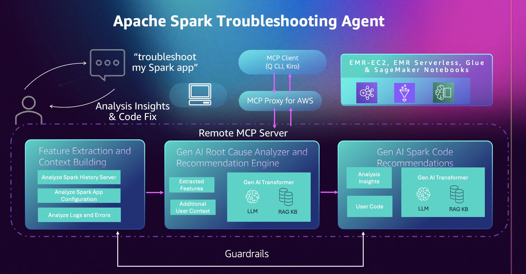
This section describes the components of the troubleshooting agent and how they connect to your development environment. The troubleshooting agent provides a single conversational entry point for your Spark applications across Amazon EMR, AWS Glue, and Amazon SageMaker Notebooks. Instead of navigating different consoles, APIs, and log locations for each service, you interact with one Model Context Protocol (MCP) server through natural language using any MCP-compatible AI assistant of your choice, including custom agents you develop using frameworks such as Strands Agents.

Operating as a fully managed cloud-hosted MCP server, the agent removes the need to maintain local servers while keeping your data and code isolated and secure in a single-tenant system design. Operations are read-only and backed by AWS Identity and Access Management (IAM) permissions; the agent only has access to resources and actions your IAM role grants. Additionally, tool calls are automatically logged to AWS CloudTrail, providing complete auditability and compliance visibility. This combination of managed infrastructure, granular IAM controls, and CloudTrail integration confirms your Spark diagnostic workflows remain secure, compliant, and fully auditable.

The agent builds on years of AWS expertise running millions of Spark applications at scale. It automatically analyzes Spark History Server data, distributed executor logs, configuration patterns, and error stack traces and extracts relevant features and signals to surface insights that would otherwise require manual correlation across multiple data sources and deep understanding of Spark and service internals.

Getting started 

Complete the following steps to get started with the Apache Spark troubleshooting agent.

Prerequisites

Verify you meet or have completed the following prerequisites.

System requirements:

  • Python 3.10 or higher
  • Install the uv package manager. For instructions, see installing uv.
  • AWS Command Line Interface (AWS CLI) (version 2.30.0 or later) installed and configured with appropriate credentials.

IAM permissions: Your AWS IAM profile needs permissions to invoke the MCP server and access your Spark workload resources. The AWS CloudFormation template in the setup documentation creates an IAM role with the required permissions. You can also manually add the required IAM permissions.

Set up using AWS CloudFormation

First, deploy the AWS CloudFormation template provided in the setup documentation. This template automatically creates the IAM roles with the permissions required to invoke the MCP server.

  1. Deploy the template within the same AWS Region you run your workloads in. For this post, we’ll use us-east-1.
  2. From the AWS CloudFormation Outputs tab, copy and execute the environment variable command:
    export SMUS_MCP_REGION=us-east-1 && export IAM_ROLE=arn:aws:iam::111122223333:role/spark-troubleshooting-role-xxxxxx

  3. Configure your AWS CLI profile:
    aws configure set profile.smus-mcp-profile.role_arn ${IAM_ROLE}
    aws configure set profile.smus-mcp-profile.source_profile default
    aws configure set profile.smus-mcp-profile.region ${SMUS_MCP_REGION}

Set up using Kiro CLI

You can use Kiro CLI to interact with the Apache Spark troubleshooting agent directly from your terminal.

Installation and configuration:

  1. Install Kiro CLI.
  2. Add both MCP servers, using the environment variables from the previous Set up using AWS CloudFormation section:
    # Add Spark Troubleshooting MCP Server
    kiro-cli-chat mcp add \
        --name "sagemaker-unified-studio-mcp-troubleshooting" \
        --command "uvx" \
        --args "[\"mcp-proxy-for-aws@latest\",\"https://sagemaker-unified-studio-mcp.${SMUS_MCP_REGION}.api.aws/spark-troubleshooting/mcp\", \"--service\", \"sagemaker-unified-studio-mcp\", \"--profile\", \"smus-mcp-profile\", \"--region\", \"${SMUS_MCP_REGION}\", \"--read-timeout\", \"180\"]" \
        --timeout 180000 \
        --scope global
    # Add Spark Code Recommendation MCP Server
    kiro-cli-chat mcp add \
        --name "sagemaker-unified-studio-mcp-code-rec" \
        --command "uvx" \
        --args "[\"mcp-proxy-for-aws@latest\",\"https://sagemaker-unified-studio-mcp.${SMUS_MCP_REGION}.api.aws/spark-code-recommendation/mcp\", \"--service\", \"sagemaker-unified-studio-mcp\", \"--profile\", \"smus-mcp-profile\", \"--region\", \"${SMUS_MCP_REGION}\", \"--read-timeout\", \"180\"]" \
        --timeout 180000 \
        --scope global

  3. Verify your setup by running the /tools command in Kiro CLI to see the available Apache Spark troubleshooting tools.

Set up using Kiro IDE

Kiro IDE provides a visual development environment with integrated AI assistance for interacting with the Apache Spark troubleshooting agent.

Installation and configuration:

  1. Install Kiro IDE.
  2. MCP configuration is shared across Kiro CLI and Kiro IDE. Open the command palette using Ctrl + Shift + P (Windows / Linux) or Cmd + Shift + P (macOS) and Search for Kiro: Open MCP Config
  3. Verify the contents of your mcp.json match the Set up using Kiro CLI section.

Using the troubleshooting agent

Next, we provide 3 reference architectures for solutions to use the troubleshooting agent in your existing workflows with ease. We also provide the reference code and AWS CloudFormation templates for these architectures in the Amazon EMR Utilities GitHub repository.

Solution 1 – Conversational troubleshooting: Troubleshooting failed Apache Spark applications with Kiro CLI

When Spark applications fail across your data platform, your debugging approach would typically involve navigating different consoles for Amazon EMR, Amazon EC2, Amazon EMR Serverless, and AWS Glue, manually reviewing Spark History Server logs, checking error stack traces, analyzing resource usage patterns, then correlating this information to find the root cause and fix. The Apache Spark troubleshooting agent automates this entire workflow through natural language, providing a unified troubleshooting experience across the three platforms. Simply describe your failed applications, for example:

# Amazon EMR-EC2
Debug my failing Amazon EMR-EC2 step. Cluster id: 'j-xxxxx' Step id: 's-xxxxx'
# Amazon EMR Serverless
Troubleshoot my Amazon EMR Serverless job. Application id: 'xxxxx' Job run id: 'xxxxx'
# AWS Glue
Analyze my failed AWS Glue job. Job name: 'my-etl-job' Job run id: 'jr_xxxxx'

The agent automatically extracts Spark event logs and metrics, analyzes the error patterns, and provides a clear root cause explanation along with recommendations, all through the same conversational interface. The following video demonstrates the complete troubleshooting workflow across Amazon EMR-EC2, Amazon EMR Serverless, and AWS Glue using Kiro CLI:

Solution 2 – Agent-driven notifications: Integrate the Apache Spark troubleshooting agent into a monitoring workflow 

In addition to troubleshooting from the command line, the troubleshooting agent can plug into your monitoring infrastructure to provide improved failure notifications.

Production data pipelines require immediate visibility when failures occur. Traditional monitoring systems can alert you when a Spark job fails, but diagnosing the root cause still requires manual investigation and an analysis of what went wrong before remediation can begin.

With the Apache Spark troubleshooting agent, you can integrate it into your existing monitoring workflows to receive root causes and recommendations as soon as you receive a failure notification. Here, we demonstrate two integration patterns that result in automatic root cause analysis within your existing workflows.

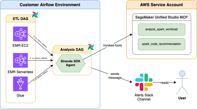
Apache Airflow Integration

This first integration pattern uses Apache Airflow callbacks to automatically trigger troubleshooting when Spark job operators fail.

When any Amazon EMR, Amazon EC2, Amazon EMR Serverless, or AWS Glue job operator fails in an Apache Airflow DAG,

  1. A callback invokes the Spark troubleshooting agent within a separate DAG.
  2. The Spark troubleshooting agent analyzes the issue, establishes the root cause, and identifies code fix recommendations.
  3. The Spark troubleshooting agent sends a comprehensive diagnostic report to a configured Slack channel.

The solution is available in the Amazon EMR Utilities GitHub repository (documentation) for immediate integration into your existing Apache Airflow deployments with a 1-line change to your Airflow DAGs. The following video demonstrates this integration:

Amazon EventBridge integration

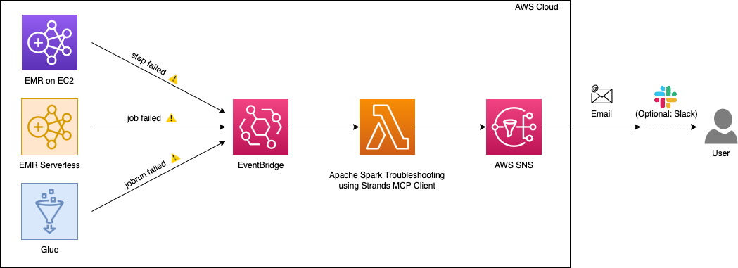
For event-driven architectures, this second pattern uses Amazon EventBridge to automatically invoke the troubleshooting agent when Spark jobs fail across your AWS environment.

This integration uses an AWS Lambda function that interacts with the Apache Spark troubleshooting agent through the Strands MCP Client.

When Amazon EventBridge detects failures from Amazon EMR-EC2 steps, Amazon EMR Serverless job runs, or AWS Glue job runs, it triggers the AWS Lambda function which:

  1. Uses the Apache Spark troubleshooting agent to analyze the failure
  2. Identifies the root cause and generates code fix recommendations
  3. Constructs a comprehensive analysis summary
  4. Sends the summary to Amazon SNS
  5. Delivers the analysis to your configured destinations (email, Slack, or other SNS subscribers)

This serverless approach provides centralized failure analysis across all your Spark platforms without requiring changes to individual pipelines. The following video demonstrates this integration:

A reference implementation of this solution is available in the Amazon EMR Utilities GitHub repository (documentation).

Solution 3 – Intelligent Dashboards: Use the Apache Spark troubleshooting agent with Kiro IDE to visualize account level application failures: what failed, why failed and how to fix

Understanding the health of your Spark workloads across multiple platforms requires consolidating data from Amazon EMR (both EC2 and Serverless) and AWS Glue. Teams typically build custom monitoring solutions by writing scripts to query multiple APIs, aggregate metrics, and generate reports which can be time consuming and require active maintenance.

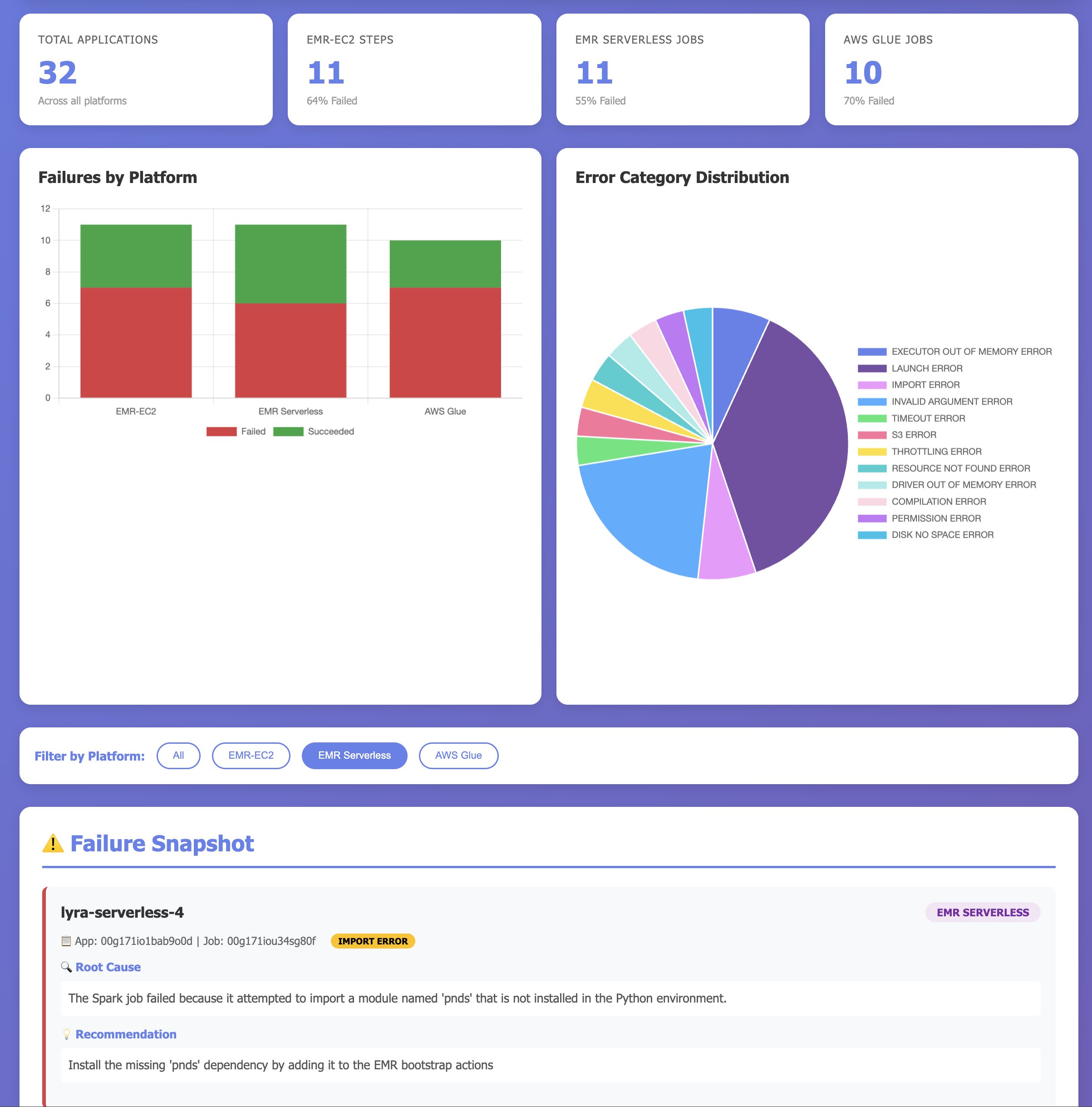
With Kiro IDE and the Apache Spark troubleshooting agent, you can build comprehensive monitoring dashboards conversationally. Instead of writing custom code to aggregate workload metrics, you can describe what you want to track, and the agent generates a complete dashboard showing overall performance metrics, error category distributions for failures, success rates across platforms, and critical failures requiring immediate attention. Unlike traditional dashboards that only show traditional KPIs and metrics on what application failed, this dashboard uses the Spark troubleshooting agent to provide insights to users on why the applications failed, and how they can be fixed. The following video demonstrates building a multi-platform monitoring dashboard using Kiro IDE:

The prompt used within the demo:

Build comprehensive monitoring dashboard for all of my Amazon EMR-EC2 steps, Amazon EMR Serverless jobs, and AWS Glue jobs for the last 30 days. Region: us-east-2. 
Execution Plan:
1. List all of my Spark applications across these services from the last 30 days. You can store any intermediate results in files in this folder as .json, but VALIDATE outputs before moving onto the next step. It's imperative to check the results before considering this done. You can write python script helpers to achieve this. Handle throttling and other exceptions gracefully. Make sure you cover all platforms: Amazon EMR-EC2, Amazon EMR Serverless, and AWS Glue.
2. Use the spark-troubleshooting-mcp to gather failure insights for each of my applications. Save this as .json as well. 
3. Then, use this information to help build the dashboard as HTML. Name the file dashboard.html.
Dashboard Requirements:
- Information from all of my Amazon EMR-EC2, Amazon EMR Serverless, and AWS Glue applications should be present
- overall success rates across platforms
- error category distributions for failures as a pie chart
- failures from last 30 days requiring attention with root causes and recommendations. Include error category and show the root causes and recommendations as they are returned by the spark-troubleshooting-mcp
- configuration comparisons per each platform. Configuration includes versions, worker types / DPUs, etc.

Clean up

To avoid incurring future AWS charges, delete the resources you created during this walkthrough:

  • Delete the AWS CloudFormation stack.
  • If you created an Amazon EventBridge rule for integration, delete those resources.

Conclusion

In this post, we demonstrated how the Apache Spark troubleshooting agent transforms hours of manual investigation into natural language conversations, significantly reducing troubleshooting time from hours to minutes and making Spark expertise accessible to all. By integrating natural language diagnostics into your existing development tools—whether Kiro CLI, Kiro IDE, or other MCP-compatible AI assistants—your teams can focus on building innovative applications instead of debugging failures.


Special thanks

A special thanks to everyone who contributed from engineering and science to the launch of the Spark troubleshooting agent and the remote MCP service: Tony Rusignuolo, Anshi Shrivastava, Martin Ma, Hirva Patel, Pranjal Srivastava, Weijing Cai, Rupak Ravi, Bo Li, Vaibhav Naik, XiaoRun Yu, Tina Shao, Pramod Chunduri, Ray Liu, Yueying Cui, Savio Dsouza, Kinshuk Pahare, Tim Kraska, Santosh Chandrachood, Paul Meighan and Rick Sears.

A special thanks to all of our partners who contributed to the launch of the Spark troubleshooting agent and the remote MCP service: Karthik Prabhakar, Suthan Phillips, Basheer Sheriff, Kamen Sharlandjiev, Archana Inapudi, Vara Bonthu, McCall Peltier, Lydia Kautsky, Larry Weber, Jason Berkovitz, Jordan Vaughn, Amar Wakharkar, Subramanya Vajiraya, Boyko Radulov and Ishan Gaur.

About the authors

Jake Zych

Jake is a Software Development Engineer at AWS Analytics. He has a deep interest in distributed systems and generative AI. In his spare time, Jake likes to create video content and play board games.

Maheedhar Reddy Chappidi

Maheedhar is a Senior Software Development Engineer at AWS Analytics. He is passionate about building fault-tolerant, reliable distributed systems at scale and generative AI applications for Data Integration. Outside of work, Maheedhar enjoys listening to podcasts and playing with his two-year-old child.

Vishal Kajjam

Vishal is a Senior Software Development Engineer at AWS Analytics. He is passionate about distributed computing and using ML/AI for designing and building end-to-end solutions to address customers’ data integration needs. In his spare time, he enjoys spending time with family and friends.

Arunav Gupta

Arunav is a Software Development Engineer at AWS Analytics. He is passionate about generative AI and orchestration and their uses in improving developer quality-of-life. In his free time, Arunav enjoys competing in a karting league and exploring new coffee shops in New York.

Wei Tang

Wei is a Software Development Engineer at AWS Analytics. She is strong developer with deep interests in solving recurring customer problems with distributed systems and AI/ML.

Andrew Kim

Andrew is a Software Development Engineer at AWS Analytics, with a deep passion for distributed systems architecture and AI-driven solutions, specializing in intelligent data integration workflows and cutting-edge feature development on Apache Spark. Andrew focuses on re-inventing and simplifying solutions to complex technical problems, and he enjoys creating web apps and producing music in his free time.

Jeremy Samuel

Jeremy is a Software Development Engineer at AWS Analytics. He has a strong interest in creating distributed systems and generative AI. In his spare time, he enjoys playing video games and listening to music.

Kartik Panjabi

Kartik is a Software Development Manager at AWS Analytics. His team builds generative AI features for the Data Integration and distributed system for data integration.

Shubham Mehta

Shubham is a Senior Product Manager at AWS Analytics. He leads generative AI feature development across services such as AWS Glue, Amazon EMR, and Amazon MWAA, using AI/ML to simplify and enhance the experience of data practitioners building data applications on AWS.

Vidyashankar Sivakumar

Vidyashankar is an applied scientist in the Data Processing and Experiences organization, where he works on DevOps agents that simplify and optimize the customer journey for AWS Big Data processing services such as Amazon EMR and AWS Glue. Outside of work, Vidyashankar enjoys listening to podcasts on current affairs, AI/ML, and AIOps, as well as following cricket.

Muhammad Ali Gulzar

Muhammad is an Amazon Scholar in the Data Processing Agents Science team, and an assistant professor in the Computer Science Department at Virginia Tech. Gulzar’s research interests lie at the intersection of software engineering and big data systems.

Mukul Prasad

Mukul is a Senior Applied Science Manager in the Data Processing and Experiences organization. He leads the Data Processing Agents Science team developing DevOps agents to simplify and optimize the customer journey in using AWS Big Data processing services including Amazon EMR, AWS Glue, and Amazon SageMaker Unified Studio. Outside of work, Mukul enjoys food, travel, photography, and Cricket.

Mohit Saxena

Mohit is a Senior Software Development Manager at AWS Analytics. He leads development of distributed systems with AI/ML-driven capabilities and Agents to simplify and optimize the experience of data practitioners that build big data applications with Apache Spark, Amazon S3 and data lakes/warehouses on the cloud.

Introducing Apache Spark upgrade agent for Amazon EMR

Post Syndicated from Keerthi Chadalavada original https://aws.amazon.com/blogs/big-data/introducing-apache-spark-upgrade-agent-for-amazon-emr/

For organizations running Apache Spark workloads, version upgrades have long represented a significant operational challenge. What should be a routine maintenance task often evolves into an engineering project spanning several months, consuming valuable resources that could drive innovation instead of managing technical debt. Engineering teams must often manually analyze API deprecation, resolve behavioral changes in the engine, address shifting dependency requirements, and re-validate both functionality and data quality, all while keeping production workloads running smoothly. This complexity delays access to performance improvements, new features, and critical security updates.

At re:Invent 2025, we announced the AI-powered upgrade agent for Apache Spark on Amazon EMR. Working directly within your IDE, this agent handles the heavy lifting of version upgrades that involves analyzing code, applying fixes, and validating results, while you maintain control over every change. What once took months can now be completed in hours.

In this post, you’ll learn how to:

  • Assess your existing Amazon EMR Spark applications
  • Use the Spark upgrade agent directly from the Kiro IDE
  • Upgrade a sample e-commerce order analytics Spark application project (build configs, source code, tests, data quality validation)
  • Review code changes and then roll them out through your CI/CD pipeline

Spark upgrade agent architecture

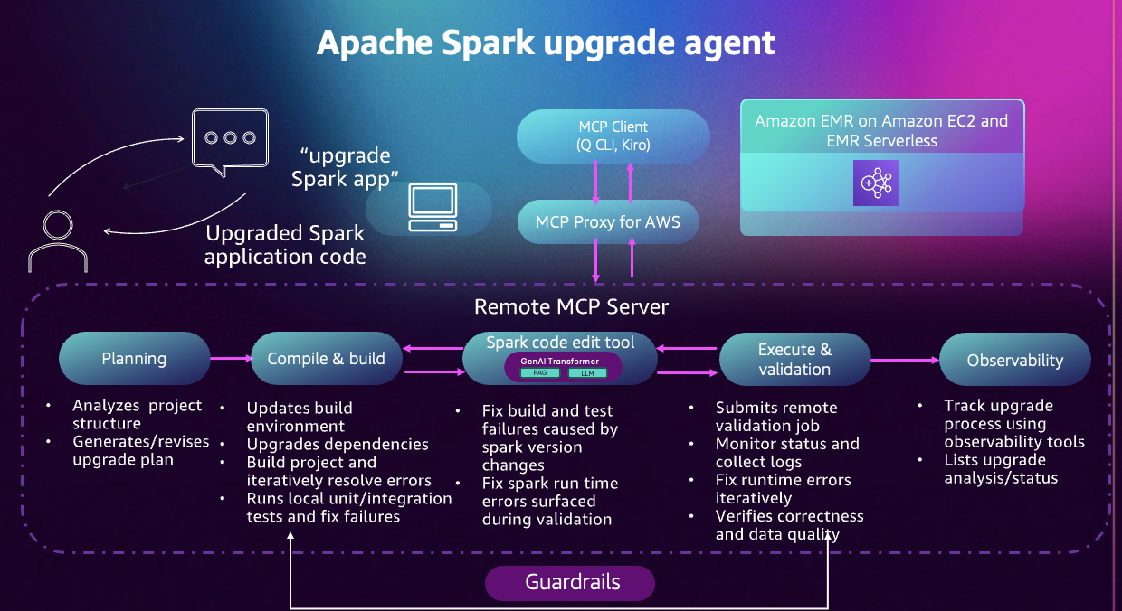
The Apache Spark upgrade agent for Amazon EMR is a conversational AI capability designed to accelerate Spark version upgrades for EMR applications. Through an MCP-compatible client, such as the Amazon Q Developer CLI, the Kiro IDE, or any custom agent built with frameworks like Strands, you can interact with a Model Context Protocol (MCP) server using natural language.


Figure 1: A diagram of the Apache Spark upgrade agent workflow.

Operating as a fully managed, cloud-hosted MCP server, the agent removes the need to maintain any local infrastructure. All tool calls and AWS resource interactions are governed by your AWS Identity and Access Management (IAM) permissions, ensuring the agent operates only within the access you authorize. Your application code remains on your machine, and only the minimal information required to diagnose and fix upgrade issues is transmitted. Every tool invocation is recorded in AWS CloudTrail, providing full auditability throughout the process.

Built on years of experience helping EMR customers upgrade their Spark applications, the upgrade agent automates the end-to-end modernization workflow, reducing manual effort and eliminating much of the trial-and-error typically involved in major version upgrades. The agent guides you through six phases:

  1. Planning: The agent analyzes your project structure, identifies compatibility issues, and generates a detailed upgrade plan. You review and customize this plan before execution begins.
  2. Environment setup: The agent configures build tools, updates language versions, and manages dependencies. For Python projects, it creates virtual environments with correct package versions.
  3. Code transformation: The agent updates build files, replaces deprecated APIs, fixes type incompatibilities, and modernizes code patterns. Changes are explained and shown before being applied.
  4. Local validation: The agent compiles your project and runs your test suite. When tests fail, it analyzes errors, applies fixes, and retries. This continues until all tests pass.
  5. EMR validation: The agent packages your application, deploys it to EMR, monitors execution, and analyzes logs. Runtime issues are fixed iteratively.
  6. Data quality checks: The agent can run your application on both source and target Spark versions, compare outputs, and report differences in schemas, values, or statistics.

Throughout the process, the agent explains its reasoning and collaborates with you on decisions.

Getting started

(Optional) Assessing your accounts for EMR Spark Upgrades

Before beginning a Spark upgrade, it’s helpful to understand the current state of your environment. Many customers run Spark applications across multiple Amazon EMR clusters and versions, making it challenging to know which workloads should be prioritized for modernization. If you have already identified the Spark applications that you would like to upgrade or already have a dashboard, you can skip this assessment step and move to the next section to get started with the Spark upgrade agent.

Building an Assessment Dashboard

To simplify this discovery process, we provide a lightweight Python-based assessment tool that scans your EMR environment and generates an interactive dashboard summarizing your Spark application footprint. The tool reviews EMR steps, extracts application metadata, and computes EMR lifecycle timelines to help you to:

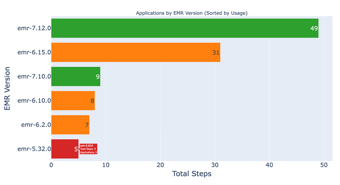
  • Understand your Spark applications and their executions distribution over different EMR versions.
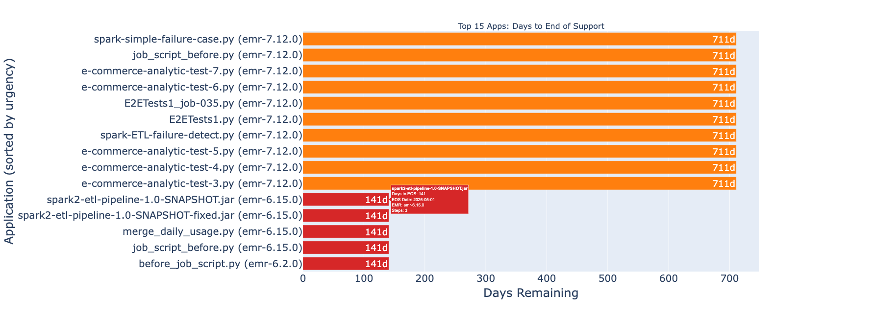
  • Review days remaining until each EMR version reaches end of support (EOS) for all Spark applications.
  • Evaluate what applications should be prioritized to migrate to newer EMR version.

Key insights from the assessment


Figure 2: A graph of EMR versions per application.

This dashboard shows how many Spark applications are running on legacy EMR versions, helping you identify which workloads to migrate first.


Figure 3: a graph of application use and current versions.

This dashboard identifies your most frequently used applications and their current EMR versions. Applications marked in red indicate high-impact workloads that should be prioritized for migration.


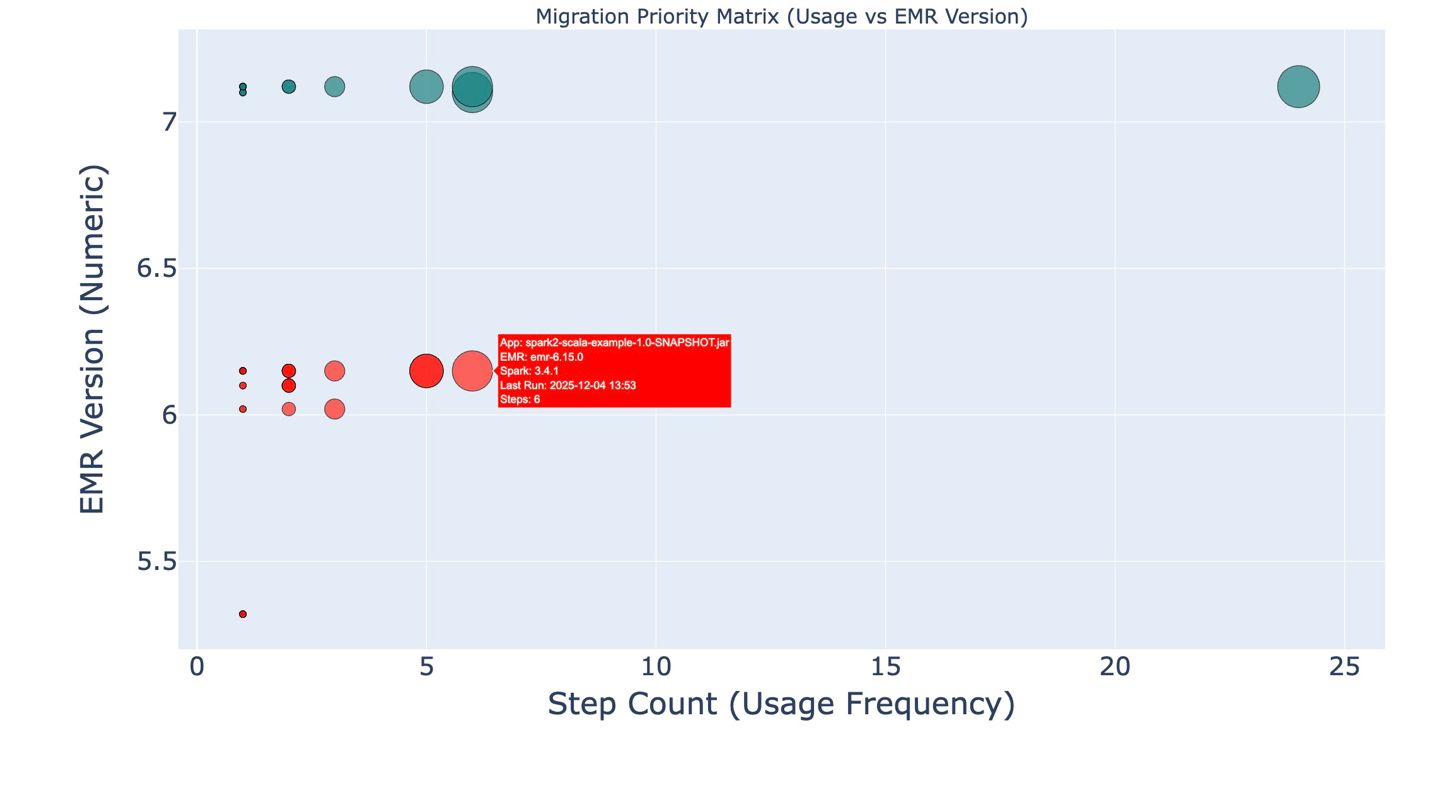
Figure 4: a utilization and EMR version graph.

This dashboard highlights high-usage applications running on older EMR versions. Larger bubbles represent more frequently used applications, and the Y-axis shows the EMR version. Together, these dimensions make it easy to spot which applications should be prioritized for upgrade.


Figure 5: a graph highlighting applications nearing End of Support.

The dashboard identifies applications approaching EMR End of Support, helping you prioritize migrations before updates and technical support are discontinued. For more information about support timelines, see Amazon EMR standard support.

Once you have identified the applications that need to be upgraded, you can use any IDE such as VS Code, Kiro IDE, or any other environment that supports installing an MCP server to begin the upgrade.

Getting started with Spark upgrade agent using Kiro IDE

Prerequisites

System requirements

IAM permissions

Your AWS IAM profile must include permissions to invoke the MCP server and access your Spark workload resources. The CloudFormation template provided in the setup documentation creates an IAM role with these permissions, along with supporting resources such as the Amazon S3 staging bucket where the upgrade artifacts will be uploaded. You can also customize the template to control which resources are created or skip resources you prefer to manage manually.

  1. Deploy the template within the same region you run your workloads in.
  2. Open the CloudFormation Outputs tab and copy the 1-line instruction ExportCommand, then execute it in your local environment.
    export SMUS_MCP_REGION=<your mcp server launch region> && export IAM_ROLE=arn:aws:iam::111122223333:role/spark-upgrade-role-xxxxxx && export STAGING_BUCKET_PATH=<your staging bucket path>

  3. Configure your AWS CLI profile:
    aws configure set profile.smus-mcp-profile.role_arn ${IAM_ROLE}
    aws configure set profile.smus-mcp-profile.source_profile default
    aws configure set profile.smus-mcp-profile.region ${SMUS_MCP_REGION}

Set up Kiro IDE and connect to the Spark upgrade agent

Kiro IDE provides a visual development environment with integrated AI assistance for interacting with the Apache Spark upgrade agent.

Installation and configuration:

  1. Install Kiro IDE
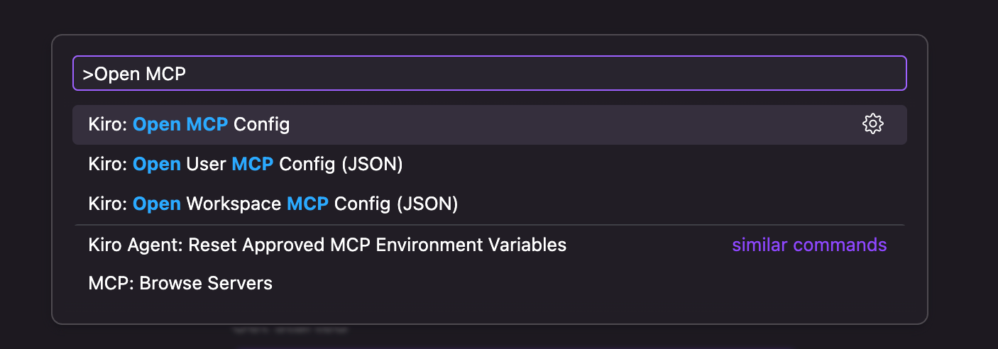
  2. Open the command palette using Ctrl + Shift + P (Linux) or Cmd + Shift + P (macOS) and Search for Kiro: Open MCP Config

    Figure 6: the Kiro command palette.
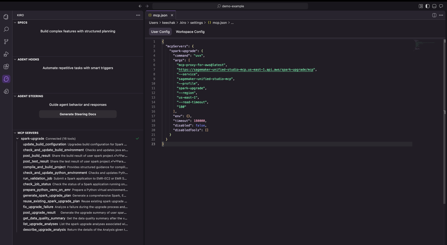
  3. Add the Spark upgrade agent configuration
    "mcpServers": {
        "upgrade-server": {
          "command": "uvx",
          "args": [
            "mcp-proxy-for-aws@latest",
            "https://sagemaker-unified-studio-mcp.${SMUS_MCP_REGION}.api.aws/spark-upgrade/mcp",
            "--service",
            "sagemaker-unified-studio-mcp",
            "--profile",
            "smus-mcp-profile",
            "--region",
            "${SMUS_MCP_REGION}",
            "--read-timeout",
            "180"
          ],
          "timeout": 180000
        }
      }
    }

  4. Once saved, the Kiro sidebar displays a successful connection to the upgrade server.

    Figure 7: Kiro IDE displaying a successful connection to the MCP server.

Upgrading a sample Spark application using Kiro IDE

To demonstrate upgrading from EMR 6.1.0 (Spark 3.0.0) to EMR 7.11.0 (Spark 3.5.6), we have prepared a sample e-commerce order processing application. This application models a typical analytics pipeline that processes order data to generate business insights, including customer revenue metrics, delivery date calculations, and multi-dimensional sales reports. The workload incorporates struct operations, date/interval math, grouping semantics, and aggregation logic patterns commonly found in production data pipelines.

Download the sample project

Clone the sample project from the Amazon EMR utilities GitHub repository:

git clone https://github.com/aws-samples/aws-emr-utilities.git
cd aws-emr-utilities/applications/spark-upgrade-assistant/demo-spark-application

Open the project in Kiro IDE

Launch Kiro IDE and open the demo-spark-application folder. Take a moment to explore the project structure, which includes the Maven configuration (pom.xml), the main Scala application, unit tests, and sample data.

Starting an upgrade

Once you have the project loaded in the Kiro IDE, select the Chat tab on the right-hand side of the IDE and type the following prompt to start the upgrade of the sample revenue analytics application:

Help me upgrade my application  from Spark 3.0 to Spark 3.5 
Use EMR-EC2 cluster j-9XXXXXXXXXX  with Spark 3.5 for validation. 
Store updated artifacts at s3://<path to upload upgrade artifacts>
Enable data quality checks.

Note: Replace j-XXXXXXXXXXXXX with your EMR cluster ID and <path to upload upgrade artifacts> with your S3 bucket name.

How the upgrade agent works

Step 1: Analyze and plan

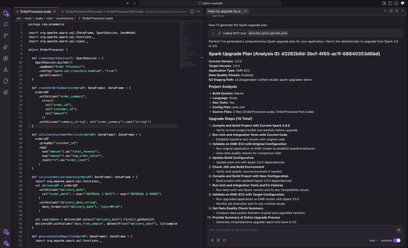
After you submit the prompt, the agent analyzes your project structure, build system, and dependencies to create an upgrade plan. You can review the proposed plan and suggest modifications before proceeding.


Figure 8: the proposed upgrade plan from the agent, ready for review.

Step 2: Upgrade dependencies

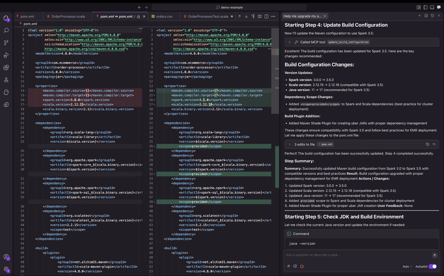
The agent will analyze all project dependencies and makes the necessary changes to upgrade the versions for compatibility with the target Spark version. It then compiles the project, builds the application, and runs tests to verify everything works correctly with the target Spark version.


Figure 9: Kiro IDE upgrading dependency versions.

Step 3: Code transformation

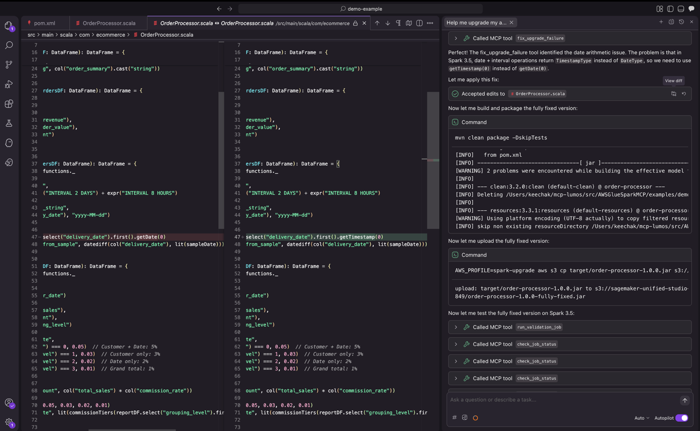
Alongside dependency updates, the agent identifies and fixes code changes in source and test files arising from deprecated APIs, modified dependencies, or backward incompatible behavior. The agent validates these modifications through unit, integration, and remote validation on Amazon EMR on Amazon EC2 or EMR Serverless depending on your deployment mode, iterating until successful execution.

Figure 10: the upgrade agent iterating through change testing.

Step 4: Validation

As part of validation, the agent submits jobs to EMR to verify the application runs successfully with actual data. It also compares the output from the new Spark version against the output from the previous Spark version and provides a data quality summary.


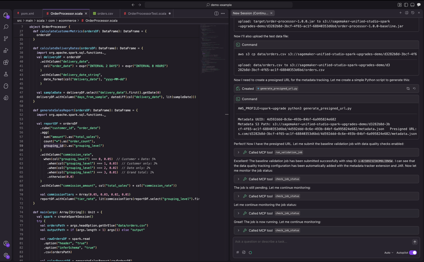
Figure 11: the upgrade agent validating changes with real data.

Step 5: Summary

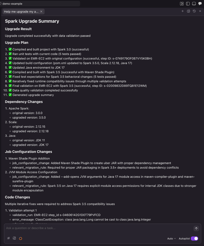
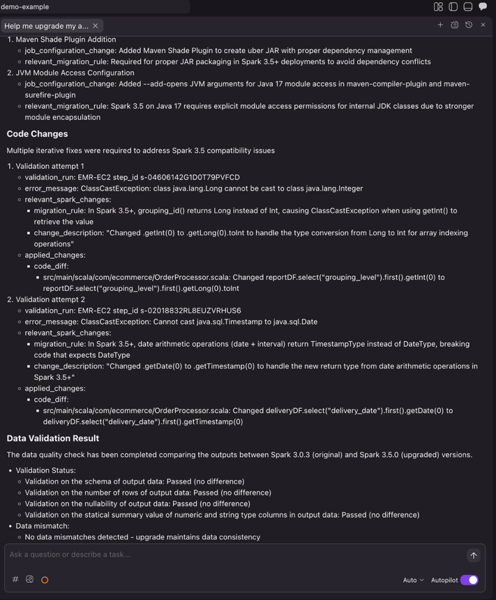
Once the agent completes the entire automation workflow, it generates a comprehensive upgrade summary. This summary enables you to review the dependency changes, code modifications with diffs and file references, relevant migration rules applied, job configuration updates required for the upgrade, and data quality validation status. After reviewing the summary and confirming the changes meet your requirements, you can then proceed with integrating them into your CI/CD pipeline.


Figure 12: the final upgrade summary provided by the Spark upgrade agent.

Integrating with your existing CI/CD framework

Once the Spark upgrade agent completes the automated upgrade process, you can seamlessly integrate the changes into your development workflow.

Pushing changes to remote repository

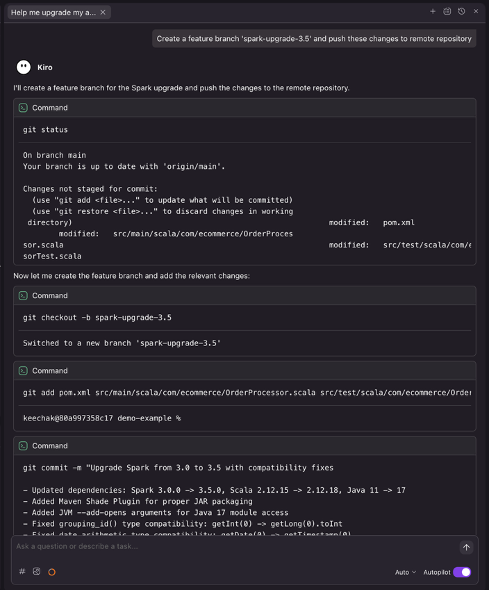
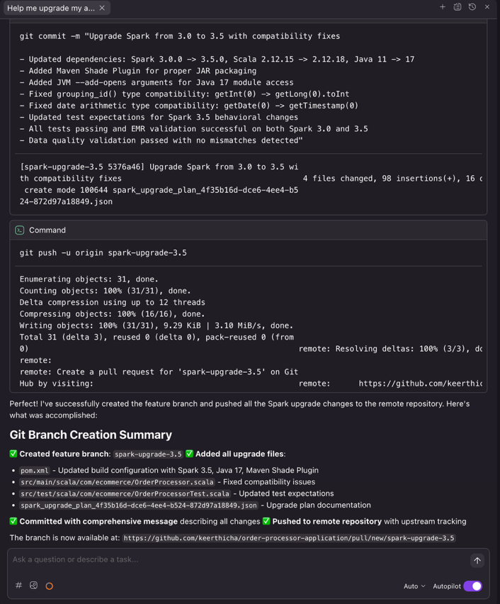
After the upgrade completes, ask Kiro to create a feature branch and push the upgraded code

Prompt to Kiro

Create a feature branch 'spark-upgrade-3.5' and push these changes to remote repository.

Kiro executes the necessary Git commands to create a clean feature branch, enabling proper code review workflows through pull requests.

CI/CD pipeline integration

Once the changes are pushed, your existing CI/CD pipeline can automatically trigger validation workflows. Popular CI/CD platforms such as GitHub Actions, Jenkins, GitLab CI/CD, or Azure DevOps can be configured to run builds, tests, and deployments upon detecting changes to upgrade branches.


Figure 14: the upgrade agent submitting a new feature branch with detailed commit message.

Conclusion

Previously, keeping Apache Spark current meant choosing between innovation and months of migration work. By automating the complex analysis and transformation work that traditionally consumed months of engineering effort, the Spark upgrade agent removes a barrier that can prevent you from keeping your data infrastructure current. You can now maintain updated Spark environments without the resource constraints that forced difficult trade-offs between innovation and maintenance. Taking the above Spark application upgrading experience as an example, what previously required 8 hours of manual work, including updating build configs, resolving build/compile failures, fixing runtime issues, and reviewing data quality results, now takes just 30 minutes with the automated agent.

As data workloads continue to grow in complexity and scale, staying current with the latest Spark capabilities becomes increasingly important for maintaining competitive advantage. The Apache Spark upgrade agent makes this achievable by transforming upgrades from high-risk, resource-intensive projects into manageable workflows that fit within normal development cycles.

Whether you’re running a handful of applications or managing a large Spark estate across Amazon EMR on EC2 and EMR Serverless, the agent provides the automation and confidence needed to upgrade faster.Ready to upgrade your Spark applications? Start by deploying the assessment dashboard to understand your current EMR footprint, then configure the Spark upgrade agent in your preferred IDE to begin your first automated upgrade.

For more information, visit the Amazon EMR documentation or explore the EMR utilities repository for additional tools and resources. Refer for details on which versions are supported are listed here in Amazon EMR documentation.


Special thanks

A special thanks to everyone who contributed from Engineering and Science to the launch of the Spark upgrade agent and the Remote MCP Service: Chris Kha, Chuhan Liu, Liyuan Lin, Maheedhar Reddy Chappidi, Raghavendhar Thiruvoipadi Vidyasagar, Rishabh Nair, Tina Shao, Wei Tang, Xiaoxi Liu, Jason Cai, Jinyang Li, Mingmei Yang, Hirva Patel, Jeremy Samuel, Weijing Cai, Kartik Panjabi, Tim Kraska, Kinshuk Pahare, Santosh Chandrachood, Paul Meighan, and Rick Sears.

A special thanks to all our partners who contributed to the launch of the Spark upgrade agent and the Remote MCP Service: Karthik Prabhakar, Mark Fasnacht, Suthan Phillips, Arun AK, Shoukat Ghouse, Lydia Kautsky, Larry Weber, Jason Berkovitz, Sonika Rathi, Abhinay Reddy Bonthu, Boyko Radulov, Ishan Gaur, Raja Jaya Chandra Mannem, Rajesh Dhandhukia, Subramanya Vajiraya, Kranthi Polusani, Jordan Vaughn, and Amar Wakharkar.

About the authors

Keerthi Chadalavada

Keerthi is a Senior Software Development Engineer in the AWS analytics organization. She focuses on combining generative AI and data integration technologies to design and build comprehensive solutions for customer data and analytics needs.

XiaoRun Yu

XiaoRun is a Software Development Engineer in the AWS analytics organization. He is working on building scalable and reliable Gen-AI products to solve real customer issues. Outside of work, Xiaorun enjoys exploring new places in the Bay Area.

Bo Li

Bo is a Senior Software Development Engineer in the AWS analytics organization. He is devoted to designing and building end-to-end solutions to address customers’ data analytic and processing needs with cloud-based, data-intensive and GenAI technologies.

Rajendra Gujja

Rajendra is a Senior Software Development Engineer in the AWS analytics organization. He is passionate about distributed computing and everything and anything about the data.

Vaibhav Naik

Vaibhav is a software engineer in the AWS analytics organization. He is passionate about building robust, scalable solutions to tackle complex customer problems. With a keen interest in generative AI, he likes to explore innovative ways to develop enterprise-level solutions that harness the power of cutting-edge AI technologies.

Malinda Malwala

Malinda is an Applied Scientist in the Data Processing Agents Science team building DevOps AI Agents for AWS Analytics services including Amazon EMR and AWS Glue. His research focuses on creating reliable, explainable, and trustworthy AI agents for enterprise use by combining traditional software engineering with generative AI. Outside of work, he enjoys hiking in the Cascade Mountains.

McCall Peltier

McCall is a Senior Product Marketing Manager at AWS focused on data processing services, including Amazon EMR. She leads messaging and launches that support customers building modern data platforms on AWS, collaborating across product and field teams to drive adoption and customer impact.

Shubham Mehta

Shubham is a Senior Product Manager at AWS Analytics. He leads generative AI feature development across services such as AWS Glue, Amazon EMR, and Amazon MWAA, using AI/ML to simplify and enhance the experience of data practitioners building data applications on AWS.

Pradeep Patel

Pradeep is a Software Development Manager at AWS Analytics. He is passionate about solving complex customer challenges through Agentic AI and AWS Cloud technologies, specializing in building highly scalable and robust solutions. Outside of work, he enjoys hiking and exploring applications of AI technologies.

Mukul Prasad

Mukul is a Senior Applied Science Manager in the Data Processing and Experiences organization. He leads the Data Processing Agents Science team developing DevOps agents to simplify and optimize the customer journey in using AWS Big Data processing services including Amazon EMR, AWS Glue, and Amazon SageMaker Unified Studio. Outside of work, Mukul enjoys food, travel, photography, and Cricket.

Mohit Saxena

Mohit is a Senior Software Development Manager at AWS Analytics. He leads development of distributed systems with AI/ML-driven capabilities and Agents to simplify and optimize the experience of data practitioners that build big data applications with Apache Spark, Amazon S3 and data lakes/warehouses on the cloud.

How to customize your response to layer 7 DDoS attacks using AWS WAF Anti-DDoS AMR

Post Syndicated from Achraf Souk original https://aws.amazon.com/blogs/security/how-to-customize-your-response-to-layer-7-ddos-attacks-using-aws-waf-anti-ddos-amr/

Over the first half of this year, AWS WAF introduced new application-layer protections to address the growing trend of short-lived, high-throughput Layer 7 (L7) distributed denial of service (DDoS) attacks. These protections are provided through the AWS WAF Anti-DDoS AWS Managed Rules (Anti-DDoS AMR) rule group. While the default configuration is effective for most workloads, you might want to tailor the response to match your application’s risk tolerance.

In this post, you’ll learn how the Anti-DDoS AMR works, and how you can customize its behavior using labels and additional AWS WAF rules. You’ll walk through three practical scenarios, each demonstrating a different customization technique.

How the Anti-DDoS AMR works at a high level

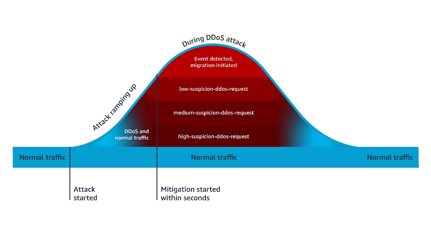
The Anti-DDoS AMR establishes a baseline of your traffic and uses it to detect anomalies within seconds. As shown in Figure 1, when the Anti-DDoS AMR detects a DDoS attack, it adds the event-detected label to all incoming requests, and the ddos-request label to incoming requests that are suspected of contributing to the attack. It also adds an additional confidence-based label, such as high-suspicion-ddos-request, when the request is suspected of contributing to the attack. In AWS WAF, a label is metadata added to a request by a rule when the rule matches the request. After being added, a label is available for subsequent rules, which can use it to enrich their evaluation logic. The Anti-DDoS AMR uses the added labels to mitigate the DDoS attack.

Figure 1 – Anti-DDOS AMR process flow

Figure 1 – Anti-DDOS AMR process flow

Default mitigations are based on a combination of Block and JavaScript Challenge actions. The Challenge action can only be handled properly by a client that’s expecting HTML content. For this reason, you need to exclude the paths of non-challengeable requests (such as API fetches) in the Anti-DDoS AMR configuration. The Anti-DDoS AMR applies the challengeable-request label to requests that don’t match the configured challenge exclusions. By default, the following mitigation rules are evaluated in order:

  • ChallengeAllDuringEvent, which is equivalent of the following logic: IF event-detected AND challengeable-request THEN challenge.
  • ChallengeDDoSRequests, which is equivalent to the following logic: IF (high-suspicion-ddos-request OR medium-suspicion-ddos-request OR low-suspicion-ddos-request) AND challengeable-request THEN challenge. Its sensitivity can be changed to match your needs, such as only challenge medium and high suspicious DDoS requests.
  • DDoSRequests, which is equivalent to the following logic: IF high-suspicion-ddos-request THEN block. Its sensitivity can be changed to match your needs, such as block medium in addition to high suspicious DDoS requests.

Customizing your response to layer 7 DDoS attacks

This customization can be done using two different approaches. In the first approach, you configure the Anti-DDoS AMR to take the action you want, then you add subsequent rules to further harden your response under certain conditions. In the second approach, you change some or all the rules of the Anti-DDoS AMR to count mode, then create additional rules that define your response to DDoS attacks.

In both approaches, the subsequent rules are configured using conditions you define, combined with conditions based on labels applied to requests by the Anti-DDoS AMR. The following section includes three examples of customizing your response to DDoS attacks. The first two examples are based on the first approach, while the last one is based on the second approach.

Example 1: More sensitive mitigation outside of core countries

Let’s suppose that your main business is conducted in two main countries, the UAE and KSA. You are happy with the default behavior of the Anti-DDoS AMR in these countries, but you want to block more aggressively outside of these countries. You can implement this using the following rules:

  • Anti-DDoS AMR with default configurations
  • A custom rule that blocks if the following conditions are met: Request is initiated from outside of UAE or KSA AND request has high-suspicion-ddos-request or medium-suspicion-ddos-request labels

Configuration

After adding your Anti-DDoS AMR with default configuration, create a subsequent custom rule with the following JSON definition.

Note: You need to use the AWS WAF JSON rule editor or infrastructure-as-code (IaC) tools (such as AWS CloudFormation or Terraform) to define this rule. The current AWS WAF console doesn’t allow creating rules with multiple AND/OR logic nesting.

{
    "Action": {
        "Block": {}
    },
    "Name": "more-sensitive-ddos-mitigation-outside-of-core-countries",
    "Priority": 1,
    "Statement": {
        "AndStatement": {
            "Statements": [
                {
                    "NotStatement": {
                        "Statement": {
                            "GeoMatchStatement": {
                                "CountryCodes": [
                                    "AE",
                                    "SA"
                                ]
                            }
                        }
                    }
                },
                {
                    "OrStatement": {
                        "Statements": [
                            {
                                "LabelMatchStatement": {
                                    "Key": "awswaf:managed:aws:anti-ddos:medium-suspicion-ddos-request",
                                    "Scope": "LABEL"
                                }
                            },
                            {
                                "LabelMatchStatement": {
                                    "Key": "awswaf:managed:aws:anti-ddos:high-suspicion-ddos-request",
                                    "Scope": "LABEL"
                                }
                            }
                        ]
                    }
                }
            ]
        }
    },
    "VisibilityConfig": {
        "CloudWatchMetricsEnabled": true,
        "MetricName": "more-sensitive-ddos-mitigation-outside-of-core-countries",
        "SampledRequestsEnabled": true
    }
}

Similarly, during an attack, you can more aggressively mitigate requests from unusual sources, such as requests labeled by the Anonymous IP managed rule group as coming from web hosting and cloud providers.

Example 2: Lower rate-limiting thresholds during DDoS attacks

Suppose that your application has sensitive URLs that are compute heavy. To protect the availability of your application, you have applied a rate limiting rule to these URLs configured with a 100 requests threshold over 2 mins window. You can harden this response during a DDoS attack by applying a more aggressive threshold. You can implement this using the following rules:

  1. An Anti-DDoS AMR with default configurations
  2. A rate-limiting rule, scoped to sensitive URLs, configured with a 100 requests threshold over a 2-minute window
  3. A rate-limiting rule, scoped to sensitive URLs and to the event-detected label, configured with a 10 requests threshold over a 10-minute window

Configuration

After adding your Anti-DDoS AMR with default configuration, and your rate-limit rule for sensitive URLs, create a subsequent new rate limiting rule with the following JSON definition.

{
    "Action": {
        "Block": {}
    },
    "Name": "ip-rate-limit-10-10mins-under-ddos",
    "Priority": 2,
    "Statement": {
        "RateBasedStatement": {
            "AggregateKeyType": "IP",
            "EvaluationWindowSec": 600,
            "Limit": 10,
            "ScopeDownStatement": {
                "AndStatement": {
                    "Statements": [
                        {
                            "ByteMatchStatement": {
                                "FieldToMatch": {
                                    "UriPath": {}
                                },
                                "PositionalConstraint": "EXACTLY",
                                "SearchString": "/sensitive-url",
                                "TextTransformations": [
                                    {
                                        "Priority": 0,
                                        "Type": "LOWERCASE"
                                    }
                                ]
                            }
                        },
                        {
                            "LabelMatchStatement": {
                                "Key": "awswaf:managed:aws:anti-ddos:event-detected",
                                "Scope": "LABEL"
                            }
                        }
                    ]
                }
            }
        }
    },
    "VisibilityConfig": {
        "CloudWatchMetricsEnabled": true,
        "MetricName": "ip-rate-limit-10-10mins-under-ddos",
        "SampledRequestsEnabled": true
    }
}

Example 3: Adaptive response according to your application scalability

Suppose that you are operating a legacy application that can safely scale to a certain threshold of traffic volume, after which it degrades. If the total traffic volume, including the DDoS traffic, is below this threshold, you decide not to challenge all requests during a DDoS attack to avoid impacting user experience. In this scenario, you’d only rely on the default block action of high suspicion DDoS requests. If the total traffic volume is above the safe threshold of your legacy application to process traffic, then you decide to use the equivalent of Anti-DDoS AMR’s default ChallengeDDoSRequests mitigation. You can implement this using the following rules:

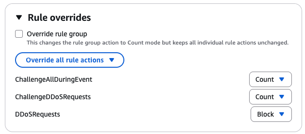
  1. An Anti-DDoS AMR with ChallengeAllDuringEvent and ChallengeDDoSRequests rules configured in count mode.
  2. A rate limiting rule that counts your traffic and is configured with a threshold corresponding to your application capacity to normally process traffic. As action, it only counts requests and applies a custom label—for example, CapacityExceeded—when its thresholds are met.
  3. A rule that mimics ChallengeDDoSRequests but only when the CapacityExceeded label is present: Challenge if ddos-request, CapacityExceeded, and challengeable-request labels are present

Configuration

First, update your Anti-DDoS AMR by changing Challenge actions to Count actions.

Figure 2 – Updated Anti-DDoS AMR rules in example 3

Figure 2 – Updated Anti-DDoS AMR rules in example 3

Then create the rate limit capacity-exceeded-detection rule in count mode, using the following JSON definition:

{
    "Action": {
        "Count": {}
    },
    "Name": "capacity-exceeded-detection",
    "Priority": 7,
    "RuleLabels": [
        {
            "Name": "mycompany:capacityexceeded"
        }
    ],
    "Statement": {
        "RateBasedStatement": {
            "AggregateKeyType": "IP",
            "EvaluationWindowSec": 120,
            "Limit": 10000
        }
    },
    "VisibilityConfig": {
        "CloudWatchMetricsEnabled": true,
        "MetricName": "capacity-exceeded-detection",
        "SampledRequestsEnabled": true
    }
}

Finally, create the challenge-if-ddos-and-capacity-exceeded challenge rule using the following JSON definition:

{
    "Action": {
        "Challenge": {}
    },
    "Name": "challenge-if-ddos-and-capacity-exceeded",
    "Priority": 2,
    "Statement": {
        "AndStatement": {
            "Statements": [
                {
                    "LabelMatchStatement": {
                        "Key": "mycompany:capacityexceeded",
                        "Scope": "LABEL"
                    }
                },
                {
                    "LabelMatchStatement": {
                        "Key": "awswaf:managed:aws:anti-ddos:ddos-request",
                        "Scope": "LABEL"
                    }
                },
                {
                    "LabelMatchStatement": {
                        "Key": "awswaf:managed:aws:anti-ddos:challengeable-request",
                        "Scope": "LABEL"
                    }
                }
            ]
        }
    },
    "VisibilityConfig": {
        "CloudWatchMetricsEnabled": true,
        "MetricName": "challenge-if-ddos-and-capacity-exceeded",
        "SampledRequestsEnabled": true
    }
}

Conclusion

By combining the built-in protections of the Anti-DDoS AMR with custom logic, you can adapt your defenses to match your unique risk profile, traffic patterns, and application scalability. The examples in this post illustrate how you can fine-tune sensitivity, enforce stronger mitigations under specific conditions, and even build adaptive defenses that respond dynamically to your system’s capacity.

You can use the dynamic labeling system in AWS WAF to implement customization granularly. You can also use AWS WAF labels to exclude costly logging of DDoS attack traffic.

If you have feedback about this post, submit comments in the Comments section below.

Achraf Souk

Achraf is a Principal Solutions Architect at AWS with more than 15 years of experience in cloud, security, and networking. He works closely with customers across industries to design resilient, fast, and secure web applications. A frequent writer and speaker, he enjoys simplifying deeply technical topics for a wider audience. Achraf has a track record in building and scaling technical organizations.

Introducing Apache Iceberg materialized views in AWS Glue Data Catalog

Post Syndicated from Tomohiro Tanaka original https://aws.amazon.com/blogs/big-data/introducing-apache-iceberg-materialized-views-in-aws-glue-data-catalog/

Hundreds of thousands of customers build artificial intelligence and machine learning (AI/ML) and analytics applications on AWS, frequently transforming data through multiple stages for improved query performance—from raw data to processed datasets to final analytical tables. Data engineers must solve complex problems, including detecting what data has changed in base tables, writing and maintaining transformation logic, scheduling and orchestrating workflows across dependencies, provisioning and managing compute infrastructure, and troubleshooting failures while monitoring pipeline health. Consider an ecommerce company where data engineers need to continuously merge clickstream logs with orders data for analytics. Each transformation requires building robust change detection mechanisms, writing complex joins and aggregations, coordinating multiple workflow steps, scaling compute resources appropriately, and maintaining operational oversight—all while supporting data quality and pipeline reliability. This complexity demands months of dedicated engineering effort and ongoing maintenance, making data transformation costly and time-intensive for organizations seeking to unlock insights from their data.

To address those challenges, AWS announced a new materialized view capability for Apache Iceberg tables in the AWS Glue Data Catalog. The new materialized view capability simplifies data pipelines and accelerates data lake query performance. A materialized view is a managed table in the AWS Glue Data Catalog that stores pre-computed results of a query in Iceberg format that is incrementally updated to reflect changes to the underlying datasets. This alleviates the need to build and maintain complex data pipelines to generate transformed datasets and accelerate query performance. Apache Spark engines across Amazon Athena, Amazon EMR, and AWS Glue support the new materialized views and intelligently rewrite queries to use materialized views that speed up performance while reducing compute costs.

In this post, we show you how Iceberg materialized view works and how to get started.

How Iceberg materialized views work

Iceberg materialized views offer a simple, managed solution built on familiar SQL syntax. Instead of building complex pipelines, you can create materialized views using standard SQL queries from Spark, transforming data with aggregates, filters, and joins without writing custom data pipelines. Change detection, incremental updates, and monitoring source tables are automatically handled in the AWS Glue Data Catalog and refreshing materialized views as new data arrive, alleviating the need for manual pipeline orchestration. Data transformations run on fully managed compute infrastructure, removing the burden of provisioning, scaling, or maintaining servers.

The resulting pre-computed data is stored as Iceberg tables in an Amazon Simple Storage Service (Amazon S3) general purpose bucket, or Amazon S3 Tables buckets within the your account, making transformed data immediately accessible to multiple query engines, including Athena, Amazon Redshift, and AWS optimized Spark runtime. Spark engines across Athena, Amazon EMR, and AWS Glue support an automatic query rewrite functionality that intelligently uses materialized views, delivering automatic performance improvement for data processing jobs or interactive notebook queries.

In the following sections, we walk through the steps to create, query, and refresh materialized views.

Pre-requisite

To follow along with this post, you must have an AWS account.

To run the instruction on Amazon EMR, complete the following steps to configure the cluster:

  1. Launch an Amazon EMR cluster 7.12.0 or higher.
  2. SSH login to the primary node of your Amazon EMR cluster, and run the following command to start a Spark application with required configurations:
    spark-sql \
      --conf spark.sql.extensions=org.apache.iceberg.spark.extensions.IcebergSparkSessionExtensions \
      --conf spark.sql.catalog.glue_catalog=org.apache.iceberg.spark.SparkCatalog \
      --conf spark.sql.catalog.glue_catalog.type=glue \
      --conf spark.sql.catalog.glue_catalog.warehouse=s3://amzn-s3-demo-bucket/warehouse \
      --conf spark.sql.catalog.glue_catalog.glue.region=us-east-1 \
      --conf spark.sql.catalog.glue_catalog.glue.id=123456789012 \
      --conf spark.sql.catalog.glue_catalog.glue.account-id=123456789012 \
      --conf spark.sql.catalog.glue_catalog.client.region=us-east-1 \
      --conf spark.sql.catalog.glue_catalog.glue.lakeformation-enabled=true \
      --conf spark.sql.optimizer.answerQueriesWithMVs.enabled=true \
      --conf spark.sql.defaultCatalog=glue_catalog
      

To run the instruction on AWS Glue for Spark, complete the following steps to configure the job:

  1. Create an AWS Glue version 5.1 job or higher.
  2. Configure a job parameter
    1. Key: --conf
    2. Value: spark.sql.extensions=org.apache.iceberg.spark.extensions.IcebergSparkSessionExtensions
  3. Configure your job with the following script:
    from pyspark.sql import SparkSession
    
    
    spark = (
        SparkSession.builder \
            .config("spark.sql.extensions", "org.apache.iceberg.spark.extensions.IcebergSparkSessionExtensions")
            .config("spark.sql.catalog.glue_catalog", "org.apache.iceberg.spark.SparkCatalog")
            .config("spark.sql.catalog.glue_catalog.type", "glue")
            .config("spark.sql.catalog.glue_catalog.warehouse", "s3://amzn- -demo-bucket/warehouse")
            .config("spark.sql.catalog.glue_catalog.glue.region", "us-east-1")
            .config("spark.sql.catalog.glue_catalog.glue.id", "123456789012")
            .config("spark.sql.catalog.glue_catalog.glue.account-id", "123456789012")
    		.config("spark.sql.catalog.glue_catalog.client.region", "us-east-1")
            .config("spark.sql.catalog.glue_catalog.glue.lakeformation-enabled", "true")
            .config("spark.sql.optimizer.answerQueriesWithMVs.enabled", "true")
            .config("spark.sql.defaultCatalog", "glue_catalog")
            .getOrCreate()
    )

  4. Run the following queries using Spark SQL to set up a base table. In AWS Glue, you can run them through spark.sql("QUERY STATEMENT").
    CREATE DATABASE IF NOT EXIST iceberg_mv;
    
    USE iceberg_mv;
    
    CREATE TABLE IF NOT EXISTS base_tbl (
        id INT,
        customer_name STRING,
        amount INT,
        order_date DATE);
        
    INSERT INTO base_tbl VALUES (1, 'John Doe', 150, DATE('2025-12-01')), (2, 'Jane Smith', 200, DATE('2025-12-02')), (3, 'Bob Johnson', 75, DATE('2025-12-03'));
    
    SELECT * FROM base_tbl;

In the subsequent sections, we create a materialized view with this base table.

If you want to store your materialized views in Amazon S3 Tables instead of a general Amazon S3 bucket, refer to Appendix 1 at the end of this post for the configuration details.

Create a materialized view

To create a materialized view, run the following command:

CREATE MATERIALIZED VIEW mv
AS SELECT
    customer_name, 
    COUNT(*) as mv_order_count, 
    SUM(amount) as mv_total_amount 
FROM glue_catalog.iceberg_mv.base_tbl
GROUP BY customer_name;

After you create a materialized view, AWS Spark’s in-memory metadata cache needs time to populate with information about the new materialized view. During this cache population period, queries against the base table will run normally without using the materialized view. After the cache is fully populated (typically within tens of seconds), Spark automatically detects that the materialized view can satisfy the query and rewrites it to use the pre-computed materialized view instead, improving performance.

To see this behavior, run the following EXPLAIN command immediately after creating the materialized view:

EXPLAIN EXTENDED
SELECT customer_name, COUNT(*) as mv_order_count, SUM(amount) as mv_total_amount 
FROM base_tbl
GROUP BY customer_name;

The following output shows the initial result before cache population:

== Parsed Logical Plan ==
'Aggregate ['customer_name], ['customer_name, 'COUNT(1) AS mv_order_count#0, 'SUM('amount) AS mv_total_amount#1]
+- 'UnresolvedRelation [base_tbl] , [], false

== Analyzed Logical Plan ==
customer_name: string, mv_order_count: bigint, mv_total_amount: bigint
Aggregate [customer_name#8], [customer_name#8, count(1) AS mv_order_count#0L, sum(amount#9) AS mv_total_amount#1L]
+- SubqueryAlias glue_catalog.iceberg_mv.base_tbl
   +- RelationV2[id#7, customer_name#8, amount#9, order_date#10] glue_catalog.iceberg_mv.base_tbl glue_catalog.iceberg_mv.base_tbl

== Optimized Logical Plan ==
Aggregate [customer_name#8], [customer_name#8, count(1) AS mv_order_count#0L, sum(amount#9) AS mv_total_amount#1L]
+- RelationV2[customer_name#8, amount#9] glue_catalog.iceberg_mv.base_tbl

== Physical Plan ==
AdaptiveSparkPlan isFinalPlan=false
+- HashAggregate(keys=[customer_name#8], functions=[count(1), sum(amount#9)], output=[customer_name#8, mv_order_count#0L, mv_total_amount#1L], schema specialized)
   +- Exchange hashpartitioning(customer_name#8, 1000), ENSURE_REQUIREMENTS, [plan_id=19]
      +- HashAggregate(keys=[customer_name#8], functions=[partial_count(1), partial_sum(amount#9)], output=[customer_name#8, count#27L, sum#29L], schema specialized)
         +- BatchScan glue_catalog.iceberg_mv.base_tbl[customer_name#8, amount#9] glue_catalog.iceberg_mv.base_tbl (branch=null) [filters=, groupedBy=, pushedLimit=None] RuntimeFilters: []

In this initial execution plan, Spark scans the base_tbl directly (BatchScan glue_catalog.iceberg_mv.base_tbl) and runs aggregations (COUNT and SUM) on the raw data. This is the behavior before the materialized view metadata cache is populated.

After waiting approximately tens of seconds for the metadata cache population, run the same EXPLAIN command again. The following output shows the primary differences in the query optimization plan after cache population:

== Optimized Logical Plan ==
Aggregate [customer_name#97], [customer_name#97, coalesce(sum(mv_order_count#98L), 0) AS mv_order_count#72L, sum(mv_total_amount#99L) AS mv_total_amount#73L]
+- RelationV2[customer_name#97, mv_order_count#98L, mv_total_amount#99L] glue_catalog.iceberg_mv.mv

== Physical  Plan ==
AdaptiveSparkPlan isFinalPlan=false
+- HashAggregate(keys=[customer_name#97], functions=[sum(mv_order_count#98L), sum(mv_total_amount#99L)], output=[customer_name#97, mv_order_count#72L, mv_total_amount#73L], schema specialized)
   +- Exchange hashpartitioning(customer_name#97, 1000), ENSURE_REQUIREMENTS, [plan_id=51]
      +- HashAggregate(keys=[customer_name#97], functions=[partial_sum(mv_order_count#98L), partial_sum(mv_total_amount#99L)], output=[customer_name#97, sum#113L, sum#115L], schema specialized)
         +- BatchScan glue_catalog.iceberg_mv.mv[customer_name#97, mv_order_count#98L, mv_total_amount#99L] glue_catalog.iceberg_mv.mv (branch=null) [filters=, groupedBy=, pushedLimit=None] RuntimeFilters: []

After the cache is populated, Spark now scans the materialized view (BatchScan glue_catalog.iceberg_mv.mv) instead of the base table. The query has been automatically rewritten to read from the pre-computed aggregated data in the materialized view. The output specifically shows the aggregation functions now simply sum the pre-computed values (sum(mv_order_count) and sum(mv_total_amount)) rather than recalculating COUNT and SUM from raw data.

Create a materialized view with scheduling automatic refresh

By default, a newly created materialized view contains the initial query results. It’s not automatically updated when the underlying base table data changes. To keep your materialized view synchronized with the base table data, you can configure automatic refresh schedules. To enable automatic refresh, use the REFRESH EVERY clause when creating the materialized view. This clause accepts a time interval and unit, so you can specify how frequently the materialized view is updated.

The following example creates a materialized view that automatically refreshes every 24 hours:

CREATE MATERIALIZED VIEW mv
REFRESH EVERY 24 HOURS
AS SELECT
    customer_name, 
    COUNT(*) as mv_order_count, 
    SUM(amount) as mv_total_amount 
FROM glue_catalog.iceberg_mv.base_tbl
GROUP BY customer_name;

You can configure the refresh interval using any of the following time units: SECONDS, MINUTES, HOURS, or DAYS. Choose an appropriate interval based on your data freshness requirements and query patterns.

If you prefer more control over when your materialized view updates, or need to refresh it outside of the scheduled intervals, you can trigger manual refreshes at any time. We provide detailed instructions on manual refresh options, including full and incremental refresh, later in this post.

Query a materialized view

To query a materialized view on your Amazon EMR cluster and retrieve its aggregated data, you can use a standard SELECT statement:

SELECT * FROM mv;

This query retrieves all rows from the materialized view. The output shows the aggregated customer order counts and total amounts. The result displays three customers with their respective metrics:

-- Result
Jane Smith    1    200
Bob Johnson    1    75
John Doe    1    150

Additionally, you can query the same materialized view from Athena SQL. The following screenshot shows the same query run on Athena and the resulting output.

Refresh a materialized view

You can refresh materialized views using two refresh types: full refresh or incremental refresh. Full refresh re-computes the entire materialized view from all base table data. Incremental refresh processes only the changes since the last refresh. Full refresh is ideal when you need consistency or after significant data changes. Incremental refresh is preferred when you need immediate updates. The following examples show both refresh types.

To use full refresh, complete the following steps:

  1. Insert three new records into the base table to simulate new data arriving:
    INSERT INTO base_tbl VALUES 
    (4, 'Jane Smith', 350, DATE('2025-11-29')), 
    (5, 'Bob Johnson', 100, DATE('2025-11-30')), 
    (6, 'Kwaku Mensah', 40, DATE('2025-12-01'));

  2. Query the materialized view to verify it still shows the old aggregated values:
    SELECT * FROM mv;
    
    -- Result
    Jane Smith    1    200
    Bob Johnson    1    75
    John Doe    1    150

  3. Run a full refresh of the materialized view using the following command:
    REFRESH MATERIALIZED VIEW mv FULL;

  4. Query the materialized view again to verify the aggregated values now include the new records:
    SELECT * FROM mv;
    
    -- Result
    Jane Smith    2    550 // Updated
    Bob Johnson    2    175  // Updated
    John Doe    1    150
    Kwaku Mensah    1    40 // Added

To use incremental refresh, complete the following steps:

  1. Enable incremental refresh by setting the Spark configuration properties:
    SET spark.sql.optimizer.incrementalMVRefresh.enabled=true;

  2. Insert two additional records into the base table:
    INSERT INTO base_tbl VALUES 
    (7, 'Jane Smith', 120, DATE('2025-11-28')), 
    (8, 'Kwaku Mensah', 90, DATE('2025-12-02'));

  3. Run an incremental refresh using the REFRESH command without the FULL clause. To verify if incremental refresh is enabled, refer to Appendix 2 at the end of this post.
    REFRESH MATERIALIZED VIEW mv;

  4. Query the materialized view to confirm the incremental changes are reflected in the aggregated results:
    SELECT * FROM mv;
    
    --Result
    Jane Smith    3    670    3    3 // Updated
    Bob Johnson    2    175    2    2 
    John Doe    1    150    1    1
    Kwaku Mensah    2    130    2    2 // Updated

In addition to using Spark SQL, you can also trigger manual refreshes through AWS Glue APIs when you need updates outside your scheduled intervals. Run the following AWS CLI command:

$ aws glue start-materialized-view-refresh-task-run \
    --catalog-id <ACCOUNT_ID> \
    --database-name <DATABASE_NAME> \
    --table-name <MV_TABLE_NAME>

The AWS Lake Formation console displays refresh history for API-triggered updates. Open your materialized view to see the refresh type (INCREMENTAL or FULL), start and end time, status and so on:

You have learned how to use Iceberg materialized views to make your efficient data processing and queries. You created a materialized view using Spark on Amazon EMR, queried it from both Amazon EMR and Athena, and used two refresh mechanisms: full refresh and incremental refresh. Iceberg materialized views help you transform and optimize your data pipelines effortlessly.

Considerations

There are important aspects to consider for optimal usage of the capability:

  • We introduced new SQL syntax to manage materialized views in the AWS optimized Spark runtime engine only. These new SQL commands are available in Spark version 3.5.6 and above across Athena, Amazon EMR, and AWS Glue. Open source Spark is not supported.
  • Materialized views are eventually consistent with base tables. When source tables change, the materialized views are updated through background refresh processes as defined by users in the refresh schedule at creation. During the refresh window, queries directly accessing materialized views might see outdated data. However, customers who need immediate access to the most up-to-date datasets can run a manual refresh with a simple REFRESH MATERIALIZED VIEW SQL command.

Clean up

To avoid incurring future charges, clean up the resources you created during this walkthrough:

  1. Run the following commands to delete a materialized view and tables:
    DROP TABLE mv PURGE;
    -- Or, DROP MATERIALIZED VIEW mv;
    
    DROP TABLE base_tbl PURGE;
    -- If necessary, delete the database by DROP DATABASE iceberg_mv;

  2. For Amazon EMR, terminate the Amazon EMR cluster.
  3. For AWS Glue, delete the AWS Glue job.

Conclusion

This post demonstrated how Iceberg materialized views facilitate efficient data lake operations on AWS. The new materialized view capability simplifies data pipelines and improves query performance by storing pre-computed results that are automatically updated as base tables change. You can create materialized views using familiar SQL syntax, using both full and incremental refresh mechanisms to maintain data consistency. This solution alleviates the need for complex pipeline maintenance while providing seamless integration with AWS services like Athena, Amazon EMR, and AWS Glue. The automatic query rewrite functionality further optimizes performance by intelligently utilizing materialized views when applicable, making it a powerful tool for organizations looking to streamline their data transformation workflows and accelerate query performance.

Appendix 1: Spark configuration to use Amazon S3 Tables storing Apache Iceberg materialized views

As mentioned earlier in this post, materialized views are stored as Iceberg tables in Amazon S3 Tables buckets within your account. When you want to use Amazon S3 Tables as the storage location for your materialized views instead of a general Amazon S3 bucket, you must configure Spark with the Amazon S3 Tables catalog.

The difference from the standard AWS Glue Data Catalog configuration shown in the prerequisites section is the glue.id parameter format. For Amazon S3 Tables, use the format <account-id>:s3tablescatalog/<s3-tables-bucket-name> instead of just the account ID:

spark-sql \
  --conf spark.sql.extensions=org.apache.iceberg.spark.extensions.IcebergSparkSessionExtensions \
  --conf spark.sql.catalog.s3t_catalog=org.apache.iceberg.spark.SparkCatalog \
  --conf spark.sql.catalog.s3t_catalog.type=glue \
  --conf spark.sql.catalog.s3t_catalog.warehouse="s3://amzn-s3-demo-bucket/warehouse" \
  --conf spark.sql.catalog.s3t_catalog.glue.region="us-east-1" \
  --conf spark.sql.catalog.s3t_catalog.glue.id="123456789012:s3tablescatalog/amzn-s3-demo-table-bucket" \
  --conf spark.sql.catalog.s3t_catalog.glue.account-id=123456789012 \
  --conf spark.sql.catalog.s3t_catalog.client.region="us-east-1" \
  --conf spark.sql.catalog.s3t_catalog.glue.lakeformation-enabled=true \
  --conf spark.sql.optimizer.answerQueriesWithMVs.enabled=true \
  --conf spark.sql.defaultCatalog=s3t_catalog

After you configure Spark with these settings, you can create and manage materialized views using the same SQL commands shown in this post, and the materialized views are stored in your Amazon S3 Tables bucket.

Appendix 2: Verify refreshing a materialized view with Spark SQL

Run SHOW TBLPROPERTIES in Spark SQL to check which refresh method was used:

+-------------------------------+----------------------------------------------------------------------------------------------------------------------------------+
|key                            |value                                                                                                                             |
+-------------------------------+----------------------------------------------------------------------------------------------------------------------------------+
|IMV_ansiEnabled                |false                                                                                                                             |
|IMV_catalogInfo                |[{"catalogId":"123456789012","catalogName":"glue_catalog"}]                                                                       |
|IMV_mvCatalogID                |123456789012                                                                                                                      |
|IMV_mvNamespace                |iceberg_mv                                                                                                                        |
|IMV_region                     |us-east-1                                                                                                                         |
|IMV_sparkVersion               |3.5.6-amzn-1                                                                                                                      |
|current-snapshot-id            |5750703934418352571                                                                                                               |
|format                         |iceberg/parquet                                                                                                                   |
|format-version                 |2                                                                                                                                 |
|isMaterializedView             |true                                                                                                                              |
|lastRefreshType                |INCREMENTAL                                                                                                                       |
|subObjects                     |[{"Version":"4887707562550190856","DatabaseName":"iceberg_mv","Region":"us-east-1","CatalogId":"123456789012","Name":"base_tbl"}] |
|tableVersionToken              |*********(redacted)                                                                                                               |
|viewOriginalText               |SELECT\ncustomer_name, \nCOUNT(*) as mv_order_count, \nSUM(amount) as mv_total_amount \nFROM base_tbl\nGROUP BY customer_name     |
|viewVersionId                  |5750703934418352571                                                                                                               |
|viewVersionToken               |*********(redacted)                                                                                                               |
|write.parquet.compression-codec|zstd                                                                                                                              |
+-------------------------------+----------------------------------------------------------------------------------------------------------------------------------+

About the authors

Tomohiro Tanaka

Tomohiro Tanaka

Tomohiro is a Senior Cloud Support Engineer at AWS. He’s passionate about helping customers use Apache Iceberg for their data lakes on AWS. In his free time, he enjoys a coffee break with his colleagues and making coffee at home.

Leon Lin

Leon Lin

Leon is a Software Development Engineer at AWS, where he focuses on Apache Iceberg and Apache Spark development within the Open Data Analytics Engines team. He is also an active contributor to the open source Apache Iceberg project.

Noritaka Sekiyama

Noritaka Sekiyama

Noritaka is a Principal Big Data Architect with AWS Analytics services. He’s responsible for building software artifacts to help customers. In his spare time, he enjoys cycling on his road bike.

Mahesh Mishra

Mahesh Mishra

Mahesh is a Principal Product Manager with the AWS Analytics team. He works with many of AWS largest customers on emerging technology needs, and leads several data and analytics initiatives within AWS, including strong support for transactional data lakes.

Layth Yassin

Layth Yassin

Layth is a Software Development Engineer on the AWS Glue team. He’s passionate about tackling challenging problems at a large scale, and building products that push the limits of the field. Outside of work, he enjoys playing/watching basketball, and spending time with friends and family.

Auto-optimize your Amazon OpenSearch Service vector database

Post Syndicated from Dylan Tong original https://aws.amazon.com/blogs/big-data/auto-optimize-your-amazon-opensearch-service-vector-database/

AWS recently announced the general availability of auto-optimize for the Amazon OpenSearch Service vector engine. This feature streamlines vector index optimization by automatically evaluating configuration trade-offs across search quality, speed, and cost savings. You can then run a vector ingestion pipeline to build an optimized index on your desired collection or domain. Previously, optimizing index configurations—including algorithm, compression, and engine settings—required experts and weeks of testing. This process must be repeated because optimizations are unique to specific data characteristics and requirements. You can now auto-optimize vector databases in under an hour without managing infrastructure and acquiring expertise in index tuning.

In this post, we discuss how the auto-optimize feature works, its benefits, and share examples of auto-optimized results.

Overview of vector search and vector indexes

Vector search is a technique that improves search quality and is a cornerstone of generative AI applications. It involves using a type of AI model to convert content into numerical encodings (vectors), enabling content matching by semantic similarity instead of just keywords. You build vector databases by ingesting vectors into OpenSearch to build indexes that enable searches across billions of vectors in milliseconds.

Benefits of optimizing vector indexes and how it works

The OpenSearch vector engine provides a variety of index configurations that help you make favorable trade-offs between search quality (recall), speed (latency), and cost (RAM requirements). There isn’t a universally optimal configuration. Experts must evaluate combinations of index settings such as Hierarchal Navigable Small Worlds (HNSW) algorithm parameters (such as m or ef_construction), quantization techniques (such as scalar, binary, or product), and engine parameters (such as memory-optimized, disk-optimized, or warm-cold storage). The difference between configurations could be a 10% or more difference in search quality, hundreds of milliseconds in search latency, or up to three times in cost savings. For large-scale deployments, cost-optimizations can make or break your budget.

The following figure is a conceptual illustration of trade-offs between index configurations.

Optimizing vector indexes is time-consuming. Experts must build an index; evaluate its speed, quality, and cost; and make appropriate configuration adjustments before repeating this process. Running these experiments at scale can take weeks because building and evaluating large-scale index requires substantial compute power, resulting in hours to days of processing for just one index. Optimizations are unique to specific business requirements and each dataset, and trade-off decisions are subjective. The best trade-offs depend on the use case, such as search for an internal wiki or an e-commerce site. Therefore, this process must be repeated for each index. Lastly, if your application data changes continuously, your vector search quality might degrade, requiring you to rebuild and re-optimize your vector indexes regularly.

Solution overview

With auto-optimize, you can run jobs to produce optimization recommendations, consisting of reports that detail performance measurements and explanations of the recommended configurations. You can configure auto-optimize jobs by simply providing your application’s acceptable search latency and quality requirements. Expertise in k-NN algorithms, quantization techniques, and engine settings aren’t required. It avoids the one-size-fits-all limitations of solutions based on a few pre-configured deployment types, offering a tailored fit for your workloads. It automates the manual labor previously described. You simply run serverless, auto-optimize jobs at a flat rate per job. These jobs don’t consume your collection or domain resources. OpenSearch Service manages a separate multi-tenant warm pool of servers, and parallelizes index evaluations across secure, single-tenant workers to deliver results quickly. Auto-optimize is also integrated with vector ingestion pipelines, so you can quickly build an optimized vector index on a collection or domain from an Amazon Simple Storage Service (Amazon S3) data source.

The following screenshot illustrates how to configure an auto-optimize job on the OpenSearch Service console.

When the job is complete (typically, within 30–60 minutes for million-plus-size datasets), you can review the recommendations and reports, as shown in the following screenshot.

The screenshot illustrates an example where you need to choose the best trade-offs. Do you select the first option, which delivers the highest cost savings (through lower memory requirements)? Or do you select the third option, which delivers a 1.76% search quality improvement, but at higher cost? If you want to understand the details of the configurations used to deliver these results, you can view the sub-tabs on the Details pane, such as the Algorithm parameters tab shown in the preceding screenshot.

After you’ve made your choice, you can build your optimized index on your target OpenSearch Service domain or collection, as shown in the following screenshot. If you’re building the index on a collection or a domain running OpenSearch 3.1+, you can enable GPU-acceleration to increase the build speed up to 10 times faster at a quarter of the indexing cost.

Auto-optimize results

The following table presents a few examples of auto-optimize results. To quantify the value of running auto-optimize, we present gains compared to default settings. The estimated RAM requirements are based on standard domain sizing estimates:

Required RAM = 1.1 x (bytes per dimension x dimensions + hnsw.parameters.m x 8) x vector count

We estimate cost savings by comparing the minimal infrastructure (has just enough RAM) to host an index with the default compared to optimized settings.

Dataset Auto-Optimize Job Configurations Recommended Changes to Defaults

Required RAM)

(% reduced)

Estimated Cost Savings

(Required data nodes for default configuration vs. optimized)

Recall

(% gain)

msmarco-distilbert-base-tas-b: 10M 384D vectors generated from MSMARCO v1 Acceptable recall >= 0.95 Modest latency (Approximately 200-300 ms) More supporting indexing and search memory (ef_search=256, ef_constructon=128)Use Lucene engineDisk optimized mode with 5X oversampling4X compression (4-bit binary quantization)

5.6 GB

(-69.4%)

Less 75%

(3 x r8g.mediumsearch vs. 3 x r8g.xlarge.search)

0.995(+2.6%)
all-mpnet-base-v2: 1M 768D vectors generated from MSMARCO v2.1 Acceptable recall >= 0.95 Modest latency (Approximately 200–300 ms) Denser HNSW Graph (m=32)More supporting indexing and search memory (ef_search=256, ef_constructon=128)Disk optimized mode with 3X oversampling8X compression (4-bit binary quantization)

0.7GB

(-80.9%)

Less 50.7%

(t3.small.search vs. t3.medium.search)

0.999 (+0.9%)
Cohere Embed V3: 113M 1024D vectors generated from MSMARCO v2.1 Acceptable recall >= 0.95 Fast latency (Approximately <= 50 ms) Denser HNSW Graph (m=32)More supporting indexing and search memory (ef_search=256, ef_constructon=128)Use Lucene engine4X compression (uint8-scalar quantization)

159GB

(-69.7%)

Less 50.7%

(6 x r8g.4xlarge.search vs. 6 x r8g.8xlarge.search)

0.997 (+8.4%)

Conclusion

You can start building auto-optimized vector databases on the Vector ingestion page of the OpenSearch Service console. Use this feature with GPU-accelerated vector indexes to build optimized, billion-scale vector databases within hours.

Auto-optimize is available for OpenSearch Service vector collections and OpenSearch 2.17+ domains in the US East (N. Virginia, Ohio), US West (Oregon), Asia Pacific (Mumbai, Singapore, Sydney, Tokyo), and Europe (Frankfurt, Ireland, Stockholm) AWS Regions.


About the authors

Dylan Tong

Dylan Tong

Dylan is a Senior Product Manager at Amazon Web Services. He leads the product initiatives for AI and machine learning (ML) on OpenSearch including OpenSearch’s vector database capabilities. Dylan has decades of experience working directly with customers and creating products and solutions in the database, analytics and AI/ML domain. Dylan holds a BSc and MEng degree in Computer Science from Cornell University.

Vamshi Vijay Nakkirtha

Vamshi Vijay Nakkirtha

Vamshi is a software engineering manager working on the OpenSearch Project and Amazon OpenSearch Service. His primary interests include distributed systems.

Vikash Tiwari

Vikash Tiwari

Vikash is a Senior Software Development Engineer at AWS, specializing in OpenSearch vector search. He is passionate about distributed systems, large-scale machine learning, scalable search architectures, and database internals. His expertise spans vector search, indexing optimizations, and efficient data retrieval, and he is deeply interested in learning and enhancing modern database systems.

Janelle Arita

Janelle Arita

Janelle is a UX Designer at AWS working on OpenSearch. She is focused on creating intuitive user experiences for observability, security analytics, and search workflows. She’s passionate about solving complex operational challenges through user-centered design and data-driven insights.

Huibin Shen

Huibin Shen

Huibin is a scientist at AWS interested in machine learning and its applications.

Build billion-scale vector databases in under an hour with GPU acceleration on Amazon OpenSearch Service

Post Syndicated from Dylan Tong original https://aws.amazon.com/blogs/big-data/build-billion-scale-vector-databases-in-under-an-hour-with-gpu-acceleration-on-amazon-opensearch-service/

AWS recently announced the general availability of GPU-accelerated vector (k-NN) indexing on Amazon OpenSearch Service. You can now build billion-scale vector databases in under an hour and index vectors up to 10 times faster at a quarter of the cost. This feature dynamically attaches serverless GPUs to boost domains and collections running CPU-based instances. With this feature, you can scale AI apps quickly, innovate faster, and run vector workloads leaner.

In this post, we discuss the benefits of GPU-accelerated vector indexing, explore key use cases, and share performance benchmarks.

Overview of vector search and vector indexes

Vector search is a technique that improves search relevance, and is a cornerstone of generative AI applications. It involves using an embeddings model to convert content into numerical encodings (vectors), enabling content matching by semantic similarity instead of just keywords. You can build vector databases by ingesting vectors into OpenSearch Service to build indexes that enable searches across billions of vectors in milliseconds.

Challenges with scaling vector databases

Customers are increasingly scaling vector databases to multi-billion-scale on OpenSearch Service to power generative AI applications, product catalogs, knowledge bases, and more. Applications are becoming increasingly agentic, integrating AI agents that rely on vector databases for high-quality search results across enterprise data sources to enable chat-based interactions and automation.

However, there are challenges on the way to billion-scale. First, multi-million to billion-scale vector indexes take hours to days to build. These indexes use algorithms like Hierarchal Navigable Small Worlds (HNSW) to enable high-quality, millisecond searches at scale. However, they require more compute power than traditional indexes to build. Furthermore, you have to rebuild your indexes whenever your model changes, such as switching between vendors, versions, or after fine-tuning. Some use cases such as personalized search require models to be fine-tuned daily and adapt to evolving user behaviors. All vectors must be regenerated when the model changes, so the index must be rebuilt. HNSW can also degrade following significant updates and deletes, so indexes must be rebuilt to regain accuracy.

Lastly, as your agentic applications become more dynamic, your vector database must scale for heavy streaming ingestion, updates, and deletes while maintaining low search latency. If search and indexing use the same infrastructure, these intensive processes will compete for limited compute and RAM, so search latency can degrade.

Solution overview

You can overcome these challenges by enabling GPU-accelerated indexing on OpenSearch Service 3.1+ domains or collections. GPU acceleration will dynamically activate, for instance, in response to a reindex command on a million-plus-size index. During activation, index tasks are offloaded to GPU servers that run NVIDIA cuVS to build HNSW graphs. Superior speed and efficiency are achieved through parallelization of vector operations. Inverted indexes will continue using your cluster’s CPU for indexing and search on non-vector data. These indexes operate alongside HNSW to support keyword, hybrid, and filtered vector search. The resources required to build inverted indexes is low compared to HNSW.

GPU acceleration is enabled as a cluster-level configuration, but it can be disabled on individual indexes. This feature is serverless, so you don’t need to manage GPU instances. You simply pay-per-use through OpenSearch Compute Units (OCUs).

The following diagram illustrates how this feature works.

The workflow consists of the following steps:

  1. You write vectors into your domain or collection, using the existing APIs: bulk, reindex, index, update, delete, and force merge.
  2. GPU acceleration is activated when the indexed vector data surpasses a configured threshold within a refresh interval.
  3. This leads to a secure, single-tenant assignment of GPU servers to your cluster from a multi-tenant warm pool of GPUs managed by OpenSearch Service.
  4. Within milliseconds, OpenSearch Service initiates and offloads HNSW operations.
  5. When the write volume falls below the threshold, GPU servers are scaled down and returned to the warm pool.

This automation is fully managed. You only pay for acceleration time, which you can monitor from Amazon CloudWatch.

This feature isn’t just designed for ease of use. It enables GPU acceleration benefits without economic challenges. For example, a domain sized to host 1 billion (1,024 dimension) vectors compressed 32 times (using binary quantization) takes three r8g.12xlarge.search instances to provide the required 1.15 TBs of RAM. A design that requires running a domain on GPU instances, would need six g6.12xlarge instances to do the same, resulting in 2.4 times higher cost and excessive GPUs. This solution delivers efficiency by providing the right amount of GPUs only when you need them, so you gain speed with cost savings.

Use cases and benefits

This feature has three primary uses and benefits:

  • Build large-scale indexes faster, increasing productivity and innovation velocity
  • Reduce cost by lowering Amazon OpenSearch Serverless indexing OCU usage, or downsizing domains with write-heavy vector workloads
  • Accelerate writes, lower search latency, and improve user experience on your dynamic AI applications

In the following sections, we discuss these use cases in more detail.

Build large-scale indexes faster

We benchmarked index builds for 1M, 10M, 113M, and 1B vector test cases to demonstrate speed gains on both domains and collections. Speed gains ranged from 6.4 to 13.8 times faster. These tests were performed with production configurations (Multi-AZ with replication) and default GPU service limits. All tests were run on right-sized search clusters, and the CPU-only tests had CPU utilization maxed exclusively for indexing. The following chart illustrates the relative speed gains from GPU acceleration on managed domains.

The total index build time on domains includes a force merge to optimize the underlying storage engine for search performance. During normal operation, merges are automatic. However, when benchmarking domains, we perform a manual merge after indexing to make sure merging impact is consistent across tests. The following table summarizes the index build benchmarks and dataset references for domains.

Dataset CPU-Only With GPU Improvements
Index (min) Force Merge (min) Index (min) Force Merge (min) Index Force Merge Total
Cohere Embed V2: 1M 768D Vectors generated from Wikipedia 32.0 50.0 7.9 2.0 4.1X 25.0X 8.3X
Cohere Embed V2: 10M 768D Vectors generated from Wikipedia 64.1 444.5 21.9 14.9 2.9X 29.8X 13.8X
Cohere Embed V3: 113M 1024D Vectors generated from MSMARCO v2.1 262.2 1460.4 68.9 198.6 3.8X 7.4X 6.4X
BigANN Benchmark (SIFT: 1B 128D Vectors generated from Flickr dataset) 251.6 1665.0 35.5 133.0 7.1 X 12.5X 11.4X

We ran the same performance tests on collections. The performance is different on OpenSearch Serverless because its serverless architecture involves performance trade-offs such as automatic scaling, which introduces a ramp-up to reach peak performance. The following table summarizes these results.

Dataset Changes to Default Settings Index Time (min) Improvements
CPU-Only With GPU
Cohere Embed V2: 1M 768D Vectors generated from Wikipedia – 60 17.25 3.48X
Cohere Embed V2: 10M 768D Vectors generated from Wikipedia Minimum OCUs: 32 146 38 3.84X
Cohere Embed V3: 113M 1024D Vectors generated from MSMARCO v2.1 Minimum OCUs: 48 1092 294 3.71X
BigANN Benchmark (SIFT: 1B 128D Vectors generated from Flickr dataset) Minimum OCUs: 48 732 203 3.61X

OpenSearch Serverless doesn’t support force merge, so the full benefit from GPU acceleration might be delayed until the automatic background merges complete. The default minimum OCUs had to be increased for tests beyond 1 million vectors to handle higher indexing throughput.

Reduce cost

Our serverless GPU design uniquely delivers speed gains and cost savings. With OpenSearch Serverless, your net indexing costs will be reduced if you have indexing workloads that are significant enough to activate GPU acceleration. The following table presents the OCU usage and cost consumption usage from the previous index build tests.

Data Set Changes to Defaults CPU-only With GPU Less Cost
Total OCU/hrs. Cost
(OCU at $0.24/hr.)
Total OCU/hrs. Cost
(OCU at $0.24/hr.)
Cohere Embed V2: 1M 768D Vectors generated from Wikipedia – 8 $1.92 1.5 $0.36 5.3X
Cohere Embed V2: 10M 768D Vectors generated from Wikipedia Minimum OCUs: 32 78 $18.72 20.3 $4.87 3.8X
Cohere Embed V3: 113M 1024D Vectors generated from MSMARCO v2.1 Minimum OCUs: 48 2721 $653.04 304.5 $73.08 8.9X
BigANN Benchmark (SIFT: 1B 128D Vectors generated from Flickr dataset) Minimum OCUs: 48 1562 $374.88 201 $48.24 7.8X

The vector acceleration OCUs offload and reduce indexing OCUs. The total OCU usage is less with GPU because the index is built more efficiently, resulting in cost savings.

With managed domains, cost savings are situational because search and indexing infrastructure isn’t decoupled like on OpenSearch Serverless. However, if you have a write-heavy, compute-bound vector search application (that is, your domain is sized for vCPUs to sustain write throughput), you could downsize your domain.

The following benchmarks demonstrate the efficiency gains from GPU acceleration. We measure the infrastructure costs during the indexing tasks. GPU acceleration has the additional cost of GPUs at $0.24 per OCU/hour. However, because indexes are built faster and more efficiently, it’s more economical to use GPU to reduce CPU utilization on your domain and downsize it.

Data Set CPU-only With GPU (OCU at $0.24/hr.) Less Cost
Index and Merge *Domain Cost during Index Build Index and Merge Total Costs during Index Build
Cohere Embed V2: 1M 768D Vectors generated from Wikipedia 1.4hr. $1.00 9.9 min $0.13 12.0X
Cohere Embed V2: 10M 768D Vectors generated from Wikipedia 8.5 hr. $37.82 36.8 min $3.10 12.2X
Cohere Embed V3: 113M 1024D Vectors generated from MSMARCO v2.1 28.7hr $712.47 4.5 hr. $121.70 5.9X
BigANN Benchmark (SIFT: 1B 128D Vectors generated from Flickr dataset) 31.9hr $1118.09 2.8 hr. $109.86 10.2X

*Domains are running a high-availability configuration without any cost-optimizations

Accelerate writes, lower search latency

In experienced hands, domains offer operational control and the ability to achieve great scalability, performance, and cost optimizations. However, operational responsibilities include managing indexing and search workloads on shared infrastructure. If your vector deployment involves heavy, sustained streaming ingestion, updates, and deletes, you might observe higher search times on your domain. As illustrated in the following chart, as you increase vector writes, the CPU utilization increases to support HNSW graph building. Concurrent search latency also increases because of competition for compute and RAM resources.

You could solve the problem by adding data nodes to increase your domain’s compute capacity. However, enabling GPU acceleration is simpler and cheaper. As illustrated in the chart, GPU frees up CPU and RAM on your domain, helping you sustain low and stable search latency under high write throughput.

Get started

Ready to get started? If you already have an OpenSearch Service vector deployment, use the AWS Management Console, AWS Command Line Interface (AWS CLI), or API to enable GPU acceleration on your OpenSearch 3.1+ domain or vector collection. Test it with your existing indexing workloads. If you’re planning to build a new vector database, try out our new vector ingestion feature, which simplifies vector ingestion, indexing, and automates optimizations. Check out this demonstration on YouTube.


Acknowledgments

The authors would like to thank Manas Singh, Nathan Stephens, Jiahong Liu, Ben Gardner, and Zack Meeks from NVIDIA, and Yigit Kiran and Jay Deng from AWS for their contributions to this post.

About the authors

Authors would like to add special thanks to Manas Singh, Nathan Stephens, Jiahong Liu, Ben Gardner, Zack Meeks NVIDIA and Yigit Kiran and Jay Deng from AWS.

Dylan Tong

Dylan Tong

Dylan is a Senior Product Manager at Amazon Web Services. He leads the product initiatives for AI and machine learning (ML) on OpenSearch including OpenSearch’s vector database capabilities. Dylan has decades of experience working directly with customers and creating products and solutions in the database, analytics and AI/ML domain. Dylan holds a BSc and MEng degree in Computer Science from Cornell University.

Vamshi Vijay Nakkirtha

Vamshi Vijay Nakkirtha

Vamshi is a software engineering manager working on the OpenSearch Project and Amazon OpenSearch Service. His primary interests include distributed systems.

Navneet Verma

Navneet Verma

Navneet is a senior software engineer at AWS OpenSearch . His primary interests include machine learning, search engines and improving search relevancy. Outside of work, he enjoys playing badminton.

Aruna Govindaraju

Aruna Govindaraju

Aruna is an Amazon OpenSearch Specialist Solutions Architect and has worked with many commercial and open-source search engines. She is passionate about search, relevancy, and user experience. Her expertise with correlating end-user signals with search engine behavior has helped many customers improve their search experience.

Corey Nolet

Corey Nolet

Corey is a principal architect for vector search, data mining, and classical ML libraries at NVIDIA, where he focuses on building and scaling algorithms to support extreme data loads at light speed. Prior to joining NVIDIA in 2018, Corey spent many years building massive-scale exploratory data science & real-time analytics platforms for big data and HPC environments in the defense industry. Corey holds BS. & MS degrees in Computer Science. He is also completing his Ph.D. in the same discipline, focusing on accelerating algorithms at the intersection of graph and machine learning. Corey has a passion for using data to make better sense of the world.

Kshitiz Gupta

Kshitiz Gupta

Kshitiz is a Solutions Architect at NVIDIA. He enjoys educating cloud customers about the GPU AI technologies NVIDIA has to offer and assisting them with accelerating their machine learning and deep learning applications. Outside of work, he enjoys running, hiking, and wildlife watching.

SAP data ingestion and replication with AWS Glue zero-ETL

Post Syndicated from Shashank Sharma original https://aws.amazon.com/blogs/big-data/sap-data-ingestion-and-replication-with-aws-glue-zero-etl/

Organizations increasingly want to ingest and gain faster access to insights from SAP systems without maintaining complex data pipelines. AWS Glue zero-ETL with SAP now supports data ingestion and replication from SAP data sources such as Operational Data Provisioning (ODP) managed SAP Business Warehouse (BW) extractors, Advanced Business Application Programming (ABAP), Core Data Services (CDS) views, and other non-ODP data sources. Zero-ETL data replication and schema synchronization writes extracted data to AWS services like Amazon Redshift, Amazon SageMaker lakehouse, and Amazon S3 Tables, alleviating the need for manual pipeline development. This creates a foundation for AI-driven insights when used with AWS services such as Amazon Q and Amazon Quick Suite, where you can use natural language queries to analyze SAP data, create AI agents for automation, and generate contextual insights across your enterprise data landscape.

In this post, we show how to create and monitor a zero-ETL integration with various ODP and non-ODP SAP sources.

Solution overview

The key component of SAP integration is the AWS Glue SAP OData connector, which is designed to work with the SAP data structures and protocols. The connector provides connectivity to ABAP-based SAP systems and adheres to the SAP security and governance frameworks. Key features of the AWS SAP connector include:

  • Uses OData protocol for data extraction from various SAP NetWeaver systems
  • Managed replication for complex SAP data models such as BW extractors (such as 2LIS_02_ITM) and CDS views (such as C_PURCHASEORDERITEMDEX)
  • Handles both ODP and non-ODP entities using the SAP change data capture (CDC) technology

The SAP connector works with both AWS Glue Studio or AWS managed replication with zero-ETL. Self-managed replication in AWS Glue Studio provides full control over data processing units, replication frequencies, adjusting price-performance, page size, data filters, destinations, file formats, data transformation, and writing your own code with selected runtime. AWS managed data replication in zero-ETL removes burden of custom configurations and provides an AWS managed alternative, allowing replication frequencies between 15 minutes to 6 days. The following solution architecture demonstrates the approaches of ingesting ODP and non-ODP SAP data using zero-ETL from various SAP sources and writing to Amazon Redshift, SageMaker lakehouse, and S3 Tables.

Change data capture for ODP sources

SAP ODP is a data extraction framework that enables incremental and data replication from SAP source systems to target systems. The ODP framework provides applications (subscribers) to request data from supported objects, such as BW extractors, CDS views, and BW objects, in an incremental manner.

AWS Glue zero-ETL data ingestion begins with executing a full initial load of entity data to establish the baseline dataset in the target system. After the initial full load is complete, SAP provisions a delta queue known as Operational Delta Queue (ODQ), which captures data changes, including deletions. The delta token is sent to the subscriber during the initial load and persisted within the zero-ETL internal state management system.

The incremental processing retrieves the last stored delta token from the state store, then sends a delta change request to SAP using this token using the OData protocol. The system processes returned INSERT/UPDATE/DELETE operations through the SAP ODQ mechanism and receives a new delta token from SAP even in scenarios where no records were modified. This new token is persisted in the state management system after successful ingestion. In error scenarios, the system preserves the existing delta token state, enabling retry mechanics without data loss.

The following screenshot illustrates a successful initial load followed by four incremental data ingestions on the SAP system.

Change data capture for non-ODP sources

Non-ODP structures are OData services that are not ODP enabled. These are APIs, functions, views, or CDS views that are exposed directly without the ODP framework. Data is extracted using this mechanism; however, incremental data extraction depends on the nature of the object. If the object, for example, contains a “last modified date” field, it is used to track changes and provide incremental data extraction.

AWS Glue zero-ETL provides out-of-the-box incremental data extraction for non-ODP OData services, provided the entity includes a field to track changes (last modified date or time). For such SAP services, zero-ETL provides two approaches for data ingestion: timestamp-based incremental processing and full load.

Timestamp-based incremental processing

Timestamp-based incremental processing uses customers’ configured timestamp fields in zero-ETL to optimize the data extraction process. The zero-ETL system establishes a starting timestamp that serves as the foundation for subsequent incremental processing operations. This timestamp, known as the watermark, is crucial for facilitating data consistency. The query construction mechanism builds OData filters based on timestamp comparisons. These queries extract records that are created or modified since the last successful processing execution. The system’s watermark management functionality maintains tracking of the highest timestamp value from each processing cycle and uses this information as the starting point for subsequent executions. The zero-ETL system performs an upsert on the target using the configured primary keys. This approach facilitates proper handling of updates while maintaining data integrity. After each successful target system update, the watermark timestamp is advanced, creating a reliable checkpoint for future processing cycles.

However, the timestamp-based approach has a limitation: it can’t track physical deletions because SAP systems don’t maintain deletion timestamps. In scenarios where timestamp fields are either unavailable or not configured, the system transitions to a full load with upsert processing.

Full load

The full load approach serves as both a standalone approach and a fallback mechanism when timestamp-based processing is not feasible. This method involves extracting the complete entity dataset during each processing cycle, making it suitable for scenarios where change tracking is not available or required. The extracted dataset is upserted in the target system. The upsert processing logic handles both new record insertions and updates to existing records.

When to choose incremental or full load

The timestamp-based incremental processing approach offers optimal performance and resource utilization for large datasets with frequent updates. Data transfer volumes are reduced through the selective transfer of only modified records, resulting in reductions in network traffic. This optimization directly translates into lower operational costs. The full load with upsert facilitates data synchronization in scenarios where incremental processing is not feasible.

Together, these approaches form a complete solution for zero-ETL integration with non-ODP SAP structures, addressing the diverse requirements of enterprise data integration scenarios. Organizations using these approaches should evaluate their specific use cases, data volumes, and performance requirements when choosing between the two approaches.The following diagram illustrates the SAP data ingestion workflow.

Flowchart diagram showing a data replication process. Starts with 'Entity Selected for Replication' at the top, flows to 'Initial Snapshot' step, then branches based on a decision 'Entity supports ODP?' into three paths: left path shows 'ODP Setup' leading to 'ODP Incremental Processing', middle path shows 'Timestamp based Incremental Setup' leading to 'Timestamp based Incremental Processing', and right path shows 'Full Load Setup' leading to 'Full Load Processing'. Each processing path includes an 'Integration Active?' decision point that loops back if yes, or flows to 'Error Recovery' at the bottom if no. The diagram uses rounded rectangles for processes, diamonds for decisions, and arrows showing flow direction.

Observing SAP zero-ETL integrations

AWS Glue maintains state management, logs, and metrics using Amazon CloudWatch logs. For instructions to configure observability, refer to Monitoring an integration. Make sure AWS Identity and Access Management (IAM) roles are configured for log delivery. The integration is monitored from both source ingestion and writing to the chosen target.

Monitoring source ingestion

The integration of AWS Glue zero-ETL with CloudWatch provides monitoring capabilities to track and troubleshoot the data integration processes. Through CloudWatch, you can access detailed logs, metrics, and events that help identify issues, monitor performance, and maintain operational health of your SAP data integrations. Let’s look at a few instances of success and error scenarios.

Scenario 1: Missing permissions on your role

This error occurred during a data integration process in AWS Glue when attempting to access SAP data. The connection encountered a CLIENT_ERROR with a 400 Bad Request status code, indicating that the role has missing permissions:

{
    "eventTimestamp": 1755031897157,
    "integrationArn": "arn:aws:glue:us-east-2:012345678901:integration:1da4dccd-96ce-4661-8ef1-bf216623d65f",
    "sourceArn": "arn:aws:glue:us-east-2:012345678901:connection/SAPOData-sap-glue-dev",
    "level": "ERROR",
    "messageType": "IngestionFailed",
    "details": {
        "loadType": "",
        "errorMessage": "You do not have the necessary permissions to access the glue connection. make sure that you have the correct IAM permissions to access AWS Glue resources.",
        "errorCode": "CLIENT_ERROR"
    }
}

Scenario 2: Broken delta links

The CloudWatch log indicates an issue with missing delta tokens during data synchronization from SAP to AWS Glue. The error occurs when attempting to access the SAP sales document item table FactsOfCSDSLSDOCITMDX through the OData service. The absence of delta tokens, which are needed for incremental data loading and tracking changes, has resulted in a CLIENT_ERROR (400 Bad Request) when the system tried to open the data extraction API RODPS_REPL_ODP_OPEN:

{
    "eventTimestamp": 1760700305466,
    "integrationArn": "arn:aws:glue:us-east-1:012345678901:integration:f62e1971-092c-46a3-ba88-d32f4c6cd649",
    "sourceArn": "arn:aws:glue:us-east-1:012345678901:connection/SAPOData-sap-glue-dev",
    "level": "ERROR",
    "messageType": "IngestionFailed",
    "details": {
        "tableName": "/sap/opu/odata/sap/Z_C_SALESDOCUMENTITEMDEX_SRV/FactsOfCSDSLSDOCITMDX",
        "loadType": "",
        "errorMessage": "Received an error from SAPOData: Could not open data access via extraction API RODPS_REPL_ODP_OPEN. Status code 400 (Bad Request).",
        "errorCode": "CLIENT_ERROR"
    }

Scenario 3: Client errors on SAP data ingestion

This CloudWatch log reveals a client exception scenario where the SAP entity EntityOf0VENDOR_ATTR is not located or accessed through the OData service. This CLIENT_ERROR occurs when the AWS Glue connector attempts to parse the response from the SAP system but fails, due to either the entity being non-existent in the source SAP system or the SAP instance being temporarily unavailable:

{
    "eventTimestamp": 1752676327649,
    "integrationArn": "arn:aws:glue:us-east-1:012345678901:integration:9f1acbc0-599f-47d2-8e84-e9779976af59",
    "sourceArn": "arn:aws:glue:us-east-1:012345678901:connection/SAPOData-sap-glue-dev",
    "level": "ERROR",
    "messageType": "IngestionFailed",
    "details": {
        "tableName": "/sap/opu/odata/sap/ZVENDOR_ATTR_SRV/EntityOf0VENDOR_ATTR",
        "loadType": "",
        "errorMessage": "Data read from source failed for entity /sap/opu/odata/sap/ZVENDOR_ATTR_SRV/EntityOf0VENDOR_ATTR using connector SAPOData; ErrorMessage: Glue connector returned client exception. The response from the connector application couldn't be parsed.",
        "errorCode": "CLIENT_ERROR"
    }
}

Monitoring target write

Zero-ETL employs monitoring mechanisms depending on the target system. For Amazon Redshift targets, it uses the svv_integration system view, which provides detailed information about integration status, job execution, and data movement statistics. When working with SageMaker lakehouse targets, zero-ETL tracks integration states through the zetl_integration_table_state table, which maintains metadata about synchronization status, timestamps, and execution details. Additionally, you can use CloudWatch logs to monitor the integration progress, capturing information about successful commits, metadata updates, and potential issues during the data writing process.

Scenario 1: Successful processing on SageMaker lakehouse target

The CloudWatch logs show successful data synchronization activity for the plant table using CDC mode. The first log entry (IngestionCompleted) confirms the successful completion of the ingestion process at timestamp 1757221555568, with a last sync timestamp of 1757220991999. The second log (IngestionTableStatistics) provides detailed statistics of the data modifications, showing that during this CDC sync 300 new records were inserted, 8 records were updated, and 2 records were deleted from the target database gluezetl. This level of detail helps in monitoring the volume and types of changes being propagated to the target system.

{
    "eventTimestamp": 1757221555568,
    "integrationArn": "arn:aws:glue:us-east-1:012345678901:integration:b7a1c69a-e180-4d27-b71d-5fcf196d9d2d",
    "sourceArn": "arn:aws:glue:us-east-1:012345678901:connection/mam301",
    "targetArn": "arn:aws:glue:us-east-1:012345678901:database/gluezetl",
    "level": "VERBOSE",
    "messageType": "IngestionCompleted",
    "details": {
        "tableName": "plant",
        "loadType": "CDC",
        "message": "Successfully completed ingestion",
        "lastSyncedTimestamp": 1757220991999,
        "consumedResourceUnits": "10"
    }
}

{
    "eventTimestamp": 1757222506936,
    "integrationArn": "arn:aws:glue:us-east-1:012345678901:integration:b7a1c69a-e180-4d27-b71d-5fcf196d9d2d",
    "sourceArn": "arn:aws:glue:us-east-1:012345678901:connection/mam301",
    "targetArn": "arn:aws:glue:us-east-1:012345678901:database/gluezetl",
    "level": "INFO",
    "messageType": "IngestionTableStatistics",
    "details": {
        "tableName": "plant",
        "loadType": "CDC",
        "insertCount": 300,
        "updateCount": 8,
        "deleteCount": 2
    }
}

Scenario 2: Metrics on Amazon SageMaker lakehouse target

The zetl_integration_table_state table in SageMaker lakehouse provides a view of integration status and data modification metrics. In this example, the table shows a successful integration for an SAP CDS view table with integration ID 62b1164f-5b85-45e4-b8db-9aa7ab841e98 in the testdb database. The record indicates that at timestamp 1733000485999, there were 10 insertion records processed (recent_insert_record_count: 10), with no updates or deletions (both counts at 0). This table serves as a monitoring tool, providing a centralized view of integration states and detailed statistics about data modifications, making it straightforward to track and verify data synchronization activities in the lakehouse.

+---+--------------------------------------+---------------+----------------------------------------------------------+-----------+--------+-----------------+-------------------------------+------------------------------+------------------------------+------------------------------+
| # | integration_id                       | target_database | table_name                                               | table_state | reason | last_updated_timestamp | recent_ingestion_record_count | recent_insert_record_count | recent_update_record_count | recent_delete_record_count |
+---+--------------------------------------+---------------+----------------------------------------------------------+-----------+--------+-----------------+-------------------------------+------------------------------+------------------------------+------------------------------+
| 2 | 62b1164f-5b85-45e4-b8db-9aa7ab841e98 | testdb        | _sap_opu_odata_sap_zcds_po_scl_new_srv_factsofzmmpurordsldex | SUCCEEDED |        | 1733000485999   | 10                            | 0                            | 0                            | 0                            |
+---+--------------------------------------+---------------+----------------------------------------------------------+-----------+--------+-----------------+-------------------------------+------------------------------+------------------------------+------------------------------+

Scenario 3: Redshift monitoring system uses two views to track zero-ETL integration status

svv_integration provides a high-level overview of the integration status, showing that integration ID 03218b8a-9c95-4ec2-81ad-dd4d5398e42a has successfully replicated 18 tables with no failures, and the last checkpoint was at transaction sequence 1761289852999.

+--------------------------------------+---------------+-----------+-----------------+-------------+----------------------------------------------+-------------------------+-----------------------+---------------+------------------+-----------------+-----------------+------------------+-----------------+-----------------+
| integration_id                       | target_database | source    | state           | current_lag | last_replicated_checkpoint                   | total_tables_replicated | total_tables_failed | creation_time | refresh_interval | source_database | is_history_mode | query_all_states | truncatecolumns | accept_invchars |
+--------------------------------------+---------------+-----------+-----------------+-------------+----------------------------------------------+-------------------------+-----------------------+---------------+------------------+-----------------+-----------------+------------------+-----------------+-----------------+
| 03218b8a-9c95-4ec2-81ad-dd4d5398e42a | test_case     | GlueSaaS  | CdcRefreshState | 771754      | {"txn_seq":"1761289852999","txn_id":"0"}     | 18                      | 0                     | 22:54.7       | 0                |                 | FALSE           | FALSE            | FALSE           | FALSE           |
+--------------------------------------+---------------+-----------+-----------------+-------------+----------------------------------------------+-------------------------+-----------------------+---------------+------------------+-----------------+-----------------+------------------+-----------------+-----------------+

svv_integration_table_state offers table-level monitoring details, showing the status of individual tables within the integration. In this case, the SAP material group text entity table is in Synced state, with its last replication checkpoint matching the integration checkpoint (1761289852999). The table currently shows 0 rows and 0 size, suggesting it’s newly created.

+--------------------------------------+---------------+-------------+--------------------------------------------------------------+-------------+----------------------------------------------+--------+-----------------------+------------+------------+-----------------+
| integration_id                       | target_database | schema_name | table_name                                                   | table_state | table_last_replicated_checkpoint             | reason | last_updated_timestamp | table_rows | table_size | is_history_mode |
+--------------------------------------+---------------+-------------+--------------------------------------------------------------+-------------+----------------------------------------------+--------+-----------------------+------------+------------+-----------------+
| 03218b8a-9c95-4ec2-81ad-dd4d5398e42a | test_case     | public      | /sap/opu/odata/sap/ZMATL_GRP_1_SRV/EntityOf0MATL_GRP_1_TEXT | Synced      | {"txn_seq":"1761289852999","txn_id":"0"}     |        | 23:03.8               | 0          | 0          | FALSE           |
+--------------------------------------+---------------+-------------+--------------------------------------------------------------+-------------+----------------------------------------------+--------+-----------------------+------------+------------+-----------------+

These views together provide a comprehensive monitoring solution for tracking both overall integration health and individual table synchronization status in Amazon Redshift.

Prerequisites

In the following sections, we walk through the steps required to set up an SAP connection and using that connection to create a zero-ETL integration. Before implementing this solution, you must have the following in place:

  • An SAP account
  • An AWS account with administrator access
  • Create an S3 Tables target and associate the S3 bucket sap_demo_table_bucket as a location of the database
  • Update AWS Glue Data Catalog settings using the following IAM policy for fine-grained access control of the Data Catalog for zero-ETL
  • Create an IAM role named zero_etl_bulk_demo_role, to be used by zero-ETL to access data from your SAP account
  • Create the secret zero_etl_bulk_demo_secret in AWS Secrets Manager to store SAP credentials

Create connection to SAP instance

To set up a connection to your SAP instance and provide data to access, complete the following steps:

  1. On the AWS Glue console, in the navigation pane under Data catalog, choose Connections, then choose Create Connection.
  2. For Data sources, select SAP OData, then choose Next.
  3. Enter the SAP instance URL.
  4. For IAM service role, choose the role zero_etl_bulk_demo_role (created as a prerequisite).
  5. For Authentication Type, choose the authentication type that you’re using for SAP.
  6. For AWS Secret, choose the secret zero_etl_bulk_demo_secret (created as a prerequisite).
  7. Choose Next.
  8. For Name, enter a name, such as sap_demo_conn.
  9. Choose Next.

Create zero-ETL integration

To create the zero-ETL integration, complete the following steps:

  1. On the AWS Glue console, in the navigation pane under Data catalog, choose Zero-ETL integrations, then choose Create zero-ETL integration.
  2. For Data source, select SAP OData, then choose Next.
  3. Choose the connection name and IAM role that you created in the previous step.
  4. Choose the SAP objects you want in your integration. The non-ODP objects are either configured for full load or incremental load, and ODP objects are automatically configured for incremental ingestion.
    1. For full load, leave Incremental update field set as No timestamp field selected.
    2. For incremental load, choose the edit icon for Incremental update field and choose a timestamp field.
    3. For ODP entities that offer delta token, the incremental update field is pre-selected, and no customer action is necessary.

      When making a new integration using the same SAP connection and entity in the data filter, you will not be able to select a different incremental update field from the first integration.
  5. For Target details, choose sap_demo_table_bucket (created as a prerequisite).
  6. For Target IAM role, choose sap_demo_role (created as a prerequisite).
  7. Choose Next.
  8. In the Integration details section, for Name, enter sap-demo-integration.
  9. Choose Next.
  10. Review the details and choose Create and launch integration.

The newly created integration is shown as Active in about a minute.

Clean up

To clean up your resources, complete the following steps. This process will permanently delete the resources created in this post; back up important data before proceeding.

  1. Delete the zero-ETL integration sap-demo-integration.
  2. Delete the S3 Tables target bucket sap_demo_table_bucket.
  3. Delete the Data Catalog connection sap_demo_conn.
  4. Delete the Secrets Manager secret zero_etl_bulk_demo_secret.

Conclusion

You can now transform your SAP data analytics without the complexity of traditional ETL processes. With AWS Glue zero-ETL, you can gain immediate access to your SAP data while maintaining its structure across S3 Tables, SageMaker lakehouse, and Amazon Redshift. Your teams can use ACID-compliant storage with time travel capabilities, schema evolution, and concurrent reads/writes at scale, while keeping data in cost-effective cloud storage. The solution’s AI capabilities through Amazon Q and SageMaker can help your business create on-demand data products, run text-to-SQL queries, and deploy AI agents using Amazon Bedrock and Quick Suite.

To learn more, refer to the following resources:

Ready to modernize your SAP data strategy? Explore AWS Glue zero-ETL and enrich your organization’s data analytics capabilities.


About the authors

Shashank Sharma

Shashank Sharma

Shashank is an Engineering Leader with over 15 years of experience in delivering data integration and replication solutions for first-party and third-party databases and SaaS for enterprise customers. He leads engineering for AWS Glue Zero-ETL and Amazon AppFlow.

Parth Panchal

Parth Panchal

Parth is an experienced Software Engineer with over 10 years of development experience, specializing in AWS Glue zero-ETL and SAP data integration solutions. He excels at diving deep into complex data replication challenges, delivering scalable solutions while maintaining high standards for performance and reliability.

Diego Lombardini

Diego Lombardini

Diego is an experienced Enterprise Architect with over 20 years’ experience across SAP technologies, specializing in SAP innovation and data and analytics. He has worked both as partner and as a customer, giving him a complete perspective on what it takes to sell, implement, and run systems and organizations. He is passionate about technology and innovation, focusing on customer outcomes and delivering business value.

Abhijeet Jangam

Abhijeet Jangam

Abhijeet is Data and AI leader with 20 years of SAP techno functional experience leading strategy and delivery across multiple industries. With dozens of SAP implementations experiences, he brings broad functional process knowledge along with deep technical expertise in application development, data engineering, and integrations.

Run Apache Spark and Iceberg 4.5x faster than open source Spark with Amazon EMR

Post Syndicated from Atul Payapilly original https://aws.amazon.com/blogs/big-data/run-apache-spark-and-iceberg-4-5x-faster-than-open-source-spark-with-amazon-emr/

This post shows how Amazon EMR 7.12 can make your Apache Spark and Iceberg workloads up to 4.5x faster performance.

The Amazon EMR runtime for Apache Spark provides a high-performance runtime environment with full API compatibility with open source Apache Spark and Apache Iceberg. Amazon EMR on EC2, Amazon EMR Serverless, Amazon EMR on Amazon EKS, Amazon EMR on AWS Outposts and AWS Glue use the optimized runtimes.

Our benchmarks show Amazon EMR 7.12 runs TPC-DS 3 TB workloads 4.5x faster than open source Spark 3.5.6 with Iceberg 1.10.0.

Performance improvements include optimizations for metadata caching, parallel I/O, adaptive query planning, data type handling, and fault tolerance. There were also some Iceberg specific regressions around data scans that we identified and fixed.

These optimizations let you match Parquet performance on Amazon EMR while keeping the key features of Iceberg key features: ACID transactions, time travel, and schema evolution.

Benchmark results compared to open source

To assess the performance of the Spark engine with the Iceberg table format, we performed benchmark tests using the 3 TB TPC-DS dataset, version 2.13, a popular industry standard benchmark. Benchmark tests for the Amazon EMR runtime for Apache Spark and Apache Iceberg were conducted on Amazon EMR 7.12 EC2 clusters compared to open source Apache Spark 3.5.6 and Apache Iceberg 1.10.0 on EC2 clusters.

Note: Our results derived from the TPC-DS dataset are not directly comparable to the official TPC-DS results due to setup differences.

The setup instructions and technical details are available in our GitHub repository. To minimize the influence of external catalogs like AWS Glue and Hive, we used the Hadoop catalog for the Iceberg tables. This uses the underlying file system, specifically Amazon S3, as the catalog. We can define this setup by configuring the property spark.sql.catalog.<catalog_name>.type. The fact tables used the default partitioning by the date column, which vary from 200–2,100 partitions. No precalculated statistics were used for these tables.

We ran a total of 104 SparkSQL queries in 3 sequential rounds, and the average runtime of each query across these rounds was taken for comparison. The average runtime for the 3 rounds on Amazon EMR 7.12 with Iceberg enabled was 0.37 hours, demonstrating a 4.5x speed increase compared to open source Spark 3.5.6 and Iceberg 1.10.0. The following figure presents the total runtimes in seconds.

The following table summarizes the metrics.

Metric Amazon EMR 7.12 on EC2 Amazon EMR 7.5 on EC2 Open source Apache Spark 3.5.6 and Apache Iceberg 1.10.0
Average runtime in seconds 1349.62 1535.62 6113.92
Geometric mean over queries in seconds 7.45910 8.30046 22.31854
Cost* $4.81 $5.47 $17.65

*Detailed cost estimates are discussed later in this post.

The following chart demonstrates the per-query performance improvement of Amazon EMR 7.12 relative to open source Spark 3.5.6 and Iceberg 1.10.0. The extent of the speedup varies from one query to another, with the fastest up to 13.6x faster for q23b, with Amazon EMR outperforming open source Spark with Iceberg tables. The horizontal axis arranges the TPC-DS 3TB benchmark queries in descending order based on the performance improvement seen with Amazon EMR, and the vertical axis depicts the magnitude of this speedup as a ratio.

Cost comparison breakdown

Our benchmark provides the total runtime and geometric mean data to assess the performance of Spark and Iceberg in a complex, real-world decision support scenario. For additional insights, we also examine the cost aspect. We calculate cost estimates using formulas that account for EC2 On-Demand instances, Amazon Elastic Block Store (Amazon EBS), and Amazon EMR expenses.

  • Amazon EC2 cost (includes SSD cost) = number of instances * r5d.4xlarge hourly rate * job runtime in hours
    • 4xlarge hourly rate = $1.152 per hour
  • Root Amazon EBS cost = number of instances * Amazon EBS per GB-hourly rate * root EBS volume size * job runtime in hours
  • Amazon EMR cost = number of instances * r5d.4xlarge Amazon EMR cost * job runtime in hours
    • 4xlarge Amazon EMR cost = $0.27 per hour
  • Total cost = Amazon EC2 cost + root Amazon EBS cost + Amazon EMR cost

The calculations reveal that the Amazon EMR 7.12 benchmark yields a 3.6x cost efficiency improvement over open source Spark 3.5.6 and Iceberg 1.10.0 in running the benchmark job.

Metric Amazon EMR 7.12 Amazon EMR 7.5 Open source Apache Spark 3.5.6 and Apache Iceberg 1.10.0
Runtime in seconds 1349.62 1535.62 6113.92

Number of EC2 instances

(Includes primary node)

9 9 9
Amazon EBS Size 20gb 20gb 20gb

Amazon EC2

(Total runtime cost)

$3.89 $4.42 $17.61
Amazon EBS cost $0.01 $0.01 $0.04
Amazon EMR cost $0.91 $1.04 $0
Total cost $4.81 $5.47 $17.65
Cost savings Amazon EMR 7.12 is 3.6x better Amazon EMR 7.5 is 3.2x better Baseline

In addition to the time-based metrics discussed so far, data from Spark event logs show that Amazon EMR scanned approximately 4.3x less data from Amazon S3 and 5.3x fewer records than the open source version in the TPC-DS 3 TB benchmark. This reduction in Amazon S3 data scanning contributes directly to cost savings for Amazon EMR workloads.

Run open source Apache Spark benchmarks on Apache Iceberg tables

We used separate EC2 clusters, each equipped with 9 r5d.4xlarge instances, for testing both open source Spark 3.5.6 and Amazon EMR 7.12 for Iceberg workload. The primary node was equipped with 16 vCPU and 128 GB of memory, and the 8 worker nodes together had 128 vCPU and 1024 GB of memory. We conducted tests using the Amazon EMR default settings to showcase the typical user experience and minimally adjusted the settings of Spark and Iceberg to maintain a balanced comparison.

The following table summarizes the Amazon EC2 configurations for the primary node and 8 worker nodes of type r5d.4xlarge.

EC2 Instance vCPU Memory (GiB) Instance storage (GB) EBS root volume (GB)
r5d.4xlarge 16 128 2 x 300 NVMe SSD 20 GB

Prerequisites

The following prerequisites are required to run the benchmarking:

  1. Using the instructions in the emr-spark-benchmark GitHub repository, set up the TPC-DS source data in your S3 bucket and on your local computer.
  2. Build the benchmark application following the steps provided in Steps to build spark-benchmark-assembly application and copy the benchmark application to your S3 bucket. Alternatively, copy spark-benchmark-assembly-3.5.6.jar to your S3 bucket.
  3. Create Iceberg tables from the TPC-DS source data. Follow the instructions on GitHub to create Iceberg tables using the Hadoop catalog. For example, the following code uses an Amazon EMR 7.12 cluster with Iceberg enabled to create the tables:
aws emr add-steps --cluster-id <cluster-id> --steps Type=Spark,Name="Create Iceberg Tables",
Args=[--class,com.amazonaws.eks.tpcds.CreateIcebergTables,--conf,spark.sql.extensions=org.apache.iceberg.spark.extensions.IcebergSparkSessionExtensions,
--conf,spark.sql.catalog.hadoop_catalog=org.apache.iceberg.spark.SparkCatalog,
--conf,spark.sql.catalog.hadoop_catalog.type=hadoop,
--conf,spark.sql.catalog.hadoop_catalog.warehouse=s3://<bucket>/<warehouse_path>/,
--conf,spark.sql.catalog.hadoop_catalog.io-impl=org.apache.iceberg.aws.s3.S3FileIO,
s3://<bucket>/<jar_location>/spark-benchmark-assembly-3.5.6.jar,s3://blogpost-sparkoneks-us-east-1/blog/BLOG_TPCDS-TEST-3T-partitioned/,
/home/hadoop/tpcds-kit/tools,parquet,3000,true,<database_name>,true,true],ActionOnFailure=CONTINUE --region <AWS region>

Note: The Hadoop catalog warehouse location and database name from the preceding step. We use the same Iceberg tables to run benchmarks with Amazon EMR 7.12 and open source Spark.

This benchmark application is built from the branch tpcds-v2.13_iceberg. If you’re building a new benchmark application, switch to the correct branch after downloading the source code from the GitHub repository.

Create and configure a YARN cluster on Amazon EC2

To compare Iceberg performance between Amazon EMR on Amazon EC2 and open source Spark on Amazon EC2, follow the instructions in the emr-spark-benchmark GitHub repository to create an open source Spark cluster on Amazon EC2 using Flintrock with 8 worker nodes.

Based on the cluster selection for this test, the following configurations are used:

Make sure to replace the placeholder <private ip of primary node>, in the yarn-site.xml file, with the primary node’s IP address of your Flintrock cluster.

Run the TPC-DS benchmark with Apache Spark 3.5.6 and Apache Iceberg 1.10.0

Complete the following steps to run the TPC-DS benchmark:

  1. Log in to the open source cluster primary node using flintrock login $CLUSTER_NAME.
  2. Submit your Spark job:
    1. Choose the correct Iceberg catalog warehouse location and database that has the created Iceberg tables.
    2. The results are created in s3://<YOUR_S3_BUCKET>/benchmark_run.
    3. You can track progress in /media/ephemeral0/spark_run.log.
spark-submit \
--master yarn \
--deploy-mode client \
--class com.amazonaws.eks.tpcds.BenchmarkSQL \
--conf spark.driver.cores=4 \
--conf spark.driver.memory=10g \
--conf spark.executor.cores=16 \
--conf spark.executor.memory=100g \
--conf spark.executor.instances=8 \
--conf spark.network.timeout=2000 \
--conf spark.executor.heartbeatInterval=300s \
--conf spark.dynamicAllocation.enabled=false \
--conf spark.shuffle.service.enabled=false \
--conf spark.hadoop.fs.s3a.aws.credentials.provider=com.amazonaws.auth.InstanceProfileCredentialsProvider \
--conf spark.hadoop.fs.s3.impl=org.apache.hadoop.fs.s3a.S3AFileSystem \
--conf spark.jars.packages=org.apache.hadoop:hadoop-aws:3.3.4,org.apache.iceberg:iceberg-spark-runtime-3.5_2.12:1.10.0,org.apache.iceberg:iceberg-aws-bundle:1.10.0 \
--conf spark.sql.extensions=org.apache.iceberg.spark.extensions.IcebergSparkSessionExtensions   \
--conf spark.sql.catalog.local=org.apache.iceberg.spark.SparkCatalog    \
--conf spark.sql.catalog.local.type=hadoop  \
--conf spark.sql.catalog.local.warehouse=s3a://<YOUR_S3_BUCKET>/<warehouse_path>/ \
--conf spark.sql.defaultCatalog=local   \
--conf spark.sql.catalog.local.io-impl=org.apache.iceberg.aws.s3.S3FileIO   \
spark-benchmark-assembly-3.5.6.jar   \
s3://<YOUR_S3_BUCKET>/benchmark_run 3000 1 false  \
q1-v2.13,q10-v2.13,q11-v2.13,q12-v2.13,q13-v2.13,q14a-v2.13,q14b-v2.13,q15-v2.13,q16-v2.13,\
q17-v2.13,q18-v2.13,q19-v2.13,q2-v2.13,q20-v2.13,q21-v2.13,q22-v2.13,q23a-v2.13,q23b-v2.13,\
q24a-v2.13,q24b-v2.13,q25-v2.13,q26-v2.13,q27-v2.13,q28-v2.13,q29-v2.13,q3-v2.13,q30-v2.13,\
q31-v2.13,q32-v2.13,q33-v2.13,q34-v2.13,q35-v2.13,q36-v2.13,q37-v2.13,q38-v2.13,q39a-v2.13,\
q39b-v2.13,q4-v2.13,q40-v2.13,q41-v2.13,q42-v2.13,q43-v2.13,q44-v2.13,q45-v2.13,q46-v2.13,\
q47-v2.13,q48-v2.13,q49-v2.13,q5-v2.13,q50-v2.13,q51-v2.13,q52-v2.13,q53-v2.13,q54-v2.13,\
q55-v2.13,q56-v2.13,q57-v2.13,q58-v2.13,q59-v2.13,q6-v2.13,q60-v2.13,q61-v2.13,q62-v2.13,\
q63-v2.13,q64-v2.13,q65-v2.13,q66-v2.13,q67-v2.13,q68-v2.13,q69-v2.13,q7-v2.13,q70-v2.13,\
q71-v2.13,q72-v2.13,q73-v2.13,q74-v2.13,q75-v2.13,q76-v2.13,q77-v2.13,q78-v2.13,q79-v2.13,\
q8-v2.13,q80-v2.13,q81-v2.13,q82-v2.13,q83-v2.13,q84-v2.13,q85-v2.13,q86-v2.13,q87-v2.13,\
q88-v2.13,q89-v2.13,q9-v2.13,q90-v2.13,q91-v2.13,q92-v2.13,q93-v2.13,q94-v2.13,q95-v2.13,\
q96-v2.13,q97-v2.13,q98-v2.13,q99-v2.13,ss_max-v2.13    \
true <database> > /media/ephemeral0/spark_run.log 2>&1 &!

Summarize the results

After the Spark job finishes, retrieve the test result file from the output S3 bucket at s3://<YOUR_S3_BUCKET>/benchmark_run/timestamp=xxxx/summary.csv/xxx.csv. This can be done either through the Amazon S3 console by navigating to the specified bucket location or by using the Amazon Command Line Interface (AWS CLI). The Spark benchmark application organizes the data by creating a timestamp folder and placing a summary file within a folder labeled summary.csv. The output CSV files contain 4 columns without headers:

  • Query name
  • Median time
  • Minimum time
  • Maximum time

With the data from 3 separate test runs with 1 iteration each time, we can calculate the average and geometric mean of the benchmark runtimes.

Run the TPC-DS benchmark with Amazon EMR runtime for Apache Spark

Most of the instructions are similar to Steps to run Spark Benchmarking with a few Iceberg-specific details.

Prerequisites

Complete the following prerequisite steps:

  1. Run aws configure to configure the AWS CLI shell to point to the benchmarking AWS account. Refer to Configure the AWS CLI for instructions.
  2. Upload the benchmark application JAR file to Amazon S3.

Deploy Amazon EMR cluster and run the benchmark job

Complete the following steps to run the benchmark job:

  1. Use the AWS CLI command as shown in Deploy EMR on EC2 Cluster and run benchmark job to deploy an Amazon EMR on EC2 cluster. Make sure to enable Iceberg. See Create an Iceberg cluster for more details. Choose the correct Amazon EMR version, root volume size, and same resource configuration as the open source Flintrock setup. Refer to create-cluster for a detailed description of the AWS CLI options.
  2. Store the cluster ID from the response. We need this for the next step.
  3. Submit the benchmark job in Amazon EMR using add-steps from the AWS CLI:
    1. Replace <cluster ID> with the cluster ID from Step 2.
    2. The benchmark application is at s3://<your-bucket>/spark-benchmark-assembly-3.5.6.jar.
    3. Choose the correct Iceberg catalog warehouse location and database that has the created Iceberg tables. This should be the same as the one used for the open source TPC-DS benchmark run.
    4. The results will be in s3://<your-bucket>/benchmark_run.
aws emr add-steps   --cluster-id <cluster-id>
--steps Type=Spark,Name="SPARK Iceberg EMR TPCDS Benchmark Job",
Args=[--class,com.amazonaws.eks.tpcds.BenchmarkSQL,
--conf,spark.driver.cores=4,
--conf,spark.driver.memory=10g,
--conf,spark.executor.cores=16,
--conf,spark.executor.memory=100g,
--conf,spark.executor.instances=8,
--conf,spark.network.timeout=2000,
--conf,spark.executor.heartbeatInterval=300s,
--conf,spark.dynamicAllocation.enabled=false,
--conf,spark.shuffle.service.enabled=false,
--conf,spark.sql.iceberg.data-prefetch.enabled=true,
--conf,spark.sql.extensions=org.apache.iceberg.spark.extensions.IcebergSparkSessionExtensions,
--conf,spark.sql.catalog.local=org.apache.iceberg.spark.SparkCatalog,
--conf,spark.sql.catalog.local.type=hadoop,
--conf,spark.sql.catalog.local.warehouse=s3://<your-bucket>/<warehouse-path>,
--conf,spark.sql.defaultCatalog=local,
--conf,spark.sql.catalog.local.io-impl=org.apache.iceberg.aws.s3.S3FileIO,
s3://<your-bucket>/spark-benchmark-assembly-3.5.6.jar,
s3://<your-bucket>/benchmark_run,3000,1,false,
'q1-v2.13\,q10-v2.13\,q11-v2.13\,q12-v2.13\,q13-v2.13\,q14a-v2.13\,q14b-v2.13\,q15-v2.13\,q16-v2.13\,q17-v2.13\,q18-v2.13\,q19-v2.13\,q2-v2.13\,q20-v2.13\,q21-v2.13\,q22-v2.13\,q23a-v2.13\,q23b-v2.13\,q24a-v2.13\,q24b-v2.13\,q25-v2.13\,q26-v2.13\,q27-v2.13\,q28-v2.13\,q29-v2.13\,q3-v2.13\,q30-v2.13\,q31-v2.13\,q32-v2.13\,q33-v2.13\,q34-v2.13\,q35-v2.13\,q36-v2.13\,q37-v2.13\,q38-v2.13\,q39a-v2.13\,q39b-v2.13\,q4-v2.13\,q40-v2.13\,q41-v2.13\,q42-v2.13\,q43-v2.13\,q44-v2.13\,q45-v2.13\,q46-v2.13\,q47-v2.13\,q48-v2.13\,q49-v2.13\,q5-v2.13\,q50-v2.13\,q51-v2.13\,q52-v2.13\,q53-v2.13\,q54-v2.13\,q55-v2.13\,q56-v2.13\,q57-v2.13\,q58-v2.13\,q59-v2.13\,q6-v2.13\,q60-v2.13\,q61-v2.13\,q62-v2.13\,q63-v2.13\,q64-v2.13\,q65-v2.13\,q66-v2.13\,q67-v2.13\,q68-v2.13\,q69-v2.13\,q7-v2.13\,q70-v2.13\,q71-v2.13\,q72-v2.13\,q73-v2.13\,q74-v2.13\,q75-v2.13\,q76-v2.13\,q77-v2.13\,q78-v2.13\,q79-v2.13\,q8-v2.13\,q80-v2.13\,q81-v2.13\,q82-v2.13\,q83-v2.13\,q84-v2.13\,q85-v2.13\,q86-v2.13\,q87-v2.13\,q88-v2.13\,q89-v2.13\,q9-v2.13\,q90-v2.13\,q91-v2.13\,q92-v2.13\,q93-v2.13\,q94-v2.13\,q95-v2.13\,q96-v2.13\,q97-v2.13\,q98-v2.13\,q99-v2.13\,ss_max-v2.13',
true,<database>],ActionOnFailure=CONTINUE --region <aws-region>

Summarize the results

After the step is complete, you can see the summarized benchmark result at s3://<YOUR_S3_BUCKET>/benchmark_run/timestamp=xxxx/summary.csv/xxx.csv in the same way as the previous run and compute the average and geometric mean of the query runtimes.

Clean up

To help prevent future charges, delete the resources you created by following the instructions provided in the Cleanup section of the GitHub repository.

Summary

Amazon EMR optimizes the runtime for Spark when used with Iceberg tables, achieving 4.5x faster performance than open source Apache Spark 3.5.6 and Apache Iceberg 1.10.0 with Amazon EMR 7.12 on TPC-DS 3 TB, v2.13. This represents a significant advancement from Amazon EMR 7.5, which delivered 3.6x faster performance and closes the gap to parquet performance on Amazon EMR so customers can use the benefits of Iceberg without a performance penalty.

We encourage you to keep up to date with the latest Amazon EMR releases to fully benefit from ongoing performance improvements.

To stay informed, subscribe to the RSS feed for the AWS Big Data Blog, where you can find updates on the Amazon EMR runtime for Spark and Iceberg, as well as tips on configuration best practices and tuning recommendations.


About the authors

Atul Felix Payapilly is a software development engineer for Amazon EMR at Amazon Web Services.

Akshaya KP is a software development engineer for Amazon EMR at Amazon Web Services.

Hari Kishore Chaparala is a software development engineer for Amazon EMR at Amazon Web Services.

Giovanni Matteo is the Senior Manager for the Amazon EMR Spark and Iceberg group.

Apache Spark encryption performance improvement with Amazon EMR 7.9

Post Syndicated from Sonu Kumar Singh original https://aws.amazon.com/blogs/big-data/apache-spark-encryption-performance-improvement-with-amazon-emr-7-9/

The Amazon EMR runtime for Apache Spark is a performance-optimized runtime for Apache Spark that is 100% API compatible with open source Apache Spark. With Amazon EMR release 7.9.0, the EMR runtime for Apache Spark introduces significant performance improvements for encrypted workloads, supporting Spark version 3.5.5.

For compliance and security requirements, many customers need to enable Apache Spark’s local storage encryption (spark.io.encryption.enabled = true) in addition to Amazon Simple Storage Service (Amazon S3) encryption (such as server-side encryption (SSE) or AWS Key Management Service (AWS KMS)). This feature encrypts shuffle files, cached data, and other intermediate data written to local disk during Spark operations, protecting sensitive data at rest on Amazon EMR cluster instances.

Industries subject to regulations such as the Health Insurance Portability and Accountability Act (HIPAA) for healthcare, Payment Card Industry Data Security Standard (PCI-DSS) for financial services, General Data Protection Regulation (GDPR) for personal data, and Federal Risk and Authorization Management Program (FedRAMP) for government often require encryption of all data at rest, including temporary files on local storage. While Amazon S3 encryption protects data in object storage, Spark’s I/O encryption secures the intermediate shuffle and spill data that Spark writes to local disk during distributed processing—data that never reaches Amazon S3 but might contain sensitive information extracted from source datasets. Generally, encrypted operations require additional computational overhead that can impact overall job performance.

With the built-in encryption optimizations of Amazon EMR 7.9.0, customers might see significant performance improvements in their Apache Spark applications without requiring any application changes. In our performance benchmark tests, derived from TPC-DS performance tests at 3 TB scale, we observed up to 20% faster performance with the EMR 7.9 optimized Spark runtime compared to Spark without these optimizations. Individual results may vary depending on specific workloads and configurations.

In this post, we analyze the results from our benchmark tests comparing the Amazon EMR 7.9 optimized Spark runtime against Spark 3.5.5 without encryption optimizations. We walk through a detailed cost analysis and provide step-by-step instructions to reproduce the benchmark.

Results observed

To evaluate the performance improvements, we used an open source Spark performance test utility derived from the TPC-DS performance test toolkit. We ran the tests on two nine-node (eight core nodes and one primary node) r5d.4xlarge Amazon EMR 7.9.0 clusters, comparing two configurations:

  • Baseline: EMR 7.9.0 cluster with a bootstrap action installing Spark 3.5.5 without encryption optimizations
  • Optimized: EMR 7.9.0 cluster using the EMR Spark 3.5.5 runtime with encryption optimizations

Both tests used data stored in Amazon Simple Storage Service (Amazon S3). All data processing was configured identically except for the Spark runtime version.

To maintain benchmarking consistency and ensure a consistent, equivalent comparison, we disabled Dynamic Resource Allocation (DRA) in both test configurations. This approach eliminates variability from dynamic scaling and so we can measure pure computational performance improvements.

The following table shows the total job runtime for all queries (in seconds) in the 3 TB query dataset between the baseline and Amazon EMR 7.9 optimized configurations:

Configuration Total runtime (seconds) Geometric mean (seconds) Performance improvement
Baseline (Spark 3.5.5 without optimization) 1,485 10.24
EMR 7.9 (with encryption optimization) 1,176 8.15 20% faster

We observed that our TPC-DS tests with the Amazon EMR 7.9 optimized Spark runtime completed about 20% faster based on total runtime and 20% faster based on geometric mean compared to the baseline configuration.

The encryption optimizations in Amazon EMR 7.9 deliver performance benefits through:

  • Improved shuffle and decryption operations reducing overhead during data exchange without compromising security
  • Better memory management for intermediate results

Cost analysis

The performance improvements of the Amazon EMR 7.9 optimized Spark runtime directly translate to lower costs. We realized an approximately 20% cost savings running the benchmark application with encryption optimizations compared to the baseline configuration, because of reduced hours of EMR, Amazon Elastic Compute Cloud (Amazon EC2) and Amazon Elastic Block Store (Amazon EBS) using General Purpose SSD (gp2).

The following table summarizes the cost comparison in the us-east-1 AWS Region:

Configuration Runtime (hours) Estimated cost Total EC2 instances Total vCPU Total memory (GiB) Root device (EBS)
Baseline: Spark 3.5.5 without optimization, 1 primary and 8 core nodes 0.41 $5.28 9 144 1152 64 GiB gp2
Amazon EMR 7.9 with optimization, 1 primary and 8 core nodes 0.33 $4.25 9 144 1152 64 GiB gp2

Cost breakdown

Formulas used:

  • Amazon EMR cost – Number of instances × EMR hourly rate × Runtime hours
  • Amazon EC2 cost – Number of instances × EC2 hourly rate × Runtime hour)
  • Amazon EBS cost – (EBS cost per GB per month ÷ hours in a month) × EBS volume size × number of instances × runtime hours

Note: EBS is priced monthly ($0.1 per GB per month), so we divide by 730 hours to convert to an hourly rate. EMR and EC2 are already priced hourly, so no conversion is needed.

Baseline configuration (0.41 hours):

  • Amazon EMR cost – 9 × $0.27 × 0.41 = $1.00
  • Amazon EC2 cost – 9 × $1.152 × 0.41 = $4.25
  • Amazon EBS cost – ($0.1/730 × 64 × 9 × 0.41) = $0.032
  • Total cost – $5.28

EMR 7.9 optimized configuration (0.33 hours):

  • Amazon EMR cost – (9 × $0.27 × 0.33) = $0.80
  • Amazon EC2 cost – (9 × $1.152 × 0.33) = $3.42
  • Amazon EBS cost – ($0.1/730 × 64 × 9 × 0.33) = $0.025
  • Total cost: $4.25

Total cost savings: 20% per benchmark run, which scales linearly with your production workload frequency.

Set up EMR benchmarking

For detailed instructions and scripts, see the companion GitHub repository.

Prerequisites

To set up Amazon EMR benchmarking, start by completing the following prerequisite steps:

  1. Configure your AWS Command Line Interface (AWS CLI) by running aws configure to point to your benchmarking account,
  2. Create an S3 bucket for test data and results.
  3. Copy the TPC-DS 3TB source data from a publicly available dataset to your S3 bucket using the following command:
    aws s3 cp s3://blogpost-sparkoneks-us-east-1/blog/BLOG_TPCDS-TEST-3T-partitioned s3://<YOUR-BUCKET-NAME>/BLOG_TPCDS-TEST-3T-partitioned --recursive

    Replace <YOUR-BUCKET-NAME> with the name of the S3 bucket you created in step 2.

  4. Build or download the benchmark application JAR file (spark-benchmark-assembly-3.3.0.jar)
  5. Ensure you have appropriate AWS Identity Access Management (IAM) roles for EMR cluster creation and Amazon S3 access

Deploy the baseline EMR cluster (without optimization)

Step 1: Launch EMR 7.9.0 cluster with bootstrap action

The baseline configuration uses a bootstrap action to install Spark 3.5.5 without encryption optimizations. We have made the bootstrap script publicly available in an S3 bucket for your convenience.

Create the default Amazon EMR roles:

aws emr create-default-roles

Now create the cluster:

aws emr create-cluster \
  --name "EMR-7.9-Baseline-Spark-3.5.5" \
  --release-label emr-7.9.0 \
  --applications Name=Spark \
  --ec2-attributes SubnetId=<YOUR-SUBNET-ID>,InstanceProfile=EMR_EC2_DefaultRole  \
  --service-role EMR_DefaultRole
  --instance-groups \
    InstanceGroupType=MASTER,InstanceCount=1,InstanceType=r5d.4xlarge \
    InstanceGroupType=CORE,InstanceCount=8,InstanceType=r5d.4xlarge \
  --bootstrap-actions \
    Path=s3://spark-ba/install-spark-3-5-5-no-encryption.sh,Name="install spark 3.5.5 without encryption optimization" \
  --use-default-roles \
  --log-uri s3://<YOUR-BUCKET-NAME>/logs/baseline/

Note: The bootstrap script is available in a public S3 bucket at s3://spark-ba/install-spark-3-5-5-no-encryption.sh. This script installs Apache Spark 3.5.5 without the encryption optimizations present in the Amazon EMR runtime.

Step 2: Submit the benchmark job to the baseline cluster

Next submit the Spark job using the following commands:

aws emr add-steps \
  --cluster-id <YOUR-BASELINE-CLUSTER-ID> \  
  --steps 'Type=Spark,Name="EMR-7.9-Baseline-Spark-3.5.5 Step",ActionOnFailure=CONTINUE,Args=["--deploy-mode","client","--conf","spark.io.encryption.enabled=false","--class","com.amazonaws.eks.tpcds.BenchmarkSQL","s3://<YOUR-BUCKET-NAME>/jar/spark-benchmark-assembly-3.3.0.jar","s3:// <YOUR-BUCKET-NAME>/blog/BLOG_TPCDS-TEST-3T-partitioned","s3:// <YOUR-BUCKET-NAME>/blog/BASELINE_TPCDS-TEST-3T-RESULT","/opt/tpcds-kit/tools","parquet","3000","3","false","q1-v2.4,q10-v2.4,q11-v2.4,q12-v2.4,q13-v2.4,q14a-v2.4,q14b-v2.4,q15-v2.4,q16-v2.4,q17-v2.4,q18-v2.4,q19-v2.4,q2-v2.4,q20-v2.4,q21-v2.4,q22-v2.4,q23a-v2.4,q23b-v2.4,q24a-v2.4,q24b-v2.4,q25-v2.4,q26-v2.4,q27-v2.4,q28-v2.4,q29-v2.4,q3-v2.4,q30-v2.4,q31-v2.4,q32-v2.4,q33-v2.4,q34-v2.4,q35-v2.4,q36-v2.4,q37-v2.4,q38-v2.4,q39a-v2.4,q39b-v2.4,q4-v2.4,q40-v2.4,q41-v2.4,q42-v2.4,q43-v2.4,q44-v2.4,q45-v2.4,q46-v2.4,q47-v2.4,q48-v2.4,q49-v2.4,q5-v2.4,q50-v2.4,q51-v2.4,q52-v2.4,q53-v2.4,q54-v2.4,q55-v2.4,q56-v2.4,q57-v2.4,q58-v2.4,q59-v2.4,q6-v2.4,q60-v2.4,q61-v2.4,q62-v2.4,q63-v2.4,q64-v2.4,q65-v2.4,q66-v2.4,q67-v2.4,q68-v2.4,q69-v2.4,q7-v2.4,q70-v2.4,q71-v2.4,q72-v2.4,q73-v2.4,q74-v2.4,q75-v2.4,q76-v2.4,q77-v2.4,q78-v2.4,q79-v2.4,q8-v2.4,q80-v2.4,q81-v2.4,q82-v2.4,q83-v2.4,q84-v2.4,q85-v2.4,q86-v2.4,q87-v2.4,q88-v2.4,q89-v2.4,q9-v2.4,q90-v2.4,q91-v2.4,q92-v2.4,q93-v2.4,q94-v2.4,q95-v2.4,q96-v2.4,q97-v2.4,q98-v2.4,q99-v2.4,ss_max-v2.4","true"]'

Deploy the optimized EMR cluster (with encryption optimization)

Step 1: Launch EMR 7.9.0 cluster with Spark runtime

The optimized configuration uses the EMR 7.9.0 Spark runtime without any bootstrap actions:

aws emr create-cluster \
  --name "EMR-7.9-Optimized-Native-Spark" \
  --release-label emr-7.9.0 \
  --applications Name=Spark \
  --ec2-attributes SubnetId=<YOUR-SUBNET-ID>,InstanceProfile=EMR_EC2_DefaultRole \
  --service-role EMR_DefaultRole
  --instance-groups \
    InstanceGroupType=MASTER,InstanceCount=1,InstanceType=r5d.4xlarge \
    InstanceGroupType=CORE,InstanceCount=8,InstanceType=r5d.4xlarge \
  --use-default-roles \
  --log-uri s3://<YOUR-BUCKET-NAME>/logs/optimized/

Example:

aws emr create-cluster \
--name "EMR-7.9-Optimized-Native-Spark" \
--release-label emr-7.9.0 \
--applications Name=Spark \
--ec2-attributes SubnetId=subnet-08a5f71f92bc8a801 \
--instance-groups \
InstanceGroupType=MASTER,InstanceCount=1,InstanceType=r5d.4xlarge \
InstanceGroupType=CORE,InstanceCount=8,InstanceType=r5d.4xlarge \
--bootstrap-actions \
Path=s3://spark-ba/install-spark-3-5-5-no-encryption.sh,Name="install spark 3.5.5 without encryption optimization" \
--use-default-roles \
--log-uri s3://aws-logs-123456789012-us-west-2/elasticmapreduce/

Step 2: Submit the benchmark job to optimized cluster

ext submit the Spark job using the following commands:

aws emr add-steps \
  --cluster-id <YOUR-OPTIMIZED-CLUSTER-ID> \ 
  --steps 'Type=Spark,Name="EMR-7.9-Optimized-Native-Spark Step",ActionOnFailure=CONTINUE,Args=["--deploy-mode","client","--conf","spark.io.encryption.enabled=true","--class","com.amazonaws.eks.tpcds.BenchmarkSQL","s3://<YOUR-BUCKET-NAME>/jar/spark-benchmark-assembly-3.3.0.jar","s3://<YOUR-BUCKET-NAME>/blog/BLOG_TPCDS-TEST-3T-partitioned","s3://<YOUR-BUCKET-NAME>/blog/BASELINE_TPCDS-TEST-3T-RESULT","/opt/tpcds-kit/tools","parquet","3000","3","false","q1-v2.4,q10-v2.4,q11-v2.4,q12-v2.4,q13-v2.4,q14a-v2.4,q14b-v2.4,q15-v2.4,q16-v2.4,q17-v2.4,q18-v2.4,q19-v2.4,q2-v2.4,q20-v2.4,q21-v2.4,q22-v2.4,q23a-v2.4,q23b-v2.4,q24a-v2.4,q24b-v2.4,q25-v2.4,q26-v2.4,q27-v2.4,q28-v2.4,q29-v2.4,q3-v2.4,q30-v2.4,q31-v2.4,q32-v2.4,q33-v2.4,q34-v2.4,q35-v2.4,q36-v2.4,q37-v2.4,q38-v2.4,q39a-v2.4,q39b-v2.4,q4-v2.4,q40-v2.4,q41-v2.4,q42-v2.4,q43-v2.4,q44-v2.4,q45-v2.4,q46-v2.4,q47-v2.4,q48-v2.4,q49-v2.4,q5-v2.4,q50-v2.4,q51-v2.4,q52-v2.4,q53-v2.4,q54-v2.4,q55-v2.4,q56-v2.4,q57-v2.4,q58-v2.4,q59-v2.4,q6-v2.4,q60-v2.4,q61-v2.4,q62-v2.4,q63-v2.4,q64-v2.4,q65-v2.4,q66-v2.4,q67-v2.4,q68-v2.4,q69-v2.4,q7-v2.4,q70-v2.4,q71-v2.4,q72-v2.4,q73-v2.4,q74-v2.4,q75-v2.4,q76-v2.4,q77-v2.4,q78-v2.4,q79-v2.4,q8-v2.4,q80-v2.4,q81-v2.4,q82-v2.4,q83-v2.4,q84-v2.4,q85-v2.4,q86-v2.4,q87-v2.4,q88-v2.4,q89-v2.4,q9-v2.4,q90-v2.4,q91-v2.4,q92-v2.4,q93-v2.4,q94-v2.4,q95-v2.4,q96-v2.4,q97-v2.4,q98-v2.4,q99-v2.4,ss_max-v2.4","true"]'

Benchmark command parameters explained

The Amazon EMR Spark step uses the following parameters:

  • EMR step configuration:
    • Type=Spark: Specifies this is a Spark application step
    • Name=”EMR-7.9-Baseline-Spark-3.5.5″: Human-readable name for the step
    • ActionOnFailure=CONTINUE: Continue with other steps if this one fails
  • Spark submit arguments:
    • –deploy-mode client: Run the driver on the master node (not cluster mode)
    • –class com.amazonaws.eks.tpcds.BenchmarkSQL: Main class for the TPC-DS benchmark
  • Application parameters:
    • JAR file: s3://<YOUR-BUCKET-NAME>/jar/spark-benchmark-assembly-3.3.0.jar
    • Input data: s3://<YOUR-BUCKET-NAME>/blog/BLOG_TPCDS-TEST-3T-partitioned (3 TB TPC-DS dataset)
    • Output location: s3://<YOUR-BUCKET-NAME>/blog/BASELINE_TPCDS-TEST-3T-RESULT (S3 path for results)
    • TPC-DS tools path: /opt/tpcds-kit/tools(local path on EMR nodes)
    • Format: parquet (output format)
    • Scale factor: 3000 (3 TB dataset size)
    • Iterations: 3 (run each query 3 times for averaging)
    • Collect results: false (don’t collect results to driver)
    • Query list: "q1-v2.4,q10-v2.4,...,ss_max-v2.4" (all 104 TPC-DS queries)
    • Final parameter: true (enable detailed logging and metrics)
  • Query coverage:
    • All 104 standard TPC-DS benchmark queries (q1-v2.4 through q99-v2.4)
    • Plus the ss_max-v2.4 query for additional testing
    • Each query runs 3 times to calculate average performance

Summarize the results

  1. Download the test result files from both output S3 locations:
    # Baseline results
    aws s3 cp s3://<YOUR-BUCKET-NAME>/blog/BASELINE_TPCDS-TEST-3T-RESULT/timestamp=xxxx/summary.csv/xxx.csv ./baseline-results.csv
       
    # Optimized results
    aws s3 cp s3://<YOUR-BUCKET-NAME>/blog/OPTIMIZED_TPCDS-TEST-3T-RESULT/timestamp=xxxx/summary.csv/xxx.csv ./optimized-results.csv

  2. The CSV files contain four columns (without headers):
    • Query name
    • Median time (seconds)
    • Minimum time (seconds)
    • Maximum time (seconds)
  3. Calculate performance metrics for comparison:
    • Average time per query: AVERAGE(median, min, max) for each query
    • Total runtime: Sum of all median times
    • Geometric mean: GEOMEAN(average times) across all queries
    • Speedup: Calculate the ratio between baseline and optimized for each query
  4. Create comparison analysis:Speedup = (Baseline Time - Optimized Time) / Baseline Time * 100%

Testing configuration details

The following table summarizes the test environment used for this post:

Parameter Value
EMR release emr-7.9.0 (both configurations)
Baseline Spark version 3.5.5 (installed through bootstrap action)
Baseline bootstrap script s3://spark-ba/install-spark-3-5-5-no-encryption.sh (public)
Optimized spark version Amazon EMR Spark runtime
Cluster size 9 nodes (1 primary and 8 core)
Instance type r5d.4xlarge
vCPUs per node 16
Memory per node 128 GB
Instance storage 600 GB SSD
EBS volume 64 GB gp2 (2 volumes per instance)
Total vCPUs 144 (9 × 16)
Total memory 1152 GB (9 × 128)
Dataset TPC-DS 3TB (Parquet format)
Queries 104 queries (TPC-DS v2.4)
Iterations 3 runs per query
DRA Disabled for consistent benchmarking

Clean up

To avoid incurring future charges, delete the resources you created:

  1. Terminate both EMR clusters:
    aws emr terminate-clusters --cluster-ids <YOUR-BASELINE-CLUSTER-ID> <YOUR-OPTIMIZED-CLUSTER-ID>

  2. Delete S3 test results if no longer needed:
    aws s3 rm s3://<YOUR-BUCKET-NAME>/blog/BASELINE_TPCDS-TEST-3T-RESULT/ --recursive
    aws s3 rm s3://<YOUR-BUCKET-NAME>/blog/OPTIMIZED_TPCDS-TEST-3T-RESULT/ --recursive
    aws s3 rm s3://<YOUR-BUCKET-NAME>/logs/ --recursive

  3. Remove IAM roles if created specifically for testing

Key findings

  • Up to 20% performance improvement using the Amazon EMR 7.9’s Spark runtime with no code changes required
  • 20% cost savings because of reduced runtime
  • Significant gains for shuffle-heavy, join-intensive workloads
  • 100% API compatibility with open source Apache Spark
  • Simple migration from custom Spark builds to EMR runtime
  • Easy benchmarking using publicly available bootstrap scripts

Conclusion

You can run your Apache Spark workloads up to 20% faster and at lower cost without making any changes to your applications by using the Amazon EMR 7.9.0 optimized Spark runtime. This improvement is achieved through numerous optimizations in the EMR Spark runtime, including enhanced encryption handling, improved data serialization, and optimized shuffle operations.

To learn more about Amazon EMR 7.9 and best practices, see the EMR documentation. For configuration guidance and tuning advice, subscribe to the AWS Big Data Blog.

Related resources:

If you’re running Spark workloads on Amazon EMR today, we encourage you to test the EMR 7.9 Spark runtime with your production workloads and measure the improvements specific to your use case.


About the authors

Sonu Kumar Singh

Sonu Kumar Singh

Sonu is a Senior Solutions Architect with more than 13 years of experience, with a specialization in Analytics and Healthcare domain. He has been instrumental in catalyzing transformative shifts in organizations by enabling data-driven decision-making thereby fueling innovation and growth. He enjoys it when something he designed or created brings a positive impact.

Roshin Babu

Roshin Babu

Roshin is a Sr. Specialist Solutions architect at AWS, where he collaborates with the sales team to support public sector clients. His role focuses on developing innovative solutions that solve complex business challenges while driving increased adoption of AWS analytics services. When he’s not working, Roshin is passionate about exploring new destinations, discovering great food, and enjoying soccer both as a player and fan.Polaris Jhandi

Polaris Jhandi

Polaris Jhandi

Polaris is a Cloud Application Architect with AWS Professional Services. He has a background in AI/ML and big data. He is currently working with customers to migrate their legacy mainframe applications to the AWS Cloud.Zheng Yuan

Zheng Yuan

Zheng Yuan

Zheng is a Software Engineer on the Amazon EMR Spark team, where he focuses on improving the performance of the Spark execution engine across various use cases.

Introducing catalog federation for Apache Iceberg tables in the AWS Glue Data Catalog

Post Syndicated from Debika D original https://aws.amazon.com/blogs/big-data/introducing-catalog-federation-for-apache-iceberg-tables-in-the-aws-glue-data-catalog/

Apache Iceberg has become the standard choice of open table format for organizations seeking robust and reliable analytics at scale. However, enterprises increasingly find themselves navigating complex multi-vendor landscapes with disparate catalog systems. Managing data across these has become a major challenge for organizations operating in multi-vendor environments. This fragmentation drives significant operational complexity, particularly around access control and governance. Customers using AWS analytics services such as Amazon Redshift, Amazon EMR, Amazon Athena, Amazon SageMaker, and AWS Glue to analyze Iceberg tables in the AWS Glue Data Catalog want to get the same price-performance for workloads in remote catalogs. Simply migrating or replacing these remote catalogs isn’t practical, leaving teams to implement and maintain synchronization processes that continuously replicate metadata across systems, creating operational overhead, escalating costs, and risking data inconsistencies.

AWS Glue now supports catalog federation for remote Iceberg tables in the Data Catalog. With catalog federation, you can query remote Iceberg tables, stored in Amazon Simple Storage Service (Amazon S3) and cataloged in remote Iceberg catalogs, using AWS analytics engines and without moving or duplicating tables. After a remote catalog is integrated, AWS Glue always fetch the latest metadata in the background, so you always have access to the Iceberg metadata through your preferred AWS analytics services. This capability supports both coarse-grained access control and fine-grained permissions through AWS Lake Formation, giving you the flexibility on how and when remote Iceberg tables are shared with data consumers. With integration for Snowflake Polaris Catalog, Databricks Unity Catalog, and other custom catalogs supporting Iceberg REST specifications, you can federate to remote catalogs, discover databases and tables, configure access permissions, and begin querying remote Iceberg data.

In this post, we discuss how to get started with catalog federation for Iceberg tables in the Data Catalog.

Solution overview

Catalog federation uses the Data Catalog to communicate with remote catalog systems to discover catalog objects and Lake Formation to authorize access to their data in Amazon S3. When you query a remote Iceberg table, the Data Catalog discovers the latest table information in the remote catalog at query runtime, getting the table’s S3 location, current schema, and partition information. Your analytics engine (Athena, Amazon EMR, or Amazon Redshift) Your analytics engine (Athena, EMR, or Redshift) then uses this information to access Iceberg data files directly from Amazon S3. And Lake Formation manages access to the table by vending scoped credentials to the table data stored in Amazon S3, allowing the engines to apply fine-grained permissions to the federated table. This approach avoids metadata and data duplication while providing real-time access to remote Iceberg tables through your preferred AWS analytics engines.

The Data Catalog facilitates connectivity to remote catalog systems that support Apache Iceberg by establishing an AWS Glue connection with the remote catalog endpoint. You can connect the Data Catalog to remote Iceberg REST catalogs using OAuth2 or custom authentication mechanisms using an access token. During integration, administrators configure a principal (service account or identity) with the appropriate permissions to access resources in the remote catalog. The AWS Glue connection object uses this configured principal’s credentials to authenticate and access metadata in the remote catalog server. You can also connect the Data Catalog to remote catalogs that use a private link or proxy for isolating and restricting network access. After it’s connected, this integration uses the standardized Iceberg REST API specification to retrieve the most current table metadata information from these remote catalogs. AWS Glue onboards these remote catalogs as federated catalogs within its own catalog infrastructure, enabling unified metadata access across multiple catalog systems.

Lake Formation serves as the centralized authorization layer for managing user access to federated catalog resources. When users attempt to access tables and databases in federated catalogs, Lake Formation evaluates their permissions and enforces fine-grained access control policies.

Beyond metadata authorization, the catalog federation also manages secure access to the actual underlying data files. It accomplishes this through credential vending mechanisms that issue temporary, scope-limited credentials. AWS Glue federated catalogs work with your preferred AWS analytics engines and query services, enabling consistent metadata access and unified data governance across your analytics workloads.

In the following sections, we walk through the steps to integrate the Data Catalog with your remote catalog server:

  1. Set up an integration principal in the remote catalog and provide required access on catalog resources to this principal. Enable OAuth based authentication for the integration principal.
  2. Create a federated catalog in the Data Catalog using the AWS Glue connection. Create an AWS Glue connection that uses the credentials of the integration principal (in Step1) to connect to the Iceberg REST endpoint of the remote catalog. Configure an AWS Identity and Access Management (IAM) role with permission to S3 locations where the remote table data resides. In a cross-account scenario, make sure the bucket policy grants required access to this IAM role. This federated catalog mirrors the catalog object in your remote catalog server.
  3. Discover Iceberg tables in federated catalogs using Lake Formation or AWS Glue APIs. Query Iceberg tables using AWS analytics engines. During query operations, Lake Formation manages fine-grained permission on federated resources and credential vending to underlying data for the end-users.

Prerequisites

Before you begin, verify you have the following setup in AWS:

  • An AWS account.
  • The AWS Command Line Interface (AWS CLI) version 2.31.38 or later installed and configured.
  • An IAM admin role or user with appropriate permissions to the following services:
    • IAM
    • AWS Glue Data Catalog
    • Amazon S3
    • AWS Lake Formation
    • AWS Secrets manager
    • Amazon Athena
  • Create a data lake admin. For instructions, see Create a data lake administrator.

Set up authentication credentials in remote Iceberg catalog

Catalog federation to a remote Iceberg catalog uses the OAuth2 credentials of the principal configured with metadata access. This authentication mechanism allows the AWS Glue Data Catalog to access the metadata of various objects (such as databases, and tables) within the remote catalogs, based on the privileges associated with the principal. To support proper functionality, you must grant the principal with the necessary permissions to read the metadata of these objects. Generate the CLIENT_ID and CLIENT_SECRET to enable OAuth based authentication for the integration principal.

Create AWS Glue catalog federation using connection to remote Iceberg catalog

Create a federated catalog in the Data Catalog that mirrors a catalog object in the remote Iceberg catalog server and is used by the AWS Glue service to federate metadata queries such as ListDatabases, ListTables, and GetTable to the remote catalog. As data lake administrator, you can create a federated catalog in the Data Catalog using an AWS Glue connection object that is registered with AWS Lake Formation.

Configure data source connection for AWS Glue connection

Catalog federation uses an AWS Glue connection for metadata access when you provide authentication and Iceberg REST API endpoint configurations in the remote catalog. The AWS Glue connection supports OAuth2 or custom as the authentication method.

Connect using OAuth2 authentication

For the OAuth2 authentication method, you can provide a client secret either directly as input or stored in AWS Secrets Manager and used by the AWS Glue connection object during authentication. AWS Glue internally manages the token refresh upon expiration. To store the client secret in Secrets manager, complete the following steps:

  1. On the Secrets Manager console, choose Secrets in the navigation pane.
  2. Choose Store a new secret.
  3. Choose Other type of secret, provide the key name as USER_MANAGED_CLIENT_APPLICATION_CLIENT_SECRET, and enter the client secret value.
  4. Choose Next and provide a name for the secret.
  5. Choose Next and choose Store to save the secret.

Connect using custom authentication

For custom authentication, use Secrets Manager to store and retrieve the access token. This access token is created, refreshed, and managed by the customer’s application or system, providing proper control and management over the authentication process. To store the access token in Secrets Manager, complete the following steps:

  1. On the Secrets Manager console, choose Secrets in the navigation pane.
  2. Choose Store a new secret.
  3. Choose Other type of secret and provide the key name as BEARER_TOKEN with the value noted as the access token of the integration principal.
  4. Choose Next and provide a name for the secret.
  5. Choose Next and choose Store to save the secret.

Register AWS Glue connection with Lake Formation

Create an IAM role that Lake Formation can use to vend credentials and attach permission on S3 bucket prefixes where the Iceberg tables are stored. Optionally, if you’re using Secrets Manager to store the client secret or are using a network configuration, you can add permissions for those services to this role. For instruction, refer to Catalog federation to remote Iceberg catalogs.

Complete the following steps to register the connection:

  1. On the Lake Formation console, choose Catalogs in the navigation pane.
  2. Choose Create catalog and select the data source.
  3. Provide the federated catalog details:
    1. Name of the federated catalog.
    2. Catalog name in the remote catalog server and this needs to match the exact catalog name in remote catalog.
  4. Provide AWS Glue connection details. To reuse an existing connection, choose Select existing connection and choose the connection to reuse. For a first-time setup, choose Input new connection configuration and provide the following information:
    1. Provide the AWS Glue connection name.
    2. Provide the remote catalog Iceberg REST API endpoint.
    3. Specify the catalog object casing type. The connection can support uppercase objects through the object hierarchy or lowercase objects.
    4. Configure authentication parameters:
      1. For OAuth2: Provide the client ID and client secret directly or choose the secret where the client secret is stored, token authorization URL, and scope mapped to the credential.
      2. For custom: Provide the secret managed by Secrets Manager where the access token is stored.
      3. Network configuration: If you have a network and/or proxy setup, you can provide this information. Otherwise, leave this section as default.
  5. Register the connection with Lake Formation using the IAM role with access to the bucket where the remote table metadata and data is stored.
  6. Verify the connection by choosing Run test.
  7. After the test is successful, create the catalog.

You can now discover remote objects under the federated catalog. You can onboard other remote catalogs by reusing the existing connection configured to the same external catalog instance.

Query the federated catalog objects using AWS analytical engines

As the data lake administrator, you can now manage access control on databases and tables in a federated catalog using AWS Lake Formation. You can also use tag-based access control to scale your permission model by tagging the resource based on the access control mechanism.

After permissions are granted, an IAM principal or an IAM user can access the federated tables using AWS analytical services including Athena, Amazon Redshift, Amazon EMR, and Amazon SageMaker. Query the federated Iceberg table using Athena as shown in the following example.

Clean up

To avoid incurring ongoing charges, complete the following steps to clean up the resources created during this walkthrough:

  1. Delete the federated catalog in the Data Catalog:
    aws glue delete-catalog \
        --name <your-federated-catalog-name>

  2. Deregister the AWS Glue connection from Lake Formation:
    aws lakeformation deregister-resource \
        --resource-arn <your-glue-connector-arn>

  3. Revoke Lake Formation permissions (if any were granted):
    # List existing permissions first
    aws lakeformation list-permissions \
        --catalog-id <your-account-id> \
        --resource '{
            "Catalog": {}
        }'
    
    # Revoke permissions as needed
    aws lakeformation revoke-permissions \
        --principal '{
            "DataLakePrincipalIdentifier": "<principal-arn>"
        }' \
        --resource '{
            "Database": {
                "CatalogId": "<catalog-id>",
                "Name": "<database-name>"
            }
        }' \
        --permissions ["SELECT", "DESCRIBE"]

  4. Delete the AWS Glue connection:
    aws glue delete-connection \
        --connection-name <your-glue-connection-to-snowflake-account>

  5. Delete IAM roles and policies associated with Lake Formation and the AWS Glue connection:
    # Detach policies from the role
    aws iam detach-role-policy \
        --role-name <your-lakeformation-role-name> \
        --policy-arn <your-lakeformation-policy-arn>
    
    # Delete the custom policy
    aws iam delete-policy \
        --policy-arn <your-lakeformation-policy-arn>
    
    # Delete the role
    aws iam delete-role \
        --role-name <your-lakeformation-role-name>
    # Detach policies from the role
    aws iam detach-role-policy \
        --role-name <your-glue-connection-role-name> \
        --policy-arn <your-glue-connection-policy-arn>
    
    # Delete the custom policy
    aws iam delete-policy \
        --policy-arn <your-glue-connection-policy-arn>
    
    # Delete the role
    aws iam delete-role \
        --role-name <your-glue-connection-role-name>

  6. Delete the Secrets Manager secret:
    # Schedule secret for deletion (7-30 days)
    aws secretsmanager delete-secret \
        --secret-id <your-snowflake-secret>

This teardown guide doesn’t affect the actual metadata in the remote catalog server nor the data in S3 buckets. It only affects the federation configurations in the Data Catalog and Lake Formation. Any corresponding service principals or configurations in the remote catalog server must be addressed separately.

Make sure you follow the teardown steps in the specified order to avoid dependency conflicts. For example, an AWS Glue connection object can’t be deleted if an AWS Glue catalog object is associated with it.

Additionally, make sure you have the necessary permissions to delete these resources.

Conclusion

In this post, we explored how catalog federation addresses the growing challenge of managing Iceberg tables across multi-vendor catalog environments. We walked through the architecture, demonstrating how the Data Catalog communicates with remote catalog systems, including Snowflake Polaris Catalog, Databricks Unity Catalog, and custom Iceberg REST-compliant catalogs, with centralized authorization and credential vending for secure data access. We covered the setup process, including configuring authentication principals, creating federated catalogs using AWS Glue connections, to implementing fine-grained access controls and querying remote Iceberg tables directly from AWS analytics engines.

Catalog federation offers several advantages:

  • Query your Iceberg data where it lives while maintaining security, governance, and price-performance benefits of AWS analytics services
  • Remove operational overheads and costs to maintain synchronization processes
  • Avoid data duplication and inconsistencies
  • Get real-time access to up-to-date table schemas without migrating or replacing existing catalogs.

To learn more, refer to Catalog federation to remote Iceberg catalogs.


About the authors

Debika D

Debika D

Debika is a Senior Product Marketing Manager with Amazon SageMaker, specializing in messaging and go-to-market strategy for lakehouse architecture. She is passionate about all things data and AI.

Srividya Parthasarathy

Srividya Parthasarathy

Srividya is a Senior Big Data Architect on the AWS Lake Formation team. She works with the product team and customers to build robust features and solutions for their analytical data platform. She enjoys building data mesh solutions and sharing them with the community.

Pratik Das

Pratik Das

Pratik is a Senior Product Manager with AWS Lake Formation. He is passionate about all things data and works with customers to understand their requirements and build delightful experiences. He has a background in building data-driven solutions and machine learning systems.

Getting started with Apache Iceberg write support in Amazon Redshift

Post Syndicated from Sanket Hase original https://aws.amazon.com/blogs/big-data/getting-started-with-apache-iceberg-write-support-in-amazon-redshift/

Many companies store structured data in warehouses for analytics while keeping diverse datasets in data lakes for flexible processing. Until now, maintaining consistency between these systems required complex ETL processes and introduced potential data synchronization challenges.

The new Amazon Redshift Apache Iceberg write support removes these complexities through direct writes to Apache Iceberg tables stored in Amazon S3 and S3 Tables. With this native integration you can write data directly from Redshift queries to your data lake without intermediate ETL steps, facilitate data consistency with ACID-compliant transactions that help optimize query performance with flexible partitioning strategies, and use the familiar Redshift SQL interface when writing to Apache Iceberg tables. For example, you can now run a complex transformation in Redshift and write the results directly to an Apache Iceberg table that other analytics engines like Amazon EMR or Amazon Athena can immediately query. By using this approach you can query the same datasets from both Redshift and other analytics tools without copying data.

In this post, we show how you can use Amazon Redshift to write data directly to Apache Iceberg tables stored in Amazon S3 and S3 Tables for seamless integration between your data warehouse and data lake while maintaining ACID compliance.

“Verisk processes billions of catastrophe risk modeling records using Amazon Redshift and Apache Iceberg, achieving 30% faster query aggregations and significant storage cost reductions”

— Karthick Shanmugam, Associate Vice President, Verisk

Solution overview 

You can now create and write directly to Apache Iceberg tables stored in Amazon S3 and S3 Tables using familiar SQL commands in Amazon Redshift. We’ll guide you through configuring permissions for S3 table buckets using AWS Lake Formation. Finally, we’ll analyze customer and order datasets across both Redshift native and Apache Iceberg data formats to derive insights. The workflow is illustrated in the following diagram:

In this post we will walk you through following steps:

  1. Create an external database named customer_db in AWS Glue Data Catalog using Amazon Redshift SQL.
  2. Create an external table named customer in the Glue database and write customer data using Amazon Redshift SQL.
  3. Create table bucket named orders on Amazon S3 Tables to write orders data.
  4. Grant permissions using AWS Lake Formation to an IAM role for reading and writing to the orders table.
  5. Write orders data to the orders Amazon S3 table bucket.

This solution uses the following AWS services:

Prerequisites 

  • Create Amazon Redshift data warehouse (provisioned or Serverless).
  • Permissions to create database on AWS Glue Data Catalog from Redshift.
  • Create a new AWS Glue database called customer_db or use an existing database of your choice. If you use an existing database or a different name, replace customer_db with your actual database name in the subsequent commands.
  • S3 bucket and S3 Table bucket in the same AWS Region as your Redshift cluster.
  • Have access to an IAM role that is a Lake Formation data lake administrator. For instructions, refer to Create a data lake administrator.
  • Create IAM role RedshifticebergRole with following policy. Add managed permission for AmazonRedshiftQueryEditorV2.
    {
        "Version": "2012-10-17",
        "Statement": [
                        {
                            "Sid": "VisualEditor0",
                            "Effect": "Allow",
                            "Action": "redshift:GetClusterCredentialsWithIAM",
                            "Resource": "arn:aws:redshift:<YOUR-REGION>:<AWS-ACCOUNT-NUMBER>:dbname::<YOUR-REDSHIFT-CLUSTER-NAME>/*"
                        }
                    ]
    }

Setting up your environment

To set up your environment, complete the following steps.

Creating Apache Iceberg tables in Amazon S3 standard buckets

  1. Connect to Redshift using Query Editor V2.
  2. Create user for the Federated role RedshifticebergRole.
    Create user IAMR:RedshifticebergRole

  3. Verify you have an Amazon Redshift External Schema configured. Run following script on Redshift:
    CREATE EXTERNAL SCHEMA demo_iceberg
    FROM DATA CATALOG DATABASE 'customer_db'
    IAM_ROLE 'arn:aws:iam::<AWS-ACCOUNT-NUMBER>:role/RedshiftCustomizedIcebergRole';

  4. Create external table customer in Apache Iceberg table format in the demo_iceberg external schema created above and then insert data.

    Use this two-step approach when you need control over column definitions or plan to append data.

    Replace your S3 bucket name in place of <<your-bucket>>.

    -- Step 1: Define your table structure
    CREATE TABLE demo_iceberg.customer
    (
    customer_id bigint,
    customer_name varchar,
    email varchar,
    city varchar
    )
    USING ICEBERG
    LOCATION 's3://<<your-bucket>>/iceberg-data/customers/';
    
    -- Step 2: Insert data
                  
    (1, 'Customer1 Smith', '[email protected]', 'New York'),
    (2, 'Customer2 Johnson', '[email protected]', 'Los Angeles'),
    (3, 'Customer3 Brown', '[email protected]', 'Chicago'),
    (4, 'Customer4 Davis', '[email protected]', 'Houston'),
    (5, 'Customer5 Wilson', '[email protected]', 'Phoenix'),
    (6, 'Customer6 Miller', '[email protected]', 'Philadelphia'),
    (7, 'Customer7 Garcia', '[email protected]', 'San Antonio'),
    (8, 'Customer8 Rodriguez', '[email protected]', 'San Diego'),
    (9, 'Customer9 Martinez', '[email protected]', 'Dallas'),
    (10, 'Customer10 Anderson', '[email protected]', 'San Jose'),
    (11, 'Customer11 Taylor', '[email protected]', 'Austin'),
    (12, 'Customer12 Thomas', '[email protected]', 'Jacksonville'),
    (13, 'Customer13 Jackson', '[email protected]', 'Fort Worth'),
    (14, 'Customer14 White', '[email protected]', 'Columbus'),
    (15, 'Customer15 Harris', '[email protected]', 'Charlotte');
    
    -- Step 3: Select data
    SELECT * FROM demo_iceberg.customer;
    

    Figure 2: Result from demo_iceberg.customer

  5. Grant access to external schema for user IAMR:RedshifticebergRole:
    Grant usage on schema demo_iceberg to "IAMR:RedshifticebergRole";

Create Apache Iceberg tables in Amazon S3 Table buckets

Amazon S3 table buckets are integrated with AWS Lake Formation, which serves as the central authority for managing data access permissions. When working with Apache Iceberg tables, Lake Formation provides a unified security framework that simplifies access control across your entire data lake. This centralized approach makes sure consistent and efficient permission management, alleviating the need to handle permissions in multiple places.

To create an S3 table bucket:

  1. Go to Amazon S3, choose Table buckets in the left navigation pane.
  2. On the Table buckets page, in the Integration with AWS analytics services section, choose Enable integration.
  3. In the Table buckets list, choose the Create table bucket button and enter a name for your table bucket, for example, iceberg-write-blog, and choose Create table bucket. After creation, the bucket will appear in the S3 tables catalog, s3tablescatalog, in the Lake Formation console.
  4. In the AWS Lake Formation console, choose Catalogs, in the Catalogs table select s3tablescatalog to open the detail page for that table.
  5. On the s3tablescatalog details page, under Catalogs, choose the table bucket iceberg-write-blog.
  6. On the iceberg-write-blog details page, under Databases, choose Create database.
  7. Enter the database name iceberg_write_namespace, select the Catalog from the drop down menu, and choose Create database.
  8. Grant a permission to create a table in the database to the Lake Formation IAM role. On the iceberg-write-blog details page select the radio button for iceberg_write_namespace, choose Actions, Grant.
  9. On the Grant permissions page, under Principal type select Principals, under Principals select IAM users and roles, in the IAM users and roles drop down menu select RedshifticebergRole.
  10. For LF-Tags or catalog resources, choose Named Data Catalog resources, for Catalogs select iceberg-write-blog and for Databases select iceberg_write_namespace.
  11. For Database permissions select the checkbox for Create table, Drop, and Describe, then choose Grant.

Creating Apache Iceberg tables in Amazon Redshift using Amazon S3 table buckets

AWS Lake Formation catalogs are automatically mounted on Amazon Redshift data warehouses in same account. Amazon Redshift writes directly to S3 Tables using the auto mounted S3 table catalog. The SQL syntax for writing to Apache Iceberg tables stored in S3 table buckets is similar to the syntax for Apache Iceberg tables stored in S3 standard buckets. The key difference is the auto mounted S3 Table catalog, which supports three-part notation access. This feature alleviates the need to create an EXTERNAL SCHEMA when referencing data lake Apache Iceberg tables residing in S3 Table buckets.

To create the Apache Iceberg table:

  1. Switch to the RedshifticebergRole. To access S3 tables through the Redshift Query Editor V2, you must use a Federated user account, the RedshifticebergRole has been granted the necessary Lake Formation permissions.
  2. Log in to Redshift using the Query Editor V2 Federated user option.
  3. In Query Editor V2, create the table named orders in Apache Iceberg table format:
    CREATE TABLE "iceberg-write-blog@s3tablescatalog".iceberg_write_namespace.orders
    (
     customer_id BIGINT,
     order_id BIGINT,
     Total_order_amt DECIMAL(10,2),
     Total_order_tax_amt REAL,
     tax_pct DOUBLE PRECISION,
     order_date DATE,
     order_created_at_tz TIMESTAMPTZ,
     is_active_ind BOOLEAN
    )
    USING ICEBERG 
    PARTITIONED BY (DAY(order_date));
    

  4. Insert data into the table using standard SQL:
    INSERT INTO "iceberg-write-blog@s3tablescatalog".iceberg_write_namespace.orders
    (order_date, order_id, customer_id, total_order_amt, total_order_tax_amt, tax_pct, order_created_at_tz, is_active_ind)
    VALUES
    ('2024-01-15', 1001, 1, 125.50, 10.04, 0.08, '2024-01-15 10:30:00-06:00', true),
    ('2024-02-20', 1002, 2, 89.99, 6.75, 0.075, '2024-02-20 14:22:15-06:00', true),
    ('2024-03-10', 1003, 3, 234.75, 20.78, 0.0885, '2024-03-10 09:15:30-06:00', false),
    ('2024-04-05', 1004, 1, 67.25, 5.38, 0.08, '2024-04-05 16:45:00-05:00', true),
    ('2024-05-18', 1005, 4, 156.80, 12.54, 0.08, '2024-05-18 11:20:45-05:00', true),
    ('2024-06-22', 1006, 5, 45.99, 4.14, 0.09, '2024-06-22 13:10:20-05:00', true),
    ('2024-07-14', 1007, 2, 312.40, 24.99, 0.08, '2024-07-14 08:35:10-05:00', false),
    ('2024-08-30', 1008, 6, 78.50, 7.07, 0.09, '2024-08-30 15:25:35-05:00', true),
    ('2024-09-12', 1009, 3, 199.99, 18.00, 0.09, '2024-09-12 12:40:50-05:00', true),
    ('2024-10-08', 1010, 7, 523.75, 41.90, 0.08, '2024-10-08 17:15:25-05:00', true),
    ('2024-10-25', 1011, 4, 92.30, 8.31, 0.09, '2024-10-25 10:05:15-05:00', false),
    ('2024-11-02', 1012, 8, 167.45, 13.40, 0.08, '2024-11-02 14:50:40-06:00', true),
    ('2024-11-08', 1013, 1, 34.99, 2.80, 0.08, '2024-11-08 09:30:20-06:00', true),
    ('2024-11-09', 1014, 9, 445.60, 40.10, 0.09, '2024-11-09 16:20:55-06:00', true),
    ('2024-11-10', 1015, 5, 278.85, 22.31, 0.08, '2024-11-10 11:45:30-06:00', true);
    

  5. Create a Redshift local_orders table and insert sample records:
    CREATE TABLE dev.public.local_orders
    (
    customer_id BIGINT,
    order_id BIGINT,
    Total_order_amt DECIMAL(10,2),
    Total_order_tax_amt REAL,
    tax_pct DOUBLE PRECISION,
    order_date DATE,
    order_created_at_tz TIMESTAMPTZ,
    is_active_ind BOOLEAN
    );
    
    
    INSERT INTO dev.public.local_orders
    (customer_id, order_id, Total_order_amt, Total_order_tax_amt, tax_pct, order_date, order_created_at_tz, is_active_ind)
    VALUES
    (1001, 5001, 299.99, 24.00, 0.08, '2024-01-15', '2024-01-15 14:30:00-05:00', true),
    (1002, 5002, 1250.50, 100.04, 0.08, '2024-01-16', '2024-01-16 09:15:22-05:00', true),
    (1003, 5003, 75.25, 6.02, 0.08, '2024-01-16', '2024-01-16 16:45:33-05:00', true),
    (1004, 5004, 499.99, 40.00, 0.08, '2024-01-17', '2024-01-17 11:20:45-05:00', true),
    (1005, 5005, 149.50, 11.96, 0.08, '2024-01-17', '2024-01-17 13:55:12-05:00', false),
    (1002, 5006, 899.99, 72.00, 0.08, '2024-01-18', '2024-01-18 10:05:30-05:00', true),
    (1006, 5007, 45.75, 3.66, 0.08, '2024-01-18', '2024-01-18 15:40:18-05:00', true),
    (1007, 5008, 1500.00, 120.00, 0.08, '2024-01-19', '2024-01-19 08:25:55-05:00', true),
    (1008, 5009, 250.25, 20.02, 0.08, '2024-01-19', '2024-01-19 12:10:40-05:00', true),
    (1009, 5010, 725.75, 58.06, 0.08, '2024-01-20', '2024-01-20 14:15:28-05:00', true);
    

  6. Using the CREATE TABLE AS (CTAS) format, create a table from the existing table with no compression:
    CREATE TABLE "iceberg-write-blog@s3tablescatalog".iceberg_write_namespace.orders_new 
    using ICEBERG
    TABLE PROPERTIES ('compression_type'='uncompressed')
    AS
    select * from dev.public.local_orders;
    

  7. Select data with standard SQL using the three-part notation:
    select * from "iceberg-write-blog@s3tablescatalog".iceberg_write_namespace.orders;

    You can also use the USE clause to specify the default database (and omit the database name):

    USE "iceberg-write-blog@s3tablescatalog";
    
    select * from iceberg_write_namespace.orders;

    The resulting table will look like the following image:

  8. Set a schema search path to further simplify table access by omitting the schema name from the notation:
    -- Redshift default database is set to 'iceberg-write-blog@s3tablescatalog'
    USE "iceberg-write-blog@s3tablescatalog";
    
    -- Redshift will search 'iceberg_write_namespace' to resolve table orders
    set search_path to iceberg_write_namespace;
    
    select * from orders;

  9. Show table:
    show table "iceberg-write-blog@s3tablescatalog".iceberg_write_namespace.orders 
    
    --Result
    CREATE TABLE "iceberg-write-blog@s3tablescatalog".iceberg_write_namespace.orders 
    (
    customer_id bigint,
    order_id bigint,
    total_order_amt decimal(10, 2),
    total_order_tax_amt float,
    tax_pct double precision,
    order_date date,
    order_created_at_tz timestamptz,
    is_active_ind Boolean
    )
    USING ICEBERG
    PARTITIONED BY (DAY(order_date))
    TABLE PROPERTIES ('compression_type'='snappy');

Bringing it together

Let’s demonstrate how to combine data from two sources and show how they can work together in a single query.

  • Customer data stored in standard S3 buckets
  • Orders data stored in S3 table buckets
  1. Log in to Redshift using Federated user:
    select 
    b.order_date,
    b.order_id,
    b.total_order_amt,
    CONVERT_TIMEZONE('America/Los_Angeles', b.order_created_at_tz) AS order_pacific_time,
    a.customer_name,
    a.email,
    a.city
    from dev.demo_iceberg.customer a join "iceberg-write-blog@s3tablescatalog".iceberg_write_namespace.orders b
    on(a.customer_id = b.customer_id)
    where b.order_date between '2024-01-15' and '2024-10-25'
    and b.is_active_ind=true;

    The result from the consolidated query:

  2. Drop table:
    Drop TABLE "iceberg-write-blog@s3tablescatalog".iceberg_write_namespace.orders_new;

Clean up

To avoid ongoing charges, follow these steps in order:

  1. Drop Apache Iceberg tables:
    DROP TABLE dev.demo_iceberg.customer;
    DROP TABLE "iceberg-write-blog@s3tablescatalog".iceberg_write_namespace.orders;

  2. Remove S3 objects, replace your-bucket with the name of the bucket you created:
    aws s3 rm s3://<your-bucket>/iceberg/ --recursive

  3. Remove Lake Formation permissions, replace your-bucket with the name of the bucket you created:
    aws lakeformation deregister-resource --resource-arn arn:aws:s3:::<your-bucket>

Conclusion

With Apache Iceberg write support in Amazon Redshift you can to build flexible data architectures that combine the performance of a data warehouse with the scalability of a data lake. You can now write data directly to Apache Iceberg tables while maintaining ACID compliance and partitioning for query optimization. You can use Amazon Redshift to create Apache Iceberg tables in your data lake, making them immediately queryable through Amazon EMR or Amazon Athena.

To learn more, review the Amazon Redshift Iceberg integration and Writing to Apache Iceberg tables documentation. Visit the AWS Database Blog for latest updates.


About the authors

Sanket Hase

Sanket Hase

Sanket is an Engineering Manager with the Amazon Redshift team, leading query execution teams in the areas of data lake analytics, hardware-software co-design, and vectorized query execution.

Harshida Patel

Harshida Patel

Harshida is a Principal Solutions Architect, Analytics with AWS.

Ritesh Kumar Sinha

Ritesh Kumar Sinha

Ritesh is an Analytics Specialist Solutions Architect based out of San Francisco. He has helped customers build scalable data warehousing and big data solutions for over 16 years. He loves to design and build efficient end-to-end solutions on AWS. In his spare time, he loves reading, walking, and doing yoga.

Raghu Kuppala

Raghu Kuppala

Raghu is an Analytics Specialist Solutions Architect experienced working in the databases, data warehousing, and analytics space. Outside of work, he enjoys trying different cuisines and spending time with his family and friends.

Xiening Dai

Xiening Dai

Xiening is a Principal Software Engineer working on Redshift Query Processing and Data Lake.

How to use the Secrets Store CSI Driver provider Amazon EKS add-on with Secrets Manager

Post Syndicated from Angad Misra original https://aws.amazon.com/blogs/security/how-to-use-the-secrets-store-csi-driver-provider-amazon-eks-add-on-with-secrets-manager/

In this post, we introduce the AWS provider for the Secrets Store CSI Driver, a new AWS Secrets Manager add-on for Amazon Elastic Kubernetes Service (Amazon EKS) that you can use to fetch secrets from Secrets Manager and parameters from AWS Systems Manager Parameter Store and mount them as files in Kubernetes pods. The add-on is straightforward to install and configure, works on Amazon Elastic Compute Cloud (Amazon EC2) instances and hybrid nodes, and includes the latest security updates and bugfixes. It provides a secure and reliable way to retrieve your secrets in Kubernetes workloads.

The AWS provider for the Secrets Store CSI Driver is an open source Kubernetes DaemonSet.

Amazon EKS add-ons provide installation and management of a curated set of add-ons for EKS clusters. You can use these add-ons to help ensure that your EKS clusters are secure and stable and reduce the number of steps required to install, configure, and update add-ons.

Secrets Manager helps you manage, retrieve, and rotate database credentials, application credentials, OAuth tokens, API keys, and other secrets throughout their lifecycles. By using Secrets Manager to store credentials, you can avoid using hard-coded credentials in application source code, helping to avoid unintended or inadvertent access.

New EKS add-on: AWS provider for the Secrets Store CSI Driver

We recommend installing the provider as an Amazon EKS add-on instead of the legacy installation methods (Helm, kubectl) to reduce the amount of time it takes to install and configure the provider. The add-on can be installed in several ways: using eksctl—which you will use in this post—the AWS Management Console, the Amazon EKS API, AWS CloudFormation, or the AWS Command Line Interface (AWS CLI).

Security considerations

The open-source Secrets Store CSI Driver maintained by the Kubernetes community enables mounting secrets as files in Kubernetes clusters. The AWS provider relies on the CSI driver and mounts secrets as file in your EKS clusters. Security best practice recommends caching secrets in memory where possible. If you prefer to adopt the native Kubernetes experience, please follow the steps in this blog post. If you prefer to cache secrets in memory, we recommend using the AWS Secrets Manager Agent.

IAM principals require Secrets Manager permissions to get and describe secrets. If using Systems Manager Parameter Store, principals also require Parameter Store permissions to get parameters. Resource policies on secrets serve as another access control mechanism, and AWS principals must be explicitly granted permissions to access individual secrets if they’re accessing secrets from a different AWS account (see Access AWS Secrets Manager secrets from a different account). The Amazon EKS add-on provides security features including support for using FIPS endpoints. AWS provides a managed IAM policy, AWSSecretsManagerClientReadOnlyAccess, which we recommend using with the EKS add-on.

Solution walkthrough

In the following sections, you’ll create an EKS cluster, create a test secret in Secrets Manager, install the Amazon EKS add-on, and use it to retrieve the test secret and mount it as a file in your cluster.

Prerequisites

  1. AWS credentials, which must be configured in your environment to allow AWS API calls and are required to allow access to Secrets Manager
  2. AWS CLI v2 or higher
  3. Your preferred AWS Region must be available in your environment. Use the following command to set your preferred region:
    aws configure set default.region <preferred_region>
    

  4. The kubectl and eksctl command-line tools
  5. A Kubernetes deployment file hosted in the GitHub repo for the provider

With the prerequisites in place, you’re ready to run the commands in the following steps in your terminal:

Create an EKS cluster

  1. Create a shell variable in your terminal with the name of your cluster:
    CLUSTER_NAME="my-test-cluster”
    

  2. Create an EKS cluster:
    eksctl create cluster $CLUSTER_NAME 
    

eksctl will automatically use a recent version of Kubernetes and create the resources needed for the cluster to function. This command typically takes about 15 minutes to finish setting up the cluster.

Create a test secret

Create a secret named addon_secret in Secrets Manager:

aws secretsmanager create-secret \
  --name addon_secret \
  --secret-string "super secret!"

Set up the Secrets Store CSI Driver provider EKS add-on

Install the Amazon EKS add-on:

eksctl create addon \
  --cluster $CLUSTER_NAME \
  --name aws-secrets-store-csi-driver-provider

Create an IAM role

Create an AWS Identity and Access Management (IAM) role that the EKS Pod Identity service principal can assume and save it in a shell variable (replace <region> with the AWS Region configured in your environment):

ROLE_ARN=$(aws --region <region> --query Role.Arn --output text iam create-role --role-name nginx-deployment-role --assume-role-policy-document '{
    "Version": "2012-10-17",
    "Statement": [
        {
            "Effect": "Allow",
            "Principal": {
                "Service": "pods.eks.amazonaws.com"
            },
            "Action": [
                "sts:AssumeRole",
                "sts:TagSession"
            ]
        }
    ]
}')

Attach a managed policy to the IAM role

Note: AWS provides a managed policy for client-side consumption of secrets through Secrets Manager: AWSSecretsManagerClientReadOnlyAccess. This policy grants access to get and describe secrets for the secrets in your account. If you want to further follow the principle of least privilege, create a custom policy scoped down to only the secrets you want to retrieve.

Attach the managed policy to the IAM role that you just created:

aws iam attach-role-policy \
  --role-name nginx-deployment-role \
  --policy-arn arn:aws:iam::aws:policy/AWSSecretsManagerClientReadOnlyAccess

Set up the EKS Pod Identity Agent

Note: The add-on provides two methods of authentication: IAM roles for service accounts (IRSA) and EKS Pod Identity. In this solution, you’ll use EKS Pod Identity.

  1. After you’ve installed the add-on in your cluster, install the EKS Pod Identity Agent add-on for authentication:
    eksctl create addon \
      --cluster $CLUSTER_NAME \
      --name eks-pod-identity-agent
    

  2. Create an EKS Pod Identity association for the cluster:
    eksctl create podidentityassociation \
        --cluster $CLUSTER_NAME \
        --namespace default \
        --region <region> \
        --service-account-name nginx-pod-identity-deployment-sa \
        --role-arn $ROLE_ARN \
        --create-service-account true
    

Set up your SecretProviderClass

The SecretProviderClass is a YAML file that defines which secrets and parameters to mount as files in your cluster.

  1. Create a minimal SecretProviderClass called spc.yaml for the test secret with the following content:
    apiVersion: secrets-store.csi.x-k8s.io/v1
    kind: SecretProviderClass
    metadata:
      name: nginx-pod-identity-deployment-aws-secrets
    spec:
      provider: aws
      parameters:
        objects: |
          - objectName: "addon_secret"
            objectType: "secretsmanager"
        usePodIdentity: "true"
    

  2. Deploy your SecretProviderClass (make sure you’re in the same directory as the spc.yaml you just created):
    kubectl apply -f spc.yaml
    

To learn more about the SecretProviderClass, see the GitHub readme for the provider.

Deploy your pod to your EKS cluster

For brevity, we’ve omitted the content of the Kubernetes deployment file. The following is an example deployment file for Pod Identity in the GitHub repository for the provider—use this file to deploy your pod:

kubectl apply -f https://raw.githubusercontent.com/aws/secrets-store-csi-driver-provider-aws/main/examples/ExampleDeployment-PodIdentity.yaml

This will mount addon_secret at /mnt/secrets-store in your cluster.

Retrieve your secret

  1. Print the value of addon_secret to confirm that the secret was mounted successfully:
    kubectl exec -it $(kubectl get pods | awk '/nginx-pod-identity-deployment/{print $1}' | head -1) -- cat /mnt/secrets-store/addon_secret
    

  2. You should see the following output:
    super secret!
    

You’ve successfully fetched your test secret from Secrets Manager using the new Amazon EKS add-on and mounted it as a file in your Kubernetes cluster.

Clean up

Run the following commands to clean up the resources that you created in this tutorial:

aws secretsmanager delete-secret \
  --secret-id addon_secret \
  --force-delete-without-recovery

aws iam delete-role --role-name nginx-deployment-role

eksctl delete cluster $CLUSTER_NAME

Conclusion

In this post, you learned how to use the new Amazon EKS add-on for the AWS Secrets Store CSI Driver provider to securely retrieve your secrets and parameters and mount them as files in your Kubernetes clusters. The new EKS add-on provides benefits such as the latest security patches and bug fixes, tighter integration with Amazon EKS, and reduces the time it takes to install and configure the AWS Secrets Store CSI Driver provider. The add-on is validated by EKS to work with EC2 instances and hybrid nodes.

Further reading

If you have feedback about this post, submit comments in the Comments section below. If you have questions about this post, contact AWS Support.

Angad Misra

Angad Misra

Angad is a Software Engineer on the AWS Secrets Manager team. When he isn’t building secure, reliable, and scalable software from first principles, he enjoys a good latte, live music, playing guitar, exploring the great outdoors, cooking, and lazing around with his cat, Freyja.

Secure Amazon Elastic VMware Service (Amazon EVS) with AWS Network Firewall

Post Syndicated from Sheng Chen original https://aws.amazon.com/blogs/architecture/secure-amazon-elastic-vmware-service-amazon-evs-with-aws-network-firewall/

Amazon Elastic VMware Service (Amazon EVS) helps organizations migrate, run, and scale VMware workloads natively on AWS. It delivers a VMware Cloud Foundation (VCF) environment that operates directly within your Amazon Virtual Private Cloud (Amazon VPC) on Amazon EC2 bare-metal instances. The solution helps customers accelerate cloud migrations and data center exits without needing to refactor existing applications.

For customers considering a hybrid cloud architecture, a unified network security solution is required to protect application traffic across Amazon EVS environments, Amazon VPCs, on-premises data centers and the internet. It also needs to provide a single point of control for firewall policy management, centralized logging, and monitoring to streamline network security operations.

AWS Network Firewall is a managed firewall and intrusion detection and prevention service (IDS/IPS) that can help address these requirements. Built on AWS managed infrastructure, it automatically scales with traffic demands while maintaining high availability and consistent performance. The service provides centralized policy management and traffic inspection across multiple VPCs and AWS accounts. Additionally, it provides comprehensive visibility and reporting through firewall log collections to Amazon Simple Storage Service (Amazon S3), Amazon CloudWatch Logs, or Amazon Data Firehose.

In this post, we demonstrate how to utilize AWS Network Firewall to secure an Amazon EVS environment, using a centralized inspection architecture across an EVS cluster, VPCs, on-premises data centers and the internet. We walk through the implementation steps to deploy this architecture using AWS Network Firewall and AWS Transit Gateway.

Architecture overview

AWS Network Firewall operates as a “bump-in-the-wire” solution, which transparently inspects and filters network traffic across Amazon VPCs. It is inserted directly into the traffic path by updating VPC or Transit Gateway route tables, allowing it to examine all packets without requiring any changes to the existing application flow patterns.

The following diagram depicts the architecture overview of our centralized inspection model using AWS Network Firewall.

Figure 1: Secure Amazon EVS with AWS Network Firewall using centralized inspection architecture

Figure 1: Secure Amazon EVS with AWS Network Firewall using centralized inspection architecture

The Amazon EVS environment is deployed directly within a customer VPC (i.e. EVS VPC), which consists of EVS VLAN subnets that form the underlay networks for VCF deployment. This infrastructure provides connectivity for NSX overlay networks, host management, vMotion, and vSAN. Amazon VPC Route Server enables dynamic routing between the underlay networks and overlay networks. For more information, see Concepts and components of Amazon EVS.

The architecture also includes a standard workload VPC (i.e. VPC01), and a Direct Connect Gateway connects to the on-premises data center via an AWS Direct Connect connection. We use a dedicated egress VPC with NAT gateways for centralized internet egress, and a separate ingress VPC with Application Load Balancers to terminate ingress web traffic and steer flows back to the target services.

With this architecture, the following traffic flow patterns can be inspected:

East-West Traffic:

  • Between EVS VPCs and Workload VPCs
  • Between Workload VPCs

North-South Traffic:

  • Between EVS/Workload VPCs and on-premises
  • Between EVS/Workload VPCs and internet
  • Between on-premises and internet

The centralized inspection architecture provides several benefits:

  • Single point of control for network security inspection across multiple VPCs
  • Enhanced rule enforcement across AWS infrastructure, on-premises resources, and the internet
  • Centralized logging and monitoring

For this demo we use the AWS Network Firewall native integration with AWS Transit Gateway capability to streamline firewall deployment and management. With a native firewall attachment, AWS automatically provisions and manages all the necessary VPC resources, reducing the operational overhead of managing subnets, route tables, and firewall endpoints within the inspection VPC.

Prerequisites

This post assumes familiarity with: AWS Command Line Interface (AWS CLI), Amazon VPC, Amazon EC2, NAT gateway, Application Load Balancer, Internet gateway, AWS Direct Connect, AWS Transit Gateway and the VMware VCF platform.

The following prerequisites are necessary to complete this solution.

  • An EVS VPC includes:
    • An Amazon EVS cluster (minimum 4x i4i nodes)
    • VPC CIDR: 10.0.0.0/16
    • NSX Segments CIDR: 192.168.0.0/19 (summarized)
    • A VPC Route Server deployed in the EVS VPC to receive NSX segment routes via BGP dynamic routing. Refer to the EVS User Guide for more details.
  • A Workload VPC (VPC01):
    • CIDR: 172.21.0.0/16
  • An Egress VPC:
    • CIDR: 172.23.0.0/16
    • 1x Internet Gateway
    • 1x NAT Gateway
  • An Ingress VPC:
    • CIDR: 172.24.0.0/16
    • 1x Internet Gateway
    • 1x Application Load Balancer
  • Optional: a Direct Connect Gateway:
    •  connecting to the on-premises environment (10.0.0.0/8)

Note: The CIDR blocks used in this example are for demo purposes only; change the address spaces to match your own networking environment. The design can also be scaled to include additional EVS environments and/or other VPCs based on workload needs.

Walkthrough

In this section, we walk through the implementation steps to deploy the centralized inspection architecture with AWS Network Firewall and AWS Transit Gateway. We focus on the overall network integration of the architecture without diving into the detailed configurations of AWS Network Firewall or Transit Gateway.

1. Create an AWS Transit Gateway

In the VPC console, create a Transit Gateway. Make sure to deselect the following options:

  • Default route table association
  • Default route table propagation

Create two empty transit gateway route tables and associate them with the Transit Gateway.

  • Pre-inspection route table: steers traffic into the AWS Network Firewall for centralized inspection
  • Post-inspection route table: returns traffic back to its original destination after inspection and is permitted by the AWS Network Firewall

2. Attach VPCs to the Transit Gateway

Attach all four VPCs (EVS, VPC01, Ingress, Egress) to the same Transit Gateway. The Direct Connect Gateway can also be attached to the Transit Gateway if AWS Network Firewall is needed to inspect traffic between the on-premises environment and AWS or the internet.

Figure 2: Attach VPCs to the Transit Gateway

Figure 2: Attach VPCs to the Transit Gateway

Associate all attachments to the pre-inspection Transit Gateway route table.

Figure 3: Associate VPC attachments to the pre-inspection route table

Figure 3: Associate VPC attachments to the pre-inspection route table

3. Create an AWS Network Firewall with Transit Gateway native integration

In the Network Firewall section of the VPC console, choose Create firewall.

At the Attachment type section, select Transit Gateway to enable native integration with the existing Transit Gateway.

Figure 4: Enable AWS Network Firewall native integration with Transit Gateway

Figure 4: Enable AWS Network Firewall native integration with Transit Gateway

At the Logging configuration, enable the following log types with CloudWatch log group as the log destination. Create a log group for each log type in the CloudWatch Console.

  • Alert: /anfw-centralized/anfw01/alert
  • Flow: /anfw-centralized/anfw01/flow

Create and associate an empty firewall policy to deploy the AWS Network Firewall instance. The firewall policy contains a list of rule groups that define how the firewall inspects and manages traffic. This empty firewall policy can be configured later.

With the Transit Gateway native integration enabled, a Transit Gateway attachment is automatically created for the AWS Network Firewall, with the resource type shown as Network Function. In addition, the Appliance Mode is automatically enabled for the firewall attachment to make sure the Transit Gateway continues to use the same Availability Zone (AZ) for the attachment over the lifetime of a flow.

Associate the firewall attachment to the post-inspection Transit Gateway route table.

Figure 5: AWS Network Firewall native attachment

Figure 5: AWS Network Firewall native attachment

4. Update Transit Gateway route tables

Update the pre-inspection Transit Gateway route table with a default route that points to the AWS Network Firewall attachment. This makes sure traffic that arrives to the Transit Gateway from all VPC attachments and the Direct Connect Gateway attachment is sent to the firewall for centralized inspection.

Figure 6: Transit Gateway pre-inspection route table

Figure 6: Transit Gateway pre-inspection route table

Add the following static routes to the post-inspection route table to direct return traffic back to each VPC and the Direct Connect Gateway accordingly.

Figure 7: Transit Gateway post-inspection route table

Figure 7: Transit Gateway post-inspection route table

5. Update VPC route tables

Finally, update route tables at each VPC as per the following table.

Make sure to add the following routes at the relevant VPC route tables:

  • EVS VPC and VPC01 have a default route (marked in blue) to steer all egress flows into AWS Network Firewall for centralized inspection.
  • Ingress VPC and Egress VPC have RFC-1918 routes (marked in green) to direct return traffic to the Transit Gateway.

Within the EVS VPC, notice the NSX segment routes are automatically propagated to the NSX uplink subnet route table and the private subnet route table via the VPC Route Server.

Figure 8: NSX uplink subnet route table within EVS VPC

Figure 8: NSX uplink subnet route table within EVS VPC

A centralized security inspection architecture has now been deployed for the EVS environment, using AWS Network Firewall with Transit Gateway native integration.

6. Testing

Egress inspection (FQDN filtering)

To test egress inspection from EVS VPC or VPC01 to the internet, create a stateful rule group for the firewall instance using FQDN filtering:

  • Rule group format: Domain list
  • Domain names: .google.com
  • Source IPs: 192.168.0.0/19, 172.21.0.0/16
  • Protocols: HTTP & HTTPS
  • Action: Allow

As expected, testing web access from a virtual machine (192.168.12.10) within the EVS environment to the allowed domain (i.e. google.com) is permitted by the AWS Network Firewall. However, access to unauthorized domain (i.e. facebook.com) is blocked at the firewall with an alert trigged, which can be verified at the CloudWatch log group at /aws/network-firewall/alert/.

Figure 9: Egress inspection from EVS to internet with FQDN filtering

Figure 9: Egress inspection from EVS to internet with FQDN filtering

Ingress inspection

Create another stateful rule group to allow Application Load Balancers deployed within the Ingress VPC to access a web server running in the EVS environment via HTTP protocol:

  • Rule group format: Standard stateful rule
  • Geographic IP Filtering: Disable Geographic IP filtering
  • Protocol: HTTP
  • Source: 172.24.0.0/16
  • Source Port: ANY
  • Destination: 192.168.12.10/32
  • Destination Port ANY
  • Traffic direction: Forward
  • Action: Alert

The CloudWatch firewall logs show an Application Load Balancer (172.24.6.45) from the Ingress VPC can establish HTTP connection to the EVS web server (192.168.12.10). Additionally, the Application Load Balancer has successfully registered the EVS web server as a remote IP target.

Figure 10: Ingress inspection from Ingress VPC to EVS

Figure 10: Ingress inspection from Ingress VPC to EVS

East-West inspection

For East-West inspection testing, update the previous stateful rule group to add a new rule to block ICMP traffic from VPC01 to the EVS VPC.

  • Rule group format: Standard stateful rule
  • Geographic IP Filtering: Disable Geographic IP filtering
  • Protocol: ICMP
  • Source: 172.21.0.0/16
  • Source Port: ANY
  • Destination: 192.168.0.0/19
  • Destination Port: ANY
  • Action: Drop

As a result, pings from an EC2 instance (172.21.128.4) from VPC01 to the EVS web server (192.168.12.10) are being dropped.

Figure 11: East-West Inspection from VPC01 to EVS

Figure 11: East-West Inspection from VPC01 to EVS

Conclusion

In this post, we demonstrated how to utilize AWS Network Firewall to secure Amazon EVS workloads and to provide centralized traffic inspection between Amazon EVS environments, Amazon VPCs, on-premises data centers, and the internet. We walked through the implementation steps for deploying the centralized inspection architecture using AWS Network Firewall and AWS Transit Gateway.

To learn more, review these resources:


About the authors

Orchestrating data processing tasks with a serverless visual workflow in Amazon SageMaker Unified Studio

Post Syndicated from Suba Palanisamy original https://aws.amazon.com/blogs/big-data/orchestrating-data-processing-tasks-with-a-serverless-visual-workflow-in-amazon-sagemaker-unified-studio/

Automation of data processing and data integration tasks is essential for data engineers and analysts to maintain up-to-date data pipelines and reports. Amazon SageMaker Unified Studio is a single data and AI development environment where you can find and access the data in your organization and act on it using the ideal tools for your use case. SageMaker Unified Studio offers multiple ways to integrate with data through its editorial tools, including Visual ETL, Query Editor, and JupyterLab builders.

Recently, AWS launched the visual workflow experience in SageMaker Unified Studio IAM-based domains. With visual workflows, you don’t need to code Python DAGs manually or have deep expertise in Apache Airflow. Instead, you can visually define orchestration workflows through an intuitive drag-and-drop interface in SageMaker Unified Studio. The visual definition is automatically converted to workflow definitions that leverage Amazon Managed Workflows for Apache Airflow (Amazon MWAA) Serverless, providing enterprise-grade orchestration capabilities with a simplified user experience.

In this post, we show how to use the new visual workflow experience in SageMaker Unified Studio IAM-based domains to orchestrate an end-to-end machine learning workflow. The workflow ingests weather data, applies transformations, and generates predictions—all through a single, intuitive interface, without writing any orchestration code.

For more details on Amazon MWAA Serverless, see Introducing Amazon MWAA Serverless.

Example use case

To demonstrate how SageMaker Unified Studio simplifies end-to-end workflow orchestration, let’s walk through a real-world scenario from agricultural analytics. The following diagram shows a weather data processing workflow that we will orchestrate using the visual workflow experience in SageMaker Unified Studio.

A regional agricultural extension office collects hourly weather data from multiple stations across farming communities. Their goal is to analyze this data and provide farmers with actionable insights into weather patterns and their impact on crop conditions. To achieve this, the team built a ML–powered analytics workflow using SageMaker Unified Studio to automate the processing of incoming weather data and predict irrigation needs.

In this walkthrough, we demonstrate how the visual workflow experience in Unified Studio can orchestrate an end-to-end data pipeline that:

  • Monitors and ingests hourly weather data from Amazon Simple Storage Service (Amazon S3)
  • Transforms raw weather measurements using Visual ETL jobs (type casting, SQL operations, and data cleansing)
  • Generates seasonal irrigation predictions and crop impact insights using JupyterLab notebooks

Whenever new weather data arrives, the workflow automatically routes it through a series of transformation steps, and produces ready-to-use insights—all visually orchestrated in SageMaker Unified Studio with no custom orchestration code required.

Prerequisites

Before you begin, complete the following steps:

  1. Signup for an AWS account and create a user with administrative access using the setup guide.
  2. Setup your SageMaker Unified Studio IAM-based domain:
    1. Navigate to the Amazon SageMaker console and use the Region selector in the top navigation bar to choose the appropriate AWS Region.
    2. On the Amazon SageMaker home page, choose Get started.
    3. For Project data access, choose to Auto-create a new role with admin permissions.
    4. Select the checkbox for S3 table integration with AWS Analytics services, for Data encryption choose Use AWS owned key, and then Set up.
  3. Go back to the Amazon SageMaker home page and choose Open to access the SageMaker Unified Studio experience.
  4. From the SageMaker Studio UI you can access the project in the SageMaker Unified Studio IAM-based domain. This project curates all assets accessible through the designated Execution IAM role.

Workflow implementation steps

In this section, we use Amazon SageMaker Studio to create an end-to-end visual workflow in IAM-based domain.

Step 1: Set up data storage and import weather dataset

First, we’ll prepare the Amazon S3 storage locations for raw and processed data:

  1. Download this weather dataset file to your local environment.
  2. From the left menu of the project, choose Files. Under Shared, create two new folders raw_data and processed_data.
  3. Upload the weather dataset file downloaded locally into raw_data folder.

Step 2: Create the weather data transformation job using Visual ETL

Next, create a Visual ETL job to transform the raw weather data through type casting, SQL transformations, and data cleansing:

  1. From the left menu, under Data Analytics, choose Visual ETL and Create Visual Job.
  2. Choose the + sign, and under Data sources, choose Amazon S3.
  3. For the Amazon S3 node settings, choose the following:
    • S3 URI: Choose Browse S3 and Select
    • Delimiter: ,
    • Multiline: Disabled
    • Header: Enabled
    • Infer schema: Disabled
    • Recursive file lookup: Disabled

  4. Choose the + sign next to the Amazon S3 box to add another node, under Transforms select Change columns.
  5. Connect the Amazon S3 node to the change columns node.
  6. Select the Change columns node to open the configuration window.
    • Choose Add type cast. Select temperature_2m (¬∞C) as the source column and add temperature_celsius as the target column. Select float as the Type.
    • Select precipitation (mm) as the source column and add Precipitation_mm as the target column. Select float as the Type.
    • Select rain (mm) as the source column and add Rain_mm as the target column. Select float as the Type.
    • Select windspeed_10m (km/h) as the source column and add windspeed as the target column. Select float as the Type.
    • Close the configuration window.

  7. Choose the + sign to add another node, under Transforms select SQL query . In the configuration window, paste in the following SQL statement:
    SELECT 
        MAKE_TIMESTAMP(2016, 1, day_of_year, hour, 0, 0) as timestamp,
        (temperature_celsius * 9 / 5) + 32 as temp_f,
        rain_mm * 25.4 as rain_inches,
        windspeed
    FROM {myDataSource}

  8. Choose the + sign to add another node, under Data targets, choose Amazon S3 and provide the following options:
    • S3 URI: Choose Browse S3 and select the processed_data folder created in Step 1.
    • Format: CSV
    • Update catalog: true
    • Database: sagemaker_sample_db
    • Table: weather_data
    • Include header: true
    • Ouput to a single file: false

  9. Connect the nodes to create a complete job.
  10. Save the Visual ETL and name it DataProcessing.

Step 3: Create the analysis and prediction notebook using JupyterLab

Now, we’ll set up the JupyterLab notebook that performs seasonal irrigation analysis and crop impact predictions based on temperature, rainfall, and wind speed patterns.Complete the following steps:

  1. Download the Crop Irrigation Prediction Python notebook to your local environment.
  2. In the SageMaker Unified Studio, from the left menu, choose JupyterLab. Wait for a few seconds for JupyterLab to be set up if you are trying for the first time.
  3. Upload CropIrrigationPrediction.ipynb using the upload files option.
  4. Review the notebook code to understand how it processes the weather data and generates irrigation predictions.

Step 4: Orchestrate the workflow

Finally, we will use the visual workflow to orchestrate tasks. With visual workflows, you can define a collection of tasks organized as a directed acyclic graph (DAG) that can run on a user-defined schedule.

  1. Choose Workflows from the left menu.
  2. Choose Create new Workflow.
  3. Rename the workflow to WeatherDataProcessingOrchestration.
  4. Create S3 task for monitoring and ingesting raw weather data:
    1. Choose the + sign, then choose S3 Key Sensor.
    2. Select S3-task to open the configuration window.
    3. For Bucket key choose Browse S3 and choose the synthetic_weather_hourly_data.csv file from the shared/raw_data S3 folder.


  5. Create a Glue task to transform the weather data:
    1. Choose the + Sign and add Data Processing Job / Glue Job Operator.
    2. Select Glue-task node to open the configuration window. For Operation type select Choose an existing Glue job.
    3. For Job name, choose Browse Jobs and select DataProcessing (this is the visual ETL job we created in the previous step.


  6. Choose the + sign and add SageMaker Unified Studio Jupyter Notebook Operator.
  7. Select the Notebook-task to open the configuration window. For Source, choose Browse Files and choose CropIrrigationPrediction.ipynb.

  8. Connect the tasks to create the complete workflow.
  9. Review the Workflow settings and choose Save.
    1. Provide a workflow description, “Workflow for Weather Data Processing”
    2. For Trigger, choose Manual only, because in this example you will trigger the workflow manually. You can also configure the workflow to trigger automatically on a schedule or disable it from running

Step 5: Execute and monitor the workflow

To run your workflow, complete the following steps:

  1. Choose Run to trigger workflow execution.
  2. Choose View runs to see the running workflow.
  3. Choose the Run ID for detailed logs on the execution.
  4. When the run is complete, you can review the task logs by choosing the Task ID.

The model’s output is written to the S3 processed data output folder. You can review the crop irrigation prediction results to verify they reflect realistic weather patterns and field conditions. If any results appear unexpected or unclear, examine the upstream transformation steps or adjust the notebook logic to refine the outputs.

Clean up

To avoid incurring future charges, clean up the resources you created during this walkthrough. Leaving these resources running may result in ongoing costs for storage and compute.To clean up your resources:

  1. On the workflows page, select your workflow, and under Actions, choose Delete workflow.
  2. In Visual ETL, select your weather data transformation flow, and under Actions, choose Delete job.
  3. In Query Editor, use the three dots next to the name of the table weather_data and choose Drop table.
  4. In JupyterLab, in the File Browser sidebar, choose (right-click) your notebook and choose Delete.
  5. In Files, choose the folder raw_data and under Actions, choose Delete. Repeat the steps for the folders processed_data and output.

Conclusion

In this post, you learned how you can use the visual workflow experience in Amazon SageMaker Unified Studio to build end-to-end data processing pipelines through an intuitive, no-code interface. This experience removes the need to write orchestration logic manually while still offering production-grade reliability and scalability powered by Amazon MWAA Serverless. Whether you’re processing weather data for agricultural insights or building more complex machine learning pipelines, the visual workflow experience accelerates development and makes workflow automation accessible to data engineers, analysts, and data scientists alike.As organizations increasingly rely on automated data pipelines to drive business decisions, the visual workflow experience provides the perfect balance of simplicity and power. We encourage you to explore this new capability in Amazon SageMaker Unified Studio and discover how it can transform your data processing workflows.

To learn more, visit the Amazon SageMaker Unified Studio page.


About the authors

Suba Palanisamy

Suba Palanisamy

Suba is an Enterprise Support Lead, helping customers achieve operational excellence on AWS. Suba is passionate about all things data and analytics. She enjoys traveling with her family and playing board games.

Vinod Jayendra

Vinod Jayendra

Vinod is an Enterprise Support Lead in ISV accounts at Amazon Web Services, where he helps customers in solving their architectural, operational, and cost optimization challenges. With a particular focus on Serverless & Analytics technologies, he draws from his extensive background in application development to deliver top-tier solutions. Beyond work, he finds joy in quality family time, embarking on biking adventures, and coaching youth sports team.

Kamen Sharlandjiev

Kamen Sharlandjiev

Kamen is a Senior Worldwide Specialist SA, Big Data expert. He’s on a mission to make life easier for customers who are facing complex data integration and orchestration challenges. His secret weapon? Fully managed AWS services that can get the job done with minimal effort. Follow Kamen on LinkedIn to keep up to date with the latest MWAA and AWS Glue features and news!

Yuhang Huang

Yuhang Huang

Yuhang is a Software Development Manager on the Amazon SageMaker Unified Studio team. He leads the engineering team to design, build, and operate scheduling and orchestration capabilities in SageMaker Unified Studio. In his free time, he enjoys playing tennis.

Vasudevan Venkataramanan

Vasudevan Venkataramanan

Vasudevan is a Senior Software Engineer on the Amazon SageMaker Unified Studio team. He is responsible for technical direction of scheduling and orchestration within SageMaker Unified Studio. Outside of his professional work, he enjoys spending time with his kid and playing pickleball and cricket.

Gal Heyne

Gal Heyne

Gal is a Senior Technical Product Manager for AWS Analytics services with a strong focus on AI/ML and data engineering. She is passionate about developing a deep understanding of customers’ business needs and collaborating with engineers to design simple-to-use data products.

Introducing guidelines for network scanning

Post Syndicated from Stephen Goodman original https://aws.amazon.com/blogs/security/introducing-guidelines-for-network-scanning/

Amazon Web Services (AWS) is introducing guidelines for network scanning of customer workloads. By following these guidelines, conforming scanners will collect more accurate data, minimize abuse reports, and help improve the security of the internet for everyone.

Network scanning is a practice in modern IT environments that can be used for either legitimate security needs or abused for malicious activity. On the legitimate side, organizations conduct network scans to maintain accurate inventories of their assets, verify security configurations, and identify potential vulnerabilities or outdated software versions that require attention. Security teams, system administrators, and authorized third-party security researchers use scanning in their standard toolkit for collecting security posture data. However, scanning is also performed by threat actors attempting to enumerate systems, discover weaknesses, or gather intelligence for attacks. Distinguishing between legitimate scanning activity and potentially harmful reconnaissance is a constant challenge for security operations.

When software vulnerabilities are found through scanning a given system, it’s particularly important that the scanner is well-intentioned. If a software vulnerability is discovered and attacked by a threat actor, it could allow unauthorized access to an organization’s IT systems. Organizations must effectively manage their software vulnerabilities to protect themselves from ransomware, data theft, operational issues, and regulatory penalties. At the same time, the scale of known vulnerabilities is growing rapidly, at a rate of 21% per year for the past 10 years as reported in the NIST National Vulnerability Database.

With these factors at play, network scanners need to scan and manage the collected security data with care. There are a variety of parties interested in security data, and each group uses the data differently. If security data is discovered and abused by threat actors, then system compromises, ransomware, and denial of service can create disruption and costs for system owners. With the exponential growth of data centers and connected software workloads providing critical services across energy, manufacturing, healthcare, government, education, finance, and transportation sectors, the impact of security data in the wrong hands can have significant real-world consequences.

Multiple parties

Multiple parties have vested interests in security data, including at least the following groups:

  • Organizations want to understand their asset inventories and patch vulnerabilities quickly to protect their assets.
  • Program auditors want evidence that organizations have robust controls in place to manage their infrastructure.
  • Cyber insurance providers want risk evaluations of organizational security posture.
  • Investors performing due diligence want to understand the cyber risk profile of an organization.
  • Security researchers want to identify risks and notify organizations to take action.
  • Threat actors want to exploit unpatched vulnerabilities and weaknesses for unauthorized access.

The sensitive nature of security data creates a complex ecosystem of competing interests, where an organization must maintain different levels of data access for different parties.

Motivation for the guidelines

We’ve described both the legitimate and malicious uses of network scanning, and the different parties that have an interest in the resulting data. We’re introducing these guidelines because we need to protect our networks and our customers; and telling the difference between these parties is challenging. There’s no single standard for the identification of network scanners on the internet. As such, system owners and defenders often don’t know who is scanning their systems. Each system owner is independently responsible for managing identification of these different parties. Network scanners might use unique methods to identify themselves, such as reverse DNS, custom user agents, or dedicated network ranges. In the case of malicious actors, they might attempt to evade identification altogether. This degree of identity variance makes it difficult for system owners to know the motivation of parties performing network scanning.

To address this challenge, we’re introducing behavioral guidelines for network scanning. AWS seeks to provide network security for every customer; our goal is to screen out abusive scanning that doesn’t meet these guidelines. Parties that broadly network scan can follow these guidelines to receive more reliable data from AWS IP space. Organizations running on AWS receive a higher degree of assurance in their risk management.

When network scanning is managed according to these guidelines, it helps system owners strengthen their defenses and improve visibility across their digital ecosystem. For example, Amazon Inspector can detect software vulnerabilities and prioritize remediation efforts while conforming to these guidelines. Similarly, partners in AWS Marketplace use these guidelines to collect internet-wide signals and help organizations understand and manage cyber risk.

“When organizations have clear, data-driven visibility into their own security posture and that of their third parties, they can make faster, smarter decisions to reduce cyber risk across the ecosystem.” – Dave Casion, CTO, Bitsight

Of course, security works better together, so AWS customers can report abusive scanning to our Trust & Safety Center as type Network Activity > Port Scanning and Intrusion Attempts. Each report helps improve the collective protection against malicious use of security data.

The guidelines

To help ensure that legitimate network scanners can clearly differentiate themselves from threat actors, AWS offers the following guidance for scanning customer workloads. This guidance on network scanning complements the policies on penetration testing and vulnerability reporting. AWS reserves the right to limit or block traffic that appears non-compliant with these guidelines. A conforming scanner adheres to the following practices:

Observational

  • Perform no actions that attempt to create, modify, or delete resources or data on discovered endpoints.
  • Respect the integrity of targeted systems. Scans cause no degradation to system function and cause no change in system configuration.
  • Examples of non-mutating scanning include:
    • Initiating and completing a TCP handshake
    • Retrieving the banner from an SSH service

Identifiable

  • Provide transparency by publishing sources of scanning activity.
  • Implement a verifiable process for confirming the authenticity of scanning activities.
  • Examples of identifiable scanning include:
    • Supporting reverse DNS lookups to one of your organization’s public DNS zones for scanning Ips.
    • Publishing scanning IP ranges, organized by types of requests (such as service existence, vulnerability checks).
    • If HTTP scanning, have meaningful content in user agent strings (such as names from your public DNS zones, URL for opt-out)

Cooperative

  • Limit scan rates to minimize impact on target systems.
  • Provide an opt-out mechanism for verified resource owners to request cessation of scanning activity.
  • Honor opt-out requests within a reasonable response period.
  • Examples of cooperative scanning include:
    • Limit scanning to one service transaction per second per destination service.
    • Respect site settings as expressed in robots.txt and security.txt and other such industry standards for expressing site owner intent.

Confidential

  • Maintain secure infrastructure and data handling practices as reflected by industry-standard certifications such as SOC2.
  • Ensure no unauthenticated or unauthorized access to collected scan data.
  • Implement user identification and verification processes.

See the full guidance on AWS.

What’s next?

As more network scanners follow this guidance, system owners will benefit from reduced risk to their confidentiality, integrity, and availability. Legitimate network scanners will send a clear signal of their intention and improve their visibility quality. With the constantly changing state of networking, we expect that this guidance will evolve along with technical controls over time. We look forward to input from customers, system owners, network scanners and others to continue improving security posture across AWS and the internet.

If you have feedback about this post, submit comments in the Comments section below or contact AWS Support.

Stephen Goodman

Stephen Goodman

As a senior manager for Amazon active defense, Stephen leads data-driven programs to protect AWS customers and the internet from threat actors.

Save up to 24% on Amazon Redshift Serverless compute costs with Reservations

Post Syndicated from Satesh Sonti original https://aws.amazon.com/blogs/big-data/save-up-to-24-on-amazon-redshift-serverless-compute-costs-with-reservations/

 Amazon Redshift Serverless makes it convenient to run and scale analytics without managing clusters, offering a flexible pay-as-you-go model. With Redshift Serverless Reservations, you can optimize compute costs and improve cost predictability for your Redshift Serverless workloads.

In this post, you learn how Amazon Redshift Serverless Reservations can help you lower your data warehouse costs. We explore ways to determine the optimal number of RPUs to reserve, review example scenarios, and discuss important considerations when purchasing these reservations.

How Amazon Redshift Serverless Reservations work

Amazon Redshift measures data warehouse capacity in Redshift Processing Units (RPUs). You pay for the workloads you run in RPU-hours on a per-second basis (with a 60-second minimum charge). 1 RPU provides 16 GB of memory. You can commit to a specific number of Redshift Processing Units (RPUs) for a one-year term. Two payment options are available: a no-upfront option with a 20% discount off on-demand rates, or an all-upfront option with a 24% discount. The reserved amount of RPUs is billed 24 hours a day, seven days a week

Amazon Redshift Serverless Reservations are managed at the AWS payer account level and can be shared across multiple AWS accounts. Any usage beyond your committed RPU level is charged at standard on-demand rates. You can purchase Serverless Reservations through either the Amazon Redshift console or the Amazon Redshift Serverless Reservations API using the create-reservation command.

Key benefits of Amazon Redshift Serverless Reservations

The following are some of the key benefits of subscribing to Redshift Serverless Reservations.

  • Cost savings through commitment: Redshift Serverless Reservations help you reduce your overall Redshift Serverless spend compared to on-demand (non-reserved) usage.
  • Centralized management: Supports reservation administration at the AWS payer account level for simplified governance and visibility across your organization.
  • Per-second metering with hourly billing: Offers per-second metering with hourly billing, so that you only pay for what you use. This cost-effective pricing model eliminates wasted resources and unnecessary charges, lowering your Amazon Redshift Serverless spend.
  • Predictable costs: The 24 hours a day, 7 days a week billing model offers stable monthly costs that simplify forecasting and budgeting.
  • Sharing capabilities between multiple AWS accounts: Enhances collaboration across different teams and departments, enabling improved resource utilization throughout your organization.

Determining optimal RPU reservation

You can determine your RPU reservation level through your serverless usage history and the AWS Billing and Cost Management recommendations.

Serverless usage history

You can use the Redshift Serverless Dashboard, which provides a detailed view of your workgroup and namespace activities. The dashboard helps you to analyze trends and patterns in your data warehouse usage. You can easily monitor your RPU capacity usage and total compute usage, helping you make informed decisions about resource allocation. For more granular analysis, you have the option to query the SYS_SERVERLESS_USAGE system table, which provides detailed historical usage data. To optimize costs while ensuring performance, you can reserve the minimum consistent RPUs used per hour by analyzing the usage patterns across all your workgroups.

AWS Billing and Cost Management recommendations

You can use AWS Billing and Cost Management to help you estimate your capacity needs:

  1. Navigate to your Billing and Cost Management dashboard.
  2. On the left navigation pane, expand Reservations.
  3. Choose Recommendations.
  4. Select Redshift in the Service drop down menu.
  5. Choose required Term, Payment option, and Based on the past to select the history to determine reservation recommendations.
  6. You will find the recommendations in the Recommendations section. The following is an example screen:

Recommendations Section

The following example shows a Redshift Serverless purchase recommendation from AWS Cost Management. The interface displays a specific recommendation to buy Reserved Instances with key details including the term length, AWS Region, payment option, and expected utilization rate. The recommendation includes upfront and recurring cost information, with a direct link to the Amazon Redshift console for implementation.

RS Serverless RPU instances

If reservations are not recommended based on your usage, then you will see “Based on your selections, no purchase recommendations are available for you at this time. Adjust your selections to view recommendation” message under the Recommended actions section.

Cost Explorer generates your reservation recommendations by identifying your On-demand usage during a specific period and identifying the best number of reservations to purchase to maximize your estimated savings.

Disclaimer: The approaches described above provide an estimate of your optimal RPU reservation level. Actual results may vary depending on workload patterns, peak usage, and utilization variability. Your RPU commitment may not always yield the maximum available discount percentage, as savings depend on how closely your Redshift Serverless Reserved RPUs aligns with real usage over time. This recommendation does not guarantee the cost for your actual use of AWS services.

For more details visit Accessing reservation recommendations.

Real-world scenarios

Let’s examine two different scenarios to understand how reservations can help you optimize costs, we’ll walk through the scenario of a single Redshift Serverless workgroup and a scenario with multiple Redshift serverless workgroups.

Scenario 1: Single Redshift Serverless workgroup

Let’s consider you have only one Redshift Serverless workgroup in your environment and the workload is spread as described in the following table.

In the table, hourly RPU consumption metrics for workgroup1 across different time intervals. The data shows a reservation of 64 RPUs with no upfront payment option, which provides a 20% discount. The table breaks down the compute usage into two categories: Reserved compute, consistently showing 64 RPUs across all hours, and On-demand compute, which varies based on actual consumption above the reserved capacity. The bottom row displays the Total charged RPUs, which reflects the final billing after applying the reserved instance discount. This helps visualize how the workload utilizes the reserved capacity and any additional on-demand usage throughout the specified time period.The total actual RPU consumption is 1,664 and the total charged consumption is 1,484.8. This configuration results in a 10.7% net discount.

Scenario 2: Multiple Redshift Serverless workgroups

In this scenario, you have multiple Redshift serverless workgroup in your environment and the workload is spread as described in the following table.

Similar to the previous single workgroup scenario, you can see hourly RPU consumption metrics for workgroups across different time intervals. In this scenario, you have also opted for 64 RPUs reserved with no upfront option, which applies a 20% discount to the workload. However, you can notice that the total consumption across workgroups matches the total reserved RPUs. This maximizes your total savings even though individual workgroups consumed less than the total RPUs reserved at the payer account level.

The total actual RPU consumption is 1,536 (768+512+256) across workgroups and the total charged consumption is 1,228.8. This configuration results in a 20% net discount.

You can use the following query to find the average RPUs consumed in each hour in a workgroup.

SELECT
date_trunc('hour',end_time) AS run_hr,
avg(compute_capacity)
FROM SYS_SERVERLESS_USAGE
GROUP BY 1
ORDER BY 1

You can use the output of this query to populate a spreadsheet with a similar structure as the ones used in the previous scenarios.

Considerations

We recommend you consider the following when using Redshift Serverless Reservations:

  • Start conservatively: Avoid over-purchasing Serverless Reservations RPUs. It’s best to begin with a minimum base RPU level or align your commitment to the average RPU usage across all Redshift Serverless workgroups under your AWS payer and linked accounts.
  • Reservations are immutable: Once purchased, Redshift Serverless Reservations can’t be changed or deleted. However, you can add additional reservations later to increase your coverage as your workloads grow.
  • Discount sharing control: The management account in an AWS Organization can disable Reserved Instance or Savings Plan discount sharing for any linked accounts, including itself. See the AWS documentation for details.
  • Automatic discount application: Redshift Serverless Reservations billing model automatically applies all the reserved RPU discount to your workloads before using on-demand cost, helping you save on costs.
  • Reservations are Regional: They apply only within the AWS Region where they are purchased and cannot be shared across Regions.
  • Handling excess usage: If your workload exceeds the number of reserved RPUs, the additional usage is billed at the standard on-demand rate.
  • Use a 30 to 60-day window for recommendations: To receive the most accurate reservation recommendations, we suggest using a 30- to 60-day usage window in the Billing and Cost Management console, under Reservations, in the Recommendations section. This approach assumes that your typical production workloads have been running during that period so that the recommendations reflect real-world usage.

Conclusion

In this post, we described how Amazon Redshift Serverless Reservations provide a way to reduce your data warehouse costs while maintaining the flexibility of Redshift serverless pricing. By carefully planning your Amazon Redshift Serverless Reservation strategy and monitoring usage patterns, you can achieve up to 24% cost savings for your Redshift Serverless analytics workloads. For detailed documentation, see Billing for serverless reservations.


About the authors

Satesh Sonti

Satesh Sonti

Satesh is a Principal Specialist Solutions Architect based out of Atlanta, specializing in building enterprise data platforms, data warehousing, and analytics solutions. He has over 20 years of experience in building data assets and leading complex data platform programs for banking and insurance clients across the globe.

Ashish Agrawal

Ashish Agrawal

Ashish is a Principal Product Manager with Amazon Redshift, building cloud-based data warehouses and analytics cloud services. Ashish has over 25 years of experience in IT. Ashish has expertise in data warehouses, data lakes, and platform as a service. Ashish has been a speaker at worldwide technical conferences.

Improving throughput of serverless streaming workloads for Kafka

Post Syndicated from Anton Aleksandrov original https://aws.amazon.com/blogs/compute/improving-throughput-of-serverless-streaming-workloads-for-kafka/

Event-driven applications often need to process data in real-time. When you use AWS Lambda to process records from Apache Kafka topics, you frequently encounter two typical requirements: you need to process very high volumes of records in close to real-time, and you want your consumers to have the ability to scale rapidly to handle traffic spikes. Achieving both necessitates understanding how Lambda consumes Kafka streams, where the potential bottlenecks are, and how to optimize configurations for high throughput and best performance.

In this post, we discuss how to optimize Kafka processing with Lambda for both high throughput and predictable scaling. We explore the Lambda’s Kafka Event Source Mappings (ESMs) scaling, optimization techniques available during record consumption, how to use ESM Provisioned Mode for bursty workloads, and which observability metrics you need to use for performance optimization.

Overview

To start processing records from a Kafka topic with a Lambda function, whether using Amazon Managed Streaming for Apache Kafka (Amazon MSK) or a self-managed Kafka cluster, you create an ESM: a lightweight serverless resource that consumes records from Kafka topics and invokes your function.

The scaling behavior of Kafka ESMs is based on the offset lag. This is a metric indicating the number of records in the topic that have not yet been consumed by the Lambda function. This metric typically grows when producers publish new records faster than consumers process them. As the lag grows, the Lambda service gradually adds more Kafka consumers (also known as pollers) to your ESM. To preserve ordering guarantees, the maximum number of pollers is capped by the number of partitions in the topic. Lambda also scales pollers down automatically when lag decreases.

Each ESM follows a consistent polling workflow: poll -> filter -> batch -> invoke, as shown in the following diagram. Every stage has configurable options that directly affect performance, latency, and cost.


Figure 1. ESM processing workflow.

Polling: Increasing predictability with Provisioned Mode

By default, Kafka ESM uses the on-demand polling mode. In this mode, ESM starts with one poller, automatically adds more pollers when the offset lag grows, and scales the number of pollers down as lag decreases. On-demand mode does not need upfront scaling configuration and is the lowest-cost option for steady workloads. For many applications, this behavior is sufficient: scaling up can take several minutes, but the throughput eventually catches up, and you only pay for the resources you use, such as number of invocations.

However, if your workloads are bursty and latency-sensitive, then on-demand scaling may not be fast enough and can result in a rapidly growing lag. This can be addressed by switching to Provisioned Mode, which gives you more fine-grained control to configure a minimum and maximum number of always-on pollers for your Kafka ESM. These pollers remain connected even when traffic is low, so consumption begins immediately when a spike occurs, and scaling within the configured range is faster and more predictable.

The following diagram shows the performance improvements of using the ESM in Provisioned Mode for bursty workloads. You can see that in on-demand mode it took ESM over 15 minutes to eventually catch up to the new traffic volume, while in Provisioned Mode the ESM handled the traffic increase instantly.


Figure 2. Comparing Kafka ESM on-demand and Provisioned Mode.

Best practices for using Provisioned Mode:

  • Start small: Provisioned Mode is a paid capability. AWS recommends that for smaller topics (less than 10 partitions) you start with a single provisioned poller to evaluate throughput and observe workload behavior. For larger topics, you can start with a higher number of provisioned pollers to accommodate the baseline consumption. You can adjust this configuration at any time as you learn traffic patterns and refine your performance targets.
  • Estimate throughput: A single provisioned poller can process up to 5 MB/s of Kafka data. Monitor your average record size and per-record processing time to establish a baseline for minimum and maximum pollers, then validate with real workload metrics.
  • Set a low floor and flexible ceiling: Choose a minimum number of pollers that makes sure that latency targets are met when a traffic burst occurs, then allow the ESM to scale toward a higher maximum as needed.

See Low latency processing for Kafka event sources for more information.

To summarize:

  • Use Provisioned Mode for bursty traffic, strict SLOs, or when backlogs pose downstream risk.
  • Use on-demand polling mode for steady traffic, flexible latency requirements, or when minimizing cost is the primary objective.

Filtering: Drop irrelevant records early

By default, all records from Kafka are delivered to your Lambda function. This approach is direct and flexible. Your handler code decides which records to process and which to ignore. This default behavior is highly efficient for workloads where nearly all records are valuable.

When you find yourself discarding a large portion of records in your handler code, you can use native ESM filtering capabilities to drop irrelevant records before they reach your function. You can filter early to reduce cost, free up concurrency, increase throughput, and make sure that your Lambda function spends cycles on valuable work only.

The following diagram shows the application of an ESM filter to only process telemetry that meets a specified condition.


Figure 3. ESM filtering configuration.

Batching: Processing more records per invocation

You can batch multiple Kafka records together to process more data per invocation and increase the efficiency of your Lambda functions. Larger batches help you achieve higher throughput and reduce costs by making better use of each invocation run. To get the best results, you should balance batch size and latency targets and adjust the configuration based on your workload’s specific traffic patterns and SLOs.

Lambda gives you two primary controls for configuring ESM batching behavior:

  • Batch window: This is how long the ESM waits to accumulate records before invoking your function. A shorter window produces smaller batches and more frequent invocations. A longer window (up to 5 minutes) produces larger batches and less frequent invocations.
  • Batch size: This is the maximum number of records that the ESM can accumulate before invoking your function, up to 10,000.

There’s no single setting that universally works for all workloads. Your optimal configuration depends on workload characteristics such as latency tolerance and record size. AWS recommends starting with the default values and then gradually adjusting the configuration based on your requirements. For example, you can increase the batch size while monitoring function duration, error rates, and end-to-end latency.

The following diagram shows how to configure batch window and size using Terraform:


Figure 4. ESM batch window and batch size configuration with Terraform.

The ESM invokes your function when one of the following three conditions is met:

  1. The batch window elapses.
  2. The accumulated batch reaches the configured maximum batch size.
  3. The accumulated payload approaches the 6 MB maximum invocation payload limit of Lambda.

When using higher batch window values during traffic spikes, you typically see more records-per-batch and longer function invocation durations. This is normal: larger batches can take longer to process. Always interpret the Duration metric in the context of the batch size being processed.

Invoke: Process each batch faster and more efficiently

You control how quickly each batch completes through two main factors: the efficiency of your function code and the compute resources you allocate to your functions. You can improve both to process more records per second, reduce the necessary concurrency, and lower cost.

Optimize your code: Review your function handler code to identify where you can reduce work per record. For example, eliminate redundant serialization, initialize dependencies once during function startup, and consider parallel processing within the handler (where applicable). For performance-critical workloads, you can also choose languages that compile to binary, such as Go or Rust, which typically deliver high performance with lower resource usage.

Tune compute resources: Increasing the memory function allocation proportionally increases vCPU. Use the Lambda PowerTuning tool to find the memory configuration that best balances performance and cost for your workload.

Correlate metrics: As you optimize, monitor Duration and Concurrency. You should see the concurrency drop as duration improves. That correlation confirms that your changes are improving the system throughput and efficiency.

When you combine handler optimizations with early filtering and efficient batching, even small improvements can make your pipeline noticeably faster to operate under load.

Observability drives good decisions

You can’t optimize what you can’t see. To tune your data processing pipeline, use a combination of OffsetLag, function invocation metrics, and Kafka broker metrics to understand your data processing performance. OffsetLag tells you whether your function is keeping up with incoming records, as shown in the following figure. Function metrics such as Duration, Concurrency, Errors, and Throttles show how efficiently your code is processing record batches. If you use Provisioned Mode, then you can use the Provisioned Pollers metric to track the poller capacity.


Figure 5. Kafka consumption observability with Amazon CloudWatch.

Always interpret function duration in the context of batch size. During traffic spikes, you can typically observe both duration and actual batch size increase, which is expected amortization, not a regression. For alerting, monitor lag growth, unexpected drops in invocation rate, and error spikes. With these signals in place, you can detect issues early and tune your configuration with confidence.

A sample step-by-step optimization loop

  1. Establish a clean baseline: Make your handler idempotent and batch-aware, start with a short batch window and moderate batch size. Monitor your ESM and confirm offset lag stays near zero at steady state.
  2. Filter early: Move static checks (record type, version, other custom properties) into ESM filtering and verify invoked counts drop relative to polled counts, proving the filter saves cost and concurrency.
  3. Increase batch size gradually while monitoring the duration, error rates, and latency metrics. Extend the batch window slightly if spikes cause too many invocations.
  4. Speed up the handler: Increase memory for more CPU, reduce per-record I/O, remove redundant serialization, and parallelize safely inside the batch while tracking duration and concurrency metrics together.
  5. Prove spike readiness: Replay realistic surges, monitor offset lag and drain time, and enable Provisioned Mode with a small minimum if recovery takes too long, adjusting with MB/s-per-poller estimates.
  6. Implement alerting: Watch for sustained lag growth, unexpected gaps between polled and invoked, and error spikes tied to partitions or large batches. Always read metrics in context with batch size.
  7. Re-evaluate periodically: Re-measure system throughput, confirm filter effectiveness, and retune batch and memory settings regularly as workloads evolve.

Conclusion

Optimizing Kafka streams processing with AWS Lambda necessitates understanding how ESMs work and tuning consumption components: polling, filtering, batching, and invoking. Filtering redundant records early removes unnecessary work, batching helps you process more records per invocation, and handler optimizations make sure that you make the most of the compute that you allocate. Together, these adjustments let you scale efficiently and keep offset lag under control.

When your workload is bursty, use Provisioned Mode to absorb spikes without long recovery times. With the right alerts on lag, errors, and unexpected polled versus invoked behavior, you can spot problems early and adjust before they impact users. Following this optimization guide gives you a practical way to measure, tune, and revisit your setup as traffic patterns change.

To learn more about optimizing Kafka consumption, see the AWS re:Invent 2024 session about Improving throughput and monitoring of serverless streaming workloads.

To learn more about building Serverless architectures see Serverless Land.

Serverless strategies for streaming LLM responses

Post Syndicated from KyungYong Shim original https://aws.amazon.com/blogs/compute/serverless-strategies-for-streaming-llm-responses/

Modern generative AI applications often need to stream large language model (LLM) outputs to users in real-time. Instead of waiting for a complete response, streaming delivers partial results as they become available, which significantly improves the user experience for chat interfaces and long-running AI tasks. This post compares three serverless approaches to handle Amazon Bedrock LLM streaming on Amazon Web Services (AWS), which helps you choose the best fit for your application.

  1. AWS Lambda function URLs with response streaming
  2. Amazon API Gateway WebSocket APIs
  3. AWS AppSync GraphQL subscriptions

We cover how each option works, the implementation details, authentication with Amazon Cognito, and when to choose one over the others.

Lambda function URLs with response streaming

AWS Lambda function URLs provide a direct HTTP(S) endpoint to invoke your Lambda function. Response streaming allows your function to send incremental chunks of data back to the caller without buffering the entire response. This approach is ideal for forwarding the Amazon Bedrock streamed output, providing a faster user experience. Streaming is supported in Node.js 18+. In Node.js, you wrap your handler with awslambda.streamifyResponse(), which provides a stream to write data to, and which sends it immediately to the HTTP response.

Architecture

The following figure shows the architecture.

Lambda function URLs with Amazon Bedrock architecture

  1. The client makes a fetch() call to the Lambda function URL.
  2. Lambda invokes InvokeModelWithResponseStream using the AWS SDK for JavaScript.
  3. As tokens arrive from Amazon Bedrock, they are written to the response stream.

Implementation steps

  1. Create a streaming Lambda function: Use a Node.js 18+ or later runtime (necessary for native streaming). Install the AWS SDK to call Amazon Bedrock. In the handler code, wrap the function with awslambda.streamifyResponse and stream the model output. For example, in Node.js you might do the following:
    const bedrock = new BedrockRuntimeClient({region: “us-east-1”});
    
    // Please consider adding more details when you use it for your application.
    exports.handler = awslambda.streamifyResponse(async (event, responseStream) => 
    {
        // 1. Parse input (e.g., prompt from event)
        const prompt = event.body?.prompt;
        // 2. Call Amazon Bedrock with streaming (using AWS SDK for Amazon Bedrock)
        const command = new InvokeModelWithResponseStreamCommand({ modelId: "YOUR_MODEL_ID", body: { prompt }});
        const response = await bedrock.send(command);
        // 3. Stream Bedrock tokens to client
        for await (const event of response.body) {
            if (event.content) {
                responseStream.write(event.content); // write partial output
            }
        }
        // 4. End stream when done
        responseStream.end();
    });
    

  2. This code snippet uses the Amazon Bedrock SDK’s async iterable to read the event stream of tokens and writes each to the responseStream.
  3. Configure the Lambda role: the execution role must allow the Amazon Bedrock invocation (such as bedrock:InvokeModelWithResponseStream on the LLM model Amazon Resource Name (ARN)).

Authentication with Amazon Cognito

Lambda function URLs can be set to “None” (public) or “AWS_IAM”. Native Cognito User Pool token authentication isn’t supported, thus you need to implement a solution.

  1. JWT verification in Lambda: Allow public access and verify a valid JWT from Amazon Cognito in the request header within your Lambda code. This necessitates development effort.
    // Initialize Cognito JWT Verifier
    const { CognitoJwtVerifier } = require('aws-jwt-verify');
    
    const jwtVerifier = CognitoJwtVerifier.create({
      userPoolId: USER_POOL_ID,
      tokenUse: 'id',
      clientId: USER_POOL_CLIENT_ID
    });
    
    // Verify JWT token from Cognito
    async function verifyToken(token) {
      try {
        if (!token) throw new Error('No authorization token provided');
        
        // Remove 'Bearer ' prefix if present
        if (token.startsWith('Bearer ')) {
          token = token.slice(7);
        }
    
        // Verify the token using Cognito JWT Verifier
        const payload = await jwtVerifier.verify(token);
        logger.info(`Verified token for user: ${payload.sub}`);
        
        return payload;
      } catch (error) {
        logger.error(`Token verification failed: ${error.message}`);
        throw new Error(`Invalid token: ${error.message}`);
      }
    }
    
    //...
    
        // Verify authentication
        let userId;
        try {
          const authHeader = event.headers?.Authorization;
          const payload = await verifyToken(authHeader);
          userId = payload.sub;
          logger.info(`Authenticated user: ${userId}`);
        } catch (error) {
          responseStream.write(`data: ${JSON.stringify({ type: 'error', error: 'Unauthorized', message: error.message })}\n\n`);
          return;
        }
    

  2. IAM authorization with Amazon Cognito identity: Use AWS credentials obtained from Amazon Cognito. A more complex setup, especially for web apps, is potentially overkill for a single function.

Pros and cons of Lambda function URLs

Pros:

  • Clarity: No API Gateway or other services are needed, which minimizes operational overhead.
  • Low latency, high throughput: The response is delivered directly from Lambda to the client. This yields excellent Time To First Byte (TTFB) performance, with no intermediate buffering.
  • Direct implementation: For Node.js developers, enabling streaming is as direct as a wrapper and writing to a stream. This is ideal for quick prototypes or single function microservices.
  • Lower cost for low concurrent usage: You pay only for Lambda execution time. There’s no persistent connection cost, which is the same as with WebSocket or AWS AppSync. If invocations are infrequent or short, then this could be cost-efficient.

Cons:

  • Limited runtime support: Native streaming is only supported in Node.js.
  • No built-in user pool auth: Unlike API Gateway or AWS AppSync, Lambda URLs don’t directly support Amazon Cognito user pool authorizers. You must handle auth either through AWS Identity and Access Management (IAM) or manual token validation, adding some development effort and potential security pitfalls if done incorrectly.
  • Error handling complexity: Streaming makes error propagation trickier. If an error occurs mid-stream, then you need to decide how to inform the client.

API Gateway WebSocket for streaming

API Gateway WebSocket APIs establish persistent, stateful connections between clients and your backend. This is ideal for real-time applications needing server-initiated messages. The client connects once, sends a prompt to Amazon Bedrock through the WebSocket, and the server pushes the streamed response back over the same connection.

Architecture

The following figure shows the architecture.

API Gateway WebSocket with Amazon Bedrock architecture

  1. Client connects through the WebSocket URL and store connectionId.
  2. Client sends a prompt through a custom route to the LLMHandler.
  3. Lambda as LLMHandler invokes Amazon Bedrock and streams back through WebSocket.
  4. Client disconnects through the DisconnectHandler and removes connectionId.

Implementation steps

  1. Create a WebSocket API in API Gateway with routes
    1. $connect: Connected to ConnectHandler Lambda.
    2. $disconnect: Connected to DisconnectHandler Lambda.
    3. $stream: All messages go to StreamHandler Lambda.
  2. Create Lambda Authorizer
    1. Receives the connection request with token in query string.
    2. Validates the JWT token against Amazon Cognito.
    3. Returns Allow/Deny policy for the connection.
      def lambda_handler(event, context):
          # Extract token from querystring
          token = event.get("queryStringParameters", {}).get("token", "")
          
          # Validate JWT token against Cognito
          if validate_token(token):
              return {
                  "isAuthorized": True,
                  # Optionally include context that other handlers can access
                  "context": {
                      "userId": extracted_user_id
                  }
              }
          else:
              return {"isAuthorized": False}
      

  3. Create Connection Handler
    1. Connection Lambda runs after successful authorization.
    2. Receives the new connection’s unique connectionId.
    3. Store connection info in Amazon DynamoDB (optional).
    4. Returns 200 status to complete the connection.
      def lambda_handler(event, context):
          # Extract connectionId
          connection_id = event.get("requestContext", {}).get("connectionId")
          
          # Optionally store in DynamoDB
          # dynamodb.put_item(...)
          
          # Connection established successfully
          return {"statusCode": 200}
      

  4. Create Disconnect Handler
    1. Disconnect Lambda is triggered automatically when clients disconnect.
    2. Receives the terminated connection’s connectionId.
    3. Cleans up any stored connection data.
    4. Returns 200 status
      def lambda_handler(event, context):
          # Extract connectionId
          connection_id = event.get("requestContext", {}).get("connectionId")
          
          # Optionally remove from DynamoDB
          # dynamodb.delete_item(...)
          
          # Disconnection handled successfully
          return {"statusCode": 200}
      

  5. Create LLM Handler
      1. Receives messages sent to the stream route.
      2. Extracts prompt from the message body.
      3. Calls Amazon Bedrock model with streaming response.
      4. Streams tokens back to the client using the connection ID.
        def lambda_handler(event, context):
            # Extract connectionId and domain details for sending responses
            connection_id = event["requestContext"]["connectionId"]
            domain = event["requestContext"]["domainName"]
            stage = event["requestContext"]["stage"]
            
            # Parse message body to get the prompt
            body = json.loads(event.get("body", "{}"))
            prompt = body.get("prompt", "")
            
            # Create API Gateway management client for sending responses
            api_client = boto3.client(
                'apigatewaymanagementapi',
                endpoint_url=f'https://{domain}/{stage}'
            )
            
            # Call Amazon Bedrock with streaming response
            response = bedrock_client.invoke_model_with_response_stream(...)
            
            # Stream tokens back to client
            for chunk in response["body"]:
                # Extract token from chunk
                token = process_chunk(chunk)
                
                # Send token directly back through the WebSocket
                api_client.post_to_connection(
                    ConnectionId=connection_id,
                    Data=json.dumps({"token": token, "isComplete": False})
                )
            
            # Send completion message
            api_client.post_to_connection(
                ConnectionId=connection_id,
                Data=json.dumps({"token": "", "isComplete": True})
            )
            
            return {"statusCode": 200}
        

Authentication with Amazon Cognito

Securing a WebSocket API with Amazon Cognito needs a bit more work. API Gateway WebSocket doesn’t have a built-in Amazon Cognito User Pool authorizer:

  1. Lambda authorizer with JWT authentication: API Gateway invokes your Lambda authorizer upon connection, validating the Amazon Cognito JWT (passed as a query parameter). The Lambda generates an IAM policy granting access and returns it.
  2. IAM authentication for WebSockets: Clients sign requests with SigV4 using AWS credentials from an Amazon Cognito Identity Pool. API Gateway evaluates the request against IAM policies.

Pros and cons of API Gateway WebSocket APIs

Pros:

  • Bidirectional real-time communication: WebSockets are ideal for applications where the server needs to push data such as the LLM’s response without explicit requests.
  • Persistent connection for multi-turn conversations: After the initial handshake, the same connection can be reused for subsequent prompts and responses, avoiding repeated setup latency. This is great for a chat UI where the user asks multiple questions in one session.
  • Scalability: API Gateway is a managed service that can handle 500 connections/second and 10,000 requests/second across APIs, which can be increased by request.

Cons:

  • Higher development complexity: When compared to the clarity of a direct Lambda URL, a WebSocket API involves multiple Lambdas and coordination to manage the connection state.
  • Custom auth implementation: There is no built-in Amazon Cognito user pool integration, thus you must implement a Lambda authorizer.
  • Timeout management: The API Gateway integration timeout is 29 s, thus your Lambda function should return the response promptly.

AWS AppSync GraphQL subscription

AWS AppSync is a fully managed GraphQL service that streamlines building real-time APIs. It handles WebSocket connections and client fan-out automatically. Clients subscribe to a GraphQL subscription, and a Lambda resolver pushes the Amazon Bedrock streamed tokens back.

Architecture

The following figure shows the architecture.

AWS AppSync GraphQL subscription with Amazon Bedrock architecture

  1. Client calls a startStream mutation. AppSync invokes the Request Lambda.
  2. The Request Lambda immediately returns a unique sessionId and sends the processing task to an Amazon Simple Queue Service (Amazon SQS) queue.
  3. Client uses the sessionId to subscribe to an onTokenReceived GraphQL subscription.
  4. The Processing Lambda (triggered by Amazon SQS) invokes Amazon Bedrock and, for each token, calls a publishToken mutation in AWS AppSync.
  5. AWS AppSync automatically pushes the token to all clients subscribed with the matching sessionId.

Implementation steps

  1. Design the GraphQL Schema: define types and operations.
    type StreamResponse {
      sessionId: String!
      status: String!
      message: String
      timestamp: String!
      error: String
    }
    
    type TokenEvent {
      sessionId: String!
      token: String!
      isComplete: Boolean!
      timestamp: String!
    }
    
    type Mutation {
      startStream(prompt: String!): StreamResponse!
      publishToken(sessionId: String!, token: String!, isComplete: Boolean!): TokenEvent!
    }
    
    type Subscription {
      onTokenReceived(sessionId: String!): TokenEvent
    

  2. Create the Request Handler (Request Lambda)
    1. Receives the GraphQL mutation with the prompt.
    2. Generates a unique session ID.
    3. Sends the prompt and session ID to the SQS queue.
    4. Returns the session ID to the client immediately.
      def lambda_handler(event, context):
          # Extract prompt from GraphQL event
          prompt = event["arguments"]["prompt"]
          
          # Generate unique session ID
          session_id = str(uuid.uuid4())
          
          # Send message to SQS queue
          sqs_client.send_message(
              QueueUrl="your-sqs-queue-url",
              MessageBody=json.dumps({
                  "prompt": prompt,
                  "sessionId": session_id
              })
          )
          
          # Return session ID to client
          return {
              "sessionId": session_id,
              "status": "streaming_started",
              "timestamp": datetime.datetime.utcnow().isoformat()
          }
      

  3. Create the Processing Handler (Processing Lambda)
    1. It is triggered by Amazon SQS messages.
    2. It calls Amazon Bedrock with streaming enabled.
    3. For each token generated, it calls the AppSync publishToken mutation.
      def lambda_handler(event, context):
          # Process SQS event records
          for record in event["Records"]:
              body = json.loads(record["body"])
              prompt = body["prompt"]
              session_id = body["sessionId"]
              
              # Call Amazon Bedrock with streaming
              response = bedrock_client.invoke_model_with_response_stream(...)
              
              # Process streaming response
              for chunk in response["body"]:
                  # Extract token from chunk
                  token = process_chunk(chunk)
                  
                  # Publish token to AppSync
                  publish_token_to_appsync(
                      session_id=session_id,
                      token=token,
                      is_complete=False
                  )
              
              # Send completion token
              publish_token_to_appsync(
                  session_id=session_id,
                  token="",
                  is_complete=True
              )
      

  4. Configure GraphQL Resolvers
    1. StartStream resolver: Connect to the Request Lambda.
    2. PublishToken resolver: Trigger subscription with a NONE data source.
  5. Client subscription setup
    1. Make a startStream mutation.
      const { sessionId } = await client.mutate({
        mutation: START_STREAM,
        variables: { prompt }
      });
      

    2. Subscribe to receive tokens.
      client.subscribe({
        query: ON_TOKEN_RECEIVED,
        variables: { sessionId }
      }).subscribe({
        next: ({ data }) => {
          if (data.onTokenReceived.isComplete) {
            // Handle completion
          } else {
            // Append token to UI
            appendToken(data.onTokenReceived.token);
          }
        }
      });
      

Authentication with Amazon Cognito

AWS AppSync integrates seamlessly with Amazon Cognito User Pools. Setting the API’s auth mode to Amazon Cognito User Pool needs a valid JWT for every GraphQL operation. This is the most developer-friendly option for authentication. AWS AppSync handles the handshake and token refresh.

Pros and cons of AWS AppSync subscriptions

Pros:

  • Fully managed real-time protocol: You don’t deal with raw WebSockets or connection IDs at all. AWS AppSync automatically establishes and maintains a secure WebSocket for subscriptions (no need for a connect or disconnect Lambda).
  • Streamlined authentication: Built-in support for Amazon Cognito User Pool tokens means that you can secure the API without writing custom authorizers.

Cons:

  • Potential overhead and complexity: For a direct case (one prompt—one stream), introducing GraphQL and AWS AppSync might be seen as over-engineering if your app doesn’t use GraphQL for other use cases.
  • 30-second resolver limit: AWS AppSync has a 30-second limit for mutation resolvers, thus you need to design the initial request to start the process and immediately return, relying on a subscription to stream the results progressively to avoid blocking the user.

Conclusion

The Amazon Bedrock streaming interface unlocks fluid, low-latency LLM experiences. You can use the right AWS serverless architecture to deliver streamed responses in a secure, scalable, and cost-effective way.

  • Lambda function URLs with streaming: Direct, single-user applications and prototypes.
  • API Gateway WebSocket: Multi-turn conversations, collaborative applications.
  • AppSync: Complex applications already using GraphQL.

Each method is serverless, production-ready, and fully integrated with Amazon Cognito for secure access control. AWS provides the flexibility to design high-quality AI user experiences at scale.

Refer to GitHub sample source code for more details.

Comparative table

Feature LAMBDA FUNCTION URLS API GATEWAY WEBSOCKET APIs APPSYNC GRAPHQL SUBSCRIPTIONS
Complexity Lowest Medium High
Real-time focus Limited Strong Strong
Authentication Needs custom logic Needs custom logic Built-in Amazon Cognito support
Scalability Good Good Excellent
GraphQL support None None Native
Use cases Q&A Chatbots, real-time apps Complex apps, multi-user scenarios
Cost Pay per invocation Connection time and Lambda execution Request/connection-based pricing


Enhanced data discovery in Amazon SageMaker Catalog with custom metadata forms and rich text documentation

Post Syndicated from Ramesh H Singh original https://aws.amazon.com/blogs/big-data/enhanced-data-discovery-in-amazon-sagemaker-catalog-with-custom-metadata-forms-and-rich-text-documentation/

Amazon SageMaker Catalog now supports custom metadata forms and rich text descriptions at the column level, extending existing curation capabilities for business names, descriptions, and glossary term classifications.

With these new features, data stewards can define and capture business-specific metadata directly in individual columns, and authors can use markdown-enabled rich text to provide detailed documentation and business context. Both form fields and formatted descriptions are indexed in real time, making them immediately discoverable through catalog search.

Column-level context is essential for understanding and trusting data. This release helps organizations improve data discoverability, collaboration, and governance by letting metadata stewards document columns using structured and formatted information that aligns with internal standards.

In this post, we show how to enhance data discovery in SageMaker Catalog with custom metadata forms and rich text documentation at the schema level.

Key capabilities

SageMaker Catalog now offers the following key capabilities:

  • Custom metadata forms – Data stewards can now use custom metadata forms to capture organization-specific metadata fields for columns such as Business Owner, Regulatory Classification, Units of Measure, or Approved Use Case. Each field is stored as a key-value pair and indexed for search, enabling business-level queries like “find columns where sensitivity = confidential.”
  • Rich text (markdown) descriptions – Each column supports a markdown-enabled description field. Authors can format text with headings, bullet lists, and hyperlinks to add deeper business or operational context—for example, logic definitions, sample values, or data lineage references.
  • Real-time indexing for search – Custom form values and rich text content are indexed as soon as they are saved. Users can search using a metadata value, keyword, or glossary term across columns.

Solution overview

For this post, we explore a financial services use case. Our example financial services organization defines a column metadata form that includes several fields, as illustrated in the following table.

Field Example Value
Approved Use Case Financial revenue modeling
Business Owner Finance Office
Domain RF

For a dataset column named revenue, the author adds the following markdown description:

# Business Revenue

- Use for Financial Modeling
- Use only for batch use cases

When analysts search for Domain = RF, this column appears in results with complete business context.

In the following sections, we demonstrate how to use to use metadata forms for columns and add rich text descriptions that is searchable.

Prerequisites

To test this solution, you should have an Amazon SageMaker Unified Studio domain set up with a domain owner or domain unit owner privileges. You should also have an existing project to publish assets and catalog assets. For instructions to create these assets, see the Getting started guide.

In this example, we created a project named financial_analysis and a test table. To create a similar table, see Get started with Amazon S3 Tables in Amazon SageMaker Unified Studio. To ingest the sample data to SageMaker Catalog and generate business metadata, see Create an Amazon SageMaker Unified Studio data source for Amazon Redshift in the project catalog.

Create new metadata form

Complete the following steps to create a new metadata form:

  1. In SageMaker Unified Studio, go to your project.
  2. Under Project catalog in the navigation pane, choose Metadata entities.
  3. Choose Create metadata form.
  4. Provide an optional display name, a technical name, and an optional description, then choose Create metadata form.
  5. Define the form fields. In this example, we add the fields Domain, Business Owner, and Approved Use Case.
  6. For Requirement Options, select the configuration for each field. For our use case, we select Always required.
  7. Choose Create field.
  8. Turn on Enabled so the form is visible and can be used for assets.

Attach metadata form to column

Complete the following steps to attach the metadata form to a column:

  1. Under Project catalog in the navigation pane, choose Assets.
  2. Search for and select your asset (for this example, we use the asset business_finance).
  3. On the Schema tab, choose View/Edit next to the revenue field.
  4. Choose Add metadata form.
  5. Choose the form you created and choose Add.
  6. Add details for the metadata form fields

Add additional context as formatted text

Next, we enter a rich text description for each column using the markdown editor, including headings, bullet lists, links, and sample values. Complete the following steps:

  1. Choose Edit next to README for the revenue field where you added the metadata form.
  2. Enter details and choose Save.
  3. Choose Preview to view the formatted README at the column level.

Publish and verify search

Now you’re ready to publish the asset. The metadata form values and markdown descriptions become part of the catalog record and are indexed for search. You can also see the history of revisions on the History tab. Other project users can see the metadata form and rich text description for the published assets and subscribe to the data asset. You can create more data products with these assets, and they will also have the column metadata form and README.

In the catalog search UI, data users can now filter on custom form fields (for example, “Domain = RF”) or search in natural language for text that matches the column description.

Best practices

Consider the following best practices when using this feature:

  • Define metadata forms aligned with your business vocabulary (domains, owners, sensitivity levels) proactively before publishing assets at scale.
  • Make column descriptions actionable—include business definitions, value ranges, logic, update cadence, and dependencies.
  • Verify the catalog indexing is timely; publish changes proactively so search results reflect new metadata.
  • Use governance controls. You can combine column-level metadata with existing asset-level templates and approval workflows to enforce publishing standards.
  • Monitor search usage and metadata completeness; target high-value datasets for complete column-level documentation first.
  • Do not store confidential or sensitive information in your metadata forms.

Conclusion

With column-level metadata forms and rich text descriptions, SageMaker Catalog helps organizations deliver higher-quality metadata, stronger governance, and better data discovery. These features make it straightforward for teams to capture complete business context and for analysts to quickly locate and understand the data they need.

Custom metadata forms and rich text descriptions at the column level are now available in AWS Regions where SageMaker is supported.

To learn more about SageMaker, see the Amazon SageMaker User Guide. Get started with this capability, refer to the user guide.
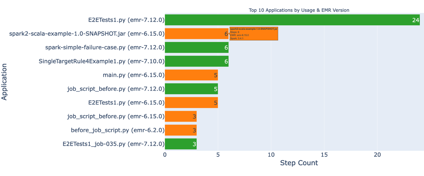

About the Authors

Ramesh Singh

Ramesh Singh

Ramesh is a Senior Product Manager Technical (External Services) at AWS in Seattle, Washington, currently with the Amazon SageMaker team. He is passionate about building high-performance ML/AI and analytics products that enable enterprise customers to achieve their critical goals using cutting-edge technology.

Pradeep Misra

Pradeep Misra

Pradeep is a Principal Analytics and Applied AI Solutions Architect at AWS. He is passionate about solving customer challenges using data, analytics, and AI/ML. Outside of work, he likes exploring new places, trying new cuisines, and playing badminton with his family. He also likes doing science experiments, building LEGOs, and watching anime with his daughters.
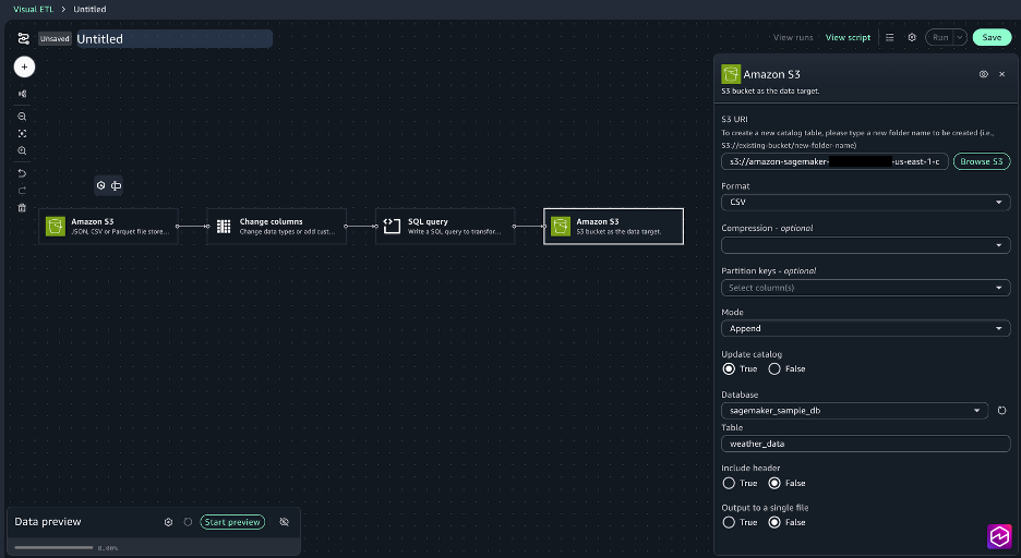
Abbas Makhdum

Abbas Makhdum

Abbas is Head of Product Marketing for Amazon SageMaker Catalog at AWS, where he leads go-to-market strategy and launches for data and AI governance solutions. With deep expertise across data, AI, and analytics, Abbas has also authored a book on data and AI governance with O’Reilly. He is passionate about helping organizations unlock business value by making data and AI more accessible, transparent, and governed.
Harish Panwar

Harish Panwar

Harish is a Software Development Manager at AWS in Bangalore, India. He is leading the Catalog engineering team, which is building data and AI governance solutions. Harish is a veteran in Amazon SageMaker, with deep expertise across SageMaker AI and SageMaker Catalog. He is passionate about creating simple and intuitive AI solutions making AI accessible to everyone.