AWS is committed to bringing you the most advanced foundation models (FMs) in the industry, continuously expanding our selection to include groundbreaking models from leading AI innovators so that you always have access to the latest advancements to drive your business forward.
These open weight models excel at coding, scientific analysis, and mathematical reasoning, with performance comparable to leading alternatives. Both models support a 128K context window and provide adjustable reasoning levels (low/medium/high) to match your specific use case requirements. The models support external tools to enhance their capabilities and can be used in an agentic workflow, for example, using a framework like Strands Agents.
With Amazon Bedrock and Amazon SageMaker JumpStart, AWS gives you the freedom to innovate with access to hundreds of FMs from leading AI companies, including OpenAI open weight models. With our comprehensive selection of models, you can match your AI workloads to the perfect model every time.
Through Amazon Bedrock, you can seamlessly experiment with different models, mix and match capabilities, and switch between providers without rewriting code—turning model choice into a strategic advantage that helps you continuously evolve your AI strategy as new innovations emerge. At launch, these new models are available in Bedrock via an OpenAI compatible endpoint. You can point the OpenAI SDK to this endpoint or use the Bedrock InvokeModel and Converse API.
With SageMaker JumpStart, you can quickly evaluate, compare, and customize models for your use case. You can then deploy the original or the customized model in production with the SageMaker AI console or using the SageMaker Python SDK.
Let’s see how these work in practice.
Getting started with OpenAI open weight models in Amazon Bedrock In the Amazon Bedrock console, I choose Model access from the Configure and learn section of the navigation pane. Then, I navigate to the two listed OpenAI models on this page and request access.
Now that I have access, I use the Chat/Test playground to test and evaluate the models. I select OpenAI as the category and then the gpt-oss-120b model.
Using this model, I run the following sample prompt:
A family has $5,000 to save for their vacation next year. They can place the money in a savings account earning 2% interest annually or in a certificate of deposit earning 4% interest annually but with no access to the funds until the vacation. If they need $1,000 for emergency expenses during the year, how should they divide their money between the two options to maximize their vacation fund?
This prompt generates an output that includes the chain of thought used to produce the result.
I can use these models with the OpenAI SDK by configuring the API endpoint (base URL) and using an Amazon Bedrock API key for authentication. For example, I set this environment variables to use the US West (Oregon) AWS Region endpoint (us-west-2) and my Amazon Bedrock API key:
Now I invoke the model using the OpenAI Python SDK.
client = OpenAI()

response = client.chat.completion.create(
    messages=[{
        "role": "user",
        "content": "Hello, how are you?"
    }],
    model="openai.gpt-oss-120b-1:0",
    stream=True
)

for item in response:
    print(item)
To build an AI agent, I can choose any framework that supports the Amazon Bedrock API or the OpenAI API. For example, here’s the starting code for Strands Agents using the Amazon Bedrock API:
from strands import Agent
from strands.models import BedrockModel
from strands_tools import calculator

model = BedrockModel(
    model_id="openai.gpt-oss-120b-1:0"
)
agent = Agent(
    model=model,
    tools=[calculator]
)

agent("Tell me the square root of 42 ^ 3")
I save the code (app.py file), install the dependencies, and run the agent locally:
When I am satisfied with the agent, I can deploy in production using the capabilities offered by Amazon Bedrock AgentCore, including a fully managed serverless runtime and memory and identity management.
Getting started with OpenAI open weight models in Amazon SageMaker JumpStart In the Amazon SageMaker AI console, you can use OpenAI open weight models in the SageMaker Studio. The first time I do this, I need to set up a SageMaker domain. There are options to set it up for a single user (simpler) or an organization. For these tests, I use a single user setup.
In the SageMaker JumpStart model view, I have access to a detailed description of the gpt-oss-120b or gpt-oss-20b model.
I choose the gpt-oss-20b model and then deploy the model. In the next steps, I select the instance type and the initial instance count. After a few minutes, the deployment creates an endpoint that I can then invoke in SageMaker Studio and using any AWS SDKs.
Each model comes equipped with full chain-of-thought output capabilities, providing you with detailed visibility into the model’s reasoning process. This transparency is particularly valuable for applications requiring high levels of interpretability and validation. These models give you the freedom to modify, adapt, and customize them to your specific needs. This flexibility allows you to fine-tune the models for your unique use cases, integrate them into your existing workflows, and even build upon them to create new, specialized models tailored to your industry or application.
Security and safety are built into the core of these models, with comprehensive evaluation processes and safety measures in place. The models maintain compatibility with the standard GPT-4 tokenizer.
Both models can be used in your preferred environment, whether that’s through the serverless experience of Amazon Bedrock or the extensive machine learning (ML) development capabilities of SageMaker JumpStart. For information about the costs associated with using these models and services, visit the Amazon Bedrock pricing and Amazon SageMaker AI pricing pages.
Many organizations running VMware workloads on premises want to move to the cloud to benefit from improved scalability, reliability, and access to cloud services, but migrating these workloads often requires substantial changes to applications and infrastructure configurations. Amazon EVS lets customers continue using their existing VMware expertise and tools without having to re-architect applications or change established practices, thereby simplifying the migration process while providing access to AWS’s scale, reliability, and broad set of services.
With Amazon EVS, you can run VMware workloads directly in your Amazon VPC. This gives you full control over your environments while being on AWS infrastructure. You can extend your on-premises networks and migrate workloads without changing IP addresses or operational runbooks, reducing complexity and risk.
Key capabilities and features
Amazon EVS delivers a comprehensive set of capabilities designed to streamline your VMware workload migration and management experience. The service enables seamless workload migration without the need for replatforming or changing hypervisors, which means you can maintain your existing infrastructure investments while moving to AWS. Through an intuitive, guided workflow on the AWS Management Console, you can efficiently provision and configure your EVS environments, significantly reducing the complexity to migrate your workloads to AWS.
With Amazon EVS, you can deploy a fully functional VCF environment running on AWS in a few hours. This process eliminates many of the manual steps and potential configuration errors that often occur during traditional deployments. Furthermore, with Amazon EVS you can optimize your virtualization stack on AWS. Given the VCF environment runs inside your VPC, you have full full administrative access to the environment and the associated management appliances. You also have the ability to integrate third-party solutions, from external storage such as Amazon FSx for NetApp ONTAP or Pure Cloud Block Store or backup solutions such as Veeam Backup and Replication.
The service also gives you the ability to self-manage or work with AWS Partners to build, manage, and operate your environments. This provides you with flexibility to match your approach with your overall goals.
Setting up a new VCF environment
Organizations can streamline their setup process by ensuring they have all the necessary pre-requisites in place ahead of creating a new VCF environment. These prerequisites include having an active AWS account, configuring the appropriate AWS Identity and Access Management (IAM) permissions, and setting up a Amazon VPC with sufficient CIDR space and two Route Server endpoints, with each endpoint having its own peer. Additionally, customers will need to have their VMware Cloud Foundation license keys ready, secure Amazon EC2 capacity reservations specifically for i4i.metal instances, and prepare their VLAN subnet information planning.
To help ensure a smooth deployment process, we’ve provided a Getting started hub, which you can access from the EVS homepage as well as a comprehensive guide in our documentation. By following these preparation steps, you can avoid potential setup delays and ensure a successful environment creation.
Let’s walk through the process of setting up a new VCF environment using Amazon EVS.
You will need to provide your Site ID, which is allocated by Broadcom when purchasing VCF licenses, along with your license keys. To ensure a successful initial deployment, you should verify you have sufficient licensing coverage for a minimum of 256 cores. This translates to at least four i4i.metal instances, with each instance providing 64 physical cores.
This licensing requirement helps you maintain optimal performance and ensures your environment meets the necessary infrastructure specifications. By confirming these requirements upfront, you can avoid potential deployment delays and ensure a smooth setup process.
Once you have provided all the required details, you will be prompted to specify your host details. These are the underlying Amazon EC2 instances that your VCF environment will get deployed in.
Once you have filled out details for each of your host instances, you will need to configure your networking and management appliance DNS details. For further information on how to create a new VCF environment on Amazon EVS, follow the documentation here.
After you have created your VCF environment, you will be able to look over all of the host and configuration details through the AWS Console.
Additional things to know
Amazon EVS currently supports VCF version 5.2.1 and runs on i4i.metal instances. Future releases will expand VCF versions, licensing options, and more instance type support to provide even more flexibility for your deployments.
Amazon EVS provides flexible storage options. Your Amazon EVS local Instance storage is powered by VMware’s vSAN solution, which pools local disks across multiple ESXi hosts into a single distributed datastore. To scale your storage, you can leverage external Network File System (NFS) or iSCSI-based storage solutions. For example, Amazon FSx for NetApp ONTAP is particularly well-suited for use as an NFS datastore or shared block storage over iSCSI.
Additionally, Amazon EVS makes connecting your on-premises environments to AWS simple. You can connect from on-premises vSphere environment into Amazon EVS using a Direct Connect connection or a VPN that terminates into a transit gateway. Amazon EVS also manages the underlying connectivity from your VLAN subnets into your VMs.
AWS provides comprehensive support for all AWS services deployed by Amazon EVS, handling direct customer support while engaging with Broadcom for advanced support needs. Customers must maintain AWS Business Support on accounts running the service.
Availability and pricing
Amazon EVS is now generally available in US East (N. Virginia), US East (Ohio), US West (Oregon), Europe (Frankfurt), Europe (Ireland), and Asia Pacific (Tokyo) AWS Regions, with additional Regions coming soon. Pricing is based on the Amazon EC2 instances and AWS resources you use, with no minimum fees or upfront commitments.
Our customers tell us that scientists are increasingly spending more time managing data-related challenges than focusing on science. The primary reason for this challenge is that scientific data comes in many types and is siloed across systems, groups, and stages, and scientists struggle to efficiently discover, access, share, and analyze datasets across silos. This fragmentation creates lengthy cycles full of manual interventions, leading to inefficiencies. Mapping data sources and negotiating access across silos can take 4–6 weeks, integrating datasets can extend to months, and fully connecting data from source to tooling can take years, if ever achieved. These data challenges reduce lab productivity and slow down scientific innovation, which decrease drug and product pipeline throughput, and ultimately delay time-to-market. The solution lies in breaking down data silos by creating digital environments that help scientists efficiently connect disparate datasets and analytical tools, so they can conduct iterative hypothesis and product testing without technology friction.
Part 1 of this series shows an example project in drug target identification where two groups of scientists need to collaborate as they integrate no-code knowledge searching, scientific data management, and sophisticated analytics. In this example, a computational biology team begins by mining the scientific literature on a knowledge search GUI. Next, they navigate to a data catalog to find and access relevant datasets, which they share with the data scientist team to run analytics with sophisticated tools (see the following figure). Although the end-to-end journey illustrates the benefits to a target identification example, the underlying data challenges and technology solution apply to any life sciences use case requiring the integration of data management and analytics. Details of the implementation and technical solution will be discussed in Part 2 of the series.
Example use case
A computational biologist has been tasked with identifying a target for Non-Alcoholic Fatty Liver Disease (NAFLD). A typical question from the biologist might be “Can I find genes associated with NAFLD and do we have a patient cohort with variants in those genes?” The solution we designed for this use case involves three simple steps:
Search the scientific literature through a no-code interface to identify genomic variants associated with NAFLD.
Search an internal data catalog with natural language:
Find datasets of interest, such as multi-omics and clinical data for patients associated with NAFLD.
Request access to the relevant datasets.
Share relevant datasets with a data scientist collaborator for deeper analysis.
In designing this solution, we focused on the following features:
Providing no-code scientists with point-and-click and natural-language interfaces
Reducing silos with data findability, governance automation, and seamless collaboration
Providing technical personas with the sophisticated tools and environments they prefer
SageMaker Catalog supports certain system asset types, such as tables from Amazon Redshift, tables from AWS Glue, and object collections from Amazon Simple Storage Service (Amazon S3). It also offers the ability to support custom asset types, which gives users flexibility to catalog data that can’t be categorized as a system asset type. For asset type S3ObjectCollectionType, see Implement a custom subscription workflow for unmanaged Amazon S3 assets published with Amazon DataZone. SageMaker Catalog also offers the ability to support custom asset types, which gives users flexibility to catalog data that can’t be categorized as a system asset type. For this example use case, we used AWS HealthOmics variant stores to store and allow querying of genomic variant data. This example lists HealthOmics variant stores as a custom asset type within the catalog. Details of the implementation and technical solution for access management will be discussed in Part 2 of the series.
In the example use case, a computational biologist, in order to identify a target for NAFLD, relies heavily on diverse datasets from multiple sources (genomic sequences, gene expression data, clinical records, and more). This data comes from both internal sources (first-party) and external partners or public databases (third-party). Multiple teams are responsible for collecting and processing this data before making it available to computational biologists, researchers, data scientists, and bioinformaticians within the organization.
In this solution, users (data engineers, data scientists, bioinformaticians, computational biologists) log in to a project-based environment from SageMaker Unified Studio with a preconfigured authentication method. A typical workflow involves the following steps:
Data stewards as authorized members of projects publish data assets into the SageMaker catalog.
Data consumers as authorized members of projects seeking to analyze data for their scientific needs find and discover available data assets of interest from the SageMaker catalog.
Data consumers request to subscribe to the relevant discovered data assets.
Data producers review and decide to approve or reject the subscription request.
Data consumers access and analyze the data using preconfigured tools from SageMaker Unified Studio.
The following diagram illustrates the solution architecture and workflow.
In the following sections, we explore each step of the workflow in more detail.
Step 1: Data producers publish data assets
As shown in the preceding workflow diagram, data producers can use SageMaker Catalog to publish their datasets as data assets or data products with appropriate business (such as source, license, vendor, study identifier), scientific (such as disease name, cohort information, data modality, assay type), or technical (file types, data formats, file sizes) metadata. In our example use case, the data producers publish clinical data as AWS Glue tables and genomic variant data as a table within the HealthOmics variant store. Additionally, data producers can use AI-based recommendations to automatically populate descriptors, making it straightforward for consumers to find and understand its use.
Step 2: Data consumers find relevant datasets
Data consumers, such as data scientists and bioinformaticians, can log in to SageMaker Unified Studio and navigate to SageMaker Catalog to search for the appropriate data assets and products, such as “NAFLD Variants” or “NAFLD Clinical.” They can also find data assets or products using metadata filters such as study identifiers or disease names to discover the possible datasets associated with a study or disease.
Step 3: Data consumers subscribe to required data assets or products
After the data consumers see a data asset or data product of interest (for example, the clinical and genomics data for NAFLD), they can subscribe to them. Data consumers can also optionally include a comment in the subscription request to add more context to the request. This initiates the subscription workflow based on the asset type.
Step 4: Data producers review and approve the subscription request
Data producers get notified of subscription requests and review if access should be granted and approve accordingly. The response can optionally include a comment for reasoning and traceability. In addition, data producers can limit access to certain rows and columns to protect controlled data.
Step 5: Data consumers access the subscribed data assets or products
Upon approval from the data producer, the data consumer gets access to those data assets and can use them in the appropriate environments configured within their project. For example, data scientists can open a workspace with a JupyterLab notebook already available within SageMaker Unified Studio. Subsequently, the data scientist can start analyzing the tabular clinical and variant data that was just approved for access.
Conclusion
The next generation of SageMaker transforms how scientists work with data by creating an integrated data and analytics environment. In this unified environment, data producers are empowered to publish datasets with rich metadata. Data consumers are able to use the catalog within SageMaker Unified Studio to search for their required datasets, either using free text or using metadata and business glossary filters. Data consumers can subscribe to data securely, tap into powerful search capabilities using free text or metadata filters, and access essential analysis tools (Amazon Athena, JupyterLab IDE, Amazon EMR) directly. The result is a unified digital workspace that reduces communication bottlenecks, speeds up scientific cycles, and removes technical barriers. Scientists can now focus on what matters most—testing hypotheses and products, and scaling scientific innovation to production—within a unified, powerful platform. This streamlined approach accelerates data-driven science, enabling research institutions, pharmaceutical companies, and clinical laboratories to innovate more efficiently. For example, data scientists can launch a space with a JupyterLab notebook preinstalled.
Consider using the next generation of SageMaker to increase productivity within your organization. Contact your account representatives or an AWS Representative to learn how we can help accelerate your projects and your business.
About the authors
Nadeem Bulsara is a Principal Solutions Architect at AWS specializing in Genomics and Life Sciences. He brings his 13+ years of Bioinformatics, Software Engineering, and Cloud Development skills as well as experience in research and clinical genomics and multi-omics to help Healthcare and Life Sciences organizations globally. He is motivated by the industry’s mission to enable people to have a long and healthy life.
Chaitanya Vejendla is a Senior Solutions Architect specialized in DataLake & Analytics primarily working for Healthcare and Life Sciences industry division at AWS. Chaitanya is responsible for helping life sciences organizations and healthcare companies in developing modern data strategies, deploy data governance and analytical applications, electronic medical records, devices, and AI/ML-based applications, while educating customers about how to build secure, scalable, and cost-effective AWS solutions. His expertise spans across data analytics, data governance, AI, ML, big data, and healthcare-related technologies.
Dr. Mileidy Giraldo has over 20 years of experience bridging bioinformatics, research, and industry technology strategy. She specializes in making technology accessible for organizations in the life sciences sector. In her current role as WW Lead for Life Sciences Strategy and Lab of the Future at AWS, she helps biotechs, biopharma, and diagnostics organizations design Data & AI-driven initiatives that modernize labs and help scientists unlock the full value of their data.
Chris Clark is a Senior Solutions Architect focused on helping Life Science customers leverage AWS technology to advance their operational capabilities. With 20+ years of hands-on experience in life sciences manufacturing and supply chain, he combines deep industry knowledge with his AWS expertise to guide his customers. When he’s not working to solve customer challenges, he enjoys cycling and building and repairing things in his workshop.
Nick Furr is a Specialist Solutions Architect at AWS, supporting Data & Analytics for Healthcare and Life Sciences. He helps providers, payers, and life sciences organizations build secure, scalable data platforms to drive innovation and improve outcomes. His work focuses on modernizing data strategies through cloud analytics, governed data processing, and machine learning for use cases like clinical research and population health.
Subrat Das is a Principal Solutions Architect for Global Healthcare and Life Sciences accounts at AWS. He is passionate about modernizing and architecting complex customers workloads. When he’s not working on technology solutions, he enjoys long hikes and traveling around the world.
This week brings an array of innovations spanning from generative AI capabilities to enhancements of foundational services. Whether you’re building AI-powered applications, managing databases, or optimizing your cloud infrastructure, these updates help build more advanced, robust, and flexible applications.
Last week’s launches Here are the launches that got my attention this week:
Amazon Q Developer CLI – You can now create custom agents to help you customize the CLI agent to be more effective when performing specialized tasks such as code reviews and troubleshooting. More info in this blog.
AWS Lambda – Response streaming now supports a default maximum response payload size of 200 MB, 10 times higher than before. Lambda response streaming helps you build applications that progressively stream response payloads back to clients, improving performance for latency sensitive workloads by reducing time to first byte (TTFB) performance.
Powertools for AWS – Introducing v2 of Powertools for AWS Lambda (Java), a developer toolkit that helps you implement serverless best practices and directly translates AWS Well-Architected recommendations.
Amazon SNS – Now supports three additional message filtering operators: wildcard matching, anything-but wildcard matching, and anything-but prefix matching. SNS now also supports message group IDs in standard topics, enabling fair queue functionality for subscribed Amazon SQS standard queues.
Amazon CloudFront – Now offers two capabilities to enhance origin timeout controls: a response completion timeout and support for custom response timeout values for Amazon S3 origins. These capabilities give you more control over how to handle slow or unresponsive origins.
Amazon EC2 Auto Scaling – You can now use AWS Lambda functions as notification targets for EC2 Auto Scaling lifecycle hooks. For example, you can use this to trigger custom actions when an instance enters a wait state.
AWS Clean Rooms – Now publishes events to Amazon EventBridge for status changes in a Clean Rooms collaboration, further simplifying how companies and their partners analyze and collaborate on their collective datasets without revealing or copying one another’s underlying data.
Upcoming AWS events Check your calendars so that you can sign up for these upcoming events:
AWS re:Invent 2025 (December 1-5, 2025, Las Vegas) — AWS’s flagship annual conference offering collaborative innovation through peer-to-peer learning, expert-led discussions, and invaluable networking opportunities.
AWS Summits — Join free online and in-person events that bring the cloud computing community together to connect, collaborate, and learn about AWS. Register in your nearest city: Mexico City (August 6) and Jakarta (August 7).
AWS Community Days — Join community-led conferences that feature technical discussions, workshops, and hands-on labs led by expert AWS users and industry leaders from around the world: Australia (August 15), Adria (September 5), Baltic (September 10), and Aotearoa (September 18).
As a developer advocate at AWS, I’ve worked with many enterprise organizations who operate critical applications across multiple AWS Regions. A key concern they often share is the lack of confidence in their Region failover strategy—whether it will work when needed, whether all dependencies have been identified, and whether their teams have practiced the procedures enough. Traditional approaches often leave them uncertain about their readiness for Regional switch.
Today, I’m excited to announce Amazon Application Recovery Controller (ARC) Region switch, a fully managed, highly available capability that enables organizations to plan, practice, and orchestrate Region switches with confidence, eliminating the uncertainty around cross-Region recovery operations. Region switch helps you orchestrate recovery for your multi-Region applications on AWS. It gives you a centralized solution to coordinate and automate recovery tasks across AWS services and accounts when you need to switch your application’s operations from one AWS Region to another.
Many customers deploy business-critical applications across multiple AWS Regions to meet their availability requirements. When an operational event impacts an application in one Region, switching operations to another Region involves coordinating multiple steps across different AWS services, such as compute, databases, and DNS. This coordination typically requires building and maintaining complex scripts that need regular testing and updates as applications evolve. Additionally, orchestrating and tracking the progress of Region switches across multiple applications and providing evidence of successful recovery for compliance purposes often involves manual data gathering.
Region switch is built on a Regional data plane architecture, where Region switch plans are executed from the Region being activated. This design eliminates dependencies on the impacted Region during the switch, providing a more resilient recovery process since the execution is independent of the Region you’re switching from.
Building a recovery plan with ARC Region switch With ARC Region switch, you can create recovery plans that define the specific steps needed to switch your application between Regions. Each plan contains execution blocks that represent actions on AWS resources. At launch, Region switch supports nine types of execution blocks:
ARC Region switch plan execution block–let you orchestrate the order in which multiple applications switch to the Region you want to activate by referencing other Region switch plans.
Amazon EC2 Auto Scaling execution block–Scales Amazon EC2 compute resources in your target Region by matching a specified percentage of your source Region’s capacity.
ARC routing controls execution block–Changes routing control states to redirect traffic using DNS health checks.
Amazon Aurora global database execution block–Performs database failover with potential data loss or switchover with zero data loss for Aurora Global Database.
Manual approval execution block–Adds approval checkpoints in your recovery workflow where team members can review and approve before proceeding.
Custom Action AWS Lambda execution block–Adds custom recovery steps by executing Lambda functions in either the activating or deactivating Region.
Amazon Route 53 health check execution block–Let you to specify which Regions your application’s traffic will be redirected to during failover. When executing your Region switch plan, the Amazon Route 53 health check state is updated and traffic is redirected based on your DNS configuration.
Amazon Elastic Kubernetes Service (Amazon EKS) resource scaling execution block–Scales Kubernetes pods in your target Region during recovery by matching a specified percentage of your source Region’s capacity.
Amazon Elastic Container Service (Amazon ECS) resource scaling execution block–Scales ECS tasks in your target Region by matching a specified percentage of your source Region’s capacity.
Region switch continually validates your plans by checking resource configurations and AWS Identity and Access Management (IAM) permissions every 30 minutes. During execution, Region switch monitors the progress of each step and provides detailed logs. You can view execution status through the Region switch dashboard and at the bottom of the execution details page.
To help you balance cost and reliability, Region switch offers flexibility in how you prepare your standby resources. You can configure the desired percentage of compute capacity to target in your destination Region during recovery using Region switch scaling execution blocks. For critical applications expecting surge traffic during recovery, you might choose to scale beyond 100 percent capacity, and setting a lower percentage can help achieve faster overall execution times. However, it’s important to note that using one of the scaling execution blocks does not guarantee capacity, and actual resource availability depends on the capacity in the destination Region at the time of recovery. To facilitate the best possible outcomes, we recommend regularly testing your recovery plans and maintaining appropriate Service Quotas in your standby Regions.
ARC Region switch includes a global dashboard you can use to monitor the status of Region switch plans across your enterprise and Regions. Additionally, there’s a Regional executions dashboard that only displays executions within the current console Region. This dashboard is designed to be highly available across each Region so it can be used during operational events.
Region switch allows resources to be hosted in an account that is separate from the account that contains the Region switch plan. If the plan uses resources from an account that is different from the account that hosts the plan, then Region switch uses the executionRole to assume the crossAccountRole to access those resources. Additionally, Region switch plans can be centralized and shared across multiple accounts using AWS Resource Access Manager (AWS RAM), enabling efficient management of recovery plans across your organization.
Let’s see how it works Let me show you how to create and execute a Region switch plan. There are three parts in this demo. First, I create a Region switch plan. Then, I define a workflow. Finally, I configure the triggers.
Step 1: Create a plan
I navigate to the Application Recovery Controller section of the AWS Management Console. I choose Region switch in the left navigation menu. Then, I choose Create Region switch plan.
After I give a name to my plan, I specify a Multi-Region recovery approach (active/passive or active/active). In Active/Passive mode, two application replicas are deployed into two Regions, with traffic routed into the active Region only. The replica in the passive Region can be activated by executing the Region switch plan.
Then, I select the Primary Region and Standby Region. Optionally, I can enter a Desired recovery time objective (RTO). The service will use this value to provide insight into how long Region switch plan executions take in relation to my desired RTO.
I enter the Plan execution IAM role. This is the role that allows Region switch to call AWS services during execution. I make sure the role I choose has permissions to be invoked by the service and contains the minimum set of permissions allowing ARC to operate. Refer to the IAM permissions section of the documentation for the details.
Step 2: Create a workflow
When the two Plan evaluation status notifications are green, I create a workflow. I choose Build workflows to get started.
Plans enable you to build specific workflows that will recover your applications using Region switch execution blocks. You can build workflows with execution blocks that run sequentially or in parallel to orchestrate the order in which multiple applications or resources recover into the activating Region. A plan is made up of these workflows that allow you to activate or deactivate a specific Region.
For this demo, I use the graphical editor to create the workflow. But you can also define the workflow in JSON. This format is better suited for automation or when you want to store your workflow definition in a source code management system (SCMS) and your infrastructure as code (IaC) tools, such as AWS CloudFormation.
I can alternate between the Design and the Code views by selecting the corresponding tab next to the Workflow builder title. The JSON view is read-only. I designed the workflow with the graphical editor and I copied the JSON equivalent to store it alongside my IaC project files.
Region switch launches an evaluation to validate your recovery strategy every 30 minutes. It regularly checks that all actions defined in your workflows will succeed when executed. This proactive validation assesses various elements, including IAM permissions and resource states across accounts and Regions. By continually monitoring these dependencies, Region switch helps ensure your recovery plans remain viable and identifies potential issues before they impact your actual switch operations.
However, just as an untested backup is not a reliable backup, an untested recovery plan cannot be considered truly validated. While continuous evaluation provides a strong foundation, we strongly recommend regularly executing your plans in test scenarios to verify their effectiveness, understand actual recovery times, and ensure your teams are familiar with the recovery procedures. This hands-on testing is essential for maintaining confidence in your disaster recovery strategy.
Step 3: Create a trigger
A trigger defines the conditions to activate the workflows just created. It’s expressed as a set of CloudWatch alarms. Alarm-based triggers are optional. You can also use Region switch with manual triggers.
From the Region switch page in the console, I choose the Triggers tab and choose Add triggers.
For each Region defined in my plan, I choose Add trigger to define the triggers that will activate the Region.Finally, I choose the alarms and their state (OK or Alarm) that Region switch will use to trigger the activation of the Region.
I’m now ready to test the execution of the plan to switch Regions using Region switch. It’s important to execute the plan from the Region I’m activating (the target Region of the workflow) and use the data plane in that specific Region.
Pricing and availability Region switch is available in all commercial AWS Regions at $70 per month per plan. Each plan can include up to 100 execution blocks, or you can create parent plans to orchestrate up to 25 child plans.
Having seen firsthand the engineering effort that goes into building and maintaining multi-Region recovery solutions, I’m thrilled to see how Region switch will help automate this process for our customers. To get started with ARC Region switch, visit the ARC console and create your first Region switch plan. For more information about Region switch, visit the Amazon Application Recovery Controller (ARC) documentation. You can also reach out to your AWS account team with questions about using Region switch for your multi-Region applications.
I look forward to hearing about how you use Region switch to strengthen your multi-Region applications’ resilience.
Modern applications increasingly rely on Serverless technologies such as Amazon Web Services (AWS) Lambda to provide scalability, cost efficiency, and agility. The Serverless Applications Lens for the AWS Well-Architected Framework focuses on how to design, deploy, and architect your Serverless applications to overcome some of these challenges.
Powertools for AWS Lambda is a developer toolkit that helps you implement Serverless best practices and directly translates AWS Well-Architected recommendations into actionable, developer friendly utilities. Following the community’s continued successful adoption of Powertools for AWS in Python, Java, TypeScript, and .NET, this post announces the general availability of Powertools for AWS Lambda (Java) v2 coming with major performance improvements, enhanced core utilities, and a brand-new Kafka utility.
Powertools for AWS (Java) v2 provides three updated core utilities:
Logging: A re-designed Java idiomatic logging module providing structured logging that streamlines log aggregation and analysis.
Tracing: An annotation-based way to collect distributed tracing data with AWS X-Ray to visualize and analyze request flows.
Along with the updated core utilities, v2 of the developer toolkit adds two brand new features:
GraalVM native image support: Native image support for GraalVM across all core utilities reducing Lambda cold start times up to 75.61% (p95).
Kafka utility: This new utility integrates with Amazon Managed Streaming for Apache Kafka (Amazon MSK) and self-managed Kafka event sources on Lambda and allows developers to deserialize directly into Kafka native types such as ConsumerRecords.
Learn more about how to migrate to v2 in our upgrade guide.
Getting started using Powertools for AWS Lambda (Java) v2
Powertools for AWS Lambda (Java) v2 is readily accessible as a Java package on Maven Central and integrates with popular build tools such as Maven and Gradle. This post focuses on Maven-based implementation samples to help you get started quickly. Gradle examples are available for all utilities in the documentation and the examples repository.
The toolkit is compatible with Java 11 and newer versions, making sure you can use modern Java features while building Serverless applications. Examples on how to install each utility are outlined in each section of the post and complete configuration examples are also available in the Powertools documentation.
Logging
The Logging utility helps implement structured logging when running on Lambda while still using familiar Java logging libraries such as slf4j, log4j, and logback. v2 of Logging allows you to do the following:
Output structured JSON logs enriched with Lambda context
Choose the logging backend of your choice among log4j2 and logback
Add structured arguments to logs that get serialized into arbitrarily nested JSON objects
To add the logging utility to your project, include it as a dependency in your Java Maven project. The following example shows how to add the log4j2 logging backend to your application:
<!-- In the dependencies section -->
<dependency>
    <groupId>software.amazon.lambda</groupId>
    <artifactId>powertools-logging-log4j</artifactId>
    <!-- Alternatively, if you wish to use the logback backend
    <artifactId>powertools-logging-logback</artifactId>
    -->
    <version>2.1.1</version>
</dependency>
<!-- In the build plugins section -->
<plugin>
    <groupId>dev.aspectj</groupId>
    <artifactId>aspectj-maven-plugin</artifactId>
    <configuration>
        <aspectLibraries>
            <aspectLibrary>
                <groupId>software.amazon.lambda</groupId>
                <artifactId>powertools-logging</artifactId>
                <version>2.1.1</version>
            </aspectLibrary>
        </aspectLibraries>
    </configuration>
</plugin>
Create a custom JsonTemplateLayout appender in your log4j2.xml file:
To add structured logging to your functions, apply the @Logging annotation to your Lambda handler and use the familiar slf4j Java API when writing log statements. This allows you to adopt the logging utility without major code refactoring. Powertools handles routing to the correct logging backend for you. The following example shows how to add global log keys using MDC, and add a structured entry argument to your log message:
public class App implements RequestHandler<SQSEvent, String> {
    private static final Logger log = LoggerFactory.getLogger(App.class);

    @Logging
    public String handleRequest(final SQSEvent input, final Context context) {
        // Add a global log key using Mapped Diagnostic Context MDC
        MDC.put("myCustomKey", "willBeLoggedForAllLogStatements");

        // Log a message with a structured argument (any JSON serializable Object)
        log.info("My message", entry("anotherCustomKey", Map.of("nested", "object")));

        // ... return response
    }
}
Lambda sends the following JSON-formatted output to Amazon CloudWatch Logs (note how the Java Map gets auto-serialized into a JSON object):
CloudWatch offers essential built-in service metrics for monitoring application throughput, error rates, and resource usage. Users also need to capture workload specific custom metrics relevant to their business use-case following AWS Well-Architected best-practices.
Powertools for AWS (Java) enables you to create custom metrics asynchronously by outputting metrics in CloudWatch EMF directly to standard output—an approach that needs no other configuration. The Lambda service sends the EMF formatted metrics to CloudWatch on your behalf.
The Metrics utility allows you to:
Create custom metrics asynchronously using CloudWatch EMF
Reduce latency by avoiding synchronous metric publishing
Automatically track cold starts in a custom CloudWatch metric
Avoid manually validating your output against the EMF specification
Keep you code clean by avoiding manual flushing to standard output
To add the Metrics utility to your project, add the following Maven dependency:
<!-- In the dependencies section -->
<dependency>
    <groupId>software.amazon.lambda</groupId>
    <artifactId>powertools-metrics</artifactId>
    <version>2.1.1</version>
</dependency>
<!-- In the build plugins section -->
<plugin>
    <groupId>dev.aspectj</groupId>
    <artifactId>aspectj-maven-plugin</artifactId>
    <configuration>
        <aspectLibraries>
            <aspectLibrary>
                <groupId>software.amazon.lambda</groupId>
                <artifactId>powertools-metrics</artifactId>
                <version>2.1.1</version>
            </aspectLibrary>
        </aspectLibraries>
    </configuration>
</plugin>
To add custom metrics to your Lambda function, place the @FlushMetrics annotation on your Lambda handler. The library takes care of validating and flushing your metrics to standard output before the Lambda function terminates. The following example shows how you can automatically capture a cold start metric and emit your own custom metrics:
public class App implements RequestHandler<SQSEvent, String> {
    private static final Logger log = LoggerFactory.getLogger(App.class);
    private static final Metrics metrics = MetricsFactory.getMetricsInstance();

    // This configures a default namespace and service dimension for all metrics
    @FlushMetrics(namespace = "ServerlessAirline", service = "payment", captureColdStart = true)
    public String handleRequest(final SQSEvent input, final Context context) {
        // The Metrics instance is a singleton
        metrics.addMetric("CustomMetric1", 1, MetricUnit.COUNT);

        // Publish metrics with non-default configuration options
        DimensionSet dimensionSet = new DimensionSet();
        dimensionSet.addDimension("Service", "AnotherService");
        metrics.flushSingleMetric("CustomMetric2", 1, MetricUnit.COUNT, "AnotherNamespace", dimensionSet);

        // ... return response
    }
}
Figure 1. AWS CloudWatch Metrics Graph View
Tracing
The Tracing utility provides an annotation-based integration with X-Ray for distributed tracing with minimal configuration. Tracing allows you to:
Gain visibility into your own methods calls and AWS service interactions visualized in the X-Ray console
Automatically capture method responses and errors
Automatically capture Lambda cold start information as part of your traces
Add custom metadata to traces for more context and debugging information
Enable or disable tracing features through environment variables without code changes
To add the Tracing utility to your project, add the following Maven dependency:
<!-- In the dependencies section -->
<dependency>
    <groupId>software.amazon.lambda</groupId>
    <artifactId>powertools-tracing</artifactId>
    <version>2.1.1</version>
</dependency>
<!-- In the build plugins section -->
<plugin>
    <groupId>dev.aspectj</groupId>
    <artifactId>aspectj-maven-plugin</artifactId>
    <configuration>
        <aspectLibraries>
            <aspectLibrary>
                <groupId>software.amazon.lambda</groupId>
                <artifactId>powertools-tracing</artifactId>
                <version>2.1.1</version>
            </aspectLibrary>
        </aspectLibraries>
    </configuration>
</plugin>
To enable tracing in your Lambda function, annotate your Lambda handler and your custom methods that you want to trace with the @Tracing annotation. Each annotation maps to a sub-segment of your main Lambda handler in X-Ray and becomes visible in the console.
public class App implements RequestHandler<APIGatewayProxyRequestEvent, APIGatewayProxyResponseEvent> {
    private static final Logger log = LoggerFactory.getLogger(App.class);

    @Tracing
    public APIGatewayProxyResponseEvent handleRequest(final APIGatewayProxyRequestEvent input, final Context context) {
        // ... business logic

        // Get calling IP with tracing
        String location = getCallingIp("https://checkip.amazonaws.com");

        // ... return response
    }

    @Tracing(segmentName = "Location service")
    private String getCallingIp(String address) {
        // Implementation to get IP address
        log.info("Retrieving caller IP address");

        // Add custom metadata to current sub-segment
        URL url = new URL(address);
        putMetadata("getCallingIp", address);

        // ...
        return "127.0.0.1";
    }
}
The X-Ray console displays a generated service map when traffic begins flowing through your application. Applying the Tracing annotation to your Lambda function handler method or any other methods in the execution chain provides you with comprehensive visibility into the traffic patterns throughout your application. The following figure shows how the custom metadata added in the example is associated with the custom sub-segment.
Figure 2. AWS X-Ray waterfall trace view
Reducing Lambda cold start duration
A key feature in Powertools for AWS Lambda (Java) v2 is GraalVM native image support for all core utilities. Compiling your Lambda functions to native executables allows you to significantly reduce cold start times and memory usage. Using Powertools v2 with GraalVM allows you to reduce cold starts up to 75.61% (p95) compared to using the managed Java runtime. The following benchmark compares the cold start times of an application using all core utilities (logging, metrics, tracing) on the managed java21 runtime as compared to the Lambda provided.al2023 runtime running a GraalVM compiled native image (go to the supported Lambda runtimes):
Environment
p95 (ms)
Min (ms)
Avg (ms)
Max (ms)
Max Memory (MB)
N
Powertools for AWS (Java) v2: JVM
1682.92
1224.55
1224.55
2229.81
205.04
234
Powertools for AWS (Java) v2: GraalVM
542.86
404.92
504.77
752.85
93.46
369
This improvement is particularly valuable for latency-sensitive applications and functions that scale frequently. Check out a full working example on GitHub.
Lambda MSK Event Source Mapping Integration
The new Kafka utility introduced with Powertools for AWS Lambda (Java) v2 streamlines working with the Lambda MSK Event Source Mapping (ESM) and self-managed Kafka event sources. It provides a familiar experience for developers working with Apache Kafka by allowing direct conversion from Lambda events to Kafka’s native types. The key features include:
Direct deserialization into Kafka ConsumerRecords<K, V> objects while using the Lambda-native RequestHandler interface
Support for deserializing JSON, Avro, and Protobuf encoded records for key and value fields with and without usage of a Schema Registry when producing the messages
To add the Kafka utility to your project, include the powertools-kafka library as a Maven dependency in your pom.xml:
<!-- In the dependencies section -->
<dependency>
    <groupId>software.amazon.lambda</groupId>
    <artifactId>powertools-kafka</artifactId>
    <version>2.1.1</version>
</dependency>
<!-- Kafka clients dependency - compatibility works for >= 3.0.0 -->
<dependency>
    <groupId>org.apache.kafka</groupId>
    <artifactId>kafka-clients</artifactId>
    <version>4.0.0</version>
</dependency>
Use the @Deserialization annotation on your Lambda handler to deserialize messages as native Kafka ConsumerRecords. Make sure to specify the deserializer type. The following example shows how to deserialize Avro encoded record values with String keys. As in a regular Lambda handler, declare the input type to your function in the RequestHandler generic parameters and the utility discovers the deserialization types automatically. The AvroProduct class in the following example is an auto-generated Java class using the Java org.apache.avro.avro library.
public class App implements RequestHandler<ConsumerRecords<String, AvroProduct>, Void> {
    private static final Logger log = LoggerFactory.getLogger(App.class);

    @Deserialization(type = DeserializationType.KAFKA_AVRO)
    public Void handleRequest(ConsumerRecords<String, AvroProduct> consumerRecords, Context context) {
        log.info("Deserialized {} records.", consumerRecords.records().size());

        // ... Business logic

        return null;
    }
}
Conclusion
Powertools for AWS Lambda (Java) v2 represents the next evolution in the toolkit for building robust, observable, and high-performing Serverless applications. Throughout this post, we’ve explored the enhanced core observability utilities with their new features, the performance gains through GraalVM native image support, and the new Kafka utility that supports using familiar Kafka patterns when working on Lambda.
Powertools also offers more utilities to handle common Serverless design patterns. Each utility is designed with the same principles of clarity and minimal overhead.To learn more:
Visit the documentation for detailed guides and examples
As a developer who has embraced the power of the Model Context Protocol (MCP)to enhance my workflows, I’m thrilled to see the addition of custom agents in the Amazon Q Developer CLI. This new feature takes the capabilities I’ve come to rely on to a whole new level, allowing me to seamlessly manage different development contexts and easily switch between them.
In my previous post, I discussed how MCP servers have revolutionized the way I interact with AWS services, databases, and other essential tools. MCP integration in Amazon Q Developer allows me to query my database schemas, automate infrastructure deployments, and so much more. However, as I started juggling multiple projects, each with their own unique tech stacks and requirements, I found myself needing a more structured approach to managing these diverse development environments.
Enter custom agents. With this new feature, I can now create and use a custom agent by bringing together specific tools, prompt, context and tool permissions for tasks appropriate for the stage of development. In this post I will explain how to configure a cusom agent for front-end and back-end development. Allowing me to easily optimize Amazon Q Developer for each task.
Background
Imagine that I am working on a multi-tier web application. The application has a React front-end written in Typescript and a FastAPI back-end written in Python. In addition to me, the team includes a designer that uses Figma, and the database administrator that manages a PostgreSQL database. There are subtle differences in how I communicate with the designer and the database administrator. For example, when I discuss a “table” with the designer, I’m likely referring to an HTML table and how the page is structured. However, when I discuss a table with the database administrator, I’m likely talking about a SQL table and how data is stored.
In the past, I had both the Figma Dev Mode MCP server and Amazon Aurora PostgreSQL MCP server configured in my environment. While this allowed me to easily work on either the front-end or back-end code, it introduced some challenges. If I asked Amazon Q Developer “how many tables do I have?” Amazon Q Developer would have to guess if I was talking about HTML tables or SQL tables. If the question is about HTML, it should use the Figma server. If the question is about SQL, it should use the Aurora server. This is not a technical limitation, it’s a language limitation. Just as I have to adjust my assumptions to talk with the designer and database administrator, Amazon Q Developer has to make the same adjustments.
Enter Amazon Q Developer CLI custom agents. Custom agents allow me to optimize Q Developer’s configuration for each scenario. Let’s walk through my front-end and back-end configuration to understand the impact.
Front-end agent
My front-end custom agent is optimized for front-end web development using React and Figma. The following code example is the configuration for my front-end agent stored in ~/.aws/amazonq/agents/front-end.json. Let’s discuss the major sections of the configuration.
mcpServers – Here I have configured the Figma Dev Mode MCP Server. This simply communicates with the Figma Web Design App installed locally. Note that this replaces the MCP configuration that was stored in ~/.aws/amazonq/mcp.json
tools and allowedTools – These two sections are related, so I will discuss them together. tools defines the tools are available to Amazon Q Developer while allowedTools defines which tools are trusted. In other words, Q Developer is able to use all configured tools, and it does not have to ask my permission to use fs_read, fs_write, and @Figma. @Figma allows Amazon Q Developer to use all Figma tools without asking for permission. More on this in the next section.
resources – Here I have configured the files that should be added to the context. I have included the README.md (stored in the project folder) and my own preferences for React (stored in my profile). You can read more in the context management section of the user guide.
hooks – In addition to the resources, I have also included a hook. This hook will run a command and inject it into the context at runtime. In the example, I am adding the current git status. You can read more in the context hooks section of the user guide.
{
  "description": "Optimized for front-end web development using React and Figma",
  "mcpServers": {
    "Figma": {
      "command": "npx",
      "args": [
        "mcp-remote",
        "http://127.0.0.1:3845/sse"
      ]
    }
  },
  "tools": ["*"],
  "allowedTools": [
    "fs_read",
    "fs_write",
    "report_issues",
    "@Figma"
  ],
  "resources": [
    "file://README.md",
    "file://~/.aws/amazonq/react-preferences.md"
  ],
  "hooks": {
    "agentSpawn": [
      {
        "command": "git status"
      }
    ]
  }
}
Back-end agent
My back-end custom agent is optimized for back-end development with Python and PostgreSQL. The following code example is the configuration for my back-end agent stored in ~/.aws/amazonq/agents/back-end.json. Rather than describing the sections, as I did earlier, I will focus on the differences between the front-end and back-end.
mcpServers – Here I have configured the Amazon Aurora PostgreSQL MCP Server. This allows Amazon Q Developer to query my dev database to learn about the schema. Notice that I have configured a read-only connection to ensure that I don’t accidentally update the database.
tools and allowedTools – Once again, I have enabled Amazon Q Developer to use all tools. However, notice that I am more restrictive about what tools are trusted. Amazon Q Developer will need to ask permission to use fs_write or @PostgreSQL/run_query. Notice that I can allow the entire MCP server as I did with Figma or specific tools as I did here.
resources – Again, I have included the README.md (stored in the project folder) and my own preferences for Python and SQL (both stored in my profile). Note that I can also use glob patterns here. For example, file://.amazonq/rules/**/*.md would include the rules created by the Amazon Q Developer IDE plugins.
hooks – Finally, I have also included the hook for the front-end and back-end. However, I could have included project specific options such as npm run for the front-end and pip freeze for the back-end.
The real power of agents becomes evident when I need to switch between these different development contexts. I can now simply run q chat --agent front-end when I am working on React and Figma or q chat --agent back-end when I am working with Python and SQL. Amazon Q Developer will configure the correct agent with all my preferences.
In the following image, you can see the configuration in the Amazon Q Developer CLI. Notice that the front-end agent has an additional tool called Figma while the back-end agent has an additional tool called PostgreSQL. In addition, the front-end agent trusts fs_write and all of the Figma tools while the back-end agent will ask permission to use fs_write and only trusts one of the two PostgreSQL tools.
Similarly, let’s look at the context configuration in both the front-end and back-end agents. In the following image, I have included my React preferences for front-end development, and both Python and SQL preferences for back-end development.
As you can see, custom agents allow me to optimize the Amazon Q Developer CLI for each task. Of course, front-end and back-end agents are just an example. You might have a developer and testing agents, data science and analytics agents, etc. Custom agents allow you to tailor the configuration to most any task.
Conclusion
Amazon Q Developer CLI custom agents represent a significant improvement in managing complex development environments. By allowing developers to seamlessly switch between different contexts, they eliminate the cognitive overhead of manually reconfiguring tools and permissions for different tasks. Ready to streamline your development workflow? Get started with Amazon Q Developer today.
Today, we’re announcing the general availability of Amazon DocumentDB Serverless, a new configuration for Amazon DocumentDB (with MongoDB compatibility) that automatically scales compute and memory based on your application’s demand. Amazon DocumentDB Serverless simplifies database management with no upfront commitments or additional costs, offering up to 90 percent cost savings compared to provisioning for peak capacity.
With Amazon DocumentDB Serverless, you can use the same MongoDB compatible-APIs and capabilities as Amazon DocumentDB, including read replicas, Performance Insights, I/O optimized, and integrations with other Amazon Web Services (AWS) services.
Amazon DocumentDB Serverless introduces a new database configuration measured in a DocumentDB Capacity Unit (DCU), a combination of approximately 2 gibibytes (GiB) of memory, corresponding CPU, and networking. It continually tracks utilization of resources such as CPU, memory, and network coming from database operations performed by your application.
Amazon DocumentDB Serverless automatically scales DCUs up or down to meet demand without disrupting database availability. Switching from provisioned instances to serverless in an existing cluster is as straightforward as adding or changing the instance type. This transition doesn’t require any data migration. To learn more, visit How Amazon DocumentDB Serverless works.
Some key use cases and advantages of Amazon DocumentDB Serverless include:
Variable workloads – With Amazon DocumentDB Serverless, you can handle sudden traffic spikes such as periodic promotional events, development and testing environments, and new applications where usage might ramp up quickly. You can also build agentic AI applications that benefit from built-in vector search for Amazon DocumentDB and serverless adaptability to handle dynamically invoked agentic AI workflows.
Multi-tenant workloads – You can use Amazon DocumentDB Serverless to manage individual database capacity across the entire database fleet. You don’t need to manage hundreds or thousands of databases for enterprises applications or multi-tenant environments of a software as a service (SaaS) vendor.
Mixed-use workloads – You can balance read and write capacity in workloads that periodically experience spikes in query traffic, such as online transaction processing (OLTP) applications. By specifying promotion tiers for Amazon DocumentDB Serverless instances in a cluster, you can configure your cluster so that the reader instances can scale independently of the writer instance to handle the additional load.
For steady workloads, Amazon DocumentDB provisioned instances are more suitable. You can select an instance class that offers a predefined amount of memory, CPU power, and I/O bandwidth. If your workload changes when using provisioned instances, you should manually modify the instance class of your writer and readers. Optionally, you can add serverless instances to an existing provisioned Amazon DocumentDB cluster at any time.
Amazon DocumentDB Serverless in action To get started with Amazon DocumentDB Serverless, go to the Amazon DocumentDB console. In the left navigation pane, choose Clusters and Create.
On the Create Amazon DocumentDB cluster page, choose Instance-based cluster type and then Serverless instance configuration. You can choose minimum and maximum capacity DCUs. Amazon DocumentDB Serverless is supported starting with Amazon DocumentDB 5.0.0 and higher with a capacity range of 0.5–256 DCUs.
To add a serverless instance to an existing provisioned cluster, choose Add instances on the Actions menu when you choose the provisioned cluster. If you use a cluster with an earlier version such as 3.6 or 4.0, you should first upgrade the cluster to the supported engine version (5.0).
On the Add instances page, choose Serverless in the DB instance class section for each new serverless instance you want to create. To add another instance, choose Add instance and continue adding instances until you have reached the desired number of new instances. Choose Create.
Now, you can connect to your Amazon DocumentDB cluster using AWS CloudShell. Choose Connect to cluster, and you can see the AWS CloudShell Run command screen. Enter a unique name in New environment name and choose Create and run.
When prompted, enter the password for the Amazon DocumentDB cluster. You’re successfully connected to your Amazon DocumentDB cluster, and you can run a few queries to get familiar with using a document database.
Now available Amazon DocumentDB Serverless is now available starting with Amazon DocumentDB 5.0 for both new and existing clusters. You only pay a flat rate per second of DCU usage. To learn more about pricing details and Regional availability, visit the Amazon DocumentDB pricing page.
Meanwhile, it’s been an exciting week for AWS builders focused on reliability and observability. The standout announcement has to be Amazon SQS fair queues, which tackles one of the most persistent challenges in multi-tenant architectures: the “noisy neighbor” problem. If you’ve ever dealt with one tenant’s message processing overwhelming shared infrastructure and affecting other tenants, you’ll appreciate how this feature enables more balanced message distribution across your applications.
On the AI front, we’re also seeing AWS continue to enhance our observability capabilities with the preview launch of Amazon CloudWatch generative AI observability. This brings AI-powered insights directly into your monitoring workflows, helping you understand infrastructure and application performance patterns in new ways. And for those managing Amazon Connect environments, the addition of AWS CloudFormation for message template attachments makes it easier to programmatically deploy and manage email campaign assets across different environments.
Last week’s launches
Amazon SQS Fair Queues — AWS launched Amazon SQS fair queues to help mitigate the “noisy neighbor” problem in multi-tenant systems, enabling more balanced message processing and improved application resilience across shared infrastructure.
Amazon CloudWatch Generative AI Observability (Preview) — AWS launched a preview of Amazon CloudWatch generative AI observability, enabling users to gain AI-powered insights into their cloud infrastructure and application performance through advanced monitoring and analysis capabilities.
Amazon Connect CloudFormation Support for Message Template Attachments —AWS has expanded the capabilities of Amazon Connect by introducing support for AWS CloudFormation for Outbound Campaign message template attachments, enabling customers to programmatically manage and deploy email campaign attachments across different environments.
Amazon Connect Forecast Editing — Amazon Connect introduces a new forecast editing UI that allows contact center planners to quickly adjust forecasts by percentage or exact values across specific date ranges, queues, and channels for more responsive workforce planning.
Bloom Filters for Amazon ElastiCache — Amazon ElastiCache now supports Bloom filters in version 8.1 for Valkey, offering a space-efficient way to quickly check if an item is in a set with over 98% memory efficiency compared to traditional sets.
Amazon EC2 Skip OS Shutdown Option — AWS has introduced a new option for Amazon EC2 that allows customers to skip the graceful operating system shutdown when stopping or terminating instances, enabling faster application recovery and instance state transitions.
AWS HealthOmics Git Repository Integration — AWS HealthOmics now supports direct Git repository integration for workflow creation, allowing researchers to seamlessly pull workflow definitions from GitHub, GitLab, and Bitbucket repositories while enabling version control and reproducibility.
AWS Organizations Tag Policies Wildcard Support — AWS Organizations now supports a wildcard statement (ALL_SUPPORTED) in Tag Policies, allowing users to apply tagging rules to all supported resource types for a given AWS service in a single line, simplifying policy creation and reducing complexity.
Blogs of note
Beyond IAM Access Keys: Modern Authentication Approaches — AWS recommends moving beyond traditional IAM access keys to more secure authentication methods, reducing risks of credential exposure and unauthorized access by leveraging modern, more robust approaches to identity management.
Upcoming AWS events
AWS re:Invent 2025 (December 1-5, 2025, Las Vegas) — AWS’s flagship annual conference offering collaborative innovation through peer-to-peer learning, expert-led discussions, and invaluable networking opportunities.
AWS Summits — Join free online and in-person events that bring the cloud computing community together to connect, collaborate, and learn about AWS. Register in your nearest city: Mexico City (August 6) and Jakarta (August 7).
AWS Community Days — Join community-led conferences that feature technical discussions, workshops, and hands-on labs led by expert AWS users and industry leaders from around the world: Singapore (August 2), Australia (August 15), Adria (September 5), Baltic (September 10), and Aotearoa (September 18).
The updated whitepaper continues our efforts to help AWS customers navigate APRA’s regulatory expectations in a shared responsibility environment. It is intended for APRA-regulated institutions that are looking to run workloads on AWS and is particularly useful for leadership, governance, security, risk, and compliance teams that need to understand APRA requirements and guidance.
The whitepaper summarizes APRA’s requirements and guidance related to operational risk management and information security. It also gives APRA-regulated institutions information they can use to commence their due diligence and assess how to implement the appropriate programs for their use of AWS.
As the regulatory environment continues to evolve, we’ll provide further updates through the AWS Security Blog and the AWS Compliance page. You can find more information on cloud-related regulatory compliance at the AWS Compliance Center. You can also reach out to your AWS account manager for help finding the resources you need.
If you have feedback about this post, submit comments in the Comments section below. If you have questions about this post, contact AWS Support.
We’re excited to announce the release of our latest whitepaper, AICPA SOC 2 Compliance Guide on AWS, which provides in-depth guidance on implementing and maintaining SOC 2-aligned controls using AWS services.
Building and operating cloud-native services in alignment with the AICPA’s Trust Services Criteria requires thoughtful planning and robust implementation. This new whitepaper helps cloud architects, security and compliance teams, and DevOps professionals design environments that meet SOC 2 requirements while leveraging AWS’s shared responsibility model.
What’s inside the whitepaper:
Overview of the SOC 2 framework—including Common Criteria (CC 1–CC 9) and category-specific criteria (Security, Availability, Processing Integrity, Confidentiality, Privacy)
Mapping of each Trust Services Criterion to AWS services and constructs
Guidance on implementing complementary user entity controls (CUECs)
Strategies for evidence collection, documentation, and audit procedures
Risk and governance for executives
Best practices for automating compliance and preparing for SOC 2 readiness assessments
Organizations running Apache Spark workloads, whether on Amazon EMR, AWS Glue, Amazon Elastic Kubernetes Service (Amazon EKS), or self-managed clusters, invest countless engineering hours in performance troubleshooting and optimization. When a critical extract, transform, and load (ETL) pipeline fails or runs slower than expected, engineers end up spending hours navigating through multiple interfaces such as logs or Spark UI, correlating metrics across different systems and manually analyzing execution patterns to identify root causes. Although Spark History Server provides detailed telemetry data, including job execution timelines, stage-level metrics, and resource consumption patterns, accessing and interpreting this wealth of information requires deep expertise in Spark internals and navigating through multiple interconnected web interface tabs.
Today, we’re announcing the open source release of Spark History Server MCP, a specialized Model Context Protocol (MCP) server that transforms this workflow by enabling AI assistants to access and analyze your existing Spark History Server data through natural language interactions. This project, developed collaboratively by AWS open source and Amazon SageMaker Data Processing, turns complex debugging sessions into conversational interactions that deliver faster, more accurate insights without requiring changes to your current Spark infrastructure. You can use this MCP server with your self-managed or AWS managed Spark History Servers to analyze Spark applications running in the cloud or on-premises deployments.
Understanding Spark observability challenge
Apache Spark has become the standard for large-scale data processing, powering critical ETL pipelines, real-time analytics, and machine learning (ML) workloads across thousands of organizations. Building and maintaining Spark applications is, however, still an iterative process, where developers spend significant time testing, optimizing, and troubleshooting their code. Spark application developers focused on data engineering and data integration use cases often encounter significant operational challenges due to a few different reasons:
Complex connectivity and configuration optionsto a variety of resources with Spark – Although this makes it a popular data processing platform, it often makes it challenging to find the root cause of inefficiencies or failures when Spark configurations aren’t optimally or correctly configured.
Spark’s in-memory processing model and distributed partitioning of datasetsacross its workers – Although good for parallelism, this often makes it difficult for users to identify inefficiencies. This results in slow application execution or root cause of failures caused by resource exhaustion issues such as out of memory and disk exceptions.
Lazy evaluation of Spark transformations – Although lazy evaluation optimizes performance, it makes it challenging to accurately and quickly identify the application code and logic that caused the failure from the distributed logs and metrics emitted from different executors.
Spark History Server
Spark History Server provides a centralized web interface for monitoring completed Spark applications, serving comprehensive telemetry data including job execution timelines, stage-level metrics, task distribution, executor resource consumption, and SQL query execution plans. Although Spark History Server assists developers for performance debugging, code optimization, and capacity planning, it still has challenges:
Time-intensive manual workflows – Engineers spend hours navigating through the Spark History Server UI, switching between multiple tabs to correlate metrics across jobs, stages, and executors. Engineers must constantly switch between the Spark UI, cluster monitoring tools, code repositories, and documentation to piece together a complete picture of application performance, which often takes days.
Expertise bottlenecks – Effective Spark debugging requires deep understanding of execution plans, memory management, and shuffle operations. This specialized knowledge creates dependencies on senior engineers and limits team productivity.
Reactive problem-solving – Teams typically discover performance issues only after they impact production systems. Manual monitoring approaches don’t scale to proactively identify degradation patterns across hundreds of daily Spark jobs.
How MCP transforms Spark observability
The Model Context Protocol provides a standardized interface for AI agents to access domain-specific data sources. Unlike general-purpose AI assistants operating with limited context, MCP-enabled agents can access technical information about specific systems and provide insights based on actual operational data rather than generic recommendations.With the help of Spark History Server accessible through MCP, instead of manually gathering performance metrics from multiple sources and correlating them to understand application behavior, engineers can engage with AI agents that have direct access to all Spark execution data. These agents can analyze execution patterns, identify performance bottlenecks, and provide optimization recommendations based on actual job characteristics rather than general best practices.
Introduction to Spark History Server MCP
The Spark History Server MCP is a specialized bridge between AI agents and your existing Spark History Server infrastructure. It connects to one or more Spark History Server instances and exposes their data through standardized tools that AI agents can use to retrieve application metrics, job execution details, and performance data.
The Spark History Server MCP directly addresses these operational challenges by enabling AI agents to access Spark performance data programmatically. This transforms the debugging experience from manual UI navigation to conversational analysis. Instead of hours in the UI, ask, “Why did job spark-abcd fail?” and receive root cause analysis of the failure. This allows users to use AI agents for expert-level performance analysis and optimization recommendations, without requiring deep Spark expertise.
The MCP server provides comprehensive access to Spark telemetry across multiple granularity levels. Application-level tools retrieve execution summaries, resource utilization patterns, and success rates across job runs. Job and stage analysis tools provide execution timelines, stage dependencies, and task distribution patterns for identifying critical path bottlenecks. Task-level tools expose executor resource consumption patterns and individual operation timings for detailed optimization analysis. SQL-specific tools provide query execution plans, join strategies, and shuffle operation details for analytical workload optimization. You can review the complete set of tools available in the MCP server in the project README.
How to use the MCP server
The MCP is an open standard that enables secure connections between AI applications and data sources. This MCP server implementation supports both Streamable HTTP and STDIO protocols for maximum flexibility.
The MCP server runs as a local service within your infrastructure either on Amazon Elastic Compute Cloud (Amazon EC2) or Amazon EKS, connecting directly to your Spark History Server instances. You maintain complete control over data access, authentication, security, and scalability.
All the tools are available with streamable HTTP and STDIO protocol:
Streamable HTTP – Full advanced tools for LlamaIndex, LangGraph, and programmatic integrations
For deployment, it supports multiple Spark History Server instances and provides deployments with AWS Glue, Amazon EMR, and Kubernetes.
Quick local setup
To set up Spark History MCP server locally, execute the following commands in your terminal:
git clone
cd spark-history-server-mcp

# Install Task (if not already installed)
brew install go-task # macOS, see  for others

# Setup and start testing
task install            # Install dependencies
task start-spark-bg     # Start Spark History Server with sample data
task start-mcp-bg       # Start MCP Server
task start-inspector-bg # Start MCP Inspector

# Opens  for interactive testing
# When done, run task stop-all
For comprehensive configuration examples and integration guides, refer to the project README.
Integration with AWS managed services
The Spark History Server MCP integrates seamlessly with AWS managed services, offering enhanced debugging capabilities for Amazon EMR and AWS Glue workloads. This integration adapts to various Spark History Server deployments available across these AWS managed services while providing a consistent, conversational debugging experience:
AWS Glue – Users can use the Spark History Server MCP integration with self-managed Spark History Server on an EC2 instance or launch locally using Docker container. Setting up the integration is straightforward. Follow the step-by-step instructions in the README to configure the MCP server with your preferred Spark History Server deployment. Using this integration, AWS Glue users can analyze AWS Glue ETL job performance regardless of their Spark History Server deployment approach.
Amazon EMR – Integration with Amazon EMR uses the service-managed Persistent UI feature for EMR on Amazon EC2. The MCP server requires only an EMR cluster Amazon Resource Name (ARN) to discover the available Persistent UI on the EMR cluster or automatically configure a new one for cases its missing with token-based authentication. This eliminates the need for manually configuring Spark History Server setup while providing secure access to detailed execution data from EMR Spark applications. Using this integration, data engineers can ask questions about their Spark workloads, such as “Can you get job bottle neck for spark-<emr-applicationId>? ” The MCP responds with detailed analysis of execution patterns, resource utilization differences, and targeted optimization recommendations, so teams can fine-tune their Spark applications for optimal performance across AWS services.
For comprehensive configuration examples and integration details, refer to the AWS Integration Guides.
Looking ahead: The future of AI-assisted Spark optimization
This open-source release establishes the foundation for enhanced AI-powered Spark capabilities. This project establishes the foundation for deeper integration with AWS Glue and Amazon EMR to simplify the debugging and optimization experience for customers using these Spark environments. The Spark History Server MCP is open source under the Apache 2.0 license. We welcome contributions including new tool extensions, integrations, documentation improvements, and deployment experiences.
Get started today
Transform your Spark monitoring and optimization workflow today by providing AI agents with intelligent access to your performance data.
Review the comprehensive README for setup and integration instructions
Join discussions and submit issues for enhancements
Contribute new features and deployment patterns
Acknowledgment: A special thanks to everyone who contributed to the development and open-sourcing of the Apache Spark history server MCP: Vaibhav Naik, Akira Ajisaka, Rich Bowen, Savio Dsouza.
About the authors
Manabu McCloskey is a Solutions Architect at Amazon Web Services. He focuses on contributing to open source application delivery tooling and works with AWS strategic customers to design and implement enterprise solutions using AWS resources and open source technologies. His interests include Kubernetes, GitOps, Serverless, and Souls Series.
Vara Bonthu is a Principal Open Source Specialist SA leading Data on EKS and AI on EKS at AWS, driving open source initiatives and helping AWS customers to diverse organizations. He specializes in open source technologies, data analytics, AI/ML, and Kubernetes, with extensive experience in development, DevOps, and architecture. Vara focuses on building highly scalable data and AI/ML solutions on Kubernetes, enabling customers to maximize cutting-edge technology for their data-driven initiatives
Andrew Kim is a Software Development Engineer at AWS Glue, with a deep passion for distributed systems architecture and AI-driven solutions, specializing in intelligent data integration workflows and cutting-edge feature development on Apache Spark. Andrew focuses on re-inventing and simplifying solutions to complex technical problems, and he enjoys creating web apps and producing music in his free time.
Shubham Mehta is a Senior Product Manager at AWS Analytics. He leads generative AI feature development across services such as AWS Glue, Amazon EMR, and Amazon MWAA, using AI/ML to simplify and enhance the experience of data practitioners building data applications on AWS.
Kartik Panjabi is a Software Development Manager on the AWS Glue team. His team builds generative AI features for the Data Integration and distributed system for data integration.
Mohit Saxena is a Senior Software Development Manager on the AWS Data Processing Team (AWS Glue and Amazon EMR). His team focuses on building distributed systems to enable customers with new AI/ML-driven capabilities to efficiently transform petabytes of data across data lakes on Amazon S3, databases and data warehouses on the cloud.
Amazon MQ is a fully managed service for open-source message brokers such as RabbitMQ and Apache ActiveMQ. Today, we are announcing the availability of AWS Graviton3-based Rabbit MQ brokers on Amazon MQ, which runs on Amazon EC2 M7g instances. AWS Graviton processors are custom designed server processors developed by AWS to provide the best price performance for cloud workloads running on Amazon EC2. It uses the Arm (arm64) instruction set. For example, when running an Amazon MQ for RabbitMQ cluster broker using M7g.4xlarge instances, you can achieve up to 50% higher workload capacity and up to 85% higher throughput compared to M5.4xlarge instances. Additionally, M7g brokers on Amazon MQ offer optimized disk sizes for clusters, providing reduction in storage cost savings over M5 brokers depending on the instance size chosen. To learn more, refer to Amazon EC2 M7g instances.
Amazon MQ helps you reduce the operational overhead of using open source message brokers like RabbitMQ while providing security, high availability, and durability. Many organizations use Amazon MQ to decouple applications, asynchronously process messages, and build event-driven architectures. We tested and validated M7g instances for RabbitMQ version 3.13, so you can run your critical messaging workloads on Amazon MQ brokers with improved performance characteristics, while also saving on costs. Amazon MQ supports M7g instances in a wide variety of sizes, ranging from medium to 16xlarge sizes, to suit your different messaging workloads. M7g instances support Amazon MQ for RabbitMQ features, making it straightforward for you to run your existing RabbitMQ workloads with minimal changes. You can get started by provisioning new brokers or upgrading your existing RabbitMQ brokers using Amazon EC2 M5 instances to Graviton3-based M7g instances as the broker type using the AWS Management Console, APIs using the AWS SDK, and the AWS Command Line Interface (AWS CLI).
The following table lists the specific characteristics of M7g instances on Amazon MQ.
M7g specs for Amazon MQ
Instance Name (MQ.m7g.*)
vCPUs
Memory (GiB)
Network Bandwidth
medium
1
4
Up to 12.5 Gb
large
2
8
Up to 12.5 Gb
xlarge
4
16
Up to 12.5 Gb
2xlarge
8
32
Up to 15 Gb
4xlarge
16
64
Up to 15 Gb
8xlarge
32
128
15 Gb
12xlarge
48
192
22.5 Gb
16xlarge
64
256
30 Gb
M7g instances vs. M5 instances on Amazon MQ
Customers can see both performance improvements and cost savings for their RabbitMQ workloads when moving from M5 instances to M7g instances. In terms of performance, you can size your RabbitMQ brokers for workloads by measuring the workload capacity and throughput. Amazon MQ has improved the performance of RabbitMQ on both workload capacity and throughput for M7g instances. In terms of cost, you pay for the instance per hour, disk usage per Gb-month, and data transfer. Amazon MQ has optimized disk sizes to offer cost savings for customers on disk usage. Let’s first examine the performance improvements.
Workload capacity improvements
Workload capacity represents the total number of connections, channels, and queues that you can use without running into memory alarm. The actual usage of these resources is limited by the high memory watermark value. Every resource (for example, a queue) on creation uses up a small amount of memory, but when these resources are used, the memory used increases depending on the number and size of messages processed up until a memory threshold. The RabbitMQ broker goes into memory alarm when the memory used on a node reaches this pre-defined threshold known as high memory watermark. When a broker raises a memory alarm, it will block all connections that are publishing messages. After the memory alarm has cleared (for example, due to delivering some messages to clients that consume and acknowledge the deliveries), normal service resumes. The open source community guidance for RabbitMQ 3.13 is to configure the memory threshold at 40% of the available memory per node. M5 brokers have the memory threshold set at 40% on Amazon MQ.
We evaluated this recommendation across M7g instances and determined that the memory threshold can be increased for instances on Amazon MQ to more than 40% due to the operational improvements by the service, as illustrated in the following figure. This increase in available memory translates to a higher use of resources like queues, channels, and connections within the resource limits of the broker. The change in available memory results in up to 50% improvement in workload capacity for customers when compared to M5 brokers today.
Throughput improvements
The throughput of a broker varies widely with the queue type and usage pattern of customers. Amazon MQ evaluated the throughput capacity of a RabbitMQ three-node cluster broker by measuring the publish throughput in messages per second for 10 quorum queues with a message size of 1 KB and a ratio of 1:20 for connection to channels. We arrived at this benchmark test after evaluating multiple scenarios with the goal of providing you a simple way to estimate the average throughput you can expect from a RabbitMQ broker when following best practices. You can see up to 85% higher throughput compared to equivalent M5 brokers on Amazon MQ, as illustrated in the following figure.
The performance of a RabbitMQ broker depends on the version, queue type, and usage pattern in addition to the infrastructure used. You might see different performance improvements based on your specific usage patterns and resources used. We recommend using the Amazon MQ sizing guidance to size your broker and benchmarking the performance for your specific workload using M7g instances.
Cost savings on cluster disk usage
Customers using M7g brokers in cluster deployment mode are provisioned with a disk volume per node that varies in size depending on the instance size. For M5 brokers, the RabbitMQ brokers were provisioned with a fixed disk volume of 200 GB per node. The open source guidance around disk sizes is to use a size higher than twice the memory threshold. We tested various disk sizes and identified optimal disk sizes that would provide a better operational posture. With this change, customers using M7g cluster brokers on Amazon MQ will get cost savings due to the smaller disk size provisioned per node as compared to equivalent M5 brokers, as shown in the following table. Single-instance M7g brokers will continue to be provisioned with 200 GB of disk size.
Instance size
Disk Volume M5 cluster(GB)
Disk Volume M7g Cluster(GB)
Cost savings for customersM5 vs. M7g (%)
medium
–
15
–
large
600
45
92.50%
xlarge
600
75
87.50%
2xlarge
600
135
77.50%
4xlarge
600
270
55.00%
8xlarge
–
525
–
12xlarge
–
780
–
16xlarge
–
1035
–
Pricing and Regional availability
M7g instances are available in AWS Regions where Amazon MQ is available at the time of writing except Africa (Cape Town), Canada West (Calgary), and Europe (Milan) Regions. Refer to Amazon MQ Pricing to learn about the availability of specific instance sizes by Region and the pricing for M7g instances.
Summary
In this post, we discussed the performance gains and cost savings achieved while using Graviton-based M7g instances. These instances can provide significant improvement in throughput and workload capacity compared to similar sized M5 instances for Amazon MQ workloads. To get started, create a new broker with M7g brokers using the console, and refer to the Amazon MQ Developer Guide for more information.
About the authors
Vignesh Selvam is the Principal Product Manager for Amazon MQ at AWS. He works with customers to solve their messaging needs and with the open-source communities for innovating with message brokers. Prior to joining AWS, he built products for security and analytics.
Samuel Massé is a Software Development Engineer at AWS. He has been leading the engineering effort to support M7g on the RabbitMQ team. In his free time he enjoys coding unfinished side projects.
Vinodh Kannan Sadayamuthu is a Senior Specialist Solutions Architect at Amazon Web Services (AWS). His expertise centers on AWS messaging and streaming services, where he provides architectural best practices consultation to AWS customers.
The AWS Security Reference Architecture (AWS SRA) provides prescriptive guidance for deploying AWS security services in a multi-account environment. However, validating that your implementation aligns with these best practices can be challenging and time-consuming.
Today, we’re announcing the open source release of SRA Verify, a security assessment tool that helps you assess your organization’s alignment to the AWS SRA.
The AWS SRA is a holistic set of guidelines for deploying the full complement of AWS security services in a multi-account environment. You can use it to design, implement, and manage AWS security services so that they align with AWS recommended practices. The recommendations are built around a single-page architecture that includes AWS security services—how they help achieve security objectives, where they can be best deployed and managed in your AWS accounts, and how they interact with other security services. This overall architectural guidance complements detailed, service-specific recommendations such as those found in AWS Security Documentation.
SRA Verify directly maps to these recommendations by providing automated checks that validate your implementation against the AWS SRA guidance. The tool helps you verify that security services are properly configured according to the reference architecture. To assist with remediation and implementing the guidance in the AWS SRA, review the infrastructure as code (IaC) examples in the AWS Security Reference Architecture Github repo.
At Amazon Web Services (AWS), customer privacy and security are our top priority. We provide our customers with industry-leading privacy and security when they use the AWS Cloud anywhere in the world. In recent months, we’ve noticed an increase in inquiries about how we manage government requests for data. While many of the questions center around a 2018 U.S. law known as the Clarifying Lawful Overseas Use of Data Act (CLOUD Act), the CLOUD Act in fact did not give the U.S. government any new authority to compel data from providers and provides critical legal guardrails to protect content.
To put this whole issue in context—there have been no data requests to AWS that resulted in disclosure to the U.S. government of enterprise or government content data stored outside the U.S. since we started reporting the statistic in 2020. Our commitment to protecting customer data is underpinned by several layers of legal, technical, and operational protection. For example, AWS has designed its core products and services to prevent anyone but the customer and those authorized by the customer from accessing the customer’s content. And in these instances, any government that wants access to the customer’s content would have to seek that data directly from the customer. Additionally, U.S. law itself provides numerous statutory protections that help lower the risk that AWS could be required to disclose enterprise or government content data, and the U.S. Department of Justice (DOJ) has implemented additional operational protections over the past eight years.
With that in mind, we want to address some common misconceptions about the CLOUD Act and provide some clarity about how this law impacts—or doesn’t impact—AWS customers worldwide. We’re also expanding our FAQs on the CLOUD Act to help our customers and partners better navigate this topic.
Fact 1: The CLOUD Act does not give the U.S. government unfettered or automatic access to data stored in the cloud
The CLOUD Act was passed to address challenges law enforcement faced in obtaining data stored abroad in cross-border investigations involving serious crimes, ranging from terrorism and violent crime to sexual exploitation of children and cybercrime. The CLOUD Act primarily enabled the U.S. to enter into reciprocal executive agreements with trusted foreign partners to obtain access to electronic evidence for investigations of serious crimes, wherever the evidence happens to be located, by lifting blocking statutes under U.S. law. Many governments rely on domestic laws to require providers within their jurisdiction to disclose electronic data under the companies’ control, regardless of where the data is stored. Similarly, The CLOUD Act clarified that U.S. law enforcement can use existing authorities such as a court-approved search warrant to compel data within a provider’s control, regardless of where the data is stored; the executive agreements enable the effectiveness of these reciprocal laws, supported by strong procedural and substantive safeguards.
Access to data under U.S. law is far from unfettered or automatic, and law enforcement must meet strict legal standards. Under U.S. law, providers are actually prohibited from disclosing data to the U.S. government absent a legal exception. To compel a provider to disclose content data, law enforcement must convince an independent federal judge that probable cause exists related to a particular crime, and that evidence of the crime will be found in the place to be searched (that is, a specific electronic account such as an email account). This legal standard must be established through specific and trustworthy facts. Each search warrant must pass this stringent probable cause determination using credible facts, particularity, and legality, must receive approval from an independent judge, and must meet requirements regarding scope and jurisdiction. In May 2023, the DOJ also issued a policy that prosecutors seeking evidence known to be located abroad must obtain approval from Department’s Office of International Affairs (OIA) prior to obtaining an order for such evidence. The DOJ policy on evidence abroad notes that every nation enacts laws to protect its sovereignty; OIA works to address these issues and assist prosecutors in selecting an appropriate mechanism to secure evidence.
Fact 2: AWS has not disclosed any enterprise or government customer content data under the CLOUD Act since we started tracking the statistic
AWS has rigorous procedures in place for handling law enforcement requests from any country to validate legitimacy and verify that they comply with applicable law. AWS recognizes the legitimate needs of law enforcement agencies in investigating criminal and terrorist activity, but they must observe legal safeguards for conducting such investigations. We do not disclose customer data in response to any government request unless we are obligated to do so by a legally valid and binding order. We have publicly committed to this in our legal terms. Additionally, we will challenge government requests that conflict with the law, are overbroad, or are otherwise inappropriate (for example, if such a request would violate individuals’ fundamental rights). When we receive such requests for enterprise customer content, we make every reasonable effort to redirect law enforcement to the customer and notify the customer when legally permitted. If we are required to disclose customer content, we notify customers before disclosure to provide them an opportunity to seek protection from disclosure unless prohibited by law. If after exhausting these steps, AWS remains compelled to disclose customer data, and we have the technical ability to do so (which, as described above, in many instances we do not), we disclose only the minimum necessary to satisfy the legal process.
Consistent with our policy to redirect law enforcement to customers, the DOJ’s Computer Crime and Intellectual Property Section has also issued guidance advising prosecutors to generally seek data directly from an enterprise, such as a company that stores data with a cloud provider, rather than from the provider.
A clear measure of the effectiveness of our measures and the rigorous legal requirements embodied in law is the fact that since we began reporting this statistic in 2020, AWS has not disclosed any enterprise or government customer content data stored outside the U.S. to the U.S. government. This record reflects the technical safeguards AWS offers, the robust legal protections within U.S. law, policies implemented by the DOJ, and the nature of law enforcement investigations which primarily focus on collecting electronic evidence from consumer accounts.
Fact 3: The CLOUD Act does not only apply to U.S.-headquartered companies—it applies to all providers that do business in the United States
The CLOUD Act applies to all electronic communication service or remote computing service providers that operate or have a legal presence in the U.S.—regardless of where their headquarters are located. For example, European-headquartered cloud providers with U.S. operations are also subject to the Act’s requirements. OVHcloud, a French headquartered cloud service provider that operates in the U.S., notes in its CLOUD Act FAQ page that “OVHcloud will comply with lawful requests from public authorities. Under the CLOUD Act, that could include data stored outside of the United States.” Similarly, other cloud providers headquartered in the E.U. and elsewhere, also have operations in the U.S.
Fact 4: The principles in the CLOUD Act are consistent with international law and the laws of other countries
The CLOUD Act did not introduce a new legal concept regarding the scope of electronic data that must be disclosed as part of legitimate criminal investigations. Many countries require disclosure of customer data wherever it’s stored in response to legal process involving serious crimes. The United Kingdom’s (U.K.’s) Crime (Overseas Production Orders) Act, for instance, allows U.K. law enforcement agencies to obtain stored electronic data located outside of the U.K. in connection to a criminal investigation. According to a 2024 filing by the U.S. DOJ, the laws of several European Union member states, including Belgium, Denmark, France, Ireland, and Spain, have similar requirements. In fact, since 2023, most law enforcement requests that AWS receives come from authorities outside of the United States.
This concept is also enshrined within the Budapest Convention on Cybercrime, which was the first international treaty aimed at improving cooperation in investigations of cybercrimes. Additionally, the EU’s e-Evidence Regulation, 2023/1543, adopted in August 2023, authorizes Member States to “order a service provider…to produce or preserve electronic evidence regardless of the location of data.” The GDPR also allows for transfers of personal data in response to compelled disclosure requests from third countries, provided that the relevant party can cite an appropriate legal basis and transfer mechanism or derogation (see EDPB’s recent Guidelines 02/2024 on Article 48).
AWS is advocating for governments to conclude reciprocal executive agreements under the CLOUD Act, including between the U.S. and the European Union, and the U.S. and Canada. We believe these agreements are important to definitively resolve potential conflicts of law and enable effective investigation of serious crimes to advance public safety, while recognizing the strong substantive and procedural safeguards that already exist under U.S. law.
Fact 5: The CLOUD Act does not limit the technical measures and operational controls AWS offers to customers to prevent unauthorized access to customer data
We can only respond to legal requests for data where we have the technical ability to do so. AWS has a number of products and services designed to make sure that no one—not even AWS operators—can access customer content. AWS customers also have a range of additional technical measures and operational controls to prevent access to data. For example, many of the AWS core systems and services are designed with zero operator access, meaning the services don’t have any technical means for AWS operators to access customer data in response to a legal request.
The AWS Nitro System, which is the foundation of AWS computing services, uses specialized hardware and software to protect data from outside access during processing on Amazon Elastic Compute Cloud (Amazon EC2). By providing a strong physical and logical security boundary, Nitro is designed so that no unauthorized person—not even AWS operators—can access customer workloads on EC2. The design of the Nitro System has been validated by the NCC Group, an independent cybersecurity firm. The controls that help prevent operator access are so fundamental to the Nitro System that we’ve added them in our AWS Service Terms to provide an additional contractual assurance to all of our customers.
We also give customers features and controls to encrypt data, whether in transit, at rest, or in memory. All AWS services already support encryption, with most also supporting encryption with customer managed keys that are inaccessible to AWS. AWS Key Management Service (AWS KMS) is the first highly scalable, cloud-native key management system with FIPS 140-3 Security Level 3 certification. In plain English, this means AWS offers encryption that is super strong and where our customers control who gets a key.
Continuing our customer obsession
At AWS, our customer-first approach drives everything we do—from how we design our services to how we protect your data. We understand that your trust is earned through transparency, strong technical controls, and unwavering advocacy for your interests. That’s why we’ve been clear about how we handle government requests for data, including the impact of the CLOUD Act, and the multiple layers of protection—legal, operational, and technical—to safeguard your data.
We encourage you to learn more about this important topic by reviewing our expanded CLOUD Act FAQ. We will continue to innovate on your behalf, building new features and services that put you in control of your data, and maintaining our commitment to the highest standards of privacy and security.
French version
CLOUD Act : cinq points clés pour comprendre son fonctionnement réel
Chez Amazon Web Services (AWS), la confidentialité et la sécurité des clients constituent notre priorité absolue. Nous mettons à leur disposition une confidentialité et une sécurité à la pointe de l’industrie lorsqu’ils utilisent le Cloud AWS, partout dans le monde. Ces derniers mois, nous avons constaté une augmentation des questions concernant notre gestion des demandes d’accès aux données émanant d’autorités gouvernementales. Si de nombreuses interrogations portent sur une loi américaine de 2018 connue sous le nom de Clarifying Lawful Overseas Use of Data Act (CLOUD Act), cette loi n’a en réalité octroyé aucune nouvelle prérogative au gouvernement américain pour contraindre les fournisseurs à divulguer des données. Elle prévoit des garde-fous juridiques essentiels pour protéger les données des utilisateurs.
Replaçons cette question en perspective : depuis que nous avons commencé à publier des rapports sur les demandes d’informations en 2020, aucune demande n’a abouti à la divulgation auprès du gouvernement américain, de données d’entreprises ou de gouvernements stockées hors des États-Unis. Notre engagement à protéger les données de nos clients repose sur plusieurs niveaux de protection juridique, technique et opérationnelle. A titre d’exemple, les principaux produits et services d’AWS ont été conçus by design de manière à empêcher quiconque, hormis le client et les personnes autorisées par celui-ci, d’accéder à ses données. Ainsi, toute autorité gouvernementale souhaitant accéder aux données d’un client doit en faire la demande directement auprès de celui-ci. En outre, la législation américaine prévoit elle-même de nombreuses protections statutaires qui limitent la possibilité qu’AWS soit contrainte de divulguer des données d’entreprises ou de gouvernements. Le Département de la Justice américain (DOJ) a mis en place des mesures de protections supplémentaires au cours des huit dernières années d’un point de vue opérationnel.
Dans ce contexte, nous souhaitons revenir sur certaines idées reçues courantes à propos du CLOUD Act et apporter des éclaircissements sur l’impact – ou l’absence d’impact – de cette loi sur les clients d’AWS dans le monde entier. Afin d’aider nos clients et partenaires à mieux appréhender ce sujet, nous avons également complété notre FAQ sur le CLOUD Act.
Fait n°1 : Le CLOUD Act n’accorde pas au gouvernement américain un accès illimité ou automatique aux données stockées dans le cloud
Le CLOUD Act a été adopté pour répondre aux défis rencontrés par les autorités judiciaires dans l’obtention des données stockées à l’étranger dans le cadre d’enquêtes transfrontalières sur des crimes graves, allant du terrorisme et des crimes violents à l’exploitation sexuelle d’enfants et à la cybercriminalité. Le CLOUD Act a principalement permis aux États-Unis de conclure des accords exécutifs réciproques avec des partenaires étrangers de confiance. Ces accords visent à faciliter l’accès aux preuves électroniques dans le cadre d’enquêtes sur des crimes graves, indépendamment de la localisation de ces preuves. Pour ce faire, le CLOUD Act lève certaines restrictions prévues par la législation américaine.
De nombreux gouvernements s’appuient sur leurs lois nationales pour exiger des fournisseurs assujettis à ces lois qu’ils divulguent des données électroniques sous leur contrôle, indépendamment du lieu de stockage de ces données. De même, le CLOUD Act a clarifié que les autorités judiciaires américaines pouvaient s’appuyer sur les dispositifs légaux existants, tel qu’un mandat de perquisition autorisé par un tribunal, pour exiger d’un fournisseur la divulgation de données sous son contrôle, indépendamment de leur localisation. Les accords exécutifs bilatéraux permettent la mise en œuvre effective de ces accords de réciprocité, encadrée par des garanties procédurales et juridiques rigoureuses.
L’accès à des données en vertu de la loi américaine est loin d’être illimité ou automatique, et les autorités judiciaires doivent respecter des conditions juridiques strictes. En vertu de la loi américaine, il est de fait interdit aux fournisseurs de divulguer des données au gouvernement américain, sauf exception spécifique. Pour contraindre un fournisseur à la divulgation de données, les autorités judiciaires doivent démontrer devant un juge fédéral indépendant qu’il existe des indices graves et concordants relatifs à un crime et qu’il est probable que des éléments de preuve de ce crime se trouvent dans le périmètre visé par la perquisition (par exemple, un compte électronique spécifique tel qu’une messagerie). La mise en œuvre de cette exception doit s’appuyer sur des éléments factuels précis et vérifiables.
Chaque mandat de perquisition est soumis à cette évaluation stricte de la présence d’indices graves et concordants, qui doit reposer sur des faits crédibles, respecter les critères de spécificité et de légalité, être autorisé par un juge indépendant et satisfaire aux conditions de compétence matérielle et juridictionnelle. En mai 2023, le DOJ a par ailleurs publié des directives imposant aux procureurs qui recherchent des preuves localisées à l’étranger d’obtenir préalablement l’autorisation du Bureau des Affaires Internationales (OIA) avant d’obtenir toute ordonnance. La politique du DOJ concernant les preuves situées à l’étranger reconnaît que chaque État adopte des lois pour protéger sa souveraineté. L’OIA intervient pour traiter ces questions et accompagner les procureurs dans l’identification des mécanismes appropriés d’obtention des preuves.
Fait n°2 : Depuis la mise en place du suivi statistique, AWS n’a divulgué aucune donnée d’entreprise ou de gouvernement en vertu du CLOUD Act
AWS applique des procédures strictes pour traiter les demandes des autorités judiciaires de tout pays, en vérifiant leur légitimité et leur conformité à la réglementation applicable. Si AWS reconnaît les besoins légitimes des autorités judiciaires dans leurs enquêtes sur les activités criminelles et terroristes, les autorités doivent respecter les mesures de protection juridiques encadrant ces enquêtes. En effet, notre politique est claire : nous ne divulguons pas les données des clients en réponse à une demande gouvernementale, sauf si nous en sommes contraints par une ordonnance juridiquement valide et contraignante. Nous avons pris cet engagement publiquement dans nos conditions juridiques.
Nous contestons les demandes gouvernementales qui s’avèrent illégales, disproportionnées ou inappropriées (notamment celles qui porteraient atteintes aux droits fondamentaux des individus). Pour les demandes concernant les données d’entreprises clientes, nous mettons tout en œuvre pour rediriger les autorités judiciaires vers le client et l’informer lorsque la loi le permet. En cas d’obligation de divulgation des données d’un client, nous l’en informons au préalable pour lui permettre de se prémunir contre cette divulgation, sauf interdiction par la loi. Si, après ces étapes, AWS reste contrainte de divulguer des données client et dispose de la capacité technique de le faire (ce qui, comme mentionné précédemment, est rarement le cas), nous limitons la divulgation au strict minimum requis par la procédure judiciaire.
Conformément à notre politique de redirection des autorités judiciaires vers les clients, le département des crimes informatiques et de la propriété intellectuelle du DOJ américain a également émis des lignes directrices recommandant aux procureurs de privilégier l’obtention des données directement auprès de l’entreprise concernée, plutôt qu’auprès du fournisseur cloud hébergeant ces données.
Une preuve tangible de l’efficacité de nos mesures et des exigences juridiques rigoureuses inscrites dans la loi : depuis le début du suivi de cette statistique en 2020, AWS n’a divulgué au gouvernement américain aucune donnée de client d’entreprise ou de gouvernement stockée hors des États-Unis. Ce bilan résulte des garanties techniques offertes par AWS, des conditions juridiques strictes prévues par la législation américaine, des politiques mises en œuvre par le DOJ, et de la nature des enquêtes des autorités judiciaires qui ciblent principalement la collecte de preuves électroniques issues de comptes de particuliers.
Fait n°3 : Le CLOUD Act ne s’applique pas uniquement aux entreprises dont le siège est situé aux États-Unis, mais à toute entreprise exerçant une activité commerciale aux États-Unis
Le CLOUD Act s’applique à l’ensemble des fournisseurs de services de communication électronique ou de services informatiques à distance qui exercent une activité ou disposent d’une présence juridique aux États-Unis, indépendamment de la localisation de leur siège social. Par conséquent, les fournisseurs de services cloud européens ayant des activités aux États-Unis sont également assujettis aux dispositions de cette loi. À titre d’exemple, OVHcloud, entreprise française de services cloud présente aux États-Unis, précise dans sa FAQ relative au CLOUD Act qu’”OVHcloud se conformera aux demandes légales des autorités publiques. En vertu du CLOUD Act, cela pourrait inclure des données stockées en dehors des États-Unis.” De même, d’autres fournisseurs de cloud dont le siège est situé dans l’Union européenne ou ailleurs exercent également des activités aux États-Unis.
Fait n°4 : Les principes du CLOUD Act s’inscrivent dans le cadre du droit international et des législations nationales
Le CLOUD Act n’a pas introduit de nouveau concept juridique concernant l’accès aux données électroniques dans le cadre d’enquêtes pénales. De nombreux États exigent la divulgation de données clients quel que soit leur lieu de stockage en réponse à des procédures judiciaires impliquant des crimes graves. La loi britannique Crime (Overseas Production Orders) Act, par exemple, permet aux autorités judiciaires britanniques d’obtenir des données électroniques stockées hors du Royaume-Uni dans le cadre d’une enquête pénale. Selon un document du DOJ américain publié en 2024, plusieurs États membres de l’Union européenne, dont la Belgique, le Danemark, la France, l’Irlande et l’Espagne, disposent d’exigences similaires. En réalité, depuis 2023, la majorité des demandes d’accès aux données reçues par AWS émanent d’autorités situées en dehors des États-Unis.
Ce principe est également inscrit dans la Convention de Budapest sur la cybercriminalité, premier traité international visant à renforcer la coopération en matière d’enquêtes sur la cybercriminalité. Par ailleurs, le Règlement européen e-Evidence (2023/1543), adopté en août 2023, habilite les États membres à “ordonner à un fournisseur de services de produire ou de conserver des preuves électroniques, quelle que soit la localisation des données.” Le RGPD prévoit également la possibilité de transferts de données personnelles en réponse aux demandes contraignantes de pays tiers, sous réserve d’une base juridique appropriée et d’un mécanisme de transfert ou d’une dérogation (voir les Lignes directrices 02/2024 du Comité européen de la protection des données sur l’Article 48).
AWS soutient la conclusion d’accords de coopération bilatéraux dans le cadre du CLOUD Act, notamment entre les États-Unis et l’Union européenne, ainsi qu’entre les États-Unis et le Canada. Ces accords sont essentiels pour résoudre les conflits potentiels de lois et permettre des enquêtes efficaces sur les crimes graves afin d’améliorer la sécurité publique, tout en s’appuyant sur les garanties procédurales et juridiques substantielles déjà prévues par la législation américaine.
Fait n°5 : Le CLOUD Act n’a pas d’impact sur les dispositifs techniques et les mesures de contrôle qu’AWS met à disposition de ses clients pour prévenir tout accès non autorisé à leurs données
AWS ne peut répondre aux demandes judiciaires de communication de données que lorsqu’elle dispose de la capacité technique de le faire. Or, AWS a développé de nombreux produits et services garantissant qu’aucun tiers – y compris ses propres employés – ne peut accéder aux données des clients. Les clients d’AWS ont également à leur disposition un ensemble de dispositifs techniques et de mesures de contrôle complémentaires pour protéger leurs données. À titre d’exemple, la plupart des principaux systèmes et services d’AWS sont conçus sans aucune possibilité d’accès technique, selon le principe d’absence d’accès pour les opérateurs (zero operator access). Cela signifie que les services ne disposent d’aucun moyen technique permettant aux opérateurs d’AWS d’accéder aux données des clients en réponse à une demande judiciaire.
Le système AWS Nitro, qui est à la base des services informatiques AWS, utilise des composants matériels et logiciels spécifiques pour protéger les données de tout accès externe lors de leur traitement sur Amazon Elastic Compute Cloud (Amazon EC2). En établissant une barrière physique et logique renforcée, le système Nitro est conçu de sorte qu’aucune personne non autorisée – y compris les opérateurs d’AWS – ne peut accéder aux charges de travail des clients sur EC2. L’architecture du système Nitro a été certifiée par NCC Group, organisme indépendant en cybersécurité. Ces dispositifs de contrôle empêchant tout accès de nos opérateurs sont si essentiels au système Nitro que nous les avons intégrés dans nos Conditions de Service AWS, offrant ainsi une garantie contractuelle supplémentaire à l’ensemble de nos clients.
Nous proposons également à nos clients des fonctionnalités et des mécanismes de chiffrement des données, qu’elles soient en transit, au repos ou en mémoire. L’ensemble des services AWS intègrent le chiffrement, la majorité permettant également le chiffrement via des clés gérées par le client et inaccessibles à AWS. AWS Key Management Service (AWS KMS) est le premier système de gestion de clés natif au cloud, hautement évolutif, à obtenir la certification FIPS 140-3 Niveau 3. Concrètement, AWS propose un chiffrement de niveau supérieur où les clients conservent le contrôle exclusif de l’accès aux clés.
Poursuivre notre obsession client
Chez AWS, notre approche centrée sur le client guide l’ensemble de nos actions, de la conception de nos services à la protection de vos données. La confiance que vous nous accordez repose sur notre transparence, la robustesse de nos dispositifs techniques de contrôle et notre détermination à défendre vos intérêts.
C’est dans cet esprit que nous avons établi une communication claire et transparente sur notre traitement des demandes d’accès aux données émanant des autorités, notamment concernant l’application du CLOUD Act, ainsi que sur les différents niveaux de protection – juridiques, opérationnels et techniques – mis en œuvre pour sécuriser vos données.
Nous vous invitons à approfondir vos connaissances de ce sujet en consultant notre FAQ détaillée sur le CLOUD Act.
Nous poursuivrons nos efforts d’innovation, à votre service, en développant de nouvelles fonctionnalités et de nouveaux services vous garantissant la maîtrise de vos données, tout en maintenant nos engagements en matière de confidentialité et de sécurité.
A propos de l’auteur
Bob Kimball occupe le poste de Chief Regulatory Officer après avoir été General Counsel d’AWS. Dans ses fonctions actuelles, il pilote les questions réglementaires mondiales d’AWS, travaillant en étroite collaboration avec les régulateurs et les clients sur des enjeux tels que l’IA, la souveraineté numérique, l’énergie et d’autres sujets clés liés à l’exploitation des infrastructures et services cloud.
German version
Fünf Fakten zur tatsächlichen Funktionsweise des CLOUD Act
Bei Amazon Web Services (AWS) haben Kundendatenschutz und -sicherheit höchste Priorität. Wir bieten unseren Kunden branchenführenden Datenschutz und erstklassige Sicherheit bei der Nutzung der AWS Cloud – weltweit. In den vergangenen Monaten haben wir ein gestiegenes Interesse zum Umgang mit behördlichen Datenanfragen festgestellt. Viele dieser Fragen beziehen sich auf ein US-amerikanisches Gesetz aus dem Jahr 2018, den Clarifying Lawful Overseas Use of Data Act (CLOUD Act). Tatsächlich hat der CLOUD Act der US-Regierung keinerlei neue Befugnisse eingeräumt, Daten von Anbietern anzufordern, sondern schafft vielmehr wichtige rechtliche Leitplanken zum Schutz von Inhalten.
Um diese Thematik in den richtigen Kontext zu setzen: Seit wir 2020 mit der statistischen Erfassung begonnen haben, gab es keine Datenanfragen an AWS, die zur Offenlegung von außerhalb der USA gespeicherten Kundeninhalten von Unternehmens- oder Regierungsdaten gegenüber der US-Regierung geführt haben. Unser Engagement zum Schutz von Kundendaten wird durch mehrere Ebenen rechtlichen, technischen und operativen Schutzes untermauert. AWS hat beispielsweise seine Kernprodukte und -services so konzipiert, dass nur Kunden selbst und die von ihnen autorisierten Personen auf die Kundeninhalte zugreifen können. In diesen Fällen müsste jede Regierung, die Zugriff auf Kundeninhalte wünscht, diese Daten direkt beim Kunden anfragen. Darüber hinaus bietet das US-Recht selbst zahlreiche gesetzliche Schutzmaßnahmen, die das Risiko verringern, dass AWS zur Offenlegung von Unternehmens- oder Regierungsdaten verpflichtet werden könnte. Das US-Justizministerium (DOJ) hat in den letzten acht Jahren zusätzliche operative Schutzmaßnahmen implementiert.
Vor diesem Hintergrund möchten wir einige häufige Missverständnisse über den CLOUD Act ansprechen und Klarheit darüber schaffen, wie sich dieses Gesetz auf AWS Kunden weltweit auswirkt – oder eben nicht auswirkt. Außerdem erweitern wir unsere FAQ zum CLOUD Act, um unseren Kunden und Partnern den Umgang mit diesem Thema zu erleichtern.
Fakt 1: Der CLOUD Act gewährt der US-Regierung keinen uneingeschränkten oder automatischen Zugriff auf in der Cloud gespeicherte Daten
Der CLOUD Act wurde verabschiedet, um Herausforderungen zu bewältigen, denen Strafverfolgungsbehörden bei der Beschaffung von im Ausland gespeicherten Daten in grenzüberschreitenden Ermittlungen zu schweren Straftaten begegneten. Dazu gehören Terrorismus und Gewaltverbrechen bis hin zu sexueller Ausbeutung von Kindern und Cyberkriminalität. Der CLOUD Act ermöglicht es den USA in erster Linie, gegenseitige Vollzugsvereinbarungen mit vertrauenswürdigen ausländischen Partnern zu schließen, um Zugang zu elektronischen Beweismitteln für Ermittlungen bei schweren Straftaten zu erhalten, unabhängig vom Speicherort der Beweise, indem Sperrgesetze nach US-Recht aufgehoben wurden. Viele Regierungen stützen sich auf nationale Gesetze, um von Anbietern innerhalb ihres Zuständigkeitsbereichs die Offenlegung elektronischer Daten unter der Kontrolle der Unternehmen zu verlangen, unabhängig davon, wo die Daten gespeichert sind. In ähnlicher Weise stellte der CLOUD Act klar, dass US-Strafverfolgungsbehörden bestehende Befugnisse wie einen gerichtlich genehmigten Durchsuchungsbeschluss nutzen können, um Daten unter der Kontrolle eines Anbieters anzufordern, unabhängig vom Speicherort der Daten; die Vollzugsvereinbarungen ermöglichen die Wirksamkeit dieser gegenseitigen Gesetze, unterstützt durch strenge verfahrensrechtliche und materielle Schutzmaßnahmen.
Der Zugriff auf Daten nach US-Recht ist bei weitem nicht uneingeschränkt oder automatisch möglich, und Strafverfolgungsbehörden müssen strenge rechtliche Standards erfüllen. Nach US-Recht ist es Anbietern sogar untersagt, Daten ohne rechtliche Ausnahmeregelung an die US-Regierung weiterzugeben. Um einen Anbieter zur Offenlegung von Inhaltsdaten zu verpflichten, muss die Strafverfolgungsbehörde einen unabhängigen Bundesrichter davon überzeugen, dass ein hinreichender Verdacht bezüglich einer bestimmten Straftat besteht und dass Beweise für diese Straftat am zu durchsuchenden Ort gefunden werden (das heißt in einem bestimmten elektronischen Konto wie einem E-Mail-Account). Dieser Rechtsstandard muss durch konkrete und vertrauenswürdige Fakten belegt werden. Jeder Durchsuchungsbeschluss muss diese strenge Prüfung des hinreichenden Verdachts anhand glaubwürdiger Fakten, Spezifität und Rechtmäßigkeit bestehen, muss von einem unabhängigen Richter genehmigt werden und muss die Anforderungen hinsichtlich Umfang und Zuständigkeit erfüllen. Im Mai 2023 hat das DOJ außerdem eine Richtlinie erlassen, wonach Staatsanwälte, die nachweislich im Ausland gespeicherte Beweismittel anfordern, vor Erhalt einer entsprechenden Anordnung die Genehmigung des Office of International Affairs (OIA) des Ministeriums einholen müssen. Die DOJ-Richtlinie zu Beweismitteln im Ausland weist darauf hin, dass jede Nation Gesetze zum Schutz ihrer Souveränität erlässt; das OIA arbeitet daran, diesbezügliche Fragen zu klären und Staatsanwälte bei der Auswahl eines geeigneten Mechanismus zur Sicherung von Beweismitteln zu unterstützen.
Fakt 2: AWS hat seit Beginn der statistischen Erfassung keine Kundeninhalte von Unternehmens- oder Regierungskundendaten aufgrund des CLOUD Act offengelegt
AWS verfügt über strenge Verfahren zur Bearbeitung von Anfragen von Strafverfolgungsbehörden aus allen Ländern, um deren Legitimität zu prüfen und sicherzustellen, dass sie geltendem Recht entsprechen. AWS erkennt die legitimen Bedürfnisse von Strafverfolgungsbehörden bei der Untersuchung krimineller und terroristischer Aktivitäten an, aber diese müssen die rechtlichen Schutzmaßnahmen für solche Ermittlungen beachten. Wir geben Kundendaten auf keinerlei behördliche Anfragen heraus, es sei denn, wir sind dazu durch eine rechtlich gültige und verbindliche Anordnung verpflichtet. Dies haben wir in unseren rechtlichen Bedingungen öffentlich zugesichert. Darüber hinaus werden wir behördliche Anfragen anfechten, die gegen das Gesetz verstoßen, zu weitreichend oder anderweitig unangemessen sind (beispielsweise, wenn eine solche Anfrage die Grundrechte von Personen verletzen würde). Wenn wir solche Anfragen nach Inhalten von Unternehmenskunden erhalten, unternehmen wir alle angemessenen Anstrengungen, um Strafverfolgungsbehörden an den Kunden zu verweisen und den Kunden zu benachrichtigen, wenn dies rechtlich zulässig ist. Wenn wir zur Offenlegung von Kundeninhalten verpflichtet sind, benachrichtigen wir die Kunden vor der Offenlegung, um ihnen die Möglichkeit zu geben, sich gegen die Offenlegung zu schützen, sofern dies nicht gesetzlich untersagt ist. Wenn AWS nach Ausschöpfung dieser Schritte weiterhin zur Offenlegung von Kundendaten verpflichtet ist und wir die technische Möglichkeit dazu haben (was, wie oben beschrieben, in vielen Fällen nicht der Fall ist), legen wir nur das zur Erfüllung des rechtlichen Verfahrens unbedingt Notwendige offen.
In Übereinstimmung mit unserer Richtlinie, Strafverfolgungsbehörden an die Kunden zu verweisen, hat auch die Computer Crime and Intellectual Property Section des DOJ Leitlinien herausgegeben, die Staatsanwälte anweisen, Daten grundsätzlich direkt von einem Unternehmen anzufordern, wie beispielsweise von einem Unternehmen, das Daten bei einem Cloud-Anbieter speichert, und nicht vom Anbieter selbst.
Ein deutlicher Beleg für die Wirksamkeit unserer Maßnahmen und der strengen gesetzlichen Anforderungen ist die Tatsache, dass AWS seit Beginn der statistischen Erfassung im Jahr 2020 keine außerhalb der USA gespeicherten Kundeninhalte von Unternehmens- oder Regierungskundendaten an die US-Regierung weitergegeben hat. Diese Bilanz spiegelt die technischen Schutzmaßnahmen von AWS, die robusten rechtlichen Schutzmaßnahmen im US-Recht, die vom DOJ umgesetzten Richtlinien und die Art der strafrechtlichen Ermittlungen wider, die sich hauptsächlich auf die Sammlung elektronischer Beweise aus Verbraucherkonten konzentrieren.
Fakt 3: Der CLOUD Act gilt nicht nur für Unternehmen mit Hauptsitz in den USA – er gilt für alle Anbieter, die Geschäfte in den Vereinigten Staaten tätigen
Der CLOUD Act gilt für alle Anbieter von elektronischen Kommunikationsdiensten oder Remote-Computing-Diensten, die in den USA tätig sind oder dort eine rechtliche Präsenz haben – unabhängig vom Standort ihres Hauptsitzes. Beispielsweise unterliegen auch Cloud-Anbieter mit Hauptsitz in Europa, die Geschäfte in den USA tätigen, den Anforderungen des Gesetzes. OVHcloud, ein Cloud-Service-Anbieter mit Hauptsitz in Frankreich, der in den USA tätig ist, vermerkt auf seiner CLOUD Act FAQ-Seite, dass “OVHcloud rechtmäßigen Anfragen von Behörden nachkommen wird. Im Rahmen des CLOUD Act könnte dies auch Daten einschließen, die außerhalb der Vereinigten Staaten gespeichert sind.” Ähnlich verhält es sich mit anderen Cloud-Anbietern mit Hauptsitz in der EU und anderswo, die ebenfalls in den USA tätig sind.
Fakt 4: Die Grundsätze des CLOUD Act stehen im Einklang mit internationalem Recht und den Gesetzen anderer Länder
Der CLOUD Act hat keine neue Rechtsposition bezüglich des Umfangs elektronischer Daten eingeführt, die im Rahmen legitimer strafrechtlicher Ermittlungen offengelegt werden müssen. Viele Länder verlangen die Offenlegung von Kundendaten, unabhängig vom Speicherort, als Reaktion auf rechtliche Verfahren im Zusammenhang mit schweren Straftaten. Der britische Crime (Overseas Production Orders) Act beispielsweise ermöglicht es britischen Strafverfolgungsbehörden, im Zusammenhang mit strafrechtlichen Ermittlungen auf außerhalb des Vereinigten Königreichs gespeicherte elektronische Daten zuzugreifen. Laut einer Einreichung des US-DOJ von 2024 haben mehrere EU-Mitgliedstaaten, darunter Belgien, Dänemark, Frankreich, Irland und Spanien, ähnliche Anforderungen. Tatsächlich kommt seit 2023 die Mehrheit der Strafverfolgungsanfragen, die AWS erhält, von Behörden außerhalb der Vereinigten Staaten.
Dieses Konzept ist auch in der Budapest-Konvention zur Cyberkriminalität verankert, dem ersten internationalen Vertrag zur Verbesserung der Zusammenarbeit bei der Untersuchung von Cyberkriminalität. Darüber hinaus ermächtigt die EU-Verordnung e-Evidence, 2023/1543, die im August 2023 verabschiedet wurde, die Mitgliedstaaten dazu, “einen Dienstanbieter anzuweisen, elektronische Beweismittel unabhängig vom Standort der Daten zu erstellen oder zu sichern”. Die DSGVO erlaubt ebenfalls die Übermittlung personenbezogener Daten als Reaktion auf verpflichtende Offenlegungsanfragen aus Drittländern – vorausgesetzt, die betreffende Partei kann sich auf eine geeignete Rechtsgrundlage und ein Übertragungsinstrument oder eine Ausnahmeregelung berufen (siehe die aktuellen EDSA Leitlinien 02/2024 zu Artikel 48).
AWS setzt sich dafür ein, dass Regierungen gegenseitige Vollzugsvereinbarungen im Rahmen des CLOUD Act abschließen, einschließlich zwischen den USA und der Europäischen Union sowie den USA und Kanada. Wir glauben, dass diese Vereinbarungen wichtig sind, um potenzielle Gesetzeskonflikte endgültig zu lösen und eine effektive Untersuchung schwerer Straftaten zur Förderung der öffentlichen Sicherheit zu ermöglichen. Dabei werden die bereits bestehenden starken materiell- und verfahrensrechtlichen Schutzmaßnahmen nach US-Recht anerkannt.
Fakt 5: Der CLOUD Act beschränkt nicht die technischen Maßnahmen und operativen Kontrollen, die AWS seinen Kunden zum Schutz vor unbefugtem Zugriff auf Kundendaten anbietet
Wir können auf rechtliche Datenanfragen nur dann reagieren, wenn wir die technische Möglichkeit dazu haben. AWS verfügt über eine Reihe von Produkten und Services, die sicherstellen, dass niemand – nicht einmal Mitarbeiter:innen von AWS – auf Kundeninhalte zugreifen können. AWS Kunden verfügen auch über eine Reihe zusätzlicher technischer Maßnahmen und operativer Kontrollen, um den Zugriff auf Daten zu verhindern. Beispielsweise sind viele der AWS Kernsysteme und Services mit Zero-Operator-Zugriff konzipiert, was bedeutet, dass die Services keine technischen Möglichkeiten für AWS Mitarbeiter:innen bieten, auf Kundendaten als Reaktion auf eine rechtliche Anfrage zuzugreifen.
Das AWS Nitro System, das die Grundlage der AWS Rechendienstleistungen bildet, verwendet spezialisierte Hardware und Software, um Daten während der Verarbeitung auf Amazon Elastic Compute Cloud (Amazon EC2) vor externem Zugriff zu schützen. Durch eine starke physische und logische Sicherheitsgrenze ist Nitro so konzipiert, dass keine unbefugte Person – nicht einmal AWS Mitarbeiter:innen – auf Workloads von Kunden auf EC2 zugreifen kann. Das Design des Nitro Systems wurde von der NCC Group, einem unabhängigen Cybersicherheitsunternehmen, validiert. Die Kontrollen, die den Betreiberzugriff verhindern, sind für das Nitro System so grundlegend, dass wir sie in unsere AWS Servicebedingungen aufgenommen haben, um allen unseren Kunden eine zusätzliche vertragliche Zusicherung zu geben.
Wir bieten Kunden auch Funktionen und Kontrollen zur Verschlüsselung von Daten, sei es während der Übertragung, im Ruhezustand oder im Arbeitsspeicher. Alle AWS Services unterstützen bereits Verschlüsselung, wobei die meisten auch die Verschlüsselung mit kundenverwalteten Schlüsseln unterstützen, die für AWS nicht zugänglich sind. Der AWS Key Management Service (AWS KMS) ist das erste hochskalierbare, Cloud-native Schlüsselverwaltungssystem mit FIPS 140-3 Level 3-Zertifizierung. Vereinfacht ausgedrückt bedeutet dies, dass AWS eine äußerst starke Verschlüsselung anbietet, bei der unsere Kunden kontrollieren, wer einen Schlüssel erhält.
Fortsetzung unserer Kundenorientierung
Bei AWS bestimmt unser kundenorientierter Ansatz alles, was wir tun – von der Gestaltung unserer Services bis zum Schutz Ihrer Daten. Wir verstehen, dass Ihr Vertrauen durch Transparenz, starke technische Kontrollen und unermüdlichen Einsatz für Ihre Interessen verdient wird. Deshalb haben wir klar kommuniziert, wie wir mit behördlichen Datenanfragen umgehen, einschließlich der Auswirkungen des CLOUD Act, und der mehrschichtigen Schutzmaßnahmen – rechtlich, operativ und technisch – zum Schutz Ihrer Daten.
Wir ermutigen Sie, mehr über dieses wichtige Thema zu in unseren erweiterten CLOUD Act FAQs zu lesen. Wir werden weiterhin in Ihrem Interesse innovativ sein, neue Funktionen und Services entwickeln, die Ihnen die Kontrolle über Ihre Daten geben, und unser Engagement für höchste Datenschutz- und Sicherheitsstandards aufrechterhalten.
Über den Autor
Bob Kimball ist Chief Regulatory Officer und ehemaliger General Counsel bei AWS. In seiner aktuellen Position ist Bob ein AWS-Experte für globale regulatorische Fragen und arbeitet eng mit Aufsichtsbehörden und Kunden zu Themen wie KI, digitale Souveränität, Energie und anderen Schlüsselthemen zusammen, die den Betrieb von Cloud-Infrastruktur und -Services betreffen.
If you have feedback about this post, submit comments in the Comments section below. If you have questions about this post, contact AWS Support.
Today, AWS introduced Amazon Simple Queue Service (Amazon SQS) fair queues, a new feature that mitigates noisy neighbor impact in multi-tenant systems. With fair queues, your applications become more resilient and easier to operate, reducing operational overhead while improving quality of service for your customers.
In distributed architectures, message queues have become the backbone of resilient system design. They act as buffers between components, allowing services to process work asynchronously and at their own pace. When a sudden traffic spike hits your application, queues prevent cascading failures by buffering work and ensuring that downstream services aren’t overwhelmed. Amazon SQS has long been a go-to solution for developers building scalable applications because it’s a fully managed serverless solution that can seamlessly scale to ingest millions of messages per second.
In this post, you learn how to use Amazon SQS fair queues and understand their inner workings through a practical example.
Overview
Many modern applications follow a multi-tenant architecture, where a single application instance serves multiple tenants. A tenant is any entity that shares resources with others. It could be a customer, client application, or request type. This approach reduces operational costs and simplifies maintenance through efficient resource utilization. One example of such shared resources are queues and their associated consumer capacity.
However, multi-tenant systems face challenges when one tenant becomes a noisy neighbor. This tenant impacts others by overutilizing your system’s resources. With queues, this tenant causes a backlog by sending a large volume of messages or by requiring longer processing time. Regular queues deliver older messages first, which increases message dwell time for all tenants in such scenarios. This makes it difficult to maintain quality of service and forces teams to over-provision resources or build complex custom solutions.
Amazon SQS fair queues help maintain low dwell time for other tenants when there is a noisy neighbor. This happens transparently without requiring changes to your existing message processing logic. You define what constitutes a tenant in your system, and Amazon SQS handles the complex orchestration of mitigating noisy neighbor impact.
How it works
Amazon SQS continually monitors the distribution of messages received but not yet deleted (in-flight) by consumers across all tenants. When the system detects an imbalance:
It identifies the noisy tenant, the one causing the queue to build a backlog.
It automatically adjusts message delivery order to prioritize messages belonging to quiet (non-noisy) tenants.
It maintains overall queue throughput.
Consider the following example that consists of a multi-tenant queue and four different tenants (A, B, C, and D).
In the steady state condition, the queue has no backlog, and in-flight messages are evenly distributed among tenants. All messages are consumed immediately when they land in the queue. The dwell time of messages is low for all tenants. Notice that not all consumer capacity is fully utilized in this steady state. The steady state condition is illustrated in the following diagram.
Figure 1: A multi-tenant queue in steady state condition
Now consider a noisy tenant scenario in which the number of messages of tenant A increases significantly and creates a backlog in the queue. Consumers are busy processing the messages mostly from tenant A, and messages from other tenants are waiting in the backlog, leading to a higher dwell time for all tenants. This noisy tenant scenario is illustrated in the following screenshot.
Figure 2: A multi-tenant queue with a noisy tenant
When a single tenant starts to occupy a significant portion of consumer resources, Amazon SQS fair queues considers this tenant as a noisy neighbor and prioritizes returning messages belonging to other tenants. This prioritization helps maintain low dwell times for quiet tenants (B, C, D), while the dwell time for tenant A’s messages will be elevated until the queue backlog is consumed—but without impacting other tenants. Fair queues are illustrated in the following diagram.
Figure 3: A multi-tenant queue with fair queues
Amazon SQS doesn’t limit the consumption rate per tenant. Consumers can receive messages from noisy neighbor tenants when there is consumer capacity and the queue has no other messages to return. Like Amazon SQS standard queues, fair queues allow virtually unlimited throughput, and there are no limits on the number of tenants you can have in your queue.
How to use
The following is a quick overview of how to get started with Amazon SQS fair queues in your applications. See the feature documentation for a detailed walkthrough. These are the high-level steps the walkthrough follows:
Enable Amazon SQS fair queues by adding a tenant identifier (MessageGroupId) to your messages
You can use the example application to observe the Amazon SQS fair queues behavior with varying message volumes
Enable Amazon SQS fair queues by adding a tenant identifier (MessageGroupId) to your messages
Your message producers can add a tenant identifier by setting a MessageGroupId on an outgoing message:
// Send message with tenant identifier
SendMessageRequest request = new SendMessageRequest()
    .withQueueUrl(queueUrl)
    .withMessageBody(messageBody)
    .withMessageGroupId("tenant-123");  // Tenant identifier
sqs.sendMessage(request);
The new fairness capability will be applied automatically in all Amazon SQS standard queues for messages with the MessageGroupId property. It’s important to mention that it doesn’t require any change in the consumer code. It has no impact on API latency and doesn’t come with any throughput limitations.
The new ApproximateNumberOfNoisyGroups metric gives the number of message groups (tenants) that are considered noisy in a fair queue. This metric helps identify the number of potential noisy neighbors in multi-tenant environments by tracking message groups consuming disproportionate resources. Use this metric to set alarms that trigger when the number of noisy groups exceeds your acceptable threshold, indicating potential queue fairness issues.
Amazon SQS already provides several standard queue-level metrics that offer approximate insights into the queue’s state, message processing, and potential bottlenecks. These metrics look at all messages in a queue. With fair queues, there’s a new set of four equivalent metrics, shown in the preceding list, that allow the exclusion of messages from noisy neighbor groups and target only quiet groups (non-noisy tenants). Hence, they all have the InQuietGroups suffix.
To monitor the effect of Amazon SQS fair queues you can compare metrics that have the InQuietGroups suffix with standard queue-level metrics. During traffic surges for a specific tenant, the general queue-level metrics might reveal increasing backlogs or older message ages. However, looking at the quiet groups in isolation, you can identify that most non-noisy message groups or tenants aren’t impacted, and you can estimate the total number of impacted message groups.
The following graph shows how the standard queue backlog metric (ApproximateNumberOfMessagesVisible) increases due to a noisy tenant while the backlog for non-noisy tenants (ApproximateNumberOfMessagesVisibleInQuietGroups) remains low.
Figure 4: Queue backlog for noisy and quiet groups
While these new metrics provide a good overview of Amazon SQS fair queues behavior, it can be beneficial to understand which specific tenant is causing the load. Use Amazon CloudWatch Contributor Insights to see metrics about the top-N contributors, the total number of unique contributors, and their usage. This is especially helpful in scenarios where you’re dealing with thousands of tenants that would otherwise lead to high-cardinality data (and cost) when emitting traditional metrics. The following screenshot shows an example of a Contributor Insights dashboard on the AWS console that visualizes the top 10 contributors based on MessageGroupId.
Contributor Insights creates these metrics based on data from your application log output. Let your code log the number of messages being processed, and the corresponding MessageGroupId within your application. You can find a full example in the sample application in the next section.
Example application
To make it even more straightforward to get started, we’ve prepared an example application that you can use to observe the Amazon SQS fair queues behavior with varying message volumes. You can find the source code repository, infrastructure as code (IaC), and the instructions to run the sample on the sqs-fair-queues repository on GitHub.
The example application includes a load generator to simulate multi-tenant traffic and provides an Amazon CloudWatch dashboard that displays the most important metrics to visualize fair queue behavior. The following screenshot shows an example of the dashboard.
Figure 6: CloudWatch FairQueuesDashboard
Conclusion
Amazon SQS fair queues automatically mitigates the noisy neighbor impact in multi-tenant queues. Even when one tenant generates high message volumes or requires longer processing times (that is, becomes a noisy neighbor), the feature maintains consistent message dwell times for other tenants. When you add a tenant identifier to your messages, Amazon SQS fair queues will automatically detect and mitigate noisy neighbor impact, providing fair access to the queue for other tenants.
We recommend reviewing the Amazon SQS Developer Guide to get started and exploring the sample applications to test the behavior with varying message volumes.
I’m writing this as I depart from Ho Chi Minh City back to Singapore. Just realized what a week it’s been, so let me rewind a bit. This week, I tried my first Corne keyboard, wrapped up rehearsals for AWS Summit Jakarta with speakers who are absolutely raising the bar, and visited Vietnam to participate as a technical keynote speaker in AWS Community Day Vietnam, an energetic gathering of hundreds of cloud practitioners and AWS enthusiasts who shared knowledge through multiple technical tracks and networking sessions.
What I presented was a keynote titled “Reinvent perspective as modern developers”, featuring serverless, containers, and how we can cut the learning curves and be more productive with Amazon Q Developer and Kiro. I got a chance to discuss with a couple of AWS Community Builders and community developers, who shared how Amazon Q Developer actually addressed their challenges on building applications, with several highlighting significant productivity improvements and smoother learning curves in their cloud development journeys.
As I head back to Singapore, I’m carrying with me not just memories of delicious cà phê sữa đá (iced milk coffee), but also fresh perspectives and inspirations from this vibrant community of cloud innovators.
Introducing Kiro One of the highlights from last week was definitely Kiro, an AI IDE that helps you deliver from concept to production through a simplified developer experience for working with AI agents. Kiro goes beyond “vibe coding” with features like specs and hooks that help get prototypes into production systems with proper planning and clarity.
Last week’s AWS Launches In other news, last week we had AWS Summit in New York, where we released several services. Here are some launches that caught my attention:
Simplify serverless development with console to IDE and remote debugging for AWS Lambda — AWS Lambda now offers console to IDE integration and remote debugging capabilities that streamline the developer workflow from browser to Visual Studio Code. These enhancements eliminate time-consuming context switching and enable developers to debug Lambda functions directly in their preferred IDE environment.
Accelerate safe software releases with new built-in blue/green deployments in Amazon ECS — Amazon ECS now provides built-in blue-green deployment capability that makes containerized application deployments safer and more consistent. This eliminates the need to build custom deployment tooling while giving you confidence to ship software updates with rollback capability and deployment lifecycle hooks.
Introducing Amazon Bedrock AgentCore: Securely deploy and operate AI agents at any scale — Amazon Bedrock AgentCore is a comprehensive set of enterprise-grade services that help developers quickly and securely deploy AI agents at scale using any framework and model. It includes AgentCore Runtime, Memory, Observability, Identity, Gateway, Browser, and Code Interpreter services that work together to eliminate infrastructure complexity.
AWS Free Tier update: New customers can get started and explore AWS with up to $200 in credits — AWS Free Tier now offers enhanced benefits with up to $200 in AWS credits for new customers. You receive $100 upon sign-up and can earn an additional $100 by completing activities with EC2, RDS, Lambda, Bedrock, and AWS Budgets, making it easier to explore AWS services without incurring costs.
Monitor and debug event-driven applications with new Amazon EventBridge logging — Amazon EventBridge now provides enhanced logging capabilities that offer comprehensive event lifecycle tracking with detailed information about successes, failures, and status codes. This new observability feature addresses microservices and event-driven architecture monitoring challenges by providing visibility into the complete event journey.
Introducing Amazon S3 Vectors: First cloud storage with native vector support at scale — Amazon S3 Vectors is a purpose-built durable vector storage solution that can reduce the total cost of uploading, storing, and querying vectors by up to 90%. It’s the first cloud object store with native support to store large vector datasets and provide subsecond query performance for AI applications.
Amazon EKS enables ultra-scale AI/ML workloads with support for 100k nodes per cluster — Amazon EKS now supports up to 100,000 worker nodes in a single cluster, enabling customers to scale up to 1.6 million AWS Trainium accelerators or 800K NVIDIA GPUs. This industry-leading scale empowers customers to train trillion-parameter models and advance AGI development while maintaining Kubernetes conformance and familiar developer experience.
From AWS Builder Center In case you missed it, we just launched AWS Builder Center and integrated community.aws. Here are my top picks from the posts:
How to setup MCP with UV in Python the right way by Du’An Lightfoot — A practical guide on setting up Model Context Protocol (MCP) with UV package manager in Python for optimal development workflow.
Upcoming AWS events Check your calendars and sign up for upcoming AWS and AWS Community events:
AWS re:Invent – Register now to get a head start on choosing your best learning path, booking travel and accommodations, and bringing your team to learn, connect, and have fun. If you’re an early-career professional, you can apply to the All Builders Welcome Grant program, which is designed to remove financial barriers and create diverse pathways into cloud technology.
AWS Builders Online Series – If you’re based in one of the Asia Pacific time zones, join and learn fundamental AWS concepts, architectural best practices, and hands-on demonstrations to help you build, migrate, and deploy your workloads on AWS.
AWS Summits — Join free online and in-person events that bring the cloud computing community together to connect, collaborate, and learn about AWS. Register in your nearest city: Taipei (July 29), Mexico City (August 6), and Jakarta (June 26–27).
AWS Community Days — Join community-led conferences that feature technical discussions, workshops, and hands-on labs led by expert AWS users and industry leaders from around the world: Singapore (August 2), Australia (August 15), Adria (September 5), Baltic (September 10), and Aotearoa (September 18).
Amazon SageMaker has announced an integration with Amazon QuickSight, bringing together data in SageMaker seamlessly with QuickSight capabilities like interactive dashboards, pixel perfect reports and generative business intelligence (BI)—all in a governed and automated manner. With this integration users can go from exploring data in SageMaker to visualizing it in QuickSight with a single click.
“The integration between Amazon SageMaker and Amazon QuickSight will help us streamline how our teams move from data exploration to insights. Our analysts can go from data discovery to building and sharing dashboards through a unified, governed experience. Dashboards are no longer siloed, one-off reports. They’re cataloged, discoverable assets that others can find and access. This has made insight delivery faster, more consistent, and far easier to scale across the business.”
– Lingam Chockalingam, Chief Data Architect, Maryland Department of Human Services – MD THINK
About QuickSight
QuickSight is a cloud-powered BI service that revolutionizes data analysis and visualization. It seamlessly integrates data from various sources, including AWS services, third-party applications, and software as a service (SaaS) platforms into a single, intuitive dashboard. As a fully managed service, QuickSight offers enterprise-grade security, global accessibility, and scalability without the hassle of infrastructure management. Amazon Q in QuickSight transforms access to data insights for the entire organization using generative AI. Using Amazon Q, business analysts can generate dashboards and reports using natural language prompts. With Amazon Q, business users can ask and answer questions of data using data Q&A, get natural language executive summaries of data to see trends and insights, and use the powerful new agentic data analysis experience of scenarios to discover patterns and outliers in data and perform what-if analysis.
About SageMaker
Amazon SageMaker Unified Studio provides a unified, end-to-end experience consisting of data, analytics, and AI capabilities. You can use familiar AWS services for model development, generative AI, data processing, and analytics—all within a single, governed environment. Users can now build, deploy, and execute end-to-end workflows from a single interface. SageMaker is built on the foundations of Amazon DataZone, where it uses domains to categorize and structure the data assets, while offering project-based collaboration features that teams can use to securely share artifacts and work together across various compute services. This experience allows multiple personas to seamlessly collaborate, while operating under appropriate access controls and governance policies.
Dashboard and insight workflows simplified
Today administrators can configure SageMaker projects with QuickSight to streamline the flow of building insights from your data lake. After being set up, the integration automatically creates a restricted folders that provides a governed context to share assets and data sources, pre-configured with secure connections to data lake tables. This serves as the foundation for any project member securely building and sharing insights. When exploring data in your project the integration allows for one-click access to building a dashboard from any table. Behind the scenes, SageMaker creates a QuickSight dataset in the project’s restricted folder that’s accessible only to members within the project. Not only do dashboards you build in QuickSight stay within this folder, they’re also automatically added as assets to your SageMaker project. There, you can add custom metadata, publish to the SageMaker Catalog and share with users or groups in your corporate directory for broader access—all within SageMaker Unified Studio. This keeps your dashboards organized, discoverable, shareable, and governed, making cross-team collaboration and asset reuse straightforward.
Configure SageMaker and QuickSight
To get started with SageMaker and QuickSight integration, you enable the QuickSight blueprint and create project profiles in the AWS Management Console.
Note that both your SageMaker Unified Studio domain and QuickSight account must be integrated with AWS IAM Identity Center using the same Identity Center instance. Additionally, your QuickSight account must exist in the same AWS account.
Go to the SageMaker console and choose Domain in the navigation pane.
Select the Blueprints tab.
To enable the QuickSight Blueprint, select it from the list, then choose Enable.
On the Enable QuickSight page:
For Provisioning role, select your provisioning role.
For QuickSight VPC manager role, select the AmazonSageMakerQuickSightVPC role.
Choose Enable blueprint.
A confirmation message will appear after the blueprint is successfully enabled.
Go back to the Domains page and select the Project profiles tab and then select the SQL analytics project profile.
Choose Addblueprint deployment settings.
Configure the blueprint deployment settings as follows:
Blueprint deployment settings name: Enter a name for your settings. For this post, we used QuickSight-BDS.
Blueprint: Select the QuickSight blueprint from the list.
Other parameters: Adjust these based on your use case. For this post, we kept the default values.
Scroll down and choose Add blueprint deployment settings to save your configuration.
You’ll receive a confirmation message, and you’ll see that the QuickSight Blueprint deployment setting (QuickSight-BDS) has been added to the list.
Create a SageMaker project with QuickSight enabled:
After the QuickSight integration has been set up by the administrator, data consumers such as analysts and data scientists can begin using it in the SageMaker portal by creating a new project.
Go to the SageMaker portal.
Choose Select a project, then, choose Create project.
On the Create project page:
Project name: Enter the name of your project. For this post, we’re using KPI-Analysis.
Project profile: Select the SQL Analytics project profile.
Choose Continue.
Leave the remaining parameters set to their default values and choose Continue.
Review the information displayed, then choose Create project.
You’ll be redirected to the Creating new project page. Wait for the process to complete.
After the project creation process is complete, you’ll be taken to the Project overview page.
Create a data asset to build the analysis
For this post, you’ll use the transactions.csv file, which contains financial transaction data from various departments.
Choose Build in the top-right menu.
Then select Query Editor from the dropdown.
Choose the plus (+) icon
Select Create table, then choose Next.
On the Set table properties page:
Upload file: Upload the transactions.csv file.
Table type: Select S3/external table.
Leave the remaining parameters at the default values.
Choose Next.
On the Preview schema page, verify that the schema matches the expected structure, then choose Create table.
The Transactions table has now been successfully created.
Create a dashboard using QuickSight
Choose the KPI-Analysis project, then choose Data.
On the Data page: Select the Transactions table, choose Actions, then select Open in QuickSight.
This step redirects you to the QuickSight UI, specifically to the transactions dataset page.
Choose USE IN ANALYSIS to begin exploring the data.
Choose a folder to save your new analysis—for this post, we selected the Assets folder.
Choose Add to save the analysis.
On the New sheet page, leave all parameters at the default values, then choose CREATE.
You’ll now be taken to the Analysis page. In this example, you analyze credit card spending at gas stations, focusing on identifying the most popular fuel type among your cardholders. The goal is to use this insight to design targeted promotions.
Under Visuals, select Pie chart.
Under GROUP/COLOR, select fuel_type.
Under Value, select amount[Sum].
You will see that credit card holders of AWSome-Bank prefer the Premium fuel type.
Publish this new dashboard to the enterprise data catalog. To do that, choose PUBLISH located in the top right corner.
On the Publish Dashboard page:
Enter a name for the dashboard. For this post, we’re using gas_consumption_analysis.
Leave the remaining parameters set to their default values.
Choose PUBLISH DASHBOARD.
Documenting and publishing a QuickSight asset
After the dashboard is created, it’s automatically added to the SageMaker project. From there, analysts or BI engineers can enrich it with business metadata, make it discoverable across the organization, and share it with other users or groups in their corporate directory.
Go back to the Amazon SageMaker portal
Select the Assets tab.
On the Inventory tab, select the gas_consumption_analysis asset.
This will take you to the main asset page, where you can add business metadata, view the lineage diagram, and review the asset history.
For this post, you will only add a README section.
Choose CREATE README to get started.
Add a description for the asset. For this POST, we used the following:
Overview
This Amazon QuickSight dashboard provides insights into the fuel type preferences of a bank’s credit card holders. It helps business stakeholders and analysts understand customer behavior at fuel stations, supporting data-driven marketing strategies and product personalization.
Purpose
The goal of this dashboard is to:
Analyze which fuel types (for example, Regular, Premium, Diesel, Electric) are most frequently purchased using the bank’s credit cards.
Identify customer segments (for example, age groups, locations, income brackets) that prefer specific fuel types.
Understand transaction patterns such as frequency, average spend per fuel type, and purchase timeframes.
Choose SAVE README to save the description.
On this page, you can also add glossary terms and metadata forms to provide additional business context to the asset. For this post, leave these fields empty.
Now you’re ready to publish the QuickSight asset to the enterprise data catalog. To do this, choose PUBLISH ASSET.
A confirmation prompt will appear. Choose PUBLISH ASSET again to complete the publishing process.
Search for a QuickSight asset
For this post, we created a second project called Marketing, but you can use any other project within your domain or even reuse the one created in the earlier steps.
Navigate to the SageMaker home page.
In the catalog search field, enter gas to find the published asset.
Select the relevant result for the published asset from the search results.
This will take you to the asset’s main page, where you can view the metadata added by the producer.
Sharing a QuickSight asset
You can share the QuickSight dashboard with users and groups in your organization directly from within SageMaker.
Go back to the KPI-Analysis project.
Choose the Data tab.
Then, select Assets from the Project catalog.
Go to the PUBLISHED tab, then select the gas_consumption_analysis asset.
Choose Actions, then select Share.
You can share the asset with individual SSO users or with groups. For this post, we selected an SSO group named quicksight-users, but you can choose any user or group you have previously created.
Choose Share.
A confirmation message will appear after the asset has been successfully shared.
Clean up
When you’re done with these exercises, complete the following steps to delete your resources to avoid incurring costs:
Delete the QuickSight assets that you created.
If QuickSight is enabled solely for testing, make sure to cancel the QuickSight account.
Delete the project created in SageMaker.
If SageMaker is enabled solely for testing, make sure to cancel the SageMaker account.
Conclusion
This post walked through the complete process of integrating Amazon QuickSight with Amazon SageMaker Unified Studio, demonstrating how teams can move from raw data to published dashboards in a secure and governed environment. By combining the advanced analytics capabilities of QuickSight with the collaborative project-based structure of SageMaker, organizations can accelerate insight delivery while maintaining clear control over data access and governance.
The integration simplifies creating datasets directly from Amazon Athena or Amazon Redshift tables, enrich them with business metadata, and publish dashboards to the SageMaker Catalog. When published, these dashboards can be shared with users or groups across the organization, making insights both discoverable and actionable.
With the added power of Amazon Q in QuickSight and generative BI, users can ask questions in plain English and receive real-time visualizations and insights. This makes data exploration intuitive and inclusive, empowering more users to make informed decisions. Combined with the unified analytics and AI environment of SageMaker Unified Studio, this solution supports secure, scalable, and collaborative data-driven innovation.
About the authors
Ramon Lopez is a Principal Solutions Architect for Amazon QuickSight. With many years of experience building BI solutions and a background in accounting, he loves working with customers, creating solutions, and making world-class services. When not working, he prefers to be outdoors in the ocean or up on a mountain.
Leonardo Gomez is a Principal Analytics Specialist Solutions Architect at AWS. He has over a decade of experience in data management, helping customers around the globe address their business and technical needs. Connect with him on LinkedIn.
With AWS Glue, organizations can discover, prepare, and combine data for analytics, machine learning (ML), AI, and application development. At its core, AWS Glue for Apache Spark jobs operate by specifying your code and the number of Data Processing Units (DPUs) needed, with each DPU providing computing resources to power your data integration tasks. However, although the existing workers effectively serve most data integration needs, today’s data landscapes are becoming increasingly complex at larger scale. Organizations are dealing with larger data volumes, more diverse data sources, and increasingly sophisticated transformation requirements.
Although horizontal scaling (adding more workers) effectively addresses many data processing challenges, certain workloads benefit significantly from vertical scaling (increasing the capacity of individual workers). These scenarios include processing large, complex query plans, handling memory-intensive operations, or managing workloads that require substantial per-worker resources for operations such as large join operations, complex aggregations, and data skew scenarios. The ability to scale both horizontally and vertically provides the flexibility needed to optimize performance across diverse data processing requirements.
Responding to these growing demands, today we are pleased to announce the general availability of AWS Glue R type, G.12X, and G.16X workers, the new AWS Glue worker types for the most demanding data integration workloads. G.12X and G.16X workers offer increased compute, memory, and storage, making it possible for you to vertically scale and run even more intensive data integration jobs. R type workers offer increased memory to meet even more memory-intensive requirements. Larger worker types not only benefit the Spark executors, but also in cases where the Spark driver needs larger capacity—for instance, because the job query plan is large. To learn more about Spark driver and executors, see Key topics in Apache Spark.
This post demonstrates how AWS Glue R type, G.12X, and G.16X workers help you scale up your AWS Glue for Apache Spark jobs.
R type workers
AWS Glue R type workers are designed for memory-intensive workloads where you need more memory per worker than G worker types. G worker types run with a 1:4 vCPU to memory (GB) ratio, whereas R worker types run with a 1:8 vCPU to memory (GB) ratio. R.1X workers provide 1 DPU, with 4 vCPU, 32 GB memory, and 94 GB of disk per node. R.2X workers provide 2 DPU, with 8 vCPU, 64 GB memory, and 128 GB of disk per node. R.4X workers provide 4 DPU, with 16 vCPU, 128 GB memory, and 256 GB of disk per node. R.8X workers provide 8 DPU, with 32 vCPU, 256 GB memory, and 512 GB of disk per node. As with G worker types, you can choose R type workers with a single parameter change in the API, AWS Command Line Interface (AWS CLI), or AWS Glue Studio. Regardless of the worker used, the AWS Glue jobs have the same capabilities, including automatic scaling and interactive job authoring using notebooks. R type workers are available with AWS Glue 4.0 and 5.0.
The following table shows compute, memory, disk, and Spark configurations for each R worker type.
AWS Glue Worker Type
DPU per Node
vCPU
Memory (GB)
Disk (GB)
Approximate Free Disk Space (GB)
Number of Spark Executors per Node
Number of Cores per Spark Executor
R.1X
1
4
32
94
44
1
4
R.2X
2
8
64
128
78
1
8
R.4X
4
16
128
256
230
1
16
R.8X
8
32
256
512
485
1
32
To use R type workers on an AWS Glue job, change the setting of the worker type parameter. In AWS Glue Studio, you can choose R 1X, R 2X, R 4X, or R 8X under Worker type.
In the AWS API or AWS SDK, you can specify R worker types in the WorkerType parameter. In the AWS CLI, you can use the --worker-type parameter in a create-job command.
To use R worker types on an AWS Glue Studio notebook or interactive sessions, set R.1X, R.2X, R.4X, or R.8X in the %worker_type magic:
R type workers are priced at $0.52 per DPU-hour for each job, billed per second with a 1-minute minimum.
G.12X and G.16X workers
AWS Glue G.12X and G.16X workers give you more compute, memory, and storage to run your most demanding jobs. G.12X workers provide 12 DPU, with 48 vCPU, 192 GB memory, and 768 GB of disk per worker node. G.16X workers provide 16 DPU, with 64 vCPU, 256 GB memory, and 1024 GB of disk per node. G.16x is double the resources of the existing largest worker type G.8X. You can enable G.12X and G.16X workers with a single parameter change in the API, AWS CLI, or AWS Glue Studio. Regardless of the worker used, the AWS Glue jobs have the same capabilities, including automatic scaling and interactive job authoring using notebooks. G.12X and G.16X workers are available with AWS Glue 4.0 and 5.0.The following table shows compute, memory, disk, and Spark configurations for each G worker type.
AWS Glue Worker Type
DPU per Node
vCPU
Memory (GB)
Disk (GB)
Approximate Free Disk Space (GB)
Number of Spark Executors per Node
Number of Cores per Spark Executor
G.025X
0.25
2
4
84
34
1
2
G.1X
1
4
16
94
44
1
4
G.2X
2
8
32
138
78
1
8
G.4X
4
16
64
256
230
1
16
G.8X
8
32
128
512
485
1
32
G.12X (new)
12
48
192
768
741
1
48
G.16X (new)
16
64
256
1024
996
1
64
To use G.12X and G.16X workers on an AWS Glue job, change the setting of the worker type parameter to G.12X or G.16X. In AWS Glue Studio, you can choose G 12X or G 16X under Worker type.
In the AWS API or AWS SDK, you can specify G.12X or G.16X in the WorkerType parameter. In the AWS CLI, you can use the --worker-type parameter in a create-job command.
To use G.12X and G.16X on an AWS Glue Studio notebook or interactive sessions, set G.12X or G.16X in the %worker_type magic:
G type workers are priced at $0.44 per DPU-hour for each job, billed per second with a 1-minute minimum. This is the same pricing as the existing worker types.
When your data processing workload is well distributed across workers, G.1X or G.2X work very well. However, some workloads might require more resources per worker. You can use the new G.12X, G.16X, and R type workers to address them. In this section, we discuss typical use cases where vertical scaling is effective.
Large join operations
Some joins might involve large tables where one or both sides need to be broadcast. Multi-way joins require multiple large datasets to be held in memory. With skewed joins, certain partition keys have disproportionately large data volumes. Horizontal scaling doesn’t help when the entire dataset needs to be in memory on each node for broadcast joins.
High-cardinality group by operations
This use case includes aggregations on columns with many unique values, operations requiring maintenance of large hash tables for grouping, and distinct counts on columns with high uniqueness. High-cardinality operations often result in large hash tables that need to be maintained in memory on each node. Adding more nodes doesn’t reduce the size of these per-node data structures.
Window functions and complex aggregations
Some operations might require a large window frame, or involve computing percentiles, medians, or other rank-based analytics across large datasets, in addition to complex grouping sets or CUBE operations on high-cardinality columns. These operations often require keeping large portions of data in memory per partition. Adding more nodes doesn’t reduce the memory requirement for each individual window or grouping operation.
Complex query plans
Complex query plans can have many stages and deep dependency chains, operations requiring large shuffle buffers, or multiple transformations that need to maintain large intermediate results. These query plans often involve large amounts of intermediate data that need to be held in memory. More nodes don’t necessarily simplify the plan or reduce per-node memory requirements.
Machine learning and complex analytics
With ML and analytics use cases, model training might involve large feature sets, wide transformations requiring substantial intermediate data, or complex statistical computations requiring entire datasets in memory. Many ML algorithms and complex analytics require the entire dataset or large portions of it to be processed together, which can’t be effectively distributed across more nodes.
Data skew scenarios
In some data skew scenarios, you might have to process heavily skewed data where certain partitions are significantly larger, or perform operations on datasets with high-cardinality keys, leading to uneven partition sizes. Horizontal scaling can’t address the fundamental issue of data skew, where some partitions remain much larger than others regardless of the number of nodes.
State-heavy stream processing
State-heavy stream processing can include stateful operations with large state requirements, windowed operations over streaming data with large window sizes, or processing micro-batches with complex state management. Stateful stream processing often requires maintaining large amounts of state per key or window, which can’t be easily distributed across more nodes without compromising the integrity of the state.
In-memory caching
These scenarios might include large datasets that must be be cached for repeated access, iterative algorithms requiring multiple passes over the same data, or caching large datasets for fast access, which often requires keeping substantial portions of data in each node’s memory. Horizontal scaling might not help if the entire dataset needs to be cached on each node for optimal performance.
Data skew example scenarios
Several common patterns can typically cause data skew, such as sorting or groupBy transformations on columns with non-uniformed value distributions, and join operations where certain keys appear more frequently than other keys.
In the following example, we compare the behavior with two different worker types, G.2X and R.2X in the same sample workload to process skewed data.
With G.2X workers
With the G.2X worker type, an AWS Glue job with 10 workers failed due to a No space on left device error while writing records into Amazon Simple Storage Service (Amazon S3). This was mainly caused by large shuffling on a specific column. The following Spark UI view shows the job details.
The Jobs tab shows two completed jobs and one active job where 8 tasks failed out of 493 tasks. Let’s drill down to the details.
The Executors tab shows an uneven distribution of data processing across the Spark executors, which indicates data skew in this failed job. Executors with IDs 2, 7, and 10 have failed tasks and read approximately 64.5 GiB of shuffle data as shown in the Shuffle Read column. In contrast, the other executors show 0.0 B of shuffle data in the Shuffle Read column.
The G.2X worker type can handle most Spark workloads such as data transformations and join operations. However, in this example, there was significant data skew, which caused certain executors to fail due to exceeding the allocated memory.
With R.2X workers
With the R.2X worker type, an AWS Glue job with 10 workers successfully ran without any failures. The number of workers is the same as the previous example—the only difference is the worker type. R workers have two times more memory compared to G workers. The following Spark UI view shows more details.
The Jobs tab shows three completed jobs. No failures are shown on this page.
The Executors tab shows no failed tasks per executor even though there’s an uneven distribution of shuffle reads across executors.
The results showed that R.2X workers successfully completed the workload that failed on G.2X workers using the same number of executors but with the additional memory capacity to handle the skewed data distribution.
Conclusion
In this post, we demonstrated how AWS Glue R type, G.12X, and G.16X workers can help you vertically scale your AWS Glue for Apache Spark jobs. You can start using the new R type, G.12X, and G.16X workers to scale your workload today. For more information on these new worker types and AWS Regions where the new workers are available, visit the AWS Glue documentation.
Noritaka Sekiyama is a Principal Big Data Architect with AWS Analytics services. He’s responsible for building software artifacts to help customers. In his spare time, he enjoys cycling on his road bike.
Tomohiro Tanaka is a Senior Cloud Support Engineer at Amazon Web Services. He’s passionate about helping customers use Apache Iceberg for their data lakes on AWS. In his free time, he enjoys a coffee break with his colleagues and making coffee at home.
Peter Tsai is a Software Development Engineer at AWS, where he enjoys solving challenges in the design and performance of the AWS Glue runtime. In his leisure time, he enjoys hiking and cycling.
Matt Su is a Senior Product Manager on the AWS Glue team. He enjoys helping customers uncover insights and make better decisions using their data with AWS Analytics services. In his spare time, he enjoys skiing and gardening.
Sean McGeehan is a Software Development Engineer at AWS, where he builds features for the AWS Glue fulfillment system. In his leisure time, he explores his home of Philadelphia and work city of New York.
Today, we’re announcing two significant enhancements to AWS Lambda that make it easier than ever for developers to build and debug serverless applications in their local development environments: console to IDE integration and remote debugging. These new capabilities build upon our recent improvements to the Lambda development experience, including the enhanced in-console editing experience and the improved local integrated development environment (IDE) experience launched in late 2024.
When building serverless applications, developers typically focus on two areas to streamline their workflow: local development environment setup and cloud debugging capabilities. While developers can bring functions from the console to their IDE, they’re looking for ways to make this process more efficient. Additionally, as functions interact with various AWS services in the cloud, developers want enhanced debugging capabilities to identify and resolve issues earlier in the development cycle, reducing their reliance on local emulation and helping them optimize their development workflow.
Console to IDE integration
To address the first challenge, we’re introducing console to IDE integration, which streamlines the workflow from the AWS Management Console to Visual Studio Code (VS Code). This new capability adds an Open in Visual Studio Code button to the Lambda console, enabling developers to quickly move from viewing their function in the browser to editing it in their IDE, eliminating the time-consuming setup process for local development environments.
The console to IDE integration automatically handles the setup process, checking for VS Code installation and the AWS Toolkit for VS Code. For developers that have everything already configured, choosing the button immediately opens their function code in VS Code, so they can continue editing and deploy changes back to Lambda in seconds. If VS Code isn’t installed, it directs developers to the download page, and if the AWS Toolkit is missing, it prompts for installation.
To use console to IDE, look for the Open in VS Code button in either the Getting Started popup after creating a new function or the Code tab of existing Lambda functions. After selecting, VS Code opens automatically (installing AWS Toolkit if needed). Unlike the console environment, you now have access to a full development environment with integrated terminal – a significant improvement for developers who need to manage packages (npm install, pip install), run tests, or use development tools like linters and formatters. You can edit code, add new files/folders, and any changes you make will trigger an automatic deploy prompt. When you choose to deploy, the AWS Toolkit automatically deploys your function to your AWS account.
Remote debugging
Once developers have their functions in their IDE, they can use remote debugging to debug Lambda functions deployed in their AWS account directly from VS Code. The key benefit of remote debugging is that it allows developers to debug functions running in the cloud while integrated with other AWS services, enabling faster and more reliable development.
Getting started with remote debugging is straightforward. Developers can select a Lambda function in VS Code and enable debugging in seconds. AWS Toolkit for VS Code automatically downloads the function code, establishes a secure debugging connection, and enables breakpoint setting. When debugging is complete, AWS Toolkit for VS Code automatically cleans up the debugging configuration to prevent any impact on production traffic.
Let’s try it out
To take remote debugging for a spin, I chose to start with a basic “hello world” example function, written in Python. I had previously created the function using the AWS Management Console for AWS Lambda. Using the AWS Toolkit for VS Code, I can navigate to my function in the Explorer pane. Hovering over my function, I can right-click (ctrl-click in Windows) to download the code to my local machine to edit the code in my IDE. Saving the file will ask me to decide if I want to deploy the latest changes to Lambda.
From here, I can select the play icon to open the Remote invoke configuration page for my function. This dialog will now display a Remote debugging option, which I configure to point at my local copy of my function handler code. Before choosing Remote invoke, I can set breakpoints on the left anywhere I want my code to pause for inspection.
My code will be running in the cloud after it’s invoked, and I can monitor its status in real time in VS Code. In the following screenshot, you can see I’ve set a breakpoint at the print statement. My function will pause execution at this point in my code, and I can inspect things like local variable values before either continuing to the next breakpoint or stepping into the code line by line.
Here, you can see that I’ve chosen to step into the code, and as I go through it line by line, I can see the context and local and global variables displayed on the left side of the IDE. Additionally, I can follow the logs in the Output tab at the bottom of the IDE. As I step through, I’ll see any log messages or output messages from the execution of my function in real time.
Enhanced development workflow
These new capabilities work together to create a more streamlined development experience. Developers can start in the console, quickly transition to VS Code using the console to IDE integration, and then use remote debugging to debug their functions running in the cloud. This workflow eliminates the need to switch between multiple tools and environments, helping developers identify and fix issues faster.
Now available
You can start using these new features through the AWS Management Console and VS Code with the AWS Toolkit for VS Code (v3.69.0 or later) installed. Console to IDE integration is available in all commercial AWS Regions where Lambda is available, except AWS GovCloud (US) Regions. Learn more about it in Lambda and AWS Toolkit for VS Code documentation. To learn more about remote debugging capability, including AWS Regions it is available in, visit the AWS Toolkit for VS Code and Lambda documentation.
Console to IDE and remote debugging are available to you at no additional cost. With remote debugging, you pay only for the standard Lambda execution costs during debugging sessions. Remote debugging will support Python, Node.js, and Java runtimes at launch, with plans to expand support to additional runtimes in the future.
These enhancements represent a significant step forward in simplifying the serverless development experience, which means developers can build and debug Lambda functions more efficiently than ever before.
The collective thoughts of the interwebz
Manage Consent
To provide the best experiences, we use technologies like cookies to store and/or access device information. Consenting to these technologies will allow us to process data such as browsing behavior or unique IDs on this site. Not consenting or withdrawing consent, may adversely affect certain features and functions.
Functional
Always active
The technical storage or access is strictly necessary for the legitimate purpose of enabling the use of a specific service explicitly requested by the subscriber or user, or for the sole purpose of carrying out the transmission of a communication over an electronic communications network.
Preferences
The technical storage or access is necessary for the legitimate purpose of storing preferences that are not requested by the subscriber or user.
Statistics
The technical storage or access that is used exclusively for statistical purposes.The technical storage or access that is used exclusively for anonymous statistical purposes. Without a subpoena, voluntary compliance on the part of your Internet Service Provider, or additional records from a third party, information stored or retrieved for this purpose alone cannot usually be used to identify you.
Marketing
The technical storage or access is required to create user profiles to send advertising, or to track the user on a website or across several websites for similar marketing purposes.
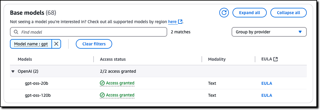
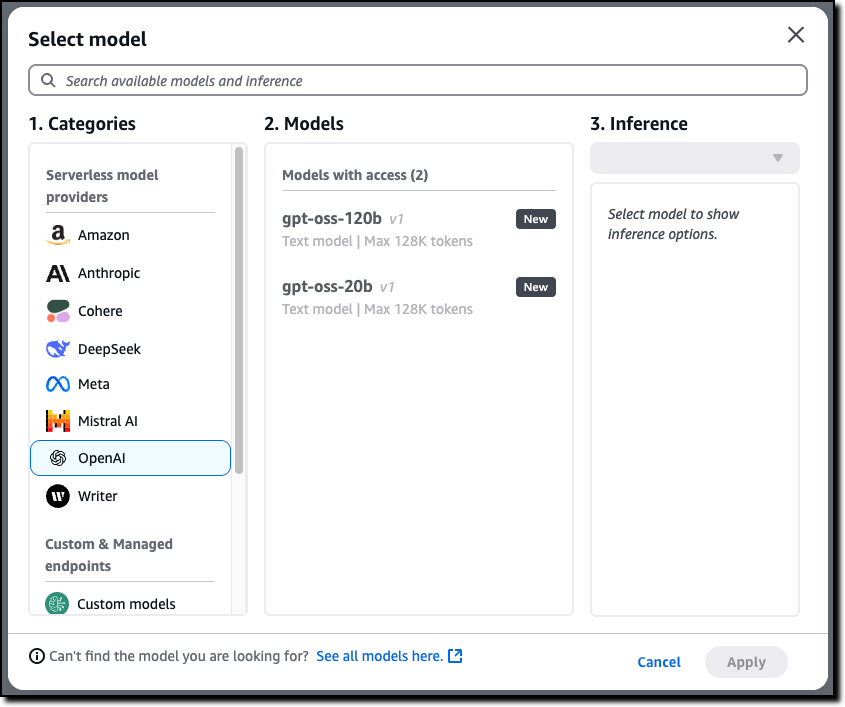
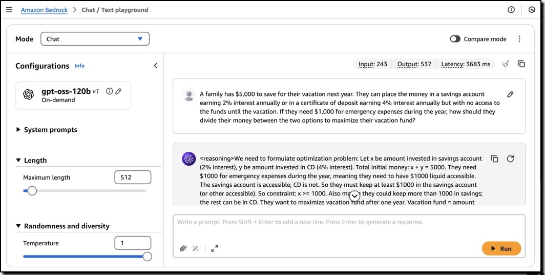
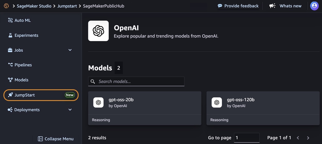
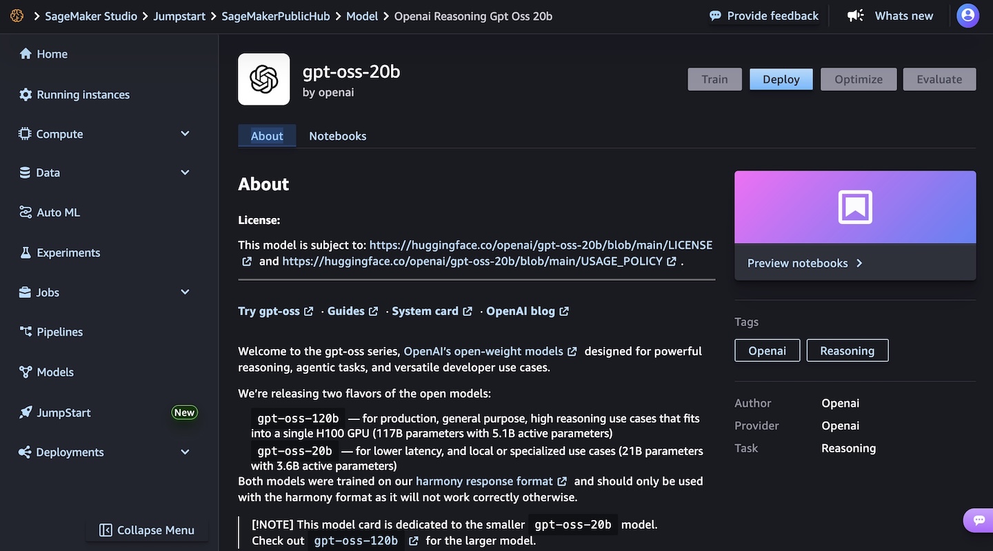
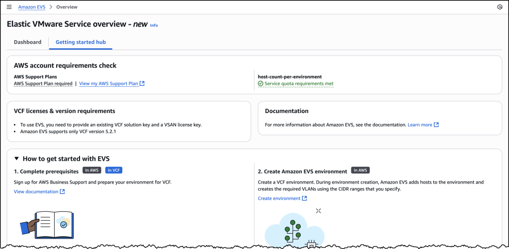
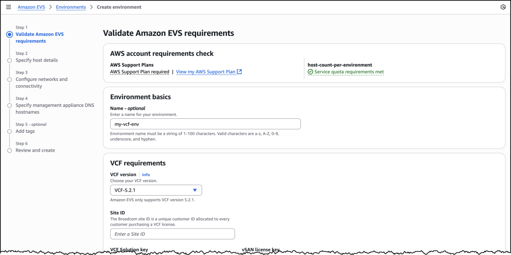
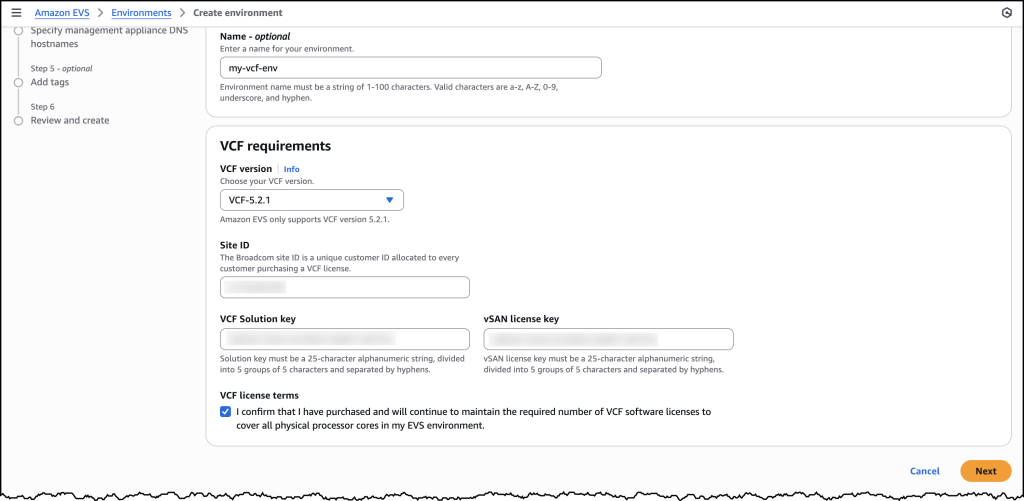
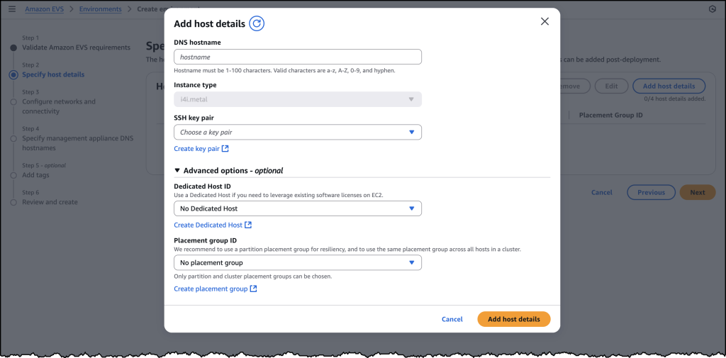
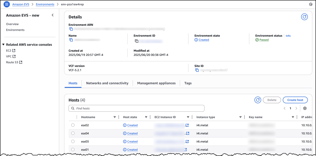
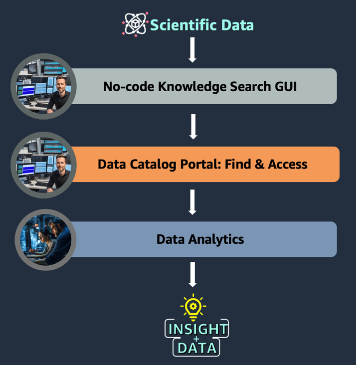
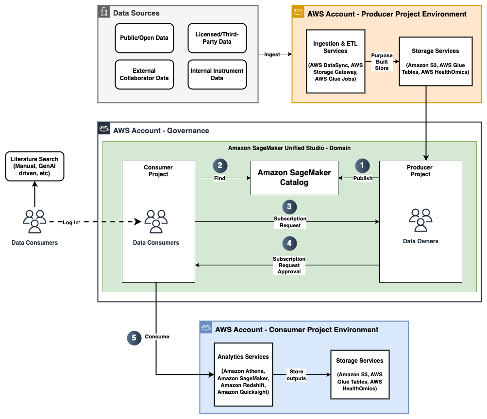
 Nadeem Bulsara is a Principal Solutions Architect at AWS specializing in Genomics and Life Sciences. He brings his 13+ years of Bioinformatics, Software Engineering, and Cloud Development skills as well as experience in research and clinical genomics and multi-omics to help Healthcare and Life Sciences organizations globally. He is motivated by the industry’s mission to enable people to have a long and healthy life.
 Chaitanya Vejendla is a Senior Solutions Architect specialized in DataLake & Analytics primarily working for Healthcare and Life Sciences industry division at AWS. Chaitanya is responsible for helping life sciences organizations and healthcare companies in developing modern data strategies, deploy data governance and analytical applications, electronic medical records, devices, and AI/ML-based applications, while educating customers about how to build secure, scalable, and cost-effective AWS solutions. His expertise spans across data analytics, data governance, AI, ML, big data, and healthcare-related technologies.
 Dr. Mileidy Giraldo has over 20 years of experience bridging bioinformatics, research, and industry technology strategy. She specializes in making technology accessible for organizations in the life sciences sector. In her current role as WW Lead for Life Sciences Strategy and Lab of the Future at AWS, she helps biotechs, biopharma, and diagnostics organizations design Data & AI-driven initiatives that modernize labs and help scientists unlock the full value of their data.
 Chris Clark is a Senior Solutions Architect focused on helping Life Science customers leverage AWS technology to advance their operational capabilities. With 20+ years of hands-on experience in life sciences manufacturing and supply chain, he combines deep industry knowledge with his AWS expertise to guide his customers. When he’s not working to solve customer challenges, he enjoys cycling and building and repairing things in his workshop.
 Nick Furr is a Specialist Solutions Architect at AWS, supporting Data & Analytics for Healthcare and Life Sciences. He helps providers, payers, and life sciences organizations build secure, scalable data platforms to drive innovation and improve outcomes. His work focuses on modernizing data strategies through cloud analytics, governed data processing, and machine learning for use cases like clinical research and population health.
 Subrat Das is a Principal Solutions Architect for Global Healthcare and Life Sciences accounts at AWS. He is passionate about modernizing and architecting complex customers workloads. When he’s not working on technology solutions, he enjoys long hikes and traveling around the world.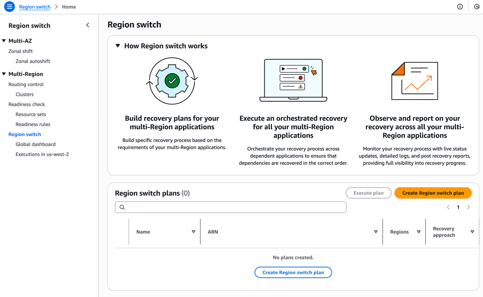
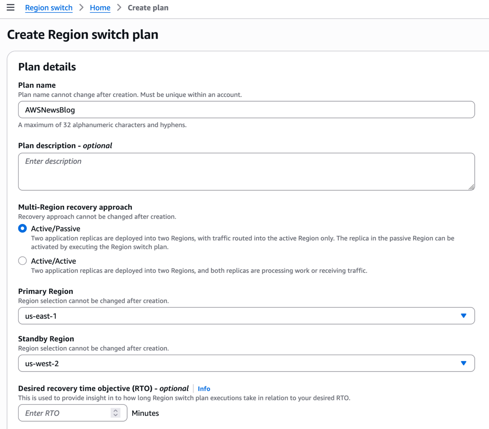
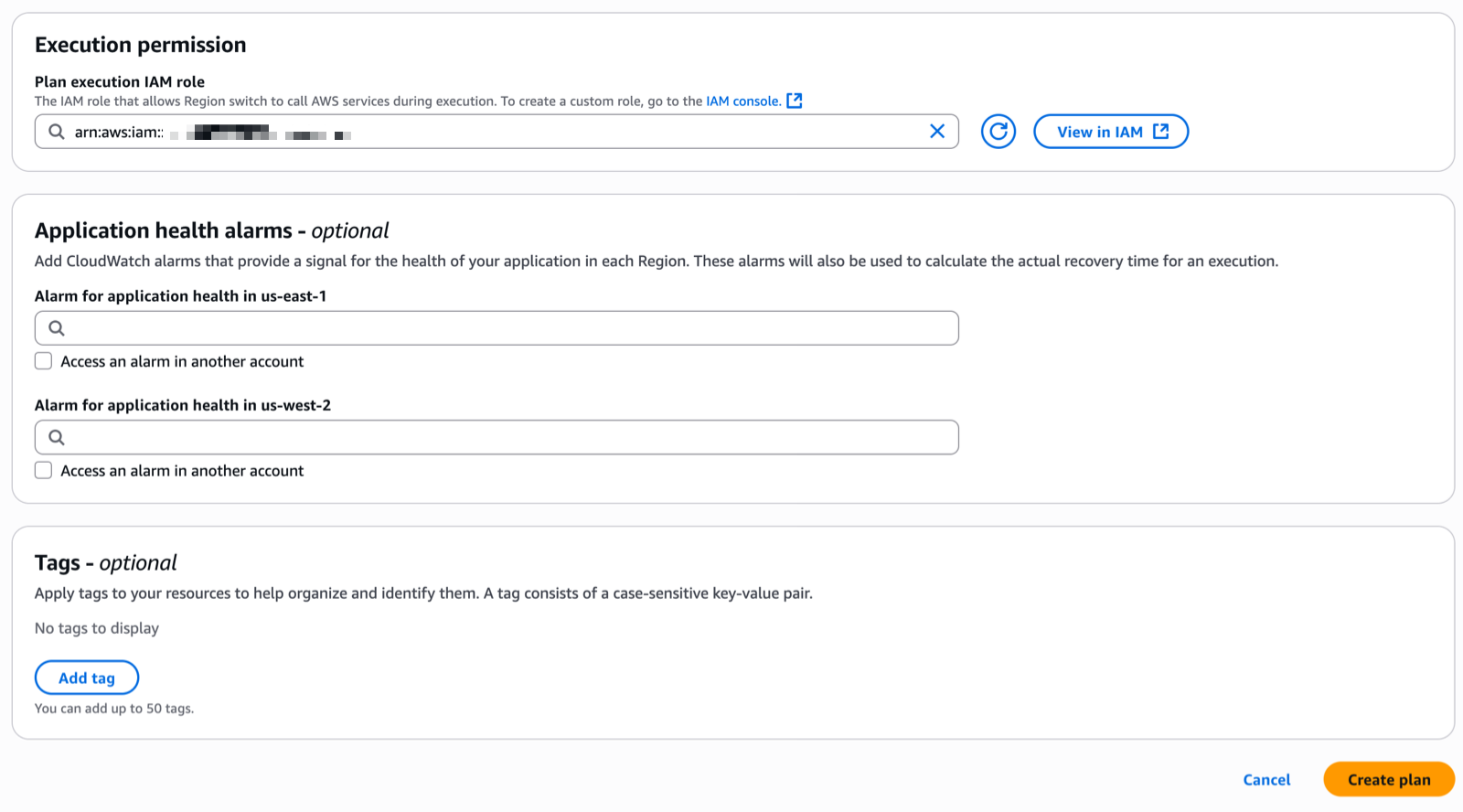
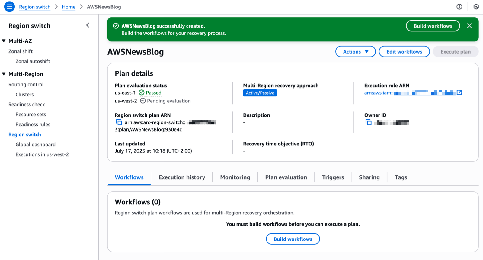
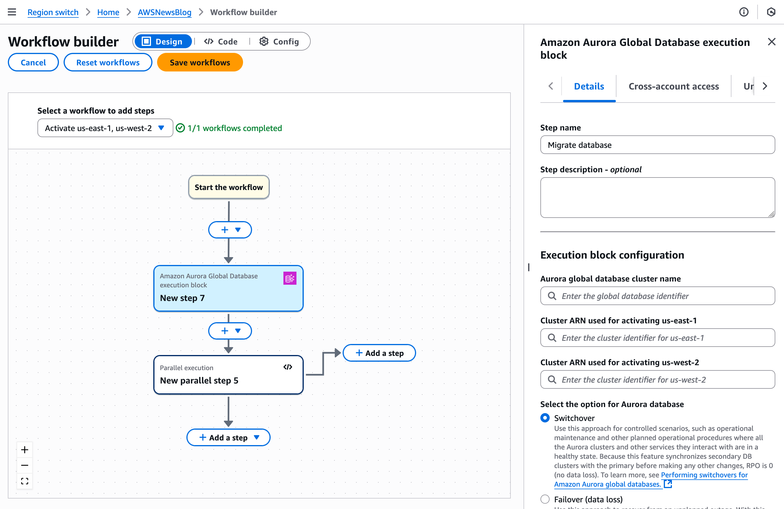
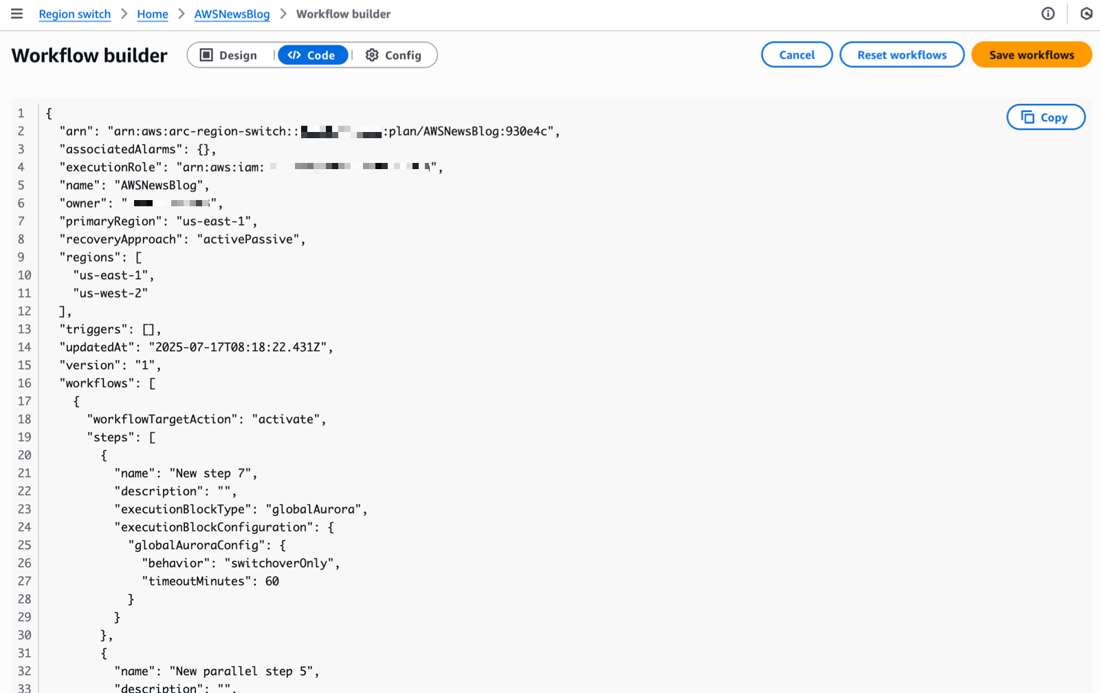
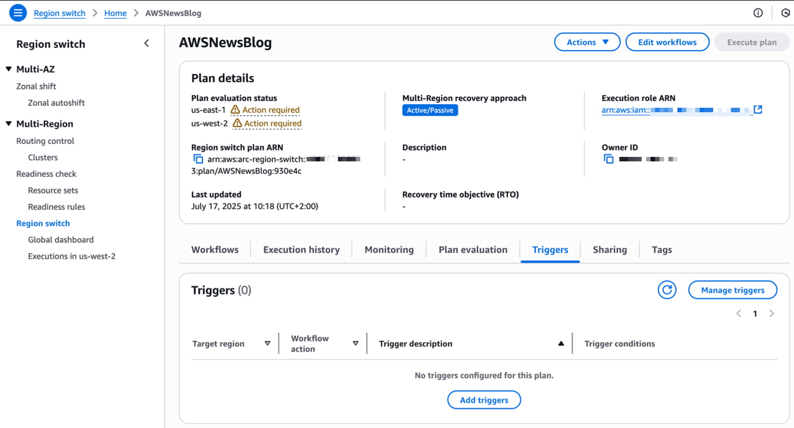
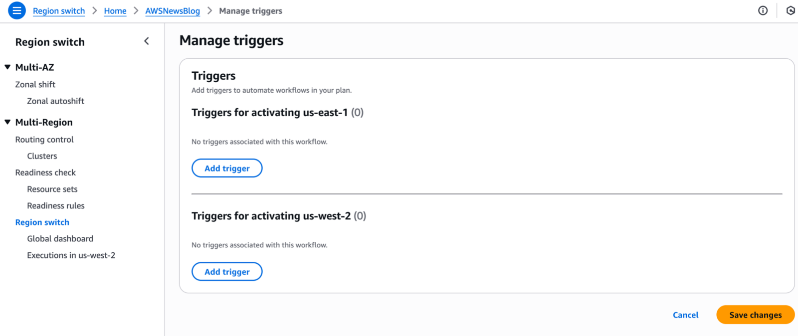
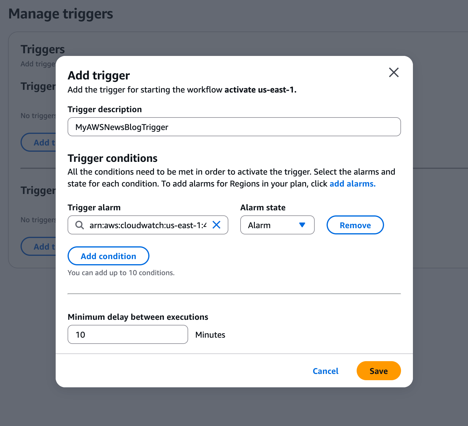
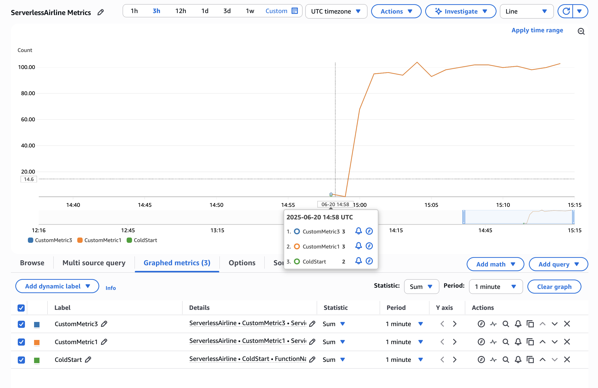
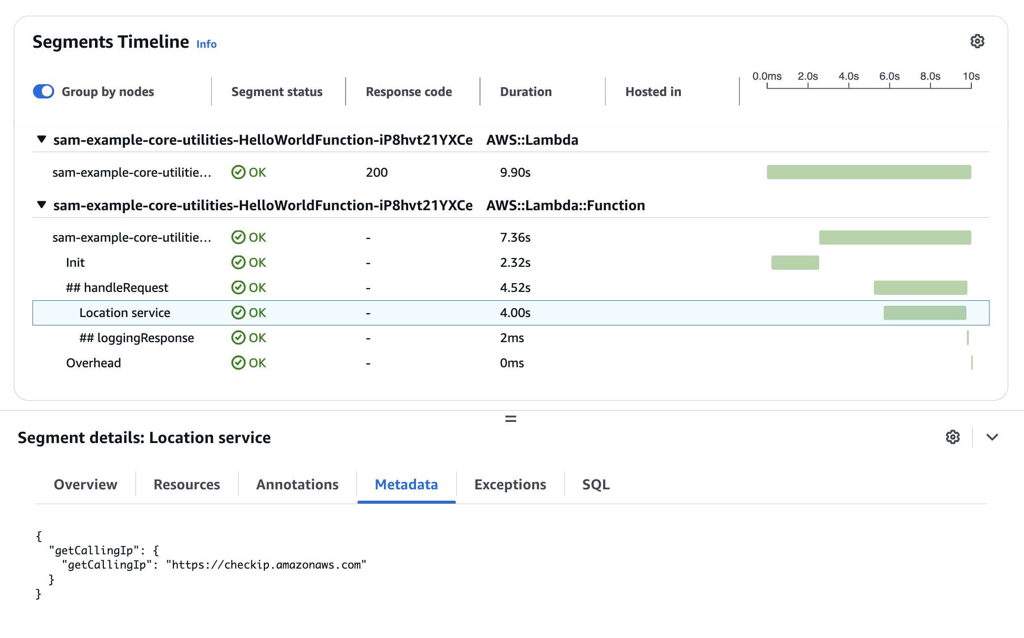
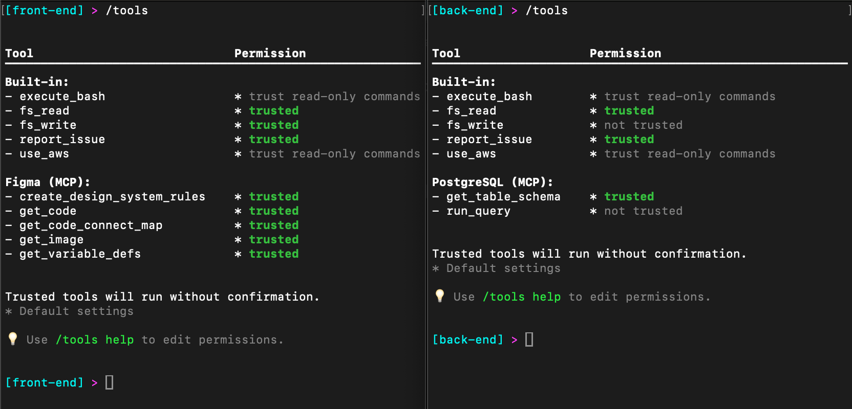
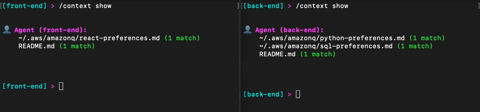
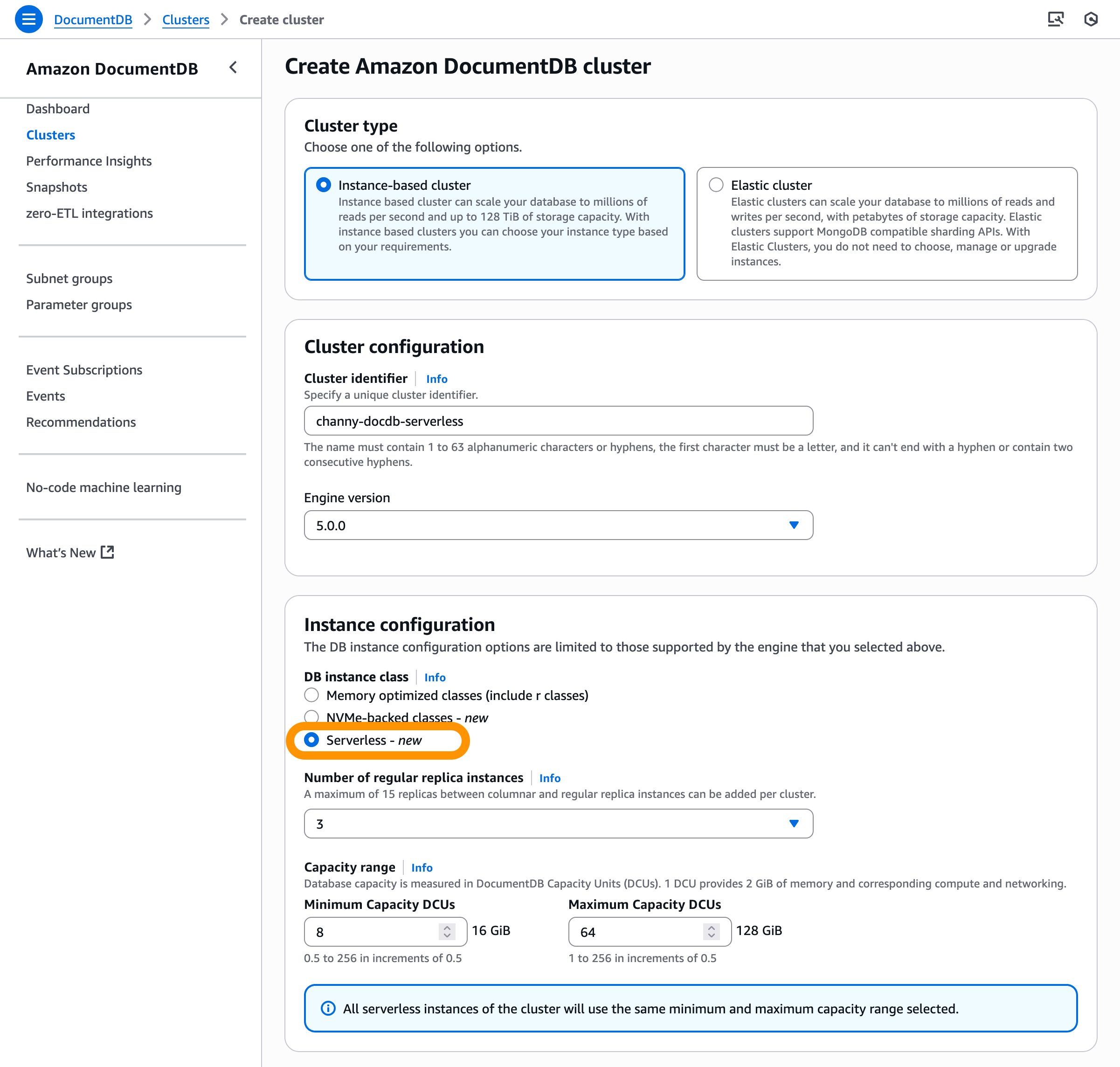
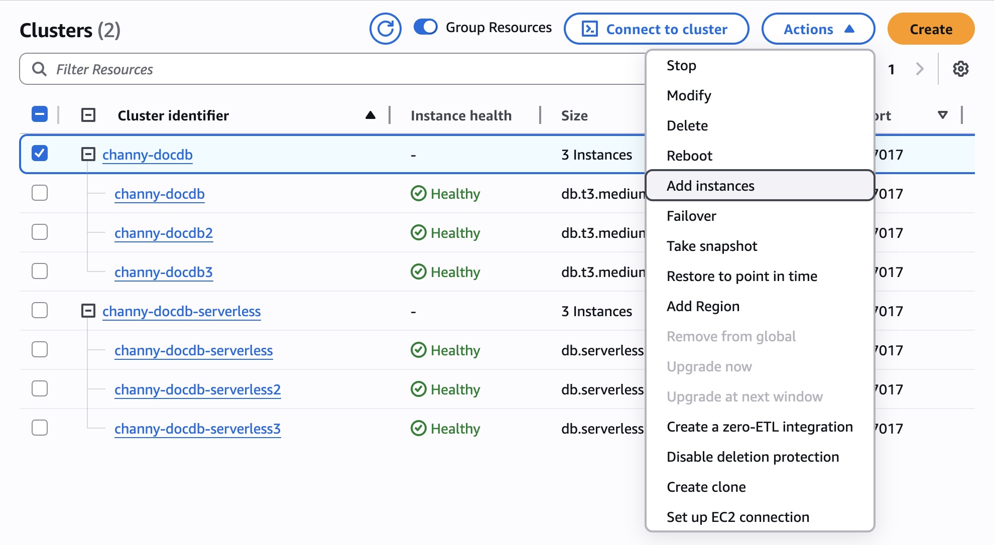
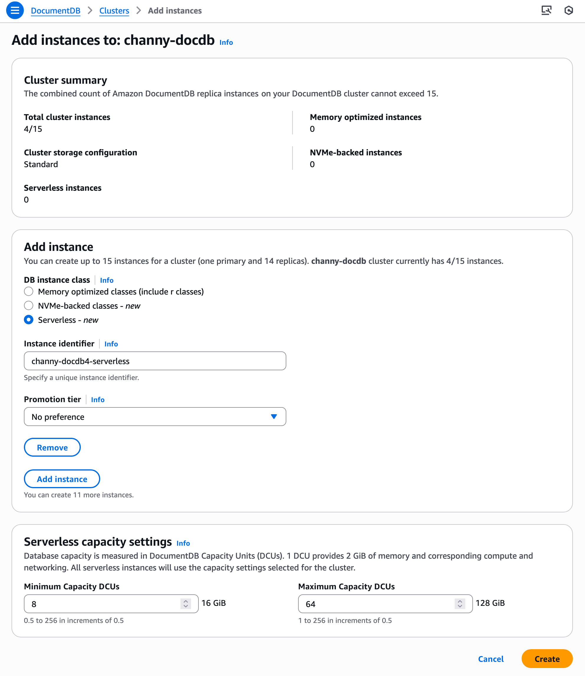
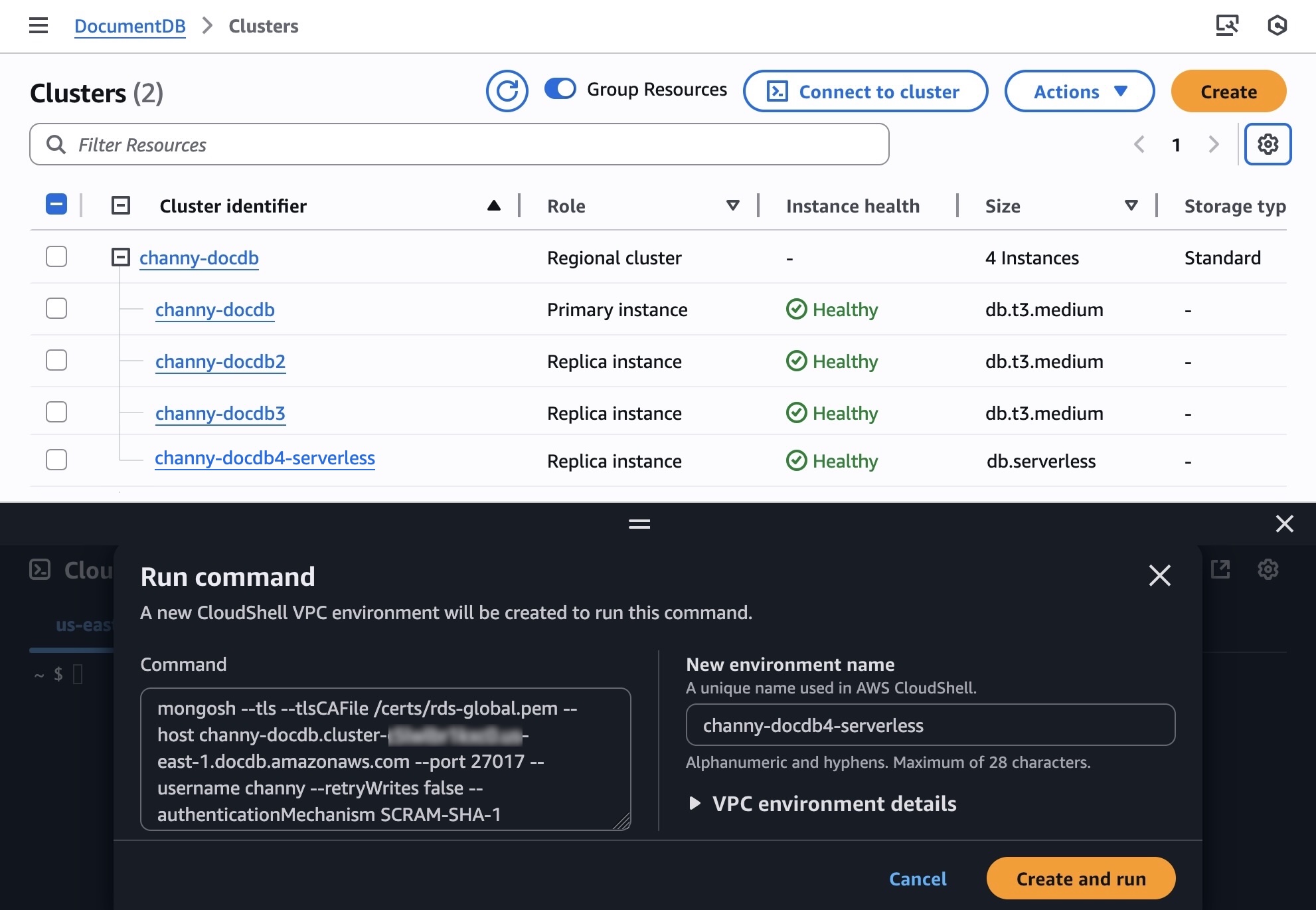
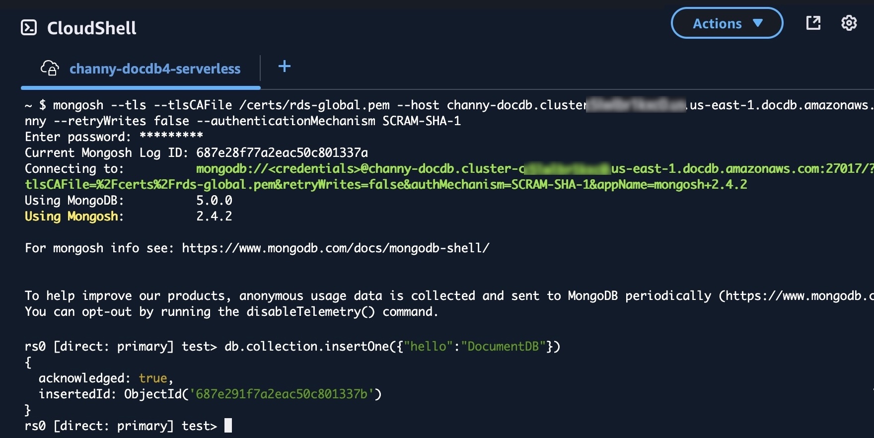
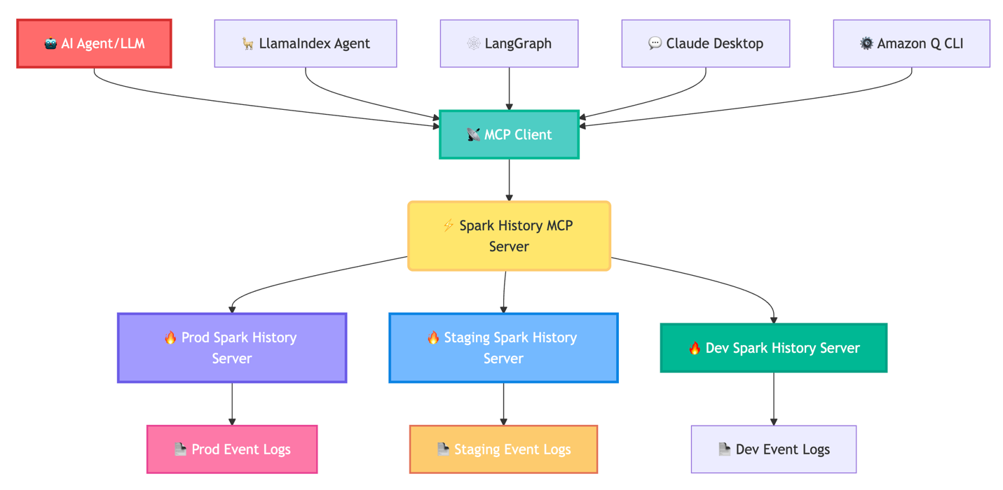
 Manabu McCloskey is a Solutions Architect at Amazon Web Services. He focuses on contributing to open source application delivery tooling and works with AWS strategic customers to design and implement enterprise solutions using AWS resources and open source technologies. His interests include Kubernetes, GitOps, Serverless, and Souls Series.
 Vara Bonthu is a Principal Open Source Specialist SA leading Data on EKS and AI on EKS at AWS, driving open source initiatives and helping AWS customers to diverse organizations. He specializes in open source technologies, data analytics, AI/ML, and Kubernetes, with extensive experience in development, DevOps, and architecture. Vara focuses on building highly scalable data and AI/ML solutions on Kubernetes, enabling customers to maximize cutting-edge technology for their data-driven initiatives
 Andrew Kim is a Software Development Engineer at AWS Glue, with a deep passion for distributed systems architecture and AI-driven solutions, specializing in intelligent data integration workflows and cutting-edge feature development on Apache Spark. Andrew focuses on re-inventing and simplifying solutions to complex technical problems, and he enjoys creating web apps and producing music in his free time.
 Shubham Mehta is a Senior Product Manager at AWS Analytics. He leads generative AI feature development across services such as AWS Glue, Amazon EMR, and Amazon MWAA, using AI/ML to simplify and enhance the experience of data practitioners building data applications on AWS.
 Kartik Panjabi is a Software Development Manager on the AWS Glue team. His team builds generative AI features for the Data Integration and distributed system for data integration.
 Mohit Saxena is a Senior Software Development Manager on the AWS Data Processing Team (AWS Glue and Amazon EMR). His team focuses on building distributed systems to enable customers with new AI/ML-driven capabilities to efficiently transform petabytes of data across data lakes on Amazon S3, databases and data warehouses on the cloud.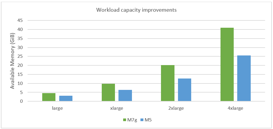
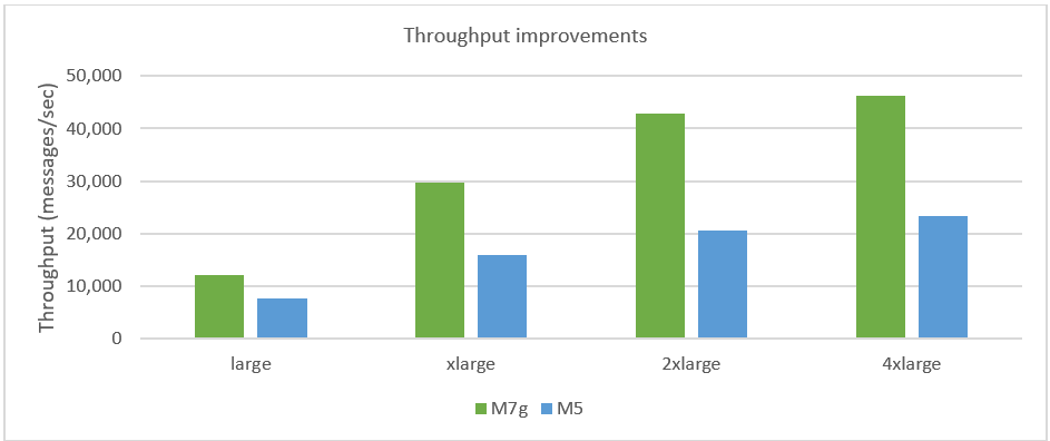
 Vignesh Selvam is the Principal Product Manager for Amazon MQ at AWS. He works with customers to solve their messaging needs and with the open-source communities for innovating with message brokers. Prior to joining AWS, he built products for security and analytics.
 Samuel Massé is a Software Development Engineer at AWS. He has been leading the engineering effort to support M7g on the RabbitMQ team. In his free time he enjoys coding unfinished side projects.
 Vinodh Kannan Sadayamuthu is a Senior Specialist Solutions Architect at Amazon Web Services (AWS). His expertise centers on AWS messaging and streaming services, where he provides architectural best practices consultation to AWS customers.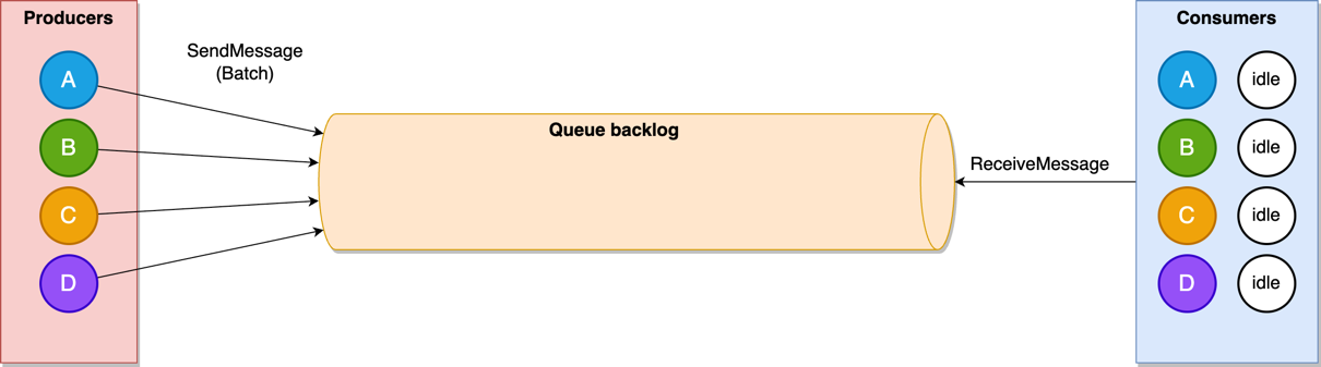
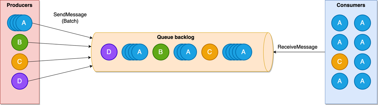
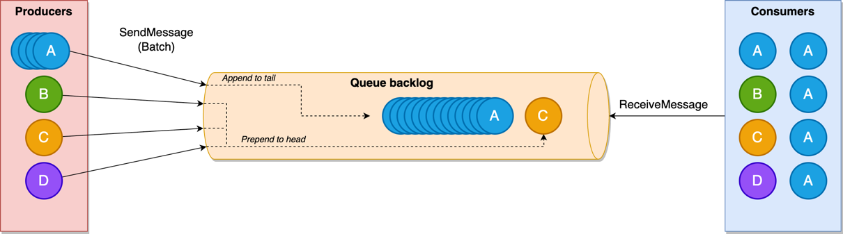
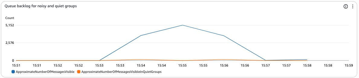
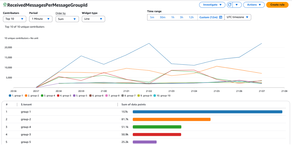
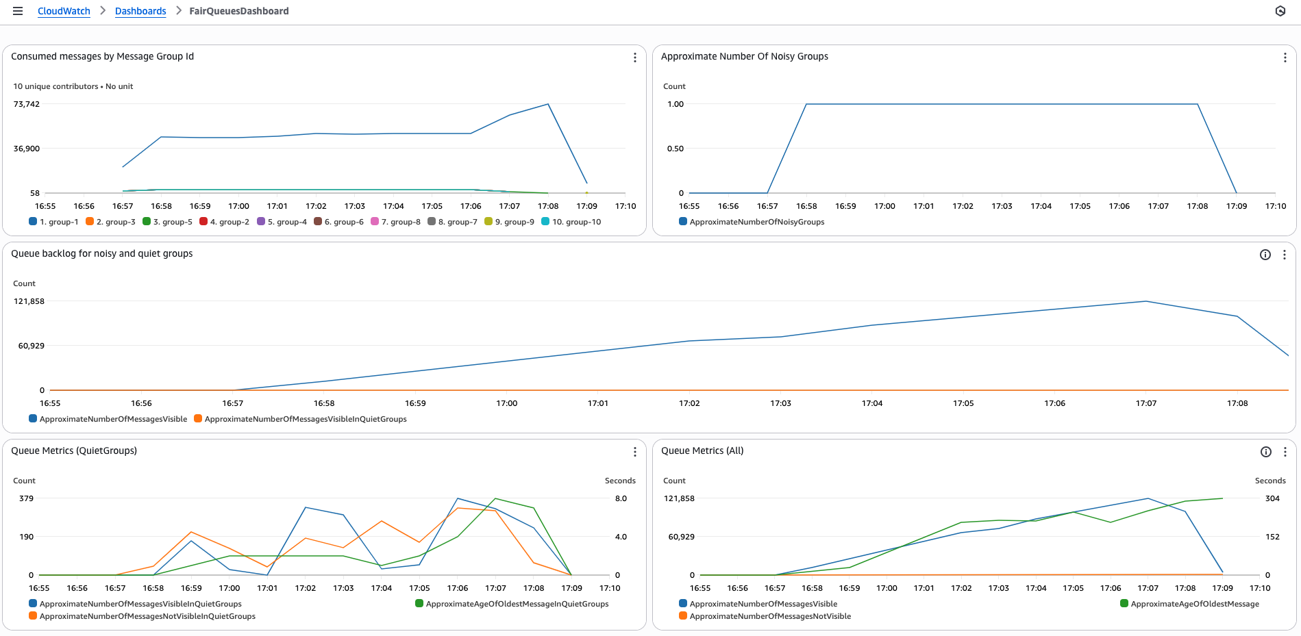
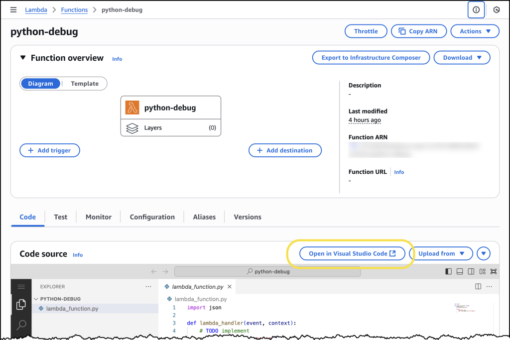
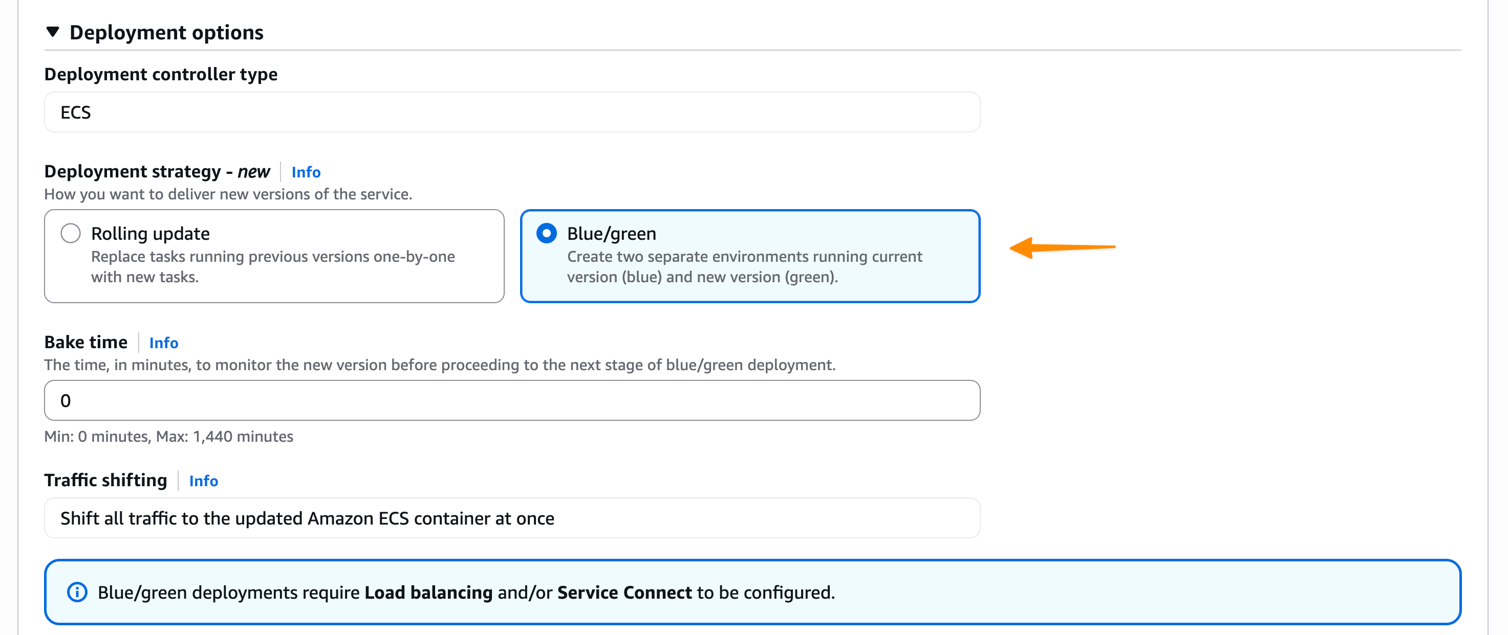


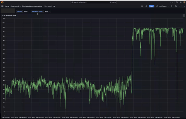
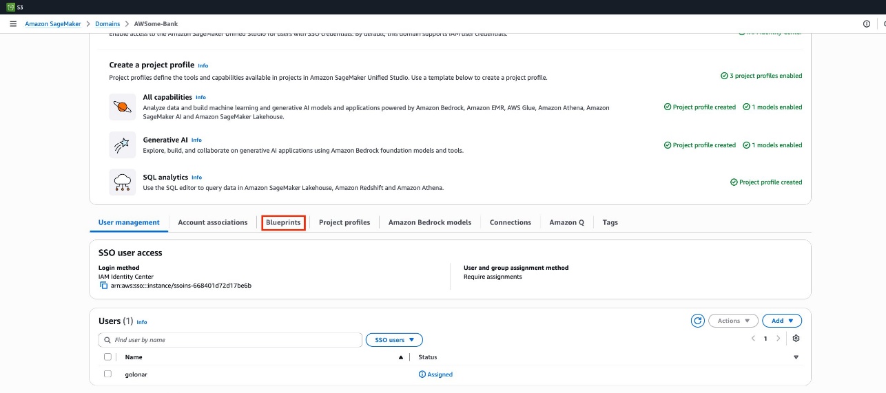
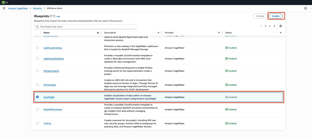
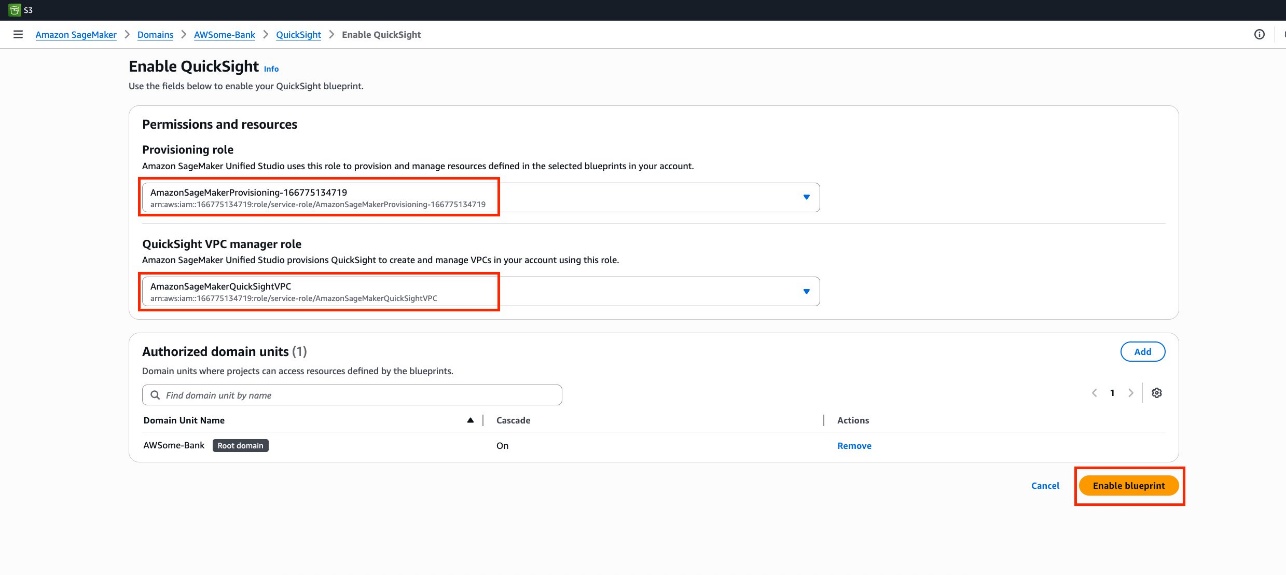
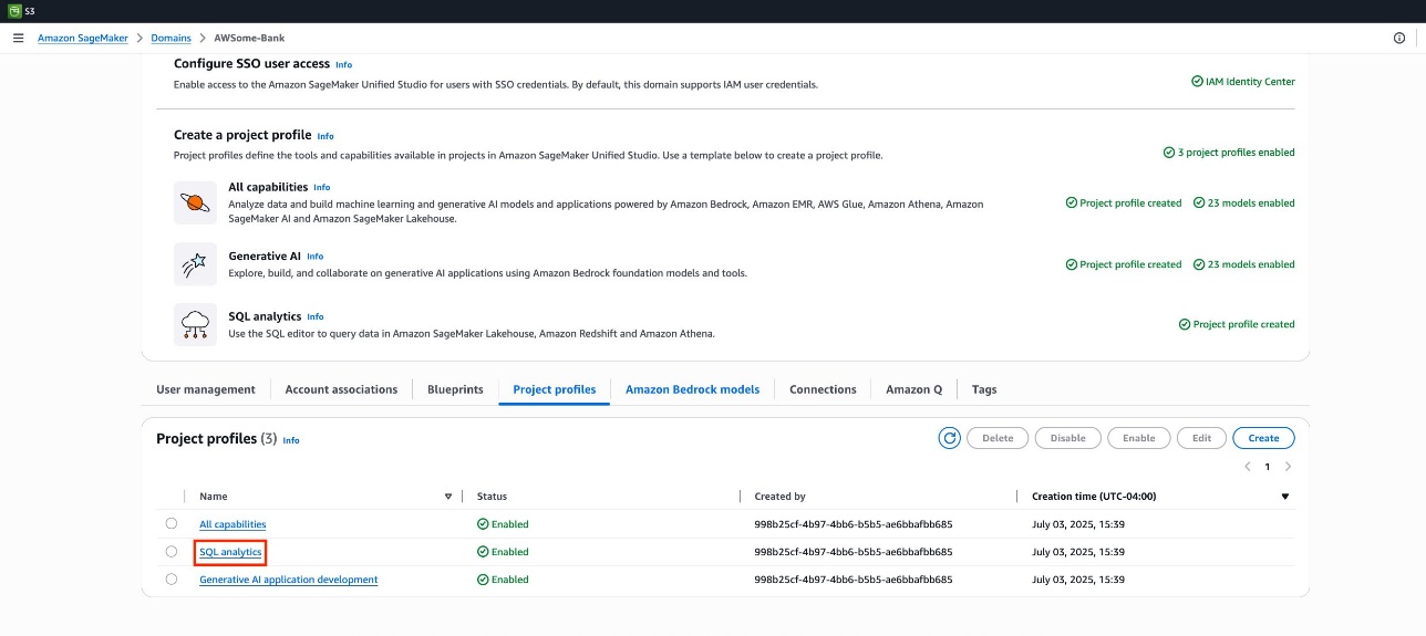
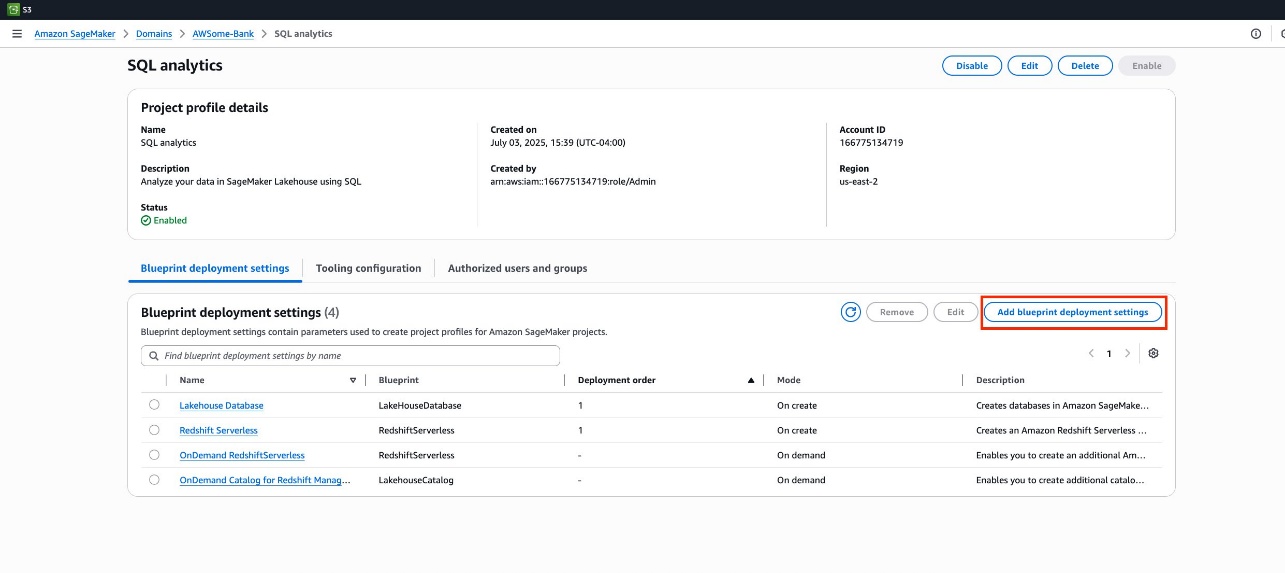
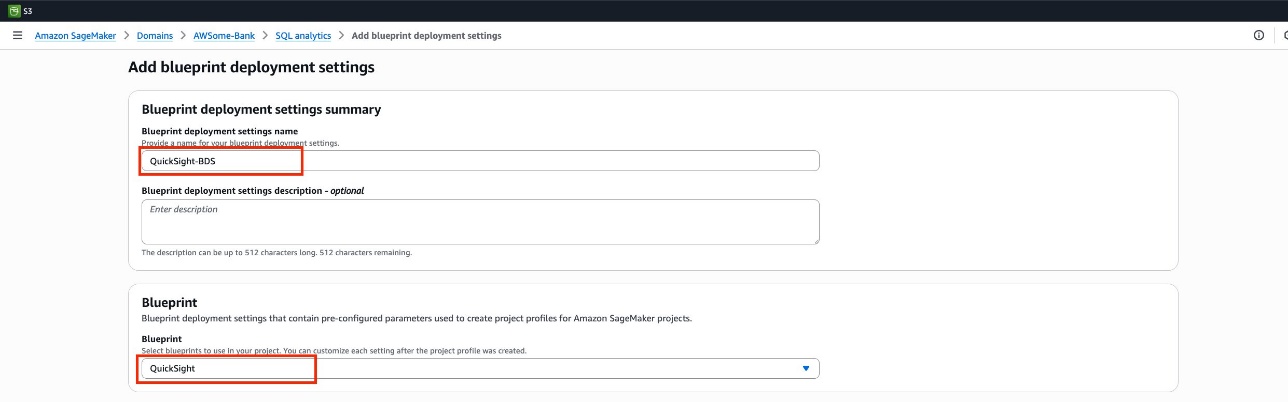
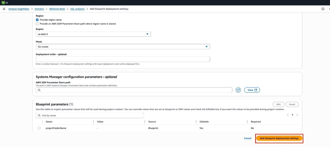
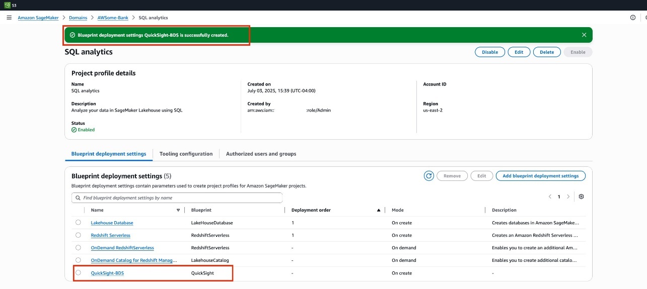
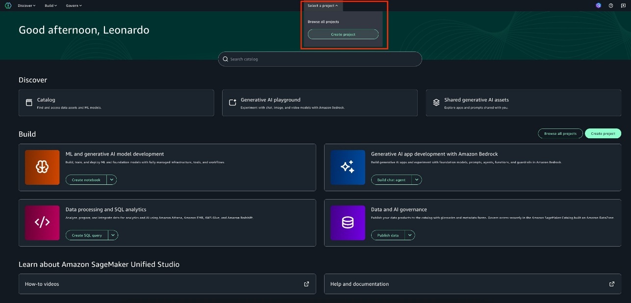
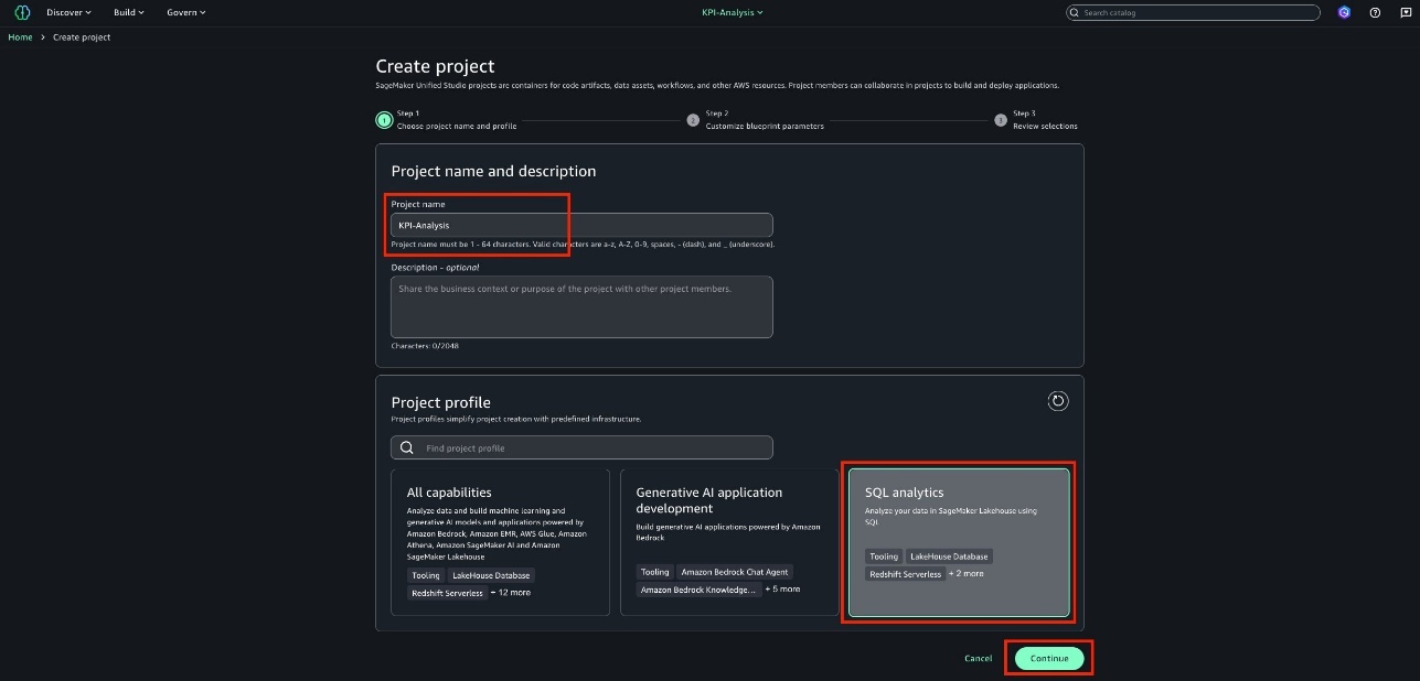
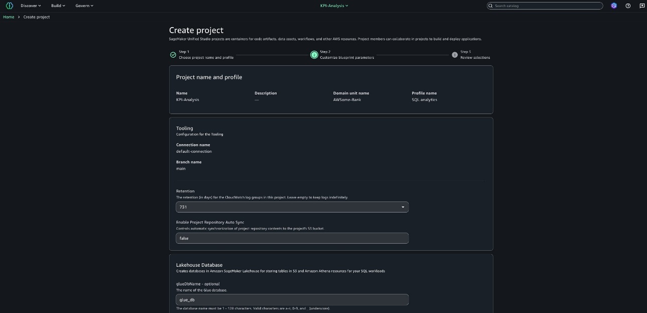
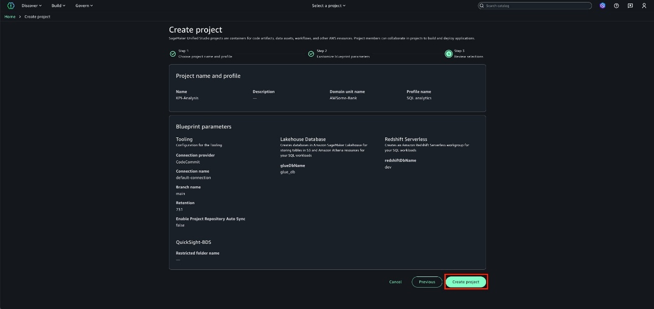
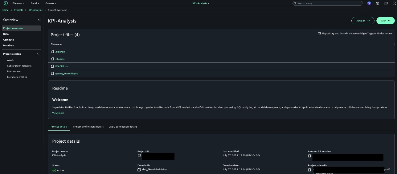
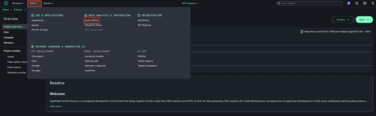
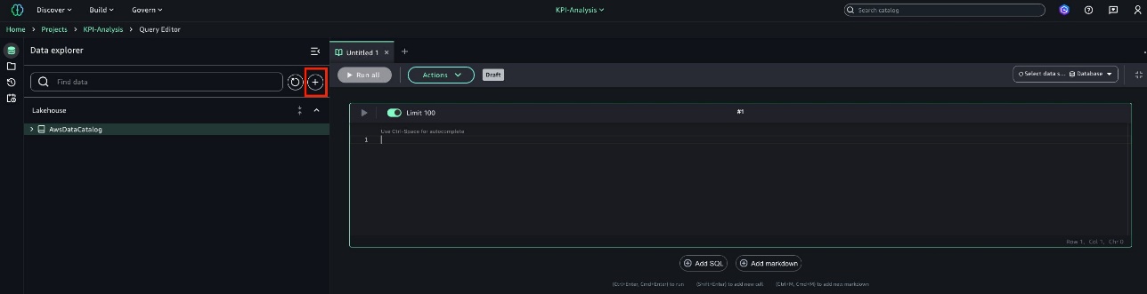

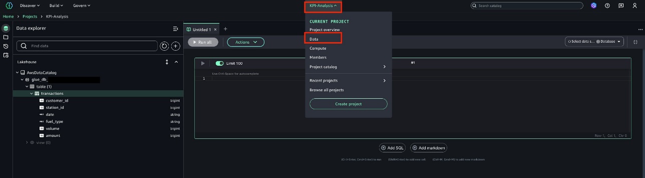

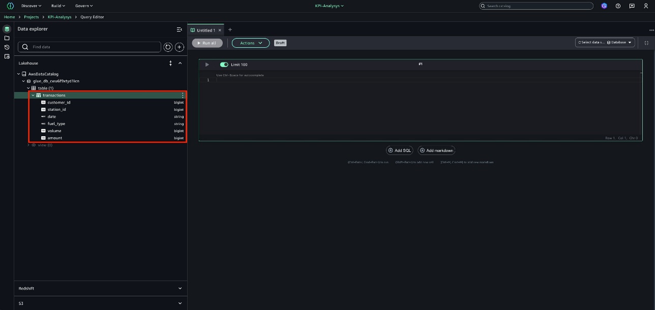
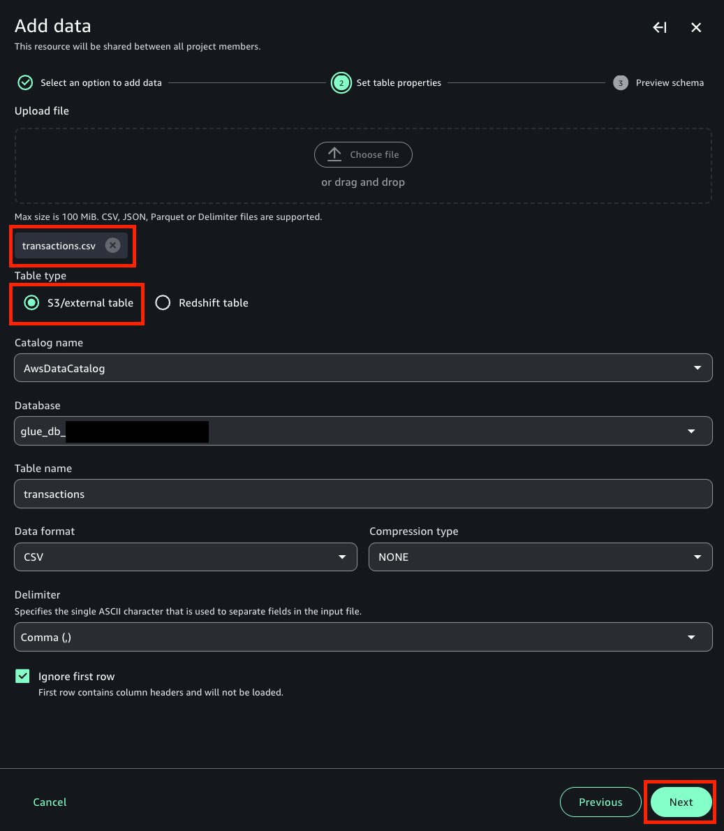
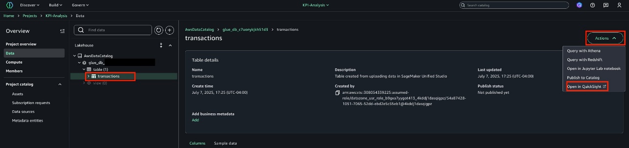
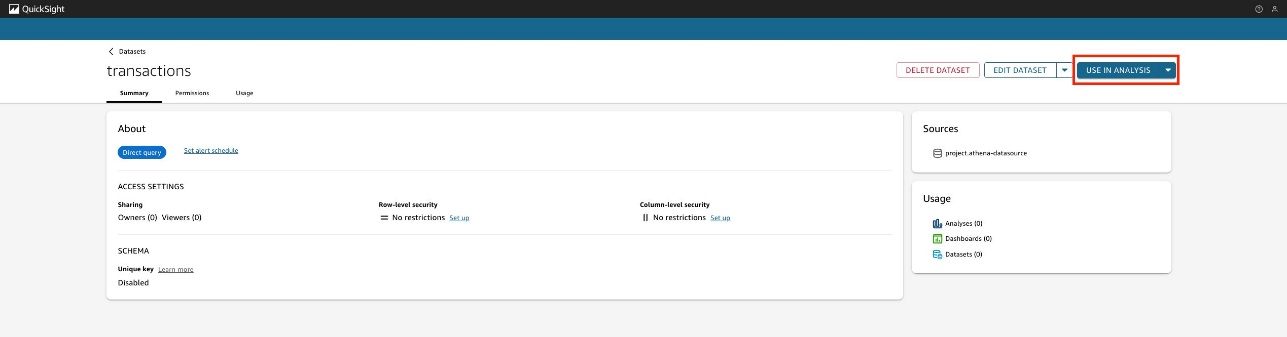
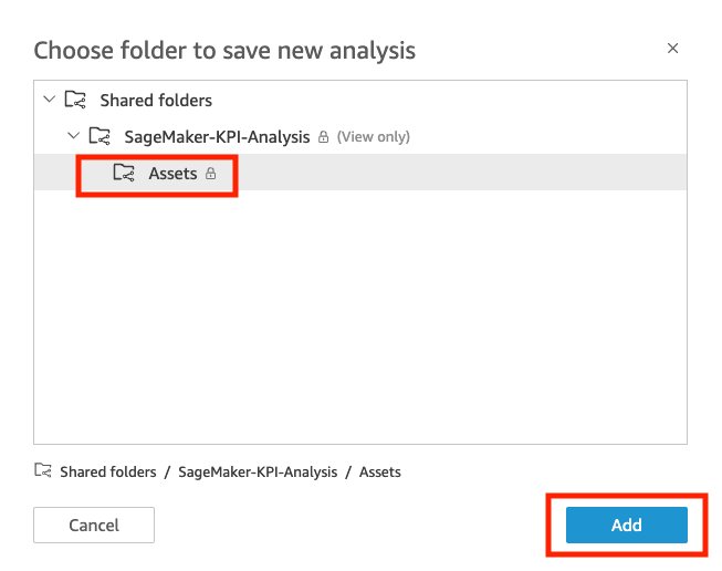

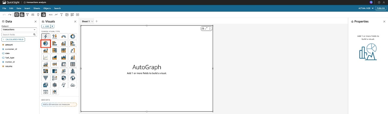
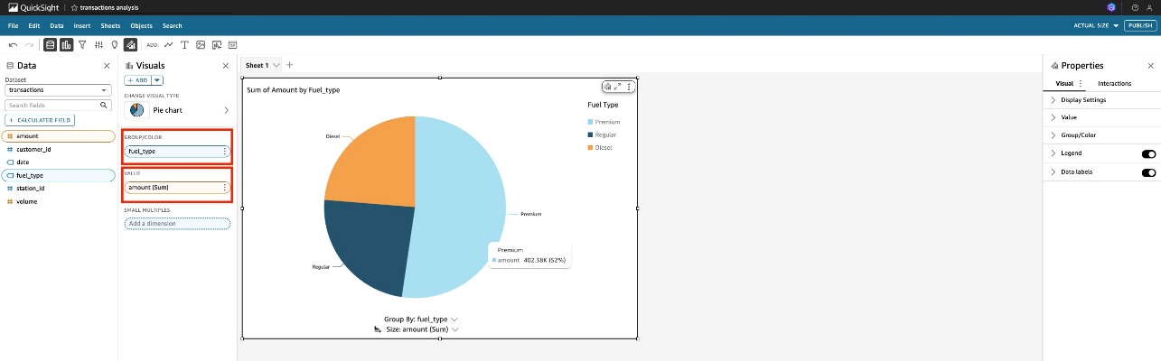
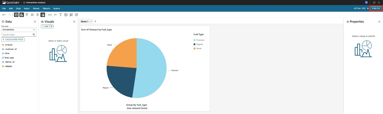
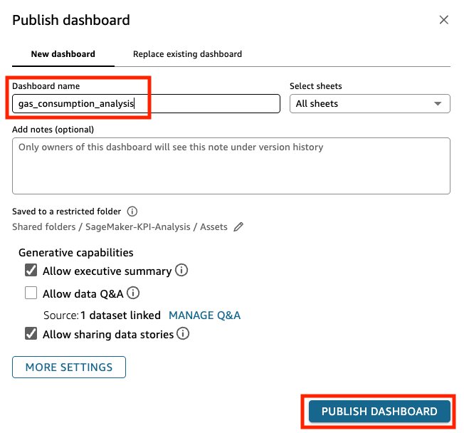
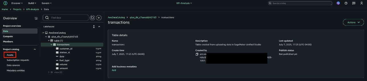
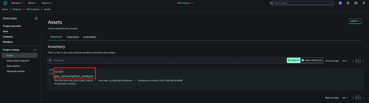
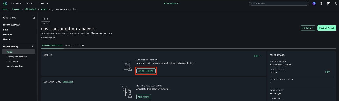
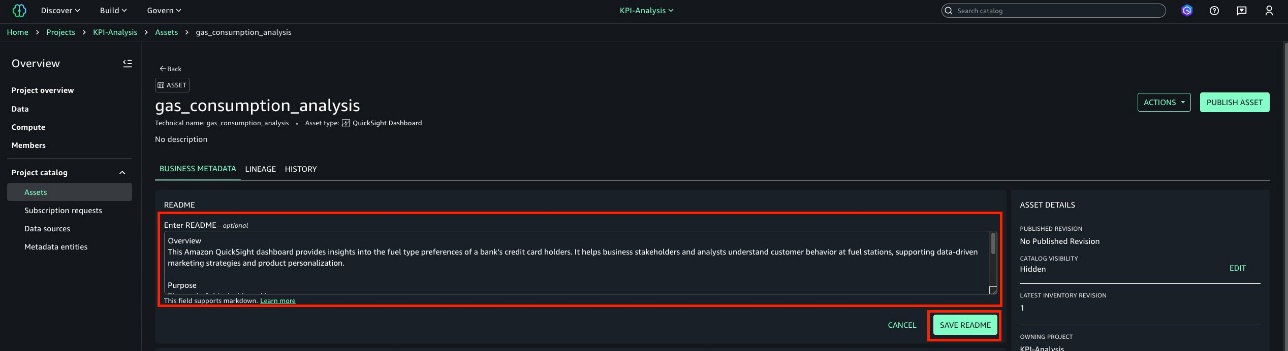
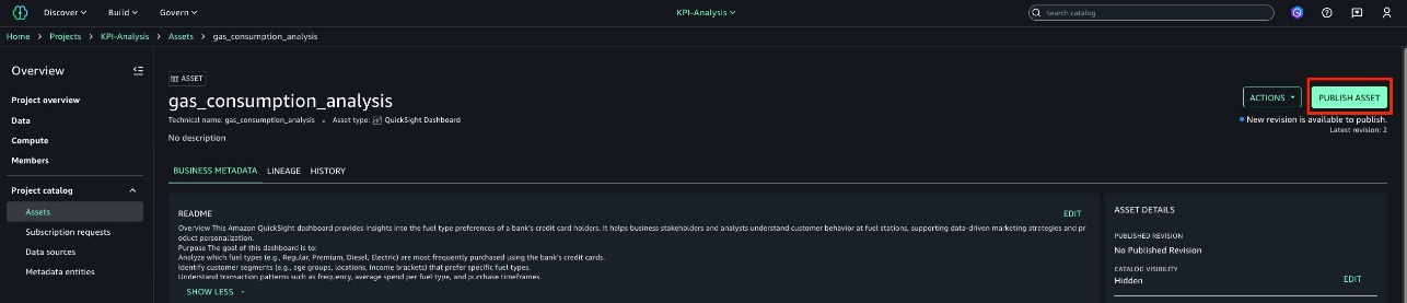
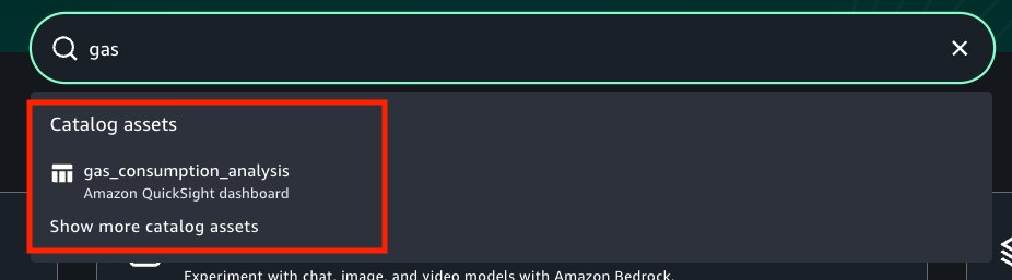
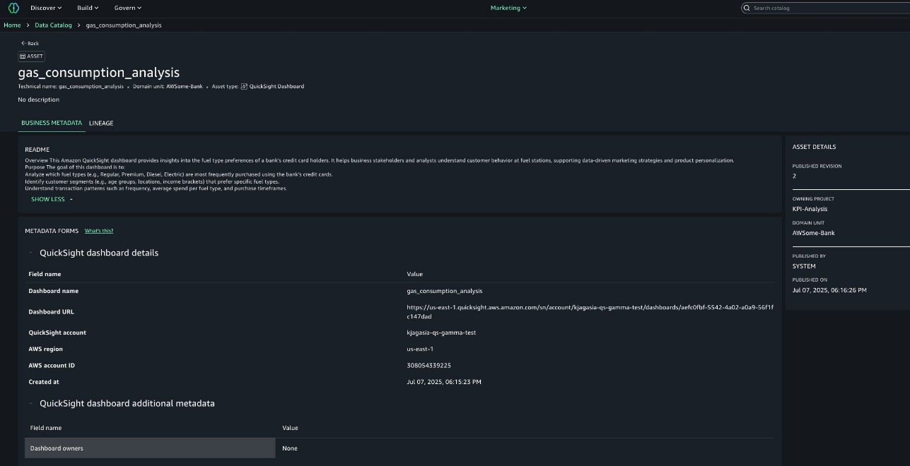
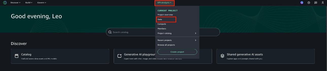
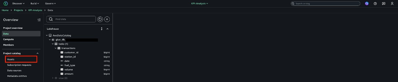
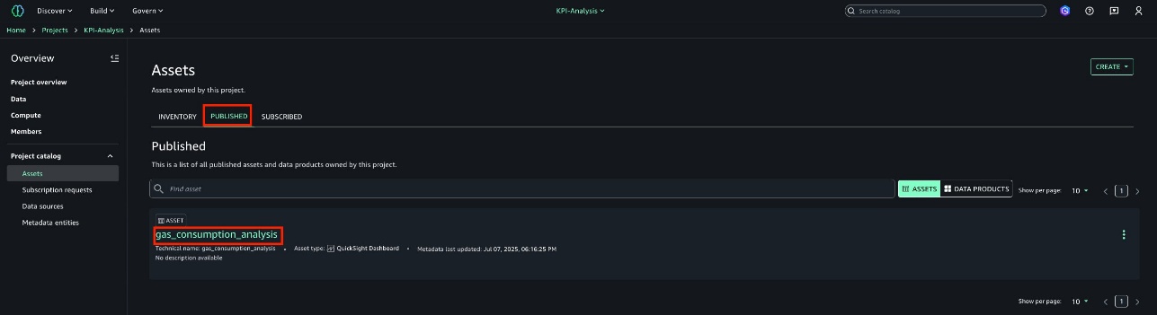
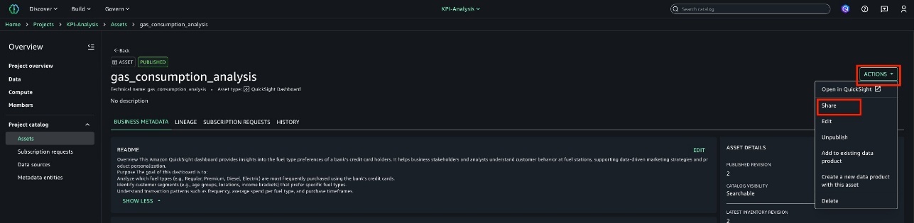
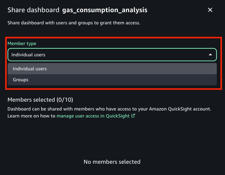
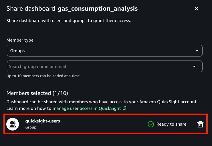

 Ramon Lopez is a Principal Solutions Architect for Amazon QuickSight. With many years of experience building BI solutions and a background in accounting, he loves working with customers, creating solutions, and making world-class services. When not working, he prefers to be outdoors in the ocean or up on a mountain.
 Leonardo Gomez is a Principal Analytics Specialist Solutions Architect at AWS. He has over a decade of experience in data management, helping customers around the globe address their business and technical needs. Connect with him on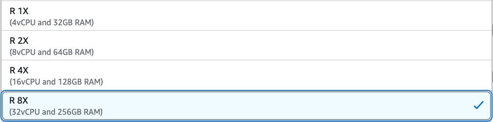
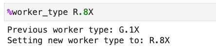
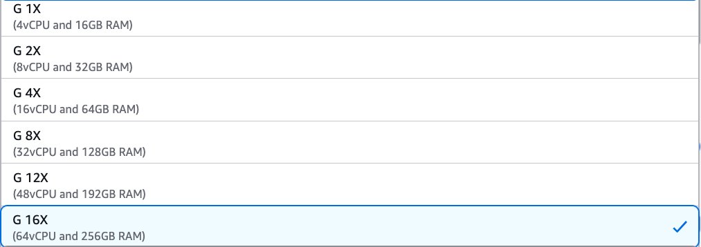
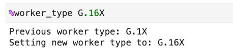
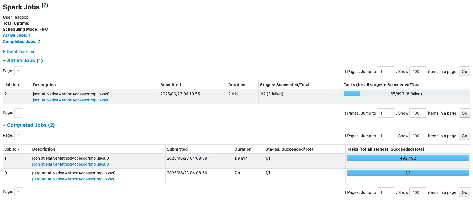
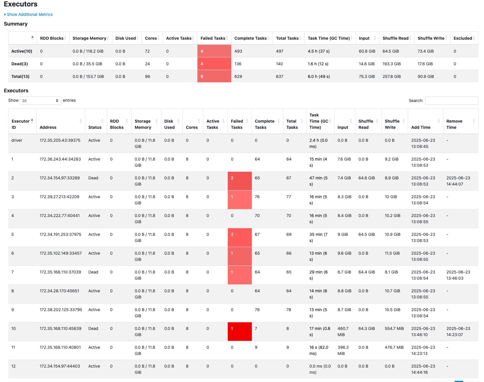
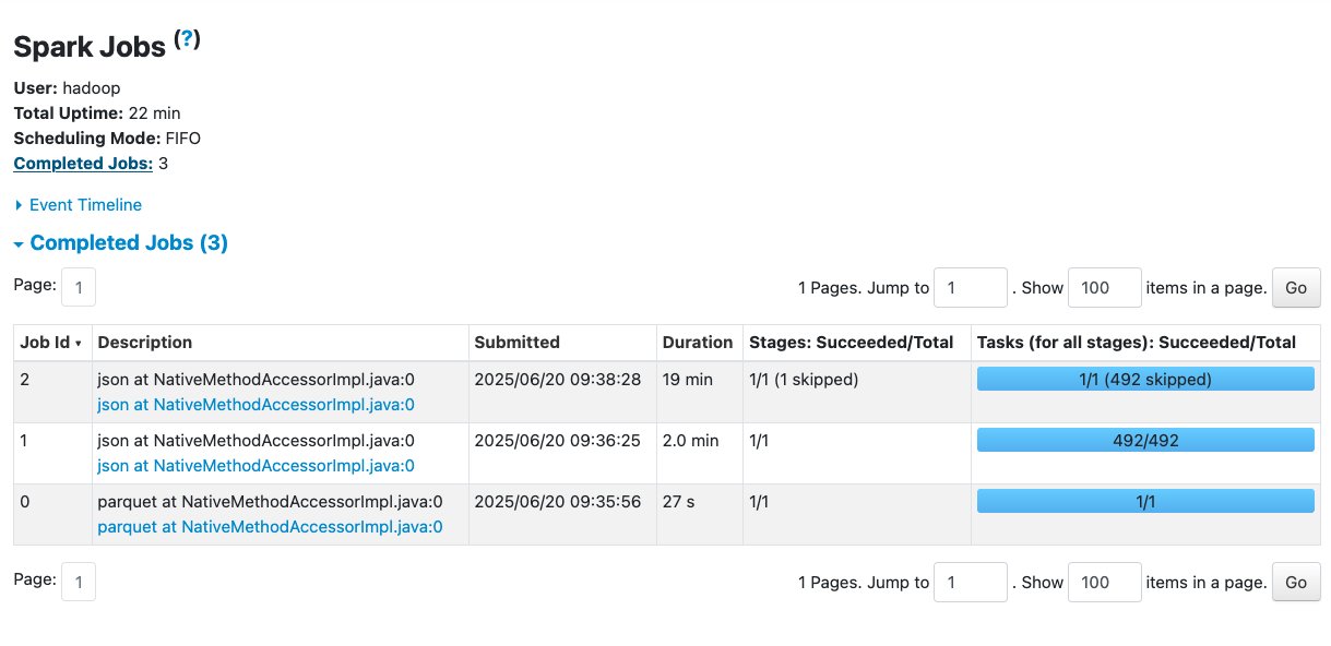
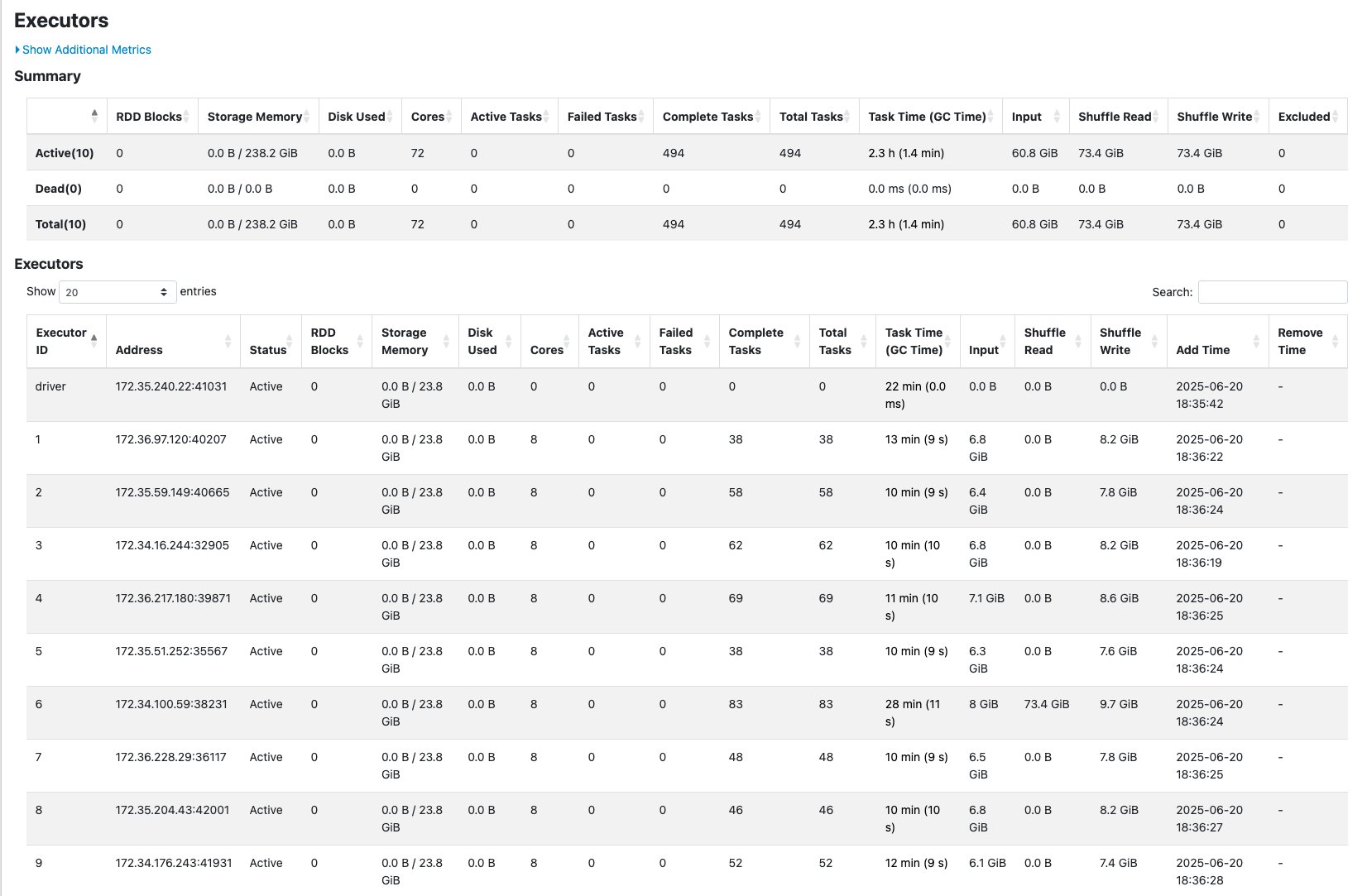
 Noritaka Sekiyama is a Principal Big Data Architect with AWS Analytics services. He’s responsible for building software artifacts to help customers. In his spare time, he enjoys cycling on his road bike.
 Tomohiro Tanaka is a Senior Cloud Support Engineer at Amazon Web Services. He’s passionate about helping customers use Apache Iceberg for their data lakes on AWS. In his free time, he enjoys a coffee break with his colleagues and making coffee at home.
 Peter Tsai is a Software Development Engineer at AWS, where he enjoys solving challenges in the design and performance of the AWS Glue runtime. In his leisure time, he enjoys hiking and cycling.
 Matt Su is a Senior Product Manager on the AWS Glue team. He enjoys helping customers uncover insights and make better decisions using their data with AWS Analytics services. In his spare time, he enjoys skiing and gardening.
 Sean McGeehan is a Software Development Engineer at AWS, where he builds features for the AWS Glue fulfillment system. In his leisure time, he explores his home of Philadelphia and work city of New York.