Post Syndicated from Vaidy Kalpathy original https://aws.amazon.com/blogs/big-data/simplify-data-loading-into-type-2-slowly-changing-dimensions-in-amazon-redshift/
Thousands of customers rely on Amazon Redshift to build data warehouses to accelerate time to insights with fast, simple, and secure analytics at scale and analyze data from terabytes to petabytes by running complex analytical queries. Organizations create data marts, which are subsets of the data warehouse and usually oriented for gaining analytical insights specific to a business unit or team. The star schema is a popular data model for building data marts.
In this post, we show how to simplify data loading into a Type 2 slowly changing dimension in Amazon Redshift.
Star schema and slowly changing dimension overview
A star schema is the simplest type of dimensional model, in which the center of the star can have one fact table and a number of associated dimension tables. A dimension is a structure that captures reference data along with associated hierarchies, while a fact table captures different values and metrics that can be aggregated by dimensions. Dimensions provide answers to exploratory business questions by allowing end-users to slice and dice data in a variety of ways using familiar SQL commands.
Whereas operational source systems contain only the latest version of master data, the star schema enables time travel queries to reproduce dimension attribute values on past dates when the fact transaction or event actually happened. The star schema data model allows analytical users to query historical data tying metrics to corresponding dimensional attribute values over time. Time travel is possible because dimension tables contain the exact version of the associated attributes at different time ranges. Relative to the metrics data that keeps changing on a daily or even hourly basis, the dimension attributes change less frequently. Therefore, dimensions in a star schema that keeps track of changes over time are referred to as slowly changing dimensions (SCDs).
Data loading is one of the key aspects of maintaining a data warehouse. In a star schema data model, the central fact table is dependent on the surrounding dimension tables. This is captured in the form of primary key-foreign key relationships, where the dimension table primary keys are referred by foreign keys in the fact table. In the case of Amazon Redshift, uniqueness, primary key, and foreign key constraints are not enforced. However, declaring them will help the optimizer arrive at optimal query plans, provided that the data loading processes enforce their integrity. As part of data loading, the dimension tables, including SCD tables, get loaded first, followed by the fact tables.
SCD population challenge
Populating an SCD dimension table involves merging data from multiple source tables, which are usually normalized. SCD tables contain a pair of date columns (effective and expiry dates) that represent the record’s validity date range. Changes are inserted as new active records effective from the date of data loading, while simultaneously expiring the current active record on a previous day. During each data load, incoming change records are matched against existing active records, comparing each attribute value to determine whether existing records have changed or were deleted or are new records coming in.
In this post, we demonstrate how to simplify data loading into a dimension table with the following methods:
- Using Amazon Simple Storage Service (Amazon S3) to host the initial and incremental data files from source system tables
- Accessing S3 objects using Amazon Redshift Spectrum to carry out data processing to load native tables within Amazon Redshift
- Creating views with window functions to replicate the source system version of each table within Amazon Redshift
- Joining source table views to project attributes matching with dimension table schema
- Applying incremental data to the dimension table, bringing it up to date with source-side changes
Solution overview
In a real-world scenario, records from source system tables are ingested on a periodic basis to an Amazon S3 location before being loaded into star schema tables in Amazon Redshift.
For this demonstration, data from two source tables, customer_master and customer_address, are combined to populate the target dimension table dim_customer, which is the customer dimension table.
The source tables customer_master and customer_address share the same primary key, customer_id, and will be joined on the same to fetch one record per customer_id along with attributes from both tables. row_audit_ts contains the latest timestamp at which the particular source record was inserted or last updated. This column helps identify the change records since the last data extraction.
rec_source_status is an optional column that indicates if the corresponding source record was inserted, updated, or deleted. This is applicable in cases where the source system itself provides the changes and populates rec_source_status appropriately.
The following figure provides the schema of the source and target tables.

Let’s look closer at the schema of the target table, dim_customer. It contains different categories of columns:
- Keys – It contains two types of keys:
customer_sk is the primary key of this table. It is also called the surrogate key and has a unique value that is monotonically increasing.customer_id is the source primary key and provides a reference back to the source system record.
- SCD2 metadata –
rec_eff_dt and rec_exp_dt indicate the state of the record. These two columns together define the validity of the record. The value in rec_exp_dt will be set as ‘9999-12-31’ for presently active records.
- Attributes – Includes
first_name, last_name, employer_name, email_id, city, and country.
Data loading into a SCD table involves a first-time bulk data loading, referred to as the initial data load. This is followed by continuous or regular data loading, referred to as an incremental data load, to keep the records up to date with changes in the source tables.
To demonstrate the solution, we walk through the following steps for initial data load (1–7) and incremental data load (8–12):
- Land the source data files in an Amazon S3 location, using one subfolder per source table.
- Use an AWS Glue crawler to parse the data files and register tables in the AWS Glue Data Catalog.
- Create an external schema in Amazon Redshift to point to the AWS Glue database containing these tables.
- In Amazon Redshift, create one view per source table to fetch the latest version of the record for each primary key (
customer_id) value.
- Create the
dim_customer table in Amazon Redshift, which contains attributes from all relevant source tables.
- Create a view in Amazon Redshift joining the source table views from Step 4 to project the attributes modeled in the dimension table.
- Populate the initial data from the view created in Step 6 into the
dim_customer table, generating customer_sk.
- Land the incremental data files for each source table in their respective Amazon S3 location.
- In Amazon Redshift, create a temporary table to accommodate the change-only records.
- Join the view from Step 6 and
dim_customer and identify change records comparing the combined hash value of attributes. Populate the change records into the temporary table with an I, U, or D indicator.
- Update
rec_exp_dt in dim_customer for all U and D records from the temporary table.
- Insert records into
dim_customer, querying all I and U records from the temporary table.
Prerequisites
Before you get started, make sure you meet the following prerequisites:

Land data from source tables
Create separate subfolders for each source table in an S3 bucket and place the initial data files within the respective subfolder. In the following image, the initial data files for customer_master and customer_address are made available within two different subfolders. To try out the solution, you can use customer_master_with_ts.csv and customer_address_with_ts.csv as initial data files.

It’s important to include an audit timestamp (row_audit_ts) column that indicates when each record was inserted or last updated. As part of incremental data loading, rows with the same primary key value (customer_id) can arrive more than once. The row_audit_ts column helps identify the latest version of such records for a given customer_id to be used for further processing.
Register source tables in the AWS Glue Data Catalog
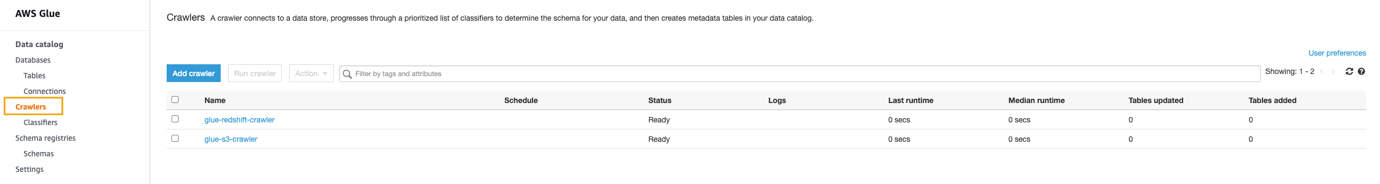
We use an AWS Glue crawler to infer metadata from delimited data files like the CSV files used in this post. For instructions on getting started with an AWS Glue crawler, refer to Tutorial: Adding an AWS Glue crawler.
Create an AWS Glue crawler and point it to the Amazon S3 location that contains the source table subfolders, within which the associated data files are placed. When you’re creating the AWS Glue crawler, create a new database named rs-dimension-blog. The following screenshots show the AWS Glue crawler configuration chosen for our data files.


Note that for the Set output and scheduling section, the advanced options are left unchanged.

Running this crawler should create the following tables within the rs-dimension-blog database:
customer_addresscustomer_master
Create schemas in Amazon Redshift
First, create an AWS Identity and Access Management (IAM) role named rs-dim-blog-spectrum-role. For instructions, refer to Create an IAM role for Amazon Redshift.
The IAM role has Amazon Redshift as the trusted entity, and the permissions policy includes AmazonS3ReadOnlyAccess and AWSGlueConsoleFullAccess, because we’re using the AWS Glue Data Catalog. Then associate the IAM role with the Amazon Redshift cluster or endpoint.
Instead, you can also set the IAM role as the default for your Amazon Redshift cluster or endpoint. If you do so, in the following create external schema command, pass the iam_role parameter as iam_role default.
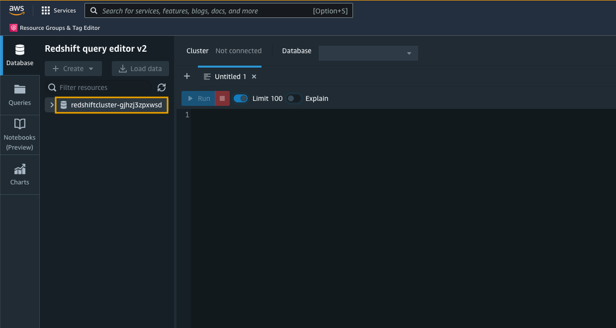
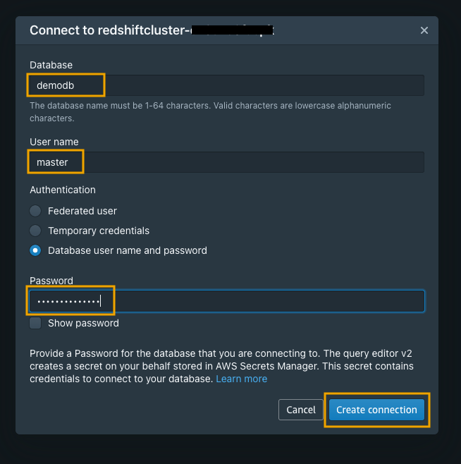
Now, open Amazon Redshift Query Editor V2 and create an external schema passing the newly created IAM role and specifying the database as rs-dimension-blog. The database name rs-dimension-blog is the one created in the Data Catalog as part of configuring the crawler in the preceding section. See the following code:
create external schema spectrum_dim_blog
from data catalog
database 'rs-dimension-blog'
iam_role 'arn:aws:iam::<accountid>:role/rs-dim-blog-spectrum-role';
Check if the tables registered in the Data Catalog in the preceding section are visible from within Amazon Redshift:
select *
from spectrum_dim_blog.customer_master
limit 10;

select *
from spectrum_dim_blog.customer_address
limit 10;
Each of these queries will return 10 rows from the respective Data Catalog tables.
Create another schema in Amazon Redshift to host the table, dim_customer:
create schema rs_dim_blog;
Create views to fetch the latest records from each source table
Create a view for the customer_master table, naming it vw_cust_mstr_latest:
create view rs_dim_blog.vw_cust_mstr_latest as with rows_numbered as (
  select
    customer_id,
    first_name,
    last_name,
    employer_name,
    row_audit_ts,
    row_number() over(
      partition by customer_id
      order by
        row_audit_ts desc
    ) as rnum
  from
    spectrum_dim_blog.customer_master
)
select
  customer_id,
  first_name,
  last_name,
  employer_name,
  row_audit_ts,
  rnum
from
  rows_numbered
where
  rnum = 1 with no schema binding;
The preceding query uses row_number, which is a window function provided by Amazon Redshift. Using window functions enables you to create analytic business queries more efficiently. Window functions operate on a partition of a result set, and return a value for every row in that window. The row_number window function determines the ordinal number of the current row within a group of rows, counting from 1, based on the ORDER BY expression in the OVER clause. By including the PARTITION BY clause as customer_id, groups are created for each value of customer_id and ordinal numbers are reset for each group.
Create a view for the customer_address table, naming it vw_cust_addr_latest:
create view rs_dim_blog.vw_cust_addr_latest as with rows_numbered as (
  select
    customer_id,
    email_id,
    city,
    country,
    row_audit_ts,
    row_number() over(
      partition by customer_id
      order by
        row_audit_ts desc
    ) as rnum
  from
    spectrum_dim_blog.customer_address
)
select
  customer_id,
  email_id,
  city,
  country,
  row_audit_ts,
  rnum
from
  rows_numbered
where
  rnum = 1 with no schema binding;
Both view definitions use the row_number window function of Amazon Redshift, ordering the records by descending order of the row_audit_ts column (the audit timestamp column). The condition rnum=1 fetches the latest record for each customer_id value.
Create the dim_customer table in Amazon Redshift
Create dim_customer as an internal table in Amazon Redshift within the rs_dim_blog schema. The dimension table includes the column customer_sk, that acts as the surrogate key column and enables us to capture a time-sensitive version of each customer record. The validity period for each record is defined by the columns rec_eff_dt and rec_exp_dt, representing record effective date and record expiry date, respectively. See the following code:
create table rs_dim_blog.dim_customer (
  customer_sk bigint,
  customer_id bigint,
  first_name varchar(100),
  last_name varchar(100),
  employer_name varchar(100),
  email_id varchar(100),
  city varchar(100),
  country varchar(100),
  rec_eff_dt date,
  rec_exp_dt date
) diststyle auto;
Create a view to consolidate the latest version of source records
Create the view vw_dim_customer_src, which consolidates the latest records from both source tables using left outer join, keeping them ready to be populated into the Amazon Redshift dimension table. This view fetches data from the latest views defined in the section “Create views to fetch the latest records from each source table”:
create view rs_dim_blog.vw_dim_customer_src as
select
  m.customer_id,
  m.first_name,
  m.last_name,
  m.employer_name,
  a.email_id,
  a.city,
  a.country
from
  rs_dim_blog.vw_cust_mstr_latest as m
  left join rs_dim_blog.vw_cust_addr_latest as a on m.customer_id = a.customer_id
order by
  m.customer_id with no schema binding;
At this point, this view fetches the initial data for loading into the dim_customer table that we are about to create. In your use-case, use a similar approach to create and join the required source table views to populate your target dimension table.
Populate initial data into dim_customer
Populate the initial data into the dim_customer table by querying the view vw_dim_customer_src. Because this is the initial data load, running row numbers generated by the row_number window function will suffice to populate a unique value in the customer_sk column starting from 1:
insert into rs_dim_blog.dim_customer
select
  row_number() over() as customer_sk,
  customer_id,
  first_name,
  last_name,
  employer_name,
  email_id,
  city,
  country,
  cast('2022-07-01' as date) rec_eff_dt,
  cast('9999-12-31' as date) rec_exp_dt
from
  rs_dim_blog.vw_dim_customer_src;
In this query, we have specified ’2022-07-01’ as the value in rec_eff_dt for all initial data records. For your use-case, you can modify this date value as appropriate to your situation.
The preceding steps complete the initial data loading into the dim_customer table. In the next steps, we proceed with populating incremental data.
Land ongoing change data files in Amazon S3
After the initial load, the source systems provide data files on an ongoing basis, either containing only new and change records or a full extract containing all records for a particular table.
You can use the sample files customer_master_with_ts_incr.csv and customer_address_with_ts_incr.csv, which contain changed as well as new records. These incremental files need to be placed in the same location in Amazon S3 where the initial data files were placed. Please see section “Land data from source tables”. This will result in the corresponding Redshift Spectrum tables automatically reading the additional rows.
If you used the sample file for customer_master, after adding the incremental files, the following query shows the initial as well as incremental records:
select
  customer_id,
  first_name,
  last_name,
  employer_name,
  row_audit_ts
from
  spectrum_dim_blog.customer_master
order by
  customer_id;

In case of full extracts, we can identify deletes occurring in the source system tables by comparing the previous and current versions and looking for missing records. In case of change-only extracts where the rec_source_status column is present, its value will help us identify deleted records. In either case, land the ongoing change data files in the respective Amazon S3 locations.
For this example, we have uploaded the incremental data for the customer_master and customer_address source tables with a few customer_id records receiving updates and a few new records being added.
Create a temporary table to capture change records
Create the temporary table temp_dim_customer to store all changes that need to be applied to the target dim_customer table:
create temp table temp_dim_customer (
  customer_sk bigint,
  customer_id bigint,
  first_name varchar(100),
  last_name varchar(100),
  employer_name varchar(100),
  email_id varchar(100),
  city varchar(100),
  country varchar(100),
  rec_eff_dt date,
  rec_exp_dt date,
  iud_operation character(1)
);
Populate the temporary table with new and changed records
This is a multi-step process that can be combined into a single complex SQL. Complete the following steps:
- Fetch the latest version of all customer attributes by querying the view
vw_dim_customer_src:
select
  customer_id,
  sha2(
    coalesce(first_name, '') || coalesce(last_name, '') || coalesce(employer_name, '') || coalesce(email_id, '') || coalesce(city, '') || coalesce(country, ''), 512
  ) as hash_value,
  first_name,
  last_name,
  employer_name,
  email_id,
  city,
  country,
  current_date rec_eff_dt,
  cast('9999-12-31' as date) rec_exp_dt
from
  rs_dim_blog.vw_dim_customer_src;
Amazon Redshift offers hashing functions such as sha2, which converts a variable length string input into a fixed length character output. The output string is a text representation of the hexadecimal value of the checksum with the specified number of bits. In this case, we pass a concatenated set of customer attributes whose change we want to track, specifying the number of bits as 512. We’ll use the output of the hash function to determine if any of the attributes have undergone a change. This dataset will be called newver (new version).
Because we landed the ongoing change data in the same location as the initial data files, the records retrieved from the preceding query (in newver) include all records, even the unchanged ones. But because of the definition of the view vw_dim_customer_src, we get only one record per customerid, which is its latest version based on row_audit_ts.
- In a similar manner, retrieve the latest version of all customer records from
dim_customer, which are identified by rec_exp_dt=‘9999-12-31’. While doing so, also retrieve the sha2 value of all customer attributes available in dim_customer:
select
  customer_id,
  sha2(
    coalesce(first_name, '') || coalesce(last_name, '') || coalesce(employer_name, '') || coalesce(email_id, '') || coalesce(city, '') || coalesce(country, ''), 512
  ) as hash_value,
  first_name,
  last_name,
  employer_name,
  email_id,
  city,
  country
from
  rs_dim_blog.dim_customer
where
  rec_exp_dt = '9999-12-31';
This dataset will be called oldver (old or existing version).
- Identify the current maximum surrogate key value from the
dim_customer table:
select
  max(customer_sk) as maxval
from
  rs_dim_blog.dim_customer;
This value (maxval) will be added to the row_number before being used as the customer_sk value for the change records that need to be inserted.
- Perform a full outer join of the old version of records (
oldver) and the new version (newver) of records on the customer_id column. Then compare the old and new hash values generated by the sha2 function to determine if the change record is an insert, update, or delete:
case when oldver.customer_id is null then 'I'
when newver.customer_id is null then 'D'
when oldver.hash_value != newver.hash_value then 'U'
else 'N' end as iud_op
We tag the records as follows:
- If the
customer_id is non-existent in the oldver dataset (oldver.customer_id is null), it’s tagged as an insert (‘I').
- Otherwise, if the
customer_id is non-existent in the newver dataset (newver.customer_id is null), it’s tagged as a delete (‘D').
- Otherwise, if the old
hash_value and new hash_value are different, these records represent an update (‘U').
- Otherwise, it indicates that the record has not undergone any change and therefore can be ignored or marked as not-to-be-processed (
‘N').
Make sure to modify the preceding logic if the source extract contains rec_source_status to identify deleted records.
Although sha2 output maps a possibly infinite set of input strings to a finite set of output strings, the chances of collision of hash values for the original row values and changed row values are very unlikely. Instead of individually comparing each column value before and after, we compare the hash values generated by sha2 to conclude if there has been a change in any of the attributes of the customer record. For your use-case, we recommend you choose a hash function that works for your data conditions after adequate testing. Instead, you can compare individual column values if none of the hash functions satisfactorily meet your expectations.
- Combining the outputs from the preceding steps, let’s create the INSERT statement that captures only change records to populate the temporary table:
insert into temp_dim_customer (
  customer_sk, customer_id, first_name,
  last_name, employer_name, email_id,
  city, country, rec_eff_dt, rec_exp_dt,
  iud_operation
) with newver as (
  select
    customer_id,
    sha2(
      coalesce(first_name, '') || coalesce(last_name, '') || coalesce(employer_name, '') || coalesce(email_id, '') || coalesce(city, '') || coalesce(country, ''), 512
    ) as hash_value,
    first_name,
    last_name,
    employer_name,
    email_id,
    city,
    country,
    current_date rec_eff_dt,
    cast('9999-12-31' as date) rec_exp_dt
  from
    rs_dim_blog.vw_dim_customer_src
),
oldver as (
  select
    customer_id,
    sha2(
      coalesce(first_name, '') || coalesce(last_name, '') || coalesce(employer_name, '') || coalesce(email_id, '') || coalesce(city, '') || coalesce(country, ''), 512
    ) as hash_value,
    first_name,
    last_name,
    employer_name,
    email_id,
    city,
    country
  from
    rs_dim_blog.dim_customer
  where
    rec_exp_dt = '9999-12-31'
),
maxsk as (
  select
    max(customer_sk) as maxval
  from
    rs_dim_blog.dim_customer
),
allrecs as (
  select
    coalesce(oldver.customer_id, newver.customer_id) as customer_id,
    case when oldver.customer_id is null then 'I' when newver.customer_id is null then 'D' when oldver.hash_value != newver.hash_value then 'U' else 'N' end as iud_op,
    newver.first_name,
    newver.last_name,
    newver.employer_name,
    newver.email_id,
    newver.city,
    newver.country,
    newver.rec_eff_dt,
    newver.rec_exp_dt
  from
    oldver full
    outer join newver on oldver.customer_id = newver.customer_id
)
select
  (maxval + (row_number() over())) as customer_sk,
  customer_id,
  first_name,
  last_name,
  employer_name,
  email_id,
  city,
  country,
  rec_eff_dt,
  rec_exp_dt,
  iud_op
from
  allrecs,
  maxsk
where
  iud_op != 'N';
Expire updated customer records
With the temp_dim_customer table now containing only the change records (either ‘I’, ‘U’, or ‘D’), the same can be applied on the target dim_customer table.
Let’s first fetch all records with values ‘U’ or ‘D’ in the iud_op column. These are records that have either been deleted or updated in the source system. Because dim_customer is a slowly changing dimension, it needs to reflect the validity period of each customer record. In this case, we expire the presently active recorts that have been updated or deleted. We expire these records as of yesterday (by setting rec_exp_dt=current_date-1) matching on the customer_id column:
update
  rs_dim_blog.dim_customer
set
  rec_exp_dt = current_date - 1
where
  customer_id in (
    select
      customer_id
    from
      temp_dim_customer as t
    where
      iud_operation in ('U', 'D')
  )
  and rec_exp_dt = '9999-12-31';
Insert new and changed records
As the last step, we need to insert the newer version of updated records along with all first-time inserts. These are indicated by ‘U’ and ‘I’, respectively, in the iud_op column in the temp_dim_customer table:
insert into rs_dim_blog.dim_customer (
  customer_sk, customer_id, first_name,
  last_name, employer_name, email_id,
  city, country, rec_eff_dt, rec_exp_dt
)
select
  customer_sk,
  customer_id,
  first_name,
  last_name,
  employer_name,
  email_id,
  city,
  country,
  rec_eff_dt,
  rec_exp_dt
from
  temp_dim_customer
where
  iud_operation in ('I', 'U');
Depending on the SQL client setting, you might want to run a commit transaction; command to verify that the preceding changes are persisted successfully in Amazon Redshift.
Check the final output
You can run the following query and see that the dim_customer table now contains both the initial data records plus the incremental data records, capturing multiple versions for those customer_id values that got changed as part of incremental data loading. The output also indicates that each record has been populated with appropriate values in rec_eff_dt and rec_exp_dt corresponding to the record validity period.
select
  *
from
  rs_dim_blog.dim_customer
order by
  customer_id,
  customer_sk;
For the sample data files provided in this article, the preceding query returns the following records. If you’re using the sample data files provided in this post, note that the values in customer_sk may not match with what is shown in the following table.

In this post, we only show the important SQL statements; the complete SQL code is available in load_scd2_sample_dim_customer.sql.
Clean up
If you no longer need the resources you created, you can delete them to prevent incurring additional charges.
Conclusion
In this post, you learned how to simplify data loading into Type-2 SCD tables in Amazon Redshift, covering both initial data loading and incremental data loading. The approach deals with multiple source tables populating a target dimension table, capturing the latest version of source records as of each run.
Refer to Amazon Redshift data loading best practices for further materials and additional best practices, and see Updating and inserting new data for instructions to implement updates and inserts.
About the Author
 Vaidy Kalpathy is a Senior Data Lab Solution Architect at AWS, where he helps customers modernize their data platform and defines end to end data strategy including data ingestion, transformation, security, visualization. He is passionate about working backwards from business use cases, creating scalable and custom fit architectures to help customers innovate using data analytics services on AWS.


 Babu Srinivasan is a Senior Partner Solutions Architect at MongoDB. In his current role, he is working with AWS to build the technical integrations and reference architectures for the AWS and MongoDB solutions. He has more than two decades of experience in Database and Cloud technologies . He is passionate about providing technical solutions to customers working with multiple Global System Integrators(GSIs) across multiple geographies.


 Noritaka Sekiyama is a Principal Big Data Architect on the AWS Glue team. He is responsible for building software artifacts to help customers. In his spare time, he enjoys cycling with his new road bike.


 Debaprasun Chakraborty is an AWS Solutions Architect, specializing in the analytics domain. He has around 20 years of software development and architecture experience. He is passionate about helping customers in cloud adoption, migration and strategy.
 Suraj Subramani Vineet is a Senior Cloud Architect at Amazon Web Services (AWS) Professional Services in Sydney, Australia. He specializes in designing and building scalable and cost-effective data platforms and AI/ML solutions in the cloud. Outside of work, he enjoys playing soccer on weekends.


 Vikram Sahadevan is a Senior Resident Architect on the AWS Data Lab team. He enjoys efforts that focus around providing prescriptive architectural guidance, sharing best practices, and removing technical roadblocks with joint engineering engagements between customers and AWS technical resources that accelerate data, analytics, artificial intelligence, and machine learning initiatives.
 Suvendu Kumar Patra possesses 18 years of experience in infrastructure, database design, and data engineering, and he currently holds the position of Senior Resident Architect at Amazon Web Services. He is a member of the specialized focus group, AWS Data Lab, and his primary duties entail working with executive leadership teams of strategic AWS customers to develop their roadmaps for data, analytics, and AI/ML. Suvendu collaborates closely with customers to implement data engineering, data hub, data lake, data governance, and EDW solutions, as well as enterprise data strategy and data management.


 Aniket Jiddigoudar is a Big Data Architect on the AWS Glue team. He works with customers to help improve their big data workloads. In his spare time, he enjoys trying out new food, playing video games, and kickboxing.
 Sean Ma is a Principal Product Manager on the AWS Glue team. He has an 18+ year track record of innovating and delivering enterprise products that unlock the power of data for users. Outside of work, Sean enjoys scuba diving and college football.


 Vinay Kumar Khambhampati is a Lead Consultant with the AWS ProServe Team, helping customers with cloud adoption. He is passionate about big data and data analytics.
 Sandeep Singh is a Lead Consultant at AWS ProServe, focused on analytics, data lake architecture, and implementation. He helps enterprise customers migrate and modernize their data lake and data warehouse using AWS services.
 Amol Guldagad is a Data Analytics Consultant based in India. He has worked with customers in different industries like banking and financial services, healthcare, power and utilities, manufacturing, and retail, helping them solve complex challenges with large-scale data platforms. At AWS ProServe, he helps customers accelerate their journey to the cloud and innovate using AWS analytics services.
 Jason D’Alba is an AWS Solutions Architect leader focused on databases and enterprise applications, helping customers architect highly available and scalable solutions.
 Navnit Shukla is an AWS Specialist Solution Architect, Analytics, and is passionate about helping customers uncover insights from their data. He has been building solutions to help organizations make data-driven decisions.
 Vetri Natarajan is a Specialist Solutions Architect for Amazon QuickSight. Vetri has 15 years of experience implementing enterprise business intelligence (BI) solutions and greenfield data products. Vetri specializes in integration of BI solutions with business applications and enable data-driven decisions.
 Sindhura Palakodety is a Solutions Architect at AWS. She is passionate about helping customers build enterprise-scale Well-Architected solutions on the AWS platform and specializes in Data Analytics domain.

 Ashish Prabhu is a Senior Manager of Software Engineering in Morningstar, Inc. He focuses on the solutioning and delivering the different aspects of Data Lake and Data Warehouse for Morningstar’s Enterprise Data and Platform Team. In his spare time he enjoys playing basketball, painting and spending time with his family.
 Stephen Johnston is a Distinguished Software Architect at Morningstar, Inc. His focus is on data lake and data warehousing technologies for Morningstar’s Enterprise Data Platform team.
 Colin Ingarfield is a Lead Software Engineer at Morningstar, Inc. Based in Austin, Colin focuses on access control and data entitlements on Morningstar’s growing Data Lake platform.
 Don Drake is a Senior Analytics Specialist Solutions Architect at AWS. Based in Chicago, Don helps Financial Services customers migrate workloads to AWS.


 Aaron Chong is an Enterprise Solutions Architect at Amazon Web Services Hong Kong. He specializes in the data analytics domain, and works with a wide range of customers to build big data analytics platforms, modernize data engineering practices, and advocate AI/ML democratization.


 Nith Govindasivan, is a Data Lake Architect with AWS Professional Services, where he helps onboarding customers on their modern data architecture journey through implementing Big Data & Analytics solutions. Outside of work, Nith is an avid Cricket fan, watching almost any cricket during his spare time and enjoys long drives, and traveling internationally.
 Vijay Velpula is a Data Architect with AWS Professional Services. He helps customers implement Big Data and Analytics Solutions. Outside of work, he enjoys spending time with family, traveling, hiking and biking.
 Sriharsh Adari is a Senior Solutions Architect at Amazon Web Services (AWS), where he helps customers work backwards from business outcomes to develop innovative solutions on AWS. Over the years, he has helped multiple customers on data platform transformations across industry verticals. His core area of expertise include Technology Strategy, Data Analytics, and Data Science. In his spare time, he enjoys playing sports, binge-watching TV shows, and playing Tabla.


 Alternatively, you can also use the AWS CLI to grant data location permission on bucket registered in central account to the crawler role using below command:


 Sandeep Adwankar is a Senior Technical Product Manager at AWS. Based in the California Bay Area, he works with customers around the globe to translate business and technical requirements into products that enable customers to improve how they manage, secure, and access data.
 Srividya Parthasarathy is a Senior Big Data Architect on the AWS Lake Formation team. She enjoys building data mesh solutions and sharing them with the community.
 Piyali Kamra is a seasoned enterprise architect and a hands-on technologist who believes that building large scale enterprise systems is not an exact science but more like an art, in which tools and technologies must be carefully selected based on the team’s culture , strengths , weaknesses and risks , in tandem with having a futuristic vision as to how you want to shape your product a few years down the road.


 Scott Long is a Front End Engineer on the AWS Glue team. He is responsible for implementing new features in AWS Glue Studio. In his spare time, he enjoys socializing with friends and participating in various outdoor activities.
 Gowtham Dandu is an Engineering Lead at Infomedia Ltd with a passion for building efficient and effective solutions on the cloud, especially involving data, APIs, and modern SaaS applications. He specializes in building microservices and data platforms that are cost-effective and highly scalable.
 Praveen Kumar is a Specialist Solution Architect at AWS with expertise in designing, building, and implementing modern data and analytics platforms using cloud-native services. His areas of interests are serverless technology, streaming applications, and modern cloud data warehouses.


 Vaidy Kalpathy is a Senior Data Lab Solution Architect at AWS, where he helps customers modernize their data platform and defines end to end data strategy including data ingestion, transformation, security, visualization. He is passionate about working backwards from business use cases, creating scalable and custom fit architectures to help customers innovate using data analytics services on AWS.

 Kalyan Janaki is Senior Big Data & Analytics Specialist with Amazon Web Services. He helps customers architect and build highly scalable, performant, and secure cloud-based solutions on AWS.


 Flora Wu is a Sr. Resident Architect at AWS Data Lab. She helps enterprise customers create data analytics strategies and build solutions to accelerate their businesses outcomes. In her spare time, she enjoys playing tennis, dancing salsa, and traveling.
 Daniel Li is a Sr. Solutions Architect at Amazon Web Services. He focuses on helping customers develop, adopt, and implement cloud services and strategy. When not working, he likes spending time outdoors with his family.


 Kachi Odoemene is an Applied Scientist at AWS AI. He builds AI/ML solutions to solve business problems for AWS customers.
 Taylor McNally is a Deep Learning Architect at Amazon Machine Learning Solutions Lab. He helps customers from various industries build solutions leveraging AI/ML on AWS. He enjoys a good cup of coffee, the outdoors, and time with his family and energetic dog.
 Austin Welch is a Data Scientist in the Amazon ML Solutions Lab. He develops custom deep learning models to help AWS public sector customers accelerate their AI and cloud adoption. In his spare time, he enjoys reading, traveling, and jiu-jitsu.


 AWS and Hugging Face collaborate to make generative AI more accessible and cost-efficient – This previous week, we announced an expanded collaboration between AWS and
 AWS Pi Day – Join me on March 14 for the third annual


 Dhiraj Thakur is a Solutions Architect with Amazon Web Services. He works with AWS customers and partners to provide guidance on enterprise cloud adoption, migration, and strategy. He is passionate about technology and enjoys building and experimenting in the analytics and AI/ML space.
 Rajdip Chaudhuri is Solutions Architect with Amazon Web Services specializing in data and analytics. He enjoys working with AWS customers and partners on data and analytics requirements. In his spare time, he enjoys soccer.