Post Syndicated from Sheila Busser original https://aws.amazon.com/blogs/compute/building-diversified-and-cost-optimized-ec2-server-groups-in-spinnaker/
This blog post is written by Sandeep Palavalasa, Sr. Specialist Containers SA, and Prathibha Datta-Kumar, Software Development Engineer
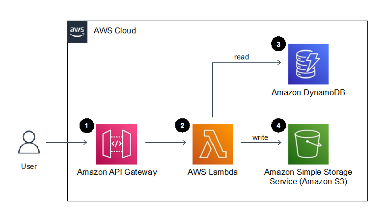
Spinnaker is an open source continuous delivery platform created by Netflix for releasing software changes rapidly and reliably. It enables teams to automate deployments into pipelines that are run whenever a new version is released with proven deployment strategies that are faster and more dependable with zero downtime. For many AWS customers, Spinnaker is a critical piece of technology that allows developers to deploy their applications safely and reliably across different AWS managed services.
Listening to customer requests on the Spinnaker open source project and in the Amazon EC2 Spot Instances integrations roadmap, we have further enhanced Spinnaker’s ability to deploy on Amazon Elastic Compute Cloud (Amazon EC2). The enhancements make it easier to combine Spot Instances with On-Demand, Reserved, and Savings Plans Instances to optimize workload costs with performance. You can improve workload availability when using Spot Instances with features such as allocation strategies and proactive Spot capacity rebalancing, when you are flexible about Instance types and Availability Zones. Combinations of these features offer the best possible experience when using Amazon EC2 with Spinnaker.
In this post, we detail the recent enhancements, along with a walkthrough of how you can use them following the best practices.
Amazon EC2 Spot Instances
EC2 Spot Instances are spare compute capacity in the AWS Cloud available at steep discounts of up to 90% when compared to On-Demand Instance prices. The primary difference between an On-Demand Instance and a Spot Instance is that a Spot Instance can be interrupted by Amazon EC2 with a two-minute notification when Amazon EC2 needs the capacity back. Amazon EC2 now sends rebalance recommendation notifications when Spot Instances are at an elevated risk of interruption. This signal can arrive sooner than the two-minute interruption notice. This lets you proactively replace your Spot Instances before it’s interrupted.
The best way to adhere to Spot best practices and instance fleet management is by using an Amazon EC2 Auto Scaling group When using Spot Instances in Auto Scaling group, enabling Capacity Rebalancing helps you maintain workload availability by proactively augmenting your fleet with a new Spot Instance before a running instance is interrupted by Amazon EC2.
Spinnaker concepts
Spinnaker uses three key concepts to describe your services, including applications, clusters, and server groups, and how your services are exposed to users is expressed as Load balancers and firewalls.
An application is a collection of clusters, a cluster is a collection of server groups, and a server group identifies the deployable artifact and basic configuration settings such as the number of instances, autoscaling policies, metadata, etc. This corresponds to an Auto Scaling group in AWS. We use Auto Scaling groups and server groups interchangeably in this post.
Spinnaker and Amazon EC2 Integration
In mid-2020, we started looking into customer requests and gaps in the Amazon EC2 feature set supported in Spinnaker. Around the same time, Spinnaker OSS added support for Amazon EC2 Launch Templates. Thanks to their effort, we could follow-up and expand the Amazon EC2 feature set supported in Spinnaker. Now that we understand the new features, let’s look at how to use some of them in the following tutorial spinnaker.io.
Here are some highlights of the features contributed recently:
| Feature |
Why use it? (Example use cases) |
| Multiple Instance Types |
Tap into multiple capacity pools to achieve and maintain the desired scale using Spot Instances. |
| Combining On-Demand and Spot Instances |
– Control the proportion of On-Demand and Spot Instances launched in your sever group.
– Combine Spot Instances with Amazon EC2 Reserved Instances or Savings Plans.
|
| Amazon EC2 Auto Scaling allocation strategies |
Reduce overall Spot interruptions by launching from Spot pools that are optimally chosen based on the available Spot capacity, using capacity-optimized Spot allocation strategy. |
| Capacity rebalancing |
Improve your workload availability by proactively shifting your Spot capacity to optimal pools by enabling capacity rebalancing along with capacity-optimized allocation strategy. |
| Improved support for burstable performance instance types with custom credit specification |
Reduce costs by preventing wastage of CPU cycles. |
We recommend using Spinnaker stable release 1.28.x for API users and 1.29.x for UI users. Here is the Git issue for related PRs and feature releases.
Now that we understand the new features, let’s look at how to use some of them in the following tutorial.
Example tutorial: Deploy a demo web application on an Auto Scaling group with On-Demand and Spot Instances
In this example tutorial, we setup Spinnaker to deploy to Amazon EC2, create an Application Load Balancer, and deploy a demo application on a server group diversified across multiple instance types and purchase options – this case On-Demand and Spot Instances.
We leverage Spinnaker’s API throughout the tutorial to create new resources, along with a quick guide on how to deploy the same using Spinnaker UI (Deck) and leverage UI to view them.
Prerequisites
As a prerequisite to complete this tutorial, you must have an AWS Account with an AWS Identity and Access Management (IAM) User that has the AdministratorAccess configured to use with AWS Command Line Interface (AWS CLI).
1. Spinnaker setup
We will use the AWS CloudFormation template setup-spinnaker-with-deployment-vpc.yml to setup Spinnaker and the required resources.
1.1 Create an Secure Shell(SSH) keypair used to connect to Spinnaker and EC2 instances launched by Spinnaker.
AWS_REGION=us-west-2 # Change the region where you want Spinnaker deployed
EC2_KEYPAIR_NAME=spinnaker-blog-${AWS_REGION}
aws ec2 create-key-pair --key-name ${EC2_KEYPAIR_NAME} --region ${AWS_REGION} --query KeyMaterial --output text > ~/${EC2_KEYPAIR_NAME}.pem
chmod 600 ~/${EC2_KEYPAIR_NAME}.pem
1.2 Deploy the Cloudformation stack.
STACK_NAME=spinnaker-blog
SPINNAKER_VERSION=1.29.1 # Change the version if newer versions are available
NUMBER_OF_AZS=3
AVAILABILITY_ZONES=${AWS_REGION}a,${AWS_REGION}b,${AWS_REGION}c
ACCOUNT_ID=$(aws sts get-caller-identity --query "Account" --output text)
S3_BUCKET_NAME=spin-persitent-store-${ACCOUNT_ID}

# Download template
curl -o setup-spinnaker-with-deployment-vpc.yml https://raw.githubusercontent.com/awslabs/ec2-spot-labs/master/ec2-spot-spinnaker/setup-spinnaker-with-deployment-vpc.yml

# deploy stack
aws cloudformation deploy --template-file setup-spinnaker-with-deployment-vpc.yml \
    --stack-name ${STACK_NAME} \
    --parameter-overrides NumberOfAZs=${NUMBER_OF_AZS} \
    AvailabilityZones=${AVAILABILITY_ZONES} \
    EC2KeyPairName=${EC2_KEYPAIR_NAME} \
    SpinnakerVersion=${SPINNAKER_VERSION} \
    SpinnakerS3BucketName=${S3_BUCKET_NAME} \
    --capabilities CAPABILITY_NAMED_IAM --region ${AWS_REGION}
1.3 Connecting to Spinnaker
1.3.1 Get the SSH command to port forwarding for Deck – the browser-based UI (9000) and Gate – the API Gateway (8084) to access the Spinnaker UI and API.
SPINNAKER_INSTANCE_DNS_NAME=$(aws cloudformation describe-stacks --stack-name ${STACK_NAME} --region ${AWS_REGION} --query "Stacks[].Outputs[?OutputKey=='SpinnakerInstance'].OutputValue" --output text)
echo 'ssh -A -L 9000:localhost:9000 -L 8084:localhost:8084 -L 8087:localhost:8087 -i ~/'${EC2_KEYPAIR_NAME}' ubuntu@$'{SPINNAKER_INSTANCE_DNS_NAME}''
1.3.2 Open a new terminal and use the SSH command (output from the previous command) to connect to the Spinnaker instance. After you successfully connect to the Spinnaker instance via SSH, access the Spinnaker UI here and API here.
2. Deploy a demo web application
Let’s make sure that we have the environment variables required in the shell before proceeding. If you’re using the same terminal window as before, then you might already have these variables.
STACK_NAME=spinnaker-blog
AWS_REGION=us-west-2 # use the same region as before
EC2_KEYPAIR_NAME=spinnaker-blog-${AWS_REGION}
VPC_ID=$(aws cloudformation describe-stacks --stack-name ${STACK_NAME} --region ${AWS_REGION} --query "Stacks[].Outputs[?OutputKey=='VPCID'].OutputValue" --output text)
2.1 Create a Spinnaker Application
We start by creating an application in Spinnaker, a placeholder for the service that we deploy.
curl 'http://localhost:8084/tasks' \
-H 'Content-Type: application/json;charset=utf-8' \
--data-raw \
'{
   "job":[
      {
         "type":"createApplication",
         "application":{
            "cloudProviders":"aws",
            "instancePort":80,
            "name":"demoapp",
            "email":"[email protected]",
            "providerSettings":{
               "aws":{
                  "useAmiBlockDeviceMappings":true
               }
            }
         }
      }
   ],
   "application":"demoapp",
   "description":"Create Application: demoapp"
}'

2.2 Create an Application Load Balancer
Let’s create an Application Load Balanacer and a target group for port 80, spanning the three availability zones in our public subnet. We use the Demo-ALB-SecurityGroup for Firewalls to allow public access to the ALB on port 80.
As Spot Instances are interrupted with a two minute warning, you must adjust the Target Group’s deregistration delay to a slightly lower time. Recommended values are 90 seconds or less. This allows time for in-flight requests to complete and gracefully close existing connections before the instance is interrupted.
curl 'http://localhost:8084/tasks' \
-H 'Content-Type: application/json;charset=utf-8' \
--data-binary \
'{
   "application":"demoapp",
   "description":"Create Load Balancer: demoapp",
   "job":[
      {
         "type":"upsertLoadBalancer",
         "name":"demoapp-lb",
         "loadBalancerType":"application",
         "cloudProvider":"aws",
         "credentials":"my-aws-account",
         "region":"'"${AWS_REGION}"'",
         "vpcId":"'"${VPC_ID}"'",
         "subnetType":"public-subnet",
         "idleTimeout":60,
         "targetGroups":[
            {
               "name":"demoapp-targetgroup",
               "protocol":"HTTP",
               "port":80,
               "targetType":"instance",
               "healthCheckProtocol":"HTTP",
               "healthCheckPort":"traffic-port",
               "healthCheckPath":"/",
               "attributes":{
                  "deregistrationDelay":90
               }
            }
         ],
         "regionZones":[
            "'"${AWS_REGION}"'a",
            "'"${AWS_REGION}"'b",
            "'"${AWS_REGION}"'c"
         ],
         "securityGroups":[
            "Demo-ALB-SecurityGroup"
         ],
         "listeners":[
            {
               "protocol":"HTTP",
               "port":80,
               "defaultActions":[
                  {
                     "type":"forward",
                     "targetGroupName":"demoapp-targetgroup"
                 }
               ]
            }
         ]
      }
   ]
}'

2.3 Create a server group
Before creating a server group (Auto Scaling group), here is a brief overview of the features used in the example:
-
-
- onDemandBaseCapacity (default 0): The minimum amount of your ASG’s capacity that must be fulfilled by On-Demand instances (can also be applied toward Reserved Instances or Savings Plans). The example uses an onDemandBaseCapacity of three.
- onDemandPercentageAboveBaseCapacity (default 100): The percentages of On-Demand and Spot Instances for additional capacity beyond OnDemandBaseCapacity. The example uses onDemandPercentageAboveBaseCapacity of 10% (i.e. 90% Spot).
- spotAllocationStrategy: This indicates how you want to allocate instances across Spot Instance pools in each Availability Zone. The example uses the recommended Capacity Optimized strategy. Instances are launched from optimal Spot pools that are chosen based on the available Spot capacity for the number of instances that are launching.
- launchTemplateOverridesForInstanceType: The list of instance types that are acceptable for your workload. Specifying multiple instance types enables tapping into multiple instance pools in multiple Availability Zones, designed to enhance your service’s availability. You can use the ec2-instance-selector, an open source AWS Command Line Interface(CLI) tool to narrow down the instance types based on resource criteria like vcpus and memory.
-
-
- capacityRebalance: When enabled, this feature proactively manages the EC2 Spot Instance lifecycle leveraging the new EC2 Instance rebalance recommendation. This increases the emphasis on availability by automatically attempting to replace Spot Instances in an ASG before they are interrupted by Amazon EC2. We enable this feature in this example.
Learn more on spinnaker.io: feature descriptions and use cases and sample API requests.
Let’s create a server group with a desired capacity of 12 instances diversified across current and previous generation instance types, attach the previously created ALB, use Demo-EC2-SecurityGroup for the Firewalls which allows http traffic only from the ALB, use the following bash script for UserData to install httpd, and add instance metadata into the index.html.
2.3.1 Save the userdata bash script into a file user-date.sh.
Note that Spinnaker only support base64 encoded userdata. We use base64 bash command to encode the file contents in the next step.
cat << "EOF" > user-data.sh
#!/bin/bash
yum update -y
yum install httpd -y
echo "<html>
<head>
<title>Demo Application</title>
<style>body {margin-top: 40px; background-color: #Gray;} </style>
</head>
<body>
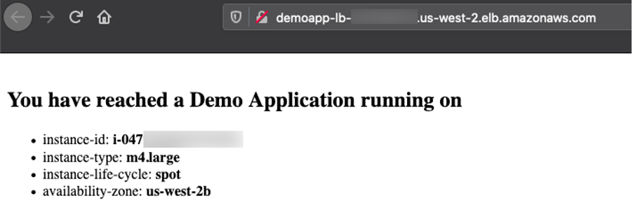
<h2>You have reached a Demo Application running on</h2>
<ul>
<li>instance-id: <b> `curl http://169.254.169.254/latest/meta-data/instance-id` </b></li>
<li>instance-type: <b> `curl http://169.254.169.254/latest/meta-data/instance-type` </b></li>
<li>instance-life-cycle: <b> `curl http://169.254.169.254/latest/meta-data/instance-life-cycle` </b></li>
<li>availability-zone: <b> `curl http://169.254.169.254/latest/meta-data/placement/availability-zone` </b></li>
</ul>
</body>
</html>" > /var/www/html/index.html
systemctl start httpd
systemctl enable httpd
EOF
2.3.2 Create the server group by running the following command. Note we use the KeyPairName that we created as part of the prerequisites.
curl 'http://localhost:8084/tasks' \
-H 'Content-Type: application/json;charset=utf-8' \
-d \
'{
   "job":[
      {
         "type":"createServerGroup",
         "cloudProvider":"aws",
         "account":"my-aws-account",
         "application":"demoapp",
         "stack":"",
         "credentials":"my-aws-account",
	"healthCheckType": "ELB",
	"healthCheckGracePeriod":600,
	"capacityRebalance": true,
         "onDemandBaseCapacity":3,
         "onDemandPercentageAboveBaseCapacity":10,
         "spotAllocationStrategy":"capacity-optimized",
         "setLaunchTemplate":true,
         "launchTemplateOverridesForInstanceType":[
            {
               "instanceType":"m4.large"
            },
            {
               "instanceType":"m5.large"
            },
            {
               "instanceType":"m5a.large"
            },
            {
               "instanceType":"m5ad.large"
            },
            {
               "instanceType":"m5d.large"
            },
            {
               "instanceType":"m5dn.large"
            },
            {
               "instanceType":"m5n.large"
            }

         ],
         "capacity":{
            "min":6,
            "max":21,
            "desired":12
         },
         "subnetType":"private-subnet",
         "availabilityZones":{
            "'"${AWS_REGION}"'":[
               "'"${AWS_REGION}"'a",
               "'"${AWS_REGION}"'b",
               "'"${AWS_REGION}"'c"
            ]
         },
         "keyPair":"'"${EC2_KEYPAIR_NAME}"'",
         "securityGroups":[
            "Demo-EC2-SecurityGroup"
         ],
         "instanceType":"m5.large",
         "virtualizationType":"hvm",
         "amiName":"'"$(aws ec2 describe-images --owners amazon --filters "Name=name,Values=amzn2-ami-hvm-2*x86_64-gp2" --query 'reverse(sort_by(Images, &CreationDate))[0].Name' --region ${AWS_REGION} --output text)"'",
         "targetGroups":[
            "demoapp-targetgroup"
         ],
         "base64UserData":"'"$(base64 user-data.sh)"'",,
        "associatePublicIpAddress":false,
         "instanceMonitoring":false
      }
   ],
   "application":"demoapp",
   "description":"Create New server group in cluster demoapp"
}'
Spinnaker creates an Amazon EC2 Launch Template and an ASG with specified parameters and waits until the ALB health check passes before sending traffic to the EC2 Instances.
The server group and launch template that we just created will look like this in Spinnaker UI:

The UI also displays capacity type, such as the purchase option for each instance type in the Instance Information section:


3. Access the application
Copy the Application Load Balancer URL by selecting the tree icon in the right top corner of the server group, and access it in a browser. You can refresh multiple times to see that the requests are going to different instances every time.

Congratulations! You successfully deployed the demo application on an Amazon EC2 server group diversified across multiple instance types and purchase options.
Moreover, you can clone, modify, disable, and destroy these server groups, as well as use them with Spinnaker pipelines to effectively release new versions of your application.
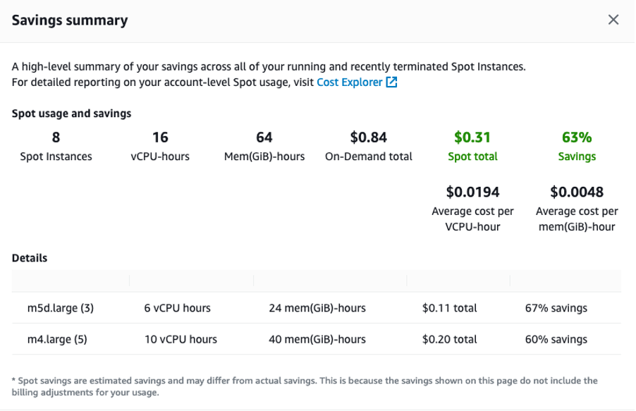
Cost savings
Check the savings you realized by deploying your demo application on EC2 Spot Instances by going to EC2 console > Spot Requests > Saving Summary.

Cleanup
To avoid incurring any additional charges, clean up the resources created in the tutorial.
Frist, delete the server group, application load balancer and application in Spinnaker.
curl 'http://localhost:8084/tasks' \
-H 'Content-Type: application/json;charset=utf-8' \
--data-raw \
'{
   "job":[
      {
         "reason":"Cleanup",
         "asgName":"demoapp-v000",
         "moniker":{
            "app":"demoapp",
            "cluster":"demoapp",
            "sequence":0
         },
         "serverGroupName":"demoapp-v000",
         "type":"destroyServerGroup",
         "region":"'"${AWS_REGION}"'",
         "credentials":"my-aws-account",
         "cloudProvider":"aws"
      },
      {
         "cloudProvider":"aws",
         "loadBalancerName":"demoapp-lb",
         "loadBalancerType":"application",
         "regions":[
            "'"${AWS_REGION}"'"
         ],
         "credentials":"my-aws-account",
         "vpcId":"'"${VPC_ID}"'",
         "type":"deleteLoadBalancer"
      },
      {
         "type":"deleteApplication",
         "application":{
            "name":"demoapp",
            "cloudProviders":"aws"
         }
      }
   ],
   "application":"demoapp",
   "description":"Deleting ServerGroup, ALB and Application: demoapp"
}'
Wait for Spinnaker to delete all of the resources before proceeding further. You can confirm this either on the Spinnaker UI or AWS Management Console.
Then delete the Spinnaker infrastructure by running the following command:
aws ec2 delete-key-pair --key-name ${EC2_KEYPAIR_NAME} --region ${AWS_REGION}
rm ~/${EC2_KEYPAIR_NAME}.pem
aws s3api delete-objects \
--bucket ${S3_BUCKET_NAME} \
--delete "$(aws s3api list-object-versions \
--bucket ${S3_BUCKET_NAME} \
--query='{Objects: Versions[].{Key:Key,VersionId:VersionId}}')" #If error occurs, there are no Versions and is OK
aws s3api delete-objects \
--bucket ${S3_BUCKET_NAME} \
--delete "$(aws s3api list-object-versions \
--bucket ${S3_BUCKET_NAME} \
--query='{Objects: DeleteMarkers[].{Key:Key,VersionId:VersionId}}')" #If error occurs, there are no DeleteMarkers and is OK
aws s3 rb s3://${S3_BUCKET_NAME} --force #Delete Bucket
aws cloudformation delete-stack --region ${AWS_REGION} --stack-name ${STACK_NAME}
Conclusion
In this post, we learned about the new Amazon EC2 features recently added to Spinnaker, and how to use them to build diversified and optimized Auto Scaling Groups. We also discussed recommended best practices for EC2 Spot and how they can improve your experience with it.
We would love to hear from you! Tell us about other Continuous Integration/Continuous Delivery (CI/CD) platforms that you want to use with EC2 Spot and/or Auto Scaling Groups by adding an issue on the Spot integrations roadmap.


 Ashish Prabhu is a Senior Manager of Software Engineering in Morningstar, Inc. He focuses on the solutioning and delivering the different aspects of Data Lake and Data Warehouse for Morningstar’s Enterprise Data and Platform Team. In his spare time he enjoys playing basketball, painting and spending time with his family.
 Stephen Johnston is a Distinguished Software Architect at Morningstar, Inc. His focus is on data lake and data warehousing technologies for Morningstar’s Enterprise Data Platform team.
 Colin Ingarfield is a Lead Software Engineer at Morningstar, Inc. Based in Austin, Colin focuses on access control and data entitlements on Morningstar’s growing Data Lake platform.
 Don Drake is a Senior Analytics Specialist Solutions Architect at AWS. Based in Chicago, Don helps Financial Services customers migrate workloads to AWS.
 Shruthi Panicker is a Senior Product Marketing Manager with Amazon QuickSight at AWS. As an engineer turned product marketer, Shruthi has spent over 15 years in the technology industry in various roles from software engineering, to solution architecting to product marketing. She is passionate about working at the intersection of technology and business to tell great product stories that help drive customer value.


 This online and mobile usage drives very specific traffic patterns on IT systems: a huge peak of connections and authentications in the few minutes before the start of a game and millions of video streams that must be delivered reliably over a variety of changing network qualities. In addition to these technical challenges, there is also an economic challenge: to deliver advertisements at key moments, such as before a national anthem or during a 15-minute half-time. The digital platform sells its own set of commercials, which are different from the commercials broadcast over the air, and might also be different from region to region. All these video streams have to be delivered to millions of viewers on a wide range of devices and a variety of network conditions: from 1 Gbs fiber at home down to 3 G networks in remote areas.
 By the time France took to the pitch on Dec. 18, 2022, TF1 knew they would break records on the platform. Thierry said the traffic was higher than estimated, but the platform absorbed it. He also described that during the first part of the game, when Argentina was leading, the TF1 team observed a slow decline of connections… that is, until


 The following screenshot shows the same query in Amazon RedShift Query Editor V2.


 Erol Murtezaoglu, a Technical Product Manager at AWS, is an inquisitive and enthusiastic thinker with a drive for self-improvement and learning. He has a strong and proven technical background in software development and architecture, balanced with a drive to deliver commercially successful products. Erol highly values the process of understanding customer needs and problems, in order to deliver solutions that exceed expectations.
 Mohamed Shaaban is a Senior Software Engineer in Amazon Redshift and is based in Berlin, Germany. He has over 12 years of experience in the software engineering. He is passionate about cloud services and building solutions that delight customers. Outside of work, he is an amateur photographer who loves to explore and capture unique moments.


 Mahesh Pasupuleti is a VP of Data & Machine Learning Engineering at Poshmark. He has helped several startups succeed in different domains, including media streaming, healthcare, the financial sector, and marketplaces. He loves software engineering, building high performance teams, and strategy, and enjoys gardening and playing badminton in his free time.
 Gaurav Shah is Director of Data Engineering and ML at Poshmark. He and his team help build data-driven solutions to drive growth at Poshmark.
 Raghu Mannam is a Sr. Solutions Architect at AWS in San Francisco. He works closely with late-stage startups, many of which have had recent IPOs. His focus is end-to-end solutioning including security, DevOps automation, resilience, analytics, machine learning, and workload optimization in the cloud.
 Deepesh Malviya is Solutions Architect Manager on the AWS Data Lab team. He and his team help customers architect and build data, analytics, and machine learning solutions to accelerate their key initiatives as part of the AWS Data Lab.

 Alexander Plumb is a Product Manager at Mitratech. Alexander has been a product leader with over 5 years of experience leading to highly successful product launches that meet customer needs.
 Bani Sharma is a Sr Solutions Architect with Amazon Web Services (AWS), based out of Denver, Colorado. As a Solutions Architect, she works with a large number of Small and Medium businesses, and provides technical guidance and solutions on AWS. She has an area of depth in Containers and Modernization. Prior to AWS, Bani worked in various technical roles for a large Telecom provider Dish Networks and worked as a Senior Developer for HSBC Bank Software development.
 Brian Klein is a Sr Technical Account Manager with Amazon Web Services (AWS), helping digital native businesses utilize AWS services to bring value to their organizations. Brian has worked with AWS technologies for 9 years, designing and operating production internet-facing workloads, with a focus on security, availability, and resilience while demonstrating operational efficiency.

 Anish Moorjani is a Data Engineer in the Data and Analytics team at SafetyCulture. He helps SafetyCulture’s analytics infrastructure scale with the exponential increase in the volume and variety of data.
 Randy Chng is an Analytics Solutions Architect at Amazon Web Services. He works with customers to accelerate the solution of their key business problems.
 Gowtham Dandu is an Engineering Lead at Infomedia Ltd with a passion for building efficient and effective solutions on the cloud, especially involving data, APIs, and modern SaaS applications. He specializes in building microservices and data platforms that are cost-effective and highly scalable.
 Praveen Kumar is a Specialist Solution Architect at AWS with expertise in designing, building, and implementing modern data and analytics platforms using cloud-native services. His areas of interests are serverless technology, streaming applications, and modern cloud data warehouses.
 Parag Doshi is Vice President of Engineering at Tricentis, where he continues to lead towards the vision of Innovation at the Speed of Imagination. He brings innovation to market by building world-class quality engineering SaaS such as qTest, the flagship test management product, and a new capability called Tricentis Analytics, which unlocks software development lifecycle insights across all types of testing. Prior to Tricentis, Parag was the founder of Anthem’s Cloud Platform Services, where he drove a hybrid cloud and DevSecOps capability and migrated 100 mission-critical applications. He enabled Anthem to build a new pharmacy benefits management business in AWS, resulting in $800 million in total operating gain for Anthem in 2020 per Forbes and CNBC. He also held posts at Hewlett-Packard, having multiple roles including Chief Technologist and head of architecture for DXC’s Virtual Private Cloud, and CTO for HP’s Application Services in the Americas region.
 Guru Havanur serves as a Principal, Big Data Engineering and Analytics team in Tricentis. Guru is responsible for data, analytics, development, integration with other products, security, and compliance activities. He strives to work with other Tricentis products and customers to improve data sharing, data quality, data integrity, and data compliance through the modern big data platform. With over 20 years of experience in data warehousing, a variety of databases, integration, architecture, and management, he thrives for excellence.
 Simon Guindon is an Architect at Tricentis. He has expertise in large-scale distributed systems and database consistency models, and works with teams in Tricentis around the world on scalability and high availability. You can follow his Twitter @simongui.
 Ricardo Serafim is a Senior AWS Data Lab Solutions Architect. With a focus on data pipelines, data lakes, and data warehouses, Ricardo helps customers create an end-to-end architecture and test an MVP as part of their path to production. Outside of work, Ricardo loves to travel with his family and watch soccer games, mainly from the “Timão” Sport Club Corinthians Paulista.