Post Syndicated from Sheila Busser original https://aws.amazon.com/blogs/compute/architecting-for-data-residency-with-aws-outposts-rack-and-landing-zone-guardrails/
This blog post was written by Abeer Naffa’, Sr. Solutions Architect, Solutions Builder AWS, David Filiatrault, Principal Security Consultant, AWS and Jared Thompson, Hybrid Edge SA Specialist, AWS.
In this post, we will explore how organizations can use AWS Control Tower landing zone and AWS Organizations custom guardrails to enable compliance with data residency requirements on AWS Outposts rack. We will discuss how custom guardrails can be leveraged to limit the ability to store, process, and access data and remain isolated in specific geographic locations, how they can be used to enforce security and compliance controls, as well as, which prerequisites organizations should consider before implementing these guardrails.
Data residency is a critical consideration for organizations that collect and store sensitive information, such as Personal Identifiable Information (PII), financial, and healthcare data. With the rise of cloud computing and the global nature of the internet, it can be challenging for organizations to make sure that their data is being stored and processed in compliance with local laws and regulations.
One potential solution for addressing data residency challenges with AWS is to use Outposts rack, which allows organizations to run AWS infrastructure on premises and in their own data centers. This lets organizations store and process data in a location of their choosing. An Outpost is seamlessly connected to an AWS Region where it has access to the full suite of AWS services managed from a single plane of glass, the AWS Management Console or the AWS Command Line Interface (AWS CLI). Outposts rack can be configured to utilize landing zone to further adhere to data residency requirements.
The landing zones are a set of tools and best practices that help organizations establish a secure and compliant multi-account structure within a cloud provider. A landing zone can also include Organizations to set policies – guardrails – at the root level, known as Service Control Policies (SCPs) across all member accounts. This can be configured to enforce certain data residency requirements.
When leveraging Outposts rack to meet data residency requirements, it is crucial to have control over the in-scope data movement from the Outposts. This can be accomplished by implementing landing zone best practices and the suggested guardrails. The main focus of this blog post is on the custom policies that restrict data snapshots, prohibit data creation within the Region, and limit data transfer to the Region.
Prerequisites
Landing zone best practices and custom guardrails can help when data needs to remain in a specific locality where the Outposts rack is also located. This can be completed by defining and enforcing policies for data storage and usage within the landing zone organization that you set up. The following prerequisites should be considered before implementing the suggested guardrails:
1. AWS Outposts rack
AWS has installed your Outpost and handed off to you. An Outpost may comprise of one or more racks connected together at the site. This means that you can start using AWS services on the Outpost, and you can manage the Outposts rack using the same tools and interfaces that you use in AWS Regions.
2. Landing Zone Accelerator on AWS
We recommend using Landing Zone Accelerator on AWS (LZA) to deploy a landing zone for your organization. Make sure that the accelerator is configured for the appropriate Region and industry. To do this, you must meet the following prerequisites:
-
- A clear understanding of your organization’s compliance requirements, including the specific Region and industry rules in which you operate.
- Knowledge of the different LZAs available and their capabilities, such as the compliance frameworks with which you align.
- Have the necessary permissions to deploy the LZAs and configure it for your organization’s specific requirements.
Note that LZAs are designed to help organizations quickly set up a secure, compliant multi-account environment. However, it’s not a one-size-fits-all solution, and you must align it with your organization’s specific requirements.
3. Set up the data residency guardrails
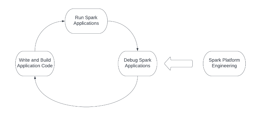
Using Organizations, you must make sure that the Outpost is ordered within a workload account in the landing zone.
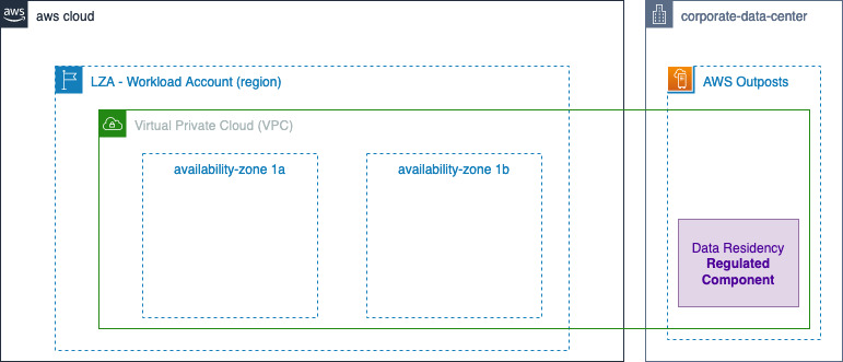
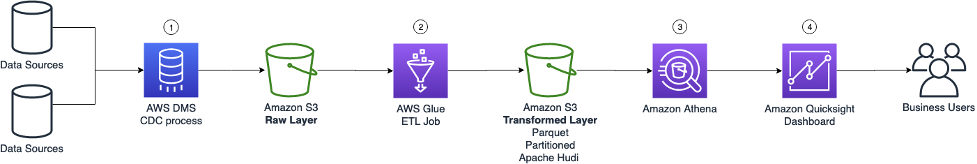
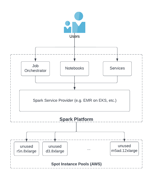
Figure 1: Landing Zone Accelerator – Outposts workload on AWS high level Architecture
Utilizing Outposts rack for regulated components
When local regulations require regulated workloads to stay within a specific boundary, or when an AWS Region or AWS Local Zone isn’t available in your jurisdiction, you can still choose to host your regulated workloads on Outposts rack for a consistent cloud experience. When opting for Outposts rack, note that, as part of the shared responsibility model, customers are responsible for attesting to physical security, access controls, and compliance validation regarding the Outposts, as well as, environmental requirements for the facility, networking, and power. Utilizing Outposts rack requires that you procure and manage the data center within the city, state, province, or country boundary for your applications’ regulated components, as required by local regulations.
Procuring two or more racks in the diverse data centers can help with the high availability for your workloads. This is because it provides redundancy in case of a single rack or server failure. Additionally, having redundant network paths between Outposts rack and the parent Region can help make sure that your application remains connected and continue to operate even if one network path fails.
However, for regulated workloads with strict service level agreements (SLA), you may choose to spread Outposts racks across two or more isolated data centers within regulated boundaries. This helps make sure that your data remains within the designated geographical location and meets local data residency requirements.
In this post, we consider a scenario with one data center, but consider the specific requirements of your workloads and the regulations that apply to determine the most appropriate high availability configurations for your case.
Outposts rack workload data residency guardrails
Organizations provide central governance and management for multiple accounts. Central security administrators use SCPs with Organizations to establish controls to which all AWS Identity and Access Management (IAM) principals (users and roles) adhere.
Now, you can use SCPs to set permission guardrails. A suggested preventative controls for data residency on Outposts rack that leverage the implementation of SCPs are shown as follows. SCPs enable you to set permission guardrails by defining the maximum available permissions for IAM entities in an account. If an SCP denies an action for an account, then none of the entities in the account can take that action, even if their IAM permissions let them. The guardrails set in SCPs apply to all IAM entities in the account, which include all users, roles, and the account root user.
Upon finalizing these prerequisites, you can create the guardrails for the Outposts Organization Unit (OU).
| Note that while the following guidelines serve as helpful guardrails – SCPs – for data residency, you should consult internally with legal and security teams for specific organizational requirements. |
To exercise better control over workloads in the Outposts rack and prevent data transfer from Outposts to the Region or data storage outside the Outposts, consider implementing the following guardrails. Additionally, local regulations may dictate that you set up these additional guardrails.
- When your data residency requirements require restricting data transfer/saving to the Region, consider the following guardrails:
a. Deny copying data from Outposts to the Region for Amazon Elastic Compute Cloud (Amazon EC2), Amazon Relational Database Service (Amazon RDS), Amazon ElastiCache and data sync “DenyCopyToRegion”.
b. Deny Amazon Simple Storage Service (Amazon S3) put action to the Region “DenyPutObjectToRegionalBuckets”.
|
If your data residency requirements mandate restrictions on data storage in the Region, consider implementing this guardrail to prevent the use of S3 in the Region. Note: You can use Amazon S3 for Outposts. |
c. If your data residency requirements mandate restrictions on data storage in the Region, consider implementing “DenyDirectTransferToRegion” guardrail.
|
Out of Scope is metadata such as tags, or operational data such as KMS keys. |
{
  "Version": "2012-10-17",
  "Statement": [
      {
      "Sid": "DenyCopyToRegion",
      "Action": [
        "ec2:ModifyImageAttribute",
        "ec2:CopyImage",
        "ec2:CreateImage",
        "ec2:CreateInstanceExportTask",
        "ec2:ExportImage",
        "ec2:ImportImage",
        "ec2:ImportInstance",
        "ec2:ImportSnapshot",
        "ec2:ImportVolume",
        "rds:CreateDBSnapshot",
        "rds:CreateDBClusterSnapshot",
        "rds:ModifyDBSnapshotAttribute",
        "elasticache:CreateSnapshot",
        "elasticache:CopySnapshot",
        "datasync:Create*",
        "datasync:Update*"
      ],
      "Resource": "*",
      "Effect": "Deny"
    },
    {
      "Sid": "DenyDirectTransferToRegion",
      "Action": [
        "dynamodb:PutItem",
        "dynamodb:CreateTable",
        "ec2:CreateTrafficMirrorTarget",
        "ec2:CreateTrafficMirrorSession",
        "rds:CreateGlobalCluster",
        "es:Create*",
        "elasticfilesystem:C*",
        "elasticfilesystem:Put*",
        "storagegateway:Create*",
        "neptune-db:connect",
        "glue:CreateDevEndpoint",
        "glue:UpdateDevEndpoint",
        "datapipeline:CreatePipeline",
        "datapipeline:PutPipelineDefinition",
        "sagemaker:CreateAutoMLJob",
        "sagemaker:CreateData*",
        "sagemaker:CreateCode*",
        "sagemaker:CreateEndpoint",
        "sagemaker:CreateDomain",
        "sagemaker:CreateEdgePackagingJob",
        "sagemaker:CreateNotebookInstance",
        "sagemaker:CreateProcessingJob",
        "sagemaker:CreateModel*",
        "sagemaker:CreateTra*",
        "sagemaker:Update*",
        "redshift:CreateCluster*",
        "ses:Send*",
        "ses:Create*",
        "sqs:Create*",
        "sqs:Send*",
        "mq:Create*",
        "cloudfront:Create*",
        "cloudfront:Update*",
        "ecr:Put*",
        "ecr:Create*",
        "ecr:Upload*",
        "ram:AcceptResourceShareInvitation"
      ],
      "Resource": "*",
      "Effect": "Deny"
    },
    {
      "Sid": "DenyPutObjectToRegionalBuckets",
      "Action": [
        "s3:PutObject"
      ],
      "Resource": ["arn:aws:s3:::*"],
      "Effect": "Deny"
    }
  ]
}
- If your data residency requirements require limitations on data storage in the Region, consider implementing this guardrail “DenySnapshotsToRegion” and “DenySnapshotsNotOutposts” to restrict the use of snapshots in the Region.
a. Deny creating snapshots of your Outpost data in the Region “DenySnapshotsToRegion”
Make sure to update the Outposts “<outpost_arn_pattern>”.
b. Deny copying or modifying Outposts Snapshots “DenySnapshotsNotOutposts”
Make sure to update the Outposts “<outpost_arn_pattern>”.
Note: “<outpost_arn_pattern>” default is arn:aws:outposts:*:*:outpost/*
{
  "Version": "2012-10-17",
  "Statement": [

    {
      "Sid": "DenySnapshotsToRegion",
      "Effect":"Deny",
      "Action":[
        "ec2:CreateSnapshot",
        "ec2:CreateSnapshots"
      ],
      "Resource":"arn:aws:ec2:*::snapshot/*",
      "Condition":{
         "ArnLike":{
            "ec2:SourceOutpostArn":"<outpost_arn_pattern>"
         },
         "Null":{
            "ec2:OutpostArn":"true"
         }
      }
    },
    {

      "Sid": "DenySnapshotsNotOutposts",
      "Effect":"Deny",
      "Action":[
        "ec2:CopySnapshot",
        "ec2:ModifySnapshotAttribute"
      ],
      "Resource":"arn:aws:ec2:*::snapshot/*",
      "Condition":{
         "ArnLike":{
            "ec2:OutpostArn":"<outpost_arn_pattern>"
         }
      }
    }

  ]
}
- This guardrail helps to prevent the launch of Amazon EC2 instances or creation of network interfaces in non-Outposts subnets. It is advisable to keep data residency workloads within the Outposts rather than the Region to ensure better control over regulated workloads. This approach can help your organization achieve better control over data residency workloads and improve governance over your AWS Organization.
Make sure to update the Outposts subnets “<outpost_subnet_arns>”.
{
"Version": "2012-10-17",
  "Statement":[{
    "Sid": "DenyNotOutpostSubnet",
    "Effect":"Deny",
    "Action": [
      "ec2:RunInstances",
      "ec2:CreateNetworkInterface"
    ],
    "Resource": [
      "arn:aws:ec2:*:*:network-interface/*"
    ],
    "Condition": {
      "ForAllValues:ArnNotEquals": {
        "ec2:Subnet": ["<outpost_subnet_arns>"]
      }
    }
  }]
}
Additional considerations
When implementing data residency guardrails on Outposts rack, consider backup and disaster recovery strategies to make sure that your data is protected in the event of an outage or other unexpected events. This may include creating regular backups of your data, implementing disaster recovery plans and procedures, and using redundancy and failover systems to minimize the impact of any potential disruptions. Additionally, you should make sure that your backup and disaster recovery systems are compliant with any relevant data residency regulations and requirements. You should also test your backup and disaster recovery systems regularly to make sure that they are functioning as intended.
Additionally, the provided SCPs for Outposts rack in the above example do not block the “logs:PutLogEvents”. Therefore, even if you implemented data residency guardrails on Outpost, the application may log data to CloudWatch logs in the Region.
|
Highlights By default, application-level logs on Outposts rack are not automatically sent to Amazon CloudWatch Logs in the Region. You can configure CloudWatch logs agent on Outposts rack to collect and send your application-level logs to CloudWatch logs. logs: PutLogEvents does transmit data to the Region, but it is not blocked by the provided SCPs, as it’s expected that most use cases will still want to be able to use this logging API. However, if blocking is desired, then add the action to the first recommended guardrail. If you want specific roles to be allowed, then combine with the ArnNotLike condition example referenced in the previous highlight. |
Conclusion
The combined use of Outposts rack and the suggested guardrails via AWS Organizations policies enables you to exercise better control over the movement of the data. By creating a landing zone for your organization, you can apply SCPs to your Outposts racks that will help make sure that your data remains within a specific geographic location, as required by the data residency regulations.
Note that, while custom guardrails can help you manage data residency on Outposts rack, it’s critical to thoroughly review your policies, procedures, and configurations to make sure that they are compliant with all relevant data residency regulations and requirements. Regularly testing and monitoring your systems can help make sure that your data is protected and your organization stays compliant.

 Anish Moorjani is a Data Engineer in the Data and Analytics team at SafetyCulture. He helps SafetyCulture’s analytics infrastructure scale with the exponential increase in the volume and variety of data.
 Randy Chng is an Analytics Solutions Architect at Amazon Web Services. He works with customers to accelerate the solution of their key business problems.
 Gowtham Dandu is an Engineering Lead at Infomedia Ltd with a passion for building efficient and effective solutions on the cloud, especially involving data, APIs, and modern SaaS applications. He specializes in building microservices and data platforms that are cost-effective and highly scalable.
 Praveen Kumar is a Specialist Solution Architect at AWS with expertise in designing, building, and implementing modern data and analytics platforms using cloud-native services. His areas of interests are serverless technology, streaming applications, and modern cloud data warehouses.
 Parag Doshi is Vice President of Engineering at Tricentis, where he continues to lead towards the vision of Innovation at the Speed of Imagination. He brings innovation to market by building world-class quality engineering SaaS such as qTest, the flagship test management product, and a new capability called Tricentis Analytics, which unlocks software development lifecycle insights across all types of testing. Prior to Tricentis, Parag was the founder of Anthem’s Cloud Platform Services, where he drove a hybrid cloud and DevSecOps capability and migrated 100 mission-critical applications. He enabled Anthem to build a new pharmacy benefits management business in AWS, resulting in $800 million in total operating gain for Anthem in 2020 per Forbes and CNBC. He also held posts at Hewlett-Packard, having multiple roles including Chief Technologist and head of architecture for DXC’s Virtual Private Cloud, and CTO for HP’s Application Services in the Americas region.
 Guru Havanur serves as a Principal, Big Data Engineering and Analytics team in Tricentis. Guru is responsible for data, analytics, development, integration with other products, security, and compliance activities. He strives to work with other Tricentis products and customers to improve data sharing, data quality, data integrity, and data compliance through the modern big data platform. With over 20 years of experience in data warehousing, a variety of databases, integration, architecture, and management, he thrives for excellence.
 Simon Guindon is an Architect at Tricentis. He has expertise in large-scale distributed systems and database consistency models, and works with teams in Tricentis around the world on scalability and high availability. You can follow his Twitter @simongui.
 Ricardo Serafim is a Senior AWS Data Lab Solutions Architect. With a focus on data pipelines, data lakes, and data warehouses, Ricardo helps customers create an end-to-end architecture and test an MVP as part of their path to production. Outside of work, Ricardo loves to travel with his family and watch soccer games, mainly from the “Timão” Sport Club Corinthians Paulista.


 Raghu Boppanna works as an Enterprise Architect at Vanguard’s Chief Technology Office. Raghu specializes in Data Analytics, Data Migration/Replication including CDC Pipelines, Disaster Recovery and Databases. He has earned several AWS Certifications including AWS Certified Security – Specialty & AWS Certified Data Analytics – Specialty.
 Parameswaran V Vaidyanathan is a Senior Cloud Resilience Architect with Amazon Web Services. He helps large enterprises achieve the business goals by architecting and building scalable and resilient solutions on the AWS Cloud.
 Mithil Prasad is a Principal Customer Solutions Manager with Amazon Web Services. In his role, Mithil works with Customers to drive cloud value realization, provide thought leadership to help businesses achieve speed, agility, and innovation.
 Olivia Michele is a Data Scientist Lead at Ruparupa, where she has worked in a variety of data roles over the past 5 years, including building and integrating Ruparupa data systems with AWS to improve user experience with data and reporting tools. She is passionate about turning raw information into valuable actionable insights and delivering value to the company.
 Dariswan Janweri P. is a Data Engineer at Ruparupa. He considers challenges or problems as interesting riddles and finds satisfaction in solving them, and even more satisfaction by being able to help his colleagues and friends, “two birds one stone.” He is excited to be a major player in Indonesia’s technology transformation.
 Adrianus Budiardjo Kurnadi is a Senior Solutions Architect at Amazon Web Services Indonesia. He has a strong passion for databases and machine learning, and works closely with the Indonesian machine learning community to introduce them to various AWS Machine Learning services. In his spare time, he enjoys singing in a choir, reading, and playing with his two children.
 Nico Anandito is an Analytics Specialist Solutions Architect at Amazon Web Services Indonesia. He has years of experience working in data integration, data warehouses, and big data implementation in multiple industries. He is certified in AWS data analytics and holds a master’s degree in the data management field of computer science.


 Nan Zhu is the engineering lead of the platform team in SafeGraph. He leads the team to build a broad range of infrastructure and internal toolings to improve the reliability, efficiency and productivity of the SafeGraph engineering process, e.g. internal Spark ecosystem, metrics store and CI/CD for large mono repos, etc. He is also involved in multiple open source projects like Apache Spark, Apache Iceberg, Gluten, etc.
 Dave Thibault is a Sr. Solutions Architect serving AWS’s independent software vendor (ISV) customers. He’s passionate about building with serverless technologies, machine learning, and accelerating his AWS customers’ business success. Prior to joining AWS, Dave spent 17 years in life sciences companies doing IT and informatics for research, development, and clinical manufacturing groups. He also enjoys snowboarding, plein air oil painting, and spending time with his family.


 Frank Contrepois is the Head of FinOps at
  Aaron Edell is Head of GTM for Customer Cloud Intelligence for Amazon Web Services. He is responsible for building and scaling businesses around Cloud Financial Management, FinOps, and the Well-Architected Cost Optimization pillar. He focuses his GTM efforts on the Cloud Intelligence Dashboards and remains obsessed with helping all customers get better visibility and access to their cost and usage data.
 Suresh Dakshina is the Co-founder & President at Chargeback Gurus. A pioneer in data analytics and industry-specific risk management, he is a certified e-commerce fraud prevention specialist and Certified Payments Professional. He understands first-hand the challenges that business owners face, especially when it comes to chargebacks and fraud. He is a veteran speaker, and works closely with Card Networks like Visa and American Express on chargeback process optimization and compelling evidence policies. He loves spending time with his family and his Labradoodle, Joy, when not working.
 Damodharan Sampathkumar is the Chief Product Officer & GM-India at Chargeback Gurus. He is responsible for product strategy, platform development, and leading innovation for the next generation in payments technology with a specific focus on Chargebacks and Risk mitigation at Chargeback Gurus. He specializes in cloud-native, mission-critical, real-time payment systems, group-up technology platform setup, and operations. He has successfully championed multiple new-age digital payment platforms across North America, Europe, India, and the Middle East for Central Banks, Acquirer processors, and Fintech innovators. He is an avid cyclist and regular endurance rider who loves to ride during his time off to bring the right balance between work and life.


 Miguel Chin is a Data Engineering Manager at OLX Group, one of the world’s fastest-growing networks of trading platforms. He is responsible for managing a domain-oriented team of data engineers that helps shape the company’s data ecosystem by evangelizing cutting-edge data concepts like data mesh.
 David Greenshtein is a Specialist Solutions Architect for Analytics at AWS with a passion for ETL and automation. He works with AWS customers to design and build analytics solutions enabling business to make data-driven decisions. In his free time, he likes jogging and riding bikes with his son.