Tag Archives: Technical How-to

How to use managed dedicated IPs for email sending

Post Syndicated from Tyler Holmes original https://aws.amazon.com/blogs/messaging-and-targeting/how-to-use-managed-dedicated-ips-for-email-sending/

Starting to use dedicated IPs has always been a long, complicated process driven by factors such as the large effort to monitor and maintain the IPs and the costs, both in infrastructure and management of IP and Domain reputation. The Dedicated IP (Managed) feature in Amazon SES eliminates much of the complexity of sending email via dedicated IPs and allows you to start sending through dedicated IPs much faster and with less management overhead.

What’s the Difference Between standard dedicated IPs and managed dedicated IPs?

You can use SES for dedicated IP addresses in two ways: standard and managed. Both allow you to lease dedicated IP addresses for an additional fee, but differ in how they’re configured and managed. While there are shared commonalities they each have unique advantages dependent on your use case, see here for a comparison.

Standard dedicated IPs are manually set up and managed in SES. They allow you full control over your sending reputation but require you to fully manage your dedicated IPs, including warming them up, scaling them out, and managing your pools.

Managed dedicated IPs are a quick, and easy, way to start using dedicated IP addresses. These dedicated IP addresses leverage machine learning to remove the need to manage the IP warm-up process. The feature also handles the scaling of your IPs up or down as your volume increases (or decreases) to provide a quick, easy, and cost-efficient way to start using dedicated IP addresses that are managed by SES.

How Does the Managed Dedicated IP Feature Automate IP Warming?

Great deliverability through your dedicated IP address requires that you have a good reputation with the receiving ISPs, also known as a mailbox provider. Mailbox providers will only accept a small volume of email from an IP that they don’t recognize. When you’re first allocated an IP, it’s new and won’t be recognized by the receiving mailbox provider because it doesn’t have any reputation associated with it. In order for an IP’s reputation to be established, it must gradually build trust with receiving mailbox providers—this gradual trust building process is referred to as warming-up. Adding to the complexity is that each mailbox provider has their own concept of warming, accepting varying volumes of email as you work through the warm up process.

The concept of IP warming has always been a misnomer, with customers thinking that once their IP is “warm” that it stays that way when in reality the process is an ongoing one, fluctuating as your recipient domain mix changes and your volume changes. Ensuring that you have the best deliverability when sending via dedicated IPs requires monitoring more than just recipient engagement rates (opens, clicks, bounces, complaints, opt-ins, etc.), you also need to manage volume per mailbox provider. Understanding the volumes that recipient mailbox providers will accept is very difficult if not impossible for senders using standard Dedicated IPs. Managing this aspect of the warm up creates risk for sending too little, meaning warm-up takes longer, or too much, which means receiving mailbox providers may throttle, reduce IP reputation, or even filter out email being sent by an IP that is not properly warming up.

This process is a costly, risky, and time consuming one that can be eliminated using the managed feature. Managed dedicated IPs will automatically apportion the right amount of traffic per mailbox provider to your dedicated IPs and any leftover email volume is sent over the shared network of IPs, allowing you to send as you normally would. As time goes on, the proportion of email traffic being sent over your dedicated IPs increases until they are warm, at which point all of your emails will be sent through your dedicated IPs. In later stages, any sending that is in excess of your normal patterns is proactively queued to ensure the best deliverability to each mailbox provider.

As an example, if you’ve been sending all your traffic to Gmail, the IP addresses are considered warmed up only for Gmail and cold for other mailbox providers. If your customer domain mix changes and includes a large proportion of email sends to Hotmail, SES ramps up traffic slowly for Hotmail as the IP addresses are not warmed up yet while continuing to deliver all the traffic to Gmail via your dedicated IPs. The warmup adjustment is adaptive and is based on your actual sending patterns.

The managed feature is great for those that prioritize and want to be in complete control of their reputation while not wanting to spend the time and effort to manage the warm-up process or the scaling of IPs as your volume grows. A full breakdown of the use cases that are a good fit for the managed feature can be found here

How to Configure Managed Pools and Configuration Sets

Enabling managed dedicated IPs can be configured in just a few steps and can be done either from the console or programmatically. The first step is to create a managed IP pool, then the managed dedicated IPs feature will determine how many dedicated IPs you require based on your sending patterns, provision them for you, and then manage how they scale based on your sending requirements. Note that this process is not instantaneous, dependent on your sending patterns it may take more or less time for the dedicated IPs to be provisioned, you need to have consistent email volume coming from your account in order for the feature to provision the correct number of IPs.

Once enabled, you can utilize managed dedicated IPs in your email sending by associating the managed IP pool with a configuration set, and then specifying that configuration set when sending email. The configuration set can also be applied to a sending identity by using a default configuration set, which can simplify your sending, as anytime the associated sending identity is used to send email your managed dedicated IPs will be used.

Instructions

Configure Via The Console

To enable Dedicated IPs (Managed) via the Amazon SES console:

  • Sign in to the AWS Management Console and open the Amazon SES console at https://console.aws.amazon.com/ses/.
  • In the left navigation pane, choose Dedicated IPs.
  • Do one of the following (Note: You will begin to incur charges after creating a Dedicated IPs (Managed) pool below)
    • If you don’t have existing dedicated IPs in your account:
      • The Dedicated IPs onboarding page is displayed. In the Dedicated IPs (Managed) overview panel, choose Enable dedicated IPs. The Create IP Pool page opens.
    • If you have existing dedicated IPs in your account:
      • Select the Managed IP pools tab on the Dedicated IPs page.
      • In the All Dedicated IP (managed) pools panel, choose Create Managed IP pool. The Create IP Pool page opens.
  • In the Pool details panel,
    • Choose Managed (auto managed) in the Scaling mode field.
    • Enter a name for your managed pool in the IP pool name field.
    • Note
      • The IP pool name must be unique. It can’t be a duplicate of a standard dedicated IP pool name in your account.
      • You can have a mix of up to 50 pools split between both Standard and Dedicated IPs (Managed) per AWS Region in your account.
  • (Optional) You can associate this managed IP pool with a configuration set by choosing one from the dropdown list in the Configuration sets field.
    • Note
      • If you choose a configuration set that’s already associated with an IP pool, it will become associated with this managed pool, and no longer be associated with the previous pool.
      • To add or remove associated configuration sets after this managed pool is created, edit the configuration set’s Sending IP pool parameter in the General details panel.
      • If you haven’t created any configuration sets yet, see Using configuration sets in Amazon SES.
  • (Optional) You can add one or more Tags to your IP pool by including a tag key and an optional value for the key.
    • Choose Add new tag and enter the Key. You can also add an optional Value for the tag. You can add up to 50 tags, if you make a mistake, choose Remove.
    • To add the tags, choose Save changes. After you create the pool, you can add, remove, or edit tags by selecting the managed pool and choosing Edit.
  • Select Create pool.
    • Note
      • After you create a managed IP pool, it can’t be converted to a standard IP pool.
      • When using Dedicated IPs (Managed), you can’t have more than 10,000 sending identities (domains and email addresses, in any combination) per AWS Region in your account.
  • After you create your managed IP pool, a link will automatically be generated in the CloudWatch metrics column in the All Dedicated IPs (Managed) pools table in the SES console, that when selected, will open the Amazon CloudWatch console and display your sending reputation at an effective daily rate with specific mailbox providers for the managed pool using the following metrics:


Metric Description
1 Available24HourSend Indicates how  much volume the managed pool has available to send towards a specific mailbox provider.
2 SentLast24Hours Indicates how  much volume of email has been sent through the managed pool by dedicated IPs  towards a specific mailbox provider.

You can also track the managed pool’s sending performance by using event publishing.

Configure VIA The API

You can configure your Managed Dedicated IP Pool through the API as well. A dedicated pool can be specified to be managed by setting the scaling-mode to “MANAGED” when creating the dedicated pool.

Configure Via The CLI

You can configure your SES resources through the CLI. A dedicated pool can be specified to be managed by setting the —scaling-mode MANAGED parameter when creating the dedicated pool.

  • # Specify which AWS region to use
    • export AWS_DEFAULT_REGION=’us-east-1′
  • # Create a managed dedicated pool
    • aws sesv2 create-dedicated-ip-pool —pool-name dedicated1 —scaling-mode MANAGED
  • # Create a configuration set that that will send through the dedicated pool
    • aws sesv2 create-configuration-set —configuration-set-name cs_dedicated1 —delivery-options SendingPoolName=dedicated1
  • # Configure the configuration set as the default for your sending identity
    • aws sesv2 put-email-identity-configuration-set-attributes —email-identity {{YOUR-SENDING-IDENTITY-HERE}} —configuration-set-name cs_dedicated1
  • # Send SES email through the API or SMTP without requiring any code changes. Emails will # be sent out through the dedicated pool.
    • aws sesv2 send-email –from-email-address “{YOUR-SENDING-IDENTITY-HERE}}” –destination “[email protected]” —content ‘{“Simple”: {“Subject”: {“Data”: “Sent from a Dedicated IP Managed pool”},”Body”: {“Text”: {“Data”: “Hello”}}}}’

Monitoring

We recommend customers onboard to event destinations and delivery delay events to more accurately track the sending performance of their dedicated sending.

Conclusion

In this blog post we explained the benefits of sending via a Dedicated IPs (Managed) feature as well as how to configure and begin sending through a Managed Dedicated IP. Dedicated IPs (Managed) pricing can be reviewed at the pricing page for SES here.

Reserving EC2 Capacity across Availability Zones by utilizing On Demand Capacity Reservations (ODCRs)

Post Syndicated from Sheila Busser original https://aws.amazon.com/blogs/compute/reserving-ec2-capacity-across-availability-zones-by-utilizing-on-demand-capacity-reservations-odcrs/

This post is written by Johan Hedlund, Senior Solutions Architect, Enterprise PUMA.

Many customers have successfully migrated business critical legacy workloads to AWS, utilizing services such as Amazon Elastic Compute Cloud (Amazon EC2), Auto Scaling Groups (ASGs), as well as the use of Multiple Availability Zones (AZs), Regions for Business Continuity, and High Availability.

These critical applications require increased levels of availability to meet strict business Service Level Agreements (SLAs), even in extreme scenarios such as when EC2 functionality is impaired (see Advanced Multi-AZ Resilience Patterns for examples). Following AWS best practices such as architecting for flexibility will help here, but for some more rigid designs there can still be challenges around EC2 instance availability.

In this post, I detail an approach for Reserving Capacity for this type of scenario to mitigate the risk of the instance type(s) that your application needs being unavailable, including code for building it and ways of testing it.

Baseline: Multi-AZ application with restrictive instance needs

To focus on the problem of Capacity Reservation, our reference architecture is a simple horizontally scalable monolith. This consists of a single executable running across multiple instances as a cluster in an Auto Scaling group across three AZs for High Availability.

Architecture diagram featuring an Auto Scaling Group spanning three Availability Zones within one Region for high availability.

The application in this example is both business critical and memory intensive. It needs six r6i.4xlarge instances to meet the required specifications. R6i has been chosen to meet the required memory to vCPU requirements.

The third-party application we need to run, has a significant license cost, so we want to optimize our workload to make sure we run only the minimally required number of instances for the shortest amount of time.

The application should be resilient to issues in a single AZ. In the case of multi-AZ impact, it should failover to Disaster Recovery (DR) in an alternate Region, where service level objectives are instituted to return operations to defined parameters. But this is outside the scope for this post.

The problem: capacity during AZ failover

In this solution, the Auto Scaling Group automatically balances its instances across the selected AZs, providing a layer of resilience in the event of a disruption in a single AZ. However, this hinges on those instances being available for use in the Amazon EC2 capacity pools. The criticality of our application comes with SLAs which dictate that even the very low likelihood of instance types being unavailable in AWS must be mitigated.

The solution: Reserving Capacity

There are 2 main ways of Reserving Capacity for this scenario: (a) Running extra capacity 24/7, (b) On Demand Capacity Reservations (ODCRs).

In the past, another recommendation would have been to utilize Zonal Reserved Instances (Non Zonal will not Reserve Capacity). But although Zonal Reserved Instances do provide similar functionality as On Demand Capacity Reservations combined with Savings Plans, they do so in a less flexible way. Therefore, the recommendation from AWS is now to instead use On Demand Capacity Reservations in combination with Savings Plans for scenarios where Capacity Reservation is required.

The TCO impact of the licensing situation rules out the first of the two valid options. Merely keeping the spare capacity up and running all the time also doesn’t cover the scenario in which an instance needs to be stopped and started, for example for maintenance or patching. Without Capacity Reservation, there is a theoretical possibility that that instance type would not be available to start up again.

This leads us to the second option: On Demand Capacity Reservations.

How much capacity to reserve?

Our failure scenario is when functionality in one AZ is impaired and the Auto Scaling Group must shift its instances to the remaining AZs while maintaining the total number of instances. With a minimum requirement of six instances, this means that we need 6/2 = 3 instances worth of Reserved Capacity in each AZ (as we can’t know in advance which one will be affected).

Illustration of number of instances required per Availability Zone, in order to keep the total number of instances at six when one Availability Zone is removed. When using three AZs there are two instances per AZ. When using two AZs there are three instances per AZ.

Spinning up the solution

If you want to get hands-on experience with On Demand Capacity Reservations, refer to this CloudFormation template and its accompanying README file for details on how to spin up the solution that we’re using. The README also contains more information about the Stack architecture. Upon successful creation, you have the following architecture running in your account.

Architecture diagram featuring adding a Resource Group of On Demand Capacity Reservations with 3 On Demand Capacity Reservations per Availability Zone.

Note that the default instance type for the AWS CloudFormation stack has been downgraded to t2.micro to keep our experiment within the AWS Free Tier.

Testing the solution

Now we have a fully functioning solution with Reserved Capacity dedicated to this specific Auto Scaling Group. However, we haven’t tested it yet.

The tests utilize the AWS Command Line Interface (AWS CLI), which we execute using AWS CloudShell.

To interact with the resources created by CloudFormation, we need some names and IDs that have been collected in the “Outputs” section of the stack. These can be accessed from the console in a tab under the Stack that you have created.

Example of outputs from running the CloudFormation stack. AutoScalingGroupName, SubnetForManuallyAddedInstance, and SubnetsToKeepWhenDroppingASGAZ.

We set these as variables for easy access later (replace the values with the values from your stack):

export AUTOSCALING_GROUP_NAME=ASGWithODCRs-CapacityBackedASG-13IZJWXF9QV8E
export SUBNET_FOR_MANUALLY_ADDED_INSTANCE=subnet-03045a72a6328ef72
export SUBNETS_TO_KEEP=subnet-03045a72a6328ef72,subnet-0fd00353b8a42f251

How does the solution react to scaling out the Auto Scaling Group beyond the Capacity Reservation?

First, let’s look at what happens if the Auto Scaling Group wants to Scale Out. Our requirements state that we should have a minimum of six instances running at any one time. But the solution should still adapt to increased load. Before knowing anything about how this works in AWS, imagine two scenarios:

  1. The Auto Scaling Group can scale out to a total of nine instances, as that’s how many On Demand Capacity Reservations we have. But it can’t go beyond that even if there is On Demand capacity available.
  2. The Auto Scaling Group can scale just as much as it could when On Demand Capacity Reservations weren’t used, and it continues to launch unreserved instances when the On Demand Capacity Reservations run out (assuming that capacity is in fact available, which is why we have the On Demand Capacity Reservations in the first place).

The instances section of the Amazon EC2 Management Console can be used to show our existing Capacity Reservations, as created by the CloudFormation stack.

Listing of consumed Capacity Reservations across the three Availability Zones, showing two used per Availability Zone.

As expected, this shows that we are currently using six out of our nine On Demand Capacity Reservations, with two in each AZ.

Now let’s scale out our Auto Scaling Group to 12, thus using up all On Demand Capacity Reservations in each AZ, as well as requesting one extra Instance per AZ.

aws autoscaling set-desired-capacity \
--auto-scaling-group-name $AUTOSCALING_GROUP_NAME \
--desired-capacity 12

The Auto Scaling Group now has the desired Capacity of 12:

Group details of the Auto Scaling Group, showing that Desired Capacity is set to 12.

And in the Capacity Reservation screen we can see that all our On Demand Capacity Reservations have been used up:

Listing of consumed Capacity Reservations across the three Availability Zones, showing that all nine On Demand Capacity Reservations are used.

In the Auto Scaling Group we see that – as expected – we weren’t restricted to nine instances. Instead, the Auto Scaling Group fell back on launching unreserved instances when our On Demand Capacity Reservations ran out:

Listing of Instances in the Auto Scaling Group, showing that the total count is 12.

How does the solution react to adding a matching instance outside the Auto Scaling Group?

But what if someone else/another process in the account starts an EC2 instance of the same type for which we have the On Demand Capacity Reservations? Won’t they get that Reservation, and our Auto Scaling Group will be left short of its three instances per AZ, which would mean that we won’t have enough reservations for our minimum of six instances in case there are issues with an AZ?

This all comes down to the type of On Demand Capacity Reservation that we have created, or the “Eligibility”. Looking at our Capacity Reservations, we can see that they are all of the “targeted” type. This means that they are only used if explicitly referenced, like we’re doing in our Target Group for the Auto Scaling Group.

Listing of existing Capacity Reservations, showing that they are of the targeted type.

It’s time to prove that. First, we scale in our Auto Scaling Group so that only six instances are used, resulting in there being one unused capacity reservation in each AZ. Then, we try to add an EC2 instance manually, outside the target group.

First, scale in the Auto Scaling Group:

aws autoscaling set-desired-capacity \
--auto-scaling-group-name $AUTOSCALING_GROUP_NAME \
--desired-capacity 6

Listing of consumed Capacity Reservations across the three Availability Zones, showing two used reservations per Availability Zone.

Listing of Instances in the Auto Scaling Group, showing that the total count is six

Then, spin up the new instance, and save its ID for later when we clean up:

export MANUALLY_CREATED_INSTANCE_ID=$(aws ec2 run-instances \
--image-id resolve:ssm:/aws/service/ami-amazon-linux-latest/amzn2-ami-hvm-x86_64-gp2 \
--instance-type t2.micro \
--subnet-id $SUBNET_FOR_MANUALLY_ADDED_INSTANCE \
--query 'Instances[0].InstanceId' --output text) 

Listing of the newly created instance, showing that it is running.

We still have the three unutilized On Demand Capacity Reservations, as expected, proving that the On Demand Capacity Reservations with the “targeted” eligibility only get used when explicitly referenced:

Listing of consumed Capacity Reservations across the three Availability Zones, showing two used reservations per Availability Zone.

How does the solution react to an AZ being removed?

Now we’re comfortable that the Auto Scaling Group can grow beyond the On Demand Capacity Reservations if needed, as long as there is capacity, and that other EC2 instances in our account won’t use the On Demand Capacity Reservations specifically purchased for the Auto Scaling Group. It’s time for the big test. How does it all behave when an AZ becomes unavailable?

For our purposes, we can simulate this scenario by changing the Auto Scaling Group to be across two AZs instead of the original three.

First, we scale out to seven instances so that we can see the impact of overflow outside the On Demand Capacity Reservations when we subsequently remove one AZ:

aws autoscaling set-desired-capacity \
--auto-scaling-group-name $AUTOSCALING_GROUP_NAME \
--desired-capacity 7

Then, we change the Auto Scaling Group to only cover two AZs:

aws autoscaling update-auto-scaling-group \
--auto-scaling-group-name $AUTOSCALING_GROUP_NAME \
--vpc-zone-identifier $SUBNETS_TO_KEEP

Give it some time, and we see that the Auto Scaling Group is now spread across two AZs, On Demand Capacity Reservations cover the minimum six instances as per our requirements, and the rest is handled by instances without Capacity Reservation:

Network details for the Auto Scaling Group, showing that it is configured for two Availability Zones.

Listing of consumed Capacity Reservations across the three Availability Zones, showing two Availability Zones using three On Demand Capacity Reservations each, with the third Availability Zone not using any of its On Demand Capacity Reservations.

Listing of Instances in the Auto Scaling Group, showing that there are 4 instances in the eu-west-2a Availability Zone.

Cleanup

It’s time to clean up, as those Instances and On Demand Capacity Reservations come at a cost!

  1. First, remove the EC2 instance that we made:
    aws ec2 terminate-instances --instance-ids $MANUALLY_CREATED_INSTANCE_ID
  2. Then, delete the CloudFormation stack.

Conclusion

Using a combination of Auto Scaling Groups, Resource Groups, and On Demand Capacity Reservations (ODCRs), we have built a solution that provides High Availability backed by reserved capacity, for those types of workloads where the requirements for availability in the case of an AZ becoming temporarily unavailable outweigh the increased cost of reserving capacity, and where the best practices for architecting for flexibility cannot be followed due to limitations on applicable architectures.

We have tested the solution and confirmed that the Auto Scaling Group falls back on using unreserved capacity when the On Demand Capacity Reservations are exhausted. Moreover, we confirmed that targeted On Demand Capacity Reservations won’t risk getting accidentally used by other solutions in our account.

Now it’s time for you to try it yourself! Download the IaC template and give it a try! And if you are planning on using On Demand Capacity Reservations, then don’t forget to look into Savings Plans, as they significantly reduce the cost of that Reserved Capacity..

Simplify AWS Glue job orchestration and monitoring with Amazon MWAA

Post Syndicated from Rushabh Lokhande original https://aws.amazon.com/blogs/big-data/simplify-aws-glue-job-orchestration-and-monitoring-with-amazon-mwaa/

Organizations across all industries have complex data processing requirements for their analytical use cases across different analytics systems, such as data lakes on AWS, data warehouses (Amazon Redshift), search (Amazon OpenSearch Service), NoSQL (Amazon DynamoDB), machine learning (Amazon SageMaker), and more. Analytics professionals are tasked with deriving value from data stored in these distributed systems to create better, secure, and cost-optimized experiences for their customers. For example, digital media companies seek to combine and process datasets in internal and external databases to build unified views of their customer profiles, spur ideas for innovative features, and increase platform engagement.

In these scenarios, customers looking for a serverless data integration offering use AWS Glue as a core component for processing and cataloging data. AWS Glue is well integrated with AWS services and partner products, and provides low-code/no-code extract, transform, and load (ETL) options to enable analytics, machine learning (ML), or application development workflows. AWS Glue ETL jobs may be one component in a more complex pipeline. Orchestrating the run of and managing dependencies between these components is a key capability in a data strategy. Amazon Managed Workflows for Apache Airflows (Amazon MWAA) orchestrates data pipelines using distributed technologies including on-premises resources, AWS services, and third-party components.

In this post, we show how to simplify monitoring an AWS Glue job orchestrated by Airflow using the latest features of Amazon MWAA.

Overview of solution

This post discusses the following:

  • How to upgrade an Amazon MWAA environment to version 2.4.3.
  • How to orchestrate an AWS Glue job from an Airflow Directed Acyclic Graph (DAG).
  • The Airflow Amazon provider package’s observability enhancements in Amazon MWAA. You can now consolidate run logs of AWS Glue jobs on the Airflow console to simplify troubleshooting data pipelines. The Amazon MWAA console becomes a single reference to monitor and analyze AWS Glue job runs. Previously, support teams needed to access the AWS Management Console and take manual steps for this visibility. This feature is available by default from Amazon MWAA version 2.4.3.

The following diagram illustrates our solution architecture.

Prerequisites

You need the following prerequisites:

Set up the Amazon MWAA environment

For instructions on creating your environment, refer to Create an Amazon MWAA environment. For existing users, we recommend upgrading to version 2.4.3 to take advantage of the observability enhancements featured in this post.

The steps to upgrade Amazon MWAA to version 2.4.3 differ depending on whether the current version is 1.10.12 or 2.2.2. We discuss both options in this post.

Prerequisites for setting up an Amazon MWAA environment

You must meet the following prerequisites:

Upgrade from version 1.10.12 to 2.4.3

If you’re using Amazon MWAA version 1.10.12, refer to Migrating to a new Amazon MWAA environment to upgrade to 2.4.3.

Upgrade from version 2.0.2 or 2.2.2 to 2.4.3

If you’re using Amazon MWAA environment version 2.2.2 or lower, complete the following steps:

  1. Create a requirements.txt for any custom dependencies with specific versions required for your DAGs.
  2. Upload the file to Amazon S3 in the appropriate location where the Amazon MWAA environment points to the requirements.txt for installing dependencies.
  3. Follow the steps in Migrating to a new Amazon MWAA environment and select version 2.4.3.

Update your DAGs

Customers who upgraded from an older Amazon MWAA environment may need to make updates to existing DAGs. In Airflow version 2.4.3, the Airflow environment will use the Amazon provider package version 6.0.0 by default. This package may include some potentially breaking changes, such as changes to operator names. For example, the AWSGlueJobOperator has been deprecated and replaced with the GlueJobOperator. To maintain compatibility, update your Airflow DAGs by replacing any deprecated or unsupported operators from previous versions with the new ones. Complete the following steps:

  1. Navigate to Amazon AWS Operators.
  2. Select the appropriate version installed in your Amazon MWAA instance (6.0.0. by default) to find a list of supported Airflow operators.
  3. Make the necessary changes in the existing DAG code and upload the modified files to the DAG location in Amazon S3.

Orchestrate the AWS Glue job from Airflow

This section covers the details of orchestrating an AWS Glue job within Airflow DAGs. Airflow eases the development of data pipelines with dependencies between heterogeneous systems such as on-premises processes, external dependencies, other AWS services, and more.

Orchestrate CloudTrail log aggregation with AWS Glue and Amazon MWAA

In this example, we go through a use case of using Amazon MWAA to orchestrate an AWS Glue Python Shell job that persists aggregated metrics based on CloudTrail logs.

CloudTrail enables visibility into AWS API calls that are being made in your AWS account. A common use case with this data would be to gather usage metrics on principals acting on your account’s resources for auditing and regulatory needs.

As CloudTrail events are being logged, they are delivered as JSON files in Amazon S3, which aren’t ideal for analytical queries. We want to aggregate this data and persist it as Parquet files to allow for optimal query performance. As an initial step, we can use Athena to do the initial querying of the data before doing additional aggregations in our AWS Glue job. For more information about creating an AWS Glue Data Catalog table, refer to Creating the table for CloudTrail logs in Athena using partition projection data. After we’ve explored the data via Athena and decided what metrics we want to retain in aggregate tables, we can create an AWS Glue job.

Create an CloudTrail table in Athena

First, we need to create a table in our Data Catalog that allows CloudTrail data to be queried via Athena. The following sample query creates a table with two partitions on the Region and date (called snapshot_date). Be sure to replace the placeholders for your CloudTrail bucket, AWS account ID, and CloudTrail table name:

create external table if not exists `<<<CLOUDTRAIL_TABLE_NAME>>>`(
  `eventversion` string comment 'from deserializer', 
  `useridentity` struct<type:string,principalid:string,arn:string,accountid:string,invokedby:string,accesskeyid:string,username:string,sessioncontext:struct<attributes:struct<mfaauthenticated:string,creationdate:string>,sessionissuer:struct<type:string,principalid:string,arn:string,accountid:string,username:string>>> comment 'from deserializer', 
  `eventtime` string comment 'from deserializer', 
  `eventsource` string comment 'from deserializer', 
  `eventname` string comment 'from deserializer', 
  `awsregion` string comment 'from deserializer', 
  `sourceipaddress` string comment 'from deserializer', 
  `useragent` string comment 'from deserializer', 
  `errorcode` string comment 'from deserializer', 
  `errormessage` string comment 'from deserializer', 
  `requestparameters` string comment 'from deserializer', 
  `responseelements` string comment 'from deserializer', 
  `additionaleventdata` string comment 'from deserializer', 
  `requestid` string comment 'from deserializer', 
  `eventid` string comment 'from deserializer', 
  `resources` array<struct<arn:string,accountid:string,type:string>> comment 'from deserializer', 
  `eventtype` string comment 'from deserializer', 
  `apiversion` string comment 'from deserializer', 
  `readonly` string comment 'from deserializer', 
  `recipientaccountid` string comment 'from deserializer', 
  `serviceeventdetails` string comment 'from deserializer', 
  `sharedeventid` string comment 'from deserializer', 
  `vpcendpointid` string comment 'from deserializer')
PARTITIONED BY ( 
  `region` string,
  `snapshot_date` string)
ROW FORMAT SERDE 
  'com.amazon.emr.hive.serde.CloudTrailSerde' 
STORED AS INPUTFORMAT 
  'com.amazon.emr.cloudtrail.CloudTrailInputFormat' 
OUTPUTFORMAT 
  'org.apache.hadoop.hive.ql.io.HiveIgnoreKeyTextOutputFormat'
LOCATION
  's3://<<<CLOUDTRAIL_BUCKET>>>/AWSLogs/<<<ACCOUNT_ID>>>/CloudTrail/'
TBLPROPERTIES (
  'projection.enabled'='true', 
  'projection.region.type'='enum',
  'projection.region.values'='us-east-2,us-east-1,us-west-1,us-west-2,af-south-1,ap-east-1,ap-south-1,ap-northeast-3,ap-northeast-2,ap-southeast-1,ap-southeast-2,ap-northeast-1,ca-central-1,eu-central-1,eu-west-1,eu-west-2,eu-south-1,eu-west-3,eu-north-1,me-south-1,sa-east-1',
  'projection.snapshot_date.format'='yyyy/mm/dd', 
  'projection.snapshot_date.interval'='1', 
  'projection.snapshot_date.interval.unit'='days', 
  'projection.snapshot_date.range'='2020/10/01,now', 
  'projection.snapshot_date.type'='date',
  'storage.location.template'='s3://<<<CLOUDTRAIL_BUCKET>>>/AWSLogs/<<<ACCOUNT_ID>>>/CloudTrail/${region}/${snapshot_date}')

Run the preceding query on the Athena console, and note the table name and AWS Glue Data Catalog database where it was created. We use these values later in the Airflow DAG code.

Sample AWS Glue job code

The following code is a sample AWS Glue Python Shell job that does the following:

  • Takes arguments (which we pass from our Amazon MWAA DAG) on what day’s data to process
  • Uses the AWS SDK for Pandas to run an Athena query to do the initial filtering of the CloudTrail JSON data outside AWS Glue
  • Uses Pandas to do simple aggregations on the filtered data
  • Outputs the aggregated data to the AWS Glue Data Catalog in a table
  • Uses logging during processing, which will be visible in Amazon MWAA
import awswrangler as wr
import pandas as pd
import sys
import logging
from awsglue.utils import getResolvedOptions
from datetime import datetime, timedelta

# Logging setup, redirects all logs to stdout
LOGGER = logging.getLogger()
formatter = logging.Formatter('%(asctime)s.%(msecs)03d %(levelname)s %(module)s - %(funcName)s: %(message)s')
streamHandler = logging.StreamHandler(sys.stdout)
streamHandler.setFormatter(formatter)
LOGGER.addHandler(streamHandler)
LOGGER.setLevel(logging.INFO)

LOGGER.info(f"Passed Args :: {sys.argv}")

sql_query_template = """
select
region,
useridentity.arn,
eventsource,
eventname,
useragent

from "{cloudtrail_glue_db}"."{cloudtrail_table}"
where snapshot_date='{process_date}'
and region in ('us-east-1','us-east-2')
"""

required_args = ['CLOUDTRAIL_GLUE_DB',
                'CLOUDTRAIL_TABLE',
                'TARGET_BUCKET',
                'TARGET_DB',
                'TARGET_TABLE',
                'ACCOUNT_ID']
arg_keys = [*required_args, 'PROCESS_DATE'] if '--PROCESS_DATE' in sys.argv else required_args
JOB_ARGS = getResolvedOptions ( sys.argv, arg_keys)

LOGGER.info(f"Parsed Args :: {JOB_ARGS}")

# if process date was not passed as an argument, process yesterday's data
process_date = (
    JOB_ARGS['PROCESS_DATE']
    if JOB_ARGS.get('PROCESS_DATE','NONE') != "NONE" 
    else (datetime.today() - timedelta(days=1)).strftime("%Y-%m-%d") 
)

LOGGER.info(f"Taking snapshot for :: {process_date}")

RAW_CLOUDTRAIL_DB = JOB_ARGS['CLOUDTRAIL_GLUE_DB']
RAW_CLOUDTRAIL_TABLE = JOB_ARGS['CLOUDTRAIL_TABLE']
TARGET_BUCKET = JOB_ARGS['TARGET_BUCKET']
TARGET_DB = JOB_ARGS['TARGET_DB']
TARGET_TABLE = JOB_ARGS['TARGET_TABLE']
ACCOUNT_ID = JOB_ARGS['ACCOUNT_ID']

final_query = sql_query_template.format(
    process_date=process_date.replace("-","/"),
    cloudtrail_glue_db=RAW_CLOUDTRAIL_DB,
    cloudtrail_table=RAW_CLOUDTRAIL_TABLE
)

LOGGER.info(f"Running Query :: {final_query}")

raw_cloudtrail_df = wr.athena.read_sql_query(
    sql=final_query,
    database=RAW_CLOUDTRAIL_DB,
    ctas_approach=False,
    s3_output=f"s3://{TARGET_BUCKET}/athena-results",
)

raw_cloudtrail_df['ct']=1

agg_df = raw_cloudtrail_df.groupby(['arn','region','eventsource','eventname','useragent'],as_index=False).agg({'ct':'sum'})
agg_df['snapshot_date']=process_date

LOGGER.info(agg_df.info(verbose=True))

upload_path = f"s3://{TARGET_BUCKET}/{TARGET_DB}/{TARGET_TABLE}"

if not agg_df.empty:
    LOGGER.info(f"Upload to {upload_path}")
    try:
        response = wr.s3.to_parquet(
            df=agg_df,
            path=upload_path,
            dataset=True,
            database=TARGET_DB,
            table=TARGET_TABLE,
            mode="overwrite_partitions",
            schema_evolution=True,
            partition_cols=["snapshot_date"],
            compression="snappy",
            index=False
        )
        LOGGER.info(response)
    except Exception as exc:
        LOGGER.error("Uploading to S3 failed")
        LOGGER.exception(exc)
        raise exc
else:
    LOGGER.info(f"Dataframe was empty, nothing to upload to {upload_path}")

The following are some key advantages in this AWS Glue job:

  • We use an Athena query to ensure initial filtering is done outside of our AWS Glue job. As such, a Python Shell job with minimal compute is still sufficient for aggregating a large CloudTrail dataset.
  • We ensure the analytics library-set option is turned on when creating our AWS Glue job to use the AWS SDK for Pandas library.

Create an AWS Glue job

Complete the following steps to create your AWS Glue job:

  1. Copy the script in the preceding section and save it in a local file. For this post, the file is called script.py.
  2. On the AWS Glue console, choose ETL jobs in the navigation pane.
  3. Create a new job and select Python Shell script editor.
  4. Select Upload and edit an existing script and upload the file you saved locally.
  5. Choose Create.

  1. On the Job details tab, enter a name for your AWS Glue job.
  2. For IAM role, choose an existing role or create a new role that has the required permissions for Amazon S3, AWS Glue, and Athena. The role needs to query the CloudTrail table you created earlier and write to an output location.

You can use the following sample policy code. Replace the placeholders with your CloudTrail logs bucket, output table name, output AWS Glue database, output S3 bucket, CloudTrail table name, AWS Glue database containing the CloudTrail table, and your AWS account ID.

{
    "Version": "2012-10-17",
    "Statement": [
        {
            "Action": [
                "s3:List*",
                "s3:Get*"
            ],
            "Resource": [
                "arn:aws:s3:::<<<CLOUDTRAIL_LOGS_BUCKET>>>/*",
                "arn:aws:s3:::<<<CLOUDTRAIL_LOGS_BUCKET>>>*"
            ],
            "Effect": "Allow",
            "Sid": "GetS3CloudtrailData"
        },
        {
            "Action": [
                "glue:Get*",
                "glue:BatchGet*"
            ],
            "Resource": [
                "arn:aws:glue:us-east-1:<<<YOUR_AWS_ACCT_ID>>>:catalog",
                "arn:aws:glue:us-east-1:<<<YOUR_AWS_ACCT_ID>>>:database/<<<GLUE_DB_WITH_CLOUDTRAIL_TABLE>>>",
                "arn:aws:glue:us-east-1:<<<YOUR_AWS_ACCT_ID>>>:table/<<<GLUE_DB_WITH_CLOUDTRAIL_TABLE>>>/<<<CLOUDTRAIL_TABLE>>>*"
            ],
            "Effect": "Allow",
            "Sid": "GetGlueCatalogCloudtrailData"
        },
        {
            "Action": [
                "s3:PutObject*",
                "s3:Abort*",
                "s3:DeleteObject*",
                "s3:GetObject*",
                "s3:GetBucket*",
                "s3:List*",
                "s3:Head*"
            ],
            "Resource": [
                "arn:aws:s3:::<<<OUTPUT_S3_BUCKET>>>",
                "arn:aws:s3:::<<<OUTPUT_S3_BUCKET>>>/<<<OUTPUT_GLUE_DB>>>/<<<OUTPUT_TABLE_NAME>>>/*"
            ],
            "Effect": "Allow",
            "Sid": "WriteOutputToS3"
        },
        {
            "Action": [
                "glue:CreateTable",
                "glue:CreatePartition",
                "glue:UpdatePartition",
                "glue:UpdateTable",
                "glue:DeleteTable",
                "glue:DeletePartition",
                "glue:BatchCreatePartition",
                "glue:BatchDeletePartition",
                "glue:Get*",
                "glue:BatchGet*"
            ],
            "Resource": [
                "arn:aws:glue:us-east-1:<<<YOUR_AWS_ACCT_ID>>>:catalog",
                "arn:aws:glue:us-east-1:<<<YOUR_AWS_ACCT_ID>>>:database/<<<OUTPUT_GLUE_DB>>>",
                "arn:aws:glue:us-east-1:<<<YOUR_AWS_ACCT_ID>>>:table/<<<OUTPUT_GLUE_DB>>>/<<<OUTPUT_TABLE_NAME>>>*"
            ],
            "Effect": "Allow",
            "Sid": "AllowOutputToGlue"
        },
        {
            "Action": [
                "logs:CreateLogGroup",
                "logs:CreateLogStream",
                "logs:PutLogEvents"
            ],
            "Resource": "arn:aws:logs:*:*:/aws-glue/*",
            "Effect": "Allow",
            "Sid": "LogsAccess"
        },
        {
            "Action": [
                "s3:GetObject*",
                "s3:GetBucket*",
                "s3:List*",
                "s3:DeleteObject*",
                "s3:PutObject",
                "s3:PutObjectLegalHold",
                "s3:PutObjectRetention",
                "s3:PutObjectTagging",
                "s3:PutObjectVersionTagging",
                "s3:Abort*"
            ],
            "Resource": [
                "arn:aws:s3:::<<<ATHENA_RESULTS_BUCKET>>>",
                "arn:aws:s3:::<<<ATHENA_RESULTS_BUCKET>>>/*"
            ],
            "Effect": "Allow",
            "Sid": "AccessToAthenaResults"
        },
        {
            "Action": [
                "athena:StartQueryExecution",
                "athena:StopQueryExecution",
                "athena:GetDataCatalog",
                "athena:GetQueryResults",
                "athena:GetQueryExecution"
            ],
            "Resource": [
                "arn:aws:glue:us-east-1:<<<YOUR_AWS_ACCT_ID>>>:catalog",
                "arn:aws:athena:us-east-1:<<<YOUR_AWS_ACCT_ID>>>:datacatalog/AwsDataCatalog",
                "arn:aws:athena:us-east-1:<<<YOUR_AWS_ACCT_ID>>>:workgroup/primary"
            ],
            "Effect": "Allow",
            "Sid": "AllowAthenaQuerying"
        }
    ]
}

For Python version, choose Python 3.9.

  1. Select Load common analytics libraries.
  2. For Data processing units, choose 1 DPU.
  3. Leave the other options as default or adjust as needed.

  1. Choose Save to save your job configuration.

Configure an Amazon MWAA DAG to orchestrate the AWS Glue job

The following code is for a DAG that can orchestrate the AWS Glue job that we created. We take advantage of the following key features in this DAG:

"""Sample DAG"""
import airflow.utils
from airflow.providers.amazon.aws.operators.glue import GlueJobOperator
from airflow import DAG
from datetime import timedelta
import airflow.utils

# allow backfills via DAG run parameters
process_date = '{{ dag_run.conf.get("process_date") if dag_run.conf.get("process_date") else "NONE" }}'

dag = DAG(
    dag_id = "CLOUDTRAIL_LOGS_PROCESSING",
    default_args = {
        'depends_on_past':False, 
        'start_date':airflow.utils.dates.days_ago(0),
        'retries':1,
        'retry_delay':timedelta(minutes=5),
        'catchup': False
    },
    schedule_interval = None, # None for unscheduled or a cron expression - E.G. "00 12 * * 2" - at 12noon Tuesday
    dagrun_timeout = timedelta(minutes=30),
    max_active_runs = 1,
    max_active_tasks = 1 # since there is only one task in our DAG
)

## Log ingest. Assumes Glue Job is already created
glue_ingestion_job = GlueJobOperator(
    task_id="<<<some-task-id>>>",
    job_name="<<<GLUE_JOB_NAME>>>",
    script_args={
        "--ACCOUNT_ID":"<<<YOUR_AWS_ACCT_ID>>>",
        "--CLOUDTRAIL_GLUE_DB":"<<<GLUE_DB_WITH_CLOUDTRAIL_TABLE>>>",
        "--CLOUDTRAIL_TABLE":"<<<CLOUDTRAIL_TABLE>>>",
        "--TARGET_BUCKET": "<<<OUTPUT_S3_BUCKET>>>",
        "--TARGET_DB": "<<<OUTPUT_GLUE_DB>>>", # should already exist
        "--TARGET_TABLE": "<<<OUTPUT_TABLE_NAME>>>",
        "--PROCESS_DATE": process_date
    },
    region_name="us-east-1",
    dag=dag,
    verbose=True
)

glue_ingestion_job

Increase observability of AWS Glue jobs in Amazon MWAA

The AWS Glue jobs write logs to Amazon CloudWatch. With the recent observability enhancements to Airflow’s Amazon provider package, these logs are now integrated with Airflow task logs. This consolidation provides Airflow users with end-to-end visibility directly in the Airflow UI, eliminating the need to search in CloudWatch or the AWS Glue console.

To use this feature, ensure the IAM role attached to the Amazon MWAA environment has the following permissions to retrieve and write the necessary logs:

{
  "Version": "2012-10-17",
  "Statement": [
    {
      "Effect": "Allow",
      "Action": [
        "logs:CreateLogGroup",
        "logs:CreateLogStream",
        "logs:PutLogEvents",
        "logs:GetLogEvents",
        "logs:GetLogRecord",
        "logs:DescribeLogStreams",
        "logs:FilterLogEvents",
        "logs:GetLogGroupFields",
        "logs:GetQueryResults",
        
      ],
      "Resource": [
        "arn:aws:logs:*:*:log-group:airflow-243-<<<Your environment name>>>-*"--Your Amazon MWAA Log Stream Name
      ]
    }
  ]
}

If verbose=true, the AWS Glue job run logs show in the Airflow task logs. The default is false. For more information, refer to Parameters.

When enabled, the DAGs read from the AWS Glue job’s CloudWatch log stream and relay them to the Airflow DAG AWS Glue job step logs. This provides detailed insights into an AWS Glue job’s run in real time via the DAG logs. Note that AWS Glue jobs generate an output and error CloudWatch log group based on the job’s STDOUT and STDERR, respectively. All logs in the output log group and exception or error logs from the error log group are relayed into Amazon MWAA.

AWS admins can now limit a support team’s access to only Airflow, making Amazon MWAA the single pane of glass on job orchestration and job health management. Previously, users needed to check AWS Glue job run status in the Airflow DAG steps and retrieve the job run identifier. They then needed to access the AWS Glue console to find the job run history, search for the job of interest using the identifier, and finally navigate to the job’s CloudWatch logs to troubleshoot.

Create the DAG

To create the DAG, complete the following steps:

  1. Save the preceding DAG code to a local .py file, replacing the indicated placeholders.

The values for your AWS account ID, AWS Glue job name, AWS Glue database with CloudTrail table, and CloudTrail table name should already be known. You can adjust the output S3 bucket, output AWS Glue database, and output table name as needed, but make sure the AWS Glue job’s IAM role that you used earlier is configured accordingly.

  1. On the Amazon MWAA console, navigate to your environment to see where the DAG code is stored.

The DAGs folder is the prefix within the S3 bucket where your DAG file should be placed.

  1. Upload your edited file there.

  1. Open the Amazon MWAA console to confirm that the DAG appears in the table.

Run the DAG

To run the DAG, complete the following steps:

  1. Choose from the following options:
    • Trigger DAG – This causes yesterday’s data to be used as the data to process
    • Trigger DAG w/ config – With this option, you can pass in a different date, potentially for backfills, which is retrieved using dag_run.conf in the DAG code and then passed into the AWS Glue job as a parameter

The following screenshot shows the additional configuration options if you choose Trigger DAG w/ config.

  1. Monitor the DAG as it runs.
  2. When the DAG is complete, open the run’s details.

On the right pane, you can view the logs, or choose Task Instance Details for a full view.

  1. View the AWS Glue job output logs in Amazon MWAA without using the AWS Glue console thanks to the GlueJobOperator verbose flag.

The AWS Glue job will have written results to the output table you specified.

  1. Query this table via Athena to confirm it was successful.

Summary

Amazon MWAA now provides a single place to track AWS Glue job status and enables you to use the Airflow console as the single pane of glass for job orchestration and health management. In this post, we walked through the steps to orchestrate AWS Glue jobs via Airflow using GlueJobOperator. With the new observability enhancements, you can seamlessly troubleshoot AWS Glue jobs in a unified experience. We also demonstrated how to upgrade your Amazon MWAA environment to a compatible version, update dependencies, and change the IAM role policy accordingly.

For more information about common troubleshooting steps, refer to Troubleshooting: Creating and updating an Amazon MWAA environment. For in-depth details of migrating to an Amazon MWAA environment, refer to Upgrading from 1.10 to 2. To learn about the open-source code changes for increased observability of AWS Glue jobs in the Airflow Amazon provider package, refer to the relay logs from AWS Glue jobs.

Finally, we recommend visiting the AWS Big Data Blog for other material on analytics, ML, and data governance on AWS.


About the Authors

Rushabh Lokhande is a Data & ML Engineer with the AWS Professional Services Analytics Practice. He helps customers implement big data, machine learning, and analytics solutions. Outside of work, he enjoys spending time with family, reading, running, and golf.

Ryan Gomes is a Data & ML Engineer with the AWS Professional Services Analytics Practice. He is passionate about helping customers achieve better outcomes through analytics and machine learning solutions in the cloud. Outside of work, he enjoys fitness, cooking, and spending quality time with friends and family.

Vishwa Gupta is a Senior Data Architect with the AWS Professional Services Analytics Practice. He helps customers implement big data and analytics solutions. Outside of work, he enjoys spending time with family, traveling, and trying new food.

Amazon SES – How to set up EasyDKIM for a new domain

Post Syndicated from Vinay Ujjini original https://aws.amazon.com/blogs/messaging-and-targeting/amazon-ses-how-to-set-up-easydkim-for-a-new-domain/

What is email authentication and why is it important?

Amazon Simple Email Service (SES) lets you reach customers confidently without an on-premises Simple Mail Transfer Protocol (SMTP) system. Amazon SES provides built-in support for email authentication protocols, including DKIM, SPF, and DMARC, which help improve the deliverability and authenticity of outgoing emails.

Email authentication is the process of verifying the authenticity of an email message to ensure that it is sent from a legitimate source and has not been tampered with during transmission. Email authentication methods use cryptographic techniques to add digital signatures or authentication headers to outgoing emails, which can be verified by email receivers to confirm the legitimacy of the email.

Email authentication helps establish a sender’s reputation as a trusted sender. Additionally, when email receivers can verify that emails are legitimately sent from a sender’s domain using authentication methods, it also helps establish the sender’s reputation as a trusted sender. Email authentication involves one or more technical processes used by mail systems (sending and receiving) that make certain key information in an email message verifiable. Email authentication generates signals about the email, which can be utilized in decision-making processes related to spam filtering and other email handling tasks.

There are currently two widely used email authentication mechanisms – SPF (Sender Policy Framework) and DKIM (DomainKeys Identified Mail). They provide information that the receiving domain can use to verify that the sending of the message was authorized in some way by the sending domain. DKIM can also help determine that the content was not altered in transit. And the DMARC (Domain-based Message Authentication, Reporting and Conformance) protocol allows sending domains to publish verifiable policies that can help receiving domains decide how best to handle messages that fail authentication by SPF and DKIM.

Email authentication protocols:

  1. SPF (Sender Policy Framework): SPF is an email authentication protocol that checks which IP addresses are authorized to send mail on behalf of the originating domain. Domain owners use SPF to tell email providers which servers are allowed to send email from their domains. This is an email validation standard that’s designed to prevent email spoofing.
  2. DKIM (DomainKeys Identified Mail): DKIM is an email authentication protocol that allows a domain to attach its identifier to a message. This asserts some level of responsibility or involvement with the message. A sequence of messages signed with the same domain name is assumed to provide a reliable base of information about mail associated with the domain name’s owner, which may feed into an evaluation of the domain’s “reputation”. It uses public-key cryptography to sign an email with a private key. Recipient servers can then use a public key published to a domain’s DNS to verify that parts of the emails have not been modified during the transit.
  3. DMARC (Domain-based Message Authentication, Reporting and Conformance): is an email authentication protocol that uses Sender Policy Framework (SPF) and DomainKeys Identified Mail (DKIM) to detect email spoofing. In order to comply with DMARC, messages must be authenticated through either SPF or DKIM, or both.

Let us dive deep into DKIM in this blog. Amazon SES provides three options for signing your messages using a DKIM signature:

  1. Easy DKIM: To set up a sending identity so that Amazon SES generates a public-private key pair and automatically adds a DKIM signature to every message that you send from that identity.
  2. BYODKIM (Bring Your Own DKIM): To provide your own public-private key pair for so SES adds a DKIM signature to every message that you send from that identity, see Provide your own DKIM authentication token (BYODKIM) in Amazon SES.
  3. Manually add DKIM signature: To add your own DKIM signature to email that you send using the SendRawEmail API, see Manual DKIM signing in Amazon SES.

The purpose of EasyDKIM is to simplify the process of generating DKIM keys, adding DKIM signatures to outgoing emails, and managing DKIM settings, making it easier for users to implement DKIM authentication for their email messages. Using EasyDKIM, Amazon SES aims to improve email deliverability, prevent email fraud and phishing attacks, establish sender reputation, enhance brand reputation, and comply with industry regulations or legal requirements. EasyDKIM doubles as domain verification (simplification) and it eliminates the need for customers to worry about DKIM key rotation (managed automation). By automating and simplifying the DKIM process, EasyDKIM helps users ensure the integrity and authenticity of their email communications, while reducing the risk of fraudulent activities and improving the chances of emails being delivered to recipients’ inboxes.

Setting up Easy DKIM in Amazon SES:

When you set up Easy DKIM for a domain identity, Amazon SES automatically adds a 2048-bit DKIM signature to every email that you send from that identity. You can configure EasyDKIM by using the Amazon SES console, or by using the API.

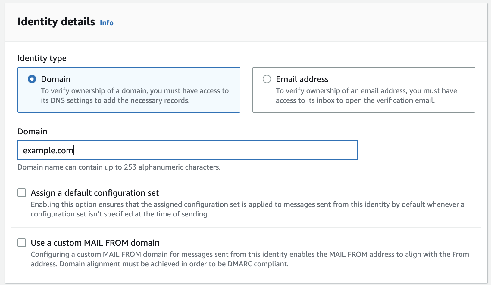
The procedure in this section is streamlined to just show the steps necessary to configure Easy DKIM on a domain identity that you’ve already created. If you haven’t yet created a domain identity or you want to see all available options for customizing a domain identity, such as using a default configuration set, custom MAIL FROM domain, and tags, see Creating a domain identity. Part of creating an Easy DKIM domain identity is configuring its DKIM-based verification where you will have the choice to either accept the Amazon SES default of 2048 bits, or to override the default by selecting 1024 bits. Steps to set up easyDKIM for a verified identity:

  1. Sign in to the AWS Management Console and open the Amazon SES console at https://console.aws.amazon.com/ses/
  2. In the navigation pane, under Configuration, choose Verified identities.
  3. List of verified identities in SES console

    Verified identities

  4. In the list of identities, choose an identity where the Identity type is Domain.
  5. Under the Authentication tab, in the DomainKeys Identified Mail (DKIM) container, choose Edit.
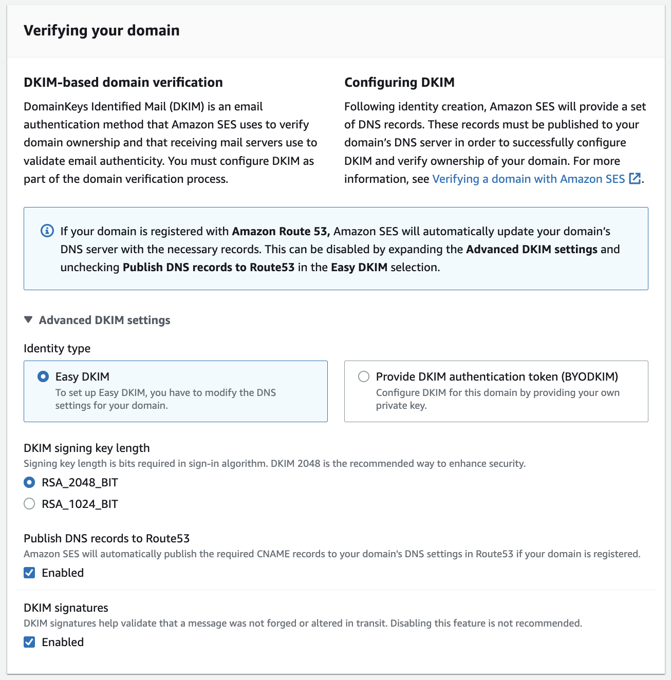
  6. In the Advanced DKIM settings container, choose the Easy DKIM button in the Identity type field.
  7. Choose EasyDKIM as identity type; RSA_2048_BITT in DKIM signing key length; Check Enabled checkbox under DKIM signatures.

    DKIM settings

  8. In the DKIM signing key length field, choose either RSA_2048_BIT or RSA_1024_BIT.
  9. In the DKIM signatures field, check the Enabled box.
  10. Choose Save changes.
  11. After configuring your domain identity with Easy DKIM, you must complete the verification process with your DNS provider – proceed to Verifying a DKIM domain identity with your DNS provider and follow the DNS authentication procedures for Easy DKIM.

Conclusion:

Email authentication, especially DKIM, is crucial in securing your emails, establishing sender reputation, and improving email deliverability. EasyDKIM provides a simplified and automated way to implement DKIM authentication. It removes the hassles of generating DKIM keys and managing settings, while additionally reducing risks and and enhancing sender authenticity. By following the steps outlined in this blog post, you can easily set up easyDKIM in Amazon SES and start using DKIM authentication for your email campaigns.

About the Author

Vinay Ujjini is an Amazon Pinpoint and Amazon Simple Email Service Worldwide Principal Specialist Solutions Architect at AWS. He has been solving customer’s omni-channel challenges for over 15 years. He is an avid sports enthusiast and in his spare time, enjoys playing tennis & cricket.

Share and query encrypted data in AWS Clean Rooms

Post Syndicated from Jonathan Herzog original https://aws.amazon.com/blogs/security/share-and-query-encrypted-data-in-aws-clean-rooms/

In this post, we’d like to introduce you to the cryptographic computing feature of AWS Clean Rooms. With AWS Clean Rooms, customers can run collaborative data-query sessions on sensitive data sets that live in different AWS accounts, and can do so without having to share, aggregate, or replicate the data. When customers also use the cryptographic computing feature, their data remains cryptographically protected even while it is being processed by an AWS Clean Rooms collaboration.

Where would AWS Clean Rooms be useful? Consider a scenario where two different insurance companies want to identify duplicate claims so they can identify potential fraud. This would be simple if they could compare their claims with each other, but they might not be able to do so due to privacy constraints.

Alternately, consider an advertising network and a client that want to measure the effectiveness of an advertising campaign. To that end, they would like to know how many of the people who saw the campaign (exposures) went on to make a purchase from the client (purchasers). However, confidentiality concerns might prevent the advertising network from sharing their list of exposures with the client or prevent the client from sharing their list of purchasers with the advertising network.

As these examples show, there can be many situations in which different organizations want to collaborate on a joint analysis of their pooled data, but cannot share their individual datasets directly. One solution to this problem is a data clean room, which is a service trusted by a collaboration’s participants to do the following:

  • Hold the data of individual parties
  • Enforce access-control rules that collaborators specify regarding their data
  • Perform analyses over the pooled data

To serve customers with these needs, AWS recently launched a new data clean-room service called AWS Clean Rooms. This service provides AWS customers with a way to collaboratively analyze data (stored in other AWS services as SQL tables) without having to replicate the data, move the data outside of the AWS Cloud, or allow their collaborators to see the data itself.

Additionally, AWS Clean Rooms provides a feature that gives customers even more control over their data: cryptographic computing. This feature allows AWS Clean Rooms to operate over data that customers encrypt themselves and that the service cannot actually read. Specifically, customers can use this feature to select which portions of their data should be encrypted and to encrypt that data themselves. Collaborators can continue to analyze that data as if it were in the clear, however, even though the data in question remains encrypted while it is being processed in AWS Clean Rooms collaborations. In this way, customers can use AWS Clean Rooms to securely collaborate on data they may not have been able to share due to internal policies or regulations.

Cryptographic computing

Using the cryptographic computing feature of AWS Clean Rooms involves these steps:

  • Users create AWS Clean Rooms collaborations and set collaboration-wide encryption settings. They then invite collaborators to support the analysis process.
  • Outside of AWS Clean Rooms, those collaborators agree on a shared secret: a common, secret, cryptographic key.
  • Collaborators individually encrypt their tables outside of the AWS Cloud (typically on their own premises) using the shared secret, the collaboration ID of the intended collaboration, and the Cryptographic Computing for Clean Rooms (C3R) encryption client (which AWS provides as an open-source package). Collaborators then provide the encrypted tables to AWS Clean Rooms, just as they would have provided plaintext tables.
  • Collaborators continue to use AWS Clean Rooms for their data analysis. They impose access-control rules on their tables, submit SQL queries over the tables in the collaboration, and retrieve results.
  • These results might contain encrypted columns, and so collaborators decrypt the results by using the shared secret and the C3R encryption client.

As a result, data that enters AWS Clean Rooms in encrypted format will remain encrypted from input tables to intermediate values to result sets. AWS Clean Rooms will be unable to decrypt or read the data even while performing the queries.

Note: For those interested in the academic aspects of this process, the cryptographic computing feature of AWS Clean Rooms is based on server-aided private set intersection (PSI). Server-aided PSI allows two or more participants to submit sets of values to a server and learn which elements are found in all sets, but without (1) allowing the participants to learn anything about the other (non-shared) elements, or (2) allowing the server to learn anything about the underlying data (aside from the degrees to which the sets overlap). PSI is just one example of the field of cryptographic computing, which provides a variety of new methods by which encrypted data can be processed for various purposes and without decryption. These techniques allow our customers to use the scale and power of AWS systems on data that AWS will not be able to read. See our Cryptographic Computing webpage for more about our work in this area.

Let’s dive deeper into each new step in the process for using cryptographic computing in AWS Clean Rooms.

Key agreement. Each collaboration needs its own shared secret: a secure cryptographic secret (of at least 256 bits). Customers sometimes have a regulatory need to maintain ownership of their encryption keys. Therefore, the cryptographic computing feature supports the case where customers generate, distribute, and store their collaboration’s secret themselves. In this way, customers’ encryption keys are never stored on an AWS system.

Encryption. AWS Clean Rooms allows table owners to control how tables are encrypted on a column-by-column basis. In particular, each column in an encrypted table will be one of three types: cleartext, sealed, or fingerprint. These types map directly to both how columns are used in queries and how they are protected with cryptography, described as follows:

  • Cleartext columns are not cryptographically processed at all. They are copied to encrypted tables verbatim, and can be used anywhere in a SQL query.
  • Sealed columns are encrypted. The encryption scheme used (AES-GCM) is randomized, meaning that encrypting the same value multiple times yields different ciphertexts each time. This helps prevent the statistical analysis of these columns, but also means that these columns cannot be used in JOIN clauses. They can be used in SELECT clauses, however, which allows them to appear in query results.
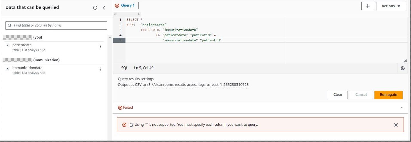
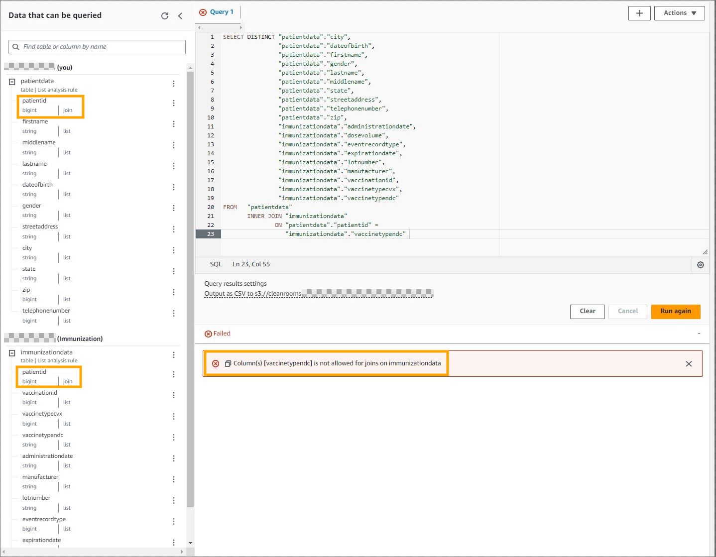
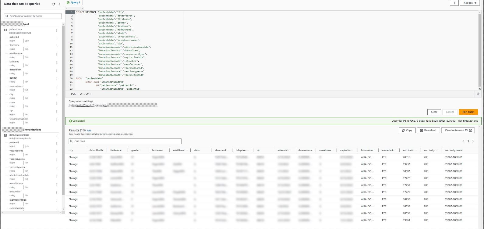
  • Fingerprint columns are hashed using the Hash-based Message Authentication Code (HMAC) algorithm. There is no way to decrypt these values, and therefore no reason for them to appear in the SELECT clause of a query. They can, however, be used in JOIN clauses: HMAC will map a given value to the same fingerprint every time, meaning that JOINs will be able to unify common values across different fingerprint columns.

Encryption settings. This last point—that fingerprint values will always map a given plaintext value to the same fingerprint—might give pause to some readers. If this is true, won’t the encrypted table be vulnerable to statistical analysis? That is absolutely correct: it will. For this reason, users might wish to set collaboration-wide encryption settings to control these forms of analysis.

To see how statistical analysis might be a concern, imagine a table where one fingerprint column is named US_State. In this case, a simple frequency analysis will reverse-engineer the plaintext values relatively quickly: the most common fingerprint is almost certain to be “California”, followed by “Texas”, “Florida”, and so on. Also, imagine that the same table has another fingerprint column called US_City, and that a given fingerprint appears in both columns. In that case, the fingerprint in question is almost certain to be “New York”. If a row has a fingerprint in the US_City column but a NULL in the US_State column, furthermore, it’s very likely that the fingerprint is for “District of Columbia”. And finally, imagine that the table has a cleartext column called Time_Zone. In this case, values of “HST” (Hawaii standard time) or “AKST” (Alaska standard time) reveal the value in the US_State column regardless of the cryptography.

Not all datasets will be vulnerable to these kinds of statistical analysis, but some will. Only customers can determine which types of analysis may reveal their data and which may not. Because of this, the cryptographic computing feature allows the customer to decide which protections will be needed. At the time of collaboration creation, that is, the creator of the AWS Clean Rooms collaboration can configure the following collaboration-wide encryption settings:

  • Whether or not fingerprint columns can contain duplicate plaintext values (addressing the “California” example)
  • Whether or not fingerprint columns with different names should fingerprint values in the same way (addressing the “New York” example)
  • Whether or not NULL values in the plaintext table should be left as NULL in the encrypted table (addressing the “District of Columbia” example)
  • Whether or not encrypted tables should be allowed to have cleartext columns at all (addressing the time zone example)

Security is maximized when all of these options are set to “no,” but each “no” will limit the queries that C3R will be able to support. For example, the choice of whether or not encrypted tables should be allowed to have cleartext columns will determine which WHERE clauses will be supported: If cleartext columns are not supported, then the Time_Zone column must be cryptographically processed — meaning that the clause WHERE Time_Zone=”EST” will not act as intended. There might be reasons to set these options to “yes” in order to enable a wider variety of queries, which we discuss in the Query behavior section later in this post.

Decryption. AWS Clean Rooms will write query results to an Amazon Simple Storage Service (Amazon S3) bucket. The recipient copies these results from the bucket to some on-premises storage and then runs the C3R encryption client. The client will find encrypted elements of the output and decrypt them. Note that the client can only decrypt elements from sealed columns. If the output contains elements from a fingerprint column, the client will warn you, but will also leave these elements untouched, as cryptographic fingerprints can’t be decrypted.

Having finished our overview, let’s return to the discussion regarding how encryption can affect the behavior of queries.

Query behavior

Implicit in the discussion so far is something worth calling out explicitly: AWS Clean Rooms runs queries over the data that is provided to it. If the data given to AWS Clean Rooms is encrypted, therefore, queries will be run on the ciphertexts and not the plaintexts. This will not affect the results returned, so long as the columns are used for their intended purposes:

  • Fingerprint columns are used in JOIN clauses
  • Sealed columns are used in SELECT clauses

(Cleartext columns can be used anywhere.) Queries might produce unexpected results, however, if the columns are used outside of their intended purposes:

  • Sometimes queries will fail when they would have succeeded on the plaintext. For example, ciphertexts and fingerprints will be string values, even if the original plaintext values were another type. Therefore, SUM() or AVG() calls on fingerprint or sealed columns will yield errors even if the corresponding plaintext columns were numeric.
  • Sometimes queries will omit results that would have been found by querying the plaintext. For example, attempting to JOIN on sealed columns will yield empty result sets: no two ciphertexts will be the same, even if they encrypt the same plaintext value. (Also, performing a JOIN on fingerprint columns with different names will exhibit the same behavior, if the collaboration-wide encryption settings specified that fingerprint columns of different names should fingerprint values differently.)
  • Sometimes results will include rows that would not be found by querying the plaintext. As mentioned, ciphertexts and fingerprints will be string values—base64 encodings of random-looking bytes, specifically. This means that a clause such as WHERE ‘US_State’ CONTAINS ‘CA’ will match some ciphertexts or fingerprints even when they would not match the plaintext.

To avoid these issues, fingerprint and sealed columns should only be used for their intended purposes (JOIN and SELECT clauses, respectively).

Conclusion

In this blog post, you have learned how AWS Clean Rooms can help you harness the power of AWS services to query and analyze your most-sensitive data. By using cryptographic computing, you can work with collaborators to perform joint analyses over pooled data without sharing your “raw” data with each other—or with AWS. If you believe that you can benefit from cryptographic computing (in AWS Clean Rooms or elsewhere), we’d like to hear from you. Please contact us with any questions or feedback. Also, we invite you to learn more about AWS Clean Rooms (including its use of cryptographic computing). Finally, the C3R client is open source, and can be downloaded from its GitHub page.

 
If you have feedback about this post, submit comments in the Comments section below. If you have questions about this post, contact AWS Support.

Want more AWS Security news? Follow us on Twitter.

Jonathan Herzog

Jonathan Herzog

Jonathan is a Principal Security Engineer in AWS Cryptographyand has worked in cryptography for 25 years. He received his PhD in crypto from MIT, and has developed cryptographic systems for the US Air Force, the National Security Agency, Akamai Technologies, and (now) Amazon.

How Zoom implemented streaming log ingestion and efficient GDPR deletes using Apache Hudi on Amazon EMR

Post Syndicated from Sekar Srinivasan original https://aws.amazon.com/blogs/big-data/how-zoom-implemented-streaming-log-ingestion-and-efficient-gdpr-deletes-using-apache-hudi-on-amazon-emr/

In today’s digital age, logging is a critical aspect of application development and management, but efficiently managing logs while complying with data protection regulations can be a significant challenge. Zoom, in collaboration with the AWS Data Lab team, developed an innovative architecture to overcome these challenges and streamline their logging and record deletion processes. In this post, we explore the architecture and the benefits it provides for Zoom and its users.

Application log challenges: Data management and compliance

Application logs are an essential component of any application; they provide valuable information about the usage and performance of the system. These logs are used for a variety of purposes, such as debugging, auditing, performance monitoring, business intelligence, system maintenance, and security. However, although these application logs are necessary for maintaining and improving the application, they also pose an interesting challenge. These application logs may contain personally identifiable data, such as user names, email addresses, IP addresses, and browsing history, which creates a data privacy concern.

Laws such as the General Data Protection Regulation (GDPR) and the California Consumer Privacy Act (CCPA) require organizations to retain application logs for a specific period of time. The exact length of time required for data storage varies depending on the specific regulation and the type of data being stored. The reason for these data retention periods is to ensure that companies aren’t keeping personal data longer than necessary, which could increase the risk of data breaches and other security incidents. This also helps ensure that companies aren’t using personal data for purposes other than those for which it was collected, which could be a violation of privacy laws. These laws also give individuals the right to request the deletion of their personal data, also known as the “right to be forgotten.” Individuals have the right to have their personal data erased, without undue delay.

So, on one hand, organizations need to collect application log data to ensure the proper functioning of their services, and keep the data for a specific period of time. But on the other hand, they may receive requests from individuals to delete their personal data from the logs. This creates a balancing act for organizations because they must comply with both data retention and data deletion requirements.

This issue becomes increasingly challenging for larger organizations that operate in multiple countries and states, because each country and state may have their own rules and regulations regarding data retention and deletion. For example, the Personal Information Protection and Electronic Documents Act (PIPEDA) in Canada and the Australian Privacy Act in Australia are similar laws to GDPR, but they may have different retention periods or different exceptions. Therefore, organizations big or small must navigate this complex landscape of data retention and deletion requirements, while also ensuring that they are in compliance with all applicable laws and regulations.

Zoom’s initial architecture

During the COVID-19 pandemic, the use of Zoom skyrocketed as more and more people were asked to work and attend classes from home. The company had to rapidly scale its services to accommodate the surge and worked with AWS to deploy capacity across most Regions globally. With a sudden increase in the large number of application endpoints, they had to rapidly evolve their log analytics architecture and worked with the AWS Data Lab team to quickly prototype and deploy an architecture for their compliance use case.

At Zoom, the data ingestion throughput and performance needs are very stringent. Data had to be ingested from several thousand application endpoints that produced over 30 million messages every minute, resulting in over 100 TB of log data per day. The existing ingestion pipeline consisted of writing the data to Apache Hadoop HDFS storage through Apache Kafka first and then running daily jobs to move the data to persistent storage. This took several hours while also slowing the ingestion and creating the potential for data loss. Scaling the architecture was also an issue because HDFS data would have to be moved around whenever nodes were added or removed. Furthermore, transactional semantics on billions of records were necessary to help meet compliance-related data delete requests, and the existing architecture of daily batch jobs was operationally inefficient.

It was at this time, through conversations with the AWS account team, that the AWS Data Lab team got involved to assist in building a solution for Zoom’s hyper-scale.

Solution overview

The AWS Data Lab offers accelerated, joint engineering engagements between customers and AWS technical resources to create tangible deliverables that accelerate data, analytics, artificial intelligence (AI), machine learning (ML), serverless, and container modernization initiatives. The Data Lab has three offerings: the Build Lab, the Design Lab, and Resident Architect. During the Build and Design Labs, AWS Data Lab Solutions Architects and AWS experts supported Zoom specifically by providing prescriptive architectural guidance, sharing best practices, building a working prototype, and removing technical roadblocks to help meet their production needs.

Zoom and the AWS team (collectively referred to as “the team” going forward) identified two major workflows for data ingestion and deletion.

Data ingestion workflow

The following diagram illustrates the data ingestion workflow.

Data Ingestion Workflow

The team needed to quickly populate millions of Kafka messages in the dev/test environment to achieve this. To expedite the process, we (the team) opted to use Amazon Managed Streaming for Apache Kafka (Amazon MSK), which makes it simple to ingest and process streaming data in real time, and we were up and running in under a day.

To generate test data that resembled production data, the AWS Data Lab team created a custom Python script that evenly populated over 1.2 billion messages across several Kafka partitions. To match the production setup in the development account, we had to increase the cloud quota limit via a support ticket.

We used Amazon MSK and the Spark Structured Streaming capability in Amazon EMR to ingest and process the incoming Kafka messages with high throughput and low latency. Specifically, we inserted the data from the source into EMR clusters at a maximum incoming rate of 150 million Kafka messages every 5 minutes, with each Kafka message holding 7–25 log data records.

To store the data, we chose to use Apache Hudi as the table format. We opted for Hudi because it’s an open-source data management framework that provides record-level insert, update, and delete capabilities on top of an immutable storage layer like Amazon Simple Storage Service (Amazon S3). Additionally, Hudi is optimized for handling large datasets and works well with Spark Structured Streaming, which was already being used at Zoom.

After 150 million messages were buffered, we processed the messages using Spark Structured Streaming on Amazon EMR and wrote the data into Amazon S3 in Apache Hudi-compatible format every 5 minutes. We first flattened the message array, creating a single record from the nested array of messages. Then we added a unique key, known as the Hudi record key, to each message. This key allows Hudi to perform record-level insert, update, and delete operations on the data. We also extracted the field values, including the Hudi partition keys, from incoming messages.

This architecture allowed end-users to query the data stored in Amazon S3 using Amazon Athena with the AWS Glue Data Catalog or using Apache Hive and Presto.

Data deletion workflow

The following diagram illustrates the data deletion workflow.

Data Deletion Workflow

Our architecture allowed for efficient data deletions. To help comply with the customer-initiated data retention policy for GDPR deletes, scheduled jobs ran daily to identify the data to be deleted in batch mode.

We then spun up a transient EMR cluster to run the GDPR upsert job to delete the records. The data was stored in Amazon S3 in Hudi format, and Hudi’s built-in index allowed us to efficiently delete records using bloom filters and file ranges. Because only those files that contained the record keys needed to be read and rewritten, it only took about 1–2 minutes to delete 1,000 records out of the 1 billion records, which had previously taken hours to complete as entire partitions were read.

Overall, our solution enabled efficient deletion of data, which provided an additional layer of data security that was critical for Zoom, in light of its GDPR requirements.

Architecting to optimize scale, performance, and cost

In this section, we share the following strategies Zoom took to optimize scale, performance, and cost:

  • Optimizing ingestion
  • Optimizing throughput and Amazon EMR utilization
  • Decoupling ingestion and GDPR deletion using EMRFS
  • Efficient deletes with Apache Hudi
  • Optimizing for low-latency reads with Apache Hudi
  • Monitoring

Optimizing ingestion

To keep the storage in Kafka lean and optimal, as well as to get a real-time view of data, we created a Spark job to read incoming Kafka messages in batches of 150 million messages and wrote to Amazon S3 in Hudi-compatible format every 5 minutes. Even during the initial stages of the iteration, when we hadn’t started scaling and tuning yet, we were able to successfully load all Kafka messages consistently under 2.5 minutes using the Amazon EMR runtime for Apache Spark.

Optimizing throughput and Amazon EMR utilization

We launched a cost-optimized EMR cluster and switched from uniform instance groups to using EMR instance fleets. We chose instance fleets because we needed the flexibility to use Spot Instances for task nodes and wanted to diversify the risk of running out of capacity for a specific instance type in our Availability Zone.

We started experimenting with test runs by first changing the number of Kafka partitions from 400 to 1,000, and then changing the number of task nodes and instance types. Based on the results of the run, the AWS team came up with the recommendation to use Amazon EMR with three core nodes (r5.16xlarge (64 vCPUs each)) and 18 task nodes using Spot fleet instances (a combination of r5.16xlarge (64 vCPUs), r5.12xlarge (48 vCPUs), r5.8xlarge (32 vCPUs)). These recommendations helped Zoom to reduce their Amazon EMR costs by more than 80% while meeting their desired performance goals of ingesting 150 million Kafka messages under 5 minutes.

Decoupling ingestion and GDPR deletion using EMRFS

A well-known benefit of separation of storage and compute is that you can scale the two independently. But a not-so-obvious advantage is that you can decouple continuous workloads from sporadic workloads. Previously data was stored in HDFS. Resource-intensive GDPR delete jobs and data movement jobs would compete for resources with the stream ingestion, causing a backlog of more than 5 hours in upstream Kafka clusters, which was close to filling up the Kafka storage (which only had 6 hours of data retention) and potentially causing data loss. Offloading data from HDFS to Amazon S3 allowed us the freedom to launch independent transient EMR clusters on demand to perform data deletion, helping to ensure that the ongoing data ingestion from Kafka into Amazon EMR is not starved for resources. This enabled the system to ingest data every 5 minutes and complete each Spark Streaming read in 2–3 minutes. Another side effect of using EMRFS is a cost-optimized cluster, because we removed reliance on Amazon Elastic Block Store (Amazon EBS) volumes for over 300 TB storage that was used for three copies (including two replicas) of HDFS data. We now pay for only one copy of the data in Amazon S3, which provides 11 9s of durability and is relatively inexpensive storage.

Efficient deletes with Apache Hudi

What about the conflict between ingest writes and GDPR deletes when running concurrently? This is where the power of Apache Hudi stands out.

Apache Hudi provides a table format for data lakes with transactional semantics that enables the separation of ingestion workloads and updates when run concurrently. The system was able to consistently delete 1,000 records in less than a minute. There were some limitations in concurrent writes in Apache Hudi 0.7.0, but the Amazon EMR team quickly addressed this by back-porting Apache Hudi 0.8.0, which supports optimistic concurrency control, to the current (at the time of the AWS Data Lab collaboration) Amazon EMR 6.4 release. This saved time in testing and allowed for a quick transition to the new version with minimal testing. This enabled us to query the data directly using Athena quickly without having to spin up a cluster to run ad hoc queries, as well as to query the data using Presto, Trino, and Hive. The decoupling of the storage and compute layers provided the flexibility to not only query data across different EMR clusters, but also delete data using a completely independent transient cluster.

Optimizing for low-latency reads with Apache Hudi

To optimize for low-latency reads with Apache Hudi, we needed to address the issue of too many small files being created within Amazon S3 due to the continuous streaming of data into the data lake.

We utilized Apache Hudi’s features to tune file sizes for optimal querying. Specifically, we reduced the degree of parallelism in Hudi from the default value of 1,500 to a lower number. Parallelism refers to the number of threads used to write data to Hudi; by reducing it, we were able to create larger files that were more optimal for querying.

Because we needed to optimize for high-volume streaming ingestion, we chose to implement the merge on read table type (instead of copy on write) for our workload. This table type allowed us to quickly ingest the incoming data into delta files in row format (Avro) and asynchronously compact the delta files into columnar Parquet files for fast reads. To do this, we ran the Hudi compaction job in the background. Compaction is the process of merging row-based delta files to produce new versions of columnar files. Because the compaction job would use additional compute resources, we adjusted the degree of parallelism for insertion to a lower value of 1,000 to account for the additional resource usage. This adjustment allowed us to create larger files without sacrificing performance throughput.

Overall, our approach to optimizing for low-latency reads with Apache Hudi allowed us to better manage file sizes and improve the overall performance of our data lake.

Monitoring

The team monitored MSK clusters with Prometheus (an open-source monitoring tool). Additionally, we showcased how to monitor Spark streaming jobs using Amazon CloudWatch metrics. For more information, refer to Monitor Spark streaming applications on Amazon EMR.

Outcomes

The collaboration between Zoom and the AWS Data Lab demonstrated significant improvements in data ingestion, processing, storage, and deletion using an architecture with Amazon EMR and Apache Hudi. One key benefit of the architecture was a reduction in infrastructure costs, which was achieved through the use of cloud-native technologies and the efficient management of data storage. Another benefit was an improvement in data management capabilities.

We showed that the costs of EMR clusters can be reduced by about 82% while bringing the storage costs down by about 90% compared to the prior HDFS-based architecture. All of this while making the data available in the data lake within 5 minutes of ingestion from the source. We also demonstrated that data deletions from a data lake containing multiple petabytes of data can be performed much more efficiently. With our optimized approach, we were able to delete approximately 1,000 records in just 1–2 minutes, as compared to the previously required 3 hours or more.

Conclusion

In conclusion, the log analytics process, which involves collecting, processing, storing, analyzing, and deleting log data from various sources such as servers, applications, and devices, is critical to aid organizations in working to meet their service resiliency, security, performance monitoring, troubleshooting, and compliance needs, such as GDPR.

This post shared what Zoom and the AWS Data Lab team have accomplished together to solve critical data pipeline challenges, and Zoom has extended the solution further to optimize extract, transform, and load (ETL) jobs and resource efficiency. However, you can also use the architecture patterns presented here to quickly build cost-effective and scalable solutions for other use cases. Please reach out to your AWS team for more information or contact Sales.


About the Authors

Sekar Srinivasan is a Sr. Specialist Solutions Architect at AWS focused on Big Data and Analytics. Sekar has over 20 years of experience working with data. He is passionate about helping customers build scalable solutions modernizing their architecture and generating insights from their data. In his spare time he likes to work on non-profit projects focused on underprivileged Children’s education.

Chandra DhandapaniChandra Dhandapani is a Senior Solutions Architect at AWS, where he specializes in creating solutions for customers in Analytics, AI/ML, and Databases. He has a lot of experience in building and scaling applications across different industries including Healthcare and Fintech. Outside of work, he is an avid traveler and enjoys sports, reading, and entertainment.

Amit Kumar Agrawal is a Senior Solutions Architect at AWS, based out of San Francisco Bay Area. He works with large strategic ISV customers to architect cloud solutions that address their business challenges. During his free time he enjoys exploring the outdoors with his family.

Viral Shah is a Analytics Sales Specialist working with AWS for 5 years helping customers to be successful in their data journey. He has over 20+ years of experience working with enterprise customers and startups, primarily in the data and database space. He loves to travel and spend quality time with his family.

Perform secure database write-backs with Amazon QuickSight

Post Syndicated from Srikanth Baheti original https://aws.amazon.com/blogs/big-data/perform-secure-database-write-backs-with-amazon-quicksight/

Amazon QuickSight is a scalable, serverless, machine learning (ML)-powered business intelligence (BI) solution that makes it easy to connect to your data, create interactive dashboards, get access to ML-enabled insights, and share visuals and dashboards with tens of thousands of internal and external users, either within QuickSight itself or embedded into any application.

A write-back is the ability to update a data mart, data warehouse, or any other database backend from within BI dashboards and analyze the updated data in near-real time within the dashboard itself. In this post, we show how to perform secure database write-backs with QuickSight.

Use case overview

To demonstrate how to enable a write-back capability with QuickSight, let’s consider a fictional company, AnyCompany Inc. AnyCompany is a professional services firm that specializes in providing workforce solutions to their customers. AnyCompany determined that running workloads in the cloud to support its growing global business needs is a competitive advantage and uses the cloud to host all its workloads. AnyCompany decided to enhance the way its branches provide quotes to its customers. Currently, the branches generate customer quotes manually, and as a first step in this innovation journey, AnyCompany is looking to develop an enterprise solution for customer quote generation with the capability to dynamically apply local pricing data at the time of quote generation.

AnyCompany currently uses Amazon Redshift as their enterprise data warehouse platform and QuickSight as their BI solution.

Building a new solution comes with the following challenges:

  • AnyCompany wants a solution that is easy to build and maintain, and they don’t want to invest in building a separate user interface.
  • AnyCompany wants to extend the capabilities of their existing QuickSight BI dashboard to also enable quote generation and quote acceptance. This will simplify feature rollouts because their employees already use QuickSight dashboards and enjoy the easy-to-use interface that QuickSight provides.
  • AnyCompany wants to store the quote negotiation history that includes generated, reviewed, and accepted quotes.
  • AnyCompany wants to build a new dashboard with quote history data for analysis and business insights.

This post goes through the steps to enable write-back functionality to Amazon Redshift from QuickSight. Note that the traditional BI tools are read-only with little to no options to update source data.

Solution overview

This solution uses the following AWS services:

  • Amazon API Gateway – Hosts and secures the write-back REST API that will be invoked by QuickSight
  • AWS Lambda – Runs the compute function required to generate the hash and a second function to securely perform the write-back
  • Amazon QuickSight – Offers BI dashboards and quote generation capabilities
  • Amazon Redshift – Stores quotes, prices, and other relevant datasets
  • AWS Secrets Manager – Stores and manages keys to sign hashes (message digest)

Although this solution uses Amazon Redshift as the data store, a similar approach can be implemented with any database that supports creating user-defined functions (UDFs) that can invoke Lambda.

The following figure shows the workflow to perform write-backs from QuickSight.

The first step in the solution is to generate a hash or a message digest of the set of attributes in Amazon Redshift by invoking a Lambda function. This step prevents request tampering. To generate a hash, Amazon Redshift invokes a scalar Lambda UDF. The hashing mechanism used here is the popular BLAKE2 function (available in the Python library hashlib). To further secure the hash, keyed hashing is used, which is a faster and simpler alternative to hash-based message authentication code (HMAC). This key is generated and stored by Secrets Manager and should be accessible only to allowed applications. After the secure hash is generated, it’s returned to Amazon Redshift and combined in an Amazon Redshift view.

Writing the generated quote back to Amazon Redshift is performed by the write-back Lambda function, and an API Gateway REST API endpoint is created to secure and pass requests to the write-back function. The write-back function performs the following actions:

  1. Generate the hash based on the API input parameters received from QuickSight.
  2. Sign the hash by applying the key from Secrets Manager.
  3. Compare the generated hash with the hash received from the input parameters using the compare_digest method available in the HMAC module.
  4. Upon successful validation, write the record to the quote submission table in Amazon Redshift.

The following section provide detailed steps with sample payloads and code snippets.

Generate the hash

The hash is generated using a Lambda UDF in Amazon Redshift. Additionally, a Secrets Manager key is used to sign the hash. To create the hash, complete the following steps:

  1. Create the Secrets Manager key from the AWS Command Line Interface (AWS CLI):
aws secretsmanager create-secret --name “name_of_secret” --description "Secret key to sign hash" --secret-string '{" name_of_key ":"value"}' --region us-east-1
  1. Create a Lambda UDF to generate a hash for encryption:
import boto3	
import base64
import json
from hashlib import blake2b
from botocore.exceptions import ClientError

def get_secret(): 	#This key is used by the Lambda function to further secure the hash.

    secret_name = "<name_of_secret>"
    region_name = "<aws_region_name>"

    # Create a Secrets Manager client
    session = boto3.session.Session()
    client = session.client(service_name='secretsmanager', region_name=<aws_region_name>    )

    # In this sample we only handle the specific exceptions for the 'GetSecretValue' API.
    # See https://docs.aws.amazon.com/secretsmanager/latest/apireference/API_GetSecretValue.html
    # We rethrow the exception by default.

    try:
        get_secret_value_response = client.get_secret_value(SecretId=secret_name)
    except Exception as e:
            raise e

   if "SecretString" in get_secret_value_response:
       access_token = get_secret_value_response["SecretString"]
   else:
       access_token = get_secret_value_response["SecretBinary"]

   return json.loads(access_token)[<token key name>]

SECRET_KEY = get_secret()
AUTH_SIZE = 16 

def sign(payload):
    h = blake2b(digest_size=AUTH_SIZE, key=SECRET_KEY)
    h.update(payload)
    return h.hexdigest().encode('utf-8')

def lambda_handler(event, context):
ret = dict()
 try:
  res = []
  for argument in event['arguments']:
   
   try:
     msg = json.dumps(argument)
     signed_key = sign(str.encode(msg))
     res.append(signed_key.decode('utf-8'))
     
   except:
   res.append(None)     
   ret['success'] = True
   ret['results'] = res
    
except Exception as e:
  ret['success'] = False
  ret['error_msg'] = str(e)
  
 return json.dumps(ret)
  1. Define an Amazon Redshift UDF to call the Lambda function to create a hash:
CREATE OR REPLACE EXTERNAL FUNCTION udf_get_digest (par1 varchar)
RETURNS varchar STABLE
LAMBDA 'redshift_get_digest'
IAM_ROLE 'arn:aws:iam::<AWSACCOUNTID>role/service-role/<role_name>';

The AWS Identity and Access Management (IAM) role in the preceding step should have the following policy attached to be able to invoke the Lambda function:

{
    "Version": "2012-10-17",
    "Statement": [
        {
            "Effect": "Allow",
            "Action": "lambda:InvokeFunction",
            "Resource": "arn:aws:lambda:us-east-1:<AWSACCOUNTID>1:function:redshift_get_digest"
        }
}
  1. Fetch the key from Secrets Manager.

This key is used by the Lambda function to further secure the hash. This is indicated in the get_secret function in Step 2.

Set up Amazon Redshift datasets in QuickSight

The quote generation dashboard uses the following Amazon Redshift view.

Create an Amazon Redshift view that uses all the preceding columns along with the hash column:

create view quote_gen_vw as select *, udf_get_digest 
( customername || BGCheckRequired || Skill|| Shift ||State ||Cost ) from billing_input_tbl

The records will look like the following screenshot.

The preceding view will be used as the QuickSight dataset to generate quotes. A QuickSight analysis will be created using the dataset. For near-real-time analysis, you can use QuickSight direct query mode.

Create API Gateway resources

The write-back operation is initiated by QuickSight invoking an API Gateway resource, which invokes the Lambda write-back function. As a prerequisite for creating the calculated field in QuickSight to call the write-back API, you must first create these resources.

API Gateway secures and invokes the write-back Lambda function with the parameters created as URL query string parameters with mapping templates. The mapping parameters can be avoided by using the Lambda proxy integration.

Create a REST API resource of method type GET that uses Lambda functions (created in the next step) as the integration type. For instructions, refer to Creating a REST API in Amazon API Gateway and Set up Lambda integrations in API Gateway.

The following screenshot shows the details for creating a query string parameter for each parameter passed to API Gateway.

The following screenshot shows the details for creating a mapping template parameter for each parameter passed to API Gateway.

Create the Lambda function

Create a new Lambda function for the API Gateway to invoke. The Lambda function performs the following steps:

  1. Receive parameters from QuickSight through API Gateway and hash the concatenated parameters.

The following code example retrieves parameters from the API Gateway call using the event object of the Lambda function:

   customer= event['customer’])
    bgc = event['bgc']

The function performs the hashing logic as shown in the create hash step earlier using the concatenated parameters passed by QuickSight.

  1. Compare the hashed output with the hash parameter.

If these don’t match, the write-back won’t happen.

  1. If the hashes match, perform a write-back. Check for the presence of a record in the quote generation table by generating a query from the table using the parameters passed from QuickSight:
query_str = "select * From tbquote where cust = '" + cust + "' and bgc = '" + bgc +"'" +" and skilledtrades = '" + skilledtrades + "'  and shift = '" +shift + "' and jobdutydescription ='" + jobdutydescription + "'"
  1. Complete the following action based on the results of the query:
    1. If no record exists for the preceding combination, generate and run an insert query using all parameters with the status as generated.
    2. If a record exists for the preceding combination, generate and run an insert query with the status as in review. The quote_Id for the existing combination will be reused.

Create a QuickSight visual

This step involves creating a table visual that uses a calculated field to pass parameters to API Gateway and invoke the preceding Lambda function.

  1. Add a QuickSight calculated field named Generate Quote to hold the API Gateway hosted URL that will be triggered to write back the quote history into Amazon Redshift:
concat("https://xxxxx.execute-api.us-east-1.amazonaws.com/stage_name/apiresourcename/?cust=",customername,"&bgc=",bgcheckrequired,"&billrate=",toString(billrate),"&skilledtrades=",skilledtrades,"&shift=",shift,"&jobdutydescription=",jobdutydescription,"&hash=",hashvalue)
  1. Create a QuickSight table visual.
  2. Add required fields such as Customer, Skill, and Cost.
  3. Add the Generate Quote calculated field and style this as a hyperlink.

Choosing this link will write the record into Amazon Redshift. This is incumbent on the same hash value returning when the Lambda function performs the hash on the parameters.

The following screenshot shows a sample table visual.

Write to the Amazon Redshift database

The Secrets Manager key is fetched and used by the Lambda function to generate the hash for comparison. The write-back will be performed only if the hash matches with the hash passed in the parameter.

The following Amazon Redshift table will capture the quote history as populated by the Lambda function. Records in green represent the most recent records for the quote.

Considerations and next steps

Using secure hashes prevents the tampering of payload parameters that are visible in the browser window when the write-back URL is invoked. To further secure the write-back URL, you can employ the following techniques:

  • Deploy the REST API in a private VPC that is accessible only to QuickSight users.
  • To prevent replay attacks, a timestamp can be generated alongside the hashing function and passed as an additional parameter in the write-back URL. The backend Lambda function can then be modified to only allow write-backs within a certain time-based threshold.
  • Follow the API Gateway access control and security best practices.
  • Mitigate potential Denial of Service for public-facing APIs.

You can further enhance this solution to render a web-based form when the write-back URL is opened. This could be implemented by dynamically generating an HTML form in the backend Lambda function to support the input of additional information. If your workload requires a high number of write-backs that require higher throughput or concurrency, a purpose-built data store like Amazon Aurora PostgreSQL-Compatible Edition might be a better choice. For more information, refer to Invoking an AWS Lambda function from an Aurora PostgreSQL DB cluster. These updates can then be synchronized into Amazon Redshift tables using federated queries.

Conclusion

This post showed how to use QuickSight along with Lambda, API Gateway, Secrets Manager, and Amazon Redshift to capture user input data and securely update your Amazon Redshift data warehouse without leaving your QuickSight BI environment. This solution eliminates the need to create an external application or user interface for database update or insert operations, and reduces related development and maintenance overhead. The API Gateway call can also be secured using a key or token to ensure only calls originating from QuickSight are accepted by the API Gateway. This will be covered in subsequent posts.


About the Authors

Srikanth Baheti is a Specialized World Wide Principal Solutions Architect for Amazon QuickSight. He started his career as a consultant and worked for multiple private and government organizations. Later he worked for PerkinElmer Health and Sciences & eResearch Technology Inc, where he was responsible for designing and developing high traffic web applications, highly scalable and maintainable data pipelines for reporting platforms using AWS services and Serverless computing.

Raji Sivasubramaniam is a Sr. Solutions Architect at AWS, focusing on Analytics. Raji is specialized in architecting end-to-end Enterprise Data Management, Business Intelligence and Analytics solutions for Fortune 500 and Fortune 100 companies across the globe. She has in-depth experience in integrated healthcare data and analytics with wide variety of healthcare datasets including managed market, physician targeting and patient analytics.

Ten new visual transforms in AWS Glue Studio

Post Syndicated from Gonzalo Herreros original https://aws.amazon.com/blogs/big-data/ten-new-visual-transforms-in-aws-glue-studio/

AWS Glue Studio is a graphical interface that makes it easy to create, run, and monitor extract, transform, and load (ETL) jobs in AWS Glue. It allows you to visually compose data transformation workflows using nodes that represent different data handling steps, which later are converted automatically into code to run.

AWS Glue Studio recently released 10 more visual transforms to allow creating more advanced jobs in a visual way without coding skills. In this post, we discuss potential uses cases that reflect common ETL needs.

The new transforms that will be demonstrated in this post are: Concatenate, Split String, Array To Columns, Add Current Timestamp, Pivot Rows To Columns, Unpivot Columns To Rows, Lookup, Explode Array Or Map Into Columns, Derived Column, and Autobalance Processing.

Solution overview

In this use case, we have some JSON files with stock option operations. We want to make some transformations before storing the data to make it easier to analyze, and we also want to produce a separate dataset summary.

In this dataset, each row represents a trade of option contracts. Options are financial instruments that provide the right—but not the obligation—to buy or sell stock shares at a fixed price (called  strike price) before a defined expiration date.

Input data

The data follows the following schema:

  • order_id – A unique ID
  • symbol – A code generally based on a few letters to identify the corporation that emits the underlying stock shares
  • instrument – The name that identifies the specific option being bought or sold
  • currency – The ISO currency code in which the price is expressed
  • price – The amount that was paid for the purchase of each option contract (on most exchanges, one contract allows you to buy or sell 100 stock shares)
  • exchange – The code of the exchange center or venue where the option was traded
  • sold – A list of the number of contracts that where allocated to fill the sell order when this is a sell trade
  • bought – A list of the number of contracts that where allocated to fill the buy order when this is buy trade

The following is a sample of the synthetic data generated for this post:

{"order_id": 1679931512485, "symbol": "AMZN", "instrument": "AMZN MAR 24 23 102 PUT", "currency": "usd", "price": 17.18, "exchange": "EDGX", "bought": [18, 38]}
{"order_id": 1679931512486, "symbol": "BMW.DE", "instrument": "BMW.DE MAR 24 23 96 PUT", "currency": "eur", "price": 2.98, "exchange": "XETR", "bought": [28]}
{"order_id": 1679931512487, "symbol": "BMW.DE", "instrument": "BMW.DE APR 28 23 101 CALL", "currency": "eur", "price": 14.71, "exchange": "XETR", "sold": [9, 59, 54]}
{"order_id": 1679931512489, "symbol": "JPM", "instrument": "JPM JUN 30 23 140 CALL", "currency": "usd", "price": 11.83, "exchange": "EDGX", "bought": [33, 42, 55, 67]}
{"order_id": 1679931512490, "symbol": "SIE.DE", "instrument": "SIE.DE MAR 24 23 149 CALL", "currency": "eur", "price": 13.68, "exchange": "XETR", "bought": [96, 89, 82]}
{"order_id": 1679931512491, "symbol": "NKE", "instrument": "NKE MAR 24 23 112 CALL", "currency": "usd", "price": 3.23, "exchange": "EDGX", "sold": [67]}
{"order_id": 1679931512492, "symbol": "AMZN", "instrument": "AMZN MAY 26 23 95 CALL", "currency": "usd", "price": 11.44, "exchange": "EDGX", "sold": [41, 62, 12]}
{"order_id": 1679931512493, "symbol": "JPM", "instrument": "JPM MAR 24 23 121 PUT", "currency": "usd", "price": 1.0, "exchange": "EDGX", "bought": [61, 34]}
{"order_id": 1679931512494, "symbol": "SAP.DE", "instrument": "SAP.DE MAR 24 23 132 CALL", "currency": "eur", "price": 15.9, "exchange": "XETR", "bought": [69, 33]}

ETL requirements

This data has a number of unique characteristics, as often found on older systems, that make the data harder to use.

The following are the ETL requirements:

  • The instrument name has valuable information that is intended for humans to understand; we want to normalize it into separate columns for easier analysis.
  • The attributes bought and sold are mutually exclusive; we can consolidate them into a single column with the contract numbers and have another column indicating if the contracts where bought or sold in this order.
  • We want to keep the information about the individual contract allocations but as individual rows instead of forcing users to deal with an array of numbers. We could add up the numbers, but we would lose information about how the order was filled (indicating market liquidity). Instead, we choose to denormalize the table so each row has a single number of contracts, splitting orders with multiple numbers into separate rows. In a compressed columnar format, the extra dataset size of this repetition is often small when compression is applied, so it’s acceptable to make the dataset easier to query.
  • We want to generate a summary table of volume for each option type (call and put) for each stock. This provides an indication of the market sentiment for each stock and the market in general (greed vs. fear).
  • To enable overall trade summaries, we want to provide for each operation the grand total and standardize the currency to US dollars, using an approximate conversion reference.
  • We want to add the date when these transformations took place. This could be useful, for instance, to have a reference on when was the currency conversion made.

Based on those requirements, the job will produce two outputs:

  • A CSV file with a summary of the number of contracts for each symbol and type
  • A catalog table to keep a history of the order, after doing the transformations indicated
    Data schema

Prerequisites

You will need your own S3 bucket to follow along with this use case. To create a new bucket, refer to Creating a bucket.

Generate synthetic data

To follow along with this post (or experiment with this kind of data on your own), you can generate this dataset synthetically. The following Python script can be run on a Python environment with Boto3 installed and access to Amazon Simple Storage Service (Amazon S3).

To generate the data, complete the following steps:

  1. On AWS Glue Studio, create a new job with the option Python shell script editor.
  2. Give the job a name and on the Job details tab, select a suitable role and a name for the Python script.
  3. In the Job details section, expand Advanced properties and scroll down to Job parameters.
  4. Enter a parameter named --bucket and assign as the value the name of the bucket you want to use to store the sample data.
  5. Enter the following script into the AWS Glue shell editor:
    import argparse
    import boto3
    from datetime import datetime
    import io
    import json
    import random
    import sys
    
    # Configuration
    parser = argparse.ArgumentParser()
    parser.add_argument('--bucket')
    args, ignore = parser.parse_known_args()
    if not args.bucket:
        raise Exception("This script requires an argument --bucket with the value specifying the S3 bucket where to store the files generated")
    
    data_bucket = args.bucket
    data_path = "transformsblog/inputdata"
    samples_per_file = 1000
    
    # Create a single file with synthetic data samples
    s3 = boto3.client('s3')
    buff = io.BytesIO()
    
    sample_stocks = [("AMZN", 95, "usd"), ("NKE", 120, "usd"), ("JPM", 130, "usd"), ("KO", 130, "usd"),
                     ("BMW.DE", 95, "eur"), ("SIE.DE", 140, "eur"), ("SAP.DE", 115, "eur")]
    option_type = ["PUT", "CALL"]
    operations = ["sold", "bought"]
    dates = ["MAR 24 23", "APR 28 23", "MAY 26 23", "JUN 30 23"]
    for i in range(samples_per_file):
        stock = random.choice(sample_stocks)
        symbol = stock[0]
        ref_price = stock[1]
        currency = stock[2]
        strike_price = round(ref_price * 0.9 + ref_price * random.uniform(0.01, 0.3))
        sample = {
            "order_id": int(datetime.now().timestamp() * 1000) + i,
            "symbol": stock[0],
            "instrument":f"{symbol} {random.choice(dates)} {strike_price} {random.choice(option_type)}",
            "currency": currency,
            "price": round(random.uniform(0.5, 20.1), 2),
            "exchange": "EDGX" if currency == "usd" else "XETR"
         }
        sample[random.choice(operations)] = [random.randrange(1,100) for i in range(random.randrange(1,5))]
        buff.write(json.dumps(sample).encode())
        buff.write("\n".encode())
    
    s3.put_object(Body=buff.getvalue(), Bucket=data_bucket, Key=f"{data_path}/{int(datetime.now().timestamp())}.json")

  6. Run the job and wait until it shows as successfully completed on the Runs tab (it should take just a few seconds).

Each run will generate a JSON file with 1,000 rows under the bucket specified and prefix transformsblog/inputdata/. You can run the job multiple times if you want to test with more input files.
Each line in the synthetic data is a data row representing a JSON object like the following:

{
 "order_id":1681986991888,
 "symbol":"AMZN",
 "instrument":"AMZN APR 28 23 100 PUT",
 "currency":"usd",
 "price":2.89,
 "exchange":"EDGX",
 "sold":[88,49]
}

Create the AWS Glue visual job

To create the AWS Glue visual job, complete the following steps:

  1. Go to AWS Glue Studio and create a job using the option Visual with a blank canvas.
  2. Edit Untitled job to give it a name and assign a role suitable for AWS Glue on the Job details tab.
  3. Add an S3 data source (you can name it JSON files source) and enter the S3 URL under which the files are stored (for example, s3://<your bucket name>/transformsblog/inputdata/), then select JSON as the data format.
  4. Select Infer schema so it sets the output schema based on the data.

From this source node, you’ll keep chaining transforms. When adding each transform, make sure the selected node is the last one added so it gets assigned as the parent, unless indicated otherwise in the instructions.

If you didn’t select the right parent, you can always edit the parent by selecting it and choosing another parent in the configuration pane.

Node parent configuration

For each node added, you’ll give it a specific name (so the node purpose shows in the graph) and configuration on the Transform tab.

Every time a transform changes the schema (for instance, add a new column), the output schema needs to be updated so it’s visible to the downstream transforms. You can manually edit the output schema, but it’s more practical and safer to do it using the data preview.
Additionally, that way you can verify the transformation are working so far as expected. To do so, open the Data preview tab with the transform selected and start a preview session. After you have verified the transformed data looks as expected, go to the Output schema tab and choose Use data preview schema to update the schema automatically.

As you add new kinds of transforms, the preview might show a message about a missing dependency. When this happens, choose End Session and the start a new one, so the preview picks up the new kind of node.

Extract instrument information

Let’s start by dealing with the information on the instrument name to normalize it into columns that are easier to access in the resulting output table.

  1. Add a Split String node and name it Split instrument, which will tokenize the instrument column using a whitespace regex: \s+ (a single space would do in this case, but this way is more flexible and visually clearer).
  2. We want to keep the original instrument information as is, so enter a new column name for the split array: instrument_arr.
    Split config
  3. Add an Array To Columns node and name it Instrument columns to convert the array column just created into new fields, except for symbol, for which we already have a column.
  4. Select the column instrument_arr, skip the first token and tell it to extract the output columns month, day, year, strike_price, type using indexes 2, 3, 4, 5, 6 (the spaces after the commas are for readability, they don’t impact the configuration).
    Array config

The year extracted is expressed with two digits only; let’s put a stopgap to assume it’s in this century if they just use two digits.

  1. Add a Derived Column node and name it Four digits year.
  2. Enter year as the derived column so it overrides it, and enter the following SQL expression:
    CASE WHEN length(year) = 2 THEN ('20' || year) ELSE year END
    Year derived column config

For convenience, we build an expiration_date field that a user can have as reference of the last date the option can be exercised.

  1. Add a Concatenate Columns node and name it Build expiration date.
  2. Name the new column expiration_date, select the columns year, month, and day (in that order), and a hyphen as spacer.
    Concatenated date config

The diagram so far should look like the following example.

DAG

The data preview of the new columns so far should look like the following screenshot.

Data preview

Normalize the number of contracts

Each of the rows in the data indicates the number of contracts of each option that were bought or sold and the batches on which the orders were filled. Without losing the information about the individual batches, we want to have each amount on an individual row with a single amount value, while the rest of the information is replicated in each row produced.

First, let’s merge the amounts into a single column.

  1. Add an Unpivot Columns Into Rows node and name it Unpivot actions.
  2. Choose the columns bought and sold to unpivot and store the names and values in columns named action and contracts, respectively.
    Unpivot config
    Notice in the preview that the new column contracts is still an array of numbers after this transformation.
  1. Add an Explode Array Or Map into Rows row named Explode contracts.
  2. Choose the contracts column and enter contracts as the new column to override it (we don’t need to keep the original array).

The preview now shows that each row has a single contracts amount, and the rest of the fields are the same.

This also means that order_id is no longer a unique key. For your own use cases, you need to decide how to model your data and if you want to denormalize or not.
Explode config

The following screenshot is an example of what the new columns look like after the transformations so far.
Data preview

Create a summary table

Now you create a summary table with the number of contracts traded for each type and each stock symbol.

Let’s assume for illustration purposes that the files processed belong to a single day, so this summary gives the business users information about what the market interest and sentiment are that day.

  1. Add a Select Fields node and select the following columns to keep for the summary: symbol, type, and contracts.
    Selected fields
  2. Add a Pivot Rows Into Columns node and name it Pivot summary.
  3. Aggregate on the contracts column using sum and choose to convert the type column.
    Pivot config

Normally, you would store it on some external database or file for reference; in this example, we save it as a CSV file on Amazon S3.

  1. Add an Autobalance Processing node and name it Single output file.
  2. Although that transform type is normally used to optimize the parallelism, here we use it to reduce the output to a single file. Therefore, enter 1 in the number of partitions configuration.
    Autobalance config
  3. Add an S3 target and name it CSV Contract summary.
  4. Choose CSV as the data format and enter an S3 path where the job role is allowed to store files.

The last part of the job should now look like the following example.
DAG

  1. Save and run the job. Use the Runs tab to check when it has finished successfully.
    You’ll find a file under that path that is a CSV, despite not having that extension. You’ll probably need to add the extension after downloading it to open it.
    On a tool that can read the CSV, the summary should look something like the following example.
    Spreadsheet

Clean up temporary columns

In preparation for saving the orders into a historical table for future analysis, let’s clean up some temporary columns created along the way.

  1. Add a Drop Fields node with the Explode contracts node selected as its parent (we are branching the data pipeline to generate a separate output).
  2. Select the fields to be dropped: instrument_arr, month, day, and year.
    The rest we want to keep so they are saved in the historical table we’ll create later.
    Drop fields

Currency standardization

This synthetic data contains fictional operations on two currencies, but in a real system you could get currencies from markets all over the world. It’s useful to standardize the currencies handled into a single reference currency so they can be easily be compared and aggregated for reporting and analysis.

We use Amazon Athena to simulate a table with approximate currency conversions that gets updated periodically (here we assume we process the orders timely enough that the conversion is a reasonable representative for comparison purposes).

  1. Open the Athena console in the same Region where you’re using AWS Glue.
  2. Run the following query to create the table by setting an S3 location where both your Athena and AWS Glue roles can read and write. Also, you might want to store the table in a different database than default (if you do that, update the table qualified name accordingly in the examples provided).
    CREATE EXTERNAL TABLE default.exchange_rates(currency string, exchange_rate double)
    ROW FORMAT DELIMITED
    FIELDS TERMINATED BY ','
    STORED AS TEXTFILE
    LOCATION 's3://<enter some bucket>/exchange_rates/';

  3. Enter a few sample conversions into the table:
    INSERT INTO default.exchange_rates VALUES ('usd', 1.0), ('eur', 1.09), ('gbp', 1.24);
  4. You should now be able to view the table with the following query:
    SELECT * FROM default.exchange_rates
  5. Back on the AWS Glue visual job, add a Lookup node (as a child of Drop Fields) and name it Exchange rate.
  6. Enter the qualitied name of the table you just created, using currency as the key and select the exchange_rate field to use.
    Because the field is named the same in both the data and the lookup table, we can just enter the name currency and don’t need to define a mapping.Lookup config
    At the time of this writing, the Lookup transform is not supported in the data preview and it will show an error that the table doesn’t exist. This is only for the data preview and doesn’t prevent the job from running correctly. The few remaining steps of the post don’t require you to update the schema. If you need to run a data preview on other nodes, you can remove the lookup node temporarily and then put it back.
  7. Add a Derived Column node and name it Total in usd.
  8. Name the derived column total_usd and use the following SQL expression:
    round(contracts * price * exchange_rate, 2)
    Currency conversion config
  9. Add a Add Current Timestamp node and name the column ingest_date.
  10. Use the format %Y-%m-%d for your timestamp (for demonstration purposes, we are just using the date; you can make it more precise if you want to).
    Timestamp config

Save the historical orders table

To save the historical orders table, complete the following steps:

  1. Add an S3 target node and name it Orders table.
  2. Configure Parquet format with snappy compression, and provide an S3 target path under which to store the results (separate from the summary).
  3. Select Create a table in the Data Catalog and on subsequent runs, update the schema and add new partitions.
  4. Enter a target database and a name for the new table, for instance: option_orders.
    Table sink config

The last part of the diagram should now look similar to the following, with two branches for the two separate outputs.
DAG

After you run the job successfully, you can use a tool like Athena to review the data the job has produced by querying the new table. You can find the table on the Athena list and choose Preview table or just run a SELECT query (updating the table name to the name and catalog you used):

SELECT * FROM default.option_orders limit 10

Your table content should look similar to the following screenshot.
Table content

Clean up

If you don’t want to keep this example, delete the two jobs you created, the two tables in Athena, and the S3 paths where the input and output files were stored.

Conclusion

In this post, we showed how the new transforms in AWS Glue Studio can help you do more advanced transformation with minimum configuration. This means you can implement more ETL uses cases without having to write and maintain any code. The new transforms are already available on AWS Glue Studio, so you can use the new transforms today in your visual jobs.


About the author

Gonzalo Herreros is a Senior Big Data Architect on the AWS Glue team.

Use SAML Identities for programmatic access to Amazon OpenSearch Service

Post Syndicated from Muthu Pitchaimani original https://aws.amazon.com/blogs/big-data/use-saml-identities-for-programmatic-access-to-amazon-opensearch-service/

Customers of Amazon OpenSearch Service can already use Security Assertion Markup Language (SAML) to access OpenSearch Dashboards.

This post outlines two methods by which programmatic users can now access OpenSearch using SAML identities. This applies to all identity providers (IdPs) that support SAML 2.0, including prevalent ones like Active Directory Federation Service (ADFS), Okta, AWS IAM Identity Center (Successor to AWS Single Sign-On), KeyCloak, and others. Although we outline the methods as they pertain to OpenSearch Service and AWS Identity and Access Management (IAM), programmatic access to each of these individual providers is outside the scope of this post. Most of these providers do provide such a facility.

Single sign-on methods

When you use single sign-on (SSO), there are two different authentication methods:

  • Identity provider initiated – This is when a user or a user-agent first authenticates with an IdP and gets a SAML assertion that establishes the identity of the user. This assertion is then passed to a service provider (SP) that provides access to a protected resource.
  • Service provider initiated – Although the IdP-initiated exchange is straightforward, a more typical sign-on experience is when the protected resource is accessed directly. The SP then redirects the user to the IdP for authentication along with a SAML authentication request. The IdP responds with an authentication assertion inside a SAML response. After that, the SSO experience is the same as that of an IdP-initiated flow.

For programmatic access to OpenSearch Service, an external IdP is the IdP, and OpenSearch Service and IAM both serve as SPs. To configure your IdP of choice as the SAML IdP for IAM, refer to Creating IAM SAML identity providers. To configure OpenSearch Service, refer to SAML authentication for OpenSearch Dashboards.

In the following sections, we outline two methods to access OpenSearch Service API:

Method 1: Use AWS STS

The following figure shows the sequence of calls to access OpenSearch Service API using AWS STS.

Let’s explore each step in more detail.

Steps 1 and 2

Steps 1 and 2 vary depending upon your chosen IdP. In general, they typically provide an authentication API or session API or another similar API to authenticate and retrieve the SAML authentication assertion response. We use this SAML assertion in the next step.

Steps 3 and 4

Call the AssumeRoleWithSAML AWS STS API to exchange the SAML assertion for temporary credentials associated with your SAML identity. See the following code:

curl --location 'https://sts.amazonaws.com?
Version=2011-06-15&
Action=AssumeRoleWithSAML&
RoleArn=<ARN of the role being assumed>&
PrincipalArn=<ARN of the IdP integrated with IAM>&
SAMLAssertion=<Base-64 encoded SAML assertion>'

The response contains the temporary AWS STS credentials with AccessKeyId, SecretAccessKey, and a SessionToken.

Step 5

Use the temporary credentials from the last step to sign all API requests to OpenSearch Service. Also ensure the role that you assumed with the AssumeRoleWithSAML call has sufficient permission to access the requisite data in OpenSearch Service. Refer to Mapping roles to users for more information about mapping this role as a backend role. As an additional step to ensure consistency, this AWS STS role and any SAML group the user is part of can be mapped to the same role in OpenSearch Service. The following code shows a model to make this call:

curl --location ‘<OpenSearch Service domain URL>/_search' \
--header 'X-Amz-Security-Token: Fwo...==(truncated)' \
--header 'X-Amz-Date: 20230327T134710Z' \
--header 'Authorization: AWS4-HMAC-SHA256 Credential=ASI..(truncated)/20230327/us-east-1/es/aws4_request, SignedHeaders=host;x-amz-date;x-amz-security-token, Signature=95eb…(truncated)'

Method 2: Use OpenSearch Dashboards’ console proxy

OpenSearch Dashboards has a component called a console proxy that can proxy requests to OpenSearch. This allows OpenSearch clients to make the same API calls in Domain Specific Language (DSL) to this console proxy instead of directly calling OpenSearch. The console proxy forwards these calls to OpenSearch and responds back to the clients in the same format as OpenSearch.

The following figure shows the sequence of calls you can make to the console proxy to gain programmatic access to OpenSearch Service.

Steps 1 and 2

The first two steps are similar to method 1, and they will vary depending on what IdP is chosen. Essentially, you need to obtain a SAML authentication assertion response from the IdP.

Steps 3 and 4

Use the SAML assertion from the previous steps and POST it to the Assertion Consumer Service (ACS) URL, _opendistro/_security/saml/acs/idpinitiated, to exchange the assertion for the security_authentication token. The following code shows the command line for these steps:

curl --location ‘<dashboards URL>/_opendistro/_security/saml/acs/idpinitiated' \
--header 'content-type: application/x-www-form-urlencoded' \
--data-urlencode ‘SAMLResponse=Base-64 encoded SAML assertion' \
--data-urlencode 'RelayState=’

If you’re using the OpenSearch engine, the dashboard URL is <domain URL>/_dashboards. If you’re using the Elasticsearch engine, the dashboard URL is <domain URL>/_plugin/kibana. OpenSearch Dashboards processes this and responds with a redirect response with code 302 and an empty body. The response headers now also contain a cookie named security_authentication, which is the token you must use in all subsequent calls.

Steps 5–8

Use the security_authentication cookie in the API calls to the console proxy to perform programmatic API calls. The following code shows a command line for these steps:

curl --location ‘<dashboardsURL>/api/console/proxy?path=_search&method=GET' \
--header 'content-type: application/json' \
--header 'cookie: security_authentication=Fe26.2**1...(truncated)' \
--header 'osd-xsrf: true' \
--data '{
  "query": {
    "match_all": {}
  }
}’

Make sure to include a header called osd-xsrf : true for programmatic access to dashboards. The console proxy path is /api/console/proxy for Elasticsearch engines version 6.x and 7.x and OpenSearch engine version 1.x and 2.x.

Similar to method 1, make sure to map roles and groups associated with a particular SAML identity as the correct backend role with requisite permissions.

Comparing these methods

You can use method 1 in any domain regardless of the engine as long as fine-grained access control is enabled. Method 2 only works for domains with Elasticsearch engine versions greater than 6.7 and all OpenSearch engine versions.

The OpenSearch Dashboards process is generally meant for human interactions, which has a lower API call rate and volume than those of programmatic calls. OpenSearch can handle considerably higher API call rates and volume, so take care not to send high-volume API calls using method 2. As a best practice for programmatic access with SAML identities, we recommend method 1 wherever possible to avoid performance bottlenecks.

Conclusion

Both of the methods outlined in this post provide a similar flow to access OpenSearch Service programmatically using SAML identities (exchanging a SAML assertion for an authentication token). AssumeRoleWithSAML is a key and fairly straightforward-to-use API that enables this access and is our recommended method. Try one of OpenSearch Service labs and launch an OpenSearch Service domain to experiment with these methods. Good luck!


About the author

Muthu Pitchaimani is a Search Specialist with Amazon OpenSearch Service. He builds large-scale search applications and solutions. Muthu is interested in the topics of networking and security, and is based out of Austin, Texas.

Single sign-on with Amazon Redshift Serverless with Okta using Amazon Redshift Query Editor v2 and third-party SQL clients

Post Syndicated from Maneesh Sharma original https://aws.amazon.com/blogs/big-data/single-sign-on-with-amazon-redshift-serverless-with-okta-using-amazon-redshift-query-editor-v2-and-third-party-sql-clients/

Amazon Redshift Serverless makes it easy to run and scale analytics in seconds without the need to set up and manage data warehouse clusters. With Redshift Serverless, users such as data analysts, developers, business professionals, and data scientists can get insights from data by simply loading and querying data in the data warehouse.

Customers use their preferred SQL clients to analyze their data in Redshift Serverless. They want to use an identity provider (IdP) or single sign-on (SSO) credentials to connect to Redshift Serverless to reuse existing using credentials and avoid additional user setup and configuration. When you use AWS Identity and Access Management (IAM) or IdP-based credentials to connect to a serverless data warehouse, Amazon Redshift automatically creates a database user for the end-user. You can simplify managing user privileges by using role-based access control. Admins can use a database-role mapping for SSO with the IAM roles that users are assigned to get their database privileges automatically. With this integration, organizations can simplify user management because they no longer need to create users and map them to database roles manually. You can define the mapped database roles as a principal tag for the IdP groups or IAM role, so Amazon Redshift database roles and users who are members of those IdP groups are granted to the database roles automatically.

In this post, we focus on Okta as the IdP and provide step-by-step guidance to integrate Redshift Serverless with Okta using the Amazon Redshift Query Editor V2 and with SQL clients like SQL Workbench/J. You can use this mechanism with other IdP providers such as Azure Active Directory or Ping with any applications or tools using Amazon’s JDBC/ODBC/Python driver.

Solution overview

The following diagram illustrates the authentication flow of Okta with Redshift Serverless using federated IAM roles and automatic database-role mapping.

The workflow contains the following steps:

  1. Either the user chooses an IdP app in their browser, or the SQL client initiates a user authentication request to the IdP (Okta).
  2. Upon a successful authentication, Okta submits a request to the AWS federation endpoint with a SAML assertion containing the PrincipalTags.
  3. The AWS federation endpoint validates the SAML assertion and invokes the AWS Security Token Service (AWS STS) API AssumeRoleWithSAML. The SAML assertion contains the IdP user and group information that is stored in the RedshiftDbUser and RedshiftDbRoles principal tags, respectively. Temporary IAM credentials are returned to the SQL client or, if using the Query Editor v2, the user’s browser is redirected to the Query Editor v2 console using the temporary IAM credentials.
  4. The temporary IAM credentials are used by the SQL client or Query Editor v2 to call the Redshift Serverless GetCredentials API. The API uses the principal tags to determine the user and database roles that the user belongs to. An associated database user is created if the user is signing in for the first time and is granted the matching database roles automatically. A temporary password is returned to the SQL client.
  5. Using the database user and temporary password, the SQL client or Query Editor v2 connects to Redshift Serverless. Upon login, the user is authorized based on the Amazon Redshift database roles that were assigned in Step 4.

To set up the solution, we complete the following steps:

  1. Set up your Okta application:
    • Create Okta users.
    • Create groups and assign groups to users.
    • Create the Okta SAML application.
    • Collect Okta information.
  2. Set up AWS configuration:
    • Create the IAM IdP.
    • Create the IAM role and policy.
  3. Configure Redshift Serverless role-based access.
  4. Federate to Redshift Serverless using the Query Editor V2.
  5. Configure the SQL client (for this post, we use SQL Workbench/J).
  6. Optionally, implement MFA with SQL Client and Query Editor V2.

Prerequisites

You need the following prerequisites to set up this solution:

Set up Okta application

In this section, we provide the steps to configure your Okta application.

Create Okta users

To create your Okta users, complete the following steps:

  1. Sign in to your Okta organization as a user with administrative privileges.
  2. On the admin console, under Directory in the navigation pane, choose People.
  3. Choose Add person.
  4. For First Name, enter the user’s first name.
  5. For Last Name, enter the user’s last name.
  6. For Username, enter the user’s user name in email format.
  7. Select I will set password and enter a password.
  8. Optionally, deselect User must change password on first login if you don’t want the user to change their password when they first sign in. Choose Save.

Create groups and assign groups to users

To create your groups and assign them to users, complete the following steps:

  1. Sign in to your Okta organization as a user with administrative privileges.
  2. On the admin console, under Directory in the navigation pane, choose Groups.
  3. Choose Add group.
  4. Enter a group name and choose Save.
  5. Choose the recently created group and then choose Assign people.
  6. Choose the plus sign and then choose Done.
  7. Repeat Steps 1–6 to add more groups.

In this post, we create two groups: sales and finance.

Create an Okta SAML application

To create your Okta SAML application, complete the following steps:

  1. Sign in to your Okta organization as a user with administrative privileges.
  2. On the admin console, under Applications in the navigation pane, choose Applications.
  3. Choose Create App Integration.
  4. Select SAML 2.0 as the sign-in method and choose Next.
  5. Enter a name for your app integration (for example, redshift_app) and choose Next.
  6. Enter following values in the app and leave the rest as is:
    • For Single Sign On URL, enter https://signin.aws.amazon.com/saml.
    • For Audience URI (SP Entity ID), enter urn:amazon:webservices.
    • For Name ID format, enter EmailAddress.
  7. Choose Next.
  8. Choose I’m an Okta customer adding an internal app followed by This is an internal app that we have created.
  9. Choose Finish.
  10. Choose Assignments and then choose Assign.
  11. Choose Assign to groups and then select Assign next to the groups that you want to add.
  12. Choose Done.

Set up Okta advanced configuration

After you create the custom SAML app, complete the following steps:

  1. On the admin console, navigate to General and choose Edit under SAML settings.
  2. Choose Next.
  3. Set Default Relay State to the Query Editor V2 URL, using the format https://<region>.console.aws.amazon.com/sqlworkbench/home. For this post, we use https://us-west-2.console.aws.amazon.com/sqlworkbench/home.
  4. Under Attribute Statements (optional), add the following properties:
    • Provide the IAM role and IdP in comma-separated format using the Role attribute. You’ll create this same IAM role and IdP in a later step when setting up AWS configuration.
    • Set user.login for RoleSessionName. This is used as an identifier for the temporary credentials that are issued when the role is assumed.
    • Set the DB roles using PrincipalTag:RedshiftDbRoles. This uses the Okta groups to fill the principal tags and map them automatically with the Amazon Redshift database roles. Its value must be a colon-separated list in the format role1:role2.
    • Set user.login for PrincipalTag:RedshiftDbUser. This uses the user name in the directory. This is a required tag and defines the database user that is used by Query Editor V2.
    • Set the transitive keys using TransitiveTagKeys. This prevents users from changing the session tags in case of role chaining.

The preceding tags are forwarded to the GetCredentials API to get temporary credentials for your Redshift Serverless instance and map automatically with Amazon Redshift database roles. The following table summarizes their attribute statements configuration.

Name Name Format Format Example
https://aws.amazon.com/SAML/Attributes/Role Unspecified arn:aws:iam::<yourAWSAccountID>:role/role-name,arn:aws:iam:: <yourAWSAccountID>:saml-provider/provider-name arn:aws:iam::112034567890:role/oktarole,arn:aws:iam::112034567890:saml-provider/oktaidp
https://aws.amazon.com/SAML/Attributes/RoleSessionName Unspecified user.login user.login
https://aws.amazon.com/SAML/Attributes/PrincipalTag:RedshiftDbRoles Unspecified String.join(":", isMemberOfGroupName("group1") ? 'group1' : '', isMemberOfGroupName("group2") ? 'group2' : '') String.join(":", isMemberOfGroupName("sales") ? 'sales' : '', isMemberOfGroupName("finance") ? 'finance' : '')
https://aws.amazon.com/SAML/Attributes/PrincipalTag:RedshiftDbUser Unspecified user.login user.login
https://aws.amazon.com/SAML/Attributes/TransitiveTagKeys Unspecified Arrays.flatten("RedshiftDbUser", "RedshiftDbRoles") Arrays.flatten("RedshiftDbUser", "RedshiftDbRoles")
  1. After you add the attribute claims, choose Next followed by Finish.

Your attributes should be in similar format as shown in the following screenshot.

Collect Okta information

To gather your Okta information, complete the following steps:

  1. On the Sign On tab, choose View SAML setup instructions.
  2. For Identity Provider Single Sign-on URL, Use this URL when connecting with any third-party SQL client such as SQL Workbench/J.
  3. Use the IdP metadata in block 4 and save the metadata file in .xml format (for example, metadata.xml).

Set up AWS configuration

In this section, we provide the steps to configure your IAM resources.

Create the IAM IdP

To create your IAM IdP, complete the following steps:

  1. On the IAM console, under Access management in the navigation pane, choose Identity providers.
  2. Choose Add provider.
  3. For Provider type¸ select SAML.
  4. For Provider name¸ enter a name.
  5. Choose Choose file and upload the metadata file (.xml) you downloaded earlier.
  6. Choose Add provider.

Create the IAM Amazon Redshift access policy

To create your IAM policy, complete the following steps:

  1. On the IAM console, choose Policies.
  2. Choose Create policy.
  3. On the Create policy page, choose the JSON tab.
  4. For the policy, enter the JSON in following format:
    {
        "Version": "2012-10-17",
        "Statement": [
            {
                "Sid": "VisualEditor0",
                "Effect": "Allow",
                "Action": "redshift-serverless:GetCredentials",
                "Resource": "<Workgroup ARN>"
            },
            {
                "Sid": "VisualEditor1",
                "Effect": "Allow",
                "Action": "redshift-serverless:ListWorkgroups",
                "Resource": "*"
            }
        ]
    }

The workgroup ARN is available on the Redshift Serverless workgroup configuration page.

The following example policy includes only a single Redshift Serverless workgroup; you can modify the policy to include multiple workgroups in the Resource section:

{
    "Version": "2012-10-17",
    "Statement": [
        {
            "Sid": "VisualEditor0",
            "Effect": "Allow",
            "Action": "redshift-serverless:GetCredentials",
            "Resource": "arn:aws:redshift-serverless:us-west-2:123456789012:workgroup/4a4f12vc-123b-2d99-fd34-a12345a1e87f"
        },
        {
            "Sid": "VisualEditor1",
            "Effect": "Allow",
            "Action": "redshift-serverless:ListWorkgroups",
            "Resource": "*"
        }
    ]
}

  1. Choose Next: Tags.
  2. Choose Next: Review.
  3. In the Review policy section, for Name, enter the name of your policy; for example, OktaRedshiftPolicy.
  4. For Description, you can optionally enter a brief description of what the policy does.
  5. Choose Create policy.

Create the IAM role

To create your IAM role, complete the following steps:

  1. On the IAM console, choose Roles in the navigation pane.
  2. Choose Create role.
  3. For Trusted entity type, select SAML 2.0 federation.
  4. For SAML 2.0-based provider, choose the IdP you created earlier.
  5. Select Allow programmatic and AWS Management Console access.
  6. Choose Next.
  7. Choose the policy you created earlier.
  8. Also, add the policy AmazonRedshiftQueryEditorV2ReadSharing.
  9. Choose Next.
  10. In the Review section, for Role Name, enter the name of your role; for example, oktarole.
  11. For Description, you can optionally enter a brief description of what the role does.
  12. Choose Create role.
  13. Navigate to the role that you just created and choose Trust Relationships.
  14. Choose Edit trust policy and choose TagSession under Add actions for STS.

When using session tags, trust policies for all roles connected to the IdP passing tags must have the sts:TagSession permission. For roles without this permission in the trust policy, the AssumeRole operation fails.

  1. Choose Update policy.

The following screenshot shows the role permissions.

The following screenshot shows the trust relationships.

Update the advanced Okta Role Attribute

Complete the following steps:

  1. Switch back to Okta.com.
  2. Navigate to the application which you created earlier.
  3. Navigate to General and click Edit under SAML settings.
  4. Under Attribute Statements (optional), update the value for the attribute – https://aws.amazon.com/SAML/Attributes/Role, using the actual role and identity provider arn values from the above step. For example, arn:aws:iam::123456789012:role/oktarole,arn:aws:iam::123456789012:saml-provider/oktaidp.

Configure Redshift Serverless role-based access

In this step, we create database roles in Amazon Redshift based on the groups that you created in Okta. Make sure the role name matches with the Okta Group name.

Amazon Redshift roles simplify managing privileges required for your end-users. In this post, we create two database roles, sales and finance, and grant them access to query tables with sales and finance data, respectively. You can download this sample SQL Notebook and import into Redshift Query Editor v2 to run all cells in the notebook used in this example. Alternatively, you can copy and enter the SQL into your SQL client.

The following is the syntax to create a role in Redshift Serverless:

create role <IdP groupname>;

For example:

create role sales;
create role finance;

Create the sales and finance database schema:

create schema sales_schema;
create schema finance_schema;

Create the tables:

CREATE TABLE IF NOT EXISTS finance_schema.revenue
(
account INTEGER   ENCODE az64
,customer VARCHAR(20)   ENCODE lzo
,salesamt NUMERIC(18,0)   ENCODE az64
)
DISTSTYLE AUTO
;

insert into finance_schema.revenue values (10001, 'ABC Company', 12000);
insert into finance_schema.revenue values (10002, 'Tech Logistics', 175400);
insert into finance_schema.revenue values (10003, 'XYZ Industry', 24355);
insert into finance_schema.revenue values (10004, 'The tax experts', 186577);

CREATE TABLE IF NOT EXISTS sales_schema.store_sales
(
ID INTEGER   ENCODE az64,
Product varchar(20),
Sales_Amount INTEGER   ENCODE az64
)
DISTSTYLE AUTO
;

Insert into sales_schema.store_sales values (1,'product1',1000);
Insert into sales_schema.store_sales values (2,'product2',2000);
Insert into sales_schema.store_sales values (3,'product3',3000);
Insert into sales_schema.store_sales values (4,'product4',4000);

The following is the syntax to grant permission to the Redshift Serverless role:

GRANT { { SELECT | INSERT | UPDATE | DELETE | DROP | REFERENCES } [,...]| ALL [ PRIVILEGES ] } ON { [ TABLE ] table_name [, ...] | ALL TABLES IN SCHEMA schema_name [, ...] } TO role <IdP groupname>;

Grant relevant permission to the role as per your requirements. In the following example, we grant full permission to the role sales on sales_schema and only select permission on finance_schema to the role finance:

grant usage on schema sales_schema to role sales;
grant select on all tables in schema sales_schema to role sales;

grant usage on schema finance_schema to role finance;
grant select on all tables in schema finance_schema to role finance;

Federate to Redshift Serverless using Query Editor V2

The RedshiftDbRoles principal tag and DBGroups are both mechanisms that can be used to integrate with an IdP. However, federating with the RedshiftDbRoles principal has some clear advantages when it comes to connecting with an IdP because it provides automatic mapping between IdP groups and Amazon Redshift database roles. Overall, RedshiftDbRoles is more flexible, easier to manage, and more secure, making it the better option for integrating Amazon Redshift with your IdP.

Now you’re ready to connect to Redshift Serverless using the Query Editor V2 and federated login:

  1. Use the SSO URL you collected earlier and log in to your Okta account with your user credentials. For this demo, we log in with user Ethan.
  2. In the Query Editor v2, choose your Redshift Serverless instance (right-click) and choose Create connection.
  3. For Authentication, select Federated user.
  4. For Database, enter the database name you want to connect to.
  5. Choose Create Connection.

User Ethan will be able to access sales_schema tables. If Ethan tries to access the tables in finance_schema, he will get a permission denied error.

Configure the SQL client (SQL Workbench/J)

To set up SQL Workbench/J, complete the following steps:

  1. Create a new connection in SQL Workbench/J and choose Redshift Serverless as the driver.
  2. Choose Manage drivers and add all the files from the downloaded AWS JDBC driver pack .zip file (remember to unzip the .zip file).
  3. For Username and Password, enter the values that you set in Okta.
  4. Capture the values for app_id, app_name, and idp_host from the Okta app embed link, which can be found on the General tab of your application.
  5. Set the following extended properties:
    • For app_id, enter the value from app embed link (for example, 0oa8p1o1RptSabT9abd0/avc8k7abc32lL4izh3b8).
    • For app_name, enter the value from app embed link (for example, dev-123456_redshift_app_2).
    • For idp_host, enter the value from app embed link (for example, dev-123456.okta.com).
    • For plugin_name, enter com.amazon.redshift.plugin.OktaCredentialsProvider. The following screenshot shows the SQL Workbench/J extended properties.

      1. Choose OK.
      2. Choose Test from SQL Workbench/J to test the connection.
      3. When the connection is successful, choose OK.
      4. Choose OK to sign in with the users created.

User Ethan will be able to access the sales_schema tables. If Ethan tries to access the tables in the finance_schema, he will get a permission denied error.

Congratulations! You have federated with Redshift Serverless and Okta with SQL Workbench/J using RedshiftDbRoles.

[Optional] Implement MFA with SQL Client and Query Editor V2

Implementing MFA poses an additional challenge because the nature of multi-factor authentication is an asynchronous process between initiating the login (the first factor) and completing the login (the second factor). The SAML response will be returned to the appropriate listener in each scenario; the SQL Client or the AWS console in the case of QEV2. Depending on which login options you will be giving your users, you may need an additional Okta application. See below for the different scenarios:

  1. If you are ONLY using QEV2 and not using any other SQL client, then you can use MFA with Query Editor V2 with the above application. There are no changes required in the custom SAML application which we have created above.
  2. If you are NOT using QEV2 and only using third party SQL client (SQL Workbench/J etc), then you need to modify the above custom SAML app as mentioned below.
  3. If you want to use QEV2 and third-party SQL Client with MFA, then you need create an additional custom SAML app as mentioned below.

Prerequisites for MFA

Each identity provider (IdP) has step for enabling and managing MFA for your users. In the case of Okta, see the following guides on how to enable MFA using the Okta Verify application and by defining an authentication policy.

Steps to create/update SAML application which supports MFA for a SQL Client

  1. If creating a second app, follow all the steps which are described under section 1 (Create Okta SAML application).
  2. Open the custom SAML app and select General.
  3. Select Edit under SAML settings
  4. Click Next in General Settings
  5. Under General, update the Single sign-on URL to http://localhost:7890/redshift/
  6. Select Next followed by Finish.

Below is the screenshot from the MFA App after making above changes:

Configure SQL Client for MFA

To set up SQL Workbench/J, complete the following steps:

  1. Follow all the steps which are described under (Configure the SQL client (SQL Workbench/J))
  2. Modify your connection updating the extended properties:
    • login_url – Get the Single Sign-on URL as shown in section -Collect Okta information. (For example, https://dev-123456.okta.com/app/dev-123456_redshiftapp_2/abc8p6o5psS6xUhBJ517/sso/saml)
    • plugin_name – com.amazon.redshift.plugin.BrowserSamlCredentialsProvider
  3. Choose OK
  4. Choose OK from SQL Workbench/J. You’re redirected to the browser to sign in with your Okta credentials.
  5. After that, you will get prompt for MFA. Choose either Enter a code or Get a push notification.
  6. Once authentication is successful, log in to be redirected to a page showing the connection as successful.
  7. With this connection profile, run the following query to return federated user name.

Troubleshooting

If your connection didn’t work, consider the following:

  • Enable logging in the driver. For instructions, see Configure logging.
  • Make sure to use the latest Amazon Redshift JDBC driver version.
  • If you’re getting errors while setting up the application on Okta, make sure you have admin access.
  • If you can authenticate via the SQL client but get a permission issue or can’t see objects, grant the relevant permission to the role, as detailed earlier in this post.

Clean up

When you’re done testing the solution, clean up the resources to avoid incurring future charges:

  1. Delete the Redshift Serverless instance by deleting both the workgroup and the namespace.
  2. Delete the IAM roles, IAM IdPs, and IAM policies.

Conclusion

In this post, we provided step-by-step instructions to integrate Redshift Serverless with Okta using the Amazon Redshift Query Editor V2 and SQL Workbench/J with the help of federated IAM roles and automatic database-role mapping. You can use a similar setup with any other SQL client (such as DBeaver or DataGrip) or business intelligence tool (such as Tableau Desktop). We also showed how Okta group membership is mapped automatically with Redshift Serverless roles to use role-based authentication seamlessly.

For more information about Redshift Serverless single sign-on using database roles, see Defining database roles to grant to federated users in Amazon Redshift Serverless.


About the Authors

Maneesh Sharma is a Senior Database Engineer at AWS with more than a decade of experience designing and implementing large-scale data warehouse and analytics solutions. He collaborates with various Amazon Redshift Partners and customers to drive better integration.

Debu-PandaDebu Panda is a Senior Manager, Product Management at AWS. He is an industry leader in analytics, application platform, and database technologies, and has more than 25 years of experience in the IT world.

Mohamed ShaabanMohamed Shaaban is a Senior Software Engineer in Amazon Redshift and is based in Berlin, Germany. He has over 12 years of experience in the software engineering. He is passionate about cloud services and building solutions that delight customers. Outside of work, he is an amateur photographer who loves to explore and capture unique moments.

Rajiv Gupta is Sr. Manager of Analytics Specialist Solutions Architects based out of Irvine, CA. He has 20+ years of experience building and managing teams who build data warehouse and business intelligence solutions.

Amol Mhatre is a Database Engineer in Amazon Redshift and works on Customer & Partner engagements. Prior to Amazon, he has worked on multiple projects involving Database & ERP implementations.

Ning Di is a Software Development Engineer at Amazon Redshift, driven by a genuine passion for exploring all aspects of technology.

Harsha Kesapragada is a Software Development Engineer for Amazon Redshift with a passion to build scalable and secure systems. In the past few years, he has been working on Redshift Datasharing, Security and Redshift Serverless.

Process price transparency data using AWS Glue

Post Syndicated from Hari Thatavarthy original https://aws.amazon.com/blogs/big-data/process-price-transparency-data-using-aws-glue/

The Transparency in Coverage rule is a federal regulation in the United States that was finalized by the Center for Medicare and Medicaid Services (CMS) in October 2020. The rule requires health insurers to provide clear and concise information to consumers about their health plan benefits, including costs and coverage details. Under the rule, health insurers must make available to their members a list of negotiated rates for in-network providers, as well as an estimate of the member’s out-of-pocket costs for specific health care services. This information must be made available to members through an online tool that is accessible and easy to use. The Transparency in Coverage rule also requires insurers to make available data files that contain detailed information on the prices they negotiate with health care providers. This information can be used by employers, researchers, and others to compare prices across different insurers and health care providers. Phase 1 implementation of this regulation, which went into effect on July 1, 2022, requires that payors publish machine-readable files publicly for each plan that they offer. CMS (Center for Medicare and Medicaid Services) has published a technical implementation guide with file formats, file structure, and standards on producing these machine-readable files.

This post walks you through the preprocessing and processing steps required to prepare data published by health insurers in light of this federal regulation using AWS Glue. We also show how to query and derive insights using Amazon Athena.

AWS Glue is a serverless data integration service that makes it straightforward to discover, prepare, move, and integrate data from multiple sources for analytics, machine learning (ML), and application development. Athena is a serverless, interactive analytics service built on open-source frameworks, supporting open-table and file formats. Athena provides a simplified, flexible way to analyze petabytes of data.

Challenges processing these machine-readable files

The machine-readable files published by these payors vary in size. A single file can range from a few megabytes to hundreds of gigabytes. These files contain large JSON objects that are deeply nested. Unlike NDJSON and JSONL formats, where each line in the file is a JSON object, these files contain a single large JSON object that can span across multiple lines. The following figure represents the schema of an in_network rate file published by a major health insurer on their website for public access. This file, when uncompressed, is about 20 GB in size, contains a single JSON object, and is deeply nested. The following figure represents the schema of this JSON object when printed using the Spark printSchema() function. Each highlighted box in red is a nested array structure.

JSON Schema

Loading a 20 GB deeply nested JSON object requires a machine with a large memory footprint. Data when loaded into memory is 4–10 times its size on disk. A 20 GB JSON object may need a machine with up to 200 GB memory. To process workloads larger than 20 GB, these machines need to be scaled vertically, thereby significantly increasing hardware costs. Vertical scaling has its limits, and it’s not possible to scale beyond a certain point. Analyzing this data requires unnesting and flattening of deeply nested array structures. These transformations explode the data at an exponential rate, thereby adding to the need for more memory and disk space.

You can use an in-memory distributed processing framework such as Apache Spark to process and analyze such large volumes of data. However, to load this single large JSON object as a Spark DataFrame and perform an action on it, a worker node needs enough memory to load this object in full. When a worker node tries to load this large deeply nested JSON object and there isn’t enough memory to load it in full, the processing job will fail with out-of-memory issues. This calls for splitting the large JSON object into smaller chunks using some form of preprocessing logic. Once preprocessed, these smaller files can then be further processed in parallel by worker nodes without running into out-of-memory issues.

Solution overview

The solution involves a two-step approach. The first is a preprocessing step, which takes the large JSON object as input and splits it to multiple manageable chunks. This is required to address the challenges we mentioned earlier. The second is a processing step, which prepares and publishes data for analysis.

The preprocessing step uses an AWS Glue Python shell job to split the large JSON object into smaller JSON files. The processing step unnests and flattens the array items from these smaller JSON files in parallel. It then partitions and writes the output as Parquet on Amazon Simple Storage Service (Amazon S3). The partitioned data is cataloged and analyzed using Athena. The following diagram illustrates this workflow.

Solution Overview

Prerequisites

To implement the solution in your own AWS account, you need to create or configure the following AWS resources in advance:

  • An S3 bucket to persist the source and processed data. Download the input file and upload it to the path s3://yourbucket/ptd/2023-03-01_United-HealthCare-Services—Inc-_Third-Party-Administrator_PS1-50_C2_in-network-rates.json.gz.
  • An AWS Identity and Access Management (IAM) role for your AWS Glue extract, transform, and load (ETL) job. For instructions, refer to Setting up IAM permissions for AWS Glue. Adjust the permissions to ensure AWS Glue has read/write access to Amazon S3 locations.
  • An IAM role for Athena with AWS Glue Data Catalog permissions to create and query tables.

Create an AWS Glue preprocessing job

The preprocessing step uses ijson, an open-source iterative JSON parser to extract items in the outermost array of top-level attributes. By streaming and iteratively parsing the large JSON file, the preprocessing step loads only a portion of the file into memory, thereby avoiding out-of-memory issues. It also uses s3pathlib, an open-source Python interface to Amazon S3. This makes it easy to work with S3 file systems.

To create and run the AWS Glue job for preprocessing, complete the following steps:

  1. On the AWS Glue console, choose Jobs under Glue Studio in the navigation pane.
  2. Create a new job.
  3. Select Python shell script editor.
  4. Select Create a new script with boilerplate code.
    Python Shell Script Editor
  5. Enter the following code into the editor (adjust the S3 bucket names and paths to point to the input and output locations in Amazon S3):
import ijson
import json
import decimal
from s3pathlib import S3Path
from s3pathlib import context
import boto3
from io import StringIO

class JSONEncoder(json.JSONEncoder):
    def default(self, obj):
        if isinstance(obj, decimal.Decimal):
            return float(obj)
        return json.JSONEncoder.default(self, obj)
        
def upload_to_s3(data, upload_path):
    data = bytes(StringIO(json.dumps(data,cls=JSONEncoder)).getvalue(),encoding='utf-8')
    s3_client.put_object(Body=data, Bucket=bucket, Key=upload_path)
        
s3_client = boto3.client('s3')

#Replace with your bucket and path to JSON object on your bucket
bucket = 'yourbucket'
largefile_key = 'ptd/2023-03-01_United-HealthCare-Services--Inc-_Third-Party-Administrator_PS1-50_C2_in-network-rates.json.gz'
p = S3Path(bucket, largefile_key)


#Replace the paths to suit your needs
upload_path_base = 'ptd/preprocessed/base/base.json'
upload_path_in_network = 'ptd/preprocessed/in_network/'
upload_path_provider_references = 'ptd/preprocessed/provider_references/'

#Extract top the values of the following top level attributes and persist them on your S3 bucket
# -- reporting_entity_name
# -- reporting_entity_type
# -- last_updated_on
# -- version

base ={
    'reporting_entity_name' : '',
    'reporting_entity_type' : '',
    'last_updated_on' :'',
    'version' : ''
}

with p.open("r") as f:
    obj = ijson.items(f, 'reporting_entity_name')
    for evt in obj:
        base['reporting_entity_name'] = evt
        break
    
with p.open("r") as f:
    obj = ijson.items(f, 'reporting_entity_type')
    for evt in obj:
        base['reporting_entity_type'] = evt
        break
    
with p.open("r") as f:
    obj = ijson.items(f, 'last_updated_on')
    for evt in obj:
        base['last_updated_on'] = evt
        break
    
with p.open("r") as f:
    obj = ijson.items(f,'version')
    for evt in obj:
        base['version'] = evt
        break
        
upload_to_s3(base,upload_path_base)

#Seek the position of JSON key provider_references 
#Iterate through items in provider_references array, and for every 1000 items create a JSON file on S3 bucket
with p.open("r") as f:
    provider_references = ijson.items(f, 'provider_references.item')
    fk = 0
    lst = []
    for rowcnt,row in enumerate(provider_references):
        if rowcnt % 1000 == 0:
            if fk > 0:
                dest = upload_path_provider_references + path
                upload_to_s3(lst,dest)
            lst = []
            path = 'provider_references_{0}.json'.format(fk)
            fk = fk + 1

        lst.append(row)

    path = 'provider_references_{0}.json'.format(fk)
    dest = upload_path_provider_references + path
    upload_to_s3(lst,dest)
    
#Seek the position of JSON key in_network
#Iterate through items in in_network array, and for every 25 items create a JSON file on S3 bucket
with p.open("r") as f:
    in_network = ijson.items(f, 'in_network.item')
    fk = 0
    lst = []
    for rowcnt,row in enumerate(in_network):
        if rowcnt % 25 == 0:
            if fk > 0:
                dest = upload_path_in_network + path
                upload_to_s3(lst,dest)
            lst = []
            path = 'in_network_{0}.json'.format(fk)
            fk = fk + 1

        lst.append(row)


    path = 'in_network_{0}.json'.format(fk)
    dest = upload_path_in_network + path
    upload_to_s3(lst,dest)
  1. Update the properties of your job on the Job details tab:
    1. For Type, choose Python Shell.
    2. For Python version, choose Python 3.9.
    3. For Data processing units, choose 1 DPU.

For Python shell jobs, you can allocate either 0.0625 or 1 DPU. The default is 0.0625 DPU. A DPU is a relative measure of processing power that consists of 4 vCPUs of compute capacity and 16 GB of memory.

python shell job config

The Python libraries ijson and s3pathlib are available in pip and can be installed using the AWS Glue job parameter --additional-python-modules. You can also choose to package these libraries, upload them to Amazon S3, and refer to them from your AWS Glue job. For instructions on packaging your library, refer to Providing your own Python library.

  1. To install the Python libraries, set the following job parameters:
    • Key – --additional-python-modules
    • Value – ijson,s3pathlibinstall python modules
  2. Run the job.

The preprocessing step creates three folders in the S3 bucket: base, in_network and provider_references.

s3_folder_1

Files in in_network and provider_references folders contains array of JSON objects. Each of these JSON objects represents an element in the outermost array of the original large JSON object.

s3_folder_2

Create an AWS Glue processing job

The processing job uses the output of the preprocessing step to create a denormalized view of data by extracting and flattening elements and attributes from nested arrays. The extent of unnesting depends on the attributes we need for analysis. For example, attributes such as negotiated_rate, npi, and billing_code are essential for analysis and extracting values associated with these attributes requires multiple levels of unnesting. The denormalized data is then partitioned by the billing_code column, persisted as Parquet on Amazon S3, and registered as a table on the AWS Glue Data Catalog for querying.

The following code sample guides you through the implementation using PySpark. The columns used to partition the data depends on query patterns used to analyze the data. Arriving at a partitioning strategy that is in line with the query patterns will improve overall query performance during analysis. This post assumes that the queries used for analyzing data will always use the column billing_code to filter and fetch data of interest. Data in each partition is bucketed by npi to improve query performance.

To create your AWS Glue job, complete the following steps:

  1. On the AWS Glue console, choose Jobs under Glue Studio in the navigation pane.
  2. Create a new job.
  3. Select Spark script editor.
  4. Select Create a new script with boilerplate code.
  5. Enter the following code into the editor (adjust the S3 bucket names and paths to point to the input and output locations in Amazon S3):
import sys
from pyspark.context import SparkContext
from pyspark.sql import SparkSession
sc = SparkContext.getOrCreate()
spark = SparkSession(sc)
from pyspark.sql.functions import explode

#create a dataframe of base objects - reporting_entity_name, reporting_entity_type, version, last_updated_on
#using the output of preprocessing step

base_df = spark.read.json('s3://yourbucket/ptd/preprocessed/base/')

#create a dataframe over provider_references objects using the output of preprocessing step
prvd_df = spark.read.json('s3://yourbucket/ptd/preprocessed/provider_references/')

#cross join dataframe of base objects with dataframe of provider_references 
prvd_df = prvd_df.crossJoin(base_df)

#create a dataframe over in_network objects using the output of preprocessing step
in_ntwrk_df = spark.read.json('s3://yourbucket/ptd/preprocessed/in_network/')

#unnest and flatten negotiated_rates and provider_references from in_network objects
in_ntwrk_df2 = in_ntwrk_df.select(
 in_ntwrk_df.billing_code, in_ntwrk_df.billing_code_type, in_ntwrk_df.billing_code_type_version,
 in_ntwrk_df.covered_services, in_ntwrk_df.description, in_ntwrk_df.name,
 explode(in_ntwrk_df.negotiated_rates).alias('exploded_negotiated_rates'),
 in_ntwrk_df.negotiation_arrangement)


in_ntwrk_df3 = in_ntwrk_df2.select(
 in_ntwrk_df2.billing_code, in_ntwrk_df2.billing_code_type, in_ntwrk_df2.billing_code_type_version,
 in_ntwrk_df2.covered_services, in_ntwrk_df2.description, in_ntwrk_df2.name,
 in_ntwrk_df2.exploded_negotiated_rates.negotiated_prices.alias(
 'exploded_negotiated_rates_negotiated_prices'),
 explode(in_ntwrk_df2.exploded_negotiated_rates.provider_references).alias(
 'exploded_negotiated_rates_provider_references'),
 in_ntwrk_df2.negotiation_arrangement)

#join the exploded in_network dataframe with provider_references dataframe
jdf = prvd_df.join(
 in_ntwrk_df3,
 prvd_df.provider_group_id == in_ntwrk_df3.exploded_negotiated_rates_provider_references,"fullouter")

#un-nest and flatten attributes from rest of the nested arrays.
jdf2 = jdf.select(
 jdf.reporting_entity_name,jdf.reporting_entity_type,jdf.last_updated_on,jdf.version,
 jdf.provider_group_id, jdf.provider_groups, jdf.billing_code,
 jdf.billing_code_type, jdf.billing_code_type_version, jdf.covered_services,
 jdf.description, jdf.name,
 explode(jdf.exploded_negotiated_rates_negotiated_prices).alias(
 'exploded_negotiated_rates_negotiated_prices'),
 jdf.exploded_negotiated_rates_provider_references,
 jdf.negotiation_arrangement)

jdf3 = jdf2.select(
 jdf2.reporting_entity_name,jdf2.reporting_entity_type,jdf2.last_updated_on,jdf2.version,
 jdf2.provider_group_id,
 explode(jdf2.provider_groups).alias('exploded_provider_groups'),
 jdf2.billing_code, jdf2.billing_code_type, jdf2.billing_code_type_version,
 jdf2.covered_services, jdf2.description, jdf2.name,
 jdf2.exploded_negotiated_rates_negotiated_prices.additional_information.
 alias('additional_information'),
 jdf2.exploded_negotiated_rates_negotiated_prices.billing_class.alias(
 'billing_class'),
 jdf2.exploded_negotiated_rates_negotiated_prices.billing_code_modifier.
 alias('billing_code_modifier'),
 jdf2.exploded_negotiated_rates_negotiated_prices.expiration_date.alias(
 'expiration_date'),
 jdf2.exploded_negotiated_rates_negotiated_prices.negotiated_rate.alias(
 'negotiated_rate'),
 jdf2.exploded_negotiated_rates_negotiated_prices.negotiated_type.alias(
 'negotiated_type'),
 jdf2.exploded_negotiated_rates_negotiated_prices.service_code.alias(
 'service_code'), jdf2.exploded_negotiated_rates_provider_references,
 jdf2.negotiation_arrangement)

jdf4 = jdf3.select(jdf3.reporting_entity_name,jdf3.reporting_entity_type,jdf3.last_updated_on,jdf3.version,
 jdf3.provider_group_id,
 explode(jdf3.exploded_provider_groups.npi).alias('npi'),
 jdf3.exploded_provider_groups.tin.type.alias('tin_type'),
 jdf3.exploded_provider_groups.tin.value.alias('tin'),
 jdf3.billing_code, jdf3.billing_code_type,
 jdf3.billing_code_type_version, jdf3.covered_services,
 jdf3.description, jdf3.name, jdf3.additional_information,
 jdf3.billing_class, jdf3.billing_code_modifier,
 jdf3.expiration_date, jdf3.negotiated_rate,
 jdf3.negotiated_type, jdf3.service_code,
 jdf3.negotiation_arrangement)

#repartition by billing_code. 
#Repartition changes the distribution of data on spark cluster. 
#By repartition data we will avoid writing too many small files.
jdf5=jdf4.repartition("billing_code")
 
datasink_path = "s3://yourbucket/ptd/processed/billing_code_npi/parquet/"

#persist dataframe as parquet on S3 and catalog it
#Partition the data by billing_code. This enables analytical queries to skip data and improve performance of queries
#Data is also bucketed and sorted npi to improve query performance during analysis

jdf5.write.format('parquet').mode("overwrite").partitionBy('billing_code').bucketBy(2, 'npi').sortBy('npi').saveAsTable('ptdtable', path = datasink_path)
  1. Update the properties of your job on the Job details tab:
    1. For Type, choose Spark.
    2. For Glue version, choose Glue 4.0.
    3. For Language, choose Python 3.
    4. For Worker type, choose G 2X.
    5. For Requested number of workers, enter 20.

Arriving at the number of workers and worker type to use for your processing job depends on factors such as the amount of data being processed, the speed at which it needs to be processed, and the partitioning strategy used. Repartitioning of data can result in out-of-memory issues, especially when data is heavily skewed on the column used to repartition. It’s possible to reach Amazon S3 service limits if too many workers are assigned to the job. This is because tasks running on these worker nodes may try to read/write from the same S3 prefix, causing Amazon S3 to throttle the incoming requests. For more details, refer to Best practices design patterns: optimizing Amazon S3 performance.

processing job config

Exploding array elements creates new rows and columns, thereby exponentially increasing the amount of data that needs to be processed. Apache Spark splits this data into multiple Spark partitions on different worker nodes so that it can process large amounts of data in parallel. In Apache Spark, shuffling happens when data needs to be redistributed across the cluster. Shuffle operations are commonly triggered by wide transformations such as join, reduceByKey, groupByKey, and repartition. In case of exceptions due to local storage limitations, it helps to supplement or replace local disk storage capacity with Amazon S3 for large shuffle operations. This is possible with the AWS Glue Spark shuffle plugin with Amazon S3. With the cloud shuffle storage plugin for Apache Spark, you can avoid disk space-related failures.

  1. To use the Spark shuffle plugin, set the following job parameters:
    • Key – --write-shuffle-files-to-s3
    • Value – true
      spark shuffle plugin

Query the data

You can query the cataloged data using Athena. For instructions on setting up Athena, refer to Setting up.

On the Athena console, choose Query editor in the navigation pane to run your query, and specify your data source and database.

sql query

To find the minimum, maximum, and average negotiated rates for procedure codes, run the following query:

SELECT
billing_code,
round(min(negotiated_rate),2) as min_price,
round(avg(negotiated_rate),2) as avg_price,
round(max(negotiated_rate),2) as max_price,
description
FROM "default"."ptdtable"
group by billing_code, description
limit 10;

The following screenshot shows the query results.

sql query results

Clean up

To avoid incurring future charges, delete the AWS resources you created:

  1. Delete the S3 objects and bucket.
  2. Delete the IAM policies and roles.
  3. Delete the AWS Glue jobs for preprocessing and processing.

Conclusion

This post guided you through the necessary preprocessing and processing steps to query and analyze price transparency-related machine-readable files. Although it’s possible to use other AWS services to process such data, this post focused on preparing and publishing data using AWS Glue.

To learn more about the Transparency in Coverage rule, refer to Transparency in Coverage. For best practices for scaling Apache Spark jobs and partitioning data with AWS Glue, refer to Best practices to scale Apache Spark jobs and partition data with AWS Glue. To learn how to monitor AWS Glue jobs, refer to Monitoring AWS Glue Spark jobs.

We look forward to hearing any feedback or questions.


About the Authors

hari thatavarthyHari Thatavarthy is a Senior Solutions Architect on the AWS Data Lab team. He helps customers design and build solutions in the data and analytics space. He believes in data democratization and loves to solve complex data processing-related problems. In his spare time, he loves to play table tennis.

Krishna MaddiletiKrishna Maddileti is a Senior Solutions Architect on the AWS Data Lab team. He partners with customers on their AWS journey and helps them with data engineering, data lakes, and analytics. In his spare time, he enjoys spending time with his family and playing video games with his 7-year-old.

yadukishore tatavartiYadukishore Tatavarthi is a Senior Partner Solutions Architect at AWS. He works closely with global system integrator partners to enable and support customers moving their workloads to AWS.

Manish KolaManish Kola is a Solutions Architect on the AWS Data Lab team. He partners with customers on their AWS journey.

Noritaki SakayamiNoritaka Sekiyama is a Principal Big Data Architect on the AWS Glue team. He is responsible for building software artifacts to help customers. In his spare time, he enjoys cycling with his new road bike.

The history and future roadmap of the AWS CloudFormation Registry

Post Syndicated from Eric Z. Beard original https://aws.amazon.com/blogs/devops/cloudformation-coverage/

AWS CloudFormation is an Infrastructure as Code (IaC) service that allows you to model your cloud resources in template files that can be authored or generated in a variety of languages. You can manage stacks that deploy those resources via the AWS Management Console, the AWS Command Line Interface (AWS CLI), or the API. CloudFormation helps customers to quickly and consistently deploy and manage cloud resources, but like all IaC tools, it faced challenges keeping up with the rapid pace of innovation of AWS services. In this post, we will review the history of the CloudFormation registry, which is the result of a strategy we developed to address scaling and standardization, as well as integration with other leading IaC tools and partner products. We will also give an update on the current state of CloudFormation resource coverage and review the future state, which has a goal of keeping CloudFormation and other IaC tools up to date with the latest AWS services and features.

History

The CloudFormation service was first announced in February of 2011, with sample templates that showed how to deploy common applications like blogs and wikis. At launch, CloudFormation supported 13 out of 15 available AWS services with 48 total resource types. At first, resource coverage was tightly coupled to the core CloudFormation engine, and all development on those resources was done by the CloudFormation team itself. Over the past decade, AWS has grown at a rapid pace, and there are currently 200+ services in total. A challenge over the years has been the coverage gap between what was possible for a customer to achieve using AWS services, and what was possible to define in a CloudFormation template.

It became obvious that we needed a change in strategy to scale resource development in a way that could keep up with the rapid pace of innovation set by hundreds of service teams delivering new features on a daily basis. Over the last decade, our pace of innovation has increased nearly 40-fold, with 80 significant new features launched in 2011 versus more than 3,000 in 2021. Since CloudFormation was a key adoption driver (or blocker) for new AWS services, those teams needed a way to create and manage their own resources. The goal was to enable day one support of new services at the time of launch with complete CloudFormation resource coverage.

In 2016, we launched an internal self-service platform that allowed service teams to control their own resources. This began to solve the scaling problems inherent in the prior model where the core CloudFormation team had to do all the work themselves. The benefits went beyond simply distributing developer effort, as the service teams have deep domain knowledge on their products, which allowed them to create more effective IaC components. However, as we developed resources on this model, we realized that additional design features were needed, such as standardization that could enable automatic support for features like drift detection and resource imports.

We embarked on a new project to address these concerns, with the goal of improving the internal developer experience as well as providing a public registry where customers could use the same programming model to define their own resource types. We realized that it wasn’t enough to simply make the new model available—we had to evangelize it with a training campaign, conduct engineering boot-camps, build better tooling like dashboards and deployment pipeline templates, and produce comprehensive on-boarding documentation. Most importantly, we made CloudFormation support a required item on the feature launch checklist for new services, a requirement that goes beyond documentation and is built into internal release tooling (exceptions to this requirement are rare as training and awareness around the registry have improved over time). This was a prime example of one of the maxims we repeat often at Amazon: good mechanisms are better than good intentions.

In 2019, we made this new functionality available to customers when we announced the CloudFormation registry, a capability that allowed developers to create and manage private resource types. We followed up in 2021 with the public registry where third parties, such as partners in the AWS Partner Network (APN), can publish extensions. The open source resource model that customers and partners use to publish third-party registry extensions is the same model used by AWS service teams to provide CloudFormation support for their features.

Once a service team on-boards their resources to the new resource model and builds the expected Create, Read, Update, Delete, and List (CRUDL) handlers, managed experiences like drift detection and resource import are all supported with no additional development effort. One recent example of day-1 CloudFormation support for a popular new feature was Lambda Function URLs, which offered a built-in HTTPS endpoint for single-function micro-services. We also migrated the Amazon Relational Database Service (Amazon RDS) Database Instance resource (AWS::RDS::DBInstance) to the new resource model in September 2022, and within a month, Amazon RDS delivered support for Amazon Aurora Serverless v2 in CloudFormation. This accelerated delivery is possible because teams can now publish independently by taking advantage of the de-centralized Registry ownership model.

Current State

We are building out future innovations for the CloudFormation service on top of this new standardized resource model so that customers can benefit from a consistent implementation of event handlers. We built AWS Cloud Control API on top of this new resource model. Cloud Control API takes the Create-Read-Update-Delete-List (CRUDL) handlers written for the new resource model and makes them available as a consistent API for provisioning resources. APN partner products such as HashiCorp Terraform, Pulumi, and Red Hat Ansible use Cloud Control API to stay in sync with AWS service launches without recurring development effort.

Figure 1. Cloud Control API Resource Handler Diagram

Figure 1. Cloud Control API Resource Handler Diagram

Besides 3rd party application support, the public registry can also be used by the developer community to create useful extensions on top of AWS services. A common solution to extending the capabilities of CloudFormation resources is to write a custom resource, which generally involves inline AWS Lambda function code that runs in response to CREATE, UPDATE, and DELETE signals during stack operations. Some of those use cases can now be solved by writing a registry extension resource type instead. For more information on custom resources and resource types, and the differences between the two, see Managing resources using AWS CloudFormation Resource Types.

CloudFormation Registry modules, which are building blocks authored in JSON or YAML, give customers a way to replace fragile copy-paste template reuse with template snippets that are published in the registry and consumed as if they were resource types. Best practices can be encapsulated and shared across an organization, which allows infrastructure developers to easily adhere to those best practices using modular components that abstract away the intricate details of resource configuration.

CloudFormation Registry hooks give security and compliance teams a vital tool to validate stack deployments before any resources are created, modified, or deleted. An infrastructure team can activate hooks in an account to ensure that stack deployments cannot avoid or suppress preventative controls implemented in hook handlers. Provisioning tools that are strictly client-side do not have this level of enforcement.

A useful by-product of publishing a resource type to the public registry is that you get automatic support for the AWS Cloud Development Kit (CDK) via an experimental open source repository on GitHub called cdk-cloudformation. In large organizations it is typical to see a mix of CloudFormation deployments using declarative templates and deployments that make use of the CDK in languages like TypeScript and Python. By publishing re-usable resource types to the registry, all of your developers can benefit from higher level abstractions, regardless of the tool they choose to create and deploy their applications. (Note that this project is still considered a developer preview and is subject to change)

If you want to see if a given CloudFormation resource is on the new registry model or not, check if the provisioning type is either Fully Mutable or Immutable by invoking the DescribeType API and inspecting the ProvisioningType response element.

Here is a sample CLI command that gets a description for the AWS::Lambda::Function resource, which is on the new registry model.

$ aws cloudformation describe-type --type RESOURCE \
    --type-name AWS::Lambda::Function | grep ProvisioningType

   "ProvisioningType": "FULLY_MUTABLE",

The difference between FULLY_MUTABLE and IMMUTABLE is the presence of the Update handler. FULLY_MUTABLE types includes an update handler to process updates to the type during stack update operations. Whereas, IMMUTABLE types do not include an update handler, so the type can’t be updated and must instead be replaced during stack update operations. Legacy resource types will be NON_PROVISIONABLE.

Opportunities for improvement

As we continue to strive towards our ultimate goal of achieving full feature coverage and a complete migration away from the legacy resource model, we are constantly identifying opportunities for improvement. We are currently addressing feature gaps in supported resources, such as tagging support for EC2 VPC Endpoints and boosting coverage for resource types to support drift detection, resource import, and Cloud Control API. We have fully migrated more than 130 resources, and acknowledge that there are many left to go, and the migration has taken longer than we initially anticipated. Our top priority is to maintain the stability of existing stacks—we simply cannot break backwards compatibility in the interest of meeting a deadline, so we are being careful and deliberate. One of the big benefits of a server-side provisioning engine like CloudFormation is operational stability—no matter how long ago you deployed a stack, any future modifications to it will work without needing to worry about upgrading client libraries. We remain committed to streamlining the migration process for service teams and making it as easy and efficient as possible.

The developer experience for creating registry extensions has some rough edges, particularly for languages other than Java, which is the language of choice on AWS service teams for their resource types. It needs to be easier to author schemas, write handler functions, and test the code to make sure it performs as expected. We are devoting more resources to the maintenance of the CLI and plugins for Python, Typescript, and Go. Our response times to issues and pull requests in these and other repositories in the aws-cloudformation GitHub organization have not been as fast as they should be, and we are making improvements. One example is the cloudformation-cli repository, where we have merged more than 30 pull requests since October of 2022.

To keep up with progress on resource coverage, check out the CloudFormation Coverage Roadmap, a GitHub project where we catalog all of the open issues to be resolved. You can submit bug reports and feature requests related to resource coverage in this repository and keep tabs on the status of open requests. One of the steps we took recently to improve responses to feature requests and bugs reported on GitHub is to create a system that converts GitHub issues into tickets in our internal issue tracker. These tickets go directly to the responsible service teams—an example is the Amazon RDS resource provider, which has hundreds of merged pull requests.

We have recently announced a new GitHub repository called community-registry-extensions where we are managing a namespace for public registry extensions. You can submit and discuss new ideas for extensions and contribute to any of the related projects. We handle the testing, validation, and deployment of all resources under the AwsCommunity:: namespace, which can be activated in any AWS account for use in your own templates.

To get started with the CloudFormation registry, visit the user guide, and then dive in to the detailed developer guide for information on how to use the CloudFormation Command Line Interface (CFN-CLI) to write your own resource types, modules, and hooks.

We recently created a new Discord server dedicated to CloudFormation. Please join us to ask questions, discuss best practices, provide feedback, or just hang out! We look forward to seeing you there.

Conclusion

In this post, we hope you gained some insights into the history of the CloudFormation registry, and the design decisions that were made during our evolution towards a standardized, scalable model for resource development that can be shared by AWS service teams, customers, and APN partners. Some of the lessons that we learned along the way might be applicable to complex design initiatives at your own company. We hope to see you on Discord and GitHub as we build out a rich set of registry resources together!

About the authors:

Eric Beard

Eric is a Solutions Architect at Amazon Web Services in Seattle, Washington, where he leads the field specialist group for Infrastructure as Code. His technology career spans two decades, preceded by service in the United States Marine Corps as a Russian interpreter and arms control inspector.

Rahul Sharma

Rahul is a Senior Product Manager-Technical at Amazon Web Services with over two years of product management spanning AWS CloudFormation and AWS Cloud Control API.

Integrating DevOps Guru Insights with CloudWatch Dashboard

Post Syndicated from Suresh Babu original https://aws.amazon.com/blogs/devops/integrating-devops-guru-insights-with-cloudwatch-dashboard/

Many customers use Amazon CloudWatch dashboards to monitor applications and often ask how they can integrate Amazon DevOps Guru Insights in order to have a unified dashboard for monitoring.  This blog post showcases integrating DevOps Guru proactive and reactive insights to a CloudWatch dashboard by using Custom Widgets. It can help you to correlate trends over time and spot issues more efficiently by displaying related data from different sources side by side and to have a single pane of glass visualization in the CloudWatch dashboard.

Amazon DevOps Guru is a machine learning (ML) powered service that helps developers and operators automatically detect anomalies and improve application availability. DevOps Guru’s anomaly detectors can proactively detect anomalous behavior even before it occurs, helping you address issues before they happen; detailed insights provide recommendations to mitigate that behavior.

Amazon CloudWatch dashboard is a customizable home page in the CloudWatch console that monitors multiple resources in a single view. You can use CloudWatch dashboards to create customized views of the metrics and alarms for your AWS resources.

Solution overview

This post will help you to create a Custom Widget for Amazon CloudWatch dashboard that displays DevOps Guru Insights. A custom widget is part of your CloudWatch dashboard that calls an AWS Lambda function containing your custom code. The Lambda function accepts custom parameters, generates your dataset or visualization, and then returns HTML to the CloudWatch dashboard. The CloudWatch dashboard will display this HTML as a widget. In this post, we are providing sample code for the Lambda function that will call DevOps Guru APIs to retrieve the insights information and displays as a widget in the CloudWatch dashboard. The architecture diagram of the solution is below.

Solution Architecture

Figure 1: Reference architecture diagram

Prerequisites and Assumptions

  • An AWS account. To sign up:
  • DevOps Guru should be enabled in the account. For enabling DevOps guru, see DevOps Guru Setup
  • Follow this Workshop to deploy a sample application in your AWS Account which can help generate some DevOps Guru insights.

Solution Deployment

We are providing two options to deploy the solution – using the AWS console and AWS CloudFormation. The first section has instructions to deploy using the AWS console followed by instructions for using CloudFormation. The key difference is that we will create one Widget while using the Console, but three Widgets are created when we use AWS CloudFormation.

Using the AWS Console:

We will first create a Lambda function that will retrieve the DevOps Guru insights. We will then modify the default IAM role associated with the Lambda function to add DevOps Guru permissions. Finally we will create a CloudWatch dashboard and add a custom widget to display the DevOps Guru insights.

  1. Navigate to the Lambda Console after logging to your AWS Account and click on Create function.

    Figure 2a: Create Lambda Function

    Figure 2a: Create Lambda Function

  2. Choose Author from Scratch and use the runtime Node.js 16.x. Leave the rest of the settings at default and create the function.

    Figure 2b: Create Lambda Function

    Figure 2b: Create Lambda Function

  3. After a few seconds, the Lambda function will be created and you will see a code source box. Copy the code from the text box below and replace the code present in code source as shown in screen print below.
    // SPDX-License-Identifier: MIT-0
    // CloudWatch Custom Widget sample: displays count of Amazon DevOps Guru Insights
    const aws = require('aws-sdk');
    
    const DOCS = `## DevOps Guru Insights Count
    Displays the total counts of Proactive and Reactive Insights in DevOps Guru.
    `;
    
    async function getProactiveInsightsCount(DevOpsGuru, StartTime, EndTime) {
        let NextToken = null;
        let proactivecount=0;
    
        do {
            const args = { StatusFilter: { Any : { StartTimeRange: { FromTime: StartTime, ToTime: EndTime }, Type: 'PROACTIVE'  }}}
            const result = await DevOpsGuru.listInsights(args).promise();
            console.log(result)
            NextToken = result.NextToken;
            result.ProactiveInsights.forEach(res =&gt; {
            console.log(result.ProactiveInsights[0].Status)
            proactivecount++;
            });
            } while (NextToken);
        return proactivecount;
    }
    
    async function getReactiveInsightsCount(DevOpsGuru, StartTime, EndTime) {
        let NextToken = null;
        let reactivecount=0;
    
        do {
            const args = { StatusFilter: { Any : { StartTimeRange: { FromTime: StartTime, ToTime: EndTime }, Type: 'REACTIVE'  }}}
            const result = await DevOpsGuru.listInsights(args).promise();
            NextToken = result.NextToken;
            result.ReactiveInsights.forEach(res =&gt; {
            reactivecount++;
            });
            } while (NextToken);
        return reactivecount;
    }
    
    function getHtmlOutput(proactivecount, reactivecount, region, event, context) {
    
        return `DevOps Guru Proactive Insights&lt;br&gt;&lt;font size="+10" color="#FF9900"&gt;${proactivecount}&lt;/font&gt;
        &lt;p&gt;DevOps Guru Reactive Insights&lt;/p&gt;&lt;font size="+10" color="#FF9900"&gt;${reactivecount}`;
    }
    
    exports.handler = async (event, context) =&gt; {
        if (event.describe) {
            return DOCS;
        }
        const widgetContext = event.widgetContext;
        const timeRange = widgetContext.timeRange.zoom || widgetContext.timeRange;
        const StartTime = new Date(timeRange.start);
        const EndTime = new Date(timeRange.end);
        const region = event.region || process.env.AWS_REGION;
        const DevOpsGuru = new aws.DevOpsGuru({ region });
    
        const proactivecount = await getProactiveInsightsCount(DevOpsGuru, StartTime, EndTime);
        const reactivecount = await getReactiveInsightsCount(DevOpsGuru, StartTime, EndTime);
    
        return getHtmlOutput(proactivecount, reactivecount, region, event, context);
        
    };

    Figure 3: Lambda Function Source Code

    Figure 3: Lambda Function Source Code

  4. Click on Deploy to save the function code
  5. Since we used the default settings while creating the function, a default Execution role is created and associated with the function. We will need to modify the IAM role to grant DevOps Guru permissions to retrieve Proactive and Reactive insights.
  6. Click on the Configuration tab and select Permissions from the left side option list. You can see the IAM execution role associated with the function as shown in figure 4.

    Figure 4: Lambda function execution role

    Figure 4: Lambda function execution role

  7. Click on the IAM role name to open the role in the IAM console. Click on Add Permissions and select Attach policies.

    Figure 5: IAM Role Update

    Figure 5: IAM Role Update

  8. Search for DevOps and select the AmazonDevOpsGuruReadOnlyAccess. Click on Add permissions to update the IAM role.

    Figure 6: IAM Role Policy Update

    Figure 6: IAM Role Policy Update

  9. Now that we have created the Lambda function for our custom widget and assigned appropriate permissions, we can navigate to CloudWatch to create a Dashboard.
  10. Navigate to CloudWatch and click on dashboards from the left side list. You can choose to create a new dashboard or add the widget in an existing dashboard.
  11. We will choose to create a new dashboard

    Figure 7: Create New CloudWatch dashboard

    Figure 7: Create New CloudWatch dashboard

  12. Choose Custom Widget in the Add widget page

    Figure 8: Add widget

    Figure 8: Add widget

  13. Click Next in the custom widge page without choosing a sample

    Figure 9: Custom Widget Selection

    Figure 9: Custom Widget Selection

  14. Choose the region where devops guru is enabled. Select the Lambda function that we created earlier. In the preview pane, click on preview to view DevOps Guru metrics. Once the preview is successful, create the Widget.

    Figure 10: Create Custom Widget

    Figure 10: Create Custom Widget

  15. Congratulations, you have now successfully created a CloudWatch dashboard with a custom widget to get insights from DevOps Guru. The sample code that we provided can be customized to suit your needs.

Using AWS CloudFormation

You may skip this step and move to future scope section if you have already created the resources using AWS Console.

In this step we will show you how to  deploy the solution using AWS CloudFormation. AWS CloudFormation lets you model, provision, and manage AWS and third-party resources by treating infrastructure as code. Customers define an initial template and then revise it as their requirements change. For more information on CloudFormation stack creation refer to  this blog post.

The following resources are created.

  • Three Lambda functions that will support CloudWatch Dashboard custom widgets
  • An AWS Identity and Access Management (IAM) role to that allows the Lambda function to access DevOps Guru Insights and to publish logs to CloudWatch
  • Three Log Groups under CloudWatch
  • A CloudWatch dashboard with widgets to pull data from the Lambda Functions

To deploy the solution by using the CloudFormation template

  1. You can use this downloadable template  to set up the resources. To launch directly through the console, choose Launch Stack button, which creates the stack in the us-east-1 AWS Region.
  2. Choose Next to go to the Specify stack details page.
  3. (Optional) On the Configure Stack Options page, enter any tags, and then choose Next.
  4. On the Review page, select I acknowledge that AWS CloudFormation might create IAM resources.
  5. Choose Create stack.

It takes approximately 2-3 minutes for the provisioning to complete. After the status is “Complete”, proceed to validate the resources as listed below.

Validate the resources

Now that the stack creation has completed successfully, you should validate the resources that were created.

  • On AWS Console, head to CloudWatch, under Dashboards – there will be a dashboard created with name <StackName-Region>.
  • On AWS Console, head to CloudWatch, under LogGroups there will be 3 new log-groups created with the name as:
    • lambdaProactiveLogGroup
    • lambdaReactiveLogGroup
    • lambdaSummaryLogGroup
  • On AWS Console, head to Lambda, there will be lambda function(s) under the name:
    • lambdaFunctionDGProactive
    • lambdaFunctionDGReactive
    • lambdaFunctionDGSummary
  • On AWS Console, head to IAM, under Roles there will be a new role created with name “lambdaIAMRole”

To View Results/Outcome

With the appropriate time-range setup on CloudWatch Dashboard, you will be able to navigate through the insights that have been generated from DevOps Guru on the CloudWatch Dashboard.

Figure 11: DevOpsGuru Insights in Cloudwatch Dashboard

Figure 11: DevOpsGuru Insights in Cloudwatch Dashboard

Cleanup

For cost optimization, after you complete and test this solution, clean up the resources. You can delete them manually if you used the AWS Console or by deleting the AWS CloudFormation stack called devopsguru-cloudwatch-dashboard if you used AWS CloudFormation.

For more information on deleting the stacks, see Deleting a stack on the AWS CloudFormation console.

Conclusion

This blog post outlined how you can integrate DevOps Guru insights into a CloudWatch Dashboard. As a customer, you can start leveraging CloudWatch Custom Widgets to include DevOps Guru Insights in an existing Operational dashboard.

AWS Customers are now using Amazon DevOps Guru to monitor and improve application performance. You can start monitoring your applications by following the instructions in the product documentation. Head over to the Amazon DevOps Guru console to get started today.

To learn more about AIOps for Serverless using Amazon DevOps Guru check out this video.

Suresh Babu

Suresh Babu is a DevOps Consultant at Amazon Web Services (AWS) with 21 years of experience in designing and implementing software solutions from various industries. He helps customers in Application Modernization and DevOps adoption. Suresh is a passionate public speaker and often speaks about DevOps and Artificial Intelligence (AI)

Venkat Devarajan

Venkat Devarajan is a Senior Solutions Architect at Amazon Webservices (AWS) supporting enterprise automotive customers. He has over 18 years of industry experience in helping customers design, build, implement and operate enterprise applications.

Ashwin Bhargava

Ashwin is a DevOps Consultant at AWS working in Professional Services Canada. He is a DevOps expert and a security enthusiast with more than 15 years of development and consulting experience.

Murty Chappidi

Murty is an APJ Partner Solutions Architecture Lead at Amazon Web Services with a focus on helping customers with accelerated and seamless journey to AWS by providing solutions through our GSI partners. He has more than 25 years’ experience in software and technology and has worked in multiple industry verticals. He is the APJ SME for AI for DevOps Focus Area. In his free time, he enjoys gardening and cooking.

How to scan your AWS Lambda functions with Amazon Inspector

Post Syndicated from Vamsi Vikash Ankam original https://aws.amazon.com/blogs/security/how-to-scan-your-aws-lambda-functions-with-amazon-inspector/

Amazon Inspector is a vulnerability management and application security service that helps improve the security of your workloads. It automatically scans applications for vulnerabilities and provides you with a detailed list of security findings, prioritized by their severity level, as well as remediation instructions. In this blog post, we’ll introduce new features from Amazon Inspector that can help you improve the security posture of your AWS Lambda functions.

At re:Invent 2022, Amazon Inspector announced the ability to perform automated security scans of the application package dependencies and associated layers in your Lambda functions. This adds to the existing ability to scan Amazon Elastic Compute Cloud (Amazon EC2) instances and container images in the Amazon Elastic Container Registry (Amazon ECR). The list of operating systems and programming languages that are supported for scanning is available in the Amazon Inspector documentation. On February 28, 2023, Amazon Inspector also announced a new feature, in public preview, to scan your application code in Lambda functions for vulnerabilities. This new feature uses the Detector Library from Amazon CodeGuru to scan your Lambda code. For more details on how the service scans your code, see the Amazon Inspector documentation.

Security is the top priority at AWS. For Lambda, our serverless compute offering, we released a whitepaper that goes into more detail about the security underpinnings of the service. It is important to highlight some differences in the model between infrastructure services such as Amazon EC2 and serverless options such as Lambda. Given the serverless nature of Lambda, besides the infrastructure, AWS also manages the Firecracker microVM software patches, the execution environment, and runtimes. Meanwhile, customers are responsible for using AWS Identity and Access Management (IAM) to create roles and permissions for their Lambda functions and for securing their code that is used with Lambda.

Activate Amazon Inspector

Let’s go over the steps for activating Amazon Inspector.

First, if you’re an existing Amazon Inspector customer, you can enable the new Lambda features from the Amazon Inspector console.

To enable Lambda scanning from the Amazon Inspector console

  1. Sign in to one of your AWS accounts.
  2. Navigate to the Amazon Inspector console.
  3. In the left navigation pane, expand the Settings section, and choose Account Management.
  4. On the Accounts tab, choose Activate, and then select one of two options:
    • Lambda standard scanning — With this option enabled, Amazon Inspector only scans for package dependencies in your Lambda functions and associated layers.
    • Lambda standard scanning and Lambda code scanning — With this option enabled, Amazon Inspector scans for package dependencies and also scans your proprietary application code in Lambda for code vulnerabilities. The code scanning feature is only available in certain AWS Regions.

You can also activate Amazon Inspector in a multi-account environment by enabling it from the Amazon Inspector delegated administrator account.

If you’re a new Amazon Inspector customer, we encourage you to try the service by enabling the 15-day free trial, which includes both Lambda function standard scanning and, if available in your Region, code scanning. Figure 1 shows how the Account Management section of the Amazon Inspector console will look, after you enable both features for Lambda. You also have the ability to exclude Lambda functions from being scanned by using AWS tags, as explained in the Amazon Inspector documentation.

Note: The Export CSV button in Figure 1 will be displayed only when you are logged in as the designated Inspector delegated administrator in the Region.

Figure 1: Amazon Inspector account management area

Figure 1: Amazon Inspector account management area

Let’s see these features in action.

To view security findings in the console

  • In the Amazon Inspector console, on the Findings menu, choose By Lambda function to display the security scan results that were performed on Lambda functions.

You won’t see Lambda functions in the findings if there are no potential vulnerabilities detected by Amazon Inspector. Amazon Inspector discovers eligible Lambda functions in near real time when it is deployed to Lambda and automatically scans the function code and dependencies. For more details on how Lambda functions are scanned, see the Amazon Inspector documentation.

Package vulnerability findings examples

As an example, we will walk through a simple Node.js 12 application. Figure 2 shows a sample Lambda function for which Amazon Inspector generated findings.

Figure 2: Lambda function finding summary

Figure 2: Lambda function finding summary

Amazon Inspector found three findings marked with a severity rating of High or Medium, shown in Figure 3. Amazon Inspector detects software vulnerabilities in Lambda functions and categorizes them as type Package Vulnerability (a vulnerable package in Lambda functions or associated layers) or Code Vulnerability (code vulnerabilities in custom code written by a developer – this does not include third-party dependencies, because these are covered under package vulnerabilities). The three findings in Figure 3 are of type Package Vulnerability, and when you choose the Common Vulnerabilities and Exposures (CVE) title, you can find more details about the vulnerability and its status

Figure 3: Amazon Inspector findings for a sample Lambda function

Figure 3: Amazon Inspector findings for a sample Lambda function

Each Lambda function can have up to five layers (at the time of this writing). A layer is a .zip file archive that can contain additional code or data. Amazon Inspector will also scan the functions’ available layers, and the findings from these scans will be available on the Layers tab, as shown in Figure 4.

Figure 4: Amazon Inspector findings for Lambda Layers

Figure 4: Amazon Inspector findings for Lambda Layers

Amazon Inspector sources the data for its vulnerability intelligence database from more than 50 data feeds to generate its CVE findings. Let’s dive deeper into one finding from the sample application—for instance, the CVE-2021-43138-async package shown in Figure 5. The description of the CVE gives a high-level overview of the vulnerability, along with a CVE score to determine the severity.

Figure 5: CVE-2021-43138 finding details

Figure 5: CVE-2021-43138 finding details

The Amazon Inspector score assigned to the vulnerability will be affected by details such as whether an exploit is available. Amazon Inspector also uses the network reachability of the function as one of its score parameters. This helps you triage your findings appropriately to focus on the functions that could be most vulnerable.

Amazon Inspector will also provide you with remediation instructions for the vulnerable package, if available. In Figure 6, the recommendation to address this particular finding is to upgrade the async package to 3.2.2 to mitigate the vulnerability.

Figure 6: Remediation instructions for the sample application finding

Figure 6: Remediation instructions for the sample application finding

Code vulnerability findings examples

Now let’s look at the new code scanning feature of Amazon Inspector. With this release, Amazon Inspector reviews the security and quality of the code written in your Lambda functions. To do this, the service uses the Amazon CodeGuru Detector Library, which has trained data across millions of code reviews, to generate findings. Amazon Inspector scans the Lambda function code to detect security flaws like cross-site scripting, injection flaws, data leaks, log injection, OS command injections, and other risk categories in the OWASP Top 10 and CWE Top 25. When you enable code scanning, you can focus on building your application while also following current security recommendations. At the time of this writing, Amazon Inspector supports scanning Java, Node.js, Python, and Go Lambda runtimes. For a full list of supported programming language runtimes, see the Amazon Inspector documentation.

As a demonstration of the Amazon Inspector code scanning feature, let’s take the simple Python Lambda function shown following, which accidentally overrides the Lambda reserved environment variables and also has an open-to-all socket connection.

import os
import json
import socket

def lambda_handler(event, context):
    
    # print("Scenario 1");
    os.environ['_HANDLER'] = 'hello'
    # print("Scenario 1 ends")
    # print("Scenario 2");
    s = socket.socket(socket.AF_INET, socket.SOCK_STREAM)
    s.bind(('',0))
    # print("Scenario 2 ends")
    
    return {
        'statusCode': 200,
        'body': json.dumps("Inspector Code Scanning", default=str)
    } 

Overriding reserved environment variables might lead to unexpected behavior or failure of the Lambda function. You can learn more about this vulnerability by reviewing the Detector Library documentation. Similarly, a socket connection without an IP address opens the connection to all entities, allowing the function code to potentially access public IPv4 addresses from within the code. There can be external dependencies in your code, which might reuse the insecure socket connection. To learn more about insecure socket binds, see the Detector Library documentation.

As shown in Figure 7, Amazon Inspector automatically detects these vulnerabilities and tags them as Code Vulnerability, which indicates that the vulnerability is in the code of the function, and not in one of the code-dependent libraries. You can see more details for these new finding types under the By Lambda function section of the Amazon Inspector console. You can filter the results based on the function name to see the active vulnerabilities. For this particular function, Amazon Inspector found two vulnerabilities.

Figure 7: Code Vulnerability sample findings

Figure 7: Code Vulnerability sample findings

Similar to other finding types, Amazon Inspector tagged the vulnerability based on its severity level, which can help you to triage findings. Let’s focus on the High severity vulnerability in Figure 8 to learn how you can remediate the issue. Selecting the finding reveals additional details, like the name of the detector, the vulnerability location, and remediation details.

Figure 8: Code Vulnerability finding details

Figure 8: Code Vulnerability finding details

Now let’s see how you can remediate these vulnerabilities according to the suggested remediation. The code is attempting to change the function handler. AWS recommends that you don’t try to override reserved Lambda environment variables, because this can lead to unexpected results. For this case, we recommend that you delete line 8 from the sample code shown here and instead update the Lambda function handler name by using the runtime settings configuration in the Lambda console, as shown in Figure 9.

To change the Lambda function handler

  1. In the Lambda console, search for and then select your Lambda function.
  2. Scroll down to the Runtime settings area and choose Edit.
  3. Under Edit runtime settings, update the handler name, and then choose Save.
    Figure 9: Lambda function runtime settings

    Figure 9: Lambda function runtime settings

To address the second finding, we also updated the function by passing an IP address when binding to a socket, according to the recommendations that were included in the finding. Amazon Inspector will automatically detect the changes that are made to fix the issues, and change the status of the finding to closed, as shown in Figure 10. By changing the findings filter to Show all, you can see active and closed findings.

Figure 10: Findings summary after remediation

Figure 10: Findings summary after remediation

You can create more complex workflows by using the Amazon Inspector integration with Amazon EventBridge to manually or automatically respond to findings by creating various playbooks to respond to unique events. These findings will also be routed to AWS Security Hub for a centralized view of your Amazon Inspector findings in your AWS accounts and Regions.

Pricing

Pricing for Lambda standard scanning is available on the Amazon Inspector pricing page. During the public preview, the code scanning feature will be available at no additional cost.

Conclusion

In this blog post, we introduced two new Amazon Inspector features that scan your Lambda function application package dependencies, as well as your application code, for security vulnerabilities. With these new features, you can strengthen your security posture by scanning for code security vulnerabilities such as injection flaws, data leaks, and unsanitized input, according to current AWS security recommendations. We encourage you to test Lambda function scanning in your own environment by enabling the free trial for Amazon Inspector and following the steps in the Amazon Inspector documentation.

If you have feedback about this post, submit comments in the Comments section below. If you have questions about this post, start a new thread on the Security, Identity, & Compliance re:Post or contact AWS Support.

Want more AWS Security news? Follow us on Twitter.

Vamsi Vikash Ankam

Vamsi Vikash Ankam

Vamsi Vikash is a globally recognized AWS Serverless expert, with over 10 years of experience architecting, developing, and maintaining applications in the cloud infrastructure. Vamsi works with Enterprise customers and Industry Partners to help build innovative, highly scalable, resilient and robust event-driven Serverless solutions.

Author

Gabriel Santamaria

Gabriel is a Senior Solutions Architect at AWS. He holds an MS in Information Technology from George Mason University, as well as multiple professional and speciality AWS certifications. In his free time he enjoys spending time with his family catching up on the latest TV shows and is an avid fan of board games.

Compose your ETL jobs for MongoDB Atlas with AWS Glue

Post Syndicated from Igor Alekseev original https://aws.amazon.com/blogs/big-data/compose-your-etl-jobs-for-mongodb-atlas-with-aws-glue/

In today’s data-driven business environment, organizations face the challenge of efficiently preparing and transforming large amounts of data for analytics and data science purposes. Businesses need to build data warehouses and data lakes based on operational data. This is driven by the need to centralize and integrate data coming from disparate sources.

At the same time, operational data often originates from applications backed by legacy data stores. Modernizing applications requires a microservice architecture, which in turn necessitates the consolidation of data from multiple sources to construct an operational data store. Without modernization, legacy applications may incur increasing maintenance costs. Modernizing applications involves changing the underlying database engine to a modern document-based database like MongoDB.

These two tasks (building data lakes or data warehouses and application modernization) involve data movement, which uses an extract, transform, and load (ETL) process. The ETL job is a key functionality to having a well-structured process in order to succeed.

AWS Glue is a serverless data integration service that makes it straightforward to discover, prepare, move, and integrate data from multiple sources for analytics, machine learning (ML), and application development. MongoDB Atlas is an integrated suite of cloud database and data services that combines transactional processing, relevance-based search, real-time analytics, and mobile-to-cloud data synchronization in an elegant and integrated architecture.

By using AWS Glue with MongoDB Atlas, organizations can streamline their ETL processes. With its fully managed, scalable, and secure database solution, MongoDB Atlas provides a flexible and reliable environment for storing and managing operational data. Together, AWS Glue ETL and MongoDB Atlas are a powerful solution for organizations looking to optimize how they build data lakes and data warehouses, and to modernize their applications, in order to improve business performance, reduce costs, and drive growth and success.

In this post, we demonstrate how to migrate data from Amazon Simple Storage Service (Amazon S3) buckets to MongoDB Atlas using AWS Glue ETL, and how to extract data from MongoDB Atlas into an Amazon S3-based data lake.

Solution overview

In this post, we explore the following use cases:

  • Extracting data from MongoDB – MongoDB is a popular database used by thousands of customers to store application data at scale. Enterprise customers can centralize and integrate data coming from multiple data stores by building data lakes and data warehouses. This process involves extracting data from the operational data stores. When the data is in one place, customers can quickly use it for business intelligence needs or for ML.
  • Ingesting data into MongoDB – MongoDB also serves as a no-SQL database to store application data and build operational data stores. Modernizing applications often involves migration of the operational store to MongoDB. Customers would need to extract existing data from relational databases or from flat files. Mobile and web apps often require data engineers to build data pipelines to create a single view of data in Atlas while ingesting data from multiple siloed sources. During this migration, they would need to join different databases to create documents. This complex join operation would need significant, one-time compute power. Developers would also need to build this quickly to migrate the data.

AWS Glue comes handy in these cases with the pay-as-you-go model and its ability to run complex transformations across huge datasets. Developers can use AWS Glue Studio to efficiently create such data pipelines.

The following diagram shows the data extraction workflow from MongoDB Atlas into an S3 bucket using the AWS Glue Studio.

Extracting Data from MongoDB Atlas into Amazon S3

In order to implement this architecture, you will need a MongoDB Atlas cluster, an S3 bucket, and an AWS Identity and Access Management (IAM) role for AWS Glue. To configure these resources, refer to the prerequisite steps in the following GitHub repo.

The following figure shows the data load workflow from an S3 bucket into MongoDB Atlas using AWS Glue.

Loading Data from Amazon S3 into MongoDB Atlas

The same prerequisites are needed here: an S3 bucket, IAM role, and a MongoDB Atlas cluster.

Load data from Amazon S3 to MongoDB Atlas using AWS Glue

The following steps describe how to load data from the S3 bucket into MongoDB Atlas using an AWS Glue job. The extraction process from MongoDB Atlas to Amazon S3 is very similar, with the exception of the script being used. We call out the differences between the two processes.

  1. Create a free cluster in MongoDB Atlas.
  2. Upload the sample JSON file to your S3 bucket.
  3. Create a new AWS Glue Studio job with the Spark script editor option.

Glue Studio Job Creation UI

  1. Depending on whether you want to load or extract data from the MongoDB Atlas cluster, enter the load script or extract script in the AWS Glue Studio script editor.

The following screenshot shows a code snippet for loading data into the MongoDB Atlas cluster.

Code snippet for loading data into MongoDB Atlas

The code uses AWS Secrets Manager to retrieve the MongoDB Atlas cluster name, user name, and password. Then, it creates a DynamicFrame for the S3 bucket and file name passed to the script as parameters. The code retrieves the database and collection names from the job parameters configuration. Finally, the code writes the DynamicFrame to the MongoDB Atlas cluster using the retrieved parameters.

  1. Create an IAM role with the permissions as shown in the following screenshot.

For more details, refer to Configure an IAM role for your ETL job.

IAM Role permissions

  1. Give the job a name and supply the IAM role created in the previous step on the Job details tab.
  2. You can leave the rest of the parameters as default, as shown in the following screenshots.
    Job DetailsJob details continued
  3. Next, define the job parameters that the script uses and supply the default values.
    Job input parameters
  4. Save the job and run it.
  5. To confirm a successful run, observe the contents of the MongoDB Atlas database collection if loading the data, or the S3 bucket if you were performing an extract.

The following screenshot shows the results of a successful data load from an Amazon S3 bucket into the MongoDB Atlas cluster. The data is now available for queries in the MongoDB Atlas UI.
Data Loaded into MongoDB Atlas Cluster

  1. To troubleshoot your runs, review the Amazon CloudWatch logs using the link on the job’s Run tab.

The following screenshot shows that the job ran successfully, with additional details such as links to the CloudWatch logs.

Successful job run details

Conclusion

In this post, we described how to extract and ingest data to MongoDB Atlas using AWS Glue.

With AWS Glue ETL jobs, we can now transfer the data from MongoDB Atlas to AWS Glue-compatible sources, and vice versa. You can also extend the solution to build analytics using AWS AI and ML services.

To learn more, refer to the GitHub repository for step-by-step instructions and sample code. You can procure MongoDB Atlas on AWS Marketplace.


About the Authors

Igor Alekseev is a Senior Partner Solution Architect at AWS in Data and Analytics domain. In his role Igor is working with strategic partners helping them build complex, AWS-optimized architectures. Prior joining AWS, as a Data/Solution Architect he implemented many projects in Big Data domain, including several data lakes in Hadoop ecosystem. As a Data Engineer he was involved in applying AI/ML to fraud detection and office automation.


Babu Srinivasan
is a Senior Partner Solutions Architect at MongoDB. In his current role, he is working with AWS to build the technical integrations and reference architectures for the AWS and MongoDB solutions. He has more than two decades of experience in Database and Cloud technologies . He is passionate about providing technical solutions to customers working with multiple Global System Integrators(GSIs) across multiple geographies.

How to monitor the expiration of SAML identity provider certificates in an Amazon Cognito user pool

Post Syndicated from Karthik Nagarajan original https://aws.amazon.com/blogs/security/how-to-monitor-the-expiration-of-saml-identity-provider-certificates-in-an-amazon-cognito-user-pool/

With Amazon Cognito user pools, you can configure third-party SAML identity providers (IdPs) so that users can log in by using the IdP credentials. The Amazon Cognito user pool manages the federation and handling of tokens returned by a configured SAML IdP. It uses the public certificate of the SAML IdP to verify the signature in the SAML assertion returned by the IdP. Public certificates have an expiry date, and an expired public certificate will result in a SAML user federation failing because it can no longer be used for signature verification. To avoid user authentication failures, you must monitor and rotate SAML public certificates before expiration.

You can configure SAML IdPs in an Amazon Cognito user pool by using a SAML metadata document or a URL that points to the metadata document. If you use the SAML metadata document option, you must manually upload the SAML metadata. If you use the URL option, Amazon Cognito downloads the metadata from the URL and automatically configures the SAML IdP. In either scenario, if you don’t rotate the SAML certificate before expiration, users can’t log in using that SAML IdP.

In this blog post, I will show you how to monitor SAML certificates that are about to expire or already expired in an Amazon Cognito user pool by using an AWS Lambda function initiated by an Amazon EventBridge rule.

Solution overview

In this section, you will learn how to configure a Lambda function that checks the validity period of the SAML IdP certificates in an Amazon Cognito user pool, logs the findings to AWS Security Hub, and sends out an Amazon Simple Notification Service (Amazon SNS) notification with the list of certificates that are about to expire or have already expired. This Lambda function is invoked by an EventBridge rule that uses a rate or cron expression and runs on a defined schedule. For example, if the rate expression is defined as 1 day, the EventBridge rule initiates the Lambda function once each day. Figure 1 shows an overview of this process.

Figure 1: Lambda function initiated by EventBridge rule

Figure 1: Lambda function initiated by EventBridge rule

As shown in Figure 1, this process involves the following steps:

  1. EventBridge runs a rule using a rate expression or cron expression and invokes the Lambda function.
  2. The Lambda function performs the following tasks:
    1. Gets the list of SAML IdPs and corresponding X509 certificates.
    2. Verifies if the X509 certificates are about to expire or already expired based on the dates in the certificate.
  3. Based on the results of step 2, the Lambda function logs the findings in AWS Security Hub. Each finding shows the SAML certificate that is about to expire or is already expired.
  4. Based on the results of step 2, the Lambda function publishes a notification to the Amazon SNS topic with the certificate expiration details. For example, if CERT_EXPIRY_DAYS=60, the details of SAML certificates that are going to expire within 60 days or are already expired are published in the SNS notification.
  5. Amazon SNS sends messages to the subscribers of the topic, such as an email address.

Prerequisites

For this setup, you will need to have the following in place:

Implementation details

In this section, we will walk you through how to deploy the Lambda function and configure an EventBridge rule that invokes the Lambda function.

Step 1: Create the Node.js Lambda package

  1. Open a command line terminal or shell.
  2. Create a folder named saml-certificate-expiration-monitoring.
  3. Install the fast-xml-parser module by running the following command:
    cd saml-certificate-expiration-monitoring
    npm install fast-xml-parser
  4. Create a file named index.js and paste the following content in the file.
    const AWS = require('aws-sdk');
    const { X509Certificate } = require('crypto');
    const { XMLParser} = require("fast-xml-parser");
    const https = require('https');
    
    exports.handler = async function(event, context, callback) {
      
        const cognitoUPID = process.env.COGNITO_UPID;
        const expiryDays = process.env.CERT_EXPIRY_DAYS;
        const snsTopic = process.env.SNS_TOPIC_ARN;
        const postToSh = process.env.ENABLE_SH_MONITORING; //Enable security hub monitoring
        var securityhub = new AWS.SecurityHub({apiVersion: '2018-10-26'});
        
        var shParams = {
          Findings: []
        };
    
        AWS.config.apiVersions = {
          cognitoidentityserviceprovider: '2016-04-18',
        };
    
        // Initialize CognitoIdentityServiceProvider.
        const cognitoidentityserviceprovider = new AWS.CognitoIdentityServiceProvider();
    
        let listProvidersParams = {
          UserPoolId: cognitoUPID /* required */
        };
        
        let hasNext = true;
        const providerNames = [];
        
        while (hasNext) {
          const listProvidersResp = await cognitoidentityserviceprovider.listIdentityProviders(listProvidersParams).promise();
          listProvidersResp['Providers'].forEach(function(provider) {
                if(provider.ProviderType == 'SAML') {
                  providerNames.push(provider.ProviderName);
                }
            });
          
          listProvidersParams.NextToken = listProvidersResp.NextToken;
          hasNext = !!listProvidersResp.NextToken; //Keep iterating if there are more pages
        }
     
        let describeIdentityProviderParams = {
          UserPoolId: cognitoUPID /* required */
        };
        
        //Initialize the options for fast-xml-parser  
        //Parse KeyDescriptor as an array
        const alwaysArray = [
          "EntityDescriptor.IDPSSODescriptor.KeyDescriptor"
        ];
        const options = {
          removeNSPrefix: true,
          isArray: (name, jpath, isLeafNode, isAttribute) => { 
            if( alwaysArray.indexOf(jpath) !== -1) return true;
          },
          ignoreDeclaration: true
        };
        const parser = new XMLParser(options);
        
        let certExpMessage = '';
        const today = new Date();
        
        if(providerNames.length == 0) {
          console.log("There are no SAML providers in this Cognito user pool. ID : " + cognitoUPID);
        }
        
        for (let provider of providerNames) {
          describeIdentityProviderParams.ProviderName = provider;
          const descProviderResp = await cognitoidentityserviceprovider.describeIdentityProvider(describeIdentityProviderParams).promise();
          let xml = '';
          //Read SAML metadata from Cognito if the file is available. Else, read the SAML metadata from URL
          if('MetadataFile' in descProviderResp.IdentityProvider.ProviderDetails) {
            xml = descProviderResp.IdentityProvider.ProviderDetails.MetadataFile;
          } else {
            let metadata_promise = getMetadata(descProviderResp.IdentityProvider.ProviderDetails.MetadataURL);
    		    xml = await metadata_promise;
          }
          let jObj = parser.parse(xml);
          if('EntityDescriptor' in jObj) {
            //SAML metadata can have multiple certificates for signature verification. 
            for (let cert of jObj['EntityDescriptor']['IDPSSODescriptor']['KeyDescriptor']) {
              let certificate = '-----BEGIN CERTIFICATE-----\n' 
              + cert['KeyInfo']['X509Data']['X509Certificate'] 
              + '\n-----END CERTIFICATE-----';
              let x509cert = new X509Certificate(certificate);
              console.log("------ Provider : " + provider + "-------");
              console.log("Cert Expiry: " + x509cert.validTo);
              const diffTime = Math.abs(new Date(x509cert.validTo) - today);
              const diffDays = Math.ceil(diffTime / (1000 * 60 * 60 * 24));
              console.log("Days Remaining: " + diffDays);
              if(diffDays <= expiryDays) {
                
                certExpMessage += 'Provider name: ' + provider + ' SAML certificate (serialnumber : '+ x509cert.serialNumber + ') expiring in ' + diffDays + ' days \n';
                
                if(postToSh === 'true') {
                  //Log finding for security hub
                  logFindingToSh(context, shParams,
                  'Provider name: ' + provider + ' SAML certificate is expiring in ' + diffDays + ' days. Please contact the Identity provider to rotate the certificate.',
                  x509cert.fingerprint, cognitoUPID, provider); 
                }
              }
            }
          }
        }
        //Send a SNS message if a certificate is about to expire or already expired
        if(certExpMessage) {
          console.log("SAML certificates expiring within next " + expiryDays + " days :\n");
          console.log(certExpMessage);
          certExpMessage = "SAML certificates expiring within next " + expiryDays + " days :\n" + certExpMessage;
          // Create publish parameters
          let snsParams = {
            Message: certExpMessage, /* required */
            TopicArn: snsTopic
          };
          // Create promise and SNS service object
          let publishTextPromise = await new AWS.SNS({apiVersion: '2010-03-31'}).publish(snsParams).promise();
          console.log(publishTextPromise);
          
          if(postToSh === 'true') {
            console.log("Posting the finding to SecurityHub");
            let shPromise = await securityhub.batchImportFindings(shParams).promise();
            console.log("shPromise : " + JSON.stringify(shPromise));
          }
          
        } else {
          console.log("No certificates are expiring within " + expiryDays + " days");
        }
    };
    
    function getMetadata(url) {
    	return new Promise((resolve, reject) => {
    		https.get(url, (response) => {
    			let chunks_of_data = [];
    
    			response.on('data', (fragments) => {
    				chunks_of_data.push(fragments);
    			});
    
    			response.on('end', () => {
    				let response_body = Buffer.concat(chunks_of_data);
    				resolve(response_body.toString());
    			});
    
    			response.on('error', (error) => {
    				reject(error);
    			});
    		});
    	});
    }
    
    function logFindingToSh(context, shParams, remediationMsg, certFp, cognitoUPID, provider) {
      const accountID = context.invokedFunctionArn.split(':')[4];
      const region = process.env.AWS_REGION;
      const sh_product_arn = `arn:aws:securityhub:${region}:${accountID}:product/${accountID}/default`;
      const today = new Date().toISOString();
      
      shParams.Findings.push(
            {
          SchemaVersion: "2018-10-08",
          AwsAccountId: `${accountID}`, /* required */
          CreatedAt: `${today}`, /* required */
          UpdatedAt: `${today}`,
          Title: 'SAML Certificate expiration',
          Description: 'SAML certificate expiry', /* required */
          GeneratorId: `${context.invokedFunctionArn}`, /* required */
          Id: `${cognitoUPID}:${provider}:${certFp}`, /* required */
          ProductArn: `${sh_product_arn}`, /* required */
          Severity: {
              Original: '89.0',
              Label: 'HIGH'
          },
          Types: [
                    "Software and Configuration Checks/AWS Config Analysis"
          ],
          Compliance: {Status: 'WARNING'},
          Resources: [ /* required */
            {
              Id: `${cognitoUPID}`, /* required */
              Type: 'AWSCognitoUserPool', /* required */
              Region: `${region}`,
              Details : {
                Other: { 
                           "IdPIdentifier" : `${provider}` 
                }
              }
            }
          ],
          Remediation: {
                    Recommendation: {
                        Text: `${remediationMsg}`,
                        Url: `https://console.aws.amazon.com/cognito/v2/idp/user-pools/${cognitoUPID}/sign-in/identity-providers/details/${provider}`
                    }
          }
        }
      );
    }
  5. To create the deployment package for a .zip file archive, you can use a built-in .zip file archive utility or other third-party zip file utility. If you are using Linux or Mac OS, run the following command.
    zip -r saml-certificate-expiration-monitoring.zip .

Step 2: Create an Amazon SNS topic

  1. Create a standard Amazon SNS topic named saml-certificate-expiration-monitoring-topic for the Lambda function to use to send out notifications, as described in Creating an Amazon SNS topic.
  2. Copy the Amazon Resource Name (ARN) for Amazon SNS. Later in this post, you will use this ARN in the AWS Identity and Access Management (IAM) policy and Lambda environment variable configuration.
  3. After you create the Amazon SNS topic, create email subscribers to this topic.

Step 3: Configure the IAM role and policies and deploy the Lambda function

  1. In the IAM documentation, review the section Creating policies on the JSON tab. Then, using those instructions, use the following template to create an IAM policy named lambda-saml-certificate-expiration-monitoring-function-policy for the Lambda role to use. Replace <REGION> with your Region, <AWS-ACCT-NUMBER> with your AWS account ID, <SNS-ARN> with the Amazon SNS ARN from Step 2: Create an Amazon SNS topic, and <USER_POOL_ID> with your Amazon Cognito user pool ID that you want to monitor.
    {
        "Version": "2012-10-17",
        "Statement": [
            {
                "Sid": "AllowLambdaToCreateGroup",
                "Effect": "Allow",
                "Action": "logs:CreateLogGroup",
                "Resource": "arn:aws:logs:<REGION>:<AWS-ACCT-NUMBER>:*"
            },
            {
                "Sid": "AllowLambdaToPutLogs",
                "Effect": "Allow",
                "Action": [
                    "logs:CreateLogStream",
                    "logs:PutLogEvents"
                ],
                "Resource": [
                    "arn:aws:logs:<REGION>:<AWS-ACCT-NUMBER>:log-group:/aws/lambda/saml-certificate-expiration-monitoring:*"
                ]
            },
            {
                "Sid": "AllowLambdaToGetCognitoIDPDetails",
                "Effect": "Allow",
                "Action": [
                    "cognito-idp:DescribeIdentityProvider",
                    "cognito-idp:ListIdentityProviders",
                    "cognito-idp:GetIdentityProviderByIdentifier"
                ],
                "Resource": "arn:aws:cognito-idp:<REGION>:<AWS-ACCT-NUMBER>:userpool/<USER_POOL_ID>"
            },
            {
                "Sid": "AllowLambdaToPublishToSNS",
                "Effect": "Allow",
                "Action": "SNS:Publish",
                "Resource": "<SNS-ARN>"
            } ,
            {
                "Sid": "AllowLambdaToPublishToSecurityHub",
                "Effect": "Allow",
                "Action": [
                    "SecurityHub:BatchImportFindings"
                ],
                "Resource": "arn:aws:securityhub:<REGION>:<AWS-ACCT-NUMBER>:product/<AWS-ACCT-NUMBER>/default"
            }
        ]
    }

  2. After the policy is created, create a role for the Lambda function to use the policy, by following the instructions in Creating a role to delegate permissions to an AWS service. Choose Lambda as the service to assume the role and attach the policy lambda-saml-certificate-expiration-monitoring-function-policy that you created in step 1 of this section. Specify a role named lambda-saml-certificate-expiration-monitoring-function-role, and then create the role.
  3. Review the topic Create a Lambda function with the console within the Lambda documentation. Then create the Lambda function, choosing the following options:
    1. Under Create function, choose Author from scratch to create the function.
    2. For the function name, enter saml-certificate-expiration-monitoring, and for Runtime, choose Node.js 16.x.
    3. For Execution role, expand Change default execution role, select Use an existing role, and select the role created in step 2 of this section.
    4. Choose Create function to open the Designer, and upload the zip file that was created in Step 1: Create the Node.js Lambda package.
    5. You should see the index.js code in the Lambda console.
  4. After the Lambda function is created, you will need to adjust the timeout duration. Set the Lambda timeout to 10 seconds. For more information, see the timeout entry in Configuring functions in the console. If you receive a timeout error, see How do I troubleshoot Lambda function invocation timeout errors?
  5. If you make code changes after uploading, deploy the Lambda function.

Step 4: Create an EventBridge rule

  1. Follow the instructions in creating an Amazon EventBridge rule that runs on a schedule to create a rule named saml-certificate-expiration-monitoring-rule. You can use a rate expression of 24 hours to initiate the event. This rule will invoke the Lambda function once per day.
  2. For Select a target, choose AWS Lambda service.
  3. For Lambda function, select the saml-certificate-expiration-monitoring function that you deployed in Step 3: Configure the IAM role and policies and deploy the Lambda function.

Step 5: Test the Lambda function

  1. Open the Lambda console, select the function that you created earlier, and configure the following environment variables:
    1. Create an environment variable called CERT_EXPIRY_DAYS. This specifies how much lead time, in days, you want to have before the certificate expiration notification is sent.
    2. Create an environment variable called COGNITO_UPID. This identifies the Amazon Cognito user pool ID that needs to be monitored.
    3. Create an environment variable called SNS_TOPIC_ARN and set it to the Amazon SNS topic ARN from Step 2: Create an Amazon SNS topic.
    4. Create an environment variable called ENABLE_SH_MONITORING and set it to true or false. If you set it to true, the Lambda function will log the findings in AWS Security Hub.
  2. Configure a test event for the Lambda function by using the default template and name it TC1, as shown in Figure 2.
    Figure 2: Create a Lambda test case

    Figure 2: Create a Lambda test case

  3. Run the TC1 test case to test the Lambda function. To make sure that the Lambda function ran successfully, check the Amazon CloudWatch logs. You should see the console log messages from the Lambda function. If ENABLE_SH_MONITORING is set to true in the Lambda environment variables, you will see a list of findings in AWS Security Hub for certificates with an expiry of less than or equal to the value of the CERT_EXPIRY_DAYS environment variable. Also, an email will be sent to each subscriber of the Amazon SNS topic.

Cleanup

To avoid future charges, delete the following resources used in this post (if you don’t need them) and disable AWS Security Hub.

  • Lambda function
  • EventBridge rule
  • CloudWatch logs associated with the Lambda function
  • Amazon SNS topic
  • IAM role and policy that you created for the Lambda function

Conclusion

An Amazon Cognito user pool with hundreds of SAML IdPs can be challenging to monitor. If a SAML IdP certificate expires, users can’t log in using that SAML IdP. This post provides the steps to monitor your SAML IdP certificates and send an alert to Amazon Cognito user pool administrators when a certificate is about to expire so that you can proactively work with your SAML IdP administrator to rotate the certificate. Now that you’ve learned the benefits of monitoring your IdP certificates for expiration, I recommend that you implement these, or similar, controls to make sure that you’re notified of these events before they occur.

If you have feedback about this post, submit comments in the Comments section below. If you have questions about this post, start a new thread on the Amazon Cognito re:Post or contact AWS Support.

Want more AWS Security news? Follow us on Twitter.

Karthik Nagarajan

Karthik Nagarajan

Karthik is Security Engineer with AWS Identity Security Team. He helps the Amazon Cognito team to build a secure product for the customers.

Build an analytics pipeline for a multi-account support case dashboard

Post Syndicated from Sindhura Palakodety original https://aws.amazon.com/blogs/big-data/build-an-analytics-pipeline-for-a-multi-account-support-case-dashboard/

As organizations mature in their cloud journey, they have many accounts (even hundreds) that they need to manage. Imagine having to manage support cases for these accounts without a unified dashboard. Administrators have to access each account either by switching roles or with single sign-on (SSO) in order to view and manage support cases.

This post demonstrates how you can build an analytics pipeline to push support cases created in individual member AWS accounts into a central account. We also show you how to build an analytics dashboard to gain visibility and insights on all support cases created in various accounts within your organization.

Overview of solution

In this post, we go through the process to create a pipeline to ingest, store, process, analyze, and visualize AWS support cases. We use the following AWS services as key components:

The following diagram illustrates the architecture.

The central account is the AWS account that you use to centrally manage the support case data.

Member accounts are the AWS accounts where, whenever the support cases are created, the data flows into an S3 bucket in the central account that can be visualized using the QuickSight dashboard in the central account.

To implement this solution, you complete the following high-level steps:

  1. Determine the AWS accounts to use for the central account and member accounts.
  2. Set up permissions for AWS CloudFormation StackSets on the central account and member accounts.
  3. Create resources on the central account using AWS CloudFormation.
  4. Create resources on the member accounts using CloudFormation StackSets.
  5. Open up support cases on the member accounts.
  6. Visualize the data in a QuickSight dashboard in the central account.

Prerequisites

Complete the following prerequisite steps:

  1. Create AWS accounts if you haven’t done so already.
  2. Before you get started, make sure that you have a Business or Enterprise support plan for your member accounts.
  3. Sign up for QuickSight if you have never used QuickSight in this account before. To use the forecast capability in QuickSight, sign up for the Enterprise Edition.

Preparation for CloudFormation StackSets

In this section, we go through the steps to set up permissions for StackSets in both the central and member accounts.

Set up permissions for StackSets on the central account

To set up permissions on the central account, complete the following steps:

  1. Sign in to the AWS Management Console of the central account.
  2. Download the administrator role CloudFormation template.
  3. On the AWS CloudFormation console, choose Create stack and With new resources.
  4. Leave the Prepare template setting as default.
  5. For Template source, select Upload a template file.
  6. Choose Choose file and supply the CloudFormation template you downloaded: AWSCloudFormationStackSetAdministrationRole.yml.
  7. Choose Next.
  8. For Stack name, enter StackSetAdministratorRole.
  9. Choose Next.
  10. For Configure stack options, we recommend configuring tags, which are key-value pairs that can help you identify your stacks and the resources they create. For example, enter Owner as the key, and your email address as the value.
  11. We don’t use additional permissions or advanced options, so accept the default values and choose Next.
  12. Review your configuration and select I acknowledge that AWS CloudFormation might create IAM resources with custom names.
  13. Choose Create stack.

The stack takes about 30 seconds to complete.

Set up permissions for StackSets on member accounts

Now that we’ve created a StackSet administrator role on the central account, we need to create the StackSet execution role on the member accounts. Perform the following steps on all member accounts:

  1. Sign in to the console on the member account.
  2. Download the execution role CloudFormation template.
  3. On the AWS CloudFormation console, choose Create stack and With new resources.
  4. Leave the Prepare template setting as default.
  5. For Template source, select Upload a template file.
  6. Choose Choose file and supply the CloudFormation template you downloaded: AWSCloudFormationStackSetExecutionRole.yml.
  7. Choose Next.
  8. For Stack name, use StackSetExecutionRole.
  9. For Parameters, enter the 12-digit account ID for the central account.
  10. Choose Next.
  11. For Configure stack options, we recommend configuring tags. For example, enter Owner as the key and your email address as the value.
  12. We don’t use additional permissions or advanced options, so choose Next.

For more information, see Setting AWS CloudFormation stack options.

  1. Review your configuration and select I acknowledge that AWS CloudFormation might create IAM resources with custom names.
  2. Choose Create stack.

The stack takes about 30 seconds to complete.

Set up the infrastructure for the central account and member accounts

In this section, we go through the steps to create your resources for both accounts and launch the StackSets.

Create resources on the central account with AWS CloudFormation

To launch the provided CloudFormation template, complete the following steps:

  1. Sign in to the console on the central account.
  2. Choose Launch Stack:
  3. Choose Next.
  4. For Stack name, enter a name. For example, support-case-central-account.
  5. For AWSMemberAccountIDs, enter the member account IDs separated by commas from where support case data is gathered.
  6. For Support Case Raw Data Bucket, enter the S3 bucket in the central account that holds the support case raw data from all member accounts. Note the name of this bucket to use in future steps.
  7. For Support Case Transformed Data Bucket, enter the S3 bucket in central account that holds the support case transformed data. Note the name of this bucket to use in future steps.
  8. Choose Next.
  9. Enter any tags you want to assign to the stack and choose Next.
  10. Select the acknowledgement check boxes and choose Create stack.

The stack takes approximately 5 minutes to complete. Wait until the stack is complete before proceeding to the next steps.

Launch CloudFormation StackSets from the central account

To launch StackSets, complete the following steps:

  1. Sign in to the console on the central account.
  2. On the AWS CloudFormation console, choose StackSets in the navigation pane.
  3. Choose Create StackSet.
  4. Leave the IAM execution role name as AWSCloudFormationStackSetExecutionRole.
  5. If AWS Organizations is enabled, under permissions, select Service-managed permissions.
  6. Leave the Prepare template setting as default.
  7. For Template source, select Amazon S3 URL.
  8. Enter the following Amazon S3 URL under Specify Template: https://aws-blogs-artifacts-public.s3.amazonaws.com/artifacts/BDB-2583/AWS_MemberAccount_SupportCaseDashboard_CF.yaml
  9. Choose Next.
  10. For StackSet name, enter a name. For example, support-case-member-account.
  11. For CentralSupportCaseRawBucket, enter the name of the Support Case Raw Data Bucket created in the central account, which you noted previously.
  12. For CentralAccountID, enter the account ID of the central account.
  13. For Configure StackSet options, we recommend configuring tags.
  14. Leave the rest as default and choose Next.
  15. If AWS Organizations is enabled, in the Set deployment options step, for Deployment targets, you can either choose Deploy to organization or Deploy to organizational units (OU).
    • If you deploy to OUs, you will need to specify the AWS OU ID.
  16. If AWS Organizations is not enabled, on the Set Deployment Options page, under Accounts, select Deploy stacks in accounts.
    • Under Account numbers, enter the 12-digit account IDs for the member accounts as a comma-separated list. For example: 111111111111,222222222222.
  17. Under Specify regions, choose US East (N. Virginia).

Due to the limitation of EventBridge with the AWS Support API, this StackSet has to be deployed only in the US East (N. Virginia) Region.

  1. Optionally, you can change the maximum concurrent accounts to match the number of member accounts, adjust the failure tolerance to at least 1, and choose Region Concurrency to be Parallel to set up resources in parallel on the member accounts.
  2. Review your selections, select the acknowledgement check boxes, and choose Submit.

The operation takes about 2–3 minutes to complete.

Visualize your support cases in QuickSight in the central account

In this section, we go through the steps to visualize your support cases in QuickSight.

Grant QuickSight permissions

To grant QuickSight permissions, complete the following steps:

  1. Sign in to the console on the central account.
  2. On the QuickSight console, on the Admin drop-down menu in top right-hand corner, choose Manage QuickSight.
  3. In the navigation pane, choose Security & permissions.
  4. Under QuickSight access to AWS services, choose Manage.
  5. Select Amazon Athena.
  6. Select Amazon S3 to edit QuickSight access to your S3 buckets.
  7. Select the bucket you specified during stack creation.
  8. Choose Finish.
  9. Choose Save.

Prepare the datasets

To prepare your datasets, complete the following steps:

  1. On the QuickSight console, choose Datasets in the navigation pane.
  2. Choose New dataset.
  3. Choose Athena.
  4. For Data source name, enter support-case-data-source.
  5. Choose Validate connection.
  6. After your connection is validated, choose Create data source.
  7. For Database, choose support-case-transformed-data.
  8. For Tables, select the table under the database (there should only be one table that matches the name of the S3 bucket you set as the destination for the transformed data).
  9. Choose Edit/Preview data.
  10. Leave Query mode set as Direct Query.
  11. Choose the options menu (three dots) next to the field case_creation_year and set Change data type to Date.
  12. Enter the date format as yyyy, then choose Validate and Update.
  13. Similarly, right-click on the field case_creation_month and set Change data type to Date.
  14. Enter the date format as MM, then choose Validate and Update.
  15. Right-click on the field case_creation_day and set Change data type to Date.
  16. Enter the date format as dd, then choose Validate and Update.
  17. Right-click on the field case_creation_time and set Change data type to Date.
  18. Enter the date format as yyyy-MM-dd’T’HH:mm:ss.SSSZ, then choose Validate and Update.
  19. Change the name of the QuickSight dataset to support-cases-dataset.
  20. Choose Save & publish.
  21. Note the dataset ID from the URL (alpha-numeric string between datasets and view, excluding slashes) to use later for QuickSight dashboard creation.

  1. Choose Cancel to exit this page.

Set up the QuickSight dashboard from a template

To set up your QuickSight dashboard, complete the following steps:

  1. Navigate to the following link, then right-click and choose Save As to download the QuickSight dashboard JSON template from the browser.
  2. On the console, choose the user profile drop-down menu.
  3. Choose the copy icon next to the Account ID: field (of the central account).

  1. Open the JSON file with a text editor and replace xxxxx with the account ID. This will be replaced in two places.
  2. Replace yyyyy with the dataset ID that you previously noted.
  3. Replace rrrrr with the Region where you deployed resources in the central account.

To determine the principal (user) to be used for the dashboard creation, you can use AWS CloudShell.

  1. Navigate to CloudShell on the console. Ensure it’s the same Region where your resources are deployed.

  1. Wait until the environment gets created and you see the CloudShell prompt.

  1. Run the following command, providing your account ID (central account) and Region:
    aws quicksight list-users –region <region> --aws-account-id <account-id> --namespace default

  2. From the output, select the value of the ARN field. Replace the value of zzzzz with the ARN.
  3. Optionally, you can change the name of the dashboard by changing the value of the fields in the JSON file:
    • For DashboardId, enter SupportCaseCentralDashboard.
    • For Name, enter SupportCaseCentralDashboard.
  4. Save the changes to the JSON file.

Now we use CloudShell to upload the JSON file provided in the previous step.

  1. On the Actions menu, choose Upload file.

  1. To create the QuickSight dashboard from the JSON template, use the following AWS Command Line Interface (AWS CLI) command and pass the updated JSON file as an argument, providing your Region:
    aws quicksight create-dashboard –region <region> --cli-input-json file://support-case-dashboard-template.json

The output of the command looks similar to the following screenshot.

  1. In case of any issues or if you want to see more details about the dashboard, you can use the following command:
    aws quicksight describe-dashboard --region <region> --aws-account-id <central-account-id> --dashboard-id <DashboardId in screenshot above>

  2. On the QuickSight console, choose Dashboards in the navigation pane.
  3. Choose Support Cases Dashboard.

You should see a dashboard similar to the screenshot shown at the beginning of this post, but there should only be one case.

Add additional member accounts

If you want to add additional member accounts, you need to update the CloudFormation stack that you created earlier on the central account. If you followed our name recommendation, the stack is called support-case-central-account-stack. Add the additional account number in the Member Account IDs parameter.

Next, go to the StackSet in the central account. If you followed our naming recommendation, the StackSet is called support-case-member-account. Select the StackSet and on the Actions menu, choose Add stacks to StackSet. Then follow the same instructions that you followed previously when you created the StackSet.

Monitor support cases created in the central account

So far, our setup will monitor all support cases created in the member accounts that you specified. However, it doesn’t include support cases that you create in the central account. To set up monitoring for the central account, complete the following steps:

  1. Update the CloudFormation stack that you created earlier on the central account. If you followed our name recommendation, the stack is called support-case-central-account-stack. Add the central account ID in the Member Account IDs parameter.
  2. Sign in to the CloudFormation console in the central account.
  3. Choose Launch Stack:
  4. Choose Next.
  5. For Stack name, enter a name. For example, support-case-central-as-member-account.
  6. For CentralAccountIDs, enter the central account ID.
  7. For CentralSupportCaseRawBucket, enter the S3 bucket in the central account that holds the support case raw data from all member accounts.
  8. Choose Next.
  9. Enter any tags you want to assign to the stack and choose Next.
  10. Select the acknowledgement check boxes and choose Create stack.

Clean up

To avoid incurring future charges, delete the resources you created as part of this solution.

Troubleshooting

Note the following troubleshooting tips:

  • Make sure that you create the CloudFormation stacks and StackSet in the correct accounts: central and member.
  • If you get a permission denied error from Athena on the S3 path (see the following screenshot), review the steps to grant QuickSight permissions.

  • When creating the QuickSight dashboard using the template, if you get an error similar to the following, make sure that you use the ARN value from the output generated by the aws quicksight list-users --region <region> --aws-account-id <account-id> --namespace default command.

An error occurred (InvalidParameterValueException) when calling the CreateDashboard operation: Principal ARN xxxx is not part of the same account yyyy

  • When deleting the stack, if you encounter the DELETE_FAILED error, it means that your S3 bucket is not empty. To fix it, empty the contents of the bucket and try to delete the Stack again.

Conclusion

Congratulations! You have successfully built an analytics pipeline to push support cases created in individual member accounts into a central account. You have also built an analytics dashboard to gain visibility and insights on all support cases created in various accounts. As you start creating support cases in your member accounts, you will be able to view them in a single pane of glass.

With the steps and resources described in this post, you can build your own analytics dashboard to gain visibility and insights on all support cases created in various accounts within your organization.


About the authors

Sindhura Palakodety is a Solutions Architect at AWS. She is passionate about helping customers build enterprise-scale Well-Architected solutions on the AWS platform and specializes in the data analytics domain.

Shu Sia Lukito is a Partner Solutions Architect at AWS. She is on a mission to help AWS partners build successful AWS practices and help their customers accelerate their journey to the cloud. In her spare time, she enjoys spending time with her family and making spicy food.

Real-time anomaly detection via Random Cut Forest in Amazon Kinesis Data Analytics

Post Syndicated from Daren Wong original https://aws.amazon.com/blogs/big-data/real-time-anomaly-detection-via-random-cut-forest-in-amazon-kinesis-data-analytics/

Real-time anomaly detection describes a use case to detect and flag unexpected behavior in streaming data as it occurs. Online machine learning (ML) algorithms are popular for this use case because they don’t require any explicit rules and are able to adapt to a changing baseline, which is particularly useful for continuous streams of data where incoming data changes continuously over time.

Random Cut Forest (RCF) is one such algorithm widely used for anomaly detection use cases. In typical setups, we want to be able to run the RCF algorithm on input data with large throughput, and streaming data processing frameworks can help with that. We are excited to share that RCF is possible with Amazon Kinesis Data Analytics for Apache Flink. Apache Flink is a popular open-source framework for real-time, stateful computations over data streams, and can be used to run RCF on input streams with large throughput.

This post demonstrates how we can use Kinesis Data Analytics for Apache Flink to run an online RCF algorithm for anomaly detection.

Solution overview

The following diagram illustrates our architecture, which consists of three components: an input data stream using Amazon Kinesis Data Streams, a Flink job, and an output Kinesis data stream. In terms of data flow, we use a Python script to generate anomalous sine wave data into the input data stream, the data is then processed by RCF in a Flink job, and the resultant anomaly score is delivered to the output data stream.

The following graph shows an example of our expected result, which indicates that the anomaly score peaked when the sine wave data source anomalously dropped to constant -17.

We can implement this solution in three simple steps:

  1. Set up AWS resources via AWS CloudFormation.
  2. Set up a data generator to produce data into the source data stream.
  3. Run the RCF Flink Java code on Kinesis Data Analytics.

Set up AWS resources via AWS CloudFormation

The following CloudFormation stack will create all the AWS resources we need for this tutorial, including two Kinesis data streams, a Kinesis Data Analytics app, and an Amazon Simple Storage Service (Amazon S3) bucket.

Sign in to your AWS account, then choose Launch Stack:

BDB-2063-launch-cloudformation-stack

Follow the steps on the AWS CloudFormation console to create the stack.

Set up a data generator

Run the following Python script to populate the input data stream with the anomalous sine wave data:

import json
import boto3
import math 

STREAM_NAME = "ExampleInputStream-RCF"


def get_data(time):
    rad = (time/100)%360
    val = math.sin(rad)*10 + 10

    if rad > 2.4 and rad < 2.6:
        val = -17

    return {'time': time, 'value': val}

def generate(stream_name, kinesis_client):
    time = 0

    while True:
        data = get_data(time)
        kinesis_client.put_record(
            StreamName=stream_name,
            Data=json.dumps(data),
            PartitionKey="partitionkey")

        time += 1


if __name__ == '__main__':
    generate(STREAM_NAME, boto3.client('kinesis', region_name='us-west-2'))

Run the RCF Flink Java code on Kinesis Data Analytics

The CloudFormation stack automatically downloaded and packaged the RCF Flink job JAR file for you. Therefore, you can simply go to the Kinesis Data Analytics console to run your application.

That’s it! We now have a running Flink job that continuously reads in data from an input Kinesis data stream and calculates the anomaly score for each new data point given the previous data points it has seen.

The following sections explain the RCF implementation and Flink job code in more detail.

RCF implementation

Numerous RCF implementations are publicly available. For this tutorial, we use the AWS implementation by wrapping it around a custom wrapper (RandomCutForestOperator) to be used in our Flink job.

RandomCutForestOperator is implemented as an Apache Flink ProcessFunction, which is a function that allows us to write custom logic to process every element in the stream. Our custom logic starts with a data transformation via inputDataMapper.apply, followed by getting the anomaly score by calling the AWS RCF library via rcf.getAnomalyScore. The code implementation of RandomCutForestOperator can be found on GitHub.

RandomCutForestOperatorBuilder requires two main types of parameters:

  • RandomCutForestOperator hyperparameters – We use the following:
    • Dimensions – We set this to 1 because our input data is a 1-dimensional sine wave consisting of the float data type.
    • ShingleSize – We set this to 1, which means our RCF algorithm will take into account the previous and current data points in anomaly score deduction. Note that this can be increased to account for seasonality in data.
    • SampleSize – We set this to 628, which means a maximum of 628 data points is kept in the data sample for each tree.
  • DataMapper parameters for input and output processing – We use the following:
    • InputDataMapper – We use RandomCutForestOperator.SIMPLE_FLOAT_INPUT_DATA_MAPPER to map input data from float to float[].
    • ResultMapper – We use RandomCutForestOperator.SIMPLE_TUPLE_RESULT_DATA_MAPPER, which is a BiFunction that joins the anomaly score with the corresponding sine wave data point into a tuple.

Flink job code

The following code snippet illustrates the core streaming structure of our Apache Flink streaming Java code. It first reads in data from the source Kinesis data stream, then processes it using the RCF algorithm. The computed anomaly score is then written to an output Kinesis data stream.

DataStream<Float> sineWaveSource = createSourceFromStaticConfig(env);

sineWaveSource
        .process(
                RandomCutForestOperator.<Float, Tuple2<Float, Double>>builder()
                        .setDimensions(1)
                        .setShingleSize(1)
                        .setSampleSize(628)
                        .setInputDataMapper(RandomCutForestOperator.SIMPLE_FLOAT_INPUT_DATA_MAPPER)
                        .setResultMapper(RandomCutForestOperator.SIMPLE_TUPLE_RESULT_DATA_MAPPER)
                        .build(),
                TupleTypeInfo.getBasicTupleTypeInfo(Float.class, Double.class))
       .addSink(createSinkFromStaticConfig());

In this example, our baseline input data is a sine wave. As shown in the following screenshot, a low anomaly score is returned when the data is regular. However, when there is an anomaly in the data (when the sine wave input data drops to a constant), a high anomaly score is returned. The anomaly score is delivered into an output Kinesis data stream. You can visualize this result by creating a Kinesis Data Analytics Studio app; for instructions, refer to Interactive analysis of streaming data.

Because this is an unsupervised algorithm, you don’t need to provide any explicit rules or labeled datasets for this operator. In short, only the input data stream, data conversions, and some hyperparameters were provided. The RCF algorithm itself determined the expected baseline based on the input data and identified any unexpected behavior.

Furthermore, this means the model will continuously adapt even if the baseline changes over time. As such, minimal retraining cadence is required. This is powerful for anomaly detection on streaming data because the data will often drift slowly over time due seasonal trends, inflation, equipment calibration drift, and so on.

Clean up

To avoid incurring future charges, complete the following steps:

  1. On the Amazon S3 console, empty the S3 bucket created by the CloudFormation stack.
  2. On the AWS CloudFormation console, delete the CloudFormation stack.

Conclusion

This post demonstrated how to perform anomaly detection on input streaming data with RCF, an online unsupervised ML algorithm using Kinesis Data Analytics. We also showed how this algorithm learns the data baseline on its own, and can adapt to changes in the baseline over time. We hope you consider this solution for your real-time anomaly detection use cases.


About the Authors

Daren Wong is a Software Development Engineer in AWS. He works on Amazon Kinesis Data Analytics, the managed offering for running Apache Flink applications on AWS.

Aleksandr Pilipenko is a Software Development Engineer in AWS. He works on Amazon Kinesis Data Analytics, the managed offering for running Apache Flink applications on AWS.

Hong Liang Teoh is a Software Development Engineer in AWS. He works on Amazon Kinesis Data Analytics, the managed offering for running Apache Flink applications on AWS.

Monitor and optimize cost on AWS Glue for Apache Spark

Post Syndicated from Leonardo Gomez original https://aws.amazon.com/blogs/big-data/monitor-optimize-cost-glue-spark/

AWS Glue is a serverless data integration service that makes it simple to discover, prepare, and combine data for analytics, machine learning (ML), and application development. You can use AWS Glue to create, run, and monitor data integration and ETL (extract, transform, and load) pipelines and catalog your assets across multiple data stores.

One of the most common questions we get from customers is how to effectively monitor and optimize costs on AWS Glue for Spark. The diversity of features and pricing options for AWS Glue offers the flexibility to effectively manage the cost of your data workloads and still keep the performance and capacity as per your business needs. Although the fundamental process of cost optimization for AWS Glue workloads remains the same, you can monitor job runs and analyze the costs and usage to find savings and take action to implement improvements to the code or configurations.

In this post, we demonstrate a tactical approach to help you manage and reduce cost through monitoring and optimization techniques on top of your AWS Glue workloads.

Monitor overall costs on AWS Glue for Apache Spark

AWS Glue for Apache Spark charges an hourly rate in 1-second increments with a minimum of 1 minute based on the number of data processing units (DPUs). Learn more in AWS Glue Pricing. This section describes a way to monitor overall costs on AWS Glue for Apache Spark.

AWS Cost Explorer

In AWS Cost Explorer, you can see overall trends of DPU hours. Complete the following steps:

  1. On the Cost Explorer console, create a new cost and usage report.
  2. For Service, choose Glue.
  3. For Usage type, choose the following options:
    1. Choose <Region>-ETL-DPU-Hour (DPU-Hour) for standard jobs.
    2. Choose <Region>-ETL-Flex-DPU-Hour (DPU-Hour) for Flex jobs.
    3. Choose <Region>-GlueInteractiveSession-DPU-Hour (DPU-Hour) for interactive sessions.
  4. Choose Apply.

Cost Explorer for Glue usage

Learn more in Analyzing your costs with AWS Cost Explorer.

Monitor individual job run costs

This section describes a way to monitor individual job run costs on AWS Glue for Apache Spark. There are two options to achieve this.

AWS Glue Studio Monitoring page

On the Monitoring page in AWS Glue Studio, you can monitor the DPU hours you spent on a specific job run. The following screenshot shows three job runs that processed the same dataset; the first job run spent 0.66 DPU hours, and the second spent 0.44 DPU hours. The third one with Flex spent only 0.33 DPU hours.

Glue Studio Job Run Monitoring

GetJobRun and GetJobRuns APIs

The DPU hour values per job run can be retrieved through AWS APIs.

For auto scaling jobs and Flex jobs, the field DPUSeconds is available in GetJobRun and GetJobRuns API responses:

$ aws glue get-job-run --job-name ghcn --run-id jr_ccf6c31cc32184cea60b63b15c72035e31e62296846bad11cd1894d785f671f4
{
    "JobRun": {
        "Id": "jr_ccf6c31cc32184cea60b63b15c72035e31e62296846bad11cd1894d785f671f4",
        "Attempt": 0,
        "JobName": "ghcn",
        "StartedOn": "2023-02-08T19:14:53.821000+09:00",
        "LastModifiedOn": "2023-02-08T19:19:35.995000+09:00",
        "CompletedOn": "2023-02-08T19:19:35.995000+09:00",
        "JobRunState": "SUCCEEDED",
        "PredecessorRuns": [],
        "AllocatedCapacity": 10,
        "ExecutionTime": 274,
        "Timeout": 2880,
        "MaxCapacity": 10.0,
        "WorkerType": "G.1X",
        "NumberOfWorkers": 10,
        "LogGroupName": "/aws-glue/jobs",
        "GlueVersion": "3.0",
        "ExecutionClass": "FLEX",
        "DPUSeconds": 1137.0
    }
}

The field DPUSeconds returns 1137.0. This means 0.32 DPU hours which can be calculated in 1137.0/(60*60)=0.32.

For the other standard jobs without auto scaling, the field DPUSeconds is not available:

$ aws glue get-job-run --job-name ghcn --run-id jr_10dfa93fcbfdd997dd9492187584b07d305275531ff87b10b47f92c0c3bd6264
{
    "JobRun": {
        "Id": "jr_10dfa93fcbfdd997dd9492187584b07d305275531ff87b10b47f92c0c3bd6264",
        "Attempt": 0,
        "JobName": "ghcn",
        "StartedOn": "2023-02-07T16:38:05.155000+09:00",
        "LastModifiedOn": "2023-02-07T16:40:48.575000+09:00",
        "CompletedOn": "2023-02-07T16:40:48.575000+09:00",
        "JobRunState": "SUCCEEDED",
        "PredecessorRuns": [],
        "AllocatedCapacity": 10,
        "ExecutionTime": 157,
        "Timeout": 2880,
        "MaxCapacity": 10.0,
        "WorkerType": "G.1X",
        "NumberOfWorkers": 10,
        "LogGroupName": "/aws-glue/jobs",
        "GlueVersion": "3.0",
        "ExecutionClass": "STANDARD"
    }
}

For these jobs, you can calculate DPU hours by ExecutionTime*MaxCapacity/(60*60). Then you get 0.44 DPU hour by 157*10/(60*60)=0.44. Note that AWS Glue versions 2.0 and later have a 1-minute minimum billing.

AWS CloudFormation template

Because DPU hours can be retrieved through the GetJobRun and GetJobRuns APIs, you can integrate this with other services like Amazon CloudWatch to monitor trends of consumed DPU hours over time. For example, you can configure an Amazon EventBridge rule to invoke an AWS Lambda function to publish CloudWatch metrics every time AWS Glue jobs finish.

To help you configure that quickly, we provide an AWS CloudFormation template. You can review and customize it to suit your needs. Some of the resources this stack deploys incur costs when in use.

The CloudFormation template generates the following resources:

To create your resources, complete the following steps:

  1. Sign in to the AWS CloudFormation console.
  2. Choose Launch Stack:
  3. Choose Next.
  4. Choose Next.
  5. On the next page, choose Next.
  6. Review the details on the final page and select I acknowledge that AWS CloudFormation might create IAM resources.
  7. Choose Create stack.

Stack creation can take up to 3 minutes.

After you complete the stack creation, when AWS Glue jobs finish, the following DPUHours metrics are published under the Glue namespace in CloudWatch:

  • Aggregated metrics – Dimension=[JobType, GlueVersion, ExecutionClass]
  • Per-job metrics – Dimension=[JobName, JobRunId=ALL]
  • Per-job run metrics – Dimension=[JobName, JobRunId]

Aggregated metrics and per-job metrics are shown as in the following screenshot.

CloudWatch DPUHours Metrics

Each datapoint represents DPUHours per individual job run, so valid statistics for the CloudWatch metrics is SUM. With the CloudWatch metrics, you can have a granular view on DPU hours.

Options to optimize cost

This section describes key options to optimize costs on AWS Glue for Apache Spark:

  • Upgrade to the latest version
  • Auto scaling
  • Flex
  • Set the job’s timeout period appropriately
  • Interactive sessions
  • Smaller worker type for streaming jobs

We dive deep to the individual options.

Upgrade to the latest version

Having AWS Glue jobs running on the latest version enables you to take advantage of the latest functionalities and improvements offered by AWS Glue and the upgraded version of the supported engines such as Apache Spark. For example, AWS Glue 4.0 includes the new optimized Apache Spark 3.3.0 runtime and adds support for built-in pandas APIs as well as native support for Apache Hudi, Apache Iceberg, and Delta Lake formats, giving you more options for analyzing and storing your data. It also includes a new highly performant Amazon Redshift connector that is 10 times faster on TPC-DS benchmarking.

Auto scaling

One of the most common challenges to reduce cost is to identify the right amount of resources to run jobs. Users tend to overprovision workers in order to avoid resource-related problems, but part of those DPUs are not used, which increases costs unnecessarily. Starting with AWS Glue version 3.0, AWS Glue auto scaling helps you dynamically scale resources up and down based on the workload, for both batch and streaming jobs. Auto scaling reduces the need to optimize the number of workers to avoid over-provisioning resources for jobs, or paying for idle workers.

To enable auto scaling on AWS Glue Studio, go to the Job Details tab of your AWS Glue job and select Automatically scale number of workers.

Glue Auto Scaling

You can learn more in Introducing AWS Glue Auto Scaling: Automatically resize serverless computing resources for lower cost with optimized Apache Spark.

Flex

For non-urgent data integration workloads that don’t require fast job start times or can afford to rerun the jobs in case of a failure, Flex could be a good option. The start times and runtimes of jobs using Flex vary because spare compute resources aren’t always available instantly and may be reclaimed during the run of a job. Flex-based jobs offer the same capabilities, including access to custom connectors, a visual job authoring experience, and a job scheduling system. With the Flex option, you can optimize the costs of your data integration workloads by up to 34%.

To enable Flex on AWS Glue Studio, go to the Job Details tab of your job and select Flex execution.

Glue Flex

You can learn more in Introducing AWS Glue Flex jobs: Cost savings on ETL workloads.

Interactive sessions

One common practice among developers that create AWS Glue jobs is to run the same job several times every time a modification is made to the code. However, this may not be cost-effective depending of the number of workers assigned to the job and the number of times that it’s run. Also, this approach may slow down the development time because you have to wait until every job run is complete. To address this issue, in 2022 we released AWS Glue interactive sessions. This feature let developers process data interactively using a Jupyter-based notebook or IDE of their choice. Sessions start in seconds and have built-in cost management. As with AWS Glue jobs, you pay for only the resources you use. Interactive sessions allow developers to test their code line by line without needing to run the entire job to test any changes made to the code.

Set the job’s timeout period appropriately

Due to configuration issues, script coding errors, or data anomalies, sometimes AWS Glue jobs can take an exceptionally long time or struggle to process the data, and it can cause unexpected charges. AWS Glue gives you the ability to set a timeout value on any jobs. By default, an AWS Glue job is configured with 48 hours as the timeout value, but you can specify any timeout. We recommend identifying the average runtime of your job, and based on that, set an appropriate timeout period. This way, you can control cost per job run, prevent unexpected charges, and detect any problems related to the job earlier.

To change the timeout value on AWS Glue Studio, go to the Job Details tab of your job and enter a value for Job timeout.

Glue job timeout

Interactive sessions also have the same ability to set an idle timeout value on sessions. The default idle timeout value for Spark ETL sessions is 2880 minutes (48 hours). To change the timeout value, you can use %idle_timeout magic.

Smaller worker type for streaming jobs

Processing data in real time is a common use case for customers, but sometimes these streams have sporadic and low data volumes. G.1X and G.2X worker types could be too big for these workloads, especially if we consider streaming jobs may need to run 24/7. To help you reduce costs, in 2022 we released G.025X, a new quarter DPU worker type for streaming ETL jobs. With this new worker type, you can process low data volume streams at one-fourth of the cost.

To select the G.025X worker type on AWS Glue Studio, go to the Job Details tab of your job. For Type, choose Spark Streaming, then choose G 0.25X for Worker type.

Glue smaller worker

You can learn more in Best practices to optimize cost and performance for AWS Glue streaming ETL jobs.

Performance tuning to optimize cost

Performance tuning plays an important role in reducing cost. The first action for performance tuning is to identify the bottlenecks. Without measuring the performance and identifying bottlenecks, it’s not realistic to optimize cost-effectively. CloudWatch metrics provide a simple view for quick analysis, and the Spark UI provides deeper view for performance tuning. It’s highly recommended to enable Spark UI for your jobs and then view the UI to identify the bottleneck.

The following are high-level strategies to optimize costs:

  • Scale cluster capacity
  • Reduce the amount of data scanned
  • Parallelize tasks
  • Optimize shuffles
  • Overcome data skew
  • Accelerate query planning

For this post, we discuss the techniques for reducing the amount of data scanned and parallelizing tasks.

Reduce the amount of data scanned: Enable job bookmarks

AWS Glue job bookmarks are a capability to process data incrementally when running a job multiple times on a scheduled interval. If your use case is an incremental data load, you can enable job bookmarks to avoid a full scan for all job runs and process only the delta from the last job run. This reduces the amount of data scanned and accelerates individual job runs.

Reduce the amount of data scanned: Partition pruning

If your input data is partitioned in advance, you can reduce the amount of data scan by pruning partitions.

For AWS Glue DynamicFrame, set push_down_predicate (and catalogPartitionPredicate), as shown in the following code. Learn more in Managing partitions for ETL output in AWS Glue.

# DynamicFrame
dyf = Glue_context.create_dynamic_frame.from_catalog(
    database=src_database_name,
    table_name=src_table_name,
    push_down_predicate = "year='2023' and month ='03'",
)

For Spark DataFrame (or Spark SQL), set a where or filter clause to prune partitions:

# DataFrame
df = spark.read.format("json").load("s3://<YourBucket>/year=2023/month=03/*/*.gz")
 
# SparkSQL 
df = spark.sql("SELECT * FROM <Table> WHERE year= '2023' and month = '03'")

Parallelize tasks: Parallelize JDBC reads

The number of concurrent reads from the JDBC source is determined by configuration. Note that by default, a single JDBC connection will read all the data from the source through a SELECT query.

Both AWS Glue DynamicFrame and Spark DataFrame support parallelize data scans across multiple tasks by splitting the dataset.

For AWS Glue DynamicFrame, set hashfield or hashexpression and hashpartition. Learn more in Reading from JDBC tables in parallel.

For Spark DataFrame, set numPartitions, partitionColumn, lowerBound, and upperBound. Learn more in JDBC To Other Databases.
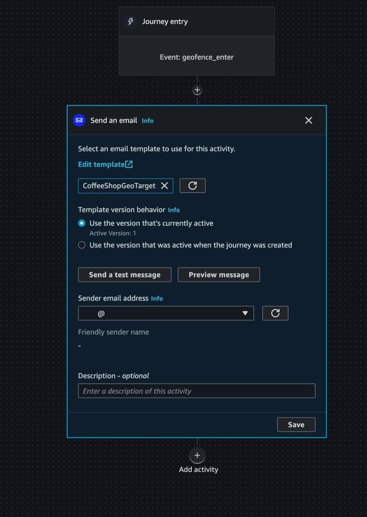
Conclusion

In this post, we discussed methodologies for monitoring and optimizing cost on AWS Glue for Apache Spark. With these techniques, you can effectively monitor and optimize costs on AWS Glue for Spark.
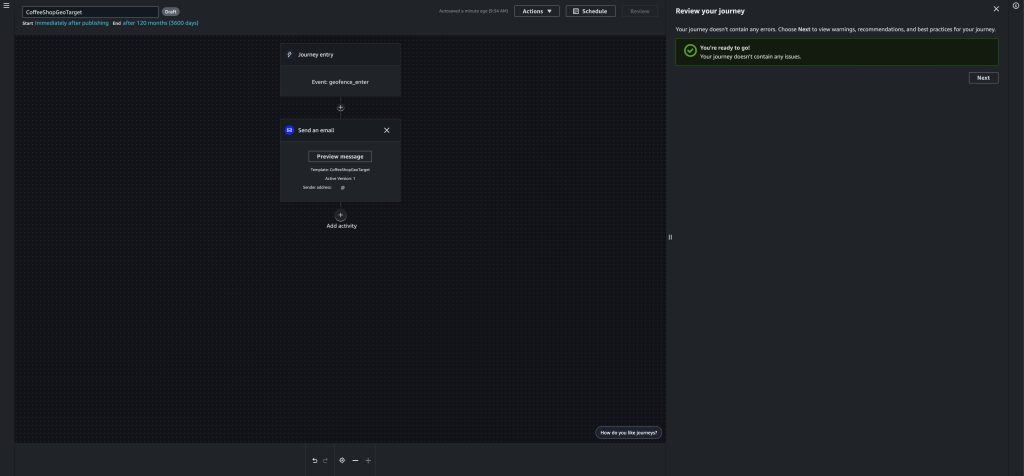
If you have comments or feedback, please leave them in the comments.


About the Authors

Leonardo Gómez is a Principal Analytics Specialist Solutions Architect at AWS. He has over a decade of experience in data management, helping customers around the globe address their business and technical needs. Connect with him on LinkedIn

Noritaka Sekiyama is a Principal Big Data Architect on the AWS Glue team. He is responsible for building software artifacts to help customers. In his spare time, he enjoys cycling with his new road bike.