Tag Archives: Advanced (300)

Break down data silos and seamlessly query Iceberg tables in Amazon SageMaker from Snowflake

2025-09-15 Nidhi Gupta

Post Syndicated from Nidhi Gupta original https://aws.amazon.com/blogs/big-data/break-down-data-silos-and-seamlessly-query-iceberg-tables-in-amazon-sagemaker-from-snowflake/

Organizations often struggle to unify their data ecosystems across multiple platforms and services. The connectivity between Amazon SageMaker and Snowflake’s AI Data Cloud offers a powerful solution to this challenge, so businesses can take advantage of the strengths of both environments while maintaining a cohesive data strategy.

In this post, we demonstrate how you can break down data silos and enhance your analytical capabilities by querying Apache Iceberg tables in the lakehouse architecture of SageMaker directly from Snowflake. With this capability, you can access and analyze data stored in Amazon Simple Storage Service (Amazon S3) through AWS Glue Data Catalog using an AWS Glue Iceberg REST endpoint, all secured by AWS Lake Formation, without the need for complex extract, transform, and load (ETL) processes or data duplication. You can also automate table discovery and refresh using Snowflake catalog-linked databases for Iceberg. In the following sections, we show how to set up this integration so Snowflake users can seamlessly query and analyze data stored in AWS, thereby improving data accessibility, reducing redundancy, and enabling more comprehensive analytics across your entire data ecosystem.

Business use cases and key benefits

The capability to query Iceberg tables in SageMaker from Snowflake delivers significant value across multiple industries:

Financial services – Enhance fraud detection through unified analysis of transaction data and customer behavior patterns
Healthcare – Improve patient outcomes through integrated access to clinical, claims, and research data
Retail – Increase customer retention rates by connecting sales, inventory, and customer behavior data for personalized experiences
Manufacturing – Boost production efficiency through unified sensor and operational data analytics
Telecommunications – Reduce customer churn with comprehensive analysis of network performance and customer usage data

Key benefits of this capability include:

Accelerated decision-making – Reduce time to insight through integrated data access across platforms
Cost optimization – Accelerate time to insight by querying data directly in storage without the need for ingestion
Improved data fidelity – Reduce data inconsistencies by establishing a single source of truth
Enhanced collaboration – Increase cross-functional productivity through simplified data sharing between data scientists and analysts

By using the lakehouse architecture of SageMaker with Snowflake’s serverless and zero-tuning computational power, you can break down data silos, enabling comprehensive analytics and democratizing data access. This integration supports a modern data architecture that prioritizes flexibility, security, and analytical performance, ultimately driving faster, more informed decision-making across the enterprise.

Solution overview

The following diagram shows the architecture for catalog integration between Snowflake and Iceberg tables in the lakehouse.

Catalog integration to query Iceberg tables in S3 bucket using Iceberg REST Catalog (IRC) with credential vending

The workflow consists of the following components:

Data storage and management:
- Amazon S3 serves as the primary storage layer, hosting the Iceberg table data
- The Data Catalog maintains the metadata for these tables
- Lake Formation provides credential vending
Authentication flow:
- Snowflake initiates queries using a catalog integration configuration
- Lake Formation vends temporary credentials through AWS Security Token Service (AWS STS)
- These credentials are automatically refreshed based on the configured refresh interval
Query flow:
- Snowflake users submit queries against the mounted Iceberg tables
- The AWS Glue Iceberg REST endpoint processes these requests
- Query execution uses Snowflake’s compute resources while reading directly from Amazon S3
- Results are returned to Snowflake users while maintaining all security controls

There are four patterns to query Iceberg tables in SageMaker from Snowflake:

Iceberg tables in an S3 bucket using an AWS Glue Iceberg REST endpoint and Snowflake Iceberg REST catalog integration, with credential vending from Lake Formation
Iceberg tables in an S3 bucket using an AWS Glue Iceberg REST endpoint and Snowflake Iceberg REST catalog integration, using Snowflake external volumes to Amazon S3 data storage
Iceberg tables in an S3 bucket using AWS Glue API catalog integration, also using Snowflake external volumes to Amazon S3
Amazon S3 Tables using Iceberg REST catalog integration with credential vending from Lake Formation

In this post, we implement the first of these four access patterns using catalog integration for the AWS Glue Iceberg REST endpoint with Signature Version 4 (SigV4) authentication in Snowflake.

Prerequisites

You must have the following prerequisites:

A Snowflake account.
An AWS Identity and Access Management (IAM) role that is a Lake Formation data lake administrator in your AWS account. A data lake administrator is an IAM principal that can register Amazon S3 locations, access the Data Catalog, grant Lake Formation permissions to other users, and view AWS CloudTrail. See Create a data lake administrator for more information.
An existing AWS Glue database named iceberg_db and Iceberg table named customer with data stored in an S3 general purpose bucket with a unique name. To create the table, refer to the table schema and dataset.
A user-defined IAM role that Lake Formation assumes when accessing the data in the aforementioned S3 location to vend scoped credentials (see Requirements for roles used to register locations). For this post, we use the IAM role LakeFormationLocationRegistrationRole.

The solution takes approximately 30–45 minutes to set up. Cost varies based on data volume and query frequency. Use the AWS Pricing Calculator for specific estimates.

Create an IAM role for Snowflake

To create an IAM role for Snowflake, you first create a policy for the role:

On the IAM console, choose Policies in the navigation pane.
Choose Create policy.
Choose the JSON editor and enter the following policy (provide your AWS Region and account ID), then choose Next.

{
     "Version": "2012-10-17",
     "Statement": [
         {
             "Sid": "AllowGlueCatalogTableAccess",
             "Effect": "Allow",
             "Action": [
                 "glue:GetCatalog",
                 "glue:GetCatalogs",
                 "glue:GetPartitions",
                 "glue:GetPartition",
                 "glue:GetDatabase",
                 "glue:GetDatabases",
                 "glue:GetTable",
                 "glue:GetTables",
                 "glue:UpdateTable"
             ],
             "Resource": [
                 "arn:aws:glue:<region>:<account-id>:catalog",
                 "arn:aws:glue:<region>:<account-id>:database/iceberg_db",
                 "arn:aws:glue:<region>:<account-id>:table/iceberg_db/*",
             ]
         },
         {
             "Effect": "Allow",
             "Action": [
                 "lakeformation:GetDataAccess"
             ],
             "Resource": "*"
         }
     ]
 }

Enter iceberg-table-access as the policy name.
Choose Create policy.

Now you can create the role and attach the policy you created.

Choose Roles in the navigation pane.
Choose Create role.
Choose AWS account.
Under Options, select Require External Id and enter an external ID of your choice.
Choose Next.
Choose the policy you created (iceberg-table-access policy).
Enter snowflake_access_role as the role name.
Choose Create role.

Configure Lake Formation access controls

To configure your Lake Formation access controls, first set up the application integration:

Sign in to the Lake Formation console as a data lake administrator.
Choose Administration in the navigation pane.
Select Application integration settings.
Enable Allow external engines to access data in Amazon S3 locations with full table access.
Choose Save.

Now you can grant permissions to the IAM role.

Choose Data permissions in the navigation pane.
Choose Grant.
Configure the following settings:
1. For Principals, select IAM users and roles and choose snowflake_access_role.
2. For Resources, select Named Data Catalog resources.
3. For Catalog, choose your AWS account ID.
4. For Database, choose iceberg_db.
5. For Table, choose customer.
6. For Permissions, select SUPER.
Choose Grant.

SUPER access is required for mounting the Iceberg table in Amazon S3 as a Snowflake table.

Register the S3 data lake location

Complete the following steps to register the S3 data lake location:

As data lake administrator on the Lake Formation console, choose Data lake locations in the navigation pane.
Choose Register location.
Configure the following:
1. For S3 path, enter the S3 path to the bucket where you will store your data.
2. For IAM role, choose LakeFormationLocationRegistrationRole.
3. For Permission mode, choose Lake Formation.
Choose Register location.

Set up the Iceberg REST integration in Snowflake

Complete the following steps to set up the Iceberg REST integration in Snowflake:

Log in to Snowflake as an admin user.
Execute the following SQL command (provide your Region, account ID, and external ID that you provided during IAM role creation):

CREATE OR REPLACE CATALOG INTEGRATION glue_irc_catalog_int
CATALOG_SOURCE = ICEBERG_REST
TABLE_FORMAT = ICEBERG
CATALOG_NAMESPACE = 'iceberg_db'
REST_CONFIG = (
    CATALOG_URI = 'https://glue.<region>.amazonaws.com/iceberg'
    CATALOG_API_TYPE = AWS_GLUE
    CATALOG_NAME = '<account-id>'
    ACCESS_DELEGATION_MODE = VENDED_CREDENTIALS
)
REST_AUTHENTICATION = (
    TYPE = SIGV4
    SIGV4_IAM_ROLE = 'arn:aws:iam::<account-id>:role/snowflake_access_role'
    SIGV4_SIGNING_REGION = '<region>'
    SIGV4_EXTERNAL_ID = '<external-id>'
)
REFRESH_INTERVAL_SECONDS = 120
ENABLED = TRUE;

Execute the following SQL command and retrieve the value for API_AWS_IAM_USER_ARN:

DESCRIBE CATALOG INTEGRATION glue_irc_catalog_int;

On the IAM console, update the trust relationship for snowflake_access_role with the value for API_AWS_IAM_USER_ARN:

{
    "Version": "2012-10-17",
    "Statement": [
        {
            "Sid": "",
            "Effect": "Allow",
            "Principal": {
                "AWS": [
                   "<API_AWS_IAM_USER_ARN>"
                ]
            },
            "Action": "sts:AssumeRole",
            "Condition": {
                "StringEquals": {
                    "sts:ExternalId": [
                        "<external-id>"
                    ]
                }
            }
        }
    ]
}

Verify the catalog integration:

SELECT SYSTEM$VERIFY_CATALOG_INTEGRATION('glue_irc_catalog_int');

Mount the S3 table as a Snowflake table:

CREATE OR REPLACE ICEBERG TABLE s3iceberg_customer
 CATALOG = 'glue_irc_catalog_int'
 CATALOG_NAMESPACE = 'iceberg_db'
 CATALOG_TABLE_NAME = 'customer'
 AUTO_REFRESH = TRUE;

Query the Iceberg table from Snowflake

To test the configuration, log in to Snowflake as an admin user and run the following sample query:SELECT * FROM s3iceberg_customer LIMIT 10;

Clean up

To clean up your resources, complete the following steps:

Delete the database and table in AWS Glue.
Drop the Iceberg table, catalog integration, and database in Snowflake:

DROP ICEBERG TABLE iceberg_customer;
DROP CATALOG INTEGRATION glue_irc_catalog_int;

Make sure all resources are properly cleaned up to avoid unexpected charges.

Conclusion

In this post, we demonstrated how to establish a secure and efficient connection between your Snowflake environment and SageMaker to query Iceberg tables in Amazon S3. This capability can help your organization maintain a single source of truth while also letting teams use their preferred analytics tools, ultimately breaking down data silos and enhancing collaborative analysis capabilities.

To further explore and implement this solution in your environment, consider the following resources:

Technical documentation:
- Review the Amazon SageMaker Lakehouse User Guide
- Explore Security in AWS Lake Formation for best practices to optimize your security controls
- Learn more about Iceberg table format and its benefits for data lakes
- Refer to Configuring secure access from Snowflake to Amazon S3
Related blog posts:
- Build real-time data lakes with Snowflake and Amazon S3 Tables
- Simplify data access for your enterprise using Amazon SageMaker Lakehouse

These resources can help you to implement and optimize this integration pattern for your specific use case. As you begin this journey, remember to start small, validate your architecture with test data, and gradually scale your implementation based on your organization’s needs.

About the authors

Automate and orchestrate Amazon EMR jobs using AWS Step Functions and Amazon EventBridge

2025-09-15 Senthil Kamala Rathinam

Post Syndicated from Senthil Kamala Rathinam original https://aws.amazon.com/blogs/big-data/automate-and-orchestrate-amazon-emr-jobs-using-aws-step-functions-and-amazon-eventbridge/

Many enterprises are adopting Apache Spark for scalable data processing tasks such as extract, transform, and load (ETL), batch analytics, and data enrichment. As data pipelines evolve, the need for flexible and cost-efficient execution environments that support automation, governance, and performance at scale also evolve in parallel. Amazon EMR provides a powerful environment to run Spark workloads, and depending on workload characteristics and compliance requirements, teams can choose between fully managed options like Amazon EMR Serverless or more customizable configurations using Amazon EMR on Amazon Elastic Compute Cloud (Amazon EC2).

In use cases where infrastructure control, data locality, or strict security postures are essential, such as in financial services, healthcare, or government, running transient EMR on EC2 clusters becomes a preferred choice. However, orchestrating the full lifecycle of these clusters, from provisioning to job submission and eventual teardown, can introduce operational overhead and risk if done manually.

To streamline this process, the AWS Cloud offers built-in orchestration capabilities using AWS Step Functions and Amazon EventBridge. Together, these services help you automate and schedule the entire EMR job lifecycle, reducing manual intervention while optimizing cost and compliance. Step Functions provides the workflow logic to manage cluster creation, Spark job execution, and cluster termination, and EventBridge schedules these workflows based on business or operational needs.

In this post, we discuss how to build a fully automated, scheduled Spark processing pipeline using Amazon EMR on EC2, orchestrated with Step Functions and triggered by EventBridge. We walk through how to deploy this solution using AWS CloudFormation, processes COVID-19 public dataset data in Amazon Simple Storage Service (Amazon S3), and store the aggregated results in Amazon S3. This architecture is ideal for periodic or scheduled batch processing scenarios where infrastructure control, auditability, and cost-efficiency are critical.

Solution overview

This solution uses the publicly available COVID-19 dataset to illustrate how to build a modular, scheduled architecture for scalable and cost-efficient batch processing for time-bound data workloads.The solution follows these steps:

Raw COVID-19 data in CSV format is stored in an S3 input bucket.
A scheduled rule in EventBridge triggers a Step Functions workflow.
The Step Functions workflow provisions a transient Amazon EMR cluster using EC2 instances.
A PySpark job is submitted to the cluster to calculate COVID-19 hospital utilization data to compute monthly state-level averages of inpatient and ICU bed utilization, and COVID-19 patient percentages.
The processed results are written back to an S3 output bucket.
After successful job completion, the EMR cluster is automatically deleted.
Logs are persisted to Amazon S3 for observability and troubleshooting.

By automating this workflow, you alleviate the need to manually manage EMR clusters while gaining cost-efficiency by running compute only when needed. This architecture is ideal for periodic Spark jobs such as ETL pipelines, regulatory reporting, and batch analytics, especially when control, compliance, and customization are required.The following diagram illustrates the architecture for this use case.

The infrastructure is deployed using AWS CloudFormation to provide consistency and repeatability. AWS Identity and Access Management (IAM) roles grant least‑privilege access to Step Functions, Amazon EMR, EC2 instances, and S3 buckets, and optional AWS Key Management Service (AWS KMS) encryption can secure data at rest in Amazon S3 and Amazon CloudWatch Logs. By combining a scheduled trigger, stateful orchestration, and centralized logging, this solution delivers a fully automated, cost‑optimized, and secure way to run transient Spark workloads in production.

Prerequisites

Before you get started, make sure you have the following prerequisites:

An AWS account. If you don’t have one, you can sign up for one.
An IAM user with administrator access. For instructions, see Create a user with administrative access.
The AWS Command Line Interface (AWS CLI) is installed on your local machine
A default virtual private cloud (VPC) and subnet in the target AWS Region where you plan to run the CloudFormation template.

Set up resources with AWS CloudFormation

To provision the required resources using a single CloudFormation template, complete the following steps:

Clone the sample repository to your local machine or AWS CloudShell and navigate into the project directory.

git clone https://github.com/aws-samples/sample-emr-transient-cluster-step-functions-eventbridge.git
cd sample-emr-transient-cluster-step-functions-eventbridge

Set an environment variable for the AWS Region where you plan to deploy the resources. Replace the placeholder with your Region code, for example, us-east-1.
```
export AWS_REGION=<YOUR AWS REGION>
```

Deploy the stack using the following command. Update the stack name if needed. In this example, the stack is created with the name covid19-analysis.

aws cloudformation deploy \
--template-file emr_transient_cluster_step_functions_eventbridge.yaml \
--stack-name covid19-analysis \
--capabilities CAPABILITY_IAM \
--region $AWS_REGION

You can monitor the stack creation progress on the AWS CloudFormation console on the Events tab. The deployment typically completes in under 5 minutes.

After the stack is successfully created, go to the Outputs tab on the AWS CloudFormation console and note the following values for use in later steps:

InputBucketName
OutputBucketName
LogBucketName

Set up the COVID-19 dataset

With your infrastructure in place, complete the following steps to set up the input data:

Download the COVID-19 data CSV file from HealthData.gov to your local machine.
Rename the downloaded file to covid19-dataset.csv.
Upload the renamed file to your S3 input bucket under the raw/ folder path.

Set up the PySpark Script

Complete the following steps to set up the PySpark script:

Open AWS CloudShell from the console.
Confirm that you are working inside the sample-emr-transient-cluster-step-functions-eventbridge directory before running the next command.
Copy the PySpark script needed for this walkthrough into your input bucket:
```
aws s3 cp covid19_processor.py s3://<InputBucketName>/scripts/
```

This script processes COVID-19 hospital utilization data stored as CSV files in your S3 input bucket. When running the job, provide the following command-line arguments:

--input – The S3 path to the input CSV files
--output – The S3 path to store the processed results

The script reads the raw dataset, standardizes various date formats, and filters out records with invalid or missing dates. It then extracts key utilization metrics such as inpatient bed usage, ICU bed usage, and the percentage of beds occupied by COVID-19 patients and calculates monthly averages grouped by state. The aggregated output is saved as timestamped CSV files in the specified S3 location.

This example demonstrates how you can use PySpark to efficiently clean, transform, and analyze large-scale healthcare data to gain actionable insights on hospital capacity trends during the pandemic.

Configure a schedule in EventBridge

The Step Functions state machine is by default scheduled to run on December 31, 2025, as a one-time execution. You can update the schedule for recurring or one-time execution as needed. Complete the following steps:

On the EventBridge console, choose Schedules under Scheduler in the navigation pane.
Select the schedule named <StackName>-covid19-analysis and choose Edit.
Set your preferred schedule pattern.
1. If you want to run the schedule one time, select One-time schedule for Occurrence and enter a date and time.
2. If you want to run this on a recurring basis, select Recurring schedule. Specify the schedule type as either Cron-based schedule or Rate-based schedule as needed.
Choose Next twice and choose Save schedule.

Start the workflow in Step Functions

Based on your EventBridge schedule, the Step Functions workflow will run automatically. For this walkthrough, complete the following steps to trigger it manually:

On the Step Functions console, choose State machines in the navigation pane.
Choose the state machine that begins with Covid19AnalysisStateMachine-*.
Choose Start execution.
In the Input section, provide the following JSON (provide the log bucket and output bucket names with the appropriate values captured earlier):
```
{
  "LogUri": "s3://<LogBucketName>/logs/",
  "OutputS3Location": "s3://<OutputBucketName>/processed/"
}
```
Choose Start execution to initiate the workflow.

Monitor the EMR job and workflow execution

After you start the workflow, you can track both the Step Functions state transitions and the EMR job progress in real time on the console.

Monitor the Step Functions state machine

Complete the following steps to monitor the Step Functions state machine:

On the Step Functions console, choose State machines in the navigation pane.
Choose the state machine that begins with Covid19AnalysisStateMachine-*.
Choose the running execution to view the visual workflow.
Each state node will update as it progresses—green for success, red for failure.
To explore a step, choose its node and inspect the input, output, and error details in the side pane.

The following screenshot shows an example of a successfully executed workflow.

Monitor the EMR cluster and EMR step

Complete the following steps to monitor the EMR cluster and EMR step status:

While the cluster is active, open the Amazon EMR console and choose Clusters in the navigation pane.
Locate the Covid19Cluster transient EMR cluster.
Initially, it will be in Starting status.

On the Steps tab, you can see your Spark submit step listed. As the job progresses, the step status changes from Pending to Running to finally Completed or Failed.
Choose the Applications tab to view the application UIs, in which you can access the Spark History Server and YARN Timeline Server for monitoring and troubleshooting.

Monitor CloudWatch logs

To enable CloudWatch logging and enhanced monitoring for your EMR on EC2 cluster, refer to Amazon EMR on EC2 – Enhanced Monitoring with CloudWatch using custom metrics and logs. This guide explains how to install and configure the CloudWatch agent using a bootstrap action, so you can stream system-level metrics (such as CPU, memory, and disk usage) and application logs from EMR nodes directly to CloudWatch. With this setup, you can gain real-time visibility into cluster health and performance, simplify troubleshooting, and retain critical logs even after the cluster is terminated.

For this walkthrough, check the logs in the S3 log output location.

Confirm cluster deletion

When the Spark step is complete, Step Functions will automatically delete the Amazon EMR cluster. Refresh the Clusters page on the Amazon EMR console. You should see your cluster status change from Terminating to Terminated within a minute.

By following these steps, you gain full end-to-end visibility into your workflow from the moment the Step Functions state machine is triggered to the automatic shutdown of the EMR cluster. You can monitor execution progress, troubleshoot issues, confirm job success, and continuously optimize your transient Spark workloads.

Verify job output in Amazon S3

When the job is complete, complete the following steps to check the processed results in the S3 output bucket:

On the Amazon S3 console, choose Buckets in the navigation pane.
Open the output S3 bucket you noted earlier.
Open the processed folder.
Navigate into the timestamped subfolder to view the CSV output file.
Download the CSV file to view the processed results, as shown in the following screenshot.

Monitoring and troubleshooting

To monitor the progress of your Spark job running on a transient EMR on EC2 cluster, use the Step Functions console. It provides real-time visibility into each state transition in your workflow, from cluster creation and job submission to cluster deletion. This makes it straightforward to track execution flow and identify where issues might occur.During job execution, you can use the Amazon EMR console to access cluster-level monitoring. This includes YARN application statuses, step-level logs, and overall cluster health. If CloudWatch logging is enabled in your job configuration, driver and executor logs stream in near real time, so you can quickly detect and diagnose errors, resource constraints, or data skew within your Spark application.

After the workflow is complete, regardless of whether it succeeds or fails, you can perform a detailed post-execution analysis by reviewing the logs stored in the S3 bucket specified in the LogUri parameter. This log directory includes standard output and error logs, along with Spark history files, offering insights into execution behavior and performance metrics.

For continued access to the Spark UI during job execution, you can use persistent application UIs on the EMR console. These links remain accessible even after the cluster is stopped, enabling deeper root-cause analysis and performance tuning for future runs.

This visibility into both workflow orchestration and job execution can help teams optimize their Spark workloads, reduce troubleshooting time, and build confidence in their EMR automation pipelines.

Clean up

To avoid incurring ongoing charges, clean up the resources provisioned during this walkthrough:

Empty the S3 buckets:
1. On the Amazon S3 console, choose Buckets in the navigation pane.
2. Select the input, output, and log buckets used in this tutorial.
3. Choose Empty to remove all objects before deleting the buckets (optional).
Delete the CloudFormation stack:
1. On the AWS CloudFormation console, choose Stacks in the navigation pane.
2. Select the stack you created for this solution and choose Delete.
3. Confirm the deletion to remove associated resources.

Conclusion

In this post, we showed how to build a fully automated and cost-effective Spark processing pipeline using Step Functions, EventBridge, and Amazon EMR on EC2. The workflow provisions a transient EMR cluster, runs a Spark job to process data, and stops the cluster after the job completes. This approach helps reduce costs while giving you full control over the process. This solution is ideal for scheduled data processing tasks such as ETL jobs, log analytics, or batch reporting, especially when you need detailed control over infrastructure, security, and compliance settings.

To get started, deploy the solution in your environment using the CloudFormation stack provided and adjust it to fit your data processing needs. Check out the Step Functions Developer Guide and Amazon EMR Management Guide to explore further.

Share your feedback and ideas in the comments or connect with your AWS Solutions Architect to fine-tune this pattern for your use case.

About the authors

Decrease your storage costs with Amazon OpenSearch Service index rollups

2025-09-09 Luis Tiani

Post Syndicated from Luis Tiani original https://aws.amazon.com/blogs/big-data/decrease-your-storage-costs-with-amazon-opensearch-service-index-rollups/

Amazon OpenSearch Service is a fully managed service to support search, log analytics, and generative AI Retrieval Augment Generation (RAG) workloads in the AWS Cloud. It simplifies the deployment, security, and scaling of OpenSearch clusters. As organizations scale their log analytics workloads by continuously collecting and analyzing vast amounts of data, they often struggle to maintain quick access to historical information while managing costs effectively. OpenSearch Service addresses these challenges through its tiered storage options: hot, UltraWarm, and cold storage. These storage tiers are great options to help optimize costs and offer a balance between performance and affordability, so organizations can manage their data more efficiently. Organizations can choose between these different storage tiers by keeping data in expensive hot storage for quick access or moving it to cheaper cold storage with limited accessibility. This trade-off becomes particularly challenging when organizations need to analyze both recent and historical data for compliance, trend analysis, or business intelligence.

In this post, we explore how to use index rollups in Amazon OpenSearch Service to address this challenge. This feature helps organizations efficiently manage their historical data by automatically summarizing and compressing older data while maintaining its analytical value, significantly reducing storage costs in any storage tier without sacrificing the ability to query historical information effectively.

Index rollups overview

Index rollups provide a mechanism to aggregate historical data into summarized indexes at specified time intervals. This feature is particularly useful for time series data where the granularity of older data can be reduced while maintaining meaningful analytics capabilities.

Key benefits include:

Reduced storage costs (varies by granularity level), for example:
- Larger savings when aggregating from seconds to hours
- Moderate savings when aggregating from seconds to minutes
Improved query performance of historical data
Maintained data accessibility for long-term analytics
Automated data summarization process

Index rollups are part of a comprehensive data management strategy. The real cost savings come from properly managing your data lifecycle in conjunction with rollups. To achieve meaningful cost reductions, you must remove or move the original data to a lower-cost storage tier after creating the rollup.

For customers already using Index State Management (ISM) to move older data to UltraWarm or cold tiers, rollups can provide significant additional benefits. By aggregating data at higher time intervals before moving it to lower-cost tiers, you can dramatically reduce the volume of data in these tiers, leading to further cost savings. This strategy is particularly effective for workloads with large amounts of time series data, typically measuring in terabytes or petabytes. The larger your data volume, the more impactful your savings will be when implementing rollups correctly.

Index rollups can be implemented using ISM policies through the OpenSearch Dashboards UI or the OpenSearch API. Index rollups require OpenSearch or Elasticsearch 7.9 or later.

The decision to use different storage tiers requires careful consideration of an organization’s specific needs, balancing the desire for cost savings with the requirement for data accessibility and performance. As data volumes continue to grow and analytics become increasingly important, finding the right storage strategy becomes crucial for businesses to remain competitive and compliant while managing their budgets effectively.

In this post, we consider a scenario with a large volume of time series data that can be aggregated using the Rollup API. With rollups, you have the flexibility to either store aggregated data in the hot tier for rapid access or aggregate and promote it to more cost-effective tiers such as UltraWarm or cold storage. This approach allows for efficient data and index lifecycle management while optimizing both performance and cost.

Index rollups are often confused with index rollovers, which are automated OpenSearch Service operations that create new indexes when specified thresholds are met, for example by age, size, or document count. This feature maintains raw data while optimizing cluster performance through controlled index growth. For example, rolling over when an index reaches 50 GB or is 30 days old.

Use cases for index rollups

Index rollups are ideal for scenarios where you need to balance storage costs with data granularity, such as:

Time series data that requires different granularity levels over time – For example, Internet of Things (IoT) sensor data where real-time precision matters only for the most recent data.
- Traditional approach – It is common for users to keep all data in expensive hot storage for instant accessibility. However, this isn’t optimal for cost.
- Recommended – Retain recent (per second) data in hot storage for immediate access. For older periods, store aggregated (hourly or daily) data using index rollups. Move or delete the higher-granularity old data from the hot tier. This balances accessibility and cost-effectiveness.
Historical data with cost-optimization needs – For example, system performance metrics where overall trends are more valuable than precise values over time.
- Traditional approach – It is common for users to store all performance metrics at full granularity indefinitely, consuming excessive storage space. We don’t recommend storing data indefinitely. Implement a data retention policy based on your specific business needs and compliance requirements.
- Recommended – Maintain detailed metrics for recent monitoring (last 30 days) and aggregate older data into hourly or daily summaries. This preserves the trend analysis capability while significantly reducing storage costs.
Log data with infrequent historical access and low value – For example, application error logs where detailed investigation is primarily needed for recent incidents.
- Traditional approach – It is common for users to keep all log entries at full detail, regardless of age or access frequency.
- Recommended – Preserve detailed logs for an active troubleshooting period (for example, 1 week) and maintain summarized error patterns and statistics for older periods. This enables historical pattern analysis while reducing storage overhead.

Schema design

A well-planned schema is crucial for successful rollup implementation. Proper schema design makes sure your rolled-up data remains valuable for analysis while maximizing storage savings. Consider the following key aspects:

Identify fields required for long-term analysis – Carefully select fields that provide meaningful insights over time, avoiding unnecessary data retention.
Define aggregation types for each field, such as min, max, sum, and average – Choose appropriate aggregation methods that preserve the analytical value of your data.
Determine which fields can be excluded from rollups – Reduce storage costs by omitting fields that don’t contribute to long-term analysis.
Consider mapping compatibility between source and target indexes – Provide successful data transition without mapping conflicts. This involves:
- Matching data types (for example, date fields remain as date in rollups)
- Handling nested fields appropriately
- Ensuring all required fields are included in the rollup
- Considering the impact of analyzed vs. non-analyzed fields
- Incompatible mappings can lead to failed rollup jobs or incorrect data aggregation.

Functional and non-functional requirements

Before implementing index rollups, consider the following:

Data access patterns – When implementing data rollup strategies, it’s crucial to first analyze data access patterns, including query frequency and usage periods, to determine optimal rollup intervals. This analysis should lead to specific granularity metrics, such as deciding between hourly or daily aggregations, while establishing clear thresholds based on both data volume and query requirements. These decisions should be documented alongside specific aggregation rules for each data type.
Data growth rate – Storage optimization begins with calculating your current dataset size and its growth rate. This information helps quantify potential space reductions across different rollup strategies. Performance metrics, particularly expected query response times, should be defined upfront. Additionally, establish monitoring KPIs focusing on latency, throughput, and resource usage to make sure the system meets performance expectations.
Compliance or data retention requirements – Retention planning requires careful consideration of regulatory requirements and business needs. Develop a clear retention policy that specifies how long to keep different types of data at various granularity levels. Implement systematic processes for archiving or deleting older data and maintain detailed documentation of storage costs across different retention periods.
Resource utilization and planning – For successful implementation, proper cluster capacity planning is essential. This involves accurately sizing computing resources, including CPU, RAM, and storage requirements. Define specific time windows for executing rollup jobs to minimize impact on regular operations. Set clear resource utilization thresholds and implement proactive capacity monitoring. Finally, develop a scalability plan that accounts for both horizontal and vertical growth to accommodate future needs.

Operational requirements

Proper operational planning facilitates smooth ongoing management of your rollup implementation. This is essential for maintaining data reliability and system health:

Monitoring – You must monitor rollup jobs for their accuracy and desired results. This means implementing automated checks that validate data completeness, aggregation accuracy, and job execution status. Set up alerts for failed jobs, data inconsistencies, or when aggregation results fall outside expected ranges.
Scheduling hours – Schedule rollup operations during periods of low system usage, typically during off-peak hours. Document these maintenance windows clearly and communicate them to all stakeholders. Include buffer time for potential issues and establish clear procedures for what happens if a maintenance window needs to be extended.
Backup and recovery – OpenSearch Service takes automated snapshots of your data at 1-hour intervals. But you can define and implement comprehensive backup procedures using snapshot management functionality to support your Recovery Time Objective (RTO) and Recovery Point Objective (RPO).

Your RPO can be customized through different rollup schedules based on index patterns. This flexibility helps you define varied data loss tolerance levels according to your data’s criticality. For mission-critical indexes, you can configure more frequent rollups, while maintaining less frequent schedules for analytical data.

You can tailor RTO management in OpenSearch per index pattern through backup and replication options. For critical rollup indexes, implementing cross-cluster replication maintains up-to-date copies, significantly reducing recovery time. Other indexes might use standard backup procedures, balancing recovery speed with operational costs. This flexible approach helps you optimize both storage costs and recovery objectives based on your specific business requirements for different types of data within your OpenSearch deployment.

Before implementing rollups, audit all applications and dashboards that use the data being aggregated. Update queries and visualizations to accommodate the new data structure. Test these changes thoroughly in a staging environment to confirm they continue to provide accurate results with the rolled-up data. Create a rollback plan in case of unexpected issues with dependent applications.

In the following sections, we walk through the steps to create, run, and monitor a rollup job.

Create a rollup job

As discussed in previous sections, there are some considerations when choosing good candidates for index rollup usage. Building on this concept, identify your indexes to roll up their data and create the jobs.The following code is an example of creating a basic rollup job:

PUT /_plugins/_rollup/jobs/sensor_hourly_rollup
{
  "rollup": {
    "rollup_id": "sensor_1_hour_rollup",
    "enabled": true,
    "schedule": {
      "interval": {
        "start_time": 1746632400,        
        "period": 1,
        "unit": "hours",
        "schedule_delay": 0
      }
    },
    "description": "Rolls up sensor data 1 hourly per device_id",
    "source_index": "sensor-*",           
    "target_index": "sensor_rolled_hour",
    "page_size": 1000,
    "delay": 0,
    "continuous": true,
    "dimensions": [
      {
        "date_histogram": {
          "fixed_interval": "1h",
          "source_field": "timestamp",
          "target_field": "timestamp",
          "timezone": "UTC"
        }
      },
      {
        "terms": {
          "source_field": "device_id",
          "target_field": "device_id"
        }
      }
    ],
    "metrics": [
      {
        "source_field": "temperature",
        "metrics": [
          { "avg": {} },
          { "min": {} },
          { "max": {} }
        ]
      },
      {
        "source_field": "humidity",
        "metrics": [
          { "avg": {} },
          { "min": {} },
          { "max": {} }
        ]
      },
      {
        "source_field": "pressure",
        "metrics": [
          { "avg": {} },
          { "min": {} },
          { "max": {} }
        ]
      },
      {
        "source_field": "battery",
        "metrics": [
          { "avg": {} },
          { "min": {} },
          { "max": {} }
        ]
      }
    ]
  }
}

This rollup job processes IoT sensor data, aggregating readings from the sensor-* index pattern into hourly summaries stored in sensor_rolled_hour. It maintains device-level granularity while calculating average, minimum, and maximum values for temperature, humidity, pressure, and battery levels. The job executes hourly, processing 1,000 documents per batch.

The preceding code assumes that the device_id field is of type keyword; note that aggregation can’t be performed on the text field.

Start the rollup job

After you create the job, it will automatically be scheduled based on the job’s configuration (refer to the schedule: part of the job example code in the previous section). However, you can also trigger the job manually using the following API call:

POST _plugins/_rollup/jobs/sensor_hourly_rollup/_start

The following is an example of the results:

{
  "acknowledged": true
}

Monitor progress

Using Dev Tools, run the following command to monitor the progress:

GET _plugins/_rollup/jobs/sensor_hourly_rollup/_explain

The following is an example of the results:

{
  "sensor_hourly_rollup": {
    "metadata_id": "pCDjMZcBgTxYF90dWEfP",
    "rollup_metadata": {
      "rollup_id": "sensor_hourly_rollup",
      "last_updated_time": 1749043472416,
      "continuous": {
        "next_window_start_time": 1749043440000,
        "next_window_end_time": 1749043560000
      },
      "status": "started",
      "failure_reason": null,
      "stats": {
        "pages_processed": 374603,
        "documents_processed": 390,
        "rollups_indexed": 200,
        "index_time_in_millis": 789,
        "search_time_in_millis": 402202
      }
    }
  }
}

The GET _plugins/_rollup/jobs/sensor_hourly_rollup/_explain command shows the current status and statistics of the sensor_hourly_rollup job. The response shows important statistics such as the number of processed documents, indexed rollups, time spent on indexing and searching, and records of any failures. The status indicates whether the job is active (started) or stopped (stopped) and shows the last processed timestamp. This information is crucial for monitoring the efficiency and health of the rollup process, helping administrators track progress, identify potential issues or bottlenecks, and confirm the job is operating as expected. Regular checks of these statistics can help in optimizing the rollup job’s performance and maintaining data integrity.

Real-world example

Let’s consider a scenario where a company collects IoT sensor data, ingesting 240 GB of data per day to an OpenSearch cluster, which totals 7.2 TB per month.

The following is an example record:

"_source": {
          "timestamp": "2024-01-01T10:00:00Z",
          "device_id": "sensor_001",
          "temperature": 26.1,
          "humidity": 43,
          "pressure": 1009.3,
          "battery": 90
}

Assume you have a time series index with the following configuration:

Ingest rate: 10 million documents per hour
Retention period: 30 days
Each document size: Approximately 1 KB

The total storage without rollups is as follows:

Per-day storage size: 10,000,000 docs per hour × ~1 KB × 24 hours per day = ~240 GB
Per-month storage size: 240 GB × 30 days = ~7.2 TB

The decision to implement rollups should be based on a cost-benefit analysis. Consider the following:

Current storage costs vs. potential savings
Compute costs for running rollup jobs
Value of granular data over time
Frequency of historical data access

For smaller datasets (for example, less than 50 GB/day), the benefits might be less significant. As data volumes grow, the cost savings become more compelling.

Rollup configuration

Let’s roll up the data with the following configuration:

From 1-minute granularity to 1-hour granularity
Aggregating average, min, and max, grouped by device_id
Reducing 60 documents per minute to 1 rollup document per minute

The new document count per hour is as follows:

Per-hour documents: 10,000,000/60 = 166,667 docs per hour
Assuming each rollup document is 2 KB (extra metadata), total rollup storage: 166,667 docs per hour × 24 hours per day × 30 days × 2KB ˜= 240 GB/month

Verify all required data exists in the new rolled index, then delete the original index to remove raw data manually or by using ISM policies (as discussed in the next section).

Execute the rollup job following the preceding instructions to aggregate data into the new rolled up index. To view your aggregated results, run the following code:

GET sensor_rolled_hour/_search
{
  "size": 0,
  "aggs": {
    "per_device": {
      "terms": {
        "field": "device_id",
        "size": 200,
        "shard_size": 200
      },
      "aggs": {
        "temperature_avg": {
          "avg": {
            "field": "temperature"
          }
        },
        "temperature_min": {
          "min": {
            "field": "temperature"
          }
        },
        "temperature_max": {
          "max": {
            "field": "temperature"
          }
        }
      }
      }
    }
  }

The following code shows the example results:

"aggregations": {
    "per_device": {
      "doc_count_error_upper_bound": 0,
      "sum_other_doc_count": 0,
      "buckets": [
        {
          "key": "sensor_001",
          "doc_count": 98,
          "temperature_min": {
            "value": 24.100000381469727
          },
          "temperature_avg": {
            "value": 26.287754603794642
          },
          "temperature_max": {
            "value": 27.5
          }
        },
        {
          "key": "sensor_002",
          "doc_count": 98,
          "temperature_min": {
            "value": 20.600000381469727
          },
          "temperature_avg": {
            "value": 22.192856146364797
          },
          "temperature_max": {
            "value": 22.799999237060547
          }
        },...]

This document represents the rolled-up data for sensor_001 and sensor_002 during a 1-hour period. It aggregates 1 hour of sensor readings into a single record, storing minimum, average, and maximum values for temperature levels. The record includes metadata about the rollup process and timestamps for data tracking. This aggregated format significantly reduces storage requirements while maintaining essential statistical information about the sensor’s performance during that hour.

We can calculate the storage savings as follows:

Original storage: 7.2 TB (or 7200 GB)
Post-rollup storage: 240 GB
Storage savings: ((7.2 TB – 240 GB)/7.2 GB) × 100 = 96.67% savings

Using OpenSearch rollups as demonstrated in this example, you can achieve approximately 96% storage savings while preserving important aggregate insights.

The aggregation levels and document sizes can be customized according to your specific use case requirements.

Automate rollups with ISM

To fully realize the benefits of index rollups, automate the process using ISM policies. The following code is an example that implements a rollup strategy based on the given scenario:

PUT _plugins/_ism/policies/sensor_rollup_policy
{
  "policy": {
    "description": "Roll up sensor data and delete original",
    "default_state": "hot",
    "ism_template": {
      "index_patterns": ["sensor-*"],
      "priority": 100
    },
    "states": [
      {
        "name": "hot",
        "actions": [],
        "transitions": [
          {
            "state_name": "rollup",
            "conditions": {
              "min_index_age": "1d"
            }
          }
        ]
      },
      {
        "name": "rollup",
        "actions": [
          {
            "rollup": {
              "ism_rollup": {
                "target_index": "sensor_rolled_minutely",
                "description": "Rollup sensor data to minutely aggregations",
                "page_size": 1000,
                "dimensions": [
                  {
                    "date_histogram": {
                      "fixed_interval": "1m",
                      "source_field": "timestamp",
                      "target_field": "timestamp"
                    }
                  },
                  {
                    "terms": {
                      "source_field": "device_id",
                      "target_field": "device_id"
                    }
                  }
                ],
                "metrics": [
                  {
                    "source_field": "temperature",
                    "metrics": [{ "avg": {} }, { "min": {} }, { "max": {} }]
                  },
                  {
                    "source_field": "humidity",
                    "metrics": [{ "avg": {} }, { "min": {} }, { "max": {} }]
                  }
                ]
              }
            }
          }
        ],
        "transitions": [
          {
            "state_name": "delete",
            "conditions": {
              "min_index_age": "2d"
            }
          }
        ]
      },
      {
        "name": "delete",
        "actions": [
          {
            "delete": {}
          }
        ]
      }
    ]
  }
}

This ISM policy automates the rollup process and data lifecycle:

1. Applies to all indexes matching the sensor-* pattern.
2. Keeps original data in the hot state for 1 day.
3. After 1 day, rolls up the data into minutely aggregations. Aggregates by device_id and calculates average, minimum, and maximum for temperature and humidity.
4. Stores rolled-up data in the sensor_rolled_minutely index.
5. Deletes the original index 2 days after rollup.

This strategy offers the following benefits:

Recent data is available at full granularity
Historical data is efficiently summarized
Storage is optimized by removing original data after rollup

You can monitor the policy’s execution using the following command:

GET _plugins/_ism/policies/sensor_rollup_policy

Remember to adjust the timeframes, metrics, and aggregation intervals based on your specific requirements and data patterns.

Conclusion

Index rollups in OpenSearch Service provide a powerful way to manage storage costs while maintaining valuable historical data access. By implementing a well-planned rollup strategy, organizations can achieve significant cost savings while making sure their data remains available for analysis.

To get started, take the following next steps:

Review your current index patterns and data retention requirements
Analyze your historical data volumes and access patterns
Start with a proof-of-concept rollup implementation in a test environment
Monitor performance and storage metrics to optimize your rollup strategy
Move the infrequently accessed data between storage tiers:
- Delete data you’ll no longer use
- Automate the process using ISM policies

To learn more, refer to the following resources:

About the authors

Accessing private Amazon API Gateway endpoints through custom Amazon CloudFront distribution using VPC Origins

2025-09-09 Napoleone Capasso

Post Syndicated from Napoleone Capasso original https://aws.amazon.com/blogs/compute/accessing-private-amazon-api-gateway-endpoints-through-custom-amazon-cloudfront-distribution-using-vpc-origins/

Organizations can use Amazon CloudFront Virtual Private Cloud (VPC) Origins to deliver content from applications hosted in private subnets within Amazon VPC. Network traffic flows between Amazon CloudFront and Application Load Balancers (ALBs), Network Load Balancers (NLBs), or Amazon Elastic Compute Cloud (Amazon EC2) instances deployed within private subnets. This means that Amazon CloudFront can access both public and private Amazon Web Services (AWS) resources seamlessly.

This post demonstrates how you can connect CloudFront with a Private REST API in Amazon REST API Gateway using a VPC origin.

Overview

Organizations looking to enhance their application security and performance can find several key benefits in this architecture. You can use it to keep your APIs private and access them through CloudFront, implementing more security layers such as AWS Shield Advanced, geoblocking and TLSv1.3 support along with custom cipher suites. You can use this approach to engage the global CloudFront content delivery network while maintaining more control over the distribution.

Furthermore, you can enhance security controls through the built-in features of CloudFront, such as AWS WAF integration, custom SSL certificates, and field-level encryption. The VPC Origins feature eliminates any need to expose your internal resources to the public internet, which reduces your application’s potential attack surface.

Enterprises that need to maintain strict compliance requirements while delivering content globally can find this solution particularly valuable. Contain all traffic within the AWS private network to better meet your security and compliance objectives while still providing fast, reliable access to your applications.

Solution overview

You can set up CloudFront as the front door to your application and use VPC Origins integrated with an internal ALB to route traffic to Private Rest API through an execute-api VPC endpoint. All traffic between CloudFront and Private REST API remains within the AWS Private network.

The following figure provides an overview of the solution.

This diagram depicts three services running in an AWS account. The CloudFront distribution serves as the main entry point for the application. This distribution connects to an internal ALB using VPC Origins. The interface VPC endpoint execute-api is set as the target for the internal ALB to route requests to the Private Amazon API Gateway.

Solution deployment

To deploy this solution, follow the instructions in the GitHub repository and clone the repository.

The solution can be deployed in any AWS Region. Make sure to have a valid SSL certificate in AWS Certificate Manager (ACM) in the us-east-1 Region for the CloudFront distribution. All other resources must be in the same Region.

Prerequisites

For this walkthrough, the following resources are needed:

An Amazon VPC with at least 2 Private Subnets.
A Public Hosted Zone in Amazon Route 53.
A valid public SSL certificate in ACM in the us-east-1 Region for CloudFront and another certificate in the same Region as an ALB.
A custom domain name, covered by the ACM certificate for CloudFront distribution.

These are the input parameters for the solution deployment.

Walkthrough

The AWS Serverless Application Model (AWS SAM) template from the sample GitHub repository creates a secure, private networking architecture that provides controlled access to an API Gateway through CloudFront. It provisions a private API Gateway with a VPC endpoint, an internal ALB, and a CloudFront distribution. The template establishes secure communication channels by implementing private networking components, configuring SSL certificates, and setting up Route53 DNS routing. It uses custom AWS Lambda resources to dynamically manage network interfaces and security group configurations, providing a robust and flexible infrastructure for private API access, as shown in the following figure.

Step 1: Create the CloudFront distribution and the VPC Origins

The solution creates a CloudFront distribution that enables wide range of HTTP clients by supporting HTTP2 and HTTP3, enhances your solution security by enforcing HTTPS-only traffic, and uses a custom domain with the user-provided SSL certificate.The internal ALB is configured as the origin for the CloudFront distribution, and it is created using the VPC Origins feature.

########### Cloudfront Distribution ###############
  CloudFrontDistribution:
    Type: AWS::CloudFront::Distribution
    Properties:
      DistributionConfig:
        HttpVersion: http2and3
        Comment: CloudFront Distribution with VPC Origin Integration
        Aliases: 
        - !Ref CloudFrontDomainName
        ViewerCertificate:
          AcmCertificateArn: !Ref CloudFrontCertificateARN
          MinimumProtocolVersion: TLSv1.2_2021
          SslSupportMethod: sni-only
        Origins:
        - Id: AlbOrigin
          DomainName: !GetAtt ApplicationLoadBalancer.DNSName
          VpcOriginConfig:
            OriginKeepaliveTimeout: 60
            OriginReadTimeout: 60
            VpcOriginId: !GetAtt CloudFrontVpcOrigin.Id
        Enabled: true
        DefaultCacheBehavior:
          TargetOriginId: AlbOrigin
          CachePolicyId: 83da9c7e-98b4-4e11-a168-04f0df8e2c65
          OriginRequestPolicyId: 216adef6-5c7f-47e4-b989-5492eafa07d3
          ViewerProtocolPolicy: https-only

The VPC Origins references the internal ALB, and only supports HTTPS protocol.

  ########### Cloudfront VPC Origin ###############
  CloudFrontVpcOrigin:
    Type: AWS::CloudFront::VpcOrigin
    Properties:
      VpcOriginEndpointConfig:
          Arn: !Ref ApplicationLoadBalancer
          Name: !Sub vpc-origin-${AWS::StackName}
          OriginProtocolPolicy: https-only
          OriginSSLProtocols: 
          - TLSv1.2

When the VPC Origins is created, the custom resource Lambda function adds an inbound rule to the CloudFront VPC Origin security group to allow traffic only from the CloudFront prefix list in the chosen Region.

        ec2_client.authorize_security_group_ingress(
            GroupId=cloudfront_sg_id,
            IpPermissions=[
                {
                    'IpProtocol': 'tcp',  
                    'FromPort': 443,      
                    'ToPort': 443,        
                    'PrefixListIds': [{'PrefixListId': cloudfront_prefix_id}]
                }
            ]
        )

Step 2: Create the ALB

The internal ALB is configured with an HTTPS listener using the user-provided SSL certificate. This maintains the encryption of the traffic between CloudFront and the ALB.

########### ALB Listener ###########  
  ALBListener:
    Type: AWS::ElasticLoadBalancingV2::Listener
    Properties:
      DefaultActions:
        - Type: forward
          TargetGroupArn: !Ref ALBTargetGroup
      LoadBalancerArn: !Ref ApplicationLoadBalancer
      Port: '443'
      Protocol: HTTPS
      SslPolicy: ELBSecurityPolicy-TLS-1-2-2017-01
      Certificates:
        - CertificateArn: !Ref ALBCertificateARN

The target group of the ALB points to the execute API VPC endpoint IP addresses. These IP addresses are fetched using a custom resource Lambda function.

  ########### ALB Target Group ###########
  ALBTargetGroup:
    Type: AWS::ElasticLoadBalancingV2::TargetGroup
    Properties:
      Port: 443
      Name: !Sub TargetGroup-${AWS::StackName}
      Protocol: HTTPS
      VpcId: !Ref VPCId
      Targets:
        - Id: !GetAtt GetPrivateIPs.IP0
          Port: 443
        - Id: !GetAtt GetPrivateIPs.IP1
          Port: 443
      TargetType: ip
      Matcher:
        HttpCode: '200,403'

The custom resource Lambda function fetches private IPs for given network interface IDs using the EC2 client and returns a dictionary with keys IP0 and IP1 values as the private IPs.

def fetch_interface_ips(network_interface_ids):
    """
    Fetch private IPs for given network interface IDs using ec2 client
    Returns a dictionary with keys IP0, IP1, etc. and values as the private IPs
    """
    responseData = {}
    
    # Use describe_network_interfaces instead of the resource approach
    response = ec2_client.describe_network_interfaces(
        NetworkInterfaceIds=network_interface_ids
    )
    
    for index, interface in enumerate(response['NetworkInterfaces']):
        responseData[f'IP{index}'] = interface['PrivateIpAddress']
    
    return responseData

Furthermore, the Lambda function adds an inbound rule to the internal ALB security group to allow traffic from the VPC Origin security group.

ec2_client.authorize_security_group_ingress(
            GroupId=security_group_id,
            IpPermissions=[
                {
                    'IpProtocol': 'tcp',  
                    'FromPort': 443,     
                    'ToPort': 443,  
                    'UserIdGroupPairs': [{'GroupId': cloudfront_sg_id}]
                }
            ]
        )

Step 3: Create the VPC endpoint for Private API Gateway

The execute-api VPC Endpoint is configured to route traffic from the internal ALB to the Private API Gateway. Only VPC endpoints can resolve private endpoints and route traffic securely.

  ########### execute-api VPC Endpoint ###########
  ExecuteApiVpcEndpoint:
    Type: AWS::EC2::VPCEndpoint
    Properties:
      ServiceName: !Sub "com.amazonaws.${AWS::Region}.execute-api"
      VpcId: !Ref VPCId
      SubnetIds: !Ref PrivateSubnets
      VpcEndpointType: Interface
      PrivateDnsEnabled: true
      SecurityGroupIds:
        - !Ref VpcEndpointSG

Step 4: Create the Private API Gateway Resource Policy

The Resource Policy set up on the Private API Gateway only allows traffic from the VPC endpoint placed within the user-defined VPC.

        x-amazon-apigateway-policy:
          Version: "2012-10-17"
          Statement:
          - Effect: "Allow"
            Principal: "*"
            Action: "execute-api:Invoke"
            Resource: "execute-api:/*"
            Condition:
              StringEquals:
                aws:sourceVpce: 
                - !Ref ExecuteApiVpcEndpoint

Testing

Fetch the CloudFront URL from the Outputs section of the deployed stack and test it by using the curl command or your web browser.

curl https://{your custom domain name} 
{"message": "Hello from API GW"}

Conclusion

This post demonstrates how you can establish a secure architecture to access a Private REST API Gateway through a Private ALB, using Amazon CloudFront as the entry point for your application. The solution uses the CloudFront VPC Origins feature, a powerful capability that you can use to directly integrate CloudFront with resources that you host within your Amazon VPC. You can implement this architecture to significantly enhance your application’s security posture as you restrict access to your backend services and minimize the potential attack surface. This approach provides you with a robust and reliable method to protect your applications from unauthorized access while maintaining high availability and performance through the CloudFront global content delivery network.

Accelerate AWS Glue Zero-ETL data ingestion using Salesforce Bulk API

2025-09-08 Shashank Sharma

Post Syndicated from Shashank Sharma original https://aws.amazon.com/blogs/big-data/accelerate-aws-glue-zero-etl-data-ingestion-using-salesforce-bulk-api/

Efficiently integrating and analyzing Salesforce data is essential in today’s business environment. AWS Glue Zero ETL (extract, transform, and load) now supports Salesforce Bulk API, delivering substantial performance gains compared to Salesforce REST API for large-scale data integration for targets such as Amazon SageMaker lakehouse and Amazon Redshift. You can use this enhancement to process millions of Salesforce records in minutes while efficiently handling wide-column entities with hundreds of fields. In this blog post, we show you how to use Zero-ETL powered by AWS Glue with Salesforce Bulk API to accelerate your data integration processes.

Zero-ETL represents a modern approach to data integration that eliminates the need for traditional ETL processes by establishing direct connections between data sources and destinations. Rather than explicitly extracting data, transforming it, and loading it in separate steps, Zero-ETL handles these operations in the background. Zero-ETL enables direct integration with software as a service (SaaS) applications like Salesforce, automatically synchronizing data while maintaining consistency and eliminating the complexity of manual ETL pipeline development. This approach reduces development time, maintenance overhead, and the potential for errors in data movement processes.

Solution overview

Traditionally, Zero-ETL used Salesforce REST API for data ingestion. While the REST API provides a straightforward way to interact with Salesforce data, it comes with certain limitations, especially when dealing with large datasets. These include request limits, data volume constraints, performance overhead, and concurrency limitations. As of August 2025, depending on the Salesforce edition and license type, you might be limited to between 15,000 and 100,000 API calls per 24-hour period. When retrieving large volumes of data, multiple API calls are required, leading to inefficiency and extended processing times.

To address these limitations and enhance performance, AWS Glue Zero-ETL now supports Salesforce Bulk API. The Bulk API is designed for processing large datasets, offering several advantages over the REST API. It uses asynchronous processing, so you can process much larger data volumes without timing out. Data is processed in batches, which can be parallelized for faster processing. As of August 2025, the Bulk API also has more generous limits; up to 150,000,000 API calls, which is 15,000 batches, per 24-hour period, with each batch containing up to 10,000 records. The following diagram shows a Salesforce Zero-ETL architecture ingesting data through Salesforce Bulk and REST APIs and writing to Amazon SageMaker Lakehouse (in Amazon Simple Storage Service (Amazon S3) or Apache Iceberg) or Amazon Redshift.

The diagram illustrates the Zero-ETL data flow from Salesforce to AWS analytics services. Salesforce data is ingested using smart API processing, which intelligently selects between Bulk API for standard fields and REST API for compound fields. This approach is necessary because, as of now, the Salesforce Bulk API does not support compound fields (such as Address). Therefore, you must use the REST API in such cases for comprehensive data extraction. The solution supports Salesforce wide-column entities containing up to 800 fields, enabling comprehensive data integration. The processed data is then staged in an S3 bucket owned by the service team before being made available in the AWS Glue Data Catalog or Amazon Redshift, ready for analytics and machine learning applications.

AWS Glue Zero-ETL now uses the Salesforce Bulk API by default for most data integration scenarios, delivering superior performance and scalability. This approach optimizes data extraction for most use cases, particularly when dealing with large datasets. However, the solution automatically switches to the REST API when handling compound fields. Compound fields, such as addresses (which include street, city, state, postal code, and country), are automatically processed using the REST API.This intelligent API selection provides efficient processing while maintaining the performance benefits of the Bulk API for standard data extraction. This hybrid approach provides the best of both worlds: the scalability and throughput of the Bulk API for most operations, with the specialized handling capabilities of the REST API where it makes the most sense. The system handles this switch automatically, so you don’t need to worry about which API to use for different scenarios.

Performance details

After implementing Salesforce Bulk API support in AWS Glue Zero-ETL, you can see significant performance improvements that scale dramatically with data volume. To test performance benefits, we created a custom object in our Salesforce account and populated it with 10 million records. We then established a Zero-ETL integration between Salesforce and AWS Glue databases to measure data transfer performance. The most impressive gains are evident with large-scale operations: processing 10 million records now completes in 6 minutes and 20 seconds compared to 28 minutes and 53 seconds with the REST API—representing a 4.6-fold improvement in processing time in our controlled testing environment, as shown in the following figure. Performance improvements can vary depending on factors such as data volume, field complexity, network conditions, and computational resources.

Multi-entity processing scenarios, where four different Salesforce objects are processed simultaneously, demonstrate the solution’s scalability. Even with this concurrent load, 1 million records across multiple entities complete processing in under 3 minutes, showcasing the Bulk API’s superior handling of real-world data integration scenarios, as shown in the following figure.

This performance pattern demonstrates that the Bulk API’s asynchronous, batch-oriented architecture delivers exceptional results when handling the large-scale data volumes that enterprises typically encounter in production Salesforce integrations. The performance advantage scales directly with data volume, making it particularly valuable for organizations processing millions of records in their daily operations. As dataset size increases, the efficiency gains become increasingly pronounced, establishing the Bulk API as the optimal choice for enterprise-scale data processing requirements.Beyond the impressive performance gains with large datasets, our recent enhancements have also unlocked another critical capability: efficient processing of wide-column entities. Our performance benchmarks demonstrate this capability in action, with custom objects containing up to 800 columns and 226 KB record sizes processing in just 2 minutes and 11 seconds, while entities with 500 columns and 140 KB records complete in 2 minutes and 3 seconds, and 100-column entities with 28 KB records process in 1 minute and 56 seconds (shown in the following figure). This remarkable consistency across varying column counts and record sizes demonstrates that Zero-ETL from SaaS applications maintains excellent performance while efficiently ingesting and processing these wide-column entities, which means that you can use your complete Salesforce datasets for analytics and machine learning initiatives.

Impact

The performance improvements, demonstrated by AWS Glue Zero-ETL with Salesforce Bulk API support, offer tangible benefits for businesses managing large volumes of Salesforce data. As mentioned earlier, our controlled testing, demonstrated a 4.6-fold improvement over the REST API when processing 10 million records. With these results, you can significantly reduce your data integration time windows. This faster processing allows for more frequent data updates, potentially enabling you to work with fresher data for your analytics and reporting needs. Additionally, the efficient handling of wide-column entities, such as processing custom objects with up to 800 columns in just over 2 minutes, means that you can more readily use your complete Salesforce datasets without sacrificing performance.

Prerequisites

Before implementing this solution, you need to have the following in place:

A Salesforce Enterprise, Unlimited, or Performance Edition account
An AWS account with administrator access
Create an AWS Glue database with a name such as zero_etl_bulk_demo_db and associate the S3 bucket zeroetl-etl-bulk-demo-bucket as a location of the database.
Update AWS Glue Data Catalog settings using the following IAM policy for fine-grained access control of the data catalog for zero-ETL.
Create an AWS Identity and Access Management (IAM) role named zero_etl_bulk_role. The IAM role will be used by Zero-ETL to access data from your Saleforce account
Create the secret zero_etl_bulk_demo_secret in AWS Secrets Manager to store Salesforce credentials.

Build and verify the zero-ETL integration

This section covers the steps required to set up a Salesforce connection and using that connection to create a Zero-ETL integration.

Step 1: Set up a connector to your Salesforce instance to enable data access

Open the AWS Management Console for AWS Glue.
In the navigation pane, under Data catalog, choose Connections.
Choose Create Connection.
In the Create Connection pane, enter Salesforce in Data Sources.
Choose Salesforce.
Choose Next.

Enter the Salesforce URL Instance URL
For IAM service role, select the zero_etl_bulk_demo_role (created as part of the prerequisites).
For Authentication Type, select the authentication type that you’re using for Salesforce. In this example, we selected Authorization Code.
For AWS Secret, select the secret zero_etl_bulk_demo_secret (created as part of the prerequisites).
Choose Next.

AWS Glue data connection interface for configuring Salesforce integration with security credentials

In the Connection Properties section, for Name, enter zero_etl_bulk_demo_conn.
Choose Next.

Successfully configured AWS Glue Salesforce connector interface with connection details

Step 2: Set up Zero-ETL integration

Open the AWS Glue console.
In the navigation pane, under Data catalog, choose Zero-ETL integrations.
Choose Create zero-ETL integration.
In the Create integration pane, enter Salesforce in Data Sources.
Choose Salesforce.
Choose Next.

AWS Glue integration wizard displaying Salesforce data source options with four-step configuration process

Select the connection name that you created in the previous step.
Select the IAM role which you created in the previous step.
For Salesforce object, select the objects you want to perform the ingestion managed by Zero-ETL integration. For this post, select Opportunity.

AWS Glue Zero-ETL configuration interface displaying Salesforce connection settings and opportunity objects selection

For Namespace or Database In this example, we use the zero_etl_bulk_demo_db (from the prerequisites).

For Target IAM role, select the zero_etl_demo_role (from the prerequisites).
Choose Next.

AWS Glue Zero-ETL target configuration interface with data warehouse selection

In the Integration details section, for Name, enter zero-etl-bulk-demo-integration.
Choose Next.

AWS Glue Zero-ETL configuration interface displaying AWS-managed KMS encryption, customizable replication timing, and integration naming

Review the details and choose Create and launch integration.
The newly created integration will show as Active in about a minute.

AWS Glue Zero-ETL integration dashboard displaying successful creation confirmation and monitoring status

Clean up

Note that following these steps will permanently delete the resources created in this post; back up any important data before proceeding.

Delete the Zero-ETL integration zero-etl-bulk-demo-integration.
Delete content from the S3 bucket zeroetl-etl-bulk-demo-bucket.
Delete the Data Catalog database zero_etl_bulk_demo_db.
Delete the Data Catalog connection zero_etl_bulk_demo_conn.
Delete the Secrets Manager secret zero_etl_bulk_demo_secret.

Conclusion

The integration of Salesforce Bulk API support in AWS Glue Zero-ETL marks a significant advancement in our data integration capabilities. By addressing the limitations of the REST API, efficiently handling wide-column entities and compound fields, and implementing robust error handling, you can now use AWS Glue Zero-ETL to ingest larger volumes of Salesforce data more efficiently.This enhancement improves performance and opens up new possibilities for your organization to use their Salesforce data for analytics, machine learning, and other data-driven initiatives. As we continue to evolve AWS Glue Zero-ETL, we remain committed to providing cutting-edge solutions that empower our customers to make the most of their data integration processes.

Learn more

About the authors

Building resilient multi-Region Serverless applications on AWS

2025-09-08 Vamsi Vikash Ankam

Post Syndicated from Vamsi Vikash Ankam original https://aws.amazon.com/blogs/compute/building-resilient-multi-region-serverless-applications-on-aws/

Mission-critical applications demand high availability and resilience against potential disruptions. In online gaming, millions of players connect simultaneously, making availability challenges evident. When gaming platforms experience outages, players lose progress, tournaments get disrupted, and brand reputation suffers. Traditional environments often overprovision compute to address these challenges, resulting in complex setups and high infrastructure and operation costs. Modern Amazon Web Services (AWS) serverless infrastructure offers a more efficient approach. This post presents architectural best practices for building resilient serverless applications, demonstrated through a multi-Region serverless authorizer implementation.

Overview

It’s too late if you are recognizing the importance of availability only after experiencing a disaster event. Applications fail for a variety of reasons, such as infrastructure issues, code defects, configuration errors, unexpected traffic spikes, or service disruptions at a regional level. Critical business services such as authentication systems, payment processors, and real-time gaming features necessitate high availability. To minimize impact on user experience and business revenue, establish bounded recovery times for critical services during outages.

AWS serverless architectures inherently provide high availability through multi-Availability Zone (AZ) deployments and built-in scalability. These services minimize infrastructure management while operating on a pay-for-value pricing model at a Regional level. The AWS serverless pay-for-value model enables cost-effective multi-Region deployments, making it ideal for building resilient architectures.

Figure 1. Chart showing various causes of failure, their impact, and how often they happen

The preceding chart maps failures—from common operational errors to rare catastrophic events. It guides organizations in prioritizing multi-Region recovery strategies based on the likelihood and the potential impact to the business.

Regional decisions

To determine the appropriate multi-Region approach, carefully evaluate the following factors:

Evaluate if your Recovery Time Objective (RTO) and Recovery Point Objective (RPO) requirements can be met within a single Region, or if a multi-Region architecture is necessary to achieve your recovery objectives.
Do the business benefits of multi-Region redundancy outweigh the operational costs of data replication, synchronization, and increased implementation cost and complexity?
Evaluate if data sovereignty laws, compliance requirements, or geographic restrictions prevent data replication across specific AWS Regions.
Make sure that the chosen Regions in a multi-Region solution have service compatibility, quota limits, and pricing to match your needs.

After evaluating these requirements, if organizations determine the need for multi-Region workloads, then they must choose between two architectural patterns: Active-Passive or Active-Active deployments. Each pattern offers distinct advantages and trade-offs for resilience, costs, and operational complexity.

Multi-Region deployment patterns

The following sections outline the different multi-Region deployment patterns: Active-Passive, and Active-Active.

Active-Passive

In this pattern, one AWS Region serves as the “Active” Region, handling all production traffic, while other Region(s) remain “Passive”, as shown in the following figure. Passive Region(s) replicate data and configurations from the Active Region without serving requests and are prepared to handle requests during service disruptions in the “Active” Region. Depending on application criticality, passive Regions implement varying levels of infrastructure readiness: fully deployed infrastructure (Hot Standby), partially deployed infrastructure (Warm Standby), or minimal core infrastructure (Pilot Light).

Traditional Active-Passive architectures need significant investment in idle infrastructure: load balancers, auto-scaling groups, running compute resources, and monitoring systems. Organizations can use AWS serverless applications, with their pay-for-value pricing, to pay primarily for data replication, not idle compute resources. AWS manages the underlying infrastructure, eliminating most operational overhead.

Service quotas, API limits, and concurrency settings must match between AWS Regions to provide seamless failover. AWS Lambda offers provisioned concurrency to keep functions warm and responsive, which is particularly useful for secondary Regions during failover. It helps reduce cold starts by maintaining warm execution environments, thus the system can handle sudden traffic spikes with fewer cold starts. Note that provisioned concurrency incurs compute costs regardless of usage. Consider implementing auto-scaling for provisioned concurrency based on traffic patterns to optimize costs during idle periods.

This pattern suits organizations seeking a cost-effective disaster recovery (DR) solution, because AWS serverless charges apply only when resources are actively used in the secondary Region. Managed services such as Amazon DynamoDB Global Tables and Amazon Aurora Global Database handle data replication, further streamlining the implementation. The serverless authorizer discussed later in this article demonstrates this pattern in practice.

Figure 2: Active-Passive pattern with dotted lines shows standby Regions, while Active-Active patterns serve concurrent traffic

Active-Active

In this pattern, multiple Regions actively serve traffic concurrently, distributing the load and providing rapid failover capabilities. Active-Active architectures are expensive and designed for highest availability. However, they do not inherently provide DR for all potential failure modes. This approach suits applications needing geolocation-based routing, or highest availability requirements.

Active-Active deployments need rigorous engineering to handle data synchronization and conflict resolution. Each Region must be sized to handle full application load if another Region experiences service impairments. Active users are distributed across AWS Regions, thus a disruption in the service in one Region redirects all of the traffic to the remaining Regions, which necessitates them handling the combined load. To improve application resiliency, implement retry mechanisms, circuit breakers, and fallback strategies. Plan for static stability by pre-provisioning capacity and implementing client-side caching. Services such as Amazon Route 53 with latency-based routing and Amazon DynamoDB Global Tables with strong consistency provide the foundation but need thorough testing under various failure scenarios. This blog will not cover Active-Active deployments.

Multi-Region serverless authorizer

To demonstrate the Active-Passive scenario, we build a sample application that demonstrates how to build a multi-Region serverless authorizer using Amazon API Gateway, Lambda functions, and Amazon Route53. Modern gaming and entertainment platforms host critical services such as player matchmaking, live streaming, and real-time sports analytics. These services depend on robust authorization systems—when authorization fails, players cannot join matches, viewers lose access to streams, and live events becomes inaccessible. This post demonstrates how to build a fault-tolerant, multi-Region serverless authorizer while maintaining lower costs as compared to traditional environments.

Serverless multi-Region architectures typically comprise Routing, Compute, and Data layers. When implementing multi-Region deployments, data replication across AWS Regions is essential, regardless of the compute services used. The compute layer should prioritize idempotency to make sure of safe event processing across AWS Regions. Use Powertools for Lambda for efficient idempotency handling, or implement custom solutions using unique event IDs with DynamoDB as an idempotency store. Although this post focuses on the authorizer service implementation, this pattern can be applied to build multi-Region microservices handling various critical functions, such as game session management, content delivery orchestration, user preference management, and profile services.

Demo overview

To demonstrate the multi-Region serverless authorizer operation, we can examine the workflow:

The frontend application authenticates with the Identity Provider to obtain an authentication token.
The authentication token is sent to a resilient multi-Region DNS endpoint, which is hosted on Route 53 in this demo.
Route 53 routes the request with the token to API Gateway in the primary Region.
Route 53 monitors application health using a mock Lambda function in this demo. In production environments, implement deep health checks to monitor the complete service stack.
Upon successful authorization, the application receives a response. If Route 53 detects primary Region impairment, then it triggers Amazon CloudWatch alarms, which application owners can use to evaluate and approve traffic redirection to the secondary Region.
New traffic routes to the API Gateway in the secondary Region after manual failover approval.
Route 53 health checks continue monitoring the primary Region’s health and restores request traffic when the Region recovers.

Figure 3: Multi-Region serverless authorizer workflow with Route 53 failover between primary and secondary Regions

The preceding figure shows the architecture, which demonstrates both failover and fallback capabilities through CloudWatch alarms and a manual approval process. This approach aligns with best practices for critical applications, where automated failover is not recommended despite being technically possible. Teams can use this approach to assess technical readiness, evaluate business impact, and make informed business decisions about timing and potential revenue implications. The demo implements a multi-Region serverless authorizer that serves as a reference architecture. Real-world implementations should carefully evaluate the failover strategies based on business criticality and operational requirements.

Testing multi-Region scenarios

The demo application hosts its frontend on Amazon Elastic Container Service (Amazon ECS). The Route 53 health check configuration in this GitHub defines key failover parameters:

FailureThreshold: Specifies the number of consecutive health check failures before Route 53 marks an endpoint as unhealthy
RequestInterval:
1. Standard: 30-second interval ($0.50 per health check/month)
2. Fast: 10-second intervals ($1.00 per health check/month)

```
Route53HealthCheck:
    Type: AWS::Route53::HealthCheck
    Properties:
      HealthCheckConfig:
        FailureThreshold: 2
        FullyQualifiedDomainName: !Ref DomainName
        Port: 443
        RequestInterval: 10
        ResourcePath: /failure
        Type: HTTPS
      HealthCheckTags:
        - Key: Environment
          Value: Production
        - Key: Name
          Value: multi-authorizer-health-check
```

The faster interval enables quicker failure detection. However, it increases health check costs through more logging, request handling, and backend compute resources. Temporary issues such as network glitches, transient errors, or third-party dependency delays may resolve within minutes. Implementing effective retry handling introduces unnecessary complexities and potential data inconsistencies. Choose the appropriate interval based on your business SLAs and cost considerations.

For testing failover scenarios, the architecture uses a mock Lambda function as the health check endpoint. We trigger CloudWatch alarms by simulating a response status code of 500 from this function, which prompts the manual failover decision process, as shown in the following figure.

Figure 4. Console screenshot showing multi-authorizer-health-check with status “Unhealthy”

DNS caching occurs at multiple levels (browser, operating system, ISP, and VPN). To observe failover behavior immediately, clear DNS resolver caches at each level

For more comprehensive resilience testing, consider implementing chaos engineering practices. You can use the chaos-lambda-extension to introduce latency or modify the function responses in a controlled manner. AWS Fault Injection Service (AWS FIS), a fully managed service, enables fault inject experiments to improve application resilience, performance, and observability. Combining these tools helps validate your multi-Region architectures under various controlled failure conditions.

Observability in multi-Region deployments

Implementing a multi-Region architecture is only the first step. Cross-Region observability necessitates monitoring Region A’s resource from Region B and the other way around. CloudWatch enables this through cross-account and cross-Region monitoring, providing consolidated logs and metrics in a single dashboard. Implement deep health checks to verify critical application functionality across AWS Regions.

Although AWS serverless services are distributed, identifying exact failures necessitates combining multiple data points. CloudWatch composite alarms help aggregate these insights, thus facilitating informed decisions. Consider implementing custom monitoring solutions for end-to-end request tracing across AWS Regions. This comprehensive view helps manage the complexity of multi-Region complexity and provides rapid responses to potential issues.

Conclusion

Building resilient multi-Region applications necessitate careful considerations of architecture patterns, costs, and operational complexities. AWS Serverless services, with their pay-for-value model, significantly reduce the challenges to implementing multi-Region architectures. The authorizer pattern demonstrated in this post shows how organizations can achieve high availability without the traditional overhead of idle infrastructure. Teams can follow these architectural patterns and best practices to build robust, cost-effective solutions that maintain service availability during service disruptions.

To learn the concepts of resilience, visit the AWS Developer Center. The complete source code for the demo used in this post is available in our GitHub repository. To expand your serverless knowledge, visit Serverless Land.

Achieve full control over your data encryption using customer managed keys in Amazon Managed Service for Apache Flink

2025-09-05 Lorenzo Nicora

Post Syndicated from Lorenzo Nicora original https://aws.amazon.com/blogs/big-data/achieve-full-control-over-your-data-encryption-using-customer-managed-keys-in-amazon-managed-service-for-apache-flink/

Encryption of both data at rest and in transit is a non-negotiable feature for most organizations. Furthermore, organizations operating in highly regulated and security-sensitive environments—such as those in the financial sector—often require full control over the cryptographic keys used for their workloads.

Amazon Managed Service for Apache Flink makes it straightforward to process real-time data streams with robust security features, including encryption by default to help protect your data in transit and at rest. The service removes the complexity of managing the key lifecycle and controlling access to the cryptographic material.

If you need to retain full control over your key lifecycle and access, Managed Service for Apache Flink now supports the use of customer managed keys (CMKs) stored in AWS Key Management Service (AWS KMS) for encrypting application data.

This feature helps you manage your own encryption keys and key policies, so you can meet strict compliance requirements and maintain complete control over sensitive data. With CMK integration, you can take advantage of the scalability and ease of use that Managed Service for Apache Flink offers, while meeting your organization’s security and compliance policies.

In this post, we explore how the CMK functionality works with Managed Service for Apache Flink applications, the use cases it unlocks, and key considerations for implementation.

Data encryption in Managed Service for Apache Flink

In Managed Service for Apache Flink, there are multiple aspects where data should be encrypted:

Data at rest directly managed by the service – Durable application storage (checkpoints and snapshots) and running application state storage (disk volumes used by RocksDB state backend) are automatically encrypted
Data in transit internal to the Flink cluster – Automatically encrypted using TLS/HTTPS
Data in transit to and at rest in external systems that your Flink application accesses – For example, an Amazon Managed Streaming for Apache Kafka (Amazon MSK) topic through the Kafka connector or calling an endpoint through a custom AsyncIO); encryption depends on the external service, user settings, and code

For data at rest managed by the service, checkpoints, snapshots, and running application state storage are encrypted by default using AWS owned keys. If your security requirements require you to directly control the encryption keys, you can use the CMK held in AWS KMS.

Key components and roles

To understand how CMKs work in Managed Service for Apache Flink, we first need to introduce the components and roles involved in managing and running an application using CMK encryption:

Customer managed key (CMK):
- Resides in AWS KMS within the same AWS account as your application
- Has an attached key policy that defines access permissions and usage rights to other components and roles
- Encrypts both durable application storage (checkpoints and snapshots) and running application state storage
Managed Service for Apache Flink application:
- The application whose storage you want to encrypt using the CMK
- Has an attached AWS Identity and Access Management (IAM) execution role that grants permissions to access external services
- The execution role doesn’t have to provide any specific permissions to use the CMK for encryption operations
Key administrator:
- Manages the CMK lifecycle (creation, rotation, policy updates, and so on)
- Can be an IAM user or IAM role, and used by a human operator or by automation
- Requires administrative access to the CMK
- Permissions are defined by the attached IAM policies and the key policy
Application operator:
- Manages the application lifecycle (start/stop, configuration updates, snapshot management, and so on)
- Can be an IAM User or IAM role, and used by a human operator or by automation
- Requires permissions to manage the Flink application and use the CMK for encryption operations
- Permissions are defined by the attached IAM policies and the key policy

The following diagram illustrates the solution architecture.

Actors

Enabling CMK following the principle of least privilege

When deploying applications in production environments or handling sensitive data, you should follow the principle of least privilege. CMK support in Managed Service for Apache Flink has been designed with this principle in mind, so each component receives only the minimum permissions necessary to function.

For detailed information about the permissions required by the application operator and key policy configurations, refer to Key management in Amazon Managed Service for Apache Flink. Although these policies might appear complex at first glance, this complexity is intentional and necessary. For more details about the requirements for implementing the most restrictive key management possible while maintaining functionality, refer to Least-privilege permissions.

For this post, we highlight some important points about CMK permissions:

Application execution role – Requires no additional permissions to use a CMK. You don’t need to change the permissions of an existing application; the service handles CMK operations transparently during runtime.
Application operator permissions – The operator is the user or role who controls the application lifecycle. For the permissions required to operate an application that uses CMK encryption, refer to Key management in Amazon Managed Service for Apache Flink. In addition to these permissions, an operator normally has permissions on actions with the kinesisanalytics prefix. It is a best practice to restrict these permissions to a specific application defining the Resource. The operator must also have the iam:PassRole permission to pass the service execution role to the application.

To simplify managing the permissions of the operator, we recommend creating two separate IAM policies, to be attached to the operator’s role or user:

A base operator policy defining the basic permissions to operate the application lifecycle without a CMK
An additional CMK operator policy that adds permissions to operate the application with a CMK

The following IAM policy example illustrates the permissions that should be included in the base operator policy:

{
  "Version": "2012-10-17",
  "Statement": [
    {
      "Sid": "Allow Managed Flink operations",
      "Effect": "Allow",
      "Action": "kinesisanalytics:*",
      "Resource": "arn:aws:kinesisanalytics:<region>:<account-id>:application/MyApplication"
    },
    {
      "Sid": "Allow passing service execution role",
      "Effect": "Allow",
      "Action": [
        "iam:PassRole"
      ],
      "Resource": "arn:aws:iam::<account-id>:role/MyApplicationRole"
    },
  ]
}

Refer to Application lifecycle operator (API caller) permissions for the permissions to be included with the additional CMK operator policy.

Separating these two policies has an additional benefit of simplifying the process of setting up an application for the CMK, due to the dependencies we illustrate in the following section.

Dependencies between the key policy and CMK operator policy

If you carefully observe the operator’s permissions and the key policy explained in Create a KMS key policy, you will notice some interdependencies, illustrated by the following diagram.

Dependencies

In particular, we highlight the following:

CMK key policy dependencies – The CMK policy requires references to both the application Amazon Resource Name (ARN) and the key administrator or operator IAM roles or users. This policy must be defined at key creation time by the key administrator.
IAM policy dependencies – The operator’s IAM policy must reference both the application ARN and the CMK key itself. The operator role is responsible for various tasks, including configuring the application to use the CMK.

To properly follow the principle of least privilege, each component requires the others to exist before it can be correctly configured. This necessitates a carefully orchestrated deployment sequence.

In the following section, we demonstrate the precise order required to resolve these dependencies while maintaining security best practices.

Sequence of operations to create a new application with a CMK

When deploying a new application that uses CMK encryption, we recommend following this sequenced approach to resolve dependency conflicts while maintaining security best practices:

Create the operator IAM role or user with a base policy that includes application lifecycle permissions. Do not include CMK permissions at this stage, because the key doesn’t exist yet.
The operator creates the application using the default AWS owned key. Keep the application in a stopped state to prevent data creation—there should be no data at rest to encrypt during this phase.
Create the key administrator IAM role or user, if not already available, with permissions to create and manage KMS keys. Refer to Using IAM policies with AWS KMS for detailed permission requirements.
The key administrator creates the CMK in AWS KMS. At this point, you have the required components for the key policy: application ARN, operator IAM role or user ARN, and key administrator IAM role or user ARN.
Create and attach to the operator an additional IAM policy that includes the CMK-specific permissions. See Application lifecycle operator (API caller) permissions for the complete operator policy definition.
The operator can now modify the application configuration using the UpdateApplication action, to enable CMK encryption, as illustrated in the following section.
The application is now ready to run with all data at rest encrypted using your CMK.

Enable the CMK with UpdateApplication

You can configure a Managed Service for Apache Flink application to use a CMK using the AWS Management Console, the AWS API, AWS Command Line Interface (AWS CLI), or infrastructure as code (IaC) tools like the AWS Cloud Development Kit (AWS CDK) or AWS CloudFormation templates.

When setting up CMK encryption in a production environment, you will probably use an automation tool rather than the console. These tools eventually use the AWS API under the hood, and the UpdateApplication action of the kinesisanalyticsv2 API in particular. In this post, we analyze the additions to the API that you can use to control the encryption configuration.

An additional top-level block ApplicationEncryptionConfigurationUpdate has been added to the UpdateApplication request payload. With this block, you can enable and disable the CMK.

You must add the following block to the UpdateApplication request:

{
  "ApplicationEncryptionConfigurationUpdate": {
    "KeyTypeUpdate": "CUSTOMER_MANAGED_KEY",
    "KeyIdUpdate": "arn:aws:kms:us-east-1:123456789012:key/01234567-99ab-cdef-0123-456789abcdef"
  }
}

The KeyIdUpdate value can be the key ARN, key ID, key alias name, or key alias ARN.

Disable the CMK

Similarly, the following requests disable the CMK, switching back to the default AWS owned key:

{
  "ApplicationEncryptionConfigurationUpdate": {
    "KeyTypeUpdate": "AWS_OWNED_KEY"
  }
}

Enable the CMK with CreateApplication

Theoretically, you can enable the CMK directly when you first create the application using the CreateApplication action.

A top-level block ApplicationEncryptionConfiguration has been added to the CreateApplication request payload, with a syntax similar to UpdateApplication.

However, due to the interdependencies described in the previous section, you will most often create an application with the default AWS owned key and later use UpdateApplication to enable the CMK.

If you omit ApplicationEncryptionConfiguration when you create the application, the default behavior is using the AWS owned key, for backward compatibility.

Sample CloudFormation templates to create IAM roles and the KMS key

The process you use to create the roles and key and configure the application to use the CMK will vary, depending on the automation you use and your approval and security processes. Any automation example we can provide will likely not fit your processes or tooling.

However, the following GitHub repository provides some example CloudFormation templates to generate some of the IAM policies and the KMS key with the correct key policy:

IAM policy for the key administrator – Allows managing the key
Base IAM policy for the operator – Allows managing the normal application lifecycle operations without the CMK
CMK IAM policy for the operator – Provides additional permissions required to manage the application lifecycle when the CMK is enabled
KMS key policy – Allows the application to encrypt and decrypt the application state and the operator to manage the application operations

CMK operations

We have described the process of creating a new Managed Service for Apache Flink application with CMK. Let’s now examine other common operations you can perform.

Changes to the encryption key become effective when the application is restarted. If you update the configuration of a running application, this causes the application to restart and the new key to be used immediately. Conversely, if you change the key of a READY (not running) application, the new key is not actually used until the application is restarted.

Enable a CMK on an existing application

If you have an application running with an AWS owned key, the process is similar to what we described for creating new applications. In this case, you already have a running application state and older snapshots that are encrypted using the AWS owned key.

Also, if you have a running application, you probably already have an operator role with an IAM policy that you can use to control the operator lifecycle.

The sequence of steps to enable a CMK on an existing and running application is as follows:

If you don’t already have one, create a key administrator IAM role or user with permissions to create and manage keys in AWS KMS. See Using IAM policies with AWS KMS for more details about the permissions required to manage keys.
The key administrator creates the CMK. The key policy references the application ARN, the operator’s ARN, and the key administrator’s role or user ARN.
Create an additional IAM policy that allows the use of the CMK and attach this policy to the operator. Alternatively, modify the operator’s existing IAM policy by adding these permissions.
Finally, the operator can update the application and enable the CMK.The following diagram illustrates the process that occurs when you execute an UpdateApplication action on the running application to enable a CMK.

The workflow consists of the following steps:
When you update the application to set up the CMK, the following happens:
1. The application running state, at the moment it is encrypted with the AWS owned key, is saved in a snapshot while the application is stopped. This snapshot is encrypted with the default AWS owned key. The running application state storage is volatile and destroyed when the application is stopped.
2. The application is redeployed, restoring the snapshot into the running application state.
3. The running application state storage is now encrypted with the CMK.
New snapshots created from this point on are encrypted using the CMK.
You will probably want to delete all the old snapshots, including the one created automatically by the UpdateApplication that enabled the CMK, because they are all encrypted using the AWS owned key.

Rotate the encryption key

As with any cryptographic key, it’s a best practice to rotate the key periodically for enhanced security. Managed Service for Apache Flink does not support AWS KMS automatic key rotation, so you have two primary options for rotating your CMK.

Option 1: Create a new CMK and update the application

The first approach involves creating an entirely new KMS key and then updating your application configuration to use the new key. This method provides a clean separation between the old and new encryption keys, making it easier to track which data was encrypted with which key version.

Let’s assume you have a running application using CMK#1 (the current key) and want to rotate to CMK#2 (the new key) for enhanced security:

Prerequisites and preparation – Before initiating the key rotation process, you must update the operator’s IAM policy to include permissions for both CMK#1 and CMK#2. This dual-key access supports uninterrupted operation during the transition period. After the application configuration has been successfully updated and verified, you can safely remove all permissions to CMK#1.
Application update process – The UpdateApplication operation used to configure CMK#2 automatically triggers an application restart. This restart mechanism makes sure both the application’s running state and any newly created snapshots are encrypted using the new CMK#2, providing immediate security benefits from the updated encryption key.
Important security considerations – Existing snapshots, including the automatic snapshot created during the CMK update process, remain encrypted with the original CMK#1. For complete security hygiene and to minimize your cryptographic footprint, consider deleting these older snapshots after verifying that your application is functioning correctly with the new encryption key.

This approach provides a clean separation between old and new encrypted data while maintaining application availability throughout the key rotation process.

Option 2: Rotate the key material of the existing CMK

The second option is to rotate the cryptographic material within your existing KMS key. For a CMK used for Managed Service for Apache Flink, we recommend using on-demand key material rotation.

The benefit of this approach is simplicity: no change is required to the application configuration nor to the operator’s IAM permissions.

Important security considerations

The new encryption key is used by the Managed Service for Apache Flink application only after the next application restart. To make the new key material effective, immediately after the rotation, you need to stop and start using snapshots to preserve the application state or execute an UpdateApplication, which also forces a stop-and-restart. After the restart, you should consider deleting the old snapshots, including the one taken automatically in the last stop-and-restart.

Switch back to the AWS owned key

At any time, you can decide to switch back to using an AWS owned key. The application state is still encrypted, but using the AWS owned key instead of your CMK.

If you are using the UpdateApplication API or AWS CLI command to switch back to CMK, you must explicitly pass ApplicationEncryptionConfigurationUpdate, setting the key type to AWS_OWNED_KEY as shown in the following snippet:

{
  "ApplicationEncryptionConfigurationUpdate": {
    "KeyTypeUpdate": "AWS_OWNED_KEY"
  }
}

When you execute UpdateApplication to switch off the CMK, the operator must still have permissions on the CMK. After the application is successfully running using the AWS owned key, you can safely remove any CMK-related permissions from the operator’s IAM policy.

Test the CMK in development environments

In a production environment—or an environment containing sensitive data—you should follow the principle of least privilege and apply the restrictive permissions described so far.

However, if you want to experiment with CMKs in a development setting, such as using the console, strictly following the production process might become cumbersome. In these environments, the roles of key administrator and operator are often filled by the same person.

For testing purposes in development environments, you might want to use a permissive key policy like the following, so you can freely experiment with CMK encryption:

{
  "Version": "2012-10-17",
  "Id": "key-policy-permissive-for-dev-only",
  "Statement": [
    {
      "Sid": "Allow any KMS action to Admin",
      "Effect": "Allow",
      "Principal": {
        "AWS": "arn:aws:iam::<account-id>:role/Admin"
      },
      "Action": "kms:*",
      "Resource": "*"
    },
    {
      "Sid": "Allow any KMS action to Managed Flink",
      "Effect": "Allow",
      "Principal": { 
        "Service": [
          "kinesisanalytics.amazonaws.com",
          "infrastructure.kinesisanalytics.amazonaws.com"
        ]
      },
      "Action": [
        "kms:DescribeKey",
        "kms:Decrypt",
        "kms:GenerateDataKey",
        "kms:GenerateDataKeyWithoutPlaintext",
        "kms:CreateGrant"
      ],
      "Resource": "*"
    }
  ]
}

This policy must never be used in an environment containing sensitive data, and especially not in production.

Common caveats and pitfalls

As discussed earlier, this feature is designed to maximize security and promote best practices such as the principle of least privilege. However, this focus can introduce some corner cases you should be aware of.

The CMK must be enabled for the service to encrypt and decrypt snapshots and running state

With AWS KMS, you can disable one key at any time. If you disable the CMK while the application is running, it might cause unpredictable failures. For example, an application will not be able to restore a snapshot if the CMK used to encrypt that snapshot has been disabled. For example, if you attempt to roll back an UpdateApplication that changed the CMK, and the previous key has since been disabled, you might not be able to restore from an old snapshot. Similarly, you might not be able to restart the application from an older snapshot if the corresponding CMK is disabled.

If you encounter these scenarios, the solution is to reenable the required key and retry the operation.

The operator requires permissions to all keys involved

To perform an action on the application (such as Start, Stop, UpdateApplication, or CreateApplicationSnapshot), the operator must have permissions for all CMKs involved in that operation. AWS owned keys don’t require explicit permission.

Some operations implicitly involve two CMKs—for example, when switching from one CMK to another, or when switching from a CMK to an AWS owned key by disabling the CMK. In these cases, the operator must have permissions for both keys for the operation to succeed.

The same rule applies when rolling back an UpdateApplication action that involved multiple CMKs.

A new encryption key takes effect only after restart

A new encryption key is only used after the application is restarted. This is important when you rotate the key material for a CMK. Rotating the key material in AWS KMS doesn’t require updating the Managed Flink application’s configuration. However, you must restart the application as a separate step after rotating the key. If you don’t restart the application, it will continue to use the old encryption key for its running state and snapshots until the next restart.

For this reason, it is recommended not to enable automatic key rotation for the CMK. When automatic rotation is enabled, AWS KMS might rotate the key material at any time, but your application will not start using the new key until it is next restarted.

CMKs are only supported with Flink runtime 1.20 or later

CMKs are only supported when you are using the Flink runtime 1.20 or later. If your application is currently using an older runtime, you should upgrade to Flink 1.20 first. Managed Service for Apache Flink makes it straightforward to upgrade your existing application using the in-place version upgrade.

Conclusion

Managed Service for Apache Flink provides robust security by enabling encryption by default, protecting both the running state and persistently saved state of your applications. For organizations that require full control over their encryption keys (often due to regulatory or internal policy needs), the ability to use a CMK integrated with AWS KMS offers a new level of assurance.

By using CMKs, you can tailor encryption controls to your specific compliance requirements. However, this flexibility comes with the need for careful planning: the CMK feature is intentionally designed to enforce the principle of least privilege and strong role separation, which can introduce complexity around permissions and operational processes.

In this post, we reviewed the key steps for enabling CMKs on existing applications, creating new applications with a CMK, and managing key rotation. Each of these processes gives you greater control over your data security but also requires attention to access management and operational best practices.

To get started with CMKs and for more comprehensive guidance, refer to Key management in Amazon Managed Service for Apache Flink.

About the authors

Serverless generative AI architectural patterns – Part 2

2025-09-05 Michael Hume

Post Syndicated from Michael Hume original https://aws.amazon.com/blogs/compute/part-2-serverless-generative-ai-architectural-patterns/

In Part 1 of this series, we discussed three patterns and general best practices for building real-time, interactive, generative AI applications. However, not all generative AI workflows require immediate responses. This post explores two complementary approaches for non-real-time scenarios: buffered asynchronous processing for time-intensive individual requests, and batch processing for scheduled or event-driven workflows.

Buffered asynchronous processing is useful for use cases demanding time-consuming processing to yield the most precise outcomes. Consequently, these benefit from an interactive delayed request response cycle that can be achieved through a buffered asynchronous integration. Examples include generating video or music from text, conducting medical or scientific analysis and visualization, creating complete virtual worlds for gaming or the metaverse, fashion and lifestyle graphics generation, and more.

The second approach addresses a different challenge: processing extensive datasets on a schedule or when specific events occur. Examples include bulk image enhancement and optimization, weekly or monthly report generation, weekly customer review analysis, and social media content creation. These non-interactive, batch-oriented generative AI workflows necessitate repeatability, scalability, parallelism, and dependency management to manage large data volumes. The non-interactive batch implements this processing pattern.

Pattern 4: Buffered asynchronous request response

This asynchronous pattern uses event-driven architectures to enhance application scalability and reliability. This approach offers several advantages, including improved performance through concurrent processing, enhanced scalability through group processing, and better reliability through decoupled components. This pattern is particularly effective for handling high-volume requests or long-running processes.

The implementation typically involves message queuing services like Amazon Simple Queue Service (Amazon SQS) to buffer requests and manage processing loads. This pattern can be particularly effective when combined with WebSocket APIs for interactive updates, alleviating the need for client-side polling. For complex scenarios involving multiple LLM models, the multimodal fan-out pattern (refer pattern 5 below) using Amazon EventBridge or Amazon Simple Notification Service (Amazon SNS) enables parallel processing across different endpoints. This pattern can be implemented through several architectural approaches.

REST APIs with message queuing

To limit scaling challenges with your LLM endpoint, use an Amazon SQS queue to buffer messages. The frontend sends messages to Amazon API Gateway REST endpoints, which pushes them to the queue. API Gateway returns an acknowledgement and a unique identifier (the message ID) to the frontend. The middleware running on compute services like AWS Lambda, Amazon EC2 or AWS Fargate processes messages in batches, creating entries in Amazon DynamoDB for each record. It then calls LLM endpoints to generate responses, storing the results back in the DynamoDB table with the corresponding message ID. The frontend polls the API Gateway endpoint to check if the response message is generated, querying the DynamoDB table using the message ID. This pattern helps overcome the API Gateway limit of 29 seconds for the request response cycle. For an example implementation, see API Gateway REST API to SQS to Lambda to Bedrock. A similar solution can be implemented using AWS AppSync GraphQL APIs instead of Amazon API Gateway. The following diagram illustrates an example architecture.

Fig 11: Buffered asynchronous request response using Amazon API integrations services and Amazon SQS queues

WebSocket APIs with message queuing

This is a variation of the previous pattern but uses API Gateway WebSocket APIs instead of REST endpoints. In this pattern, instead of the frontend client having to continuously poll for the response, the middleware sends back the result back to the client after it is generated. This uses WebSocket omni-channel communication to accept and respond to messages, all maintained by API Gateway. For an example implementation, refer to the aws-apigatewayv2websocket-sqs AWS Solutions Construct. The following diagram illustrates this architecture.

Fig 12: Buffered asynchronous request response using Amazon API Gateway WebSocket APIs and Amazon SQS queues

Pattern 5: Multimodal parallel fan-out

For use cases that require interacting with multiple LLM models, data sources, or agents, you can use the messaging fan-out pattern, which distributes messages to multiple destinations in parallel. You can use Amazon EventBridge or Amazon SNS to send specific messages to target LLM endpoints or agents using rules-based message fan-out. This pattern decomposes complex tasks into sub-tasks and executes them in parallel, minimizing overall generation time. For an example implementation, see SNS to SQS fanout pattern. The following diagram illustrates the architecture.

Fig 13: Multimodal parallel fan-out using Amazon API integration and messaging services

Pattern 6: Non-interactive batch processing

Non-interactive batch processing pipelines are ideal when you need to process large volumes of data efficiently without real-time user interaction, typically running on a scheduled basis to maximize resource usage and throughput. This pattern uses AWS Step Functions, AWS Glue, or other compute services to create a serverless data processing and inferencing pipeline. The data integration, transformation, and inference jobs can be triggered based on a schedule or occurrence of events. This pattern offers higher throughput, optimizes on resource usage, and enhances automation through volume processing. For an example implementation, refer to the aws-sqs-pipes-stepfunctions AWS Solutions Construct. The following diagram illustrates an example architecture.

Fig 14: Non-interactive batch processing using Amazon data integration services

Conclusion

In this post (series), you learned six architectural patterns on building generative AI applications using AWS serverless services. These patterns implement interactive real-time, asynchronous or batch-oriented workloads without a lot of operational overhead. You can combine these patterns to deliver modern cloud native applications. Given the current trajectory of innovation in this domain, it is anticipated that further blueprints will emerge to augment or evolve these in the future.The successful deployment of production-ready generative AI applications requires careful consideration of architectural patterns and implementation approaches. You must evaluate various factors such as response time, scalability, integration needs, reliability, and user experience when selecting appropriate patterns or a combination of them.

To learn more about Serverless architectures see Serverless Land.

Serverless generative AI architectural patterns – Part 1

2025-09-05 Michael Hume

Post Syndicated from Michael Hume original https://aws.amazon.com/blogs/compute/serverless-generative-ai-architectural-patterns/

Organizations of all sizes and types are harnessing large language models (LLMs) and foundation models (FMs) to build generative AI applications that deliver new customer and employee experiences. Serverless computing offers the perfect solution, empowering organizations to focus on innovation, flexibility, and cost-efficiency without the complexity of infrastructure management. Organizations transitioning their experimental implementations into production-ready applications can implement proven, scalable, and maintainable software design patterns as the cornerstone of their architecture.

This two-part series explores the different architectural patterns, best practices, code implementations, and design considerations essential for successfully integrating generative AI solutions into both new and existing applications. In this post, we focus on patterns applicable for architecting real-time generative AI applications. Part 2 addresses patterns for building batch-oriented generative AI implementations using serverless services.

Separation of concerns

A fundamental principle in building robust generative AI applications is the separation of concerns, which involves dividing the application stack into three distinct components: frontend, middleware, and backend service layers. This architectural approach (as shown in the following diagram) offers multiple benefits, including reduced complexity, enhanced maintainability, and the ability to scale components independently. By implementing this separation, you can develop cross-platform solutions while maintaining the flexibility to evolve each component according to specific requirements.

Fig 1: 3 Tier generative AI Architecture

Although these layers are merely extensions to the traditional software stack, they do perform some specific tasks in generative AI applications.

Frontend layer

The frontend layer serves as the primary interface between end-users and the generative AI application. For organizations integrating generative AI into existing applications, this layer might already be established. The frontend handles critical responsibilities including user authentication, UI/UX presentation, and API communication. AWS provides a robust suite of serverless services to support frontend implementations, including AWS Amplify for full-stack development, Amazon CloudFront paired with Amazon Simple Storage Service (Amazon S3) for content delivery, and container services like Amazon Elastic Container Service (Amazon ECS) and Amazon Elastic Kubernetes Service (Amazon EKS) for application hosting. Specialized services such as Amazon Lex can enhance the user experience through conversational interfaces and intelligent search capabilities for building interactive chatbots.

Middleware layer

This represents the integration layer, comprising of three essential sub-layers that manage different aspects of the application logic and data flow:

API layer – This layer exposes backend services through various protocols, including REST, GraphQL, and WebSockets. It handles essential functions such as input validation, traffic management, and CORS support. The API layer also implements authorization and access control mechanisms, manages API versioning, and provides monitoring capabilities. It provides secure and efficient communication between the frontend and backend components while maintaining scalability and reliability. AWS managed services like Amazon API Gateway and AWS AppSync can help create an AI gateway to simplify access and API management.
Prompt engineering layer – This layer encapsulates the business logic necessary for interacting with LLMs. It handles dynamic prompt generation, model selection, prompt caching, model routing, guardrails, and security enforcement. This layer implements token and context window optimization, sensitive information filtering, output content moderation, error handling, retry logic, and audit trails. By centralizing these functions, you can maintain consistent prompt strategies, enforce security, and optimize model interactions across applications. You can use Amazon DynamoDB to store prompt templates and configurations, and use Amazon Bedrock Guardrails, Amazon Bedrock prompt caching, and Amazon Bedrock Intelligent Prompt Routing to implement responsible AI safeguards, reuse of prompt prefixes, and dynamic routing, respectively.
Orchestration layer – This layer manages complex interactions between various system components. It coordinates external API calls and agent calls, manages vector database queries, stores user sessions and conversation histories, and maintains conversation context across multiple LLM interactions. Frameworks like LangChain and LlamaIndex are commonly used to simplify these operations and provide standardized approaches to common generative AI tasks. AWS Step Functions has direct integrations with over 220 AWS services, including Amazon Bedrock, enabling you to construct intricate generative AI workflows without incurring additional computational resources. Additionally, with Amazon Bedrock Flows, you can create complex, flexible, multi-prompt workflows to evaluate, compare, and version.

Backend services, agents, and private data sources

The backend layer forms the core of generative AI response generation powered by LLMs. It consists of hosting and invoking the LLM model, agents, knowledge bases, or a Model Context Protocol (MCP) server. Amazon Bedrock, Amazon SageMaker JumpStart, and Amazon SageMaker offer a variety of high-performing FMs from leading AI companies or the option to bring your own. You can securely run an MCP server using a containerized architecture, as described in Guidance for Deploying Model Context Protocol Servers on AWS.

Private data sources complement LLMs by providing authoritative proprietary knowledge outside of its training data. For Retrieval Augmented Generation (RAG) implementations, Amazon Kendra, Amazon OpenSearch Serverless, and Amazon Aurora PostgreSQL-Compatible Edition with the pgVector extension provide robust, scalable vector database options. For a deeper dive, please read The role of vector databases in generative AI applications on available AWS service options to store embeddings in a purpose built vector database.

Real-time applications process and deliver responses with minimal latency, enhancing the user experience and facilitating faster decision-making. In the following sections, we explore some architectural patterns that can be used to implement real-time generative AI applications.

Pattern 1: Synchronous request response

In this pattern, responses are generated and immediately delivered, while the client blocks/waits for response. Although this is simple to implement, has a predictable flow, and offers strong consistency, it suffers from blocking operations, high latency, and potential timeouts. When implemented for generative AI applications, this pattern is particularly suited for certain modalities like video or image generations. For fast LLM interactions, it can handle multiple concurrent requests while maintaining consistent performance under varying loads. This model can be implemented through several architectural approaches.

REST APIs

You can use RESTful APIs to communicate with your backend over HTTP requests. You can use REST or HTTP APIs in API Gateway or an Application Load Balancer for path-based routing to the middleware. API Gateway offers additional features like token-based authentication, custom authorizers, resource-based permissions, request/response mapping and transformation, versioning, and rate-limiting. However, with REST/HTTP APIs in API Gateway, the response must be generated within 29 seconds to meet the default integration timeout. You can extend this default limit to 5 minutes for REST APIs with a possible reduction in your AWS Region-level throttle quota for your account. For an example implementation, refer to Interact with Bedrock models from a Lambda function fronted with an API Gateway. The following diagram illustrates this architecture.

Fig 2: Synchronous REST/HTTP APIs using Amazon API Gateway

GraphQL HTTP APIs

You can use AWS AppSync as the API layer to take advantage of the benefits of GraphQL APIs. GraphQL APIs offer declarative and efficient data fetching using a typed schema definition, serverless data caching, offline data synchronization, security, and fine-grained access control. It also provides data sources and resolvers for writing business logic. If you don’t need the mutation layer, AWS AppSync can directly invoke an LLM in Amazon Bedrock. AWS AppSync integration timeout is set to 30 seconds by default and can’t be extended. If you need to perform operations that might take longer, consider implementing asynchronous patterns or breaking down the operation into smaller chunks. For an example integration, see Invoke Amazon Bedrock models from AWS AppSync HTTP resolver. The following diagram illustrates the solution architecture.

Fig 3: Synchronous GraphQL HTTP APIs using AWS AppSync

Conversational chatbot interface

Amazon Lex is a service for building conversational interfaces with voice and text, offering speech recognition and language understanding capabilities. It simplifies multimodal development and enables publication of chatbots to various chat services and mobile devices. It offers native integration with Lambda to streamline chatbot development. When a Lambda function is used for fulfilment, the default response timeout is set to 30 seconds. To bypass, you can use fulfilment updates to provide periodic updates to the user, so the user knows that the chatbot is still working on their request. For an example implementation, see Enhance Amazon Connect and Lex with generative AI capabilities. The following diagram illustrates the solution architecture.

Fig 4: Synchronous conversational APIs using Amazon Lex

Model invocation using orchestration

AWS Step Functions enables orchestration and coordination of multiple tasks, with native integrations across AWS services like Amazon API Gateway, AWS Lambda, and Amazon DynamoDB. AWS Step Functions offers built-in features like function orchestration, branching, error handling, parallel processing, and human-in-the-loop capabilities. It also has an optimized integration with Amazon Bedrock, allowing direct invocation of Amazon Bedrock FMs from AWS Step Functions workflows. With this integration, you can accomplish the following:

Enrich Step Functions data processing with generative AI capabilities for tasks like text summarization, image generation, or personalization
Retrieve and inject up-to-date data (such as product pricing or user profiles) into LLM prompts for improved accuracy
Orchestrate LLM and agent calls in a customized processing chain, using the best-suited models at each stage
Implement human-in-the-loop interactions to moderate responses and handle hallucinations of the FM

For an example implementation using API Gateway, see Prompt chaining with Amazon API Gateway and AWS Step Functions. For an example implementation using AWS AppSync, see Prompt chaining with AWS AppSync, AWS Step Functions and Amazon Bedrock. The following diagram illustrates an example architecture.

Fig 5: Synchronous model invocations using AWS Step Functions

Pattern 2: Asynchronous request response

This pattern provides a full-duplex, bidirectional communication channel between the client and server without clients having to wait for updates. The biggest advantages is its non-blocking nature that can handle long-running operations. However, they are more complex to implement because they require channel, message, and state management. This model can be implemented through two architectural approaches.

WebSocket APIs

The WebSocket protocol enables real-time, synchronous communication between the frontend and middleware, allowing for bidirectional, full-duplex messaging over a persistent TCP connection. This bidirectional behavior enhances client/service interactions, enabling services to push data to clients without requiring explicit requests. Using API Gateway, you can create a WebSocket APIs as a stateful frontend for an AWS service (such as Lambda or DynamoDB) or for an HTTP endpoint. The WebSocket API invokes your backend based on the content of the messages it receives from client apps. After the message is generated, the backend can send callback messages to connected clients. Each request-response cycle must complete within 29 seconds, as defined by the API Gateway integration timeout for WebSockets. The connection duration for API Gateway WebSocket APIs can be up to 2 hours with an idle connection timeout of 10 minutes—these can’t be extended. For an example implementation, refer to AI Chat with Amazon API Gateway (WebSockets), AWS Lambda and Amazon Bedrock. The following diagram illustrates an example architecture.

Fig 6: Asynchronous WebSocket APIs using Amazon API Gateway

GraphQL WebSocket APIs

AWS AppSync can establish and maintain secure WebSocket connections for GraphQL subscription operations, enabling middleware applications to distribute data in real time from data sources to subscribers. It also supports a simple publish-subscribe model, where client frontends can listen to specific channels or topics, with AWS AppSync managing multiple temporary pub/sub channels and WebSocket connections to deliver and filter data based on the channel name. For an example implementation, refer to AI Chat with AWS AppSync (WebSockets), AWS Lambda, and Amazon Bedrock. The following diagram illustrates an example architecture.

Fig 7: Asynchronous GraphQL WebSocket APIs using AWS

Pattern 3: Asynchronous streaming response

This streaming pattern enables real-time response flow to clients in chunks, enhancing the user experience and minimizing first response latency. This pattern uses built-in streaming capabilities in services like Amazon Bedrock (InvokeModelWithResponseStream or ConverseStream APIs) and SageMaker real-time inference, enabling applications to display results incrementally rather than waiting for complete responses. This pattern is particularly effective for applications implementing text modality such as chat interfaces and word-based content generation tools.

Implementation is achieved through the API Gateway WebSocket API or AWS AppSync WebSocket APIs or GraphQL subscriptions, with careful consideration given to timeout management and connection handling.

The following diagram illustrates the architecture of asynchronous streaming using API Gateway WebSocket APIs.

Fig 8: Asynchronous streaming response using Amazon API Gateway WebSockets APIs

The following diagram illustrates the architecture of asynchronous streaming using AWS AppSync WebSocket APIs.

Fig 9: Asynchronous streaming response using AWS AppSync WebSocket APIs

If you don’t need an API layer, Lambda response streaming lets a Lambda function progressively stream response payloads back to clients. For more details, see Using Amazon Bedrock with AWS Lambda. The following diagram illustrates this architecture.

Fig 10: Asynchronous response using AWS Lambda response streaming

Conclusion

This post introduced three design patterns applicable for real-time generative AI applications: synchronous request response, asynchronous request response, and asynchronous streaming response. We also highlighted how to implement these patterns using AWS serverless services. When selecting an appropriate pattern for your implementation, it is crucial to consider the anticipated end-user experience, the existing technical stack, AWS service quotas, and the latency of your LLM responses. In Part 2, we discuss patterns for building batch-oriented generative AI implementations using AWS serverless services.

Use account-agnostic, reusable project profiles in Amazon SageMaker to streamline governance

2025-09-03 Ramesh H Singh

Post Syndicated from Ramesh H Singh original https://aws.amazon.com/blogs/big-data/use-account-agnostic-reusable-project-profiles-in-amazon-sagemaker-to-streamline-governance/

Amazon SageMaker now supports account-agnostic project profiles, so you can create reusable project templates across multiple AWS accounts and organizational units. In this post, we demonstrate how account-agnostic project profiles can help you simplify and streamline the management of SageMaker project creation while maintaining security and governance features. We walk through the technical steps to configure account-agnostic, reusable project profiles, helping you maximize the flexibility of your SageMaker deployments.

New feature: Account-agnostic project profiles

Previously, SageMaker provided the ability to create project profiles, which required selecting an AWS account and AWS Region at the time of profile creation. This feature provides you the flexibility to insert the AWS account and Region dynamically when creating projects.

SageMaker now supports generic, account-agnostic project profiles (templates) in SageMaker domains, so domain administrators can define project configurations one time and reuse them across multiple AWS accounts and Regions.

Project profiles are no longer tied to a specific AWS account or Region. Instead, platform teams can reference an account pool—a new domain entity that enables dynamic account and Region selection at the time of project creation, based on custom enterprise authorization policies or user-specific logic. This decoupling of profile definitions from static deployment settings is designed to simplify governance, reduce duplication, and accelerate onboarding across large-scale data and machine learning (ML) environments.

Account-agnostic project profiles offer the following key benefits:

Project creators benefit from a more flexible experience – During project creation, project creators can select from a personalized list of authorized AWS accounts and Regions, powered by custom resolution strategies or predefined account pools.
The feature streamlines project profile governance – This model is intended to enable organizations operating across many different accounts to scale efficiently across those accounts, while preserving organization’s centralized control and permission boundaries.

Customer spotlight

As a large data-driven organization, Bayer AG looks to harness the power of data, analytics, and ML to help researchers and engineers accelerate pharmaceutical innovation. With the ability to create account agnostic templates and reusable templates in SageMaker, the research teams at Bayer can innovate faster without platform and engineering overhead.

“At Bayer, we use Amazon SageMaker Unified Studio as a unified, governed workspace that brings together data from multiple AWS accounts—enabling our users to run analytics, build pipelines, and train models as part of their day-to-day work. With the new capability to create account-agnostic templates, our platform team can publish reusable templates once, and teams can select the right authorized AWS account at project creation—without relying on platform hand-offs. This will support faster onboarding, improved agility, and consistent governance as we scale ML across our global operations.”

— Avinash Reddy Erupaka, Principal Engineering Lead, Drug Innovation Platform, Bayer

Solution overview

For our example use case, a leading pharmaceutical company has implemented SageMaker to manage their enterprise-wide data governance initiatives. The organization faces the complex challenge of managing thousands of AWS accounts across their global operations.

To streamline this process, their platform administrator needs to develop a system of reusable project profiles that map to specific account pools, organized according to the company’s organizational structure. For instance, they’ve created a specialized Corporate HR project profile tailored to meet the Corporate HR team’s specific requirements, as well as a comprehensive Data Engineer project profile designed for data engineering teams operating across North America, Asia-Pacific, and European Regions. This strategic approach helps data engineers efficiently create new projects using these preconfigured profiles while selecting from pre-authorized account and Region combinations. This structure strikes an optimal balance between operational flexibility and enhanced security and governance features.

In the following sections, we provide a detailed, step-by-step implementation guide for this solution.

Prerequisites

For this walkthrough, you must have the following prerequisites:

An AWS account – If you don’t have an account, you can create one. The account should have permission to do the following:
- Create and manage SageMaker domains
- Create and manage AWS Identity and Access Management (IAM) roles
- Create and invoke AWS Lambda functions (optional)
SageMaker domain – For instructions, refer to Create a domain – quick setup.
AWS CLI installed – The AWS Command Line Interface (AWS CLI) version 2.11 or later.
Python installed – Python 3.8 or later (if using custom Lambda handlers).
IAM permissions – The following IAM permissions are required:
- sagemaker:CreateProject
- sagemaker:CreateProjectProfile
- datazone:CreateAccountPool

Platform administrator tasks

The platform administrator is responsible for two key setup tasks: creating account pools and establishing project profiles associated with these pools. This section provides the steps to accomplish both crucial processes.

Create account pools

There are two ways to create account pools:

For static account sources, provide a list of accounts and Regions
For dynamic account sources, use a custom Lambda handler to authorize account and Region pair information

As of this writing, the creation, update, and deletion of account pools are only supported in the AWS CLI.

For creating account pools, use the create-account-pool command and provide the resources. We used the following commands to create account pools for our example use case. Replace the relevant values with your own resources, such as domain identifier, account, and Region.

First, create the account pool hr-accountpool with a single AWS account. In the following command, the parameter MANUAL refers to the mechanism by which an account is chosen from the pool at project creation time. Because the platform admin is manually choosing the accounts, the resolution strategy is set to MANUAL.

aws datazone create-account-pool --domain-identifier dzd_5yxxxxxxxxxxxx --name hr-accountpool --resolution-strategy MANUAL --account-source '{"accounts": [{"awsAccountId": "633xxxxxxxxx", "supportedRegions": ["us-east-1"], "awsAccountName": "HRaccount"}]}'

Next, create the account pool namer-data-engg-pool with multiple AWS accounts. Use the same code to create account pools for the EMEA and APAC Regions:

aws datazone create-account-pool --domain-identifier dzd_5yxxxxxxxxxxxx --name namer-data-engg-pool --resolution-strategy MANUAL --account-source '{"accounts": [{"awsAccountId": "633xxxxxxxxx", "supportedRegions": ["us-east-1"], "awsAccountName": "usaccount1"}, {"awsAccountId": "635xxxxxxxxx ", "supportedRegions": ["us-east-1"], "awsAccountName": "usaccount2"}]}'

You will use these account pools in subsequent steps to create project profiles.

To verify account pool creation, use the following command:

aws datazone list-account-pools --domain-identifier <domain-id>

If you have an external permissioning system, you can use the following custom Lambda command to create your account pool that will dynamically resolve during project creation:

aws datazone create-account-pool --domain-identifier dzd_cdy9yy904sxxxx --name custom- accountpool --resolution-strategy MANUAL --account-source '{"customAccountPoolHandler": {"lambdaFunctionArn": "<<Lambda ARN>>","lambdaExecutionRoleArn": "<<Lambda execution role>>"}}'

Create project profiles and account pool assignments

In this step, we establish project profiles and connect them to authorized account pools. There are three possible scenarios for setting up project profiles.

Scenario 1: Project profile associated with a single account pool

This is the simplest configuration, where one project profile is mapped to a single account pool. In the following steps, we create a project profile for the Corporate HR team and tie it to the HR account pool:

On the SageMaker console, choose Domains in the navigation pane.
On the Project profiles tab, choose Create.
Enter a name and description for your profile.
Choose an appropriate project profile template that aligns with your project’s needs.
Select Choose account and region during project creation.
Select Choose account pool(s) and choose the account pool you created for the HR team.
Leave the remaining settings as default and choose Create project profile.
On the project details page, choose Enable to activate your profile.
Choose Enable in the confirmation pop-up to proceed.

You will see a success message confirming that the Corporate HR profile has been created and linked to one account pool.

On the Project profiles tab, you should now see your newly created Corporate HR profile listed among the available project profiles.

To explore further, navigate to the Corporate HR project profile and choose the Blueprints tab to see a list of available blueprints. Choose a blueprint to view its details.

On the blueprint details page, the blueprint shows as deployable to the single account pool you associated with this project profile.

Scenario 2: Project profile associated with multiple account pools

In this example, we create a project profile for a global Data Engineering team, connecting it to three Regional account pools: NAMER (North America), APAC (Asia Pacific), and EMEA (Europe, Middle East, and Africa). Complete the following steps:

On the SageMaker console, choose Domains in the navigation pane.
On the Project profiles tab, choose Create.
Enter a name and description for your profile.
Choose an appropriate project profile template that aligns with your project’s needs.
Select Choose account and region during project creation.
Select Choose account pool(s) and choose all three Regional pools:
1. NAMER Data Engineering team
2. EMEA Data Engineering team
3. APAC Data Engineering team
Leave the remaining settings as default and choose Create project profile.
On the project details page, choose Enable to activate your profile.
Choose Enable in the confirmation pop-up to proceed.

You will see a success message confirming the Data Engineer profile creation. The profile will show connections to all three Regional account pools.

You can find your new profile listed on the Project profiles tab.

Navigate to your project profile and choose the Blueprints tab to see a list of available blueprints. Choose a blueprint to view its details.

On the blueprint details page, the blueprint shows as deployable to the three account pools you associated with this project profile.

Scenario 3: Project profile with all associated accounts

In this scenario, we create a project profile linked to all the associated accounts for this domain. Complete the following steps:

On the SageMaker console, choose Domains in the navigation pane.
On the Project profiles tab, choose Create.
Enter a name and description for your profile.
Choose an appropriate project profile template that aligns with your project’s needs.
Select Choose account and region during project creation.
Select All associated accounts.
Leave the remaining settings as default and choose Create project profile.

You can find your new profile listed on the Project profiles tab.

Project owner tasks

Now that the administrator has created project profiles for the account pools, project owners can log in to SageMaker to create projects for their account pools. In this section, we demonstrate the procedure to create a project using an account-agnostic project profile with a single account pool. You can use the same procedure to create projects using an account-agnostic project profile with multiple account pools.

For this scenario, Sarah from HR will create a project for the HR team, using the Corporate HR team profile that is associated with the HR account pool.

On the SageMaker portal, choose Create project.
Enter a name and optional description.
Choose the Corporate HR project profile.
Choose Continue.
For Account and AWS Region, choose the HR account.
Choose Continue.
Review the information and choose Create project.

You can view the successfully created project.

Clean up

To clean up resources, complete the following steps:

Delete the projects using the AWS CLI:

aws sagemaker delete-project --project-name <project-name>

Delete the account pools:

aws datazone delete-account-pool --domain-identifier <domain-id> --name <pool-name>

Conclusion

In this post, we discussed how account-agnostic project profiles can help organizations simplify and streamline the management of SageMaker project creation while maintaining enhanced security and governance features. To learn more about account-agnostic project profiles in SageMaker, refer to Account pools in Amazon SageMaker Unified Studio, and demo: account-agnostic project profile in Amazon SageMaker.

About the Authors

Deploy Apache YuniKorn batch scheduler for Amazon EMR on EKS

2025-09-02 Suvojit Dasgupta

Post Syndicated from Suvojit Dasgupta original https://aws.amazon.com/blogs/big-data/deploy-apache-yunikorn-batch-scheduler-for-amazon-emr-on-eks/

As organizations successfully grow their Apache Spark workloads on Amazon EMR on EKS, they may seek to optimize resource scheduling to further enhance cluster utilization, minimize job queuing, and maximize performance. Although Kubernetes’ default scheduler, kube-scheduler, works well for most containerized applications, it lacks feature sets capable of managing complex big data workloads with specific requirements such as gang scheduling, resource quotas, job priorities, multi-tenancy, and hierarchical queue management. This limitation can result in inefficient resource utilization, longer job completion times, and increased operational costs for organizations running large-scale data processing workloads.

Apache YuniKorn addresses these limitations by providing a custom resource scheduler specifically designed for big data and machine learning (ML) workloads running on Kubernetes. Unlike kube-scheduler, YuniKorn offers features such as gang scheduling, making sure all containers of a Spark application start together, resource fairness amongst multiple tenants, priority and preemption capabilities, and queue management with hierarchical resource allocation. For data engineering and platform teams managing large-scale Spark workloads on Amazon EMR on EKS, YuniKorn can improve resource utilization rates, reduce job completion times, and provide improved resource allocation for multi-tenant clusters. This is particularly valuable for organizations running mixed workloads with varying resource requirements, strict SLA requirements, or complex resource sharing policies across different teams and applications.

This post explores Kubernetes scheduling fundamentals, examines the limitations of the default kube-scheduler for batch workloads, and demonstrates how YuniKorn addresses these challenges. We discuss how to deploy YuniKorn as a custom scheduler for Amazon EMR on EKS, its integration with job submissions, how to configure queues and placement rules, and how to establish resource quotas. We also show these features in action through practical Spark job examples.

Understanding Kubernetes scheduling and the need for YuniKorn

In this section, we dive into the details of Kubernetes scheduling and the need for YuniKorn.

How Kubernetes scheduling works

Kubernetes scheduling is the process of assigning pods to nodes within a cluster while considering resource requirements, scheduling constraints, and isolation constraints. The scheduler evaluates each pod individually against all schedulable worker nodes, considering multiple factors, including resource requirements such as CPU, memory and I/O requests, node affinity preferences for specific node characteristics, inter-pod affinity and anti-affinity rules that determine whether the pods should be distributed across multiple worker nodes or require colocation, taints and tolerations that dictate scheduling constraints, and Quality of Service classifications that influence scheduling priority.

The scheduling process operates through a two-phase approach. During the filtering phase, the scheduler identifies all worker nodes that could potentially host the pod by eliminating those that don’t meet the basic requirements. The scoring phase then ranks all feasible worker nodes using scoring algorithms to determine the optimal placement, ultimately selecting the highest-scoring node for pod assignment.

Default implementation of kube-scheduler

kube-scheduler serves as the Kubernetes default scheduler. This scheduler operates on a pod-by-pod basis, treating each scheduling decision as an independent operation without consideration for the broader application context.When kube-scheduler processes scheduling requests, it follows a continuous workflow. The API server is monitored for newly created pods awaiting node assignment, applies filtering logic to eliminate unsuitable worker nodes, executes its scoring algorithm to rank the remaining candidates, binds the selected pod to the optimal node, and repeats the process with the next unscheduled pod in the queue.This individual pod scheduling approach works well for microservices and web applications where each pod has fewer interdependencies. However, this design creates significant challenges when applied to distributed big data frameworks like Spark that require coordinated scheduling of multiple interdependent pods.

Challenges using kube-scheduler for batch jobs

Batch processing workloads, particularly those built on Spark, present different scheduling requirements that expose limitations in kube-scheduler algorithm. Such applications consist of multiple pods that must operate as a cohesive unit, yet kube-scheduler lacks the application-level awareness necessary to handle coordinated scheduling requirements.

Gang scheduling challenges

The most significant challenge emerges from the need for gang scheduling, where all components of a distributed application must be scheduled simultaneously. A typical Spark application requires a driver pod and multiple executor pods running in parallel to function correctly. Without YuniKorn, kube-scheduler first schedules the driver pod without knowing the total amount of resources that the driver and executors will need together. When the driver pod starts running, it attempts to spin up the required executor pods but might fail to find sufficient resources in the cluster. This sequential approach can result in the driver being scheduled successfully while some or all executor pods remain in a pending state due to insufficient cluster capacity.This partial scheduling creates a problematic scenario where the application consumes cluster resources but can’t execute meaningful work. The partially scheduled application will hold onto allocated resources indefinitely while waiting for the missing components, preventing other applications from utilizing those resources and resulting in a deadlock situation.

Resource fragmentation issues

Resource fragmentation represents another critical issue that emerges from individual pod scheduling. When multiple batch applications compete for cluster resources, the lack of coordinated scheduling leads to scenarios where sufficient total resources exist for a given application, but they become fragmented across multiple incomplete applications. This fragmentation prevents efficient resource utilization and can leave applications in perpetual pending states.

The absence of hierarchical queue management further compounds these challenges. kube-scheduler provides limited support for hierarchical resource allocation, making it difficult to implement fair sharing policies across different tenants. Organizations can’t easily establish resource quotas that guarantee minimum allocations while setting maximum limits, nor can they implement preemption policies that allow higher-priority jobs to reclaim resources from lower-priority workloads.

The Need for YuniKorn

YuniKorn addresses these batch scheduling limitations through a set of features designed for distributed computing workloads. Unlike the pod-centric approach of kube-scheduler, YuniKorn operates with application-level awareness, understanding the relationships between different components of distributed applications and making scheduling decisions accordingly. The features are as follows:

Gang scheduling for atomic application deployment – Gang scheduling represents YuniKorn’s advantage for batch workloads. This capability makes sure pods belonging to an application are scheduled atomically—either all components receive node assignments, or none are scheduled until sufficient resources become available. YuniKorn’s all-or-nothing approach to scheduling minimizes resource deadlocks and partial application failures that impact kube-scheduler based deployments, resulting in more predictable job execution and higher completion rates.
Hierarchical queue management and resource organization – YuniKorn’s queue management system provides the hierarchical resource organization that enterprise batch processing environments require. Organizations can establish multi-level queue structures that mirror their organizational hierarchy, implementing resource quotas at each level to facilitate fair resource distribution. The scheduler supports guaranteed resource allocations that provide minimum resource commitments and maximum limits that prevent a single queue from monopolizing cluster resources.
Dynamic resource preemption based on priority – The preemption capabilities built into YuniKorn enable dynamic resource reallocation based on job priorities and queue policies. When higher-priority applications require resources currently allocated to lower-priority workloads, YuniKorn can gracefully stop lower-priority pods and reallocate their resources, making sure critical jobs receive the resources they need without manual intervention.
Intelligent resource pooling and fair share distribution – Resource pooling and fair share scheduling further enhance YuniKorn’s effectiveness for batch workloads. Rather than treating each scheduling decision in isolation, YuniKorn considers the broader resource allocation landscape, implementing fair-share algorithms that facilitate equitable resource distribution across different applications and users while maximizing overall cluster utilization.

These features add to the existing capabilities of Amazon EMR on EKS by establishing an enhanced environment in which the unique requirements of distributed computing workloads are satisfied.

Solution overview

Consider HomeMax, a fictitious company operating a shared Amazon EMR on EKS cluster where three teams regularly submit Spark jobs with distinct characteristics and priorities:

Analytics team – Runs time-sensitive customer analysis jobs requiring immediate processing for business decisions
Marketing team – Executes large overnight batch jobs for campaign optimization with predictable resource patterns
Data science team – Runs experimental workloads with varying resource needs throughout the day for model development and research

Without proper resource scheduling, these teams face common challenges: resource contention, job failures due to partial scheduling, and inability to guarantee SLAs for critical workloads.For our YuniKorn demonstration, we configured an Amazon EMR on EKS cluster with the following specifications:

Amazon EKS cluster: Four worker nodes using m5.2xlarge Amazon Elastic Compute Cloud (Amazon EC2) instances
Per-node resources: 8 vCPUs, 32 GiB memory
Total cluster capacity: 32 vCPU cores and 128 GiB memory
Available for Spark: Approximately 30 vCPUs and approximately 120 GiB memory (after system overhead)
Kubernetes version: 1.30+ (required for YuniKorn 1.6.x compatibility)

The following code shows the node group configuration:

# EKS Node Group specification
NodeGroup:
  InstanceTypes:
    - m5.2xlarge
  ScalingConfig:
    MinSize: 4
    DesiredSize: 4
    MaxSize: 4
  DiskSize: 20
  AmiType: AL2023_x86_64_STANDARD

We intentionally use a fixed-capacity cluster to provide a controlled environment that showcases YuniKorn’s scheduling capabilities with consistent, predictable resources. This approach makes resource contention scenarios more apparent and demonstrates how YuniKorn resolves them.

Amazon EMR on EKS offers robust scaling capabilities through Karpenter. The principles demonstrated in this fixed environment apply equally to dynamic environments, where YuniKorn’s capabilities complement the scaling features of Amazon EMR on EKS to optimize resource utilization during peak demand periods or when scaling limits are reached.

The following diagram shows the high-level architecture of the YuniKorn scheduler running on Amazon EMR on EKS. This solution also includes a secure bastion host not shown in the architecture diagram that provides access to the EKS cluster via AWS Systems Manager (SSM) Session Manager. The bastion host is deployed in a private subnet with all necessary tools pre-installed with proper permissions for seamless cluster interaction.

In the following sections, we explore YuniKorn’s queue architecture optimized for this use case. We examine various demonstration scenarios, including gang scheduling, queue-based resource management, priority-based preemption, and fair share distribution. We walk through the process of deploying an Amazon EMR on EKS cluster, implementing the YuniKorn scheduler, configuring the specified queues, and submitting Spark jobs to showcase these scenarios.

YuniKorn integration on Amazon EMR on EKS

The integration involves three key components working together: the Amazon EMR on EKS virtual cluster configuration, YuniKorn’s admission webhook system, and job-level queue annotations.

Namespace and virtual cluster foundation

The integration begins with a dedicated Kubernetes namespace where your Amazon EMR on EKS jobs will run. In our demonstration, we use the emr namespace, created as a standard Kubernetes namespace:

apiVersion: v1
kind: Namespace
metadata:
  name: emr

The Amazon EMR on EKS virtual cluster is configured to deploy all jobs within this specific namespace. When creating the virtual cluster, you specify the namespace in the container provider configuration:

aws emr-containers create-virtual-cluster \
    --name "emr-on-eks-cluster-v" \
    --container-provider "{
        \"id\": \"my-eks-cluster\",
        \"type\": \"EKS\",
        \"info\": {
            \"eksInfo\": {
                \"namespace\": \"emr\"
            }
        }
    }"

This configuration makes sure all jobs submitted to this virtual cluster will be deployed in the emr namespace, establishing the foundation for YuniKorn integration.

The YuniKorn interception mechanism

When YuniKorn is installed using Helm, it automatically registers a MutatingAdmissionWebhook with the Kubernetes API server. This webhook acts as an interceptor that monitors pod creation events in your designated namespace. The webhook registration tells Kubernetes to call YuniKorn whenever pods are created in the emr namespace:

# YuniKorn registers this webhook configuration
apiVersion: admissionregistration.k8s.io/v1
kind: MutatingAdmissionWebhook
rules:
- operations: ["CREATE"]
  resources: ["pods"]
  namespaces: ["emr"]  # Intercepts pods in EMR namespace

This webhook is triggered by any pod creation in the emr namespace, not specifically by YuniKorn annotations. However, the webhook’s logic only modifies pods that contain YuniKorn queue annotations, leaving other pods unchanged.

End-to-end job flow

When you submit a Spark job through the Spark Operator, the following sequence occurs:

Your Spark job includes YuniKorn queue annotations on both driver and executor pods:

driver:
  annotations:
    yunikorn.apache.org/queue: "root.analytics-queue"
executor:
  annotations:
    yunikorn.apache.org/queue: "root.analytics-queue"

The Spark Operator processes your SparkApplication and creates individual Kubernetes pods for the driver and executors. These pods inherit the YuniKorn annotations from your job template.
When the Spark Operator attempts to create pods in the emr namespace, Kubernetes calls YuniKorn’s admission webhook. The webhook examines each pod and performs the following actions:
1. Detects pods with yunikorn.apache.org/queue annotations.
2. Adds schedulerName: yunikorn to those pods.
3. Leaves pods without YuniKorn annotations unchanged.

This interception means you don’t need to manually specify schedulerName: yunikorn in your Spark jobs—YuniKorn claims the pods transparently based on the presence of queue annotations.

The YuniKorn scheduler receives the scheduling requests and applies the queue placement rules configured in the YuniKorn ConfigMap:

placementrules:
  - name: provided    # Uses the annotation value
    create: false.    # Doesn’t create the queue if not present
  - name: fixed       # Fallback to root.default queue
    value: root.default

The provided rule reads the yunikorn.apache.org/queue annotation and places the job in the specified queue (for example, root.analytics-queue). YuniKorn then applies gang scheduling logic, holding all pods until sufficient resources are available for the entire application, preventing the partial scheduling issues that come with kube-scheduler.

After YuniKorn determines that all pods can be scheduled according to the queue’s resource guarantees and limits, it schedules all driver and executor pods. The Spark job begins execution with the guaranteed resource allocation defined in the queue configuration.

The combination of namespace-based virtual cluster configuration, admission webhook interception, and annotation-driven queue placement creates an integration that transforms Amazon EMR on EKS job scheduling without disrupting existing workflows.

YuniKorn queue architecture

To demonstrate the various YuniKorn features described in the next section, we configured three job-specific queues and a default queue representing our enterprise teams with carefully balanced resource allocations:

# Analytics Queue - Time-sensitive workloads
analytics-queue:
  guaranteed: 10 vCPUs, 38GB memory (30% of cluster)
  max: 24 vCPUs, 96GB memory (80% burst capacity)
  priority: 100 (highest)
  policy: FIFO (predictable scheduling)
# Marketing Queue - Large batch jobs
marketing-queue:
  guaranteed: 8 vCPUs, 32GB memory (25% of cluster)
  max: 24 vCPUs, 96GB memory (80% burst capacity)
  priority: 75 (medium)
  policy: Fair Share (balanced resource distribution)
# Data Science Queue - Experimental workloads
datascience-queue:
  guaranteed: 6 vCPUs, 26GB memory (20% of cluster)
  max: 24 vCPUs, 96GB memory (80% burst capacity)
  priority: 50 (lower)
  policy: Fair Share (experimental workload balancing)
# Default Queue - Fallback for unmatched jobs
default:
  guaranteed: 6 vCPUs, 26GB memory (20% of cluster)
  max: 24 vCPUs, 96GB memory (80% burst capacity)
  priority: 25 (lowest)
  policy: FIFO (predictable job submission)

Demonstration scenarios

This section outlines key YuniKorn scheduling capabilities and their corresponding Spark job submissions. These scenarios demonstrate guaranteed resource allocation and burst capacity usage. Guaranteed resources represent minimum allocations that queues can always access, but jobs might exceed these allocations when additional cluster capacity is available. The marketing-job specifically demonstrates burst capacity usage beyond its guaranteed allocation.

Gang scheduling – In this scenario, we submit analytics-job.py (analytics-queue, 9 total cores) and marketing-job.py (marketing-queue, 17 total cores) simultaneously. YuniKorn makes sure all pods for each job are scheduled atomically, preventing partial resource allocation that could cause job failures in our resource-constrained cluster.
Queue-based resource management – We run all three jobs concurrently to observe guaranteed resource allocation. YuniKorn distributes remaining capacity proportionally based on queue weights and maximum limits.
- analytics-job.py (analytics-queue) receives guaranteed 10 vCPUs and 38 GB memory.
- marketing-job.py (marketing-queue) receives guaranteed 8 vCPUs and 32 GB memory.
- datascience-job.py (datascience-queue) receives guaranteed 6 vCPUs and 26 GB memory.
Priority-based preemption – We start datascience-job.py (datascience-queue, priority 25) and marketing-job.py (marketing-queue, priority 50) consuming cluster resources, then submit high-priority analytics-job.py (analytics-queue, priority 100). YuniKorn preempts lower-priority jobs to make sure the time-sensitive analytics workload gets its guaranteed resources, maintaining SLA compliance.
Fair share distribution – We submit multiple jobs to each queue when all queues have available capacity. YuniKorn applies configured fair share policies within queues—the analytics queue uses First In, First Out (FIFO) method for predictable scheduling, and the marketing and data science queues use fair sharing method for balanced resource distribution.

Source code

You can find the codebase in the AWS Samples GitHub repository.

Prerequisites

Before you deploy this solution, make sure the following prerequisites are in place:

Access to a valid AWS account
The AWS Command Line Interface (AWS CLI) is installed on your local machine
AWS Session Manager plugin installed for secure bastion host access
Git, Docker, eksctl, kubectl, Helm, and jq utilities are installed on your local machine
Permission to create AWS resources
Familiarity with Kubernetes, Apache Spark, Amazon EKS, and Amazon EMR on EKS

Set up the solution infrastructure

Complete the following steps to set up the infrastructure:

Clone the repository to your local machine and set the two environment variables. Replace <AWS_REGION> with the AWS Region where you want to deploy these resources.

git clone https://github.com/aws-samples/sample-emr-eks-yunikorn-scheduler.git
cd sample-emr-eks-yunikorn-scheduler
export REPO_DIR=$(pwd)
export AWS_REGION=<AWS_REGION>

Execute the following script to create the infrastructure:

cd $REPO_DIR/infrastructure
./setup-infra.sh

To verify successful infrastructure deployment, open the AWS CloudFormation console, choose your stack, and check the Events, Resources, and Outputs tabs for completion status, details, and list of resources created.

Deploy YuniKorn on Amazon EMR on EKS

Run the following script to deploy the Yunikorn helm chart and update the configmap with the queues and placement rules:

cd $REPO_DIR/yunikorn/
./setup-yunikorn.sh

Establish EKS cluster connectivity

Complete the following steps to establish secure connectivity to your private EKS cluster:

Execute the following script in a new terminal window. This script establishes port forwarding through the bastion host to make your private EKS cluster accessible from your local machine. Keep this terminal window open and running throughout your work session. The script maintains the connection to your EKS cluster.

export REPO_DIR=$(pwd)
export AWS_REGION=<AWS_REGION>
cd $REPO_DIR/port-forward
./eks-connect.sh --start

Test kubectl connectivity in the main terminal window to verify that you can successfully communicate with the EKS cluster. You should see the EKS worker nodes listed, confirming that the port forwarding is working correctly.

kubectl get nodes

Verify successful YuniKorn deployment

Complete the following steps to verify a successful deployment:

List all Kubernetes objects in the yunikorn namespace:

kubectl get all -n yunikorn

You will see details like the following screenshot.

Check the YuniKorn scheduler logs for configuration loading and look for queue configuration messages:

kubectl logs -n yunikorn deployment/yunikorn-scheduler --tail=50
kubectl logs -n yunikorn deployment/yunikorn-scheduler | grep -i queue

Access the YuniKorn web UI by navigating to http://127.0.0.1:9889 in your browser. Port 9889 is the default port for the YuniKorn web UI.

# macOS
open http://127.0.0.1:9889
# Linux
xdg-open http://127.0.0.1:9889
# Windows
start http://127.0.0.1:9889

The following screenshots show the YuniKorn web UI with queues but no running applications.

Run Spark jobs with YuniKorn on Amazon EMR on EKS

Complete the following steps to run Spark jobs with YuniKorn on Amazon EMR on EKS:

Execute the following script to set up the Spark jobs environment. The script uploads PySpark scripts to Amazon Simple Storage Service (Amazon S3) bucket locations and creates ready-to-use YAML files from templates.

cd $REPO_DIR/spark-jobs
./setup-spark-jobs.sh

Submit analytics, marketing, and data science Spark jobs using the following commands. YuniKorn will place the jobs in their respective queues and allocate resources to execution. Refer to Using YuniKorn as a custom scheduler for Apache Spark on Amazon EMR on EKS for supported job submission methods with YuniKorn as a custom scheduler.

kubectl apply -f spark-operator/analytics-job.yaml
kubectl apply -f spark-operator/marketing-job.yaml
kubectl apply -f spark-operator/datascience-job.yaml

Review the previous section describing different demonstration scenarios and submit the Spark jobs using various combinations to see YuniKorn scheduler’s capabilities in action. We encourage you to adjust the cores, instances, and memory parameters and explore the scheduler’s behavior by executing the jobs. We also encourage you to modify the queues’ guaranteed and max capacities in the file yunikorn/queue-config-provided.yaml, apply the changes, and submit jobs to further understand Yunikorn scheduler behavior under various circumstances.

Clean up

To avoid incurring future charges, complete the following steps to delete the resources you created:

Stop the port forwarding sessions:

cd $REPO_DIR/port-forwarding
./eks-connect.sh --stop

Remove all created AWS resources:

cd $REPO_DIR
./cleanup.sh

Conclusion

YuniKorn addresses the scheduling limitations of default kube-scheduler while running Spark workloads on Amazon EMR on EKS through gang scheduling, intelligent queue management, and priority-based resource allocation. This post showed how YuniKorn’s queue system enables better resource utilization, prevents job failure due to poor allocation of resources, and supports multi-tenant environments.

To get started with YuniKorn on Amazon EMR on EKS, explore the Apache YuniKorn documentation for implementation guides, review Amazon EMR on EKS best practices for optimization strategies, and engage with the YuniKorn community for ongoing support.

About the authors

Suvojit Dasgupta is a Principal Data Architect at Amazon Web Services. He leads a team of skilled engineers in designing and building scalable data solutions for diverse customers. He specializes in developing and implementing innovative data architectures to address complex business challenges.

Peter Manastyrny is a Senior Product Manager at AWS Analytics. He leads Amazon EMR on EKS, a product that makes it straightforward and efficient to run open-source data analytics frameworks such as Spark on Amazon EKS.

Matt Poland is a Senior Cloud Infrastructure Architect at Amazon Web Services. He is passionate about solving complex problems and delivering well-structured solutions for diverse customers. His expertise spans across a range of cloud technologies, providing scalable and reliable infrastructure tailored to each project’s unique challenges.

Gregory Fina is a Principal Startup Solutions Architect for Generative AI at Amazon Web Services, where he empowers startups to accelerate innovation through cloud adoption. He specializes in application modernization, with a strong focus on serverless architectures, containers, and scalable data storage solutions. He is passionate about using generative AI tools to orchestrate and optimize large-scale Kubernetes deployments, as well as advancing GitOps and DevOps practices for high-velocity teams. Outside of his customer-facing role, Greg actively contributes to open source projects, especially those related to Backstage.

Modernize Amazon Redshift authentication by migrating user management to AWS IAM Identity Center

2025-08-28 Ziad Wali

Post Syndicated from Ziad Wali original https://aws.amazon.com/blogs/big-data/modernize-amazon-redshift-authentication-by-migrating-user-management-to-aws-iam-identity-center/

Amazon Redshift is a powerful cloud-based data warehouse that organizations can use to analyze both structured and semi-structured data through advanced SQL queries. As a fully managed service, it provides high performance and scalability while allowing secure access to the data stored in the data warehouse. Organizations worldwide rely on Amazon Redshift to handle massive datasets, upgrade their analytics capabilities, and deliver valuable business intelligence to their stakeholders.

AWS IAM Identity Center serves as the preferred platform for controlling workforce access to AWS tools, including Amazon Q Developer. It allows for a single connection to your existing identity provider (IdP), creating a unified view of users across AWS applications and applying trusted identity propagation for a smooth and consistent experience.

You can access data in Amazon Redshift using local users or external users. A local user in Amazon Redshift is a database user account that is created and managed directly within the Redshift cluster itself. Amazon Redshift also integrates with IAM Identity Center, and supports trusted identity propagation, so you can use third-party IdPs such as Microsoft Entra ID (Azure AD), Okta, Ping, OneLogin, or use IAM Identity Center as an identity source. The IAM Identity Center integration with Amazon Redshift supports centralized authentication and SSO capabilities, simplifying access management across multi-account environments. As organizations grow in scale, it is recommended to use external users for cross-service integration and centralized access management.

In this post, we walk you through the process of smoothly migrating your local Redshift user management to IAM Identity Center users and groups using the RedshiftIDCMigration utility.

Solution overview

The following diagram illustrates the solution architecture.

The RedshiftIDCMigration utility accelerates the migration of your local Redshift users, groups, and roles to your IAM Identity Center instance by performing the following activities:

Create users in IAM Identity Center for every local user in a given Redshift instance.
Create groups in IAM Identity Center for every group or role in a given Redshift instance.
Assign users to groups in IAM Identity Center according to existing assignments in the Redshift instance.
Create IAM Identity Center roles in the Redshift instance matching the groups created in IAM Identity Center.
Grant permissions to IAM Identity Center roles in the Redshift instance based on the current permissions given to local groups and roles.

Prerequisites

Before running the utility, complete the following prerequisites:

Enable IAM Identity Center in your account.
Follow the steps in the post Integrate Identity Provider (IdP) with Amazon Redshift Query Editor V2 and SQL Client using AWS IAM Identity Center for seamless Single Sign-On (specifically, follow Steps 1–8, skipping Steps 4 and 6).
Configure the IAM Identity Center application assignments:
1. On the IAM Identity Center console, choose Application Assignments and Applications.
2. Select your application and on the Actions dropdown menu, choose Edit details.
3. For User and group assignments, choose Do not require assignments. This setting makes it possible to test Amazon Redshift connectivity without configuring specific data access permissions.
Configure IAM Identity Center authentication with administrative access from either Amazon Elastic Compute Cloud (Amazon EC2) or AWS CloudShell.

The utility will be run from either an EC2 instance or CloudShell. If you’re using an EC2 instance, an IAM role is attached to the instance. Make sure that the IAM role used during the execution has the following permissions (if not, create a new policy with those permissions and attach it to the IAM role):

Amazon Redshift permissions (for serverless):

{
    "Version": "2012-10-17",
    "Statement": [
        {
            "Sid": "VisualEditor0",
            "Effect": "Allow",
            "Action": [
                "redshift-serverless:GetCredentials",
                "redshift-serverless:GetNamespace",
                "redshift-serverless:GetWorkgroup"
            ],
            "Resource": [
                "arn:aws:redshift-serverless:${region}:${account-id}:namespace/${namespace-id}",
                "arn:aws:redshift-serverless:${region}:${account-id}:workgroup/${workgroup-id}"
            ]
        },
        {
            "Sid": "VisualEditor1",
            "Effect": "Allow",
            "Action": [
                "redshift-serverless:ListNamespaces",
                "redshift-serverless:ListWorkgroups"
            ],
            "Resource": "*"
        },
        {
            "Sid": "VisualEditor2",
            "Effect": "Allow",
            "Action": [
                "redshift:CreateClusterUser",
                "redshift:JoinGroup",
                "redshift:GetClusterCredentials",
                "redshift:ExecuteQuery",
                "redshift:FetchResults",
                "redshift:DescribeClusters",
                "redshift:DescribeTable"
            ],
            "Resource": [
                "arn:aws:redshift:${region}:${account-id}:cluster:redshift-serverless-${workgroup-name}",
                "arn:aws:redshift:${region}:${account-id}:dbgroup:redshift-serverless-${workgroup-name}/${dbgroup}",
                "arn:aws:redshift:${region}:${account-id}:dbname:redshift-serverless-${workgroup-name}/${dbname}",
                "arn:aws:redshift:${region}:${account-id}:dbuser:redshift-serverless-${workgroup-name}/${dbuser}"
            ]
        }
    ]
}

Amazon Redshift permissions (for provisioned):

{
    "Version": "2012-10-17",
    "Statement": [
        {
            "Sid": "VisualEditor0",
            "Effect": "Allow",
            "Action": "redshift:GetClusterCredentials",
            "Resource": [
                "arn:aws:redshift: ${region}:${account-id}:dbname:${cluster_name}/${dbname}",
                "arn:aws:redshift: ${region}: ${account-id}:dbuser:${cluster-name}/${dbuser}"
            ]
        },
        {
            "Sid": "VisualEditor1",
            "Effect": "Allow",
            "Action": [
                "redshift:DescribeClusters",
                "redshift:ExecuteQuery",
                "redshift:FetchResults",
                "redshift:DescribeTable"
            ],
            "Resource": "*"
        }
    ]
}

Amazon Simple Storage Service (Amazon S3) permissions:

{
    "Version": "2012-10-17",
    "Statement": [
        {
            "Sid": "VisualEditor0",
            "Effect": "Allow",
            "Action": [
                "s3:PutObject",
                "s3:GetObject",
                "s3:GetEncryptionConfiguration",
                "s3:ListBucket",
                "s3:DeleteObject"
            ],
            "Resource": [
                "arn:aws:s3:::${s3_bucket_name}/*",
                "arn:aws:s3:::${s3_bucket_name}"
            ]
        }
    ]
}

Identity store permissions:

{
    "Version": "2012-10-17",
    "Statement": [
        {
            "Sid": "VisualEditor0",
            "Effect": "Allow",
            "Action": "identitystore:*",
            "Resource": [
                "arn:aws:identitystore:::group/*",
                "arn:aws:identitystore:::user/*",
                "arn:aws:identitystore::${account_id}:identitystore/${identity_store_id}",
                "arn:aws:identitystore:::membership/*"
            ]
        },
        {
            "Sid": "VisualEditor1",
            "Effect": "Allow",
            "Action": "identitystore:*",
            "Resource": [
                "arn:aws:identitystore:::membership/*",
                "arn:aws:identitystore:::user/*",
                "arn:aws:identitystore:::group/*"
            ]
        }
    ]
}

Artifacts

Download the following utility artifacts from the GitHub repo:

idc_redshift_unload_indatabase_groups_roles_users.py – A Python script to unload users, groups, roles and their associations.
redshift_unload.ini – The config file used in the preceding script to read Redshift data warehouse details and Amazon S3 locations to unload the files.
idc_add_users_groups_roles_psets.py – A Python script to create users and groups in IAM Identity Center, and then associate the users to groups in IAM Identity Center.
idc_config.ini – The config file used in the preceding script to read IAM Identity Center details.
vw_local_ugr_to_idc_urgr_priv.sql – A script that generates SQL statements that perform two tasks in Amazon Redshift:
- Create roles that exactly match your IAM Identity Center group names, adding a specified prefix.
- Grant appropriate permissions to these newly created Redshift roles.

Testing scenario

This test case is designed to offer practical experience and familiarize you with the utility’s functionality. The scenario is structured around a hierarchical nested roles system, starting with object-level permissions assigned to technical roles. These technical roles are then allocated to business roles. Finally, business roles are granted to individual users. To enhance the testing environment, the scenario also incorporates a user group.The following diagram illustrates this hierarchy.

Create datasets

Set up two separate schemas (tickit and tpcds) in a Redshift database using the create schema command. Then, create and populate a few tables in each schema using the tickit and tpcds sample datasets.

Specify the appropriate IAM role Amazon Resource Name (ARN) in the copy commands if necessary.

Create users

Create users with the following code:

-- ETL users
create user etl_user_1 password 'EtlUser1!';
create user etl_user_2 password 'EtlUser2!';
create user etl_user_3 password 'EtlUser3!';

-- Reporting users
create user reporting_user_1 password 'ReportingUser1!';
create user reporting_user_2 password 'ReportingUser2!';
create user reporting_user_3 password 'ReportingUser3!';

-- Adhoc users
create user adhoc_user_1 password 'AdhocUser1!';
create user adhoc_user_2 password 'AdhocUser2!';

-- Analyst users
create user analyst_user_1 password 'AnalystUser1!';

Create business roles

Create business users with the following code:

-- ETL business roles
create role role_bn_etl_tickit;
create role role_bn_etl_tpcds;

-- Reporting business roles
create role role_bn_reporting_tickit;
create role role_bn_reporting_tpcds;

-- Analyst business roles
create role role_bn_analyst_tickit;

Create technical roles

Create technical roles with the following code:

-- Technical roles for tickit schema
create role role_tn_sel_tickit;
create role role_tn_dml_tickit;
create role role_tn_cte_tickit;

-- Technical roles for tpcds schema
create role role_tn_sel_tpcds;
create role role_tn_dml_tpcds;
create role role_tn_cte_tpcds;

Create groups

Create groups with the following code:

-- Adhoc users group
create group group_adhoc;

Grant rights to technical roles

To grant rights to the technical roles, use the following code:

-- role_tn_sel_tickit
grant usage on schema tickit to role role_tn_sel_tickit;
grant select on all tables in schema tickit to role role_tn_sel_tickit;

-- role_tn_dml_tickit
grant usage on schema tickit to role role_tn_dml_tickit;
grant insert, update, delete on all tables in schema tickit to role role_tn_dml_tickit;

-- role_tn_cte_tickit
grant usage, create on schema tickit to role role_tn_cte_tickit;
grant drop on all tables in schema tickit to role role_tn_cte_tickit;

-- role_tn_sel_tpcds
grant usage on schema tpcds to role role_tn_sel_tpcds;
grant select on all tables in schema tpcds to role role_tn_sel_tpcds;

-- role_tn_dml_tpcds
grant usage on schema tpcds to role role_tn_dml_tpcds;
grant insert, update, delete on all tables in schema tpcds to role role_tn_dml_tpcds;

-- role_tn_cte_tpcds
grant usage, create on schema tpcds to role role_tn_cte_tpcds;
grant drop on all tables in schema tpcds to role role_tn_cte_tpcds;

Grant technical roles to business roles

To grant the technical roles to the business roles, use the following code:

-- Business role role_bn_etl_tickit
grant role role_tn_sel_tickit to role role_bn_etl_tickit;
grant role role_tn_dml_tickit to role role_bn_etl_tickit;
grant role role_tn_cte_tickit to role role_bn_etl_tickit;

-- Business role role_bn_etl_tpcds
grant role role_tn_sel_tpcds to role role_bn_etl_tpcds;
grant role role_tn_dml_tpcds to role role_bn_etl_tpcds;
grant role role_tn_cte_tpcds to role role_bn_etl_tpcds;

-- Business role role_bn_reporting_tickit
grant role role_tn_sel_tickit to role role_bn_reporting_tickit;

-- Business role role_bn_reporting_tpcds
grant role role_tn_sel_tpcds to role role_bn_reporting_tpcds;

-- Business role role_bn_analyst_tickit
grant role role_tn_sel_tickit to role role_bn_analyst_tickit;

Grant business roles to users

To grant the business roles to users, use the following code:

-- etl_user_1
grant role role_bn_etl_tickit to etl_user_1;

-- etl_user_2
grant role role_bn_etl_tpcds to etl_user_2;

-- etl_user_3
grant role role_bn_etl_tickit to etl_user_3;
grant role role_bn_etl_tpcds to etl_user_3;

-- reporting_user_1
grant role role_bn_reporting_tickit to reporting_user_1;

-- reporting_user_2
grant role role_bn_reporting_tpcds to reporting_user_2;

-- reporting_user_3
grant role role_bn_reporting_tickit to reporting_user_3;
grant role role_bn_reporting_tpcds to reporting_user_3;

-- analyst_user_1
grant role role_bn_analyst_tickit to analyst_user_1;

Grant rights to groups

To grant rights to the groups, use the following code:

-- Group group_adhoc
grant usage on schema tickit to group group_adhoc;
grant select on all tables in schema tickit to group group_adhoc;

grant usage on schema tpcds to group group_adhoc;
grant select on all tables in schema tpcds to group group_adhoc;

Add users to groups

To add users to the groups, use the following code:

alter group group_adhoc add user adhoc_user_1;
alter group group_adhoc add user adhoc_user_2;

Deploy the solution

Complete the following steps to deploy the solution:

Update Redshift cluster or serverless endpoint details and Amazon S3 location in redshift_unload.ini:
- cluster_type = provisioned or serverless
- cluster_id = ${cluster_identifier} (required if cluster_type is provisioned)
- db_user = ${database_user}
- db_name = ${database_name}
- host = ${host_url} (required if cluster_type is provisioned)
- port = ${port_number}
- workgroup_name = ${workgroup_name} (required if cluster_type is serverless)
- region = ${region}
- s3_bucket = ${S3_bucket_name}
- roles = roles.csv
- users = users.csv
- role_memberships = role_memberships.csv
Update IAM Identity Center details in idc_config.ini:
- region = ${region}
- account_id = ${account_id}
- identity_store_id = ${identity_store_id} (available on the IAM Identity Center console Settings page)
- instance_arn = ${iam_identity_center_instance_arn} (available on the IAM Identity Center console Settings page)
- permission_set_arn = ${permission_set_arn}
- assign_permission_set = True or False (True if permission_set_arn is defined)
- s3_bucket = ${S3_bucket_name}
- users_file = users.csv
- roles_file = roles.csv
- role_memberships_file = role_memberships.csv
Create a directory in CloudShell or on your own EC2 instance with connectivity to Amazon Redshift.
Copy the two .ini files and download the Python scripts to that directory.
Run idc_redshift_unload_indatabase_groups_roles_users.py either from CloudShell or your EC2 instance:python idc_redshift_unload_indatabase_groups_roles_users.py
Run idc_add_users_groups_roles_psets.py either from CloudShell or your EC2 instance:python idc_add_users_groups_roles_psets.py
Connect your Redshift cluster using the Amazon Redshift query editor v2 or preferred SQL client, using superuser credentials.
Copy the SQL in the vw_local_ugr_to_idc_urgr_priv.sql file and run it in the query editor to create the vw_local_ugr_to_idc_urgr_priv view.

Run following SQL command to generate the SQL statements for creating roles and permissions:

select existing_grants,idc_based_grants from vw_local_ugr_to_idc_urgr_priv;

For example, consider the following existing grants:

CREATE GROUP "group_adhoc";
CREATE ROLE "role_bn_etl_tickit";
GRANT USAGE ON SCHEMA tpcds TO role "role_tn_sel_tpcds" ;

These grants are converted to the following code:

CREATE role "AWSIDC:group_adhoc";
CREATE role "AWSIDC:role_bn_etl_tickit";
GRANT USAGE ON SCHEMA tpcds TO role "AWSIDC:role_tn_sel_tpcds";

Review the statements in the idc_based_grants column.
This might not be a comprehensive list of permissions, so review them carefully.
If everything is correct, run the statements from the SQL client.

When you have completed the process, you should have the following configuration:

IAM Identity Center now contains newly created users from Amazon Redshift
The Redshift local groups and roles are created as groups in IAM Identity Center
New roles are established in Amazon Redshift, corresponding to the groups created in IAM Identity Center
The newly created Redshift roles are assigned appropriate permissions

If you encounter an issue while connecting to Amazon Redshift with the query editor using IAM Identity Center, refer to Troubleshooting connections from Amazon Redshift query editor v2.

Considerations

Consider the following when using this solution:

At the time of writing, creating permissions in AWS Lake Formation is not in scope.
IAM Identity Center and IdP integration setup is out of scope for this utility. However, you can use the view vw_local_ugr_to_idc_urgr_priv.sqlto create roles and grant permissions to the IdP users and groups passed through IAM Identity Center.
If you have permissions given directly to local user IDs (not using groups or roles), you must change that to a role-based permission approach for IAM Identity Center integration. Create roles and provide permissions using roles instead of directly giving permissions to users.

Clean up

If you have completed the testing scenario, clean up your environment:

Remove the new Redshift roles that were created by the utility, corresponding to the groups established in IAM Identity Center.
Delete the users and groups created by the utility within IAM Identity Center.
Delete the users, groups, and roles specified in the testing scenario.
Drop the tickit and tpcds schemas.

You can use the FORCE parameter when dropping the roles to remove associated assignments.

Conclusion

In this post, we showed how to migrate your Redshift local user management to IAM Identity Center. This transition offers several key advantages for your organization, such as simplified access management through centralized user and group administration, a streamlined user experience across AWS services, and reduced administrative overhead. You can implement this migration process step by step, so you can test and validate each step before fully transitioning your production environment.

As organizations continue to scale their AWS infrastructure, using IAM Identity Center becomes increasingly valuable for maintaining secure and efficient access management, including Amazon SageMaker Unified Studio for an integrated experience for all your data and AI.

About the authors

How Ancestry optimizes a 100-billion-row Iceberg table

2025-08-28 Thomas Cardenas

Post Syndicated from Thomas Cardenas original https://aws.amazon.com/blogs/big-data/how-ancestry-optimizes-a-100-billion-row-iceberg-table/

This is a guest post by Thomas Cardenas, Staff Software Engineer at Ancestry, in partnership with AWS.

Ancestry, the global leader in family history and consumer genomics, uses family trees, historical records, and DNA to help people on their journeys of personal discovery. Ancestry has the largest collection of family history records, consisting of 40 billion records. They serve more than 3 million subscribers and have over 23 million people in their growing DNA network. Their customers can use this data to discover their family story.

Ancestry is proud to connect users with their families past and present. They help people learn more about their own identity by learning about their ancestors. Users build a family tree through which we surface relevant records, historical documents, photos, and stories that might contain details about their ancestors. These artifacts are surfaced through Hints. The Hints dataset is one of the most interesting datasets at Ancestry. It’s used to alert users that potential new information is available. The dataset has multiple shards, and there are currently 100 billion rows being used by machine learning models and analysts. Not only is the dataset large, it also changes rapidly.

In this post, we share the best practices that Ancestry used to implement an Apache Iceberg-based hints table capable of handling 100 billion rows with 7 million hourly changes. The optimizations covered here resulted in cost reductions of 75%.

Overview of solution

Ancestry’s Enterprise Data Management (EDM) team faced a critical challenge—how to provide a unified, performant data ecosystem that could serve diverse analytical workloads across financial, marketing, and product analytics teams. The ecosystem needed to support everything from data scientists training recommendation models to geneticists developing population studies—all requiring access to the same Hints data.

The ecosystem around Hints data had been developed organically, without a well-defined architecture. Teams independently accessed Hints data through direct service calls, Kafka topic subscriptions, or warehouse queries, creating significant data duplication and unnecessary system load. To reduce cost and improve performance, EDM implemented a centralized Apache Iceberg data lake on Amazon Simple Storage Service (Amazon S3), with Amazon EMR providing the processing power. This architecture, shown in the following image, creates a single source of truth for the Hints dataset while using Iceberg’s ACID transactions, schema evolution, and partition evolution capabilities to handle scale and update frequency.

End-to-end AWS analytics architecture showcasing data movement from Fargate through MSK, EMR, to S3 data lake with Glue Catalog

Hints table management architecture

Managing datasets exceeding one billion rows presents unique challenges, and Ancestry faced this challenge with the trees collection of 20–100 billion rows across multiple tables. At this scale, dataset updates require careful execution to control costs and prevent memory issues. To solve these challenges, EDM chose Amazon EMR on Amazon EC2 running Spark to write Iceberg tables on Amazon S3 for storage. With large and steady Amazon EMR workloads, running the clusters on Amazon EC2, as opposed to Serverless, proved cost effective. EDM has scheduled an Apache Spark job to run every hour on their Amazon EMR on EC2. This job uses the merge operation to update the Iceberg table with recently changed rows. Performing updates like this on such a large dataset can easily lead to runaway costs and out-of-memory errors.

Key optimization techniques

The engineers needed to enable fast, row-level updates without impacting query performance or incurring substantial cost. To achieve this, Ancestry used a combination of partitioning strategies, table configurations, Iceberg procedures, and incremental updates. The following is covered in detail:

Partitioning
Sorting
Merge-on-read
Compaction
Snapshot management
Storage-partitioned joins

Partitioning strategy

Developing an effective partitioning strategy was crucial for the 100-billion-row Hints table. Iceberg supports various partition transforms including column value, temporal functions (year, month, day, hour), and numerical transforms (bucket, truncate). Following AWS best practices, Ancestry carefully analyzed query patterns to identify a partitioning approach that would support these queries while balancing these two competing considerations:

Too few partitions would force queries to scan excessive data, degrading performance and increasing costs.
Too many partitions would create small files and excessive metadata, causing management overhead and slower query planning. It’s generally best to avoid parquet files smaller than 100 MB.

Through query pattern analysis, Ancestry discovered that most analytical queries filtered on hint status (particularly pending status) and hint type. This insight led us to implement a two-level partitioning strategy-first on status and then on type, which dramatically reduced the amount of data scanned during typical queries.

Sorting

To further optimize query performance, Ancestry implemented strategic data organization within partitions using Iceberg’s sort orders. While Iceberg doesn’t maintain perfect ordering, even approximate sorting significantly improves data locality and compression ratios.

For the Hints table with 100 billion rows, Ancestry faced a unique challenge: the primary identifiers (PersonId and HintId) are high-cardinality numeric columns that would be prohibitively expensive to sort completely. The solution uses Iceberg’s truncate transform function to support sorting on just a portion of the number, effectively creating another partition by grouping a collection of IDs together. For example, we can specify truncate(100_000_000, hintId) to create groups of 100 million hint IDs, greatly improving the performance of queries that specify that column.

Merge on read

With 7 million changes to the Hints table occurring hourly, optimizing write performance became critical to the architecture. In addition to making sure queries performed well, Ancestry also needed to make sure our frequent updates would perform well in both time and cost. It was quickly discovered that the default copy-on-write (CoW) strategy, which copies an entire file when any part of it changes, was too slow and expensive for their use case. Ancestry was able to get the performance we needed by instead specifying the merge-on-read (MoR) update strategy, which maintains new information in diff files that are reconciled on read. The large updates that happen every hour led us to choose faster updates at the cost of slower reads.

File compaction

The frequent updates mean files are constantly needing to be re-written to maintain performance. Iceberg provides the rewrite_data_files procedure for compaction, but default configurations proved insufficient for our scale. Leaving the default configuration in place, the rewrite operation wrote to five partitions at a time and didn’t meet our performance objective. We found that increasing the concurrent writes improved performance. We used the following set of parameters, setting a relatively high max-concurrent-file-group-rewrites value of 100 to more efficiently deal with our thousands of partitions. The default of rewriting only one file at a time couldn’t keep up with the frequency of our updates.

CALL datalake.system.rewrite_data_files(
  table => ‘database.table’, 
  strategy => ‘binpack’, 
  options => map (
    'max-concurrent-file-group-rewrites','100',
    'partial-progress.enabled','true',
    'rewrite-all','true'
  )
)

Key optimizations in Ancestry’s approach include:

High concurrency: We increased max-concurrent-file-group-rewrites from the default 5 to 100, enabling parallel processing of our thousands of partitions. This increased compute costs but was necessary to help ensure that the jobs finished.
Resilience at scale: We enabled partial-progress to create compaction checkpoints, essential when operating at our scale where failures are particularly costly.
Comprehensive delta elimination: Setting rewrite-all to true helps ensure that both data files and delete files are compacted, preventing the accumulation of delete files. By default, the delete files created as part of this strategy aren’t re-written and would continue to accumulate, slowing queries.

We arrived at these optimizations through successive trials and evaluations. For example, with our very large dataset, we discovered that we could use a WHERE clause to limit re-writes to a single partition. Based on the partitions, we see varied execution times and resource utilization. For some partitions, we needed to reduce concurrency to avoid running into out of memory errors.

Snapshot management

Iceberg tables maintain snapshots to preserve the history of the table, allowing you to time travel through the changes. As these snapshots accrue, they add to storage costs and degrade performance. This is why maintaining an Iceberg table requires you to periodically call the expire_snapshots procedure. We found we needed to enable concurrency for snapshot management so that it would complete in a timely manner:

CALL datalake.system.expire_snapshots(
        table => '`database`.table', 
        retain_last => 1, 
        max_concurrent_deletes => 20)

Consider how to balance performance, cost, and the need to keep historical records depending on your use case. When you do so, note that there is a table-level setting for maximum snapshot age which can override the retain_last parameter and retain only the active snapshot.

Reducing shuffle with Storage-Partitioned Joins

We use Storage-Partitioned Joins (SPJ) in Iceberg tables to minimize expensive shuffles during data processing. SPJ is an advanced Iceberg feature (available in Spark 3.3 or later with Iceberg 1.2 or later) that uses the physical storage layout of tables to eliminate shuffle operations entirely. For our Hints update pipeline, this optimization was transformational.

SPJ is especially useful during MERGE INTO operations, where datasets have identical partitioning. Proper configuration helps ensure effective use of SPJ to optimize joins.

SPJ has a few requirements such as both tables must be Iceberg partitioned the same way and joined on the partition key. Then Iceberg will know that it doesn’t have to shuffle the data when the tables are loaded. This even works when there are a different number of partitions on either side.

Updates to the Hints database are first staged in the Hint Changes database where data is transformed from the original Kafka data format into how it will look in the target (Hints) table. This is a temporary Iceberg table where we are able to perform audits using Write-Audit-Publish (WAP) pattern. In addition to using the WAP pattern we are able to use the SPJ functionality.

Technical workflow showing AWS data processing pipeline with following sequence: Amazon MSK starting point Parallel paths to: Hint changes in S3 (Apache Iceberg) Hint backups in S3 (Apache Iceberg) Stage hourly updates via EMR Cluster Staging table in S3 (Apache Iceberg) EMR hourly table maintenance jobs Final hints table in S3 (Apache Iceberg)

The Hints data pipeline

Reducing full-table scans

Another strategy to reduce shuffle is minimizing the data involved in joins by dynamically pushing down filters. In production, these filters vary between batches, so a multi-step operation is often necessary for setting up merges. The following example code first limits its scope by setting minimum and maximum values for the ID, then performs an update or delete to the target table depending on whether a target value exists.

val stats: Dataset[Row] = session.read.table("catalog.database.source")
  .agg(
    min(col("id")).as("min_value"),
    max(col("id")).as("max_value")
)

val statRow: Row = stats.head
val minId: String = statRow.getInt(0)
val maxId: String = statRow.getInt(1)

session.sql(s"""
  MERGE INTO catalog.database.target t
    USING (SELECT * FROM catalog.database.source) s
  ON (t.id BETWEEN $minId AND $maxId)
    AND (t.id = s.id)
  WHEN MATCHED
    THEN UPDATE SET *
  WHEN NOT MATCHED
    THEN INSERT *
""")

This technique reduces cost in several ways: the bounded merge reduces the number of affected rows, it allows for predicate pushdown optimization, which filters at the storage layer, and it reduces shuffle operations when compared with a join.

Additional insights

Apart from the Hints table, we have implemented over 1,000 Iceberg tables in our data ecosystem. The following are some key insights that we observed:

Updating a table using MERGE is typically the most expensive action, so this is where we spent the most time optimizing. It was still our best option.
Using complex data types can help co-locate similar data in the table.
Monitor costs of each pipeline because while following good practice you can stumble across things you miss that are causing costs to increase.

Conclusion

Organizations can use Apache Iceberg tables on Amazon S3 with Amazon EMR to manage massive datasets with frequent updates. Many customers will be able to achieve excellent performance with a low maintenance burden by using the AWS Glue table optimizer for automatic, asynchronous compaction. Some customers, like Ancestry, will require custom optimizations of their maintenance procedures to meet their cost and performance goals. These customers should start with a careful assessment of query patterns to develop a partitioning strategy to minimize the amount of data that needs to be read and processed. Update frequency and latency requirements will dictate other choices, like whether merge-on-read or copy-on-write is the better strategy.

If your organization faces similar challenges with high volumes of data requiring frequent updates, you can use a combination of Apache Iceberg’s advanced features with AWS services like Amazon EMR Serverless, Amazon S3, and AWS Glue to build a truly modern data lake that delivers the scale, performance, and cost-efficiency you need.

How AppZen enhances operational efficiency, scalability, and security with Amazon OpenSearch Serverless

2025-08-26 Prashanth Dudipala, Madhuri Andhale

Post Syndicated from Prashanth Dudipala, Madhuri Andhale original https://aws.amazon.com/blogs/big-data/how-appzen-enhances-operational-efficiency-scalability-and-security-with-amazon-opensearch-serverless/

AppZen is a leading provider of AI-driven finance automation solutions. The company’s core offering centers around an innovative AI platform designed for modern finance teams, featuring expense management, fraud detection, and autonomous accounts payable solutions. AppZen’s technology stack uses computer vision, deep learning, and natural language processing (NLP) to automate financial processes and ensure compliance. With this comprehensive solution approach, AppZen has a well-established enterprise customer base that includes one-third of the Fortune 500 companies.

AppZen hosts all its workloads and application infrastructure on Amazon Web Services (AWS), continuously modernizing its technology stack to effectively operationalize and host its applications. Centralized logging, a critical component of this infrastructure, is essential for monitoring and managing operations across AppZen’s diverse workloads. As the company experienced rapid growth, the legacy logging solution struggled to keep pace with expanding needs. Consequently, modernizing this system became one of AppZen’s top priorities, prompting a comprehensive overhaul to enhance operational efficiency and scalability.

In this blog we show, how AppZen modernizes its central log analytics solution from Elasticsearch to Amazon OpenSearch Serverless providing an optimized architecture to meet above mentioned requirements.

Challenges with the legacy logging solution

With a growing number of business applications and workloads, AppZen had an increasing need for comprehensive operational analytics using log data across its multi-account organization in AWS Organizations. AppZen’s legacy logging solution created several key challenges. It lacked the flexibility and scalability to efficiently index and make the logs available for real-time analysis, which was crucial for tracking anomalies, optimizing workloads, and ensuring efficient operations.

The legacy logging solution consisted of a 70-node Elasticsearch cluster (with 30 hot nodes and 40 warm nodes), it struggled to keep up with the growing volume of log data as AppZen’s customer base expanded and new mission-critical workloads were added. This led to performance issues and increased operational complexity. Maintaining and managing the self-hosted Elasticsearch cluster required frequent software updates and infrastructure patching, resulting in system downtime, data loss, and added operational overhead for the AppZen CloudOps team.

Migrating the data to a patched node cluster took 7 days, far exceeding industry standard and AppZen’s operational requirements. This extended downtime introduced data integrity risk and directly impacted the operational availability of the centralized logging system crucial for teams to troubleshoot across critical workloads. The system also suffered frequent data loss that impacted real-time metrics monitoring, dashboarding, and alerting because its application log-collecting agent Fluent Bit lacked essential features such as backoff and retry.

AppZen has an NGINX proxy instance controlling authorized user access to data hosted on Elasticsearch. Upgrades and patching of the instance introduced frequent system downtimes. All user requests are routed through this proxy layer, where the user’s permission boundary is evaluated. This had an added operations overhead for administrators to manage users and group mapping at the proxy layer.

Solution overview

AppZen re-platformed its central log analytics solution with Amazon OpenSearch Serverless and Amazon OpenSearch Ingestion. Amazon OpenSearch Serverless lets you run OpenSearch in the AWS Cloud, so you can run large workloads without configuring, managing, and scaling OpenSearch clusters. You can ingest, analyze, and visualize your time-series data without infrastructure provisioning. OpenSearch Ingestion is a fully managed data collector that simplifies data processing with built-in capabilities to filter, transform, and enrich your logs before analysis.

This new serverless architecture, shown in the following architecture diagram, is cost-optimized, secure, high-performing, and designed to scale efficiently for future business needs. It serves the following use cases:

Centrally monitor business operations and data analysis for deep insights
Application monitoring and infrastructure troubleshooting

Together, OpenSearch Ingestion and OpenSearch Serverless provide a serverless infrastructure capable of running large workloads without configuring, managing, and scaling the cluster. It provides data resilience with persistent buffers that can support the current 2 TB per day pipeline data ingestion requirement. IAM Identity Center support for OpenSearch Serverless helped manage users and their access centrally eliminating a need for NGINX proxy layer.

The architecture diagram also shows how separate ingestion pipelines were deployed. This configuration option improves deployment flexibility based on the workload’s throughput and latency requirements. In this architecture, Flow-1 is a push-based data source (such as HTTP and OTel logs) where the workload’s Fluent Bit DaemonSet is configured to ingest log messages into the OpenSearch Ingestion pipeline. These messages are retained in the pipeline’s persistent buffer to provide data durability. After processing the message, it’s inserted into OpenSearch Serverless.

And Flow-2 is a pull-based data source such as Amazon Simple Storage Service (Amazon S3) for OpenSearch Ingestion where the workload’s Fluent Bit DaemonSets are configured to sync data to an S3 bucket. Using S3 Event Notifications, the new log records creation notifications are sent to Amazon Simple Queue Service (Amazon SQS). OpenSearch Ingestion consumes this notification and processes the record to insert into OpenSearch Serverless, delegating the data durability to the data source. For both Flow-1 and Flow-2, the OpenSearch Ingestion pipelines are configured with a dead-letter queue to record failed ingestion messages to the S3 source, making them accessible for further analysis.

AWS logging architecture with ingestion flows to OpenSearch Serverless

For service log analytics, AppZen adopted a pull-based approach as shown in the following figure, where all service logs published to Amazon CloudWatch are migrated an S3 bucket for further processing. An AWS Lambda processor is triggered when every new message is ingested to the S3 bucket, and the processed message is then uploaded to the S3 bucket for OpenSearch ingestion. The following diagram shows the OpenSearch Serverless architecture for the service log analytics pipeline.

A log ingestion architecture for service log analytics

Workloads and infrastructure spread across multiple AWS accounts can securely send logs to the central log analytics platform over a private network using virtual private cloud (VPC) peering and AWS PrivateLink endpoints, as shown in the following figure. Both OpenSearch Ingestion and OpenSearch Serverless are provisioned in the same account and Region, with cross-account ingestion enabled for workloads in other member accounts of the AWS Organizations account.

Cross-account AWS logging with secure centralized collection

Migration approach

The migration to OpenSearch Serverless and OpenSearch Ingestion involved performance evaluation and fine-tuning the configuration of the logging stack, followed by migration of production traffic to new platform. The first step was to configure and benchmark the infrastructure for cost-optimized performance.

Parallel ingestion to benchmark OCU capacity requirements

OpenSearch Ingestion scales elastically to meet throughput requirements during workload spikes. Enabling persistent buffering on ingestion pipelines with push-based data sources provided data durability and reliability. Data ingestion pipelines are ingesting at a rate of 2 TB per day. Due to AppZen’s 90-day data retention requirement around its ingested data, at any time, there is approximately 200 TB of indexed historical data stored in the OpenSearch Serverless cluster. To evaluate performance and costs before deploying to production, data sources were configured to ingest data in parallel into the new OpenSearch Serverless environment along with an existing setup already running in production with Elasticsearch.

To achieve parallel ingestion, AppZen installed another Fluent Bit DaemonSet configured to ingest into the new pipeline. This was for two reasons: 1) To avoid interruption due to changes to existing ingestion flow and 2) New workflows are much more straightforward when the data preprocessing step is offloaded to OpenSearch Ingestion, eliminating the need for custom lua script use in Fluent Bit.

Pipeline configuration

The production pipeline configuration was implemented with different strategies based on data source types. Push-based data sources were configured with persistent buffer enabled for data durability and a minimum of three OpenSearch Compute Units (OCUs) to provide high availability across three Availability Zones. In contrast, pull-based data sources, which used Amazon S3 as their source, didn’t require persistent buffering due to the inherent durability features of Amazon S3. Both pipeline types were initially configured with a minimum of three OCUs and a maximum of 50 OCUs to establish baseline performance metrics. This setup meant the team could monitor and analyze actual workload patterns, and therefore fine-tune worker configurations for optimal OCU usage. Through continuous monitoring and adjustment, the pipeline configurations were changed and optimized to efficiently handle both daily average loads and peak traffic periods, providing cost-effective and reliable data processing operations.

For AppZen’s throughput requirement, in the pull-based approach, they identified six Amazon S3 workers in the OpenSearch Ingestion pipelines optimally processing 1 OCU at 80% efficiency. Following the best practices recommendation, at this system.cpu.usage.value metrics threshold, the pipeline was configured to auto scale. With each worker capable of processing 10 messages, AppZen identified cost-optimized configuration of 50 OCUs as maximum OCU configuration for its pipelines that is capable of processing up to 3,000 messages in parallel. This pipeline configuration shown below supports its peak throughput requirements

# This is an OpenSearch Ingestion - pipeline configuration for processing Kubernetes logs and sending them to OpenSearch Serverless
# Data Flow: S3 -> SQS -> OpenSearch Ingestion -> OpenSearch + S3 Archive
# index_name here is kubernetes.namespace_name or k8 service name
# If k8 Index name is dev: Service1-dev
# If k8 Index name is non-dev: Service1-allenv
version: "2"
entry-pipeline:
  # Source (S3 + SQS)
  # Reads logs from S3 bucket via SQS notifications
  # 6 workers process JSON files. Deletes S3 objects after processing
  source:
    s3:
      workers: 6
      notification_type: "sqs"
      codec:
        ndjson:
      compression: "none"
      aws:
        region: "us-east-1"
        sts_role_arn: "<roleArn>"
      acknowledgments: true
      delete_s3_objects_on_read: true
      sqs:
        queue_url: "https://sqs.us-east-1.amazonaws.com/********1234/us-s3-k8-log"
        visibility_duplication_protection: true
  # Processing Pipeline
  # Timestamp: Adds @timestamp from ingestion time
  # Index naming: Sets index_name from Kubernetes namespace
  processor:
    - date:
        from_time_received: true
        destination: "@timestamp"
    - add_entries:
        entries:
        - key: "index_name"
          value_expression: "/kubernetes_namespace/name"
          add_when: "/index_name == null"
    - delete_entries:
        with_keys: [ "tmp" ]
    
    # JSON parsing: Parses nested JSON in log and message fields
    # Failed JSON parsing skipped silently
    - parse_json:
        source: /log
        handle_failed_events: 'skip_silently'
    - parse_json:
        source: /message
        handle_failed_events: 'skip_silently'
    
    # Environment detection: Uses grok patterns to extract environment from namespace names
    - grok:
        grok_when: 'contains(/index_name, "prod-") or contains(/index_name, "prod-k1-") or contains(/index_name, " prod-k2-")'
        match:
          index_name:
            - '%{WORD:prefix}-%{GREEDYDATA:suffix}-%{INT:ignore}'
            - '%{WORD:prefix}-%{GREEDYDATA:suffix}'
    - add_entries:
        entries:
        - key: "/suffix"
          value_expression: "/index_name"
          add_when: "/suffix == null"
        - key: "/labels/environment"
          value_expression: "/prefix"
          add_when: "/prefix != null"
          overwrite_if_key_exists: true
        - key: "/labels/environment"
          value_expression: "/labels_environment"
          add_when: "/labels_environment != null"
          overwrite_if_key_exists: true
  # Routing Logic 
  # k8: Normal Kubernetes logs
  # k8-debug: DEBUG level logs (separate retention)
  # unknown: Logs without proper metadata
  routes:
    - k8: '/kubernetes_namespace/name != null or /data_source == "kubernetes"'
    - k8-debug: '/data_source == "kubernetes" and /levelname == "DEBUG"'
    - unknown: '/kubernetes_namespace/name == null and /suffix == null and /log_group == null'
  # Sinks (3 destinations)
  # S3 Archive: All logs stored in S3 with date partitioning
  # OpenSearch (Normal): ${suffix}-v4-k8 index for regular logs
  # OpenSearch (Debug): ${suffix}-v4-k8-debug index for debug logs
  sink:
    - s3:
        aws:
          region: "us-east-1"
          sts_role_arn: "<roleArn>"
        bucket: <logS3Bucket>
        object_key:
          path_prefix: 'us/${getMetadata("s3-prefix")}/%{yyyy}/%{MM}/%{dd}/'
        codec:
          json:
        compression: "none"
        threshold:
          maximum_size: 20mb
          event_collect_timeout: PT10M
    - opensearch:
        hosts: ["https://<AossDomainUrl>"]
        index: "${/suffix}-v4-k8"
        index_type: custom
        # Max 15 retries for OpenSearch operations
        max_retries: 15
        aws:
          # IAM role that the pipeline assumes to access the domain sink
          sts_role_arn: "<roleArn>"
          region: "us-east-1"
          serverless: true
          serverless_options:
            network_policy_name: "prod-logging-network"
        # Error Handling:
        # Dead Letter Queue (DLQ) to S3 for failed OpenSearch writes
        dlq:
          s3:
            bucket: "<dlqS3Bucket>"
            key_path_prefix: "/k8/"
            region: "us-east-1"
            sts_role_arn: "<roleArn>"
        routes:
          - k8
    - opensearch:
        hosts: ["https://<AossDomainUrl>"]
        index: "${/suffix}-v4-k8-debug"
        index_type: custom
        max_retries: 15
        aws:
          # IAM role that the pipeline assumes to access the domain sink
          sts_role_arn: "<roleArn>"
          region: "us-east-1"
          serverless: true
          serverless_options:
            network_policy_name: "prod-logging-network"
        dlq:
          s3:
            bucket: "<dlqS3Bucket>"
            key_path_prefix: "/k8-debug/"
            region: "us-east-1"
            sts_role_arn: "<roleArn>"
        routes:
          - k8-debug
    - opensearch:
        hosts: ["https://<AossDomainUrl>"]
        index: "unknown"
        index_type: custom
        max_retries: 15
        aws:
          # IAM role that the pipeline assumes to access the domain sink
          sts_role_arn: "<roleArn>"
          region: "us-east-1"
          serverless: true
          serverless_options:
            network_policy_name: "prod-logging-network"
        dlq:
          s3:
            bucket: "<dlqS3Bucket>"
            key_path_prefix: "/unknown/"
            region: "us-east-1"
            sts_role_arn: "<roleArn>"
        routes:
          - unknown

Indexing strategy

When working with search engine, understanding index and shard management is crucial. Indexes and their corresponding shards consume memory and CPU resources to maintain metadata. A key challenge emerges when having numerous small shards in a system because it leads to higher resource consumption and operational overhead. In the traditional approach, you typically create indices at the microservice level for each environment (prod, qa, and dev). For example, indices would be named like prod-k1-service or prod-k2-service, where k1 and k2 represent different microservices. With hundreds of services and daily index rotation, this approach results in thousands of indices, making management complex and resource intensive. When implementing OpenSearch Serverless, you should adopt a consolidated indexing strategy that moves away from microservice-level index creation. Rather than creating individual indices like prod-k1-service and prod-k2-service for each microservice and environment, you should consolidate the data into broader environment-based indices such as prod-service, which contains all service data for the production environment. This consolidation is essential because OpenSearch Serverless scales based on resources and has specific limitations on the number of shards per OCU. This means that having a higher number of small shards will lead to higher OCU consumption.

However, although this consolidated approach can significantly reduce operational costs and simplify management through built-in data lifecycle policies, it presents a notable challenge for multi-tenant scenarios. Organizations with strict security requirements, where different teams need access to specific indices only, might find this consolidated approach challenging to implement. For such cases, a more granular indices approach might be necessary to maintain proper access control, even though it can result in higher resource consumption.

By carefully evaluating your security requirements and access control needs, you can choose between a consolidated approach for optimized resource utilization or a more granular approach that better supports fine-grained access control. Both approaches are supported in OpenSearch Serverless, so you can balance resource optimization with security requirements based on your specific use case.

Cost optimization

OpenSearch Ingestion allocates some OCUs from configured pipeline capacity for persistent buffering, which provides data durability. While monitoring, AppZen observed higher OCU usage for this persistent buffer when processing high-throughput workloads. To optimize this capacity configuration, AppZen decided to classify its workloads into push-based and pull-based categories depending on their throughput and latency requirements. Achieving this created new parallel pipelines to operate these flows in parallel, as shown in the architecture diagram earlier in the post. Fluent Bit agent collector configurations were accordingly modified based on the workload classification.

Depending on the cost and performance requirements for the workload, AppZen adopted the appropriate ingestion flow. For low latency and low-throughput workload requirements, AppZen chose the push-based approach. For high-throughput workload requirements, AppZen adopted the pull-based approach, which helped lower the persistent buffer OCU usage by relying on durability to the data source. In the pull-based approach, AppZen further optimized on the storage cost by configuring the pipeline to automatically delete the processed data from the S3 bucket after successful ingestion

Monitoring and dashboard

One of the key design principles for operational excellence in the cloud is to implement observability for actionable insights. This helps gain a comprehensive understanding of the workloads to help improve performance, reliability, and the cost involved. Both OpenSearch Serverless and OpenSearch Ingestion publish all metrics and logs data to Amazon CloudWatch. After identifying key operational OpenSearch Serverless metrics and OpenSearch Service pipeline metrics, AppZen set up CloudWatch alarms to send a notification when certain defined thresholds are met. The following screenshot shows the number of OCUs used to index and search collection data.

The following screenshot shows the number of Ingestion OCUs in use by the pipeline.

The following screenshot shows the percentage of available CPU usage for OCU.

The following screenshot shows the percent usage of buffer based on the number of records in the buffer.

Conclusion

AppZen successfully modernized their logging infrastructure by migrating to a serverless architecture using Amazon OpenSearch Serverless and OpenSearch Ingestion. By adopting this new serverless solution, AppZen eliminated an operations overhead that involved 7 days of data migration effort during each quarterly upgrade and patching cycle of Kubernetes cluster hosting Elasticsearch nodes. Also, with the serverless approach, AppZen was able to avoid index mapping conflicts by using index templates and a new indexing strategy. This helped the team save an average 5.2 hours per week of operational effort and instead use the time to focus on other priority business challenges. AppZen achieved a better security posture through centralized access controls with OpenSearch Serverless, eliminating the overhead of managing a duplicate set of user permissions at the proxy layer. The new solution helped AppZen handle growing data volume and build real-time operational analytics while optimizing cost, improving scalability and resiliency. AppZen optimized costs and performance by classifying workloads into push-based and pull-based flows, so they could choose the appropriate ingestion approach based on latency and throughput requirements.

With this modernized logging solution, AppZen is well positioned to efficiently monitor their business operations, perform in-depth data analysis, and effectively monitor and troubleshooting the application as they continue to grow. Looking ahead, AppZen plans to use OpenSearch Serverless as a vector database, incorporating Amazon S3 Vectors, generative AI, and foundation models (FMs) to enhance operational tasks using natural language processing.

To implement a similar logging solution for your organization, begin by exploring AWS documentation on migrating to Amazon OpenSearch Serverless and setting up OpenSearch Serverless. For guidance on creating ingestion pipelines, refer to the AWS guide on OpenSearch Ingestion to begin modernizing your logging infrastructure.

About the authors

Prashanth Dudipala is a DevOps Architect at AppZen, where he helps build scalable, secure, and automated cloud platforms on AWS. He’s passionate about simplifying complex systems, enabling teams to move faster, and sharing practical insights with the cloud community.

Madhuri Andhale is a DevOps Engineer at AppZen, focused on building and optimizing cloud-native infrastructure. She is passionate about managing efficient CI/CD pipelines, streamlining infrastructure and deployments, modernizing systems, and enabling development teams to deliver faster and more reliably. Outside of work, Madhuri enjoys exploring emerging technologies, traveling to new places, experimenting with new recipes, and finding creative ways to solve everyday challenges.

Manoj Gupta is a Senior Solutions Architect at AWS, based in San Francisco. With over 4 years of experience at AWS, he works closely with customers like AppZen to build optimized cloud architectures. His primary focus areas are Data, AI/ML, and Security, helping organizations modernize their technology stacks. Outside of work, he enjoys outdoor activities and traveling with family.

Prashant Agrawal is a Sr. Search Specialist Solutions Architect with Amazon OpenSearch Service. He works closely with customers to help them migrate their workloads to the cloud and helps existing customers fine-tune their clusters to achieve better performance and save on cost. Before joining AWS, he helped various customers use OpenSearch and Elasticsearch for their search and log analytics use cases. When not working, you can find him traveling and exploring new places. In short, he likes doing Eat → Travel → Repeat.

Implementing advanced AWS Graviton adoption strategies across AWS Regions

2025-08-26 Matt Howard

Post Syndicated from Matt Howard original https://aws.amazon.com/blogs/compute/implementing-advanced-aws-graviton-adoption-strategies-across-aws-regions/

AWS Graviton Processors can offer cost savings, improved performance, and reduce your carbon footprint when using Amazon Elastic Compute Cloud (Amazon EC2) instances. When expanding your Graviton deployment across multiple AWS Regions, careful planning helps you navigate considerations around regional instance type availability and capacity optimization. This post shows how to implement advanced configuration strategies for Graviton-enabled EC2 Auto Scaling groups across multiple Regions, helping you maximize instance availability, reduce costs, and maintain consistent application performance even in AWS Regions with limited Graviton instance type availability.

Instance type flexibility strategies

One of the most effective strategies for maximizing Graviton availability is to be flexible across multiple instance types and families. Instance families (such as m7g, c7g, and r7g) group similar instances with different sizes, where each size offers proportionally more vCPUs and memory. When configuring EC2 Auto Scaling groups, aim for at least 10 instance types rather than limiting to just one or two specific types. EC2 Auto Scaling supports this flexibility through the mixed instances group, which allows you to specify multiple instance types in a single group. Consider this example AWS CloudFormation template snippet for an EC2 Auto Scaling group MixedInstancesPolicy that only specifies two Graviton instance types across two different families:

"MixedInstancesPolicy": {
  "Overrides": [
    {
      "InstanceType": "m7g.large"
    },
    {
      "InstanceType": "c7g.xlarge"
    }
  ]
}

This limited selection significantly reduces your ability to access available capacity pools. Assuming this workload needs a minimum of 2 vCPU and 8 GiB of memory, you can add these additional eight Graviton instance types: m6g.large, m8g.large, m6gd.large, m7gd.large, m8gd.large, c6g.xlarge, c6gd.xlarge, and c8g.xlarge. These allow you to meet the recommendation of being flexible across 10 instance types. While some of these instance types may have different price points, you can manage these cost implications through allocation strategies discussed later in this post.

To efficiently identify all compatible Graviton instance types available for your workload, you can use the GetInstanceTypesFromInstanceRequirements Amazon EC2 API. This approach removes the manual effort of researching and choosing individual instance types.

aws ec2 get-instance-types-from-instance-requirements \
--architecture-types arm64 \
--virtualization-types hvm \
--instance-requirements '{"VCpuCount": {"Min": 2,"Max":8}, "MemoryMiB": {"Min": 8000}, "InstanceGenerations":["current"]}' \
--region us-east-1

This example command returns dozens of compatible Graviton instance types across multiple families (c7g, c7gd, c7gn, m7g, m7gd, etc.), thus expanding your capacity options. An EC2 Auto Scaling group’s mixed instance policy can allow up to 40 instance types, thus you have more room for even greater flexibility.

After expanding your instance type selection, you need to configure how EC2 Auto Scaling chooses between the available instance types. The OnDemandAllocationStrategy CloudFormation property controls this behavior, offering two approaches: “lowest-price” and “prioritized”. With the “lowest-price” strategy, EC2 Auto Scaling launches instances from the lowest-priced capacity pool available:

"OnDemandAllocationStrategy": "lowest-price"

This strategy helps manage costs when you’ve included a variety of instance types. Even with expanded instance type flexibility, your workloads will automatically select the most cost-effective option from available capacity pools. Alternatively, you can use the “prioritized” strategy when you want more control over which instance types are chosen first:

"OnDemandAllocationStrategy": "prioritized"

Regional adaptation techniques

Not all AWS Regions have the same Graviton instance types available. Regional variation in instance type availability creates a challenge when deploying applications consistently across multiple AWS Regions. To handle these differences, expand your instance type flexibility beyond the minimum 10 types to make sure of sufficient options in each AWS Region where you operate.

To implement this flexibility across AWS Regions, you must determine which Graviton instance types are available in each target AWS Region. AWS provides several methods to access this information: check the Amazon EC2 Instance Types by Region documentation for a comprehensive list, use the DescribeInstanceTypeOfferings Amazon EC2 API to programmatically identify available types, or visit the EC2 Instance Types page in the AWS Management Console.

You can also run the GetInstanceTypesFromInstanceRequirements API across different AWS Regions to understand Regional differences. For example, running identical queries in the US East (N. Virginia) and Asia Pacific (Taipei) Regions reveals significant variations: over 70 compatible instance types in the US East (N. Virginia) and 27 in Asia Pacific (Taipei) Regions.

# Query for US East (N. Virginia)
aws ec2 get-instance-types-from-instance-requirements \
--architecture-types arm64 \
--virtualization-types hvm \
--instance-requirements '{"VCpuCount": {"Min": 2,"Max":8}, "MemoryMiB": {"Min": 8000}, "InstanceGenerations":["current"]}' \
--region us-east-1

# Query for Asia Pacific (Taipei)
aws ec2 get-instance-types-from-instance-requirements \
--architecture-types arm64 \
--virtualization-types hvm \
--instance-requirements '{"VCpuCount": {"Min": 2,"Max":8}, "MemoryMiB": {"Min": 8000}, "InstanceGenerations":["current"]}' \
--region ap-east-2

When operating across multiple AWS Regions, design a single mixed instance policy that works everywhere by including instance types available in all AWS Regions where you operate. Based on the previous query results, you might include these 10 instance types that are available in both AWS Regions: m6g.large, m7g.large, m6gd.large, m7gd.large, c6g.xlarge, c7g.xlarge, m6g.xlarge, m7g.xlarge, c6gn.xlarge, and m6gd.xlarge.

You should also span your EC2 Auto Scaling group across multiple Availability Zones (AZs) for greater resiliency and access to deeper capacity pools. To determine available AZs in your AWS Region, refer to the Availability Zones documentation or check your Amazon Virtual Private Cloud (Amazon VPC) to identify which AZs its subnets use through the DescribeSubnets Amazon EC2 API. Configure your EC2 Auto Scaling group to use all available AZs using the CloudFormation AWS::AutoScaling::AutoScalingGroup AvailabilityZones parameter:

"AvailabilityZones": [
  "us-west-2a",
  "us-west-2b",
  "us-west-2c",
  "us-west-2d",
]

Best practices for EC2 Spot Instances usage with Graviton-based instances

Although optimizing for regional availability and AZ distribution provides a strong foundation, further enhancing your Graviton deployment strategy with proper Amazon EC2 Spot Instances configuration can significantly improve cost efficiency without sacrificing reliability. When using Spot Instances with Graviton, you should implement strategies that maximize your chances of obtaining and maintaining capacity.

First, the Spot Instance Advisor provides valuable information about the interruption frequency of different instance types across AWS Regions. Use this tool to identify Graviton instance types with lower interruption rates in your target AWS Regions. Then, expand your mixed instance group to include these other instance types. Especially for Spot Instance workloads, maximize your instance type flexibility by specifying up to the full limit of 40 instance types for EC2 Auto Scaling groups mixed instance policies. This broad selection increases your chances of finding available Spot Instances capacity.

Beyond instance type selection, the allocation strategy you choose significantly impacts your ability to maintain Spot Instances capacity. Configure your Spot allocation strategy using the AWS::AutoScaling::AutoScalingGroup InstancesDistribution property with the SpotAllocationStrategy parameter set to price-capacity-optimized to choose Spot pools with the lowest interruption risk while still considering price:

"InstancesDistribution": {
  "SpotAllocationStrategy": "price-capacity-optimized"
}

For workloads that can benefit from more time beyond the standard two-minute Spot interruption notice, enable Capacity Rebalancing. This feature, configured using the AWS::AutoScaling::AutoScalingGroup CapacityRebalanceproperty, enables EC2 Auto Scaling to proactively respond to rebalance recommendations by launching a new Spot Instance before a running instance receives the two-minute Spot Instance interruption notice, which provides more time for graceful transitions:

"CapacityRebalance": true

For maximum flexibility and capacity access, consider mixing x86 and ARM architectures in your launch templates. Although the Graviton capacity pools are newer and sometimes smaller than their x86 counterparts, a mixed architecture approach makes sure that you can still launch instances even when one architecture has limited availability. For detailed instructions, refer to the AWS post: Supporting AWS Graviton2 and x86 instance types in the same Auto Scaling group.

Attribute-based instance type selection

Although mixed instance policies with explicit instance type lists provide excellent flexibility, AWS offers an even more powerful approach for dynamic instance selection: attribute-based instance type selection. This streamlines management by allowing you to specify the attributes your application needs rather than specific instance types, automatically adapting to new instance types and handling Regional differences in availability.

Implement attribute-based instance type selection in your EC2 Launch Template through the AWS::EC2::LaunchTemplate InstanceRequirements property:

{
  "InstanceRequirements": {
    "AcceleratorCount": {
      "Max": 0
    },
    "BareMetal": "excluded",
    "BaselinePerformanceFactors": {
      "Cpu": {
        "References": [
          {
            "InstanceFamily": "c7g"
          }
        ]
      }
    },
    "InstanceGenerations": [
      "current"
    ],
    "MemoryMiB": {
      "Min": 8000
    },
    "VCpuCount": {
      "Min": 4
    }
  }
}

The BaselinePerformanceFactors parameter of the AWS::EC2::LaunchTemplate InstanceRequirements property enables performance protection. This feature makes sure that your EC2 Auto Scaling group uses instance types that meet or exceed a specified performance baseline. When you specify an instance family such as “c7g” as the baseline reference, Amazon EC2 automatically excludes instance types that fall below this performance level, even if they match your other specified attributes. For Graviton deployments, specifying “c7g” makes sure that only instance types with performance like or better than Graviton3 processors are chosen.

Attribute-based instance type selection also allows you to specify instance types in your template that may not yet be available in an AWS Region by using the AllowedInstanceTypes parameter:

{
  "AllowedInstanceTypes": [
    "m6g.large",
    "m7g.large",
    "m8g.large"
  ]
}

This approach allows your EC2 Auto Scaling group to use newer instance types where available and automatically deploy them in other AWS Regions as soon as they become available. This single template approach simplifies the deployment and management of your EC2 instance selection in EC2 Auto Scaling groups across many regions.

Special considerations

The following special considerations should be taken into account.

Performance testing with multiple instance types

When implementing instance type flexibility, a common concern is the need to test all instance types with your application. Testing 40 different instance types isn’t practical for most organizations. Instead, consider these streamlined approaches to reduce testing overhead while maintaining performance confidence. First, Graviton instance families within the same generation (for example, c7g, m7g, and r7g) use the same processor, providing similar performance profiles across families. Therefore, you can include multiple instance types from the same generation after testing a representative instance. Second, you should also consider including variants within families (such as c7gd with NVMe storage), because these provide specialized capabilities without changing the fundamental CPU architecture. Third, for maximum flexibility, include multiple instance generations. If your application runs well on Graviton3, then it likely performs even better on Graviton4, allowing you to specify both in your EC2 Auto Scaling group.

Reserving specific Graviton instance types

If your workload needs a specific Graviton instance type, then we recommend that you use EC2 Capacity Reservations, which allow you to reserve compute capacity for EC2 instances in a specific AZ for any duration. On-Demand Capacity Reservations (ODCR) are for immediate use and come with no term commitment. Alternatively, Future-dated Capacity Reservations allow you to specify when you need the capacity to become available along with a commitment duration.

Amazon EMR workloads

Although Amazon EMR clusters must exist in only one AZ, you can use Amazon EMR instance fleets to choose multiple subnets across different AZs. Then, when launching a cluster, Amazon EMR searches across these subnets to find specified instances and purchasing options, thus providing access to a deeper capacity pool. For Instance Fleets you can specify up to 30 EC2 instance types for each primary, core, and task node group, which significantly improves instance flexibility and availability. For more information go to the Responding to Amazon EMR cluster insufficient instance capacity events documentation.

Conclusion

In this post, we covered advanced strategies for maximizing AWS Graviton adoption across multiple AWS Regions. You can use the AWS CloudFormation examples provided in this post as templates for your own implementations. Following these approaches allows you to maintain consistent application performance and maximize Graviton instance availability across all AWS Regions where you operate, even as Graviton availability continues to expand across the AWS global infrastructure. For comprehensive guidance on maximizing your Graviton deployment, explore the AWS Graviton Technical Guide.

Simplify multi-tenant encryption with a cost-conscious AWS KMS key strategy

2025-08-22 Itay Meller

Post Syndicated from Itay Meller original https://aws.amazon.com/blogs/architecture/simplify-multi-tenant-encryption-with-a-cost-conscious-aws-kms-key-strategy/

Organizations face diverse challenges when it comes to managing encryption keys. While some scenarios demand strict separation, there are compelling use cases where a centralized approach can streamline operations and reduce complexity. In this post, our focus is on a software-as-a-service (SaaS) provider scenario, but the principles we discuss can be adopted by large organization facing similar key management challenges.

Managing encryption across a multi-tenant, multi-service architecture presents a significant challenge. Many organizations find themselves struggling with the complexity and costs associated with provisioning separate AWS Key Management Service (AWS KMS) customer managed keys for each tenant and service. This approach, while secure, often leads to growing operational overhead and increased AWS KMS usage costs over time.

But what if there was a more efficient way?

In this post, we unveil a strategy that uses a single customer managed key (symmetric) per tenant across services. By the end of this post, you’ll learn:

How to implement a scalable, secure, and cost-effective encryption model
Techniques for using one customer managed key per tenant across multiple services and environments
Methods for encrypting tenant data in Amazon DynamoDB and other storage types while maintaining tenant isolation

Multi-tenant encryption requirements for SaaS providers

Data isolation is fundamental to multi-tenant SaaS architectures, serving both compliance requirements and customer confidence. Many SaaS providers need to encrypt sensitive information—from API keys and credentials to personal data—across storage solutions such as DynamoDB and Amazon Simple Storage Service (Amazon S3).

While these storage services provide default encryption at rest, they typically use a single shared key across data items. Consider DynamoDB in a shared pool model, where one table contains data from multiple tenants. In this setup, the tenant data is encrypted using the same AWS KMS Key, regardless of ownership.

KMS key represents a container for top-level key material and is uniquely defined within the KMS, for more information on the different keys involved when encrypting or decrypting data using KMS, see AWS KMS key hierarchy.

This shared-key approach often proves insufficient for SaaS providers operating under strict security and compliance frameworks. Some customers require:

Bring your own key (BYOK) capabilities
Logical isolation of their data through dedicated encryption keys

To meet these requirements, providers can implement customer-specific AWS KMS managed keys, helping to ensure that each customer’s sensitive data remains isolated and inaccessible to other tenants.

Alternatively, providers might consider a silo model with separate tables for each customer. However, this approach introduces its own challenges—as the tenant base grows, managing numerous individual tables becomes increasingly complex and service quota limits might become a constraint.

Managing growth: KMS key management at scale

When scaling a SaaS platform, empowering teams to develop services independently is crucial. A quick way to scale is to have each team develop independently using a dedicated account. This often leads to a decentralized approach where each service manages its own KMS keys per customer. However, this autonomy comes with hidden costs as your customer base and service portfolio expand.

The challenge of key proliferation

As the company grows, the number of keys multiplies with each new customer and service addition. This proliferation creates several organizational challenges:

Cost impact: A single AWS KMS key costs $1 monthly, increasing to a maximum of $3 per month with two or more key rotations.
Operational complexity: Managing many KMS keys across environments and accounts is error-prone and hard to scale.
Organizational waste: Duplicate efforts across teams because each develops and maintains their own code for managing customer key lifecycles.
Governance overhead: It becomes difficult to enforce consistent policies or track KMS key usage across multiple AWS accounts.

A streamlined approach

The solution lies in implementing a centralized key management strategy. One KMS key per tenant, maintained in a central AWS account. This approach effectively addresses the cost, operational, and governance challenges while maintaining security.

In the following sections, we explore how to implement this centralized approach and securely share KMS keys across various services and AWS accounts.

Solution overview: Centralizing tenant key management

At the heart of our solution lies a centralized tenant key management service (shown as Service A in the following figure). This service handles every aspect of customer KMS key lifecycle—from creation during tenant onboarding to managing aliases, access policies and deletion.

The service achieves secure, scalable key usage across the organization through cross-account AWS Identity and Access Management (IAM) access. It grants other services (for example, the customer-facing service in Account B in the following figure) a permission to perform specific encryption operations using tenant-specific KMS keys through role delegation. This implementation follows AWS best practices for cross-account access, utilizing IAM and AWS Security Token Service (AWS STS) role assumption as described in the AWS documentation and this blog post.

Architecture diagram showing centralizing tenant key management flow with JWT authentication, role assumption ,data encryption and saving in DynamoDB

Centralized key management in practice: Encrypting customer data

Let’s examine how this works in practice with a common scenario:

Service A: Our centralized tenant key management service in Account A
Service B: A customer-facing workload running in Account B

When a customer interacts with Service B, it needs to store sensitive information securely, whether that’s secrets, API keys, or license information in a DynamoDB table. Instead of relying on shared KMS keys or default encryption, Service B encrypts data using the customer’s dedicated KMS key managed by Service A. The process works through AWS Identity and Access Management (IAM) role delegation. Service B temporarily assumes a role (ServiceARole) in Account A, receiving fine-grained, scoped down permissions for the specific tenant’s KMS key. With these temporary credentials, Service B can perform client-side encryption operations on sensitive information using the AWS SDK or the AWS Encryption SDK.

In this blog post, we used Boto3. For more advanced use-cases requiring data key caching or keyrings, use the AWS Encryption SDK.

Solution walkthrough

Let’s expand the technical aspects of the solution depicted above. Assumptions and definitions:

Incoming requests include an authentication header with a JSON Web Token (JWT) that includes data identifying the current tenant’s ID. These tokens are signed by an identity provider, making sure that the JWT cannot be modified, and the tenant identity can be trusted.
Account A: Centralized key management service.
Account B: Business service that serves customer requests.
alias/customer-<tenant-id> is the format of the aliases in account A. Each alias points to the KMS key of the corresponding customer identified by value of <tenant-id>. Service A creates these aliases during tenant onboarding and deletes them during tenant offboarding.
ServiceARole: A role in Account A that can encrypt and decrypt a KMS key that has an alias prefixed with alias/customer-*. The permissions are scoped down further using session policies when ServiceBRole assumes ServiceARole.
ServiceBRole: A role in Account B that can assume ServiceARole in Account A to gain access to the customer’s KMS key. This will be the AWS Lambda function’s execution role.

Note that Service B’s compute layer in this case is a Lambda function, but the solution works for other compute architectures. Let’s go over the flow in more detail:

Use service with JWT

A customer who belongs to a tenant signs in to the SaaS solution and is given a JWT that identifies its tenants with a tenant ID (<tenant-id>). The customer makes an action in ServiceB and sends sensitive information.

ServiceB handles the request (in a Lambda function), verifies the JWT token and wants to:

1. Encrypt the customer’s sensitive data
2. Save the encrypted data along with other data in the DynamoDB table

Assume role

In this example, the Lambda function uses its execution role credentials to assume the ServiceA role in the ServiceA account. Another way to grant cross-account access to KMS keys is by using KMS grants, to learn more, see Allowing users in other accounts to use a KMS key.

Let’s review the ServiceRoleA IAM policy:

Grants encrypt and decrypt access to a KMS key using the alias/customer-* pattern.

{
  "Version": "2012-10-17",
  "Statement": [
    {
      "Sid": "AllowKMSByAlias",
      "Effect": "Allow",
      "Action": [
        "kms:Encrypt",
        "kms:Decrypt",
        "kms:GenerateDataKey*"
      ],
      "Resource": "*",
      "Condition": {
        "StringLike": {
          "kms:RequestAlias": "alias/customer-*"
        }
      }
    }
  ]
}

To encrypt tenant secrets securely and at scale, we grant application roles cross-account access to KMS keys—but only through their alias, which maps to a tenant identifier present in their JWT authentication token, enforcing strong isolation.

You can control access to KMS keys based on the aliases that are associated with each KMS key. To do so, use the kms:RequestAlias and kms:ResourceAliases condition keys as specified in the Use aliases to control access to KMS keys.

In addition, the trust relationship policy of the ServiceARole allows the ServiceBRole in account B to assume it:

{
  "Version": "2012-10-17",
  "Statement": [
    {
      "Effect": "Allow",
      "Principal": {
        "AWS": "arn:aws:iam::<ACCOUNT_B_ID>:role/ServiceBRole"
      },
      "Action": "sts:AssumeRole"
    }
  ]
}

Depending on your environment, you can add additional conditions to this trust policy to further reduce the scope of who can assume this role. For more information, see IAM and AWS STS condition context keys.

Then, each KMS customer managed key will have the following policy. For example, a KMS key for a customer with <tenant-id>: 123 will have a policy that restricts access to the key using the specific customer alias and only through ServiceRoleA.

{
  "Version": "2012-10-17",
  "Id": "TenantKeyPolicy",
  "Statement": [
    {
      "Sid": "AllowServiceARoleViaAlias",
      "Effect": "Allow",
      "Principal": {
        "AWS": "arn:aws:iam::<ACCOUNT_A_ID>:role/ServiceARole"
      },
      "Action": [
        "kms:Encrypt",
        "kms:Decrypt",
        "kms:GenerateDataKey*"
      ],
      "Resource": "*",
      "Condition": {
        "StringLike": {
          "kms:RequestAlias": "alias/customer-123"
        }
      }
    }
  ]
}

The following is a Python code example demonstrating how Service B dynamically assumes a role in Account A to encrypt data for a specific tenant using a session-scoped IAM policy that allows access only to that tenant’s KMS key alias.

This pattern follows the same principles outlined in Isolating SaaS Tenants with Dynamically Generated IAM Policies. The idea is to generate and attach a tenant-specific IAM policy at runtime, granting the minimum required permissions to operate on tenant-owned resources—in this case, a KMS key alias. The credentials will allow the Lambda function to use only the KMS key that belongs to a customer (identified by tenant_id).

We will call the assume_role_for_tenant for every tenant.

The condition of "StringEquals" - "kms:RequestAlias": alias is the magical AWS STS sauce, it restricts ServiceB to use the current tenant’s alias in its encryption SDK calls and relies on alias authorization

import boto3
def assume_role_for_tenant(tenant_id: str):
    alias = f"alias/customer-{tenant_id}"
    # Session policy scoped to only the specific alias
    session_policy = {
        "Version": "2012-10-17",
        "Statement": [
            {
                "Effect": "Allow",
                "Action": [
                    "kms:Encrypt",
                    "kms:Decrypt",
                    "kms:GenerateDataKey*"
                ],
                "Resource": "*",
                "Condition": {
                    "StringEquals": {
                        "kms:RequestAlias": alias
                    }
                }
            }
        ]
    }
    # Assume ServiceARole in Account A with inline session policy
    sts = boto3.client("sts")
    assumed = sts.assume_role(
        RoleArn="arn:aws:iam::<ACCOUNT_A_ID>:role/ServiceARole",
        RoleSessionName=f"Tenant{tenant_id}Session",
        Policy=json.dumps(session_policy)
    )
    return assumed["Credentials"]

Encrypt data and save in DynamoDB

Now, what remains to do is use the assumed role credentials and use AWS SDK to encrypt the sensitive customer data and store it in the DynamoDB table.

# Use temporary credentials to create a KMS client
    creds = assume_role_for_tenant(tenant_id, plaintext)
    kms = boto3.client(
        "kms",
        region_name="us-east-1",
        aws_access_key_id=creds["AccessKeyId"],
        aws_secret_access_key=creds["SecretAccessKey"],
        aws_session_token=creds["SessionToken"]
    )
    # Encrypt using the alias
    response = kms.encrypt(
        KeyId= f"alias/customer-{tenant_id}"
        Plaintext=plaintext
    )
    # store response["CiphertextBlob"] in DynamoDB table

This post doesn’t address isolation between different services, only between tenants. If such service isolation is required, you can use encryption context, an optional set of non-secret key/value pairs that can contain additional contextual information about the data, for example the service identifier. This helps ensure that services can only encrypt or decrypt data using the relevant service encryption context.

Benefits of centralized key management

Let’s examine how this solution addresses our earlier challenges.

Tenant isolation by design

Despite reducing the total number of KMS keys, we maintain strict tenant isolation. Each customer’s sensitive data remains encrypted with their dedicated key, identified by a unique alias (alias/customer-<tenant-id>). Access control to the tenant key is tightly managed through IAM role delegation, following least privilege principles:

Service A exclusively controls the management of the tenants’ KMS keys.
Service B can only assume a role that grants restricted encrypt, decrypt, and GenerateDataKey access for the customer managed key designated by the alias: alias/customer-<tenant-id>.

Optimized cost management

Our approach significantly reduces costs by moving from multiple service-specific KMS keys per tenant to a single KMS key per tenant that is shared securely across services and environments. This behavior introduces a new centralized account (Account A) that provides access to encryption keys under the right circumstances. It is important to understand AWS STS limits, specifically for AssumeRole calls and consider temporary IAM credentials caching mechanisms if those limits become a bottleneck. Additionally, if KMS limits are a bottleneck, consider using data key caching by using the AWS Encryption SDK.

Streamlined operations and governance

By centralizing key management in Service A, you can achieve:

Consistent KMS key lifecycle management across the organization
Improved audit capabilities using AWS CloudTrail to better understand key access patterns by service
Reduced operational overhead
Simplified compliance monitoring

The only additional complexity is the initial cross-account role delegation setup between Service A and other services. After being established, this framework can be scaled to accommodate new tenants and services.

It’s best to encapsulate the assume-role logic, policy generation, and AWS SDK client initialization within a shared organization-wide SDK. This abstraction reduces cognitive load for developers and minimizes the risk of misconfigurations. You can take it a step further by exposing high-level utility functions such as encrypt_tenant_data() and decrypt_tenant_data(), hiding the underlying complexity while promoting secure and consistent usage patterns across teams.

Conclusion

In this post, we explored an efficient approach to managing encryption keys in a multi-tenant SaaS environment through centralization. We examined common challenges faced by growing SaaS providers, including key proliferation, rising costs, and operational complexity across multiple AWS accounts and services. The solution, centralizing key management, uses AWS best practices for IAM role delegation and cross-account access, enabling organizations to maintain security and compliance while reducing operational overhead. By implementing this approach, SaaS providers or large organizations facing similar challenges can effectively manage their encryption infrastructure as they scale, without compromising on security or increasing complexity.

About the authors

Zeta reduces banking incident response time by 80% with Amazon OpenSearch Service observability

2025-08-21 Deepesh Dhapola

Post Syndicated from Deepesh Dhapola original https://aws.amazon.com/blogs/big-data/zeta-reduces-banking-incident-response-time-by-80-with-amazon-opensearch-service-observability/

This is a guest post co-written with Shashidhar Soppin, Manochandra Menni and Anchal Kansal from Zeta.

Zeta is a core banking technology provider that enables banks to rapidly launch extensible banking assets and liability products. Zeta’s primary products are Olympus and Tachyon. Olympus is a platform as a service (PaaS) that simplifies building and operating cloud-native, secure and distributed multi-tenant software as a service (SaaS) products. It blends infrastructure as code and GitOps methodologies for efficient and consistent deployment of SaaS products. Its architecture prioritizes strong tenant isolation, real-time event processing, and comprehensive observability, supporting robust API integrations and seamless deployment. Zeta’s Tachyon is a full-stack, cloud-native, API-first digital-banking SaaS service delivered via Olympus. The banking services of Tachyon include payment engines (for UPI, credit, debit, and prepaid cards), savings & checking account management, etc. Tachyon is a modern debit processing product with personal finance management and card controls. It is designed to increase usage, upsell credit, reduce fraud, and improve customer satisfaction. The Tachyon product offers comprehensive provisioning, payments, and account management APIs and SDKs, enabling seamless integration of financial products into third-party apps without compromising privacy and security. Zeta operates Tachyon as a multi-tenant SaaS product, serving customers who are configured as individual tenants within the system. Zeta’s technology stack is monitored by their Customer Service Navigator product (CSN), which is part of Olympus.

As a global SaaS provider, Zeta needed a solution capable of monitoring tenants, measuring SLAs, meeting local regulatory requirements, and scaling efficiently with both new tenant onboarding and seasonal usage spikes. Zeta sought a cost-effective, scalable system that would provide a unified “single pane of glass” to monitor the application services, cloud infrastructure, open-source components, and third-party products.

Zeta faced a formidable challenge in orchestrating a cohesive monitoring system across a rapidly expanding multi-tenant environment, diverse domains, and numerous tools. As more tenants joined their system, the complexity grew exponentially, making Zeta’s monitoring solution increasingly difficult to maintain. The primary challenge stemmed from fragmented monitoring tools that made it difficult to quickly identify root causes across interconnected systems, leading to prolonged troubleshooting times and potential service degradation. When users reported issues, such as credit card payment problems, Site Reliability Engineering (SRE) team had to navigate through a several disparate monitoring tools and siloed data, and the lack of integrated observability resulted in time-consuming manual correlation efforts. This multi-tenant, multi-solution landscape significantly complicated the ability to maintain consistent monitoring standards and service levels. The challenge was further complicated by the complex regulatory landscape, where global expansion required adherence to diverse local regulations, necessitating a flexible architecture capable of accommodating varying data retention policies and access controls across different jurisdictions. Each new tenant addition multiplied the complexity of balancing the monitoring needs of internal SRE teams and customers, requiring sophisticated data segregation and access management. Additionally, Zeta required comprehensive anomaly detection capabilities across systems, components, infrastructure, and operations, requiring a solution that could scale dynamically while establishing dynamic baselines and identifying subtle patterns that might indicate emerging issues. As the tenant base continued to grow, the need for a unified, scalable monitoring solution that could streamline these processes, enhance operational visibility, and maintain system integrity became critical.

Zeta’s goal was to streamline their processes and enhance operational visibility across the entire technology landscape. By addressing these challenges, Zeta aimed to create a unified observability solution that would significantly improve incident response times, enhance regulatory compliance posture, and ultimately deliver a more reliable and performant service to their global customer base.

In this post we explain how Zeta built a more unified monitoring solution using Amazon OpenSearch Service that improved performance, reduced manual processes, and increased end-user satisfaction. Zeta has achieved over an 80% reduction in mean time to resolution (MTTR), with incident response times decreasing from 30+ minutes to under 5 minutes.

Solution overview

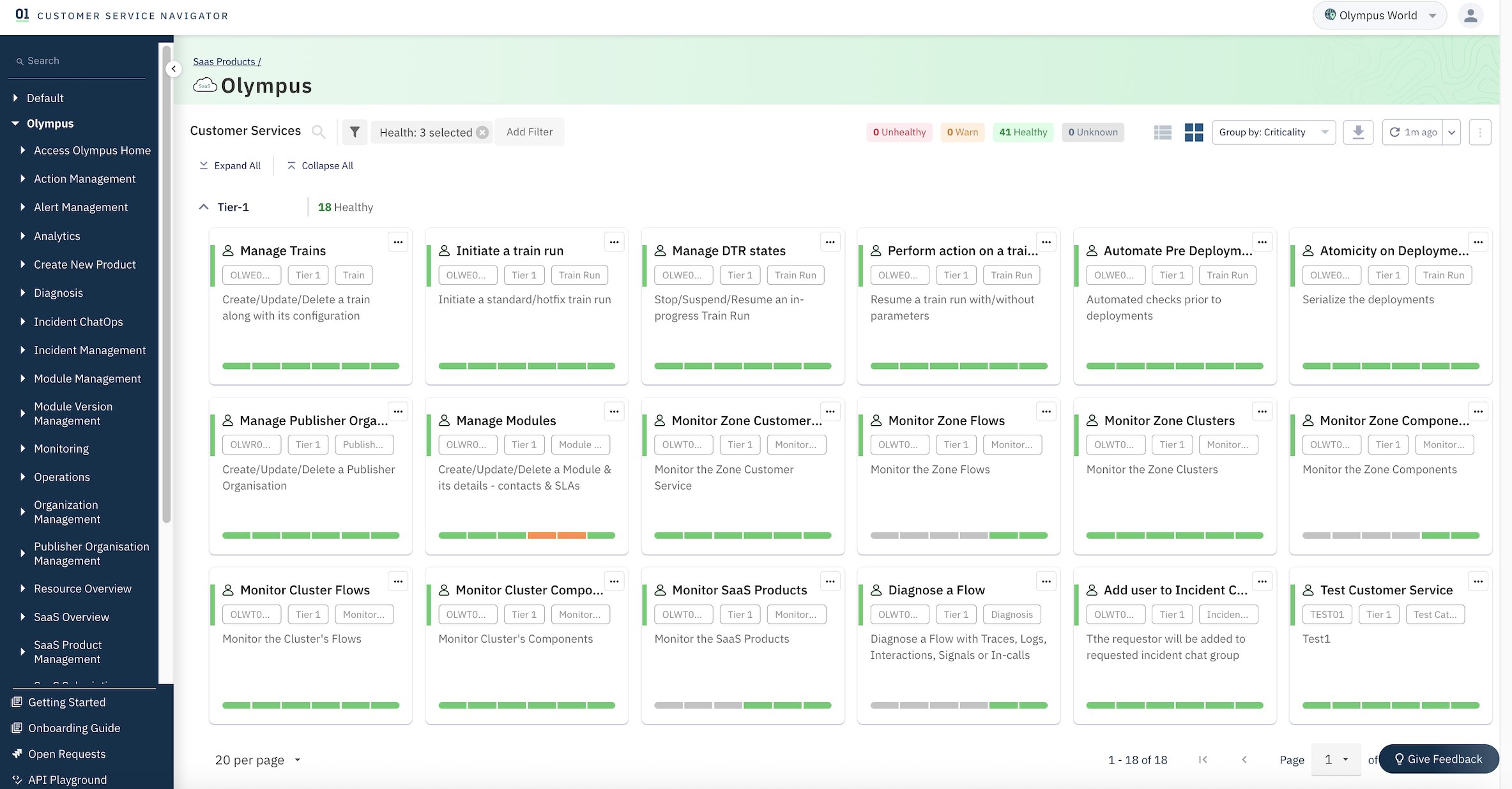
Zeta designed and built an observability system, CSN, to deliver comprehensive visibility across the service environment. CSN is part of the Olympus suite of products. CSN serves as the primary interface for the SRE team, offering real-time service health dashboards, infrastructure monitoring, SLA performance analytics, and an admin panel for user management. The system is equipped with single sign-on (SSO) integration and enforces role-based access control (RBAC) to enable secure, granular access. With CSN, SREs can efficiently monitor system health, receive actionable alerts and warnings, and manage operational workflows across critical services.

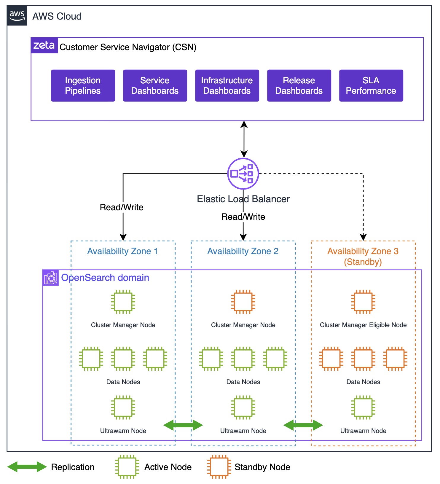
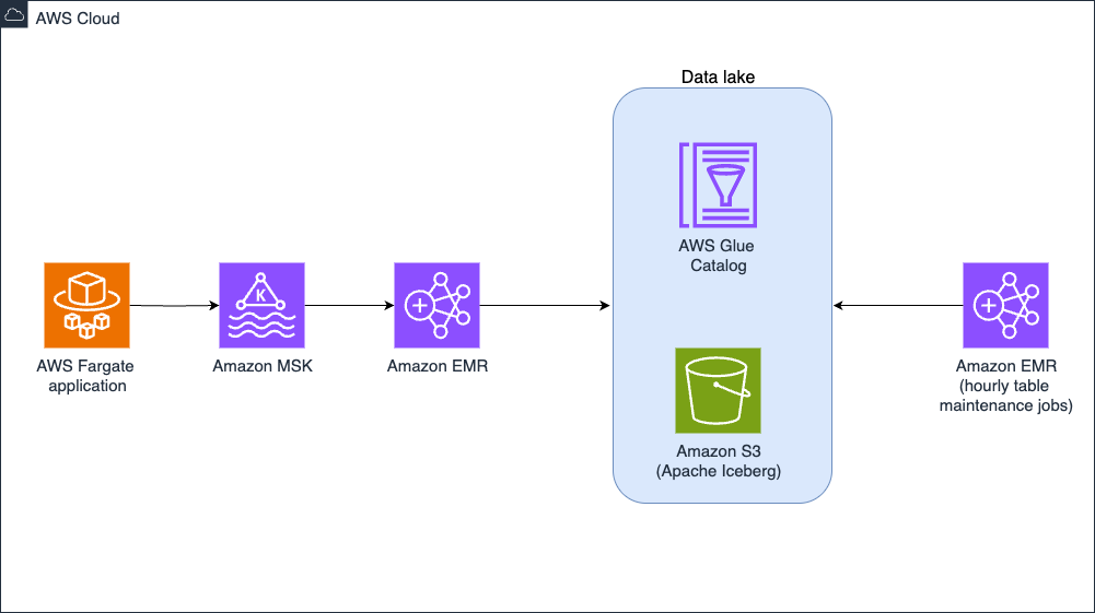
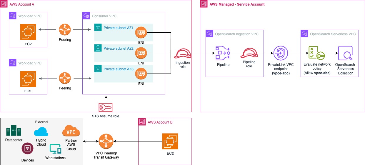
CSN is powered by OpenSearch Service to provide an integrated solution for DevOps and Site Reliability Engineers to help identify critical events and issues. Zeta chose OpenSearch Service because it offers a fully managed, open-source search analytics engine that scales effortlessly to handle the increasing number of tenants, associated data growth, and analytics needs. It’s seamless integration with AWS services, robust security features, and support for real-time data ingestion and querying make it ideal for powering the CSN dashboards and analytics workloads. The following diagram illustrates the CSN deployment architecture.

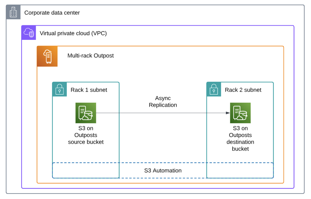
The OpenSearch Service domain uses the Multi-AZ with Standby deployment model, following AWS best practices for high availability and fault tolerance. Nodes—including dedicated cluster manager nodes, data nodes, and UltraWarm nodes—are distributed evenly across three Availability Zones in the same AWS Region. Availability Zones 1 and 2 handle active indexing and search traffic, and Availability Zone 3 contains standby nodes that remain passive during normal operations. If an Availability Zone failure occurs, OpenSearch Service automatically promotes standby nodes to active status, maintaining cluster operations with minimal disruption and no need for data redistribution.

The OpenSearch cluster consists of three dedicated cluster manager nodes and a multiple-of-three data node count to maintain quorum and balanced shard allocation. Each index uses at least two replicas, providing redundant copies of data across the Availability Zones. This Multi-AZ with Standby configuration delivers high resilience and rapid failover, supporting continuous service availability and robust disaster recovery for the observability workloads.

Data collection and ingestion

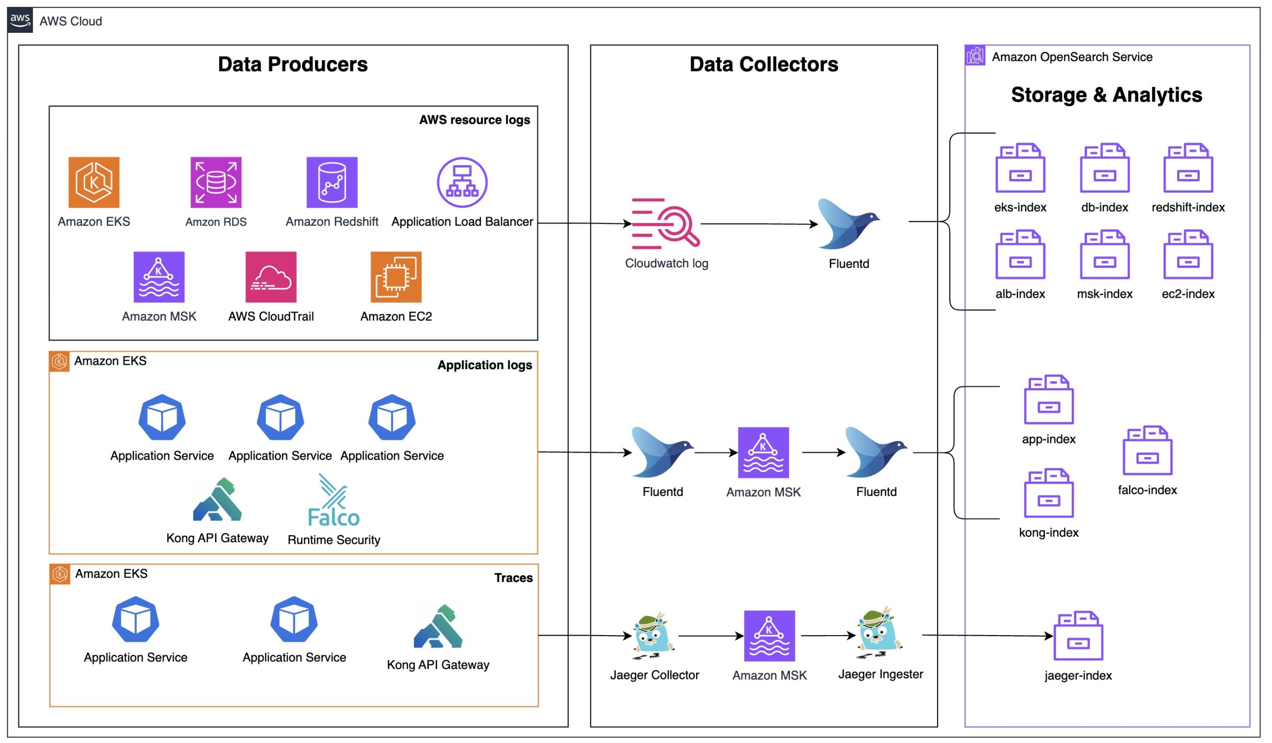
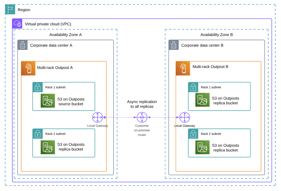
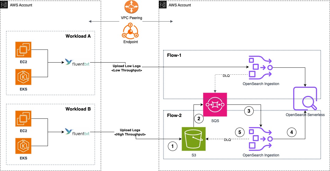
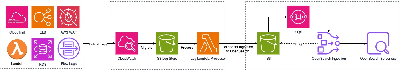
The observability strategy centers on a data collection and ingestion pipeline designed to handle the complexity and scale. The architecture, as shown in the following diagram, addresses three critical data types: AWS resource logs, application logs, and distributed traces, with each data type using tailored collection and processing methods optimized for the workloads.

AWS resource logs collection

The infrastructure spans multiple AWS services including Amazon Elastic Kubernetes Service(Amazon EKS), Amazon Relational Database Service(Amazon RDS), Amazon Redshift, Application Load Balancer, Amazon Managed Streaming for Apache Kafka (Amazon MSK), Amazon Elastic Compute Cloud (Amazon EC2) and more. Zeta uses Amazon CloudWatch Logs as the primary collection point for AWS service logs, which provides native integration with these services.

AWS services send their logs directly to CloudWatch Logs, which are then pulled by Fluentd running on the Amazon EKS cluster for centralized processing. This approach natively captures operational data from the AWS resources, including:

Database operational logs and audit trails from Amazon RDS instances
Data warehouse query execution logs from Amazon Redshift
Application Load Balancer access logs capturing traffic patterns and performance metrics
Kafka cluster operational logs from Amazon MSK
AWS API invocation audit trails from AWS CloudTrail
Container runtime and operating system logs from Amazon EC2
During the log collection, personally identifiable information (PII) is filtered out. The solution adheres strictly to PCI-DSS guidelines throughout this process.

Zeta used Amazon MSK as a scalable and reliable backbone for collecting and streaming logs from various sources across the AWS resources. Logs are ingested into Amazon MSK, providing a durable and fault-tolerant buffer that decouples log producers from consumers. This architecture enables real-time log streaming and supports advanced processing pipelines before the logs are routed to the OpenSearch Service. By integrating Amazon MSK into the logging workflow, scalability, resilience, and flexibility is improved, so that high log volumes are efficiently managed without impacting downstream systems. This approach, combined with native AWS integrations, minimizes operational complexity and maintains comprehensive, centralized log visibility across the cloud environment.

Fluentd processes these logs and routes them directly to OpenSearch Service, maintaining the benefits of AWS integration while providing centralized accessibility. This centralized logging approach with built-in buffering capabilities reduces the direct load on OpenSearch Service by batching and optimizing log delivery, helping to prevent potential ingestion bottlenecks during high-volume periods. The approach alleviates the need for custom log shipping agents on AWS resources, reducing operational overhead while maintaining comprehensive coverage of the cloud infrastructure.

Application logs processing

For application-level observability, a pipeline using Fluentd is deployed as Kubernetes DaemonSet. Application microservices running on Amazon EKS generate logs that Fluentd DaemonSets collect, parses, and enrich with metadata such as pod names, namespaces, and service identifiers. The processed logs then flow through Amazon MSK for reliable, high-throughput message streaming before final processing by Fluentd and indexing in OpenSearch Service.

This Kafka-based approach provides several advantages:

Decoupling – This helps producers and consumers to operate independently, so that Zeta can scale ingestion and processing separately based on demand.
Backpressure handling – Using Kafka’s buffering capabilities, this manages traffic spikes during peak banking hours, absorbing sudden increases in log volume while maintaining system stability during seasonal usage surges.
Durability of logs – The system maintains logs durably so that no log data is lost during system maintenance or unexpected failures through message persistence.

The logs then pass through a second Fluentd layer for final processing and routing to OpenSearch Service, where they’re indexed across service-specific indexes (app-index, falco-index, kong-index).

Distributed trace collection

To address the challenge of correlating issues across Zeta’s microservices architecture, system uses distributed tracing using Jaeger, an open-source, end-to-end distributed tracing system. Jaeger enables monitoring and troubleshooting transactions in complex distributed systems by tracking requests as they flow through multiple services. The application services and Kong API Gateway are instrumented with Jaeger client libraries that generate trace data including spans, which represent individual operations within a trace. Each span contains metadata such as operation names, start and finish timestamps, tags, and logs that provide context about the operation being performed. The Jaeger Collector aggregates these spans from multiple services, performing validation, indexing, and transformation before forwarding the data.

The traces flow through Amazon MSK for the same reliability benefits as the logging pipeline – providing durability, decoupling, and backpressure handling during high-volume periods. Jaeger Ingester then consumes traces from Amazon MSK and processes them for storage in the jaeger-index within OpenSearch Service.

This data collection and ingestion strategy provides complete end-to-end visibility and builds an observability system that enables SRE teams to monitor, troubleshoot, and optimize the services across the entire technology stack.

Storage tiering

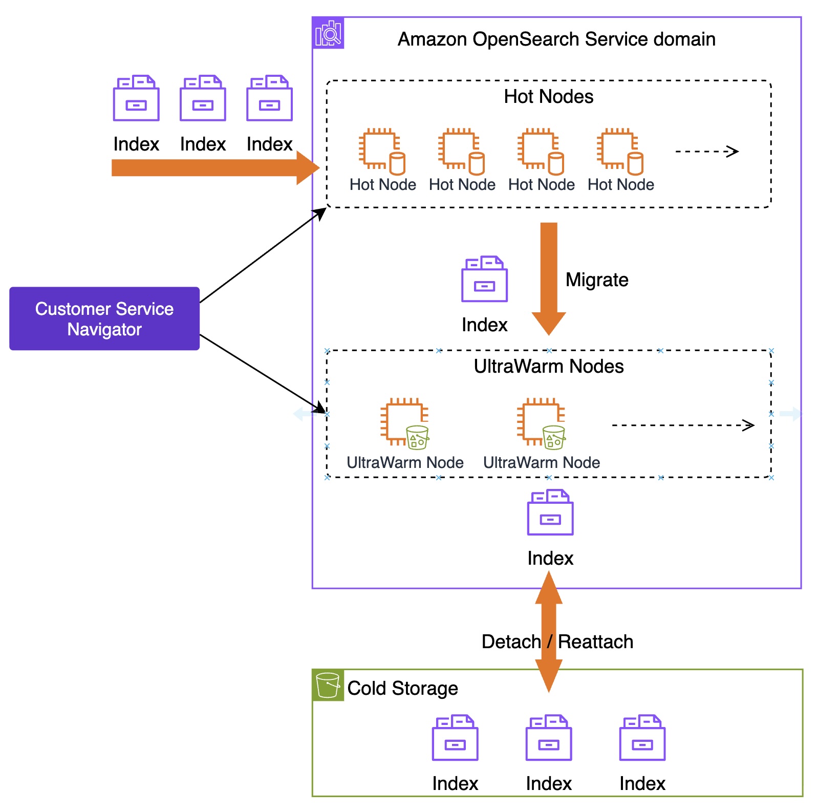
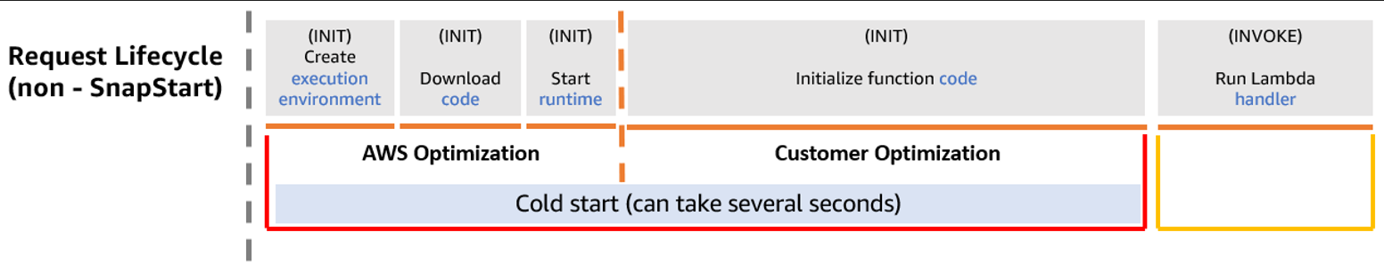
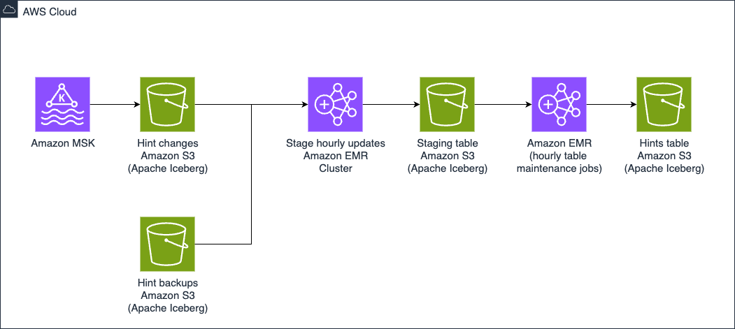
To manage the log, metric, and trace data at scale—about 3TB generated daily—the solution implemented OpenSearch Service storage tiering to balance performance, retention, and cost. Zeta requires near real-time search and retrieval for at least a week, while retaining logs and traces for up to 10 years. Keeping this data in active clusters would impact search performance and significantly increase costs, so the solution uses the OpenSearch Service hot, UltraWarm, and cold storage tiers to optimize the data lifecycle. The following diagram illustrates storage tiering in OpenSearch Service.

Hot storage is used for the most recent and frequently accessed data, supporting real-time indexing and low-latency queries. This tier relies on high-performance storage attached to standard data nodes, making it ideal for powering live dashboards and analytics where speed is critical. The solution uses AWS Graviton 2 powered m6g.4xlarge.search instance types to run the OpenSearch Service domain which provides upto 40% lower cost compared to x86 based instances. Each hot data node has an attached gp3 EBS volume to store indexes. Zeta maintains data in hot storage for 1 week.

UltraWarm storage serves as a cost-effective layer for older, read-only data that is queried less frequently but still needs to remain searchable. UltraWarm nodes use Amazon Simple Storage Service (Amazon S3) as the backing store with an integrated caching mechanism, to retain large volumes of data at a fraction of the cost of hot storage while still supporting interactive queries for historical analysis. Zeta uses ultrawarm1.large.search instance types in the UltraWarm storage tier and maintains data in UltraWarm storage for 15 days.

Cold storage is designed for long-term archival of infrequently accessed or compliance-driven data. Data in cold storage is detached from active compute resources and resides in Amazon S3, incurring minimal cost. When historical data needs to be queried, the indexes are attached to the UltraWarm nodes using OpenSearch API calls. This helps extracting historical data for audits, periodic research or forensic investigations without maintaining active compute for the entire retention period, thereby reducing storage cost.

OpenSearch Service automates index transitions between hot, UltraWarm, and cold storage tiers using Index State Management (ISM) policies. ISM policies specify the conditions and actions for each state, such as transitioning based on index age, size, or document count. When an index qualifies for a transition, ISM jobs—running every 5 to 8 minutes—evaluate the policy and move the index to the next tier. When indexes reach the UltraWarm threshold, they are migrated to UltraWarm nodes backed by Amazon S3, which reduces storage costs while keeping data accessible for queries. After the UltraWarm retention period, ISM archives the indexes to cold storage, detaching them from compute resources but allowing reattachment for future queries or compliance needs. This automated lifecycle management reduces operational overhead, optimizes storage costs, and maintains performance for both recent and historical data.

For observability data, new indexes are created in the hot tier, where they remain for 7 days to support fast ingestion and low-latency queries. After this period, ISM transitions these indexes to UltraWarm storage, where they are retained for an additional 15 days as read-only data, balancing cost with searchability.

Security

Security is the most critical part of the architecture. Zeta’s observability system implements multiple layers of protection for data confidentiality, integrity, and compliance with banking regulations, and is built using a zero-trust approach following the AWS shared responsibility model for OpenSearch Service:

Infrastructure security: The OpenSearch Service domain is deployed within a virtual private cloud (VPC) with private subnets, isolating it from direct internet access. Security groups enforce restrictive ingress rules, allowing access only from authorized sources. The OpenSearch Service domain uses encryption at rest through AWS Key Management Service (KMS). Data in transit is secured using TLS 1.3 encryption, so that log data, traces, and search queries remain protected during transmission. Service-to-service communication uses AWS Identity and Access Management (IAM) roles and encrypted connections, alleviating the need for hardcoded credentials.
Access control and authentication: The solution uses Amazon OpenSearch Service fine-grained access control(FGAC) integrated with IAM, where IAM serves as the authentication provider and FGAC handles authorization by mapping IAM roles to OpenSearch backend roles. This approach helps Zeta to control access permissions at the index and document level based on tenant requirements and user responsibilities. The data ingestion pipeline implements end-to-end security with Fluentd authenticating to Amazon MSK using IAM roles over encrypted connections. Amazon MSK clusters use encryption in transit and at rest, protecting log data throughout the streaming pipeline. Kubernetes RBAC policies restrict pod-to-pod communication and limit service account permissions.
Data privacy and tenant isolation: Each tenants’ data is maintained in logical separation in OpenSearch Service using tenant id. CSN implements tenant-aware authentication and authorization with FGAC, restricting users to their authorized tenants’ dashboards and data. Every API endpoint validates tenant context, so that users can only access data within their authorized scope. Importantly, no customer data is captured in the logs – only system metrics are used to build the monitoring system, adhering to banking security standards and best practices. User actions are audited and logged for compliance purposes, with audit trails maintained according to regulatory requirements.

This security framework enables the observability system meet the security requirements of core banking operations while maintaining operational efficiency and regulatory compliance across global industries.

Customer Service Navigator

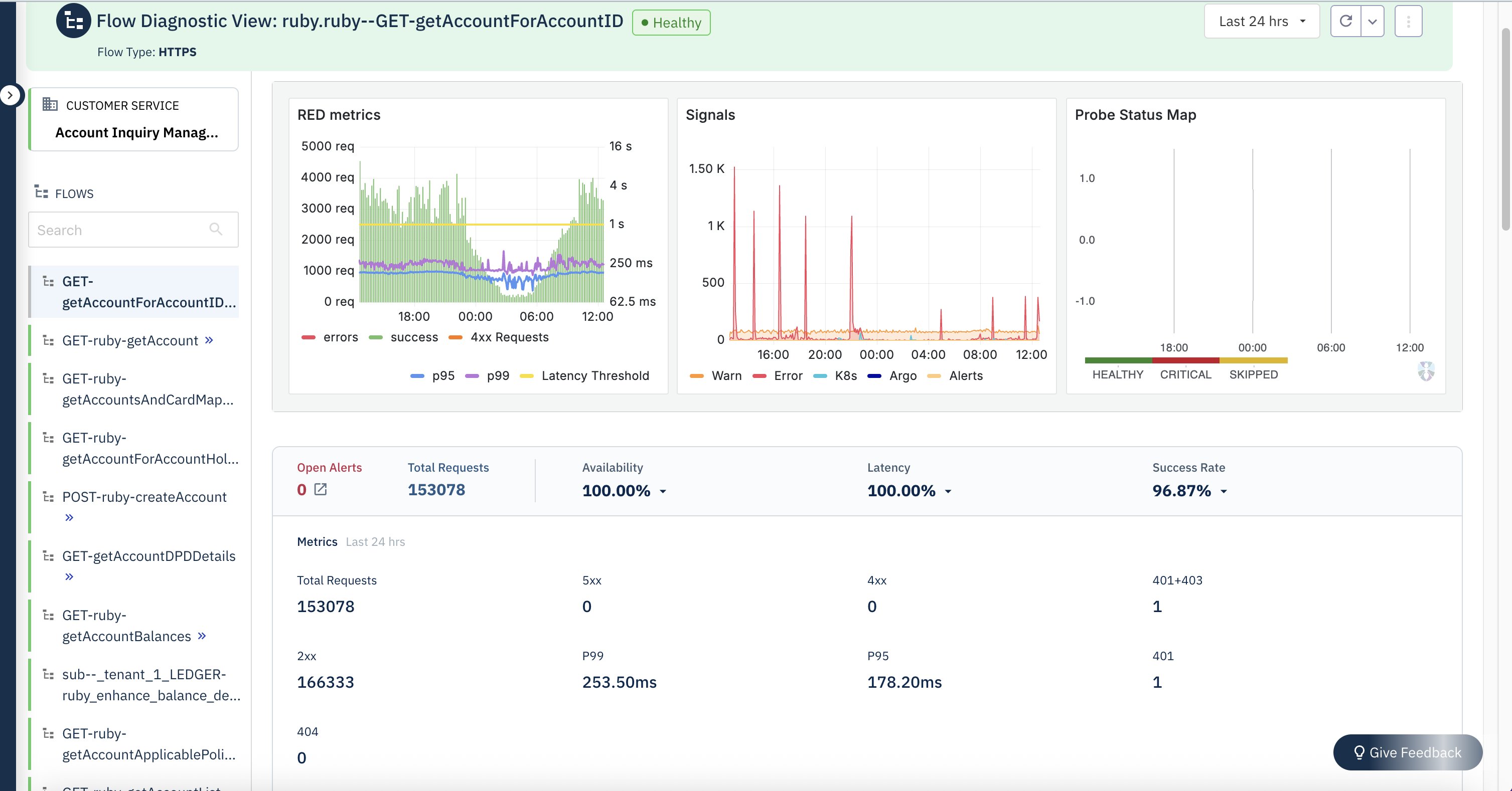
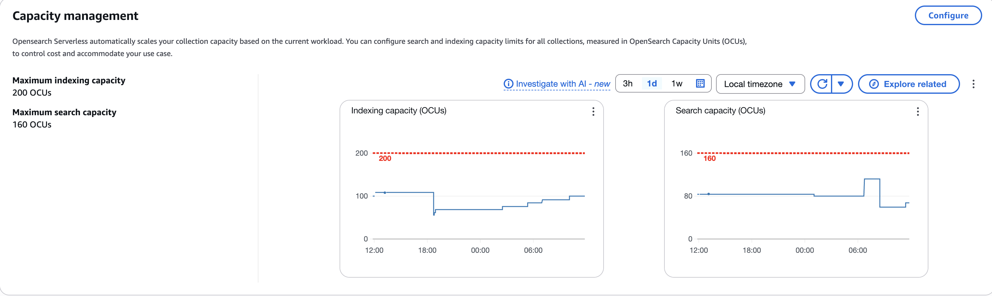
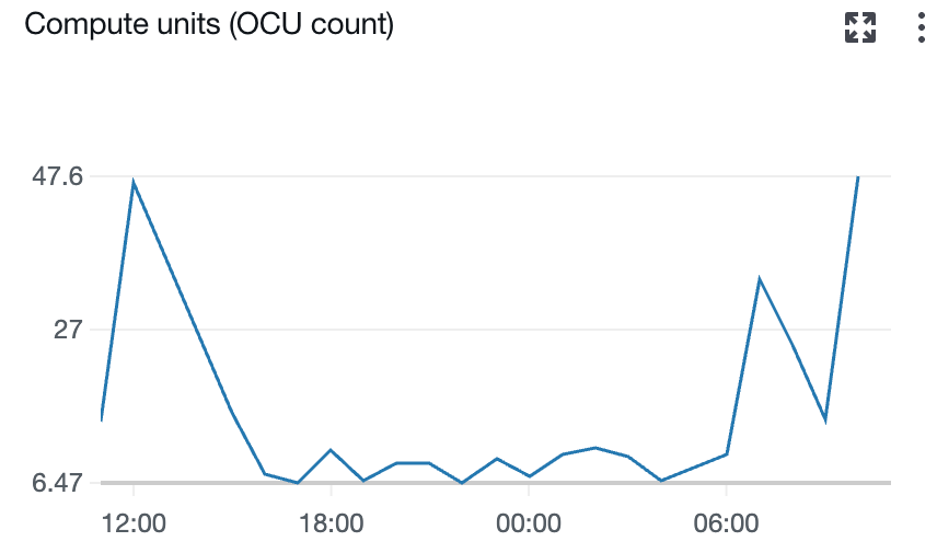
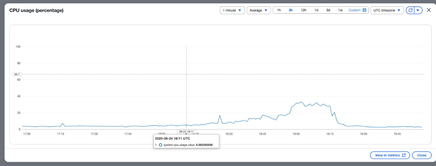
CSN delivers SREs a powerful diagnostics interface engineered for high-efficiency monitoring, deep analysis, and rapid troubleshooting of system performance across distributed environments. The system ingests and processes telemetry data at sub-minute intervals, providing near-real-time metrics, traces, and logs from critical infrastructure components. Actionable, interactive visualizations—such as heatmaps, anomaly graphs, and dependency maps— helps SREs to quickly detect SLO breaches and drill down to granular root causes, often within a few minutes of an incident.

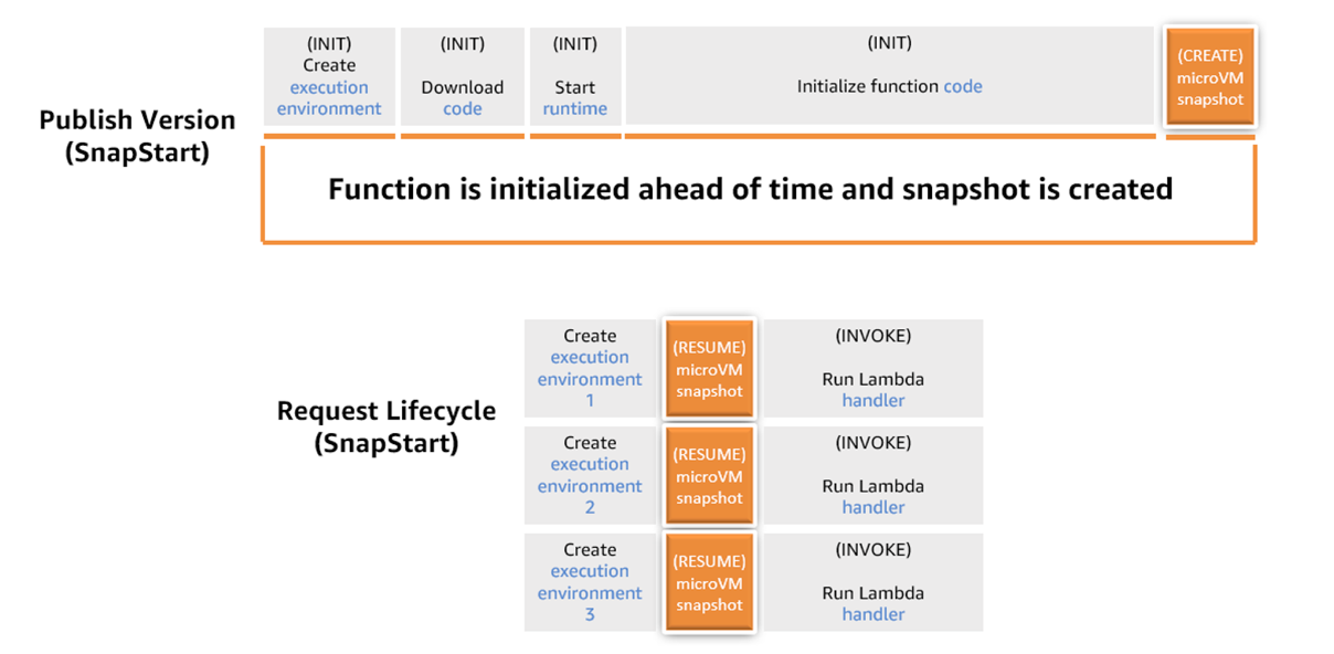
The following screenshot shows an example service health dashboard in CSN for an Olympus tenant.

The following screenshot shows an example of the API performance insights dashboard in CSN.

Business and technical benefits

The OpenSearch Service-based CSN System provides the following business and technical benefits:

Manual effort is reduced through automated Index State Management (ISM) and lifecycle policies, so that Zeta’s teams to focus on innovation
Automated lifecycle policies facilitate seamless retention and archiving of compliance data, reducing the risk of non-compliance
The system supports log retention for over 10 years to meet regulatory requirements for Zeta’s banking and financial services customers
Multiple layers of security—including encryption at rest and in transit, FGAC, and tenant isolation to protect customer data and support Zeta’s zero-trust architecture
By consolidating logs, traces, and metrics from disparate systems into OpenSearch, SRE teams can correlate events more effectively, thereby reducing troubleshooting efforts and achieving an 80% improvement in MTTR
Zeta achieved 99.999999999% data durability for archived logs stored in Amazon S3, providing long-term data integrity
Zstandard compression is being implemented to optimize long-term storage costs

Conclusion

CSN’s advanced correlation engine automatically associates related events across microservices, databases, network layers, and infrastructure, significantly streamlining root cause analysis. Integrated alerting and automated runbooks further reduce response times. Since implementing CSN, Zeta has achieved over an 80% reduction in MTTR, with incident response times decreasing from 30+ minutes to under 5 minutes. The service supports seamless multi-tenant monitoring, processes 3TB of machine-generated data daily, and is architected for petabyte-scale growth. Additionally, CSN helps Zeta meet regulatory requirements for retaining historical logs over several years while keeping storage costs under control. This has substantially improved operational resilience, increased service availability, and empowered teams to proactively resolve issues before they affect end users.

Ready to take your organization’s observability capabilities to the next level? Dive into the technical details of OpenSearch Service in the Amazon OpenSearch Developer Guide. Visit our new migration hub page for more prescriptive guidance on moving your workloads to OpenSearch Service.

About the authors

Deepesh Dhapola is a Senior Solutions Architect at AWS India, where he architects high-performance, resilient cloud solutions for financial services and fintech organizations. He specializes in using advanced AI technologies—including generative AI, intelligent agents, and the Model Context Protocol (MCP)—to design secure, scalable, and context-aware applications. With deep expertise in machine learning and a keen focus on emerging trends, Deepesh drives digital transformation by integrating cutting-edge AI capabilities to enhance operational efficiency and foster innovation for AWS customers. Beyond his technical pursuits, he enjoys quality time with his family and explores creative culinary techniques.

Shashidhar (Shashi) Soppin is an accomplished Enterprise Architect and cloud transformation leader with over 24+ years of experience spanning regulated industries and high-growth technology environments. Currently steering strategic initiatives as Lead Architect at Zeta’s CTO office, Shashidhar has helped in building and led world-class engineering teams, driving innovation in cloud, security, and fintech domains. He has architected secure, scalable platforms—scaling user bases by 10x, enabling complex integrations for leading Bank’s migration to Zeta’s platforms, and pioneering Zero Trust frameworks that achieved outstanding regulatory compliance. A results-driven executive and former DMTS at Wipro, Shashidhar holds 25+ granted patents and has delivered multi-million dollar enterprise deals across domains including AI/ML. Renowned as a published author (“Essentials of Deep Learning”), frequent industry speaker, and hands-on innovator, he combines technical expertise with business acumen, propelling organizations toward robust, future-ready cloud ecosystems and operational excellence. Prior to Wipro he worked in IBM-ISL as well.

Anchal Kansal is a Lead Site Reliability Engineer at Zeta, where she has spent the past four years building and scaling reliable, high-performance systems. With deep expertise in OpenSearch, observability platforms, and large-scale infrastructure, she focuses on ensuring uptime, performance, and operational efficiency. Anchal is passionate about solving complex reliability challenges and sharing practical insights with the engineering community.

Manochandra (Mano) is the Site Reliability Engineering (SRE) expert at Zeta, specializing in data management-oriented systems. With a deep understanding of large-scale distributed architectures, he has extensive experience designing, deploying, and maintaining resilient, production-grade OpenSearch systems. Mano is known for his proactive approach in optimizing infrastructure reliability and performance, as well as his ability to troubleshoot complex operational challenges. His expertise spans implementing automation, monitoring, and incident management best practices, making him a go-to resource for ensuring service availability and scalability at Zeta.

Hitesh Subnani is a FSI Solutions Architect at AWS India, where he works with customers to design and build architectures that deliver business value. He specializes in comprehensive observability and analytics systems, enabling organizations to gain deep insights from operational data. With expertise in search and analytics technologies, Hitesh focuses on scalable monitoring systems, real-time dashboards, and compliance-driven architectures for AWS customers in the financial sector.

Tarun Chakraborty is a Sr. Technical Account Manager (TAM) at AWS India, where he partners with leading banks and fintech organizations to accelerate their cloud transformation journeys. With over 15 years of experience in technology and financial services, he serves as a trusted advisor helping customers leverage AWS’s comprehensive suite of services to drive innovation and achieve their business objectives.

Multi-rack and multiple logical AWS Outposts architecture considerations for resiliency

2025-08-21 Brianna Rosentrater

Post Syndicated from Brianna Rosentrater original https://aws.amazon.com/blogs/compute/multi-rack-and-multiple-logical-aws-outposts-architecture-considerations-for-resiliency/

AWS Outposts rack offers the same Amazon Web Services (AWS) infrastructure, AWS services, APIs, and tools to virtually any on-premises data center or colocation space for a truly consistent hybrid experience. A logical Outpost (hereafter referred to as an Outpost) is a deployment of one or more physically connected Outposts racks managed as a single entity under one Amazon Resource Name (ARN). An Outpost provides a pool of AWS compute and storage capacity at one of your sites as a private extension of an Availability Zone (AZ) in an AWS Region. Several AWS services that support Outposts offer deployment options that improve your workload’s fault tolerance. However, certain Outposts configuration requirements have to be met in order to use them.

In this post, we explore the architecture considerations that come into play when deciding between a multi-rack logical Outposts rack, or using multiple Outposts racks to support your highly available workloads.

Amazon EC2 on AWS Outposts rack

The following sections cover Amazon Elastic Compute Cloud (Amazon EC2) on Outposts rack

Multi-rack logical Outposts

When using a multi-rack logical Outpost, you can use a rack level spread Amazon EC2 placement group. A rack level spread placement group can have as many partitions as you have racks in your Outpost deployment, and this allows you to spread out your instances to improve the fault tolerance of your workloads. In the following example, we have C5 instances in an Amazon EC2 Auto Scaling group that uses a launch template specifying a rack level spread placement group strategy should be used. This multi-rack Outpost has four racks, thus the instances are spread across the four racks as evenly as possible.

Rack level spread EC2 placement group example

Figure 1: Rack level spread Amazon EC2 placement group example

This placement group strategy can make your workloads more resilient to rack or host failures, but it would not be useful in mitigating an AZ failure. EC2 instances on Outposts are statically stable to network disconnects. Therefore, workloads would continue running during an AZ failure, but mutating actions would be unavailable. Read on to see how this strategy can be used with multiple Outposts to create a multi-AZ resilient architecture.

Multiple Outposts racks

If you have more than one logical Outpost in the same Region, we recommend connecting each Outpost to a different AZ. This would allow you to create multi-AZ resilient architectures, and when used in combination with features such as Intra-VPC communication between your Outposts, you can stretch an Amazon EC2 Auto Scaling group across two or more Outposts in the same VPC. If each Outpost is a single rack deployment, then this can be combined with a host level spread placement group specified in your instance launch template. A host level spread placement group can have as many partitions as you have hosts of that instance type in your Outpost, and would improve your workload’s resiliency to host failures.

For the highest level of spread and resiliency, consider using multiple multi-rack logical Outposts. This would allow you to use rack level spread placement groups, and intra-VPC communication between Outposts, as shown in the following figure. Having more than one multi-rack Outpost allows you to create application architectures that are resilient toward hardware and AZ level failures by spreading your workload across as many fault domains as possible.

Intra-VPC communication between two multi-rack logical Outposts using an EC2 auto scaling group with rack level spread

Figure 2: Intra-VPC communication between two multi-rack logical Outposts using an Amazon EC2 Auto Scaling group with rack level spread

Amazon RDS on AWS Outposts rack

The following sections cover Amazon Relational Database Service (Amazon RDS) on Outposts rack.

Multi-rack logical Outposts

Amazon RDS on Outposts rack supports read replicas, which use the MySQL and PostgreSQL database engines’ built-in asynchronous replication functionality to create a read replica from a source database instance. Read replicas on Amazon RDS on Outposts can be located on the same Outpost or another Outpost in the same VPC as the source database instance, as shown in the following figure. Furthermore, these can be used to scale out beyond the capacity constraints of a single database instance for read-heavy database workloads. They can also be used to maintain a second copy of your database, which can be used in the event of a host failure to improve workload resiliency. The process to promote a read replica to primary must be manually initiated, and your DNS records must be updated to the new primary instance. However, this is a good option to improve database durability if you only have one logical Outpost. Multiple read replicas can be created for a single database instance for added resiliency. You can also create an Amazon RDS read replica for a single rack Outpost to improve your resiliency to host failures. However, having a multi-rack Outpost would allow you to spread your read replica to another rack within your Outpost.

Figure 3: Amazon RDS read replicas used with a multi-rack Outpost

Multiple Outposts racks

Multi-AZ Amazon RDS deployments are supported on Outposts rack for MySQL and PostgreSQL database instances, as shown in the following figure. Using your Outposts Local Gateway and synchronous data replication, Amazon RDS creates a primary database instance on one Outpost, and maintains a standby database instance on a different Outpost. Failover to a multi-AZ Amazon RDS standby instance is automatic, and the DNS records are also automatically updated as part of the failover process. Using this deployment option protects you from AZ, host, and Outpost failures. You can also use multi-AZ Amazon RDS in combination with read replicas spread across different hosts on the same rack, or across multiple racks if using two multi-rack Outposts to provide more database durability.

Multi-AZ RDS on Outposts using read replicas for added durability.

Figure 4: Multi-AZ Amazon RDS on Outposts using read replicas for added durability

Amazon EKS on Outposts rack

The following sections cover Amazon Elastic Kubernetes Service (Amazon EKS) on Outposts rack.

Multi-rack logical Outposts

Outposts rack supports two Amazon EKS deployment methods: EKS extended cluster, and EKS local cluster, as shown in the following figure. Go to our documentation for help deciding which method is right for your workload. Using the rack level placement group strategy discussed earlier in this post allows you to spread your EKS instances (worker and control plane depending on the deployment model used) across multiple racks within your Outpost. Amazon EKS control plane instances are automatically replaced in the event of an instance, host, or rack failure, and self-managed worker node instances are typically placed in an Amazon EC2 Auto Scaling group. Therefore, when they’re used with a rack level spread placement group, you can increase your Amazon EKS resiliency and use automation to handle failures.

Figure 5: EKS local cluster with rack level spread placement group and auto scaling

Multiple Outposts racks

When using multiple Outposts racks, you’re unable to spread EKS control plane instances across two disparate Outposts. Go to Deploy an Amazon EKS cluster across AWS Outposts with Intra-VPC communication for more information on how to stretch an EKS extended cluster across multiple Outposts racks. If EKS local cluster is a requirement for your workload, you could use an external load balancer and deploy one instance of EKS local cluster on each Outpost in an active/active or active/passive configuration, and use the load balancer to direct incoming traffic to each respective EKS cluster. If your EKS cluster is using persistent storage, then you should consider whether each cluster needs access to the other clusters data, and centralized storage or replication should be used if needed.

Alternatively, if you are using EKS local cluster with two single rack Outposts, then you can also choose to only spread your EKS worker node instances across both of your Outposts. Furthermore, you can use host level spread on your primary Outpost to provide host level resiliency for your control plane instances. This would provide some added durability in the event of a host failure, and you could withstand the failure of your secondary Outpost that is only running some of your worker node instances. If you have two multi-rack Outposts, even though you couldn’t spread your control plane instances across Outposts, you can still use a rack level spread placement group to spread them across racks within your primary multi-rack Outpost. This would provide resiliency against instance, host, rack, and AZ level failures, and you could withstand the failure of your secondary multi-rack Outpost that isn’t running your EKS control plane instances as well.

Figure 6: EKS local cluster using two multi-rack Outposts and rack level spread

Amazon S3 on Outposts rack

The following sections cover Amazon S3 on Outposts rack.

Multi-rack logical Outposts

Amazon S3 on Outposts supports object replication, either across distinct Outposts, or between buckets on the same Outpost to help meet data-residency needs. The Outpost or bucket you’re replicating to can be in the same AWS account, or a different account. If you have a multi-rack Outpost, then you can replicate your S3 objects to another bucket on the same Outpost to create a copy of your data locally for added resiliency.

Figure 7: Amazon S3 replication between buckets on the same Outpost

Multiple Outposts racks

Moreover, if you have multiple Outposts, then you can replicate S3 objects between buckets on each Outpost, as shown in the following figure. Connect each Outpost to a unique AZ to create a multi-AZ resilient architecture, and store a copy of your data on each Outpost. You can combine this with Amazon S3 replication to a bucket on the same Outpost as well, and have multiple replicas managed through Amazon S3 automation for the highest availability. AWS DataSync also supports Amazon S3 on Outposts, and can be used to replicate S3 objects to the Region your Outpost is connected to if you want to store a copy of your data in the cloud, or use Amazon S3 in the Region for data tiering. Refer to Automate data synchronization between AWS Outposts racks and Amazon S3 with AWS DataSync for more information.

Figure 8: Amazon S3 replication across two multi-rack Outposts

Further considerations

When using multiple Outposts, we recommend connecting each Outpost to a unique availability zone to use multi-AZ deployment options.
Outposts are designed to be a connected service, and network outages could cause workflow disruptions. AWS can help you design for continued operations during network outages. We recommend creating a redundant service link connection to support workloads on Outposts with high availability requirements. Go to AWS Direct Connect Resiliency Recommendations for guidance on how to create a highly available service link connection through AWS Direct Connect, and Satellite Resiliency for AWS Outposts.
Outposts have a finite amount of compute resources based on the physical configuration chosen, and the logical capacity configuration on your Outpost can be changed at any time using a capacity task. If the Amazon EC2 compute requirements for your workload change over time, then your Outposts capacity configuration can be updated to meet these requirements non-disruptively. Go to Dynamically reconfigure your AWS Outposts capacity using Capacity Tasks for more information.

Conclusion

This post explores the architecture options and considerations for deciding between a multi-rack Outpost, and using multiple Outposts to support your highly available workloads. For more information on how to design highly available architecture patterns for Outposts, go to the AWS Outposts High Availability Design and Architecture Considerations whitepaper. Reach out to your AWS account team, or fill out this form to learn more about Outposts and self-service capacity management.

Under the hood: how AWS Lambda SnapStart optimizes function startup latency

2025-08-19 Ayush Kulkarni

Post Syndicated from Ayush Kulkarni original https://aws.amazon.com/blogs/compute/under-the-hood-how-aws-lambda-snapstart-optimizes-function-startup-latency/

When building applications using AWS Lambda, optimizing function startup is an important step to improve performance for latency sensitive applications. The largest contributor to startup latency (often referred to as cold start time) is the time that Lambda spends initializing your function code. Lambda SnapStart is a feature available for Java, Python, and .NET runtimes that helps reduce variable cold start latency from several seconds (or higher) to as low as sub-second. SnapStart typically needs zero or minimal changes to your application code and makes it easier to build highly responsive and scalable applications without implementing complex performance optimizations. This post explains how SnapStart works under the hood and provides recommendations to improve application performance when using SnapStart.

If your function already initializes within hundreds of milliseconds, then AWS recommends using Lambda Provisioned Concurrency to achieve double-digit millisecond startup latency.

What is a cold-start?

Lambda runs your function code in an isolated, secure execution environment that uses Firecracker microVM technology. When you first invoke a Lambda function, Lambda creates a new execution environment for the function to run in. Lambda downloads your function code, starts the language runtime, and runs your function initialization code, which is code outside the handler. This initialization process (INIT) is called a cold start. Then, Lambda runs your function handler code to invoke the function. A Lambda execution environment only handles a single invoke request at a time. The following figure shows the lifecycle of a typical invocation request.

Figure 1. Function invocation lifecycle without SnapStart

After the function finishes running, Lambda doesn’t stop the execution environment right away. When your function receives another invocation request, Lambda attempts to route the request to the idle but already running execution environment. As the INIT process has already run for this execution environment, this invoke is called a warm start. When more traffic arrives than Lambda has available idle execution environments, Lambda initializes new execution environments to serve the additional requests, performing the cold start initialization process again.

The last step of the cold start, initializing function code, typically takes the longest. This depends on the startup tasks that you execute in your code and the programming language runtime or framework you use. For languages such as Java and .NET, startup latency is impacted by just-in-time compilation of static code in loaded classes. For Python, it can be impacted if your executed code contains numerous or large modules. Other startup tasks, such as downloading machine learning (ML) models, can also take several seconds to complete, which adds to your function’s initialization latency. SnapStart is designed to optimize this last step of the cold start process and achieves this in three stages.

Stage 1: Snapshotting your Lambda function

When using SnapStart, the Lambda execution environment lifecycle changes. When you enable SnapStart for a particular function, publishing a new function version triggers the snapshotting process. The process runs the function initialization phase and takes an immutable, encrypted Firecracker microVM snapshot of the memory and disk state of the initialized execution environment, caching and chunking the snapshot for reuse. Code paths that are not executed during initialization, such as classes loaded on-demand through dependency injection, are not included in your function’s snapshot. To improve snapshot efficiency, proactively execute code paths during the initialization phase, or use runtime hooks to run code before Lambda creates a snapshot.

Snapshot creation can take a few minutes, during which your function version remains in the PENDING state, becoming ACTIVE when the snapshot is ready.

When you subsequently invoke your function, Lambda restores new execution environments from this snapshot. This optimization makes the invocation time faster and more predictable, because creating new a execution environment no longer requires an initialization.

The following figure shows the lifecycle of a SnapStart configured function.

Diagram illustrating how AWS Lambda SnapStart works. The top section shows the 'Publish Version' phase, where the function is initialized ahead of time by creating the execution environment, downloading the code, starting the runtime, and initializing the function code. At the end of this phase, a microVM snapshot is created. The bottom section shows the 'Request Lifecycle' using SnapStart: each new execution environment resumes from the pre-initialized microVM snapshot and immediately invokes the Lambda handler. This allows multiple environments to start faster by skipping initialization steps.

Figure 2. Function invocation lifecycle with SnapStart

After Lambda creates a snapshot, it periodically regenerates it to apply security patches, runtime updates, and software upgrades. Your invocation requests continue to work throughout the regeneration process.

Stage 2: Storing snapshots for low-latency retrieval at Lambda scale

Lambda operates at a high scale, processing tens of trillions of invocation requests every month. To efficiently manage and retrieve snapshots at this volume of traffic, Lambda uses storage and caching components. These consist of three layers: Amazon S3 for durable storage, a dedicated distributed cache, and a local cache on Lambda worker nodes.

Lambda stores function snapshots in Amazon S3, dividing them into 512 KB chunks to optimize retrieval latency. Retrieval latency from Amazon S3 can take up to hundreds of milliseconds for each 512 KB chunk. Therefore, Lambda uses a two-layer cache to speed-up snapshot retrieval.

When you enable SnapStart, during the optimization process, Lambda stores snapshot chunks in a layer two (L2) cache. This layer is a dedicated distributed cache instance fleet purpose-built by Lambda. Lambda stores a separate copy of each snapshot per AWS Availability Zone (AZ). To balance performance with costs, Lambda may not proactively cache unused snapshot chunks, instead caching them after they are first accessed. Chunks remain cached in the L2 fleet as long as your function version is active. The snapshot restore performance from the L2 layer is typically single digit milliseconds for a 512 KB chunk.

Lambda also maintains a layer one (L1) cache located on Lambda worker nodes, the Amazon Elastic Compute Cloud (Amazon EC2) instances handling function invocations. This layer is available locally, thus it provides the fastest performance, typically 1 millisecond for a 512 KB chunk. Functions with more frequent invocations are more likely to have their snapshot chunks cached in this layer. Functions with fewer invocations are automatically evicted from this cache, because it is bound by the worker instance disk capacity. When a snapshot chunk is not available in the L1 cache, Lambda retrieves the chunk from the L2 cache layer.

Figure 3. SnapStart tiered cache

Stage 3: Resuming execution from restored snapshots

Resuming execution from snapshots with low latency is the final SnapStart stage. This involves loading the retrieved snapshot chunks into your function execution environment. Typically, only a subset of the retrieved snapshot is needed to serve an invocation. Storing snapshots as chunks lets Lambda optimize the resume process by proactively loading only the necessary subset of chunks. To achieve this, Lambda tracks and records the snapshot chunks that the function accesses during each function invocation, as shown in the following figure.

Figure 4. Initial invocation, record chunk access pattern

After the first function invocation, Lambda refers to this recorded chunk access data for subsequent invokes, as shown in the following figure. Lambda proactively retrieves and loads this “working set” of chunks before they are needed for execution. This significantly speeds up cold-start latency. If every invoke executes the same code path, then all necessary chunks are tracked after the first invoke. If your Lambda function includes a method that is conditionally invoked once every five cold starts, then Lambda adds the corresponding chunks representing this method to the chunk access metadata after five cold starts.

Figure 5. Subsequent invocation, load chunks in order of access

Understanding SnapStart function performance

The speed of restoring a snapshot depends on its contents, size, and the caching tier used. As a result, SnapStart performance can vary across individual functions.

Function performance improves with more invocations

Frequently invoked functions are more likely to have their snapshots cached in the L1 layer, which provides the fastest retrieval latency. Infrequently accessed portions of snapshots for functions with sporadic invokes are less likely to be present in the L1 layer, resulting in slower retrieval latency from the L2 and S3 cache layers. Chunk access data for functions with more invocations is also more likely to be “complete”, which speeds up snapshot restore latency.

Pre-load code paths to optimize snapshot restore latency

To maximize the benefits of SnapStart, preload dependencies, initialize resources, and perform heavy computation tasks that contribute to startup latency in your initialization code instead of in the function handler. Code paths not executed during your function’s INIT phase, such as application classes loaded on-demand through dependency injection, are not included in your function’s snapshot. You can further improve SnapStart effectiveness by proactively executing these code paths during function initialization. You can also run code using runtime hooks and invoking your handler during the initialization phase before creating the snapshot. To achieve this, refer to the documentation and posts for Spring Boot and .NET applications to implement the performance tuning.

Performance differs depending on function size

SnapStart performance depends on how quickly Lambda can retrieve and load cached snapshots into your function execution environment. Larger function sizes increase the size of snapshots, and thus the number of chunks, which causes performance to differ for functions of varying sizes.

Not all functions benefit from SnapStart

SnapStart is designed to improve startup latency when function initialization takes several seconds, due to language-specific factors or because of initializing and loading software dependencies and frameworks. If your functions initialize within hundreds of milliseconds, you are unlikely to experience a significant performance improvement with SnapStart. For these scenarios, we recommend Provisioned Concurrency, which pre-initializes execution environments, delivering double-digit millisecond latency.

Conclusion

AWS Lambda SnapStart can deliver as low as sub-second startup performance for Java, .NET, and Python functions with long initialization times. This post explores how the Lambda lifecycle changes with SnapStart and how Lambda efficiently stores and loads snapshots to improve start up performance. SnapStart helps developers build highly responsive and scalable applications without provisioning resources or implementing complex performance optimizations.

To learn more about SnapStart, refer to the documentation and launch posts for Java, and Python and .NET. For performance tuning, refer to the SnapStart best practices section for your preferred language runtime. This post outlines approaches to pre-load code paths to further optimize startup latency. Find more information and sample applications built using SnapStart on Serverlessland.com.

Improve Amazon EMR HBase availability and tail latency using generational ZGC

2025-08-19 Vishal Chaudhary

Post Syndicated from Vishal Chaudhary original https://aws.amazon.com/blogs/big-data/improve-amazon-emr-hbase-availability-and-tail-latency-using-generational-zgc/

At Amazon EMR, we constantly listen to our customers’ challenges with running large-scale Amazon EMR HBase deployments. One consistent pain point that kept emerging is unpredictable application behavior due to garbage collection (GC) pauses on HBase. Customers running critical workloads on HBase were experiencing occasional latency spikes due to varying GC pauses, particularly impacting when they occurred during peak business hours.

To reduce this unpredictable impact to business-critical applications running on HBase, we turn to Oracle’s Z Garbage Collector (ZGC), specifically it’s generational support introduced in JDK 21. Generational ZGC delivers consistent sub-millisecond pause times that dramatically reduce tail latency.

In this post, we examine how unpredictable GC pauses affect business-critical workloads, benefits of enabling generational ZGC in HBase. We also cover additional GC tuning techniques to improve the application throughput and reduce tail latency. Amazon EMR 7.10.0 introduces new configuration parameters that allow you to seamlessly configure and tune the garbage collector for HBase RegionServers.

By incorporating generational collection into ZGC’s ultra-low pause architecture, it efficiently handles both short-lived and long-lived objects, making it exceptionally well-suited to HBase’s workload characteristics:

Handling mixed object lifetimes – HBase operations create a mix of short-lived objects (such as temporary buffers for read/write operations) and long-lived objects (such as cached data blocks and metadata). Generational ZGC can efficiently manage both, reducing overall GC frequency and impact.
Adapting to workload patterns – As workload patterns change throughout the day — for instance, from write-heavy ingestion to read-heavy analytics — generational ZGC adapts its collection strategy, maintaining optimal performance.
Scaling with heap size – As data volumes grow and HBase clusters require larger heaps, generational ZGC maintains it’s sub-millisecond pause times, providing consistent performance even as you scale up.

Understanding the impact of GC pauses on HBase

When running HBase RegionServers, the JVM heap can accumulate a large number of objects, both short-lived (temporary objects created during operations) and long-lived (cached data, metadata). Traditional garbage collectors like Garbage-First Garbage Collector (G1 GC) need to pause application threads during certain phases of garbage collection, particularly during “stop-the-world” (STW) events. GC pauses can have several impacts on HBase :

Latency spikes – GC pauses introduce latency spikes, often impacting tail latencies (p99.9 and p99.99) of the application which can lead to timeout for client requests and inconsistent response times..
Application availability – All application threads are halted during STW events and it negatively impacts overall application availability.
RegionServer failures – If GC pauses exceed the configured ZooKeeper session timeout, they might lead to RegionServer failures.

HBase RegionServer reports whenever there is an unusually long GC pause time using the JvmPauseMonitor. The following log entry shows an example of GC pauses reported by HBase RegionServer. During YCSB benchmarking, G1 GC exhibited 75 such pauses over a 7-hour period, whereas generational ZGC showed no long pauses under identical workload and testing conditions.

INFO  [JvmPauseMonitor] util.JvmPauseMonitor: Detected pause in JVM or host machine (eg GC): pause of approximately 2839ms
INFO  [JvmPauseMonitor] util.JvmPauseMonitor: Detected pause in JVM or host machine (eg GC): pause of approximately 3021ms

G1 GC pauses are proportional to the pressure on the heap and the object allocation patterns. As a result, the pauses might get worse if the heap is under too much load, whereas generational ZGC maintains it’s pause times goals even under high pressure.

Pause time and availability (uptime) comparison: Generational ZGC vs. G1GC in Amazon EMR HBase

Our testing revealed significant differences in GC pause time between the generational ZGC and G1 GC for HBase on Amazon EMR 7.10. We used 1 m5.4xlarge (primary), 5 m5.4xlarge (core) nodes cluster settings and ran multiple iterations of 1-billion rows YCSB workloads to compare the GC pauses and uptime percentage. Based on our test cluster, we observed a GC pause time improvement from over 1 minute, 24 seconds, to under 1 seconds for over an hour-long execution, improving the application uptime from 98.08% to 99.99%.

We conducted extensive performance testing comparing G1 GC and generational ZGC on HBase clusters running on Amazon EMR, using the default heap settings automatically configured based on Amazon Elastic Compute Cloud (Amazon EC2) instance type. The following image shows the comparison in both GC pause time and uptime percentage at a peak load of 3,00,000 requests per second (data sampled over 1 hour).

The following figures show the breakdown of the 1-hour runtime in 10-minute intervals. The left vertical axis measures the uptime, the right vertical axis measures the GC pause time, and the horizontal axis shows the interval. The generational ZGC maintained consistent uptime and pause time in milliseconds, and G1 GC demonstrated inconsistent and decreased uptime, pause times in seconds.

Tail latency comparison: Generational ZGC vs. G1GC in Amazon EMR HBase

One of the most compelling advantages of generational ZGC over G1 GC is its predictable garbage collection behavior and the impact on application tail latency. G1 GC’s collection triggers are non-deterministic, meaning pause times can vary significantly and occur at unpredictable intervals. These unexpected pauses, though generally manageable, can create latency spikes that particularly affect the slowest percentile of operations. In contrast, generational ZGC maintains consistent, sub-millisecond pause times throughout its operation. This predictability proves crucial for applications requiring stable performance, especially at the highest percentiles of latency (99.9th and 99.99th percentiles). Our YCSB benchmark testing reveals the real-world impact of these different approaches. The following graph illustrates tail latency distribution between G1 GC and generational ZGC over a 2-hour sampling period :

Improvements to BucketCache

BucketCache is an off-heap cache in HBase that is used to cache the frequently accessed data blocks and minimize disk I/O. Bucket cache and heap memory works in conjunction and might increase the contention on the heap depending on the workload. Generational ZGC maintains it’s pause time goals even with a terabyte-sized bucket cache. We benchmarked multiple HBase clusters with varying bucket cache sizes and 32 GB RegionServer heap. The following figures show the peak pause times observed over a 1-hour sampling period, comparing G1 GC and generational ZGC performance.

Enabling this feature and additional fine-tuning parameters

To enable this feature, follow the configurations mentioned in the Performance Considerations. In the following sections, we discuss additional fine-tuning parameters to tailor the configuration for your specific use case.

Fixed JVM heap

Batch processing jobs and short-lived applications benefit from dynamic allocation’s ability to adapt to varying input sizes and processing demands when multiple applications co-exist on the same cluster and run with resource constraints. The memory footprint can expand during peak processing and contract when the workload diminishes. However, for production HBase deployments without any co-existing applications in the same fixed heap allocation offers stable, reliable performance.

Dynamic heap allocation is when the JVM flexibly grows and shrinks its memory usage between minimum (-Xms) and maximum (-Xmx) limits based on application needs, returning unused memory to the operating system. However, this flexibility comes at the cost of performance overhead and memory fragmentation. Dynamic allocation seemed flexible, but it created constant disruptions. The JVM was always negotiating with the operating system for memory, leading to performance overhead and fragmentation. On the other hand, fixed heap allocation pre-allocates a constant amount of memory for the JVM at startup and maintains it throughout runtime, providing better performance by reducing memory negotiation overhead with the operating system. To enable this feature, use the following configuration: :

[
    {
        "Classification": "hbase",
        "Properties": {
            "hbase.regionserver.fixed.heap.enabled": "true"
        }
    }
]

Enable pre-touch

Applications with large heaps can experience more significant pauses when the JVM needs to allocate and fault in new memory pages. Pre-touch (-XX:+AlwaysPreTouch) instructs the JVM to physically touch and commit all memory pages during heap initialization, rather than waiting until they’re first accessed during runtime. This early commitment reduces the latency of on-demand page faults and memory mappings that occur when pages are first accessed, resulting in more predictable performance especially during heavy load situations. By pre-touching memory pages at startup, you trade a slightly longer JVM startup time for more consistent runtime performance. To enable pre-touch for your HBase cluster, use the following configuration :

[
    {
        "Classification": "hbase-env",
        "Properties": {},
        "Configurations": [
            {
                "Classification": "export",
                "Properties": {
                    "JAVA_HOME": "/usr/lib/jvm/jre-21",
                    "HBASE_REGIONSERVER_GC_OPTS": "\"-XX:+UseZGC -XX:+ZGenerational -XX:+AlwaysPreTouch\""
                }
            }
        ]
    }
]

Increasing memory mappings for large heaps

Depending on the workload and scale, you might need to increase the Java heap size to accommodate large data in memory. When using the generational ZGC with a large heap setup, it’s critical to also increase the operating system’s memory mapping limit (vm.max_map_count).

When a ZGC-enabled application starts, the JVM proactively checks the system’s vm.max_map_count value. If the limit is too low to support the configured heap, it will issue the following warning :

[warning] The system limit on number of memory mappings per process might be too low for the given
[warning] max Java heap size (131072M). Please adjust /proc/sys/vm/max_map_count to allow for at
[warning] least 235929 mappings (current limit is 65530). Continuing execution with the current
[warning] limit could lead to a premature OutOfMemoryError being thrown, due to failure to map memory.

To increase the memory mappings, use the following configuration and adjust the count value in the command based on the heap size of the application.

echo "vm.max_map_count = 262144" | sudo tee -a /etc/sysctl.conf
sudo sysctl -p

sudo systemctl restart hbase-regionserver

Conclusion

The introduction of generational ZGC and fixed heap allocation for HBase on Amazon EMR marks a significant leap forward in the predictable performance and tail latency reduction. By addressing the long-standing challenges of GC pauses and memory management, these features unlock new levels of efficiency and stability for Amazon EMR HBase deployments. Although the performance improvements vary depending on workload characteristics, you can expect to see significant enhancements in your Amazon EMR HBase clusters’ responsiveness and stability. As data volumes continue to grow and low-latency requirements become increasingly stringent, features like generational ZGC and fixed heap allocation become indispensable. We encourage HBase users on Amazon EMR to enable these features and experience the benefits firsthand. As always, we recommend testing in a staging environment that mirrors your production workload to fully understand the impact and optimize configurations for your specific use case.

Stay tuned for more innovations as we continue to push the boundaries of what’s possible with HBase on Amazon EMR.

About the authors

Vishal Chaudhary is a Software Development Engineer at Amazon EMR. His expertise is in Amazon EMR, HBase and Hive Query Engine. His dedication towards solving distributed system problems is helping Amazon EMR to achieve higher performance improvements.

Ramesh Kandasamy is an Engineering Manager at Amazon EMR. He is a long tenured Amazonian dedicated to solve distributed systems problems.