Tag Archives: Advanced (300)

Use account-agnostic, reusable project profiles in Amazon SageMaker to streamline governance

2025-09-03 Ramesh H Singh

Post Syndicated from Ramesh H Singh original https://aws.amazon.com/blogs/big-data/use-account-agnostic-reusable-project-profiles-in-amazon-sagemaker-to-streamline-governance/

Amazon SageMaker now supports account-agnostic project profiles, so you can create reusable project templates across multiple AWS accounts and organizational units. In this post, we demonstrate how account-agnostic project profiles can help you simplify and streamline the management of SageMaker project creation while maintaining security and governance features. We walk through the technical steps to configure account-agnostic, reusable project profiles, helping you maximize the flexibility of your SageMaker deployments.

New feature: Account-agnostic project profiles

Previously, SageMaker provided the ability to create project profiles, which required selecting an AWS account and AWS Region at the time of profile creation. This feature provides you the flexibility to insert the AWS account and Region dynamically when creating projects.

SageMaker now supports generic, account-agnostic project profiles (templates) in SageMaker domains, so domain administrators can define project configurations one time and reuse them across multiple AWS accounts and Regions.

Project profiles are no longer tied to a specific AWS account or Region. Instead, platform teams can reference an account pool—a new domain entity that enables dynamic account and Region selection at the time of project creation, based on custom enterprise authorization policies or user-specific logic. This decoupling of profile definitions from static deployment settings is designed to simplify governance, reduce duplication, and accelerate onboarding across large-scale data and machine learning (ML) environments.

Account-agnostic project profiles offer the following key benefits:

Project creators benefit from a more flexible experience – During project creation, project creators can select from a personalized list of authorized AWS accounts and Regions, powered by custom resolution strategies or predefined account pools.
The feature streamlines project profile governance – This model is intended to enable organizations operating across many different accounts to scale efficiently across those accounts, while preserving organization’s centralized control and permission boundaries.

Customer spotlight

As a large data-driven organization, Bayer AG looks to harness the power of data, analytics, and ML to help researchers and engineers accelerate pharmaceutical innovation. With the ability to create account agnostic templates and reusable templates in SageMaker, the research teams at Bayer can innovate faster without platform and engineering overhead.

“At Bayer, we use Amazon SageMaker Unified Studio as a unified, governed workspace that brings together data from multiple AWS accounts—enabling our users to run analytics, build pipelines, and train models as part of their day-to-day work. With the new capability to create account-agnostic templates, our platform team can publish reusable templates once, and teams can select the right authorized AWS account at project creation—without relying on platform hand-offs. This will support faster onboarding, improved agility, and consistent governance as we scale ML across our global operations.”

— Avinash Reddy Erupaka, Principal Engineering Lead, Drug Innovation Platform, Bayer

Solution overview

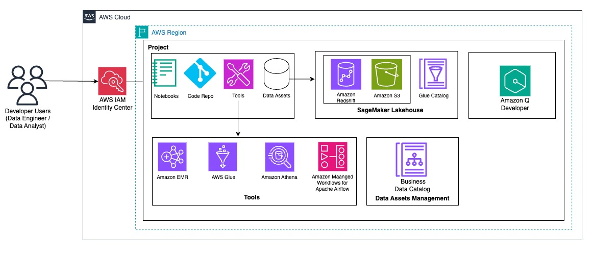
For our example use case, a leading pharmaceutical company has implemented SageMaker to manage their enterprise-wide data governance initiatives. The organization faces the complex challenge of managing thousands of AWS accounts across their global operations.

To streamline this process, their platform administrator needs to develop a system of reusable project profiles that map to specific account pools, organized according to the company’s organizational structure. For instance, they’ve created a specialized Corporate HR project profile tailored to meet the Corporate HR team’s specific requirements, as well as a comprehensive Data Engineer project profile designed for data engineering teams operating across North America, Asia-Pacific, and European Regions. This strategic approach helps data engineers efficiently create new projects using these preconfigured profiles while selecting from pre-authorized account and Region combinations. This structure strikes an optimal balance between operational flexibility and enhanced security and governance features.

In the following sections, we provide a detailed, step-by-step implementation guide for this solution.

Prerequisites

For this walkthrough, you must have the following prerequisites:

An AWS account – If you don’t have an account, you can create one. The account should have permission to do the following:
- Create and manage SageMaker domains
- Create and manage AWS Identity and Access Management (IAM) roles
- Create and invoke AWS Lambda functions (optional)
SageMaker domain – For instructions, refer to Create a domain – quick setup.
AWS CLI installed – The AWS Command Line Interface (AWS CLI) version 2.11 or later.
Python installed – Python 3.8 or later (if using custom Lambda handlers).
IAM permissions – The following IAM permissions are required:
- sagemaker:CreateProject
- sagemaker:CreateProjectProfile
- datazone:CreateAccountPool

Platform administrator tasks

The platform administrator is responsible for two key setup tasks: creating account pools and establishing project profiles associated with these pools. This section provides the steps to accomplish both crucial processes.

Create account pools

There are two ways to create account pools:

For static account sources, provide a list of accounts and Regions
For dynamic account sources, use a custom Lambda handler to authorize account and Region pair information

As of this writing, the creation, update, and deletion of account pools are only supported in the AWS CLI.

For creating account pools, use the create-account-pool command and provide the resources. We used the following commands to create account pools for our example use case. Replace the relevant values with your own resources, such as domain identifier, account, and Region.

First, create the account pool hr-accountpool with a single AWS account. In the following command, the parameter MANUAL refers to the mechanism by which an account is chosen from the pool at project creation time. Because the platform admin is manually choosing the accounts, the resolution strategy is set to MANUAL.

aws datazone create-account-pool --domain-identifier dzd_5yxxxxxxxxxxxx --name hr-accountpool --resolution-strategy MANUAL --account-source '{"accounts": [{"awsAccountId": "633xxxxxxxxx", "supportedRegions": ["us-east-1"], "awsAccountName": "HRaccount"}]}'

Next, create the account pool namer-data-engg-pool with multiple AWS accounts. Use the same code to create account pools for the EMEA and APAC Regions:

aws datazone create-account-pool --domain-identifier dzd_5yxxxxxxxxxxxx --name namer-data-engg-pool --resolution-strategy MANUAL --account-source '{"accounts": [{"awsAccountId": "633xxxxxxxxx", "supportedRegions": ["us-east-1"], "awsAccountName": "usaccount1"}, {"awsAccountId": "635xxxxxxxxx ", "supportedRegions": ["us-east-1"], "awsAccountName": "usaccount2"}]}'

You will use these account pools in subsequent steps to create project profiles.

To verify account pool creation, use the following command:

aws datazone list-account-pools --domain-identifier <domain-id>

If you have an external permissioning system, you can use the following custom Lambda command to create your account pool that will dynamically resolve during project creation:

aws datazone create-account-pool --domain-identifier dzd_cdy9yy904sxxxx --name custom- accountpool --resolution-strategy MANUAL --account-source '{"customAccountPoolHandler": {"lambdaFunctionArn": "<<Lambda ARN>>","lambdaExecutionRoleArn": "<<Lambda execution role>>"}}'

Create project profiles and account pool assignments

In this step, we establish project profiles and connect them to authorized account pools. There are three possible scenarios for setting up project profiles.

Scenario 1: Project profile associated with a single account pool

This is the simplest configuration, where one project profile is mapped to a single account pool. In the following steps, we create a project profile for the Corporate HR team and tie it to the HR account pool:

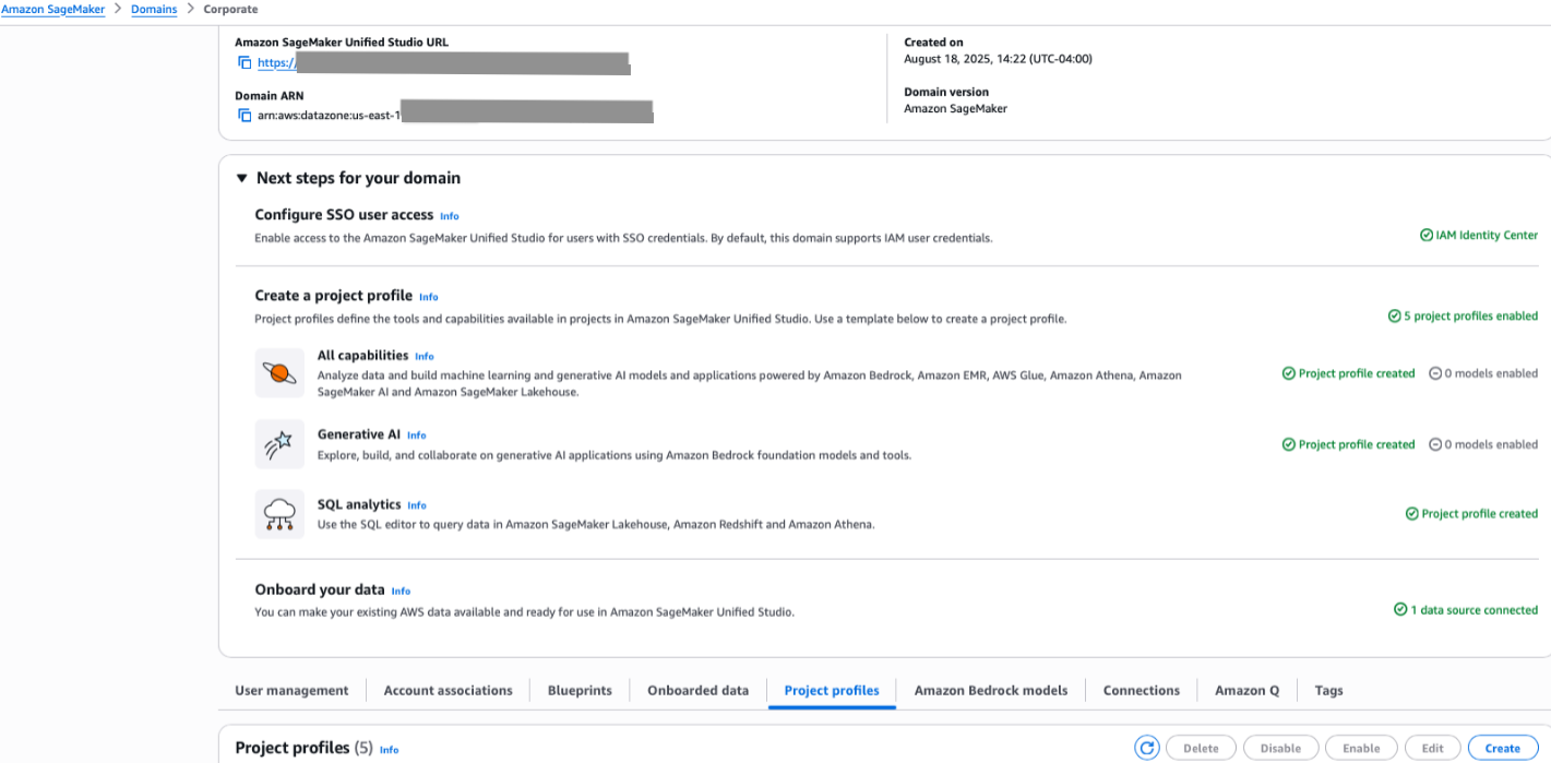
On the SageMaker console, choose Domains in the navigation pane.
On the Project profiles tab, choose Create.
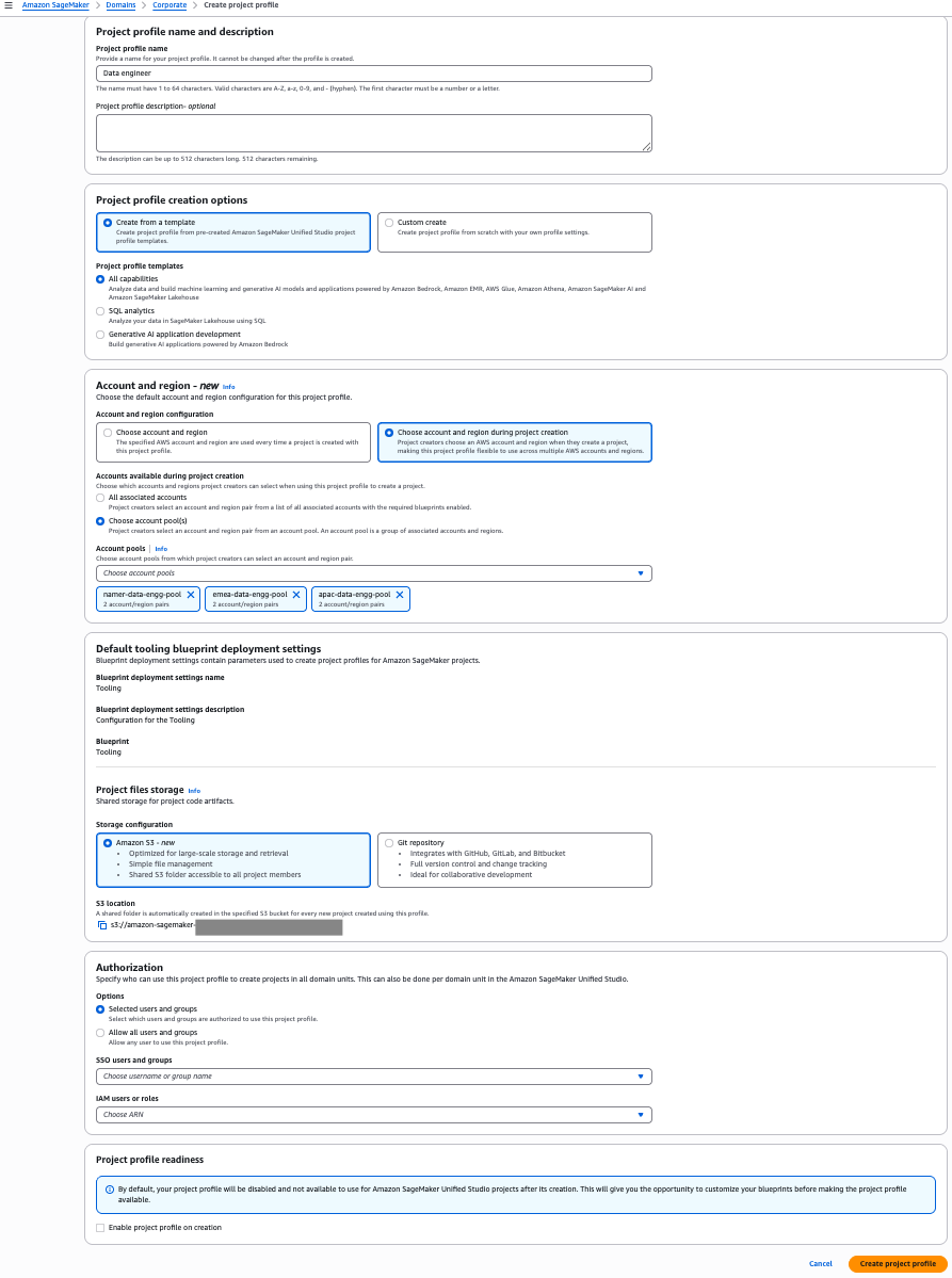
Enter a name and description for your profile.
Choose an appropriate project profile template that aligns with your project’s needs.
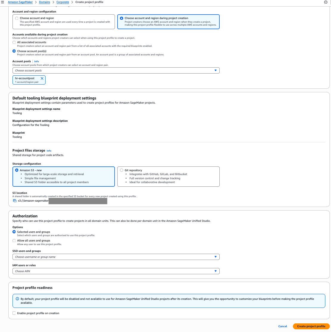
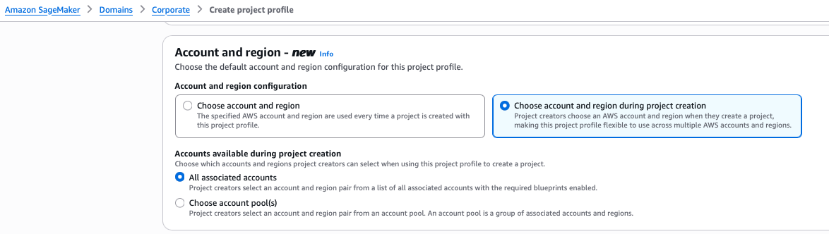
Select Choose account and region during project creation.
Select Choose account pool(s) and choose the account pool you created for the HR team.
Leave the remaining settings as default and choose Create project profile.
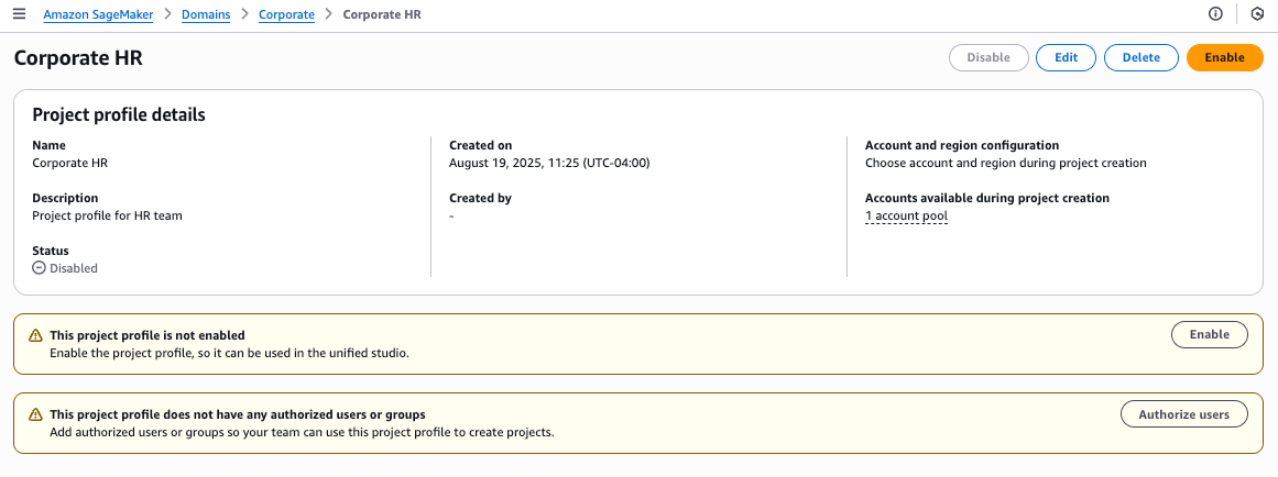
On the project details page, choose Enable to activate your profile.
Choose Enable in the confirmation pop-up to proceed.

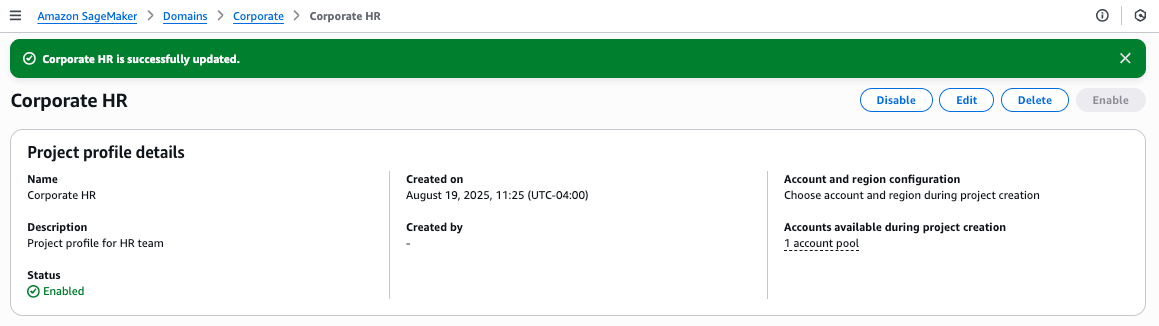
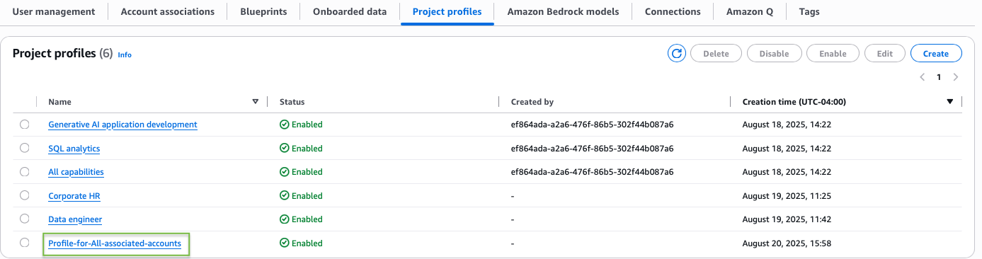
You will see a success message confirming that the Corporate HR profile has been created and linked to one account pool.

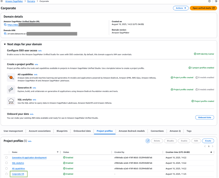
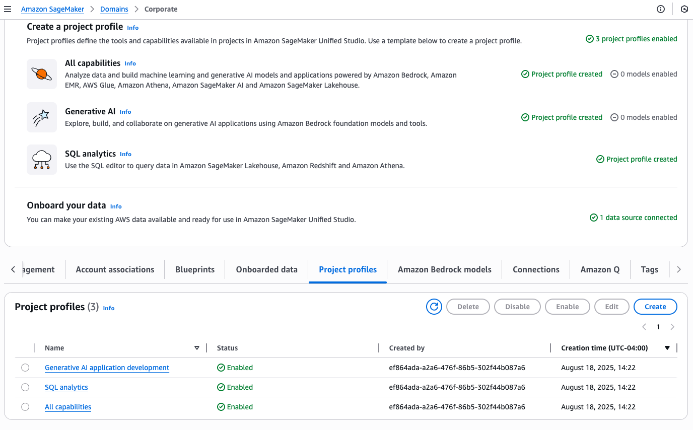
On the Project profiles tab, you should now see your newly created Corporate HR profile listed among the available project profiles.

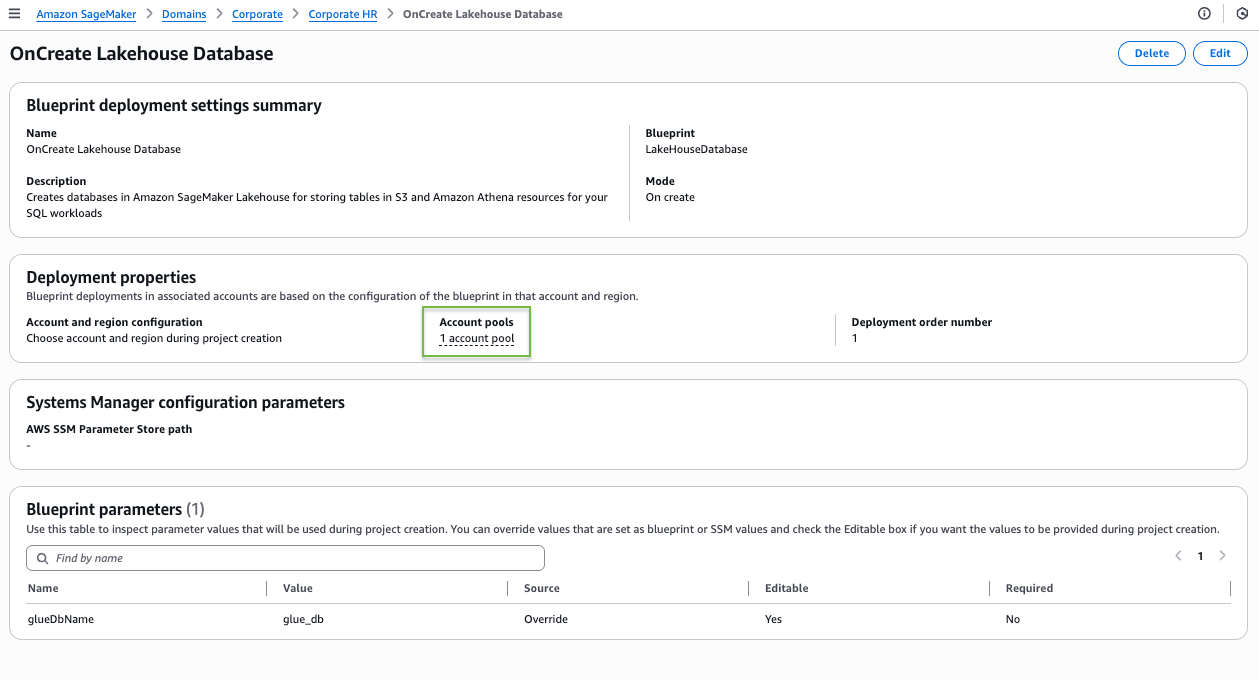
To explore further, navigate to the Corporate HR project profile and choose the Blueprints tab to see a list of available blueprints. Choose a blueprint to view its details.

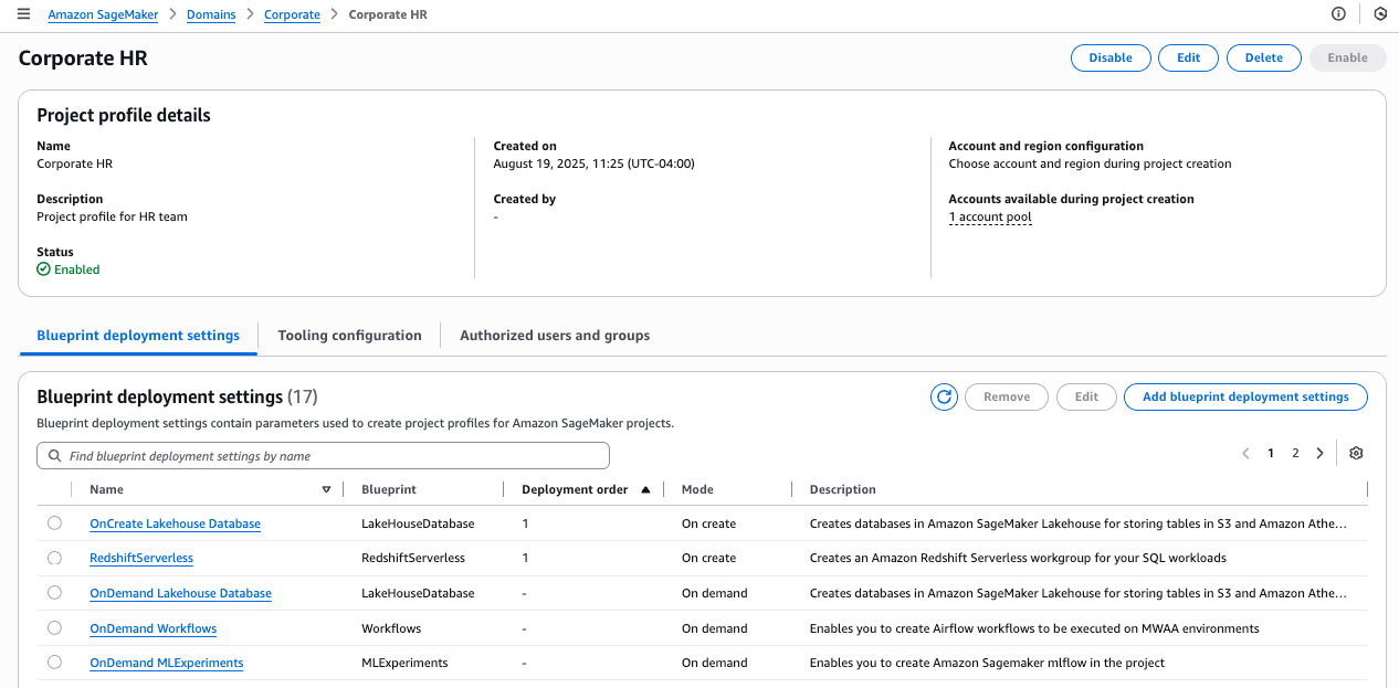
On the blueprint details page, the blueprint shows as deployable to the single account pool you associated with this project profile.

Scenario 2: Project profile associated with multiple account pools

In this example, we create a project profile for a global Data Engineering team, connecting it to three Regional account pools: NAMER (North America), APAC (Asia Pacific), and EMEA (Europe, Middle East, and Africa). Complete the following steps:

On the SageMaker console, choose Domains in the navigation pane.
On the Project profiles tab, choose Create.
Enter a name and description for your profile.
Choose an appropriate project profile template that aligns with your project’s needs.
Select Choose account and region during project creation.
Select Choose account pool(s) and choose all three Regional pools:
1. NAMER Data Engineering team
2. EMEA Data Engineering team
3. APAC Data Engineering team
Leave the remaining settings as default and choose Create project profile.
On the project details page, choose Enable to activate your profile.
Choose Enable in the confirmation pop-up to proceed.

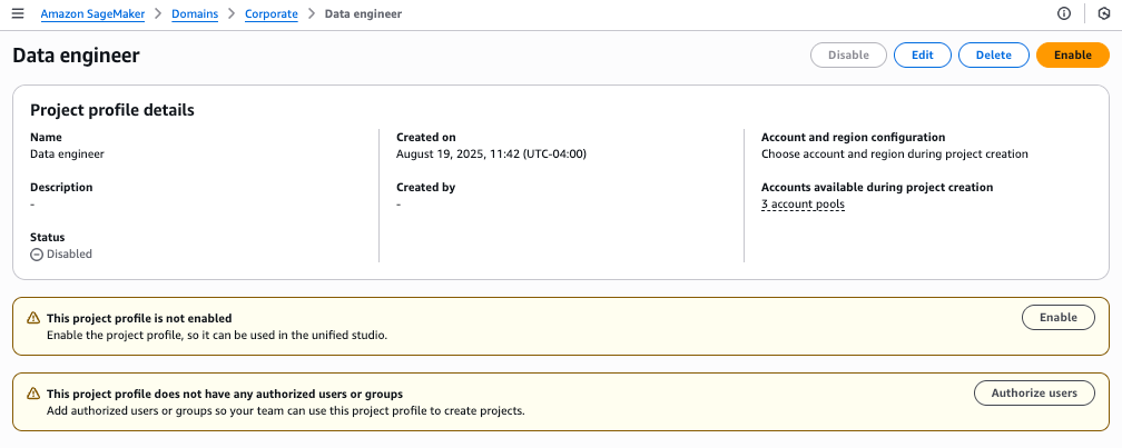
You will see a success message confirming the Data Engineer profile creation. The profile will show connections to all three Regional account pools.

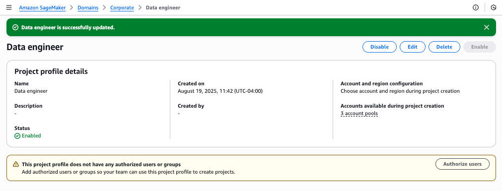
You can find your new profile listed on the Project profiles tab.

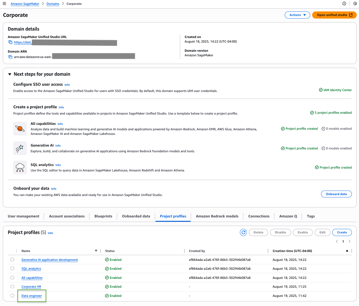
Navigate to your project profile and choose the Blueprints tab to see a list of available blueprints. Choose a blueprint to view its details.

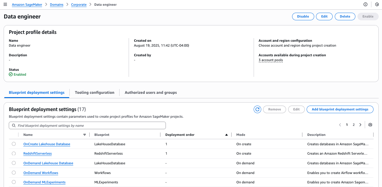
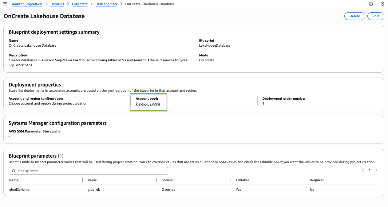
On the blueprint details page, the blueprint shows as deployable to the three account pools you associated with this project profile.

Scenario 3: Project profile with all associated accounts

In this scenario, we create a project profile linked to all the associated accounts for this domain. Complete the following steps:

On the SageMaker console, choose Domains in the navigation pane.
On the Project profiles tab, choose Create.
Enter a name and description for your profile.
Choose an appropriate project profile template that aligns with your project’s needs.
Select Choose account and region during project creation.
Select All associated accounts.
Leave the remaining settings as default and choose Create project profile.

You can find your new profile listed on the Project profiles tab.

Project owner tasks

Now that the administrator has created project profiles for the account pools, project owners can log in to SageMaker to create projects for their account pools. In this section, we demonstrate the procedure to create a project using an account-agnostic project profile with a single account pool. You can use the same procedure to create projects using an account-agnostic project profile with multiple account pools.

For this scenario, Sarah from HR will create a project for the HR team, using the Corporate HR team profile that is associated with the HR account pool.

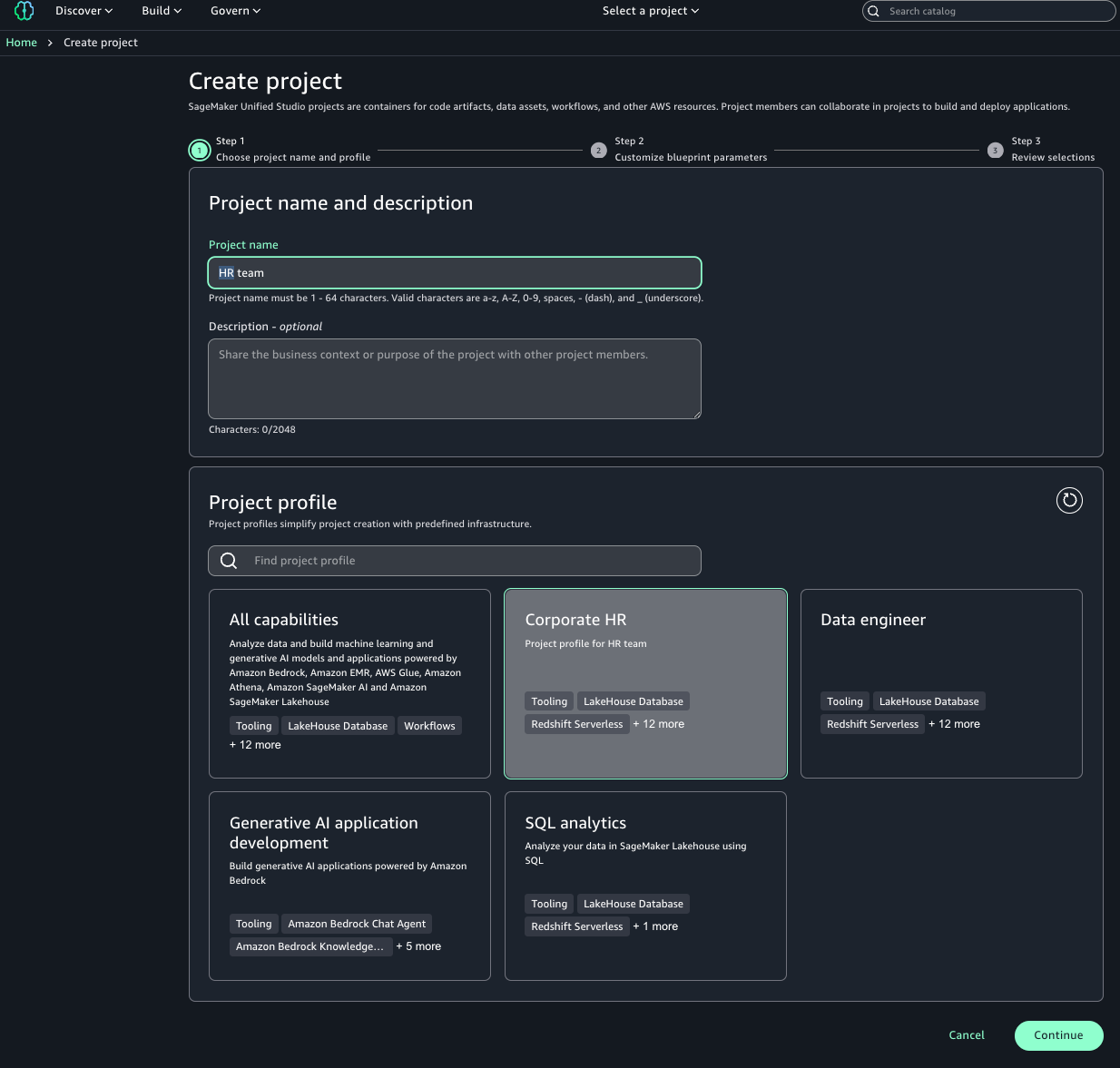
On the SageMaker portal, choose Create project.
Enter a name and optional description.
Choose the Corporate HR project profile.
Choose Continue.
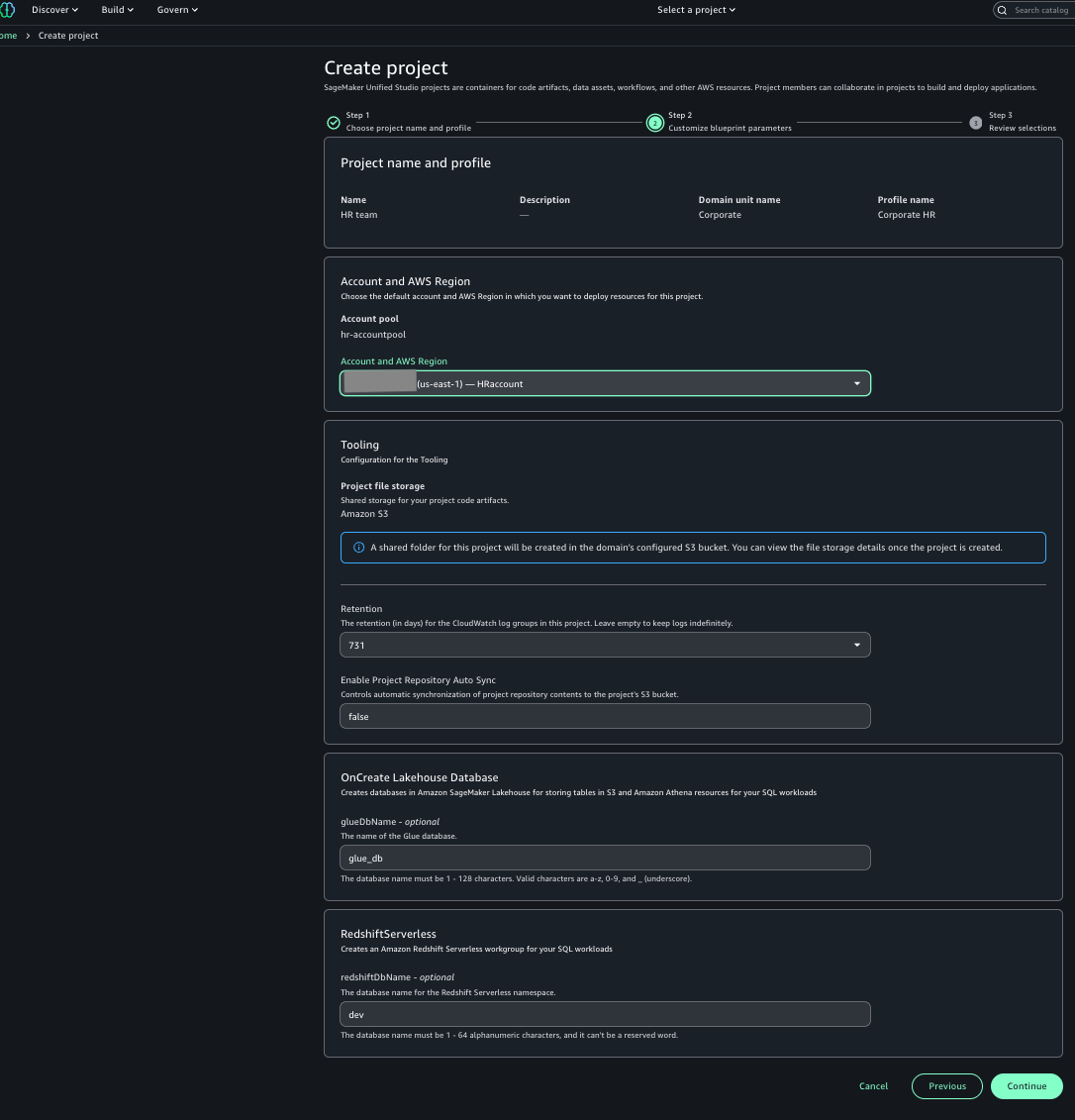
For Account and AWS Region, choose the HR account.
Choose Continue.
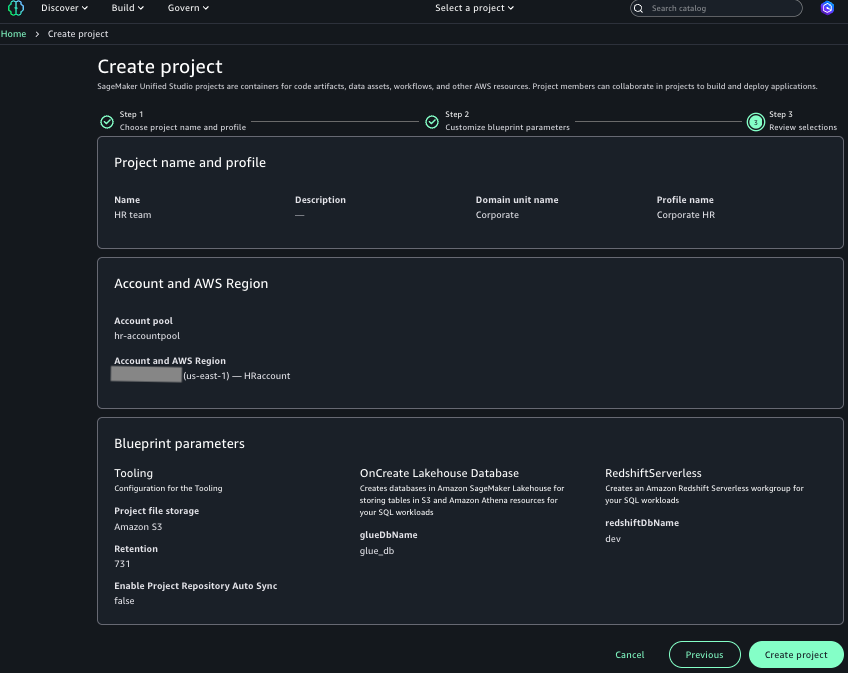
Review the information and choose Create project.

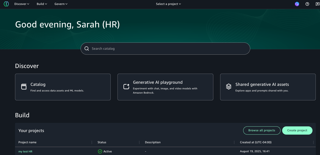
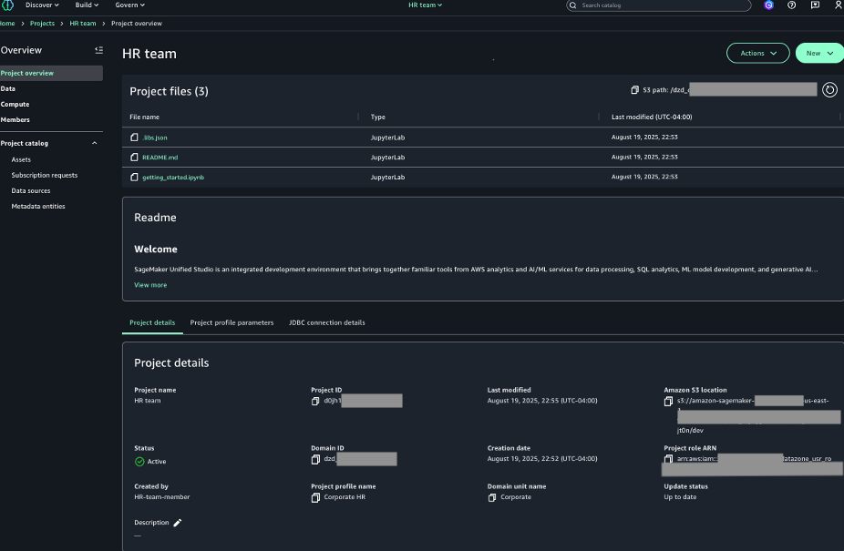
You can view the successfully created project.

Clean up

To clean up resources, complete the following steps:

Delete the projects using the AWS CLI:

aws sagemaker delete-project --project-name <project-name>

Delete the account pools:

aws datazone delete-account-pool --domain-identifier <domain-id> --name <pool-name>

Conclusion

In this post, we discussed how account-agnostic project profiles can help organizations simplify and streamline the management of SageMaker project creation while maintaining enhanced security and governance features. To learn more about account-agnostic project profiles in SageMaker, refer to Account pools in Amazon SageMaker Unified Studio, and demo: account-agnostic project profile in Amazon SageMaker.

About the Authors

Deploy Apache YuniKorn batch scheduler for Amazon EMR on EKS

2025-09-02 Suvojit Dasgupta

Post Syndicated from Suvojit Dasgupta original https://aws.amazon.com/blogs/big-data/deploy-apache-yunikorn-batch-scheduler-for-amazon-emr-on-eks/

As organizations successfully grow their Apache Spark workloads on Amazon EMR on EKS, they may seek to optimize resource scheduling to further enhance cluster utilization, minimize job queuing, and maximize performance. Although Kubernetes’ default scheduler, kube-scheduler, works well for most containerized applications, it lacks feature sets capable of managing complex big data workloads with specific requirements such as gang scheduling, resource quotas, job priorities, multi-tenancy, and hierarchical queue management. This limitation can result in inefficient resource utilization, longer job completion times, and increased operational costs for organizations running large-scale data processing workloads.

Apache YuniKorn addresses these limitations by providing a custom resource scheduler specifically designed for big data and machine learning (ML) workloads running on Kubernetes. Unlike kube-scheduler, YuniKorn offers features such as gang scheduling, making sure all containers of a Spark application start together, resource fairness amongst multiple tenants, priority and preemption capabilities, and queue management with hierarchical resource allocation. For data engineering and platform teams managing large-scale Spark workloads on Amazon EMR on EKS, YuniKorn can improve resource utilization rates, reduce job completion times, and provide improved resource allocation for multi-tenant clusters. This is particularly valuable for organizations running mixed workloads with varying resource requirements, strict SLA requirements, or complex resource sharing policies across different teams and applications.

This post explores Kubernetes scheduling fundamentals, examines the limitations of the default kube-scheduler for batch workloads, and demonstrates how YuniKorn addresses these challenges. We discuss how to deploy YuniKorn as a custom scheduler for Amazon EMR on EKS, its integration with job submissions, how to configure queues and placement rules, and how to establish resource quotas. We also show these features in action through practical Spark job examples.

Understanding Kubernetes scheduling and the need for YuniKorn

In this section, we dive into the details of Kubernetes scheduling and the need for YuniKorn.

How Kubernetes scheduling works

Kubernetes scheduling is the process of assigning pods to nodes within a cluster while considering resource requirements, scheduling constraints, and isolation constraints. The scheduler evaluates each pod individually against all schedulable worker nodes, considering multiple factors, including resource requirements such as CPU, memory and I/O requests, node affinity preferences for specific node characteristics, inter-pod affinity and anti-affinity rules that determine whether the pods should be distributed across multiple worker nodes or require colocation, taints and tolerations that dictate scheduling constraints, and Quality of Service classifications that influence scheduling priority.

The scheduling process operates through a two-phase approach. During the filtering phase, the scheduler identifies all worker nodes that could potentially host the pod by eliminating those that don’t meet the basic requirements. The scoring phase then ranks all feasible worker nodes using scoring algorithms to determine the optimal placement, ultimately selecting the highest-scoring node for pod assignment.

Default implementation of kube-scheduler

kube-scheduler serves as the Kubernetes default scheduler. This scheduler operates on a pod-by-pod basis, treating each scheduling decision as an independent operation without consideration for the broader application context.When kube-scheduler processes scheduling requests, it follows a continuous workflow. The API server is monitored for newly created pods awaiting node assignment, applies filtering logic to eliminate unsuitable worker nodes, executes its scoring algorithm to rank the remaining candidates, binds the selected pod to the optimal node, and repeats the process with the next unscheduled pod in the queue.This individual pod scheduling approach works well for microservices and web applications where each pod has fewer interdependencies. However, this design creates significant challenges when applied to distributed big data frameworks like Spark that require coordinated scheduling of multiple interdependent pods.

Challenges using kube-scheduler for batch jobs

Batch processing workloads, particularly those built on Spark, present different scheduling requirements that expose limitations in kube-scheduler algorithm. Such applications consist of multiple pods that must operate as a cohesive unit, yet kube-scheduler lacks the application-level awareness necessary to handle coordinated scheduling requirements.

Gang scheduling challenges

The most significant challenge emerges from the need for gang scheduling, where all components of a distributed application must be scheduled simultaneously. A typical Spark application requires a driver pod and multiple executor pods running in parallel to function correctly. Without YuniKorn, kube-scheduler first schedules the driver pod without knowing the total amount of resources that the driver and executors will need together. When the driver pod starts running, it attempts to spin up the required executor pods but might fail to find sufficient resources in the cluster. This sequential approach can result in the driver being scheduled successfully while some or all executor pods remain in a pending state due to insufficient cluster capacity.This partial scheduling creates a problematic scenario where the application consumes cluster resources but can’t execute meaningful work. The partially scheduled application will hold onto allocated resources indefinitely while waiting for the missing components, preventing other applications from utilizing those resources and resulting in a deadlock situation.

Resource fragmentation issues

Resource fragmentation represents another critical issue that emerges from individual pod scheduling. When multiple batch applications compete for cluster resources, the lack of coordinated scheduling leads to scenarios where sufficient total resources exist for a given application, but they become fragmented across multiple incomplete applications. This fragmentation prevents efficient resource utilization and can leave applications in perpetual pending states.

The absence of hierarchical queue management further compounds these challenges. kube-scheduler provides limited support for hierarchical resource allocation, making it difficult to implement fair sharing policies across different tenants. Organizations can’t easily establish resource quotas that guarantee minimum allocations while setting maximum limits, nor can they implement preemption policies that allow higher-priority jobs to reclaim resources from lower-priority workloads.

The Need for YuniKorn

YuniKorn addresses these batch scheduling limitations through a set of features designed for distributed computing workloads. Unlike the pod-centric approach of kube-scheduler, YuniKorn operates with application-level awareness, understanding the relationships between different components of distributed applications and making scheduling decisions accordingly. The features are as follows:

Gang scheduling for atomic application deployment – Gang scheduling represents YuniKorn’s advantage for batch workloads. This capability makes sure pods belonging to an application are scheduled atomically—either all components receive node assignments, or none are scheduled until sufficient resources become available. YuniKorn’s all-or-nothing approach to scheduling minimizes resource deadlocks and partial application failures that impact kube-scheduler based deployments, resulting in more predictable job execution and higher completion rates.
Hierarchical queue management and resource organization – YuniKorn’s queue management system provides the hierarchical resource organization that enterprise batch processing environments require. Organizations can establish multi-level queue structures that mirror their organizational hierarchy, implementing resource quotas at each level to facilitate fair resource distribution. The scheduler supports guaranteed resource allocations that provide minimum resource commitments and maximum limits that prevent a single queue from monopolizing cluster resources.
Dynamic resource preemption based on priority – The preemption capabilities built into YuniKorn enable dynamic resource reallocation based on job priorities and queue policies. When higher-priority applications require resources currently allocated to lower-priority workloads, YuniKorn can gracefully stop lower-priority pods and reallocate their resources, making sure critical jobs receive the resources they need without manual intervention.
Intelligent resource pooling and fair share distribution – Resource pooling and fair share scheduling further enhance YuniKorn’s effectiveness for batch workloads. Rather than treating each scheduling decision in isolation, YuniKorn considers the broader resource allocation landscape, implementing fair-share algorithms that facilitate equitable resource distribution across different applications and users while maximizing overall cluster utilization.

These features add to the existing capabilities of Amazon EMR on EKS by establishing an enhanced environment in which the unique requirements of distributed computing workloads are satisfied.

Solution overview

Consider HomeMax, a fictitious company operating a shared Amazon EMR on EKS cluster where three teams regularly submit Spark jobs with distinct characteristics and priorities:

Analytics team – Runs time-sensitive customer analysis jobs requiring immediate processing for business decisions
Marketing team – Executes large overnight batch jobs for campaign optimization with predictable resource patterns
Data science team – Runs experimental workloads with varying resource needs throughout the day for model development and research

Without proper resource scheduling, these teams face common challenges: resource contention, job failures due to partial scheduling, and inability to guarantee SLAs for critical workloads.For our YuniKorn demonstration, we configured an Amazon EMR on EKS cluster with the following specifications:

Amazon EKS cluster: Four worker nodes using m5.2xlarge Amazon Elastic Compute Cloud (Amazon EC2) instances
Per-node resources: 8 vCPUs, 32 GiB memory
Total cluster capacity: 32 vCPU cores and 128 GiB memory
Available for Spark: Approximately 30 vCPUs and approximately 120 GiB memory (after system overhead)
Kubernetes version: 1.30+ (required for YuniKorn 1.6.x compatibility)

The following code shows the node group configuration:

# EKS Node Group specification
NodeGroup:
  InstanceTypes:
    - m5.2xlarge
  ScalingConfig:
    MinSize: 4
    DesiredSize: 4
    MaxSize: 4
  DiskSize: 20
  AmiType: AL2023_x86_64_STANDARD

We intentionally use a fixed-capacity cluster to provide a controlled environment that showcases YuniKorn’s scheduling capabilities with consistent, predictable resources. This approach makes resource contention scenarios more apparent and demonstrates how YuniKorn resolves them.

Amazon EMR on EKS offers robust scaling capabilities through Karpenter. The principles demonstrated in this fixed environment apply equally to dynamic environments, where YuniKorn’s capabilities complement the scaling features of Amazon EMR on EKS to optimize resource utilization during peak demand periods or when scaling limits are reached.

The following diagram shows the high-level architecture of the YuniKorn scheduler running on Amazon EMR on EKS. This solution also includes a secure bastion host not shown in the architecture diagram that provides access to the EKS cluster via AWS Systems Manager (SSM) Session Manager. The bastion host is deployed in a private subnet with all necessary tools pre-installed with proper permissions for seamless cluster interaction.

In the following sections, we explore YuniKorn’s queue architecture optimized for this use case. We examine various demonstration scenarios, including gang scheduling, queue-based resource management, priority-based preemption, and fair share distribution. We walk through the process of deploying an Amazon EMR on EKS cluster, implementing the YuniKorn scheduler, configuring the specified queues, and submitting Spark jobs to showcase these scenarios.

YuniKorn integration on Amazon EMR on EKS

The integration involves three key components working together: the Amazon EMR on EKS virtual cluster configuration, YuniKorn’s admission webhook system, and job-level queue annotations.

Namespace and virtual cluster foundation

The integration begins with a dedicated Kubernetes namespace where your Amazon EMR on EKS jobs will run. In our demonstration, we use the emr namespace, created as a standard Kubernetes namespace:

apiVersion: v1
kind: Namespace
metadata:
  name: emr

The Amazon EMR on EKS virtual cluster is configured to deploy all jobs within this specific namespace. When creating the virtual cluster, you specify the namespace in the container provider configuration:

aws emr-containers create-virtual-cluster \
    --name "emr-on-eks-cluster-v" \
    --container-provider "{
        \"id\": \"my-eks-cluster\",
        \"type\": \"EKS\",
        \"info\": {
            \"eksInfo\": {
                \"namespace\": \"emr\"
            }
        }
    }"

This configuration makes sure all jobs submitted to this virtual cluster will be deployed in the emr namespace, establishing the foundation for YuniKorn integration.

The YuniKorn interception mechanism

When YuniKorn is installed using Helm, it automatically registers a MutatingAdmissionWebhook with the Kubernetes API server. This webhook acts as an interceptor that monitors pod creation events in your designated namespace. The webhook registration tells Kubernetes to call YuniKorn whenever pods are created in the emr namespace:

# YuniKorn registers this webhook configuration
apiVersion: admissionregistration.k8s.io/v1
kind: MutatingAdmissionWebhook
rules:
- operations: ["CREATE"]
  resources: ["pods"]
  namespaces: ["emr"]  # Intercepts pods in EMR namespace

This webhook is triggered by any pod creation in the emr namespace, not specifically by YuniKorn annotations. However, the webhook’s logic only modifies pods that contain YuniKorn queue annotations, leaving other pods unchanged.

End-to-end job flow

When you submit a Spark job through the Spark Operator, the following sequence occurs:

Your Spark job includes YuniKorn queue annotations on both driver and executor pods:

driver:
  annotations:
    yunikorn.apache.org/queue: "root.analytics-queue"
executor:
  annotations:
    yunikorn.apache.org/queue: "root.analytics-queue"

The Spark Operator processes your SparkApplication and creates individual Kubernetes pods for the driver and executors. These pods inherit the YuniKorn annotations from your job template.
When the Spark Operator attempts to create pods in the emr namespace, Kubernetes calls YuniKorn’s admission webhook. The webhook examines each pod and performs the following actions:
1. Detects pods with yunikorn.apache.org/queue annotations.
2. Adds schedulerName: yunikorn to those pods.
3. Leaves pods without YuniKorn annotations unchanged.

This interception means you don’t need to manually specify schedulerName: yunikorn in your Spark jobs—YuniKorn claims the pods transparently based on the presence of queue annotations.

The YuniKorn scheduler receives the scheduling requests and applies the queue placement rules configured in the YuniKorn ConfigMap:

placementrules:
  - name: provided    # Uses the annotation value
    create: false.    # Doesn’t create the queue if not present
  - name: fixed       # Fallback to root.default queue
    value: root.default

The provided rule reads the yunikorn.apache.org/queue annotation and places the job in the specified queue (for example, root.analytics-queue). YuniKorn then applies gang scheduling logic, holding all pods until sufficient resources are available for the entire application, preventing the partial scheduling issues that come with kube-scheduler.

After YuniKorn determines that all pods can be scheduled according to the queue’s resource guarantees and limits, it schedules all driver and executor pods. The Spark job begins execution with the guaranteed resource allocation defined in the queue configuration.

The combination of namespace-based virtual cluster configuration, admission webhook interception, and annotation-driven queue placement creates an integration that transforms Amazon EMR on EKS job scheduling without disrupting existing workflows.

YuniKorn queue architecture

To demonstrate the various YuniKorn features described in the next section, we configured three job-specific queues and a default queue representing our enterprise teams with carefully balanced resource allocations:

# Analytics Queue - Time-sensitive workloads
analytics-queue:
  guaranteed: 10 vCPUs, 38GB memory (30% of cluster)
  max: 24 vCPUs, 96GB memory (80% burst capacity)
  priority: 100 (highest)
  policy: FIFO (predictable scheduling)
# Marketing Queue - Large batch jobs
marketing-queue:
  guaranteed: 8 vCPUs, 32GB memory (25% of cluster)
  max: 24 vCPUs, 96GB memory (80% burst capacity)
  priority: 75 (medium)
  policy: Fair Share (balanced resource distribution)
# Data Science Queue - Experimental workloads
datascience-queue:
  guaranteed: 6 vCPUs, 26GB memory (20% of cluster)
  max: 24 vCPUs, 96GB memory (80% burst capacity)
  priority: 50 (lower)
  policy: Fair Share (experimental workload balancing)
# Default Queue - Fallback for unmatched jobs
default:
  guaranteed: 6 vCPUs, 26GB memory (20% of cluster)
  max: 24 vCPUs, 96GB memory (80% burst capacity)
  priority: 25 (lowest)
  policy: FIFO (predictable job submission)

Demonstration scenarios

This section outlines key YuniKorn scheduling capabilities and their corresponding Spark job submissions. These scenarios demonstrate guaranteed resource allocation and burst capacity usage. Guaranteed resources represent minimum allocations that queues can always access, but jobs might exceed these allocations when additional cluster capacity is available. The marketing-job specifically demonstrates burst capacity usage beyond its guaranteed allocation.

Gang scheduling – In this scenario, we submit analytics-job.py (analytics-queue, 9 total cores) and marketing-job.py (marketing-queue, 17 total cores) simultaneously. YuniKorn makes sure all pods for each job are scheduled atomically, preventing partial resource allocation that could cause job failures in our resource-constrained cluster.
Queue-based resource management – We run all three jobs concurrently to observe guaranteed resource allocation. YuniKorn distributes remaining capacity proportionally based on queue weights and maximum limits.
- analytics-job.py (analytics-queue) receives guaranteed 10 vCPUs and 38 GB memory.
- marketing-job.py (marketing-queue) receives guaranteed 8 vCPUs and 32 GB memory.
- datascience-job.py (datascience-queue) receives guaranteed 6 vCPUs and 26 GB memory.
Priority-based preemption – We start datascience-job.py (datascience-queue, priority 25) and marketing-job.py (marketing-queue, priority 50) consuming cluster resources, then submit high-priority analytics-job.py (analytics-queue, priority 100). YuniKorn preempts lower-priority jobs to make sure the time-sensitive analytics workload gets its guaranteed resources, maintaining SLA compliance.
Fair share distribution – We submit multiple jobs to each queue when all queues have available capacity. YuniKorn applies configured fair share policies within queues—the analytics queue uses First In, First Out (FIFO) method for predictable scheduling, and the marketing and data science queues use fair sharing method for balanced resource distribution.

Source code

You can find the codebase in the AWS Samples GitHub repository.

Prerequisites

Before you deploy this solution, make sure the following prerequisites are in place:

Access to a valid AWS account
The AWS Command Line Interface (AWS CLI) is installed on your local machine
AWS Session Manager plugin installed for secure bastion host access
Git, Docker, eksctl, kubectl, Helm, and jq utilities are installed on your local machine
Permission to create AWS resources
Familiarity with Kubernetes, Apache Spark, Amazon EKS, and Amazon EMR on EKS

Set up the solution infrastructure

Complete the following steps to set up the infrastructure:

Clone the repository to your local machine and set the two environment variables. Replace <AWS_REGION> with the AWS Region where you want to deploy these resources.

git clone https://github.com/aws-samples/sample-emr-eks-yunikorn-scheduler.git
cd sample-emr-eks-yunikorn-scheduler
export REPO_DIR=$(pwd)
export AWS_REGION=<AWS_REGION>

Execute the following script to create the infrastructure:

cd $REPO_DIR/infrastructure
./setup-infra.sh

To verify successful infrastructure deployment, open the AWS CloudFormation console, choose your stack, and check the Events, Resources, and Outputs tabs for completion status, details, and list of resources created.

Deploy YuniKorn on Amazon EMR on EKS

Run the following script to deploy the Yunikorn helm chart and update the configmap with the queues and placement rules:

cd $REPO_DIR/yunikorn/
./setup-yunikorn.sh

Establish EKS cluster connectivity

Complete the following steps to establish secure connectivity to your private EKS cluster:

Execute the following script in a new terminal window. This script establishes port forwarding through the bastion host to make your private EKS cluster accessible from your local machine. Keep this terminal window open and running throughout your work session. The script maintains the connection to your EKS cluster.

export REPO_DIR=$(pwd)
export AWS_REGION=<AWS_REGION>
cd $REPO_DIR/port-forward
./eks-connect.sh --start

Test kubectl connectivity in the main terminal window to verify that you can successfully communicate with the EKS cluster. You should see the EKS worker nodes listed, confirming that the port forwarding is working correctly.

kubectl get nodes

Verify successful YuniKorn deployment

Complete the following steps to verify a successful deployment:

List all Kubernetes objects in the yunikorn namespace:

kubectl get all -n yunikorn

You will see details like the following screenshot.

Check the YuniKorn scheduler logs for configuration loading and look for queue configuration messages:

kubectl logs -n yunikorn deployment/yunikorn-scheduler --tail=50
kubectl logs -n yunikorn deployment/yunikorn-scheduler | grep -i queue

Access the YuniKorn web UI by navigating to http://127.0.0.1:9889 in your browser. Port 9889 is the default port for the YuniKorn web UI.

# macOS
open http://127.0.0.1:9889
# Linux
xdg-open http://127.0.0.1:9889
# Windows
start http://127.0.0.1:9889

The following screenshots show the YuniKorn web UI with queues but no running applications.

Run Spark jobs with YuniKorn on Amazon EMR on EKS

Complete the following steps to run Spark jobs with YuniKorn on Amazon EMR on EKS:

Execute the following script to set up the Spark jobs environment. The script uploads PySpark scripts to Amazon Simple Storage Service (Amazon S3) bucket locations and creates ready-to-use YAML files from templates.

cd $REPO_DIR/spark-jobs
./setup-spark-jobs.sh

Submit analytics, marketing, and data science Spark jobs using the following commands. YuniKorn will place the jobs in their respective queues and allocate resources to execution. Refer to Using YuniKorn as a custom scheduler for Apache Spark on Amazon EMR on EKS for supported job submission methods with YuniKorn as a custom scheduler.

kubectl apply -f spark-operator/analytics-job.yaml
kubectl apply -f spark-operator/marketing-job.yaml
kubectl apply -f spark-operator/datascience-job.yaml

Review the previous section describing different demonstration scenarios and submit the Spark jobs using various combinations to see YuniKorn scheduler’s capabilities in action. We encourage you to adjust the cores, instances, and memory parameters and explore the scheduler’s behavior by executing the jobs. We also encourage you to modify the queues’ guaranteed and max capacities in the file yunikorn/queue-config-provided.yaml, apply the changes, and submit jobs to further understand Yunikorn scheduler behavior under various circumstances.

Clean up

To avoid incurring future charges, complete the following steps to delete the resources you created:

Stop the port forwarding sessions:

cd $REPO_DIR/port-forwarding
./eks-connect.sh --stop

Remove all created AWS resources:

cd $REPO_DIR
./cleanup.sh

Conclusion

YuniKorn addresses the scheduling limitations of default kube-scheduler while running Spark workloads on Amazon EMR on EKS through gang scheduling, intelligent queue management, and priority-based resource allocation. This post showed how YuniKorn’s queue system enables better resource utilization, prevents job failure due to poor allocation of resources, and supports multi-tenant environments.

To get started with YuniKorn on Amazon EMR on EKS, explore the Apache YuniKorn documentation for implementation guides, review Amazon EMR on EKS best practices for optimization strategies, and engage with the YuniKorn community for ongoing support.

About the authors

Suvojit Dasgupta is a Principal Data Architect at Amazon Web Services. He leads a team of skilled engineers in designing and building scalable data solutions for diverse customers. He specializes in developing and implementing innovative data architectures to address complex business challenges.

Peter Manastyrny is a Senior Product Manager at AWS Analytics. He leads Amazon EMR on EKS, a product that makes it straightforward and efficient to run open-source data analytics frameworks such as Spark on Amazon EKS.

Matt Poland is a Senior Cloud Infrastructure Architect at Amazon Web Services. He is passionate about solving complex problems and delivering well-structured solutions for diverse customers. His expertise spans across a range of cloud technologies, providing scalable and reliable infrastructure tailored to each project’s unique challenges.

Gregory Fina is a Principal Startup Solutions Architect for Generative AI at Amazon Web Services, where he empowers startups to accelerate innovation through cloud adoption. He specializes in application modernization, with a strong focus on serverless architectures, containers, and scalable data storage solutions. He is passionate about using generative AI tools to orchestrate and optimize large-scale Kubernetes deployments, as well as advancing GitOps and DevOps practices for high-velocity teams. Outside of his customer-facing role, Greg actively contributes to open source projects, especially those related to Backstage.

Modernize Amazon Redshift authentication by migrating user management to AWS IAM Identity Center

2025-08-28 Ziad Wali

Post Syndicated from Ziad Wali original https://aws.amazon.com/blogs/big-data/modernize-amazon-redshift-authentication-by-migrating-user-management-to-aws-iam-identity-center/

Amazon Redshift is a powerful cloud-based data warehouse that organizations can use to analyze both structured and semi-structured data through advanced SQL queries. As a fully managed service, it provides high performance and scalability while allowing secure access to the data stored in the data warehouse. Organizations worldwide rely on Amazon Redshift to handle massive datasets, upgrade their analytics capabilities, and deliver valuable business intelligence to their stakeholders.

AWS IAM Identity Center serves as the preferred platform for controlling workforce access to AWS tools, including Amazon Q Developer. It allows for a single connection to your existing identity provider (IdP), creating a unified view of users across AWS applications and applying trusted identity propagation for a smooth and consistent experience.

You can access data in Amazon Redshift using local users or external users. A local user in Amazon Redshift is a database user account that is created and managed directly within the Redshift cluster itself. Amazon Redshift also integrates with IAM Identity Center, and supports trusted identity propagation, so you can use third-party IdPs such as Microsoft Entra ID (Azure AD), Okta, Ping, OneLogin, or use IAM Identity Center as an identity source. The IAM Identity Center integration with Amazon Redshift supports centralized authentication and SSO capabilities, simplifying access management across multi-account environments. As organizations grow in scale, it is recommended to use external users for cross-service integration and centralized access management.

In this post, we walk you through the process of smoothly migrating your local Redshift user management to IAM Identity Center users and groups using the RedshiftIDCMigration utility.

Solution overview

The following diagram illustrates the solution architecture.

The RedshiftIDCMigration utility accelerates the migration of your local Redshift users, groups, and roles to your IAM Identity Center instance by performing the following activities:

Create users in IAM Identity Center for every local user in a given Redshift instance.
Create groups in IAM Identity Center for every group or role in a given Redshift instance.
Assign users to groups in IAM Identity Center according to existing assignments in the Redshift instance.
Create IAM Identity Center roles in the Redshift instance matching the groups created in IAM Identity Center.
Grant permissions to IAM Identity Center roles in the Redshift instance based on the current permissions given to local groups and roles.

Prerequisites

Before running the utility, complete the following prerequisites:

Enable IAM Identity Center in your account.
Follow the steps in the post Integrate Identity Provider (IdP) with Amazon Redshift Query Editor V2 and SQL Client using AWS IAM Identity Center for seamless Single Sign-On (specifically, follow Steps 1–8, skipping Steps 4 and 6).
Configure the IAM Identity Center application assignments:
1. On the IAM Identity Center console, choose Application Assignments and Applications.
2. Select your application and on the Actions dropdown menu, choose Edit details.
3. For User and group assignments, choose Do not require assignments. This setting makes it possible to test Amazon Redshift connectivity without configuring specific data access permissions.
Configure IAM Identity Center authentication with administrative access from either Amazon Elastic Compute Cloud (Amazon EC2) or AWS CloudShell.

The utility will be run from either an EC2 instance or CloudShell. If you’re using an EC2 instance, an IAM role is attached to the instance. Make sure that the IAM role used during the execution has the following permissions (if not, create a new policy with those permissions and attach it to the IAM role):

Amazon Redshift permissions (for serverless):

{
    "Version": "2012-10-17",
    "Statement": [
        {
            "Sid": "VisualEditor0",
            "Effect": "Allow",
            "Action": [
                "redshift-serverless:GetCredentials",
                "redshift-serverless:GetNamespace",
                "redshift-serverless:GetWorkgroup"
            ],
            "Resource": [
                "arn:aws:redshift-serverless:${region}:${account-id}:namespace/${namespace-id}",
                "arn:aws:redshift-serverless:${region}:${account-id}:workgroup/${workgroup-id}"
            ]
        },
        {
            "Sid": "VisualEditor1",
            "Effect": "Allow",
            "Action": [
                "redshift-serverless:ListNamespaces",
                "redshift-serverless:ListWorkgroups"
            ],
            "Resource": "*"
        },
        {
            "Sid": "VisualEditor2",
            "Effect": "Allow",
            "Action": [
                "redshift:CreateClusterUser",
                "redshift:JoinGroup",
                "redshift:GetClusterCredentials",
                "redshift:ExecuteQuery",
                "redshift:FetchResults",
                "redshift:DescribeClusters",
                "redshift:DescribeTable"
            ],
            "Resource": [
                "arn:aws:redshift:${region}:${account-id}:cluster:redshift-serverless-${workgroup-name}",
                "arn:aws:redshift:${region}:${account-id}:dbgroup:redshift-serverless-${workgroup-name}/${dbgroup}",
                "arn:aws:redshift:${region}:${account-id}:dbname:redshift-serverless-${workgroup-name}/${dbname}",
                "arn:aws:redshift:${region}:${account-id}:dbuser:redshift-serverless-${workgroup-name}/${dbuser}"
            ]
        }
    ]
}

Amazon Redshift permissions (for provisioned):

{
    "Version": "2012-10-17",
    "Statement": [
        {
            "Sid": "VisualEditor0",
            "Effect": "Allow",
            "Action": "redshift:GetClusterCredentials",
            "Resource": [
                "arn:aws:redshift: ${region}:${account-id}:dbname:${cluster_name}/${dbname}",
                "arn:aws:redshift: ${region}: ${account-id}:dbuser:${cluster-name}/${dbuser}"
            ]
        },
        {
            "Sid": "VisualEditor1",
            "Effect": "Allow",
            "Action": [
                "redshift:DescribeClusters",
                "redshift:ExecuteQuery",
                "redshift:FetchResults",
                "redshift:DescribeTable"
            ],
            "Resource": "*"
        }
    ]
}

Amazon Simple Storage Service (Amazon S3) permissions:

{
    "Version": "2012-10-17",
    "Statement": [
        {
            "Sid": "VisualEditor0",
            "Effect": "Allow",
            "Action": [
                "s3:PutObject",
                "s3:GetObject",
                "s3:GetEncryptionConfiguration",
                "s3:ListBucket",
                "s3:DeleteObject"
            ],
            "Resource": [
                "arn:aws:s3:::${s3_bucket_name}/*",
                "arn:aws:s3:::${s3_bucket_name}"
            ]
        }
    ]
}

Identity store permissions:

{
    "Version": "2012-10-17",
    "Statement": [
        {
            "Sid": "VisualEditor0",
            "Effect": "Allow",
            "Action": "identitystore:*",
            "Resource": [
                "arn:aws:identitystore:::group/*",
                "arn:aws:identitystore:::user/*",
                "arn:aws:identitystore::${account_id}:identitystore/${identity_store_id}",
                "arn:aws:identitystore:::membership/*"
            ]
        },
        {
            "Sid": "VisualEditor1",
            "Effect": "Allow",
            "Action": "identitystore:*",
            "Resource": [
                "arn:aws:identitystore:::membership/*",
                "arn:aws:identitystore:::user/*",
                "arn:aws:identitystore:::group/*"
            ]
        }
    ]
}

Artifacts

Download the following utility artifacts from the GitHub repo:

idc_redshift_unload_indatabase_groups_roles_users.py – A Python script to unload users, groups, roles and their associations.
redshift_unload.ini – The config file used in the preceding script to read Redshift data warehouse details and Amazon S3 locations to unload the files.
idc_add_users_groups_roles_psets.py – A Python script to create users and groups in IAM Identity Center, and then associate the users to groups in IAM Identity Center.
idc_config.ini – The config file used in the preceding script to read IAM Identity Center details.
vw_local_ugr_to_idc_urgr_priv.sql – A script that generates SQL statements that perform two tasks in Amazon Redshift:
- Create roles that exactly match your IAM Identity Center group names, adding a specified prefix.
- Grant appropriate permissions to these newly created Redshift roles.

Testing scenario

This test case is designed to offer practical experience and familiarize you with the utility’s functionality. The scenario is structured around a hierarchical nested roles system, starting with object-level permissions assigned to technical roles. These technical roles are then allocated to business roles. Finally, business roles are granted to individual users. To enhance the testing environment, the scenario also incorporates a user group.The following diagram illustrates this hierarchy.

Create datasets

Set up two separate schemas (tickit and tpcds) in a Redshift database using the create schema command. Then, create and populate a few tables in each schema using the tickit and tpcds sample datasets.

Specify the appropriate IAM role Amazon Resource Name (ARN) in the copy commands if necessary.

Create users

Create users with the following code:

-- ETL users
create user etl_user_1 password 'EtlUser1!';
create user etl_user_2 password 'EtlUser2!';
create user etl_user_3 password 'EtlUser3!';

-- Reporting users
create user reporting_user_1 password 'ReportingUser1!';
create user reporting_user_2 password 'ReportingUser2!';
create user reporting_user_3 password 'ReportingUser3!';

-- Adhoc users
create user adhoc_user_1 password 'AdhocUser1!';
create user adhoc_user_2 password 'AdhocUser2!';

-- Analyst users
create user analyst_user_1 password 'AnalystUser1!';

Create business roles

Create business users with the following code:

-- ETL business roles
create role role_bn_etl_tickit;
create role role_bn_etl_tpcds;

-- Reporting business roles
create role role_bn_reporting_tickit;
create role role_bn_reporting_tpcds;

-- Analyst business roles
create role role_bn_analyst_tickit;

Create technical roles

Create technical roles with the following code:

-- Technical roles for tickit schema
create role role_tn_sel_tickit;
create role role_tn_dml_tickit;
create role role_tn_cte_tickit;

-- Technical roles for tpcds schema
create role role_tn_sel_tpcds;
create role role_tn_dml_tpcds;
create role role_tn_cte_tpcds;

Create groups

Create groups with the following code:

-- Adhoc users group
create group group_adhoc;

Grant rights to technical roles

To grant rights to the technical roles, use the following code:

-- role_tn_sel_tickit
grant usage on schema tickit to role role_tn_sel_tickit;
grant select on all tables in schema tickit to role role_tn_sel_tickit;

-- role_tn_dml_tickit
grant usage on schema tickit to role role_tn_dml_tickit;
grant insert, update, delete on all tables in schema tickit to role role_tn_dml_tickit;

-- role_tn_cte_tickit
grant usage, create on schema tickit to role role_tn_cte_tickit;
grant drop on all tables in schema tickit to role role_tn_cte_tickit;

-- role_tn_sel_tpcds
grant usage on schema tpcds to role role_tn_sel_tpcds;
grant select on all tables in schema tpcds to role role_tn_sel_tpcds;

-- role_tn_dml_tpcds
grant usage on schema tpcds to role role_tn_dml_tpcds;
grant insert, update, delete on all tables in schema tpcds to role role_tn_dml_tpcds;

-- role_tn_cte_tpcds
grant usage, create on schema tpcds to role role_tn_cte_tpcds;
grant drop on all tables in schema tpcds to role role_tn_cte_tpcds;

Grant technical roles to business roles

To grant the technical roles to the business roles, use the following code:

-- Business role role_bn_etl_tickit
grant role role_tn_sel_tickit to role role_bn_etl_tickit;
grant role role_tn_dml_tickit to role role_bn_etl_tickit;
grant role role_tn_cte_tickit to role role_bn_etl_tickit;

-- Business role role_bn_etl_tpcds
grant role role_tn_sel_tpcds to role role_bn_etl_tpcds;
grant role role_tn_dml_tpcds to role role_bn_etl_tpcds;
grant role role_tn_cte_tpcds to role role_bn_etl_tpcds;

-- Business role role_bn_reporting_tickit
grant role role_tn_sel_tickit to role role_bn_reporting_tickit;

-- Business role role_bn_reporting_tpcds
grant role role_tn_sel_tpcds to role role_bn_reporting_tpcds;

-- Business role role_bn_analyst_tickit
grant role role_tn_sel_tickit to role role_bn_analyst_tickit;

Grant business roles to users

To grant the business roles to users, use the following code:

-- etl_user_1
grant role role_bn_etl_tickit to etl_user_1;

-- etl_user_2
grant role role_bn_etl_tpcds to etl_user_2;

-- etl_user_3
grant role role_bn_etl_tickit to etl_user_3;
grant role role_bn_etl_tpcds to etl_user_3;

-- reporting_user_1
grant role role_bn_reporting_tickit to reporting_user_1;

-- reporting_user_2
grant role role_bn_reporting_tpcds to reporting_user_2;

-- reporting_user_3
grant role role_bn_reporting_tickit to reporting_user_3;
grant role role_bn_reporting_tpcds to reporting_user_3;

-- analyst_user_1
grant role role_bn_analyst_tickit to analyst_user_1;

Grant rights to groups

To grant rights to the groups, use the following code:

-- Group group_adhoc
grant usage on schema tickit to group group_adhoc;
grant select on all tables in schema tickit to group group_adhoc;

grant usage on schema tpcds to group group_adhoc;
grant select on all tables in schema tpcds to group group_adhoc;

Add users to groups

To add users to the groups, use the following code:

alter group group_adhoc add user adhoc_user_1;
alter group group_adhoc add user adhoc_user_2;

Deploy the solution

Complete the following steps to deploy the solution:

Update Redshift cluster or serverless endpoint details and Amazon S3 location in redshift_unload.ini:
- cluster_type = provisioned or serverless
- cluster_id = ${cluster_identifier} (required if cluster_type is provisioned)
- db_user = ${database_user}
- db_name = ${database_name}
- host = ${host_url} (required if cluster_type is provisioned)
- port = ${port_number}
- workgroup_name = ${workgroup_name} (required if cluster_type is serverless)
- region = ${region}
- s3_bucket = ${S3_bucket_name}
- roles = roles.csv
- users = users.csv
- role_memberships = role_memberships.csv
Update IAM Identity Center details in idc_config.ini:
- region = ${region}
- account_id = ${account_id}
- identity_store_id = ${identity_store_id} (available on the IAM Identity Center console Settings page)
- instance_arn = ${iam_identity_center_instance_arn} (available on the IAM Identity Center console Settings page)
- permission_set_arn = ${permission_set_arn}
- assign_permission_set = True or False (True if permission_set_arn is defined)
- s3_bucket = ${S3_bucket_name}
- users_file = users.csv
- roles_file = roles.csv
- role_memberships_file = role_memberships.csv
Create a directory in CloudShell or on your own EC2 instance with connectivity to Amazon Redshift.
Copy the two .ini files and download the Python scripts to that directory.
Run idc_redshift_unload_indatabase_groups_roles_users.py either from CloudShell or your EC2 instance:python idc_redshift_unload_indatabase_groups_roles_users.py
Run idc_add_users_groups_roles_psets.py either from CloudShell or your EC2 instance:python idc_add_users_groups_roles_psets.py
Connect your Redshift cluster using the Amazon Redshift query editor v2 or preferred SQL client, using superuser credentials.
Copy the SQL in the vw_local_ugr_to_idc_urgr_priv.sql file and run it in the query editor to create the vw_local_ugr_to_idc_urgr_priv view.

Run following SQL command to generate the SQL statements for creating roles and permissions:

select existing_grants,idc_based_grants from vw_local_ugr_to_idc_urgr_priv;

For example, consider the following existing grants:

CREATE GROUP "group_adhoc";
CREATE ROLE "role_bn_etl_tickit";
GRANT USAGE ON SCHEMA tpcds TO role "role_tn_sel_tpcds" ;

These grants are converted to the following code:

CREATE role "AWSIDC:group_adhoc";
CREATE role "AWSIDC:role_bn_etl_tickit";
GRANT USAGE ON SCHEMA tpcds TO role "AWSIDC:role_tn_sel_tpcds";

Review the statements in the idc_based_grants column.
This might not be a comprehensive list of permissions, so review them carefully.
If everything is correct, run the statements from the SQL client.

When you have completed the process, you should have the following configuration:

IAM Identity Center now contains newly created users from Amazon Redshift
The Redshift local groups and roles are created as groups in IAM Identity Center
New roles are established in Amazon Redshift, corresponding to the groups created in IAM Identity Center
The newly created Redshift roles are assigned appropriate permissions

If you encounter an issue while connecting to Amazon Redshift with the query editor using IAM Identity Center, refer to Troubleshooting connections from Amazon Redshift query editor v2.

Considerations

Consider the following when using this solution:

At the time of writing, creating permissions in AWS Lake Formation is not in scope.
IAM Identity Center and IdP integration setup is out of scope for this utility. However, you can use the view vw_local_ugr_to_idc_urgr_priv.sqlto create roles and grant permissions to the IdP users and groups passed through IAM Identity Center.
If you have permissions given directly to local user IDs (not using groups or roles), you must change that to a role-based permission approach for IAM Identity Center integration. Create roles and provide permissions using roles instead of directly giving permissions to users.

Clean up

If you have completed the testing scenario, clean up your environment:

Remove the new Redshift roles that were created by the utility, corresponding to the groups established in IAM Identity Center.
Delete the users and groups created by the utility within IAM Identity Center.
Delete the users, groups, and roles specified in the testing scenario.
Drop the tickit and tpcds schemas.

You can use the FORCE parameter when dropping the roles to remove associated assignments.

Conclusion

In this post, we showed how to migrate your Redshift local user management to IAM Identity Center. This transition offers several key advantages for your organization, such as simplified access management through centralized user and group administration, a streamlined user experience across AWS services, and reduced administrative overhead. You can implement this migration process step by step, so you can test and validate each step before fully transitioning your production environment.

As organizations continue to scale their AWS infrastructure, using IAM Identity Center becomes increasingly valuable for maintaining secure and efficient access management, including Amazon SageMaker Unified Studio for an integrated experience for all your data and AI.

About the authors

How Ancestry optimizes a 100-billion-row Iceberg table

2025-08-28 Thomas Cardenas

Post Syndicated from Thomas Cardenas original https://aws.amazon.com/blogs/big-data/how-ancestry-optimizes-a-100-billion-row-iceberg-table/

This is a guest post by Thomas Cardenas, Staff Software Engineer at Ancestry, in partnership with AWS.

Ancestry, the global leader in family history and consumer genomics, uses family trees, historical records, and DNA to help people on their journeys of personal discovery. Ancestry has the largest collection of family history records, consisting of 40 billion records. They serve more than 3 million subscribers and have over 23 million people in their growing DNA network. Their customers can use this data to discover their family story.

Ancestry is proud to connect users with their families past and present. They help people learn more about their own identity by learning about their ancestors. Users build a family tree through which we surface relevant records, historical documents, photos, and stories that might contain details about their ancestors. These artifacts are surfaced through Hints. The Hints dataset is one of the most interesting datasets at Ancestry. It’s used to alert users that potential new information is available. The dataset has multiple shards, and there are currently 100 billion rows being used by machine learning models and analysts. Not only is the dataset large, it also changes rapidly.

In this post, we share the best practices that Ancestry used to implement an Apache Iceberg-based hints table capable of handling 100 billion rows with 7 million hourly changes. The optimizations covered here resulted in cost reductions of 75%.

Overview of solution

Ancestry’s Enterprise Data Management (EDM) team faced a critical challenge—how to provide a unified, performant data ecosystem that could serve diverse analytical workloads across financial, marketing, and product analytics teams. The ecosystem needed to support everything from data scientists training recommendation models to geneticists developing population studies—all requiring access to the same Hints data.

The ecosystem around Hints data had been developed organically, without a well-defined architecture. Teams independently accessed Hints data through direct service calls, Kafka topic subscriptions, or warehouse queries, creating significant data duplication and unnecessary system load. To reduce cost and improve performance, EDM implemented a centralized Apache Iceberg data lake on Amazon Simple Storage Service (Amazon S3), with Amazon EMR providing the processing power. This architecture, shown in the following image, creates a single source of truth for the Hints dataset while using Iceberg’s ACID transactions, schema evolution, and partition evolution capabilities to handle scale and update frequency.

End-to-end AWS analytics architecture showcasing data movement from Fargate through MSK, EMR, to S3 data lake with Glue Catalog

Hints table management architecture

Managing datasets exceeding one billion rows presents unique challenges, and Ancestry faced this challenge with the trees collection of 20–100 billion rows across multiple tables. At this scale, dataset updates require careful execution to control costs and prevent memory issues. To solve these challenges, EDM chose Amazon EMR on Amazon EC2 running Spark to write Iceberg tables on Amazon S3 for storage. With large and steady Amazon EMR workloads, running the clusters on Amazon EC2, as opposed to Serverless, proved cost effective. EDM has scheduled an Apache Spark job to run every hour on their Amazon EMR on EC2. This job uses the merge operation to update the Iceberg table with recently changed rows. Performing updates like this on such a large dataset can easily lead to runaway costs and out-of-memory errors.

Key optimization techniques

The engineers needed to enable fast, row-level updates without impacting query performance or incurring substantial cost. To achieve this, Ancestry used a combination of partitioning strategies, table configurations, Iceberg procedures, and incremental updates. The following is covered in detail:

Partitioning
Sorting
Merge-on-read
Compaction
Snapshot management
Storage-partitioned joins

Partitioning strategy

Developing an effective partitioning strategy was crucial for the 100-billion-row Hints table. Iceberg supports various partition transforms including column value, temporal functions (year, month, day, hour), and numerical transforms (bucket, truncate). Following AWS best practices, Ancestry carefully analyzed query patterns to identify a partitioning approach that would support these queries while balancing these two competing considerations:

Too few partitions would force queries to scan excessive data, degrading performance and increasing costs.
Too many partitions would create small files and excessive metadata, causing management overhead and slower query planning. It’s generally best to avoid parquet files smaller than 100 MB.

Through query pattern analysis, Ancestry discovered that most analytical queries filtered on hint status (particularly pending status) and hint type. This insight led us to implement a two-level partitioning strategy-first on status and then on type, which dramatically reduced the amount of data scanned during typical queries.

Sorting

To further optimize query performance, Ancestry implemented strategic data organization within partitions using Iceberg’s sort orders. While Iceberg doesn’t maintain perfect ordering, even approximate sorting significantly improves data locality and compression ratios.

For the Hints table with 100 billion rows, Ancestry faced a unique challenge: the primary identifiers (PersonId and HintId) are high-cardinality numeric columns that would be prohibitively expensive to sort completely. The solution uses Iceberg’s truncate transform function to support sorting on just a portion of the number, effectively creating another partition by grouping a collection of IDs together. For example, we can specify truncate(100_000_000, hintId) to create groups of 100 million hint IDs, greatly improving the performance of queries that specify that column.

Merge on read

With 7 million changes to the Hints table occurring hourly, optimizing write performance became critical to the architecture. In addition to making sure queries performed well, Ancestry also needed to make sure our frequent updates would perform well in both time and cost. It was quickly discovered that the default copy-on-write (CoW) strategy, which copies an entire file when any part of it changes, was too slow and expensive for their use case. Ancestry was able to get the performance we needed by instead specifying the merge-on-read (MoR) update strategy, which maintains new information in diff files that are reconciled on read. The large updates that happen every hour led us to choose faster updates at the cost of slower reads.

File compaction

The frequent updates mean files are constantly needing to be re-written to maintain performance. Iceberg provides the rewrite_data_files procedure for compaction, but default configurations proved insufficient for our scale. Leaving the default configuration in place, the rewrite operation wrote to five partitions at a time and didn’t meet our performance objective. We found that increasing the concurrent writes improved performance. We used the following set of parameters, setting a relatively high max-concurrent-file-group-rewrites value of 100 to more efficiently deal with our thousands of partitions. The default of rewriting only one file at a time couldn’t keep up with the frequency of our updates.

CALL datalake.system.rewrite_data_files(
  table => ‘database.table’, 
  strategy => ‘binpack’, 
  options => map (
    'max-concurrent-file-group-rewrites','100',
    'partial-progress.enabled','true',
    'rewrite-all','true'
  )
)

Key optimizations in Ancestry’s approach include:

High concurrency: We increased max-concurrent-file-group-rewrites from the default 5 to 100, enabling parallel processing of our thousands of partitions. This increased compute costs but was necessary to help ensure that the jobs finished.
Resilience at scale: We enabled partial-progress to create compaction checkpoints, essential when operating at our scale where failures are particularly costly.
Comprehensive delta elimination: Setting rewrite-all to true helps ensure that both data files and delete files are compacted, preventing the accumulation of delete files. By default, the delete files created as part of this strategy aren’t re-written and would continue to accumulate, slowing queries.

We arrived at these optimizations through successive trials and evaluations. For example, with our very large dataset, we discovered that we could use a WHERE clause to limit re-writes to a single partition. Based on the partitions, we see varied execution times and resource utilization. For some partitions, we needed to reduce concurrency to avoid running into out of memory errors.

Snapshot management

Iceberg tables maintain snapshots to preserve the history of the table, allowing you to time travel through the changes. As these snapshots accrue, they add to storage costs and degrade performance. This is why maintaining an Iceberg table requires you to periodically call the expire_snapshots procedure. We found we needed to enable concurrency for snapshot management so that it would complete in a timely manner:

CALL datalake.system.expire_snapshots(
        table => '`database`.table', 
        retain_last => 1, 
        max_concurrent_deletes => 20)

Consider how to balance performance, cost, and the need to keep historical records depending on your use case. When you do so, note that there is a table-level setting for maximum snapshot age which can override the retain_last parameter and retain only the active snapshot.

Reducing shuffle with Storage-Partitioned Joins

We use Storage-Partitioned Joins (SPJ) in Iceberg tables to minimize expensive shuffles during data processing. SPJ is an advanced Iceberg feature (available in Spark 3.3 or later with Iceberg 1.2 or later) that uses the physical storage layout of tables to eliminate shuffle operations entirely. For our Hints update pipeline, this optimization was transformational.

SPJ is especially useful during MERGE INTO operations, where datasets have identical partitioning. Proper configuration helps ensure effective use of SPJ to optimize joins.

SPJ has a few requirements such as both tables must be Iceberg partitioned the same way and joined on the partition key. Then Iceberg will know that it doesn’t have to shuffle the data when the tables are loaded. This even works when there are a different number of partitions on either side.

Updates to the Hints database are first staged in the Hint Changes database where data is transformed from the original Kafka data format into how it will look in the target (Hints) table. This is a temporary Iceberg table where we are able to perform audits using Write-Audit-Publish (WAP) pattern. In addition to using the WAP pattern we are able to use the SPJ functionality.

Technical workflow showing AWS data processing pipeline with following sequence: Amazon MSK starting point Parallel paths to: Hint changes in S3 (Apache Iceberg) Hint backups in S3 (Apache Iceberg) Stage hourly updates via EMR Cluster Staging table in S3 (Apache Iceberg) EMR hourly table maintenance jobs Final hints table in S3 (Apache Iceberg)

The Hints data pipeline

Reducing full-table scans

Another strategy to reduce shuffle is minimizing the data involved in joins by dynamically pushing down filters. In production, these filters vary between batches, so a multi-step operation is often necessary for setting up merges. The following example code first limits its scope by setting minimum and maximum values for the ID, then performs an update or delete to the target table depending on whether a target value exists.

val stats: Dataset[Row] = session.read.table("catalog.database.source")
  .agg(
    min(col("id")).as("min_value"),
    max(col("id")).as("max_value")
)

val statRow: Row = stats.head
val minId: String = statRow.getInt(0)
val maxId: String = statRow.getInt(1)

session.sql(s"""
  MERGE INTO catalog.database.target t
    USING (SELECT * FROM catalog.database.source) s
  ON (t.id BETWEEN $minId AND $maxId)
    AND (t.id = s.id)
  WHEN MATCHED
    THEN UPDATE SET *
  WHEN NOT MATCHED
    THEN INSERT *
""")

This technique reduces cost in several ways: the bounded merge reduces the number of affected rows, it allows for predicate pushdown optimization, which filters at the storage layer, and it reduces shuffle operations when compared with a join.

Additional insights

Apart from the Hints table, we have implemented over 1,000 Iceberg tables in our data ecosystem. The following are some key insights that we observed:

Updating a table using MERGE is typically the most expensive action, so this is where we spent the most time optimizing. It was still our best option.
Using complex data types can help co-locate similar data in the table.
Monitor costs of each pipeline because while following good practice you can stumble across things you miss that are causing costs to increase.

Conclusion

Organizations can use Apache Iceberg tables on Amazon S3 with Amazon EMR to manage massive datasets with frequent updates. Many customers will be able to achieve excellent performance with a low maintenance burden by using the AWS Glue table optimizer for automatic, asynchronous compaction. Some customers, like Ancestry, will require custom optimizations of their maintenance procedures to meet their cost and performance goals. These customers should start with a careful assessment of query patterns to develop a partitioning strategy to minimize the amount of data that needs to be read and processed. Update frequency and latency requirements will dictate other choices, like whether merge-on-read or copy-on-write is the better strategy.

If your organization faces similar challenges with high volumes of data requiring frequent updates, you can use a combination of Apache Iceberg’s advanced features with AWS services like Amazon EMR Serverless, Amazon S3, and AWS Glue to build a truly modern data lake that delivers the scale, performance, and cost-efficiency you need.

How AppZen enhances operational efficiency, scalability, and security with Amazon OpenSearch Serverless

2025-08-26 Prashanth Dudipala, Madhuri Andhale

Post Syndicated from Prashanth Dudipala, Madhuri Andhale original https://aws.amazon.com/blogs/big-data/how-appzen-enhances-operational-efficiency-scalability-and-security-with-amazon-opensearch-serverless/

AppZen is a leading provider of AI-driven finance automation solutions. The company’s core offering centers around an innovative AI platform designed for modern finance teams, featuring expense management, fraud detection, and autonomous accounts payable solutions. AppZen’s technology stack uses computer vision, deep learning, and natural language processing (NLP) to automate financial processes and ensure compliance. With this comprehensive solution approach, AppZen has a well-established enterprise customer base that includes one-third of the Fortune 500 companies.

AppZen hosts all its workloads and application infrastructure on Amazon Web Services (AWS), continuously modernizing its technology stack to effectively operationalize and host its applications. Centralized logging, a critical component of this infrastructure, is essential for monitoring and managing operations across AppZen’s diverse workloads. As the company experienced rapid growth, the legacy logging solution struggled to keep pace with expanding needs. Consequently, modernizing this system became one of AppZen’s top priorities, prompting a comprehensive overhaul to enhance operational efficiency and scalability.

In this blog we show, how AppZen modernizes its central log analytics solution from Elasticsearch to Amazon OpenSearch Serverless providing an optimized architecture to meet above mentioned requirements.

Challenges with the legacy logging solution

With a growing number of business applications and workloads, AppZen had an increasing need for comprehensive operational analytics using log data across its multi-account organization in AWS Organizations. AppZen’s legacy logging solution created several key challenges. It lacked the flexibility and scalability to efficiently index and make the logs available for real-time analysis, which was crucial for tracking anomalies, optimizing workloads, and ensuring efficient operations.

The legacy logging solution consisted of a 70-node Elasticsearch cluster (with 30 hot nodes and 40 warm nodes), it struggled to keep up with the growing volume of log data as AppZen’s customer base expanded and new mission-critical workloads were added. This led to performance issues and increased operational complexity. Maintaining and managing the self-hosted Elasticsearch cluster required frequent software updates and infrastructure patching, resulting in system downtime, data loss, and added operational overhead for the AppZen CloudOps team.

Migrating the data to a patched node cluster took 7 days, far exceeding industry standard and AppZen’s operational requirements. This extended downtime introduced data integrity risk and directly impacted the operational availability of the centralized logging system crucial for teams to troubleshoot across critical workloads. The system also suffered frequent data loss that impacted real-time metrics monitoring, dashboarding, and alerting because its application log-collecting agent Fluent Bit lacked essential features such as backoff and retry.

AppZen has an NGINX proxy instance controlling authorized user access to data hosted on Elasticsearch. Upgrades and patching of the instance introduced frequent system downtimes. All user requests are routed through this proxy layer, where the user’s permission boundary is evaluated. This had an added operations overhead for administrators to manage users and group mapping at the proxy layer.

Solution overview

AppZen re-platformed its central log analytics solution with Amazon OpenSearch Serverless and Amazon OpenSearch Ingestion. Amazon OpenSearch Serverless lets you run OpenSearch in the AWS Cloud, so you can run large workloads without configuring, managing, and scaling OpenSearch clusters. You can ingest, analyze, and visualize your time-series data without infrastructure provisioning. OpenSearch Ingestion is a fully managed data collector that simplifies data processing with built-in capabilities to filter, transform, and enrich your logs before analysis.

This new serverless architecture, shown in the following architecture diagram, is cost-optimized, secure, high-performing, and designed to scale efficiently for future business needs. It serves the following use cases:

Centrally monitor business operations and data analysis for deep insights
Application monitoring and infrastructure troubleshooting

Together, OpenSearch Ingestion and OpenSearch Serverless provide a serverless infrastructure capable of running large workloads without configuring, managing, and scaling the cluster. It provides data resilience with persistent buffers that can support the current 2 TB per day pipeline data ingestion requirement. IAM Identity Center support for OpenSearch Serverless helped manage users and their access centrally eliminating a need for NGINX proxy layer.

The architecture diagram also shows how separate ingestion pipelines were deployed. This configuration option improves deployment flexibility based on the workload’s throughput and latency requirements. In this architecture, Flow-1 is a push-based data source (such as HTTP and OTel logs) where the workload’s Fluent Bit DaemonSet is configured to ingest log messages into the OpenSearch Ingestion pipeline. These messages are retained in the pipeline’s persistent buffer to provide data durability. After processing the message, it’s inserted into OpenSearch Serverless.

And Flow-2 is a pull-based data source such as Amazon Simple Storage Service (Amazon S3) for OpenSearch Ingestion where the workload’s Fluent Bit DaemonSets are configured to sync data to an S3 bucket. Using S3 Event Notifications, the new log records creation notifications are sent to Amazon Simple Queue Service (Amazon SQS). OpenSearch Ingestion consumes this notification and processes the record to insert into OpenSearch Serverless, delegating the data durability to the data source. For both Flow-1 and Flow-2, the OpenSearch Ingestion pipelines are configured with a dead-letter queue to record failed ingestion messages to the S3 source, making them accessible for further analysis.

AWS logging architecture with ingestion flows to OpenSearch Serverless

For service log analytics, AppZen adopted a pull-based approach as shown in the following figure, where all service logs published to Amazon CloudWatch are migrated an S3 bucket for further processing. An AWS Lambda processor is triggered when every new message is ingested to the S3 bucket, and the processed message is then uploaded to the S3 bucket for OpenSearch ingestion. The following diagram shows the OpenSearch Serverless architecture for the service log analytics pipeline.

A log ingestion architecture for service log analytics

Workloads and infrastructure spread across multiple AWS accounts can securely send logs to the central log analytics platform over a private network using virtual private cloud (VPC) peering and AWS PrivateLink endpoints, as shown in the following figure. Both OpenSearch Ingestion and OpenSearch Serverless are provisioned in the same account and Region, with cross-account ingestion enabled for workloads in other member accounts of the AWS Organizations account.

Cross-account AWS logging with secure centralized collection

Migration approach

The migration to OpenSearch Serverless and OpenSearch Ingestion involved performance evaluation and fine-tuning the configuration of the logging stack, followed by migration of production traffic to new platform. The first step was to configure and benchmark the infrastructure for cost-optimized performance.

Parallel ingestion to benchmark OCU capacity requirements

OpenSearch Ingestion scales elastically to meet throughput requirements during workload spikes. Enabling persistent buffering on ingestion pipelines with push-based data sources provided data durability and reliability. Data ingestion pipelines are ingesting at a rate of 2 TB per day. Due to AppZen’s 90-day data retention requirement around its ingested data, at any time, there is approximately 200 TB of indexed historical data stored in the OpenSearch Serverless cluster. To evaluate performance and costs before deploying to production, data sources were configured to ingest data in parallel into the new OpenSearch Serverless environment along with an existing setup already running in production with Elasticsearch.

To achieve parallel ingestion, AppZen installed another Fluent Bit DaemonSet configured to ingest into the new pipeline. This was for two reasons: 1) To avoid interruption due to changes to existing ingestion flow and 2) New workflows are much more straightforward when the data preprocessing step is offloaded to OpenSearch Ingestion, eliminating the need for custom lua script use in Fluent Bit.

Pipeline configuration

The production pipeline configuration was implemented with different strategies based on data source types. Push-based data sources were configured with persistent buffer enabled for data durability and a minimum of three OpenSearch Compute Units (OCUs) to provide high availability across three Availability Zones. In contrast, pull-based data sources, which used Amazon S3 as their source, didn’t require persistent buffering due to the inherent durability features of Amazon S3. Both pipeline types were initially configured with a minimum of three OCUs and a maximum of 50 OCUs to establish baseline performance metrics. This setup meant the team could monitor and analyze actual workload patterns, and therefore fine-tune worker configurations for optimal OCU usage. Through continuous monitoring and adjustment, the pipeline configurations were changed and optimized to efficiently handle both daily average loads and peak traffic periods, providing cost-effective and reliable data processing operations.

For AppZen’s throughput requirement, in the pull-based approach, they identified six Amazon S3 workers in the OpenSearch Ingestion pipelines optimally processing 1 OCU at 80% efficiency. Following the best practices recommendation, at this system.cpu.usage.value metrics threshold, the pipeline was configured to auto scale. With each worker capable of processing 10 messages, AppZen identified cost-optimized configuration of 50 OCUs as maximum OCU configuration for its pipelines that is capable of processing up to 3,000 messages in parallel. This pipeline configuration shown below supports its peak throughput requirements

# This is an OpenSearch Ingestion - pipeline configuration for processing Kubernetes logs and sending them to OpenSearch Serverless
# Data Flow: S3 -> SQS -> OpenSearch Ingestion -> OpenSearch + S3 Archive
# index_name here is kubernetes.namespace_name or k8 service name
# If k8 Index name is dev: Service1-dev
# If k8 Index name is non-dev: Service1-allenv
version: "2"
entry-pipeline:
  # Source (S3 + SQS)
  # Reads logs from S3 bucket via SQS notifications
  # 6 workers process JSON files. Deletes S3 objects after processing
  source:
    s3:
      workers: 6
      notification_type: "sqs"
      codec:
        ndjson:
      compression: "none"
      aws:
        region: "us-east-1"
        sts_role_arn: "<roleArn>"
      acknowledgments: true
      delete_s3_objects_on_read: true
      sqs:
        queue_url: "https://sqs.us-east-1.amazonaws.com/********1234/us-s3-k8-log"
        visibility_duplication_protection: true
  # Processing Pipeline
  # Timestamp: Adds @timestamp from ingestion time
  # Index naming: Sets index_name from Kubernetes namespace
  processor:
    - date:
        from_time_received: true
        destination: "@timestamp"
    - add_entries:
        entries:
        - key: "index_name"
          value_expression: "/kubernetes_namespace/name"
          add_when: "/index_name == null"
    - delete_entries:
        with_keys: [ "tmp" ]
    
    # JSON parsing: Parses nested JSON in log and message fields
    # Failed JSON parsing skipped silently
    - parse_json:
        source: /log
        handle_failed_events: 'skip_silently'
    - parse_json:
        source: /message
        handle_failed_events: 'skip_silently'
    
    # Environment detection: Uses grok patterns to extract environment from namespace names
    - grok:
        grok_when: 'contains(/index_name, "prod-") or contains(/index_name, "prod-k1-") or contains(/index_name, " prod-k2-")'
        match:
          index_name:
            - '%{WORD:prefix}-%{GREEDYDATA:suffix}-%{INT:ignore}'
            - '%{WORD:prefix}-%{GREEDYDATA:suffix}'
    - add_entries:
        entries:
        - key: "/suffix"
          value_expression: "/index_name"
          add_when: "/suffix == null"
        - key: "/labels/environment"
          value_expression: "/prefix"
          add_when: "/prefix != null"
          overwrite_if_key_exists: true
        - key: "/labels/environment"
          value_expression: "/labels_environment"
          add_when: "/labels_environment != null"
          overwrite_if_key_exists: true
  # Routing Logic 
  # k8: Normal Kubernetes logs
  # k8-debug: DEBUG level logs (separate retention)
  # unknown: Logs without proper metadata
  routes:
    - k8: '/kubernetes_namespace/name != null or /data_source == "kubernetes"'
    - k8-debug: '/data_source == "kubernetes" and /levelname == "DEBUG"'
    - unknown: '/kubernetes_namespace/name == null and /suffix == null and /log_group == null'
  # Sinks (3 destinations)
  # S3 Archive: All logs stored in S3 with date partitioning
  # OpenSearch (Normal): ${suffix}-v4-k8 index for regular logs
  # OpenSearch (Debug): ${suffix}-v4-k8-debug index for debug logs
  sink:
    - s3:
        aws:
          region: "us-east-1"
          sts_role_arn: "<roleArn>"
        bucket: <logS3Bucket>
        object_key:
          path_prefix: 'us/${getMetadata("s3-prefix")}/%{yyyy}/%{MM}/%{dd}/'
        codec:
          json:
        compression: "none"
        threshold:
          maximum_size: 20mb
          event_collect_timeout: PT10M
    - opensearch:
        hosts: ["https://<AossDomainUrl>"]
        index: "${/suffix}-v4-k8"
        index_type: custom
        # Max 15 retries for OpenSearch operations
        max_retries: 15
        aws:
          # IAM role that the pipeline assumes to access the domain sink
          sts_role_arn: "<roleArn>"
          region: "us-east-1"
          serverless: true
          serverless_options:
            network_policy_name: "prod-logging-network"
        # Error Handling:
        # Dead Letter Queue (DLQ) to S3 for failed OpenSearch writes
        dlq:
          s3:
            bucket: "<dlqS3Bucket>"
            key_path_prefix: "/k8/"
            region: "us-east-1"
            sts_role_arn: "<roleArn>"
        routes:
          - k8
    - opensearch:
        hosts: ["https://<AossDomainUrl>"]
        index: "${/suffix}-v4-k8-debug"
        index_type: custom
        max_retries: 15
        aws:
          # IAM role that the pipeline assumes to access the domain sink
          sts_role_arn: "<roleArn>"
          region: "us-east-1"
          serverless: true
          serverless_options:
            network_policy_name: "prod-logging-network"
        dlq:
          s3:
            bucket: "<dlqS3Bucket>"
            key_path_prefix: "/k8-debug/"
            region: "us-east-1"
            sts_role_arn: "<roleArn>"
        routes:
          - k8-debug
    - opensearch:
        hosts: ["https://<AossDomainUrl>"]
        index: "unknown"
        index_type: custom
        max_retries: 15
        aws:
          # IAM role that the pipeline assumes to access the domain sink
          sts_role_arn: "<roleArn>"
          region: "us-east-1"
          serverless: true
          serverless_options:
            network_policy_name: "prod-logging-network"
        dlq:
          s3:
            bucket: "<dlqS3Bucket>"
            key_path_prefix: "/unknown/"
            region: "us-east-1"
            sts_role_arn: "<roleArn>"
        routes:
          - unknown

Indexing strategy

When working with search engine, understanding index and shard management is crucial. Indexes and their corresponding shards consume memory and CPU resources to maintain metadata. A key challenge emerges when having numerous small shards in a system because it leads to higher resource consumption and operational overhead. In the traditional approach, you typically create indices at the microservice level for each environment (prod, qa, and dev). For example, indices would be named like prod-k1-service or prod-k2-service, where k1 and k2 represent different microservices. With hundreds of services and daily index rotation, this approach results in thousands of indices, making management complex and resource intensive. When implementing OpenSearch Serverless, you should adopt a consolidated indexing strategy that moves away from microservice-level index creation. Rather than creating individual indices like prod-k1-service and prod-k2-service for each microservice and environment, you should consolidate the data into broader environment-based indices such as prod-service, which contains all service data for the production environment. This consolidation is essential because OpenSearch Serverless scales based on resources and has specific limitations on the number of shards per OCU. This means that having a higher number of small shards will lead to higher OCU consumption.

However, although this consolidated approach can significantly reduce operational costs and simplify management through built-in data lifecycle policies, it presents a notable challenge for multi-tenant scenarios. Organizations with strict security requirements, where different teams need access to specific indices only, might find this consolidated approach challenging to implement. For such cases, a more granular indices approach might be necessary to maintain proper access control, even though it can result in higher resource consumption.

By carefully evaluating your security requirements and access control needs, you can choose between a consolidated approach for optimized resource utilization or a more granular approach that better supports fine-grained access control. Both approaches are supported in OpenSearch Serverless, so you can balance resource optimization with security requirements based on your specific use case.

Cost optimization

OpenSearch Ingestion allocates some OCUs from configured pipeline capacity for persistent buffering, which provides data durability. While monitoring, AppZen observed higher OCU usage for this persistent buffer when processing high-throughput workloads. To optimize this capacity configuration, AppZen decided to classify its workloads into push-based and pull-based categories depending on their throughput and latency requirements. Achieving this created new parallel pipelines to operate these flows in parallel, as shown in the architecture diagram earlier in the post. Fluent Bit agent collector configurations were accordingly modified based on the workload classification.

Depending on the cost and performance requirements for the workload, AppZen adopted the appropriate ingestion flow. For low latency and low-throughput workload requirements, AppZen chose the push-based approach. For high-throughput workload requirements, AppZen adopted the pull-based approach, which helped lower the persistent buffer OCU usage by relying on durability to the data source. In the pull-based approach, AppZen further optimized on the storage cost by configuring the pipeline to automatically delete the processed data from the S3 bucket after successful ingestion

Monitoring and dashboard

One of the key design principles for operational excellence in the cloud is to implement observability for actionable insights. This helps gain a comprehensive understanding of the workloads to help improve performance, reliability, and the cost involved. Both OpenSearch Serverless and OpenSearch Ingestion publish all metrics and logs data to Amazon CloudWatch. After identifying key operational OpenSearch Serverless metrics and OpenSearch Service pipeline metrics, AppZen set up CloudWatch alarms to send a notification when certain defined thresholds are met. The following screenshot shows the number of OCUs used to index and search collection data.

The following screenshot shows the number of Ingestion OCUs in use by the pipeline.

The following screenshot shows the percentage of available CPU usage for OCU.

The following screenshot shows the percent usage of buffer based on the number of records in the buffer.

Conclusion

AppZen successfully modernized their logging infrastructure by migrating to a serverless architecture using Amazon OpenSearch Serverless and OpenSearch Ingestion. By adopting this new serverless solution, AppZen eliminated an operations overhead that involved 7 days of data migration effort during each quarterly upgrade and patching cycle of Kubernetes cluster hosting Elasticsearch nodes. Also, with the serverless approach, AppZen was able to avoid index mapping conflicts by using index templates and a new indexing strategy. This helped the team save an average 5.2 hours per week of operational effort and instead use the time to focus on other priority business challenges. AppZen achieved a better security posture through centralized access controls with OpenSearch Serverless, eliminating the overhead of managing a duplicate set of user permissions at the proxy layer. The new solution helped AppZen handle growing data volume and build real-time operational analytics while optimizing cost, improving scalability and resiliency. AppZen optimized costs and performance by classifying workloads into push-based and pull-based flows, so they could choose the appropriate ingestion approach based on latency and throughput requirements.

With this modernized logging solution, AppZen is well positioned to efficiently monitor their business operations, perform in-depth data analysis, and effectively monitor and troubleshooting the application as they continue to grow. Looking ahead, AppZen plans to use OpenSearch Serverless as a vector database, incorporating Amazon S3 Vectors, generative AI, and foundation models (FMs) to enhance operational tasks using natural language processing.

To implement a similar logging solution for your organization, begin by exploring AWS documentation on migrating to Amazon OpenSearch Serverless and setting up OpenSearch Serverless. For guidance on creating ingestion pipelines, refer to the AWS guide on OpenSearch Ingestion to begin modernizing your logging infrastructure.

About the authors

Prashanth Dudipala is a DevOps Architect at AppZen, where he helps build scalable, secure, and automated cloud platforms on AWS. He’s passionate about simplifying complex systems, enabling teams to move faster, and sharing practical insights with the cloud community.

Madhuri Andhale is a DevOps Engineer at AppZen, focused on building and optimizing cloud-native infrastructure. She is passionate about managing efficient CI/CD pipelines, streamlining infrastructure and deployments, modernizing systems, and enabling development teams to deliver faster and more reliably. Outside of work, Madhuri enjoys exploring emerging technologies, traveling to new places, experimenting with new recipes, and finding creative ways to solve everyday challenges.

Manoj Gupta is a Senior Solutions Architect at AWS, based in San Francisco. With over 4 years of experience at AWS, he works closely with customers like AppZen to build optimized cloud architectures. His primary focus areas are Data, AI/ML, and Security, helping organizations modernize their technology stacks. Outside of work, he enjoys outdoor activities and traveling with family.

Prashant Agrawal is a Sr. Search Specialist Solutions Architect with Amazon OpenSearch Service. He works closely with customers to help them migrate their workloads to the cloud and helps existing customers fine-tune their clusters to achieve better performance and save on cost. Before joining AWS, he helped various customers use OpenSearch and Elasticsearch for their search and log analytics use cases. When not working, you can find him traveling and exploring new places. In short, he likes doing Eat → Travel → Repeat.

Implementing advanced AWS Graviton adoption strategies across AWS Regions

2025-08-26 Matt Howard

Post Syndicated from Matt Howard original https://aws.amazon.com/blogs/compute/implementing-advanced-aws-graviton-adoption-strategies-across-aws-regions/

AWS Graviton Processors can offer cost savings, improved performance, and reduce your carbon footprint when using Amazon Elastic Compute Cloud (Amazon EC2) instances. When expanding your Graviton deployment across multiple AWS Regions, careful planning helps you navigate considerations around regional instance type availability and capacity optimization. This post shows how to implement advanced configuration strategies for Graviton-enabled EC2 Auto Scaling groups across multiple Regions, helping you maximize instance availability, reduce costs, and maintain consistent application performance even in AWS Regions with limited Graviton instance type availability.

Instance type flexibility strategies

One of the most effective strategies for maximizing Graviton availability is to be flexible across multiple instance types and families. Instance families (such as m7g, c7g, and r7g) group similar instances with different sizes, where each size offers proportionally more vCPUs and memory. When configuring EC2 Auto Scaling groups, aim for at least 10 instance types rather than limiting to just one or two specific types. EC2 Auto Scaling supports this flexibility through the mixed instances group, which allows you to specify multiple instance types in a single group. Consider this example AWS CloudFormation template snippet for an EC2 Auto Scaling group MixedInstancesPolicy that only specifies two Graviton instance types across two different families:

"MixedInstancesPolicy": {
  "Overrides": [
    {
      "InstanceType": "m7g.large"
    },
    {
      "InstanceType": "c7g.xlarge"
    }
  ]
}

This limited selection significantly reduces your ability to access available capacity pools. Assuming this workload needs a minimum of 2 vCPU and 8 GiB of memory, you can add these additional eight Graviton instance types: m6g.large, m8g.large, m6gd.large, m7gd.large, m8gd.large, c6g.xlarge, c6gd.xlarge, and c8g.xlarge. These allow you to meet the recommendation of being flexible across 10 instance types. While some of these instance types may have different price points, you can manage these cost implications through allocation strategies discussed later in this post.

To efficiently identify all compatible Graviton instance types available for your workload, you can use the GetInstanceTypesFromInstanceRequirements Amazon EC2 API. This approach removes the manual effort of researching and choosing individual instance types.

aws ec2 get-instance-types-from-instance-requirements \
--architecture-types arm64 \
--virtualization-types hvm \
--instance-requirements '{"VCpuCount": {"Min": 2,"Max":8}, "MemoryMiB": {"Min": 8000}, "InstanceGenerations":["current"]}' \
--region us-east-1

This example command returns dozens of compatible Graviton instance types across multiple families (c7g, c7gd, c7gn, m7g, m7gd, etc.), thus expanding your capacity options. An EC2 Auto Scaling group’s mixed instance policy can allow up to 40 instance types, thus you have more room for even greater flexibility.

After expanding your instance type selection, you need to configure how EC2 Auto Scaling chooses between the available instance types. The OnDemandAllocationStrategy CloudFormation property controls this behavior, offering two approaches: “lowest-price” and “prioritized”. With the “lowest-price” strategy, EC2 Auto Scaling launches instances from the lowest-priced capacity pool available:

"OnDemandAllocationStrategy": "lowest-price"

This strategy helps manage costs when you’ve included a variety of instance types. Even with expanded instance type flexibility, your workloads will automatically select the most cost-effective option from available capacity pools. Alternatively, you can use the “prioritized” strategy when you want more control over which instance types are chosen first:

"OnDemandAllocationStrategy": "prioritized"

Regional adaptation techniques

Not all AWS Regions have the same Graviton instance types available. Regional variation in instance type availability creates a challenge when deploying applications consistently across multiple AWS Regions. To handle these differences, expand your instance type flexibility beyond the minimum 10 types to make sure of sufficient options in each AWS Region where you operate.

To implement this flexibility across AWS Regions, you must determine which Graviton instance types are available in each target AWS Region. AWS provides several methods to access this information: check the Amazon EC2 Instance Types by Region documentation for a comprehensive list, use the DescribeInstanceTypeOfferings Amazon EC2 API to programmatically identify available types, or visit the EC2 Instance Types page in the AWS Management Console.

You can also run the GetInstanceTypesFromInstanceRequirements API across different AWS Regions to understand Regional differences. For example, running identical queries in the US East (N. Virginia) and Asia Pacific (Taipei) Regions reveals significant variations: over 70 compatible instance types in the US East (N. Virginia) and 27 in Asia Pacific (Taipei) Regions.

# Query for US East (N. Virginia)
aws ec2 get-instance-types-from-instance-requirements \
--architecture-types arm64 \
--virtualization-types hvm \
--instance-requirements '{"VCpuCount": {"Min": 2,"Max":8}, "MemoryMiB": {"Min": 8000}, "InstanceGenerations":["current"]}' \
--region us-east-1

# Query for Asia Pacific (Taipei)
aws ec2 get-instance-types-from-instance-requirements \
--architecture-types arm64 \
--virtualization-types hvm \
--instance-requirements '{"VCpuCount": {"Min": 2,"Max":8}, "MemoryMiB": {"Min": 8000}, "InstanceGenerations":["current"]}' \
--region ap-east-2

When operating across multiple AWS Regions, design a single mixed instance policy that works everywhere by including instance types available in all AWS Regions where you operate. Based on the previous query results, you might include these 10 instance types that are available in both AWS Regions: m6g.large, m7g.large, m6gd.large, m7gd.large, c6g.xlarge, c7g.xlarge, m6g.xlarge, m7g.xlarge, c6gn.xlarge, and m6gd.xlarge.

You should also span your EC2 Auto Scaling group across multiple Availability Zones (AZs) for greater resiliency and access to deeper capacity pools. To determine available AZs in your AWS Region, refer to the Availability Zones documentation or check your Amazon Virtual Private Cloud (Amazon VPC) to identify which AZs its subnets use through the DescribeSubnets Amazon EC2 API. Configure your EC2 Auto Scaling group to use all available AZs using the CloudFormation AWS::AutoScaling::AutoScalingGroup AvailabilityZones parameter:

"AvailabilityZones": [
  "us-west-2a",
  "us-west-2b",
  "us-west-2c",
  "us-west-2d",
]

Best practices for EC2 Spot Instances usage with Graviton-based instances

Although optimizing for regional availability and AZ distribution provides a strong foundation, further enhancing your Graviton deployment strategy with proper Amazon EC2 Spot Instances configuration can significantly improve cost efficiency without sacrificing reliability. When using Spot Instances with Graviton, you should implement strategies that maximize your chances of obtaining and maintaining capacity.

First, the Spot Instance Advisor provides valuable information about the interruption frequency of different instance types across AWS Regions. Use this tool to identify Graviton instance types with lower interruption rates in your target AWS Regions. Then, expand your mixed instance group to include these other instance types. Especially for Spot Instance workloads, maximize your instance type flexibility by specifying up to the full limit of 40 instance types for EC2 Auto Scaling groups mixed instance policies. This broad selection increases your chances of finding available Spot Instances capacity.

Beyond instance type selection, the allocation strategy you choose significantly impacts your ability to maintain Spot Instances capacity. Configure your Spot allocation strategy using the AWS::AutoScaling::AutoScalingGroup InstancesDistribution property with the SpotAllocationStrategy parameter set to price-capacity-optimized to choose Spot pools with the lowest interruption risk while still considering price:

"InstancesDistribution": {
  "SpotAllocationStrategy": "price-capacity-optimized"
}

For workloads that can benefit from more time beyond the standard two-minute Spot interruption notice, enable Capacity Rebalancing. This feature, configured using the AWS::AutoScaling::AutoScalingGroup CapacityRebalanceproperty, enables EC2 Auto Scaling to proactively respond to rebalance recommendations by launching a new Spot Instance before a running instance receives the two-minute Spot Instance interruption notice, which provides more time for graceful transitions:

"CapacityRebalance": true

For maximum flexibility and capacity access, consider mixing x86 and ARM architectures in your launch templates. Although the Graviton capacity pools are newer and sometimes smaller than their x86 counterparts, a mixed architecture approach makes sure that you can still launch instances even when one architecture has limited availability. For detailed instructions, refer to the AWS post: Supporting AWS Graviton2 and x86 instance types in the same Auto Scaling group.

Attribute-based instance type selection

Although mixed instance policies with explicit instance type lists provide excellent flexibility, AWS offers an even more powerful approach for dynamic instance selection: attribute-based instance type selection. This streamlines management by allowing you to specify the attributes your application needs rather than specific instance types, automatically adapting to new instance types and handling Regional differences in availability.

Implement attribute-based instance type selection in your EC2 Launch Template through the AWS::EC2::LaunchTemplate InstanceRequirements property:

{
  "InstanceRequirements": {
    "AcceleratorCount": {
      "Max": 0
    },
    "BareMetal": "excluded",
    "BaselinePerformanceFactors": {
      "Cpu": {
        "References": [
          {
            "InstanceFamily": "c7g"
          }
        ]
      }
    },
    "InstanceGenerations": [
      "current"
    ],
    "MemoryMiB": {
      "Min": 8000
    },
    "VCpuCount": {
      "Min": 4
    }
  }
}

The BaselinePerformanceFactors parameter of the AWS::EC2::LaunchTemplate InstanceRequirements property enables performance protection. This feature makes sure that your EC2 Auto Scaling group uses instance types that meet or exceed a specified performance baseline. When you specify an instance family such as “c7g” as the baseline reference, Amazon EC2 automatically excludes instance types that fall below this performance level, even if they match your other specified attributes. For Graviton deployments, specifying “c7g” makes sure that only instance types with performance like or better than Graviton3 processors are chosen.

Attribute-based instance type selection also allows you to specify instance types in your template that may not yet be available in an AWS Region by using the AllowedInstanceTypes parameter:

{
  "AllowedInstanceTypes": [
    "m6g.large",
    "m7g.large",
    "m8g.large"
  ]
}

This approach allows your EC2 Auto Scaling group to use newer instance types where available and automatically deploy them in other AWS Regions as soon as they become available. This single template approach simplifies the deployment and management of your EC2 instance selection in EC2 Auto Scaling groups across many regions.

Special considerations

The following special considerations should be taken into account.

Performance testing with multiple instance types

When implementing instance type flexibility, a common concern is the need to test all instance types with your application. Testing 40 different instance types isn’t practical for most organizations. Instead, consider these streamlined approaches to reduce testing overhead while maintaining performance confidence. First, Graviton instance families within the same generation (for example, c7g, m7g, and r7g) use the same processor, providing similar performance profiles across families. Therefore, you can include multiple instance types from the same generation after testing a representative instance. Second, you should also consider including variants within families (such as c7gd with NVMe storage), because these provide specialized capabilities without changing the fundamental CPU architecture. Third, for maximum flexibility, include multiple instance generations. If your application runs well on Graviton3, then it likely performs even better on Graviton4, allowing you to specify both in your EC2 Auto Scaling group.

Reserving specific Graviton instance types

If your workload needs a specific Graviton instance type, then we recommend that you use EC2 Capacity Reservations, which allow you to reserve compute capacity for EC2 instances in a specific AZ for any duration. On-Demand Capacity Reservations (ODCR) are for immediate use and come with no term commitment. Alternatively, Future-dated Capacity Reservations allow you to specify when you need the capacity to become available along with a commitment duration.

Amazon EMR workloads

Although Amazon EMR clusters must exist in only one AZ, you can use Amazon EMR instance fleets to choose multiple subnets across different AZs. Then, when launching a cluster, Amazon EMR searches across these subnets to find specified instances and purchasing options, thus providing access to a deeper capacity pool. For Instance Fleets you can specify up to 30 EC2 instance types for each primary, core, and task node group, which significantly improves instance flexibility and availability. For more information go to the Responding to Amazon EMR cluster insufficient instance capacity events documentation.

Conclusion

In this post, we covered advanced strategies for maximizing AWS Graviton adoption across multiple AWS Regions. You can use the AWS CloudFormation examples provided in this post as templates for your own implementations. Following these approaches allows you to maintain consistent application performance and maximize Graviton instance availability across all AWS Regions where you operate, even as Graviton availability continues to expand across the AWS global infrastructure. For comprehensive guidance on maximizing your Graviton deployment, explore the AWS Graviton Technical Guide.

Simplify multi-tenant encryption with a cost-conscious AWS KMS key strategy

2025-08-22 Itay Meller

Post Syndicated from Itay Meller original https://aws.amazon.com/blogs/architecture/simplify-multi-tenant-encryption-with-a-cost-conscious-aws-kms-key-strategy/

Organizations face diverse challenges when it comes to managing encryption keys. While some scenarios demand strict separation, there are compelling use cases where a centralized approach can streamline operations and reduce complexity. In this post, our focus is on a software-as-a-service (SaaS) provider scenario, but the principles we discuss can be adopted by large organization facing similar key management challenges.

Managing encryption across a multi-tenant, multi-service architecture presents a significant challenge. Many organizations find themselves struggling with the complexity and costs associated with provisioning separate AWS Key Management Service (AWS KMS) customer managed keys for each tenant and service. This approach, while secure, often leads to growing operational overhead and increased AWS KMS usage costs over time.

But what if there was a more efficient way?

In this post, we unveil a strategy that uses a single customer managed key (symmetric) per tenant across services. By the end of this post, you’ll learn:

How to implement a scalable, secure, and cost-effective encryption model
Techniques for using one customer managed key per tenant across multiple services and environments
Methods for encrypting tenant data in Amazon DynamoDB and other storage types while maintaining tenant isolation

Multi-tenant encryption requirements for SaaS providers

Data isolation is fundamental to multi-tenant SaaS architectures, serving both compliance requirements and customer confidence. Many SaaS providers need to encrypt sensitive information—from API keys and credentials to personal data—across storage solutions such as DynamoDB and Amazon Simple Storage Service (Amazon S3).

While these storage services provide default encryption at rest, they typically use a single shared key across data items. Consider DynamoDB in a shared pool model, where one table contains data from multiple tenants. In this setup, the tenant data is encrypted using the same AWS KMS Key, regardless of ownership.

KMS key represents a container for top-level key material and is uniquely defined within the KMS, for more information on the different keys involved when encrypting or decrypting data using KMS, see AWS KMS key hierarchy.

This shared-key approach often proves insufficient for SaaS providers operating under strict security and compliance frameworks. Some customers require:

Bring your own key (BYOK) capabilities
Logical isolation of their data through dedicated encryption keys

To meet these requirements, providers can implement customer-specific AWS KMS managed keys, helping to ensure that each customer’s sensitive data remains isolated and inaccessible to other tenants.

Alternatively, providers might consider a silo model with separate tables for each customer. However, this approach introduces its own challenges—as the tenant base grows, managing numerous individual tables becomes increasingly complex and service quota limits might become a constraint.

Managing growth: KMS key management at scale

When scaling a SaaS platform, empowering teams to develop services independently is crucial. A quick way to scale is to have each team develop independently using a dedicated account. This often leads to a decentralized approach where each service manages its own KMS keys per customer. However, this autonomy comes with hidden costs as your customer base and service portfolio expand.

The challenge of key proliferation

As the company grows, the number of keys multiplies with each new customer and service addition. This proliferation creates several organizational challenges:

Cost impact: A single AWS KMS key costs $1 monthly, increasing to a maximum of $3 per month with two or more key rotations.
Operational complexity: Managing many KMS keys across environments and accounts is error-prone and hard to scale.
Organizational waste: Duplicate efforts across teams because each develops and maintains their own code for managing customer key lifecycles.
Governance overhead: It becomes difficult to enforce consistent policies or track KMS key usage across multiple AWS accounts.

A streamlined approach

The solution lies in implementing a centralized key management strategy. One KMS key per tenant, maintained in a central AWS account. This approach effectively addresses the cost, operational, and governance challenges while maintaining security.

In the following sections, we explore how to implement this centralized approach and securely share KMS keys across various services and AWS accounts.

Solution overview: Centralizing tenant key management

At the heart of our solution lies a centralized tenant key management service (shown as Service A in the following figure). This service handles every aspect of customer KMS key lifecycle—from creation during tenant onboarding to managing aliases, access policies and deletion.

The service achieves secure, scalable key usage across the organization through cross-account AWS Identity and Access Management (IAM) access. It grants other services (for example, the customer-facing service in Account B in the following figure) a permission to perform specific encryption operations using tenant-specific KMS keys through role delegation. This implementation follows AWS best practices for cross-account access, utilizing IAM and AWS Security Token Service (AWS STS) role assumption as described in the AWS documentation and this blog post.

Architecture diagram showing centralizing tenant key management flow with JWT authentication, role assumption ,data encryption and saving in DynamoDB

Centralized key management in practice: Encrypting customer data

Let’s examine how this works in practice with a common scenario:

Service A: Our centralized tenant key management service in Account A
Service B: A customer-facing workload running in Account B

When a customer interacts with Service B, it needs to store sensitive information securely, whether that’s secrets, API keys, or license information in a DynamoDB table. Instead of relying on shared KMS keys or default encryption, Service B encrypts data using the customer’s dedicated KMS key managed by Service A. The process works through AWS Identity and Access Management (IAM) role delegation. Service B temporarily assumes a role (ServiceARole) in Account A, receiving fine-grained, scoped down permissions for the specific tenant’s KMS key. With these temporary credentials, Service B can perform client-side encryption operations on sensitive information using the AWS SDK or the AWS Encryption SDK.

In this blog post, we used Boto3. For more advanced use-cases requiring data key caching or keyrings, use the AWS Encryption SDK.

Solution walkthrough

Let’s expand the technical aspects of the solution depicted above. Assumptions and definitions:

Incoming requests include an authentication header with a JSON Web Token (JWT) that includes data identifying the current tenant’s ID. These tokens are signed by an identity provider, making sure that the JWT cannot be modified, and the tenant identity can be trusted.
Account A: Centralized key management service.
Account B: Business service that serves customer requests.
alias/customer-<tenant-id> is the format of the aliases in account A. Each alias points to the KMS key of the corresponding customer identified by value of <tenant-id>. Service A creates these aliases during tenant onboarding and deletes them during tenant offboarding.
ServiceARole: A role in Account A that can encrypt and decrypt a KMS key that has an alias prefixed with alias/customer-*. The permissions are scoped down further using session policies when ServiceBRole assumes ServiceARole.
ServiceBRole: A role in Account B that can assume ServiceARole in Account A to gain access to the customer’s KMS key. This will be the AWS Lambda function’s execution role.

Note that Service B’s compute layer in this case is a Lambda function, but the solution works for other compute architectures. Let’s go over the flow in more detail:

Use service with JWT

A customer who belongs to a tenant signs in to the SaaS solution and is given a JWT that identifies its tenants with a tenant ID (<tenant-id>). The customer makes an action in ServiceB and sends sensitive information.

ServiceB handles the request (in a Lambda function), verifies the JWT token and wants to:

1. Encrypt the customer’s sensitive data
2. Save the encrypted data along with other data in the DynamoDB table

Assume role

In this example, the Lambda function uses its execution role credentials to assume the ServiceA role in the ServiceA account. Another way to grant cross-account access to KMS keys is by using KMS grants, to learn more, see Allowing users in other accounts to use a KMS key.

Let’s review the ServiceRoleA IAM policy:

Grants encrypt and decrypt access to a KMS key using the alias/customer-* pattern.

{
  "Version": "2012-10-17",
  "Statement": [
    {
      "Sid": "AllowKMSByAlias",
      "Effect": "Allow",
      "Action": [
        "kms:Encrypt",
        "kms:Decrypt",
        "kms:GenerateDataKey*"
      ],
      "Resource": "*",
      "Condition": {
        "StringLike": {
          "kms:RequestAlias": "alias/customer-*"
        }
      }
    }
  ]
}

To encrypt tenant secrets securely and at scale, we grant application roles cross-account access to KMS keys—but only through their alias, which maps to a tenant identifier present in their JWT authentication token, enforcing strong isolation.

You can control access to KMS keys based on the aliases that are associated with each KMS key. To do so, use the kms:RequestAlias and kms:ResourceAliases condition keys as specified in the Use aliases to control access to KMS keys.

In addition, the trust relationship policy of the ServiceARole allows the ServiceBRole in account B to assume it:

{
  "Version": "2012-10-17",
  "Statement": [
    {
      "Effect": "Allow",
      "Principal": {
        "AWS": "arn:aws:iam::<ACCOUNT_B_ID>:role/ServiceBRole"
      },
      "Action": "sts:AssumeRole"
    }
  ]
}

Depending on your environment, you can add additional conditions to this trust policy to further reduce the scope of who can assume this role. For more information, see IAM and AWS STS condition context keys.

Then, each KMS customer managed key will have the following policy. For example, a KMS key for a customer with <tenant-id>: 123 will have a policy that restricts access to the key using the specific customer alias and only through ServiceRoleA.

{
  "Version": "2012-10-17",
  "Id": "TenantKeyPolicy",
  "Statement": [
    {
      "Sid": "AllowServiceARoleViaAlias",
      "Effect": "Allow",
      "Principal": {
        "AWS": "arn:aws:iam::<ACCOUNT_A_ID>:role/ServiceARole"
      },
      "Action": [
        "kms:Encrypt",
        "kms:Decrypt",
        "kms:GenerateDataKey*"
      ],
      "Resource": "*",
      "Condition": {
        "StringLike": {
          "kms:RequestAlias": "alias/customer-123"
        }
      }
    }
  ]
}

The following is a Python code example demonstrating how Service B dynamically assumes a role in Account A to encrypt data for a specific tenant using a session-scoped IAM policy that allows access only to that tenant’s KMS key alias.

This pattern follows the same principles outlined in Isolating SaaS Tenants with Dynamically Generated IAM Policies. The idea is to generate and attach a tenant-specific IAM policy at runtime, granting the minimum required permissions to operate on tenant-owned resources—in this case, a KMS key alias. The credentials will allow the Lambda function to use only the KMS key that belongs to a customer (identified by tenant_id).

We will call the assume_role_for_tenant for every tenant.

The condition of "StringEquals" - "kms:RequestAlias": alias is the magical AWS STS sauce, it restricts ServiceB to use the current tenant’s alias in its encryption SDK calls and relies on alias authorization

import boto3
def assume_role_for_tenant(tenant_id: str):
    alias = f"alias/customer-{tenant_id}"
    # Session policy scoped to only the specific alias
    session_policy = {
        "Version": "2012-10-17",
        "Statement": [
            {
                "Effect": "Allow",
                "Action": [
                    "kms:Encrypt",
                    "kms:Decrypt",
                    "kms:GenerateDataKey*"
                ],
                "Resource": "*",
                "Condition": {
                    "StringEquals": {
                        "kms:RequestAlias": alias
                    }
                }
            }
        ]
    }
    # Assume ServiceARole in Account A with inline session policy
    sts = boto3.client("sts")
    assumed = sts.assume_role(
        RoleArn="arn:aws:iam::<ACCOUNT_A_ID>:role/ServiceARole",
        RoleSessionName=f"Tenant{tenant_id}Session",
        Policy=json.dumps(session_policy)
    )
    return assumed["Credentials"]

Encrypt data and save in DynamoDB

Now, what remains to do is use the assumed role credentials and use AWS SDK to encrypt the sensitive customer data and store it in the DynamoDB table.

# Use temporary credentials to create a KMS client
    creds = assume_role_for_tenant(tenant_id, plaintext)
    kms = boto3.client(
        "kms",
        region_name="us-east-1",
        aws_access_key_id=creds["AccessKeyId"],
        aws_secret_access_key=creds["SecretAccessKey"],
        aws_session_token=creds["SessionToken"]
    )
    # Encrypt using the alias
    response = kms.encrypt(
        KeyId= f"alias/customer-{tenant_id}"
        Plaintext=plaintext
    )
    # store response["CiphertextBlob"] in DynamoDB table

This post doesn’t address isolation between different services, only between tenants. If such service isolation is required, you can use encryption context, an optional set of non-secret key/value pairs that can contain additional contextual information about the data, for example the service identifier. This helps ensure that services can only encrypt or decrypt data using the relevant service encryption context.

Benefits of centralized key management

Let’s examine how this solution addresses our earlier challenges.

Tenant isolation by design

Despite reducing the total number of KMS keys, we maintain strict tenant isolation. Each customer’s sensitive data remains encrypted with their dedicated key, identified by a unique alias (alias/customer-<tenant-id>). Access control to the tenant key is tightly managed through IAM role delegation, following least privilege principles:

Service A exclusively controls the management of the tenants’ KMS keys.
Service B can only assume a role that grants restricted encrypt, decrypt, and GenerateDataKey access for the customer managed key designated by the alias: alias/customer-<tenant-id>.

Optimized cost management

Our approach significantly reduces costs by moving from multiple service-specific KMS keys per tenant to a single KMS key per tenant that is shared securely across services and environments. This behavior introduces a new centralized account (Account A) that provides access to encryption keys under the right circumstances. It is important to understand AWS STS limits, specifically for AssumeRole calls and consider temporary IAM credentials caching mechanisms if those limits become a bottleneck. Additionally, if KMS limits are a bottleneck, consider using data key caching by using the AWS Encryption SDK.

Streamlined operations and governance

By centralizing key management in Service A, you can achieve:

Consistent KMS key lifecycle management across the organization
Improved audit capabilities using AWS CloudTrail to better understand key access patterns by service
Reduced operational overhead
Simplified compliance monitoring

The only additional complexity is the initial cross-account role delegation setup between Service A and other services. After being established, this framework can be scaled to accommodate new tenants and services.

It’s best to encapsulate the assume-role logic, policy generation, and AWS SDK client initialization within a shared organization-wide SDK. This abstraction reduces cognitive load for developers and minimizes the risk of misconfigurations. You can take it a step further by exposing high-level utility functions such as encrypt_tenant_data() and decrypt_tenant_data(), hiding the underlying complexity while promoting secure and consistent usage patterns across teams.

Conclusion

In this post, we explored an efficient approach to managing encryption keys in a multi-tenant SaaS environment through centralization. We examined common challenges faced by growing SaaS providers, including key proliferation, rising costs, and operational complexity across multiple AWS accounts and services. The solution, centralizing key management, uses AWS best practices for IAM role delegation and cross-account access, enabling organizations to maintain security and compliance while reducing operational overhead. By implementing this approach, SaaS providers or large organizations facing similar challenges can effectively manage their encryption infrastructure as they scale, without compromising on security or increasing complexity.

About the authors

Zeta reduces banking incident response time by 80% with Amazon OpenSearch Service observability

2025-08-21 Deepesh Dhapola

Post Syndicated from Deepesh Dhapola original https://aws.amazon.com/blogs/big-data/zeta-reduces-banking-incident-response-time-by-80-with-amazon-opensearch-service-observability/

This is a guest post co-written with Shashidhar Soppin, Manochandra Menni and Anchal Kansal from Zeta.

Zeta is a core banking technology provider that enables banks to rapidly launch extensible banking assets and liability products. Zeta’s primary products are Olympus and Tachyon. Olympus is a platform as a service (PaaS) that simplifies building and operating cloud-native, secure and distributed multi-tenant software as a service (SaaS) products. It blends infrastructure as code and GitOps methodologies for efficient and consistent deployment of SaaS products. Its architecture prioritizes strong tenant isolation, real-time event processing, and comprehensive observability, supporting robust API integrations and seamless deployment. Zeta’s Tachyon is a full-stack, cloud-native, API-first digital-banking SaaS service delivered via Olympus. The banking services of Tachyon include payment engines (for UPI, credit, debit, and prepaid cards), savings & checking account management, etc. Tachyon is a modern debit processing product with personal finance management and card controls. It is designed to increase usage, upsell credit, reduce fraud, and improve customer satisfaction. The Tachyon product offers comprehensive provisioning, payments, and account management APIs and SDKs, enabling seamless integration of financial products into third-party apps without compromising privacy and security. Zeta operates Tachyon as a multi-tenant SaaS product, serving customers who are configured as individual tenants within the system. Zeta’s technology stack is monitored by their Customer Service Navigator product (CSN), which is part of Olympus.

As a global SaaS provider, Zeta needed a solution capable of monitoring tenants, measuring SLAs, meeting local regulatory requirements, and scaling efficiently with both new tenant onboarding and seasonal usage spikes. Zeta sought a cost-effective, scalable system that would provide a unified “single pane of glass” to monitor the application services, cloud infrastructure, open-source components, and third-party products.

Zeta faced a formidable challenge in orchestrating a cohesive monitoring system across a rapidly expanding multi-tenant environment, diverse domains, and numerous tools. As more tenants joined their system, the complexity grew exponentially, making Zeta’s monitoring solution increasingly difficult to maintain. The primary challenge stemmed from fragmented monitoring tools that made it difficult to quickly identify root causes across interconnected systems, leading to prolonged troubleshooting times and potential service degradation. When users reported issues, such as credit card payment problems, Site Reliability Engineering (SRE) team had to navigate through a several disparate monitoring tools and siloed data, and the lack of integrated observability resulted in time-consuming manual correlation efforts. This multi-tenant, multi-solution landscape significantly complicated the ability to maintain consistent monitoring standards and service levels. The challenge was further complicated by the complex regulatory landscape, where global expansion required adherence to diverse local regulations, necessitating a flexible architecture capable of accommodating varying data retention policies and access controls across different jurisdictions. Each new tenant addition multiplied the complexity of balancing the monitoring needs of internal SRE teams and customers, requiring sophisticated data segregation and access management. Additionally, Zeta required comprehensive anomaly detection capabilities across systems, components, infrastructure, and operations, requiring a solution that could scale dynamically while establishing dynamic baselines and identifying subtle patterns that might indicate emerging issues. As the tenant base continued to grow, the need for a unified, scalable monitoring solution that could streamline these processes, enhance operational visibility, and maintain system integrity became critical.

Zeta’s goal was to streamline their processes and enhance operational visibility across the entire technology landscape. By addressing these challenges, Zeta aimed to create a unified observability solution that would significantly improve incident response times, enhance regulatory compliance posture, and ultimately deliver a more reliable and performant service to their global customer base.

In this post we explain how Zeta built a more unified monitoring solution using Amazon OpenSearch Service that improved performance, reduced manual processes, and increased end-user satisfaction. Zeta has achieved over an 80% reduction in mean time to resolution (MTTR), with incident response times decreasing from 30+ minutes to under 5 minutes.

Solution overview

Zeta designed and built an observability system, CSN, to deliver comprehensive visibility across the service environment. CSN is part of the Olympus suite of products. CSN serves as the primary interface for the SRE team, offering real-time service health dashboards, infrastructure monitoring, SLA performance analytics, and an admin panel for user management. The system is equipped with single sign-on (SSO) integration and enforces role-based access control (RBAC) to enable secure, granular access. With CSN, SREs can efficiently monitor system health, receive actionable alerts and warnings, and manage operational workflows across critical services.

CSN is powered by OpenSearch Service to provide an integrated solution for DevOps and Site Reliability Engineers to help identify critical events and issues. Zeta chose OpenSearch Service because it offers a fully managed, open-source search analytics engine that scales effortlessly to handle the increasing number of tenants, associated data growth, and analytics needs. It’s seamless integration with AWS services, robust security features, and support for real-time data ingestion and querying make it ideal for powering the CSN dashboards and analytics workloads. The following diagram illustrates the CSN deployment architecture.

The OpenSearch Service domain uses the Multi-AZ with Standby deployment model, following AWS best practices for high availability and fault tolerance. Nodes—including dedicated cluster manager nodes, data nodes, and UltraWarm nodes—are distributed evenly across three Availability Zones in the same AWS Region. Availability Zones 1 and 2 handle active indexing and search traffic, and Availability Zone 3 contains standby nodes that remain passive during normal operations. If an Availability Zone failure occurs, OpenSearch Service automatically promotes standby nodes to active status, maintaining cluster operations with minimal disruption and no need for data redistribution.

The OpenSearch cluster consists of three dedicated cluster manager nodes and a multiple-of-three data node count to maintain quorum and balanced shard allocation. Each index uses at least two replicas, providing redundant copies of data across the Availability Zones. This Multi-AZ with Standby configuration delivers high resilience and rapid failover, supporting continuous service availability and robust disaster recovery for the observability workloads.

Data collection and ingestion

The observability strategy centers on a data collection and ingestion pipeline designed to handle the complexity and scale. The architecture, as shown in the following diagram, addresses three critical data types: AWS resource logs, application logs, and distributed traces, with each data type using tailored collection and processing methods optimized for the workloads.

AWS resource logs collection

The infrastructure spans multiple AWS services including Amazon Elastic Kubernetes Service(Amazon EKS), Amazon Relational Database Service(Amazon RDS), Amazon Redshift, Application Load Balancer, Amazon Managed Streaming for Apache Kafka (Amazon MSK), Amazon Elastic Compute Cloud (Amazon EC2) and more. Zeta uses Amazon CloudWatch Logs as the primary collection point for AWS service logs, which provides native integration with these services.

AWS services send their logs directly to CloudWatch Logs, which are then pulled by Fluentd running on the Amazon EKS cluster for centralized processing. This approach natively captures operational data from the AWS resources, including:

Database operational logs and audit trails from Amazon RDS instances
Data warehouse query execution logs from Amazon Redshift
Application Load Balancer access logs capturing traffic patterns and performance metrics
Kafka cluster operational logs from Amazon MSK
AWS API invocation audit trails from AWS CloudTrail
Container runtime and operating system logs from Amazon EC2
During the log collection, personally identifiable information (PII) is filtered out. The solution adheres strictly to PCI-DSS guidelines throughout this process.

Zeta used Amazon MSK as a scalable and reliable backbone for collecting and streaming logs from various sources across the AWS resources. Logs are ingested into Amazon MSK, providing a durable and fault-tolerant buffer that decouples log producers from consumers. This architecture enables real-time log streaming and supports advanced processing pipelines before the logs are routed to the OpenSearch Service. By integrating Amazon MSK into the logging workflow, scalability, resilience, and flexibility is improved, so that high log volumes are efficiently managed without impacting downstream systems. This approach, combined with native AWS integrations, minimizes operational complexity and maintains comprehensive, centralized log visibility across the cloud environment.

Fluentd processes these logs and routes them directly to OpenSearch Service, maintaining the benefits of AWS integration while providing centralized accessibility. This centralized logging approach with built-in buffering capabilities reduces the direct load on OpenSearch Service by batching and optimizing log delivery, helping to prevent potential ingestion bottlenecks during high-volume periods. The approach alleviates the need for custom log shipping agents on AWS resources, reducing operational overhead while maintaining comprehensive coverage of the cloud infrastructure.

Application logs processing

For application-level observability, a pipeline using Fluentd is deployed as Kubernetes DaemonSet. Application microservices running on Amazon EKS generate logs that Fluentd DaemonSets collect, parses, and enrich with metadata such as pod names, namespaces, and service identifiers. The processed logs then flow through Amazon MSK for reliable, high-throughput message streaming before final processing by Fluentd and indexing in OpenSearch Service.

This Kafka-based approach provides several advantages:

Decoupling – This helps producers and consumers to operate independently, so that Zeta can scale ingestion and processing separately based on demand.
Backpressure handling – Using Kafka’s buffering capabilities, this manages traffic spikes during peak banking hours, absorbing sudden increases in log volume while maintaining system stability during seasonal usage surges.
Durability of logs – The system maintains logs durably so that no log data is lost during system maintenance or unexpected failures through message persistence.

The logs then pass through a second Fluentd layer for final processing and routing to OpenSearch Service, where they’re indexed across service-specific indexes (app-index, falco-index, kong-index).

Distributed trace collection

To address the challenge of correlating issues across Zeta’s microservices architecture, system uses distributed tracing using Jaeger, an open-source, end-to-end distributed tracing system. Jaeger enables monitoring and troubleshooting transactions in complex distributed systems by tracking requests as they flow through multiple services. The application services and Kong API Gateway are instrumented with Jaeger client libraries that generate trace data including spans, which represent individual operations within a trace. Each span contains metadata such as operation names, start and finish timestamps, tags, and logs that provide context about the operation being performed. The Jaeger Collector aggregates these spans from multiple services, performing validation, indexing, and transformation before forwarding the data.

The traces flow through Amazon MSK for the same reliability benefits as the logging pipeline – providing durability, decoupling, and backpressure handling during high-volume periods. Jaeger Ingester then consumes traces from Amazon MSK and processes them for storage in the jaeger-index within OpenSearch Service.

This data collection and ingestion strategy provides complete end-to-end visibility and builds an observability system that enables SRE teams to monitor, troubleshoot, and optimize the services across the entire technology stack.

Storage tiering

To manage the log, metric, and trace data at scale—about 3TB generated daily—the solution implemented OpenSearch Service storage tiering to balance performance, retention, and cost. Zeta requires near real-time search and retrieval for at least a week, while retaining logs and traces for up to 10 years. Keeping this data in active clusters would impact search performance and significantly increase costs, so the solution uses the OpenSearch Service hot, UltraWarm, and cold storage tiers to optimize the data lifecycle. The following diagram illustrates storage tiering in OpenSearch Service.

Hot storage is used for the most recent and frequently accessed data, supporting real-time indexing and low-latency queries. This tier relies on high-performance storage attached to standard data nodes, making it ideal for powering live dashboards and analytics where speed is critical. The solution uses AWS Graviton 2 powered m6g.4xlarge.search instance types to run the OpenSearch Service domain which provides upto 40% lower cost compared to x86 based instances. Each hot data node has an attached gp3 EBS volume to store indexes. Zeta maintains data in hot storage for 1 week.

UltraWarm storage serves as a cost-effective layer for older, read-only data that is queried less frequently but still needs to remain searchable. UltraWarm nodes use Amazon Simple Storage Service (Amazon S3) as the backing store with an integrated caching mechanism, to retain large volumes of data at a fraction of the cost of hot storage while still supporting interactive queries for historical analysis. Zeta uses ultrawarm1.large.search instance types in the UltraWarm storage tier and maintains data in UltraWarm storage for 15 days.

Cold storage is designed for long-term archival of infrequently accessed or compliance-driven data. Data in cold storage is detached from active compute resources and resides in Amazon S3, incurring minimal cost. When historical data needs to be queried, the indexes are attached to the UltraWarm nodes using OpenSearch API calls. This helps extracting historical data for audits, periodic research or forensic investigations without maintaining active compute for the entire retention period, thereby reducing storage cost.

OpenSearch Service automates index transitions between hot, UltraWarm, and cold storage tiers using Index State Management (ISM) policies. ISM policies specify the conditions and actions for each state, such as transitioning based on index age, size, or document count. When an index qualifies for a transition, ISM jobs—running every 5 to 8 minutes—evaluate the policy and move the index to the next tier. When indexes reach the UltraWarm threshold, they are migrated to UltraWarm nodes backed by Amazon S3, which reduces storage costs while keeping data accessible for queries. After the UltraWarm retention period, ISM archives the indexes to cold storage, detaching them from compute resources but allowing reattachment for future queries or compliance needs. This automated lifecycle management reduces operational overhead, optimizes storage costs, and maintains performance for both recent and historical data.

For observability data, new indexes are created in the hot tier, where they remain for 7 days to support fast ingestion and low-latency queries. After this period, ISM transitions these indexes to UltraWarm storage, where they are retained for an additional 15 days as read-only data, balancing cost with searchability.

Security

Security is the most critical part of the architecture. Zeta’s observability system implements multiple layers of protection for data confidentiality, integrity, and compliance with banking regulations, and is built using a zero-trust approach following the AWS shared responsibility model for OpenSearch Service:

Infrastructure security: The OpenSearch Service domain is deployed within a virtual private cloud (VPC) with private subnets, isolating it from direct internet access. Security groups enforce restrictive ingress rules, allowing access only from authorized sources. The OpenSearch Service domain uses encryption at rest through AWS Key Management Service (KMS). Data in transit is secured using TLS 1.3 encryption, so that log data, traces, and search queries remain protected during transmission. Service-to-service communication uses AWS Identity and Access Management (IAM) roles and encrypted connections, alleviating the need for hardcoded credentials.
Access control and authentication: The solution uses Amazon OpenSearch Service fine-grained access control(FGAC) integrated with IAM, where IAM serves as the authentication provider and FGAC handles authorization by mapping IAM roles to OpenSearch backend roles. This approach helps Zeta to control access permissions at the index and document level based on tenant requirements and user responsibilities. The data ingestion pipeline implements end-to-end security with Fluentd authenticating to Amazon MSK using IAM roles over encrypted connections. Amazon MSK clusters use encryption in transit and at rest, protecting log data throughout the streaming pipeline. Kubernetes RBAC policies restrict pod-to-pod communication and limit service account permissions.
Data privacy and tenant isolation: Each tenants’ data is maintained in logical separation in OpenSearch Service using tenant id. CSN implements tenant-aware authentication and authorization with FGAC, restricting users to their authorized tenants’ dashboards and data. Every API endpoint validates tenant context, so that users can only access data within their authorized scope. Importantly, no customer data is captured in the logs – only system metrics are used to build the monitoring system, adhering to banking security standards and best practices. User actions are audited and logged for compliance purposes, with audit trails maintained according to regulatory requirements.

This security framework enables the observability system meet the security requirements of core banking operations while maintaining operational efficiency and regulatory compliance across global industries.

Customer Service Navigator

CSN delivers SREs a powerful diagnostics interface engineered for high-efficiency monitoring, deep analysis, and rapid troubleshooting of system performance across distributed environments. The system ingests and processes telemetry data at sub-minute intervals, providing near-real-time metrics, traces, and logs from critical infrastructure components. Actionable, interactive visualizations—such as heatmaps, anomaly graphs, and dependency maps— helps SREs to quickly detect SLO breaches and drill down to granular root causes, often within a few minutes of an incident.

The following screenshot shows an example service health dashboard in CSN for an Olympus tenant.

The following screenshot shows an example of the API performance insights dashboard in CSN.

Business and technical benefits

The OpenSearch Service-based CSN System provides the following business and technical benefits:

Manual effort is reduced through automated Index State Management (ISM) and lifecycle policies, so that Zeta’s teams to focus on innovation
Automated lifecycle policies facilitate seamless retention and archiving of compliance data, reducing the risk of non-compliance
The system supports log retention for over 10 years to meet regulatory requirements for Zeta’s banking and financial services customers
Multiple layers of security—including encryption at rest and in transit, FGAC, and tenant isolation to protect customer data and support Zeta’s zero-trust architecture
By consolidating logs, traces, and metrics from disparate systems into OpenSearch, SRE teams can correlate events more effectively, thereby reducing troubleshooting efforts and achieving an 80% improvement in MTTR
Zeta achieved 99.999999999% data durability for archived logs stored in Amazon S3, providing long-term data integrity
Zstandard compression is being implemented to optimize long-term storage costs

Conclusion

CSN’s advanced correlation engine automatically associates related events across microservices, databases, network layers, and infrastructure, significantly streamlining root cause analysis. Integrated alerting and automated runbooks further reduce response times. Since implementing CSN, Zeta has achieved over an 80% reduction in MTTR, with incident response times decreasing from 30+ minutes to under 5 minutes. The service supports seamless multi-tenant monitoring, processes 3TB of machine-generated data daily, and is architected for petabyte-scale growth. Additionally, CSN helps Zeta meet regulatory requirements for retaining historical logs over several years while keeping storage costs under control. This has substantially improved operational resilience, increased service availability, and empowered teams to proactively resolve issues before they affect end users.

Ready to take your organization’s observability capabilities to the next level? Dive into the technical details of OpenSearch Service in the Amazon OpenSearch Developer Guide. Visit our new migration hub page for more prescriptive guidance on moving your workloads to OpenSearch Service.

About the authors

Deepesh Dhapola is a Senior Solutions Architect at AWS India, where he architects high-performance, resilient cloud solutions for financial services and fintech organizations. He specializes in using advanced AI technologies—including generative AI, intelligent agents, and the Model Context Protocol (MCP)—to design secure, scalable, and context-aware applications. With deep expertise in machine learning and a keen focus on emerging trends, Deepesh drives digital transformation by integrating cutting-edge AI capabilities to enhance operational efficiency and foster innovation for AWS customers. Beyond his technical pursuits, he enjoys quality time with his family and explores creative culinary techniques.

Shashidhar (Shashi) Soppin is an accomplished Enterprise Architect and cloud transformation leader with over 24+ years of experience spanning regulated industries and high-growth technology environments. Currently steering strategic initiatives as Lead Architect at Zeta’s CTO office, Shashidhar has helped in building and led world-class engineering teams, driving innovation in cloud, security, and fintech domains. He has architected secure, scalable platforms—scaling user bases by 10x, enabling complex integrations for leading Bank’s migration to Zeta’s platforms, and pioneering Zero Trust frameworks that achieved outstanding regulatory compliance. A results-driven executive and former DMTS at Wipro, Shashidhar holds 25+ granted patents and has delivered multi-million dollar enterprise deals across domains including AI/ML. Renowned as a published author (“Essentials of Deep Learning”), frequent industry speaker, and hands-on innovator, he combines technical expertise with business acumen, propelling organizations toward robust, future-ready cloud ecosystems and operational excellence. Prior to Wipro he worked in IBM-ISL as well.

Anchal Kansal is a Lead Site Reliability Engineer at Zeta, where she has spent the past four years building and scaling reliable, high-performance systems. With deep expertise in OpenSearch, observability platforms, and large-scale infrastructure, she focuses on ensuring uptime, performance, and operational efficiency. Anchal is passionate about solving complex reliability challenges and sharing practical insights with the engineering community.

Manochandra (Mano) is the Site Reliability Engineering (SRE) expert at Zeta, specializing in data management-oriented systems. With a deep understanding of large-scale distributed architectures, he has extensive experience designing, deploying, and maintaining resilient, production-grade OpenSearch systems. Mano is known for his proactive approach in optimizing infrastructure reliability and performance, as well as his ability to troubleshoot complex operational challenges. His expertise spans implementing automation, monitoring, and incident management best practices, making him a go-to resource for ensuring service availability and scalability at Zeta.

Hitesh Subnani is a FSI Solutions Architect at AWS India, where he works with customers to design and build architectures that deliver business value. He specializes in comprehensive observability and analytics systems, enabling organizations to gain deep insights from operational data. With expertise in search and analytics technologies, Hitesh focuses on scalable monitoring systems, real-time dashboards, and compliance-driven architectures for AWS customers in the financial sector.

Tarun Chakraborty is a Sr. Technical Account Manager (TAM) at AWS India, where he partners with leading banks and fintech organizations to accelerate their cloud transformation journeys. With over 15 years of experience in technology and financial services, he serves as a trusted advisor helping customers leverage AWS’s comprehensive suite of services to drive innovation and achieve their business objectives.

Multi-rack and multiple logical AWS Outposts architecture considerations for resiliency

2025-08-21 Brianna Rosentrater

Post Syndicated from Brianna Rosentrater original https://aws.amazon.com/blogs/compute/multi-rack-and-multiple-logical-aws-outposts-architecture-considerations-for-resiliency/

AWS Outposts rack offers the same Amazon Web Services (AWS) infrastructure, AWS services, APIs, and tools to virtually any on-premises data center or colocation space for a truly consistent hybrid experience. A logical Outpost (hereafter referred to as an Outpost) is a deployment of one or more physically connected Outposts racks managed as a single entity under one Amazon Resource Name (ARN). An Outpost provides a pool of AWS compute and storage capacity at one of your sites as a private extension of an Availability Zone (AZ) in an AWS Region. Several AWS services that support Outposts offer deployment options that improve your workload’s fault tolerance. However, certain Outposts configuration requirements have to be met in order to use them.

In this post, we explore the architecture considerations that come into play when deciding between a multi-rack logical Outposts rack, or using multiple Outposts racks to support your highly available workloads.

Amazon EC2 on AWS Outposts rack

The following sections cover Amazon Elastic Compute Cloud (Amazon EC2) on Outposts rack

Multi-rack logical Outposts

When using a multi-rack logical Outpost, you can use a rack level spread Amazon EC2 placement group. A rack level spread placement group can have as many partitions as you have racks in your Outpost deployment, and this allows you to spread out your instances to improve the fault tolerance of your workloads. In the following example, we have C5 instances in an Amazon EC2 Auto Scaling group that uses a launch template specifying a rack level spread placement group strategy should be used. This multi-rack Outpost has four racks, thus the instances are spread across the four racks as evenly as possible.

Rack level spread EC2 placement group example

Figure 1: Rack level spread Amazon EC2 placement group example

This placement group strategy can make your workloads more resilient to rack or host failures, but it would not be useful in mitigating an AZ failure. EC2 instances on Outposts are statically stable to network disconnects. Therefore, workloads would continue running during an AZ failure, but mutating actions would be unavailable. Read on to see how this strategy can be used with multiple Outposts to create a multi-AZ resilient architecture.

Multiple Outposts racks

If you have more than one logical Outpost in the same Region, we recommend connecting each Outpost to a different AZ. This would allow you to create multi-AZ resilient architectures, and when used in combination with features such as Intra-VPC communication between your Outposts, you can stretch an Amazon EC2 Auto Scaling group across two or more Outposts in the same VPC. If each Outpost is a single rack deployment, then this can be combined with a host level spread placement group specified in your instance launch template. A host level spread placement group can have as many partitions as you have hosts of that instance type in your Outpost, and would improve your workload’s resiliency to host failures.

For the highest level of spread and resiliency, consider using multiple multi-rack logical Outposts. This would allow you to use rack level spread placement groups, and intra-VPC communication between Outposts, as shown in the following figure. Having more than one multi-rack Outpost allows you to create application architectures that are resilient toward hardware and AZ level failures by spreading your workload across as many fault domains as possible.

Intra-VPC communication between two multi-rack logical Outposts using an EC2 auto scaling group with rack level spread

Figure 2: Intra-VPC communication between two multi-rack logical Outposts using an Amazon EC2 Auto Scaling group with rack level spread

Amazon RDS on AWS Outposts rack

The following sections cover Amazon Relational Database Service (Amazon RDS) on Outposts rack.

Multi-rack logical Outposts

Amazon RDS on Outposts rack supports read replicas, which use the MySQL and PostgreSQL database engines’ built-in asynchronous replication functionality to create a read replica from a source database instance. Read replicas on Amazon RDS on Outposts can be located on the same Outpost or another Outpost in the same VPC as the source database instance, as shown in the following figure. Furthermore, these can be used to scale out beyond the capacity constraints of a single database instance for read-heavy database workloads. They can also be used to maintain a second copy of your database, which can be used in the event of a host failure to improve workload resiliency. The process to promote a read replica to primary must be manually initiated, and your DNS records must be updated to the new primary instance. However, this is a good option to improve database durability if you only have one logical Outpost. Multiple read replicas can be created for a single database instance for added resiliency. You can also create an Amazon RDS read replica for a single rack Outpost to improve your resiliency to host failures. However, having a multi-rack Outpost would allow you to spread your read replica to another rack within your Outpost.

Figure 3: Amazon RDS read replicas used with a multi-rack Outpost

Multiple Outposts racks

Multi-AZ Amazon RDS deployments are supported on Outposts rack for MySQL and PostgreSQL database instances, as shown in the following figure. Using your Outposts Local Gateway and synchronous data replication, Amazon RDS creates a primary database instance on one Outpost, and maintains a standby database instance on a different Outpost. Failover to a multi-AZ Amazon RDS standby instance is automatic, and the DNS records are also automatically updated as part of the failover process. Using this deployment option protects you from AZ, host, and Outpost failures. You can also use multi-AZ Amazon RDS in combination with read replicas spread across different hosts on the same rack, or across multiple racks if using two multi-rack Outposts to provide more database durability.

Multi-AZ RDS on Outposts using read replicas for added durability.

Figure 4: Multi-AZ Amazon RDS on Outposts using read replicas for added durability

Amazon EKS on Outposts rack

The following sections cover Amazon Elastic Kubernetes Service (Amazon EKS) on Outposts rack.

Multi-rack logical Outposts

Outposts rack supports two Amazon EKS deployment methods: EKS extended cluster, and EKS local cluster, as shown in the following figure. Go to our documentation for help deciding which method is right for your workload. Using the rack level placement group strategy discussed earlier in this post allows you to spread your EKS instances (worker and control plane depending on the deployment model used) across multiple racks within your Outpost. Amazon EKS control plane instances are automatically replaced in the event of an instance, host, or rack failure, and self-managed worker node instances are typically placed in an Amazon EC2 Auto Scaling group. Therefore, when they’re used with a rack level spread placement group, you can increase your Amazon EKS resiliency and use automation to handle failures.

Figure 5: EKS local cluster with rack level spread placement group and auto scaling

Multiple Outposts racks

When using multiple Outposts racks, you’re unable to spread EKS control plane instances across two disparate Outposts. Go to Deploy an Amazon EKS cluster across AWS Outposts with Intra-VPC communication for more information on how to stretch an EKS extended cluster across multiple Outposts racks. If EKS local cluster is a requirement for your workload, you could use an external load balancer and deploy one instance of EKS local cluster on each Outpost in an active/active or active/passive configuration, and use the load balancer to direct incoming traffic to each respective EKS cluster. If your EKS cluster is using persistent storage, then you should consider whether each cluster needs access to the other clusters data, and centralized storage or replication should be used if needed.

Alternatively, if you are using EKS local cluster with two single rack Outposts, then you can also choose to only spread your EKS worker node instances across both of your Outposts. Furthermore, you can use host level spread on your primary Outpost to provide host level resiliency for your control plane instances. This would provide some added durability in the event of a host failure, and you could withstand the failure of your secondary Outpost that is only running some of your worker node instances. If you have two multi-rack Outposts, even though you couldn’t spread your control plane instances across Outposts, you can still use a rack level spread placement group to spread them across racks within your primary multi-rack Outpost. This would provide resiliency against instance, host, rack, and AZ level failures, and you could withstand the failure of your secondary multi-rack Outpost that isn’t running your EKS control plane instances as well.

Figure 6: EKS local cluster using two multi-rack Outposts and rack level spread

Amazon S3 on Outposts rack

The following sections cover Amazon S3 on Outposts rack.

Multi-rack logical Outposts

Amazon S3 on Outposts supports object replication, either across distinct Outposts, or between buckets on the same Outpost to help meet data-residency needs. The Outpost or bucket you’re replicating to can be in the same AWS account, or a different account. If you have a multi-rack Outpost, then you can replicate your S3 objects to another bucket on the same Outpost to create a copy of your data locally for added resiliency.

Figure 7: Amazon S3 replication between buckets on the same Outpost

Multiple Outposts racks

Moreover, if you have multiple Outposts, then you can replicate S3 objects between buckets on each Outpost, as shown in the following figure. Connect each Outpost to a unique AZ to create a multi-AZ resilient architecture, and store a copy of your data on each Outpost. You can combine this with Amazon S3 replication to a bucket on the same Outpost as well, and have multiple replicas managed through Amazon S3 automation for the highest availability. AWS DataSync also supports Amazon S3 on Outposts, and can be used to replicate S3 objects to the Region your Outpost is connected to if you want to store a copy of your data in the cloud, or use Amazon S3 in the Region for data tiering. Refer to Automate data synchronization between AWS Outposts racks and Amazon S3 with AWS DataSync for more information.

Figure 8: Amazon S3 replication across two multi-rack Outposts

Further considerations

When using multiple Outposts, we recommend connecting each Outpost to a unique availability zone to use multi-AZ deployment options.
Outposts are designed to be a connected service, and network outages could cause workflow disruptions. AWS can help you design for continued operations during network outages. We recommend creating a redundant service link connection to support workloads on Outposts with high availability requirements. Go to AWS Direct Connect Resiliency Recommendations for guidance on how to create a highly available service link connection through AWS Direct Connect, and Satellite Resiliency for AWS Outposts.
Outposts have a finite amount of compute resources based on the physical configuration chosen, and the logical capacity configuration on your Outpost can be changed at any time using a capacity task. If the Amazon EC2 compute requirements for your workload change over time, then your Outposts capacity configuration can be updated to meet these requirements non-disruptively. Go to Dynamically reconfigure your AWS Outposts capacity using Capacity Tasks for more information.

Conclusion

This post explores the architecture options and considerations for deciding between a multi-rack Outpost, and using multiple Outposts to support your highly available workloads. For more information on how to design highly available architecture patterns for Outposts, go to the AWS Outposts High Availability Design and Architecture Considerations whitepaper. Reach out to your AWS account team, or fill out this form to learn more about Outposts and self-service capacity management.

Under the hood: how AWS Lambda SnapStart optimizes function startup latency

2025-08-19 Ayush Kulkarni

Post Syndicated from Ayush Kulkarni original https://aws.amazon.com/blogs/compute/under-the-hood-how-aws-lambda-snapstart-optimizes-function-startup-latency/

When building applications using AWS Lambda, optimizing function startup is an important step to improve performance for latency sensitive applications. The largest contributor to startup latency (often referred to as cold start time) is the time that Lambda spends initializing your function code. Lambda SnapStart is a feature available for Java, Python, and .NET runtimes that helps reduce variable cold start latency from several seconds (or higher) to as low as sub-second. SnapStart typically needs zero or minimal changes to your application code and makes it easier to build highly responsive and scalable applications without implementing complex performance optimizations. This post explains how SnapStart works under the hood and provides recommendations to improve application performance when using SnapStart.

If your function already initializes within hundreds of milliseconds, then AWS recommends using Lambda Provisioned Concurrency to achieve double-digit millisecond startup latency.

What is a cold-start?

Lambda runs your function code in an isolated, secure execution environment that uses Firecracker microVM technology. When you first invoke a Lambda function, Lambda creates a new execution environment for the function to run in. Lambda downloads your function code, starts the language runtime, and runs your function initialization code, which is code outside the handler. This initialization process (INIT) is called a cold start. Then, Lambda runs your function handler code to invoke the function. A Lambda execution environment only handles a single invoke request at a time. The following figure shows the lifecycle of a typical invocation request.

Figure 1. Function invocation lifecycle without SnapStart

After the function finishes running, Lambda doesn’t stop the execution environment right away. When your function receives another invocation request, Lambda attempts to route the request to the idle but already running execution environment. As the INIT process has already run for this execution environment, this invoke is called a warm start. When more traffic arrives than Lambda has available idle execution environments, Lambda initializes new execution environments to serve the additional requests, performing the cold start initialization process again.

The last step of the cold start, initializing function code, typically takes the longest. This depends on the startup tasks that you execute in your code and the programming language runtime or framework you use. For languages such as Java and .NET, startup latency is impacted by just-in-time compilation of static code in loaded classes. For Python, it can be impacted if your executed code contains numerous or large modules. Other startup tasks, such as downloading machine learning (ML) models, can also take several seconds to complete, which adds to your function’s initialization latency. SnapStart is designed to optimize this last step of the cold start process and achieves this in three stages.

Stage 1: Snapshotting your Lambda function

When using SnapStart, the Lambda execution environment lifecycle changes. When you enable SnapStart for a particular function, publishing a new function version triggers the snapshotting process. The process runs the function initialization phase and takes an immutable, encrypted Firecracker microVM snapshot of the memory and disk state of the initialized execution environment, caching and chunking the snapshot for reuse. Code paths that are not executed during initialization, such as classes loaded on-demand through dependency injection, are not included in your function’s snapshot. To improve snapshot efficiency, proactively execute code paths during the initialization phase, or use runtime hooks to run code before Lambda creates a snapshot.

Snapshot creation can take a few minutes, during which your function version remains in the PENDING state, becoming ACTIVE when the snapshot is ready.

When you subsequently invoke your function, Lambda restores new execution environments from this snapshot. This optimization makes the invocation time faster and more predictable, because creating new a execution environment no longer requires an initialization.

The following figure shows the lifecycle of a SnapStart configured function.

Diagram illustrating how AWS Lambda SnapStart works. The top section shows the 'Publish Version' phase, where the function is initialized ahead of time by creating the execution environment, downloading the code, starting the runtime, and initializing the function code. At the end of this phase, a microVM snapshot is created. The bottom section shows the 'Request Lifecycle' using SnapStart: each new execution environment resumes from the pre-initialized microVM snapshot and immediately invokes the Lambda handler. This allows multiple environments to start faster by skipping initialization steps.

Figure 2. Function invocation lifecycle with SnapStart

After Lambda creates a snapshot, it periodically regenerates it to apply security patches, runtime updates, and software upgrades. Your invocation requests continue to work throughout the regeneration process.

Stage 2: Storing snapshots for low-latency retrieval at Lambda scale

Lambda operates at a high scale, processing tens of trillions of invocation requests every month. To efficiently manage and retrieve snapshots at this volume of traffic, Lambda uses storage and caching components. These consist of three layers: Amazon S3 for durable storage, a dedicated distributed cache, and a local cache on Lambda worker nodes.

Lambda stores function snapshots in Amazon S3, dividing them into 512 KB chunks to optimize retrieval latency. Retrieval latency from Amazon S3 can take up to hundreds of milliseconds for each 512 KB chunk. Therefore, Lambda uses a two-layer cache to speed-up snapshot retrieval.

When you enable SnapStart, during the optimization process, Lambda stores snapshot chunks in a layer two (L2) cache. This layer is a dedicated distributed cache instance fleet purpose-built by Lambda. Lambda stores a separate copy of each snapshot per AWS Availability Zone (AZ). To balance performance with costs, Lambda may not proactively cache unused snapshot chunks, instead caching them after they are first accessed. Chunks remain cached in the L2 fleet as long as your function version is active. The snapshot restore performance from the L2 layer is typically single digit milliseconds for a 512 KB chunk.

Lambda also maintains a layer one (L1) cache located on Lambda worker nodes, the Amazon Elastic Compute Cloud (Amazon EC2) instances handling function invocations. This layer is available locally, thus it provides the fastest performance, typically 1 millisecond for a 512 KB chunk. Functions with more frequent invocations are more likely to have their snapshot chunks cached in this layer. Functions with fewer invocations are automatically evicted from this cache, because it is bound by the worker instance disk capacity. When a snapshot chunk is not available in the L1 cache, Lambda retrieves the chunk from the L2 cache layer.

Figure 3. SnapStart tiered cache

Stage 3: Resuming execution from restored snapshots

Resuming execution from snapshots with low latency is the final SnapStart stage. This involves loading the retrieved snapshot chunks into your function execution environment. Typically, only a subset of the retrieved snapshot is needed to serve an invocation. Storing snapshots as chunks lets Lambda optimize the resume process by proactively loading only the necessary subset of chunks. To achieve this, Lambda tracks and records the snapshot chunks that the function accesses during each function invocation, as shown in the following figure.

Figure 4. Initial invocation, record chunk access pattern

After the first function invocation, Lambda refers to this recorded chunk access data for subsequent invokes, as shown in the following figure. Lambda proactively retrieves and loads this “working set” of chunks before they are needed for execution. This significantly speeds up cold-start latency. If every invoke executes the same code path, then all necessary chunks are tracked after the first invoke. If your Lambda function includes a method that is conditionally invoked once every five cold starts, then Lambda adds the corresponding chunks representing this method to the chunk access metadata after five cold starts.

Figure 5. Subsequent invocation, load chunks in order of access

Understanding SnapStart function performance

The speed of restoring a snapshot depends on its contents, size, and the caching tier used. As a result, SnapStart performance can vary across individual functions.

Function performance improves with more invocations

Frequently invoked functions are more likely to have their snapshots cached in the L1 layer, which provides the fastest retrieval latency. Infrequently accessed portions of snapshots for functions with sporadic invokes are less likely to be present in the L1 layer, resulting in slower retrieval latency from the L2 and S3 cache layers. Chunk access data for functions with more invocations is also more likely to be “complete”, which speeds up snapshot restore latency.

Pre-load code paths to optimize snapshot restore latency

To maximize the benefits of SnapStart, preload dependencies, initialize resources, and perform heavy computation tasks that contribute to startup latency in your initialization code instead of in the function handler. Code paths not executed during your function’s INIT phase, such as application classes loaded on-demand through dependency injection, are not included in your function’s snapshot. You can further improve SnapStart effectiveness by proactively executing these code paths during function initialization. You can also run code using runtime hooks and invoking your handler during the initialization phase before creating the snapshot. To achieve this, refer to the documentation and posts for Spring Boot and .NET applications to implement the performance tuning.

Performance differs depending on function size

SnapStart performance depends on how quickly Lambda can retrieve and load cached snapshots into your function execution environment. Larger function sizes increase the size of snapshots, and thus the number of chunks, which causes performance to differ for functions of varying sizes.

Not all functions benefit from SnapStart

SnapStart is designed to improve startup latency when function initialization takes several seconds, due to language-specific factors or because of initializing and loading software dependencies and frameworks. If your functions initialize within hundreds of milliseconds, you are unlikely to experience a significant performance improvement with SnapStart. For these scenarios, we recommend Provisioned Concurrency, which pre-initializes execution environments, delivering double-digit millisecond latency.

Conclusion

AWS Lambda SnapStart can deliver as low as sub-second startup performance for Java, .NET, and Python functions with long initialization times. This post explores how the Lambda lifecycle changes with SnapStart and how Lambda efficiently stores and loads snapshots to improve start up performance. SnapStart helps developers build highly responsive and scalable applications without provisioning resources or implementing complex performance optimizations.

To learn more about SnapStart, refer to the documentation and launch posts for Java, and Python and .NET. For performance tuning, refer to the SnapStart best practices section for your preferred language runtime. This post outlines approaches to pre-load code paths to further optimize startup latency. Find more information and sample applications built using SnapStart on Serverlessland.com.

Improve Amazon EMR HBase availability and tail latency using generational ZGC

2025-08-19 Vishal Chaudhary

Post Syndicated from Vishal Chaudhary original https://aws.amazon.com/blogs/big-data/improve-amazon-emr-hbase-availability-and-tail-latency-using-generational-zgc/

At Amazon EMR, we constantly listen to our customers’ challenges with running large-scale Amazon EMR HBase deployments. One consistent pain point that kept emerging is unpredictable application behavior due to garbage collection (GC) pauses on HBase. Customers running critical workloads on HBase were experiencing occasional latency spikes due to varying GC pauses, particularly impacting when they occurred during peak business hours.

To reduce this unpredictable impact to business-critical applications running on HBase, we turn to Oracle’s Z Garbage Collector (ZGC), specifically it’s generational support introduced in JDK 21. Generational ZGC delivers consistent sub-millisecond pause times that dramatically reduce tail latency.

In this post, we examine how unpredictable GC pauses affect business-critical workloads, benefits of enabling generational ZGC in HBase. We also cover additional GC tuning techniques to improve the application throughput and reduce tail latency. Amazon EMR 7.10.0 introduces new configuration parameters that allow you to seamlessly configure and tune the garbage collector for HBase RegionServers.

By incorporating generational collection into ZGC’s ultra-low pause architecture, it efficiently handles both short-lived and long-lived objects, making it exceptionally well-suited to HBase’s workload characteristics:

Handling mixed object lifetimes – HBase operations create a mix of short-lived objects (such as temporary buffers for read/write operations) and long-lived objects (such as cached data blocks and metadata). Generational ZGC can efficiently manage both, reducing overall GC frequency and impact.
Adapting to workload patterns – As workload patterns change throughout the day — for instance, from write-heavy ingestion to read-heavy analytics — generational ZGC adapts its collection strategy, maintaining optimal performance.
Scaling with heap size – As data volumes grow and HBase clusters require larger heaps, generational ZGC maintains it’s sub-millisecond pause times, providing consistent performance even as you scale up.

Understanding the impact of GC pauses on HBase

When running HBase RegionServers, the JVM heap can accumulate a large number of objects, both short-lived (temporary objects created during operations) and long-lived (cached data, metadata). Traditional garbage collectors like Garbage-First Garbage Collector (G1 GC) need to pause application threads during certain phases of garbage collection, particularly during “stop-the-world” (STW) events. GC pauses can have several impacts on HBase :

Latency spikes – GC pauses introduce latency spikes, often impacting tail latencies (p99.9 and p99.99) of the application which can lead to timeout for client requests and inconsistent response times..
Application availability – All application threads are halted during STW events and it negatively impacts overall application availability.
RegionServer failures – If GC pauses exceed the configured ZooKeeper session timeout, they might lead to RegionServer failures.

HBase RegionServer reports whenever there is an unusually long GC pause time using the JvmPauseMonitor. The following log entry shows an example of GC pauses reported by HBase RegionServer. During YCSB benchmarking, G1 GC exhibited 75 such pauses over a 7-hour period, whereas generational ZGC showed no long pauses under identical workload and testing conditions.

INFO  [JvmPauseMonitor] util.JvmPauseMonitor: Detected pause in JVM or host machine (eg GC): pause of approximately 2839ms
INFO  [JvmPauseMonitor] util.JvmPauseMonitor: Detected pause in JVM or host machine (eg GC): pause of approximately 3021ms

G1 GC pauses are proportional to the pressure on the heap and the object allocation patterns. As a result, the pauses might get worse if the heap is under too much load, whereas generational ZGC maintains it’s pause times goals even under high pressure.

Pause time and availability (uptime) comparison: Generational ZGC vs. G1GC in Amazon EMR HBase

Our testing revealed significant differences in GC pause time between the generational ZGC and G1 GC for HBase on Amazon EMR 7.10. We used 1 m5.4xlarge (primary), 5 m5.4xlarge (core) nodes cluster settings and ran multiple iterations of 1-billion rows YCSB workloads to compare the GC pauses and uptime percentage. Based on our test cluster, we observed a GC pause time improvement from over 1 minute, 24 seconds, to under 1 seconds for over an hour-long execution, improving the application uptime from 98.08% to 99.99%.

We conducted extensive performance testing comparing G1 GC and generational ZGC on HBase clusters running on Amazon EMR, using the default heap settings automatically configured based on Amazon Elastic Compute Cloud (Amazon EC2) instance type. The following image shows the comparison in both GC pause time and uptime percentage at a peak load of 3,00,000 requests per second (data sampled over 1 hour).

The following figures show the breakdown of the 1-hour runtime in 10-minute intervals. The left vertical axis measures the uptime, the right vertical axis measures the GC pause time, and the horizontal axis shows the interval. The generational ZGC maintained consistent uptime and pause time in milliseconds, and G1 GC demonstrated inconsistent and decreased uptime, pause times in seconds.

Tail latency comparison: Generational ZGC vs. G1GC in Amazon EMR HBase

One of the most compelling advantages of generational ZGC over G1 GC is its predictable garbage collection behavior and the impact on application tail latency. G1 GC’s collection triggers are non-deterministic, meaning pause times can vary significantly and occur at unpredictable intervals. These unexpected pauses, though generally manageable, can create latency spikes that particularly affect the slowest percentile of operations. In contrast, generational ZGC maintains consistent, sub-millisecond pause times throughout its operation. This predictability proves crucial for applications requiring stable performance, especially at the highest percentiles of latency (99.9th and 99.99th percentiles). Our YCSB benchmark testing reveals the real-world impact of these different approaches. The following graph illustrates tail latency distribution between G1 GC and generational ZGC over a 2-hour sampling period :

Improvements to BucketCache

BucketCache is an off-heap cache in HBase that is used to cache the frequently accessed data blocks and minimize disk I/O. Bucket cache and heap memory works in conjunction and might increase the contention on the heap depending on the workload. Generational ZGC maintains it’s pause time goals even with a terabyte-sized bucket cache. We benchmarked multiple HBase clusters with varying bucket cache sizes and 32 GB RegionServer heap. The following figures show the peak pause times observed over a 1-hour sampling period, comparing G1 GC and generational ZGC performance.

Enabling this feature and additional fine-tuning parameters

To enable this feature, follow the configurations mentioned in the Performance Considerations. In the following sections, we discuss additional fine-tuning parameters to tailor the configuration for your specific use case.

Fixed JVM heap

Batch processing jobs and short-lived applications benefit from dynamic allocation’s ability to adapt to varying input sizes and processing demands when multiple applications co-exist on the same cluster and run with resource constraints. The memory footprint can expand during peak processing and contract when the workload diminishes. However, for production HBase deployments without any co-existing applications in the same fixed heap allocation offers stable, reliable performance.

Dynamic heap allocation is when the JVM flexibly grows and shrinks its memory usage between minimum (-Xms) and maximum (-Xmx) limits based on application needs, returning unused memory to the operating system. However, this flexibility comes at the cost of performance overhead and memory fragmentation. Dynamic allocation seemed flexible, but it created constant disruptions. The JVM was always negotiating with the operating system for memory, leading to performance overhead and fragmentation. On the other hand, fixed heap allocation pre-allocates a constant amount of memory for the JVM at startup and maintains it throughout runtime, providing better performance by reducing memory negotiation overhead with the operating system. To enable this feature, use the following configuration: :

[
    {
        "Classification": "hbase",
        "Properties": {
            "hbase.regionserver.fixed.heap.enabled": "true"
        }
    }
]

Enable pre-touch

Applications with large heaps can experience more significant pauses when the JVM needs to allocate and fault in new memory pages. Pre-touch (-XX:+AlwaysPreTouch) instructs the JVM to physically touch and commit all memory pages during heap initialization, rather than waiting until they’re first accessed during runtime. This early commitment reduces the latency of on-demand page faults and memory mappings that occur when pages are first accessed, resulting in more predictable performance especially during heavy load situations. By pre-touching memory pages at startup, you trade a slightly longer JVM startup time for more consistent runtime performance. To enable pre-touch for your HBase cluster, use the following configuration :

[
    {
        "Classification": "hbase-env",
        "Properties": {},
        "Configurations": [
            {
                "Classification": "export",
                "Properties": {
                    "JAVA_HOME": "/usr/lib/jvm/jre-21",
                    "HBASE_REGIONSERVER_GC_OPTS": "\"-XX:+UseZGC -XX:+ZGenerational -XX:+AlwaysPreTouch\""
                }
            }
        ]
    }
]

Increasing memory mappings for large heaps

Depending on the workload and scale, you might need to increase the Java heap size to accommodate large data in memory. When using the generational ZGC with a large heap setup, it’s critical to also increase the operating system’s memory mapping limit (vm.max_map_count).

When a ZGC-enabled application starts, the JVM proactively checks the system’s vm.max_map_count value. If the limit is too low to support the configured heap, it will issue the following warning :

[warning] The system limit on number of memory mappings per process might be too low for the given
[warning] max Java heap size (131072M). Please adjust /proc/sys/vm/max_map_count to allow for at
[warning] least 235929 mappings (current limit is 65530). Continuing execution with the current
[warning] limit could lead to a premature OutOfMemoryError being thrown, due to failure to map memory.

To increase the memory mappings, use the following configuration and adjust the count value in the command based on the heap size of the application.

echo "vm.max_map_count = 262144" | sudo tee -a /etc/sysctl.conf
sudo sysctl -p

sudo systemctl restart hbase-regionserver

Conclusion

The introduction of generational ZGC and fixed heap allocation for HBase on Amazon EMR marks a significant leap forward in the predictable performance and tail latency reduction. By addressing the long-standing challenges of GC pauses and memory management, these features unlock new levels of efficiency and stability for Amazon EMR HBase deployments. Although the performance improvements vary depending on workload characteristics, you can expect to see significant enhancements in your Amazon EMR HBase clusters’ responsiveness and stability. As data volumes continue to grow and low-latency requirements become increasingly stringent, features like generational ZGC and fixed heap allocation become indispensable. We encourage HBase users on Amazon EMR to enable these features and experience the benefits firsthand. As always, we recommend testing in a staging environment that mirrors your production workload to fully understand the impact and optimize configurations for your specific use case.

Stay tuned for more innovations as we continue to push the boundaries of what’s possible with HBase on Amazon EMR.

About the authors

Vishal Chaudhary is a Software Development Engineer at Amazon EMR. His expertise is in Amazon EMR, HBase and Hive Query Engine. His dedication towards solving distributed system problems is helping Amazon EMR to achieve higher performance improvements.

Ramesh Kandasamy is an Engineering Manager at Amazon EMR. He is a long tenured Amazonian dedicated to solve distributed systems problems.

Guide to adopting Amazon SageMaker Unified Studio from ATPCO’s Journey

2025-08-18 Mitesh Patel

Post Syndicated from Mitesh Patel original https://aws.amazon.com/blogs/big-data/guide-to-adopting-amazon-sagemaker-unified-studio-from-atpcos-journey/

This blog post is co-written with Raj Samineni from ATPCO.

Launched at AWS re:Invent 2024, the next generation of Amazon SageMaker is expediting innovation for organizations such as ATPCO through a unified data management and tooling experience for analytics and AI use cases. This comprehensive service provides both technical and business users with Amazon SageMaker Unified Studio, a single data and AI development environment to discover the data and put it to work using familiar AWS tools. SageMaker Unified Studio offers a single governed environment to complete end-to-end development workflows, including data analysis, data processing, model training, generative AI application building, and more. It simplifies the creation of analytics and AI applications, fast-tracking the journey from raw data to actionable insights through its integrated data and tooling environment.

ATPCO is the backbone of modern airline retailing, helping airlines and third-party channels deliver the right offers to customers at the right time. ATPCO’s vision is to be the platform driving innovation in airline retailing while remaining a trusted partner to the airline ecosystem. ATPCO aims to support data-driven decision-making by making high-quality data discoverable by every business unit, with the appropriate governance on who can access what, and required tooling to support their needs. ATPCO addressed data governance challenges using Amazon DataZone. SageMaker Unified Studio, built on the same architecture as Amazon DataZone, offers additional capabilities, so users can complete various tasks such as building data pipelines using AWS Glue and Amazon EMR, or conducting analyses using Amazon Athena and Amazon Redshift query editor across diverse datasets, all within a single, unified environment.

In this post, we walk you through the challenges ATPCO addresses for their business using SageMaker Unified Studio. We start with the admin flow, a one-time setup process that lays the foundation for non-admin users in preparation for a company-wide rollout. When onboarding users from different business units to SageMaker Unified Studio, it’s crucial to make sure they have immediate access to their data sources such as Amazon Simple Storage Service (Amazon S3), AWS Glue Data Catalog, and Redshift tables as well as tools like Amazon EMR, AWS Glue, and Amazon Redshift that they already use. This helps users become productive swiftly and use the full potential of SageMaker Unified Studio. Next, we walk you through the developer flow, detailing how non-admin users can use SageMaker Unified Studio to access their data and act on it using their choice of tools.

“SageMaker Unified Studio has transformed how our teams access and collaborate on data. It’s the first time business and technical users can work together in a single, intuitive environment—no more tool switching or fragmented workflows.”
–Rajesh Samineni, Director of Data Engineering at ATPCO

ATPCO’s challenges

The implementation of SageMaker Unified Studio at ATPCO has been instrumental in addressing several critical challenges and unlocking new use cases across various business units within the organization. By building on the foundation laid by Amazon DataZone, ATPCO is helping users self-serve insights and fostering a culture of shared understanding and reusability of data assets, leading to more informed decision-making and a robust data culture.

SageMaker Unified Studio helped address the following challenges:

Data silos and discoverability – Analysts often struggled to locate the right data sources, verify data freshness, and maintain consistent definitions across different departments. By offering a single entry point for searching and subscribing to curated datasets, SageMaker Unified Studio minimizes these barriers. Integrated tools for data exploration, querying, and visualization, along with contextual metadata and lineage, builds trust in the data, making it straightforward for users to find and use the information they need.
Manual data handling – Teams relied heavily on manual exports and custom reports to gather insights, leading to inefficiencies and delays in decision-making. SageMaker Unified Studio helps users across departments, including product, sales, operations, and analytics, self-serve insights without manual intervention. This accelerates the decision-making process and helps teams focus on strategic initiatives rather than data collection.

Solution overview

The following diagram illustrates ATPCO’s architecture for SageMaker Unified Studio.

ATPCO-Solution-SMUS-AdminFlow-1

The following sections walk you through the steps that ATPCO went through to prepare the SageMaker Unified Studio environment for use by different personas in engineering and business units.

Prerequisites

If you’re new to SageMaker Unified Studio, you should first become familiar with concepts such as domains, domain units, projects, project profiles, blueprints, lakehouses, and catalogs before continuing with this post. For a company-wide rollout of SageMaker Unified Studio, it’s important to understand the foundation setup required as an admin user. For more information about the role of a SageMaker Unified Studio admin user and steps required to set up a SageMaker Unified Studio domain,refer to Foundational blocks of Amazon SageMaker Unified Studio: An admin’s guide to implement unified access to all your data, analytics, and AI. As an admin user, start with domain units and projects based on the need of different business units for the data and tooling.

Create domain units and set up projects with required tools

As an admin or root domain owner, you begin with the design of domain units and projects to organize different teams and users to their respective domain units. When non-admin users log in to the SageMaker Unified Studio portal, they should have seamless access to necessary AWS resources. These resources include the required tools and data sources to perform their job. Providing users access to these resources is critical for the successful adoption and utilization of SageMaker Unified Studio in your organization. ATPCO created separate domain units for engineering teams and non-engineering business units, as shown in the preceding architecture diagram. It only shows few examples. In reality, they have more domain units to meet their business needs, which we discuss in the following sections.

Data engineering domain

This domain unit has the Operational Metrics project, managed by the data engineering team, which supports a key backbone of visibility across the organization: understanding how ATPCO’s products perform in real time. Data engineers bring together signals from infrastructure, application logs, API monitoring, and internal systems to build aggregated, curated datasets that track latency, availability, adoption, and reliability. These operational metrics are published using SageMaker Unified Studio for consumption by other domains. Rather than fielding one-off requests or maintaining bespoke dashboards for different stakeholders, the engineering team now:

Builds reusable data assets that can be subscribed to one time and reused by many
Creates unified views of system health that are automatically updated and versioned
Supports other teams such as Product, Sales, and analysts with quick access to performance indicators in a format aligned with their needs

SageMaker Unified Studio becomes the center for operational intelligence, reducing duplication and making sure data engineers can focus on scale and automation rather than ticket-based support.

Analyst domain

The Data Exploration project in this domain unit serves the entire ATPCO community. Its purpose is to make available datasets regardless of their owning domain easily discoverable and ready for analysis. Previously, analysts struggled with locating the right data source, verifying its freshness, or aligning on consistent definitions. With SageMaker Unified Studio, those barriers are removed. The project provides:

A single entry point where users can search and subscribe to curated datasets
Integrated tools for exploration, query, and visualization
Contextual metadata and lineage to build trust in the data

Users in product, strategy, operations, or analytics can self-serve insights without waiting on manual exports or custom reports.

Sales domain

The Customer Profile project in this domain unit helps the Sales team understand which customers are actively engaging with ATPCO’s products, how they are using them, and where there might be opportunities to strengthen relationships. By using SageMaker Unified Studio, Sales team members can access the following:

Customer data sourced from CRM systems, including interaction history, product adoption, and support engagement
Operational metrics from the Data Engineering team, revealing which features are being used, how often, and whether the customer is experiencing reliability issues

With this combined insight, the Sales team can accomplish the following:

Identify high-value accounts for follow-up based on recent usage
Detect drop-off in engagement or technical issues before a customer raises a concern
Tailor outreach and proposals using objective data, not assumptions

All of this happens within SageMaker Unified Studio, reducing the time spent on manual data gathering and enabling more strategic, proactive customer engagement.

Onboard data sources to domain units and projects

Now that domain units and projects are created for different business units, the next step is to onboard existing Amazon S3 data sources, Data Catalog tables, and database tables available in Amazon Redshift. After logging in, users have access to the required data and tools. This required the ATPCO team to build the inventory to see which team has access to what data sources and what level of permissions are needed. For example, the Data Engineering team needs access to raw, processed and curated S3 buckets for building data processing jobs. They must also read and write to the Data Catalog, and prepare and write curated and aggregated data to the Redshift tables. The following sections guide you through configuring these various data sources within SageMaker Unified Studio, making sure users can access the data sources to continue their work in SageMaker Unified Studio.

Configure existing Amazon S3 data sources into SageMaker Unified Studio

To use an existing S3 bucket in SageMaker Unified Studio, configure an S3 bucket policy that allows the appropriate actions for the project AWS Identity and Access Management (IAM) role.

The Data Engineering team that owns the data processing pipeline must grant access to raw, processed, and curated S3 buckets to the data engineering project role. To learn more about using existing S3 buckets, refer to Access your existing data and resources through Amazon SageMaker Unified Studio, Part 2: Amazon S3, Amazon RDS, Amazon DynamoDB, and Amazon EMR.

Configure an existing Data Catalog into SageMaker Unified Studio

The next generation of SageMaker is built on a lakehouse architecture, which streamlines cataloging and managing permissions on data from multiple sources. Built on the Data Catalog and AWS Lake Formation, it organizes data through catalogs that can be accessed through an open, Apache Iceberg REST API to help enforce secure access to data with consistent, fine-grained access controls. SageMaker Lakehouse organizes data access through two types of catalogs: federated catalogs and managed catalogs (shown in the following figure). A catalog is a logical container that organizes objects from a data store, such as schemas, tables, views, or materialized views from Amazon Redshift. The following diagram illustrates this architecture.

ATPCO-Solution-SMUS-Catalog-2

ATPCO built a data lake on Amazon S3 using the Data Catalog and implemented data governance and fine-grained access control using Lake Formation. When developer users log in to SageMaker Unified Studio, they need access to the Data Catalog tables owned by their respective team. Existing Data Catalog databases are made available in SageMaker Lakehouse as a federated catalog because they’re created outside of SageMaker Lakehouse and not managed by it.

To access an existing Data Catalog, you must provide explicit permissions to SageMaker Unified Studio to be able to access the Data Catalog databases and tables. For more details, see Configure Lake Formation permissions for Amazon SageMaker Unified Studio. To onboard Data Catalog tables to SageMaker Lakehouse in SageMaker Unified Studio, the Lake Formation admin must grant access to specific Data Catalog database tables to the SageMaker Unified Studio project role. For more details, refer to Access your existing data and resources through Amazon SageMaker Unified Studio, Part 1: AWS Glue Data Catalog and Amazon Redshift. The Lake Formation permission model is the prerequisite to grant access to SageMaker Unified Studio. If Lake Formation is not the permission model for the Data Catalog, then you must register the S3 path and delegate the permission model to Lake Formation before it can be granted to the SageMaker Unified Studio project role. After you complete these steps, users of the project can access the Data Catalog database and are granted tables under the AwsDataCatalog namespace, and your tables will be visible in the Data Explorer (see the following screenshot). Your data is now ready for tagging, searching, enrichment, and data analysis.

Configure Redshift data into SageMaker Unified Studio

ATPCO relies on Amazon Redshift as their enterprise data warehouse and stores their aggregated data for insights and dashboarding. Users can combine the data from Amazon Redshift and SageMaker Lakehouse for unified data analysis in SageMaker Unified Studio without leaving SageMaker Unified Studio. For more information about how to add existing Redshift data sources, refer to Access your existing data and resources through Amazon SageMaker Unified Studio, Part 1: AWS Glue Data Catalog and Amazon Redshift.

After it’s connected, the Amazon Redshift compute engine becomes visible in the Data Explorer of your project. Project users can perform the following actions:

Write and run SQL queries directly against Amazon Redshift
Explore Redshift schemas and tables
Use Redshift tables to define SageMaker Unified Studio data sources
Combine Redshift data with metadata tagging, glossary linking, and publishing

ATPCO-Solution-SMUS-Compute-4

This doesn’t require copying or duplicating data. You’re using the data exactly where it lives in your Redshift cluster while benefiting from the collaborative features of SageMaker Unified Studio. Adding compute makes the data within the warehouse available to query inside the SageMaker Unified Studio query editor.

ATPCO-Solution-SMUS-DataExplore-5

Onboard users to their respective domain units and projects

Now that as an admin you have created the environments for different business units, your next step is to add domain owner users to the respective domain units. First, you must add domain and project owners’ users for them to get access to the SageMaker Unified Studio domain portal.

ATPCO-Solution-SMUS-Domain-6

Domain units make it possible to organize your assets and other domain entities under specific business units and teams. Domain unit owners can create policies such as membership, domain, and project creation.

ATPCO-Solution-SMUS-Owner-7

Domain unit owners can add one of the members as owner of the project so that when the owner user logs in, they can add other users of their team as an owner or contributor to the project. This helps other users get access to the projects when they login to SageMaker Unified Studio.

ATPCO-Solution-SMUS-members-8

Use the SageMaker Unified Studio environment

After the admin completes the required setup for different business units and onboardsproject members, users can log in to the portal and start using the preconfigured SageMaker Unified Studio environment. Users have access to respective data sources and tools as shown in the following developer flow diagram.

ATPCO-Solution-SMUS-DeveloperFlow-9

At ATPCO, developers must often combine data from various sources to perform extract, transform, and load (ETL) processes efficiently. In this section, we demonstrate how developers can benefit from the SageMaker unified lakehouse environment by seamlessly integrating data from both Amazon Redshift and the Data Catalog. Using PySpark within SageMaker Unified Studio notebooks, we read transactional data from Amazon Redshift and enrich it with metadata stored in AWS Glue backed S3 tables such as warehouse or product attributes. This integrated view supports complex transformations and aggregations across disparate sources without needing to move or duplicate data. By using native connectors and Spark’s distributed processing, users can join, filter, and analyze multi-source datasets efficiently and write the results back to Amazon Redshift for downstream analytics or dashboarding, all within a single, interactive lakehouse interface.

The following code snippet sets up a Spark session to directly query Amazon Redshift managed storage tables using the lakehouse architecture. It registers an AWS Glue backed Iceberg catalog (rmscatalog) that points to a specific Redshift lakehouse catalog and database, allowing Spark to read from and write to Redshift Iceberg tables. By enabling Iceberg extensions and linking the catalog to AWS Glue and Lake Formation, this setup provides seamless, scalable access to Amazon Redshift managed data using standard Spark SQL.

from pyspark.sql import SparkSession
from pyspark.sql.functions import count, avg, round as _round, col
catalog_name = "rmscatalog"
#Change <your_account_id> with your AWS account ID
rms_catalog_id = "<your_account_id>:rms-catalog-demo/dev"
#Change with your AWS region
aws_region="<region>"
spark = SparkSession.builder.appName('rms_demo') \
.config(f'spark.sql.catalog.{catalog_name}', 'org.apache.iceberg.spark.SparkCatalog') \
.config(f'spark.sql.catalog.{catalog_name}.type', 'glue') \
.config(f'spark.sql.catalog.{catalog_name}.glue.id', rms_catalog_id) \
.config(f'spark.sql.catalog.{catalog_name}.client.region', aws_region) \
.config('spark.sql.extensions','org.apache.iceberg.spark.extensions.IcebergSparkSessionExtensions').getOrCreate()

ATPCO-Solution-SMUS-Code-10

=== Check for the tables and load them into dataframes
SHOW TABLES IN rmscatalog.salesdb

ATPCO-Solution-SMUS-Code-11

city_info_df = spark.table("rmscatalog.salesdb.city_info") 
carrier_info_df = spark.table("rmscatalog.salesdb.carrier_info")

The following step sets the active AWS Glue database to shopping_data and retrieves metadata for the shopping_data_catalog table using DESCRIBE EXTENDED. It filters for key properties like Provider, Location, and Table Properties to understand the table’s storage and configuration. Finally, it loads the entire table into a Spark DataFrame (shopping_data_df) for downstream processing.

# === Use Glue Catalog and Load Shopping Data ===
spark.sql("USE shopping_data")
# describing the glue table properties
desc_df = spark.sql("DESCRIBE EXTENDED shopping_data_catalog")
desc_df.filter("col_name IN ('Provider', 'Location', 'Table Properties')") \
.selectExpr("col_name AS Property", "data_type AS Value") \
.show(truncate=True)
shopping_data_df = spark.sql("SELECT * FROM shopping_data_catalog")

ATPCO-Solution-SMUS-Code-13

The following code shows how you can seamlessly combine and aggregate two disparate data sources, Amazon Redshift and the Data Catalog, within SageMaker Unified Studio. Using PySpark, we perform transformations and derive meaningful summaries across the unified view. This facilitates streamlined analysis and reporting without the need for complex data movement or duplication.

# == Join and Aggregate Data ===
shopping_with_cities_df = shopping_data_df \
.join(city_info_df.alias("origin_city"), shopping_data_df.origincitycode == col("origin_city.citycode"), "left") \
.join(city_info_df.alias("dest_city"), shopping_data_df.destinationcitycode == col("dest_city.citycode"), "left")
shopping_full_df = shopping_with_cities_df \
.join(carrier_info_df, col("validatingcarrier") == col("carrier_code"), "left")
result_df = shopping_full_df.groupBy("origin_city.region", "alliance") \
.agg(
count("*").alias("total_trips"),
_round(avg("totalamount"), 2).alias("avg_amount")
) \
.orderBy("total_trips", ascending=False)
result_df.show(10, truncate=False)

ATPCO-Solution-SMUS-Code-14

After the job runs, it writes the transformed dataset directly into a Data Catalog table that is Iceberg-compatible. This integration makes sure the data is stored in Amazon S3 with ACID transaction support, and also registered and tracked in the Data Catalog for unified governance, schema discovery, and downstream query access. The Iceberg table format organizes the data into Parquet files under a data/ directory and maintains rich versioned metadata in a metadata/ folder, supporting features like schema evolution, time travel, and partition pruning. This design facilitates scalable, reliable, and SQL-compatible analytics on modern data lakes.

ATPCO-Solution-SMUS-Code-15

ATPCO-Solution-SMUS-Data-File-16

The table becomes immediately available for querying through the Athena query editor, providing interactive access to fresh, transactional data without additional ingestion steps or manual registration.This approach streamlines the end-to-end data flow, from processing in Spark to interactive querying in Athena within the modern SageMaker Lakehouse environment.

ATPCO-Solution-SMUS-Query-Data-16

Conclusion

This post walked you through the steps to prepare a SageMaker Unified Studio environment for a company-wide rollout, using APTCO’s journey as an example. We covered the domain design and admin flow, which is a one-time setup to prepare the SageMaker Unified Studio environment for different teams in the organization who requires different levels of access to the data and tools. After the admin flow, we demonstrated the developer flow and how to use tools like a Jupyter notebook and SQL editor to use the data across different sources such as Amazon S3, the Data Catalog, and Redshift assets to perform a unified analysis.

Try out this solution and get started with SageMaker Unified Studio and modernize with the next generation of SageMaker. To learn more about SageMaker Unified Studio and how to get started, refer to the Amazon SageMaker Unified Studio Administrator Guide, and the latest AWS Big Data Blog posts.

About the authors

Mitesh Patel is a Principal Solutions Architect at AWS. His passion is helping customers harness the power of Analytics, Machine Learning, AI & GenAI to drive business growth. He engages with customers to create innovative solutions on AWS.

Nikki Rouda works in product marketing at AWS. He has many years experience across a wide range of IT infrastructure, storage, networking, security, IoT, analytics, and modern applications.

Raj Samineni is the Director of Data Engineering at ATPCO, leading the creation of advanced cloud-based data platforms. His work ensures robust, scalable solutions that support the airline industry’s strategic transformational objectives. By leveraging machine learning and AI, Raj drives innovation and data culture, positioning ATPCO at the forefront of technological advancement.

Saurabh Rawat is a Solution Architect at AWS with 13 years of experience working with enterprise data systems. He has designed and delivered large-scale, cloud-native solutions for customers across industries, with a focus on data engineering, analytics, and well-architected architectures. Over his career, he has helped organizations modernize their data platforms, optimize for performance, and cost, and adopt best practices for scalability and security. Outside of work, he is a passionate musician and enjoys playing with his band.

Achieve low-latency data processing with Amazon EMR on AWS Local Zones

2025-08-18 Gagan Brahmi

Post Syndicated from Gagan Brahmi original https://aws.amazon.com/blogs/big-data/achieve-low-latency-data-processing-with-amazon-emr-on-aws-local-zones/

Enterprises today require both single-digit millisecond latency data processing and data residency compliance for their applications. By deploying Amazon EMR on AWS Local Zones, organizations can achieve single-digit millisecond latency data processing for applications while maintaining data residency compliance. This post demonstrates how to use AWS Local Zones to deploy EMR clusters closer to your users, enabling millisecond-level response times. We use a Secure Web Gateway as an example and implement Amazon EMR with Apache Flink on AWS Local Zones to process network traffic with ultra-low latency. We also go through the process of creating an EMR cluster on AWS Local Zones, highlighting performance optimizations and architecture considerations specific to edge deployments. This approach uses AWS Local Zones to bring Amazon EMR’s data processing capabilities closer to your users and data sources – ideal for security applications or any other latency-sensitive workloads.

Solution overview

The following diagram illustrates the solution architecture.

Sample Architecture for Secure Web Gateway on AWS LocalZones

The solution consists of several key components:

AWS Local Zones deployment – Positioned close to corporate offices to minimize latency
Network traffic interception – Using AWS Transit Gateway and virtual private cloud (VPC) endpoints
Request queuing and rules streaming – Using Apache Kafka on Amazon Elastic Kubernetes Service (Amazon EKS) to queue the incoming and outgoing network requests as well as stream rules as they are updated by the security administrator
EMR cluster – Running Flink for real-time stream processing and functions to combine rules
Policy management system – For defining and updating security rules
Logging – Using Amazon Simple Storage Service (Amazon S3) for visibility, compliance, and data analytics

In this scenario, the Secure Web Gateway is designed to inspect and make decisions on network traffic within single-digit milliseconds. The workflow consists of the following steps:

The corporate office uses AWS Direct Connect to connect to AWS Local Zones.
The security administrator defines the rules from a rules interface running on Kubernetes pods on Amazon EKS. As the rules are added or modified, they are sent to the swg_rules Kafka topic running on Amazon EKS. These rules are stored and processed by Flink running on the EMR cluster.
A corporate user requests for a software as a service (SaaS) application from the corporate office. The request is routed through Direct Connect to the Local Zone.
The Secure Web Gateway proxy service running on Kubernetes pods on Amazon EKS receives the access request, which is sent to the swg_requests Kafka topic.
Flink running on EMR evaluates and consumes the messages from the swg_requests Kafka topic and determines the routing decision, which is sent back to the swg_decisions Kafka topic.
The Secure Web Gateway proxy service consumes the swg_decisions topic and routes the traffic to the SaaS application, if the access request is allowed. If the request is denied, the proxy responds back to the users with the reason or violations details, if any.

Due to the real-time nature of the solution, the security administrator can add, modify, or remove the rules through the swg_rules topic as Flink constantly consumes and evaluates this topic.In the following sections, we discuss the key components of the solution in more detail.

AWS Local Zones: The foundation

AWS Local Zones provide low-latency extensions of AWS Regions positioned near large population and industry centers. For our Secure Web Gateway use case, deploying in a Local Zones offers several advantages:

Proximity to corporate offices – Reducing round-trip latency for traffic inspection. AWS Local Zones is designed to provide applications with low latency aiming for single-digit millisecond performance.
AWS-native security controls – Using AWS security features.
Consistent connectivity – Reliable connection between corporate networks and AWS resources.

The Local Zone hosts our EMR cluster and networking components, making sure traffic inspection through the Secure Web Gateway happens with single-digit millisecond latency. For scenarios where traffic inspection doesn’t require single-digit millisecond latency, deploying hosting the solution on EMR cluster in a Region should work fine.

Amazon EMR with Apache Flink: The decision engine

The core intelligence of our Secure Web Gateway solution is powered by Amazon EMR running Flink for real-time stream processing. With Amazon EMR running on Flink, we take advantage of the optimized real-time stream processing capability offered by Flink. EMR running in AWS Local Zones helps users perform complex data processing closer to their data centers or corporate locations without worrying any potential latency introduced for moving the data to other Regions. In this particular solution, we use Flink’s stateful processing, which allows for maintaining the session context across multiple network requests/packets. The solution also provides a dynamic rules engine that is combined with the real-time stream of requests for network access.

Architectural component choice considerations

Amazon EMR offers several deployment options for different kinds of workloads and use cases, including Amazon EMR on EKS. AWS also provides Amazon Managed Service for Apache Flink, a fully managed service that simplifies the process of building and managing Flink applications. As of this writing, both the EMR on EKS deployment option and Amazon Managed Service for Apache Flink are not available in AWS Local Zones.

Prerequisites

Before proceeding with this deployment, ensure you have:

AWS account with AWS IAM permissions for Amazon VPC, EMR, and Local Zones management
Basic familiarity with the AWS Management Console

Deploy Amazon EMR on a Local Zone

To deploy Amazon EMR on a Local Zone, you first need to enable the Local Zone for the AWS account. For instructions, refer to Step 1 and Step 2 in Getting started with AWS Local Zones.

After you have enabled a Local Zone and created a Local Zone subnet, create your EMR cluster. For instructions, refer to Step 1: Configure data resources and launch an Amazon EMR cluster. You can follow the instructions provided for the AWS Management Console. Make sure you select the appropriate Amazon EMR release version (5.28.0 or later for Local Zone support). Select the applications you need, which in this case is Hadoop and Flink.

A crucial step to launching an EMR cluster in a Local Zone is selecting the Local Zone network configuration. Choose the VPC that contains your Local Zone subnet, and choose the subnet that you created in the Local Zone.

Review all other configurations and settings for your cluster and make any final adjustments as needed, then choose Create cluster to launch your EMR cluster in the Local Zone.

Performance and scaling considerations

The Local Zone EMR deployment can be scaled based on traffic patterns. You can manually scale the EMR cluster horizontally by adding more worker nodes during peak traffics to provide low-latency performance, after you have increased the number of users that access the Secure Web Gateway. Alternatively, you can set up a scheduled action to scale the EMR cluster at predetermined times based on known workload patterns. You can also perform vertical scaling by using Amazon Elastic Compute Cloud (Amazon EC2) instance types with more compute capacity. Consider using the manual resize option for EMR clusters to modify the cluster size based on workload requirements.

Another important performance consideration is to optimize Flink checkpointing for fault tolerance. To learn more, see Optimizing job restart times for task recovery and scaling operations.

Security considerations

Although this architecture prioritizes low-latency performance, implementing proper security controls is essential for production deployments. The solution handles sensitive corporate network traffic that requires protection through encryption, access controls, and monitoring. For comprehensive security guidance specific to EMR deployments, refer to Security in Amazon EMR. Consider the following key areas:

Data protection – Enable encryption at rest and in transit using Amazon EMR security configurations, including Amazon S3 encryption and TLS certificates for inter-node communication
Access control – Implement AWS Identity and Access Management (IAM) roles with least privilege for Amazon EMR service roles, EC2 instance profiles, and runtime roles to isolate job access
Network security – Deploy EMR clusters in private subnets with security groups following least privilege, and enable the Amazon EMR block public access feature

Benefits of Amazon EMR

Using Amazon EMR on AWS Local Zones in this architecture offers several key benefits:

Low latency – Providing the compute in AWS Local Zones close to corporate offices helps you achieve low-latency processing.
Real-time inspection – Flink’s streaming capabilities unlocks the ability to process real-time inspection for network requests.
Complex policy application – With Flink on Amazon EMR, you can build a complex policy application that, for instance, can detect sophisticated access patterns across multiple events and time windows that would be impossible with traditional rule-based systems.
Scalability – Amazon EMR provides the flexibility to automatically scale the cluster with a custom policy. Moreover, Amazon EMR release 6.15.0 and higher supports Flink autoscaler, which automatically scales the individual Flink job vertexes based on the job metrics.
Compliance – Logging all the events to a durable storage like Amazon S3 helps users improve their security and audit posture.

Clean up

To avoid incurring unnecessary charges, clean up the resources you created during this walkthrough. Follow these steps in order:

Step 1: Terminate the EMR cluster

Open the Amazon EMR console
Select your EMR cluster from the list
Choose Terminate
Confirm the termination when prompted
Wait for the cluster status to change to “TERMINATED”

Step 2: Clean up VPC resources

In the Amazon VPC console, delete the Local Zone subnet you created
If you created a custom VPC specifically for this demo, delete any associated:
- Route tables
- Internet gateways
- Security groups (other than default)
- The VPC itself

Step 3: Disable the Local Zone (optional)

In the EC2 console, go to Zones under “Settings”
Find your enabled Local Zone
Choose Manage and disable the zone if you no longer need it for other workloads

Step 4: Review additional resources Check for and clean up any other resources you may have created:

S3 buckets used for logging or EMR storage
CloudWatch log groups
Any custom IAM roles or policies created specifically for this architecture

Conclusion

This implementation of Amazon EMR on AWS Local Zones demonstrates how enterprises can bring powerful data processing capabilities to the edge while maintaining single-digit millisecond latency. By showcasing a Secure Web Gateway application, we have illustrated just one of many possible use cases where performance-sensitive workloads can benefit from this architecture.As the edge computing landscape evolves, we anticipate organizations will increasingly use this pattern for additional use cases, including:

Real-time fraud detection for financial transactions requiring immediate decision-making
Connected vehicle applications where processing telemetry data with minimal latency is critical
Internet of Things (IoT) sensor analytics that require immediate insights from operational technology environments
Augmented reality experiences where processing must happen close to end-users

We encourage you to evaluate your latency-sensitive workloads and consider how AWS Local Zones with Amazon EMR might help you implement architectures previously perceived highly challenging. Start small with a proof of concept like the one outlined here, measure the performance gains, and expand to production use cases with confidence. Implementing a Secure Web Gateway in AWS Local Zones with Amazon EMR and Flink offers enterprises a powerful solution for securing corporate traffic. By using the proximity of Local Zones and the real-time processing capabilities of Flink, organizations can implement sophisticated security policies without the latency penalties traditionally associated with traffic inspection.

About the authors

Gagan Brahmi is a Specialist Senior Solutions Architect at Amazon Web Services (AWS), specializing in Data Analytics and AI/ML solutions. With over 20 years in information technology, he helps customers architect scalable, high-performance analytics platforms using distributed data processing, real-time streaming technologies, and machine learning services on AWS. When not designing cloud solutions, Gagan enjoys exploring new places with his family.

Arun Shanmugam is a Senior Analytics Solutions Architect at AWS, with a focus on building modern data architecture. He has been successfully delivering scalable data analytics solutions for customers across diverse industries. Outside of work, Arun is an avid outdoor enthusiast who actively engages in CrossFit, road biking, and cricket.

George Oakes is a Senior Hybrid Solutions Architect at AWS, with a focus on edge, on-premise, and low latency architectures. He has been successfully delivering scalable hybrid AWS solutions for customers across diverse industries. Outside of work, George is an avid outdoor enthusiast who enjoys hiking and visiting parks and UNESCO sites around.

Export JMX metrics from Kafka connectors in Amazon Managed Streaming for Apache Kafka Connect with a custom plugin

2025-08-15 Jaydev Nath

Post Syndicated from Jaydev Nath original https://aws.amazon.com/blogs/big-data/export-jmx-metrics-from-kafka-connectors-in-amazon-managed-streaming-for-apache-kafka-connect-with-a-custom-plugin/

Organizations use streaming applications to process and analyze data in real time and adopt the Amazon MSK Connect feature of Amazon Managed Streaming for Apache Kafka (Amazon MSK) to run fully managed Kafka Connect workloads on AWS. Message brokers like Apache Kafka allow applications to handle large volumes and diverse types of data efficiently and enable timely decision-making and instant insights. It’s crucial to monitor the performance and health of each component to help ensure the seamless operation of data streaming pipelines.

Amazon MSK is a fully managed service that simplifies the deployment and operation of Apache Kafka clusters on AWS. It simplifies building and running applications that use Apache Kafka to process streaming data. Amazon MSK Connect simplifies the deployment, monitoring, and automatic scaling of connectors that transfer data between Apache Kafka clusters and external systems such as databases, file systems, and search indices. Amazon MSK Connect is fully compatible with Kafka Connect and supports Amazon MSK, Apache Kafka, and Apache Kafka compatible clusters. Amazon MSK Connect uses a custom plugin as the container for connector implementation logic.

Custom MSK connect plugins use Java Management Extensions (JMX) to expose runtime metrics. While Amazon MSK Connect sends a set of connect metrics to Amazon CloudWatch, it currently does not support exporting the JMX metrics emitted by the connector plugins natively. These metrics can be exported by modifying the custom connect plugin code directly, but it requires maintenance overhead because the plugin code needs to be modified every time it’s updated. In this post, we demonstrate an optimal approach by extending a custom connect plugin with additional modules to export JMX metrics and publish them to CloudWatch as custom metrics. These additional JMX metrics emitted by the custom connectors provide rich insights into their performance and health of the connectors. In this post, we demonstrate how you can export the JMX metrics for Debezium connector when used with MSK Connect.

Understanding JMX

Before we dive deep into exporting JMX metrics, let’s understand how JMX works. JMX is a technology that you can use to monitor and manage Java applications. Key components involved in JMX monitoring are:

Managed beans (MBeans) are Java objects that represent the metrics of the Java application being monitored. They contain the actual data points of the resources being monitored.
JMX server creates and registers the MBeans with the PlatformMBeanServer. The Java application that is being monitored acts as the JMX server and exposes the MBeans.
MBeanServer or JMX registry is the central registry that keeps track of all the registered MBeans in the JMX server. It is the access point for all the MBeans within the Java virtual machine (JVM).
JMXConnectorServer acts as a bridge between the JMX client and the JMX server and enables remote access to the exposed MBeans. JMXConnectorServerFactory creates and manages the JMXConnectorServer. It allows for the customization of the server’s properties and uses the JMXServiceURL to define the endpoint where the JMX client can connect to the JMX server.
JMXServiceURL provides the necessary information such as the protocol, host, and port for the client to connect to the JMX server and access the desired MBeans.
JMX client is an external application or tool that connect to the JMX server to access and monitor the exposed metrics.

JMX monitoring involves the steps shown in the following figure:

JMX architecture diagram showing connection flow from client to server with MBeans

JMX monitoring steps include:

The Java application acting as the JMX server creates and configures MBeans for the desired metrics.
JMX server registers the MBeans with the JMX registry.
JMXConnectorServerFactory creates the JMXConnectorServer that defines the JMXServiceURL that provides the entry point details for the JMX client.
JMXClient connects to the JMX registry in the JMX server using the JMXServiceURL and the JMXConnectorServer.
The JMX server handles client requests, interacting with the JMX registry to retrieve the MBean data.

Solution overview

This method of wrapping supported Kafka connectors with custom code that exposes connector-specific operational metrics enables teams to get better insights by correlating various connector metrics with cloud-centered metrics in monitoring systems such as Amazon CloudWatch. This approach enables consistent monitoring across different components of the change data capture (CDC) pipeline, ultimately feeding metrics into unified dashboards while respecting each connector’s architectural philosophy. The consolidated metrics can be delivered to CloudWatch or the monitoring tool of your choice including partner specific application performance management (APM) tools such as Datadog, New Relic, and so on.

We have the working implementation of this same approach with two popular connectors: Debezium source connector and MongoDB Sink Connector. You can find the Github sample and ready to use plugins built for each in the repository. Review the README file for this custom implementation for more details.

For example, our custom implementation for the MongoDB Sink Connector adds a metrics export layer that calculates critical performance indicators such as latest-kafka-time-difference-ms – which measures the latency between Kafka message timestamps and connector processing time by subtracting the connector’s current clock time from the last received record’s timestamp. This custom wrapper around the MongoDB Sink Connector enables exporting relevant JMX metrics and publishing them as custom metrics to CloudWatch. We’ve open sourced this solution on GitHub, along with a ready-to-use plugin and detailed configuration guidance in the README.

CDC is the process of identifying and capturing changes made in a database and delivering those changes in real time to a downstream system. Debezium is an open source distributed platform built on top of Apache Kafka that provides CDC functionality. It provides a set of connectors to track and stream changes from databases to Kafka.

In the next section, we dive deep into the implementation details of how to export JMX metrics from Debezium MySQL Connector deployed as a custom plugin in Amazon MSK Connect. The connector plugin takes care of creating and configuring the MBeans and registering them with the JMX registry.

The following diagram shows the workflow of using Debezium MySQL Connector as a custom plugin in Amazon MSK Connect for CDC from an Amazon Aurora MySQL-Compatible Edition data source.

Data flow diagram illustrating custom Amazon MSK Connect plugin integrating Aurora, Kafka, and CloudWatch metrics

MySQL binary log (binlog) is enabled in Amazon Aurora for MySQL to record all the operations in the order in which they are committed to the database.
The Debezium connector plugin component of the MSK Connect custom plugin continuously monitors the MySQL database, captures the row-level changes by reading the MySQL bin logs, and streams them as change events to Kafka topics in Amazon MSK.
We’ll build a custom module to enable JMX monitoring on the Debezium connector. This module will act as a JMX client to retrieve the JMX metrics from the connector and publish them as custom metrics to CloudWatch.

The Debezium connector provides three types of metrics in addition to the built-in support for default Kafka and Kafka Connect JMX metrics.

Snapshot metrics provide information about connector operation while performing a snapshot.
Streaming metrics provide information about connector operation when the connector is reading the binlog.
Schema history metrics provide information about the status of the connector’s schema history.

In this solution, we export the MilliSecondsBehindSource streaming metrics emitted by the Debezium MySQL connector. This metric provides the number of milliseconds that the connector is lagging behind the change events in the database.

Prerequisites

Following are the prerequisites you need:

Access to the AWS account where you want to set up this solution.
You have set up the source database and MSK cluster by following this setup instructions in the MSK Connect workshop.

Create a custom plugin

Creating a custom plugin for Amazon MSK Connect for the solution involves the following steps:

Create a custom module: Create a new Maven module or project that will contain your custom code to:
1. Enable JMX monitoring in the connector application by starting the JMX server.
2. Create a Remote Method Invocation (RMI) registry to enable the access to the JMX metrics to the clients.
3. Create a JMX metrics exporter to query the JMX metrics by connecting to the JMX server and push the metrics to CloudWatch as custom metrics.
4. Schedule to run the JMX metrics exporter at a configured interval.
Package and deploy the custom module as an MSK Connect custom plugin.
Create a connector using the custom plugin to capture CDC from the source, stream it and validate the metrics in Amazon CloudWatch.

This custom module extends the connector functionality to export the JMX metrics without requiring any changes in the underlying connector implementation. This helps ensure that upgrading the custom plugin requires only upgrading the plugin version in the pom.xml of the custom module.

Let’s deep dive and understand the implementation of each step mentioned above.

1. Create a custom module

Create a new Maven project with dependencies on Debezium MySQL Connector to enable JMX monitoring, Kafka Connect API for configuration, and CloudWatch AWS SDK to push the metrics to CloudWatch.
Set up a JMX connector server to enable JMX monitoring: To enable JMX monitoring, the JMX server needs to be started at the time of initializing the connector. This is usually done by setting the environment variables with JMX options as described in Monitoring Debezium. In the case of an Amazon MSK Connect custom plugin, JMX monitoring is enabled programmatically at the time of connector plugin initialization. To achieve this:

Extend the MySqlConnector class and override the start which is the connector’s entry point to execute custom code.

public class DebeziumMySqlMetricsConnector extends MySqlConnector{
@Override
	public void start(Map<String, String> props) {

In the start method of the custom connector class (DebeziumMySqlMetricsConnector) that we are creating, set the following parameters to allow customization of the JMX Server properties by retrieving connector configuration from a config file.

connect.jmx.port – The port number on which the RMI registry needs to be created. JMXConnectorServer would listen to the incoming connections on this port.

database.server.name – Name of the database that is the source for the CDC.

It also retrieves the CloudWatch configuration related properties that will be used while pushing the JMX metrics to CloudWatch.

cloudwatch.namespace.name – CloudWatch NameSpace to which the metrics need to be pushed as custom metrics

cloudwatch.region – CloudWatch Region where the custom namespace is created in your AWS account

connectJMXPort = Integer.parseInt(props.getOrDefault(CONNECT_JMX_PORT_KEY, String.valueOf(DEFAULT_JMX_PORT)));
databaseServerName = props.getOrDefault(DATABASE_SERVER_NAME_KEY, "");
cwNameSpace = props.getOrDefault(CW_NAMESPACE_KEY, DEFAULT_CW_NAMESPACE);
cwRegion = props.getOrDefault(CW_REGION_KEY, null);

Create an RMI registry on the specified port (connectJMXPort). This registry is used by the JMXConnectorServer to store the RMI objects corresponding to the MBeans in the JMX registry. This allows the JMX clients to look up and access the MBeans on the PlatformMBeanServer.

LocateRegistry.createRegistry(connectJMXPort);

Retrieve the PlatformMBeanServer and construct the JMXServiceURL which is in the format service:jmx:rmi://localhost/jndi/rmi://localhost:<<jmx.port>>/jmxrmi. Create a new JMXConnectorServer instance using the JMXConnectorServerFactory and the JMXServiceURL and start the JMXConnectorServer instance.

MBeanServer mbs = ManagementFactory.getPlatformMBeanServer();
String jmxServiceURL = String.format(JMX_URL_TEMPLATE, connectJMXPort);
JMXServiceURL url = new JMXServiceURL(jmxServiceURL);
JMXConnectorServer svr = JMXConnectorServerFactory.newJMXConnectorServer(url, null, mbs);
svr.start();

Implement JMX metrics exporter: Create a JMX client to connect to the JMX server, query the MilliSecondBehindSource metric from the JMX server, convert it into the required format, and export it to CloudWatch.

Connect to the JMX Server using the JMXConnectorFactory and JMXServiceURL

JMXServiceURL jmxUrl = new JMXServiceURL(String.format(JMX_URL_TEMPLATE,DebeziumMySqlMetricsConnector.getConnectJMXPort()));
JMXConnector jmxConnector = JMXConnectorFactory.connect(jmxUrl, null);
jmxConnector.connect();

Query the MBean object that holds the corresponding metric, for example, MilliSecondsBehindSource, and retrieve the metric value using sample code provided in msk-connect-custom-plugin-jmx. (you can choose one or more metrics).
Schedule the execution of your JMX metrics exporter at regular intervals.

getScheduler().schedule(new JMXMetricsExporter(), SCHEDULER_INITIAL_DELAY, SCHEDULER_PERIOD);

Export metrics to CloudWatch: Implement the logic to push relevant JMX metrics to CloudWatch. You can use the AWS SDK for Java to interact with the CloudWatch PutMetricData API or use the CloudWatch Logs subscription filter to ingest the metrics from a dedicated Kafka topic.

Dimension dimension = Dimension.builder()
.name("DBServerName")
.value(DebeziumMySqlMetricsConnector.getDatabaseServerName())
.build();
MetricDatum datum = MetricDatum.builder()
	     .metricName("MilliSecondsBehindSource")
	     .unit(StandardUnit.NONE)
	     .value(Double.valueOf(msBehindSource))
	     .timestamp(instant)
	     .dimensions(dimension).build();
PutMetricDataRequest request = PutMetricDataRequest.builder()
	  .namespace(DebeziumMySqlMetricsConnector.getCWNameSpace())
	  .metricData(datum).build();
cw.putMetricData(request);

For more information, see the sample implementation for the custom module in aws-samples in GitHub. This sample also provides custom plugins packaged with two different versions of Debezium MySQL connector (debezium-connector-mysql-2.5.2.Final-plugin and debezium-connector-mysql-2.7.3.Final-plugin) and the following steps would explain the steps to build a custom plugin using your custom code.

2. Package the custom module and Debezium MySQL connector as a custom plugin

Build and package the Maven project with the custom code as a JAR file and include the JAR file in the debezium-connector-mysql-2.5.2.Final-plugin folder downloaded from maven repo. Package the updated debezium-connector-mysql-2.5.2.Final-plugin as a ZIP file (Amazon MSK Connect accepts custom plugins in ZIP or JAR format). Alternatively, you can use the prebuiltcustom-debezium-mysql-connector-plugin.zip available in GitHub.

Choose the Debezium connector version (2.5 or 2.7) that fits your requirement.

When you have to upgrade to a new version of the Debezium MySQL connector, you can update the version of the dependency and build the custom module and deploy it. By doing this, you can maintain the custom plugin without modifying the original connector code. The GitHub samples provide ready-to-use plugins for two Debezium connector versions. However, you can follow the same approach to upgrade to the latest connector version as well.

Create a custom plugin in Amazon MSK

If you have set up your AWS resources by following the Getting Started lab, open Amazon S3 console and locate the bucket msk-lab-${ACCOUNT_ID}-plugins-bucket/debezium .
Upload the custom plugin created in the previous section custom-debezium-mysql-connector-plugin.zip to msk-lab-${ACCOUNT_ID}-plugins-bucket/debezium, as shown in the following figure.

msk-lab-s3-plugin-bucket

Switch to the Amazon MSK console and choose Custom plugins in the navigation pane. Choose Create custom plugin and, browse the S3 bucket that you created above and select the custom plugin ZIP file you just uploaded.

custom-connector-plugin-s3-object

Enter custom-debezium-mysql-connector-plugin for the plugin name. Optionally, enter a description and choose Create Custom Plugin.

msk-connect-create-custom-plugin-console

After a few seconds you should see the plugin is created and the status is Active.
Customize the worker configuration for the connector by following the instructions in the Customize worker configuration lab.

3. Create an Amazon MSK connector

The next step is to create an MSK connector.

From the MSK section choose Connectors, then choose Create connector. Choose custom-debezium-mysql-connector-plugin from the list of Custom plugins, then choose Next.

msk-plugin-create

Enter custom-debezium-mysql-connector in the Name textbox, and a description for the connector.

connector-properties-console-in-MSK-connect

Select the MSKCluster-msk-connect-lab from the listed MSK clusters. From the Authentication dropdown, select IAM.
Copy the following configuration and paste it in the connector configuration textbox.

Replace the <Your Aurora MySQL database endpoint>, <Your Database Password>, <Your MSK Bootstrap Server Address>, and <Your CloudWatch Region>placeholders with the corresponding details for the resources in your account.
Review the topic.prefix, database.user, topic.prefix, database.server.id, database.server.name, database.port, database.include.listparameters in the configuration. These parameters are configured with the values used in the workshop. Update them with the details corresponding to your configuration if you have customized it in your account.
Note that the connector.classparameter is updated with the qualified name of the subclass of MySqlConnector class that you created in the custom module.
The connect.jmx.portparameter specifies the default port to start the JMX server. You can configure this to any available port.

connector.class=com.amazonaws.msk.debezium.mysql.connect.DebeziumMySqlMetricsConnector tasks.max=1
include.schema.changes=true
topic.prefix=salesdb
value.converter=org.apache.kafka.connect.json.JsonConverter
key.converter=org.apache.kafka.connect.storage.StringConverter
database.user=master
database.server.id=123456
database.server.name=salesdb
database.port=3306
key.converter.schemas.enable=false
database.hostname=<Your Aurora MySQL database endpoint>
database.password=<Your Database Password>
value.converter.schemas.enable=false
database.include.list=salesdb
schema.history.internal.kafka.topic=internal.dbhistory.salesdb
schema.history.internal.kafka.bootstrap.servers=<Your MSK Bootstrap Server Address>
schema.history.internal.producer.sasl.mechanism=AWS_MSK_IAM
schema.history.internal.consumer.sasl.mechanism=AWS_MSK_IAM
schema.history.internal.producer.sasl.jaas.config=software.amazon.msk.auth.iam.IAMLoginModule required;
schema.history.internal.consumer.sasl.jaas.config=software.amazon.msk.auth.iam.IAMLoginModule required;
schema.history.internal.producer.sasl.client.callback.handler.class=software.amazon.msk.auth.iam.IAMClientCallbackHandler
schema.history.internal.consumer.sasl.client.callback.handler.class=software.amazon.msk.auth.iam.IAMClientCallbackHandler
schema.history.internal.consumer.security.protocol=SASL_SSL
schema.history.internal.producer.security.protocol=SASL_SSL
connect.jmx.port=7098
cloudwatch.namespace.name=MSK_Connect
cloudwatch.region=<Your CloudWatch Region>

connector-properties-configuration-settings

5. Follow the remaining instructions from the Create MSK Connector lab and create the connector. Verify that the connector status changes to Running.

Debezium MySQL custom connector version (2.7.3) provides additional flexibility to configure optional properties that can be added to your MSK connector configuration and selectively include and exclude metrics to emit to CloudWatch. The following are the example configuration properties that can be used with version 2.7.3 :

cloudwatch.debezium.streaming.metrics.include – A comma-separated list of streaming metrics type that must be exported to CloudWatch as custom metrics.
cloudwatch.debezium.streaming.metrics.exclude – Specify a comma-separated list of streaming metrics types to exclude from being sent to CloudWatch as custom metrics.
Similarly include and exclude properties for snapshot metrics type are cloudwatch.debezium.snapshot.metrics.include and cloudwatch.debezium.snapshot.metrics.exclude
Include and exclude properties for schema history metrics type are cloudwatch.debezium.schema.history.metrics.include and cloudwatch.debezium.schema.history.metrics.exclude

The following is a sample configuration excerpt.

  "cloudwatch.debezium.streaming.metrics.include": "LastTransactionId, TotalNumberOfEventsSeen, MilliSecondsBehindSource,CapturedTables",
  "cloudwatch.debezium.streaming.metrics.exclude": "LastTransactionId",
  "cloudwatch.debezium.schema.history.metrics.exclude": "MilliSecondsSinceLastAppliedChange",

Review the GitHub README file for more details on the use of these properties with MSK connector configurations.

Verify the replication in the Kafka cluster and CloudWatch metrics

Follow the instructions in the Verify the replication in the Kafka cluster lab to set up a client and make changes to the source DB and verify that the changes are captured and sent to Kafka topics by the connector.

To verify that the connector has published the JMX metrics to CloudWatch, go to the CloudWatch console and choose Metrics in the navigation pane, then choose All Metrics. Under Custom namespace, you can see MSK_Connect with database name as the dimension. Select the database name to view the metrics.

Amazon CloudWatch interface with time series graph and MSK Connect metric details

Select the MilliSecondBehindSource metric with statistic as Average in the Graphed Metric to plot the graph. You can verify that the MilliSecondBehindSource metric value is greater than zero whenever any operation is being performed on the source database and returns to zero during the idle time.

Amazon CloudWatch console showing custom metric visualization with detailed controls and timeline analysis

Clean up

Delete the resources that you created such as the Aurora DB, Amazon MSK Cluster and connectors by following the instructions at Cleanup in the Amazon MSK Connect lab if you have been following along to set up the solution on your account.

Conclusion

In this post, we showed you how to extend the Debezium MySQL connector plugin with an additional module to export the JMX metrics to CloudWatch as custom metrics. As a next step, you can create a CloudWatch alarm to monitor the metrics and take remediation actions when the alarm is triggered. In addition to exporting the JMX metrics to CloudWatch, you can export these metrics to third-party applications such as Prometheus or DataDog using CloudWatch Metric Streams. You can follow a similar approach to export the JMX metrics of other connectors from MSK Connect. You can learn more about creating your own connectors by visiting the Connector Developer Guide and how to deploy them as custom plugins in the MSK Connect documentation.

About the authors

Jaydev Nath is a Solutions Architect at AWS, where he works with ISV customers to build secure, scalable, reliable, and cost-efficient cloud solutions. He brings strong expertise in building SaaS architecture on AWS with a focus on Generative AI and data analytics technologies to help deliver practical, valuable business outcomes for customers.

David John Chakram is a Principal Solutions Architect at AWS. He specializes in building data platforms and architecting seamless data ecosystems. With a profound passion for databases, data analytics, and machine learning, he excels at transforming complex data challenges into innovative solutions and driving businesses forward with data-driven insights.

Sharmila Shanmugam is a Solutions Architect at Amazon Web Services. She is passionate about solving the customers’ business challenges with technology and automation and reduce the operational overhead. In her current role, she helps customers across industries in their digital transformation journey and build secure, scalable, performant and optimized workloads on AWS.

Effectively building AI agents on AWS Serverless

2025-08-15 Anton Aleksandrov

Post Syndicated from Anton Aleksandrov original https://aws.amazon.com/blogs/compute/effectively-building-ai-agents-on-aws-serverless/

Imagine an AI assistant that doesn’t just respond to prompts – it reasons through goals, acts, and integrates with real-time systems. This is the promise of agentic AI.

According to Gartner, by 2028 over 33% of enterprise applications will embed agentic capabilities – up from less than 1% today. While early generative AI efforts focused on GPUs and model training, agentic systems shift the focus to CPUs, orchestration, and integration with live data – the places where organizations are starting to see real return on investment (ROI).

In this post, you’ll learn how to build and run serverless AI agents on AWS using services such as Amazon Bedrock AgentCore (preview as of this post publication), AWS Lambda, and Amazon Elastic Container Service (Amazon ECS), which provide scalable compute foundations for agentic workloads. You’ll also explore architectural patterns, state management, identity, observability, and tool usage to support production-ready deployments.

Overview

Early AI assistants were stateless and reactive – each prompt processed in isolation, with no memory of prior interactions or awareness of broader context. Gradually, AI assistants became more capable by injecting system prompts, preserving conversation history, and incorporating enterprise knowledge using Retrieval-Augmented Generation (RAG), as illustrated in the following diagram.

Despite these improvements, traditional AI assistants still lacked true autonomy. They couldn’t reason through multi-step goals, make decisions on their own, or adjust workflows dynamically based on outcomes. As a result, they worked well for simpler Q&A or predefined workflows, but struggled with dynamic, more complex, real-world tasks that require planning, using external tools, and making decisions along the way.

Agentic AI systems shift from passive content generation to autonomous, goal-driven behavior. Powered by Large Language Models (LLMs) and enhanced with memory, planning, and tool use, these systems can break down complex tasks into smaller steps, reason through each step, and take real-time actions, such as calling APIs, executing tools, or interacting with live data. By referencing the LLM within a control cycle that manages context, memory, and decision-making, these systems can choose the right tools, adapt workflows, and integrate deeply into enterprise environments, with use cases ranging from travel booking and financial analysis to DevOps automation and code debugging. This is referred to as an agentic loop. In this system, the agent relies on the LLM’s reasoning output to execute tools, capture tool results, and feed these results to the LLM as updated context (as shown in the following diagram). This happens in a loop until LLM instructs the agent to return the final output to the caller.

While agentic loop is a lightweight approach to structuring these systems, other control flow paradigms, such as graph, swarm, and workflows, are also available in open-source frameworks like LangGraph.

Introducing Strands Agents SDK

Strands Agents SDK is a code-first framework to build production-ready AI agents with minimal boilerplate. It utilizes the above-mentioned agentic loop system and abstracts common challenges like memory management, tool integration, and multi-step reasoning in a lightweight, modular Python framework. Strands SDK handles state, tool orchestration, and multi-step reasoning so agents can remember past conversations, call external APIs, enforce business rules, and adapt to changing inputs. This allows you to focus on the application’s business logic.

Because agents built with Strands SDK are essentially Python apps, they’re portable and can run across different compute options, such as Bedrock AgentCore Runtime, Lambda functions, ECS tasks, or even locally. This makes Strands Agents SDK a powerful foundation for building scalable and goal-driven AI systems. The following sections assume you’re running your AI agents built with Strands Agents SDK on Lambda functions.

Building your first serverless AI agent

Imagine you’re building an AI-powered corporate travel assistant on AWS, and you have the following technical requirements:

Define the system prompts, memory, and model you want to use
Integrate tools for API calls, business logic, and knowledge bases
Ensure authentication and observability

Strands SDK handles heavy lifting, so you can focus on building smart, responsive agents with minimal overhead. The following code snippet creates a simple agent, according to your configuration.

from strands import Agent

agent = Agent(
    system_prompt=
      """You're a travel assistant that helps 
         employees book business trips 
         according to policy.""",
    model=my_model,
    tools=[get_policies, get_hotels, get_cars, book_travel]
)

response = agent("Book me a flight to NYC next Monday.")

That’s it. Your agent now has a personality, memory, and ability to use external tools. The Agent class in the Strands SDK abstracts agentic logic, such as maintaining conversation history, handling LLM interactions, orchestrating tools and external knowledge sources, and running the full agentic loop.

Session state management

Session state management is critical for agentic workflows. It allows agents to track goals across interactions – enabling coherent conversations, retaining context, and providing personalized experiences. Without state management, each prompt is handled in isolation, making it impossible for the agent to reference prior context or track ongoing tasks. In cloud environments, where applications need to be stateless and scalable, the solution is to externalize session state to persistent storage, such as Amazon Simple Storage Service (Amazon S3). This allows any agent instance to reconstruct the conversation history on demand, delivering a seamless, stateful user experience while keeping the agentic app itself stateless for scalability and resilience.

AI agents built with Strands store conversation history in the agent.messages property (see documentation). To support stateless compute environments, you can externalize the agent state, persisting it after each interaction and restoring it before the next. This preserves continuity across invocations while keeping your agent instances stateless. In user-aware agentic applications, you want to persist state for each user, typically associated with the user’s unique ID. The following example illustrates how you can do it with the built-in S3SessionManager class when running your agent in a stateless environment such as a Lambda function:

    session_manager = S3SessionManager(
        session_id=f"session_for_user_{user.id}",
        bucket=SESSION_STORE_BUCKET_NAME,
        prefix="agent_sessions"
    )

    agent = Agent(
        session_manager=session_manager
    )

When using Bedrock AgentCore, use the fully managed, serverless AgentCore Memory primitive to manage sessions and long-term memory. It provides relevant context to models while helping agents learn from past interactions. You can make Strands’ session manager work with AgentCore Memory similar to S3SessionManager.

Authentication and authorization

For enterprise AI agents to operate safely, they must know who the user is and what they are allowed to do. This goes beyond basic identity validation – AI agents often act on behalf of users, so they might need to enforce role-based access controls, support audit, and comply with corporate policies.

AWS services like Amazon Cognito, Amazon Identity and Access Management (IAM), and Amazon API Gateway provide a solid foundation for authentication and authorization. For example, you can use Cognito to authenticate users through user pools or federated identity providers, combined with API Gateway and Lambda authorizer to validate user access permissions before forwarding requests to the agent, as shown in the preceding diagram. IAM policies define what the agent is allowed to do. After the user is both authenticated and authorized, the agent can extract the identity context, for example, from a JSON Web Token (JWT), to personalize prompts, enforce rules, or dynamically restrict actions.

The following code snippet illustrates retrieving user’s identity from the Authorization header and passing it to an agent:

def handler(event: dict, ctx):
    user_id = extract_user_id(event["headers"]["Authorization"])
    user_prompt: dict = json.loads(event["body"])["prompt"]
    agent_response = agent.prompt(user_id, user_prompt)
  
    return {
        "statusCode": 200,
        "body": json.dumps({"text": agent_response.text})
    }

The identity context can become a part of the agent’s execution loop. An agent might check the user’s department before booking travel or restrict access to sensitive tools unless the user has the appropriate permissions. By integrating authentication early, you not only enhance security, but also unlock rich personalization and audit capabilities that make agents enterprise-ready from day one.

When using Bedrock AgentCore, the AgentCore Identity primitive allows your AI agents to securely access AWS services and third-party tools either on behalf of users or as themselves with pre-authorized user consent. It provides managed OAuth 2.0 supported providers for both inbound and outbound authentication. During the preview phase, AgentCore Identity supports identity providers like Amazon Cognito, Auth0 by Okta, Microsoft Entra ID, GitHub, Google, Salesforce, and Slack. Refer to the samples for implementation details.

Building portable Strands agents on AWS

Strands Agents SDK is compute-agnostic. The agents you build are standard Python applications, which can run on any compute type.

For portability and maintainability, separate your agent’s business logic from the interface layer. By doing this, you can reuse the same core agent code across environments, whether invoked through API Gateway and Lambda functions, accessed through Application Load Balancer and Amazon ECS, running on AgentCore Runtime, or even executed locally during development, as shown in the following figure.

The following code snippets illustrate this technique.

Lambda handler code:

def handler(event: dict, ctx):
     user_id = extract_user_id(event)
     user_prompt = json.loads(event["body"])["prompt"]
     agent_response = call_agent(user_id, user_prompt)
     return {
          "statusCode":200,
          "body": json.dumps({
               "text": agent_response.mesage
          })
     }

AgentCore code:

@app.entrypoint
def invoke(payload):
     user_id = extract_user_id(payload)
     user_prompt = payload.get("prompt")
     agent_response = call_agent(user_id, user_prompt)
     return {"result": agent_response.message)

HTTP Handler code:

@app.post("/prompt")
async def prompt(request: Request, prompt_request: PromptRequest):
    user_id=extract_user_id(request)
    user_prompt = prompt_request.prompt
    agent_response = call_agent(user_id, user_prompt)
    return {"text": agent_response.message)

For local testing:

if __name__ == "__main__":
     user_id="local-testing-user"
     user_prompt="book me a trip to NYC"
     agent_response = call_agent(user_id, user_prompt)
     return agent_response.message

Agent code:

def call_agent(user_id, user_prompt):
     agent = Agent(
          system_prompt="You’re a travel agent…",
          model=my_model,
          session_manager = my_session_manager,    
      )
     agent_response = agent(user_prompt)
     return agent_response

Extending agent functionality with tools

A key strength of agentic systems is their ability to invoke tools that perform actions or retrieve real-time data, enabling agents to interact with the outside world, not just generate text. The Strands Agents SDK includes built-in tools and allows you to define your own custom tools, as either in-process Python functions or external tools accessible over HTTP using the Model Context Protocol (MCP). These tools can fetch data, call APIs, or trigger workflows, and can be registered for the agent to reason over and use during execution.

The following snippet illustrates creating an in-process tool. See the documentation for more examples.

from strands import tool 

@tool
def get_weather(city: str) -> str:
    weather = call_weather_api(city)
    return f"The current weather in {city} is {weather}"

Integrating with remote MCP servers

Model Context Protocol (MCP) is an open standard that decouples agents from tools using a client-server model. Instead of embedding tool logic directly into the agent, your agent becomes an MCP client that connects to one or more MCP servers – each exposing tools, resources, and reusable prompts.

Running remote MCP servers is especially valuable when tools span multiple business domains or are provided by third-party vendors, just like how microservices separate responsibilities across teams and systems. This separation allows each domain team to manage their own tools independently while exposing a consistent, standardized interface to agents. It also enables reuse, versioning, and centralized governance without tightly coupling logic into the agent itself. By decoupling tools from agents, MCP unlocks composability, scalability, and long-term ecosystem growth.

The following snippet illustrates configuring an MCP client to connect to a remote MCP Server, retrieving the list of tools, and integrating those tools with an agent.

mcp_client = MCPClient(lambda: streamablehttp_client(
    url=mcp_endpoint,
    headers={"Authorization": f"Bearer {token}"},
))

with mcp_client:
  tools = mcp_client.list_tools_sync()
  agent = Agent(tools=tools)

When using Bedrock AgentCore, you can operate MCP at scale through AgentCore Gateway. It provides an easy and secure way for developers to build, deploy, discover, and connect to remote tools like above at scale. With AgentCore Gateway, developers can convert APIs, Lambda functions, and existing services into Model Context Protocol (MCP)-compatible tools and make them available to agents through Gateway endpoints with just a few lines of code.

Monitoring and observability

Observability is essential when running AI agents. Beyond traditional metrics such as uptime and latency, agentic systems introduce new telemetry dimensions, such as LLM latency, token consumption, and tracing reasoning cycles. These new metrics are essential for understanding both the performance and cost of your agentic systems.

When deploying agents using AWS services such as Bedrock AgentCore, Lambda, or ECS, you inherit the built-in observability capabilities, such as seamless integration with Amazon CloudWatch for metrics, logs, and distributed tracing. This simplifies tracking invocation counts, errors, request duration, and concurrency, as shown in the following figure – essential for operating reliable and scalable agentic applications.

In addition, the Strands Agents SDK provides built-in agent observability features. It uses OpenTelemetry (OTEL) to automatically trace each agent interaction, including spans for LLM calls, tool usage, and context updates. It also exports detailed metrics such as token counts, tool execution times, and decision cycle durations. These metrics can be sent to any OTEL-compatible backend, giving you deep, real-time visibility into how your agents reason, act, and adapt. The following snippet shows built-in token usage metrics:

{
  "accumulated_usage": {
    "inputTokens": 1539,
    "outputTokens": 122,
    "totalTokens": 1661
  },
  "average_cycle_time": 0.881234884262085,
  "total_cycles": 2,
  "total_duration": 1.881234884262085,
  ... redacted ...
}

Learn more about observability and evaluation of Strands agents from this sample code.

When using Bedrock AgentCore, the AgentCore Observability primitive helps you to log and capture metrics and traceability from other AgentCore primitives like runtime, memory, and gateway, as described in this tutorial.

Security considerations

You should build secure communication and access controls layers deploying AI agents that integrate with remote MCP servers. All client-server interactions should be encrypted using TLS, ideally with mutual TLS for bidirectional authentication. Access to tools should be validated through authorization checks with fine-grained permissions to enforce least privilege access. Deploying MCP servers behind an API Gateway provides additional security layers like DDoS protection, WAF, and centralized authentication. Use API Gateway logging capabilities to capture caller identity and execution outcomes. Using trusted, versioned MCP repositories helps protect against supply chain attacks and ensures consistent tool governance across teams. Protocols such as MCP are evolving rapidly, you should always use the most recent versions to minimize potential security vulnerabilities risk.

In addition, you should leverage security best practices described in the AWS Well-Architected Framework Security Pillar, such as enforcing strict IAM role scoping, integrating with identity providers for user context, encrypting all data in transit and at rest, and using VPC endpoints and PrivateLink to limit network exposure. To protect against prompt injection attacks, sanitize inputs, and ensure you maintain comprehensive audit logs for compliance and governance.

Sample project

Follow instructions in this GitHub repo to deploy a sample project implementing the practices described in this post using the AWS Serverless compute. The repo includes a travel agent implemented with Strands Agents SDK and a remote MCP server, both running as Lambda functions.

Conclusion

Agentic AI moves beyond simple prompt-response interactions to enable dynamic, goal-driven workflows. In this post, you learned how to build scalable, production-ready agents on AWS using the Strands Agents SDK and serverless services such as Lambda and Amazon ECS.

By externalizing state, integrating authentication, and adding observability, agents can operate securely and at scale. With support for in-process and remote tools through the MCP, you can cleanly separate responsibilities and build composable, enterprise-ready systems. You can combine these patterns to deliver intelligent, adaptable AI agents that fit naturally into modern cloud and event-driven architectures.

Useful resources

To learn more about Serverless architectures see Serverless Land.

How Karrot built a feature platform on AWS, Part 1: Motivation and feature serving

2025-08-14 Hyeonho Kim

Post Syndicated from Hyeonho Kim original https://aws.amazon.com/blogs/architecture/how-karrot-built-a-feature-platform-on-aws-part-1-motivation-and-feature-serving/

This post is co-written with Hyeonho Kim, Jinhyeong Seo and Minjae Kwon from Karrot.

Karrot is Korea’s leading local community and a service centered on all possible connections in the neighborhood. Beyond simple flea markets, it strengthens connections between neighbors, local stores, and public institutions, and creates a warm and active neighborhood as its core value.

Karrot uses a recommendation system to provide users with connections that match their interests and neighborhoods, and to provide personalized experiences. In particular, you can check customized content on the home screen of the Karrot application. Personalized content is continuously updated by analyzing the user’s activity patterns without having to set a special interest category. The core of the feed is to provide new and interesting content, and Karrot is constantly working to improve user satisfaction for this purpose. Karrot actively uses a recommendation system to provide personalized and recommended content. In this system, the feature platform plays a key role along with the machine learning (ML) recommendation model. The feature platform acts as a data store that stores and serves data necessary for the ML recommendation model, such as the user’s behavior history and article information.

This two-part series starts by presenting our motivation, our requirements, and the solution architecture, focusing on feature serving. Part 2 covers the process of collecting features in real-time and batch ingestion into an online store, and the technical approaches for stable operation.

Background of the feature platform at Karrot

Karrot recognized the need for a feature platform in early 2021, about 2 years after implementing a recommendation system in their application. At that time, Karrot was achieving significant growth in various metrics through active usage of the recommendation system. By showing personalized feeds to each user beyond chronological feeds, they observed a more than 30% increase in click-through rates and higher user satisfaction. As the recommendation system’s impact continued to grow, the ML team naturally faced the challenge of advancing the system.

In ML-based systems, various high-quality input data (clicks, conversion actions, and so on) is considered a crucial element. These input data are typically called features. At Karrot, data including user behavior logs, action logs, and status values are collectively referred to as user features, and logs related to articles are called article features.

To improve the accuracy of personalized recommendations, various types of features are needed. A system that can efficiently manage these features and quickly deliver them to ML recommendation models is essential. Here, serving means the process of providing real-time data needed when the recommendation system suggests personalized content to users. However, the feature management approach in the existing recommendation system had some limitations, with the following key issues:

Dependency on flea market server – Because the initial recommendation system existed as an internal library on the flea market server, the source code of the web application had to be changed whenever the recommendation logic was modified or a feature was added. This reduced the flexibility of deployment and made it difficult to optimize resources.
Limited scalability of recommendation logic and features – The initial recommendation system directly depended on the flea market database and only considered flea market articles. This made it impossible to expand to new article types like local community, local jobs, and advertisements, which are managed by different data sources. Additionally, feature-related code was hardcoded, making it difficult to explore, add, or modify features.
Lack of feature data source reliability – Although features were retrieved from various repositories such as Amazon Simple Storage Service (Amazon S3), Amazon ElastiCache, and Amazon Aurora, the reliability of data quality was low due to the lack of a consistent schema and collection pipeline. This was a major limitation in securing the latest features and consistency.

The following diagram illustrates the initial recommendation system backend structure.

To solve these problems, we needed a new central system that could efficiently support feature management, real-time ingestion, and serving, and so we started the feature platform project.

Requirements of the feature platform

The following functional requirements were organized by separating the feature platform into an independent service:

Record and rapidly serve the top N most recent actions performed by users. Allow parameterization of both the top N value and the lookup period.
Support user-specific features such as notification keywords in addition to action features.
Process features from various article types beyond just flea market articles.
Handle arbitrary data types for all features, including primitive types, lists, sets, and maps.
Provide real-time updates for both action features and user characteristic features.
Provide flexibility in feature lists, counts, and lookup periods for each request.

To implement these functional requirements, a new platform was necessary. This platform needed three core capabilities: real-time ingestion of various feature types, storage with consistent schema, and quick response to diverse query requests. Although these requirements initially seemed ambiguous, designing a generalized structure enabled efficient configuration of data ingestion pipelines, storage methods, and serving schemas, leading to clearer development objectives.

In addition to functional requirements, the technical requirements included:

Serving traffic: 1,500 or more requests per second (RPS)
Ingestion traffic: 400 or more writes per second (WPS)
Top N values: 30–50
Single feature size: Up to 8 KB
Total number of features: Over 3 billion or more

At the time, the variety and number of features in use were limited, and the recommendation models were simple, resulting in modest technical requirements. However, considering the rapid growth rate, a significant increase in system requirements was anticipated. Based on this prediction, higher targets were set beyond the initial requirements. As of February 2025, the serving and ingestion traffic has increased by about 90 times compared to the initial requirements, and the total number of features has increased by hundreds of times. The ability to handle this rapid growth was made possible by the highly scalable architecture of the feature platform, which we discuss in the following sections.

Solution overview

The following diagram illustrates the architecture of the feature platform.

The feature platform consists of three main components: feature serving, a stream ingestion pipeline, and a batch ingestion pipeline.

Part 1 of this series will cover feature serving. Feature serving is the core function of receiving client requests and providing the required features. Karrot designed this system with four major components:

Server – A server that receives and processes feature serving requests, and is a pod located on Amazon Elastic Kubernetes Service (Amazon EKS)
Remote cache – A remote cache layer shared by servers, and uses ElastiCache
Database – A persistence layer that stores features, and uses Amazon DynamoDB
On-demand feature server – A server that serves features that can’t be stored in the remote cache and database due to compliance issues, or that require real-time calculations every time

From a data store perspective, feature serving should serve high-cardinality features with low latency at scale. Karrot introduced multi-level cache and subdivided serving strategies according to the characteristics of the features:

Local cache (tier 1 cache) – An in-memory store located within the server, suitable for cases where the data size is small and is frequently accessed or requires fast response times
Remote cache (tier 2 cache) – Suitable for cases where the data size is medium and is frequently accessed
Database (tier 3 cache) – Suitable for cases where the data size is large and is not frequently accessed or is less sensitive to response times

Schema design

The feature platform stores multiple features together using the concept of feature groups, such as column families. All feature groups are defined through the feature group schema, called feature group specifications, and each feature group specification defines the name of the feature group, required features, and so on.

Based on this concept, the key design is defined as follows:

Partition key: <feature_group_name>#<feature_group_id>
Sort key: <feature_group_timestamp> or a string representing null

To illustrate how this works in practice, let’s explore an example of a feature group representing recently clicked flea market articles by user 1234. Consider the following scenario:

Feature group name: recent_user_clicked_fleaMarketArticles
User ID: 1234
Click timestamp: 987654321
Features in the feature group:
- Clicked article ID: a
- User session ID: 1111

In this example, the keys and feature group are created as follows:

Partition key: recent_user_clicked_fleaMarketArticles#1234
Sort Key: 987654321
Value: {"0": "a", "1": "1111"}

Features defined in the feature group specification maintain a fixed order, using this ordering like an enum when saving the feature group.

Feature serving read/write flow

The feature platform uses a multi-level cache and database for feature serving, as shown in the following diagram.

To illustrate this process, let’s examine how the system retrieves feature groups 1, 2, and 3 from flea market articles. The read flow (solid lines in the preceding diagram) demonstrates data access optimization using a multi-level cache strategy:

When a query request comes in, first check the local cache.
Data not in the local cache is searched in ElastiCache.
Data not in ElastiCache is searched in DynamoDB.
The feature groups found at each stage are collected and returned as the final response.

The write flow (dotted lines in the preceding diagram) consists of the following steps:

Feature groups that have cache misses are stored in each cache level.
Data not found in the local cache but found in the remote cache or database is stored in the upper-level cache.
1. Data found in ElastiCache is stored in the local cache.
2. Data found in DynamoDB is stored in both ElastiCache and the local cache.
Cache write operations are performed asynchronously in the background.

This approach presents a strategy to maintain data consistency and improve future access time in the multi-level cache structure. In an ideal situation, serving works well without any problems with just the preceding flow. However, the reality was not like that. The problems experienced included cache misses, consistency, and penetration problems:

Cache miss problem – Frequent cache misses slow down the response time and put a burden on the next level cache or database. Karrot uses the Probabilistic Early Expirations (PEE) technique to proactively refresh data that is likely to be retrieved again in the future, thereby maintaining low latency and mitigating cache stampede.
Cache consistency problem – If the Time-To-Live (TTL) of a cache is set incorrectly, it can affect recommendation quality or reduce system efficiency. Karrot sets soft and hard TTL separately, and sometimes uses a write-through caching strategy together to synchronize cache and database to alleviate consistency problems. In addition, jitter is added to spread out the TTL deletion time to alleviate the cache stampede of feature groups written at similar times.
Cache penetration problem – Continuous queries for non-existent feature groups can lead to DynamoDB queries, resulting in increased costs and response times. The platform resolves this through negative caching, storing information about non-existent feature groups to reduce unnecessary database queries. Additionally, the system monitors the ratio of missing feature groups in DynamoDB, negative cache hit rates, and potential consistency problems.

Future improvements for feature serving

Karrot is considering the following future improvements to their feature serving solution:

Large data caching – Recently, the demand for storing large data features has been increasing. This is because as Karrot grows, the number of features also increases. Also, as the demand for embeddings increases along with the rapid growth of large language models (LLMs), the size of data to be stored has increased. Accordingly, we are reviewing more efficient serving by using an embedded database.
Efficient use of cache memory – Even if an efficient TTL value is set initially, the efficiency tends to decrease as the user’s usage pattern changes and the model is changed. Also, as more feature groups are defined, monitoring becomes more difficult. It should be straightforward to find the optimal TTL value for the cache based on data. We are considering a method to efficiently use memory while maintaining a high recommendation quality through cache hit rate and feature group loss prevention. Should we cache a feature group that is only retrieved once? What about a feature group that is retrieved twice? The current feature platform attempts caching even if a cache miss occurs only one time. We believe that all feature groups that have cache misses are worth caching. This naturally increases the inefficiency of caching. An advanced policy is needed to determine and cache feature groups that are worth caching based on various data. This will increase the efficiency of cache usage.
Multi-level cache optimization – Currently, the feature platform has a multi-level cache structure, and the complexity will increase if an embedded database is added in the future. Therefore, it is necessary to find and set the optimal settings by considering different cache levels. In the future, we will try to maximize efficiency by considering different levels of cache settings.

Conclusion

In this post, we examined how Karrot built their feature platform, focusing on feature serving capabilities. As of February 2025, the platform reliably handles over 100,000 RPS with P99 latency under 30 milliseconds, providing stable recommendation services through a scalable architecture that efficiently manages traffic increases.

Part 2 will explore how features are generated using consistent feature schemas and ingestion pipelines through the feature platform.

About the authors

How Karrot built a feature platform on AWS, Part 2: Feature ingestion

2025-08-14 Hyeonho Kim

Post Syndicated from Hyeonho Kim original https://aws.amazon.com/blogs/architecture/how-karrot-built-a-feature-platform-on-aws-part-2-feature-ingestion/

This post is co-written with Hyeonho Kim, Jinhyeong Seo and Minjae Kwon from Karrot.

In Part 1 of this series, we discussed how Karrot developed a new feature platform, which consists of three main components: feature serving, a stream ingestion pipeline, and a batch ingestion pipeline. We discussed their requirements, the solution architecture, and feature serving using a multi-level cache. In this post, we share the stream and batch ingestion pipelines and how they ingest data into an online store from various event sources.

Solution overview

The following diagram illustrates the solution architecture, as introduced in Part 1.

Stream ingestion

Stream ingestion is the process of collecting data from various event sources in real time, transforming it into features, and storing them. It consists of two main components:

Message broker – Amazon Managed Streaming for Apache Kafka (Amazon MSK) is used to store events published from various platform services and change data capture (CDC) events from Amazon Aurora.
Consumer – These are pods located on Amazon Elastic Kubernetes Service (Amazon EKS) that process events according to feature group specifications defined in the feature platform and load them into the database and remote cache.

Consumers handle not only the source events, but also re-published events. When loading features, they are performed by considering different strategies, such as write-through and write-around, and are loaded in detail considering cardinality, data size, and access patterns.

Most features are generated based on two types of events: events that occur due to real-time user actions, and asynchronous events that occur due to state changes in user and article data. These events and features have an M:N relationship, meaning one event can be the source of multiple features, and one feature can be generated based on multiple events.

The following diagram illustrates the architecture of the stream ingestion pipeline.

To efficiently handle M:N relationships, a structure was needed to receive events and distribute them to multiple feature processing logics. Two core components were designed for this purpose:

Dispatcher – Receives events from multiple consumer groups and propagates them to relevant feature processing logic
Aggregator – Processes events received from the dispatcher into actual features

This stream processing pipeline enables real-time feature generation and storage.

Message broker optimization: Fast at-least-once delivery

The feature platform processes up to 25,000 events per second, including user behavior log events, at high speed. However, when worker traffic surges, event processing failures or infrastructure failures occasionally cause event loss. To solve this problem, the existing automatic commit mode was changed to manual commit in Amazon MSK. This allows events to be committed only when they are definitely processed, and failed events are sent to a separate retry topic and postprocessed through a dedicated worker.

However, processing large volumes of events synchronously with manual commit resulted in approximately 10 times slower processing speed and increased latency. Although consumer group resources were available, simply increasing the number of partitions in Amazon MSK wasn’t a solution due to team-specific partitioning permissions. The platform designed parallel processing within single partitions and implemented a custom consumer supporting retry functionality. The core of the implementation is to read as many messages from the partition as the fetch size at a time and process them by spawning worker threads in parallel for each message. When processing is complete, the offsets of successful messages are sorted and a manual commit is performed for the largest offset, and failed messages are republished to the retry topic. This enables parallel processing even in a single partition, and the concurrency can be controlled automatically. As a result, the event processing speed is faster than the existing automatic commit method, and it is stably processed without delay even when the number of events increases.

Stream processing

The stream ingestion pipeline performs only simple extract, transform, and load (ETL) logic and validation. There were already many requirements for complex stream processing in the feature platform, and a separate service was created to accommodate them. The feature platform didn’t address these requirements for the following reasons:

The purpose of stream ingestion in the feature platform is to collect and store features in real time, whereas the main purpose of stream processing is to process data.
Not all features require complex processing. We decided that it wasn’t appropriate to make the entire stream collection process complicated for some features.
The result data of stream processing could be used outside the feature platform, and there were requirements to consider this. Therefore, creating a separate service was more suitable for Karrot’s situation.
Additionally, some source data didn’t exist in AWS, which could have resulted in significant additional costs if everything was handled within the feature platform.

Although it’s a separate service from the feature platform, the following is a brief introduction to how the feature platform uses data through stream processing:

Various content embedding cases – We perform stream processing using models, and use various contents (articles, images, and so on) as input values to pre-trained models to create embeddings. These embeddings are stored in the feature platform and used as features during recommendation to improve recommendation quality.
Rich feature generation cases – Some of the processed data is further processed using large language models (LLMs) for use as features. One example is predicting which category a specific second-hand product belongs to and using this prediction value as a feature.

Batch ingestion

Batch ingestion is responsible for processing and storing large amounts of data into features in batches. This is divided into a cron job that runs periodically and a backfill job that loads large amounts of data one time.

For this purpose, AWS Batch based on AWS Fargate is used. AWS Batch jobs running on Fargate are provisioned independently from the other environments, enabling safe large-scale processing. For example, even if more than 1,000 servers or 10,000 vCPUs are used for backfilling large amounts of data, they are operated separately from the other services and can be operated efficiently with a usage-based billing method.

When adding new features, batch loading of past data or periodic loading of large amounts of data is one of the core functions of the feature platform. The main requirements considered in the design are as follows:

It must be able to process large amounts of data.
It must be able to start at the time desired by the user and finish the work within an appropriate time.
It must have low operating costs. It should be a managed service if possible, and it’s better if there is less additional work or specific domain knowledge for operation. Also, it should reuse existing service code as much as possible.
Complex operations for features or the configuration of Directed Acyclic Graphs (DAGs) are not necessarily required.

There were several options to choose from, such as Apache Airflow, but AWS Batch was chosen to avoid over-engineering considering the operating cost according to the current requirements.

The following diagram illustrates the architecture of the batch ingestion pipeline.

The key components are as follows:

Scheduler – It extracts the targets that need to perform the batch jobs according to the specifications such as FeatureGroupSpec and IngestionSpec written by the user on the feature platform, and registers the corresponding job specifications to an AWS Batch job (submit job).
AWS Batch – The jobs submitted by the scheduler are executed using the preconfigured job queue and computing environment. In the case of AWS Batch, you can configure a Fargate environment separately from the other production services, so that even if you provision large-scale resources and perform tasks, you can perform tasks stably without affecting the other production services.

Future improvements for batch ingestion

The current configuration works well and reliably, but there are some areas for improvement:

No DAG support – The initial feature platform performed relatively simple tasks, such as parsing batch data sources, converting them to the feature schema, and storing them. However, as the platform became more advanced, more complex operations became necessary, and therefore support for DAG configurations that can process features by sequentially performing various dependent jobs became necessary.
Manual configuration for parallel processing – Currently, when processing large-scale data in parallel, the worker must manually estimate the number of jobs to be processed in parallel and provide it in the specification, and the scheduler performs a submit job in parallel based on this. This method is based purely on experience, and in order for the system to become more advanced, the system must be able to automatically abstract and optimize the appropriate level of parallel processing.
Limited AWS Batch monitoring usability – AWS Batch monitoring has some limitations, such as jobs don’t transition from Runnable to Running state, a lack of appropriate notification systems for such cases, and the inability to directly check failed jobs through URL parameters when receiving alerts. These aspects should be improved from an operational convenience perspective.

Results

As of February 2025, Karrot has addressed the major problems mentioned in the early stages of feature platform development:

Decoupling recommendation logic from flea market server – The recommendation system now uses the feature platform across more than 10 different recommendation spaces and services.
Securing scalability of features used in recommendation logic – With more than 1,000 high-quality and rich features acquired from various services such as flea market, advertisements, local jobs, and real estate, we are contributing to the advancement of recommendation logic and making it straightforward for all Karrot engineers to explore and add features.
Maintaining the reliability of feature data sources – Through the feature platform, we are providing reliable data using a consistent schema and ingestion pipeline.

Karrot engineers are continuously improving the user experience by advancing recommendations through high-quality features through the feature platform. This has contributed to increasing click-through rates by 30% and conversion rates by 70% compared to before by recommending articles that users might be interested in.

This was possible because the AWS services used in the feature platform were firmly supporting it. Amazon DynamoDB has amazing scalability in all aspects of read, write, and storage, so it was possible to handle dynamically changing workloads without incurring separate operating costs. Amazon ElastiCache showed highly reliable service stability, so we could use it with confidence. In addition, it was straightforward and stable to scale up, down, in, and out, so it was possible to reduce the operational burden. It also seamlessly integrated with the ecosystem of Redis OSS, so we could use open source ecosystems such as Redis Exporter. Amazon MSK also supports reliable operation and seamless integration with the Apache Kafka ecosystem, making the development and operation of the feature platform effortless.

Furthermore, working with AWS enables cost-efficient operations based on their various support and expertise. Recently, we had an over-provisioning problem with our ElastiCache cluster. Right-sizing our ElastiCache cluster with various experts (including Solutions Architects) made it possible to optimize ElastiCache costs by nearly 40%. Such technical human resources from AWS have been invaluable in operating the feature platform using AWS products.

Conclusion

In this series, we discussed how Karrot built a feature platform on AWS. We believe that by combining AWS services and our experience, you can develop and operate a feature store without difficulty by modifying it to suit your company’s requirements. Try out this implementation and let us know your thoughts in the comments.

About the authors

Build data pipelines with dbt in Amazon Redshift using Amazon MWAA and Cosmos

2025-08-13 Cindy Li

Post Syndicated from Cindy Li original https://aws.amazon.com/blogs/big-data/build-data-pipelines-with-dbt-in-amazon-redshift-using-amazon-mwaa-and-cosmos/

Effective collaboration and scalability are essential for building efficient data pipelines. However, data modeling teams often face challenges with complex extract, transform, and load (ETL) tools, requiring programming expertise and a deep understanding of infrastructure. This complexity can lead to operational inefficiencies and challenges in maintaining data quality at scale.

dbt addresses these challenges by providing a simpler approach where data teams can build robust data models using SQL, a language they’re already familiar with. When integrated with modern development practices, dbt projects can use version control for collaboration, incorporate testing for data quality, and utilize reusable components through macros. dbt also automatically manages dependencies, making sure data transformations execute in the correct sequence.

In this post, we explore a streamlined, configuration-driven approach to orchestrate dbt Core jobs using Amazon Managed Workflows for Apache Airflow (Amazon MWAA) and Cosmos, an open source package. These jobs run transformations on Amazon Redshift, a fully managed data warehouse that enables fast, scalable analytics using standard SQL. With this setup, teams can collaborate effectively while maintaining data quality, operational efficiency, and observability. Key steps covered include:

Creating a sample dbt project
Enabling auditing within the dbt project to capture runtime metrics for each model
Creating a GitHub Actions workflow to automate deployments
Setting up Amazon Simple Notification Service (Amazon SNS) to proactively alert on failures

These enhancements enable model-level auditing, automated deployments, and real-time failure alerts. By the end of this post, you will have a practical and scalable framework for running dbt Core jobs with Cosmos on Amazon MWAA, so your team can ship reliable data workflows faster.

Solution overview

The following diagram illustrates the solution architecture.

The workflow contains the following steps:

Analytics engineers manage their dbt project in their version control tool. In this post, we use GitHub as an example.
We configure an Apache Airflow Directed Acyclic Graph (DAG) to use the Cosmos library to create an Airflow task group that contains all the dbt models as part of the dbt project.
We use a GitHub Actions workflow to sync the dbt project files and the DAG to an Amazon Simple Storage Service (Amazon S3) bucket.
During the DAG run, dbt converts the models, tests, and macros to Amazon Redshift SQL statements, which run directly on the Redshift cluster.
If a task in the DAG fails, the DAG invokes an AWS Lambda function to send out a notification using Amazon SNS.

Prerequisites

You must have the following prerequisites:

A Redshift provisioned cluster or a Redshift serverless workgroup. For creation instructions, refer to the Amazon Redshift Management Guide.
An S3 bucket to store dbt project files and DAGs.
An Amazon MWAA environment. For creation instructions, refer to Create an Amazon MWAA Environment.
Network connectivity from Amazon MWAA to Amazon Redshift. Deploy Amazon MWAA and your Redshift cluster in the same virtual private cloud (VPC). Add an Amazon MWAA security group as a source for the Redshift security group inbound rule.
An AWS Identity and Access Management (IAM) role to connect GitHub Actions to actions in AWS. For creation instructions, refer to Use IAM roles to connect GitHub Actions to actions in AWS and Security best practices in IAM.

Create a dbt project

A dbt project is structured to facilitate modular, scalable, and maintainable data transformations. The following code is a sample dbt project structure that this post will follow:

MY_SAMPLE_DBT_PROJECT
├── .github
│   └── workflows
│       └── publish_assets.yml
└── src
    ├── dags
    │   └── dbt_sample_dag.py
    └── my_sample_dbt_project
        ├── macros
        ├── models
        └── dbt_project.yml

dbt uses the following YAML files:

dbt_project.yml – Serves as the main configuration for your project. Objects in this project will inherit settings defined here unless overridden at the model level. For example:

# Name your project! Project names should contain only lowercase characters
# and underscores. 
name: 'my_sample_dbt_project'
version: '1.0.0'

# These configurations specify where dbt should look for different types of files.
# The `model-paths` config, for example, states that models in this project can be
# found in the "models/" directory. 
model-paths: ["models"]
macro-paths: ["macros"]

# Configuring models
# Full documentation: https://docs.getdbt.com/docs/configuring-models
# In this example config, we tell dbt to build models in the example/
# directory as views. These settings can be overridden in the individual model
# files using the `{{ config(...) }}` macro.
models:
  my_sample_dbt_project:
    # Config indicated by + and applies to files under models/example/
    example:
      +materialized: view
      
on-run-end:
# add run results to audit table 
  - "{{ log_audit_table(results) }}"

sources.yml – Defines the external data sources that your dbt models will reference. For example:

sources:
  - name: sample_source
    database: sample_database
    schema: sample_schema
    tables:
      - name: sample_table

schema.yml – Outlines the schema of your models and data quality tests. In the following example, we have defined two columns, full_name for the model model1 and sales_id for model2. We have declared them as the primary key and defined data quality tests to check if the two columns are unique and not null.

version: 2

models:
  - name: model1
    config: 
      contract: {enforced: true}

    columns:
      - name: full_name
        data_type: varchar(100)
        constraints:
          - type: primary_key
        tests:
          - unique
          - not_null

  - name: model2
    config: 
      contract: {enforced: true}

    columns:
      - name: sales_id
        data_type: varchar(100)
        constraints:
          - type: primary_key
        tests:
          - unique
          - not_null

Enable auditing within dbt project

Enabling auditing within your dbt project is crucial for facilitating transparency, traceability, and operational oversight across your data pipeline. You can capture run metrics at the model level for each execution in an audit table. By capturing detailed run metrics such as load identifier, runtime, and number of rows affected, teams can systematically monitor the health and performance of each load, quickly identify issues, and trace changes back to specific runs.

The audit table consists of the following attributes:

load_id – An identifier for each model run executed as part of the load
database_name – The name of the database within which data is being loaded
schema_name – The name of the schema within which data is being loaded
name – The name of the object within which data is being loaded
resource_type – The type of object to which data is being loaded
execution_time – The time duration taken for each dbt model to complete execution as part of each load
rows_affected – The number of rows affected in the dbt model as part of the load

Complete the following steps to enable auditing within your dbt project:

Navigate to the models directory (src/my_sample_dbt_project/models) and create the audit_table.sql model file:

{%- set run_date = "CURRENT_DATE" -%}
{{
    config(
        materialized='incremental',
        incremental_strategy='append',
        tags=["audit"]
    )
}}

with empty_table as (
    select
        'test_load_id'::varchar(200) as load_id,
        'test_invocation_id'::varchar(200) as invocation_id,
        'test_database_name'::varchar(200) as database_name,
        'test_schema_name'::varchar(200) as schema_name,
        'test_model_name'::varchar(200) as name,
        'test_resource_type'::varchar(200) as resource_type,
        'test_status'::varchar(200) as status,
        cast('12122012' as float) as execution_time,
        cast('100' as int) as rows_affected,
        {{run_date}} as model_execution_date
)

select * from empty_table
-- This is a filter so we will never actually insert these values
where 1 = 0

Navigate to the macros directory (src/my_sample_dbt_project/macros) and create the parse_dbt_results.sql macro file:

{% macro parse_dbt_results(results) %}
    -- Create a list of parsed results
    {%- set parsed_results = [] %}
    -- Flatten results and add to list
    {% for run_result in results %}
        -- Convert the run result object to a simple dictionary
        {% set run_result_dict = run_result.to_dict() %}
        -- Get the underlying dbt graph node that was executed
        {% set node = run_result_dict.get('node') %}
        {% set rows_affected = run_result_dict.get(
        'adapter_response', {}).get('rows_affected', 0) %}
        {%- if not rows_affected -%}
            {% set rows_affected = 0 %}
        {%- endif -%}
        {% set parsed_result_dict = {
                'load_id': invocation_id ~ '.' ~ node.get('unique_id'),
                'invocation_id': invocation_id,
                'database_name': node.get('database'),
                'schema_name': node.get('schema'),
                'name': node.get('name'),
                'resource_type': node.get('resource_type'),
                'status': run_result_dict.get('status'),
                'execution_time': run_result_dict.get('execution_time'),
                'rows_affected': rows_affected
                }%}
        {% do parsed_results.append(parsed_result_dict) %}
    {% endfor %}
    {{ return(parsed_results) }}
{% endmacro %}

Navigate to the macros directory (src/my_sample_dbt_project/macros) and create the log_audit_table.sql macro file:

{% macro log_audit_table(results) %}
    -- depends_on: {{ ref('audit_table') }}
    {%- if execute -%}
        {{ print("Running log_audit_table Macro") }}
        {%- set run_date = "CURRENT_DATE" -%}
        {%- set parsed_results = parse_dbt_results(results) -%}
        {%- if parsed_results | length  > 0 -%}
            {% set allowed_columns = ['load_id', 'invocation_id', 'database_name', 
            'schema_name', 'name', 'resource_type', 'status', 'execution_time', 
            'rows_affected', 'model_execution_date'] -%}
            {% set insert_dbt_results_query -%}
                insert into {{ ref('audit_table') }}
                    (
                        load_id,
                        invocation_id,
                        database_name,
                        schema_name,
                        name,
                        resource_type,
                        status,
                        execution_time,
                        rows_affected,
                        model_execution_date
                ) values
                    {%- for parsed_result_dict in parsed_results -%}
                        (
                            {%- for column, value in parsed_result_dict.items() %}
                                {% if column not in allowed_columns %}
                                    {{ exceptions.raise_compiler_error("Invalid
                                     column") }}
                                {% endif %}
                                {% set sanitized_value = value | replace("'", "''") %}
                                '{{ sanitized_value }}'
                                {%- if not loop.last %}, {% endif %}
                            {%- endfor -%}
                        )
                        {%- if not loop.last %}, {% endif %}
                    {%- endfor -%}
            {%- endset -%}
            {%- do run_query(insert_dbt_results_query) -%}
        {%- endif -%}
    {%- endif -%}
    {{ return ('') }}
{% endmacro %}

Append the following lines to the dbt_project.yml file:

on-run-end:
  - "{{ log_audit_table(results) }}"

Create a GitHub Actions workflow

This step is optional. If you prefer, you can skip it and instead upload your files directly to your S3 bucket.

The following GitHub Actions workflow automates the deployment of dbt project files and DAG file to Amazon S3. Replace the placeholders {s3_bucket_name}, {account_id}, {role_name}, and {region} with your S3 bucket name, account ID, IAM role name, and AWS Region in the workflow file.

To enhance security, it’s recommended to use OpenID Connect (OIDC) for authentication with IAM roles in GitHub Actions instead of relying on long-lived access keys.

name: Sync dbt Project with S3

on:
  workflow_dispatch:
  push:
    branches: [ main ]
    paths:
      - "src/**"

permissions:
  id-token: write   # This is required for requesting the JWT
  contents: read    # This is required for actions/checkout
  pull-requests: write

jobs:
  sync-dev:
    runs-on: ubuntu-latest
    environment: dev
    defaults:
      run:
        shell: bash
    steps:
      - uses: actions/checkout@v4
      - name: Assume AWS IAM Role
        uses: aws-actions/[email protected]
        with:
          aws-region: {region}
          role-to-assume: arn:aws:iam::{account_id}:role/{role_name}
          role-session-name: my_sample_dbt_project_${{ github.run_id }}
          role-duration-seconds: 3600 # 1 hour

      - run: aws sts get-caller-identity

      - name: Sync dbt Model files
        id: dbt_project_files
        working-directory: src/my_sample_dbt_project
        run: aws s3 sync . s3://{s3_bucket_name}/dags/dbt/my_sample_dbt_project 
        --delete
        continue-on-error: false

      - name: Sync DAG files
        id: dag_file
        working-directory: src/dags
        run: aws s3 sync . s3://{s3_bucket_name}/dags

GitHub has the following security requirements:

Branch protection rules – Before proceeding with the GitHub Actions workflow, make sure branch protection rules are in place. These rules enforce required status checks before merging code into protected branches (such as main).
Code review guidelines – Implement code review processes to make sure changes undergo review. This can include requiring at least one approving review before code is merged into the protected branch.
Incorporate security scanning tools – This can help detect vulnerabilities in your repository.

Make sure you are also adhering to dbt-specific security best practices:

Pay attention to dbt macros with variables and validate their inputs.
When adding new packages to your dbt project, evaluate their security, compatibility, and maintenance status to make sure they don’t introduce vulnerabilities or conflicts into your project.
Review dynamically generated SQL to safeguard against issues like SQL injection.

Update the Amazon MWAA instance

Complete the following steps to update the Amazon MWAA instance:

Install the Cosmos library on Amazon MWAA by adding astronomer-cosmos in the requirements.txt file. Make sure to check for version compatibility for Amazon MWAA and the Cosmos library.
Add the following entries in your startup.sh script:
1. In the following code, DBT_VENV_PATH specifies the location where the Python virtual environment for dbt will be created. DBT_PROJECT_PATH points to the location of your dbt project inside Amazon MWAA.
```
#!/bin/sh
export DBT_VENV_PATH="${AIRFLOW_HOME}/dbt_venv"
export DBT_PROJECT_PATH="${AIRFLOW_HOME}/dags/dbt"
```
2. The following code creates a Python virtual environment at the path ${DBT_VENV_PATH} and installs the dbt-redshift adapter to run dbt transformations on Amazon Redshift:
```
python3 -m venv "${DBT_VENV_PATH}"
${DBT_VENV_PATH}/bin/pip install dbt-redshift
```

Create a dbt user in Amazon Redshift and store credentials

To create dbt models in Amazon Redshift, you must set up a native Redshift user with the necessary permissions to access source tables and create new tables. It is essential to create separate database users with minimal permissions to follow the principle of least privilege. The dbt user should not be granted admin privileges, instead, it should only have access to the specific schemas required for its tasks.

Complete the following steps:

Open the Amazon Redshift console and connect as an admin (for more details, refer to Connecting to an Amazon Redshift database).
Run the following command in the query editor v2 to create a native user, and note down the values for dbt_user_name and password_value:
```
create user {dbt_user_name} password 'sha256|{password_value}';
```
Run the following commands in the query editor v2 to grant permissions to the native user:
1. Connect to the database where you want to source tables from and run the following commands:
```
grant usage on schema {schema_name} to {dbt_user_name};
grant select on all tables in schema {schema_name} to {dbt_user_name};
```
2. To allow the user to create tables within a schema, run the following command:
```
grant create on schema {schema_name} to {dbt_user_name};
```
Optionally, create a secret in AWS Secrets Manager and store the values for dbt_user_name and password_value from the previous step as plaintext:

{
    "username":"dbt_user_name",
    "password":"password_value"
}

Creating a Secrets Manager entry is optional, but recommended for securely storing your credentials instead of hardcoding them. To learn more, refer to AWS Secrets Manager best practices.

Create a Redshift connection in Amazon MWAA

We create one Redshift connection in Amazon MWAA for each Redshift database, making sure that each data pipeline (DAG) can only access one database. This approach provides distinct access controls for each pipeline, helping prevent unauthorized access to data. Complete the following steps:

Log in to the Amazon MWAA UI.
On the Admin menu, choose Connections.
Choose Add a new record.
For Connection Id, enter a name for this connection.
For Connection Type, choose Amazon Redshift.
For Host, enter the endpoint of the Redshift cluster without the port and database name (for example, redshift-cluster-1.xxxxxx.us-east-1.redshift.amazonaws.com).
For Database, enter the database of the Redshift cluster.
For Port, enter the port of the Redshift cluster.

Set up an SNS notification

Setting up SNS notifications is optional, but they can be a useful enhancement to receive alerts on failures. Complete the following steps:

Create an SNS topic.
Create a subscription to the SNS topic.
Create a Lambda function with the Python runtime.
Modify the function code in your Lambda function, and replace {topic_arn} with your SNS topic Amazon Resource Name (ARN):

import json

sns_client = boto3.client('sns')

def lambda_handler(event, context):
     try:
        # Extract DAG name from event
        failed_dag = event['dag_name']
        
        # Send notification 
        sns_client.publish(
            TopicArn={topic_arn}, 
            Subject="Data modelling dags - WARNING", 
            Message=json.dumps({'default': json.dumps(f"Data modelling DAG - 
            {failed_dag} has failed, please inform the data modelling team")}),
            MessageStructure='json'
        )
        
    except KeyError as e:
        # Handle missing 'dag_name' in the event
        logger.error(f"KeyError: invalid payload - dag_name not present")

Configure a DAG

The following sample DAG orchestrates a dbt workflow for processing and auditing data models in Amazon Redshift. It retrieves credentials from Secrets Manager, runs dbt tasks in a virtual environment, and sends an SNS notification if a failure occurs. The workflow consists of the following steps:

It starts with the audit_dbt_task task group, which creates the audit model.
The transform_data task group executes the other dbt models, excluding the audit-tagged one. Inside the transform_data group, there are two dbt models, model1 and model2, and each is followed by a corresponding test task that runs data quality tests defined in the schema.yml file.
To properly detect and handle failures, the DAG includes a dbt_check Python task that runs a custom function, check_dbt_failures. This is important because when using DbtTaskGroup, individual model-level failures inside the group don’t automatically propagate to the task group level. As a result, downstream tasks (such as the Lambda operator sns_notification_for_failure) configured with trigger_rule='one_failed' will not be triggered unless a failure is explicitly raised.

The check_dbt_failures function addresses this by inspecting the results of each dbt model and test, and raising an AirflowException if a failure is found. When an AirflowException is raised, the sns_notification_for_failure task is triggered.

If a failure occurs, the sns_notification_for_failure task invokes a Lambda function to send an SNS notification. If no failures are detected, this task is skipped.

The following diagram illustrates this workflow.

Configure DAG variables

To customize this DAG for your environment, configure the following variables:

project_name – Make sure the project_name matches the S3 prefix of your dbt project
secret_name – Provide the name of the secret that stores dbt user credentials
target_database and target_schema – Update these variables to reflect where you want to land your dbt models in Amazon Redshift
redshift_connection_id – Set this to match the connection configured in Amazon MWAA for this Redshift database
sns_lambda_function_name – Provide the Lambda function name to send SNS notifications
dag_name – Provide the DAG name that will be passed to the SNS notification Lambda function

import os
import json
import boto3
from airflow import DAG
from cosmos import (
    DbtTaskGroup, ProfileConfig, ProjectConfig,
    ExecutionConfig, RenderConfig
)
from cosmos.constants import ExecutionMode, LoadMode
from cosmos.profiles import RedshiftUserPasswordProfileMapping
from pendulum import datetime
from airflow.operators.python_operator import PythonOperator
from airflow.providers.amazon.aws.operators.lambda_function import (
    LambdaInvokeFunctionOperator
)
from airflow.exceptions import AirflowException

# project name - should match the s3 prefix of your dbt project
project_name = "my_sample_dbt_project"
# name of the secret that stores dbt user credentials 
secret_name = "dbt_user_credentials_secret"
# target database to land dbt models
target_database = "sample_database"
# target schema to land dbt models
target_schema = "sample_schema"
# Redshift connection name from MWAA
redshift_connection_id = "my_sample_dbt_project_connection"
# sns lambda function name
sns_lambda_function_name = "sns_notification"
# dag name - this will be passed to SNS for notification
payload = json.dumps({
            "dag_name": "my_sample_dbt_project_dag"
        })

Incorporate DAG components

After setting the variables, you can now incorporate the following components to complete the DAG.

Secrets Manager

The DAG retrieves dbt user credentials from Secrets Manager:

sm_client = boto3.client('secretsmanager')

def get_secret(secret_name):
    try:
        get_secret_value_response = sm_client.get_secret_value(SecretId=secret_name)
        return json.loads(get_secret_value_response["SecretString"])
    except Exception as e:
        raise

secret_value = get_secret(secret_name)
username = secret_value["username"]
password = secret_value["password"]

Redshift connection configuration

It uses RedshiftUserPasswordProfileMapping to authenticate:

profile_config = ProfileConfig(
    profile_name="redshift",
    target_name=target_database,
    profile_mapping=RedshiftUserPasswordProfileMapping(
        conn_id=redshift_connection_id,
        profile_args={"schema": target_schema,
                      "user": username, "password": password}
    ),
)

dbt execution setup

This code contains the following variables:

dbt executable path – Uses a virtual environment
dbt project path – Is located in the environment variable DBT_PROJECT_PATH under your project

execution_config = ExecutionConfig(
    dbt_executable_path=f"{os.environ['DBT_VENV_PATH']}/bin/dbt",
    execution_mode=ExecutionMode.VIRTUALENV,
)

project_config = ProjectConfig(
    dbt_project_path=f"{os.environ['DBT_PROJECT_PATH']}/{project_name}",
)

Tasks and execution flow

This step includes the following components:

Audit dbt task group (audit_dbt_task) – Runs the dbt model tagged with audit
dbt task group (transform_data) – Runs the dbt models tagged with operations, excluding the audit model

In dbt, tags are labels that you can assign to models, tests, seeds, and other dbt resources to organize and selectively run subsets of your dbt project. In your render_config, you have exclude=["tag:audit"]. This means dbt will exclude models that have the tag audit, because the audit model runs separately.

Failure check (dbt_check) – Checks for dbt model failures, raises an AirflowException if upstream dbt tasks fail
SNS notification on failure (sns_notification_for_failure) – Invokes a Lambda function to send an SNS notification upon a dbt task failure (for example, a dbt model in the task group)

def check_dbt_failures(**kwargs):
    if kwargs['ti'].state == 'failed':
        raise AirflowException('Failure in dbt task group')

with DAG(
    dag_id="my_sample_dbt_project_dag",
    start_date=datetime(2025, 4, 2),
    schedule_interval="@daily",
    catchup=False,
    tags=["dbt"]
):

    audit_dbt_task = DbtTaskGroup(
        group_id="audit_dbt_task",
        execution_config=execution_config,
        profile_config=profile_config,
        project_config=project_config,
        operator_args={
            "install_deps": True,
        },
        render_config= RenderConfig(
            select=["tag:audit"],
            load_method=LoadMode.DBT_LS
        )
    )

    transform_data = DbtTaskGroup(
        group_id="transform_data",
        execution_config=execution_config,
        profile_config=profile_config,
        project_config=project_config,
        operator_args={
            "install_deps": True,
            # install necessary dependencies before running dbt command
        },
        render_config= RenderConfig(
            exclude=["tag:audit"],
            load_method=LoadMode.DBT_LS
        )
    )

    dbt_check = PythonOperator(
        task_id='dbt_check', 
        python_callable=check_dbt_failures,
        provide_context=True,
    )

    sns_notification_for_failure = LambdaInvokeFunctionOperator(
        task_id="sns_notification_for_failure",
        function_name=sns_lambda_function_name,
        payload=payload,
        trigger_rule='one_failed'
    )

    audit_dbt_task >> transform_data >> dbt_check >> sns_notification_for_failure

The sample dbt orchestrates a dbt workflow in Amazon Redshift, starting with an audit task and followed by a task group that processes data models. It includes a failure handling mechanism that checks for failures and raises an exception to trigger an SNS notification using Lambda if a failure occurs. If no failures are detected, the SNS notification task is skipped.

Clean up

If you no longer need the resources you created, delete them to avoid additional charges. This includes the following:

Amazon MWAA environment
S3 bucket
IAM role
Redshift cluster or serverless workgroup
Secrets Manager secret
SNS topic
Lambda function

Conclusion

By integrating dbt with Amazon Redshift and orchestrating workflows using Amazon MWAA and the Cosmos library, you can simplify data transformation workflows while maintaining robust engineering practices. The sample dbt project structure, combined with automated deployments through GitHub Actions and proactive monitoring using Amazon SNS, provides a foundation for building reliable data pipelines. The addition of audit logging facilitates transparency across your transformations, so teams can maintain high data quality standards.

You can use this solution as a starting point for your own dbt implementation on Amazon MWAA. The approach we outlined emphasizes SQL-based transformations while incorporating essential operational capabilities like deployment automation and failure alerting. Get started by adapting the configuration to your environment, and build upon these practices as your data needs evolve.

For more resources, refer to Manage data transformations with dbt in Amazon Redshift and Redshift setup.

About the authors

Cindy Li is an Associate Cloud Architect at AWS Professional Services, specialising in Data Analytics. Cindy works with customers to design and implement scalable data analytics solutions on AWS. When Cindy is not diving into tech, you can find her out on walks with her playful toy poodle Mocha.

Akhil B is a Data Analytics Consultant at AWS Professional Services, specializing in cloud-based data solutions. He partners with customers to design and implement scalable data analytics platforms, helping organizations transform their traditional data infrastructure into modern, cloud-based solutions on AWS. His expertise helps organizations optimize their data ecosystems and maximize business value through modern analytics capabilities.

Joao Palma is a Senior Data Architect at Amazon Web Services, where he partners with enterprise customers to design and implement comprehensive data platform solutions. He specializes in helping organizations transform their data into strategic business assets and enabling data-driven decision making.

Harshana Nanayakkara is a Delivery Consultant at AWS Professional Services, where he helps customers tackle complex business challenges using AWS Cloud technology. He specializes in data and analytics, data governance, and AI/ML implementations.

Flexibility to Framework: Building MCP Servers with Controlled Tool Orchestration

2025-08-13 Kevon Mayers

Post Syndicated from Kevon Mayers original https://aws.amazon.com/blogs/devops/flexibility-to-framework-building-mcp-servers-with-controlled-tool-orchestration/

MCP (Model Control Protocol) is a protocol designed to standardize interactions with Generative AI models, making it easier to build and manage AI applications. It provides a consistent way to communicate context with different types of models, regardless of where they’re hosted or how they’re implemented. The protocol helps bridge the gap between model deployment and application development by providing a unified interface for model interactions. While this protocol provides flexibility in tool choice, there are key challenges when the order of tool usage needs to be enforced. In this blog post, you will learn about how I designed this functionality and implemented it into the AWS Cloud Control API (CCAPI) MCP server .

The Challenge – Enforcing Tool Ordering in MCP

When you think of MCP, you likely think of choice. Arguably one of the main reasons you may want to use an MCP server, is to allow a Large Language Model (LLM) (through agents) to access a set of tools such as reading from a database, sending an email, or in something along those lines. The MCP framework doesn’t provide a native mechanism to enforce the sequence in which tools must be called.

Let’s take as an example two tools – fetch_weather_data() and send_email(). For the LLM using your MCP server, it is reasonable to think that you may want to enforce that an email that is sent has the current weather included. Or for another example, tools getOrderId() and getOrderDetail(), where the OrderId would be required to subsequently fetch the OrderDetail. Since MCP currently lacks tool ordering preferences, these types of sequential dependencies can be challenging to enforce.

MCP tools are designed to be independent functions that an LLM can invoke as needed. There’s no built-in concept of “workflow” or “sequence” in the MCP framework itself. Each tool call is treated as a separate operation, with no inherent knowledge of what came before or what should come after. This means that by default, an LLM can technically call your tools in any order it chooses, regardless of the logical workflow you intend.

While LLMs excel at flexible decision-making, some scenarios like infrastructure management require strict operational ordering. This presents a unique challenge when building MCP servers: how do you maintain the LLM’s natural flexibility while enforcing critical sequential dependencies?

When you think of Infrastructure as Code (IaC), you think of repeatability, consistency, versioning, and continuous integration/continuous deployment (CI/CD). Within CI/CD you have a set flow:

Pull request is generated
CI/CD pipeline is triggered
Series of steps runs to run linting, security tests, unit tests, end-to-end tests, etc.
A failure in any stage should stop the entire pipeline run

This posed a challenge with IaC and LLMs. Generative AI is non-deterministic, meaning the same prompt may not always generate the same exact response. If the result deviates significantly from what it should be, it is considered a hallucination. So, what can be done to guide the LLM on what you want it to do? Let’s talk about how this was addressed in the CCAPI MCP server.

Understanding MCP Tool Discovery and Initialization

Before diving into the solution, it’s important to understand how MCP servers communicate with AI Agents. During initialization, the MCP protocol follows specific lifecycle phases where capabilities and tools are discovered.

The Model Context Protocol defines a structured lifecycle for client-server connections that ensures proper capability negotiation and state management.

MCP Lifecycle

These phases include:

Initialization: Capability negotiation and protocol version agreement
Operation: Normal protocol communication
Shutdown: Graceful termination of the connection

The initialization phase establishes protocol compatibility and shares implementation details. This is when an AI Agent learns about available tools through schema definitions and receives instructions for tool usage. This initialization process is crucial to the solution, as it’s where AI Agents first discover what tools are available and how they should be used. During this phase, the client sends information about its protocol version, capabilities, and implementation details. This is how tools like Amazon Q CLI receive information about an MCP server’s version, available tools, and usage instructions.

Note: For more information on the MCP lifecycle, see these docs.

Solution – Token-Based Tool Orchestration: A New Pattern for AI Agents in MCP

MCP Token Orchestration

MCP presents a specific challenge: tools cannot directly communicate with each other to enforce execution order. The CCAPI MCP server addresses this through a token messenger pattern shown above, where the server generates and controls validation tokens, and the AI Agent (as the MCP client) passes these tokens between tool calls.

Core Implementation:

Function Enhancement – The mcp.tool() decorator transforms each function into a more capable entity. It wraps the function with a schema that defines required inputs and their validation rules, while preserving detailed documentation through docstrings. Each enhanced function clearly communicates its requirements and provides explicit error messages when dependencies aren’t met.
Dependency Discovery – During the initialize phase in the MCP lifecycle, the AI Agent (as the MCP client) receives a complete map of all defined tools and their schemas from the MCP server. The LLM, which is part of the AI Agent, uses these schemas to understand dependencies through both parameter descriptions and required input arguments. For instance, when a tool requires a parameter described as “Result from get_aws_session_info()” and defines security_scan_token as a required input argument, the LLM understands it needs both valid tokens before proceeding. This combination of descriptive text and explicit input requirements enables the AI Agent to execute sequences like get_aws_session_info() → generate_infrastructure_code() → run_checkov() → create_resource().
Token Validation Control –The server generates and controls all workflow tokens through a unified server-side storage system (_workflow_store). Each tool in the workflow generates cryptographically secure tokens, and these tokens are stored server-side with their associated data.

The AI Agent maintains these tokens in its conversation context throughout the workflow, passing them between tool calls. For security, each token used by the AI Agent must be validated against the server’s token storage. Since these tokens are short-lived, they are stored in memory (RAM) and are actively managed by the MCP server, which deletes tokens after use to maintain freshness. Any remaining tokens are automatically cleared when the server process ends or restarts. If a token doesn’t exist in the server’s storage (either because it’s invalid or already consumed), the operation fails immediately with an error. This validation is uniform across all token types, ensuring the AI Agent cannot create or modify tokens.

As the workflow progresses, tools consume existing tokens and generate new ones. For example, when explain() receives a properties_token, it first validates it exists and matches what is in _workflow_store, then consumes it and generates a new explained_properties_token. This creates a cryptographically secure chain of operations that enforces the workflow sequence (generate → scan → create), with server-side validation at every step.

The result is a predictable workflow system with strong security controls – tokens must be generated by the server and validated against server-side storage at each step, helping ensure the integrity of the infrastructure management process. This approach provides robust workflow enforcement within the confines of the current functionality of the FastMCP framework. While explicit schema-defined dependencies like @mcp.tool(depends_on=["run_checkov"]) as mentioned in this GitHub Issue would be ideal and could hopefully be added in future FastMCP versions, the current token-based approach with descriptive parameter names and clear validation provides reliable tool ordering that LLMs consistently follow without confusion.

Potential Limitations and Solutions

Session Management – When an AI Agent’s session ends or refreshes, any in-progress workflows must be restarted. This is by design – tokens are meant to be short-lived and tied to specific workflow sequences. AWS credentials naturally expire within hours as part of standard security practices, providing a natural boundary for workflow sessions.
Concurrent Workflows – Each AI Agent interaction operates independently, which is appropriate for maintaining security boundaries between different workflow instances. While this means each session starts fresh, it ensures clean separation between different infrastructure operations.
Implementation Options – For organizations requiring workflow persistence, traditional database storage could maintain session state between restarts. However, since tokens are designed to be short-lived security controls, most implementations can rely on the default in-memory storage with natural session boundaries.

The token messenger pattern provides a solid foundation for secure workflow orchestration, with its intentionally ephemeral tokens ensuring proper tool sequencing and data integrity during infrastructure operations.

The Future of MCP

While the above solution works, this process made me think about the future of MCP and how it can and should continue to grow. There are many updates to the framework I’ve seen recently, and it’s great to see activity. For Agentic AI in general, there are strong signs that the future of agentic platforms may be more deterministic in nature, as highlighted by Claude Code’s new support for lifecycle hooks. Per their docs, “Hooks provide deterministic control over Claude Code’s behavior, ensuring certain actions always happen rather than relying on the LLM to choose to run them.” For IaC and other deterministic technologies that it is desired to integrate AI with, this is essential for wide-scale adoption.

Conclusion

The journey of Model Control Protocol (MCP) and this new frontier of leveraging AI for managing cloud infrastructure continues to evolve, presenting both opportunities and challenges in the world of cloud computing and artificial intelligence. Current approaches using prompt loading and parameter dependencies have helped address initial challenges around tool ordering and security protocols, demonstrating how MCP can be effectively used in enterprise applications.

While the current implementation using workflow tokens and validation checks provides a functional solution, we continue to explore ways to enhance the protocol’s capabilities. For those interested in contributing to MCP’s evolution, you can find our proposals for protocol improvements, including enhanced dependency management, in the modelcontextprotocol GitHub org as well as in the FastMCP GitHub repository.

If you’d like to learn more about the AWS Cloud Control API MCP server mentioned in this blog, check out the documentation and GitHub repo. If you’d like to get hands on with it and other AWS MCP servers, check out this AWS workshop. Happy vibe coding my friends.

Authors

Amazon EC2 defenses against L1TF Reloaded

2025-08-11 Ali Saidi

Post Syndicated from Ali Saidi original https://aws.amazon.com/blogs/security/ec2-defenses-against-l1tf-reloaded/

The guest data of AWS customers running on the AWS Nitro System and Nitro Hypervisor is not at risk from a new attack dubbed “L1TF Reloaded.” No additional action is required by AWS customers; however, AWS continues to recommend that customers isolate their workloads using instance, enclave, or function boundaries as described in AWS public documentation. The AWS Nitro System and Nitro Hypervisor are designed to help protect against this class of attacks.

A research paper titled Rain: Transiently Leaking Data from Public Clouds Using Old Vulnerabilities, and its presentation titled Spectre in the real world: Leaking your private data from the cloud with CPU vulnerabilities, demonstrate the attack L1TF Reloaded, which combines half-Spectre gadgets with L1 Terminal Fault (L1TF) to leak guest data. While this attack can successfully leak guest data from upstream Linux/Kernel-based Virtual Machine (KVM) and other cloud providers, it does not impact the guest data of AWS customers running on the AWS Nitro System and Nitro Hypervisor.

The Nitro Hypervisor’s protection against L1TF Reloaded is not the result of a specific patch or reactive mitigation, but rather due to the proactive approach to security at AWS. The fundamental security design principles of the Nitro Hypervisor—particularly the implementation of secret hiding through an extensive use of the eXclusive Page Frame Ownership (XFPO) concept (in some contexts referred to as process-local memory)—provides robust protection against this class of attacks. L1TF Reloaded represents an innovative approach to transient execution attacks, showing how threat actors can combine seemingly mitigated vulnerabilities to create new attacks that are more than the sum of their parts. The research is impressive and constructs a multilayer end-to-end exploit with real-world applicability. AWS sponsored a portion of this work and would like to thank the researchers for their collaboration and coordinated disclosure. The remainder of this post is a deeper dive into the published research.

The Nitro Hypervisor: Purpose-built for security

The Nitro Hypervisor is a foundational component of the AWS Nitro System, designed from the ground up with security as a primary consideration. Unlike traditional hypervisors that evolved from general-purpose operating systems, the Nitro Hypervisor, which is based on Linux/Kernel-based Virtual Machine (KVM), has been intentionally minimized and purpose-built with only the capabilities needed to perform its assigned functions.

The Nitro Hypervisor’s responsibilities are deliberately constrained: it receives virtual machine (VM) management requests from the Nitro Controller, partitions memory and CPU resources using hardware virtualization features, and assigns PCIe devices, including both Physical (PF) and Single Root I/O Virtualization (SR-IOV) Virtual Functions (VF) provided by Nitro hardware (such as NVMe for EBS and instance storage, and Elastic Network Adapter for networking) and third party devices (GPUs), to VMs. Critically, the Nitro Hypervisor excludes entire categories of functionality that exist in conventional hypervisors. There is no networking stack, no general-purpose file system implementations, no peripheral device-driver support, no shell, and no interactive access mode. This meticulous exclusion of non-essential features helps avoid entire classes of issues and attack vectors that can impact other hypervisors, such as remote networking attacks or driver-based privilege escalations.

Understanding transient execution vulnerabilities

To understand why the Nitro Hypervisor’s defenses are effective against L1TF Reloaded, it is important to first understand the fundamentals of transient execution vulnerabilities that emerged in 2018. Modern CPUs implement out-of-order and prediction-based speculative execution to optimize performance by executing operations before they are needed or before the CPU knows whether it should perform them at all. When predictions are wrong, or the CPU encounters execution faults, the CPU will eventually detect these errors and roll back all speculatively computed changes to the architectural state. However, traces of these “transient executions” remain detectable in the microarchitectural state, such as data that was speculatively loaded into CPU caches, creating opportunities for data leakage through side-channel attacks.

Half-Spectre gadgets: Incomplete but dangerous code patterns

While traditional Spectre attacks require complete “gadgets” that both access secret data and transmit it through side channels, researchers have identified a weaker class of gadgets called “half-Spectre gadgets.” These are incomplete Spectre-like code patterns that perform speculative out-of-bounds memory accesses, but lack the transmission component that would make them immediately exploitable.

A classic Spectre v1 gadget contains two key elements: first, a speculative access that loads secret data (such as x = A[index] where index is out of bounds), and second, a transmission mechanism that leaks the data through a side channel (such as y = B[64 * x] that creates cache patterns based on the secret value). Half-Spectre gadgets contain only the first element—the speculative access—without the transmission component.

Because half-Spectre gadgets appear harmless in isolation, they are commonly found throughout software, including hypervisors. These gadgets typically arise from array-indexing operations where bounds checking occurs, but the transient execution window allows out-of-bounds access before the bounds check resolves. The gadgets can be either absolute (directly providing the address to access) or relative (controlling an offset from a base address), with relative gadgets being more common due to typical array indexing patterns. The key insight of L1TF Reloaded is that half-Spectre gadgets, while harmless alone, become dangerous when combined with other vulnerabilities like L1TF. A threat actor can trigger a half-Spectre gadget in the hypervisor to speculatively load arbitrary data into the L1 data cache and then use L1TF to extract that cached data—effectively turning the “harmless” half-Spectre gadget into a complete gadget.

Intel L1TF: Leveraging speculative address translation

L1 Terminal Fault (L1TF), discovered in January 2018 and disclosed in August 2018, represents a significant type of transient execution vulnerability that affects Intel processors up to Coffee Lake. These processors are used in some 5th generation EC2 instance families and all older instance types. L1TF leverages faulty address translations during transient execution when accessing invalid page table entries. Under normal operation, when a CPU encounters a Page Table Entry (PTE) with the present bit cleared or reserved bits set, address translation should halt immediately. However, during transient execution, Intel processors affected by L1TF ignore these invalid page table states and utilize a partially translated address. If the target data exists in the L1 data cache, the CPU will speculatively load it and make it available to subsequent instructions, even though the access should be blocked. This behavior is particularly problematic in virtualized environments. A malicious guest operating system can deliberately clear present bits in its own page tables to trigger terminal faults. When this happens, the CPU skips the normal host address translation process and passes the guest physical address directly to the L1 data cache. This allows the threat actor to potentially read any cached physical memory on the system, regardless of ownership or privilege boundaries. For affected processors, comprehensive software mitigation requires expensive measures, like disabling Simultaneous Multi-Threading (SMT), flushing the L1 data cache on every context switch, or disabling Extended Page Tables (EPT) entirely—performance costs so significant that many systems implement only partial mitigations.

The L1TF Reloaded attack: Exploiting mitigation gaps using Spectre

The research paper demonstrates how threat actors can combine half-Spectre gadgets with L1TF to create a powerful attack vector against hypervisors that lack complete implementation of the previously outlined mitigations. The attack shows that vulnerabilities considered individually mitigated can still be leveraged if combined in novel ways. L1TF Reloaded works by leveraging the fact that while L1TF mitigations like L1 data cache flushing and core scheduling help prevent guest-to-guest attacks, they do not fully mitigate guest-to-host attacks. The attack operates across logical cores that share the L1 data cache in an SMT core. On one logical core, the threat actor triggers a half-Spectre gadget. By mistraining the branch predictor, the threat actor causes the hypervisor to speculatively access out-of-bounds memory, loading sensitive data into the shared L1 data cache. Simultaneously, on the other logical core, the threat actor uses L1TF to extract the cached data. While other research papers have demonstrated L1TF exploitation, this research paper has successfully demonstrated a multilayer end-to-end attack on upstream Linux/KVM and other cloud providers. The authors were able to use an existing half-Spectre gadget, break host Kernel Address Space Layout Randomization (KASLR), gain host address translation capability, find all the processes running on the host, identify the victim VM, break guest KASLR, gain guest address translation capability, identify the init process in the victim VM, enumerate the child processes of the init process, identify the nginx webserver process, locate the private TLS certificate in the guest process heap, and finally leak the private TLS certificate. However, when they attempted the same attack on AWS instances, they encountered a critical limitation: while they could leak some non-sensitive host data, they were unable to access guest data due to what they described as “an undocumented defense in the hypervisor that unmaps victim data from it. This “undocumented defense” is the Nitro Hypervisor’s implementation of secret hiding—a fundamental architectural decision that prevented this type of attack.

Secret hiding: Rethinking hypervisor memory architecture

Traditional hypervisor designs follow a hierarchical privilege model where each higher level of privilege is granted access to all lower level memory. In conventional systems, the hypervisor running at the highest privilege level can access all VM memory, ostensibly for legitimate management purposes. However, this design creates a vulnerability: if a threat actor can trick the hypervisor into speculatively accessing guest data, that data becomes available for extraction through side-channel attacks. The Nitro Hypervisor takes a fundamentally different approach through a technique called secret hiding. Instead of following the traditional model where the hypervisor has access to all VM memory (Figure 1), the Nitro Hypervisor makes sure that guest data is not present in the hypervisor’s virtual address space. By removing VM memory pages from the hypervisor’s virtual address space (Figure 2), we avoid the possibility of transient execution attacks accessing guest data, even if a threat actor successfully triggers gadgets within the hypervisor.

Figure 1: Memory view of the hypervisor without mitigations in the context of VM1

Figure 2: Memory view of the Nitro Hypervisor in the context of VM1. While no guest memory is mapped, only the state of the active guest can be accessed with other guest states remaining inaccessible.

This architectural decision means that when transient execution occurs in the Nitro Hypervisor—whether through L1TF, half-Spectre gadgets, or other transient execution vulnerabilities—there is simply no guest data available to be leaked, creating a barrier against this class of vulnerabilities. The Nitro Hypervisor retains access only to its own data, but guest data remain isolated and inaccessible. While we could not anticipate L1TF Reloaded exactly, we knew transient execution vulnerabilities would continue to be discovered and built defense-in-depth mechanisms which blocked extraction of guest data on AWS instances. This design decision was made proactively during the Nitro Hypervisor development, based on our threat model that explicitly includes guest-to-host attacks that exploit the hypervisor. By assuming that threat actors might find ways to trigger transient execution vulnerabilities within the Nitro Hypervisor—whether through known vulnerabilities like L1TF or future unknown attack vectors—we designed the system to limit the scope of such attacks from the outset.

Beyond memory: Protecting guest CPU context

When VMs are scheduled and context-switched, guest CPU context information such as general-purpose and floating-point register content must be saved and restored. Guest CPU context can contain highly sensitive information. Registers might contain cryptographic keys, memory addresses that could defeat Address Space Layout Randomization (ASLR), or other secrets that applications rely on for security. In traditional hypervisors, guest CPU context is often stored in memory accessible to the hypervisor, creating another potential target for transient execution attacks. The original XPFO (eXclusive Page Frame Ownership) implementation makes sure that either user space or the kernel—but not both—can access a memory page and does not protect guest CPU context since it is exclusively owned by the kernel. The Nitro Hypervisor extends the XPFO concept to guest CPU context by saving it in memory—also known as process-local memory—that is solely mapped by process-specific kernel Page Table Entries (PTEs), as is shown in Figure 2 above. This memory is specifically designed to be only accessible from the Nitro Hypervisor in the context of the process it belongs to. This makes sure that even if a threat actor successfully triggers transient execution vulnerabilities within the Nitro Hypervisor, they cannot access the guest CPU context from other guests. The researchers confirmed this protection, noting that the AWS threat model accounts for guest-to-host attacks and that secret hiding, combined with existing L1 data cache flushing and core scheduling, prevented them from leaking guest data. This comprehensive approach to secret hiding demonstrates the defense-in-depth philosophy of the Nitro System: rather than protecting only known attack vectors, AWS systematically identifies and protects potential sources of guest data leakage, including both VM memory and guest CPU context.

Applying secret hiding principles to Xen

Most AWS Xen instances are now running on the AWS Nitro System and hence enjoy the benefits of the Nitro Hypervisor thanks to Xen-on-Nitro. For our portfolio of instance families running on the AWS Xen Hypervisor, we have implemented similar secret hiding principles to provide protection against transient execution attacks.

Defense in depth: The Nitro Hypervisor’s proven security model

L1TF Reloaded represents an important advancement in our understanding of how seemingly mitigated vulnerabilities can be combined to create new attack vectors. The researchers of the Rain paper demonstrated how L1TF and half-Spectre gadgets can work together to leak guest data from hypervisors. We are pleased to support their work and collaborate with them. The Nitro Hypervisor’s protection against L1TF Reloaded is not the result of a specific patch or reactive mitigation, but rather due to AWS deeply investing in securing multi-tenant cloud environments against sophisticated adversaries. This research reinforces our confidence in the Nitro System’s security model against both known and unknown attack vectors. The proactive security approach of AWS includes designing systems with defense-in-depth principles from the ground up. The threat landscape will continue to evolve, and at the same time, the defense-in-depth mechanisms built into the Nitro Hypervisor and our other products and services will continue to help protect AWS customers from sophisticated attacks, while maintaining the performance and functionality they depend on.

If you have questions or feedback about this post, contact AWS Support.

New feature: Account-agnostic project profiles

Customer spotlight

Solution overview

Prerequisites

Platform administrator tasks

Create account pools

Create project profiles and account pool assignments

Scenario 1: Project profile associated with a single account pool

Scenario 2: Project profile associated with multiple account pools

Scenario 3: Project profile with all associated accounts

Project owner tasks

Clean up

Conclusion

About the Authors

Understanding Kubernetes scheduling and the need for YuniKorn

How Kubernetes scheduling works

Default implementation of kube-scheduler

Challenges using kube-scheduler for batch jobs

Gang scheduling challenges

Resource fragmentation issues

The Need for YuniKorn

Solution overview

YuniKorn integration on Amazon EMR on EKS

Namespace and virtual cluster foundation

The YuniKorn interception mechanism

End-to-end job flow

YuniKorn queue architecture

Demonstration scenarios

Source code

Prerequisites

Set up the solution infrastructure

Deploy YuniKorn on Amazon EMR on EKS

Establish EKS cluster connectivity

Verify successful YuniKorn deployment

Run Spark jobs with YuniKorn on Amazon EMR on EKS

Clean up

Conclusion

About the authors

Solution overview

Prerequisites

Artifacts

Testing scenario

Create datasets

Create users

Create business roles

Create technical roles

Create groups

Grant rights to technical roles

Grant technical roles to business roles

Grant business roles to users

Grant rights to groups

Add users to groups

Deploy the solution

Considerations

Clean up

Conclusion

About the authors

Overview of solution

Key optimization techniques

Partitioning strategy

Sorting

Merge on read

File compaction

Snapshot management

Reducing shuffle with Storage-Partitioned Joins

Reducing full-table scans

Additional insights

Conclusion

Further reading

About the authors

Challenges with the legacy logging solution

Solution overview

Migration approach

Parallel ingestion to benchmark OCU capacity requirements

Pipeline configuration

Indexing strategy

Cost optimization

Monitoring and dashboard

Conclusion

About the authors