Tag Archives: Advanced (300)

Building a real-time ICU patient analytics pipeline with AWS Lambda event source mapping

2025-10-11 Priyanka Chaudhary

Post Syndicated from Priyanka Chaudhary original https://aws.amazon.com/blogs/big-data/building-a-real-time-icu-patient-analytics-pipeline-with-aws-lambda-event-source-mapping/

In hospital intensive care units (ICUs), continuous patient monitoring is critical. Medical devices generate vast amounts of real-time data on vital signs such as heart rate, blood pressure, and oxygen saturation. The key challenge lies in early detection of patient deterioration through vital sign trending. Healthcare teams must process thousands of data points daily per patient to identify concerning patterns, a task crucial for timely intervention and potentially life-saving care.

AWS Lambda event source mapping can help in this scenario by automatically polling data streams and triggering functions in real-time without additional infrastructure management. By using AWS Lambda for real-time processing of sensor data and storing aggregated results in secure data structures designed for large analytic datasets called Iceberg tables in Amazon Simple Storage Service (Amazon S3) buckets, medical teams can achieve both immediate alerting capabilities and gain long-term analytical insights, enhancing their ability to provide timely and effective care.

In this post, we demonstrate how to build a serverless architecture that processes real-time ICU patient monitoring data using Lambda event source mapping for immediate alert generation and data aggregation, followed by persistent storage in Amazon S3 with an Iceberg catalog for comprehensive healthcare analytics. The solution demonstrates how to handle high-frequency vital sign data, implement critical threshold monitoring, and create a scalable analytics platform that can grow with your healthcare organization’s needs and help monitor sensor alert fatigue in the ICU.

Architecture

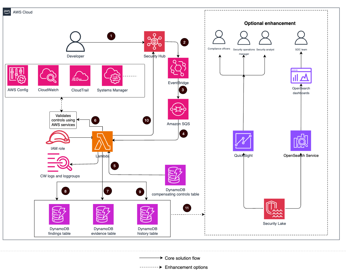
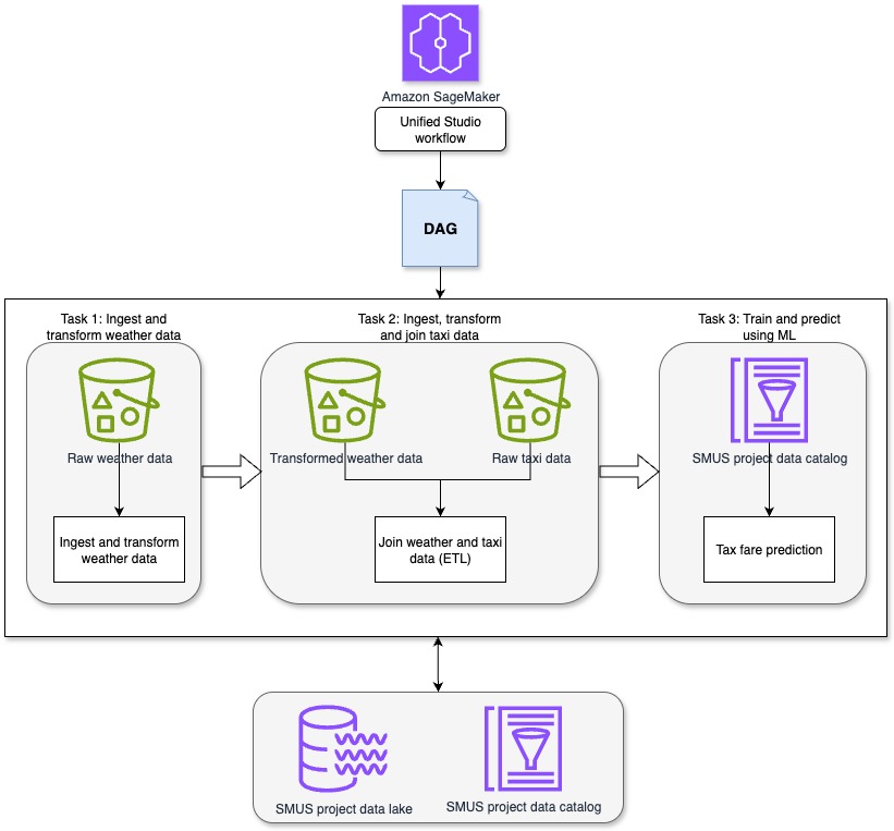
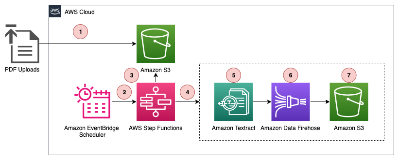
The following architecture diagram illustrates a real-time ICU patient analytics system.

Arch diagram

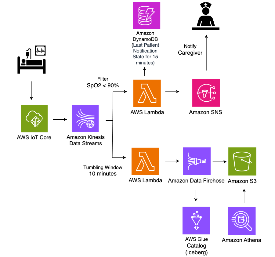
In this architecture, real-time patient monitoring data from hospital ICU sensors is ingested into AWS IoT Core, which then streams the data into Amazon Kinesis Data Streams. Two Lambda functions consume this streaming data concurrently for different purposes, both using Lambda event source mapping integration with Kinesis Data Streams. The first Lambda function uses the filtering feature of event source mapping to detect critical health events where SpO2(blood oxygen saturation) levels fall below 90%, immediately triggering notifications to caregivers through Amazon Simple Notification Service (Amazon SNS) for rapid response. The second Lambda function employs the tumbling window feature of event source mapping to aggregate sensor data over 10-minute time intervals. This aggregated data is then systematically stored in S3 buckets in Apache Iceberg format for historical analysis and reporting. The entire pipeline operates in a serverless manner, providing scalable, real-time processing of critical healthcare data while maintaining both immediate alerting capabilities and long-term data storage for analytics.

Amazon S3 data, with its support for Apache Iceberg table format, enables healthcare organizations to efficiently store and query large volumes of time-series patient data. This solution allows for complex analytical queries across historical patient data while maintaining high performance and cost efficiency.

Prerequisites

To implement the solution provided in this post, you should have the following:

An active AWS account
IAM permissions to deploy CloudFormation templates and provision AWS resources
Python installed on your machine to run the ICU patient sensor data simulator code

Deploy a real-time ICU patient analytics pipeline using CloudFormation

You use AWS CloudFormation templates to create the resources for a real-time data analytics pipeline.

To get started, Sign in to the console as Account user and select the appropriate Region.
Download and launch CloudFormation template where you want to host the Lambda functions.
Choose Next.
On the Specify stack details page, enter a Stack name (for example, IoTHealthMonitoring).
For Parameters, enter the following:
1. IoTTopic: Enter the MQTT topic for your IoT devices (for example, icu/sensors).
2. EmailAddress: Enter an email address for receiving notifications.
Wait for the stack creation to complete. This process might take 5-10 minutes.
After the CloudFormation stack completes, it creates following resources:
1. An AWS IoT Core rule to capture data from the specified IoTTopic topic and routes it to Kinesis data stream.
2. A Kinesis data stream for ingesting IoT sensor data.
3. Two Lambda functions:
  - FilterSensorData: Monitors critical health metrics and sends alerts.
  - AggregateSensorData: Aggregates sensor data in 10 minutes window.
4. An Amazon DynamoDB table (NotificationTimestamps) to store notification timestamps for rate limiting alerts.
5. An Amazon SNS topic and subscription to send email notifications for critical patient conditions.
6. An Amazon Data Firehose delivery stream to deliver processed data to Amazon S3 using Iceberg format.
7. Amazon S3 buckets to store sensor data.
8. Amazon Athena and AWS Glue resources for the database and an Iceberg table for querying aggregated data.
9. AWS Identity and Access Management (IAM) roles and policies to support required permissions for Amazon IoT rules, Lambda functions, and Data Firehose streams.
10. Amazon CloudWatch log groups to record for Kinesis Firehose activity and Lambda functions.

Solution walkthrough

Now that you’ve deployed the solution, let’s review a functional walkthrough. First, simulate patient vital signs data and send it to AWS IoT Core using the following Python code on your local machine. To run this code successfully, ensure you have the necessary IAM permissions to publish messages to the IoT topic in the AWS account where the solution is deployed.

import boto3
import json
import random
import time
# AWS IoT Data client
iot_data_client = boto3.client(
    'iot-data',
    region_name='us-west-2'
)
# IOT Topic to publish
topic = 'icu/sensors'
# Fixed set of patient IDs
patient_ids = [1, 2, 3, 4, 5, 6, 7, 8, 9, 10]
print("Infinite sensor data simulation...")
try:
    while True:
        for patient_id in patient_ids:
            # Generate sensor data
            message = {
                "patient_id": patient_id,
                "timestamp": int(time.time()),
                "spo2": random.randint(91, 99),
                "heart_rate": random.randint(60, 100),
                "temperature_f": round(random.uniform(97.0, 100.0), 1)
            }
            # Publish to topic
            response = iot_data_client.publish(
                topic=topic,
                qos=1,
                payload=json.dumps(message)
            )
            print(f"Published: {message}")
        # Wait 30 seconds before next round
        print("Sleeping for 30 seconds...\n")
        time.sleep(30)
except KeyboardInterrupt:
    print("\nSimulation stopped by user.")

The following is the format of a sample ICU sensor message produced by the simulator.

{
    "patient_id": 1,
    "timestamp": 1683000000,
    "spo2": 85,
    "heart_rate": 75,
    "temperature_f": 98.6
}

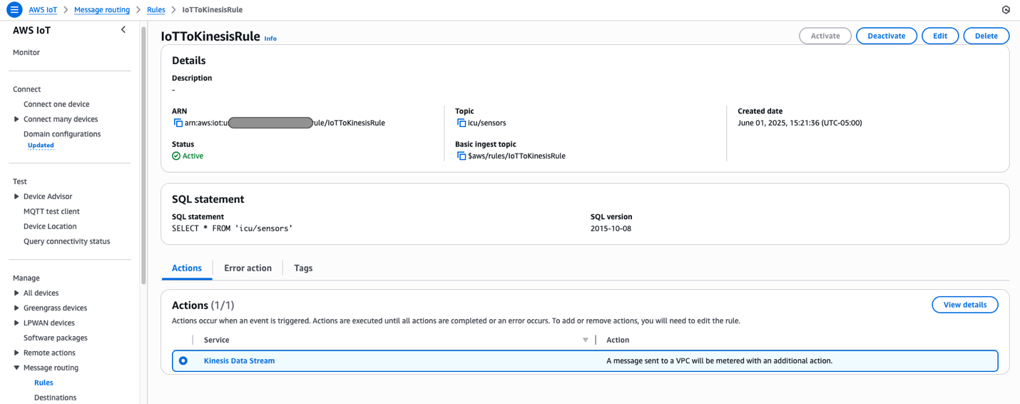
Data is published to the icu/sensors IoT topic every 30 seconds for 10 different patients, creating a continuous stream of ICU patient monitoring data. Messages published to AWS IoT Core are passed to Kinesis Data Streams using the following message routing rule deployed by our solution.

Two Lambda functions consume data from Data Streams concurrently, both using the Lambda event source mapping integration with Kinesis Data Streams.

Event source mapping

Lambda event source mapping automatically triggers Lambda functions in response to data changes from supported event sources like Amazon DynamoDB Streams, Amazon Kinesis Data Streams, Amazon Simple Queue Service (Amazon SQS), Amazon MQ, and Amazon Managed Streaming for Apache Kafka. This serverless integration works by having Lambda poll these sources for new records, which are then processed in configurable batch sizes ranging from 1 to 10,000 records. When new data is detected, Lambda automatically invokes the function synchronously, handling the scaling automatically based on the workload. The service supports at-least-once delivery and provides robust error handling through retry policies and dead-letter queues for failed events. Event source mappings can be fine-tuned through various parameters such as batch windows, maximum record age, and retry attempts, making them highly adaptable to different use cases. This feature is particularly valuable in event-driven architectures, so that customers can focus on business logic while AWS manages the complexities of event processing, scaling, and reliability.

Event source mapping uses tumbling windows and filtering to process and analyze data.

Tumbling windows

Tumbling windows in Lambda event processing enable data aggregation in fixed, non-overlapping time intervals, where each event belongs to exactly one window. This is ideal for time-based analytics and periodic reporting. When combined with event source mapping, this approach allows efficient batch processing of events within defined time periods (for example, 10-minute windows), enabling calculations such as average vital signs or cumulative fluid intake and output while optimizing function invocations and resource usage.

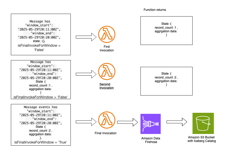
When you configure an event source mapping between Kinesis Data Streams and a Lambda function, use the Tumbling Window Duration setting, which appears in the trigger configuration in the Lambda console. The solution you deployed using the CloudFormation template includes the AggregateSensorData Lambda function, which uses a 10-minute tumbling window configuration. Depending on the volume of messages flowing through the Amazon Kinesis stream, the AggregateSensorData function can be invoked multiple times for each 10-minute window, sequentially, with the following attributes in the event supplied to the function.

Window start and end: The beginning and ending timestamps for the current tumbling window.
State: An object containing the state returned from the previous window, which is initially empty. The state object can contain up to 1 MB of data.
isFinalInvokeForWindow: Indicates if this is the last invocation for the tumbling window. This only occurs once per window period.
isWindowTerminatedEarly: A window ends early only if the state exceeds the maximum allowed size of 1 MB.

In a tumbling window, there is a series of Lambda invocations in the following pattern:

AggregateSensorData Lambda code snippet:

def handler(event, context):
    
    state_across_window = event['state']
    # Iterate through each record and decode the base64 data
    for record in event['Records']:
        encoded_data = record['kinesis']['data']
        partition_key = record['kinesis']['partitionKey']
        decoded_bytes = base64.b64decode(encoded_data)
        decoded_str = decoded_bytes.decode('utf-8')
        decoded_json = json.loads(decoded_str)
        # create partition_key attribute if it do not exists in state
        if partition_key not in state_across_window:
            state_across_window[partition_key] = {"min_spo2": decoded_json['spo2'], "max_spo2": decoded_json['spo2'], "avg_spo2": decoded_json['spo2'], "sum_spo2": decoded_json['spo2'], "min_heart_rate": decoded_json['heart_rate'], "max_heart_rate": decoded_json['heart_rate'], "avg_heart_rate": decoded_json['heart_rate'], "sum_heart_rate": decoded_json['heart_rate'], "min_temperature_f": decoded_json['temperature_f'], "max_temperature_f": decoded_json['temperature_f'], "avg_temperature_f": decoded_json['temperature_f'], "sum_temperature_f": decoded_json['temperature_f'], "record_count": 1}
        else:
            min_spo2 = state_across_window[partition_key]['min_spo2'] if state_across_window[partition_key]['min_spo2'] < decoded_json['spo2'] else decoded_json['spo2']
            max_spo2 = state_across_window[partition_key]['max_spo2'] if state_across_window[partition_key]['max_spo2'] > decoded_json['spo2'] else decoded_json['spo2']
            sum_spo2 = state_across_window[partition_key]['sum_spo2'] + decoded_json['spo2']
            min_heart_rate = state_across_window[partition_key]['min_heart_rate'] if state_across_window[partition_key]['min_heart_rate'] < decoded_json['heart_rate'] else decoded_json['heart_rate']
            max_heart_rate = state_across_window[partition_key]['max_heart_rate'] if state_across_window[partition_key]['max_heart_rate'] > decoded_json['heart_rate'] else decoded_json['heart_rate']
            sum_heart_rate = state_across_window[partition_key]['sum_heart_rate'] + decoded_json['heart_rate']
            
            min_temperature_f = state_across_window[partition_key]['min_temperature_f'] if state_across_window[partition_key]['min_temperature_f'] < decoded_json['temperature_f'] else decoded_json['temperature_f']
            max_temperature_f = state_across_window[partition_key]['max_temperature_f'] if state_across_window[partition_key]['max_temperature_f'] > decoded_json['temperature_f'] else decoded_json['temperature_f']
            sum_temperature_f = state_across_window[partition_key]['sum_temperature_f'] + decoded_json['temperature_f']
            
            record_count = state_across_window[partition_key]['record_count'] + 1
            avg_spo2 = sum_spo2/record_count
            avg_heart_rate = sum_heart_rate/record_count
            avg_temperature_f = sum_temperature_f/record_count
            
            state_across_window[partition_key] = {"min_spo2": min_spo2, "max_spo2": max_spo2, "avg_spo2": avg_spo2, "sum_spo2": sum_spo2, "min_heart_rate": min_heart_rate, "max_heart_rate": max_heart_rate, "avg_heart_rate": avg_heart_rate, "sum_heart_rate": sum_heart_rate, "min_temperature_f": min_temperature_f, "max_temperature_f": max_temperature_f, "avg_temperature_f": avg_temperature_f, "sum_temperature_f": sum_temperature_f, "record_count": record_count}
        
    # Determine if the window is final (window end)
    is_final_window = event.get('isFinalInvokeForWindow', False)
    # Determine if the window is terminated (window ended early)
    is_terminated_window = event.get('isWindowTerminatedEarly', False)
    window_start = event['window']['start']
    window_end = event['window']['end']
    if is_final_window or is_terminated_window:
        firehose_client = boto3.client('firehose')
        firehose_stream = os.environ['FIREHOSE_STREAM_NAME']
        for key, value in state_across_window.items():
            value['patient_id'] = key
            value['window_start'] = window_start
            value['window_end'] = window_end
            
            firehose_client.put_record(
                DeliveryStreamName= firehose_stream,
                Record={'Data': json.dumps(value) }
            )
        
        return {
            "state": {},
            "batchItemFailures": []
        }
    else:
        print(f"interim call for window: ws: {window_start} we: {window_end}")
        return {
            "state": state_across_window,
            "batchItemFailures": []
        }

The first invocation contains an empty state object in the event. The function returns a state object containing custom attributes that are specific to the custom logic in the aggregation.
The second invocation contains the state object provided by the first Lambda invocation. This function returns an updated state object with new aggregated values. Subsequent invocations follow this same sequence. Following is a sample of the aggregated state, which can be supplied to subsequent Lambda invocations within the same 10-minute tumbling window.

{
    "min_spo2": 88,
    "max_spo2": 90,
    "avg_spo2": 89.2,
    "sum_spo2": 625,
    "min_heart_rate": 21,
    "max_heart_rate": 22,
    "avg_heart_rate": 21.1,
    "sum_heart_rate": 148,
    "min_temperature_f": 90,
    "max_temperature_f": 91,
    "avg_temperature_f": 90.1,
    "sum_temperature_f": 631,
    "record_count": 7,
    "patient_id": "44",
    "window_start": "2025-05-29T20:51:00Z",
    "window_end": "2025-05-29T20:52:00Z"
}

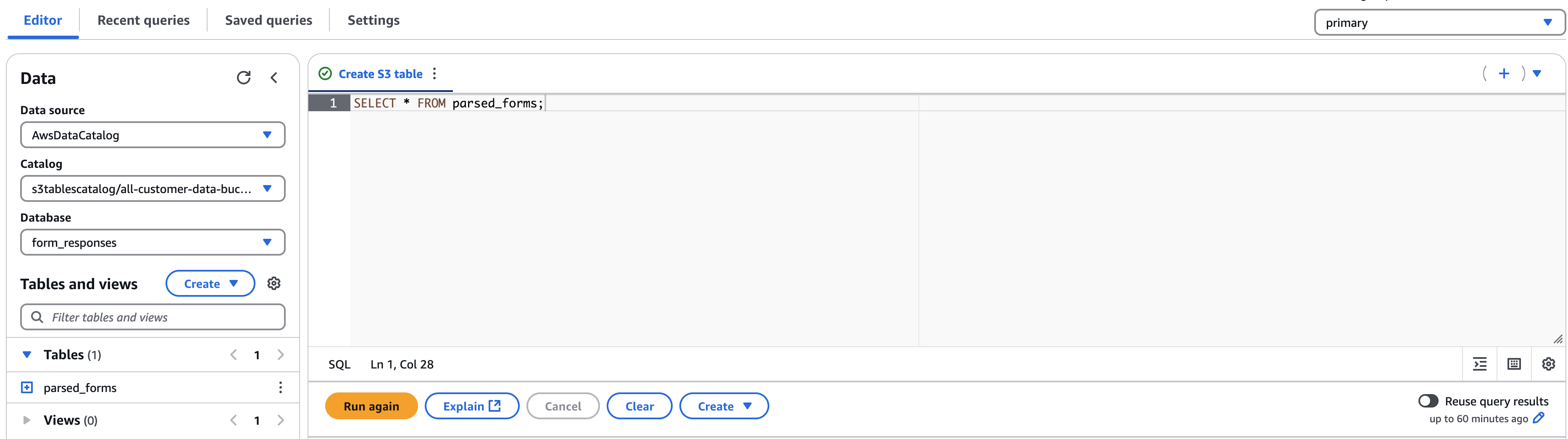
The final invocation in the tumbling window has the isFinalInvokeForWindow flag set to the true. This contains the state returned by the most recent Lambda invocation. This invocation is responsible for passing aggregated state messages to the Data Firehose stream, which delivers data to the Amazon S3 bucket using Iceberg data format.
After the aggregated data is sent to Amazon S3, you can query the data using Athena.

Query: SELECT * FROM "cfdb_<<Database>>"."table_<<Table>>"

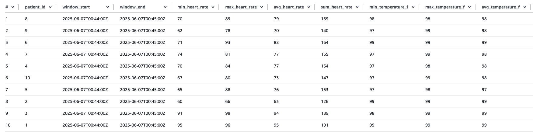
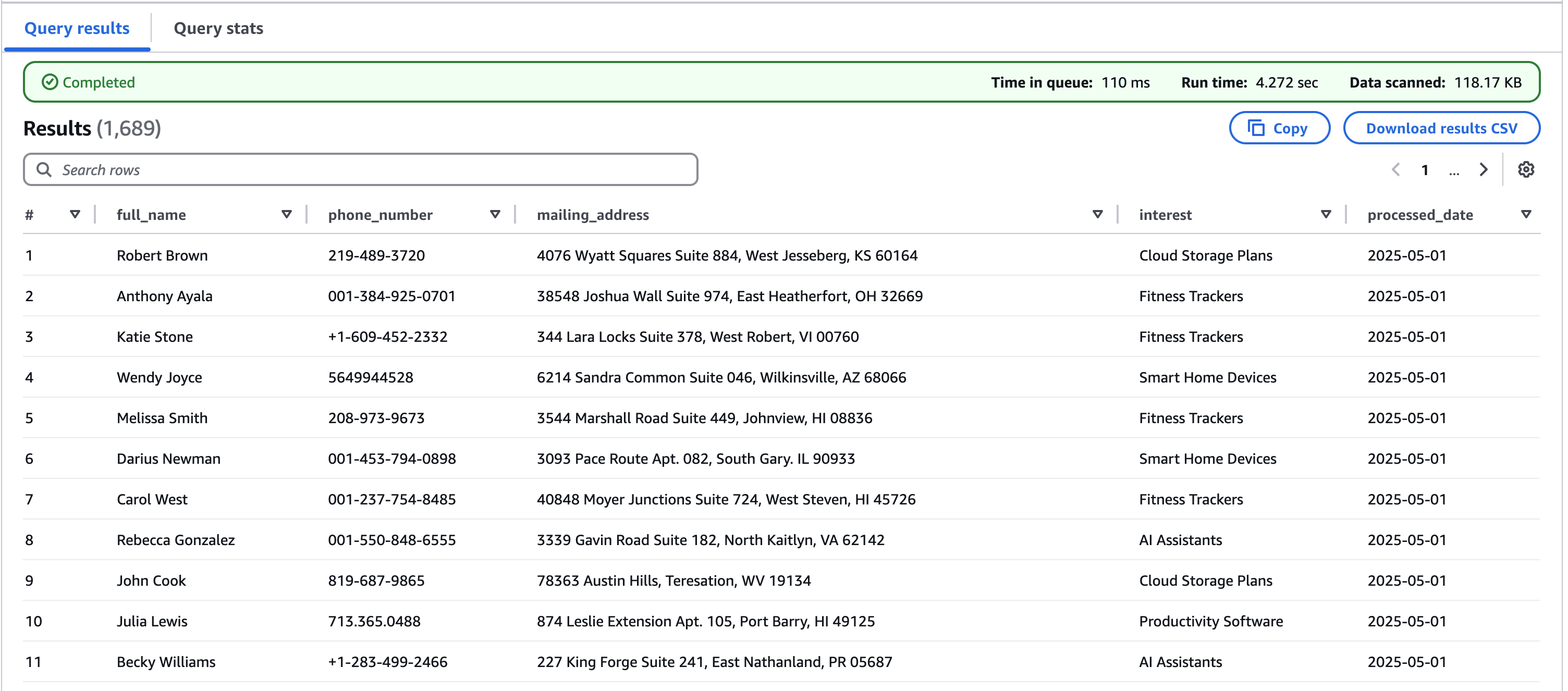
Sample result of the preceding Athena query:

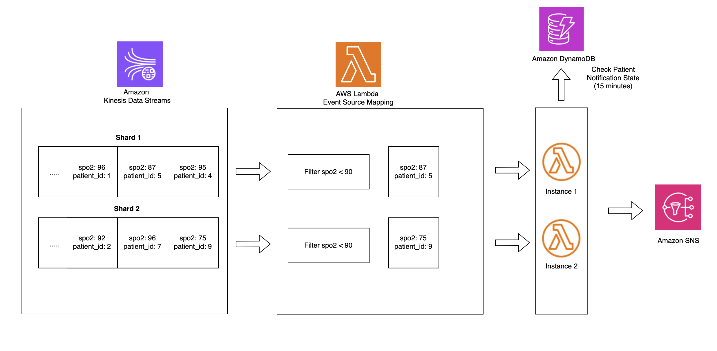
Event source mapping with filtering

Lambda event source mapping with filtering optimizes data processing from sources like Amazon Kinesis by applying JSON pattern filtering before function invocation. This is demonstrated in the ICU patient monitoring solution, where the system filters for SpO2 readings from Kinesis Data Streams that are below 90%. Instead of processing all incoming data, the filtering capability is used to selectively processes only critical readings, significantly reducing costs and processing overhead. The solution uses DynamoDB for sophisticated state management, tracking low SpO2 events through a schema combining PatientID and timestamp-based keys within defined monitoring windows.

This state-aware implementation balances clinical urgency with operational efficiency by sending immediate Amazon SNS notifications when critical conditions are first detected while implementing a 15-minute alert suppression window to prevent alert fatigue among healthcare providers. By maintaining state across multiple Lambda invocations, the system helps ensure rapid response to potentially life-threatening situations while minimizing unnecessary notifications for the same patient condition. The integration of Lambda’event filtering, DynamoDB state management, and reliable alert delivery provided by Amazon SNS creates a robust, scalable healthcare monitoring solution that exemplifies how AWS services can be strategically combined to address complex requirements while balancing technical efficiency with clinical effectiveness.

Filter sensor data Lambda code snippet:

sns_client = boto3.client('sns')
dynamodb = boto3.resource('dynamodb')
table_name = os.environ['DYNAMODB_TABLE']
sns_topic_arn = os.environ['SNS_TOPIC_ARN']
table = dynamodb.Table(table_name)
FIFTEEN_MINUTES = 15 * 60  # 15 minutes in seconds
def handler(event, context):
    for record in event['Records']:
        print(f"Aggregated event: {record}")
        encoded_data = record['kinesis']['data']
        partition_key = record['kinesis']['partitionKey']
        decoded_bytes = base64.b64decode(encoded_data)
        decoded_str = decoded_bytes.decode('utf-8')
        # Check last notification timestamp from DynamoDB
        try:
            response = table.get_item(Key={'partition_key': partition_key})
            item = response.get('Item')
            now = int(time.time())
            if item:
                last_sent = item.get('timestamp', 0)
                if now - last_sent < FIFTEEN_MINUTES:
                    print(f"Notification for {partition_key} skipped (sent recently)")
                    continue
            # Send SNS Notification
            sns_response = sns_client.publish(
                TopicArn=sns_topic_arn,
                Message=f"Patient SpO2 below 90 percentage event information: {decoded_str}",
                Subject=f"Low SpO2 detected for patient ID {partition_key}"
            )
            print("Message sent to SNS! MessageId:", sns_response['MessageId'])
            # Update DynamoDB with current timestamp and TTL
            table.put_item(Item={
                'partition_key': partition_key,
                'timestamp': now,
                'ttl': now + FIFTEEN_MINUTES + 60  # Add extra buffer to TTL
            })
        except Exception as e:
            print("Error processing event:", e)
            return {
                'statusCode': 500,
                'body': json.dumps('Error processing event')
            }
    return {
        'statusCode': 200,
        'body': {}
    }

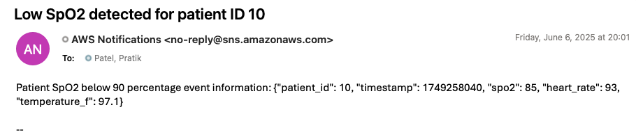
To generate an alert notification through the deployed solution, update the preceding simulator code by setting the SpO2 value to less than 90 and run it again. Within 1 minute, you should receive an alert notification at the email address you provided during stack creation. The following image is an example of an alert notification generated by the deployed solution.

Clean up

To avoid ongoing costs after completing this tutorial, delete the CloudFormation stack that you deployed earlier in this post. This will remove most of the AWS resources created for this solution. You might need to manually delete objects created in Amazon S3, because CloudFormation won’t remove non-empty buckets during stack deletion.

Conclusion

As demonstrated in this post, you can build a serverless real-time analytics pipeline for healthcare monitoring by using AWS IoT Core, Amazon S3 buckets with iceberg format, and Amazon Kinesis Data Streams integration with AWS Lambda event source mapping. This architectural approach eliminates the need for complex code while enabling rapid critical patient care alerts and data aggregation for analysis using Lambda. The solution is particularly valuable for healthcare organizations looking to modernize their patient monitoring systems with real-time capabilities. The architecture can be extended to handle various medical devices and sensor data streams, making it adaptable for different healthcare monitoring scenarios. This post presents one implementation approach, and organizations adopting this solution should ensure the architecture and code meets their specific application performance, security, privacy, and regulatory compliance needs.

If this post helps you or inspires you to solve a problem, we would love to hear about it!

About the authors

Best practices for migrating from Apache Airflow 2.x to Apache Airflow 3.x on Amazon MWAA

2025-10-07 Anurag Srivastava

Post Syndicated from Anurag Srivastava original https://aws.amazon.com/blogs/big-data/best-practices-for-migrating-from-apache-airflow-2-x-to-apache-airflow-3-x-on-amazon-mwaa/

Apache Airflow 3.x on Amazon MWAA introduces architectural improvements such as API-based task execution that provides enhanced security and isolation. Other major updates include a redesigned UI for better user experience, scheduler-based backfills for improved performance, and support for Python 3.12. Unlike in-place minor Airflow version upgrades in Amazon MWAA, upgrading to Airflow 3 from Airflow 2 requires careful planning and execution through a migration approach due to fundamental breaking changes.

This migration presents an opportunity to embrace next-generation workflow orchestration capabilities while providing business continuity. However, it’s more than a simple upgrade. Organizations migrating to Airflow 3.x on Amazon MWAA must understand key breaking changes, including the removal of direct metadata database access from workers, deprecation of SubDAGs, changes to default scheduling behavior, and library dependency updates. This post provides best practices and a streamlined approach to successfully navigate this critical migration, providing minimal disruption to your mission-critical data pipelines while maximizing the enhanced capabilities of Airflow 3.

Understanding the migration process

The journey from Airflow 2.x to 3.x on Amazon MWAA introduces several fundamental changes that organizations must understand before beginning their migration. These changes affect core workflow operations and require careful planning to achieve a smooth transition.

You should be aware of the following breaking changes:

Removal of direct database access – A critical change in Airflow 3 is the removal of direct metadata database access from worker nodes. Tasks and custom operators must now communicate through the REST API instead of direct database connections. This architectural change affects code that previously accessed the metadata database directly through SQLAlchemy connections, requiring refactoring of existing DAGs and custom operators.
SubDAG deprecation – Airflow 3 removes the SubDAG construct in favor of TaskGroups, Assets, and Data Aware Scheduling. Organizations must refactor existing SubDAGs to one of the previously mentioned constructs.
Scheduling behavior changes – Two notable changes to default scheduling options require an impact analysis:
- The default values for catchup_by_default and create_cron_data_intervals changed to False. This change affects DAGs that don’t explicitly set these options.
- Airflow 3 removes several context variables, such as execution_date, tomorrow_ds, yesterday_ds, prev_ds, and next_ds. You must replace these variables with currently supported context variables.
Library and dependency changes – A significant number of libraries change in Airflow 3.x, requiring DAG code refactoring. Many previously included provider packages might need explicit addition to the requirements.txt file.
REST API changes – The REST API path changes from /api/v1 to /api/v2, affecting external integrations. For more information about using the Airflow REST API, see Creating a web server session token and calling the Apache Airflow REST API.
Authentication system – Although Airflow 3.0.1 and later versions default to SimpleAuthManager instead of Flask-AppBuilder, Amazon MWAA will continue using Flask-AppBuilder for Airflow 3.x. This means customers on Amazon MWAA will not see any authentication changes.

The migration requires creating a new environment rather than performing an in-place upgrade. Although this approach demands more planning and resources, it provides the advantage of maintaining your existing environment as a fallback option during the transition, facilitating business continuity throughout the migration process.

Pre-migration planning and assessment

Successful migration depends on thorough planning and assessment of your current environment. This phase establishes the foundation for a smooth transition by identifying dependencies, configurations, and potential compatibility issues. Evaluate your environment and code against the previously mentioned breaking changes to have a successful migration.

Environment assessment

Begin by conducting a complete inventory of your current Amazon MWAA environment. Document all DAGs, custom operators, plugins, and dependencies, including their specific versions and configurations. Make sure your current environment is on version 2.10.x, because this provides the best compatibility path for upgrading to Amazon MWAA with Airflow 3.x.

Identify the structure of the Amazon Simple Storage Service (Amazon S3) bucket containing your DAG code, requirements file, startup script, and plugins. You will replicate this structure in a new bucket for the new environment. Creating separate buckets for each environment avoids conflicts and allows continued development without affecting current pipelines.

Configuration documentation

Document all custom Amazon MWAA environment variables, Airflow connections, and environment configurations. Review AWS Identity and Access Management (IAM) resources, because your new environment’s execution role will need identical policies. IAM users or roles accessing the Airflow UI require the CreateWebLoginToken permission for the new environment.

Pipeline dependencies

Understanding pipeline dependencies is critical for a successful phased migration. Identify interdependencies through Datasets (now Assets), SubDAGs, TriggerDagRun operators, or external API interactions. Develop your migration plan around these dependencies so related DAGs can migrate at the same time.

Consider DAG scheduling frequency when planning migration waves. DAGs with longer intervals between runs provide larger migration windows and lower risk of duplicate execution compared with frequently running DAGs.

Testing strategy

Create your testing strategy by defining a systematic approach to identifying compatibility issues. Use the ruff linter with the AIR30 ruleset to automatically identify code requiring updates:

ruff check --preview --select AIR30 <path_to_your_dag_code>

Then, review and update your environment’s requirements.txt file to make sure package versions comply with the updated constraints file. Additionally, commonly used Operators previously included in the airflow-core package now reside in a separate package and need to be added to your requirements file.

Test your DAGs using the Amazon MWAA Docker images for Airflow 3.x. These images make it possible to create and test your requirements file, and confirm the Scheduler successfully parses your DAGs.

Migration strategy and best practices

A methodical migration approach minimizes risk while providing clear validation checkpoints. The recommended strategy employs a phased blue/green deployment model that provides reliable migrations and immediate rollback capabilities.

Phased migration approach

The following migration phases can assist you in defining your migration plan:

Phase 1: Discovery, assessment, and planning – In this phase, complete your environment inventory, dependency mapping, and breaking change analysis. With the gathered information, develop the detailed migration plan. This plan will include steps for updating code, updating your requirements file, creating a test environment, testing, creating the blue/green environment (discussed later in this post), and the migration steps. Planning must also include the training, monitoring strategy, rollback conditions, and the rollback plan.
Phase 2: Pilot migration – The pilot migration phase serves to validate your detailed migration plan in a controlled environment with a small range of impact. Focus the pilot on two or three non-critical DAGs with diverse characteristics, such as different schedules and dependencies. Migrate the selected DAGs using the migration plan defined in the previous phase. Use this phase to validate your plan and monitoring tools, and adjust both based on actual results. During the pilot, establish baseline migration metrics to help predict the performance of the full migration.
Phase 3: Wave-based production migration – After a successful pilot, you are ready to begin the full wave-based migration for the remaining DAGs. Group remaining DAGs into logical waves based on business criticality (least critical first), technical complexity, interdependencies (migrate dependent DAGs together), and scheduling frequency (less frequent DAGs provide larger migration windows). After you define the waves, work with stakeholders to develop the wave schedule. Include sufficient validation periods between waves to confirm the wave is successful before starting the next wave. This time also reduces the range of impact in the event of a migration issue, and provides sufficient time to perform a rollback.
Phase 4: Post-migration review and decommissioning – After all waves are complete, conduct a post-migration review to identify lessons learned, optimization opportunities, and any other unresolved items. This is also a good time to provide an approval on system stability. The final step is decommissioning the original Airflow 2.x environment. After stability is determined, based on business requirements and input, decommission the original (blue) environment.

Blue/green deployment strategy

Implement a blue/green deployment strategy for safe, reversible migration. With this strategy, you will have two Amazon MWAA environments operating during the migration and manage which DAGs operate in which environment.

The blue environment (current Airflow 2.x) maintains production workloads during transition. You can implement a freeze window for DAG changes before migration to avoid last-minute code conflicts. This environment serves as the immediate rollback environment if an issue is identified in the new (green) environment.

The green environment (new Airflow 3.x) receives migrated DAGs in controlled waves. It mirrors the networking, IAM roles, and security configurations from the blue environment. Configure this environment with the same options as the blue environment, and create identical monitoring mechanisms so both environments can be monitored simultaneously. To avoid duplicate DAG runs, make sure a DAG only runs in a single environment. This involves pausing the DAG in the blue environment before activating the DAG in the green environment.Maintain the blue environment in warm standby mode during the entire migration. Document specific rollback steps for each migration wave, and test your rollback procedure for at least one non-critical DAG. Additionally, define clear criteria for triggering the rollback (such as specific failure rates or SLA violations).

Step-by-step migration process

This section provides detailed steps for conducting the migration.

Pre-migration assessment and preparation

Before initiating the migration process, conduct a thorough assessment of your current environment and develop the migration plan:

Make sure your current Amazon MWAA environment is on version 2.10.x
Create a detailed inventory of your DAGs, custom operators, and plugins including their dependencies and versions
Review your current requirements.txt file to understand package requirements
Document all environment variables, connections, and configuration settings
Review the Apache Airflow 3.x release notes to understand breaking changes
Determine your migration success criteria, rollback conditions, and rollback plan
Identify a small number of DAGs suitable for the pilot migration
Develop a plan to train, or familiarize, Amazon MWAA users on Airflow 3

Compatibility checks

Identifying compatibility issues is critical to a successful migration. This step helps developers focus on specific code that is incompatible with Airflow 3.

Use the ruff linter with the AIR30 ruleset to automatically identify code requiring updates:

ruff check --preview --select AIR30 <path_to_your_dag_code>

Additionally, review your code for instances of direct metadatabase access.

DAG code updates

Based on your findings during compatibility testing, update the affected DAG code for Airflow 3.x. The ruff DAG check utility can automatically fix common changes. Use the following command to run the utility in update mode:

ruff check dag/ --select AIR301 --fix –preview

Common changes include:

Replace direct metadata database access with API calls:

# Before (Airflow 2.x) - Direct DB access
from airflow.settings import Session
from airflow.models.taskInstance import TaskInstance
session=Session()
result=session.query(TaskInstance)

For Apache Airflow v3.x, utilize  in the Amazon MWAA SDK.
Update core construct imports with the new Airflow SDK namespace:
# Before (Airflow 2.x)
from airflow.decorators import dag, task

# After (Airflow 3.x)
from airflow.sdk import dag, task

Replace deprecated context variables with their modern equivalents:

# Before (Airflow 2.x)
def my_task(execution_date, **context):
    # Using execution_date

# After (Airflow 3.x)
def my_task(logical_date, **context):
    # Using logical_date

Next, evaluate the usage of the two scheduling-related default changes. catchup_by_default is now False, meaning missing DAG runs will no longer automatically backfill. If backfill is required, update the DAG definition with catchup=True. If your DAGs require backfill, you must consider the impact of this migration and backfilling. Because you’re migrating a DAG to a clean environment with no history, enabling backfilling will create DAG runs for all runs beginning with the specified start_date. Consider updating the start_date to avoid unnecessary runs.

create_cron_data_intervals is also now False. With this change, cron expressions are evaluated as a CronTriggerTimetable construct.

Finally, evaluate the usage of deprecated context variables for manually and Asset-triggered DAGs, then update your code with suitable replacements.

Updating requirements and testing

In addition to possible package version changes, several core Airflow operators previously included in the airflow-core package moved to the apache-airflow-providers-standard package. These changes must be incorporated into your requirements.txt file. Specifying, or pinning, package versions in your requirements file is a best practice and recommended for this migration.To update your requirements file, complete the following steps:

Download and configure the Amazon MWAA Docker images. For more details, refer to the GitHub repo.
Copy the current environment’s requirements.txt file to a new file.
If needed, add the apache-airflow-providers-standard package to the new requirements file.
Download the appropriate Airflow constraints file for your target Airflow version to your working director. A constraints file is available for each Airflow version and Python version combination. The URL takes the following form:
https://raw.githubusercontent.com/apache/airflow/constraints-${AIRFLOW_VERSION}/constraints-${PYTHON_VERSION}.txt
Create your versioned requirements file using your un-versioned file and the constraints file. For guidance on creating a requirements file, see Creating a requirements.txt file. Make sure there are no dependency conflicts before moving forward.
Verify your requirements file using the Docker image. Run the following command inside the running container:
```
./run.sh test-requirements
```
Address any installation errors by updating package versions.

As a best practice, we recommend packaging your packages into a ZIP file for deployment in Amazon MWAA. This makes sure the same exact packages are installed on all Airflow nodes. Refer to Installing Python dependencies using PyPi.org Requirements File Format for detailed information about packaging dependencies.

Creating a new Amazon MWAA 3.x environment

Because Amazon MWAA requires a migration approach for major version upgrades, you must create a new environment for your blue/green deployment. This post uses the AWS Command Line Interface (AWS CLI) as an example, you can also use infrastructure as code (IaC).

Create a new S3 bucket using the same structure as the current S3 bucket.
Upload the updated requirements file and any plugin packages to the new S3 bucket.

Generate a template for your new environment configuration:

aws mwaa create-environment --generate-cli-skeleton > new-mwaa3-env.json

Modify the generated JSON file:
1. Copy configurations from your existing environment.
2. Update the environment name.
3. Set the AirflowVersion parameter to the target 3.x version.
4. Update the S3 bucket properties with the new S3 bucket name.
5. Review and update other configuration parameters as needed.
Configure the new environment with the same networking settings, security groups, and IAM roles as your existing environment. Refer to the Amazon MWAA User Guide for these configurations.

Create your new environment:

aws mwaa create-environment --cli-input-json file://new-mwaa3-env.json

Metadata migration

Your new environment requires the same variables, connections, roles, and pool configurations. Use this section as a guide for migrating this information. If you’re using AWS Secrets Manager as your secrets backend, you don’t need to migrate any connections. Depending your environment’s size, you can migrate this metadata using the Airflow UI or the Apache Airflow REST API.

Update any custom pool information in the new environment using the Airflow UI.
For environments using the metadatabase as a secrets backend, migrate all connections to the new environment.
Migrate all variables to the new environment.
Migrate any custom Airflow roles to the new environment.

Migration execution and validation

Plan and execute the transition from your old environment to the new one:

Schedule the migration during a period of low workflow activity to minimize disruption.
Implement a freeze window for DAG changes before and during the migration.
Execute the migration in phases:
1. Pause DAGs in the old environment. For a small number of DAGs, you can use the Airflow UI. For larger groups, consider using the REST API.
2. Verify all running tasks have completed in the Airflow UI.
3. Redirect DAG triggers and external integrations to the new environment.
4. Copy the updated DAGs to the new environment’s S3 bucket.
5. Enable DAGs in the new environment. For a small number of DAGs, you can use the Airflow UI. For larger groups, consider using the REST API.
Monitor the new environment closely during the initial operation period:
1. Watch for failed tasks or scheduling issues.
2. Check for missing variables or connections.
3. Verify external system integrations are functioning correctly.
4. Monitor Amazon CloudWatch metrics to confirm the environment is performing as expected.

Post-migration validation

After the migration, thoroughly validate the new environment:

Verify that all DAGs are being scheduled correctly according to their defined schedules
Check that task history and logs are accessible and complete
Test critical workflows end-to-end to confirm they execute successfully
Validate connections to external systems are functioning properly
Monitor CloudWatch metrics for performance validation

Cleanup and documentation

When the migration is complete and the new environment is stable, complete the following steps:

Document the changes made during the migration process.
Update runbooks and operational procedures to reflect the new environment.
After a sufficient stability period, defined by stakeholders, decommission the old environment:
```
aws mwaa delete-environment --name old-mwaa2-env
```
Archive backup data according to your organization’s retention policies.

Conclusion

The journey from Airflow 2.x to 3.x on Amazon MWAA is an opportunity to embrace next-generation workflow orchestration capabilities while maintaining the reliability of your workflow operations. By following these best practices and maintaining a methodical approach, you can successfully navigate this transition while minimizing risks and disruptions to your business operations.

A successful migration requires thorough preparation, systematic testing, and maintaining clear documentation throughout the process. Although the migration approach requires more initial effort, it provides the safety and control needed for such a significant upgrade.

About the authors

Breaking down data silos: Volkswagen’s approach with Amazon DataZone

2025-10-07 Bandana Das

Post Syndicated from Bandana Das original https://aws.amazon.com/blogs/big-data/breaking-down-data-silos-volkswagens-approach-with-amazon-datazone/

Over the years, organizations have invested in building purpose-built cloud-based data warehouses that are siloed from one another. One of the major challenges these organizations encounter today is enabling cross-organization discovery and access to data across these siloed data warehouses built using different technology stacks. The data mesh pattern addresses these issues, founded in four principles: domain-oriented decentralized data ownership and architecture, treating data as a product, providing self-serve data infrastructure as a platform, and implementing federated governance. The data mesh pattern helps organizations mimic their organizational structure into data domains and makes it possible to share the data across the organization and beyond to improve their business models.

In 2019, Volkswagen AG and Amazon Web Services (AWS) started their collaboration to co-develop the Digital Production Platform (DPP), with the goal of enhancing production and logistics efficiency by 30% while reducing production costs by the same margin. The DPP was developed to streamline access to data from shop floor devices and manufacturing systems by handling integrations and providing a range of standardized interfaces. However, as applications and use cases evolved on the platform, a significant challenge emerged: the ability to share data across applications stored in isolated data warehouses (within Amazon Redshift in isolated AWS accounts designated for specific use cases), without the need to consolidate data into a central data warehouse. Another challenge was discovering all the available data stored across multiple data warehouses and facilitating a workflow to request access to data across business domains within each plant. The common method used was largely manual, relying on emails and general communication (through tickets and emails). The manual approach not only increased the overhead but also varied from one use case to another in terms of data governance.

In this post, we introduce Amazon DataZone and explore how Volkswagen used Amazon DataZone to build their data mesh, tackle the challenges encountered, and break the data silos. A key aspect of the solution was enabling data providers to automatically publish their data products to Amazon DataZone, serving as a central data mesh for enhanced data discoverability. Additionally, we provide code to guide you through the deployment and implementation process.

Introduction to Amazon DataZone

Amazon DataZone is a data management service that makes it faster and straightforward to catalog, discover, share, and govern data stored across AWS, on-premises, and third-party sources. Key features of Amazon DataZone include the business data catalog, with which users can search for published data, request access, and start working on data in days instead of weeks. In addition, the service facilitates collaboration across teams and helps them manage and monitor data assets across different organizational units. The service also includes the Amazon DataZone portal, which offers a personalized analytics experience for data assets through a web-based application or API. Lastly, Amazon DataZone offers governed data sharing, which makes sure the right data is accessed by the right user for the right purpose with a governed workflow.

Solution overview

The following architecture diagram represents a high-level design that is built on top of the data mesh pattern. It separates source systems, data domain producers (data publishers), data domain subscribers (data consumers), and central governance to highlight the key aspects. This data mesh architecture is specially tailored for cross-AWS account usage. The objective of this approach is to create a foundation for building data governance on a scale, supporting the objectives of data producers and consumers with strong and consistent governance.

This architecture allows for the integration of multiple data warehouses into a centralized governance account that stores all the metadata from each environment.

A data domain producer uses Amazon Redshift as their analytical data warehouse to store, process, and manage structured and semi-structured data. The data domain producers load data into their respective Amazon Redshift clusters through extract, transform, and load (ETL) pipelines they manage, own, and operate. The producers maintain control over their data through Amazon Redshift security features, including column-level access controls and dynamic data masking, supporting data governance at the source. A data domain producer uses Amazon Redshift ETL and Amazon Redshift Spectrum to process and transform raw data into consumable data products. The data products could be Amazon Redshift tables, views, or materialized views.

Data domain producers expose datasets to the rest of the organization by registering them to Amazon DataZone service, which acts as a central data catalog. They can choose what data assets to share, for how long, and how consumers can interact with these. They’re also responsible for maintaining the data and making sure it’s accurate and current.

The data assets from the producers are then published using the data source run to Amazon DataZone in the central governance account. This process populates the technical metadata into the business data catalog for each data asset. The business metadata can be added by business users (data analysts) to provide business context, tags, and data classification for the datasets. This approach provides the required features to allow producers to create catalog entries with Amazon Redshift from all their data warehouses built in with Redshift clusters. In addition, the central data governance account is used to share datasets securely between producers and consumers. It’s important to note that sharing is done through metadata linking alone. No data (except logs) exists in the governance account. The data isn’t copied to the central account; just a reference to the data is used, so that the data ownership remains with the producer.

Amazon DataZone provides a streamlined way to search for data. The Amazon DataZone data portal provides a personalized view for users to discover and search data assets. An Amazon DataZone user (consumer) with permissions to access the data portal can search for assets and submit requests for subscription of data assets using a web-based application. An approver can then approve or reject the subscription request.

When a data domain consumer has access to an asset in the catalog, they can consume it (query and analyze) using the Amazon Redshift query editor. Each consumer runs their own workload based on their use case. In this way, the team can choose the tools for the job to perform analytics and machine learning activities in its AWS consumer environment.

Publishing and registering data assets to Amazon DataZone

To publish a data asset from the producer account, each asset must be registered in Amazon DataZone for consumer subscription. For more information, refer to Create and run an Amazon DataZone data source for Amazon Redshift. In the absence of an automated registration process, required tasks must be completed manually for each data asset.

Using the automated registration workflow, the manual steps can be automated for the Amazon Redshift data asset (Redshift table or view) that needs to be published in an Amazon DataZone domain or when there’s a schema change in an already published data asset.

The following architecture diagram represents how data assets from Amazon Redshift data warehouses have been automatically published to the data mesh created with Amazon DataZone.

The process consists of the following steps:

In the producer account (Account B), the data to be shared resides in a Redshift cluster.
The producer account (Account B) uses a mechanism to trigger the dataset registration AWS Lambda function with a specific payload containing the information and name of the database, schema, table, or view that has a change in metadata.
The Lambda function performs the steps to automatically register and publish the dataset in Amazon DataZone:
1. Get the Amazon Redshift clusterName, dbName, schemas, and tables from the JSON payload, which is used as the event to trigger the Lambda function.
2. Get the Amazon DataZone data warehouse blueprint ID.
3. Enable the blueprint in the data producer account.
4. Identify the Amazon DataZone Domain ID and project ID for the producer via assuming role in Amazon DataZone account (Account A).
5. Check if an environment already exists in the project. If not, create an environment.
6. Create a new Redshift data source by providing the correct Redshift database information in the newly created environment.
7. Initiate a data source run request in the data source to make the Redshift tables or views available in Amazon DataZone.
8. Publish the tables or views in the Amazon DataZone catalog.

Prerequisites

The following prerequisites are required before starting:

Two AWS accounts to implement the solution have been described in this post. However, you can also use Amazon DataZone to publish data within a single account or across multiple accounts.
- Amazon DataZone account (Account A) – This is the central data governance account, which will have the Amazon DataZone domain and project.
- Data domain producer account (Account B) – This account acts as the data domain producer. It has been added as an associated account to Account A.

Prerequisites in data domain producer account (Account B)

As part of this post, we want to publish assets and subscribe to assets from a Redshift cluster that already exists. Complete the following prerequisite steps to set up Account B:

Set up the Redshift cluster, including database, schema, tables, and views (optional). The node type must be from the RA3 family. For more information, see Amazon Redshift provisioned clusters.
Create a superuser in Amazon Redshift for Amazon DataZone. For the Redshift cluster, the database user you provide in AWS Secrets Manager must have superuser permissions. For reference please see the note section in this QuickStart guide with sample Amazon Redshift data
Store the user’s credentials in Secrets Manager. Select the credential type, enter the credential values, and choose the AWS Key Management Service (AWS KMS) key with which to encrypt the secret.
Add the tags to the Secret Manager secret to allow Amazon DataZone to find this secret and limit the access to a particular Amazon DataZone domain and Amazon DataZone project. The Redshift cluster Amazon Resource Name (ARN) must be added as a tag so it can be used by Amazon Redshift as a valid credential. For reference please see the note section in this QuickStart guide with sample Amazon Redshift data

Add an Amazon DataZone provisioning IAM role and Amazon Redshift manage access IAM role in the secret’s resource policy. The AWS Identity and Access Management (IAM) roles are created as part of the AWS Cloud Development Kit (AWS CDK) deployment (discussed later in this post). The following code shows an example of the Secrets Manager secret’s resource policy. Store the secret ARN in an AWS Systems Manager parameter.

{
  "Version" : "2012-10-17",
  "Statement" : [ {
    "Effect" : "Allow",
    "Principal" : "*",
    "Action" : "secretsmanager:GetSecretValue",
    "Resource" : "*",
    "Condition" : {
      "ArnEquals" : {
        "aws:PrincipalArn" : [ 
          "arn:aws:iam::<<Data_Producer_Acct_Id(Account B)>>:role/DzRedshiftAccess-<<AWS_Region>>-<< Amazon_DataZone _Domain_Name>>",
          "arn:aws:iam::<<Data_Producer_Acct_Id(Account B)>>:role/DataZoneProvisioning-<< Amazon_DataZone_Account_id(Account A)>>"
        ]
      }
    }
  } ]
}

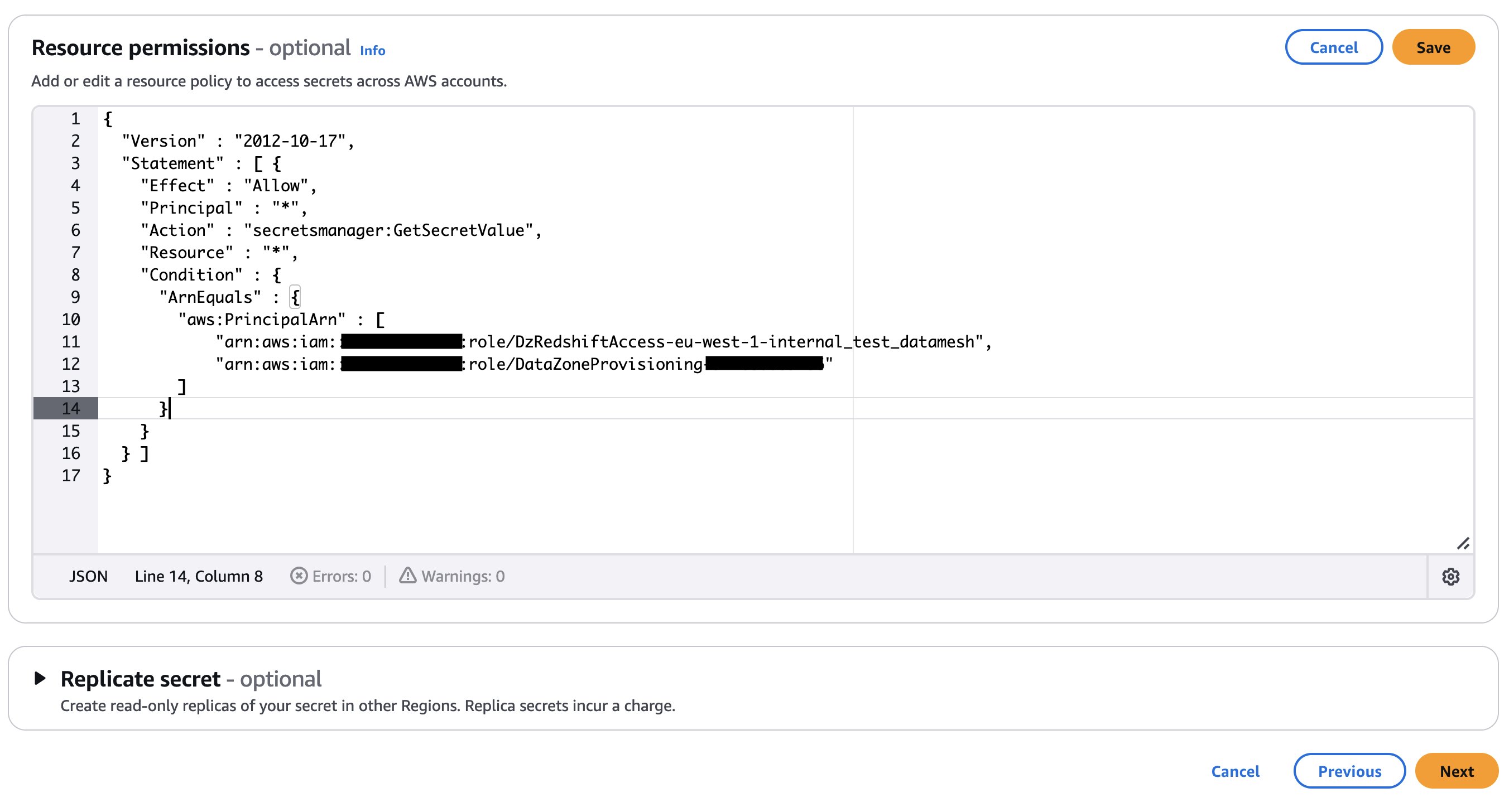
If your secret is encrypted with a custom KMS key, append the key policy with the following statement and add a tag to the key: AmazonDatazoneEnvironment = All. You can skip this step if you’re using an AWS managed KMS key.

{
    "Effect": "Allow",
    "Principal": {
        "Service": "logs.<<AWS_Region>>.amazonaws.com",
        "AWS": "arn:aws:iam::<<Data_Producer_Acct_Id(Account B)>>:root"
    },
    "Action": [
        "kms:Decrypt",
        "kms:Encrypt",
        "kms:GenerateDataKey*",
        "kms:ReEncrypt*"
    ],
    "Resource": "*"
 },
 {
    "Sid": "AllowDatazoneRoles-DEV",
    "Effect": "Allow",
    "Principal": {
        "AWS": "*"
    },
    "Action": [
        "kms:Decrypt",
        "kms:Describe*",
        "kms:Get*",
        "kms:Encrypt",
        "kms:GenerateDataKey",
        "kms:ReEncrypt*",
        "kms:CreateGrant"
    ],
    "Resource": "*",
    "Condition": {
        "StringLike": {
            "aws:PrincipalArn": [
                "arn:aws:iam::<<Data_Producer_Acct_Id(Account B)>>:role/aws-service-role/redshift.amazonaws.com/AWSServiceRoleForRedshift",
                "arn:aws:iam::<<Data_Producer_Acct_Id(Account B)>>:role/datazone_*",
                "arn:aws:iam::<<Data_Producer_Acct_Id(Account B)>>:role/<<Redshift_Cluster_IAM_Role>>",
                "arn:aws:iam::<<Data_Producer_Acct_Id(Account B)>>:role/service-role/AmazonDataZoneRedshiftAccess-<<AWS_Region>>-*"
            ]
         }
     }
 }

Place a mechanism to generate the following payload to trigger the dataset registration Lambda function. The payload must contain the relevant Redshift database, schema, and table or view that you want to publish in the Amazon DataZone domain. The following example code assumes you have three databases in your Redshift cluster and within those databases you have different schemas, tables, and views. You should adjust the payload based on your use case.

{
    "source": "redshift-user-initiated",
    "detail-type": "Amazon Redshift dataset registration in Amazon DataZone",
    "datasets": [
        {
            "clusterName": "<<YOUR_REDSHIFT_CLUSTER_NAME>>",
            "dbName":"<<YOUR_REDSHIFT_DATABASE_NAME_1>>",
            "schemas": [
                {
                    "schemaName":"<<YOUR_REDSHIFT_SCHEMA_NAME>>",
                    "addAllTables":false,
                    "addAllViews":false,
                    "tables":[
                        "<<YOUR_REDSHIFT_TABLE_NAME>>",
                        "<<YOUR_REDSHIFT_TABLE_NAME>>"
                    ],
                    "views":[
                        "<<YOUR_REDSHIFT_VIEW_NAME>>"
                    ]
                }
            ]
        },
        {
            "clusterName": "<<YOUR_REDSHIFT_CLUSTER_NAME>>",
            "dbName":"<<YOUR_REDSHIFT_DATABASE_NAME_2>>",
            "schemas": [
                {
                    "schemaName":"<<YOUR_REDSHIFT_SCHEMA_NAME>>",
                    "addAllTables":true,
                    "addAllViews":true,
                    "tables":[],
                    "views":[]
                }
            ]
        },
        {
            "clusterName": "<<YOUR_REDSHIFT_CLUSTER_NAME>>",
            "dbName":"<<YOUR_REDSHIFT_DATABASE_NAME_3>>",
            "schemas": [
                {
                    "schemaName":"<<YOUR_REDSHIFT_SCHEMA_NAME>>",
                    "addAllTables":true,
                    "addAllViews":false,
                    "tables":[],
                    "views":[
                        "<<YOUR_REDSHIFT_VIEW_NAME>>"
                    ]
                }
            ]
        }
    ]
}

Prerequisites in Amazon DataZone account (Account A)

Complete the following steps to set up your Amazon DataZone account (Account A):

Sign in to Account A and make sure you have already deployed an Amazon DataZone domain and a project within that domain. Refer to Create Amazon DataZone domains for instructions to create a domain.
If your Amazon DataZone domain is encrypted with a KMS key, add the data domain account (Account B) to the KMS key policy with the following actions:
```
"Action": [
    "kms:Encrypt",
    "kms:Decrypt",
    "kms:ReEncrypt*",
    "kms:GenerateDataKey*",
    "kms:DescribeKey"
]
```

Create an IAM role that is assumable by Account B and make sure the role has a following policy attached and is a member (as contributor) of your Amazon DataZone project. For this post, we call the role dz-assumable-env-dataset-registration-role. By adding this role, you can successfully run the registration Lambda function.

In the following policy, provide the AWS Region and account ID corresponding to where your Amazon DataZone domain is created, and the KMS key ARN used to encrypt the domain:

  {
    "Version": "2012-10-17",
    "Statement": [
        {
            "Action": [
                "datazone:CreateDataSource",
                "datazone:CreateEnvironment",
                "datazone:CreateEnvironmentProfile",
                "datazone:GetDataSource",
                "datazone:GetDataSourceRun",
                "datazone:GetEnvironment",
                "datazone:GetEnvironmentProfile",
                "datazone:GetIamPortalLoginUrl",
                "datazone:ListDataSources",
                "datazone:ListDomains",
                "datazone:ListEnvironmentProfiles",
                "datazone:ListEnvironments",
                "datazone:ListProjectMemberships",
                "datazone:ListProjects",
                "datazone:StartDataSourceRun",
                "datazone:UpdateDataSource",
                "datazone:SearchUserProfiles"
            ],
            "Resource": "*",
            "Effect": "Allow"
        },
        {
            "Action": [
                "kms:Decrypt",
                "kms:DescribeKey",
                "kms:GenerateDataKey"
            ],
            "Resource": "arn:aws:kms:<<account_region>>:<<Datazone_Account_id(Account A)>>


}:key/${DataZonekmsKey}",
            "Effect": "Allow"
        }
    ]
}

Add Account B in the trust relationship of this role with the following trust relationship:

{
    "Version": "2012-10-17",
    "Statement": [
        {
            "Effect": "Allow",
            "Principal": {
                "AWS": [
                    "arn:aws:iam::<<Data_Producer_Acct_Id(Account B)>>:root",
                    "arn:aws:iam::<<Datazone_Account_id(Account A)>>:root",
                ]
            },
            "Action": "sts:AssumeRole"
        }
    ]
}

Add the role as a member of the Amazon DataZone project in which you want to register your data sources. For more information, see Add members to a project.

Additional tools

The following tools are needed to deploy the solution using the AWS CDK:

Either Bash/ or ZSH terminal
Node and NPM using Node Version Manager:
- Install Node Version Manager (NVM)
- Install Node version 18.12.0 using the following command (node and npm binaries should now be available):
```
$ nvm install 18.12.0
```
Python
AWS Command Line Interface (AWS CLI); see Installing or updating to the latest version of the AWS CLI
AWS CDK for Python (Boto3); see Installation
AWS CDK

Deploy the solution

After you complete the prerequisites, use the AWS CDK stack provided on the GitHub repo to deploy the solution for automatic registration of data assets into the Amazon DataZone domain. Complete the following steps:

Clone the repository from GitHub to your preferred integrated development environment (IDE) using the following commands:

git clone https://github.com/aws-samples/sample-how-to-automate-amazon-redshift-cluster-data-asset-publish-to-amazon-datazone

$ cd sample-how-to-automate-amazon-redshift-cluster-data-asset-publish-to-amazon-datazone

At the base of the repository folder, run the following commands to build and deploy resources to AWS:
```
$ npm install
```
```
$ npm run lint
```
Sign in to Account B (the data domain producer account) using the AWS CLI with your profile name.
Make sure you have configured the Region in your credential’s configuration file.
Bootstrap the AWS CDK environment with the following commands at the base of the repository folder. Provide the profile name of your deployment account (Account B). Bootstrapping is a one-time activity and is not needed if your AWS account is already bootstrapped.
```
$ export AWS_PROFILE=<<PROFILE_NAME>>
```
```
$ npm run cdk bootstrap
```
Replace the placeholder parameters (marked with the suffix _PLACEHOLDER) in the file config/DataZoneConfig.ts:
1. Amazon DataZone domain and project name of your Amazon DataZone instance. Make sure all names are in lowercase.
2. The AWS account ID of the Amazon DataZone account (Account A).
3. The assumable IAM role from the prerequisites.
4. The AWS Systems Manager parameter name containing the Secrets Manager secret ARN of the Amazon Redshift credentials.
Use the following command in the base folder to deploy the AWS CDK solution. During deployment, enter y if you want to deploy the changes for some stacks when you see the prompt Do you wish to deploy these changes (y/n)?
```
npm run cdk deploy --all
```
After the deployment is complete, sign in to Account B and open the AWS CloudFormation console to verify that the infrastructure was deployed.

Test automatic data registration to Amazon DataZone

Complete the following steps to test the solution:

Sign in to Account B (producer account).
On the Lambda console, open the datazone-redshift-dataset-registration function.
Under TEST EVENTS, choose Create new test event.

For Event name, enter Redshift, and for Event JSON, enter the following JSON structure (change the cluster, schema, database, and table names according to your environment):

{
  "source": "redshift-user-initiated",
  "detail-type": "Amazon Redshift dataset registration in Amazon DataZone",
  "datasets": [
    {
      "clusterName": "YOUR_REDSHIFT_CLUSTER_NAME",
      "dbName": "DATABASE_NAME",
      "schemas": [
        {
          "schemaName": "SCHEMA_NAME_1",
          "addAllTables": false,
          "addAllViews": false,
          "tables": [
            "TABLE_NAME"
          ],
          "views": []
        },
        {
          "schemaName": "SCHEMA_NAME_2",
          "addAllTables": false,
          "addAllViews": false,
          "tables": [],
          "views": [
            "VIEW_NAME"
          ]
        }
      ]
    }
  ]
}

Choose Save.
Choose Invoke.
Open the Amazon DataZone console in Account A where you deployed the resources.
Choose Domains in the navigation pane, then open your domain.
On the domain details page, locate the Amazon DataZone data portal URL in the Summary section. Choose the link to the data portal.
For more details about accessing Amazon DataZone, refer to How can I access Amazon DataZone?
In the data portal, open your project and choose the Data tab.
In the navigation pane, choose Data sources and find the newly created data source for Amazon Redshift.
Verify that the data source has been successfully published.

After the data sources are published, users can discover the published data and submit a subscription request. The data producer can approve or reject requests. Upon approval, users can consume the data by querying the data in the Amazon Redshift query editor. The following screenshot illustrates data discovery in the Amazon DataZone data portal.

Clean up

Complete the following steps to clean up the resources deployed through the AWS CDK:

Sign in to Account B, go to the Amazon DataZone domain portal, and check there is no subscription for your published data asset. If there is a subscription, either ask the subscriber to unsubscribe or revoke the subscription request.
Delete the published data assets that were created in the Amazon DataZone project by the dataset registration Lambda function.
Delete the remaining resources created using the following command in the base folder:
```
npm run cdk destroy –all
```

Conclusion

Amazon DataZone offers a seamless integration with AWS services, providing a powerful solution for organizations like Volkswagen to break down their data silos and implement effective data mesh architectures through a straightforward implementation highlighted in this post. By using Amazon DataZone, Volkswagen addressed its immediate data sharing hurdles and laid the groundwork for a more agile, data-driven future in automotive manufacturing. The automated data publishing from various warehouses, coupled with standardized governance workflows, has significantly reduced the manual overhead that once slowed down Volkswagen’s data engineering teams. Now, instead of navigating a labyrinth of emails, tickets, and communication, Volkswagen’s data engineers and data scientists can quickly discover and access the data they need, all while maintaining their security and compliance standards.

By using Amazon DataZone, organizations can bring their isolated data together in ways that make it simpler for teams to collaborate while maintaining security and compliance at scale. This approach not only addresses current data governance challenges but also creates a highly scalable foundation for future data-driven innovations. For guidance on establishing your organization’s data mesh with Amazon DataZone, contact your AWS team today.

About the Authors

Seamlessly Integrate Data on Google BigQuery and ClickHouse Cloud with AWS Glue

2025-10-07 Ray Wang

Post Syndicated from Ray Wang original https://aws.amazon.com/blogs/big-data/seamlessly-integrate-data-on-google-bigquery-and-clickhouse-cloud-with-aws-glue/

Migrating from Google Cloud’s BigQuery to ClickHouse Cloud on AWS allows businesses to leverage the speed and efficiency of ClickHouse for real-time analytics while benefiting from AWS’s scalable and secure environment. This article provides a comprehensive guide to executing a direct data migration using AWS Glue ETL, highlighting the advantages and best practices for a seamless transition.

AWS Glue ETL enables organizations to discover, prepare, and integrate data at scale without the burden of managing infrastructure. With its built-in connectivity, Glue can seamlessly read data from Google Cloud’s BigQuery and write it to ClickHouse Cloud on AWS, removing the need for custom connectors or complex integration scripts. Beyond connectivity, Glue also provides advanced capabilities such as a visual ETL authoring interface, automated job scheduling, and serverless scaling, allowing teams to design, monitor, and manage their pipelines more efficiently. Together, these features simplify data integration, reduce latency, and deliver significant cost savings, enabling faster and more reliable migrations.

Prerequisites

Before using AWS Glue to integrate data into ClickHouse Cloud, you must first set up the ClickHouse environment on AWS. This includes creating and configuring your ClickHouse Cloud on AWS, making sure network access and security groups are properly defined, and verifying that the cluster endpoint is accessible. Once the ClickHouse environment is ready, you can leverage the AWS Glue built-in connector to seamlessly write data into ClickHouse Cloud from sources such as Google Cloud BigQuery. You can follow the next section to complete the setup.

Set up ClickHouse Cloud on AWS
1. Follow the ClickHouse official website to set up environment (remember to allow remote access in the config file if using Clickhouse OSS)
  https://clickhouse.com/docs/get-started/quick-start
Subscribe the ClickHouse Glue marketplace connector
1. Open Glue Connectors and choose Go to AWS Marketplace
2. On the list of AWS Glue marketplace connectors, enter ClickHouse in the search bar. Then choose ClickHouse Connector for AWS Glue
3. Choose View purchase options on the right top of the view
4. Review Terms and Conditions and choose Accept Terms
5. Choose Continue to Configuration once it’s enabled
6. On Follow the vendor’s instructions part in the connector instructions as below, choose the connector enabling link at step 3

Configure AWS Glue ETL Job for ClickHouse Integration

AWS Glue enables direct migration by connecting with ClickHouse Cloud on AWS through built-in connectors, allowing for seamless ETL operations. Within the Glue console, users can configure jobs to read data from S3 and write it directly to ClickHouse Cloud. Using AWS Glue Data Catalog, data in S3 can be indexed for efficient processing, while Glue’s PySpark support allows for complex data transformations, including data type conversions, to support compatibility with ClickHouse’s schema.

Open AWS Glue in the AWS Management Console
1. Navigate to Data Catalog and Connections
2. Create a new connection
Configure BigQuery Connection in Glue
1. Prepare a Google Cloud BigQuery Environment
2. Create and Store Google Cloud Service Account Key (JSON format) in AWS Secret Manager, you can find the details in BigQuery connections.
3. The JSON Format content example is as following:
```
{
  "type": "service_account",
  "project_id": "h*********g0",
  "private_key_id": "cc***************81",
  "private_key": "-----BEGIN PRIVATE KEY-----\nMI***zEc=\n-----END PRIVATE KEY-----\n",
  "client_email": "clickhouse-sa@h*********g0.iam.gserviceaccount.com",
  "client_id": "1*********8",
  "auth_uri": "https://accounts.google.com/o/oauth2/auth",
  "token_uri": "https://oauth2.googleapis.com/token",
  "auth_provider_x509_cert_url": "https://www.googleapis.com/oauth2/v1/certs",
  "client_x509_cert_url": "https://www.googleapis.com/robot/v1/metadata/x509/clickhouse-sa%40h*********g0.iam.gserviceaccount.com",
  "universe_domain": "googleapis.com"
}
```
  - type: service_account.
  - project_id: The ID of the GCP project.
  - private_key_id: A unique ID for the private key within the file.
  - private_key: The actual private key.
  - client_email: The email address of the service account.
  - client_id: A unique client ID associated with the service account.
  - auth_uri, token_uri, auth_provider_x509_cert_url
  - client_x509_cert_url: URLs for authentication and token exchange with Google’s identity and access management systems.
  - universe_domain: The domain name of GCP, googleapis.com
4. Create Google BigQuery Connection in AWS Glue
5. Grant the IAM role associated with your AWS Glue job permission for S3, Secret Manager, Glue services, and AmazonEC2ContainerRegistryReadOnly for accessing connectors purchased from AWS Marketplace (reference doc)
Create ClickHouse connection in AWS Glue
1. Enter clickhouse-connection as its connection name
2. Choose Create connection and activate connector

Create a Glue job

On the Connectors view as below, select clickhouse-connection and choose Create job
Enter bq_to_clickhouse as its job name and configure gc_connector_role as its IAM Role
Configure BigQuery connection and clickhouse-connection to the Connection property
Choose the Script tab and Edit script. Then choose Confirm on the Edit script popup view.
Copy and paste the following code onto the script editor which can be referred from clickhouse official doc

The source code is as following:

import sys
from pyspark.sql import SparkSession
from awsglue.context import GlueContext
from awsglue.job import Job
from awsglue.utils import getResolvedOptions

args = getResolvedOptions(sys.argv, ['JOB_NAME'])
spark = SparkSession.builder.getOrCreate()
glueContext = GlueContext(spark.sparkContext)
job = Job(glueContext)
job.init(args['JOB_NAME'], args)

connection_options = {
    "connectionName": "Bigquery connection",
    "parentProject": "YOUR_GCP_PROJECT_ID",
    "query": "SELECT * FROM `YOUR_GCP_PROJECT_ID.bq_test_dataset.bq_test_table`",
    "viewsEnabled": "true",
    "materializationDataset": "bq_test_dataset"
}
jdbc_url = " jdbc:clickhouse://YOUR_CLICKHOUSE_CONNECTION.us-east-1.aws.clickhouse.cloud:8443/clickhouse_database?ssl=true "
username = "default"
password = "YOUR_PASSWORD"
query = "select * from clickhouse_database.clickhouse_test_table"
# Add this before writing to test connection
try:
    # Read from BigQuery with Glue Connection
    print("Reading data from BigQuery...")
    GoogleBigQuery_node1742453400261 = glueContext.create_dynamic_frame.from_options(
        connection_type="bigquery",
        connection_options=connection_options,
        transformation_ctx="GoogleBigQuery_node1742453400261"
    )
    # Convert to DataFrame
    bq_df = GoogleBigQuery_node1742453400261.toDF()
    print("Show data from BigQuery:")
    bq_df.show()
    
    # Write BigQuery Data to Clickhouse with JDBC
    bq_df.write \
    .format("jdbc") \
    .option("driver", 'com.clickhouse.jdbc.ClickHouseDriver') \
    .option("url", jdbc_url) \
    .option("user", username) \
    .option("password", password) \
    .option("dbtable", "clickhouse_test_table") \
    .mode("append") \
    .save()
    
    print("Write BigQuery Data to ClickHouse successfully")
    
    # Read from Clickhouse with JDBC
    reaf_df = (spark.read.format("jdbc")
    .option("driver", 'com.clickhouse.jdbc.ClickHouseDriver')
    .option("url", jdbc_url)
    .option("user", username)
    .option("password", password)
    .option("query", query)
    .option("ssl", "true")
    .load())
    
    print("Show Data from ClickHouse:")
    reaf_df.show()
    
except Exception as e:
    print(f"ClickHouse connection test failed: {str(e)}")
    raise e
finally:
    job.commit()

Choose Save and Run on the right top of the current view

Testing and Validation

Testing is crucial to verify data accuracy and performance in the new environment. After the migration completes, run data integrity checks to confirm record counts and data quality in ClickHouse Cloud. Schema validation is essential, as each data field must align correctly with ClickHouse’s format. Running performance benchmarks, such as sample queries, will help verify that ClickHouse’s setup delivers the desired speed and efficiency gains.

The Schema and Data in source BigQuery and destination Clickhouse
AWS Glue output logs

Clean Up

After completing the migration, it’s important to clean up unused resources—such as BigQuery for sample data import and database resources in ClickHouse Cloud—to avoid unnecessary costs. Regarding IAM permissions, adhering to the principle of least privilege is advisable. This involves granting users and roles only the permissions necessary for their tasks and removing unnecessary permissions when they are no longer required. This approach enhances security by minimizing potential threat surfaces. Additionally, reviewing AWS Glue job costs and configurations can help identify optimization opportunities for future migrations. Monitoring overall costs and analyzing usage can reveal areas where code or configuration improvements may lead to cost savings.

Conclusion

AWS Glue ETL offers a robust and user-friendly solution for migrating data from BigQuery to ClickHouse Cloud on AWS. By utilizing Glue’s serverless architecture, organizations can perform data migrations that are efficient, secure, and cost-effective. The direct integration with ClickHouse streamlines data transfer, supporting high performance and flexibility. This migration approach is particularly well-suited for companies looking to enhance their real-time analytics capabilities on AWS.

About the Authors

Deploying AI models for inference with AWS Lambda using zip packaging

2025-10-03 Ayush Kulkarni

Post Syndicated from Ayush Kulkarni original https://aws.amazon.com/blogs/compute/deploying-ai-models-for-inference-with-aws-lambda-using-zip-packaging/

AWS Lambda provides an event-driven programming model, scale-to-zero capability, and integrations with over 200 AWS services. This can make it a good fit for CPU-based inference applications that use customized, lightweight models and complete within 15 minutes.

Users usually package their function code as container images when using machine learning (ML) models that are larger than 250 MB, which is the Lambda deployment package size limit for zip files. In this post, we demonstrate an approach that downloads ML models directly from Amazon S3 into your function’s memory so that you can continue packaging your function code using zip files. To optimize startup latency without implementing application-level performance optimizations, we use Lambda SnapStart. SnapStart is an opt-in capability available for Java, Python, and .NET functions that optimizes startup latency—from 16.5s down to 1.6s for the application used in this post.

Application architecture

In this post, we demonstrate how to build a chatbot, using a 4-bit quantized version of the DeepSeek-R1-Distill-Qwen-1.5B-GGUF model for inference along with Lambda Function URL (FURL) and Lambda Web Adapter (LWA) to stream text responses. A FURL is a dedicated HTTP(s) endpoint for your Lambda function, and you can use LWA, an open-source project available on AWS Labs, for familiar web application frameworks (such as FastAPI, Next.JS, or Spring Boot) with Lambda. For a detailed explanation of how this response streaming architecture works, refer to this AWS Compute post.

Today, Lambda functions are run on CPU-based Amazon Elastic Compute Cloud (Amazon EC2) instances that use x86 and ARM64 architectures. For this reason, you must use SDKs that enable large language model (LLM) inference on CPUs. In this post, we also demonstrate how to use the llama.cpp project (through the llama-cpp-python library) and the FastAPI web framework to handle web requests. To use models that exceed the 250 MB zip package size limit of Lambda, you can download them from an S3 bucket during function initialization. The following figure describes this architecture in detail.

Architecture diagram demonstrating an AI inference workload with AWS Lambda FURLs and AWS Lambda Web Adapter

Figure 1: Application architecture

You can refer to this GitHub repository for the application code used in this example.

Downloading ML models during function initialization

As an alternative to packaging ML models using OCI container images, you can download them from durable storage, such as Amazon S3, during initialization. Initialization (or INIT) refers to the phase when Lambda downloads your function code, starts the language runtime and runs your function initialization code, which is code outside the handler. Loading large files directly into memory can be faster than first downloading them to disk and then loading them into memory. To do so, you can use a Linux capability called memfd, to directly download the ML model from Amazon S3 directly into memory, while referencing it using a standard file descriptor. Referencing the model using a file descriptor is necessary for llama.cpp to successfully import the model. This is comprised of two steps.

First, create a memory-only file descriptor:


    libc = ctypes.CDLL("libc.so.6", use_errno=True)
    MFD_CLOEXEC = 1
    
    memfd_create = libc.memfd_create
    memfd_create.argtypes = [ctypes.c_char_p, ctypes.c_uint]
    memfd_create.restype = ctypes.c_int
    
    fd = memfd_create(b"model", MFD_CLOEXEC)
    if fd == -1:
        errno = ctypes.get_errno()
    raise OSError(errno, f"memfd_create failed: {os.strerror(errno)}")
    
    return fd

Then, download the model into the memory-mapped file referenced by the previously created file descriptor.

def download_model_to_memfd(bucket, key, chunk_size=100*1024*1024):  # 100MB chunks

    s3 = boto3.client('s3')
    
    # Get file size
    response = s3.head_object(Bucket=bucket, Key=key)
    file_size = response['ContentLength']
    
    # Create memory file
    fd = create_memfd()
    
    # Pre-allocate the full file size
    try:
        os.ftruncate(fd, file_size)
    except OSError as e:
        logger.error(f"Failed to allocate {file_size/1024/1024:.2f}MB in memory: {e}")
        cleanup_fd(fd)
        raise RuntimeError(f"Not enough memory to load model of size {file_size/1024/1024:.2f}MB")
    
    # Calculate parts
    parts = []
    for start in range(0, file_size, chunk_size):
        end = min(start + chunk_size - 1, file_size - 1)
        parts.append({'start': start, 'end': end})
    
    logger.info(f"Downloading {file_size/1024/1024:.2f}MB in {len(parts)} parts")
    
    # Download parts concurrently
    download_func = partial(download_part, s3, bucket, key, fd)
    with ThreadPoolExecutor(max_workers=multiprocessing.cpu_count()) as executor:
        executor.map(download_func, parts)
    
    fd_path = f"/proc/self/fd/{fd}"
    return fd, fd_path

Querying the chatbot

After deploying our sample chatbot application, we begin interacting with it.

The first query to the chatbot results in a new execution environment being initialized. When Lambda runs the initialization code described in the previous section, your ML model is directly downloaded from Amazon S3 into the function’s memory. After this, Lambda runs the function’s handler method. Looking at the X-Ray trace segment in the following figure, we observe that the first Init times out after 10 s. The second Init completes in 16.68 s. Furthermore, the first Init times out because Lambda limits the duration of this phase to 10s. If Init takes longer than this, then Lambda retries it during function invocation applying the function’s configured execution duration timeout.

Screenshot of AWS X-Ray Segments demonstrating INIT duration of 16.68 s

Figure 2: Init duration, indicated by AWS X-Ray trace segment

Optimizing startup performance with SnapStart

To optimize function startup latency, you can use Lambda SnapStart. SnapStart is designed to optimize startup latency stemming from long-running function initialization code. Lambda uses SnapStart to initialize your function when you publish a function version, as shown in the following figure. Then, Lambda takes a Firecracker microVM snapshot of the memory and disk state of the initialized execution environment, encrypts the snapshot, and intelligently caches it to optimize retrieval latency.

Screenshot of AWS Lambda Console showing how to enable SnapStart for your Lambda function

Figure 3: Enabling SnapStart

Querying the chatbot again shows a significant speed-up in initialization latency. You can verify this by viewing your function’s Amazon CloudWatch Logs, and searching for the “RESTORE_REPORT” log line, as shown in the following figure. For the sample application used, restore duration is 1.39 s. This is a considerable improvement over the Init duration of 16.68 s. Performance results may vary. But best of all, you don’t need to change a single line of code to achieve this improvement!

Screenshot of Amazon CloudWatch Logs demonstrating RESTORE duration of 1.39 s

Figure 4: Achieving faster startup latency with SnapStart

Tuning inference performance

Inference performance depends on the CPU resources allocated to your function. Lambda allocates CPU power in proportion to the amount of memory configured for your function. Allocating more memory results in faster inference results, measured by the rate at which prompt tokens are evaluated (tokens evaluated per second), and the rate at which output tokens are produced (tokens generated per second). For this example, we allocate the maximum—in other words 10 GB memory—to maximize performance. Performance results obtained at other memory size configurations are included in the following table. As the table shows, doubling the memory allocated from 5 GB to 10 GB results in an 83% improvement in tokens evaluated and generated (per second), with only a 24% increase in billed GB-seconds. Performance results may vary. Refer to the sample code to instrument performance at different memory sizes.

Memory Size (MB)	Tokens evaluated per second	Tokens generated per second	Billed Duration (ms)	Billed GB-seconds
10240	44.68	29.53	36,660	366.60
9216	41.67	26.77	37,690	339.21
8192	37.17	22.05	44,298	354.38
7168	33.67	21.78	44,818	313.73
6144	28.89	18.43	52,579	315.47
5120	24.41	16.07	59,036	295.18
4096	19.07	12.94	72,648	290.59
3072	13.39	9.20	101,468	304.40
2048	10.01	6.77	135,862	271.72

Table 1: Inference performance at different memory sizes

Understanding how application costs scale with usage

To estimate the cost of running this workload, we begin by making some assumptions about our traffic patterns. We estimate about 30,000 inference calls per month to our Lambda function, with each inference call averaging 10s in duration. We set function memory to 10 GB, because it represents the ideal price-performance for our use case. We deploy our application in the US-West-2 (Oregon) AWS Region. Initially, because our number of invokes is low, we assume a 5% cold-start rate. In other words, 5% of invokes result in a cold-start when a new execution environment is created. When using SnapStart with the Lambda managed Python runtime, you are charged for caching your function’s snapshot and for restoring execution from your function’s snapshot.

With these parameters, the monthly Lambda bill is $91.1, calculated as shown in the following table. The monthly costs shown in the table are only illustrative.

Charge	Calculation	Monthly Cost
Compute	30,000 inferences * 10 seconds per inference * 10 GB (configured memory) * $0.00001667 per GB-second	$50.01
Requests	$0.2 per million requests * 30,000 inferences	$0.006
SnapStart – Cache	10 GB function memory * 2.59M GB-seconds per month * $0.0000015046 per GB-second	$38.99
SnapStart – Restore	10 GB function memory * $0.0001397998 per GB restore * 1500 cold-starts	$2.09
Total	Compute + Requests + SnapStart Cache + SnapStart Restore	$91.1

At low invocation volume, the added charges for the SnapStart account for approximately 50% of total monthly cost. For this added charge, cold-start latency reduces from 16.68 s to1.39 s, without having to implement complex optimizations ourselves. We can demonstrate how these costs scale with usage. We assume that our chatbot grows in popularity with traffic increasing 10 times to 300,000 monthly inference calls. Although cold-start rates for individual Lambda functions can vary due to several factors, Lambda’s re-use of execution environments generally results in cold-start rates decreasing with higher traffic volume. For the purposes of this example, we assume that our cold-start rate drops to 1% of all invokes with the 10 times growth in traffic.With these assumptions, our monthly Lambda bill at 10 times higher traffic volume is $543.3. Added charges for SnapStart now constitute less than 10% of our total bill, as shown in the following table. Monthly costs shown in this table are only illustrative.

Charge	Calculation	Monthly Cost
Compute	300,000 inferences * 10 seconds per inference * 10 GB (configured memory) * $0.00001667 per GB-second	$500.01
Requests	$0.2 per million requests * 300,000 inferences	$0.06
SnapStart – Cache	10 GB function memory * 2.59M GB-seconds per month * $0.0000015046 per GB-second	$38.99
SnapStart – Restore	10 GB function memory * $0.0001397998 per GB restore * 3000 cold-starts	$4.18
Total	Compute + Requests + SnapStart Cache + SnapStart Restore	$543.24

Considerations

Lambda functions are run on CPU-based EC2 instances. If your ML models need GPU-based inference, foundational LLMs, or exceed the Lambda limits on execution duration (15 minutes) and function memory (10 GB), then you can use AWS Machine Learning, AWS Generative AI, or AWS Compute services.

Moreover, you should know the following things about Lambda SnapStart:

Handling uniqueness: If your initialization code generates unique content that is included in the snapshot, then the content isn’t unique when it’s reused across execution environments. To maintain uniqueness when using SnapStart, you must generate unique content after initialization, such as if your code uses custom random number generation that doesn’t rely on built-in-libraries or caches any information such as DNS entries that might expire during initialization. To learn how to restore uniqueness, visit Handling uniqueness with Lambda SnapStart in the Lambda Developer Guide.

Performance tuning: To maximize performance, we recommend that you preload dependencies and initialize resources that contribute to startup latency in your initialization code instead of in the function handler. This moves the latency associated with these operations during version publish, rather than during function invocation and can yield faster startup performance. To learn more, visit Performance tuning for Lambda SnapStart in the Lambda Developer Guide.

Networking best practices: The state of connections that your function establishes during the initialization phase isn’t guaranteed when Lambda resumes your function from a snapshot. In most cases, network connections that an AWS SDK establishes automatically resume. For other connections, review the Networking best practices for Lambda SnapStart in the Lambda Developer Guide.

Conclusion

In this post, we demonstrated how you can download ML models directly from Amazon S3 into your function’s memory, enabling you to deploy your AWS Lambda functions using zip packages. To optimize startup latency without implementing application-level performance optimizations, we also demonstrated the use of Lambda SnapStart, an opt-in capability available for Java, Python, and .NET. For the application used in this post, SnapStart reduced startup latency from 16.68 s down to 1.39 s.

To learn more about Lambda, refer to our documentation. For details about Lambda SnapStart, refer to our launch posts for Java, Python and .Net, and the documentation.

You can refer to this GitHub repository for the application code used in this example.

How to export to Amazon S3 Tables by using AWS Step Functions Distributed Map

2025-10-01 Chetan Makvana

Post Syndicated from Chetan Makvana original https://aws.amazon.com/blogs/compute/how-to-export-to-amazon-s3-tables-by-using-aws-step-functions-distributed-map/

Companies running serverless workloads often need to perform extract, transform, and load (ETL) operations on data files stored in Amazon Simple Storage Service (Amazon S3) buckets. Though traditional approaches such as an AWS Lambda trigger for Amazon S3 or Amazon S3 Event Notifications can handle these operations, they might fall short when workflows require enhanced visibility, control, or human intervention. For example, some processes might need manual review of failed records or explicit approval before proceeding to subsequent stages. Customer orchestration solutions to these issues can prove to be complex and error prone.

AWS Step Functions address these challenges by providing built-in workflow management and monitoring capabilities. The Step Functions Distributed Map feature is designed for high-throughput, parallel data processing workflows so that companies can handle complex ETL jobs, fan-out processing, and data visualization at scale. Distributed Map handles each dataset item as an independent child workflow, processing millions of records while maintaining built-in concurrency controls, fault tolerance, and progress tracking. The processed data can be seamlessly exported to various destinations, including Amazon S3 Tables with Apache Iceberg support.

In this post, we show how to use Step Functions Distributed Map to process Amazon S3 objects and export results to Amazon S3 Tables, creating a scalable and maintainable data processing pipeline.

See the associated GitHub repository for detailed instructions about deploying this solution as well as sample code.

Solution overview

Consider a consumer electronics company that regularly participates in industry trade shows and conferences. During these events, interested attendees fill out paper sign-up forms to request product demos, receive newsletters, or join early access programs. After the events, the company’s team scans hundreds of thousands of these forms and uploads them to Amazon S3.Rather than manually reviewing each form, the company wants to automate the extraction of key customer details such as name, email address, mailing address, and interest areas. They’d like to store this structured data in S3 Tables with Apache Iceberg format for downstream analytics and marketing campaign targeting.

Let’s look at how this post’s solution uses Distributed Map to process PDFs in parallel, extract data using Amazon Textract, and write the cleaned output directly to S3 Tables. The result is scalable, serverless post-event data onboarding, as shown in the following figure.

The data processing workflow as shown in the preceding diagram includes the following steps:

A user uploads customer interest forms as scanned PDFs to an Amazon S3 bucket.
An Amazon EventBridge Scheduler rule triggers at regular intervals, initiating a Step Functions workflow execution.
The workflow execution activates a Step Functions Distributed Map state, which lists all PDF files uploaded to Amazon S3 since the previous run.
The Distributed Map iterates over the list of objects and passes each object’s metadata (bucket, key, size, entity tag [ETag]) to a child workflow execution.
For each object, the child workflow calls Amazon Textract with the provided bucket and key to extract raw text and relevant fields (name, email address, mailing address, interest area) from the PDF.
The child workflow sends the extracted data to Amazon Data Firehose, which is configured to forward data to S3 Tables.
Firehose batches the incoming data from the child workflow and writes it to S3 Tables at a preconfigured time interval of your choosing.

With data now structured and accessible in S3 Tables, users can easily analyze them using standard SQL queries with Amazon Athena or business intelligence like Amazon QuickSight.

The data-processing workflow

EventBridge Scheduler starts new Step Functions workflows at regular intervals. The timeline for this schedule is flexible. However, When setting up your schedule, make sure the frequency aligns with how far back your state machine is configured to look for PDFs. For example, if your state machine checks for PDFs from the past week, you’d want to schedule it to run weekly. The Step Functions workflow subsequently performs the following three steps (note that these steps are steps 4, 5, 6, and 7 in the preceding workflow diagram:

Extract relevant user data from the PDFs.
Send the extracted user data to Firehose.
Write the data to S3 Tables in Apache Iceberg table format.

The following diagram illustrates this workflow.

Let’s look at each step of the preceding workflow in more detail.

Extract relevant user data from PDF documents

Step Functions uses Distributed Map to process PDFs concurrently in parallel child workflows. It accepts input from JSON, JSONL, CSV, Parquet files, Amazon S3 manifest files stored in Amazon S3 (used to specify particular files for processing), or an Amazon S3 bucket prefix (allows iteration over file metadata for all objects under that prefix). The Step Functions automatically handles parallelization by splitting the dataset and running child workflows for each item, with the ItemBatcher field allowing to group multiple PDFs into a single child workflow execution (e.g., 10 PDFs per batch) to optimize performance and cost.

The following screenshot of the Step Functions console shows the configuration for Distributed Map. For example, we have configured Distributed Map to process 10 customer interest PDFs in a single child workflow.

The following image shows one example of these scanned PDFs, which includes the customer information that this post’s solution processes.

Each child workflow then calls the Amazon Textract AnalyzeDocument API with specific queries to extract customer information.

{
  "Document": {
    "S3Object": {
      "Bucket": "<input PDFs bucket>",
      "Name": "{% $states.input.Key %}"
    }
  },
  "FeatureTypes": [
    "QUERIES"
  ],
  "QueriesConfig": {
    "Queries": [
      {
        "Alias": "full_name",
        "Text": "What is the customer's name?"
      },
      {
        "Alias": "phone_number",
        "Text": "What is the customer’s phone number?"
      },
      {
        "Alias": "mailing_address",
        "Text": "What is the customer’s mailing address?"
      },
      {
        "Alias": "interest",
        "Text": "What is the customer’s interest?"
      }
    ]
  }
}

The API analyzes each scanned PDF and returns a JSON structure containing the extracted customer information.

Send the extracted user data to Firehose

The child workflow then uses a Firehose PutRecordBatch API action with service integrations to queue the extracted customer information for further processing. The PutRecordBatch action request includes the Firehose stream name and the data records. The data records include a data blob from step 1 that contains extracted customer information, as shown in the following example.

{
  "DeliveryStreamName": "put_raw_form_data_100",
  "Records": [
    {
      "Data": "{\"full_name\":\"Anthony Ayala\",\"phone_number\":\"001-384-925-0701\",\"mailing_address\":\"38548 Joshua Wall Suite 974, East Heatherfort, OH 32669\",\"interest\":\"Fitness Trackers\",\"processed_date\":\"2025-05-01\"}"
    },
    {
      "Data": "{\"full_name\":\"Becky Williams\",\"phone_number\":\"+1-283-499-2466\",\"mailing_address\":\"227 King Forge Suite 241, East Nathanland, PR 05687\",\"interest\":\"Al Assistants\",\"processed_date\":\"2025-05-01\"}"
    }
  ]
}

Write the data to S3 Tables in Apache Iceberg table format

Firehose efficiently manages data buffering, format conversion, and reliable delivery to various destinations, including Apache Iceberg, raw files in Amazon S3, Amazon OpenSearch Service, or any of the other supported destinations. Apache Iceberg tables can be either self-managed in Amazon S3 or hosted in S3 Tables. Though self-managed Iceberg tables require manual optimization—such as compaction and snapshot expiration—S3 Tables automatically optimize storage for large-scale analytics workloads, improving query performance and reducing storage costs.

Firehose simplifies the process of streaming data by configuring a delivery stream, selecting a data source, and setting an Iceberg table as the destination. After you’ve set it up, the Firehose stream is ready to deliver data. The delivered data can be queried from S3 Tables by using Athena, as shown in the following screenshot of the Athena console.

The query results include all processed customer data from the PDFs, as shown in the following screenshot.

This integration demonstrates a powerful, code-free solution for transforming raw PDF forms into enriched, queryable data in an Iceberg table. You can use these data for further analysis.

Conclusion

In this post, we showed how to build a scalable, serverless solution for processing PDF documents and exporting the extracted data to S3 Tables by using Step Functions Distributed Map. This architecture offers several key benefits such as reliability, cost-effectiveness, visibility, and maintainability. By leveraging AWS services such as Step Functions, Amazon Textract, Firehose, and S3 Tables, companies can automate their document processing workflows while ensuring optimal performance and operational excellence. This solution can be adapted for various use cases beyond customer interest forms, such as invoice processing, application forms, or any scenario requiring structured data extraction from documents at scale.

Though this example focuses on processing PDF data and writing to S3 Tables, Distributed Map can handle various input sources including JSON, JSONL, CSV, and Parquet files in Amazon S3; items in Amazon DynamoDB tables; Athena query results; and all paginated AWS List APIs. Similarly, through Step Functions service integrations, you can write results to multiple destinations such as DynamoDB tables by using the PutItem service integration.

To get started with this solution, see the associated GitHub repository for deployment instructions and sample code.

Introducing Apache Airflow 3 on Amazon MWAA: New features and capabilities

2025-10-01 Anurag Srivastava

Post Syndicated from Anurag Srivastava original https://aws.amazon.com/blogs/big-data/introducing-apache-airflow-3-on-amazon-mwaa-new-features-and-capabilities/

Today, Amazon Web Services (AWS) announced the general availability of Apache Airflow 3 on Amazon Managed Workflows for Apache Airflow (Amazon MWAA). This release transforms how organizations use Apache Airflow to orchestrate data pipelines and business processes in the cloud, bringing enhanced security, improved performance, and modern workflow orchestration capabilities to Amazon MWAA customers.

Amazon MWAA introduces Airflow 3 features that modernize workflow management for AWS customers. Following the April 2025 release of Airflow 3 by the Apache community, AWS has incorporated these capabilities into Amazon MWAA. Airflow now features a completely redesigned, intuitive UI that simplifies workflow orchestration for users across experience levels. With the Task Execution Interface (Task API), tasks can run both within Airflow and as standalone Python scripts, improving code portability and testing. Scheduler-managed Backfill moves operations from the CLI to the scheduler, providing centralized control and visibility through the Airflow UI. CLI security improvements replace direct database access with API calls, maintaining consistent security across interfaces. Airflow now supports event-driven workflows, enabling triggers from AWS services and external sources. Amazon MWAA also adds support for Python 3.12, bringing the latest language capabilities to workflow development.

This post explores the features of Airflow 3 on Amazon MWAA and outlines enhancements that improve your workflow orchestration capabilities. The service maintains the Amazon MWAA pay-as-you-go pricing model with no upfront commitments. You can begin immediately by visiting the Amazon MWAA console, launching new Apache Airflow environments through the AWS Management Console, AWS Command Line Interface (AWS CLI), AWS CloudFormation, or AWS SDK within minutes.

Architectural advancements in Airflow 3 on Amazon MWAA

Airflow 3 on Amazon MWAA introduces significant architectural improvements that enhance security, performance, and flexibility. These advancements create a more robust foundation for workflow orchestration while maintaining backward compatibility with existing workflows.

Enhanced security

Amazon MWAA with Airflow 3 changes the security model by making component isolation a standard practice rather than optional. In Airflow 2, the DAG processor (the component that parses and processes DAG files) runs within the scheduler process by default, but can optionally be separated into its own process for better scalability and security isolation. Airflow 3 makes this separation standard, maintaining consistent security practices across deployments.

API server and Task API

Building on this security foundation, a new API server component is introduced in Amazon MWAA with Airflow 3, which serves as an intermediary between task instances and the Airflow metadata database. This change improves your workflows’ security posture by minimizing direct access to the Airflow metadata database from tasks. Tasks now operate with least privilege database access, reducing the risk of one task affecting others and improving overall system stability through fewer direct database connections.

The standardized communication through well-defined API endpoints creates a foundation for more secure, scalable, and flexible workflow orchestration. The Task Execution Interface (Task API) helps tasks run both within Airflow and as standalone Python scripts, improving code portability and testing capabilities.

From data-aware to event-driven scheduling

Airflow’s evolution toward event-driven scheduling began with the introduction of data-aware scheduling in Airflow 2.4, so DAGs could be triggered based on data availability rather than time schedules alone. Amazon MWAA with Airflow 3 builds on this foundation through a transition that includes the renaming of datasets to assets and introduces advanced capabilities, including asset partitions, external event integration, and asset-centric workflow design.

The transition from datasets to assets represents more than a simple rename. A data asset is a collection of logically related data that can represent diverse data products, including database tables, persisted ML models, embedded dashboards, or directories containing files.

Amazon MWAA with Airflow 3 introduces a new asset-centric syntax that represents an important shift in how workflows can be designed. The @asset decorator helps developers put data assets at the center of their workflow design, creating more intuitive asset-driven pipelines.

The following code is an example of asset-aware DAG scheduling:

from airflow.sdk import DAG, Asset
from airflow.providers.standard.operators.python import PythonOperator

# Define the asset
customer_data_asset = Asset(name="customer_data", uri="s3://my-bucket/customer-data.csv")

def process_customer_data():
    """Process customer data..."""
    # Implementation here

# Create the DAG and task
with DAG(dag_id="process_customer_data", schedule="@daily"):
    PythonOperator(
        task_id="process_data", 
        outlets=[customer_data_asset], 
        python_callable=process_customer_data
    )

The following code shows an asset-centric approach with the @asset decorator:

from airflow.sdk import asset

@asset(uri="s3://my-bucket/customer-data.csv", schedule="@daily")
def customer_data():
    """Process customer data..."""
    # Implementation here

The @asset decorator automatically creates an asset with the function name, a DAG with the same identifier, and a task that produces the asset. This reduces code complexity and facilitates automatic DAG creation, where each asset becomes a self-contained workflow unit.

External event-driven scheduling with Asset Watchers

A significant advancement in Amazon MWAA with Airflow 3 is the introduction of Asset Watchers, which help Airflow react to events happening outside of the Airflow system itself. Whereas previous versions supported internal cross-DAG dependencies, Asset Watchers extend this capability to external data systems and message queues through the AssetWatcher class.

Amazon MWAA with Airflow 3 includes support for Amazon Simple Queue Service (Amazon SQS) through Asset Watchers. This allows your workflows to be triggered by external messages and facilitates more event-driven scheduling. Airflow now supports event-driven workflows, enabling triggers from AWS services and external sources. Asset Watchers monitor external systems asynchronously and trigger workflow execution when specific events occur, enabling workflows to respond to business events, data updates, or system notifications without the overhead of traditional sensor-based polling mechanisms.

Modern React-based UI

Amazon MWAA with Airflow 3 features a completely redesigned, intuitive UI built with React and FastAPI that simplifies workflow orchestration for users across experience levels. The new interface provides more intuitive navigation and workflow visualization, with an enhanced grid view that offers better visibility into task status and history. Users will appreciate the addition of dark mode support, which reduces eye strain during extended use, and the overall faster performance that’s especially noticeable when working with large DAGs.

The new UI maintains familiar workflows while providing a more modern and efficient experience for DAG management and monitoring, making daily operations more productive for both developers and operators. The legacy UI has been completely removed, offering a cleaner, more consistent experience across the system. The foundation for the new UI is built on REST APIs and a set of internal APIs for UI operations, both of which are now based on FastAPI, creating a more cohesive and secure architecture for both programmatic access and UI operations.

Scheduler optimizations

Amazon MWAA with Airflow 3’s enhanced scheduler delivers performance improvements for task execution and workflow management. The redesigned scheduling engine processes tasks more efficiently, reducing the time between task submissions and executions. This optimization benefits data pipeline operations that require rapid task processing and timely workflow completion.

The scheduler now manages computing resources more effectively, enabling stable performance even as workloads scale. When running multiple DAGs simultaneously, the improved resource allocation system helps prevent bottlenecks and maintains consistent execution speeds. This advancement is particularly useful for organizations running complex workflows with varying resource requirements. The new scheduler also handles concurrent operations with increased precision, so teams can run multiple DAG instances simultaneously while maintaining system stability and predictable performance.

Enhanced scheduler backfill operations

Scheduler-managed backfill (the process of running DAGs for historical dates) moves operations from the CLI to the scheduler, providing centralized control and visibility through the Airflow UI. Amazon MWAA with Airflow 3 delivers important upgrades to the scheduler’s backfill capabilities, helping data teams process historical data more efficiently. The backfill process has been optimized for better performance, reducing the database load during these operations and making sure backfills can be completed more quickly, minimizing the impact on near real-time workflow execution.

Amazon MWAA with Airflow 3 also improves the management of backfill operations, with the scheduler providing better isolation between backfill jobs and supporting more efficient processing of historical datasets. Operators now have better monitoring tools to track the progress and status of their backfill jobs, resulting in more effective management of these critical data processing tasks.

Developer-focused improvements

Airflow 3 on Amazon MWAA delivers several enhancements designed to improve the developer experience, from simplified task definition to better workflow management capabilities.

Task SDK

The Task SDK provides a more intuitive way to define tasks and DAGs:

# Example using the Task SDK
from airflow.sdk import dag, task
from datetime import datetime

@dag(
    start_date=datetime(2023, 1, 1),
    schedule="@daily",
    catchup=False
)
def modern_etl_workflow():
    
    @task
    def extract():
        # Extract data from source
        return {"data": [1, 2, 3, 4, 5]}
    
    @task
    def transform(input_data):
        # Transform the data
        return [x * 10 for x in input_data]
    
    @task
    def load(transformed_data):
        # Load data to destination
        print(f"Loading data: {transformed_data}")
    
    # Define the workflow
    extracted_data = extract()
    transformed_data = transform(extracted_data["data"])
    load(transformed_data)

# Instantiate the DAG
etl_dag = modern_etl_workflow()

This approach offers more intuitive data flow between tasks, better integrated development environment (IDE) support with improved type hinting, and more straightforward unit testing of task logic. The result is cleaner, more maintainable code that better represents the actual data flow of your pipelines. Teams adopting this pattern often find their DAGs become more readable and simpler to maintain over time, especially as workflows grow in complexity.

DAG versioning

Amazon MWAA with Airflow 3 includes basic DAG versioning capabilities that come by default with Airflow 3. Each time a DAG is modified and deployed, Airflow serializes and stores the DAG definition to preserve history. This automatic version tracking minimizes the need for manual record-keeping and ensures every modification is documented.

Through the Airflow UI, teams can access and review the history of their DAGs. This visual representation shows version numbers (v1, v2, v3, etc.) and helps teams understand how their workflows have evolved over time.

The DAG versioning supported in Amazon MWAA provides the capability to see different DAG versions that were run in the Airflow UI, offering improved workflow visibility and enhanced collaboration for data engineering teams managing complex, evolving data pipelines.

Python 3.12 support

Amazon MWAA adds support for Python 3.12, bringing the latest language capabilities to workflow development. This upgrade provides access to the latest Python language improvements, performance enhancements, and library updates, keeping your data pipelines modern and efficient.

Features not currently supported in Amazon MWAA

Although we are launching most of the Airflow 3 features on Amazon MWAA in this release, some features are not supported at this time:

DAG versioning (AIP-63) – Advanced versioning features beyond basic version tracking
Replace Flask AppBuilder (AIP-79) – Full replacement capabilities
Edge Executor and task isolations (AIP-69) – Remote execution capabilities
Multi-language support (AIP-72) – Support for languages other than Python

We plan to support these features in subsequent versions of Airflow on Amazon MWAA.

Conclusion

Airflow 3 on Amazon MWAA delivers enhanced workflow automation capabilities. The architectural improvements, enhanced security model, and developer-friendly features provide a solid foundation for building more reliable and maintainable data pipelines.The introduction of Asset Watchers changes how workflows can respond to external events, enabling truly event-driven scheduling. This capability, combined with the new asset-centric workflow design, makes Airflow 3 a more powerful and flexible orchestration service.

The scheduler optimizations deliver performance improvements for task execution and workflow management, and the enhanced backfill capabilities make historical data processing more efficient. The DAG versioning system improves workflow stability and collaboration, and Python 3.12 support keeps your data pipelines modern and efficient.

Organizations can now take advantage of these new features and improvements in Airflow 3 on Amazon MWAA to enhance their workflow orchestration capabilities. To get started, visit the Amazon MWAA product page.

About the authors

Anurag Srivastava works as a Senior Big Data Cloud Engineer at Amazon Web Services (AWS), specializing in Amazon MWAA. He’s passionate about helping customers build scalable data pipelines and workflow automation solutions on AWS.

Kamen Sharlandjiev is a Sr. Big Data and ETL Solutions Architect, Amazon MWAA and AWS Glue ETL expert. He’s on a mission to make life easier for customers who are facing complex data integration and orchestration challenges. His secret weapon? Fully managed AWS services that can get the job done with minimal effort. Follow Kamen on LinkedIn to keep up to date with the latest Amazon MWAA and AWS Glue features and news!

Ankit Sahu brings over 18 years of expertise in building innovative digital products and services. His diverse experience spans product strategy, go-to-market execution, and digital transformation initiatives. Currently, Ankit serves as Senior Product Manager at Amazon Web Services (AWS), where he leads the Amazon MWAA service.

Mohammad Sabeel works as a Senior Cloud Support Engineer at Amazon Web Services (AWS), specializing in AWS Analytics services including AWS Glue, Amazon MWAA, and Amazon Athena. With over 14 years of IT experience, he’s passionate about helping customers build scalable data processing pipelines and optimize their analytics solutions on AWS.

Satya Chikkala is a Solutions Architect at Amazon Web Services. Based in Melbourne, Australia, he works closely with enterprise customers to accelerate their cloud journey. Beyond work, he is very passionate about nature and photography.

Sriharsh Adari is a Senior Solutions Architect at Amazon Web Services (AWS), where he helps customers work backward from business outcomes to develop innovative solutions on AWS. Over the years, he has helped multiple customers on data system transformations across industry verticals. His core area of expertise include technology strategy, data analytics, and data science. In his spare time, he enjoys playing sports, binge-watching TV shows, and playing Tabla.

Build resilient generative AI agents

2025-09-30 Yiwen Zhang

Post Syndicated from Yiwen Zhang original https://aws.amazon.com/blogs/architecture/build-resilient-generative-ai-agents/

Generative AI agents in production environments demand resilience strategies that go beyond traditional software patterns. AI agents make autonomous decisions, consume substantial computational resources, and interact with external systems in unpredictable ways. These characteristics create failure modes that conventional resilience approaches might not address.

This post presents a framework for AI agent resilience risk analysis that applies to most AI developments and deployment architectures. We also explore practical strategies to help prevent, detect, and mitigate the most common resilience challenges when deploying and scaling AI agents.

Generative AI agent resilience risk dimensions

To identify resilience risks, we break down the generative AI agent systems into seven dimensions:

Foundation models – Foundation models (FMs) provide core reasoning and planning capabilities. Your deployment choice determines your resilience responsibilities and costs. The three deployment approaches are fully self-managed such as using Amazon Elastic Compute Cloud (Amazon EC2), server-based managed services such as using Amazon SageMaker AI, or serverless managed services such as Amazon Bedrock.
Agent orchestration – This component controls how multiple AI agents and tools coordinate to achieve complex goals, containing logic for tool selection, human escalation triggers, and multi-step workflow management.
Agent deployment infrastructure – The infrastructure encompasses the underlying hardware and system where agents run. The infrastructure options include using fully self-managed EC2 instances, managed services such as Amazon Elastic Container Services (Amazon ECS), and specialized managed services designed specifically for agent deployment, such as Amazon Bedrock AgentCore Runtime.
Knowledge base – The knowledge base includes vector database storage, embedding models, and data pipelines that create vector embeddings, forming the foundation for Retrieval Augmented Generation (RAG) applications. Amazon Bedrock Knowledge Bases supports fully managed RAG workflows.
Agent tools – This includes API tools, Model Context Protocol (MCP) servers, memory management, and prompt caching features that extend agent capabilities.
Security and compliance – This component encompasses user and agent security controls as well as content compliance monitoring, supporting proper authentication, authorization, and content validation. Security includes inbound authentication that manages users’ access to agents, and outbound authentication and authorization that manages agents’ access to other resources. Outbound authorization is more complex because agents might require their own identity. Amazon Bedrock AgentCore Identity is the identity and credential management service designed specifically for AI agents, providing inbound and outbound authentication and authorization capabilities. To help prevent compliance violations, organizations should establish comprehensive responsible AI policies. Amazon Bedrock Guardrails provides configurable safeguards for responsible AI policy implementation.
Evaluation and observability – These systems track metrics from basic infrastructure statistics to detailed AI-specific traces, including ongoing performance evaluation and detection of behavioral deviations. Agent evaluation and observability requires a combination of traditional system metrics and agent-specific signals, such as reasoning traces and tool invocation results.

The following diagram illustrates these dimensions.

This configuration provides visibility into agent applications, enabling subsequent sessions to deliver targeted resilience analysis and mitigation recommendations.

Operational excellence: Integrating traditional and AI-specific practices

Operational excellence in agentic AI integrates proven DevOps practices with AI-specific requirements for running agentic systems reliably in production. Continuous integration and continuous delivery (CI/CD) pipelines orchestrate the full agent lifecycle, and infrastructure as code (IaC) standardizes deployments across environments, reducing manual error and improving reproducibility.

Agent observability requires a combination of traditional metrics and agent-specific signals such as reasoning traces and tool invocation results. Although traditional system metrics and logs can be obtained from Amazon CloudWatch, agent-level tracing requires additional software build. The recently announced Amazon Bedrock AgentCore Observability (preview) supports OpenTelemetry to integrate agent telemetry data with existing observability services, including CloudWatch, Datadog, LangSmith, and Langfuse. For more details the Amazon Bedrock AgentCore Observability features, see Launching Amazon CloudWatch generative AI observability  (Preview).

Beyond monitoring, testing and validation of agents also extend beyond conventional software practices. Automated test suites such as promptfoo help development teams configure tests to evaluate reasoning quality, task completion, and dialogue coherence. Pre-deployment checks confirm tool connectivity and knowledge access, and fault injection simulates tool outages, API failures, and data inconsistencies to surface reasoning flaws before they affect users.

When issues arise, mitigation relies on playbooks covering both infrastructure-level and agent-specific issues. These playbooks support live sessions, enabling seamless handoffs to fallback agents or human operators without losing context.

Summary

In this post, we introduced a seven-dimension architecture model to map your AI agents and analyze where resilience risks emerge. We also identified five common failure modes related to AI agents, and their mitigation strategies.

These strategies illustrated how resilience principles apply to common agentic workloads, but they are not exhaustive. Each AI system has unique characteristics and dependencies. You must analyze your specific architecture across the seven risk dimensions to identify the resilience challenges within your own workloads, prioritizing areas based on user impact and business criticality rather than technical complexity.

Resilience represents an ongoing journey rather than a destination. As your AI agents evolve and handle new use cases, your resilience strategies must evolve accordingly. You can establish regular testing, monitoring, and improvement processes to make sure your AI systems remain resilient as they scale. For more information about generative AI agents and resilience on AWS, refer to the following resources:

Chaos Engineering Scenarios for GenAI workloads
Designing generative AI workloads for resilience
Introducing Amazon Bedrock AgentCore: Securely deploy and operate AI agents at any scale (preview)
Implement effective data authorization mechanisms to secure your data used in generative AI applications: Part 1 and Part 2

Build secure network architectures for generative AI applications using AWS services

2025-09-29 Joydipto Banerjee

Post Syndicated from Joydipto Banerjee original https://aws.amazon.com/blogs/security/build-secure-network-architectures-for-generative-ai-applications-using-aws-services/

As generative AI becomes foundational across industries—powering everything from conversational agents to real-time media synthesis—it simultaneously creates new opportunities for bad actors to exploit. The complex architectures behind generative AI applications expose a large surface area including public-facing APIs, inference services, custom web applications, and integrations with cloud infrastructure. These systems are not immune to classic or emerging external threats. We have introduced a series of posts on securing generative AI, starting with Securing generative AI: An introduction to the Generative AI Security Scoping Matrix, which establishes a model for the risk and security implications based on the type of generative AI workload you are deploying and lays the foundation for the rest of our series.

This post continues the series, and provides guidance on how to build secure, scalable network architectures for generative AI applications on Amazon Web Services (AWS) through a defense-in-depth approach. You’ll learn how to protect your AI workloads while maintaining performance and reliability. We cover multiple security layers including virtual private cloud (VPC) isolation, network firewalls, application protection, and edge security controls that you can use to create a comprehensive defense strategy for generative AI workloads.

Common generative AI external threats

In this section, we review some of the most common external threats facing generative AI applications today.

Network level DDoS attacks (layer 4)

Network level distributed denial-of-service (DDoS) or volumetric attacks such as SYN floods, UDP floods, and ICMP floods, target the network layer by sending a flood of layer 4 requests to a server. The aim is to exhaust the server’s resources by initiating multiple half-open layer 4 connections, ultimately rendering the system unresponsive to legitimate users. For generative AI applications, which often require sustained sessions and low-latency responses, such exploits can severely disrupt availability and user experience. Another type of volumetric attack is reflection attacks, where threat actors exploit services such as DNS to amplify the volume of traffic sent to a target. A small request sent to a vulnerable third-party server is reflected and expanded into a large response directed at the victim. This technique is particularly dangerous when generative AI APIs are exposed to the public internet, because it can flood the endpoints with unexpected traffic, causing service degradation.

Web request flood (layer 7)

These sophisticated exploits on layer 7 mimic legitimate traffic patterns to evade traditional security filters. By overwhelming application endpoints with excessive HTTP requests, bad actors can cause compute exhaustion, especially in inference-heavy AI workloads. Unlike volumetric DDoS, these requests are often hard to distinguish from real users, making mitigation more complex.

Application-specific exploits

Bad actors increasingly focus on exploiting vulnerabilities in application-specific code or the systems on which the code runs—such as Apache, Nginx, or Tomcat. For generative AI applications, which often involve custom APIs and orchestration layers, even a small misconfiguration or unpatched component can open the door to unauthorized access, data leakage, or system compromise.

SQL injection

By injecting malicious SQL code through input fields or query parameters, bad actors can manipulate backend databases to exfiltrate or corrupt data. Generative AI apps that log prompts or store user interactions are especially susceptible if input sanitization is not enforced rigorously.

Cross-site scripting

Cross-site scripting (XSS) attacks involve injecting malicious scripts into trusted web pages. When unsuspecting users interact with these scripts, bad actors can hijack sessions, steal data, or redirect users to malicious sites. Frontend interfaces for AI services, especially dashboards or prompt consoles, are particularly vulnerable.

OWASP top application security risks

The OWASP Top 10 serves as a critical framework for identifying common security risks in web applications. These include issues such as broken access control, security misconfigurations, and insufficient logging and monitoring. Generative AI solutions must adhere to OWASP guidelines to mitigate the broader landscape of web application threats.

Common vulnerabilities and exposures

Security professionals must remain vigilant to known common vulnerabilities and exposures (CVEs) impacting AI stack components—ranging from open-source libraries to model-serving infrastructure. Ignoring CVEs can lead to exploits that compromise sensitive model outputs, internal APIs, or user data.

Malicious bots and crawlers

Malicious bots increasingly target AI applications to scrape content such as generated text, pricing data, proprietary models, or images behind paywalls. These bots can masquerade as legitimate crawlers or scanners but are designed to harvest content at scale, potentially violating terms of service and impacting infrastructure costs.

Content scrapers and probing tools

Automated tools that crawl, scrape, or scan generative AI systems are often used for competitive intelligence, model inversion, or discovering exposed endpoints. These tools can weaken privacy guarantees and expose AI behavior to unintended third parties.

Securing your generative AI applications

Here are some of the common strategies that you can use to help secure your generative AI applications using AWS services.

Private networking with Amazon Bedrock

Amazon Bedrock is a fully managed service provided by AWS that offers developers access to foundation models (FMs) and the tools to customize them for specific applications. Developers can use it to build and scale generative AI applications using FMs through an API, without managing infrastructure. A typical set of environments is shown in Figure 1. It has the following network components:

The Amazon Bedrock service accounts, which hold the service components and exposes its API endpoint within the same AWS Region as the customer’s account.
The customer’s AWS account, from which the application needs to use Amazon Bedrock and invokes the Amazon Bedrock API with the query request.
The customer’s corporate network within the existing data center, which is external to the AWS global network, and holds the customer’s application that also needs to use Amazon Bedrock and can involve the Amazon Bedrock API request. AWS Direct Connect provides a dedicated network connection between an on-premises network and AWS, bypassing the public internet.

Figure 1 – Private networking architecture with Amazon Bedrock

You can use AWS PrivateLink to establish private connectivity between the FMs and the generative AI applications running in on-premises networks or your Amazon Virtual Private Cloud (Amazon VPC), without exposing your traffic to the public internet. In the case of Amazon VPC, the application running on the private subnet instance invokes the Amazon Bedrock API call. The API call is routed to the Amazon Bedrock VPC endpoint that is associated to the VPC endpoint policy and then to Amazon Bedrock APIs. The Amazon Bedrock service API endpoint receives the API request over PrivateLink without traversing the public internet. You also have the option of connecting to the Amazon Bedrock service API through the NAT Gateway. Note that in this case, the traffic goes over the AWS network backbone without being exposed to the public internet.

You can also privately access Amazon Bedrock APIs over the VPC endpoint from your corporate network through an AWS Direct Connect gateway. In case you don’t have Direct Connect, you can connect to the Amazon Bedrock service API over public internet (shown by the lower arrow in figure 1). In each of these cases, traffic to the API endpoint for Amazon Bedrock is encrypted in flight using TLS 1.2 or later, and traffic within the Amazon Bedrock service is also encrypted in flight to at least this standard. Customer content processed by Amazon Bedrock is encrypted and stored at rest in the Region where you are using Amazon Bedrock.

Minimize layer 7 generative AI threats with AWS WAF

As generative AI systems become integral to content creation, customer service, and decision-making processes, they are increasingly targeted by malicious bot threats. These exploits can distort outputs, flood models with biased or harmful training data (data poisoning), exploit vulnerabilities for prompt injection, or overwhelm systems through automated abuse. The consequences include degraded model performance, spread of misinformation, compromised data privacy, and erosion of user trust. To mitigate these threats, safeguards such as user authentication, input validation, anomaly detection, and continuous monitoring must be embedded into generative AI pipelines. AWS WAF is a web application firewall that helps protect applications (OSI Layer 7) from bot exploits by using intelligent detection and rule-based defenses. Its Bot Control feature identifies and filters out harmful bots while allowing legitimate ones. Through rate limiting, custom rules, and anomaly detection, AWS WAF can block scraping, credential stuffing, and distributed denial-of-service attempts (DDoS). Anti-DDoS rule group—targeted specifically at automatic mitigation of application exploits that involve HTTP request floods—is available as a Managed Rules group through AWS WAF. It removes the complexity associated with managing various AWS WAF rules and ACLs to handle these increasingly agile threats.

AWS WAF can be enabled on Amazon CloudFront, Amazon API Gateway, Application Load Balancer (ALB) and is deployed alongside these services (Figure 2). These AWS services terminate the TCP/TLS connection, process incoming HTTP requests, and then forward the request to AWS WAF for inspection and filtering. There is no need for reverse proxy, DNS setup, or TLS certification.

Figure 2 – Architecture using AWS WAF to minimize layer 7 generative AI threats

Mitigate DDoS at the edge for generative AI applications

DDoS attacks pose a serious threat to generative AI applications by overwhelming servers with massive traffic, leading to latency, degraded performance, or complete outages. Because generative AI workloads are often resource-intensive and operate in real time (for example, chatbots, image generators, and coding assistants), even brief disruptions can impact user experience and trust. Moreover, DDoS attacks can be used as a smokescreen for other exploits, such as data exfiltration or prompt injection. Protecting generative AI systems with scalable defenses such as rate limiting, traffic filtering, and auto-scaling infrastructure is crucial to help maintain availability and service continuity.

AWS Shield safeguards generative AI applications from DDoS attacks by providing always-on detection and automated mitigation. The standard tier, AWS Shield Standard, defends against common volumetric and state-exhaustion attacks with no additional cost. For advanced protection, AWS Shield Advanced offers real-time threat intelligence, adaptive rate limiting, and 24/7 access to the AWS Shield Response Team (SRT). To use the services of the SRT, you must be subscribed to the Business Support plan or the Enterprise Support plan. This helps makes sure that generative AI services—often reliant on high availability and low latency—remain resilient under threat, maintaining performance and uptime even during large-scale traffic surges. Integration with services like Amazon CloudFront and Elastic Load Balancing further enhances scalability and protection (Figure 3).

Figure 3 – Help protect your applications from DDoS attack by using AWS Shield Advance at the edge

Perimeter firewall for generative AI applications

AWS Network Firewall is a managed network security service that you can use to deploy stateful and stateless packet inspection, intrusion prevention (IPS), and domain filtering capabilities directly into your Amazon VPCs. It helps inspect and filter both inbound and outbound traffic at the subnet level. For generative AI applications, this means enforcing fine-grained traffic controls without the complexity of managing your own appliances or proxies. You can use AWS Network Firewall to create custom stateless or stateful rules to block specific payloads, known signatures, or unusual traffic patterns. In multi-model or multi-tenant environments, the firewall can help enforce east-west segmentation, so that a compromised microservice cannot laterally access other AI components or sensitive services. Network Firewall can also be effective in collecting hostnames of the specific sites that are being accessed by your generative AI application. This process is called egress filtering and is specifically helpful in case an adversary compromises the generative AI workload and tries to establish a connection to an external command and control system. Network Firewall can be used to help secure outbound traffic by blocking packets that fail to meet certain security requirements.

Monitor for malicious activity

Monitoring for malicious activity is essential to protect generative AI applications from evolving security threats. These applications process unpredictable user inputs and generate dynamic outputs, making them particularly vulnerable to exploitation. Continuous monitoring enables early detection of unusual traffic patterns, excessive API usage, or anomalous input behavior, symptoms which might indicate potential exploits. It also helps prevent misuse of AI models through prompt injection, adversarial inputs, or attempts to extract sensitive information from model responses. In addition, monitoring plays a critical role in identifying DDoS attempts and resource abuse, which could otherwise disrupt the availability of AI services. By observing and analyzing real-time activity, organizations can take proactive steps to block malicious actors, adjust security controls, and maintain the integrity and reliability of their generative AI applications. Amazon GuardDuty, a threat detection service, continuously analyzes AWS account activity, network flow logs, and DNS queries to uncover potential compromises or malicious behaviors targeting your environment. GuardDuty identifies suspicious activity such as AWS credential exfiltration and suspicious user API usage in Amazon SageMaker APIs. Additionally, GuardDuty offers protection plans for Amazon Simple Storage Service (Amazon S3), Amazon Relational Database Service (Amazon RDS), Amazon Elastic Kubernetes Service (Amazon EKS), EKS Runtime Monitoring, Runtime Monitoring for Amazon ECS and Amazon EC2, Malware Protection for Amazon EC2 and S3, and AWS Lambda Protection. Amazon Inspector is an automated vulnerability management service that continually scans AWS workloads for software vulnerabilities and unintended network exposure. Amazon Detective simplifies the investigative process and helps security teams conduct faster and more effective forensic investigations.

Network defense in depth for generative AI

Like other modern applications, a defense-in-depth approach is recommended when designing network architectures for generative AI applications. A complete reference architecture of a generative AI application showing defense in depth protection using AWS services is shown in Figure 4.

Figure 4 – Workflow for generative AI network defense in depth

The workflow shown in Figure 4 is as follows:

A client makes a request to your application. DNS directs the client to a CloudFront location, where AWS WAF and Shield are deployed.
CloudFront sends the request through an AWS WAF rule to determine whether to block, monitor, or allow the traffic. Shield can mitigate a wide range of known DDoS attack vectors and zero-day attack vectors. Depending on the configuration, Shield Advanced and AWS WAF work together to rate-limit traffic coming from individual IP addresses. If AWS WAF or Shield Advanced don’t block the traffic, the services will send it to the CloudFront routing rules.
CloudFront sends the traffic to the ALB. However, before reaching the ALB, the traffic is inspected through a Network Firewall endpoint. Network Firewall supports deep packet inspection to decrypt, inspect, and re-encrypt inbound and outbound TLS traffic destined for the Internet, another VPC, or another subnet to help protect data. You can limit access to threat actors at this stage with additional safeguards. If you are not expecting traffic from high risk countries, it is advisable to restrict access through geographic blocking or you could at least put a strict rate limit for those countries where you don’t expect traffic through AWS WAF rules on ingress and Network Firewall on egress.

Note: If you use Amazon CloudFront geographic restrictions to block a country’s access to your content, then CloudFront blocks every request from that country. CloudFront doesn’t forward the requests to AWS WAF. To use AWS WAF criteria to allow or block requests based on geography, use an AWS WAF geographic match rule statement instead.
The ALB is in a public subnet. To keep the instances that run your app isolated from the rest of the world using the ALB, you can additionally, help protect from common layer 7 exploits with AWS WAF.
The ALB has target groups in the form of instances that are running the generative AI application running in a private subnet. You can help protect the instances and their network interfaces with the foundational VPC constructs like security groups, network ACLs (NACLs), and segmentation.
The application calls the Amazon Bedrock API. You can use PrivateLink to create a private connection between your VPC and Amazon Bedrock. You can then access Amazon Bedrock as if it were in your VPC, without the use of an internet gateway, NAT device, VPN connection, or Direct Connect connection. Instances in your VPC don’t need public IP addresses to access Amazon Bedrock. You establish this private connection by creating an interface endpoint, powered by PrivateLink. You create an endpoint network interface in each subnet that you enable for the interface endpoint. These are requester-managed network interfaces that serve as the entry point for traffic destined for Amazon Bedrock.
Create an interface endpoint for Amazon Bedrock using either the Amazon VPC console or the AWS Command Line Interface (AWS CLI). Create an interface endpoint for Amazon Bedrock using the following service name: com.amazonaws.region.bedrock-runtime
Create an endpoint policy for your interface endpoint. An endpoint policy is an AWS Identity and Access Management (IAM) resource that you can attach to an interface endpoint. The default endpoint policy allows full access to Amazon Bedrock through the interface endpoint. To control the access allowed to Amazon Bedrock from your VPC, attach a custom endpoint policy to the interface endpoint. An example of a custom endpoint policy is shown in Figure 4. When you attach this policy to your interface endpoint, it grants access to the listed Amazon Bedrock actions for all principals on all resources.
This solution uses Amazon CloudWatch to collect operational metrics from various services to generate custom dashboards that you can use to monitor the deployment’s performance and operational health.
The return flow of the traffic traverses the same path in reverse direction.

Conclusion

In this post, we reviewed the secure network design principles that provide a robust foundation for deploying generative AI applications on AWS while maintaining strong security controls. By implementing the patterns described in this post, you can confidently use AI capabilities while protecting sensitive data and infrastructure.

Want to dive deeper into additional areas of generative AI security? Check out the other posts in the Securing generative AI series:

Part 1 – Securing generative AI: An introduction to the generative AI Security Scoping Matrix
Part 2 – Designing generative AI workloads for resilience
Part 3 – Securing generative AI: Applying relevant security controls
Part 4 – Securing generative AI: data, compliance, and privacy considerations
Part 5 – Build secure network architectures for generative AI applications using AWS services (this post)

Scaling cluster manager and admin APIs in Amazon OpenSearch Service

2025-09-26 Rajiv Kumar Vaidyanathan

Post Syndicated from Rajiv Kumar Vaidyanathan original https://aws.amazon.com/blogs/big-data/scaling-cluster-manager-and-admin-apis-in-amazon-opensearch-service/

Amazon OpenSearch Service is a managed service that makes it simple to deploy, secure, and operate OpenSearch clusters at scale in the AWS Cloud. A typical OpenSearch cluster is comprised of cluster manager, data, and coordinator nodes. It is recommended to have three cluster manager nodes, and one of them will be elected as a leader node.

Amazon OpenSearch Service introduced support for 1,000-node OpenSearch Service clusters capable of handling 500,000 shards with OpenSearch Service version 2.17. For large clusters, we have identified bottlenecks in admin API interactions (with the leader) and introduced improvements in OpenSearch Service version 2.17. These improvements have helped OpenSearch Service to publish cluster metrics and monitor at same frequency for large clusters while maintaining the optimal resource usage (less than 10% CPU and less than 75% JVM usage) on the leader node (16 core CPU with 64 GB JVM heap). It has also ensured that metadata management can be performed on large clusters with predictable latency without destabilizing the leader node.

General monitoring of an OpenSearch node using health check and statistics API endpoints doesn’t cause visible load to the leader. But as the number of nodes increase in the cluster, the volume of these monitoring calls also increases proportionally. The increase in the call volume coupled with the less optimal implementation of these endpoints overwhelms the leader node, resulting in stability issues. In this post, we demonstrate the different bottlenecks that were identified and the corresponding solutions that were implemented in OpenSearch Service to scale cluster manager for large cluster deployments. These optimizations are available to all new domains or existing domains upgraded to OpenSearch Service versions 2.17 or above.

Cluster state

To understand the various bottlenecks with the cluster manager, let’s examine the cluster state, whose management is the core operation of the leader. The cluster state contains the following key metadata information:

Cluster settings
Index metadata, which includes index settings, mappings, and alias
Routing table and shard metadata, which contains details of shard allocation to nodes
Node information and attributes
Snapshot information, custom metadata, and so on

Node, index, and shard are managed as first-class entities by the cluster manager and contain information such as identifier, name, and attributes for each of their instances.

The following screenshots are from a sample cluster state for a cluster with three cluster manager and three data nodes. The cluster has a single index (sample-index1) with one primary and two replicas.

Cluster metadata showing index and shard configuration

Nodes metadata

As shown in the screenshots, the number of entries in the cluster state is as follows:

IndexMetadata (metadata#indices) has entries equal to the total number of indexes
RoutingTable (routing_table) has entries equal to the number of indexes multiplied by the number of shards per index
NodeInfo (nodes) has entries equal to the number of nodes in the cluster

The size of a sample cluster state with six nodes, one index, and three shards is around 15 KB (size of JSON response from the API). Consider a cluster with 1,000 nodes, which has 10,000 indexes with an average of 50 shards per index. The cluster state would have 10,000 entries for IndexMetadata, 500,000 entries for RoutingTable, and 1,000 entries for NodeInfo.

Bottleneck 1: Cluster state communication

OpenSearch provides admin APIs as a REST endpoint for users to manage and configure the cluster metadata. Admin API requests are handled by either coordinator node (or) by data node if the cluster does not have dedicated coordinator node provisioned. You can use admin APIs to check cluster health, modify settings, retrieve statistics, and more. Some of the examples are the CAT, Cluster Settings, and Node Stats APIs.

The following diagram illustrates the admin API control flow.

Admin API Request Flow

Let’s consider a Read API request to fetch information about the cluster settings.

The user makes the call to the HTTP endpoint backed by the coordinator node.
The coordinator node initiates an internal transport call to the leader of the cluster.
The transport handler in the leader node performs a filter and selection of metadata based on the input request from the latest cluster state.
The processed cluster state is then returned back to the coordinating node, which then generates the response and finishes the request processing.

The cluster state processing on the nodes is shown in the following diagram.

Request Processing using Cluster State

As discussed earlier, most of the admin read requests require the latest cluster state and the node which processes the API request and makes a _cluster/state call to the leader. In a cluster setup of 1,000 nodes and 500,000 shards, the size of the cluster state would be around 250 MB. This can overload leader and cause the following issues:

CPU usage increases on the leader due to simultaneous admin calls because the leader has to vend the latest state to many coordinating nodes in the cluster simultaneously.
The heap memory consumption of the cluster state can grow to multiples of 100 MB depending upon the number of index mappings and settings configured by the user. It causes JVM memory pressure to build on the leader, causing frequent garbage collection pauses.
Repeated serialization and transfer of the large cluster state causes transport worker threads to be busy on the leader node, potentially causing delays and timeouts of further requests.

The leader node sends periodic ping requests to follower nodes and requires transport threads to process the responses. Because the number of threads serving the transport channel is limited (defaults to the number of processor cores), the responses are not processed in a timely fashion. The leader-follower health checks in the cluster get timed out, thereby causing a spiral effect of nodes leaving the cluster and more shard recoveries being initiated by the leader.

Solution: Latest local cluster state

Cluster state is versioned using two long fields: term and version. The term number is incremented whenever a new leader is elected, and the version number is incremented with every metadata update. Given that the latest cluster state is cached on all the nodes, it can be used to serve the admin API request if it is up-to-date with the leader. To check the freshness of the cached copy, a light-weight transport API is introduced, which fetches only the term and version corresponding to the latest cluster state from leader. The request-coordinating node matches it with the local term and version, and if they’re the same, it uses the local cluster sate to serve the admin API read request. If the cached cluster state is out of sync, the node makes a subsequent transport call to fetch the latest cluster state and then serves the incoming API request. This offloads the responsibility of serving read requests to the coordinating node, thereby reducing the load on the leader node.

Cluster state processing on the nodes after the optimization is shown in the following diagram.

Optimized Request Processing

Term-version checks for cluster state processing are now used by 17 read APIs across the _cat and _cluster APIs in OpenSearch.

Impact: Less CPU resource usage on leader

From our load tests, we observed at least 50% reduction in CPU usage without a change in the API latency due to the aforementioned improvement. The load test was performed on an OpenSearch cluster consisting of 3 cluster manager nodes (8 cores each), 5 data nodes (64 cores each), and 25,000 shards with a cluster state size of around 50 MB. The workload consists of the following admin APIs invoked, with periodicity mentioned in the following table:

/_cluster/state
/_cat/indices
/_cat/shards
/_cat/allocation

Request Count / 5 minutes	CPU (max)
	Existing Setup	With Optimization
3000	14%	7%
6000	20%	10%
9000	28%	12%

Bottleneck 2: Scatter-gather nature of statistics admin APIs

The next group of admin APIs are used to fetch the statistics information of the cluster. These APIs include _cat/indices, _cat/shards, _cat/segments, _cat/nodes, _cluster/stats, and _nodes/stats, to name a few. Unlike metadata, which is managed by the leader, the statistics information is distributed across the data nodes in the cluster.

For example, consider the response to the _cat/indices API for the index sample-index1:

[
  {
    "health": "green",
    "status": "open",
    "index": "sample-index1",
    "uuid": "QrWpe7aDTRGklmSp5joKyg",
    "pri": "1",
    "rep": "2",
    "docs.count": "30",
    "docs.deleted": "0",
    "store.size": "624b",
    "pri.store.size": "208b"
  }
]

The values for fields docs.count, docs.deleted , store.size, and pri.store.size are fetched from the data nodes, which have the corresponding shards, and are then aggregated by the coordinating node. To compute the preceding response for sample-index1, the coordinator node collects the statistics responses from three data nodes hosting one primary and two replica shards, respectively.

Every data node in the cluster collects statistics related to operations such as indexing, search, merges, and flushes for the shards it manages. Every shard in the cluster has about 150 indices metrics tracked across 20 metric groups.

The response from the data node to coordinator contains all the shard statistics of the index and not just the ones (docs and store stats) requested by the user. The response size of stats returned from data node for a single shard is around 4 KB. The following diagram illustrates the stats data flow among nodes in a cluster.

Stats API Request Flow

For a cluster with 500,000 shards, the coordinator node needs to retrieve stats responses from different nodes whose sizes sum to around 2.5 GB. The retrieval of such large response sizes can cause the following issues:

High network throughput volume between nodes.
Increased memory pressure because statistics responses returned by data nodes are accumulated in memory of the coordinator node before constructing the user-facing response.

The memory pressure can cause a circuit breaker of the coordinator node to trip, resulting in 429 TOO MANY REQUEST responses. It also results in an increase in CPU utilization on the coordinator node due to garbage collection cycles being triggered to reclaim the heap used for stats requests. The overloading of the coordinator node to fetch statistics information for admin requests can potentially result in rejecting critical API requests such as health check, search, and indexing, resulting in a spiral effect of failures.

Solution: Local aggregation and filtering

Because the admin API returns only the user-requested stats in the response, it is not required by data nodes to send the entire shard-level stats because it’s not requested by the user. We have now introduced stats aggregation at transport action so each data node aggregates the stats locally and then responds back to the coordinator node. Additionally, data nodes support filtering of statistics so only specific shard stats, as requested by the user, can be returned to the coordinator. This results in reduced compute and memory on coordinator nodes because they now work with responses that are far smaller.

The following output is the shard stats returned by a data node to the coordinator node after local aggregation by index. The response is also filtered based on user-requested statistics. The response contains only docs and store metrics aggregated by index for shards present on the node.

Stats Received on Coordinator after Optimization

Impact: Faster response time

The following table shows the latency for health and stats API endpoints in a large cluster. These results are for a cluster size of 3 cluster manager nodes, 1,000 data nodes, and 500,000 shards. As explained in the following pull request, the optimization to pre-compute statistics prior to sending response helps reduce response size and improve latency.

API	Response Latency
	Existing Setup	With Optimization
_cluster/stats	15s	0.65s
_nodes/stats	13.74s	1.69s
_cluster/health	0.56s	0.15s

Bottleneck 3: Long-running stats request

With admin APIs, users can specify the timeout parameter as part of the request. This helps the client fail fast if requests are taking more time to be processed due to an overloaded leader or data node. However, the coordinator node continues to process the request and initiate internal transport requests to data nodes even after the user’s request gets disconnected. This is wasteful work and causes unnecessary load on the cluster because the response from the data node is discarded by the coordinator after the request has timed out. No mechanism exists for the coordinator to track that the request has been cancelled by the user and further downstream transport calls don’t need to be attempted.

Solution: Cancellation at transport layer

To prevent long-running transport requests for admin APIs and reduce the overhead on the already overwhelmed data nodes, cancellation has been implemented at the transport layer. This is now used by the coordinator to cancel the transport requests to data nodes after the user-specified timeout expires.

Impact: Fail fast without cascading failures

The _cat/shards API fails gracefully if the leader is overloaded in case of large clusters. The API returns a timeout response to the user without issuing broadcast calls to data nodes.

Bottleneck 4: Huge response size

Let’s now look at challenges with the popular _cat APIs. Historically, CAT APIs didn’t support pagination because the metadata wasn’t expected to grow to tens of thousands in size when it was designed. This assumption no longer holds for large clusters and can cause compute and memory spikes while serving these APIs.

Solution: Paginated APIs

After careful deliberations with the community, we introduced a new set of paginated list APIs for metadata retrieval. The APIs _list/indices and _list/shards are pagination counterparts to _cat/indices and _cat/shards. The _list APIs maintain pagination stability, so that a paginated dataset maintains order and consistency even when a new index is added or an existing index is removed. This is achieved by using a combination of index creation timestamps and index names as page tokens.

Impact: Bounded response time

_list/shards can now successfully return paginated responses for a cluster with 500,000 shards without getting timed out. Fixed response sizes facilitate faster data retrieval without overwhelming the cluster for large datasets.

Conclusion

Admin API’s are critical for observability and metadata management of OpenSearch domains. Admin APIs, if not designed properly, introduce bottlenecks in the system and impacts the performance of OpenSearch domains. The improvements made for these APIs in version 2.17 have performance gains for all customers of OpenSearch service irrespective of whether it is large-sized (1,000 nodes), mid-sized (200 nodes), or small-sized (20 nodes). It ensures that elected cluster manager node is stable even when the API’s are exercised for domains with large metadata size. OpenSearch is an open source, community-driven software. The foundational pieces of APIs such as pagination, cancellation, and local aggregation are extensible and can be used for other APIs.

If you would like to contribute to OpenSearch, open up a GitHub issue and let us know your thoughts. You could get started with these open PR’s in Github [PR1] [PR2] [PR3] [PR4].

About the authors

Amazon OpenSearch Serverless monitoring: A CloudWatch setup guide

2025-09-24 Urmila Iyer

Post Syndicated from Urmila Iyer original https://aws.amazon.com/blogs/big-data/amazon-opensearch-serverless-monitoring-a-cloudwatch-setup-guide/

Amazon OpenSearch Serverless simplifies the deployment and management of OpenSearch workloads by automatically scaling based on your usage patterns. The service considers key metrics such as shard utilization, storage consumption, and CPU usage while maintaining millisecond-level response times, with the simplicity of a serverless environment.

While OpenSearch Serverless handles scaling automatically, implementing robust monitoring remains crucial for understanding usage patterns, optimizing costs, helping to ensure performance, and maintaining reliability. Proactive monitoring helps organizations detect critical issues with the applications or infrastructure in real time and identify root causes quickly.

This post is part of our Amazon OpenSearch service monitoring series, focusing on OpenSearch Serverless workloads and deployments. In this post, we explore commonly used Amazon CloudWatch metrics and alarms for OpenSearch Serverless, walking through the process of selecting relevant metrics, setting appropriate thresholds, and configuring alerts. This guide will provide you with a comprehensive monitoring strategy that complements the serverless nature of your OpenSearch deployment while maintaining full operational visibility.

Key benefits of CloudWatch monitoring for OpenSearch Serverless

Implementing CloudWatch monitoring for your OpenSearch Serverless collections offers several key advantages:

Near real-time performance monitoring – CloudWatch provides near real-time monitoring, enabling you to track your OpenSearch Serverless collections’ performance as they operate. This immediate visibility allows for swift detection of anomalies or performance issues, enabling prompt response to potential problems.
Efficient error diagnosis – You can quickly identify and address common errors without extensive log analysis. For instance, by monitoring ingestion request errors, you can preemptively mitigate bulk indexing request failures.
Proactive alerting system – Use the CloudWatch alarm functionality in conjunction with Amazon Simple Notification Service (SNS) to set up custom alerts. By defining specific thresholds for critical metrics, you can receive instant notifications through email or SMS when your OpenSearch Serverless collections approach or exceed these limits.
Comprehensive historical analysis – The data retention capabilities of CloudWatch allow for in-depth historical analysis. This helps you to identify long-term performance trends, recognize recurring patterns in resource utilization and optimize workload distribution based on historical insights.

Solution overview

Understanding which metrics to monitor in OpenSearch Serverless helps optimize your system’s performance and reliability. This guide explains the key metrics to monitor, their significance, how to determine appropriate thresholds, and the step-by-step process for setting up alarms. Understanding these fundamentals will help you establish effective monitoring for your OpenSearch Serverless collections and help maintain optimal performance and reliability.

Prerequisites

Before getting started, you must have the following prerequisites:

An AWS account that provides access to AWS services.
An OpenSearch Serverless collection.

CloudWatch metrics and recommended alarms for OpenSearch Serverless

The following table summarizes key CloudWatch metrics for OpenSearch Serverless, including recommended alarm thresholds, metric descriptions, and applicable workload types.

Alarm	Metric Level	Metric Description	Alarm Description	Use case
IndexingOCU maximum is >= 10 for 5 minutes, three consecutive times	Account Level	Serverless compute capacity is measured in OpenSearch Compute Units (OCUs). Each OCU is a combination of 6 GiB of memory and corresponding virtual CPU (vCPU), in addition to data transfer to Amazon Simple Storage Service (Amazon S3). The IndexingOCU metric reports the number of OCUs used for data ingestion across all collections.	This alarm will alert you when Indexing OCUs scale upto / beyond 10 for more than 15 minutes.	Monitor and Optimize Costs
SearchOCU maximum is >= 10 for 5 minutes, three consecutive times	Account Level	Serverless compute capacity is measured in OCUs. Each OCU is a combination of 6 GiB of memory and corresponding virtual CPU (vCPU), in addition to data transfer to Amazon S3. The SearchOCU metric reports the number of OCUs used to search collection data across all collections.	This alarm will alert you when Search OCUs scale upto / beyond 10 for more than 15 minutes.	Monitor and Optimize Costs
IngestionRequestLatency maximum is >= 3 secs for 1 minutes, five consecutive times.	Collection Level	The IngestionRequestLatency metric reports the latency, in seconds, for bulk write operations to a collection.	This alarm monitors the maximum latency of bulk write operations to a collection. It triggers when the maximum IngestionRequestLatency exceeds 3 seconds for five consecutive 1-minute intervals (for a total of 5 minutes). This indicates a sustained performance degradation in data ingestion operations, which could impact application performance and data availability.	This metric might be crucial to monitor for log-based workloads, where indexing time is critical.
SearchRequestLatency maximum is >= 2 secs for 1 minutes, five consecutive times.	Collection Level	The SearchRequestLatency metric reports the latency, in seconds, that it takes to complete a search operation against a collection.	This alarm monitors the maximum latency of search operations against a collection. It triggers when the maximum SearchRequestLatency exceeds 2 seconds for five consecutive 1-minute intervals (for a total of 5 minutes). Consistently high search latency indicates performance issues that could degrade user experience and application responsiveness.	This metric might be crucial to monitor for vector and search-based workloads, where search time is critical.
IngestionRequestErrors sum is >= 100 errors for 1 minute, five consecutive times	Collection Level	The IngestionRequestErrors metric reports the total number of bulk indexing request errors to a collection. OpenSearch Serverless emits this metric when there are bulk indexing request failures, such as an authentication or availability issue.	This alarm monitors the total count of failed bulk indexing operations to a collection. It triggers when the number of IngestionRequestErrors equals or exceeds 100 errors for five consecutive 1-minute intervals (for a total of 5 minutes).	Persistent ingestion errors indicate systemic issues that could lead to data loss or inconsistency.
SearchRequestErrors sum is >= 50 errors for 1 minute, five consecutive times	Collection Level	The SearchRequestErrors metric reports the total number of query errors per minute for a collection.	This alarm monitors the total count of failed search query operations in a collection. It triggers when the number of SearchRequestErrors equals or exceeds 50 errors for five consecutive 1-minute intervals (for a total of 5 minutes).	Persistent search errors indicate potential issues that could impact application functionality and user experience.
ActiveCollection minimum is 0 for 1 minutes, three consecutive times.	Collection Level	This metric indicates whether a collection is active. A value of 1 means that the collection is in an ACTIVE state. This value is emitted upon successful creation of a collection and remains 1 until you delete the collection. The metric can’t have a value of 0.	The alarm triggers when the metric is missing for three consecutive 1-minute intervals (for a total of 3 minutes). Because an active collection always emits a value of 1, missing data indicates the collection has been deleted or is experiencing serious issues. Note: Make sure to setup the CloudWatch alarm so that it will treat missing data as breaching.	Monitor Availability of Collection

The specific threshold values mentioned are examples. However, you may need to adjust these thresholds based on the unique requirements and SLAs of your own applications and workloads running on OpenSearch Serverless.

To decide when to raise the global OCU limits, you should regularly review the IndexingOCU and SearchOCU metrics at the account level. If you notice the metrics consistently approaching the set threshold, it’s a good indication that you should consider increasing the overall account limits to accommodate your growing usage.

Additionally, monitor the collection-level metrics like IngestionRequestLatency and SearchRequestLatency. If you notice certain collections have consistently high latency, it might be a sign that the OCU allocation for those specific collections is insufficient. In such cases, you could consider increasing the OCU limits for those high-usage collections, rather than raising the global account limits.

By closely monitoring both the account-level and collection-level metrics, you can make informed decisions about when and how to adjust your OCU limits to maintain optimal performance and cost efficiency for your OpenSearch Serverless deployment.

Steps to create a CloudWatch alarm

CloudWatch Alarms can be created using any of the following methods:

AWS Management Console
AWS Command Line Interface (AWS CLI)
CloudFormation template (JSON or / YAML)

Detailed steps and a / sample code snippet for each method are provided in the following sections.

Using the console

The AWS Management Console provides a user-friendly, visual interface for creating CloudWatch alarms. Follow these step-by-step instructions to set up your alarm through the console.

Navigate to the CloudWatch console
In the navigation pane, choose Alarms and then, All alarms.
Choose Create alarm.

Choose Select Metric.
Select the namespace AOSS

To setup alerting on IndexingOCU across all collections, navigate to ClientId and select the metric.
Under Conditions:
1. For Statistic: Select Maximum.
2. For Period: Select 5 minutes.
3. For Threshold type: Choose Static and Greater.

Choose Next. Under Notification, select an SNS topic to notify when the alarm is in ALARM state, OK state, or INSUFFICIENT_DATA state.

When finished, choose Next. Enter a name and description for the alarm. The name must contain only UTF-8 characters, and can’t contain ASCII control characters. The description can include markdown formatting, which is displayed only in the alarm Details tab in the CloudWatch console. The markdown can be useful to add links to runbooks or other internal resources. Then choose Next.
Under Preview and create, confirm that the information and conditions are what you want, then choose Create alarm.

For detailed documentation, refer to Create a CloudWatch alarm based on a static threshold.

Using the AWS CLI

For those who prefer command-line interfaces or need to automate alarm creation, the AWS CLI offers an efficient alternative. This section demonstrates how to create a CloudWatch alarm using a single CLI command.

To set up a CloudWatch alarm using the AWS CLI, you can use the put-metric-alarm command. The following example demonstrates how to create an alarm that sends an Amazon SNS email when the IndexingOCU exceeds 2 for 15 minutes at the account level. Replace [region] and [account-id] with your AWS Region and account ID.

aws cloudwatch put-metric-alarm \
--alarm-description '# IndexingOCU scaling out' \
--actions-enabled \
--alarm-actions 'arn:aws:sns:[region]:[account-id]:SecurityHubRecurringSummary' \
--metric-name 'IndexingOCU' \
--namespace 'AWS/AOSS' \
--statistic 'Maximum' \
--dimensions '[{"Name":"ClientId","Value":"[account-id]"}]' \
--period 300 \
--evaluation-periods 3 \
--datapoints-to-alarm 3 \
--threshold 2 \
--comparison-operator 'GreaterThanThreshold' \
--treat-missing-data 'ignore'

CloudFormation JSON

Infrastructure as Code (IaC) enables version-controlled, repeatable deployments. This JSON template shows how to define a CloudWatch alarm using AWS CloudFormation, suitable for those who prefer JSON syntax for their IaC implementations.

Replace [region] and [account-id] with your AWS Region and account ID.

{
    "Type": "AWS::CloudWatch::Alarm",
    "Properties": {
        "AlarmDescription": "# IndexingOCU scaling out",
        "ActionsEnabled": true,
        "OKActions": [],
        "AlarmActions": [
            "arn:aws:sns:[region]:[account-id]:SecurityHubRecurringSummary"
        ],
        "InsufficientDataActions": [],
        "MetricName": "IndexingOCU",
        "Namespace": "AWS/AOSS",
        "Statistic": "Maximum",
        "Dimensions": [
            {
                "Name": "ClientId",
                "Value": "[account-id]"
            }
        ],
        "Period": 300,
        "EvaluationPeriods": 3,
        "DatapointsToAlarm": 3,
        "Threshold": 2,
        "ComparisonOperator": "GreaterThanThreshold",
        "TreatMissingData": "ignore"
    }
}

CloudFormation YAML

For teams that prefer YAML’s more readable format, this section provides the equivalent CloudFormation template in YAML. The template creates the same CloudWatch alarm with identical configurations as the JSON version.

Replace [region] and [account-id] with your AWS Region and account ID.

Type: AWS::CloudWatch::Alarm
Properties:
    AlarmDescription: "# IndexingOCU scaling out"
    ActionsEnabled: true
    OKActions: []
    AlarmActions:
        - arn:aws:sns:[region]:[account-id]:SecurityHubRecurringSummary
    InsufficientDataActions: []
    MetricName: IndexingOCU
    Namespace: AWS/AOSS
    Statistic: Maximum
    Dimensions:
        - Name: ClientId
          Value: "[account-id]"
    Period: 300
    EvaluationPeriods: 3
    DatapointsToAlarm: 3
    Threshold: 2
    ComparisonOperator: GreaterThanThreshold
    TreatMissingData: ignore

CloudWatch dashboards

You can use Amazon CloudWatch dashboards to monitor multiple resources in a unified view. For example, the following dashboard provides a consolidated view of OpenSearch Serverless OCU usage, helping you track and manage costs.

Clean up

To avoid incurring unintended future charges, delete the following resources that were created as part of solution walk-through of this post:

CloudWatch alarms
CloudFormation stacks
SNS topics

Conclusion

Effective monitoring helps maintain optimal performance and reliability of your OpenSearch Serverless collections. By implementing the CloudWatch alarms and monitoring strategies outlined in this post, you can work towards proactively identifying and responding to performance issues before they impact your applications, optimize costs by tracking OCU usage patterns, support high availability objectives by monitoring collection health and error rates, and help maintain consistent performance through latency monitoring. Remember that the thresholds suggested in this guide serve as a starting point, you should adjust them based on your specific use cases, performance requirements, and budget constraints. Regular review and refinement of these alarms will help you maintain an efficient and cost-effective OpenSearch Serverless deployment.

Accelerating SQL analytics with Amazon Redshift MCP server

2025-09-24 Ramkumar Nottath

Post Syndicated from Ramkumar Nottath original https://aws.amazon.com/blogs/big-data/accelerating-sql-analytics-with-amazon-redshift-mcp-server/

As data analysts and engineers, we often find ourselves switching between multiple tools to explore database schemas, understand table structures, and execute queries across different Amazon Redshift data warehouses. Using natural language to explore metadata and data can simplify this process, but an AI agent often needs the additional context of your Redshift cluster configurations and schemas to successfully discover and build the best execution path.

This is where the Model Context Protocol (MCP) can act as a bridge between the AI agent and your Redshift clusters to provide the necessary information to better support natural language interfaces to your data. MCP is an open standard that enables AI applications to securely connect to external data sources and tools, providing them with rich, real-time context about your specific environment. Unlike static tools, MCP allows AI agents to dynamically discover database structures, understand table relationships, and execute queries with full awareness of your Amazon Redshift setup.

To address these challenges and unlock the full potential of conversational data analysis, Amazon Web Services (AWS) released the Amazon Redshift MCP server, an open source solution that innovates how you interact with Amazon Redshift data warehouses. The Amazon Redshift MCP server integrates seamlessly with Amazon Q Developer command line interface (CLI), Claude Desktop, Kiro, and other MCP-compatible tools. It can enable discover, explore, and analyze your Amazon Redshift metadata and data through natural language conversations with an AI assistant that truly understands your database environment.

In this post, we walk through setting up the Amazon Redshift MCP server and demonstrate how a data analyst can efficiently explore Redshift data warehouses and perform data analysis using natural language queries.

What is the Amazon Redshift MCP Server?

The Amazon Redshift MCP server is a MCP implementation that provides AI agents with safe, structured access to Amazon Redshift resources. It enables:

Cluster discovery – Automatically discover both provisioned Redshift clusters and serverless workgroups
Metadata exploration – Browse databases, schemas, tables, and columns through natural language
Safe query execution – Execute SQL queries in READ ONLY mode with built-in safety protections
Multi-cluster support – Work with multiple clusters and workgroups simultaneously for data reconciliation tasks

The MCP server acts as a bridge between Amazon Q CLI and your Amazon Redshift infrastructure, translating natural language requests into appropriate API calls and SQL queries. The following diagram illustrates the high-level architecture.

Figure 1 - High level architecture diagram

The following video demonstrates the solution outlined in this post.

Prerequisites

Before you begin, ensure you have the following:

System requirements

Python 3.10 or newer
uv package manager (installation guide)
Amazon Q CLI or other tools such as Claude Desktop installed and configured

AWS requirements

AWS credentials configured using AWS Command Line Interface (AWS CLI), environment variables, or AWS Identity and Access Management (IAM) roles
Appropriate IAM permissions for Amazon Redshift access
At least one Redshift cluster or serverless workgroup

Required IAM permissions

The user identity needs the following IAM permissions in your access policies:

{
  "Version": "2012-10-17",
  "Statement": [
    {
      "Effect": "Allow",
      "Action": [
        "redshift:DescribeClusters",
        "redshift-serverless:ListWorkgroups",
        "redshift-serverless:GetWorkgroup",
        "redshift-data:ExecuteStatement",
        "redshift-data:BatchExecuteStatement",
        "redshift-data:DescribeStatement",
        "redshift-data:GetStatementResult"
      ],
      "Resource": "*"
    }
  ]
}

Installation and configuration

The following section covers the steps required to install and configure Amazon Redshift MCP server.

Install required dependencies

Complete the following steps to install required dependencies:

Install the uv package manager if you haven’t already:

# macOS/Linux
curl -LsSf https://astral.sh/uv/install.sh | sh

# Windows
powershell -c "irm https://astral.sh/uv/install.ps1 | iex"

Install Python 3.10 or newer:

uv python install 3.10

Configure the MCP server

The MCP server can be configured using several MCP supported clients. In this post we discuss the steps using Amazon Q Developer CLI and Claude Desktop.Complete the following instructions to set up Amazon Q Developer CLI on your host machine and access the Amazon Redshift MCP Server:

Install the Amazon Q Developer CLI.
Configure the Amazon Redshift MCP server in your Amazon Q CLI configuration. Edit the MCP configuration file at ~/.aws/amazonq/mcp.json:

{
  "mcpServers": {
    "awslabs.redshift-mcp-server": {
      "command": "uvx",
      "args": ["awslabs.redshift-mcp-server@latest"],
      "env": {
        "AWS_PROFILE": "default",
        "AWS_REGION": "us-east-1",
        "FASTMCP_LOG_LEVEL": "INFO"
      },
      "disabled": false,
      "autoApprove": []
    }
  }
}

For further details on installation, refer to the Installation section in the Amazon Redshift MCP server README.md.

Start Amazon Q CLI to verify the MCP server is properly configured:

q chat

/tools

You should notice the Amazon Redshift MCP server initialize successfully in the startup logs.To set up Amazon Q Developer CLI on your host machine and access the Amazon Redshift MCP Server using Claude Desktop, complete the following steps:

Download and install Claude Desktop for your operating system
Open Claude Desktop and in the bottom left, choose the gear icon to navigate to Settings
Choose the Developer tab and configure your MCP server by adding the same configuration as step 3 in the Amazon Q CLI setup
Restart Claude Desktop to activate the MCP server connection
Test the integration by starting a new conversation and asking: Show me all available Redshift clusters

Use case: Customer purchase analysis

Imagine a practical scenario where a data analyst needs to explore customer purchase data across multiple Redshift clusters. The following walkthrough demonstrates how the MCP server simplifies this workflow.As a data analyst at an ecommerce company, you need to:

Discover available Redshift clusters
Explore the database structure to find customer and sales data
Analyze customer purchase patterns
Generate insights for the business team

To accomplish these tasks, you follow these steps:

Ask Amazon Q to show you available Amazon Redshift resources:

Show me all available Redshift clusters

Amazon Q will use the MCP server to discover your clusters and provide details such as cluster identifiers and types (provisioned or serverless), current status and availability, connection endpoints and configuration, and node types and capacity information.

Explore the database structure to understand your data organization:

What databases and tables are available in the analytics-cluster?

Amazon Q will use the MCP server to systematically explore the objects in the cluster:

Before analyzing data, understand the table schemas:

Show me the structure of the customers and orders tables in analytics-cluster

Amazon Q will use the MCP server to will examine the table columns and provide detailed schema information.

Analyze customer purchase patterns using natural language queries:

Analyze customer purchase pattern from analytics cluster. Show me the top 10 customers by total purchase amount and their buying frequency

Amazon Q will use the MCP server to run the appropriate SQL queries and provide insights.

The MCP server supports analyzing data across multiple clusters:

Compare customer acquisition costs between the analytics-cluster and marketing-cluster data.

Amazon Q will use the MCP server to run the appropriate SQL queries compare the data across analytics-cluster and marketing-cluster.

Best Practices

The MCP server comes equipped with several essential safety protections designed to safeguard your data and system performance. The READ ONLY mode serves as a critical safeguard against unintended data modifications, and we recommend enabling this feature when applicable to your use case. To further enhance security, the server implements query validation mechanisms that scrutinize operations for potential harmful impacts, with user-in-loop validation being recommended for optimal safety. For resource management, the server enforces resource limits to prevent performance-impacting runaway queries, again benefiting from user-in-loop validation for best results. In terms of accessibility, the MCP capability maintains broad availability across all AWS Regions where Amazon Redshift Data API is supported, with throttling limits aligned to existing Amazon Redshift Data API service quotas to ensure consistent performance and reliability.For best results, follow these recommendations:

Start with discovery – Begin by exploring cluster and database structure and tables
Use natural language – Describe what you want to analyze rather than writing SQL directly
Iterate gradually – Build complex analyses step by step
Verify results – Cross-check important findings with business stakeholders
Document insights – Save important queries and results for future reference

Conclusion

The Amazon Redshift MCP server transforms how data analysts interact with Redshift clusters by enabling natural language data exploration and analysis through agentic tooling like Kiro and Amazon Q CLI. By eliminating the need to manually write SQL queries and navigate complex database structures, analysts can focus on generating insights rather than wrestling with syntax and schema discovery.Whether you’re performing a one-time analysis, generating regular reports, or exploring new datasets, the Amazon Redshift MCP server provides a powerful, intuitive interface for your data analysis workflows.Ready to get started? Here’s what to do next:

Install the MCP server following the configuration steps in this post
Explore your Amazon Redshift environment using natural language queries
Start with simple analyses and gradually build complexity
Share insights with your team using the natural language summaries
Provide feedback to help improve the MCP server capabilities

Check out these blog posts to help you navigate using natural language with your use cases:

About the authors

How to accelerate security finding reviews using automated business context validation in AWS Security Hub

2025-09-23 Reetesh Surjani

Post Syndicated from Reetesh Surjani original https://aws.amazon.com/blogs/security/how-to-accelerate-security-finding-reviews-using-automated-business-context-validation-in-aws-security-hub/

Security teams must efficiently validate and document exceptions to AWS Security Hub findings, while maintaining proper governance. Enterprise security teams need to make sure that exceptions to security best practices are properly validated and documented, while development teams need a streamlined process for implementing and verifying compensating controls.

In this blog post, we show you an automated solution that’s ideal for organizations using AWS Security Hub that need to manage security exceptions at scale while maintaining governance controls. It’s particularly valuable for enterprises that have complex compliance requirements and multiple development teams. By implementing this solution, you can accelerate the Security Hub findings review process while maintaining proper security governance and providing clear business context for security exceptions.

Note: The solution in this post is provided as a reference architecture and should not be implemented as-is in production environments. Organizations must thoroughly review, customize, and enhance this solution to align with their specific security requirements, compliance frameworks, governance policies, and risk tolerance. Engage with your security, compliance, and legal teams before deploying this automated security validation solution.

The challenge

Security Hub provides a comprehensive view of your AWS security posture across AWS accounts. However, in real-world scenarios, you’ll encounter legitimate business reasons for exceptions to security best practices. For example:

Amazon GuardDuty not enabled: Because of an alternative monitoring solution, an organization has deferred the implementation of Amazon GuardDuty but requires compensating controls such as Amazon Virtual Private Cloud (VPC) Flow logs, Amazon CloudWatch alarms, and organization-specific incident response procedures.
Amazon S3 Block Public Access not enabled: A marketing team might need a public Amazon Simple Storage Service (Amazon S3) bucket for website assets, but should implement the following compensating controls:

- Amazon CloudFront distributions in front of Amazon S3
- Server-side encryption with AWS KMS keys (SSE-KMS) enabled on the S3 bucket
- Enable Amazon S3 bucket logging
- Enable Amazon S3 bucket versioning
- Amazon CloudWatch alarms for suspicious access patterns and comprehensive access logging

Managing exceptions to security best practices can be challenging and typically involve multiple steps. Security teams spend significant time reviewing exception requests and defining and validating compensating controls, and developers must then implement and validate those controls. Multiple teams must be included to create and manage documentation for compliance and audit purposes. Overall, this process, if done manually, is time intensive, error-prone (with a risk of missing implementation issues), and has a risk of poor visibility because of limited or missing documentation of the business context in the security findings.

Solution prerequisites

For this solution, you must have the following elements in place:

An AWS account with appropriate service quotas for Amazon DynamoDB, AWS Lambda, and Amazon Simple Queue Service (Amazon SQS)
Required AWS Identity and Access Management (IAM) permissions for deployment of various AWS resources including:
- IAM create-role and IAM put-role-policy permission (to create the security team role and developer role)
- AWS CloudFormation stack management
- DynamoDB table creation and management
- Amazon SQS
- AWS Lambda event source mapping with Amazon SQS
- Amazon SQS policy
- Lambda function deployment and configuration
- Lambda execution role
- Amazon EventBridge rule configuration
- Amazon S3 bucket operations for deployment artifacts
AWS Command Line Interface (AWS CLI) version 2.17.44 or later
Python version 3.12 or later
jq JSON processing utility for script operations
Security Hub enabled in your target AWS Region

aws securityhub enable-security-hub

AWS Config is recommended for enhanced validation capabilities

aws configservice put-configuration-recorder \
    --configuration-recorder name=default,roleARN=arn:aws:iam::ACCOUNT_ID:role/aws-service-role/config.amazonaws.com/AWSServiceRoleForConfig

Automated validation

The solution includes a pre-deployment validation script (validate-environment.sh) that automatically verifies the following:

Tool versions and installations
AWS service enablement status
Resource conflicts

This validation runs automatically during deployment (Integrated in deploy.sh script) to help make sure that required prerequisites are met before infrastructure creation begins.

Additional resources

See the Cost Estimation Guide for a detailed pricing breakdown of prerequisites and the Troubleshooting Guide for common setup issues and solutions.

Solution overview

This solution provides sample code and CloudFormation templates that organizations can deploy to automate the validation of compensating controls for suppressed Security Hub findings while maintaining proper segregation of duties between the security and development teams.

Architecture

Figure 1: Solution architecture diagram

Figure 1 illustrates the solution workflow that’s initiated when a developer changes a Security Hub finding’s workflow status to SUPPRESSED to request a business-justified security exception. The process concludes with the solution adding validation results as notes to the respective Security Hub finding, maintaining a complete audit trail of the exception request and validation outcome.

Note: Before initiating this workflow, developers must first consult with their organization’s security team to explain their business justification for the exception. During this initial consultation, the security team defines required compensating controls for the finding type. The security team uses the add-controls-role-based.sh script to add controls to DynamoDB. A developer enables the required compensating controls before proceeding with the workflow status change.

The workflow shown in Figure 1 includes the following steps:

A developer changes the Security Hub finding status to SUPPRESSED.
EventBridge detects the status change to SUPPRESSED.
An EventBridge rule sends an event to the Amazon SQS queue.
A Lambda function retrieves messages from the Amazon SQS queue.
The Lambda function fetches compensating controls from the DynamoDB compensating controls table.
The Lambda function validates each control using the appropriate AWS services APIs.
Evidence is collected for each validation and stored in DynamoDB.
Findings validation results and timestamps are stored in the DynamoDB Findings table.
A versioned history of finding validation attempts is stored in the DynamoDB History table.
If the security team provided controls pass validation, the finding remains SUPPRESSED, and a note is added in the respective Security Hub finding with adjusted severity information (the original severity assigned by Security Hub isn’t changed by this solution). If one of these control fails validation, finding status is changed to NOTIFIED, and a note is added in the respective Security Hub finding of failed controls (the original severity assigned by Security Hub isn’t changed by this solution).
OPTIONAL: Extend the solution with Amazon OpenSearch for SOC teams to perform advanced search, correlation, and visualization of validation evidence across findings, and historical trend analysis of compensating control effectiveness. Use Amazon QuickSight for visualization of compliance metrics, and AWS Security Lake to centralize validation data across multiple accounts and Regions, standardizing it in OCSF format for comprehensive cross-account analysis and long-term compliance reporting.

Note: This solution should be deployed in accordance with your organization’s security policies and the AWS Shared Responsibility Model. Review and test security controls before deploying in production environments.

How it works

This solution is designed exclusively for deployment and management by organizational security teams. Only security teams should have permissions to deploy the AWS CloudFormation stack, modify Lambda validation code, add/modify compensating controls, or access the four DynamoDB tables (Controls, Findings, History, Evidence).

Developers are restricted to two specific actions: suppressing Security Hub findings and reading compensating control requirements. This strict role separation facilitates proper governance and helps prevent bypass of security validation logic. Organizations must implement appropriate IAM policies to enforce these access restrictions in production environments.

Here’s how the solution works:

The security team defines controls: A Security team establishes compensating controls for specific Security Hub finding types and stores them in a DynamoDB table. This helps make sure that approved exceptions follow security-approved guidelines and maintain compliance standards.

Key files for security teams:

File	Purpose
`add-controls-role-based.sh`	Utility script for adding compensating controls
`/templates/findings/*.json`	Example compensating controls for reference
`/docs/guides/compensating-controls.md`	Guide for defining controls

Supported validation Types: The solution supports 13 validation methods to accommodate diverse security requirements:

Validation type	Description	Example use case
`CONFIG_RULE`	Validates using AWS Config rules	For GuardDuty not enabled finding: `vpc-flow-logs-enabled` Config rule helps make sure that network traffic is monitored
`API_CALL`	Validates using direct AWS API calls	For Amazon S3 public access finding: API call to verify CloudFront distribution exists in front of the S3 bucket
`SECURITY_HUB_CONTROL`	Validates using Security Hub control status	For GuardDuty not enabled finding: `CloudTrail.1` control passing confirms comprehensive API logging
`CLOUDWATCH`	Validates using CloudWatch alarms	For GuardDuty not enabled finding: Alarms monitoring for suspicious API calls and network traffic patterns
`CLOUDTRAIL`	Validates CloudTrail configuration	For GuardDuty not enabled finding: Multi-Region CloudTrail with log validation and CloudWatch integration
`SYSTEMS_MANAGER`	Validates using Systems Manager parameters	For GuardDuty not enabled finding: Parameter confirming custom threat detection solution is enabled
`PROCESS_CONTROL`	Validates process-based controls	For GuardDuty not enabled finding: Documented incident response process for network security events
`INSPECTOR`	Validates Amazon Inspector configuration	For vulnerability finding: Inspector EC2 scanning enabled with zero critical findings allowed
`ACCESS_ANALYZER`	Validates AWS IAM Access Analyzer	For IAM permission finding: IAM Access Analyzer enabled with zero active findings allowed
`MACIE`	Validates Amazon Macie configuration	For data protection finding: Macie enabled with sensitive data discovery and zero sensitive buckets allowed
`AUDIT_MANAGER`	Validates AWS Audit Manager frameworks	For compliance finding: Custom security framework active with required control sets
`EVENTBRIDGE`	Validates EventBridge rules	For GuardDuty not enabled finding: Rules monitoring AWS CloudTrail events with Lambda targets for automated response
`TRUSTED_ADVISOR`	Validates AWS Trusted Advisor checks	For security best practice finding: S3 bucket permissions check passing with zero warnings or error resources

Note: Only security team members have access to add or modify compensating controls. The solution enforces this through IAM permissions and runtime checks to maintain proper governance.

Approved security exceptions must have an expiration date to facilitate periodic review. The solution automatically enforces these time limits based on the expiration date defined by the security team.

For this post, we provide a utility script (add-controls-role-based.sh) to demonstrate adding compensating controls. However, in a production enterprise environment, organizations should integrate DynamoDB with their existing governance systems (such as Jira, ServiceNow, and so on) to automatically populate controls from authorized security team sources. This solution focuses on validating controls, not prescribing how they’re ingested.

2. Developers implement controls: When Security Hub findings are suppressed, developers must implement the required compensating controls defined by the security team.

How developers interact with the solution:

View required controls: The solution provides clear requirements for each finding type.
Implement compensating controls: Developers should implement the security team provided compensating controls in their AWS environment, referring to the compensating controls defined by Security team. The specific compensating controls depend on the finding type and security team requirements.
Finding status change: Developers change the Security Hub finding status to SUPPRESSED in Security Hub.
Automatic validation: The solution validates compensating controls when Security Hub findings workflow status is changed.
Status updates: Findings remain SUPPRESSED if controls pass validation; they change to NOTIFIED with failure details if validation fails.

Note: This solution doesn’t modify the original severity of findings in Security Hub. It adds business context with security-approved adjusted severity to findings based on security-approved compensating controls validation, helping security teams make informed decisions.

For this solution, we’re simulating the developer workflow of addressing Security Hub findings by implementing and validating compensating controls. In a production environment, developers would receive notifications about findings that require attention, implement the necessary controls according to security team guidance, and use this validation system to verify their implementations. The solution focuses on the validation aspect but assumes organizations will integrate it with their existing developer workflows, ticketing systems, and continuous integration and delivery (CI/CD) pipelines to create a seamless process from finding detection to remediation verification.

Evidence collection and audit trail

The solution automatically captures comprehensive evidence for each validation activity. The key features of the solution are:

Four-table design: Separate tables for Controls, Findings, History, and Evidence (shown in Figure 2) provide security through segregation while maintaining a complete audit trail

Figure 2: The four-table design for storing compensating controls, evidence, findings, and history

Detailed evidence: Each validation stores specific evidence based on its type—from AWS Config rule compliance details to API responses and process documentation verification
Immutable records: Each evidence includes timestamps, validation context, and results that cannot be modified after collection (shown in Figure 3)

Figure 3: Sample evidence collected for a CONFIG_RULE validation showing PASSED status

Historical tracking: The solution maintains a complete history of each validation attempt, allowing organizations to demonstrate continuous compliance over time

Deployment and configuration

You can deploy the solution using the provided scripts.

Use the following command to clone the repository:

git clone https://github.com/aws-samples/sample-automated-securityhub-validator.git
cd automated-securityhub-validator

Use the following command to check service quotas and to create the security team and developer roles:

cd scripts
./create-roles-quotas-check.sh

Use the following command to assume the security team role:

aws sts assume-role --role-arn arn:aws:iam:: ACCOUNT_ID:role/securityhub-validator-SecurityTeamRole --role-session-name SecurityTeamSession

In the preceding command’s output, note the AccessKeyId, SecretAccessKey, and SessionToken. The timestamp in the expiration field is in the UTC time zone and shows when the IAM role’s temporary credentials expire. After the temporary credentials expire, the user must assume the role again.

Note: For temporary credentials, you can use the DurationSeconds parameter to increase the maximum session duration for IAM roles.

Create environment variables to assume the security team role and verify user assumed the IAM role:

Run the following commands to set the environment variables to assume the IAM role:

export AWS_ACCESS_KEY_ID=RoleAccessKeyID
export AWS_SECRET_ACCESS_KEY=RoleSecretKey
export AWS_SESSION_TOKEN=RoleSessionToken

Note: Replace the example values with the values that you noted when you assumed the IAM role. For Windows (OS, replace export with set.

Run the get-caller-identity command to verify that the user assumed the IAM role:

aws sts get-caller-identity

Note: In the preceding command’s output, confirm that the ARN is arn:aws:sts::ACCOUNT_ID:assumed-role/securityhub-validator-SecurityTeamRole/SecurityTeamSession instead of arn:aws:iam::ACCOUNT_ID:user/username.

Use the following command to deploy the solution:

cd scripts
./deploy.sh

You can verify that the stack has been created by going to the AWS Management Console for CloudFormation and using the following steps:
1. In the CloudFormation console, choose Stacks and then Stack details in the navigation pane.
2. Locate and select the stack securityhub-validator to open its details page.
3. On the stack details page, select the Resources tab.
4. In the Resources section, you’ll see a list of the resources that are part of the stack.

Figure 4: Resources created using the CloudFormation stack

The deployment script creates a CloudFormation stack with the necessary resources:

DynamoDB tables for controls, findings, history, and evidence
A Lambda function for validation and Security Hub updates
An EventBridge rule for capturing finding status changes
An Amazon SQS queue and dead letter queue (DLQ) for message processing
IAM roles with least privilege permissions

Add compensating controls (security team):

cd scripts
./add-controls-role-based.sh

Implement controls (developers).

Now, a developer will assume the developer role and implement the required controls based on the security team’s specifications. The solution automatically validates these implementations when the Security Hub finding workflow status is changed to SUPPRESSED by a developer.

For an example implementations of common controls, see the example of compensating controls for GuardDuty.1 finding.

Test the solution

To test the solution, you can validate the compensating controls for a GuardDuty finding using the following example scenario:

A developer wants a security exception for the Security Hub finding GuardDuty.1: GuardDuty should be enabled, and because of cost constraints, the developer’s organization hasn’t implemented GuardDuty and requested a security exception from their organization’s security team.

Compensating controls provided by the security team include:

Amazon Virtual Private Cloud (Amazon VPC) Flow Logs must be enabled for network monitoring
CloudWatch alarms are enabled to monitor for suspicious activity

Note: To simulate this finding, do not enable GuardDuty so that the GuardDuty should be enabled finding appears in the Security Hub console.

Approximately 20–30 mins after enabling AWS Config and Security Hub, you can locate the finding in the console using the following steps and then add the compensating controls provided by the security team.

For this use case, we’re using the GuardDuty should be enabled Security Hub finding:

Navigate to the AWS Security Hub console and choose Findings in the navigation pane.
In the Add filter search bar at the top, select Severity label and set the is value to HIGH.
After applying the filter, select GuardDuty should be enabled in the Finding column to view its details in the righthand pane.
Choose Actions in the top-right corner and select View JSON.

Figure 5: Security Hub findings

In the JSON details window, locate the SecurityControlId field and note the value. You’ll be prompted to enter it by the add-controls-role-based.sh utility in the next step.

Note: The SecurityControlId value is required by the add-controls-role-based.sh utility to properly associate your compensating control with the correct Security Hub finding.

Figure 6: SecurityControlId from the GuardDuty finding

Use the following command to clone the repository:

git clone https://github.com/aws-samples/sample-automated-securityhub-validator.git
cd sample-automated-securityhub-validator

For this demo, you will act as a member of the security team by assuming security team role and use the add-controls-role-based.sh utility to create compensating controls and push them to the compensating control DynamoDB table.

cd sample-automated-securityhub-validator/scripts
./add-controls-role-based.sh

Use the following prompt values in add-controls-role-based.sh to create compensating control table entries using four compensating controls given by the security team for the GuardDuty.1 finding type:

./add-controls-role-based.sh
Security Team - Compensating Controls Management Utility
--------------------------------------------------------
SECURITY NOTICE: This utility is restricted to security team members only
Validating security team role...
✓ Security team role validated: arn:aws:sts::xxxxxxxxxxx:assumed-role/securityhub-validator-SecurityTeamRole/SecurityTeamSession
Using AWS Region: us-east-1
Using stack: securityhub-validator
Using controls table: securityhub-validator-ControlsTable-ARDQCU67CBCN
Enter finding type (e.g., GuardDuty.1): GuardDuty.1
Security approved adjusted risk level [CRITICAL/HIGH/MEDIUM/LOW/INFORMATIONAL]: MEDIUM
Expiration date (YYYY-MM-DD): 2026-12-31
Ticket reference: JIRA-SEC-1234
Business justification: Alternative monitoring solution provides equivalent detection capabilities
Adding Control #1
Control ID: VPC-FLOW-LOGS
Control description: VPC Flow logs must be enabled for network monitoring 
Validation type [CONFIG_RULE/API_CALL/SECURITY_HUB_CONTROL/INSPECTOR/ACCESS_ANALYZER/CLOUDTRAIL/MACIE/AUDIT_MANAGER/CLOUDWATCH/SYSTEMS_MANAGER/EVENTBRIDGE/TRUSTED_ADVISOR/PROCESS_CONTROL]: CONFIG_RULE
Config rule name (exact name): vpc-flow-logs-enabled
Description of how this rule mitigates the finding: Provides comprehensive network traffic visibility similar to GuardDuty's network monitoring capabilities
Add another control? [y/n]: y
Adding Control #2
Control ID: SECURITY-ALARMS
Control description: CloudWatch alarms for suspicious activity
Validation type [CONFIG_RULE/API_CALL/SECURITY_HUB_CONTROL/INSPECTOR/ACCESS_ANALYZER/CLOUDTRAIL/MACIE/AUDIT_MANAGER/CLOUDWATCH/SYSTEMS_MANAGER/EVENTBRIDGE/TRUSTED_ADVISOR/PROCESS_CONTROL]: CLOUDWATCH
Alarm name pattern: SecurityMonitoring-
Required metrics (comma-separated): UnauthorizedAPICalls,NetworkPortProbing
Required alarm state [ALARM/OK/INSUFFICIENT_DATA/ANY]: ANY
Minimum number of matching alarms required: 2
Description of how these alarms mitigate the finding: Alarms detect suspicious API calls and network activity similar to GuardDuty's threat detection
Add another control? [y/n]: n
Generated controls:
{
  "findingType": {
    "S": "GuardDuty.1"
  },
  "securityApprovedAdjustedRiskLevel": {
    "S": "MEDIUM"
  },
  "expirationDate": {
    "S": "2026-12-31T00:00:00Z"
  },
  "ticketReference": {
    "S": "JIRA-SEC-1234"
  },
  "businessJustification": {
    "S": "Alternative monitoring solution provides equivalent detection capabilities"
  },
  "auditInfo": {
    "S": "{\"createdBy\":\"arn:aws:sts::xxxxxxxxxxx:assumed-role/securityhub-validator-SecurityTeamRole/SecurityTeamSession\",\"createdAt\":\"2025-08-05T08:49:51Z\",\"lastModifiedBy\":\"arn:aws:sts::xxxxxxxxxxx:assumed-role/securityhub-validator-SecurityTeamRole/SecurityTeamSession\",\"lastModifiedAt\":\"2025-08-05T08:49:51Z\"}"
  },
  "securityControlHash": {
    "S": "a0b33a0a96a6b282bad1c093586d89cef832d40bb379abd4a004d00afdf603d1"
  },
  "requiredControls": {
    "S": "[{\"controlId\":\"VPC-FLOW-LOGS\",\"description\":\"VPC Flow logs must be enabled for network monitoring\",\"validationType\":\"CONFIG_RULE\",\"validationParams\":{\"ruleName\":\"vpc-flow-logs-enabled\",\"justification\":\"Provides comprehensive network traffic visibility similar to GuardDuty's network monitoring capabilities\"}},{\"controlId\":\"SECURITY-ALARMS\",\"description\":\"CloudWatch alarms for suspicious activity\",\"validationType\":\"CLOUDWATCH\",\"validationParams\":{\"alarmNamePattern\":\"SecurityMonitoring-\",\"requiredMetrics\":[\"UnauthorizedAPICalls\",\"NetworkPortProbing\"],\"requiredState\":\"ANY\",\"minimumAlarms\":2,\"justification\":\"Alarms detect suspicious API calls and network activity similar to GuardDuty's threat detection\"}}]"
  }
}
Save to DynamoDB? [y/n]: y
Compensating controls saved to DynamoDB!
This action has been logged for audit purposes.

When prompted to save to DynamoDB, enter Y. Compensating controls will be added to the DynamoDB compensating controls table.

Figure 7: Compensating controls for GuardDuty.1 finding

For this proof-of-concept demonstration, the compensating controls implementation requires additional AWS permissions beyond what the developer role provides. In a production environment, these controls would typically be implemented by infrastructure teams or through automated deployment pipelines.

Switch to administrative credentials.

For the demonstration, temporarily switch back to your administrative AWS credentials (the ones used to create the roles):

Unset the security team role credentials

unset AWS_ACCESS_KEY_ID AWS_SECRET_ACCESS_KEY AWS_SESSION_TOKEN

Implement the required controls

Control 1: Enable VPC Flow Logs, starting by getting your VPC IDVPC_ID=$(aws ec2 describe-vpcs --query 'Vpcs[0].VpcId' --output text)

Create flow logs:

aws ec2 create-flow-logs \
    --resource-type VPC \
    --resource-ids $VPC_ID \
    --traffic-type ALL \
    --log-destination-type cloud-watch-logs \
    --log-group-name VPCFlowLogs

Create the AWS Config Rule:

aws configservice put-config-rule \
    --config-rule '{
        "ConfigRuleName": "vpc-flow-logs-enabled",
        "Source": {
            "Owner": "AWS",
            "SourceIdentifier": "VPC_FLOW_LOGS_ENABLED"
        }
    }'

Control 2: Create security monitoring alarms starting with creating metric filters for CloudTrail Logs; start by creating a log group for CloudTrail (if none exists):aws logs create-log-group --log-group-name CloudTrail/SecurityEventsCreate a metric filter for unauthorized API calls:

aws logs put-metric-filter \
    --log-group-name CloudTrail/SecurityEvents \
    --filter-name UnauthorizedAPICallsFilter \
    --filter-pattern '{ ($.errorCode = "*UnauthorizedOperation") || ($.errorCode = "AccessDenied*") }' \
    --metric-transformations metricName=UnauthorizedAPICalls,metricNamespace=SecurityMetrics,metricValue=1

Create a filter for network port probing:

aws logs put-metric-filter \
    --log-group-name CloudTrail/SecurityEvents \
    --filter-name NetworkPortProbingFilter \
    --filter-pattern '[version, account, eni, source, destination, srcport, destport="22" || destport="3389" || destport="1433", protocol, packets, bytes, windowstart, windowend, action="REJECT", flowlogstatus]' \
    --metric-transformations metricName=NetworkPortProbing,metricNamespace=SecurityMetrics,metricValue=1

Create required CloudWatch alarms, starting with Alarm 1 for Unauthorized API calls:

aws cloudwatch put-metric-alarm \
    --alarm-name "SecurityMonitoring-UnauthorizedAPICalls" \
    --alarm-description "Detects unauthorized API calls" \
    --metric-name "UnauthorizedAPICalls" \
    --namespace "SecurityMetrics" \
    --statistic Sum \
    --period 300 \
    --threshold 1 \
    --comparison-operator GreaterThanOrEqualToThreshold \
    --evaluation-periods 1

Alarm 2: Network port probing:

aws cloudwatch put-metric-alarm \
    --alarm-name "SecurityMonitoring-NetworkPortProbing" \
    --alarm-description "Detects network port probing activity" \
    --metric-name "NetworkPortProbing" \
    --namespace "SecurityMetrics" \
    --statistic Sum \
    --period 300 \
    --threshold 5 \
    --comparison-operator GreaterThanOrEqualToThreshold \
    --evaluation-periods 1

Now assume the DeveloperRole to suppress the finding:

aws sts assume-role \
    --role-arn arn:aws:iam::ACCOUNT_ID:role/securityhub-validator-DeveloperRole \
    --role-session-name DeveloperSession

Configure the returned credentials:

export AWS_ACCESS_KEY_ID=<from assume-role output>
export AWS_SECRET_ACCESS_KEY=<from assume-role output>
export AWS_SESSION_TOKEN=<from assume-role output>

Change the workflow status of the Security Hub finding related to GuardDuty from NEW to SUPPRESSED.

To change the workflow status using the AWS CLI (developer):

# Get the finding ARN first (command shown for reference)
aws securityhub get-findings \
    --filters '{"GeneratorId":[{"Value":"security-control/GuardDuty.1","Comparison":"EQUALS"}]}' \
    --query 'Findings[0].Id'
# Get the product ARN (command shown for reference)
aws securityhub get-findings \
    --filters '{"GeneratorId":[{"Value":"security-control/GuardDuty.1","Comparison":"EQUALS"}]}' \
    --query 'Findings[0].ProductArn' \
    --output text
# Then suppress the finding
aws securityhub batch-update-findings \
  --finding-identifiers '[{"Id":"finding-arn-from-above","ProductArn":"product-arn-from-above"}]' \
  --workflow '{"Status":"SUPPRESSED"}' \
  --note '{"Text":"Implemented compensating controls as per security team requirements","UpdatedBy":"[email protected]"}'

To change the workflow status using the console (developer):

Go to the Security Hub console.
In the navigation pane, choose Findings.
In the search bar, select Compliance Security Control ID filter and enter the value of Is as GuardDuty.1.
Select the finding GuardDuty should be enabled and under Workflow status, select SUPPRESSED.
In the Note field, enter Implemented compensating controls as per security team requirements.
Choose Set status to save the note.

Figure 8: GuardDuty.1 finding workflow status changed from NEW to SUPPRESSED

Note: Only suppress findings after implementing the required compensating controls provided by the security team.

After the Workflow status of the finding is SUPPRESSED, the automated validation process begins and you can see the Lambda function logs in the CloudWatch console related to different validations performed.

To view Lambda function logs in the CloudWatch console:

Go to the Amazon CloudWatch console.
In the navigation pane, under Logs, choose Log groups.
Select the log group with the Lambda function name.
Select the most recent log stream to view the logs.

Figure 9: Lambda function CloudWatch logs

The solution updates the note section of the findings in Security Hub with the validation results:

If all controls pass:

Finding status remains SUPPRESSED.
A note is added with validation results and adjusted risk level.
Business context is added to the finding.

If one of the controls fails:

Finding status changes to NOTIFIED.
A note is added with details about failed controls.
The security team reviews the changes as part of their standard process.

To view the finding’s workflow status and updated note using the console (developer):

Go to the Security Hub console.
In the navigation pane, choose Findings.
In the search bar, select Compliance Security Control ID filter and enter value of Is as GuardDuty.1.
Select the finding GuardDuty should be enabled and check the Workflow status.
For Actions, choose Add note.
Check the Last note added.

Figure 10: Security Hub updated finding note

The finding note shows that automated validation has performed checks and documented the results, also note that the original severity of HIGH that was assigned by Security Hub is maintained and the adjusted severity of MEDIUM that was provided by the security team is added in the Note section and to the Evidence table, providing transparency and accountability while maintaining the original severity assigned by Security Hub.

Clean up

To avoid incurring ongoing charges, use the following command to clean up resources created for this post.

./cleanup.sh

This deployment process is designed to be straightforward and to maintain security best practices such as encryption, least privilege, and segregation of duties.

Conclusion

In this post, we showed you how to implement a solution that security teams can use to define compensating controls for AWS Security Hub findings and automatically validate their implementation. We walked through the challenges of managing security exceptions and demonstrated how this solution helps to bridge the gap between security requirements and practical implementation.

The solution provides a structured workflow where security teams define acceptable compensating controls, developers implement them, and an automated system validates their effectiveness. With support for 13 different validation types, from AWS Config rules to process documentation, the solution offers comprehensive coverage for various security scenarios.

We also demonstrated the end-to-end process of adding compensating controls for a GuardDuty finding and showed how the solution maintains the original finding severity assigned by Security Hub while documenting the adjusted risk level approved by the security team. This approach helps maintain transparency and auditability while allowing for necessary exceptions.

Give it a try and share your feedback in the comments section.

Security Implication Disclaimer: The Amazon S3 configurations demonstrated in this post involve public access settings that expose data to the internet and should only be used for demonstration or non-sensitive content. Public S3 buckets carry significant risks including data exposure, unexpected costs from unauthorized usage, compliance violations, and potential security breaches. For production environments, use IAM roles, implement least privilege access policies, enable S3 Block Public Access settings, and consider CloudFront with Origin Access Control for public content delivery. Consult your security team and make sure of compliance with organizational policies before implementing public S3 configurations in production systems.

A scalable, elastic database and search solution for 1B+ vectors built on LanceDB and Amazon S3

2025-09-22 Audra Devoto

Post Syndicated from Audra Devoto original https://aws.amazon.com/blogs/architecture/a-scalable-elastic-database-and-search-solution-for-1b-vectors-built-on-lancedb-and-amazon-s3/

This post was co-authored with Owen Janson, Audra Devoto, and Christopher Brown of Metagenomi.

From CRISPR gene editing to industrial biocatalysis, enzymes power some of the most transformative technologies in healthcare, energy, and manufacturing. But discovering novel enzymes that can transform an industry — such as Cas9 for genome engineering — requires sifting through the billions of diverse enzymes encoded by organisms spanning the tree of life. Advances in DNA sequencing and metagenomics have enabled the growth of vast public and proprietary databases containing known protein sequences, but scanning through these collections to identify high value candidates is fundamentally a big data problem as well as a biological one.

At Metagenomi, we’re developing potentially curative therapeutics by using our extensive metagenomics database (MGXdb) to build a toolbox of novel gene editing systems. In this post, we highlight how Metagenomi is tackling the challenge of enzyme discovery at the billion protein scale by using the scalable infrastructure of Amazon Web Services (AWS) to build a high-performance protein database and search solution based on embeddings. By embedding every protein in our large proprietary database into a vector space, making the data accessible using LanceDB built on Amazon Simple Storage Service (Amazon S3), and accessed with AWS Lambda, we were able to transform enzyme discovery into a nearest neighbor search problem and rapidly access previously unexplored discovery space.

Solution overview

At the core of our solution is LanceDB. LanceDB is an open source vector database that enables rapid approximate nearest neighbor (ANN) searches on indexed vectors. LanceDB is particularly well suited for a serverless stack because it’s entirely file-based and is also compatible with Amazon S3 storage. As a result, we can store our database of embedded protein sequences on relatively low-cost Amazon S3, rather than a persistent disk storage such as Amazon Elastic Block Store (Amazon EBS). Instead of constantly running servers, all that is needed to rapidly query the database on-demand is a Lambda function that uses LanceDB to find nearest neighbors directly from the data on S3.

To overcome the challenge of ingesting and querying billions of vector embeddings representing Metagenomi’s large protein database, we devised a method for splitting the database into equal sized parts (folders) stored for low cost on Amazon S3 that can be indexed in parallel and searched with a map-reduce approach using Lambda. The following diagram illustrates this architecture.

AWS architecture showing protein vector processing workflow with ECR, Lambda, and LanceDB

The process follows four steps:

Data vectorization
Data bucketing
Indexing and ingesting data
Querying the database

Data vectorization

To make use of LanceDB’s fast ANN search capabilities, the data must be in vector form. Our metagenomics database consists of billions of proteins, each a string of amino acids. To convert each protein into a vector that captures biologically meaningful information, we run them through a protein language model (pLM), capturing the model’s hidden layers as a vector representation of that protein. Many pLMs can be used to generate protein embeddings, depending on the desired biological information and computational requirements. Here, we use the AMPLIFY_350M model, a transformer encoder model that is fast enough to scale to our entire protein database. We perform a mean-pool of the final hidden layer of the model to produce a 960-dimension vector for each protein. These vectors and their respective unique protein IDs are then stored in HDF5 files.

Data bucketing

To turn our protein vectors into a searchable database, we use LanceDB to build an index suitable for quickly finding ANNs to a query. However, indexing can take a long time and is difficult to distribute across nodes. To speed up indexing, we first divide our data into roughly evenly sized buckets. We then assign each of our embedding HDF5 files to buckets of size roughly equal to 200 million total vectors using a best-fit bin packing algorithm. The exact size packing method used to bucket data depends on the number and dimension of the vectors, as well as their format. Each bucket is ingested into a separate table that will separately reside in a single LanceDB database object store on Amazon S3.

S3 bucket structure showing LanceDB database organization with vector buckets

By bucketing our data, we can produce several smaller databases that can be indexed on separate nodes in a much shorter amount of time. We can also add more data to our database incrementally as a new bucket, instead of reindexing all the existing data.

Ingesting and indexing bucketed data

After the vectorized data has been assigned to a bucket, it’s time to turn it into a LanceDB table and index it to enable fast ANN querying. The details on how to convert your specific data into a LanceDB table can be found in the LanceDB documentation. For each of our buckets of approximately 200 million vectors, we create a LanceDB table with an IVF-PQ index on the cosine distance. For indexing, we use several partitions equal to the square root of the number of inserted rows, and several sub vectors equal to the number of dimensions of our vectors divided by 16.

To make things smoother to query, we name each table after the bucket from which it was created and upload them to a single S3 directory such that their file structure indicates a single LanceDB database with multiple tables.

The following code snippet provides an example of how you might ingest vectors from an HDF5 file containing id and embedding columns into a LanceDB database and index for fast ANN searches based on cosine distance. The only requirements for running this snippet are python >= 3.9, as well as the lancedb, pyarrow, and h5py packages. It should be noted that this snippet was tested and developed using lancedb version 0.21.1 using the asynchronous LanceDB API.

from typing import List, Iterable
from itertools import islice
from math import sqrt
import pyarrow as pa
import datetime
import asyncio
import lancedb
import h5py

def batched(iterable: Iterable, n: int) -> Iterable[List]:
    """Yield batches of n items from iterable."""
    while batch := list(islice(iterable, n)):
        yield batch

async def vectors_to_db(
    vectors: str,
    db: str,
    table_name: str,
    vector_dim: int,
    ingestion_batch_size: int,
) -> int:
    """Ingest and index vectors from an HDF5 file into a LanceDB table.
    Args:
        vectors (str): An HDF5 file containing protein IDs and their
            960-dimension vector representations.
        db (str): Path to the LanceDB database.
        table_name (str): Name of the table to create.
        vector_dim (int): Dimension of the vectors.
    """
    # create db and table
    custom_schema = pa.schema(
        [
            pa.field("embedding", pa.list_(pa.float32(), vector_dim)),
            pa.field("id", pa.string()),
        ]
    )

    # count the total number of rows as they are added to the table
    total_rows = 0

    # open a connection to the new database and create a table
    with await lancedb.connect_async(db) as db_connection:
        with await db_connection.create_table(
            table_name, schema=custom_schema
        ) as table_connection:
            # open vectors file
            with h5py.File(vectors, "r") as vectors_handle:
                # create a generator over the rows
                rows = (
                    {"embedding": e, "id": i}
                    for e, i in zip(
                        vectors_handle["embedding"],
                        vectors_handle["id"],
                    )
                )

                # insert rows in batches to avoid memory issues
                for batch in batched(rows, ingestion_batch_size):
                    total_rows += len(batch)
                    await table_connection.add(batch)

            # optimize the table and remove old data
            await table_connection.optimize(
                cleanup_older_than=datetime.timedelta(days=0)
            )

            # configure the index for the table
            index_config = lancedb.index.IvfPq(
                distance_type="cosine",
                num_partitions=int(sqrt(total_rows)),
                num_sub_vectors=int(
                    vector_dim / 16
                ),
            )

            # index the table
            await table_connection.create_index(
                "embedding", config=index_config
            )

# ingest and index your data
asyncio.run(
    vectors_to_db(
        vectors="./my_vectors.h5",
        db="./test_db",
        table_name="bucket1",
        vector_dim=960,
        ingestion_batch_size=50000
    )
)

The task of vectorizing, ingesting, indexing each bucket could be parallelized over multiple AWS Batch jobs or run on a single Amazon Elastic Compute Cloud (Amazon EC2) instance.

Querying the database

After the data has been bucketed and ingested into a LanceDB database on Amazon S3, we need a way to query it. Because LanceDB can be queried directly from Amazon S3 using the LanceDB Python API, we can use Lambda functions to take a user-provided query vector and search for ANNs, then return the data to the user. However, because our data has been bucketed across several tables in the database, we need to search for nearest neighbors in each bucket and aggregate the results before passing them back to the user.

We implement the query workflow as an AWS Step Functions state machine that manages a query process for each bucket as Lambda processes, as well as a single Lambda process at the end that aggregates the data and writes the resulting ANNs to a .csv file on Amazon S3. However, this could also be implemented as a series of AWS Batch processes or even run locally. The following snippet shows how a process assigned to one bucket could run an ANN query against one of the database’s buckets, requiring only pandas and lancedb to run on python >= 3.9. As detailed before in the ingestion section, we use the asynchronous LanceDB API and lancedb package version 0.21.1.

from typing import List, Iterable
import asyncio
import lancedb
import pandas
import random

async def run_query_async(
    lancedb_s3_uri: str,
    table_name: str,
    q_vec: List[float],
    k: int,
    vec_col: str,
    n_probes: int,
    refine_factor: int,
) -> pandas.DataFrame:
    """Run a query on a LanceDB table.
    Args:
        lancedb_s3_uri (str): S3 URI of the LanceDB database.
        table_name (str): Name of the table to query.
        q_vec (List[float]): Query vector.
        k (int): Number of nearest neighbors to return.
        vec_col (str): Column name of the vector column.
        n_probes (int): Number of probes to use for the query.
        refine_factor (int): Refine factor for the query.
    Returns:
        pandas.DataFrame: DataFrame containing the approximate nearest
        neighbors to the query vector.
    """
    # open a connection to the database and table
    with await lancedb.connect_async(
        lancedb_s3_uri, storage_options={"timeout": "120s"}
    ) as db_connection:
        with await db_connection.open_table(table_name) as table_connection:
            # query the approximate nearest neighbors to the query vector
            df = (
                await table_connection.query()
                .nearest_to(q_vec)
                .column(vec_col)
                .nprobes(n_probes)
                .refine_factor(refine_factor)
                .limit(k)
                .distance_type("cosine")
                .to_pandas()
            )

    return df

# query the example bucket we produced in the last section
bucket1_df = asyncio.run(
    snippets.run_query_async(
        lancedb_s3_uri="s3://mg-analysis/owen/20250415_lancedb_snippet_testing/test_db/",
        table_name="bucket1",
        q_vec=[random.random() for _ in range(960)],
        k=3,
        vec_col="embedding",
        n_probes=1,
        refine_factor=1,
    )
)

The preceding query will return a panda DataFrame of the following structure:

embedding	id	_distance
[-5.124435, 4.242000, …]	id_1	0.000000
[-5.783999, 4.340500, …]	id_2	0.001000
[-6.932943, 3.394850, …]	id_3	0.04020

Where the embedding column contains the vector representations of the nearest neighbors, the id column their IDs, and the _distance column their cosine distances to the queried vector.

After each bucket has been independently queried across nodes and each has returned a nearest neighbors DataFrame, the results must be merged and subset to return the user. The following snippet shows how you might do this.

def aggregate_nearest_neighbors(
    dfs: List[pandas.DataFrame], k: int
):
    """Aggregate the nearest neighbors for each query vector.
    Args:
        dfs (List[pandas.DataFrame]): A list of DataFrames containing the
            nearest neighbors queried from each bucket.
        k (int): The number of nearest neighbors to aggregate.
    Returns:
        pd.DataFrame: A DataFrame with the aggregated nearest neighbors.
    """
    # concatenate the DataFrames and get the top k nearest neighbors
    return (
        pandas.concat(dfs, ignore_index=True)
        .sort_values(by=["_distance"], ascending=True)
        .reset_index(drop=True)
        .head(k)
    )

# add the dataframes from querying each bucket to a list
dfs = [bucket1_df, bucket2_df, bucket3_df, bucket4_df, bucket_5]

# aggregate the nearest neighbors across all buckets
nearest_neighbors_all_buckets_df = aggregate_nearest_neighbors(dfs, 5)

Optimizing for large batches of queries

Though querying a LanceDB database directly from its S3 object store on Lambda works well for querying the ANNs of one or a few query vectors, some use cases might require querying thousands or even millions of vectors.

One solution we’ve found that scales well to large batches of queries is to modify the preceding query implementation such that it first downloads one of the database buckets to local storage, then queries it locally using the LanceDB API. Because database buckets can have a large storage footprint, this implementation is better suited for AWS Batch jobs than Lambda, and we recommend using optimized instance storage (for example, i4i instances) rather than EBS volumes. After all query Batch jobs finish, a final job can aggregate their results before returning to the user. Orchestration of parallel query jobs and the aggregation job can be done with Nextflow. Though this implementation will have significantly more overhead and latency from downloading the buckets to disk, it can handle larger batches of queries more efficiently and still requires no continuously running server-based database.

Benchmarking results

Indexing strategies and database split sizes depend on your personal need for performance. Consider the following general optimization guidance when customizing to your use case.

An example database created by Metagenomi consisted of 3.5 billion vector embeddings produced by AMPLIFY, of dimension 960. Ingesting and indexing these 3.5B vector embeddings in split sizes of 200M vectors on i4i.8xlarge instances took 108 total compute hours. Because this solution is serverless and can be queried directly from its S3 object store, the only fixed cost of this database is its storage footprint on Amazon S3 (for an indexed database of 3.5B vectors, this is approximately 12.9 TB). Lambda queries can be an exceptionally low-cost querying solution, with many queries costing fractions of a cent.

In general, larger database splits will be more cost effective to query but will result in longer runtimes and longer indexing times. We recommend scaling up database split sizes to the maximum size that results in an acceptable query return time for a single split while also considering limits of parallelization such as maximum concurrent Lambda functions running. Metagenomi identified database splits of 200M vectors each to yield an optimal trade-off in cost and runtime for both small and large queries. We recommend ingesting and indexing on storage-optimized instances, such as those in the i4i family, for optimal performance and cost savings. If querying is to be done on an instance using a disk-based database (as opposed to Lambda and Amazon S3), we also recommend using storage-optimized instances for queries. We found the Lambda implementation could quickly handle single queries requesting up to 50,000 ANNs, or multi queries of up to 100 sequences with fewer than 5 ANNs. Runtime increases linearly with the number of ANNs requested, as shown in the following graph.

Line graph showing query runtime increasing with number of nearest neighbors

Conclusion

In this post, we showed how Metagenomi was able to store and query billions of protein embeddings at low cost using LanceDB implemented with Amazon S3 and AWS Lambda. This work expands on Metagenomi’s patient-driven mission to create curative genetic medicines by accelerating our discovery and engineering platform. Having quick access to the ANN embedding space of a query protein in seconds has enabled the integration of rapid search methods in our extensive analysis pipelines, accelerated the discovery of several diverse and novel enzyme families, and enabled protein engineering efforts by providing scientists with methods to generate and search embeddings on the fly. As Metagenomi continues to rapidly scale protein and DNA databases, horizontal scaling enabled by database splits that can be indexed and searched in parallel facilitates an embedding database solution that scales to future needs.

The solution outlined in this post focuses on vectors produced by a protein large language model (LLM) but can be applied to other vectorized datasets. To learn more about LanceDB integrated with Amazon S3, refer to the LanceDB documentation.

References

Fournier, Quentin, et al. “Protein language models: is scaling necessary?.” bioRxiv (2024): 2024-09.

About the authors

Use Apache Airflow workflows to orchestrate data processing on Amazon SageMaker Unified Studio

2025-09-22 Vinod Jayendra

Post Syndicated from Vinod Jayendra original https://aws.amazon.com/blogs/big-data/use-apache-airflow-workflows-to-orchestrate-data-processing-on-amazon-sagemaker-unified-studio/

Orchestrating machine learning pipelines is complex, especially when data processing, training, and deployment span multiple services and tools. In this post, we walk through a hands-on, end-to-end example of developing, testing, and running a machine learning (ML) pipeline using workflow capabilities in Amazon SageMaker, accessed through the Amazon SageMaker Unified Studio experience. These workflows are powered by Amazon Managed Workflows for Apache Airflow (Amazon MWAA).

While SageMaker Unified Studio includes a visual builder for low-code workflow creation, this guide focuses on the code-first experience: authoring and managing workflows as Python-based Apache Airflow DAGs (Directed Acyclic Graphs). A DAG is a set of tasks with defined dependencies, where each task runs only after its upstream dependencies are complete, promoting correct execution order and making your ML pipeline more reproducible and resilient.We’ll walk through an example pipeline that ingests weather and taxi data, transforms and joins datasets, and uses ML to predict taxi fares—all orchestrated using SageMaker Unified Studio workflows.

If you prefer a simpler, low-code experience, see Orchestrate data processing jobs, querybooks, and notebooks using visual workflow experience in Amazon SageMaker.

Solution overview

This solution demonstrates how SageMaker Unified Studio workflows can be used to orchestrate a complete data-to-ML pipeline in a centralized environment. The pipeline runs through the following sequential tasks, as shown in the preceding diagram.

Task 1: Ingest and transform weather data: This task uses a Jupyter notebook in SageMaker Unified Studio to ingest and preprocess synthetic weather data. The synthetic weather dataset includes hourly observations with attributes such as time, temperature, precipitation, and cloud cover. For this task, the focus is on time, temperature, rain, precipitation, and wind speed.
Task 2: Ingest, transform and join taxi data: A second Jupyter notebook in SageMaker Unified Studio ingests the raw New York City taxi ride dataset. This dataset includes attributes such as pickup time, drop-off time, trip distance, passenger count, and fare amount. The relevant fields for this task include pickup and drop-off time, trip distance, number of passengers, and total fare amount. The notebook transforms the taxi dataset in preparation for joining it with the weather data. After transformation, the taxi and weather datasets are joined to create a unified dataset, which is then written to Amazon S3 for downstream use.
Task 3: Train and predict using ML: A third Jupyter notebook in SageMaker Unified Studio applies regression techniques to the joined dataset to create a model to determine how attributes of the weather and taxi data such as rain and trip distance impact taxi fares and create a fare prediction model. The trained model is then used to generate fare predictions for new trip data.

This unified approach enables orchestration of extract, transform, and load (ETL) and ML steps with full visibility into the data lifecycle and reproducibility through governed workflows in SageMaker Unified Studio.

Prerequisites

Before you begin, complete the following steps:

Create a SageMaker Unified Studio domain: Follow the instructions in Create an Amazon SageMaker Unified Studio domain – quick setup
Sign in to your SageMaker Unified Studio domain: Use the domain you created in Step 1 sign in. For more information, see Access Amazon SageMaker Unified Studio.
Create a SageMaker Unified Studio project: Create a new project in your domain by following the project creation guide. For Project profile, select All capabilities.

Set up workflows

You can use workflows in SageMaker Unified Studio to set up and run a series of tasks using Apache Airflow to design data processing procedures and orchestrate your querybooks, notebooks, and jobs. You can create workflows in Python code, test and share them with your team, and access the Airflow UI directly from SageMaker Unified Studio. It provides features to view workflow details, including run results, task completions, and parameters. You can run workflows with default or custom parameters and monitor their progress. Now that you have your SageMaker Unified Studio project set up, you can build your workflows.

In your SageMaker Unified Studio project, navigate to the Compute section and select Workflow environment.
Choose Create environment to set up a new workflow environment.
Review the options and choose Create environment. By default, SageMaker Unified Studio creates an mw1.micro class environment, which is suitable for testing and small-scale workflows. To update the environment class before project creation, navigate to Domain and select Project Profiles and then All Capabilities and go to OnDemand Workflows blueprint deployment settings. By using these settings, you can override default parameters and tailor the environment to your specific project requirements.

Develop workflows

You can use workflows to orchestrate notebooks, querybooks, and more in your project repositories. With workflows, you can define a collection of tasks organized as a DAG that can run on a user-defined schedule.To get started:

Download Weather Data Ingestion, Taxi Ingest and Join to Weather, and Prediction notebooks to your local environment.
Go to Build and select JupyterLab; choose Upload files and import the three notebooks you downloaded in the previous step.

Configure your SageMaker Unified Studio space: Spaces are used to manage the storage and resource needs of the relevant application. For this demo, configure the space with an ml.m5.8xlarge instance
1. Choose Configure Space in the right-hand corner and stop the space.
2. Update instance type to ml.m5.8xlarge and start the space. Any active processes will be paused during the restart, and any unsaved changes will be lost. Updating the workspace might take a take few minutes.
Go to Build and select Orchestration and then Workflows.
Select the down arrow (▼) next to Create new workflow. From the dropdown menu that appears, select Create in code editor.
In the editor, create a new Python file named multinotebook_dag.py under src/workflows/dags. Copy the following DAG code, which implements a sequential ML pipeline that orchestrates multiple notebooks in SageMaker Unified Studio. Replace <REPLACE-OWNER> with your username. Update NOTEBOOK_PATHS to match your actual notebook locations.

from airflow.decorators import dag
from airflow.utils.dates import days_ago
from workflows.airflow.providers.amazon.aws.operators.sagemaker_workflows import NotebookOperator

WORKFLOW_SCHEDULE = '@daily'

NOTEBOOK_PATHS = [
'<REPLACE FULL PATH FOR Weather_Data_Ingestion.ipynb>',
'<REPLACE FULL PATH FOR Taxi_Weather_Data_Collection.ipynb>',
'<REPLACE FULL PATH FOR Prediction.ipynb>'
]

default_args = {
    'owner': '<REPLACE-OWNER>',
}

@dag(
    dag_id='workflow-multinotebooks',
    default_args=default_args,
    schedule_interval=WORKFLOW_SCHEDULE,
    start_date=days_ago(2),
    is_paused_upon_creation=False,
    tags=['MLPipeline'],
    catchup=False
)
def multi_notebook():
    previous_task = None

    for idx, notebook_path in enumerate(NOTEBOOK_PATHS, 1):
        current_task = NotebookOperator(
            task_id=f"Notebook{idx}task",
            input_config={'input_path': notebook_path, 'input_params': {}},
            output_config={'output_formats': ['NOTEBOOK']},
            wait_for_completion=True,
            poll_interval=5
        )

        # Ensure tasks run sequentially
        if previous_task:
            previous_task >> current_task

        previous_task = current_task  # Update previous task

multi_notebook()

The code uses the NotebookOperator to execute three notebooks in order: data ingestion for weather data, data ingestion for taxi data, and the trained model created by combining the weather and taxi data. Each notebook runs as a separate task, with dependencies to help ensure that they execute in sequence. You can customize with your own notebooks. You can modify the NOTEBOOK_PATHS list to orchestrate any number of notebooks in their workflow while maintaining sequential execution order.

The workflow schedule can be customized by updating WORKFLOW_SCHEDULE (for example: '@hourly', '@weekly', or cron expressions like ‘13 2 1 * *’) to match your specific business needs.

After a workflow environment has been created by a project owner, and once you’ve saved your workflows DAG files in JupyterLab, they are automatically synced to the project. After the files are synced, all project members can view the workflows you have added in the workflow environment. See Share a code workflow with other project members in an Amazon SageMaker Unified Studio workflow environment.

Test and monitor workflow execution

To validate your DAG, Go to Build > Orchestration > Workflows. You should now see the workflow running in Local Space based on the Schedule.

Once the execution completes, workflow would change to success start as shown below.

For each execution, you can zoom in to get a detailed workflow run details and task logs

Access the airflow UI from actions for more information on the dag and execution.

Results

The model’s output is written to the Amazon Simple Storage Service (Amazon S3) output folder as shown the following figure. These results should be evaluated for correctness of fit, prediction accuracy, and the consistency of relationships between variables. If any results appear unexpected or unclear, it is important to review the data, engineering steps, and model assumptions to verify that they align with the intended use case.

Clean up

To avoid incurring additional charges associated with resources created as part of this post, make sure you delete the items created in the AWS account for this post.

The SageMaker domain
The S3 bucket associated with the SageMaker domain

Conclusion

In this post, we demonstrated how you can use Amazon SageMaker to build powerful, integrated ML workflows that span the full data and AI/ML lifecycle. You learned how to create an Amazon SageMaker Unified Studio project, use a multi-compute notebook to process data, and use the built-in SQL editor to explore and visualize results. Finally, we showed you how to orchestrate the entire workflow within the SageMaker Unified Studio interface.

SageMaker offers a comprehensive set of capabilities for data practitioners to perform end-to-end tasks, including data preparation, model training, and generative AI application development. When accessed through SageMaker Unified Studio, these capabilities come together in a single, centralized workspace that helps eliminate the friction of siloed tools, services, and artifacts.

As organizations build increasingly complex, data-driven applications, teams can use SageMaker, together with SageMaker Unified Studio, to collaborate more effectively and operationalize their AI/ML assets with confidence. You can discover your data, build models, and orchestrate workflows in a single, governed environment.

To learn more, visit the Amazon SageMaker Unified Studio page.

About the authors

Authorizing access to data with RAG implementations

2025-09-19 Riggs Goodman III

Post Syndicated from Riggs Goodman III original https://aws.amazon.com/blogs/security/authorizing-access-to-data-with-rag-implementations/

Organizations are increasingly using large language models (LLMs) to provide new types of customer interactions through generative AI-powered chatbots, virtual assistants, and intelligent search capabilities. To enhance these interactions, organizations are using Retrieval-Augmented Generation (RAG) to incorporate proprietary data, industry-specific knowledge, and internal documentation to provide more accurate, contextual responses. With RAG, LLMs use an external knowledge base that uses a vector store to incorporate specific knowledge data before generating responses.

Our customers have told us that they’re concerned adding additional context to prompts will lead to leakage of sensitive information to principals (persons or applications) that might exist in some of these tools or to unstructured data within the knowledge base. As mentioned in previous posts (Part 1, Part 2), LLMs should be considered untrusted entities because they do not implement authorization as part of a response. A good mental model for organizations is to assume that any data passed to an LLM as part of a prompt could be returned to the principal. With tools (APIs that an LLM can invoke to interact with external resources), you can pass the identity tokens of the principal to the tool to determine what the principal is permitted to access and actions that are allowed. Capabilities across different vector databases—including metadata filters and syncing identity information between the data source and the knowledge base—support providing better results from the knowledge base and provide a baseline filtering capability. This does not provide for strong authorization capabilities using the data source as the source of truth, which some customers are looking for.

In this blog post, I show you an architecture pattern for providing strong authorization for results returned from knowledge bases with a walkthrough example of this using Amazon S3 Access Grants with Amazon Bedrock Knowledge Bases. I also provide an outline of considerations when implementing similar architecture patterns with other data sources.

RAG usage overview

RAG architectures share similarities with search engines but have key differences. While both use indexed data sources to find relevant information, their approaches to data access differ. Search engines provide links to information sources, requiring users to access the original data source directly based on their permissions. This flow is shown in Figure 1.

Figure 1: A principal, User in this example, accessing a data source after the search engine returns results

Unlike search engines, RAG implementations return vector database results directly from the LLM, bypassing permission checks at the original data source. While metadata filtering can help control access, it presents two key challenges. First, vector databases only sync periodically, meaning permission changes in the source data aren’t immediately reflected. Second, complex identity permissions—where principals might belong to hundreds of groups—make it difficult to accurately filter results. This makes metadata filtering insufficient for organizations that require stronger authorization controls. This flow is shown in Figure 2.

Figure 2: An application accessing data in a vector database

To implement robust authorization for knowledge base data access, verify permissions directly at the data source rather than relying on intermediate systems. When using the search engine example, access verification occurs when retrieving the actual result from the data source, not during the initial search. For vector databases, the generative AI application validates access rights by sending an authorization request to the data source before retrieving the data. This helps make sure that the data source that maintains the authoritative access control rules determines whether the principal has permission to access specific objects. This real-time authorization check means permission changes are immediately reflected when accessing the data source. This authorization pattern is similar to how AWS Lake Formation manages access to structured data. Lake Formation evaluates permissions when a principal requests access to databases or tables, granting or denying access based on the principal’s defined permissions. You can implement comparable authorization controls for vector database results before providing that context to large language models.

Let’s look at a solution using S3 Access Grants with Amazon Bedrock Knowledge Bases as an example use case.

Solution overview: S3 Access Grants with Bedrock Knowledge Bases

In the following example, you have an ACME organization that wants to create a generative AI chatbot for their employees. There are multiple teams within the organization (Marketing, Sales, HR, and IT) that work on projects throughout the organization. You have five users (the principals accessing the application) with the following group permissions:

Alice: Marketing Team
Bob: Sales Team, Project A Team
Carol: HR Team, Project B Team
Dave: IT Support, Project C Team
Eve: Marketing Team

Each principal will have access to their respective project (for example /projects/projectA) or department folders (for example departments/marketing/). Marketing also will have access to everything in the projects folder (/projects/*) unless they are considered highly confidential files. To mark Project B files as highly confidential, you will include a metadata tag for objects within the Project C prefix with classification = ‘highly confidential’. Figure 3 shows the relationship between the principals and access to the different folders within the data source. As an example, only Carol has access to highly confidential data in the Project B folder.

Figure 3: Group permissions for the organization

To authorize access for each principal to the objects within the knowledge base, you will use Amazon S3 Access Grants. You can learn how to set up S3 Access Grants in Part 1 or Part 2 of the blog series.

Within AWS IAM Identity Center, you will add each user to their respective groups. Bob will be added to both the Sales Team group and Project A Team group, similar to what is shown in Figure 3.

Each prefix (projectA/, marketing/) will have a single file that provides a status for the team. In addition, for Project B, you will also add a status.txt.metadata.json file to tag the object as highly confidential, because it’s a HR project. For example, for Project B, the status.txt file looks like the following:

Project B status is as follows:
Project B = Compensation Update
STATUS = YELLOW
Project completion = 50%
Notes: we are tracking behind schedule. Need to pull more resources to get it completed by next month.

And the metadata.json file is as follows:

{
    "metadataAttributes" : { 
        "classification" : "highly confidential"
    }
}

After the knowledge base and S3 access grants are configured, you can now test the authorization of knowledge base chunks. The application flow is the following, as shown in Figure 4:

The user uses their identity provider (IdP) to sign in to the generative AI application (steps 1a, 1b, and 1c).
The generative AI application exchanges a token with IAM Identity Center and assumes the role on behalf of the user (step 2).
The generative AI application calls S3 Access Grants to get a list of the grants the user is authorized to access (step 3).
The user sends a query to the generative AI application (step 4).
The generative AI application sends a query to knowledge base (step 5).
The generative AI application reviews chunks from the knowledge base against the scopes the user is authorized to access (step 6).
Only scopes the user is authorized to will be passed to the LLM for a response (step 7).
The generative AI application will continue steps 5–7 until you want to get a new list of authorized scopes (repeat step 4) or the token expires (repeat steps 3 and 4).

Figure 4: Application flow to authorize data from knowledge bases

The grant scopes are shown in the following table:

Grant scope	Grant ID
s3:// amzn-s3-demo-bucket/departments/sales/*	edbd7575-0ba8-4837-8df1-07fe5d89f973 (sales group)
s3:// amzn-s3-demo-bucket/departments/it/*	a8f1d390-10d1-7037-7b27-c9fcf0b04441 (it group)
s3:// amzn-s3-demo-bucket/departments/marketing/*	28f1e3c0-8081-70fe-6b4f-531ae370e7fd (marketing group
s3:// amzn-s3-demo-bucket/departments/hr/*	38f11380-d011-70fb-261b-aa50d7edc1d5 (hr group)
s3:// amzn-s3-demo-bucket/projects/projectA/*	c84173b0-b071-70c5-3207-dadc1e6f76a9 (project A group)
s3:// amzn-s3-demo-bucket/projects/projectB/*	2871d3c0-6001-7073-baaf-62717f56b8d0 (project B group)
s3:// amzn-s3-demo-bucket/projects/projectC/*	f8a183b0-f001-707b-aa8e-1826ca04595e (project C group)
s3:// amzn-s3-demo-bucket/projects/*	28f1e3c0-8081-70fe-6b4f-531ae370e7fd (marketing group)

For this example, you can use Bob’s role to demonstrate how chunk authorization works. When you call the knowledge base without performing any data authorization, you receive the following back when asking “What is the status of my project.” With each object within the data source, you also include meta data, in the form of *.metadata.json, which is used by the knowledge base to assign specific key/value pairs to each object. This is where you add the classification for Projects A and C as confidential and Project B as highly confidential, as mentioned previously. You pass this filter as part of the Bedrock knowledge base request, using a RetrievalFilter within the retrievalConfiguration. The following code shows the response from the Bedrock knowledge base:

{
    "ResponseMetadata": {
        ...
    },
    "retrievalResults": [
        {
            "content": {
                "text": "Project A status is as follows:  Project A = Sales Strategy STATUS = GREEN Project completion = 80% Notes:  we are on track to complete the project by end of month",
                "type": "TEXT"
            },
            "location": {
                "s3Location": {
                    "uri": "s3://amzn-s3-demo-bucket/projects/projectA/status.txt"
                },
                "type": "S3"
            },
            "metadata": {
                "x-amz-bedrock-kb-source-uri": "s3://amzn-s3-demo-bucket/projects/projectA/status.txt",
                "classification": "confidential",
                "x-amz-bedrock-kb-chunk-id": "1%3A0%3AnTT-15UBTG7d8qG4nL6p",
                "x-amz-bedrock-kb-data-source-id": "CIUUDCONV2"
            },
            "score": 0.558023
        },
        {
            "content": {
                "text": "Project C status is as follows:  Project C = Infrastucture Update STATUS = RED Project completion = 30% Notes:  ROI is not meeting expectations, rethinking strategy with project",
                "type": "TEXT"
            },
            "location": {
                "s3Location": {
                    "uri": "s3://amzn-s3-demo-bucket/projects/projectC/status.txt"
                },
                "type": "S3"
            },
            "metadata": {
                "x-amz-bedrock-kb-source-uri": "s3://amzn-s3-demo-bucket/projects/projectC/status.txt",
                "classification": "confidential",
                "x-amz-bedrock-kb-chunk-id": "1%3A0%3AnDT-15UBTG7d8qG4mb78",
                "x-amz-bedrock-kb-data-source-id": "CIUUDCONV2"
            },
            "score": 0.52052265
        }
    ]
}

The data from Project B isn’t included in the output because it’s tagged as highly confidential. Data from Project C is included, which Bob shouldn’t have access to, so let’s step through how to authorize Bob to the correct data.In the following steps and using the provided sample Python code, I will walk through calling each one of the functions shown in the following code block. You can use this code as part of your application to validate permissions for data returned from the Bedrock knowledge base.

# Execute the workflow
# 1. Assume role for S3 access
client_s3_oidc = assume_role(
   args.client_id, args.grant_type, args.assertion,
   args.role_arn, args.role_session_name, args.provider_arn
)
    
# 2. Get caller's authorized S3 scopes
scopes = get_caller_grant_scopes(client_s3_oidc, args.account)
        
# 3. Filter chunks based on caller's authorization
authorized, not_authorized = check_grant_scopes(chunks, scopes)

Step 1: User uses the IdP to sign in to the generative AI application

When Bob first accesses the generative AI application, the application will redirect him using a single sign-on flow for him to authenticate with their IdP. Bob will receive a signed identity token from the IdP that will validate who Bob is from an identity perspective. An example identity token for Bob is shown in the following example:

{
    "sub": "sub",
    "email": "[email protected]",
    "aud": "bob",
    "iss": "https://tokens.identity-solutions.example.com",
    "exp": 1744219319,
    "iat": 1744218719,
    "name": "bob"
}

Step 2: Token exchange with IAM Identity Center

After Bob is authenticated and passes his token to the generative AI application, the application will exchange the identity token from the IdP with the IAM Identity Center identity token and retrieve temporary credentials on behalf of Bob. You will create a function called assume_role in Python that passes multiple different variables used to allow Bob to assume a role inside AWS:

client_id: The unique identifier string for the client or application. This value is an application Amazon Resource Name (ARN) that has OAuth grants configured.
grant_type: OAuth grant type, which for our example will be JWT Bearer.
role_arn: The ARN of the role to assume.
role_session_name: An identifier for the assumed role session.
provider_arn: The context provider ARN from which the trusted context assertion was generated.
client_assertion: This value specifies the JSON Web Token (JWT) issued by a trusted token issuer.

In the sample Python function, shown in the following example code, you will perform the following steps:

You open both a boto3 client for sso-oidc (to create a token with IAM) and sts (to assume the temporary role for Bob).
Next, you will use the client_id, grant_type, and client_assertion to call create_token_with_iam to create an IAM Identity Center token that is passed back to the token_response variable.
Within the token_response, there is an sts:identity_context that is needed to assume the role for Bob.
With the identity_context, you pass the identity context to assume_role with the role_arn, role_session_name, and provider_arn to retrieve temporary credentials for Bob.
Lastly, you return to the application a boto3 client for s3-control that uses Bob’s temporary credentials to validate his authorization with S3 access grants.

def assume_role(client_id, grant_type, client_assertion, role_arn, role_session_name, provider_arn):
    """
    Assume an IAM role using SSO/OIDC authentication and return an S3 control client.
    
    Args:
        client_id: The ID of the OIDC client
        grant_type: The type of grant being requested
        client_assertion: The client assertion token
        role_arn: ARN of the role to assume
        role_session_name: Name for the temporary session
        provider_arn: ARN of the identity provider
        
    Returns:
        boto3.client: An S3 control client with temporary credentials
    """
    client_oidc = boto3.client('sso-oidc')
    client_sts = boto3.client('sts')
    try:
        # Get ID token from IAM using SSO OIDC
        token_response = client_oidc.create_token_with_iam(
            clientId=client_id,
            grantType=grant_type,
            assertion=client_assertion
        )
        
        # Extract identity context from token
        id_token = jwt.decode(token_response['idToken'], options={'verify_signature': False})
        identity_context = id_token['sts:identity_context']
        
        # Assume role using identity context
        temp_credentials = client_sts.assume_role(
            RoleArn=role_arn,
            RoleSessionName=role_session_name,
            ProvidedContexts=[{
                'ProviderArn': provider_arn,
                'ContextAssertion': identity_context
            }]
        )
        
        # Create and return S3 control client with temporary credentials
        creds = temp_credentials['Credentials']
        return boto3.client(
            's3control',
            region_name='us-west-2',
            aws_access_key_id=creds['AccessKeyId'],
            aws_secret_access_key=creds['SecretAccessKey'],
            aws_session_token=creds['SessionToken']
        )
    except ClientError as e:
        print(f'Error: {e}')
        sys.exit(1)

Step 3: Retrieve the caller grant scopes

Next, you need to retrieve what Bob is allowed to access in the data source by using S3 Access Grants. In our example, you need to validate the data Bob is authorized to access with the data source, not the S3 object itself. To obtain the prefixes Bob is authorized to access, you will need to do the following in the get_caller_grant_scopes function.

First, you will pass the s3control client that was returned from assume_role. in addition to the account for the S3 access grants.
With the temporary role for Bob, you will call list_caller_access_grants. This will return a list of caller access grants available to Bob. So, for example, when you call this for Bob, you would receive the following response from list_caller_access_grants, where you can see he has access to the sales prefix and projectA prefix. This is shown in the following example code.

{
    "ResponseMetadata": {
        ...
    },
    "CallerAccessGrantsList": [
        {
            "Permission": "READ",
            "GrantScope": "s3:// amzn-s3-demo-bucket/departments/sales/*",
            "ApplicationArn": "ALL"
        },
        {
            "Permission": "READ",
            "GrantScope": "s3:// amzn-s3-demo-bucket/projects/projectA/*",
            "ApplicationArn": "ALL"
        }
    ]
}

You add the scopes to an array and return the array back to the application. The code example for this follows. Note: you remove the * from the access grant, because the chunk URI is the full path, not just the prefix.

def get_caller_grant_scopes(client, account):
    """
    Retrieve the S3 access scopes granted to a caller.
    
    Args:
        client: S3 control client with assumed role credentials
        account: AWS account ID
        
    Returns:
        List of S3 path prefixes the caller is authorized to access
    """
    try:
        # Get list of access grants for the caller
        response = client.list_caller_access_grants(AccountId=account)
        
        # Extract S3 path prefixes and remove trailing wildcards
        scopes = [grant['GrantScope'].replace('*','') for grant in response['CallerAccessGrantsList']]
        return scopes
    except ClientError as e:
        print(f'Error: {e}')
        sys.exit(1)

At this point, you have a list of the grant scopes that Bob is authorized to access in the data source. This information can now be used to check against chunks that are returned from the knowledge base to authorize access to the data before passing the final prompt with additional context to the LLM.

Step 4: Check caller grant scopes

The last step is to check chunks returned by the knowledge base against the list of the grants Bob has access to. For this, you define check_grant_scopes and pass both the chunks and the scopes Bob is authorized to access. The variable chunks is an array of dictionaries that you will parse, validating it against the list of scopes, shown in the following code example.

You first loop through each chunk that was passed to the function.
For each chunk, you will check to see if the chunk location starts with a given prefix that is in the S3 access grant.
If a match is found, you add it to the chunk, along with the scope found in the S3 access grant, to the list of e chunks. If a match is not found in the scopes, then you add it to the not_authorized chunks.

The function will return both the list of authorized chunks and not_authorized chunks to provide visibility into the different chunks Bob was denied access to.

def check_grant_scopes(chunks, scopes):
    """
    Check which chunks a user is authorized to access based on their granted scopes.
    
    Args:
        chunks: List of dictionaries containing content chunks with 'location' keys
        scopes: List of authorized S3 path prefixes the user has access to
        
    Returns:
        tuple: (authorized_chunks, unauthorized_chunks)
    """
    authorized = []
    not_authorized = []
    # If user has no scopes, they are not authorized for any chunks
    if not scopes:
        return [], chunks
    
    # Check each chunk against available scopes
    for chunk in chunks:
        location = chunk['location']
        authorized_scope = next((scope for scope in scopes if location.startswith(scope)), None)
        
        if authorized_scope:
            chunk['scope'] = authorized_scope
            authorized.append(chunk)
        else:
            not_authorized.append(chunk)
    
    return authorized, not_authorized

When running the preceding function for Bob and the chunks returned from the knowledge base, you get the following authorized chunks and not authorized chunks as shown in the following example. The authorized chunks are added to the query, which is then passed to the LLM, returning a response.

# Authorized:
[
    {
        "content": "Project A status is as follows:  Project A = Sales Strategy STATUS = GREEN Project completion = 80% Notes:  we are on track to complete the project by end of month",
        "location": "s3://amzn-s3-demo-bucket/projects/projectA/status.txt",
        "scope": "s3://amzn-s3-demo-bucket/projects/projectA/"
    }
]
# Not Authorized:
[
    {
        "content": "Project C status is as follows:  Project C = Infrastucture Update STATUS = RED Project completion = 30% Notes:  ROI is not meeting expectations, rethinking strategy with project",
        "location": "s3://amzn-s3-demo-bucket/projects/projectC/status.txt"
    }
]

Solution considerations

When implementing this authorization architecture for RAG implementations, it’s important to understand several key considerations that impact security, performance, and scalability. These considerations help make sure your implementation maintains strong security controls, while optimizing system performance and providing flexibility for different data sources. The following points outline important aspects to evaluate when designing and implementing this authorization pattern:

For this example, you used S3 Access Grants as the example of how to check for authorization. However, this architecture can be used with your choice of data source, if the URI for the data source is returned from the knowledge base and there is an API that can be called to validate what a principal is authorized to access, like the get_caller_grant_scopes function described previously.
The use of S3 Access Grants provides authorization for a principal to access the data source. Additional access control policies could be applied to each bucket by adding a key/value tag or data source if desired. By doing this, the principal would be denied access to the bucket even though S3 Access Grants provides authorization. To support this functionality, you can add metadata for the vector database to ingest and filter on the query to the knowledge base, as shown in the preceding example.
Similar to stale data until resync of the knowledge base, the list of authorized scopes can also become stale. It’s up to you to decide how often you refresh the list of authorized scopes (step 3 in Figure 4) and the duration of the assume role of the principal (step 2 in Figure 4).
Depending on the chunks the principal is authorized to access and what the knowledge base returns, chunks could be dropped before sending to the LLM. From a security point of view, this is preferred so principals will not get access to chunks they aren’t authorized to. From an architecture point of view, you should optimize the knowledge base query and add additional metadata tags to limit the number of non-authorized chunks returned from the knowledge base. This is one reason to include a not_authorized list as part of the check_grant_scopes function.

Conclusion

In this post, I showed you an architecture pattern to provide strong authorization for results returned from knowledge bases. You walked through the importance of strong authorization with knowledge bases and how to implement authorization with Amazon S3 Access Grants. Lastly, you walked through code examples of how this would work in practice using Amazon Bedrock Knowledge Bases with S3 Access Grants.

For additional information on generative AI security, take a look at other posts in the AWS Security Blog and AWS blog posts covering generative AI.

If you have feedback about this post, submit comments in the Comments section below. If you have questions about this post, contact AWS Support.

Integrate Tableau and PingFederate with Amazon Redshift using AWS IAM Identity Center

2025-09-19 Rohit Vashishtha

Post Syndicated from Rohit Vashishtha original https://aws.amazon.com/blogs/big-data/integrate-tableau-and-pingfederate-with-amazon-redshift-using-aws-iam-identity-center/

The series of posts on single sign-on to Amazon Redshift with AWS IAM Identity Center (successor to AWS Single Sign-On) integration continues from our prior post.

In this post, we outline a comprehensive guide for setting up single sign-on from Tableau desktop to Amazon Redshift using integration with IAM Identity Center and PingFederate as the identity provider (IdP) with an LDAP based data store, AWS Directory Service for Microsoft Active Directory.

Prerequisites

You should have the following prerequisites:

A PingFederate account that has an active subscription. You need an admin role to set up the application on PingFederate. If you’re new to PingFederate, you can reach out to Ping Identity Sales.
A working PingFederate server.
Amazon Redshift Serverless workgroup or a provisioned Amazon Redshift data warehouse.
Download and install the latest Redshift ODBC 2.X driver.
Download and install Tableau Desktop 2024.1 or later
Install Tableau Server 2023.3.9 or later. For Tableau Server installation, see Install and Configure Tableau Server.

Solution overview

PingFederate instance connects to IAM Identity Center using SAML. The users and groups in PingFederate are synced to IAM Identity Center using an open standard SCIM. After you set up SAML and SCIM, you will be able to enable single sign-on to Amazon Redshift from the AWS Management Console using Amazon Redshift Query Editor v2. This is achieved by creating an Identity Center application in the Amazon Redshift console.

To enable single sign-on to Amazon Redshift from outside of AWS using a third-party client like Tableau, you set up a trusted token issuer token exchange using OIDC standard.

Figure 1 : Solution overview for Tableau integration with Amazon Redshift using IAM Identity Center and Ping Federate

The workflow, shown in the preceding figure, includes the following steps:

The user configures Tableau to access Amazon Redshift using IAM Identity Center authentication.
On a user sign-in attempt, Tableau initiates a browser-based OAuth flow and redirects the user to the PingFederate sign in page to enter the sign-in credentials. Password validation is done against the AWS Managed Microsoft AD data store.
On successful authentication, PingFederate issues an authentication token (ID and access token) to Tableau.
The Amazon Redshift driver then makes a call to the Amazon Redshift-enabled Identity Center application and forwards the access token.
Amazon Redshift passes the token to Identity Center and requests an access token.
Identity Center verifies the token using the OIDC discovery connection to the trusted token issuer and returns an Identity Center-generated access token for the same user. In the preceding figure, trusted token issuer (TTI) is the PingFederate server that Identity Center trusts to provide tokens that third-party applications like Tableau use to call AWS services.
Amazon Redshift then uses the token to obtain the user and group membership information from Identity Center.
Tableau user will be able to connect with Amazon Redshift and access data based on the user and group membership returned from Identity Center. The user and group settings in the LDAP-based AWS Managed Microsoft AD data store for PingFederate are propagated to identity center using SCIM protocol for outbound provisioning.

Walkthrough

In this walkthrough, you will use the following steps to build the solution:

SAML and SCIM set up between PingFederate and IAM Identity Center
Connect to Amazon Redshift using Query Editor v2
Configure identity federation from a third-party client
1. Create an access token manager and access token mapping
2. Create an OIDC policy
3. Create an OAuth client
4. Set up a PingFederate Authorization Server
5. Policy Contract Grant Mapping
6. Collect PingFederate information
7. Set up a trusted token issuer in IAM Identity Center
8. Set up client connections and trusted token issuers in Amazon Redshift
9. Configure Tableau OAuth config files for PingFederate to integrate with Amazon Redshift using IAM Identity Center
10. Install a Tableau OAuth config file on a client machine for Tableau Desktop
11. Install a Tableau OAuth config file for a site on Tableau Server or Tableau Cloud
12. Federate to Amazon Redshift from Tableau Desktop using Identity Center
13. Federate to Amazon Redshift from Tableau Server using Identity Center authentication

SAML and SCIM set up between PingFederate and IAM Identity Center

IAM Identity Center integration with PingFederate starts with SAML set up followed by SCIM.

Set up SAML 2.0 for SP Connection of type Browser SSO (single sign-on) in PingFederate.
Set up SCIM 2.0 for outbound provisioning. It will sync the users and groups created in an LDAP based data store like AWS managed Microsoft AD for PingFederate to the users and groups in IAM Identity Center.

The implementation for the cloud based IdP option PingOne is not in scope of this post and follows steps similar to those described in Integrate IdP with Amazon Redshift Query Editor v2 using AWS IAM Identity Center for seamless Single Sign-On.

Further details of SAML and SCIM set up are as follows.

1. Install PingFederate Server.
2. Set up IAM Identity center integration by following the Ping documentation including the download for Identity Center integration files.
  1. Deploy the integration files to your PingFederate installation.
  2. Enable provisioning and configure IdP Browser SSO (SAML connection). (You can implement Browser SSO connection only using IAM Identity Center metadata file.)
    1. Under System > Server > Protocol Settings > Federation Info BASE_URL field, use the publicly accessible fully qualified domain name of the PingFederate server.
    2. Create an LDAP based data store (the name used in this example is AWSManagedMSAD) because SCIM 2.0 protocol for outbound provisioning only works with LDAP based data stores with PingFederate. If you are using a cloud-based solution like PinOne, you can set up outbound provisioning in PingOne itself. Thus for this writing, we have used AWS Managed Microsoft AD as a data store created using AWS Directory Service.
    3. Create a password credential validator (name used in this example is awsmanagedmsadpassval) and IdP adapters (name used in this example is awsmanagedmsadadapter) for your data store as applicable.
    4. Create an SP connection of type Browser SSO using the sp-saml-metadata.xml file as explained in creating a provisioning connection.
  3. Export SAML metadata from PingFederate.
  4. Register PingFederate as an IdP in Identity Center.
  5. Navigate back to the connection saved in step b, and configure outbound provisioning.
3. Enable provisioning in IAM Identity Center by following step 1 in the documentation.
4. Then, configure provisioning in PingFederate by following step 2 in the documentation.
5. Optionally, you can configure and pass user attributes from PingFederate for access control in Identity Center.

Next, connect to Amazon Redshift using its native query editor, Query Editor v2, to validate AWS services’ connectivity using IAM Identity Center.

Connect to Amazon Redshift using Query Editor v2

Complete the Walkthrough section of IAM Identity Center integration with Amazon Redshift, which will set up your Amazon Redshift connectivity with Query Editor v2.

If you need further help with SAML and SCIM set up, and connecting to Amazon Redshift using Query Editor v2, you can also follow step by step guided demo video single sign-on to Amazon Redshift with IAM IDC integration using PingFederate with AWS Managed MSAD Demo

Configure identity federation from a third-party client

Configure identity federation enabled by IAM Identity Center from IdP PingFederate to the service provider Amazon Redshift using an external client like Tableau. The following steps in the PingFederate admin console and Identity Center guide you through the identity federation process.

Create an access token manager and access token mapping

To map PingFederate attributes to OAuth access tokens and OpenID Connect ID (OIDC) tokens, create an access token manager and token mapping. For complete details and set up based on your security needs, see Token mapping in PingFederate, which explains access token management in detail. Complete the following steps to create a token manager.

In the PingFederate administrative console, go to Applications > OAuth > Access Token Management, and choose Create New Instance.
In Type tab,
1. Enter an Instance Name and Instance ID of your choice, for example TrustedTokenIssuerMgr.
2. Select the Type from drop down list as JSON Web Tokens, commonly called JWT.
3. Leave Parent instance as None and choose Next.
In Instance configuration tab,
1. Under Certificates, select Add a new row to ‘Certificates’, select the certificate for token manager from the drop-down list, enter a Key ID such as certkey, and choose Update under Action. You can create a new certificate by navigating to Security > Certificate & Key Management > Signing & Decryption Keys & Certificates > Create New.
2. Select Use Centralized Signing Key.
3. In JWS Algorithm, select RSA using SHA-256.
4. Select Enable Token Revocation. Leave everything else as default and choose Next.
Under Session Validation tab,
1. Select Include Session Identifier in Access Token.
2. Select Check for valid authentication session.
3. Leave other choices as is and choose Next.
In the Access Token Attribute Contract tab, leave the Subject Attribute Name as the e default and proceed to Extend the Contract to add the following attribute and values.
1. Enter aud, leave multi-value unchecked. Choose Add under Action.
2. Repeat the same to enter email, exp, iss, sub. When completed, choose Next.
On each of Resource URIs and Access Control tabs, leave as is and choose Next.
On the Summary tab, review your changes and choose Save. An instance name with the name you provided, like TrustedTokenIssuerMgr appears in Applications > Oauth > Access Token Management.

Figure 2 : Access Token Management Configuration Summary

Navigate to Applications > OAuth > Access Token Mappings, select the default Context and Access Token Manager, TrustedTokenIssuerMgr that was created in the previous step. Choose Add Mapping.
Leave Attribute Sources & User Lookup as is and choose Next.
Under Contract Fulfillment tab,
1. For Contract aud, select Text from the Source, and enter the Value as AWSIdentityCenter.
2. For Contract email, select Persistent Grant from the Source, and Value as email.
3. For Contract exp, select Persistent Grant from the Source, and Value as EXPIRES_AT.
4. For Contract iss, select Text from the Source, and enter your base URL as the Value, like https://yourwebsite.domain.com, the same as in System > Server > Protocol Settings > BASE URL.
5. For Attribute Contract sub, select Persistent Grant from the Source, and Value as USER_KEY.
6. Choose on Next.
Leave Issuance Criteria as is and choose Next.
On the Summary tab, review all your changes and choose Save. A new default Context with Access Token Manager if TrustedTokenIssuerMgr appears in Applications > OAuth > Access Token Mappings.

Figure 3: Access Token Mappings Summary

Create an OIDC policy

For complete details and set up based on your security needs, see to Open ID connect (OIDC) policy management in PingFederate. Complete the following steps to set up an OIDC policy.

In the PingFederate administrative console, go to Applications > OAuth > OpenID Connect Policy Management, and choose Add Policy.
In the Manage Policy tab,
1. Enter the Policy ID and Name of your choice, for example OIDCPolicy.
2. Select the Access Token Manager from drop down list created in the previous section—TrustedTokenIssuerMgr.
3. Select Include Session Identifier in ID Token
4. Select Include User Info in ID Token
5. Select Return ID Token on Refresh Grant
6. Leave others as is and choose Next.
In the Attribute Contract tab, keep only the required attributes in extended contract and delete the others.
1. Leave the sub attribute under Attribute Contract as is.
2. Under Extend the contract, choose delete for all attributes except email. choose Next.
In the Attribute Scopes tab,
1. Select openid from the Scope list.
2. Select email from Attributes.
3. Choose Add from Actions. Choose Next.
Leave Attribute Sources & User Lookup as is and choose Next.
In Contract Fulfillment tab,
1. For Attribute Contract email, select Persistent Grant from the Source, and Value as email.
2. For Attribute Contract sub, select Persistent Grant from the Source, and Value as USER_KEY.
3. Choose Next.
Leave Issuance Criteria as is and choose Next.
On the Summary tab, review your changes and choose Save. A policy ID with the name you provided, like OIDCPolicy, appears in Applications > Oauth > OpenID Connect Policy Management.

Figure 4 : OpenID Connect Policy Management Summary

Create OAuth client

For complete details and set up based on your security needs, see configure an OAuth client in PingFederate, which explains each field in detail. Complete the following steps to create an OAuth client.

In the PingFederate administrative console, go to Applications > OAuth > Clients, and choose Add Client.
In the Client ID field, enter a unique, immutable client ID. We use tableauredshiftpingfed as the name in this example.
Enter a Name and Description for the client.
Select a Client Authentication method. You can select from None, Client TLS Certificate, Private Key JWT, or Client Secret. For this scenario, select Client Secret. Choose Generate Secret to create a new one or use select Change secret to create your own.
Leave Request object signing algorithm set to Allow Any. You can override to use the algorithm of your choice if needed.
In the Redirect URIs field, add each of the following values.
1. http://localhost:8080/authorization-code/callback
2. http://localhost:55556/Callback
3. http://localhost:55557/Callback
4. http://localhost:55558/Callback
5. http://localhost/auth/add_oauth_token
Select Restrict common scopes. Restrict scopes by selecting the checkboxes for email, offline_access, openid, and profile as required.
In Logo URL, optionally enter the URL for logo you want to display on the User Grant Authorization and Revocation pages.
In the Allowed Grant Types list, you can choose from a list of authorization options. In this example, select Authorization code. Optionally, you can select Implicit, Refresh Token, and Client Credentials.
Under Default access token manager, select the access token manager TrustedTokenIssuerMgr created in the earlier section.
Select the Restrict box for Restrict to default access token manager.
Customize Persistent grants max lifetime to match your requirements. Set it to 12 hours for this example by using the third radio button.
For Openid connect, choose your preferred ID token signing algorithm. Select RSA using SHA-256 for this example. Optionally, for Policy you can choose the OIDC policy created in the earlier section.
Leave the remaining settings as default and choose Save.

Figure 5 : OAuth Client Configuration

The Tableau Desktop redirect URLs should always use localhost. The following example, also use localhost for the Tableau Server hostname to simplify testing in a test environment. For this setup, you should also access the server at localhost in the browser. In a production environment, or Tableau Cloud, you should use the full hostname that your users will use to access Tableau on the web, along with HTTPS. If you already have an environment with HTTPS configured, you can skip the localhost configuration and use the full hostname from the start.

Set up a PingFederate authorization server

For complete details and set up based on your security needs, see PingFederate authorization server settings in PingFederate. Complete the following steps to configure an authorization server.

In the PingFederate administrative console, go to System > OAuth Settings > Authorization Server Settings, and make following changes.
Leave the initial configurations as default and scroll down to Persistent Grant Extended Attributes, add Attribute email.
For OAuth Administrative Web Services Settings, in Password Credential Validator, select awsmanagedmsadpassval that you created in the SAML and SCIM set up section.
For Persistent Grant Management API,
1. In Access Token Manager, select the TrustedTokenIssuerMgr created earlier.
2. In Required Scope, select openid.
Leave remaining the settings as default and choose Save.

Figure 6 : PingFederate Authorization Server Setting

Policy contract grant mapping

For complete details and set up based on your security needs, see Grant contract mapping in PingFederate. For this illustration, we set up a policy contract grant mapping for authentication in a three-step process.

Step 1: Create a policy contract

In the PingFederate administrative console, go to Authentication > Policies > Policy Contracts, and choose Create New Contract.
In Contract Info tab, enter a name. For this example, we use OIDCPolicyContract.
In Contract Attributes tab, choose Extend the Contract to add email attribute.
Review and choose Save.

Figure 7 : Policy Contract Summary

Step 2: Add authentication policy

In the PingFederate administrative console, go to Authentication > Policies > Policies, and choose Add Policy.
Enter a policy name. In this example, we use OAuthOIDCPolicy.
In the Policy drop down, select IdP Adapter and select the awsmanagedmsadadapter that you created in the SAML and SCIM set up section.
Set FAIL to Done and under SUCCESS, select Policy Contracts from the drop-down menu and select the OIDCPolicyContract created in step 1. Choose Done.

Figure 8 : Authentication Policy Configuration

Step 3: Policy contract grant mapping

In the PingFederate administrative console, go to Authentication > OAuth > Policy Contract Grant Mapping, and under Mappings, select OIDCPolicyContract created in Step1 and choose Add Mapping.
On the Attribute Sources & User Lookup tab, choose Next.
In the Contract Fulfillment tab,
1. For Contract USER_KEY, pick Authentication Policy Contract from the Source, and Value as subject.
2. For Contract USER_NAME, pick Authentication Policy Contract from the Source, and Value as subject.
3. For Contract email, pick Authentication Policy Contract from the Source, and Value as email.
4. Choose Next.
Leave Issuance Criteria as is, review and choose Save.

Figure 9 : Policy Contract Grant Mapping Summary

Collect PingFederate information

To configure your PingFederate with IAM Identity Center and Amazon Redshift, collect the following parameters. If you don’t have these parameters, contact your PingFederate admin.

Issuer URL, auth URL (authUri), and token URL (tokenUri).

You can get these values from the OIDC IdP URL: https://pingfedserver.example.com/.well-known/openid-configuration. Open this URL in a web browser, replacing pingfedserver.example.com with your IdP server name.

The following is an example screenshot of IdP attributes using OIDC IdP URL where:

The issuer URL corresponds to the issuer
The auth URL (authUri) corresponds to authorization_endpoint
The token URL (tokenUri) corresponds to token_endpoint

Figure 10 : Screenshot of IdP Attributes

Audience value

To get the Audience value from PingFederate, sign in as an admin to PingFederate and navigate to the following path to get the audience value that you created during access token mapping creation in PingFederate:

Applications > OAuth > Access Token Mappings > TrustedTokenIssuerMgr → Summary > aud

Figure 11 : Access Token Mapping

Set up a trusted token issuer in IAM Identity Center

Switch from the PingFederate console to the IAM Identity Center console for the AWS side of configuration. Start by adding a trusted token issuer (TTI), which makes it possible to authorize Tableau to make requests on behalf of their users to access data in Amazon Redshift. A TTI is an OAuth 2.0 authorization server that issues tokens to applications that initiate requests (requesting applications). The tokens authorize these applications to initiate requests on behalf of their users to a receiving application (an AWS service). In this step, you create a TTI in the central management account. To create a TTI,

Open the AWS Management Console and navigate to IAM Identity Center, and then to the Settings page.
Select the Authentication tab and under Trusted token issuers, choose Create trusted token issuer.
On the Set up an external IdP to issue trusted tokens page, under Trusted token issuer details, do the following:
- For Issuer URL, enter the OIDC discovery URL of the external IdP that will issue tokens for trusted identity propagation. You can get issuer the URL as mentioned in step 1 of the preceding section Collect PingFederate information.
For Trusted token issuer name, enter a name to identify this TTI in Identity Center and in the application console.
Under Map attributes, do the following:
1. For the identity provider attribute, select an attribute from the list to map to an attribute in the Identity Center identity store. You can select Email, Object Identifier, Subject, and Other.
2. For Identity Center attribute, select the corresponding attribute for the attribute mapping.
Under Tags (optional), choose Add new tag, enter a value for Key, and optionally for Value. For information about tags, see Tagging AWS IAM Identity Center resources.

The following figure shows the set up for TTI:

Figure 12 : Configuring Trusted Token Issuer

Set up client connections and trusted token issuers in Amazon Redshift

In this step, the Amazon Redshift applications that exchange externally generated tokens must be configured to use the TTI you created in the previous step. Also, the audience claim (or aud claim) from PingFederate must be specified. In this example, you are configuring the Amazon Redshift application in the member account where the Amazon Redshift cluster or serverless instance exists.

Select IAM Identity Center connection from the Amazon Redshift console menu.
Select the Amazon Redshift application that you created as part of the prerequisites.
Select the Client connections tab and choose Edit.
Choose Yes under Configure client connections that use third-party IdPs.
Select the checkbox for Trusted token issuer that you created in the previous section.
Enter the Aud claim value under Configure selected trusted token issuers. For example, AWSIdentityCenter. You can get the audience value from the PingFederate path: Applications > OAuth > Access Token Mappings > TrustedTokenIssuerMgr > Summary > aud.
Choose Save.

Figure 13 : Configure Audience Value in Amazon Redshift

At this point, your IAM Identity Center, Amazon Redshift, and PingFederate configuration are complete. Next, you need to configure Tableau.

Configure Tableau OAuth config files for PingFederate to integrate with Amazon Redshift using IAM Identity Center

This XML file used in this section will be used for all the Tableau products like Tableau Desktop, Server and Cloud.

To integrate Tableau with Amazon Redshift using IAM Identity Center, you need to use a custom XML file. In this step, you will use the following XML and replace the values starting with a $ sign and highlighted in bold. The rest of the values can be kept as it is or you can modify them based on your specific needs. For detailed information on each of the elements in the file, see the Tableau documentation on GitHub.

You can get authUri and tokenUri as mentioned in step 1 of preceding section, Collect PingFederate information.

<?xml version="1.0" encoding="utf-8"?>
<pluginOAuthConfig>
  <dbclass>redshift</dbclass>
  <oauthConfigId>custom_redshift_pingfed</oauthConfigId>
  <clientIdDesktop></clientIdDesktop>
  <clientSecretDesktop></clientSecretDesktop>
  <redirectUrisDesktop>http://localhost:55556/Callback</redirectUrisDesktop>
  <redirectUrisDesktop>http://localhost:55557/Callback</redirectUrisDesktop>
  <redirectUrisDesktop>http://localhost:55558/Callback</redirectUrisDesktop>
  <authUri>https://.com/as/authorization.oauth2</authUri>
  <tokenUri>https://.com/as/token.oauth2</tokenUri>
  <scopes>openid</scopes>
  <scopes>email</scopes>
  <scopes>profile</scopes>
  <scopes>offline_access</scopes>
  <capabilities>
    <entry>
      <key>OAUTH_CAP_FIXED_PORT_IN_CALLBACK_URL</key>
      <value>true</value>
    </entry>
    <entry>
      <key>OAUTH_CAP_PKCE_REQUIRES_CODE_CHALLENGE_METHOD</key>
      <value>true</value>
    </entry>
    <entry>
      <key>OAUTH_CAP_REQUIRE_PKCE</key>
      <value>true</value>
    </entry>
    <entry>
      <key>OAUTH_CAP_SUPPORTS_STATE</key>
      <value>true</value>
    </entry>
    <entry>
      <key>OAUTH_CAP_CLIENT_SECRET_IN_URL_QUERY_PARAM</key>
      <value>true</value>
    </entry>
    <entry>
      <key>OAUTH_CAP_SUPPORTS_GET_USERINFO_FROM_ID_TOKEN</key>
      <value>true</value>
    </entry>
  </capabilities>
  <accessTokenResponseMaps>
    <entry>
      <key>ACCESSTOKEN</key>
      <value>access_token</value>
    </entry>
    <entry>
      <key>REFRESHTOKEN</key>
      <value>refresh_token</value>
    </entry>
    <entry>
      <key>id-token</key>
      <value>id_token</value>
    </entry>
    <entry>
      <key>access-token-issue-time</key>
      <value>issued_at</value>
    </entry>
    <entry>
      <key>access-token-expires-in</key>
      <value>expires_in</value>
    </entry>
    <entry>
      <key>username</key>
      <value>email</value>
    </entry>
  </accessTokenResponseMaps>
</pluginOAuthConfig>

The following is the example XML:

<?xml version="1.0" encoding="utf-8"?>
<pluginOAuthConfig>
  <dbclass>redshift</dbclass>
  <oauthConfigId>custom_redshift_pingfed</oauthConfigId>
  <clientIdDesktop>tableauredshiftpingfed</clientIdDesktop>
  <clientSecretDesktop></clientSecretDesktop>
  <redirectUrisDesktop>http://localhost:55556/Callback</redirectUrisDesktop>
  <redirectUrisDesktop>http://localhost:55557/Callback</redirectUrisDesktop>
  <redirectUrisDesktop>http://localhost:55558/Callback</redirectUrisDesktop>
  <authUri>https://pingfedserver.example.com/as/authorization.oauth2</authUri>
  <tokenUri>https://pingfedserver.example.com/as/token.oauth2</tokenUri>
  <scopes>openid</scopes>
  <scopes>email</scopes>
  <scopes>profile</scopes>
  <scopes>offline_access</scopes>
  <capabilities>
    <entry>
      <key>OAUTH_CAP_FIXED_PORT_IN_CALLBACK_URL</key>
      <value>true</value>
    </entry>
    <entry>
      <key>OAUTH_CAP_PKCE_REQUIRES_CODE_CHALLENGE_METHOD</key>
      <value>true</value>
    </entry>
    <entry>
      <key>OAUTH_CAP_REQUIRE_PKCE</key>
      <value>true</value>
    </entry>
    <entry>
      <key>OAUTH_CAP_SUPPORTS_STATE</key>
      <value>true</value>
    </entry>
    <entry>
      <key>OAUTH_CAP_CLIENT_SECRET_IN_URL_QUERY_PARAM</key>
      <value>true</value>
    </entry>
    <entry>
      <key>OAUTH_CAP_SUPPORTS_GET_USERINFO_FROM_ID_TOKEN</key>
      <value>true</value>
    </entry>
  </capabilities>
  <accessTokenResponseMaps>
    <entry>
      <key>ACCESSTOKEN</key>
      <value>access_token</value>
    </entry>
    <entry>
      <key>REFRESHTOKEN</key>
      <value>refresh_token</value>
    </entry>
    <entry>
      <key>id-token</key>
      <value>id_token</value>
    </entry>
    <entry>
      <key>access-token-issue-time</key>
      <value>issued_at</value>
    </entry>
    <entry>
      <key>access-token-expires-in</key>
      <value>expires_in</value>
    </entry>
    <entry>
      <key>username</key>
      <value>email</value>
    </entry>
  </accessTokenResponseMaps>
</pluginOAuthConfig>

Install Tableau OAuth config file on a client machine for Tableau Desktop

After the XML configuration file is created, it should be copied to a specific location to be used by Amazon Redshift Connector from Tableau Desktop. Save the preceding file as .xml and save it under Documents\My Tableau Repository\OAuthConfigs.

Note: Currently this integration is not supported in macOS because the Amazon Redshift ODBC 2.X Driver is not supported yet for MAC.

Install Tableau OAuth config file for a site on Tableau Server or Tableau Cloud

To integrate with Amazon Redshift using IAM Identity Center authentication, you need to install the Tableau OAuth config file in Tableau Server or Tableau Cloud.

Sign in to the Tableau Server or Tableau Cloud using admin credentials.
Navigate to Settings.
Go to OAuth Clients Registry and select Add OAuth Client.
Choose the following settings:
1. Connection type: Select Amazon Redshift.
2. OAuth Provider: Select Custom_IdP.
3. Client ID: Enter your IdP client ID value.
4. Client Secret: Enter your client secret value.
5. Redirect URL: Enter the value as http://localhost/auth/add_oauth_token. In this post, we are using localhost for testing in the local environment. You should ideally use the full hostname with https.
6. Choose OAuth Config File: Select the XML file that you configured in Configure Tableau Desktop.
7. Select Add OAuth Client and choose Save.

Figure 14: Create an OAuth connection in Tableau Server or Cloud

Federate to Amazon Redshift from Tableau Desktop using IAM Identity Center

Now, you’re ready to connect from Tableau and federated sign-in using IAM Identity Center authentication. In this step, you will create a Tableau Desktop report and publish it to Tableau Server.

Open Tableau Desktop.
Choose Amazon Redshift Connector and enter the following values:
1. Server: Enter the name of the server that hosts the database and the name of the database you want to connect to.
2. Port: Enter 5439.
3. Database: Enter your database name. In this example, we use dev.
4. Authentication: Select OAuth.
5. Federation Type: Select Identity Center
6. Identity Center Namespace: You can leave this blank.
7. OAuth Provider: This value should automatically be pulled from your configured XML. It will be the value from the element oauthConfigId.
8. Select checkbox for Require SSL.
Choose Sign-In.
A browser pop-up will initiate where you will enter your IdP credentials.

Figure 15: Tableau Desktop OAuth connection

When authentication is successful, you will see the message Tableau created this window to authenticate. It is now safe to close it.

Figure 16: Successful authentication using Tableau

Congratulations! You are signed in using the IAM Identity Center integration with Amazon Redshift and are ready to explore and analyze your data using Tableau Desktop.

Figure 17: Successful connection using Tableau Desktop

The following is a screenshot from Amazon Redshift system table (sys_query_history) showing that user Ethan from PingFederate is accessing the sales report.

Figure 18: User audit in sys_query_history

Now you can create your own Tableau Report on the desktop version and publish it to your Tableau Server. For the next section, you create and publish a report named Account Level Sales.

Federate to Amazon Redshift from Tableau Server using IAM Identity Center authentication

After you have published the report from Tableau Desktop to Tableau Server, sign in as non-admin user and view the published report using IAM Identity Center authentication.

Sign in to the Tableau Server site as a non-admin user.
Navigate to Explore and go to the folder where your published report is stored.
Select the report and choose Sign In.

Figure 19: Sign In Prompt on Tableau Cloud/Server

Enter your PingFederate credentials to the browser pop-up to authenticate.
After successful authentication, you can access the data and create reports.

Figure 20: Tableau report

Clean up

Complete the following steps to clean up your resources:

Delete the IdP applications that you created to integrate with IAM Identity Center.
Delete Identity Center configuration.
Delete the Amazon Redshift application and the Amazon Redshift provisioned cluster or Serverless instance that you created for testing.
Delete the IAM role and IAM policy that you created for Identity Center and Amazon Redshift integration.
Delete the permission set from Identity Center that you created for Amazon Redshift Query Editor v2 in the management account.
Clean up resources related to PingFederate.

Conclusion

This post covered streamlining access management for data analytics by using Tableau’s capability to support single sign-on based on the OAuth 2.0 and OIDC protocol. This setup facilitates federated user authentication, where user identities from an external identity provider like PingFederate are trusted and propagated to Amazon Redshift. You walked through the steps to configure Tableau Desktop and Tableau Server to integrate seamlessly with Amazon Redshift using AWS IAM Identity Center for single sign-on. By harnessing this integration of a third-party IdP with IAM Identity Center, analysts can securely access Amazon Redshift data sources within Tableau without managing separate database credentials.

Learn more about Amazon Redshift integration with IAM Identity Center using PingFederate as an identity provider by visiting the following resources.

About the authors

Enhance TLS inspection with SNI session holding in AWS Network Firewall

2025-09-18 Amit Gaur

Post Syndicated from Amit Gaur original https://aws.amazon.com/blogs/security/enhance-tls-inspection-with-sni-session-holding-in-aws-network-firewall/

AWS Network Firewall is a managed firewall service that filters and controls network traffic in Amazon Virtual Private Cloud (Amazon VPC). Unlike traditional network controls such as security groups or network access control lists (NACLs), Network Firewall can inspect and make decisions based on information from higher layers of the OSI model, including the Transport through Application layers. Furthermore, you can use the TLS inspection capability of Network Firewall to create firewall rules that match the content of encrypted TLS traffic. Network Firewall decrypts the traffic using your configured certificate and matches the decrypted payload against the rules in the firewall policy.

This post introduces Server Name Indication (SNI) session holding, which enhances TLS inspection by stopping TCP or TLS establishment packets from reaching the destination server until TLS inspection rules for SNI have been applied. When SNI is enabled, Network Firewall will not initiate an outbound TCP connection to the target until it has received the client hello and matched its domain information sent through SNI against firewall rules. The TCP session between the firewall and the upstream server is only initiated after the firewall validates traffic to that domain. This offers you additional security controls on outbound traffic with minimal latency and performance overheads, helping protect against malicious targets.

Network Firewall TLS inspection prior to SNI session holding

When TLS inspection is enabled, Network Firewall acts as an intermediary between the client and server, maintaining separate connections with each endpoint. Throughout this process, Network Firewall evaluates outbound traffic against configured rules to determine whether the traffic should be allowed to exit the firewall.As shown in Figure 1, the steps prior to availability of SNI session holding were:

The client creates a TCP connection, and Network Firewall evaluates the stateless rules to determine if the traffic is allowed. If not, the connection is terminated.
Network Firewall creates a TCP Connection to the destination server.
The client sends a ClientHello message, including SNI information, to Network Firewall. The firewall validates that the SNI is valid, otherwise the connection is terminated.
Network Firewall forwards the ClientHello message to the destination server.
The destination server responds with a ServerHello message and its certificate.
Network Firewall validates the certificates downloaded from the destination server.
At this point, the server name indication is validated against the certificate subject name.
Network Firewall forwards the server’s certificate to the client and completes the TLS connection with the client.
The client encrypts the application payload using the session keys it negotiated during TLS handshake and sends it to Network Firewall.
Network Firewall decrypts the traffic, uses its stateful engine to evaluate rules against the traffic, and determines if it is allowed.
If traffic is allowed, Network Firewall re-encrypts the application layer payload with the destination server’s session keys and forwards it to the destination server.
The destination server sends back response data to Network Firewall.
The Network Firewall stateful engine analyzes the destination server’s response.
Network Firewall forwards the server response to the client. The communication continues until the client or destination server terminates the connection.

Figure 1: Steps prior to availability of SNI session holding

With the current sequence of traffic inspection, the TCP connection is established before the TLS SNI field is evaluated, which could lead to a server learning about a connection before the firewall inspects the SNI.

For example, when customers configure rules to reject traffic based on TLS SNI fields (such as example.com), they expect these connections to be blocked before opening a connection to the destination server and before data transmission occurs. However, because of the inherent protocol sequence, TCP connections are briefly established before SNI rule validation takes place. This processing order creates a narrow window where sophisticated threat actors could potentially attempt to circumvent data exfiltration prevention controls, even with properly configured SNI-based blocking rules.

Session holding addresses this concern so that the traffic originating from within VPCs cannot connect to destination servers until Network Firewall verifies the TLS SNI.

How TLS inspection works with session holding

SNI session holding implements a two-step validation process. First, the firewall examines the TLS layer and validates the SNI when the client sends the TLS client hello message. After the message is approved, Network Firewall allows the connection to the destination server, permitting encrypted upper-layer protocols like HTTP or SMTP to initiate their negotiations. This approach creates a distinct separation between TLS validation and protocol inspection, where protocol examination only occurs after successful TLS handshake authorization.As shown in Figure 2, the steps in this scenario with SNI session holding are:

Note: Steps 2–5 are part of SNI session holding.

The client creates a TCP connection, and Network Firewall evaluates the stateless rules to determine if the traffic is allowed. If not, the connection is terminated.
The Client sends a ClientHello message including SNI information to Network Firewall. Network Firewall performs validation of the SNI.
The firewall evaluates the TLS inspection rules, including the SNI rules, to determine if the traffic is allowed. If not, the connection is terminated.
Network Firewall creates a TCP connection to the destination server.
Network Firewall forwards the ClientHello message to the destination server.
The destination server responds with a ServerHello message and its certificate.
Network Firewall validates the certificates downloaded from the destination server.
Network Firewall forwards the server’s certificate to the client and completes the TLS connection with the client.
The client encrypts the application payload using the session keys it negotiated during TLS handshake and sends it to Network Firewall.
Network Firewall decrypts the traffic, uses its stateful engine to evaluate rules against the traffic, and determines if it is allowed.
If traffic is allowed, Network Firewall re-encrypts the application layer payload with the destination server’s session keys and forwards it to destination server.
The destination server sends back response data to Network Firewall.
Network Firewall stateful engine analyzes the destination server response.
Network Firewall forwards the server response to the client. The communication continues until the client, or the destination server terminates the connection.

Figure 2: Steps after session holding

Getting started

Session holding can be enabled while creating a TLS inspection configuration directly within a Network Firewall policy using the AWS Management Console, AWS Command Line Interface (AWS CLI), or AWS SDK.

Prerequisites

To get started setting up a Network Firewall policy with session holding, visit the Network Firewall console or see the AWS Network Firewall Developers Guide. Session holding is supported in AWS Regions where Network Firewall is available today, including the AWS GovCloud (US) Regions and China Regions.

If this is your first time using Network Firewall, make sure to complete the following prerequisites. If you already have a firewall and TLS inspection configuration, you can skip this section.

Enable session holding

To enable session holding, follow the steps to create a firewall policy. On the step to Add TLS Inspection configuration, you will have an option to enable session holding by selecting the box as shown in Figure 3.

Figure 3: Enable session holding

After adding the TLS inspection configuration and selecting the box to enable session holding, continue to create the new firewall policy and then associate this policy to your firewall.

If you have an existing policy that is attached to a TLS inspection configuration, choose Manage TLS Inspection Configuration on your firewall policy.

Figure 4: TLS inspection configuration

This will provide the option to enable session holding as shown in figure 3.

Pricing

SNI session holding is included in the cost of TLS advanced inspection. For TLS advanced inspection pricing, see AWS Network Firewall pricing.

Considerations

When enabling the session holding, note the following considerations:

Keywords: Session holding is only applicable to Suricata rules using the TLS.SNI keyword. It does not apply to rules using other TLS application keywords, such as TLS.CERT or TLS.VERSION.
Performance: Because TCP connection establishment packets are held until the SNI validation is complete, session holding might introduce latency in the TCP connection establishment. You’ll notice the impact only when there is a surge in new TCP connections being inspected by Network Firewall with TLS inspection enabled.
Compatibility: TLS.SNI takes priority over http.host rules when session holding is enabled. When disabled, the traffic can match rules based on the http.host keyword and tls.sni keyword simultaneously, resulting in an outcome defined by the combination of the actions in these two types of rules. However, when this session holding is enabled, this traffic can only match the rule with TLS.SNI keyword and the rule with http.host keyword is applied only when the decrypted traffic has not matched other TLS.SNI-based pass rules.

Conclusion

As a preventive measure, this session holding helps make sure that SNI validation happens before a connection is established with the destination server, avoiding even initial contact with potentially malicious endpoints. For more information, see What is AWS Network Firewall?

If you have feedback about this post, submit comments in the Comments section below.

Unlock the power of Apache Iceberg v3 deletion vectors on Amazon EMR

2025-09-17 Arun Shanmugam

Post Syndicated from Arun Shanmugam original https://aws.amazon.com/blogs/big-data/unlock-the-power-of-apache-iceberg-v3-deletion-vectors-on-amazon-emr/

As modern data architectures expand, Apache Iceberg has become a widely popular open table format, providing ACID transactions, time travel, and schema evolution. In table format v2, Iceberg introduced merge-on-read, improving delete and update handling through positional delete files. These files improve write performance but can slow down reads when not compacted, since Iceberg must merge them during query execution to return the latest snapshot. Iceberg v3 enhances merge performance during reads by replacing positional delete files with deletion vectors for handling row-level deletes in Merge-on-Read (MoR) tables. This change deprecates the use of positional delete files in v3, which marked specific row positions as deleted, in favor of the more efficient deletion vectors.

In this post, we compare and evaluate the performance of the new binary deletion vectors in Iceberg v3 with respect to traditional position delete files of Iceberg v2 using Amazon EMR version 7.10.0 with Apache Spark 3.5.5. We provide insights into the practical impacts of these advanced row-level delete mechanisms on data management efficiency and performance.

Understanding binary deletion vectors and Puffin files

Binary deletion vectors stored in Puffin files use compressed bitmaps to efficiently represent which rows have been deleted within a data file. In contrast, previous Iceberg versions (v2) relied on positional delete files—Parquet files that enumerated rows to delete by file and position. This older approach resulted in many small delete files, which placed a heavy burden on query engines due to numerous file reads and costly in-memory conversions. Puffin files reduce this overhead by compactly encoding deletions, improving query performance and resource utilization.

Iceberg v3 improves this in the following aspects:

Reduced I/O – Fewer small delete files lower metadata overhead by introducing deletion vectors—compressed bitmaps that efficiently represent deleted rows. These vectors are stored persistently in Puffin files, a compact binary format optimized for low-latency access.
Query performance – Bitmap-based deletion vectors enable faster scan filtering by allowing multiple vectors to be stored in a single Puffin file. This reduces metadata and file count overhead while preserving file-level granularity for efficient reads. The design supports continuous merging of deletion vectors, promoting ongoing compaction that maintains stable query performance and reduces fragmentation over time. It removes the trade-off between partition-level and file-level delete granularity seen in v2, enabling consistently fast reads even in heavy-update scenarios.
Storage efficiency – Iceberg v3 uses a compressed binary format instead of verbose Parquet positioning. Engines maintain a single deletion vector per data file at write time, enabling better compaction and consistent query performance.

Solution overview

To explore the performance characteristics of delete operations in Iceberg v2 and v3, we use PySpark to run our comparison tests focusing on delete operation runtime and delete file size. This implementation helps us effectively benchmark and compare the deletion mechanisms between Iceberg v2’s position-delete files using Parquet and v3’s newer Puffin-based deletion vectors.

Our solution demonstrates how to configure Spark with the AWS Glue Data Catalog and Iceberg, create tables, and run delete operations programmatically. We first create Iceberg tables with format versions 2 and 3, insert 10,000 rows, then perform delete operations on a range of record IDs. We also perform table compaction and then measure delete operation runtime and size and count of associated delete files.

In Iceberg v3, deleting rows introduces binary deletion vectors stored in Puffin files (compact binary sidecar files). These allow more efficient query planning and faster read performance by consolidating deletes and avoiding large numbers of small files.

For this test, the Spark job was submitted by SSH’ing into the EMR cluster and using spark-submit directly from the shell, with the required Iceberg JAR file being referenced directly from the Amazon Simple Storage Service (Amazon S3) bucket in the submission command. When running the job, make sure you provide your S3 bucket name. See the following code:

spark-submit --jars s3://< S3-BUCKET-NAME >/iceberg/jars/iceberg-spark-runtime-3.5_2.12-1.9.2.jar v3_deletion_vector_test.py

Prerequisites

To follow along with this post, you must have the following prerequisites:

Amazon EMR on Amazon EC2 with version 7.10.0 integrated with the Glue Data Catalog, which includes Spark 3.5.5.
The Iceberg 1.9.2 JAR file from the official Iceberg documentation, which includes important deletion vector improvements such as v2 to v3 rewrites and dangling deletion vector detection. Optionally, you can use the default Iceberg 1.8.1-amzn-0 bundled with Amazon EMR 7.10 if these Iceberg 1.9.x improvements are not required.
An S3 bucket to store Iceberg data.
An AWS Identity and Access management (IAM) role for Amazon EMR configured with the necessary permissions.

The upcoming Amazon EMR 7.11 will ship with Iceberg 1.9.1-amzn-1, which includes deletion vector improvements such as v2 to v3 rewrites and dangling deletion vector detection. This means you no longer need to manually download or upload the Iceberg JAR file, because it will be included and managed natively by Amazon EMR.

Code walkthrough

The following PySpark script demonstrates how to create, write, compact, and delete records in Iceberg tables with two different format versions (v2 and v3) using the Glue Data Catalog as the metastore. The main goal is to compare both write and read performance, along with storage characteristics (delete file format and size) between Iceberg format versions 2 and 3.

The code performs the following functions:

Creates a SparkSession configured to use Iceberg with Glue Data Catalog integration.
Creates a synthetic dataset simulating user records:
- Uses a fixed random seed (42) to provide consistent data generation
- Creates identical datasets for both v2 and v3 tables for fair comparison
Defines the function test_read_performance(table_name) to perform the following actions:
- Measure full table scan performance
- Measure filtered read performance (with WHERE clause)
- Track record counts for both operations
Defines the function test_iceberg_table(version, test_df) to perform the following actions:
- Create or use an Iceberg table for the specified format version
- Append data to the Iceberg table
- Trigger Iceberg’s data compaction using a system procedure
- Delete rows with IDs between 1000–1099
- Collect statistics about inserted data files and delete-related files
- Measure and record read performance metrics
- Track operation timing for inserts, deletes, and reads
Defines a function to print a comprehensive comparative report including the following information:
- Delete operation performance
- Read performance (both full table and filtered)
- Delete file characteristics (formats, counts, sizes)
- Performance improvements as percentages
- Storage efficiency metrics
Orchestrate the main execution flow:
- Create a single dataset to ensure identical data for both versions
- Clean up existing tables for fresh testing
- Run tests for Iceberg format version 2 and version 3
- Output a detailed comparison report
- Handle exceptions and shut down the Spark session

See the following code:

from pyspark.sql import SparkSession
from pyspark.sql.types import StructType, StructField, IntegerType, StringType
from pyspark.sql import functions as F
import time
import random
import logging
from pyspark.sql.utils import AnalysisException
# Logging
logging.basicConfig(level=logging.INFO, format='%(message)s')
logger = logging.getLogger(__name__)
# Constants
ROWS_COUNT = 10000
DELETE_RANGE_START = 1000
DELETE_RANGE_END = 1099
SAMPLE_NAMES = ["Alice", "Bob", "Charlie", "Diana",
                "Eve", "Frank", "Grace", "Henry", "Ivy", "Jack"]
# Spark Session
spark = (
    SparkSession.builder
    .appName("IcebergWithGlueCatalog")
    .config("spark.sql.extensions", "org.apache.iceberg.spark.extensions.IcebergSparkSessionExtensions")
    .config("spark.sql.catalog.glue_catalog", "org.apache.iceberg.spark.SparkCatalog")
    .config("spark.sql.catalog.glue_catalog.catalog-impl", "org.apache.iceberg.aws.glue.GlueCatalog")
    .config("spark.sql.catalog.glue_catalog.warehouse", "s3://<S3-BUCKET-NAME>/blog/glue/")
    .config("spark.sql.catalog.glue_catalog.io-impl", "org.apache.iceberg.aws.s3.S3FileIO")
    .getOrCreate()
)
spark.sql("CREATE DATABASE IF NOT EXISTS glue_catalog.blog")
def create_dataset(num_rows=ROWS_COUNT):
    # Set a fixed seed for reproducibility
    random.seed(42)
    
    data = [(i,
             random.choice(SAMPLE_NAMES) + str(i),
             random.randint(18, 80))
            for i in range(1, num_rows + 1)]
    schema = StructType([
        StructField("id", IntegerType(), False),
        StructField("name", StringType(), True),
        StructField("age", IntegerType(), True)
    ])
    df = spark.createDataFrame(data, schema)
    df = df.withColumn("created_at", F.current_timestamp())
    return df
def test_read_performance(table_name):
    """Test read performance of the table"""
    start_time = time.time()
    count = spark.sql(f"SELECT COUNT(*) FROM glue_catalog.blog.{table_name}").collect()[0][0]
    read_time = time.time() - start_time
    
    # Test filtered read performance
    start_time = time.time()
    filtered_count = spark.sql(f"""
        SELECT COUNT(*) 
        FROM glue_catalog.blog.{table_name} 
        WHERE age > 30
    """).collect()[0][0]
    filtered_read_time = time.time() - start_time
    
    return read_time, filtered_read_time, count, filtered_count
def test_iceberg_table(version, test_df):
    try:
        table_name = f"iceberg_table_v{version}"
        logger.info(f"\n=== TESTING ICEBERG V{version} ===")
        spark.sql(f"""
            CREATE TABLE IF NOT EXISTS glue_catalog.blog.{table_name} (
                id int,
                name string,
                age int,
                created_at timestamp
            ) USING iceberg
            TBLPROPERTIES (
                'format-version'='{version}',
                'write.delete.mode'='merge-on-read'
            )
        """)
        start_time = time.time()
        test_df.writeTo(f"glue_catalog.blog.{table_name}").append()
        insert_time = time.time() - start_time
        logger.info("Compaction...")
        spark.sql(
            f"CALL glue_catalog.system.rewrite_data_files('glue_catalog.blog.{table_name}')")
        start_time = time.time()
        spark.sql(f"""
            DELETE FROM glue_catalog.blog.{table_name}
            WHERE id BETWEEN {DELETE_RANGE_START} AND {DELETE_RANGE_END}
        """)
        delete_time = time.time() - start_time
        files_df = spark.sql(
            f"SELECT COUNT(*) as data_files FROM glue_catalog.blog.{table_name}.files")
        delete_files_df = spark.sql(f"""
            SELECT COUNT(*) as delete_files,
                   file_format,
                   SUM(file_size_in_bytes) as total_size
            FROM glue_catalog.blog.{table_name}.delete_files
            GROUP BY file_format
        """)
        data_files = files_df.collect()[0]['data_files']
        delete_stats = delete_files_df.collect()
        # Add read performance testing
        logger.info("\nTesting read performance...")
        read_time, filtered_read_time, total_count, filtered_count = test_read_performance(table_name)
        
        logger.info(f"Insert time: {insert_time:.3f}s")
        logger.info(f"Delete time: {delete_time:.3f}s")
        logger.info(f"Full table read time: {read_time:.3f}s")
        logger.info(f"Filtered read time: {filtered_read_time:.3f}s")
        logger.info(f"Data files: {data_files}")
        logger.info(f"Total records: {total_count}")
        logger.info(f"Filtered records: {filtered_count}")
        if len(delete_stats) > 0:
            stats = delete_stats[0]
            logger.info(f"Delete files: {stats.delete_files}")
            logger.info(f"Delete format: {stats.file_format}")
            logger.info(f"Delete files size: {stats.total_size} bytes")
            return delete_time, stats.total_size, stats.file_format, read_time, filtered_read_time
        else:
            logger.info("No delete files found")
            return delete_time, 0, "N/A", read_time, filtered_read_time
    except AnalysisException as e:
        logger.error(f"SQL Error: {str(e)}")
        raise
    except Exception as e:
        logger.error(f"Error: {str(e)}")
        raise
def print_comparison_results(v2_results, v3_results):
    v2_delete_time, v2_size, v2_format, v2_read_time, v2_filtered_read_time = v2_results
    v3_delete_time, v3_size, v3_format, v3_read_time, v3_filtered_read_time = v3_results
    logger.info("\n=== PERFORMANCE COMPARISON ===")
    logger.info(f"v2 delete time: {v2_delete_time:.3f}s")
    logger.info(f"v3 delete time: {v3_delete_time:.3f}s")
    if v2_delete_time > 0:
        improvement = ((v2_delete_time - v3_delete_time) / v2_delete_time) * 100
        logger.info(f"v3 Delete performance improvement: {improvement:.1f}%")
    logger.info("\n=== READ PERFORMANCE COMPARISON ===")
    logger.info(f"v2 full table read time: {v2_read_time:.3f}s")
    logger.info(f"v3 full table read time: {v3_read_time:.3f}s")
    logger.info(f"v2 filtered read time: {v2_filtered_read_time:.3f}s")
    logger.info(f"v3 filtered read time: {v3_filtered_read_time:.3f}s")
    
    if v2_read_time > 0:
        read_improvement = ((v2_read_time - v3_read_time) / v2_read_time) * 100
        logger.info(f"v3 Read performance improvement: {read_improvement:.1f}%")
    
    if v2_filtered_read_time > 0:
        filtered_improvement = ((v2_filtered_read_time - v3_filtered_read_time) / v2_filtered_read_time) * 100
        logger.info(f"v3 Filtered read performance improvement: {filtered_improvement:.1f}%")
    logger.info("\n=== DELETE FILE COMPARISON ===")
    logger.info(f"v2 delete format: {v2_format}")
    logger.info(f"v2 delete size: {v2_size} bytes")
    logger.info(f"v3 delete format: {v3_format}")
    logger.info(f"v3 delete size: {v3_size} bytes")
    if v2_size > 0:
        size_reduction = ((v2_size - v3_size) / v2_size) * 100
        logger.info(f"v3 size reduction: {size_reduction:.1f}%")
# Main
try:
    # Create dataset once and reuse for both versions
    test_dataset = create_dataset()
    
    # Drop existing tables if they exist
    spark.sql("DROP TABLE IF EXISTS glue_catalog.blog.iceberg_table_v2")
    spark.sql("DROP TABLE IF EXISTS glue_catalog.blog.iceberg_table_v3")
    
    # Test both versions with the same dataset
    v2_results = test_iceberg_table(2, test_dataset)
    v3_results = test_iceberg_table(3, test_dataset)
    print_comparison_results(v2_results, v3_results)
finally:
    spark.stop()

Results summary

The output generated by the code includes the results summary section that shows several key comparisons, as shown in the following screenshot. For delete operations, Iceberg v3 uses the Puffin file format compared to Parquet in v2, resulting in significant improvements. The delete operation time decreased from 3.126 seconds in v2 to 1.407 seconds in v3, achieving a 55.0% performance improvement. Additionally, the delete file size was reduced from 1801 bytes using Parquet in v2 to 475 bytes using Puffin in v3, representing a 73.6% reduction in storage overhead. Read operations also saw notable improvements, with full table reads 28.5% faster and filtered reads 23% faster in v3. These improvements demonstrate the efficiency gains from v3’s implementation of binary deletion vectors through the Puffin format.

The actual measured performance and storage improvements depend on workload and environment and might differ from the preceding example.

This following screenshot from the S3 bucket demonstrates a Puffin delete file stored alongside data files.

Clean up

After you finish your tests, it’s important to clean up your environment to avoid unnecessary costs:

Drop the test tables you created to remove associated data from your S3 bucket and prevent ongoing storage charges.
Delete any temporary data left in the S3 bucket used for Iceberg data.
Delete the EMR cluster to stop billing for running compute resources.

Cleaning up resources promptly helps maintain cost-efficiency and resource hygiene in your AWS environment.

Considerations

Iceberg features are introduced through a phased process: first in the specification, then in the core library, and finally in engine implementations. Deletion vector support is currently available in the specification and core library, with Spark being the only supported engine. We validated this capability on Amazon EMR 7.10 with Spark 3.5.5.

Conclusion

Iceberg v3 introduces a significant advancement in managing row-level deletes for merge-on-read operations through binary deletion vectors stored in compact Puffin files. Our performance tests, conducted with Iceberg 1.9.2 on Amazon EMR 7.10.0 and EMR Spark 3.5.5, show clear improvements in both delete operation speed and read performance, along with a considerable reduction in delete file storage compared to Iceberg v2’s positional delete Parquet files. For more information about deletion vectors, refer to Iceberg v3 deletion vectors.

About the authors

Automate OIDC client secret rotation with Application Load Balancer

2025-09-17 Kani Murugan

Post Syndicated from Kani Murugan original https://aws.amazon.com/blogs/security/automate-oidc-client-secret-rotation-with-application-load-balancer/

Elastic Load Balancing simplifies authentication by offloading it to OpenID Connect (OIDC) compatible identity providers (IdPs). This lets builders focus on application logic while using robust identity management.

OIDC client secrets are confidential credentials used in OAuth 2.0 and OIDC protocols for authenticating clients (applications). However, manual management of OIDC client secrets introduces security risks and operational overhead.
As shown in Figure 1, manual management of OIDC client secrets starts with authentication through a third-party IdP.

Figure 1: Manual management of OIDC client secrets

The risks of manual management of OIDC client secrets include:

Exposure of plaintext credentials
The need for manual intervention to adjust the Application Load Balancer (ALB) configuration
Lack of proactive monitoring of credential changes
Lack of continued verification of authentication credentials
Not scalable for ALB configuration with multiple listener rules

In this blog post I show you how to automate OIDC client secret rotation using AWS Secrets Manager, AWS Lambda, and Amazon EventBridge, helping to enhance security and streamline operations. Automating secret rotation is a critical security practice that minimizes the risk of credential compromise and helps facilitate ongoing compliance.

For the ALB-OIDC authentication setup, see Authenticate users using an Application Load Balancer.

Solution overview

This solution provides a flexible framework for automated credential management across various OIDC providers (Auth0 as an example), with a specific implementation demonstrating integration with AWS services. The core architecture supports automated credential rotation, secure secret storage, provider agnostic design, and scalable implementation across different authentication workflows. The key components are:

Secrets Manager: Securely stores and manages OIDC (Auth0) client credentials.
Lambda: Executes the secret rotation logic on a scheduled basis.
Elastic Load Balancing: Offloads authentication using OIDC listener rules.
EventBridge (scheduled): Triggers the Lambda function according to a defined schedule.
Custom AWS CloudFormation resource: Automates the entire stack and architecture used in this post.

Figure 2: Automated OIDC client secret rotation

The authentication workflow, as shown in Figure 2, is:

EventBridge triggers the Auth0CredentialHandler Lambda handler every 15 minutes
The Auth0CredentialHandler Lambda handler connects to the Auth0 management domain and gets the current client credentials—auth0_current.
The Auth0CredentialHandler Lambda handler fetches the existing credentials auth0/credentials/${Auth0-dev-domain} from Secrets Manager and compares them with the credential auth0_current retrieved in the previous step.
- If the secret isn’t found, the handler retries three times within a 30-minute period and then logs AWS CloudWatch alarms.
- Assumes that the secret Amazon Resource Name (ARN) is already present in Secrets Manager.
If the credentials are different, Auth0CredentialHandler updates the auth0/credentials/${Auth0-dev-domain} with the new value. If the credentials are the same, no action is taken. CloudWatch alarms are configured to trigger for successful and for failed secret updates.
The ALB listener rule is configured to pull client credentials dynamically from the auth0/credentials/${Auth0-dev-domain} resource ARN in Secrets Manager.

Security recommendations

There are several things you can do to improve the security of your authentication system, starting with implementing centralized secret management with encryption enabled for data at rest. You can also configure Lambda functions with least-privilege permissions, limiting access to only required Secrets Manager and ALB listener resources, which can reduce the security blast radius.

Use CloudWatch alarms to monitor key operational events, including secret updates, update failures, and ALB credential issues and use AWS Config to track rule configurations and perform regular security audits.

By creating separate secrets for each ALB listener rule, you can enable granular access control and narrow the scope of permissions, helping to enhance overall system security.

By following these practices, you can establish a robust security framework for your application and provide proper data protection and access management.

Prerequisites

This solution assumes that the following prerequisites are met before beginning implementation:

An existing ALB configured with a listener and target groups to be used as Listenerarn and targetarn in the CloudFormation template
An OIDC IdP (for example, Auth0) account and client application
Auth0 IdP application client credentials stored in Secrets Manager

      {
       "domain": "your-tenant.auth0.com",
       "client_id": "your-client-id",
       "client_secret": "your-client-secret"
       }

Implementation details

Note: This solution demonstrates OIDC client secret rotation using Auth0 as the IdP. While the core principles and architectural patterns are generally applicable, specific implementation details might vary across different identity providers. Users are advised to consult their specific IdP’s documentation for precise configuration steps, API interactions, and AWS compatible authentication mechanisms.

This is an automated, simple and scalable approach using a CloudFormation custom resource to create the resources mentioned in architecture diagram. The CloudFormation template and AWS Lambda implementation are hosted in demo-stack

Core components

In this section, I explain the key components of the solution.

Credential refresh rule

An EventBridge rule is scheduled to trigger the Auth0CredentialHandler Lambda function at 15-minute intervals using the LambdaInvokePermission AWS Identity and Access Management (IAM) role.

Auth0CredentialHandler Lambda function

The Auth0CredentialHandler Lambda function is responsible for securely managing client credentials. It retrieves the Auth0 configuration from the Secrets Manager resource auth0/credentials/${Auth0-dev-domain}, makes API calls to the Auth0 domain to obtain new tokens, and manages the updating of these credentials in Secrets Manager. It requires permissions to interact with Secrets Manager, which are provided through its execution role.

This IAM role used by Lambda has two main permission sets.

The AWS managed policy AWSLambdaBasicExecutionRole, which allows the Lambda function to create CloudWatch logs.
A custom policy that grants specific Secrets Manager permissions (GetSecretValue, CreateSecret, UpdateSecret) for secrets under the auth0/credentials/${Auth0-dev-domain} path.

Lambda will retry three times within a 30 minute period. If all attempts fail, then a CloudWatch warning will be logged and create alarms.

  ManagedPolicyArns:
        - arn:aws:iam::aws:policy/service-role/AWSLambdaBasicExecutionRole
      Policies:
        - PolicyName: SecretsManagerAccess
          PolicyDocument:
            Version: '2012-10-17'
            Statement:
              - Effect: Allow
                Action:
                  - secretsmanager:GetSecretValue
                  - secretsmanager:CreateSecret
                  - secretsmanager:UpdateSecret
                Resource:
                  - !Sub 
arn:aws:secretsmanager:${AWS::Region}:${AWS::AccountId}:secret:auth0/*

# Permission for Amazon EventBridge to invoke Lambda
  
  LambdaInvokePermission:
    Type: AWS::Lambda::Permission
    Properties:
      Action: lambda:InvokeFunction
      FunctionName: !Ref Auth0CredentialHandler
      Principal: events.amazonaws.com
      SourceArn: !GetAtt CredentialRefreshRule.Arn

ALB listener rules

Elastic Load Balancing listener rule resources in CloudFormation are configured to dynamically resolve the client credentials from Secrets Manager and forwards authenticated requests to a specific target group. It integrates with the Auth0 credentials that are regularly refreshed by the Auth0CredentialHandler. This configuration requires read access to Secrets Manager to obtain the Auth0 client credentials for authentication.

# ALB Listener Rules - replace the Oidc config with your endpoints. Only Client credentials are stored in SecretsManager
  ListenerRule1:
    Type: AWS::ElasticLoadBalancingV2::ListenerRule
    Properties:
      ListenerArn: arn:aws:elasticloadbalancing:region:account-id:listener/app/my-load-balancer/1234567890/abcdef
      Priority: 1
      Actions:
        - Type: authenticate-oidc
          AuthenticateOidcConfig:
            ClientId: 
'{{resolve:secretsmanager:auth0/credentials/your-tenant.auth0.com:SecretString:client_id}}'
            ClientSecret: 
'{{resolve:secretsmanager:auth0/credentials/your-tenant.auth0.com:SecretString:client_secret}}'
            Issuer: https://idp1.example.com
            AuthorizationEndpoint: https://idp1.example.com/auth
            TokenEndpoint: https://idp1.example.com/token
            UserInfoEndpoint: https://idp1.example.com/userinfo
            OnUnauthenticatedRequest: authenticate
        - Type: forward
          TargetGroupArn: 
arn:aws:elasticloadbalancing:region:account-id:targetgroup/target-group-1/1234567890abc
      Conditions:
        - Field: path-pattern
          Values:
            - /app1/*

CloudWatch monitoring and alerting

The provided CloudFormation template is configured to establish security monitoring for secret updates. The template provisions alerts for successful and failed secret updates. The template creates CloudWatch metric filters using AWS CloudTrail logs, sets up corresponding alarms with defined thresholds, and establishes an Amazon Simple Notification Service (Amazon SNS) topic for consolidated alert delivery. Upon deployment, this infrastructure-as-code solution enables automated detection and notification of potential security events related to secrets management and unauthorized access attempts.

  # CloudWatch Log Group
  CloudTrailLogGroup:
    Type: AWS::Logs::LogGroup
    Properties:
      LogGroupName: secrets-manager-monitoring
      RetentionInDays: 14
      
  # Combined Metric Filter for Both Success and Failed Updates
  SecretUpdateMetricFilter:
    Type: AWS::Logs::MetricFilter
    Properties:
      LogGroupName: !Ref CloudTrailLogGroup
      FilterPattern: !Sub '{ $.eventSource = secretsmanager.amazonaws.com && ($.eventName = UpdateSecret || $.eventName = PutSecretValue) && $.responseElements.ARN = "${MyCustomResource.SecretArn}" }'
      MetricTransformations:
        - MetricNamespace: 'SecretsManager/Updates'
          MetricName: 'SecretUpdates'
          MetricValue: '1'
          DefaultValue: 0

  # Combined Alarm for Both Success and Failed Updates
  SecretUpdateAlarm:
    Type: AWS::CloudWatch::Alarm
    Properties:
      AlarmName: !Sub '${AWS::StackName}-secret-update'
      AlarmDescription: !Sub 'Alarm for any updates (success or failure) to secret ${MyCustomResource.SecretArn}'
      MetricName: SecretUpdates
      Namespace: SecretsManager/Updates
      Statistic: Sum
      Period: 300
      EvaluationPeriods: 1
      Threshold: 0
      ComparisonOperator: GreaterThanThreshold
      TreatMissingData: notBreaching
      AlarmActions:
        - !Ref SecretMonitoringTopic

To enhance the reliability of the secret rotation process, implement comprehensive monitoring by creating CloudWatch alarms to detect Lambda rotation failures beyond threshold and high rates of authentication failures, unusual spikes in HTTP 4xx and 5xx error rates from ALB and using CloudTrail to track API calls and configuration changes related to secrets in Secrets Manager and load balancer settings. By implementing these custom alarms alongside standard configurations, potential security incidents and unauthorized access attempts can be quickly detected across your AWS resources. This multi-layered approach helps maintain visibility into the rotation process and helps quickly identify and respond to potential issues.

See Creating CloudWatch alarms for CloudTrail events: examples for detailed guidance.

Deployment process

Deploy the CloudFormation template using the AWS Command Line Interface (AWS CLI) or AWS Management Console. Replace <your-region> with the AWS Region where you want to deploy the solution.

aws cloudformation deploy \
  --template-file template.yaml \
  --stack-name oidc-credential-manager-stack \
  --capabilities CAPABILITY_IAM \
  --region

Note: You can add additional parameters if required by your IdP configuration.

Testing and verification

Disclaimer: It’s recommended to test in a separate non-critical environment to make sure that any customer-specific settings are fully verified before deploying in production environments.

For secret updates, verify that the configured CloudWatch alarms are triggered. For ALB authentication, examine ALB access logs for authentication_success entries and the presence of OIDC identity tokens.

Set up CloudWatch metrics and alarms to monitor the rotation process and authentication success rates.Verify failure cases by manually editing ALB rule configuration to point to a different secret ARN and confirm that the CloudWatch alarm is triggered.The following is an example CloudTrail event for a successful Secrets Manager update:

{
  "source": ["aws.secretsmanager"],
  "detail-type": ["AWS API Call via CloudTrail"],
  "detail": {
    "eventSource": ["secretsmanager.amazonaws.com"],
    "eventName": ["UpdateSecret"],
    "responseElements": {"status": "Success"}
  }
}

The following is an example of ALB access logs:

/aws/alb/<your-alb-name>:
- Look for entries containing:
  "authentication_success"
  "id_token_authentication_successful"
  "x-amzn-oidc-identity"
  HTTP status code 200
- Example log pattern:
  timestamp elb_name client:port target:port request_processing_time 
  target_processing_time response_processing_time status_code 
  "authentication_success" "x-amzn-oidc-identity: [token]"

Advanced scenarios

In this section, you learn how to reduce the wait time and make the Secrets Manager update nearly synchronous.

Optimize the Secrets Manager sync: Use EventBridge partner integration to configure EventBridge to invoke the Lambda function based on the events received from third-party IdP. See Receiving events from a SaaS partner with Amazon EventBridge for detailed guidance.
Rotate the client ID: While rotating the client secret is the most common scenario, there might be instances where rotating the client ID is also necessary. In most identity providers, this means creating a new application client and migrating resources. To do this, the Auth0CredentialHandler requires permissions to modify ALB listener rules (elasticloadbalancing:ModifyRule, elasticloadbalancing:DescribeListeners, elasticloadbalancing:DescribeRules). Client ID rotation can cause temporary authentication disruptions, so thorough testing is crucial. Use AWS Config to monitor ALB rule configurations for unexpected changes. This feature empowers a more comprehensive security posture, although it can increase the complexity of the solution and might require manual intervention.
Multi-provider strategies: If your organization handles multiple IdPs, implement a centralized rotation framework that abstracts provider-specific nuances, focusing on core security principles outlined in this post. Key considerations include creating provider-agnostic interfaces to support comprehensive monitoring and minimizing configuration overhead.

Conclusion

In this post, you explored a comprehensive approach to automating OIDC client secret rotation using AWS services. By implementing this solution, you can enhance your application’s security, reduce manual management overhead, and maintain a robust authentication strategy.

Consider exploring advanced identity management techniques or integrating multi-factor authentication with your OIDC implementation. If you are new to automated secrets rotation, visit Back to Basics: Secrets Management.

If you have questions or feedback about this post, contact AWS Support.

Architecture

Prerequisites

Deploy a real-time ICU patient analytics pipeline using CloudFormation

Solution walkthrough

Event source mapping

Tumbling windows

Event source mapping with filtering

Clean up

Conclusion

About the authors

Understanding the migration process

Pre-migration planning and assessment

Environment assessment

Configuration documentation

Pipeline dependencies

Testing strategy

Migration strategy and best practices

Phased migration approach

Blue/green deployment strategy

Step-by-step migration process

Pre-migration assessment and preparation

Compatibility checks

DAG code updates

Updating requirements and testing

Creating a new Amazon MWAA 3.x environment

Metadata migration

Migration execution and validation

Post-migration validation

Cleanup and documentation

Conclusion

About the authors

Introduction to Amazon DataZone

Solution overview

Publishing and registering data assets to Amazon DataZone

Prerequisites

Prerequisites in data domain producer account (Account B)

Prerequisites in Amazon DataZone account (Account A)

Additional tools

Deploy the solution

Test automatic data registration to Amazon DataZone

Clean up

Conclusion

About the Authors

Prerequisites

Configure AWS Glue ETL Job for ClickHouse Integration

Testing and Validation

Clean Up

Conclusion

About the Authors

Application architecture

Downloading ML models during function initialization

Querying the chatbot

Optimizing startup performance with SnapStart

Tuning inference performance

Understanding how application costs scale with usage

Considerations

Conclusion

Solution overview

The data-processing workflow

Extract relevant user data from PDF documents

Send the extracted user data to Firehose

Write the data to S3 Tables in Apache Iceberg table format

Conclusion

Architectural advancements in Airflow 3 on Amazon MWAA

Enhanced security

API server and Task API

From data-aware to event-driven scheduling

External event-driven scheduling with Asset Watchers

Modern React-based UI

Scheduler optimizations

Enhanced scheduler backfill operations

Developer-focused improvements

Task SDK

DAG versioning

Python 3.12 support

Features not currently supported in Amazon MWAA

Conclusion

About the authors

Generative AI agent resilience risk dimensions

Top 5 resilience problems for agents and mitigation plans