Tag Archives: Amazon DynamoDB

ICYMI: Serverless pre:Invent 2020

2020-11-27 James Beswick

Post Syndicated from James Beswick original https://aws.amazon.com/blogs/compute/icymi-serverless-preinvent-2020/

During the last few weeks, the AWS serverless team has been releasing a wave of new features in the build-up to AWS re:Invent 2020. This post recaps some of the most important releases for serverless developers.

re:Invent is virtual and free to all attendees in 2020 – register here. See the complete list of serverless sessions planned and join the serverless DA team live on Twitch. Also, follow your DAs on Twitter for live recaps and Q&A during the event.

AWS Lambda

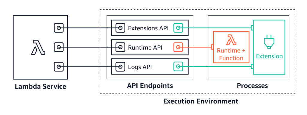
We launched Lambda Extensions in preview, enabling you to more easily integrate monitoring, security, and governance tools into Lambda functions. You can also build your own extensions that run code during Lambda lifecycle events, and there is an example extensions repo for starting development.

You can now send logs from Lambda functions to custom destinations by using Lambda Extensions and the new Lambda Logs API. Previously, you could only forward logs after they were written to Amazon CloudWatch Logs. Now, logging tools can receive log streams directly from the Lambda execution environment. This makes it easier to use your preferred tools for log management and analysis, including Datadog, Lumigo, New Relic, Coralogix, Honeycomb, or Sumo Logic.

Lambda launched support for Amazon MQ as an event source. Amazon MQ is a managed broker service for Apache ActiveMQ that simplifies deploying and scaling queues. This integration increases the range of messaging services that customers can use to build serverless applications. The event source operates in a similar way to using Amazon SQS or Amazon Kinesis. In all cases, the Lambda service manages an internal poller to invoke the target Lambda function.

We also released a new layer to make it simpler to integrate Amazon CodeGuru Profiler. This service helps identify the most expensive lines of code in a function and provides recommendations to help reduce cost. With this update, you can enable the profiler by adding the new layer and setting environment variables. There are no changes needed to the custom code in the Lambda function.

Lambda announced support for AWS PrivateLink. This allows you to invoke Lambda functions from a VPC without traversing the public internet. It provides private connectivity between your VPCs and AWS services. By using VPC endpoints to access the Lambda API from your VPC, this can replace the need for an Internet Gateway or NAT Gateway.

For developers building machine learning inferencing, media processing, high performance computing (HPC), scientific simulations, and financial modeling in Lambda, you can now use AVX2 support to help reduce duration and lower cost. By using packages compiled for AVX2 or compiling libraries with the appropriate flags, your code can then benefit from using AVX2 instructions to accelerate computation. In the blog post’s example, enabling AVX2 for an image-processing function increased performance by 32-43%.

Lambda now supports batch windows of up to 5 minutes when using SQS as an event source. This is useful for workloads that are not time-sensitive, allowing developers to reduce the number of Lambda invocations from queues. Additionally, the batch size has been increased from 10 to 10,000. This is now the same as the batch size for Kinesis as an event source, helping Lambda-based applications process more data per invocation.

Code signing is now available for Lambda, using AWS Signer. This allows account administrators to ensure that Lambda functions only accept signed code for deployment. Using signing profiles for functions, this provides granular control over code execution within the Lambda service. You can learn more about using this new feature in the developer documentation.

Amazon EventBridge

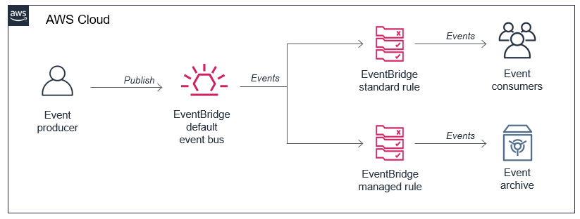
You can now use event replay to archive and replay events with Amazon EventBridge. After configuring an archive, EventBridge automatically stores all events or filtered events, based upon event pattern matching logic. You can configure a retention policy for archives to delete events automatically after a specified number of days. Event replay can help with testing new features or changes in your code, or hydrating development or test environments.

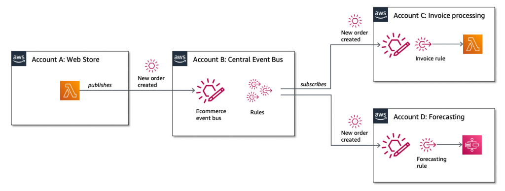
EventBridge also launched resource policies that simplify managing access to events across multiple AWS accounts. This expands the use of a policy associated with event buses to authorize API calls. Resource policies provide a powerful mechanism for modeling event buses across multiple account and providing fine-grained access control to EventBridge API actions.

EventBridge announced support for Server-Side Encryption (SSE). Events are encrypted using AES-256 at no additional cost for customers. EventBridge also increased PutEvent quotas to 10,000 transactions per second in US East (N. Virginia), US West (Oregon), and Europe (Ireland). This helps support workloads with high throughput.

AWS Step Functions

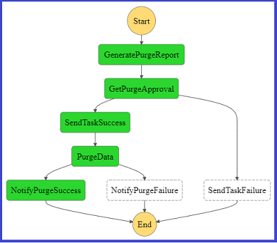
Synchronous Express Workflows have been launched for AWS Step Functions, providing a new way to run high-throughput Express Workflows. This feature allows developers to receive workflow responses without needing to poll services or build custom solutions. This is useful for high-volume microservice orchestration and fast compute tasks communicating via HTTPS.

The Step Functions service recently added support for other AWS services in workflows. You can now integrate API Gateway REST and HTTP APIs. This enables you to call API Gateway directly from a state machine as an asynchronous service integration.

Step Functions now also supports Amazon EKS service integration. This allows you to build workflows with steps that synchronously launch tasks in EKS and wait for a response. In October, the service also announced support for Amazon Athena, so workflows can now query data in your S3 data lakes.

These new integrations help minimize custom code and provide built-in error handling, parameter passing, and applying recommended security settings.

AWS SAM CLI

The AWS Serverless Application Model (AWS SAM) is an AWS CloudFormation extension that makes it easier to build, manage, and maintains serverless applications. On November 10, the AWS SAM CLI tool released version 1.9.0 with support for cached and parallel builds.

By using sam build --cached, AWS SAM no longer rebuilds functions and layers that have not changed since the last build. Additionally, you can use sam build --parallel to build functions in parallel, instead of sequentially. Both of these new features can substantially reduce the build time of larger applications defined with AWS SAM.

Amazon SNS

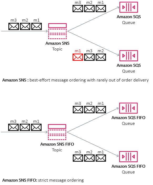
Amazon SNS announced support for First-In-First-Out (FIFO) topics. These are used with SQS FIFO queues for applications that require strict message ordering with exactly once processing and message deduplication. This is designed for workloads that perform tasks like bank transaction logging or inventory management. You can also use message filtering in FIFO topics to publish updates selectively.

AWS X-Ray

X-Ray now integrates with Amazon S3 to trace upstream requests. If a Lambda function uses the X-Ray SDK, S3 sends tracing headers to downstream event subscribers. With this, you can use the X-Ray service map to view connections between S3 and other services used to process an application request.

AWS CloudFormation

AWS CloudFormation announced support for nested stacks in change sets. This allows you to preview changes in your application and infrastructure across the entire nested stack hierarchy. You can then review those changes before confirming a deployment. This is available in all Regions supporting CloudFormation at no extra charge.

The new CloudFormation modules feature was released on November 24. This helps you develop building blocks with embedded best practices and common patterns that you can reuse in CloudFormation templates. Modules are available in the CloudFormation registry and can be used in the same way as any native resource.

Amazon DynamoDB

For customers using DynamoDB global tables, you can now use your own encryption keys. While all data in DynamoDB is encrypted by default, this feature enables you to use customer managed keys (CMKs). DynamoDB also announced support for global tables in the Europe (Milan) and Europe (Stockholm) Regions. This feature enables you to scale global applications for local access in workloads running in different Regions and replicate tables for higher availability and disaster recovery (DR).

The DynamoDB service announced the ability to export table data to data lakes in Amazon S3. This enables you to use services like Amazon Athena and AWS Lake Formation to analyze DynamoDB data with no custom code required. This feature does not consume table capacity and does not impact performance and availability. To learn how to use this feature, see this documentation.

AWS Amplify and AWS AppSync

You can now use existing Amazon Cognito user pools and identity pools for Amplify projects, making it easier to build new applications for an existing user base. AWS Amplify Console, which provides a fully managed static web hosting service, is now available in the Europe (Milan), Middle East (Bahrain), and Asia Pacific (Hong Kong) Regions. This service makes it simpler to bring automation to deploying and hosting single-page applications and static sites.

AWS AppSync enabled AWS WAF integration, making it easier to protect GraphQL APIs against common web exploits. You can also implement rate-based rules to help slow down brute force attacks. Using AWS Managed Rules for AWS WAF provides a faster way to configure application protection without creating the rules directly. AWS AppSync also recently expanded service availability to the Asia Pacific (Hong Kong), Middle East (Bahrain), and China (Ningxia) Regions, making the service now available in 21 Regions globally.

Still looking for more?

Join the AWS Serverless Developer Advocates on Twitch throughout re:Invent for live Q&A, session recaps, and more! See this page for the full schedule.

For more serverless learning resources, visit Serverless Land.

Detect change points in your event data stream using Amazon Kinesis Data Streams, Amazon DynamoDB and AWS Lambda

2020-11-18 Marco Guerriero

Post Syndicated from Marco Guerriero original https://aws.amazon.com/blogs/big-data/detect-change-points-in-your-event-data-stream-using-amazon-kinesis-data-streams-amazon-dynamodb-and-aws-lambda/

The success of many modern streaming applications depends on the ability to sequentially detect each change as soon as possible after it occurs, while continuing to monitor the data stream as it evolves. Applications of change point detection range across genomics, marketing, and finance, to name a few. In genomics, change point detection can help identify genes that are damaged. In marketing, we can identify things like customer churns in real time or when customer engagement changes over time. This is very useful in areas like online retail where, if change detection is implemented, we can adapt much more quickly to customer behavior. In finance, we can detect moments in time when stock prices have significantly changed. As opposed to online batch methodologies that take a batch of historical data and look for the change points in that data, we use a streaming procedure where we detect change points as fast as possible in real time as new data comes in.

In this post, we demonstrate automated event detection (AED), a fully automated, non-parametric, multiple change point detection algorithm that can operate on massive streaming data with low computational complexity, quickly reacting to the changes. Quick change detection [1] can help a system raise a timely alarm. Quickly reacting to a sudden fault arising in an industrial process or a production process could lead to significant savings in unplanned downtime. Detecting the onset of the outbreak of a disease, or the effect of a bio-terrorist attack, is critical, both for effective initiation of public health intervention measures and to timely alert government agencies and the general public.

In AED, no statistical assumption (such as Gaussian) is made on the generative process of the time series or data streams being processed. We rely on a class of tests called non-parametric or distribution-free tests [2, 3, 4, 5]. These tests are the natural choice for performing change point detection on data streams with unknown statistical distribution, which represents a common scenario that applies to a wide variety of real-world processes. We demonstrate a Python implementation of AED embedded within AWS Lambda over a data stream processed and managed by Amazon Kinesis Data Streams.

Understanding event detection

Let’s talk for a moment about anomaly detection, data drift, and change point detection in time series.

In machine learning (ML), we hear a lot about anomaly detection. In the context of a time series, that often means a data point that is outside the expected range. That range may have a static definition, such as “we never expect the temperature to exceed 130F,” or a dynamic definition, such as “it should not vary from recent averages by more than three standard deviations.” An example of a dynamic anomaly detection algorithm is Random Cut Forest.

In contrast, data drift describes a slower shift in the stream’s data distribution. It may mean a shift in the mean of a variable, such as a shift in temperatures between summer and winter, or a change in behavior of visitors to a website as certain product categories fall out of favor and others become fashionable. A frequently recommended approach for dealing with data drift is frequent retraining of an ML model, to keep recommendations fresh and relevant based on recent data.

The events AED focuses on are in a different category altogether: sudden shifts in the data stream to a new level, sometimes called regime change. These are occasions where human intervention may be desired to see whether automated responses are appropriate. For example, a slow shift in readings from a temperature sensor may be normal, whereas a sudden large change may be a sign of a major malfunction in progress. Other data streams that constantly fluctuate but where a sudden large change may require oversight include equipment monitoring and malfunctions, cyber attacks, stock market movements, power grids and outages, and operational variations in manufacturing processes, to name a few [1].

Our goal is to automatically detect multiple events when the time series or the data streams change their behavior. In this version, we focus on sudden changes in mean or offset in time series. AED is an unsupervised, automatic, statistically rigorous, real-time procedure for detecting relevant events, which doesn’t require any training data. It can also be used as an automatic process for feature extraction (such as time series segmentation) that can be used in downstream ML systems.

Automated event detection

AED operates sequentially as data comes in, continuously performing a novel statistical test to identify a change event—a significant shift in the data from the data that preceded that point in time. If an event is detected at time t_i, all the previous data prior to t_i is discarded. AED is then reset to process new data points starting with the (t_i +1)th data point, looking for a new change event. This procedure is repeated sequentially until no more data points are available.

The core of AED is represented by the statistical test called the Modified Practical Pettitt (MPP) test. The MPP test is a variant of the Pettitt test [6], which is a very powerful and robust non-parametrical statistical procedure to detect a single change point in data streams where the distribution is completely unknown. Pettitt’s test is based on Null Hypothesis Significance Testing (NHST), which comes with some constraints and fallacies. In fact, a very important problem with NHST is that the result of the test doesn’t provide information about the magnitude of the effect of the event—which is key information we’re interested in. A consequence of this limit is that an event (change point) can be detected despite a very small effect. But is an increase of 0.001 Celsius degrees in temperature data streams coming from some IoT devices or a decrease of $1 in a particular stock price noteworthy events? Statistical significance doesn’t tell us anything about practical relevance. The MPP test solves this problem by incorporating a practical significance threshold into the definition of the decision test statistic. In this way, only events that are both statistically and practically significant are detected and reported by AED.

The decision statistic of the MPP test can be computed recursively, resulting in a computational complexity that is linear in the number of data points processed by AED up to the reset time.

Prerequisites

To get started, we need the following:

A continuous or discrete time series (data stream). No knowledge of the distribution of the data is needed.
Some guidance for the algorithm in terms of when to alert us:
- The statistical confidence level we require that an event has occurred (p value).
- The practical significance level we require (our practical significance threshold).

The output of AED is a list of change points specified by their time of occurrence, their p-value, and the magnitude of the offset.

Solution overview

The following diagram illustrates the AWS services used to implement the solution.

The steps in the process are as follows:

One or more programs, devices, or sensors generate events and place them into a Kinesis data stream. These events make up a time series. In our case, we provide a sample generator function.
The event recorder Lambda function consumes records from the data stream.
The Lambda function stores them in an Amazon DynamoDB events table.
The DynamoDB table streams the inserted events to the event detection Lambda function.
The Lambda function checks each event to see whether this is a change point. To do so, it performs the following actions:
- Reads the last change point recorded from the DynamoDB change points table (or creates one if this is the first data point for this device).
- Reads the prior events since the last change point from the events table, as a time series.
- Runs the event-detection algorithm over the retrieved time series.
If a new change point is detected, the function does the following:
- Writes the change point into the DynamoDB change points table, for later use.
- Sends an Amazon Simple Notification Service (Amazon SNS) message to a topic with the change point details.

Setting up the solution infrastructure

To set up the infrastructure components and configure the connections, launch a predefined AWS CloudFormation stack. The stack sets up the following resources:

A Kinesis data stream.
Two Lambda functions: the event recorder, and the event detection. Each function has an associated AWS Identity and Access Management (IAM) role.
Two DynamoDB tables: one to hold events, and one for detected change points.
An SNS topic and a subscription, for notifying that a change point has been detected.

To see this solution in operation in the US East (N. Virginia) Region, launch the provided CloudFormation stack. The total solution costs approximately $0.02 per hour to run, depending on the volume of data sent to the components. Remember to delete the CloudFormation stack when you’re finished with the solution to avoid additional charges.

To run the stack, complete the following steps:

Choose Launch Stack:

Choose Next.
Update the email address for notifications to be a valid email address of your choice.
Update the following parameters for your environment if necessary, or, for now, leave the defaults:
1. Environment parameters – Names for your DynamoDB tables, Kinesis stream, and SNS topic
2. AED parameters – Startup, alpha level, change difference window, and practical significance threshold
Choose Next.
Select I acknowledge that AWS CloudFormation might create IAM resources with custom names.
Choose Create stack.
Wait for the CloudFormation stack to reach a status of CREATE COMPLETE (around 5 minutes).
Check the Outputs tab for the resources created.

If you want to receive the SNS messages for detected change points, remember to confirm your SNS subscription for the email address.

Generating data

After AWS CloudFormation creates the system resources for us, we’re ready to start generating some data. For this post, we provide a client that generates a time series with periodic regime shifts. For simplicity and to show generality, the client also runs AED over the time series it creates. At the end, it generates a time series plot of the generated data along with the detected change points. These should match the SNS notifications you receive.

To download and set up the test clients, copy the following files to your local desktop:
Install boto3, numpy, and matplotlib, if you don’t already have them installed.

Two test clients are provided:

The time_series_client.py generates data and puts it into Kinesis Data Streams; this is what your device does.
For easier demonstration, we also provide a time_series_validation_client. This version also runs AED locally and generates an annotated plot showing the input data, where the change points are detected, and where the change actually occurred.

To run the validation client, open a command prompt to the folder where you copied the client files and run the following code:

python time_series_validation_client.py  -r us-east-1 -s aed_events_data_stream

You can pass the –h parameter to find out the other parameters. By default, the client generates 1 minute’s worth of data. The parameters let you configure the client for your environment, and, when running the validation client, for the local AED detection (which is independent of that being performed in the Lambda function).

You can use four parameters to configure AED’s behavior to match your environment:

“-a”, “–alpha” – The AED alpha level, that is, the smallest change to identify. The default is 0.01.
“-w”, “–window” – The AED change difference window, the number of points around the change to ignore. The default is 5.
“-x”, “–startup” – The number of samples to include in the AED initialization stage. The default is 5.
“-p”, “–practicalthreshold” – The AED practical significance threshold. Changes smaller than this are not designated as change points. The default is 0.

At the end of the time period, the client displays an image of the generated time series. The following time series is annotated with a small blue triangle whenever the client created a change point. The small red triangles mark the points where the AED algorithm, running independently over the generated data, detected the change points. The blue triangle always precedes the red triangle in our DetectBeforeDecide framework, where the AED algorithm has to first detect that something is changing (red triangle) and then work backwards to decide when in time the change most likely occurred (blue triangle).

The turquoise dot shows where the data generation was restarted; this change point may not be detected because AED isn’t running at that time. As you can see, each generated change point was detected. At the same time, the significant variation between the change points—in essence, within a single regime—didn’t cause a spurious change point detection.

The practical significance threshold additionally allows you to specify when the change is small enough that it’s not relevant and should be ignored.

You can also review the contents of the DynamoDB tables on the AWS Management Console (see the following screenshot). The table aed_stream_data shows each event in the stream logged. The aed_change_points table shows the individual change points detected, along with the timestamp of the detection and the data point at the time the change was detected by the Lambda function running over the stream data. This data lets you construct a history of the event stream and the change points, and manipulate them according to your need.

Each Lambda function is started by the Kinesis stream; it checks to see when the last change point occurred. It then retrieves the data since that change point from the aed_stream_data table and reprocesses it, looking for a new change point. As the gaps between change points get very large, this may become a large sequence to retrieve and process. If this is your use case, you may wish to artificially create a new set point every so often to reduce the amount of data that must be reread.

Cleaning up

To avoid additional charges, you should delete the CloudFormation stack after walking through the solution.

To implement AED in a different Region or to adapt it to your own needs, download the aed.zip file.

Conclusion

In this post, we introduced automated event detection (AED), a new, fast, scalable, fully automated, non-parametric, multiple change point detection service that can operate on massive streaming data with low computational complexity. AED efficiently identifies shifts in the data stream that have both statistical and practical significance. This ability to locate the time and magnitude of a shift in the data stream, and to differentiate it from normal data fluctuations, is key in many applications. The appropriate action varies by use case: it may be appropriate to take automated action, or call a human to evaluate whether the preplanned actions should be taken. A natural extension of AED would be to add an algorithm to detect trends (gradual changes as opposed to sudden shifts) in data streams using non-parametric tests such as Mann-Kendall [7, 8]. Combining these functions allows you to identify both kinds of changes in your incoming data stream and distinguish between them, further broadening the use cases.

In this post, we demonstrated a Python implementation of AED embedded within Lambda over a data stream processed and managed by Kinesis Data Streams. We also provided a standalone client implementation to show an alternate implementation. The code is available for you to download and integrate into your applications. Do you have any data streams where sudden shifts may happen? Do you want to know when they happen? Are there automated actions that should be taken, or should someone be alerted? If your answer to any of these questions is “Yes!” then consider implementing AED.

If you have any comments about this post, submit them in the comments section.

References

[1] H. V. Poor and O. Hadjiliadis (2009). Quickest detection. Cambridge University Press, 2009.

[2] Brodsky, E., and Boris S. Darkhovsky (2013). Nonparametric methods in change point problems. Vol. 243. Springer Science & Business Media.

[3] Csörgö, Miklós, and Lajos Horváth (1997). Limit theorems in change-point analysis. Vol. 18. John Wiley & Sons Inc,.

[4] Ross GJ, Tasoulis DK, Adams NM (2011). Nonparametric Monitoring of Data Streams for Changes in Location and Scale. Technometrics, 53(4), 379–389.

[5] Chu, Lynna, and Hao Chen (2019). Asymptotic distribution-free change-point detection for multivariate and non-euclidean data. The Annals of Statistics 47.1, 382-414.

[6] Pettitt AN (1979). A Non-Parametric Approach to the Change-Point Problem. Journal of the Royal Statistical Society C, 28(2), 126–135.

[7] H. B. Mann (1945). Nonparametric tests against trend, Econometrica, vol. 13, pp. 245–259, 1945.

[8] M. G. Kendal (1975). Rank Correlation Methods, Griffin, London, UK, 1975

About the Authors

Marco Guerriero, PhD, is a Practice Manager for Emergent Technologies and Intelligence Platform for AWS Professional Services. I love working on ways for emergent technologies such as AI/ML, Big Data, IoT, and Quantum to help businesses across different industry vertical succeed within their innovation journey.

Veronika Megler, PhD, is Principal Data Scientist for Amazon.com Customer Packaging Experience. Until recently, she was the Principal Data Scientist for AWS Professional Services. She enjoys adapting innovative big data, AI, and ML technologies to help companies solve new problems, and to solve old problems more efficiently and effectively. Her work has lately been focused more heavily on economic impacts of ML models and exploring causality.

New – Export Amazon DynamoDB Table Data to Your Data Lake in Amazon S3, No Code Writing Required

2020-11-10 Alex Casalboni

Post Syndicated from Alex Casalboni original https://aws.amazon.com/blogs/aws/new-export-amazon-dynamodb-table-data-to-data-lake-amazon-s3/

Hundreds of thousands of AWS customers have chosen Amazon DynamoDB for mission-critical workloads since its launch in 2012. DynamoDB is a nonrelational managed database that allows you to store a virtually infinite amount of data and retrieve it with single-digit-millisecond performance at any scale. To get the most value out of this data, customers had […]

Rapid and flexible Infrastructure as Code using the AWS CDK with AWS Solutions Constructs

2020-10-31 Biff Gaut

Post Syndicated from Biff Gaut original https://aws.amazon.com/blogs/devops/rapid-flexible-infrastructure-with-solutions-constructs-cdk/

Introduction

As workloads move to the cloud and all infrastructure becomes virtual, infrastructure as code (IaC) becomes essential to leverage the agility of this new world. JSON and YAML are the powerful, declarative modeling languages of AWS CloudFormation, allowing you to define complex architectures using IaC. Just as higher level languages like BASIC and C abstracted away the details of assembly language and made developers more productive, the AWS Cloud Development Kit (AWS CDK) provides a programming model above the native template languages, a model that makes developers more productive when creating IaC. When you instantiate CDK objects in your Typescript (or Python, Java, etc.) application, those objects “compile” into a YAML template that the CDK deploys as an AWS CloudFormation stack.

AWS Solutions Constructs take this simplification a step further by providing a library of common service patterns built on top of the CDK. These multi-service patterns allow you to deploy multiple resources with a single object, resources that follow best practices by default – both independently and throughout their interaction.

Comparison of an Application stack with Assembly Language, 4th generation language and Object libraries such as Hibernate with an IaC stack of CloudFormation, AWS CDK and AWS Solutions Constructs

Application Development Stack vs. IaC Development Stack

Solution overview

To demonstrate how using Solutions Constructs can accelerate the development of IaC, in this post you will create an architecture that ingests and stores sensor readings using Amazon Kinesis Data Streams, AWS Lambda, and Amazon DynamoDB.

An architecture diagram showing sensor readings being sent to a Kinesis data stream. A Lambda function will receive the Kinesis records and store them in a DynamoDB table.

Prerequisite – Setting up the CDK environment

Tip – If you want to try this example but are concerned about the impact of changing the tools or versions on your workstation, try running it on AWS Cloud9. An AWS Cloud9 environment is launched with an AWS Identity and Access Management (AWS IAM) role and doesn’t require configuring with an access key. It uses the current region as the default for all CDK infrastructure.

To prepare your workstation for CDK development, confirm the following:

Node.js 10.3.0 or later is installed on your workstation (regardless of the language used to write CDK apps).
You have configured credentials for your environment. If you’re running locally you can do this by configuring the AWS Command Line Interface (AWS CLI).
TypeScript 2.7 or later is installed globally (npm -g install typescript)

Before creating your CDK project, install the CDK toolkit using the following command:

npm install -g aws-cdk

Create the CDK project

First create a project folder called stream-ingestion with these two commands:

mkdir stream-ingestion
cd stream-ingestion

Now create your CDK application using this command:

npx [email protected] init app --language=typescript

Tip – This example will be written in TypeScript – you can also specify other languages for your projects.

At this time, you must use the same version of the CDK and Solutions Constructs. We’re using version 1.68.0 of both based upon what’s available at publication time, but you can update this with a later version for your projects in the future.

Let’s explore the files in the application this command created:

bin/stream-ingestion.ts – This is the module that launches the application. The key line of code is:

new StreamIngestionStack(app, 'StreamIngestionStack');

This creates the actual stack, and it’s in StreamIngestionStack that you will write the CDK code that defines the resources in your architecture.

lib/stream-ingestion-stack.ts – This is the important class. In the constructor of StreamIngestionStack you will add the constructs that will create your architecture.

During the deployment process, the CDK uploads your Lambda function to an Amazon S3 bucket so it can be incorporated into your stack.

To create that S3 bucket and any other infrastructure the CDK requires, run this command:

cdk bootstrap

The CDK uses the same supporting infrastructure for all projects within a region, so you only need to run the bootstrap command once in any region in which you create CDK stacks.

To install the required Solutions Constructs packages for our architecture, run the these two commands from the command line:

npm install @aws-solutions-constructs/[email protected]
npm install @aws-solutions-constructs/[email protected]

Write the code

First you will write the Lambda function that processes the Kinesis data stream messages.

Create a folder named lambda under stream-ingestion
Within the lambda folder save a file called lambdaFunction.js with the following contents:

var AWS = require("aws-sdk");

// Create the DynamoDB service object
var ddb = new AWS.DynamoDB({ apiVersion: "2012-08-10" });

AWS.config.update({ region: process.env.AWS_REGION });

// We will configure our construct to 
// look for the .handler function
exports.handler = async function (event) {
  try {
    // Kinesis will deliver records 
    // in batches, so we need to iterate through
    // each record in the batch
    for (let record of event.Records) {
      const reading = parsePayload(record.kinesis.data);
      await writeRecord(record.kinesis.partitionKey, reading);
    };
  } catch (err) {
    console.log(`Write failed, err:\n${JSON.stringify(err, null, 2)}`);
    throw err;
  }
  return;
};

// Write the provided sensor reading data to the DynamoDB table
async function writeRecord(partitionKey, reading) {

  var params = {
    // Notice that Constructs automatically sets up 
    // an environment variable with the table name.
    TableName: process.env.DDB_TABLE_NAME,
    Item: {
      partitionKey: { S: partitionKey },  // sensor Id
      timestamp: { S: reading.timestamp },
      value: { N: reading.value}
    },
  };

  // Call DynamoDB to add the item to the table
  await ddb.putItem(params).promise();
}

// Decode the payload and extract the sensor data from it
function parsePayload(payload) {

  const decodedPayload = Buffer.from(payload, "base64").toString(
    "ascii"
  );

  // Our CLI command will send the records to Kinesis
  // with the values delimited by '|'
  const payloadValues = decodedPayload.split("|", 2)
  return {
    value: payloadValues[0],
    timestamp: payloadValues[1]
  }
}

We won’t spend a lot of time explaining this function – it’s pretty straightforward and heavily commented. It receives an event with one or more sensor readings, and for each reading it extracts the pertinent data and saves it to the DynamoDB table.

You will use two Solutions Constructs to create your infrastructure:

The aws-kinesisstreams-lambda construct deploys an Amazon Kinesis data stream and a Lambda function.

aws-kinesisstreams-lambda creates the Kinesis data stream and Lambda function that subscribes to that stream. To support this, it also creates other resources, such as IAM roles and encryption keys.

The aws-lambda-dynamodb construct deploys a Lambda function and a DynamoDB table.

aws-lambda-dynamodb creates an Amazon DynamoDB table and a Lambda function with permission to access the table.

To deploy the first of these two constructs, replace the code in lib/stream-ingestion-stack.ts with the following code:

import * as cdk from "@aws-cdk/core";
import * as lambda from "@aws-cdk/aws-lambda";
import { KinesisStreamsToLambda } from "@aws-solutions-constructs/aws-kinesisstreams-lambda";

import * as ddb from "@aws-cdk/aws-dynamodb";
import { LambdaToDynamoDB } from "@aws-solutions-constructs/aws-lambda-dynamodb";

export class StreamIngestionStack extends cdk.Stack {
  constructor(scope: cdk.Construct, id: string, props?: cdk.StackProps) {
    super(scope, id, props);

    const kinesisLambda = new KinesisStreamsToLambda(
      this,
      "KinesisLambdaConstruct",
      {
        lambdaFunctionProps: {
          // Where the CDK can find the lambda function code
          runtime: lambda.Runtime.NODEJS_10_X,
          handler: "lambdaFunction.handler",
          code: lambda.Code.fromAsset("lambda"),
        },
      }
    );

    // Next Solutions Construct goes here
  }
}

Let’s explore this code:

It instantiates a new KinesisStreamsToLambda object. This Solutions Construct will launch a new Kinesis data stream and a new Lambda function, setting up the Lambda function to receive all the messages in the Kinesis data stream. It will also deploy all the additional resources and policies required for the architecture to follow best practices.
The third argument to the constructor is the properties object, where you specify overrides of default values or any other information the construct needs. In this case you provide properties for the encapsulated Lambda function that informs the CDK where to find the code for the Lambda function that you stored as lambda/lambdaFunction.js earlier.

Now you’ll add the second construct that connects the Lambda function to a new DynamoDB table. In the same lib/stream-ingestion-stack.ts file, replace the line // Next Solutions Construct goes here with the following code:

    // Define the primary key for the new DynamoDB table
    const primaryKeyAttribute: ddb.Attribute = {
      name: "partitionKey",
      type: ddb.AttributeType.STRING,
    };

    // Define the sort key for the new DynamoDB table
    const sortKeyAttribute: ddb.Attribute = {
      name: "timestamp",
      type: ddb.AttributeType.STRING,
    };

    const lambdaDynamoDB = new LambdaToDynamoDB(
      this,
      "LambdaDynamodbConstruct",
      {
        // Tell construct to use the Lambda function in
        // the first construct rather than deploy a new one
        existingLambdaObj: kinesisLambda.lambdaFunction,
        tablePermissions: "Write",
        dynamoTableProps: {
          partitionKey: primaryKeyAttribute,
          sortKey: sortKeyAttribute,
          billingMode: ddb.BillingMode.PROVISIONED,
          removalPolicy: cdk.RemovalPolicy.DESTROY
        },
      }
    );

    // Add autoscaling
    const readScaling = lambdaDynamoDB.dynamoTable.autoScaleReadCapacity({
      minCapacity: 1,
      maxCapacity: 50,
    });

    readScaling.scaleOnUtilization({
      targetUtilizationPercent: 50,
    });

Let’s explore this code:

The first two const objects define the names and types for the partition key and sort key of the DynamoDB table.
The LambdaToDynamoDB construct instantiated creates a new DynamoDB table and grants access to your Lambda function. The key to this call is the properties object you pass in the third argument.
- The first property sent to LambdaToDynamoDB is existingLambdaObj – by setting this value to the Lambda function created by KinesisStreamsToLambda, you’re telling the construct to not create a new Lambda function, but to grant the Lambda function in the other Solutions Construct access to the DynamoDB table. This illustrates how you can chain many Solutions Constructs together to create complex architectures.
- The second property sent to LambdaToDynamoDB tells the construct to limit the Lambda function’s access to the table to write only.
- The third property sent to LambdaToDynamoDB is actually a full properties object defining the DynamoDB table. It provides the two attribute definitions you created earlier as well as the billing mode. It also sets the RemovalPolicy to DESTROY. This policy setting ensures that the table is deleted when you delete this stack – in most cases you should accept the default setting to protect your data.
The last two lines of code show how you can use statements to modify a construct outside the constructor. In this case we set up auto scaling on the new DynamoDB table, which we can access with the dynamoTable property on the construct we just instantiated.

That’s all it takes to create the all resources to deploy your architecture.

Save all the files, then compile the Typescript into a CDK program using this command:

npm run build

Finally, launch the stack using this command:

cdk deploy

(Enter “y” in response to Do you wish to deploy all these changes (y/n)?)

You will see some warnings where you override CDK default values. Because you are doing this intentionally you may disregard these, but it’s always a good idea to review these warnings when they occur.

Tip – Many mysterious CDK project errors stem from mismatched versions. If you get stuck on an inexplicable error, check package.json and confirm that all CDK and Solutions Constructs libraries have the same version number (with no leading caret ^). If necessary, correct the version numbers, delete the package-lock.json file and node_modules tree and run npm install. Think of this as the “turn it off and on again” first response to CDK errors.

You have now deployed the entire architecture for the demo – open the CloudFormation stack in the AWS Management Console and take a few minutes to explore all 12 resources that the program deployed (and the 380 line template generated to created them).

Feed the Stream

Now use the CLI to send some data through the stack.

Go to the Kinesis Data Streams console and copy the name of the data stream. Replace the stream name in the following command and run it from the command line.

aws kinesis put-records \
--stream-name StreamIngestionStack-KinesisLambdaConstructKinesisStreamXXXXXXXX-XXXXXXXXXXXX \
--records \
PartitionKey=1301,'Data=15.4|2020-08-22T01:16:36+00:00' \
PartitionKey=1503,'Data=39.1|2020-08-22T01:08:15+00:00'

Tip – If you are using the AWS CLI v2, the previous command will result in an “Invalid base64…” error because v2 expects the inputs to be Base64 encoded by default. Adding the argument --cli-binary-format raw-in-base64-out will fix the issue.

To confirm that the messages made it through the service, open the DynamoDB console – you should see the two records in the table.

Now that you’ve got it working, pause to think about what you just did. You deployed a system that can ingest and store sensor readings and scale to handle heavy loads. You did that by instantiating two objects – well under 60 lines of code. Experiment with changing some property values and deploying the changes by running npm run build and cdk deploy again.

Cleanup

To clean up the resources in the stack, run this command:

cdk destroy

Conclusion

Just as languages like BASIC and C allowed developers to write programs at a higher level of abstraction than assembly language, the AWS CDK and AWS Solutions Constructs allow us to create CloudFormation stacks in Typescript, Java, or Python instead JSON or YAML. Just as there will always be a place for assembly language, there will always be situations where we want to write CloudFormation templates manually – but for most situations, we can now use the AWS CDK and AWS Solutions Constructs to create complex and complete architectures in a fraction of the time with very little code.

AWS Solutions Constructs can currently be used in CDK applications written in Typescript, Javascript, Java and Python and will be available in C# applications soon.

About the Author

Biff Gaut has been shipping software since 1983, from small startups to large IT shops. Along the way he has contributed to 2 books, spoken at several conferences and written many blog posts. He is now a Principal Solutions Architect at AWS working on the AWS Solutions Constructs team, helping customers deploy better architectures more quickly.

Optimizing the cost of serverless web applications

2020-10-19 James Beswick

Post Syndicated from James Beswick original https://aws.amazon.com/blogs/compute/optimizing-the-cost-of-serverless-web-applications/

Web application backends are one of the most frequent types of serverless use-case for customers. The pay-for-value model can make it cost-efficient to build web applications using serverless tools.

While serverless cost is generally correlated with level of usage, there are architectural decisions that impact cost efficiency. The impact of these choices is more significant as your traffic grows, so it’s important to consider the cost-effectiveness of different designs and patterns.

This blog post reviews some common areas in web applications where you may be able to optimize cost. It uses the Happy Path web application as a reference example, which you can read about in the introductory blog post.

Serverless web applications generally use a combination of the services in the following diagram. I cover each of these areas to highlight common areas for cost optimization.

The API management layer: Selecting the right API type

Most serverless web applications use an API between the frontend client and the backend architecture. Amazon API Gateway is a common choice since it is a fully managed service that scales automatically. There are three types of API offered by the service – REST APIs, WebSocket APIs, and the more recent HTTP APIs.

HTTP APIs offer many of the features in the REST APIs service, but the cost is often around 70% less. It supports Lambda service integration, JWT authorization, CORS, and custom domain names. It also has a simpler deployment model than REST APIs. This feature set tends to work well for web applications, many of which mainly use these capabilities. Additionally, HTTP APIs will gain feature parity with REST APIs over time.

The Happy Path application is designed for 100,000 monthly active users. It uses HTTP APIs, and you can inspect the backend/template.yaml to see how to define these in the AWS Serverless Application Model (AWS SAM). If you have existing AWS SAM templates that are using REST APIs, in many cases you can change these easily:

Content distribution layer: Optimizing assets

Amazon CloudFront is a content delivery network (CDN). It enables you to distribute content globally across 216 Points of Presence without deploying or managing any infrastructure. It reduces latency for users who are geographically dispersed and can also reduce load on other parts of your service.

A typical web application uses CDNs in a couple of different ways. First, there is the distribution of the application itself. For single-page application frameworks like React or Vue.js, the build processes create static assets that are ideal for serving over a CDN.

However, these builds may not be optimized and can be larger than necessary. Many frameworks offer optimization plugins, and the JavaScript community frequently uses Webpack to bundle modules and shrink deployment packages. Similarly, any media assets used in the application build should be optimized. You can use tools like Lighthouse to analyze your web apps to find images that can be resized or compressed.

The second common CDN use-case for web apps is for user-generated content (UGC). Many apps allow users to upload images, which are then shared with other users. A typical photo from a 12-megapixel smartphone is 3–9 MB in size. This high resolution is not necessary when photos are rendered within web apps. Displaying the high-resolution asset results in slower download performance and higher data transfer costs.

The Happy Path application uses a Resizer Lambda function to optimize these uploaded assets. This process creates two different optimized images depending upon which component loads the asset.

The upload S3 bucket shows the original size of the upload from the smartphone:

The distribution S3 bucket contains the two optimized images at different sizes:

The distribution file sizes are 98–99% smaller. For a busy web application, using optimized image assets can make a significant difference to data transfer and CloudFront costs.

Additionally, you can convert to highly optimized file formats such as WebP to reduce file size even further. Not all browsers support this format, but you can use CSS on the frontend to fall back to other types if needed:

<img src="myImage.webp" onerror="this.onerror=null; this.src='myImage.jpg'">

The data layer

AWS offers many different database and storage options that can be useful for web applications. Billing models vary by service and Region. By understanding the data access and storage requirements of your app, you can make informed decisions about the right service to use.

Generally, it’s more cost-effective to store binary data in S3 than a database. First, when the data is uploaded, you can upload directly to S3 with presigned URLs instead of proxying data via API Gateway or another service.

If you are using Amazon DynamoDB, it’s best practice to store larger items in S3 and include a reference token in a table item. Part of DynamoDB pricing is based on read capacity units (RCUs). For binary items such as images, it is usually more cost-efficient to use S3 for storage.

Many web developers who are new to serverless are familiar with using a relational database, so choose Amazon RDS for their database needs. Depending upon your use-case and data access patterns, it may be more cost effective to use DynamoDB instead. RDS is not a serverless service so there are monthly charges for the underlying compute instance. DynamoDB pricing is based upon usage and storage, so for many web apps may be a lower-cost choice.

Integration layer

This layer includes services like Amazon SQS, Amazon SNS, and Amazon EventBridge, which are essential for decoupling serverless applications. Each of these have a request-based pricing component, where 64 KB of a payload is billed as one request. For example, a single SQS message with a 256 KB payload is billed as four requests. There are two optimization methods common for web applications.

1. Combine messages

Many messages sent to these services are much smaller than 64 KB. In some applications, the publishing service can combine multiple messages to reduce the total number of publish actions to SNS. Additionally, by either eliminating unused attributes in the message or compressing the message, you can store more data in a single request.

For example, a publishing service may be able to combine multiple messages together in a single publish action to an SNS topic:

Before optimization, a publishing service sends 100,000,000 1KB-messages to an SNS topic. This is charged as 100 million messages for a total cost of $50.00.
After optimization, the publishing service combines messages to send 1,562,500 64KB-messages to an SNS topic. This is charged as 1,562,500 messages for a total cost of $0.78.

2. Filter messages

In many applications, not every message is useful for a consuming service. For example, an SNS topic may publish to a Lambda function, which checks the content and discards the message based on some criteria. In this case, it’s more cost effective to use the native filtering capabilities of SNS. The service can filter messages and only invoke the Lambda function if the criteria is met. This lowers the compute cost by only invoking Lambda when necessary.

For example, an SNS topic receives messages about customer orders and forwards these to a Lambda function subscriber. The function is only interested in canceled orders and discards all other messages:

Before optimization, the SNS topic sends all messages to a Lambda function. It evaluates the message for the presence of an order canceled attribute. On average, only 25% of the messages are processed further. While SNS does not charge for delivery to Lambda functions, you are charged each time the Lambda service is invoked, for 100% of the messages.
After optimization, using an SNS subscription filter policy, the SNS subscription filters for canceled orders and only forwards matching messages. Since the Lambda function is only invoked for 25% of the messages, this may reduce the total compute cost by up to 75%.

3. Choose a different messaging service

For complex filtering options based upon matching patterns, you can use EventBridge. The service can filter messages based upon prefix matching, numeric matching, and other patterns, combining several rules into a single filter. You can create branching logic within the EventBridge rule to invoke downstream targets.

EventBridge offers a broader range of targets than SNS destinations. In cases where you publish from an SNS topic to a Lambda function to invoke an EventBridge target, you could use EventBridge instead and eliminate the Lambda invocation. For example, instead of routing from SNS to Lambda to AWS Step Functions, instead create an EventBridge rule that routes events directly to a state machine.

Business logic layer

Step Functions allows you to orchestrate complex workflows in serverless applications while eliminating common boilerplate code. The Standard Workflow service charges per state transition. Express Workflows were introduced in December 2019, with pricing based on requests and duration, instead of transitions.

For workloads that are processing large numbers of events in shorter durations, Express Workflows can be more cost-effective. This is designed for high-volume event workloads, such as streaming data processing or IoT data ingestion. For these cases, compare the cost of the two workflow types to see if you can reduce cost by switching across.

Lambda is the on-demand compute layer in serverless applications, which is billed by requests and GB-seconds. GB-seconds is calculated by multiplying duration in seconds by memory allocated to the function. For a function with a 1-second duration, invoked 1 million times, here is how memory allocation affects the total cost in the US East (N. Virginia) Region:

Memory (MB)	GB/S	Compute cost	Total cost
128	125,000	$ 2.08	$ 2.28
512	500,000	$ 8.34	$ 8.54
1024	1,000,000	$ 16.67	$ 16.87
1536	1,500,000	$ 25.01	$ 25.21
2048	2,000,000	$ 33.34	$ 33.54
3008	2,937,500	$ 48.97	$ 49.17

There are many ways to optimize Lambda functions, but one of the most important choices is memory allocation. You can choose between 128 MB and 3008 MB, but this also impacts the amount of virtual CPU as memory increases. Since total cost is a combination of memory and duration, choosing more memory can often reduce duration and lower overall cost.

Instead of manually setting the memory for a Lambda function and running executions to compare duration, you can use the AWS Lambda Power Tuning tool. This uses Step Functions to run your function against varying memory configurations. It can produce a visualization to find the optimal memory setting, based upon cost or execution time.

Conclusion

Web application backends are one of the most popular workload types for serverless applications. The pay-per-value model works well for this type of workload. As traffic grows, it’s important to consider the design choices and service configurations used to optimize your cost.

Serverless web applications generally use a common range of services, which you can logically split into different layers. This post examines each layer and suggests common cost optimizations helpful for web app developers.

To learn more about building web apps with serverless, see the Happy Path series. For more serverless learning resources, visit https://serverlessland.com.

Unified serverless streaming ETL architecture with Amazon Kinesis Data Analytics

2020-09-30 Ram Vittal

Post Syndicated from Ram Vittal original https://aws.amazon.com/blogs/big-data/unified-serverless-streaming-etl-architecture-with-amazon-kinesis-data-analytics/

Businesses across the world are seeing a massive influx of data at an enormous pace through multiple channels. With the advent of cloud computing, many companies are realizing the benefits of getting their data into the cloud to gain meaningful insights and save costs on data processing and storage. As businesses embark on their journey towards cloud solutions, they often come across challenges involving building serverless, streaming, real-time ETL (extract, transform, load) architecture that enables them to extract events from multiple streaming sources, correlate those streaming events, perform enrichments, run streaming analytics, and build data lakes from streaming events.

In this post, we discuss the concept of unified streaming ETL architecture using a generic serverless streaming architecture with Amazon Kinesis Data Analytics at the heart of the architecture for event correlation and enrichments. This solution can address a variety of streaming use cases with various input sources and output destinations. We then walk through a specific implementation of the generic serverless unified streaming architecture that you can deploy into your own AWS account for experimenting and evolving this architecture to address your business challenges.

Overview of solution

As data sources grow in volume, variety, and velocity, the management of data and event correlation become more challenging. Most of the challenges stem from data silos, in which different teams and applications manage data and events using their own tools and processes.

Modern businesses need a single, unified view of the data environment to get meaningful insights through streaming multi-joins, such as the correlation of sensory events and time-series data. Event correlation plays a vital role in automatically reducing noise and allowing the team to focus on those issues that really matter to the business objectives.

To realize this outcome, the solution proposes creating a three-stage architecture:

Ingestion
Processing
Analysis and visualization

The source can be a varied set of inputs comprising structured datasets like databases or raw data feeds like sensor data that can be ingested as single or multiple parallel streams. The solution envisions multiple hybrid data sources as well. After it’s ingested, the data is divided into single or multiple data streams depending on the use case and passed through a preprocessor (via an AWS Lambda function). This highly customizable processor transforms and cleanses data to be processed through analytics application. Furthermore, the architecture allows you to enrich data or validate it against standard sets of reference data, for example validating against postal codes for address data received from the source to verify its accuracy. After the data is processed, it’s sent to various sink platforms depending on your preferences, which could range from storage solutions to visualization solutions, or even stored as a dataset in a high-performance database.

The solution is designed with flexibility as a key tenant to address multiple, real-world use cases. The following diagram illustrates the solution architecture.

The architecture has the following workflow:

We use AWS Database Migration Service (AWS DMS) to push records from the data source into AWS in real time or batch. For our use case, we use AWS DMS to fetch records from an on-premises relational database.
AWS DMS writes records to Amazon Kinesis Data Streams. The data is split into multiple streams as necessitated through the channels.
A Lambda function picks up the data stream records and preprocesses them (adding the record type). This is an optional step, depending on your use case.
Processed records are sent to the Kinesis Data Analytics application for querying and correlating in-application streams, taking into account Amazon Simple Storage Service (Amazon S3) reference data for enrichment.

Solution walkthrough

For this post, we demonstrate an implementation of the unified streaming ETL architecture using Amazon RDS for MySQL as the data source and Amazon DynamoDB as the target. We use a simple order service data model that comprises orders, items, and products, where an order can have multiple items and the product is linked to an item in a reference relationship that provides detail about the item, such as description and price.

We implement a streaming serverless data pipeline that ingests orders and items as they are recorded in the source system into Kinesis Data Streams via AWS DMS. We build a Kinesis Data Analytics application that correlates orders and items along with reference product information and creates a unified and enriched record. Kinesis Data Analytics outputs output this unified and enriched data to Kinesis Data Streams. A Lambda function consumer processes the data stream and writes the unified and enriched data to DynamoDB.

To launch this solution in your AWS account, use the GitHub repo.

Prerequisites

Before you get started, make sure you have the following prerequisites:

An AWS account
Maven 3.x installed
JDK 1.8+ installed
The AWS Cloud Development Kit (AWS CDK)
MySQL Workbench

Setting up AWS resources in your account

To set up your resources for this walkthrough, complete the following steps:

Set up the AWS CDK for Java on your local workstation. For instructions, see Getting Started with the AWS CDK.
Install Maven binaries for Java if you don’t have Maven installed already.
If this is the first installation of the AWS CDK, make sure to run cdk bootstrap.
Clone the following GitHub repo.
Navigate to the project root folder and run the following commands to build and deploy:
1. mvn compile
2. cdk deploy UnifiedStreamETLCommonStack UnifiedStreamETLDataStack UnifiedStreamETLProcessStack

Setting up the orders data model for CDC

In this next step, you set up the orders data model for change data capture (CDC).

On the Amazon Relational Database Service (Amazon RDS) console, choose Databases.
Choose your database and make sure that you can connect to it securely for testing using bastion host or other mechanisms (not detailed in scope of this post).
Start MySQL Workbench and connect to your database using your DB endpoint and credentials.
To create the data model in your Amazon RDS for MySQL database, run orderdb-setup.sql.
On the AWS DMS console, test the connections to your source and target endpoints.
Choose Database migration tasks.
Choose your AWS DMS task and choose Table statistics.
To update your table statistics, restart the migration task (with full load) for replication.
From your MySQL Workbench session, run orders-data-setup.sql to create orders and items.
Verify that CDC is working by checking the Table statistics

Setting up your Kinesis Data Analytics application

To set up your Kinesis Data Analytics application, complete the following steps:

Upload the product reference products.json to your S3 bucket with the logical ID prefix unifiedBucketId (which was previously created by cdk deploy).

You can now create a Kinesis Data Analytics application and map the resources to the data fields.

On the Amazon Kinesis console, choose Analytics Application.
Choose Create application.
For Runtime, choose SQL.
Connect the streaming data created using the AWS CDK as a unified order stream.
Choose Discover schema and wait for it to discover the schema for the unified order stream. If discovery fails, update the records on the source Amazon RDS tables and send streaming CDC records.
Save and move to the next step.
Connect the reference S3 bucket you created with the AWS CDK and uploaded with the reference data.
Input the following:
1. “products.json” on the path to the S3 object
2. Products on the in-application reference table name
Discover the schema, then save and close.
Choose SQL Editor and start the Kinesis Data Analytics application.
Edit the schema for SOURCE_SQL_STREAM_001 and map the data resources as follows:

Column Name	Column Type	Row Path
orderId	INTEGER	$.data.orderId
itemId	INTEGER	$.data.orderId
itemQuantity	INTEGER	$.data.itemQuantity
itemAmount	REAL	$.data.itemAmount
itemStatus	VARCHAR	$.data.itemStatus
COL_timestamp	VARCHAR	$.metadata.timestamp
recordType	VARCHAR	$.metadata.table-name
operation	VARCHAR	$.metadata.operation
partitionkeytype	VARCHAR	$.metadata.partition-key-type
schemaname	VARCHAR	$.metadata.schema-name
tablename	VARCHAR	$.metadata.table-name
transactionid	BIGINT	$.metadata.transaction-id
orderAmount	DOUBLE	$.data.orderAmount
orderStatus	VARCHAR	$.data.orderStatus
orderDateTime	TIMESTAMP	$.data.orderDateTime
shipToName	VARCHAR	$.data.shipToName
shipToAddress	VARCHAR	$.data.shipToAddress
shipToCity	VARCHAR	$.data.shipToCity
shipToState	VARCHAR	$.data.shipToState
shipToZip	VARCHAR	$.data.shipToZip

Choose Save schema and update stream samples.

When it’s complete, verify for 1 minute that nothing is in the error stream. If an error occurs, check that you defined the schema correctly.

On your Kinesis Data Analytics application, choose your application and choose Real-time analytics.
Go to the SQL results and run kda-orders-setup.sql to create in-application streams.
From the application, choose Connect to destination.
For Kinesis data stream, choose unifiedOrderEnrichedStream.
For In-application stream, choose ORDER_ITEM_ENRICHED_STREAM.
Choose Save and Continue.

Testing the unified streaming ETL architecture

You’re now ready to test your architecture.

Navigate to your Kinesis Data Analytics application.
Choose your app and choose Real-time analytics.
Go to the SQL results and choose Real-time analytics.
Choose the in-application stream ORDER_ITEM_ENRCIHED_STREAM to see the results of the real-time join of records from the order and order item streaming Kinesis events.
On the Lambda console, search for UnifiedStreamETLProcess.
Choose the function and choose Monitoring, Recent invocations.
Verify the Lambda function run results.
On the DynamoDB console, choose the OrderEnriched table.
Verify the unified and enriched records that combine order, item, and product records.

The following screenshot shows the OrderEnriched table.

Operational aspects

When you’re ready to operationalize this architecture for your workloads, you need to consider several aspects:

Monitoring metrics for Kinesis Data Streams: GetRecords.IteratorAgeMilliseconds, ReadProvisionedThroughputExceeded, and WriteProvisionedThroughputExceeded
Monitoring metrics available for the Lambda function, including but not limited to Duration, IteratorAge, Error count and success rate (%), Concurrent executions, and Throttles
Monitoring metrics for Kinesis Data Analytics (millisBehindLatest)
Monitoring DynamoDB provisioned read and write capacity units
Using the DynamoDB automatic scaling feature to automatically manage throughput

We used the solution architecture with the following configuration settings to evaluate the operational performance:

Kinesis OrdersStream with two shards and Kinesis OrdersEnrichedStream with two shards
The Lambda function code does asynchronous processing with Kinesis OrdersEnrichedStream records in concurrent batches of five, with batch size as 500
DynamoDB provisioned WCU is 3000, RCU is 300

We observed the following results:

100,000 order items are enriched with order event data and product reference data and persisted to DynamoDB
An average of 900 milliseconds latency from the time of event ingestion to the Kinesis pipeline to when the record landed in DynamoDB

The following screenshot shows the visualizations of these metrics.

Cleaning up

To avoid incurring future charges, delete the resources you created as part of this post (the AWS CDK provisioned AWS CloudFormation stacks).

Conclusion

In this post, we designed a unified streaming architecture that extracts events from multiple streaming sources, correlates and performs enrichments on events, and persists those events to destinations. We then reviewed a use case and walked through the code for ingesting, correlating, and consuming real-time streaming data with Amazon Kinesis, using Amazon RDS for MySQL as the source and DynamoDB as the target.

Managing an ETL pipeline through Kinesis Data Analytics provides a cost-effective unified solution to real-time and batch database migrations using common technical knowledge skills like SQL querying.

About the Authors

Ram Vittal is an enterprise solutions architect at AWS. His current focus is to help enterprise customers with their cloud adoption and optimization journey to improve their business outcomes. In his spare time, he enjoys tennis, photography, and movies.

Akash Bhatia is a Sr. solutions architect at AWS. His current focus is helping customers achieve their business outcomes through architecting and implementing innovative and resilient solutions at scale.

How to delete user data in an AWS data lake

2020-09-18 George Komninos

Post Syndicated from George Komninos original https://aws.amazon.com/blogs/big-data/how-to-delete-user-data-in-an-aws-data-lake/

General Data Protection Regulation (GDPR) is an important aspect of today’s technology world, and processing data in compliance with GDPR is a necessity for those who implement solutions within the AWS public cloud. One article of GDPR is the “right to erasure” or “right to be forgotten” which may require you to implement a solution to delete specific users’ personal data.

In the context of the AWS big data and analytics ecosystem, every architecture, regardless of the problem it targets, uses Amazon Simple Storage Service (Amazon S3) as the core storage service. Despite its versatility and feature completeness, Amazon S3 doesn’t come with an out-of-the-box way to map a user identifier to S3 keys of objects that contain user’s data.

This post walks you through a framework that helps you purge individual user data within your organization’s AWS hosted data lake, and an analytics solution that uses different AWS storage layers, along with sample code targeting Amazon S3.

Reference architecture

To address the challenge of implementing a data purge framework, we reduced the problem to the straightforward use case of deleting a user’s data from a platform that uses AWS for its data pipeline. The following diagram illustrates this use case.

We’re introducing the idea of building and maintaining an index metastore that keeps track of the location of each user’s records and allows us locate to them efficiently, reducing the search space.

You can use the following architecture diagram to delete a specific user’s data within your organization’s AWS data lake.

For this initial version, we created three user flows that map each task to a fitting AWS service:

Flow 1: Real-time metastore update

The S3 ObjectCreated or ObjectDelete events trigger an AWS Lambda function that parses the object and performs an add/update/delete operation to keep the metadata index up to date. You can implement a simple workflow for any other storage layer, such as Amazon Relational Database Service (RDS), Amazon Aurora, or Amazon Elasticsearch Service (ES). We use Amazon DynamoDB and Amazon RDS for PostgreSQL as the index metadata storage options, but our approach is flexible to any other technology.

Flow 2: Purge data

When a user asks for their data to be deleted, we trigger an AWS Step Functions state machine through Amazon CloudWatch to orchestrate the workflow. Its first step triggers a Lambda function that queries the metadata index to identify the storage layers that contain user records and generates a report that’s saved to an S3 report bucket. A Step Functions activity is created and picked up by a Lambda Node JS based worker that sends an email to the approver through Amazon Simple Email Service (SES) with approve and reject links.

The following diagram shows a graphical representation of the Step Function state machine as seen on the AWS Management Console.

The approver selects one of the two links, which then calls an Amazon API Gateway endpoint that invokes Step Functions to resume the workflow. If you choose the approve link, Step Functions triggers a Lambda function that takes the report stored in the bucket as input, deletes the objects or records from the storage layer, and updates the index metastore. When the purging job is complete, Amazon Simple Notification Service (SNS) sends a success or fail email to the user.

The following diagram represents the Step Functions flow on the console if the purge flow completed successfully.

For the complete code base, see step-function-definition.json in the GitHub repo.

Flow 3: Batch metastore update

This flow refers to the use case of an existing data lake for which index metastore needs to be created. You can orchestrate the flow through AWS Step Functions, which takes historical data as input and updates metastore through a batch job. Our current implementation doesn’t include a sample script for this user flow.

Our framework

We now walk you through the two use cases we followed for our implementation:

You have multiple user records stored in each Amazon S3 file
A user has records stored in homogenous AWS storage layers

Within these two approaches, we demonstrate alternatives that you can use to store your index metastore.

Indexing by S3 URI and row number

For this use case, we use a free tier RDS Postgres instance to store our index. We created a simple table with the following code:

CREATE UNLOGGED TABLE IF NOT EXISTS user_objects (
				userid TEXT,
				s3path TEXT,
				recordline INTEGER
			);

You can index on user_id to optimize query performance. On object upload, for each row, you need to insert into the user_objects table a row that indicates the user ID, the URI of the target Amazon S3 object, and the row that corresponds to the record. For instance, when uploading the following JSON input, enter the following code:

{"user_id":"V34qejxNsCbcgD8C0HVk-Q","body":"…"}
{"user_id":"ofKDkJKXSKZXu5xJNGiiBQ","body":"…"}
{"user_id":"UgMW8bLE0QMJDCkQ1Ax5Mg","body ":"…"}

We insert the tuples into user_objects in the Amazon S3 location s3://gdpr-demo/year=2018/month=2/day=26/input.json. See the following code:

(“V34qejxNsCbcgD8C0HVk-Q”, “s3://gdpr-demo/year=2018/month=2/day=26/input.json”, 0)
(“ofKDkJKXSKZXu5xJNGiiBQ”, “s3://gdpr-demo/year=2018/month=2/day=26/input.json”, 1)
(“UgMW8bLE0QMJDCkQ1Ax5Mg”, “s3://gdpr-demo/year=2018/month=2/day=26/input.json”, 2)

You can implement the index update operation by using a Lambda function triggered on any Amazon S3 ObjectCreated event.

When we get a delete request from a user, we need to query our index to get some information about where we have stored the data to delete. See the following code:

SELECT s3path,
                ARRAY_AGG(recordline)
                FROM user_objects
                WHERE userid = ‘V34qejxNsCbcgD8C0HVk-Q’
                GROUP BY;

The preceding example SQL query returns rows like the following:

(“s3://gdpr-review/year=2015/month=12/day=21/review-part-0.json“, {2102,529})

The output indicates that lines 529 and 2102 of S3 object s3://gdpr-review/year=2015/month=12/day=21/review-part-0.json contain the requested user’s data and need to be purged. We then need to download the object, remove those rows, and overwrite the object. For a Python implementation of the Lambda function that implements this functionality, see deleteUserRecords.py in the GitHub repo.

Having the record line available allows you to perform the deletion efficiently in byte format. For implementation simplicity, we purge the rows by replacing the deleted rows with an empty JSON object. You pay a slight storage overhead, but you don’t need to update subsequent row metadata in your index, which would be costly. To eliminate empty JSON objects, we can implement an offline vacuum and index update process.

Indexing by file name and grouping by index key

For this use case, we created a DynamoDB table to store our index. We chose DynamoDB because of its ease of use and scalability; you can use its on-demand pricing model so you don’t need to guess how many capacity units you might need. When files are uploaded to the data lake, a Lambda function parses the file name (for example, 1001-.csv) to identify the user identifier and populates the DynamoDB metadata table. Userid is the partition key, and each different storage layer has its own attribute. For example, if user 1001 had data in Amazon S3 and Amazon RDS, their records look like the following code:

{"userid:": 1001, "s3":{"s3://path1", "s3://path2"}, "RDS":{"db1.table1.column1"}}

For a sample Python implementation of this functionality, see update-dynamo-metadata.py in the GitHub repo.

On delete request, we query the metastore table, which is DynamoDB, and generate a purge report that contains details on what storage layers contain user records, and storage layer specifics that can speed up locating the records. We store the purge report to Amazon S3. For a sample Lambda function that implements this logic, see generate-purge-report.py in the GitHub repo.

After the purging is approved, we use the report as input to delete the required resources. For a sample Lambda function implementation, see gdpr-purge-data.py in the GitHub repo.

Implementation and technology alternatives

We explored and evaluated multiple implementation options, all of which present tradeoffs, such as implementation simplicity, efficiency, critical data compliance, and feature completeness:

Scan every record of the data file to create an index – Whenever a file is uploaded, we iterate through its records and generate tuples (userid, s3Uri, row_number) that are then inserted to our metadata storing layer. On delete request, we fetch the metadata records for requested user IDs, download the corresponding S3 objects, perform the delete in place, and re-upload the updated objects, overwriting the existing object. This is the most flexible approach because it supports a single object to store multiple users’ data, which is a very common practice. The flexibility comes at a cost because it requires downloading and re-uploading the object, which introduces a network bottleneck in delete operations. User activity datasets such as customer product reviews are a good fit for this approach, because it’s unexpected to have multiple records for the same user within each partition (such as a date partition), and it’s preferable to combine multiple users’ activity in a single file. It’s similar to what was described in the section “Indexing by S3 URI and row number” and sample code is available in the GitHub repo.

Store metadata as file name prefix – Adding the user ID as the prefix of the uploaded object under the different partitions that are defined based on query pattern enables you to reduce the required search operations on delete request. The metadata handling utility finds the user ID from the file name and maintains the index accordingly. This approach is efficient in locating the resources to purge but assumes a single user per object, and requires you to store user IDs within the filename, which might require InfoSec considerations. Clickstream data, where you would expect to have multiple click events for a single customer on a single date partition during a session, is a good fit. We covered this approach in the section “Indexing by file name and grouping by index key” and you can download the codebase from the GitHub repo.

Use a metadata file – Along with uploading a new object, we also upload a metadata file that’s picked up by an indexing utility to create and maintain the index up to date. On delete request, we query the index, which points us to the records to purge. A good fit for this approach is a use case that already involves uploading a metadata file whenever a new object is uploaded, such as uploading multimedia data, along with their metadata. Otherwise, uploading a metadata file on every object upload might introduce too much of an overhead.

Use the tagging feature of AWS services – Whenever a new file is uploaded to Amazon S3, we use the Put Object Tagging Amazon S3 operation to add a key-value pair for the user identifier. Whenever there is a user data delete request, it fetches objects with that tag and deletes them. This option is straightforward to implement using the existing Amazon S3 API and can therefore be a very initial version of your implementation. However, it involves significant limitations. It assumes a 1:1 cardinality between Amazon S3 objects and users (each object only contains data for a single user), searching objects based on a tag is limited and inefficient, and storing user identifiers as tags might not be compliant with your organization’s InfoSec policy.

Use Apache Hudi – Apache Hudi is becoming a very popular option to perform record-level data deletion on Amazon S3. Its current version is restricted to Amazon EMR, and you can use it if you start to build your data lake from scratch, because you need to store your as Hudi datasets. Hudi is a very active project and additional features and integrations with more AWS services are expected.

The key implementation decision of our approach is separating the storage layer we use for our data and the one we use for our metadata. As a result, our design is versatile and can be plugged in any existing data pipeline. Similar to deciding what storage layer to use for your data, there are many factors to consider when deciding how to store your index:

Concurrency of requests – If you don’t expect too many simultaneous inserts, even something as simple as Amazon S3 could be a starting point for your index. However, if you get multiple concurrent writes for multiple users, you need to look into a service that copes better with transactions.

Existing team knowledge and infrastructure – In this post, we demonstrated using DynamoDB and RDS Postgres for storing and querying the metadata index. If your team has no experience with either of those but are comfortable with Amazon ES, Amazon DocumentDB (with MongoDB compatibility), or any other storage layer, use those. Furthermore, if you’re already running (and paying for) a MySQL database that’s not used to capacity, you could use that for your index for no additional cost.

Size of index – The volume of your metadata is orders of magnitude lower than your actual data. However, if your dataset grows significantly, you might need to consider going for a scalable, distributed storage solution rather than, for instance, a relational database management system.

Conclusion

GDPR has transformed best practices and introduced several extra technical challenges in designing and implementing a data lake. The reference architecture and scripts in this post may help you delete data in a manner that’s compliant with GDPR.

Let us know your feedback in the comments and how you implemented this solution in your organization, so that others can learn from it.

About the Authors

George Komninos is a Data Lab Solutions Architect at AWS. He helps customers convert their ideas to a production-ready data product. Before AWS, he spent 3 years at Alexa Information domain as a data engineer. Outside of work, George is a football fan and supports the greatest team in the world, Olympiacos Piraeus.

Sakti Mishra is a Data Lab Solutions Architect at AWS. He helps customers architect data analytics solutions, which gives them an accelerated path towards modernization initiatives. Outside of work, Sakti enjoys learning new technologies, watching movies, and travel.

Building a serverless document scanner using Amazon Textract and AWS Amplify

2020-09-03 Moheeb Zara

Post Syndicated from Moheeb Zara original https://aws.amazon.com/blogs/compute/building-a-serverless-document-scanner-using-amazon-textract-and-aws-amplify/

This guide demonstrates creating and deploying a production ready document scanning application. It allows users to manage projects, upload images, and generate a PDF from detected text. The sample can be used as a template for building expense tracking applications, handling forms and legal documents, or for digitizing books and notes.

The frontend application is written in Vue.js and uses the Amplify Framework. The backend is built using AWS serverless technologies and consists of an Amazon API Gateway REST API that invokes AWS Lambda functions. Amazon Textract is used to analyze text from uploaded images to an Amazon S3 bucket. Detected text is stored in Amazon DynamoDB.

An architectural diagram of the application.

Prerequisites

You need the following to complete the project:

Node.js and npm installed on a computer.
An AWS account. This project can be completed using the AWS Free Tier.

Deploy the application

The solution consists of two parts, the frontend application and the serverless backend. The Amplify CLI deploys all the Amazon Cognito authentication, and hosting resources for the frontend. The backend requires the Amazon Cognito user pool identifier to configure an authorizer on the API. This enables an authorization workflow, as shown in the following image.

A diagram showing how an Amazon Cognito authorization workflow works

First, configure the frontend. Complete the following steps using a terminal running on a computer or by using the AWS Cloud9 IDE. If using AWS Cloud9, create an instance using the default options.

From the terminal:

Install the Amplify CLI by running this command.
```
npm install -g @aws-amplify/cli
```
Configure the Amplify CLI using this command. Follow the guided process to completion.
```
amplify configure
```

Clone the project from GitHub.

git clone https://github.com/aws-samples/aws-serverless-document-scanner.git

Navigate to the amplify-frontend directory and initialize the project using the Amplify CLI command. Follow the guided process to completion.
```
cd aws-serverless-document-scanner/amplify-frontend

amplify init
```
Deploy all the frontend resources to the AWS Cloud using the Amplify CLI command.
```
amplify push
```
After the resources have finishing deploying, make note of the StackName and UserPoolId properties in the amplify-frontend/amplify/backend/amplify-meta.json file. These are required when deploying the serverless backend.

Next, deploy the serverless backend. While it can be deployed using the AWS SAM CLI, you can also deploy from the AWS Management Console:

Navigate to the document-scanner application in the AWS Serverless Application Repository.
In Application settings, name the application and provide the StackName and UserPoolId from the frontend application for the UserPoolID and AmplifyStackName parameters. Provide a unique name for the BucketName parameter.
Choose Deploy.
Once complete, copy the API endpoint so that it can be configured on the frontend application in the next section.

Configure and run the frontend application

Create a file, amplify-frontend/src/api-config.js, in the frontend application with the following content. Include the API endpoint and the unique BucketName from the previous step. The s3_region value must be the same as the Region where your serverless backend is deployed.
```
const apiConfig = {
	"endpoint": "<API ENDPOINT>",
	"s3_bucket_name": "<BucketName>",
	"s3_region": "<Bucket Region>"
};

export default apiConfig;
```
In a terminal, navigate to the root directory of the frontend application and run it locally for testing.
```
cd aws-serverless-document-scanner/amplify-frontend

npm install

npm run serve
```
You should see an output like this:
To publish the frontend application to cloud hosting, run the following command.
```
amplify publish
```
Once complete, a URL to the hosted application is provided.

Using the frontend application

Once the application is running locally or hosted in the cloud, navigating to it presents a user login interface with an option to register. The registration flow requires a code sent to the provided email for verification. Once verified you’re presented with the main application interface.

Once you create a project and choose it from the list, you are presented with an interface for uploading images by page number.

On mobile, it uses the device camera to capture images. On desktop, images are provided by the file system. You can replace an image and the page selector also lets you go back and change an image. The corresponding analyzed text is updated in DynamoDB as well.

Each time you upload an image, the page is incremented. Choosing “Generate PDF” calls the endpoint for the GeneratePDF Lambda function and returns a PDF in base64 format. The download begins automatically.

You can also open the PDF in another window, if viewing a preview in a desktop browser.

Understanding the serverless backend

An architecture diagram of the serverless backend.

In the GitHub project, the folder serverless-backend/ contains the AWS SAM template file and the Lambda functions. It creates an API Gateway endpoint, six Lambda functions, an S3 bucket, and two DynamoDB tables. The template also defines an Amazon Cognito authorizer for the API using the UserPoolID passed in as a parameter:

Parameters:
  UserPoolID:
    Type: String
    Description: (Required) The user pool ID created by the Amplify frontend.

  AmplifyStackName:
    Type: String
    Description: (Required) The stack name of the Amplify backend deployment. 

  BucketName:
    Type: String
    Default: "ds-userfilebucket"
    Description: (Required) A unique name for the user file bucket. Must be all lowercase.  


Globals:
  Api:
    Cors:
      AllowMethods: "'*'"
      AllowHeaders: "'*'"
      AllowOrigin: "'*'"

Resources:

  DocumentScannerAPI:
    Type: AWS::Serverless::Api
    Properties:
      StageName: Prod
      Auth:
        DefaultAuthorizer: CognitoAuthorizer
        Authorizers:
          CognitoAuthorizer:
            UserPoolArn: !Sub 'arn:aws:cognito-idp:${AWS::Region}:${AWS::AccountId}:userpool/${UserPoolID}'
            Identity:
              Header: Authorization
        AddDefaultAuthorizerToCorsPreflight: False

This only allows authenticated users of the frontend application to make requests with a JWT token containing their user name and email. The backend uses that information to fetch and store data in DynamoDB that corresponds to the user making the request.

Two DynamoDB tables are created. A Project table, which tracks all the project names by user, and a Pages table, which tracks pages by project and user. The DynamoDB tables are created by the AWS SAM template with the partition key and range key defined for each table. These are used by the Lambda functions to query and sort items. See the documentation to learn more about DynamoDB table key schema.

ProjectsTable:
    Type: AWS::DynamoDB::Table
    Properties: 
      AttributeDefinitions: 
        - 
          AttributeName: "username"
          AttributeType: "S"
        - 
          AttributeName: "project_name"
          AttributeType: "S"
      KeySchema: 
        - AttributeName: username
          KeyType: HASH
        - AttributeName: project_name
          KeyType: RANGE
      ProvisionedThroughput: 
        ReadCapacityUnits: "5"
        WriteCapacityUnits: "5"

  PagesTable:
    Type: AWS::DynamoDB::Table
    Properties: 
      AttributeDefinitions: 
        - 
          AttributeName: "project"
          AttributeType: "S"
        - 
          AttributeName: "page"
          AttributeType: "N"
      KeySchema: 
        - AttributeName: project
          KeyType: HASH
        - AttributeName: page
          KeyType: RANGE
      ProvisionedThroughput: 
        ReadCapacityUnits: "5"
        WriteCapacityUnits: "5"

When an API Gateway endpoint is called, it passes the user credentials in the request context to a Lambda function. This is used by the CreateProject Lambda function, which also receives a project name in the request body, to create an item in the Project Table and associate it with a user.

The endpoint for the FetchProjects Lambda function is called to retrieve the list of projects associated with a user. The DeleteProject Lambda function removes a specific project from the Project table and any associated pages in the Pages table. It also deletes the folder in the S3 bucket containing all images for the project.

When a user enters a Project, the API endpoint calls the FetchPageCount Lambda function. This returns the number of pages for a project to update the current page number in the upload selector. The project is retrieved from the path parameters, as defined in the AWS SAM template:

FetchPageCount:
    Type: AWS::Serverless::Function
    Properties:
      Handler: app.handler
      Runtime: python3.8
      CodeUri: lambda_functions/fetchPageCount/
      Policies:
        - DynamoDBCrudPolicy:
            TableName: !Ref PagesTable
      Environment:
        Variables:
          PAGES_TABLE_NAME: !Ref PagesTable
      Events:
        GetResource:
          Type: Api
          Properties:
            RestApiId: !Ref DocumentScannerAPI
            Path: /pages/count/{project+}
            Method: get

The template creates an S3 bucket and two AWS IAM managed policies. The policies are applied to the AuthRole and UnauthRole created by Amplify. This allows users to upload images directly to the S3 bucket. To understand how Amplify works with Storage, see the documentation.

The template also sets an S3 event notification on the bucket for all object create events with a “.png” suffix. Whenever the frontend uploads an image to S3, the object create event invokes the ProcessDocument Lambda function.

The function parses the object key to get the project name, user, and page number. Amazon Textract then analyzes the text of the image. The object returned by Amazon Textract contains the detected text and detailed information, such as the positioning of text in the image. Only the raw lines of text are stored in the Pages table.

import os
import json, decimal
import boto3
import urllib.parse
from boto3.dynamodb.conditions import Key, Attr

client = boto3.resource('dynamodb')
textract = boto3.client('textract')

tableName = os.environ.get('PAGES_TABLE_NAME')

def handler(event, context):

  table = client.Table(tableName)

  print(table.table_status)
 
  key = urllib.parse.unquote(event['Records'][0]['s3']['object']['key'])
  bucket = event['Records'][0]['s3']['bucket']['name']
  project = key.split('/')[3]
  page = key.split('/')[4].split('.')[0]
  user = key.split('/')[2]
  
  response = textract.detect_document_text(
    Document={
        'S3Object': {
            'Bucket': bucket,
            'Name': key
        }
    })
    
  fullText = ""
  
  for item in response["Blocks"]:
    if item["BlockType"] == "LINE":
        fullText = fullText + item["Text"] + '\n'
  
  print(fullText)

  table.put_item(Item= {
    'project': user + '/' + project,
    'page': int(page), 
    'text': fullText
    })

  # print(response)
  return

The GeneratePDF Lambda function retrieves the detected text for each page in a project from the Pages table. It combines the text into a PDF and returns it as a base64-encoded string for download. This function can be modified if your document structure differs.

Understanding the frontend

In the GitHub repo, the folder amplify-frontend/src/ contains all the code for the frontend application. In main.js, the Amplify VueJS modules are configured to use the resources defined in aws-exports.js. It also configures the endpoint and S3 bucket of the serverless backend, defined in api-config.js.

In components/DocumentScanner.vue, the API module is imported and the API is defined.

API calls are defined as Vue methods that can be called by various other components and elements of the application.

In components/Project.vue, the frontend uses the Storage module for Amplify to upload images. For more information on how to use S3 in an Amplify project see the documentation.

Conclusion

This blog post shows how to create a multiuser application that can analyze text from images and generate PDF documents. This guide demonstrates how to do so in a secure and scalable way using a serverless approach. The example also shows an event driven pattern for handling high volume image processing using S3, Lambda, and Amazon Textract.

The Amplify Framework simplifies the process of implementing authentication, storage, and backend integration. Explore the full solution on GitHub to modify it for your next project or startup idea.

To learn more about AWS serverless and keep up to date on the latest features, subscribe to the YouTube channel.

#ServerlessForEveryone

Jump-starting your serverless development environment

2020-09-02 Benjamin Smith

Post Syndicated from Benjamin Smith original https://aws.amazon.com/blogs/compute/jump-starting-your-serverless-development-environment/

Developers building serverless applications often wonder how they can jump-start their local development environment. This blog post provides a broad guide for those developers wanting to set up a development environment for building serverless applications.

AWS and open source tools for a serverless development environment .

To use AWS Lambda and other AWS services, create and activate an AWS account.

Command line tooling

Command line tools are scripts, programs, and libraries that enable rapid application development and interactions from within a command line shell.

The AWS CLI

The AWS Command Line Interface (AWS CLI) is an open source tool that enables developers to interact with AWS services using a command line shell. In many cases, the AWS CLI increases developer velocity for building cloud resources and enables automating repetitive tasks. It is an important piece of any serverless developer’s toolkit. Follow these instructions to install and configure the AWS CLI on your operating system.

AWS enables you to build infrastructure with code. This provides a single source of truth for AWS resources. It enables development teams to use version control and create deployment pipelines for their cloud infrastructure. AWS CloudFormation provides a common language to model and provision these application resources in your cloud environment.

AWS Serverless Application Model (AWS SAM CLI)

AWS Serverless Application Model (AWS SAM) is an extension for CloudFormation that further simplifies the process of building serverless application resources.

It provides shorthand syntax to define Lambda functions, APIs, databases, and event source mappings. During deployment, the AWS SAM syntax is transformed into AWS CloudFormation syntax, enabling you to build serverless applications faster.

The AWS SAM CLI is an open source command line tool used to locally build, test, debug, and deploy serverless applications defined with AWS SAM templates.

Install AWS SAM CLI on your operating system.

Test the installation by initializing a new quick start project with the following command:

$ sam init

Choose 1 for the “Quick Start Templates”
Choose 1 for the “Node.js runtime”
Use the default name.

The generated /sam-app/template.yaml contains all the resource definitions for your serverless application. This includes a Lambda function with a REST API endpoint, along with the necessary IAM permissions.

Resources:
  HelloWorldFunction:
    Type: AWS::Serverless::Function # More info about Function Resource: https://github.com/awslabs/serverless-application-model/blob/master/versions/2016-10-31.md#awsserverlessfunction
    Properties:
      CodeUri: hello-world/
      Handler: app.lambdaHandler
      Runtime: nodejs12.x
      Events:
        HelloWorld:
          Type: Api # More info about API Event Source: https://github.com/awslabs/serverless-application-model/blob/master/versions/2016-10-31.md#api
          Properties:
            Path: /hello
            Method: get

Deploy this application using the AWS SAM CLI guided deploy:

$ sam deploy -g

Local testing with AWS SAM CLI

The AWS SAM CLI requires Docker containers to simulate the AWS Lambda runtime environment on your local development environment. To test locally, install Docker Engine and run the Lambda function with following command:

$ sam local invoke "HelloWorldFunction" -e events/event.json

The first time this function is invoked, Docker downloads the lambci/lambda:nodejs12.x container image. It then invokes the Lambda function with a pre-defined event JSON file.

Helper tools

There are a number of open source tools and packages available to help you monitor, author, and optimize your Lambda-based applications. Some of the most popular tools are shown in the following list.

Template validation tooling

CloudFormation Linter is a validation tool that helps with your CloudFormation development cycle. It analyses CloudFormation YAML and JSON templates to resolve and validate intrinsic functions and resource properties. By analyzing your templates before deploying them, you can save valuable development time and build automated validation into your deployment release cycle.

Follow these instructions to install the tool.

Once, installed, run the cfn-lint command with the path to your AWS SAM template provided as the first argument:

cfn-lint template.yaml

AWS SAM template validation with cfn-lint

The following example shows that the template is not valid because the !GettAtt function does not evaluate correctly.

IDE tooling

Use AWS IDE plugins to author and invoke Lambda functions from within your existing integrated development environment (IDE). AWS IDE toolkits are available for PyCharm, IntelliJ. Visual Studio.

The AWS Toolkit for Visual Studio Code provides an integrated experience for developing serverless applications. It enables you to invoke Lambda functions, specify function configurations, locally debug, and deploy—all conveniently from within the editor. The toolkit supports Node.js, Python, and .NET.

The AWS Toolkit for Visual Studio Code

From Visual Studio Code, choose the Extensions icon on the Activity Bar. In the Search Extensions in Marketplace box, enter AWS Toolkit and then choose AWS Toolkit for Visual Studio Code as shown in the following example. This opens a new tab in the editor showing the toolkit’s installation page. Choose the Install button in the header to add the extension.

AWS Toolkit extension for Visual Studio Code

AWS Cloud9

Another option to build a development environment without having to install anything locally is to use AWS Cloud9. AWS Cloud9 is a cloud-based integrated development environment (IDE) for writing, running, and debugging code from within the browser.

It provides a seamless experience for developing serverless applications. It has a preconfigured development environment that includes AWS CLI, AWS SAM CLI, SDKs, code libraries, and many useful plugins. AWS Cloud9 also provides an environment for locally testing and debugging AWS Lambda functions. This eliminates the need to upload your code to the Lambda console. It allows developers to iterate on code directly, saving time, and improving code quality.

Follow this guide to set up AWS Cloud9 in your AWS environment.

Advanced tooling

Efficient configuration of Lambda functions is critical when expecting optimal cost and performance of your serverless applications. Lambda allows you to control the memory (RAM) allocation for each function.

Lambda charges based on the number of function requests and the duration, the time it takes for your code to run. The price for duration depends on the amount of RAM you allocate to your function. A smaller RAM allocation may reduce the performance of your application if your function is running compute-heavy workloads. If performance needs outweigh cost, you can increase the memory allocation.

Cost and performance optimization tooling

AWS Lambda power tuner is an open source tool that uses an AWS Step Functions state machine to suggest cost and performance optimizations for your Lambda functions. It invokes a given function with multiple memory configurations. It analyzes the execution log results to determine and suggest power configurations that minimize cost and maximize performance.

To deploy the tool:

Clone the repository as follows:

$ git clone https://github.com/alexcasalboni/aws-lambda-power-tuning.git

Create an Amazon S3 bucket and enter the deployment configurations in /scripts/deploy.sh:

# config
BUCKET_NAME=your-sam-templates-bucket
STACK_NAME=lambda-power-tuning
PowerValues='128,512,1024,1536,3008'

Run the deploy.sh script from your terminal, this uses the AWS SAM CLI to deploy the application:
```
$ bash scripts/deploy.sh
```

Run the power tuning tool from the terminal using the AWS CLI:

aws stepfunctions start-execution \
--state-machine-arn arn:aws:states:us-east-1:0123456789:stateMachine:powerTuningStateMachine-Vywm3ozPB6Am \
--input "{\"lambdaARN\": \"arn:aws:lambda:us-east-1:1234567890:function:testytest\", \"powerValues\":[128,256,512,1024,2048],\"num\":50,\"payload\":{},\"parallelInvocation\":true,\"strategy\":\"cost\"}" \
--output json

The Step Functions execution output produces a link to a visual summary of the suggested results:

AWS Lambda power tuning results

Monitoring and debugging tooling

Sls-dev-tools is an open source serverless tool that delivers serverless metrics directly to the terminal. It provides developers with feedback on their serverless application’s metrics and key bindings that deploy, open, and manipulate stack resources. Bringing this data directly to your terminal or IDE, reduces context switching between the developer environment and the web interfaces. This can increase application development speed and improve user experience.

Follow these instructions to install the tool onto your development environment.

To open the tool, run the following command:

$ Sls-dev-tools

Follow the in-terminal interface to choose which stack to monitor or edit.

The following example shows how the tool can be used to invoke a Lambda function with a custom payload from within the IDE.

Invoke an AWS Lambda function with a custom payload using sls-dev-tools

Serverless database tooling

NoSQL Workbench for Amazon DynamoDB is a GUI application for modern database development and operations. It provides a visual IDE tool for data modeling and visualization with query development features to help build serverless applications with Amazon DynamoDB tables. Define data models using one or more tables and visualize the data model to see how it works in different scenarios. Run or simulate operations and generate the code for Python, JavaScript (Node.js), or Java.

Choose the correct operating system link to download and install NoSQL Workbench on your development machine.

The following example illustrates a connection to a DynamoDB table. A data scan is built using the GUI, with Node.js code generated for inclusion in a Lambda function:

Connecting to an Amazon DynamoBD table with NoSQL Workbench for AmazonDynamoDB

Connecting to an Amazon DynamoDB table with NoSQL Workbench for Amazon DynamoDB

Generating query code with NoSQL Workbench for Amazon DynamoDB

Conclusion

Building serverless applications allows developers to focus on business logic instead of managing and operating infrastructure. This is achieved by using managed services. Developers often struggle with knowing which tools, libraries, and frameworks are available to help with this new approach to building applications. This post shows tools that builders can use to create a serverless developer environment to help accelerate software development.

This list represents AWS and open source tools but does not include our APN Partners. For partner offers, check here.

Read more to start building serverless applications.

Fundbox: Simplifying Ways to Query and Analyze Data by Different Personas

2020-08-25 Annik Stahl

Post Syndicated from Annik Stahl original https://aws.amazon.com/blogs/architecture/fundbox-simplifying-ways-to-query-and-analyze-data-by-different-personas/

Fundbox is a leading technology platform focused on disrupting the $21 trillion B2B commerce market by building the world’s first B2B payment and credit network. With Fundbox, sellers of all sizes can quickly increase average order volumes (AOV) and improve close rates by offering more competitive net terms and payment plans to their SMB buyers. With heavy investments in machine learning and the ability to quickly analyze the transactional data of SMB’s, Fundbox is reimagining B2B payments and credit products in new category-defining ways.

Learn how how the company simplified the way different personas in the organization query and analyze data by building a self-service data orchestration platform. The platform architecture is entirely serverless, which simplifies the ability to scale and adopt to unpredictable demand. The platform was built using AWS Step Functions, AWS Lambda, Amazon API Gateway, Amazon DynamoDB, AWS Fargate, and other AWS Serverless managed services.

For more content like this, subscribe to our YouTube channels This is My Architecture, This is My Code, and This is My Model, or visit the This is My Architecture on AWS, which has search functionality and the ability to filter by industry, language, and service.

AWS Lambda

Amazon EventBridge

AWS Step Functions

AWS SAM CLI

Amazon SNS

AWS X-Ray

AWS CloudFormation

Amazon DynamoDB

AWS Amplify and AWS AppSync

Still looking for more?

Understanding event detection

Automated event detection

Prerequisites

Solution overview

Setting up the solution infrastructure

Generating data

Cleaning up

Conclusion

References

About the Authors

Introduction

Solution overview

Prerequisite – Setting up the CDK environment

Create the CDK project

Write the code

Feed the Stream

Cleanup

Conclusion

About the Author

The API management layer: Selecting the right API type

Content distribution layer: Optimizing assets

The data layer

Integration layer

Business logic layer

Conclusion

Overview of solution

Solution walkthrough

Prerequisites

Setting up AWS resources in your account

Setting up the orders data model for CDC

Setting up your Kinesis Data Analytics application

Testing the unified streaming ETL architecture

Operational aspects

Cleaning up

Conclusion

About the Authors

Reference architecture

Flow 1: Real-time metastore update

Flow 2: Purge data

Flow 3: Batch metastore update

Our framework

Indexing by S3 URI and row number

Indexing by file name and grouping by index key

Implementation and technology alternatives

Conclusion

About the Authors

Prerequisites

Deploy the application

Configure and run the frontend application

Using the frontend application

Understanding the serverless backend

Understanding the frontend

Conclusion

Command line tooling

The AWS CLI

AWS Serverless Application Model (AWS SAM CLI)

Local testing with AWS SAM CLI

Helper tools

Template validation tooling

IDE tooling

The AWS Toolkit for Visual Studio Code

AWS Cloud9

Advanced tooling

Cost and performance optimization tooling

Monitoring and debugging tooling

Serverless database tooling

Conclusion

The collective thoughts of the interwebz