Post Syndicated from Mostafa Safipour original https://aws.amazon.com/blogs/big-data/set-up-federated-access-to-amazon-athena-for-microsoft-ad-fs-users-using-aws-lake-formation-and-a-jdbc-client/
Tens of thousands of AWS customers choose Amazon Simple Storage Service (Amazon S3) as their data lake to run big data analytics, interactive queries, high-performance computing, and artificial intelligence (AI) and machine learning (ML) applications to gain business insights from their data. On top of these data lakes, you can use AWS Lake Formation to ingest, clean, catalog, transform, and help secure your data and make it available for analysis and ML. Once you have setup your data lake, you can use Amazon Athena which is an interactive query service that makes it easy to analyze data in Amazon Simple Storage Service (Amazon S3) using standard SQL.
With Lake Formation, you can configure and manage fine-grained access control to new or existing databases, tables, and columns defined in the AWS Glue Data Catalog for data stored in Amazon S3. After you set access permissions using Lake Formation, you can use analytics services such as Amazon Athena, Amazon Redshift, and Amazon EMR without needing to configure policies for each service.
Many of our customers use Microsoft Active Directory Federation Services (AD FS) as their identity provider (IdP) while using cloud-based services. In this post, we provide a step-by-step walkthrough of configuring AD FS as the IdP for SAML-based authentication with Athena to query data stored in Amazon S3, with access permissions defined using Lake Formation. This enables end-users to log in to their SQL client using Active Directory credentials and access data with fine-grained access permissions.
Solution overview
To build the solution, we start by establishing trust between AD FS and your AWS account. With this trust in place, AD users can federate into AWS using their AD credentials and assume permissions of an AWS Identity and Access Management (IAM) role to access AWS resources such as the Athena API.
To create this trust, you add AD FS as a SAML provider into your AWS account and create an IAM role that federated users can assume. On the AD FS side, you add AWS as a relying party and write SAML claim rules to send the right user attributes to AWS (specifically Lake Formation) for authorization purposes.
The steps in this post are structured into the following sections:
- Set up an IAM SAML provider and role.
- Configure AD FS.
- Create Active Directory users and groups.
- Create a database and tables in the data lake.
- Set up the Lake Formation permission model.
- Set up a SQL client with JDBC connection.
- Verify access permissions.
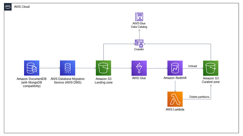
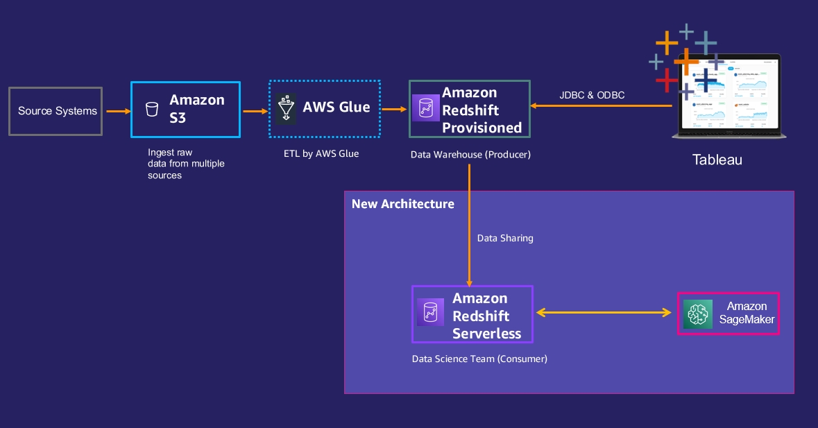
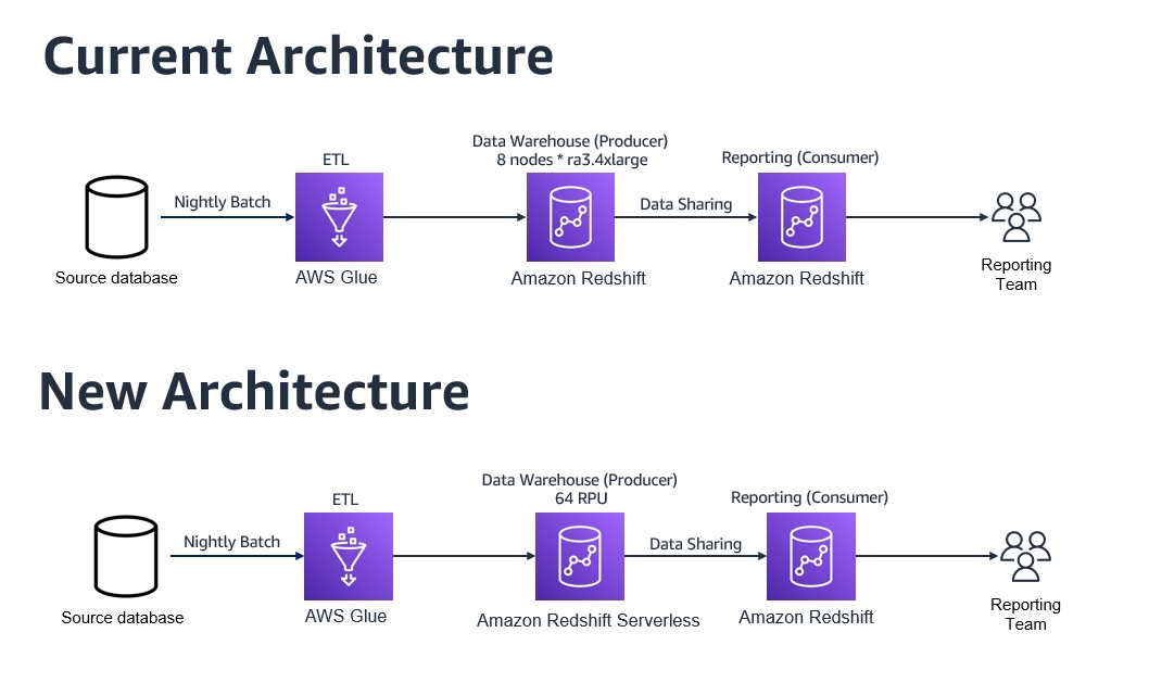
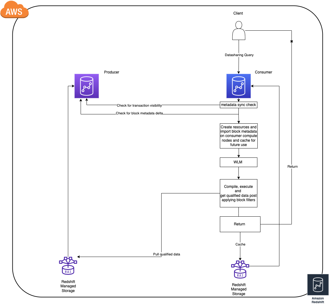
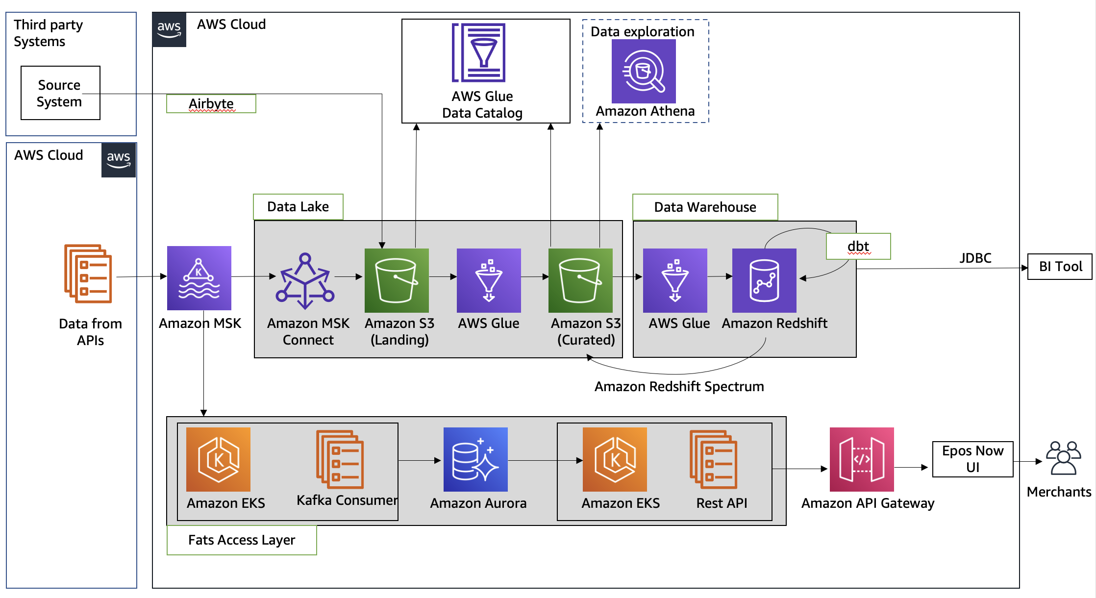
The following diagram provides an overview of the solution architecture.

The flow for the federated authentication process is as follows:
- The SQL client which has been configured with Active Directory credentials sends an authentication request to AD FS.
- AD FS authenticates the user using Active Directory credentials, and returns a SAML assertion.
- The client makes a call to Lake Formation, which initiates an internal call with AWS Security Token Service (AWS STS) to assume a role with SAML for the client.
- Lake Formation returns temporary AWS credentials with permissions of the defined IAM role to the client.
- The client uses the temporary AWS credentials to call the Athena API
StartQueryExecution.
- Athena retrieves the table and associated metadata from the AWS Glue Data Catalog.
- On behalf of the user, Athena requests access to the data from Lake Formation (
GetDataAccess). Lake Formation assumes the IAM role associated with the data lake location and returns temporary credentials.
- Athena uses the temporary credentials to retrieve data objects from Amazon S3.
- Athena returns the results to the client based on the defined access permissions.
For our use case, we use two sample tables:
- LINEORDER – A fact table containing orders
- CUSTOMER – A dimension table containing customer information including Personally Identifiable Information (PII) columns (
c_name, c_phone, c_address)
We also have data consumer users who are members of the following teams:
- CustomerOps – Can see both orders and customer information, including PII attributes of the customer
- Finance – Can see orders for analytics and aggregation purposes but only non-PII attributes of the customer
To demonstrate this use case, we create two users called CustomerOpsUser and FinanceUser and three AD groups for different access patterns: data-customer (customer information access excluding PII attributes), data-customer-pii (full customer information access including PII attributes), and data-order (order information access). By adding the users to these three groups, we can grant the right level of access to different tables and columns.
Prerequisites
To follow along with this walkthrough, you must meet the following prerequisites:
Set up an IAM SAML provider and role
To set up your SAML provider, complete the following steps:
- In the IAM console, choose Identity providers in the navigation pane.
- Choose Add provider.
- For Provider Type, choose SAML.
- For Provider Name, enter
adfs-saml-provider.
- For Metadata Document, download your AD FS server’s federation XML file by entering the following address in a browser with access to the AD FS server:
https://<adfs-server-name>/FederationMetadata/2007-06/FederationMetadata.xml
- Upload the file to AWS by choosing Choose file.
- Choose Add provider to finish.
Now you’re ready to create a new IAM role.
- In the navigation pane, choose Roles.
- Choose Create role.
- For the type of trusted entity, choose SAML 2.0 federation.
- For SAML provider, choose the provider you created (
adfs-saml-provider).
- Choose Allow programmatic and AWS Management Console access.
- The Attribute and Value fields should automatically populate with
SAML:aud and https://signin.aws.amazon.com/saml.
- Choose Next:Permissions.
- Add the necessary IAM permissions to this role. For this post, attach
AthenaFullAccess.
If the Amazon S3 location for your Athena query results doesn’t start with aws-athena-query-results, add another policy to allow users write query results into your Amazon S3 location. For more information, see Specifying a Query Result Location Using the Athena Console and Writing IAM Policies: How to Grant Access to an Amazon S3 Bucket.
- Leave the defaults in the next steps and for Role name, enter
adfs-data-access.
- Choose Create role.
- Take note of the SAML provider and IAM role names to use in later steps when creating the trust between the AWS account and AD FS.
Configure AD FS
SAML-based federation has two participant parties: the IdP (Active Directory) and the relying party (AWS), which is the service or application that wants to use authentication from the IdP.
To configure AD FS, you first add a relying party trust, then you configure SAML claim rules for the relying party. Claim rules are the way that AD FS forms a SAML assertion sent to a relying party. The SAML assertion states that the information about the AD user is true, and that it has authenticated the user.
Add a relying party trust
To create your relying party in AD FS, complete the following steps:
- Log in to the AD FS server.
- On the Start menu, open ServerManger.
- On the Tools menu, choose the AD FS Management console.
- Under Trust Relationships in the navigation pane, choose Relying Party Trusts.
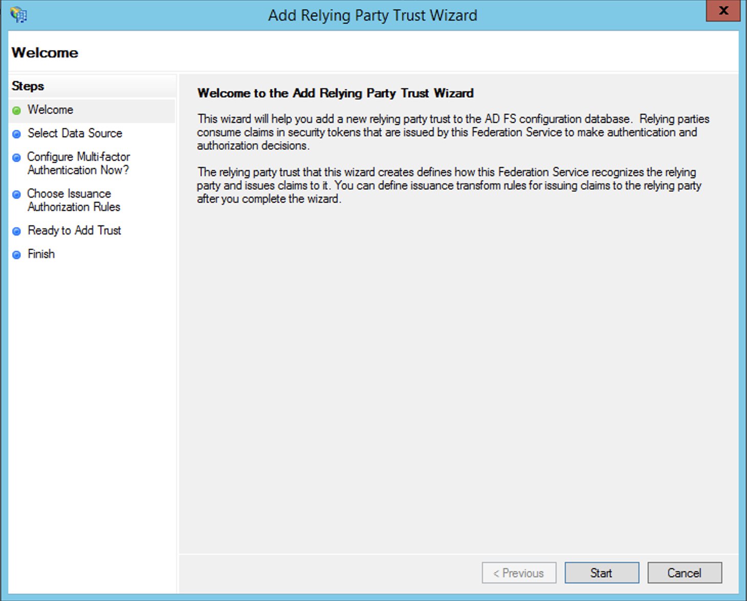
- Choose Add Relying Party Trust.
- Choose Start.

- Select Import data about the relying party published online or on a local network and enter the URL
https://signin.aws.amazon.com/static/saml-metadata.xml.
The metadata XML file is a standard SAML metadata document that describes AWS as a relying party.
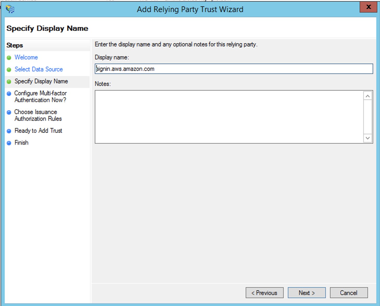
- Choose Next.

- For Display name, enter a name for your relying party.
- Choose Next.
- Select I do not want to configure multi-factor authentication.
For increased security, we recommend that you configure multi-factor authentication to help protect your AWS resources. We don’t enable multi-factor authentication for this post because we’re using a sample dataset.
- Choose Next.

- Select Permit all users to access this relying party and choose Next.
This allows all users in Active Directory to use AD FS with AWS as a relying party. You should consider your security requirements and adjust this configuration accordingly.

- Finish creating your relying party.
Configure SAML claim rules for the relying party
You create two sets of claim rules in this post. The first set (rules 1–4) contains AD FS claim rules that are required to assume an IAM role based on AD group membership. These are the rules that you also create if you want to establish federated access to the AWS Management Console. The second set (rules 5–6) are claim rules that are required for Lake Formation fine-grained access control.
To create AD FS claim rules, complete the following steps:
- On the AD FS Management console, find the relying party you created in the previous step.
- Right-click the relying party and choose Edit Claim Rules.
- Choose Add Rule and create your six new rules.

- Create claim rule 1, called
NameID:
- For Rule template, use Transform an Incoming Claim.
- For Incoming claim type, choose Windows account name.
- For Outgoing claim type, choose Name ID.
- For Outgoing name ID format, choose Persistent Identifier.
- Select Pass through all claim values.

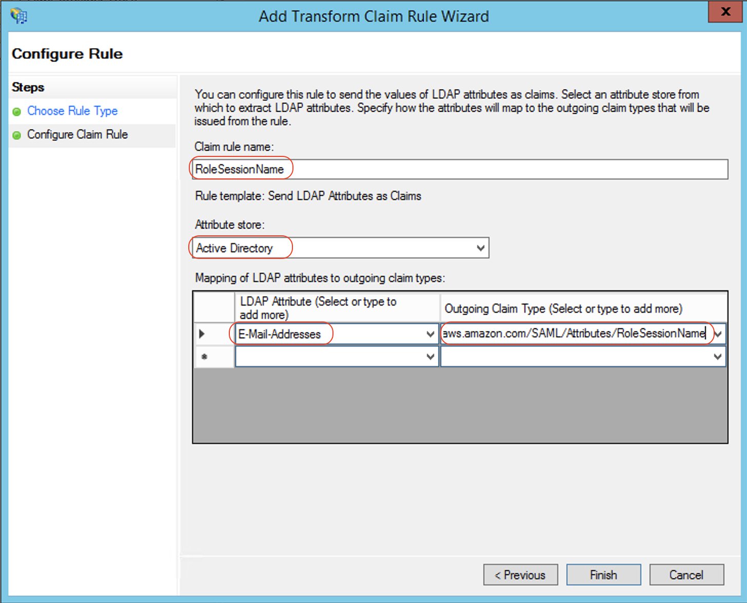
- Create claim rule 2, called
RoleSessionName:
- For Rule template, use Send LDAP Attribute as Claims.
- For Attribute store, choose Active Directory.
- For Mapping of LDAP attributes to outgoing claim types, add the attribute
E-Mail-Addresses and outgoing claim type https://aws.amazon.com/SAML/Attributes/RoleSessionName.
- Create claim rule 3, called
Get AD Groups:
- For Rule template, use Send Claims Using a Custom Rule.
- For Custom rule, enter the following code:
c:[Type == "http://schemas.microsoft.com/ws/2008/06/identity/claims/windowsaccountname", Issuer == "AD AUTHORITY"]
=> add(store = "Active Directory", types = ("http://temp/variable"), query = ";tokenGroups;{0}", param = c.Value);

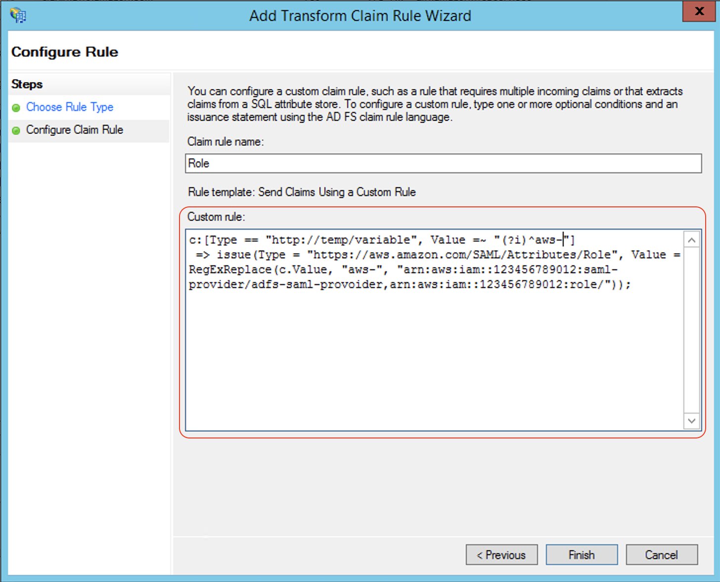
- Create claim rule 4, called
Roles:
- For Rule template, use Send Claims Using a Custom Rule.
- For Custom rule, enter the following code (enter your account number and name of the SAML provider you created earlier):
c:[Type == "http://temp/variable", Value =~ "(?i)^aws-"]
=> issue(Type = "https://aws.amazon.com/SAML/Attributes/Role", Value = RegExReplace(c.Value, "aws-", "arn:aws:iam::<AWS ACCOUNT NUMBER>:saml-provider/<adfs-saml-provider>,arn:aws:iam::<AWS ACCOUNT NUMBER>:role/"));
Claim rules 5 and 6 allow Lake Formation to make authorization decisions based on user name or the AD group membership of the user.
- Create claim rule 5, called
LF-UserName, which passes the user name and SAML assertion to Lake Formation:
- For Rule template, use Send LDAP Attributes as Claims.
- For Attribute store, choose Active Directory.
- For Mapping of LDAP attributes to outgoing claim types, add the attribute
User-Principal-Name and outgoing claim type https://lakeformation.amazon.com/SAML/Attributes/Username.

- Create claim rule 6, called
LF-Groups, which passes data and analytics-related AD groups that the user is a member of, along with the SAML assertion to Lake Formation:
- For Rule template, use Send Claims Using a Custom Rule.
- For Custom rule, enter the following code:
c:[Type == "http://temp/variable", Value =~ "(?i)^data-"]
=> issue(Type = "https://lakeformation.amazon.com/SAML/Attributes/Groups", Value = c.Value);
The preceding rule snippet filters AD group names starting with data-. This is an arbitrary naming convention; you can adopt your preferred naming convention for AD groups that are related to data lake access.
Create Active Directory users and groups
In this section, we create two AD users and required AD groups to demonstrate varying levels of access to the data.
Create users
You create two AD users: FinanceUser and CustomerOpsUser. Each user corresponds to an individual who is a member of the Finance or Customer business units. The following table summarizes the details of each user.
To create your users, complete the following steps:
- On the Server Manager Dashboard, on the Tools menu, choose Active Directory Users and Computers.

- In the navigation pane, choose Users.
- On the tool bar, choose the Create user icon.

- For First name, enter
FinanceUser.
- For Full name, enter
FinanceUser.
- For User logon name, enter
[email protected].
- Choose Next.

- Enter a password and deselect User must change password at next logon.
We choose this option for simplicity, but in real-world scenarios, newly created users must change their password for security reasons.
- Choose Next.
- In Active Directory Users and Computers, choose the user name.
- For Email, enter
[email protected].
Adding an email is mandatory because it’s used as the RoleSessionName value in the SAML assertion.
- Choose OK.

- Repeat these steps to create
CustomerOpsUser.
Create AD groups to represent data access patterns
Create the following AD groups to represent three different access patterns and also the ability to assume an IAM role:
- data-customer – Members have access to non-PII columns of the
customer table
- data-customer-pii – Members have access to all columns of the
customer table, including PII columns
- data-order – Members have access to the
lineorder table
- aws-adfs-data-access – Members assume the
adfs-data-access IAM role when logging in to AWS
To create the groups, complete the following steps:
- On the Server Manager Dashboard, on the Tools menu, choose Active Directory Users and Computers.
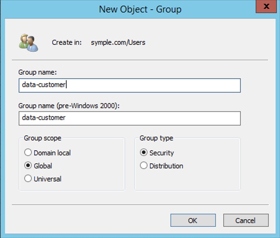
- On the tool bar, choose the Create new group icon.
- For Group name¸ enter
data-customer.
- For Group scope, select Global.
- For Group type¸ select Security.
- Choose OK.

- Repeat these steps to create the remaining groups.
Add users to appropriate groups
Now you add your newly created users to their appropriate groups, as detailed in the following table.
| User |
Group Membership |
Description |
| CustomerOpsUser |
data-customer-pii
data-order
aws-adfs-data-access |
Sees all customer information including PII and their orders |
| FinanceUser |
data-customer
data-order
aws-adfs-data-access |
Sees only non-PII customer data and orders |
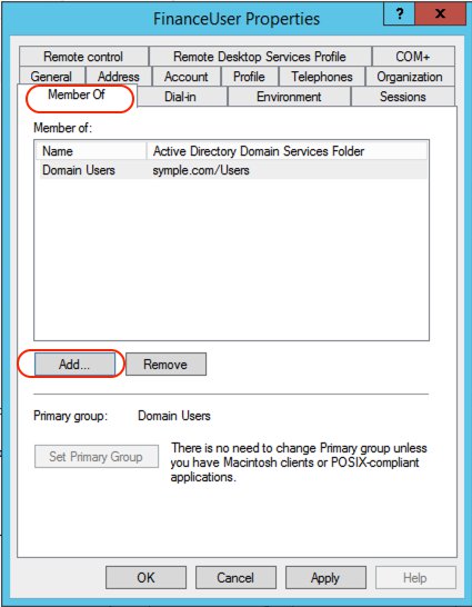
Complete the following steps:
- On the Server Manager Dashboard, on the Tools menu, choose Active Directory Users and Computers.
- Choose the user
FinanceUser.
- On the Member Of tab, choose Add.

- Add the appropriate groups.
- Repeat these steps for
CustomerOpsUser.
Create a database and tables in the data lake
In this step, you copy data files to an S3 bucket in your AWS account by running the following AWS Command Line Interface (AWS CLI) commands. For more information on how to set up the AWS CLI, refer to Configuration Basics.
These commands copy the files that contain data for customer and lineorder tables. Replace <BUCKET NAME> with the name of an S3 bucket in your AWS account.
aws s3 sync s3://awssampledb/load/ s3://<BUCKET NAME>/customer/ \
--exclude "*" --include "customer-fw.tbl-00*" --exclude "*.bak"

aws s3api copy-object --copy-source awssampledb/load/lo/lineorder-single.tbl000.gz \
--key lineorder/lineorder-single.tbl000.gz --bucket <BUCKET NAME> \
--tagging-directive REPLACE
For this post, we use the default settings for storing data and logging access requests within Amazon S3. You can enhance the security of your sensitive data with the following methods:
- Implement encryption at rest using AWS Key Management Service (AWS KMS) and customer managed encryption keys
- Use AWS CloudTrail and audit logging
- Restrict access to AWS resources based on the least privilege principle
Additionally, Lake Formation is integrated with CloudTrail, a service that provides a record of actions taken by a user, role, or AWS service in Lake Formation. CloudTrail captures all Lake Formation API calls as events and is enabled by default when you create a new AWS account. When activity occurs in Lake Formation, that activity is recorded as a CloudTrail event along with other AWS service events in event history. For audit and access monitoring purposes, all federated user logins are logged via CloudTrail under the AssumeRoleWithSAML event name. You can also view specific user activity based on their user name in CloudTrail.
To create a database and tables in the Data Catalog, open the query editor on the Athena console and enter the following DDL statements. Replace <BUCKET NAME> with the name of the S3 bucket in your account.
CREATE DATABASE salesdata;
CREATE EXTERNAL TABLE salesdata.customer
(
    c_custkey VARCHAR(10),
    c_name VARCHAR(25),
    c_address VARCHAR(25),
    c_city VARCHAR(10),
    c_nation VARCHAR(15),
    c_region VARCHAR(12),
    c_phone VARCHAR(15),
    c_mktsegment VARCHAR(10)
)
-- The data files contain fixed width columns hence using RegExSerDe
ROW FORMAT SERDE 'org.apache.hadoop.hive.serde2.RegexSerDe'
WITH SERDEPROPERTIES (
    "input.regex" = "(.{10})(.{25})(.{25})(.{10})(.{15})(.{12})(.{15})(.{10})"
)
LOCATION 's3://<BUCKET NAME>/customer/';

CREATE EXTERNAL TABLE salesdata.lineorder(
  `lo_orderkey` int,
  `lo_linenumber` int,
  `lo_custkey` int,
  `lo_partkey` int,
  `lo_suppkey` int,
  `lo_orderdate` int,
  `lo_orderpriority` varchar(15),
  `lo_shippriority` varchar(1),
  `lo_quantity` int,
  `lo_extendedprice` int,
  `lo_ordertotalprice` int,
  `lo_discount` int,
  `lo_revenue` int,
  `lo_supplycost` int,
  `lo_tax` int,
  `lo_commitdate` int,
  `lo_shipmode` varchar(10))
ROW FORMAT DELIMITED
  FIELDS TERMINATED BY '|'
LOCATION 's3://<BUCKET NAME>/lineorder/';
Verify that tables are created and you can see the data:
SELECT * FROM "salesdata"."customer" limit 10;
SELECT * FROM "salesdata"."lineorder" limit 10;
Set up the Lake Formation permission model
Lake Formation uses a combination of Lake Formation permissions and IAM permissions to achieve fine-grained access control. The recommended approach includes the following:
- Coarse-grained IAM permissions – These apply to the IAM role that users assume when running queries in Athena. IAM permissions control access to Lake Formation, AWS Glue, and Athena APIs.
- Fine-grained Lake Formation grants – These control access to Data Catalog resources, Amazon S3 locations, and the underlying data at those locations. With these grants, you can give access to specific tables or only columns that contain specific data values.

Configure IAM role permissions
Earlier in the walkthrough, you created the IAM role adfs-data-access and attached the AWS managed IAM policy AthenaFullAccess to it. This policy has all the permissions required for the purposes of this post.
For more information, see the Data Analyst Permissions section in Lake Formation Personas and IAM Permissions Reference.
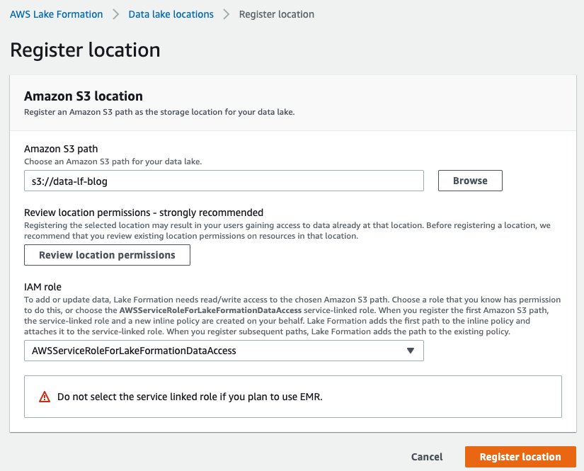
Register an S3 bucket as a data lake location
The mechanism to govern access to an Amazon S3 location using Lake Formation is to register a data lake location. Complete the following steps:
- On the Lake Formation console, choose Data lake locations.
- Choose Register location.
- For Amazon S3 path, choose Browse and locate your bucket.
- For IAM role, choose
AWSServiceRoleForLakeFormationDataAccess.
In this step, you specify an IAM service-linked role, which Lake Formation assumes when it grants temporary credentials to integrated AWS services that access the data in this location. This role and its permissions are managed by Lake Formation and can’t be changed by IAM principals.
- Choose Register location.

Configure data permissions
Now that you have registered the Amazon S3 path, you can give AD groups appropriate permissions to access tables and columns in the salesdata database. The following table summarizes the new permissions.
| Database and Table |
AD Group Name |
Table Permissions |
Data Permissions |
| salesdata.customer |
data-customer |
Select |
c_city, c_custkey, c_mktsegment, c_nation, and c_region |
| salesdata.customer |
data-customer-pii |
Select |
All data access |
| salesdata.lineorder |
data-order |
Select |
All data access |
- On the Lake Formation console, choose Tables in the navigation pane.
- Filter tables by the
salesdata database.
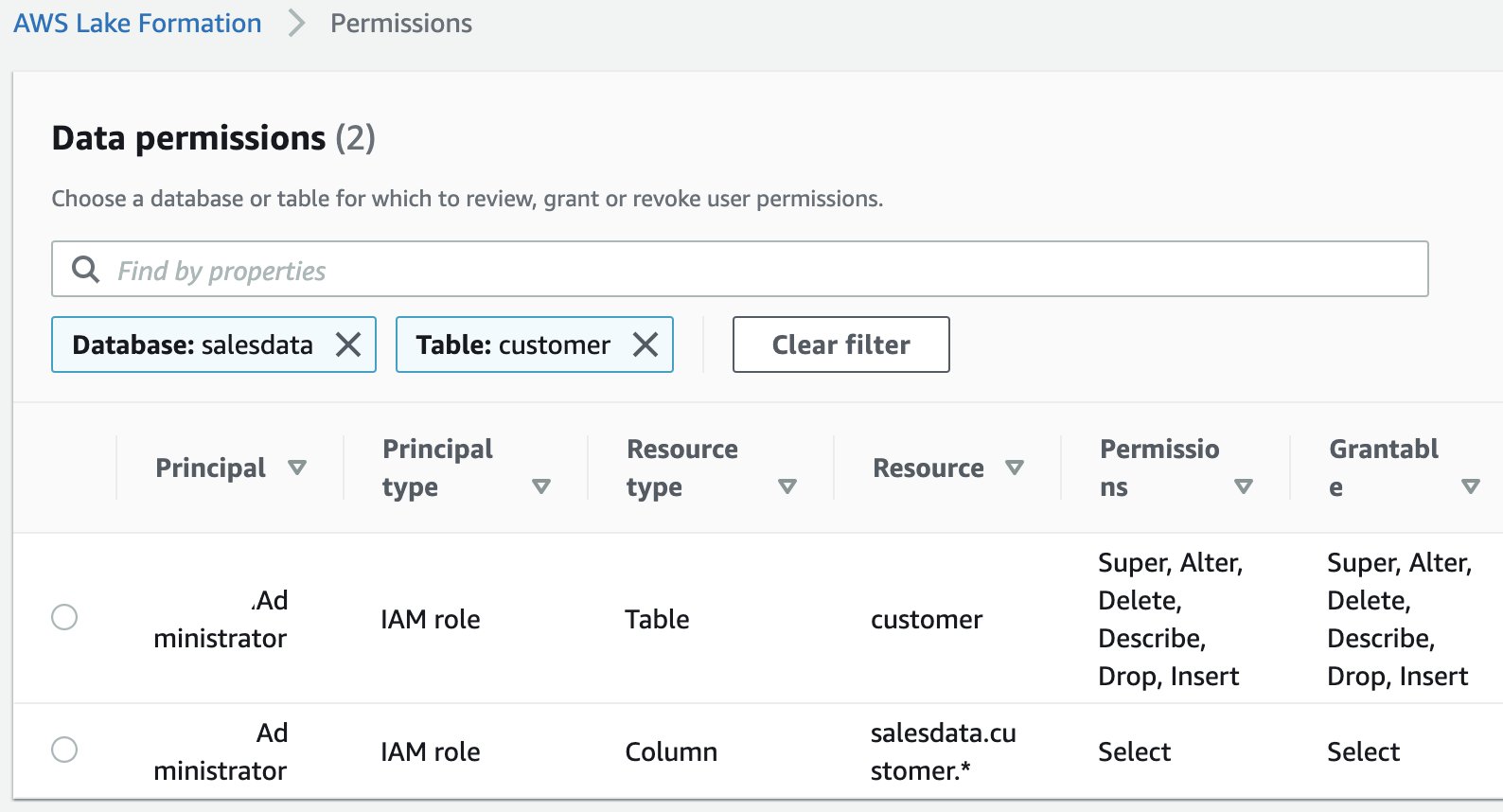
- Select the
customer table and on the Actions menu, choose View permissions.

You should see following existing permissions. These entries allow the current data lake administrator to access the table and all its columns.

- To add new permissions, select the table and on the Actions menu, choose Grant.
- Select SAML user and groups.
- For SAML and Amazon QuickSight users and groups, enter
arn:aws:iam::<AWS ACCOUNT NUMBER>:saml-provider/adfs-saml-provider:group/data-customer.
To get this value, get the ARN of the SAML provider from the IAM console and append :group/data-customer to the end of it.
- Select Named data catalog resources.
- For Databases, choose the
salesdata database.
- For Tables, choose the
customer table.

- For Table permissions, select Select.
- For Data permissions, select Column-based access.
- For Select columns, add the columns
c_city, c_custkey, c_mktsegment, c_nation, and c_region.
- Choose Grant.

You have now allowed members of the AD group data-customer to have access to columns of the customer table that don’t include PII.
- Repeat these steps for the
customer table and data-customer-pii group with all data access.
- Repeat these steps for the
lineorder table and data-order group with all data access.
Set up a SQL client with JDBC connection and verify permissions
In this post, we use SQL Workbench to access Athena through AD authentication and verify the Lake Formation permissions you created in the previous section.
Prepare the SQL client
To set up the SQL client, complete the following steps:
- Download and extract the Lake Formation-compatible Athena JDBC driver with AWS SDK (2.0.14 or later version) from Using Athena with the JDBC Driver.
- Go to the SQL Workbench/J website and download the latest stable package.
- Install SQL Workbench/J on your client computer.
- In SQL Workbench, on the File menu, choose Manage Drivers.
- Choose the New driver icon.
- For Name, enter
Athena JDBC Driver.
- For Library, browse to and choose the Simba Athena JDBC .jar file that you just downloaded.
- Choose OK.

You’re now ready to create connections in SQL Workbench for your users.
Create connections in SQL Workbench
To create your connections, complete the following steps:
- On the File menu, choose Connect.
- Enter the name
Athena-FinanceUser.
- For Driver, choose the Simba Athena JDBC driver.
- For URL, enter the following code (replace the placeholders with actual values from your setup and remove the line breaks to make a single line connection string):
jdbc:awsathena://AwsRegion=<AWS Region Name e.g. ap-southeast-2>;
S3OutputLocation=s3://<Athena Query Result Bucket Name>/jdbc;
plugin_name=com.simba.athena.iamsupport.plugin.AdfsCredentialsProvider;
idp_host=<adfs-server-name e.g. adfs.company.com>;
idp_port=443;
preferred_role=<ARN of the role created in step1 e.g. arn>;
user=financeuser@<Domain Name e.g. company.com>;
password=<password>;
SSL_Insecure=true;
LakeFormationEnabled=true;
For this post, we used a self-signed certificate with AD FS. This certificate is not trusted by the client, therefore authentication doesn’t succeed. This is why the SSL_Insecure attribute is set to true to allow authentication despite the self-signed certificate. In real-world setups, you would use valid trusted certificates and can remove the SSL_Insecure attribute.
- Create a new SQL workbench profile named
Athena-CustomerOpsUser and repeat the earlier steps with CustomerOpsUser in the connection URL string.
- To test the connections, choose Test for each user, and confirm that the connection succeeds.

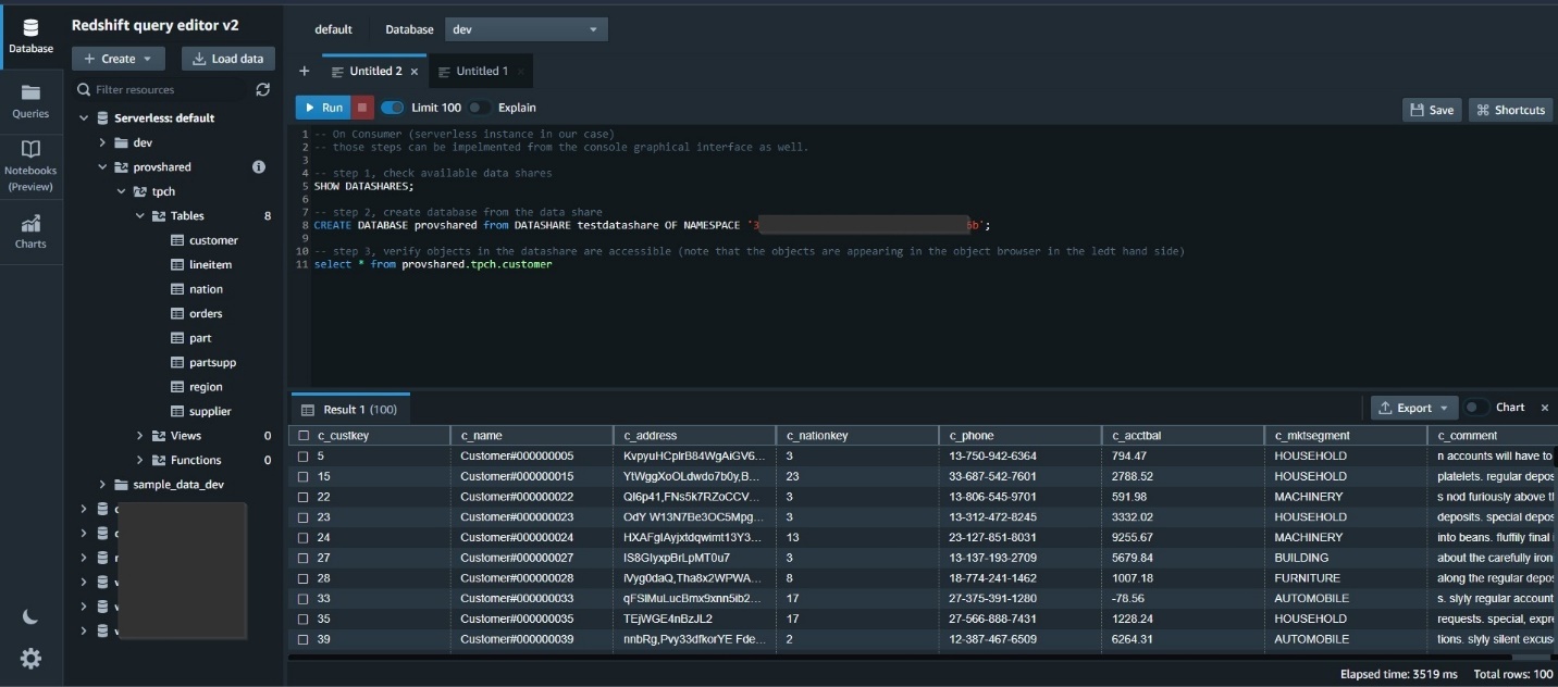
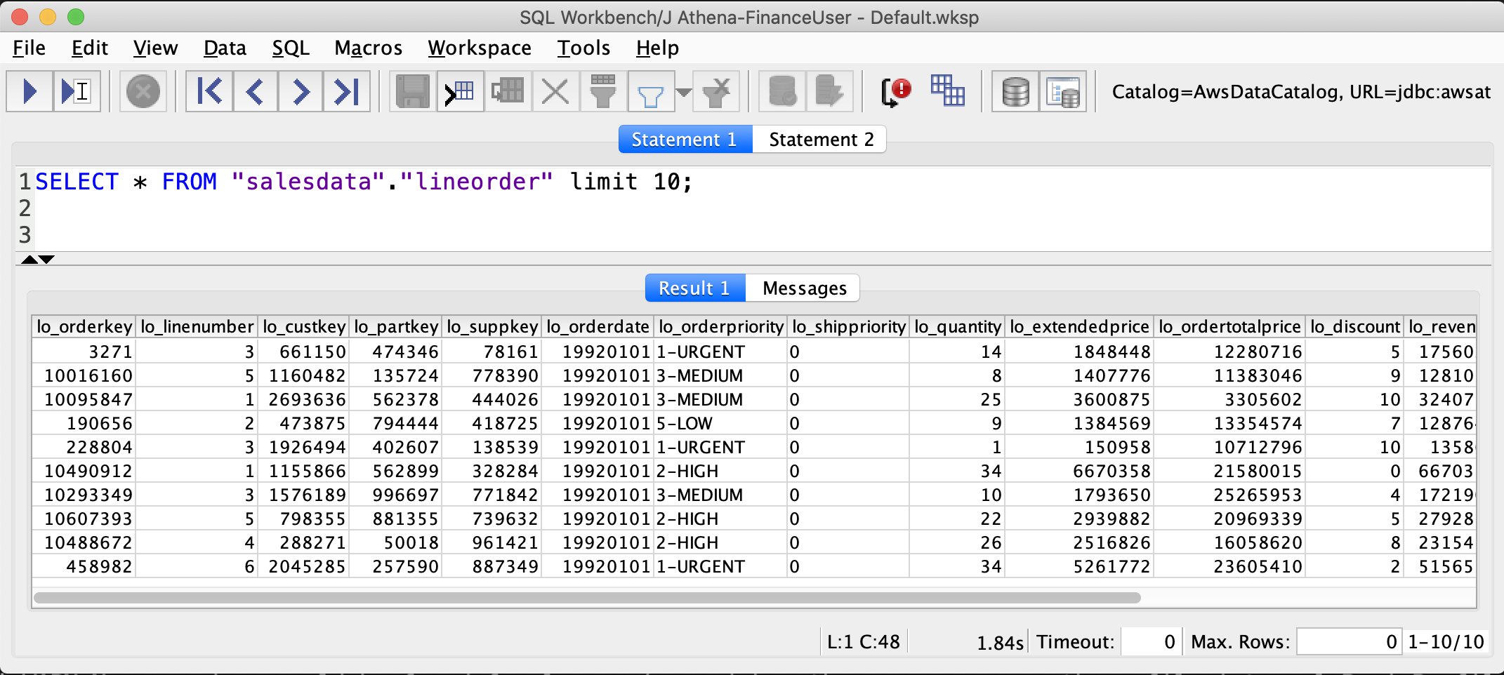
Verify access permissions
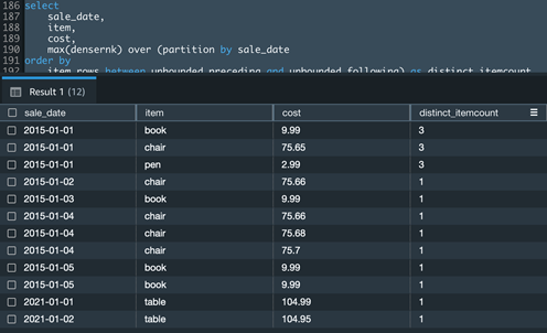
Now we can verify permissions for FinanceUser. In the SQL Workbench Statement window, run the following SQL SELECT statement:
SELECT * FROM "salesdata"."lineorder" limit 10;
SELECT * FROM "salesdata"."customer" limit 10;
Verify that only non-PII columns are returned from the customer table.

As you see in the preceding screenshots, FinanceUser only has access to non-PII columns of the customer table and full access to (all columns) of the lineorder table. This allows FinanceUser, for example, to run aggregate and summary queries based on market segment or location of customers without having access to their personal information.
Run a similar query for CustomerOpsUser. You should be able to see all columns, including columns containing PII, in the customer table.
Conclusion
This post demonstrated how to configure your data lake permissions using Lake Formation for AD users and groups. We configured AD FS 3.0 on your Active Directory and used it as an IdP to federate into AWS using SAML. This post also showed how you can integrate your Athena JDBC driver to AD FS and use your AD credentials directly to connect to Athena.
Integrating your Active Directory with the Athena JDBC driver gives you the flexibility to access Athena from business intelligence tools you’re already familiar with to analyze the data in your Amazon S3 data lake. This enables you to have a consistent central permission model that is managed through AD users and their group memberships.
About the Authors
 Mostafa Safipour is a Solutions Architect at AWS based out of Sydney. Over the past decade he has helped many large organizations in the ANZ region build their data, digital, and enterprise workloads on AWS.
Praveen Kumar is a Specialist Solution Architect at AWS with expertise in designing, building, and implementing modern data and analytics platforms using cloud-native services. His areas of interests are serverless technology, streaming applications, and modern cloud data warehouses.


 Poulomi Dasgupta is a Senior Analytics Solutions Architect with AWS. She is passionate about helping customers build cloud-based analytics solutions to solve their business problems. Outside of work, she likes travelling and spending time with her family.
 Raks Khare is an Analytics Specialist Solutions Architect at AWS based out of Pennsylvania. He helps customers architect data analytics solutions at scale on the AWS platform.


 Chao Pan is a Data Analytics Solutions Architect at Amazon Web Services. He’s responsible for the consultation and design of customers’ big data solution architectures. He has extensive experience in open-source big data. Outside of work, he enjoys hiking.


 Randy Chng is an Analytics Acceleration Lab Solutions Architect at Amazon Web Services. He works with customers to accelerate their Amazon Redshift journey by delivering proof of concepts on key business problems.
 Sean Beath is an Analytics Acceleration Lab Solutions Architect at Amazon Web Services. He delivers proof of concepts with customers on Amazon Redshift, helping customers drive analytics value on AWS.
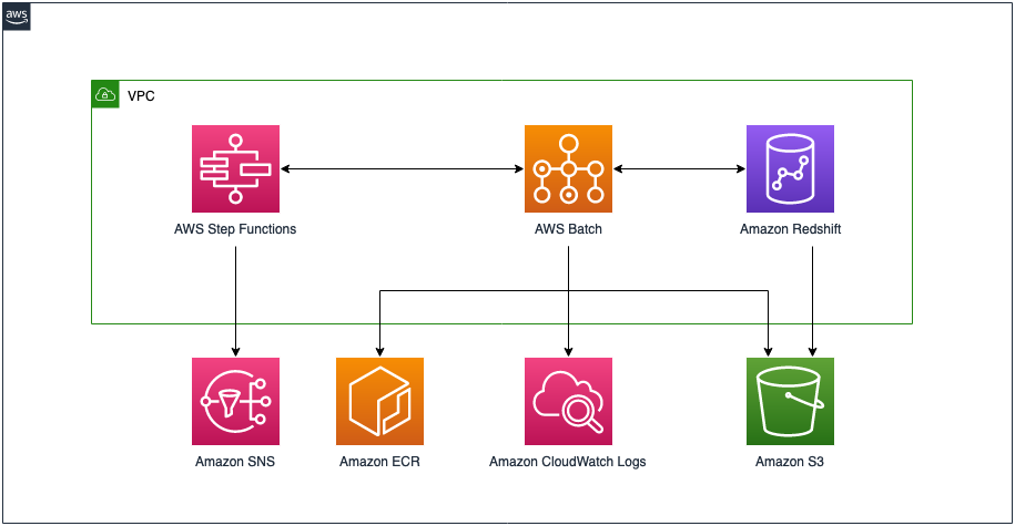


 Dhiraj Thakur is a Solutions Architect with Amazon Web Services. He works with AWS customers and partners to provide guidance on enterprise cloud adoption, migration, and strategy. He is passionate about technology and enjoys building and experimenting in the analytics and AI/ML space.


 Michael Soo is a Principal Database Engineer with the AWS Database Migration Service team. He builds products and services that help customers migrate their database workloads to the AWS cloud.
 Illia Kravtsov is a Database Developer with the AWS Project Delta Migration team. He has 10+ years experience in data warehouse development with Teradata and other MPP databases.