Post Syndicated from Satish Sathiya original https://aws.amazon.com/blogs/big-data/work-with-semistructured-data-using-amazon-redshift-super/
With the new SUPER data type and the PartiQL language, Amazon Redshift expands data warehouse capabilities to natively ingest, store, transform, and analyze semi-structured data. Semi-structured data (such as weblogs and sensor data) fall under the category of data that doesn’t conform to a rigid schema expected in relational databases. It often contain complex values such as arrays and nested structures that are associated with serialization formats, such as JSON.
The schema of the JSON can evolve over time according to the business use case. Traditional SQL users who are experienced in handling structured data often find it challenging to deal with semi-structured data sources such as nested JSON documents due to lack of SQL support, the need to learn multiple complex functions, and the need to use third-party tools.
This post is part of a series that talks about ingesting and querying semi-structured data in Amazon Redshift using the SUPER data type.
With the introduction of the SUPER data type, Amazon Redshift provides a rapid and flexible way to ingest JSON data and query it without the need to impose a schema. This means that you don’t need to worry about the schema of the incoming document, and can load it directly into Amazon Redshift without any ETL to flatten the data. The SUPER data type is stored in an efficient binary encoded Amazon Redshift native format.
The SUPER data type can represent the following types of data:
- An Amazon Redshift scalar value:
- A null
- A Boolean
- Amazon Redshift numbers, such as SMALLINT, INTEGER, BIGINT, DECIMAL, or floating point (such as FLOAT4 or FLOAT8)
- Amazon Redshift string values, such as VARCHAR and CHAR
- Complex values:
- An array of values, including scalar or complex
- A structure, also known as tuple or object, that is a map of attribute names and values (scalar or complex)
For more information about the SUPER type, see Ingesting and querying semistructured data in Amazon Redshift.
After the semi-structured and nested data is loaded into the SUPER data type, you can run queries on it by using the PartiQL extension of SQL. PartiQL is backward-compatible to SQL. It enables seamless querying of semi-structured and structured data and is used by multiple AWS services, such as Amazon DynamoDB, Amazon Quantum Ledger Database (Amazon QLDB), and AWS Glue Elastic Views. With PartiQL, the query engine can work with schema-less SUPER data that originated in serialization formats, such as JSON. With the use of PartiQL, familiar SQL constructs seamlessly combine access to both the classic, tabular SQL data and the semi-structured data in SUPER. You can perform object and array navigation and also unnesting with simple and intuitive extensions to SQL semantics.
For more information about PartiQL, see Announcing PartiQL: One query language for all your data.
Use cases
The SUPER data type is useful when processing and querying semi-structured or nested data such as web logs, data from industrial Internet of Things (IoT) machines and equipment, sensors, genomics, and so on. To explain the different features and functionalities of SUPER, we use sample industrial IoT data from manufacturing.
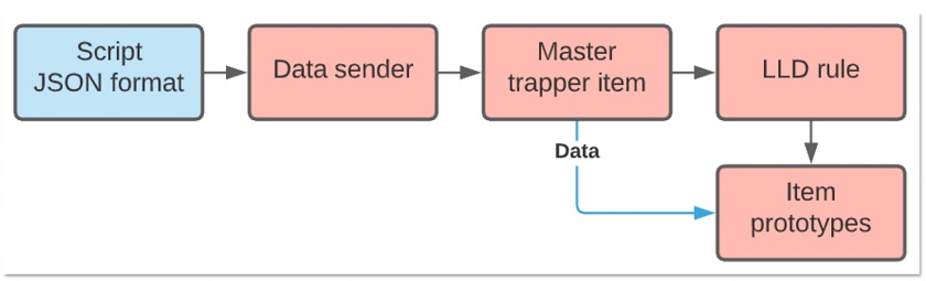
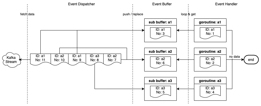
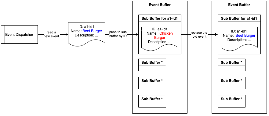
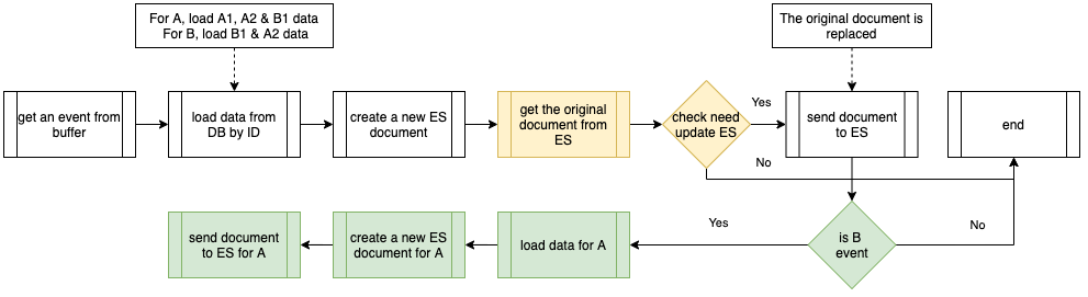
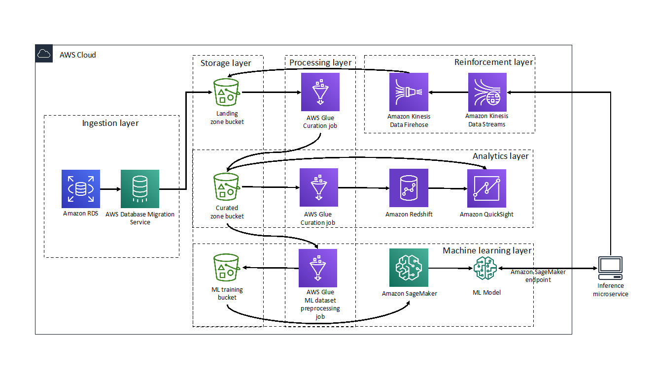
The following diagram shows the sequence of events in which the data is generated, collected, and finally stored in Amazon Redshift as the SUPER data type.

Manufacturers are embracing the cloud solutions with connected machines and factories to transform and use data to make data-driven decisions so they can optimize operations, increase productivity, and improve availability while reducing costs.
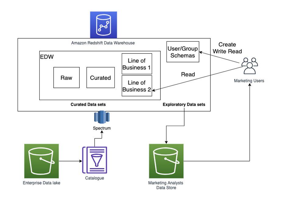
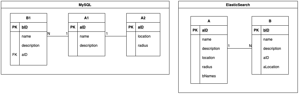
As an example, the following diagram depicts a common asset hierarchy of a fictional smart manufacturing company.

This data is typically semi-structured and hierarchical in nature. To find insights from this data using traditional methods and tools, you need to extract, preprocess, load, and transform it into the proper structured format to run typical analytical queries using a data warehouse. The time to insight is delayed because of the initial steps required for data cleansing and transformation typically performed using third-party tools or other AWS services.
Amazon Redshift SUPER handles these use cases by helping manufacturers extract, load, and query (without any transformation) a variety of data sources collected from edge computing and industrial IoT devices. Let’s use this sample dataset to drive our examples to explain the capabilities of Amazon Redshift SUPER.
The following is an example subscription dataset for assets (such as crowder, gauge, and pneumatic cylinder) in the workshop, which collects metrics on different properties (such as air pressure, machine state, finished parts count, and failures). Data on these metrics is generated continuously in a time series fashion and pushed to the AWS Cloud using the AWS IoT SiteWise connector. This specific example collects the Machine State property for an asset. The following sample data called subscriptions.json has scalar columns like topicId and qos, and a nested array called messages, which has metrics on the assets.

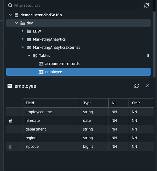
The following is another dataset called asset_metadata.json, which describes different assets and their properties, more like a dimension table. In this example, the asset_name is IAH10 Line 1, which is a processing plant line for a specific site.

Load data into SUPER columns
Now that we covered the basics behind Amazon Redshift SUPER and the industrial IoT use case, let’s look at different ways to load this dataset.
Copy the JSON document into multiple SUPER data columns
In this use case for handling semi-structured data, the user knows the incoming data’s top-level schema and structure, but some of the columns are semi-structured and nested in structures or arrays. You can choose to shred a JSON document into multiple columns that can be a combination of the SUPER data type and Amazon Redshift scalar types. The following code shows what the table DDL looks like if we translate the subscriptions.json semi-structured schema into a SUPER equivalent:
CREATE TABLE subscription_auto (
topicId INT
,topicFilter VARCHAR
,qos INT
,messages SUPER
);
To load data into this table, specify the auto option along with FORMAT JSON in the COPY command to split the JSON values across multiple columns. The COPY matches the JSON attributes with column names and allows nested values, such as JSON arrays and objects, to be ingested as SUPER values. Run the following command to ingest data into the subscription_auto table. Replace the AWS Identity and Access Management (IAM) role with your own credentials. The ignorecase option passed along with auto is required only if your JSON attribute names are in CamelCase. In our case, our columns topicId and topicFilter scalar columns are in CamelCase.
COPY subscription_auto FROM 's3://redshift-downloads/semistructured/super-blog/subscriptions/'
IAM_ROLE '<< your IAM role >>'
FORMAT JSON 'auto ignorecase';
A select * from subscription_auto command looks like the following code. The messages SUPER column holds the entire array in this case.
-- A sample output
SELECT * FROM subscription_auto;
[ RECORD 1 ]
topicid     | 1001
topicfilter | $aws/sitewise/asset-models/+/assets/+/properties/+
qos         | 0
messages    | [{"format":"json","topic":"$aws\/sitewise\/asset-models\/8926cf44-14ea-4cd8-a7c6-e61af641dbeb\/assets\/0aaf2aa2-0299-442a-b2ea-ecf3d62f2a2c\/properties\/3ff67d41-bf69-4d57-b461-6f1513e127a4","timestamp":1616381297183,"payload":{"type":"PropertyValueUpdate","payload":{"assetId":"0aaf2aa2-0299-442a-b2ea-ecf3d62f2a2c","propertyId":"3ff67d41-bf69-4d57-b461-6f1513e127a4","values":[{"timestamp":{"timeInSeconds":1616381289,"offsetInNanos":425000000},"quality":"GOOD","value":{"doubleValue":0}},{"timestamp":{"timeInSeconds":1616381292,"offsetInNanos":425000000},"quality":"FAIR","value":{"doubleValue":0}},{"timestamp":{"timeInSeconds":1616381286,"offsetInNanos":425000000},"quality":"GOOD","value":{"doubleValue":0}},{"timestamp":{"timeInSeconds":1616381293,"offsetInNanos":425000000},"quality":"GOOD","value":{"doubleValue":0}},{"timestamp":{"timeInSeconds":1616381287,"offsetInNanos":425000000},"quality":"GOOD","value":{"doubleValue":0}},{"timestamp":{"timeInSeconds":1616381290,"offsetInNanos":425000000},"quality":"GOOD","value":{"doubleValue":0}},{"timestamp":{"timeInSeconds":1616381290,"offsetInNanos":925000000},"quality":"GOOD","value":{"doubleValue":0}},{"timestamp":{"timeInSeconds":1616381294,"offsetInNanos":425000000},"quality":"FAIR","value":{"doubleValue":0}},{"timestamp":{"timeInSeconds":1616381285,"offsetInNanos":425000000},"quality":"GOOD","value":{"doubleValue":0}},{"timestamp":{"timeInSeconds":1616381288,"offsetInNanos":425000000},"quality":"GOOD","value":{"doubleValue":0}}]}}}]
Alternatively, you can specify jsonpaths to load the same data, as in the following code. The jsonpaths option is helpful if you want to load only selective columns from your JSON document. For more information, see COPY from JSON format.
COPY subscription_auto FROM 's3://redshift-downloads/semistructured/super-blog/subscriptions/'
IAM_ROLE '<< your IAM role >>'
FORMAT JSON 's3://redshift-downloads/semistructured/super-blog/jsonpaths/subscription_jsonpaths.json';
subscription_jsonpaths.json looks like the following:
{"jsonpaths": [
    "$.topicId",
    "$.topicFilter",
    "$.qos",
    "$.messages"
   ]
}
While we’re in the section about loading, let’s also create the asset_metadata table and load it with relevant data, which we need in our later examples. The asset_metadata table has more information about industry shop floor assets and their properties like asset_name, property_name, and model_id.
CREATE TABLE asset_metadata (
asset_id VARCHAR
,asset_name VARCHAR
,asset_model_id VARCHAR
,asset_property_id VARCHAR
,asset_property_name VARCHAR
,asset_property_data_type VARCHAR
,asset_property_unit VARCHAR
,asset_property_alias VARCHAR
);

COPY asset_metadata FROM 's3://redshift-downloads/semistructured/super-blog/asset_metadata/'
IAM_ROLE '<< your IAM role >>'
FORMAT JSON 'auto';
Copy the JSON document into a single SUPER column
You can also load a JSON document into a single SUPER data column. This is typical when the schema of the incoming JSON is unknown and evolving. SUPER’s schema-less ingestion comes to the forefront here, letting you load the data in a flexible fashion.
For this use case, assume that we don’t know the names of the columns in subscription.json and want to load it into Amazon Redshift. It’s as simple as the following code:
CREATE TABLE subscription_noshred (s super);
After the table is created, we can use the COPY command to ingest data from Amazon Simple Storage Service (Amazon S3) into the single SUPER column. The noshred is a required option to go along with FORMAT JSON, which tells the COPY parser not to shred the document but load it into a single column.
COPY subscription_noshred FROM 's3://redshift-downloads/semistructured/super-blog/subscriptions/'
IAM_ROLE '<< your IAM role >>'
FORMAT JSON 'noshred';
After the COPY has successfully ingested the JSON, the subscription_noshred table has a SUPER column s that contains the data of the entire JSON object. The ingested data maintains all the properties of the JSON nested structure but in a SUPER data type.
The following code shows how select star (*) into subscription_noshred looks; the entire JSON structure is in SUPER column s:
--A sample output
SELECT * FROM subscription_noshred;
[ RECORD 1 ]
s | {"topicId":1001,"topicFilter":"$aws\/sitewise\/asset-models\/+\/assets\/+\/properties\/+","qos":0,"messages":[{"format":"json","topic":"$aws\/sitewise\/asset-models\/8926cf44-14ea-4cd8-a7c6-e61af641dbeb\/assets\/0aaf2aa2-0299-442a-b2ea-ecf3d62f2a2c\/properties\/3ff67d41-bf69-4d57-b461-6f1513e127a4","timestamp":1616381297183,"payload":{"type":"PropertyValueUpdate","payload":{"assetId":"0aaf2aa2-0299-442a-b2ea-ecf3d62f2a2c","propertyId":"3ff67d41-bf69-4d57-b461-6f1513e127a4","values":[{"timestamp":{"timeInSeconds":1616381289,"offsetInNanos":425000000},"quality":"GOOD","value":{"doubleValue":0}},{"timestamp":{"timeInSeconds":1616381292,"offsetInNanos":425000000},"quality":"FAIR","value":{"doubleValue":0}},{"timestamp":{"timeInSeconds":1616381286,"offsetInNanos":425000000},"quality":"GOOD","value":{"doubleValue":0}},{"timestamp":{"timeInSeconds":1616381293,"offsetInNanos":425000000},"quality":"GOOD","value":{"doubleValue":0}},{"timestamp":{"timeInSeconds":1616381287,"offsetInNanos":425000000},"quality":"GOOD","value":{"doubleValue":0}},{"timestamp":{"timeInSeconds":1616381290,"offsetInNanos":425000000},"quality":"GOOD","value":{"doubleValue":0}},{"timestamp":{"timeInSeconds":1616381290,"offsetInNanos":925000000},"quality":"GOOD","value":{"doubleValue":0}},{"timestamp":{"timeInSeconds":1616381294,"offsetInNanos":425000000},"quality":"FAIR","value":{"doubleValue":0}},{"timestamp":{"timeInSeconds":1616381285,"offsetInNanos":425000000},"quality":"GOOD","value":{"doubleValue":0}},{"timestamp":{"timeInSeconds":1616381288,"offsetInNanos":425000000},"quality":"GOOD","value":{"doubleValue":0}}]}}}]}
Similar to the noshred option, we can also use jsonpaths to load complete documents. This can be useful in cases where we want to extract additional columns, such as distribution and sort keys, while still loading the complete document as a SUPER column. In the following example, we map our first column to the root JSON object, while also mapping a distribution key to the second column, and a sort key to the third column.
subscription_sorted_jsonpaths.json looks like the following:
{"jsonpaths": [
"$",
"$.topicId",
"$.topicFilter"
]
}
CREATE TABLE subscription_sorted (
s super
,topicId INT
,topicFilter VARCHAR
) DISTKEY(topicFilter) SORTKEY(topicId);

COPY subscription_sorted FROM 's3://redshift-downloads/semistructured/super-blog/subscriptions/'
IAM_ROLE '<< your IAM role >>'
FORMAT JSON 's3://redshift-downloads/semistructured/superblog/jsonpaths/subscription_sorted_jsonpaths.json';
Copy data from columnar formats like Parquet and ORC
If your semi-structured or nested data is already available in either Apache Parquet or Apache ORC formats, you can use the COPY command with the SERIALIZETOJSON option to ingest data into Amazon Redshift. The Amazon Redshift table structure should match the number of columns and the column data types of the Parquet or ORC files. Amazon Redshift can replace any Parquet or ORC column, including structure and array types, with SUPER data columns. The following are the COPY examples to load from Parquet and ORC format:
--Parquet
COPY subscription_auto FROM 's3://redshift-downloads/semistructured/super-blog/subscriptions_parquet/'
IAM_ROLE '<< your IAM role >>' FORMAT PARQUET SERIALIZETOJSON;

--ORC
COPY subscription_auto FROM 's3://redshift-downloads/semistructured/super-blog/subscriptions_orc/'
IAM_ROLE '<< your IAM role >>' FORMAT ORC SERIALIZETOJSON;
Apart from COPY, you can load the same data in columnar format in Amazon S3 using Amazon Redshift Spectrum and the INSERT command. The following example assumes the Redshift Spectrum external schema super_workshop and the external table subscription_parquet is already created and available in the database.
We need to set an important session-level configuration parameter for this to work: SET json_serialization_enable TO true. For more information, see Serializing complex nested JSON. This session-level parameter allows you to query top-level nested collection columns as serialized JSON.
/* -- Set the GUC for JSON serialization -- */
SET json_serialization_enable TO true;

INSERT INTO subscription_parquet
SELECT topicId
,topicFilter
,qos
,JSON_PARSE(messages) FROM super_workshop.subscription_parquet;
As of this writing, we can’t use the SUPER column as such as a distribution or sort key, but if we need to use one of the attributes in a SUPER column as a distribution a sort key and keep the entire SUPER column intact as a separate column, we can use the following code as a workaround (apart from the jsonpaths example described earlier). For example, let’s assume the column format within the array messages needs to be used a distribution key for the Amazon Redshift table:
SET json_serialization_enable TO true;

DROP TABLEIF EXISTS subscription_messages;

CREATE TABLE subscription_messages (
m_format VARCHAR
,m_messages super
) distkey (m_format);

--'format' scalar column is extracted from 'messages' super column
INSERT INTO subscription_messages
SELECT element.format::VARCHAR
,supercol FROM (
SELECT JSON_PARSE(messages) AS supercol FROM super_workshop.subscription_parquet
) AS tbl,tbl.supercol element;
Apart from using the Amazon Redshift COPY command, we can also ingest JSON-formatted data into Amazon Redshift using the traditional SQL INSERT command:
--Insert example
INSERT INTO subscription_auto VALUES (
0000
,'topicFiltervalue'
,0000
,JSON_PARSE('[{"format":"json"},{"topic": "sample topic"},[1,2,3]]')
);
The JSON_PARSE() function parses the incoming data in proper JSON format and helps convert it into the SUPER data type. Without the JSON_PARSE() function, Amazon Redshift treats and ingests the value as a single string into SUPER instead of a JSON-formatted value.
Query SUPER columns
Amazon Redshift uses the PartiQL language to offer SQL-compatible access to relational, semi-structured, and nested data. PartiQL’s extensions to SQL are straightforward to understand, treat nested data as first-class citizens, and seamlessly integrate with SQL. The PartiQL syntax uses dot notation and array subscript for path navigation when accessing nested data.
The Amazon Redshift implementation of PartiQL supports dynamic typing for querying semi-structured data. This enables automatic filtering, joining, and aggregation on the combination of structured, semi-structured, and nested datasets. PartiQL allows the FROM clause items to iterate over arrays and use unnest operations.
The following sections focus on different query access patterns that involve navigating the SUPER data type with path and array navigation, unnest, or joins.
Navigation
We may want to find an array element by its index, or we may want to find the positions of certain elements in their arrays, such as the first element or the last element. We can reference a specific element simply by using the index of the element within square brackets (the index is 0-based) and within that element we can reference an object or struct by using the dot notation.
Let’s use our subscription_auto table to demonstrate the examples. We want to access the first element of the array, and within that we want to know the value of the attribute format:
SELECT messages[0].format FROM subscription_auto ;
--A sample output
 format
--------
 "json"
 "json"
 "json"
(3 rows)
Amazon Redshift can also use a table alias as a prefix to the notation. The following example is the same query as the previous example:
SELECT sub.messages[0].format FROM subscription_auto AS sub;
--A sample output
 format
--------
 "json"
 "json"
 "json"
(3 rows)
You can use the dot and bracket notations in all types of queries, such as filtering, join, and aggregation. You can use them in a query in which there are normally column references. The following example uses a SELECT statement that filters results:
SELECT COUNT(*) FROM subscription_auto WHERE messages[0].format IS NOT NULL;
-- A sample output
 count
-------
    11
(1 row)
Unnesting and flattening
To unnest or flatten an array, Amazon Redshift uses the PartiQL syntax to iterate over SUPER arrays by using the FROM clause of a query. We continue with the previous example in the following code, which iterates over the array attribute messages values:
SELECT c.*, o FROM subscription_auto c, c.messages AS o WHERE o.topic='sample topic';
-- A sample output
                             messages                 |        o
------------------------------------------------------+--------------------------
[{"format":"json"},{"topic":"sample topic"},[1,2,3]]  | {"topic":"sample topic"}
(1 row)
The preceding query has one extension over standard SQL: the c.messages AS o, where o is the alias for the SUPER array messages and serves to iterate over it. In standard SQL, the FROM clause x (AS) y means “for each tuple y in table x.” Similarly, the FROM clause x (AS) y, if x is a SUPER value, translates to “for each (SUPER) value y in (SUPER) array value x.” The projection list can also use the dot and bracket notation for regular navigation.
When unnesting an array, if we want to get the array subscripts (starting from 0) as well, we can specify AT some_index right after unnest. The following examples iterates over both the array values and array subscripts:
SELECT o, index FROM subscription_auto c, c.messages AS o AT index
WHERE o.topic='sample topic';

-- A sample output
       o                  | index
--------------------------+-------
{"topic":"sample topic"}  | 1
(1 row)
If we have an array of arrays, we can do multiple unnestings to iterate into the inner arrays. The following example shows how we do it. Note that unnesting non-array expressions (the objects inside c.messages) are ignored, only the arrays are unnested.
SELECT messages, array, inner_array_element FROM subscription_auto c, c.messages AS array, array AS inner_array_element WHERE array = json_parse('[1,2,3]');

-- A sample output
    messages                                          | array   | inner_array_element
------------------------------------------------------+---------+---------------------
[{"format":"json"},{"topic":"sample topic"},[1,2,3]]  | [1,2,3] | 1
[{"format":"json"},{"topic":"sample topic"},[1,2,3]]  | [1,2,3] | 2
[{"format":"json"},{"topic":"sample topic"},[1,2,3]]  | [1,2,3] | 3
(3 rows)
Dynamic typing
With the schema-less nature of semi-structured data, the same attributes within the JSON might have values of different types. For example, asset_id from our example might have initially started with integers and then because of a business decision changed into alphanumeric (string) values before finally settling on array type. Amazon Redshift SUPER handles this situation by using dynamic typing. Schema-less SUPER data is processed without the need to statically declare the data types before using them in a query. Dynamic typing is most useful in joins and GROUP BY clauses. Although deep comparing of SUPER column is possible, we recommend restricting the joins and aggregations to use the leaf-level scalar attribute for optimal performance. The following example uses a SELECT statement that requires no explicit casting of the dot and bracket expressions to the usual Amazon Redshift types:
SELECT messages[0].format,
        messages[0].topic
FROM subscription_auto
WHERE messages[0].payload.payload."assetId" > 0;

--A sample output
 format | topic
--------+-------
"json"  | "sample topic"
(1 rows)
When your JSON attribute names are in mixed case or CamelCase, the following session parameter is required to query the data. In the preceding query, assetId is in mixed case. For more information, see SUPER configurations.
SET enable_case_sensitive_identifier to TRUE;
The greater than (>) sign in this query evaluates to true when messages[0].payload.payload."assetId" is greater than 0. In all other cases, the equality sign evaluates to false, including the cases where the arguments of the equality are different types. The messages[0].payload.payload."assetId" attribute can potentially contain a string, integer, array, or structure, and Amazon Redshift only knows that it is a SUPER data type. This is where dynamic typing helps in processing the schemaless data by evaluating the types at runtime based on the query. For example, processing the first record of “assetId” may result in an integer, whereas the second record can be a string, and so on. When using an SQL operator or function with dot and bracket expressions that have dynamic types, Amazon Redshift produces results similar to using a standard SQL operator or function with the respective static types. In this example, when the dynamic type of the path expression is an integer, the comparison with the integer 0 is meaningful. Whenever the dynamic type of “assetId” is any other data type except being an integer, the equality returns false.
For queries with joins and aggregations, dynamic typing automatically matches values with different dynamic types without performing a long CASE WHEN analysis to find out what data types may appear. The following code is an example of an aggregation query in which we count the number of topics:
SELECT messages[0].format,
count(messages[0].topic)
FROM subscription_auto WHERE messages[0].payload.payload."assetId" > 'abc' GROUP BY 1;

-- a sample output
 format | count
--------+-------
"json"  |   2
(1 row)
For the next join query example, we unnest and flatten the messages array from subscription_auto and join with the asset_metadata table to get the asset_name and property_name based on the asset_id and property_id, which we use as join keys.
Joins on SUPER should preferably be on an extracted path and avoid deep compare of the entire nested field for performance. In the following examples, the join keys used are on extracted path keys and not on the whole array:
SELECT c.topicId
,c.qos
,a.asset_name
,o.payload.payload."assetId"
,a.asset_property_name
,o.payload.payload."propertyId"
FROM subscription_auto AS c
,c.messages AS o -- o is the alias for messages array
,asset_metadata AS a
WHERE o.payload.payload."assetId" = a.asset_id AND o.payload.payload."propertyId" = a.asset_property_id AND o.payload.type = 'PropertyValueUpdate';

--A sample output
 topicid | qos |  asset_name  |                assetId                 | asset_property_name |               propertyId
---------+-----+--------------+----------------------------------------+---------------------+----------------------------------------
    1001 |   0 | IAH10 Line 1 | "0aaf2aa2-0299-442a-b2ea-ecf3d62f2a2c" | stop                | "3ff67d41-bf69-4d57-b461-6f1513e127a4"
(1 row)
The following code is another join query that is looking for a count on the quality of the metrics collected for a specific asset (in this case IAH10 Line) and it is property (Machine State) and categorizes it based on the quality:
SELECT v.quality::VARCHAR
,count(*)
FROM subscription_auto AS c
,c.messages AS o -- o is the alias for messages array
,o.payload.payload.VALUES AS v -- v is the alias for values array
,asset_metadata AS a
WHERE o."assetId" = a.asset_name
AND o."propertyId" = a.asset_property_name
AND a.asset_name = 'IAH10 Line 1'
AND a.asset_property_name = 'Machine State'
GROUP BY v.quality;

-- A sample output
quality   | count
----------+-------
CRITICAL  | 152
GOOD      | 2926
FAIR      | 722
Summary
This post discussed the benefits of the new SUPER data type and use cases in which nested data types can help improve storage efficiency, performance, or simplify analysis. Amazon Redshift SUPER along with PartiQL enables you to write queries over relational and hierarchical data model with ease. The next post in this series will focus on how to speed up frequent queries on SUPER columns using materialized views. Try it out and share your experience!
About the Authors
 Satish Sathiya is a Senior Product Engineer at Amazon Redshift. He is an avid big data enthusiast who collaborates with customers around the globe to achieve success and meet their data warehousing and data lake architecture needs.
 Runyao Chen is a Software Development Engineer at Amazon Redshift. He is passionate about MPP databases and has worked on SQL language features such as querying semistructured data using SUPER. In his spare time, he enjoys reading and exploring new restaurants.
Cody Cunningham is a Software Development Engineer at Amazon Redshift. He works on Redshift’s data ingestion, implementing new features and performance improvements, and recently worked on the ingestion support for SUPER.


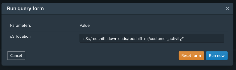
 You would probably like to reuse the load query in the future to load data in from another S3 location. In that case, you can use the parameterized query by replacing the S3 URL of the as shown in the following screenshot:


 Debu Panda is a Principal Product Manager at AWS, is an industry leader in analytics, application platform, and database technologies, and has more than 25 years of experience in the IT world.
 Cansu Aksu is a Front End Engineer at AWS, has a several years of experience in developing user interfaces. She is detail oriented, eager to learn and passionate about delivering products and features that solve customer needs and problems
 Chengyang Wang is a Frontend Engineer in Redshift Console Team. He worked on a number of new features delivered by redshift in the past 2 years. He thrives to deliver high quality products and aim to improve customer experience from UI


 Lotfi Mouhib is a Senior Solutions Architect working for the Public Sector team with Amazon Web Services. He helps public sector customers across EMEA realize their ideas, build new services, and innovate for citizens. In his spare time, Lotfi enjoys cycling and running.


 Satish Sathiya is a Senior Product Engineer at Amazon Redshift. He is an avid big data enthusiast who collaborates with customers around the globe to achieve success and meet their data warehousing and data lake architecture needs.
 Runyao Chen is a Software Development Engineer at Amazon Redshift. He is passionate about MPP databases and has worked on SQL language features such as querying semistructured data using SUPER. In his spare time, he enjoys reading and exploring new restaurants.
 Cody Cunningham is a Software Development Engineer at Amazon Redshift. He works on Redshift’s data ingestion, implementing new features and performance improvements, and recently worked on the ingestion support for SUPER.


 Praveen Krishnamoorthy Ravikumar is a Data Architect with AWS Professional Services Intelligence Practice. He helps customers implement big data and analytics platform and solutions.
 Abhishek Gupta is a Data and ML Engineer with AWS Professional Services Practice.
 Ashok Yoganand Sridharan is a Big Data Consultant with AWS Professional Services Intelligence Practice. He helps customers implement big data and analytics platform and solutions