Amazon DynamoDB, a serverless NoSQL database, has been a go-to solution for over one million customers to build low-latency and high-scale applications. As data grows, organizations are constantly seeking ways to extract valuable insights from operational data, which is often stored in DynamoDB. However, to make the most of this data in Amazon DynamoDB for analytics and machine learning (ML) use cases, customers often build custom data pipelines—a time-consuming infrastructure task that adds little unique value to their core business.
Starting today, you can use Amazon DynamoDB zero-ETL integration with Amazon SageMaker Lakehouse to run analytics and ML workloads in just a few clicks without consuming your DynamoDB table capacity. Amazon SageMaker Lakehouse unifies all your data across Amazon S3 data lakes and Amazon Redshift data warehouses, helping you build powerful analytics and AI/ML applications on a single copy of data.
Zero-ETL is a set of integrations that eliminates or minimizes the need to build ETL data pipelines. This zero-ETL integration reduces the complexity of engineering efforts required to build and maintain data pipelines, benefiting users running analytics and ML workloads on operational data in Amazon DynamoDB without impacting production workflows.
Let’s get started For the following demo, I need to set up zero-ETL integration for my data in Amazon DynamoDB with an Amazon Simple Storage Service data lake managed by Amazon SageMaker Lakehouse. Before setting up the zero-ETL integration, there are prerequisites to complete. If you want to learn more on how to set up, refer to this Amazon DynamoDB documentation page.
With all the prerequisites completed, I can get started with this integration. I navigate to the AWS Glue console and select Zero-ETL integrations under Data Integration and ETL. Then, I choose Create zero-ETL integration.
Here, I have options to select my data source. I choose Amazon DynamoDB and choose Next.
Next, I need to configure the source and target details. In the Source details section, I select my Amazon DynamoDB table. In the Target details section, I specify the S3 bucket that I’ve set up in the AWS Glue Data Catalog.
To set up this integration, I need an IAM role that grants AWS Glue the necessary permissions. For guidance on configuring IAM permissions, visit the Amazon DynamoDB documentation page. Also, if I haven’t configured a resource policy for my AWS Glue Data Catalog, I can select Fix it for me to automatically add the required resource policies.
Here, I have options to configure the output. Under Data partitioning, I can either use DynamoDB table keys for partitioning or specify custom partition keys. After completing the configuration, I choose Next.
Because I select the Fix it for me checkbox, I need to review the required changes and choose Continue before I can proceed to the next step.
On the next page, I have the flexibility to configure data encryption. I can use AWS Key Management Service (AWS KMS) or a custom encryption key. Then, I assign a name to the integration and choose Next.
On the last step, I need to review the configurations. When I’m happy, I choose Next to create the zero-ETL integration.
After the initial data ingestion completes, my zero-ETL integration will be ready for use. The completion time varies depending on the size of my source DynamoDB table.
If I navigate to Tables under Data Catalog in the left navigation panel, I can observe more details including Schema. Under the hood, this zero-ETL integration uses Apache Iceberg to transform related to data format and structure in my DynamoDB data into Amazon S3.
Lastly, I can tell that all my data is available in my S3 bucket.
This zero-ETL integration significantly reduces the complexity and operational burden of data movement, and I can therefore focus on extracting insights rather than managing pipelines.
Available now This new zero-ETL capability is available in the following AWS Regions: US East (N. Virginia, Ohio), US West (Oregon), Asia Pacific (Hong Kong, Singapore, Sydney, Tokyo), Europe (Frankfurt, Ireland, Stockholm).
Explore how to streamline your data analytics workflows using Amazon DynamoDB zero-ETL integration with Amazon SageMaker Lakehouse. Learn more how to get started on the Amazon DynamoDB documentation page.
Providing highly available applications while maintaining low latency reads and writes across AWS Regions is a common challenge faced by many customers. Accessing data from different Regions can cause a delay of hundreds of milliseconds compared to microseconds within the same Region. The necessity for developers to create complex custom solutions for data replication and conflict resolution can lead to increased operational workload and potential errors. Beyond multi-Region replication, these customers have to implement manual database failover procedures and provide data consistency and recovery to deliver highly available applications and data durability.
Today, Amazon Web Services (AWS) announced the general availability of Amazon MemoryDB Multi-Region, a fully managed, active-active, multi-Region database that you can use to build applications with up to 99.999 percent availability, microsecond read, and single-digit millisecond write latencies across multiple AWS Regions. MemoryDB Multi-Region is available for Valkey, which is a Redis Open Source Software (OSS) drop-in replacement stewarded by Linux Foundation. This new feature builds upon the existing benefits of Amazon MemoryDB, such as multi-AZ durability and high throughput across multiple AWS Regions, and addresses these common challenges faced by many customers.
MemoryDB Multi-Region provides the following benefits to customers:
High availability and disaster recovery – With MemoryDB Multi-Region, you can build applications with up to 99.999 percent availability. It also makes sure that if an application is unable to connect to MemoryDB in a local Region, the application can connect to MemoryDB from another AWS Regional endpoint with full read and write access to the data. When the application reconnects to the original MemoryDB Regional endpoint, MemoryDB Multi-Region will automatically synchronize data across all AWS Regions.
Microsecond read and single-digit millisecond write latency for multi-Region distributed applications – MemoryDB Multi-Region offers active-active replication, so you can serve both reads and writes locally from the Regions closest to your customers with microsecond read and single-digit millisecond write latency at any scale. It automatically replicates data asynchronously between AWS Regions with data typically propagated in less than one second.
Adhere to compliance and regulatory requirements where data needs to reside in a specific geography – There are compliance and regulatory requirements under which data needs to be within a geographic location. MemoryDB Multi-Region can help you meet these requirements as it allows customers to choose which region they want their data to reside.
Getting started with Amazon MemoryDB Multi-Region
Setting up MemoryDB Multi-Region is straightforward and can be accomplished through the AWS Management Console, AWS SDK, or AWS CLI.
Getting started with MemoryDB Multi-Region using the console
To set up your MemoryDB Multi-Region cluster using the console, complete the following steps:
On the MemoryDB console, choose Clusters in the navigation pane, choose Create cluster, select Multi-Region cluster for Cluster type, and Create new cluster for the Cluster creation method.
You can select the Node type and number of shards based on your workload requirement when you set up your Multi-Region cluster.
Create the Regional cluster within your Multi-Region cluster with the appropriate cluster settings.
You can add a second Regional cluster to your Multi-Region cluster by choosing Add AWS region after the Multi-Region cluster and the first Regional cluster are set up.
When the cluster creation workflow finishes successfully, you can observe that there are two Regional clusters within the Multi-Region cluster.
Here are the steps to get started using the AWS CLI
To begin, create a new MemoryDB Multi-Region cluster:
Amazon MemoryDB Multi-Region is available for Valkey and in the following AWS Regions: US East (N. Virginia, Ohio), US West (N. California, Oregon), Asia Pacific (Mumbai, Seoul, Singapore, Sydney, Tokyo), and Europe (Frankfurt, Ireland, London).
AWS DMS is a cloud service that makes it possible to migrate relational databases, data warehouses, NoSQL databases, and other types of data stores. You can use AWS DMS to migrate your data into the Amazon Web Services (AWS) Cloud or between combinations of cloud and on-premises setups.
Today, more than 1 million databases have been migrated using AWS Database Migration Service. AWS DMS helps you migrate your data from one database system to another. And, when migrating between different database engines, AWS DMS SC helps to convert the source database schema and procedures to the target database system.
However, although AWS DMS SC automates many steps in these migrations, certain complex database code elements still require manual intervention, which can extend migration timelines and add cost. This is particularly the case with proprietary system functions or procedures, and data type conversions, which don’t always have direct equivalents in PostgreSQL.
The new generative AI capability in AWS DMS SC is designed to address these challenges by automating some of the most time-intensive schema conversion tasks. Using large language models (LLMs) hosted on Amazon Bedrock, the new capability expands the existing conversion capabilities. It converts code snippets in the source database that were otherwise not supported by traditional rule-based techniques, including complex procedures and functions.
Generative AI–assisted code conversion helps to reduce migration costs and accelerate project timelines. Because AWS DMS SC automates more of the schema conversion process, you can focus on higher value tasks such as refining and optimizing your applications post-migration rather than manually resolving conversion gaps. Our beta customers have already experienced success with these AI-powered features in AWS DMS SC, achieving cost savings and faster migrations.
Let’s find out how it works To demonstrate the ease of using this new generative AI capability, I’ll walk through the schema conversion process in AWS DMS SC. AWS DMS SC simplifies database migration by automatically converting my source database’s structure, including tables, views, stored procedures, functions, and more, to a format compatible with my target database. Any objects that can’t be automatically converted are flagged for manual attention.
After my project is created, I select it, and on the Schema conversion tab, I choose Launch schema conversion. It takes a couple of minutes to launch the conversion tool the first time.
AWS DMS SC with generative AI is an opt-in capability. I first activate the option. On the Settings tab, I turn on Enable Generative AI feature for conversion.
Before diving into the details of the conversion, I would like to get an overall assessment of the migration complexity. I select the schema I want to migrate. Then I select Assess in the menu.
After a few minutes, a high-level Summary is available. The Action items tab has more details. I choose Export results and choose PDF to receive a report to share with my colleagues. The report is generated and available from an S3 bucket.
The summary screen shows the percentage of Database storage objects and Database code objects that can be converted by the rule-based method. That’s 100% and 57% in this example. Let’s see how the generative AI-based conversion will change that.
The PDF contains an executive summary, various statistics about the number of objects to be migrated, the feasibility of conversion with generative AI, and the complexity of the migration.
By reading the report, I learn there is no blocker detected to migrate the stored procedures. I select the stored procedure I want to migrate (PRC_AIML_DEMO6). Then, I select the Actions menu on the source database (the left one) and choose Convert.
After a minute or two, I can read the original procedure code in the left pane and the proposed migrated version on the right panel.
The summary screen has been updated. Now, it shows that 100 percent of the code can be converted automatically.
I can edit the code and make changes as required. When I’m comfortable with the proposed new version, I select the Actions menu on the target database side (the right one) and choose Apply changes.
With this new generative AI capability, AWS DMS SC can automatically convert up to 90 percent of schema objects from commercial databases to PostgreSQL.
To support your compliance requirements, this capability is initially turned off, and you can enable it as needed. If you choose to use the generative AI features in AWS DMS SC, it will flexibly decide between traditional rule-based methods and generative AI based on the complexity of the objects being converted. Customers with strict policies against generative AI can continue to rely solely on the rule-based approach, with any unconverted or partially converted objects requiring manual adjustments.
Availability and pricing This new capability is available today in the following AWS Regions: US East (Ohio, N. Virginia), US West (Oregon), and Europe (Frankfurt).
AWS DMS Schema Conversion with generative AI provides you with a faster migration pathway and helps you accelerate your transition to AWS.
To get started, visit the AWS DMS Schema Conversion documentation and learn how this generative AI capability can simplify your next database migration.
Apache Iceberg is a high-performance open-source table format for performing big data analytics. Apache Iceberg brings the reliability and simplicity of SQL tables to S3 data lakes and makes it possible for open source analytics engines such as Apache Spark, Apache Flink, Trino, Apache Hive, and Apache Impala to concurrently work with the same data.
This new capability provides a simple, end-to-end solution to stream database updates without impacting transaction performance of database applications. You can set up a Data Firehose stream in minutes to deliver change data capture (CDC) updates from your database. Now, you can easily replicate data from different databases into Iceberg tables on Amazon S3 and use up-to-date data for large-scale analytics and machine learning (ML) applications.
Typical Amazon Web Services (AWS) enterprise customers use hundreds of databases for transactional applications. To perform large scale analytics and ML on the latest data, they want to capture changes made in databases, such as when records in a table are inserted, modified, or deleted, and deliver the updates to their data warehouse or Amazon S3 data lake in open source table formats such as Apache Iceberg.
To do so, many customers develop extract, transform, and load (ETL) jobs to periodically read from databases. However, ETL readers impact database transaction performance, and batch jobs can add several hours of delay before data is available for analytics. To mitigate impact on database transaction performance, customers want the ability to stream changes made in the database. This stream is referred to as a change data capture (CDC) stream.
I met multiple customers that use open source distributed systems, such as Debezium, with connectors to popular databases, an Apache Kafka Connect cluster, and Kafka Connect Sink to read the events and deliver them to the destination. The initial configuration and test of such systems involves installing and configuring multiple open source components. It might take days or weeks. After setup, engineers have to monitor and manage clusters, and validate and apply open source updates, which adds to the operational overhead.
With this new data streaming capability, Amazon Data Firehose adds the ability to acquire and continually replicate CDC streams from databases to Apache Iceberg tables on Amazon S3. You set up a Data Firehose stream by specifying the source and destination. Data Firehose captures and continually replicates an initial data snapshot and then all subsequent changes made to the selected database tables as a data stream. To acquire CDC streams, Data Firehose uses the database replication log, which reduces impact on database transaction performance. When the volume of database updates increases or decreases, Data Firehose automatically partitions the data, and persists records until they’re delivered to the destination. You don’t have to provision capacity or manage and fine-tune clusters. In addition to the data itself, Data Firehose can automatically create Apache Iceberg tables using the same schema as the database tables as part of the initial Data Firehose stream creation and automatically evolve the target schema, such as new column addition, based on source schema changes.
Since Data Firehose is a fully managed service, you don’t have to rely on open source components, apply software updates, or incur operational overhead.
The continual replication of database changes to Apache Iceberg tables in Amazon S3 using Amazon Data Firehose provides you with a simple, scalable, end-to-end managed solution to deliver CDC streams into your data lake or data warehouse, where you can run large-scale analysis and ML applications.
I also have an S3 bucket to host the Iceberg table, and I have an AWS Identity and Access Management (IAM) role setup with correct permissions. You can refer to the list of prerequisites in the Data Firehose documentation.
To get started, I open the console and navigate to the Amazon Data Firehose section. I can see the stream already created. To create a new one, I select Create Firehose stream.
I select a Source and Destination. In this example: a MySQL database and Apache Iceberg Tables. I also enter a Firehose stream name for my stream.
I enter the fully qualified DNS name of my Database endpoint and the Database VPC endpoint service name. I verify that Enable SSL is checked and, under Secret name, I select the name of the secret in AWS Secrets Manager where the database username and password are securely stored.
Next, I configure Data Firehose to capture specific data by specifying databases, tables, and columns using explicit names or regular expressions.
I must create a watermark table. A watermark, in this context, is a marker used by Data Firehose to track the progress of incremental snapshots of database tables. It helps Data Firehose identify which parts of the table have already been captured and which parts still need to be processed. I can create the watermark table manually or let Data Firehose automatically create it for me. In that case, the database credentials passed to Data Firehose must have permissions to create a table in the source database.
Next, I configure the S3 bucket Region and name to use. Data Firehose can automatically create the Iceberg tables when they don’t exist yet. Similarly, it can update the Iceberg table schema when detecting a change in your database schema.
After having reviewed my configuration, I select Create Firehose stream.
Once the stream is created, it will start to replicate the data. I can monitor the stream’s status and check for eventual errors.
Now, it’s time to test the stream.
I open a connection to the database and insert a new line in a table.
Then, I navigate to the S3 bucket configured as the destination and I observe that a file has been created to store the data from the table.
I download the file and inspect its content with the parq command (you can install that command with pip install parquet-cli)
Of course, downloading and inspecting Parquet files is something I do only for demos. In real life, you’re going to use AWS Glue and Amazon Athena to manage your data catalog and to run SQL queries on your data.
Things to know Here are a few additional things to know.
This new capability supports self-managed PostgreSQL and MySQL databases on Amazon EC2 and the following databases on Amazon RDS:
The team will continue to add support for additional databases during the preview period and after general availability. They told me they are already working on supporting SQL Server, Oracle, and MongoDB databases.
When setting up an Amazon Data Firehose delivery stream, you can either specify specific tables and columns or use wildcards to specify a class of tables and columns. When you use wildcards, if new tables and columns are added to the database after the Data Firehose stream is created and if they match the wildcard, Data Firehose will automatically create those tables and columns in the destination.
Pricing and availability The new data streaming capability is available today in all AWS Regions except China Regions, AWS GovCloud (US) Regions, and Asia Pacific (Malaysia) Regions. We want you to evaluate this new capability and provide us with feedback. There are no charges for your usage at the beginning of the preview. At some point in the future, it will be priced based on your actual usage, for example, based on the quantity of bytes read and delivered. There are no commitments or upfront investments. Make sure to read the pricing page to get the details.
Data is the fuel for AI; modern data is even more important for generative AI and advanced data analytics, producing more accurate, relevant, and impactful results. Modern data comes in various forms: real-time, unstructured, or user-generated. Each form requires a different solution. AWS’s data journey began with Amazon Simple Storage Service (Amazon S3) in 2006, marking the start of cloud-based data storage at scale. Since then, AWS has expanded its data offerings to cover the entire data lifecycle, offering a comprehensive ecosystem of services designed to harness the full potential of modern data, from ingestion and storage to processing and analysis, supporting the entire lifecycle of AI-driven innovation.
In this blog post, we will cover some AWS use cases for modern data architectures, showing how AWS enables organizations to leverage the power of data and generative AI technologies.
This blog focuses on selecting the right database for generative AI applications and provide knowledge that can enhance your understanding, guide your decision making, and ultimately lead to more successful AI projects. Selecting the right database for generative AI applications is not just about storage; it significantly impacts performance, scalability, ease of integration, and overall effectiveness of the AI solution.
Figure 1. Diagram that shows the key steps in a RAG workflow
Adopting a data mesh architecture can enhance an organization’s ability to manage data effectively, leading to improved performance, innovation, and overall business success. In this guidance, you will discover some strategies to build data mesh solutions on AWS.
Figure 2. The data mesh organizes data into domains, where data are seen as quality products to expose for consumption
Amazon S3 is an object storage service that supports multiple use cases, including data architectures. Big data pipelines can use Amazon S3 to store input, output, and intermediate results. Machine learning systems use Amazon S3 to process application logs and build the datasets both for experimentation and for production model training. Given the importance of the service and the number of use cases that a foundational storage service can support, we want to share best practices, performance optimization, and cost optimization strategies to work with Amazon S3. This video shows how Anthropic designs its architecture around Amazon S3 in their data architecture.
Figure 3. Workloads with predictable patterns often have low retrieval rates for long periods of time after, so we can design to adopt cheaper storage classes for them
If you are curious about the underlying architecture of Amazon S3 and want to drill down into its internal design, you can watch the re:Invent video Dive deep on Amazon S3.
This is an AWS case study on how HPE Aruba Supply Chain successfully re-architected and deployed their data solution by adopting a modern data architecture on AWS. The new solution has helped Aruba integrate data from multiple sources, along with optimizing their cost, performance, and scalability. This has also allowed the Aruba Supply Chain leadership to receive in-depth and timely insights for better decision-making, thereby elevating the customer experience.
This workshop highlights advantage of adopting a modern data architecture on AWS. By integrating the flexibility of a data lake with specialized analytics services, organizations can significantly enhance their data-driven decision-making capabilities. We encourage everyone to explore how this architecture can streamline their analytics processes and support diverse use cases, from real-time insights to advanced machine learning. It’s an excellent opportunity to leverage modern data architecture.
Figure 5. Data architectures are fundamental to power use cases ranging from analytics to machine learning
Thanks for reading! In the next blog, we will cover some tips on how to get the best out of your developer experience on AWS. To revisit any of our previous posts or explore the entire series, visit the Let’s Architect! page.
Today, we are announcing the general availability of Amazon Aurora PostgreSQL Limitless Database, a new serverless horizontal scaling (sharding) capability of Amazon Aurora. With Aurora PostgreSQL Limitless Database, you can scale beyond the existing Aurora limits for write throughput and storage by distributing a database workload over multiple Aurora writer instances while maintaining the ability to use it as a single database.
When we previewed Aurora PostgreSQL Limitless Database at AWS re:Invent 2023, I explained that it uses a two-layer architecture consisting of multiple database nodes in a DB shard group – either routers or shards to scale based on the workload.
Routers – Nodes that accept SQL connections from clients, send SQL commands to shards, maintain system-wide consistency, and return results to clients.
Shards – Nodes that store a subset of tables and full copies of data, which accept queries from routers.
There will be three types of tables that contain your data: sharded, reference, and standard.
Sharded tables – These tables are distributed across multiple shards. Data is split among the shards based on the values of designated columns in the table, called shard keys. They are useful for scaling the largest, most I/O-intensive tables in your application.
Reference tables – These tables copy data in full on every shard so that join queries can work faster by eliminating unnecessary data movement. They are commonly used for infrequently modified reference data, such as product catalogs and zip codes.
Standard tables – These tables are like regular Aurora PostgreSQL tables. Standard tables are all placed together on a single shard so join queries can work faster by eliminating unnecessary data movement. You can create sharded and reference tables from standard tables.
Once you have created the DB shard group and your sharded and reference tables, you can load massive amounts of data into Aurora PostgreSQL Limitless Database and query data in those tables using standard PostgreSQL queries. To learn more, visit Limitless Database architecture in the Amazon Aurora User Guide.
Getting started with Aurora PostgreSQL Limitless Database You can get started in the AWS Management Console and AWS Command Line Interface (AWS CLI) to create a new DB cluster that uses Aurora PostgreSQL Limitless Database, add a DB shard group to the cluster, and query your data.
1. Create an Aurora PostgreSQL Limitless Database Cluster Open the Amazon Relational Database Service (Amazon RDS) console and choose Create database. For Engine options, choose Aurora (PostgreSQL Compatible) and Aurora PostgreSQL with Limitless Database (Compatible with PostgreSQL 16.4).
For Aurora Limitless Database, enter a name for your DB shard group and values for minimum and maximum capacity measured by Aurora capacity units (ACUs) across all routers and shards. The initial number of routers and shards in a DB shard group is determined by this maximum capacity. Aurora PostgreSQL Limitless Database scales a node up to a higher capacity when its current utilization is too low to handle the load. It scales the node down to a lower capacity when its current capacity is higher than needed.
For DB shard group deployment, choose whether to create standbys for the DB shard group: no compute redundancy, one compute standby in a different Availability Zone, or two compute standbys in two different Availability Zones.
You can set the remaining DB settings to what you prefer and choose Create database. After the DB shard group are created, they’re displayed on the Databases page.
You can connect, reboot, or delete a DB shard group, or you can change the capacity, split a shard, or add a router in the DB shard group. To learn more, visit Working with DB shard groups in the Amazon Aurora User Guide.
2. Create Aurora PostgreSQL Limitless Database tables As shared previously, Aurora PostgreSQL Limitless Database has three table types: sharded, reference, and standard. You can convert standard tables to sharded or reference tables to distribute or replicate existing standard tables or create new sharded and reference tables.
You can use variables to create sharded and reference tables by setting the table creation mode. The tables that you create will use this mode until you set a different mode. The following examples show how to use these variables to create sharded and reference tables.
For example, create a sharded table named items with a shard key composed of the item_id and item_cat columns.
SET rds_aurora.limitless_create_table_mode='sharded';
SET rds_aurora.limitless_create_table_shard_key='{"item_id", "item_cat"}';
CREATE TABLE items(item_id int, item_cat varchar, val int, item text);
Now, create a sharded table named item_description with a shard key composed of the item_id and item_cat columns and collocate it with the items table.
You can also create a reference table named colors.
SET rds_aurora.limitless_create_table_mode='reference';
CREATE TABLE colors(color_id int primary key, color varchar);
You can find information about Limitless Database tables by using the rds_aurora.limitless_tables view, which contains information about tables and their types.
postgres_limitless=> SELECT * FROM rds_aurora.limitless_tables;

 table_gid | local_oid | schema_name | table_name  | table_status | table_type  | distribution_key
-----------+-----------+-------------+-------------+--------------+-------------+------------------
         1 |     18797 | public      | items       | active       | sharded     | HASH (item_id, item_cat)
         2 |     18641 | public      | colors      | active       | reference   |

(2 rows)
You can convert standard tables into sharded or reference tables. During the conversion, data is moved from the standard table to the distributed table, then the source standard table is deleted. To learn more, visit Converting standard tables to limitless tables in the Amazon Aurora User Guide.
3. Query Aurora PostgreSQL Limitless Database tables Aurora PostgreSQL Limitless Database is compatible with PostgreSQL syntax for queries. You can query your Limitless Database using psql or any other connection utility that works with PostgreSQL. Before querying tables, you can load data into Aurora Limitless Database tables by using the COPY command or by using the data loading utility.
To run queries, connect to the cluster endpoint, as shown in Connecting to your Aurora Limitless Database DB cluster. All PostgreSQL SELECT queries are performed on the router to which the client sends the query and shards where the data is located.
To achieve a high degree of parallel processing, Aurora PostgreSQL Limitless Database utilizes two querying methods: single-shard queries and distributed queries, which determines whether your query is single-shard or distributed and processes the query accordingly.
Single-shard query – A query where all the data needed for the query is on one shard. The entire operation can be performed on one shard, including any result set generated. When the query planner on the router encounters a query like this, the planner sends the entire SQL query to the corresponding shard.
Distributed query – A query run on a router and more than one shard. The query is received by one of the routers. The router creates and manages the distributed transaction, which is sent to the participating shards. The shards create a local transaction with the context provided by the router, and the query is run.
For examples of single-shard queries, you use the following parameters to configure the output from the EXPLAIN command.
postgres_limitless=> SET rds_aurora.limitless_explain_options = shard_plans, single_shard_optimization;
SET

postgres_limitless=> EXPLAIN SELECT * FROM items WHERE item_id = 25;

                     QUERY PLAN
--------------------------------------------------------------
 Foreign Scan  (cost=100.00..101.00 rows=100 width=0)
   Remote Plans from Shard postgres_s4:
         Index Scan using items_ts00287_id_idx on items_ts00287 items_fs00003  (cost=0.14..8.16 rows=1 width=15)
           Index Cond: (id = 25)
 Single Shard Optimized
(5 rows)
To learn more about the EXPLAIN command, see EXPLAIN in the PostgreSQL documentation.
For examples of distributed queries, you can insert new items named Book and Pen into the items table.
postgres_limitless=> INSERT INTO items(item_name)VALUES ('Book'),('Pen')
This makes a distributed transaction on two shards. When the query runs, the router sets a snapshot time and passes the statement to the shards that own Book and Pen. The router coordinates an atomic commit across both shards, and returns the result to the client.
You can use distributed query tracing, a tool to trace and correlate queries in PostgreSQL logs across Aurora PostgreSQL Limitless Database. To learn more, visit Querying Limitless Database in the Amazon Aurora User Guide.
Things to know Here are a couple of things that you should know about this feature:
Compute – You can only have one DB shard group per DB cluster and set the maximum capacity of a DB shard group to 16–6144 ACUs. Contact us if you need more than 6144 ACUs. The initial number of routers and shards is determined by the maximum capacity that you set when you create a DB shard group. The number of routers and shards doesn’t change when you modify the maximum capacity of a DB shard group. To learn more, see the table of the number of routers and shards in the Amazon Aurora User Guide.
Storage – Aurora PostgreSQL Limitless Database only supports the Amazon Aurora I/O-Optimized DB cluster storage configuration. Each shard has a maximum capacity of 128 TiB. Reference tables have a size limit of 32 TiB for the entire DB shard group. To reclaim storage space by cleaning up your data, you can use the vacuuming utility in PostgreSQL.
Now available Amazon Aurora PostgreSQL Limitless Database is available today with PostgreSQL 16.4 compatibility in the AWS US East (N. Virginia), US East (Ohio), US West (Oregon), Asia Pacific (Hong Kong), Asia Pacific (Singapore), Asia Pacific (Sydney), Asia Pacific (Tokyo), Europe (Frankfurt), Europe (Ireland), and Europe (Stockholm) Regions.
This is the final part of a three-part series where we show how to build a data lake on AWS using a modern data architecture. This post shows how to process data with Amazon Redshift Spectrum and create the gold (consumption) layer. To review the first two parts of the series where we load data from SQL Server into Amazon Simple Storage Service (Amazon S3) using AWS Database Migration Service (AWS DMS) and load the data into the silver layer of the data lake, see the following:
Choosing the right tools and technology stack to build the data lake in order to build a scalable solution and have shorter time to market is critical. In this post, we go over the process of building a data lake, providing rationale behind the different decisions, and share best practices when building such a data solution.
The following diagram illustrates the different layers of the data lake.
The data lake is designed to serve a multitude of use cases. In the silver layer of the data lake, the data is stored as it is loaded from sources, preserving the table and schema structure. In the gold layer, we create data marts by combining, aggregating, and enriching data as required by our use cases. The gold layer is the consumption layer for the data lake. In this post, we describe how you can use Redshift Spectrum as an API to query data.
To create data marts, we use Amazon Redshift Query Editor. It provides a web-based analyst workbench to create, explore, and share SQL queries. In our use case, we use Redshift Query Editor to create data marts using SQL code. We also use Redshift Spectrum, which allows you to efficiently query and retrieve structured and semi-structured data from files stored on Amazon S3 without having to load the data into the Redshift tables. The Apache Iceberg tables, which we created and cataloged in Part 2, can be queried using Redshift Spectrum. For the latest information on Redshift Spectrum integration with Iceberg, see Using Apache Iceberg tables with Amazon Redshift.
We also show how to use RedshiftDataAPIService to run SQL commands to query the data mart using a Boto3 Python SDK. You can use the Redshift Data API to create the resulting datasets on Amazon S3, and then use the datasets in use cases such as business intelligence dashboards and machine learning (ML).
In this post, we walk through the following steps:
Set up a Redshift cluster.
Set up a data mart.
Query the data mart.
Prerequisites
To follow the solution, you need to set up certain access rights and resources:
An AWS Identity and Access Management (IAM) role for the Redshift cluster with access to an external data catalog in AWS Glue and data files in Amazon S3 (these are the data files populated by the silver layer in Part 2). The role also needs Redshift cluster permissions. This policy must include permissions to do the following:
Run SQL commands to copy, unload, and query data with Amazon Redshift.
Grant permissions to run SELECT statements for related services, such as Amazon S3, Amazon CloudWatch logs, Amazon SageMaker, and AWS Glue.
Manage AWS Lake Formation permissions (in case the AWS Glue Data Catalog is managed by Lake Formation).
An IAM execution role for AWS Lambda with permissions to access Amazon Redshift and AWS
Redshift Spectrum is a feature of Amazon Redshift that queries data stored in Amazon S3 directly, without having to load it into Amazon Redshift. In our use case, we use Redshift Spectrum to query Iceberg data stored as Parquet files on Amazon S3. To use Redshift Spectrum, we first need a Redshift cluster to run the Redshift Spectrum compute jobs. Complete the following steps to provision a Redshift cluster:
On the Amazon Redshift console, choose Clusters in the navigation pane.
Choose Create cluster.
For Cluster identifier, enter a name for your cluster.
For Choose the size of the cluster, select I’ll choose.
For Node type, choose xlplus.
For Number of nodes, enter 1.
For Admin password, select Manage admin credentials in AWS Secrets Manager if you want to use Secrets Manager, otherwise you can generate and store the credentials manually.
For the IAM role, choose the IAM role created in the prerequisites.
Choose Create cluster.
We chose the cluster Availability Zone, number of nodes, compute type, and size for this post to minimize costs. If you’re working on larger datasets, we recommend reviewing the different instance types offered by Amazon Redshift to select the one that is appropriate for your workloads.
Set up a data mart
A data mart is a collection of data organized around a specific business area or use case, providing focused and quickly accessible data for analysis or consumption by applications or users. Unlike a data warehouse, which serves the entire organization, a data mart is tailored to the specific needs of a particular department, allowing for more efficient and targeted data analysis. In our use case, we use data marts to create aggregated data from the silver layer and store it in the gold layer for consumption. For our use case, we use the schema HumanResources in the AdventureWorks sample database we loaded in Part 1 (FIX LINK). This database contains a factory’s employee shift information for different departments. We use this database to create a summary of the shift rate changes for different departments, years, and shifts to see which years had the most rate changes.
We recommend using the auto mount feature in Redshift Spectrum. This feature removes the need to create an external schema in Amazon Redshift to query tables cataloged in the Data Catalog.
Complete the following steps to create a data mart:
On the Amazon Redshift console, choose Query editor v2 in the navigation pane.
Choose the cluster you created and choose AWS Secrets Manager or Database username and password depending on how you chose to store the credentials.
After you’re connected, open a new query editor.
You will be able to see the AdventureWorks database under awsdatacatalog. You can now start querying the Iceberg database in the query editor.
If you encounter permission issues, choose the options menu (three dots) next to the cluster, choose Edit connection, and connect using Secrets Manager or your database user name and password. Then grant privileges for the IAM user or role with the following command, and reconnect with your IAM identity:
GRANT USAGE ON DATABASE awsdatacatalog to "IAMR:MyRole"
Next, you create a local schema to store the definition and data for the view.
On the Create menu, choose Schema.
Provide a name and set the type as local.
For the data mart, create a dataset that combines different tables in the silver layer to generate a report of the total shift rate changes by department, year, and shift. The following SQL code will return the required dataset:
SELECT dep.name AS "Department Name",
extract(year from emp_pay_hist.ratechangedate) AS "Rate Change Year",
shift.name AS "Shift",
COUNT(emp_pay_hist.rate) AS "Rate Changes"
FROM "dev"."{redshift_schema_name}"."department" dep
INNER JOIN "dev"."{redshift_schema_name}"."employeedepartmenthistory" emp_hist
ON dep.departmentid = emp_hist.departmentid
INNER JOIN "dev"."{redshift_schema_name}"."employeepayhistory" emp_pay_hist
ON emp_pay_hist.businessentityid = emp_hist.businessentityid
INNER JOIN "dev"."{redshift_schema_name}"."employee" emp
ON emp_hist.businessentityid = emp.businessentityid
INNER JOIN "dev"."{redshift_schema_name}"."shift" shift
ON emp_hist.shiftid = shift.shiftid
WHERE emp.currentflag = 'true'
GROUP BY dep.name, extract(year from emp_pay_hist.ratechangedate), shift.name;
Create an internal schema where you want Amazon Redshift to store the view definition:
CREATE SCHEMA IF NOT EXISTS {internal_schema_name};
Create a view in Amazon Redshift that you can query to get the dataset:
CREATE OR REPLACE VIEW {internal_schema_name}.rate_changes_by_department_year AS
SELECT dep.name AS "Department Name",
extract(year from emp_pay_hist.ratechangedate) AS "Rate Change Year",
shift.name AS "Shift",
COUNT(emp_pay_hist.rate) AS "Rate Changes"
FROM "dev"."{redshift_schema_name}"."department" dep
INNER JOIN "dev"."{redshift_schema_name}"."employeedepartmenthistory" emp_hist
ON dep.departmentid = emp_hist.departmentid
INNER JOIN "dev"."{redshift_schema_name}"."employeepayhistory" emp_pay_hist
ON emp_pay_hist.businessentityid = emp_hist.businessentityid
INNER JOIN "dev"."{redshift_schema_name}"."employee" emp
ON emp_hist.businessentityid = emp.businessentityid
INNER JOIN "dev"."{redshift_schema_name}"."shift" shift
ON emp_hist.shiftid = shift.shiftid
WHERE emp.currentflag = 'true'
GROUP BY dep.name, extract(year from emp_pay_hist.ratechangedate), shift.name
WITH NO SCHEMA BINDING;
If the SQL takes a long time to run or produces a large result set, consider using Redshift Unlike regular views, which are computed in the moment, the results from materialized views can be pre-computed and stored on Amazon S3. When the data is requested, Amazon Redshift can point to an Amazon S3 location where the results are stored. Materialized views can be refreshed on demand and on a schedule.
Query the data mart
Lastly, we query the data mart using a Lambda function to show how the data can be retrieved using an API. The Lambda function requires an IAM role to access Secrets Manager where the Redshift user credentials are stored. We use the Redshift Data API to retrieve the dataset we created in the previous step. First, we call the execute_statement() command to run the view. Next , we check the status of the run by calling the describe_statement() call. Finally , when the statement has successfully run, we use the get_statement_result() call to get the result set. The Lambda function shown in the following code implements this logic and returns the result set from querying the view rate_changes_by_department_year:
import json
import boto3
import time

def lambda_handler(event, context):
	client = boto3.client('redshift-data')

	# Use the Redshift execute statement api to query the data mart
	response = client.execute_statement(
	ClusterIdentifier='{redshift cluster name}',
	Database='dev',
	SecretArn='{redshift cluster secrets manager secret arn}',
	Sql='select * from {internal_schema_name}.rate_changes_by_department_year',
	StatementName='query data mart'
	)

	statement_id = response["Id"]
	query_status = True
	resultSet = []

	# Check the status of the sql statement, once the statement has finished executing we can retrive the resultset
	while query_status:
	if client.describe_statement(Id=statement_id)["Status"] == "FINISHED":

	print("SQL statement has finished successfully and we can get the resultset")

	response = client.get_statement_result(
	Id=statement_id
	)
	columns = response["ColumnMetadata"]
	results = response["Records"]
	while "NextToken" in response:
	response = client.get_servers(NextToken=response["NextToken"])
	results.extend(response["Records"])

	resultSet.append(str(columns[0].get("label")) + "," + str(columns[1].get("label")) + "," + str(columns[2].get("label")) + "," + str(columns[3].get("label")))

	for result in results:
	resultSet.append(str(result[0].get("stringValue")) + "," + str(result[1].get("longValue")) + "," + str(result[2].get("stringValue")) + "," + str(result[3].get("longValue")))

	query_status = False

	# In case the statement runs into errors we abort the resultset retrival
	if client.describe_statement(Id=statement_id)["Status"] == "ABORTED" or client.describe_statement(Id=statement_id)["Status"] == "FAILED":
	query_status = False
	print("SQL statement has failed or aborted")

	# To avoid spamming the API with requests on the status of the statement, we introduce a 2 second wait between calls
	else:
	print("Query Status ::" + client.describe_statement(Id=statement_id)["Status"])
	time.sleep(2)

	return {
	'statusCode': 200,
	'body': resultSet
	}
The Redshift Data API allows you to access data from many different types of traditional, cloud-based, containerized, web service-based, and event-driven applications. The API is available in many programming languages and environments supported by the AWS SDK, such as Python, Go, Java, Node.js, PHP, Ruby, and C++. For larger datasets that don’t fit into memory, such as ML training datasets, you can use the Redshift UNLOAD command to move the results of the query to an Amazon S3 location.
Clean up
In this post, you created an IAM role, Redshift cluster, and Lambda function. To clean up your resources, complete the following steps:
Delete the IAM role:
On the IAM console, choose Roles in the navigation pane.
Select the role and choose Delete.
Delete the Redshift cluster:
On the Amazon Redshift console, choose Clusters in the navigation pane.
Select the cluster you created and on the Actions menu, choose Delete.
Delete the Lambda function:
On the Lambda console, choose Functions in the navigation pane.
Select the function you created and on the Actions menu, choose Delete.
Conclusion
In this post, we showed how you can use Redshift Spectrum to create data marts on top of the data in your data lake. Redshift Spectrum can query Iceberg data stored in Amazon S3 and cataloged in AWS Glue. You can create views in Amazon Redshift that compute the results from the underlying data on demand, or pre-compute results and store them (using materialized views). Lastly, the Redshift Data API is a great tool for running SQL queries on the data lake from a wide variety of sources.
Shaheer Mansoor is a Senior Machine Learning Engineer at AWS, where he specializes in developing cutting-edge machine learning platforms. His expertise lies in creating scalable infrastructure to support advanced AI solutions. His focus areas are MLOps, feature stores, data lakes, model hosting, and generative AI.
Anoop Kumar K M is a Data Architect at AWS with focus in the data and analytics area. He helps customers in building scalable data platforms and in their enterprise data strategy. His areas of interest are data platforms, data analytics, security, file systems and operating systems. Anoop loves to travel and enjoys reading books in the crime fiction and financial domains.
Sreenivas Nettem is a Lead Database Consultant at AWS Professional Services. He has experience working with Microsoft technologies with a specialization in SQL Server. He works closely with customers to help migrate and modernize their databases to AWS.
According to a survey done by W3Techs, as of October 2024, Cloudflare is used as an authoritative DNS provider by 14.5% of all websites. As an authoritative DNS provider, we are responsible for managing and serving all the DNS records for our clients’ domains. This means we have an enormous responsibility to provide the best service possible, starting at the data plane. As such, we are constantly investing in our infrastructure to ensure the reliability and performance of our systems.
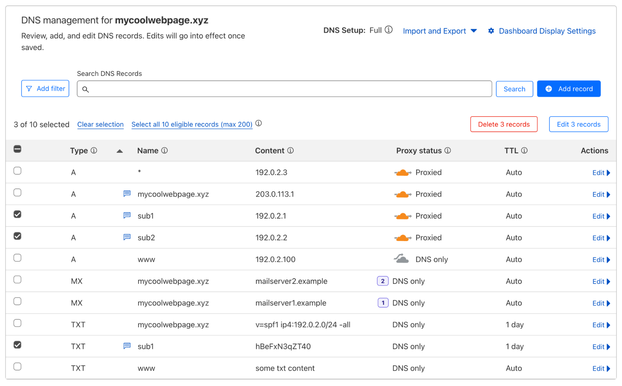
DNS is often referred to as the phone book of the Internet, and is a key component of the Internet. If you have ever used a phone book, you know that they can become extremely large depending on the size of the physical area it covers. A zone file in DNS is no different from a phone book. It has a list of records that provide details about a domain, usually including critical information like what IP address(es) each hostname is associated with. For example:
example.com      59 IN A 198.51.100.0
blog.example.com 59 IN A 198.51.100.1
ask.example.com  59 IN A 198.51.100.2
It is not unusual for these zone files to reach millions of records in size, just for a single domain. The biggest single zone on Cloudflare holds roughly 4 million DNS records, but the vast majority of zones hold fewer than 100 DNS records. Given our scale according to W3Techs, you can imagine how much DNS data alone Cloudflare is responsible for. Given this volume of data, and all the complexities that come at that scale, there needs to be a very good reason to move it from one database cluster to another.
Why migrate
When initially measured in 2022, DNS data took up approximately 40% of the storage capacity in Cloudflare’s main database cluster (cfdb). This database cluster, consisting of a primary system and multiple replicas, is responsible for storing DNS zones, propagated to our data centers in over 330 cities via our distributed KV store Quicksilver. cfdb is accessed by most of Cloudflare’s APIs, including the DNS Records API. Today, the DNS Records API is the API most used by our customers, with each request resulting in a query to the database. As such, it’s always been important to optimize the DNS Records API and its surrounding infrastructure to ensure we can successfully serve every request that comes in.
As Cloudflare scaled, cfdb was becoming increasingly strained under the pressures of several services, many unrelated to DNS. During spikes of requests to our DNS systems, other Cloudflare services experienced degradation in the database performance. It was understood that in order to properly scale, we needed to optimize our database access and improve the systems that interact with it. However, it was evident that system level improvements could only be just so useful, and the growing pains were becoming unbearable. In late 2022, the DNS team decided, along with the help of 25 other teams, to detach itself from cfdb and move our DNS records data to another database cluster.
Pre-migration
From a DNS perspective, this migration to an improved database cluster was in the works for several years. Cloudflare initially relied on a single Postgres database cluster, cfdb. At Cloudflare’s inception, cfdb was responsible for storing information about zones and accounts and the majority of services on the Cloudflare control plane depended on it. Since around 2017, as Cloudflare grew, many services moved their data out of cfdb to be served by a microservice. Unfortunately, the difficulty of these migrations are directly proportional to the amount of services that depend on the data being migrated, and in this case, most services require knowledge of both zones and DNS records.
Although the term “zone” was born from the DNS point of view, it has since evolved into something more. Today, zones on Cloudflare store many different types of non-DNS related settings and help link several non-DNS related products to customers’ websites. Therefore, it didn’t make sense to move both zone data and DNS record data together. This separation of two historically tightly coupled DNS concepts proved to be an incredibly challenging problem, involving many engineers and systems. In addition, it was clear that if we were going to dedicate the resources to solving this problem, we should also remove some of the legacy issues that came along with the original solution.
One of the main issues with the legacy database was that the DNS team had little control over which systems accessed exactly what data and at what rate. Moving to a new database gave us the opportunity to create a more tightly controlled interface to the DNS data. This was manifested as an internal DNS Records gRPC API which allows us to make sweeping changes to our data while only requiring a single change to the API, rather than coordinating with other systems. For example, the DNS team can alter access logic and auditing procedures under the hood. In addition, it allows us to appropriately rate-limit and cache data depending on our needs. The move to this new API itself was no small feat, and with the help of several teams, we managed to migrate over 20 services, using 5 different programming languages, from direct database access to using our managed gRPC API. Many of these services touch very important areas such as DNSSEC, TLS, Email, Tunnels, Workers, Spectrum, and R2 storage. Therefore, it was important to get it right.
One of the last issues to tackle was the logical decoupling of common DNS database functions from zone data. Many of these functions expect to be able to access both DNS record data and DNS zone data at the same time. For example, at record creation time, our API needs to check that the zone is not over its maximum record allowance. Originally this check occurred at the SQL level by verifying that the record count was lower than the record limit for the zone. However, once you remove access to the zone itself, you are no longer able to confirm this. Our DNS Records API also made use of SQL functions to audit record changes, which requires access to both DNS record and zone data. Luckily, over the past several years, we have migrated this functionality out of our monolithic API and into separate microservices. This allowed us to move the auditing and zone setting logic to the application level rather than the database level. Ultimately, we are still taking advantage of SQL functions in the new database cluster, but they are fully independent of any other legacy systems, and are able to take advantage of the latest Postgres version.
Now that Cloudflare DNS was mostly decoupled from the zones database, it was time to proceed with the data migration. For this, we built what would become our Change Data Capture and Transfer Service (CDCTS).
Requirements for the Change Data Capture and Transfer Service
The Database team is responsible for all Postgres clusters within Cloudflare, and were tasked with executing the data migration of two tables that store DNS data: cf_rec and cf_archived_rec, from the original cfdb cluster to a new cluster we called dnsdb. We had several key requirements that drove our design:
Don’t lose data. This is the number one priority when handling any sort of data. Losing data means losing trust, and it is incredibly difficult to regain that trust once it’s lost. Important in this is the ability to prove no data had been lost. The migration process would, ideally, be easily auditable.
Minimize downtime. We wanted a solution with less than a minute of downtime during the migration, and ideally with just a few seconds of delay.
These two requirements meant that we had to be able to migrate data changes in near real-time, meaning we either needed to implement logical replication, or some custom method to capture changes, migrate them, and apply them in a table in a separate Postgres cluster.
We first looked at using Postgres logical replication using pgLogical, but had concerns about its performance and our ability to audit its correctness. Then some additional requirements emerged that made a pgLogical implementation of logical replication impossible:
The ability to move data must be bidirectional. We had to have the ability to switch back to cfdb without significant downtime in case of unforeseen problems with the new implementation.
Partition the cf_rec table in the new database. This was a long-desired improvement and since most access to cf_rec is by zone_id, it was decided that mod(zone_id, num_partitions) would be the partition key.
Transferred data accessible from original database. In case we had functionality that still needed access to data, a foreign table pointing to dnsdb would be available in cfdb. This could be used as emergency access to avoid needing to roll back the entire migration for a single missed process.
Only allow writes in one database. Applications should know where the primary database is, and should be blocked from writing to both databases at the same time.
Details about the tables being migrated
The primary table, cf_rec, stores DNS record information, and its rows are regularly inserted, updated, and deleted. At the time of the migration, this table had 1.7 billion records, and with several indexes took up 1.5 TB of disk. Typical daily usage would observe 3-5 million inserts, 1 million updates, and 3-5 million deletes.
The second table, cf_archived_rec, stores copies of cf_rec that are obsolete — this table generally only has records inserted and is never updated or deleted. As such, it would see roughly 3-5 million inserts per day, corresponding to the records deleted from cf_rec. At the time of the migration, this table had roughly 4.3 billion records.
Fortunately, neither table made use of database triggers or foreign keys, which meant that we could insert/update/delete records in this table without triggering changes or worrying about dependencies on other tables.
Ultimately, both of these tables are highly active and are the source of truth for many highly critical systems at Cloudflare.
Designing the Change Data Capture and Transfer Service
There were two main parts to this database migration:
Initial copy: Take all the data from cfdb and put it in dnsdb.
Change copy: Take all the changes in cfdb since the initial copy and update dnsdb to reflect them. This is the more involved part of the process.
Normally, logical replication replays every insert, update, and delete on a copy of the data in the same transaction order, making a single-threaded pipeline. We considered using a queue-based system but again, speed and auditability were both concerns as any queue would typically replay one change at a time. We wanted to be able to apply large sets of changes, so that after an initial dump and restore, we could quickly catch up with the changed data. For the rest of the blog, we will only speak about cf_rec for simplicity, but the process for cf_archived_rec is the same.
What we decided on was a simple change capture table. Rows from this capture table would be loaded in real-time by a database trigger, with a transfer service that could migrate and apply thousands of changed records to dnsdb in each batch. Lastly, we added some auditing logic on top to ensure that we could easily verify that all data was safely transferred without downtime.
Basic model of change data capture
For cf_rec to be migrated, we would create a change logging table, along with a trigger function and a table trigger to capture the new state of the record after any insert/update/delete.
The change logging table named log_cf_rec had the same columns as cf_rec, as well as four new columns:
change_id: a sequence generated unique identifier of the record
action: a single character indicating whether this record represents an [i]nsert, [u]pdate, or [d]elete
change_timestamp: the date/time when the change record was created
change_user: the database user that made the change.
A trigger was placed on the cf_rec table so that each insert/update would copy the new values of the record into the change table, and for deletes, create a ‘D’ record with the primary key value.
Here is an example of the change logging where we delete, re-insert, update, and finally select from the log_cf_rectable. Note that the actual cf_rec and log_cf_rec tables have many more columns, but have been edited for simplicity.
dns_records=# DELETE FROM  cf_rec WHERE rec_id = 13;

dns_records=# SELECT * from log_cf_rec;
Change_id | action | rec_id | zone_id | name
----------------------------------------------
1         | D      | 13     |         |

dns_records=# INSERT INTO cf_rec VALUES(13,299,'cloudflare.example.com');

dns_records=# UPDATE cf_rec SET name = 'test.example.com' WHERE rec_id = 13;

dns_records=# SELECT * from log_cf_rec;
Change_id | action | rec_id | zone_id | name
----------------------------------------------
1         | D      | 13     |         |
2         | I      | 13     | 299     | cloudflare.example.com
3         | U      | 13     | 299     | test.example.com
In addition to log_cf_rec, we also introduced 2 more tables in cfdb and 3 more tables in dnsdb:
cfdb
transferred_log_cf_rec: Responsible for auditing the batches transferred to dnsdb.
log_change_action:Responsible for summarizing the transfer size in order to compare with the log_change_action in dnsdb.
dnsdb
migrate_log_cf_rec:Responsible for collecting batch changes in dnsdb, which would later be applied to cf_rec in dnsdb.
applied_migrate_log_cf_rec:Responsible for auditing the batches that had been successfully applied to cf_rec in dnsdb.
log_change_action:Responsible for summarizing the transfer size in order to compare with the log_change_action in cfdb.
Initial copy
With change logging in place, we were now ready to do the initial copy of the tables from cfdb to dnsdb. Because we were changing the structure of the tables in the destination database and because of network timeouts, we wanted to bring the data over in small pieces and validate that it was brought over accurately, rather than doing a single multi-hour copy or pg_dump. We also wanted to ensure a long-running read could not impact production and that the process could be paused and resumed at any time. The basic model to transfer data was done with a simple psql copy statement piped into another psql copy statement. No intermediate files were used.
psql_cfdb -c "COPY (SELECT * FROM cf_rec WHERE id BETWEEN n and n+1000000 TO STDOUT)" |
psql_dnsdb -c "COPY cf_rec FROM STDIN"
Prior to a batch being moved, the count of records to be moved was recorded in cfdb, and after each batch was moved, a count was recorded in dnsdb and compared to the count in cfdb to ensure that a network interruption or other unforeseen error did not cause data to be lost. The bash script to copy data looked like this, where we included files that could be touched to pause or end the copy (if they cause load on production or there was an incident). Once again, this code below has been heavily simplified.
#!/bin/bash
for i in "$@"; do
   # Allow user to control whether this is paused or not via pause_copy file
   while [ -f pause_copy ]; do
      sleep 1
   done
   # Allow user to end migration by creating end_copy file
   if [ ! -f end_copy ]; then
      # Copy a batch of records from cfdb to dnsdb
      # Get count of records from cfdb
	# Get count of records from dnsdb
 	# Compare cfdb count with dnsdb count and alert if different
   fi
done
Bash copy script
Change copy
Once the initial copy was completed, we needed to update dnsdb with any changes that had occurred in cfdb since the start of the initial copy. To implement this change copy, we created a function fn_log_change_transfer_log_cf_rec that could be passed a batch_id and batch_size, and did 5 things, all of which were executed in a single database transaction:
Select a batch_size of records from log_cf_rec in cfdb.
Copy the batch to transferred_log_cf_rec in cfdb to mark it as transferred.
Delete the batch from log_cf_rec.
Write a summary of the action to log_change_action table. This will later be used to compare transferred records with cfdb.
Return the batch of records.
We then took the returned batch of records and copied them to migrate_log_cf_rec in dnsdb. We used the same bash script as above, except this time, the copy command looked like this:
psql_cfdb -c "COPY (SELECT * FROM fn_log_change_transfer_log_cf_rec(<batch_id>,<batch_size>) TO STDOUT" |
psql_dnsdb -c "COPY migrate_log_cf_rec FROM STDIN"
Applying changes in the destination database
Now, with a batch of data in the migrate_log_cf_rec table, we called a newly created function log_change_apply to apply and audit the changes. Once again, this was all executed within a single database transaction. The function did the following:
Move a batch from the migrate_log_cf_rec table to a new temporary table.
Write the counts for the batch_id to the log_change_action table.
Delete from the temporary table all but the latest record for a unique id (last action). For example, an insert followed by 30 updates would have a single record left, the final update. There is no need to apply all the intermediate updates.
Delete any record from cf_rec that has any corresponding changes.
Insert any [i]nsert or [u]pdate records in cf_rec.
Copy the batch to applied_migrate_log_cf_rec for a full audit trail.
Putting it all together
There were 4 distinct phases, each of which was part of a different database transaction:
Call fn_log_change_transfer_log_cf_rec in cfdb to get a batch of records.
Copy the batch of records to dnsdb.
Call log_change_apply in dnsdb to apply the batch of records.
Compare the log_change_action table in each respective database to ensure counts match.
This process was run every 3 seconds for several weeks before the migration to ensure that we could keep dnsdb in sync with cfdb.
Managing which database is live
The last major pre-migration task was the construction of the request locking system that would be used throughout the actual migration. The aim was to create a system that would allow the database to communicate with the DNS Records API, to allow the DNS Records API to handle HTTP connections more gracefully. If done correctly, this could reduce downtime for DNS Record API users to nearly zero.
In order to facilitate this, a new table called cf_migration_manager was created. The table would be periodically polled by the DNS Records API, communicating two critical pieces of information:
Which database was active. Here we just used a simple A or B naming convention.
If the database was locked for writing. In the event the database was locked for writing, the DNS Records API would hold HTTP requests until the lock was released by the database.
Both pieces of information would be controlled within a migration manager script.
The benefit of migrating the 20+ internal services from direct database access to using our internal DNS Records gRPC API is that we were able to control access to the database to ensure that no one else would be writing without going through the cf_migration_manager.
During the migration
Although we aimed to complete this migration in a matter of seconds, we announced a DNS maintenance window that could last a couple of hours just to be safe. Now that everything was set up, and both cfdb and dnsdb were roughly in sync, it was time to proceed with the migration. The steps were as follows:
Lower the time between copies from 3s to 0.5s.
Lock cfdb for writes via cf_migration_manager. This would tell the DNS Records API to hold write connections.
Make cfdb read-only and migrate the last logged changes to dnsdb.
Enable writes to dnsdb.
Tell DNS Records API that dnsdb is the new primary database and that write connections can proceed via the cf_migration_manager.
Since we needed to ensure that the last changes were copied to dnsdb before enabling writing, this entire process took no more than 2 seconds. During the migration we saw a spike of API latency as a result of the migration manager locking writes, and then dealing with a backlog of queries. However, we recovered back to normal latencies after several minutes.
DNS Records API Latency and Requests during migration
Unfortunately, due to the far-reaching impact that DNS has at Cloudflare, this was not the end of the migration. There were 3 lesser-used services that had slipped by in our scan of services accessing DNS records via cfdb. Fortunately, the setup of the foreign table meant that we could very quickly fix any residual issues by simply changing the table name.
Post-migration
Almost immediately, as expected, we saw a steep drop in usage across cfdb. This freed up a lot of resources for other services to take advantage of.
cfdb usage dropped significantly after the migration period.
Since the migration, the average requests per second to the DNS Records API has more than doubled. At the same time, our CPU usage across both cfdb and dnsdb has settled at below 10% as seen below, giving us room for spikes and future growth.
cfdb and dnsdb CPU usage now
As a result of this improved capacity, our database-related incident rate dropped dramatically.
As for query latencies, our latency post-migration is slightly lower on average, with fewer sustained spikes above 500ms. However, the performance improvement is largely noticed during high load periods, when our database handles spikes without significant issues. Many of these spikes come as a result of clients making calls to collect a large amount of DNS records or making several changes to their zone in short bursts. Both of these actions are common use cases for large customers onboarding zones.
In addition to these improvements, the DNS team also has more granular control over dnsdb cluster-specific settings that can be tweaked for our needs rather than catering to all the other services. For example, we were able to make custom changes to replication lag limits to ensure that services using replicas were able to read with some amount of certainty that the data would exist in a consistent form. Measures like this reduce overall load on the primary because almost all read queries can now go to the replicas.
Although this migration was a resounding success, we are always working to improve our systems. As we grow, so do our customers, which means the need to scale never really ends. We have more exciting improvements on the roadmap, and we are looking forward to sharing more details in the future.
The DNS team at Cloudflare isn’t the only team solving challenging problems like the one above. If this sounds interesting to you, we have many more tech deep dives on our blog, and we are always looking for curious engineers to join our team — see open opportunities here.
Today, we are announcing the general availability (GA) of AWS Console-to-Code that makes it easy to convert AWS console actions to reusable code. You can use AWS Console-to-Code to record your actions and workflows in the console, such as launching an Amazon Elastic Compute Cloud (Amazon EC2) instance, and review the AWS Command Line Interface (AWS CLI) commands for your console actions. With just a few clicks, Amazon Q can generate code for you using the infrastructure-as-code (IaC) format of your choice, including AWS CloudFormation template (YAML or JSON), and AWS Cloud Development Kit (AWS CDK) (TypeScript, Python or Java). This can be used as a starting point for infrastructure automation and further customized for your production workloads, included in pipelines, and more.
Since we announced the preview last year, AWS Console-to-Code has garnered positive response from customers. It has now been improved further in this GA version, because we have continued to work backwards from customer feedback.
Simplified experience – The new user experience makes it easier for customers to manage the prototyping, recording and code generation workflows.
Preview code – The launch wizards for EC2 instances and Auto Scaling groups have been updated to allow customers to generate code for these resources without actually creating them.
Advanced code generation – AWS CDK and CloudFormation code generation is powered by Amazon Q machine learning models.
Getting started with AWS Console-to-Code Let’s begin with a simple scenario of launching an Amazon EC2 instance. Start by accessing the Amazon EC2 console. Locate the AWS Console-to-Code widget on the right and choose Start recording to initiate the recording.
Now, launch an Amazon EC2 instance using the launch instance wizard in the Amazon EC2 console. After the instance is launched, choose Stop to complete the recording.
In the Recorded actions table, review the actions that were recorded. Use the Type dropdown list to filter by write actions (Write). Choose the RunInstances action. Select Copy CLI to copy the corresponding AWS CLI command.
This is the CLI command that I got from AWS Console-to-Code:
This command can be easily modified. For this example, I updated it to launch two instances (--count 2) of type t3.micro (--instance-type). This is a simplified example, but the same technique can be applied to other workflows.
I executed the command using AWS CloudShell and it worked as expected, launching two t3.micro EC2 instances:
The single-click CLI code generation experience is based on the API commands that were used when actions were executed (while launching the EC2 instance). Its interesting to note that the companion screen surfaces recorded actions as you complete them in console. And thanks to the interactive UI with start and stop functionality, its easy to clearly scope actions for prototyping.
IaC generation using AWS CDK AWS CDK is an open-source framework for defining cloud infrastructure in code and provisioning it through AWS CloudFormation. With AWS Console-to-Code, you can generate AWS CDK code (currently in Java, Python and TypeScript) for your infrastructure workflows.
Lets continue with the EC2 launch instance use case. If you haven’t done it already, in the Amazon EC2 console, locate the AWS Console-to-Code widget on the right, choose Start recording, and launch an EC2 instance. After the instance is launched, choose Stop to complete the recording and choose the RunInstances action from the Recorded actions table.
To generate AWS CDK Python code, choose the Generate CDK Python button from the dropdown list.
You can use the code as a starting point, customizing it to make it production-ready for your specific use case.
I already had the AWS CDK installed, so I created a new Python CDK project:
mkdir c2c_cdk_demo
cd c2c_cdk_demo
cdk init app --language python
Then, I plugged in the generated code in the Python CDK project. For this example, I refactored the code into a AWS CDK Stack, changed the EC2 instance type, and made other minor changes to ensure that the code was correct. I successfully deployed it using cdk deploy.
I was able to go from the console action to launch an EC2 instance and then all the way to AWS CDK to reproduce the same result.
You can also generate CloudFormation template in YAML or JSON format:
Preview code You can also directly access AWS Console-to-Code from Preview code feature in Amazon EC2 and Amazon EC2 Auto Scaling group launch experience. This means that you don’t have to actually create the resource in order to get the infrastructure code.
To try this out, follow the steps to create an Auto Scaling group using a launch template. However, instead of Create Auto Scaling group, click Preview code. You should now see the options to generate infrastructure code or copy the AWS CLI command.
Things to know Here are a few things you should consider while using AWS Console-to-Code:
Anyone can use AWS Console-to-Code to generate AWS CLI commands for their infrastructure workflows. The code generation feature for AWS CDK and CloudFormation formats has a free quota of 25 generations per month, after which you will need an Amazon Q Developer subscription.
It’s recommended that you test and verify the generated IaC code code before deployment.
At GA, AWS Console-to-Code only records actions in Amazon EC2, Amazon VPC and Amazon RDS consoles.
The Recorded actions table in AWS Console-to-Code only display actions taken during the current session within the specific browser tab, and it does not retain actions from previous sessions or other tabs. Note that refreshing the browser tab will result in the loss of all recorded actions.
Customers that use Cloudflare to manage their DNS often need to create a whole batch of records, enable proxying on many records, update many records to point to a new target at the same time, or even delete all of their records. Historically, customers had to resort to bespoke scripts to make these changes, which came with their own set of issues. In response to customer demand, we are excited to announce support for batched API calls to the DNS records API starting today. This lets customers make large changes to their zones much more efficiently than before. Whether sending a POST, PUT, PATCH or DELETE, users can now execute these four different HTTP methods, and multiple HTTP requests all at the same time.
Efficient zone management matters
DNS records are an essential part of most web applications and websites, and they serve many different purposes. The most common use case for a DNS record is to have a hostname point to an IPv4 address, this is called an A record:
example.com 59 IN A 198.51.100.0
blog.example.com 59 IN A 198.51.100.1
ask.example.com 59 IN A 198.51.100.2
In its most simple form, this enables Internet users to connect to websites without needing to memorize their IP address.
Often, our customers need to be able to do things like create a whole batch of records, or enable proxying on many records, or update many records to point to a new target at the same time, or even delete all of their records. Unfortunately, for most of these cases, we were asking customers to write their own custom scripts or programs to do these tasks for them, a number of which are open sourced and whose content has not been checked by us. These scripts are often used to avoid needing to repeatedly make the same API calls manually. This takes time, not only for the development of the scripts, but also to simply execute all the API calls, not to mention it can leave the zone in a bad state if some changes fail while others succeed.
Introducing /batch
Starting today, everyone with a Cloudflare zone will have access to this endpoint, with free tier customers getting access to 200 changes in one batch, and paid plans getting access to 3,500 changes in one batch. We have successfully tested up to 100,000 changes in one call. The API is simple, expecting a POST request to be made to the new API endpoint /dns_records/batch, which passes in a JSON object in the body in the format:
Each list of records []Record will follow the same requirements as the regular API, except that the record ID on deletes, patches, and puts will be required within the Record object itself. Here is a simple example:
Our API will then parse this and execute these calls in the following order:
deletes
patches
puts
posts
Each of these respective lists will be executed in the order given. This ordering system is important because it removes the need for our clients to worry about conflicts, such as if they need to create a CNAME on the same hostname as a to-be-deleted A record, which is not allowed in RFC 1912. In the event that any of these individual actions fail, the entire API call will fail and return the first error it sees. The batch request will also be executed inside a single database transaction, which will roll back in the event of failure.
After the batch request has been successfully executed in our database, we then propagate the changes to our edge via Quicksilver, our distributed KV store. Each of the individual record changes inside the batch request is treated as a single key-value pair, and database transactions are not supported. As such, we cannot guarantee that the propagation to our edge servers will be atomic. For example, if replacing a delegation with an A record, some resolvers may see the NS record removed before the A record is added.
The response will follow the same format as the request. Patches and puts that result in no changes will be placed at the end of their respective lists.
We are also introducing some new changes to the Cloudflare dashboard, allowing users to select multiple records and subsequently:
Delete all selected records
Change the proxy status of all selected records
We plan to continue improving the dashboard to support more batch actions based on your feedback.
The journey
Although at the surface, this batch endpoint may seem like a fairly simple change, behind the scenes it is the culmination of a multi-year, multi-team effort. Over the past several years, we have been working hard to improve the DNS pipeline that takes our customers’ records and pushes them to Quicksilver, our distributed database. As part of this effort, we have been improving our DNS Records API to reduce the overall latency. The DNS Records API is Cloudflare’s most used API externally, serving twice as many requests as any other API at peak. In addition, the DNS Records API supports over 20 internal services, many of which touch very important areas such as DNSSEC, TLS, Email, Tunnels, Workers, Spectrum, and R2 storage. Therefore, it was important to build something that scales.
To improve API performance, we first needed to understand the complexities of the entire stack. At Cloudflare, we use Jaeger tracing to debug our systems. It gives us granular insights into a sample of requests that are coming into our APIs. When looking at API request latency, the span that stood out was the time spent on each individual database lookup. The latency here can vary anywhere from ~1ms to ~5ms.
Jaeger trace showing variable database latency
Given this variability in database query latency, we wanted to understand exactly what was going on within each DNS Records API request. When we first started on this journey, the breakdown of database lookups for each action was as follows:
Action
Database Queries
Reason
POST
2
One to write and one to read the new record.
PUT
3
One to collect, one to write, and one to read back the new record.
PATCH
3
One to collect, one to write, and one to read back the new record.
DELETE
2
One to read and one to delete.
The reason we needed to read the newly created records on POST, PUT, and PATCH was because the record contains information filled in by the database which we cannot infer in the API.
Let’s imagine that a customer needed to edit 1,000 records. If each database lookup took 3ms to complete, that was 3ms * 3 lookups * 1,000 records = 9 seconds spent on database queries alone, not taking into account the round trip time to and from our API or any other processing latency. It’s clear that we needed to reduce the number of overall queries and ideally minimize per query latency variation. Let’s tackle the variation in latency first.
Each of these calls is not a simple INSERT, UPDATE, or DELETE, because we have functions wrapping these database calls for sanitization purposes. In order to understand the variable latency, we enlisted the help of PostgreSQL’s “auto_explain”. This module gives a breakdown of execution times for each statement without needing to EXPLAIN each one by hand. We used the following settings:
A handful of queries showed durations like the one below, which took an order of magnitude longer than other queries.
We noticed that in several locations we were doing queries like:
IF (EXISTS (SELECT id FROM table WHERE row_hash = __new_row_hash))
If you are trying to insert into very large zones, such queries could mean even longer database query times, potentially explaining the discrepancy between 1ms and 5ms in our tracing images above. Upon further investigation, we already had a unique index on that exact hash. Unique indexes in PostgreSQL enforce the uniqueness of one or more column values, which means we can safely remove those existence checks without risk of inserting duplicate rows.
The next task was to introduce database batching into our DNS Records API. In any API, external calls such as SQL queries are going to add substantial latency to the request. Database batching allows the DNS Records API to execute multiple SQL queries within one single network call, subsequently lowering the number of database round trips our system needs to make.
According to the table above, each database write also corresponded to a read after it had completed the query. This was needed to collect information like creation/modification timestamps and new IDs. To improve this, we tweaked our database functions to now return the newly created DNS record itself, removing a full round trip to the database. Here is the updated table:
Action
Database Queries
Reason
POST
1
One to write
PUT
2
One to read, one to write.
PATCH
2
One to read, one to write.
DELETE
2
One to read, one to delete.
We have room for improvement here, however we cannot easily reduce this further due to some restrictions around auditing and other sanitization logic.
Results:
Action
Average database time before
Average database time after
Percentage Decrease
POST
3.38ms
0.967ms
71.4%
PUT
4.47ms
2.31ms
48.4%
PATCH
4.41ms
2.24ms
49.3%
DELETE
1.21ms
1.21ms
0%
These are some pretty good improvements! Not only did we reduce the API latency, we also reduced the database query load, benefiting other systems as well.
Weren’t we talking about batching?
I previously mentioned that the /batch endpoint is fully atomic, making use of a single database transaction. However, a single transaction may still require multiple database network calls, and from the table above, that can add up to a significant amount of time when dealing with large batches. To optimize this, we are making use of pgx/batch, a Golang object that allows us to write and subsequently read multiple queries in a single network call. Here is a high level of how the batch endpoint works:
Collect all the records for the PUTs, PATCHes and DELETEs.
Apply any per record differences as requested by the PATCHes and PUTs.
Format the batch SQL query to include each of the actions.
Execute the batch SQL query in the database.
Parse each database response and return any errors if needed.
Audit each change.
This takes at most only two database calls per batch. One to fetch, and one to write/delete. If the batch contains only POSTs, this will be further reduced to a single database call. Given all of this, we should expect to see a significant improvement in latency when making multiple changes, which we do when observing how these various endpoints perform:
Note: Each of these queries was run from multiple locations around the world and the median of the response times are shown here. The server responding to queries is located in Portland, Oregon, United States. Latencies are subject to change depending on geographical location.
Create only:
10 Records
100 Records
1,000 Records
10,000 Records
Regular API
7.55s
74.23s
757.32s
7,877.14s
Batch API – Without database batching
0.85s
1.47s
4.32s
16.58s
Batch API – with database batching
0.67s
1.21s
3.09s
10.33s
Delete only:
10 Records
100 Records
1,000 Records
10,000 Records
Regular API
7.28s
67.35s
658.11s
7,471.30s
Batch API – without database batching
0.79s
1.32s
3.18s
17.49s
Batch API – with database batching
0.66s
0.78s
1.68s
7.73s
Create/Update/Delete:
10 Records
100 Records
1,000 Records
10,000 Records
Regular API
7.11s
72.41s
715.36s
7,298.17s
Batch API – without database batching
0.79s
1.36s
3.05s
18.27s
Batch API – with database batching
0.74s
1.06s
2.17s
8.48s
Overall Average:
10 Records
100 Records
1,000 Records
10,000 Records
Regular API
7.31s
71.33s
710.26s
7,548.87s
Batch API – without database batching
0.81s
1.38s
3.51s
17.44s
Batch API – with database batching
0.69s
1.02s
2.31s
8.85s
We can see that on average, the new batching API is significantly faster than the regular API trying to do the same actions, and it’s also nearly twice as fast as the batching API without batched database calls. We can see that at 10,000 records, the batching API is a staggering 850x faster than the regular API. As mentioned above, these numbers are likely to change for a number of different reasons, but it’s clear that making several round trips to and from the API adds substantial latency, regardless of the region.
Batch overload
Making our API faster is awesome, but we don’t operate in an isolated environment. Each of these records needs to be processed and pushed to Quicksilver, our distributed database. If we have customers creating tens of thousands of records every 10 seconds, we need to be able to handle this downstream so that we don’t overwhelm our system. In a May 2022 blog post titled How we improved DNS record build speed by more than 4,000x, I notedthat:
We plan to introduce a batching system that will collect record changes into groups to minimize the number of queries we make to our database and Quicksilver.
This task has since been completed, and our propagation pipeline is now able to batch thousands of record changes into a single database query which can then be published to Quicksilver in order to be propagated to our global network.
Next steps
We have a couple more improvements we may want to bring into the API. We also intend to improve the UI to bring more usability improvements to the dashboard to more easily manage zones. We would love to hear your feedback, so please let us know what you think and if you have any suggestions for improvements.
When I speak to large-scale AWS customers about their challenges and concerns, the conversation often turns to the topic of multicloud. Whether by intent or by accident, these customers sometimes choose to make use of services from more than one cloud provider, sometimes in conjunction with applications or services that are still hosted on-premises. In some cases they made early, bottom-up choices at the team and division level, choosing cloud offerings from multiple vendors in the absence of a top-down mandate. In others, they acquired or merged with another organization and discovered a similar multi-vendor situation.
Regardless of the path, these customers tell me that they want to simplify and centralize their oversight and management of this diverse portfolio of cloud and on-premises resources. It is sometimes the case that the “multi” situation is time-bound, with a plan in place to ultimately consolidate operations in one place. It is also sometimes the case that the customer plans to retain their diverse portfolio.
AWS and multicloud Our goal with AWS is to make you successful no matter what architectural choices you have made. In this post I want to outline our approach, share some capabilities that our customers have been using over the years, and provide you with an update on some of the more recent service announcements and content that we have created to give you guidance that will help you to succeed.
Our approach is to extend existing AWS operational and management capabilities to work in multicloud and hybrid environments. Because we extend existing capabilities, your investment in training, development, scripting, and runbooks is preserved, and actually becomes even more worthwhile since it applies to your other (non-AWS) resources. For example, you can use the same service (AWS Systems Manager) to patch and update Amazon Elastic Compute Cloud (Amazon EC2) instances, servers running on-premises, and servers provided by other cloud providers. Similarly, you can use Amazon CloudWatch to monitor applications, compute resources, and other cloud resources in all of those environments. These are two examples of how we are putting our approach into practice for you.
The AWS Solutions for Hybrid and Multicloud page contains additional examples of our extension-based approach to adding new capabilities, along some success stories from customers who have put the capabilities to use including Phillips 66 and Deutsche Börse.
Whether you choose to operate entirely on AWS or in multicloud and hybrid environments, one of the primary reasons to adopt AWS is the broad choice of services we offer, enabling you to innovate, build, deploy, and monitor your workloads. Just as we recently launched free data transfer out to the internet (DTO) when you want to move outside of AWS, we are committed to helping you be successful regardless of your approach.
Now that I have explained our approach and highlighted some of the principal multicloud service offerings, let’s take a look at a few of the newest multicloud and hybrid capabilities.
Multicloud launches Since the beginning of 2023 we have launched eighteen new multicloud capabilities to existing AWS services, including 15 for data & analytics, 1 for security, and 2 for identity. Many of these launches add to the existing multicloud capabilities of the respective services:
AWS DataSync – This service transfers data between storage services. In addition to existing support for Google Cloud Storage, Azure Files, and Azure Blob Storage, we added support for five additional cloud service providers and storage services including Oracle Cloud Storage and DigitalOcean Spaces (full list). To learn more about this service, read What is AWS DataSync. To get started, I create a source location:
Amazon Athena – This serverless analytics service lets you use interactive SQL queries to analyze petabyte-scale data where it lives (more than 25 external data sources, including other cloud data stores), without copying or transforming it. Last year we added a new data source connector that allows you to query data in Google Cloud Storage. To learn more about Amazon Athena, read What is Amazon Athena.
Amazon AppFlow – You can take advantage of data and analytics in Google BigQuery using a connector available in Amazon AppFlow. To get started with Amazon AppFlow I create a flow and configure a data source:
Amazon Security Lake – This service helps you to achieve a more complete, organization-wide view of your security posture. It centralizes security data from your AWS environments, SaaS providers, on-premises environments, and cloud sources (Azure and GCP) into a purpose-built data lake. It became generally available last year, and now supports collection and analysis of security data from sources that support the Open Cybersecurity Schema Framework (OCSF) standard—more than 80 sources (full list).
Multicloud content and guidance Now that you know about some of our latest multicloud launches, let’s take a look at some of the blog posts and other content that my colleagues have created.
We’re here to help If you are running in a multicloud environment and are ready to simplify and centralize, be sure to reach out to your AWS Account Manager (AM) or Technical Account Manager (TAM). Both will be happy to help!
Today, we are announcing the general availability of vector search for Amazon MemoryDB, a new capability that you can use to store, index, retrieve, and search vectors to develop real-time machine learning (ML) and generative artificial intelligence (generative AI) applications with in-memory performance and multi-AZ durability.
With this launch, Amazon MemoryDB delivers the fastest vector search performance at the highest recall rates among popular vector databases on Amazon Web Services (AWS). You no longer have to make trade-offs around throughput, recall, and latency, which are traditionally in tension with one another.
You can now use one MemoryDB database to store your application data and millions of vectors with single-digit millisecond query and update response times at the highest levels of recall. This simplifies your generative AI application architecture while delivering peak performance and reducing licensing cost, operational burden, and time to deliver insights on your data.
With vector search for Amazon MemoryDB, you can use the existing MemoryDB API to implement generative AI use cases such as Retrieval Augmented Generation (RAG), anomaly (fraud) detection, document retrieval, and real-time recommendation engines. You can also generate vector embeddings using artificial intelligence and machine learning (AI/ML) services like Amazon Bedrock and Amazon SageMaker and store them within MemoryDB.
Which use cases would benefit most from vector search for MemoryDB? You can use vector search for MemoryDB for the following specific use cases:
1. Real-time semantic search for retrieval-augmented generation (RAG) You can use vector search to retrieve relevant passages from a large corpus of data to augment a large language model (LLM). This is done by taking your document corpus, chunking them into discrete buckets of texts, and generating vector embeddings for each chunk with embedding models such as the Amazon Titan Multimodal Embeddings G1 model, then loading these vector embeddings into Amazon MemoryDB.
With RAG and MemoryDB, you can build real-time generative AI applications to find similar products or content by representing items as vectors, or you can search documents by representing text documents as dense vectors that capture semantic meaning.
2. Low latency durable semantic caching Semantic caching is a process to reduce computational costs by storing previous results from the foundation model (FM) in-memory. You can store prior inferenced answers alongside the vector representation of the question in MemoryDB and reuse them instead of inferencing another answer from the LLM.
If a user’s query is semantically similar based on a defined similarity score to a prior question, MemoryDB will return the answer to the prior question. This use case will allow your generative AI application to respond faster with lower costs from making a new request to the FM and provide a faster user experience for your customers.
3. Real-time anomaly (fraud) detection You can use vector search for anomaly (fraud) detection to supplement your rule-based and batch ML processes by storing transactional data represented by vectors, alongside metadata representing whether those transactions were identified as fraudulent or valid.
The machine learning processes can detect users’ fraudulent transactions when the net new transactions have a high similarity to vectors representing fraudulent transactions. With vector search for MemoryDB, you can detect fraud by modeling fraudulent transactions based on your batch ML models, then loading normal and fraudulent transactions into MemoryDB to generate their vector representations through statistical decomposition techniques such as principal component analysis (PCA).
As inbound transactions flow through your front-end application, you can run a vector search against MemoryDB by generating the transaction’s vector representation through PCA, and if the transaction is highly similar to a past detected fraudulent transaction, you can reject the transaction within single-digit milliseconds to minimize the risk of fraud.
Getting started with vector search for Amazon MemoryDB Look at how to implement a simple semantic search application using vector search for MemoryDB.
Step 1. Create a cluster to support vector search You can create a MemoryDB cluster to enable vector search within the MemoryDB console. Choose Enable vector search in the Cluster settings when you create or update a cluster. Vector search is available for MemoryDB version 7.1 and a single shard configuration.
Step 2. Create vector embeddings using the Amazon Titan Embeddings model You can use Amazon Titan Text Embeddings or other embedding models to create vector embeddings, which is available in Amazon Bedrock. You can load your PDF file, split the text into chunks, and get vector data using a single API with LangChain libraries integrated with AWS services.
import redis
import numpy as np
from langchain.document_loaders import PyPDFLoader
from langchain.text_splitter import RecursiveCharacterTextSplitter
from langchain.embeddings import BedrockEmbeddings

# Load a PDF file and split document
loader = PyPDFLoader(file_path=pdf_path)
        pages = loader.load_and_split()
        text_splitter = RecursiveCharacterTextSplitter(
            separators=["\n\n", "\n", ".", " "],
            chunk_size=1000,
            chunk_overlap=200,
        )
        chunks = loader.load_and_split(text_splitter)

# Create MemoryDB vector store the chunks and embedding details
client = RedisCluster(
        host=' mycluster.memorydb.us-east-1.amazonaws.com',
        port=6379,
        ssl=True,
        ssl_cert_reqs="none",
        decode_responses=True,
    )

embedding =  BedrockEmbeddings (
           region_name="us-east-1",
 endpoint_url=" https://bedrock-runtime.us-east-1.amazonaws.com",
    )

#Save embedding and metadata using hset into your MemoryDB cluster
for id, dd in enumerate(chucks*):
     y = embeddings.embed_documents([dd])
     j = np.array(y, dtype=np.float32).tobytes()
     client.hset(f'oakDoc:{id}', mapping={'embed': j, 'text': chunks[id] } )
Once you generate the vector embeddings using the Amazon Titan Text Embeddings model, you can connect to your MemoryDB cluster and save these embeddings using the MemoryDB HSET command.
Step 3. Create a vector index To query your vector data, create a vector index using theFT.CREATE command. Vector indexes are also constructed and maintained over a subset of the MemoryDB keyspace. Vectors can be saved in JSON or HASH data types, and any modifications to the vector data are automatically updated in a keyspace of the vector index.
In MemoryDB, you can use four types of fields: numbers fields, tag fields, text fields, and vector fields. Vector fields support K-nearest neighbor searching (KNN) of fixed-sized vectors using the flat search (FLAT) and hierarchical navigable small worlds (HNSW) algorithm. The feature supports various distance metrics, such as euclidean, cosine, and inner product. We will use the euclidean distance, a measure of the angle distance between two points in vector space. The smaller the euclidean distance, the closer the vectors are to each other.
Step 4. Search the vector space You can use FT.SEARCH and FT.AGGREGATE commands to query your vector data. Each operator uses one field in the index to identify a subset of the keys in the index. You can query and find filtered results by the distance between a vector field in MemoryDB and a query vector based on some predefined threshold (RADIUS).
from redis.commands.search.query import Query

# Query vector data
query = (
    Query("@vector:[VECTOR_RANGE $radius $vec]=>{$YIELD_DISTANCE_AS: score}")
     .paging(0, 3)
     .sort_by("vector score")
     .return_fields("id", "score")
     .dialect(2)
)

# Find all vectors within 0.8 of the query vector
query_params = {
    "radius": 0.8,
    "vec": np.random.rand(VECTOR_DIMENSIONS).astype(np.float32).tobytes()
}

results = client.ft(index).search(query, query_params).docs
For example, when using cosine similarity, the RADIUS value ranges from 0 to 1, where a value closer to 1 means finding vectors more similar to the search center.
Here is an example result to find all vectors within 0.8 of the query vector.
What’s new at GA At re:Invent 2023, we released vector search for MemoryDB in preview. Based on customers’ feedback, here are the new features and improvements now available:
VECTOR_RANGE to allow MemoryDB to operate as a low latency durable semantic cache, enabling cost optimization and performance improvements for your generative AI applications.
SCORE to better filter on similarity when conducting vector search.
Shared memory to not duplicate vectors in memory. Vectors are stored within the MemoryDB keyspace and pointers to the vectors are stored in the vector index.
Performance improvements at high filtering rates to power the most performance-intensive generative AI applications.
Now available Vector search is available in all Regions that MemoryDB is currently available. Learn more about vector search for Amazon MemoryDB in the AWS documentation.
Foundational models (FMs) are trained on large volumes of data and use billions of parameters. However, in order to answer customers’ questions related to domain-specific private data, they need to reference an authoritative knowledge base outside of the model’s training data sources. This is commonly achieved using a technique known as Retrieval Augmented Generation (RAG). By fetching data from the organization’s internal or proprietary sources, RAG extends the capabilities of FMs to specific domains, without needing to retrain the model. It is a cost-effective approach to improving model output so it remains relevant, accurate, and useful in various contexts.
Knowledge Bases for Amazon Bedrock is a fully managed capability that helps you implement the entire RAG workflow from ingestion to retrieval and prompt augmentation without having to build custom integrations to data sources and manage data flows.
Build RAG applications with MongoDB Atlas and Knowledge Bases for Amazon Bedrock Vector Search in MongoDB Atlas is powered by the vectorSearch index type. In the index definition, you must specify the field that contains the vector data as the vector type. Before using MongoDB Atlas vector search in your application, you will need to create an index, ingest source data, create vector embeddings and store them in a MongoDB Atlas collection. To perform queries, you will need to convert the input text into a vector embedding, and then use an aggregation pipeline stage to perform vector search queries against fields indexed as the vector type in a vectorSearch type index.
Thanks to the MongoDB Atlas integration with Knowledge Bases for Amazon Bedrock, most of the heavy lifting is taken care of. Once the vector search index and knowledge base are configured, you can incorporate RAG into your applications. Behind the scenes, Amazon Bedrock will convert your input (prompt) into embeddings, query the knowledge base, augment the FM prompt with the search results as contextual information and return the generated response.
Let me walk you through the process of setting up MongoDB Atlas as a vector store in Knowledge Bases for Amazon Bedrock.
Enter the basic information for the MongoDB Atlas cluster (Hostname, Database name, etc.) as well as the ARN of the AWS Secrets Manager secret you had created earlier. In the Metadata field mapping attributes, enter the vector store specific details. They should match the vector search index definition you used earlier.
Initiate the knowledge base creation. Once complete, synchronise the data source (S3 bucket data) with the MongoDB Atlas vector search index.
Once the synchronization is complete, navigate to MongoDB Atlas to confirm that the data has been ingested into the collection you created.
Notice the following attributes in each of the MongoDB Atlas documents:
AMAZON_BEDROCK_TEXT_CHUNK – Contains the raw text for each data chunk.
AMAZON_BEDROCK_CHUNK_VECTOR – Contains the vector embedding for the data chunk.
AMAZON_BEDROCK_METADATA – Contains additional data for source attribution and rich query capabilities.
Test the knowledge base It’s time to ask questions about Amazon Bedrock by querying the knowledge base. You will need to choose a foundation model. I picked Claude v2 in this case and used “What is Amazon Bedrock” as my input (query).
If you are using a different source document, adjust the questions accordingly.
You can also change the foundation model. For example, I switched to Claude 3 Sonnet. Notice the difference in the output and select Show source details to see the chunks cited for each footnote.
Integrate knowledge base with applications To build RAG applications on top of Knowledge Bases for Amazon Bedrock, you can use the RetrieveAndGenerate API which allows you to query the knowledge base and get a response.
If you want to further customize your RAG solutions, consider using the Retrieve API, which returns the semantic search responses that you can use for the remaining part of the RAG workflow.
AWS PrivateLink – For the purposes of this demo, MongoDB Atlas database IP Access List was configured to allow access from anywhere. For production deployments, AWS PrivateLink is the recommended way to have Amazon Bedrock establish a secure connection to your MongoDB Atlas cluster. Refer to the Amazon Bedrock User guide (under MongoDB Atlas) for details.
Vector embedding size – The dimension size of the vector index and the embedding model should be the same. For example, if you plan to use Cohere Embed (which has a dimension size of 1024) as the embedding model for the knowledge base, make sure to configure the vector search index accordingly.
Metadata filters – You can add metadata for your source files to retrieve a well-defined subset of the semantically relevant chunks based on applied metadata filters. Refer to the documentation to learn more about how to use metadata filters.
Now available MongoDB Atlas vector store in Knowledge Bases for Amazon Bedrock is available in the US East (N. Virginia) and US West (Oregon) Regions. Be sure to check the full Region list for future updates.
Try out the MongoDB Atlas integration with Knowledge Bases for Amazon Bedrock! Send feedback to AWS re:Post for Amazon Bedrock or through your usual AWS contacts and engage with the generative AI builder community at community.aws.
Developers who build Worker applications focus on what they’re creating, not the infrastructure required, and benefit from the global reach of Cloudflare’s network. Many applications require persistent data, from personal projects to business-critical workloads. Workers offer various database and storage options tailored to developer needs, such as key-value and object storage.
Relational databases are the backbone of many applications today. D1, Cloudflare’s relational database complement, is now generally available. Our journey from alpha in late 2022 to GA in April 2024 focused on enabling developers to build production workloads with the familiarity of relational data and SQL.
What’s D1?
D1 is Cloudflare’s built-in, serverless relational database. For Worker applications, D1 offers SQL’s expressiveness, leveraging SQLite’s SQL dialect, and developer tooling integrations, including object-relational mappers (ORMs) like Drizzle ORM. D1 is accessible via Workers or an HTTP API.
Serverless means no provisioning, default disaster recovery with Time Travel, and usage-based pricing. D1 includes a generous free tier that allows developers to experiment with D1 and then graduate those trials to production.
How to make data global?
D1 GA has focused on reliability and developer experience. Now, we plan on extending D1 to better support globally-distributed applications.
In the Workers model, an incoming request invokes serverless execution in the closest data center. A Worker application can scale globally with user requests. Application data, however, remains stored in centralized databases, and global user traffic must account for access round trips to data locations. For example, a D1 database today resides in a single location.
Workers support Smart Placement to account for frequently accessed data locality. Smart Placement invokes a Worker closer to centralized backend services like databases to lower latency and improve application performance. We’ve addressed Workers placement in global applications, but need to solve data placement.
The question, then, is how can D1, as Cloudflare’s built-in database solution, better support data placement for global applications? The answer is asynchronous read replication.
What is asynchronous read replication?
In a server-based database management system, like Postgres, MySQL, SQL Server, or Oracle, a read replica is a separate database server that serves as a read-only, almost up-to-date copy of the primary database server. An administrator creates a read replica by starting a new server from a snapshot of the primary server and configuring the primary server to send updates asynchronously to the replica server. Since the updates are asynchronous, the read replica may be behind the current state of the primary server. The difference between the primary server and a replica is called replica lag. It’s possible to have more than one read replica.
Asynchronous read replication is a time-proven solution for improving the performance of databases:
It’s possible to increase throughput by distributing load across multiple replicas.
It’s possible to lower query latency when the replicas are close to the users making queries.
Note that some database systems also offer synchronous replication. In a synchronous replicated system, writes must wait until all replicas have confirmed the write. Synchronous replicated systems can run only as fast as the slowest replica and come to a halt when a replica fails. If we’re trying to improve performance on a global scale, we want to avoid synchronous replication as much as possible!
Consistency models & read replicas
Most database systems provide read committed, snapshot isolation, or serializable consistency models, depending on their configuration. For example, Postgres defaults to read committed but can be configured to use stronger modes. SQLite provides snapshot isolation in WAL mode. Stronger modes like snapshot isolation or serializable are easier to program against because they limit the permitted system concurrency scenarios and the kind of concurrency race conditions the programmer has to worry about.
Read replicas are updated independently, so each replica’s contents may differ at any moment. If all of your queries go to the same server, whether the primary or a read replica, your results should be consistent according to whatever consistency model your underlying database provides. If you’re using a read replica, the results may just be a little old.
In a server-based database with read replicas, it’s important to stick with the same server for all of the queries in a session. If you switch among different read replicas in the same session, you compromise the consistency model provided by your application, which may violate your assumptions about how the database acts and cause your application to return incorrect results!
Example For example, there are two replicas, A and B. Replica A lags the primary database by 100ms, and replica B lags the primary database by 2s. Suppose a user wishes to:
Execute query 1
1a. Do some computation based on query 1 results
Execute query 2 based on the results of the computation in (1a)
At time t=10s, query 1 goes to replica A and returns. Query 1 sees what the primary database looked like at t=9.9s. Suppose it takes 500ms to do the computation, so at t=10.5s, query 2 goes to replica B. Remember, replica B lags the primary database by 2s, so at t=10.5s, query 2 sees what the database looks like at t=8.5s. As far as the application is concerned, the results of query 2 look like the database has gone backwards in time!
Formally, this is read committed consistency since your queries will only see committed data, but there’s no other guarantee – not even that you can read your own writes. While read committed is a valid consistency model, it’s hard to reason about all of the possible race conditions the read committed model allows, making it difficult to write applications correctly.
Snapshot isolation is a familiar consistency model that most developers find easy to use. We implement this consistency model in D1 by ensuring at most one active copy of the D1 database and routing all HTTP requests to that single database. While ensuring that there’s at most one active copy of the D1 database is a gnarly distributed systems problem, it’s one that we’ve solved by building D1 using Durable Objects. Durable Objects guarantee global uniqueness, so once we depend on Durable Objects, routing HTTP requests is easy: just send them to the D1 Durable Object.
This trick doesn’t work if you have multiple active copies of the database since there’s no 100% reliable way to look at a generic incoming HTTP request and route it to the same replica 100% of the time. Unfortunately, as we saw in the previous section’s example, if we don’t route related requests to the same replica 100% of the time, the best consistency model we can provide is read committed.
Given that it’s impossible to route to a particular replica consistently, another approach is to route requests to any replica and ensure that the chosen replica responds to requests according to a consistency model that “makes sense” to the programmer. If we’re willing to include a Lamport timestamp in our requests, we can implement sequential consistency using any replica. The sequential consistency model has important properties like “read my own writes” and “writes follow reads,” as well as a total ordering of writes. The total ordering of writes means that every replica will see transactions commit in the same order, which is exactly the behavior we want in a transactional system. Sequential consistency comes with the caveat that any individual entity in the system may be arbitrarily out of date, but that caveat is a feature for us because it allows us to consider replica lag when designing our APIs.
The idea is that if D1 gives applications a Lamport timestamp for every database query and those applications tell D1 the last Lamport timestamp they’ve seen, we can have each replica determine how to make queries work according to the sequential consistency model.
A robust, yet simple, way to implement sequential consistency with replicas is to:
Associate a Lamport timestamp with every single request to the database. A monotonically increasing commit token works well for this.
Send all write queries to the primary database to ensure the total ordering of writes.
Send read queries to any replica, but have the replica delay servicing the query until the replica receives updates from the primary database that are later than the Lamport timestamp in the query.
What’s nice about this implementation is that it’s fast in the common case where a read-heavy workload always goes to the same replica and will work even if requests get routed to different replicas.
Sneak Preview: bringing read replication to D1 with Sessions
To bring read replication to D1, we will expand the D1 API with a new concept: Sessions. A Session encapsulates all the queries representing one logical session for your application. For example, a Session might represent all requests coming from a particular web browser or all requests coming from a mobile app. If you use Sessions, your queries will use whatever copy of the D1 database makes the most sense for your request, be that the primary database or a nearby replica. D1’s Sessions implementation will ensure sequential consistency for all queries in the Session.
Since the Sessions API changes D1’s consistency model, developers must opt-in to the new API. Existing D1 API methods are unchanged and will still have the same snapshot isolation consistency model as before. However, only queries made using the new Sessions API will use replicas.
Here’s an example of the D1 Sessions API:
export default {
  async fetch(request: Request, env: Env) {
    // When we create a D1 Session, we can continue where we left off
    // from a previous Session if we have that Session's last commit
    // token.  This Worker will return the commit token back to the
    // browser, so that it can send it back on the next request to
    // continue the Session.
    //
    // If we don't have a commit token, make the first query in this
    // session an "unconditional" query that will use the state of the
    // database at whatever replica we land on.
    const token = request.headers.get('x-d1-token') ?? 'first-unconditional'
    const session = env.DB.withSession(token)


    // Use this Session for all our Workers' routes.
    const response = await handleRequest(request, session)


    if (response.status === 200) {
      // Set the token so we can continue the Session in another request.
      response.headers.set('x-d1-token', session.latestCommitToken)
    }
    return response
  }
}


async function handleRequest(request: Request, session: D1DatabaseSession) {
  const { pathname } = new URL(request.url)


  if (pathname === '/api/orders/list') {
    // This statement is a read query, so it will execute on any
    // replica that has a commit equal or later than `token` we used
    // to create the Session.
    const { results } = await session.prepare('SELECT * FROM Orders').all()


    return Response.json(results)
  } else if (pathname === '/api/orders/add') {
    const order = await request.json<Order>()


    // This statement is a write query, so D1 will send the query to
    // the primary, which always has the latest commit token.
    await session
      .prepare('INSERT INTO Orders VALUES (?, ?, ?)')
      .bind(order.orderName, order.customer, order.value)
      .run()


    // In order for the application to be correct, this SELECT
    // statement must see the results of the INSERT statement above.
    // The Session API keeps track of commit tokens for queries
    // within the session and will ensure that we won't execute this
    // query until whatever replica we're using has seen the results
    // of the INSERT.
    const { results } = await session
      .prepare('SELECT COUNT(*) FROM Orders')
      .all()


    return Response.json(results)
  }


  return new Response('Not found', { status: 404 })
}
D1’s implementation of Sessions makes use of commit tokens. Commit tokens identify a particular committed query to the database. Within a session, D1 will use commit tokens to ensure that queries are sequentially ordered. In the example above, the D1 session ensures that the “SELECT COUNT(*)” query happens after the “INSERT” of the new order, even if we switch replicas between the awaits.
There are several options on how you want to start a session in a Workers fetch handler. db.withSession(<condition>) accepts these arguments:
condition argument
Behavior
<commit_token>
(1) starts Session as of given commit token
(2) subsequent queries have sequential consistency
first-unconditional
(1) if the first query is read, read whatever current replica has and use the commit token of that read as the basis for subsequent queries. If the first query is a write, forward the query to the primary and use the commit token of the write as the basis for subsequent queries.
(2) subsequent queries have sequential consistency
first-primary
(1) runs first query, read or write, against the primary
(2) subsequent queries have sequential consistency
null or missing argument
treated like first-unconditional
It’s possible to have a session span multiple requests by “round-tripping” the commit token from the last query of the session and using it to start a new session. This enables individual user agents, like a web app or a mobile app, to make sure that all of the queries the user sees are sequentially consistent.
D1’s read replication will be built-in, will not incur extra usage or storage costs, and will require no replica configuration. Cloudflare will monitor an application’s D1 traffic and automatically create database replicas to spread user traffic across multiple servers in locations closer to users. Aligned with our serverless model, D1 developers shouldn’t worry about replica provisioning and management. Instead, developers should focus on designing applications for replication and data consistency tradeoffs.
We’re actively working on global read replication and realizing the above proposal (share feedback In the #d1 channel on our Developer Discord). Until then, D1 GA includes several exciting new additions.
Check out D1 GA
Since D1’s open beta in October 2023, we’ve focused on D1’s reliability, scalability, and developer experience demanded of critical services. We’ve invested in several new features that allow developers to build and debug applications faster with D1.
Build bigger with larger databases We’ve listened to developers who requested larger databases. D1 now supports up to 10GB databases, with 50K databases on the Workers Paid plan. With D1’s horizontal scaleout, applications can model database-per-business-entity use cases. Since beta, new D1 databases process 40x more requests than D1 alpha databases in a given period.
Import & export bulk data Developers import and export data for multiple reasons:
Database migration testing to/from different database systems
Data copies for local development or testing
Manual backups for custom requirements like compliance
While you could execute SQL files against D1 before, we’re improving wrangler d1 execute –file=<filename> to ensure large imports are atomic operations, never leaving your database in a halfway state. wrangler d1 execute also now defaults to local-first to protect your remote production database.
To import our Northwind Traders demo database, you can download the schema & data and execute the SQL files.
npx wrangler d1 create northwind-traders

# omit --remote to run on a local database for development
npx wrangler d1 execute northwind-traders --remote --file=./schema.sql

npx wrangler d1 execute northwind-traders --remote --file=./data.sql
D1 database data & schema, schema-only, or data-only can be exported to a SQL file using:
# database schema & data
npx wrangler d1 export northwind-traders --remote --output=./database.sql

# single table schema & data
npx wrangler d1 export northwind-traders --remote --table='Employee' --output=./table.sql

# database schema only
npx wrangler d1 export <database_name> --remote --output=./database-schema.sql --no-data=true
Debug query performance Understanding SQL query performance and debugging slow queries is a crucial step for production workloads. We’ve added the experimental wrangler d1 insights to help developers analyze query performance metrics also available via GraphQL API.
# To find top 10 queries by average execution time:
npx wrangler d1 insights <database_name> --sort-type=avg --sort-by=time --count=10
Developer tooling Various community developer projects support D1. New additions include Prisma ORM, in version 5.12.0, which now supports Workers and D1.
Next steps
The features available now with GA and our global read replication design are just the start of delivering the SQL database needs for developer applications. If you haven’t yet used D1, you can get started right now, visit D1’s developer documentation to spark some ideas, or join the #d1 channel on our Developer Discord to talk to other D1 developers and our product engineering team.
Starting today, you can use InfluxDB as a database engine in Amazon Timestream. This support makes it easy for you to run near real-time time-series applications using InfluxDB and open source APIs, including open source Telegraf agents that collect time-series observations.
Now you have two database engines to choose in Timestream: Timestream for LiveAnalytics and Timestream for InfluxDB.
You should use the Timestream for InfluxDB engine if your use cases require near real-time time-series queries or specific features in InfluxDB, such as using Flux queries. Another option is the existing Timestream for LiveAnalytics engine, which is suitable if you need to ingest more than tens of gigabytes of time-series data per minute and run SQL queries on petabytes of time-series data in seconds.
With InfluxDB support in Timestream, you can use a managed instance that is automatically configured for optimal performance and availability. Furthermore, you can increase resiliency by configuring multi-Availability Zone support for your InfluxDB databases.
Timestream for InfluxDB and Timestream for LiveAnalytics complement each other for low-latency and large-scale ingestion of time-series data.
Getting started with Timestream for InfluxDB Let me show you how to get started.
First, I create an InfluxDB instance. I navigate to the Timestream console, go to InfluxDB databases in Timestream for InfluxDB and select Create Influx database.
On the next page, I specify the database credentials for the InfluxDB instance.
I also specify my instance class in Instance configuration and the storage type and volume to suit my needs.
In the next part, I can choose a multi-AZ deployment, which synchronously replicates data to a standby database in a different Availability Zone or just a single instance of InfluxDB. In the multi-AZ deployment, if a failure is detected, Timestream for InfluxDB will automatically fail over to the standby instance without data loss.
Then, I configure how to connect to my InfluxDB instance in Connectivity configuration. Here, I have the flexibility to define network type, virtual private cloud (VPC), subnets, and database port. I also have the flexibility to configure my InfluxDB instance to be publicly accessible by specifying public subnets and set the public access to Publicly Accessible, allowing Amazon Timestream will assign a public IP address to my InfluxDB instance. If you choose this option, make sure that you have proper security measures to protect your InfluxDB instances.
In this demo, I set my InfluxDB instance as Not publicly accessible, which also means I can only access it through the VPC and subnets I defined in this section.
Once I configure my database connectivity, I can define the database parameter group and the log delivery settings. In Parameter group, I can define specific configurable parameters that I want to use for my InfluxDB database. In the log delivery settings, I also can define which Amazon Simple Storage Service (Amazon S3) bucket I have to export the system logs. To learn more about the required AWS Identity and Access Management (IAM) policy for the Amazon S3 bucket, visit this page.
Once I’m happy with the configuration, I select Create Influx database.
Once my InfluxDB instance is created, I can see more information on the detail page.
With the InfluxDB instance created, I can also access the InfluxDB user interface (UI). If I configure my InfluxDB as publicly accessible, I can access the UI using the console by selecting InfluxDB UI. As shown on the setup, I configured my InfluxDB instance as not publicly accessible. In this case, I need to access the InfluxDB UI with SSH tunneling through an Amazon Elastic Compute Cloud (Amazon EC2) instance within the same VPC as my InfluxDB instance.
With the URL endpoint from the detail page, I navigate to the InfluxDB UI and use the username and password I configured in the creation process.
With access to the InfluxDB UI, I can now create a token to interact with my InfluxDB instance.
I can also use the Influx command line interface (CLI) to create a token. Before I can create the token, I create a configuration to interact with my InfluxDB instance. The following is the sample command to create a configuration:
influx config create --config-name demo  \
    --host-url https://<TIMESTREAM for INFLUX DB ENDPOINT> \
   --org demo-org
   --username-password [USERNAME] \
   --active
With the InfluxDB configuration created, I can now create an operator, all-access or read/write token. The following is an example for creating an all-access token to grant permissions to all resources in the organization that I defined:
influx auth create --org demo-org --all-access
With the required token for my use case, I can use various tools, such as the Influx CLI, Telegraf agent, and InfluxDB client libraries, to start ingesting data into my InfluxDB instance. Here, I’m using the Influx CLI to write sample home sensor data in the line protocol format, which you can also get from the InfluxDB documentation page.
Finally, I can query the data using the InfluxDB UI. I navigate to the Data Explorer page in the InfluxDB UI, create a simple Flux script, and select Submit.
Timestream for InfluxDB makes it easier for you to develop applications using InfluxDB, while continuing to use your existing tools to interact with the database. With the multi-AZ configuration, you can increase the availability of your InfluxDB data without worrying about the underlying infrastructure.
AWS and InfluxDB partnership Celebrating this launch, here’s what Paul Dix, Founder and Chief Technology Officer at InfluxData, said about this partnership:
“The future of open source is powered by the public cloud—reaching the broadest community through simple entry points and practical user experience. Amazon Timestream for InfluxDB delivers on that vision. Our partnership with AWS turns InfluxDB open source into a force multiplier for real-time insights on time-series data, making it easier than ever for developers to build and scale their time-series workloads on AWS.”
Things to know Here are some additional information that you need to know:
Availability – Timestream for InfluxDB is now generally available in the following AWS Regions: US East (Ohio, N. Virginia), US West (Oregon), Asia Pacific (Mumbai, Singapore, Sydney, Tokyo), and Europe (Frankfurt, Ireland, Stockholm).
Migration scenario – To migrate from a self-managed InfluxDB instance, you can simply restore a backup from an existing InfluxDB database into Timestream for InfluxDB. If you need to migrate from existing Timestream LiveAnalytics engine to Timestream for InfluxDB, you can leverage Amazon S3. Read more on how to do migration for various use cases on Migrating data from self-managed InfluxDB to Timestream for InfluxDB page.
Supported version – Timestream for InfluxDB currently supports the open source 2.7.5 version of InfluxDB
Demo – To see Timestream for InfluxDB in action, have a look at this demo created by my colleague, Derek:
Start building time-series applications and dashboards with millisecond response times using Timestream for InfluxDB. To learn more, visit Amazon Timestream for InfluxDB page.
Today, I am pleased to announce the availability of Provisioned IOPS (PIOPS) io2 Block Express storage volumes for all database engines in Amazon Relational Database Service (Amazon RDS). Amazon RDS provides you the flexibility to choose between different storage types depending on the performance requirements of your database workload. io2 Block Express volumes are designed for critical database workloads that require high performance and high throughput at low latency.
Lower latency and higher availability for I/O intensive workloads With io2 Block Express volumes, your database workloads will benefit from consistent sub-millisecond latency, enhanced durability to 99.999 percent over io1 volumes, and drive 20x more IOPS from provisioned storage (up to 1,000 IOPS per GB) at the same price as io1. You can upgrade from io1 volumes to io2 Block Express volumes without any downtime, significantly improving the performance and reliability of your applications without increasing storage cost.
“We migrated all of our primary Amazon RDS instances to io2 Block Express within 2 weeks,” said Samir Goel, Director of Engineering at Figma, a leading platform for teams that design and build digital products. “Io2 Block Express has had a profound impact on the availability of the database layer at Figma. We have deeply appreciated the consistency of performance with io2 Block Express — in our observations, the latency variability has been under 0.1ms.”
io2 Block Express volumes support up to 64 TiB of storage, up to 256,000 Provisioned IOPS, and a maximum throughput of 4,000 MiB/s. The throughput of io2 Block Express volumes varies based on the amount of provisioned IOPS and volume storage size. Here is the range for each database engine and storage size:
Database engine
Storage size
Provisioned IOPS
Maximum throughput
Db2, MariaDB, MySQL, and PostgreSQL
Between 100 and 65,536 GiB
1,000–256,000 IOPS
4,000 MiB/s
Oracle
Between 100 and 199 GiB
1,000–199,000 IOPS
4,000 MiB/s
Oracle
Between 200 and 65,536 GiB
1,000–256,000 IOPS
4,000 MiB/s
SQL Server
Between 20 and 16,384 GiB
1,000–64,000 IOPS
4,000 MiB/s
Getting started with io2 Block Express in Amazon RDS You can use the Amazon RDS console to create a new RDS instance configured with an io2 Block Express volume or modify an existing instance with io1, gp2, or gp3 volumes.
Here’s how you would create an Amazon RDS for PostgreSQL instance with io2 Block Express volume.
Start with the basic information such as engine and version. Then, choose Provisioned IOPS SDD (io2) from the Storage type options:
Use the following AWS CLI command to create a new RDS instance with io2 Block Express volume:
io2 Block Express volumes are available on all RDS databases using AWS Nitro System instances.
io2 Block Express volumes support an IOPS to allocated storage ratio of 1000:1. As an example, With an RDS for PostgreSQL instance, the maximum IOPS can be provisioned with volumes 256 GiB and larger (1,000 IOPS × 256 GiB = 256,000 IOPS).
For DB instances not based on the AWS Nitro System, the ratio of IOPS to allocated storage is 500:1. In this case, maximum IOPS can be achieved with 512 GiB volume (500 IOPS x 512 GiB = 256,000 IOPS).
Available now Amazon RDS io2 Block Express storage volumes are supported for all RDS database engines and are available in US East (Ohio, N. Virginia), US West (N. California, Oregon), Asia Pacific (Hong Kong, Mumbai, Osaka, Seoul, Singapore, Sydney, Tokyo), Canada (Central), Europe (Frankfurt, Ireland, London, Stockholm), and Middle East (Bahrain) Regions.
In terms of pricing and billing, io1 volumes and io2 Block Express storage volumes are billed at the same rate. For more information, see the Amazon RDS pricing page.
Learn more by reading about Provisioned IOPS SSD storage in the Amazon RDS User Guide.
During AWS re:Invent 2023, we announced the general availability of Knowledge Bases for Amazon Bedrock. With a knowledge base, you can securely connect foundation models (FMs) in Amazon Bedrock to your company data for Retrieval Augmented Generation (RAG).
In my previous post, I described how Knowledge Bases for Amazon Bedrock manages the end-to-end RAG workflow for you. You specify the location of your data, select an embedding model to convert the data into vector embeddings, and have Amazon Bedrock create a vector store in your AWS account to store the vector data, as shown in the following figure. You can also customize the RAG workflow, for example, by specifying your own custom vector store.
Additional choice for embedding model The embedding model converts your data, such as documents, into vector embeddings. Vector embeddings are numeric representations of text data within your documents. Each embedding aims to capture the semantic or contextual meaning of the data.
Additional choice for vector stores Each vector embedding is put into a vector store, often with additional metadata such as a reference to the original content the embedding was created from. The vector store indexes the stored vector embeddings, which enables quick retrieval of relevant data.
Knowledge Bases gives you a fully managed RAG experience that includes creating a vector store in your account to store the vector data. You can also select a custom vector store from the list of supported options and provide the vector database index name as well as index field and metadata field mappings.
We have made three recent updates to vector stores that I want to highlight: The addition of Amazon Aurora PostgreSQL-Compatible and Pinecone serverless to the list of supported custom vector stores, as well as an update to the existing Amazon OpenSearch Serverless integration that helps to reduce cost for development and testing workloads.
Amazon Aurora PostgreSQL – In addition to vector engine for Amazon OpenSearch Serverless, Pinecone, and Redis Enterprise Cloud, you can now also choose Amazon Aurora PostgreSQL as your vector database for Knowledge Bases.
Aurora is a relational database service that is fully compatible with MySQL and PostgreSQL. This allows existing applications and tools to run without the need for modification. Aurora PostgreSQL supports the open source pgvector extension, which allows it to store, index, and query vector embeddings.
Many of Aurora’s features for general database workloads also apply to vector embedding workloads:
Aurora offers up to 3x the database throughput when compared to open source PostgreSQL, extending to vector operations in Amazon Bedrock.
Aurora Serverless v2 provides elastic scaling of storage and compute capacity based on real-time query load from Amazon Bedrock, ensuring optimal provisioning.
Aurora global database provides low-latency global reads and disaster recovery across multiple AWS Regions.
Blue/green deployments replicate the production database in a synchronized staging environment, allowing modifications without affecting the production environment.
Aurora Optimized Reads on Amazon EC2 R6gd and R6id instances use local storage to enhance read performance and throughput for complex queries and index rebuild operations. With vector workloads that don’t fit into memory, Aurora Optimized Reads can offer up to 9x better query performance over Aurora instances of the same size.
Aurora seamlessly integrates with AWS services such as Secrets Manager, IAM, and RDS Data API, enabling secure connections from Amazon Bedrock to the database and supporting vector operations using SQL.
Pinecone serverless – Pinecone recently introduced Pinecone serverless. If you choose Pinecone as a custom vector store in Knowledge Bases, you can provide either Pinecone or Pinecone serverless configuration details. Both options are supported.
Reduce cost for development and testing workloads in Amazon OpenSearch Serverless When you choose the option to quickly create a new vector store, Amazon Bedrock creates a vector index in Amazon OpenSearch Serverless in your account, removing the need to manage anything yourself.
Since becoming generally available in November, vector engine for Amazon OpenSearch Serverless gives you the choice to disable redundant replicas for development and testing workloads, reducing cost. You can start with just two OpenSearch Compute Units (OCUs), one for indexing and one for search, cutting the costs in half compared to using redundant replicas. Additionally, fractional OCU billing further lowers costs, starting with 0.5 OCUs and scaling up as needed. For development and testing workloads, a minimum of 1 OCU (split between indexing and search) is now sufficient, reducing cost by up to 75 percent compared to the 4 OCUs required for production workloads.
Usability improvement – Redundant replicas disabled is now the default selection when you choose the quick-create workflow in Knowledge Bases for Amazon Bedrock. Optionally, you can create a collection with redundant replicas by selecting Update to production workload.
For more details on vector engine for Amazon OpenSearch Serverless, check out Channy’s post.
Additional choice for FM At runtime, the RAG workflow starts with a user query. Using the embedding model, you create a vector embedding representation of the user’s input prompt. This embedding is then used to query the database for similar vector embeddings to retrieve the most relevant text as the query result. The query result is then added to the original prompt, and the augmented prompt is passed to the FM. The model uses the additional context in the prompt to generate the completion, as shown in the following figure.
Anthropic Claude 2.1 – In addition to Anthropic Claude Instant 1.2 and Claude 2, you can now choose Claude 2.1 for Knowledge Bases. Compared to previous Claude models, Claude 2.1 doubles the supported context window size to 200 K tokens.
Check out the Anthropic Blog to learn more about Claude 2.1.
Now available Knowledge Bases for Amazon Bedrock, including the additional choice in embedding models, vector stores, and FMs, is available in the AWS Regions US East (N. Virginia) and US West (Oregon).
As usual, a lot has happened in the Amazon Web Services (AWS) universe this past week. I’m also excited about all the AWS Community events and initiatives that are happening around the world. Let’s take a look together!
Last week’s launches Here are some launches that got my attention:
Amazon Elastic Container Service (Amazon ECS) now supports managed instance draining – Managed instance draining allows you to gracefully shutdown workloads deployed on Amazon Elastic Compute Cloud (Amazon EC2) instances by safely stopping and rescheduling them to other, non-terminating instances. This new capability streamlines infrastructure maintenance, such as deploying a new AMI version, eliminating the need for custom solutions to shutdown instances without disrupting their workloads. To learn more, check out Nathan’s post on the AWS Containers Blog.
Amazon Relational Database Service (Amazon RDS) for MySQL now supports multi-source replication – Using multi-source replication, you can configure multiple RDS for MySQL database instances as sources for a single target database instance. This feature facilitates tasks such as merging shards into a single target, consolidating data for analytics, or creating long-term backups within a single RDS for MySQL instance. The Amazon RDS for MySQL User Guide has all the details.
Amazon EMR Studio now comes with simplified create experience and improved start times – With the simplified console experience for creating EMR Studio, you can launch interactive and batch workloads with default settings more easily. The improved start times let you launch EMR Studio Workspaces for performing interactive analysis in notebooks in seconds. Have a look at the Amazon EMR User Guide to learn more.
Other AWS news Here are some additional projects, programs, and news items that you might find interesting:
Summarize news using Amazon Bedrock – My colleague Danilo built this application to summarize the most recent news from an RSS or Atom feed using Amazon Bedrock. The application is deployed as an AWS Lambda function. The function downloads the most recent entries from an RSS or Atom feed, downloads the linked content, extracts text, and makes a summary.
AWS Community Builders program – Interested in joining our AWS Community Builders program? The 2024 application is open until January 28. The AWS Community Builders program offers technical resources, education, and networking opportunities to AWS technical enthusiasts who are passionate about sharing knowledge and connecting with the technical community.
AWS User Groups – The AWS User Group Yaounde Cameroon embarked on a 12-week workshop challenge. Over 12 weeks, participants explored various aspects of AWS and cloud computing, including architecture, security, storage, and more, to develop skills and share knowledge. You can read more about this amazing initiative in this LinkedIn post.
AWS open-source news and updates – My colleague Ricardo writes this weekly open source newsletter in which he highlights new open source projects, tools, and demos from the AWS Community.
Upcoming AWS events Check your calendars and sign up for these AWS events:
AWS Innovate: AI/ML and Data Edition – Register now for the Asia Pacific & Japan AWS Innovate online conference on February 22, 2024, to explore, discover, and learn how to innovate with artificial intelligence (AI) and machine learning (ML). Choose from over 50 sessions in three languages and get hands-on with technical demos aimed at generative AI builders.
AWS Community re:Invent re:Caps – Join a Community re:Cap event organized by volunteers from AWS User Groups and AWS Cloud Clubs around the world to learn about the latest announcements from AWS re:Invent.
Today, we are announcing that your MySQL 5.7 and PostgreSQL 11 database instances running on Amazon Aurora and Amazon Relational Database Service (Amazon RDS) will be automatically enrolled into Amazon RDS Extended Support starting on February 29, 2024.
This will help avoid unplanned downtime and compatibility issues that can arise with automatically upgrading to a new major version. This provides you with more control over when you want to upgrade the major version of your database.
This automatic enrollment may mean that you will experience higher charges when RDS Extended Support begins. You can avoid these charges by upgrading your database to a newer DB version before the start of RDS Extended Support.
What is Amazon RDS Extended Support? In September 2023, we announced Amazon RDS Extended Support, which allows you to continue running your database on a major engine version past its RDS end of standard support date on Amazon Aurora or Amazon RDS at an additional cost.
Until community end of life (EoL), the MySQL and PostgreSQL open source communities manage common vulnerabilities and exposures (CVE) identification, patch generation, and bug fixes for the respective engines. The communities release a new minor version every quarter containing these security patches and bug fixes until the database major version reaches community end of life. After the community end of life date, CVE patches or bug fixes are no longer available and the community considers those engines unsupported. For example, MySQL 5.7 and PostgreSQL 11 are no longer supported by the communities as of October and November 2023 respectively. We are grateful to the communities for their continued support of these major versions and a transparent process and timeline for transitioning to the newest major version.
With RDS Extended Support, Amazon Aurora and RDS takes on engineering the critical CVE patches and bug fixes for up to three years beyond a major version’s community EoL. For those 3 years, Amazon Aurora and RDS will work to identify CVEs and bugs in the engine, generate patches and release them to you as quickly as possible. Under RDS Extended Support, we will continue to offer support, such that the open source community’s end of support for an engine’s major version does not leave your applications exposed to critical security vulnerabilities or unresolved bugs.
You might wonder why we are charging for RDS Extended Support rather than providing it as part of the RDS service. It’s because the engineering work for maintaining security and functionality of community EoL engines requires AWS to invest developer resources for critical CVE patches and bug fixes. This is why RDS Extended Support is only charging customers who need the additional flexibility to stay on a version past community EoL.
RDS Extended Support may be useful to help you meet your business requirements for your applications if you have particular dependencies on a specific MySQL or PostgreSQL major version, such as compatibility with certain plugins or custom features. If you are currently running on-premises database servers or self-managed Amazon Elastic Compute Cloud (Amazon EC2) instances, you can migrate to Amazon Aurora MySQL-Compatible Edition, Amazon Aurora PostgreSQL-Compatible Edition, Amazon RDS for MySQL, Amazon RDS for PostgreSQL beyond the community EoL date, and continue to use these versions these versions with RDS Extended Support while benefiting from a managed service. If you need to migrate many databases, you can also utilize RDS Extended Support to split your migration into phases, ensuring a smooth transition without overwhelming IT resources.
In 2024, RDS Extended Support will be available for RDS for MySQL major versions 5.7 and higher, RDS for PostgreSQL major versions 11 and higher, Aurora MySQL-compatible version 2 and higher, and Aurora PostgreSQL-compatible version 11 and higher. For a list of all future supported versions, see Supported MySQL major versions on Amazon RDS and Amazon Aurora major versions in the AWS documentation.
Why are we automatically enrolling all databases to Amazon RDS Extended Support? We had originally informed you that RDS Extended Support would provide the opt-in APIs and console features in December 2023. In that announcement, we said that if you decided not to opt your database in to RDS Extended Support, it would automatically upgrade to a newer engine version starting on March 1, 2024. For example, you would be upgraded from Aurora MySQL 2 or RDS for MySQL 5.7 to Aurora MySQL 3 or RDS for MySQL 8.0 and from Aurora PostgreSQL 11 or RDS for PostgreSQL 11 to Aurora PostgreSQL 15 and RDS for PostgreSQL 15, respectively.
However, we heard lots of feedback from customers that these automatic upgrades may cause their applications to experience breaking changes and other unpredictable behavior between major versions of community DB engines. For example, an unplanned major version upgrade could introduce compatibility issues or downtime if applications are not ready for MySQL 8.0 or PostgreSQL 15.
Automatic enrollment in RDS Extended Support gives you additional time and more control to organize, plan, and test your database upgrades on your own timeline, providing you flexibility on when to transition to new major versions while continuing to receive critical security and bug fixes from AWS.
If you’re worried about increased costs due to automatic enrollment in RDS Extended Support, you can avoid RDS Extended Support and associated charges by upgrading before the end of RDS standard support.
How to upgrade your database to avoid RDS Extended Support charges Although RDS Extended Support helps you schedule your upgrade on your own timeline, sticking with older versions indefinitely means missing out on the best price-performance for your database workload and incurring additional costs from RDS Extended Support.
Major version upgrades may make database changes that are not backward-compatible with existing applications. You should manually modify your database instance to upgrade to the major version. It is strongly recommended that you thoroughly test any major version upgrade on non-production instances before applying it to production to ensure compatibility with your applications. For more information about an in-place upgrade from MySQL 5.7 to 8.0, see the incompatibilities between the two versions, Aurora MySQL in-place major version upgrade, and RDS for MySQL upgrades in the AWS documentation. For the in-place upgrade from PostgreSQL 11 to 15, you can use the pg_upgrade method.
To minimize downtime during upgrades, we recommend using Fully Managed Blue/Green Deployments in Amazon Aurora and Amazon RDS. With just a few steps, you can use Amazon RDS Blue/Green Deployments to create a separate, synchronized, fully managed staging environment that mirrors the production environment. This involves launching a parallel green environment with upper version replicas of your production databases lower version. After validating the green environment, you can shift traffic over to it. Then, the blue environment can be decommissioned. To learn more, see Blue/Green Deployments for Aurora MySQL and Aurora PostgreSQL or Blue/Green Deployments for RDS for MySQL and RDS for PostgreSQL in the AWS documentation. In most cases, Blue/Green Deployments are the best option to reduce downtime, except for limited cases in Amazon Aurora or Amazon RDS.
For more information on performing a major version upgrade in each DB engine, see the following guides in the AWS documentation.
Now available Amazon RDS Extended Support is now available for all customers running Amazon Aurora and Amazon RDS instances using MySQL 5.7, PostgreSQL 11, and higher major versions in AWS Regions, including the AWS GovCloud (US) Regions beyond the end of the standard support date in 2024. You don’t need to opt in to RDS Extended Support, and you get the flexibility to upgrade your databases and continued support for up to 3 years.
Today we are announcing the general availability to connect and query your existing MySQL and PostgreSQL databases with support for AWS Cloud Development Kit (AWS CDK), a new feature to create a real-time, secure GraphQL API for your relational database within or outside Amazon Web Services (AWS). You can now generate the entire API for all relational database operations with just your database endpoint and credentials. When your database schema changes, you can run a command to apply the latest table schema changes.
In 2021, we announced AWS Amplify GraphQL Transformer version 2, enabling developers to develop more feature-rich, flexible, and extensible GraphQL-based app backends even with minimal cloud expertise. This new GraphQL Transformer was redesigned from the ground up to generate extensible pipeline resolvers to route a GraphQL API request, apply business logic, such as authorization, and communicate with the underlying data source, such as Amazon DynamoDB.
However, customers wanted to use relational database sources for their GraphQL APIs such as their Amazon RDS or Amazon Aurora databases in addition to Amazon DynamoDB. You can now use @model types of Amplify GraphQL APIs for both relational database and DynamoDB data sources. Relational database information is generated to a separate schema.sql.graphql file. You can continue to use the regular schema.graphql files to create and manage DynamoDB-backed types.
When you simply provide any MySQL or PostgreSQL database information, whether behind a virtual private cloud (VPC) or publicly accessible on the internet, AWS Amplify automatically generates a modifiable GraphQL API that securely connects to your database tables and exposes create, read, update, or delete (CRUD) queries and mutations. You can also rename your data models to be more idiomatic for the frontend. For example, a database table is called “todos” (plural, lowercase) but is exposed as “ToDo” (singular, PascalCase) to the client.
With one line of code, you can add any of the existing Amplify GraphQL authorization rules to your API, making it seamless to build use cases such as owner-based authorization or public read-only patterns. Because the generated API is built on AWS AppSync‘ GraphQL capabilities, secure real-time subscriptions are available out of the box. You can subscribe to any CRUD events from any data model with a few lines of code.
Getting started with your MySQL database in AWS CDK The AWS CDK lets you build reliable, scalable, cost-effective applications in the cloud with the considerable expressive power of a programming language. To get started, install the AWS CDK on your local machine.
$ npm install -g aws-cdk
Run the following command to verify the installation is correct and print the version number of the AWS CDK.
$ cdk –version
Next, create a new directory for your app:
$ mkdir amplify-api-cdk
$ cd amplify-api-cdk
Initialize a CDK app by using the cdk init command.
$ cdk init app --language typescript
Install Amplify’s GraphQL API construct in the new CDK project:
$ npm install @aws-amplify/graphql-api-construct
Open the main stack file in your CDK project (usually located in lib/<your-project-name>-stack.ts). Import the necessary constructs at the top of the file:
import {
    AmplifyGraphqlApi,
    AmplifyGraphqlDefinition
} from '@aws-amplify/graphql-api-construct';
Generate a GraphQL schema for a new relational database API by executing the following SQL statement on your MySQL database. Make sure to output the results to a .csv file, including column headers, and replace <database-name> with the name of your database, schema, or both.
SELECT
  INFORMATION_SCHEMA.COLUMNS.TABLE_NAME,
  INFORMATION_SCHEMA.COLUMNS.COLUMN_NAME,
  INFORMATION_SCHEMA.COLUMNS.COLUMN_DEFAULT,
  INFORMATION_SCHEMA.COLUMNS.ORDINAL_POSITION,
  INFORMATION_SCHEMA.COLUMNS.DATA_TYPE,
  INFORMATION_SCHEMA.COLUMNS.COLUMN_TYPE,
  INFORMATION_SCHEMA.COLUMNS.IS_NULLABLE,
  INFORMATION_SCHEMA.COLUMNS.CHARACTER_MAXIMUM_LENGTH,
  INFORMATION_SCHEMA.STATISTICS.INDEX_NAME,
  INFORMATION_SCHEMA.STATISTICS.NON_UNIQUE,
  INFORMATION_SCHEMA.STATISTICS.SEQ_IN_INDEX,
  INFORMATION_SCHEMA.STATISTICS.NULLABLE
      FROM INFORMATION_SCHEMA.COLUMNS
      LEFT JOIN INFORMATION_SCHEMA.STATISTICS ON INFORMATION_SCHEMA.COLUMNS.TABLE_NAME=INFORMATION_SCHEMA.STATISTICS.TABLE_NAME AND INFORMATION_SCHEMA.COLUMNS.COLUMN_NAME=INFORMATION_SCHEMA.STATISTICS.COLUMN_NAME
      WHERE INFORMATION_SCHEMA.COLUMNS.TABLE_SCHEMA = '<database-name>';
Run the following command, replacing <path-schema.csv> with the path to the .csv file created in the previous step.
$ npx @aws-amplify/cli api generate-schema \
    --sql-schema <path-to-schema.csv> \
    --engine-type mysql –out lib/schema.sql.graphql
You can open schema.sql.graphql file to see the imported data model from your MySQL database schema.
If you haven’t already done so, go to the Parameter Store in the AWS Systems Manager console and create a parameter for the connection details of your database, such as hostname/url, database name, port, username, and password. These will be required in the next step for Amplify to successfully connect to your database and perform GraphQL queries or mutations against it.
In the main stack class, add the following code to define a new GraphQL API. Replace the dbConnectionConfg options with the parameter paths created in the previous step.
This configuration assums that your database is accessible from the internet. Also, the default authorization mode is set to Api Key for AWS AppSync and the sandbox mode is enabled to allow public access on all models. This is useful for testing your API before adding more fine-grained authorization rules.
Finally, deploy your GraphQL API to AWS Cloud.
$ cdk deploy
You can now go to the AWS AppSync console and find your created GraphQL API.
Choose your project and the Queries menu. You can see newly created GraphQL APIs compatible with your tables of MySQL database, such as getMeals to get one item or listRestaurants to list all items.
For example, when you select items with fields of address, city, name, phone_number, and so on, you can see a new GraphQL query. Choose the Run button and you can see the query results from your MySQL database.
When you query your MySQL database, you can see the same results.
How to customize your GraphQL schema for your database To add a custom query or mutation in your SQL, open the generated schema.sql.graphql file and use the @sql(statement: "") pass in parameters using the :<variable> notation.
type Query {
     listRestaurantsInState(state: String): Restaurants @sql("SELECT * FROM Restaurants WHERE state = :state;”)
}
For longer, more complex SQL queries, you can reference SQL statements in the customSqlStatements config option. The reference value must match the name of a property mapped to a SQL statement. In the following example, a searchPosts property on customSqlStatements is being referenced:
type Query {
      searchPosts(searchTerm: String): [Post]
      @sql(reference: "searchPosts")
}
Here is how the SQL statement is mapped in the API definition.
new AmplifyGraphqlApi(this, "MyAmplifyGraphQLApi", {
    apiName: "MySQLApi",
    definition: AmplifyGraphqlDefinition.fromFilesAndStrategy( [path.join(__dirname, "schema.sql.graphql")],
    {
        name: "MyAmplifyGraphQLSchema",
        dbType: "MYSQL",
        dbConnectionConfig: {
        //	...ssmPaths,
     }, customSqlStatements: {
        searchPosts: // property name matches the reference value in schema.sql.graphql
        "SELECT * FROM posts WHERE content LIKE CONCAT('%', :searchTerm, '%');",
     },
    }
  ),
//...
});
The SQL statement will be executed as if it were defined inline in the schema. The same rules apply in terms of using parameters, ensuring valid SQL syntax, and matching return types. Using a reference file keeps your schema clean and allows the reuse of SQL statements across fields. It is best practice for longer, more complicated SQL queries.
Or you can change a field and model name using the @refersTo directive. If you don’t provide the @refersTo directive, AWS Amplify assumes that the model name and field name exactly match the database table and column names.
type Todo @model @refersTo(name: "todos") {
     content: String
     done: Boolean
}
When you want to create relationships between two database tables, use the @hasOne and @hasMany directives to establish a 1:1 or 1:M relationship. Use the @belongsTo directive to create a bidirectional relationship back to the relationship parent. For example, you can make a 1:M relationship between a restaurant and its meals menus.
Whenever you make any change to your GraphQL schema or database schema in your DB instances, you should deploy your changes to the cloud:
Whenever you make any change to your GraphQL schema or database schema in your DB instances, you should re-run the SQL script and export to .csv step mentioned earlier in this guide to re-generate your schema.sql.graphql file and then deploy your changes to the cloud:
Now available The relational database support for AWS Amplify now works with any MySQL and PostgreSQL databases hosted anywhere within Amazon VPC or even outside of AWS Cloud.
P.S. Specially thanks to René Huangtian Brandel, a principal product manager at AWS for his contribution to write sample codes.
The collective thoughts of the interwebz
Manage Consent
To provide the best experiences, we use technologies like cookies to store and/or access device information. Consenting to these technologies will allow us to process data such as browsing behavior or unique IDs on this site. Not consenting or withdrawing consent, may adversely affect certain features and functions.
Functional
Always active
The technical storage or access is strictly necessary for the legitimate purpose of enabling the use of a specific service explicitly requested by the subscriber or user, or for the sole purpose of carrying out the transmission of a communication over an electronic communications network.
Preferences
The technical storage or access is necessary for the legitimate purpose of storing preferences that are not requested by the subscriber or user.
Statistics
The technical storage or access that is used exclusively for statistical purposes.The technical storage or access that is used exclusively for anonymous statistical purposes. Without a subpoena, voluntary compliance on the part of your Internet Service Provider, or additional records from a third party, information stored or retrieved for this purpose alone cannot usually be used to identify you.
Marketing
The technical storage or access is required to create user profiles to send advertising, or to track the user on a website or across several websites for similar marketing purposes.


 Shaheer Mansoor is a Senior Machine Learning Engineer at AWS, where he specializes in developing cutting-edge machine learning platforms. His expertise lies in creating scalable infrastructure to support advanced AI solutions. His focus areas are MLOps, feature stores, data lakes, model hosting, and generative AI.
 Anoop Kumar K M is a Data Architect at AWS with focus in the data and analytics area. He helps customers in building scalable data platforms and in their enterprise data strategy. His areas of interest are data platforms, data analytics, security, file systems and operating systems. Anoop loves to travel and enjoys reading books in the crime fiction and financial domains.
 Sreenivas Nettem is a Lead Database Consultant at AWS Professional Services. He has experience working with Microsoft technologies with a specialization in SQL Server. He works closely with customers to help migrate and modernize their databases to AWS.