Tag Archives: Amazon Simple Queue Service (SQS)

How Launchmetrics improves fashion brands performance using Amazon EC2 Spot Instances

Post Syndicated from Ivo Pinto original https://aws.amazon.com/blogs/architecture/how-launchmetrics-improves-fashion-brands-performance-using-amazon-ec2-spot-instances/

Launchmetrics offers its Brand Performance Cloud tools and intelligence to help fashion, luxury, and beauty retail executives optimize their global strategy. Launchmetrics initially operated their whole infrastructure on-premises; however, they wanted to scale their data ingestion while simultaneously providing improved and faster insights for their clients. These business needs led them to build their architecture in AWS cloud.

In this blog post, we explain how Launchmetrics’ uses Amazon Web Services (AWS) to crawl the web for online social and print media. Using the data gathered, Launchmetrics is able to provide prescriptive analytics and insights to their clients. As a result, clients can understand their brand’s momentum and interact with their audience, successfully launching their products.

Architecture overview

Launchmetrics’ platform architecture is represented in Figure 1 and composed of three tiers:

  1. Crawl
  2. Data Persistence
  3. Processing
Launchmetrics backend architecture

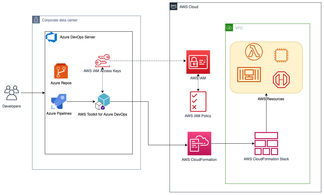
Figure 1. Launchmetrics backend architecture

The Crawl tier is composed of several Amazon Elastic Compute Cloud (Amazon EC2) Spot Instances launched via Auto Scaling groups. Spot Instances take advantage of unused Amazon EC2 capacity at a discounted rate compared with On-Demand Instances, which are compute instances that are billed per-hour or -second with no long-term commitments. Launchmetrics heavily leverages Spot Instances. The Crawl tier is responsible for retrieving, processing, and storing data from several media sources (represented in Figure 1 with the number 1).

The Data Persistence tier consists of two components: Amazon Kinesis Data Streams and Amazon Simple Queue Service (Amazon SQS). Kinesis Data Streams stores data that the Crawl tier collects, while Amazon SQS stores the metadata of the whole process. In this context, metadata helps Launchmetrics gain insight into when the data is collected and if it has started processing. This is key information if a Spot Instance is interrupted, which we will dive deeper into later.

The third tier, Processing, also makes use of Spot Instances and is responsible for pulling data from the Data Persistence tier (represented in Figure 1 with the number 2). It then applies proprietary algorithms, both analytics and machine learning models, to create consumer insights. These insights are stored in a data layer (not depicted) that consists of an Amazon Aurora cluster and an Amazon OpenSearch Service cluster.

By having this separation of tiers, Launchmetrics is able to use a decoupled architecture, where each component can scale independently and is more reliable. Both the Crawl and the Data Processing tiers use Spot Instances for up to 90% of their capacity.

Data processing using EC2 Spot Instances

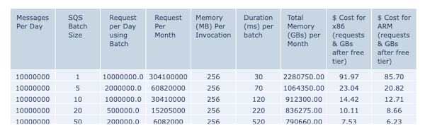
When Launchmetrics decided to migrate their workloads to the AWS cloud, Spot Instances were one of the main drivers. As Spot Instances offer large discounts without commitment, Launchmetrics was able to track more than 1200 brands, translating to 1+ billion end users. Daily, this represents tracking upwards of 500k influencer profiles, 8 million documents, and around 70 million social media comments.

Aside from the cost-savings with Spot Instances, Launchmetrics incurred collateral benefits in terms of architecture design: building stateless, decoupled, elastic, and fault-tolerant applications. In turn, their stack architecture became more loosely coupled, as well.

All Launchmetrics Auto Scaling groups have the following configuration:

  • Spot allocation strategy: cost-optimized
  • Capacity rebalance: true
  • Three availability zones
  • A diversified list of instance types

By using Auto Scaling groups, Launchmetrics is able to scale worker instances depending on how many items they have in the SQS queue, increasing the instance efficiency. Data processing workloads like the ones Launchmetrics’ platform have, are an exemplary use of multiple instance types, such as M5, M5a, C5, and C5a. When adopting Spot Instances, Launchmetrics considered other instance types to have access to spare capacity. As a result, Launchmetrics found out that workload’s performance improved, as they use instances with more resources at a lower cost.

By decoupling their data processing workload using SQS queues, processes are stopped when an interruption arrives. As the Auto Scaling group launches a replacement Spot Instance, clients are not impacted and data is not lost. All processes go through a data checkpoint, where a new Spot Instance resumes processing any pending data. Spot Instances have resulted in a reduction of up to 75% of related operational costs.

To increase confidence in their ability to deal with Spot interruptions and service disruptions, Launchmetrics is exploring using AWS Fault Injection Simulator to simulate faults on their architecture, like a Spot interruption. Learn more about how this service works on the AWS Fault Injection Simulator now supports Spot Interruptions launch page.

Reporting data insights

After processing data from different media sources, AWS aided Launchmetrics in producing higher quality data insights, faster: the previous on-premises architecture had a time range of 5-6 minutes to run, whereas the AWS-driven architecture takes less than 1 minute.

This is made possible by elasticity and availability compute capacity that Amazon EC2 provides compared with an on-premises static fleet. Furthermore, offloading some management and operational tasks to AWS by using AWS managed services, such as Amazon Aurora or Amazon OpenSearch Service, Launchmetrics can focus on their core business and improve proprietary solutions rather than use that time in undifferentiated activities.

Building continuous delivery pipelines

Let’s discuss how Launchmetrics makes changes to their software with so many components.

Both of their computing tiers, Crawl and Processing, consist of standalone EC2 instances launched via Auto Scaling groups and EC2 instances that are part of an Amazon Elastic Container Service (Amazon ECS) cluster. Currently, 70% of Launchmetrics workloads are still running with Auto Scaling groups, while 30% are containerized and run on Amazon ECS. This is important because for each of these workload groups, the deployment process is different.

For workloads that run on Auto Scaling groups, they use an AWS CodePipeline to orchestrate the whole process, which includes:

I.  Creating a new Amazon Machine Image (AMI) using AWS CodeBuild
II. Deploying the newly built AMI using Terraform in CodeBuild

For containerized workloads that run on Amazon ECS, Launchmetrics also uses a CodePipeline to orchestrate the process by:

III. Creating a new container image, and storing it in Amazon Elastic Container Registry
IV. Changing the container image in the task definition, and updating the Amazon ECS service using CodeBuild

Conclusion

In this blog post, we explored how Launchmetrics is using EC2 Spot Instances to reduce costs while producing high-quality data insights for their clients. We also demonstrated how decoupling an architecture is important for handling interruptions and why following Spot Instance best practices can grant access to more spare capacity.

Using this architecture, Launchmetrics produced faster, data-driven insights for their clients and increased their capacity to innovate. They are continuing to containerize their applications and are projected to have 100% of their workloads running on Amazon ECS with Spot Instances by the end of 2023.

To learn more about handling EC2 Spot Instance interruptions, visit the AWS Best practices for handling EC2 Spot Instance interruptions blog post. Likewise, if you are interested in learning more about AWS Fault Injection Simulator and how it can benefit your architecture, read Increase your e-commerce website reliability using chaos engineering and AWS Fault Injection Simulator.

A multi-dimensional approach helps you proactively prepare for failures, Part 2: Infrastructure layer

Post Syndicated from Piyali Kamra original https://aws.amazon.com/blogs/architecture/a-multi-dimensional-approach-helps-you-proactively-prepare-for-failures-part-2-infrastructure-layer/

Distributed applications resiliency is a cumulative resiliency of applications, infrastructure, and operational processes. Part 1 of this series explored application layer resiliency. In Part 2, we discuss how using Amazon Web Services (AWS) managed services, redundancy, high availability, and infrastructure failover patterns based on recovery time and point objectives (RTO and RPO, respectively) can help in building more resilient infrastructures.

Pattern 1: Recognize high impact/likelihood infrastructure failures

To ensure cloud infrastructure resilience, we need to understand the likelihood and impact of various infrastructure failures, so we can mitigate them. Figure 1 illustrates that most of the failures with high likelihood happen because of operator error or poor deployments.

Automated testing, automated deployments, and solid design patterns can mitigate these failures. There could be datacenter failures—like whole rack failures—but deploying applications using auto scaling and multi-availability zone (multi-AZ) deployment, plus resilient AWS cloud native services, can mitigate the impact.

Likelihood and impact of failure events

Figure 1. Likelihood and impact of failure events

As demonstrated in the Figure 1, infrastructure resiliency is a combination of high availability (HA) and disaster recovery (DR). HA involves increasing the availability of the system by implementing redundancy among the application components and removing single points of failure.

Application layer decisions, like creating stateless applications, make it simpler to implement HA at the infrastructure layer by allowing it to scale using Auto Scaling groups and distributing the redundant applications across multiple AZs.

Pattern 2: Understanding and controlling infrastructure failures

Building a resilient infrastructure requires understanding which infrastructure failures are under control and which ones are not, as demonstrated in Figure 2.

These insights allow us to automate the detection of failures, control them, and employ pro-active patterns, such as static stability, to mitigate the need to scale up the infrastructure by over-provisioning it in advance.

Proactively designing systems in the event of failure

Figure 2. Proactively designing systems in the event of failure

The infrastructure decisions under our control that can increase the infrastructure resiliency of our system, include:

  • AWS services have control and data planes designed for minimum blast radius. Data planes typically have higher availability design goals than control planes and are usually less complex. When implementing recovery or mitigation responses to events that can affect resiliency, using control plane operations can lower the overall resiliency of your architectures. For example, Amazon Route 53 (Route 53) has a data plane designed for a 100% availability SLA. A good fail-over mechanism should rely on the data plane and not the control plane, as explained in Creating Disaster Recovery Mechanisms Using Amazon Route 53.
  • Understanding networking design and routes implemented in a virtual private cloud (VPC) are critical when testing the flow of traffic in our application. Understanding the flow of traffic helps us design better applications and see how one component failure can affect overall ingress/egress traffic. To achieve better network resiliency, it’s important to implement a good subnet strategy and manage our IP addresses to avoid fail-over issues and asymmetric routing in hybrid architectures. Use IP address management tools for established subnet strategies and routing decisions.
  • When designing VPCs and AZs, understanding the service limits, deploying independent routing tables and components in each zone increases availability. For example, highly available NAT gateways are preferred over NAT instances, as noted in the comparison provided in the Amazon VPC documentation.

Pattern 3: Considering different ways of increasing HA at the infrastructure layer

As already detailed, infrastructure resiliency = HA + DR.

Different ways by which system availability can be increased include:

  • Building for redundancy: Redundancy is the duplication of application components to increase the overall availability of the distributed system. After following application layer best practices, we can build auto healing mechanisms at the infrastructure layer.

We can take advantage of auto scaling features and use Amazon CloudWatch metrics and alarms to set up auto scaling triggers and deploy redundant copies of our applications across multiple AZs. This protects workloads from AZ failures, as shown in Figure 3.

Redundancy increases availability

Figure 3. Redundancy increases availability

  • Auto scale your infrastructure: When there are AZ failures, infrastructure auto scaling maintains the desired number of redundant components, which helps maintain the base level application throughput. This way, HA system and manage costs are maintained. Auto scaling uses metrics to scale in and out, appropriately, as shown in Figure 4.
How auto scaling improves availability

Figure 4. How auto scaling improves availability

  • Implement resilient network connectivity patterns: While building highly resilient distributed systems, network access to AWS infrastructure also needs to be highly resilient. While deploying hybrid applications, the capacity needed for hybrid applications to communicate with their cloud native application counterparts is an important consideration in designing the network access using AWS Direct Connect or VPNs.

Testing failover and fallback scenarios helps validate that network paths operate as expected and routes fail over as expected to meet RTO objectives. As the number of connection points between the data center and AWS VPCs increases, a hub and spoke configuration provided by the Direct Connect gateway and transit gateways simplify network topology, testing, and fail over. For more information, visit the AWS Direct Connect Resiliency Recommendations.

  • Whenever possible, use the AWS networking backbone to increase security, resiliency, and lower cost. AWS PrivateLink provides secure access to AWS services and exposes the application’s functionalities and APIs to other business units or partner accounts hosted on AWS.
  • Security appliances need to be set up in HA configuration, so that even if one AZ is unavailable, security inspection can be taken over by the redundant appliances in the other AZs.
  • Think ahead about DNS resolution: DNS is a critical infrastructure component; hybrid DNS resolution should be designed carefully with Route 53 HA inbound and outbound resolver endpoints instead of using self-managed proxies.

Implement a good strategy to share DNS resolver rules across AWS accounts and VPC’s with Resource Access Manager. Network failover tests are an important part of Disaster Recovery and Business Continuity Plans. To learn more, visit Set up integrated DNS resolution for hybrid networks in Amazon Route 53.

Additionally, ELB uses health checks to make sure that requests will route to another component if the underlying traffic application component fails. This improves the distributed system’s availability, as it is the cumulative availability of all different layers in our system. Figure 5 details advantages of some AWS managed services.

AWS managed services help in building resilient infrastructures (click the image to enlarge)

Figure 5. AWS managed services help in building resilient infrastructures (click the image to enlarge)

Pattern 4: Use RTO and RPO requirements to determine the correct failover strategy for your application

Capture RTO and RPO requirements early on to determine solid failover strategies (Figure 6). Disaster recovery strategies within AWS range from low cost and complexity (like backup and restore), to more complex strategies when lower values of RTO and RPO are required.

In pilot light and warm standby, only the primary region receives traffic. Pilot light only critical infrastructure components run in the backup region. Automation is used to check failures in the primary region using health checks and other metrics.

When health checks fail, use a combination of auto scaling groups, automation, and Infrastructure as Code (IaC) for quick deployment of other infrastructure components.

Note: This strategy depends on control plane availability in the secondary region for deploying the resources; keep this point in mind if you don’t have compute pre-provisioned in the secondary region. Carefully consider the business requirements and a distributed system’s application-level characteristics before deciding on a failover strategy. To understand all the factors and complexities involved in each of these disaster recovery strategies refer to disaster recovery options in the cloud.

Relationship between RTO, RPO, cost, data loss, and length of service interruption

Figure 6. Relationship between RTO, RPO, cost, data loss, and length of service interruption

Conclusion

In Part 2 of this series, we discovered that infrastructure resiliency is a combination of HA and DR. It is important to consider likelihood and impact of different failure events on availability requirements. Building in application layer resiliency patterns (Part 1 of this series), along with early discovery of the RTO/RPO requirements, as well as operational and process resiliency of an organization helps in choosing the right managed services and putting in place the appropriate failover strategies for distributed systems.

It’s important to differentiate between normal and abnormal load threshold for applications in order to put automation, alerts, and alarms in place. This allows us to auto scale our infrastructure for normal expected load, plus implement corrective action and automation to root out issues in case of abnormal load. Use IaC for quick failover and test failover processes.

Stay tuned for Part 3, in which we discuss operational resiliency!

Estimating cost for Amazon SQS message processing using AWS Lambda

Post Syndicated from James Beswick original https://aws.amazon.com/blogs/compute/estimating-cost-for-amazon-sqs-message-processing-using-aws-lambda/

This post was written by Sabha Parameswaran, Senior Solutions Architect.

AWS Lambda enables fully managed asynchronous messaging processing through integration with Amazon SQS. This blog post helps estimate the cost and performance benefits when using Lambda to handle millions of messages per day by using a simulated setup.

Overview

Lambda supports asynchronous handling of messages using SQS integration as an event source and can scale for handling millions of messages per day. Customers often ask about the cost of implementing a Lambda-based messaging solution.

There are multiple variables like Lambda function runtime, individual message size, batch size for consuming from SQS, processing latency per message (depending on the backend services invoked), and function memory size settings. These can determine the overall performance and associated cost of a Lambda-based messaging solution.

This post provides cost estimation using these variables, along with guidance around optimization. The estimates focus on consuming from standard queues and not FIFO queues.

SQS event source

The Lambda event source mapping supports integration for SQS. Lambda users specify the SQS queue to consume messages. Lambda internally polls the queue and invokes the function synchronously with an event containing the queue messages.

The configuration controls in Lambda for consuming messages from an SQS queue are:

  • Batch size: The maximum number of records that can be batched as one event delivered to the consuming Lambda function. The maximum batch size is 10,000 records.
  • Batch window: The maximum time (in seconds) to gather records as a single batch. A larger batch window size means waiting longer for a larger SQS batch of messages before passing to the Lambda function.
  • SQS content filtering: Selecting only the messages that match a defined content criteria. This can reduce cost by removing unwanted or irrelevant messages. Lambda now supports content filtering (for SQS, Kinesis, and DynamoDB) and developers can use the filtering capabilities to avoid processing SQS messages, reducing unnecessary invocations and associated cost.

Lambda sends as many records in a single batch as allowed by the batch size, as long as it’s earlier than the batch window value, and smaller than the maximum payload size of 6 MB. Having large batch sizes means that a single Lambda invocation can handle more messages rather than multiple Lambda invocations to handle smaller batches (which translates to setting higher concurrency limits).

The cost and time to process might vary based on the actual number of messages in the batch. A larger batch size can imply longer processing but requires lower concurrency (number of concurrent Lambda invocations).

Lambda configurations

Lambda function costs are calculated based on memory used and time spent (in GB-second) in execution of a function. Aside from the event source configuration, there are several other Lambda function configurations that impact cost and performance:

  • Processor type: Lambda functions provide options to choose between x86 and Arm/Graviton processors. The newer Arm/Graviton processors can yield a higher performance and lower cost compared to x86 based on the workload. Compare the options and run tests before selecting.
  • Memory allotted: This is directly proportional to the CPU allotted to the function and translates to price for each invocation. Higher memory can lead to faster execution but also higher cost. The optimal memory required for a small batch versus large batch can vary based on the workload, size of incoming messages, transformations, requirements to store intermediate, or final results. Optimal tuning of the memory configurations is key to ensuring right cost versus performance. See the AWS Lambda Power Tuning documentation for more details on identifying the optimal memory versus performance for a fixed batch size and then extrapolate the memory settings for larger batch sizes.
  • Lambda function runtime: Some runtimes have a smaller memory footprint and may be more cost effective than others that are memory intensive. Choosing the runtime affects the memory allocation.
  • Function performance: This can be considered as TPS – total number of requests completed per second. Or conversely measured as time to complete one request. The performance – time to finish a function execution can be dependent on the event containing the batch of messages; bigger batches mean more time to complete an event and complexity and dependencies (performance of the backend that needs to be invoked) of the message processing. The calculations are based on the assumption that the Lambda function and related dependencies have been optimized and tuned to scale linearly with various batch sizes and number of invocations.
  • Concurrency: Number of concurrent Lambda function executions. Concurrency is important for scaling of Lambda functions, allowing users to delegate the capacity planning and scaling to thee Lambda service.

The higher the concurrency, the more workloads it can process in a shorter time, allowing better performance, but this does not change the overall cost. Concurrency is not equivalent to TPS: it is more of a scaling factor in overall TPS. For example, a workload comprised of a set of messages takes 20 seconds to complete. 100 workloads would mean 2000 seconds to complete. With a concurrency of 10, it takes 200 seconds. With a concurrency of 100, the time drops to 20 seconds as each of the 100 workloads are handled concurrently. But each function essentially runs for the same duration and memory, regardless of concurrency. So the cost remains the same, as it is measured in GB-hours (memory multiplied by time). But the performance view differs. So, the cost estimations do not consider the concurrency settings of Lambda functions as the workloads have to be processed either sequential or concurrently.

Assumptions

The cost estimation tool presented helps users estimate monthly Lambda function costs for processing SQS standard queue messages based on the following assumptions:

  • The system has reached steady state and has millions of messages available to be consumed per day in standard queues. The number of messages per day remains constant throughout the entire month.
  • Since it’s a steady state, there are no associated Lambda function cold start delays.
  • All SQS messages that need to be processed successfully have already met the filter criteria. Also, no poison messages that have to be re-tried repeatedly. Messages are not going to be rejected, unacknowledged, or reprocessed.
  • The workload scales linearly in performance versus batch size. All the associated dependencies can scale linearly and a batch of N messages should take the same time as N x a single message with a fixed overhead per function invocation irrespective of the batch size. For example, a function’s overhead is 50 ms irrespective of the batch size. Processing a single message takes 20 ms. So a batch of 20 messages should take 490 ms (50 + 20*20) versus a batch of 5 messages takes 150 ms (50 + 5*20).
  • Function memory increases in steps, based on increasing the batch size. For example, 100 messages uses a 256 MB of baseline memory. Every additional 500 messages require additional 128 MB of memory. A sliding window of memory to batch size:
Batch size Memory
1–100 256 MB
100–600 384 MB
600–1100 512 MB
1100–1600 640 MB

Lambda uses SQS APIs internally to poll and dequeue the messages. The costs for the polling and dequeue operations using SQS APIs are not included as part of the estimations. The internal SQS dequeue portion is outside the control of the Lambda developer and the cost estimates only cover the message processing using Lambda. Also, the tool does not consider any reprocessing or duplicate processing of messages due to exceptions or errors that can vary the cost.

Using the cost estimation tool

The estimator tool is a Python-based command line program that takes in an input properties file that specifies the various input parameters to come up with Lambda function cost versus performance estimations for various batch sizes, messages per day, etc. The tool does take into account the eligible monthly free tier for Lambda function executions.

Pre-requisites: Running the tool requires Python 3.9 and installation of Plotly package (5.7.+) or creating and using Docker images.

To run the tool:

  1. Clone the repo:
    git clone https://github.com/aws-samples/aws-lambda-sqs-cost-estimator
  2. Install the tool:
    cd aws-lambda-sqs-cost-estimator/code
    pip3 install -r requirements.txt
  3. Edit the input.prop file and run the tool to generate cost estimations:
    python3 LambdaPlotly.py

This shows the cost estimates on a local browser instance. Running the code as a Docker image is also supported. Refer to the GitHub repo for additional instructions.

  1. Clone the repo and build the Docker container:
    git clone https://github.com/aws-samples/aws-lambda-sqs-cost-estimator
    cd aws-lambda-sqs-cost-estimator/code
    docker build -t lambda-dash .
  2. Edit the input.prop file and run the tool to generate cost estimations:
    docker run -it -v `pwd`:/app -p 8080:8080 lambda-dash
  3. Navigate to http://0.0.0.0:8080/app in a browser to view the generated cost estimate plot.

There are various input parameters for the cost estimations specified inside the input.prop file. Tune the input parameters as needed:

Parameter Description Sample value (units not included)
base_lambda_memory_mb Baseline memory for the Lambda function (in MB) 128
warm_latency_ms Invocation time for Lambda handler method (going with warm start) irrespective of batch size in the incoming event payload in ms 20
process_per_message_ms Time to process a single message (linearly scales with number of messages per batch in event payload) in ms 10
max_batch_size Maximum batch size per event payload processed by a single Lambda instance 1000 (max is 10000)
batch_memory_overhead_mb Additional memory for processing increments in batch size (in MB) 128
batch_increment Increments of batch size for increased memory 300

The following is sample input.prop file content:

base_lambda_memory_mb=128

# Total process time for N messages in batch = warm_latency_ms + (process_per_message_ms * N)

# Time spent in function initialization/warm-up

warm_latency_ms=20

# Time spent for processing each message in milliseconds

process_per_message_ms=10

# Max batch size

max_batch_size=1000

# Additional lambda memory X mb required for managing/parsing/processing N additional messages processed when using variable batch sizes

#batch_memory_overhead_mb=X

#batch_increment=N

batch_memory_overhead_mb=128

batch_increment=300

The tool generates a page with plot graphs and tables with 3 sections:

Cost example

There is an accompanying interactive legend showing cost and batch size. The top section shows a graph of cost versus message volumes versus batch size:

cost versus message volumes vs Batch size

The second section shows the actual cost variation for different batch sizes for 10 million messages:

actual cost variation for different batch sizes for 10 million messages.

The third section shows the memory and time required to process with different batch sizes:

memory and time required to process with different batch sizes

The various control input parameters used for graph generation are shown at the bottom of the page.

Double-clicking on a specific batch size or line on the right-hand legend displays that specific plot with its pricing details.

specific plot to be displayed with its pricing details

You can modify the input parameters with different settings for memory, batch sizes, memory for increased batches and rerun the program to create different cost estimations. You can also export the generated graphs as PNG image files for reference.

Conclusion

You can use Lambda functions to handle fully managed asynchronous processing of SQS messages. Estimating the cost and optimal setup depends on leveraging the various configurations of SQS and Lambda functions. The cost estimator tool presented in this blog should help you understand these configurations and their impact on the overall cost and performance of the Lambda function-based messaging solutions.

For more serverless learning resources, visit Serverless Land.

Coordinating large messages across accounts and Regions with Amazon SNS and SQS

Post Syndicated from Mrudhula Balasubramanyan original https://aws.amazon.com/blogs/architecture/coordinating-large-messages-across-accounts-and-regions-with-amazon-sns-and-sqs/

Many organizations have applications distributed across various business units. Teams in these business units may develop their applications independent of each other to serve their individual business needs. Applications can reside in a single Amazon Web Services (AWS) account or be distributed across multiple accounts. Applications may be deployed to a single AWS Region or span multiple Regions.

Irrespective of how the applications are owned and operated, these applications need to communicate with each other. Within an organization, applications tend to be part of a larger system, therefore, communication and coordination among these individual applications is critical to overall operation.

There are a number of ways to enable coordination among component applications. It can be done either synchronously or asynchronously:

  • Synchronous communication uses a traditional request-response model, in which the applications exchange information in a tightly coupled fashion, introducing multiple points of potential failure.
  • Asynchronous communication uses an event-driven model, in which the applications exchange messages as events or state changes and are loosely coupled. Loose coupling allows applications to evolve independently of each other, increasing scalability and fault-tolerance in the overall system.

Event-driven architectures use a publisher-subscriber model, in which events are emitted by the publisher and consumed by one or more subscribers.

A key consideration when implementing an event-driven architecture is the size of the messages or events that are exchanged. How can you implement an event-driven architecture for large messages, beyond the default maximum of the services? How can you architect messaging and automation of applications across AWS accounts and Regions?

This blog presents architectures for enhancing event-driven models to exchange large messages. These architectures depict how to coordinate applications across AWS accounts and Regions.

Challenge with application coordination

A challenge with application coordination is exchanging large messages. For the purposes of this post, a large message is defined as an event payload between 256 KB and 2 GB. This stems from the fact that Amazon Simple Notification Service (Amazon SNS) and Amazon Simple Queue Service (Amazon SQS) currently have a maximum event payload size of 256 KB. To exchange messages larger than 256 KB, an intermediate data store must be used.

To exchange messages across AWS accounts and Regions, set up the publisher access policy to allow subscriber applications in other accounts and Regions. In the case of large messages, also set up a central data repository and provide access to subscribers.

Figure 1 depicts a basic schematic of applications distributed across accounts communicating asynchronously as part of a larger enterprise application.

Asynchronous communication across applications

Figure 1. Asynchronous communication across applications

Architecture overview

The overview covers two scenarios:

  1. Coordination of applications distributed across AWS accounts and deployed in the same Region
  2. Coordination of applications distributed across AWS accounts and deployed to different Regions

Coordination across accounts and single AWS Region

Figure 2 represents an event-driven architecture, in which applications are distributed across AWS Accounts A, B, and C. The applications are all deployed to the same AWS Region, us-east-1. A single Region simplifies the architecture, so you can focus on application coordination across AWS accounts.

Application coordination across accounts and single AWS Region

Figure 2. Application coordination across accounts and single AWS Region

The application in Account A (Application A) is implemented as an AWS Lambda function. This application communicates with the applications in Accounts B and C. The application in Account B is launched with AWS Step Functions (Application B), and the application in Account C runs on Amazon Elastic Container Service (Application C).

In this scenario, Applications B and C need information from upstream Application A. Application A publishes this information as an event, and Applications B and C subscribe to an SNS topic to receive the events. However, since they are in other accounts, you must define an access policy to control who can access the SNS topic. You can use sample Amazon SNS access policies to craft your own.

If the event payload is in the 256 KB to 2 GB range, you can use Amazon Simple Storage Service (Amazon S3) as the intermediate data store for your payload. Application A uses the Amazon SNS Extended Client Library for Java to upload the payload to an S3 bucket and publish a message to an SNS topic, with a reference to the stored S3 object. The message containing the metadata must be within the SNS maximum message limit of 256 KB. Amazon EventBridge is used for routing events and handling authentication.

The subscriber Applications B and C need to de-reference and retrieve the payloads from Amazon S3. The SQS queue in Account B and Lambda function in Account C subscribe to the SNS topic in Account A. In Account B, a Lambda function is used to poll the SQS queue and read the message with the metadata. The Lambda function uses the Amazon SQS Extended Client Library for Java to retrieve the S3 object referenced in the message.

The Lambda function in Account C uses the Payload Offloading Java Common Library for AWS to get the referenced S3 object.

Once the S3 object is retrieved, the Lambda functions in Accounts B and C process the data and pass on the information to downstream applications.

This architecture uses Amazon SQS and Lambda as subscribers because they provide libraries that support offloading large payloads to Amazon S3. However, you can use any Java-enabled endpoint, such as an HTTPS endpoint that uses Payload Offloading Java Common Library for AWS to de-reference the message content.

Coordination across accounts and multiple AWS Regions

Sometimes applications are spread across AWS Regions, leading to increased latency in coordination. For existing applications, it could take substantive effort to consolidate to a single Region. Hence, asynchronous coordination would be a good fit for this scenario. Figure 3 expands on the architecture presented earlier to include multiple AWS Regions.

Application coordination across accounts and multiple AWS Regions

Figure 3. Application coordination across accounts and multiple AWS Regions

The Lambda function in Account C is in the same Region as the upstream application in Account A, but the Lambda function in Account B is in a different Region. These functions must retrieve the payload from the S3 bucket in Account A.

To provide access, configure the AWS Lambda execution role with the appropriate permissions. Make sure that the S3 bucket policy allows access to the Lambda functions from Accounts B and C.

Considerations

For variable message sizes, you can specify if payloads are always stored in Amazon S3 regardless of their size, which can help simplify the design.

If the application that publishes/subscribes large messages is implemented using the AWS Java SDK, it must be Java 8 or higher. Service-specific client libraries are also available in Python, C#, and Node.js.

An Amazon S3 Multi-Region Access Point can be an alternative to a centralized bucket for the payloads. It has not been explored in this post due to the asynchronous nature of cross-region replication.

In general, retrieval of data across Regions is slower than in the same Region. For faster retrieval, workloads should be run in the same AWS Region.

Conclusion

This post demonstrates how to use event-driven architectures for coordinating applications that need to exchange large messages across AWS accounts and Regions. The messaging and automation are enabled by the Payload Offloading Java Common Library for AWS and use Amazon S3 as the intermediate data store. These components can simplify the solution implementation and improve scalability, fault-tolerance, and performance of your applications.

Ready to get started? Explore SQS Large Message Handling.

Amazon Prime Day 2022 – AWS for the Win!

Post Syndicated from Jeff Barr original https://aws.amazon.com/blogs/aws/amazon-prime-day-2022-aws-for-the-win/

As part of my annual tradition to tell you about how AWS makes Prime Day possible, I am happy to be able to share some chart-topping metrics (check out my 2016, 2017, 2019, 2020, and 2021 posts for a look back).

My purchases this year included a first aid kit, some wood brown filament for my 3D printer, and a non-stick frying pan! According to our official news release, Prime members worldwide purchased more than 100,000 items per minute during Prime Day, with best-selling categories including Amazon Devices, Consumer Electronics, and Home.

Powered by AWS
As always, AWS played a critical role in making Prime Day a success. A multitude of two-pizza teams worked together to make sure that every part of our infrastructure was scaled, tested, and ready to serve our customers. Here are a few examples:

Amazon Aurora – On Prime Day, 5,326 database instances running the PostgreSQL-compatible and MySQL-compatible editions of Amazon Aurora processed 288 billion transactions, stored 1,849 terabytes of data, and transferred 749 terabytes of data.

Amazon EC2 – For Prime Day 2022, Amazon increased the total number of normalized instances (an internal measure of compute power) on Amazon Elastic Compute Cloud (Amazon EC2) by 12%. This resulted in an overall server equivalent footprint that was only 7% larger than that of Cyber Monday 2021 due to the increased adoption of AWS Graviton2 processors.

Amazon EBS – For Prime Day, the Amazon team added 152 petabytes of EBS storage. The resulting fleet handled 11.4 trillion requests per day and transferred 532 petabytes of data per day. Interestingly enough, due to increased efficiency of some of the internal Amazon services used to run Prime Day, Amazon actually used about 4% less EBS storage and transferred 13% less data than it did during Prime Day last year. Here’s a graph that shows the increase in data transfer during Prime Day:

Amazon SES – In order to keep Prime Day shoppers aware of the deals and to deliver order confirmations, Amazon Simple Email Service (SES) peaked at 33,000 Prime Day email messages per second.

Amazon SQS – During Prime Day, Amazon Simple Queue Service (SQS) set a new traffic record by processing 70.5 million messages per second at peak:

Amazon DynamoDB – DynamoDB powers multiple high-traffic Amazon properties and systems including Alexa, the Amazon.com sites, and all Amazon fulfillment centers. Over the course of Prime Day, these sources made trillions of calls to the DynamoDB API. DynamoDB maintained high availability while delivering single-digit millisecond responses and peaking at 105.2 million requests per second.

Amazon SageMaker – The Amazon Robotics Pick Time Estimator, which uses Amazon SageMaker to train a machine learning model to predict the amount of time future pick operations will take, processed more than 100 million transactions during Prime Day 2022.

Package Planning – In North America, and on the highest traffic Prime 2022 day, package-planning systems performed 60 million AWS Lambda invocations, processed 17 terabytes of compressed data in Amazon Simple Storage Service (Amazon S3), stored 64 million items across Amazon DynamoDB and Amazon ElastiCache, served 200 million events over Amazon Kinesis, and handled 50 million Amazon Simple Queue Service events.

Prepare to Scale
Every year I reiterate the same message: rigorous preparation is key to the success of Prime Day and our other large-scale events. If you are preparing for a similar chart-topping event of your own, I strongly recommend that you take advantage of AWS Infrastructure Event Management (IEM). As part of an IEM engagement, my colleagues will provide you with architectural and operational guidance that will help you to execute your event with confidence!

Jeff;

Serverless architecture for optimizing Amazon Connect call-recording archival costs

Post Syndicated from Brian Maguire original https://aws.amazon.com/blogs/architecture/serverless-architecture-for-optimizing-amazon-connect-call-recording-archival-costs/

In this post, we provide a serverless solution to cost-optimize the storage of contact-center call recordings. The solution automates the scheduling, storage-tiering, and resampling of call-recording files, resulting in immediate cost savings. The solution is an asynchronous architecture built using AWS Step Functions, Amazon Simple Queue Service (Amazon SQS), and AWS Lambda.

Amazon Connect provides an omnichannel cloud contact center with the ability to maintain call recordings for compliance and gaining actionable insights using Contact Lens for Amazon Connect and AWS Contact Center Intelligence Partners. The storage required for call recordings can quickly increase as customers meet compliance retention requirements, often spanning six or more years. This can lead to hundreds of terabytes in long-term storage.

Solution overview

When an agent completes a customer call, Amazon Connect sends the call recording to an Amazon Simple Storage Solution (Amazon S3) bucket with: a date and contact ID prefix, the file stored in the .WAV format and encoded using bitrate 256 kb/s, pcm_s16le, 8000 Hz, two channels, and 256 kb/s. The call-recording files are approximately 2 Mb/minute optimized for high-quality processing, such as machine learning analysis (see Figure 1).

Asynchronous architecture for batch resampling for call-recording files on Amazon S3

Figure 1. Asynchronous architecture for batch resampling for call-recording files on Amazon S3

When a call recording is sent to Amazon S3, downstream post-processing is often performed to generate analytics reports for agents and quality auditors. The downstream processing can include services that provide transcriptions, quality-of-service metrics, and sentiment analysis to create reports and trigger actionable events.

While this processing is often completed within minutes, the downstream applications could require processing retries. As audio resampling reduces the quality of the audio files, it is essential to delay resampling until after processing is completed. As processed call recordings are infrequently accessed days after a call is completed, with only a small percentage accessed by agents and call quality auditors, call recordings can benefit from resampling and transitioning to long-term Amazon S3 storage tiers.

In Figure 2, multiple AWS services work together to provide an end-to-end cost-optimization solution for your contact center call recordings.

AWS Step Function orchestrates the batch resampling of call recordings

Figure 2. AWS Step Function orchestrates the batch resampling of call recordings

An Amazon EventBridge schedule rule triggers the step function to perform the batch resampling process for all call recordings from the previous 7 days.

In the first step function task, the Lambda function task iterates the S3 bucket using the ListObjectsV2 API, obtaining the call recordings (1000 objects per iteration) with the date prefix from 7 days ago.

The next task invokes a Lambda function inserting the call recording objects into the Amazon SQS queue. The audio-conversion Lambda function receives the Amazon SQS queue events via the event source mapping Lambda integration. Each concurrent Lambda invocation downloads a stored call recording from Amazon S3, resampling the .WAV with ffmpeg and tagging the S3 object with a “converted=True” tag.

Finally, the conversion function uploads the resampled file to Amazon S3, overwriting the original call recording with the resampled recording using a cost-optimized storage class, such as S3 Glacier Instant Retrieval. S3 Glacier Instant Retrieval provides the lowest cost for long-lived data that is rarely accessed and requires milliseconds retrieval, such as for contact-center call-recording playback. By default, Amazon Connect stores call recordings with S3 Versioning enabled, maintaining the original file as a version. You can use lifecycle policies to delete object versions from a version-enabled bucket to permanently remove the original version, as this will minimize the storage of the original call recording.

This solution captures failures within the step function workflow with logging and a dead-letter queue, such as when an error occurs with resampling a recording file. A Step Function task monitors the Amazon SQS queue using the AWS Step Function integration with AWS SDK with SQS and ending the workflow when the queue is emptied. Table 1 demonstrates the default and resampled formats.

Detailed AWS Step Functions state machine diagram

Figure 3. Detailed AWS Step Functions state machine diagram

Resampling

Table 1. Default and resampled call recording audio formats

Audio sampling formats File size/minute Notes
Bitrate 256 kb/s, pcm_s16le, 8000 Hz, 2 channels, 256 kb/s 2 MB The default for Amazon Connect call recordings. Sampled for audio quality and call analytics processing.
Bitrate 64 kb/s, pcm_alaw, 8000 Hz, 1 channel, 64 kb/s 0.5 MB Resampled to mono channel 8 bit. This resampling is not reversible and should only be performed after all call analytics processing has been completed.

Cost assessment

For pricing information for the primary services used in the solution, visit:

The costs incurred by the solution are based on usage and are AWS Free Tier eligible. After the AWS Free Tier allowance is consumed, usage costs are approximately $0.11 per 1000 minutes of call recordings. S3 Standard starts at $0.023 per GB/month; and S3 Glacier Instant Retrieval is $0.004 per GB/month, with $0.003 per GB of data retrieval. During a 6-year compliance retention term, the schedule-based resampling and storage tiering results in significant cost savings.

In the 6-year example detailed in Table 2, the S3 Standard storage costs would be approximately $356,664 for 3 million call-recording minutes/month. The audio resampling and S3 Glacier Instant Retrieval tiering reduces the 6-year cost to approximately $41,838.

Table 2. Multi-year costs savings scenario (3 million minutes/month) in USD

Year Total minutes (3 million/month) Total storage (TB) Cost of storage, S3 Standard (USD) Cost of running the resampling (USD) Cost of resampling solution with S3 Glacier Instant Retrieval (USD)
1 36,000,000 72 10,764 3,960 4,813
2 72,000,000 108 30,636 3,960 5,677
3 108,000,000 144 50,508 3,960 6,541
4 144,000,000 180 70,380 3,960 7,405
5 180,000,000 216 90,252 3,960 8,269
6 216,000,000 252 110,124 3,960 9,133
Total 1,008,000,000 972 356,664 23,760 41,838

To explore PCA costs for yourself, use AWS Cost Explorer or choose Bill Details on the AWS Billing Dashboard to see your month-to-date spend by service.

Deploying the solution

The code and documentation for this solution are available by cloning the git repository and can be deployed with AWS Cloud Development Kit (AWS CDK).

Bash
# clone repository
git clone https://github.com/aws-samples/amazon-connect-call-recording-cost-optimizer.git
# navigate the project directory
cd amazon-connect-call-recording-cost-optimizer

Modify the cdk.context.json with your environment’s configuration setting, such as the bucket_name. Next, install the AWS CDK dependencies and deploy the solution:

:# ensure you are in the root directory of the repository

./cdk-deploy.sh

Once deployed, you can test the resampling solution by waiting for the EventBridge schedule rule to execute based on the num_days_age setting that is applied. You can also manually run the AWS Step Function with a specified date, for example {"specific_date":"01/01/2022"}.

The AWS CDK deployment creates the following resources:

  • AWS Step Function
  • AWS Lambda function
  • Amazon SQS queues
  • Amazon EventBridge rule

The solution handles the automation of transitioning a storage tier, such as S3 Glacier Instant Retrieval. In addition, Amazon S3 Lifecycles can be set manually to transition the call recordings after resampling to alternative Amazon S3 Storage Classes.

Cleanup

When you are finished experimenting with this solution, cleanup your resources by running the command:

cdk destroy

This command deletes the AWS CDK-deployed resources. However, the S3 bucket containing your call recordings and CloudWatch log groups are retained.

Conclusion

This call recording resampling solution offers an automated, cost-optimized, and scalable architecture to reduce long-term compliance call recording archival costs.

Use the AWS Toolkit for Azure DevOps to automate your deployments to AWS

Post Syndicated from Mahmoud Abid original https://aws.amazon.com/blogs/devops/use-the-aws-toolkit-for-azure-devops-to-automate-your-deployments-to-aws/

Many developers today seek to improve productivity by finding better ways to collaborate, enhance code quality and automate repetitive tasks. We hear from some of our customers that they would like to leverage services such as AWS CloudFormation, AWS CodeBuild and other AWS Developer Tools to manage their AWS resources while continuing to use their existing CI/CD pipelines which they are familiar with. These services range from popular open-source solutions, such as Jenkins, to paid commercial solutions, such as Azure DevOps Server (formerly Team Foundation Server (TFS)).

In this post, I will walk you through an example to leverage the AWS Toolkit for Azure DevOps to deploy your Infrastructure as Code templates, i.e. AWS CloudFormation stacks, directly from your existing Azure DevOps build pipelines.

The AWS Toolkit for Azure DevOps is a free-to-use extension for hosted and on-premises Microsoft Azure DevOps that makes it easy to manage and deploy applications using AWS. It integrates with many AWS services, including Amazon S3, AWS CodeDeploy, AWS Lambda, AWS CloudFormation, Amazon SQS and others. It can also run commands using the AWS Tools for Windows PowerShell module as well as the AWS CLI.

Solution Overview

The solution described in this post consists of leveraging the AWS Toolkit for Azure DevOps to manage resources on AWS via Infrastructure as Code templates with AWS CloudFormation:

Solution high-level overview

Figure 1. Solution high-level overview

Prerequisites and Assumptions

You will need to go through three main steps in order to set up your environment, which are summarized here and detailed in the toolkit’s user guide:

  • Install the toolkit into your Azure DevOps account or choose Download to install it on an on-premises server (Figure 2).
  • Create an IAM User and download its keys. Keep the principle of least privilege in mind when associating the policy to your user.
  • Create a Service Connection for your project in Azure DevOps. Service connections are how the Azure DevOps tooling manages connecting and providing access to Azure resources. The AWS Toolkit also provides a user interface to configure the AWS credentials used by the service connection (Figure 3).

In addition to the above steps, you will need a sample AWS CloudFormation template to use for testing the deployment such as this sample template creating an EC2 instance. You can find more samples in the Sample Templates page or get started with authoring your own templates.

AWS Toolkit for Azure DevOps in the Visual Studio Marketplace

Figure 2. AWS Toolkit for Azure DevOps in the Visual Studio Marketplace

A new Service Connection of type “AWS” will appear after installing the extension

Figure 3. A new Service Connection of type “AWS” will appear after installing the extension

Model your CI/CD Pipeline to Automate Your Deployments on AWS

One common DevOps model is to have a CI/CD pipeline that deploys an application stack from one environment to another. This model typically includes a Development (or integration) account first, then Staging and finally a Production environment. Let me show you how to make some changes to the service connection configuration to apply this CI/CD model to an Azure DevOps pipeline.

We will create one service connection per AWS account we want to deploy resources to. Figure 4 illustrates the updated solution to showcase multiple AWS Accounts used within the same Azure DevOps pipeline.

Solution overview with multiple target AWS accounts

Figure 4. Solution overview with multiple target AWS accounts

Each service connection will be configured to use a single, target AWS account. This can be done in two ways:

  1. Create an IAM User for every AWS target account and supply the access key ID and secret access key for that user.
  2. Alternatively, create one central IAM User and have it assume an IAM Role for every AWS deployment target. The AWS Toolkit extension enables you to select an IAM Role to assume. This IAM Role can be in the same AWS account as the IAM User or in a different accounts as depicted in Figure 5.
Use a single IAM User to access all other accounts

Figure 5. Use a single IAM User to access all other accounts

Define Your Pipeline Tasks

Once a service connection for your AWS Account is created, you can now add a task to your pipeline that references the service connection created in the previous step. In the example below, I use the CloudFormation Create/Update Stack task to deploy a CloudFormation stack using a template file named my-aws-cloudformation-template.yml:

- task: CloudFormationCreateOrUpdateStack@1
  displayName: 'Create/Update Stack: Development-Deployment'
  inputs:
    awsCredentials: 'development-account'
    regionName:     'eu-central-1'
    stackName:      'my-stack-name'
    useChangeSet:   true
    changeSetName:  'my-stack-name-change-set'
    templateFile:   'my-aws-cloudformation-template.yml'
    templateParametersFile: 'development/parameters.json'
    captureStackOutputs: asVariables
    captureAsSecuredVars: false

I used the service connection that I’ve called development-account and specified the other required information such as the templateFile path for the AWS CloudFormation template. I also specified the optional templateParametersFile path because I used template parameters in my template.

A template parameters file is particularly useful if you need to use custom values in your CloudFormation templates that are different for each stack. This is a common case when deploying the same application stack to different environments (Development, Staging, and Production).

The task below will to deploy the same template to a Staging environment:

- task: CloudFormationCreateOrUpdateStack@1
  displayName: 'Create/Update Stack: Staging-Deployment'
  inputs:
    awsCredentials: 'staging-account'
    regionName:     'eu-central-1'
    stackName:      'my-stack-name'
    useChangeSet:   true
    changeSetName:  'my-stack-name-changeset'
    templateFile:   'my-aws-cloudformation-template.yml'
    templateParametersFile: 'staging/parameters.json'
    captureStackOutputs: asVariables
    captureAsSecuredVars: false

The differences between Development and Staging deployment tasks are the service connection name and template parameters file path used. Remember that each service connection points to a different AWS account and the corresponding parameter values are specific to the target environment.

Use Azure DevOps Parameters to Switch Between Your AWS Accounts

Azure DevOps lets you define reusable contents via pipeline templates and pass different variable values to them when defining the build tasks. You can leverage this functionality so that you easily replicate your deployment steps to your different environments.

In the pipeline template snippet below, I use three template parameters that are passed as input to my task definition:

# File pipeline-templates/my-application.yml

parameters:
  deploymentEnvironment: ''         # development, staging, production, etc
  awsCredentials:        ''         # service connection name
  region:                ''         # the AWS region

steps:

- task: CloudFormationCreateOrUpdateStack@1
  displayName: 'Create/Update Stack: Staging-Deployment'
  inputs:
    awsCredentials: '${{ parameters.awsCredentials }}'
    regionName:     '${{ parameters.region }}'
    stackName:      'my-stack-name'
    useChangeSet:   true
    changeSetName:  'my-stack-name-changeset'
    templateFile:   'my-aws-cloudformation-template.yml'
    templateParametersFile: '${{ parameters.deploymentEnvironment }}/parameters.json'
    captureStackOutputs: asVariables
    captureAsSecuredVars: false

This template can then be used when defining your pipeline with steps to deploy to the Development and Staging environments. The values passed to the parameters will control the target AWS Account the CloudFormation stack will be deployed to :

# File development/pipeline.yml

container: amazon/aws-cli

trigger:
  branches:
    include:
    - master
    
steps:
- template: ../pipeline-templates/my-application.yml  
  parameters:
    deploymentEnvironment: 'development'
    awsCredentials:        'deployment-development'
    region:                'eu-central-1'
    
- template: ../pipeline-templates/my-application.yml  
  parameters:
    deploymentEnvironment: 'staging'
    awsCredentials:        'deployment-staging'
    region:                'eu-central-1'

Putting it All Together

In the snippet examples below, I defined an Azure DevOps pipeline template that builds a Docker image, pushes it to Amazon ECR (using the ECR Push Task) , creates/updates a stack from an AWS CloudFormation template with a template parameter files, and finally runs a AWS CLI command to list all Load Balancers using the AWS CLI Task.

The template below can be reused across different AWS accounts by simply switching the value of the defined parameters as described in the previous section.

Define a template containing your AWS deployment steps:

# File pipeline-templates/my-application.yml

parameters:
  deploymentEnvironment: ''         # development, staging, production, etc
  awsCredentials:        ''         # service connection name
  region:                ''         # the AWS region

steps:

# Build a Docker image
  - task: Docker@1
    displayName: 'Build docker image'
    inputs:
      dockerfile: 'Dockerfile'
      imageName: 'my-application:${{parameters.deploymentEnvironment}}'

# Push Docker Image to Amazon ECR
  - task: ECRPushImage@1
    displayName: 'Push image to ECR'
    inputs:
      awsCredentials: '${{ parameters.awsCredentials }}'
      regionName:     '${{ parameters.region }}'
      sourceImageName: 'my-application'
      repositoryName: 'my-application'
  
# Deploy AWS CloudFormation Stack
- task: CloudFormationCreateOrUpdateStack@1
  displayName: 'Create/Update Stack: My Application Deployment'
  inputs:
    awsCredentials: '${{ parameters.awsCredentials }}'
    regionName:     '${{ parameters.region }}'
    stackName:      'my-application'
    useChangeSet:   true
    changeSetName:  'my-application-changeset'
    templateFile:   'cfn-templates/my-application-template.yml'
    templateParametersFile: '${{ parameters.deploymentEnvironment }}/my-application-parameters.json'
    captureStackOutputs: asVariables
    captureAsSecuredVars: false
         
# Use AWS CLI to perform commands, e.g. list Load Balancers 
 - task: AWSShellScript@1
    displayName: 'AWS CLI: List Elastic Load Balancers'
    inputs:
    awsCredentials: '${{ parameters.awsCredentials }}'
    regionName:     '${{ parameters.region }}'
    scriptType:     'inline'
    inlineScript:   'aws elbv2 describe-load-balancers'

Define a pipeline file for deploying to the Development account:

# File development/azure-pipelines.yml

container: amazon/aws-cli

variables:
- name:  deploymentEnvironment
  value: 'development'
- name:  awsCredentials
  value: 'deployment-development'
- name:  region
  value: 'eu-central-1'  

trigger:
  branches:
    include:
    - master
    - dev
  paths:
    include:
    - "${{ variables.deploymentEnvironment }}/*"  
    
steps:
- template: ../pipeline-templates/my-application.yml  
  parameters:
    deploymentEnvironment: ${{ variables.deploymentEnvironment }}
    awsCredentials:        ${{ variables.awsCredentials }}
    region:                ${{ variables.region }}

(Optionally) Define a pipeline file for deploying to the Staging and Production accounts

<p># File staging/azure-pipelines.yml</p>
container: amazon/aws-cli

variables:
- name:  deploymentEnvironment
  value: 'staging'
- name:  awsCredentials
  value: 'deployment-staging'
- name:  region
  value: 'eu-central-1'  

trigger:
  branches:
    include:
    - master
  paths:
    include:
    - "${{ variables.deploymentEnvironment }}/*"  
    
    
steps:
- template: ../pipeline-templates/my-application.yml  
  parameters:
    deploymentEnvironment: ${{ variables.deploymentEnvironment }}
    awsCredentials:        ${{ variables.awsCredentials }}
    region:                ${{ variables.region }}
	
# File production/azure-pipelines.yml

container: amazon/aws-cli

variables:
- name:  deploymentEnvironment
  value: 'production'
- name:  awsCredentials
  value: 'deployment-production'
- name:  region
  value: 'eu-central-1'  

trigger:
  branches:
    include:
    - master
  paths:
    include:
    - "${{ variables.deploymentEnvironment }}/*"  
    
    
steps:
- template: ../pipeline-templates/my-application.yml  
  parameters:
    deploymentEnvironment: ${{ variables.deploymentEnvironment }}
    awsCredentials:        ${{ variables.awsCredentials }}
    region:                ${{ variables.region }}

Cleanup

After you have tested and verified your pipeline, you should remove any unused resources by deleting the CloudFormation stacks to avoid unintended account charges. You can delete the stack manually from the AWS Console or use your Azure DevOps pipeline by adding a CloudFormationDeleteStack task:

- task: CloudFormationDeleteStack@1
  displayName: 'Delete Stack: My Application Deployment'
  inputs:
    awsCredentials: '${{ parameters.awsCredentials }}'
    regionName:     '${{ parameters.region }}'
    stackName:      'my-application'       

Conclusion

In this post, I showed you how you can easily leverage the AWS Toolkit for AzureDevOps extension to deploy resources to your AWS account from Azure DevOps and Azure DevOps Server. The story does not end here. This extension integrates directly with others services as well, making it easy to build your pipelines around them:

  • AWSCLI – Interact with the AWSCLI (Windows hosts only)
  • AWS Powershell Module – Interact with AWS through powershell (Windows hosts only)
  • Beanstalk – Deploy ElasticBeanstalk applications
  • CodeDeploy – Deploy with CodeDeploy
  • CloudFormation – Create/Delete/Update CloudFormation stacks
  • ECR – Push an image to an ECR repository
  • Lambda – Deploy from S3, .net core applications, or any other language that builds on Azure DevOps
  • S3 – Upload/Download to/from S3 buckets
  • Secrets Manager – Create and retrieve secrets
  • SQS – Send SQS messages
  • SNS – Send SNS messages
  • Systems manager – Get/set parameters and run commands

The toolkit is an open-source project available in GitHub. We’d love to see your issues, feature requests, code reviews, pull requests, or any positive contribution coming up.

Author:

Mahmoud Abid

Mahmoud Abid is a Senior Customer Delivery Architect at Amazon Web Services. He focuses on designing technical solutions that solve complex business challenges for customers across EMEA. A builder at heart, Mahmoud has been designing large scale applications on AWS since 2011 and, in his spare time, enjoys every DIY opportunity to build something at home or outdoors.

Migrating a self-managed message broker to Amazon SQS

Post Syndicated from Vikas Panghal original https://aws.amazon.com/blogs/architecture/migrating-a-self-managed-message-broker-to-amazon-sqs/

Amazon Payment Services is a payment service provider that operates across the Middle East and North Africa (MENA) geographic regions. Our mission is to provide online businesses with an affordable and trusted payment experience. We provide a secure online payment gateway that is straightforward and safe to use.

Amazon Payment Services has regional experts in payment processing technology in eight countries throughout the Gulf Cooperation Council (GCC) and Levant regional areas. We offer solutions tailored to businesses in their international and local currency. We are continuously improving and scaling our systems to deliver with near-real-time processing capabilities. Everything we do is aimed at creating safe, reliable, and rewarding payment networks that connect the Middle East to the rest of the world.

Our use case of message queues

Our business built a high throughput and resilient queueing system to send messages to our customers. Our implementation relied on a self-managed RabbitMQ cluster and consumers. Consumer is a software that subscribes to a topic name in the queue. When subscribed, any message published into the queue tagged with the same topic name will be received by the consumer for processing. The cluster and consumers were both deployed on Amazon Elastic Compute Cloud (Amazon EC2) instances. As our business scaled, we faced challenges with our existing architecture.

Challenges with our message queues architecture

Managing a RabbitMQ cluster with its nodes deployed inside Amazon EC2 instances came with some operational burdens. Dealing with payments at scale, managing queues, performance, and availability of our RabbitMQ cluster introduced significant challenges:

  • Managing durability with RabbitMQ queues. When messages are placed in the queue, they persist and survive server restarts. But during a maintenance window they can be lost because we were using a self-managed setup.
  • Back-pressure mechanism. Our setup lacked a back-pressure mechanism, which resulted in flooding our customers with huge number of messages in peak times. All messages published into the queue were getting sent at the same time.
  • Customer business requirements. Many customers have business requirements to delay message delivery for a defined time to serve their flow. Our architecture did not support this delay.
  • Retries. We needed to implement a back-off strategy to space out multiple retries for temporarily failed messages.
Figure 1. Amazon Payment Services’ previous messaging architecture

Figure 1. Amazon Payment Services’ previous messaging architecture

The previous architecture shown in Figure 1 was able to process a large load of messages within a reasonable delivery time. However, when the message queue built up due to network failures on the customer side, the latency of the overall flow was affected. This required manually scaling the queues, which added significant human effort, time, and overhead. As our business continued to grow, we needed to maintain a strict delivery time service level agreement (SLA.)

Using Amazon SQS as the messaging backbone

The Amazon Payment Services core team designed a solution to use Amazon Simple Queue Service (SQS) with AWS Fargate (see Figure 2.) Amazon SQS is a fully managed message queuing service that enables customers to decouple and scale microservices, distributed systems, and serverless applications. It is a highly scalable, reliable, and durable message queueing service that decreases the complexity and overhead associated with managing and operating message-oriented middleware.

Amazon SQS offers two types of message queues. SQS standard queues offer maximum throughput, best-effort ordering, and at-least-once delivery. SQS FIFO queues provide that messages are processed exactly once, in the exact order they are sent. For our application, we used SQS FIFO queues.

In SQS FIFO queues, messages are stored in partitions (a partition is an allocation of storage replicated across multiple Availability Zones within an AWS Region). With message distribution through message group IDs, we were able to achieve better optimization and partition utilization for the Amazon SQS queues. We could offer higher availability, scalability, and throughput to process messages through consumers.

Figure 2. Amazon Payment Services’ new architecture using Amazon SQS, Amazon ECS, and Amazon SNS

Figure 2. Amazon Payment Services’ new architecture using Amazon SQS, Amazon ECS, and Amazon SNS

This serverless architecture provided better scaling options for our payment processing services. This helps manage the MENA geographic region peak events for the customers without the need for capacity provisioning. Serverless architecture helps us reduce our operational costs, as we only pay when using the services. Our goals in developing this initial architecture were to achieve consistency, scalability, affordability, security, and high performance.

How Amazon SQS addressed our needs

Migrating to Amazon SQS helped us address many of our requirements and led to a more robust service. Some of our main issues included:

Losing messages during maintenance windows

While doing manual upgrades on RabbitMQ and the hosting operating system, we sometimes faced downtimes. By using Amazon SQS, messaging infrastructure became automated, reducing the need for maintenance operations.

Handling concurrency

Different customers handle messages differently. We needed a way to customize the concurrency by customer. With SQS message group ID in FIFO queues, we were able to use a tag that groups messages together. Messages that belong to the same message group are always processed one by one, in a strict order relative to the message group. Using this feature and a consistent hashing algorithm, we were able to limit the number of simultaneous messages being sent to the customer.

Message delay and handling retries

When messages are sent to the queue, they are immediately pulled and received by customers. However, many customers ask to delay their messages for preprocessing work, so we introduced a message delay timer. Some messages encounter errors that can be resubmitted. But the window between multiple retries must be delayed until we receive delivery confirmation from our customer, or until the retries limit is exceeded. Using SQS, we were able to use the ChangeMessageVisibility operation, to adjust delay times.

Scalability and affordability

To save costs, Amazon SQS FIFO queues and Amazon ECS Fargate tasks run only when needed. These services process data in smaller units and run them in parallel. They can scale up efficiently to handle peak traffic loads. This will satisfy most architectures that handle non-uniform traffic without needing additional application logic.

Secure delivery

Our service delivers messages to the customers via host-to-host secure channels. To secure this data outside our private network, we use Amazon Simple Notification Service (SNS) as our delivery mechanism. Amazon SNS provides HTTPS endpoint delivery of messages coming to topics and subscriptions. AWS enables at-rest and/or in-transit encryption for all architectural components. Amazon SQS also provides AWS Key Management Service (KMS) based encryption or service-managed encryption to encrypt the data at rest.

Performance

To quantify our product’s performance, we monitor the message delivery delay. This metric evaluates the time between sending the message and when the customer receives it from Amazon payment services. Our goal is to have the message sent to the customer in near-real time once the transaction is processed. The new Amazon SQS/ECS architecture enabled us to achieve 200 ms with p99 latency.

Summary

In this blog post, we have shown how using Amazon SQS helped transform and scale our service. We were able to offer a secure, reliable, and highly available solution for businesses. We use AWS services and technologies to run Amazon Payment Services payment gateway, and infrastructure automation to deliver excellent customer service. By using Amazon SQS and Amazon ECS Fargate, Amazon Payment Services can offer secure message delivery at scale to our customers.

Queueing Amazon Pinpoint API calls to distribute SMS spikes

Post Syndicated from satyaso original https://aws.amazon.com/blogs/messaging-and-targeting/queueing-amazon-pinpoint-api-calls-to-distribute-sms-spikes/

Organizations across industries and verticals have user bases spread around the globe. Amazon Pinpoint enables them to send SMS messages to a global audience through a single API endpoint, and the messages are routed to destination countries by the service. Amazon Pinpoint utilizes downstream SMS providers to deliver the messages and these SMS providers offer a limited country specific threshold for sending SMS (referred to as Transactions Per Second or TPS). These thresholds are imposed by telecom regulators in each country to prohibit spamming. If customer applications send more messages than the threshold for a country, downstream SMS providers may reject the delivery.

Such scenarios can be avoided by ensuring that upstream systems do not send more than the permitted number of messages per second. This can be achieved using one of the following mechanisms:

  • Implement rate-limiting on upstream systems which call Amazon Pinpoint APIs.
  • Implement queueing and consume jobs at a pre-configured rate.

While rate-limiting and exponential backoffs are regarded best practices for many use cases, they can cause significant delays in message delivery in particular instances when message throughput is very high. Furthermore, utilizing solely a rate-limiting technique eliminates the potential to maximize throughput per country and priorities communications accordingly. In this blog post, we evaluate a solution based on Amazon SQS queues and how they can be leveraged to ensure that messages are sent with predictable delays.

Solution Overview

The solution consists of an Amazon SNS topic that filters and fans-out incoming messages to set of Amazon SQS queues based on a country parameter on the incoming JSON payload. The messages from the queues are then processed by AWS Lambda functions that in-turn invoke the Amazon Pinpoint APIs across one or more Amazon Pinpoint projects or accounts. The following diagram illustrates the architecture:

Step 1: Ingesting message requests

Upstream applications post messages to a pre-configured SNS topic instead of calling the Amazon Pinpoint APIs directly. This allows applications to post messages at a rate that is higher than Amazon Pinpoint’s TPS limits per country. For applications that are hosted externally, an Amazon API Gateway can also be configured to receive the requests and publish them to the SNS topic – allowing features such as routing and authentication.

Step 2: Queueing and prioritization

The SNS topic implements message filtering based on the country parameter and sends incoming JSON messages to separate SQS queues. This allows configuring downstream consumers based on the priority of individual queues and processing these messages at different rates.

The algorithm and attribute used for implementing message filtering can vary based on requirements. Similarly, filtering can be enabled based on business use-cases such as “REMINDERS”,   “VERIFICATION”, “OFFERS”, “EVENT NOTIFICATIONS” etc. as well. In this example, the messages are filtered based on a country attribute shown below:

Based on the filtering logic implemented, the messages are delivered to the corresponding SQS queues for further processing. Delivery failures are handled through a Dead Letter Queue (DLQ), enabling messages to be retried and pushed back into the queues.

Step 3: Consuming queue messages at fixed-rate

The messages from SQS queues are consumed by AWS Lambda functions that are configured per queue. These are light-weight functions that read messages in pre-configured batch sizes and call the Amazon Pinpoint Send Messages API. API call failures are handled through 1/ Exponential Backoff within the AWS SDK calls and 2/ DLQs setup as Destination Configs on the Lambda functions. The Amazon Pinpoint Send Messages API is a batch API that allows sending messages to 100 recipients at a time. As such, it is possible to have requests succeed partially – messages, within a single API call, that fail/throttle should also be sent to the DLQ and retried again.

The Lambda functions are configured to run at a fixed reserve concurrency value. This ensures that a fixed rate of messages is fetched from the queue and processed at any point of time. For example, a Lambda function receives messages from an SQS queue and calls the Amazon Pinpoint APIs. It has a reserved concurrency of 10 with a batch size of 10 items. The SQS queue rapidly receives 1,000 messages. The Lambda function scales up to 10 concurrent instances, each processing 10 messages from the queue. While it takes longer to process the entire queue, this results in a consistent rate of API invocations for Amazon Pinpoint.

Step 4: Monitoring and observability

Monitoring tools record performance statistics over time so that usage patterns can be identified. Timely detection of a problem (ideally before it affects end users) is the first step in observability. Detection should be proactive and multi-faceted, including alarms when performance thresholds are breached. For the architecture proposed in this blog, observability is enabled by using Amazon Cloudwatch and AWS X-Ray.

Some of the key metrics that are monitored using Amazon Cloudwatch are as follows:

  • Amazon Pinpoint
    • DirectSendMessagePermanentFailure
    • DirectSendMessageTemporaryFailure
    • DirectSendMessageThrottled
  • AWS Lambda
    • Invocations
    • Errors
    • Throttles
    • Duration
    • ConcurrentExecutions
  • Amazon SQS
    • ApproximateAgeOfOldestMessage
    • NumberOfMessagesSent
    • NumberOfMessagesReceived
  • Amazon SNS
    • NumberOfMessagesPublished
    • NumberOfNotificationsDelivered
    • NumberOfNotificationsFailed
    • NumberOfNotificationsRedrivenToDlq

AWS X-Ray helps developers analyze and debug production, distributed applications, such as those built using a microservices architecture. With X-Ray, you can understand how the application and its underlying services are performing, to identify and troubleshoot the root cause of performance issues and errors. X-Ray provides an end-to-end view of requests as they travel through your application, and shows a map of your application’s underlying components.

Notes:

  1. If you are using Amazon Pinpoint’s Campaign or Journey feature to deliver SMS to recipients in various countries, you do not need to implement this solution. Amazon Pinpoint will drain messages depending on the MessagesPerSecond configuration pre-defined in the campaign/journey settings.
  2. If you need to send transactional SMS to a small number of countries (one or two), you should work with AWS support to define your SMS sending throughput for those countries to accommodate spikey SMS message traffic instead.

Conclusion

This post shows how customers can leverage Amazon Pinpoint along with Amazon SQS and AWS Lambda to build, regulate and prioritize SMS deliveries across multiple countries or business use-cases. This leads to predictable delays in message deliveries and provides customers with the ability to control the rate and priority of messages sent using Amazon Pinpoint.


About the Authors

Satyasovan Tripathy works as a Senior Specialist Solution Architect at AWS. He is situated in Bengaluru, India, and focuses on the AWS Digital User Engagement product portfolio. He enjoys reading and travelling outside of work.

Rajdeep Tarat is a Senior Solutions Architect at AWS. He lives in Bengaluru, India and helps customers architect and optimize applications on AWS. In his spare time, he enjoys music, programming, and reading.

Automate your Data Extraction for Oil Well Data with Amazon Textract

Post Syndicated from Ashutosh Pateriya original https://aws.amazon.com/blogs/architecture/automate-your-data-extraction-for-oil-well-data-with-amazon-textract/

Traditionally, many businesses archive physical formats of their business documents. These can be invoices, sales memos, purchase orders, vendor-related documents, and inventory documents. As more and more businesses are moving towards digitizing their business processes, it is becoming challenging to effectively manage these documents and perform business analytics on them. For example, in the Oil and Gas (O&G) industry, companies have numerous documents that are generated through the exploration and production lifecycle of an oil well. These documents can provide many insights that can help inform business decisions.

As documents are usually stored in a paper format, information retrieval can be time consuming and cumbersome. Even those available in a digital format may not have adequate metadata associated to efficiently perform search and build insights.

In this post, you will learn how to build a text extraction solution using Amazon Textract service. This will automatically extract text and data from scanned documents and upload into Amazon Simple Storage Service (S3). We will show you how to find insights and relationships in the extracted text using Amazon Comprehend. This data is indexed and populated into Amazon OpenSearch Service to search and visualize it in a Kibana dashboard.

Figure 1 illustrates a solution built with AWS, which extracts O&G well data information from PDF documents. This solution is serverless and built using AWS Managed Services. This will help you to decrease system maintenance overhead while making your solution scalable and reliable.

Figure 1. Automated form data extraction architecture

Figure 1. Automated form data extraction architecture

Following are the high-level steps:

  1. Upload an image file or PDF document to Amazon S3 for analysis. Amazon S3 is a durable document storage used for central document management.
  2. Amazon S3 event initiates the AWS Lambda function Fn-A. AWS Lambda has functional logic to call the Amazon Textract and Comprehend services and processing.
  3. AWS Lambda function Fn-A invokes Amazon Textract to extract text as key-value pairs from image or PDF. Amazon Textract automatically extracts data from the scanned documents.
  4. Amazon Textract sends the extracted keys from image/PDF to Amazon SNS.
  5. Amazon SNS notifies Amazon SQS when text extraction is complete by sending the extracted keys to Amazon SQS.
  6. Amazon SQS initiates AWS Lambda function Fn-B with the extracted keys.
  7. AWS Lambda function Fn-B invokes Amazon Comprehend for the custom entity recognition. Comprehend uses custom-trained machine learning (ML) to find discrepancies in key names from Amazon Textract.
  8. The data is indexed and loaded into Amazon OpenSearch, which indexes and visualizes the data.
  9. Kibana processes the indexed data.
  10. User accesses Kibana to search documents.

Steps illustrated with more detail:

1. User uploads the document for analysis to Amazon S3. Uploaded document can be an image file or a PDF. Here we are using the S3 console for document upload. Figure 2 shows the sample file used for this demo.

Figure 2. Sample input form

Figure 2. Sample input form

2. Amazon S3 upload event initiates AWS Lambda function Fn-A. Refer to the AWS tutorial to learn about S3 Lambda configuration. View Sample code for Lambda FunctionA.

3. AWS Lambda function Fn-A invokes Amazon Textract. Amazon Textract uses artificial intelligence (AI) to read as a human would, by extracting text, layouts, tables, forms, and structured data with context and without configuration, training, or custom code.

4. Amazon Textract starts processing the file as it is uploaded. This process takes few minutes since the file is a multipage document.

5. Amazon SNS notifies Amazon Textract of completion. Amazon Textract processing works asynchronously, as we decouple our architecture using Amazon SQS. To configure Amazon SNS to send data to Amazon SQS:

  • Create an SNS topic. ‘AmazonTextract-SNS’ is the SNS topic that we created for this demo.
  • Then create an SQS queue. ‘AmazonTextract-SQS’ is the queue that we created for this demo.
  • To receive messages published to a topic, you must subscribe an endpoint to the topic. When you subscribe an endpoint to a topic, the endpoint begins to receive messages published to the associated topic. Figure 3 shows the SNS topic ‘AmazonTextract-SNS’ subscribed to Amazon SQS queue.
Figure 3. Amazon SNS configuration

Figure 3. Amazon SNS configuration

Figure 4. Amazon SQS configuration

Figure 4. Amazon SQS configuration

6. Configure SQS queue to initiate the AWS Lambda function Fn-B. This should happen upon receiving extracted data via SNS topic. Refer to this SQS tutorial to learn about SQS Lambda configuration. See Sample code for Lambda FunctionB.

7. AWS Lambda function Fn-B invokes Amazon Comprehend for the custom entity recognition.

Figure 5. Lambda FunctionB configuration in Amazon Comprehend

Figure 5. Lambda FunctionB configuration in Amazon Comprehend

  • Configure Amazon Comprehend to create a custom entity recognition (text-job2) for the entities. These can be API Number, Lease_Number, Water_Depth, Well_Number, and can use the model created in previous step (well_no, well#, well num). For instructions on labeling your data, see Developing NER models with Amazon SageMaker Ground Truth and Amazon Comprehend.
Figure 6. Comprehend job

Figure 6. Comprehend job

  • Now create an endpoint for the custom entity recognition for the Lambda function, to send the data to Amazon Comprehend service, as shown in Figure 7 and 8.
Figure 7. Comprehend endpoint creation

Figure 7. Comprehend endpoint creation

  • Copy the Amazon Comprehend endpoint ARN to include it in the Lambda function as an environment variable (see Figure 5).
Figure 8. Comprehend endpoint created successfully

Figure 8. Comprehend endpoint created successfully

8. Launch an Amazon OpenSearch domain. See Creating and managing Amazon OpenSearch Service domains. The data is indexed and populated into Amazon OpenSearch. The Amazon OpenSearch domain name is configured at Lambda FnB as an environment variable to push the extracted data to OpenSearch.

9. Kibana processes the indexed data from Amazon OpenSearch. Amazon OpenSearch data is populated on Kibana, shown in Figure 9.

Figure 9. Kibana dashboard showing Amazon OpenSearch data

Figure 9. Kibana dashboard showing Amazon OpenSearch data

10. Access Kibana for document search. The selected fields can be viewed as a table using filters, see Figure 10.

Figure 10. Kibana dashboard table view for selected fields

Figure 10. Kibana dashboard table view for selected fields

You can s­earch the LEASE_NUMBER = OCS-031, as shown in Figure 11.

Figure 11. Kibana dashboard search on Lease Number

Figure 11. Kibana dashboard search on Lease Number

OR you can search all the information for the WATER_DEPTH = 60, see Figure 12.

Figure 12. Kibana dashboard search on Water Depth

Figure 12. Kibana dashboard search on Water Depth

Cleanup

  1. Shut down OpenSearch domain
  2. Delete the Comprehend endpoint
  3. Clear objects from S3 bucket

Conclusion

Data is growing at an enormous pace in all industries. As we have shown, you can build an ML-based text extraction solution to uncover the unstructured data from PDFs or images. You can derive intelligence from diverse data sources by incorporating a data extraction and optimization function. You can gain insights into the undiscovered data, by leveraging managed ML services, Amazon Textract, and Amazon Comprehend.

The extracted data from PDFs or images is indexed and populated into Amazon OpenSearch. You can use Kibana to search and visualize the data. By implementing this solution, customers can reduce the costs of physical document storage, in addition to labor costs for manually identifying relevant information.

This solution will drive decision-making efficiency. We discussed the oil and gas industry vertical as an example for this blog. But this solution can be applied to any industry that has physical/scanned documents such as legal documents, purchase receipts, inventory reports, invoices, and purchase orders.

For further reading:

ICYMI: Serverless Q4 2021

Post Syndicated from James Beswick original https://aws.amazon.com/blogs/compute/icymi-serverless-q4-2021/

Welcome to the 15th edition of the AWS Serverless ICYMI (in case you missed it) quarterly recap. Every quarter, we share all of the most recent product launches, feature enhancements, blog posts, webinars, Twitch live streams, and other interesting things that you might have missed!

Q4 calendar

In case you missed our last ICYMI, check out what happened last quarter here.

AWS Lambda

For developers using Amazon MSK as an event source, Lambda has expanded authentication options to include IAM, in addition to SASL/SCRAM. Lambda also now supports mutual TLS authentication for Amazon MSK and self-managed Kafka as an event source.

Lambda also launched features to make it easier to operate across AWS accounts. You can now invoke Lambda functions from Amazon SQS queues in different accounts. You must grant permission to the Lambda function’s execution role and have SQS grant cross-account permissions. For developers using container packaging for Lambda functions, Lambda also now supports pulling images from Amazon ECR in other AWS accounts. To learn about the permissions required, see this documentation.

The service now supports a partial batch response when using SQS as an event source for both standard and FIFO queues. When messages fail to process, Lambda marks the failed messages and allows reprocessing of only those messages. This helps to improve processing performance and may reduce compute costs.

Lambda launched content filtering options for functions using SQS, DynamoDB, and Kinesis as an event source. You can specify up to five filter criteria that are combined using OR logic. This uses the same content filtering language that’s used in Amazon EventBridge, and can dramatically reduce the number of downstream Lambda invocations.

Amazon EventBridge

Previously, you could consume Amazon S3 events in EventBridge via CloudTrail. Now, EventBridge receives events from the S3 service directly, making it easier to build serverless workflows triggered by activity in S3. You can use content filtering in rules to identify relevant events and forward these to 18 service targets, including AWS Lambda. You can also use event archive and replay, making it possible to reprocess events in testing, or in the event of an error.

AWS Step Functions

The AWS Batch console has added support for visualizing Step Functions workflows. This makes it easier to combine these services to orchestrate complex workflows over business-critical batch operations, such as data analysis or overnight processes.

Additionally, Amazon Athena has also added console support for visualizing Step Functions workflows. This can help when building distributed data processing pipelines, allowing Step Functions to orchestrate services such as AWS Glue, Amazon S3, or Amazon Kinesis Data Firehose.

Synchronous Express Workflows now supports AWS PrivateLink. This enables you to start these workflows privately from within your virtual private clouds (VPCs) without traversing the internet. To learn more about this feature, read the What’s New post.

Amazon SNS

Amazon SNS announced support for token-based authentication when sending push notifications to Apple devices. This creates a secure, stateless communication between SNS and the Apple Push Notification (APN) service.

SNS also launched the new PublishBatch API which enables developers to send up to 10 messages to SNS in a single request. This can reduce cost by up to 90%, since you need fewer API calls to publish the same number of messages to the service.

Amazon SQS

Amazon SQS released an enhanced DLQ management experience for standard queues. This allows you to redrive messages from a DLQ back to the source queue. This can be configured in the AWS Management Console, as shown here.

Amazon DynamoDB

The NoSQL Workbench for DynamoDB is a tool to simplify designing, visualizing and querying DynamoDB tables. The tools now supports importing sample data from CSV files and exporting the results of queries.

DynamoDB announced the new Standard-Infrequent Access table class. Use this for tables that store infrequently accessed data to reduce your costs by up to 60%. You can switch to the new table class without an impact on performance or availability and without changing application code.

AWS Amplify

AWS Amplify now allows developers to override Amplify-generated IAM, Amazon Cognito, and S3 configurations. This makes it easier to customize the generated resources to best meet your application’s requirements. To learn more about the “amplify override auth” command, visit the feature’s documentation.

Similarly, you can also add custom AWS resources using the AWS Cloud Development Kit (CDK) or AWS CloudFormation. In another new feature, developers can then export Amplify backends as CDK stacks and incorporate them into their deployment pipelines.

AWS Amplify UI has launched a new Authenticator component for React, Angular, and Vue.js. Aside from the visual refresh, this provides the easiest way to incorporate social sign-in in your frontend applications with zero-configuration setup. It also includes more customization options and form capabilities.

AWS launched AWS Amplify Studio, which automatically translates designs made in Figma to React UI component code. This enables you to connect UI components visually to backend data, providing a unified interface that can accelerate development.

AWS AppSync

You can now use custom domain names for AWS AppSync GraphQL endpoints. This enables you to specify a custom domain for both GraphQL API and Realtime API, and have AWS Certificate Manager provide and manage the certificate.

To learn more, read the feature’s documentation page.

News from other services

Serverless blog posts

October

November

December

AWS re:Invent breakouts

AWS re:Invent was held in Las Vegas from November 29 to December 3, 2021. The Serverless DA team presented numerous breakouts, workshops and chalk talks. Rewatch all our breakout content:

Serverlesspresso

We also launched an interactive serverless application at re:Invent to help customers get caffeinated!

Serverlesspresso is a contactless, serverless order management system for a physical coffee bar. The architecture comprises several serverless apps that support an ordering process from a customer’s smartphone to a real espresso bar. The customer can check the virtual line, place an order, and receive a notification when their drink is ready for pickup.

Serverlesspresso booth

You can learn more about the architecture and download the code repo at https://serverlessland.com/reinvent2021/serverlesspresso. You can also see a video of the exhibit.

Videos

Serverless Land videos

Serverless Office Hours – Tues 10 AM PT

Weekly live virtual office hours. In each session we talk about a specific topic or technology related to serverless and open it up to helping you with your real serverless challenges and issues. Ask us anything you want about serverless technologies and applications.

YouTube: youtube.com/serverlessland
Twitch: twitch.tv/aws

October

November

December

Still looking for more?

The Serverless landing page has more information. The Lambda resources page contains case studies, webinars, whitepapers, customer stories, reference architectures, and even more Getting Started tutorials.

You can also follow the Serverless Developer Advocacy team on Twitter to see the latest news, follow conversations, and interact with the team.

Increasing McGraw-Hill’s Application Throughput with Amazon SQS

Post Syndicated from Vikas Panghal original https://aws.amazon.com/blogs/architecture/increasing-mcgraw-hills-application-throughput-with-amazon-sqs/

This post was co-authored by Vikas Panghal, Principal Product Mgr – Tech, AWS and Nick Afshartous, Principal Data Engineer at McGraw-Hill

McGraw-Hill’s Open Learning Solutions (OL) allow instructors to create online courses using content from various sources, including digital textbooks, instructor material, open educational resources (OER), national media, YouTube videos, and interactive simulations. The integrated assessment component provides instructors and school administrators with insights into student understanding and performance.

McGraw-Hill measures OL’s performance by observing throughput, which is the amount of work done by an application in a given period. McGraw-Hill worked with AWS to ensure OL continues to run smoothly and to allow it to scale with the organization’s growth. This blog post shows how we reviewed and refined their original architecture by incorporating Amazon Simple Queue Service (Amazon SQS). to achieve better throughput and stability.

Reviewing the original Open Learning Solutions architecture

Figure 1 shows the OL original architecture, which works as follows:

  1. The application makes a REST call to DMAPI. DMAPI is an API layer over the Datamart. The call results in a row being inserted in a job requests table in Postgres.
  2. A monitoring process called Watchdog periodically checks the database for pending requests.
  3. Watchdog spins up an Apache Spark on Databricks (Spark) cluster and passes up to 10 requests.
  4. The report is processed and output to Amazon Simple Storage Service (Amazon S3).
  5. Report status is set to completed.
  6. User can view report.
  7. The Databricks clusters shut down.
Original OL architecture

Figure 1. Original OL architecture

To help isolate longer running reports, we separated requests that have up to five schools (P1) from those having more than five (P2) by allocating a different pool of clusters. Each of the two groups can have up to 70 clusters running concurrently.

Challenges with original architecture

There are several challenges inherent in this original architecture, and we concluded that this architecture will fail under heavy load.

It takes 5 minutes to spin up a Spark cluster. After processing up to 10 requests, each cluster shuts down. Pending requests are processed by new clusters. This results in many clusters continuously being cycled.

We also identified a database resource contention problem. In testing, we couldn’t process 142 reports out of 2,030 simulated reports within the allotted 4 hours. Furthermore, the architecture cannot be scaled out beyond 70 clusters for the P1 and P2 pools. This is because adding more clusters will increase the number of database connections. Other production workloads on Postgres would also be affected.

Refining the architecture with Amazon SQS

To address the challenges with the existing architecture, we rearchitected the pipeline using Amazon SQS. Figure 2 shows the revised architecture. In addition to inserting a row to the requests table, the API call now inserts the job request Id into one of the SQS queues. The corresponding SQS consumers are embedded in the Spark clusters.

New OL architecture with Amazon SQS

Figure 2. New OL architecture with Amazon SQS

The revised flow is as follows:

  1. An API request results in a job request Id being inserted into one of the queues and a row being inserted into the requests table.
  2. Watchdog monitors SQS queues.
  3. Pending requests prompt Watchdog to spin up a Spark cluster.
  4. SQS consumer consumes the messages.
  5. Report data is processed.
  6. Report files output to Amazon S3
  7. Job status is updated in the requests table.
  8. Report can be viewed in the application.

After deploying the Amazon SQS architecture, we reran the previous load of 2,030 reports with a configuration ceiling of up to five Spark clusters. This time all reports were completed within the 4-hour time limit, including the 142 reports that timed out previously. Not only did we achieve better throughput and stability, but we did so by running far fewer clusters.

Reducing the number of clusters reduced the number of concurrent database connections that access Postgres. Unlike the original architecture, we also now have room to scale by adding more clusters and consumers. Another benefit of using Amazon SQS is a more loosely coupled architecture. The Watchdog process now only prompts Spark clusters to spin up, whereas previously it had to extract and pass job requests Ids to the Spark job.

Consumer code and multi-threading

The following code snippet shows how we consumed the messages via Amazon SQS and performed concurrent processing. Messages are consumed and submitted to a thread pool that utilizes Java’s ThreadPoolExecutor for concurrent processing. The full source is located on GitHub.

/**
  * Main Consumer run loop performs the following steps:
  *   1. Consume messages
  *   2. Convert message to Task objects
  *   3. Submit tasks to the ThreadPool
  *   4. Sleep based on the configured poll interval.
  */
 def run(): Unit = {
   while (!this.shutdownFlag) {
     val receiveMessageResult = sqsClient.receiveMessage(new  
                                           ReceiveMessageRequest(queueURL)
       .withMaxNumberOfMessages(threadPoolSize))
     val messages = receiveMessageResult.getMessages
     val tasks = getTasks(messages.asScala.toList)

     threadPool.submitTasks(tasks, sqsConfig.requestTimeoutMinutes)
     Thread.sleep(sqsConfig.pollIntervalSeconds * 1000)
   }

   threadPool.shutdown()
 }

Kafka versus Amazon SQS

We also considered routing the report requests via Kafka, because Kafka is part of our analytics platform. However, Kafka is not a queue, it is a publish-subscribe streaming system with different operational semantics. Unlike queues, Kafka messages are not removed by the consumer. Publish-subscribe semantics can be useful for data processing scenarios. In other words, it can be used in cases where it’s required to reprocess data or to transform data in different ways using multiple independent consumers.

In contrast, for performing tasks, the intent is to process a message exactly once. There can be multiple consumers, and with queue semantics, the consumers work together to pull messages off the queue. Because report processing is a type of task execution, we decided that SQS queue semantics better fit the use case.

Conclusion and future work

In this blog post, we described how we reviewed and revised a report processing pipeline by incorporating Amazon SQS as a messaging layer. Embedding SQS consumers in the Spark clusters resulted in fewer clusters and more efficient cluster utilization. This, in turn, reduced the number of concurrent database connections accessing Postgres.

There are still some improvements that can be made. The DMAPI call currently inserts the report request into a queue and the database. In case of an error, it’s possible for the two to become out of sync. In the next iteration, we can have the consumer insert the request into the database. Hence, the DMAPI call would only insert the SQS message.

Also, the Java ThreadPoolExecutor API being used in the source code exhibits the slow poke problem. Because the call to submit the tasks is synchronous, it will not return until all tasks have completed. Here, any idle threads will not be utilized until the slowest task has completed. There’s an opportunity for improved throughput by using a thread pool that allows idle threads to pick up new tasks.

Ready to get started? Explore the source code illustrating how to build a multi-threaded AWS SQS consumer.

Looking for more architecture content? AWS Architecture Center provides reference architecture diagrams, vetted architecture solutions, Well-Architected best practices, patterns, icons, and more!

Modernized Database Queuing using Amazon SQS and AWS Services

Post Syndicated from Scott Wainner original https://aws.amazon.com/blogs/architecture/modernized-database-queuing-using-amazon-sqs-and-aws-services/

A queuing system is composed of producers and consumers. A producer enqueues messages (writes messages to a database) and a consumer dequeues messages (reads messages from the database). Business applications requiring asynchronous communications often use the relational database management system (RDBMS) as the default message storage mechanism. But the increased message volume, complexity, and size, competes with the inherent functionality of the database. The RDBMS becomes a bottleneck for message delivery, while also impacting other traditional enterprise uses of the database.

In this blog, we will show how you can mitigate the RDBMS performance constraints by using Amazon Simple Queue Service (Amazon SQS), while retaining the intrinsic value of the stored relational data.

Problems with legacy queuing methods

Commercial databases such as Oracle offer Advanced Queuing (AQ) mechanisms, while SQL Server supports Service Broker for queuing. The database acts as a message queue system when incoming messages are captured along with metadata. A message stored in a database is often processed multiple times using a sequence of message extraction, transformation, and loading (ETL). The message is then routed for distribution to a set of recipients based on logic that is often also stored in the database.

The repetitive manipulation of messages and iterative attempts at distributing pending messages may create a backlog that interferes with the primary function of the database. This backpressure can propagate to other systems that are trying to store and retrieve data from the database and cause a performance issue (see Figure 1).

Figure 1. A relational database serving as a message queue.

Figure 1. A relational database serving as a message queue.

There are several scenarios where the database can become a bottleneck for message processing:

Message metadata. Messages consist of the payload (the content of the message) and metadata that describes the attributes of the message. The metadata often includes routing instructions, message disposition, message state, and payload attributes.

  • The message metadata may require iterative transformation during the message processing. This creates an inefficient sequence of read, transform, and write processes. This is especially inefficient if the message attributes undergo multiple transformations that must be reflected in the metadata. The iterative read/write process of metadata consumes the database IOPS, and forces the database to scale vertically (add more CPU and more memory).
  • A new paradigm emerges when message management processes exist outside of the database. Here, the metadata is manipulated without interacting with the database, except to write the final message disposition. Application logic can be applied through functions such as AWS Lambda to transform the message metadata.

Message large object (LOB). A message may contain a large binary object that must be stored in the payload.

  • Storing large binary objects in the RDBMS is expensive. Manipulating them consumes the throughput of the database with iterative read/write operations. If the LOB must be transformed, then it becomes wasteful to store the object in the database.
  • An alternative approach offers a more efficient message processing sequence. The large object is stored external to the database in universally addressable object storage, such as Amazon Simple Storage Service (Amazon S3). There is only a pointer to the object that is stored in the database. Smaller elements of the message can be read from or written to the database, while large objects can be manipulated more efficiently in object storage resources.

Message fan-out. A message can be loaded into the database and analyzed for routing, where the same message must be distributed to multiple recipients.

  • Messages that require multiple recipients may require a copy of the message replicated for each recipient. The replication creates multiple writes and reads from the database, which is inefficient.
  • A new method captures only the routing logic and target recipients in the database. The message replication then occurs outside of the database in distributed messaging systems, such as Amazon Simple Notification Service (Amazon SNS).

Message queuing. Messages are often kept in the database until they are successfully processed for delivery. If a message is read from the database and determined to be undeliverable, then the message is kept there until a later attempt is successful.

  • An inoperable message delivery process can create backpressure on the database where iterative message reads are processed for the same message with unsuccessful delivery. This creates a feedback loop causing even more unsuccessful work for the database.
  • Try a message queuing system such as Amazon MQ or Amazon SQS, which offloads the message queuing from the database. These services offer efficient message retry mechanisms, and reduce iterative reads from the database.

Sequenced message delivery. Messages may require ordered delivery where the delivery sequence is crucial for maintaining application integrity.

  • The application may capture the message order within database tables, but the sorting function still consumes processing capabilities. The order sequence must be sorted and maintained for each attempted message delivery.
  • Message order can be maintained outside of the database using a queue system, such as Amazon SQS, with first-in/first-out (FIFO) delivery.

Message scheduling. Messages may also be queued with a scheduled delivery attribute. These messages require an event driven architecture with initiated scheduled message delivery.

  • The database often uses trigger mechanisms to initiate message delivery. Message delivery may require a synchronized point in time for delivery (many messages at once), which can cause a spike in work at the scheduled interval. This impacts the database performance with artificially induced peak load intervals.
  • Event signals can be generated in systems such as Amazon EventBridge, which can coordinate the transmission of messages.

Message disposition. Each message maintains a message disposition state that describes the delivery state.

  • The database is often used as a logging system for message transmission status. The message metadata is updated with the disposition of the message, while the message remains in the database as an artifact.
  • An optimized technique is available using Amazon CloudWatch as a record of message disposition.

Modernized queuing architecture

Decoupling message queuing from the database improves database availability and enables greater message queue scalability. It also provides a more cost-effective use of the database, and mitigates backpressure created when database performance is constrained by message management.

The modernized architecture uses loosely coupled services, such as Amazon S3, AWS Lambda, Amazon Message Queue, Amazon SQS, Amazon SNS, Amazon EventBridge, and Amazon CloudWatch. This loosely coupled architecture lets each of the functional components scale vertically and horizontally independent of the other functions required for message queue management.

Figure 2 depicts a message queuing architecture that uses Amazon SQS for message queuing and AWS Lambda for message routing, transformation, and disposition management. An RDBMS is still leveraged to retain metadata profiles, routing logic, and message disposition. The ETL processes are handled by AWS Lambda, while large objects are stored in Amazon S3. Finally, message fan-out distribution is handled by Amazon SNS, and the queue state is monitored and managed by Amazon CloudWatch and Amazon EventBridge.

Figure 2. Modernized queuing architecture using Amazon SQS

Figure 2. Modernized queuing architecture using Amazon SQS

Conclusion

In this blog, we show how queuing functionality can be migrated from the RDMBS while minimizing changes to the business application. The RDBMS continues to play a central role in sourcing the message metadata, running routing logic, and storing message disposition. However, AWS services such as Amazon SQS offload queue management tasks related to the messages. AWS Lambda performs message transformation, queues the message, and transmits the message with massive scale, fault-tolerance, and efficient message distribution.

Read more about the diverse capabilities of AWS messaging services:

By using AWS services, the RDBMS is no longer a performance bottleneck in your business applications. This improves scalability, and provides resilient, fault-tolerant, and efficient message delivery.

Read our blog on modernization of common database functions:

Migrating a Database Workflow to Modernized AWS Workflow Services

Post Syndicated from Scott Wainner original https://aws.amazon.com/blogs/architecture/migrating-a-database-workflow-to-modernized-aws-workflow-services/

The relational database is a critical resource in application architecture. Enterprise organizations often use relational database management systems (RDBMS) to provide embedded workflow state management. But this can present problems, such as inefficient use of data storage and compute resources, performance issues, and decreased agility. Add to this the responsibility of managing workflow states through custom triggers and job-based algorithms, which further exacerbate the performance constraints of the database. The complexity of modern workflows, frequency of runtime, and external dependencies encourages us to seek alternatives to using these database mechanisms.

This blog describes how to use modernized workflow methods that will mitigate database scalability constraints. We’ll show how transitioning your workflow state management from a legacy database workflow to AWS services enables new capabilities with scale.

A workflow system is composed of an ordered set of tasks. Jobs are submitted to the workflow where tasks are initiated in the proper sequence to achieve consistent results. Each task is defined with a task input criterion, task action, task output, and task disposition, see Figure 1.

Figure 1. Task with input criteria, an action, task output, and task disposition

Figure 1. Task with input criteria, an action, task output, and task disposition

Embedded Workflow

Figure 2 depicts the database serving as the workflow state manager where an external entity submits a job for execution into the database workflow. This can be challenging, as the embedded workflow definition requires the use of well-defined database primitives. In addition, any external tasks require tight coupling with database primitives that constrains workflow agility.

Figure 2. Embedded database workflow mechanisms with internal and external task entities

Figure 2. Embedded database workflow mechanisms with internal and external task entities

Externalized workflow

A paradigm change is made with use of a modernized workflow management system, where the workflow state exists external to the relational database. A workflow management system is essentially a modernized database specifically designed to manage the workflow state (depicted in Figure 3.)

Figure 3. External task manager extracting workflow state, job data, performing the task, and re-inserting the job data back into the database

Figure 3. External task manager extracting workflow state, job data, performing the task, and re-inserting the job data back into the database

AWS offers two workflow state management services: Amazon Simple Workflow Service (Amazon SWF) and AWS Step Functions. The workflow definition and workflow state are no longer stored in a relational database; these workflow attributes are incorporated into the AWS service. The AWS services are highly scalable, enable flexible workflow definition, and integrate tasks from many other systems, including relational databases. These capabilities vastly expand the types of tasks available in a workflow. Migrating the workflow management to an AWS service reduces demand placed upon the database. In this way, the database’s primary value of representing structured and relational data is preserved. AWS Step Functions offers a well-defined set of task  primitives for the workflow designer. The designer can still incorporate tasks that leverage the inherent relational database capabilities.

Pull and push workflow models

First, we must differentiate between Amazon SWF and AWS Step Functions to determine which service is optimal for your workflow. Amazon SWF uses an HTTPS API pull model where external Workers and Deciders execute Tasks and assert the Next-Step, respectively. The workflow state is captured in the Amazon SWF history table. This table tracks the state of jobs and tasks so a common reference exists for all the candidate Workers and Deciders.

Amazon SWF does require development of external entities that make the appropriate API calls into Amazon SWF. It inherently supports external tasks that require human intervention. This workflow can tolerate long lead times for task execution. The Amazon SWF pull model is represented in the Figure 4.

Figure 4. ‘Pull model’ for workflow definition when using Amazon SWF

Figure 4. ‘Pull model’ for workflow definition when using Amazon SWF

In contrast, AWS Step Functions uses a push model, shown in Figure 5, that initiates workflow tasks and integrates seamlessly with other AWS services. AWS Step Functions may also incorporate mechanisms that enable long-running tasks that require human intervention. AWS Step Functions provides the workflow state management, requires minimal coding, and provides traceability of all transactions.

Figure 5. ‘Push model’ for workflow definition when using AWS Step Functions

Figure 5. ‘Push model’ for workflow definition when using AWS Step Functions

Workflow optimizations

The introduction of an external workflow manager such as AWS Step Functions or Amazon SWF, can effectively handle long-running tasks, computationally complex processes, or large media files. AWS workflow managers support asynchronous call-back mechanisms to track task completion. The state of the workflow is intrinsically captured in the service, and the logging of state transitions is automatically captured. Computationally expensive tasks are addressed by invoking high-performance computational resources.

Finally, the AWS workflow manager also improves the handling of large data objects. Previously, jobs would transfer large data objects (images, videos, or audio) into a database’s embedded workflow manager. But this impacts the throughput capacity and consumes database storage.

In the new paradigm, large data objects are no longer transferred to the workflow as jobs, but as job pointers. These are transferred to the workflow whenever tasks must reference external object storage systems. The sequence of state transitions can be traced through CloudWatch Events. This verifies workflow completion, diagnostics of task execution (start, duration, and stop) and metrics on the number of jobs entering the various workflows.

Large data objects are best captured in more cost-effective object storage solutions such as Amazon Simple Storage Service (Amazon S3). Data records may be conveyed via a variety of NoSQL storage mechanisms including:

The workflow manager stores pointer references so tasks can directly access these data objects and perform transformation on the data. It provides pointers to the results without transferring the data objects to the workflow. Transferring pointers in the workflow as opposed to transferring large data objects significantly improves the performance, reduces costs, and dramatically improves scalability. You may continue to use the RDBMS for the storage of structured data and use its SQL capabilities with structured tables, joins, and stored procedures. AWS Step Functions enable indirect integration with relational databases using tools such as the following:

  • AWS Lambda: Short-lived execution of custom code to handle tasks
  • AWS Glue: Data integration enabling combination and preparation of data including SQL

AWS Step Functions can be coupled with AWS Lambda, a serverless compute capability. Lambda code can manipulate the job data and incorporate many other AWS services. AWS Lambda can also interact with any relational database including Amazon Relational Database Service (RDS) or Amazon Aurora as the executor of a task.

The modernized architecture shown in Figure 6 offers more flexibility in creating new workflows that can evolve with your business requirements.

Figure 6. Using Step Functions as workflow state manager

Figure 6. Using Step Functions as workflow state manager

Summary

Several key advantages are highlighted with this modernized architecture using either Amazon SWF or AWS Step Functions:

  • You can manage multiple versions of a workflow. Backwards compatibility is maintained as capability expands. Previous business requirements using metadata interpretation on job submission is preserved.
  • Tasks leverage loose coupling of external systems. This provides far more data processing and data manipulation capabilities in a workflow.
  • Upgrades can happen independently. A loosely coupled system enables independent upgrade capabilities of the workflow or the external system executing the task.
  • Automatic scaling. Serverless architecture scales automatically with the growth in job submissions.
  • Managed services. AWS provides highly resilient and fault tolerant managed services
  • Recovery. Instance recovery mechanisms can manage workflow state machines.

The modernized workflow using Amazon SWF or AWS Step Functions offers many key advantages. It enables application agility to adapt to changing business requirements. By using a managed service, the enterprise architect can focus on the workflow requirements and task actions, rather than building out a workflow management system. Finally, critical intellectual property developed in the RDBMS system can be preserved as tasks in the modernized workflow using AWS services.

Further reading:

Introducing Amazon Simple Queue Service dead-letter queue redrive to source queues

Post Syndicated from Julian Wood original https://aws.amazon.com/blogs/compute/introducing-amazon-simple-queue-service-dead-letter-queue-redrive-to-source-queues/

This blog post is written by Mark Richman, a Senior Solutions Architect for SMB.

Today AWS is launching a new capability to enhance the dead-letter queue (DLQ) management experience for Amazon Simple Queue Service (SQS). DLQ redrive to source queues allows SQS to manage the lifecycle of unconsumed messages stored in DLQs.

SQS is a fully managed message queuing service that enables you to decouple and scale microservices, distributed systems, and serverless applications. Using Amazon SQS, you can send, store, and receive messages between software components at any volume without losing messages or requiring other services to be available.

To use SQS, a producer sends messages to an SQS queue, and a consumer pulls the messages from the queue. Sometimes, messages can’t be processed due to a number of possible issues. These can include logic errors in consumers that cause message processing to fail, network connectivity issues, or downstream service failures. This can result in unconsumed messages remaining in the queue.

Understanding SQS dead-letter queues (DLQs)

SQS allows you to manage the life cycle of the unconsumed messages using dead-letter queues (DLQs).

A DLQ is a separate SQS queue that one or many source queues can send messages that can’t be processed or consumed. DLQs allow you to debug your application by letting you isolate messages that can’t be processed correctly to determine why their processing didn’t succeed. Use a DLQ to handle message consumption failures gracefully.

When you create a source queue, you can specify a DLQ and the condition under which SQS moves messages from the source queue to the DLQ. This is called the redrive policy. The redrive policy condition specifies the maxReceiveCount. When a producer places messages on an SQS queue, the ReceiveCount tracks the number of times a consumer tries to process the message. When the ReceiveCount for a message exceeds the maxReceiveCount for a queue, SQS moves the message to the DLQ. The original message ID is retained.

For example, a source queue has a redrive policy with maxReceiveCount set to 5. If the consumer of the source queue receives a message 6, without successfully consuming it, SQS moves the message to the dead-letter queue.

You can configure an alarm to alert you when any messages are delivered to a DLQ. You can then examine logs for exceptions that might have caused them to be delivered to the DLQ. You can analyze the message contents to diagnose consumer application issues. Once the issue has been resolved and the consumer application recovers, these messages can be redriven from the DLQ back to the source queue to process them successfully.

Previously, this required dedicated operational cycles to review and redrive these messages back to their source queue.

DLQ redrive to source queues

DLQ redrive to source queues enables SQS to manage the second part of the lifecycle of unconsumed messages that are stored in DLQs. Once the consumer application is available to consume the failed messages, you can now redrive the messages from the DLQ back to the source queue. You can optionally review a sample of the available messages in the DLQ. You redrive the messages using the Amazon SQS console. This allows you to more easily recover from application failures.

Using redrive to source queues

To show how to use the new functionality there is an existing standard source SQS queue called MySourceQueue.

SQS does not create DLQs automatically. You must first create an SQS queue and then use it as a DLQ. The DLQ must be in the same region as the source queue.

Create DLQ

  1. Navigate to the SQS Management Console and create a standard SQS queue for the DLQ called MyDLQ. Use the default configuration. Refer to the SQS documentation for instructions on creating a queue.
  2. Navigate to MySourceQueue and choose Edit.
  3. Navigate to the Dead-letter queue section and choose Enabled.
  4. Select the Amazon Resource Name (ARN) of the MyDLQ queue you created previously.
  5. You can configure the number of times that a message can be received before being sent to a DLQ by setting Set Maximum receives to a value between 1 and 1,000. For this demo enter a value of 1 to immediately drive messages to the DLQ.
  6. Choose Save.
Configure source queue with DLQ

Configure source queue with DLQ

The console displays the Details page for the queue. Within the Dead-letter queue tab, you can see the Maximum receives value and DLQ ARN.

DLQ configuration

DLQ configuration

Send and receive test messages

You can send messages to test the functionality in the SQS console.

  1. Navigate to MySourceQueue and choose Send and receive messages
  2. Send a number of test messages by entering the message content in Message body and choosing Send message.
  3. Send and receive messages

    Send and receive messages

  4. Navigate to the Receive messages section where you can see the number of messages available.
  5. Choose Poll for messages. The Maximum message count is set to 10 by default If you sent more than 10 test messages, poll multiple times to receive all the messages.
Poll for messages

Poll for messages

All the received messages are sent to the DLQ because the maxReceiveCount is set to 1. At this stage you would normally review the messages. You would determine why their processing didn’t succeed and resolve the issue.

Redrive messages to source queue

Navigate to the list of all queues and filter if required to view the DLQ. The queue displays the approximate number of messages available in the DLQ. For standard queues, the result is approximate because of the distributed architecture of SQS. In most cases, the count should be close to the actual number of messages in the queue.

Messages available in DLQ

Messages available in DLQ

  1. Select the DLQ and choose Start DLQ redrive.
  2. DLQ redrive

    DLQ redrive

    SQS allows you to redrive messages either to their source queue(s) or to a custom destination queue.

  3. Choose to Redrive to source queue(s), which is the default.
  4. Redrive has two velocity control settings.

  • System optimized sends messages back to the source queue as fast as possible
  • Custom max velocity allows SQS to redrive messages with a custom maximum rate of messages per second. This feature is useful for minimizing the impact to normal processing of messages in the source queue.

You can optionally inspect messages prior to redrive.

  • To redrive the messages back to the source queue, choose DLQ redrive.
  • DLQ redrive

    DLQ redrive

    The Dead-letter queue redrive status panel shows the status of the redrive and percentage processed. You can refresh the display or cancel the redrive.

    Dead-letter queue redrive status

    Dead-letter queue redrive status

    Once the redrive is complete, which takes a few seconds in this example, the status reads Successfully completed.

    Redrive status completed

    Redrive status completed

  • Navigate back to the source queue and you can see all the messages are redriven back from the DLQ to the source queue.
  • Messages redriven from DLQ to source queue

    Messages redriven from DLQ to source queue

    Conclusion

    Dead-letter queue redrive to source queues allows you to effectively manage the life cycle of unconsumed messages stored in dead-letter queues. You can build applications with the confidence that you can easily examine unconsumed messages, recover from errors, and reprocess failed messages.

    You can redrive messages from their DLQs to their source queues using the Amazon SQS console.

    Dead-letter queue redrive to source queues is available in all commercial regions, and coming soon to GovCloud.

    To get started, visit https://aws.amazon.com/sqs/

    For more serverless learning resources, visit Serverless Land.

    New – Enhanced Dead-letter Queue Management Experience for Amazon SQS Standard Queues

    Post Syndicated from Alex Casalboni original https://aws.amazon.com/blogs/aws/enhanced-dlq-management-sqs/

    Hundreds of thousands of customers use Amazon Simple Queue Service (SQS) to build message-based applications to decouple and scale microservices, distributed systems, and serverless apps. When a message cannot be successfully processed by the queue consumer, you can configure SQS to store it in a dead-letter queue (DLQ).

    As a software developer or architect, you’d like to examine and review unconsumed messages in your DLQs to figure out why they couldn’t be processed, identify patterns, resolve code errors, and ultimately reprocess these messages in the original queue. The life cycle of these unconsumed messages is part of your error-handling workflow, which is often manual and time consuming.

    Today, I’m happy to announce the general availability of a new enhanced DLQ management experience for SQS standard queues that lets you easily redrive unconsumed messages from your DLQ to the source queue.

    This new functionality is available in the SQS console and helps you focus on the important phase of your error handling workflow, which consists of identifying and resolving processing errors. With this new development experience, you can easily inspect a sample of the unconsumed messages and move them back to the original queue with a click, and without writing, maintaining, and securing any custom code. This new experience also takes care of redriving messages in batches, reducing overall costs.

    DLQ and Lambda Processor Setup
    If you’re already comfortable with the DLQ setup, then skip the setup and jump into the new DLQ redrive experience.

    First, I create two queues: the source queue and the dead-letter queue.

    I edit the source queue and configure the Dead-letter queue section. Here, I pick the DLQ and configure the Maximum receives, which is the number of times after which a message is reprocessed before being sent to the DLQ. For this demonstration, I’ve set it to one. This means that every failed message goes to the DLQ immediately. In a real-world environment, you might want to set a higher number depending on your requirements and based on what a failure means with respect to your application.

    I also edit the DLQ to make sure that only my source queue is allowed to use this DLQ. This configuration is optional: when this Redrive allow policy is disabled, any SQS queue can use this DLQ. There are cases where you want to reuse a single DLQ for multiple queues. But usually it’s considered best practices to setup independent DLQs per source queue to simplify the redrive phase without affecting cost. Keep in mind that you’re charged based on the number of API calls, not the number of queues.

    Once the DLQ is correctly set up, I need a processor. Let’s implement a simple message consumer using AWS Lambda.

    The Lambda function written in Python will iterate over the batch of incoming messages, fetch two values from the message body, and print the sum of these two values.

    import json
    
    def lambda_handler(event, context):
        for record in event['Records']:
            payload = json.loads(record['body'])
    
            value1 = payload['value1']
            value2 = payload['value2']
    
            value_sum = value1 + value2
            print("the sum is %s" % value_sum)
            
        return "OK"
    

    The code above assumes that each message’s body contains two integer values that can be summed, without dealing with any validation or error handling. As you can imagine, this will lead to trouble later on.

    Before processing any messages, you must grant this Lambda function enough permissions to read messages from SQS and configure its trigger. For the IAM permissions, I use the managed policy named AWSLambdaSQSQueueExecutionRole, which grants permissions to invoke sqs:ReceiveMessage, sqs:DeleteMessage, and sqs:GetQueueAttributes.

    I use the Lambda console to set up the SQS trigger. I could achieve the same from the SQS console too.

    Now I’m ready to process new messages using Send and receive messages for my source queue in the SQS console. I write {"value1": 10, "value2": 5} in the message body, and select Send message.

    When I look at the CloudWatch logs of my Lambda function, I see a successful invocation.

    START RequestId: 637888a3-c98b-5c20-8113-d2a74fd9edd1 Version: $LATEST
    the sum is 15
    END RequestId: 637888a3-c98b-5c20-8113-d2a74fd9edd1
    REPORT RequestId: 637888a3-c98b-5c20-8113-d2a74fd9edd1	Duration: 1.31 ms	Billed Duration: 2 ms	Memory Size: 128 MB	Max Memory Used: 39 MB	Init Duration: 116.90 ms	

    Troubleshooting powered by DLQ Redrive
    Now what if a different producer starts publishing messages with the wrong format? For example, {"value1": "10", "value2": 5}. The first number is a string and this is quite likely to become a problem in my processor.

    In fact, this is what I find in the CloudWatch logs:

    START RequestId: 542ac2ca-1db3-5575-a1fb-98ce9b30f4b3 Version: $LATEST
    [ERROR] TypeError: can only concatenate str (not "int") to str
    Traceback (most recent call last):
      File "/var/task/lambda_function.py", line 8, in lambda_handler
        value_sum = value1 + value2
    END RequestId: 542ac2ca-1db3-5575-a1fb-98ce9b30f4b3
    REPORT RequestId: 542ac2ca-1db3-5575-a1fb-98ce9b30f4b3	Duration: 1.69 ms	Billed Duration: 2 ms	Memory Size: 128 MB	Max Memory Used: 39 MB	

    To figure out what’s wrong in the offending message, I use the new SQS redrive functionality, selecting DLQ redrive in my dead-letter queue.

    I use Poll for messages and fetch all unconsumed messages from the DLQ.

    And then I inspect the unconsumed message by selecting it.

    The problem is clear, and I decide to update my processing code to handle this case properly. In the ideal world, this is an upstream issue that should be fixed in the message producer. But let’s assume that I can’t control that system and it’s critically important for the business that I process this new type of messages.

    Therefore, I update the processing logic as follows:

    import json
    
    def lambda_handler(event, context):
        for record in event['Records']:
            payload = json.loads(record['body'])
            value1 = int(payload['value1'])
            value2 = int(payload['value2'])
            value_sum = value1 + value2
            print("the sum is %s" % value_sum)
            # do some more stuff
            
        return "OK"
    

    Now that my code is ready to process the unconsumed message, I start a new redrive task from the DLQ to the source queue.

    By default, SQS will redrive unconsumed messages to the source queue. But you could also specify a different destination and provide a custom velocity to set the maximum number of messages per second.

    I wait for the redrive task to complete by monitoring the redrive status in the console. This new section always shows the status of most recent redrive task.

    The message has been moved back to the source queue and successfully processed by my Lambda function. Everything looks fine in my CloudWatch logs.

    START RequestId: 637888a3-c98b-5c20-8113-d2a74fd9edd1 Version: $LATEST
    the sum is 15
    END RequestId: 637888a3-c98b-5c20-8113-d2a74fd9edd1
    REPORT RequestId: 637888a3-c98b-5c20-8113-d2a74fd9edd1	Duration: 1.31 ms	Billed Duration: 2 ms	Memory Size: 128 MB	Max Memory Used: 39 MB	Init Duration: 116.90 ms	

    Available Today at No Additional Cost
    Today you can start leveraging the new DLQ redrive experience to simplify your development and troubleshooting workflows, without any additional cost. This new console experience is available in all AWS Regions where SQS is available, and we’re looking forward to hearing your feedback.

    Alex

    Introducing mutual TLS authentication for Amazon MSK as an event source

    Post Syndicated from Julian Wood original https://aws.amazon.com/blogs/compute/introducing-mutual-tls-authentication-for-amazon-msk-as-an-event-source/

    This post is written by Uma Ramadoss, Senior Specialist Solutions Architect, Integration.

    Today, AWS Lambda is introducing mutual TLS (mTLS) authentication for Amazon Managed Streaming for Apache Kafka (Amazon MSK) and self-managed Kafka as an event source.

    Many customers use Amazon MSK for streaming data from multiple producers. Multiple subscribers can then consume the streaming data and build data pipelines, analytics, and data integration. To learn more, read Using Amazon MSK as an event source for AWS Lambda.

    You can activate any combination of authentication modes (mutual TLS, SASL SCRAM, or IAM access control) on new or existing clusters. This is useful if you are migrating to a new authentication mode or must run multiple authentication modes simultaneously. Lambda natively supports consuming messages from both self-managed Kafka and Amazon MSK through event source mapping.

    By default, the TLS protocol only requires a server to authenticate itself to the client. The authentication of the client to the server is managed by the application layer. The TLS protocol also offers the ability for the server to request that the client send an X.509 certificate to prove its identity. This is called mutual TLS as both parties are authenticated via certificates with TLS.

    Mutual TLS is a commonly used authentication mechanism for business-to-business (B2B) applications. It’s used in standards such as Open Banking, which enables secure open API integrations for financial institutions. It is one of the popular authentication mechanisms for customers using Kafka.

    To use mutual TLS authentication for your Kafka-triggered Lambda functions, you provide a signed client certificate, the private key for the certificate, and an optional password if the private key is encrypted. This establishes a trust relationship between Lambda and Amazon MSK or self-managed Kafka. Lambda supports self-signed server certificates or server certificates signed by a private certificate authority (CA) for self-managed Kafka. Lambda trusts the Amazon MSK certificate by default as the certificates are signed by Amazon Trust Services CAs.

    This blog post explains how to set up a Lambda function to process messages from an Amazon MSK cluster using mutual TLS authentication.

    Overview

    Using Amazon MSK as an event source operates in a similar way to using Amazon SQS or Amazon Kinesis. You create an event source mapping by attaching Amazon MSK as event source to your Lambda function.

    The Lambda service internally polls for new records from the event source, reading the messages from one or more partitions in batches. It then synchronously invokes your Lambda function, sending each batch as an event payload. Lambda continues to process batches until there are no more messages in the topic.

    The Lambda function’s event payload contains an array of records. Each array item contains details of the topic and Kafka partition identifier, together with a timestamp and base64 encoded message.

    Kafka event payload

    Kafka event payload

    You store the signed client certificate, the private key for the certificate, and an optional password if the private key is encrypted in the AWS Secrets Manager as a secret. You provide the secret in the Lambda event source mapping.

    The steps for using mutual TLS authentication for Amazon MSK as event source for Lambda are:

    1. Create a private certificate authority (CA) using AWS Certificate Manager (ACM) Private Certificate Authority (PCA).
    2. Create a client certificate and private key. Store them as secret in AWS Secrets Manager.
    3. Create an Amazon MSK cluster and a consuming Lambda function using the AWS Serverless Application Model (AWS SAM).
    4. Attach the event source mapping.

    This blog walks through these steps in detail.

    Prerequisites

    1. Creating a private CA.

    To use mutual TLS client authentication with Amazon MSK, create a root CA using AWS ACM Private Certificate Authority (PCA). We recommend using independent ACM PCAs for each MSK cluster when you use mutual TLS to control access. This ensures that TLS certificates signed by PCAs only authenticate with a single MSK cluster.

    1. From the AWS Certificate Manager console, choose Create a Private CA.
    2. In the Select CA type panel, select Root CA and choose Next.
    3. Select Root CA

      Select Root CA

    4. In the Configure CA subject name panel, provide your certificate details, and choose Next.
    5. Provide your certificate details

      Provide your certificate details

    6. From the Configure CA key algorithm panel, choose the key algorithm for your CA and choose Next.
    7. Configure CA key algorithm

      Configure CA key algorithm

    8. From the Configure revocation panel, choose any optional certificate revocation options you require and choose Next.
    9. Configure revocation

      Configure revocation

    10. Continue through the screens to add any tags required, allow ACM to renew certificates, review your options, and confirm pricing. Choose Confirm and create.
    11. Once the CA is created, choose Install CA certificate to activate your CA. Configure the validity of the certificate and the signature algorithm and choose Next.
    12. Configure certificate

      Configure certificate

    13. Review the certificate details and choose Confirm and install. Note down the Amazon Resource Name (ARN) of the private CA for the next section.
    14. Review certificate details

      Review certificate details

    2. Creating a client certificate.

    You generate a client certificate using the root certificate you previously created, which is used to authenticate the client with the Amazon MSK cluster using mutual TLS. You provide this client certificate and the private key as AWS Secrets Manager secrets to the AWS Lambda event source mapping.

    1. On your local machine, run the following command to create a private key and certificate signing request using OpenSSL. Enter your certificate details. This creates a private key file and a certificate signing request file in the current directory.
    2. openssl req -new -newkey rsa:2048 -days 365 -keyout key.pem -out client_cert.csr -nodes
      OpenSSL create a private key and certificate signing request

      OpenSSL create a private key and certificate signing request

    3. Use the AWS CLI to sign your certificate request with the private CA previously created. Replace Private-CA-ARN with the ARN of your private CA. The certificate validity value is set to 300, change this if necessary. Save the certificate ARN provided in the response.
    4. aws acm-pca issue-certificate --certificate-authority-arn Private-CA-ARN --csr fileb://client_cert.csr --signing-algorithm "SHA256WITHRSA" --validity Value=300,Type="DAYS"
    5. Retrieve the certificate that ACM signed for you. Replace the Private-CA-ARN and Certificate-ARN with the ARN you obtained from the previous commands. This creates a signed certificate file called client_cert.pem.
    6. aws acm-pca get-certificate --certificate-authority-arn Private-CA-ARN --certificate-arn Certificate-ARN | jq -r '.Certificate + "\n" + .CertificateChain' >> client_cert.pem
    7. Create a new file called secret.json with the following structure
    8. {
      "certificate":"",
      "privateKey":""
      }
      
    9. Copy the contents of the client_cert.pem in certificate and the content of key.pem in privatekey. Ensure that there are no extra spaces added. The file structure looks like this:
    10. Certificate file structure

      Certificate file structure

    11. Create the secret and save the ARN for the next section.
    aws secretsmanager create-secret --name msk/mtls/lambda/clientcert --secret-string file://secret.json

    3. Setting up an Amazon MSK cluster with AWS Lambda as a consumer.

    Amazon MSK is a highly available service, so it must be configured to run in a minimum of two Availability Zones in your preferred Region. To comply with security best practice, the brokers are usually configured in private subnets in each Region.

    You can use AWS CLI, AWS Management Console, AWS SDK and AWS CloudFormation to create the cluster and the Lambda functions. This blog uses AWS SAM to create the infrastructure and the associated code is available in the GitHub repository.

    The AWS SAM template creates the following resources:

    1. Amazon Virtual Private Cloud (VPC).
    2. Amazon MSK cluster with mutual TLS authentication.
    3. Lambda function for consuming the records from the Amazon MSK cluster.
    4. IAM roles.
    5. Lambda function for testing the Amazon MSK integration by publishing messages to the topic.

    The VPC has public and private subnets in two Availability Zones with the private subnets configured to use a NAT Gateway. You can also set up VPC endpoints with PrivateLink to allow the Amazon MSK cluster to communicate with Lambda. To learn more about different configurations, see this blog post.

    The Lambda function requires permission to describe VPCs and security groups, and manage elastic network interfaces to access the Amazon MSK data stream. The Lambda function also needs two Kafka permissions: kafka:DescribeCluster and kafka:GetBootstrapBrokers. The policy template AWSLambdaMSKExecutionRole includes these permissions. The Lambda function also requires permission to get the secret value from AWS Secrets Manager for the secret you configure in the event source mapping.

      ConsumerLambdaFunctionRole:
        Type: AWS::IAM::Role
        Properties:
          AssumeRolePolicyDocument:
            Version: "2012-10-17"
            Statement:
              - Effect: Allow
                Principal:
                  Service: lambda.amazonaws.com
                Action: sts:AssumeRole
          ManagedPolicyArns:
            - arn:aws:iam::aws:policy/service-role/AWSLambdaMSKExecutionRole
          Policies:
            - PolicyName: SecretAccess
              PolicyDocument:
                Version: "2012-10-17"
                Statement:
                  - Effect: Allow
                    Action: "SecretsManager:GetSecretValue"
                    Resource: "*"

    This release adds two new SourceAccessConfiguration types to the Lambda event source mapping:

    1. CLIENT_CERTIFICATE_TLS_AUTH – (Amazon MSK, Self-managed Apache Kafka) The Secrets Manager ARN of your secret key containing the certificate chain (PEM), private key (PKCS#8 PEM), and private key password (optional) used for mutual TLS authentication of your Amazon MSK/Apache Kafka brokers. A private key password is required if the private key is encrypted.

    2. SERVER_ROOT_CA_CERTIFICATE – This is only for self-managed Apache Kafka. This contains the Secrets Manager ARN of your secret containing the root CA certificate used by your Apache Kafka brokers in PEM format. This is not applicable for Amazon MSK as Amazon MSK brokers use public AWS Certificate Manager certificates which are trusted by AWS Lambda by default.

    Deploying the resources:

    To deploy the example application:

    1. Clone the GitHub repository
    2. git clone https://github.com/aws-samples/aws-lambda-msk-mtls-integration.git
    3. Navigate to the aws-lambda-msk-mtls-integration directory. Copy the client certificate file and the private key file to the producer lambda function code.
    4. cd aws-lambda-msk-mtls-integration
      cp ../client_cert.pem code/producer/client_cert.pem
      cp ../key.pem code/producer/client_key.pem
    5. Navigate to the code directory and build the application artifacts using the AWS SAM build command.
    6. cd code
      sam build
    7. Run sam deploy to deploy the infrastructure. Provide the Stack Name, AWS Region, ARN of the private CA created in section 1. Provide additional information as required in the sam deploy and deploy the stack.
    8. sam deploy -g
      Running sam deploy -g

      Running sam deploy -g

      The stack deployment takes about 30 minutes to complete. Once complete, note the output values.

    9. Create the event source mapping for the Lambda function. Replace the CONSUMER_FUNCTION_NAME and MSK_CLUSTER_ARN from the output of the stack created by the AWS SAM template. Replace SECRET_ARN with the ARN of the AWS Secrets Manager secret created previously.
    10. aws lambda create-event-source-mapping --function-name CONSUMER_FUNCTION_NAME --batch-size 10 --starting-position TRIM_HORIZON --topics exampleTopic --event-source-arn MSK_CLUSTER_ARN --source-access-configurations '[{"Type": "CLIENT_CERTIFICATE_TLS_AUTH","URI": "SECRET_ARN"}]'
    11. Navigate one directory level up and configure the producer function with the Amazon MSK broker details. Replace the PRODUCER_FUNCTION_NAME and MSK_CLUSTER_ARN from the output of the stack created by the AWS SAM template.
    12. cd ../
      ./setup_producer.sh MSK_CLUSTER_ARN PRODUCER_FUNCTION_NAME
    13. Verify that the event source mapping state is enabled before moving on to the next step. Replace UUID from the output of step 5.
    14. aws lambda get-event-source-mapping --uuid UUID
    15. Publish messages using the producer. Replace PRODUCER_FUNCTION_NAME from the output of the stack created by the AWS SAM template. The following command creates a Kafka topic called exampleTopic and publish 100 messages to the topic.
    16. ./produce.sh PRODUCER_FUNCTION_NAME exampleTopic 100
    17. Verify that the consumer Lambda function receives and processes the messages by checking in Amazon CloudWatch log groups. Navigate to the log group by searching for aws/lambda/{stackname}-MSKConsumerLambda in the search bar.
    Consumer function log stream

    Consumer function log stream

    Conclusion

    Lambda now supports mutual TLS authentication for Amazon MSK and self-managed Kafka as an event source. You now have the option to provide a client certificate to establish a trust relationship between Lambda and MSK or self-managed Kafka brokers. It supports configuration via the AWS Management Console, AWS CLI, AWS SDK, and AWS CloudFormation.

    To learn more about how to use mutual TLS Authentication for your Kafka triggered AWS Lambda function, visit AWS Lambda with self-managed Apache Kafka and Using AWS Lambda with Amazon MSK.

    Understanding how AWS Lambda scales with Amazon SQS standard queues

    Post Syndicated from James Beswick original https://aws.amazon.com/blogs/compute/understanding-how-aws-lambda-scales-when-subscribed-to-amazon-sqs-queues/

    This post is written by John Lee, Solutions Architect, and Isael Pelletier, Senior Solutions Architect.

    Many architectures use Amazon SQS, a fully managed message queueing service, to decouple producers and consumers. SQS is a fundamental building block for building decoupled architectures. AWS Lambda is also fully managed by AWS and is a common choice as a consumer as it supports native integration with SQS. This combination of services allows you to write and maintain less code and unburden you from the heavy lifting of server management.

    This blog post looks into optimizing the scaling behavior of Lambda functions when subscribed to an SQS standard queue. It discusses how Lambda’s scaling works in this configuration and reviews best practices for maximizing message throughput. The post provides insight into building your own scalable workload and guides you in building well-architected workloads.

    Scaling Lambda functions

    When a Lambda function subscribes to an SQS queue, Lambda polls the queue as it waits for messages to arrive. Lambda consumes messages in batches, starting at five concurrent batches with five functions at a time.

    If there are more messages in the queue, Lambda adds up to 60 functions per minute, up to 1,000 functions, to consume those messages. This means that Lambda can scale up to 1,000 concurrent Lambda functions processing messages from the SQS queue.

    Lambda poller

    Figure 1. The Lambda service polls the SQS queue and batches messages that are processed by automatic scaling Lambda functions. You start with five concurrent Lambda functions.

    This scaling behavior is managed by AWS and cannot be modified. To process more messages, you can optimize your Lambda configuration for higher throughput. There are several strategies you can implement to do this.

    Increase the allocated memory for your Lambda function

    The simplest way to increase throughput is to increase the allocated memory of the Lambda function. While you do not have control over the scaling behavior of the Lambda functions subscribed to an SQS queue, you control the memory configuration.

    Faster Lambda functions can process more messages and increase throughput. This works even if a Lambda function’s memory utilization is low. This is because increasing memory also increases vCPUs in proportion to the amount configured. Each function now supports up to 10 GB of memory and you can access up to six vCPUs per function.

    You may need to modify code to take advantage of the extra vCPUs. This consists of implementing multithreading or parallel processing to use all the vCPUs. You can find a Python example in this blog post.

    To see the average cost and execution speed for each memory configuration before making a decision, Lambda Power Tuning tool helps to visualize the tradeoffs.

    Optimize batching behavior

    Batching can increase message throughput. By default, Lambda batches up to 10 messages in a queue to process them during a single Lambda execution. You can increase this number up to 10,000 messages, or up to 6 MB of messages in a single batch for standard SQS queues.

    If each payload size is 256 KB (the maximum message size for SQS), Lambda can only take 23 messages per batch, regardless of the batch size setting. Similar to increasing memory for a Lambda function, processing more messages per batch can increase throughput.

    However, increasing the batch size does not always achieve this. It is important to understand how message batches are processed. All messages in a failed batch return to the queue. This means that if a Lambda function with five messages fails while processing the third message, all five messages are returned to the queue, including the successfully processed messages. The Lambda function code must be able to process the same message multiple times without side effects.

    Failed message processing

    Figure 2. A Lambda function returning all five messages to the queue after failing to process the third message.

    To prevent successfully processed messages from being returned to SQS, you can add code to delete the processed messages from the queue manually. You can also use existing open source libraries, such as Lambda Powertools for Python or Lambda Powertools for Java that provide this functionality.

    Catch errors from the Lambda function

    The Lambda service scales to process messages from the SQS queue when there are sufficient messages in the queue.

    However, there is a case where Lambda scales down the number of functions, even when there are messages remaining in the queue. This is when a Lambda function throws errors. The Lambda function scales down to minimize erroneous invocations. To sustain or increase the number of concurrent Lambda functions, you must catch the errors so the function exits successfully.

    To retain the failed messages, use an SQS dead-letter queue (DLQ). There are caveats to this approach. Catching errors without proper error handling and tracking mechanisms can result in errors being ignored instead of raising alerts. This may lead to silent failures while Lambda continues to scale and process messages in the queue.

    Relevant Lambda configurations

    There are several Lambda configuration settings to consider for optimizing Lambda’s scaling behavior. Paying attention to the following configurations can help prevent throttling and increase throughput of your Lambda function.

    Reserved concurrency

    If you use reserved concurrency for a Lambda function, set this value greater than five. This value sets the maximum number of concurrent Lambda functions that can run. Lambda allocates five functions to consume five batches at a time. If the reserved concurrency value is lower than five, the function is throttled when it tries to process more than this value concurrently.

    Batching Window

    For larger batch sizes, set the MaximumBatchingWindowInSeconds parameter to at least 1 second. This is the maximum amount of time that Lambda spends gathering records before invoking the function. If this value is too small, Lambda may invoke the function with a batch smaller than the batch size. If this value is too large, Lambda polls for a longer time before processing the messages in the batch. You can adjust this value to see how it affects your throughput.

    Queue visibility timeout

    All SQS messages have a visibility timeout that determines how long the message is hidden from the queue after being selected up by a consumer. If the message is not successfully processed or deleted, the message reappears in the queue when the visibility timeout ends.

    Give your Lambda function enough time to process the message by setting the visibility timeout based on your function-specific metrics. You should set this value to six times the Lambda function timeout plus the value of MaximumBatchingWindowInSeconds. This prevents other functions from unnecessarily processing the messages while the message is already being processed.

    Dead-letter queues (DLQs)

    Failed messages are placed back in the queue to be retried by Lambda. To prevent failed messages from getting added to the queue multiple times, designate a DLQ and send failed messages there.

    The number of times the messages should be retried is set by the Maximum receives value for the DLQ. Once the message is re-added to the queue more than the Maximum receives value, it is placed in the DLQ. You can then process this message at a later time.

    This allows you to avoid situations where many failed messages are continuously placed back into the queue, consuming Lambda resources. Failed messages scale down the Lambda function and add the entire batch to the queue, which can worsen the situation. To ensure smooth scaling of the Lambda function, move repeatedly failing messages to the DLQ.

    Conclusion

    This post explores Lambda’s scaling behavior when subscribed to SQS standard queues. It walks through several ways to scale faster and maximize Lambda throughput when needed. This includes increasing the memory allocation for the Lambda function, increasing batch size, catching errors, and making configuration changes. Better understanding the levers available for SQS and Lambda interaction can help in meeting your scaling needs.

    To learn more about building decoupled architectures, see these videos on Amazon SQS. For more serverless learning resources, visit https://serverlessland.com.

    Get Started with Amazon S3 Event Driven Design Patterns

    Post Syndicated from Micah Walter original https://aws.amazon.com/blogs/architecture/get-started-with-amazon-s3-event-driven-design-patterns/

    Event driven programs use events to initiate succeeding steps in a process. For example, the completion of an upload job may then initiate an image processing job. This allows developers to create complex architectures by using the principle of decoupling. Decoupling is preferable for many workflows, as it allows each component to perform its tasks independently, which improves efficiency. Examples are ecommerce order processing, image processing, and other long running batch jobs.

    Amazon Simple Storage Service (S3) is an object-based storage solution from Amazon Web Services (AWS) that allows you to store and retrieve any amount of data, at any scale. Amazon S3 Event Notifications provides users a mechanism for initiating events when certain actions take place inside an S3 bucket.

    In this blog post, we will illustrate how you can use Amazon S3 Event Notifications in combination with a powerful suite of Amazon messaging services. This will allow you to implement an event driven architecture for a variety of common use cases.

    Setting up Amazon S3 Event Notifications

    We first must understand the types of events that can be initiated with Amazon S3 Event Notifications. Events can be initiated by uploading, modifying, deleting an object, or other actions. When an event is initiated, a payload is created containing the event metadata. This includes information about the object that initiated the event itself.

    To enable notifications, you must first add a notification configuration that identifies the events you want Amazon S3 to publish. Specify the destinations where you want Amazon S3 to send the notifications. This configuration is stored in the notification subresource, which you can find under the Properties tab within your S3 bucket, see Figure 1.

    Figure 1. Properties tab showing S3 Event Notifications subresource

    Figure 1. Properties tab showing S3 Event Notifications subresource

    An event notification can be initiated anytime an object is uploaded, modified, or deleted, depending on your configuration details. You can create multiple notification configurations for different scenarios, shown in Figure 2. For example, one configuration can handle new or modified objects, and another configuration can handle deletions. You can specify that events will only be initiated when objects contain a specific prefix, or following the restoration of an object. For a complete listing of all the configuration options and event types, read documentation on supported event types.

    Figure 2. S3 Event Notifications subresource details and options

    Figure 2. S3 Event Notifications subresource details and options

    When all of the conditions in your configuration have been met, a new event will be initiated and sent to the destination you specify. An S3 event destination can be an AWS Lambda function, an Amazon Simple Queue Service (SQS) queue, or an Amazon Simple Notification Service (SNS) topic, see Figure 3.

    Figure 3. S3 Event Notifications subresource destination settings

    Figure 3. S3 Event Notifications subresource destination settings

    Event driven design patterns

    There are many common design patterns for building event driven programs with Amazon S3 Event Notifications. Once you have set up your notification configuration, the next step is to consume the event. The following describes a few typical architectures you might consider, depending on the needs of your application.

    Synchronous and reliable point-to-point processing

    Figure 4. Point-to-point processing with S3 and Lambda as a destination

    Figure 4. Point-to-point processing with S3 and Lambda as a destination

    One common use case for event driven processing, is when synchronous and reliable information is required. For example, a mobile application processes images uploaded by users and automatically tags the images with the detected objects using Artificial Intelligence/Machine Learning (AI/ML). From an architectural perspective (Figure 4), an image is uploaded to an S3 bucket, which generates an event notification. This initiates a Lambda function that sends the details of the uploaded image to Amazon Rekognition for tagging. Results from Amazon Rekognition could be further processed by the Lambda function and stored in a database like Amazon DynamoDB.

    With this type of architecture, there is no contingency for dealing with multiple images arriving simultaneously in the S3 bucket. If this application sends too many requests to Lambda, events can start to pile up. This can cause a failure to process some of the images. To make our program more fault tolerant, adding an Amazon SQS queue would help, as shown in Figure 5.

    Asynchronous and queued point-to-point processing 

    Figure 5. Queued point-to-point processing with S3, SQS, and Lambda

    Figure 5. Queued point-to-point processing with S3, SQS, and Lambda

    Architectures that require the processing of information in an asynchronous fashion can use this pattern. Building off the first example, a mobile application might provide a solution to allow end users to bulk upload thousands of images simultaneously. It can then use AWS Lambda to send the images to Amazon Rekognition for tagging.

    By providing a queue-based asynchronous solution, the Lambda function can retrieve work from the SQS queue at its own pace. This allows it to control the processing flow by processing files sequentially without risk of being overloaded. This is especially useful if the application must handle incomplete or partial uploads when a connection is temporarily lost.

    Currently, Amazon S3 Event Notifications only work with standard SQS queues, and first-in-first-out (FIFO) SQS queues are not supported. Read more about how to configure S3 event notification with an SQS queue as a destination. Your Lambda function in this architecture must be adjusted to handle the message payload arriving from SQS. This is because it will have a slightly different form than the original event notification body generated from S3.

    Parallel processing with “Fan Out” architecture

    Figure 6. Fan out design pattern with S3, SNS, and SQS before sending to a Lambda function

    Figure 6. Fan out design pattern with S3, SNS, and SQS before sending to a Lambda function

    To create a “fan out” style architecture where a single event is propagated to many destinations in parallel, SNS is combined with SQS. Configure your S3 event notification to use an SNS topic as its destination, as shown in Figure 6. You can then direct multiple subsequent processes to act on the same event. This is especially useful if you aim to do parallel processing on the same object in S3.

    For example, if you wanted to process a source image into multiple target resolutions, you could create a Lambda function. The function will use the “fan-out” pattern to process all images at the same time, at each resolution. You could then subscribe an SQS queue to your SNS topics. This ensures that Event Notifications sent to SNS are verified as complete by SQS, once they’ve been processed by your Lambda function.

    Figure 7. Fan out design pattern including secondary pipeline for deleting images

    Figure 7. Fan out design pattern including secondary pipeline for deleting images

    To extend the use case of image processing even further, you could create multiple SNS topics to handle different types of events from the same S3 bucket. As depicted in Figure 7, this architecture would allow your program to handle creations and updates differently than deletions. You could also process images differently based on their S3 prefix.

    Adjust your Lambda code to handle messages making their way through SNS and SQS. Their payloads will be slightly different than the original S3 Event Notification payload.

    Real-time notifications

    Figure 8. Event driven design pattern for real-time notifications

    Figure 8. Event driven design pattern for real-time notifications

    In addition to application-to-application messaging, Amazon SNS provides application-to-person (A2P) communication (see Figure 8). Amazon SNS can send SMS text messages to mobile subscribers in over 100 countries. It can also send push notifications to Android and Apple devices and emails over SMTP. Using A2P, uploading an image to an Amazon S3 bucket can generate a notification to a group of users via their choice of Amazon SNS A2P platform.

    Conclusion

    In this blog post, we’ve shown you the basic design patterns for developing an event driven architecture using Amazon S3 Event Notifications. You can create many more complicated architecture patterns to suit your needs. By using Amazon SQS, Amazon SNS, and AWS Lambda, you can design an event driven program that is fault tolerant, scalable, and smartly decoupled. But don’t stop there! Consider expanding your program further by utilizing AWS Lambda destinations. Or combine parallel image processing with highly scalable A2P notifications, which will alert your users when a task is complete.

    For further reading:

    Creating a serverless face blurring service for photos in Amazon S3

    Post Syndicated from James Beswick original https://aws.amazon.com/blogs/compute/creating-a-serverless-face-blurring-service-for-photos-in-amazon-s3/

    Many workloads process photos or imagery from web applications or mobile applications. For privacy reasons, it can be useful to identify and blur faces in these photos. This blog post shows how to build a serverless face blurring service for photos uploaded to an Amazon S3 bucket.

    The example application uses the AWS Serverless Application Model (AWS SAM), enabling you to deploy the application more easily in your own AWS account. This walkthrough creates resources covered in the AWS Free Tier but usage beyond the Free Tier allowance may incur cost. To set up the example, visit the GitHub repo and follow the instructions in the README.md file.

    Overview

    Using a serverless approach, this face blurring microservice runs on demand in response to new photos being uploaded to S3. The solution uses the following architecture:

    Reference architecture

    1. When an image is uploaded to the source S3 bucket, S3 sends a notification event to an Amazon SQS queue.
    2. The Lambda service polls the SQS queue and invokes an AWS Lambda function when messages are available.
    3. The Lambda function uses Amazon Rekognition to detect faces in the source image. The service returns the coordinates of faces to the function.
    4. After blurring the faces in the source image, the function stores the resulting image in the output S3 bucket.

    Deploying the solution

    Before deploying the solution, you need:

    To deploy:

    1. From a terminal window, clone the GitHub repo:
      git clone https://github.com/aws-samples/serverless-face-blur-service
    2. Change directory:
      cd ./serverless-face-blur-service
    3. Download and install dependencies:
      sam build
    4. Deploy the application to your AWS account:
      sam deploy --guided
    5. During the guided deployment process, enter unique names for the two S3 buckets. These names must be globally unique.

    To test the application, upload a JPG file containing at least one face into the source S3 bucket. After a few seconds, the destination bucket contains the output file, with the same name. The output file shows blur content when the faces are detected:

    Blurred faces output

    How the face blurring Lambda function works

    The Lambda function receives messages from the SQS queue when available. These messages contain metadata about the JPG object uploaded to S3:

    {
        "Records": [
            {
                "messageId": "e9a12dd2-1234-1234-1234-123456789012",
                "receiptHandle": "AQEBnjT2rUH+kmEXAMPLE",
                "body": "{\"Records\":[{\"eventVersion\":\"2.1\",\"eventSource\":\"aws:s3\",\"awsRegion\":\"us-east-1\",\"eventTime\":\"2021-06-21T19:48:14.418Z\",\"eventName\":\"ObjectCreated:Put\",\"userIdentity\":{\"principalId\":\"AWS:AROA3DTKMEXAMPLE:username\"},\"requestParameters\":{\"sourceIPAddress\":\"73.123.123.123\"},\"responseElements\":{\"x-amz-request-id\":\"AZ39QWJFVEQJW9RBEXAMPLE\",\"x-amz-id-2\":\"MLpNwwQGQtrNai/EXAMPLE\"},\"s3\":{\"s3SchemaVersion\":\"1.0\",\"configurationId\":\"5f37ac0f-1234-1234-82f12343-cbc8faf7a996\",\"bucket\":{\"name\":\"s3-face-blur-source\",\"ownerIdentity\":{\"principalId\":\"EXAMPLE\"},\"arn\":\"arn:aws:s3:::s3-face-blur-source\"},\"object\":{\"key\":\"face.jpg\",\"size\":3541,\"eTag\":\"EXAMPLE\",\"sequencer\":\"123456789\"}}}]}",
                "attributes": {
                    "ApproximateReceiveCount": "6",
                    "SentTimestamp": "1624304902103",
                    "SenderId": "AIDAJHIPREXAMPLE",
                    "ApproximateFirstReceiveTimestamp": "1624304902103"
                },
                "messageAttributes": {},
                "md5OfBody": "12345",
                "eventSource": "aws:sqs",
                "eventSourceARN": "arn:aws:sqs:us-east-1:123456789012:s3-lambda-face-blur-S3EventQueue-ABCDEFG01234",
                "awsRegion": "us-east-1"
            }
        ]
    }
    

    The body attribute contained a serialized JSON object with an array of records, containing the S3 bucket name and object keys. The Lambda handler in app.js uses the JSON.parse method to create a JSON object from the string:

      const s3Event = JSON.parse(event.Records[0].body)

    The handler extracts the bucket and key information. Since the S3 key attribute is URL encoded, it must be decoded before further processing:

    const Bucket = s3Event.Records[0].s3.bucket.name
    const Key = decodeURIComponent(s3Event.Records[0].s3.object.key.replace(/\+/g, " "))

    There are three steps in processing each image: detecting faces in the source image, blurring faces, then storing the output in the destination bucket.

    Detecting faces in the source image

    The detectFaces.js file contains the detectFaces function. This accepts the bucket name and key as parameters, then uses the AWS SDK for JavaScript to call the Amazon Rekognition service:

    const AWS = require('aws-sdk')
    AWS.config.region = process.env.AWS_REGION 
    const rekognition = new AWS.Rekognition()
    
    const detectFaces = async (Bucket, Name) => {
    
      const params = {
        Image: {
          S3Object: {
           Bucket,
           Name
          }
         }    
      }
    
      console.log('detectFaces: ', params)
    
      try {
        const result = await rekognition.detectFaces(params).promise()
        return result.FaceDetails
      } catch (err) {
        console.error('detectFaces error: ', err)
        return []
      }  
    }
    

    The detectFaces method of the Amazon Rekognition API accepts a parameter object defining a reference to the source S3 bucket and key. The service returns a data object with an array called FaceDetails:

    {
        "BoundingBox": {
            "Width": 0.20408163964748383,
            "Height": 0.4340078830718994,
            "Left": 0.727995753288269,
            "Top": 0.3109045922756195
        },
        "Landmarks": [
            {
                "Type": "eyeLeft",
                "X": 0.784351646900177,
                "Y": 0.46120116114616394
            },
            {
                "Type": "eyeRight",
                "X": 0.8680923581123352,
                "Y": 0.5227685570716858
            },
            {
                "Type": "mouthLeft",
                "X": 0.7576283812522888,
                "Y": 0.617080807685852
            },
            {
                "Type": "mouthRight",
                "X": 0.8273565769195557,
                "Y": 0.6681531071662903
            },
            {
                "Type": "nose",
                "X": 0.8087539672851562,
                "Y": 0.5677543878555298
            }
        ],
        "Pose": {
            "Roll": 23.821317672729492,
            "Yaw": 1.4818285703659058,
            "Pitch": 2.749311685562134
        },
        "Quality": {
            "Brightness": 83.74250793457031,
            "Sharpness": 89.85481262207031
        },
        "Confidence": 99.9793472290039
    }
    

    The Confidence score is the percentage confidence that the image contains a face. This example uses the BoundingBox coordinates to find the location of the face in the image. The response also includes positional data for facial features like the mouth, nose, and eyes.

    Blurring faces in the source image

    In the blurFaces.js file, the blurFaces function uses the open source GraphicsMagick library to process the source image. The function takes the bucket and key as parameters with the metadata returned by the Amazon Rekognition service:

    const AWS = require('aws-sdk')
    AWS.config.region = process.env.AWS_REGION 
    const s3 = new AWS.S3()
    const gm = require('gm').subClass({imageMagick: process.env.localTest})
    
    const blurFaces = async (Bucket, Key, faceDetails) => {
    
      const object = await s3.getObject({ Bucket, Key }).promise()
      let img = gm(object.Body)
    
      return new Promise ((resolve, reject) => {
        img.size(function(err, dimensions) {
            if (err) reject(err)
            console.log('Image size', dimensions)
    
            faceDetails.map((faceDetail) => {
                const box = faceDetail.BoundingBox
                const width  = box.Width * dimensions.width
                const height = box.Height * dimensions.height
                const left = box.Left * dimensions.width
                const top = box.Top * dimensions.height
    
                img.region(width, height, left, top).blur(0, 70)
            })
    
            img.toBuffer((err, buffer) => resolve(buffer))
        })
      })
    }
    

    The function loads the source object from S3 using the getObject method of the S3 API. In the response, the Body attribute contains a buffer with the image data – this is used to instantiate a ‘gm’ object for processing.

    Amazon Rekognition’s bounding box coordinates are percentage-based relative to the size of the image. This code converts these percentages to X- and Y-based coordinates and uses the region method to identify a portion of the image. The blur method uses a Gaussian operator based on the inputs provided. Once the transformation is complete, the function returns a buffer with the new image.

    Using GraphicsMagick with Lambda functions

    The GraphicsMagick package contains operating system-specific binaries. Depending on the operating system of your development machine, you may install binaries locally that are not compatible with Lambda. The Lambda service uses Amazon Linux 2 (AL2).

    To simplify local testing and deployment, the sample application uses Lambda layers to package this library. This open source Lambda layer repo shows how to build, deploy, and test GraphicsMagick as a Lambda layer. It also publishes public layers to help you use the library in your Lambda functions.

    When testing this function locally with the test.js script, the GM npm package uses the binaries on the local development machine. When the function is deployed to the Lambda service, the package uses the Lambda layer with the AL2-compatible binaries.

    Limiting throughput with Amazon Rekognition

    Both S3 and Lambda are highly scalable services and in this example can handle thousands of image uploads a second. In this configuration, S3 sends Event Notifications to an SQS queue each time an object is uploaded. The Lambda function processes events from this queue.

    When using downstream services in Lambda functions, it’s important to note the quotas and throughputs in place for those services. This can help avoid throttling errors or overwhelming non-serverless services that may not be able to handle the same level of traffic.

    The Amazon Rekognition service sets default transaction per second (TPS) rates for AWS accounts. For the DetectFaces API, the default is between 5-50 TPS depending upon the AWS Region. If you need a higher throughput, you can request an increase in the Service Quotas console.

    In the AWS SAM template of the example application, the definition of the Lambda function uses two attributes to control the throughput. The ReservedConcurrentExecutions attribute is set to 1, which prevents the Lambda service from scaling beyond one instance of the function. The BatchSize in event source mapping is also set to 1, so each invocation contains only a single S3 event from the SQS queue:

      BlurFunction:
        Type: AWS::Serverless::Function
        Properties:
          CodeUri: src/
          Handler: app.handler
          Runtime: nodejs14.x
          Timeout: 10
          MemorySize: 2048
          ReservedConcurrentExecutions: 1
          Policies:
            - S3ReadPolicy:
                BucketName: !Ref SourceBucketName
            - S3CrudPolicy:
                BucketName: !Ref DestinationBucketName
            - RekognitionDetectOnlyPolicy: {}
          Environment:
            Variables:
              DestinationBucketName: !Ref DestinationBucketName
          Events:
            MySQSEvent:
              Type: SQS
              Properties:
                Queue: !GetAtt S3EventQueue.Arn
                BatchSize: 1
    

    The combination of these two values means that this function processes images one at a time, regardless of how many images are uploaded to S3. By increasing these values, you can change the scaling behavior and number of messages processed per invocation. This allows you to control the throughput of the number of the messages sent to Amazon Rekognition for processing.

    Conclusion

    A serverless face blurring service can provide a simpler way to process photos in workloads with large amounts of traffic. This post introduces an example application that blurs faces when images are saved in an S3 bucket. The S3 PutObject event invokes a Lambda function that uses Amazon Rekognition to detect faces and GraphicsMagick to process the images.

    This blog post shows how to deploy the example application and walks through the functions that process the images. It explains how to use GraphicsMagick and how to control throughput in the SQS event source mapping.

    For more serverless learning resources, visit Serverless Land.