Tag Archives: Architecture

QsrSoft launches Digital Huddle Board in 3 months with AWS serverless and Fire devices

Post Syndicated from Sushanth Mangalore original https://aws.amazon.com/blogs/architecture/qsrsoft-launches-digital-huddle-board-in-3-months-with-aws-serverless-and-fire-devices/

QsrSoft is a software as a service (SaaS) company that develops solutions for clients in the restaurant, hospitality, and retail industries to help them achieve operational excellence. QsrSoft has provided these services for more than two decades and now services over 14,000 locations. QsrSoft started using AWS in 2015 and fully migrated all their workloads to AWS by 2016. QsrSoft can innovate rapidly with AWS and use best-in class technologies for cloud-native solutions for their customers.

In QsrSoft’s target industries, it is important to have a way to focus and motivate employees on common objectives. It can be hard to stay on top of ongoing activities and inspire a team towards operational goals. Through client engagement and data collection, QsrSoft identified this as a pressing business challenge that could be solved with technology. After attending an AWS Digital Innovation Program workshop, QsrSoft conceptualized a digital huddle board that connects teams through gamification, communication, recognition, and excellence in shift management. To bring QsrSoft TV to market in the shortest possible time, QsrSoft decided to build using the AWS serverless suite of services.

QsrSoft successfully lowered the barrier of entry when installing a digital huddle board. Using commodity hardware from Amazon devices such as Fire TV Sticks and Fire Smart TVs, QsrSoft released the product as an app in the Amazon App store. Clients can use existing TV screens when rolling out QsrSoft TV, and only have to plug in a Fire TV Stick and pair it with a five-digit code. This blog post describes QsrSoft TV’s architecture and the AWS services employed in building it.

QsrSoft TV architecture

Building on top of their existing microservices architecture and AWS Amplify, a team of three developers brought QsrSoft TV to market in three months. The solution relies heavily on serverless technologies on AWS. Traditionally, in developing a new product, QsrSoft would need to engage several specialized technical resources. Using the fully managed experience of serverless technologies, QsrSoft can focus on delivering business value for the use case. AWS takes care of managing the technology’s hosting and implementation. With serverless, you only pay for what you use, which makes it possible to correlate your costs with the success of your solution.

Figure 1 illustrates the architecture of this solution:

Figure 1. Architecture diagram of QsrSoft TV solution

Figure 1. Architecture diagram of QsrSoft TV solution

Digital huddle board app

The customer-facing component of the solution is the application, which runs on Fire devices in restaurants. AWS Amplify is a service that streamlines development of both web applications and native apps. The app is derived from a single-page application (SPA) developed with Vue.js. AWS Amplify provides features such as integrated authentication, CI/CD, and Web Preview. It also provides GraphQL-based endpoints to access Amazon DynamoDB using AWS AppSync. This enables the QsrSoft development team to function autonomously without dependency on the operations or data integration teams. You can connect to the different Amplify backends from the AWS Management Console or with command line interface (CLI) commands. With the Amplify CLI, you can use default categories for the backends or use the AWS Cloud Development Kit (CDK) to customize them.

GraphQL based API layer

The heart of QsrSoft TV is the API that provides the application with its core functionality. QsrSoft built an AWS AppSync endpoint to power QsrSoft TV’s business logic. AWS Amplify provides an easy way to create a secure AWS AppSync API endpoint through integrated authentication and transport layer security (TLS) for in-transit encryption. The development team can first model the data visually in Amplify Studio. Amplify then creates the queries, subscriptions, and mutations. With a single click from the Studio, you can deploy this model to an AWS AppSync API endpoint. The use of annotations permitted the dev team to customize the model further for the application’s needs, such as indexing by key attributes, authorization, and model relationships. This feature of Amplify Studio saved the development team up to 50% of the total API development effort.

Continuous automated deployments and releases

AWS Amplify abstracts the need for a dedicated operations team. This is enabled by AWS Amplify’s fully managed deployment and hosting for full-stack web applications. The development team connected Amplify to the GitHub repository, and in minutes had a complete CI/CD pipeline in place. There was no need to configure any pipelines or handcraft any YAML files. QsrSoft uses Amplify Web Previews, which enabled the product team and beta testers to preview multiple changes and experiments without releasing code to production. While Amplify deployed the Vue.js application, QsrSoft used fastlane to automate the deployment of the Fire TV application into the Amazon App Store. fastlane is an open-source tool that automates tasks like code signing and releasing the Fire TV binary to the Amazon App Store. This enabled QsrSoft to stay true to its automated deployments and infrastructure as code (IaC) practices.

Simplified password-less authentication

With this command line statement, amplify add auth, QsrSoft laid the groundwork for securing their TV application. Behind the scenes, Amplify uses Amazon Cognito to set up a user pool for the app users. QsrSoft TV provides a password-less login experience to the users, by abstracting the need to log in using a username and password. Instead, you use a five-digit code to pair the Fire TV app with a specific location. Amazon Cognito enables this by securing the app with JSON web tokens (JWT).

Automatic data synchronization

The development team focused on data modeling using the visual tools built into Amplify Studio. Amplify provided an AWS AppSync endpoint, so the developers could use GraphQL to interact with Amplify DataStore. Since the data models in the Amplify Studio support DataStore, the development team can now support an app that works offline. Offline mode is vital to any enterprise application, and it engages QsrSoft TV’s users even during an internet outage. Amplify is used to create an AWS AppSync backend with Amazon DynamoDB tables that match the schema created at the application. As the app interacts with the local DataStore, it starts an instance of its Sync Engine, which publishes the data changes by the application to the DynamoDB backend. An additional AWS Lambda-based backend called QORM, aggregates information from QsrSoft’s custom data warehouse implementation based on Amazon S3 and Amazon Aurora.

The scaling and performance provided by DynamoDB and Lambda allowed QsrSoft to scale without extensive planning, as the number of installs increased. This fully serverless application stack is cost-effective and enables QsrSoft to innovate freely. QsrSoft TV onboarded 100 locations in the first week. QsrSoft projects 7,000+ installs in the first year.

Conclusion

AWS is constantly innovating on behalf of our customers like QsrSoft. By leveraging serverless technologies on AWS, QsrSoft accelerated the go-to-market time for QsrSoft TV. Serverless on AWS provides a low barrier to entry for innovation-focused organizations who want to bring an idea to life quickly to provide business value to their customers.

Amazon Fire devices enable software vendors to make their applications available for large-scale distribution. Fire devices are today being used by several thousand households and workplaces worldwide. Many industries can benefit from developing apps for Amazon Fire devices that can be used on large displays and television screens.

Further reading:

Avoid affecting your production environment during migration with AWS Application Migration Service

Post Syndicated from Michael Spence original https://aws.amazon.com/blogs/architecture/avoid-affecting-your-production-environment-during-migration-with-aws-application-migration-service/

Customers commonly use AWS Application Migration Service to migrate Active Directory joined Windows or Linux servers to Amazon Web Services (AWS). However, this process can affect the production environment during testing. For example, if you update DNS addresses during testing, clients that try to reach the original server will be redirected to the testing server.

To avoid this issue, you could launch instances in a completely isolated network environment. However, this may not be an option for you if your application stack depends on other applications or services.

In this post, we offer an architecture and process that can be applied to applications that cannot be completely isolated during testing. It uses Microsoft Domain Name System (DNS) Query Policies and a Group Policy and does not affect the production environment.

Overview of solution

Using a simple application stack of a WordPress site as an example, we’ll show you how to implement this solution. We’ll also discuss the prequisites required to implement this solution and describe potential domain issues you may encounter and how to solve them.

Figure 1 shows a view of the testing architecture on-premises and in AWS:

  1. It uses an Amazon Virtual Private Cloud (Amazon VPC) that was set up specifically for testing.
  2. Within this Amazon VPC, a management subnet that runs on Amazon Elastic Compute Cloud (Amazon EC2) contains the production environment’s self-managed domain controller. This domain controller provides authentication and DNS services to the instances launched during testing.
  3. The client that tests the application is located within the same private subnet as the applications being tested.
Testing architecture design

Figure 1. Testing architecture design

Prerequisites

To implement this solution, you will need:

  • An AWS account
  • Network connectivity between an on-premises server (or other cloud) and AWS
  • Active Directory (Windows Server 2016 or later)
  • Active Directory Integrated DNS
  • Basic understanding of the following technologies:
    • Application Migration Service
    • EC2 launch templates
    • Active Directory (Windows Version 2016, 2019, or 2022)
    • Microsoft Group Policy
    • Active Directory Integrated DNS
    • Windows PowerShell

Potential domain issues and how to solve them

Application Migration Service is a block-level replication of the original source server, meaning that the replicated server is an exact copy of the original server. During testing, the original source server and the server that was launched for testing are active on the domain at the same time.

This has the potential to create these issues:

  • Each server joined to an Active Directory domain has an associated computer object, and that object has a password. The server will change this password automatically every 30 days by default. If either server changes the password for that object, it will cause the other server to fail because it cannot establish a secure session with a domain controller.
  • Active Directory supports dynamic DNS updates by allowing servers to register and dynamically update their resource records. If the replicated server updates DNS with a new IP address, that change can propagate to the rest of the environment. This means that clients trying to reach the original server will be redirected to the testing server, which will affect the production environment.

By creating a new Group Policy Object (GPO) with the following settings (and as shown in Figure 2), you can avoid these potential issues.

  1. Disable Machine Password Changes. Use reverse logic notation to enable the setting to disable the automatic password changes on the server.
  2. Disable Dynamic Updates from the DNS Client. This setting will prevent the server from updating DNS with a new IP address when you are testing it.

Apply this newly created GPO to the servers that are being migrated. The servers can be targeted for the policy by Active Directory security group, or you can move the servers to a separate organizational unit (OU) within Active Directory and apply the GPO to that OU.

GPO settings

Figure 2. GPO settings

After you apply GPO settings to the server being migrated, verify the GPO settings from an administrative command prompt:

C:\> gpupdate /force

C:\> gpresult /r /scope computer

Active Directory replication

You can disable outbound replication from the domain controller in the testing VPC while still allowing inbound replication. We intentionally configured the network configuration within the testing VPC to allow connectivity to on-premises and other networks.

To do this, issue the following command from an administrative command prompt with a domain administrator privileged user:

C:\> repadmin /options <Testing DC> +disable_outbound_repl

Example walkthrough

1.     Example application description

Let’s look at a simple application stack of a WordPress site. It consists of a single web server and a single database server that are being migrated from on-premises to AWS. The WordPress stack could be Linux or Windows. The WordPress configuration on the web server points to the database by hostname only (not by IP address).

When the web server starts up during the testing phase, it issues a DNS query to find the database server by name. Note that we don’t want to return the IP address of the current production database server; we want the one currently being tested. When our workstation in the testing VPC opens up a browser to the WordPress site, we also want it to return the IP address of the web server being tested.

For reference, Table 1 reflects the IP addresses, network information, and URL used in the testing example.

Table 1. Example values for the testing scenario
Testing Private Subnet CIDR 10.0.67.0/24
Domain Zone Name awslaunch.local
WordPress Site URL http://wswpweb1
Hostname Original IP Address Testing IP Address
wswpweb1 10.0.4.171 10.0.67.171
wswpsql1 10.0.4.202 10.0.67.202

2.     Modify EC2 launch templates

To ensure that we launch the EC2 instances with the IP addresses we specified in Table 1, let’s change the EC2 launch template associated with each of the source servers from within Application Migration Service. The EC2 launch template should specify the testing subnet and the IP address to be assigned to the test instances.

EC2 launch template settings

Figure 3. EC2 launch template settings

Once you’ve modified the EC2 launch template, be sure to set it as the “Default” template because this is the version of the template that Application Migration Service will launch upon testing.

3.     Create Microsoft DNS Query Policies

Now that we’ve launched the EC2 instances for testing, let’s set up DNS Query Policies for DNS to return an alternate set of IP addresses during the testing phase.

We’ll set these policies to return alternate IP addresses from DNS for the servers involved in testing and only within the boundary of the testing private subnet (Policy 3.4). By doing this, if any client outside of the testing private subnet queries this domain controller, it will return the original IP addresses and not the testing ones.

Because DNS Query Policies are specific to a specific domain controller, let’s issue the following PowerShell commands on the domain controller that is active in our testing VPC (AD-DC-2 in Figure 1) to create the following policies:

Policy 3.1       A client subnet that represents our private subnet in the testing VPC. This is a one-time configuration.

Add-DnsServerClientSubnet -Name
"MGN-Testing-AZ1" -IPv4Subnet "10.0.67.0/24"

Policy 3.2       A zone scope within the domain zone name. This is a one-time configuration.

Add-DnsServerZoneScope -ZoneName
"awslaunch.local" -Name "MGN-Testing-AZ1-Scope"

Policy 3.3       Alternative IP addresses in the new zone scope.

Add-DnsServerResourceRecord -ZoneName
"awslaunch.local" -A -Name "wswpweb1" -IPv4Address
"10.0.67.171" -ZoneScope "MGN-Testing-AZ1-Scope"

Add-DnsServerResourceRecord -ZoneName
"awslaunch.local" -A -Name "wswpsql1" -IPv4Address
"10.0.67.202" -ZoneScope "MGN-Testing-AZ1-Scope"

Policy 3.4       A query resolution policy that returns alternate IP addresses for our testing servers without impacting the rest of the domain.

Add-DnsServerQueryResolutionPolicy -Name
"MGN-Testing-AZ1-Policy" -Action ALLOW -FQDN "eq,wswpweb1.awslaunch.local,wswpsql1.awslaunch.local"
-ClientSubnet "eq,MGN-Testing-AZ1" -ZoneScope
"MGN-Testing-AZ1-Scope,1" -ZoneName "awslaunch.local"

4.     Verify current production IP addresses

Now that we have our policies set, let’s make sure that the application stack IP addresses are still returning correctly from the current production environment with the following command:

C:\>nslookup wswpweb1

Server: WSDC1.awslaunch.local

Address: 10.0.5.10


Name: wswpweb1.awslaunch.local

Address: 10.0.4.171


C:\>nslookup wswpsql1

Server: WSDC1.awslaunch.local

Address: 10.0.5.10


Name: wswpsql1.awslaunch.local

Address: 10.0.4.202

These are the correct IP addresses. They match the original IP addresses from Table 1.

5.    Verify testing IP addresses

Now let’s verify that the application stack IP addresses are returning correctly from the testing environment.

C:\>nslookup wswpweb1

Server: WSDC5.awslaunch.local

Address: 10.0.69.10


Name: wswpweb1.awslaunch.local

Address: 10.0.67.171


C:\>nslookup wswpsql1

Server: WSDC5.awslaunch.local

Address: 10.0.69.10


Name: wswpsql1.awslaunch.local

Address: 10.0.67.202

There are the correct addresses. They match the testing IP addresses from Table 1.

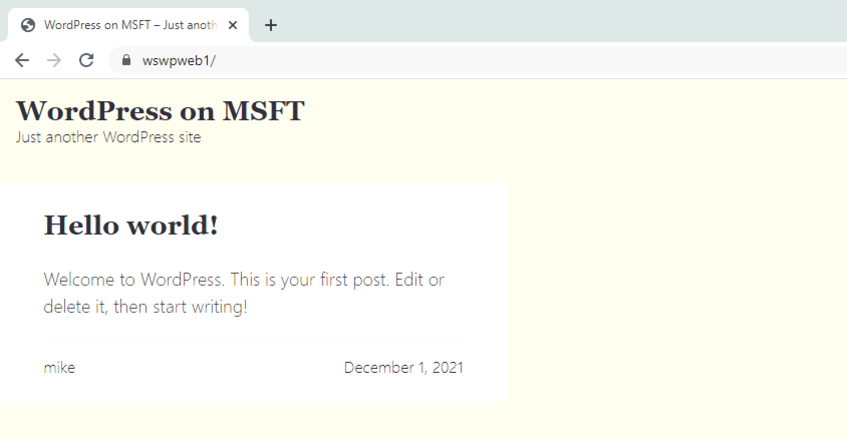
We can also verify that the WordPress site is functional by opening a browser from our testing client and browsing to the URL (https://wswpweb1, listed in Table 1).

WordPress site verification

Figure 4. WordPress site verification

Additionally, we can verify that the web server is connecting to the correct SQL server database by issuing the following command when logged into the WordPress web server:

C:\ >netstat | findstr /c:"ms-sql-s"

 TCP 10.0.67.171:50355 10.0.67.202:ms-sql-s TIME_WAIT

 TCP 10.0.67.171:50361
10.0.67.202:ms-sql-s
TIME_WAIT

6.     Cleanup

After you’ve tested everything, mark the source servers in Application Migration Service as “Ready for Cutover.” This will terminate the EC2 testing instances.

The following PowerShell commands will remove the DNS resource records and the DNS Query Policy:

Remove-DnsServerResourceRecord -ZoneName
"awslaunch.local" -ZoneScope "MGN-Testing-AZ1-Scope"
-RRType "A" -Name "wswpweb1"

Remove-DnsServerResourceRecord -ZoneName
"awslaunch.local" -ZoneScope "MGN-Testing-AZ1-Scope"
-RRType "A" -Name "wswpsql1"

Remove-DnsServerQueryResolutionPolicy -Name
"MGN-Testing-AZ1-Policy" -ZoneName "awslaunch.local"

This command will re-enable replication from the testing domain controller.

C:\> repadmin /options <Testing DC>
-disable_outbound_repl

Once the servers are launched for final cutover, you can remove the Group Policy applied to the servers to allow the server to resume password changes and dynamic DNS updates.

Conclusion

When you migrate your server resources to AWS with Application Migration Service, the testing phase of the migration lifecycle is critical. It verifies that your application will function properly within the AWS environment before committing to a final cutover. The testing phase can uncover unexpected application dependencies, gauge application performance, and deliver the confidence that your migration to AWS will be successful without risks to your production environment.

In this blog post, we explored an architecture and process that uses Microsoft DNS Query Policies and Group Policy to address potential domain issues and avoids affecting the production environment. This testing framework persists during the entire cloud migration and across multiple application migrations. Once migration is complete, the testing architecture can be removed or maintained for future cloud migrations.

Ready to get started? Read more about the AWS Application Migration Service and other blog posts related to migrations on the AWS Cloud Enterprise Strategy Blog and the AWS Architecture Blog.

Looking for more architecture content? AWS Architecture Center provides reference architecture diagrams, vetted architecture solutions, Well-Architected best practices, patterns, icons, and more!

Using DevOps Automation to Deploy Lambda APIs across Accounts and Environments

Post Syndicated from Subrahmanyam Madduru original https://aws.amazon.com/blogs/architecture/using-devops-automation-to-deploy-lambda-apis-across-accounts-and-environments/

by Subrahmanyam Madduru – Global Partner Solutions Architect Leader, AWS, Sandipan Chakraborti – Senior AWS Architect, Wipro Limited, Abhishek Gautam – AWS Developer and Solutions Architect, Wipro Limited, Arati Deshmukh – AWS Architect, Infosys

As more and more enterprises adopt serverless technologies to deliver their business capabilities in a more agile manner, it is imperative to automate release processes. Multiple AWS Accounts are needed to separate and isolate workloads in production versus non-production environments. Release automation becomes critical when you have multiple business units within an enterprise, each consisting of a number of AWS accounts that are continuously deploying to production and non-production environments.

As a DevOps best practice, the DevOps engineering team responsible for build-test-deploy in a non-production environment should not release the application and infrastructure code on to both non-production and production environments.  This risks introducing errors in application and infrastructure deployments in production environments. This in turn results in significant rework and delays in delivering functionalities and go-to-market initiatives. Deploying the code in a repeatable fashion while reducing manual error requires automating the entire release process. In this blog, we show how you can build a cross-account code pipeline that automates the releases across different environments using AWS CloudFormation templates and AWS cross-account access.

Cross-account code pipeline enables an AWS Identity & Access Management (IAM) user to assume an IAM Production role using AWS Secure Token Service (Managing AWS STS in an AWS Region – AWS Identity and Access Management) to switch between non-production and production deployments based as required. An automated release pipeline goes through all the release stages from source, to build, to deploy, on non-production AWS Account and then calls STS Assume Role API (cross-account access) to get temporary token and access to AWS Production Account for deployment. This follow the least privilege model for granting role-based access through IAM policies, which ensures the secure automation of the production pipeline release.

Solution Overview

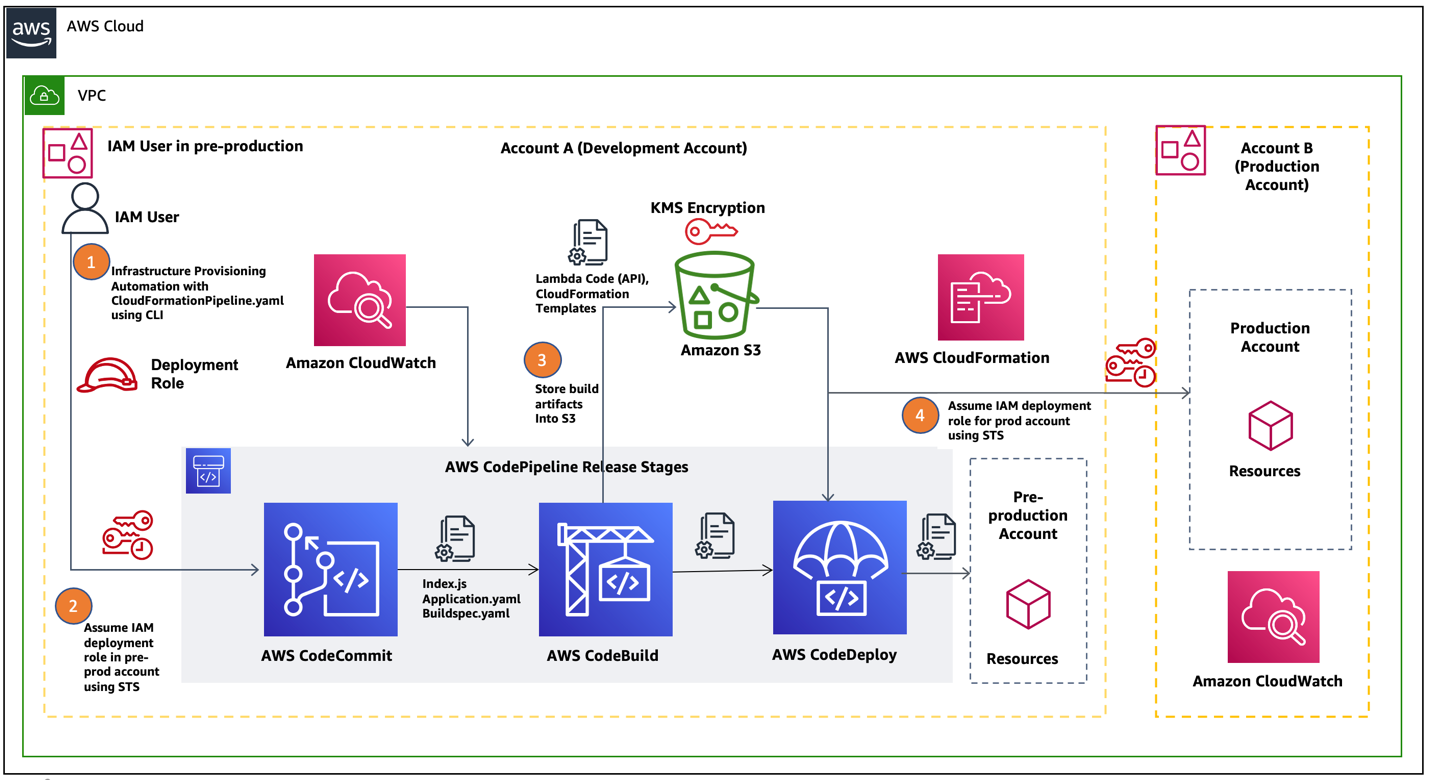
In this blog post, we will show how a cross-account IAM assume role can be used to deploy AWS Lambda Serverless API code into pre-production and production environments. We are building on the process outlined in this blog post: Building a CI/CD pipeline for cross-account deployment of an AWS Lambda API with the Serverless Framework by programmatically automating the deployment of Amazon API Gateway using CloudFormation templates. For this use case, we are assuming a single tenant customer with separate AWS Accounts to isolate pre-production and production workloads.  In Figure 1, we have represented the code pipeline workflow diagramatically for our use case.

Figure 1. AWS cross-account CodePipeline for production and non-production workloads

Figure 1. AWS cross-account AWS CodePipeline for production and non-production workloads

Let us describe the code pipeline workflow in detail for each step noted in the preceding diagram:

  1. An IAM user belonging to the DevOps engineering team logs in to AWS Command-line Interface (AWS CLI) from a local machine using an IAM secret and access key.
  2. Next, the  IAM user assumes the IAM role to the corresponding activities – AWS Code Commit, AWS CodeBuild, AWS CodeDeploy, AWS CodePipeline Execution and deploys the code for pre-production.
  3. A typical AWS CodePipeline comprises of build, test and deploy stages. In the build stage, the AWS CodeBuild service generates the Cloudformation template stack (template-export.yaml) into Amazon S3.
  4. In the deploy stage, AWS CodePipeline uses a CloudFormation template (a yaml file) to deploy the code from an S3 bucket containing the application API endpoints via Amazon API Gateway in the pre-production environment.
  5. The final step in the pipeline workflow is to deploy the application code changes onto the Production environment by assuming STS production IAM role.

Since the AWS CodePipeline is fully automated, we can use the same pipeline by switching between  pre-production and production accounts. These accounts assume the IAM role appropriate to the target environment and deploy the validated build to that environment using CloudFormation templates.

Prerequisites

Here are the pre-requisites before you get started with implementation.

  • A user  with appropriate privileges (for example: Project Admin) in a production AWS account
  • A user with appropriate privileges (for example: Developer Lead) in a pre-production AWS account such as development
  • A CloudFormation template for deploying infrastructure in the pre-production account
  • Ensure your local machine has AWS CLI installed and configured 

Implementation Steps

In this section, we show how you can use AWS CodePipeline to release a serverless API in a secure manner to pre-production and production environments. AWS CloudWatch logging will be used to monitor the events on the AWS CodePipeline.

1. Create Resources in a pre-production account

In this step, we create the required resources such as a code repository, an S3 bucket, and a KMS key in a pre-production environment.

  • Clone the code repository into your CodeCommit. Make necessary changes to index.js and ensure the buildspec.yaml is there to build the artifacts.
    • Using codebase (lambda APIs) as input, you output a CloudFormation template, and environmental configuration JSON files (used for configuring Production and other non-Production environments such as dev, test). The build artifacts are packaged using AWS Serverless Application Model into a zip file and uploads it to an S3 bucket created for storing artifacts. Make note of the repository name as it will be required later.
  • Create an S3 bucket in a Region (Example: us-east-2). This bucket will be used by the pipeline for get and put artifacts. Make a note of the bucket name.
    • Make sure you edit the bucket policy to have your production account ID and the bucket name. Refer to AWS S3 Bucket Policy documentation to make changes to Amazon S3 bucket policies and permissions.
  • Navigate to AWS Key Management Service (KMS) and create a symmetric key.
  • Then create a new secret, configure the KMS key and provide access to development and production account. Make a note of the ARN for the key.

2. Create IAM Roles in the Production Account and required policies

In this step, we create roles and policies required to deploy the code.

{
    "Version": "2012-10-17",
    "Statement": [
      {
        "Effect": "Allow",
        "Action": [
        "kms:DescribeKey",
        "kms:GenerateDataKey*",
        "kms:Encrypt",
        "kms:ReEncrypt*",
        "kms:Decrypt"
      ],
      "Resource": [
        "Your KMS Key ARN you created in Development Account"
      ]
    }
  ]
}

Once you’ve created both policies, attach them to the previously created cross-account role.

3. Create a CloudFormation Deployment role

In this step, you need to create another IAM role, “CloudFormationDeploymentRole” for Application deployment. Then attach the following four policies to it.

Policy 1: For Cloudformation to deploy the application in the Production account

{
  "Version": "2012-10-17",
  "Statement": [
    {
      "Sid": "VisualEditor0",
      "Effect": "Allow",
      "Action": [
        "cloudformation:DetectStackDrift",
        "cloudformation:CancelUpdateStack",
        "cloudformation:DescribeStackResource",
        "cloudformation:CreateChangeSet",
        "cloudformation:ContinueUpdateRollback",
        "cloudformation:DetectStackResourceDrift",
        "cloudformation:DescribeStackEvents",
        "cloudformation:UpdateStack",
        "cloudformation:DescribeChangeSet",
        "cloudformation:ExecuteChangeSet",
        "cloudformation:ListStackResources",
        "cloudformation:SetStackPolicy",
        "cloudformation:ListStacks",
        "cloudformation:DescribeStackResources",
        "cloudformation:DescribePublisher",
        "cloudformation:GetTemplateSummary",
        "cloudformation:DescribeStacks",
        "cloudformation:DescribeStackResourceDrifts",
        "cloudformation:CreateStack",
        "cloudformation:GetTemplate",
        "cloudformation:DeleteStack",
        "cloudformation:TagResource",
        "cloudformation:UntagResource",
        "cloudformation:ListChangeSets",
        "cloudformation:ValidateTemplate"
      ],
      "Resource": "arn:aws:cloudformation:us-east-2:940679525002:stack/DevOps-Automation-API*/*"        }
  ]
}

Policy 2: For Cloudformation to perform required IAM actions

{
  "Version": "2012-10-17",
  "Statement": [
    {
      "Sid": "VisualEditor0",
      "Effect": "Allow",
      "Action": [
        "iam:GetRole",
        "iam:GetPolicy",
        "iam:TagRole",
        "iam:DeletePolicy",
        "iam:CreateRole",
        "iam:DeleteRole",
        "iam:AttachRolePolicy",
        "iam:PutRolePolicy",
        "iam:TagPolicy",
        "iam:CreatePolicy",
        "iam:PassRole",
        "iam:DetachRolePolicy",
        "iam:DeleteRolePolicy"
      ],
      "Resource": "*"
    }
  ]
}

Policy 3: Lambda function service invocation policy

{
  "Version": "2012-10-17",
  "Statement": [
    {
      "Sid": "VisualEditor0",
      "Effect": "Allow",
      "Action": [
        "lambda:CreateFunction",
        "lambda:UpdateFunctionCode",
        "lambda:AddPermission",
        "lambda:InvokeFunction",
        "lambda:GetFunction",
        "lambda:DeleteFunction",
        "lambda:PublishVersion",
        "lambda:CreateAlias"
      ],
      "Resource": "arn:aws:lambda:us-east-2:Your_Production_AccountID:function:SampleApplication*"
    }
  ]
}

Policy 4: API Gateway service invocation policy

{
  "Version": "2012-10-17",
  "Statement": [
    {
      "Sid": "VisualEditor0",
      "Effect": "Allow",
      "Action": [
        "apigateway:DELETE",
        "apigateway:PATCH",
        "apigateway:POST",
        "apigateway:GET"
      ],
      "Resource": [
        "arn:aws:apigateway:*::/restapis/*/deployments/*",
        "arn:aws:apigateway:*::/restapis/*/stages/*",
        "arn:aws:apigateway:*::/clientcertificates",
        "arn:aws:apigateway:*::/restapis/*/models",
        "arn:aws:apigateway:*::/restapis/*/resources/*",
        "arn:aws:apigateway:*::/restapis/*/models/*",
        "arn:aws:apigateway:*::/restapis/*/gatewayresponses/*",
        "arn:aws:apigateway:*::/restapis/*/stages",
        "arn:aws:apigateway:*::/restapis/*/resources",
        "arn:aws:apigateway:*::/restapis/*/gatewayresponses",
        "arn:aws:apigateway:*::/clientcertificates/*",
        "arn:aws:apigateway:*::/account",
        "arn:aws:apigateway:*::/restapis/*/deployments",
        "arn:aws:apigateway:*::/restapis"
      ]
    },
    {
      "Sid": "VisualEditor1",
      "Effect": "Allow",
      "Action": [
        "apigateway:DELETE",
        "apigateway:PATCH",
        "apigateway:POST",
        "apigateway:GET"
      ],
      "Resource": "arn:aws:apigateway:*::/restapis/*/resources/*/methods/*/responses/*"
    },
    {
      "Sid": "VisualEditor2",
      "Effect": "Allow",
      "Action": [
        "apigateway:DELETE",
        "apigateway:PATCH",
        "apigateway:GET"
      ],
      "Resource": "arn:aws:apigateway:*::/restapis/*"
    },
    {
      "Sid": "VisualEditor3",
      "Effect": "Allow",
      "Action": [
        "apigateway:DELETE",
        "apigateway:PATCH",
        "apigateway:GET"
      ],
      "Resource": "arn:aws:apigateway:*::/restapis/*/resources/*/methods/*"
    }
  ]
}

Make sure you also attach the S3 read/write access and KMS policies created in Step-2, to the CloudFormationDeploymentRole.

4. Setup and launch CodePipeline

You can launch the CodePipeline either manually in the AWS console using “Launch Stack” or programmatically via command-line in CLI.

On your local machine go to terminal/ command prompt and launch this command:

aws cloudformation deploy –template-file <Path to pipeline.yaml> –region us-east-2 –stack-name <Name_Of_Your_Stack> –capabilities CAPABILITY_IAM –parameter-overrides ArtifactBucketName=<Your_Artifact_Bucket_Name>  ArtifactEncryptionKeyArn=<Your_KMS_Key_ARN>  ProductionAccountId=<Your_Production_Account_ID>  ApplicationRepositoryName=<Your_Repository_Name> RepositoryBranch=master

If you have configured a profile in AWS CLI,  mention that profile while executing the command:

–profile <your_profile_name>

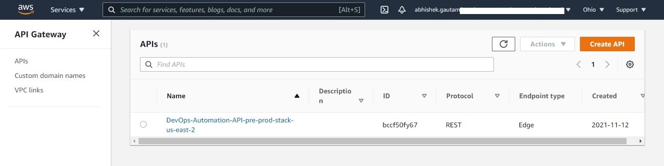
After launching the pipeline, your serverless API gets deployed in pre-production as well as in the production Accounts. You can check the deployment of your API in production or pre-production Account, by navigating to the API Gateway in the AWS console and looking for your API in the Region where it was deployed.

Figure 2. Check your deployment in pre-production/production environment

Figure 2. Check your deployment in pre-production/production environment

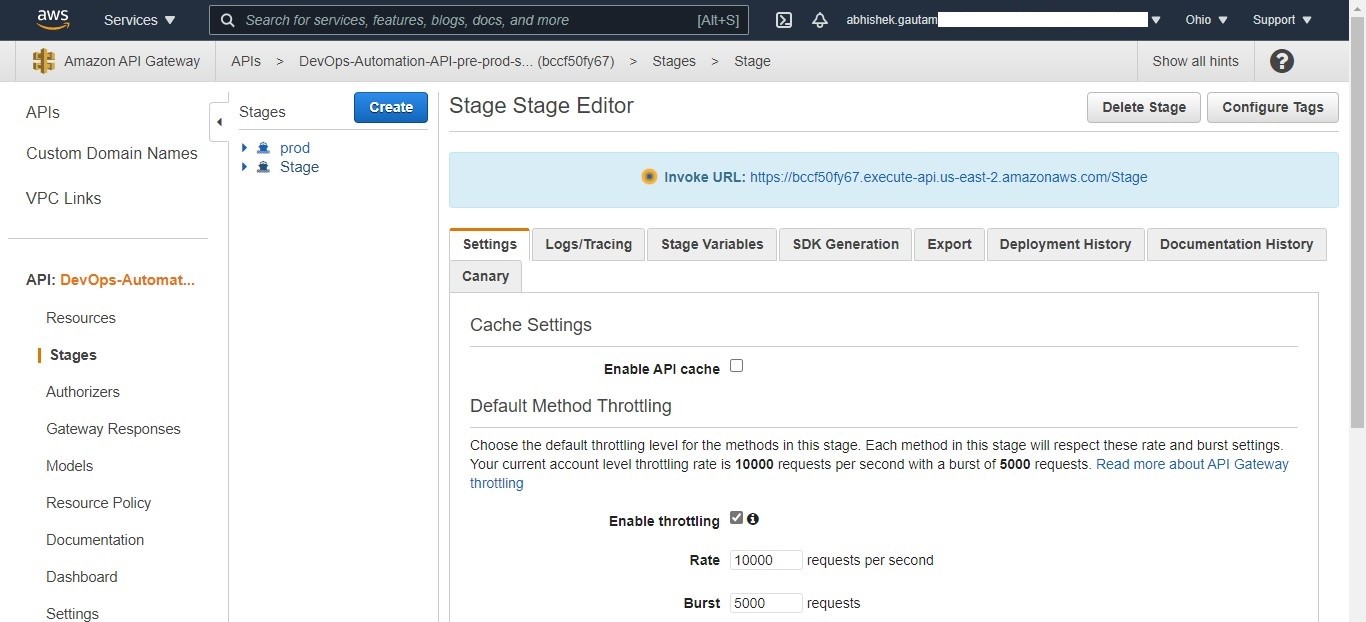
Then select your API and navigate to stages, to view the published API with an endpoint. Then validate your API response by selecting the API link.

Figure 3. Check whether your API is being published in pre-production/production environment

Figure 3. Check whether your API is being published in pre-production/production environment

Alternatively you can also navigate to your APIs by navigating through your deployed application CloudFormation stack and selecting the link for API in the Resources tab.

Cleanup

If you are trying this out in your AWS accounts, make sure to delete all the resources created during this exercise to avoid incurring any AWS charges.

Conclusion

In this blog, we showed how to build a cross-account code pipeline to automate releases across different environments using AWS CloudFormation templates and AWS Cross Account Access. You also learned how serveless APIs can be securely deployed across pre-production and production accounts. This helps enterprises automate release deployments in a repeatable and agile manner, reduce manual errors and deliver business cababilities more quickly.

Automate your Data Extraction for Oil Well Data with Amazon Textract

Post Syndicated from Ashutosh Pateriya original https://aws.amazon.com/blogs/architecture/automate-your-data-extraction-for-oil-well-data-with-amazon-textract/

Traditionally, many businesses archive physical formats of their business documents. These can be invoices, sales memos, purchase orders, vendor-related documents, and inventory documents. As more and more businesses are moving towards digitizing their business processes, it is becoming challenging to effectively manage these documents and perform business analytics on them. For example, in the Oil and Gas (O&G) industry, companies have numerous documents that are generated through the exploration and production lifecycle of an oil well. These documents can provide many insights that can help inform business decisions.

As documents are usually stored in a paper format, information retrieval can be time consuming and cumbersome. Even those available in a digital format may not have adequate metadata associated to efficiently perform search and build insights.

In this post, you will learn how to build a text extraction solution using Amazon Textract service. This will automatically extract text and data from scanned documents and upload into Amazon Simple Storage Service (S3). We will show you how to find insights and relationships in the extracted text using Amazon Comprehend. This data is indexed and populated into Amazon OpenSearch Service to search and visualize it in a Kibana dashboard.

Figure 1 illustrates a solution built with AWS, which extracts O&G well data information from PDF documents. This solution is serverless and built using AWS Managed Services. This will help you to decrease system maintenance overhead while making your solution scalable and reliable.

Figure 1. Automated form data extraction architecture

Figure 1. Automated form data extraction architecture

Following are the high-level steps:

  1. Upload an image file or PDF document to Amazon S3 for analysis. Amazon S3 is a durable document storage used for central document management.
  2. Amazon S3 event initiates the AWS Lambda function Fn-A. AWS Lambda has functional logic to call the Amazon Textract and Comprehend services and processing.
  3. AWS Lambda function Fn-A invokes Amazon Textract to extract text as key-value pairs from image or PDF. Amazon Textract automatically extracts data from the scanned documents.
  4. Amazon Textract sends the extracted keys from image/PDF to Amazon SNS.
  5. Amazon SNS notifies Amazon SQS when text extraction is complete by sending the extracted keys to Amazon SQS.
  6. Amazon SQS initiates AWS Lambda function Fn-B with the extracted keys.
  7. AWS Lambda function Fn-B invokes Amazon Comprehend for the custom entity recognition. Comprehend uses custom-trained machine learning (ML) to find discrepancies in key names from Amazon Textract.
  8. The data is indexed and loaded into Amazon OpenSearch, which indexes and visualizes the data.
  9. Kibana processes the indexed data.
  10. User accesses Kibana to search documents.

Steps illustrated with more detail:

1. User uploads the document for analysis to Amazon S3. Uploaded document can be an image file or a PDF. Here we are using the S3 console for document upload. Figure 2 shows the sample file used for this demo.

Figure 2. Sample input form

Figure 2. Sample input form

2. Amazon S3 upload event initiates AWS Lambda function Fn-A. Refer to the AWS tutorial to learn about S3 Lambda configuration. View Sample code for Lambda FunctionA.

3. AWS Lambda function Fn-A invokes Amazon Textract. Amazon Textract uses artificial intelligence (AI) to read as a human would, by extracting text, layouts, tables, forms, and structured data with context and without configuration, training, or custom code.

4. Amazon Textract starts processing the file as it is uploaded. This process takes few minutes since the file is a multipage document.

5. Amazon SNS notifies Amazon Textract of completion. Amazon Textract processing works asynchronously, as we decouple our architecture using Amazon SQS. To configure Amazon SNS to send data to Amazon SQS:

  • Create an SNS topic. ‘AmazonTextract-SNS’ is the SNS topic that we created for this demo.
  • Then create an SQS queue. ‘AmazonTextract-SQS’ is the queue that we created for this demo.
  • To receive messages published to a topic, you must subscribe an endpoint to the topic. When you subscribe an endpoint to a topic, the endpoint begins to receive messages published to the associated topic. Figure 3 shows the SNS topic ‘AmazonTextract-SNS’ subscribed to Amazon SQS queue.
Figure 3. Amazon SNS configuration

Figure 3. Amazon SNS configuration

Figure 4. Amazon SQS configuration

Figure 4. Amazon SQS configuration

6. Configure SQS queue to initiate the AWS Lambda function Fn-B. This should happen upon receiving extracted data via SNS topic. Refer to this SQS tutorial to learn about SQS Lambda configuration. See Sample code for Lambda FunctionB.

7. AWS Lambda function Fn-B invokes Amazon Comprehend for the custom entity recognition.

Figure 5. Lambda FunctionB configuration in Amazon Comprehend

Figure 5. Lambda FunctionB configuration in Amazon Comprehend

  • Configure Amazon Comprehend to create a custom entity recognition (text-job2) for the entities. These can be API Number, Lease_Number, Water_Depth, Well_Number, and can use the model created in previous step (well_no, well#, well num). For instructions on labeling your data, see Developing NER models with Amazon SageMaker Ground Truth and Amazon Comprehend.
Figure 6. Comprehend job

Figure 6. Comprehend job

  • Now create an endpoint for the custom entity recognition for the Lambda function, to send the data to Amazon Comprehend service, as shown in Figure 7 and 8.
Figure 7. Comprehend endpoint creation

Figure 7. Comprehend endpoint creation

  • Copy the Amazon Comprehend endpoint ARN to include it in the Lambda function as an environment variable (see Figure 5).
Figure 8. Comprehend endpoint created successfully

Figure 8. Comprehend endpoint created successfully

8. Launch an Amazon OpenSearch domain. See Creating and managing Amazon OpenSearch Service domains. The data is indexed and populated into Amazon OpenSearch. The Amazon OpenSearch domain name is configured at Lambda FnB as an environment variable to push the extracted data to OpenSearch.

9. Kibana processes the indexed data from Amazon OpenSearch. Amazon OpenSearch data is populated on Kibana, shown in Figure 9.

Figure 9. Kibana dashboard showing Amazon OpenSearch data

Figure 9. Kibana dashboard showing Amazon OpenSearch data

10. Access Kibana for document search. The selected fields can be viewed as a table using filters, see Figure 10.

Figure 10. Kibana dashboard table view for selected fields

Figure 10. Kibana dashboard table view for selected fields

You can s­earch the LEASE_NUMBER = OCS-031, as shown in Figure 11.

Figure 11. Kibana dashboard search on Lease Number

Figure 11. Kibana dashboard search on Lease Number

OR you can search all the information for the WATER_DEPTH = 60, see Figure 12.

Figure 12. Kibana dashboard search on Water Depth

Figure 12. Kibana dashboard search on Water Depth

Cleanup

  1. Shut down OpenSearch domain
  2. Delete the Comprehend endpoint
  3. Clear objects from S3 bucket

Conclusion

Data is growing at an enormous pace in all industries. As we have shown, you can build an ML-based text extraction solution to uncover the unstructured data from PDFs or images. You can derive intelligence from diverse data sources by incorporating a data extraction and optimization function. You can gain insights into the undiscovered data, by leveraging managed ML services, Amazon Textract, and Amazon Comprehend.

The extracted data from PDFs or images is indexed and populated into Amazon OpenSearch. You can use Kibana to search and visualize the data. By implementing this solution, customers can reduce the costs of physical document storage, in addition to labor costs for manually identifying relevant information.

This solution will drive decision-making efficiency. We discussed the oil and gas industry vertical as an example for this blog. But this solution can be applied to any industry that has physical/scanned documents such as legal documents, purchase receipts, inventory reports, invoices, and purchase orders.

For further reading:

Let’s Architect! Architecting for Security

Post Syndicated from Luca Mezzalira original https://aws.amazon.com/blogs/architecture/lets-architect-architecting-for-security/

At AWS, security is “job zero” for every employee—it’s even more important than any number one priority. In this Let’s Architect! post, we’ve collected security content to help you protect data, manage access, protect networks and applications, detect and monitor threats, and ensure privacy and compliance.

Managing temporary elevated access to your AWS environment

One challenge many organizations face is maintaining a solid security governance across AWS accounts.

This Security Blog post provides a practical approach to temporarily elevate access for specific users. For example, imagine a developer wants to access a resource in the production environment. With elevated access, you won’t have to provide them an account that has access to the production environment. You would just elevate their access for a short period of time. The following diagram shows the few steps needed to temporarily elevate access to a user.

This diagram shows the few steps needed to temporarily elevate access to a user

This diagram shows the few steps needed for to temporarily elevate access to a user

Security should start left: The problem with shift left

You already know security is job zero at AWS. But it’s not just a technology challenge. The gaps between security, operations, and development cycles are widening. To close these gaps, teams must have real-time visibility and control over their tools, processes, and practices to prevent security breaches.

This re:Invent session shows how establishing relationships, empathy, and understanding between development and operations teams early in the development process helps you maintain the visibility and control you need to keep your applications secure.

Screenshot from re:Invent session

Empowering developers means shifting security left and presenting security issues as early as possible in your process

AWS Security Reference Architecture: Visualize your security

Securing a workload in the cloud can be tough; almost every workload is unique and has different requirements. This re:Invent video shows you how AWS can simplify the security of your workloads, no matter their complexity.

You’ll learn how various services work together and how you can deploy them to meet your security needs. You’ll also see how the AWS Security Reference Architecture can automate common security tasks and expand your security practices for the future. The following diagram shows how AWS Security Reference Architecture provides guidelines for securing your workloads in multiple AWS Regions and accounts.

The AWS Security Reference Architecture provides guidelines for securing your workloads in multiple AWS Regions and accounts

The AWS Security Reference Architecture provides guidelines for securing your workloads in multiple AWS Regions and accounts

Network security for serverless workloads

Serverless technologies can improve your security posture. You can build layers of control and security with AWS managed and abstracted services, meaning that you don’t have to do as much security work and can focus on building your system.

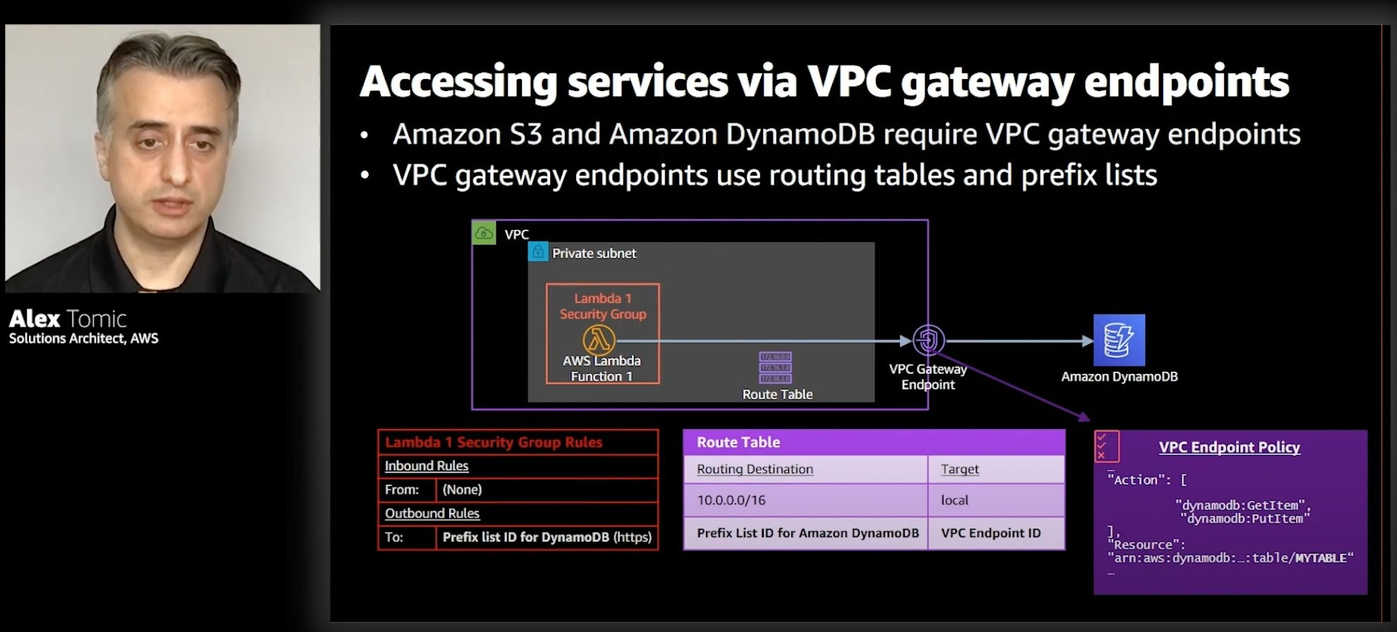
This video from re:Invent provides serverless strategies to consider to gain greater control of networking security. You will learn patterns to implement security at the edge, as well as options for controlling an AWS Lambda function’s network traffic. These strategies are designed to securely access resources (for example, databases) placed in a virtual private cloud (VPC), as well as resources outside of a VPC. The following screenshot shows how
Lambda functions can run in a VPC and connect to services like Amazon DynamoDB using VPC gateway endpoints.

Lambda functions can run in a VPC and connect to services like Amazon DynamoDB using VPC gateway endpoints

Lambda functions can run in a VPC and connect to services like Amazon DynamoDB using VPC gateway endpoints

See you next time!

Thanks for reading! If you’re looking for more ways to architect your workload for security, check out Best Practices for Security, Identity, & Compliance in the AWS Architecture Center.

See you in a couple of weeks when we discuss the best tools offered by AWS for software architects!

Other posts in this series

Rapid Event Notification System at Netflix

Post Syndicated from Netflix Technology Blog original https://netflixtechblog.com/rapid-event-notification-system-at-netflix-6deb1d2b57d1

By: Ankush Gulati, David Gevorkyan
Additional credits: Michael Clark, Gokhan Ozer

Intro

Netflix has more than 220 million active members who perform a variety of actions throughout each session, ranging from renaming a profile to watching a title. Reacting to these actions in near real-time to keep the experience consistent across devices is critical for ensuring an optimal member experience. This is not an easy task, considering the wide variety of supported devices and the sheer volume of actions our members perform. To this end, we developed a Rapid Event Notification System (RENO) to support use cases that require server initiated communication with devices in a scalable and extensible manner.

In this blog post, we will give an overview of the Rapid Event Notification System at Netflix and share some of the learnings we gained along the way.

Motivation

With the rapid growth in Netflix member base and the increasing complexity of our systems, our architecture has evolved into an asynchronous one that enables both online and offline computation. Providing a seamless and consistent Netflix experience across various platforms (iOS, Android, smart TVs, Roku, Amazon FireStick, web browser) and various device types (mobile phones, tablets, televisions, computers, set top boxes) requires more than the traditional request-response model. Over time, we’ve seen an increase in use cases where backend systems need to initiate communication with devices to notify them of member-driven changes or experience updates quickly and consistently.

Use cases

  • Viewing Activity
    When a member begins to watch a show, their “Continue Watching” list should be updated across all of their devices to reflect that viewing.
  • Personalized Experience Refresh
    Netflix Recommendation engine continuously refreshes recommendations for every member. The updated recommendations need to be delivered to the device timely for an optimal member experience.
  • Membership Plan Changes
    Members often change their plan types, leading to a change in their experience that must be immediately reflected across all of their devices.
  • Member “My List” Updates
    When members update their “My List” by adding or removing titles, the changes should be reflected across all of their devices.
  • Member Profile Changes
    When members update their account settings like add/delete/rename profiles or change their preferred maturity level for content, these updates must be reflected across all of their devices.
  • System Diagnostic Signals
    In special scenarios, we need to send diagnostic signals to the Netflix app on devices to help troubleshoot problems and enable tracing capabilities.

Design Decisions

In designing the system, we made a few key decisions that helped shape the architecture of RENO:

  1. Single Events Source
  2. Event Prioritization
  3. Hybrid Communication Model
  4. Targeted Delivery
  5. Managing High RPS

Single Events Source

The use cases we wanted to support originate from various internal systems and member actions, so we needed to listen for events from several different microservices. At Netflix, our near-real-time event flow is managed by an internal distributed computation framework called Manhattan (you can learn more about it here). We leveraged Manhattan’s event management framework to create a level of indirection serving as the single source of events for RENO.

Event Prioritization

Considering the use cases were wide ranging both in terms of their sources and their importance, we built segmentation into the event processing. For example, a member-triggered event such as “change in a profile’s maturity level” should have a much higher priority than a “system diagnostic signal”. We thus assigned a priority to each use case and sharded event traffic by routing to priority-specific queues and the corresponding event processing clusters. This separation allows us to tune system configuration and scaling policies independently for different event priorities and traffic patterns.

Hybrid Communication Model

As mentioned earlier in this post, one key challenge for a service like RENO is supporting multiple platforms. While a mobile device is almost always connected to the internet and reachable, a smart TV is only online while in use. This network connection heterogeneity made choosing a single delivery model difficult. For example, entirely relying on a Pull model wherein the device frequently calls home for updates would result in chatty mobile apps. That in turn will be triggering the per-app communication limits that iOS and Android platforms enforce (we also need to be considerate of low bandwidth connections). On the other hand, using only a Push mechanism would lead smart TVs to miss notifications while they are powered off during most of the day. We therefore chose a hybrid Push AND Pull communication model wherein the server tries to deliver notifications to all devices immediately using Push notifications, and devices call home at various stages of the application lifecycle.

Using a Push-and-Pull delivery model combination also supports devices limited to a single communication model. This includes older, legacy devices that do not support Push Notifications.

Targeted Delivery

Considering the use cases were wide ranging in terms of both sources and target device types, we built support for device specific notification delivery. This capability allows notifying specific device categories as per the use case. When an actionable event arrives, RENO applies the use case specific business logic, gathers the list of devices eligible to receive this notification and attempts delivery. This helps limit the outgoing traffic footprint considerably.

Managing High RPS

With over 220 million members, we were conscious of the fact that a service like RENO needs to process many events per member during a viewing session. At peak times, RENO serves about 150k events per second. Such a high RPS during specific times of the day can create a thundering herd problem and put strain on internal and external downstream services. We therefore implemented a few optimizations:

  • Event Age
    Many events that need to be notified to the devices are time sensitive, and they are of no or little value unless sent almost immediately. To avoid processing old events, a staleness filter is applied as a gating check. If an event age is older than a configurable threshold, it is not processed. This filter weeds out events that have no value to the devices early in the processing phase and protects the queues from being flooded due to stale upstream events that may have been backed up.
  • Online Devices
    To reduce the ongoing traffic footprint, notifications are sent only to devices that are currently online by leveraging an existing registry that is kept up-to-date by Zuul (learn more about it here).
  • Scaling Policies
    To address the thundering herd problem and to keep latencies under acceptable thresholds, the cluster scale-up policies are configured to be more aggressive than the scale-down policies. This approach enables the computing power to catch up quickly when the queues grow.
  • Event Deduplication
    Both iOS and Android platforms aggressively restrict the level of activity generated by backgrounded apps, hence the reason why incoming events are deduplicated in RENO. Duplicate events can occur in case of high RPS, and they are merged together when it does not cause any loss of context for the device.
  • Bulkheaded Delivery
    Multiple downstream services are used to send push notifications to different device platforms including external ones like Apple Push Notification Service (APNS) for Apple devices and Google’s Firebase Cloud Messaging (FCM) for Android. To safeguard against a downstream service bringing down the entire notification service, the event delivery is parallelized across different platforms, making it best-effort per platform. If a downstream service or platform fails to deliver the notification, the other devices are not blocked from receiving push notifications.

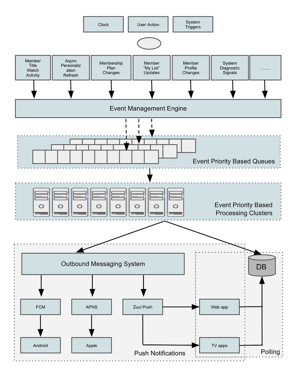
Architecture

As shown in the diagram above, the RENO service can be broken down into the following components.

Event Triggers

Member actions and system-driven updates that require refreshing the experience on members’ devices.

Event Management Engine

The near-real-time event flow management framework at Netflix referred to as Manhattan can be configured to listen to specific events and forward events to different queues.

Event Priority Based Queues

Amazon SQS queues that are populated by priority-based event forwarding rules are set up in Manhattan to allow priority based sharding of traffic.

Event Priority Based Clusters

AWS Instance Clusters that subscribe to the corresponding queues with the same priority. They process all the events arriving on those queues and generate actionable notifications for devices.

Outbound Messaging System

The Netflix messaging system that sends in-app push notifications to members is used to send RENO-produced notifications on the last mile to mobile devices. This messaging system is described in this blog post.

For notifications to web, TV & other streaming devices, we use a homegrown push notification solution ​​called Zuul Push that provides “always-on” persistent connections with online devices. To learn more about the Zuul Push solution, listen to this talk from a Netflix colleague.

Persistent Store

A Cassandra database that stores all the notifications emitted by RENO for each device to allow those devices to poll for their messages at their own cadence.

Observability

At Netflix, we put a strong emphasis on building robust monitoring into our systems to provide a clear view of system health. For a high RPS service like RENO that relies on several upstream systems as its traffic source and simultaneously produces heavy traffic for different internal and external downstream systems, it is important to have a strong combination of metrics, alerting and logging in place. For alerting, in addition to the standard system health metrics such as CPU, memory, and performance, we added a number of “edge-of-the-service” metrics and logging to capture any aberrations from upstream or downstream systems. Furthermore, in addition to real-time alerting, we added trend analysis for important metrics to help catch longer term degradations. We instrumented RENO with a real time stream processing application called Mantis (you can learn more about it here). It allowed us to track events in real-time over the wire at device specific granularity thus making debugging easier. Finally, we found it useful to have platform-specific alerting (for iOS, Android, etc.) in finding the root causes of issues faster.

Wins

  • Can easily support new use cases
  • Scales horizontally with higher throughput

When we set out to build RENO the goal was limited to the “Personalized Experience Refresh” use case of the product. As the design of RENO evolved, support for new use cases became possible and RENO was quickly positioned as the centralized rapid notification service for all product areas at Netflix.

The design decisions we made early on paid off, such as making addition of new use cases a “plug-and-play” solution and providing a hybrid delivery model across all platforms. We were able to onboard additional product use cases at a fast pace thus unblocking a lot of innovation.

An important learning in building this platform was ensuring that RENO could scale horizontally as more types of events and higher throughput was needed over time. This ability was primarily achieved by allowing sharding based on either event type or priority, along with using an asynchronous event driven processing model that can be scaled by simply adding more machines for event processing.

Looking Ahead

As Netflix’s member base continues to grow at a rapid pace, it is increasingly beneficial to have a service like RENO that helps give our members the best and most up to date Netflix experience. From membership related updates to contextual personalization, and more — we are continually evolving our notifications portfolio as we continue to innovate on our member experience. Architecturally, we are evaluating opportunities to build in more features such as guaranteed message delivery and message batching that can open up more use cases and help reduce the communication footprint of RENO.

Building Great Things Together

We are just getting started on this journey to build impactful systems that help propel our business forward. The core to bringing these engineering solutions to life is our direct collaboration with our colleagues and using the most impactful tools and technologies available. If this is something that excites you, we’d love for you to join us.


Rapid Event Notification System at Netflix was originally published in Netflix TechBlog on Medium, where people are continuing the conversation by highlighting and responding to this story.

Multi-Region Migration using AWS Application Migration Service

Post Syndicated from Shreya Pathak original https://aws.amazon.com/blogs/architecture/multi-region-migration-using-aws-application-migration-service/

AWS customers are in various stages of their cloud journey. Frequently, enterprises begin that journey by rehosting (lift-and-shift migrating) their on-premises workloads into AWS, and running Amazon Elastic Compute Cloud (Amazon EC2) instances. You can rehost using AWS Application Migration Service (MGN), a cloud-native migration tool.

You may need to relocate instances and workloads to a Region that is closer in proximity to one of your offices or data centers. Or you may have a resilience requirement to balance your workloads across multiple Regions. This rehosting migration pattern with AWS MGN can also be used to migrate Amazon EC2-hosted workloads from one AWS Region to another.

In this blog post, we will show you how to configure AWS MGN for migrating your workloads from one AWS Region to another.

Overview of AWS MGN migration

AWS MGN, an AWS native service, minimizes time-intensive, error-prone, manual processes by automatically converting your source servers from physical, virtual, or cloud infrastructure to run natively on AWS. It reduces overall migration costs, such as investment in multiple migration solutions, specialized cloud development, or application-specific skills. With AWS MGN, you can migrate your applications from physical infrastructure, VMware vSphere, Microsoft Hyper-V, Amazon EC2, and Amazon Virtual Private Cloud (Amazon VPC) to AWS.

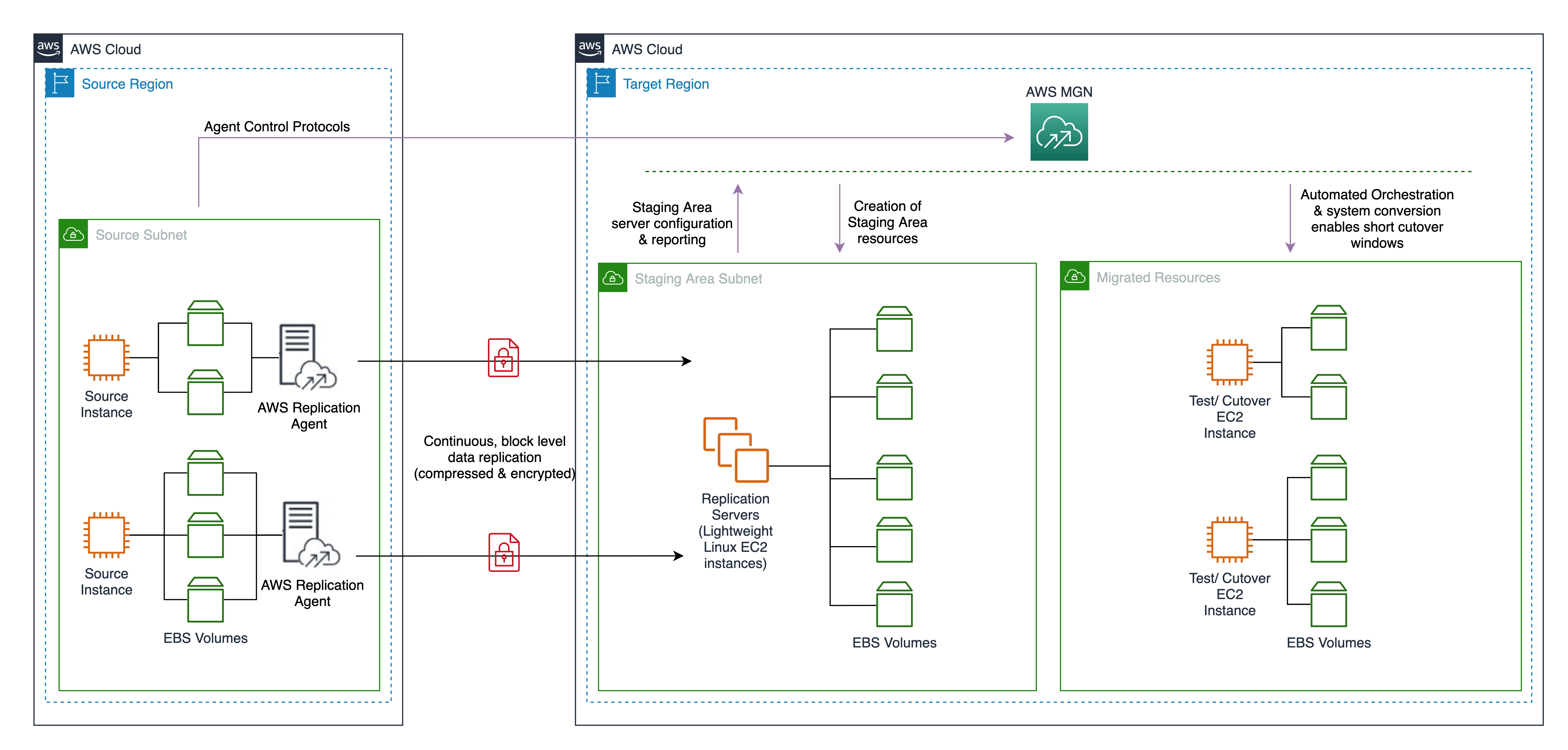
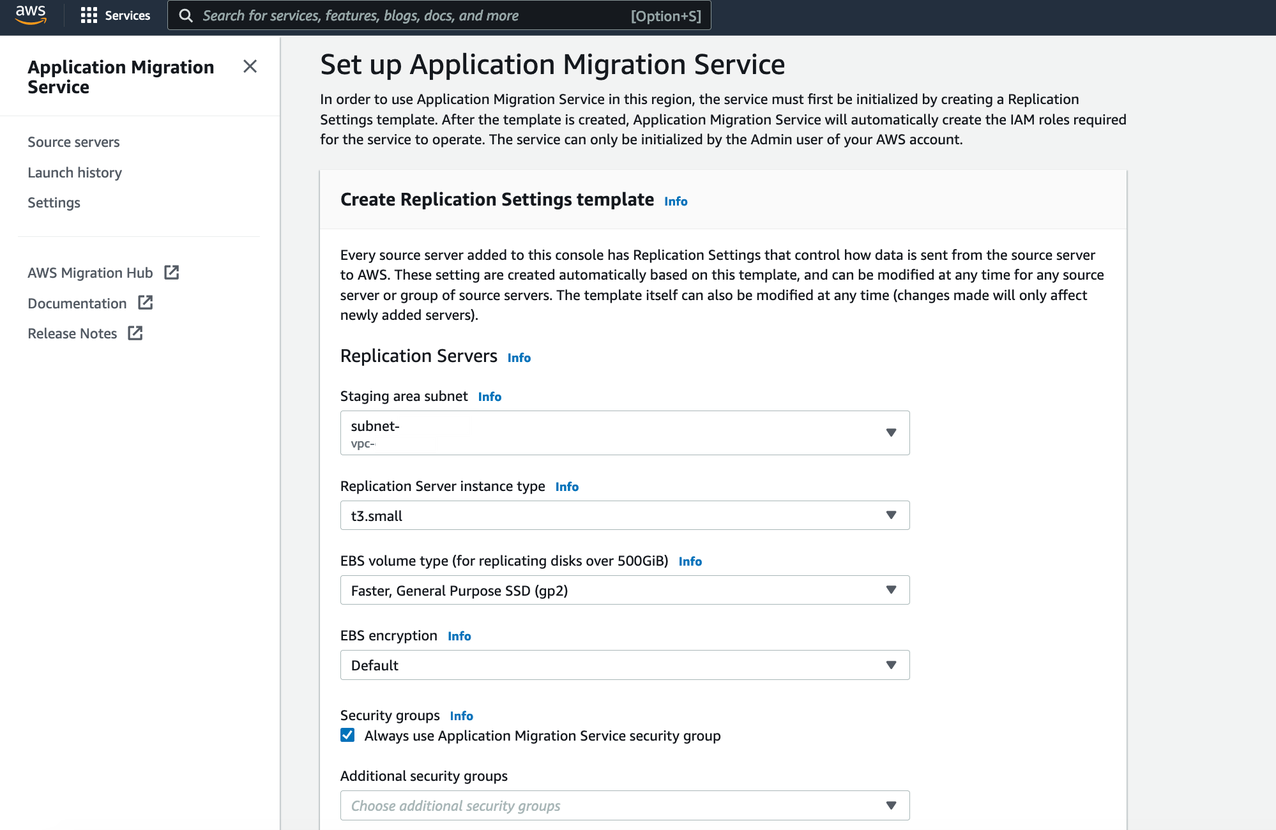
To migrate to AWS, install the AWS MGN Replication Agent on your source servers and define replication settings in the AWS MGN console, shown in Figure 1. Replication servers receive data from an agent running on source servers, and write this data to the Amazon Elastic Block Store (EBS) volumes. Your replicated data is compressed and encrypted in transit and at rest using EBS encryption.

AWS MGN keeps your source servers up to date on AWS using nearly continuous, block-level data replication. It uses your defined launch settings to launch instances when you conduct non-disruptive tests or perform a cutover. After confirming that your launched instances are operating properly on AWS, you can decommission your source servers.

Figure 1. MGN service architecture

Figure 1. MGN service architecture

Steps for migration with AWS MGN

This tutorial assumes that you already have your source AWS Region set up with Amazon EC2-hosted workloads running and a target AWS Region defined.

Migrating Amazon EC2 workload across AWS Regions include the following steps:

  1. Create the Replication Settings template. These settings are used to create and manage your staging area subnet with lightweight Amazon EC2 instances. These instances act as replication servers used to replicate data between your source servers and AWS.
  2. Install the AWS Replication Agent on your source instances to add them to the AWS MGN console.
  3. Configure the launch settings for each source server. These are a set of instructions that determine how a Test or Cutover instance will be launched for each source server on AWS.
  4. Initiate the test/cutover to the target Region.

Prerequisites

Following are the prerequisites:

Setting up AWS MGN for multi-Region migration

This section will guide you through AWS MGN configuration setup for multi-Region migration.

Log into your AWS account, select the target AWS Region, and complete the prerequisites. Then you are ready to configure AWS MGN:

1.      Choose Get started on the AWS MGN landing page.

2.      Create the Replication Settings template (see Figure 2):

  • Select Staging area subnet for Replication Server
  • Choose Replication Server instance type (By default, AWS MGN uses t3.small instance type)
  • Choose default or custom Amazon EBS encryption
  • Enable ‘Always use the Application Migration Service security group’
  • Add custom Replication resources tags
  • Select Create Template button
Figure 2. Replication Settings template creation

Figure 2. Replication Settings template creation

3.      Add source servers to AWS MGN:

  • Select Add Servers following Source Servers (AWS MGN > Source Servers)
  • Enter OS, Replication Preferences, IAM Access Key and Secret Access Key ID of the IAM user created following Prerequisites. This does not expose your Secret Access Key ID in any request
  • Copy the installation command and run on your source server for agent installation

After successful agent installation, the source server is listed on the Source Servers page. Data replication begins after completion of the Initial Sync steps.

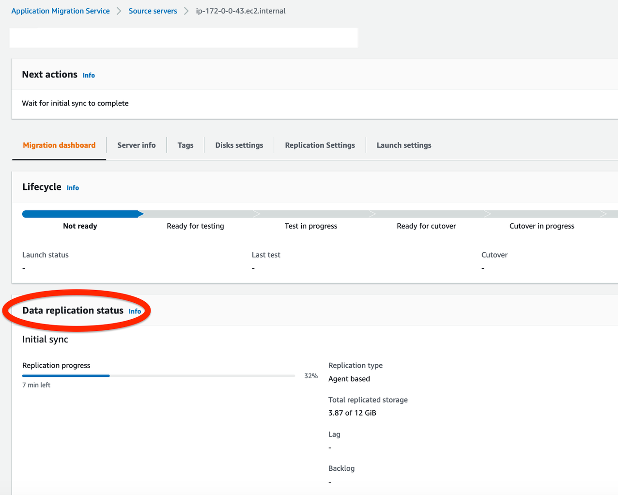
4.      Monitor the Initial Sync status (shown in Figure 3):

  •  Source server name > Migration Dashboard > Data Replication Status
    (Refer to the Source Servers page documentation for more details)
  • After 100% initial data replication confirm:
    • Migration Lifecycle = Ready for testing
    • Next step = Launch test instance
Figure 3. Monitoring initial replication status

Figure 3. Monitoring initial replication status

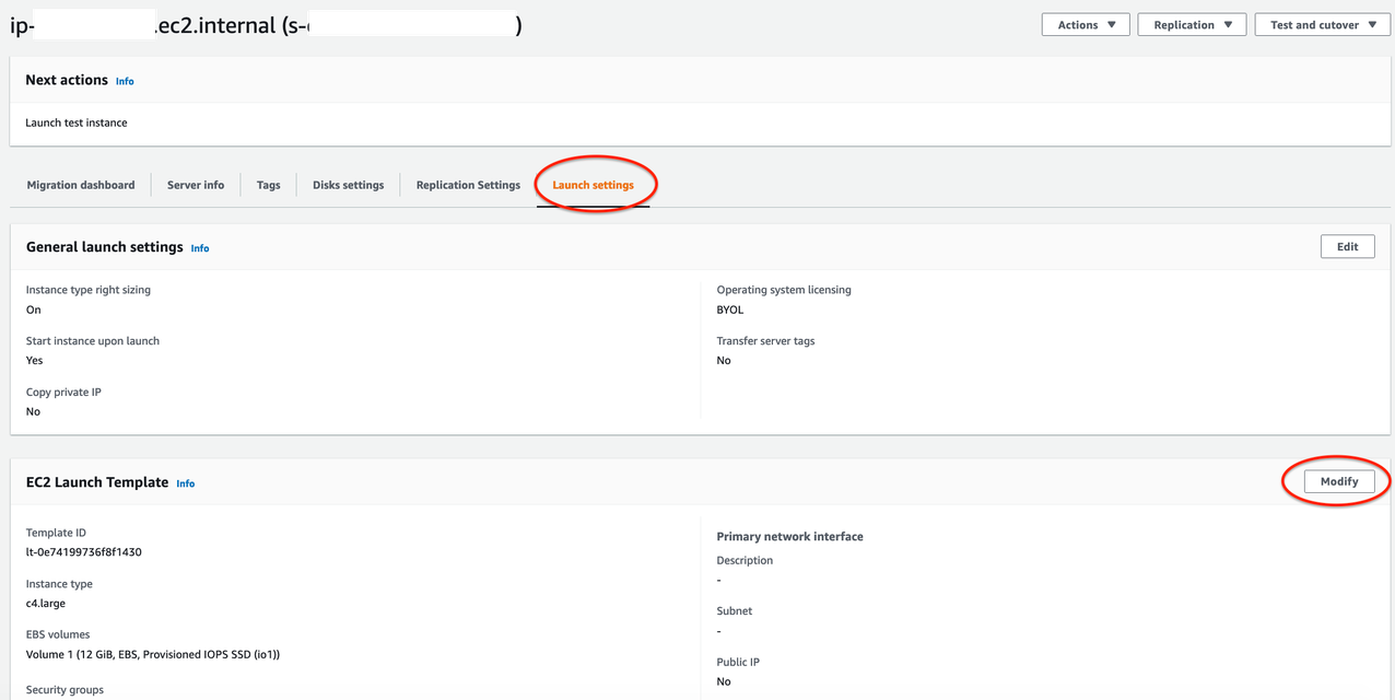
5.      Configure Launch Settings for each server:

  • Source servers page > Select source server
  • Navigate to the Launch settings tab (see Figure 4.) For this tutorial we won’t adjust the General launch settings. We will modify the EC2 Launch Template instead
  • Click on EC2 Launch Template > About modifying EC2 Launch Templates > Modify
Figure 4. Modifying EC2 Launch Template

Figure 4. Modifying EC2 Launch Template

6.      Provide values for Launch Template:

  • AMI: Recents tab > Don’t include in launch template
  • Instance Type: Can be kept same as source server or changed as per expected workload
  • Key pair (login): Create new or use existing if already created in the Target AWS Region
  • Network Settings > Subnet: Subnet for launching Test instance
  • Advanced network configuration:
    • Security Groups: For access to the test and final cutover instances
    • Configure Storage: Size – Do not change or edit this field
    • Volume type: Select any volume type (io1 is default)
  • Review details and click Create Template Version under the Summary section on right side of the console

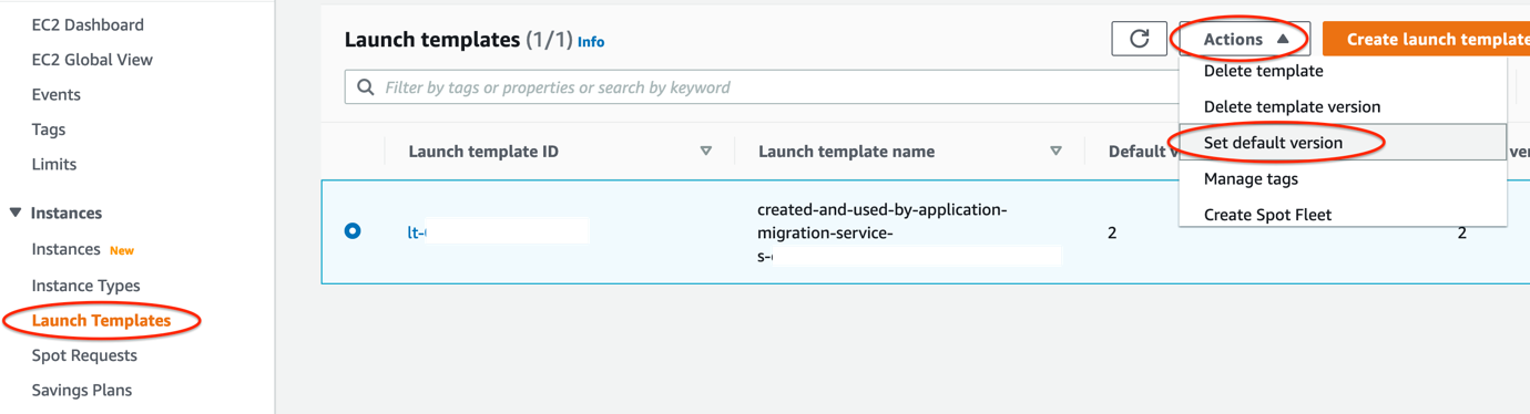
7.      Every time you modify the Launch template, a new version is created. Set the launch template that you want to use with MGN as the default (shown in Figure 5):

  • Navigate to Amazon EC2 dashboard > Launch Templates page
  • Select the Launch template ID
  • Open the Actions menu and choose Set default version and select the latest Launch template created
Figure 5. Setting up your Launch template as the default

Figure 5. Setting up your Launch template as the default

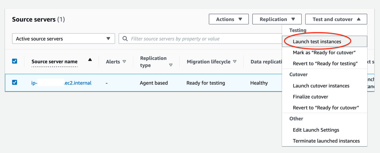
8.      Launch a test instance and perform a Test prior to Cutover to identify potential problems and solve them before the actual Cutover takes place:

  • Go to the Source Servers page (see Figure 6)
  • Select source server > Open Test and Cutover menu
  • Under Testing, choose Launch test instances
  • Launch test instances for X servers > Launch
  • Choose View job details on the ‘Launch Job Created’ dialog box to view the specific Job details for the test launch in the Launch History tab
Figure 6. Launching test instances

Figure 6. Launching test instances

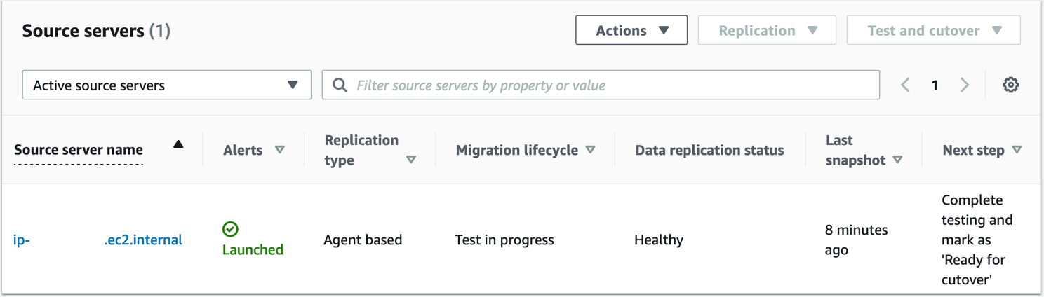
9.      Validate launch of test instance (shown in Figure 7) by confirming:

  • Alerts column = Launched
  • Migration lifecycle column = Test in progress
  • Next step column = Complete testing and mark as ‘Ready for cutover’
Figure 7. Validating launch of test instances

Figure 7. Validating launch of test instances

10.  SSH/ RDP into Test instance (view from EC2 console) and validate connectivity. Perform acceptance tests for your application as required. Revert the test if you encounter any issues.

11.  Terminate Test instances after successful testing:

  • Go to Source servers page
  • Select source server > Open Test and Cutover menu
  • Under Testing, choose Mark as “Ready for cutover”
  • Mark X servers as “Ready for cutover” > Yes, terminate launched instances (recommended) > Continue

12.  Validate the status of termination job and cutover readiness:

  • Migration Lifecycle = Ready for cutover
  • Next step = Launch cutover instance

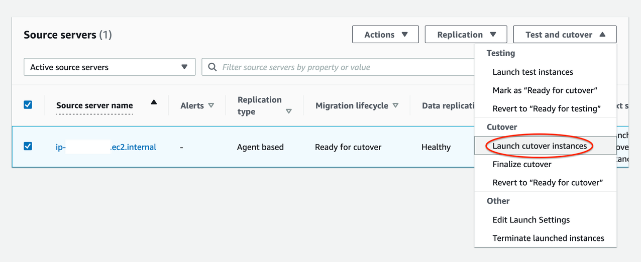
13.  Perform the final cutover at a set date and time:

  • Go to Source servers page (see Figure 8)
  • Select source server > Open Test and Cutover menu
  • Under Cutover, choose Launch cutover instances
  • Launch cutover instances for X > Launch
Figure 8. Performing final Cutover by launching Cutover instances

Figure 8. Performing final Cutover by launching Cutover instances

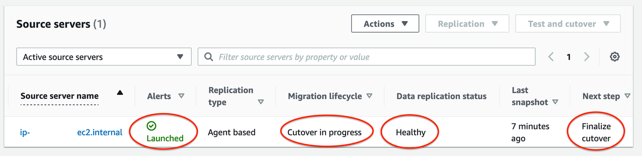
14.  Monitor the indicators to validate the success of the launch of your Cutover instance (shown in Figure 9):

  • Alerts column = Launched
  • Migration lifecycle column = Cutover in progress
  • Data replication status = Healthy
  • Next step column = Finalize cutover
Figure 9. Indicators for successful launch of Cutover instances

Figure 9. Indicators for successful launch of Cutover instances

15.  Test Cutover Instance:

  • Navigate to Amazon EC2 console > Instances (running)
  • Select Cutover instance
  • SSH/ RDP into your Cutover instance to confirm that it functions correctly
  • Validate connectivity and perform acceptance tests for your application
  • Revert Cutover if any issues

16.  Finalize the cutover after successful validation:

  • Navigate to AWS MGN console > Source servers page
  • Select source server > Open Test and Cutover menu
  • Under Cutover, choose Finalize Cutover
  • Finalize cutover for X servers > Finalize

17.  At this point, if your cutover is successful:

  • Migration lifecycle column = Cutover complete,
  • Data replication status column = Disconnected
  • Next step column = Mark as archived

The cutover is now complete and that the migration has been performed successfully. Data replication has also stopped and all replicated data will now be discarded.

Cleaning up

Archive your source servers that have launched Cutover instances to clean up your Source Servers page-

  • Navigate to Source Servers page (see Figure 10)
  • Select source server > Open Actions
  • Choose Mark as archived
  • Archive X server > Archive
Figure 10. Mark source servers as archived that are cutover

Figure 10. Mark source servers as archived that are cutover

Conclusion

In this post, we demonstrated how AWS MGN simplifies, expedites, and reduces the cost of migrating Amazon EC2-hosted workloads from one AWS Region to another. It integrates with AWS Migration Hub, enabling you to organize your servers into applications. You can track the progress of all your MGN at the server and app level, even as you move servers into multiple AWS Regions. Choose a Migration Hub Home Region for MGN to work with the Migration Hub.

Here are the AWS MGN supported AWS Regions. If your preferred AWS Region isn’t currently supported or you cannot install agents on your source servers, consider using CloudEndure Migration or AWS Server Migration Service respectively. CloudEndure Migration will be discontinued in all AWS Regions on December 30, 2022. Refer to CloudEndure Migration EOL for more information.

Note: Use of AWS MGN is free for 90 days but you will incur charges for any AWS infrastructure that is provisioned during migration and after cutover. For more information, refer to the pricing page.

Thanks for reading this blog post! If you have any comments or questions, feel free to put them in the comments section.

Deploying Sample UI Forms using React, Formik, and AWS CDK

Post Syndicated from Kevin Rivera original https://aws.amazon.com/blogs/architecture/deploying-sample-ui-forms-using-react-formik-and-aws-cdk/

Companies in many industries use UI forms to collect customer data for account registrations, online shopping, and surveys. It can be tedious to create form fields. Proper use of input validation can help users easily find and fix mistakes. Best practice is that users should not see a form filled with “this field is required” or “your email is invalid” errors until they have first attempted to complete the form.

Forms can be difficult to write, maintain, and test. They often have to be repeated in multiple areas on even the most basic interactive web application. Fortunately, third-party libraries provide front-end developers with tools to manage these complexities.

This blog post will describe an example solution for implementing simple forms for a user interface using the JavaScript libraries React and Formik. We will also use AWS resources to host the application. The blog will describe how the application is provisioned using the AWS Cloud Development Kit (CDK).

Our sample form and code

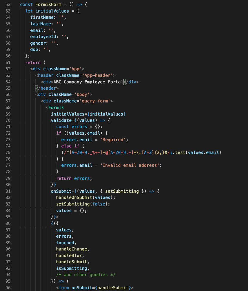
Our solution demonstrates a straightforward way for a front-end or full stack developer to rapidly create forms. We will show how a popular React form library, Formik, abstracts input field state management and reduces the amount of written code.

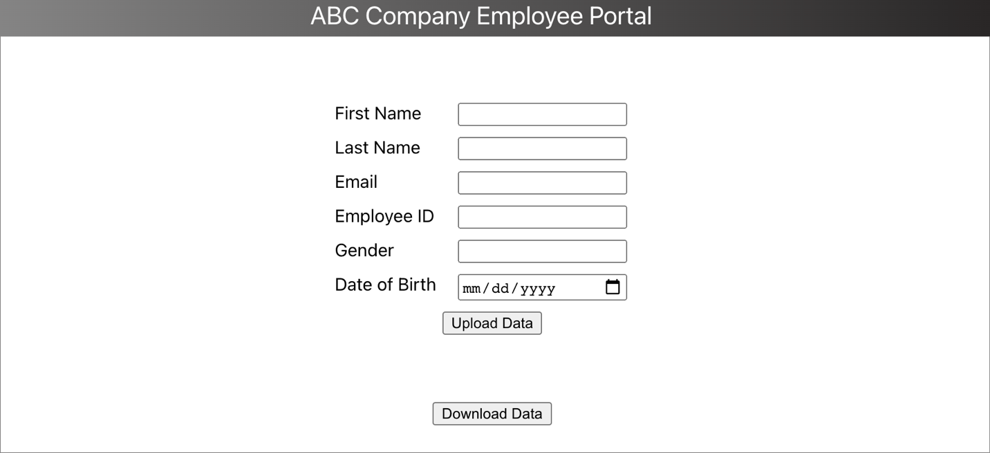
Our sample form will collect the user’s information (name, email, and date of birth) and store the data to a private Amazon S3 bucket for later retrieval using a presigned URL. The sample code gives developers a structure with which to build on and experiment. The code provides example integration with AWS services to host a React form application.

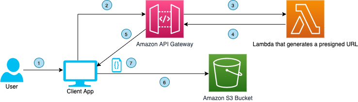
Figure 1 demonstrates how the user’s information flows through various AWS services and finally gets uploaded to private Amazon S3 bucket.

Figure 1. User interface communicating with API Gateway to upload a file to a S3 bucket using a presigned URL

Figure 1. User interface communicating with API Gateway to upload a file to a S3 bucket using a presigned URL

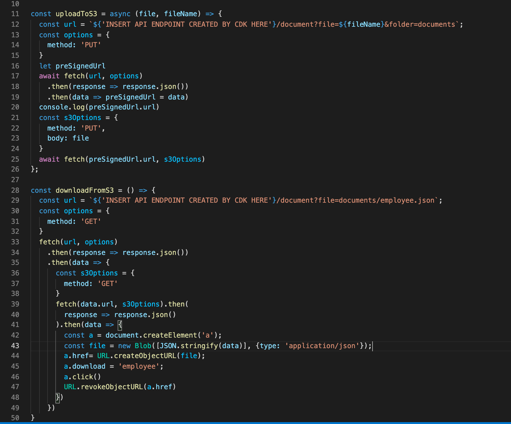
  1. Click the Upload button. The user visits the webpage, fills the form, and clicks the ‘Upload Data’ button
  2. HTTP request to Amazon API Gateway. The front end makes an HTTP request to the API Gateway
  3. Forward HTTP request. The API Gateway forwards the HTTP request to the Lambda function that generates a presigned URL for uploading data to a S3 bucket
  4. Presigned URL. The presigned URL for uploading data to a S3 bucket is returned by the Lambda function to the API Gateway as HTTP response.
  5. Forward HTTP response. The API Gateway forwards the presigned URL to the client application
  6. Upload data to Amazon S3. The client application uses the presigned URL to upload the form data to a S3 bucket

The code also demonstrates the flow of data when a download request is made by the user. The download process is shown in Figure 2.

Figure 2. User interface communicating with API Gateway to download a file from a S3 bucket using presigned URL

Figure 2. User interface communicating with API Gateway to download a file from a S3 bucket using presigned URL

  1. Click Download button. The user clicks the ‘Download Data’ button
  2. HTTP request to API Gateway. The front end makes an HTTP request to the API Gateway
  3. Forward HTTP request. The API Gateway forwards the HTTP request to the Lambda function that generates a presigned URL for downloading data from a S3 bucket
  4. Presigned URL. The presigned URL for downloading data from a S3 bucket is returned by the Lambda function to the API Gateway as HTTP response.
  5. Forward HTTP response. The API Gateway forwards the presigned URL to the client application
  6. Upload data to Amazon S3. The client application uses the presigned URL to download the form data to S3 bucket
  7. File downloads. The file downloads to user’s computer

Here are the four steps to demonstrate this solution:

  1. Provisioning the infrastructure (backend). The infrastructure will consist of:
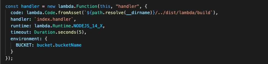
    • An AWS Lambda function, which will generate a presigned URL when requested by the UI and respond with the URL for uploading/downloading data
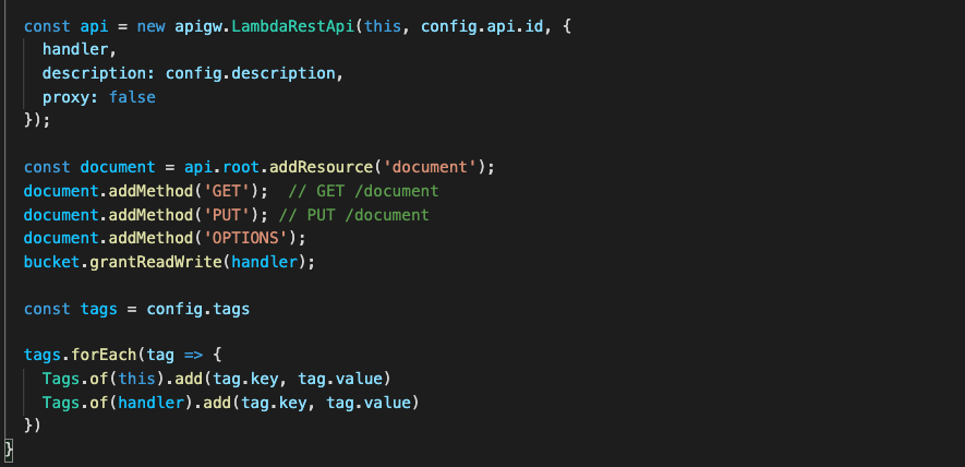
    • An API Gateway, which will handle the requests and responses from UI and Lambda
    • Two separate S3 buckets, which will host the static UI forms and store the uploaded data (different buckets for each).
  2. Deploying the front end. We will use sample React/Formik code on S3.
  3. Testing. Once our code is deployed, we will test the form by uploading a file though the UI, and then retrieve that file.
  4. Clean up. Finally, we will clean up the S3 bucket.

Prerequisites

For this walkthrough, you should have the following prerequisites:

Deploying the backend and front end

Clone code

The sample code for this application is available on GitHub. Clone the repo to follow along in a terminal.

git clone https://github.com/aws-samples/react-formik-on-aws

Install dependencies

Change the directory to the folder the clone created and install dependencies for the API.

cd formik-presigned-s3/ npm install

After installing the dependencies for the API, let’s install the dependencies in the UI.

cd ui/formik-s3-react-app
npm install

Bundling

Let’s bundle our Lambda function that currently exists in the index.js file inside the resources/lambda directory. This will create our Lambda function inside a directory that our stack can read from, to create the handler.

npx esbuild resources/lambda/index.js –bundle –platform=node –target=node12 –external:aws-sdk –outfile=dist/lambda/build/index.js

Let’s go into more detail about the function of the Lambda handler. As seen in Figure 3, the handler is using three helper functions that are written in the file (isExisted, fetchUploadUrl, fetchViewUrl). It creates a presigned URL for uploads/downloads of data, confirms that the URL was created, and fetches the URL. Lines 6874 are calling the helper functions based on the API request needed.

Figure 3. Lambda’s handler function for GET request type

Figure 3. Lambda’s handler function for GET request type

Build the React app

#Make sure you are in the ui/formik-s3-react-app directory
npm run build

This command will create your index.html file and its dependencies, which will be the source of your UI site. When we deploy our stack, we will inspect the CDK code. The Lambda bundler and the React app build step work together to source the directory and create the S3 bucket that will eventually host the React application.

Note: If you are deploying AWS CDK apps into an AWS environment, you must provision these resources for a specific location and account. In this case you must run the following command:

cdk bootstrap aws://<aws_account_number>/<aws_region>

This is the error that you will see if you do not bootstrap:

This stack uses assets, so the toolkit stack must be deployed to the environment (Run "cdk bootstrap aws://aws_account_number/aws_region")

Let’s deploy!

Before we run the deploy command, let’s understand what exactly we are deploying and the advantages of the CDK.

Note: We won’t go into depth on how the AWS CDK works, but we will demonstrate implementation of the code for our infrastructure and website hosting.

Our configuration code for deploying our CDK is found in the root directory in a file called cdk.json. It’s important that we can configure certain properties. This is where we map to our bin file that creates our CDK app. As you can see in Figure 4, the app key points to bin/formic-s3.ts.

Figure 4. cdk.json file

Figure 4. Contents of cdk.json file

Now let’s look at the CDK stack code, shown in Figure 5. This can be found in the lib directory of the root file and it is called formik-s3-stack.ts.

Figure 5. CDK stack code that creates a new S3 bucket for hosting the React webpage

Figure 5. CDK stack code that creates a new S3 bucket for hosting the React webpage

This is the part of the code that creates our S3 bucket for hosting our React UI. The first few lines create the bucket name and point to the file that will be seen by the world (index.html). The deployment function has a source that will be searching for the path in your local directory where the build files were created. This will source the directory and then create it in an S3 bucket in the cloud.

Notice how our publicReadAccess is commented out. This is because it is not best practice to leave your bucket exposed publicly. For this blog, we will host this simple form site and allow public access. However, a CDN such as Amazon CloudFront should be used for distribution of traffic to keep your S3 bucket secure.

Figure 6. CDK stack code that creates a new S3 bucket

Figure 6. CDK stack code that creates a new S3 bucket for uploading and downloading data using S3 presigned URL

Figure 6 shows the second S3 bucket that will be used for our Formik data.

Figure 7. CDK code stack used to create the Lambda function

Figure 7. CDK code stack used to create the Lambda function

Figure 7 shows how to create your Lambda function, which also will be reading from the ‘bundling’ step.

Figure 8. CDK code stack used to create API Gateway

Figure 8. CDK code stack used to create API Gateway

Figure 8 shows how to create your API Gateway resources. Notice the ‘OPTIONS’ document is used here. This is because our front-end request URLs are not from the same origin as our APIs. Including the ‘OPTIONS’ document enables our browser to succeed in its preflight request and avoid any CORS issues.

Now that we understand our CDK, let’s finally DEPLOY!

npx cdk deploy

You will receive the output in the terminal that will be the storage API endpoint. You can also view this in CloudFormation under the Output tab for the stack the CDK spun up (FormikS3Stack). You should also see your S3 URL to view your React app.

What is React’s form?

Once you have your URL, you should see the form, shown in Figure 9.

Figure 9. Portal form designed using Formik in ReactJS

Figure 9. Portal form designed using Formik in ReactJS

Why is Formik so special?

Let’s preface this with how our forms had to be created using the old method, shown in Figure 10.

Figure 10. This is from https://www.bitnative.com/2020/08/19/formik-vs-plain-react-for-forms-worth-it/ showing a form without Formik

Figure 10. This is from https://www.bitnative.com/2020/08/19/formik-vs-plain-react-for-forms-worth-it/ showing a form without Formik

Figure 11 shows our code:

Figure 11. React code with the UI components

Figure 11. React code with the UI components

One of the first things you can notice when comparing both methods, is the location of your initial values. Formik handles the state of your fields. Without it, we would need to manage this with React’s state object if we were using class components, or with hooks inside functional components. With Formik, we don’t have to handle these tasks.

Another benefit of using Formik is its handling of input validation, errors, and handler functions that we can use to manage our UI (lines 7079 and 8793.) Formik reduces the need to write extra lines of code to handle validation and errors, managing states, and creating event handler logic.

Read this blog post that compares both methods of creating forms.

Making our API calls from the UI

Our Formik form is simple to implement, but one more step remains. We need to handle uploading the information, and then downloading it.

With all our resources created and our form done, we put it all together by creating our API requests, shown in Figure 12.

Figure 12. Code to upload to S3 bucket and download from S3 bucket

Figure 12. Code to upload to S3 bucket and download from S3 bucket

Due to the efficiency of AWS and Formik, we can upload and download with fewer than 50 lines of code.

Lines 1126 is where we call our API Gateway URL that our CDK created for us. With this API, when the user first clicks the upload button, the request hits the endpoint to create the presigned URL. It waits for its creation and in lines 2125 we PUT our data into our S3 bucket.

Lastly, we are able to hit that same presigned URL to download our information we uploaded into a JSON file.

Cleaning up

To avoid incurring future charges, delete the resources. Let’s run:

npx cdk destroy

You can confirm the removal by going into CloudFormation and confirming the resources were deleted.

Conclusion

In this blog post, we learned how we can create a simple server for our form submissions. We spun it up easily with the CDK toolkit and provisioned our resources. We hosted our UI and created a sample form using Formik, which handles state and reduces the amount of code we must write. We then hit the endpoints given to us by the deployment and tested the app by uploading and downloading our form data. Traditional form data management requires a separate function for handling data and errors in forms. This is a cleaner and more efficient way to handle form data.

For further reading:

Running IBM MQ on AWS using High-performance Amazon FSx for NetApp ONTAP

Post Syndicated from Senthil Nagaraj original https://aws.amazon.com/blogs/architecture/running-ibm-mq-on-aws-using-high-performance-amazon-fsx-for-netapp-ontap/

Many Amazon Web Services (AWS) customers use IBM MQ on-premises and are looking to migrate it to the AWS Cloud. For persistent storage requirements with IBM MQ on AWS, Amazon Elastic File System (Amazon EFS) can be used for distributed storage and to provide high availability. The AWS QuickStart to deploy IBM MQ with Amazon EFS is an architecture used for applications where the file system throughput requirements are within the Amazon EFS limits.

However, there are scenarios where customers need increased capacity for their IBM MQ workloads. These could be applications that rely heavily on IBM MQ, which result in a much higher message data throughput. This means that the persistent messages must be written to and read from the shared file system more frequently. IBM MQ facilitates writing log information into the shared file system. These are two such situations where such application requirements translate to a higher number of read/write operations.

For applications using IBM MQ and requiring a higher file system throughput, Amazon provides Amazon FSx for NetApp ONTAP. This is a fully managed shared storage in the AWS Cloud, with the popular data access and management capabilities of ONTAP.

This blog explains how to use Amazon FSx for NetApp ONTAP for distributed storage and high availability with IBM MQ. Read more about Amazon FSx for NetApp ONTAP features, and performance details, throughput options, and performance tips.

Overview of IBM MQ architecture on AWS

For recovering queue data upon failure, you can set up IBM MQ with high availability.

The solution architecture is shown in Figure 1. This blog post assumes familiarity with AWS services such as Amazon EC2, VPCs, and subnets. For additional information on these topics, see the AWS documentation.

Figure 1. IBM MQ with Amazon FSx NetApp ONTAP

Figure 1. IBM MQ with Amazon FSx NetApp ONTAP

  1. IBM MQ is deployed in an Auto Scaling group spanning two Availability Zones.
  2. Amazon FSx NetApp ONTAP is used for data persistence and high availability of queue message data.
  3. Amazon FSx NetApp ONTAP is set up in the same Availability Zones as IBM MQ.
  4. Amazon FSx NetApp ONTAP provides automatic failover that is transparent to the application and completes in 60 seconds.

Considerations for the Amazon FSx NetApp ONTAP file system

When creating the Amazon FSx NetApp ONTAP file system as in Figure 1, consider the following:
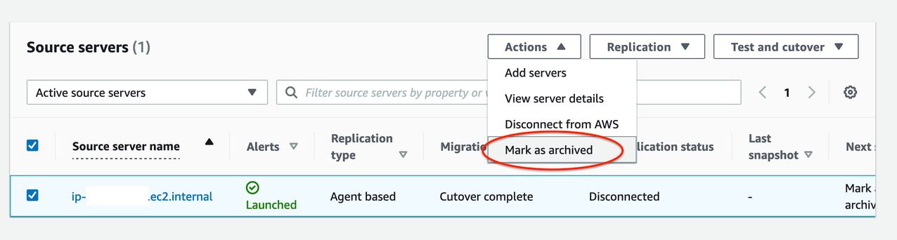
  1. The subnets used for the file system should have connectivity with the subnets where your IBM MQ is running. See VPC documentation.
  2. Ensure that the security group(s) used by the elastic network interfaces (ENI) for Amazon FSx allow communication with the IBM MQ environment. Read more about limiting access security groups.
  3. When choosing the storage capacity, IOPS, and throughput capacity, make sure it aligns to your application requirements.
  4. If you choose to use AWS Key Management System (KMS) encryption, configure those details correctly.
  5. Be sure to provide an appropriate name for the volume junction, as you will use it to mount the file system onto your IBM MQ instance(s).
  6. Choose appropriate backup and maintenance windows according to your application needs.

Mount the Amazon FSx NetApp ONTAP file system onto the instance(s) where IBM MQ is running. Use either the DNS name or the IP address for the file system, as well as the correct volume junction name while mounting. Configure IBM MQ to make use of this mount for persisting the queue data.

This mount point must be included when updating fstab for Linux machines. This will allow for the file system to be mounted automatically in case the instance restarts. For Windows, take the appropriate steps to mount the file system automatically upon restart.

Conclusion

In this post, you have learned how to use Amazon FSx NetApp ONTAP with IBM MQ to maximize queue data throughput, while continuing to have persistent message storage. You can provision the Amazon FSx NetApp ONTAP file system, and mount its volume junction onto the IBM MQ instance(s).

Build a reliable, scalable, and cost-efficient IBM MQ solution on AWS, by using the fully elastic features that Amazon FSx NetApp ONTAP provides.

Related information:

How to Audit and Report S3 Prefix Level Access Using S3 Access Analyzer

Post Syndicated from Somdeb Bhattacharjee original https://aws.amazon.com/blogs/architecture/how-to-audit-and-report-s3-prefix-level-access-using-s3-access-analyzer/

Data Services teams in all industries are developing centralized data platforms that provide shared access to datasets across multiple business units and teams within the organization. This makes data governance easier, minimizes data redundancy thus reducing cost, and improves data integrity. The central data platform is often built with AWS Simple Storage Service (S3).

A common pattern for providing access to this data is for you to set up cross-account IAM Users and IAM Roles to allow direct access to the datasets stored in S3 buckets. You then enforce the permission on these datasets with S3 Bucket Policies or S3 Access Point policies. These policies can be very granular and you can provide access at the bucket level, prefix level as well as object level within an S3 bucket.

To reduce risk and unintended access, you can use Access Analyzer for S3 to identify S3 buckets within your zone of trust (Account or Organization) that are shared with external identities. Access Analyzer for S3 provides a lot of useful information at the bucket level but you often need S3 audit capability one layer down, at the S3 prefix level, since you are most likely going to organize your data using S3 prefixes.

Common use cases

Many organizations need to ingest a lot of third-party/vendor datasets and then distribute these datasets within the organization in a subscription-based model. Irrespective of how the data is ingested, whether it is using AWS Transfer Family service or other mechanisms, all the ingested datasets are stored in a single S3 bucket with a separate prefix for each vendor dataset. The hierarchy can be represented as:

vendor-s3-bucket
       ->vendorA-prefix
               ->vendorA.dataset.csv
       ->vendorB-prefix
               ->vendorB.dataset.csv

Based on this design, access is also granted to the data subscribers at the S3 prefix level. Access Analyzer for S3 does not provide visibility at the S3 prefix level so you need to develop custom scripts to extract this information from the S3 policy documents. You also need the information in an easy-to-consume format, for example, a csv file, that can be queried, filtered, readily downloaded and shared across the organization.

To help address this requirement, we show how to implement a solution that builds on the S3 access analyzer findings to generate a csv file on a pre-configured frequency. This solution provides details about:

  • External Principals outside your trust zone that have access to your S3 buckets
  • Permissions granted to these external principals (read, write)
  • List of s3 prefixes these external principals have access to that is configured using S3 bucket policy and/or S3 access point policies.

Architecture Overview

Architecture Diagram showing How to Audit and Report S3 prefix level access using S3 Access Analyzer

Figure 1 – How to Audit and Report S3 prefix level access using S3 Access Analyzer

The solution entails the following steps:

Step 1 – The Access Analyzer ARN and the S3 bucket parameters are passed to an AWS Lambda function via Environment variables.

Step 2 – The Lambda code uses the Access Analyzer ARN to call the list-findings API to retrieve the findings information and store it in the S3 bucket (under json prefix) in JSON format.

Step 3 – The Lambda function then also parses the JSON file to get the required fields and store it as a csv file in the same S3 bucket (under report prefix). It also scans the bucket policy and/or the access point policies to retrieve the S3 prefix level permission granted to the external identity. That information is added to the csv file.

Steps 4 and 5 – As part of the initial deployment, an AWS Glue crawler is provided to discover and create the schema of the csv file and store it in the AWS Glue Data Catalog.

Step 6 – An Amazon Athena query is run to create a spreadsheet of the findings that can be downloaded and distributed for audit.

Prerequisites

For this walkthrough, you should have the following prerequisites:

  • An AWS account
  • S3 buckets that are shared with external identities via cross-account IAM roles or IAM users.  Follow these instructions in this user guide to set up cross-account S3 bucket access.
  • IAM Access Analyzer enabled for your AWS account. Follow these instructions to enable IAM Access Analyzer within your account.

Once the IAM Access Analyzer is enabled, you should be able to view the Analyzer findings from the S3 console by selecting the bucket name and clicking on the ‘View findings’ box or directly going to the Access Analyzer findings on the IAM console.

When you select a ‘Finding id’ for an S3 Bucket, a screen similar to the following will appear:

Figure 2 - IAM Console Screenshot

Figure 2 – IAM Console Screenshot

Setup

Now that your access analyzer is running, you can open the link below to deploy the CloudFormation template. Make sure to launch the CloudFormation in the same AWS Region where IAM Access Analyzer has been enabled.

Launch template

Specify a name for the stack and input the following parameters:

  • ARN of the Access Analyzer which you can find from the IAM Console.
  • New S3 bucket where your findings will be stored. The Cloudformation template will add a suffix to the bucket name you provide to ensure uniqueness.
Figure 3 - CloudFormation Template screenshot

Figure 3 – CloudFormation Template screenshot

  • Select Next twice and on the final screen check the box allowing CloudFormation to create the IAM resources before selecting Create Stack.
  • It will take a couple of minutes for the stack to create the resources and launch the AWS Lambda function.
  • Once the stack is in CREATE_COMPLETE status, go to the Outputs tab of the stack and note down the value against the DataS3BucketName key. This is the S3 bucket the template generated. It would be of the format analyzer-findings-xxxxxxxxxxxx. Go to the S3 console and view the contents of the bucket.
    There should be two folders archive/ and report/. In the report folder you should have the csv file containing the findings report.
  • You can download the csv directly and open it in a excel sheet to view the contents. If would like to query the csv based on different attributes, follow the next set of steps.
    Go to the AWS Glue console and click on Crawlers. There should be an analyzer-crawler created for you. Select the crawler to run it.
  • After the crawler runs successfully, you should see a new table, analyzer-report created under analyzerdb Glue database.
  • Select the tablename to view the table properties and schema.
  • To query the table, go to the Athena console and select the analyzerdb database. Then you can run a query like “Select * from analyzer-report where externalaccount = <<valid external account>>” to list all the S3 buckets the external account has access to.
Figure 4 - Amazon Athena Console screenshot

Figure 4 – Amazon Athena Console screenshot

The output of the query with a subset of columns is shown as follows:

Figure 5 - Output of Amazon Athena Query

Figure 5 – Output of Amazon Athena Query

This CloudFormation template also creates a Cloudwatch event rule, testanalyzer-ScheduledRule-xxxxxxx, that launches the Lambda function every Monday to generate a new version of the findings csv file. You can update the rule to set it to a frequency you desire.

Clean Up

To avoid incurring costs, remember to delete the resources you created. First, manually delete the folders ‘archive’ and ‘report’ in the S3 bucket and then delete the CloudFormation stack you deployed at the beginning of the setup.

Conclusion

In this blog, we showed how you can build audit capabilities for external principals accessing your S3 buckets at a prefix level. Organizations looking to provide shared access to datasets across multiple business units will find this solution helpful in improving their security posture. Give this solution a try and share your feedback!

How to Run Massively Scalable ADAS Simulation Workloads on CAEdge

Post Syndicated from Hendrik Schoeneberg original https://aws.amazon.com/blogs/architecture/how-to-run-massively-scalable-adas-simulation-workloads-on-caedge/

This post was co-written by Hendrik Schoeneberg, Sr. Global Big Data Architect, The An Binh Nguyen, Product Owner for Cloud Simulation at Continental, Autonomous Mobility – Engineering Platform, Rumeshkrishnan Mohan, Global Big Data Architect, and Junjie Tang, Principal Consultant at AWS Professional Services.

AV/ADAS simulations processing large-scale field sensor data such as radar, lidar, and high-resolution video come with many challenges. Typically, the simulation workloads are spiky with occasional, but high compute demands, so the platform must scale up or down elastically to match the compute requirements. The platform must be flexible enough to integrate specialized ADAS simulation software, use distributed computing or HPC frameworks, and leverage GPU accelerated compute resources where needed.

Continental created the Continental Automotive Edge (CAEdge) Framework to address these challenges. It is a modular multi-tenant hardware and software framework that connects the vehicle to the cloud. You can learn more about this in Developing a Platform for Software-defined Vehicles with Continental Automotive Edge (CAEdge) and Developing a platform for software-defined vehicles (re:Invent session-AUT304).

In this blog post, we’ll illustrate how the CAEdge Framework orchestrates ADAS simulation workloads with Amazon Managed Workflows for Apache Airflow (MWAA). We’ll show how it delegates the high-performance workloads to AWS Batch for elastic, highly scalable, and customizable compute needs. We’ll showcase the “bring your own software-in-the-loop” (BYO-SIL) pattern, detailing how to leverage specialized and proprietary simulation software in your workflow. We’ll also demonstrate how to integrate the simulation platform with tenant data in the CAEdge framework. This orchestrate and delegate pattern has previously been introduced in Field Notes: Deploying Autonomous Driving and ADAS Workloads at Scale with Amazon Managed Workflows for Apache Airflow and the Reference Architecture for Autonomous Driving Data Lake.

Solution overview for autonomous driving simulation

The following diagram shows a high-level overview of this solution.

Figure 1. Architecture diagram for autonomous driving simulation

Figure 1. Architecture diagram for autonomous driving simulation

It can be broken down into five major parts, illustrated in Figure 1.

  1. Simulation API: Amazon API Gateway (label 1) provides a REST API for authenticated users to schedule or monitor simulation. It runs on Amazon Managed Workflows for Apache Airflow (MWAA) using AWS Lambda (label 2).
  2. Simulation control plane: The simulation control plane (label 3) built on MWAA enables users to design and initiate workflows and integrate with AWS services.
  3. Scalable compute backend: We leverage the parallelization and elastic scalability capabilities of AWS Batch to distribute the workload (label 4). Additionally, we want to be able to run proprietary software components as part of the simulation workflows and use highly customizable Amazon EC2 compute environments. For example, we can use GPU acceleration or Graviton-based instances for workloads that must run on ARM, instead of x86 architectures.
  4. Autonomous Driving Data Lake (ADDL) integration: The simulations’ input and output data will be stored in a data lake (label 5) on Amazon S3. To provide efficient read and write access, data gets copied before each simulation run using RAID0 bundled ephemeral instance storage drives. After the simulation, results are written back to the data lake and are ready for reporting and analytics. We use AWS Lake Formation for metadata storage, data cataloging, and permission handling.
  5. Automated deployment: The solution architecture’s deployment is fully automated using a CI/CD pipeline in AWS CodePipeline and AWS CodeBuild (label 6). We can then perform automated testing and deployment to multiple target environments.

In this blog we will focus on the simulation control plane, scalable compute backend, and ADDL integration.

Simulation control plane

In a typical simulation, there are tasks like data movement (copying input data and persisting the results). These steps can require high levels of parallelization or GPU support. In addition, they can involve third-party or proprietary software, specialized runtime environments, or architectures like ARM. To facilitate all task requirements, we will delegate task initiation to the AWS services that best match the requirements. Correct sequence of tasks is achieved by an orchestration layer. Decoupling the simulation orchestration from task initiation follows the key design pattern to separate concerns. This enables the architecture to be adapted to specific requirements.

For the high-level task orchestration, we’ll introduce a simulation control plane built on MWAA. Modeling all simulation tasks in a directed acyclic graph (DAG), MWAA performs scheduling and task initiation in the correct sequence. It also handles the integration with AWS’ services. You can intuitively monitor and debug the progress of a simulation run across different services and networks. For the workflow within CAEdge, we’ll use AWS Batch to run simulations that are packaged as Docker containers.

Parameterizable workflows: Airflow supports parameterization of DAGs by providing a JSON object when triggering a DAG run that can be accessed at runtime. This enables us to create a simulation execution framework in which we model the simulation steps. It lets you specify the simulations’ parameters such as which Docker container to execute, runtime configuration, or input and output data locations, see Figures 2 and 3.

Figure 2. Specify simulations’ parameters in JSON

Figure 2. Specify simulations’ parameters in JSON

Figure 3. Read simulations’ parameters from JSON

Figure 3. Read simulations’ parameters from JSON

Scalable compute backend

Publishing the Docker image: To run a simulation, you must provide a Docker container in Amazon Elastic Container Registry (ECR). Manually push Docker images to ECR using the command line interface (CLI) or using CI/CD pipeline automation.

Choosing the compute option: Containers at AWS describes the services options for developers. Various factors can contribute to your decision-making. For the CAEdge platform, we want to run thousands of containers with fine-grained control over the underlying compute instance’s configuration. We also want to run containers in privileged mode, so AWS Batch on EC2 is a great match. Figure 4 outlines the compute backend’s architecture.

Figure 4. Compute backend architecture diagram

Figure 4. Compute backend architecture diagram

To run a Docker container on AWS Batch, we need three components: A job definition, a compute environment, and a job queue. The AWS Batch job definition specifies which job to run and how to run it. For example, we can define the Docker image to use, and specify the vCPU and memory configuration. The job definition will be submitted to a job queue, which in turn is linked to one or more compute environments. The compute environment specifies the compute configuration used to run a containerized workload, in addition to instance types and storage configurations. Creating a compute environment describes this more in detail. In the section ‘ADDL integration,’ we’ll describe how to select and configure the EC2 container instances to maximize network and disk I/O.

The AWS Batch array job feature can spin up thousands of independent, but similarly configured jobs. Instead of submitting a single job for each input file from the simulation control plane, we can instead submit a single array job. This provides the collection of input files as input. AWS Batch can spin up child jobs to process each entry of the collection in parallel, reducing operational overhead drastically.

With these components, we can now submit a job definition to a job queue from the simulation control plane, which will initiate on the corresponding compute environment.

ADDL integration

In the CAEdge platform, all simulation recordings and their metadata are stored and cataloged in the data lake. On average, single recordings are around 100 GB in size with simulation requests containing 100–300 recordings. A simulation request can therefore require 10–30 TB of data movement from S3 to the containers before the simulation starts. The containers’ performance will directly depend on I/O performance, as the input data is read and processed during execution. To provide the highest performance of data transfer and simulation workload, we need data storage options that maximize network and disk I/O throughput.

Choosing the storage option: For CAEdge’s simulation workloads, the storage solution acts as a temporary scratch space for the simulation containers’ input data. It should maximize I/O throughput. These requirements are met in the most cost-efficient way by choosing EC2 instances of the M5d family and their attached instance storage.

The M5d are general-purpose instances with NVMe-based SSDs, which are physically connected to the host server and provide block-level storage coupled to the lifetime of the instance. As described in the previous section, we configured AWS Batch to create compute environments using EC2’s M5d instances. While other storage options like Amazon Elastic File System (EFS) and Amazon Elastic Block Storage (EBS) can scale to match even demanding throughput scenarios, the simulation benefits from a high-performance, temporary storage location that is directly attached to the host.

Bundling the volumes: M5d instances can have multiple NVMe drives attached, depending on their size and storage configuration. To provide a single stable storage location for the simulation containers, bundle all attached NVMe SSDs into a single RAID0 volume during the instance’s launch, using a modified user data script. With this, we can provide a fixed storage location that can be accessed from the simulation containers. Additionally, we are distributing I/O operations evenly across all disks in the RAID0 configuration, which improves the read and write performance.

KPIs used for measurement

The SIL factor tells you how long the simulation takes compared to the duration of the recorded data.

SIL factor example:

  • For a recording with 60 minutes of data and a simulation duration of 120 minutes, the resulting SIL factor is 120 / 60 = 2. The simulation runs twice as long as real time.
  • For a recording with 60 minutes of data and a simulation duration of 60 minutes, the resulting SIL factor is 60 / 60 = 1. The simulation runs in real time.

Similarly, the aggregated SIL factor tells you how long the simulation for multiple recordings takes compared to the duration of the recorded data. It also factors in the horizontal scaling capabilities.

Aggregated SIL factor example:

  • For 3 recordings with 60 minutes of data and an overall simulation duration of 120 minutes, the resulting SIL factor is 120 / 3 * 60 = 0.67. The overall simulation is a third faster than real time.

Performance results

The storage optimizations described in the ADDL integration KPI section preceding, led to an improvement of the overall simulation duration of 50%. To benchmark the overall simulation platform’s performance, we created a simulation run with 15 recordings. The simulation run completed successfully with an aggregated SIL factor of 0.363, or, alternatively put, the simulation was roughly three times faster than real time. During production use, the platform will handle simulation runs with an average of 100-300 recordings. For these runs, the aggregated SIL factor is expected to be even smaller, as more simulations can be processed in parallel.

Conclusion

In this post, we showed how to design a platform for ADAS simulation workloads using the Bring Your Own Software-In-the-Loop (BYO-SIL) concept. We covered the key components including simulation control plane, scalable compute backend, and ADDL integration based on Continental Automotive Edge (CAEdge). We discussed the key performance benefits due to horizontal scalability and how to choose an optimized storage integration pattern. This led to an improvement of the overall simulation duration of 50%.

Let’s Architect! Architecting for Machine Learning

Post Syndicated from Luca Mezzalira original https://aws.amazon.com/blogs/architecture/architecting-for-machine-learning/

Though it seems like something out of a sci-fi movie, machine learning (ML) is part of our day-to-day lives. So often, in fact, that we may not always notice it. For example, social networks and mobile applications use ML to assess user patterns and interactions to deliver a more personalized experience.

However, AWS services provide many options for the integration of ML. In this post, we will show you some use cases that can enhance your platforms and integrate ML into your production systems.

Dynamic A/B testing for machine learning models with Amazon SageMaker MLOps projects

Performing A/B testing on production traffic to compare a new ML model with the old model is a recommended step after offline evaluation.

This blog post explains how A/B testing works and how it can be combined with multi-armed bandit testing to gradually send traffic to the more effective variants during the experiment. It will teach you how to build it with AWS Cloud Development Kit (AWS CDK), architect your system for MLOps, and automate the deployment of the solutions for A/B testing.

This diagram shows the iterative process to analyze the performance of ML models in online and offline scenarios.

This diagram shows the iterative process to analyze the performance of ML models in online and offline scenarios

Enhance your machine learning development by using a modular architecture with Amazon SageMaker projects

Modularity is a key characteristic for modern applications. You can modularize code, infrastructure, and even architecture.

A modular architecture provides an architecture and framework that allows each development role to work on their own part of the system, and hide the complexity of integration, security, and environment configuration. This blog post provides an approach to building a modular ML workload that is easy to evolve and maintain across multiple teams.

A modular architecture allows you to easily assemble different parts of the system and replace them when needed

A modular architecture allows you to easily assemble different parts of the system and replace them when needed

Automate model retraining with Amazon SageMaker Pipelines when drift is detected

The accuracy of ML models can deteriorate over time because of model drift or concept drift. This is a common challenge when deploying your models to production. Have you ever experienced it? How would you architect a solution to address this challenge?

Without metrics and automated actions, maintaining ML models in production can be overwhelming. This blog post shows you how to design an MLOps pipeline for model monitoring to detect concept drift. You can then expand the solution to automatically launch a new training job after the drift was detected to learn from the new samples, update the model, and take into account the changes in the data distribution.

Concept drift happens when there is a shift in the distribution. In this case, the distribution of the newly collected data (in blue) starts differing from the baseline distribution (in green)

Concept drift happens when there is a shift in the distribution. In this case, the distribution of the newly collected data (in blue) starts differing from the baseline distribution (in green)

Architect and build the full machine learning lifecycle with AWS: An end-to-end Amazon SageMaker demo

Moving from experimentation to production forces teams to move fast and automate their operations. Adopting scalable solutions for MLOps is a fundamental step to successfully create production-oriented ML processes.

This blog post provides an extended walkthrough of the ML lifecycle and explains how to optimize the process using Amazon SageMaker. Starting from data ingestion and exploration, you will see how to train your models and deploy them for inference. Then, you’ll make your operations consistent and scalable by architecting automated pipelines. This post offers a fraud detection use case so you can see how all of this can be used to put ML in production.

The ML lifecycle involves three macro steps: data preparation, train and tuning, and deployment with continuous monitoring.

The ML lifecycle involves three macro steps: data preparation, train and tuning, and deployment with continuous monitoring

See you next time!

Thanks for reading! We’ll see you in a couple of weeks when we discuss how to secure your workloads in AWS.

Looking for more architecture content? AWS Architecture Center provides reference architecture diagrams, vetted architecture solutions, Well-Architected best practices, patterns, icons, and more!

Other posts in this series

How UnitedHealth Group Improved Disaster Recovery for Machine-to-Machine Authentication

Post Syndicated from Vinodh Kumar Rathnasabapathy original https://aws.amazon.com/blogs/architecture/how-unitedhealth-group-improved-disaster-recovery-for-machine-to-machine-authentication/

This blog post was co-authored by Vinodh Kumar Rathnasabapathy, Senior Manager of Software Engineering, UnitedHealth Group. 

Engineers who use Amazon Cognito for machine-to-machine authentication select a primary Region where they deploy their application infrastructure and the Amazon Cognito authorization endpoint. Amazon Cognito is a highly available service in single Region deployments with a published service-level agreement (SLA) target of 99.9%. The UnitedHealth Group (UHG) team needed a solution that would enable them to build and deploy their applications in multiple Regions to achieve higher availability targets. A multi-Region application architecture would also allow UHG engineers to failover to a secondary Region in the event that their application experienced issues in the primary Region.

At UHG, Federated Data Services (FDS) is a business-critical customer-facing application, which requires 99.95% availability and disaster recovery features. The FDS engineering team needed their Amazon Cognito infrastructure to be highly available in case of any service events in AWS Regions, along with having greater flexibility of switching between Regions.

The FDS engineering team worked on a custom solution using existing AWS services to fulfill their availability and recovery requirements. This solution not only serves the purpose of their current business needs but also provides recovery in case of any future disaster.

Overview of the solution

In this solution, we select two AWS Regions which will include the primary Region and the failover Region. Amazon Cognito app clients (including client ID and client secret pair) are created in both Regions and stored in an Amazon DynamoDB table. Client applications are given the client ID and client secret of the primary Region. Optionally, an application-generated ID and secret can be provided to the client to conceal the actual Amazon Cognito client ID and client secret. The process is as follows:

  • The client application (machine) initiates an authentication request by sending the Amazon Cognito app client ID and client secret to an Amazon Route 53 domain record.
  • Route 53 routes authentication requests to the in-Region Amazon API Gateway utilizing a Simple routing policy. From there, API Gateway shuts down the TLS connection using AWS Certificate Manager (ACM), and serves as a proxy for the authentication request to AWS Lambda.
  • AWS Lambda verifies the client ID and client secret, and uses them to look up the in-Region client ID and client secret.
  • Lambda uses preconfigured environment variables to request the appropriate Region from DynamoDB.
  • AWS Lambda then passes the returned app client credentials to the in-Region Amazon Cognito deployment. Amazon Cognito verifies the client ID and client secret, and returns an access token to the Lambda function.
  • The client application (machine) can now use this token to access downstream applications.
  • The client authentication process in the secondary (failover) Region is the same, with one exception. In the secondary Region, the Lambda environment variables retrieve app client credentials from the DynamoDB database for the secondary Region Amazon Cognito instance.

To initiate a failover between Regions, the Route 53 domain record needs to be pointed to the secondary Region API Gateway Regional endpoint. The downstream application’s Amazon Cognito configuration files must also be updated to point to the secondary Region Amazon Cognito instance. Alerts can be enabled using Amazon CloudWatch alarms to notify system operators of issues that may warrant a failover (a manual process to help system operators decide when to failover). The entire failover process takes just a couple of seconds for DNS to switch over and for the application to start accepting tokens from the secondary Region. This failover process could be automated based on generated alerts.

This architecture is suitable for a hot standby, active-passive type of application deployment. It is important to note that independent Amazon Cognito environments are being used in each Region, so you will need to set up your application to failover to the secondary Region for authentication. For example, your backend should be able to accept and validate access tokens from both primary and secondary Amazon Cognito user pools. To learn more about disaster recovery options in AWS, visit Disaster recovery options in the cloud.

Architecture overview

Figure 1 shows you how to build a multi-Region machine-to-machine architecture using Amazon Cognito, which uses DynamoDB global tables to perform the data replication. A Lambda function is utilized to retrieve the credentials for the active Region that the application is operating in, and a Regional Amazon Cognito endpoint returns the required token.

Figure 1. Multi-Region Amazon Cognito machine-to-machine architecture

Figure 1. Multi-Region Amazon Cognito machine-to-machine architecture

Process flow

  1. The Route53 domain record for the authentication proxy service is given to the client application and pointed at the API Gateway Regional endpoint. The client passes primary Region app client credentials to the API Gateway.
  2. API Gateway passes Lambda the client ID and client secret pair.
  3. Lambda does a lookup in DynamoDB to verify the client ID and client secret. After the identity is confirmed, Lambda uses Region-based environment variables to identify if the client should be using the primary Region or secondary Region for authenticating to Amazon Cognito. Lambda retrieves the Region-based client ID and client secret from DynamoDB.
  4. Lambda passes the Region-based app ID and secret to Amazon Cognito, which verifies the client ID and client secret, and returns an access token to the Lambda function.
  5. Lambda passes the access token from the Regional Amazon Cognito environment back to the client to be used against Region-based backend applications.

Prerequisites

For this walkthrough, you should have the following prerequisites:

Note: Ensure that you are following your organization’s security best practices while deploying this architecture.

Implementation

This implementation will focus on the Lambda logic that is used to retrieve user credentials based on Lambda environment variables. We will share snippets of the Lambda function code so you can create the logic necessary to enable multi-Region application architecture using Amazon Cognito app clients. In addition to the Lambda function, you will also need to create and configure the following resources using security implementation designated by your organization:

  1. DynamoDB table with fields primaryClientID, primaryClientSecret, secondaryClientID, and secondaryClientSecret.
    1. Because this table is used to store secrets, make sure encryption is enabled and you follow Security Best Practices for Amazon DynamoDB and your organization’s security best practices.
    2. Enable DynamoDB global tables.
  1. API Gateway Regional endpoint with TLS encryption using ACM.
  2. Route53 domain record routing traffic to Regional API Gateway.
  3. Downstream application configuration pointing at the Regional Amazon Cognito endpoint.
  4. IAM role that grants access from Lambda to DynamoDB.

Now let’s configure our Lambda function using Node.js language. Within the Lambda console create a new Lambda function that you will author from scratch. Select the Node.js runtime and change the runtime Lambda execution role to the IAM role that you have created for Lambda. Next, we will walk through the Lambda function code and configuration.

  1. Attach your new IAM role as a Lambda runtime role that will grant your Lambda function access to the DynamoDB table.
  2. Within the Lambda configuration environment variables, create several key-value variables in the Lambda function. The following are the environmental variables we will add.
    1. key: OAUTH_HOST_PRIMARY, value: https://${cognito-primary-region-domain-name}/oauth2/token
    2. key: OAUTH_HOST_SECONDARY, value: https://${cognito-secondary-region-domain-name}/oauth2/token
  1. Import the Node.js libraries using the following code.
"dependencies": {
    "aws-sdk": "^2.723.0",
    "aws-serverless-express": "^3.3.8",
    "axios": "^0.21.1",
    "base-64": "^1.0.0",
    "cors": "^2.8.5",
    "dotenv": "^8.2.0",
    "express": "^4.17.1",
    "jsonwebtoken": "^8.5.1",
    "jwt-decode": "^2.2.0",
    }
  1. Parse data from the incoming client application authentication request.
router.post("/", async (request, response) => {
  const client_id = request.body["client_id"];
  const client_secret = request.body["client_secret"]
      
  const client = await dynamoDB.getClientCredentialById(client_id, client_secret);
    
  if (client === undefined) {
    return response.status(400).json({
       message:
          "Client not configured for in Cognito. Please check with support team",
        });
      }
    
   const client_credentials = getClientCredentials(client);
   let access_token = await authService.getJwtToken(client_credentials);
          
   response.send(access_token);
});
  1. Reference the environment variables to determine the Region that the Lambda function is operating in and set the Region as primary or secondary.
getClientCredentials = client => {
   return region === "us-east-1" ? { clientId: client.primaryClientId, clientSecret: client.primaryClientSecret, oAuthHost: config.OAUTH_HOST }
   : region === "us-east-2" ? { clientId: client.secondaryClientId, clientSecret: client.secondaryClientSecret, oAuthHost: config.OAUTH_HOST_EAST_2 }
   : {};
}
  1. Verify the client ID and client secret against the DynamoDB table and get the Region-based client ID and client secret.
const getClientCredentialById = async (client_id, client_secret) => {

  let params = {
    TableName: clientCredentialTable,
    Key: {
      primaryClientId: client_id,
      primaryClientSecret: client_secret,
    },
  };

  const clientCredential = await ddb.get(params).promise();
  return clientCredential.Item;
};
  1. Pass the Regional client ID and client secret to Amazon Cognito. You will receive an access token from Amazon Cognito.
   const base64ClientCredentials = base64.encode(
     client_credentials.clientId.concat(":").concat(client_credentials.clientSecret)
   );
   const headers = {
     "content-type": "application/x-www-form-urlencoded",
     authorization: "Basic " + base64ClientCredentials,
    };
    const data = "grant_type=client_credentials";
    
    // Post request to Cognito OAuth URL
    const token = await Axios.post(client_credentials.oAuthHost, data, { headers });
    return token.data;
 };
  1. Pass the access token from the Regional Amazon Cognito environment back to the client to be used against Region-based backend applications.
let access_token = await authService.getJwtToken(client_credentials);
 
  response.send(access_token);

New app client creation

You need to implement this Lambda function in both the primary and secondary Regions. Modify the environmental variables in the secondary Region with the secondary Region’s information.

To enroll a new client in this multi-Region architecture using Amazon Cognito we will go through the process as shown in the following illustration.

Figure 2. Creating a new app client

Figure 2. Creating a new app client

You need to create a new:

  1. App ID and secret in Amazon Cognito in the primary Region.
  2. App ID and secret in Amazon Cognito in the secondary Region.
  3. Item in DynamoDB table consisting of the Amazon Cognito credentials created: primaryClientID, primaryClientSecret, secondaryClientID, and secondaryClientSecret.

Failover process

In this blog post we are creating a hot standby, active-passive type of application deployment. You will need to ensure your application is configured to be able to use either the primary Region Amazon Cognito or the secondary Region Amazon Cognito environment. The process to failover between Regions consists of the following:
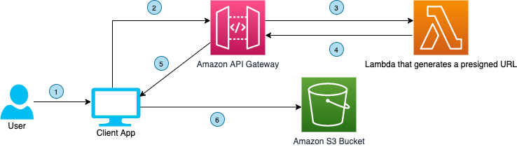
  1. Start application backend in the secondary Region.
  2. Reconfigure the application backend Amazon Cognito identity provider YAML file to point at the secondary Region Amazon Cognito identity provider.
  3. Modify the Route 53 domain record to point client applications at the secondary Region API Gateway Regional endpoint.

Cleaning up

In order to avoid unnecessary charges, please be sure to clean up any resources that were built as part of this architecture that are no longer in use.

Conclusion

In this blog post, we presented a solution that allows you to failover Amazon Cognito app clients from one AWS Region to another Region. The benefits of this architecture will allow you to have greater flexibility for running your Amazon Cognito app clients in the Region that is best suited for your use case. With this solution you now have the capability to failover Amazon Cognito app clients to a different AWS Region in the event of application or system errors.

Several variants of this solution can be implemented using the provided Lambda failover logic. You can store App ID and secret in AWS Secrets Manager. To learn more, see How to replicate secrets in AWS Secrets Manager to multiple Regions. You can also automate the failover process between primary and secondary Regions. To accomplish this, you will need to evaluate events which should cause a failover in your environment. Later, build the appropriate automation to failover your downstream application to the secondary Region Amazon Cognito deployment.

Amazon Cognito can be used for machine authentication as per the limits posted in Quotas in Amazon Cognito. Review the limits of number of app clients per user pool and the other applicable rate limits (for example, client credentials rate limits) and verify that these limits meet the needs of your application.

Optum’s Story

UnitedHealth Group (UHG) is the health and well-being company responsible for over 150 million lives globally. Optum, a part of UnitedHealth Group, is a health services business serving the healthcare marketplace, including payers, care providers, employers, governments, life sciences companies and consumers, through its OptumHealth, OptumInsight, OptumRx, and OptumServe businesses.

Federated Data Services (FDS) is the power behind the scenes that enables interoperability and secure transmission of personally identifiable information. It protects health information between lines of businesses, technology systems, applications, members and providers. With FDS, data is centralized, making it easier to share and retrieve by other systems. This assures businesses get a flexible and scalable solution that adapts to changes in technology and business needs.

Automate Amazon Connect Data Streaming using AWS CDK

Post Syndicated from Tarik Makota original https://aws.amazon.com/blogs/architecture/automate-amazon-connect-data-streaming-using-aws-cdk/

Many customers want to provision Amazon Web Services (AWS) cloud resources quickly and consistently with lifecycle management, by treating infrastructure as code (IaC). Commonly used services are AWS CloudFormation and HashiCorp Terraform. Currently, customers set up Amazon Connect data streaming manually, as the service is not available under CloudFormation resource types. Customers may want to extend it to retrieve real-time contact and agent data. Integration is done manually and can result in issues with IaC.

Amazon Connect contact trace records (CTRs) capture the events associated with a contact in the contact center. Amazon Connect agent event streams are Amazon Kinesis Data Streams that provide near real-time reporting of agent activity within the Amazon Connect instance. The events published to the stream include these contact control panel (CCP) events:
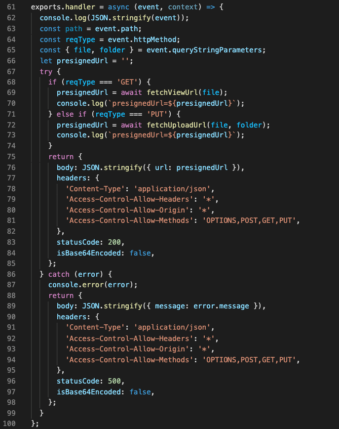
  • Agent login
  • Agent logout
  • Agent connects with a contact
  • Agent status change, such as to available to handle contacts, or on break, or at training.

In this blog post, we will show you how to automate Amazon Connect data streaming using AWS Cloud Development Kit (AWS CDK). AWS CDK is an open source software development framework to define your cloud application resources using familiar programming languages. We will create a custom CDK resource, which in turn uses Amazon Connect API. This can be used as a template to automate other parts of Amazon Connect, or for other AWS services that don’t expose its full functionality through CloudFormation.

Overview of Amazon Connect automation solution

Amazon Connect is an omnichannel cloud contact center that helps you provide superior customer service. We will stream Amazon Connect agent activity and contact trace records to Amazon Kinesis. We will assume that data will then be used by other services or third-party integrations for processing. Here are the high-level steps and AWS services that we are going use, see Figure 1:

  1. Amazon Connect: We will create an instance and enable data streaming
  2. Cloud Deployment Toolkit: We will create custom resource and orchestrate automation
  3. Amazon Kinesis Data Streams and Amazon Kinesis Data Firehose: To stream data out of Connect
  4. AWS Identity and Access Management (IAM): To govern access and permissible actions across all AWS services
  5. Third-party tool or Amazon S3: Used as a destination of Connect data via Amazon Kinesis data
Figure 1. Connect data streaming automation workflow

Figure 1. Connect data streaming automation workflow

Walkthrough and deployment tasks

Sample code for this solution is provided in this GitHub repo. The code is packaged as a CDK application, so the solution can be deployed in minutes. The deployment tasks are as follows:

  • Deploy the CDK app
  • Update Amazon Connect instance settings
  • Import the demo flow and data

Custom Resources enables you to write custom logic in your CloudFormation deployment. You implement the creation, update, and deletion logic to define the custom resource deployment.

CDK implements the AWSCustomResource, which is an AWS Lambda backed custom resource that uses the AWS SDK to provision your resources. This means that the CDK stack deploys a provisioning Lambda. Upon deployment, it calls the AWS SDK API operations that you defined for the resource lifecycle (create, update, and delete).

Prerequisites

For this walkthrough, you need the following prerequisites:

Deploy and verify

1. Deploy the CDK application.

The resources required for this demo are packaged as a CDK app. Before proceeding, confirm you have command line interface (CLI) access to the AWS account where you would like to deploy your solution.

  • Open a terminal window and clone the GitHub repository in a directory of your choice:
    git clone [email protected]:aws-samples/connect-cdk-blog
  • Navigate to the cdk-app directory and follow the deployment instructions. The default Region is usually us-east-1. If you would like to deploy in another Region, you can run:
    export AWS_DEFAULT_REGION=eu-central-1

2. Create the CloudFormation stack by initiating the following commands.

source .env/bin/activate
pip install -r requirements.txt
cdk synth
cdk bootstrap
cdk deploy  --parametersinstanceId={YOUR-AMAZON-CONNECT-INSTANCE-ID}

--parameters ctrStreamName={CTRStream}

--parameters agentStreamName={AgentStream}

Note: By default, the stack will create contact trace records stream [ctrStreamName] as a Kinesis Data Stream. If you want to use an Amazon Kinesis Data Firehose delivery stream instead, you can modify this behavior by going to cdk.json and adding “ctr_stream_type”: “KINESIS_FIREHOSE” as a parameter under “context.”

Once the status of CloudFormation stack is updated to CREATE_COMPLETE, the following resources are created:

  • Kinesis Data Stream
  • IAM roles
  • Lambda

3. Verify the integration.

  • Kinesis Data Streams are added to the Amazon Connect instance
Figure 2. Screenshot of Amazon Connect with Data Streaming enabled

Figure 2. Screenshot of Amazon Connect with Data Streaming enabled

Cleaning up

You can remove all resources provisioned for the CDK app by running the following command under connect-app directory:

cdk destroy

This will not remove your Amazon Connect instance. You can remove it by navigating to the AWS Management Console -> Services -> Amazon Connect. Find your Connect instance and click Delete.

Conclusion

In this blog, we demonstrated how to maintain Amazon Connect as Infrastructure as Code (IaC). Using a custom resource of AWS CDK, we have shown how to automate setting Amazon Kinesis Data Streams to Data Streaming in Amazon Connect. The same approach can be extended to automate setting other Amazon Connect properties such as Amazon Lex, AWS Lambda, Amazon Polly, and Customer Profiles. This approach will help you to integrate Amazon Connect with your Workflow Management Application in a faster and consistent manner, and reduce manual configuration.

For more information, refer to Enable Data Streaming for your instance.

Enhance Your Contact Center Solution with Automated Voice Authentication and Visual IVR

Post Syndicated from Soonam Jose original https://aws.amazon.com/blogs/architecture/enhance-your-contact-center-solution-with-automated-voice-authentication-and-visual-ivr/

Recently, the Accenture AWS Business Group (AABG) assisted a customer in developing a secure and personalized Interactive Voice Response (IVR) contact center experience that receives and processes payments and responds to customer inquiries.

Our solution uses Amazon Connect at its core to help customers efficiently engage with customer service agents. To ensure transactions are completed securely and to prevent fraud, the architecture provides voice authentication using Amazon Connect Voice ID and a visual portal to submit payments. The visual IVR feature allows customers to easily provide the required information online while the IVR is on standby. The solution also provides agents the information they need to effectively and efficiently understand and resolve callers’ inquiries, which helps improve the quality of their service.

Overview of solution

Our IVR is designed using Contact Flows on Amazon Connect and uses the following services:

  • Amazon Lex provides the voice-based intent analysis. Intent analysis is the process of determining the underlying intention behind customer interactions.
  • Amazon Connect integrates with other AWS services using AWS Lambda.
  • Amazon DynamoDB stores customer data.
  • Amazon Pinpoint notifies customers via text and email.
  • AWS Amplify provides the customized agent dashboard and generates the visual IVR portal.

Figure 1 shows how this architecture routes customer calls:

  1. Callers dial the main line to interact with the IVR in Amazon Connect.
  2. Amazon Connect Voice ID sets up a voiceprint for first time callers or performs voice authentication for repeat callers for added security.
  3. Upon successful voice authentication, callers can proceed to IVR self-service functions, such as checking their account balance or making a payment. Amazon Lex handles the voice intent analysis.
  4. When callers make a payment request, they are given the option to be handed off securely to a visual IVR portal to process their payment.
  5. If a caller requests to be connected to an agent, the agent will be presented with the customer’s information and IVR interaction details on their agent dashboard.
Architecture diagram

Figure 1. Architecture diagram

Customer IVR experience

Figure 2 describes how callers navigate through the IVR:

  1. The IVR asks the caller the purpose of the call.
  2. The caller’s answer is sent for voice intent analysis. The IVR also attempts to authenticate the caller’s voice using Amazon Connect Voice ID. If authenticated, the caller is automatically routed to the correct flow based on the analyzed intent.
    • For the “Account Balance” flow, the caller is provided the account balance information.
    • For the “Make a Payment” flow, the caller can use the IVR or a visual IVR portal to process the payment. Upon payment completion, the caller is immediately notified their transaction has completed via SMS or email. Both flows allow the caller to be transferred to an agent. The caller also has the option to be called back when an agent becomes available or choose a specific date and time for the callback.
Customer IVR experience diagram

Figure 2. Customer IVR experience diagram

The intelligent self-service IVR solution includes the following features:

  • The IVR can redirect callers to a payment portal for scenarios like making a payment while the IVR remains on standby.
  • IVR transaction tracking helps agents understand the current status of the caller’s transaction and quickly determines the caller’s situation.
  • Callers have the option to receive a call as soon as the next agent becomes available or they can schedule a time that works for them to receive a callback.
  • IVR activity logging gives agents a detailed summary of the caller’s actions within the IVR.
  • Transaction confirmation which notifies callers of successful transactions via SMS or email.

Solution walkthrough

Amazon Connect Voice ID authenticates a caller’s voice as an added level of security. It requires 30 seconds to create the initial enrollment voiceprint and 10 seconds of a caller’s voice to authenticate. If there is not enough net speech to perform the voice authentication, the IVR asks the caller more questions, such as their first name and last name, until it has collected enough net speech.

The IVR falls back to dual tone multi-frequency (DTMF) input for the caller’s credentials in case the system cannot successfully authenticate. This can include information like the last four digits of their national identification number or postal code.

In contact flows, you will enable voice authentication by adding the “Set security behavior” contact block and specifying the authentication threshold, as shown in Figure 3.

Set security behavior contact block

Figure 3. Set security behavior contact block

Figure 4 shows the “Check security status” contact block, which determines if the user has been successfully authenticated or not. It also shows results that it may return if the caller is not successfully authenticated, including, “Not authenticated,” “Inconclusive,” “Not enrolled,” “Opted out,” and “Error.”

Check security status contact block

Figure 4. Check security status contact block

Providing a personalized experience for callers

To provide a personalized experience for callers, sample customer data is stored in a DynamoDB table. A Lambda function queries this table when callers call the contact center. The query returns information about the caller, such as their name, so the IVR can offer a customized greeting.

Transaction tracking

The table can also query if a customer previously called and attempted to make a payment but didn’t complete it successfully. This feature is called “transaction tracking.” Here’s how it works:

  • When the caller progresses through the “make a payment” flow, a field in the table is updated to reflect their transaction’s status.
  • If the payment is abandoned, the status in the table remains open, and the IVR prompts the caller to pick up where they left off the next time they call.
  • Once they have successfully completed their payment, we update the status in the table to “complete.”
  • When the IVR confirms that the caller’s payment has gone through, they will receive a confirmation via SMS and email. A Lambda function in the contact flow receives the caller’s phone number and email address. Then it distributes the confirmation messages via Amazon Pinpoint.

If a call is escalated to an agent, the “Check contact attributes” contact block in Figure 5 helps to check the caller’s intent and provide the agent with a customized whisper.

Agent whisper sample contact flow

Figure 5. Agent whisper sample contact flow

Making payments via the payment portal

To make a payment, an Amazon Lex bot presents the caller with the option to provide payment details over the phone or through a visual IVR portal.

If they choose to use the visual IVR portal (Figure 6), they can enter their payment details while maintaining an open phone connection with the contact center, in case they need additional assistance. Here’s how it works:

  • When callers select to use the payment portal, it prompts a Lambda function that generates a universally unique identifier (UUID) and provides the caller a unique PIN.
  • The UUID and PIN are stored in the DynamoDB table along with the caller’s information.
  • Another Lambda function generates a secure link using the UUID. It then uses Amazon Pinpoint to send the link to the caller over text message to their phone number on record. When they open the link, they are prompted to enter their unique PIN.
  • Then, the webpage makes an API call that validates the payment request by comparing the entered PIN to the PIN stored in the DynamoDB table.
  • Once validated, the caller can enter their payment information.
Visual IVR portal

Figure 6. Visual IVR portal

Figure 7 illustrates visual IVR portal contact flow:

  • Every 10 seconds, a Lambda function checks the caller’s payment status. It provides the caller the option to escalate to an agent if they have questions.
  • If the caller does not fill out all the information when they hit “Submit Payment,” an IVR prompt will ask them to provide all payment details before proceeding.
  • The IVR phone call stays active until the user’s payment status is updated to “complete” in the DynamoDB table. This generates an IVR prompt stating that their payment was successful.
Visual IVR portal sample contact flow

Figure 7. Visual IVR portal sample contact flow

Generating a chat transcript for agents

When the customer’s call is escalated to an agent, the agent receives a chat transcript. Here’s how it works:

  • After the caller’s intent is captured at the start of the call, the IVR logs activity using a “Set contact attribute” contact block, which prompts the $.Lex.SessionAttributes.transcript.
  • This transcript is used in a Lambda function to build a chat interface.
  • This transcript is shown on the agent’s dashboard, along with the Contact Control Panel (CCP) and a few key pieces of caller information.
IVR transcript

Figure 8. IVR transcript

The agent’s customized dashboard and the visual IVR portal are deployed and hosted on Amplify. This allows us to seamlessly connect to our code repository and automate deployments after changes are committed. It removed the need to configure Amazon Simple Storage Service (Amazon S3) buckets, an Amazon CloudFront distribution, and Amazon Route 53 DNS to host our front-end components.

This solution also offers callers the ability to opt-in for a callback or to schedule a callback. A “Check queue status” contact block checks the current time in queue, and if it reaches a certain threshold, the IVR will offer a callback. The caller has the option to receive a call as soon as the next agent becomes available or to schedule a time to receive a callback. A Lex bot gathers the date and time slots, which are then passed to a Lambda function that will validate the proposed callback option.

Once confirmed, the scheduled callback is placed into a DynamoDB table along with the caller’s phone number. Another Lambda function scans the table every 5 minutes to see if there are any callbacks scheduled within that 5-minute time period. You’ll add an Amazon EventBridge prompt to the Lambda function that specifies a schedule expression like cron(0/5 8-17 ? * MON-FRI *), which means the Lambda function will execute every 5 minutes, Monday through Friday from 8:00 AM to 4:55 PM.

Conclusion

This solution helps you increase customer satisfaction by making it easier for callers to complete transactions over the phone. The visual IVR provides added web-based support experience to submit payments. It also improves the quality of service of your customer service agents by making relevant information available to agents during the call.

This solution also allows you to scale out the resources to handle increasing demand. Custom features can easily be added using serverless technology, such as Lambda functions or other cloud-native services on AWS.

Ready to get started? The AABG helps customers accelerate their pace of digital innovation and realize incremental business value from cloud adoption and transformation. Connect with our team at [email protected] to learn how to use machine learning in your products and services.

Looking for more architecture content? AWS Architecture Center provides reference architecture diagrams, vetted architecture solutions, Well-Architected best practices, patterns, icons, and more!

Optimizing Your IoT Devices for Environmental Sustainability

Post Syndicated from Jonas Bürkel original https://aws.amazon.com/blogs/architecture/optimizing-your-iot-devices-for-environmental-sustainability/

To become more environmentally sustainable, customers commonly introduce Internet of Things (IoT) devices. These connected devices collect and analyze data from commercial buildings, factories, homes, cars, and other locations to measure, understand, and improve operational efficiency. (There will be an estimated 24.1 billion active IoT devices by 2030 according to Transforma Insights.)

IoT devices offer several efficiencies. However, you must consider their environmental impact when using them. Devices must be manufactured, shipped, and installed; they consume energy during operations; and they must eventually be disposed of. They are also a challenge to maintain—an expert may need physical access to the device to diagnose issues and update it. This is especially true for smaller and cheaper devices, because extended device support and ongoing enhancements are often not economically feasible, which results in more frequent device replacements.

When architecting a solution to tackle operational efficiency challenges with IoT, consider the devices’ impact on environmental sustainability. Think critically about the impact of the devices you deploy and work to minimize their overall carbon footprint. This post considers device properties that influence an IoT device’s footprint throughout its lifecycle and shows you how Amazon Web Services (AWS) IoT services can help.

Architect for lean, efficient, and durable devices

So which device properties contribute towards minimizing environmental impact?

  • Lean devices use just the right amount of resources to do their job. They are designed, equipped, and built to use fewer resources, which reduces the impact of manufacturing and disposing them as well as their energy consumption. For example, electronic devices like smartphones use rare-earth metals in many of their components. These materials impact the environment when mined and disposed of. By reducing the amount of these materials used in your design, you can move towards being more sustainable.
  • Efficient devices lower their operational impact by using up-to-date and secure software and enhancements to code and data handling.
  • Durable devices remain in the field for a long time and still provide their intended function and value. They can adapt to changing business requirements and are able to recover from operational failure. The longer the device functions, the lower its carbon footprint will be. This is because device manufacturing, shipping, installing, and disposing will require relatively less effort.

In summary, deploy devices that efficiently use resources to bring business value for as long as possible. Finding the right tradeoff for your requirements allows you to improve operational efficiency while also maximizing your benefit on environmental sustainability.

High-level sustainable IoT architecture

Figure 1 shows building blocks that support sustainable device properties. Their main capabilities are:

  • Enabling remote device management
  • Allowing over-the-air (OTA) updates
  • Integrating with cloud services to access further processing capabilities while ensuring security of devices and data, at rest and in transit
Generic architecture for sustainable IoT devices

Figure 1. Generic architecture for sustainable IoT devices

Introducing AWS IoT Core and AWS IoT Greengrass to your architecture

Assuming you have an at least partially connected environment, the capabilities outlined in Figure 1 can be achieved by using mainly two AWS IoT services:

  • AWS IoT Core is a managed cloud platform that lets connected devices easily and securely interact with cloud applications and other devices.
  • AWS IoT Greengrass is an IoT open-source edge runtime and cloud service that helps you build, deploy, and manage device software.

Figure 2 shows how the building blocks introduced in Figure 1 translate to AWS IoT services.

AWS architecture for sustainable IoT devices

Figure 2. AWS architecture for sustainable IoT devices

Optimize your IoT devices for leanness and efficiency with AWS IoT Core

AWS IoT Core securely integrates IoT devices with other devices and the cloud. It allows devices to publish and subscribe to data in the cloud using device communication protocols. You can use this functionality to create event-driven data processing flows that can be integrated with additional services. For example, you can run machine learning inference, perform analytics, or interact with applications running on AWS.

According to a 451 Research report published in 2019, AWS can perform the same compute task with an 88% lower carbon footprint compared to the median of surveyed US enterprise data centers. More than two-thirds of this carbon reduction is attributable to more efficient servers and a higher server utilization. In 2021, 451 Research published similar reports for data centers in Asia Pacific and Europe.

AWS IoT Core offers this higher utilization and efficiency to edge devices in the following ways:

  • Non-latency critical, resource-intensive tasks can be run in the cloud where they can use managed services and be decommissioned when not in use.
  • Having less code on IoT devices also reduces maintenance efforts and attack surface while making it simpler to architect its software components for efficiency.
  • From a security perspective, AWS IoT Core protects and governs data exchange with the cloud in a central place. Each connected device must be credentialed to interact with AWS IoT. All traffic to and from AWS IoT is sent securely using Transport Layer Security (TLS) mutual authentication protocols. Services like AWS IoT Device Defender are available to analyze, audit, and monitor connected fleets of devices and cloud resources in AWS IoT at scale to detect abnormal behavior and mitigate security risks.

Customer Application:
Tibber, a Nordic energy startup, uses AWS IoT Core to securely exchange billions of messages per month about their clients’ real-time energy usage and aggregate data and perform analytics centrally. This allows them to keep their smart appliance lean and efficient while gaining access to scalable and more sustainable data processing capabilities.


Ensure device durability and longevity with AWS IoT Greengrass

Tasks like interacting with sensors or latency-critical computation must remain local. AWS IoT Greengrass, an edge runtime and cloud service, securely manages devices and device software, thereby enabling remote maintenance and secure OTA updates. It builds upon and extends the capabilities of AWS IoT Core and AWS IoT Device Management, which securely registers, organizes, monitors, and manages IoT devices.

AWS IoT Greengrass brings offline capabilities and simplifies the definition and distribution of business logic across Greengrass core devices. This allows for OTA updates of this business logic as well as the AWS IoT Greengrass Core software itself.

This is a distinctly different approach to what device manufacturers did in the past. Devices no longer need to be designed to run all code for one immutable purpose. Instead, they can be built to be flexible for potential future use cases, which ensures that business logic can be dynamically tweaked, maintained, and troubleshooted remotely when needed.

AWS IoT Greengrass does this using components. Components can represent applications, runtime installers, libraries, or any code that you would run on a device that are then distributed and managed through AWS IoT. Multiple AWS-provided components as well as the recently launched Greengrass Software Catalog extend the edge runtime’s default capabilities. The secure tunneling component, for example, establishes secure bidirectional communication with a Greengrass core device that is behind restricted firewalls, which can then be used for remote assistance and troubleshooting over SSH.

Conclusion

Historically, IoT devices were designed to stably and reliably serve one predefined purpose and were equipped for peak resource usage. However, as discussed in this post, to be sustainable, devices must now be lean, efficient, and durable. They must be manufactured, shipped, and installed once. From there, they should be able to be used flexibly for a long time. This way, they will consume less energy. Their smaller resource footprint and more efficient software allows organizations to improve operational efficiency but also fully realize their positive impact on emissions by minimizing devices’ carbon footprint throughout their lifecycle.

Ready to get started? Familiarize yourself with the topics of environmental sustainability and AWS IoT. Our AWS re:Invent 2021 Sustainability Attendee Guide covers this. When designing your IoT based solution, keep these device properties in mind. Follow the sustainability best practices described in the Sustainability Pillar of the AWS Well-Architected Framework.

Related information

Financial Crime Discovery using Amazon EKS and Graph Databases

Post Syndicated from Severin Gassauer-Fleissner original https://aws.amazon.com/blogs/architecture/financial-crime-discovery-using-amazon-eks-and-graph-databases/

Discovering and solving financial crimes has become a challenge due to an increasing amount of financial data. While storing transactional payment data in a structured table format is useful for searching, filtering, and calculations, it is not always an ideal way to represent transactional data. For example, determining if there is a suspicious financial relationship between entity A and entity B is difficult to visualize in a table. Using tables, we would have to do SQL joins for every possible transaction from entity A to every possible subsequent transaction. We would then have to iterate this process until we found a relationship to entity B. Moreover, certain queries are challenging to run on a relational database management system (RDBMS). For example, it can be quite time consuming to discover which account received a minimum amount of $10,000,000 from other accounts.

Graph databases such as Amazon Neptune can be helpful with performing queries, because they can traverse the data and perform calculations simultaneously. Graphs enable us to represent transactions and parties over a multi-connected network, and discover patterns and chains of connections. It is common to use them in anti-money laundering (AML) applications, as they can help find patterns of suspicious transactions.

We needed a solution that could scale and process millions of transactions, by effectively using high memory and CPU configurations to perform complex queries quickly. As part of our customer demonstration to show how graph databases can help discover financial crimes, we also sourced a large dataset on which to test the solution. We used a graph database, Amazon Elastic Kubernetes Service (EKS), and Amazon Neptune, to search for suspicious financial chains across large amounts of transactional data in minutes.

Overview of our conceptual financial crime discovery solution

Figure 1. Workflow for financial crime discovery

Figure 1. Workflow for financial crime discovery

We first needed to find a rules engine that could perform transaction inferencing and reasoning. It had to be able to process various rules on our data, be efficient, and able to scale. Next, we needed a straightforward way to ingest data into the solution. Once we had the data available, we needed to initiate a task to begin our inference job. Finally, we needed a location to store the result for further analysis and persistence, see Figure 1.

Using the AWS Cloud to scale up a graph database

We used multiple AWS services to create a fully automated end-to-end batch-based transaction process, shown in Figure 2. We used RDFox, which is an AWS Marketplace product, created by Oxford Semantic Technologies. RDFox is a high-performance in-memory graph database and semantic reasoner. To orchestrate RDFox, we used Amazon EKS Autoscaler to spin up a cluster to instantiate the RDFox container. Amazon EKS can spin up multiple containers for difference inference jobs and recycle the resources when the job finishes. We also used Amazon Neptune, an Amazon managed distributed graph database that can store up to 64 TiB of the results for diagnosis and long-term retention.

The data is stored in Amazon S3 buckets, which provide a streamlined way to feed a large dataset for processing.

Figure 2. Architecture diagram for financial crime discovery

Figure 2. Architecture diagram for financial crime discovery

Financial crimes rules

The power of graphs can help discover financial crimes that are reflected in relationships and monetary transactions. To demonstrate this, we will write two rules to detect two scenarios:

  1. Given two suspicious parties X and Y, find out if there is a transactional relationship between them, and if so, provide the chain that connects them. This is a common scenario that financial institutions must detect.
  2. Given a chain identifying suspicious behavior, find out if the minimum transaction amount that reached the beneficiary exceeds a threshold of Z dollars.

Generating data

To generate data for testing, we used a synthetic data generator written in Python (see GitHub repo in References). The generator built two sets of graph artifacts – parties and transactions. Every transaction is being paired with two random parties, and this iterative process creates a network of connected transactions and parties.

We created a dataset with a small percentage (0.01%) of parties tagged as “Suspicious Party,” to simulate the preceding business scenario. Note that those parties will have transactions going both in and out. In some cases, this will collide with other suspicious parties and establish a chain. This method enables us to get simulated data without engineering the suspicious chains.
The test dataset used with this solution comprises 1M transactions and thousands of parties.
For more information on generating data, see GitHub: Transaction Chains Data Generator.

Walkthrough of the financial investigator workflow

Once deployed, this solution can assist investigators as follows:

  1. An investigator places the transactions and party data (nt triples) in a subdirectory within the input bucket. Typically, subdirectories can be named as a date or range of dates. In addition, the investigator uploads the particular rules (dlog files) and queries (rq files) that must be processed on the data.
  2. Once the data is ready, the investigator uploads a job spec file (simple JSON, see References section). This contains the description of what resources the job requires (CPUs and memory), along with other configurations for the job.
  3. Once the job spec has been uploaded to the bucket’s subdirectory, the job is automatically initiated. The Kubernetes scheduler will allocate enough resources to initiate the RDFox pod. The containers in the pod will then load, process, query results, and upload them to the output bucket.
  4. Once the data reaches the output bucket, an AWS Lambda function is initiated. This invokes the Amazon Neptune Bulk Loader, which asynchronously loads the results to the Neptune cluster in a parallelized manner.
  5. Once the load completes, the investigator gets an email notification that the job has been completed, and the results are ready for view.

Additionally:

  • The investigator can upload multiple rules and queries, they will all be processed automatically.
  • The investigator can launch multiple jobs with different/same data, and with different rules and queries at the same time.
  • All jobs outputs are saved in a unique job ID subdirectory in the output bucket.

To create the solution in your account, follow the instruction here: GitHub repo

Prerequisites

For this walkthrough, you should have the following prerequisites:

Rules

We create two materialization rule sets to fetch the two scenarios described.

1. detect-suspicious-parties-pair.dlog

The purpose of this first set of rules is to detect chains that might exist between two suspicious parties. The idea of these chains is to represent all the possible relationships that contain monetary transfers between a suspicious originator and the beneficiary. This will include non-suspicious parties in the chain. The rule tags these chains with the “SuspiciousChain” flag.

2. detect-chains-exceed-100-dollars.dlog

This set of rules is designed to tag the chains identified by the first set of rules. It also contains a minimum amount of $100 passed to the beneficiary. We can change the amount to check for different compliance requirements. We tag those chains as “HighValueChain.”

Run the job and check your results

Now we can run our job, with the given data, rules, and two additional queries (to extract “SuspiciousChain” and “HighValueChain” respectively). The result of the queries will be loaded to Amazon Neptune automatically for persistent storage, and is made durably available for further analysis.

Let’s look at the results. The following query can be initiated against RDFox console or Amazon Neptune.

Visualization

PREFIX : <http://oxfordsemantic.tech/transactions/entities#>

PREFIX prop: <http://oxfordsemantic.tech/transactions/properties#>

PREFIX type: <http://oxfordsemantic.tech/transactions/classes#>

PREFIX tt: <http://oxfordsemantic.tech/transactions/tupletables#>

SELECT ?S ?P ?O WHERE {

            ?S a type:SuspiciousChain .

            ?S ?P ?O .

}

Figure 3. Visualizing suspicious chains

Figure 3. Visualizing suspicious chains

Whoa! Figure 3 might look complicated at first, but this is because we are visualizing every pair of suspicious parties that have a relationship with another suspicious party. Let’s filter the query to look only at a single particular chain, which exceeds a minimum of $100 to the beneficiary. The following query can be executed against RDFox console or Amazon Neptune.

PREFIX : <http://oxfordsemantic.tech/transactions/entities#>
PREFIX prop: <http://oxfordsemantic.tech/transactions/properties#>
PREFIX type: <http://oxfordsemantic.tech/transactions/classes#>
PREFIX tt: <http://oxfordsemantic.tech/transactions/tupletables#>

SELECT * WHERE {
?S ?P ?O
{
SELECT ?S WHERE {
?S a type:HighValueChain .

} Limit 1

}

Figure 4. Visualizing a particular chain

Figure 4. Visualizing a particular chain

In Figure 4, we can see that Allison, the suspicious originator of the chain, has sent a transaction to Troy. Troy, who is not suspicious, sent the transaction to Karina. Karina is the suspicious beneficiary. We can also see additional information, such as the transaction amount that Karina received, and the chain length of 2 in this case.

In our testing, we were able to scale up to 500M transactions with 50M parties and process this in less than two hours! And we performed this at a significant lower cost when compared to running constant, fixed similar hardware.

Cleaning up

Follow Terraform cleanup instructions.

Conclusion

Graph databases are a powerful tool to apply reasoning on complex financial relationships. The combination of Amazon Web Services and the RDFox engine results in an automated, scalable, and cost-effective, thanks to the dynamic Kubernetes Cluster Autoscaler. Customers can use this solution and provide their investigators with a tool they can experiment and reason on financial transactions. This solution simplifies the process, and makes it easier to try different rules and queries on complex large data collections.

This blog post is written with Oxford Semantic.

Oxford Semantic Logo

References

Solution:

Further reading

RDFox:

Other:

Scaling DLT to 1M TPS on AWS: Optimizing a Regulated Liabilities Network

Post Syndicated from Erica Salinas original https://aws.amazon.com/blogs/architecture/scaling-dlt-to-1m-tps-on-aws-optimizing-a-regulated-liabilities-network/

SETL is an open source, distributed ledger technology (DLT) company that enables tokenisation, digital custody, and DLT for securities markets and payments. In mid-2021, they developed a blueprint for a Regulated Liabilities Network (RLN) that enables holding and managing a variety of tokenized value irrespective of its form. In a December 2021 collaboration with Amazon Web Services (AWS), SETL demonstrated that their RLN platform could support one million transactions per second. These findings were published in their whitepaper, The Regulated Liability Network: Whitepaper on scalability and performance.

This AWS-hosted architecture scaled each processing component and the complete transaction flow. It was built using Amazon Elastic Kubernetes Service (EKS), Amazon Elastic Cloud Compute (EC2), and Amazon Managed Streaming for Apache Kafka (MSK).

This post discusses the technical implementation of the simulated network. We show how scaling characteristics were achieved, while maintaining the business requirements of atomicity and finality. We also discuss how each RLN component was optimized for high performance.

Background: What is an RLN?

In The Regulated Internet of Value, Tony McLaughlin of Citi proposed a single network to record ownership of multiple token types, each which represents a liability of a regulated entity. The RLN would give commercial banks, e-money providers, and central banks, the ability to issue liabilities and immutably record all balances and owners. Because it is designed to maintain a globally sequenced set of state changes, an unambiguous ledger of token balances can be computed and updated. Transactions, which result in two or more ledger updates, are proposed to the network. They are authorized by all impacted network participants, ordered for distribution to participant ledgers, and then persisted by multiple participant ledgers. This process is completed with five processing components.

Figure 1. Core components and queues of RLN

Figure 1. Core components and queues of RLN

Given the existing performance limitations faced by many DLT platforms, a main concern with the network design was its ability to meet throughput requirements. SETL collaborated with AWS to define an architecture that integrated decoupled processing components, as shown in Figure 2. The target throughput was 1,000,000 TPS for each component through the simulated network.

Figure 2. Simulated RLN architecture in the AWS Cloud

Figure 2. Simulated RLN architecture in the AWS Cloud

A queue – process – queue architectural model

The basic architectural model applied was “queue – process – queue.” Each component consumed transactions from one or more Kafka topics, performed its requisite activities, and produced output to a second Kafka topic. Components of the message flow used Amazon EKS, Amazon EC2, and Amazon MSK.

Specific techniques were applied to achieve the scaling characteristics of components in the main message flow.

  • A distinct EKS-managed node group was used for each RLN component. Each node within the group had its own EC2 instance that housed at most two Kubernetes Pods. This technique decreased potential network throttling and enabled the monitoring of pod resource utilization using Amazon CloudWatch at the EC2 level. This aided in identifying bottlenecks, which can be challenging if large EC2 nodes house many Kubernetes Pods.
  • Each RLN queue component had its own dedicated Kafka cluster. By isolating the Kafka topics to their own cluster, we were able to scale and monitor the cluster individually. This decreased potential chokepoints.
  • A combination of eksctl, kubectl, and EC2 Auto Scaling groups was used to deploy and horizontally scale each RLN component. The tooling enabled rapid results by controlling pod configuration, automating deployments, and supporting multiple performance testing iterations.

Fine tuning RLN system components

The key metric tested was message throughput in transactions per second (TPS) consumed, processed, and produced for each component. An end-to-end test was performed, which measured throughput of the complete simulated network. Each RLN component was tuned to meet this metric as follows.

The Transaction Generator acted as the customer entering transactions into the system (see Figure 3.) The Kafka producer property buffer.memory was changed to 536870912 to simulate an increase in producer TPS for each component.

Figure 3. Simulated RLN Transaction Generator

Figure 3. Simulated RLN Transaction Generator

The Scheduler’s scaling technique was a dedicated Compute (one Pod/EC2 node) that listened to one Kafka partition in the Transaction Queue as seen in Figure 4. Additionally, turning on gzip compression (compression.type) on the producer resolved a network bottleneck for the downstream Kafka cluster.

Figure 4. Simulated RLN Scheduler

Figure 4. Simulated RLN Scheduler

The Approver’s scaling technique was like the Scheduler, however, the Proposal Queue had 10 topics as opposed to one. The approver is stateless, so it randomly selects a Kafka topic and partition to listen to. When scaling to 100 Kubernetes Pods, there would be roughly one Kafka partition per pod. As shown in Figure 5, each pod has its own EC2 instance. The Assembler’s scaling techniques were the same as for the Scheduler and Approver components.

Figure 5. Simulated RLN Approver

Figure 5. Simulated RLN Approver

The Sequencer, as designed, cannot scale horizontally due to the nature of the sequencing algorithm. However, without any special tuning of the Kafka consumer configuration or any significant increase in EC2 sizing, it was able to achieve one million TPS. Its architecture is shown in Figure 6.

Figure 6. Simulated RLN Sequencer

Figure 6. Simulated RLN Sequencer

The State Updater scaled with each Kubernetes Pod listening to an assigned Approved Proposal topic (one-to-one mapping) and receiving all sequenced hashes from the Hash Queue. Achieving 1 million TPS throughput required 10 nodes configured with c5.4xlarge, as seen in Figure 7.

Figure 7. Simulated RLN State Updater

Figure 7. Simulated RLN State Updater

Successful throughput testing

Test results demonstrate that each component can sustain over 1 million TPS. While horizontal scaling was applied, even a single instance achieved over 10,000 TPS. Individual component performance test results can be seen in Table 1.

Component Single Instance (TPS) # of Instances Multiple Instances (TPS)
Generator ~ 629,219 2 1,258,438
Scheduler ~11,019 100 1,101,928
Approver ~10,348 100 1,034,868
Assembler ~10,691 100 1,069,100
Sequencer ~1,052,845 1 N/A
State Updater ~100,256 10 1,002,569

Table 1. Test results per individual component

Network tests were performed with all components integrated to create a simulated RLN network. The tests were executed with transaction generation of ~1,000,000 TPS. Throughput was measured at the output of the final component’s (State Updater) instances (see Figure 8). It was also measured in aggregate at over 1.2 million TPS (see Figure 9).

Figure 8. Individual TPS for State Update component nodes

Figure 8. Individual TPS for State Update component nodes

Figure 9. Aggregate TPS for State Update component nodes

Figure 9. Aggregate TPS for State Update component nodes

While this study was designed to demonstrate capacity and throughput, the tests did replicate Kafka partitions across three Availability Zones in the selected AWS Region. Thus, testing demonstrated that the proposed architecture supports geographic resilience while meeting the throughput benchmark. Resiliency and security are areas of focus for testing in the next phases of architecting a production-ready version of RLN.

Looking forward

During the month of joint work between the SETL and AWS technical teams, we stood up and tuned basic RLN functionality. We successfully demonstrated the scalability of the environment to at least 1M TPS. By using Kafka queues and the horizontal and vertical scalability of AWS services, we addressed the primary concern of reaching production-level throughput.

The industry group collaborating on the RLN concept now has a solid technical foundation on which to build a production-ready RLN architecture. Future experimentation will include integration with financial institutions and technology partners that will provide the capabilities needed to build a successful RLN ecosystem.

Further explorations include enabling digital signing, verification at scale, and expanding the network to include financial institution environments integrated with their own RLN partitions.

Codacy Measures Developer Productivity using AWS Serverless

Post Syndicated from Catarina Gralha original https://aws.amazon.com/blogs/architecture/codacy-measures-developer-productivity-using-aws-serverless/

Codacy is a DevOps insights company based in Lisbon, Portugal. Since its launch in 2012, Codacy has helped software development and engineering teams reduce defects, keep technical debt in check, and ship better code, faster.

Codacy’s latest product, Pulse, is a service that helps understand and improve the performance of software engineering teams. This includes measuring metrics such as deployment frequency, lead time for changes, or mean time to recover. Codacy’s main platform is built on top of AWS products like Amazon Elastic Kubernetes Service (EKS), but they have taken Pulse one step further with AWS serverless.

In this post, we will explore the Pulse’s requirements, architecture, and the services it is built on, including AWS Lambda, Amazon API Gateway, and Amazon DynamoDB.

Pulse prototype requirements

Codacy had three clear requirements for their initial Pulse prototype.

  1. The solution must enable the development team to iterate quickly and have minimal time-to-market (TTM) to validate the idea.
  2. The solution must be easily scalable and match the demands of both startups and large enterprises alike. This was of special importance, as Codacy wanted to onboard Pulse with some of their existing customers. At the time, these customers already had massive amounts of information.
  3. The solution must be cost-effective, particularly during the early stages of the product development.

Enter AWS serverless

Codacy could have built Pulse on top of Amazon EC2 instances. However, this brings the undifferentiated heavy lifting of having to provision, secure, and maintain the instances themselves.

AWS serverless technologies are fully managed services that abstract the complexity of infrastructure maintenance away from developers and operators, so they can focus on building products.

Serverless applications also scale elastically and automatically behind the scenes, so customers don’t need to worry about capacity provisioning. Furthermore, these services are highly available by design and span multiple Availability Zones (AZs) within the Region in which they are deployed. This gives customers higher confidence that their systems will continue running even if one Availability Zone is impaired.

AWS serverless technologies are cost-effective too, as they are billed per unit of value, as opposed to billing per provisioned capacity. For example, billing is calculated by the amount of time a function takes to complete or the number of messages published to a queue, rather than how long an EC2 instance runs. Customers only pay when they are getting value out of the services, for example when serving an actual customer request.

Overview of Pulse’s solution architecture

An event is generated when a developer performs a specific action as part of their day-to-day tasks, such as committing code or merging a pull request. These events are the foundational data that Pulse uses to generate insights and are thus processed by multiple Pulse components called modules.

Let’s take a detailed look at a few of them.

Ingestion module

Figure 1. Pulse ingestion module architecture

Figure 1. Pulse ingestion module architecture

Figure 1 shows the ingestion module, which is the entry point of events into the Pulse platform and is built on AWS serverless applications as follows:

  • The ingestion API is exposed to customers using Amazon API Gateway. This defines REST, HTTP, and WebSocket APIs with sophisticated functionality such as request validation, rate limiting, and more.
  • The actual business logic of the API is implemented as AWS Lambda functions. Lambda can run custom code in a fully managed way. You only pay for the time that the function takes to run, in 1-millisecond increments. Lambda natively supports multiple languages, but customers can also bring their own runtimes or container images as needed.
  • API requests are authorized with keys, which are stored in Amazon DynamoDB, a key-value NoSQL database that delivers single-digit millisecond latency at any scale. API Gateway invokes a Lambda function that validates the key against those stored in DynamoDB (this is called a Lambda authorizer.)
  • While API Gateway provides a default domain name for each API, Codacy customizes it with Amazon Route 53, a service that registers domain names and configures DNS records. Route 53 offers a service level agreement (SLA) of 100% availability.
  • Events are stored in raw format in Pulse’s data lake, which is built on top of AWS’ object storage service, Amazon Simple Storage Service (S3). With Amazon S3, you can store massive amounts of information at low cost using simple HTTP requests. The data is highly available and durable.
  • Whenever a new event is ingested by the API, a message is published in Pulse’s message bus. (More information later in this post.)

Events module

Figure 2. Pulse events module architecture

Figure 2. Pulse events module architecture

The events module handles the aggregation and storage of events for actual consumption by customers, see Figure 2:

  • Events are consumed from the message bus and processed with a Lambda function, which stores them in Amazon Redshift.
  • Amazon Redshift is AWS’ managed data warehouse, and enables Pulse’s users to get insights and metrics by running analytical (OLAP) queries with the highest performance.
  • These metrics are exposed to customers via another API (the public API), which is also built on API Gateway.
  • The business logic for this API is implemented using Lambda functions, like the Ingestion module.

Message bus

Figure 3. Message bus architecture

Figure 3. Message bus architecture

We mentioned earlier that Pulse’s modules communicate messages with each other via the “message bus.” When something occurs at a specific component, a message (event) is published to the bus. At the same time, developers create subscriptions for each module that should receive these messages. This is known as the publisher/subscriber pattern (pub/sub for short), and is a fundamental piece of event-driven architectures.

With the message bus, you can decouple all modules from each other. In this way, a publisher does not need to worry about how many or who their subscribers are, or what to do if a new one arrives. This is all handled by the message bus.

Pulse’s message bus is built like this, shown in Figure 3:

  • Events are published via Amazon Simple Notification Service (SNS), using a construct called a topic. Topics are the basic unit of message publication and consumption. Components are subscribed to this topic, and you can filter out unwanted messages.
  • Developers configure Amazon SNS subscriptions to have the events sent to a queue, which provides a buffering layer from which workers can process messages. At the same time, queues also ensure that messages are not lost if there is an error. In Pulse’s case, these queues are implemented with Amazon Simple Queue Service (SQS).

Other modules

There are other parts of Pulse architecture that also use AWS serverless. For example, user authentication and sign-up are handled by Amazon Cognito, and Pulse’s frontend application is hosted on Amazon S3. This app is served to customers worldwide with low latency using Amazon CloudFront, a content delivery network.

Summary and next steps

By using AWS serverless, Codacy has been able to reduce the time required to bring Pulse to market by staying focused on developing business logic, rather than managing servers. Furthermore, Codacy is confident they can handle Pulse’s growth, as this serverless architecture will scale automatically according to demand.

Let’s Architect! Architecture and Sustainability

Post Syndicated from Luca Mezzalira original https://aws.amazon.com/blogs/architecture/lets-architect-1-architecture-and-sustainability/

We often read news about sustainability and how governments and large corporations are working to build a better world for the future. But, have you ever asked yourself what you can do? As a software architect, how can you make a difference by addressing sustainability challenges?

In this first post of Let’s Architect!, a series of posts that gathers content to help software architects and tech leaders explore new ideas, case studies, and technical approaches, we provide materials to help you design sustainable architectures and create awareness on sustainability.

Optimizing your AWS Infrastructure for Sustainability

How do you optimize the compute layer of your environment from a sustainability perspective? An idle server still consumes power, and regulating its power consumption is one way to improve environmental impact. But, the cloud offers many other metrics and features to monitor and optimize your system.

This blog post shows you how to analyze the utilization of your compute resources, explains the main features to automatically scale based on demand, and highlights how serverless can optimize your resource utilization. Knowing how to use your resources efficiently will help reduce the amount of energy spent by your workload.

The shared responsibility model for sustainability shows how it is a shared responsibility between AWS and customers

The shared responsibility model for sustainability shows how it is a shared responsibility between AWS and customers

Building Sustainably on AWS

This talk provides several best practices you can follow as to design more sustainable architectures. It gives different tips to integrate sustainable practices throughout business operations and provides some guardrails that could help you achieve your organization’s sustainability goals more quickly.

Luke Hargreaves explaining how to build sustainably on AWS

Luke Hargreaves explaining how to build sustainably on AWS

Moving to event-driven architectures

An efficient architecture is typically a more sustainable architecture. This video explains how Amazon.com approaches event-driven architectures.

Event-driven architectures use events to communicate across different microservices. This architectural pattern works to reduce bandwidth consumption and CPU utilization and potentially lower cost. By choosing a serverless event-driven architecture, you’ll optimize your overall resource utilization because the code is run in response to events.

Tim Bray presenting how to move to an event-driven architecture at re:Invent 2019

Tim Bray presenting how to move to an event-driven architecture at re:Invent 2019

Supporting climate model simulations to accelerate climate science

This blog post discusses how collaborating research teams use the data generated through climate model simulations to study impacts on Earth and human systems—including agriculture, drought, flooding, and human health—in various parts of the world.

These studies will advance understanding of near-term climate and climate-intervention responses, and accelerate progress on a time-sensitive problem for humanity.

This architecture built on AWS Parallel Cluster supports weather and climate modeling workloads

This architecture built on AWS ParallelCluster supports weather and climate modeling workloads

See you next time!

Thanks for reading! If you want to deep dive into the topic of sustainability even more, don’t miss the Architecture Monthly edition on Sustainability.

See you in a couple of weeks when we discuss novel ways to use machine learning and artificial intelligence!

Looking for more architecture content? AWS Architecture Center provides reference architecture diagrams, vetted architecture solutions, Well-Architected best practices, patterns, icons, and more!