As a manufacturing enterprise, maximizing your operational efficiency and optimizing output are critical factors in this competitive global market. However, many manufacturers are unable to frequently collect data, link data together, and generate insights to help them optimize performance. Furthermore, decades of competing standards for connectivity have resulted in the lack of universal protocols to connect underlying equipment and assets.
Machine to Cloud Connectivity Framework (M2C2) is an Amazon Web Services (AWS) Solution that provides the secure ingestion of equipment telemetry data to the AWS Cloud. This allows you to use AWS services to conduct analysis on your equipment data, instead of managing underlying infrastructure operations. The solution allows for robust data ingestion from industrial equipment that use OPC Data Access (OPC DA) and OPC Unified Access (OPC UA) protocols.
Secure, automated configuration and ingestion of industrial data
M2C2 allows manufacturers to ingest their shop floor data into various data destinations in AWS. These include AWS IoT SiteWise, AWS IoT Core, Amazon Kinesis Data Streams, and Amazon Simple Storage Service (S3). The solution is integrated with AWS IoT SiteWise so you can store, organize, and monitor data from your factory equipment at scale. Additionally, the solution provides customers an intuitive user interface to create, configure, monitor, and manage connections.
Automated setup and configuration
Figure 1. Automatically create and configure connections
With M2C2, you can connect to your operational technology assets (see Figure 1). The solution automatically creates AWS IoT certificates, keys, and configuration files for AWS IoT Greengrass. This allows you to set up Greengrass to run on your industrial gateway. It also automates the deployment of any Greengrass group configuration changes required by the solution. You can define a connection with the interface, and specify attributes about equipment, tags, protocols, and read frequency for equipment data.
Figure 2. Send data to different destinations in the AWS Cloud
Once the connection details have been specified, you can send data to different destinations in AWS Cloud (see Figure 2). M2C2 provides capability to ingest data from industrial equipment using OPC-DA and OPC-UA protocols. The solution collects the data, and then publishes the data to AWS IoT SiteWise, AWS IoT Core, or Kinesis Data Streams.
Publishing data to AWS IoT SiteWise allows for end-to-end modeling and monitoring of your factory floor assets. When using the default solution configuration, publishing data to Kinesis Data Streams allows for ingesting and storing data in an Amazon S3 bucket. This gives you the capability for custom advanced analytics use cases and reporting.
You can choose to create multiple connections, and specify sites, areas, processes, and machines, by using the setup UI.
Management of connections and messages
Figure 3. Manage your connections
M2C2 provides a straightforward connections screen (see Figure 3), where production managers can monitor and review the current state of connections. You can start and stop connections, view messages and errors, and gain connectivity across different areas of your factory floor. The Manage connections UI allows you to holistically manage data connectivity from a centralized place. You can then make changes and corrections as needed.
Architecture and workflow
Figure 4. Machine to Cloud Connectivity (M2C2) Framework architecture
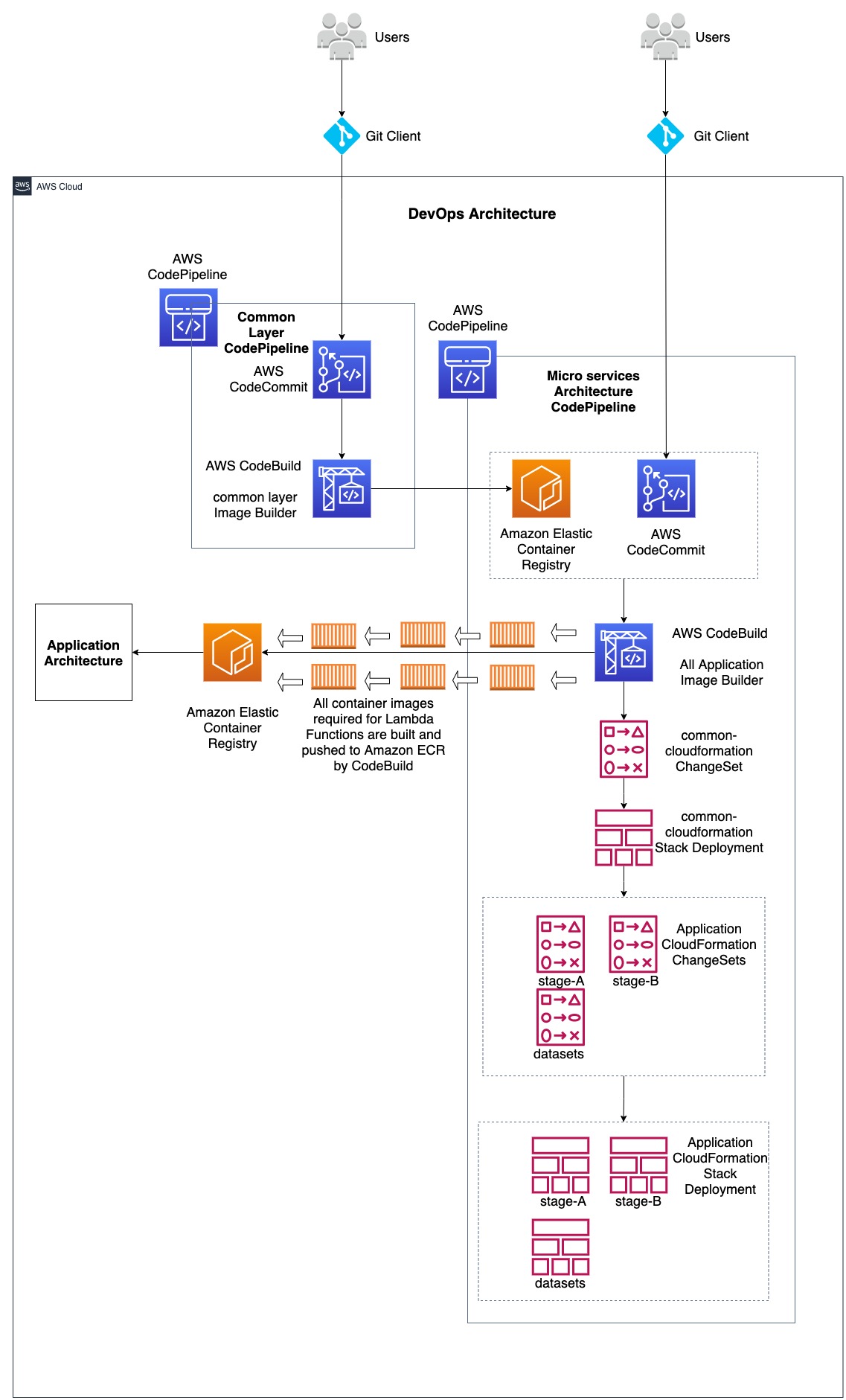
The AWS CloudFormation template deploys the following infrastructure, shown in Figure 4:
An Amazon CloudFront user interface that deploys into an Amazon S3 bucket configured for web hosting.
An Amazon API Gateway API provides the user interface for client requests.
An Amazon Cognito user pool authenticates the API requests.
AWS Lambda functions power the user interface, in addition to the configuration and deployment mechanism for AWS IoT Greengrass and AWS IoT SiteWise gateway resources. Amazon DynamoDB tables store the connection metadata.
An AWS IoT SiteWise gateway configuration can be used for any OPC UA data sources.
An Amazon Kinesis Data Streams data stream, Amazon Kinesis Data Firehose, and Amazon S3 bucket to store telemetry data.
AWS IoT Greengrass is installed and used on an on-premises industrial gateway to run protocol connector Lambda functions. These connect and read telemetry data from your OPC UA and OPC DA servers.
Lambda functions are deployed onto AWS IoT Greengrass Core software on the industrial gateway. They connect to the servers and send the data to one or more configured destinations.
Lambda functions that collect the telemetry data write to AWS IoT Greengrass stream manager streams. The publisher Lambda functions read from the streams.
Publisher Lambda functions forward the data to the appropriate endpoint.
Data collection
The Machine to Cloud Connectivity solution uses Lambda functions running on Greengrass to connect to your on-premises OPC-DA and OPC-UA industrial devices. When you deploy a connection for an OPC-DA device, the solution configures a connection-specific OPC-DA connector Lambda. When you deploy a connection for an OPC-UA device, the solution uses the AWS IoT SiteWise Greengrass connector to collect the data.
Regardless of protocol, the solution configures a publisher Lambda function, which takes care of sending your streaming data to one or more desired destinations. Stream Manager enables the reading and writing of stream data from multiple sources and to multiple destinations within the Greengrass core. This enables each configured collector to write data to a stream. The publisher reads from that stream and sends the data to your desired AWS resource.
Conclusion
Machine to Cloud Connectivity (M2C2) Framework is a self-deployable solution that provides secure connectivity between your technology (OT) assets and the AWS Cloud. With M2C2, you can send data to AWS IoT Core or AWS IoT SiteWise for analytics and monitoring. You can store your data in an industrial data lake using Kinesis Data Streams and Amazon S3. Get started with Machine to Cloud Connectivity (M2C2) Framework today.
This series of blog posts uses the AWS Well-Architected Tool with the Serverless Lens to help customers build and operate applications using best practices. In each post, I address the serverless-specific questions identified by the Serverless Lens along with the recommended best practices. See the introduction post for a table of contents and explanation of the example application.
COST 1. How do you optimize your serverless application costs?
Design, implement, and optimize your application to maximize value. Asynchronous design patterns and performance practices ensure efficient resource use and directly impact the value per business transaction. By optimizing your serverless application performance and its code patterns, you can directly impact the value it provides, while making more efficient use of resources.
Serverless architectures are easier to manage in terms of correct resource allocation compared to traditional architectures. Due to its pay-per-value pricing model and scale based on demand, a serverless approach effectively reduces the capacity planning effort. As covered in the operational excellence and performance pillars, optimizing your serverless application has a direct impact on the value it produces and its cost. For general serverless optimization guidance, see the AWS re:Invent talks, “Optimizing your Serverless applications” Part 1 and Part 2, and “Serverless architectural patterns and best practices”.
Required practice: Minimize external calls and function code initialization
AWS Lambda functions may call other managed services and third-party APIs. Functions may also use application dependencies that may not be suitable for ephemeral environments. Understanding and controlling what your function accesses while it runs can have a direct impact on value provided per invocation.
Review code initialization
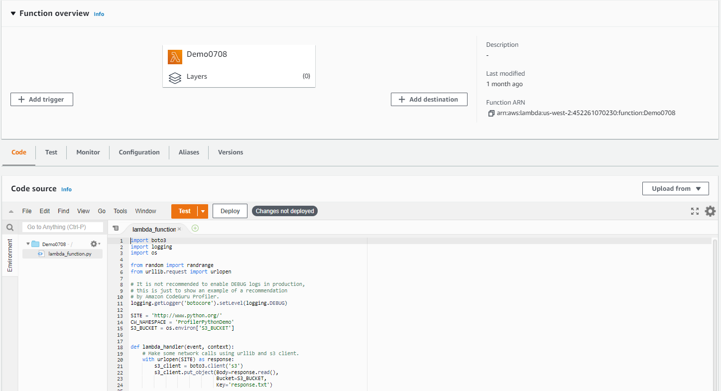
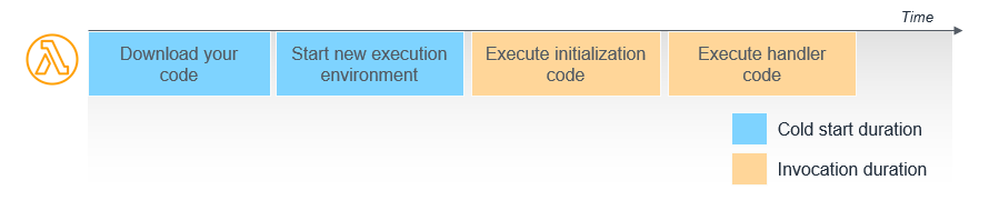
I explain the Lambda initialization process with cold and warm starts in “Optimizing application performance – part 1”. Lambda reports the time it takes to initialize application code in Amazon CloudWatch Logs. As Lambda functions are billed by request and duration, you can use this to track costs and performance. Consider reviewing your application code and its dependencies to improve the overall execution time to maximize value.
You can take advantage of Lambda execution environment reuse to make external calls to resources and use the results for subsequent invocations. Use TTL mechanisms inside your function handler code. This ensures that you can prevent additional external calls that incur additional execution time, while preemptively fetching data that isn’t stale.
Review third-party application deployments and permissions
When using Lambda layers or applications provisioned by AWS Serverless Application Repository, be sure to understand any associated charges that these may incur. When deploying functions packaged as container images, understand the charges for storing images in Amazon Elastic Container Registry (ECR).
Ensure that your Lambda function only has access to what its application code needs. Regularly review that your function has a predicted usage pattern so you can factor in the cost of other services, such as Amazon S3 and Amazon DynamoDB.
Required practice: Optimize logging output and its retention
Considering reviewing your application logging level. Ensure that logging output and log retention are appropriately set to your operational needs to prevent unnecessary logging and data retention. This helps you have the minimum of log retention to investigate operational and performance inquiries when necessary.
Emit and capture only what is necessary to understand and operate your component as intended.
With Lambda, any standard output statements are sent to CloudWatch Logs. Capture and emit business and operational events that are necessary to help you understand your function, its integration, and its interactions. Use a logging framework and environment variables to dynamically set a logging level. When applicable, sample debugging logs for a percentage of invocations.
In the serverless airline example used in this series, the booking service Lambda functions use Lambda Powertools as a logging framework with output structured as JSON.
Lambda Powertools is added to the Lambda functions as a shared Lambda layer in the AWS Serverless Application Model (AWS SAM) template. The layer ARN is stored in Systems Manager Parameter Store.
The LOG_LEVEL and other Powertools settings are configured in the Globals section as Lambda environment variable for all functions.
Globals:
    Function:
        Environment:
            Variables:
                POWERTOOLS_SERVICE_NAME: booking
                POWERTOOLS_METRICS_NAMESPACE: ServerlessAirline
                LOG_LEVEL: INFO
For Amazon API Gateway, there are two types of logging in CloudWatch: execution logging and access logging. Execution logs contain information that you can use to identify and troubleshoot API errors. API Gateway manages the CloudWatch Logs, creating the log groups and log streams. Access logs contain details about who accessed your API and how they accessed it. You can create your own log group or choose an existing log group that could be managed by API Gateway.
Enable AWS AppSync logging which uses CloudWatch to monitor and debug requests. You can configure two types of logging: request-level and field-level. For more information, see “Monitoring and Logging”.
AWS AppSync logging
Define and set a log retention strategy
Define a log retention strategy to satisfy your operational and business needs. Set log expiration for each CloudWatch log group as they are kept indefinitely by default.
For example, in the booking service AWS SAM template, log groups are explicitly created for each Lambda function with a parameter specifying the retention period.
The Serverless Application Repository application, auto-set-log-group-retention can update the retention policy for new and existing CloudWatch log groups to the specified number of days.
For log archival, you can export CloudWatch Logs to S3 and store them in Amazon S3 Glacier for more cost-effective retention. You can use CloudWatch Log subscriptions for custom processing, analysis, or loading to other systems. Lambda extensions allows you to process, filter, and route logs directly from Lambda to a destination of your choice.
Good practice: Optimize function configuration to reduce cost
Benchmark your function using a different set of memory size
For Lambda functions, memory is the capacity unit for controlling the performance and cost of a function. You can configure the amount of memory allocated to a Lambda function, between 128 MB and 10,240 MB. The amount of memory also determines the amount of virtual CPU available to a function. Benchmark your AWS Lambda functions with differing amounts of memory allocated. Adding more memory and proportional CPU may lower the duration and reduce the cost of each invocation.
In “Optimizing application performance – part 2”, I cover using AWS Lambda Power Tuning to automate the memory testing process to balances performance and cost.
Best practice: Use cost-aware usage patterns in code
Reduce the time your function runs by reducing job-polling or task coordination. This avoids overpaying for unnecessary compute time.
Decide whether your application can fit an asynchronous pattern
Avoid scenarios where your Lambda functions wait for external activities to complete. I explain the difference between synchronous and asynchronous processing in “Optimizing application performance – part 1”. You can use asynchronous processing to aggregate queues, streams, or events for more efficient processing time per invocation. This reduces wait times and latency from requesting apps and functions.
Long polling or waiting increases the costs of Lambda functions and also reduces overall account concurrency. This can impact the ability of other functions to run.
Consider using other services such as AWS Step Functions to help reduce code and coordinate asynchronous workloads. You can build workflows using state machines with long-polling, and failure handling. Step Functions also supports direct service integrations, such as DynamoDB, without having to use Lambda functions.
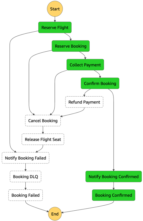
In the serverless airline example used in this series, Step Functions is used to orchestrate the Booking microservice. The ProcessBooking state machine handles all the necessary steps to create bookings, including payment.
Booking service state machine
To reduce costs and improves performance with CloudWatch, create custom metrics asynchronously. You can use the Embedded Metrics Format to write logs, rather than the PutMetricsData API call. I cover using the embedded metrics format in “Understanding application health” – part 1 and part 2.
For example, once a booking is made, the logs are visible in the CloudWatch console. You can select a log stream and find the custom metric as part of the structured log entry.
Custom metric structured log entry
CloudWatch automatically creates metrics from these structured logs. You can create graphs and alarms based on them. For example, here is a graph based on a BookingSuccessful custom metric.
CloudWatch metrics custom graph
Consider asynchronous invocations and review run away functions where applicable
Take advantage of Lambda’s event-based model. Lambda functions can be triggered based on events ingested into Amazon Simple Queue Service (SQS) queues, S3 buckets, and Amazon Kinesis Data Streams. AWS manages the polling infrastructure on your behalf with no additional cost. Avoid code that polls for third-party software as a service (SaaS) providers. Rather use Amazon EventBridge to integrate with SaaS instead when possible.
Carefully consider and review recursion, and establish timeouts to prevent run away functions.
Conclusion
Design, implement, and optimize your application to maximize value. Asynchronous design patterns and performance practices ensure efficient resource use and directly impact the value per business transaction. By optimizing your serverless application performance and its code patterns, you can reduce costs while making more efficient use of resources.
In this post, I cover minimizing external calls and function code initialization. I show how to optimize logging output with the embedded metrics format, and log retention. I recap optimizing function configuration to reduce cost and highlight the benefits of asynchronous event-driven patterns.
Operations research (OR) uses mathematical and analytical tools to arrive at optimal solutions for complex business problems like workforce scheduling. The mathematical techniques used to solve these problems, such as linear programming and mixed-integer programming, require the use of optimization software (solvers). There are several popular and powerful solvers available, ranging from commercial options like IBM CPLEX to open-source packages like ORTools. While these solvers incorporate decades of algorithmic expertise and can solve large and complex problems effectively, they have some scalability limitations.
In this post, we’ll describe three alternatives that you can consider for solving OR problems (see Figure 1). None of these are as general purpose as traditional solvers, but they should be on your “emerging technologies” radar.
Figure 1. OR optimization options
These include:
A traditional solver running on a compute platform
Reinforcement and machine learning (ML) algorithms running on Amazon SageMaker
Let’s start with a reference problem and solve it with a traditional solver. We’ll tackle an inventory management issue (see Figure 2). We have a sales depot that supplies products for local sales outlets. For the depot’s Region, there are seven weeks of historical sales data for each product. We also know how much each product costs and for how much it can be sold. Finally, we know the overall weekly capacity of the depot. This depends on logistical constraints like the size of the warehouse and transportation availability. This scenario is loosely based on the Grupo Bimbo retailer’s Kaggle competition and dataset.
Our job is to place an inventory order to restock our sales depot each week. We quantify our work through a reward function. We want to maximize our revenue:
revenue = (sale price * number of units sold)
(Note that the sample dataset does not include cost of goods sold, only sale price.)
We use these constraints:
total units sold <= depot capacity 0 <= quantity sold of any given item <= forecasted demand for that item
There are many possible solutions to this problem. Using ORTools, we get an average reward (profit) of about $5,700, in about 1,000 simulations.
We can make the scenario slightly more realistic by acknowledging that our sales forecasts are not perfect. After we get the solution from the solver, we can penalize the reward (profit) by subtracting the cost of unsold goods. With this approach, we get a reward of about $2,450.
Solving OR problems with reinforcement learning
An alternative approach to the traditional solver is reinforcement learning (RL). RL is a field of ML that handles problems where the right answer is not immediately known, like playing a game of chess. RL fits our sales depot scenario, because we don’t know how well we will do until after we place the order and are able to view a week of sales activity.
Our sales depot problem resembles a knapsack problem. This is a common OR pattern where we want to fill a container (in this case, our sales depot) with as many items as possible until capacity is reached. Each item has a value (sales price) and a weight (cost). In RL we have to translate this into an observation space, an action space, a state, and a reward (see Figure 3).
The observation space is what our purchasing agent sees. This includes our depot capacity, the sales price, and the forecasted demand. The action space is what our agent can do. In the simplest case, it’s the number of each item to order for the depot, each week. The state is what the agent sees right now, and we model that as the sales results from last week. Finally, the reward function is our profit equation.
One important distinction between OR solvers and RL is that we can’t easily enforce hard constraints in RL. We can limit the amount of an individual product we purchase each week, but we can’t enforce an overall limit on the number of items purchased. We may exceed the capacity of our depot. The simplest way to handle that is to enforce a penalty. There are more sophisticated techniques available, such as interpreting our action as the percentage of budget to spend on each item. But let’s illustrate the simple case here.
Using an RL algorithm from the Ray RLLib package, our reward was $7,000 on average, including penalties for ordering too much of any given item.
Figure 3. Translating OR problem to RL
Solving OR problems with machine learning
It’s possible to model a knapsack problem using ML rather than RL in some cases, and there are simple reference implementations available. The design assumes that we know, or can accurately estimate the reward for a given week. With our simple scenario, we can compute the reward using estimates of future sales. We can use this in a custom loss function to train a neural network.
Solving OR problems with quantum computing
Quantum computers are fundamentally different than the computers most of us use. The appeal of quantum computers is that they can tackle some types of problems much more efficiently than standard computers. Quantum computers can, in theory, solve prime number factoring for decryption in orders of magnitude faster than a standard computer. But they are still in their infancy and limited to the size of problem they can handle, due to hardware limitations.
D-Wave Systems, which make some of the types of quantum computers available through Amazon Braket, has a solver called QBSolv. QBSolv works on a specific type of optimization problem called quadratic unconstrained binary optimization (QUBO). It breaks large problems into smaller pieces that a quantum computer can handle. There is a reference pattern for translating a knapsack problem to a QUBO problem.
Running the sales depot problem through QBSolv on Amazon Braket and using a subset of the data, I was able to obtain a reward of $900. When I tried to run on the full dataset, I was not able to complete the decomposition step, likely due to a hardware limitation.
Conclusion
In this blog post, I review OR problems and traditional OR solvers. I then discussed three alternative approaches, RL, ML, and quantum computing. Each of these alternatives has drawbacks and none is a general-purpose replacement for traditional OR solvers.
However, RL and ML are potentially more scalable because you can train those solutions on a cluster of machines, rather than running an OR solver on a single machine. RL agents can also learn from experience, giving them flexibility to handle scenarios that may be difficult to incorporate into an OR solver. Quantum computing solutions are promising but the current state of the art for quantum computers limits their application to small-scale problems at the moment. All of these alternatives can potentially derive a solution more quickly than an OR solver.
This post was co-written with Mamoon Chowdry, Solutions Architect, previously at AWS.
Businesses and organizations from many industries often struggle to ensure that their data is accurate. Data often has to match people or things exactly in the real world, such as a customer name, an address, or a company. Matching our data is important to validate it, de-duplicate it, or link records in different systems together. Know Your Customer (KYC) regulations also mean that we must be confident in who or what our data is referring to. We must match millions of records from different data sources. Some of that data may have been entered manually and contain inconsistencies.
It can often be hard to match data with the entity it is supposed to represent. For example, if a customer enters their details as, “Mr. John Doe, #1a 123 Main St.“ and you have a prior record in your customer database for ”J. Doe, Apt 1A, 123 Main Street“, are they referring to the same or a different person?
In cases like this, we often have to manually update our data to make sure it accurately and consistently matches a real-world entity. You may want to have consistent company names across a list of business contacts. When there isn’t an exact match, we have to reconcile our data with the available facts we know about that entity. This reconciliation is commonly referred to as entity resolution (ER). This process can be labor-intensive and error-prone.
This blog will explore some of the common types of ER. We will share a basic architectural pattern for near real-time ER processing. You will see how ER using fuzzy text matching can reconcile manually entered names with reference data.
Multiple ways to do entity resolution
Entity resolution is a broad and deep topic, and a complete discussion would be beyond the scope of this blog. However, at a high level there are four common approaches to matching ambiguous fields or records, to known entities.
Fuzzy text matching. We might normally compare two strings to see if they are identical. If they don’t exactly match, it is often helpful to find the nearest match. We do this by calculating a similarity score. For example, “John Doe” and “J Doe” may have a similarity score of 80%. A common way to compare the similarity of two strings is to use the Levenshtein distance, which measures the distance between two sequences.
We may also examine more than one field. For example, we may compare a name and address. Is “Mr. J Doe, 123 Main St” likely to be the same person as “Mr John Doe, 123 Main Street”? If we compare multiple fields in a record and analyze all of their similarity scores, this is commonly called Pairwise comparison.
2. Clustering. We can plot records in an n-dimensional space based on values computed from their fields. Their similarity to other reference records is then measured by calculating how close they are to each other in that space. Those that are clustered together are likely to refer to the same entity. Clustering is an effective method for grouping or segmenting data for computer vision, astronomy, or market segmentation. An example of this method is K-means clustering.
3. Graph networks. Graph networks are commonly used to store relationships between entities, such as people who are friends with each other, or residents of a particular address. When we need to resolve an ambiguous record, we can use a graph database to identify potential relationships to other records. For example, “J Doe, 123 Main St,” may be the same as “John Doe, 123 Main St,” because they have the same address and similar names.
Graph networks are especially helpful when dealing with complex relationships over millions of entities. For example, you can build a customer profile using web server logs and other data.
4. Commercial off-the-shelf (COTS) software. Enterprises can also deploy ER software, such as these offerings from the AWS Marketplace and Senzing entity resolution. This is helpful when companies may not have the skill or experience to implement a solution themselves. It is important to mention the role of Master Data Management (MDM) with ER. MDM involves having a single trusted source for your data. Tools, such as Informatica, can help ER with their MDM features.
Our solution (shown in Figure 1) allows us to build a low-cost, streamlined solution using AWS serverless technology. The architecture uses AWS Lambda, which allows you to run code without having to provision or manage servers. This code will be invoked through an API, which is created with Amazon API Gateway. API Gateway is a fully managed service used by developers to create, publish, maintain, monitor, and secure API operations at any scale. Finally, we will store our reference data in Amazon Simple Storage Service (S3).
Entity resolution solution using AWS serverless services
We initially match manually entered strings to a list of reference strings. The strings we will try to match will be names of companies.
Figure 1. Example request dataflow through AWS
Our API takes a string as input
It then invokes the ER Lambda function
This loads the index and data files of our reference dataset
The ER finds the closest match in the list of real-world companies
The closest match is returned
The reference data and index files were created from an export of the fuzzy match algorithm.
The fuzzy match algorithm in detail
The algorithm in the AWS Lambda function works by converting each string to a collection of n-grams. N-grams are smaller substrings that are commonly used for analyzing free-form text.
The n-grams are then converted to a simple vector. Each vector is a numerical statistic that represents the Term Frequency – Inverse Document Frequency (TF-IDF). Both TF-IDF and n-grams are used to prepare text for searching. N-grams of strings that are similar in nature, tend to have similar TF-IDF vectors. We can plot these vectors in a chart. This helps us find similar strings as they are grouped or clustered together.
Comparing vectors to find similar strings can be fairly straightforward. But if you have numerous records, it can be computationally expensive and slow. To solve this, we use the NMSLIB library. This library indexes the vectors for faster similarity searching. It also gives us the degree of similarity between two strings. This is important because we may want to know the accuracy of a match we have found. For example, it can be helpful to filter out weak matches.
# initialize the index
newIndex = nmslib.init(method='napp', space='negdotprod_sparse_fast',
data_type=nmslib.DataType.SPARSE_VECTOR)
Next we imported the index and data files that were created from our reference data.
# load the index file
newIndex.loadIndex(DATA_DIR + 'index_company_names.bin',
load_data=True)
The input parameter companyName is then used to query the index to find the approximate nearest neighbor. By using the knnQueryBatch method, we distribute the work over a thread pool, which provides faster querying.
# set the input variable and empty output list
inputString = companyName
outputList = []
# Find the nearest neighbor for our company name
# (K is the number of matches, set to 1)
newQueryMatrix = vectorizer.transform(inputString)
newNbrs = index.knnQueryBatch(newQueryMatrix, k = K, num_threads = numThreads)
The best match is then returned as a JSON response.
# return the match
for i in range(K):
    outputList.append(orgNames[newNbrs[0][0][i]])
Our solution is a combination of Amazon API Gateway, AWS Lambda, and Amazon S3 (hyperlinks are to pricing pages). As an example, let’s assume that the API will receive 10 million requests per month. We can estimate the costs of running the solution as:
Service
Description
Cost
AWS Lambda
10 million requests and associated compute costs
$161.80
Amazon API Gateway
HTTP API requests, avg size of request (34 KB), Avg message size (32 KB), requests (10 million/month)
$10.00
Amazon S3
S3 Standard storage (including data transfer costs)
$7.61
Total
$179.41
Table 1. Example monthly cost estimate (USD)
Conclusion
Using AWS services to reconcile your data with real-world entities helps make your data more accurate and consistent. You can automate a manual task that could have been laborious, expensive, and error-prone.
Where can you use ER in your organization? Do you have manually entered or inaccurate data? Have you struggled to match it with real-world entities? You can experiment with this architecture to continue to improve the accuracy of your own data.
Securing east-west traffic in service meshes, such as AWS App Mesh, by using mutual Transport Layer Security (mTLS) adds an additional layer of defense beyond perimeter control. mTLS adds bidirectional peer-to-peer authentication on top of the one-way authentication in normal TLS. This is done by adding a client-side certificate during the TLS handshake, through which a client proves possession of the corresponding private key to the server, and as a result the server trusts the client. This prevents an arbitrary client from connecting to an App Mesh service, because the client wouldn’t possess a valid certificate.
You’ll first see how to derive server-side certificates from ACM Private CA into App Mesh internally by using the native integration between the two services. You’ll then see a method and code for installing client-side certificates issued from ACM Private CA into App Mesh; this method is needed because client-side certificates aren’t integrated natively.
You’ll learn how to use AWS Lambda to export a client-side certificate from ACM Private CA and store it in AWS Secrets Manager. You’ll then see Envoy proxies in App Mesh retrieve the certificate from Secrets Manager and use it in an mTLS handshake. The solution is designed to ensure confidentiality of the private key of a client-side certificate, in transit and at rest, as it moves from ACM to Envoy.
The solution described in this blog post simplifies and allows you to automate the configuration and operations of mTLS-enabled App Mesh deployments, because all of the certificates are derived from a single managed private public key infrastructure (PKI) service—ACM Private CA—eliminating the need to run your own private PKI. The solution uses Amazon Elastic Container Services (Amazon ECS) with AWS Fargate as the App Mesh hosting environment, although the design presented here can be applied to any compute environment that is supported by App Mesh.
Solution overview
ACM Private CA provides a highly available managed private PKI service that enables creation of private CA hierarchies—including root and subordinate CAs—without the investment and maintenance costs of operating your own private PKI service. The service allows you to choose among several CA key algorithms and key sizes and makes it easier for you to export and deploy private certificates anywhere by using API-based automation.
App Mesh is a service mesh that provides application-level networking across multiple types of compute infrastructure. It standardizes how your microservices communicate, giving you end-to-end visibility and helping to ensure transport security and high availability for your applications. In order to communicate securely between mesh endpoints, App Mesh directs the Envoy proxy instances that are running within the mesh to use one-way or mutual TLS.
TLS provides authentication, privacy, and data integrity between two communicating endpoints. The authentication in TLS communications is governed by the PKI system. The PKI system allows certificate authorities to issue certificates that are used by clients and servers to prove their identity. The authentication process in TLS happens by exchanging certificates via the TLS handshake protocol. By default, the TLS handshake protocol proves the identity of the server to the client by using X.509 certificates, while the authentication of the client to the server is left to the application layer. This is called one-way TLS. TLS also supports two-way authentication through mTLS. In mTLS, in addition to the one-way TLS server authentication with a certificate, a client presents its certificate and proves possession of the corresponding private key to a server during the TLS handshake.
Example application
The following sections describe one-way and mutual TLS integrations between App Mesh and ACM Private CA in the context of an example application. This example application exposes an API to external clients that returns a text string name of a color—for example, “yellow”. It’s an extension of the Color App that’s used to demonstrate several existing App Mesh examples.
The example application is comprised of two services running in App Mesh—ColorGateway and ColorTeller. An external client request enters the mesh through the ColorGateway service and is proxied to the ColorTeller service. The ColorTeller service responds back to the ColorGateway service with the name of a color. The ColorGateway service proxies the response to the external client. Figure 1 shows the basic design of the application.
Figure 1: App Mesh services in the Color App example application
The two services are mapped onto the following constructs in App Mesh:
ColorGateway is mapped as a Virtual gateway. A virtual gateway in App Mesh allows resources that are outside of a mesh to communicate to resources that are inside the mesh. A virtual gateway represents Envoy deployed by itself. In this example, the virtual gateway represents an Envoy proxy that is running as an Amazon ECS service. This Envoy proxy instance acts as a TLS client, since it initiates TLS connections to the Envoy proxy that is running in the ColorTeller service.
ColorTeller is mapped as a Virtual node. A virtual node in App Mesh acts as a logical pointer to a particular task group. In this example, the virtual node—ColorTeller—runs as another Amazon ECS service. The service runs two tasks—an Envoy proxy instance and a ColorTeller application instance. The Envoy proxy instance acts as a TLS server, receiving inbound TLS connections from ColorGateway.
Let’s review running the example application in one-way TLS mode. Although optional, starting with one-way TLS allows you to compare the two methods and establish how to look at certain Envoy proxy statistics to distinguish and verify one-way TLS versus mTLS connections.
For practice, you can deploy the example application project in your own AWS account and perform the steps described in your own test environment.
Note: In both the one-way TLS and mTLS descriptions in the following sections, we’re using a flat certificate hierarchy for demonstration purposes. The root CAs are issuing end-entity certificates. The AWS ACM Private CA best practices recommend that root CAs should only be used to issue certificates for intermediate CAs. When intermediate CAs are involved, your certificate chain has multiple certificates concatenated in it, but the mechanisms are the same as those described here.
One-way TLS in App Mesh using ACM Private CA
Because this is a one-way TLS authentication scenario, you need only one Private CA—ColorTeller—and issue one end-entity certificate from it that’s used as the server-side certificate for the ColorTeller virtual node.
Figure 2, following, shows the architecture for this setup, including notations and color codes for certificates and a step-by-step process that shows how the system is configured and functions. Because this architecture uses a server-side certificate only, you use the native integration between App Mesh and ACM Private CA and don’t need an external mechanism for certificate integration.
Figure 2: One-way TLS in App Mesh integrated with ACM Private CA
The steps in Figure 2 are:
Step 1: A Private CA instance—ColorTeller—is created in ACM Private CA. Next, an end-entity certificate is created and signed by the CA. This certificate is used as the server-side certificate in ColorTeller.
Step 2: The CloudFormation templates configure the ColorGateway to validate server certificates against the ColorTeller private CA certificate chain. As the App Mesh endpoints are starting up, the ColorTeller CA certificate trust chain is ingested into the ColorGateway Envoy instance. The TLS configuration for ColorGateway in App Mesh is shown in Figure 3.
Figure 3: One-way TLS configuration in the client policy of ColorGateway
Figure 3 shows that the client policy attributes for outbound transport connections for ColorGateway have been configured as follows:
Enforce TLS is set to Enforced. This enforces use of TLS while communicating with backends.
TLSvalidation method is set to AWS Certificate Manager Private Certificate Authority (ACM-PCA hosting). This instructs App Mesh to derive the certificate trust chain from ACM PCA.
Certificate is set to the Amazon Resource Name (ARN) of the ColorTeller Private CA, which is the identifier of the certificate trust chain in ACM PCA.
This configuration ensures that ColorGateway makes outbound TLS-only connections towards ColorTeller, extracts the CA trust chain from ACM-PCA, and validates the server certificate presented by the ColorTeller virtual node against the configured CA ARN.
Step 3: The CloudFormation templates configure the ColorTeller virtual node with the ColorTeller end-entity certificate ARN in ACM Private CA. While the App Mesh endpoints are started, the ColorTeller end-entity certificate is ingested into the ColorTeller Envoy instance.
The TLS configuration for the ColorTeller virtual node in App Mesh is shown in Figure 4.
Figure 4: One-way TLS configuration in the listener configuration of ColorTeller
Figure 4 shows that various TLS-related attributes are configured as follows:
Enable TLS termination is on.
Mode is set to Strict to limit connections to TLS only.
TLS Certificate method is set to ACM Certificate Manager (ACM) hosting as the source of the end-entity certificate.
Certificate is set to ARN of the ColorTeller end-entity certificate.
Note: Figure 4 shows an annotation where the certificate ARN has been superimposed by the cert icon in green color. This icon follows the color convention from Figure 2 and can help you relate how the individual resources are configured to construct the architecture shown in Figure 2. The cert shown (and the associated private key that is not shown) in the diagram is necessary for ColorTeller to run the TLS stack and serve the certificate. The exchange of this material happens over the internal communications between App Mesh and ACM Private CA.
Step 4: The ColorGateway service receives a request from an external client.
Step 5: This step includes multiple sub-steps:
The ColorGateway Envoy initiates a one-way TLS handshake towards the ColorTeller Envoy.
The ColorTeller Envoy presents its server-side certificate to the ColorGateway Envoy.
The ColorGateway Envoy validates the certificate against its configured CA trust chain—the ColorTeller CA trust chain—and the TLS handshake succeeds.
Verifying one-way TLS
To verify that a TLS connection was established and that it is one-way TLS authenticated, run the following command on your bastion host:
This command queries the runtime statistics that are maintained in ColorTeller Envoy and filters the output for certain SSL-related counts. The count for ssl.handshake should be one. If the ssl.handshake count is more than one, that means there’s been more than one TLS handshake. The count for ssl.no_certificate should also be one, or equal to the count for ssl.handshake. The ssl.no_certificate count tracks the total successful TLS connections with no client certificate. Since this is a one-way TLS handshake that doesn’t involve client certificates, this count is the same as the count of ssl.handshake.
The preceding statistics verify that a TLS handshake was completed and the authentication was one-way, where the ColorGateway authenticated the ColorTeller but not vice-versa. You’ll see in the next section how the ssl.no_certificate count differs when mTLS is enabled.
Mutual TLS in App Mesh using ACM Private CA
In the one-way TLS discussion in the previous section, you saw that App Mesh and ACM Private CA integration works without needing external enhancements. You also saw that App Mesh retrieved the server-side end-entity certificate in ColorTeller and the root CA trust chain in ColorGateway from ACM Private CA internally, by using the native integration between the two services.
However, a native integration between App Mesh and ACM Private CA isn’t currently available for client-side certificates. Client-side certificates are necessary for mTLS. In this section, you’ll see how you can issue and export client-side certificates from ACM Private CA and ingest them into App Mesh.
The solution uses Lambda to export the client-side certificate from ACM Private CA and store it in Secrets Manager. The solution includes an enhanced startup script embedded in the Envoy image to retrieve the certificate from Secrets Manager and place it on the Envoy file system before the Envoy process is started. The Envoy process reads the certificate, loads it in memory, and uses it in the TLS stack for the client-side certificate exchange of the mTLS handshake.
The choice of Lambda is based on this being an ephemeral workflow that needs to run only during system configuration. You need a short-lived, runtime compute context that lets you run the logic for exporting certificates from ACM Private CA and store them in Secrets Manager. Because this compute doesn’t need to run beyond this step, Lambda is an ideal choice for hosting this logic, for cost and operational effectiveness.
The choice of Secrets Manager for storing certificates is based on the confidentiality requirements of the passphrase that is used for encrypting the private key (PKCS #8) of the certificate. You also need a higher throughput data store that can support secrets retrieval from large meshes. Secrets Manager supports a higher API rate limit than the API for exporting certificates from ACM Private CA, and thus serves as a high-throughput front end for ACM Private CA for serving certificates without compromising data confidentiality.
The resulting architecture is shown in Figure 5. The figure includes notations and color codes for certificates—such as root certificates, endpoint certificates, and private keys—and a step-by-step process showing how the system is configured, started, and functions at runtime. The example uses two CA hierarchies for ColorGateway and ColorTeller to demonstrate an mTLS setup where the client and server belong to separate CA hierarchies but trust each other’s CAs.
Figure 5: mTLS in App Mesh integrated with ACM Private CA
The numbered steps in Figure 5 are:
Step 1: A Private CA instance representing the ColorGateway trust hierarchy is created in ACM Private CA. Next, an end-entity certificate is created and signed by the CA, which is used as the client-side certificate in ColorGateway.
Step 2: Another Private CA instance representing the ColorTeller trust hierarchy is created in ACM Private CA. Next, an end-entity certificate is created and signed by the CA, which is used as the server-side certificate in ColorTeller.
Step 3: As part of running CloudFormation, the Lambda function is invoked. This Lambda function is responsible for exporting the client-side certificate from ACM Private CA and storing it in Secrets Manager. This function begins by requesting a random password from Secrets Manager. This random password is used as the passphrase for encrypting the private key inside ACM Private CA before it’s returned to the function. Generating a random password from Secrets Manager allows you to generate a random password with a specified complexity.
Step 4: The Lambda function issues an export certificate request to ACM, requesting the ColorGateway end-entity certificate. The request conveys the private key passphrase retrieved from Secrets Manager in the previous step so that ACM Private CA can use it to encrypt the private key that’s sent in the response.
Step 5: The ACM Private CA responds to the Lambda function. The response carries the following elements of the ColorGateway end-entity certificate.
Step 6: The Lambda function processes the response that is returned from ACM. It extracts individual fields in the JSON-formatted response and stores them in Secrets Manager. The Lambda function stores the following four values in Secrets Manager:
The ColorGateway endpoint certificate
The ColorGateway certificate trust chain, which contains the ColorGateway Private CA root certificate
The encrypted private key for the ColorGateway end-entity certificate
The passphrase that was used to encrypt the private key
Step 7: The App Mesh services—ColorGateway and ColorTeller—are started, which then start their Envoy proxy containers. A custom startup script embedded in the Envoy docker image fetches a certificate from Secrets Manager and places it on the Envoy file system.
Note: App Mesh publishes its own custom Envoy proxy Docker container image that ensures it is fully tested and patched with the latest vulnerability and performance patches. You’ll notice in the example source code that a custom Envoy image is built on top of the base image published by App Mesh. In this solution, we add an Envoy startup script and certain utilities such as AWS Command Line Interface (AWS CLI) and jq to help retrieve the certificate from Secrets Manager and place it on the Envoy file system during Envoy startup.
Step 8: The CloudFormation scripts configure the client policy for mTLS in ColorGateway in App Mesh, as shown in Figure 6. The following attributes are configured:
Provide client certificate is enabled. This ensures that the client certificate is exchanged as part of the mTLS handshake.
Certificate method is set to Local file hosting so that the certificate is read from the local file system.
Certificate chain is set to the path for the file that contains the ColorGateway certificate chain.
Private key is set to the path for the file that contains the private key for the ColorGateway certificate.
Figure 6: Client-side mTLS configuration in ColorGateway
At the end of the custom Envoy startup script described in step 7, the core Envoy process in ColorGateway service is started. It retrieves the ColorTeller CA root certificate from ACM Private CA and configures it internally as a trusted CA. This retrieval happens due to native integration between App Mesh and ACM Private CA. This allows ColorGateway Envoy to validate the certificate presented by ColorTeller Envoy during the TLS handshake.
Step 9: The CloudFormation scripts configure the listener configuration for mTLS in ColorTeller in App Mesh, as shown in Figure 7. The following attributes are configured:
Require client certificate is enabled, which enforces mTLS.
Validation Method is set to Local file hosting, which causes Envoy to read the certificate from the local file system.
Certificate chain is set to the path for the file that contains the ColorGateway certificate chain.
Figure 7: Server-side mTLS configuration in ColorTeller
At the end of the Envoy startup script described in step 7, the core Envoy process in ColorTeller service is started. It retrieves its own server-side end-entity certificate and corresponding private key from ACM Private CA. This retrieval happens internally, driven by the native integration between App Mesh and ACM Private CA. This allows ColorTeller Envoy to present its server-side certificate to ColorGateway Envoy during the TLS handshake.
The system startup concludes with this step, and the application is ready to process external client requests.
Step 10: The ColorGateway service receives a request from an external client.
Step 11: The ColorGateway Envoy initiates a TLS handshake with the ColorTeller Envoy. During the first half of the TLS handshake protocol, the ColorTeller Envoy presents its server-side certificate to the ColorGateway Envoy. The ColorGateway Envoy validates the certificate. Because the ColorGateway Envoy has been configured with the ColorTeller CA trust chain in step 8, the validation succeeds.
Step 12: During the second half of the TLS handshake, the ColorTeller Envoy requests the ColorGateway Envoy to provide its client-side certificate. This step is what distinguishes an mTLS exchange from a one-way TLS exchange.
The ColorGateway Envoy responds with its end-entity certificate that had been placed on its file system in step 7. The ColorTeller Envoy validates the received certificate with its CA trust chain, which contains the ColorGateway root CA that was placed on its file system (in step 7). The validation succeeds, and so an mTLS session is established.
Verifying mTLS
You can now verify that an mTLS exchange happened by running the following command on your bastion host.
The count for ssl.handshake should be one. If the ssl.handshake count is more than one, that means that you’ve gone through more than one TLS handshake. It’s important to note that the count for ssl.no_certificate—the total successful TLS connections with no client certificate—is zero. This shows that mTLS configuration is working as expected. Recall that this count was one or higher—equal to the ssl.handshake count—in the previous section that described one-way TLS. The ssl.no_certificate count being zero indicates that this was an mTLS authenticated connection, where the ColorGateway authenticated the ColorTeller and vice-versa.
Step 2: CloudWatch triggers a Lambda function that is responsible for certificate renewal.
Step 3: The Lambda function renews the certificate in ACM and exports the new certificate by calling ACM APIs.
Step 4: The Lambda function writes the certificate to Secrets Manager.
Step 5: The Lambda function triggers a new service deployment in an Amazon ECS cluster. This will cause the ECS services to go through a graceful update process to acquire a renewed certificate.
Step 6: The Envoy processes in App Mesh fetch the client-side certificate from Secrets Manager using external integration, and the server-side certificate from ACM using native integration.
Conclusion
In this post, you learned a method for enabling mTLS authentication between App Mesh endpoints based on certificates issued by ACM Private CA. mTLS enhances security of App Mesh deployments due to its bidirectional authentication capability. While server-side certificates are integrated natively, you saw how to use Lambda and Secrets Manager to integrate client-side certificates externally. Because ACM Private CA certificates aren’t eligible for managed renewal, you also learned how to implement an external certificate renewal process.
This solution enhances your App Mesh security posture by simplifying configuration of mTLS-enabled App Mesh deployments. It achieves this because all mTLS certificate requirements are met by a single, managed private PKI service—ACM Private CA—which allows you to centrally manage certificates and eliminates the need to run your own private PKI.
If you have feedback about this post, submit comments in the Comments section below. If you have questions about this post, start a new thread on the AWS Certificate Manager forum or contact AWS Support.
Want more AWS Security how-to content, news, and feature announcements? Follow us on Twitter.
This post is written by Mark Sailes, Specialist Solutions Architect, Serverless and Richard Davison, Senior Partner Solutions Architect.
The Operating Lambda: Performance optimization blog series covers important topics for developers, architects, and system administrators who are managing applications using AWS Lambda functions. This post explains how you can reduce the initialization time to start a new execution environment when using the Java-managed runtimes.
Many Lambda workloads are designed to deliver fast responses to synchronous or asynchronous workloads in a fraction of a second. Examples of these could be public APIs to deliver dynamic content to websites or a near-real time data pipeline doing small batch processing.
As usage of these systems increases, Lambda creates new execution environments. When a new environment is created and used for the first time, additional work is done to make it ready to process an event. This creates two different performance profiles: one with and one without the additional work.
To improve the response time, you can minimize the effect of this additional work. One way you can minimize the time taken to create a new managed Java execution environment is to tune the JVM. It can be optimized specifically for these workloads that do not have long execution durations.
One example of this is configuring a feature of the JVM called tiered compilation. From version 8 of the Java Development Kit (JDK), the two just-in-time compilers C1 and C2 have been used in combination. C1 is designed for use on the client side and to enable short feedback loops for developers. C2 is designed for use on the server side and to achieve higher performance after profiling.
Tiering is used to determine which compiler to use to achieve better performance. These are represented as five levels:
Profiling has an overhead, and performance improvements are only achieved after a method has been invoked a number of times, the default being 10,000. Lambda customers wanting to achieve faster startup times can use level 1 with little risk of reducing warm start performance. The article “Startup, containers & Tiered Compilation” explains tiered compilation further.
For customers who are doing highly repetitive processing, this configuration might not be suited. Applications that repeat the same code paths many times want the JVM to profile and optimize these paths. Concrete examples of these would be using Lambda to run Monte Carlo simulation or hash calculations. You can run the same simulations thousands of times and the JVM profiling can reduce the total execution time significantly.
Performance improvements
The example project is a Java 11-based application used to analyze the impact of this change. The application is triggered by Amazon API Gateway and then puts an item into Amazon DynamoDB. To compare the performance difference caused by this change, there is one Lambda function with the additional changes and one without. There are no other differences in the code.
Select the following two log groups from the drop-down list: /aws/lambda/example-with-layer /aws/lambda/example-without-layer
Copy the following query and choose Run query:
    filter @type = "REPORT"
    | parse @log /\d+:\/aws\/lambda\/example-(?<function>\w+)-\w+/
    | stats
    count(*) as invocations,
    pct(@duration, 0) as p0,
    pct(@duration, 25) as p25,
    pct(@duration, 50) as p50,
    pct(@duration, 75) as p75,
    pct(@duration, 90) as p90,
    pct(@duration, 95) as p95,
    pct(@duration, 99) as p99,
    pct(@duration, 100) as p100
    group by function, ispresent(@initDuration) as coldstart
    | sort by function, coldstart
You see results similar to:
Here is a simplified table of the results:
Settings
Type
# of invocations
p90 (ms)
p95 (ms)
p99 (ms)
Default settings
Cold start
754
5,212
5,338
5,517
Default settings
Warm start
35,247
58
93
255
Tiered compilation stopping at level 1
Cold start
383
2,071
2,086
2,221
Tiered compilation stopping at level 1
Warm start
35,618
23
32
86
The results are from testing 120 concurrent requests over 5 minutes using an open-source software project called Artillery. You can find instructions on how to run these tests in the GitHub repo. The results show that for this application, cold starts for 90% of invocations improve by 3141 ms (60%). These numbers are specific for this application and your application may behave differently.
Using wrapper scripts for Lambda functions
Wrapper scripts are a feature available in Java 8 and Java 11 on Amazon Linux 2 managed runtimes. They are not available for the Java 8 on Amazon Linux 1 managed runtime.
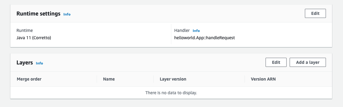
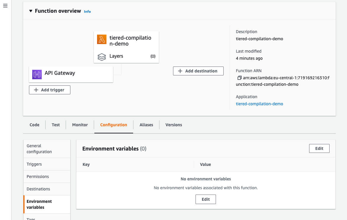
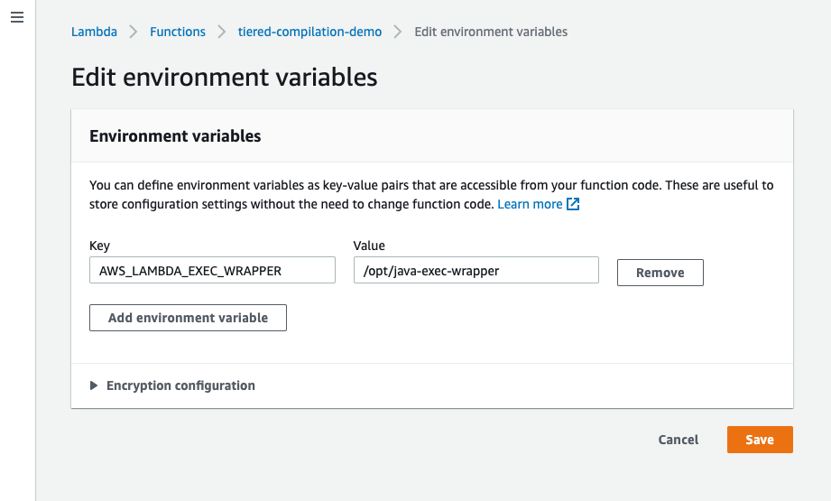
To apply this optimization flag to Java Lambda functions, create a wrapper script and add it to a Lambda layer zip file. This script will alter the JVM flags which Java is started with, within the execution environment.
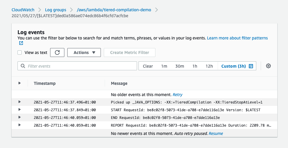
Choose Save.You can verify that the changes are applied by invoking the function and viewing the log events. The log line Picked up _JAVA_OPTIONS: -XX:+TieredCompilation -XX:TieredStopAtLevel=1 is added.
Conclusion
Tiered compilation stopping at level 1 reduces the time the JVM spends optimizing and profiling your code. This could help reduce start up times for Java applications that require fast responses, where the workload doesn’t meet the requirements to benefit from profiling.
Many video streaming services show GIF animations in the frontend when users fast forward and rewind throughout a video. This helps customers see a preview and makes the user interface more intuitive.
Generating these GIF files is a compute-intensive operation that becomes more challenging to scale when there are many videos. Over a typical 2-hour movie with GIF previews every 30 seconds, you need 240 separate GIF animations to support this functionality.
In a server-based solution, you can use a library like FFmpeg to load the underlying MP4 file and create the GIF exports. However, this may be a serial operation that slows down for longer videos or when there are many different videos to process. For a service providing thousands of videos to customers, they need a solution where the encoding process keeps pace with the number of videos.
In this two-part blog post, I show how you can use a serverless approach to create a scalable GIF generation service. I explain how you can use parallelization in AWS Lambda-based workloads to reduce processing time significantly.
The example application uses the AWS Serverless Application Model (AWS SAM), enabling you to deploy the application more easily in your own AWS account. This walkthrough creates some resources covered in the AWS Free Tier but others incur cost. To set up the example, visit the GitHub repo and follow the instructions in the README.md file.
Overview
To show the video player functionality, visit the demo front end. This loads the assets for an example video that is already processed. In the example, there are GIF animations every 30 seconds and freeze frames for every second of video. Move the slider to load the frame and GIF animation at that point in the video:
The demo site defaults to an existing video. After deploying the backend application, you can test your own videos here.
Move the slider to select a second in the video playback. This simulates a typical playback bar used in video application frontends.
This displays the frame at the chosen second, which is a JPG file created by the backend application.
The GIF animation for the selected playback point is a separate GIF file, created by the backend application.
Comparing server-based and serverless solutions
The example application uses FFmpeg, an open source application to record and process video. FFmpeg creates the GIF animations and individual frames for each second of video. You can use FFmpeg directly from a terminal or in scripts and applications. In comparing the performance, I use the AWS re:Invent 2019 keynote video, which is almost 3 hours long.
To show the server-based approach, I use a Node.js application in the GitHub repo. This loops through the video length in 30-second increments, calling FFmpeg with the necessary command line parameters:
The completed S3 PutObject operation starts the GIF generation process. The function that processes the GIF files emits the following metrics on the Monitor tab in the Lambda console:
There are 345 invocations to process the source file into 30-second GIF animations.
The average duration for each invocation is 4,311 ms. The longest is 9,021 ms.
No errors occurred in processing the video.
Lambda scaled up to 344 concurrent execution environments.
After approximately 10 seconds, the conversion is complete and there are over 10,000 objects in the application’s output S3 bucket:
The main reason that the task duration is reduced from nearly 21 minutes to around 10 seconds is parallelization. In the server-based approach, each 30 second GIF is processed sequentially. In the Lambda-based solution, all of the 30-second clips are generated in parallel, at around the same time:
Solution architecture
The example application uses the following serverless architecture:
When the original MP4 video is put into the source S3 bucket, it invokes the first Lambda function.
The Snippets Lambda function detects the length of the video. It determines the number of 30-second snippets and then puts events onto the default event bus. There is one event for each snippet.
An Amazon EventBridge rule matches for events created by the first Lambda function. It invokes the second Lambda function.
The Process MP4 Lambda function receives the event as a payload. It loads the original video using FFmpeg to generate the GIF and per-second frames.
The resulting files are stored in the output S3 bucket.
The first Lambda function uses the following code to detect the length of the video and create events for EventBridge:
const createSnippets = async (record) => {
	// Get signed URL for source object
	const params = {
		Bucket: record.s3.bucket.name,
		Key: record.s3.object.key,
		Expires: 300
	}
	const url = s3.getSignedUrl('getObject', params)

	// Get length of source video
	const metadata = await ffProbe(url)
	const length = metadata.format.duration
	console.log('Length (seconds): ', length)

	// Build data array for DynamoDB
	const items = []
	const snippetSize = parseInt(process.env.SnippetSize)

	for (let start = 0; start < length; start += snippetSize) {
		items.push({
			key: record.s3.object.key,
			start,
			end: (start + snippetSize - 1),
			length,
			tsCreated: Date.now()
		})
	}
	// Send events to EventBridge
	await writeBatch(items)
}
The eventbridge.js file contains a function that sends the event array to the default bus in EventBridge. It uses the putEvents method in the EventBridge JavaScript SDK to send events in batches of 10:
const writeBatch = async (items) => {

    console.log('writeBatch items: ', items.length)

    for (let i = 0; i < items.length; i += BATCH_SIZE ) {
        const tempArray = items.slice(i, i + BATCH_SIZE)

        // Create new params array
        const paramsArray = tempArray.map((item) => {
            return {
                DetailType: 'newVideoCreated',
                Source: 'custom.gifGenerator',
                Detail: JSON.stringify ({
                    ...item
                })
            }
        })

        // Create params object for DDB DocClient
        const params = {
            Entries: paramsArray
        }

        // Write to DDB
        const result = await eventbridge.putEvents(params).promise()
        console.log('Result: ', result)
    }
}
The second Lambda function is invoked by an EventBridge rule, matching on the Source and DetailType values. Both the Lambda function and the rule are defined in the AWS SAM template:
This Lambda function receives an event payload specifying the start and end time for the video clip it should process. The function then calls the FFmpeg application to generate the output files. It stores these in the local /tmp storage before uploading to the output S3 bucket:
const processMP4 = async (event) => {
    // Get settings from the incoming event
    const originalMP4 = event.detail.Key
    const start =  event.detail.start
    const end =  event.detail.end

    // Get signed URL for source object
    const params = {
        Bucket: process.env.SourceBucketName,
        Key: originalMP4,
        Expires
    }
    const url = s3.getSignedUrl('getObject', params)
    console.log('processMP4: ', { url, originalMP4, start, end })

    // Extract frames from MP4 (1 per second)
    console.log('Create GIF')
    const baseFilename = params.Key.split('.')[0]

    // Create GIF
    const gifName = `${baseFilename}-${start}.gif`
    // Generates gif in local tmp
    await execPromise(`${ffmpegPath} -loglevel error -ss ${start} -to ${end} -y -i "${url}" -vf "fps=10,scale=240:-1:flags=lanczos,split[s0][s1];[s0]palettegen[p];[s1][p]paletteuse" -loop 0 ${ffTmp}/${gifName}`)
    // Upload gif to local tmp
    // Generate frames
    if (process.env.GenerateFrames === 'true') {
        console.log('Capturing frames')
        await execPromise(`${ffmpegPath} -loglevel error -ss ${start} -to ${end} -i "${url}" -vf fps=1 ${ffTmp}/${baseFilename}-${start}-frame-%d.jpg`)
    }

    // Upload all generated files
    await uploadFiles(`${baseFilename}/`)

    // Cleanup temp files
    await tmpCleanup()
}
Creating and using the FFmpeg Lambda layer
FFmpeg uses operating system-specific binaries that may be different on your development machine from the Lambda execution environment. The easiest way to test the code on a local machine and deploy to Lambda with the appropriate binaries is to use a Lambda layer.
As described in the example application’s README file, you can create the FFmpeg Lambda layer by deploying the ffmpeg-lambda-layer application in the AWS Serverless Application Repository. After deployment, the Layers menu in the Lambda console shows the new layer. Copy the version ARN and use this as a parameter in the AWS SAM deployment:
On your local machine, download and install the FFmpeg binaries for your operating system. The package.json file for the Lambda functions uses two npm installer packages to help ensure the Node.js code uses the correct binaries when tested locally:
Any npm packages specified in the devDependencies section of package.json are not deployed to Lambda by AWS SAM. As a result, local testing uses local ffmpeg binaries and Lambda uses the previously deployed Lambda layer. This approach also helps to reduce the size of deployment uploads and can help make the testing and deployment cycle faster in development.
Using FFmpeg from a Lambda function
FFmpeg is an application that’s generally used via a terminal. It takes command line parameters as options to determine input files, output locations, and the type of processing needed. To use terminal commands from Lambda, both functions use the asynchronous child_process module in Node.js. The execPromise function wraps this module in a Promise so the main function can use async/await syntax:
const { exec } = require('child_process')

const execPromise = async (command) => {
    console.log(command)
    return new Promise((resolve, reject) => {
        const ls = exec(command, function (error, stdout, stderr) {
          if (error) {
            console.error('Error: ', error)
            reject(error)
          }
          if (stdout) console.log('stdout: ', stdout)
          if (stderr) console.error('stderr: ' ,stderr)
        })

        ls.on('exit', (code) => {
          console.log('execPromise finished with code ', code)
          resolve()
        })
    })
}
As a result, you can then call FFmpeg by constructing a command line with options parameters and passing to execPromise:
Alternatively, you can also use the fluent-ffmpeg npm library, which exposes the command line options as methods. The example application uses this in the ffmpeg-promisify.js file:
In the GitHub repository, there are detailed deployment instructions for the example application. The repo contains separate directories for the demo frontend application, server-based script, and the two versions of backend service.
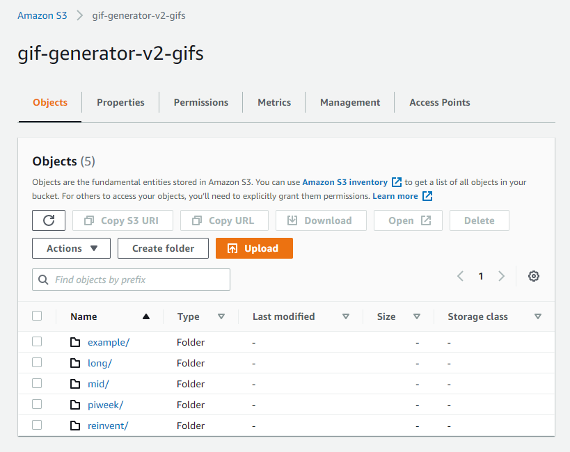
After deployment, you can test the application by uploading an MP4 video to the source S3 bucket. The output GIF and JPG files are written to the application’s destination S3 bucket. The files from each MP4 file are grouped in a folder in the bucket:
Frontend application
The frontend application allows you to visualize the outputs of the backend application. There is also a hosted version of this application. This accepts custom parameters to load graphics resources from S3 buckets in your AWS account. Alternatively, you can run the frontend application locally.
To launch the frontend application:
After cloning the repo, change to the frontend directory.
Run npm install to install Vue.js and all the required npm modules from package.json.
Run npm run serve to start the development server. After building the modules in the project, the terminal shows the local URL where the application is running:
Open a web browser and navigate to http://localhost:8080 to see the application:
Conclusion
In part 1 of this blog post, I explain how a GIF generation service can support a front-end application for video streaming. I compare the performance of a server-based and serverless approach and show how parallelization can significantly improve processing time. I walk through the solution architecture used in the example application and show how you can use FFmpeg in Lambda functions.
Part 2 covers advanced topics around this implementation. It explains the scaling behavior and considers alternative approaches, and looks at the cost of using this service.
For more serverless learning resources, visit Serverless Land.
TC’s Mobility group provides backend cloud services that are built and hosted in AWS. Together, TC and AWS engineers designed, built, and delivered their new Collision Assistance product, which debuted in early August 2021.
In the aftermath of an accident, Collision Assistance offers Toyota and Lexus drivers instructions to help them navigate a post-collision situation. This includes documenting the accident, filing an insurance claim, and transitioning to the repair process.
In this blog post, we’ll talk about how our team designed, built, refined, and deployed the Collision Assistance product with Serverless on AWS services. We’ll discuss our goals in developing this product and the architecture we developed based on those goals. We’ll also present issues we encountered when testing our initial architecture and how we resolved them to create the final product.
Building a scalable, affordable, secure, and high performing product
We used a serverless architecture because it is often less complex than other architecture types. Our goals in developing this initial architecture were to achieve scalability, affordability, security, and high performance, as described in the following sections.
Scalability and affordability
In our initial architecture, Amazon Simple Queue Service (Amazon SQS) queues, Amazon Kinesis streams, and AWS Lambda functions allow data pipelines to run servers only when they’re needed, which introduces cost savings. They also process data in smaller units and run them in parallel, which allows data pipelines to scale up efficiently to handle peak traffic loads. These services allow for an architecture that can handle non-uniform traffic without needing additional application logic.
Security
Collision Assistance can deliver information to customers via push notifications. This data must be encrypted because many data points the application collects are sensitive, like geolocation.
To secure this data outside our private network, we use Amazon Simple Notification Service (Amazon SNS) as our delivery mechanism. Amazon SNS provides HTTPS endpoint delivery of messages coming to topics and subscriptions. AWS allows us to enable at-rest and/or in-transit encryption for all of our other architectural components as well.
Performance
To quantify our product’s performance, we review the “notification delay.” This metric evaluates the time between the initial collision and when the customer receives a push notification from Collision Assistance. Our ultimate goal is to have the push notification sent within minutes of a crash, so drivers have this information in near real time.
Initial architecture
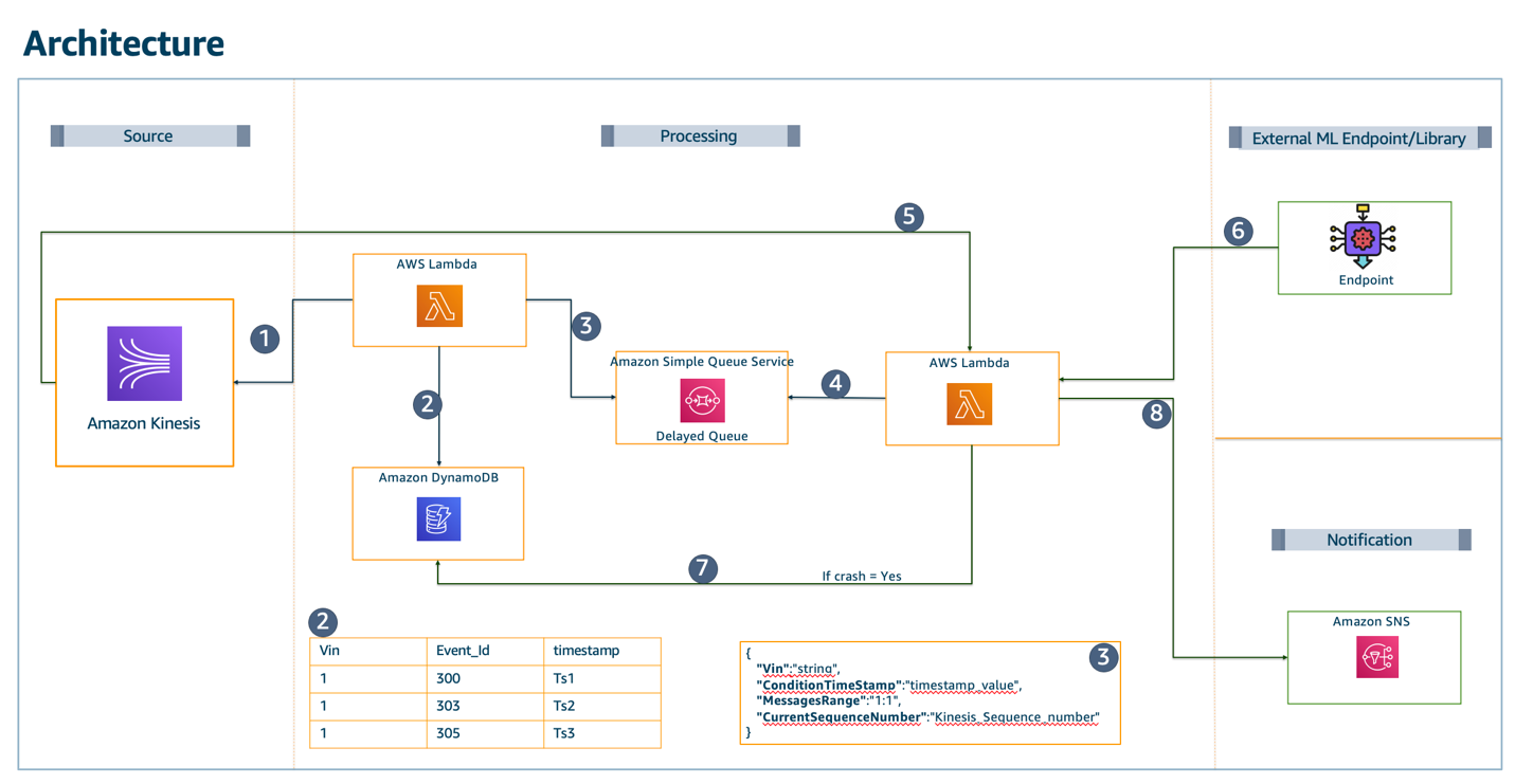
Figure 1 presents our initial architecture implementation that aims to predict whether a crash has occurred and reduce false positives through the following data pipeline:
A Lambda function writes lookup data to Amazon DynamoDB for every Kinesis record.
This Lambda function decreases obvious non-crash data. It sends the current record (X) to Amazon SQS. If X exceeds a certain threshold, it will remain a crash candidate.
Amazon SQS sets a delivery delay so that there will be more Kinesis/DynamoDB records available when X is processed later in the pipeline.
A second Lambda function reads the data from the SQS message. It queries DynamoDB to find the Kinesis lookup data for the message before (X-1) and after (X+1) the crash candidate.
Kinesis GetRecords retrieves X-1 and X+1, because X+1 will exist after the SQS delivery delay times out.
The X-1, X, and X+1 messages are sent to the data science (DS) engine.
When a crash is accurately predicted, these results are stored in a DynamoDB table.
The push notification is sent to the vehicle owner. (Note: the push notification is still in ‘select testing phase’)
Figure 1. Diagram and description of our initial architecture implementation
To be consistent with privacy best practices and reduce server uptime, this architecture uses the minimum amount of data the DS engine needs.
We filter out records that are lower than extremely low thresholds. Once these records are filtered out, around 40% of the data fits the criteria to be evaluated further. This reduces the server capacity needed by the DS engine by 60%.
To reduce false positives, we gather data before and after the timestamps where the extremely low thresholds are exceeded. We then evaluate the sensor data across this timespan and discard any sets with patterns of abnormal sensor readings or other false positive conditions. Figure 2 shows the time window we initially used.
Figure 2. Longitudinal acceleration versus time
Adjusting our initial architecture for better performance
Our initial design worked well for processing a few sample messages and achieved the desired near real-time delivery of the push notification. However, when the pipeline was enabled for over 1 million vehicles, certain limits were exceeded, particularly for Kinesis and Lambda integrations:
Our Kinesis GetRecords API exceeded the allowed five requests per shard per second. With each crash candidate retrieving an X-1 and X+1 message, we could only evaluate two per shard per second, which isn’t cost effective.
Additionally, the downstream SQS-reading Lambda function was limited to 10 records per second per invocation. This meant any slowdown that occurs downstream, such as during DS engine processing, could cause the queue to back up significantly.
To improve cost and performance for the Kinesis-related functionality, we abandoned the DynamoDB lookup table and the GetRecord calls in favor of using a Redis cache cluster on Amazon ElastiCache. This allows us to avoid all throughput exceptions from Kinesis and focus on scaling the stream based on the incoming throughput alone. The ElastiCache cluster scales capacity by adding or removing shards, which improves performance and cost efficiency.
To solve the Amazon SQS/Lambda integration issue, we funneled messages directly to an additional Kinesis stream. This allows the final Lambda function to use some of the better scaling options provided to Kinesis-Lambda event source integrations, like larger batch sizes and max-parallelism.
After making these adjustments, our tests proved we could scale to millions of vehicles as needed. Figure 3 shows a diagram of this final architecture.
Figure 3. Final architecture
Conclusion
Engineers across many functions worked closely to deliver the Collision Assistance product.
Our team of backend Java developers, infrastructure experts, and data scientists from TC and AWS built and deployed a near real-time product that helps Toyota and Lexus drivers document crash damage, file an insurance claim, and get updates on the actual repair process.
The managed services and serverless components available on AWS provided TC with many options to test and refine our team’s architecture. This helped us find the best fit for our use case. Having this flexibility in design was a key factor in designing and delivering the best architecture for our product.
In April 2021, AWS Identity and Access Management (IAM)Access Analyzer added policy generation to help you create fine-grained policies based on AWS CloudTrail activity stored within your account. Now, we’re extending policy generation to enable you to generate policies based on access activity stored in a designated account. For example, you can use AWS Organizations to define a uniform event logging strategy for your organization and store all CloudTrail logs in your management account to streamline governance activities. You can use Access Analyzer to review access activity stored in your designated account and generate a fine-grained IAM policy in your member accounts. This helps you to create policies that provide only the required permissions for your workloads.
Customers that use a multi-account strategy consolidate all access activity information in a designated account to simplify monitoring activities. By using AWS Organizations, you can create a trail that will log events for all Amazon Web Services (AWS) accounts into a single management account to help streamline governance activities. This is sometimes referred to as an organization trail. You can learn more from Creating a trail for an organization. With this launch, you can use Access Analyzer to generate fine-grained policies in your member account and grant just the required permissions to your IAM roles and users based on access activity stored in your organization trail.
When you request a policy, Access Analyzer analyzes your activity in CloudTrail logs and generates a policy based on that activity. The generated policy grants only the required permissions for your workloads and makes it easier for you to implement least privilege permissions. In this blog post, I’ll explain how to set up the permissions for Access Analyzer to access your organization trail and analyze activity to generate a policy. To generate a policy in your member account, you need to grant Access Analyzer limited cross-account access to access the Amazon Simple Storage Service (Amazon S3) bucket where logs are stored and review access activity.
Generate a policy for a role based on its access activity in the organization trail
In this example, you will set fine-grained permissions for a role used in a development account. The example assumes that your company uses Organizations and maintains an organization trail that logs all events for all AWS accounts in the organization. The logs are stored in an S3 bucket in the management account. You can use Access Analyzer to generate a policy based on the actions required by the role. To use Access Analyzer, you must first update the permissions on the S3 bucket where the CloudTrail logs are stored, to grant access to Access Analyzer.
To grant permissions for Access Analyzer to access and review centrally stored logs and generate policies
Select the bucket where the logs from the organization trail are stored.
Change object ownership to bucket owner preferred. To generate a policy, all of the objects in the bucket must be owned by the bucket owner.
Update the bucket policy to grant cross-account access to Access Analyzer by adding the following statement to the bucket policy. This grants Access Analyzer limited access to the CloudTrail data. Replace the <organization-bucket-name>, and <organization-id> with your values and then save the policy.
By using the preceding statement, you’re allowing listbucket and getobject for the bucket my-organization-bucket-name if the role accessing it belongs to an account in your Organizations and has a name that starts with AccessAnalyzerMonitorServiceRole. Using aws:PrincipalAccount in the resource section of the statement allows the role to retrieve only the CloudTrail logs belonging to its own account. If you are encrypting your logs, update your AWS Key Management Service (AWS KMS) key policy to grant Access Analyzer access to use your key.
Now that you’ve set the required permissions, you can use the development account and the following steps to generate a policy.
To generate a policy in the AWS Management Console
Use your development account to open the IAM Console, and then in the navigation pane choose Roles.
Select a role to analyze. This example uses AWS_Test_Role.
Under Generate policy based on CloudTrail events, choose Generate policy, as shown in Figure 1.
Figure 1: Generate policy from the role detail page
In the Generate policy page, select the time window for which IAM Access Analyzer will review the CloudTrail logs to create the policy. In this example, specific dates are chosen, as shown in Figure 2.
Figure 2: Specify the time period
Under CloudTrail access, select the organization trail you want to use as shown in Figure 3.
Note: If you’re using this feature for the first time: select create a new service role, and then choose Generate policy.
This example uses an existing service role “AccessAnalyzerMonitorServiceRole_MBYF6V8AIK.”
Figure 3: CloudTrail access
After the policy is ready, you’ll see a notification on the role page. To review the permissions, choose View generated policy, as shown in Figure 4.
Figure 4: Policy generation progress
After the policy is generated, you can see a summary of the services and associated actions in the generated policy. You can customize it by reviewing the services used and selecting additional required actions from the drop down. To refine permissions further, you can replace the resource-level placeholders in the policies to restrict permissions to just the required access. You can learn more about granting fine-grained permissions and creating the policy as described in this blog post.
Conclusion
Access Analyzer makes it easier to grant fine-grained permissions to your IAM roles and users by generating IAM policies based on the CloudTrail activity centrally stored in a designated account such as your AWS Organizations management accounts. To learn more about how to generate a policy, see Generate policies based on access activity in the IAM User Guide.
If you have feedback about this blog post, submit comments in the Comments section below. If you have questions about this blog post, start a new thread on the IAM forum or contact AWS Support.
Want more AWS Security how-to content, news, and feature announcements? Follow us on Twitter.
This post is written by Rafa Xu, Cloud Architect, Serverless and Joely Huang, Cloud Architect, Serverless.
Amazon Simple Notification Service (SNS) is a fast, flexible, fully managed push messaging service in the cloud. SNS can send mobile push notifications directly to applications on mobile devices such as message alerts and badge updates. SNS sends push notifications to a mobile endpoint created by supplying a mobile token and platform application.
When publishing mobile push notifications, a device token is used to generate an endpoint. This identifies where the push notification is sent (target destination). To push notifications successfully, the token must be up to date and the endpoint must be validated and enabled.
A common challenge when pushing notifications is keeping the token up to date. Tokens can automatically change due to reasons such as mobile operating system (OS) updates and application store updates.
This post provides a serverless solution to this challenge. It also provides a way to publish push notifications to specific end users by maintaining a mapping between users, endpoints, and tokens.
Overview
To publish mobile push notifications using SNS, generate an SNS endpoint to use as a destination target for the push notification. To create the endpoint, you must supply:
A mobile application token: The mobile operating system (OS) issues the token to the application. It is a unique identifier for the application and mobile device pair.
Platform Application Amazon Resource Name (ARN): SNS provides this ARN when you create a platform application object. The platform application object requires a valid set of credentials issued by the mobile platform, which you provide to SNS.
Once the endpoint is generated, you can store and reuse it again. This prevents the application from creating endpoints indefinitely, which could exhaust the SNS endpoint limit.
To reuse the endpoints and successfully push notifications, there are a number of challenges:
Mobile application tokens can change due to a number of reasons, such as application updates. As a result, the publisher must update the platform endpoint to ensure it uses an up-to-date token.
Mobile application tokens can become invalid. When this happens, messages won’t be published, and SNS disables the endpoint with the invalid token. To resolve this, publishers must retrieve a valid token and re-enable the platform endpoint
Mobile applications can have many users, each user could have multiple devices, or one device could have multiple users. To send a push notification to a specific user, a mapping between the user, device, and platform endpoints should be maintained.
For more information on best practices for managing mobile tokens, refer to this post.
Follow along the blog post to learn how to implement a serverless workflow for managing and maintaining valid endpoints and user mappings.
Solution overview
The solution uses the following AWS services:
Amazon API Gateway: Provides a token registration endpoint URL used by the mobile application. Once called, it invokes an AWS Lambda function via the Lambda integration.
Amazon SNS: Generates and maintains the target endpoint and manages platform application objects.
Amazon DynamoDB: Serverless database for storing endpoints that also maintains a mapping between the user, endpoint, and mobile operating system.
AWS Lambda: Retrieves endpoints from DynamoDB, validates and generates endpoints, and publishes notifications by making requests to SNS.
The following diagram represents a simplified interaction flow between the AWS services:
To register the token, the mobile app invokes the registration token endpoint URL generated by Amazon API Gateway. The token registration happens every time a user logs in or opens the application. This ensures that the token and endpoints are always valid during the application usage.
The mobile application passes the token, user, and mobileOS as parameters to API Gateway, which forwards the request to the Lambda function.
The Lambda function validates the token and endpoint for the user by making API calls to DynamoDB and SNS:
The Lambda function checks DynamoDB to see if the endpoint has been previously created.
To deploy the AWS SAM template, navigate to the directory where the template is located. Run the commands in the terminal:
git clone https://github.com/aws-samples/serverless-mobile-push-notification
cd serverless-mobile-push-notification
sam build
sam deploy --guided
Lambda function code snippets
The following section explains code from the Lambda function for the workflow.
Create the platform endpoint
If the endpoint exists, store it as a variable in the code. If the platform endpoint does not exist in the DynamoDB database, create a new endpoint:
        need_update_ddb = False
        response = table.get_item(Key={'username': username, 'appos': appos})
        if 'Item' not in response:
            # create endpoint
            response = snsClient.create_platform_endpoint(
                PlatformApplicationArn=SUPPORTED_PLATFORM[appos],
                Token=token,
            )
            devicePushEndpoint = response['EndpointArn']
            need_update_ddb = True
        else:
            # update the endpoint
            devicePushEndpoint = response['Item']['endpoint']
Check and update endpoint attributes
Check that the token attribute for the platform endpoint matches the token received from the mobile application through the request. This also checks for the endpoint “enabled” attribute and re-enables the endpoint if necessary:
As best practice, the code cleans up the table, in case there are multiple entries for the same endpoint mapped to different users. This can happen when the mobile application is used by multiple users on the same device. When one user logs out and a different user logs in, this creates a new entry in the DynamoDB table to map the endpoint with the new user.
As a result, you must remove the entry that maps the same endpoint to the previously logged in user. This way, you only keep the endpoint that matches the user provided by the mobile application through the request.
result = table.query(
    # Add the name of the index you want to use in your query.
        IndexName="endpoint-index",
        KeyConditionExpression=Key('endpoint').eq(devicePushEndpoint),
    )
    for item in result['Items']:
        if item['username'] != username and item['appos'] == appos:
            print(f"deleting orphan item: username {username}, os {appos}".format(username=item['username'], appos=appos))
            table.delete_item(
                Key={
                    'username': item['username'],
                    'appos': appos
                },
            )
Conclusion
This blog shows how to deploy a serverless solution for validating and managing SNS platform endpoints and tokens. To publish push notifications successfully, use SNS to check the endpoint attribute and ensure it is mapped to the correct token and the endpoint is enabled.
This approach uses DynamoDB to store the device token and platform endpoints for each user. This allows you to send push notifications to specific users, retrieve, and reuse previously created endpoints. You create a Lambda function to facilitate the workflow, including validating the DynamoDB item for storing an enabled and up-to-date token.
As businesses expand applications to reach more users and devices, they risk higher latencies that could degrade the customer experience. Slow applications can frustrate or even turn away customers. Developers therefore increasingly face the challenge of ensuring that their code runs as efficiently as possible, since application performance can make or break businesses.
Amazon CodeGuru Profiler helps developers improve their application speed by analyzing its runtime. CodeGuru Profiler analyzes single and multi-threaded applications and then generates visualizations to help developers understand the latency sources. Afterwards, CodeGuru Profiler provides recommendations to help resolve the root cause.
This post highlights these new features by explaining how to set up and utilize CodeGuru Profiler on an AWS Lambda function written in Python.
Prerequisites
This post focuses on improving the performance of an application written with AWS Lambda, so it’s important to understand the Lambda functions that work best with CodeGuru Profiler. You will get the most out of CodeGuru Profiler on long-duration Lambda functions (>10 seconds) or frequently invoked shorter generation Lambda functions (~100 milliseconds). Because CodeGuru Profiler requires five minutes of runtime data before the Lambda container is recycled, very short duration Lambda functions with an execution time of 1-10 milliseconds may not provide sufficient data for CodeGuru Profiler to generate meaningful results.
The automated CodeGuru Profiler onboarding process, which automatically creates the profiling group for you, supports Lambda functions running on Java 8 (Amazon Corretto), Java 11, and Python 3.8 runtimes. Additional runtimes, without the automated onboarding process, are supported and can be found in the Java documentation and the Python documentation.
Getting Started
Let’s quickly demonstrate the new Lambda onboarding process and the new Python recommendations. This example assumes you have already created a Lambda function, so we will just walk through the process of turning on CodeGuru Profiler and viewing results. If you don’t already have a Lambda function created, you can create one by following these set up instructions. If you would like to replicate this example, the code we used can be found on GitHub here.
On the AWS Lambda Console page, open your Lambda function. For this example, we’re using a function with a Python 3.8 runtime.
2. Navigate to the Configuration tab, go to the Monitoring and operations tools page, and click Edit on the right side of the page.
3. Scroll down to “Amazon CodeGuru Profiler” and click the button next to “Code profiling” to turn it on. After enabling Code profiling, click Save.
4. Verify that CodeGuru Profiler has been turned on within the Monitoring and operations tools page
That’s it! You can now navigate to CodeGuru Profiler within the AWS console and begin viewing results.
Viewing your results
CodeGuru Profiler requires 5 minutes of Lambda runtime data to generate results. After your Lambda function provides this runtime data, which may need multiple runs if your lambda has a short runtime, it will display within the “Profiling group” page in the CodeGuru Profiler console. The profiling group will be given a default name (i.e., aws-lambda-<lambda-function-name>), and it will take approximately 15 minutes after CodeGuru Profiler receives the runtime data before it appears on this page.
After the profile appears, customers can view their profiling results by analyzing the flame graphs. Additionally, after approximately 1 hour, customers will receive their first recommendation set (if applicable). For more information on how to reading the CodeGuru Profiler results, see Investigating performance issues with Amazon CodeGuru Profiler.
The below images show the two flame graphs (CPU Utilization and Latency) generated from profiling the Lambda function. Note that the highlighted horizontal bar (also referred to as a frame) in both images corresponds with one of the three frames that generates a recommendation. We’ll dive into more details on the recommendation in the following sections.
CPU Utilization Flame Graph:
Latency Flame Graph:
Here are the three recommendations generated from the above Lambda function:
Addressing a recommendation
Let’s dive even further into it an example recommendation. The first recommendation above notices that the Lambda function is spending more than the normal amount of runnable time (6.8% vs <1%) creating AWS SDK service clients. It recommends ensuring that the function doesn’t unnecessarily create AWS SDK service clients, which wastes CPU time.
Based on the suggested resolution step, we made a quick and easy code change, moving the client creation outside of the lambda-handler function. This ensures that we don’t create unnecessary AWS SDK clients. The code change below shows how we would resolve the issue.
After making each of the three changes recommended above by CodeGuru Profiler, look at the new flame graphs to see how the changes impacted the applications profile. You’ll notice below that we no longer see the previously wide frames for boto3 clients, put_metric_data, or the logger in the S3 API call.
CPU Utilization Flame Graph:
Latency Flame Graph:
Moreover, we can run the Lambda function for one day (1439 invocations) and see the results in Lambda Insights in order to understand our total savings. After every recommendation was addressed, this Lambda function, with a 128 MB memory and 10 second timeout, decreased in CPU time by 10% and dropped in maximum memory usage and network IO leading to a 30% drop in GB-s. Decreasing GB-s leads to 30% lower cost for the Lambda’s duration bill as explained in the AWS Lambda Pricing.
Latency (before and after CodeGuru Profiler):
The graph below displays the duration change while running the Lambda function for 1 day.
Cost (before and after CodeGuru Profiler):
The graph below displays the function cost change while running the lambda function for 1 day.
Conclusion
This post showed how developers can easily onboard onto CodeGuru Profiler in order to improve the performance of their serverless applications built on AWS Lambda. Get started with CodeGuru Profiler by visiting the CodeGuru console.
All across Amazon, numerous teams have utilized CodeGuru Profiler’s technology to generate performance optimizations for customers. It has also reduced infrastructure costs, saving millions of dollars annually.
Onboard your Python applications onto CodeGuru Profiler by following the instructions on the documentation. If you’re interested in the Python agent, note that it is open-sourced on GitHub. Also for more demo applications using the Python agent, check out the GitHub repository for additional samples.
About the authors
Vishaal is a Product Manager at Amazon Web Services. He enjoys getting to know his customers’ pain points and transforming them into innovative product solutions.
Mirela is working as a Software Development Engineer at Amazon Web Services as part of the CodeGuru Profiler team in London. Previously, she has worked for Amazon.com’s teams and enjoys working on products that help customers improve their code and infrastructure.
Parag is a Software Development Engineer at Amazon Web Services as part of the CodeGuru Profiler team in Seattle. Previously, he was working for Amazon.com’s catalog and selection team. He enjoys working on large scale distributed systems and products that help customers build scalable, and cost-effective applications.
This series of blog posts uses the AWS Well-Architected Tool with the Serverless Lens to help customers build and operate applications using best practices. In each post, I address the serverless-specific questions identified by the Serverless Lens along with the recommended best practices. See the introduction post for a table of contents and explanation of the example application.
PERF 1. Optimizing your serverless application’s performance
This post continues part 1 of this security question. Previously, I cover measuring and optimizing function startup time. I explain cold and warm starts and how to reuse the Lambda execution environment to improve performance. I show a number of ways to analyze and optimize the initialization startup time. I explain how only importing necessary libraries and dependencies increases application performance.
Good practice: Design your function to take advantage of concurrency via asynchronous and stream-based invocations
AWS Lambda functions can be invoked synchronously and asynchronously.
Favor asynchronous over synchronous request-response processing.
Consider using asynchronous event processing rather than synchronous request-response processing. You can use asynchronous processing to aggregate queues, streams, or events for more efficient processing time per invocation. This reduces wait times and latency from requesting apps and functions.
When you invoke a Lambda function with a synchronous invocation, you wait for the function to process the event and return a response.
Synchronous invocation
As synchronous processing involves a request-response pattern, the client caller also needs to wait for a response from a downstream service. If the downstream service then needs to call another service, you end up chaining calls that can impact service reliability, in addition to response times. For example, this POST /order request must wait for the response to the POST /invoice request before responding to the client caller.
Example synchronous processing
The more services you integrate, the longer the response time, and you can no longer sustain complex workflows using synchronous transactions.
Asynchronous processing allows you to decouple the request-response using events without waiting for a response from the function code. This allows you to perform background processing without requiring the client to wait for a response, improving client performance. You pass the event to an internal Lambda queue for processing and Lambda handles the rest. An external process, separate from the function, manages polling and retries. Using this asynchronous approach can also make it easier to handle unpredictable traffic with significant volumes.
Asynchronous invocation
For example, the client makes a POST /order request to the order service. The order service accepts the request and returns that it has been received, without waiting for the invoice service. The order service then makes an asynchronous POST /invoice request to the invoice service, which can then process independently of the order service. If the client must receive data from the invoice service, it can handle this separately via a GET /invoice request.
Example asynchronous processing
You can configure Lambda to send records of asynchronous invocations to another destination service. This helps you to troubleshoot your invocations. You can also send messages or events that can’t be processed correctly into a dedicated Amazon Simple Queue Service (SQS) dead-letter queue for investigation.
You can add triggers to a function to process data automatically. For more information on which processing model Lambda uses for triggers, see “Using AWS Lambda with other services”.
Asynchronous workflows handle a variety of use cases including data Ingestion, ETL operations, and order/request fulfillment. In these use-cases, data is processed as it arrives and is retrieved as it changes. For example asynchronous patterns, see “Serverless Data Processing” and “Serverless Event Submission with Status Updates”.
Tune batch size, batch window, and compress payloads for high throughput
When using Lambda to process records using Amazon Kinesis Data Streams or SQS, there are a number of tuning parameters to consider for performance.
You can configure a batch window to buffer messages or records for up to 5 minutes. You can set a limit of the maximum number of records Lambda can process by setting a batch size. Your Lambda function is invoked whichever comes first.
For high volume SQS standard queue throughput, Lambda can process up to 1000 concurrent batches of records per second. For more information, see “Using AWS Lambda with Amazon SQS”.
For high volume Kinesis Data Streams throughput, there are a number of options. Configure the ParallelizationFactor setting to process one shard of a Kinesis Data Stream with more than one Lambda invocation simultaneously. Lambda can process up to 10 batches in each shard. For more information, see “New AWS Lambda scaling controls for Kinesis and DynamoDB event sources.” You can also add more shards to your data stream to increase the speed at which your function can process records. This increases the function concurrency at the expense of ordering per shard. For more details on using Kinesis and Lambda, see “Monitoring and troubleshooting serverless data analytics applications”.
Kinesis stream producers can also compress records. This is at the expense of additional CPU cycles for decompressing the records in your Lambda function code.
Required practice: Measure, evaluate, and select optimal capacity units
Capacity units are a unit of consumption for a service. They can include function memory size, number of stream shards, number of database reads/writes, request units, or type of API endpoint. Measure, evaluate and select capacity units to enable optimal configuration of performance, throughput, and cost.
Identify and implement optimal capacity units.
For Lambda functions, memory is the capacity unit for controlling the performance of a function. You can configure the amount of memory allocated to a Lambda function, between 128 MB and 10,240 MB. The amount of memory also determines the amount of virtual CPU available to a function. Adding more memory proportionally increases the amount of CPU, increasing the overall computational power available. If a function is CPU-, network- or memory-bound, then changing the memory setting can dramatically improve its performance.
Choosing the memory allocated to Lambda functions is an optimization process that balances performance (duration) and cost. You can manually run tests on functions by selecting different memory allocations and measuring the time taken to complete. Alternatively, use the AWS Lambda Power Tuning tool to automate the process.
The tool allows you to systematically test different memory size configurations and depending on your performance strategy – cost, performance, balanced – it identifies what is the most optimum memory size to use. For more information, see “Operating Lambda: Performance optimization – Part 2”.
AWS Lambda Power Tuning report
Amazon DynamoDB manages table processing throughput using read and write capacity units. There are two different capacity modes, on-demand and provisioned.
On-demand capacity mode supports up to 40K read/write request units per second. This is recommended for unpredictable application traffic and new tables with unknown workloads. For higher and predictable throughputs, provisioned capacity mode along with DynamoDB auto scaling is recommended. For more information, see “Read/Write Capacity Mode”.
For high throughput Amazon Kinesis Data Streams with multiple consumers, consider using enhanced fan-out for dedicated 2 MB/second throughput per consumer. When possible, use Kinesis Producer Library and Kinesis Client Library for effective record aggregation and de-aggregation.
Amazon API Gateway supports multiple endpoint types. Edge-optimized APIs provide a fully managed Amazon CloudFront distribution. These are better for geographically distributed clients. API requests are routed to the nearest CloudFront Point of Presence (POP), which typically improves connection time.
Edge-optimized API Gateway deployment
Regional API endpoints are intended when clients are in the same Region. This helps you to reduce request latency and allows you to add your own content delivery network if necessary.
AWS Step Functions has two workflow types, standard and express. Standard Workflows have exactly once workflow execution and can run for up to one year. Express Workflows have at-least-once workflow execution and can run for up to five minutes. Consider the per-second rates you require for both execution start rate and the state transition rate. For more information, see “Standard vs. Express Workflows”.
Performance load testing is recommended at both sustained and burst rates to evaluate the effect of tuning capacity units. Use Amazon CloudWatch service dashboards to analyze key performance metrics including load testing results. I cover performance testing in more detail in “Regulating inbound request rates – part 1”.
Evaluate and optimize your serverless application’s performance based on access patterns, scaling mechanisms, and native integrations. You can improve your overall experience and make more efficient use of the platform in terms of both value and resources.
This post continues from part 1 and looks at designing your function to take advantage of concurrency via asynchronous and stream-based invocations. I cover measuring, evaluating, and selecting optimal capacity units.
This well-architected question will continue in part 3 where I look at integrating with managed services directly over functions when possible. I cover optimizing access patterns and applying caching where applicable.
For more serverless learning resources, visit Serverless Land.
When you provide access to a sensitive document to someone outside of your organization, you likely need to ensure that the document is read-only. In this case, your document should be associated with a specific user in case it is shared.
For example, authors often embed user-specific watermarks into their ebooks. This way, if their ebook gets posted to a file-sharing site, they can prevent the purchaser from downloading copies of the ebook in the future.
In this blog post, we provide you a cost-efficient, scalable, and secure solution to efficiently generate user-specific versions of sensitive documents. This solution helps users track who their documents are shared with. This helps prevent fraud and ensure that private information isn’t leaked. Our solution uses a RESTful API, which uses Amazon S3 Object Lambda to convert documents to PDF and apply a watermark based on the requesting user. It also provides a method for authentication and tracks access to the original document.
Architectural overview
S3 Object Lambda processes and transforms data that is requested from Amazon Simple Storage Service (Amazon S3) before it’s sent back to a client. The AWS Lambda function is invoked inline via a standard S3 GET request. It can return different results from the same document based on parameters, such as who is requesting the document. Figure 1 provides a high-level view of the different components that make up the solution.
This architecture defines a RESTful API, but users will likely be using a mobile or web application that calls the API. Thus, the application will first need to authenticate users. We do this via Amazon Cognito, which functions as its own identity provider (IdP). You could also use an external IdP, including those that support OpenID Connect and SAML.
Validating the JSON Web Token with API Gateway
Once the user is successfully authenticated with Amazon Cognito, the application will be sent a JSON Web Token (JWT). This JWT contains information about the user and will be used in subsequent requests to the API.
Now that the application has a token, it will make a request to the API, which is provided by Amazon API Gateway. API Gateway provides a secure, scalable entryway into your application. The API Gateway validates the JWT sent from the client with Amazon Cognito to make sure it is valid. If it is validated, the request is accepted and sent on to the Lambda API Handler. If it’s not, the client gets rejected and sent an error code.
Storing user data with DynamoDB
When the Lambda API Handler receives the request, it parses the JWT to extract the user making the request. It then logs that user, file, and access time into Amazon DynamoDB. Optionally, you may use DynamoDB to store an encoded string that will be used as the watermark, rather than something in plaintext, like user name or email.
Generating the PDF and user-specific watermark
At this point, the Lambda API Handler sends an S3 GET request. However, instead of going to Amazon S3 directly, it goes to a different endpoint that invokes the S3 Object Lambda function. This endpoint is called an S3 Object Lambda Access Point. The S3 GET request contains the original file name and the string that will be used for the watermark.
The S3 Object Lambda function transforms the original file that it downloads from its source S3 bucket. It uses the open-source office suite LibreOffice (and specifically this Lambda layer) to convert the source document to PDF. Once it is converted, a JavaScript library (PDF-Lib) embeds the watermark into the PDF before it’s sent back to the Lambda API Handler function.
The Lambda API Handler stores the converted file in a temporary S3 bucket, generates a presigned URL, and sends that URL back to the client as a 302 redirect. Then the client sends a request to that presigned URL to get the converted file.
Figure 2. Process workflow for document transformation
Alternate approach
Before S3 Object Lambda was available, Lambda@Edge was used. However, there are three main issues with using Lambda@Edge instead of S3 Object Lambda:
It is designed to run code closer to the end user to decrease latency, but in this case, latency is not a major concern.
It requires using an Amazon CloudFront distribution, and the single-download pattern described here will not take advantage of Lamda@Edge’s caching.
It has quotas on memory that don’t lend themselves to complex libraries like OfficeLibre.
Extending this solution
This blog post describes the basic building blocks for the solution, but it can be extended relatively easily. For example, you could add another function to the API that would convert, resize, and watermark images. To do this, create an S3 Object Lambda function to perform those tasks. Then, add an S3 Object Lambda Access Point to invoke it based on a different API call.
Monitoring any solution is critical, and understanding how an application is behaving end to end can greatly benefit optimization and troubleshooting. Adding AWS X-Ray and Amazon CloudWatch Lambda Insights will show you how functions and their interactions are performing.
Figure 3. Example expanded document processing architecture
Conclusion
You can implement this solution in a number of ways. However, by using S3 Object Lambda, you can transform documents without needing intermediary storage. S3 Object Lambda will also decouple your file logic from the rest of the application.
The Serverless on AWS components mentioned in this post allow you to reduce administrative overhead, saving you time and money.
Finally, the extensible nature of this architecture allows you to add functionality easily as your organization’s needs grow and change.
The following links provide more information on how to use S3 Object Lambda in your architectures:
Commercial off-the-shelf software and third-party services can present an integration challenge in event-driven workflows when they do not natively support AWS APIs. This is even more impactful when a workflow is subject to unpredicted usage spikes, and you want to increase decoupling and fault tolerance. Given the third-party nature of services, polling an Amazon Simple Queue Service (SQS) queue and having built-in AWS API handling logic may not be an immediate option.
In such cases, AWS Lambda helps out-task the Amazon SQS queue integration and AWS API handling to an additional layer. The success of this depends on how well exception handling is implemented across the different interacting services. In this blog post, we outline issues to consider when adopting this design pattern. We also share a reusable solution.
Design pattern for third-party integration with SQS
With this design pattern, one or more services (producers) asynchronously invoke other third-party downstream consumer services. They publish messages to an Amazon SQS queue, which acts as buffer for requests. Producers provide all commands and other parameters required for consumer service execution with the message.
Figure 1. On-premises and AWS queue integration for third-party services using AWS Lambda
The message broker asynchronously invokes the API in ‘fire-and-forget’ mode. Therefore, error handling must be built in to respond to API invocation errors. In an event-driven scenario, an error will be invoked if you asynchronously call the third-party service hundreds or thousands of times and reach Service Quotas. This is a potential issue with RunTask API actions, or a large volume of concurrent tasks running on AWS Fargate. Two mechanisms can help implement troubleshooting API request errors.
API retries with exponential backoff. The message broker retries for a number of times with configurable sleep intervals and exponential backoff in-between. This enforces progressively longer waits between retries for consecutive error responses. If the RunTask API fails to process the request and initiate the third-party service, the message remains in the queue for a subsequent retry. The AWS General Reference provides further guidance.
API error handling. Error handling and consequent logging should be implemented at every step. Since there are several services working together in tandem, crucial debugging information from errors may be lost. Additionally, error handling also provides opportunity to define automated corrective actions or notifications on event occurrence. The message broker can publish failure notifications including the root cause to an Amazon Simple Notification Service (SNS) topic.
SNS topic subscription can be configured via different protocols. You can email a distribution group for active monitoring and processing of errors. If persistence is required for messages that failed to process, error handling can be associated directly with SQS by configuring a dead letter queue.
Reference implementation for third-party integration with SQS
We implemented the design pattern in Figure 1, with Broad Institute’s Cell Painting application workflow. This is for morphological profiling from microscopy cell images running on Amazon EC2. It interacts with CellProfiler version 3.0 cell image analysis software as the downstream consumer hosted on ECS/Fargate. Every invocation of CellProfiler required approximately 1,500 tasks for a single processing step.
Resource constraints determined the rate of scale-out. In this case, it was for an Amazon ECS task creation. Address space for Amazon ECS subnets should be large enough to prevent running out of available IPs within your VPC. If Amazon ECS Service Quotas provide further constraints, a quota increase can be requested.
Exceptions must be handled both when validating and initiating requests. As part of the validation workflow, exceptions are captured as follows, also shown in Figure 2.
1. Invalid arguments exception. The message broker validates that the SQS message contains all the needed information to initiate the ECS task. This information includes subnets, security groups and container names required to start the ECS task, and else raises exception.
2. Retry limit exception. On each iteration, the message broker will evaluate whether the SQS retry limit has been reached, before invoking the RunTask API. It will then exit, by sending failure notification to SNS when the retry limit is reached.
Figure 2. Exception handling flow during request validation
As part of the initiation workflow, exceptions are handled as follows, shown in Figure 3:
1. ECS/Fargate API and concurrent execution limitations. The message broker catches API exceptions when calling the API RunTask operation. These exceptions can include:
When the call to the launch tasks exceeds the maximum allowed API request limit for your AWS account
When failing to retrieve security group information
When you have reached the limit on the number of tasks you can run concurrently
With each of the preceding exceptions, the broker will increase the retry count.
2. Networking and IP space limitations. Network interface timeouts received after initiating the ECS task set off an Amazon CloudWatch Events rule, causing the message broker to re-initiate the ECS task.
Figure 3. Exception handling flow during request initiation
While we specifically address downstream consumer services running on ECS/Fargate, this solution can be adjusted for third-party services running on Amazon EC2 or EKS. With EC2, the message broker must be adjusted to interact with the RunInstances API, and include troubleshooting API request errors. Integration with downstream consumers on Amazon EKS requires that the AWS Lambda function is associated via the IAM role with a Kubernetes service account. A Python client for Kubernetes can be used to simplify interaction with the Kubernetes REST API and AWS Lambda would invoke the run API.
Conclusion
This pattern is useful when queue polling is not an immediate option. This is typical with event-driven workflows involving third-party services and vendor applications subject to unpredictable, intermittent load spikes. Exception handling is essential for these types of workflows. Offloading AWS API handling to a separate layer orchestrated by AWS Lambda can improve the resiliency of such third-party services on AWS. This pattern represents an incremental optimization until the third party provides native SQS integration. It can be achieved with the initial move to AWS, for example as part of the V1 AWS design strategy for third-party services.
Some limitations should be acknowledged. While the pattern enables graceful failure, it does not prevent the overloading of the ECS RunTask API. By invoking Amazon ECS RunTask API in ‘fire-and-forget’ mode, it does not monitor service execution once a task was successfully invoked. Therefore, it should be adopted when direct queue polling is not an option. In our example, Broad Institute’s CellProfiler application enabled direct queue polling with its subsequent product version of Distributed CellProfiler.
Further reading
The referenced deployment with consumer services on Amazon ECS can be accessed via AWSLabs.
This post is written by Dathu Patil, Solutions Architect and Naomi Joshi, Cloud Application Architect.
AWS CloudFormation custom resources allow you to write custom provisioning logic in templates. These run anytime you create, update, or delete stacks. Using AWS Lambda-backed custom resources, you can associate a Lambda function with a CloudFormation custom resource. The function is invoked whenever the custom resource is created, updated, or deleted.
When CloudFormation asynchronously invokes the function, it passes the request data, such as the request type and resource properties to the function. The customizability of Lambda functions in combination with CloudFormation allow a wide range of scenarios. For example, you can dynamically look up Amazon Machine Image (AMI) IDs during stack creation or use utilities such as string reversal functions.
Unhandled exceptions or transient errors in the custom resource Lambda function can cause your code to exit without sending a response. CloudFormation requires an HTTPS response to confirm if the operation is successful or not. An unreported exception causes CloudFormation to wait until the operation times out before starting a stack rollback.
If the exception occurs again on rollback, CloudFormation waits for a timeout exception before ending in a rollback failure. During this time, your stack is unusable. You can learn more about this and best practices by reviewing Best Practices for CloudFormation Custom Resources.
In this blog, you learn how you can use Amazon SQS and Lambda to add resiliency to your Lambda-backed CloudFormation custom resource deployments. The example shows how to use CloudFormation custom resource to look up an AMI ID dynamically during Amazon EC2 creation.
Overview
CloudFormation templates that declare an EC2 instance must also specify an AMI ID. This includes an operating system and other software and configuration information used to launch the instance. The correct AMI ID depends on the instance type and Region in which you’re launching your stack. AMI ID can change regularly, such as when an AMI is updated with software updates.
Customers often implement a CloudFormation custom resource to look up an AMI ID while creating an EC2 instance. In this example, the lookup Lambda function calls the EC2 API. It fetches the available AMI IDs, uses the latest AMI ID, and checks for a compliance tag. This implementation assumes that there are separate processes for creating AMI and running compliance checks. The process that performs compliance and security checks creates a compliance tag on a successful scan.
This solution shows how you can use SQS and Lambda to add resiliency to handle an exception. In this case, the exception occurs in the AMI lookup custom resource due to a missing compliance tag. When the AMI lookup function fails processing, it uses the Lambda destination configuration to send the request to an SQS queue. The message is reprocessed using the SQS queue and Lambda function.
The CloudFormation custom resource asynchronously invokes the AMI lookup Lambda function to perform appropriate actions.
The AMI lookup Lambda function calls the EC2 API to fetch the list of AMIs and checks for a compliance tag. If the tag is missing, it throws an unhandled exception.
On failure, the Lambda destination configuration sends the request to the retry queue that is configured as a dead-letter queue (DLQ). SQS adds a custom delay between retry processing to support more than two retries.
The retry Lambda function processes messages in the retry queue using Lambda with SQS. Lambda polls the queue and invokes the retry Lambda function synchronously with an event that contains queue messages.
The retry function then synchronously invokes the AMI lookup function using the information from the request SQS message.
The AMI Lookup Lambda function
An AWS Serverless Application Model (AWS SAM) template is used to create the AMI lookup Lambda function. You can configure async event options such as number of retries on the Lambda function. The maximum retries allowed is 2 and there is no option to set a delay between the invocation attempts.
When a transient failure or unhandled error occurs, the request is forwarded to the retry queue. This part of the AWS SAM template creates AMI lookup Lambda function:
This function calls the EC2 API using the boto3 AWS SDK for Python. It calls the describe_images method to get a list of images with given filter conditions. The Lambda function iterates through the AMI list and checks for compliance tags. If the tag is not present, it raises an exception:
ec2_client = boto3.client('ec2', region_name=region)
         # Get AMI IDs with the specified name pattern and owner
         describe_response = ec2_client.describe_images(
            Filters=[{'Name': "name", 'Values': architectures},
                     {'Name': "tag-key", 'Values': ['ami-compliance-check']}],
            Owners=["amazon"]
        )
The queue and the retry Lambda function
The retry queue adds a 60-second delay before a message is available for the processing. The time delay between retry processing attempts provides time for transient errors to be corrected. This is the AWS SAM template for creating these resources:
The retry Lambda function periodically polls for new messages in the retry queue. The function synchronously invokes the AMI lookup Lambda function. On success, a response is sent to CloudFormation. This process runs until the AMI lookup function returns a successful response or the message is deleted from the SQS queue. The deletion is based on the MessageRetentionPeriod, which is set to 600 seconds in this case.
for record in event['Records']:
        body = json.loads(record['body'])
        response = client.invoke(
            FunctionName=body['requestContext']['functionArn'],
            InvocationType='RequestResponse',
            Payload=json.dumps(body['requestPayload']).encode()
        )
An existing Amazon EC2 public image. You can choose any of the AMIs from the AWS Management Console with Architecture = X86_64 and Owner = amazon for test purposes. Note the AMI ID.
Download the source code from the resilient-cfn-custom-resource GitHub repository. The template.yaml file is an AWS SAM template. It deploys the Lambda functions, SQS, and IAM roles required for the Lambda function. It uses Python 3.8 as the runtime and assigns 128 MB of memory for the Lambda functions.
To build and deploy this application using the AWS SAM CLI build and guided deploy:
sam build --use-container
sam deploy --guided
The custom resource stack creation invokes the AMI lookup Lambda function. This fetches the AMI ID from all public EC2 images available in your account with the tag ami-compliance-check. Typically, the compliance tags are created by a process that performs security scans.
In this example, the security scan process is not running and the tag is not yet added to any AMIs. As a result, the custom resource throws an exception, which goes to the retry queue. This is retried by the retry function until it is successfully processed.
Use the console or AWS CLI to add the tag to the chosen EC2 AMI. In this example, this is analogous to a separate governance process that checks for AMI compliance and adds the compliance tag if passed. Replace the $AMI-ID with the AMI ID captured in the prerequisites:
After the tags are added, a response is sent successfully from the custom resource Lambda function to the CloudFormation stack. It includes your $AMI-ID and a test EC2 instance is created using that image. The stack creation completes successfully with all resources deployed.
Conclusion
This blog post demonstrates how to use SQS and Lambda to add resiliency to CloudFormation custom resources deployments. This solution can be customized for use cases where CloudFormation stacks have a dependency on a custom resource.
CloudFormation custom resource failures can happen due to unhandled exceptions. These are caused by issues with a dependent component, internal service, or transient system errors. Using this solution, you can handle the failures automatically without the need for manual intervention. To get started, download the code from the GitHub repo and start customizing.
For more serverless learning resources, visit Serverless Land.
AWS Lambda launched support for packaging and deploying functions as container images at re:Invent 2020. In the post working with Lambda layers and extensions in container images, we demonstrated packaging Lambda Functions with layers while using container images. This post will teach you to use AWS CodePipeline to deploy docker images for microservices architecture involving multiple Lambda Functions and a common layer utilized as a separate container image. Lambda functions packaged as container images do not support adding Lambda layers to the function configuration. Alternatively, we can use a container image as a common layer while building other container images along with Lambda Functions shown in this post. Packaging Lambda functions as container images enables familiar tooling and larger deployment limits.
Here are some advantages of using container images for Lambda:
Easier dependency management and application building with container
Install native operating system packages
Install language-compatible dependencies
Consistent tool set for containers and Lambda-based applications
Utilize the same container registry to store application artifacts (Amazon ECR, Docker Hub)
Utilize the same build and pipeline tools to deploy
Tools that can inspect Dockerfile work the same
Deploy large applications with AWS-provided or third-party images up to 10 GB
Include larger application dependencies that previously were impossible
When using container images with Lambda, CodePipeline automatically detects code changes in the source repository in AWS CodeCommit, then passes the artifact to the build server like AWS CodeBuild and pushes the container images to ECR, which is then deployed to Lambda functions.
Architecture diagram
DevOps Architecture
Application Architecture
In the above architecture diagram, two architectures are combined, namely 1, DevOps Architecture and 2, Microservices Application Architecture. DevOps architecture demonstrates the use of AWS Developer services such as AWS CodeCommit, AWS CodePipeline, AWS CodeBuild along with Amazon Elastic Container Repository (ECR) and AWS CloudFormation. These are used to support Continuous Integration and Continuous Deployment/Delivery (CI/CD) for both infrastructure and application code. Microservices Application architecture demonstrates how various AWS Lambda Functions that are part of microservices utilize container images for application code. This post will focus on performing CI/CD for Lambda functions utilizing container containers. The application code used in here is a simpler version taken from Serverless DataLake Framework (SDLF). For more information, refer to the AWS Samples GitHub repository for SDLF here.
DevOps workflow
There are two CodePipelines: one for building and pushing the common layer docker image to Amazon ECR, and another for building and pushing the docker images for all the Lambda Functions within the microservices architecture to Amazon ECR, as well as deploying the microservices architecture involving Lambda Functions via CloudFormation. Common layer container image functions as a common layer in all other Lambda Function container images, therefore its code is maintained in a separate CodeCommit repository used as a source stage for a CodePipeline. Common layer CodePipeline takes the code from the CodeCommit repository and passes the artifact to a CodeBuild project that builds the container image and pushes it to an Amazon ECR repository. This common layer ECR repository functions as a source in addition to the CodeCommit repository holding the code for all other Lambda Functions and resources involved in the microservices architecture CodePipeline.
Due to all or the majority of the Lambda Functions in the microservices architecture requiring the common layer container image as a layer, any change made to it should invoke the microservices architecture CodePipeline that builds the container images for all Lambda Functions. Moreover, a CodeCommit repository holding the code for every resource in the microservices architecture is another source to that CodePipeline to get invoked. This has two sources, because the container images in the microservices architecture should be built for changes in the common layer container image as well as for the code changes made and pushed to the CodeCommit repository.
Below is the sample dockerfile that uses the common layer container image as a layer:
ARG ECR_COMMON_DATALAKE_REPO_URL
FROM ${ECR_COMMON_DATALAKE_REPO_URL}:latest AS layer
FROM public.ecr.aws/lambda/python:3.8
# Layer Code
WORKDIR /opt
COPY --from=layer /opt/ .
# Function Code
WORKDIR /var/task
COPY src/lambda_function.py .
CMD ["lambda_function.lambda_handler"]
where the argument ECR_COMMON_DATALAKE_REPO_URL should resolve to the ECR url for common layer container image, which is provided to the --build-args along with docker build command. For example:
Step 2: Change the directory to the cloned directory or extracted directory. The local code repository structure should appear as follows:
cd codepipeline-lambda-docker-images
Step 3: Deploy the CloudFormation stack used in the template file CodePipelineTemplate/codepipeline.yaml to your AWS account. This deploys the resources required for DevOps architecture involving AWS CodePipelines for common layer code and microservices architecture code. Deploy CloudFormation stacks using the AWS console by following the documentation here, providing the name for the stack (for example datalake-infra-resources) and passing the parameters while navigating the console. Furthermore, use the AWS CLI to deploy a CloudFormation stack by following the documentation here.
Step 4: When the CloudFormation Stack deployment completes, navigate to the AWS CloudFormation console and to the Outputs section of the deployed stack, then note the CodeCommit repository urls. Three CodeCommit repo urls are available in the CloudFormation stack outputs section for each CodeCommit repository. Choose one of them based on the way you want to access it. Refer to the following documentation Setting up for AWS CodeCommit. I will be using the git-remote-codecommit (grc) method throughout this post for CodeCommit access.
Step 5: Clone the CodeCommit repositories and add code:
Common Layer CodeCommit repository: Take the value of the Output for the key oCommonLayerCodeCommitHttpsGrcRepoUrl from datalake-infra-resourcesCloudFormation Stack Outputs section which looks like below:
Add contents to the cloned repository from the source code downloaded in Step 1. Copy the code from the CommonLayerCode directory and the repo contents should appear as follows:
Create the main branch and push to the remote repository
git checkout -b main
git add ./
git commit -m "Initial Commit"
git push -u origin main
Application CodeCommit repository: Take the value of the Output for the key oAppCodeCommitHttpsGrcRepoUrl from datalake-infra-resources CloudFormation Stack Outputs section which looks like below:
Clone the repository:
git clone codecommit::us-east-2://dev-AppCode
Change the directory to dev-CommonLayerCode
cd dev-AppCode
Add contents to the cloned repository from the source code downloaded in Step 1. Copy the code from the ApplicationCode directory and the repo contents should appear as follows from the root:
Create the main branch and push to the remote repository
git checkout -b main
git add ./
git commit -m "Initial Commit"
git push -u origin main
What happens now?
Now the Common Layer CodePipeline goes to the InProgress state and invokes the Common Layer CodeBuild project that builds the docker image and pushes it to the Common Layer Amazon ECR repository. The image tag utilized for the container image is the value resolved for the environment variable available in the AWS CodeBuild project CODEBUILD_RESOLVED_SOURCE_VERSION. This is the CodeCommit git Commit Id in this case. For example, if the CommitId in CodeCommit is f1769c87, then the pushed docker image will have this tag along with latest
buildspec.yaml files appears as follows:
version: 0.2
phases:
  install:
    runtime-versions:
      docker: 19
  pre_build:
    commands:
      - echo Logging in to Amazon ECR...
      - aws --version
      - $(aws ecr get-login --region $AWS_DEFAULT_REGION --no-include-email)
      - REPOSITORY_URI=$ECR_COMMON_DATALAKE_REPO_URL
      - COMMIT_HASH=$(echo $CODEBUILD_RESOLVED_SOURCE_VERSION | cut -c 1-7)
      - IMAGE_TAG=${COMMIT_HASH:=latest}
  build:
    commands:
      - echo Build started on `date`
      - echo Building the Docker image...
      - docker build -t $REPOSITORY_URI:latest .
      - docker tag $REPOSITORY_URI:latest $REPOSITORY_URI:$IMAGE_TAG
  post_build:
    commands:
      - echo Build completed on `date`
      - echo Pushing the Docker images...
      - docker push $REPOSITORY_URI:latest
      - docker push $REPOSITORY_URI:$IMAGE_TAG
Now the microservices architecture CodePipeline goes to the InProgress state and invokes all of the application image builder CodeBuild project that builds the docker images and pushes them to the Amazon ECR repository.
To improve the performance, every docker image is built in parallel within the codebuild project. The buildspec.yaml executes the build.sh script. This has the logic to build docker images required for each Lambda Function part of the microservices architecture. The docker images used for this sample architecture took approximately 4 to 5 minutes when the docker images were built serially. After switching to parallel building, it took approximately 40 to 50 seconds.
#!/bin/bash
set -eu
set -o pipefail

RESOURCE_PREFIX="${RESOURCE_PREFIX:=stg}"
AWS_DEFAULT_REGION="${AWS_DEFAULT_REGION:=us-east-1}"
ACCOUNT_ID=$(aws sts get-caller-identity --query Account --output text 2>&1)
ECR_COMMON_DATALAKE_REPO_URL="${ECR_COMMON_DATALAKE_REPO_URL:=$ACCOUNT_ID.dkr.ecr.$AWS_DEFAULT_REGION.amazonaws.com\/$RESOURCE_PREFIX-common-datalake-library}"
pids=()
pids1=()

PROFILE='new-profile'
aws configure --profile $PROFILE set credential_source EcsContainer

aws --version
$(aws ecr get-login --region $AWS_DEFAULT_REGION --no-include-email)
COMMIT_HASH=$(echo $CODEBUILD_RESOLVED_SOURCE_VERSION | cut -c 1-7)
BUILD_TAG=build-$(echo $CODEBUILD_BUILD_ID | awk -F":" '{print $2}')
IMAGE_TAG=${BUILD_TAG:=COMMIT_HASH:=latest}

cd dockerfiles;
mkdir ../logs
function pwait() {
    while [ $(jobs -p | wc -l) -ge $1 ]; do
        sleep 1
    done
}

function build_dockerfiles() {
    if [ -d $1 ]; then
        directory=$1
        cd $directory
        echo $directory
        echo "---------------------------------------------------------------------------------"
        echo "Start creating docker image for $directory..."
        echo "---------------------------------------------------------------------------------"
            REPOSITORY_URI=$ACCOUNT_ID.dkr.ecr.$AWS_DEFAULT_REGION.amazonaws.com/$RESOURCE_PREFIX-$directory
            docker build --build-arg ECR_COMMON_DATALAKE_REPO_URL=$ECR_COMMON_DATALAKE_REPO_URL . -t $REPOSITORY_URI:latest -t $REPOSITORY_URI:$IMAGE_TAG -t $REPOSITORY_URI:$COMMIT_HASH
            echo Build completed on `date`
            echo Pushing the Docker images...
            docker push $REPOSITORY_URI
        cd ../
        echo "---------------------------------------------------------------------------------"
        echo "End creating docker image for $directory..."
        echo "---------------------------------------------------------------------------------"
    fi
}

for directory in *; do
   echo "------Started processing code in $directory directory-----"
   build_dockerfiles $directory 2>&1 1>../logs/$directory-logs.log | tee -a ../logs/$directory-logs.log &
   pids+=($!)
   pwait 20
done

for pid in "${pids[@]}"; do
  wait "$pid"
done

cd ../cfn/
function build_cfnpackages() {
    if [ -d ${directory} ]; then
        directory=$1
        cd $directory
        echo $directory
        echo "---------------------------------------------------------------------------------"
        echo "Start packaging cloudformation package for $directory..."
        echo "---------------------------------------------------------------------------------"
        aws cloudformation package --profile $PROFILE --template-file template.yaml --s3-bucket $S3_BUCKET --output-template-file packaged-template.yaml
        echo "Replace the parameter 'pEcrImageTag' value with the latest built tag"
        echo $(jq --arg Image_Tag "$IMAGE_TAG" '.Parameters |= . + {"pEcrImageTag":$Image_Tag}' parameters.json) > parameters.json
        cat parameters.json
        ls -al
        cd ../
        echo "---------------------------------------------------------------------------------"
        echo "End packaging cloudformation package for $directory..."
        echo "---------------------------------------------------------------------------------"
    fi
}

for directory in *; do
    echo "------Started processing code in $directory directory-----"
    build_cfnpackages $directory 2>&1 1>../logs/$directory-logs.log | tee -a ../logs/$directory-logs.log &
    pids1+=($!)
    pwait 20
done

for pid in "${pids1[@]}"; do
  wait "$pid"
done

cd ../logs/
ls -al
for f in *; do
  printf '%s\n' "$f"
  paste /dev/null - < "$f"
done

cd ../
The function build_dockerfiles() loops through each directory within the dockerfiles directory and runs the docker build command in order to build the docker image. The name for the docker image and then the ECR repository is determined by the directory name in which the DockerFile is used from. For example, if the DockerFile directory is routing-lambda and the environment variables take the below values,
Then REPOSITORY_URI becomes 0123456789.dkr.ecr.us-east-2.amazonaws.com/dev-routing-lambda And the docker image is pushed to this resolved REPOSITORY_URI. Similarly, docker images for all other directories are built and pushed to Amazon ECR.
Important Note: The ECR repository names match the directory names where the DockerFiles exist and was already created as part of the CloudFormation template codepipeline.yaml that was deployed in step 3. In order to add more Lambda Functions to the microservices architecture, make sure that the ECR repository name added to the new repository in the codepipeline.yaml template matches the directory name within the AppCode repository dockerfiles directory.
Every docker image is built in parallel in order to save time. Each runs as a separate operating system process and is pushed to the Amazon ECR repository. This also controls the number of processes that could run in parallel by setting a value for the variable pwait within the loop. For example, if pwait 20, then the maximum number of parallel processes is 20 at a given time. The image tag for all docker images used for Lambda Functions is constructed via the CodeBuild BuildId, which is available via environment variable $CODEBUILD_BUILD_ID, in order to ensure that a new image gets a new tag. This is required for CloudFormation to detect changes and update Lambda Functions with the new container image tag.
Once every docker image is built and pushed to Amazon ECR in the CodeBuild project, it builds every CloudFormation package by uploading all local artifacts to Amazon S3 via AWS Cloudformation package CLI command for the templates available in its own directory within the cfn directory. Moreover, it updates every parameters.json file for each directory with the ECR image tag to the parameter value pEcrImageTag. This is required for CloudFormation to detect changes and update the Lambda Function with the new image tag.
After this, the CodeBuild project will output the packaged CloudFormation templates and parameters files as an artifact to AWS CodePipeline so that it can be deployed via AWS CloudFormation in further stages. This is done by first creating a ChangeSet and then deploying it at the next stage.
Testing the microservices architecture
As stated above, the sample application utilized for microservices architecture involving multiple Lambda Functions is a modified version of the Serverless Data Lake Framework. The microservices architecture CodePipeline deployed every AWS resource required to run the SDLF application via AWS CloudFormation stages. As part of SDLF, it also deployed a set of DynamoDB tables required for the applications to run. I utilized the meteorites sample for this, thereby the DynamoDb tables should be added with the necessary data for the application to run for this sample.
Utilize the AWS console to write data to the AWS DynamoDb Table. For more information, refer to this documentation. The sample json files are in the utils/DynamoDbConfig/ directory.
1. Add the record below to the octagon-Pipelines-dev DynamoDB table:
Now upload the sample json files to the raw s3 bucket. The raw S3 bucket name can be obtained in the output of the common-cloudformation stack deployed as part of the microservices architecture CodePipeline. Navigate to the CloudFormation console in the region where the CodePipeline was deployed and locate the stack with the name common-cloudformation, navigate to the Outputs section, and then note the output bucket name with the key oCentralBucket. Navigate to the Amazon S3 Bucket console and locate the bucket for oCentralBucket, create two path directories named engineering/meteorites, and upload every sample json file to this directory. Meteorites sample json files are available in the utils/meteorites-test-json-files directory of the previously cloned repository. Wait a few minutes and then navigate to the stage bucket noted from the common-cloudformation stack output name oStageBucket. You can see json files converted into csv in pre-stage/engineering/meteorites folder in S3. Wait a few more minutes and then navigate to the post-stage/engineering/meteorites folder in the oStageBucket to see the csv files converted to parquet format.
Cleanup
Navigate to the AWS CloudFormation console, note the S3 bucket names from the common-cloudformation stack outputs, and empty the S3 buckets. Refer to Emptying the Bucket for more information.
Delete the CloudFormation stacks in the following order: 1. Common-Cloudformation 2. stagea 3. stageb 4. sdlf-engineering-meteorites Then delete the infrastructure CloudFormation stack datalake-infra-resources deployed using the codepipeline.yaml template. Refer to the following documentation to delete CloudFormation Stacks: Deleting a stack on the AWS CloudFormation console or Deleting a stack using AWS CLI.
Conclusion
This method lets us use CI/CD via CodePipeline, CodeCommit, and CodeBuild, along with other AWS services, to automatically deploy container images to Lambda Functions that are part of the microservices architecture. Furthermore, we can build a common layer that is equivalent to the Lambda layer that could be built independently via its own CodePipeline, and then build the container image and push to Amazon ECR. Then, the common layer container image Amazon ECR functions as a source along with its own CodeCommit repository which holds the code for the microservices architecture CodePipeline. Having two sources for microservices architecture codepipeline lets us build every docker image. This is due to a change made to the common layer docker image that is referred to in other docker images, and another source that holds the code for other microservices including Lambda Function.
About the Author
Kirankumar Chandrashekar is a Sr.DevOps consultant at AWS Professional Services. He focuses on leading customers in architecting DevOps technologies. Kirankumar is passionate about DevOps, Infrastructure as Code, and solving complex customer issues. He enjoys music, as well as cooking and traveling.
If you use data lakes in Amazon Simple Storage Service (Amazon S3) and use SAP HANA as your transactional data store, you may need to join the data in your data lake with SAP HANA in the cloud, SAP HANA running on Amazon Elastic Compute Cloud (Amazon EC2), or with an on-premises SAP HANA, for example to build a dashboard or create consolidated reporting.
In such use cases, Amazon Athena Federated Query allows you to seamlessly access the data from SAP HANA database without building ETL pipelines to copy or unload the data to the S3 data lake or SAP HANA. This removes the overhead of creating additional extract, transform, and load (ETL) processes and shortens the development cycle.
In this post, we walk you through a step-by-step configuration to set up Amazon Athena Federated Query using AWS Lambda to access data in a SAP HANA database running on AWS.
For this post, we will be using the SAP HANA Athena Federated query connector developed by Trianz. You can deploy the Athena Federated query connector developed by Trianz available in the AWS Serverless Application Repository.
Let’s start with discussing the solution and then detailing the steps involved.
Solution overview
Data federation is the capability to integrate data in another data store using a single interface (Athena). The following diagram depicts how Athena federation works by using Lambda to integrate with a federated data source.
Athena is an interactive query service that makes it easy to analyze data in Amazon S3 using standard SQL. If you have data in sources other than Amazon S3, you can use Athena Federated Query to query the data in place or build pipelines to extract data from multiple data sources and store them in Amazon S3. With Athena Federated Query, you can run SQL queries across data stored in relational, non-relational, object, and custom data sources.
When a federated query is run, Athena identifies the parts of the query that should be routed to the data source connector and executes them with Lambda. The data source connector makes the connection to the source, runs the query, and returns the results to Athena. If the data doesn’t fit into Lambda RAM runtime memory, it spills the data to Amazon S3 and is later accessed by Athena.
Athena uses data source connectors which internally use Lambda to run federated queries. Data source connectors are pre-built and can be deployed from the Athena console or from the Serverless Application Repository. Based on the user submitting the query, connectors can provide or restrict access to specific data elements.
To implement this solution, we complete the following steps:
Run your federated queries using lambda:trsaphana to run against tables in the SAP HANA database. trsaphana is the name of lambda function which we have created in step 7 of previous section of this blog.
lambda:trsaphana is a reference data source connector Lambda function using the format lambda:MyLambdaFunctionName. For more information, see Writing Federated Queries.
The following screenshot demonstrates joining the dataset between SAP HANA and the data lake.
Key performance best practice considerations
If you’re considering Athena federation with a SAP HANA database, we recommend the following best practices:
Athena federation works great for queries with predicate filtering because the predicates are pushed down to the SAP HANA database. Use filter and limited-range scans in your queries to avoid full table scans.
If your SQL query requires returning a large volume of data from the SAP HANA database to Athena (which could lead to query timeouts or slow performance), unload the large tables in your query from SAP HANA to your S3 data lake.
Star schema is a commonly used data model in SAP HANA databases. In the star schema model, unload your large fact tables into your S3 data lake and leave the dimension tables in your SAP HANA database. If large dimension tables are contributing to slow performance or query timeouts, unload those tables to your S3 data lake.
When you run federated queries, Athena spins up multiple Lambda functions, which causes a spike in database connections. It’s important to monitor the SAP HANA database WLM queue slots to ensure there is no queuing. Additionally, you can use concurrency scaling on your SAP HANA database cluster to benefit from concurrent connections to queue up.
Conclusion
In this post, you learned how to configure and use Athena Federated query with SAP HANA using Lambda. Now you don’t need to wait for all the data in your SAP HANA data warehouse to be unloaded to Amazon S3 and maintained on a day-to-day basis to run your queries.
You can use the best practice considerations outlined in the post to help minimize the data transferred from SAP HANA for better performance. When queries are well-written for Federated query, the performance penalties are negligible.
Navnit Shukla is AWS Specialist Solution Architect in Analytics. He is passionate about helping customers uncover insights from their data. He has been building solutions to help organizations make data-driven decisions.
AWS Lambda support for container images allows porting containerized web applications to run in a serverless environment. This gives you automatic scaling, built-in high availability, and a pay-for-value billing model so you don’t pay for over-provisioned resources. If you are currently using containers, container image support for AWS Lambda means you can use these benefits without additional upfront engineering efforts to adopt new tooling or development workflows. You can continue to use your team’s familiarity with containers while gaining the benefits from the operational simplicity and cost effectiveness of Serverless computing.
This blog post describes the steps to take a containerized web application and run it on Lambda with only minor changes to the development, packaging, and deployment process. We use Ruby, as an example, but the steps are the same for any programming language.
Overview of solution
The following sample application is a containerized web service that generates PDF invoices. We will migrate this application to run the business logic in a Lambda function, and use Amazon API Gateway to provide a Serverless RESTful web API. API Gateway is a managed service to create and run API operations at scale.
Figure 1: Generating PDF invoice with Lambda
Walkthrough
In this blog post, you will learn how to port the containerized web application to run in a serverless environment using Lambda.
At a high level, you are going to:
Get the containerized application running locally for testing
Review the Dockerfile in the root of the cloned repository. The Dockerfile uses Bitnami’s Ruby 3.0 image from the Amazon ECR Public Gallery as the base. It follows security best practices by running the application as a non-root user and exposes the invoice generator service on port 4567. Open your terminal and navigate to the folder where you cloned the GitHub repository. Build the Docker image using the following command.
Run the application locally using the Docker run command.
```bash docker run -p 4567:4567 ruby-invoice-generator ```
In a real-world scenario, the order and customer details for the invoice would be passed as POST request body or GET request query string parameters. To keep things simple, we are randomly selecting from a few hard coded values inside lib/utils.rb. Open another terminal, and test invoice creation using the following command.
This command creates the file invoice.pdf in the folder where you ran the curl command. You can also test the URL directly in a browser. Press Ctrl+C to stop the container. At this point, we know our application works and we are ready to port it to run on Lambda as a container.
2. Port the application to run on Lambda
There is no change to the Lambda operational model and request plane. This means the function handler is still the entry point to application logic when you package a Lambda function as a container image. Also, by moving our business logic to a Lambda function, we get to separate out two concerns and replace the web server code from the container image with an HTTP API powered by API Gateway. You can focus on the business logic in the container with API Gateway acting as a proxy to route requests.
2.1. Create the Lambda function handler
The code for our Lambda function is defined in function.rb, and the handler function from that file will be described shortly. The main difference to note between the original Sintra-powered code and our Lambda handler version is the need to base64 encode the PDF. This is a requirement for returning binary media from API Gateway Lambda proxy integration. API Gateway will automatically decode this to return the PDF file to the client.
If you need a reminder on the basics of Lambda function handlers, review the documentation on writing a Lambda handler in Ruby. This completes the new addition to the development workflow—creating a Lambda function handler as the wrapper for the business logic.
2.2 Modify the container image for Lambda
AWS provides open source base images for Lambda. At this time, these base images are only available for Ruby runtime versions 2.5 and 2.7. But, you can bring any version of your preferred runtime (Ruby 3.0 in this case) by packaging it with your Docker image. We will use Bitnami’s Ruby 3.0 image from the Amazon ECR Public Gallery as the base. Amazon ECR is a fully managed container registry, and it is important to note that Lambda only supports running container images that are stored in Amazon ECR; you can’t upload an arbitrary container image to Lambda directly.
Because the function handler is the entry point to business logic, the Dockerfile CMD must be set to the function handler instead of starting the web server. In our case, because we are using our own base image to bring a custom runtime, there is an additional change we must make. Custom images need the runtime interface client to manage the interaction between the Lambda service and our function’s code.
The runtime interface client is an open-source lightweight interface that receives requests from Lambda, passes the requests to the function handler, and returns the runtime results back to the Lambda service. The following are the relevant changes to the Dockerfile.
The Docker command that is implemented when the container runs is: aws_lambda_ric function.Billing::InvoiceGenerator.process.
Refer to Dockerfile.lambda in the cloned repository for the complete code. This image follows best practices for optimizing Lambda container images by using a multi-stage build. The final image uses tag named 3.0-prod as its base. This does not include development dependencies and helps keep the image size down. Create the Lambda-compatible container image using the following command.
This concludes changes to the Dockerfile. We have introduced a new dependency on the runtime interface client and used it as our container’s entrypoint.
2.3. Test the containerized Lambda function locally
The runtime interface client expects requests from the Lambda Runtime API. But when we test on our local development workstation, we don’t run the Lambda service. So, we need a way to proxy the Runtime API for local testing. Because local testing is an integral part of most development workflows, AWS provides the Lambda runtime interface emulator. The emulator is a lightweight web server running on port 8080 that converts HTTP requests to Lambda-compatible JSON events. The flow for local testing is shown in Figure 2.
Figure 2: Testing the Lambda container image locally
When we want to perform local testing, the runtime interface emulator becomes the entrypoint. Consequently, the Docker command that is executed when the container runs locally is: aws-lambda-rie aws_lambda_ric function.Billing::InvoiceGenerator.process.
You can package the emulator with the image. The Lambda container image support launch blog documents steps for this approach. However, to keep the image as slim as possible, we recommend that you install it locally, and mount it while running the container instead. Here is the installation command for Linux platforms.
Use the Docker run command with the appropriate overrides to entrypoint and cmd to start the Lambda container. The emulator is mapped to local port 9000.
``` You will see a JSON output with the base64 encoded value of the invoice for body and isBase64Encoded property set to true. After Lambda is integrated with API Gateway, the API endpoint uses the flag to decode the text before returning the response to the caller. The client will receive the decoded PDF invoice. Push Ctrl+C to stop the container. This concludes changes to the local testing workflow.
3. Deploy and test on AWS
The final step is to deploy the invoice generator service. Set your AWS Region and AWS Account ID as environment variables.
After the push succeeds, you can create the Lambda function. You need to create a Lambda execution role first and attach the managed IAM policy named AWSLambdaBasicExecutionRole. This gives the function access to Amazon CloudWatch for logging and monitoring.
Wait for the function to be ready. Use the following command to verify that the function state is set to Active.
```bash
aws lambda get-function \
--region $AWS_REGION \
--function-name ruby-invoice-generator \
--query "Configuration.State"
```
3.3. Integrate with API Gateway
API Gateway offers two option to create RESTful APIs: HTTP and REST. We will use HTTP API because it offers lower cost and latency when compared to REST API. REST API provides additional features that we don’t need for this demo.
Record the ApiEndpoint and ApiId from the earlier command, and substitute them for the placeholders in the following command. You need to update the Lambda resource policy to allow HTTP API to invoke it.
This creates the file lambda-invoice.pdf in the local folder. You can also test directly from a browser.
This concludes the final step for porting the containerized invoice web service to Lambda. This deployment workflow is very similar to any other containerized application where you first build the image and then create or update your application to the new image as part of deployment. Only the actual deploy command has changed because we are deploying to Lambda instead of a container platform.
Cleaning up
To avoid incurring future charges, delete the resources. Follow cleanup instructions in the README file on the GitHub repo.
Conclusion
In this blog post, we learned how to port an existing containerized application to Lambda with only minor changes to development, packaging, and testing workflows. For teams with limited time, this accelerates the adoption of Serverless by using container domain knowledge and promoting reuse of existing tooling. We also saw how you can easily bring your own runtime by packaging it in your image and how you can simplify your application by eliminating the web application framework.
Field Notes provides hands-on technical guidance from AWS Solutions Architects, consultants, and technical account managers, based on their experiences in the field solving real-world business problems for customers.
This series of blog posts uses the AWS Well-Architected Tool with the Serverless Lens to help customers build and operate applications using best practices. In each post, I address the serverless-specific questions identified by the Serverless Lens along with the recommended best practices. See the introduction post for a table of contents and explanation of the example application.
PERF 1. Optimizing your serverless application’s performance
Evaluate and optimize your serverless application’s performance based on access patterns, scaling mechanisms, and native integrations. This allows you to continuously gain more value per transaction. You can improve your overall experience and make more efficient use of the platform in terms of both value and resources.
Good practice: Measure and optimize function startup time
Evaluate your AWS Lambda function startup time for both performance and cost.
Take advantage of execution environment reuse to improve the performance of your function.
Lambda invokes your function in a secure and isolated runtime environment, and manages the resources required to run your function. When a function is first invoked, the Lambda service creates an instance of the function to process the event. This is called a cold start. After completion, the function remains available for a period of time to process subsequent events. These are called warm starts.
Lambda functions must contain a handler method in your code that processes events. During a cold start, Lambda runs the function initialization code, which is the code outside the handler, and then runs the handler code. During a warm start, Lambda runs the handler code.
Lambda function cold and warm starts
Initialize SDK clients, objects, and database connections outside of the function handler so that they are started during the cold start process. These connections then remain during subsequent warm starts, which improves function performance and cost.
Lambda provides a writable local file system available at /tmp. This is local to each function but shared between subsequent invocations within the same execution environment. You can download and cache assets locally in the /tmp folder during the cold start. This data is then available locally by all subsequent warm start invocations, improving performance.
In the serverless airline example used in this series, the confirm booking Lambda function initializes a number of components during the cold start. These include the Lambda Powertools utilities and creating a session to the Amazon DynamoDB table BOOKING_TABLE_NAME.
There are a number of steps you can take to measure and optimize Lambda function initialization time.
You can view the function cold start initialization time using Amazon CloudWatch Logs and AWS X-Ray. A log REPORT line for a cold start includes the Init Duration value. This is the time the initialization code takes to run before the handler.
CloudWatch Logs cold start report line
When X-Ray tracing is enabled for a function, the trace includes the Initialization segment.
A subsequent warm start REPORT line does not include the Init Duration value, and is not present in the X-Ray trace:
CloudWatch Logs warm start report line
X-Ray trace warm start without showing initialization segment
CloudWatch Logs Insights allows you to search and analyze CloudWatch Logs data over multiple log groups. There are some useful searches to understand cold starts.
Understand cold start percentage over time:
filter @type = "REPORT"
| stats
  sum(strcontains(
    @message,
    "Init Duration"))
  / count(*)
  * 100
  as coldStartPercentage,
  avg(@duration)
  by bin(5m)
Cold start percentage over time
Cold start count and InitDuration:
filter @type="REPORT"
| fields @memorySize / 1000000 as memorySize
| filter @message like /(?i)(Init Duration)/
| parse @message /^REPORT.*Init Duration: (?<initDuration>.*) ms.*/
| parse @log /^.*\/aws\/lambda\/(?<functionName>.*)/
| stats count() as coldStarts, median(initDuration) as avgInitDuration, max(initDuration) as maxInitDuration by functionName, memorySize
Cold start count and InitDuration
Once you have measured cold start performance, there are a number of ways to optimize startup time. For Python, you can use the PYTHONPROFILEIMPORTTIME=1 environment variable.
PYTHONPROFILEIMPORTTIME environment variable
This shows how long each package import takes to help you understand how packages impact startup time.
Python import time
Previously, for the AWS Node.js SDK, you enabled HTTP keep-alive in your code to maintain TCP connections. Enabling keep-alive allows you to avoid setting up a new TCP connection for every request. Since AWS SDK version 2.463.0, you can also set the Lambda function environment variable AWS_NODEJS_CONNECTION_REUSE_ENABLED=1 to make the SDK reuse connections by default.
You can configure Lambda’s provisioned concurrency feature to pre-initialize a requested number of execution environments. This runs the cold start initialization code so that they are prepared to respond immediately to your function’s invocations.
Choose frameworks that load quickly on function initialization startup. For example, prefer simpler Java dependency injection frameworks like Dagger or Guice over more complex framework such as Spring. When using the AWS SDK for Java, there are some cold start performance optimization suggestions in the documentation. For further Java performance optimization tips, see the AWS re:Invent session, “Best practices for AWS Lambda and Java”.
To minimize deployment packages, choose lightweight web frameworks optimized for Lambda. For example, use MiddyJS, Lambda API JS, and Python Chalice over Node.js Express, Python Django or Flask.
If your function has many objects and connections, consider splitting the function into multiple, specialized functions. These are individually smaller and have less initialization code. I cover designing smaller, single purpose functions from a security perspective in “Managing application security boundaries – part 2”.
Minimize your deployment package size to only its runtime necessities
Smaller functions also allow you to separate functionality. Only import the libraries and dependencies that are necessary for your application processing. Use code bundling when you can to reduce the impact of file system lookup calls. This also includes deployment package size.
For example, if you only use Amazon DynamoDB in the AWS SDK, instead of importing the entire SDK, you can import an individual service. Compare the following three examples as shown in the Lambda Operator Guide:
In testing, importing the DynamoDB library instead of the entire AWS SDK was 125 ms faster. Importing the X-Ray core library was 5 ms faster than the X-Ray SDK. Similarly, when wrapping a service initialization, preparing a DocumentClient before wrapping showed a 140-ms gain. Version 3 of the AWS SDK for JavaScript supports modular imports, which can further help reduce unused dependencies.
For additional options when for optimizing AWS Node.js SDK imports, see the AWS Serverless Hero blog post.
Conclusion
Evaluate and optimize your serverless application’s performance based on access patterns, scaling mechanisms, and native integrations. You can improve your overall experience and make more efficient use of the platform in terms of both value and resources.
In this post, I cover measuring and optimizing function startup time. I explain cold and warm starts and how to reuse the Lambda execution environment to improve performance. I show a number of ways to analyze and optimize the initialization startup time. I explain how only importing necessary libraries and dependencies increases application performance.
This well-architected question will be continued is part 2 where I look at designing your function to take advantage of concurrency via asynchronous and stream-based invocations. I cover measuring, evaluating, and selecting optimal capacity units.
For more serverless learning resources, visit Serverless Land.
New features and improvements to the Python language
Python 3.9 introduces new features for strings and dictionaries. There are new methods to remove prefixes and suffixes in strings. To remove a prefix, use str.removeprefix(prefix). To remove a suffix, use str.removesuffix(suffix). To learn more, read about PEP 616.
Dictionaries now offer two new operators (| and |=). The first is a union operator for merging dictionaries and the second allows developers to update the contents of a dictionary with another dictionary. To learn more, read about PEP 584.
You can alter the behavior of Python functions by using decorators. Previously, these could only consist of the @ symbol, a name, a dotted name, and an optional single call. Decorators can now consist of any valid expression, as explained in PEP 614.
There are also improvements for time zone handling. The zoneinfo module now supports the IANA time zone database. This can help remove boilerplate and brings improvements for code handling multiple timezones.
While existing Python 3 versions support TLS1.2, Python 3.9 now provides support for TLS1.3. This helps improve the performance of encrypted connections with features such as False Start and Zero Round Trip Time (0-RTT).
For a complete list of updates in Python 3.9, read the launch documentation on the Python website.
Performance improvements in Python 3.9
There are two important performance improvements in Python 3.9 that you can benefit from without making any code changes.
The first impacts code that uses the built-in Python data structures tuple, list, dict, set, or frozenset. In Python 3.9, these internally use the vectorcall protocol, which can make function calls faster by reducing the number of temporary objects used. Second, Python 3.9 uses a new parser that is more performant than previous versions. To learn more, read about PEP 617.
Changes to how Lambda works with the Python runtime
In Python, the presence of an __init__.py file in a directory causes it to be treated as a package. Frequently, __init__.py is an empty file that’s used to ensure that Python identifies the directory as a package. However, it can also contain initialization code for the package. Before Python 3.9, where you provided your Lambda function in a package, Lambda did not run the __init__.py code in the handler’s directory and parent directories during function initialization. From Python 3.9, Lambda now runs this code during the initialization phase. This ensures that imported packages are properly initialized if they make use of __init__.py. Note that __init__.py code is only run when the execution environment is first initialized.
Finally, there is a change to the error response in this new version. When previous Python versions threw errors, the formatting appeared as:
{"errorMessage": "name 'x' is not defined", "errorType": "NameError", "stackTrace": [" File \"/var/task/error_function.py\", line 2, in lambda_handler\n return x + 10\n"]}
From Python 3.9, the error response includes a RequestId:
{"errorMessage": "name 'x' is not defined", "errorType": "NameError", **"requestId"**: "<request id of function invoke>" "stackTrace": [" File \"/var/task/error_function.py\", line 2, in lambda_handler\n return x + 10\n"]}
Using Python 3.9 in Lambda
You can now use the Python 3.9 runtime to develop your AWS Lambda functions. To use this version, specify a runtime parameter value python3.9 when creating or updating Lambda functions. You can see the new version in the Runtime dropdown in the Create function page.
To update an existing Lambda function to Python 3.9, navigate to the function in the Lambda console, then choose Edit in the Runtime settings panel. You see the new version in the Runtime dropdown:
In the AWS Serverless Application Model (AWS SAM), set the Runtime attribute to python3.9 to use this version in your application deployments:
AWSTemplateFormatVersion: '2010-09-09'
Transform: AWS::Serverless-2016-10-31
Description: Simple Lambda Function

Resources:
  MyFunction:
    Type: AWS::Serverless::Function
    Description: My Python Lambda Function
    Properties:
      CodeUri: my_function/
      Handler: lambda_function.lambda_handler
      Runtime: python3.9
Conclusion
You can now create new functions or upgrade existing Python functions to Python 3.9. Lambda’s support of the Python 3.9 runtime enables you to take advantage of improved performance and new features in this version. Additionally, the Lambda service now runs the __init_.py code before the handler, supports TLS 1.3, and provides enhanced logging for errors.
For more serverless learning resources, visit Serverless Land.
The collective thoughts of the interwebz
Manage Consent
To provide the best experiences, we use technologies like cookies to store and/or access device information. Consenting to these technologies will allow us to process data such as browsing behavior or unique IDs on this site. Not consenting or withdrawing consent, may adversely affect certain features and functions.
Functional
Always active
The technical storage or access is strictly necessary for the legitimate purpose of enabling the use of a specific service explicitly requested by the subscriber or user, or for the sole purpose of carrying out the transmission of a communication over an electronic communications network.
Preferences
The technical storage or access is necessary for the legitimate purpose of storing preferences that are not requested by the subscriber or user.
Statistics
The technical storage or access that is used exclusively for statistical purposes.The technical storage or access that is used exclusively for anonymous statistical purposes. Without a subpoena, voluntary compliance on the part of your Internet Service Provider, or additional records from a third party, information stored or retrieved for this purpose alone cannot usually be used to identify you.
Marketing
The technical storage or access is required to create user profiles to send advertising, or to track the user on a website or across several websites for similar marketing purposes.