Post Syndicated from Sai Parthasaradhi original https://aws.amazon.com/blogs/architecture/field-notes-set-up-a-highly-available-database-on-aws-with-ibm-db2-pacemaker/
Many AWS customers need to run mission-critical workloads—like traffic control system, online booking system, and so forth—using the IBM Db2 LUW database server. Typically, these workloads require the right high availability (HA) solution to make sure that the database is available in the event of a host or Availability Zone failure.
This HA solution for the Db2 LUW database with automatic failover is managed using IBM Tivoli System Automation for Multiplatforms (Tivoli SA MP) technology with IBM Db2 high availability instance configuration utility (db2haicu). However, this solution is not supported on AWS Cloud deployment because the automatic failover may not work as expected.
In this blog post, we will go through the steps to set up an HA two-host Db2 cluster with automatic failover managed by IBM Db2 Pacemaker with quorum device setup on a third EC2 instance. We will also set up an overlay IP as a virtual IP pointing to a primary instance initially. This instance is used for client connections and in case of failover, the overlay IP will automatically point to a new primary instance.
IBM Db2 Pacemaker is an HA cluster manager software integrated with Db2 Advanced Edition and Standard Edition on Linux (RHEL 8.1 and SLES 15). Pacemaker can provide HA and disaster recovery capabilities on AWS, and an alternative to Tivoli SA MP technology.
Note: The IBM Db2 v11.5.5 database server implemented in this blog post is a fully featured 90-day trial version. After the trial period ends, you can select the required Db2 edition when purchasing and installing the associated license files. Advanced Edition and Standard Edition are supported by this implementation.
Overview of solution
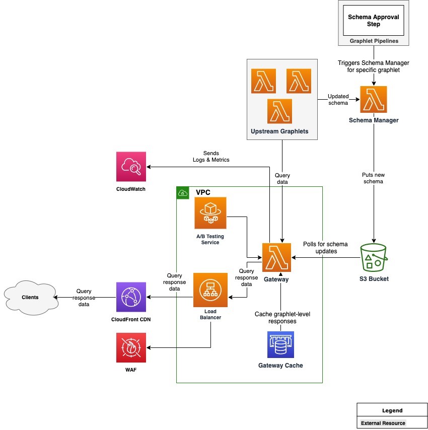
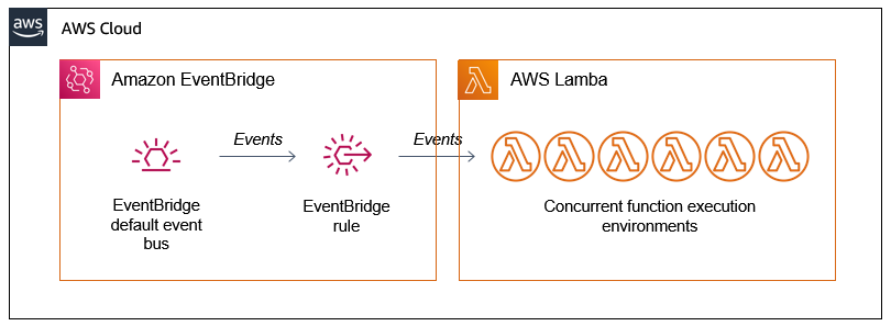
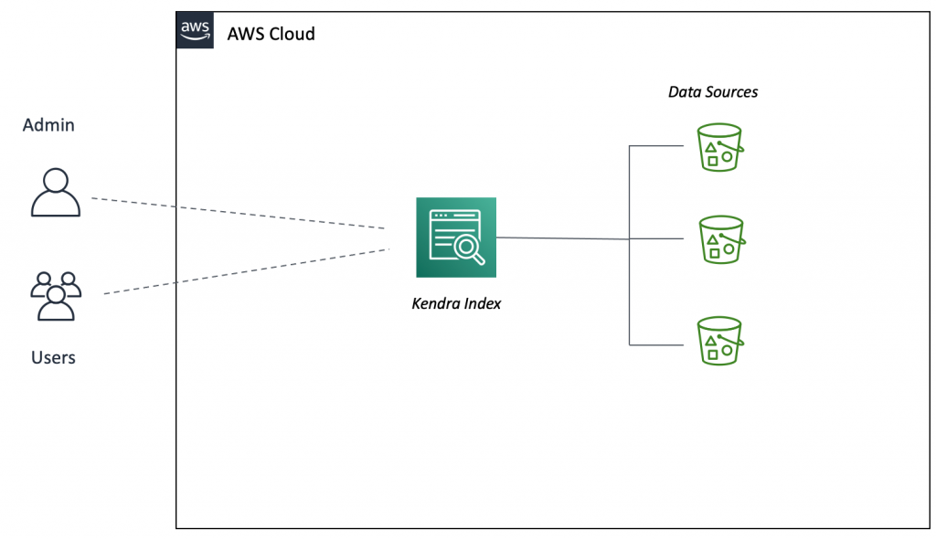
For this solution, we will go through the steps to install and configure IBM Db2 Pacemaker along with overlay IP as virtual IP for the clients to connect to the database. This blog post also includes prerequisites, and installation and configuration instructions to achieve an HA Db2 database on Amazon Elastic Compute Cloud (Amazon EC2).
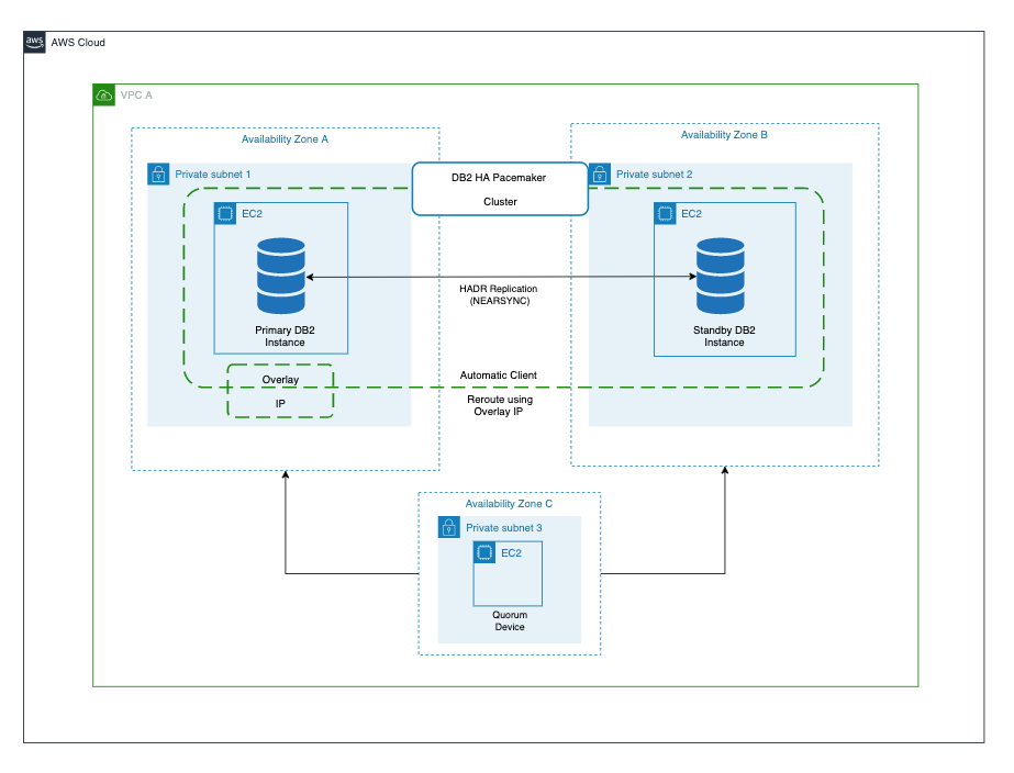
Figure 1. Cluster management using IBM Db2 Pacemaker
Prerequisites for installing Db2 Pacemaker
To set up IBM Db2 Pacemaker on a two-node HADR (high availability disaster recovery) cluster, the following prerequisites must be met.
- Set up instance user ID and group ID.
Instance user id and group id’s must be set up as part of Db2 Server installation which can be verified as follows:
grep db2iadm1 /etc/group
grep db2inst1 /etc/group
- Set up host names for all the hosts in /etc/hosts file on all the hosts in the cluster.
For both of the hosts in the HADR cluster, ensure that the host names are set up as follows.
Format: ipaddress fully_qualified_domain_name alias
- Install kornshell (ksh) on both of the hosts.
sudo yum install ksh -y
- Ensure that all instances have TCP/IP connectivity between their ethernet network interfaces.
- Enable password less secure shell (ssh) for the root and instance user IDs across both instances.After the password less root ssh is enabled, verify it using the “ssh <host name> -l root ls” command (hostname is either an alias or fully-qualified domain name).
ssh <host name> -l root ls
- Activate HADR for the Db2 database cluster.
- Make available the IBM Db2 Pacemaker binaries in the /tmp folder on both hosts for installation. The binaries can be downloaded from IBM download location (login required).
Installation steps
After completing all prerequisites, run the following command to install IBM Db2 Pacemaker on both primary and standby hosts as root user.
cd /tmp
tar -zxf Db2_v11.5.5.0_Pacemaker_20201118_RHEL8.1_x86_64.tar.gz
cd Db2_v11.5.5.0_Pacemaker_20201118_RHEL8.1_x86_64/RPMS/dnf install https://dl.fedoraproject.org/pub/epel/epel-release-latest-8.noarch.rpm -y
dnf install */*.rpm -ycp /tmp/Db2_v11.5.5.0_Pacemaker_20201118_RHEL8.1_x86_64/Db2/db2cm /home/db2inst1/sqllib/adm
chmod 755 /home/db2inst1/sqllib/adm/db2cm
Run the following command by replacing the -host parameter value with the alias name you set up in prerequisites.
/home/db2inst1/sqllib/adm/db2cm -copy_resources
/tmp/Db2_v11.5.5.0_Pacemaker_20201118_RHEL8.1_x86_64/Db2agents -host <host>
After the installation is complete, verify that all required resources are created as shown in Figure 2.
ls -alL /usr/lib/ocf/resource.d/heartbeat/db2*
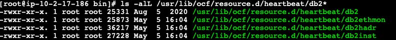
Figure 2. List of heartbeat resources
Configuring Pacemaker
After the IBM Db2 Pacemaker is installed on both primary and standby hosts, initiate the following configuration commands from only one of the hosts (either primary or standby hosts) as root user.
- Create the cluster using db2cm utility.Create the Pacemaker cluster using db2cm utility using the following command. Before running the command, replace the -domain and -host values appropriately.
/home/db2inst1/sqllib/adm/db2cm -create -cluster -domain <anydomainname> -publicEthernet eth0 -host <primary host alias> -publicEthernet eth0 -host <standby host alias>
Note: Run ifconfig to get the –publicEthernet value and replace in the former command.
- Create instance resource model using the following commands.Modify -instance and -host parameter values in the following command before running.
/home/db2inst1/sqllib/adm/db2cm -create -instance db2inst1 -host <primary host alias>
/home/db2inst1/sqllib/adm/db2cm -create -instance db2inst1 -host <standby host alias>
- Create the database instance using db2cm utility. Modify -db parameter value accordingly.
/home/db2inst1/sqllib/adm/db2cm -create -db TESTDB -instance db2inst1
After configuring Pacemaker, run crm status command from both the primary and standby hosts to check if the Pacemaker is running with automatic failover activated.
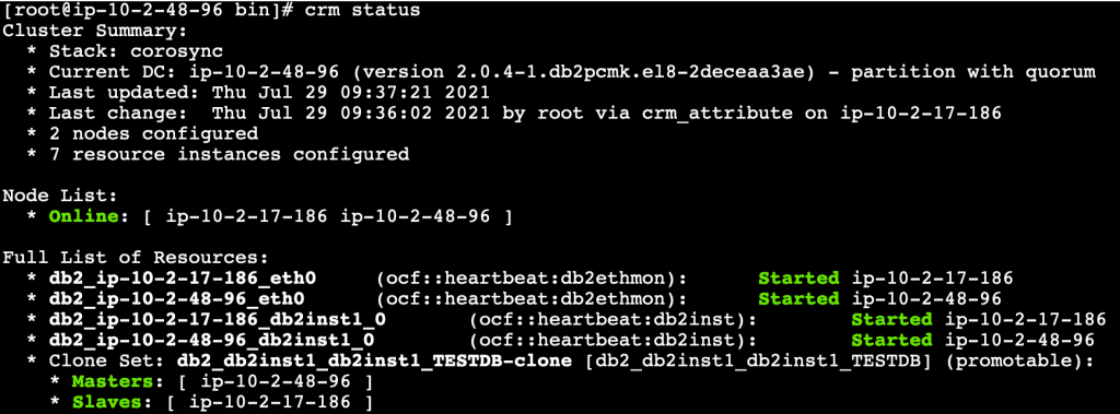
Figure 3. Pacemaker cluster status
Quorum device setup
Next, we shall set up a third lightweight EC2 instance that will act as a quorum device (QDevice) which will act as a tie breaker avoiding a potential split-brain scenario. We need to install only corsync-qnetd* package from the Db2 Pacemaker cluster software.
Prerequisites (quorum device setup)
- Update /etc/hosts file on Db2 primary and standby instances to include the host details of QDevice EC2 instance.
- Set up password less root ssh access between Db2 instances and the QDevice instance.
- Ensure TCP/IP connectivity between the Db2 instances and the QDevice instance on port 5403.
Steps to set up quorum device
Run the following commands on the quorum device EC2 instance.
cd /tmp
tar -zxf Db2_v11.5.5.0_Pacemaker_20201118_RHEL8.1_x86_64.tar.gz
cd Db2_v11.5.5.0_Pacemaker_20201118_RHEL8.1_x86_64/RPMS/
dnf install */corosync-qnetd* -y
- Run the following command from one of the Db2 instances to join the quorum device to the cluster by replacing the QDevice value appropriately.
/home/db2inst1/sqllib/adm/db2cm -create -qdevice <hostnameofqdevice>
- Verify the setup using the following commands.
From any Db2 servers:
/home/db2inst1/sqllib/adm/db2cm -list
From QDevice instance:
corosync-qnetd-tool -l
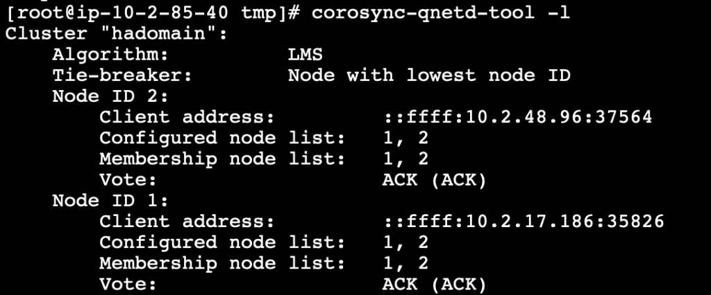
Figure 4. Quorum device status
Setting up overlay IP as virtual IP
For HADR activated databases, virtual IP provides a common connection point for the clients so that in case of failovers there is no need to update the connection strings with the actual IP address of the hosts. Furtermore, the clients can continue to establish the connection to the new primary instance.
We can use the overlay IP address routing on AWS to send the network traffic to HADR database servers within Amazon Virtual Private Cloud (Amazon VPC) using a route table so that the clients can connect to the database using the overlay IP from the same VPC (any Availability Zone) where the database exists. aws-vpc-move-ip is a resource agent from AWS which is available along with the Pacemaker software that helps to update the route table of the VPC.
If you need to connect to the database using overlay IP from on-premises or outside of the VPC (different VPC than database servers), then additional setup is needed using either AWS Transit Gateway or Network Load Balancer.
Prerequisites (setting up overlay IP as virtual IP)
- Choose the overlay IP address range which needs to be configured. This IP should not be used anywhere in the VPC or on-premises, and should be a part of the private IP address range as defined in RFC 1918. If the VPC is configured in the range of 0.0.0.0/8 or 172.16.0.0/12, we can use the overlay IP from the range of 192.168.0.0/16.We will use the following IP and ethernet settings.
192.168.1.81/32
eth0
- To route traffic through overlay IP, we need to disable source and target destination checks on the primary and standby EC2 instances.
aws ec2 modify-instance-attribute –profile <AWS CLI profile> –instance-id EC2-instance-id –no-source-dest-check
Steps to configure overlay IP
The following commands can be run as root user on the primary instance.
- Create the following AWS Identity and Access Management (IAM) policy and attach it to the instance profile. Update region, account_id, and routetableid values.
{
  "Version": "2012-10-17",
  "Statement": [
    {
      "Sid": "Stmt0",
      "Effect": "Allow",
      "Action": "ec2:ReplaceRoute",
      "Resource": "arn:aws:ec2:<region>:<account_id>:route-table/<routetableid>"
    },
    {
      "Sid": "Stmt1",
      "Effect": "Allow",
      "Action": "ec2:DescribeRouteTables",
      "Resource": "*"
    }
  ]
}
- Add the overlay IP on the primary instance.
ip address add 192.168.1.81/32 dev eth0
- Update the route table (used in Step 1) with the overlay IP specifying the node with the Db2 primary instance. The following command returns True.
aws ec2 create-route –route-table-id <routetableid> –destination-cidr-block 192.168.1.81/32 –instance-id <primrydb2instanceid>
- Create a file overlayip.txt with the following command to create the resource manager for overlay ip.
overlayip.txt
primitive db2_db2inst1_db2inst1_TESTDB_AWS_primary-OIP ocf:heartbeat:aws-vpc-move-ip \
params ip=192.168.1.81 routing_table=<routetableid> interface=<ethernet> profile=<AWS CLI profile name> \
op start interval=0 timeout=180s \
op stop interval=0 timeout=180s \
op monitor interval=30s timeout=60seifcolocation db2_db2inst1_db2inst1_TESTDB_AWS_primary-colocation inf:
db2_db2inst1_db2inst1_TESTDB_AWS_primary-OIP:Started
db2_db2inst1_db2inst1_TESTDB-clone:Master
order order-rule-db2_db2inst1_db2inst1_TESTDB-then-primary-oip Mandatory:db2_db2inst1_db2inst1_TESTDB-clone db2_db2inst1_db2inst1_TESTDB_AWS_primary-OIP
location prefer-node1_db2_db2inst1_db2inst1_TESTDB_AWS_primary-OIPdb2_db2inst1_db2inst1_TESTDB_AWS_primary-OIP 100: <primaryhostname>
location prefer-node2_db2_db2inst1_db2inst1_TESTDB_AWS_primary-OIPdb2_db2inst1_db2inst1_TESTDB_AWS_primary-OIP 100: <standbyhostname>
The following parameters must be replaced in the resource manager create command in the file.
-
- Name of the database resource agent (This can be found through crm config show | grep primitive | grep DBNAME command. For this example, we will use: db2_db2inst1_db2inst1_TESTDB)
- Overlay IP address (created earlier)
- Routing table ID (used earlier)
- AWS command-line interface (CLI) profile name
- Primary and standby host names
- After the file with commands is ready, run the following command to create the overlay IP resource manager.
crm configure load update overlayip.txt
- Next, create the VIP resource manager—not in managed state. Run the following command to manage and start the resource.
crm resource manage db2_db2inst1_db2inst1_TESTDB_AWS_primary-OIP
- Validate the setup with crm status command.
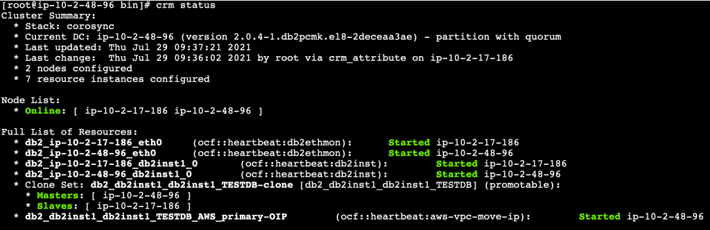
Figure 5. Pacemaker cluster status along with overlay IP resource
Test failover with client connectivity
For the purpose of this testing, launch another EC2 instance with Db2 client installed, and catalog the Db2 database server using overlay IP.
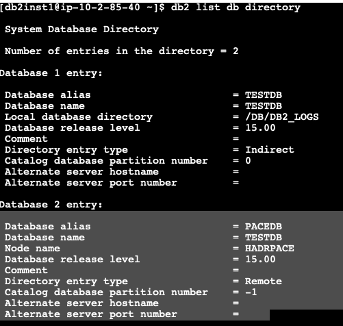
Figure 6. Database directory list
Establish a connection with the Db2 primary instance using the cataloged alias (created earlier) using overlay IP address.

Figure 7. Connect to database
If we connect to the primary instance and check the applications connected, we can see the active connection from the client’s IP as shown in Figure 8.
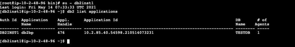
Figure 8. Check client connections before failover
Next, let’s stop the primary Db2 instance and check if the Pacemaker cluster promoted the standby to primary and we can still connect to the database using the overlay IP, which now points to the new primary instance.
If we check the CRM status from the new primary instance, we can see that the Pacemaker cluster has promoted the standby database to new primary database as shown in Figure 9.
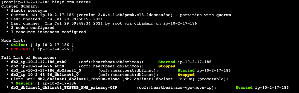
Figure 9. Automatic failover to standby
Let’s go back to our client and reestablish the connection using the cataloged DB alias created using overlay IP.
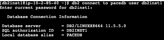
Figure 10. Database reconnection after failover
If we connect to the new promoted primary instance and check the applications connected, we can see the active connection from the client’s IP as shown in Figure 11.
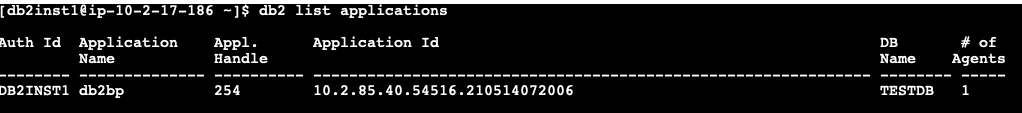
Figure 11. Check client connections after failover
Cleaning up
To avoid incurring future charges, terminate all EC2 instances which were created as part of the setup referencing this blog post.
Conclusion
In this blog post, we have set up automatic failover using IBM Db2 Pacemaker with overlay (virtual) IP to route traffic to secondary database instance during failover, which helps to reconnect to the database without any manual intervention. In addition, we can also enable automatic client reroute using the overlay IP address to achieve a seamless failover connectivity to the database for mission-critical workloads.


 Jignesh Gohel is a Technical Account Manager at AWS. In this role, he provides advocacy and strategic technical guidance to help plan and build solutions using best practices, and proactively keep customers’ AWS environments operationally healthy. He is passionate about building modular and scalable enterprise systems on AWS using serverless technologies. Besides work, Jignesh enjoys spending time with family and friends, traveling and exploring the latest technology trends.
 Suman Koduri is a Global Category Lead for Data & Analytics category in AWS Marketplace. He is focused towards business development activities to further expand the presence and success of Data & Analytics ISVs in AWS Marketplace. In this role, he leads the scaling, and evolution of new and existing ISVs, as well as field enablement and strategic customer advisement for the same. In his spare time, he loves running half marathon’s and riding his motorcycle.