Tag Archives: Best practices

Improve DynamoDB analytics with AWS Glue zero-ETL schema and partition controls

Post Syndicated from Raju Ansari original https://aws.amazon.com/blogs/big-data/improve-dynamodb-analytics-with-aws-glue-zero-etl-schema-and-partition-controls/

You store transactional data in Amazon DynamoDB and get single-digit millisecond performance. However, when you want to run analytics, machine learning (ML), or reporting on that same data, you face a gap: your flexible, semi-structured DynamoDB schemas don’t align with the flat, columnar formats that analytics engines require. Bridging this gap typically means building and maintaining custom ETL pipelines, which adds development cost and operational overhead.

AWS Glue Zero-ETL integration removes that pipeline work. It enables replication of your DynamoDB tables to Apache Iceberg tables in Amazon Simple Storage Service (Amazon S3), then query it directly with Amazon Athena. During setup, you can configure two capabilities that will shape how replicated data looks and performs: schema unnesting flattens nested attributes into individual columns, and data partitioning organizes data so your queries scan only what they need.

In this post, you learn how to replicate Amazon DynamoDB data to Apache Iceberg tables in Amazon S3 through a zero-ETL integration. We walk through the challenges that the DynamoDB nested, schema-flexible data model introduces for analytics workloads, and show you how to configure schema unnesting and data partitioning for a sample product catalog table. We also cover how to query the replicated data in Amazon Athena using standard SQL.

Semi-structured data meets analytics

Your product catalog in DynamoDB contains items with nested attributes like product details, pricing tiers, and inventory information. A typical item looks like this:

{
  "product_id": "P-1001",
  "name": "Wireless Headphones",
  "productdetails": {
    "brand": "AudioTech",
    "category": "Electronics",
    "weight_kg": 0.25,
    "specification": {
       "color": "Black",
       "storage": "128GB"
    }
  },
  "pricing": {
    "list_price": 79.99,
    "discount_pct": 10
  },
  "created_at": 1701388800000
}

This structure supports fast transactional reads and writes. However, when you replicate this data for analytics, you face two decisions:

  • You must decide whether to flatten nested maps like productdetails into individual columns or preserve them as-is.
  • You must choose how to organize the data on disk so that queries filtering by brand or date range scan only relevant partitions.

With AWS Glue Zero-ETL, you address both decisions through configurable schema unnesting and data partitioning.

Solution overview

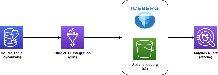
You replicate data from your DynamoDB table through AWS Glue Zero-ETL into Apache Iceberg tables stored in Amazon S3, then query the results with Amazon Athena. The following diagram illustrates the end-to-end architecture:

Data flow diagram showing AWS data pipeline: DynamoDB source table → AWS Glue zero-ETL integration → Apache Iceberg on Amazon S3 → Amazon Athena analytics query.

AWS Glue zero-ETL ingests data from Amazon DynamoDB, writes it in Apache Iceberg format to your Amazon S3 data lake, and makes it available for SQL queries in Amazon Athena—with no pipelines to build or maintain. With this integration, you:

  • Save development time by skipping custom code and ETL job management
  • Keep DynamoDB performance intact because replication doesn’t consume table’s provisioned read/write capacity
  • Get data within 15 minutes of changes in the source table
  • Query with standard tools because data lands in Apache Iceberg format, an open table format that AWS natively supports for high-performance analytics

During setup, you configure two output settings:

  1. Schema unnesting in Zero-ETL: You choose how nested attributes appear in the target. Flattening nested maps into individual columns streamlines your queries and reduces complexity.
  2. Data partitioning in Zero-ETL: You choose how data is organized into partitions. When you filter on a partition column, the query engine reads only matching data instead of scanning everything, cutting both query time and cost.

Schema unnesting

When you create a zero-ETL integration, you can choose one of three unnesting options. Schema unnesting transforms complex, nested DynamoDB structures into formats that analytics engines can query directly, removing post-processing transformations.

Each option changes how nested DynamoDB attributes appear in the target table. The right choice depends on your analytics tools and how consistent your DynamoDB schemas are.

Option 1: No unnesting

This option preserves the original nested structure. DynamoDB maps and lists remain as structured columns in the target.

Using the product example, the target table retains productid and value as columns to hold DynamoDB partition key and a DynamoDB record respectively.

Recommended for: Workloads where your analytics tools natively support querying nested data and you want to preserve the DynamoDB structure unchanged.

Option 2: Unnest one level

This option flattens top-level maps into individual columns. Lists remain nested.

With this option, productdetails and pricing each become separate columns.

Recommended for: Scenarios where your DynamoDB items have a consistent schema and you want to balance structure preservation with query simplicity.

Option 3: Unnest all levels (default)

This option recursively flattens nested structures using dot notation and produces the flattest schema.

For the product table, this creates columns such as productdetails.brand, productdetails.category, productdetails.specification.color , productdetails.specification.storage , pricing.list_price, and pricing.discount_pct. The pricing map flattens similarly. Each column is directly queryable without nested access patterns.

Recommended for: Analytics tools that prefer flat schemas when your DynamoDB items have a reasonably consistent structure. Note that deeply nested or highly variable schemas can produce very wide tables.

Data partitioning

You can speed up your queries and reduce costs by partitioning your replicated data. Partitioning divides data into logical segments on disk.

When you include a filter on a partition column in your query, the query engine skips irrelevant segments entirely. This behavior is called partition pruning: instead of scanning the entire dataset, the engine reads only the data that matches your filter conditions. For large tables, partition pruning can reduce both query runtime and cost significantly.

Default partitioning

If you don’t specify partition columns, AWS Glue Zero-ETL partitions data using the DynamoDB primary key with bucketing. This approach supports general-purpose queries without requiring manual configuration. For specific query patterns or performance requirements, you can define custom partitioning strategies described in the subsections that follow.

Identity partitioning

Identity partitioning uses raw column values to create partitions. You apply this strategy to low-to-medium cardinality columns such as brand, category, or AWS Region. To partition the product table by productdetails.brand and create a separate partition for each brand, use this configuration:

{
  "partitionSpec": [
    {
      "fieldName": "productdetails.brand",
      "functionSpec": "identity"
    }
  ]
}

With this setup, AWS Glue creates one partition directory per unique brand value. When you query for a specific brand, Athena reads only that partition.

Important: Avoid identity partitioning on high-cardinality columns such as primary keys or timestamps. This creates many small partitions, which degrades both ingestion and query performance

Time-based partitioning

Time-based partitioning organizes data by timestamp at a chosen granularity: year, month, day, or hour. You apply this strategy to time-series data and time-range queries. To partition the product table by month on the created_at column, which stores epoch milliseconds, use this configuration:

{
  "partitionSpec": [
    {
      "fieldName": "created_at",
      "functionSpec": "month",
      "conversionSpec": "epoch_milli"
    }
  ]
}

The conversionSpec parameter tells AWS Glue how to interpret the source timestamp. Supported values: epoch_sec (Unix seconds), epoch_milli (Unix milliseconds), and iso (ISO 8601 format).

Note: The original column values remain unchanged. AWS Glue transforms only the partition column values to timestamp type in the target table

Multi-level partitioning

You can combine strategies for a hierarchical scheme. To partition first by month and then by brand, use this configuration:

{
  "partitionSpec": [
    {
      "fieldName": "created_at",
      "functionSpec": "month",
      "conversionSpec": "epoch_milli"
    },
    {
      "fieldName": "productdetails.brand",
      "functionSpec": "identity"
    }
  ]
}

This scheme supports efficient queries that filter by date range, brand, or both. Place higher-selectivity columns first in the hierarchy and align the scheme with your most common query patterns.

Best practices

Keep these guidelines in mind when you configure your integration:

  • Avoid identity partitioning on high-cardinality columns such as primary keys, timestamps, or system-generated IDs. This leads to partition explosion and degrades performance.
  • Apply only one time-based function per column. For example, don’t partition col1 by year, month, day, and hour simultaneously.
  • Match conversionSpec to your actual data format. If your timestamps are in epoch milliseconds, use epoch_milli, not epoch_sec or iso.
  • Choose granularity based on data volume. High-volume tables benefit from finer granularity (day or hour). Lower-volume tables work well with coarser granularity (month or year).
  • Account for timezone implications with ISO timestamps. AWS Glue Zero-ETL normalizes timestamp partition values to UTC.

Prerequisites

To implement the AWS Glue Zero-ETL integration with a DynamoDB source, you will need:

  1. An AWS account with least privilege principle
  2. An AWS Glue database (for example, ddb_zero_etl_demo_db) with an Amazon S3 bucket associated as the database location (setup instructions)
  3. AWS Glue Data Catalog settings updated with an AWS Identity and Access Management (IAM) policy that grants fine-grained access control for zero-ETL (setup instructions)
  4. Create an IAM role named zetl-role, to be used by zero-ETL to access data from your DynamoDB table
  5. A DynamoDB source table (for example, product) configured for zero-ETL integration (setup instructions)

Walkthrough: Create the zero-ETL integration

Complete these steps to create a zero-ETL integration with DynamoDB as the source and Apache Iceberg tables in Amazon S3 as the target.

Step 1: Select the source type

  1. Open the AWS Glue console.
  2. In the navigation pane, under Data Integration and ETL, choose Zero-ETL integrations.
  3. Choose Create zero-ETL integration.
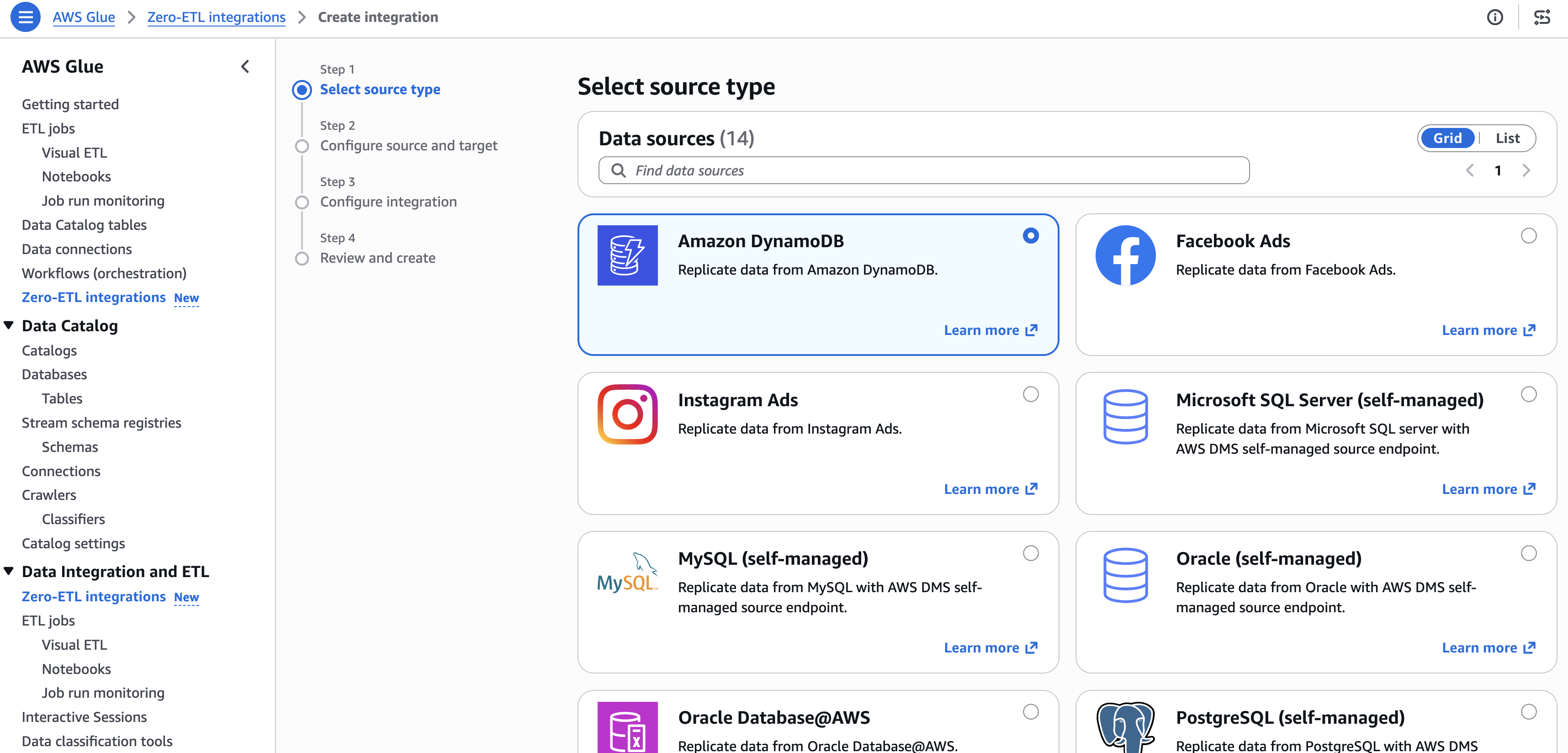
  4. Select Amazon DynamoDB as the source type, then choose Next.

AWS Glue console showing Step 1 of creating a Zero-ETL integration — selecting a source type from 14 available data sources including Amazon DynamoDB, Facebook Ads, Instagram Ads, MySQL, Oracle, PostgreSQL, and Microsoft SQL Server

[Figure 1: Selecting Amazon DynamoDB as the zero-ETL source type]

Step 2: Configure source and target

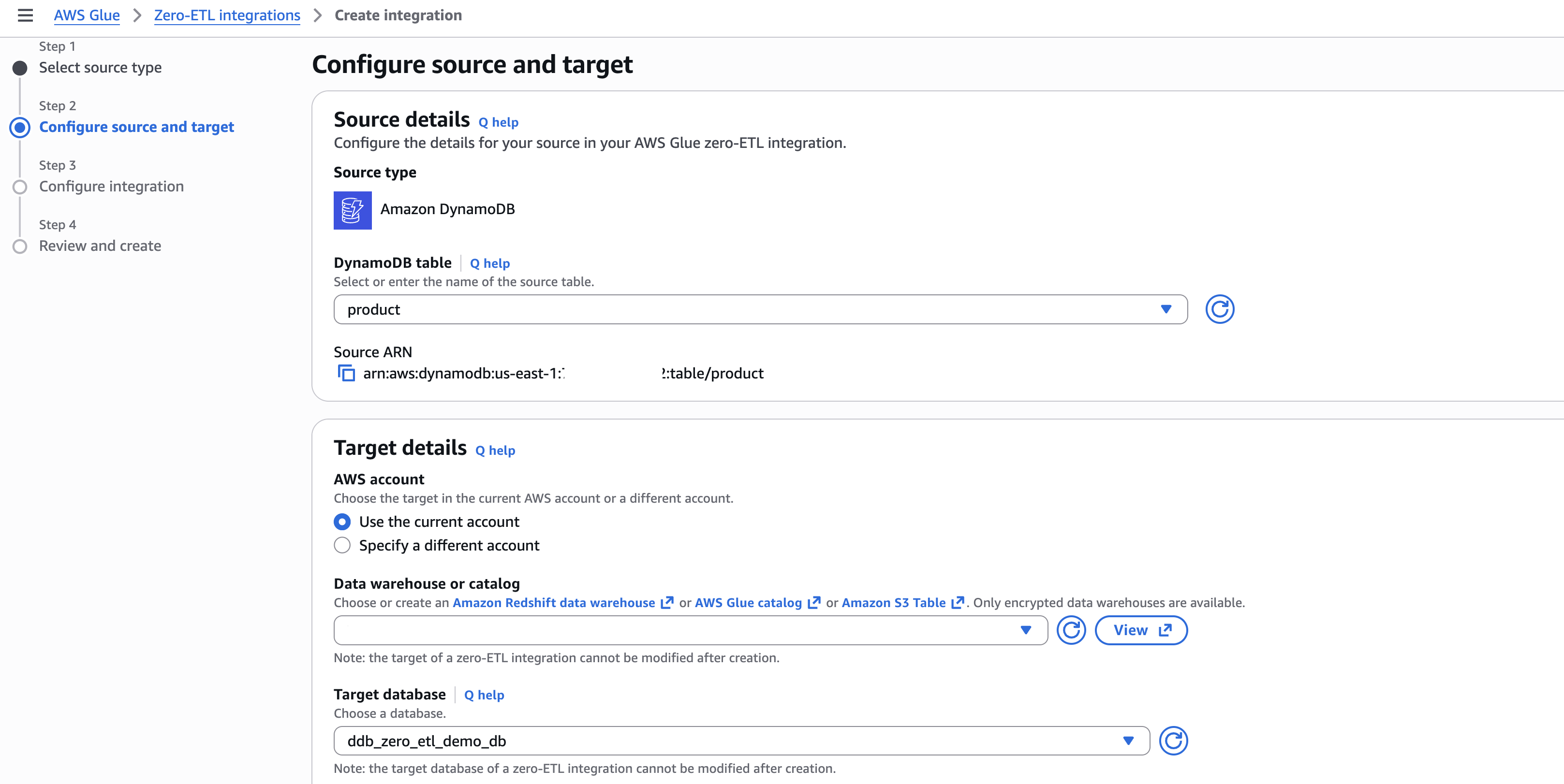
  1. In Source details, select your DynamoDB table (for example, product).
  2. In Target details:
    • Select the current account as target.
    • Choose the catalog and target database (for example, ddb_zero_etl_demo_db).
    • Select the IAM role (for example, zetl-role).

AWS Glue console Step 2 — configuring source and target for a zero-ETL integration with Amazon DynamoDB "product" table as source and an AWS Glue catalog database "ddb_zero_etl_demo_db" as target

[Figure 2: Configuring source DynamoDB table and target database]

Step 3: Configure output settings

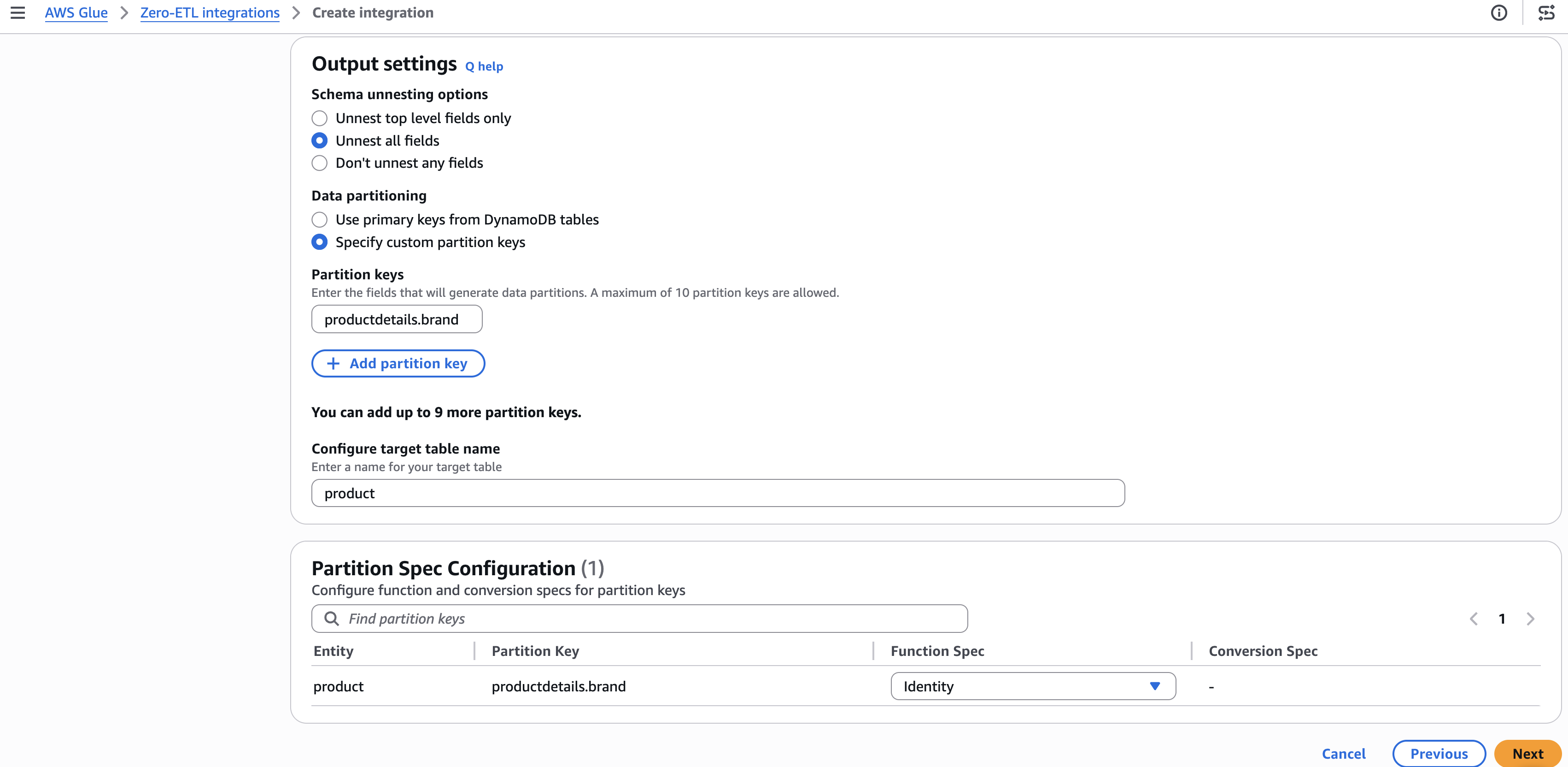
  1. Under Schema unnesting, select Unnest all fields.
  2. Under Data partitioning, select Specify custom partition keys.
  3. Enter the partition key (for example, productdetails.brand) and set the function to Identity.
  4. Choose Next.

AWS Glue Zero-ETL integration output settings showing schema unnesting set to "Unnest all fields," custom partition key "productdetails.brand" configured with Identity function, and target table named "product.

[Figure 3: Configuring schema unnesting and partition key settings]

Step 4: Set integration details

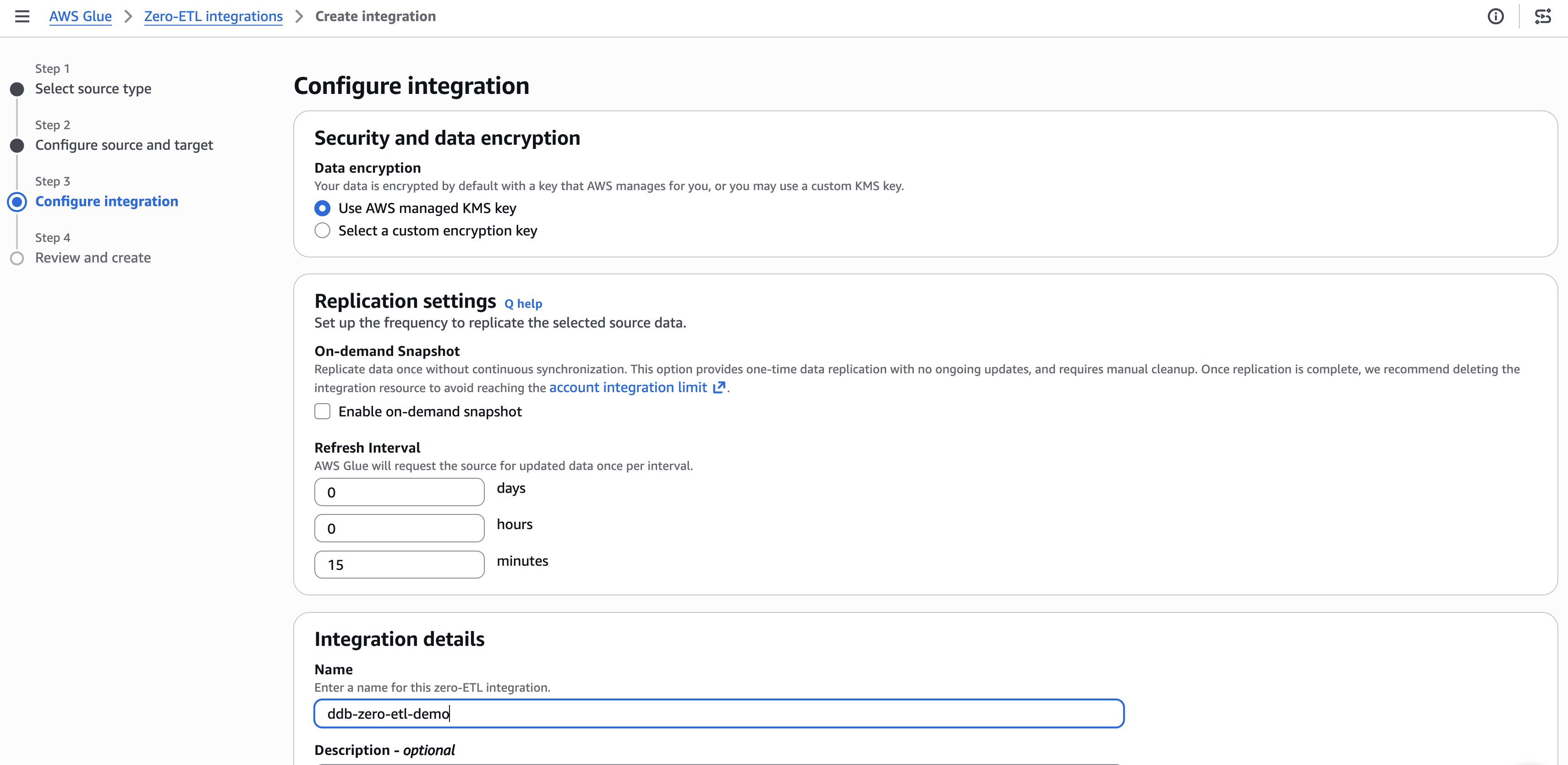
  1. Optionally configure encryption and replication settings. The default refresh interval is 15 minutes.
  2. Enter a name for the integration (for example, ddb-zero-etl-demo).
  3. Choose Next.

AWS Glue Zero-ETL integration Step 3 — configuring security with AWS managed KMS key, replication refresh interval set to 15 minutes, and integration named "ddb-zero-etl-demd

[Figure 4: Configuring encryption and replication settings]

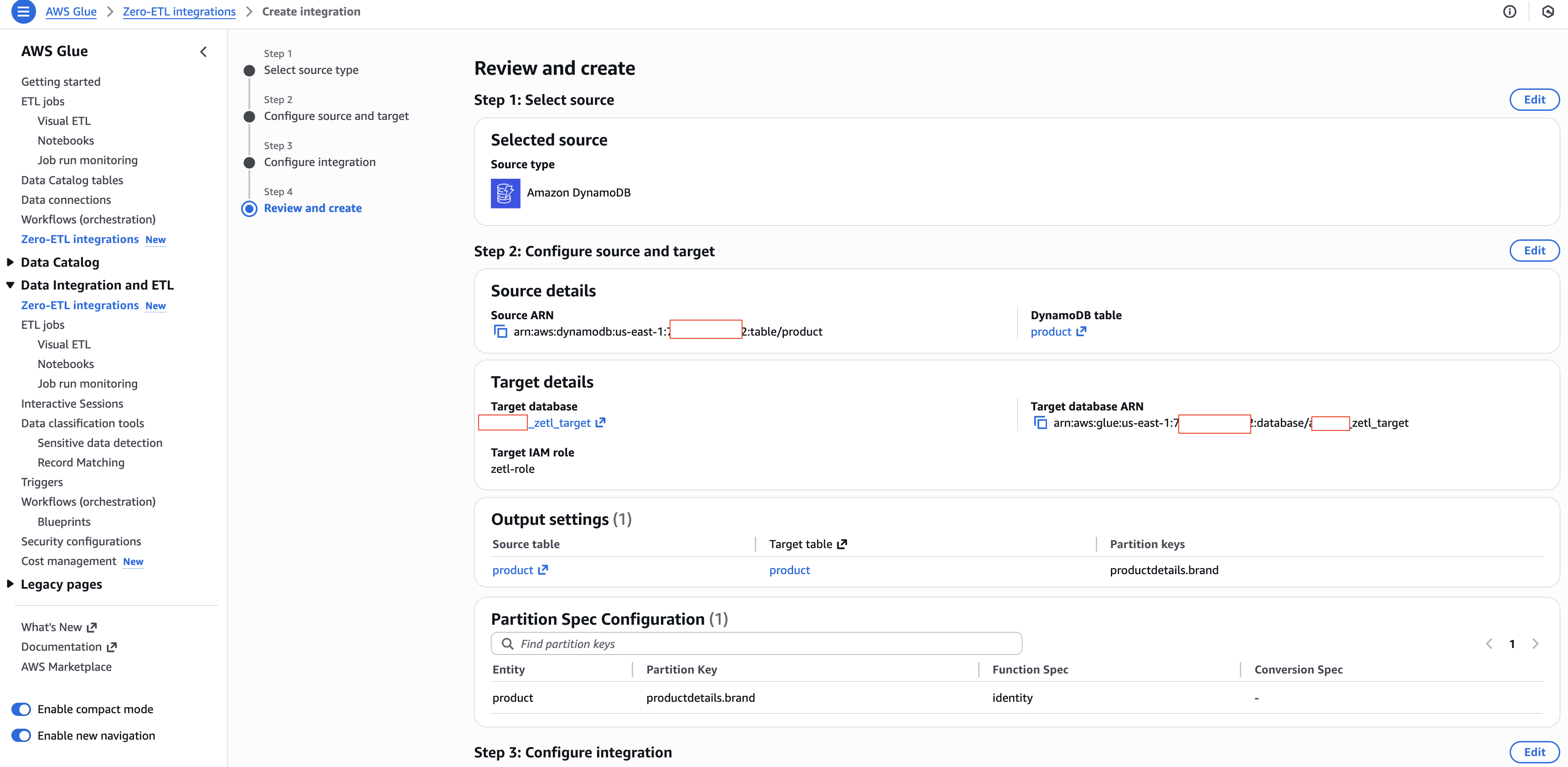
Step 5: Review and create

  1. Review your settings and choose Create and launch integration.
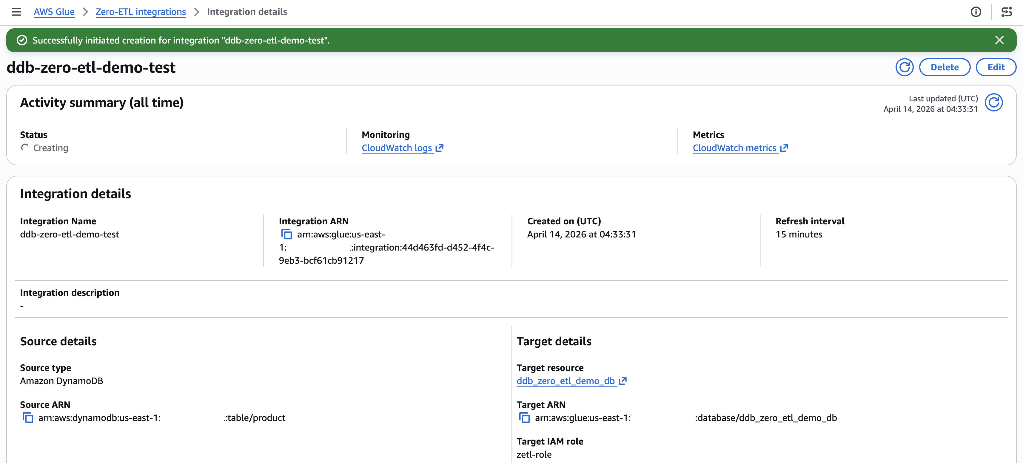
  2. The integration shows as Active within about a minute.

AWS Glue Zero-ETL integration Step 4: Review and Create — showing DynamoDB "product" table as source, Glue database "zett_target" as target with IAM role "zett-role," and partition key "productdetails.brand" with Identity function

[Figure 5: Review and create summary]

AWS Glue Zero-ETL Integration Details page showing "ddb-zero-etl-demo-test" integration with status "Creating," DynamoDB "product" table as source, Glue database "ddb_zero_etl_demo_db" as target, and a 15-minute refresh interval

[Figure 6: Integration active with successful status]

Query the replicated data

After the integration is active and the initial replication completes (typically 15–30 minutes), you can query the data in Amazon Athena.

Preview the replicated data

  1. Open the Amazon Athena console.
  2. In the query editor, select your target database (for example, ddb_zero_etl_demo_db).
  3. Run a preview query:
SELECT * FROM "ddb_zero_etl_demo_db"."product"LIMIT 10;

Verify schema unnesting

With Unnest all fields selected, nested attributes appear as individual columns with dot notation:

SELECT "productdetails.brand", "productdetails.category", "pricing.list_price" 
FROM "ddb_zero_etl_demo_db"."product"
WHERE "productdetails.category" = 'Electronics';

Verify partition pruning

Queries that filter on the partition column (productdetails.brand) automatically skip irrelevant partitions:

SELECT product_id, name, "pricing.list_price"
FROM "ddb_zero_etl_demo_db"."product"
WHERE "productdetails.brand" = 'AudioTech';

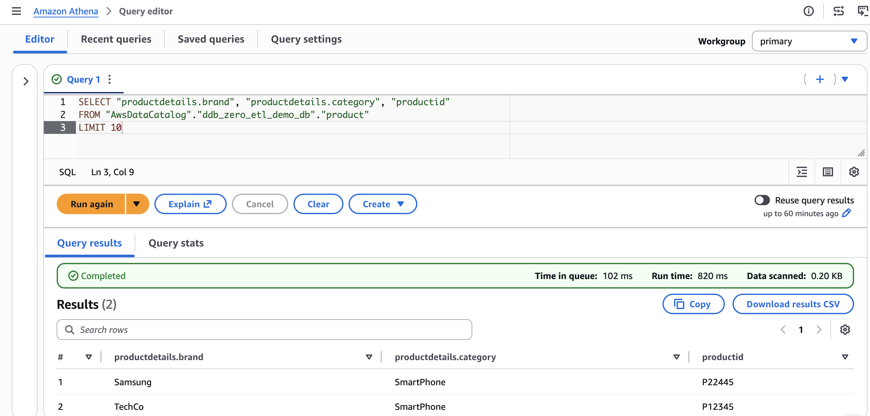
Amazon Athena Query Editor showing a completed SQL query selecting brand, category, and product ID from a DynamoDB zero-ETL Glue catalog table, returning two results: Samsung SmartPhone P22445 and TechCo SmartPhone P12345

[Figure 7: Athena query to retrieve the data from Apache Iceberg lakehouse]

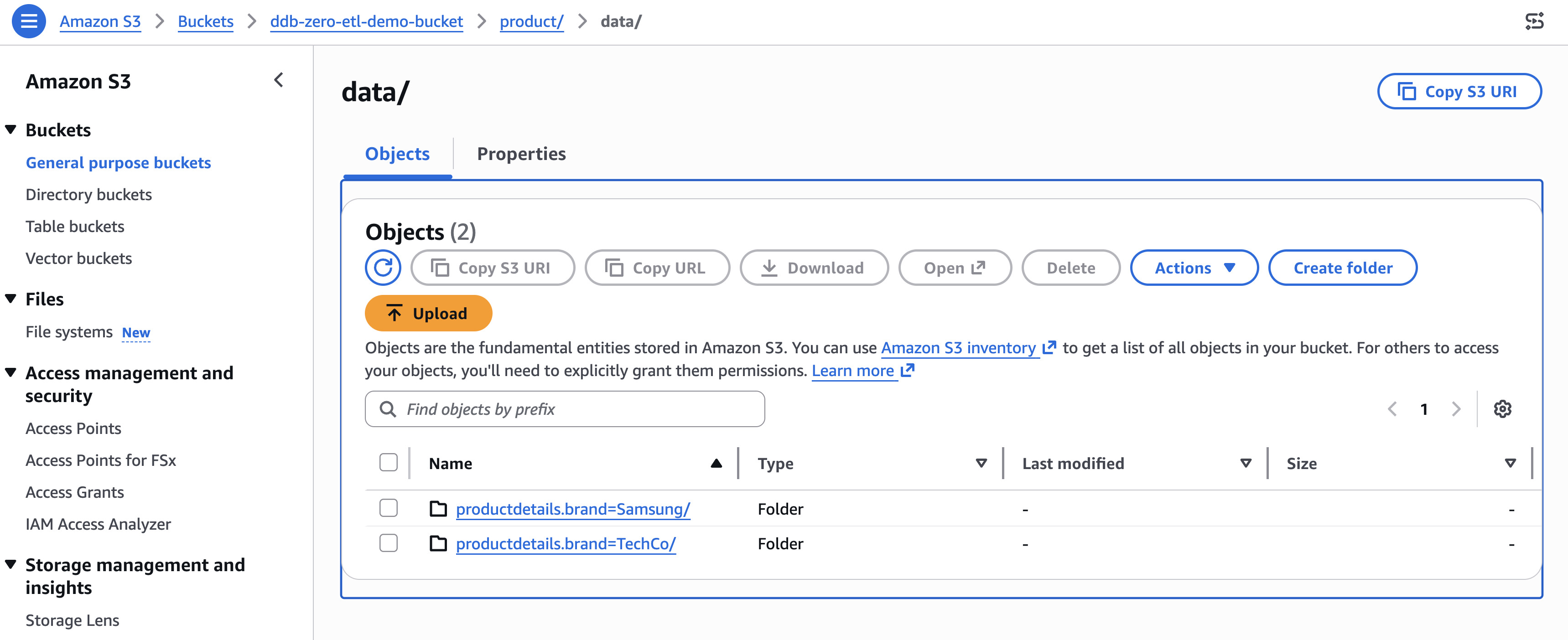
You can verify the partition structure by navigating to the Amazon S3 bucket associated with your database. The data organizes into directories like:

Amazon S3 bucket browser showing the "data/" folder in "ddb-zero-etl-demo-bucket" with two partitioned folders: "productdetails.brand=Samsung/" and "productdetails.brand=TechCo/" — confirming Iceberg partition structure from DynamoDB zero-ETL integration

[Figure 8: Amazon S3 bucket organization for the identity partition productdetails.brand]

Clean up

To avoid ongoing charges, delete the resources in this order:

  1. Delete the zero-ETL integration. In the AWS Glue console, navigate to Zero-ETL integrations, select your integration, and choose Delete. Existing replicated data remains in the target, but new changes stop replicating.
  2. Delete the replicated table. In the AWS Glue Data Catalog, navigate to Tables, select the replicated table, and delete it.
  3. Delete the AWS Glue database. In the Data Catalog, select the database and delete it.
  4. Delete the Amazon S3 data. Empty and delete the S3 bucket associated with the database.
  5. Delete the DynamoDB table. If you created it for this walkthrough, delete the source table.
  6. Delete IAM resources. Remove the IAM role and policies created for the integration.

Conclusion

You configured schema unnesting and data partitioning for a DynamoDB zero-ETL integration, replicated a product catalog table to Apache Iceberg tables in Amazon S3, and verified the results in Amazon Athena. Unnesting flattened nested attributes into directly queryable columns. Partitioning helped the query engine skip irrelevant data, reducing both query time and cost. To take your integration further, try monitoring replication lag and data freshness with Amazon CloudWatch metrics. You can also experiment with different partitioning strategies on a staging table before applying them to production workloads, testing time-based partitioning alongside identity partitioning to find the optimal scheme for your query patterns. For broader analytics coverage, query the same Iceberg tables from Amazon Redshift Spectrum or Amazon EMR alongside Athena. For more details, explore these resources:


About the authors

Raju Ansari

Raju is a Senior Software Development Engineer at AWS, specializing in building scalable, secure, serverless solutions that simplify data analytics and AI agent development. He helps organizations modernize their data analytics infrastructure and develop cutting-edge AI agentic applications. Currently, Raju focuses on building foundational AI services, including Amazon Bedrock Agents, which enable developers to create intelligent, autonomous applications at scale. Outside of work, Raju is passionate about giving back to the tech community. He actively volunteers at IEEE events and mentor early and mid-career professionals

Shashank Sharma

Shashank is an Engineering Leader with over 15 years of experience delivering data integration and replication solutions for first-party and third-party databases and SaaS for enterprise customers. He leads engineering for AWS Glue Zero-ETL and Amazon AppFlow, building fully managed pipelines that replicate data from sources like Salesforce, SAP, DynamoDB, and Oracle into Amazon Redshift and Apache Iceberg-based data lakes. Shashank advises startups on technology strategy and mentors engineers and technical leaders at various career stages

Securing open proxies in your AWS environment

Post Syndicated from Dodd Mitchell original https://aws.amazon.com/blogs/security/securing-open-proxies-in-your-aws-environment/

This article shows you how to identify and secure open proxies in your AWS environment to prevent abuse, protect your IP address reputation, and control costs.

An open proxy is a server that forwards traffic on behalf of internet users without requiring authentication. While proxies can support legitimate use cases such as load balancing or caching, open proxies allow unrestricted access that threat actors can use to hide harmful activity. In Amazon Web Services (AWS) environments, open proxies often result from misconfigured Amazon Elastic Compute Cloud (Amazon EC2) instances, containers, or compute resources such as AWS Lambda functions. These resources expose proxy functionality without access controls.

Open proxies come in several forms. Common open proxies can include:

  • HTTP proxies: HTTP proxies forward HTTP requests to web servers, making them useful for web traffic management. These proxies can create potential issues when they’re unsecured.
  • SOCKS proxies: SOCKS proxies support a wider range of traffic types and provide more flexibility. These proxies create a broader potential for misuse.
  • Transparent proxies: Transparent proxies intercept traffic without the client’s knowledge and are often used to filter content. These proxies can become security liabilities when misconfigured.
  • Reverse proxies: Reverse proxies help with internal routing. Unauthorized users can misuse these proxies if they’re exposed.

Knowing these risks can help you better protect your AWS environment.

Security risks

Because of the unrestricted configuration of open proxy servers, threat actors target them to conduct denial of service (DoS) events, intrusion attempts, distribute spam, and other forms of unauthorized activity. These open proxy servers allow threat actors to hide their actual IP address and other forms of identification from the intended targets.

When your AWS infrastructure hosts an open proxy, several risks emerge that can affect both your operations and customers:

  • Threat actors can misuse your resources, which can result in your IP address being added to security service and reputation system block lists. This can affect your legitimate business operations and customer access. When external parties use your infrastructure for harmful activities, the reputation damage extends beyond immediate technical concerns to affect your ability to reach customers and partners.
  • Unexpected costs from resource consumption occur when threat actors use your bandwidth and compute capacity. The traffic patterns that proxy abuse generate can also alert AWS security monitoring systems and create additional operational overhead as you investigate and respond to these alerts.
  • Service disruptions might affect your legitimate workloads because unauthorized traffic competes for resources with your business-critical applications. This competition for resources can potentially degrade performance or cause availability issues for your customers.

Implementing security measures

To prevent the risks associated with open proxies, it’s essential to implement proper security controls for proxy services in AWS environments. The following guidance is a comprehensive approach that you can follow to secure your proxy infrastructure.

Access control implementation

An important security step is to use passwords and authentication mechanisms to restrict access to proxy services. Configure your proxies to accept connections only from known, trusted IP address ranges. For Elastic Load Balancing (ELB), limit access based on source IP addresses and add authentication to proxies behind the load balancers. When you create new instances in Amazon Elastic Kubernetes Service (Amazon EKS), limit access to your balancer in each instance. If instances don’t have public IP addresses, then you can limit access to the balancer instead. If instances have public IP addresses, then you must limit access to those IP addresses.

When possible, use AWS PrivateLink virtual private cloud (VPC) endpoints to provide private connectivity to AWS services without exposing them to the internet. Deploy proxy services in private subnets with controlled outbound access through NAT gateways or other controlled channels. For Amazon EC2 and Amazon Lightsail resources, update the attached security group to prevent public internet access. To secure the proxy, you must either limit access to specific IP addresses or implement authentication on the endpoint.

Authentication and authorization

Turn on authentication for the proxy software and use strong credentials, certificates, or integration with AWS Identity and Access Management (IAM) and AWS Directory Service. Apply IAM policies with the principle of least privilege to limit access to only what users need to perform their tasks. This approach reduces the potential effects of credential compromise and helps maintain clear accountability for resource access.

Monitoring and detection

To detect unusual proxy activity, configure Amazon Virtual Private Cloud (Amazon VPC) Flow Logs, AWS CloudTrail, and Amazon GuardDuty. Use Amazon CloudWatch alarms to notify you of abnormal traffic patterns that might indicate unauthorized use of your proxy services. These monitoring capabilities provide visibility into your network traffic patterns and help you identify both legitimate usage and potential security concerns.

Deployment best practices

Use HTTPS for ELB traffic to protect data in transit, and restrict security groups to necessary ports to minimize the surface area for potential misuse. Integrate AWS WAF with balancers to filter web traffic based on rules that you define. You can also use AWS Network Firewall for advanced traffic filtering capabilities. For APIs, deploy Amazon API Gateway with authentication and authorization controls to manage access to your backend services. This layered approach to security helps protect your infrastructure at multiple points in the traffic flow.

Regular security assessments

Run Amazon Inspector to scan for misconfigurations in your infrastructure, and use AWS Security Hub to centralize security findings across your AWS environment. Conduct penetration tests in accordance with AWS policy to identify potential security issues before they can result in unintended access.

Incident response planning

Automate remediation with AWS Config rules and Automation, a capability of AWS Systems Manager, to respond rapidly to security events. Maintain incident response runbooks that outline clear steps for addressing proxy-related security incidents, and decommission unused resources that could become security liabilities.

Documented procedures and automated responses reduce the time between detection and remediation and minimizes the potential effects of security incidents on your operations.

Benefits of proper proxy security

When you implement these security measures, you gain the following advantages for your AWS environment:

  • Protection of your IP address reputation helps maintain customer trust and prevents security services from blocking your legitimate traffic. When your infrastructure maintains a positive reputation, your business communications reach their intended recipients without interference.
  • Cost control prevents unauthorized users from consuming your AWS resources and generating unexpected charges on your account. When you restrict access to legitimate users and use cases, you maintain predictable costs that align with your business needs.
  • Operational stability reduces the risk of service disruptions that abuse of your proxy infrastructure can cause. When you dedicate your resources to serving your customers rather than supporting unauthorized activity, you can deliver consistent performance and availability.
  • Enhanced visibility into your network traffic patterns helps you identify both legitimate usage and potential security concerns. This awareness allows you to make informed decisions about capacity planning, security improvements, and operational optimizations.

Conclusion

Open proxies present a serious risk in AWS environments, but you can effectively secure proxies with the right measures. By implementing strict access controls and additional security practices such as authentication, monitoring, and regular assessments, you can prevent misuse, protect your infrastructure, and maintain your IP address reputation.

Taking proactive steps strengthens your own environment and supports the broader security of the internet ecosystem. Under the AWS shared responsibility model, you’re responsible for the configuration and maintenance of these security controls, while AWS provides the underlying secure infrastructure. By following the guidance in this article, you can build a robust security posture that protects your proxy infrastructure while supporting your legitimate business needs.

If you have feedback about this post, submit comments in the Comments section below.
Dodd Mitchell

Dodd Mitchell

Dodd is a member of the AWS Trust and Safety team in Virginia, supporting customers in navigating abuse, phishing, and content-related risks. He works closely with partners to strengthen response processes and build more resilient, trustworthy platforms.

A guide to capacity planning for Airflow worker pool in Amazon MWAA

Post Syndicated from Boyko Radulov original https://aws.amazon.com/blogs/big-data/a-guide-to-capacity-planning-for-airflow-worker-pool-in-amazon-mwaa/

In our previous post, A guide to Airflow worker pool optimization in Amazon MWAA, we explored when adding workers to your Amazon Managed Workflows for Apache Airflow (Amazon MWAA) environment actually solves performance issues, and when it doesn’t. We walked through patterns like high CPU utilization and long queue times where scaling may be appropriate, and anti-patterns like misconfigured Airflow settings and memory leaks where adding workers only masks the real problem. The key takeaway was clear: optimize first, scale second, and always let data drive the decision.

But what happens after you’ve done the optimization work? Your DAGs are efficient, your configurations are tuned, and your environment is running well. Then the business comes knocking: new regulatory requirements, additional data pipelines, expanded reporting. The workload is about to grow, and this time, you genuinely need more capacity.

This is where capacity planning comes in. Knowing how many workers to provision, before the new workload hits production, is the difference between a smooth rollout and a 5 AM SLA breach. In this post, we walk through a practical capacity planning framework for Amazon MWAA worker pools. Using a real-world financial services scenario, we show how to assess your current capacity, project future needs, calculate the right number of base workers, and set up monitoring to keep your environment healthy as workloads evolve.

Scenario: A financial services company needs to plan capacity for a 25% directed acyclic graph (DAG) increase to support new regulatory reporting requirements.

Current vs projected state

The following table compares the current and expected state after adding 25% more DAGs.


Metric Current Projected Change
1 DAGs 20 25 25%
2 Peak Tasks (5-7 AM) 80 104 +24 tasks
3 Environment Class mw1.medium mw1.medium No change
4 Base Workers 8 11 +3 workers
5 Tasks per Worker 10 (mw1.medium default) 10 No change
6 Available Capacity 80 slots (8 × 10) 110 slots (11 × 10) +30 slots
7 Peak Utilization 100% (80/80 slots) ⚠ 95% (104/110 slots) Improved
8 Critical SLA 7 AM market open 7 AM market open No tolerance

Capacity planning goal: Reduce utilization from 100% to 95% to maintain service level agreement (SLA) compliance and handle unexpected spikes.

Understanding current capacity: The environment currently runs 8 base workers, providing 80 concurrent task slots (8 workers × 10 tasks per worker). During the 5-7 AM peak with 80 concurrent tasks, this represents 100% utilization, a risky level that leaves no headroom for unexpected spikes or volatility.
With the planned addition of 5 new regulatory reporting DAGs, peak concurrent tasks will grow to 104. To maintain healthy operations with adequate buffer, we need to increase to 11 base workers (110 slots), resulting in 95% peak utilization with 6 slots of breathing room.

Why 100% utilization is risky: Running at 100% task utilization means:

  • Zero buffer for unexpected spikes
  • Any additional task causes immediate queuing
  • No room for market volatility or data volume increases
  • High risk of SLA breaches during unpredictable events

Best practice: Maintain at least 5-15% headroom (85-95% utilization) for production workloads with critical SLAs.

Why this sizing:

  • Current: 80 tasks ÷ 80 slots = 100% utilization (at capacity – risky!)
  • Projected: 104 tasks ÷ 110 slots = 95% utilization (healthy with buffer)
  • Buffer: 6 slots (5% headroom) protects against unexpected volatility spikes
  • SLA protection: Adequate headroom prevents queuing during normal operations

Capacity analysis

Every team asks the same critical question: “How many workers do I need?” The process is to identify your peak concurrent tasks from Amazon CloudWatch metrics, dividing by your environment’s tasks-per-worker capacity, and adding a 5%-15% safety buffer.

Step 1: Identifying peak concurrent tasks from Amazon CloudWatch

To determine your peak workload, you need to analyze RunningTasks and QueuedTasks CloudWatch metrics for your Amazon MWAA environment. Navigate to Amazon CloudWatch and query the following key metrics:

Primary metrics for capacity planning:

  • RunningTasks: Number of tasks currently executing across all workers. This shows your actual concurrent task load.
  • QueuedTasks: Number of tasks waiting for available worker slots. High values indicate insufficient capacity.
  • AvailableWorkers: Current number of active workers in your environment.

How to find peak concurrent tasks:

  1. Open the Amazon CloudWatch Console.
    • Choose Metrics.
    • Choose the MWAA namespace.
  2. Select your environment name.
  3. Add the RunningTasks metric.
  4. Set time range to last 7-30 days.
  5. Change statistic to Maximum.
  6. Identify the highest value during your peak hours (for example, 5-7 AM).

Example query:
Note: The following query is conceptual and does not directly translate to Amazon CloudWatch-specific language. Please refer to the Query your CloudWatch metrics with CloudWatch Metrics Insights for more information.

SELECT MAX(RunningTasks) AS PeakConcurrentTasks
FROM MWAA_Metrics
WHERE Environment = 'prod-airflow'
  AND timestamp BETWEEN '2024-10-01' AND '2024-10-31'
  AND HOUR(timestamp) BETWEEN 5 AND 7;

In our scenario, this analysis revealed 80 concurrent tasks during the 5-7 AM window. With the planned 25% DAG increase, we project this will grow to 104 concurrent tasks.

Step 2: Calculate required workers

To calculate the number of required workers without queuing any tasks, use the following formula: Peak concurrent tasks ÷ Tasks per worker × Safety buffer = Required workers

In the projected scenario with 104 tasks at peak hours, using mw1.medium environment with default concurrency configuration and having a 5% safety buffer, we need 11 workers

  • 104 peak tasks ÷ 10 tasks per worker × 1.06 buffer = 11 workers required to handle your workload without queuing during busiest periods.

Capacity monitoring and triggers

There are a few important Amazon CloudWatch metrics to monitor for environment health.

Key metrics to monitor

Monitor these five critical Amazon CloudWatch metrics to detect capacity issues:

  • QueuedTasks (>10 for >5 minutes indicates insufficient capacity)
  • RunningTasks (consistently at maximum suggests the need for more workers)
  • AdditionalWorkers (active for more than 6 hours daily signals the permanent worker problem)
  • Worker CPU (>85% sustained requires environment class upgrade or workload optimization)
  • Task Duration (+15% increase means reduced effective capacity per worker).

These metrics provide early warning signals to adjust capacity before SLA breaches occur.


Metric Threshold Action
1 QueuedTasks >10 for >5 minutes Investigate capacity
2 RunningTasks Consistently at max Increase base workers
3 AdditionalWorkers Active >6 hours daily Increase base workers
4 Worker CPU >85% sustained Upgrade environment class
5 Task Duration +15% increase Review capacity per worker

Amazon CloudWatch monitoring queries

Note: The following queries are conceptual and do not directly translate to Amazon CloudWatch-specific language. Please refer to the Query your CloudWatch metrics with CloudWatch Metrics Insights for more information.

  • Queue depth during peak hours
    SELECT AVG(QueuedTasks)
    FROM MWAA_Metrics
    WHERE Environment = 'prod-airflow'
      AND timestamp BETWEEN '05:00' AND '07:00'
    GROUP BY 5m;

  • Worker utilization efficiency
    SELECT AVG(RunningTasks) / AVG(AvailableWorkers * 5) * 100 AS UtilizationPercent
    FROM MWAA_Metrics
    WHERE Environment = 'prod-airflow';

  • Detect permanent worker problem
    SELECT DATE(timestamp) AS date,
           AVG(AdditionalWorkers) AS avg_additional,
           MAX(AdditionalWorkers) AS max_additional
    FROM MWAA_Metrics
    WHERE AdditionalWorkers > 0
    GROUP BY DATE(timestamp)
    HAVING AVG(AdditionalWorkers) > 5;

Setting up alerts

You can configure these alarms to identify problems as soon as they are introduced.

Recommended Amazon CloudWatch alarms:

  1. High queue depth alert
    • Metric: QueuedTasks
    • Threshold: > 10 for 2 consecutive 5-minute periods
    • Action: Notify operations team
  2. Permanent worker detection
    • Metric: AdditionalWorkers
    • Threshold: > 0 for 6+ hours
    • Action: Review capacity planning
  3. SLA risk alert
    • Metric: QueuedTasks during 5-7 AM window
    • Threshold: > 5 tasks
    • Action: Page on-call engineer

When to revisit capacity planning

Conduct quarterly scheduled reviews to analyze trends and project growth. Also run immediate trigger-based assessments when:

  • DAG count increases >10% (or more than your safety buffer)
  • Performance degrades
  • Cost anomalies appear (indicating permanent workers)
  • Any SLA breach occurs.

This dual approach provides proactive capacity management while enabling rapid response to emerging issues.


Trigger Frequency Action
1 Scheduled Review Quarterly Analyze trends, project growth
2 DAG Growth >10% increase Recalculate capacity needs
3 Performance Degradation As observed Immediate capacity assessment
4 Cost Anomalies Monthly Check for permanent workers
5 SLA Breaches Any occurrence Emergency capacity review

Decision matrix

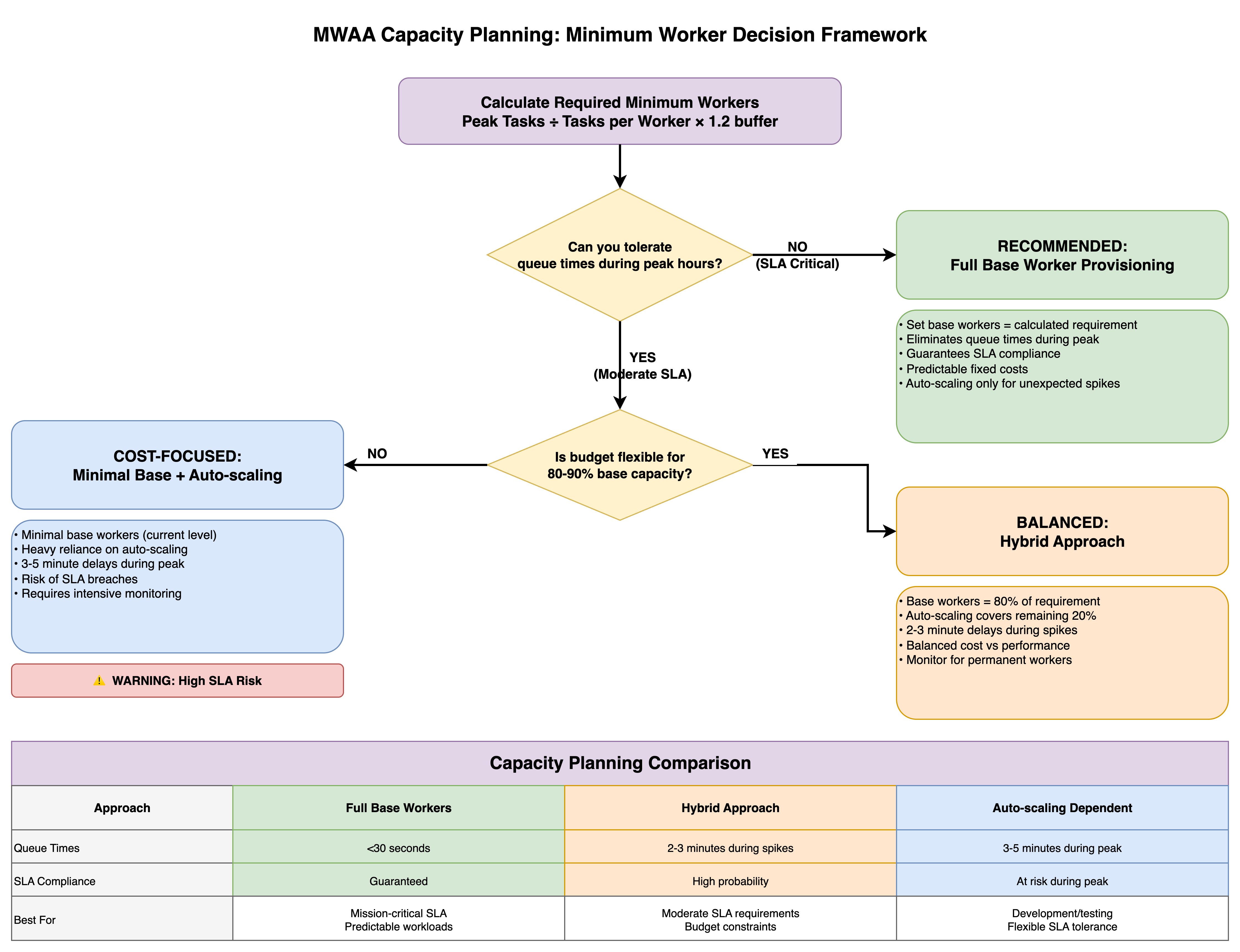
The framework presents three capacity planning approaches, each optimized for different organizational priorities.

The Full Base Worker Provisioning strategy (the conservative path) sets base workers equal to the calculated requirement, eliminating queue times during peak periods and guaranteeing SLA compliance with predictable fixed costs, while automatic scaling handles only unexpected spikes—ideal for mission-critical workloads with strict SLA requirements.

The Minimal Base + Automatic Scaling approach (the cost-focused path) maintains minimal base workers at current levels and relies heavily on automatic scaling, accepting 3-5 minute delays during peak periods and SLA breach risks in exchange for lower baseline costs, though this requires intensive monitoring and carries explicit warnings about high SLA risk.

The Hybrid Approach (the balanced path) provisions base workers at 80% of the calculated requirement with automatic scaling covering the remaining 20%, resulting in 2-3 minute delays during spikes while balancing cost against performance—suitable for moderate SLA requirements with some budget constraints.

The comparison table contrasts queue times (under 30 seconds versus 2-3 minutes versus 3-5 minutes), SLA compliance levels (guaranteed versus high probability versus at-risk during peak), and ideal use cases (mission-critical predictable workloads versus moderate SLA requirements with budget constraints versus development environments with flexible SLA tolerance), enabling teams to make informed provisioning decisions aligned with their operational requirements and financial constraints.

Key takeaway

Effective capacity planning prevents both under-provisioning (SLA breaches) and over-provisioning (cost overruns).

Capacity planning principles

  1. Calculate capacity needs BEFORE adding workload – Use peak task projections with 5-15% safety buffer
  2. Size minimum workers for peak demand – Don’t rely on automatic scaling for predictable loads
  3. Use automatic scaling only for unexpected spikes – Treat as safety net, not primary capacity
  4. Target 85-95% utilization during peak hours – Ensures headroom for unexpected growth
  5. Plan 5-15% headroom for unexpected growth – Production often differs from testing
  6. Monitor AdditionalWorkers metric – If active >6 hours daily, increase base workers
  7. Review quarterly + trigger-based assessments – Regular reviews plus immediate action on issues
  8. Balance cost and performance based on SLA criticality – Business impact justifies infrastructure investment

Success metrics

  • Queue efficiency: Average queue time <30 seconds during peak
  • SLA compliance: >99.5% of critical tasks complete on time
  • Resource utilization: 85-95% during peak hours (optimal efficiency)
  • Cost predictability: <10% variance in monthly worker costs

Conclusion

Capacity planning is not a one-time exercise. It’s an ongoing discipline. The framework we’ve outlined gives you a repeatable process: measure your current peak utilization through CloudWatch metrics, project growth based on incoming workloads, calculate the required workers with an appropriate safety buffer, and monitor continuously to catch drift before it becomes an outage.

The financial services scenario in this post illustrates a common reality: running at 100% utilization during peak hours leaves zero room for the unexpected. By sizing to 95% peak utilization with a modest buffer, the team gained the headroom needed to absorb volatility without risking their 7 AM market-open SLA.

Whether you choose full base worker provisioning for mission-critical pipelines, a hybrid approach for moderate SLA requirements, or lean on automatic scaling for development workloads, the right strategy depends on your business context, not a one-size-fits-all rule. Pair your capacity plan with the CloudWatch alarms and review triggers we covered, and you’ll catch capacity gaps early.

Combined with the optimization-first approach from Part 1, you now have a complete toolkit: diagnose before you scale, optimize before you provision, and plan before you deploy. Your MWAA environment and your on-call engineers will thank you.

To get started, visit the Amazon MWAA product page and the Amazon MWAA console page.

If you have questions or want to share your MWAA capacity planning, leave a comment.

About the authors

Boyko Radulov

Boyko Radulov

Boyko is a Senior Cloud Support Engineer at Amazon Web Services (AWS), Amazon MWAA and AWS Glue Subject Matter Expert. He works closely with customers to build and optimize their workloads on AWS while reducing the overall cost. Beyond work, he is passionate about sports and travelling.

Kamen Sharlandjiev

Kamen Sharlandjiev

Kamen is a Principal Big Data and ETL Solutions Architect, Amazon MWAA and AWS Glue ETL expert. He’s on a mission to make life easier for customers who are facing complex data integration and orchestration challenges. His secret weapon? Fully managed AWS services that can get the job done with minimal effort. Follow Kamen on LinkedIn to keep up to date with the latest Amazon MWAA and AWS Glue features and news.

Venu Thangalapally

Venu Thangalapally

Venu is a Senior Solutions Architect at AWS, based in Chicago, with deep expertise in cloud architecture, data and analytics, containers, and application modernization. He partners with financial service industry customers to translate business goals into secure, scalable, and compliant cloud solutions that deliver measurable value. Venu is passionate about using technology to drive innovation and operational excellence.

Harshawardhan Kulkarni

Harshawardhan Kulkarni

Harshawardhan is a Partner Technical Account Manager at AWS, Amazon MWAA Subject Matter Expert. Based in Dublin Ireland, he partners with Enterprise Customers across EMEA to help navigate complex workflows and orchestration challenges while ensuring best practice implementation. Outside of work, he enjoys traveling and spending time with his family.

Andrew McKenzie

Andrew McKenzie

Andrew is a Data Engineer and Educator who uses deep technical expertise from his time at AWS. As a former Amazon MWAA Subject Matter Expert, he now focuses on building data solutions and teaching data engineering best practices.

A guide to Airflow worker pool optimization in Amazon MWAA

Post Syndicated from Boyko Radulov original https://aws.amazon.com/blogs/big-data/a-guide-to-airflow-worker-pool-optimization-in-amazon-mwaa/

Optimizing the Airflow worker pool configuration in Amazon Managed Workflows for Apache Airflow (Amazon MWAA), the AWS fully managed Apache Airflow service, is an important yet often overlooked strategy for scaling workflow operations. Tasks queued for longer periods can create the illusion that additional workers are the solution, when in reality the root cause might lie elsewhere. The decision to scale isn’t always straightforward. DevOps engineers and system administrators frequently face the challenge of determining whether adding more workers will solve their performance issues or only increase operational cost without addressing the root cause.

This post explores different patterns for worker scaling decisions in Amazon MWAA, focusing on the task pool mechanism and its relationship to worker allocation. By examining specific scenarios and providing a practical decision framework, this post helps you determine whether adding workers is the right solution for your performance challenges, and if so, how to implement this scaling effectively.

Main patterns

This section discusses the most frequently seen problems that raise the question if adding additional workers would improve the health of your environment.

High CPU

Airflow serves as a workflow management platform that coordinates and schedules tasks to be run on external processing services. It acts as a central orchestrator that can trigger and monitor tasks across various data processing systems like AWS Glue, AWS Batch, Amazon EMR, and other specialized data processing tools. Rather than processing data itself, Airflow’s strength lies in managing complex workflows and coordinating jobs between different systems and services.

In Analytics and Big Data environments, there is a prevalent misconception that saturated resources automatically warrant adding more capacity. However, for Amazon MWAA, understanding your workflow characteristics and optimization opportunities should precede scaling decisions.

As you scale up your workflows, resource utilization of the Airflow clusters naturally increases. When workers consistently operate at full capacity, it may seem intuitive to add additional compute resources. However, this approach often masks underlying inefficiencies rather than resolving them.

For example, in Amazon MWAA if you are running a single task that is consuming 100% of the available CPU on your Amazon MWAA worker, adding additional workers will not resolve the problem as the task is not optimized nor split into smaller parts. As such, increasing the number of minimum workers will not bring the expected effect but will only increase the operating costs.

When your Amazon MWAA workers are consistently running above 90% CPU or Memory utilization, you’ve reached a critical decision point. Before taking actions, it is essential to understand the root cause. You have three primary options:

  1. Scale horizontally by adding additional workers to distribute the load.
  2. Scale vertically by upgrading to a larger environment class for more resources per worker.
  3. Optimize your DAGs and scheduling patterns to be more efficient and consume fewer resources.

Each approach addresses different underlying issues, and choosing the right path depends on identifying whether you are facing a capacity constraint, resource-intensive task design, or workflow inefficiency. For guidance on optimization strategies, please refer to Performance tuning for Apache Airflow on Amazon MWAA.

To monitor the CPUUtilization and MemoryUtilization on the workers, refer to the Accessing metrics in the Amazon CloudWatch console and choose the corresponding metrics.

  1. Select a time window long enough to show usage patterns.
  2. Set period to 1 Minute.
  3. Set statistics to Maximum.

Long queue time

Sometimes Airflow tasks are stuck in a queued state for a long time, which prevents DAGs from completing on time.

In Amazon MWAA, each environment class comes with configured minimum and maximum worker nodes. Each worker provides a pre-configured concurrency, which is the number of tasks that can run simultaneously on each worker at any given time. The behavior is controlled through celery.worker_autoscale=(max,min).

For example, if you have minimum 4 mw1.small workers, with default Airflow configuration, you will be able to run 20 concurrent tasks (4 workers x 5 max_tasks_per_worker). If your system suddenly requires more than 20 tasks to execute concurrently, this will result in an autoscaling event. Amazon MWAA will decide how to scale your workers efficiently, and trigger the process. The autoscaling process, however, requires additional time to provision new workers resulting in additional tasks in queued status. To mitigate this queuing issue, consider the following:

  1. If the CPU utilization on the workers is low, increasing the max value in celery.worker_autoscale=(max,min) can reduce the time tasks stay in queued state as each worker will be able to process more tasks concurrently. Airflow worker can take tasks up to the defined task concurrency regardless of the availability of its own system resources. As a result, the base worker may reach 100% CPU/Memory utilization before Autoscaling takes effect.
  2. If you do not want to increase the task concurrency on the workers, increasing the minimum worker count can also be beneficial because having more available workers allows a higher number of tasks to run concurrently.

Scheduling delays

Adding new DAGs can not only affect your system resources, but it can also create uneven scheduling patterns. Some DAGs may experience delayed execution because of resource competition, even when the overall environment metrics appear healthy. This scheduling skew often manifests as inconsistent task pickup times, where certain workflows consistently wait longer in the queue while others execute promptly.

When Amazon CloudWatch metrics show increasing variance in task scheduling times, particularly during periods of high DAG activity, it signals the need for environment optimization. This scenario requires careful analysis of execution patterns and resource utilization to determine if:

  1. While adding workers can help distribute the workload, this solution is most effective when the high utilization is primarily because of task execution load rather than DAG parsing or scheduling overhead. Adding more minimum workers will allow you to execute more tasks in parallel. For example, if you observe the value of AWS/MWAA/ApproximateAgeOfOldestTask to be steadily increasing, it means that the workers are not able to consume the messages from the queue fast enough. Additionally, you can also monitor the AWS/MWAA/QueuedTasks to identify similar patterns.
  2. Upgrading the environment class would provide better scheduling capacity. If the Scheduler is showing signs of strain or if you’re seeing high resource utilization across all components, upgrading to a larger environment class might be the most appropriate solution. This provides more resources to both the Scheduler and Workers, allowing for better handling of increased DAG complexity and volume. To validate the same, use AWS/MWAA/CPUUtilization and AWS/MWAA/MemoryUtilization in the Cluster metrics and choose Scheduler, BaseWorker and AdditionalWorker metrics.
  3. Restructuring DAG schedules would reduce resource contention.

The key is to understand your workflow patterns and identify whether the scheduling delays are because of insufficient worker capacity or other environmental constraints.

Anti patterns

This section showcases the most common anti patterns which make MWAA users think that adding more workers will improve performance.

Underutilized workers

When evaluating Amazon MWAA performance bottlenecks, it’s important to distinguish resource constraints and DAG design inefficiencies before scaling the environment.

Sometimes the Amazon MWAA environment has the capacity to run 100 tasks concurrently but your queue metrics (AWS/MWAA/RunningTasks) show only 20 tasks active most of the time with no tasks remaining in queued state. In such scenarios, you are advised to check Amazon CloudWatch for consistently low CPU and memory usage on existing workers during peak workload times. If this is confirmed, it is usually an indication of inefficiencies in DAG design, scheduling patterns, or Airflow configuration.

You have two primary options to address this:

1. Downsize: If you do not expect your workload to increase, it is safe to assume you have over-provisioned your cluster. Start by removing any extra workers first and finally resolve to downsizing your environment class.

2. Optimize: Fine tune your DAG scheduling and airflow configuration through Pools and Airflow configuration for concurrency to increase the throughput of your system.

Misconfigured Airflow configurations that create artificial bottlenecks

In Apache Airflow, performance bottlenecks often occur because of configuration settings, not actual resource constraints. At such times, DAG executions get delayed not because of insufficient compute, but because of incorrect concurrency configuration.

Efficient use of Amazon MWAA requires reviewing not only resource utilization for Workers and Schedulers but also concurrency configurations for artificially created bottlenecks. Sometimes one restrictive configuration prevents the scaling benefits of larger environment or additional workers. Always audit Airflow configurations if performance seems limited even when system metrics suggest spare capacity.

Important consideration: Amazon Managed Workflows for Apache Airflow (Amazon MWAA) does not automatically update the worker concurrency configuration when you change the environment class. This behavior is important to understand when scaling your environment. If you initially create an mw1.small environment, where each worker can handle up to 5 concurrent tasks by default. When you upgrade to a medium environment class (which supports 10 concurrent tasks per worker by default), the concurrency setting remains at 5 for in-place updated environments. You must manually update the concurrency configuration to take full advantage of the increased capacity available in the medium environment class.

Because of this you need to also update the Airflow configurations that control concurrency whenever you update the environment class. To update the concurrency setting after upgrading your environment class, modify the celery.worker_autoscale configuration in your Apache Airflow configuration options. This makes sure your workers can process the maximum number of concurrent tasks supported by your new environment class.

Other times, an Amazon MWAA environment can be constrained by max_active_runs or DAG concurrency controls instead of actual resource limits. These configuration-based throttles prevent tasks from running, even when the worker instances have available compute to handle the workload.

There is an important distinction between the two. Configuration limits act as artificial caps on parallelism, while true resource limits indicate that workers are fully utilizing their CPU or memory capacity. Understanding which type of constraint affects your environment helps you determine whether to adjust configuration settings or scale your infrastructure.

Adjusting Airflow configurations such as Pools, concurrency, max_active_runs solves performance problems without scaling workers. Some of the configurations you can use to control this behavior:

  1. max_active_runs_per_dag (DAG level): Controls how many DAG runs for a given DAG are allowed at the same time. If set to 2, only 2 DAG runs can run concurrently, even if there is plenty of worker capacity left. Extra runs queue, making the DAG executions slow even though workers are idle.
  2. max_active_tasks:Controls the concurrency field in a DAG definition (or setting at environment level) limits the number of tasks from the DAG running at any moment, regardless of overall system capacity or number of workers.
  3. Pools:Pools restrict how many tasks of a certain type (often resource heavy) can run at once. A pool with only 3 slots will throttle any tasks above 3 assigned to that pool, leaving workers idle.
  4. Execution timeouts and retries: If not tuned, failed tasks might fill up slots unnecessarily, stuck tasks can block worker slots and slow queue processing.
  5. Scheduling intervals and dependencies: Overlapping or inefficient scheduling may cause idle periods or excess contention for resources, affecting real throughput.

How Airflow configurations can override each other

Airflow has multiple layers of concurrency and scheduling controls. Some at the environment level, some at the DAG/task level, and others for pools. Sometimes more restrictive settings override more permissive ones, resulting in unexpected queue buildup.

DAG level vs Environment level: If “max_active_runs_per_dag” (DAG level) is lower than the environment-level “max_active_runs_per_dag” or system wide concurrency, the DAG setting is used, throttling tasks even if the environment could do more.

Task level overrides: Individual task definitions can have their own parameters like “max_active_tis_per_dag” which can cap runs per task and create a bottleneck if set lower than global settings.

Order of precedence: The most restrictive relevant configuration at any level (Environment, DAG, Task) effectively sets the upper bound for parallel task execution.

Setting Location Setting Effect on task throughput
Environment Level parallelism Max total tasks running on Scheduler
DAG Level max_active_runs Max simultaneous DAG runs
Task Level concurrency Max concurrent task for that DAG

Performance issues often resemble resource exhaustion, but actually derive from overly restrictive configurations. Audit all the preceding parameters carefully. You can loosen restrictive values step by step and monitor their effect before deciding to scale your cluster further. This approach ensures optimal and cost-efficient usage of your cloud resources without paying for idle capacity.

Slow resource depletion from memory leaks

A common scenario for memory leak or slow resource depletion in Amazon MWAA is when DAGs and tasks begin to fail or slow down over time. Scaling workers or increasing environment size does not resolve the underlying issue. This happens because the root cause is not a lack of capacity but rather an application-level leak that causes persistent exhaustion.

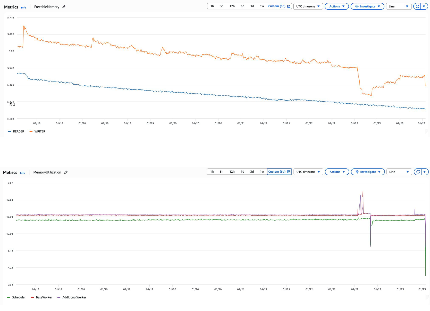
For example, as Airflow continuously runs tasks and parses DAGs over time, memory consumption can steadily increase across the environment. This might manifest as an Amazon MWAA metadata database experiencing declining FreeableMemory metrics despite consistent or even reduced workloads. When this occurs, database query performance gradually declines as memory resources become constrained for scheduler/worker & metadata database, ultimately affecting overall environment responsiveness since Airflow depends heavily on its metadata database for critical operations. This scenario is similar to how an application might create database connections without properly closing them, leading to resource exhaustion over time.

Graph: Declining FreeableMemory and MemoryUtilization

Common causes:

  1. Connection pool exhaustion: DAGs that fail to properly close database connections can lead to connection pool exhaustion and memory leaks in the database.
  2. Resource-intensive operations: Complex, long-running queries or XCOM operations against the metadata database can consume excessive memory.
  3. Inefficient DAG design: DAGs with numerous top-level Python calls can trigger database queries during DAG parsing. For instance, using variable.get() calls at the DAG level rather than at the task level creates unnecessary database load.

Recommended solutions:

  1. Implement Amazon CloudWatch monitoring: Establish Amazon CloudWatch alarms for FreeableMemory with appropriate thresholds to detect issues early.
  2. Regular database maintenance: Perform scheduled database clean-up operations to purge historical data that is no longer needed.
  3. Optimize DAG code: Refactor DAGs to move database operations like variable.get() from the DAG level to the task level to reduce parsing overhead.
  4. Connection management: Make sure all database connections are properly closed after use to prevent connection pool exhaustion.

By following the preceding recommendations you can maintain healthy memory utilization for the metadata database and maintain optimal performance of your Amazon MWAA environment without needing to scale workers.

Conclusion

The decision to add workers in Amazon MWAA environments requires careful consideration of multiple factors beyond simple task queue metrics. In this post, we showed that while adding workers can address certain performance challenges, it’s often not the optimal first response to system bottlenecks.

Key considerations before scaling workers include:

  1. Root cause analysis
    • Verify whether high CPU/memory usage stems from task optimization issues.
    • Examine if queuing problems result from configuration constraints rather than resource limitations.
    • Investigate potential memory leaks or resource depletion patterns.
  2. Configuration optimization
    • Review and adjust Airflow parameters (concurrency settings, pools, timeouts).
    • Understand the interaction between different configuration layers.
    • Optimize DAG design and scheduling patterns.

The most successful Amazon MWAA implementations follow a systematic approach: first optimizing existing resources and configurations, then scaling workers only when justified by data-driven capacity planning. This approach ensures cost-effective operations while maintaining reliable workflow performance.

Remember that worker scaling is only one tool in the Amazon MWAA optimization toolkit. Long-term success depends on building a comprehensive performance management strategy that combines proper monitoring, proactive capacity planning, and continuous optimization of your Airflow workflows.

In the next post, we discuss capacity planning and the steps you need to perform before adding additional DAGs in your environment so that you can plan for the additional load and make sure you have enough headroom.

To get started, visit the Amazon MWAA product page and the Performance tuning for Apache Airflow on Amazon MWAA page.

If you have questions or want to share your MWAA scaling experiences, leave a comment below.

About the authors

Boyko Radulov

Boyko Radulov

Boyko is a Senior Cloud Support Engineer at Amazon Web Services (AWS), Amazon MWAA and AWS Glue Subject Matter Expert. He works closely with customers to build and optimize their workloads on AWS while reducing the overall cost. Beyond work, he is passionate about sports and travelling.

Kamen Sharlandjiev

Kamen Sharlandjiev

Kamen is a Principal Big Data and ETL Solutions Architect, Amazon MWAA and AWS Glue ETL expert. He’s on a mission to make life easier for customers who are facing complex data integration and orchestration challenges. His secret weapon? Fully managed AWS services that can get the job done with minimal effort. Follow Kamen on LinkedIn to keep up to date with the latest Amazon MWAA and AWS Glue features and news.

Venu Thangalapally

Venu Thangalapally

Venu is a Senior Solutions Architect at AWS, based in Chicago, with deep expertise in cloud architecture, data and analytics, containers, and application modernization. He partners with financial service industry customers to translate business goals into secure, scalable, and compliant cloud solutions that deliver measurable value. Venu is passionate about using technology to drive innovation and operational excellence.

Harshawardhan Kulkarni

Harshawardhan Kulkarni

Harshawardhan is a Partner Technical Account Manager at AWS, Amazon MWAA Subject Matter Expert. Based in Dublin Ireland, he partners with Enterprise Customers across EMEA to help navigate complex workflows and orchestration challenges while ensuring best practice implementation. Outside of work, he enjoys traveling and spending time with his family.

Andrew McKenzie

Andrew McKenzie

Andrew is a Data Engineer and Educator who uses deep technical expertise from his time at AWS. As a former Amazon MWAA Subject Matter Expert, he now focuses on building data solutions and teaching data engineering best practices.

Designing trust and safety into Amazon Bedrock powered applications

Post Syndicated from Victor Lungu original https://aws.amazon.com/blogs/security/designing-trust-and-safety-into-amazon-bedrock-powered-applications/

Generative AI brings promising innovation, transforming how individuals and organizations approach everything from customer service to content creation and more. As AI continues to expand its capabilities, organizations are increasingly focused on how they can integrate the responsible AI concepts into the development lifecycle of their AI applications.

Research from Accenture and Amazon Web Services (AWS) reveals compelling evidence for the business value of responsible AI practices, both internally within their organizations and externally to their users. Organizations that communicate a mature approach to responsible AI see an 82% improvement in employee trust in AI adoption, which directly leads to increased innovation. Additionally, companies that offer responsible AI-enabled products and services experience a 25% increase in customer loyalty and satisfaction.

Understanding the core dimensions of responsible AI

AWS identifies these key dimensions that form the backbone of responsible AI implementation:

  • Safety focuses on preventing harmful system output and misuse. This dimension focuses on steering AI systems to prioritize user and system safety.
  • Controllability focuses on mechanisms that monitor and steer AI system behavior. This dimension refers to the ability to manage, guide, and constrain AI systems to operate within specific parameters.
  • Fairness considers the impacts of AI on different groups of users.
  • Explainability focuses on understanding and evaluating system outputs.
  • Security and privacy focuses on making sure that data and models are appropriately obtained, used, and protected.
  • Veracity and robustness focuses on achieving correct system outputs, even with unexpected or adversarial inputs.
  • Governance makes sure that development, deployment, and management of AI systems align with ethical standards, legal requirements, and societal values.
  • Transparency focuses on understanding how AI systems make decisions, why the systems produce specific results, and what data the systems use.

It’s a best practice to review and apply all these dimensions to your AI implementation. For more information, see Considerations for addressing the core dimensions of responsible AI for Amazon Bedrock applications.

The responsible AI lifecycle

When you implement AI systems, you should build safety into every phase of the AWS responsible AI lifecycle. The responsible AI lifecycle consists of the following three phases, each with distinct responsibility considerations for the safety dimension:

  1. In the design and development phases, thoroughly evaluate potential safety risks. Understand what you want your AI application to do, what you don’t want it to do, and what you want to prevent it from doing. You should build safety guardrails into your systems from the beginning and make sure that your development teams understand the capabilities and limits of your AI application.
  2. In the deployment phase, theory meets reality. During this phase, you should implement robust safety measures through multiple layers, from comprehensive user training to proactive monitoring and review processes. Every application, product, and feature must include clear safety protocols and user guidelines. You must think beyond the launch of an application and consider how to launch a holistic safety framework. This framework—which can contain steps such as red team testing—must protect your brand, users, and stakeholders.
  3. In the operations phase, it’s important to maintain vigilance. Safety, like security, isn’t something you set up once and then ignore. Safety requires continuous monitoring and adaptation. To catch potential safety issues early, you can implement real-time feedback mechanisms to conduct regular performance evaluations. You can also continuously monitor for shifts in how your application is used, or functions that could compromise safety. Because safety considerations and risks evolve as technology evolves, it’s crucial to understand that adjustments are necessary over time.

For more information, see the Responsible use of AI guide.

Abuse detection

Foundation models in Amazon Bedrock are inherently designed with safety mechanisms to prevent harmful outputs. However, you can implement additional input safety systems in production environments to provide critical early detection capabilities to identify problematic content, users, or patterns.

Note: Amazon Bedrock might implement automated abuse detection mechanisms to identify potential violations of the AWS Acceptable Use Policy (AUP) and Service Terms, including the Responsible AI Policy or a third-party model provider’s AUP.

See the Amazon Bedrock abuse detection document for more information.

AI abuse prevention tools and techniques

To maintain trust in your AI services, preventative action is key, while also efficiently planning and managing development resources. Introduce observability and safety guardrails early in development to support long-term scalability and help identify potential issues before they affect your users. To begin this process, thoroughly scope your AI use case with the following actions:

  • Understand your users
  • Anticipate potential misuse scenarios
  • Define your risk tolerance

This scope guides your development of a precise safety framework that addresses the specific risks of your AI implementation while you maintain expected performance. For this scope, you can use AWS specialized tools designed specifically to monitor and protect Amazon Bedrock applications.

Using CloudWatch to monitor Amazon Bedrock

Amazon CloudWatch provides essential visibility into AI system behavior and performance. When you configure comprehensive logging, you can capture important information across user segments and interaction types, such as the following:

  • Request volumes
  • Response latencies
  • Rejection rates
  • Content filtering triggers

You can use this information to identify potential abuse patterns or unexpected behaviors before they affect operations. CloudWatch dashboards visualize metrics according to monitoring priorities, and automated alerts provide prompt notification when you exceed thresholds. This infrastructure transforms interaction data into actionable insights and supports continuous safety improvement.

Note: By default, Amazon Bedrock logging is turned off. You must turn on logging for your application. To configure this, contact your account manager.

Using Amazon Bedrock Guardrails to customize safeguards

Amazon Bedrock Guardrails offers configurable protection mechanisms tailored to specific risk profiles and content policies. You can customize Bedrock Guardrails to match your application requirements, such as:

  • Define domain-relevant undesirable topics
  • Configure appropriate content filtering thresholds
  • Configure sensitive information detection and redaction parameters aligned with data policies

Additionally, you can configure controls that prioritize accuracy and prevent hallucinations while maintaining creative flexibility based on your application needs. When you thoughtfully configure Guardrails, you can balance performance and safety according to your specific use case requirements and risk factors.

The abuse response process

As AI safety evolves and new risks emerge, abuse might still occur even if you implement safety mechanisms. If you receive an abuse report from the AWS Trust & Safety team, then complete the following steps to help effectively address the issue:

  1. Acknowledge receipt: Acknowledge the receipt of the abuse report within 24 hours. If your team is still conducting their investigation, then inform AWS that the investigation is ongoing. Provide the number of days expected to complete the investigation.
  2. Investigate the issue: Thoroughly investigate the issue, including examining the logs (if enabled), reviewing Amazon Bedrock inputs, and checking for unauthorized access. While AWS abuse reports include a small sample of prompt IDs for you to investigate, investigate usage of your Amazon Bedrock application. Check for patterns to see if there’s a systemic issue that’s leading to abuse.
  3. Take appropriate action: If appropriate, take action to implement fixes, update safeguards, address violating users, or redesign features. Consider if you need systemic or root-cause fixes, rather than addressing one abusive end user. An abuse incident by one user could indicate vulnerabilities in your safety mechanisms that can lead to continuous abuse.
  4. Report back to AWS Trust & Safety: Following your investigation and implementation of fixes, provide an update to AWS Trust & Safety on your findings and remediation steps. Be transparent about what happened and how you addressed the issue. If you think that no violation occurred, then provide context on how you came to this conclusion. Include examples of the prompts and your business use case where possible.

Conclusion

To learn more about safety and responsible AI development, explore AWS resources, including the Responsible AI portal and machine learning best practices documentation. These resources provide additional tools and frameworks to build safe, effective AI systems that drive innovation and maintain safety standards.

Victor Lungu
Victor Lungu

Victor is a Trust & Safety AI Abuse Specialist at AWS, based in Dublin. Victor works across a broad range of AI safety domains including content safety and emerging AI risks

What the March 2026 Threat Technique Catalog update means for your AWS environment

Post Syndicated from Shannon Brazil original https://aws.amazon.com/blogs/security/what-the-march-2026-threat-technique-catalog-update-means-for-your-aws-environment/

The AWS Customer Incident Response Team (AWS CIRT) regularly encounters patterns that repeat across their engagements when helping customers respond to security incidents. We’re passionate about making sure that information is widely accessible so that everyone can improve their security posture and their organization’s resilience to disruption. The primary method we use to share this information is the Threat Technique Catalog for AWS (TTC). The latest update to the catalog for March 2026 addresses identity, persistence, infrastructure destruction, and privilege escalation. Each new entry reflects something we’ve encountered in practice, and each provides straightforward mitigations. This post breaks down what changed, why it matters, and what you can do about it today.

What we’re seeing

Based on recent observations, we’ve added three new entries to the TTC.

Cognito refresh token abuse: The quiet persistence mechanism

Amazon Cognito refresh tokens are designed for convenience. They let applications obtain new access and ID tokens without requiring users to re-authenticate. The default lifetime is 30 days and is configurable up to 10 years. Cognito provides the flexibility to address a wide range of use cases, however the AWS CIRT has seen this lifetime window used by threat actors in an unauthorized way to maintain persistence by refreshing credentials.

When a threat actor obtains a valid refresh token—through credential theft, compromised client-side storage, or elevated permissions—they can call cognito-idp:GetTokensFromRefreshToken to silently generate fresh tokens. The legitimate user’s session continues normally because their application independently refreshes tokens as needed—the threat actor’s refresh calls don’t invalidate the user’s token. This creates a parallel, persistent foothold that’s invisible to the user. In environments where refresh token rotation isn’t enabled, the same token can be reused indefinitely within its validity window.

This method of gaining persistent access is often overlooked by response teams who were confident that the initial compromise was contained, only to discover ongoing unauthorized access weeks later through a refresh token they didn’t know existed.

Enabling refresh token rotation and reducing the lifetime of tokens can help mitigate this risk. Dive deeper in the TTC (T1098.A006).

AMI image deletion: Targeting recovery capabilities

Amazon Machine Images (AMI) are a core part of many solutions and foundational to disaster recovery. They often contain the operating system, application configurations, and everything needed to rebuild your infrastructure. Threat actors know this, and we’re seeing ec2:DeregisterImage used to make it more difficult to recover from an incident.

By default, when an AMI is deregistered, it’s gone. Recycle Bin retention rules can allow the recovery of the AMI, but if you haven’t explicitly enabled that functionality, there’s no way to undo the deregister action. Working with customers, we’ve seen cases where the impact of this action goes beyond the immediate loss because the threat actors have also removed the golden images the teams planned to restore from.

The TTC has more information about how to detect and mitigate this technique, including how to enable Recycle Bin retention rules for key AMIs (T1485.A002).

Additional cloud roles: The trust policy blind spot

We’ve updated T1098.003: Additional Cloud Roles to now include UpdateAssumeRolePolicy as a tracked API call. We’ve seen an increase in the use of this call to avoid detections set to flag new role creation (iam:CreateRole). By modifying the trust policy of an existing role, a threat actor with sufficient permissions can use UpdateAssumeRolePolicy to subtly add an external account or an identity they control. No new roles appear. No new policies are created. The existing role simply trusts a new principal which the threat actor can assume.

This persistence and privilege escalation technique blends into the volume of normal AWS Identity and Access Management (IAM) operations. It’s especially effective in environments with a large number of roles where trust policy changes aren’t actively monitored.

The current trend

A common thread runs through all three of these updates: threat actors are using subtle, default, or unexpected behaviors to sidestep detection. Refresh tokens working as designed. AMI deregistration completing without guardrails. Trust policies being modified through legitimate API calls. These actions might not trigger alarms in most environments because they look like normal operations.

This is a shift worth paying attention to. Rather than relying on novel exploits or zero-days, the techniques we’re cataloging reflect threat actors who understand how cloud services work and use that knowledge to hide in plain sight. The implication for security teams is clear: prevention and detection strategies need to mature beyond monitoring for obviously malicious actions. Customers need to be watching for legitimate actions happening in illegitimate context—such as the right API call, made by the wrong principal, at the wrong time.

The Threat Technique Catalogue for AWS is designed to help with exactly this. Each technique entry includes detection guidance and mitigations specific to AWS environments. We encourage teams to review the relevant entries and assess whether their current monitoring would catch these patterns:

  • T1098.A006: Cognito Refresh Token Abuse: Are you monitoring for cognito-idp:GetTokensFromRefreshToken from unexpected sources? Is refresh token rotation enabled?
  • T1485.A002: AMI Image Deletion: Do you have Recycle Bin retention rules protecting your critical AMIs? Would you know if a production AMI was deregistered outside a maintenance window?
  • T1098.003: Additional Cloud Roles: Are trust policy modifications tracked and alerted on? Could an external account be added to an existing role without anyone noticing?

Each of these techniques leaves traces in AWS CloudTrail, and the TTC provides specific guidance on what to watch for and how to respond.

Looking ahead

The Threat Technique Catalog for AWS exists because we believe the patterns we observe during security engagements shouldn’t stay behind closed doors. When we see techniques repeating across customers, the most effective thing we can do is document them and make that knowledge available so you can act on it before you’re in the middle of an incident.

This March update adds three new entries, and the catalog will continue to evolve. Our team regularly updates it based on what we’re seeing in the real world when helping customers respond to security events. We encourage security teams to review the catalog regularly, incorporate its techniques into threat modeling exercises, and use it as a shared vocabulary for discussing cloud-specific threats.

Explore the full catalog: Threat Technique Catalog for AWS

Additional resources

If you have feedback about this post, submit comments in the Comments section below.
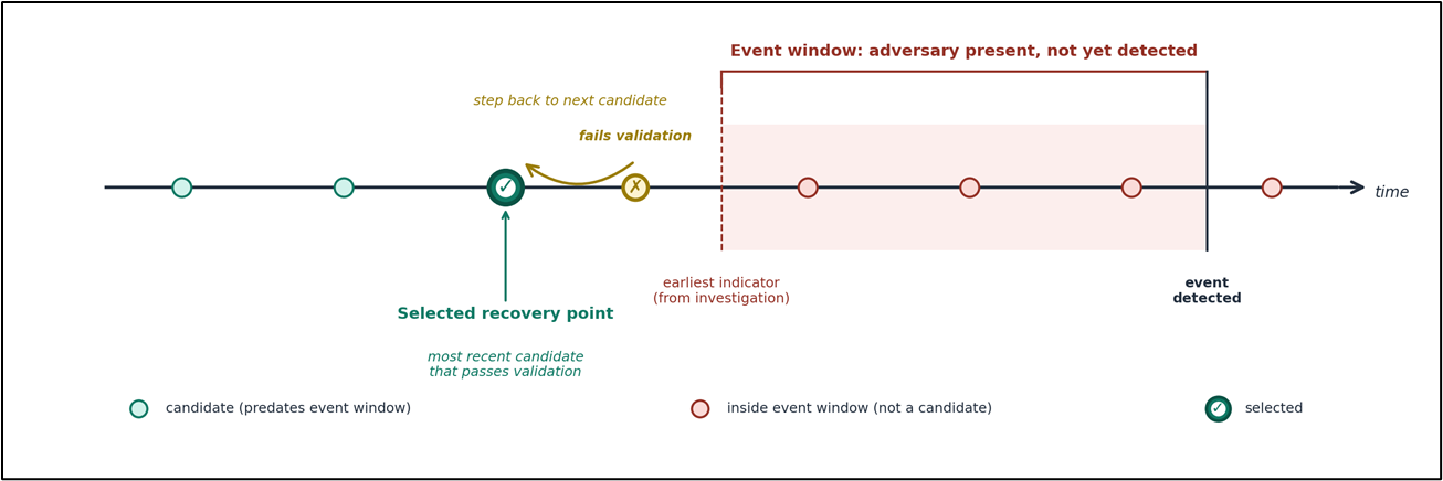

Shannon Brazil

Shannon Brazil

Shannon is a security engineer on the AWS Customer Incident Response Team (CIRT), specializing in digital forensics and cloud security investigations. Known in the community as 4n6lady, she is passionate about security education and mentoring the next generation of defenders.

Cydney Stude

Cydney Stude

Cydney is a security engineer specializing in threat intelligence and incident response at AWS. Cydney works on the ground in incident response and is passionate about turning observables into security outcomes. Cydney is an author and maintainer of the Threat Technique Catalog for AWS.

Can I do that with policy? Understanding the AWS Service Authorization Reference

Post Syndicated from Anshu Bathla original https://aws.amazon.com/blogs/security/can-i-do-that-with-policy-understanding-the-aws-service-authorization-reference/

Understanding what AWS Identity and Access Management (IAM) policies can control helps you build better security controls and avoid spending time on approaches that won’t work. You’ve likely encountered questions like:

  • Can I use AWS Organizations service control policies (SCPs) to prevent the creation of security groups that allow traffic from 0.0.0.0/0?
  • Can I block uploads unless objects are encrypted?
  • Can I prevent functions with more than 512 MB of memory allocated?

Some of these are possible with IAM policies. Others are not. The difference is determined by a fundamental principle of AWS authorization: Policies make decisions based on information available in the authorization context at the time of the API call.

In this blog post, you learn how to use the AWS Service Authorization Reference to determine what’s achievable with IAM policies, recognize scenarios that need alternative solutions, and build more effective security controls in your AWS environment.

Understanding AWS authorization context

When you make an AWS API request through the AWS Management Console, AWS Command Line Interface (AWS CLI), or AWS SDK, the specific AWS service (such as Amazon S3 or Amazon EC2) receiving the request assembles a request context containing information about that request. This context is used for policy evaluation decisions. Request context is structured using the Principal, Action, Resource, Condition (PARC) model, which has four key components.

  • Principal: Identifies the requester and their attributes (tags, session context)
  • Action: Specifies the AWS API operation being requested (for example, s3:PutObject, ec2:RunInstances)
  • Resource: Defines the target AWS resource using Amazon Resource Names (ARNs)
  • Condition: Provides additional context available at request time, such as IP address, time, encryption parameters, MFA status, and service-specific attributes

The following example shows the typical request context for an Amazon S3 object upload:

  • Principal: AIDA123456789EXAMPLE
  • Action: s3:PutObject
  • Resource: arn:aws:s3:::my-bucket/documents/samplereport.pdf
  • Condition:
    • aws:PrincipalTag/Department=Finance
    • aws:RequestedRegion=us-east-1
    • aws:SourceIp=x.x.x.x
    • aws:MultiFactorAuthPresent=true
    • s3:x-amz-server-side-encryption=AES256
    • s3:x-amz-storage-class=STANDARD_IA

IAM policies can evaluate request metadata like encryption method and storage class being specified. However, it cannot evaluate the actual file contents, object size, or specific data patterns. Policy evaluation occurs at the time of the request, using the information present in the authorization context.

An essential resource: The Service Authorization Reference

The Service Authorization Reference is the authoritative documentation for understanding what policies can control. For every AWS service, it documents:

  • Actions: Every controllable operation
  • Resources: Resource types that can be targeted
  • Condition keys: The exact context information available for policy decisions

Condition keys are broadly divided into two categories. Global condition keys, which can be used across AWS services, and service-specific condition keys, which are defined for use with an individual AWS service. Use the Service Authorization Reference to find the global-condition keys or service-specific condition keys for each AWS service.

How to use the Service Authorization Reference

Follow these steps to determine if your requirement can be controlled with IAM policies:

  1. Navigate to your service: Go to the page for the specific AWS service you’re working with, such as Actions, resources, and condition keys for Amazon S3.
  2. Find the action you want: Find the API operation you want to control. Be precise, different actions have different available condition keys.
  3. Examine available condition keys: The Condition keys column shows what context information AWS makes available for that action.
  4. Make your feasibility determination: If the information you need isn’t listed as a condition key, you will not be able to control it with IAM policies alone.

Let’s take an example from the Amazon Elastic Compute Cloud (Amazon EC2) ec2:RunInstances action to see what you can and can’t control. In the Service Authorization Reference under the Amazon EC2 section, examine the RunInstances action and check the Resource types column. The RunInstances action affects multiple resource types, each with its own set of condition keys.

For the instance* resource type:

  • ec2:InstanceType: Can restrict instance types
  • ec2:EbsOptimized: Can require EBS optimization
  • aws:RequestTag/: Can enforce tagging requirements

For the network-interface* resource type:

  • ec2:Subnet: Can control subnet placement
  • ec2:Vpc: Can limit to specific virtual private clouds (VPCs)
  • ec2:AssociatePublicIpAddress: Can control public IP assignment

Note: These are a few examples from the many condition keys available for each resource type under the RunInstances action. The Service Authorization Reference lists dozens of condition keys across resource types (instance, network interface, security group, subnet, volume, and so on) that RunInstances affects. Consult the complete reference to see the available options for your specific use case.

Access the Service Authorization Reference programmatically

Beyond the human-readable documentation, AWS provides the Service Authorization Reference in machine-readable JSON format to streamline automation of policy management workflows. Use this programmatic access to incorporate authorization metadata into your development and security workflows.
For detailed information about the JSON structure and field definitions, see the Simplified AWS service information for programmatic access.
Developers can use tools like the IAM MCP Server for AWS IAM operations. This server provides AI assistants with the ability to manage IAM users, roles, policies, and permissions while following security best practices.

Using IAM policies to control specific scenarios

The following examples show how you can use IAM policies to control specific scenarios.

Example 1: Enforce AES256 server-side encryption on S3 objects

In the Amazon S3 Service Authorization Reference, under s3:PutObject action, the s3:x-amz-server-side-encryption condition key is available in the authorization context, which can be used to control the server-side encryption of S3 objects with AES-256. Here is the required policy.

Policy 1: Deny Amazon S3 object upload if the encryption doesn’t use AES-256

{
	"Version": "2012-10-17",
	"Statement": [
		{
			"Sid": "DenyUnencryptedObjectUploads",
			"Effect": "Deny",
			"Action": "s3:PutObject",
			"Resource": "arn:aws:s3:::my-bucket/*",
			"Condition": {
				"StringNotEquals": {
					"s3:x-amz-server-side-encryption": "AES256"
				}
			}
		}
	]
}

Policy 1 is a resource-based policy that can be applied on an S3 bucket to restrict object uploads. It denies a PutObject request when the server-side encryption isn’t using the AES-256 encryption algorithm.

Example 2: Allow different instance types based on the user’s cost center tag.

When checking the Amazon EC2 Service Authorization Reference for ec2:RunInstances, the ec2:InstanceType condition key, which is resource specific, is available. To restrict instance types based on who is launching them (rather than just what is being launched), you can either combine this with a global condition key or attach different policies to different principals. By using aws:PrincipalTag/tag-key alongside ec2:InstanceType, you can identify the user’s cost center from their IAM identity tags and then apply different instance type restrictions accordingly. This allows a single policy to dynamically enforce different permissions based on the requester’s identity.

Policy 2: Restricting EC2 instance types by cost center

{
	"Version": "2012-10-17",
	"Statement": [
		{
			"Sid": "AllowDevInstanceTypes",
			"Effect": "Allow",
			"Action": "ec2:RunInstances",
			"Resource": "arn:aws:ec2:*:*:instance/*",
			"Condition": {
				"StringEquals": {
					"aws:PrincipalTag/CostCenter": "Development"
				},
				"StringLike": {
					"ec2:InstanceType": "t3.*"
				}
			}
		},
		{
			"Sid": "AllowProdInstanceTypes",
			"Effect": "Allow",
			"Action": "ec2:RunInstances",
			"Resource": "arn:aws:ec2:*:*:instance/*",
			"Condition": {
				"StringEquals": {
					"aws:PrincipalTag/CostCenter": "Production"
				},
				"StringLike": {
					"ec2:InstanceType": [
						"m5.*",
						"c5.*",
						"r5.*"
					]
				}
			}
		}
	]
}

This is an identity-based policy that you can attach to IAM users, groups, or roles to control EC2 instance launches based on cost allocation. In the first statement, aws:PrincipalTag, which is a global condition key (tags attached to the IAM user or role), is used to determine which instance types are allowed. Users tagged with CostCenter=Development can only launch cost-effective T3 instance types (t3.micro, t3.small, t3.medium, and so on)with the service specific key ec2:InstanceType.

In the second statement, users tagged with CostCenter=Production can launch more powerful instance types from the M5 (general purpose), C5 (compute optimized), and R5 (memory optimized) families. This approach lets organizations enforce cost controls and allocate resources based on workload requirements. Each cost center maintains flexibility for its specific needs.

Note: Additional resources are required in the IAM policy to successfully launch EC2 instances. For the complete list, see Launch Instances.

Example 3: Users can only access and update DynamoDB items where the partition key matches their username.

You have identified that GetItem, PutItem,and UpdateItem actions are required. Corresponding to these actions, you can use the condition key to expose partition key values in the authorization context as described in the Amazon DynamoDB Service Authorization Reference

Policy 3: DynamoDB fine-grained access control

{
	"Version": "2012-10-17",
	"Statement": [
		{
			"Effect": "Allow",
			"Action": [
				"dynamodb:GetItem",
				"dynamodb:PutItem",
				"dynamodb:UpdateItem"
			],
			"Resource": "arn:aws:dynamodb:us-east-1:111122223333:table/UserProfiles",
			"Condition": {
				"ForAllValues:StringEquals": {
					"dynamodb:LeadingKeys": ["${aws:username}"]
				}
			}
		}
	]
}

The policy allows users to perform read and write actions (GetItem, PutItem, and UpdateItem) on the UserProfiles table, but only for items where the partition key value equals their own username (using the ${aws:username} policy variable). For example, if user alice attempts to access an item with partition key bob, the request will be denied.

Scenarios that need more than policies alone

Some requirements can’t be met using IAM policies. Here are three common scenarios that aren’t achievable with IAM policies alone.

Scenario 1: Block users from creating security group rules that allow traffic from 0.0.0.0/0 on TCP port 22

Upon checking the Amazon EC2 Service Authorization Reference, you will find that the ec2:AuthorizeSecurityGroupIngress action is required in an IAM policy to add an inbound access rules to a security group.

To verify this in the Service Authorization Reference, navigate to the Amazon EC2 Service Authorization Reference and search for the AuthorizeSecurityGroupIngress action, which is the action that creates security group rules. After you locate this action, review the Condition keys column and look for condition keys related to CIDR blocks, IP ranges, ports, or protocols. Available condition keys for ec2:AuthorizeSecurityGroupIngress include:

Notice there are no condition keys for CIDR blocks (such as 0.0.0.0/0), port numbers (such as 22), or protocols (such as TCP). The authorization context doesn’t include information about the specific CIDR blocks, ports, or protocols being added to the security group rule, so IAM policies can’t control these attributes.

Solution
Take a reactive approach using the AWS Config managed rule INCOMING_SSH_DISABLED to detect overly permissive rules. You can also use a combination of Amazon EventBridge and Lambda to either send a notification to your security team for the non-compliant configuration or to restrict the security group through an automation. For more information, see How to Automatically Revert and Receive Notifications About Changes to Your Amazon VPC Security Groups.

Scenario 2: Prevent creation of Lambda functions with more than 512 MB of memory allocated

Following the same verification methodology described in Scenario 1, navigate to the AWS Lambda Service Authorization Reference and examine the CreateFunction action’s condition keys for the function* resource type.

Available condition keys for lambda:CreateFunction with the function* resource type include:

  • lambda:CodeSigningConfigArn: Filters access by the ARN of the code signing
  • configuration-lambda:Layer: Filters access by the ARN of a version of an AWS Lambda layer
  • lambda:VpcIds: Filters access by the ID of the VPC configured for the Lambda function

There is no condition key for memory allocation (MemorySize parameter), timeout settings, storage configuration (EphemeralStorage), or runtime selection. Because memory allocation isn’t exposed in the authorization context, IAM policies can’t restrict this parameter.

Solution

Key takeaways

Keep these principles in mind when working with IAM policies:

  • Policies control what’s in the authorization context, not all elements you see in API documentation
  • The Service Authorization Reference is authoritative; if something isn’t listed as a condition key, you can’t control it with policies
  • Different actions have different available contexts even within the same service
  • Alternative approaches exist. AWS Config, EventBridge, and service-specific controls can be used to achieve your goals when policies alone can’t
  • Layered security is essential; combine preventive, detective, and responsive controls to help ensure that your data is secure

Conclusion

In this post, you learned how to use the AWS Service Authorization Reference to determine what’s achievable with IAM policies and recognize scenarios that require alternative solutions. By understanding that policies can only make decisions based on information available in the authorization context, you can build more effective security controls and avoid spending time on approaches that won’t work.

The Service Authorization Reference is your authoritative source for understanding policy capabilities. When you need to implement a control, start there to see if the required condition keys exist. If they don’t, you will need to layer in detective or responsive controls using services like AWS Config, Amazon EventBridge, or AWS Lambda.

Remember that effective AWS security isn’t about finding one perfect control, it’s about combining preventive, detective, and responsive measures to create defense in depth. IAM policies are powerful tools for prevention and work as part of a comprehensive security strategy.

Next steps:

If you have feedback about this post, submit comments in the Comments section below.

Author

Anshu Bathla

Anshu is a Senior Lead Consultant – SRC at AWS, based in Gurugram, India. He works with customers across diverse verticals to help strengthen their security infrastructure and achieve their security goals. Outside of work, Anshu enjoys reading books and gardening at his home garden.

Author

Prafful Gupta

Prafful is an Associate Delivery Consultant at AWS, based in Gurugram, India. Having started his professional journey with Amazon, he specializes in DevOps and Generative AI solutions, helping customers navigate their cloud transformation journeys. Beyond work, he enjoys networking with fellow professionals and spending quality time with family.

Protecting your secrets from tomorrow’s quantum risks

Post Syndicated from Stéphanie Mbappe original https://aws.amazon.com/blogs/security/protecting-your-secrets-from-tomorrows-quantum-risks/

As outlined in the AWS post-quantum cryptography (PQC) migration plan, addressing the risk of harvest now, decrypt later (HNDL) attack is an important part of your post-quantum plan. Upgrading the client-side of your workloads to support quantum-resistant confidentiality is an important aspect of your side of the PQC shared responsibility model. Timelines to plan and execute your PQC upgrades vary by region and by industry and will depend on your own business risk profile. To learn more, see the AWS PQC frequently asked questions.

AWS Secrets Manager uses SSL/TLS to communicate with AWS resources, currently supporting TLS 1.2 and 1.3 in all AWS Regions. The service supports using TLS 1.3 with hybrid post-quantum key exchange for clients that support this capability. The hybrid post-quantum approach establishes TLS connections by combining traditional cryptography (such as X25519) with post-quantum algorithms (ML-KEM), and helps to protect your secrets against both current classical attacks and future quantum computer threats. Regardless of how your workload accesses Secrets Manager, this client-side software upgrade is the only action you need to take to address risk to secrets from HNDL. Your secrets at rest are already encrypted using keys managed by AWS Key Management Service (AWS KMS). Properly implemented symmetric encryption is considered quantum-resistant; asymmetric cryptography faces quantum threats. To learn more, watch AWS re:Inforce 2025 – Post-Quantum Cryptography Demystified.

To reduce builder effort for client-side upgrades, we’re pleased to announce the following Secrets Manager clients now enable and prefer post-quantum TLS when initiating connections to Secrets Manager: Secrets Manager Agent (v2.0.0 or later), the AWS Lambda extension (v19 or later) and the Secrets Manager CSI Driver (v2.0.0 or later). For SDK-based clients, hybrid post-quantum key exchange is available in supported AWS SDKs. Enablement requirements vary by language, version, and operating system. See the following table for your SDK client.

This launch is part of the ongoing commitment AWS has made to migrate systems to post-quantum cryptography and making it straightforward for our customers to do the same. See Post-Quantum Cryptography to learn more.

Client hybrid post-quantum key exchange requirements

The following table summarizes the behavior for each client. When the client is upgraded to support hybrid post-quantum key exchange, the Secrets Manager service endpoint automatically selects it during the TLS handshake. Upgrading to the versions listed in the table is the only action you need to take for your workload to begin using hybrid post-quantum key exchange when calling Secrets Manager APIs.

Client Requirements
Secrets Manager Agent Hybrid PQ key exchange in TLS preferred by default (v2.0.0 and later)
AWS Lambda extension Hybrid PQ key exchange in TLS preferred by default (Version 19 and later)
Secrets Manager CSI Driver Hybrid PQ key exchange in TLS preferred by default (v2.0.0 and later)
AWS SDK for Rust Hybrid PQ key exchange in TLS preferred by default (releases after August 29, 2025)
AWS SDK for Go Hybrid PQ key exchange in TLS preferred by default (Go v1.24 and later)
AWS SDK for Node.js Hybrid PQ key exchange in TLS preferred by default (Node.js v22.20 and v24.9.0 and later)
AWS SDK for Kotlin Hybrid PQ key exchange in TLS preferred by default on Linux (v1.5.78 and later)
AWS SDK for Python The AWS SDK for Python (boto3) uses the OS-provided OpenSSL for TLS.
Hybrid PQ key exchange in TLS requires running on a system with OpenSSL 3.5 or later installed.
AWS SDK for Java v2 AWS SDK for Java v2 requires an AWS CRT HTTP client that supports PQ TLS when configured using postQuantumTlsEnabled.
Secrets Manager caching clients The Secrets Manager caching libraries are built on the AWS SDKs and inherit their TLS behavior. Note for Java: The JDBC driver flag and Java Caching flag must be set to enable Hybrid PQ key exchange in TLS.

If you’re using the Secrets Manager Agent, the Lambda extension, or the CSI Driver, upgrade to the listed version to use hybrid post-quantum key exchange in TLS as the default. Customers using the AWS SDK for Rust, Go, or Node.js at the versions listed in the table are already upgraded and no additional action is required. The SDK will select the hybrid post-quantum key exchange for API calls. For customers using the AWS SDK for Python, hybrid post-quantum key exchange in TLS requires OpenSSL 3.5 or later to be present on the host system. Guidance on verifying and enabling this is available in the AWS Secrets Manager documentation. For customers using the AWS SDK for Java v2, hybrid post-quantum key exchange in TLS requires using the AWS CRT HTTP client. The postQuantumTlsEnabled(true) must be set on the CRT client to enable hybrid post-quantum key exchange in TLS.

After your client versions meet the requirements listed in the table, you can verify that your connections are actively using hybrid post-quantum key exchange.

How to verify your connection uses hybrid post-quantum key exchange

With hybrid post-quantum key exchange using ML-KEM now enabled by default for Secrets Manager clients (see the preceding table), most customers will not need ongoing monitoring to verify correct behavior or detect regressions. However, security teams and compliance officers might want to confirm that their Secrets Manager API calls are negotiating the hybrid key exchange. On the server side, you can confirm hybrid post-quantum key exchange in TLS by using AWS CloudTrail. On the client side, you can inspect TLS handshake details using a utility like Wireshark or by using developer tools built into major web browsers.

Verification is a two-step process: first, fetch a secret using your Secrets Manager client to generate a GetSecretValue API call, then confirm in AWS CloudTrail that the call negotiated hybrid post-quantum key exchange.

Fetch your secret using your Secrets Manager client

The following examples show how to retrieve your secret using the Secrets Manager Agent, Lambda extension, and CSI Driver—each of which will automatically negotiate hybrid post-quantum key exchange when calling the GetSecretValue API.

To verify hybrid post-quantum TLS with Secrets Manager Agent on EC2 instance:
Install the agent on your Amazon Elastic Compute Cloud (Amazon EC2) instance and use it as a client to fetch your secret.

  1. Follow the instructions for AWS Secrets Manager Agent.
  2. Ensure that your EC2 instance profile has the permission for secretsmanager:GetSecretValue to fetch the secret.
  3. Connect to your private EC2 instance.
  4. Install the agent on your EC2 instance.
  5. Use the agent to fetch your secret.
    curl -H “X-Aws-Parameters-Secrets-Token: $(</tmp/awssmatoken)” localhost:2773/secretsmanager/get?secretId=<YOUR-SECRET-ARN>
  6. Wait for about 5 minutes for CloudTrail to deliver the logs.
  7. Go to the CloudTrail event history and search for the event GetSecretValue.

To verify hybrid post-quantum TLS with Lambda extension:
Use the AWS parameters and Secrets Manager Lambda extension to create a Lambda function that will consume your secrets from Secrets Manager using direct API calls.

  1. Follow Using the AWS parameters and secrets Lambda extension to create the Lambda layer and the Lambda function.
  2. Select the latest extension version.
  3. Wait for about 5 minutes for CloudTrail to deliver the logs.
  4. Go to the CloudTrail event history and search for the event GetSecretValue.

To verify hybrid post-quantum TLS with CSI driver on Amazon EKS:
On your Amazon Elastic Kubernetes Service (Amazon EKS) cluster, use the AWS Secrets Store CSI Driver provider to fetch secrets from Secrets Manager in Kubernetes pods:

  1. Confirm the installed add-on version is 2.0.0 or later.
    eksctl get addon --cluster <CLUSTER-NAME> --name aws-secrets-store-csi-driver-provider
  2. Trigger a secret retrieval by restarting a pod that mounts a secret, or deploying a new one.
  3. Wait for about 5 minutes for CloudTrail to deliver the logs.
  4. Go to the CloudTrail event history and search for the event GetSecretValue.

Confirm hybrid post-quantum key exchange using CloudTrail

CloudTrail logs include a tlsDetails field for Secrets Manager API calls. When hybrid post-quantum key exchange in TLS is active, the keyExchange field in tlsDetails will show X25519MLKEM768. Each CloudTrail record includes a tlsDetails field that contains the cipher suite and, where available, the key exchange group negotiated during the TLS handshake.

You can work with CloudTrail event history using the AWS Management Console for CloudTrail or the AWS Command Line Interface (AWS CLI).

To look up CloudTrail events using the console:

  1. Verify you are in the correct AWS Region.
  2. Open the CloudTrail console and select Event History.
  3. Under Lookup attributes filter, select Event name and GetSecretValue.
    Figure 1: Search CloudTrail event history by event name

    Figure 1: Search CloudTrail event history by event name

  4. Select your event.
    Figure 2: Select the event

    Figure 2: Select the event

  5. View the output in the Event Record section of the page.
    Figure 3: CloudTrail - GetSecretValue event

    Figure 3: CloudTrail – GetSecretValue event

To look up CloudTrail events using AWS CLI :
Using AWS CLI, select the last events and look at the output.

aws cloudtrail lookup-events \
--lookup-attributes AttributeKey=EventName,AttributeValue=GetSecretValue \
--max-results 5 \
--region <YOUR-REGION> \
--query 'Events[0].CloudTrailEvent' \
--output text

Example of CloudTrail Event for GetSecretValue API call:

In the following example, the userAgent field reflects what it used as a client to connect to Secrets Manager.

Note: The userAgent value depends on the client you use.

{
    "eventVersion": "1.11",
    "userIdentity": {
        "type": "AssumedRole",
        "principalId": "AROA123456789EXAMPLE:i-0c1a23fc456b7ab89",
        "arn": "arn:aws:sts::111122223333:assumed-role/YOUR-EC2-INSTANCE-PROFILE/i-0c1a23fc456b7ab89",
        "accountId": "111122223333",
        "accessKeyId": "ASIAIOSFODNN7EXAMPLE",
        "sessionContext": {
            "sessionIssuer": {
                "type": "Role",
                "principalId": "AROA123456789EXAMPLE",
                "arn": "arn:aws:iam::111122223333:role/YOUR-EC2-INSTANCE-PROFILE",
                "accountId": "111122223333",
                "userName": "YOUR-EC2-INSTANCE-PROFILE"
            },
            "attributes": {
                "creationDate": "2026-03-27T17:08:37Z",
                "mfaAuthenticated": "false"
            },
            "ec2RoleDelivery": "2.0"
        },
        "inScopeOf": {
            "issuerType": "AWS::EC2::Instance",
            "credentialsIssuedTo": "arn:aws:ec2:eu-west-2:111122223333:instance/i-0c1a23fc456b7ab89"
        }
    },
    "eventTime": "2026-03-27T17:12:54Z",
    "eventSource": "secretsmanager.amazonaws.com",
    "eventName": "GetSecretValue",
    "awsRegion": "eu-west-2",
    "sourceIPAddress": "1.2.3.4",
    "userAgent": "aws-sdk-rust/1.3.14 os/linux lang/rust/1.94.1 aws-secrets-manager-agent/2.0.0",
    "requestParameters": {
        "secretId": "arn:aws:secretsmanager:eu-west-2:111122223333:secret:your-secret"
    },
    "responseElements": null,
    "requestID": "027507ea-f377-43d9-bf2f-646d4dc19223",
    "eventID": "f9c3ed0f-81f5-450b-a561-2b9e54fa9e73",
    "readOnly": true,
    "resources": [
        {
            "accountId": "111122223333",
            "type": "AWS::SecretsManager::Secret",
            "ARN": "arn:aws:secretsmanager:eu-west-2:111122223333:secret:your-secret"
        }
    ],
    "eventType": "AwsApiCall",
    "managementEvent": true,
    "recipientAccountId": "111122223333",
    "eventCategory": "Management",
    "tlsDetails": {
        "tlsVersion": "TLSv1.3",
        "cipherSuite": "TLS_AES_128_GCM_SHA256",
        "clientProvidedHostHeader": "secretsmanager.eu-west-2.amazonaws.com",
        "keyExchange": "X25519MLKEM768"
    }
}

If the keyExchange field shows X25519MLKEM768, then hybrid post-quantum key exchange in TLS is active. If it shows a traditional algorithm such as X25519, the client is not advertising ML-KEM support, and you should check the client version and configuration.

Troubleshooting

If your Secrets Manager API calls aren’t negotiating X25519MLKEM768 after updating your clients, check your SDK version, OpenSSL version (Python), and firewall or proxy configuration as shown in the Client Hybrid Post-Quantum Key Exchange Requirements section near the beginning of this post.

What’s next

This launch is one step in a broader migration. AWS is continuing to roll out ML-KEM support across AWS service HTTPS endpoints as part of Workstream 2 of the AWS PQC Migration Plan, with a target of full coverage across public AWS endpoints.

Support for CRYSTALS-Kyber, the pre-standardization predecessor to ML-KEM, is phasing out across AWS endpoints in 2026. Customers on older SDK versions that advertise only CRYSTALS-Kyber support will fall back gracefully to traditional TLS rather than negotiate the deprecated algorithm. To avoid this fallback, upgrade to the SDK versions listed in this post.

The journey of PQC migration extends beyond confidentiality of data in transit. To stay informed about the latest developments in the AWS PQC journey and your side of shared responsibility, follow the AWS Post-Quantum Cryptography page.

Conclusion

AWS Secrets Manager now enables hybrid post-quantum key exchange using ML-KEM by default to help protect your secrets and support your compliance efforts. This update requires no code changes or configuration updates for customers using the latest client versions.

This post covered how AWS Secrets Manager uses hybrid post-quantum cryptography to secure TLS connections, which clients support this capability, and how to verify that your connections are protected against harvest now, decrypt later attacks.

To benefit from this announcement today:

  • Upgrade your Secrets Manager client (Agent, Lambda extension, or CSI Driver) to the latest available versions to enable hybrid post-quantum key exchange using ML-KEM
  • If your workload uses the AWS SDK instead of a caching client, upgrade your AWS SDK and underlying dependencies to the minimum versions listed in this post
  • Verify hybrid post-quantum key exchange in TLS is active by checking the keyExchange field in CloudTrail tlsDetails for your Secrets Manager API calls
  • Test end-to-end hybrid post-quantum key exchange TLS connectivity in your environment, including network paths that traverse corporate firewalls or proxies

AWS will continue rolling out post-quantum cryptography support. For information about the broader migration effort, see the AWS PQC Migration Plan. Keep an updated cryptographic inventory of your broader environment to identify other uses of traditional public-key cryptography that will require migration. The CISA Quantum-Readiness guidance and the AWS PQC Migration Plan are good starting points.

Additional resources

If you have feedback about this post, submit comments in the Comments section below.
P. Stéphanie Mbappe

P. Stéphanie Mbappe

Stéphanie is a Security Consultant with Amazon Web Services. She delights in assisting her customers at any step of their security journey. Stéphanie enjoys learning, designing new solutions, and sharing her knowledge with others.

Tobias Nickl

Tobias Nickl

Tobias is a Security Consultant at Amazon Web Services, specializing in security architecture and cloud transformation. He partners with AWS customers to design and implement security architectures that address both current and emerging threats. Through his work, he helps organizations build security strategies that evolve with their cloud maturity.

Secure AI agent access patterns to AWS resources using Model Context Protocol

Post Syndicated from Riggs Goodman III original https://aws.amazon.com/blogs/security/secure-ai-agent-access-patterns-to-aws-resources-using-model-context-protocol/

AI agents and coding assistants interact with AWS resources through the Model Context Protocol (MCP). Unlike traditional applications with deterministic code paths, agents reason dynamically, choosing different tools or accessing different data depending on context. You must assume an agent can do anything within its granted entitlements, whether OAuth scopes, API keys, or AWS Identity and Access Management (IAM) permissions, and design your controls accordingly. Agents operate at machine speed, so the impact of misconfigured permissions scales quickly.

This blog post focuses on IAM as the authorization layer for AWS resource access and presents three security principles for building deterministic IAM controls for these non-deterministic AI systems. The principles apply whether you’re using AI coding assistants like Kiro and Claude Code, or deploying agents on hosting environments like Amazon Bedrock AgentCore. We cover deployment patterns, then explore each principle with concrete IAM policy examples and implementation guidance.

This post specifically addresses securing the MCP access path, where agents interact with AWS resources through MCP servers. AI coding assistants and agents can also access AWS service APIs directly through general-purpose tools like bash or shell execution, bypassing MCP servers entirely. For this reason, we recommend architecting agents to use MCP servers rather than direct service access where possible. MCP servers provide a layer of abstraction that enables the differentiation controls in principle 3 and creates additional monitoring capabilities through AWS CloudTrail. When agents bypass MCP, the differentiation mechanisms in principle 3 don’t apply, and principles 1 and 2 become your primary controls. We discuss this scope boundary in principle 3.

MCP deployment patterns

Your deployment pattern determines which security principles and implementation approaches apply. Three dimensions define this pattern, including where the agent runs, what type of MCP server offers the tools, and your level of control over the agent code. No matter how you connect to it, the MCP server needs AWS credentials to interact with AWS resources.

Where agents run

Agents access AWS resources from three locations: developer machines (where you control the infrastructure), hosting environments (where you control the infrastructure or significant aspects of it), and third-party agent platforms (where you do not control the infrastructure). This post focuses on the first two patterns. Each has a different credential model and different organizational control options.

AI coding assistants and local agents

AI coding assistants (Kiro, Claude Code) or local agent applications represent the first deployment pattern. These assistants run locally on developer machines and connect to MCP servers or use AWS Command Line Interface (AWS CLI) commands to access AWS resources. In this pattern, credentials come from the developer’s local environment. When a developer configures an MCP server in their mcp.json file, they specify which AWS credentials to use. Options include a named profile, which can use credential helpers and the credential provider chain for short-lived credentials, environment variables, or explicit credential configuration. This means the developer controls which IAM principal the agent uses to access AWS. This creates a governance challenge. Without additional controls, developers often use their developer admin credentials, shared development roles, or even production roles for agent access. Developer credentials often carry broad permissions designed for interactive use, where human judgment serves as a safeguard. When an agent inherits these permissions, it operates without that judgment at machine speed. Principle 1 explores this risk in detail.

Agents on hosting environments

Agents deployed on hosting environments represent the second deployment pattern. These agents run on infrastructure you manage, not on developer machines. This changes the credential management model. Using Amazon Bedrock AgentCore as an example, when an agent runs on AgentCore Runtime, it uses an execution IAM role that you configure when creating the runtime. The execution role’s permissions apply to all operations the agent performs and cannot be scoped down per-invocation at the runtime configuration level. For more granular control, agents can call AWS Security Token Service (AWS STS) AssumeRole or AssumeRoleWithWebIdentity (collectively referred to as AssumeRole in this post). This obtains temporary credentials with session policies that further restrict permissions beyond the role’s base permissions. Agents built with frameworks like Strands can also initialize individual MCP clients with different credential sets by calling AssumeRole and passing the resulting credentials to each client connection. This enables per-tool credential isolation within a single agent process. The same pattern applies to agents deployed on Amazon Elastic Compute Cloud (Amazon EC2) or Amazon Elastic Kubernetes Service (Amazon EKS).

With this centralized execution model, you can implement organizational controls. You define the available IAM roles through infrastructure configuration instead of relying on developer choice. However, you must design these roles carefully to prevent overly permissive access and implement session policies for tool-specific restrictions.

What type of MCP server

MCP servers come in two types, provider-managed and self-managed. AWS-managed servers are operated by AWS on your behalf. Self-managed servers are servers that you install and run yourself. The server type affects your operational overhead, available features, and how you implement security controls.

AWS offers fully managed MCP servers, including the AWS MCP Server, Amazon EKS MCP Server, and Amazon ECS MCP Server. These AWS-managed servers run on AWS infrastructure and require no installation or maintenance on your part. AWS-managed MCP servers automatically add IAM context keys (aws:ViaAWSMCPService and aws:CalledViaAWSMCP) to every downstream AWS service call. You can write IAM policies that check these keys to distinguish between AI-driven actions and human-initiated actions without any additional configuration.

Self-managed MCP servers include AWS-provided servers from the AWS MCP GitHub repository that you install and run yourself. They also include custom MCP servers that you build from scratch. With self-managed servers, you control the deployment location (local machine, Amazon EC2, Amazon EKS), the configuration, and the maintenance. These servers can be used with either AI coding assistants running locally or agents deployed on hosting environments. The key difference for security controls is that self-managed servers don’t automatically add IAM context keys for differentiation. You must configure the MCP server to add session tags when assuming IAM roles if you require differentiation between AI-driven and human-initiated actions. This requires modifying your MCP server code to call AWS STS AssumeRole with tags attached. You then write IAM policies that check for these tags using the aws:PrincipalTag condition key. Self-managed servers can also be extended to implement dynamic authorization flows, such as mapping inbound OAuth tokens to outbound IAM role assumptions, giving you control over the full authorization chain. Additionally, with AWS-managed MCP servers, AWS injects context keys at the service layer, so callers cannot spoof them. With self-managed servers, the entity calling AssumeRole sets the session tags, so you must trust that your MCP server code hasn’t been modified.

The responsibility model differs between server types. With AWS-managed MCP servers, AWS is responsible for server infrastructure, patching, and context key injection. You’re responsible for IAM policy design and credential configuration. With self-managed MCP servers, you’re additionally responsible for server patching, dependency and library supply chain security, session tag implementation, and verifying server integrity. This connects to the supply chain risk described in principle 1. While self-managed servers require more operational overhead to implement and maintain, they give you flexibility and control.

Level of client control

A third dimension shapes your security implementation, whether you control the agent and MCP client code (code-controlled) or are limited to configuring pre-built tools without modifying their runtime behavior (configuration-bound). This determines which security mechanisms are available to you at runtime.

In configuration-bound scenarios, you use an AI coding assistant such as Kiro or Claude Code and configure credentials in your mcp.json file. You select which IAM role or profile the agent uses, but you cannot modify the agent’s runtime behavior. The agent calls AWS APIs using whatever credentials you configured ahead of time, and you cannot inject session policies or tags into those calls programmatically. Your security controls must be in place before the agent runs. You select narrowly scoped roles at configuration time, and your organization enforces guardrails through permission boundaries and service control policies (SCPs). These mechanisms restrict what the agent can do regardless of which role the developer selects.

In code-controlled scenarios, you build or deploy a custom agent on Amazon Bedrock AgentCore, Amazon EC2, Amazon EKS, or your local machine, or you build and run a custom MCP server. Because you control the runtime code, you can implement credential management programmatically. For custom agents, this means calling AssumeRole with session policies scoped to each tool invocation, attaching session tags for differentiation, and obtaining temporary credentials with the minimum permissions each operation requires. For custom MCP servers, you can inject session policies into every AWS API call the server makes, applying a consistent set of restrictions across all operations. Both approaches give you runtime IAM controls that are not available in config-bound scenarios.

Deployment pattern summary

The following table summarizes how these dimensions combine.

Source type MCP server type Client control Credential source Differentiation mechanism Example use case
AI coding assistant AWS-managed MCP Config-bound Local (AWS CLI, env vars, ) Automatic context keys Kiro calling AWS-managed MCP server
AI coding assistant Self-managed MCP (local or remote) Config-bound Local (AWS CLI, env vars, ) Manual session tags or session policies Kiro calling local AWS MCP server
Agent on hosting environment AWS-managed MCP Code-controlled Execution role or AssumeRole Automatic context keys Amazon Bedrock AgentCore agent calling AWS-managed MCP server
Agent on hosting environment Self-managed MCP (remote) Code-controlled Execution role or AssumeRole Manual session tags or session policies Agent calling AWS MCP server deployed on Amazon Bedrock AgentCore

Your deployment pattern and level of client control determine which of the following security principles apply and how you implement them.

Three security principles for agent access

With this understanding of deployment patterns, let’s explore the three security principles that apply across all patterns.

  • Principle 1 – Assume all granted permissions could be used: Design permissions based on the acceptable scope of impact, not intended functionality alone.
  • Principle 2 – Provide organizational guidance on role usage: Enforce permission design through role governance, session policies, permission boundaries, and organizational policies.
  • Principle 3 – Differentiate AI-driven from human-initiated actions: Apply different IAM rules based on whether the action comes from an agent or a human.

Security principle 1: Assume all granted permissions could be used

The first security principle is fundamental. Any permission you grant to an agent can be exercised, regardless of your intended use case. If you give an agent s3:DeleteObject permission with a tool that can call the API, you must assume it can delete any Amazon Simple Storage Service (Amazon S3) object it has access to. This can happen in ways you cannot predict or fully prevent through code review alone. This non-deterministic behavior requires a shift in your approach to IAM permissions.

Traditional applications follow deterministic code paths. You can review the source code, identify every API call, and grant the permissions needed. AI agents operate differently. They make decisions at runtime based on reasoning, context, and learned patterns. You cannot predict which AWS APIs or tools an agent will call or which resources it will access. Static analysis of agent code tells you what tools are available, but not which tools will be invoked or how they’ll be used.

This creates a challenge when developers configure agents to use AWS credentials. Developers commonly use existing IAM roles, such as the role their traditional application uses or their local admin role for the AWS CLI. These roles were designed assuming predictable behavior and human judgment. Your local admin role has s3:* permissions because you exercise judgment on what to delete and when. You understand the context, recognize production resources, and can assess the impact of your actions.

An agent with that same role operates at machine speed without human judgment. It can delete production data through hallucination or be directed through prompt injection to perform unintended actions. It can also make a logical error in its reasoning that leads to unintended operations. The speed and scale at which agents operate increases the potential scope of these issues. An agent can make thousands of API calls in seconds, so the impact of misconfigured permissions scales quickly.

Consider the following scenarios with overly permissive access.

  • Hallucination: The agent misinterprets a user request and performs the wrong action. An agent designed to clean up temporary files might hallucinate that production data is temporary and delete it.
  • Prompt injection: An outside party crafts unexpected input that influences the agent’s reasoning. An agent designed to query Amazon DynamoDB tables could be directed to call dynamodb:PutItem or dynamodb:DeleteItem on resources outside its intended scope.
  • Logic errors: The agent’s reasoning leads to an incorrect conclusion. An agent analyzing S3 storage costs might conclude that frequently accessed production data is unused and delete it to save costs.
  • Tool poisoning: A compromised MCP server or dependency performs unintended operations using the agent’s credentials. An agent with broad S3 and DynamoDB permissions connects to an MCP server whose dependency has been modified to exfiltrate data. The compromised tool reads sensitive objects and writes them to an attacker-controlled location, all within the agent’s granted permissions.

This security principle reframes how you approach IAM permissions for agents. Instead of asking what does the agent need to do?, ask what is the scope of impact if the agent acts outside its intended use case? Design permissions based on the acceptable scope of access, not only on intended functionality. If an agent needs to read S3 objects, grant s3:GetObject, not s3:*. If it needs to write to specific paths, use resource-level conditions to restrict access to those paths. Consider what tools the agent has access to and what API calls those tools can make. Design permissions that limit what the agent is allowed to perform based on organizational policy. This doesn’t mean agents can’t have write or delete permissions. It means you and your organization must consider what resources those permissions apply to and what safeguards are in place.

Beyond IAM policies, consider implementing data perimeters as an additional layer of defense. Data perimeters use VPC endpoint policies, resource control policies (RCPs), resource policies, and service control policies (SCPs) to restrict access based on identity, resource, and network boundaries. For agents, data perimeters help verify that even if IAM permissions are broader than intended, access is limited to trusted resources from expected networks. For more information, see Building a data perimeter on AWS.

Practical implementation guidance:

  • Apply least privilege rigorously: If an agent needs read access, grant read permissions. If it needs write access, grant write to specific resources, not all resources of that type.
  • Use resource-level restrictions: Employ IAM policy conditions to limit permissions to specific buckets, paths, tables, or other resources. Don’t grant blanket permissions across all resources.
  • Consider read-only alternatives: Evaluate whether the agent’s task can be accomplished with read-only access. Many analysis and reporting tasks don’t require write or delete permissions.
  • Implement comprehensive monitoring: Set up Amazon CloudWatch alarms for unexpected agent actions, unusual access patterns, or operations on sensitive resources. Monitor for sensitive operations like deletions or modifications to production resources.
  • Conduct regular permission audits: As agents gain new tools and capabilities, developers often add permissions incrementally without removing unused ones. An agent that started with read-only access can gradually accumulate write and delete permissions across multiple services. Review agent IAM roles and policies regularly to identify and remove permissions that are no longer needed.
  • Verify MCP server integrity: Verify the provenance and integrity of MCP servers before granting them access to AWS credentials. Maintain an organizational registry of approved MCP servers and their expected behavior, and monitor for unauthorized server deployments that might have assumed execution roles. For more on agentic application risks, see the OWASP Top 10 for Agentic Applications.

Security principle 1 establishes the foundation. Understand the scope of every permission you grant. The next two security principles build on this foundation.

Security principle 2: Provide organizational guidance on role usage

The second security principle addresses organizational governance. Principle 1 requires that you design permissions based on acceptable scope of impact. Principle 2 addresses how your organization enforces that design through role governance, session policies, permission boundaries, and organizational policies.

When developers adopt AI coding assistants and configure MCP servers, they choose which credentials to use. Without organizational controls, developers often use existing roles (such as personal admin roles, shared development roles, or production roles) that were designed for human use with far more permissions than agents need. For agents deployed on hosting environments, you configure execution roles, but the same question applies. What permissions should those roles have, and how do you enforce consistency across deployments? The answer depends on your level of client control.

When you control the agent code

When you build or deploy custom agents on Amazon Bedrock AgentCore, Amazon EC2, Amazon EKS, or locally, you control the runtime code and can implement dynamic credential management. This is the strongest enforcement model because you can scope permissions per tool invocation at runtime. The same applies if you build or modify a custom MCP server. Because you control the server code, you can inject session policies into every AWS API call the server makes.

The IAM role defines the permission ceiling for the agent across all its tools. Instead of creating a separate role for every tool or MCP server, you use session policies to scope down the role’s permissions per operation. When the agent invokes a specific tool, it calls AssumeRole with a session policy that restricts permissions to just what that tool requires. The effective permissions are the intersection of the role’s policies and the session policy. Session policies restrict permissions but never expand them. If a role grants broad permissions but you attach the ReadOnlyAccess managed policy as a session policy, the agent can only perform read operations. You can also use inline session policies for resource-specific restrictions, such as limiting access to specific S3 buckets or DynamoDB tables.

The following example shows how to implement session policies in agent code.

import boto3

# Uses the execution IAM role as part of AgentCore Runtime
sts = boto3.client('sts')

# Assume role with ReadOnlyAccess managed policy as session policy
response = sts.assume_role(
    RoleArn='arn:aws:iam::111122223333:role/AgentDataRole',
    RoleSessionName='agent-data-reader',
    PolicyArns=[
        {'arn': 'arn:aws:iam::aws:policy/ReadOnlyAccess'}
    ],
    DurationSeconds=3600
)

# Use the temporary credentials
credentials = response['Credentials']
s3 = boto3.client(
    's3',
    aws_access_key_id=credentials['AccessKeyId'],
    aws_secret_access_key=credentials['SecretAccessKey'],
    aws_session_token=credentials['SessionToken']
)

For agents on hosting environments like Amazon Bedrock AgentCore, the execution role serves two purposes. It’s the trust anchor that lets the agent call AssumeRole for tool-specific credentials, and it can supply baseline permissions that all operations need, such as writing logs to CloudWatch. For tool-specific operations that access customer resources, use AssumeRole with session policies to obtain scoped temporary credentials rather than using the execution role’s permissions directly. This centralized execution model simplifies enforcing consistent session policies across all agent deployments. Agents can also attach tags when assuming roles for differentiation purposes (covered in Security principle 3).

When you’re configuration bound

When you use an AI coding assistant like Kiro or Claude Code with off-the-shelf MCP servers, you configure credentials in your mcp.json file but cannot modify the agent’s runtime behavior. Your security controls must be established before the agent runs.

Your first control is role selection. As described in the preceding deployment patterns section, AI coding assistants use credentials from the developer’s local environment. Create agent-specific IAM roles with narrower permissions than equivalent human roles, and direct developers to use them. For self-managed MCP servers running locally, the developer specifies the role through environment variables in the mcp.json configuration.

{
  "mcpServers": {
    "awslabs.aws-pricing-mcp-server": {
      "command": "uvx",
      "args": ["awslabs.aws-pricing-mcp-server@latest"],
      "env": {
        "AWS_PROFILE": "agent-dev-role",
        "AWS_REGION": "us-east-1"
      }
    }
  }
}

For AWS-managed MCP servers, the developer connects through the mcp-proxy-for-aws proxy and specifies the role through the profile parameter.

{
  "mcpServers": {
    "aws-mcp": {
      "command": "uvx",
      "args": [
        "mcp-proxy-for-aws@latest",
        "https://aws-mcp.us-east-1.api.aws/mcp",
        "--profile", "agent-dev-role",
        "--metadata", "AWS_REGION=us-east-1"
      ]
    }
  }
}

Only role selection depends on developer compliance. IAM permission boundaries provide organizational enforcement without requiring code changes or developer cooperation. A permission boundary is a managed policy that your security team attaches to an IAM role to set the maximum permissions that role can grant. The effective permissions are the intersection of the role’s identity-based policies and the permission boundary. Permission boundaries are most effective on agent-specific roles that your organization creates for agent use. They ensure those roles cannot exceed their intended permissions even if misconfigured. If a developer configures their existing role in mcp.json instead, a permission boundary on that role restricts all use of the role, not just agent use. For AWS-managed MCP servers, principle 3’s context keys address this gap. They let you write IAM policies that restrict actions only when they come through an MCP server, leaving the developer’s direct use of the same role unaffected. For self-managed MCP servers, modifying the server code to AssumeRole into an organization-defined role provides a similar override, and session tags can be attached during that AssumeRole for differentiation (see principle 3). For multi-account environments, SCPs in AWS Organizations provide guardrails at the account or organizational unit level. SCPs set the maximum permissions for all principals in an account, giving your central governance team control over agent permissions across your organization.

Organizational governance at scale

Whether your agents are config-bound or code-controlled, you need organizational mechanisms to enforce consistent governance across teams and accounts.

Tag IAM roles intended for agent use with a consistent identifier, such as a tag key of Usage with a value of Agent. This lets your governance team inventory all agent roles across accounts, identify roles that don’t have permission boundaries, and distinguish agent roles from human roles in audit reports. You can also use tag-based conditions in SCPs to enforce that only properly tagged roles are used for agent operations. For AWS-managed MCP servers, the automatic context keys (principle 3) provide this identification without requiring role tags, but tagging remains useful for role inventory and audit purposes.

Use CloudTrail to monitor all API calls made by agent sessions and set up CloudWatch alarms for sensitive operations like resource deletion or permission changes. Principle 3 covers how to filter and analyze agent activity using context keys (AWS-managed MCP) and session tags (self-managed MCP).

For multi-account environments, combine SCPs with permission boundaries and resource control policies (RCPs) for layered enforcement. SCPs set the maximum permissions for principals within your organization at the account or organizational unit level, while permission boundaries constrain individual roles. RCPs enforce controls at the resource level regardless of the caller’s organizational membership, protecting resources even from cross-account access. Verify that the AWS services you use support MCP context keys in RCP evaluation. This layered approach gives your central governance team control over agent permissions across your organization, even when individual teams manage their own accounts and roles. Conduct quarterly reviews of agent roles and session policies to identify permissions that are no longer needed as agent capabilities evolve.

Practical implementation guidance:

  • For code controlled agents: Implement session policies for every tool invocation. Use AssumeRole with the minimum permissions each operation requires rather than relying on the execution role’s base permissions.
  • For config-bound agents: Create agent-specific IAM roles with narrower permissions than human roles or configure self-managed MCP servers to AssumeRole into an organization-defined role. Have your security team attach permission boundaries to agent-specific roles to enforce maximum permissions regardless of developer role selection.
  • At the organization level: Tag agent roles consistently, enforce guardrails through SCPs, and monitor agent activity through CloudTrail. Conduct quarterly reviews to remove unused permissions.

Security principle 2 gives you organizational control over agent permissions through mechanisms matched to your level of client control. Session policies and dynamic credential scoping enforce permissions at runtime for code-controlled agents. Permission boundaries and SCPs enforce permissions at the organizational level for config-bound agents. The next principle adds a complementary layer of governance at the resource level based on whether a human or agent is performing the action.

Security principle 3: Differentiate AI-driven from human-initiated actions

The third security principle adds an additional level of control on top of principle 2. Where principle 2 governs what permissions an agent has, this principle governs what the agent can do with those permissions based on whether the action is AI-driven or human-initiated.

This principle is essential for two reasons. For AWS-managed MCP servers, you cannot modify the server code to inject session policies or call AssumeRole with scoped credentials. The developer’s credentials flow through as-is. Context keys are your primary mechanism to restrict agent actions differently from human-initiated actions on the same role. For self-managed MCP servers where principle 2’s session policies are already in place, differentiation adds a second layer of defense at the resource level. Even if the session policy is broader than intended, differentiation policies can deny specific dangerous operations when performed through an agent.

For example, you can allow both humans and agents to read Amazon S3 objects, but deny delete operations when accessed through agents. Without a differentiation mechanism, IAM policies can’t distinguish between AI-driven actions and human-initiated actions. If a developer has s3:DeleteObject permission and uses an agent with their credentials, the agent also has s3:DeleteObject permission with no way to restrict it.

Differentiation gives you granular governance. Allow human-initiated actions with broad permissions while restricting agent actions to narrower permissions. Apply different rules based on context and implement progressive restrictions. Allow read operations for everyone, require approval for AI-driven write operations, and deny delete operations for agent actions entirely. Maintain audit trails showing which actions were AI-driven versus human-initiated, essential for compliance and security investigations.

When agents bypass MCP servers

Differentiation through condition keys and session tags applies when the agent accesses AWS through an MCP server. AI coding assistants like Kiro and Claude Code have access to general-purpose tools, including bash, shell, and code execution. When an agent uses a bash tool to run an AWS CLI command like aws s3 rm s3://my-bucket/my-object or executes a Python script that calls boto3 directly, the request goes straight to AWS using the developer’s existing credentials. The request bypasses MCP servers entirely. The aws:ViaAWSMCPService condition key isn’t set, session tags from MCP server AssumeRole calls aren’t applied, and IAM policies conditioned on these values don’t evaluate.

This means a deny policy like “Condition": {"Bool": {"aws:ViaAWSMCPService": “true"}} blocks the agent when it calls Amazon S3 through a managed MCP server, but doesn’t block the same agent when it runs the equivalent AWS CLI command through a bash tool. The agent has two paths to the same AWS API, and differentiation controls govern one path.

The condition keys work as designed, differentiating MCP-mediated access from direct access. This is a scope boundary. Differentiation controls secure the MCP access path. For the direct access path, principles 1 and 2 are your controls. Least privilege on the underlying IAM role (principle 1) and organizational guardrails like permission boundaries and SCPs (principle 2) apply regardless of how the agent reaches AWS. If the role doesn’t have s3:DeleteObject permission, the agent can’t delete objects through a bash tool or through an MCP server.

Restricting which tools an agent can access is a complementary control outside the scope of IAM. You can use agent frameworks and hosting environments such as Amazon Bedrock AgentCore to limit the set of available tools, removing general-purpose execution capabilities for agents that interact with AWS exclusively through MCP servers. When you combine tool restriction with the IAM controls in this post, you close the gap between the MCP access path and the direct access path.

AWS-managed MCP servers: Automatic context keys

AWS-managed MCP servers, including the AWS MCP Server, Amazon EKS MCP Server, and Amazon ECS MCP Server, offer differentiation by default. They automatically add IAM context keys to every downstream AWS service call. These context keys are aws:ViaAWSMCPService, a boolean set to true when the request comes through any AWS-managed MCP server. The second key is aws:CalledViaAWSMCP, a string containing the MCP server name like aws-mcp.amazonaws.com, eks-mcp.amazonaws.com, or ecs-mcp.amazonaws.com. No configuration is required on your part. You only need to write IAM policies that check for these keys to apply different rules for agent actions.

The following IAM policy denies delete operations when accessed through any AWS-managed MCP server.

{
  "Version": "2012-10-17",
  "Statement": [{
    "Sid": "AllowS3ReadOperations",
    "Effect": "Allow",
    "Action": [
      "s3:GetObject",
      "s3:ListBucket"
    ],
    "Resource": "*"
  }, {
    "Sid": "DenyDeleteWhenAccessedViaMCP",
    "Effect": "Deny",
    "Action": [
      "s3:DeleteObject",
      "s3:DeleteBucket"
    ],
    "Resource": "*",
    "Condition": {
      "Bool": {
        "aws:ViaAWSMCPService": "true"
      }
    }
  }]
}

When a request doesn’t come through an AWS-managed MCP server, the aws:ViaAWSMCPService condition key isn’t present in the request context. The Deny statement only applies when the key is explicitly set to true, so human-initiated actions are unaffected by this policy.

You can also restrict operations to specific MCP servers. With this policy, you can run EKS operations only when accessed through the EKS MCP server, not through the AWS API MCP server.

{
  "Version": "2012-10-17",
  "Statement": [{
    "Sid": "AllowEKSOperationsViaEKSMCP",
    "Effect": "Allow",
    "Action": "eks:*",
    "Resource": "*",
    "Condition": {
      "StringEquals": {
        "aws:CalledViaAWSMCP": "eks-mcp.amazonaws.com"
      }
    }
  }, {
    "Sid": "DenyEKSOperationsViaOtherMCP",
    "Effect": "Deny",
    "Action": "eks:*",
    "Resource": "*",
    "Condition": {
      "Bool": {
        "aws:ViaAWSMCPService": "true"
      },
      "StringNotEquals": {
        "aws:CalledViaAWSMCP": "eks-mcp.amazonaws.com"
      }
    }
  }]
}

Self-managed MCP servers: Manual session tags

Self-managed MCP servers, whether AWS-provided servers from the AWS MCP GitHub repository or custom servers you build yourself, don’t automatically add IAM context keys. To implement differentiation with self-managed servers, you must configure the MCP server to add session tags when assuming IAM roles. This requires modifying your MCP server to call AWS STS AssumeRole with tags attached. The tags remain active for the duration of the assumed role session and can be referenced in IAM policies using the aws:PrincipalTag condition key. This approach gives you flexibility and control over the session tag configuration. To maintain consistency, verify that all MCP server instances add the appropriate tags.

The following example shows how to configure your MCP server to add session tags.

import boto3

sts = boto3.client('sts')

response = sts.assume_role(
    RoleArn='arn:aws:iam::111122223333:role/MCPServerRole',
    RoleSessionName='mcp-server-session',
    Tags=[
        {'Key': 'AccessType', 'Value': 'AI'},
        {'Key': 'Source', 'Value': 'AgentRuntime'},
        {'Key': 'MCPServer', 'Value': 'org-data-server'}
    ]
)

# Use the temporary credentials from response['Credentials']
credentials = response['Credentials']

After your MCP server has added session tags, you can write IAM policies that check for these tags to differentiate agent actions.

{
  "Version": "2012-10-17",
  "Statement": [{
    "Sid": "AllowS3ReadOperations",
    "Effect": "Allow",
    "Action": [
      "s3:GetObject",
      "s3:ListBucket"
    ],
    "Resource": "*"
  }, {
    "Sid": "DenyDeleteWhenAccessedViaAI",
    "Effect": "Deny",
    "Action": [
      "s3:DeleteObject",
      "s3:DeleteBucket"
    ],
    "Resource": "*",
    "Condition": {
      "StringEquals": {
        "aws:PrincipalTag/AccessType": "AI"
      }
    }
  }]
}

Session tags and session policies are both passed to AssumeRole, but serve different purposes. Session policies (covered in security principle 2) constrain what permissions the agent has. Session tags (covered here in security principle 3) mark the session as AI-driven, enabling IAM policies to differentiate between agent and human actions. You can use both in the same AssumeRole call for defense-in-depth. The session policy constrains what the agent can do. The session tags let IAM policies apply different rules based on the actor type.

The following example uses both session policies and session tags together.

import boto3

sts = boto3.client('sts')

# Assume role with both managed session policy and tags
response = sts.assume_role(
    RoleArn='arn:aws:iam::111122223333:role/AgentDataRole',
    RoleSessionName='agent-data-reader',
    PolicyArns=[                              # Principle 2: Constrains permissions
        {'arn': 'arn:aws:iam::aws:policy/ReadOnlyAccess'}
    ],
    Tags=[                                    # Principle 3: Enables differentiation
        {'Key': 'AccessType', 'Value': 'AI'},
        {'Key': 'Source', 'Value': 'AgentRuntime'},
        {'Key': 'MCPServer', 'Value': 'org-data-server'}
    ],
    DurationSeconds=3600
)

CloudTrail logging and audit trails

Both differentiation mechanisms generate CloudTrail logs for audit trails. For AWS-managed MCP servers, downstream AWS API calls include the MCP service identifier in the invokedBy, sourceIPAddress, and userAgent fields. You can filter on these fields to isolate agent activity. MCP-originated downstream calls are classified as data events, so you must enable data event logging on your CloudTrail trail to capture them.

{
  "eventVersion": "1.11",
  "userIdentity": {
    "type": "AssumedRole",
    "principalId": "AROAEXAMPLE:developer-session",
    "arn": "arn:aws:sts::111122223333:assumed-role/DeveloperRole/developer-session",
    "accountId": "111122223333",
    "sessionContext": {
      "sessionIssuer": {
        "type": "Role",
        "principalId": "AROAEXAMPLE",
        "arn": "arn:aws:iam::111122223333:role/DeveloperRole",
        "accountId": "111122223333",
        "userName": "DeveloperRole"
      }
    },
    "invokedBy": "aws-mcp.amazonaws.com"
  },
  "eventSource": "s3.amazonaws.com",
  "eventName": "GetObject",
  "sourceIPAddress": "aws-mcp.amazonaws.com",
  "userAgent": "aws-mcp.amazonaws.com",
  "eventType": "AwsApiCall",
  "managementEvent": false,
  "eventCategory": "Data"
}

For self-managed MCP servers with session tags, the tags appear in the requestParameters.principalTags field of the AssumeRole CloudTrail event. You can correlate the session name from the AssumeRole event to downstream API calls to trace agent activity.

{
  "eventSource": "sts.amazonaws.com",
  "eventName": "AssumeRole",
  "requestParameters": {
    "roleArn": "arn:aws:iam::111122223333:role/MCPServerRole",
    "roleSessionName": "mcp-server-session",
    "principalTags": {
      "AccessType": "AI",
      "Source": "AgentRuntime",
      "MCPServer": "org-data-server"
    }
  }
}

With these logs, you can query CloudTrail to find all AI-driven actions and analyze patterns of agent behavior. You can also identify unexpected or unauthorized operations and maintain compliance audit trails. Set up CloudWatch alarms to detect agent actions on sensitive resources or unusual patterns that indicate unintended access or misconfiguration.

Things to consider

When deciding between AWS-managed and self-managed MCP servers, consider the trade-offs. AWS-managed MCP servers offer the most straightforward path. Context keys are added automatically with no configuration on your part. Self-managed MCP servers require modifying code to add session tags. However, they give you complete control over the tags and let you implement custom functionality not available in AWS-managed servers. Organizations can use both approaches, AWS-managed servers for standard AWS operations and self-managed servers for specialized use cases.

Practical implementation guidance:

  • Assess direct access paths: Evaluate whether your agents have access to general-purpose tools (bash, shell, code execution) that can bypass MCP servers. If they do, rely on principles 1 and 2 for those paths and consider restricting tool availability where possible.
  • Choose a differentiation mechanism: Select based on your MCP server type (for managed, use context keys, for self-managed, use session tags).
  • For AWS-managed MCP: Write IAM policies that check aws:ViaAWSMCPService and aws:CalledViaAWSMCP condition keys. No MCP server configuration needed.
  • For self managed MCP: Modify MCP server code to add session tags when assuming roles. Verify consistent tag application across all instances.
  • Update IAM policies: Add differentiation conditions to existing policies. Test in non-production first to verify behavior.
  • Monitor CloudTrail logs: Verify differentiation is working by checking for context keys or session tags in CloudTrail events.
  • Set up alerts: Configure CloudWatch alarms for AI-driven sensitive operations or policy violations.
  • Perform regular audits: Review IAM policies quarterly to verify differentiation conditions remain correct as agent capabilities evolve.

Conclusion

Securing AI agent access to AWS resources requires building deterministic IAM controls for non-deterministic AI systems. The three security principles give you a defense-in-depth framework that adapts to your deployment pattern and level of client control.

Your implementation path depends on your situation. Start with principle 1. Audit current agent permissions and default to read-only access where possible. Next, implement principle 2. For config-bound scenarios, establish permission boundaries and select agent-specific roles. For code-controlled scenarios, implement dynamic session policies scoped to each tool invocation. Finally, add principle 3 differentiation based on your MCP server type. Use automatic context keys with AWS-managed MCP servers, or configure session tags with self-managed servers.

By applying these three security principles, you can use AI agents while maintaining the governance and compliance controls your organization requires.

Riggs Goodman III

Riggs Goodman III

Riggs is a Principal Solution Architect at AWS. His current focus is on AI security, providing technical guidance, architecture patterns, and leadership for customers and partners to build AI workloads on AWS. Internally, Riggs focuses on driving overall technical strategy and innovation across AWS service teams to address customer and partner challenges.

Troubleshooting environment with AI analysis in AWS Elastic Beanstalk

Post Syndicated from Chandu Utlapalli original https://aws.amazon.com/blogs/devops/troubleshooting-environment-with-ai-analysis-in-aws-elastic-beanstalk/

Introduction

AWS Elastic Beanstalk simplifies the process of deploying and scaling web applications. You upload your code, and Elastic Beanstalk handles capacity provisioning, load balancing, auto scaling, and application health monitoring.

Elastic Beanstalk now offers AI Analysis to help troubleshoot environment health issues. When you request an analysis, Elastic Beanstalk triggers a script on the Amazon EC2 instance in your environment. The script collects environment events, health data, and instance logs, sends them to Amazon Bedrock for analysis, and uploads the results to Amazon S3. The result is a set of step-by-step troubleshooting recommendations tailored to your environment’s specific issues, helping you reduce mean time to resolution (MTTR).

In the Elastic Beanstalk console, the AI Analysis button appears on the environment overview page when your environment’s health status changes to Warning, Degraded, or Severe. AI analysis is also accessible from the logs page in the console, the AWS CLI, or the EB CLI.

Prerequisites

Before getting started, ensure that you have the following:

  • An AWS account with access to AWS Elastic Beanstalk and Amazon Bedrock.
  • A supported Elastic Beanstalk platform version – AI analysis is available on Amazon Linux 2 and AL2023 based platform versions released on or after February 16, 2026. Update your environment to a supported platform version if needed.
  • Instance profile with required permissions – The managed policies AWSElasticBeanstalkWebTier, AWSElasticBeanstalkWorkerTier, and AWSElasticBeanstalkMulticontainerDocker now include the necessary permissions for AI analysis. Attach one or more of these managed policies to your environment’s instance profile based on your environment tier. If you use a custom instance profile, ensure it includes the following permissions:
    • bedrock:InvokeModel
    • bedrock:ListFoundationModels
    • elasticbeanstalk:DescribeEvents
    • elasticbeanstalk:DescribeEnvironmentHealth
  • AWS CLI installed and configured with appropriate permissions. See Installing the AWS CLI.
  • Anthropic use case details – AI analysis uses Anthropic Claude models through Amazon Bedrock. Anthropic requires you to submit a one-time use case details form before you can invoke their models. To submit this form, select an Anthropic model from the model catalog in the Amazon Bedrock console, or call the PutUseCaseForModelAccess API. You only need to do this once per AWS account. If you submit the form from the AWS Organizations management account, it automatically covers member accounts in the organization. For more information, see Access Amazon Bedrock foundation models.
  • GovCloud Regions – If you are using AWS GovCloud (US) Regions, you must enable access to the latest Anthropic Claude Sonnet and/or Opus model in Amazon Bedrock before using AI analysis. For instructions on enabling model access in GovCloud Regions, see Manage access to Amazon Bedrock foundation models. For information about the latest available Anthropic Claude Sonnet and/or Opus model, see Supported Regions and models for inference profiles.

Solution Overview

In the following sections, we demonstrate how to use AI Analysis to diagnose a Node.js application that fails after a deployment.

  1. Create a working environment: Deploy a Node.js application to Elastic Beanstalk using the code snippets provided below.
  2. Break the environment: Update the application with code that requires missing environment variables. This causes the environment health status to transition to Degraded.
  3. Use AI Analysis: Request an AI Analysis from the Elastic Beanstalk console or the AWS CLI to identify the root cause of the health degradation.
  4. Apply the fix and verify: Apply the recommendations generated by AI Analysis and confirm that the environment health returns to Ok.

The following figure shows how AI Analysis works:

Figure 1 – AI Analysis architecture

  1. You initiate a request through the Elastic Beanstalk console (AI Analysis button) or the AWS CLI (RequestEnvironmentInfo API with InfoType set to “analyze”).
  2. Elastic Beanstalk collects environment data, analyzes it using Amazon Bedrock (a fully managed service that provides access to foundation models through API), and stores the results in Amazon S3.
  3. You retrieve the results through the console or the RetrieveEnvironmentInfo API using CLI.

Walkthrough

Follow the steps below to set up the sample application, break it, troubleshoot with AI Analysis, and restore the environment to a healthy state.

To try this feature, open your terminal and follow the steps below to create a sample Elastic Beanstalk environment. First, set the following variables. Replace the values with your own unique S3 bucket name and the latest Node.js solution stack for your region. To find the latest solution stack, run aws elasticbeanstalk list-available-solution-stacks.

S3_BUCKET="your-unique-bucket-name"

SOLUTION_STACK_NAME="64bit Amazon Linux 2023 v6.9.0 running Node.js 22"

Setting up the application

We use two versions of a simple Node.js application. The first version (v1-working) is a basic HTTP server that responds to requests successfully. The second version (v2-broken) introduces a dependency on environment variables that are not configured in the Elastic Beanstalk environment, simulating a common deployment issue.

Create a project directory:

mkdir test-app && cd test-app

Create the working application file (v1-working):

cat << 'EOF' > workingapp.js
const http = require('http');

const server = http.createServer((req, res) => {
    res.writeHead(200, { 'Content-Type': 'application/json' });
    res.end(JSON.stringify({ status: 'healthy', message: 'App is running' }));
});

const port = process.env.PORT || 8080;
server.listen(port, () => {
    console.log(`Server running on port ${port}`);
});
EOF

Create the broken application file (v2-broken):

cat << 'EOF' > brokenapp.js
const http = require('http');

// Application requires these environment variables to function
const VAR_1 = process.env.TEST_VARIABLE_1;
const VAR_2 = process.env.TEST_VARIABLE_2;
const VAR_3 = process.env.TEST_VARIABLE_3;

if (!VAR_1 || !VAR_2 || !VAR_3) {
    throw new Error(
        `Missing required environment variables. ` +
        `TEST_VARIABLE_1: ${VAR_1 ? 'set' : 'MISSING'}, ` +
        `TEST_VARIABLE_2: ${VAR_2 ? 'set' : 'MISSING'}, ` +
        `TEST_VARIABLE_3: ${VAR_3 ? 'set' : 'MISSING'}`
    );
}

const server = http.createServer((req, res) => {
    res.writeHead(200, { 'Content-Type': 'application/json' });
    res.end(JSON.stringify({ status: 'healthy', db: VAR_1 }));
});

const port = process.env.PORT || 8080;
server.listen(port, () => {
    console.log(`Server running on port ${port}`);
});
EOF

Create the package.json:

cat << 'EOF' > package.json
{
  "name": "test-app",
  "version": "1.0.0",
  "description": "Sample app that requires environment variables",
  "main": "app.js",
  "scripts": {
    "start": "node app.js"
  }
}
EOF

Create the working application source bundle:

cp workingapp.js app.js

zip -r nodejs-working-app.zip app.js package.json

Create the broken application source bundle:

cp brokenapp.js app.js

zip -r nodejs-broken-app.zip app.js package.json

Step 1: Create a working environment

First, create the Elastic Beanstalk application and deploy the working version.

Create an S3 bucket:

aws s3 mb s3://$S3_BUCKET --region us-east-1

Upload the working application source bundle:

aws s3 cp nodejs-working-app.zip s3://$S3_BUCKET/nodejs-working-app.zip

Create the Elastic Beanstalk application:

aws elasticbeanstalk create-application \
    --application-name test-app \
    --description "Test application" \
    --region us-east-1

Create the application version:

aws elasticbeanstalk create-application-version \
    --application-name test-app \
    --version-label v1-working \
    --source-bundle S3Bucket="$S3_BUCKET",S3Key="nodejs-working-app.zip" \
    --region us-east-1

Create the environment with the working version:

aws elasticbeanstalk create-environment \
    --application-name test-app \
    --environment-name test-app-env \
    --solution-stack-name "$SOLUTION_STACK_NAME" \
    --version-label v1-working \
    --option-settings \
        Namespace=aws:elasticbeanstalk:environment,OptionName=EnvironmentType,Value=SingleInstance \
        Namespace=aws:autoscaling:launchconfiguration,OptionName=IamInstanceProfile,Value=aws-elasticbeanstalk-ec2-role \
    --region us-east-1

Once your environment is created, verify the health:

aws elasticbeanstalk describe-environment-health \
    --environment-name test-app-env \
    --attribute-names All \
    --region us-east-1

Output:

{
    "EnvironmentName": "test-app-env",
    "HealthStatus": "Ok",
    "Status": "Ready",
    "Color": "Green",
    "Causes": [
        "Initialization completed 31 seconds ago and took 2 minutes."
    ],
    "ApplicationMetrics": {
        "RequestCount": 0
    },
    "InstancesHealth": {
        "NoData": 0,
        "Unknown": 0,
        "Pending": 0,
        "Ok": 1,
        "Info": 0,
        "Warning": 0,
        "Degraded": 0,
        "Severe": 0
    },
    "RefreshedAt": "2026-03-25T16:39:11Z"
}

Figure 2 – Environment health showing Ok (Green) status after initial deployment

Step 2: Break the environment

Now, deploy the broken version that requires missing environment variables.

Upload the broken version:

aws s3 cp nodejs-broken-app.zip s3://$S3_BUCKET/nodejs-broken-app.zip

Create the broken application version:

aws elasticbeanstalk create-application-version \
    --application-name test-app \
    --version-label v2-broken \
    --source-bundle S3Bucket="$S3_BUCKET",S3Key="nodejs-broken-app.zip" \
    --region us-east-1

Deploy the broken version:

aws elasticbeanstalk update-environment \
    --environment-name test-app-env \
    --version-label v2-broken \
    --region us-east-1

Within seconds of the deployment completing, the environment health transitions from Ok to Degraded:

aws elasticbeanstalk describe-environment-health \
    --environment-name test-app-env \
    --attribute-names All \
    --region us-east-1

Output:

{
    "EnvironmentName": "test-app-env",
    "HealthStatus": "Degraded",
    "Status": "Ready",
    "Color": "Red",
    "Causes": [
        "Impaired services on all instances."
    ],
    "ApplicationMetrics": {
        "RequestCount": 0
    },
    "InstancesHealth": {
        "NoData": 0,
        "Unknown": 0,
        "Pending": 0,
        "Ok": 0,
        "Info": 0,
        "Warning": 0,
        "Degraded": 0,
        "Severe": 1
    },
    "RefreshedAt": "2026-03-25T16:43:19Z"
}

Figure 3 – Environment health showing Degraded (Red) status with the AI Analysis button visible

Step 3: Use AI Analysis

Request AI analysis from the AWS CLI or the Elastic Beanstalk console. Both methods produce the same results. The CLI approach is useful for automation and scripting, while the console provides a visual workflow where you can view results directly on the environment page. We’ll cover both options below.

Using the AWS CLI

Request the analysis:

aws elasticbeanstalk request-environment-info \
    --environment-name test-app-env \
    --info-type analyze \
    --region us-east-1

Once the request environment operation is completed, retrieve the results:

aws elasticbeanstalk retrieve-environment-info \
    --environment-name test-app-env \
    --info-type analyze \
    --region us-east-1

The response includes an EnvironmentInfo array with a Message field containing a pre-signed S3 URL to the analysis results:

{
    "EnvironmentInfo": [
        {
            "InfoType": "analyze",
            "Ec2InstanceId": "i-1234567890abcdef0",
            "SampleTimestamp": "2026-03-20T20:49:22.763Z",
            "Message": "https://elasticbeanstalk-us-east-1-123456789012.s3.us-east-1.amazonaws.com/resources/environments/logs/analyze/..."
        }
    ]
}

Download and view the analysis:

ANALYSIS_URL=$(aws elasticbeanstalk retrieve-environment-info \
    --environment-name test-app-env \
    --info-type analyze \
    --region us-east-1 \
    --query 'sort_by(EnvironmentInfo, &SampleTimestamp)[-1].Message' \
    --output text)

curl -s "$ANALYSIS_URL"

Figure 4 – AI analysis output retrieved via AWS CLI

Using the Elastic Beanstalk console

When your environment’s health status is Warning, Degraded, or Severe, the AI Analysis button appears in the environment overview section of the Elastic Beanstalk console.

  1. Navigate to the Elastic Beanstalk console.
  2. Select your environment (test-app-env).
  3. On the environment overview page, locate the AI Analysis button that appears when the health status indicates an issue.
  4. Choose AI Analysis to initiate the analysis.

Video 1 – Requesting AI analysis from the Elastic Beanstalk console

If you want to restart the analysis workflow, you can click on the Reanalyze button to start a new analysis.

Step 4: Apply the fix and verify

The AI analysis identified that the application crashes because the environment does not have three required environment variables configured: TEST_VARIABLE_1, TEST_VARIABLE_2, and TEST_VARIABLE_3. As recommended by the AI analysis, set these environment variables to resolve the issue:

aws elasticbeanstalk update-environment \
    --environment-name test-app-env \
    --option-settings \
        Namespace=aws:elasticbeanstalk:application:environment,OptionName=TEST_VARIABLE_1,Value=value1 \
        Namespace=aws:elasticbeanstalk:application:environment,OptionName=TEST_VARIABLE_2,Value=value2 \
        Namespace=aws:elasticbeanstalk:application:environment,OptionName=TEST_VARIABLE_3,Value=value3 \
    --region us-east-1

After the environment update completes, the application starts successfully and the environment health returns to Ok:

aws elasticbeanstalk describe-environment-health \
    --environment-name test-app-env \
    --attribute-names All \
    --region us-east-1

Output:

{
    "EnvironmentName": "test-app-env",
    "HealthStatus": "Ok",
    "Status": "Ready",
    "Color": "Green",
    "Causes": [
        "Configuration update completed 72 seconds ago and took 54 seconds."
    ],
    "ApplicationMetrics": {
        "RequestCount": 0
    },
    "InstancesHealth": {
        "NoData": 0,
        "Unknown": 0,
        "Pending": 0,
        "Ok": 1,
        "Info": 0,
        "Warning": 0,
        "Degraded": 0,
        "Severe": 0
    },
    "RefreshedAt": "2026-03-25T17:42:47Z"
}

Figure 5 – Environment health restored to Ok (Green) after setting environment variables

Note: The steps in this walkthrough can also be performed using the EB CLI. For more information, see the EB CLI Command Reference.

Best practices

Consider these recommendations to get the most out of AI analysis for your environments.

  1. Use supported platform versions: Ensure your environment is running an Amazon Linux 2 or AL2023 platform version released on or after February 16, 2026. Update your platform if you don’t see the AI Analysis option.
  2. Implement fixes incrementally: If the analysis recommends multiple actions, implement them one at a time to isolate which change resolves the issue.
  3. Review data privacy considerations: The analysis sends environment events and logs to Amazon Bedrock running in your account. For more information about how Amazon Bedrock handles your data, see the Amazon Bedrock security documentation.

Cleaning up

Terminate the environment:

aws elasticbeanstalk terminate-environment \
    --environment-name test-app-env \
    --region us-east-1

Delete the application (after the environment is terminated):

aws elasticbeanstalk delete-application \
    --application-name test-app \
    --terminate-env-by-force \
    --region us-east-1

Delete the S3 bucket used for source bundles:

aws s3 rb s3://$S3_BUCKET --force --region us-east-1

Remove the local project directory:

rm -rf test-app

Conclusion

AI-powered environment analysis in AWS Elastic Beanstalk significantly reduces the time and effort required to diagnose environment health issues. Instead of manually parsing through log files and cross-referencing documentation, you can now get targeted, actionable recommendations with a click of the AI Analysis button in the console or an API call.

Whether you prefer using the Elastic Beanstalk console for visual workflows or the AWS CLI/EB CLI for scripting and automation, AI analysis provides a consistent experience that helps you quickly identify root causes and resolve issues.

To learn more about AI-powered environment analysis, see the AWS Elastic Beanstalk Developer Guide. To learn more about AWS Elastic Beanstalk, visit the product page.

About the Author

Chandu Utlapalli

Chandu is a Software Development Engineer at AWS, working on the Elastic Beanstalk service. He focuses on building scalable cloud solutions and integrating AI capabilities to enhance developer productivity and cloud operations. Outside of work, Chandu enjoys playing cricket.

Introducing enhancements to Amazon EMR Managed Scaling

Post Syndicated from Amit Maindola original https://aws.amazon.com/blogs/big-data/introducing-enhancements-to-amazon-emr-managed-scaling/

Amazon EMR Managed Scaling has been helping customers automatically resize their clusters to optimize performance and reduce costs. We are excited to introduce a significant enhancement to this feature: Advanced Scaling for Amazon EMR. This new capability provides additional flexibility to configure the desired resource utilization or performance levels for your cluster using a utilization-performance slider. After the slider is set, EMR Managed Scaling intelligently scales the cluster and optimizes cluster resources based on your configured performance or resource utilization levels.

Customers appreciate the simplicity of EMR Managed Scaling, where they specify the minimum and maximum compute limits for their clusters and EMR Managed Scaling automatically resizes the cluster. EMR Managed Scaling continuously samples key metrics associated with the workloads running on clusters and scales up or down accordingly. However, customers’ workloads are increasingly getting more complex, with variability across dimensions such as data volumes and cost vs. SLA requirements. Consequently, customers prefer to have additional levers to tune the scaling behavior most suitable for their workload. In this post, we discuss the benefits of Advanced Scaling for Amazon EMR and demonstrate how it works through some example scenarios.

Advanced Scaling for Amazon EMR

Previously, customers who wanted to adjust the default EMR Managed Scaling behavior had no other option but to disable EMR Managed Scaling and create custom automatic scaling rules. Custom autoscaling rules created several problems:

  • Custom autoscaling rules are not shuffle-aware and shuffle data is lost.
  • Custom autoscaling is not aware of the application driver and can terminate it, failing the entire job.
  • Custom autoscaling can be slower to respond to real time needs.

These are some of the reasons why custom autoscaling is not the right fit. Customers wanted out-of-the-box support for Managed Scaling to handle the scaling that optimizes for the customers end goal to optimize cost or performance. The new Advanced Scaling capability enhances the existing benefits of EMR Managed Scaling by introducing additional controls and helping you configure the desired resource utilization or performance level for your cluster using a utilization-performance slider. EMR Advanced Scaling then internally translates intent into tailored algorithm strategy (UtilizationPerformanceIndex), such as how quickly to scale, how much to scale, and so on, to make scaling decisions for the cluster. This helps optimize cluster resources while making sure we meet the performance or resource utilization intent set by the customer.

For example, for a cluster running multiple tasks of relatively short duration (order of seconds), EMR Managed Scaling previously used to scale up the cluster aggressively and conservatively scale it down to avoid negative impact to job runtimes. Although this is the right approach for SLA-sensitive workloads, it might not be optimal for customers who are fine with little delay but prefers saving cost. Now, you can configure EMR Managed Scaling behavior suitable for your workload types, and we will apply tailored optimization to intelligently add or remove nodes from the clusters. This helps you achieve the optimal price-performance for your clusters along with increased flexibility of additional user-controls.

The value you set for Advanced Scaling optimizes your cluster to your requirements. Values range from 1-100. Supported values are 1255075 and 100. If you set the index to values other than these, it results in a validation error. Scaling values map to resource-utilization strategies. The following list defines several of these:

  • Utilization optimized (1) – This setting prevents resource over provisioning. Use a low value when you want to keep costs low and to prioritize efficient resource utilization. It causes the cluster to scale up less aggressively. This works well for the use case when there are regularly occurring workload spikes and you don’t want resources to ramp up too quickly.
  • Balanced (50) – This balances resource utilization and job performance. This setting is suitable for steady workloads where most stages have a stable runtime. It’s also suitable for workloads with a mix of short and long-running stages. We recommend starting with this setting if you aren’t sure which to choose.
  • Performance optimized (100) – This strategy prioritizes performance. The cluster scales up aggressively to ensure that jobs complete quickly and meet performance targets. Performance optimized is suitable for service-level-agreement (SLA) sensitive workloads where fast run time is critical.

Customers can also choose intermediate values (25 and 75) for more nuanced control. The intermediate values available provide a middle ground between strategies to fine tune your cluster’s Advanced Scaling behavior.

Use cases and benefits

Amazon EMR’s Advanced Scaling feature improves cluster management by offering dynamic adaptation to diverse business requirements across industries. The feature enables strategic timing of scaling policies throughout the day, with early morning hours dedicated to workload preparation, peak business hours focusing on maximum performance, evening periods maintaining moderate scaling for post-business processing, and overnight hours optimized for cost-effective batch operations. This comprehensive approach allows organizations to fine-tune their resource allocation based on specific operational patterns, ultimately delivering an optimal balance between performance and cost-efficiency while ensuring business needs are met across different time zones and usage patterns.

Scaling configuration

In the following sections, we walk through a range of scenarios testing against a 3 TB TPC-DS dataset, then walk you through the results of testing a sample job. We wanted to evaluate how Amazon EMR would respond with advanced scaling policies in scenarios optimizing cluster utilization, balancing performance with utilization, and aggressive performance requirements.

With Advanced Scaling currently available through API and console support coming soon, we updated existing cluster configurations. We modified UtilizationPerformanceIndex with 1, 50, and 100, to correspond to the different scaling strategies using the put-managed-scaling-policy API with an advanced scaling strategy, as seen in the following examples:

Scenario 1: Utilization optimized

In this scenario, we used a utilization optimized configuration by setting UtilizationPerformanceIndex to 1:

aws emr put-managed-scaling-policy --cluster-id <'cluster-id'> \ 
  --managed-scaling-policy '{ 
  "ComputeLimits": { 
    "UnitType": "Instances", 
    "MinimumCapacityUnits": 2, 
    "MaximumCapacityUnits": 50, 
    "MaximumOnDemandCapacityUnits": 50, 
    "MaximumCoreCapacityUnits": 2 
  	}, 
  }' 

The result of the test yielded a peak of 16 nodes running and 16 requested. The scale-up and scale-down process is conservative. It takes 15 minutes to completely release the nodes after the requested metric subsides, as shown in the following figure. The job completed in 12 minutes, 39 seconds. UtilizationPerformanceIndex of 1 or 25 can be useful when the cluster is running a sequence of jobs with little to zero idle time. It can prevent frequent node churn because nodes will be available for the next set of jobs.

Scenario 2: Balanced

In this scenario, we used a balanced configuration by setting UtilizationPerformanceIndex to 50:

aws emr put-managed-scaling-policy --cluster-id <'cluster-id'> \ 
  --managed-scaling-policy '{ 
  "ComputeLimits": { 
    "UnitType": "Instances", 
    "MinimumCapacityUnits": 2, 
    "MaximumCapacityUnits": 50, 
    "MaximumOnDemandCapacityUnits": 50, 
    "MaximumCoreCapacityUnits": 2 
  	}, 
  }' 
  

The result of the test yielded a peak of 43 nodes running and 32 requested. UtilizationPerformanceIndex of 50 uses a balanced approach for scaling the resources. Nodes requested and running are higher such that you can get a better price-performance ratio. The job completed in 7 minutes, 1 second.

Scenario 3: Performance optimized

In this scenario, we used a performance optimized configuration by setting UtilizationPerformanceIndex to 100:

aws emr put-managed-scaling-policy --cluster-id <'cluster-id'> \ 
  --managed-scaling-policy '{ 
  "ComputeLimits": { 
    "UnitType": "Instances", 
    "MinimumCapacityUnits": 2, 
    "MaximumCapacityUnits": 50, 
    "MaximumOnDemandCapacityUnits": 50, 
    "MaximumCoreCapacityUnits": 2 
	  }, 
  }' 

The result of the test yielded a peak of 50 nodes running and 46 requested. UtilizationPerformanceIndex of 100 delivers the highest performance by aggressively scaling resources up and down. You can expect the highest nodes requested and running in this configuration. Scale-down will closely follow the node requested metric and therefore can lead to frequent churn of nodes if there are short idle periods between job submissions. This setting is ideal for latency-sensitive workloads that need to finish under SLA. The example job completed in 6 minutes, 16 seconds.

Comparison

The following table summarizes the differences between these scaling methods and time taken for each.

Scaling Method Utilization Index Peak Total Nodes Requested Peak Total Nodes Running Job Run Time (Seconds) Cost to Run job Use Case
Scenario1 – Utilization optimized 1 16 16 759 Low Workloads with regular spikes; prioritizes cost efficiency with conservative scaling
Scenario 2 – Balanced 50 32 43 421 Medium Steady workloads with mixed stage durations; recommended starting point
Scenario 3 – Performance Optimized 100 46 50 376 High SLA-sensitive workloads requiring fast completion times

Advanced Managed Scaling in Amazon EMR introduces a more nuanced approach to cluster management through the customized scaling strategies to meet your business requirements. This spectrum offers fine-grained control over how clusters respond to workload demands. At one end, with a utilization optimized configuration of 1, the system prioritizes efficient resource usage, scaling up conservatively to maintain cost-effectiveness and taking advantage of existing cluster resources. In the balanced configuration at 50, the strategy aims to strike an equilibrium between resource utilization and job performance. To meet performance SLAs, the performance optimized value of 100 showed aggressive scaling responding to increased demand for resources quickly, regardless of resource consumption. This granular control helps you fine-tune your cluster’s behavior based on your specific needs, balancing cost, efficiency, and performance.

Conclusion

To Summarize, Advanced Scaling for Amazon EMR represents an advancement in cluster management, offering greater control and efficiency. By fine-tuning your clusters’ behavior, you can achieve more cost-effective and performant big data processing. We encourage you to try this new feature and discover how it can optimize your EMR workloads. Start by experimenting with different UtilizationPerformanceIndex values and closely monitor your cluster’s performance and cost metrics. Over time, you will be able to find the perfect balance that meets your specific needs.

To learn more about Amazon EMR Managed Scaling and Advanced Scaling, refer to our documentation. We’re excited to see how you use this new capability to enhance your big data processing on AWS, and we look forward to your feedback as we continue to evolve and improve our services.


About the authors

Amit Maindola

Amit is a Senior Data Architect with AWS ProServe team focused on data engineering, analytics, and AI/ML at AWS. He helps customers in their digital transformation journey and enables them to build highly scalable, robust, and secure cloud-based analytical solutions on AWS to gain timely insights and make critical business decisions.

Bret Pontillo

Bret is a Sr. Solutions Architect at AWS. He works closely with enterprise customers building data lakes and analytical applications on the AWS platform. In his free time, Bret enjoys traveling, watching sports, and trying new restaurants.

Vishal Vyas

Vishal is a Principal Software Development Engineer at Amazon Web Services.

Mukesh Punhani

Mukesh is a Senior Software Manager at Amazon Web Services.

Designing centralized and distributed network connectivity patterns for Amazon OpenSearch Serverless – Part 2

Post Syndicated from Ankush Goyal original https://aws.amazon.com/blogs/big-data/designing-centralized-and-distributed-network-connectivity-patterns-for-amazon-opensearch-serverless-part-2/

This post is Part 2 of our two-part series on hybrid multi-account access patterns for Amazon OpenSearch Serverless. In Part 1, we explored a centralized architecture where a single account hosts multiple OpenSearch Serverless collections and a shared VPC endpoint. This approach works well when a single business unit or team manages collections on behalf of the organization.

However, many enterprises have multiple business units that need independent ownership of their OpenSearch Serverless infrastructure. When each business unit wants to manage their own collections, security policies, and VPC endpoints within their own AWS accounts, the centralized model from Part 1 no longer fits.

In this post, we address this multi-business unit scenario by introducing a pattern where the central networking account manages a custom private hosted zone (PHZ) with CNAME records pointing to each business unit’s VPC endpoint. This approach maintains centralized DNS management and connectivity while giving each business unit full autonomy over their collections and infrastructure.

The challenge with multiple business units

When multiple business units independently manage their own OpenSearch Serverless collections in separate AWS accounts, each account has its own VPC endpoint with its own private hosted zones. These private hosted zones only work within their respective VPCs, creating DNS fragmentation across the organization. Consumers in spoke accounts and on-premises environments can’t resolve collection endpoints in other accounts without additional DNS configuration.

Managing individual PHZ associations for each consumer VPC doesn’t scale, and asking each business unit to coordinate DNS with every consumer creates operational overhead. You need a network architecture that gives each team autonomy while keeping DNS management and connectivity centralized.

Solution overview

This architecture solves the problem by centralizing DNS management in the networking account while leaving collection and VPC endpoint ownership with each business unit. The networking account maintains a custom PHZ with CNAME records that map each collection endpoint to the regional DNS name of its corresponding VPC endpoint. This custom PHZ is associated with a Route 53 Profile and shared through AWS Resource Access Manager (AWS RAM) to spoke accounts. On-premises DNS resolution flows through the Route 53 Resolver inbound endpoint in the central networking VPC, which uses the same custom PHZ.

We cover two complementary patterns: Pattern 1 for on-premises access to collections across multiple business unit accounts, and Pattern 2 for spoke account access to those same collections. Both patterns rely on the centralized custom PHZ managed by your networking team.

Pattern 1: On-premises access to OpenSearch Serverless collections across multiple business unit accounts

With this pattern, your on-premises clients can privately access OpenSearch Serverless collections hosted across multiple business unit accounts, each with its own VPC endpoint. The following diagram illustrates this multi-business-unit architecture. It shows how on-premises DNS queries are resolved through the custom PHZ in the central networking account and routed to the correct business unit’s VPC endpoint through AWS PrivateLink.

(A) The Route 53 Profiles are created in the central networking account and shared through AWS Resource Access Manager (AWS RAM) with the central OpenSearch Serverless account.

(B) The central networking account has a custom PHZ with domain us-east-1.aoss.amazonaws.com and associated with central networking account VPC and with Route 53 Profiles.

(C) This PHZ contains CNAME records pointing to each business unit’s VPC endpoints.

(D) Each business unit account has Private DNS enabled on its VPC endpoint.

(E) This automatically creates the following PHZs during VPC endpoint creation and associates them with the business unit’s VPC, so DNS resolution works locally within that VPC without depending on the Route 53 Profiles.

  • us-east-1.aoss.amazonaws.com
  • us-east-1.opensearch.amazonaws.com
  • us-east-1.aoss-fips.amazonaws.com
  • privatelink.c0X.sgw.iad.prod.aoss.searchservices.aws.dev

DNS resolution flow

  1. Your on-premises client initiates a request to bu-1-collection-id-1.us-east-1.aoss.amazonaws.com.
  2. The on-premises DNS resolver has a conditional forwarder for us-east-1.aoss.amazonaws.com and forwards the query over AWS Direct Connect or AWS Site-to-Site VPN to the Route 53 Resolver inbound endpoint IPs in the central networking VPC.
  3. The inbound Resolver endpoint passes the query to the Route 53 VPC Resolver in the central networking VPC.
  4. The VPC Resolver finds the custom PHZ (bu-1-collection-id-1.us-east-1.aoss.amazonaws.com) associated with the central networking VPC. The CNAME record for bu-1-collection-id-1.us-east-1.aoss.amazonaws.com resolves to the regional DNS name of BU1’s VPC endpoint (for example, vpce-1234567890abcdefghi.a2oselk.vpce-svc-0c3ebf9a1a3ad247b.us-east-1.vpce.amazonaws.com).
  5. The VPC Resolver then resolves the VPC endpoint regional DNS name to its elastic network interfaces (ENIs) private IP addresses.
  6. The traffic reaches BU1’s VPC endpoint elastic network interfaces (ENIs) through private network connectivity because the on-premises client connects over AWS Direct Connect or AWS Site-to-Site VPN through AWS Transit Gateway or AWS Cloud WAN.

Data flow

  1. Your on-premises client sends an HTTPS request to the resolved IP address with the TLS Server Name Indication (SNI) header set to bu-1-collection-id-1.us-east-1.aoss.amazonaws.com, over AWS Direct Connect or AWS Site-to-Site VPN through AWS Transit Gateway or AWS Cloud WAN.
  2. Traffic reaches the VPC endpoint ENIs in BU1’s OpenSearch Serverless VPC.
  3. The VPC endpoint forwards the request to the OpenSearch Serverless service, which inspects the hostname and routes to BU1 Collection 1.

To access a collection in BU2, your client follows the same flow using bu-2-collection-id-1.us-east-1.aoss.amazonaws.com. The custom PHZ contains a separate CNAME record pointing to BU2’s VPC endpoint, and the OpenSearch Serverless service routes to the correct collection based on the hostname.

Pattern 2: Spoke account access to OpenSearch Serverless collections across multiple business unit accounts

While Pattern 1 addresses on-premises access, you might also need to provide access from compute resources and distributed applications in spoke accounts to OpenSearch Serverless collections across multiple business unit accounts. With this pattern, compute resources in spoke account VPCs can privately access OpenSearch Serverless collections across multiple business unit accounts through the centralized private hosted zone (PHZ) in the networking account.

In the following example, we use an Amazon Elastic Compute Cloud (Amazon EC2) instance as a compute resource to illustrate the pattern. However, the same approach applies to any compute resource within the spoke VPC. The following diagram illustrates this multi-business-unit, multi-spoke architecture, showing how spoke VPCs resolve DNS through the shared Route 53 Profile and custom PHZ, then route traffic to the correct business unit’s OpenSearch Serverless collections through AWS PrivateLink.

(A) The Route 53 Profiles, created in the central networking account, are shared through AWS RAM with all spoke accounts and with the central OpenSearch Serverless account.

(B) The central networking account has a custom PHZ with domain us-east-1.aoss.amazonaws.com and associated with central networking account VPC and with Route 53 Profiles.

(C) This PHZ contains CNAME records pointing to each business unit’s VPC endpoints.

(D) Each business unit account has Private DNS enabled on its VPC endpoint.

(E) This automatically creates the following PHZs during VPC endpoint creation and associates them with the business unit’s VPC, so DNS resolution works locally within that VPC without depending on the Route 53 Profiles.

  • us-east-1.aoss.amazonaws.com
  • us-east-1.opensearch.amazonaws.com
  • us-east-1.aoss-fips.amazonaws.com
  • privatelink.c0X.sgw.iad.prod.aoss.searchservices.aws.dev

DNS resolution flow

  1. An Amazon EC2 instance in BU1 Spoke VPC 1 initiates a request to bu-1-collection-id-1.us-east-1.aoss.amazonaws.com and sends a DNS query to the Route 53 VPC Resolver.
  2. The VPC Resolver finds the Route 53 Profiles associated with the spoke VPC.
  3. The Profiles reference the custom PHZ (us-east-1.aoss.amazonaws.com) managed in the central networking account. The CNAME record for bu-1-collection-id-1.us-east-1.aoss.amazonaws.com resolves to the regional DNS name of BU1’s VPC endpoint.
  4. The VPC Resolver then resolves the VPC endpoint regional DNS name to its elastic network interfaces (ENIs) private IP addresses.
  5. Traffic reaches the VPC endpoint ENIs through private network connectivity because the spoke VPC connects to BU1’s VPC through AWS Transit Gateway or AWS Cloud WAN.

Data flow

  1. Your Amazon EC2 instance sends an HTTPS request to the resolved IP address with the TLS SNI header set to bu-1-collection-id-1.us-east-1.aoss.amazonaws.com, routed through AWS Transit Gateway or AWS Cloud WAN to BU1’s OpenSearch Serverless VPC.
  2. The request arrives at the VPC endpoint ENIs in BU1’s OpenSearch Serverless VPC.
  3. The VPC endpoint forwards the request to the OpenSearch Serverless service, which inspects the hostname and routes to BU1 Collection 1.

To access a collection in BU2, the same flow applies using bu-2-collection-id-1.us-east-1.aoss.amazonaws.com. The custom PHZ resolves to BU2’s VPC endpoint, and routes traffic through the transit gateway to BU2’s VPC. The same applies to resources in other spoke accounts with the Route 53 Profiles associated.

Custom PHZ record structure

The custom PHZ in the central networking account uses the domain us-east-1.aoss.amazonaws.com and contains CNAME records that map each collection endpoint to the regional DNS name of its corresponding VPC endpoint. Note that collections within the same business unit account share the same VPC endpoint, so their CNAME records point to the same regional DNS name. Collections in different business unit accounts point to different VPC endpoints.

Custom PHZ management

Unlike Part 1, where the auto-created PHZs from the VPC endpoint handle DNS resolution, this pattern requires your networking team to manually maintain the custom PHZ. When a business unit adds a new collection, the networking team must add a corresponding CNAME record to the custom PHZ.

Cost considerations

The architecture patterns described in this post use several AWS services that can contribute to your overall costs, including Amazon Route 53 (hosted zones, DNS queries, and Resolver endpoints), and Route 53 Profiles. We recommend reviewing the official AWS pricing pages for the most current rates:

For a full cost estimate tailored to your workload, use the AWS Pricing Calculator.

Conclusion

In this post, we showed how you can give on-premises clients and spoke account resources private access to OpenSearch Serverless collections distributed across multiple business unit accounts. By centralizing DNS management through a custom PHZ in the networking account and sharing it through Route 53 Profiles, you avoid coordinating PHZ associations across accounts while giving each business unit full ownership of their collections and VPC endpoints.

Combined with Part 1, you now have two architectural approaches for hybrid multi-account access to OpenSearch Serverless: a centralized model where one account owns all collections and a shared VPC endpoint, and a distributed model where multiple business units each manage their own collections and VPC endpoints. Choose the centralized model when a single team manages collections on behalf of the organization. Choose the distributed model when business units need independent ownership of their OpenSearch Serverless infrastructure.

For additional details, refer to the Amazon OpenSearch Serverless VPC endpoint documentation and Route 53 Profiles documentation.


About the authors

Ankush Goyal

Ankush Goyal

Ankush is a Senior Technical Account Manager at AWS Enterprise Support, specializing in helping customers in the travel and hospitality industries optimize their cloud infrastructure. With over 20 years of IT experience, he focuses on leveraging AWS networking services to drive operational efficiency and cloud adoption. Ankush is passionate about delivering impactful solutions and enabling clients to streamline their cloud operations.

author name

Salman Ahmed

Salman is a Senior Technical Account Manager at AWS. He specializes in guiding customers through the design, implementation, and support of AWS solutions. Combining his networking expertise with a drive to explore new technologies, he helps organizations successfully navigate their cloud journey. Outside of work, he enjoys photography, traveling, and watching his favorite sports teams.

Designing centralized and distributed network connectivity patterns for Amazon OpenSearch Serverless – Part 1

Post Syndicated from Ankush Goyal original https://aws.amazon.com/blogs/big-data/designing-centralized-and-distributed-network-connectivity-patterns-for-amazon-opensearch-serverless-part-1/

Amazon OpenSearch Serverless is a fully managed, serverless option for Amazon OpenSearch Service that removes the operational complexity of provisioning, configuring, and tuning OpenSearch clusters. When you run OpenSearch Serverless collections in a central account and need secure, private access from both on-premises environments and multiple AWS accounts, network architecture becomes critical. In this post, we explore two patterns to help you achieve this connectivity securely.

Solution overview

Working with customers implementing OpenSearch Serverless, we published blog posts addressing various network connectivity patterns to meet their evolving requirements:

In this post, we build on those patterns to address an additional enterprise requirement. When you manage many OpenSearch Serverless collections centrally but need access from multiple accounts and on-premises, you face several key challenges:

  • Coordinating VPC endpoints across accounts: managing endpoint provisioning and lifecycle across many consumer accounts adds operational overhead
  • Managing DNS configurations for each consumer: each new account or on-premises environment requires its own DNS setup, increasing complexity
  • Separating networking responsibilities from application ownership: without clear boundaries, networking and application teams become tightly coupled, slowing down both

This architecture solves these challenges with a clear separation of responsibilities. The central networking account shares Route 53 Profiles to manage DNS propagation across spoke accounts. The OpenSearch Serverless account owner maintains full control over their VPC endpoint and the associated private hosted zones (PHZs). Application owners retain autonomy over DNS configuration and collection management.

A single VPC endpoint handles multiple OpenSearch Serverless collections in an AWS Region, which reduces complexity and cost. Your networking team manages connectivity infrastructure while your application teams independently manage their OpenSearch Serverless collections, data access policies, and collection-specific DNS configurations. This gives you connectivity from on-premises networks (through AWS Direct Connect or AWS Site-to-Site VPN) and from compute resources across multiple AWS accounts through a unified network path.

This separation means that your network administrators and application teams can work independently. The result is a governance model that scales with your organization. We cover two complementary patterns that together give you complete hybrid access coverage, Pattern 1 for on-premises access and Pattern 2 for multi-account access, both using centralized interface VPC endpoints and Route 53 Profiles.

Before proceeding, you should be familiar with OpenSearch Serverless interface VPC endpoint DNS resolution. When creating an OpenSearch Serverless interface VPC endpoint, AWS automatically provisions four private hosted zones. The zones are three visible private hosted zones (for collections, dashboards, and FIPS endpoints) and one hidden internal private hosted zone that work together to resolve collection endpoints to private IP addresses. For more details on this DNS resolution mechanism, customers can review our previous blog post.

Pattern 1: Accessing multiple OpenSearch Serverless collections from on-premises through a centralized VPC endpoint and Route 53 Profiles in a multi-account architecture

The architecture spans three components:

  • A central OpenSearch Serverless account that hosts the collections and interface VPC endpoint.
  • A central networking account that owns the Route 53 Profiles and Inbound Resolver.
  • An on-premises environment connected using AWS Direct Connect or AWS Site-to-Site VPN.

The following diagram illustrates the architecture across these three components. It shows how DNS queries from on-premises clients are resolved through the Route 53 Profile and Inbound Resolver, and how data traffic reaches the OpenSearch Serverless collections using AWS PrivateLink.

(A) The Route 53 Profiles are created in the central networking account and shared through AWS Resource Access Manager (AWS RAM) with the central OpenSearch Serverless account. The central OpenSearch Serverless account associates the PHZs and interface VPC endpoint association with the shared Route 53 Profiles because that’s needed for end-to-end private DNS resolution.

(B) The central AOSS VPC contains an interface VPC endpoint for OpenSearch Serverless with Private DNS enabled. There are four Private Hosted Zones (PHZs):

  • us-east-1.aoss.amazonaws.com
  • us-east-1.opensearch.amazonaws.com
  • us-east-1.aoss-fips.amazonaws.com
  • privatelink.c0X.sgw.iad.prod.aoss.searchservices.aws.dev

(C) The first three PHZs must be manually associated with the Route 53 Profile.

(D) The fourth is automatically associated when the VPC endpoint is associated with the profile.

(E) On the on-premises side, the DNS resolver is configured with conditional forwarding for us-east-1.aoss.amazonaws.com, directing queries to the Route 53 Resolver Inbound Endpoint in the central networking account.

DNS resolution flow

  1. Your on-premises client initiates a request to collection-id-1.us-east-1.aoss.amazonaws.com.
  2. The on-premises DNS resolver has a conditional forwarder for us-east-1.aoss.amazonaws.com and forwards the query over AWS Direct Connect or AWS Site-to-Site VPN to the Route 53 Resolver inbound endpoint IPs in the central networking VPC.
  3. The inbound resolver receives the query and passes it to the Route 53 VPC Resolver.
  4. The VPC Resolver checks the Route 53 Profiles associated with the central networking VPC. The Profiles provide access to the visible and hidden PHZs from the central OpenSearch Serverless VPC.
  5. The VPC Resolver uses the visible PHZ to match the wildcard CNAME *.us-east-1.aoss.amazonaws.com to the interface VPC endpoint (VPCE) DNS name. It then uses the hidden PHZ to resolve the VPCE DNS name to the private elastic network interface (ENI) IP addresses of the interface VPC endpoint in the central OpenSearch Serverless VPC.
  6. The private ENI IP addresses are returned through the inbound resolver endpoint to the on-premises DNS resolver and back to the on-premises client.

Data flow

  1. The on-premises client sends an HTTPS request to the resolved private ENI IP address with the TLS Server Name Indication (SNI) header set to collection-id-1.us-east-1.aoss.amazonaws.com, over AWS Direct Connect or AWS Site-to-Site VPN through AWS Transit Gateway or AWS Cloud WAN.
  2. Traffic reaches the interface VPC endpoint ENIs in the central OpenSearch Serverless VPC.
  3. The interface VPC endpoint forwards the request to the OpenSearch Serverless service, which routes to Collection 1.

To access Collection 2, the client follows the same flow using collection-id-2.us-east-1.aoss.amazonaws.com. The wildcard DNS resolves to the same interface VPC endpoint, and the OpenSearch Serverless service routes to the correct collection based on the hostname.

Pattern 2: Accessing multiple OpenSearch Serverless collections from spoke accounts using a centralized VPC endpoint and Route 53 Profiles

While Pattern 1 addresses on-premises access, you might also need to provide access from compute resources and distributed applications across multiple AWS accounts. With this pattern, any compute resource running within spoke account VPCs can privately access multiple OpenSearch Serverless collections hosted in a central OpenSearch Serverless VPC through a single shared interface VPC endpoint.

In the following example, we use an Amazon Elastic Compute Cloud (Amazon EC2) instance as a compute resource to illustrate the pattern. However, the same approach applies to any compute resource within the spoke VPC.

The following diagram illustrates this multi-account architecture, showing how spoke account VPCs resolve DNS and route data traffic to the central OpenSearch Serverless collections through the shared Route 53 Profile and AWS PrivateLink, alongside the on-premises access path from Pattern 1.

(A) The Route 53 Profiles, created in the central networking account, are shared via AWS RAM with both the OpenSearch Serverless account and the spoke accounts. The OpenSearch Serverless account associates its interface VPC endpoint and private hosted zones (PHZs) with the Profiles, while each spoke account associates the Profiles with its VPC. Spoke VPCs get full DNS resolution for OpenSearch Serverless collection endpoints without requiring their own interface VPC endpoints, PHZs, or manual DNS configuration.

(B) The central AOSS VPC contains an interface VPC endpoint for OpenSearch Serverless with Private DNS enabled. There are four Private Hosted Zones (PHZs):

  • us-east-1.aoss.amazonaws.com
  • us-east-1.opensearch.amazonaws.com
  • us-east-1.aoss-fips.amazonaws.com
  • privatelink.c0X.sgw.iad.prod.aoss.searchservices.aws.dev

(C) The first three PHZs must be manually associated with the Route 53 Profile.

(D) The fourth is automatically associated when the VPC endpoint is associated with the profile.

DNS resolution flow

  1. An Amazon EC2 instance in Spoke VPC 1 initiates a request to collection-id-1.us-east-1.aoss.amazonaws.com and sends a DNS query to the Route 53 VPC Resolver.
  2. The VPC Resolver finds the Route 53 Profiles associated with the spoke VPC, which carries the PHZs from the central OpenSearch Serverless account.
  3. The visible PHZ matches the wildcard CNAME *.us-east-1.aoss.amazonaws.com to the VPCE DNS name. The hidden PHZ resolves the VPCE DNS name to the private ENI IP addresses of the interface VPC endpoint in the central OpenSearch Serverless VPC.
  4. Route 53 returns the private ENI IP addresses to the Amazon EC2 instance.

Data flow

  1. Your Amazon EC2 instance sends an HTTPS request to the resolved private ENI IP address with the TLS SNI header set to collection-id-1.us-east-1.aoss.amazonaws.com. This is routed through AWS Transit Gateway or AWS Cloud WAN to the central OpenSearch Serverless VPC.
  2. The request arrives at the interface VPC endpoint ENIs in the central OpenSearch Serverless VPC.
  3. The interface VPC endpoint forwards the request to the OpenSearch Serverless service, which routes to Collection 1.

To access Collection 2, the same flow applies using collection-id-2.us-east-1.aoss.amazonaws.com. The same applies to resources in Spoke Account 2 or other spoke accounts with the Route 53 Profiles associated.

AWS RAM Permission Configuration for Resource Association

When the central networking account shares the Route 53 Profiles through AWS RAM, the default AWS managed permissions policy (AWSRAMPermissionRoute53ProfileAllowAssociationActions) only grants actions for associating and disassociating the Profile with VPCs, viewing Profiles details, and listing associations. It does not include the route53profiles:AssociateResourceToProfile or route53profiles:DisassociateResourceFromProfile actions required for the OpenSearch Serverless account to associate its interface VPC endpoint and PHZs with the shared Profiles.

To enable this, the central networking account must create a custom managed permission in AWS RAM with the following actions:

  • route53profiles:AssociateProfile
  • route53profiles:AssociateResourceToProfile
  • route53profiles:DisassociateProfile
  • route53profiles:DisassociateResourceFromProfile
  • route53profiles:GetProfile
  • route53profiles:GetProfileResourceAssociation
  • route53profiles:ListProfileAssociations
  • route53profiles:ListProfileResourceAssociations
  • route53profiles:ListProfiles

This custom permission must be attached to the RAM resource share before the central OpenSearch Serverless account can associate its PHZs and interface VPC endpoint with the Profiles.

Cost considerations

The architecture patterns described in this post use several AWS services that may contribute to your overall costs, including Amazon Route 53 (hosted zones, DNS queries, and Resolver endpoints), and Route 53 Profiles. We recommend reviewing the official AWS pricing pages for the most current rates:

For a full cost estimate tailored to your workload, use the AWS Pricing Calculator.

Conclusion

In this post, we showed how organizations can provide secure, private access to multiple OpenSearch Serverless collections from both on-premises environments and distributed AWS accounts using a single centralized interface VPC endpoint and Route 53 Profiles. This architecture centralizes OpenSearch Serverless collections and network infrastructure in a dedicated account, using Route 53 Profiles to propagate DNS across accounts. This eliminates per-account VPC endpoints, manual PHZ associations, and custom DNS configuration in spoke accounts.

This pattern is a good fit when a single team or business unit manages OpenSearch Serverless collections centrally. However, many enterprises have business units that need to independently manage their own OpenSearch Serverless collections in separate AWS accounts, each with their own interface VPC endpoints, security policies, and collection lifecycle. In Part 2, we explore how the architecture changes to support this distributed ownership model, where each business unit runs OpenSearch Serverless in their own account while still relying on centralized network connectivity and DNS management through Route 53 Profiles. We will cover how DNS resolution and the Route 53 Profiles configuration adapt when interface VPC endpoints and collections are spread across multiple accounts.

For additional details, refer to the OpenSearch Serverless VPC endpoint documentation and Route 53 Profiles documentation.


About the authors

Ankush Goyal

Ankush Goyal

Ankush is a Senior Technical Account Manager at AWS Enterprise Support, specializing in helping customers in the travel and hospitality industries optimize their cloud infrastructure. With over 20 years of IT experience, he focuses on leveraging AWS networking services to drive operational efficiency and cloud adoption. Ankush is passionate about delivering impactful solutions and enabling clients to streamline their cloud operations.

author name

Salman Ahmed

Salman is a Senior Technical Account Manager at AWS. He specializes in guiding customers through the design, implementation, and support of AWS solutions. Combining his networking expertise with a drive to explore new technologies, he helps organizations successfully navigate their cloud journey. Outside of work, he enjoys photography, traveling, and watching his favorite sports teams.

Enhancing auto scaling resilience by tracking worker utilization metrics

Post Syndicated from Brian Moore original https://aws.amazon.com/blogs/compute/enhancing-auto-scaling-resilience-by-tracking-worker-utilization-metrics/

A resilient auto scaling policy requires metrics that correlate with application utilization, which may not be tied to system resources. Traditionally, auto scaling policies track system resource such as CPU utilization. These metrics are easily available, but they only work when resource consumption correlates with worker capacity. Factors such as high variance in request processing time, mixed instance types, or natural changes in application behavior over time can break this assumption.

Worker utilization tracking offers an alternative approach. Using a combination of total worker slots, work in flight, and work waiting in the backlog, a utilization value can be calculated for use in an auto scaling policy. This approach remains accurate across fleets with mixed instance types, applications with variable latencies, and requires no changes as your application evolves.

The limitations of resource-based scaling

Traditional auto scaling policies track system resource metrics like CPU utilization, assuming a direct correlation between resource consumption and available application capacity. Consider an application that reads messages from Amazon Simple Queue Service (SQS), processes them, and writes results to Amazon DynamoDB. If this application uses a fixed-size thread pool to process messages, such as 10 worker threads, the application reaches maximum capacity when all threads are busy, regardless of CPU utilization.

In our example, each worker spends most of its time waiting for DynamoDB responses rather than consuming CPU. All 10 threads become occupied handling requests, but CPU utilization stays low. From the perspective of the auto scaling policy, the fleet looks like it has enough capacity because plenty of CPU headroom remains. Meanwhile, new messages accumulate in the SQS queue because no workers are available to process them.

For queue-based workloads, AWS provides guidance to scale based on an acceptable backlog per worker. This is a calculated target based on your application’s average processing latency (queue delay). This works well when processing times are consistent, but breaks down if an application has variable latency characteristics.

Consider an image processing application that initially handles thumbnails taking 500 ms each. Using the traditional guidance with a target latency of 5 seconds you calculate an acceptable backlog of 10 messages per worker and deploy your scaling policy. Over time, the application evolves to also process 4K photos which take 2 seconds each. Eventually 4K photos are 50% of your traffic and total latency for queued messages has increased to 12.5 seconds, 2.5x more than your initial target.

The scaling policy is no longer fit for its intended purpose because your original latency assumptions no longer reflect reality. To keep this type of scaling effective you must also remember to update your scaling policies as your application behavior evolves.

A shift to using mixed instance types in your application can lead to additional complexity when using traditional resource-based scaling policies. Different instance types may handle the same workload at different CPU levels leading to an unbalanced average that misrepresents your actual application health. By changing your mental model to consider how much work your application can accept instead of how much of a system resource is available you can improve your scaling rules and better model your application’s capacity.

Understanding worker utilization

Worker utilization measures the ratio of active work to available processing capacity. To calculate it, divide total work by total workers.

We use an SQS-based processing application as an example to demonstrate how worker utilization operates, but this approach can also be applied to other applications where work units and worker capacity are measurable. In our example application total work consists of messages waiting to be processed plus messages currently being processed. Amazon CloudWatch provides these values through the ApproximateNumberOfMessagesVisible metric (messages waiting in the queue) and the ApproximateNumberOfMessagesNotVisible metric (messages currently being processed or in flight). Each host in your application should publish the number of available workers as a custom CloudWatch metric with at least a 1-minute period. For Java thread pools or Python multiprocessing pools, this represents the pool or process count. The formula works regardless of the metric period. Using the shortest period possible allows more responsive target tracking and enables Fast Target Tracking if your application has sub-minute data points.

To derive the formula, we can use the following CloudWatch Metric Math expressions:

  • totalWork = FILL(backlog, REPEAT) + FILL(inFlight, REPEAT)
  • utilizationRatio = totalWork / workers

Where:

  • backlog = ApproximateNumberOfMessagesVisible with the Maximum statistic.
  • inFlight = ApproximateNumberOfMessagesNotVisible with the Maximum statistic.
  • workers = Your custom TotalWorkers metric with the Sum statistic.

Putting the components together the final expression for your target tracking scaling policy uses the following formula:

IF(FILL(workers, 0) > 0, utilizationRatio, IF(totalWork > 0, 1, 0))

The FILL function uses last known values if SQS metrics are delayed, and the IF statement handles the case where you have no traffic and your fleet scales to zero instances. When there are no available workers, the formula metric reports 1 to indicate that the workers are fully saturated. This prevents the application from getting stuck at zero capacity and not being able to respond to any requests.

In this formula, a value of 1 or higher represents full or over saturation, where all workers are busy with no spare capacity, like running at 100% CPU. Values below 1 indicate available capacity for your application to process more work.

For applications without a measurable backlog metric, you can track worker utilization using only the in-flight work. This approach works for APIs or other synchronous workloads where work arrives and is immediately assigned to workers rather than queuing. In these cases, the formula becomes:

IF(FILL (workers, 0) > 0, utilizationRatio, IF(FILL(inFlight, 0) > 0, 1, 0))

In this scenario the utilization ratio is calculated as follows:

  • utilizationRatio = FILL(inFlight, REPEAT) / workers

The definitions of workers and inFlight remain the same for this formula. The primary difference is that the ratio directly tracks workers available and does not consider the backlog as an option.

How worker utilization prevents outages

Worker utilization-based scaling works for any application that can define available workers and total work. When the ratio of total work to available workers exceeds your threshold, the system scales out. This approach measures whether workers are available to handle the workload and treats application bottlenecks consistently. Whether workers are waiting on network I/O, performing CPU-intensive calculations, or experiencing another bottleneck doesn’t matter; the only question is whether total work exceeds available worker capacity. Any situation causing messages to accumulate on the queue increases the utilization ratio and triggers scale-out.

Implementing worker utilization scaling

To set up worker utilization-based auto scaling, identify metrics to use in the formula discussed earlier. First, identify a metric to track the amount of work being worked on. For SQS-based processing, AWS provides this metric. Second, implement a custom metric from your application representing the total workers. Optionally you can also identify a metric to track the available backlog of work.

Using CloudWatch metric math, you calculate the utilization metric and use it in a target tracking scaling policy. Here is an example AWS CloudFormation snippet showing the metric math configuration for a Amazon EC2 Auto Scaling group. This snippet shows only the scaling policy configuration and is only an example, before using in production fully test with your application. Your complete template also needs IAM roles with appropriate permissions for SQS, DynamoDB, and CloudWatch access.

ScalingPolicy: 
  Type: AWS::AutoScaling::ScalingPolicy 
  Properties: 
    AutoScalingGroupName: !Ref AutoScalingGroup 
    PolicyType: TargetTrackingScaling 
    TargetTrackingConfiguration: 
      TargetValue: 0.7 
      CustomizedMetricSpecification: 
        Metrics: 
          - Id: backlog 
            MetricStat: 
            Metric: 
              Namespace: AWS/SQS 
              MetricName: ApproximateNumberOfMessagesVisible 
              Dimensions: 
                - Name: QueueName 
                  Value: !GetAtt ProcessingQueue.QueueName 
              Stat: Maximum 
          - Id: inFlight 
            MetricStat: 
            Metric: 
              Namespace: AWS/SQS 
              MetricName: ApproximateNumberOfMessagesNotVisible 
              Dimensions: 
                - Name: QueueName 
                  Value: !GetAtt ProcessingQueue.QueueName 
              Stat: Maximum 
          - Id: workers 
            MetricStat: 
            Metric: 
              Namespace: YourApp 
              MetricName: TotalWorkers 
            Stat: Sum 
          - Id: totalWork 
            Expression: FILL(backlog, REPEAT) + FILL(inFlight, REPEAT) 
          - Id: utilizationRatio 
            Expression: totalWork / workers 
          - Id: utilization 
            Expression: IF(FILL(workers, 0) > 0, utilizationRatio, IF(totalWork > 0, 1, 0)) 
            ReturnData: true

This approach also works for Amazon ECS services using AWS Application Auto Scaling. The metric math configuration remains the same, but you create an AWS::ApplicationAutoScaling::ScalingPolicy resource instead, adapting the parameters accordingly.

Choosing a target utilization

Since the worker utilization metric directly tracks the available capacity of your application, the target utilization value you choose reflects your organization’s balance between cost efficiency and availability. Lower target values provide more headroom for traffic spikes and faster response to load changes but result in higher infrastructure costs due to lower utilization. Higher target values maximize cost efficiency by keeping workers busy but leave less headroom for sudden traffic increases.

When choosing a target consider traffic patterns, acceptable latency during scale-out events, and cost sensitivity. Applications with unpredictable traffic spikes may benefit from lower targets, while an application with predictable load can safely use higher targets. Start with a moderate value like 0.7 and adjust based on observed behavior and your business requirements. If you previously tracked a resource utilization metric such as CPU, consider starting with the same target.

Monitoring resource utilization for cost optimization

While worker utilization drives scaling decisions, CPU and latency should be regularly evaluated to ensure cost-effective operations. Resource-based metrics can identify host resizing opportunities to better match your application requirements. If no scale-in happens when CPU utilization is consistently low, you are likely running instances that are too large for your workload. By using worker utilization in an auto scaling policy, you can switch to a different instance type without adjusting the auto scaling policy. The formula automatically adapts as you add different instance types or update the capacity per worker.

Conversely, if CPU utilization is consistently high while worker utilization remains at your target, your instances might be undersized. Upgrading to larger instance types can improve per-worker throughput, allowing each worker to process tasks faster. Changes to your auto scaling policy are not needed in this situation either. As messages are processed faster, they spend less time in the in-flight state, and the utilization ratio naturally adjusts.

This approach manages application availability independent of instance size, while resource utilization guides cost optimization. Each can be optimized independently without complex coordination.

Conclusion

Worker utilization-based auto scaling reduces the operational burden of continuously validating your scaling rules as application requirements and infrastructure change. By tracking the ratio of work to workers, your auto scaling policies automatically respond to capacity constraints based on available work. The approach works across workloads with discrete processing units and remains effective when you modify instance configurations or application worker pool sizes.

Implementation requires identifying a metric for available work, publishing a custom metric representing total workers, and using CloudWatch metric math in a target tracking scaling policy. This setup provides resilience that scaling based solely on resource metrics cannot achieve, while maintaining the flexibility to optimize costs and change your instance size without impacting system availability.

To get started:

  1. Identify an application in your environment that uses a worker pool.
  2. Instrument the application to publish worker count metrics.
  3. Configure a scaling policy tracking worker utilization.
  4. Monitor how the system responds to traffic changes and capacity events.

Learn more

To learn more about auto scaling and monitoring, see the following resources:

Simplifying Kafka operations with Amazon MSK Express brokers

Post Syndicated from Mazrim Mehrtens original https://aws.amazon.com/blogs/big-data/simplifying-kafka-operations-with-amazon-msk-express-brokers/

In this post, we show you how Amazon Managed Streaming for Apache Kafka (Amazon MSK) Express brokers brokers streamline the end-to-end activities for Kafka administration. Apache Kafka has become the de facto standard for real-time data streaming, powering mission-critical applications across industries worldwide. Its popularity stems from its ability to handle high-throughput, fault-tolerant data pipelines at scale. Given its central role in modern data architectures, managing Apache Kafka with high resilience and reliability is essential for business success.

To maintain this level of resilience, administrators need to handle several important operational tasks. Apache Kafka is a distributed stateful system, whose state management requires constant communication and data movement in dynamic cloud environments. Administrators need to carefully size clusters by calculating complex compute, storage, and network requirements. They must provision storage volumes upfront and monitor utilization constantly to avoid disruptions. When workloads grow, scaling the cluster requires hours or days of effort using multiple tools to provision capacity and rebalance load.

With these operational requirements in mind, many administrators ask: is there an easier way to manage Apache Kafka at scale while maintaining the high resilience their applications demand?

Amazon MSK Express addresses these challenges directly. In this post, we show you how MSK Express brokers streamline the end-to-end activities for Kafka administration, including:

  • Sizing Kafka clusters for optimal performance and cost
  • Scaling cluster storage up and down with workload changes
  • Scaling cluster compute in and out over time
  • Monitoring cluster health
  • Managing cluster security
  • Ensuring high availability with fast and automatic broker recovery

What are Amazon MSK Express brokers?

Amazon MSK Express brokers are a transformative breakthrough for customers needing high-throughput Kafka clusters that scale faster and cost less. Express brokers reimagine Kafka’s compute and storage, decoupling to unlock performance and elasticity benefits. Express brokers deliver performance improvements that directly impact your operations:

  • Up to 3x more throughput per broker, allowing you to handle more data with fewer resources and lower costs
  • Rebalance partitions across brokers 180x faster, reducing scaling from hours to minutes
  • Scale up to 20x faster, enabling you to respond to demand spikes without lengthy planning cycles
  • Recover 90% quicker compared to standard Apache Kafka brokers, minimizing workload disruption and maintaining business continuity

To learn more about the technical details, see Express brokers for Amazon MSK: Turbo-charged Kafka scaling with up to 20 times faster performance. For a comprehensive overview of Express broker capabilities, see the MSK Express brokers documentation.

Let’s explore how MSK Express brokers simplify Apache Kafka management.

Sizing an Express cluster

Sizing a traditional Apache Kafka cluster is complex. Working backwards from your ingress and egress load, you need to consider every dimension of your cluster compute, storage, and network limitations. Each node must be carefully sized to handle:

  • Ingress and egress traffic from your clients
  • Internal Kafka operations like replication and rebalancing (the process of redistributing partitions across brokers to maintain balance)
  • High availability with node and Availability Zone failures
  • Client operations like backfill procedures when reading historical data

These activities impact your cluster storage I/O limits, network ingress/egress limits, and CPU and memory constraints. Beyond this, you need to consider the number of partitions required and determine whether your cluster can scale to handle partition management for your use case.

MSK Express brokers simplify this calculus. Rather than considering these complex variables, you can focus on what matters:

  • Your ingress throughput
  • Your egress throughput
  • Your partition needs

MSK documents the Express broker throughput throttle and partition limits by broker size. MSK pre-calculates these to consider all cluster limits. They include multi-Availability Zone high availability to handle rare events like node failures or AZ impairment.

Notice we did not discuss storage in sizing an Express cluster. That is because storage in Express scales nearly infinitely. You pay for storage as you go rather than sizing storage up front.

Scaling Express cluster storage

With sizing simplified by focusing on throughput and partitions, storage management becomes the next operational consideration.

Normally, Apache Kafka clusters need storage volumes pre-provisioned to handle all retained data. You must allocate all storage up-front and pay for that storage no matter what your actual data retention is.

Example: If you store 7 days of data at 1 MB/sec ingress, that’s 600+ GB of storage. This does not include data replication across nodes and buffers for growth and workload variability. This workload requires over 3 TB of storage, allocated up-front, to handle replicas and storage buffers.

As your workload evolves, careful monitoring of storage utilization becomes essential. Adding storage capacity prevents workload disruptions. Often, you cannot reclaim this storage. Once you increase the volume size, you continue paying for additional storage even if your workload scales down and no longer requires additional capacity.

With Express brokers, there is no need for sizing and provisioning storage volumes. You pay for what you use with no provisioning: the data ingested to the cluster and data stored in the cluster per-GB-per-hour. All data stored in the cluster is replicated across 3 Availability Zones for high availability. This pay-as-you-go model eliminates wasted capacity costs and reduces your total infrastructure spend.

  • As workloads scale up, the cluster uses more storage with no changes needed from you
  • When workloads scale down, the cluster uses less storage, reducing storage charges automatically
  • Storage management for Apache Kafka becomes simpler with Express. You focus on ensuring that your per-topic retention is right-sized for each use case. That is the only consideration. Once you set up topic retention, MSK Express automatically manages and cost-optimizes storage on your behalf.

Storage management in MSK Express brokers is far simpler than in a traditional Apache Kafka cluster. So is scaling the compute capacity for an Express-based cluster.

Scaling Express cluster compute

Just as storage scales automatically with your workload, compute capacity can also adapt to changing demands.

As your workload grows and changes, you may find that you exceed your initial sizing estimates. For a traditional Apache Kafka cluster, scaling the cluster capacity is a significant event. Scaling takes effort to provision capacity and rebalance load, it requires using multiple tools to manage the scaling process (compute, storage, DNS, rebalancing, client configs, and more). The scaling process can take hours or days to complete, which can exacerbate application impact. This means you need to plan well ahead to ensure your Kafka cluster is prepared for any load changes.

With MSK Express clusters, this process becomes much simpler and requires little to no upfront planning. It has near zero disruption to your existing workload, allowing your team to focus on building features rather than managing infrastructure.

To scale up an MSK Express cluster, you simply add brokers to the cluster. Once new brokers come online, Express Intelligent Rebalancing automatically rebalances topic partitions to the new nodes. Thanks to the Express storage architecture, the new nodes automatically have almost all the data they need. There is no significant inter-broker communication for rebalancing. This causes no disruption to existing brokers.

The cluster then elects new broker leaders for each partition, enabling producers to direct traffic to the new nodes. The same applies to consumer groups.

Express broker DNS design keeps this in mind. Express broker connection strings abstract away from the nodes themselves. Clients connect to the active broker nodes with one connection string. No changes to DNS, load balancing, or client configurations are needed.

Deciding when to scale in an Express cluster is also simpler than in a traditional Apache Kafka cluster. The simplified Express architecture means less to monitor and manage for long-term cluster operations.

Monitoring Express clusters

With simplified scaling decisions comes simplified monitoring. Express brokers reduce the number of metrics you need to track for cluster health. The below image demonstrates a dashboard which highlights the key metrics for monitoring MSK Express broker health.

Dashboard with key Amazon MSK Express brokers metrics

In a traditional Apache Kafka cluster, you need to consider dozens of metrics to understand overall cluster health. Express brokers simplify this operational process. They highlight ingress and egress throughput as two critical metrics for workload sizing and scaling. This streamlined monitoring approach reduces the expertise required to operate Kafka clusters and allows smaller teams to manage larger deployments effectively.

Other factors, like poorly designed clients, can incur additional overhead on a cluster. This can cause symptoms such as high CPU utilization without high ingress throughput. It is still important to monitor a variety of metrics with MSK Express brokers.

For Express brokers, the following table shows the critical metrics you must monitor and alert on for cluster health:

Metric Name Description Recommended Alarm
BytesInPerSec Ingress throughput to the cluster When > broker limit for > 5 minutes
BytesOutPerSec Egress throughput to the cluster When > broker limit for > 5 minutes
CpuUser + CpuSystem CPU utilization percentage When greater than 60% for 15 minutes
NetworkProcessorAvgIdlePercent Network processor thread idle time When less than 0.5 for > 5 minutes
RequestHandlerAvgIdlePercent Request processor thread idle time When less than 0.4 for > 15 minutes
FetchThrottleByteRate Consumer fetch throttling rate When < 0 for > 15 minutes
ProduceThrottleByteRate Producer ingress throttling rate When < 0 for > 15 minutes

For more information on monitoring Amazon MSK, see Monitoring Amazon MSK with Amazon CloudWatch.

Managing Express cluster access

Beyond monitoring, cluster management is another area where MSK Express brokers reduce operational complexity.

Express brokers simplify the internal management of Kafka clusters. In a traditional Kafka environment, you use schemes like SASL/SCRAM (username and password-based authentication) or mutual TLS (certificate-based authentication) for client authentication. Once authenticated, you configure complex Kafka ACLs (Access Control Lists—permissions that define who can access which topics) inside the Kafka cluster to authorize client access to topics and data.

These paradigms require you to manage all topics, authentication, and authorization inside Apache Kafka. This includes credential management, rotation, and other operational activities surrounding cluster access.

MSK simplifies this process by integrating with AWS Identity and Access Management (IAM) for access control. Clients can use IAM Roles that clearly specify cluster access boundaries. They also provide topic-level authorization to read and write data to a cluster with Kafka APIs.

Finally, clients can use MSK APIs to directly manage Kafka cluster configurations and Kafka topics, including creating new topics, updating topic configurations and partition counts, and deleting topics. Configurations and topics can be managed with the AWS Console, AWS CLI, and AWS SDK. For more information, refer to Amazon MSK simplifies Kafka topic management with new APIs and console integration.

You can focus only on your existing enterprise standards for IAM access controls, and your existing AWS CloudFormation and AWS CDK automation to manage your cluster with Infrastructure as Code (IaC). This integration reduces the operational overhead of cluster management and accelerates your time to production by leveraging existing security infrastructure.

MSK also supports using SASL/SCRAM and mutual TLS authentication modes alongside IAM access control. This gives you the flexibility to authorize applications outside of AWS. You can also provide access to legacy applications without the need for code changes.

For more information, see IAM access control for Amazon MSK and Security in Amazon MSK.

Building highly available Express brokers

With security simplified through IAM integration, high availability is the final piece of the operational puzzle.

Many of the same considerations we discussed in scaling Express cluster compute align with high availability considerations for MSK Express brokers.

Based on internal testing, MSK Express broker storage improvements enable faster recovery when broker nodes fail—90% faster than standard brokers. The new node can simply start up with almost no disruption to the rest of the cluster without needing to perform significant rebalancing. This contrasts with standard Kafka clusters, where the cluster needs to rebalance partitions to new nodes after recovery.

In addition to these improvements, MSK Express brokers are highly available by default. The service manages critical cluster and topic configurations for high availability and performance on your behalf. This eliminates the need for managing most cluster configurations.

Express fully manages configurations like min.insync.replicas, num.io.threads, and others described in Express brokers’ read-only configurations. This gives you a highly available and performant cluster out of the box.

You no longer need to worry about most cluster-level configurations of an Apache Kafka cluster. You can simply:

  • Start an MSK Express cluster
  • Configure topics and retention
  • Proceed without the fine tuning normally needed to ensure a highly available cluster

Conclusion

In this post, we showed how MSK Express brokers simplify cluster operations for Apache Kafka clusters. They lower the Total Cost of Ownership (TCO) of running an Apache Kafka cluster by simplifying sizing, storage management, compute management, high availability, and access control, while providing high performance, reliability, and cost-efficiency. These simplifications reduce the specialized expertise needed for cluster administration and accelerate your deployment timeline.

With this in mind, we recommend MSK Express brokers for almost all MSK workloads. If you are starting out with a new Kafka cluster or optimizing an existing one, MSK Express brokers provide a strong combination of simplicity, performance, and cost-efficiency.

Ready to simplify your Kafka operations? Get started using Amazon MSK to create your first Express cluster today. You can provision a fully managed, highly available Kafka cluster in minutes and start experiencing the operational benefits immediately. For pricing details, see Amazon MSK pricing.

For comprehensive information about Amazon MSK capabilities and features, visit the Amazon MSK product page and the Amazon MSK Developer Guide.


About the authors

Mazrim Mehrtens

Mazrim Mehrtens

Mazrim is a Sr. Specialist Solutions Architect for messaging and streaming workloads. Mazrim works with customers to build and support systems that process and analyze terabytes of streaming data in real time, run enterprise Machine Learning pipelines, and create systems to share data across teams seamlessly with varying data toolsets and software stacks.

Sai Maddali

Sai Maddali

Sai is a Senior Manager Product Management at AWS who leads the product team for Amazon MSK. He is passionate about understanding customer needs, and using technology to deliver services that empowers customers to build innovative applications. Besides work, he enjoys traveling, cooking, and running.

Best practices for Amazon Redshift Lambda User-Defined Functions

Post Syndicated from Sergey Konoplev original https://aws.amazon.com/blogs/big-data/best-practices-for-amazon-redshift-lambda-user-defined-functions/

While working with Lambda User-Defined Functions (UDFs) in Amazon Redshift, knowing best practices may help you streamline the respective feature development and reduce common performance bottlenecks and unnecessary costs.

You wonder what programming language could improve your UDF performance, how else can you use batch processing benefits, what concurrency management considerations might be applicable in your case? In this post, we answer these and other questions by providing a consolidated view of practices to improve your Lambda UDF efficiency. We explain how to choose a programming language, use existing libraries effectively, minimize payload sizes, manage return data, and batch processing. We discuss scalability and concurrency considerations at both the account and per-function levels. Finally, we examine the benefits and nuances of using external services with your Lambda UDFs.

Background

Amazon Redshift is a fast, petabyte-scale cloud data warehouse service that makes it simple and cost-effective to analyze data using standard SQL and existing business intelligence tools.

AWS Lambda is a compute service that lets you run code without provisioning or managing servers, supporting a wide variety of programming languages, automatically scaling your applications.

Amazon Redshift Lambda UDFs allows you to run Lambda functions directly from SQL, which unlock such capabilities like external API integration, unified code deployment, better compute scalability, cost separation.

Prerequisites

  • AWS account setup requirements
  • Basic Lambda function creation knowledge
  • Amazon Redshift cluster access and UDF permissions.

Performance optimization best practices

The following diagram contains necessary visual references from the best practices description.

Use efficient programming languages

You can choose from Lambda’s wide variety of runtime environments and programming languages. This choice affects both the performance and billing. More performant code may help reduce the cost of Lambda compute and improve SQL query speed. Faster SQL queries could also help reduce costs for Redshift Serverless and potentially improve throughput for Provisioned clusters depending on your specific workload and configuration.

When choosing a programming language for your Lambda UDFs, benchmarks may help predict performance and cost implications. The famous Debian’s Benchmarks Game Team provides publicly available insights for different languages in their micro-benchmark results. For example, their Python vs Golang comparison shows up to 2 orders of magnitude run time improvement and twice memory consumption reduction if you could use Golang instead of Python. That may positively reflect on both Lambda UDF performance and Lambda costs for the respective scenarios.

Use existing libraries efficiently

For every language provided by Lambda, you can explore the whole collection of libraries to help you implement tasks better from the speed and resource consumption point of view. When transitioning to Lambda UDFs, review this aspect carefully.

For instance, if your Python function manipulates datasets, it might be worth considering using the Pandas library.

Avoid unnecessary data in payloads

Lambda limits request and response payload size to 6 MB for synchronous invocations. Considering that, Redshift is doing best effort to batch the values so that the number of batches (and hence the Lambda calls) would be minimal which reduces the communication overhead. So, the unnecessary data, like one added for future use but not immediately actionable, may reduce efficiency of this effort.

Keep in mind returning data size

Because, from the point of view of Redshift, each Lambda function is a closed system, it is impossible to know what size the returned data can possibly be before executing the function. In this case, if the returned payload is higher than the Lambda payload limit, Redshift will have to retry with the outbound batch of a lower size. That will continue until a fit return payload will be achieved. While it is the best effort, the process might bring a notable overhead.

In order to avoid this overhead, you might use the knowledge of your Lambda code, to directly set the maximum batch size on the Redshift side using the MAX_BATCH_SIZE clause in your Lambda UDF definition.

Use benefits of processing values in batches

Batched calls provide new optimization opportunities to your UDFs. Having a batch of many values passed to the function at once, allows to use various optimization techniques.

For example, memoization (result caching), when your function can avoid running the same logic on the same values, hence reducing the total execution time. The standard Python library functools provides convenient caching and Least Recently Used (LRU) caching decorators implementing exactly that.

Scalability and concurrency management

Increase the account-level concurrency

Redshift uses advanced congestion control to provide the best performance in a highly competitive environment. Lambda provides a default concurrency limit of 1,000 concurrent execution per AWS Region for an account. However, if the latter is not enough, you can always request the account level quota increase for Lambda concurrency, which might be as high as tens of thousands.

Note that even with a restricted concurrency space, our Lambda UDF implementation will do the best effort to minimize the congestion and equalize the chances for function calls across Redshift clusters in your account.

Restrict function concurrency with reserved concurrency

If you want to isolate some of the Lambda functions in a restricted concurrency scope, for example you have a data science team experimenting with embedding generation using Lambda UDFs and you don’t want them to affect your account’s Lambda concurrency much, you might want to set a reserved concurrency for their specific functions to operate with.

Learn more about reserved concurrency in Lambda.

Integration and external services

Call existing external services for optimal execution

In some cases, it might be worth considering using existing external services or components of your application instead of re-implementing the same tasks yourself in the Lambda code. For example, you can use Open Policy Agent (OPA) for policy checking, a managed service Protegrity to protect your sensitive data, there are also a variety of services providing hardware acceleration for computationally heavy tasks.

Note that some services have their own batching control with a limited batch size. For that we implemented a per-function batch row count setting MAX_BATCH_ROWS as a clause in the Lambda UDF definition.

To learn more on the external service interaction using Lambda UDFs refer the following links:

Conclusion

Lambda UDFs provide a way to extend your data warehouse capabilities. By implementing the best practices from this post, you may help optimize your Lambda UDFs for performance and cost efficiency.The key takeaways from this post are:

  • performance optimization, showing how to choose efficient programming languages and tools, minimize payload sizes, and leverage batch processing to reduce execution time and costs
  • scalability management, showing how to configure appropriate concurrency settings at both account and function levels to handle varying workloads effectively
  • integration efficiency, explaining how to benefit from external services to avoid reinventing functionality while maintaining optimal performance.

For more information, visit the Redshift documentation and explore the integration examples referenced in this post.

About the author

Sergey Konoplev

Sergey Konoplev

Sergey is a Senior Database Engineer on the Amazon Redshift team who is driving a range of initiatives from operations to observability to AI-tooling, including pushing the boundaries of Lambda UDF. Outside of work, Sergey catches waves in Pacific Ocean and enjoys reading aloud (and voice acting) for his daughter.

Deploy AWS applications and access AWS accounts across multiple Regions with IAM Identity Center

Post Syndicated from Alex Milanovic original https://aws.amazon.com/blogs/security/deploy-aws-applications-and-access-aws-accounts-across-multiple-regions-with-iam-identity-center/

If your organization relies on AWS IAM Identity Center for workforce access, you can now extend that access across multiple AWS Regions with multi-Region replication. Previously, AWS access portal was only available in one Region, when you add an additional Region, users get an active access portal endpoint there. If the primary Region experiences a disruption, they can continue working through the additional Region. This enhancement also enables you to deploy AWS managed applications in additional Regions closer to your users, which reduces latency and helps meet regional compliance requirements. Meanwhile, you maintain centralized control by managing Identity Center configurations from the primary Region.

In this post, you’ll learn how to configure multi-Regions support, including multi-Region replication, encryption setup, adding Regions, updating your identity provider (IdP), and testing the setup end to end.

Prerequisites and considerations

Before enabling multi-Region support, confirm your environment meets these requirements and understand how this change will affect your existing setup.

Considerations

Keep the following limitations in mind before you begin:

  • IAM Identity Center account instances don’t support multiRegion replication.
  • Microsoft Active Directory and IAM Identity Center directory as identity source aren’t supported for multi-Region replication.
  • AWS opt-in Regions aren’t supported.
  • The AWS access portal in additional Regions doesn’t support the custom alias (in other words, customer-chosen subdomains).
  • AWS account access through additional Region relies on already provisioned permissions; new permission set assignments and group memberships can be managed only in the primary Region and are then automatically replicated to additional Regions.

Walkthrough

To set up multi-Region support, you’ll follow three steps: creating and configuring a customer-managed KMS key with Identity Center, enabling the additional Region in the Identity Center console, and updating your identity provider with the new regional URLs and bookmark applications.

Important: Your Identity Center instance operates on a primary-replica model where instance-level configuration changes must be made in the primary Region, while additional Regions receive read-only replications of your settings and provide Region-local access for your workforce. In this example, you will use Okta as your external IdP, with N. Virginia (us-east-1) as the primary Region and Frankfurt (eu-central-1) as the additional Region.

Before you start, ensure that you’re signed in to the console as an administrator in the same account and Region where your Identity Center instance resides.

Create and configure multi-Region customer-managed KMS keys with Identity Center

First, you must set up a multi-Region customer-managed KMS key with Identity Center in your primary Region and replicate it to additional Regions where you plan to replicate Identity Center. Identity Center uses customer-managed KMS keys for encryption of your identity data such as user attributes. Because the same key material must be available in each Region, you’ll create a multi-Region key — complete this step in the AWS Organizations management account. Before proceeding, confirm that your currently deployed AWS managed applications support customer-managed KMS keys with Identity Center. Each AWS KMS key has usage and storage cost, see AWS KMS pricing page for details.

1. Create the multi-Region customer-managed KMS keys in your primary Region and add it to your Identity Center instance
Follow the blog AWS IAM Identity Center now supports customer-managed KMS keys for encryption at rest, ensuring that you choose Multi-Region Key in Part 1: Create the key and define permissions.

For guidance on configuring your key policy, see the KMS key policy examples for common use cases in the Identity Center User Guide, which provides example policies you can adapt for your specific requirements.

2. Create replica keys in additional Regions
After completing the primary Region setup, create new replica keys in each AWS Region where you plan to replicate Identity Center. To complete this step, follow the documentation in Create multi-Region replica keys.

Note: The replica key automatically inherits the same key policy as the primary customer-managed KMS key. However, future modifications to the key policy must be manually applied to the replica key in each Region. AWS KMS replica keys are independent resources; policy changes on the primary key do not propagate automatically.

Add an additional Region to Identity Center

Now that key replication is complete, you can add an additional Region to your Identity Center instance. For this post, use Frankfurt (eu-central-1). If you have a delegated admin account configured, we recommend completing remaining configurations in that account. We will perform this configuration using the console, but you can also use the IAM Identity Center API. For detailed instructions, see Add the Region in IAM Identity Center.

  1. Open the AWS Management Console.
  2. In the search bar, enter IAM Identity Center and choose the service.
  3. In the navigation pane, choose Settings.
  4. Choose Add Region.
  5. Figure 1: Management tab with encryption and Region information

    Figure 1: Management tab with encryption and Region information

  6. From the Region list on the following page, select Frankfurt (eu-central-1). Then, choose Add Region.
  7. The Region list shows Regions enabled by default where the customer-managed KMS key was replicated, making them available for you to choose.

    Figure 2: Choose an AWS Region to add

    Figure 2: Choose an AWS Region to add

  8. You’ll return to the Settings for Identity Center page, where you’ll see the new Region with a Replicating status. A blue banner indicates that Identity Center is replicating your workforce identities, configuration, and metadata to the new Region. After the initial setup (15–30 minutes, depending on the size of your Identity Center instance), future changes replicate within seconds.
  9. Figure 3: Initial replication to the newly added Region in progress

    Figure 3: Initial replication to the newly added Region in progress

  10. After replication completes, the Replication Status column changes to Replicated. Your Identity Center endpoints in the additional Region are now active.
  11. Figure 4: A console view after the initial replication is done

    Figure 4: A console view after the initial replication is done

  12. Users can now access AWS accounts through both AWS access portal URLs. You can view and copy the enabled portal URLs either from the Region list or by choosing View AWS access portal URLs.

You can view Security Assertions Markup Language (SAML) information, such as ACS URLs, about the primary and additional Regions by choosing View ACS URLs. In the next section you will use both, your AWS access portal URLs and ACS URLs to update your external IdP configuration.

Update your IdP configuration for the additional Region

You’ve successfully replicated your Identity Center instance to the Frankfurt (eu-central-1) Region. This means your workforce identities are now available in that additional Region and can use the new AWS access portal endpoint. Identity Center supports two authentication flows: one where users start from the AWS access portal or AWS managed application (service provider-initiated), and one where users start from their IdP portal (IdP-initiated). With service provider-initiated authentication, when users attempt to authenticate, Identity Center redirects them to your IdP authentication page, and after successful authentication, their authentication response is sent to the Regional SAML assertion consumer service (ACS) endpoint in Identity Center. The ACS endpoint in the additional Region uses a different URL than the primary Region, as shown in the following image.

Figure 5: Identity Center URLs

Figure 5: Identity Center URLs

Currently, your IdP only has information about your Identity Center in the primary Region. To successfully redirect users’ authentication responses to the additional Region, you must add the new Regional endpoint to the IdP configuration.

Update the Identity Center application in your IdP:

This update enables service provider-initiated authentication to succeed. In the Identity Center app within your external IdP, add the ACS URL for the additional Region so that the app contains both Regional ACS URLs. Keep the existing URL as the first one in the list, the IdP uses the first URL as the default redirect target for IdP-initated authentication. The additional ACS URL will be used by the IdP to send the authentication response when users sign in using service provider-initiated authentication flows.

As an example, follow the instructions to configure your Identity Center application in Okta:

  1. Log in to the Okta portal as an Admin.
  2. Expand the Applications drop-down in the left pane, then choose Applications
  3. Choose your Identity Center Application
  4. Select the Sign-on tab and choose Edit in the Settings windows.
  5. In the AWS SSO ACS URL1 box add the additional ACS URL
Figure 6 – Identity Center enterprise application configuration in Okta

Figure 6: Identity Center enterprise application configuration in Okta

Users can now access accounts starting from the Region-specific AWS access portal, in this case they need to remember two Region specific URLs, one for Frankfurt (eu-central-1) and one for N. Virginia (us-east-1). To accommodate these Region-specific portal URLs, we recommend creating a bookmark application in your IdP. While users can also bookmark the URLs directly in their browsers, providing a bookmark app makes the additional Region discoverable in the IdP portal without requiring each user to manually save a URL.

This bookmark app functions like a browser bookmark and contains only the URL to the AWS access portal in the additional Region. Users can access this bookmark app from their IdP portal to reach the Region-specific AWS access portal. You also must grant your users access to the bookmark app in the external IdP. In Okta, follow the instructions below:

  1. Log in to the Okta portal as an Admin.
  2. Expand the Applications drop-down in the left pane, then choose Applications.
  3. Choose Browse App Catalog
  4. Search for “Bookmark App”, select it from the list of results, and choose Add in the left pane.
  5. Choose an app name. For this blog post, the name can be “Identity Center – Frankfurt (eu-central-1)”
  6. In the URL box, paste the Frankfurt (eu-central-1) specific URL
  7. Choose Done. You will be redirected to the Bookmark application in the Assignments tab.
  8. Choose Assign and select the Groups/People that will have access to this application.

After completing this configuration, users will see two Identity Center applications in their IdP portal—one for the primary Region and another for the additional Region.
Figure 7 shows how this configuration appears in the Okta end user dashboard.

Figure 7: Okta end-user portal with two Region-specific tiles for Identity Center

Figure 7: Okta end-user portal with two Region-specific tiles for Identity Center

If you choose the newly created bookmark app, it will direct you to the AWS access portal in the additional Region.

Note: Identity Center supports IPv4-only endpoints, and dual-stack endpoints that support both IPv6 and IPv4. Depending on where your organization is in the process of IPv6 adoption, you will need to configure corresponding Assertion Consumer Service (ACS) URLs in your external IdP and used the corresponding AWS access portal URLs in your IdP bookmark application. For more information, see IPv6 support in Identity Center blog.

Test your multi-Region configuration

In the previous sections, you finished configuring the requirements for Identity Center multi-Region replication between the primary N. Virginia (us-east-1) and additional Frankfurt (eu-central-1) Regions. With this configuration complete, users with sufficient permissions can now enable supported AWS managed applications in either Region. Additionally, users can access their AWS accounts through the AWS access portal from either Region. To validate both capabilities, you will first test AWS account access from the additional Region and then configure a supported AWS managed application in that Region.

Accessing AWS accounts from the additional Region

Permission set assignment that exists in the primary Region of your Identity Center instance will be replicated to your additional Region. This means that, if there is a service disruption in Identity Center in the primary Region, you can switch to the additional Region to access your AWS accounts through the access portal or AWS CLI. To complete this section, your user in Identity Center needs existing access to an AWS account with permission sets. For more information see Manage AWS accounts with permission sets.

Access AWS accounts from the additional Region using the AWS access portal

  1. Open the IAM Identity Center console.
  2. In the navigation pane, choose Settings.
  3. Choose the Management tab.
  4. Choose View AWS access portal URLs.
  5. Choose additional Region URL, a new browser tab will open with the AWS access portal in Frankfurt (eu-central-1).
  6. Confirm you can see permission sets assigned to you.
  7. Choose a permission set, confirm that you can access your AWS account.

Access AWS accounts from the additional Region using the AWS CLI

AWS Command Line Interface (AWS CLI) connects to a specific Identity Center Region to authenticate users and obtain credentials. For customers using multi-Region replication, we recommend creating multiple Regional CLI profiles—one for your primary Region and another for each additional Region. Separate profiles allow you to quickly switch between Regions during a disruption without reconfiguring your CLI. Before completing this section, confirm that AWS CLI version 2.x or later is installed and that you have an existing AWS CLI configuration file.
To facilitate Region-specific access through the AWS CLI, create two CLI profiles using the following configuration:

  1. Open your AWS CLI configuration file at ~/.aws/config.
  2. Add the following two profiles configurations, one per additional Region. The example below shows a user in Virginia using N. Virginia (us-east-1) as their primary Identity Center Region with Frankfurt (eu-central-1) as a backup. Replace with your actual Identity Center instance ID and with your account number. To find your Identity Center instance ID, navigate to IAM Identity Center console, Settings, Instance ARN (the instance ID is the value that starts with ‘ssoins-‘)
  3. Save the file.
    [profile ReadOnly]
    sso_role_name=ReadOnly
    sso_account=<account-Id>
    sso_session=us-east-1
    
    [sso-session us-east-1]
    sso_region=us-east-1
    sso_start_url=https://identitycenter.amazonaws.com/ssoins-<instance-Id>
    
    [profile ReadOnly-additional]
    sso_role_name=ReadOnly
    sso_account=<account-Id>
    sso_session=eu-central-1
    
    [sso-session eu-central-1]
    sso_region=eu-central-1
    sso_start_url=https://identitycenter.amazonaws.com/ssoins-<instance-Id>
    

Once the profiles have been configured, you can authenticate to each regional Identity Center endpoint independently using the following commands.
1. Run aws sso login –profile ReadOnly to log in through your primary Region N. Virginia (us-east-1),
2. Run aws sso login –profile ReadOnly-additional to log in through your additional Region Frankfurt (eu-central-1)

Each command opens a browser window to the corresponding regional AWS access portal, where you complete the authentication flow. After a successful login, the AWS CLI uses the credentials obtained from that Region for subsequent API calls made with that profile.

Deploy AWS managed applications in the additional Region

To test application deployment in the additional Region, for this blog post you will configure AWS Deadline Cloud, a managed service for rendering and visual effects workloads. You can choose other AWS managed applications that support deployment in additional Identity Center Regions — see the AWS managed applications that you can use with IAM Identity Center table in the documentation. This table is regularly updated as additional applications become available.
To configure AWS Deadline Cloud, follow the steps:

  1. Navigate to the AWS Deadline Cloud console and switch to your additional Region—for this example, Frankfurt (eu-central-1).
  2. Choose Set up Deadline Cloud on the Get Started section and follow the configuration wizard until Step 2: Set up monitor.
  3. In the Set up monitor screen, enter a name (for example, Frankfurtmonitorapp), then expand the Additional monitor settings menu. Notice how the Identity Center instance in Frankfurt (eu-central-1) is automatically selected by the AWS DeadLine Cloud wizard. Choose Next.
  4. On Define farm details, under Groups and users, select the group that will have access to the application, verify you are a member of that group. Notice how you can automatically choose groups that were synced from your IdP into your Identity Center instance.
  5. For this demonstration, leave remaining configurations with their default values and complete the application setup by following the wizard. After the application deployment is complete, choose Go to dashboard.

The application is now configured to use Region-local Identity Center service APIs for user sign-in and access to workforce identities. The dashboard displays the option to manage users, and user assignment management for this application is performed through the Frankfurt (eu-central-1) Region.

Testing user access to your AWS managed application

You can test user access to AWS Deadline Cloud by choosing Monitor in the upper right-hand corner of the dashboard. This initiates the service provider authentication workflow, which redirects you to your IdP for authentication. Because your IdP now recognizes the Frankfurt (eu-central-1) ACS URL, it knows where to send the successful authentication response, and you are authorized to access the newly created application.

You can also access the application using the application provided endpoint or through your AWS access portal. The AWS access portal in each Region displays the applications assigned to the user independent of the Region they are configured.

What happens when you try to enable your application in a Region where Identity Center isn’t configured?

If Frankfurt (eu-central-1) hasn’t been added to your Identity Center instance, the application console will detect your organization instance in N. Virginia (us-east-1), and prompt you to enable Frankfurt (eu-central-1) first.

Figure 8: AWS Deadline cloud console wizard when Identity Center isn’t configured in the current Region

Figure 8: AWS Deadline cloud console wizard when Identity Center isn’t configured in the current Region

Note: Existing deployments of AWS managed applications that use cross-Region calls with Identity Center (for example, Amazon Q Business) continue to function normally. When deploying an AWS managed application that supports cross-Region calls, we recommend configuring it to use Identity Center in the same Region, provided the prerequisites are met. Otherwise, you can configure the application to use Identity Center from one of its enabled Regions. See the respective AWS application’s User Guide to learn if it supports cross-Region calls to Identity Center.

Optional: Automatic failover of domains for AWS access portal

Identity Center provides Regional endpoints for the AWS access portal when you enable multi-Region replication. You can access these Regional instances directly, or you can build a redirection system that intelligently routes users to the nearest available AWS access portal endpoint with failover capabilities.

For a serverless implementation of automatic failover, you can combine several AWS services:

  • Amazon Route 53: Manages DNS routing with health checks and geoproximity-based routing policies to redirect users to their nearest Regional endpoint.
  • Amazon Application Recovery Controller (ARC): Orchestrates failover logic and provides readiness checks to ensure smooth transitions between Regions during service disruptions.
  • Application Load Balancer (ALB): Performs simple HTTP redirects to the appropriate Regional AWS access portal endpoints based on routing decisions.

This setup redirects users to a healthy endpoint in another Region if the primary Region goes down. Geoproximity routing sends users to their nearest endpoint under normal conditions.

Administration and auditing tasks by Region

The primary Region is the central management hub for instance-level configurations, while additional Regions provide Region-local application management and access capabilities. Application management is always performed in the Region where the application was configured.

This table shows the availability of use cases between Regions. The primary Region maintains centralized control over identity and access management, while additional Regions focus onRegion-specific application management and providing resilient access to AWS accounts.

Task category

Primary Region

Additional Region

Workforce identity management

Full management of workforce identities and user provisioning

Read-only

User session revocation

Revoke user sessions

Revoke user sessions

Instance-level configuration

Configuration changes and settings

Read-only

User assignments to applications (Region-specific)

For applications in the primary Region

For applications in an additional Region

Trusted identity propagation (TIP)

Use TIP with applications in the same Region

Use TIP with applications in the same Region

Enable/disable application access

For applications in the primary Region

For applications in an additional Region

External IdP configuration

Manage connection and configuration with external IdPs

Read-only

Customer-managed applications

Deploy and configure SAML and OAuth2 applications

Deploy and configure SAML and OAuth2 applications

AWS account access

Access AWS accounts through a Region-specific AWS access portal

Access AWS accounts through Region-specific AWS access portal

Application management (Region-specific)

Manage applications configured in the primary Region

Manage applications configured in additional Regions

Account access permissions

Configure and manage permission sets and account assignments

Not available

Conclusion

In this post, you learned how to extend your access to AWS through IAM Identity Center across multiple AWS Regions using multi-Region replication. To replicate your Identity Center instance to additional Regions, you need a multi-Region KMS key, updated IdP configuration, and network access to the new regional endpoints.

With multi-Region replication in place, your users gain resilient, low-latency access to AWS accounts and AWS managed applications through Region-specific AWS access portals. If a disruption occurs in the primary Region, users can continue working using already provisioned permissions through any additional Region. For organizations looking to deploy AWS managed applications beyond Deadline Cloud in additional Regions, consult the AWS managed applications that integrate with IAM Identity Center table in the Identity Center User Guide to verify that the application supports both customer-managed KMS keys and deployment in additional Regions before proceeding.

To explore the full range of IAM Identity Center multi-Region capabilities, including quota management, visit the Using IAM Identity Center across multiple AWS Regions user guide.


If you have feedback about this post, submit comments in the Comments section below. If you have questions about this post, contact AWS Support.
Alex Milanovic

Alex Milanovic

Alex is a Senior Product Manager at AWS Identity, with over a decade of expertise in identity and access management and more than 25 years in the tech sector. His work centers on empowering organizations of all sizes, from large enterprises to small and medium-sized businesses, to effectively adopt and implement identity and access management cloud services.

Laura Reith

Laura Reith

Laura is an Identity Solutions Architect at AWS, where she thrives on helping customers overcome security and identity challenges. In her free time, she enjoys wreck diving and traveling around the world.

Reducing costs for shuffle-heavy Apache Spark workloads with serverless storage for Amazon EMR Serverless

Post Syndicated from Praveen Mohan Prasad original https://aws.amazon.com/blogs/big-data/reducing-costs-for-shuffle-heavy-apache-spark-workloads-with-serverless-storage-for-amazon-emr-serverless/

At re:Invent 2025, we announced serverless storage for Amazon EMR Serverless, eliminating the need to provision local disk storage for Apache Spark workloads. Serverless storage of Amazon EMR Serverless reduces data processing costs by up to 20% while helping prevent job failures from disk capacity constraints.

In this post, we explore the cost improvements we observed when benchmarking Apache Spark jobs with serverless storage on EMR Serverless. We take a deeper look at how serverless storage helps reduce costs for shuffle-heavy Spark workloads, and we outline practical guidance on identifying the types of queries that can benefit most from enabling serverless storage in your EMR Serverless Spark jobs.

Benchmark results for EMR 7.12 with serverless storage against standard disks

We conducted the performance and cost savings benchmarking using the TPC-DS dataset at 3TB scale, running 100+ queries that included a mix of high and low shuffle operations. The test configuration utilized Dynamic Resource Allocation (DRA) with no pre-initialized capacity. The system was set up with 20GB of disk space, and Spark configurations included 4 cores and 14GB memory for both driver and executor, with dynamic allocation starting at 3 initial executors (spark.dynamicAllocation.initialExecutors = 3). A comparative analysis was performed between local disk storage and serverless storage configurations. The aim was to assess both total and average cost implications between these storage approaches.

The following table and chart compare the cost reduction we observed in the testing environment described above. Based on us-east-1 pricing, we saw a cost savings of more than 26% when using serverless storage.

Shuffle
serverless storage standard Disks savings
Total Cost ($) 24.28 33.1 26.65%
Average Cost ($) 0.233 0.318 26.73%

Average cost comparison between standard disks and serverless storage

% Relative savings (per query) of serverless storage compared to standard disk shuffle

In this testing, we observed that serverless storage in EMR Serverless reduces cost for approximately 80% of TPC-DS queries. For the queries where it provides benefits, it delivers an average cost saving of approximately 47%, with savings of up to 85%. Queries that regress typically have low shuffle intensity, maintain high parallelism throughout execution, or complete quickly enough that executor scale-down opportunities are minimal. The following figure shows the percentage cost difference for each of the TPC-DS queries when serverless storage was enabled, compared to the baseline configuration without serverless storage. Positive values indicate cost savings (higher is better), while negative values indicate cost regressions.

Percentage cost savings per TPC-DS query with serverless storage enabled

Percentage cost savings per TPC-DS query with serverless storage enabled

Runtime comparison

There is significant cost savings due to the increased elasticity from terminating executors earlier. However, job completion time may increase because the shuffle data is stored in serverless storage rather than locally on the executors. The additional read and write latency for shuffle data contributes to the longer runtime. The following table and chart show the runtime comparison, we observed in our testing environment.

Shuffle
serverless storage standard disks runtime
Total Duration (sec) 6770.63 4908.52 -37.94%
Average Duration (sec) 65.1 47.2 -37.92%

Runtime comparison

Storing shuffle externally and decoupling from the compute allowed the flexibility for EMR Serverless to turn off unused resources dynamically as the state info has been offloaded from the compute. However, these cost savings can be realized only when DRA is on. If DRA is turned off, Spark would keep those unused resources alive adding to the total cost.

Query patterns that benefit from serverless storage

The cost savings from serverless storage depend heavily on how executor demand changes across stages of a job. In this section, we examine common execution patterns and explain which query shapes are most likely to benefit from serverless storage of EMR Serverless and which query patterns may not benefit from shuffle externalization.

Inverted triangle pattern queries

In order to understand why externalizing the shuffle data can allow such a significant cost savings, consider a simplified query. The following query calculates annual total sales from the TPC-DS dataset by joining the store_sales and date_dim tables, summing the sales amounts per year, and ordering the results.

SELECT d_year, SUM(ss_net_paid) AS total_sales
FROM store_sales
JOIN date_dim ON store_sales.ss_sold_date_sk = date_dim.d_date_sk
GROUP BY d_year
ORDER BY d_year;

This query demonstrates that high executor demand during the map phase and low executor demand in the reduce phase is an aggregation query with a high cardinality input and a low cardinality group by.

  • Stage 1 (High Executor Demand)

The join and read steps scan the entire store_sales and date_dim tables. This often involves billions of rows in large-scale TPC-DS datasets, so Spark will try to parallelize the scan across many executors to maximize read throughput and compute efficiency.

  • Stage 2 (Low Executor Demand)

The aggregation is on d_year, which typically has few unique values, such as only a handful of years in the data. This means after the shuffle stage, the reduce phase combines the partial aggregates into a number of keys equal to the number of years (often < 10). Only a few Spark tasks are needed to finish the final aggregation, so most executors become idle.

With shuffle information stored on the local disk, the compute resources associated with these idle executors would still be running in order to keep the shuffle data available. With shuffle data offloaded from the nodes running the executors, with DRA enabled, those nodes with idle executors get released immediately.

Because early stages process high-cardinality inputs and later stages collapse data into a small number of keys, these queries form an “inverted triangle” execution pattern: wide parallelism at the top and narrow parallelism at the bottom as shown in the following image:

Inverted triangle pattern queries

Hourglass pattern queries

Depending upon the complexity of the job, there can be multiple stages with varying demand on number of executors needed for the stage. Such jobs can benefit from greater elasticity obtained by offloading shuffle data to external serverless storage. One such pattern is the hour glass pattern. The following figure shows a workload pattern where executor demand expands, contracts during shuffle-heavy stages, and expands again. Serverless storage of EMR Serverless decouples shuffle data from compute, enabling more efficient scale-down during narrow stages and helping improve cost optimization for elastic workloads.

 Hourglass pattern in Spark stage execution

Hourglass pattern queries

To identify queries of this category, consider the following example, The query progresses through three stages:

  • Stage 1: The initial join and filter between store_sales and item produces a wide, high-cardinality intermediate dataset, requiring high parallelism (many executors).
  • Stage 2: Aggregation groups by a small set of categories such as “Home” or “Electronics”, resulting in a drastic drop in output partitions. So this stage efficiently runs with only a few executors, as there’s little data to parallelize.
  • Stage 3: The small result is joined (usually a broadcast join) back to a large fact table with a date dimension, again producing a large result that is well-parallelized, causing Spark to ramp up executor usage for this stage.
WITH stage1_large_scan AS (
-- Stage 1: Scan and wide join generates lots of parallelism and needs many executors
SELECT ss_item_sk, ss_sold_date_sk, ss_net_paid, i_category
FROM store_sales
JOIN item ON store_sales.ss_item_sk = item.i_item_sk
WHERE item.i_category IN ('Home', 'Electronics')
),
stage2_small_agg AS (
-- Stage 2: Aggregate on low-cardinality column (by category), reducing to few groups, so few executors needed
SELECT i_category, SUM(ss_net_paid) AS total_cat_sales
FROM stage1_large_scan
GROUP BY i_category
),
stage3_broadcast_filter AS (
-- Stage 3: Join back to high-cardinality table, pushing parallelism up again
SELECT s.*, d.d_year
FROM store_sales s
JOIN date_dim d ON s.ss_sold_date_sk = d.d_date_sk
)

SELECT s3.d_year, s2.i_category, s2.total_cat_sales
FROM stage2_small_agg s2
JOIN stage3_broadcast_filter s3 ON s2.i_category = s3.i_category
ORDER BY s3.d_year, s2.i_category;

This pattern is common for reporting and dimensional analysis scenarios and is effective for demonstrating how Spark dynamically adjusts resource usage across job stages based on cardinality and parallelism needs. Such queries can also benefit from the elasticity enabled by external serverless storage.

Rectangle pattern queries

Not all queries benefit from externalizing the shuffle. Consider a query where the cardinality is high throughout, meaning both the stages operate on a large number of partitions and keys. Typically, queries that group by high-cardinality columns (such as item or customer) cause most stages to require similar amounts of parallelism. The following figure illustrates a Spark workload where parallelism remains consistently high across stages. In this pattern, both Stage 1 and Stage 2 operate on a large number of partitions and keys, resulting in sustained executor demand throughout the job lifecycle.

High-cardinality execution pattern with sustained parallelism

Rectangle pattern queries

The following query is the same query that we used in the inverted triangle pattern earlier, with one change. We have replaced the dim_date table (low cardinality) with item (high cardinality).

SELECT i_item_id, SUM(ss_net_paid) AS total_sales
FROM store_sales
JOIN item ON store_sales.ss_item_sk = item.i_item_sk
GROUP BY i_item_id
ORDER BY i_item_id
LIMIT 100;
  • Stage 1: Reads the rows from store_sales and joins with item, spreading data across many partitions—similar to the original query’s first stage.
  • Stage 2: The aggregation is by i_item_id, which normally has thousands to millions of distinct values in real datasets. This keeps parallelism high; many tasks handle non-overlapping keys, and shuffle outputs remain large.

There is no significant drop in cardinality: Because neither stage is reduced to a small group set, most executors stay busy throughout the job’s main phases, with little idle time even after the shuffle. This type of query results in a flatter executor utilization profile because each stage processes a similar volume of work, thus minimizing variation in resource utilization. These rectangle pattern queries will not see the cost benefit from the elasticity obtained by offloading shuffle data. However, there may still be other benefits such as reduction of job failures and performance bottlenecks from disk constraints, freedom from capacity planning and sizing, and provisioning of storage for intermediate data operations.

Conclusion

Serverless storage for Amazon EMR Serverless can deliver substantial cost savings for workloads with dynamic resource patterns, as seen in the 26% average cost savings we observed in our testing environment. By externalizing shuffle data, you can gain the elasticity to release idle executors immediately, demonstrated by the savings reaching up to 85% in our testing environment, on queries following inverted triangle and hourglass patterns when Dynamic Resource Allocation is enabled.Understanding your workload characteristics is key. While rectangle pattern queries may not see dramatic cost reductions, they can still benefit from improved reliability and removal of capacity planning overhead.

To get started: Analyze your job execution patterns, enable Dynamic Resource Allocation, and pilot serverless storage on shuffle-heavy workloads. Looking to reduce your Amazon EMR Serverless costs for Spark workloads? Explore serverless storage for EMR Serverless today.


About the authors

Sekar Srinivasan

Sekar Srinivasan

Sekar has over 20 years of experience working with data. He is passionate about helping customers build scalable solutions modernizing their architecture and generating insights from their data. In his spare time he likes to work on non-profit projects, especially those focused on underprivileged Children’s education.

Praveen Mohan Prasad

Praveen Mohan Prasad

Praveen is a data and AI Specialist with 10+ years of experience in distributed data systems and machine learning, specializing in Information Retrieval and vector search systems. Active open-source contributor and technical speaker in the ML-Search and Agentic-AI space.

Kinesis On-demand Advantage saves 60%+ on streaming costs

Post Syndicated from Pratik Patel original https://aws.amazon.com/blogs/big-data/kinesis-on-demand-advantage-saves-60-on-streaming-costs/

Amazon Kinesis Data Streams is a serverless streaming data service that helps you capture, process, and store streaming data at any scale. On November 4, 2025, Amazon Kinesis Data Streams introduced On-demand Advantage mode, a capability that enables on-demand streams to handle instant throughput increases at scale and cost optimization for consistent streaming workloads. Historically, you had to choose between provisioned mode, which required managing stream capacity, and on-demand mode, which automatically scaled capacity, but this new offering removes the need to think about stream type at all.

In this post, we show three real-world scenarios comparing different usage patterns and demonstrate how On-demand Advantage mode can optimize your streaming costs while maintaining performance and flexibility. To have a meaningful comparison, we ran simulations in two separate AWS accounts: one with On-demand Standard mode and another with On-demand Advantage mode enabled at the account level. Both deployments maintained identical stream configurations, shard allocations, and ingest patterns, providing a comparison of the billing impact for all of the following scenarios.

All prices displayed in this post are from the us-east-1 Region.

Breaking down On-demand Advantage savings

Now let’s go into more details. In the first post, we talked about the warm throughput feature and how you can use it to warm streams to handle gigabytes or millions of records per second with On-demand Advantage mode. Next, we illustrate how different streaming use cases operate most cost efficiently with the On-demand Advantage mode, while maintaining performance and flexibility.

Enabling On-demand Advantage mode in the account level gives you cost savings across many dimensions compared to On-demand Standard, here are some notable ones:

  • Provides at least 60% savings by committing to an account to stream at least 25 MiBps usage in the AWS Region. The minimum commitment is about $100 a day based on AWS N. Virginia Regions’ public pricing.
  • Enhanced Fan Out consumers usage is priced 68% lower and you can have up to 50 per stream, compared to 20 per stream without On-demand Advantage.
  • Extended retention usage is priced 77% lower when using data storage beyond 24 hours.
  • No minimum per-stream fixed charge, so you can use as many streams as you need without incurring a higher cost.

Why choose Kinesis On-demand Advantage: 60%+ savings

We evaluated Amazon Kinesis Data Streams On-demand using both Standard and Advantage modes by deploying 10 streams and generating a sustained ingest throughput of 100 MiBps across all streams. This scenario models an ecommerce company streaming user clickstream data to generate real-time insights. The simulation was run over two days in two separate AWS accounts with the different modes. On day one, we maintained a steady ingestion rate of 100 MiBps. On day two, in anticipation of a holiday sales event, we increased the warm throughput capacity by 10X across all 10 streams while keeping the actual ingest rate constant at 100 MiBps. Each stream is ingesting 10 MiBps with a total of 100 MiBps across all On-demand streams.

scenario-1-kds-od-metrics-1

On the second day, we enabled warm throughput of 100 MiBps in an account with On-demand Advantage mode configured. With warm throughput, you can proactively pre-scale your streams when expecting a traffic surge.

scenario-1-kds-od-streams

On-demand Standard Cost Explorer:

scenario-1-kds-od-cost

On-demand Advantage Mode Cost Explorer:

scenario-1-kds-od-advantage-cost

This use case is cost effective in On-demand Advantage because of the consistent data throughput traffic and the need to use multiple streams. You can see zero stream hour charges in Advantage mode but in On-demand Standard mode there is a $0.04 charge per stream hour. Additionally, the incoming bytes charge for Advantage mode is $0.032 per GB and On-demand Standard is $0.08 per GB. The On-demand Standard configuration generated total costs of $2,071.75 over the 48-hour period, which comes out to $1,037 per day, which is $378,505 annually. The identical workload running with On-demand Advantage mode costs $823.44 for the same 48-hour period, approximately $412 per day resulting in an annual cost of $150,380. There is also no additional cost for warm throughput in On-demand Advantage. This translates to a 60% cost reduction, which means annual savings of $228,125 for this single workload.

Scenario 2: 15 MiBps throughput and extended retention across 10 streams in one account

A healthcare company requires a two-day data retention period to ensure continuous replay-ability, and regulatory requirements mandate that different types of data be stored in separate streams. To emulate this scenario, we deployed 10 Amazon Kinesis Data Streams configured in both On-demand Standard and Advantage modes, each with an extended 48-hour retention period. The extended retention allows downstream systems to reprocess data and recover from transient failures. This use case is also expected to be cost-efficient in On-demand Advantage mode due to the need for multiple streams and retention, a point we explore further in the following cost breakdown image.

scenario-2-kds-od-streams

We generated consistent ingest traffic of 15 MiBps distributed across 10 streams for 48 hours to evaluate costs. On-demand Standard Mode:

scenario-2-kds-od-cost

On-demand Advantage Mode enabled:

scenario-2-kds-od-advantage-cost

The Cost Explorer screenshot gives us a side-by-side view of the pricing between On-demand Standard and Advantage modes. On-demand Standard came out to a daily cost of $176, annually becoming $64,240. For On-demand Advantage, the daily cost was $104 with an annual cost of $37,960. As a result, we achieve a 41% savings with Advantage mode despite operating with 15 MiBps throughput and implementing extended retention. Standard mode has an additional cost of $0.10 per GB of data stored beyond 24 hours, up to 7 days. Advantage mode costs an additional $0.023 per GB month (beyond 24 hours, up to 365 days) resulting in cost optimization for data storage. This scenario shows how Advantage mode delivers cost benefits across a broader range of workloads. When enabling Advantage mode, you commit to paying for usage at a minimum of 25 MiBps. However, in our simulation with 15 MiBps throughput, we found that customers still achieved significant cost savings. With Advantage mode, as long as you’re ingesting 10 MiBps or more, you will experience lower costs compared to Standard mode, even when committing to the 25 MiBps threshold.

Scenario 3: 1 Kinesis Data Stream with 10 enhanced fan-out consumers

In a microservices architecture, multiple services might need to read from the same data stream concurrently and with low latency. As the system evolves, additional Enhanced Fan-Out (EFO) consumers might be added to support new analytics use cases and derive deeper insights from the streaming data pipeline.

Next, we evaluate the cost comparison of using EFO consumers with On-demand Advantage mode in a microservices architecture. Over a 24-hour period, we tested a single Amazon Kinesis Data Stream with standard 24-hour retention, connected to 10 AWS Lambda functions configured as EFO consumers.

To assess the cost impact of multiple EFO consumers accessing the same stream simultaneously, we generated a consistent ingest rate of 25 MiBps throughout the evaluation period. The following chart shows a Kinesis Data Stream with Enhanced Fan-Out Consumers with 25MiBps payload.

scenario-3-kds-od-metrics-1

The following charts show the cost difference between On-demand Standard mode vs On-demand Advantage mode enabled:

scenario-3-kds-od-cost-comparision

Our Cost Explorer analysis demonstrates that even with multiple EFO consumers, the On-demand Advantage mode resulted in lower overall costs compared to the On-demand Standard mode. The On-demand Standard cost was $1,266 while the Advantage mode cost was $419. For the same workload characteristics, we observed approximately 67% savings with annual savings of $309,155. This is especially important for organizations building event-driven architectures where multiple services need independent, real-time access to streaming data. Enhanced fanout data retrievals are $0.016 per GB per consumer in Advantage mode compared to the $0.05 of Standard mode. Now that we’ve discussed which workloads we recommend for Kinesis On-demand Advantage, let’s turn to workloads that we recommend for On-demand Standard mode. Highly spiky, unpredictable workloads with low sustained throughput (under 10 MiBps) are recommended candidates for On-demand Standard. With these workloads, customers can let the stream automatically scale throughput capacity without committing to a consistent throughput usage.

On-demand Advantage compared to Provisioned mode:

With both On-demand Standard and On-demand Advantage modes available, customers no longer need to rely on Provisioned mode. Instead of continuously managing capacity to balance performance and cost, on-demand streams offer a streamlined pricing model and greater ease of use. Additionally, customers running provisioned workloads that operate many streams or use features such as Extended Retention and Enhanced Fan-Out should strongly consider migrating to On-demand Advantage. Data streams use the same underlying infrastructure, regardless of which mode you choose, so there is no difference in availability or reliability between On-demand Advantage and provisioned.

  1. For ensuring streams can support instant scaling at no extra cost and can reactively scale when needed, On-demand Advantage is a better fit than Provisioned mode, because warm throughput doesn’t incur an additional cost.
  2. Even at a large scale (Gbps), On-demand Advantage’s pay-for-actual-data-usage billing is competitive.
  3. On-demand Advantage has a much lower cost to use EFO (for high fanout needs like microservices) and Extended Retention.

To help you compare, you can use the Kinesis console to check if your account’s top 200 provisioned streams are a good fit to use On-demand Advantage instead.

kds-od-analyze-account-usage

Conclusion

In this post, we explored three real-world scenarios demonstrating how Amazon Kinesis Data Streams On-demand Advantage mode delivers significant cost savings while maintaining performance and flexibility. On-demand Advantage provides you with the best performance at scale, and together with On-demand Standard, Kinesis Data Streams offers you a streamlined way to use and most cost-effective streaming solution for any streaming use case. If your workloads consistently stream at least 10 MBps, fan out to two or more consumers, retain data for more than 24 hours, or operate hundreds of streams, On-demand Advantage is the most cost-effective mode. For all your other workloads, On-demand Standard mode is a great fit. Whether you’re streaming millions of records or gigabytes of data per second from diverse producers to consumers, Kinesis Data Streams has you covered. We look forward to hearing how you and your teams take advantage of Kinesis Data Streams On-demand Advantage to bring real-time insights to your organizations and processes.


About the authors

Sandhya Khanderia

Sandhya Khanderia

Sandhya is a Sr. Technical Account Manager and Data Analytics Specialist at AWS. With deep expertise in analytics and data services, Sandhya specializes in helping organizations optimize their cloud architectures for performance, scalability, and cost-efficiency.

Pratik Patel

Pratik Patel

Pratik is a Sr. Technical Account Manager and streaming analytics specialist. He works with AWS customers and provides ongoing support and technical guidance to help plan and build solutions using best practices and proactively keep customers’ AWS environments operationally healthy.

Varsha Palepu

Varsha Palepu

Varsha is a Solutions Architect at AWS, where she helps small and medium businesses innovate and build on AWS. She serves on the streaming team to create technical content and empower customers to achieve their goals on the cloud.

Kalyan Janaki

Kalyan Janaki

Kalyan is a Senior Big Data & Analytics Specialist with Amazon Web Services. He helps customers architect and build highly scalable, performant, and secure cloud-based solutions on AWS.

Enabling high availability of Amazon EC2 instances on AWS Outposts servers (Part 3)

Post Syndicated from Brianna Rosentrater original https://aws.amazon.com/blogs/compute/enabling-high-availability-of-amazon-ec2-instances-on-aws-outposts-servers-part-3/

This post is part 3 of the three-part series ‘Enabling high availability of Amazon EC2 instances on AWS Outposts servers’. We provide you with code samples and considerations for implementing custom logic to automate Amazon Elastic Compute Cloud (EC2) relaunch on Outposts servers. This post focuses on guidance for using Outposts servers with third party storage for boot and data volumes, whereas part 1 and part 2 focus on automating EC2 relaunch between standalone servers. Outposts servers support integration with Dell PowerStoreHPE Alletra Storage MP B10000 systems, NetApp on-premises enterprise storage arrays, and Pure Storage FlashArray.

Outposts servers provide compute and networking services that are designed for low-latency, local data processing needs for on-premises locations such as retail stores, branch offices, healthcare provider locations, or environments that are space-constrained. Outposts servers use EC2 instance store storage to provide non-durable block-level storage to the instances running stateless workloads. For applications that require persistent storage, you can create a three-tier architecture by connecting your Outposts servers to a third-party storage appliance. In this post, you will learn how to implement custom logic to provide high availability (HA) for your applications running on Outposts servers using two or more servers for N+1 fault tolerance. The code provided is meant to help you get started, and can be modified further for your unique workload needs.

Overview

In the following sections we will show how custom logic can be used to automate EC2 instance relaunch between two or more Outposts servers using boot and data volumes on third party storage. If your EC2 instance fails while using this solution, an Amazon CloudWatch alarm monitoring the EC2 StatusCheckFailed_Instance metric of your source EC2 instance will be triggered, and you will receive an Amazon Simple Notification Service (Amazon SNS) notification. An AWS Lambda function will then relaunch your EC2 instance onto the destination Outposts server that you’ve set up for resiliency. This is done using a launch template created during setup, and the script will connect your relaunched instance to the existing boot and data volumes on your third party storage appliance. This storage device provides shared storage for your Outposts servers. If a single server fails, new instances can connect to existing volumes on the array. This allows for a zero data loss Recovery Point Objective (RPO) and a Recovery Time Objective (RTO) equaling the time it takes to launch your EC2 instance. Take advantage of the features on your storage appliance for configuring data durability and resiliency to hardware failures, and make sure that you are regularly backing up your SAN volumes.

Figure 1 – Solution Architecture for automated EC2 Relaunch

Prerequisites

The following prerequisites are required to complete the walkthrough:

  • Two Outposts servers that can be set up as an active-active or active-passive resilient pair.
  • For workloads with a low threshold for downtime, ensure that your secondary Outpost server that’s used for recovery has a unique service link connection.
  • Outposts servers must be colocated within the same Layer 2 (L2) network.
  • Network latency between the Outposts servers must not exceed 5ms round trip time (RTT).
  • A storage appliance that supports the iSCSI protocol. Credentials to manage the storage appliance initiator/target mappings. See Simplifying the use of third-party block storage with AWS Outposts for more information.
  • If you’re setting this up from an Outposts consumer account, you must configure Amazon CloudWatch cross-account observability between the consumer account and the Outposts owning account to view Outposts metrics in your consumer account.
  • Create launch templates for the EC2 instances that you want to protect, the launch wizard will help you create these.
  • Credentials with permissions for AWS CloudFormation, Amazon EC2, and (optional) AWS Secrets Manager if authentication is required. IAM Permission Examples.md is provided in the repository.
  • A Windows or Linux host that can access the storage appliance and your AWS account (management computer).
  • AWS Outposts iPXE Amazon Machine Image (AMI) from the AWS Marketplace.
  • Python 3.8 or later (recommended) is used to run the init.py script that dynamically creates a CloudFormation stack in the account specified as an input parameter.
  • AWS SDK for Python (Boto3) version 1.26.0 or later recommended.
  • Operating system with iSCSI boot support (Windows Server 2022 and Red Hat Enterprise Linux 9 AMIs are provided).
  • Internet access to AWS service endpoints for the private subnet hosting the recovery Lambda function.
  • Download the repository sample-outposts-third-party-storage-integration.

Walkthrough

The first step is to deploy an EC2 instance configured to boot from a volume on the third-party storage that is prepared with an OS boot image. This step uses the launch wizard portion of the solution.

  1. Download and extract the OutpostServer_Recovery_3Pstorage repository to the management computer that has the AWS SDK for Python (Boto3) and Python installed.
  2. Run launch_wizard from the sample-outposts-third-party-storage-integration directory. You can run interactively or provide arguments for region, subnet, iPXE AMI, storage vendor, storage management ip, and credentials.

Figure 2 – Running launch wizard

  1. When prompted for a feature name, enter sanboot.
  2. For Guest OS type, enter in Linux or Windows.
  3. When prompted “Do you want to continue with this unverified AMI?”, select Y.
  4. The launch wizard will provide a list of instance types available on the Outpost server associated with the subnet you specified. Enter the instance type that you want to use.
  5. The launch wizard will now prompt you for optional EC2 Key Pair, Security Group, and Instance Profile settings for the EC2 instance that you are launching.
  6. Next, the launch wizard prompts you to specify an instance name. Note that specifying an instance name is required to set up automated instance recovery because the instance name is used as part of the recovery process.

Figure 3 – Taking user input for variable values

  1. The launch wizard prompts for root volume size. This is the root volume that the iPXE AMI boots from. The default is a 1GB volume on the Outpost server instance storage.
  2. Next, the launch wizard prompts you to select which third party storage controller you want to use based on the management ip that you specified. In this example, we are using NetApp, so I select a NetApp Storage Virtual Machine (SVM) named outpost_iscsi.
  3. If the connection to the storage array is successful and the protocol is available (iSCSI or NVMe over TCP) you are provided additional storage options for initiator group and logical unit number (LUN).
  4. In this example, we are using NetApp with iSCSI, so I can select an existing initiator group or create a new one.
  5. You can specify an existing initiator qualified name (IQN), or the launch wizard can generate a new one. IMPORTANT: Make sure that IQNs are unique to each instance because duplicates can cause data corruption.
  6. Next the launch wizard prompts which LUN’s you want to connect to this instance. For this example, I am going to use a Windows Server 2022 boot volume that I already created on the NetApp storage array.
  7. You are now asked which storage array target interface you want to use for connecting to these LUNs.
  8. The launch wizard provides the capability to specify guest OS scripts to customize the OS after sanboot. Combining this capability with storage array cloning provides a streamlined process for deploying new instances.
  9. The launch wizard now displays the EC2 user data template that it generated for use with the iPXE AMI and asks if you want to proceed with launching the instance.
  10. After the EC2 instance is launched, select yes to proceed with automated instance recovery setup.

Figure 4 – Running launch template creation script

Generating EC2 launch templates for recovery and failback

In the second step, we are generating EC2 launch templates for the EC2 instance launched in step 1. Launch templates can be generated for the primary and secondary Outpost servers. The launch template for the secondary Outpost server can be used for automated or manual recovery of the EC2 instance. Failback to the primary Outpost server is manual using the primary launch template.

  1. Select the instance that you want automated recovery for and select the subnet that you launched the instance in. This subnet represents the primary Outpost server that the instance is running on.

Figure 5 – Selecting subnets for EC2 instance relaunch

  1. When prompted to create a second launch template for Outpost server recovery, select yes, and then select to use the same instance (for recovery on different Outpost server).
  2. When you get a list of available subnets, select the subnet that’s associated with your secondary Outpost server. This is the server that the EC2 instance will be launched on in the event of the EC2 StatusCheckFailed_Instance metric triggers the CloudWatch alarm.
  3. You will see both launch templates created successfully.

Deploying automated EC2 instance recovery

The third step creates a CloudFormation template for monitoring, notifications, and automated recovery of the EC2 instance deployed in step 1. The CloudFormation template automatically captures the instance and secondary launch template information necessary for automatic recovery.

  1. Select Y to set up automated recovery. This will create a CloudFormation stack.
  2. Provide a name and description for the CloudFormation stack.
  3. Select whether you want automated recovery or notification only. This provides flexibility to choose manual or automatic recovery based on whether you want to verify the primary Outpost server is down before initiating recovery.
  4. In the AWS CloudFormation console, monitor the CloudFormation stack creation process.

Figure 6 – CloudFormation stack creation in progress

  1. After the CloudFormation Stack is complete, you have successfully deployed an EC2 instance using third party storage for boot and data volumes on a primary Outpost server. You also created instance recovery capabilities by using the Amazon Outpost server automated recovery solution for third party storage.
  2. You can verify whether the EC2 StatusCheckFailed_Instance is healthy under the Alarms section in the Amazon CloudWatch console.

Considerations

The logic discussed in this post relies on the secondary destination Outposts server having a connected service link. For more information about how to create a highly available service link connection for your Outpost servers, see the Networking section of AWS Outposts High Availability Design and Architecture Considerations whitepaper.

Clean up

Confirm whether it is safe to terminate the Amazon EC2 instance that you launched with this walkthrough. The operating system and data volumes are on the third party storage, so EC2 instance termination only removes the iPXE AMI from the Outposts server instance storage. To clean up, complete the following steps.

  1. Terminate the Amazon EC2 instance. Then, verify that the Instance state is Terminated to ensure that the instance is not using Outposts server resources.
  2. Delete the Amazon EC2 Launch Templates associated with the Amazon EC2 instance that you terminated. The names of the launch templates that were automatically generated will start with ‘lt-‘, followed by the instance name and the instance id. If you generated a recovery launch template, it will have a ‘-recovery’ suffix in the name.
  3. Delete the AWS CloudFormation Stack. The Stack name will start with ‘autorestart-‘ followed by the Amazon EC2 instance name.
  4. Clean up your initiators, initiator group, and LUNs on the third party storage array.

Conclusion

With the use of custom logic through AWS tools such as CloudFormation, CloudWatch, Amazon SNS, and AWS Lambda, you can architect for HA for stateful workloads on Outposts server. By implementing the custom logic in this post, you can automatically relaunch EC2 instances running on a source Outposts server to a secondary destination Outposts server if an instance fails, and connect to existing volumes on a shared storage appliance for recovery. This also reduces the downtime of your applications in the event of a hardware or service link failure. The code provided in this post can be further expanded upon to meet the unique needs of your workload.

While the use of infrastructure-as-code (IaC) can improve your application’s availability and be used to standardize deployments across multiple Outposts servers, it’s crucial to do regular failure drills to test the custom logic in place. This is to make sure that you understand your application’s expected behavior on relaunch in the event of a failure. To learn more about Outposts servers, visit the Outposts servers User Guide. Reach out to your AWS account team, or fill out this form to learn more about Outposts servers.