Tag Archives: Intermediate (200)

Should I use managed login or create a custom UI in Amazon Cognito?

Post Syndicated from Joshua Du Lac original https://aws.amazon.com/blogs/security/use-the-hosted-ui-or-create-a-custom-ui-in-amazon-cognito/

October 8, 2025: This blog post has been updated to include the Amazon Cognito managed login experience. The managed login experience has an updated look, additional features, and enhanced customization options.

September 8, 2023: It’s important to know that if you activate user sign-up in your user pool, anyone on the internet can sign up for an account and sign in to your apps. Don’t enable self-registration in your user pool unless you want to open your app to allow users to sign up.

June 9, 2023: Original publication date.


Amazon Cognito is an authentication, authorization, and user management service for your web and mobile applications. Your users can sign in directly through many different authentication methods, such as user accounts within Amazon Cognito or through social providers such as Facebook, Amazon, Apple, or Google. You can also configure federation through a third-party OpenID Connect (OIDC) or SAML 2.0 identity provider (IdP).

Amazon Cognito user pools are user directories that provide sign-up and sign-in functions for your application users, including federated authentication capabilities. A Cognito user pool has two primary UI options:

  • Managed login: AWS hosts, preconfigures, maintains, and scales the UI—including managed login branding and classic Hosted UI branding—with a set of options that you can customize or configure for sign-up and sign-in for app users.
  • Custom UI: You can configure an Amazon Cognito user pool with a completely custom UI by using the SDK. You’re accountable for hosting, configuring, maintaining, and scaling your custom UI as a part of your responsibility in the AWS Shared Responsibility Model.

In this blog post, we review the benefits of using the managed login or creating a custom UI with the SDK and things to consider in determining which to choose for your application.

Managed login

Managed login provides web interfaces for sign-up, sign-in, multi-factor authentication (MFA), password management, and passwordless and passkey sign-in capabilities in your user pool. The managed login provides an authorization server based on the OAuth 2.0 specification, and has a default implementation of user flows for sign-up and sign-in. Your application can redirect to the managed login, which will handle the user flows through the authorization code grant flow. The managed login also supports sign-in through social providers and federation from OIDC-compliant and SAML 2.0 providers. Amazon Cognito offers two visual modes and branding and customization experiences: managed login branding with branding editor and hosted UI (classic) branding.

Managed login branding with branding editor
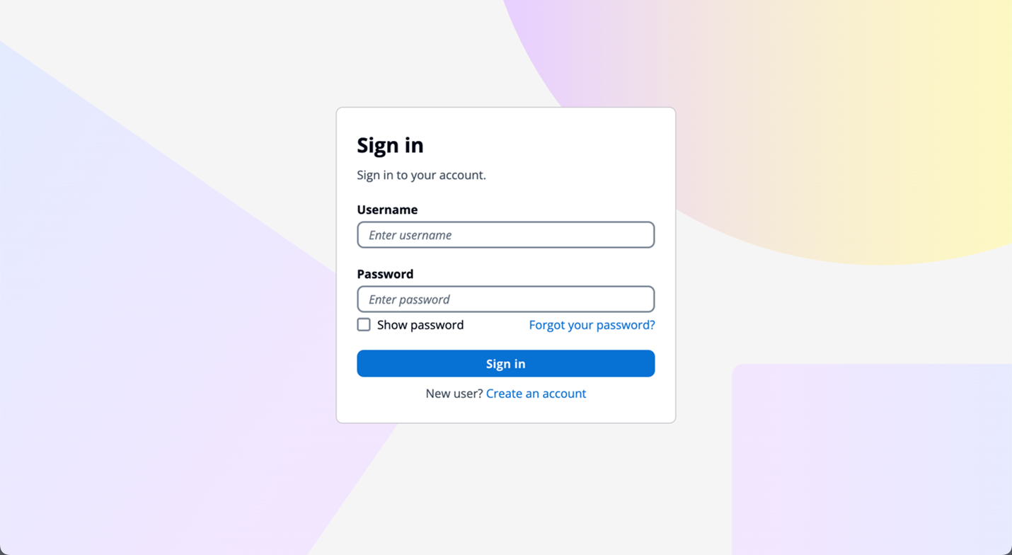
Managed login branding provides an improved user experience with the most up-to-date authentication options for the user pool UI experience. Figure 1 shows managed login using the default branding settings.

Figure 1: Managed login default branding settings

Figure 1: Managed login default branding settings

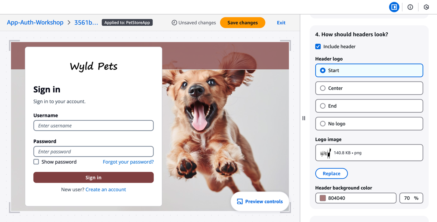
The branding editor is a no-code visual editor that you can use to customize the look and feel of the entire user journey. You can customize each user pool application client individually, and preview screens in real-time with different screen sizes, as shown in Figure 2.

Figure 2: Customization in the Amazon Cognito branding editor (Image credits)

Figure 2: Customization in the Amazon Cognito branding editor (Image credits)

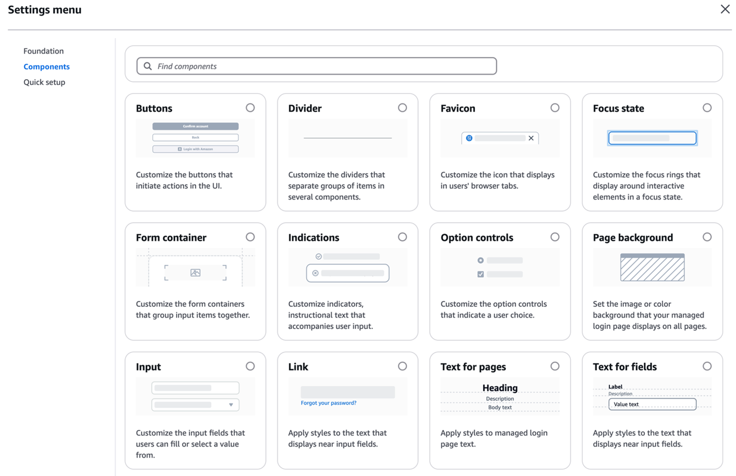
As shown in Figure 3, You can customize various components using the branding editor, including background, header and footer, buttons, focus state, icons, and more.

Figure 3: Various components customization options

Figure 3: Various components customization options

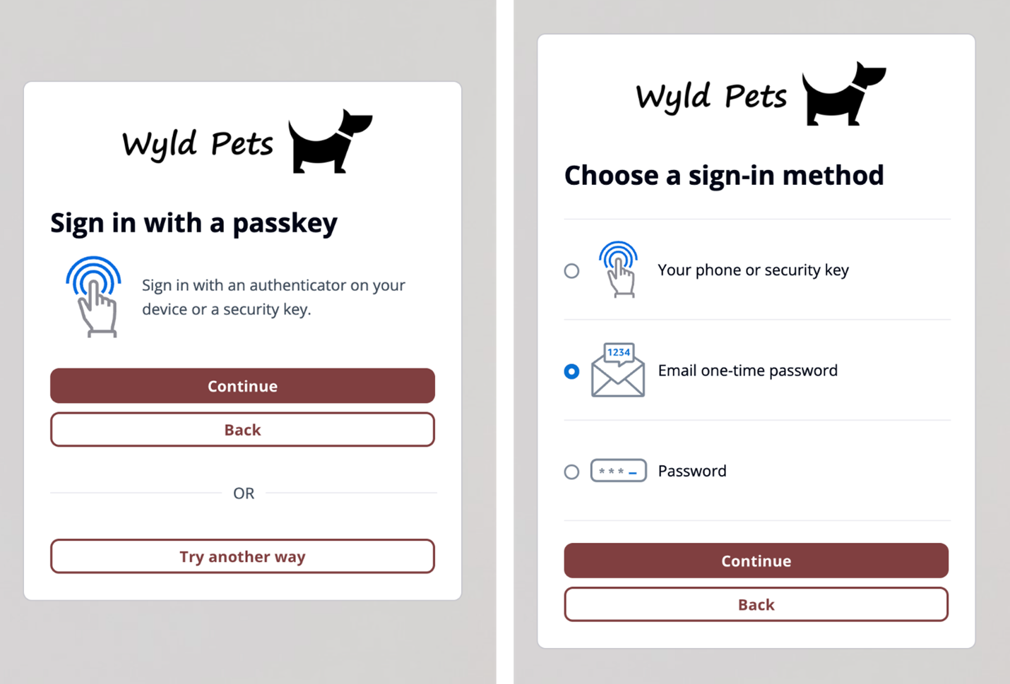
Additionally, managed login branding adds support for passwordless sign-in with passkeys, email one-time-passwords (OTP) and SMS OTPs, as shown in Figure 4. After you enable passwordless login in your user pool, managed login branding adapts to curated user flows with users’ preferred authentication methods.

Figure 4: Sign in with passkey flow (left) and user-selected sign-in method flow (right)

Figure 4: Sign in with passkey flow (left) and user-selected sign-in method flow (right)

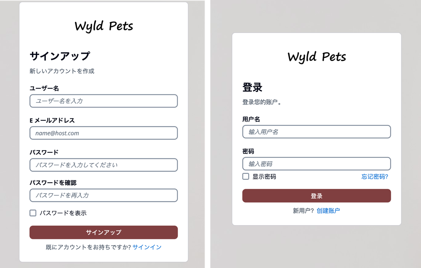
Managed login branding also offers localization options in several languages (two are shown in Figure 5). You can add a lang query parameter in the link you distribute to users, and Amazon Cognito will set a cookie in users’ browsers with their language preference after the initial request.

Figure 5: Cognito user sign up page in Japanese (left) and user sign in page in Simplified Chinese (right)

Figure 5: Cognito user sign up page in Japanese (left) and user sign in page in Simplified Chinese (right)

Hosted UI (classic) branding
For customers who prefer a traditional approach, Amazon Cognito continues to support the Hosted UI (classic) branding (shown in Figure 6) with basic customization where you can upload a CSS file to design the UI styling and upload a brand-specific logo. Hosted UI (classic) supports standard authentication flows with MFA and self-service sign up.

Figure 6: Hosted UI (classic) branding

Figure 6: Hosted UI (classic) branding

The managed login branding with branding editor is available to Amazon Cognito user pools with Essentials and Plus feature tiers, and Hosted UI (classic) branding is available to most Cognito user pools including Lite tier. To learn more about Cognito feature tiers, visit Amazon Cognito pricing.

Security and compliance capabilities

Both managed login branding and Hosted UI (classic) branding are designed to help you meet your compliance and security requirements and your users’ needs. Managed login supports custom OAuth scopes and OAuth 2.0 flows. If you want single sign-on (SSO), you can use managed login to support a single login across many application clients, with browser session cookies for the same domain. Actions are logged in AWS CloudTrail, and you can use the logs for audit and reactionary automation. The managed login experience also supports the full suite of threat protection features for Amazon Cognito. For additional protection, managed login has support for AWS WAF web ACLs and for AWS WAF CAPTCHA, which can help protect your Cognito user pools from web-based exploits and unwanted bots.

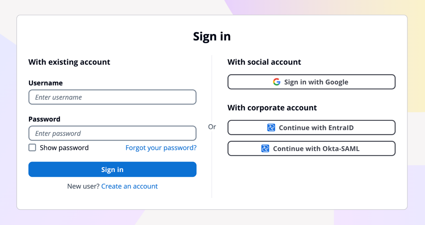
Figure 7: Example default managed login with several login providers enabled

Figure 7: Example default managed login with several login providers enabled

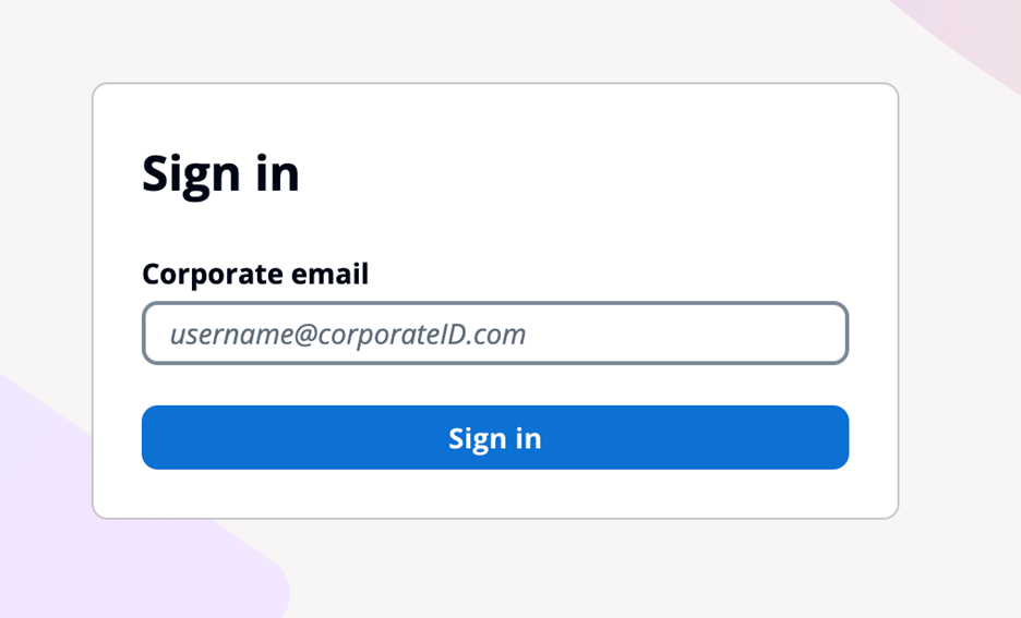
For federation, managed login supports federation with third-party IdPs that support OIDC and SAML 2.0, as well as social IdPs, as shown in Figure 7. Identity providers are connected to your Amazon Cognito user pool. In managed login, users use a button to select the federation source, and redirection is automatic. With SAML and OIDC IdPs, you can also configure mapping by using the domain in the user’s email address. In this case, a single text field is visible to your application users to enter an email address, as shown in Figure 8, and the lookup and redirect to the appropriate SAML IdP is automatic, as described in Choosing SAML identity provider names.

Figure 8: Managed login that links to corporate IdP through an email domain

Figure 8: Managed login that links to corporate IdP through an email domain

Managed login integrates with Application Load Balancer (ALB) for web applications and works with AWS Amplify to enable social identity provider and enterprise federation (SAML and OIDC) capabilities. Beyond these integrations, Amazon Cognito user pools integrate with various AWS services (such as AWS AppSync), that require user authentication and authorization, and Amazon API Gateway through Cognito authorizers to secure your REST and HTTP endpoints.

You might choose to use managed login for many reasons. AWS fully manages the hosting, maintenance, and scaling of the managed login, which can contribute to the speed of go-to-market for customers. If your app requires OAuth 2.0 custom scopes, federation, social login, or native users with basic but customized branding and potentially numerous Amazon Cognito user pools, you might benefit from using managed login.

For more information about how to configure and use the hosted UI, see Using the Amazon Cognito hosted UI for sign-up and sign-in.

Create a custom UI

Creating a custom UI using the SDK for Amazon Cognito provides a host of benefits and features that can help you completely customize the UI for your application users. With a custom UI, you have complete control over the look and feel of the UI that your application users will land on, including designing your app to support multiple languages, and you can build and design custom authentication flows.

There are numerous features that are supported when you build a custom UI. As with the managed login, the APIs invoked from a custom UI using the SDK will create log entries in CloudTrail, and you can use the logs for audit and automation. You can also create a custom authentication flow for your users with a fully custom authentication experience beyond the those available in managed login.

In a custom UI, you can build custom session management and integrate with AWS WAF. A custom UI also works with the threat protection features of Amazon Cognito.

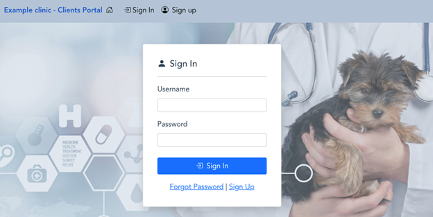
Figure 9: Example of a custom user interface

Figure 9: Example of a custom user interface

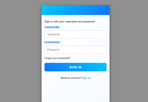
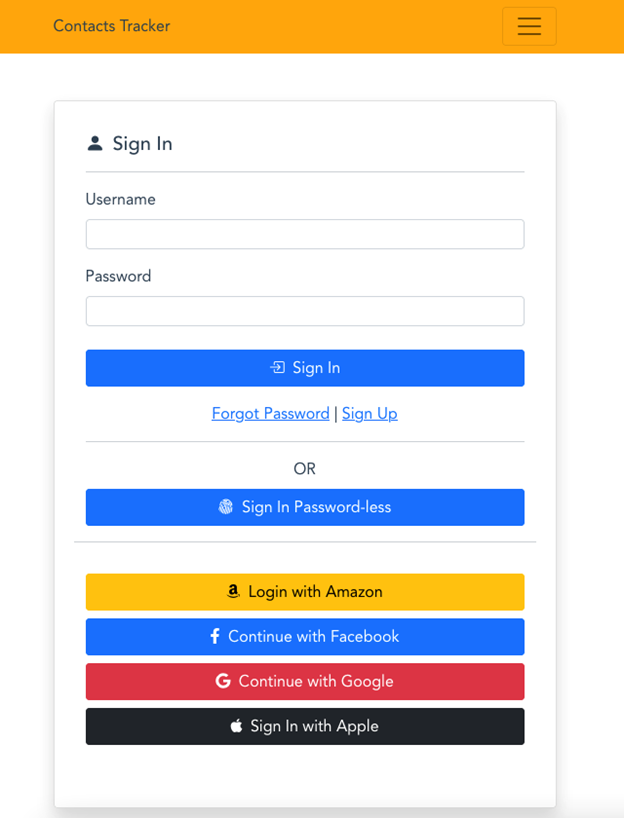
With a custom UI, such as the one shown in Figure 10, you can orchestrate a suite of sign-in options and sign-in flows for your users. For example, you can collect a user or tenant identifier at the beginning of the authentication flow and apply your own logic for user authentication flow, such as redirecting federated users to external IdPs, displaying a password prompt for local users, or directing users to create a new account if they don’t exist. You can also build flows to let a user choose alternative MFA methods if their preferred choices aren’t available.

Figure 10: Custom UI example

Figure 10: Custom UI example

When you build a custom UI, there is support for custom endpoints and proxies so that you have a wider range of options for management and consistency across application development as it relates to authentication. Custom authentication flows are only available in applications with a custom UI, which gives you the ability to make customized challenge prompts and answers to help you meet custom security requirements by using AWS Lambda triggers. For example, you could use it to implement OAuth 2.0 device grant flows. Lastly, a custom UI supports a remember device feature where you can add low-effort sign-in from trusted devices.

You might choose to build a custom UI with an SDK when full customization is a requirement or where you want to incorporate customized authentication flows using the custom authentication challenge Lambda triggers. A custom UI is a great choice if you aren’t required to use OAuth 2.0 flows and you have the resources to develop and implement a unique UI for your application users.

For more information about how to configure and use a custom UI, see Using the Amazon Cognito managed login for sign-up and sign-in. You can also visit the documentation on Building custom UIs with Amplify.

Decision criteria matrix

When deciding between Amazon Cognito managed login branding options and a custom UI, there are some unique differences that can help you determine which UI is best for your application needs. Managed login offers a modern, customizable authentication experience with advanced features like no-code visual customization, dark mode themes, and support for passwordless options. It supports OAuth 2.0 flows, custom OAuth scopes, the ability to sign in one time and access many Cognito application clients (using SSO), and full use of the Cognito threat protection features. For applications requiring complete control over the authentication experience and UX—including custom authentication flows, device fingerprinting, and reduced token expiration—a custom UI is the better choice. This option allows for full UI customization, implementation of custom authentication flows, and integration with specific frameworks or libraries not supported by managed login.

When making your decision, consider factors such as the level of customization required, specific authentication features needed, development resources available, integration requirements with other AWS services, security and compliance needs, and user experience priorities. Remember that your application authentication requirements and customer experience should take precedence over other considerations. You can use the following table to help select the best UI for your requirements.

Requirements

Managed login

Hosted UI (classic)

Custom UI (SDK)

OAuth 2.0 flows

Supported

Supported

Not available

Custom OAuth scopes

Supported

Supported

Supported

Customization of UI

No-code branding designer

Limited CSS customization

Full custom control

Custom user input forms

Not available

Not available

Supported

Custom authentication flow

Not available

Not available

Supported

Passwordless authentication flow

Supported

Not available

Custom implementation available

Localization with multiple languages

Supported

Not available

Supported

Login once across many app clients

Supported

Supported

Not available

Session expiration configurable under 1 hour

Not available

Not available

Supported

Trusted-device authentication

Not available

Not available

Supported

AWS WAF integration

Supported

Supported

Supported

Support for AWS WAF CAPTCHA

Supported

Supported

Not available

Ability to use a custom endpoint or proxy

Not available

Not available

Supported

AWS Application Load Balancer integration

Supported

Supported

Not available

Figure 11: Decision criteria matrix

Conclusion

In this post, you learned about using managed login, including its two branding options and creating a custom UI in Amazon Cognito and the many supported features and benefits of each. Each UI option targets a specific need. Choose from available options based on your list of requirements for authentication and the user sign-up and sign-in experience. You can use the information in this post as a reference as you add Amazon Cognito to your mobile and web applications for authentication.

Have a question? Contact us for general support services.

Author photo

Joshua Du Lac

Josh is a Senior Manager of Security Solutions Architects at AWS. He has advised hundreds of enterprise, global, and financial services customers to accelerate their journey to the cloud while improving their security along the way. Outside of work, Josh enjoys searching for the best tacos in Texas and practicing his handstands.

Jeremy Wave

Jeremy Ware

Jeremy is a Security Specialist Solutions Architect focused on Identity and Access Management. Jeremy and his team enable AWS customers to implement sophisticated, scalable, and secure IAM architecture and Authentication workflows to solve business challenges. With a background in Security Engineering, Jeremy has spent many years working to raise the Security Maturity gap at numerous global enterprises. Outside of work, Jeremy loves to explore the mountainous outdoors, and participate in sports such as snowboarding, wakeboarding, and dirt bike riding.

Edward Sun

Edward Sun

Edward is a Security Specialist Solutions Architect focused on identity and access management. He loves helping customers throughout their cloud transformation journey with architecture design, security best practices, migration, and cost optimizations. Outside of work, Edward enjoys hiking, golfing, and cheering for his alma mater, the Georgia Bulldogs.

Kiran Dongara

Kiran Dongara

Kiran Dongara is a Solutions Architect at Amazon Web Services (AWS) in the Worldwide Public Sector, primarily supporting US state and local government (SLG) customers and partners. His expertise lies in designing scalable and efficient architectures that adhere to well-architected framework practices, maximizing value and return on investment for his customers. When not working, Kiran prioritizes family time, nature walks, and cycling.

Choosing an open table format for your transactional data lake on AWS

Post Syndicated from Shana Schipers original https://aws.amazon.com/blogs/big-data/choosing-an-open-table-format-for-your-transactional-data-lake-on-aws/

A modern data architecture enables companies to ingest virtually any type of data through automated pipelines into a data lake, which provides highly durable and cost-effective object storage at petabyte or exabyte scale. This data is then projected into analytics services such as data warehouses, search systems, stream processors, query editors, notebooks, and machine learning (ML) models through direct access, real-time, and batch workflows. Data in customers’ data lakes is used to fulfil a multitude of use cases, from real-time fraud detection for financial services companies, inventory and real-time marketing campaigns for retailers, or flight and hotel room availability for the hospitality industry. Across all use cases, permissions, data governance, and data protection are table stakes, and customers require a high level of control over data security, encryption, and lifecycle management.

This post shows how open-source transactional table formats (or open table formats) can help you solve advanced use cases around performance, cost, governance, and privacy in your data lakes. We also provide insights into the features and capabilities of the most common open table formats available to support various use cases.

You can use this post for guidance when looking to select an open table format for your data lake workloads, facilitating the decision-making process and potentially narrowing down the available options. The content of this post is based on the latest open-source releases of the reviewed formats at the time of writing: Apache Hudi v0.13.0, Apache Iceberg 1.2.0, and Delta Lake 2.3.0.

Advanced use cases in modern data lakes

Data lakes offer one of the best options for cost, scalability, and flexibility to store data, allowing you to retain large volumes of structured and unstructured data at a low cost, and to use this data for different types of analytics workloads—from business intelligence reporting to big data processing, real-time analytics, and ML—to help guide better decisions.

Despite these capabilities, data lakes are not databases, and object storage does not provide support for ACID processing semantics, which you may require to effectively optimize and manage your data at scale across hundreds or thousands of users using a multitude of different technologies. For example:

  • Performing efficient record-level updates and deletes as data changes in your business
  • Managing query performance as tables grow to millions of files and hundreds of thousands of partitions
  • Ensuring data consistency across multiple concurrent writers and readers
  • Preventing data corruption from write operations failing partway through
  • Evolving table schemas over time without (partially) rewriting datasets

These challenges have become particularly prevalent in use cases such as CDC (change data capture) from relational database sources, privacy regulations requiring deletion of data, and streaming data ingestion, which can result in many small files. Typical data lake file formats such as CSV, JSON, Parquet, or Orc only allow for writes of entire files, making the aforementioned requirements hard to implement, time consuming, and costly.

To help overcome these challenges, open table formats provide additional database-like functionality that simplifies the optimization and management overhead of data lakes, while still supporting storage on cost-effective systems like Amazon Simple Storage Service (Amazon S3). These features include:

  • ACID transactions – Allowing a write to completely succeed or be rolled back in its entirety
  • Record-level operations – Allowing for single rows to be inserted, updated, or deleted
  • Indexes – Improving performance in addition to data lake techniques like partitioning
  • Concurrency control – Allowing for multiple processes to read and write the same data at the same time
  • Schema evolution – Allowing for columns of a table to be added or modified over the life of a table
  • Time travel – Enabling you to query data as of a point in time in the past

In general, open table formats implement these features by storing multiple versions of a single record across many underlying files, and use a tracking and indexing mechanism that allows an analytics engine to see or modify the correct version of the records they are accessing. When records are updated or deleted, the changed information is stored in new files, and the files for a given record are retrieved during an operation, which is then reconciled by the open table format software. This is a powerful architecture that is used in many transactional systems, but in data lakes, this can have some side effects that have to be addressed to help you align with performance and compliance requirements. For instance, when data is deleted from an open table format, in some cases only a delete marker is stored, with the original data retained until a compaction or vacuum operation is performed, which performs a hard deletion. For updates, previous versions of the old values of a record may be retained until a similar process is run. This can mean that data that should be deleted isn’t, or that you store a significantly larger number of files than you intend to, increasing storage cost and slowing down read performance. Regular compaction and vacuuming must be run, either as part of the way the open table format works, or separately as a maintenance procedure.

The three most common and prevalent open table formats are Apache Hudi, Apache Iceberg, and Delta Lake. AWS supports all three of these open table formats, and in this post, we review the features and capabilities of each, how they can be used to implement the most common transactional data lake use cases, and which features and capabilities are available in AWS’s analytics services. Innovation around these table formats is happening at an extremely rapid pace, and there are likely preview or beta features available in these file formats that aren’t covered here. All due care has been taken to provide the correct information as of time of writing, but we also expect this information to change quickly, and we’ll update this post frequently to contain the most accurate information. Also, this post focuses only on the open-source versions of the covered table formats, and doesn’t speak to extensions or proprietary features available from individual third-party vendors.

How to use this post

We encourage you to use the high-level guidance in this post with the mapping of functional fit and supported integrations for your use cases. Combine both aspects to identify what table format is likely a good fit for a specific use case, and then prioritize your proof of concept efforts accordingly. Most organizations have a variety of workloads that can benefit from an open table format, but today no single table format is a “one size fits all.” You may wish to select a specific open table format on a case-by-case basis to get the best performance and features for your requirements, or you may wish to standardize on a single format and understand the trade-offs that you may encounter as your use cases evolve.

This post doesn’t promote a single table format for any given use case. The functional evaluations are only intended to help speed up your decision-making process by highlighting key features and attention points for each table format with each use case. It is crucial that you perform testing to ensure that a table format meets your specific use case requirements.

This post is not intended to provide detailed technical guidance (e.g. best practices) or benchmarking of each of the specific file formats, which are available in AWS Technical Guides and benchmarks from the open-source community respectively.

Choosing an open table format

When choosing an open table format for your data lake, we believe that there are two critical aspects that should be evaluated:

  • Functional fit – Does the table format offer the features required to efficiently implement your use case with the required performance? Although they all offer common features, each table format has a different underlying technical design and may support unique features. Each format can handle a range of use cases, but they also offer specific advantages or trade-offs, and may be more efficient in certain scenarios as a result of its design.
  • Supported integrations – Does­ the table format integrate seamlessly with your data environment? When evaluating a table format, it’s important to consider supported engine integrations on dimensions such as support for reads/writes, data catalog integration, supported access control tools, and so on that you have in your organization. This applies to both integration with AWS services and with third-party tools.

General features and considerations

The following table summarizes general features and considerations for each file format that you may want to take into account, regardless of your use case. In addition to this, it is also important to take into account other aspects such as the complexity of the table format and in-house skills.

. Apache Hudi Apache Iceberg Delta Lake
Primary API
  • Spark DataFrame
  • SQL
  • Spark DataFrame
Write modes
  • Copy On Write approach only
Supported data file formats
  • Parquet
  • ORC
  • HFile
  • Parquet
  • ORC
  • Avro
  • Parquet
File layout management
  • Compaction to reorganize data (sort) and merge small files together
Query optimization
S3 optimizations
  • Metadata reduces file listing operations
Table maintenance
  • Automatic within writer
  • Separate processes
  • Separate processes
  • Separate processes
Time travel
Schema evolution
Operations
  • Hudi CLI for table management, troubleshooting, and table inspection
  • No out-of-the-box options
Monitoring
  • No out-of-the-box options that are integrated with AWS services
  • No out-of-the-box options that are integrated with AWS services
Data Encryption
  • Server-side encryption on Amazon S3 supported
  • Server-side encryption on Amazon S3 supported
Configuration Options
  • High configurability:

Extensive configuration options for customizing read/write behavior (such as index type or merge logic) and automatically performed maintenance and optimizations (such as file sizing, compaction, and cleaning)

  • Medium configurability:

Configuration options for basic read/write behavior (Merge On Read or Copy On Write operation modes)

  • Low configurability:

Limited configuration options for table properties (for example, indexed columns)

Other
  • Savepoints allow you to restore tables to a previous version without having to retain the entire history of files
  • Iceberg supports S3 Access Points in Spark, allowing you to implement failover across AWS Regions using a combination of S3 access points, S3 cross-Region replication, and the Iceberg Register Table API
  • Shallow clones allow you to efficiently run tests or experiments on Delta tables in production, without creating copies of the dataset or affecting the original table.
AWS Analytics Services Support*
Amazon EMR Read and write Read and write Read and write
AWS Glue Read and write Read and write Read and write
Amazon Athena (SQL) Read Read and write Read
Amazon Redshift (Spectrum) Read Currently not supported Read†
AWS Glue Data Catalog‡ Yes Yes Yes

* For table format support in third-party tools, consult the official documentation for the respective tool.
† Amazon Redshift only supports Delta Symlink tables (see Creating external tables for data managed in Delta Lake for more information).
‡ Refer to Working with other AWS services in the Lake Formation documentation for an overview of table format support when using Lake Formation with other AWS services.

Functional fit for common use cases

Now let’s dive deep into specific use cases to understand the capabilities of each open table format.

Getting data into your data lake

In this section, we discuss the capabilities of each open table format for streaming ingestion, batch load and change data capture (CDC) use cases.

Streaming ingestion

Streaming ingestion allows you to write changes from a queue, topic, or stream into your data lake. Although your specific requirements may vary based on the type of use case, streaming data ingestion typically requires the following features:

  • Low-latency writes – Supporting record-level inserts, updates, and deletes, for example to support late-arriving data
  • File size management – Enabling you to create files that are sized for optimal read performance (rather than creating one or more files per streaming batch, which can result in millions of tiny files)
  • Support for concurrent readers and writers – Including schema changes and table maintenance
  • Automatic table management services – Enabling you to maintain consistent read performance

In this section, we talk about streaming ingestion where records are just inserted into files, and you aren’t trying to update or delete previous records based on changes. A typical example of this is time series data (for example sensor readings), where each event is added as a new record to the dataset. The following table summarizes the features.

. Apache Hudi Apache Iceberg Delta Lake
Functional fit
Considerations Hudi’s default configurations are tailored for upserts, and need to be tuned for append-only streaming workloads. For example, Hudi’s automatic file sizing in the writer minimizes operational effort/complexity required to maintain read performance over time, but can add a performance overhead at write time. If write speed is of critical importance, it can be beneficial to turn off Hudi’s file sizing, write new data files for each batch (or micro-batch), then run clustering later to create better sized files for read performance (using a similar approach as Iceberg or Delta).
  • Iceberg doesn’t optimize file sizes or run automatic table services (for example, compaction or clustering) when writing, so streaming ingestion will create many small data and metadata files. Frequent table maintenance needs to be performed to prevent read performance from degrading over time.
  • Delta doesn’t optimize file sizes or run automatic table services (for example, compaction or clustering) when writing, so streaming ingestion will create many small data and metadata files. Frequent table maintenance needs to be performed to prevent read performance from degrading over time.
Supported AWS integrations
  • Amazon EMR (Spark Structured Streaming (streaming sink and forEachBatch), Flink, Hudi DeltaStreamer)
  • AWS Glue (Spark Structured Streaming (streaming sink and forEachBatch), Hudi DeltaStreamer)
  • Amazon Kinesis Data Analytics
  • Amazon Managed Streaming for Apache Kafka (MSK Connect)
  • Amazon EMR (Spark Structured Streaming (only forEachBatch), Flink)
  • AWS Glue (Spark Structured Streaming (only forEachBatch))
  • Amazon Kinesis Data Analytics
Conclusion Good functional fit for all append-only streaming when configuration tuning for append-only workloads is acceptable. Good fit for append-only streaming with larger micro-batch windows, and when operational overhead of table management is acceptable. Good fit for append-only streaming with larger micro-batch windows, and when operational overhead of table management is acceptable.

When streaming data with updates and deletes into a data lake, a key priority is to have fast upserts and deletes by being able to efficiently identify impacted files to be updated.

. Apache Hudi Apache Iceberg Delta Lake
Functional fit
  • Iceberg offers a Merge On Read strategy to enable fast writes.
  • Streaming upserts into Iceberg tables are natively supported with Flink, and Spark can implement streaming ingestion with updates and deletes using a micro-batch approach with MERGE INTO.
  • Using column statistics, Iceberg offers efficient updates on tables that are sorted on a “key” column.
  • Streaming ingestion with updates and deletes into OSS Delta Lake tables can be implemented using a micro-batch approach with MERGE INTO.
  • Using data skipping with column statistics, Delta offers efficient updates on tables that are sorted on a “key” column.
Considerations
  • Hudi’s automatic optimizations in the writer (for example, file sizing) add performance overhead at write time.
  • Reading from Merge On Read tables is generally slower than Copy On Write tables due to log files. Frequent compaction can be used to optimize read performance.
  • Iceberg uses a MERGE INTO approach (a join) for upserting data. This is more resource intensive and less performant for streaming data ingestion with frequent commits on (large unsorted) tables, because full table or partition scans would be performed on unsorted tables.
  • Iceberg does not optimize file sizes or run automatic table services (for example, compaction) when writing, so streaming ingestion will create many small data and metadata files. Frequent table maintenance needs to be performed to prevent read performance from degrading over time.
  • Reading from tables using the Merge On Read approach is generally slower than tables using only the Copy On Write approach due to delete files. Frequent compaction can be used to optimize read performance.
  • Iceberg Merge On Read currently does not support dynamic file pruning using its column statistics during merges and updates. This has impact on write performance, resulting in full table joins.
  • Delta uses a Copy On Write strategy that is not optimized for fast (streaming) writes, as it rewrites entire files for record updates.
  • Delta uses a MERGE INTO approach (a join). This is more resource intensive (less performant) and not suited for streaming data ingestion with frequent commits on large unsorted tables, because full table or partition scans would be performed on unsorted tables.
  • No auto file sizing is performed; separate table management processes are required (which can impact writes).
Supported AWS integrations
  • Amazon EMR (Spark Structured Streaming (streaming sink and forEachBatch), Flink, Hudi DeltaStreamer)
  • AWS Glue (Spark Structured Streaming (streaming sink and forEachBatch), Hudi DeltaStreamer)
  • Amazon Kinesis Data Analytics
  • Amazon Managed Streaming for Apache Kafka (MSK Connect)
  • Amazon EMR (Spark Structured Streaming (only forEachBatch), Flink)
  • Amazon Kinesis Data Analytics
  • Amazon EMR (Spark Structured Streaming (only forEachBatch))
  • AWS Glue (Spark Structured Streaming (only forEachBatch))
  • Amazon Kinesis Data Analytics
Conclusion Good fit for lower-latency streaming with updates and deletes thanks to native support for streaming upserts, indexes for upserts, and automatic file sizing and compaction. Good fit for streaming with larger micro-batch windows and when the operational overhead of table management is acceptable. Can be used for streaming data ingestion with updates/deletes if latency is not a concern, because a Copy-On-Write strategy may not deliver the write performance required by low latency streaming use cases.

Change data capture

Change data capture (CDC) refers to the process of identifying and capturing changes made to data in a database and then delivering those changes in real time to a downstream process or system—in this case, delivering CDC data from databases into Amazon S3.

In addition to the aforementioned general streaming requirements, the following are key requirements for efficient CDC processing:

  • Efficient record-level updates and deletes – With the ability to efficiently identify files to be modified (which is important to support late-arriving data).
  • Native support for CDC – With the following options:
  • CDC record support in the table format – The table format understands how to process CDC-generated records and no custom preprocessing is required for writing CDC records to the table.
  • CDC tools natively supporting the table format – CDC tools understand how to process CDC-generated records and apply them to the target tables. In this case, the CDC engine writes to the target table without another engine in between.

Without support for the two CDC options, processing and applying CDC records correctly into a target table will require custom code. With a CDC engine, each tool likely has its own CDC record format (or payload). For example, Debezium and AWS Database Migration Service (AWS DMS) each have their own specific record formats, and need to be transformed differently. This must be considered when you are operating CDC at scale across many tables.

All three table formats allow you to implement CDC from a source database into a target table. The difference for CDC with each format lies mainly in the ease of implementing CDC pipelines and supported integrations.

. Apache Hudi Apache Iceberg Delta Lake
Functional fit
  • Hudi’s DeltaStreamer utility provides a no-code/low-code option to efficiently ingest CDC records from different sources into Hudi tables.
  • Upserts using indexes allow you to quickly identify the target files for updates, without having to perform a full table join.
  • Unique record keys and deduplication natively enforce source databases’ primary keys and prevent duplicates in the data lake.
  • Out of order records are handled via the pre-combine feature.
  • Native support (through record payload formats) is offered for CDC formats like AWS DMS and Debezium, eliminating the need to write custom CDC preprocessing logic in the writer application to correctly interpret and apply CDC records to the target table. Writing CDC records to Hudi tables is as simple as writing any other records to a Hudi table.
  • Partial updates are supported, so the CDC payload format does not need to include all record columns.
  • Flink CDC is the most convenient way to set up CDC from downstream data sources into Iceberg tables. It supports upsert mode and can interpret CDC formats such as Debezium natively.
  • Using column statistics, Iceberg offers efficient updates on tables that are sorted on a “key” column.
  • CDC into Delta tables can be implemented using third-party tools or using Spark with custom processing logic.
  • Using data skipping with column statistics, Delta offers efficient updates on tables that are sorted on a “key” column.
Considerations
  • Natively supported payload formats can be found in the Hudi code repo. For other formats, consider creating a custom payload or adding custom logic to the writer application to correctly process and apply CDC records of that format to target Hudi tables.
  • Iceberg uses a MERGE INTO approach (a join) for upserting data. This is more resource intensive and less performant, particularly on large unsorted tables where a MERGE INTO operation could require a full table scan.
  • Regular compaction should be implemented to maintain sort order over time in order to prevent MERGE INTO performance degrading.
  • Iceberg has no native support for CDC payload formats (for example, AWS DMS or Debezium). When using other engines than Flink CDC (such as Spark), custom logic needs to be added to the writer application in order to correctly process and apply CDC records to target Iceberg tables (for example, deduplication or ordering based on operation).
  • Deduplication to enforce primary key constraints needs to be handled in the Iceberg writer application.
  • No support for out of order records handling.
  • Delta does not use indexes for upserts, but uses a MERGE INTO approach instead (a join). This is more resource intensive and less performant on large unsorted tables because those would require full table or partition scans.
  • Regular clustering should be implemented to maintain sort order over time in order to prevent MERGE INTO performance degrading.
  • Delta Lake has no native support for CDC payload formats (for example, AWS DMS or Debezium). When using Spark for ingestion, custom logic needs to be added to the writer application in order to correctly process and apply CDC records to target Delta tables (for example, deduplication or ordering based on operation).
  • Record updates on unsorted Delta tables results in full table or partition scans
  • No support for out of order records handling.
Natively supported CDC formats
  • AWS DMS
  • Debezium
  • None
  • None
CDC tool integrations
  • DeltaStreamer
  • Flink CDC
  • Debezium
  • Flink CDC
  • Debezium
  • Debezium
Conclusion All three formats can implement CDC workloads. Apache Hudi offers the best overall technical fit for CDC workloads as well as the most options for efficient CDC pipeline design: no-code/low-code with DeltaStreamer, third-party CDC tools offering native Hudi integration, or a Spark/Flink engine using CDC record payloads offered in Hudi.

Batch loads

If your use case requires only periodic writes but frequent reads, you may want to use batch loads and optimize for read performance.

Batch loading data with updates and deletes is perhaps the simplest use case to implement with any of the three table formats. Batch loads typically don’t require low latency, allowing them to benefit from the operational simplicity of a Copy On Write strategy. With Copy On Write, data files are rewritten to apply updates and add new records, minimizing the complexity of having to run compaction or optimization table services on the table.

. Apache Hudi Apache Iceberg Delta Lake
Functional fit
  • Copy On Write is supported.
  • Automatic file sizing while writing is supported, including optimizing previously written small files by adding new records to them.
  • Multiple index types are provided to optimize update performance for different workload patterns.
  • Copy On Write is supported.
  • File size management is performed within each incoming data batch (but it is not possible to optimize previously written data files by adding new records to them).
  • Copy On Write is supported.
  • File size can be indirectly managed within each data batch by setting the max number of records per file (but it is not possible to optimize previously written data files by adding new records to them).
Considerations
  • Configuring Hudi according to your workload pattern is imperative for good performance (see Apache Hudi on AWS for guidance).
  • Data deduplication needs to be handled in the writer application.
  • If a single data batch does not contain sufficient data to reach a target file size, compaction can be performed to merge smaller files together afterwards.
  • Ensuring data is sorted on a “key” column is imperative for good update performance. Regular sorting compaction should be considered to maintain sorted data over time.
  • Data deduplication needs to be handled in the writer application.
  • If a single data batch does not contain sufficient data to reach a target file size, compaction can be performed to merge smaller files together afterwards.
  • Ensuring data is sorted on a “key” column is imperative for good update performance. Regular clustering should be considered to maintain sorted data over time.
Supported AWS integrations
  • Amazon EMR (Spark)
  • AWS Glue (Spark)
  • Amazon EMR (Spark, Presto, Trino, Hive)
  • AWS Glue (Spark)
  • Amazon Athena (SQL)
  • Amazon EMR (Spark, Trino)
  • AWS Glue (Spark)
Conclusion All three formats are well suited for batch loads. Apache Hudi supports the most configuration options and may increase the effort to get started, but provides lower operational effort due to automatic table management. On the other hand, Iceberg and Delta are simpler to get started with, but require some operational overhead for table maintenance.

Working with open table formats

In this section, we discuss the capabilities of each open table format for common use cases when working with open table formats: optimizing read performance, incremental data processing and processing deletes to comply with privacy regulations.

Optimizing read performance

The preceding sections primarily focused on write performance for specific use cases. Now let’s explore how each open table format can support optimal read performance. Although there are some cases where data is optimized purely for writes, read performance is typically a very important dimension on which you should evaluate an open table format.

Open table format features that improve query performance include the following:

  • Indexes, (column) statistics, and other metadata – Improves query planning and file pruning, resulting in reduced data scanned
  • File layout optimization – Enables query performance:
  • File size management – Properly sized files provide better query performance
  • Data colocation (through clustering) according to query patterns – Reduces the amount of data scanned by queries
. Apache Hudi Apache Iceberg Delta Lake
Functional fit
  • Auto file sizing when writing results in good file sizes for read performance. On Merge On Read tables, automatic compaction and clustering improves read performance.
  • Metadata tables eliminate slow S3 file listing operations. Column statistics in the metadata table can be used for better file pruning in query planning (data skipping feature).
  • Clustering data for better data colocation with hierarchical sorting or z-ordering.
  • Hidden partitioning prevents unintentional full table scans by users, without requiring them to specify partition columns explicitly.
  • Column and partition statistics in manifest files speed up query planning and file pruning, and eliminate S3 file listing operations.
  • Optimized file layout for S3 object storage using random prefixes is supported, which minimizes chances of S3 throttling.
  • Clustering data for better data colocation with hierarchical sorting or z-ordering.
  • File size can be indirectly managed within each data batch by setting the max number of records per file (but not optimizing previously written data files by adding new records to existing files).
  • Generated columns avoid full table scans.
  • Data skipping is automatically used in Spark.
  • Clustering data for better data colocation using z-ordering.
Considerations
  • Data skipping using metadata column stats has to be supported in the query engine (currently only in Apache Spark).
  • Snapshot queries on Merge On Read tables have higher query latencies than on Copy On Write tables. This latency impact can be reduced by increasing the compaction frequency.
  • Separate table maintenance needs to be performed to maintain read performance over time.
  • Reading from tables using a Merge On Read approach is generally slower than tables using only a Copy On Write approach due to delete files. Frequent compaction can be used to optimize read performance.
  • Currently, only Apache Spark can use data skipping.
  • Separate table maintenance needs to be performed to maintain read performance over time.
Optimization & Maintenance Processes
  • Compaction of log files in Merge On Read tables can be run as part of the writing application or as a separate job using Spark on Amazon EMR or AWS Glue. Compaction does not interfere with other jobs or queries.
  • Clustering runs as part of the writing application or in a separate job using Spark on Amazon EMR or AWS Glue because clustering can interfere with other transactions.
  • See Apache Hudi on AWS for guidance.
  • Compaction API in Delta Lake can group small files or cluster data, and it can interfere with other transactions.
  • This process has to be scheduled separately by the user on a time or event basis.
  • Spark can be used to perform compaction in services like Amazon EMR or AWS Glue.
Conclusion For achieving good read performance, it’s important that your query engine supports the optimization features offered by the table formats. When using Spark, all three formats provide good read performance when properly configured. When using Trino (and therefore Athena as well), Iceberg will likely provide better query performance because the data skipping feature of Hudi and Delta is not supported in the Trino engine. Make sure to evaluate this feature support for your query engine of choice.

Incremental processing of data on the data lake

At a high level, incremental data processing is the movement of new or fresh data from a source to a destination. To implement incremental extract, transform, and load (ETL) workloads efficiently, we need to be able to retrieve only the data records that have been changed or added since a certain point in time (incrementally) so we don’t need to reprocess unnecessary data (such as entire partitions). When your data source is an open table format table, we can take advantage of incremental queries to facilitate more efficient reads in these table formats.

. Apache Hudi Apache Iceberg Delta Lake
Functional fit
  • Full incremental pipelines can be built using Hudi’s incremental queries, which capture record-level changes on a Hudi table (including updates and deletes) without the need to store and manage change data records.
  • Hudi’s DeltaStreamer utility offers simple no-code/low-code options to build incremental Hudi pipelines.
  • Iceberg incremental queries can only read new records (no updates) from upstream Iceberg tables and replicate to downstream tables.
  • Incremental pipelines with record-level changes (including updates and deletes) can be implemented using the changelog view procedure.
  • Full incremental pipelines can be built using Delta’s Change Data Feed (CDF) feature, which captures record-level changes (including updates and deletes) using change data records.
Considerations
  • ETL engine used needs to support Hudi’s incremental query type.
  • A view has to be created to incrementally read data between two table snapshots containing updates and deletes.
  • A new view has to be created (or recreated) for reading changes from new snapshots.
  • Record-level changes can only be captured from the moment CDF is turned on.
  • CDF stores change data records on storage, so a storage overhead is incurred and lifecycle management and cleaning of change data records is required.
Supported AWS integrations Incremental queries are supported in:

  • Amazon EMR (Spark, Flink, Hive, Hudi DeltaStreamer)
  • AWS Glue (Spark, Hudi DeltaStreamer)
  • Amazon Kinesis Data Analytics
Incremental queries supported in:

  • Amazon EMR (Spark, Flink)
  • AWS Glue (Spark)
  • Amazon Kinesis Data Analytics

CDC view supported in:

  • Amazon EMR (Spark)
  • AWS Glue (Spark)
CDF supported in:

  • Amazon EMR (Spark)
  • AWS Glue (Spark)
Conclusion Best functional fit for incremental ETL pipelines using a variety of engines, without any storage overhead. Good fit for implementing incremental pipelines using Spark if the overhead of creating views is acceptable. Good fit for implementing incremental pipelines using Spark if the additional storage overhead is acceptable.

Processing deletes to comply with privacy regulations

Due to privacy regulations like the General Data Protection Regulation (GDPR) and California Consumer Privacy Act (CCPA), companies across many industries need to perform record-level deletes on their data lake for “right to be forgotten” or to correctly store changes to consent on how their customers’ data can be used.

The ability to perform record-level deletes without rewriting entire (or large parts of) datasets is the main requirement for this use case. For compliance regulations, it’s important to perform hard deletes (deleting records from the table and physically removing them from Amazon S3).

. Apache Hudi Apache Iceberg Delta Lake
Functional fit Hard deletes are performed by Hudi’s automatic cleaner service. Hard deletes can be implemented as a separate process. Hard deletes can be implemented as a separate process.
Considerations Hudi cleaner needs to be configured according to compliance requirements to automatically remove older file versions in time (within a compliance window), otherwise time travel or rollback operations could recover deleted records. Previous snapshots need to be (manually) expired after the delete operation, otherwise time travel operations could recover deleted records. The vacuum operation needs to be run after the delete, otherwise time travel operations could recover deleted records.
Conclusion This use case can be implemented using all three formats, and in each case, you must ensure that your configuration or background pipelines implement the cleanup procedures required to meet your data retention requirements.

Conclusion

Today, no single table format is the best fit for all use cases, and each format has its own unique strengths for specific requirements. It’s important to determine which requirements and use cases are most crucial and select the table format that best meets those needs.

To speed up the selection process of the right table format for your workload, we recommend the following actions:

  • Identify what table format is likely a good fit for your workload using the high-level guidance provided in this post
  • Perform a proof of concept with the identified table format from the previous step to validate its fit for your specific workload and requirements

Keep in mind that these open table formats are open source and rapidly evolve with new features and enhanced or new integrations, so it can be valuable to also take into consideration product roadmaps when deciding on the format for your workloads.

AWS will continue to innovate on behalf of our customers to support these powerful file formats and to help you be successful with your advanced use cases for analytics in the cloud. For more support on building transactional data lakes on AWS, get in touch with your AWS Account Team, AWS Support, or review the following resources:


About the Authors

Shana Schipers is an Analytics Specialist Solutions Architect at AWS, focusing on big data. She supports customers worldwide in building transactional data lakes using open table formats like Apache Hudi, Apache Iceberg and Delta Lake on AWS.

Ian Meyers is a Director of Product Management for AWS Analytics Services. He works with many of AWS largest customers on emerging technology needs, and leads several data and analytics initiatives within AWS including support for Data Mesh.


Carlos Rodrigues is a Big Data Specialist Solutions Architect at AWS. He helps customers worldwide building transactional data lakes on AWS using open table formats like Apache Hudi and Apache Iceberg.

Implement alerts in Amazon OpenSearch Service with PagerDuty

Post Syndicated from Manikanta Gona original https://aws.amazon.com/blogs/big-data/implement-alerts-in-amazon-opensearch-service-with-pagerduty/

In today’s fast-paced digital world, businesses rely heavily on their data to make informed decisions. This data is often stored and analyzed using various tools, such as Amazon OpenSearch Service, a powerful search and analytics service offered by AWS. OpenSearch Service provides real-time insights into your data to support use cases like interactive log analytics, real-time application monitoring, website search, and more. Analyzing logs can help businesses quickly identify and troubleshoot issues.

However, with the increasing amount of data, it can be challenging to monitor everything manually. Manual monitoring consumes a lot of resources and is hard to maintain as the application landscape changes. We need a sustainable and automated approach to monitor critical applications and infrastructure.

With automated alerting with a third-party service like PagerDuty, an incident management platform, combined with the robust and powerful alerting plugin provided by OpenSearch Service, businesses can proactively manage and respond to critical events. You can use this proactive alerting to monitor data patterns for existing data, monitor clusters, detect patterns, and more.

OpenSearch Dashboard provides an alerting plugin that you can use to set up various types of monitors and alerts. You can use the plugin to set up different monitors, including cluster health, an individual document, a custom query, or aggregated data. These monitors can be used to send alerts to users.

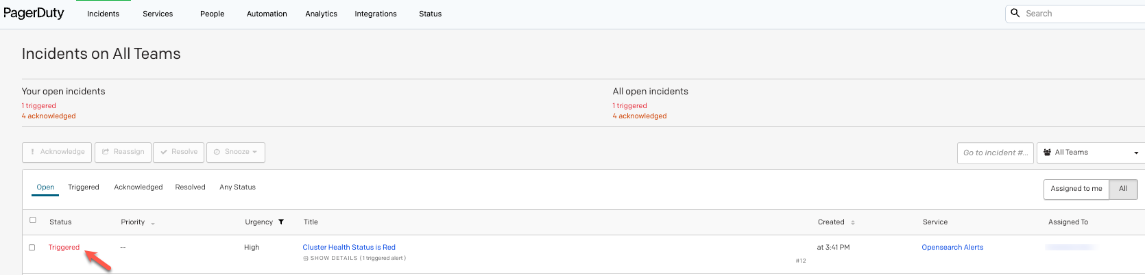
In this post, we demonstrate how to implement PagerDuty as the notification mechanism to get notified based on cluster health status. These notifications can be delivered via various channels, including email, SMS, or custom webhooks (like PagerDuty). The OpenSearch Service alerting plugin supports complex alert rules and provides a user interface to manage them.

Solution overview

PagerDuty is a cloud-based incident management platform that helps businesses handle their alerts and incidents in real time. PagerDuty works by consolidating alerts from various monitoring tools and routing them to the right team member, ensuring that issues are addressed promptly. Many businesses are using PagerDuty for real-time incident notifications via multiple channels, ensuring that the right team members are alerted quickly.

In this post, we describe how to set up PagerDuty and integrate it with an OpenSearch Service custom webhook for alert notifications when a threshold is met.

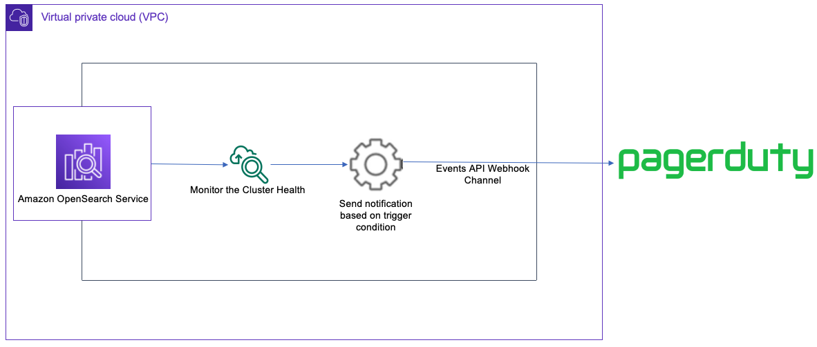
The following diagram illustrate OpenSearch Service running within an Amazon VPC using monitors and triggers to send a notification to the PagerDuty service using an Events API custom webhook

We need to set up a service and integration on PagerDuty to begin receiving incident notifications from OpenSearch Service. A service in PagerDuty represents an application, component, or team that we can trigger the notification against.

Prerequisites

Before you get started, create the following resources, if not already available:

Create a service on PagerDuty

To create a service on PagerDuty, complete the following steps:

  1. Log in to PagerDuty using your personal or enterprise account that is being used to enable the integration with OpenSearch Service.
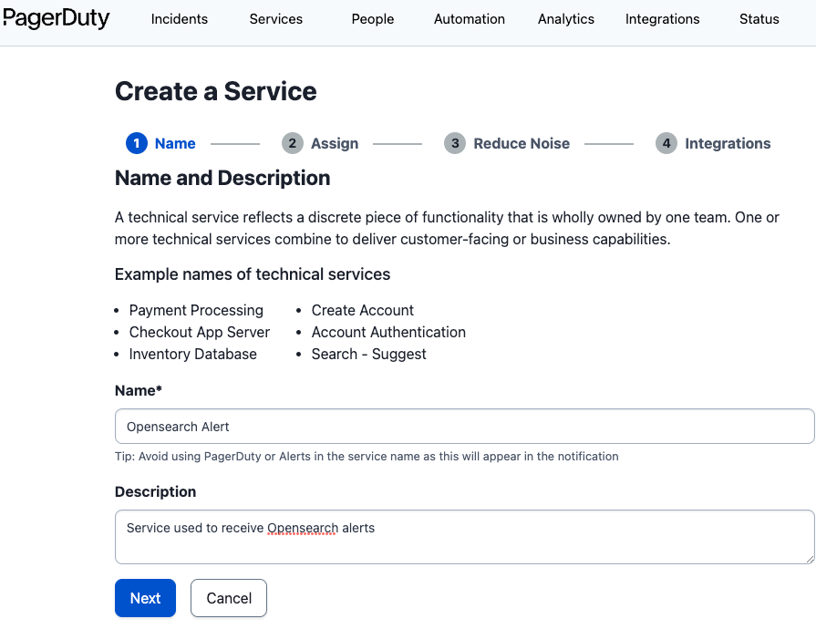
  2. On the Services tab, choose New Service.
  3. Enter a name and optional description, then choose Next.

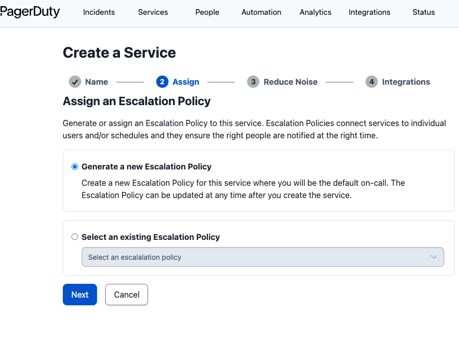
In the next step, we create or assign an escalation policy for the service. An escalation policy represents the order of responsibility for reacting to the issues detected on a service.

  1. If you already have an escalation policy defined within the organization or team, select Select an existing Escalation Policy and specify your policy. Otherwise, select Generate a new Escalation Policy, then choose Next.

In the next step, we can group the alerts based on time or content:

    • To group alerts together based on the alert content, select Content-Based grouping.
    • To group them based on a specific time duration, select Time-Based grouping.
    • Selecting the Intelligent grouping option will group the alerts intelligently based on content or time.
  1. Leave the defaults and choose Next.
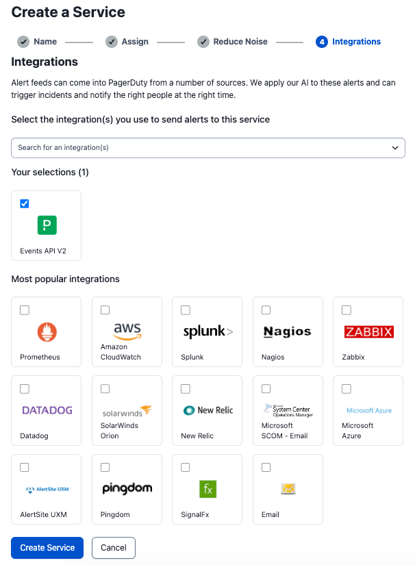
  2. On the Integrations page, select the Events API V2 integration (this will be used for integration with OpenSearch Service) and choose Create Service.

If you don’t select the integration during this step, you can add it later.

  1. Take note of the integration key on the Integrations tab.

Create a notification channel on OpenSearch Service with a custom webhook

Custom webhooks provide the ability to send these notifications to third-party services like PagerDuty using a REST API. After we configure the notification channel, we can use it for other monitors beyond this use case and to detect data patterns that are stored within the cluster.

Complete the following steps to configure the notification channel:

  1. On the OpenSearch Dashboards page, choose Notifications under Amazon OpenSearch Plugins in the navigation pane.
  2. On the Channels tab, choose Create channel.
  3. Enter a name for the channel and an optional description.
  4. For Channel type, choose Custom webhook.
  5. For Method, choose POST.
  6. For Define endpoints by, select Custom attributes URL.
  1. For Host, enter events.PagerDuty.com.
  2. For Path, enter v2/enqueue.
  3. Under Webhook headers, choose Add header.
  4. Enter X-Routing-Key as the key and the integration key you obtained earlier as the value.
  5. Choose Create and ensure the channel is successfully created.

Configure OpenSearch Service alerts to send notifications to PagerDuty

We can monitor OpenSearch cluster health in two different ways:

  • Using the OpenSearch Dashboard alerting plugin by setting up a per cluster metrics monitor. This provides a query to retrieve metrics related to the cluster health.
  • Integrating with Amazon CloudWatch, a monitoring and observability service.

In this use case, we use the alerting plugin. Complete the following steps:

  1. On the OpenSearch Dashboards page, choose Alerting under Amazon OpenSearch Plugins in the navigation pane.
  2. On the Monitors tab, choose Create monitor.
  3. For Monitor name, enter a name (for example, Monitor Cluster Health).
  4. For Monitor type, select Per cluster metrics monitor.
  5. Under Schedule¸ configure the monitor to run every minute.
  6. In the Query section, for Request type, choose Cluster health.
  7. Choose Preview query.
  8. Create a trigger by choosing Add trigger.
  9. For Trigger name, enter a name (for example, Cluster Health Status is Red).
  10. Leave Severity level at 1 (Highest).
  11. Under Trigger condition, delete the default code and enter the following:
ctx.results[0].status == "red"
  1. Choose Preview condition response to confirm that Trigger condition response shows as false, indicating that the cluster is healthy.
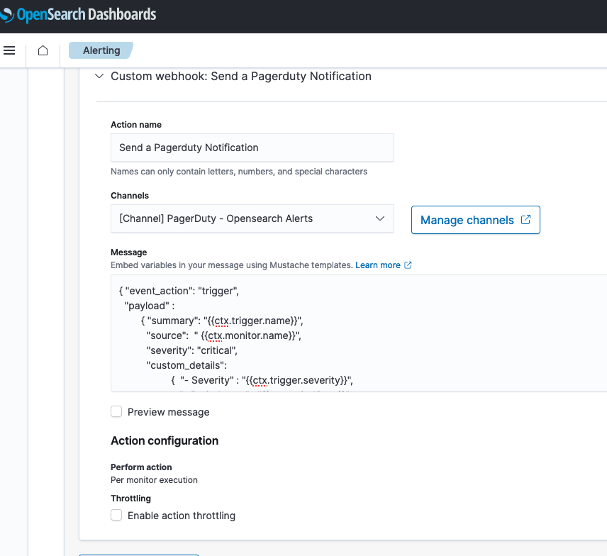
  2. Under Actions, choose Add action.
  3. For Action name, enter a name (for example, Send a PagerDuty notification).
  4. For Channels, choose the channel you created earlier.
  5. For Message, enter the following code:
{ "event_action": "trigger",
"payload" :
	{	"summary": "{{ctx.trigger.name}}",
		"source": " {{ctx.monitor.name}}",
		"severity": "critical",
		"custom_details":
			{ 
				"-Severity" : "{{ctx.trigger.severity}}",
				"-Period start" : "{{ctx.periodStart}}",
				"-Period end": "{{ctx.periodEnd}}"
			}
	}
}

Note that apart from the custom_details section in the code, the rest of the fields are mandatory for PagerDuty.

  1. Choose Send test message and test to make sure you receive an alert on the PagerDuty service.
  2. Choose Create and ensure the monitor was created successfully.

A notification will be sent to the PagerDuty service as part of the test, which will trigger a notification via a phone call or text message for the person who is available based on the escalation policy defined earlier. This notification can be safely acknowledged and resolved from PagerDuty because this is was a test.

Clean up

To clean up the infrastructure and avoid additional charges, complete the following steps:

  1. Delete the PagerDuty service.
  2. Delete the OpenSearch Service domain that was created as part of the prerequisites.

Conclusion

The integration of OpenSearch Service alerts with PagerDuty provides a powerful and efficient solution for managing and responding to critical events in real time. With this integration, you can easily set up alerts and notifications to stay informed about potential issues within your OpenSearch Service clusters or issues related to data and documents stored within the cluster, and proactively take action to resolve any problems that arise. Additionally, the integration allows for seamless collaboration between teams, enabling them to work together to identify and troubleshoot issues as they occur.

For more information about anomaly detection and alerts in OpenSearch Service, refer to Anomaly Detection in Amazon OpenSearch and Configuring Alerts in Amazon OpenSearch.


About the Authors

Manikanta Gona is a Data and ML Engineer at AWS Professional Services. He joined AWS in 2021 with 6+ years of experience in IT. At AWS, he is focused on Data Lake implementations, and Search, Analytical workloads using Amazon OpenSearch Service. In his spare time, he love to garden, and go on hikes and biking with his husband.

Vivek Shrivastava is a Principal Data Architect, Data Lake in AWS Professional Services. He is a Bigdata enthusiast and holds 14 AWS Certifications. He is passionate about helping customers build scalable and high-performance data analytics solutions in the cloud. In his spare time, he loves reading and finds areas for home automation

Ravikiran Rao is a Data Architect at AWS and is passionate about solving complex data challenges for various customers. Outside of work, he is a theatre enthusiast and an amateur tennis player.

Hari Krishna KC is a Data Architect with the AWS Professional Services Team. He specializes in AWS Data Lakes & AWS OpenSearch Service and have helped numerous client migrate their workload to Data Lakes and Search data stores

Introducing in-place version upgrades with Amazon MWAA

Post Syndicated from Parnab Basak original https://aws.amazon.com/blogs/big-data/introducing-in-place-version-upgrades-with-amazon-mwaa/

Today, AWS is announcing the availability of in-place version upgrades for Amazon Managed Workflow for Apache Airflow (Amazon MWAA). This enhancement allows you to seamlessly upgrade your existing Apache Airflow version 2.x environments to newer available versions while retaining the workflow run history and environment configurations. You can now take advantage of the latest capabilities of the Apache Airflow platform without having to create an entirely new Amazon MWAA environment.

Until now, if you wanted to upgrade your Amazon MWAA environment to a different Apache Airflow version, you had to follow the Amazon MWAA environment migration instructions. This involved creating a new Amazon MWAA environment and then migrating all of your configurations and Directed Acyclic Graphs (DAGs) to it. If you also needed to preserve the history of DAG runs, you had to take a backup of your metadata database and then restore that backup on the newly created environment. This process was error prone, manual, and involved additional costs to maintain two separate Amazon MWAA environments until you could verify the new and decommission the old.

In this post, we provide an overview of the in-place version upgrade feature, explore applicable use cases, detail the steps to use it, and provide additional guidance on its capabilities.

Overview of solution

The newly introduced in-place version upgrades by Amazon MWAA provide a streamlined transition from your existing Apache Airflow version 2.x-based environments to newer available Apache Airflow versions. Amazon MWAA manages the entire upgrade process, from provisioning new Apache Airflow versions to upgrading the metadata database. In the event of an upgrade failure, Amazon MWAA is designed to roll back to the previous stable version using the associated metadata database snapshot.

Upgrading your existing environments on Amazon MWAA is a straightforward process. You can upgrade your existing Apache Airflow 2.0 and later environments on Amazon MWAA with just a few clicks on the Amazon MWAA console, by using the Amazon MWAA API, the AWS Command Line Interface (AWS CLI), or by using tools like AWS CloudFormation, the AWS Cloud Development Kit (AWS CDK), or Terraform. This feature is available in all currently supported Amazon MWAA Regions.

On the Amazon MWAA console, simply edit the environment and select an available Apache Airflow version higher than the current version of your existing environment. You can also use the UpdateEnvironment API and specify the new Apache Airflow version to trigger an upgrade process. To learn more about in-place version upgrades, refer to Upgrading the Apache Airflow version from Amazon MWAA documentation.

During an upgrade, Amazon MWAA first creates a snapshot of the existing environment’s metadata database, which then serves as the basis for a new database. Subsequently, all Apache Airflow components—web server, scheduler, and workers—are upgraded. Finally, the newly created metadata database is upgraded, effectively completing the transition to the new environment.

Applicable use cases

You should consider upgrading your Apache Airflow version on Amazon MWAA if your existing workflows can accommodate the change and a new version is available with features or improvements that align with your use case. By upgrading, you can take advantage of the latest capabilities of the Apache Airflow platform and maintain compatibility with new features and best practices like data-driven scheduling and new Amazon provider packages released in Apache Airflow 2.4.3. The upgrade process involves an environment downtime that can take up to 2 hours to complete depending on the environment size and can be performed on demand at a time that best suits you. If your existing environment is heavily used such that you can’t afford a downtime, consider creating a new environment instead.

Prerequisites

When preparing for the upgrade, make sure you complete the following prerequisite steps:

  1. Verify Apache Airflow changes between your existing and new versions of the environment. Review the Apache Airflow release notes to understand the impact of new features, significant changes, and bug fixes that all intermediate Apache Airflow releases made between your source and destination versions.
  2. Review your existing requirements.txt file to verify the correct set of dependencies required for your target environment. Additionally, verify that your requirements.txt file has the correct constraints file added at the top of the file to match your target environment. The Apache Airflow constraints file specifies the dependent modules and provider versions available at the time of an Apache Airflow release. Adding a constraints file prevents incompatible libraries from being installed to your environment. In the following example, replace {Airflow-version} with your target environment’s version number, and {Python-version} with the version of Python that’s compatible with your environment: --constraint "https://raw.githubusercontent.com/apache/airflow/constraints-{Airflow-version}/constraints-{Python-version}.txt"
  3. Review the compatibility of additional Python libraries mentioned in your requirements.txt file to match your target environment. Apache Airflow v2.4.3 and above use Python v3.10, while older Apache Airflow versions use Python v3.7. Therefore, if you are trying to upgrade your existing Apache Airflow v2.0.2/2.2.2-based environment to Apache Airflow v2.4.3 or higher, you should update your additional Python libraries to match Python v3.10.
  4. With Apache Airflow v2.4.3 and above, the list of provider packages Amazon MWAA installs by default for your environment has changed. Note that some imports and operator names have changed in the new provider package in Apache Airflow in order to standardize the naming convention across the provider packages. Compare the list of provider packages installed by default in Apache Airflow v2.2.2 or v2.0.2, and configure any additional packages you might need for your new Apache Airflow v2.4.3 and higher environment.
  5. Make sure that your DAGs and other workflow resources are compatible with the new Apache Airflow version you are upgrading to.
  6. Use the aws-mwaa-local-runner utility to test out your existing DAGs, requirements, plugins, and dependencies locally before deploying to Amazon MWAA. You can create a target Apache Airflow environment that’s similar to an Amazon MWAA production image locally using aws-mwaa-local-runner and verify all your components work before attempting to upgrade your Amazon MWAA environment. Additionally, test the new environment upgrade process in lower Amazon MWAA environments like dev or staging before rolling out the upgrade in production environments.

Upgrade process

When an upgrade has been initiated, Amazon MWAA stops the existing underlying Apache Airflow components (web server, scheduler, and workers). This process halts any worker tasks that are currently running. The status of your environment at this stage will show as UPDATING. The upgrade process then creates a database snapshot of the metadata database, marked by the status CREATING_SNAPSHOT. When the snapshot is complete, the environment status returns to UPDATING as Amazon MWAA triggers the creation of a new Apache Airflow environment that matches your version selection and applies the necessary schema changes to the existing metadata database to align it with the target Apache Airflow environment. During this phase, your specified requirements, plugins, and other dependencies are installed.

Upon completion, your new environment is marked as AVAILABLE, indicating that the upgrade process has been successful and the environment is ready for testing. You can now log in to your Apache Airflow UI to verify the presence of your existing DAGs, their historical runs, configured connections, and more.

However, if there are failures in installing your specified requirements, plugins, and dependencies files, the environment initiates a rollback to the previous stable version. During this process, your environment status will show as ROLLING_BACK. If the rollback is successful, your previous stable environment will be available and the status will display as UPDATE_FAILED until a new update is attempted and succeeds. If the rollback fails, the status will show as UNAVAILABLE, indicating that your environment is not functional.

If your environment upgrade process fails, it is likely that the underlying Amazon Elastic Container Service (Amazon ECS) AWS Fargate clusters had stabilization issues caused by conflicting requirements and plugins, networking issues, or DB migration issues after the Apache Airflow component upgrade. To mitigate these issues, ensure that your DAGs and requirements work without issues using the aws-mwaa-local-runner utility and, ideally, test in a staging Amazon MWAA environment.

Additional considerations

Keep in mind the following additional information of this feature:

  • The upgrade process is available on demand, and will be limited to moving to newer versions. In-place version upgrades on Amazon MWAA are not supported for version 1.10.z. To perform a major version upgrade, for example from version 1.y.z to 2.y.z, you must create a new environment and migrate your resources.
  • You can only select applicable higher versions that you can upgrade to. Downgrading to a lower version is not available.
  • The rollback process can take additional time and, if you have Amazon Simple Storage Service (Amazon S3) bucket versioning enabled, Amazon MWAA is designed to revert the environment to the previous working configuration, including plugins and requirements. However, any manual changes made to your DAGs will not be reverted during this process.
  • After the upgrade process has completed successfully and the environment is available, any running DAGs that were interrupted during the upgrade are scheduled for a retry, depending on the way you configure retries for your DAGs. You can also trigger them manually or wait for the next scheduled run.
  • You should iteratively upgrade your environments starting with the least critical ones first.

Conclusion

In this post, we talked about the new feature of Amazon MWAA that allows you to upgrade your existing Amazon MWAA environment to higher Apache Airflow versions. This feature is supported on new and existing Amazon MWAA environments running Apache Airflow 2.x and above. Use this feature to upgrade your Apache Airflow versions while retaining your existing workflow run histories and environment configurations. By upgrading, you can take advantage of the latest capabilities of the Apache Airflow platform and maintain compatibility with new features and adhere to best practices.

For additional details and code examples on Amazon MWAA, visit the Amazon MWAA User Guide and the Amazon MWAA examples GitHub repo.

Apache, Apache Airflow, and Airflow are either registered trademarks or trademarks of the Apache Software Foundation in the United States and/or other countries.


About the Authors

Parnab Basak is a Solutions Architect and a Serverless Specialist at AWS. He specializes in creating new solutions that are cloud native using modern software development practices like serverless, DevOps, and analytics. Parnab works closely in the analytics and integration services space helping customers adopt AWS services for their workflow orchestration needs.

Fernando Gamero is a Senior Solutions Architect engineer at AWS, having more than 25 years of experience in the technology industry, from telecommunications, banking to startups. He is now helping customers with building Event Driven Architectures, adopting IoT solutions at the Edge, and transforming their data and machine learning pipelines at scale.

Shubham Mehta is an experienced product manager with over eight years of experience and a proven track record of delivering successful products. In his current role as a Senior Product Manager at AWS, he oversees Amazon Managed Workflows for Apache Airflow (Amazon MWAA) and spearheads the Apache Airflow open-source contributions to further enhance the product’s functionality.

Advanced patterns with AWS SDK for pandas on AWS Glue for Ray

Post Syndicated from Abdel Jaidi original https://aws.amazon.com/blogs/big-data/advanced-patterns-with-aws-sdk-for-pandas-on-aws-glue-for-ray/

AWS SDK for pandas is a popular Python library among data scientists, data engineers, and developers. It simplifies interaction between AWS data and analytics services and pandas DataFrames. It allows easy integration and data movement between 22 types of data stores, including Amazon Simple Storage Service (Amazon S3), Amazon Athena, Amazon Redshift, and Amazon OpenSearch Service.

In the previous post, we discussed how you can use AWS SDK for pandas to scale your workloads on AWS Glue for Ray. We explained how using both Ray and Modin within the library enabled us to distribute workloads across a compute cluster. To illustrate these capabilities, we explored examples of writing Parquet files to Amazon S3 at scale and querying data in parallel with Athena.

In this post, we show some more advanced ways to use this library on AWS Glue for Ray. We cover features and APIs from AWS services such as S3 Select, Amazon DynamoDB, and Amazon Timestream.

Solution overview

The Ray and Modin frameworks allow scaling of pandas workloads easily. You can write code on your laptop that uses the SDK for pandas to get data from an AWS data or analytics service to a pandas DataFrame, transform it using pandas, and then write it back to the AWS service. By using the distributed version of the SDK for pandas and replacing pandas with Modin, exactly the same code will scale on a Ray runtime—all logic about task coordination and distribution is hidden. Taking advantage of these abstractions, the AWS SDK for pandas team has made considerable use of Ray primitives to distribute some of the existing APIs (for the full list, see Supported APIs).

In this post, we show how to use some of these APIs in an AWS Glue for Ray job, namely querying with S3 Select, writing to and reading from a DynamoDB table, and writing to a Timestream table. Because AWS Glue for Ray is a fully managed environment, it’s by far the easiest way to run jobs because you don’t need to worry about cluster management. If you want to create your own cluster on Amazon Elastic Compute Cloud (Amazon EC2), refer to Distributing Calls on Ray Remote Cluster.

Configure solution resources

We use an AWS CloudFormation stack to provision the solution resources. Complete the following steps:

  1. Choose Launch stack to provision the stack in your AWS account:

Launch CloudFormation Stack

This takes about 2 minutes to complete. On successful deployment, the CloudFormation stack shows the status as CREATE_COMPLETE.

CloudFormation CREATE_COMPLETE

  1. Navigate to AWS Glue Studio to find an AWS Glue job named AdvancedGlueRayJob.

Glue for Ray Job Script

  1. On the Job details tab, scroll down and choose Advanced Properties.

Under Job Parameters, AWS SDK for pandas is specified as an additional Python module to install, along with Modin as an extra dependency.

Glue for Ray Job Details

  1. To run the job, choose Run and navigate to the Runs tab to monitor the job’s progress.

Glue for Ray Job Runs

Import the library

To import the library, use the following code:

import awswrangler as wr

AWS SDK for pandas detects if the runtime supports Ray, and automatically initializes a cluster with the default parameters. Advanced users can override this process by starting the Ray runtime before the import command.

Scale S3 Select workflows

S3 Select allows you to use SQL statements to query and filter S3 objects, including compressed files. This can be particularly useful if you have large files of several TBs and want to extract some information. Because the workload is delegated to Amazon S3, you don’t have to download and filter objects on the client side, leading to lower latency, lower cost, and higher performance.

With AWS SDK for pandas, these calls to S3 Select can be distributed across Ray workers in the cluster. In the following example, we query Amazon reviews data in Parquet format, filtering for reviews with 5-star ratings in the Mobile_Electronics partition. star_rating is a column in the Parquet data itself, while the partition is a directory.

# Filter for 5-star reviews with S3 Select within a partition
df_select = wr.s3.select_query(
    sql="SELECT * FROM s3object s where s.\"star_rating\" >= 5",
    path="s3://amazon-reviews-pds/parquet/product_category=Mobile_Electronics/",
    input_serialization="Parquet",
    input_serialization_params={},
    scan_range_chunk_size=1024*1024*16,
)

scan_range_chunk_size is an important parameter to calibrate when using S3 Select. It specifies the range of bytes to query the S3 object, thereby determining the amount of work delegated to each worker. For this example, it’s set to 16 MB, meaning the work of scanning the object is parallelized into separate S3 Select requests each 16 MB in size. A higher value equates to larger chunks per worker but fewer workers, and vice versa.

The results are returned in a Modin DataFrame, which is a drop-in replacement for pandas. It exposes the same APIs but enables you to use all the workers in the cluster. The data in the Modin DataFrame is distributed along with all the operations among the workers.

Scale DynamoDB workflows

DynamoDB is a scalable NoSQL database service that provides high-performance, low-latency, and managed storage.

AWS SDK for pandas uses Ray to scale DynamoDB workflows, allowing parallel data retrieval and insertion operations. The wr.dynamodb.read_items function retrieves data from DynamoDB in parallel across multiple workers, and the results are returned as a Modin DataFrame. Similarly, data insertion into DynamoDB can be parallelized using the wr.dynamodb.put_df function.

For example, the following code inserts the Amazon Reviews DataFrame obtained from S3 Select into a DynamoDB table and then reads it back:

# Write Modin DataFrame to DynamoDB
wr.dynamodb.put_df(
    df=df_select,
    table_name=dynamodb_table_name,
    use_threads=4,
)
# Read data back from DynamoDB to Modin
    df_dynamodb = wr.dynamodb.read_items(
    table_name=dynamodb_table_name,
    allow_full_scan=True,
)

DynamoDB calls are subject to AWS service quotas. The concurrency can be limited using the use_threads parameter.

Scale Timestream workflows

Timestream is a fast, scalable, fully managed, purpose-built time series database that makes it easy to store and analyze trillions of time series data points per day. With AWS SDK for pandas, you can distribute Timestream write operations across multiple workers in your cluster.

Data can be written to Timestream using the wr.timestream.write function, which parallelizes the data insertion process for improved performance.

In this example, we use sample data from Amazon S3 loaded into a Modin DataFrame. Familiar pandas commands such as selecting columns or resetting the index are applied at scale with Modin:

# Select columns
df_timestream = df_timestream.loc[:, ["region", "az", "hostname", "measure_kind", "measure", "time"]]
# Overwrite the time column
df_timestream["time"] = datetime.now()
# Reset the index
df_timestream.reset_index(inplace=True, drop=False)
# Filter a measure
df_timestream = df_timestream[df_timestream.measure_kind == "cpu_utilization"]

The Timestream write operation is parallelized across blocks in your dataset. If the blocks are too big, you can use Ray to repartition the dataset and increase the throughput, because each block will be handled by a separate thread:

# Repartition the data into 100 blocks
df_timestream = ray.data.from_modin(df_timestream).repartition(100).to_modin()

We are now ready to insert the data into Timestream, and a final query confirms the number of rows in the table:

# Write data to Timestream
rejected_records = wr.timestream.write(
    df=df_timestream,
    database=timestream_database_name,
    table=timestream_table_name,
    time_col="time",
    measure_col="measure",
    dimensions_cols=["index", "region", "az", "hostname"],
)

# Query
df = wr.timestream.query(f'SELECT COUNT(*) AS counter FROM "{timestream_database_name}"."{timestream_table_name}"')

Clean up

To prevent unwanted charges to your AWS account, we recommend deleting the AWS resources that you used in this post:

  1. On the Amazon S3 console, empty the data from the S3 bucket with prefix glue-ray-blog-script.

S3 Bucket

  1. On the AWS CloudFormation console, delete the AdvancedSDKPandasOnGlueRay stack.

All resources will be automatically deleted with it.

Conclusion

In this post, we showcased some more advanced patterns to run your workloads using AWS SDK for pandas. In particular, these examples demonstrated how Ray is used within the library to distribute operations for several other AWS services, not just Amazon S3. When used in combination with AWS Glue for Ray, this gives you access to a fully managed environment to run at scale. We hope this solution can help with migrating your existing pandas jobs to achieve higher performance and speedups across multiple data stores on AWS.


About the Authors

Abdel JaidiAbdel Jaidi is a Senior Cloud Engineer for AWS Professional Services. He works on open-source projects focused on AWS Data & Analytics services. In his spare time, he enjoys playing tennis and hiking.

Anton KukushkinAnton Kukushkin is a Data Engineer for AWS Professional Services based in London, UK. In his spare time, he enjoys playing musical instruments.

Leon LuttenbergerLeon Luttenberger is a Data Engineer for AWS Professional Services based in Austin, Texas. He works on AWS open-source solutions that help our customers analyze their data at scale. In his spare time, he enjoys reading and traveling.

Get custom data into Amazon Security Lake through ingesting Azure activity logs

Post Syndicated from Adam Plotzker original https://aws.amazon.com/blogs/security/get-custom-data-into-amazon-security-lake-through-ingesting-azure-activity-logs/

Amazon Security Lake automatically centralizes security data from both cloud and on-premises sources into a purpose-built data lake stored on a particular AWS delegated administrator account for Amazon Security Lake.

In this blog post, I will show you how to configure your Amazon Security Lake solution with cloud activity data from Microsoft Azure Monitor activity log, which you can query alongside your existing AWS CloudTrail data. I will walk you through the required steps — from configuring the required AWS Identity and Access Management (IAM) permissions, AWS Glue jobs, and Amazon Kinesis Data Streams required on the AWS side to forwarding that data from within Azure.

When you turn on Amazon Security Lake, it begins to collect actionable security data from various AWS sources. However, many enterprises today have complex environments that include a mix of different cloud resources in addition to on-premises data centers.

Although the AWS data sources in Amazon Security Lake encompass a large amount of the necessary security data needed for analysis, you may miss the full picture if your infrastructure operates across multiple cloud venders (for example, AWS, Azure, and Google Cloud Platform) and on-premises at the same time. By querying data from across your entire infrastructure, you can increase the number of indicators of compromise (IOC) that you identify, and thus increase the likelihood that those indicators will lead to actionable outputs.

Solution architecture

Figure 1 shows how to configure data to travel from an Azure event hub to Amazon Security Lake.

Figure 1: Solution architecture

Figure 1: Solution architecture

As shown in Figure 1, the solution involves the following steps:

  1. An AWS user instantiates the required AWS services and features that enable the process to function, including AWS Identity and Access Management (IAM) permissions, Kinesis data streams, AWS Glue jobs, and Amazon Simple Storage Service (Amazon S3) buckets, either manually or through an AWS CloudFormation template, such as the one we will use in this post.
  2. In response to the custom source created from the CloudFormation template, a Security Lake table is generated in AWS Glue.
  3. From this point on, Azure activity logs in their native format are stored within an Azure cloud event hub within an Azure account. An Azure function is deployed to respond to new events within the Azure event hub and forward these logs over the internet to the Kinesis data stream that was created in the preceding step.
  4. The Kinesis data stream forwards the data to an AWS Glue streaming job fronted by the Kinesis data.
  5. The AWS Glue job then performs the extract, transfer, and load (ETL) mapping to the appropriate Open Cybersecurity Schema Framework (OCSF) (specified for API Activity events at OCSF API Activity Mappings).
  6. The Azure events are partitioned with respect to the required partitioning requirements in Amazon Security Lake tables and stored in S3.
  7. The user can query these tables by using Amazon Athena alongside the rest of their data inside Amazon Security Lake.

Prerequisites

Before you implement the solution, complete the following prerequisites:

  • Verify that you have enabled Amazon Security Lake in the AWS Regions that correspond to the Azure Activity logs that you will forward. For more information, see What is Amazon Security Lake?
  • Preconfigure the custom source logging for the source AZURE_ACTIVITY in your Region. To configure this custom source in Amazon Security Lake, open the Amazon Security Lake console, navigate to Create custom data source, and do the following, as shown in Figure 2:
    • For Data source name, enter AZURE_ACTIVITY.
    • For Event class, select API_ACTIVITY.
    • For Account Id, enter the ID of the account which is authorized to write data to your data lake.
    • For External Id, enter “AZURE_ACTIVITY-<YYYYMMDD>“
    Figure 2:  Configure custom data source

    Figure 2: Configure custom data source

For more information on how to configure custom sources for Amazon Security Lake, see Collecting data from custom sources.

Step 1: Configure AWS services for Azure activity logging

The first step is to configure the AWS services for Azure activity logging.

  1. To configure Azure activity logging in Amazon Security Lake, first prepare the assets required in the target AWS account. You can automate this process by using the provided CloudFormation template — Security Lake CloudFormation — which will do the heavy lifting for this portion of the setup.

    Note: I have predefined these scripts to create the AWS assets required to ingest Azure activity logs, but you can generalize this process for other external log sources, as well.

    The CloudFormation template has the following components:

    • securitylakeGlueStreamingRole — includes the following managed policies:
      • AWSLambdaKinesisExecutionRole
      • AWSGlueServiceRole
    • securitylakeGlueStreamingPolicy — includes the following attributes:
      • “s3:GetObject”
      • “s3:PutObject”
    • securitylakeAzureActivityStream — This Kinesis data stream is the endpoint that acts as the connection point between Azure and AWS and the frontend of the AWS Glue stream that feeds Azure activity logs to Amazon Security Lake.
    • securitylakeAzureActivityJob — This is an AWS Glue streaming job that is used to take in feeds from the Kinesis data stream and map the Azure activity logs within that stream to OCSF.
    • securitylake-glue-assets S3 bucket — This is the S3 bucket that is used to store the ETL scripts used in the AWS Glue job to map Azure activity logs.

    Running the CloudFormation template will instantiate the aforementioned assets in your AWS delegated administrator account for Amazon Security Lake.

  2. The CloudFormation template creates a new S3 bucket with the following syntax: securityLake-glue-assets-<ACCOUNT-ID>–<REGION>. After the CloudFormation run is complete, navigate to this bucket within the S3 console.
  3. Within the S3 bucket, create a scripts and temporary folder in the S3 bucket, as shown in Figure 4.
    Figure 4: Glue assets bucket

    Figure 4: Glue assets bucket

  4. Update the Azure AWS Glue Pyspark script by replacing the following values in the file. You will attach this script to your AWS Glue job and use it to generate the AWS assets required for the implementation.
    • Replace <AWS_REGION_NAME> with the Region that you are operating in — for example, us-east-2.
    • Replace <AWS_ACCOUNT_ID> with the account ID of your delegated administrator account for Amazon Security Lake — for example, 111122223333.
    • Replace <SECURITYLAKE-AZURE-STREAM-ARN> with the Kinesis stream name created through the CloudFormation template. To find the stream name, open the Kinesis console, navigate to the Kinesis stream with the name securityLakeAzureActivityStream — <STREAM-UID>, and copy the Amazon Resource Name (ARN), as shown in the following figure.

      Figure 5: Kinesis stream ARN

      Figure 5: Kinesis stream ARN

    • Replace <SECURITYLAKE-BUCKET-NAME> with the name of your data lake S3 bucket root name — for example, s3://aws-security-data-lake-DOC-EXAMPLE-BUCKET.

    After you replace these values, navigate within the scripts folder and upload the AWS Glue PySpark Python script named azure-activity-pyspark.py, as shown in Figure 6.

    Figure 6: AWS Glue script

    Figure 6: AWS Glue script

  5. Within your AWS Glue job, choose Job details and configure the job as follows:
    • For Type, select Spark Streaming.
    • For Language, select Python 3.
    • For Script path, select the S3 path that you created in the preceding step.
    • For Temporary path, select the S3 path that you created in the preceding step.
  6. Save the changes, and run the AWS Glue job by selecting Save and then Run.
  7. Choose the Runs tab, and make sure that the Run status of the job is Running.
    igure 7: AWS Glue job status

    Figure 7: AWS Glue job status

At this point, you have finished the configurations from AWS.

Step 2: Configure Azure services for Azure activity log forwarding

You will complete the next steps in the Azure Cloud console. You need to configure Azure to export activity logs to an Azure cloud event hub within your desired Azure account or organization. Additionally, you need to create an Azure function to respond to new events within the Azure event hub and forward those logs over the internet to the Kinesis data stream that the CloudFormation template created in the initial steps of this post.

For information about how to set up and configure Azure Functions to respond to event hubs, see Azure Event Hubs Trigger for Azure Functions in the Azure documentation.

Configure the following Python script — Azure Event Hub Function — in an Azure function app. This function is designed to respond to event hub events, create a connection to AWS, and forward those events to Kinesis as deserialized JSON blobs.

In the script, replace the following variables with your own information:

  • For <SECURITYLAKE-AZURE-STREAM-ARN>, enter the Kinesis data stream ARN.
  • For <SECURITYLAKE-AZURE-STREAM-NAME>, enter the Kinesis data stream name.
  • For <SECURITYLAKE-AZURE-STREAM-KEYID>, enter the AWS Key Management Service (AWS KMS) key ID created through the CloudFormation template.

The <SECURITYLAKE-AZURE-STREAM-ARN> and securityLakeAzureActivityStream—<STREAM-UID> are the same variables that you obtained earlier in this post (see Figure 5).

You can find the AWS KMS key ID within the AWS KMS managed key policy associated with securityLakeAzureActivityStream. For example, in the key policy shown in Figure 8, the <SECURITYLAKE-AZURE-STREAM-KEYID> is shown in line 3.

Figure 8: Kinesis data stream inputs

Figure 8: Kinesis data stream inputs

Important: When you are working with KMS keys retrieved from the AWS console or AWS API keys within Azure, you should be extremely mindful of how you approach key management. Improper or poor handling of keys could result in the interception of data from the Kinesis stream or Azure function.

It’s a best security practice to use a trusted key management architecture that uses sufficient encryption and security protocols when working with keys that safeguard sensitive security information. Within Azure, consider using services such as the AWS Azure AD integration for seamless and ephemeral credential usage inside of the azure function. See – Azure AD Integration – for more information on how the Azure AD Integration works to safeguard and manage stored security keys and help make sure that no keys are accessible to unauthorized parties or stored as unencrypted text outside the AWS console.

Step 3: Validate the workflow and query Athena

After you complete the preceding steps, your logs should be flowing. To make sure that the process is working correctly, complete the following steps.

  1. In the Kinesis Data Streams console, verify that the logs are flowing to your data stream. Open the Kinesis stream that you created previously, choose the Data viewer tab, and then choose Get records, as shown in Figure 9.
    Figure 9: Kinesis data stream inputs

    Figure 9: Kinesis data stream inputs

  2. Verify that the logs are partitioned and stored within the correct Security Lake bucket associated with the configured Region. The log partitions within the Security Lake bucket should have the following syntax — “region=<region>/account_id=<account_id>/eventDay=<YYYYMMDD>/”, and they should be stored with the expected parquet compression.
     Figure 10: S3 bucket with object

    Figure 10: S3 bucket with object

  3. Assuming that CloudTrail logs exist within your Amazon Security Lake instance as well, you can now create a query in Athena that pulls data from the newly created Azure activity table and examine it alongside your existing CloudTrail logs by running queries such as the following:
    SELECT 
        api.operation,
        actor.user.uid,
        actor.user.name,
        src_endpoint.ip,
        time,
        severity,
        metadata.version,
        metadata.product.name,
        metadata.product.vendor_name,
        category_name,
        activity_name,
        type_uid,
    FROM {SECURITY-LAKE-DB}.{SECURITY-LAKE-AZURE-TABLE}
    UNION ALL
    SELECT 
        api.operation,
        actor.user.uid,
        actor.user.name,
        src_endpoint.ip,
        time,
        severity,
        metadata.version,
        metadata.product.name,
        metadata.product.vendor_name,
        category_name,
        activity_name,
        type_uid,
    FROM {SECURITY-LAKE-DB}.{SECURITY-LAKE-CLOUDTRAIL-TABLE}

    Figure 11:  Query Azure activity and CloudTrail together in Athena

    Figure 11: Query Azure activity and CloudTrail together in Athena

For additional guidance on how to configure access and query Amazon Security Lake in Athena, see the following resources:

Conclusion

In this blog post, you learned how to create and deploy the AWS and Microsoft Azure assets needed to bring your own data to Amazon Security Lake. By creating an AWS Glue streaming job that can transform Azure activity data streams and by fronting that AWS Glue job with a Kinesis stream, you can open Amazon Security Lake to intake from external Azure activity data streams.

You also learned how to configure Azure assets so that your Azure activity logs can stream to your Kinesis endpoint. The combination of these two creates a working, custom source solution for Azure activity logging.

To get started with Amazon Security Lake, see the Getting Started page, or if you already use Amazon Security Lake and want to read additional blog posts and articles about this service, see Blog posts and articles.

If you have feedback about this blog post, submit comments in the Comments section below. If you have questions about this blog post, start a new thread on Amazon Security Lake re:Post or contact AWS Support.

Want more AWS Security news? Follow us on Twitter.

Adam Plotzker

Adam Plotzker

Adam is currently a Security Engineer at AWS, working primarily on the Amazon Security Lake solution. One of the things he enjoys most about his work at AWS is his ability to be creative when exploring customer needs and coming up with unique solutions that meet those needs.

Join a streaming data source with CDC data for real-time serverless data analytics using AWS Glue, AWS DMS, and Amazon DynamoDB

Post Syndicated from Manish Kola original https://aws.amazon.com/blogs/big-data/join-streaming-source-cdc-glue/

Customers have been using data warehousing solutions to perform their traditional analytics tasks. Recently, data lakes have gained lot of traction to become the foundation for analytical solutions, because they come with benefits such as scalability, fault tolerance, and support for structured, semi-structured, and unstructured datasets.

Data lakes are not transactional by default; however, there are multiple open-source frameworks that enhance data lakes with ACID properties, providing a best of both worlds solution between transactional and non-transactional storage mechanisms.

Traditional batch ingestion and processing pipelines that involve operations such as data cleaning and joining with reference data are straightforward to create and cost-efficient to maintain. However, there is a challenge to ingest datasets, such as Internet of Things (IoT) and clickstreams, at a fast rate with near-real-time delivery SLAs. You will also want to apply incremental updates with change data capture (CDC) from the source system to the destination. To make data-driven decisions in a timely manner, you need to account for missed records and backpressure, and maintain event ordering and integrity, especially if the reference data also changes rapidly.

In this post, we aim to address these challenges. We provide a step-by-step guide to join streaming data to a reference table changing in real time using AWS Glue, Amazon DynamoDB, and AWS Database Migration Service (AWS DMS). We also demonstrate how to ingest streaming data to a transactional data lake using Apache Hudi to achieve incremental updates with ACID transactions.

Solution overview

For our example use case, streaming data is coming through Amazon Kinesis Data Streams, and reference data is managed in MySQL. The reference data is continuously replicated from MySQL to DynamoDB through AWS DMS. The requirement here is to enrich the real-time stream data by joining with the reference data in near-real time, and to make it queryable from a query engine such as Amazon Athena while keeping consistency. In this use case, reference data in MySQL can be updated when the requirement is changed, and then queries need to return results by reflecting updates in the reference data.

This solution addresses the issue of users wanting to join streams with changing reference datasets when the size of the reference dataset is small. The reference data is maintained in DynamoDB tables, and the streaming job loads the full table into memory for each micro-batch, joining a high-throughput stream to a small reference dataset.

The following diagram illustrates the solution architecture.

Architecture

Prerequisites

For this walkthrough, you should have the following prerequisites:

Create IAM roles and S3 bucket

In this section, you create an Amazon Simple Storage Service (Amazon S3) bucket and two AWS Identity and Access Management (IAM) roles: one for the AWS Glue job, and one for AWS DMS. We do this using an AWS CloudFormation template. Complete the following steps:

  1. Sign in to the AWS CloudFormation console.
  2. Choose Launch Stack::
  3. Choose Next.
  4. For Stack name, enter a name for your stack.
  5. For DynamoDBTableName, enter tgt_country_lookup_table. This is the name of your new DynamoDB table.
  6. For S3BucketNamePrefix, enter the prefix of your new S3 bucket.
  7. Select I acknowledge that AWS CloudFormation might create IAM resources with custom names.
  8. Choose Create stack.

Stack creation can take about 1 minute.

Create a Kinesis data stream

In this section, you create a Kinesis data stream:

  1. On the Kinesis console, choose Data streams in the navigation pane.
  2. Choose Create data stream.
  3. For Data stream name, enter your stream name.
  4. Leave the remaining settings as default and choose Create data stream.

A Kinesis data stream is created with on-demand mode.

Create and configure an Aurora MySQL cluster

In this section, you create and configure an Aurora MySQL cluster as the source database. First, configure your source Aurora MySQL database cluster to enable CDC through AWS DMS to DynamoDB.

Create a parameter group

Complete the following steps to create a new parameter group:

  1. On the Amazon RDS console, choose Parameter groups in the navigation pane.
  2. Choose Create parameter group.
  3. For Parameter group family, select aurora-mysql5.7.
  4. For Type, choose DB Cluster Parameter Group.
  5. For Group name, enter my-mysql-dynamodb-cdc.
  6. For Description, enter Parameter group for demo Aurora MySQL database.
  7. Choose Create.
  8. Select my-mysql-dynamodb-cdc, and choose Edit under Parameter group actions.
  9. Edit the parameter group as follows:
Name Value
binlog_row_image full
binlog_format ROW
binlog_checksum NONE
log_slave_updates 1
  1. Choose Save changes.

RDS parameter group

Create the Aurora MySQL cluster

Complete following steps to create the Aurora MySQL cluster:

  1. On the Amazon RDS console, choose Databases in the navigation pane.
  2. Choose Create database.
  3. For Choose a database creation method, choose Standard create.
  4. Under Engine options, for Engine type, choose Aurora (MySQL Compatible).
  5. For Engine version, choose Aurora (MySQL 5.7) 2.11.2.
  6. For Templates, choose Production.
  7. Under Settings, for DB cluster identifier, enter a name for your database.
  8. For Master username, enter your primary user name.
  9. For Master password and Confirm master password, enter your primary password.
  10. Under Instance configuration, for DB instance class, choose Burstable classes (includes t classes) and choose db.t3.small.
  11. Under Availability & durability, for Multi-AZ deployment, choose Don’t create an Aurora Replica.
  12. Under Connectivity, for Compute resource, choose Don’t connect to an EC2 compute resource.
  13. For Network type, choose IPv4.
  14. For Virtual private cloud (VPC), choose your VPC.
  15. For DB subnet group, choose your public subnet.
  16. For Public access, choose Yes.
  17. For VPC security group (firewall), choose the security group for your public subnet.
  18. Under Database authentication, for Database authentication options, choose Password authentication.
  19. Under Additional configuration, for DB cluster parameter group, choose the cluster parameter group you created earlier.
  20. Choose Create database.

Grant permissions to the source database

The next step is to grant the required permission on the source Aurora MySQL database. Now you can connect to the DB cluster using the MySQL utility. You can run queries to complete the following tasks:

  • Create a demo database and table and run queries on the data
  • Grant permission for a user used by the AWS DMS endpoint

Complete the following steps:

  1. Log in to the EC2 instance that you’re using to connect to your DB cluster.
  2. Enter the following command at the command prompt to connect to the primary DB instance of your DB cluster:
$ mysql -h mycluster.cluster-123456789012.us-east-1.rds.amazonaws.com -P 3306 -u admin -p
  1. Run the following SQL command to create a database:
> CREATE DATABASE mydev;
  1. Run the following SQL command to create a table:
> use mydev; 
> CREATE TABLE country_lookup_table
(
code varchar(5),
countryname varchar(40) not null,
combinedname varchar(40) not null
);
  1. Run the following SQL command to populate the table with data:
> INSERT INTO country_lookup_table(code, countryname, combinedname) VALUES ('IN', 'India', 'IN-India'), ('US', 'USA', 'US-USA'), ('CA', 'Canada', 'CA-Canada'), ('CN', 'China', 'CN-China');
  1. Run the following SQL command to create a user for the AWS DMS endpoint and grant permissions for CDC tasks (replace the placeholder with your preferred password):
> CREATE USER repl IDENTIFIED BY '<your-password>';
> GRANT REPLICATION CLIENT, REPLICATION SLAVE ON *.* TO 'repl'@'%';
> GRANT SELECT ON mydev.country_lookup_table TO 'repl'@'%';

Create and configure AWS DMS resources to load data into the DynamoDB reference table

In this section, you create and configure AWS DMS to replicate data into the DynamoDB reference table.

Create an AWS DMS replication instance

First, create an AWS DMS replication instance by completing the following steps:

  1. On the AWS DMS console, choose Replication instances in the navigation pane.
  2. Choose Create replication instance.
  3. Under Settings, for Name, enter a name for your instance.
  4. Under Instance configuration, for High Availability, choose Dev or test workload (Single-AZ).
  5. Under Connectivity and security, for VPC security groups, choose default.
  6. Choose Create replication instance.

Create Amazon VPC endpoints

Optionally, you can create Amazon VPC endpoints for DynamoDB when you need to connect to your DynamoDB table from the AWS DMS instance in a private network. Also make sure that you enable Publicly accessible when you need to connect to a database outside of your VPC.

Create an AWS DMS source endpoint

Create an AWS DMS source endpoint by completing the following steps:

  1. On the AWS DMS console, choose Endpoints in the navigation pane.
  2. Choose Create endpoint.
  3. For Endpoint type, choose Source endpoint.
  4. Under Endpoint configuration, for Endpoint identifier, enter a name for your endpoint.
  5. For Source engine, choose Amazon Aurora MySQL.
  6. For Access to endpoint database, choose Provide access information manually.
  7. For Server Name, enter the endpoint name of your Aurora writer instance (for example, mycluster.cluster-123456789012.us-east-1.rds.amazonaws.com).
  8. For Port, enter 3306.
  9. For User name, enter a user name for your AWS DMS task.
  10. For Password, enter a password.
  11. Choose Create endpoint.

Crate an AWS DMS target endpoint

Create an AWS DMS target endpoint by completing the following steps:

  1. On the AWS DMS console, choose Endpoints in the navigation pane.
  2. Choose Create endpoint.
  3. For Endpoint type, choose Target endpoint.
  4. Under Endpoint configuration, for Endpoint identifier, enter a name for your endpoint.
  5. For Target engine, choose Amazon DynamoDB.
  6. For Service access role ARN, enter the IAM role for your AWS DMS task.
  7. Choose Create endpoint.

Create AWS DMS migration tasks

Create AWS DMS database migration tasks by completing the following steps:

  1. On the AWS DMS console, choose Database migration tasks in the navigation pane.
  2. Choose Create task.
  3. Under Task configuration, for Task identifier, enter a name for your task.
  4. For Replication instance, choose your replication instance.
  5. For Source database endpoint, choose your source endpoint.
  6. For Target database endpoint, choose your target endpoint.
  7. For Migration type, choose Migrate existing data and replicate ongoing changes.
  8. Under Task settings, for Target table preparation mode, choose Do nothing.
  9. For Stop task after full load completes, choose Don’t stop.
  10. For LOB column settings, choose Limited LOB mode.
  11. For Task logs, enable Turn on CloudWatch logs and Turn on batch-optimized apply.
  12. Under Table mappings, choose JSON Editor and enter the following rules.

Here you can add values to the column. With the following rules, the AWS DMS CDC task will first create a new DynamoDB table with the specified name in target-table-name. Then it will replicate all the records, mapping the columns in the DB table to the attributes in the DynamoDB table.

{
    "rules": [
        {
            "rule-type": "selection",
            "rule-id": "1",
            "rule-name": "1",
            "object-locator": {
                "schema-name": "mydev",
                "table-name": "country_lookup_table"
            },
            "rule-action": "include"
        },
        {
            "rule-type": "object-mapping",
            "rule-id": "2",
            "rule-name": "2",
            "rule-action": "map-record-to-record",
            "object-locator": {
                "schema-name": "mydev",
                "table-name": "country_lookup_table"
            },
            "target-table-name": "tgt_country_lookup_table",
            "mapping-parameters": {
                "partition-key-name": "code",
                "sort-key-name": "countryname",
                "exclude-columns": [
                    "code",
                    "countryname"
                ],
                "attribute-mappings": [
                    {
                        "target-attribute-name": "code",
                        "attribute-type": "scalar",
                        "attribute-sub-type": "string",
                        "value": "${code}"
                    },
                    {
                        "target-attribute-name": "countryname",
                        "attribute-type": "scalar",
                        "attribute-sub-type": "string",
                        "value": "${countryname}"
                    }
                ],
                "apply-during-cdc": true
            }
        }
    ]
}

DMS table mapping

  1. Choose Create task.

Now the AWS DMS replication task has been started.

  1. Wait for the Status to show as Load complete.

DMS task

  1. On the DynamoDB console, choose Tables in the navigation pane.
  2. Select the DynamoDB reference table, and choose Explore table items to review the replicated records.

DynamoDB reference table initial

Create an AWS Glue Data Catalog table and an AWS Glue streaming ETL job

In this section, you create an AWS Glue Data Catalog table and an AWS Glue streaming extract, transform, and load (ETL) job.

Create a Data Catalog table

Create an AWS Glue Data Catalog table for the source Kinesis data stream with the following steps:

  1. On the AWS Glue console, choose Databases under Data Catalog in the navigation pane.
  2. Choose Add database.
  3. For Name, enter my_kinesis_db.
  4. Choose Create database.
  5. Choose Tables under Databases, then choose Add table.
  6. For Name, enter my_stream_src_table.
  7. For Database, choose my_kinesis_db.
  8. For Select the type of source, choose Kinesis.
  9. For Kinesis data stream is located in, choose my account.
  10. For Kinesis stream name, enter a name for your data stream.
  11. For Classification, select JSON.
  12. Choose Next.
  13. Choose Edit schema as JSON, enter the following JSON, then choose Save.
[
  {
    "Name": "uuid",
    "Type": "string",
    "Comment": ""
  },
  {
    "Name": "country",
    "Type": "string",
    "Comment": ""
  },
  {
    "Name": "itemtype",
    "Type": "string",
    "Comment": ""
  },
  {
    "Name": "saleschannel",
    "Type": "string",
    "Comment": ""
  },
  {
    "Name": "orderpriority",
    "Type": "string",
    "Comment": ""
  },
  {
    "Name": "orderdate",
    "Type": "string",
    "Comment": ""
  },
  {
    "Name": "region",
    "Type": "string",
    "Comment": ""
  },
  {
    "Name": "shipdate",
    "Type": "string",
    "Comment": ""
  },
  {
    "Name": "unitssold",
    "Type": "string",
    "Comment": ""
  },
  {
    "Name": "unitprice",
    "Type": "string",
    "Comment": ""
  },
  {
    "Name": "unitcost",
    "Type": "string",
    "Comment": ""
  },
  {
    "Name": "totalrevenue",
    "Type": "string",
    "Comment": ""
  },
  {
    "Name": "totalcost",
    "Type": "string",
    "Comment": ""
  },
  {
    "Name": "totalprofit",
    "Type": "string",
    "Comment": ""
  },
  {
    "Name": "impressiontime",
    "Type": "string",
    "Comment": ""
  }
]

Glue Catalog table schema

    1. Choose Next, then choose Create.

Create an AWS Glue streaming ETL job

Next, you create an AWS Glue streaming job. AWS Glue 3.0 and later supports Apache Hudi natively, so we use this native integration to ingest into a Hudi table. Complete the following steps to create the AWS Glue streaming job:

  1. On the AWS Glue Studio console, choose Spark script editor and choose Create.
  2. Under Job details tab, for Name, enter a name for your job.
  3. For IAM Role, choose the IAM role for your AWS Glue job.
  4. For Type, select Spark Streaming.
  5. For Glue version, choose Glue 4.0 – Supports spark 3.3, Scala 2, Python 3.
  6. For Requested number of workers, enter 3.
  7. Under Advanced properties, for Job parameters, choose Add new parameter.
  8. For Key, enter --conf.
  9. For Value, enter spark.serializer=org.apache.spark.serializer.KryoSerializer --conf spark.sql.hive.convertMetastoreParquet=false.
  10. Choose Add new parameter.
  11. For Key, enter --datalake-formats.
  12. For Value, enter hudi.
  13. For Script path, enter s3://<S3BucketName>/scripts/.
  14. For Temporary path, enter s3://<S3BucketName>/temporary/.
  15. Optionally, for Spark UI logs path, enter s3://<S3BucketName>/sparkHistoryLogs/.

Glue job parameter

  1. On the Script tab, enter the following script into the AWS Glue Studio editor and choose Create.

The near-real-time streaming job enriches data by joining a Kinesis data stream with a DynamoDB table that contains frequently updated reference data. The enriched dataset is loaded into the target Hudi table in the data lake. Replace <S3BucketName> with your bucket that you created via AWS CloudFormation:

import sys, json
import boto3
from pyspark.sql import DataFrame, Row
from pyspark.context import SparkContext
from pyspark.sql.types import *
from pyspark.sql.functions import *
from awsglue.transforms import *
from awsglue.utils import getResolvedOptions
from awsglue.context import GlueContext
from awsglue.job import Job

args = getResolvedOptions(sys.argv,["JOB_NAME"])

# Initialize spark session and Glue context
sc = SparkContext() 
glueContext = GlueContext(sc)
spark = glueContext.spark_session
job = Job(glueContext)
job.init(args["JOB_NAME"], args)

# job paramters
dydb_lookup_table = "tgt_country_lookup_table"
kin_src_database_name = "my_kinesis_db" 
kin_src_table_name = "my_stream_src_table" 
hudi_write_operation = "upsert" 
hudi_record_key = "uuid" 
hudi_precomb_key = "orderdate" 
checkpoint_path = "s3://<S3BucketName>/streamlab/checkpoint/" 
s3_output_folder = "s3://<S3BucketName>/output/"
hudi_table = "hudi_table"
hudi_database = "my_kinesis_db"

# hudi options 
additional_options={
    "hoodie.datasource.hive_sync.use_jdbc": "false",
    "hoodie.datasource.write.recordkey.field": hudi_record_key,
    "hoodie.datasource.hive_sync.database": hudi_database,
    "hoodie.table.name": hudi_table,
    "hoodie.consistency.check.enabled": "true",
    "hoodie.datasource.write.keygenerator.class": "org.apache.hudi.keygen.NonpartitionedKeyGenerator",
    "hoodie.datasource.hive_sync.partition_extractor_class": "org.apache.hudi.hive.NonPartitionedExtractor",
    "hoodie.datasource.write.hive_style_partitioning": "false",
    "hoodie.datasource.write.precombine.field": hudi_precomb_key,
    "hoodie.bulkinsert.shuffle.parallelism": "4",
    "hoodie.datasource.hive_sync.enable": "true",
    "hoodie.datasource.write.operation": hudi_write_operation,
    "hoodie.datasource.write.storage.type": "COPY_ON_WRITE",
}

# Scan and load the reference data table from DynamoDB into AWS Glue DynamicFrames using boto3 API.
def readDynamoDb():
    dynamodb = boto3.resource(“dynamodb”)
    table = dynamodb.Table(dydb_lookup_table)
    response = table.scan()
    items = response[“Items”]
    jsondata = sc.parallelize(items)
    lookupDf = glueContext.read.json(jsondata)
    return lookupDf


# Load the Amazon Kinesis data stream from Amazon Glue Data Catalog.
source_df = glueContext.create_data_frame.from_catalog(
    database=kin_src_database_name,
    table_name=kin_src_table_name,
    transformation_ctx=”source_df”,
    additional_options={“startingPosition”: “TRIM_HORIZON”},
)

# As part of batch processing, implement the transformation logic for joining streaming data frames with reference data frames.
def processBatch(data_frame, batchId):
    if data_frame.count() > 0:

        # Refresh the dymanodb table to pull latest snapshot for each microbatch
        country_lookup_df = readDynamoDb() 
                
        final_frame = data_frame.join(
            country_lookup_df, 
            data_frame["country"] == country_lookup_df["countryname"], 
            'left'
        ).drop(
            "countryname",
            "country",
            "unitprice", 
            "unitcost",
            "totalrevenue",
            "totalcost",
            "totalprofit"
        )

        # Script generated for node my-lab-hudi-connector
        final_frame.write.format("hudi") \
            .options(**additional_options) \
            .mode("append") \
            .save(s3_output_folder)
        
try:
    glueContext.forEachBatch(
        frame=source_df,
        batch_function=processBatch,
        options={"windowSize": "60 seconds", "checkpointLocation": checkpoint_path},
    )
except Exception as e:
    print(f"Error is @@@ ....{e}")
  1. Choose Run to start the streaming job.

The following screenshot shows examples of the DataFrames data_frame, country_lookup_df, and final_frame.

Glue job log output initial

The AWS Glue job successfully joined records coming from the Kinesis data stream and the reference table in DynamoDB, and then ingested the joined records into Amazon S3 in Hudi format.

Create and run a Python script to generate sample data and load it into the Kinesis data stream

In this section, you create and run a Python to generate sample data and load it into the source Kinesis data stream. Complete the following steps:

  1. Log in to AWS Cloud9, your EC2 instance, or any other computing host that puts records in your data stream.
  2. Create a Python file called generate-data-for-kds.py:
$ python3 generate-data-for-kds.py
  1. Open the Python file and enter the following script:
import json
import random
import boto3
import time

STREAM_NAME = "<mystreamname>"

def get_data():
    return {
        "uuid": random.randrange(0, 1000001, 1),
        "country": random.choice( [ "United Arab Emirates", "China", "India", "United Kingdom", "United States of America", ] ),
        "itemtype": random.choice( [ "Snacks", "Cereals", "Cosmetics", "Fruits", "Clothes", "Babycare", "Household", ] ),
        "saleschannel": random.choice( [ "Snacks", "Cereals", "Cosmetics", "Fruits", "Clothes", "Babycare", "Household", ] ),
        "orderpriority": random.choice(["H", "L", "M", "C"]),
        "orderdate": random.choice( [ "1/4/10", "2/28/10", "2/15/11", "11/8/11", "2/1/12", "2/18/12", "3/1/12", "9/24/12",
                                      "10/13/12", "12/2/12", "12/29/12", "3/30/13", "7/29/13", "3/23/14", "6/14/14", 
                                      "7/15/14", "10/19/14", "5/7/15", "10/11/15", "11/22/15", "8/23/16", "1/15/17", 
                                      "1/27/17", "2/25/17", "3/10/17", "4/1/17", ] ),
        "region": random.choice( ["Asia" "Europe", "Americas", "Middle Eastern", "Africa"] ),
        "shipdate": random.choice( [ "1/4/10", "2/28/10", "2/15/11", "11/8/11", "2/1/12", "2/18/12", "3/1/12", "9/24/12", 
                                    "10/13/12", "12/2/12", "12/29/12", "3/30/13", "7/29/13", "3/23/14", "6/14/14", "7/15/14",
                                      "10/19/14", "5/7/15", "10/11/15", "11/22/15", "8/23/16", "1/15/17", "1/27/17", 
                                      "2/25/17", "3/10/17", "4/1/17", ] ),
        "unitssold": random.choice( [ "8217", "3465", "8877", "2882", "70", "7044", "6307", "2384", "1327", "2572", "8794", 
                                     "4131", "5793", "9091", "4314", "9085", "5270", "5459", "1982", "8245", "4860", "4656", 
                                     "8072", "65", "7864", "9778", ] ),
        "unitprice": random.choice( [ "97.44", "117.11", "364.69", "502.54", "263.33", "117.11", "35.84", "6.92", "35.84", 
                                     "6.92", "35.84", "56.67", "159.42", "502.54", "117.11", "56.67", "524.96", "502.54", 
                                     "56.67", "56.67", "159.42", "56.67", "35.84", "159.42", "502.54", "31.79", ] ),
        "unitcost": random.choice( [ "97.44", "117.11", "364.69", "502.54", "263.33", "117.11", "35.84", "6.92", "35.84", 
                                    "6.92", "35.84", "56.67", "159.42", "502.54", "117.11", "56.67", "524.96", "502.54", 
                                    "56.67", "56.67", "159.42", "56.67", "35.84", "159.42", "502.54", "31.79", ] ),
        "totalrevenue": random.choice( [ "1253749.86", "712750.5", "3745117.53", "1925954.14", "30604", "1448950.8", 
                                        "689228.96", "22242.72", "145014.56", "23996.76", "961008.32", "337626.63", 
                                        "1478837.04", "6075242.57", "887389.8", "742517.05", "3431876.7", "3648085.93", 
                                        "161988.86", "673863.85", "1240660.8", "380534.88", "882108.16", "16593.2", 
                                        "5255275.28", "463966.1", ] ),
        "totalcost": random.choice( [ "800664.48", "405786.15", "3237353.13", "1448320.28", "18433.1", "824922.84", 
                                     "226042.88", "16497.28", "47559.68", "17798.24", "315176.96", "234103.77", "923520.06",
                                       "4568591.14", "505212.54", "514846.95", "2766539.2", "2743365.86", 
                                       "112319.94", "467244.15", "774781.2", "263855.52", "289300.48", "10362.3", 
                                       "3951974.56", "310842.62", ] ),
        "totalprofit": random.choice( [ "453085.38", "306964.35", "507764.4", "477633.86", "12170.9", "624027.96", 
                                       "463186.08", "5745.44", "97454.88", "6198.52", "645831.36", "103522.86", "555316.98", 
                                       "1506651.43", "382177.26", "227670.1", "665337.5", "904720.07", "49668.92", "206619.7",
                                         "465879.6", "116679.36", "592807.68", "6230.9", "1303300.72", "153123.48", ] ),
        "impressiontime": random.choice( [ "2022-10-24T02:27:41Z", "2022-10-24T02:27:41Z", "2022-11-24T02:27:41Z", 
                                          "2022-12-24T02:27:41Z", "2022-13-24T02:27:41Z", "2022-14-24T02:27:41Z", 
                                          "2022-15-24T02:27:41Z", ] ),
    }

def generate(stream_name, kinesis_client):
    while True:
        data = get_data()
        print(data)
        kinesis_client.put_record(
            StreamName=stream_name, Data=json.dumps(data), PartitionKey="partitionkey"
        )
        time.sleep(2)

if __name__ == "__main__":
    generate(STREAM_NAME, boto3.client("kinesis"))

This script puts a Kinesis data stream record every 2 seconds.

Simulate updating the reference table in the Aurora MySQL cluster

Now all the resources and configurations are ready. For this example, we want to add a 3-digit country code to the reference table. Let’s update records in the Aurora MySQL table to simulate changes. Complete the following steps:

  1. Make sure that the AWS Glue streaming job is already running.
  2. Connect to the primary DB instance again, as described earlier.
  3. Enter your SQL commands to update records:
> UPDATE country_lookup_table SET combinedname='US-USA-US' WHERE code='US';
> UPDATE country_lookup_table SET combinedname='CA-CAN-Canada' WHERE code='CA';
> UPDATE country_lookup_table SET combinedname='CN-CHN-China' WHERE code='CN';
> UPDATE country_lookup_table SET combinedname='IN-IND-India' WHERE code='IN';

Now the reference table in the Aurora MySQL source database has been updated. Then the changes are automatically replicated to the reference table in DynamoDB.

DynamoDB reference table updated

The following tables show records in data_frame, country_lookup_df, and final_frame. In country_lookup_df and final_frame, the combinedname column has values formatted as <2-digit-country-code>-<3-digit-country-code>-<country-name>, which shows that the changed records in the referenced table are reflected in the table without restarting the AWS Glue streaming job. It means that the AWS Glue job successfully joins the incoming records from the Kinesis data stream with the reference table even when the reference table is changing.
Glue job log output updated

Query the Hudi table using Athena

Let’s query the Hudi table using Athena to see the records in the destination table. Complete the following steps:

  1. Make sure that the script and the AWS Glue Streaming job is still working:
    1. The Python script (generate-data-for-kds.py) is still running.
    2. The generated data is being sent to the data stream.
    3. The AWS Glue streaming job is still running.
  2. On the Athena console, run the following SQL in the query editor:
select shipdate, unitssold, impressiontime, code,combinedname from <database>.<table>
where combinedname is not null
limit 10;

The following query result shows the records that are processed before the referenced table was changed. Records in the combinedname column are similar to <2-digit-country-code>-<country-name>.

Athena query result initial

The following query result shows the records that are processed after the referenced table was changed. Records in the combinedname column are similar to <2-digit-country-code>-<3-digit-country-code>-<country-name>.

Athena query result updated

Now you understand that the changed reference data is successfully reflected in the target Hudi table joining records from the Kinesis data stream and the reference data in DynamoDB.

Clean up

As the final step, clean up the resources:

  1. Delete the Kinesis data stream.
  2. Delete the AWS DMS migration task, endpoint, and replication instance.
  3. Stop and delete the AWS Glue streaming job.
  4. Delete the AWS Cloud9 environment.
  5. Delete the CloudFormation template.

Conclusion

Building and maintaining a transactional data lake that involves real-time data ingestion and processing has multiple variable components and decisions to be made, such as what ingestion service to use, how to store your reference data, and what transactional data lake framework to use. In this post, we provided the implementation details of such a pipeline, using AWS native components as the building blocks and Apache Hudi as the open-source framework for a transactional data lake.

We believe that this solution can be a starting point for organizations looking to implement a new data lake with such requirements. Additionally, the different components are fully pluggable and can be mixed and matched to existing data lakes to target new requirements or migrate existing ones, addressing their pain points.


About the authors

Manish Kola is a Data Lab Solutions Architect at AWS, where he works closely with customers across various industries to architect cloud-native solutions for their data analytics and AI needs. He partners with customers on their AWS journey to solve their business problems and build scalable prototypes. Before joining AWS, Manish’s experience includes helping customers implement data warehouse, BI, data integration, and data lake projects.

Santosh Kotagiri is a Solutions Architect at AWS with experience in data analytics and cloud solutions leading to tangible business results. His expertise lies in designing and implementing scalable data analytics solutions for clients across industries, with a focus on cloud-native and open-source services. He is passionate about leveraging technology to drive business growth and solve complex problems.

Chiho Sugimoto is a Cloud Support Engineer on the AWS Big Data Support team. She is passionate about helping customers build data lakes using ETL workloads. She loves planetary science and enjoys studying the asteroid Ryugu on weekends.

Noritaka Sekiyama is a Principal Big Data Architect on the AWS Glue team. He is responsible for building software artifacts to help customers. In his spare time, he enjoys cycling with his new road bike.

Exclude cipher suites at the API gateway using a Network Load Balancer security policy

Post Syndicated from Sid Singh original https://aws.amazon.com/blogs/security/exclude-cipher-suites-at-the-api-gateway-using-a-network-load-balancer-security-policy/

In this blog post, we will show you how to use Amazon Elastic Load Balancing (ELB)—specifically a Network Load Balancer—to apply a more granular control on the cipher suites that are used between clients and servers when establishing an SSL/TLS connection with Amazon API Gateway. The solution uses virtual private cloud (VPC) endpoints (powered by AWS PrivateLink) and ELB policies. By using this solution, highly regulated industries like financial services and healthcare and life sciences can exercise more control over cipher suite selection for TLS negotiation.

Configure the minimum TLS version on API Gateway

The TLS protocol is a mechanism to encrypt data in transit — data that is moving from one location to another such as across the internet or through a network. TLS requires that the client and server agree on the family of encryption algorithms — otherwise known as the cipher suite — to use to protect the communication between the client and server. The two parties agree on the cipher suite during the phase known as the TLS handshake, in which the client first provides a lists of preferred cipher suites, and the server then selects the one that it deems most appropriate.

API Gateway supports a wide range of protocols and ciphers and allows you to choose a minimum TLS version to be enforced by selecting a specific security policy. A security policy is a predefined combination of the minimum TLS version and cipher suite offered by API Gateway. Currently, you can choose either a TLS version 1.2 or TLS version 1.0 security policy. Although the usage of TLS v1.0 or TLSv1.2 covers a wide range of network security use cases, it doesn’t address the situation where you need to exclude specific ciphers that don’t meet your security requirements.

Options for granular control on TLS cipher suites

If you want to exclude specific ciphers, you can use the following solutions to offload and control the TLS connection termination with a customized cipher suite:

  • Amazon CloudFront distribution — Amazon CloudFront provides the TLS version and cipher suite in the CloudFront-Viewer-TLS-header, and you can configure it by using a CloudFront function on the Viewer request to then forward the appropriate traffic to an API Gateway. CloudFront is a global service that transfers customer data as an essential function of the service, so you should carefully consider its usage according to your specific use case.
  • Self-managed reverse proxy — Using a containerized reverse proxy (for example, an NGINX Docker image) that manages the TLS sessions and forwards traffic to an API Gateway is another approach for more granular control on the cipher suites. You can deploy and manage this solution with Amazon Elastic Container Service (Amazon ECS). You can also run Amazon ECS on AWS Fargate so that you don’t have to manage servers or clusters of Amazon Elastic Compute Cloud (Amazon EC2) instances. The self-managed reverse proxy approach entails an operational overhead associated with the configuration and management of the reverse proxy application.
  • Network Load Balancer — By placing a Network Load Balancer in front of an API Gateway, you can use the load balancer to terminate the TLS session on the client side, and reinitiate a new TLS session with the backend API gateway. This approach, in conjunction with the use of ELB policies, provides you with much more granular control on the cipher suite used for the communication. Network Load Balancer is a fully-managed service, meaning that it handles scalability and elasticity automatically. This represents the main advantage in comparison to a self-managed reverse proxy solution that would add operational overhead due to the need to manage the reverse proxy application and the ECS cluster.

Network Load Balancer is the solution with the most suitable set of trade-offs: it minimizes operational overhead while providing the necessary flexibility to control and secure the connection between client and server. Therefore, we focus on using Network Load Balancer in this post.

Prerequisites

To show how a Network Load Balancer can front-end an API gateway in practice, we will walk you through a real-world example. To follow along, make sure that you have the following prerequisites in place:

Figure 1: Sample architecture of API Gateway with Lambda backend

Figure 1: Sample architecture of API Gateway with Lambda backend

Use Network Load Balancer for cipher suite selection

We start with a scenario where a client interacts with the API gateway domain (for example, api.example.com) over a set of TLS/cipher combinations that are not acceptable for security reasons. In the subsequent steps, we will introduce a Network Load Balancer layer to frontend the API gateway domain without impacting the end-user interaction with the API gateway domain. In this section, we will walk you through how to make the application accessible through a Network Load Balancer and use ELB policies to exclude the TLS_ECDHE_RSA_WITH_AES_256_CBC_SHA384 cipher suite. In doing so, we will limit the operational overhead as much as possible, while keeping the application scalable, elastic, and highly available.

Figure 2 shows the solution that you will build.

Figure 2: Target architecture, with a load balancer for cipher suite selection

Figure 2: Target architecture, with a load balancer for cipher suite selection

The preceding diagram shows a workflow of the user interaction with the API gateway domain abstracted by the Network Load Balancer layer. For the first interaction, the user retrieves the API gateway domain from the Route 53 hosted zone. This API gateway domain aliases to the Network Load Balancer endpoint. In the next interaction, the user makes an HTTPS request to the domain endpoint with a TLS/cipher combination from the client side. The TLS connection is accepted or denied based on the security policy configured at the Network Load Balancer. In the rest of this post, we will walk you through how to set up this architecture.

Step 1: Create a VPC endpoint

The first step is to create a private VPC endpoint for API Gateway.

To create a VPC endpoint

  1. Open the Amazon VPC console.
  2. In the left navigation pane, choose Endpoints, and select Create endpoint.
  3. For Name tag, enter a name for your endpoint. For this walkthrough, we will enter MyEndPoint as the name for the endpoint.
  4. For Services, search for execute-api and select the service name, which will look similar to the following: com.amazonaws.<region-name>.execute-api.
  5. For VPC, select the VPC where you want to deploy the endpoint. For this walkthrough, we will use MyVPC as the VPC.
  6. For Subnets, select the private subnets where you want the private endpoint to be accessible. To help ensure high availability and resiliency, make sure that you select at least two subnets.
  7. (Optional) Specify the VPC endpoint policy to allow access to the VPC endpoint only for the desired users or services. Make sure that you apply the principle of least privilege.
  8. For Security Groups, select (or create) a security group for the API Gateway VPC endpoint. This security group will allow or deny traffic to the VPC endpoint. You can choose the ports and protocols along with the source and destination IP address range to allow for inbound and outbound traffic. In this example, you want the VPC endpoint to be accessed only from the Network Load Balancer, so make sure that you allow incoming traffic from the VPC’s Classless Inter-Domain Routing (CIDR) on port 443.
  9. Leave the other configuration options as they are, and then choose Create Endpoint. Wait until the VPC endpoint is deployed.
  10. When the VPC endpoint completes provisioning, take note of the endpoint ID and the IP addresses associated with it because you will need this information in the following steps. You will find one address for each subnet where you chose to deploy the VPC endpoint. After you select the newly created endpoint, you can find the assigned IP addresses in the Subnets tab.

Step 2: Associate API Gateway with the VPC endpoint and custom domain

The next step is to instruct the API Gateway to only accept invocations coming from the VPC endpoint, and then map your APIs with the custom domain name.

To associate API Gateway with the VPC endpoint and custom domain

  1. Open the Amazon API Gateway console and take note of the ID of your API.
  2. Choose your existing API in the console. For this walkthrough, we will use an API called MyAPI.
  3. In the left navigation pane, under API: <MyAPI>, choose Resource Policy.
  4. Paste the following policy, and replace <region-id>, <account-id>, <api-id>, and <endpoint-id> with your own information:
    {
        "Version": "2012-10-17",
        "Statement": [
            {
                "Effect": "Allow",
                "Principal": "*",
                "Action": "execute-api:Invoke",
                "Resource": "arn:aws:execute-api:<region-id>:<account-id>:<api-id>/*/*/*",
                "Condition": {
                    "StringEquals": {
                        "aws:SourceVpce": "<endpoint-id>"
                    }
                }
            }
        ]
    }

  5. In the left navigation pane, under API: <MyAPI>, choose Settings.
  6. In the Endpoint Configuration section, for VPC Endpoint IDs, enter your VPC endpoint ID.
  7. Leave the other configuration options as they are and choose Save Changes.
  8. In the left navigation pane, under API: <MyAPI>, choose Resources.
  9. Choose Actions and select Deploy API.
  10. Select an existing stage, or if you haven’t created one yet, select [New Stage] and enter a name for the stage (for example, prod). Then choose Deploy.
  11. Navigate back to the Amazon API Gateway console, and in the left navigation pane, choose Custom domain names.
  12. Choose Create.
  13. For Domain name, enter the full domain name that you plan to associate with your API Gateway (for example, api.example.com).
  14. For ACM certificate, select the certificate for the domain that you own (for example, *.example.com).
  15. Leave the rest as it is and choose Create domain name.
  16. Select the domain name that you just associated with API Gateway and select API mappings.
  17. Choose Configure API Mapping.
  18. For API, select your API, and for Stage, select your preferred stage.
  19. Leave the other configuration options as they are, and choose Save.

Step 3: Create a new target group for Network Load Balancer

Before creating a Network Load Balancer, you need to create a target group that it will redirect the requests to. You will configure the target group to redirect requests to the VPC endpoint.

To create a new target group for Network Load Balancer

  1. Open the Amazon EC2 console.
  2. In the left navigation pane, choose Target groups, and then choose Create target group.
  3. For Choose a target type, select IP addresses.
  4. For Target group name, enter your desired target group name. For this walkthrough, we will enter MyGroup as the target group name.
  5. For Protocol, select TLS.
  6. For Port, enter 443.
  7. Select MyVPC.
  8. Under Heath check protocol, select HTTPS, and under Health check path, enter /ping.
  9. Leave the rest as it is and choose Next.
  10. For Network, select MyVPC.
  11. Choose Add IPv4 address and add the IP addresses associated with the VPC endpoint one by one (these are the IP address associated with the VPC endpoint and detailed in step 10 of the section Step 1: Create a VPC endpoint).
  12. For Ports, enter 443, and then choose Include as pending below.
  13. Choose Create target group, and then wait for the target group to complete creation.

Step 4: Create a Network Load Balancer

Now you can create the Network Load Balancer. You will configure it to redirect traffic to the target group that you defined in Step 3.

To create the Network Load Balancer

  1. Open the Amazon EC2 console.
  2. In the left navigation pane, choose Load Balancers, and then choose Create load balancer.
  3. In the Network Load Balancer section, choose Create.
  4. For Load balancer name, enter a name for your load balancer. For this walkthrough, we will use the name MyNLB.
  5. For Scheme, select Internal.
  6. For VPC, select MyVPC.
  7. For Mappings, select the same subnets that you selected when you created the VPC endpoint in Step 1: Create a VPC endpoint.
  8. In the Listeners and routing section, for Port, enter 443.
  9. Forward the traffic to MyGroup.
  10. Select a security policy that excludes the cipher suites that you don’t want to allow. To learn more about the available policies, see Security policies. In this example, we will select ELBSecurityPolicy-TLS13-1-2-Res-2021-06, which excludes the TLS_ECDHE_RSA_WITH_AES_256_CBC_SHA384 cipher.
  11. For Default SSL cert, choose Select a certificate and then select your certificate (for example, *.example.com).
  12. Leave the rest as it is and choose Create load balancer. Wait for the load balancer to complete deployment.

Step 5: Set up DNS forwarding

The final step is to configure the Domain Name System (DNS) to associate the custom domain name with our APIs.

To set up DNS forwarding

  1. Open the Route53 console.
  2. In the left navigation pane, choose Hosted zones.
  3. Select the private hosted zone that manages your domain.
  4. Choose Create record.
  5. For Record name, enter the domain name that you plan to associate with your API (for example, api.example.com — the same name as in Step 2: Associate API Gateway with the VPC endpoint and custom domain).
  6. For Record type, leave the default A – Routes traffic to an IPV4 address and some AWS resources.
  7. Turn on Alias.
  8. For Route traffic to, select Alias to Network Load Balancer. Select the AWS Region where you deployed your resources and then select your load balancer.
  9. Choose Create records.

Step 6: Validate your solution

At this point, you have deployed the resources that you need to implement the solution. You now need to validate that it works as expected.

Your resources are deployed in private subnets, so you need to test them by sending requests from within the private subnet itself. For example, you can do that by connecting to a Linux instance that you have running inside the private subnet.

After you have logged in to your private EC2 instance, you can validate your solution by sending requests to your endpoint.

From your terminal of choice, run the following commands. Replace <endpoint> with your chosen domain name—for example, api.example.com/<your-path>.

curl https://<endpoint> ‐‐cipher ECDHE-RSA-AES128-GCM-SHA256

This command sends a GET request to API Gateway by selecting a cipher suite that’s allowed by the ELB policy. As a result, the Network Load Balancer allows the connection and returns success.

curl https://<endpoint> ‐‐cipher ECDHE-RSA-AES128-SHA256

This command sends a GET request to the API Gateway by selecting a cipher suite that is excluded by the ELB policy. As a result, the Network Load Balancer denies the connection and returns an error response.

Figure 3 shows the expected behavior.

Figure 3: Target behavior: accept only connections with selected cipher suites

Figure 3: Target behavior: accept only connections with selected cipher suites

Conclusion

In this blog post, you learned how to use a Network Load Balancer as a reverse proxy for your private APIs managed by Amazon API Gateway. With this solution, the Network Load Balancer allows you to exclude specific cipher suites by selecting the ELB policy that’s most appropriate for your use case.

 
If you have feedback about this post, submit comments in the Comments section below. If you have questions about this post, contact AWS Support.

Want more AWS Security news? Follow us on Twitter.

Sid Singh

Sid is a Solutions Architect with Amazon Web Services. He works with global financial services customers and has more than 10 years of industry experience covering a wide range of technologies. Outside of work, he loves traveling, is an avid foodie, and Bavarian beer enthusiast.

Francesco Vergona

Francesco Vergona

Francesco is a Solutions Architect for AWS Financial Services. He has been with Amazon since November 2019, first in the retail space and then in the cloud business. He assists financial services customers throughout their cloud journey, helping them craft scalable, flexible and resilient architectures. Francesco has an interest in all things serverless and enjoys helping customers understand how serverless technologies can change the way they think about building and running applications at scale with minimal operational overhead.

Real-time time series anomaly detection for streaming applications on Amazon Kinesis Data Analytics

Post Syndicated from Antonio Vespoli original https://aws.amazon.com/blogs/big-data/real-time-time-series-anomaly-detection-for-streaming-applications-on-amazon-kinesis-data-analytics/

Detecting anomalies in real time from high-throughput streams is key for informing on timely decisions in order to adapt and respond to unexpected scenarios. Stream processing frameworks such as Apache Flink empower users to design systems that can ingest and process continuous flows of data at scale. In this post, we present a streaming time series anomaly detection algorithm based on matrix profiles and left-discords, inspired by Lu et al., 2022, with Apache Flink, and provide a working example that will help you get started on a managed Apache Flink solution using Amazon Kinesis Data Analytics.

Challenges of anomaly detection

Anomaly detection plays a key role in a variety of real-world applications, such as fraud detection, sales analysis, cybersecurity, predictive maintenance, and fault detection, among others. The majority of these use cases require actions to be taken in near real-time. For instance, card payment networks must be able to identify and reject potentially fraudulent transactions before processing them. This raises the challenge to design near-real-time anomaly detection systems that are able to scale to ultra-fast arriving data streams.

Another key challenge that anomaly detection systems face is concept drift. The ever-changing nature of some use cases requires models to dynamically adapt to new scenarios. For instance, in a predictive maintenance scenario, you could use several Internet of Things (IoT) devices to monitor the vibrations produced by an electric motor with the objective of detecting anomalies and preventing unrecoverable damage. Sounds emitted by the vibrations of the motor can vary significantly over time due to different environmental conditions such as temperature variations, and this shift in pattern can invalidate the model. This class of scenarios creates the necessity for online learning—the ability of the model to continuously learn from new data.

Time series anomaly detection

Time series are a particular class of data that incorporates time in their structuring. The data points that characterize a time series are recorded in an orderly fashion and are chronological in nature. This class of data is present in every industry and is common at the core of many business requirements or key performance indicators (KPIs). Natural sources of time series data include credit card transactions, sales, sensor measurements, machine logs, and user analytics.

In the time series domain, an anomaly can be defined as a deviation from the expected patterns that characterize the time series. For instance, a time series can be characterized by its expected ranges, trends, seasonal, or cyclic patterns. Any significant alteration of this normal flow of data points is considered an anomaly.

Detecting anomalies can be more or less challenging depending on the domain. For instance, a threshold-based approach might be suitable for time series that are informed of their expected ranges, such as the working temperature of a machine or CPU utilization. On the other hand, applications such as fraud detection, cybersecurity, and predictive maintenance can’t be classified via simple rule-based approaches and require a more fine-grained mechanism to capture unexpected observations. Thanks to their parallelizable and event-driven setup, streaming engines such as Apache Flink provide an excellent environment for scaling real-time anomaly detection to fast-arriving data streams.

Solution overview

Apache Flink is a distributed processing engine for stateful computations over streams. A Flink program can be implemented in Java, Scala, or Python. It supports ingestion, manipulation, and delivery of data to the desired destinations. Kinesis Data Analytics allows you to run Flink applications in a fully managed environment on AWS.

Distance-based anomaly detection is a popular approach where a model is characterized by a number of internally stored data points that are used for comparison against the new incoming data points. At inference time, these methods compute distances and classify new data points according to how dissimilar they are from the past observations. In spite of the plethora of algorithms in literature, there is increasing evidence that distance-based anomaly detection algorithms are still competitive with the state of the art (Nakamura et al., 2020).

In this post, we present a streaming version of a distance-based unsupervised anomaly detection algorithm called time series discords, and explore some of the optimizations introduced by the Discord Aware Matrix Profile (DAMP) algorithm (Lu et al., 2022), which further develops the discords method to scale to trillions of data points.

Understanding the algorithm

A left-discord is a subsequence that is significantly dissimilar from all the subsequences that precede it. In this post, we demonstrate how to use the concept of left-discords to identify time series anomalies in streams using Kinesis Data Analytics for Apache Flink.

Let’s consider an unbounded stream and all its subsequences of length n. The m most recent subsequences will be stored and used for inference. When a new data point arrives, a new subsequence that includes the new event is formed. The algorithm compares this latest subsequence (query) to the m subsequences retained from the model, with the exclusion of the latest n subsequences because they overlap with the query and would therefore characterize a self-match. After computing these distances, the algorithm classifies the query as an anomaly if its distance from its closest non-self-matching subsequence is above a certain moving threshold.

For this post, we use a Kinesis data stream to ingest the input data, a Kinesis Data Analytics application to run the Flink anomaly detection program, and another Kinesis data stream to ingest the output produced by your application. For visualization purposes, we consume from the output stream using Kinesis Data Analytics Studio, which provides an Apache Zeppelin Notebook that we use to visualize and interact with the data in real time.

Implementation details

The Java application code for this example is available on GitHub. To download the application code, complete the following steps:

  1. Clone the remote repository using the following command:
    git clone https://github.com/aws-samples/amazon-kinesis-data-analytics-java-examples

  2. Navigate to the amazon-kinesis-data-analytics-java-examples/AnomalyDetection/LeftDiscords directory:

Let’s walk through the code step by step.

The MPStreamingJob class defines the data flow of the application, and the MPProcessFunction class defines the logic of the function that detects anomalies.

The implementation is best described by three core components:

  • The Kinesis data stream source, used to read from the input stream
  • The anomaly detection process function
  • The Kinesis data stream sink, used to deliver the output into the output stream

The anomaly detection function is implemented as a ProcessFunction<String, String>. Its method MPProcessFunction#processElement is called for every data point:

@Override
public void processElement(String dataPoint, ProcessFunction<String, OutputWithLabel>.Context context,
                            Collector<OutputWithLabel> collector) {

   Double record = Double.parseDouble(dataPoint);

   int currentIndex = timeSeriesData.add(record);

   Double minDistance = 0.0;
   String anomalyTag = "INITIALISING";

   if (timeSeriesData.readyToCompute()) {
       minDistance = timeSeriesData.computeNearestNeighbourDistance();
       threshold.update(minDistance);
   }

   /*
   * Algorithm will wait for initializationPeriods * sequenceLength data points until starting
   * to compute the Matrix Profile (MP).
   */
   if (timeSeriesData.readyToInfer()) {
       anomalyTag = minDistance > threshold.getThreshold() ? "IS_ANOMALY" : "IS_NOT_ANOMALY";
   }

   OutputWithLabel output = new OutputWithLabel(currentIndex, record, minDistance, anomalyTag);

   collector.collect(output);
}

For every incoming data point, the anomaly detection algorithm takes the following actions:

  1. Adds the record to the timeSeriesData.
  2. If it has observed at least 2 * sequenceLength data points, starts computing the matrix profile.
  3. If it has observed at least initializationPeriods * sequenceLength data points, starts outputting anomaly labels.

Following these actions, the MPProcessFunction function outputs an OutputWithLabel object with four attributes:

  • index – The index of the data point in the time series
  • input – The input data without any transformation (identity function)
  • mp – The distance to the closest non-self-matching subsequence for the subsequence ending in index
  • anomalyTag – A binary label that indicates whether the subsequence is an anomaly

In the provided implementation, the threshold is learned online by fitting a normal distribution to the matrix profile data:

/*
 * Computes the threshold as two standard deviations away from the mean (p = 0.02)
 *
 * @return an estimated threshold
 */
public Double getThreshold() {
   Double mean = sum/counter;

   return mean + 2 * Math.sqrt(squaredSum/counter - mean*mean);
}

In this example, the algorithm classifies as anomalies those subsequences whose distance from their nearest neighbor deviates significantly from the average minimum distance (more than two standard deviations away from the mean).

The TimeSeries class implements the data structure that retains the context window, namely, the internally stored records that are used for comparison against the new incoming records. In the provided implementation, the n most recent records are retained, and when the TimeSeries object is at capacity, the oldest records are overridden.

Prerequisites

Before you create a Kinesis Data Analytics application for this exercise, create two Kinesis data streams: InputStream and OutputStream in us-east-1. The Flink application will use these streams as its respective source and destination streams. To create these resources, launch the following AWS CloudFormation stack:

Launch Stack

Alternatively, follow the instructions in Creating and Updating Data Streams.

Create the application

To create your application, complete the following steps:

  1. Clone the remote repository using the following command:
    git clone https://github.com/aws-samples/amazon-kinesis-data-analytics-java-examples 

  2. Navigate to the amazon-kinesis-data-analytics-java-examples/AnomalyDetection/LeftDiscords/core directory.
    cd amazon-kinesis-data-analytics-java-examples/AnomalyDetection/LeftDiscords/core

  3. Create your JAR file by running the following Maven command in the core directory, which contains the pom.xml file:
    mvn package -Dflink.version=1.15.4
  4. Create an Amazon Simple Storage Service (Amazon S3) bucket and upload the file target/left-discords-1.0.0.jar.
  5. Create and run a Kinesis Data Analytics application as described in Create and Run the Kinesis Data Analytics Application:
    1. Use the target/left-discords-1.0.0.jar.
    2. Note that the input and output streams are called InputStream and OutputStream, respectively.
    3. The provided example is set up to run in us-east-1.

Populate the input stream

You can populate InputStream by running the script.py file from the cloned repository, using the command python script.py. By editing the last two lines, you can populate the stream with synthetic data or with real data from a CSV dataset.

Visualize data on Kinesis Data Analytics Studio

Kinesis Data Analytics Studio provides the perfect setup for observing data in real time. The following screenshot shows sample visualizations. The first plot shows the incoming time series data, the second plot shows the matrix profile, and the third plot shows which data points have been classified as anomalies.

To visualize the data, complete the following steps:

  1. Create a notebook.
  2. Add the following paragraphs to the Zeppelin note:

Create a table and define the shape of the records generated by the application:

%flink.ssql

CREATE TABLE data (
index INT,
input VARCHAR(6),
mp VARCHAR(6),
anomalyTag VARCHAR(20)
)
PARTITIONED BY (index)
WITH (
'connector' = 'kinesis',
'stream' = 'OutputStream',
'aws.region' = 'us-east-1',
'scan.stream.initpos' = 'LATEST',
'format' = 'json',
'json.timestamp-format.standard' = 'ISO-8601'
)

Visualize the input data (choose Line Chart from the visualization options):

%flink.ssql(type=update)

SELECT index, input FROM data;

Visualize the output matrix profile data (choose Scatter Chart from the visualization options):

%flink.ssql(type=update)

SELECT index, mp FROM data;

Visualize the labeled data (choose Scatter Chart from the visualization options):

%flink.ssql(type=update)

SELECT index, anomalyTag FROM data;

Clean up

To delete all the resources that you created, follow the instructions in Clean Up AWS Resources.

Future developments

In this section, we discuss future developments for this solution.

Optimize for speed

The online time series discords algorithm is further developed and optimized for speed in Lu et al., 2022. The proposed optimizations include:

  • Early stopping – If the algorithm finds a subsequence that is similar enough (below the threshold), it stops searching and marks the query as non-anomaly.
  • Look-ahead windowing – Look at some amount of data in the future and compare it to the current query to cheaply discover and prune future subsequences that could not be left-discords. Note that this introduces some delay. The reason why disqualifying improves performance is that data points that are close in time are more likely to be similar than data points that are distant in time.
  • Use of MASS – The MASS (Mueen’s Algorithm for Similarity Search) search algorithm is designed for efficiently discovering the most similar subsequence in the past.

Parallelization

The algorithm above operates with parallelism 1, which means that when a single worker is enough to handle the data stream throughput, the above algorithm can be directly used. This design can be enhanced with further distribution logic for handling high throughput scenarios. In order to parallelise this algorithm, you may to design a partitioner operator that ensures that the anomaly detection operators would have at their disposal the relevant past data points. The algorithm can maintain a set of the most recent records to which it compares the query. Efficiency and accuracy trade-offs of approximate solutions are interesting to explore. Since the best solution for parallelising the algorithm depends largely on the nature of the data, we recommend experimenting with various approaches using your domain-specific knowledge.

Conclusion

In this post, we presented a streaming version of an anomaly detection algorithm based on left-discords. By implementing this solution, you learned how to deploy an Apache Flink-based anomaly detection solution on Kinesis Data Analytics, and you explored the potential of Kinesis Data Analytics Studio for visualizing and interacting with streaming data in real time. For more details on how to implement anomaly detection solutions in Apache Flink, refer to the GitHub repository that accompanies this post. To learn more about Kinesis Data Analytics and Apache Flink, explore the Amazon Kinesis Data Analytics Developer Guide.

Give it a try and share your feedback in the comments section.


About the Authors

Antonio Vespoli is a Software Development Engineer in AWS. He works on Amazon Kinesis Data Analytics, the managed offering for running Apache Flink applications on AWS.

Samuel Siebenmann is a Software Development Engineer in AWS. He works on Amazon Kinesis Data Analytics, the managed offering for running Apache Flink applications on AWS.

Nuno Afonso is a Software Development Engineer in AWS. He works on Amazon Kinesis Data Analytics, the managed offering for running Apache Flink applications on AWS.

Simplify AWS Glue job orchestration and monitoring with Amazon MWAA

Post Syndicated from Rushabh Lokhande original https://aws.amazon.com/blogs/big-data/simplify-aws-glue-job-orchestration-and-monitoring-with-amazon-mwaa/

Organizations across all industries have complex data processing requirements for their analytical use cases across different analytics systems, such as data lakes on AWS, data warehouses (Amazon Redshift), search (Amazon OpenSearch Service), NoSQL (Amazon DynamoDB), machine learning (Amazon SageMaker), and more. Analytics professionals are tasked with deriving value from data stored in these distributed systems to create better, secure, and cost-optimized experiences for their customers. For example, digital media companies seek to combine and process datasets in internal and external databases to build unified views of their customer profiles, spur ideas for innovative features, and increase platform engagement.

In these scenarios, customers looking for a serverless data integration offering use AWS Glue as a core component for processing and cataloging data. AWS Glue is well integrated with AWS services and partner products, and provides low-code/no-code extract, transform, and load (ETL) options to enable analytics, machine learning (ML), or application development workflows. AWS Glue ETL jobs may be one component in a more complex pipeline. Orchestrating the run of and managing dependencies between these components is a key capability in a data strategy. Amazon Managed Workflows for Apache Airflows (Amazon MWAA) orchestrates data pipelines using distributed technologies including on-premises resources, AWS services, and third-party components.

In this post, we show how to simplify monitoring an AWS Glue job orchestrated by Airflow using the latest features of Amazon MWAA.

Overview of solution

This post discusses the following:

  • How to upgrade an Amazon MWAA environment to version 2.4.3.
  • How to orchestrate an AWS Glue job from an Airflow Directed Acyclic Graph (DAG).
  • The Airflow Amazon provider package’s observability enhancements in Amazon MWAA. You can now consolidate run logs of AWS Glue jobs on the Airflow console to simplify troubleshooting data pipelines. The Amazon MWAA console becomes a single reference to monitor and analyze AWS Glue job runs. Previously, support teams needed to access the AWS Management Console and take manual steps for this visibility. This feature is available by default from Amazon MWAA version 2.4.3.

The following diagram illustrates our solution architecture.

Prerequisites

You need the following prerequisites:

Set up the Amazon MWAA environment

For instructions on creating your environment, refer to Create an Amazon MWAA environment. For existing users, we recommend upgrading to version 2.4.3 to take advantage of the observability enhancements featured in this post.

The steps to upgrade Amazon MWAA to version 2.4.3 differ depending on whether the current version is 1.10.12 or 2.2.2. We discuss both options in this post.

Prerequisites for setting up an Amazon MWAA environment

You must meet the following prerequisites:

Upgrade from version 1.10.12 to 2.4.3

If you’re using Amazon MWAA version 1.10.12, refer to Migrating to a new Amazon MWAA environment to upgrade to 2.4.3.

Upgrade from version 2.0.2 or 2.2.2 to 2.4.3

If you’re using Amazon MWAA environment version 2.2.2 or lower, complete the following steps:

  1. Create a requirements.txt for any custom dependencies with specific versions required for your DAGs.
  2. Upload the file to Amazon S3 in the appropriate location where the Amazon MWAA environment points to the requirements.txt for installing dependencies.
  3. Follow the steps in Migrating to a new Amazon MWAA environment and select version 2.4.3.

Update your DAGs

Customers who upgraded from an older Amazon MWAA environment may need to make updates to existing DAGs. In Airflow version 2.4.3, the Airflow environment will use the Amazon provider package version 6.0.0 by default. This package may include some potentially breaking changes, such as changes to operator names. For example, the AWSGlueJobOperator has been deprecated and replaced with the GlueJobOperator. To maintain compatibility, update your Airflow DAGs by replacing any deprecated or unsupported operators from previous versions with the new ones. Complete the following steps:

  1. Navigate to Amazon AWS Operators.
  2. Select the appropriate version installed in your Amazon MWAA instance (6.0.0. by default) to find a list of supported Airflow operators.
  3. Make the necessary changes in the existing DAG code and upload the modified files to the DAG location in Amazon S3.

Orchestrate the AWS Glue job from Airflow

This section covers the details of orchestrating an AWS Glue job within Airflow DAGs. Airflow eases the development of data pipelines with dependencies between heterogeneous systems such as on-premises processes, external dependencies, other AWS services, and more.

Orchestrate CloudTrail log aggregation with AWS Glue and Amazon MWAA

In this example, we go through a use case of using Amazon MWAA to orchestrate an AWS Glue Python Shell job that persists aggregated metrics based on CloudTrail logs.

CloudTrail enables visibility into AWS API calls that are being made in your AWS account. A common use case with this data would be to gather usage metrics on principals acting on your account’s resources for auditing and regulatory needs.

As CloudTrail events are being logged, they are delivered as JSON files in Amazon S3, which aren’t ideal for analytical queries. We want to aggregate this data and persist it as Parquet files to allow for optimal query performance. As an initial step, we can use Athena to do the initial querying of the data before doing additional aggregations in our AWS Glue job. For more information about creating an AWS Glue Data Catalog table, refer to Creating the table for CloudTrail logs in Athena using partition projection data. After we’ve explored the data via Athena and decided what metrics we want to retain in aggregate tables, we can create an AWS Glue job.

Create an CloudTrail table in Athena

First, we need to create a table in our Data Catalog that allows CloudTrail data to be queried via Athena. The following sample query creates a table with two partitions on the Region and date (called snapshot_date). Be sure to replace the placeholders for your CloudTrail bucket, AWS account ID, and CloudTrail table name:

create external table if not exists `<<<CLOUDTRAIL_TABLE_NAME>>>`(
  `eventversion` string comment 'from deserializer', 
  `useridentity` struct<type:string,principalid:string,arn:string,accountid:string,invokedby:string,accesskeyid:string,username:string,sessioncontext:struct<attributes:struct<mfaauthenticated:string,creationdate:string>,sessionissuer:struct<type:string,principalid:string,arn:string,accountid:string,username:string>>> comment 'from deserializer', 
  `eventtime` string comment 'from deserializer', 
  `eventsource` string comment 'from deserializer', 
  `eventname` string comment 'from deserializer', 
  `awsregion` string comment 'from deserializer', 
  `sourceipaddress` string comment 'from deserializer', 
  `useragent` string comment 'from deserializer', 
  `errorcode` string comment 'from deserializer', 
  `errormessage` string comment 'from deserializer', 
  `requestparameters` string comment 'from deserializer', 
  `responseelements` string comment 'from deserializer', 
  `additionaleventdata` string comment 'from deserializer', 
  `requestid` string comment 'from deserializer', 
  `eventid` string comment 'from deserializer', 
  `resources` array<struct<arn:string,accountid:string,type:string>> comment 'from deserializer', 
  `eventtype` string comment 'from deserializer', 
  `apiversion` string comment 'from deserializer', 
  `readonly` string comment 'from deserializer', 
  `recipientaccountid` string comment 'from deserializer', 
  `serviceeventdetails` string comment 'from deserializer', 
  `sharedeventid` string comment 'from deserializer', 
  `vpcendpointid` string comment 'from deserializer')
PARTITIONED BY ( 
  `region` string,
  `snapshot_date` string)
ROW FORMAT SERDE 
  'com.amazon.emr.hive.serde.CloudTrailSerde' 
STORED AS INPUTFORMAT 
  'com.amazon.emr.cloudtrail.CloudTrailInputFormat' 
OUTPUTFORMAT 
  'org.apache.hadoop.hive.ql.io.HiveIgnoreKeyTextOutputFormat'
LOCATION
  's3://<<<CLOUDTRAIL_BUCKET>>>/AWSLogs/<<<ACCOUNT_ID>>>/CloudTrail/'
TBLPROPERTIES (
  'projection.enabled'='true', 
  'projection.region.type'='enum',
  'projection.region.values'='us-east-2,us-east-1,us-west-1,us-west-2,af-south-1,ap-east-1,ap-south-1,ap-northeast-3,ap-northeast-2,ap-southeast-1,ap-southeast-2,ap-northeast-1,ca-central-1,eu-central-1,eu-west-1,eu-west-2,eu-south-1,eu-west-3,eu-north-1,me-south-1,sa-east-1',
  'projection.snapshot_date.format'='yyyy/mm/dd', 
  'projection.snapshot_date.interval'='1', 
  'projection.snapshot_date.interval.unit'='days', 
  'projection.snapshot_date.range'='2020/10/01,now', 
  'projection.snapshot_date.type'='date',
  'storage.location.template'='s3://<<<CLOUDTRAIL_BUCKET>>>/AWSLogs/<<<ACCOUNT_ID>>>/CloudTrail/${region}/${snapshot_date}')

Run the preceding query on the Athena console, and note the table name and AWS Glue Data Catalog database where it was created. We use these values later in the Airflow DAG code.

Sample AWS Glue job code

The following code is a sample AWS Glue Python Shell job that does the following:

  • Takes arguments (which we pass from our Amazon MWAA DAG) on what day’s data to process
  • Uses the AWS SDK for Pandas to run an Athena query to do the initial filtering of the CloudTrail JSON data outside AWS Glue
  • Uses Pandas to do simple aggregations on the filtered data
  • Outputs the aggregated data to the AWS Glue Data Catalog in a table
  • Uses logging during processing, which will be visible in Amazon MWAA
import awswrangler as wr
import pandas as pd
import sys
import logging
from awsglue.utils import getResolvedOptions
from datetime import datetime, timedelta

# Logging setup, redirects all logs to stdout
LOGGER = logging.getLogger()
formatter = logging.Formatter('%(asctime)s.%(msecs)03d %(levelname)s %(module)s - %(funcName)s: %(message)s')
streamHandler = logging.StreamHandler(sys.stdout)
streamHandler.setFormatter(formatter)
LOGGER.addHandler(streamHandler)
LOGGER.setLevel(logging.INFO)

LOGGER.info(f"Passed Args :: {sys.argv}")

sql_query_template = """
select
region,
useridentity.arn,
eventsource,
eventname,
useragent

from "{cloudtrail_glue_db}"."{cloudtrail_table}"
where snapshot_date='{process_date}'
and region in ('us-east-1','us-east-2')
"""

required_args = ['CLOUDTRAIL_GLUE_DB',
                'CLOUDTRAIL_TABLE',
                'TARGET_BUCKET',
                'TARGET_DB',
                'TARGET_TABLE',
                'ACCOUNT_ID']
arg_keys = [*required_args, 'PROCESS_DATE'] if '--PROCESS_DATE' in sys.argv else required_args
JOB_ARGS = getResolvedOptions ( sys.argv, arg_keys)

LOGGER.info(f"Parsed Args :: {JOB_ARGS}")

# if process date was not passed as an argument, process yesterday's data
process_date = (
    JOB_ARGS['PROCESS_DATE']
    if JOB_ARGS.get('PROCESS_DATE','NONE') != "NONE" 
    else (datetime.today() - timedelta(days=1)).strftime("%Y-%m-%d") 
)

LOGGER.info(f"Taking snapshot for :: {process_date}")

RAW_CLOUDTRAIL_DB = JOB_ARGS['CLOUDTRAIL_GLUE_DB']
RAW_CLOUDTRAIL_TABLE = JOB_ARGS['CLOUDTRAIL_TABLE']
TARGET_BUCKET = JOB_ARGS['TARGET_BUCKET']
TARGET_DB = JOB_ARGS['TARGET_DB']
TARGET_TABLE = JOB_ARGS['TARGET_TABLE']
ACCOUNT_ID = JOB_ARGS['ACCOUNT_ID']

final_query = sql_query_template.format(
    process_date=process_date.replace("-","/"),
    cloudtrail_glue_db=RAW_CLOUDTRAIL_DB,
    cloudtrail_table=RAW_CLOUDTRAIL_TABLE
)

LOGGER.info(f"Running Query :: {final_query}")

raw_cloudtrail_df = wr.athena.read_sql_query(
    sql=final_query,
    database=RAW_CLOUDTRAIL_DB,
    ctas_approach=False,
    s3_output=f"s3://{TARGET_BUCKET}/athena-results",
)

raw_cloudtrail_df['ct']=1

agg_df = raw_cloudtrail_df.groupby(['arn','region','eventsource','eventname','useragent'],as_index=False).agg({'ct':'sum'})
agg_df['snapshot_date']=process_date

LOGGER.info(agg_df.info(verbose=True))

upload_path = f"s3://{TARGET_BUCKET}/{TARGET_DB}/{TARGET_TABLE}"

if not agg_df.empty:
    LOGGER.info(f"Upload to {upload_path}")
    try:
        response = wr.s3.to_parquet(
            df=agg_df,
            path=upload_path,
            dataset=True,
            database=TARGET_DB,
            table=TARGET_TABLE,
            mode="overwrite_partitions",
            schema_evolution=True,
            partition_cols=["snapshot_date"],
            compression="snappy",
            index=False
        )
        LOGGER.info(response)
    except Exception as exc:
        LOGGER.error("Uploading to S3 failed")
        LOGGER.exception(exc)
        raise exc
else:
    LOGGER.info(f"Dataframe was empty, nothing to upload to {upload_path}")

The following are some key advantages in this AWS Glue job:

  • We use an Athena query to ensure initial filtering is done outside of our AWS Glue job. As such, a Python Shell job with minimal compute is still sufficient for aggregating a large CloudTrail dataset.
  • We ensure the analytics library-set option is turned on when creating our AWS Glue job to use the AWS SDK for Pandas library.

Create an AWS Glue job

Complete the following steps to create your AWS Glue job:

  1. Copy the script in the preceding section and save it in a local file. For this post, the file is called script.py.
  2. On the AWS Glue console, choose ETL jobs in the navigation pane.
  3. Create a new job and select Python Shell script editor.
  4. Select Upload and edit an existing script and upload the file you saved locally.
  5. Choose Create.

  1. On the Job details tab, enter a name for your AWS Glue job.
  2. For IAM role, choose an existing role or create a new role that has the required permissions for Amazon S3, AWS Glue, and Athena. The role needs to query the CloudTrail table you created earlier and write to an output location.

You can use the following sample policy code. Replace the placeholders with your CloudTrail logs bucket, output table name, output AWS Glue database, output S3 bucket, CloudTrail table name, AWS Glue database containing the CloudTrail table, and your AWS account ID.

{
    "Version": "2012-10-17",
    "Statement": [
        {
            "Action": [
                "s3:List*",
                "s3:Get*"
            ],
            "Resource": [
                "arn:aws:s3:::<<<CLOUDTRAIL_LOGS_BUCKET>>>/*",
                "arn:aws:s3:::<<<CLOUDTRAIL_LOGS_BUCKET>>>*"
            ],
            "Effect": "Allow",
            "Sid": "GetS3CloudtrailData"
        },
        {
            "Action": [
                "glue:Get*",
                "glue:BatchGet*"
            ],
            "Resource": [
                "arn:aws:glue:us-east-1:<<<YOUR_AWS_ACCT_ID>>>:catalog",
                "arn:aws:glue:us-east-1:<<<YOUR_AWS_ACCT_ID>>>:database/<<<GLUE_DB_WITH_CLOUDTRAIL_TABLE>>>",
                "arn:aws:glue:us-east-1:<<<YOUR_AWS_ACCT_ID>>>:table/<<<GLUE_DB_WITH_CLOUDTRAIL_TABLE>>>/<<<CLOUDTRAIL_TABLE>>>*"
            ],
            "Effect": "Allow",
            "Sid": "GetGlueCatalogCloudtrailData"
        },
        {
            "Action": [
                "s3:PutObject*",
                "s3:Abort*",
                "s3:DeleteObject*",
                "s3:GetObject*",
                "s3:GetBucket*",
                "s3:List*",
                "s3:Head*"
            ],
            "Resource": [
                "arn:aws:s3:::<<<OUTPUT_S3_BUCKET>>>",
                "arn:aws:s3:::<<<OUTPUT_S3_BUCKET>>>/<<<OUTPUT_GLUE_DB>>>/<<<OUTPUT_TABLE_NAME>>>/*"
            ],
            "Effect": "Allow",
            "Sid": "WriteOutputToS3"
        },
        {
            "Action": [
                "glue:CreateTable",
                "glue:CreatePartition",
                "glue:UpdatePartition",
                "glue:UpdateTable",
                "glue:DeleteTable",
                "glue:DeletePartition",
                "glue:BatchCreatePartition",
                "glue:BatchDeletePartition",
                "glue:Get*",
                "glue:BatchGet*"
            ],
            "Resource": [
                "arn:aws:glue:us-east-1:<<<YOUR_AWS_ACCT_ID>>>:catalog",
                "arn:aws:glue:us-east-1:<<<YOUR_AWS_ACCT_ID>>>:database/<<<OUTPUT_GLUE_DB>>>",
                "arn:aws:glue:us-east-1:<<<YOUR_AWS_ACCT_ID>>>:table/<<<OUTPUT_GLUE_DB>>>/<<<OUTPUT_TABLE_NAME>>>*"
            ],
            "Effect": "Allow",
            "Sid": "AllowOutputToGlue"
        },
        {
            "Action": [
                "logs:CreateLogGroup",
                "logs:CreateLogStream",
                "logs:PutLogEvents"
            ],
            "Resource": "arn:aws:logs:*:*:/aws-glue/*",
            "Effect": "Allow",
            "Sid": "LogsAccess"
        },
        {
            "Action": [
                "s3:GetObject*",
                "s3:GetBucket*",
                "s3:List*",
                "s3:DeleteObject*",
                "s3:PutObject",
                "s3:PutObjectLegalHold",
                "s3:PutObjectRetention",
                "s3:PutObjectTagging",
                "s3:PutObjectVersionTagging",
                "s3:Abort*"
            ],
            "Resource": [
                "arn:aws:s3:::<<<ATHENA_RESULTS_BUCKET>>>",
                "arn:aws:s3:::<<<ATHENA_RESULTS_BUCKET>>>/*"
            ],
            "Effect": "Allow",
            "Sid": "AccessToAthenaResults"
        },
        {
            "Action": [
                "athena:StartQueryExecution",
                "athena:StopQueryExecution",
                "athena:GetDataCatalog",
                "athena:GetQueryResults",
                "athena:GetQueryExecution"
            ],
            "Resource": [
                "arn:aws:glue:us-east-1:<<<YOUR_AWS_ACCT_ID>>>:catalog",
                "arn:aws:athena:us-east-1:<<<YOUR_AWS_ACCT_ID>>>:datacatalog/AwsDataCatalog",
                "arn:aws:athena:us-east-1:<<<YOUR_AWS_ACCT_ID>>>:workgroup/primary"
            ],
            "Effect": "Allow",
            "Sid": "AllowAthenaQuerying"
        }
    ]
}

For Python version, choose Python 3.9.

  1. Select Load common analytics libraries.
  2. For Data processing units, choose 1 DPU.
  3. Leave the other options as default or adjust as needed.

  1. Choose Save to save your job configuration.

Configure an Amazon MWAA DAG to orchestrate the AWS Glue job

The following code is for a DAG that can orchestrate the AWS Glue job that we created. We take advantage of the following key features in this DAG:

"""Sample DAG"""
import airflow.utils
from airflow.providers.amazon.aws.operators.glue import GlueJobOperator
from airflow import DAG
from datetime import timedelta
import airflow.utils

# allow backfills via DAG run parameters
process_date = '{{ dag_run.conf.get("process_date") if dag_run.conf.get("process_date") else "NONE" }}'

dag = DAG(
    dag_id = "CLOUDTRAIL_LOGS_PROCESSING",
    default_args = {
        'depends_on_past':False, 
        'start_date':airflow.utils.dates.days_ago(0),
        'retries':1,
        'retry_delay':timedelta(minutes=5),
        'catchup': False
    },
    schedule_interval = None, # None for unscheduled or a cron expression - E.G. "00 12 * * 2" - at 12noon Tuesday
    dagrun_timeout = timedelta(minutes=30),
    max_active_runs = 1,
    max_active_tasks = 1 # since there is only one task in our DAG
)

## Log ingest. Assumes Glue Job is already created
glue_ingestion_job = GlueJobOperator(
    task_id="<<<some-task-id>>>",
    job_name="<<<GLUE_JOB_NAME>>>",
    script_args={
        "--ACCOUNT_ID":"<<<YOUR_AWS_ACCT_ID>>>",
        "--CLOUDTRAIL_GLUE_DB":"<<<GLUE_DB_WITH_CLOUDTRAIL_TABLE>>>",
        "--CLOUDTRAIL_TABLE":"<<<CLOUDTRAIL_TABLE>>>",
        "--TARGET_BUCKET": "<<<OUTPUT_S3_BUCKET>>>",
        "--TARGET_DB": "<<<OUTPUT_GLUE_DB>>>", # should already exist
        "--TARGET_TABLE": "<<<OUTPUT_TABLE_NAME>>>",
        "--PROCESS_DATE": process_date
    },
    region_name="us-east-1",
    dag=dag,
    verbose=True
)

glue_ingestion_job

Increase observability of AWS Glue jobs in Amazon MWAA

The AWS Glue jobs write logs to Amazon CloudWatch. With the recent observability enhancements to Airflow’s Amazon provider package, these logs are now integrated with Airflow task logs. This consolidation provides Airflow users with end-to-end visibility directly in the Airflow UI, eliminating the need to search in CloudWatch or the AWS Glue console.

To use this feature, ensure the IAM role attached to the Amazon MWAA environment has the following permissions to retrieve and write the necessary logs:

{
  "Version": "2012-10-17",
  "Statement": [
    {
      "Effect": "Allow",
      "Action": [
        "logs:CreateLogGroup",
        "logs:CreateLogStream",
        "logs:PutLogEvents",
        "logs:GetLogEvents",
        "logs:GetLogRecord",
        "logs:DescribeLogStreams",
        "logs:FilterLogEvents",
        "logs:GetLogGroupFields",
        "logs:GetQueryResults",
        
      ],
      "Resource": [
        "arn:aws:logs:*:*:log-group:airflow-243-<<<Your environment name>>>-*"--Your Amazon MWAA Log Stream Name
      ]
    }
  ]
}

If verbose=true, the AWS Glue job run logs show in the Airflow task logs. The default is false. For more information, refer to Parameters.

When enabled, the DAGs read from the AWS Glue job’s CloudWatch log stream and relay them to the Airflow DAG AWS Glue job step logs. This provides detailed insights into an AWS Glue job’s run in real time via the DAG logs. Note that AWS Glue jobs generate an output and error CloudWatch log group based on the job’s STDOUT and STDERR, respectively. All logs in the output log group and exception or error logs from the error log group are relayed into Amazon MWAA.

AWS admins can now limit a support team’s access to only Airflow, making Amazon MWAA the single pane of glass on job orchestration and job health management. Previously, users needed to check AWS Glue job run status in the Airflow DAG steps and retrieve the job run identifier. They then needed to access the AWS Glue console to find the job run history, search for the job of interest using the identifier, and finally navigate to the job’s CloudWatch logs to troubleshoot.

Create the DAG

To create the DAG, complete the following steps:

  1. Save the preceding DAG code to a local .py file, replacing the indicated placeholders.

The values for your AWS account ID, AWS Glue job name, AWS Glue database with CloudTrail table, and CloudTrail table name should already be known. You can adjust the output S3 bucket, output AWS Glue database, and output table name as needed, but make sure the AWS Glue job’s IAM role that you used earlier is configured accordingly.

  1. On the Amazon MWAA console, navigate to your environment to see where the DAG code is stored.

The DAGs folder is the prefix within the S3 bucket where your DAG file should be placed.

  1. Upload your edited file there.

  1. Open the Amazon MWAA console to confirm that the DAG appears in the table.

Run the DAG

To run the DAG, complete the following steps:

  1. Choose from the following options:
    • Trigger DAG – This causes yesterday’s data to be used as the data to process
    • Trigger DAG w/ config – With this option, you can pass in a different date, potentially for backfills, which is retrieved using dag_run.conf in the DAG code and then passed into the AWS Glue job as a parameter

The following screenshot shows the additional configuration options if you choose Trigger DAG w/ config.

  1. Monitor the DAG as it runs.
  2. When the DAG is complete, open the run’s details.

On the right pane, you can view the logs, or choose Task Instance Details for a full view.

  1. View the AWS Glue job output logs in Amazon MWAA without using the AWS Glue console thanks to the GlueJobOperator verbose flag.

The AWS Glue job will have written results to the output table you specified.

  1. Query this table via Athena to confirm it was successful.

Summary

Amazon MWAA now provides a single place to track AWS Glue job status and enables you to use the Airflow console as the single pane of glass for job orchestration and health management. In this post, we walked through the steps to orchestrate AWS Glue jobs via Airflow using GlueJobOperator. With the new observability enhancements, you can seamlessly troubleshoot AWS Glue jobs in a unified experience. We also demonstrated how to upgrade your Amazon MWAA environment to a compatible version, update dependencies, and change the IAM role policy accordingly.

For more information about common troubleshooting steps, refer to Troubleshooting: Creating and updating an Amazon MWAA environment. For in-depth details of migrating to an Amazon MWAA environment, refer to Upgrading from 1.10 to 2. To learn about the open-source code changes for increased observability of AWS Glue jobs in the Airflow Amazon provider package, refer to the relay logs from AWS Glue jobs.

Finally, we recommend visiting the AWS Big Data Blog for other material on analytics, ML, and data governance on AWS.


About the Authors

Rushabh Lokhande is a Data & ML Engineer with the AWS Professional Services Analytics Practice. He helps customers implement big data, machine learning, and analytics solutions. Outside of work, he enjoys spending time with family, reading, running, and golf.

Ryan Gomes is a Data & ML Engineer with the AWS Professional Services Analytics Practice. He is passionate about helping customers achieve better outcomes through analytics and machine learning solutions in the cloud. Outside of work, he enjoys fitness, cooking, and spending quality time with friends and family.

Vishwa Gupta is a Senior Data Architect with the AWS Professional Services Analytics Practice. He helps customers implement big data and analytics solutions. Outside of work, he enjoys spending time with family, traveling, and trying new food.

What’s new with Amazon MWAA support for startup scripts

Post Syndicated from Parnab Basak original https://aws.amazon.com/blogs/big-data/whats-new-with-amazon-mwaa-support-for-startup-scripts/

Amazon Managed Workflow for Apache Airflow (Amazon MWAA) is a managed service for Apache Airflow that lets you use the same familiar Apache Airflow environment to orchestrate your workflows and enjoy improved scalability, availability, and security without the operational burden of having to manage the underlying infrastructure.

In April 2023, Amazon MWAA added support for shell launch scripts for environment versions Apache Airflow 2.x and later. With this feature, you can customize the Apache Airflow environment by launching a custom shell launch script at startup to work better with existing integration infrastructure and help with your compliance needs. You can use this shell launch script to install custom Linux runtimes, set environment variables, and update configuration files. Amazon MWAA runs this script during startup on every individual Apache Airflow component (worker, scheduler, and web server) before installing requirements and initializing the Apache Airflow process.

In this post, we provide an overview of the features, explore applicable use cases, detail the steps to use it, and provide additional facts on the capabilities of this shell launch script.

Solution overview

To run Apache Airflow, Amazon MWAA builds Amazon Elastic Container Registry (Amazon ECR) images that bundle Apache Airflow releases with other common binaries and Python libraries. These images then get used by the AWS Fargate containers in the Amazon MWAA environment. You can bring in additional libraries through the requirements.txt and plugins.zip files and pass the Amazon Simple Storage Service (Amazon S3) paths as a parameter during environment creation or update.

However, this method to install packages didn’t cover all of your use cases to tailor your Apache Airflow environments. Customers asked us for a way to customize the Apache Airflow container images by specifying custom libraries, runtimes, and supported files.

Applicable use cases

The new feature adds the ability to customize your Apache Airflow image by launching a custom specified shell launch script at startup. You can use the shell launch script to perform actions such as the following:

  • Install runtimes – Install or update Linux runtimes required by your workflows and connections. For example, you can install libaio as a custom library for Oracle.
  • Configure environment variables – Set environment variables for the Apache Airflow scheduler, web server, and worker components. You can overwrite common variables such as PATH, PYTHONPATH, and LD_LIBRARY_PATH. For example, you can set LD_LIBRARY_PATH to instruct Python to look for binaries in the paths that you specify.
  • Manage keys and tokens – Pass access tokens for your private PyPI/PEP-503 compliant custom repositories to requirements.txt and configure security keys.

How it works

The shell script runs Bash commands at startup, so you can install using yum and other tools similar to how Amazon Elastic Cloud Compute Cloud (Amazon EC2) offers user data and shell scripts support. You can define a custom shell script with the .sh extension and place it in the same S3 bucket as requirements.txt and plugins.zip. You can define an S3 file version of the shell script during the environment creation or update via the Amazon MWAA console, API, or AWS Command Line Interface (AWS CLI). For details on how to configure the startup script, refer to Using a startup script with Amazon MWAA.

During the environment creation or update process, Amazon MWAA copies the plugins.zip, requirements.txt, shell script, and your Apache Airflow Directed Acrylic Graphs (DAGs) to the container images on the underlying Amazon Elastic Container Service (Amazon ECS) Fargate clusters. The Amazon MWAA instance extracts these contents and runs the startup script file that you specified. The startup script is run from the /usr/local/airflow/startup Apache Airflow directory as the airflow user. When it’s complete, the setup process will install the requirements.txt and plugins.zip files, followed by the Apache Airflow process associated with the container.

The following screenshot shows you the new optional Startup script file field on the Amazon MWAA console.

For monitoring and observability, you can view the output of the script in your Amazon MWAA environment’s Amazon CloudWatch log groups. To view the logs, you need to enable logging for the log group. If enabled, Amazon MWAA creates a new log stream starting with the prefix startup_script_exection_ip. You can retrieve log events to verify that the script is working as expected.

You can also use Amazon MWAA local-runner to test this feature on your local development environments. You can now specify your custom startup script in the startup_script directory in the local-runner. It’s recommended that you locally test your script before applying changes to your Amazon MWAA setup.

You can reference files that you package within plugins.zip or your DAGs folder from your startup script. This can be beneficial if you require installing Linux runtimes on a private web server from a local package. It’s also useful to be able to skip installation of Python libraries on a web server that doesn’t have access, either due to private web server mode or for libraries hosted on a private repository accessible only from your VPC, such as in the following example:

#!/bin/sh
export ENVIRONMENT_STAGE=”development”
echo “$ENVIRONMENT_STAGE”

if [“${MWAA_AIRFLOW_COMPONENT} != “webserver”
then
pip3 install -r /usr/local/airflow/dags/requirements.txt
fi

The MWAA_AIRFLOW_COMPONENT variable used in the script identifies each Apache Airflow scheduler, web server, and worker component that the script runs on.

Additional considerations

Keep in mind the following additional information of this feature:

  • Specifying a startup shell script file is optional. You can pick a specific S3 file version of your script.
  • Updating the startup script to an existing Amazon MWAA environment will lead to a restart of the environment. Amazon MWAA runs the startup script as each component in your environment restarts. Environment updates can take 10–30 minutes. We suggest using the Amazon MWAA local-runner to test and reduce the feedback loop.
  • You can make several changes to the Apache Airflow environment, such as setting non-reserved AIRFLOW__ environment variables and installing custom Python libraries. For a detailed list of reserved and unreserved environment variables that you can set or update, refer to Set environment variables using a startup script.
  • Upgrading Apache Airflow core libraries and dependencies or Python versions is not supported. This is because there are constraints used for the base Apache Airflow configuration in Amazon MWAA that will lead to version incompatibility with different installs of the Python runtime and dependent library versions. Amazon MWAA runs validations prior to your custom startup script run to prevent Python or Apache Airflow installs from including triggering workflows.
  • A failure during the startup script run results in an unsuccessful task stabilization of the underlying Amazon ECS Fargate containers. This can impact your Amazon MWAA environment’s ability to successfully create or update.
  • The startup script runtime is limited to 5 minutes, after which it will automatically time out.
  • To revert a startup script that is failing or is no longer required, edit your Amazon MWAA environment to reference a blank .sh file.

Conclusion

In this post, we talked about the new feature of Amazon MWAA that allows you to configure a startup shell launch script. This feature is supported on new and existing Amazon MWAA environments running Apache Airflow 2.x and above. Use this feature to install Linux runtimes, configure environment variables, and manage keys and tokens. You now have an additional option to customize your base Apache Airflow image to meet your specific needs.

For additional details and code examples on Amazon MWAA, visit the Amazon MWAA User Guide and the Amazon MWAA examples GitHub repo.


About the Authors

Parnab Basak is a Solutions Architect and a Serverless Specialist at AWS. He specializes in creating new solutions that are cloud native using modern software development practices like serverless, DevOps, and analytics. Parnab works closely in the analytics and integration services space helping customers adopt AWS services for their workflow orchestration needs.

Vishal Vijayvargiya is a Software Engineer working on Amazon MWAA at Amazon Web Services. He is passionate about building distributed and scalable software systems. Vishal also enjoys playing badminton and cricket.

Stream data with Amazon MSK Connect using an open-source JDBC connector

Post Syndicated from Manish Virwani original https://aws.amazon.com/blogs/big-data/stream-data-with-amazon-msk-connect-using-an-open-source-jdbc-connector/

Customers are adopting Amazon Managed Service for Apache Kafka (Amazon MSK) as a fast and reliable streaming platform to build their enterprise data hub. In addition to streaming capabilities, setting up Amazon MSK enables organizations to use a pub/sub model for data distribution with loosely coupled and independent components.

To publish and distribute the data between Apache Kafka clusters and other external systems including search indexes, databases, and file systems, you’re required to set up Apache Kafka Connect, which is the open-source component of Apache Kafka framework, to host and run connectors for moving data between various systems. As the number of upstream and downstream applications grow, so does the complexity to manage, scale, and administer the Apache Kafka Connect clusters. To address these scalability and manageability concerns, Amazon MSK Connect provides the functionality to deploy fully managed connectors built for Apache Kafka Connect, with the capability to automatically scale to adjust with the workload changes and pay only for the resources consumed.

In this post, we walk through a solution to stream data from Amazon Relation Database Service (Amazon RDS) for MySQL to an MSK cluster in real time by configuring and deploying a connector using Amazon MSK Connect.

Solution overview

For our use case, an enterprise wants to build a centralized data repository that has multiple producer and consumer applications. To support streaming data from applications with different tools and technologies, Amazon MSK is selected as the streaming platform. One of the primary applications that currently writes data to Amazon RDS for MySQL would require major design changes to publish data to MSK topics and write to the database at the same time. Therefore, to minimize the design changes, this application would continue writing the data to Amazon RDS for MySQL with the additional requirement to synchronize this data with the centralized streaming platform Amazon MSK to enable real-time analytics for multiple downstream consumers.

To solve this use case, we propose the following architecture that uses Amazon MSK Connect, a feature of Amazon MSK, to set up a fully managed Apache Kafka Connect connector for moving data from Amazon RDS for MySQL to an MSK cluster using the open-source JDBC connector from Confluent.

Set up the AWS environment

To set up this solution, you need to create a few AWS resources. The AWS CloudFormation template provided in this post creates all the AWS resources required as prerequisites:

The following table lists the parameters you must provide for the template.

Parameter Name Description Keep Default Value
Stack name Name of CloudFormation stack. No
DBInstanceID Name of RDS for MySQL instance. No
DBName Database name to store sample data for streaming. Yes
DBInstanceClass Instance type for RDS for MySQL instance. No
DBAllocatedStorage Allocated size for DB instance (GiB). No
DBUsername Database user for MySQL database access. No
DBPassword Password for MySQL database access. No
JDBCConnectorPluginBukcetName Bucket for storing MSK Connect connector JAR files and plugin. No
ClientIPCIDR IP address of client machine to connect to EC2 instance. No
EC2KeyPair Key pair to be used in your EC2 instance. This EC2 instance will be used as a proxy to connect from your local machine to the EC2 client instance. No
EC2ClientImageId Latest AMI ID of Amazon Linux 2. You can keep the default value for this post. Yes
VpcCIDR IP range (CIDR notation) for this VPC. No
PrivateSubnetOneCIDR IP range (CIDR notation) for the private subnet in the first Availability Zone. No
PrivateSubnetTwoCIDR IP range (CIDR notation) for the private subnet in the second Availability Zone. No
PrivateSubnetThreeCIDR IP range (CIDR notation) for the private subnet in the third Availability Zone. No
PublicSubnetCIDR IP range (CIDR notation) for the public subnet. No

To launch the CloudFormation stack, choose Launch Stack:

After the CloudFormation template is complete and the resources are created, the Outputs tab shows the resource details.

Validate sample data in the RDS for MySQL instance

To prepare the sample data for this use case, complete the following steps:

  1. SSH into the EC2 client instance MSKEC2Client using the following command from your local terminal:
    ssh -i <keypair> <user>@<hostname>

  2. Run the following commands to validate the data has been loaded successfully:
    $ mysql -h <rds_instance_endpoint_name> -u <user_name> -p
    
    MySQL [(none)]> use dms_sample;
    
    MySQL [dms_sample]> select mlb_id, mlb_name, mlb_pos, mlb_team_long, bats, throws from mlb_data limit 5;

Synchronize all tables’ data from Amazon RDS to Amazon MSK

To sync all tables from Amazon RDS to Amazon MSK, create an Amazon MSK Connect managed connector with the following steps:

  1. On the Amazon MSK console, choose Custom plugins in the navigation pane under MSK Connect.
  2. Choose Create custom plugin.
  3. For S3 URI – Custom plugin object, browse to the ZIP file named confluentinc-kafka-connect-jdbc-plugin.zip (created by the CloudFormation template) for the JDBC connector in the S3 bucket bkt-msk-connect-plugins-<aws_account_id>.
  4. For Custom plugin name, enter msk-confluent-jdbc-plugin-v1.
  5. Enter an optional description.
  6. Choose Create custom plugin.

After the custom plugin has been successfully created, it will be available in Active status

  1. Choose Connectors in the navigation pane under MSK Connect.
  2. Choose Create connector.
  3. Select Use existing custom plugin and under Custom plugins, select the plugin msk-confluent-jdbc-plugin-v1 that you created earlier.
  4. Choose Next.
  5. For Connector name, enter msk-jdbc-connector-rds-to-msk.
  6. Enter an optional description.
  7. For Cluster type, select MSK cluster.
  8. For MSK clusters, select the cluster you created earlier.
  9. For Authentication, choose IAM.
  10. Under Connector configurations, enter the following settings:
    ### CONNECTOR SPECIFIC SETTINGS
    
    ### Provide the configuration properties to connect to source and destination endpoints including authentication
    
    ### mechanism, credentials and task details such as polling interval, source and destination object names, data
    
    ### transfer mode, parallelism
    
    ### Many of these properties are connector and end-point specific, so please review the connector documentation ### for more details
    
    connector.class=io.confluent.connect.jdbc.JdbcSourceConnector
    
    connection.user=admin
    
    connection.url=jdbc:mysql://<rds_instance_endpoint_name>:3306/dms_sample
    
    connection.password=XXXXX
    
    tasks.max=1
    
    poll.interval.ms=300000
    
    topic.prefix=rds-to-msk-
    
    mode=bulk
    
    connection.attempts=1
    
    ### CONVERTING KAFKA MESSAGE BYTES TO JSON
    
    value.converter=org.apache.kafka.connect.json.JsonConverter
    
    key.converter=org.apache.kafka.connect.storage.StringConverter
    
    value.converter.schemas.enable=false
    
    key.converter.schemas.enable=false
    
    ###GENERIC AUTHENTICATION SETTINGS FOR KAFKA CONNECT
    
    security.protocol=SASL_SSL
    
    sasl.mechanism=AWS_MSK_IAM
    
    ssl.truststore.location=~/kafka.truststore.jks
    
    ssl.keystore.location=~/kafka.client.keystore.jks
    
    sasl.client.callback.handler.class=software.amazon.msk.auth.iam.IAMClientCallbackHandler
    
    sasl.jaas.config=software.amazon.msk.auth.iam.IAMLoginModule required;

The following table provides a brief summary of all the preceding configuration options.

Configuration Options Description
connector.class JAVA class for the connector
connection.user User name to authenticate with the MySQL endpoint
connection.url JDBC URL identifying the hostname and port number for the MySQL endpoint
connection.password Password to authenticate with the MySQL endpoint
tasks.max Maximum number of tasks to be launched for this connector
poll.interval.ms Time interval in milliseconds between subsequent polls for each table to pull new data
topic.prefix Custom prefix value to append with each table name when creating topics in the MSK cluster
mode The operation mode for each poll, such as bulk, timestamp, incrementing, or timestamp+incrementing
connection.attempts Maximum number of retries for JDBC connection
security.protocol Sets up TLS for encryption
sasl.mechanism Identifies the SASL mechanism to use
ssl.truststore.location Location for storing trusted certificates
ssl.keystore.location Location for storing private keys
sasl.client.callback.handler.class Encapsulates constructing a SigV4 signature based on extracted credentials
sasl.jaas.config Binds the SASL client implementation

  1. In the Connector capacity section, select Autoscaled for Capacity type and keep the default value of 1 for MCU count per worker.
  2. Set 4 for Maximum number of workers and keep all other default values for Workers and Autoscaling utilization thresholds.
  3. For Worker configuration, select Use the MSK default configuration.
  4. Under Access permissions, choose the custom IAM role msk-connect-rds-jdbc-MSKConnectServiceIAMRole-* created earlier.
  5. For Log delivery, select Deliver to Amazon CloudWatch Logs.
  6. For Log group, choose the log group msk-jdbc-source-connector created earlier.
  7. Choose Next.
  8. Under Review and Create, validate all the settings and choose Create connector.

After the connector has transitioned to RUNNING status, the data should start flowing from the RDS instance to the MSK cluster.

Validate the data

To validate and compare the data, complete the following steps:

  1. SSH into the EC2 client instance MSKEC2Client using the following command from your local terminal:
    ssh -i <keypair> <user>@<hostname>

  2. To connect to the MSK cluster with IAM authentication, enter the latest version of the aws-msk-iam-auth JAR file in the class path:
    $ export CLASSPATH=/home/ec2-user/aws-msk-iam-auth-1.1.0-all.jar

  3. On the Amazon MSK console, choose Clusters in the navigation pane and choose the cluster MSKConnect-msk-connect-rds-jdbc.
  4. On the Cluster summary page, choose View client information.
  5. In the View client information section, under Bootstrap servers, copy the private endpoint for Authentication type IAM.

  1. Set up additional environment variables for working with the latest version of Apache Kafka installation and connecting to Amazon MSK bootstrap servers, where <bootstrap servers> is the list of bootstrap servers that allow connecting to the MSK cluster with IAM authentication:
    $ export PATH=~/kafka/bin:$PATH
    
    $ cp ~/aws-msk-iam-auth-1.1.0-all.jar ~/kafka/libs/.
    
    $ export BOOTSTRAP_SERVERS=<bootstrap servers>

  2. Set up a config file named client/properties to be used for authentication:
    $ cd /home/ec2-user/kafka/config/
    
    $ vi client.properties
    
    # Sets up TLS for encryption and SASL for authN.
    
    security.protocol = SASL_SSL
    
    # Identifies the SASL mechanism to use.
    
    sasl.mechanism = AWS_MSK_IAM
    
    # Binds SASL client implementation.
    
    sasl.jaas.config = software.amazon.msk.auth.iam.IAMLoginModule required;
    
    # Encapsulates constructing a SigV4 signature based on extracted credentials.
    
    # The SASL client bound by "sasl.jaas.config" invokes this class.
    
    sasl.client.callback.handler.class = software.amazon.msk.auth.iam.IAMClientCallbackHandler

  3. Validate the list of topics created in the MSK cluster:
    $ cd /home/ec2-user/kafka/
    
    $ bin/kafka-topics.sh --list --bootstrap-server $BOOTSTRAP_SERVERS --command-config /home/ec2-user/kafka/config/client.properties

  1. Validate that data has been loaded to the topics in the MSK cluster:
    $ bin/kafka-console-consumer.sh --topic rds-to-msk-seat --from-beginning --bootstrap-server $BOOTSTRAP_SERVERS --consumer.config /home/ec2-user/kafka/config/client.properties

Synchronize data using a query to Amazon RDS and write to Amazon MSK

To synchronize the results of a query that flattens data by joining multiple tables in Amazon RDS for MySQL, create an Amazon MSK Connect managed connector with the following steps:

  1. On Amazon MSK console, choose Connectors in the navigation pane under MSK Connect.
  2. Choose Create connector.
  3. Select Use existing custom plugin and under Custom plugins, select the pluginmsk-confluent-jdbc-plugin-v1.
  4. For Connector name, enter msk-jdbc-connector-rds-to-msk-query.
  5. Enter an optional description.
  6. For Cluster type, select MSK cluster.
  7. For MSK clusters, select the cluster you created earlier.
  8. For Authentication, choose IAM.
  9. Under Connector configurations, enter the following settings:
    ### CONNECTOR SPECIFIC SETTINGS
    
    connector.class=io.confluent.connect.jdbc.JdbcSourceConnector
    
    connection.user=admin
    
    connection.url=jdbc:mysql://<rds_instance_endpoint_name>:3306/dms_sample
    
    connection.password=XXXXX
    
    tasks.max=1
    
    poll.interval.ms=300000
    
    topic.prefix=rds-to-msk-query-topic
    
    mode=bulk
    
    connection.attempts=1
    
    query=select last_name, name as team_name, sport_type_name, sport_league_short_name, sport_division_short_name from dms_sample.sport_team join dms_sample.player on player.sport_team_id = sport_team.id;
    
    ### CONVERTING KAFKA MESSAGE BYTES TO JSON
    
    value.converter=org.apache.kafka.connect.json.JsonConverter
    
    key.converter=org.apache.kafka.connect.storage.StringConverter
    
    value.converter.schemas.enable=false
    
    key.converter.schemas.enable=false
    
    ###GENERIC AUTHENTICATION SETTINGS FOR KAFKA CONNECT
    
    security.protocol=SASL_SSL
    
    sasl.mechanism=AWS_MSK_IAM
    
    ssl.truststore.location=~/kafka.truststore.jks
    
    ssl.keystore.location=~/kafka.client.keystore.jks
    
    sasl.client.callback.handler.class=software.amazon.msk.auth.iam.IAMClientCallbackHandler
    
    sasl.jaas.config=software.amazon.msk.auth.iam.IAMLoginModule required;

  10. In the Connector capacity section, select Autoscaled for Capacity type and keep the default value of 1 for MCU count per worker.
  11. Set 4 for Maximum number of workers and keep all other default values for Workers and Autoscaling utilization thresholds.
  12. For Worker configuration, select Use the MSK default configuration.
  13. Under Access permissions, choose the custom IAM role role_msk_connect_serivce_exec_custom.
  14. For Log delivery, select Deliver to Amazon CloudWatch Logs.
  15. For Log group, choose the log group created earlier.
  16. Choose Next.
  17. Under Review and Create, validate all the settings and choose Create connector.

Once the connector has transitioned to RUNNING status, the data should start flowing from the RDS instance to the MSK cluster.

  1. For data validation, SSH into the EC2 client instance MSKEC2Client and run the following command to see the data in the topic:
    $ bin/kafka-console-consumer.sh --topic rds-to-msk-query-topic --from-beginning --bootstrap-server $BOOTSTRAP_SERVERS --consumer.config /home/ec2-user/kafka/config/client.properties

Clean up

To clean up your resources and avoid ongoing charges, complete the following the steps:

  1. On the Amazon MSK console, choose Connectors in the navigation pane under MSK Connect.
  2. Select the connectors you created and choose Delete.
  3. On the Amazon S3 console, choose Buckets in the navigation pane.
  4. Search for the bucket with the naming convention bkt-msk-connect-plugins-<aws_account_id>.
  5. Delete all the folders and objects in this bucket.
  6. Delete the bucket after all contents have been removed.
  7. To delete all other resources created using the CloudFormation stack, delete the stack via the AWS CloudFormation console.

Conclusion

Amazon MSK Connect is a fully managed service that provisions the required resources, monitors the health and delivery state of connectors, maintains the underlying hardware, and auto scales connectors to balance the workloads. In this post, we saw how to set up the open-source JDBC connector from Confluent to stream data between an RDS for MySQL instance and an MSK cluster. We also explored different options to synchronize all the tables as well as use the query-based approach to stream denormalized data into the MSK topics.

For more information about Amazon MSK Connect, see Getting started using MSK Connect.


About the Authors

Manish Virwani is a Sr. Solutions Architect at AWS. He has more than a decade of experience designing and implementing large-scale big data and analytics solutions. He provides technical guidance, design advice, and thought leadership to some of the key AWS customers and partners.

Indira Balakrishnan is a Principal Solutions Architect in the AWS Analytics Specialist SA Team. She is passionate about helping customers build cloud-based analytics solutions to solve their business problems using data-driven decisions. Outside of work, she volunteers at her kids’ activities and spends time with her family.

Improve power utility operational efficiency using smart sensor data and Amazon QuickSight

Post Syndicated from Bin Qiu original https://aws.amazon.com/blogs/big-data/improve-power-utility-operational-efficiency-using-smart-sensor-data-and-amazon-quicksight/

This blog post is co-written with Steve Alexander at PG&E.

In today’s rapidly changing energy landscape, power disturbances cause businesses millions of dollars due to service interruptions and power quality issues. Large utility territories make it difficult to detect and locate faults when power outages occur, leading to longer restoration times, recurring outages, and unhappy customers. Although it’s complex and expensive to modernize distribution networks, many utilities choose to use their capital through the application of smart sensor technologies. These smart sensors are installed in selected locations on distribution networks to monitor various disturbances, such as momentary and permanent outages, line disturbances, voltage sags and surges. The sensors provide analysts with fault waveforms and alerts in addition to graphical representation of regular loads. Different communication infrastructure types such as mesh network and cellular can be used to send load information on a pre-defined schedule or event data in real time to the backend servers residing in the utility UDN (Utility Data Network).

In this series of posts, we walk you through how we use Amazon QuickSight, a serverless, fully managed, business intelligence (BI) service that enables data-driven decision making at scale. QuickSight meets varying analytics needs with modern interactive dashboards, paginated reports, natural language queries, ML-insights, and embedded analytics, from one unified service.

In this first post of the series, we show you how data collected from smart sensors is used for building automated dashboards using QuickSight to help distribution network engineers manage, maintain and troubleshoot smart sensors and perform advanced analytics to support business decision making.

Current challenges in power utility operations

To have a comprehensive monitoring coverage of the distribution networks, utilities normally deploy hundreds, if not thousands, of smart sensors. Similar to any other equipment or device, smart sensors could encounter different issues, such as having defective parts, wearing out over time, becoming obsolete due to technological advances, or suffering loss of communication due to power outages or low cellular signal coverage. Managing such a large number of devices can be challenging.

Furthermore, based on the use case, utilities normally apply sensor technologies from different vendors. Solutions from different vendors can vary, such as data protocols, formats, native connectors, and communication media, which further increases the complexity of managing these smart sensors.

To effectively solve smart sensor management issues and improve operational efficiency, distribution engineers need a BI application that is simple to use and has a powerful data processing and analytics engine. QuickSight provides an ideal solution to meet these business needs.

Solution overview

The following highly simplified architectural diagram illustrates the smart sensor data collection and processing. Smart sensors send data via cellular communication based on a predefined schedule or triggered by real-time events. Data collection and processing are handled by a third-party smart sensor manufacturer application residing in Amazon Virtual Private Cloud (Amazon VPC) private subnets behind a Network Load Balancer. Amazon Kinesis Data Streams interacts with the third-party application through a native connection and conducts necessary data transformation in real time, and Amazon Kinesis Data Firehose stores the data in Amazon Simple Storage Service (Amazon S3) buckets. The AWS Glue Data Catalog contains the table definitions for the smart sensor data sources stored in the S3 buckets. Amazon Athena runs queries using a variety of SQL statements on data stored in Amazon S3, and QuickSight is used for business intelligence and data visualization.

After the smart sensor’s data is collected and stored in Amazon S3 and is accessible via Athena, we can focus on building the following QuickSight dashboards for distribution network engineers:

  • Sensor status dashboard – Analyze and monitor the status of smart sensors
  • Distribution network events dashboard – Analyze the operational information of the distribution networks

Prerequisites

This solution requires an active AWS account with the permission to create and modify AWS Identity and Access Management (IAM) roles along with the following services enabled:

  • Athena
  • AWS Glue
  • Kinesis Data Firehose
  • Kinesis Data Streams
  • Network Load Balancer
  • QuickSight
  • Amazon S3
  • Amazon VPC

Additionally, data collection and data processing are functional blocks of the third-party smart sensor manufacturer application. The smart sensor application solution must be already deployed in the same AWS account and Region that you will use for the dashboards.

This solution uses QuickSight SPICE (Super-fast, Parallel, In-memory Calculation Engine) storage to improve dashboard performance.

Sensor status dashboard

When hundreds or thousands of line sensors are installed, it’s critical for distribution engineers to understand the status of all smart sensors on a regular basis and fix issues to ensure smart sensors provide real-time information for operator decision-making. Assuming a utility has 5,000 smart sensors installed, even if only 1% of the sensors have communication issues (a realistic scenario based on utility experience), distribution engineers need to check and troubleshoot 50 sensors per day on average. The smart sensor communication losses could be caused by low cellular signal strength, low power supply, or planned or unplanned outages. If it takes 10 minutes to analyze one sensor, it will cause the engineering team around 500 minutes per day just to analyze the questionable smart sensors.

Rather than checking smart sensor information from different applications or systems to find answers, a sensor status dashboard solves this problem by aggregating status statistics across all sensors by different attributes, including sensor location, communication status, and distributions in different regions, substations, and circuits.

In the following sensor status dashboard, a hypothetical utility has 102 smart sensors (each location needs three sensors for phases A, B, and C) deployed in five substations and six circuits. During normal operations, smart sensor reports load data every 5–15 minutes, and the event data (different fault events) could come at any time depending on the circuit situation.

Multiple panes are designed to help distribution engineers answer critical questions on smart sensors and facilitate troubleshooting in case communication issues happen to smart sensors:

  • Summary – The top summary pane provides a quick glance of the smart sensor statistics, such as number of substations, circuits, smart sensors with good communications, or smart sensors that have communication issues.
  • Smart Sensor Status By Location – This pane shows the geographical distributions of all the smart sensors. Different colors are used to demonstrate smart sensor operational status. In this case, four of the sensors have communication issues, which are shown in red on the map. The operator can identify the questionable sensors, zoom in, and determine the actual location of these sensors. When operators pick up the questionable smart sensors, the geo-map can auto focus on these smart sensors as well.
  • Sensor Status By Substation and Circuit – This pane gives operators a glance of smart sensors by substation and circuit, such as number of healthy smart sensors and number of sensors with communication issues.
  • Unhealthy Sensor Details – This pane provides information about questionable smart sensor data.
  • Cellular Communication Signal Strength Distribution – Smart sensors transmit data to the cloud using cellular communication. If the signal strength is lower than -100 dBm to -109 dBm (considered poor signal of 1 to 2 bars), the signal might be too weak for the sensor to transmit data. Distribution lines provide power to the smart sensors. If the line current is lower than 5-10 Amps, the sensor may not have enough power to transmit data as well. Therefore, cellular communication strength and circuit loads provide critical information for operators to narrow down the potential root causes of the smart sensor communication loss issues. The Cellular Communication Signal Strength Distribution pane provides this information. Red dots represent smart sensors with either very low signal strength or very low circuit load, orange dots show moderate signal strength and circuit load, and green dots are the sensors with strong signal strength as well as large circuit load.
  • Smart Sensor Health Status Trend – Although real-time information is important to understand the smart sensors’ status live, it’s critical to learn the health trend of smart sensors as well. The Smart Sensor Health Status Trend pane provides a pattern showing whether the overall operations of the smart sensor are better or worse by week or day. Operators can choose the time range, substation, or circuit to learn more granular information.
  • Sensor Distribution by Substation and Sensor Distribution by Circuit – These panes help the operator learn the smart sensor deployment distribution information.
  • Smart Sensor List – This sensor detail pane provides comprehensive information of the smart sensors in a tabular view in case the operator wants to search or sort sensors by detail information.

With aggregated smart sensor data (geo location, cellular signal strength, distributed circuit power flow), operators can quickly identify problematic sensors and narrow down the possible root causes. This approach can save a significant amount of time performing sensor maintenance and troubleshooting—up to 90% or more.

In future posts in this series, we’ll show you how to use the paginated reports function to generate daily reports to improve the operational efficiency even more. The communication pane also shows the smart sensor distribution using a bar chart, and provides insights of smart sensor deployment information based on region, division, substation, and circuit.

Distribution network events dashboard

Smart sensors measure and provide the operational information of the distribution networks. This information is critical for operators to understand the circuit running status and the distribution of different events, such as permanent outages, momentary outages, line disturbance, or voltage sags and swells. QuickSight helps operators quickly configure different views, insights, and calculations on smart sensor information.

When an operator specifies a time range, QuickSight is able to provide smart sensor statistics on various metrics, such as the following:

  • Total number of events compared to a previous time frame
  • Distribution of events across selected regions, substations, or circuits
  • Distribution of events by region, substation, or circuit
  • Distribution of events by event type such as permanent or momentary faults

This information can help operators determine the areas or fault types of interest and study more detailed information. It can also help operators identify the substations or circuits with the most events and take proactive actions to fix any existing or hidden issues. The trend information can also be used to validate the equipment repair or circuit enhancement works.

Conclusion

Many utilities today are experiencing increased integration of distributed energy resources (DERs), such as solar photovoltaic, and power electronics loads such as variable speed drive and electric vehicle battery chargers. However, the existing grid wasn’t originally designed to coordinate these DERs, which can cause hidden issues on the existing networks. A large number of smart sensors are widely used to monitor the distribution networks to improve grid resiliency and stability.

In this post, we showed how QuickSight can help power utility distribution network engineers or operators to visualize smart sensor status in real time and troubleshoot smart sensor issues. We discussed out-of-the-box QuickSight features such as its rich suite of visualizations, analytical functions and calculations, in-memory data engine, and scalability, which will greatly reduce the time, cost, and effort of managing large number of smart sensors and fixing any problems early.

Smart sensors are the eyes and ears of utility distribution networks. With QuickSight BI functions, operators can quickly and easily create circuit event dashboards; search, sort, filter, and analyze different mission-critical events; and help engineers take early action when certain abnormalities occur on the distribution networks.

In the following posts in this series, we’ll show you how to use QuickSight to generate daily paginated reports and use advanced features such as natural language processing to conduct advanced search and analytics functions.


About the Authors

Bin Qiu is a Global Partner Solutions Architect focusing on ER&I at AWS. He has more than 20 years’ experience in the energy and power industries, designing, leading, and building different smart grid projects, such as distributed energy resources, microgrid, AI/ML implementation for resource optimization, IoT smart sensor application for equipment predictive maintenance, EV car and grid integration, and more. Bin is passionate about helping utilities achieve digital and sustainability transformations.

Steve Alexander is a Senior Manager, IT Products at PG&E. He leads product teams building wildfire prevention and risk mitigation data products. Recent work has been focused on integrating data from various sources including weather, asset data, sensors, and dynamic protective devices to improve situational awareness and decision-making. Steve has over 20 years of experience with data systems and cutting-edge IT research and development, and is passionate about applying creative thinking in technical domains.

Karthik Tharmarajan is a Senior Specialist Solutions Architect for Amazon QuickSight. Karthik has over 15 years of experience implementing enterprise business intelligence (BI) solutions and specializes in integration of BI solutions with business applications and enabling data-driven decisions.

Ranjan Banerji is a Principal Partner Solutions Architect at AWS focused on the power and utilities vertical. Ranjan has been at AWS for 5 years, first on the department of defense (DoD) team helping the branches of the DoD migrate and/or build new systems on AWS ensuring security and compliance requirements and now supporting the power and utilities team. Ranjan’s expertise ranges from server less architecture to security and compliance for regulated industries. Ranjan has over 25 years of experience building and designing systems for the DoD, federal agencies, energy, and financial industry.

A walk through AWS Verified Access policies

Post Syndicated from Riggs Goodman III original https://aws.amazon.com/blogs/security/a-walk-through-aws-verified-access-policies/

AWS Verified Access helps improve your organization’s security posture by using security trust providers to grant access to applications. This service grants access to applications only when the user’s identity and the user’s device meet configured security requirements. In this blog post, we will provide an overview of trust providers and policies, then walk through a Verified Access policy for securing your corporate applications.

Understanding trust data and policies

Verified Access policies enable you to use trust data from trust providers and help protect access to corporate applications that are hosted on Amazon Web Services (AWS). When you create a Verified Access group or a Verified Access endpoint, you create a Verified Access policy, which is applied to the group or both the group and endpoint. Policies are written in Cedar, an AWS policy language. With Verified Access, you can express policies that use the trust data from the trust providers that you configure, such as corporate identity providers and device security state providers.

Verified Access receives trust data or claims from different trust providers. Currently, Verified Access supports two types of trust providers. The first type is an identity trust provider. Identity trust providers manage the identities of digital users, including the user’s email address, groups, and profile information. The second type of trust provider is a device trust provider. Device trust providers manage the device posture for users, including the OS version of the device, risk scores, and other metrics that reflect device posture. When a user makes a request to Verified Access, the request includes claims from the configured trust providers. Verified Access customers permit or forbid access to applications by evaluating the claims in Cedar policies. We will walk through the types of claims that are included from trust providers and the options for custom trust data.

End-to-end Cedar policy use cases

Let’s look at how to use policies with your applications. In general, you use Verified Access to control access to an application for purposes of authentication and initial authorization. This means that you use Verified Access to authenticate the user when they log in and to confirm that the device posture of the end device meets minimum criteria. For authorization logic to control access to actions and resources inside the application, you pass the identity claims to the application. The application uses the information to authorize users within the application after authentication. In other words, not every identity claim needs to be passed or checked in Verified Access to allow traffic to pass to the application. You can and should put additional logic in place to make decisions for users when they gain access to the backend application after initial authentication and authorization by Verified Access. From an identity perspective, this additional criteria might be an email address, a group, and possibly some additional claims. From a device perspective, Verified Access does not at this time pass device trust data to the end application. This means that you should use Verified Access to perform checks involving device posture.

We will explore the evolution of a policy by walking you through four use cases for Cedar policy. You can test the claim data and policies in the Verified Access Cedar Playground. For more information about Verified Access, see Verified Access policies and types of trust providers.

Use case 1: Basic policy

For many applications, you only need a simple policy to provide access to your users. This can include the identity information only. For example, let’s say that you want to write a policy that uses the user’s email address and matches a certain group that the user is part of. Within the Verified Access trust provider configuration, you can include “openid email groups” as the scope, and your OpenID Connect (OIDC) provider will include each claim associated with the scopes that you have configured with the OIDC provider. When the user John in this example uses case logs in to the OIDC provider, he receives the following claims from the OIDC provider. For this provider, the Verified Access Trust Provider is configured for “identity” to be the policy reference name.

{
  "identity": {
    "email": "[email protected]",
    "groups": [
      "finance",
      "employees"
    ]
  }
}

With these claims, you can write a policy that matches the email domain and the group, to allow access to the application, as follows.

permit(principal, action, resource)
when {
    // Returns true if the email ends in "@example.com"
    context.identity.email like "*@example.com" &&
    // Returns true if the user is part of the "finance" group
    context.identity.groups.contains("finance")
};

Use case 2: Custom claims within a policy

Many times, you are also interested in company-specific or custom claims from the identity provider. The claims that exist with the user endpoint are dependent on how you configure the identity provider. For OIDC providers, this is determined by the scopes that you define when you set up the identity provider. Verified Access uses OIDC scopes to authorize access to details of the user. This includes attributes such as the name, email address, email verification, and custom attributes. Each scope that you configure for the identity provider returns a set of user attributes, which we call claims. Depending on which claims you want to match on in your policy, you configure the scopes and claims in the OIDC provider, which the OIDC provider adds to the user endpoint. For a list of standard claims, including profile, email, name, and others, see the Standard Claims OIDC specification.

In this example use case, as your policy evolves from the basic policy, you decide to add additional company-specific claims to Verified Access. This includes both the business unit and the level of each employee. Within the Verified Access trust provider configuration, you can include “openid email groups profile” as the scope, and your OIDC provider will include each claim associated with the scopes that you have configured with the OIDC provider. Now, when the user John logs in to the OIDC provider, he receives the following claims from the OIDC provider, with both the business unit and role as claims from the “profile” scope in OIDC.

{
  "identity": {
    "email": "[email protected]",
    "groups": [
      "finance",
      "employees"
    ],
    "business_unit": "corp",
    "level": 8
  }
}

With these claims, the company can write a policy that matches the claims to allow access to the application, as follows.

permit(principal, action, resource)
when {
    // Returns true if the email ends in "@example.com"
    context.identity.email like "*@example.com" &&
    // Returns true if the user is part of the "finance" group
    context.identity.groups.contains("finance") &&
    // Returns true if the business unit is "corp"
    context.identity.business_unit == "corp" &&
    // Returns true if the level is greater than 6
    context.identity.level >= 6
};

Use case 3: Add a device trust provider to a policy

The other type of trust provider is a device trust provider. Verified Access supports two device trust providers today: CrowdStrike and Jamf. As detailed in the AWS Verified Access Request Verification Flow, for HTTP/HTTPS traffic, the extension in the web browser receives device posture information from the device agent on the user’s device. Each device trust provider determines what risk information and device information to include in the claims and how that information is formatted. Depending on the device trust provider, the claims are static or configurable.

In our example use case, with the evolution of the policy, you now add device trust provider checks to the policy. After you install the Verified Access browser extension on John’s computer, Verified Access receives the following claims from both the identity trust provider and the device trust provider, which uses the policy reference name “crwd”.

{
  "identity": {
    "email": "[email protected]",
    "groups": [
      "finance",
      "employees"
    ],
    "business_unit": "corp",
    "level": 8
  },
  "crwd": {
    "assessment": {
      "overall": 90,
      "os": 100,
      "sensor_config": 80,
      "version": "3.4.0"
    }
  }
}

With these claims, you can write a policy that matches the claims to allow access to the application, as follows.

permit(principal, action, resource)
when {
    // Returns true if the email ends in "@example.com"
    context.identity.email like "*@example.com" &&
    // Returns true if the user is part of the "finance" group
    context.identity.groups.contains("finance") &&
    // Returns true if the business unit is "corp"
    context.identity.business_unit == "corp" &&
    // Returns true if the level is greater than 6
    context.identity.level >= 6 &&
    // If the CrowdStrike agent is present
    ( context has "crwd" &&
      // The overall device score is greater or equal to 80 
      context.crwd.assessment.overall >= 80 )
};

For more information about these scores, see Third-party trust providers.

Use case 4: Multiple device trust providers

The final update to your policy comes in the form of multiple device trust providers. Verified Access provides the ability to match on multiple device trust providers in the same policy. This provides flexibility for your company, which in this example use case has different device trust providers installed on different types of users’ devices. For information about many of the claims that each device trust provider provides to AWS, see Third-party trust providers. However, for this updated policy, John’s claims do not change, but the new policy can match on either CrowdStrike’s or Jamf’s trust data. For Jamf, the policy reference name is “jamf”.

permit(principal, action, resource)
when {
    // Returns true if the email ends in "@example.com"
    context.identity.email like "*@example.com" &&
    // Returns true if the user is part of the "finance" group
    context.identity.groups.contains("finance") &&
    // Returns true if the business unit is "corp"
    context.identity.business_unit == "corp" &&
    // Returns true if the level is greater than 6
    context.identity.level >= 6 &&
    // If the CrowdStrike agent is present
    (( context has "crwd" &&
      // The overall device score is greater or equal to 80 
      context.crwd.assessment.overall >= 80 ) ||
    // If the Jamf agent is present
    ( context has "jamf" &&
      // The risk level is either LOW or SECURE
      ["LOW","SECURE"].contains(context.jamf.risk) ))
};

For more information about using Jamf with Verified Access, see Integrating AWS Verified Access with Jamf Device Identity.

Conclusion

In this blog post, we covered an overview of Cedar policy for AWS Verified Access, discussed the types of trust providers available for Verified Access, and walked through different use cases as you evolve your Cedar policy in Verified Access.

If you want to test your own policies and claims, see the Cedar Playground. If you want more information about Verified Access, see the AWS Verified Access documentation.

Want more AWS Security news? Follow us on Twitter.

Riggs Goodman III

Riggs Goodman III

Riggs Goodman III is the Senior Global Tech Lead for the Networking Partner Segment at Amazon Web Services (AWS). Based in Atlanta, Georgia, Riggs has over 17 years of experience designing and architecting networking solutions for both partners and customers.

Bashuman Deb

Bashuman Deb

Bashuman is a Principal Software Development Engineer with Amazon Web Services. He loves to create delightful experiences for customers when they interact with the AWS Network. He loves dabbling with software-defined-networks and virtualized multi-tenant implementations of network-protocols. He is baffled by the complexities of keeping global routing meshes in sync.

Ten new visual transforms in AWS Glue Studio

Post Syndicated from Gonzalo Herreros original https://aws.amazon.com/blogs/big-data/ten-new-visual-transforms-in-aws-glue-studio/

AWS Glue Studio is a graphical interface that makes it easy to create, run, and monitor extract, transform, and load (ETL) jobs in AWS Glue. It allows you to visually compose data transformation workflows using nodes that represent different data handling steps, which later are converted automatically into code to run.

AWS Glue Studio recently released 10 more visual transforms to allow creating more advanced jobs in a visual way without coding skills. In this post, we discuss potential uses cases that reflect common ETL needs.

The new transforms that will be demonstrated in this post are: Concatenate, Split String, Array To Columns, Add Current Timestamp, Pivot Rows To Columns, Unpivot Columns To Rows, Lookup, Explode Array Or Map Into Columns, Derived Column, and Autobalance Processing.

Solution overview

In this use case, we have some JSON files with stock option operations. We want to make some transformations before storing the data to make it easier to analyze, and we also want to produce a separate dataset summary.

In this dataset, each row represents a trade of option contracts. Options are financial instruments that provide the right—but not the obligation—to buy or sell stock shares at a fixed price (called  strike price) before a defined expiration date.

Input data

The data follows the following schema:

  • order_id – A unique ID
  • symbol – A code generally based on a few letters to identify the corporation that emits the underlying stock shares
  • instrument – The name that identifies the specific option being bought or sold
  • currency – The ISO currency code in which the price is expressed
  • price – The amount that was paid for the purchase of each option contract (on most exchanges, one contract allows you to buy or sell 100 stock shares)
  • exchange – The code of the exchange center or venue where the option was traded
  • sold – A list of the number of contracts that where allocated to fill the sell order when this is a sell trade
  • bought – A list of the number of contracts that where allocated to fill the buy order when this is buy trade

The following is a sample of the synthetic data generated for this post:

{"order_id": 1679931512485, "symbol": "AMZN", "instrument": "AMZN MAR 24 23 102 PUT", "currency": "usd", "price": 17.18, "exchange": "EDGX", "bought": [18, 38]}
{"order_id": 1679931512486, "symbol": "BMW.DE", "instrument": "BMW.DE MAR 24 23 96 PUT", "currency": "eur", "price": 2.98, "exchange": "XETR", "bought": [28]}
{"order_id": 1679931512487, "symbol": "BMW.DE", "instrument": "BMW.DE APR 28 23 101 CALL", "currency": "eur", "price": 14.71, "exchange": "XETR", "sold": [9, 59, 54]}
{"order_id": 1679931512489, "symbol": "JPM", "instrument": "JPM JUN 30 23 140 CALL", "currency": "usd", "price": 11.83, "exchange": "EDGX", "bought": [33, 42, 55, 67]}
{"order_id": 1679931512490, "symbol": "SIE.DE", "instrument": "SIE.DE MAR 24 23 149 CALL", "currency": "eur", "price": 13.68, "exchange": "XETR", "bought": [96, 89, 82]}
{"order_id": 1679931512491, "symbol": "NKE", "instrument": "NKE MAR 24 23 112 CALL", "currency": "usd", "price": 3.23, "exchange": "EDGX", "sold": [67]}
{"order_id": 1679931512492, "symbol": "AMZN", "instrument": "AMZN MAY 26 23 95 CALL", "currency": "usd", "price": 11.44, "exchange": "EDGX", "sold": [41, 62, 12]}
{"order_id": 1679931512493, "symbol": "JPM", "instrument": "JPM MAR 24 23 121 PUT", "currency": "usd", "price": 1.0, "exchange": "EDGX", "bought": [61, 34]}
{"order_id": 1679931512494, "symbol": "SAP.DE", "instrument": "SAP.DE MAR 24 23 132 CALL", "currency": "eur", "price": 15.9, "exchange": "XETR", "bought": [69, 33]}

ETL requirements

This data has a number of unique characteristics, as often found on older systems, that make the data harder to use.

The following are the ETL requirements:

  • The instrument name has valuable information that is intended for humans to understand; we want to normalize it into separate columns for easier analysis.
  • The attributes bought and sold are mutually exclusive; we can consolidate them into a single column with the contract numbers and have another column indicating if the contracts where bought or sold in this order.
  • We want to keep the information about the individual contract allocations but as individual rows instead of forcing users to deal with an array of numbers. We could add up the numbers, but we would lose information about how the order was filled (indicating market liquidity). Instead, we choose to denormalize the table so each row has a single number of contracts, splitting orders with multiple numbers into separate rows. In a compressed columnar format, the extra dataset size of this repetition is often small when compression is applied, so it’s acceptable to make the dataset easier to query.
  • We want to generate a summary table of volume for each option type (call and put) for each stock. This provides an indication of the market sentiment for each stock and the market in general (greed vs. fear).
  • To enable overall trade summaries, we want to provide for each operation the grand total and standardize the currency to US dollars, using an approximate conversion reference.
  • We want to add the date when these transformations took place. This could be useful, for instance, to have a reference on when was the currency conversion made.

Based on those requirements, the job will produce two outputs:

  • A CSV file with a summary of the number of contracts for each symbol and type
  • A catalog table to keep a history of the order, after doing the transformations indicated
    Data schema

Prerequisites

You will need your own S3 bucket to follow along with this use case. To create a new bucket, refer to Creating a bucket.

Generate synthetic data

To follow along with this post (or experiment with this kind of data on your own), you can generate this dataset synthetically. The following Python script can be run on a Python environment with Boto3 installed and access to Amazon Simple Storage Service (Amazon S3).

To generate the data, complete the following steps:

  1. On AWS Glue Studio, create a new job with the option Python shell script editor.
  2. Give the job a name and on the Job details tab, select a suitable role and a name for the Python script.
  3. In the Job details section, expand Advanced properties and scroll down to Job parameters.
  4. Enter a parameter named --bucket and assign as the value the name of the bucket you want to use to store the sample data.
  5. Enter the following script into the AWS Glue shell editor:
    import argparse
    import boto3
    from datetime import datetime
    import io
    import json
    import random
    import sys
    
    # Configuration
    parser = argparse.ArgumentParser()
    parser.add_argument('--bucket')
    args, ignore = parser.parse_known_args()
    if not args.bucket:
        raise Exception("This script requires an argument --bucket with the value specifying the S3 bucket where to store the files generated")
    
    data_bucket = args.bucket
    data_path = "transformsblog/inputdata"
    samples_per_file = 1000
    
    # Create a single file with synthetic data samples
    s3 = boto3.client('s3')
    buff = io.BytesIO()
    
    sample_stocks = [("AMZN", 95, "usd"), ("NKE", 120, "usd"), ("JPM", 130, "usd"), ("KO", 130, "usd"),
                     ("BMW.DE", 95, "eur"), ("SIE.DE", 140, "eur"), ("SAP.DE", 115, "eur")]
    option_type = ["PUT", "CALL"]
    operations = ["sold", "bought"]
    dates = ["MAR 24 23", "APR 28 23", "MAY 26 23", "JUN 30 23"]
    for i in range(samples_per_file):
        stock = random.choice(sample_stocks)
        symbol = stock[0]
        ref_price = stock[1]
        currency = stock[2]
        strike_price = round(ref_price * 0.9 + ref_price * random.uniform(0.01, 0.3))
        sample = {
            "order_id": int(datetime.now().timestamp() * 1000) + i,
            "symbol": stock[0],
            "instrument":f"{symbol} {random.choice(dates)} {strike_price} {random.choice(option_type)}",
            "currency": currency,
            "price": round(random.uniform(0.5, 20.1), 2),
            "exchange": "EDGX" if currency == "usd" else "XETR"
         }
        sample[random.choice(operations)] = [random.randrange(1,100) for i in range(random.randrange(1,5))]
        buff.write(json.dumps(sample).encode())
        buff.write("\n".encode())
    
    s3.put_object(Body=buff.getvalue(), Bucket=data_bucket, Key=f"{data_path}/{int(datetime.now().timestamp())}.json")

  6. Run the job and wait until it shows as successfully completed on the Runs tab (it should take just a few seconds).

Each run will generate a JSON file with 1,000 rows under the bucket specified and prefix transformsblog/inputdata/. You can run the job multiple times if you want to test with more input files.
Each line in the synthetic data is a data row representing a JSON object like the following:

{
 "order_id":1681986991888,
 "symbol":"AMZN",
 "instrument":"AMZN APR 28 23 100 PUT",
 "currency":"usd",
 "price":2.89,
 "exchange":"EDGX",
 "sold":[88,49]
}

Create the AWS Glue visual job

To create the AWS Glue visual job, complete the following steps:

  1. Go to AWS Glue Studio and create a job using the option Visual with a blank canvas.
  2. Edit Untitled job to give it a name and assign a role suitable for AWS Glue on the Job details tab.
  3. Add an S3 data source (you can name it JSON files source) and enter the S3 URL under which the files are stored (for example, s3://<your bucket name>/transformsblog/inputdata/), then select JSON as the data format.
  4. Select Infer schema so it sets the output schema based on the data.

From this source node, you’ll keep chaining transforms. When adding each transform, make sure the selected node is the last one added so it gets assigned as the parent, unless indicated otherwise in the instructions.

If you didn’t select the right parent, you can always edit the parent by selecting it and choosing another parent in the configuration pane.

Node parent configuration

For each node added, you’ll give it a specific name (so the node purpose shows in the graph) and configuration on the Transform tab.

Every time a transform changes the schema (for instance, add a new column), the output schema needs to be updated so it’s visible to the downstream transforms. You can manually edit the output schema, but it’s more practical and safer to do it using the data preview.
Additionally, that way you can verify the transformation are working so far as expected. To do so, open the Data preview tab with the transform selected and start a preview session. After you have verified the transformed data looks as expected, go to the Output schema tab and choose Use data preview schema to update the schema automatically.

As you add new kinds of transforms, the preview might show a message about a missing dependency. When this happens, choose End Session and the start a new one, so the preview picks up the new kind of node.

Extract instrument information

Let’s start by dealing with the information on the instrument name to normalize it into columns that are easier to access in the resulting output table.

  1. Add a Split String node and name it Split instrument, which will tokenize the instrument column using a whitespace regex: \s+ (a single space would do in this case, but this way is more flexible and visually clearer).
  2. We want to keep the original instrument information as is, so enter a new column name for the split array: instrument_arr.
    Split config
  3. Add an Array To Columns node and name it Instrument columns to convert the array column just created into new fields, except for symbol, for which we already have a column.
  4. Select the column instrument_arr, skip the first token and tell it to extract the output columns month, day, year, strike_price, type using indexes 2, 3, 4, 5, 6 (the spaces after the commas are for readability, they don’t impact the configuration).
    Array config

The year extracted is expressed with two digits only; let’s put a stopgap to assume it’s in this century if they just use two digits.

  1. Add a Derived Column node and name it Four digits year.
  2. Enter year as the derived column so it overrides it, and enter the following SQL expression:
    CASE WHEN length(year) = 2 THEN ('20' || year) ELSE year END
    Year derived column config

For convenience, we build an expiration_date field that a user can have as reference of the last date the option can be exercised.

  1. Add a Concatenate Columns node and name it Build expiration date.
  2. Name the new column expiration_date, select the columns year, month, and day (in that order), and a hyphen as spacer.
    Concatenated date config

The diagram so far should look like the following example.

DAG

The data preview of the new columns so far should look like the following screenshot.

Data preview

Normalize the number of contracts

Each of the rows in the data indicates the number of contracts of each option that were bought or sold and the batches on which the orders were filled. Without losing the information about the individual batches, we want to have each amount on an individual row with a single amount value, while the rest of the information is replicated in each row produced.

First, let’s merge the amounts into a single column.

  1. Add an Unpivot Columns Into Rows node and name it Unpivot actions.
  2. Choose the columns bought and sold to unpivot and store the names and values in columns named action and contracts, respectively.
    Unpivot config
    Notice in the preview that the new column contracts is still an array of numbers after this transformation.
  1. Add an Explode Array Or Map into Rows row named Explode contracts.
  2. Choose the contracts column and enter contracts as the new column to override it (we don’t need to keep the original array).

The preview now shows that each row has a single contracts amount, and the rest of the fields are the same.

This also means that order_id is no longer a unique key. For your own use cases, you need to decide how to model your data and if you want to denormalize or not.
Explode config

The following screenshot is an example of what the new columns look like after the transformations so far.
Data preview

Create a summary table

Now you create a summary table with the number of contracts traded for each type and each stock symbol.

Let’s assume for illustration purposes that the files processed belong to a single day, so this summary gives the business users information about what the market interest and sentiment are that day.

  1. Add a Select Fields node and select the following columns to keep for the summary: symbol, type, and contracts.
    Selected fields
  2. Add a Pivot Rows Into Columns node and name it Pivot summary.
  3. Aggregate on the contracts column using sum and choose to convert the type column.
    Pivot config

Normally, you would store it on some external database or file for reference; in this example, we save it as a CSV file on Amazon S3.

  1. Add an Autobalance Processing node and name it Single output file.
  2. Although that transform type is normally used to optimize the parallelism, here we use it to reduce the output to a single file. Therefore, enter 1 in the number of partitions configuration.
    Autobalance config
  3. Add an S3 target and name it CSV Contract summary.
  4. Choose CSV as the data format and enter an S3 path where the job role is allowed to store files.

The last part of the job should now look like the following example.
DAG

  1. Save and run the job. Use the Runs tab to check when it has finished successfully.
    You’ll find a file under that path that is a CSV, despite not having that extension. You’ll probably need to add the extension after downloading it to open it.
    On a tool that can read the CSV, the summary should look something like the following example.
    Spreadsheet

Clean up temporary columns

In preparation for saving the orders into a historical table for future analysis, let’s clean up some temporary columns created along the way.

  1. Add a Drop Fields node with the Explode contracts node selected as its parent (we are branching the data pipeline to generate a separate output).
  2. Select the fields to be dropped: instrument_arr, month, day, and year.
    The rest we want to keep so they are saved in the historical table we’ll create later.
    Drop fields

Currency standardization

This synthetic data contains fictional operations on two currencies, but in a real system you could get currencies from markets all over the world. It’s useful to standardize the currencies handled into a single reference currency so they can be easily be compared and aggregated for reporting and analysis.

We use Amazon Athena to simulate a table with approximate currency conversions that gets updated periodically (here we assume we process the orders timely enough that the conversion is a reasonable representative for comparison purposes).

  1. Open the Athena console in the same Region where you’re using AWS Glue.
  2. Run the following query to create the table by setting an S3 location where both your Athena and AWS Glue roles can read and write. Also, you might want to store the table in a different database than default (if you do that, update the table qualified name accordingly in the examples provided).
    CREATE EXTERNAL TABLE default.exchange_rates(currency string, exchange_rate double)
    ROW FORMAT DELIMITED
    FIELDS TERMINATED BY ','
    STORED AS TEXTFILE
    LOCATION 's3://<enter some bucket>/exchange_rates/';

  3. Enter a few sample conversions into the table:
    INSERT INTO default.exchange_rates VALUES ('usd', 1.0), ('eur', 1.09), ('gbp', 1.24);
  4. You should now be able to view the table with the following query:
    SELECT * FROM default.exchange_rates
  5. Back on the AWS Glue visual job, add a Lookup node (as a child of Drop Fields) and name it Exchange rate.
  6. Enter the qualitied name of the table you just created, using currency as the key and select the exchange_rate field to use.
    Because the field is named the same in both the data and the lookup table, we can just enter the name currency and don’t need to define a mapping.Lookup config
    At the time of this writing, the Lookup transform is not supported in the data preview and it will show an error that the table doesn’t exist. This is only for the data preview and doesn’t prevent the job from running correctly. The few remaining steps of the post don’t require you to update the schema. If you need to run a data preview on other nodes, you can remove the lookup node temporarily and then put it back.
  7. Add a Derived Column node and name it Total in usd.
  8. Name the derived column total_usd and use the following SQL expression:
    round(contracts * price * exchange_rate, 2)
    Currency conversion config
  9. Add a Add Current Timestamp node and name the column ingest_date.
  10. Use the format %Y-%m-%d for your timestamp (for demonstration purposes, we are just using the date; you can make it more precise if you want to).
    Timestamp config

Save the historical orders table

To save the historical orders table, complete the following steps:

  1. Add an S3 target node and name it Orders table.
  2. Configure Parquet format with snappy compression, and provide an S3 target path under which to store the results (separate from the summary).
  3. Select Create a table in the Data Catalog and on subsequent runs, update the schema and add new partitions.
  4. Enter a target database and a name for the new table, for instance: option_orders.
    Table sink config

The last part of the diagram should now look similar to the following, with two branches for the two separate outputs.
DAG

After you run the job successfully, you can use a tool like Athena to review the data the job has produced by querying the new table. You can find the table on the Athena list and choose Preview table or just run a SELECT query (updating the table name to the name and catalog you used):

SELECT * FROM default.option_orders limit 10

Your table content should look similar to the following screenshot.
Table content

Clean up

If you don’t want to keep this example, delete the two jobs you created, the two tables in Athena, and the S3 paths where the input and output files were stored.

Conclusion

In this post, we showed how the new transforms in AWS Glue Studio can help you do more advanced transformation with minimum configuration. This means you can implement more ETL uses cases without having to write and maintain any code. The new transforms are already available on AWS Glue Studio, so you can use the new transforms today in your visual jobs.


About the author

Gonzalo Herreros is a Senior Big Data Architect on the AWS Glue team.

Use SAML Identities for programmatic access to Amazon OpenSearch Service

Post Syndicated from Muthu Pitchaimani original https://aws.amazon.com/blogs/big-data/use-saml-identities-for-programmatic-access-to-amazon-opensearch-service/

Customers of Amazon OpenSearch Service can already use Security Assertion Markup Language (SAML) to access OpenSearch Dashboards.

This post outlines two methods by which programmatic users can now access OpenSearch using SAML identities. This applies to all identity providers (IdPs) that support SAML 2.0, including prevalent ones like Active Directory Federation Service (ADFS), Okta, AWS IAM Identity Center (Successor to AWS Single Sign-On), KeyCloak, and others. Although we outline the methods as they pertain to OpenSearch Service and AWS Identity and Access Management (IAM), programmatic access to each of these individual providers is outside the scope of this post. Most of these providers do provide such a facility.

Single sign-on methods

When you use single sign-on (SSO), there are two different authentication methods:

  • Identity provider initiated – This is when a user or a user-agent first authenticates with an IdP and gets a SAML assertion that establishes the identity of the user. This assertion is then passed to a service provider (SP) that provides access to a protected resource.
  • Service provider initiated – Although the IdP-initiated exchange is straightforward, a more typical sign-on experience is when the protected resource is accessed directly. The SP then redirects the user to the IdP for authentication along with a SAML authentication request. The IdP responds with an authentication assertion inside a SAML response. After that, the SSO experience is the same as that of an IdP-initiated flow.

For programmatic access to OpenSearch Service, an external IdP is the IdP, and OpenSearch Service and IAM both serve as SPs. To configure your IdP of choice as the SAML IdP for IAM, refer to Creating IAM SAML identity providers. To configure OpenSearch Service, refer to SAML authentication for OpenSearch Dashboards.

In the following sections, we outline two methods to access OpenSearch Service API:

Method 1: Use AWS STS

The following figure shows the sequence of calls to access OpenSearch Service API using AWS STS.

Let’s explore each step in more detail.

Steps 1 and 2

Steps 1 and 2 vary depending upon your chosen IdP. In general, they typically provide an authentication API or session API or another similar API to authenticate and retrieve the SAML authentication assertion response. We use this SAML assertion in the next step.

Steps 3 and 4

Call the AssumeRoleWithSAML AWS STS API to exchange the SAML assertion for temporary credentials associated with your SAML identity. See the following code:

curl --location 'https://sts.amazonaws.com?
Version=2011-06-15&
Action=AssumeRoleWithSAML&
RoleArn=<ARN of the role being assumed>&
PrincipalArn=<ARN of the IdP integrated with IAM>&
SAMLAssertion=<Base-64 encoded SAML assertion>'

The response contains the temporary AWS STS credentials with AccessKeyId, SecretAccessKey, and a SessionToken.

Step 5

Use the temporary credentials from the last step to sign all API requests to OpenSearch Service. Also ensure the role that you assumed with the AssumeRoleWithSAML call has sufficient permission to access the requisite data in OpenSearch Service. Refer to Mapping roles to users for more information about mapping this role as a backend role. As an additional step to ensure consistency, this AWS STS role and any SAML group the user is part of can be mapped to the same role in OpenSearch Service. The following code shows a model to make this call:

curl --location ‘<OpenSearch Service domain URL>/_search' \
--header 'X-Amz-Security-Token: Fwo...==(truncated)' \
--header 'X-Amz-Date: 20230327T134710Z' \
--header 'Authorization: AWS4-HMAC-SHA256 Credential=ASI..(truncated)/20230327/us-east-1/es/aws4_request, SignedHeaders=host;x-amz-date;x-amz-security-token, Signature=95eb…(truncated)'

Method 2: Use OpenSearch Dashboards’ console proxy

OpenSearch Dashboards has a component called a console proxy that can proxy requests to OpenSearch. This allows OpenSearch clients to make the same API calls in Domain Specific Language (DSL) to this console proxy instead of directly calling OpenSearch. The console proxy forwards these calls to OpenSearch and responds back to the clients in the same format as OpenSearch.

The following figure shows the sequence of calls you can make to the console proxy to gain programmatic access to OpenSearch Service.

Steps 1 and 2

The first two steps are similar to method 1, and they will vary depending on what IdP is chosen. Essentially, you need to obtain a SAML authentication assertion response from the IdP.

Steps 3 and 4

Use the SAML assertion from the previous steps and POST it to the Assertion Consumer Service (ACS) URL, _opendistro/_security/saml/acs/idpinitiated, to exchange the assertion for the security_authentication token. The following code shows the command line for these steps:

curl --location ‘<dashboards URL>/_opendistro/_security/saml/acs/idpinitiated' \
--header 'content-type: application/x-www-form-urlencoded' \
--data-urlencode ‘SAMLResponse=Base-64 encoded SAML assertion' \
--data-urlencode 'RelayState=’

If you’re using the OpenSearch engine, the dashboard URL is <domain URL>/_dashboards. If you’re using the Elasticsearch engine, the dashboard URL is <domain URL>/_plugin/kibana. OpenSearch Dashboards processes this and responds with a redirect response with code 302 and an empty body. The response headers now also contain a cookie named security_authentication, which is the token you must use in all subsequent calls.

Steps 5–8

Use the security_authentication cookie in the API calls to the console proxy to perform programmatic API calls. The following code shows a command line for these steps:

curl --location ‘<dashboardsURL>/api/console/proxy?path=_search&method=GET' \
--header 'content-type: application/json' \
--header 'cookie: security_authentication=Fe26.2**1...(truncated)' \
--header 'osd-xsrf: true' \
--data '{
  "query": {
    "match_all": {}
  }
}’

Make sure to include a header called osd-xsrf : true for programmatic access to dashboards. The console proxy path is /api/console/proxy for Elasticsearch engines version 6.x and 7.x and OpenSearch engine version 1.x and 2.x.

Similar to method 1, make sure to map roles and groups associated with a particular SAML identity as the correct backend role with requisite permissions.

Comparing these methods

You can use method 1 in any domain regardless of the engine as long as fine-grained access control is enabled. Method 2 only works for domains with Elasticsearch engine versions greater than 6.7 and all OpenSearch engine versions.

The OpenSearch Dashboards process is generally meant for human interactions, which has a lower API call rate and volume than those of programmatic calls. OpenSearch can handle considerably higher API call rates and volume, so take care not to send high-volume API calls using method 2. As a best practice for programmatic access with SAML identities, we recommend method 1 wherever possible to avoid performance bottlenecks.

Conclusion

Both of the methods outlined in this post provide a similar flow to access OpenSearch Service programmatically using SAML identities (exchanging a SAML assertion for an authentication token). AssumeRoleWithSAML is a key and fairly straightforward-to-use API that enables this access and is our recommended method. Try one of OpenSearch Service labs and launch an OpenSearch Service domain to experiment with these methods. Good luck!


About the author

Muthu Pitchaimani is a Search Specialist with Amazon OpenSearch Service. He builds large-scale search applications and solutions. Muthu is interested in the topics of networking and security, and is based out of Austin, Texas.

Scale your AWS Glue for Apache Spark jobs with new larger worker types G.4X and G.8X

Post Syndicated from Noritaka Sekiyama original https://aws.amazon.com/blogs/big-data/scale-your-aws-glue-for-apache-spark-jobs-with-new-larger-worker-types-g-4x-and-g-8x/

Hundreds of thousands of customers use AWS Glue, a serverless data integration service, to discover, prepare, and combine data for analytics, machine learning (ML), and application development. AWS Glue for Apache Spark jobs work with your code and configuration of the number of data processing units (DPU). Each DPU provides 4 vCPU, 16 GB memory, and 64 GB disk. AWS Glue manages running Spark and adjusts workers to achieve the best price performance. For workloads such as data transforms, joins, and queries, you can use G.1X (1 DPU) and G.2X (2 DPU) workers, which offer a scalable and cost-effective way to run most jobs. With exponentially growing data sources and data lakes, customers want to run more data integration workloads, including their most demanding transforms, aggregations, joins, and queries. These workloads require higher compute, memory, and storage per worker.

Today we are pleased to announce the general availability of AWS Glue G.4X (4 DPU) and G.8X (8 DPU) workers, the next series of AWS Glue workers for the most demanding data integration workloads. G.4X and G.8X workers offer increased compute, memory, and storage, making it possible for you to vertically scale and run intensive data integration jobs, such as memory-intensive data transforms, skewed aggregations, and entity detection checks involving petabytes of data. Larger worker types not only benefit the Spark executors, but also in cases where the Spark driver needs larger capacity—for instance, because the job query plan is quite large.

This post demonstrates how AWS Glue G.4X and G.8X workers help you scale your AWS Glue for Apache Spark jobs.

G.4X and G.8X workers

AWS Glue G.4X and G.8X workers give you more compute, memory, and storage to run your most demanding jobs. G.4X workers provide 4 DPU, with 16 vCPU, 64 GB memory, and 256 GB of disk per node. G.8X workers provide 8 DPU, with 32 vCPU, 128 GB memory, and 512 GB of disk per node. You can enable G.4X and G.8X workers with a single parameter change in the API, AWS Command Line Interface (AWS CLI), or visually in AWS Glue Studio. Regardless of the worker used, all AWS Glue jobs have the same capabilities, including auto scaling and interactive job authoring via notebooks. G.4X and G.8X workers are available with AWS Glue 3.0 and 4.0.

The following table shows compute, memory, disk, and Spark configurations per worker type in AWS Glue 3.0 or later.

AWS Glue Worker Type DPU per Node vCPU Memory (GB) Disk (GB) Number of Spark Executors per Node Number of Cores per Spark Executor
G.1X 1 4 16 64 1 4
G.2X 2 8 32 128 1 8
G.4X (new) 4 16 64 256 1 16
G.8X (new) 8 32 128 512 1 32

To use G.4X and G.8X workers on an AWS Glue job, change the setting of the worker type parameter to G.4X or G.8X. In AWS Glue Studio, you can choose G 4X or G 8X under Worker type.

In the AWS API or AWS SDK, you can specify G.4X or G.8X in the WorkerType parameter. In the AWS CLI, you can use the --worker-type parameter in a create-job command.

To use G.4X and G.8X on an AWS Glue Studio notebook or interactive sessions, set G.4X or G.8X in the %worker_type magic:

Performance characteristics using the TPC-DS benchmark

In this section, we use the TPC-DS benchmark to showcase performance characteristics of the new G.4X and G.8X worker types. We used AWS Glue version 4.0 jobs.

G.2X, G.4X, and G.8X results with the same number of workers

Compared to the G.2X worker type, the G.4X worker has 2 times the DPUs and the G.8X worker has 4 times the DPUs. We ran over 100 TPC-DS queries against the 3 TB TPC-DS dataset with the same number of workers but on different worker types. The following table shows the results of the benchmark.

Worker Type Number of Workers Number of DPUs Duration (minutes) Cost at $0.44/DPU-hour ($)
G.2X 30 60 537.4 $236.46
G.4X 30 120 264.6 $232.85
G.8X 30 240 122.6 $215.78

When running jobs on the same number of workers, the new G.4X and G.8x workers achieved roughly linear vertical scalability.

G.2X, G.4X, and G.8X results with the same number of DPUs

We ran over 100 TPC-DS queries against the 10 TB TPC-DS dataset with the same number of DPUs but on different worker types. The following table shows the results of the experiments.

Worker Type Number of Workers Number of DPUs Duration (minutes) Cost at $0.44/DPU-hour ($)
G.2X 40 80 1323 $776.16
G.4X 20 80 1191 $698.72
G.8X 10 80 1190 $698.13

When running jobs on the same number of total DPUs, the job performance stayed mostly the same with new worker types.

Example: Memory-intensive transformations

Data transformations are an essential step to preprocess and structure your data into an optimal form. Bigger memory footprints are consumed in some transformations such as aggregation, join, your own custom logic using user-defined functions (UDFs), and so on. The new G.4X and G.8X workers enable you to run larger memory-intensive transformations at scale.

The following example reads large JSON files compressed in GZIP from an input Amazon Simple Storage Service (Amazon S3) location, performs groupBy, calculates groups based on K-means clustering using a Pandas UDF, then shows the results. Note that this UDF-based K-means is used just for illustration purposes; it’s recommended to use native K-means clustering for production purposes.

With G.2X workers

When an AWS Glue job runs on 12 G.2X workers (24 DPU), it failed due to a No space left on device error. On the Spark UI, the Stages tab for the failed stage shows that there were multiple failed tasks in the AWS Glue job due to the error.

The Executor tab shows failed tasks per executor.

Generally, G.2X workers can process memory-intensive workload well. This time, we used a special Pandas UDF that consumes a significant amount of memory, and it caused a failure due to a large amount of shuffle writes.

With G.8X workers

When an AWS Glue job runs on 3 G.8X workers (24 DPU), it succeeded without any failures, as shown on the Spark UI’s Jobs tab.

The Executors tab also explains that there were no failed tasks.

From this result, we observed that G.8X workers processed the same workload without failures.

Conclusion

In this post, we demonstrated how AWS Glue G.4X and G.8X workers can help you vertically scale your AWS Glue for Apache Spark jobs. G.4X and G.8X workers are available today in US East (Ohio), US East (N. Virginia), US West (Oregon), Asia Pacific (Singapore), Asia Pacific (Sydney), Asia Pacific (Tokyo), Canada (Central), Europe (Frankfurt), Europe (Ireland), and Europe (Stockholm). You can start using the new G.4X and G.8X worker types to scale your workload from today. To get started with AWS Glue, visit AWS Glue.


About the authors

Noritaka Sekiyama is a Principal Big Data Architect on the AWS Glue team. He works based in Tokyo, Japan. He is responsible for building software artifacts to help customers. In his spare time, he enjoys cycling with his road bike.

Tomohiro Tanaka is a Senior Cloud Support Engineer on the AWS Support team. He’s passionate about helping customers build data lakes using ETL workloads. In his free time, he enjoys coffee breaks with his colleagues and making coffee at home.

Chuhan LiuChuhan Liu is a Software Development Engineer on the AWS Glue team. He is passionate about building scalable distributed systems for big data processing, analytics, and management. In his spare time, he enjoys playing tennis.

Matt Su is a Senior Product Manager on the AWS Glue team. He enjoys helping customers uncover insights and make better decisions using their data with AWS Analytic services. In his spare time, he enjoys skiing and gardening.

New scatter plot options in Amazon QuickSight to visualize your data

Post Syndicated from Bhupinder Chadha original https://aws.amazon.com/blogs/big-data/new-scatter-plot-options-in-amazon-quicksight-to-visualize-your-data/

Are you looking to understand the relationships between two numerical variables? Scatter plots are a powerful visual type that allow you to identify patterns, outliers, and strength of relationships between variables. In this post, we walk you through the newly launched scatter plot features in Amazon QuickSight, which will help you take your correlation analysis to the next level.

Feature overview

The scatter plot is undoubtedly one of the most effective visualizations for correlation analysis, helping to identify patterns, outliers, and the strength of the relationship between two or three variables (using a bubble chart). We have improved the performance and versatility of our scatter plots, supporting five additional use cases. The following functionalities have been added in this release:

  • Display unaggregated values – Previously, when there was no field placed on Color, QuickSight displayed unaggregated values, and when a field was placed on Color, the metrics would be aggregated and grouped by that dimension. Now, you can choose to plot unaggregated values even if you’re using a field on Color by using the new aggregate option called None from the field menu, in addition to aggregation options like Sum, Min, and Max. If one value is set to be aggregated, the other value will be automatically set as aggregated, and the same applies to unaggregated scenarios. Mixed aggregation scenarios are not supported, meaning that one value can’t be set as aggregated while the other is unaggregated. It’s worth noting that the unaggregated scenario (the None option) is only supported for numerical values, whereas categorical values (like dates and dimensions) will only display aggregate values such as Count and Count distinct.
  • Support for an additional Label field – We’re introducing a new field well called Label alongside the existing Color field. This will allow you to color by one field and label by another, providing more flexibility in data visualization.
  • Faster load time – The load time is up to six times faster, which impacts both new and existing use cases. Upon launch, you’ll notice that scatter plots render noticeably faster, especially when dealing with larger datasets.

Explore advanced scatter plot use cases

You can choose to set both X and Y values to either aggregated or unaggregated (the None option) from the X and Y axis field menus. This will define if values will be aggregated by dimensions in the Color and Label field wells or not. To get started, add the required fields and choose the appropriate aggregation based on your use case.

Unaggregated use cases

The following screenshot shows an example of unaggregated X and Y value with Color.

The following screenshot shows an example of unaggregated X and Y with Label.

The following screenshot shows an example of unaggregated X and Y with Color and Label.

Aggregated use cases

The following screenshot shows an example of X and Y aggregated by Color.

The following screenshot shows an example of X and Y aggregated by Label.

The following screenshot shows an example of X and Y aggregated by Color and Label.

Conclusion

In summary, our enhanced scatter plots offer users greater performance and versatility, catering to a wider range of use cases than before. The ability to display unaggregated values and support for additional label fields gives users the flexibility they need to visualize the data they want. For further details, refer to Amazon QuickSight Scatterplot. Try out the new scatter plot updates and let us know your feedback in the comments section.


About the authors

Bhupinder Chadha is a senior product manager for Amazon QuickSight focused on visualization and front end experiences. He is passionate about BI, data visualization and low-code/no-code experiences. Prior to QuickSight he was the lead product manager for Inforiver, responsible for building a enterprise BI product from ground up. Bhupinder started his career in presales, followed by a small gig in consulting and then PM for xViz, an add on visualization product.

Build efficient, cross-Regional, I/O-intensive workloads with Dask on AWS

Post Syndicated from Patrick O'Connor original https://aws.amazon.com/blogs/big-data/build-efficient-cross-regional-i-o-intensive-workloads-with-dask-on-aws/

Welcome to the era of data. The sheer volume of data captured daily continues to grow, calling for platforms and solutions to evolve. Services such as Amazon Simple Storage Service (Amazon S3) offer a scalable solution that adapts yet remains cost-effective for growing datasets. The Amazon Sustainability Data Initiative (ASDI) uses the capabilities of Amazon S3 to provide a no-cost solution for you to store and share climate science workloads across the globe. Amazon’s Open Data Sponsorship Program allows organizations to host free of charge on AWS.

Over the last decade, we’ve seen a surge in data science frameworks coming to fruition, along with mass adoption by the data science community. One such framework is Dask, which is powerful for its ability to provision an orchestration of worker compute nodes, thereby accelerating complex analysis on large datasets.

In this post, we show you how to deploy a custom AWS Cloud Development Kit (AWS CDK) solution that extends Dask’s functionality to work inter-Regionally across Amazon’s global network. The AWS CDK solution deploys a network of Dask workers across two AWS Regions, connecting into a client Region. For more information, refer to Guidance for Distributed Computing with Cross Regional Dask on AWS and the GitHub repo for open-source code.

After deployment, the user will have access to a Jupyter notebook, where they can interact with two datasets from ASDI on AWS: Coupled Model Intercomparison Project 6 (CMIP6) and ECMWF ERA5 Reanalysis. CMIP6 focuses on the sixth phase of global coupled ocean-atmosphere general circulation model ensemble; ERA5 is the fifth generation of ECMWF atmospheric reanalyses of the global climate, and the first reanalysis produced as an operational service.

This solution was inspired by work with a key AWS customer, the UK Met Office. The Met Office was founded in 1854 and is the national meteorological service for the UK. They provide weather and climate predictions to help you make better decisions to stay safe and thrive. A collaboration between the Met Office and EUMETSAT, detailed in Data Proximate Computation on a Dask Cluster Distributed Between Data Centres, highlights the growing need to develop a sustainable, efficient, and scalable data science solution. This solution achieves this by bringing compute closer to the data, rather than forcing the data to come closer to compute resources, which adds cost, latency, and energy.

Solution overview

Each day, the UK Met Office produces up to 300 TB of weather and climate data, a portion of which is published to ASDI. These datasets are distributed across the world and hosted for public use. The Met Office would like to enable consumers to make the more of their data to help inform critical decisions on addressing issues such as better preparation for climate change-induced wildfires and floods, and reducing food insecurity through better crop yield analysis.

Traditional solutions in use today, particularly with climate data, are time consuming and unsustainable, replicating datasets cross Regions. Unnecessary data transfer on the petabyte scale is costly, slow, and consumes energy.

We estimated that if this practice were adopted by the Met Office users, the equivalent of 40 homes’ daily power consumption could be saved every day, and they could also reduce the transfer of data between regions.

The following diagram illustrates the solution architecture.

The solution can be broken into three major segments: client, workers, and network. Let’s dive into each and see how they come together.

Client

The client represents the source Region where data scientists connect. This Region (Region A in the diagram) contains an Amazon SageMaker notebook, an Amazon OpenSearch Service domain, and a Dask scheduler as key components. System administrators have access to the built-in Dask dashboard exposed via an Elastic Load Balancer.

Data scientists have access to the Jupyter notebook hosted on SageMaker. The notebook is able to connect and run workloads on the Dask scheduler. The OpenSearch Service domain stores metadata on the datasets connected at the Regions. Notebook users can query this service to retrieve details such as the correct Region of Dask workers without needing to know the data’s Regional location beforehand.

Worker

Each of the worker Regions (Regions B and C in the diagram) is comprised of an Amazon Elastic Container Service (Amazon ECS) cluster of Dask workers, an Amazon FSx for Lustre file system, and a standalone Amazon Elastic Compute Cloud (Amazon EC2) instance. FSx for Lustre allows Dask workers to access and process Amazon S3 data from a high-performance file system by linking your file systems to S3 buckets. It provides sub-millisecond latencies, up to hundreds of GBs/s of throughput, and millions of IOPS. A key feature of Lustre is that only the file system’s metadata is synced. Lustre manages the balance of files to be loaded in and kept warm, based on demand.

Worker clusters scale based on CPU usage, provision additional workers in extended periods of demand, and scale down as resources become idle.

Each night at 0:00 UTC, a data sync job prompts the Lustre file system to resync with the attached S3 bucket, and pulls an up-to-date metadata catalog of the bucket. Subsequently, the standalone EC2 instance pushes these updates into OpenSearch Service respective to that Region’s index. OpenSearch Service provides the necessary information to the client as to which pool of workers should be called upon for a particular dataset.

Network

Networking forms the crux of this solution, utilizing Amazon’s internal backbone network. By using AWS Transit Gateway, we’re able to connect each of the Regions to each other without needing to traverse the public internet. Each of the workers are able to connect dynamically into the Dask scheduler, allowing data scientists to run inter-regional queries through Dask.

Prerequisites

The AWS CDK package uses the TypeScript programming language. Follow the steps in Getting Started for AWS CDK to set up your local environment and bootstrap your development account (you’ll need to bootstrap all Regions specified in the GitHub repo).

For a successful deployment, you’ll need Docker installed and running on your local machine.

Deploy the AWS CDK package

Deploying an AWS CDK package is straightforward. After you install the prerequisites and bootstrap your account, you can proceed with downloading the code base.

  1. Download the GitHub repository:
    # Command to clone the repository
    git clone https://github.com/aws-solutions-library-samples/distributed-compute-on-aws-with-cross-regional-dask.git
    cd distributed-compute-on-aws-with-cross-regional-dask

  2. Install node modules:
    npm install

  3. Deploy the AWS CDK:
    npx cdk deploy --all

The stack can take over an hour and a half to deploy.

Code walkthrough

In this section, we inspect some of the key features of the code base. If you’d like to inspect the full code base, refer to the GitHub repository.

Configure and customize your stack

In the file bin/variables.ts, you’ll find two variable declarations: one for the client and one for workers. The client declaration is a dictionary with a reference to a Region and CIDR range. Customizing these variables will change both the Region and CIDR range of where client resources will deploy.

The worker variable copies this same functionality; however, it’s a list of dictionaries to accommodate adding or subtracting datasets the user wishes to include. Additionally, each dictionary contains the added fields of dataset and lustreFileSystemPath. Dataset is used to specify the connecting S3 URI for Lustre to connect to. The lustreFileSystemPath variable is used as a mapping for how the user wants that dataset to map locally on the worker file system. See the following code:

export const client: IClient = { region: "eu-west-2", cidr: "10.0.0.0/16" };

export const workers: IWorker[] = [
  {
    region: "us-east-1",
    cidr: "10.1.0.0/16",
    // The public s3 dataset on https://registry.opendata.aws/ you wish to connect to
    dataset: "s3://era5-pds",
    lustreFileSystemPath: "era5-pds",
  },
...]

Dynamically publish the scheduler IP

A challenge inherent to the cross-Regional nature of this project was maintaining a dynamic connection between the Dask workers and the scheduler. How could we publish an IP address, which is capable of changing, across AWS Regions? We were able to accomplish this through the use of AWS Cloud Map and associate-vpc-with-hosted-zone. The service abstracts allowing AWS to manage this DNS namespace privately. See the following code:

    /**
     * Below we initialise a private namespace which will keep track of the changing schedulers IP
     * The workers will need this IP to connect to, so instead of tracking it statically, they can
     * Simply reference the DNS which will resolve to the IP every time
     */
    const PrivateNP = new PrivateDnsNamespace(this, "local-dask", {
      name: "local-dask",
      vpc: this.vpc,
    });
    // Other regions will have to associate-vpc-with-hosted-zone to access this namespace
    new StringParameter(this, "PrivateNP Param", {
      parameterName: `privatenp-hostedid-param-${this.region}`,
      stringValue: PrivateNP.namespaceHostedZoneId,
    });
    this.schedulerDisovery = new Service(this, "Scheduler Discovery", {
      name: "Dask-Scheduler",
      namespace: PrivateNP,
    });

Jupyter notebook UI

The Jupyter notebook hosted on SageMaker provides scientists with a ready-made environment for deployment to easily connect and experiment on the loaded datasets. We used a lifecycle configuration script to provision the notebook with a preconfigured developer environment and example code base. See the following code:

  // The Sagemaker Notebook
  new CfnNotebookInstance(this, "Dask Notebook", {
    notebookInstanceName: "Dask-Notebook",
    rootAccess: "Disabled",
    directInternetAccess: "Disabled",
    defaultCodeRepository: repo.repositoryCloneUrlHttp,
    instanceType: "ml.t3.2xlarge",
    roleArn: role.roleArn,
    subnetId: this.vpc.privateSubnets[0].subnetId,
    securityGroupIds: [SagemakerSec.securityGroupId],
    lifecycleConfigName: lifecycle.notebookInstanceLifecycleConfigName,
    kmsKeyId: nbKey.keyId,
    platformIdentifier: "notebook-al2-v1",
    volumeSizeInGb: 50,
  });

Dask worker nodes

When it comes to the Dask workers, greater customizability is provided, more specifically on instance type, threads per container, and scaling alarms. By default, the workers provision on instance type m5d.4xlarge, mount to the Lustre file system on launch, and subdivide its workers and threads dynamically to ports. All this is optionally customizable. See the following code:

capacity: {
  instanceType: new InstanceType("m5d.4xlarge"),
  minCapacity: 0,
  maxCapacity: 12,
  vpcSubnets: {
    subnetType: SubnetType.PRIVATE_WITH_EGRESS,
  },
},

command: [
  "bin/sh",
  "-c",
  `pip3 install --upgrade xarray[complete] intake_esm s3fs eccodes git+https://github.com/gjoseph92/dask-worker-pools.git@main && dask worker Dask-Scheduler.local-dask:8786 --worker-port 9000:${
    9000 + NWORKERS - 1
  } --nanny-port ${9000 + NWORKERS}:${
    9000 + NWORKERS * 2 - 1
  } --resources pool-${
    this.region
  }=1 --nworkers ${NWORKERS} --nthreads ${THREADS} --no-dashboard`,
],

Performance

To assess performance, we use a sample computation and plotting of air temperature at 2 meters based on the difference between CMIP6 prediction for a month and ERA5 mean air temperature for 10 years. We set a benchmark of two workers in each Region and assess the difference in time reduction as additional workers were added. In theory, as the solution scales, there should be a productive material difference in reducing overall time.

The following table summarizes our dataset details.

Dataset Variables Disk Size Xarray Dataset Size Region
ERA5 2011–2020 (120 netcdf files) 53.5GB 364.1 GB us-east-1
CMIP6
variable_ids = ['tas'] # tas is air temperature at 2m above surface
table_id = 'Amon' # Monthly data from Atmosphere 
grid = 'gn' 
experiment_id = 'ssp245' 
activity_ids = ['ScenarioMIP', 'CMIP'] 
institution_id = 'MOHC'

1.13GB 0.11 GB us-west-2

The following table shows the results collected, showcasing the time (in seconds) for each computation and prediction in three stages in computing CMIP6 prediction, ERA5, and difference.

. . Number of Workers
Compute Region 2(CMIP) + 2(ERA) 2(CMIP) + 4(ERA) 2(CMIP) + 8(ERA)

2(CMIP)

+ 12(ERA)

CMIP6 (predicted_tas_regridded) us-west-2 11.8 11.5 11.2 11.6
ERA5 (historic_temp_regridded) us-east-1 1512 711 427 202
Difference (propogated pool) us-west-2 and us-east-1 1527 906 469 251

The following graph visualizes the performance and scale.

From our experiment, we observed a linear improvement on computation for the ERA5 dataset as the number of workers increased. As the numbers of workers increased, computation times were at times halved.

Jupyter notebook

As part of the solution launch, we deploy a preconfigured Jupyter notebook to help test the cross-Regional Dask solution. The notebook demonstrates the removed worry of needing to know the Regional location of datasets, instead querying a catalog through a series of Jupyter notebooks running in the background.

To get started, follow the instructions in this section.

The code for the notebooks can be found in lib/SagemakerCode with the primary notebook being ux_notebook.ipynb. This notebook calls upon other notebooks, triggering helper scripts. ux_notebook is designed to be the entry point for scientists, without the need for going elsewhere.

To get started, open this notebook in SageMaker after you have deployed the AWS CDK. The AWS CDK creates a notebook instance with all of the files in the repository loaded and backed up to an AWS CodeCommit repository.

To run the application, open and run the first cell of ux_notebook. This cell runs the get_variables notebook in the background, which prompts you for an input for the data you would like to select. We include an example; however, note that questions will only appear after the previous option has been selected. This is intentional in limiting the drop-down choices and is optionally configurable by editing the get_variables notebook.

The preceding code stores variables globally so that other notebooks can retrieve and load your selection of choices. For demonstration, the next cell should output the save variables from before.

Next, a prompt for further data specifications appears. This cell refines the data you’re after by presenting the IDs of tables in human-readable format. Users select as if it were a form, but the titles map to tables in the background that help the system retrieve the appropriate datasets.

After you have stored all your choices and selection cells, load the data into the Regions by running the cell in the Getting the data set section. The %%capture command will suppress unnecessary outputs from the get_data notebook. Note you may remove this to inspect outputs from the other notebooks. Data is then retrieved in the backend.

While other notebooks are being run in the background, the only touchpoint for the user is the ux_notebook. This is to abstract the tedious process of importing data into a format any user is able to follow with ease.

With the data now loaded, we can start interacting with it. The following cells are examples of calculations you may run on weather data. Using xarrays, we import, calculate, and then plot those datasets.

Our sample illustrates a plot of predictive data retrieving data, running the computation, and plotting the results in under 7.5 seconds—orders of magnitude faster than a typical approach.
Under the hood

The notebooks get_catalog_input and get_variables use the library ipywidgets to display widgets such as drop-downs and multi-box selections. These options are saved globally using the %%store command so that they can be accessed from the ux_notebook. One of the options prompts you on whether you want historical data, predictive data, or both. This variable is passed to the get_data notebook to determine which subsequent notebooks to run.

The get_data notebook first retrieves the shared OpenSearch Service domain saved to AWS Systems Manager Parameter Store. This domain allows our notebook to run a query on collecting information that will indicate where the selected datasets are stored Regionally. With those datasets located Regionally, the notebook will make a connection attempt to the Dask scheduler, passing the information collected from OpenSearch Service. The Dask scheduler in turn will be able to call on workers in the correct Regions.

How to customize and continue development

These notebooks are meant to be an example of how you can create a way for users to interface and interact with the data. The notebook in this post serves as an illustration for what’s possible, and we invite you to continue building upon the solution to further improve user engagement. The core part of this solution is the backend technology, but without some mechanism to interact with that backend, users won’t realize the full potential of the solution.

Clean up

To avoid incurring future charges, delete the resources. Let’s destroy our deployed solution with the following command:

npx cdk destroy –all

Conclusion

This post showcases the extension of Dask inter-Regionally on AWS, and a possible integration with public datasets on AWS. The solution was built as a generic pattern, and further datasets can be loaded in to accelerate high I/O analyses on complex data.

Data is transforming every field and every business. However, with data growing faster than most companies can keep track of, collecting data and getting value out of that data is challenging. A modern data strategy can help you create better business outcomes with data. AWS provides the most complete set of services for the end-to-end data journey to help you unlock value from your data and turn it into insight.

To learn more about the various ways to use your data on the cloud, visit the AWS Big Data Blog. We further invite you to comment with your thoughts on this post, and whether this is a solution you plan on trying out.


About the Authors

 Patrick O’Connor is a WWSO Prototyping Engineer based in London. He is a creative problem-solver, adaptable across a wide range of technologies, such as IoT, serverless tech, 3D spatial tech, and ML/AI, along with a relentless curiosity on how technology can continue to evolve everyday approaches.

Chakra Nagarajan is a Principal Machine Learning Prototyping SA with 21 years of experience in machine learning, big data, and high-performance computing. In his current role, he helps customers solve real-world complex business problems by building prototypes with end-to-end AI/ML solutions in cloud and edge devices. His ML specialization includes computer vision, natural language processing, time series forecasting, and personalization.

Val Cohen is a senior WWSO Prototyping Engineer based in London. A problem solver by nature, Val enjoys writing code to automate processes, build customer obsessed tools, and create infrastructure for various applications for her global customer base. Val has experience across a wide variety of technologies, such as front-end web development, backend work, and AI/ML.

Niall Robinson is Head of product futures at the UK Met Office. He and his team explore new ways the Met Office can provide value through product innovation and strategic partnerships. He’s had a varied career, leading a multidisciplinary informatics R&D team, academic research in data science, and field scientist along with climate modeler expertise.

The history and future roadmap of the AWS CloudFormation Registry

Post Syndicated from Eric Z. Beard original https://aws.amazon.com/blogs/devops/cloudformation-coverage/

AWS CloudFormation is an Infrastructure as Code (IaC) service that allows you to model your cloud resources in template files that can be authored or generated in a variety of languages. You can manage stacks that deploy those resources via the AWS Management Console, the AWS Command Line Interface (AWS CLI), or the API. CloudFormation helps customers to quickly and consistently deploy and manage cloud resources, but like all IaC tools, it faced challenges keeping up with the rapid pace of innovation of AWS services. In this post, we will review the history of the CloudFormation registry, which is the result of a strategy we developed to address scaling and standardization, as well as integration with other leading IaC tools and partner products. We will also give an update on the current state of CloudFormation resource coverage and review the future state, which has a goal of keeping CloudFormation and other IaC tools up to date with the latest AWS services and features.

History

The CloudFormation service was first announced in February of 2011, with sample templates that showed how to deploy common applications like blogs and wikis. At launch, CloudFormation supported 13 out of 15 available AWS services with 48 total resource types. At first, resource coverage was tightly coupled to the core CloudFormation engine, and all development on those resources was done by the CloudFormation team itself. Over the past decade, AWS has grown at a rapid pace, and there are currently 200+ services in total. A challenge over the years has been the coverage gap between what was possible for a customer to achieve using AWS services, and what was possible to define in a CloudFormation template.

It became obvious that we needed a change in strategy to scale resource development in a way that could keep up with the rapid pace of innovation set by hundreds of service teams delivering new features on a daily basis. Over the last decade, our pace of innovation has increased nearly 40-fold, with 80 significant new features launched in 2011 versus more than 3,000 in 2021. Since CloudFormation was a key adoption driver (or blocker) for new AWS services, those teams needed a way to create and manage their own resources. The goal was to enable day one support of new services at the time of launch with complete CloudFormation resource coverage.

In 2016, we launched an internal self-service platform that allowed service teams to control their own resources. This began to solve the scaling problems inherent in the prior model where the core CloudFormation team had to do all the work themselves. The benefits went beyond simply distributing developer effort, as the service teams have deep domain knowledge on their products, which allowed them to create more effective IaC components. However, as we developed resources on this model, we realized that additional design features were needed, such as standardization that could enable automatic support for features like drift detection and resource imports.

We embarked on a new project to address these concerns, with the goal of improving the internal developer experience as well as providing a public registry where customers could use the same programming model to define their own resource types. We realized that it wasn’t enough to simply make the new model available—we had to evangelize it with a training campaign, conduct engineering boot-camps, build better tooling like dashboards and deployment pipeline templates, and produce comprehensive on-boarding documentation. Most importantly, we made CloudFormation support a required item on the feature launch checklist for new services, a requirement that goes beyond documentation and is built into internal release tooling (exceptions to this requirement are rare as training and awareness around the registry have improved over time). This was a prime example of one of the maxims we repeat often at Amazon: good mechanisms are better than good intentions.

In 2019, we made this new functionality available to customers when we announced the CloudFormation registry, a capability that allowed developers to create and manage private resource types. We followed up in 2021 with the public registry where third parties, such as partners in the AWS Partner Network (APN), can publish extensions. The open source resource model that customers and partners use to publish third-party registry extensions is the same model used by AWS service teams to provide CloudFormation support for their features.

Once a service team on-boards their resources to the new resource model and builds the expected Create, Read, Update, Delete, and List (CRUDL) handlers, managed experiences like drift detection and resource import are all supported with no additional development effort. One recent example of day-1 CloudFormation support for a popular new feature was Lambda Function URLs, which offered a built-in HTTPS endpoint for single-function micro-services. We also migrated the Amazon Relational Database Service (Amazon RDS) Database Instance resource (AWS::RDS::DBInstance) to the new resource model in September 2022, and within a month, Amazon RDS delivered support for Amazon Aurora Serverless v2 in CloudFormation. This accelerated delivery is possible because teams can now publish independently by taking advantage of the de-centralized Registry ownership model.

Current State

We are building out future innovations for the CloudFormation service on top of this new standardized resource model so that customers can benefit from a consistent implementation of event handlers. We built AWS Cloud Control API on top of this new resource model. Cloud Control API takes the Create-Read-Update-Delete-List (CRUDL) handlers written for the new resource model and makes them available as a consistent API for provisioning resources. APN partner products such as HashiCorp Terraform, Pulumi, and Red Hat Ansible use Cloud Control API to stay in sync with AWS service launches without recurring development effort.

Figure 1. Cloud Control API Resource Handler Diagram

Figure 1. Cloud Control API Resource Handler Diagram

Besides 3rd party application support, the public registry can also be used by the developer community to create useful extensions on top of AWS services. A common solution to extending the capabilities of CloudFormation resources is to write a custom resource, which generally involves inline AWS Lambda function code that runs in response to CREATE, UPDATE, and DELETE signals during stack operations. Some of those use cases can now be solved by writing a registry extension resource type instead. For more information on custom resources and resource types, and the differences between the two, see Managing resources using AWS CloudFormation Resource Types.

CloudFormation Registry modules, which are building blocks authored in JSON or YAML, give customers a way to replace fragile copy-paste template reuse with template snippets that are published in the registry and consumed as if they were resource types. Best practices can be encapsulated and shared across an organization, which allows infrastructure developers to easily adhere to those best practices using modular components that abstract away the intricate details of resource configuration.

CloudFormation Registry hooks give security and compliance teams a vital tool to validate stack deployments before any resources are created, modified, or deleted. An infrastructure team can activate hooks in an account to ensure that stack deployments cannot avoid or suppress preventative controls implemented in hook handlers. Provisioning tools that are strictly client-side do not have this level of enforcement.

A useful by-product of publishing a resource type to the public registry is that you get automatic support for the AWS Cloud Development Kit (CDK) via an experimental open source repository on GitHub called cdk-cloudformation. In large organizations it is typical to see a mix of CloudFormation deployments using declarative templates and deployments that make use of the CDK in languages like TypeScript and Python. By publishing re-usable resource types to the registry, all of your developers can benefit from higher level abstractions, regardless of the tool they choose to create and deploy their applications. (Note that this project is still considered a developer preview and is subject to change)

If you want to see if a given CloudFormation resource is on the new registry model or not, check if the provisioning type is either Fully Mutable or Immutable by invoking the DescribeType API and inspecting the ProvisioningType response element.

Here is a sample CLI command that gets a description for the AWS::Lambda::Function resource, which is on the new registry model.

$ aws cloudformation describe-type --type RESOURCE \
    --type-name AWS::Lambda::Function | grep ProvisioningType

   "ProvisioningType": "FULLY_MUTABLE",

The difference between FULLY_MUTABLE and IMMUTABLE is the presence of the Update handler. FULLY_MUTABLE types includes an update handler to process updates to the type during stack update operations. Whereas, IMMUTABLE types do not include an update handler, so the type can’t be updated and must instead be replaced during stack update operations. Legacy resource types will be NON_PROVISIONABLE.

Opportunities for improvement

As we continue to strive towards our ultimate goal of achieving full feature coverage and a complete migration away from the legacy resource model, we are constantly identifying opportunities for improvement. We are currently addressing feature gaps in supported resources, such as tagging support for EC2 VPC Endpoints and boosting coverage for resource types to support drift detection, resource import, and Cloud Control API. We have fully migrated more than 130 resources, and acknowledge that there are many left to go, and the migration has taken longer than we initially anticipated. Our top priority is to maintain the stability of existing stacks—we simply cannot break backwards compatibility in the interest of meeting a deadline, so we are being careful and deliberate. One of the big benefits of a server-side provisioning engine like CloudFormation is operational stability—no matter how long ago you deployed a stack, any future modifications to it will work without needing to worry about upgrading client libraries. We remain committed to streamlining the migration process for service teams and making it as easy and efficient as possible.

The developer experience for creating registry extensions has some rough edges, particularly for languages other than Java, which is the language of choice on AWS service teams for their resource types. It needs to be easier to author schemas, write handler functions, and test the code to make sure it performs as expected. We are devoting more resources to the maintenance of the CLI and plugins for Python, Typescript, and Go. Our response times to issues and pull requests in these and other repositories in the aws-cloudformation GitHub organization have not been as fast as they should be, and we are making improvements. One example is the cloudformation-cli repository, where we have merged more than 30 pull requests since October of 2022.

To keep up with progress on resource coverage, check out the CloudFormation Coverage Roadmap, a GitHub project where we catalog all of the open issues to be resolved. You can submit bug reports and feature requests related to resource coverage in this repository and keep tabs on the status of open requests. One of the steps we took recently to improve responses to feature requests and bugs reported on GitHub is to create a system that converts GitHub issues into tickets in our internal issue tracker. These tickets go directly to the responsible service teams—an example is the Amazon RDS resource provider, which has hundreds of merged pull requests.

We have recently announced a new GitHub repository called community-registry-extensions where we are managing a namespace for public registry extensions. You can submit and discuss new ideas for extensions and contribute to any of the related projects. We handle the testing, validation, and deployment of all resources under the AwsCommunity:: namespace, which can be activated in any AWS account for use in your own templates.

To get started with the CloudFormation registry, visit the user guide, and then dive in to the detailed developer guide for information on how to use the CloudFormation Command Line Interface (CFN-CLI) to write your own resource types, modules, and hooks.

We recently created a new Discord server dedicated to CloudFormation. Please join us to ask questions, discuss best practices, provide feedback, or just hang out! We look forward to seeing you there.

Conclusion

In this post, we hope you gained some insights into the history of the CloudFormation registry, and the design decisions that were made during our evolution towards a standardized, scalable model for resource development that can be shared by AWS service teams, customers, and APN partners. Some of the lessons that we learned along the way might be applicable to complex design initiatives at your own company. We hope to see you on Discord and GitHub as we build out a rich set of registry resources together!

About the authors:

Eric Beard

Eric is a Solutions Architect at Amazon Web Services in Seattle, Washington, where he leads the field specialist group for Infrastructure as Code. His technology career spans two decades, preceded by service in the United States Marine Corps as a Russian interpreter and arms control inspector.

Rahul Sharma

Rahul is a Senior Product Manager-Technical at Amazon Web Services with over two years of product management spanning AWS CloudFormation and AWS Cloud Control API.