In Part 1: Rethinking Cache Purge, Fast and Scalable Global Cache Invalidation, we outlined the importance of cache invalidation and the difficulties of purging caches, how our existing purge system was designed and performed, and we gave a high level overview of what we wanted our new Cache Purge system to look like.
It’s been a while since we published the first blog post and it’s time for an update on what we’ve been working on. In this post we’ll be talking about some of the architecture improvements we’ve made so far and what we’re working on now.
Cache Purge end to end
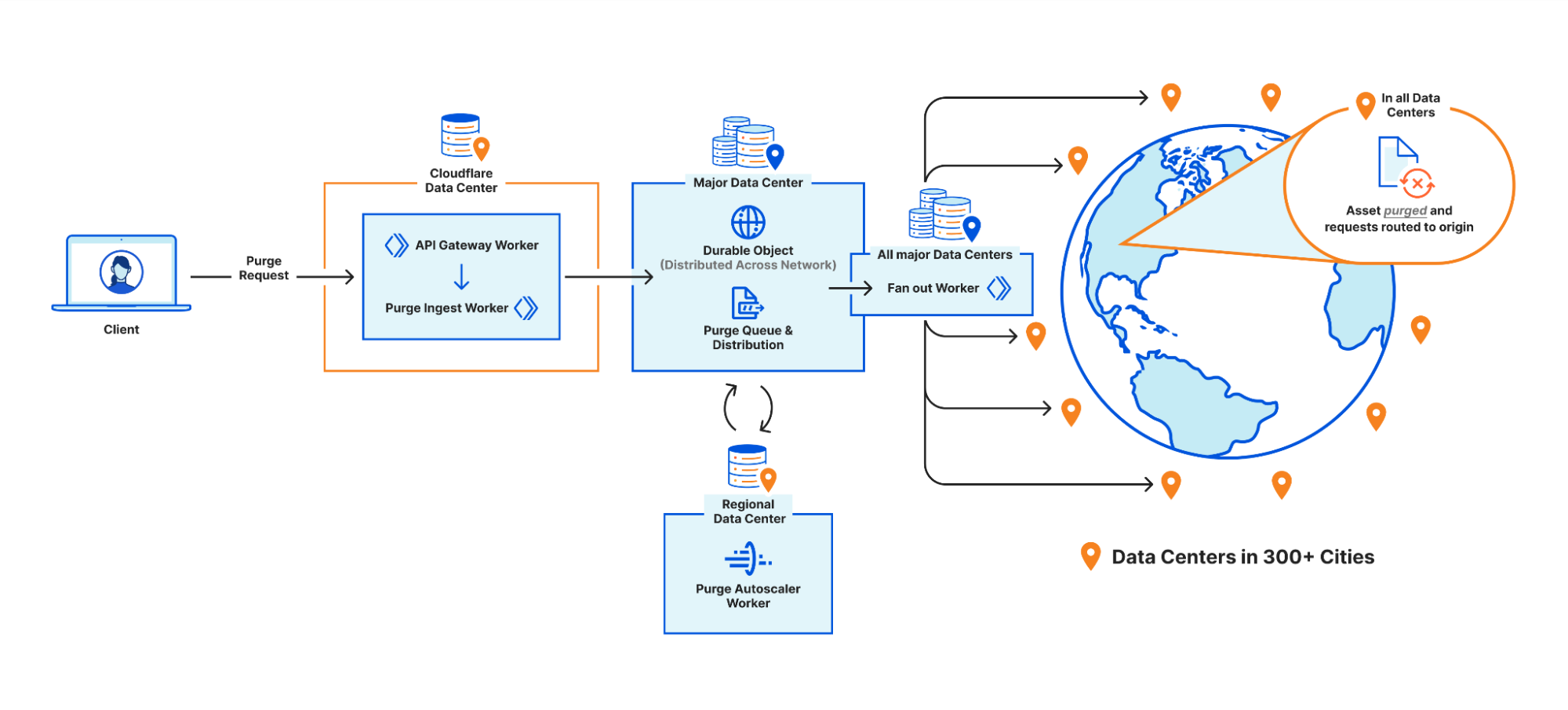
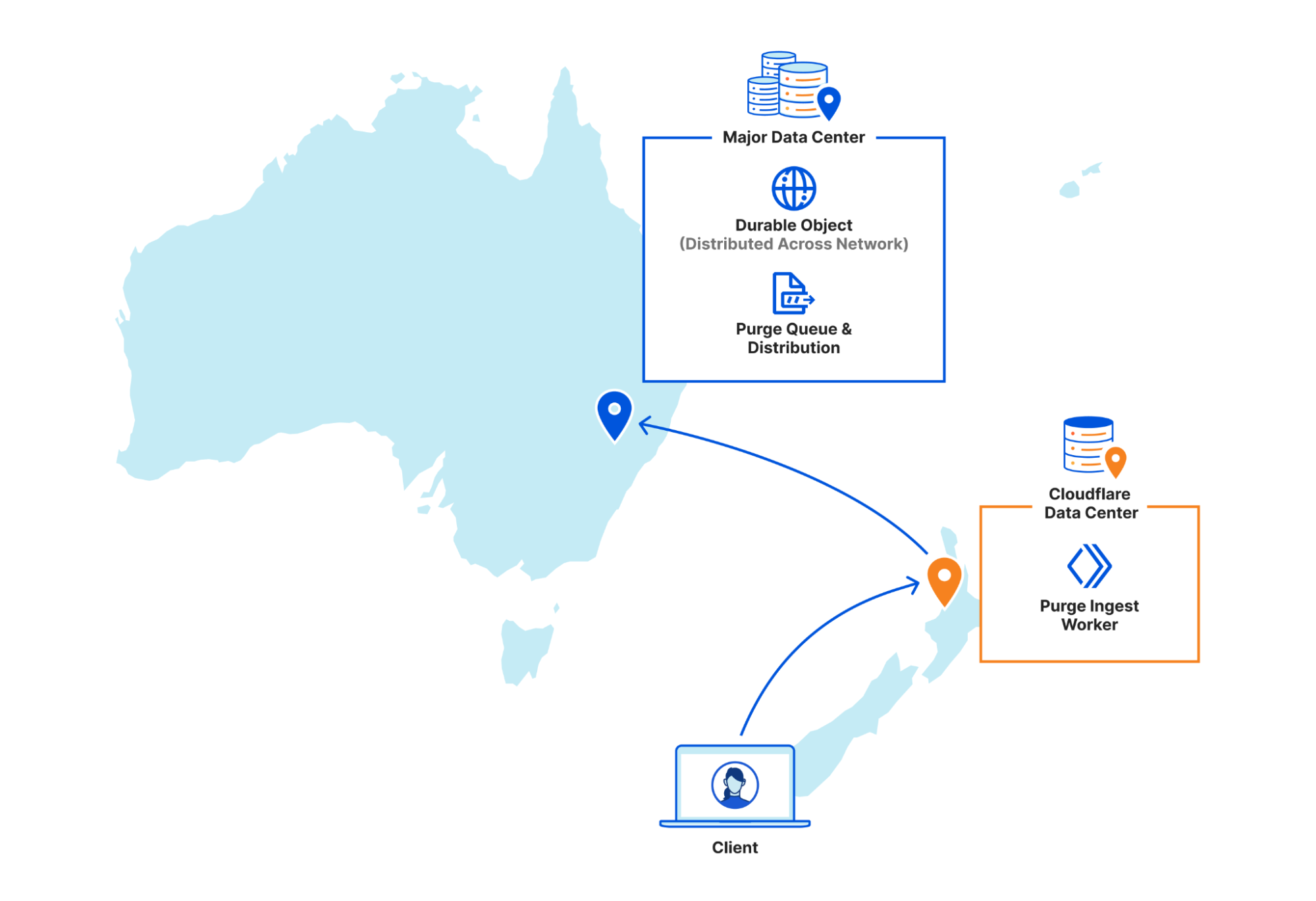
We touched on the high level design of what we called the “coreless” purge system in part 1, but let’s dive deeper into what that design encompasses by following a purge request from end to end:
Step 1: Request received locally
An API request to Cloudflare is routed to the nearest Cloudflare data center and passed to an API Gateway worker. This worker looks at the request URL to see which service it should be sent to and forwards the request to the appropriate upstream backend. Most endpoints of the Cloudflare API are currently handled by centralized services, so the API Gateway worker is often just proxying requests to the nearest “core” data center which have their own gateway services to handle authentication, authorization, and further routing. But for endpoints which aren’t handled centrally the API Gateway worker must handle authentication and route authorization, and then proxy to an appropriate upstream. For cache purge requests that upstream is a Purge Ingest worker in the same data center.
Step 2: Purges tested locally
The Purge Ingest worker evaluates the purge request to make sure it is processible. It scans the URLs in the body of the request to see if they’re valid, then attempts to purge the URLs from the local data center’s cache. This concept of local purging was a new step introduced with the coreless purge system allowing us to capitalize on existing logic already used in every data center.
By leveraging the same ownership checks our data centers use to serve a zone’s normal traffic on the URLs being purged, we can determine if those URLs are even cacheable by the zone. Currently more than 50% of the URLs we’re asked to purge can’t be cached by the requesting zones, either because they don’t own the URLs (e.g. a customer asking us to purge https://cloudflare.com) or because the zone’s settings for the URL prevent caching (e.g. the zone has a “bypass” cache rule that matches the URL). All such purges are superfluous and shouldn’t be processed further, so we filter them out and avoid broadcasting them to other data centers freeing up resources to process more legitimate purges.
On top of that, generating the cache key for a file isn’t free; we need to load zone configuration options that might affect the cache key, apply various transformations, et cetera. The cache key for a given file is the same in every data center though, so when we purge the file locally we now return the generated cache key to the Purge Ingest worker and broadcast that key to other data centers instead of making each data center generate it themselves.
Step 3: Purges queued for broadcasting
Once the local purge is done the Purge Ingest worker forwards the purge request with the cache key obtained from the local cache to a Purge Queue worker. The queue worker is a Durable Object worker using its persistent state to hold a queue of purges it receives and pointers to how far along in the queue each data center in our network is in processing purges.
The queue is important because it allows us to automatically recover from a number of scenarios such as connectivity issues or data centers coming back online after maintenance. Having a record of all purges since an issue arose lets us replay those purges to a data center and “catch up”.
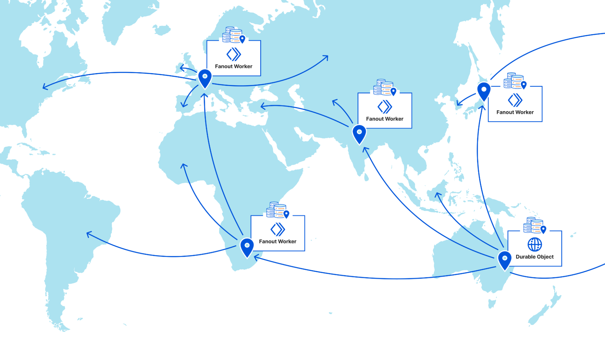
But Durable Objects are globally unique, so having one manage all global purges would have just moved our centrality problem from a core data center to wherever that Durable Object was provisioned. Instead we have dozens of Durable Objects in each region, and the Purge Ingest worker looks at the load balancing pool of Durable Objects for its region and picks one (often in the same data center) to forward the request to. The Durable Object will write the purge request to its queue and immediately loop through all the data center pointers and attempt to push any outstanding purges to each.
While benchmarking our performance we found our particular workload exhibited a “goldilocks zone” of throughput to a given Durable Object. On script startup we have to load all sorts of data like network topology and data center health–then refresh it continuously in the background–and as long as the Durable Object sees steady traffic it stays active and we amortize those startup costs. But if you ask a single Durable Object to do too much at once like send or receive too many requests, the single-threaded runtime won’t keep up. Regional purge traffic fluctuates a lot depending on local time of day, so there wasn’t a static quantity of Durable Objects per region that would let us stay within the goldilocks zone of enough requests to each to keep them active but not too many to keep them efficient. So we built load monitoring into our Durable Objects, and a Regional Autoscaler worker to aggregate that data and adjust load balancing pools when we start approaching the upper or lower edges of our efficiency goldilocks zone.
Step 4: Purges broadcast globally
Once a purge request is queued by a Purge Queue worker it needs to be broadcast to the rest of Cloudflare’s data centers to be carried out by their caches. The Durable Objects will broadcast purges directly to all data centers in their region, but when broadcasting to other regions they pick a Purge Fanout worker per region to take care of their region’s distribution. The fanout workers manage queues of their own as well as pointers for all of their region’s data centers, and in fact they share a lot of the same logic as the Purge Queue workers in order to do so. One key difference is fanout workers aren’t Durable Objects; they’re normal worker scripts, and their queues are purely in memory as opposed to being backed by Durable Object state. This means not all queue worker Durable Objects are talking to the same fanout worker in each region. Fanout workers can be dropped and spun up again quickly by any metal in the data center because they aren’t canonical sources of state. They maintain queues and pointers for their region but all of that info is also sent back downstream to the Durable Objects who persist that data themselves, reliably.
But what does the fanout worker get us? Cloudflare has hundreds of data centers all over the world, and as we mentioned above we benefit from keeping the number of incoming and outgoing requests for a Durable Object fairly low. Sending purges to a fanout worker per region means each Durable Object only has to make a fraction of the requests it would if it were broadcasting to every data center directly, which means it can process purges faster.
On top of that, occasionally a request will fail to get where it was going and require retransmission. When this happens between data centers in the same region it’s largely unnoticeable, but when a Durable Object in Canada has to retry a request to a data center in rural South Africa the cost of traversing that whole distance again is steep. The data centers elected to host fanout workers have the most reliable connections in their regions to the rest of our network. This minimizes the chance of inter-regional retries and limits the latency imposed by retries to regional timescales.
The introduction of the Purge Fanout worker was a massive improvement to our distribution system, reducing our end-to-end purge latency by 50% on its own and increasing our throughput threefold.
Current status of coreless purge
We are proud to say our new purge system has been in production serving purge by URL requests since July 2022, and the results in terms of latency improvements are dramatic. In addition, flexible purge requests (purge by tag/prefix/host and purge everything) share and benefit from the new coreless purge system’s entrypoint workers before heading to a core data center for fulfillment.
The reason flexible purge isn’t also fully coreless yet is because it’s a more complex task than “purge this object”; flexible purge requests can end up purging multiple objects–or even entire zones–from cache. They do this through an entirely different process that isn’t coreless compatible, so to make flexible purge fully coreless we would have needed to come up with an entirely new multi-purge mechanism on top of redesigning distribution. We chose instead to start with just purge by URL so we could focus purely on the most impactful improvements, revamping distribution, without reworking the logic a data center uses to actually remove an object from cache.
This is not to say that the flexible purges haven’t benefited from the coreless purge project. Our cache purge API lets users bundle single file and flexible purges in one request, so the API Gateway worker and Purge Ingest worker handle authorization, authentication and payload validation for flexible purges too. Those flexible purges get forwarded directly to our services in core data centers pre-authorized and validated which reduces load on those core data center auth services. As an added benefit, because authorization and validity checks all happen at the edge for all purge types users get much faster feedback when their requests are malformed.
Next steps
While coreless cache purge has come a long way since the part 1 blog post, we’re not done. We continue to work on reducing end-to-end latency even more for purge by URL because we can do better. Alongside improvements to our new distribution system, we’ve also been working on the redesign of flexible purge to make it fully coreless, and we’re really excited to share the results we’re seeing soon. Flexible cache purge is an incredibly popular API and we’re giving its refresh the care and attention it deserves.
In January and in March we posted blogs outlining how Cloudflare performed against others in Zero Trust. The conclusion in both cases was that Cloudflare was faster than Zscaler and Netskope in a variety of Zero Trust scenarios. For Speed Week, we’re bringing back these tests and upping the ante: we’re testing more providers against more public Internet endpoints in more regions than we have in the past.
For these tests, we tested three Zero Trust scenarios: Secure Web Gateway (SWG), Zero Trust Network Access (ZTNA), and Remote Browser Isolation (RBI). We tested against three competitors: Zscaler, Netskope, and Palo Alto Networks. We tested these scenarios from 12 regions around the world, up from the four we’d previously tested with. The results are that Cloudflare is the fastest Secure Web Gateway in 42% of testing scenarios, the most of any provider. Cloudflare is 46% faster than Zscaler, 56% faster than Netskope, and 10% faster than Palo Alto for ZTNA, and 64% faster than Zscaler for RBI scenarios.
In this blog, we’ll provide a refresher on why performance matters, do a deep dive on how we’re faster for each scenario, and we’ll talk about how we measured performance for each product.
Performance is a threat vector
Performance in Zero Trust matters; when Zero Trust performs poorly, users disable it, opening organizations to risk. Zero Trust services should be unobtrusive when the services become noticeable they prevent users from getting their job done.
Zero Trust services may have lots of bells and whistles that help protect customers, but none of that matters if employees can’t use the services to do their job quickly and efficiently. Fast performance helps drive adoption and makes security feel transparent to the end users. At Cloudflare, we prioritize making our products fast and frictionless, and the results speak for themselves. So now let’s turn it over to the results, starting with our secure web gateway.
Cloudflare Gateway: security at the Internet
A secure web gateway needs to be fast because it acts as a funnel for all of an organization’s Internet-bound traffic. If a secure web gateway is slow, then any traffic from users out to the Internet will be slow. If traffic out to the Internet is slow, users may see web pages load slowly, video calls experience jitter or loss, or generally unable to do their jobs. Users may decide to turn off the gateway, putting the organization at risk of attack.
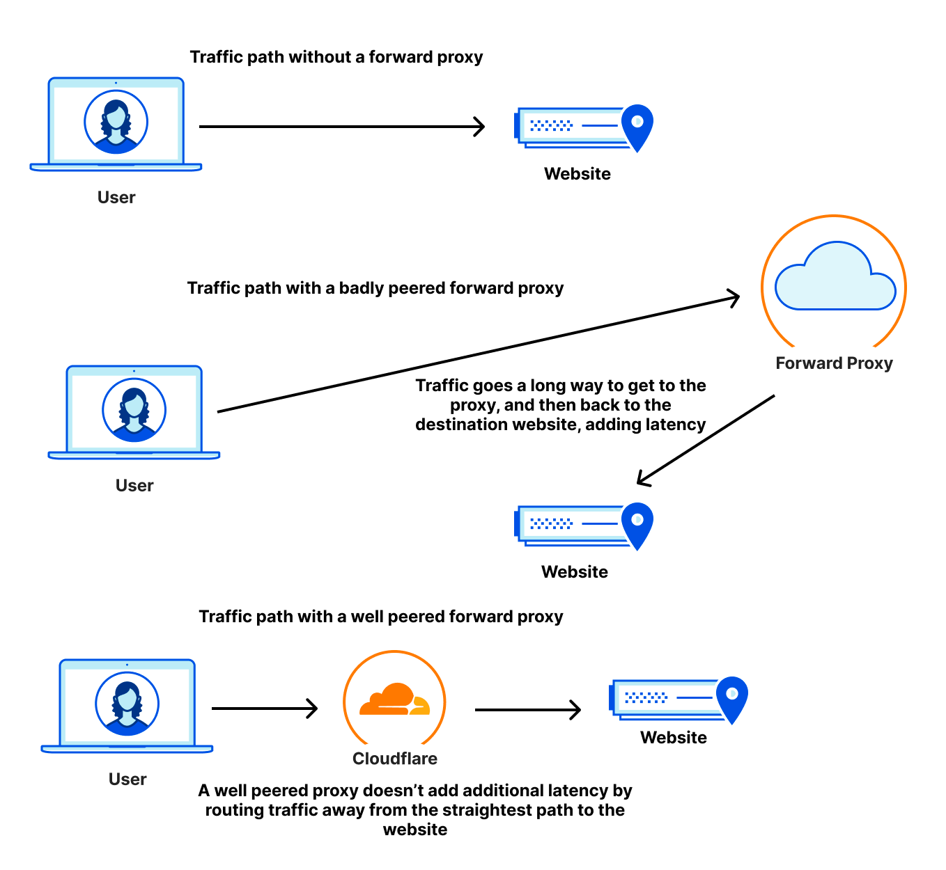
In addition to being close to users, a performant web gateway needs to also be well-peered with the rest of the Internet to avoid slow paths out to websites users want to access. Many websites use CDNs to accelerate their content and provide a better experience. These CDNs are often well-peered and embedded in last mile networks. But traffic through a secure web gateway follows a forward proxy path: users connect to the proxy, and the proxy connects to the websites users are trying to access. If that proxy isn’t as well-peered as the destination websites are, the user traffic could travel farther to get to the proxy than it would have needed to if it was just going to the website itself, creating a hairpin, as seen in the diagram below:
A well-connected proxy ensures that the user traffic travels less distance making it as fast as possible.
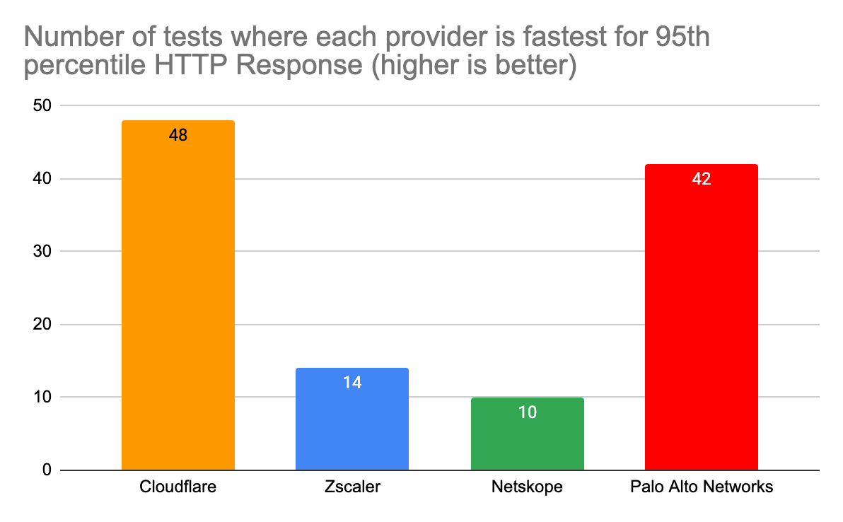
To compare secure web gateway products, we pitted the Cloudflare Gateway and WARP client against Zscaler, Netskope, and Palo Alto which all have products that perform the same functions. Cloudflare users benefit from Gateway and Cloudflare’s network being embedded deep into last mile networks close to users, being peered with over 12,000 networks. That heightened connectivity shows because Cloudflare Gateway is the fastest network in 42% of tested scenarios:
Number of testing scenarios where each provider is fastest for 95th percentile HTTP Response time (higher is better)
Provider
Scenarios where this provider is fastest
Cloudflare
48
Zscaler
14
Netskope
10
Palo Alto Networks
42
This data shows that we are faster to more websites from more places than any of our competitors. To measure this, we look at the 95th percentile HTTP response time: how long it takes for a user to go through the proxy, have the proxy make a request to a website on the Internet, and finally return the response. This measurement is important because it’s an accurate representation of what users see. When we look at the 95th percentile across all tests, we see that Cloudflare is 2.5% faster than Palo Alto Networks, 13% faster than Zscaler, and 6.5% faster than Netskope.
95th percentile HTTP response across all tests
Provider
95th percentile response (ms)
Cloudflare
515
Zscaler
595
Netskope
550
Palo Alto Networks
529
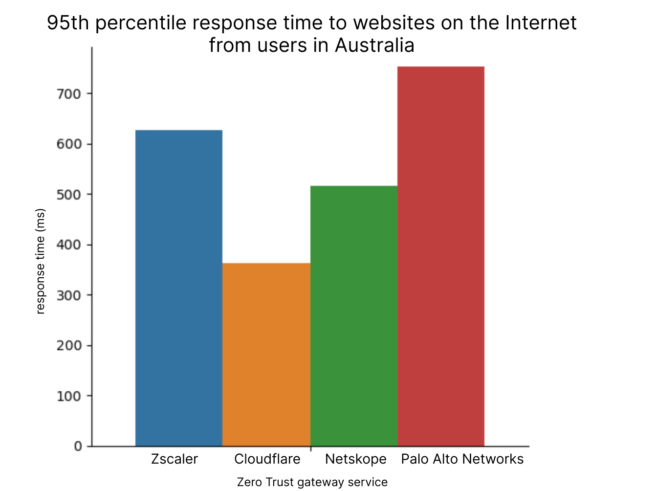
Cloudflare wins out here because Cloudflare’s exceptional peering allows us to succeed in places where others were not able to succeed. We are able to get locally peered in hard-to-reach places on the globe, giving us an edge. For example, take a look at how Cloudflare performs against the others in Australia, where we are 30% faster than the next fastest provider:
Cloudflare establishes great peering relationships in countries around the world: in Australia we are locally peered with all of the major Australian Internet providers, and as such we are able to provide a fast experience to many users around the world. Globally, we are peered with over 12,000 networks, getting as close to end users as we can to shorten the time requests spend on the public Internet. This work has previously allowed us to deliver content quickly to users, but in a Zero Trust world, it shortens the path users take to get to their SWG, meaning they can quickly get to the services they need.
Previously when we performed these tests, we only tested from a single Azure region to five websites. Existing testing frameworks like Catchpoint are unsuitable for this task because performance testing requires that you run the SWG client on the testing endpoint. We also needed to make sure that all of the tests are running on similar machines in the same places to measure performance as well as possible. This allows us to measure the end-to-end responses coming from the same location where both test environments are running.
In our testing configuration for this round of evaluations, we put four VMs in 12 cloud regions side by side: one running Cloudflare WARP connecting to our gateway, one running ZIA, one running Netskope, and one running Palo Alto Networks. These VMs made requests every five minutes to the 11 different websites mentioned below and logged the HTTP browser timings for how long each request took. Based on this, we are able to get a user-facing view of performance that is meaningful. Here is a full matrix of locations that we tested from, what websites we tested against, and which provider was faster:
Endpoints
SWG Regions
Shopify
Walmart
Zendesk
ServiceNow
Azure Site
Slack
Zoom
Box
M365
GitHub
Bitbucket
East US
Cloudflare
Cloudflare
Palo Alto Networks
Cloudflare
Palo Alto Networks
Cloudflare
Palo Alto Networks
Cloudflare
West US
Palo Alto Networks
Palo Alto Networks
Cloudflare
Cloudflare
Palo Alto Networks
Cloudflare
Palo Alto Networks
Cloudflare
South Central US
Cloudflare
Cloudflare
Palo Alto Networks
Cloudflare
Palo Alto Networks
Cloudflare
Palo Alto Networks
Cloudflare
Brazil South
Cloudflare
Palo Alto Networks
Palo Alto Networks
Palo Alto Networks
Zscaler
Zscaler
Zscaler
Palo Alto Networks
Cloudflare
Palo Alto Networks
Palo Alto Networks
UK South
Cloudflare
Palo Alto Networks
Palo Alto Networks
Palo Alto Networks
Palo Alto Networks
Palo Alto Networks
Palo Alto Networks
Cloudflare
Palo Alto Networks
Palo Alto Networks
Palo Alto Networks
Central India
Cloudflare
Cloudflare
Cloudflare
Palo Alto Networks
Palo Alto Networks
Cloudflare
Cloudflare
Cloudflare
Southeast Asia
Cloudflare
Cloudflare
Cloudflare
Cloudflare
Palo Alto Networks
Cloudflare
Cloudflare
Cloudflare
Canada Central
Cloudflare
Cloudflare
Palo Alto Networks
Cloudflare
Cloudflare
Palo Alto Networks
Palo Alto Networks
Palo Alto Networks
Zscaler
Cloudflare
Zscaler
Switzerland North
netskope
Zscaler
Zscaler
Cloudflare
netskope
netskope
netskope
netskope
Cloudflare
Cloudflare
netskope
Australia East
Cloudflare
Cloudflare
netskope
Cloudflare
Cloudflare
Cloudflare
Cloudflare
Cloudflare
UAE Dubai
Zscaler
Zscaler
Cloudflare
Cloudflare
Zscaler
netskope
Palo Alto Networks
Zscaler
Zscaler
netskope
netskope
South Africa North
Palo Alto Networks
Palo Alto Networks
Palo Alto Networks
Zscaler
Palo Alto Networks
Palo Alto Networks
Palo Alto Networks
Palo Alto Networks
Zscaler
Palo Alto Networks
Palo Alto Networks
Blank cells indicate that tests to that particular website did not report accurate results or experienced failures for over 50% of the testing period. Based on this data, Cloudflare is generally faster, but we’re not as fast as we’d like to be. There are still some areas where we need to improve, specifically in South Africa, UAE, and Brazil. By Birthday Week in September, we want to be the fastest to all of these websites in each of these regions, which will bring our number up from fastest in 54% of tests to fastest in 79% of tests.
To summarize, Cloudflare’s Gateway is still the fastest SWG on the Internet. But Zero Trust isn’t all about SWG. Let’s talk about how Cloudflare performs in Zero Trust Network Access scenarios.
Instant (Zero Trust) access
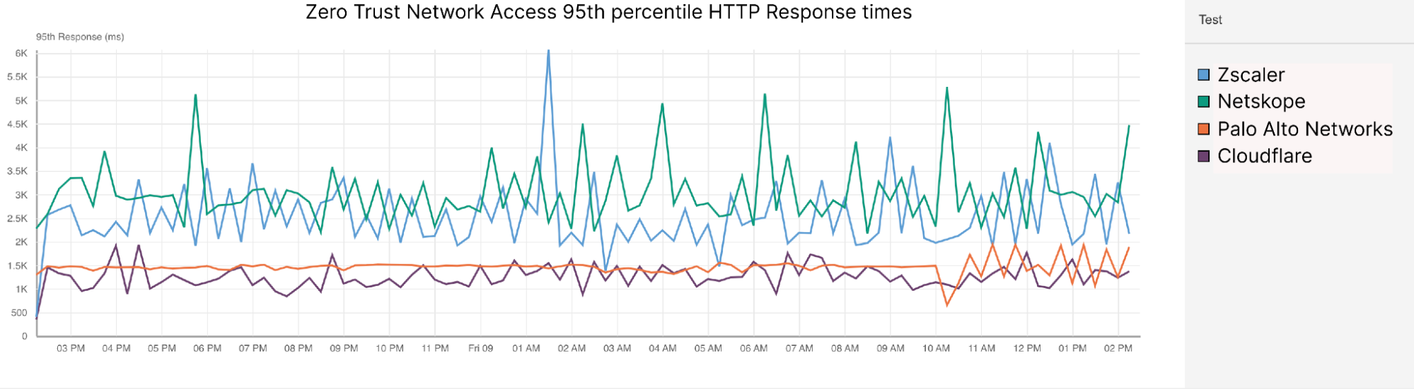
Access control needs to be seamless and transparent to the user: the best compliment for a Zero Trust solution is for employees to barely notice it’s there. Services like Cloudflare Access protect applications over the public Internet, allowing for role-based authentication access instead of relying on things like a VPN to restrict and secure applications. This form of access management is more secure, but with a performant ZTNA service, it can even be faster.
Cloudflare outperforms our competitors in this space, being 46% faster than Zscaler, 56% faster than Netskope, and 10% faster than Palo Alto Networks:
Zero Trust Network Access P95 HTTP Response times
Provider
P95 HTTP response (ms)
Cloudflare
1252
Zscaler
2388
Netskope
2974
Palo Alto Networks
1471
For this test, we created applications hosted in three different clouds in 12 different locations: AWS, GCP, and Azure. However, it should be noted that Palo Alto Networks was the exception, as we were only able to measure them using applications hosted in one cloud from two regions due to logistical challenges with setting up testing: US East and Singapore.
For each of these applications, we created tests from Catchpoint that accessed the application from 400 locations around the world. Each of these Catchpoint nodes attempted two actions:
New Session: log into an application and receive an authentication token
Existing Session: refresh the page and log in passing the previously obtained credentials
We like to measure these scenarios separately, because when we look at 95th percentile values, we would almost always be looking at new sessions if we combined new and existing sessions together. For the sake of completeness though, we will also show the 95th percentile latency of both new and existing sessions combined.
Cloudflare was faster in both US East and Singapore, but let’s spotlight a couple of regions to delve into. Let’s take a look at a region where resources are heavily interconnected equally across competitors: US East, specifically Ashburn, Virginia.
In Ashburn, Virginia, Cloudflare handily beats Zscaler and Netskope for ZTNA 95th percentile HTTP Response:
95th percentile HTTP Response times (ms) for applications hosted in Ashburn, VA
AWS East US
Total (ms)
New Sessions (ms)
Existing Sessions (ms)
Cloudflare
2849
1749
1353
Zscaler
5340
2953
2491
Netskope
6513
3748
2897
Palo Alto Networks
Azure East US
Cloudflare
1692
989
1169
Zscaler
5403
2951
2412
Netskope
6601
3805
2964
Palo Alto Networks
GCP East US
Cloudflare
2811
1615
1320
Zscaler
Netskope
6694
3819
3023
Palo Alto Networks
2258
894
1464
You might notice that Palo Alto Networks looks to come out ahead of Cloudflare for existing sessions (and therefore for overall 95th percentile). But these numbers are misleading because Palo Alto Networks’ ZTNA behavior is slightly different than ours, Zscaler’s, or Netskope’s. When they perform a new session, it does a full connection intercept and returns a response from its processors instead of directing users to the login page of the application they are trying to access.
This means that Palo Alto Networks' new session response times don’t actually measure the end-to-end latency we’re looking for. Because of this, their numbers for new session latency and total session latency are misleading, meaning we can only meaningfully compare ourselves to them for existing session latency. When we look at existing sessions, when Palo Alto Networks acts as a pass-through, Cloudflare still comes out ahead by 10%.
This is true in Singapore as well, where Cloudflare is 50% faster than Zscaler and Netskope, and also 10% faster than Palo Alto Networks for Existing Sessions:
95th percentile HTTP Response times (ms) for applications hosted in Singapore
AWS Singapore
Total (ms)
New Sessions (ms)
Existing Sessions (ms)
Cloudflare
2748
1568
1310
Zscaler
5349
3033
2500
Netskope
6402
3598
2990
Palo Alto Networks
Azure Singapore
Cloudflare
1831
1022
1181
Zscaler
5699
3037
2577
Netskope
6722
3834
3040
Palo Alto Networks
GCPSingapore
Cloudflare
2820
1641
1355
Zscaler
5499
3037
2412
Netskope
6525
3713
2992
Palo Alto Networks
2293
922
1476
One critique of this data could be that we’re aggregating the times of all Catchpoint nodes together at P95, and we’re not looking at the 95th percentile of Catchpoint nodes in the same region as the application. We looked at that, too, and Cloudflare’s ZTNA performance is still better. Looking at only North America-based Catchpoint nodes, Cloudflare performs 50% better than Netskope, 40% better than Zscaler, and 10% better than Palo Alto Networks at P95 for warm connections:
Zero Trust Network Access 95th percentile HTTP Response times for warm connections with testing locations in North America
Provider
P95 HTTP response (ms)
Cloudflare
810
Zscaler
1290
Netskope
1351
Palo Alto Networks
871
Finally, one thing we wanted to show about our ZTNA performance was how well Cloudflare performed per cloud per region. This below chart shows the matrix of cloud providers and tested regions:
Fastest ZTNA provider in each cloud provider and region by 95th percentile HTTP Response
AWS
Azure
GCP
Australia East
Cloudflare
Cloudflare
Cloudflare
Brazil South
Cloudflare
Cloudflare
N/A
Canada Central
Cloudflare
Cloudflare
Cloudflare
Central India
Cloudflare
Cloudflare
Cloudflare
East US
Cloudflare
Cloudflare
Cloudflare
South Africa North
Cloudflare
Cloudflare
N/A
South Central US
N/A
Cloudflare
Zscaler
Southeast Asia
Cloudflare
Cloudflare
Cloudflare
Switzerland North
N/A
N/A
Cloudflare
UAE Dubai
Cloudflare
Cloudflare
Cloudflare
UK South
Cloudflare
Cloudflare
netskope
West US
Cloudflare
Cloudflare
N/A
There were some VMs in some clouds that malfunctioned and didn’t report accurate data. But out of 30 available cloud regions where we had accurate data, Cloudflare was the fastest ZT provider in 28 of them, meaning we were faster in 93% of tested cloud regions.
To summarize, Cloudflare also provides the best experience when evaluating Zero Trust Network Access. But what about another piece of the puzzle: Remote Browser Isolation (RBI)?
Remote Browser Isolation: a secure browser hosted in the cloud
Remote browser isolation products have a very strong dependency on the public Internet: if your connection to your browser isolation product isn’t good, then your browser experience will feel weird and slow. Remote browser isolation is extraordinarily dependent on performance to feel smooth and seamless to the users: if everything is fast as it should be, then users shouldn’t even notice that they’re using browser isolation.
For this test, we’re again pitting Cloudflare against Zscaler. While Netskope does have an RBI product, we were unable to test it due to it requiring a SWG client, meaning we would be unable to get full fidelity of testing locations like we would when testing Cloudflare and Zscaler. Our tests showed that Cloudflare is 64% faster than Zscaler for remote browsing scenarios: Here’s a matrix of fastest provider per cloud per region for our RBI tests:
Fastest RBI provider in each cloud provider and region by 95th percentile HTTP Response
AWS
Azure
GCP
Australia East
Cloudflare
Cloudflare
Cloudflare
Brazil South
Cloudflare
Cloudflare
Cloudflare
Canada Central
Cloudflare
Cloudflare
Cloudflare
Central India
Cloudflare
Cloudflare
Cloudflare
East US
Cloudflare
Cloudflare
Cloudflare
South Africa North
Cloudflare
Cloudflare
South Central US
Cloudflare
Cloudflare
Southeast Asia
Cloudflare
Cloudflare
Cloudflare
Switzerland North
Cloudflare
Cloudflare
Cloudflare
UAE Dubai
Cloudflare
Cloudflare
Cloudflare
UK South
Cloudflare
Cloudflare
Cloudflare
West US
Cloudflare
Cloudflare
Cloudflare
This chart shows the results of all of the tests run against Cloudflare and Zscaler to applications hosted on three different clouds in 12 different locations from the same 400 Catchpoint nodes as the ZTNA tests. In every scenario, Cloudflare was faster. In fact, no test against a Cloudflare-protected endpoint had a 95th percentile HTTP Response of above 2105 ms, while no Zscaler-protected endpoint had a 95th percentile HTTP response of below 5000 ms.
To get this data, we leveraged the same VMs to host applications accessed through RBI services. Each Catchpoint node would attempt to log into the application through RBI, receive authentication credentials, and then try to access the page by passing the credentials. We look at the same new and existing sessions that we do for ZTNA, and Cloudflare is faster in both new sessions and existing session scenarios as well.
Gotta go fast(er)
Our Zero Trust customers want us to be fast not because they want the fastest Internet access, but because they want to know that employee productivity won’t be impacted by switching to Cloudflare. That doesn’t necessarily mean that the most important thing for us is being faster than our competitors, although we are. The most important thing for us is improving our experience so that our users feel comfortable knowing we take their experience seriously. When we put out new numbers for Birthday Week in September and we’re faster than we were before, it won’t mean that we just made the numbers go up: it means that we are constantly evaluating and improving our service to provide the best experience for our customers. We care more that our customers in UAE have an improved experience with Office365 as opposed to beating a competitor in a test. We show these numbers so that we can show you that we take performance seriously, and we’re committed to providing the best experience for you, wherever you are.
Today, we’re making the case for why Time To First Byte (TTFB) is not a good metric for evaluating how fast web pages load. There are better metrics out there that give a more accurate representation of how well a server or content delivery network performs for end users. In this blog, we’ll go over the ambiguity of measuring TTFB, touch on more meaningful metrics such as Core Web Vitals that should be used instead, and finish on scenarios where TTFB still makes sense to measure.
Many of our customers ask what the best way would be to evaluate how well a network like ours works. This is a good question! Measuring performance is difficult. It’s easy to simplify the question to “How close is Cloudflare to end users?” The predominant metric that’s been used to measure that is round trip time (RTT). This is the time it takes for one network packet to travel from an end user to Cloudflare and back. We measure this metric and mention it from time to time: Cloudflare has an average RTT of 50 milliseconds for 95% of the Internet-connected population.
Whilst RTT is a relatively good indicator of the quality of a network, it doesn’t necessarily tell you that much about how good it is at actually delivering actual websites to end users. For instance, what if the web server is really slow? A user might be very close to the data center that serves the traffic, but if it takes a long time to actually grab the asset from disk and serve it the result will still be a poor experience.
This is where TTFB comes in. It measures the time it takes between a request being sent from an end user until the very first byte of the response being received. This sounds great on paper! However it doesn’t capture how a webpage or web application loads, and what happens after the first byte is received.
In this blog we’ll cover what TTFB is a good indicator of, what it's not great for, and what you should be using instead.
What is TTFB?
TTFB is a metric which reports the duration between sending the request from the client to a server for a given file, and the receipt of the first byte of said file. For example, if you were to download the Cloudflare logo from our website the TTFB would be how long it took to receive the first byte of that image. Similarly, if you were to measure the TTFB of a request to cloudflare.com the metric would return the TTFB of how long it took from request to receiving the first byte of the first HTTP response. Not how long it took for the image to be fully visible or for the web page to be loaded in a state that allowed a user to begin using it.
The simplest answer therefore is to look at the diametrically opposite measurement, Time to Last Byte (TTLB). TTLB, as you’d expect, measures how long it takes until the last byte of data is received from the server. For the Cloudflare logo file this would make sense, as until the image is fully downloaded it's not exactly useful. But what about for a webpage? Do you really need to wait until every single file is fully downloaded, even those images at the bottom of the page you can't immediately see? TTLB is fine for measuring how long it took to download a single file from a CDN / server. However for multi-faceted traffic, like web pages, it is too conservative, as it doesn’t tell you how long it took for the web page to be usable.
As an analogy we can look at measuring how long it takes to process an incoming airplane full of passengers. What's important is to understand how long it takes for those passengers to disembark, pass through passport control, collect their baggage and leave the terminal, if no onward journeys. TTFB would measure success as how long it took to get the first passenger off of the airplane. TTLB would measure how long it took the last passenger to leave the terminal, even if this passenger remained in the terminal for hours afterwards due to passport issues or getting lost. Neither are a good measure of success for the airline.
Why TTFB doesn't make sense
TTFB is a widely-used metric because it is easy-to-understand and it is a great signal for connection setup time, server time and network latency. It can help website owners identify when performance issues originate from their server. But is TTFB a good signal for how real users experience the loading speed of a web page in a browser?
When a web page loads in a browser, the user’s perception of speed isn’t related to the moment the browser first receives bytes of data. It is related to when the user starts to see the page rendering on the screen.
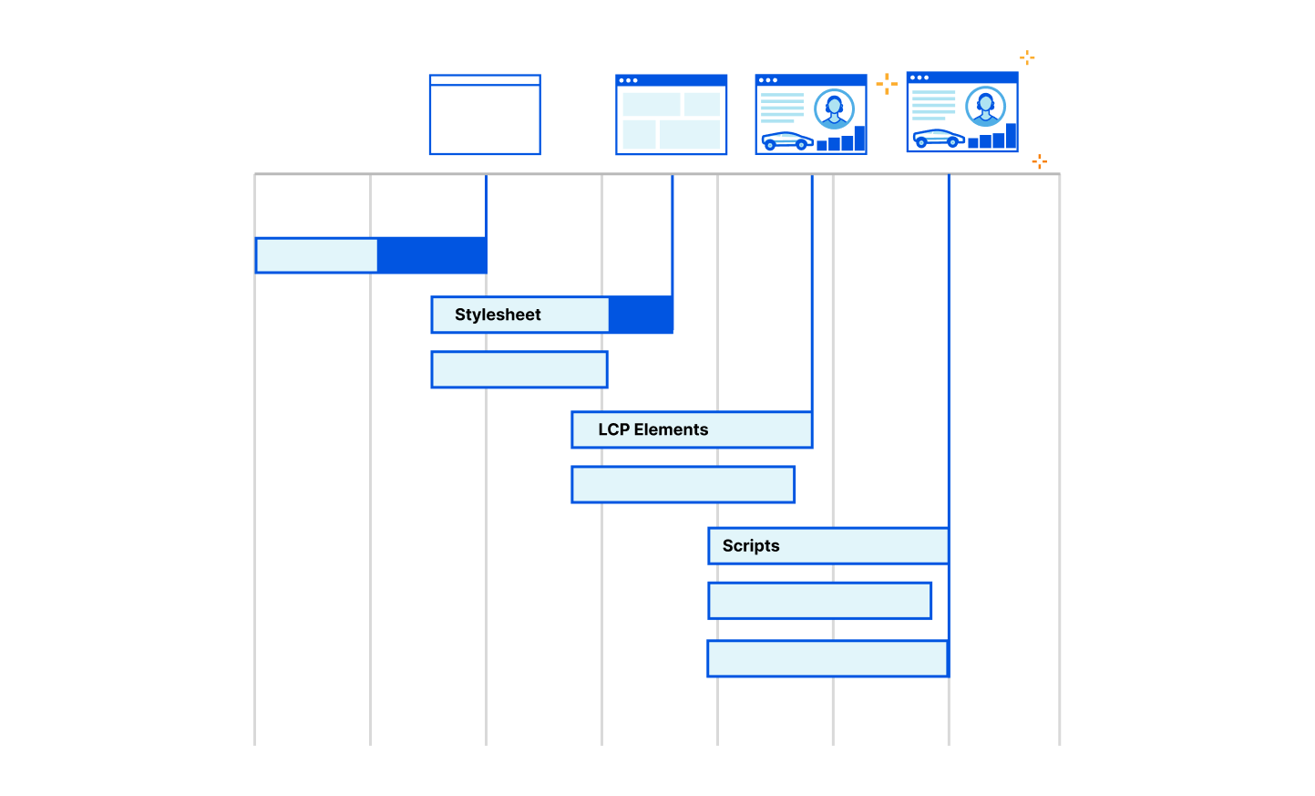
The loading of a web page in a browser is a very complex process. Almost all of this process happens after TTFB is reported. After the first byte has been received, the browser still has to load the main HTML file. It also has to load fonts, stylesheets, javascript, images and other resources. Often these resources link to other resources that also must be downloaded. Often these resources entirely block the rendering of the page. Alongside all these downloads, the browser is also parsing the HTML, CSS and JavaScript. It is building data structures that represent the content of the web page as well as how it is styled. All of this is in preparation to start rendering the final page onto the screen for the user.
When the user starts seeing the web page actually rendered on the screen, TTFB has become a distant memory for the browser. For a metric that signals the loading speed as perceived by the user, TTFB falls dramatically short.
Receiving the first byte isn't sufficient to determine a good end user experience as most pages have additional render blocking resources that get loaded after the initial document request. Render-blocking resources are scripts, stylesheets, and HTML imports that prevent a web page from loading quickly. From a TTFB perspective it means the client could stop the ‘TTFB clock’ on receipt of the first byte of one of these files, but the web browser is blocked from showing anything to the user until the remaining critical assets are downloaded.
This is because browsers need instructions for what to render and what resources need to be fetched to complete “painting” a given web page. These instructions come from a server response. But the servers sending these responses often need time to compile these resources — this is known as “server think time.” While the servers are busy during this time… browsers sit idle and wait. And the TTFB counter goes up.
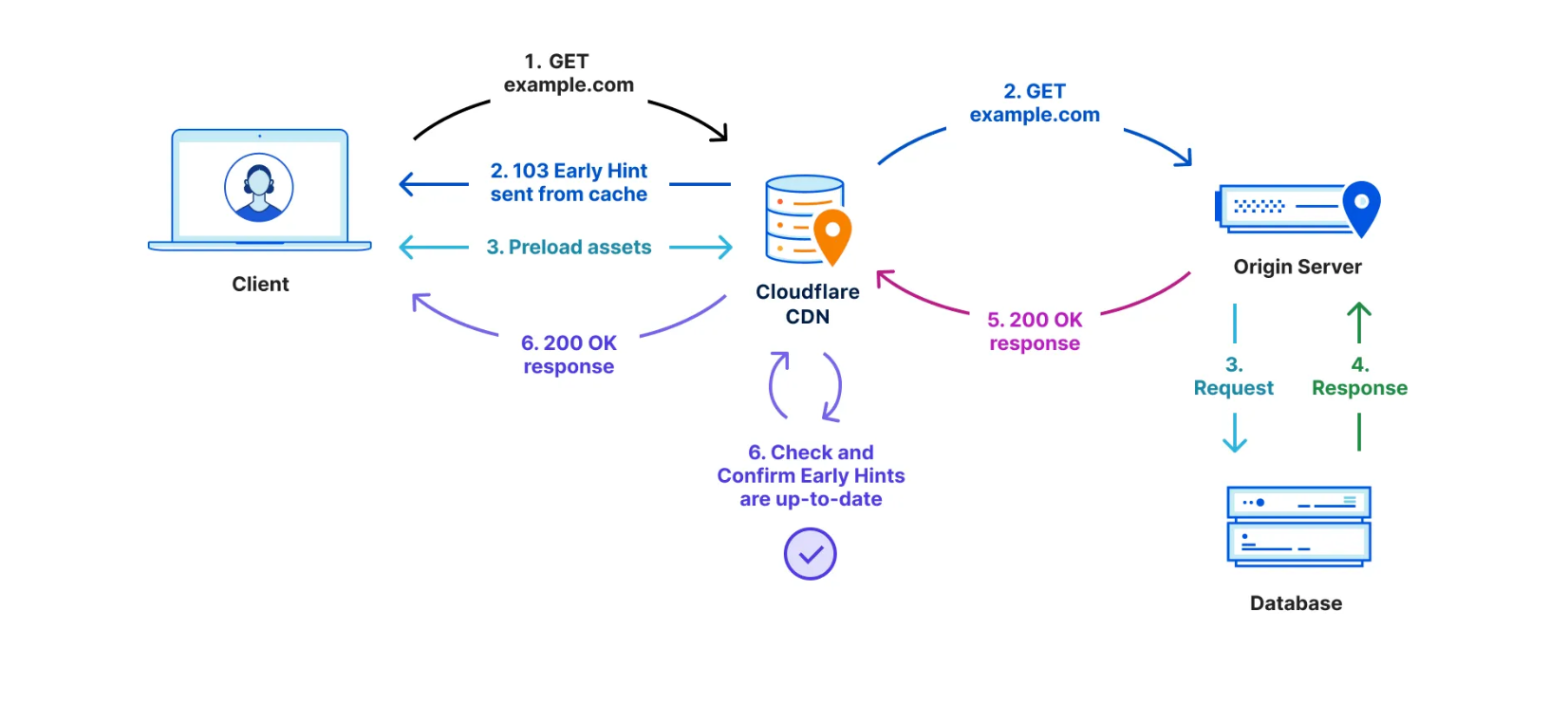
There have been a number of attempts over the years to benefit from this “think time”. First came Server Push, which was superseded last year by Early Hints. Early Hints take advantage of “server think time” to asynchronously send instructions to the browser to begin loading resources while the origin server is compiling the full response. By sending these hints to a browser before the full response is prepared, the browser can figure out what it needs to do to load the webpage faster for the end user. It also stops the TTFB clock, meaning a lower TTFB. This helps ensure the browser gets the critical files sooner to begin loading the webpage, and it also means the first byte is delivered sooner as there is no waiting on the server for the whole dataset to be prepared and ready to send. Even with Early Hints, though, TTFB doesn’t accurately define how long it took the web page to be in a usable state.
TTFB also does not take into account multiplexing benefits of HTTP/2 and HTTP/3 which allow browsers to load files in parallel. It also doesn't take into account compression on the origin, which would result in a higher TTFB but a quicker page load overall due to the time the server took to compress the assets and send them in a small format over the network.
Cloudflare offers many features that can improve the loading speed of a website, but don’t necessarily impact the TTFB score. These features include Zaraz, Rocket Loader, HTTP/2 and HTTP/3 Prioritization, Mirage, Polish, Image Resizing, Auto Minify and Cache. These features improve the loading time of a webpage, ensuring they load optimally through a series of enhancements from image optimization and compression to render blocking elimination by optimizing the sending of assets from the server to the browser in the best possible order.
More comprehensive metrics are required to illustrate the full loading process of a web page, and the benefit provided by these features. This is where Real User Monitoring helps. At Cloudflare we are all-in on Real User Monitoring (RUM) as the future of website performance. We’re investing heavily in it: both from an observation point of view and from an optimization one also.
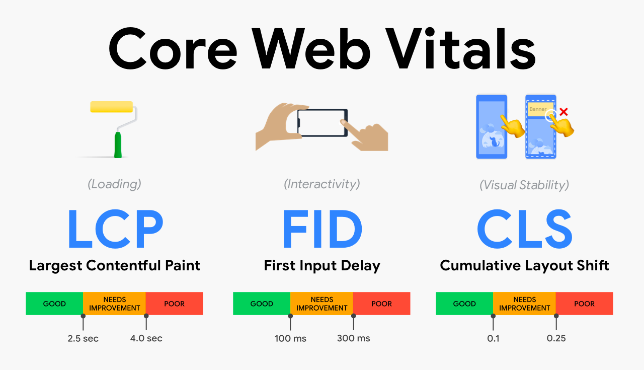
For those unfamiliar with RUM, we typically optimize websites for three main metrics – known as the “Core Web Vitals”. This is a set of key metrics which are believed to be the best and most accurate representation of a poorly performing website vs a well performing one. These key metrics are Largest Contentful Paint, First Input Delay and Cumulative Layout Shift.
LCP measures loading performance; typically how long it takes to load the largest image or text block visible in the browser. FID measures interactivity. For example, the time between when a user clicks or taps on a button to when the browser responds and starts doing something. Finally, CLS measures visual stability. A good, or bad example of CLS is when you go to a website on your mobile phone, tap on a link and the page moves at the last second meaning you tap something you didn't want to. That would be a lower CLS score as its poor user experience.
Looking at these metrics gives us a good idea of how the end user is truly experiencing your website (RUM) vs. how quickly the first byte of the file was retrieved from the nearest Cloudflare data center (TTFB).
Good TTFB, bad user experience
One of the “sub parts” that comprise LCP is TTFB. That means a poor TTFB is very likely to result in a poor LCP. If it takes you 20 seconds to retrieve the first byte of the first image, your user isn't going to have a good experience – regardless of your outlook on TTFB vs RUM.
Conversely, we found that a good TTFB does not always mean a good LCP score, or FID or CLS. We ran a query to collect RUM metrics of web pages we served which had a good TTFB score. Good is defined as a TTFB as less than 800ms. This allowed us to ask the question: TTFB says these websites are good. Does the RUM data support that?
We took four distinct samples from our RUM data in June. Each sample had a different date-range and sample-rate combination. In each sample we queried for 200,000 page views. From these 200,000 page views we filtered for only the page views that reported a 'Good' TTFB. Across the samples, of all page views that have a good TTFB, about 21% of them did not have a “good” LCP score. 46% of them did not have a “good” FID score. And 57% of them did not have a good CLS score.
This clearly shows the disparity between measuring the time it takes to receive the first byte of traffic, vs the time it takes for a webpage to become stable and interactive. In summary, LCP includes TTFB but also includes other parts of the loading experience. LCP is a more comprehensive, user-centric metric.
TTFB is not all bad
Reading this post and others from Speed Week 2023 you may conclude we really don't like TTFB and you should stop using it. That isn't the case.
There are a few situations where TTFB does matter. For starters, there are many applications that aren’t websites. File servers, APIs and all sorts of streaming protocols don’t have the same semantics as web pages and the best way to objectively measure performance is to in fact look at exactly when the first byte is returned from a server.
To help optimize TTFB for these scenarios we are announcing Timing Insights, a new analytics tool to help you understand what is contributing to "Time to First Byte" (TTFB) of Cloudflare and your origin. Timing Insights breaks down TTFB from the perspective of our servers to help you understand what is slow, so that you can begin addressing it.
Get started with RUM today
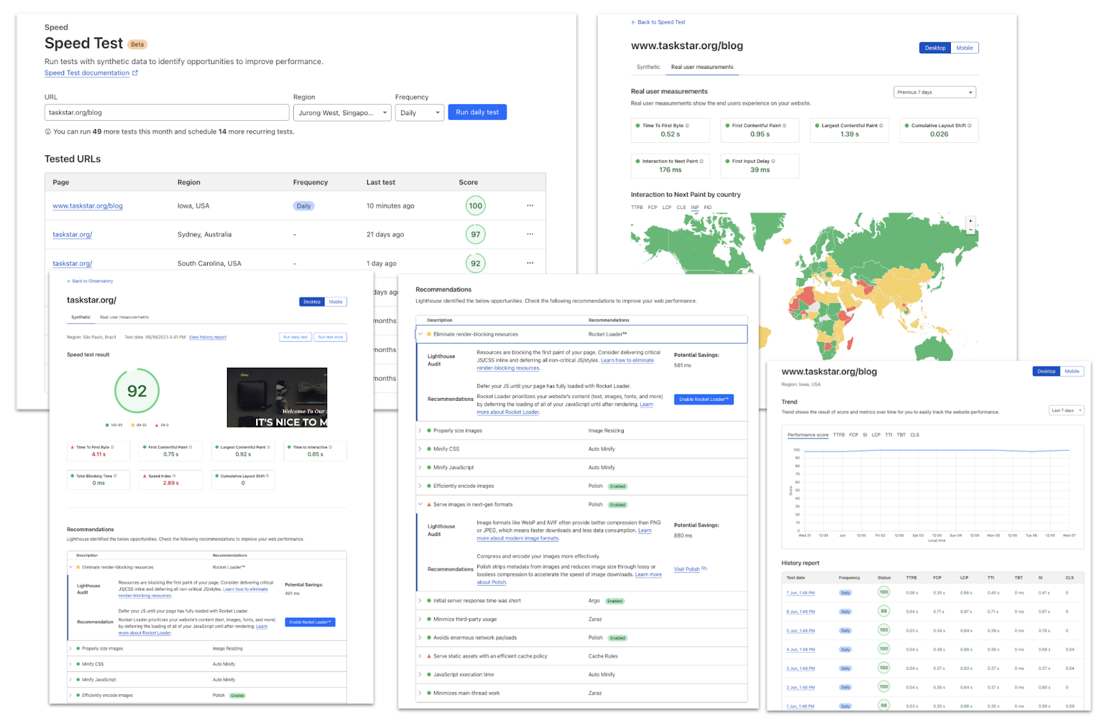
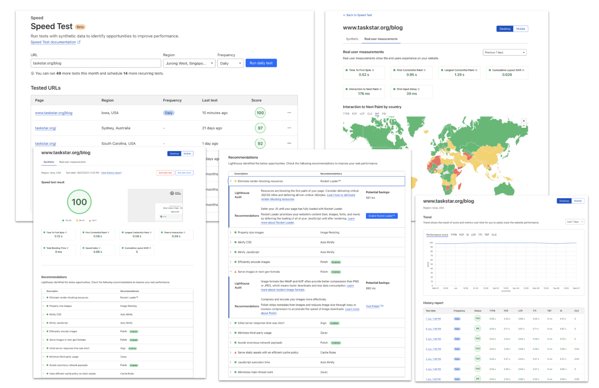
To help you understand the real user experience of your website we have today launched Cloudflare Observatory– the new home of performance at Cloudflare.
Cloudflare users can now easily monitor website performance using Real User Monitoring (RUM) data along with scheduled synthetic tests from different regions in a single dashboard. This will identify any performance issues your website may have. The best bit? Once we’ve identified any issues, Observatory will highlight customized recommendations to resolve these issues, all with a single click.
Start making your website faster today with Observatory.
If you care about the performance of your website or APIs, it’s critical to understand why things are slow.
Today we're introducing new analytics tools to help you understand what is contributing to "Time to First Byte" (TTFB) of Cloudflare and your origin. TTFB is just a simple timer from when a client sends a request until it receives the first byte in response. Timing Insights breaks down TTFB from the perspective of our servers to help you understand what is slow, so that you can begin addressing it.
But wait – maybe you've heard that you should stop worrying about TTFB? Isn't Cloudflare moving away from TTFB as a metric? Read on to understand why there are still situations where TTFB matters.
Why you may need to care about TTFB
It's true that TTFB on its own can be a misleading metric. When measuring web applications, metrics like Web Vitals provide a more holistic view into user experience. That's why we offer Web Analytics and Lighthouse within Cloudflare Observatory.
But there are two reasons why you still may need to pay attention to TTFB:
1. Not all applications are websites More than half of Cloudflare traffic is for APIs, and many customers with API traffic don't control the environments where those endpoints are called. In those cases, there may not be anything you can monitor or improve besides TTFB.
2. Sometimes TTFB is the problem Even if you are measuring Web Vitals metrics like LCP, sometimes the reason your site is slow is because TTFB is slow! And when that happens, you need to know why, and what you can do about it.
When you need to know why TTFB is slow, we’re here to help.
How Timing Insights can help
We now expose performance data through our GraphQL Analytics API that will let you query TTFB performance, and start to drill into what contributes to TTFB.
Specifically, customers on our Pro, Business, and Enterprise plans can now query for the following fields in the httpRequestsAdaptiveGroups dataset:
Time to First Byte (edgeTimeToFirstByteMs)
What is the time elapsed between when Cloudflare started processing the first byte of the request received from an end user, until when we started sending a response?
Origin DNS lookup time (edgeDnsResponseTimeMs)
If Cloudflare had to resolve a CNAME to reach your origin, how long did this take?
Origin Response Time (originResponseDurationMs)
How long did it take to reach, and receive a response from your origin?
We are exposing each metric as an average, median, 95th, and 99th percentiles (i.e. P50 / P95 / P99).
The httpRequestAdaptiveGroups dataset powers the Traffic analytics page in our dashboard, and represents all of the HTTP requests that flow through our network. The upshot is that this dataset gives you the ability to filter and “group by” any aspect of the HTTP request.
An example of how to use Timing Insights
Let’s walk through an example of how you’d actually use this data to pin-point a problem.
To start with, I want to understand the lay of the land by querying TTFB at various quantiles:
This shows that TTFB is over 1.3 seconds at P95 – that’s fairly slow, given that best practices are for 75% of pages to finish rendering within 2.5 seconds, and TTFB is just one component of LCP.
If I want to dig into why TTFB, it would be helpful to understand which URLs are slowest. In this query I’ll filter to that slowest 5% of page loads, and now look at the aggregate time taken – this helps me understand which pages contribute most to slow loads:
Based on this query, it looks like the /api/v2 path is most often responsible for these slow requests. In order to know how to fix the problem, we need to know why these pages are slow. To do this, we can query for the average (mean) DNS and origin response time for queries on these paths, where TTFB is above our P95 threshold:
According to this, most of the long TTFB values are actually due to resolving DNS! The good news is that’s something we can fix – for example, by setting longer TTLs with my DNS provider.
Conclusion
Coming soon, we’ll be bringing this to Cloudflare Observatory in the dashboard so that you can easily explore timing data via the UI.
And we’ll be adding even more granular metrics so you can see exactly which components are contributing to high TTFB. For example, we plan to separate out the difference between origin “connection time” (how long it took to establish a TCP and/or TLS connection) vs “application response time” (how long it took an HTTP server to respond).
We’ll also be making improvements to our GraphQL API to allow more flexible querying – for example, the ability to query arbitrary percentiles, not just 50th, 95th, or 99th.
Start using the GraphQL API today to get Timing Insights, or hop on the discussion about our Analytics products in Discord.
Website performance is crucial to the success of online businesses. Study after study has shown that an increased load time directly affects sales. But how do you get test products that could improve your website speed without incurring an element of risk?
In today's digital landscape, it is easy to find code optimizations on the Internet including our own developers documentation to improve the performance of your website or web applications. However, implementing these changes without knowing the impact they’ll have can be daunting. It could also cause an outage, taking websites or applications offline entirely, leaving admins scrambling to remove the offending code and get the business back online.
Users need a way to see the impact of these improvements on their websites without impacting uptime. They want to understand “If I enabled this, what performance boost should I expect to get?”.
Today, we are excited to announce Performance Experiments in Cloudflare Observatory. Performance Experiments gives users a safe place to experiment and determine what the best setup is to improve their website performance before pushing it live for all visitors to benefit from. Cloudflare users will be able to simply enter the desired code, run our Observatory testing suite and view the impact it would have on their Lighthouse score. If they are satisfied with the results they can push the experiment live. With the click of a button.
Experimenting within Observatory
Cloudflare Observatory, announced today, allows users to easily monitor website performance by integrating Real-User Monitoring (RUM) data and synthetic tests in one location.. This allows users to easily identify areas for optimization and leverage Cloudflare's features to address performance issues.
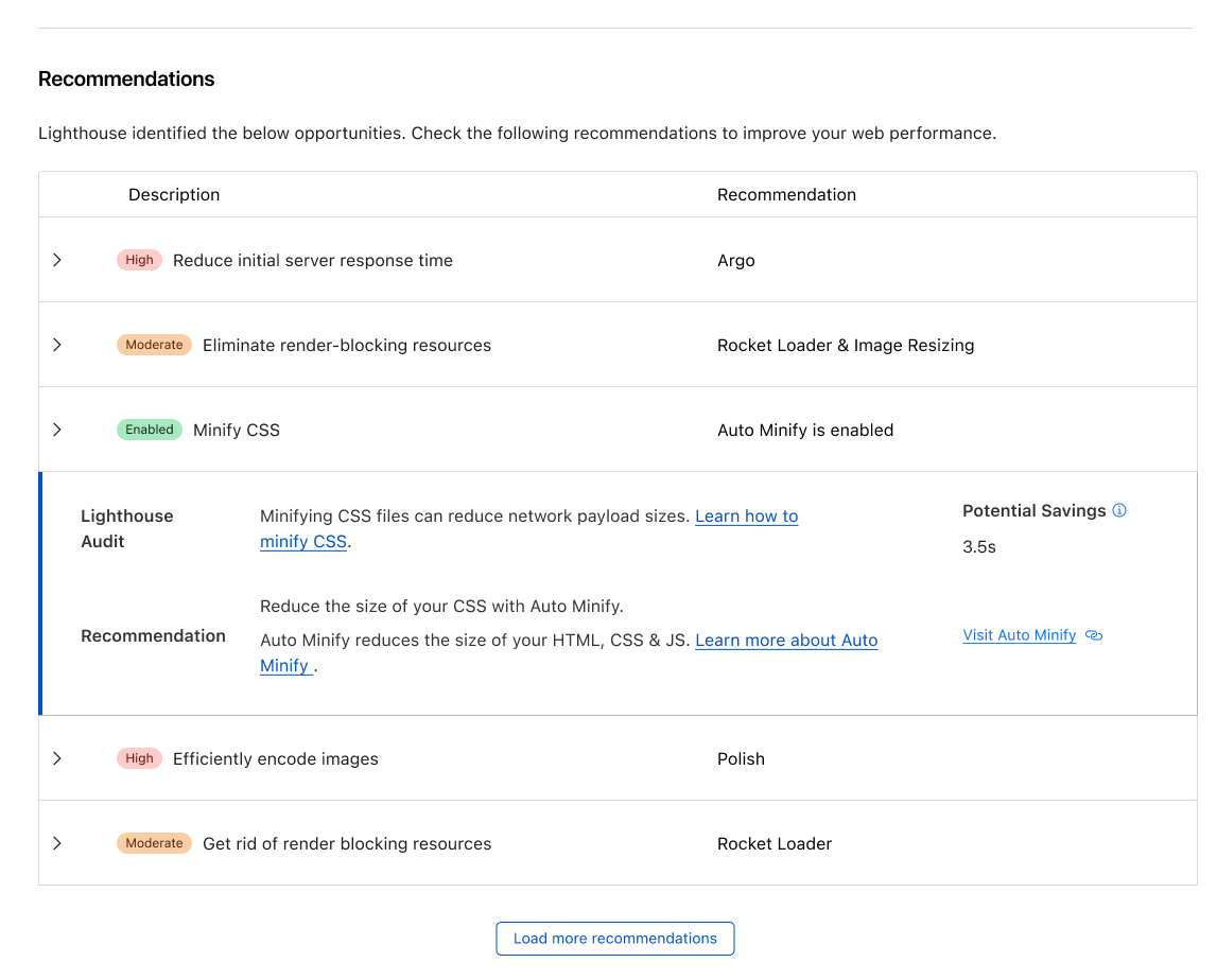
Observatory's recommendations leverage insights from these Lighthouse test and RUM data, enabling precise identification of issues and offering tailored Cloudflare settings for enhanced performance. For example, when a Lighthouse report suggests image optimization improvements, Cloudflare recommends enabling Polish or utilizing Image Resizing. These recommendations can be implemented with a single click, allowing customers to boost their performance score effortlessly.
Fine tuning with Experiments
Cloudflare’s Observatory allows customers to easily enable recommended Cloudflare settings. However, through the medium of Cloudflare Workers web performance advocates have been able to create and share JavaScript examples of how to improve and optimize a website.
A great example of this is Fast Fonts. Google Fonts are slow due to how they are served. When using Google Fonts on your website, you include a stylesheet URL that contains the font styles you want to use. The CSS file is hosted on one domain (fonts.googleapis.com), while the font files are on another domain (fonts.gstatic.com). This separation means that each resource requires at least four round trips to the server for DNS lookup, establishing the socket connection, negotiating TLS encryption (for https), and making the request itself.
These requests cannot be done in parallel because the fonts are not known until after the CSS is downloaded and applied to the page. In the best-case scenario, this leads to eight round trips before the text can be displayed. On a slower 3G connection with a 300ms round-trip time, this delay can add up to 2.4 seconds. To fix this issue Cloudflare Workers can be used to reduce the performance penalties of serving Google Fonts directly from Google by 81%.
Another issue is resource prioritization. When all requests come from the same domain on the same HTTP/2 connection, critical resources like CSS and fonts can be prioritized and delivered before lower priority resources like images. However, since Google Fonts (and most third-party resources) are served from a different domain than the main page resources, they cannot be prioritized and end up competing with each other for download bandwidth. This competition can result in significantly longer fetch times than the best-case scenario of eight round trips.
To implement this Worker first create a Cloudflare Worker, implement the code from the GitHub repository using Wrangler and then run manual tests to see if performance has been improved and that there are no issues or problems with the website loading. Users can choose to implement the Cloudflare Worker on a test path that may not be a true reflection of production or complicate the Cloudflare Worker further by implementing an A/B test that could still have an impact on your end users. So how can users test code on their website to easily see if the code will improve the performance of their website and not have any adverse impact on end users?
Introducing Performance Experiments
Last year we announced Cloudflare Snippets. Snippets is a platform for running discrete pieces of JavaScript code on Cloudflare before your website is served to the user. They provide a convenient way to customize and enhance your website's functionality. If you are already familiar with Cloudflare Workers, our developer platform, you'll find Snippets to be a familiar and welcome addition to your toolkit. With Snippets, you can easily execute small pieces of user-created JavaScript code to modify the behavior of your website and improve performance, security, and user experience.
Combining Snippets with Observatory lets users easily run experiments and get instant feedback on the performance impact. Users will be able to find a piece of JavaScript, insert it into the Experiments window and hit test. Observatory will then automatically run multiple Lighthouse tests with the experiment disabled and then enabled. The results will show the before and after scores allowing users to determine the impact of the experiment e.g. “If I put this JavaScript on my website, my Lighthouse score would improve by 15 points”.
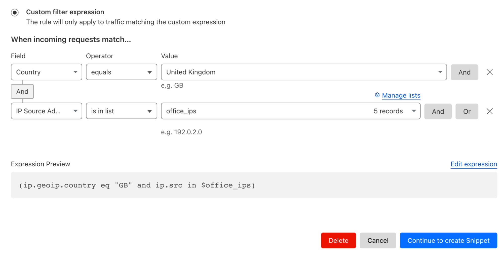
This allows users to understand if the JavaScript has had a positive performance impact on their website. Users can then deploy this JavaScript, via Snippets, against all requests or on a specific subset of traffic. For example, if I only wanted it run on traffic from the UK or my office IPs I would use the rule below:
Alternatively, if the results impact performance customers negatively users can safely discard the experiment or try another example. All without real visitors to the website being impacted or ever at risk.
Accessing Performance Experiments
Performance Experiments are currently under development — you can sign up here to join the waitlist for access.
We hope to begin admitting users later in the year, with an open beta to follow.
Today, Cloudflare is super excited to announce that we’re bringing traffic acceleration to customer’s UDP traffic. Now, you can improve the latency of UDP-based applications like video games, voice calls, and video meetings by up to 17%. Combining the power of Argo Smart Routing (our traffic acceleration product) with UDP gives you the ability to supercharge your UDP-based traffic.
When applications use TCP vs. UDP
Typically when people talk about the Internet, they think of websites they visit in their browsers, or apps that allow them to order food. This type of traffic is sent across the Internet via HTTP which is built on top of the Transmission Control Protocol (TCP). However, there’s a lot more to the Internet than just browsing websites and using apps. Gaming, live video, or tunneling traffic to different networks via a VPN are all common applications that don’t use HTTP or TCP. These popular applications leverage the User Datagram Protocol (or UDP for short). To understand why these applications use UDP instead of TCP, we’ll need to dig into how these different applications work.
When you load a web page, you generally want to see the entire web page; the website would be confusing if parts of it are missing. For this reason, HTTP uses TCP as a method of transferring website data. TCP ensures that if a packet ever gets lost as it crosses the Internet, that packet will be resent. Having a reliable protocol like TCP is generally a good idea when 100% of the information sent needs to be loaded. It’s worth noting that later HTTP versions like HTTP/3 actually deviated from TCP as a transmission protocol, but they still ensure packet delivery by handling packet retransmission using the QUIC protocol.
There are other applications that prioritize quickly sending real time data and are less concerned about perfectly delivering 100% of the data. Let’s explore Real-Time Communications (RTC) like video meetings as an example. If two people are streaming video live, all they care about is what is happening now. If a few packets are lost during the initial transmission, retransmission is usually too slow to render the lost packet data in the current video frame. TCP doesn’t really make sense in this scenario.
Instead, RTC protocols are built on top of UDP. TCP is like a formal back and forth conversation where every sentence matters. UDP is more like listening to your friend's stream of consciousness: you don’t care about every single bit as long as you get the gist of it. UDP transfers packet data with speed and efficiency without guaranteeing the delivery of those packets. This is perfect for applications like RTC where reducing latency is more important than occasionally losing a packet here or there. The same applies to gaming traffic; you generally want the most up-to-date information, and you don’t really care about retransmitting lost packets.
Gaming and RTC applications really care about latency. Latency is the length of time it takes a packet to be sent to a server plus the length of time to receive a response from the server (called round-trip time or RTT). In the case of video games, the higher the latency, the longer it will take for you to see other players move and the less time you’ll have to react to the game. With enough latency, games become unplayable: if the players on your screen are constantly blipping around it’s near impossible to interact with them. In RTC applications like video meetings, you’ll experience a delay between yourself and your counterpart. You may find yourselves accidentally talking over each other which isn’t a great experience.
Companies that host gaming or RTC infrastructure often try to reduce latency by spinning up servers that are geographically closer to their users. However, it’s common to have two users that are trying to have a video call between distant locations like Amsterdam and Los Angeles. No matter where you install your servers, that's still a long distance for that traffic to travel. The longer the path, the higher the chances are that you're going to run into congestion along the way. Congestion is just like a traffic jam on a highway, but for networks. Sometimes certain paths get overloaded with traffic. This causes delays and packets to get dropped. This is where Argo Smart Routing comes in.
Argo Smart Routing
Cloudflare customers that want the best cross-Internet application performance rely on Argo Smart Routing’s traffic acceleration to reduce latency. Argo Smart Routing is like the GPS of the Internet. It uses real time global network performance measurements to accelerate traffic, actively route around Internet congestion, and increase your traffic’s stability by reducing packet loss and jitter.
Argo Smart Routing was launched in May 2017, and its first iteration focused on reducing website traffic latency. Since then, we’ve improved Argo Smart Routing and also launched Argo Smart Routing for Spectrum TCP traffic which reduces latency in any TCP-based protocols. Today, we’re excited to bring the same Argo Smart Routing technology to customer’s UDP traffic which will reduce latency, packet loss, and jitter in gaming, and live audio/video applications.
Argo Smart Routing accelerates Internet traffic by sending millions of synthetic probes from every Cloudflare data center to the origin of every Cloudflare customer. These probes measure the latency of all possible routes between Cloudflare’s data centers and a customer’s origin. We then combine that with probes running between Cloudflare’s data centers to calculate possible routes. When an Internet user makes a request to an origin, Cloudflare calculates the results of our real time global latency measurements, examines Internet congestion data, and calculates the optimal route for customer’s traffic. To enable Argo Smart Routing for UDP traffic, Cloudflare extended the route computations typically used for HTTP and TCP traffic and applied them to UDP traffic.
We knew that Argo Smart Routing offered impressive benefits for HTTP traffic, reducing time to first byte by up to 30% on average for customers. But UDP can be treated differently by networks, so we were curious to see if we would see a similar reduction in round-trip-time for UDP. To validate, we ran a set of tests. We set up an origin in Iowa, USA and had a client connect to it from Tokyo, Japan. Compared to a regular Spectrum setup, we saw a decrease in round-trip-time of up to 17.3% on average. For the standard setup, Spectrum was able to proxy packets to Iowa in 173.3 milliseconds on average. Comparatively, turning on Argo Smart Routing reduced the average round-trip-time down to 143.3 milliseconds. The distance between those two cities is 6,074 miles (9,776 kilometers), meaning we've effectively moved the two closer to each other by over a thousand miles (or 1,609 km) just by turning on this feature.
We're incredibly excited about Argo Smart Routing for UDP and what our customers will use it for. If you're in gaming or real-time-communications, or even have a different use-case that you think would benefit from speeding up UDP traffic, please contact your account team today. We are currently in closed beta but are excited about accepting applications.
On May 10, 2023, Google announced that INP will replace FID in the Core Web Vitals in March 2024. The Core Web Vitals play a role in the Google Search algorithm. So website owners who care about Search Engine Optimization (SEO) should prepare for the change. Otherwise their search ranking might suffer.
This post will first explain what FID, INP and the Core Web Vitals are. Then it will show how FID and INP relate to each other across a large range of Cloudflare sites. (Spoiler alert – If a site has ‘Good’ scoring FID, it might not have ‘Good’ scoring INP). Then it will discuss how to prepare for this change and how Cloudflare can help.
A few definitions
In order to make sense of the upcoming change, here are some definitions that will set the scene.
Core Web Vitals
Measuring user-centric web performance is challenging. To face this challenge, Google developed a series of metrics called the Web Vitals. These Web Vitals are signals that measure different aspects of web performance. For example Time To First Byte (TTFB) is one of the Web Vitals: from the perspective of the browser, TTFB “measures the time between the request for a resource and when the first byte of a response begins to arrive.” – https://web.dev/ttfb/
A subset of the Web Vitals are the Core Web Vitals. The Core Web Vitals are identified as the most critical Web Vitals to pay attention to. As such, they play a role in the Google Search algorithm. Improving a webpage’s Core Web Vitals can improve success with Google Search. The Core Web Vitals currently consist of three metrics: Largest Contentful Paint (LCP), First Input Delay (FID) and Cumulative Layout Shift (CLS). Respectively they measure Loading Speed, Interactivity and Visual Stability. This will change in March 2024 when Interaction To Next Paint (INP) replaces FID as the Core Web Vital for Interactivity.
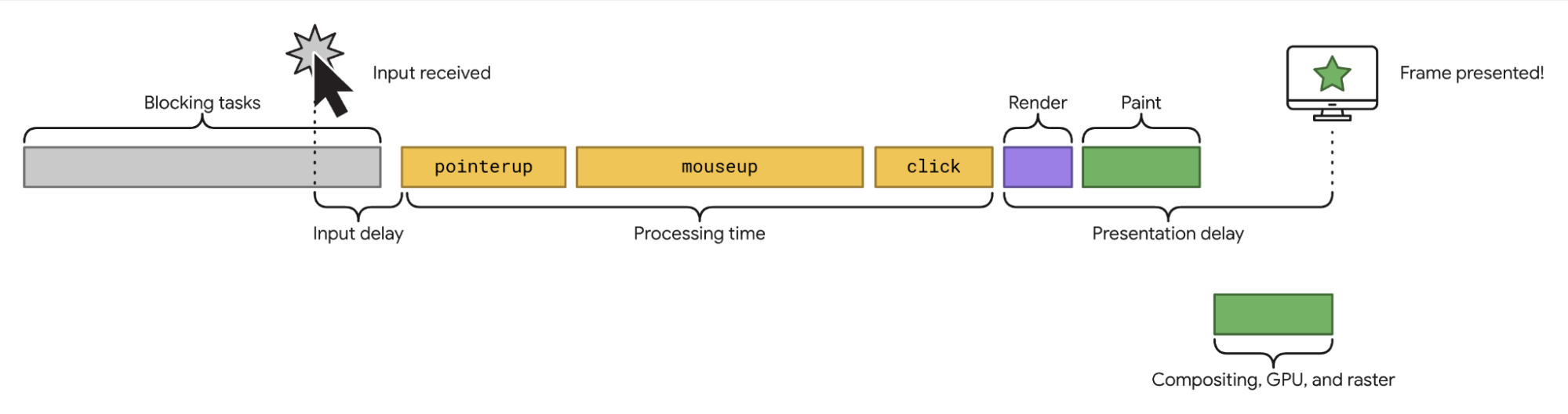
Interaction
An Interaction on a webpage starts with a user input. The browser then reacts to this input. This includes the input delay, the processing time and the presentation delay before the next paint occurs and the new frame is presented.
Keeping in mind that an interaction is composed of these three serialized durations – input delay, processing time and presentation delay – will help later on to understand the difference between FID and INP.
First Input Delay (FID)
“FID measures the time from when a user first interacts with a page (that is, when they click a link, tap on a button, or use a custom, JavaScript-powered control) to the time when the browser is actually able to begin processing event handlers in response to that interaction.” – https://web.dev/fid/
FID is the current Core Web Vital that measures interactivity. FID measures the first interaction with the page. User interactions after the first interaction are not measured with FID. FID also only measures the input delay part of the first interaction. It does not measure the processing time and the presentation delay.
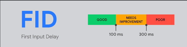
FID is classed as ‘Good’ if the input delay is less than 100 ms. FID is classed as ‘Needs Improvement’ between 100ms and 300ms. Delays above 300 ms are classed as ‘Poor’.
“INP is a metric that assesses a page's overall responsiveness to user interactions by observing the latency of all click, tap, and keyboard interactions that occur throughout the lifespan of a user's visit to a page. The final INP value is the longest interaction observed, ignoring outliers.” - https://web.dev/inp/
INP, like FID, is also a Web Vital that measures interactivity. INP observes all user interactions in a page view and reports the longest. It measures more than just the input delay duration of each interaction. It also measures the processing time and the presentation delay until the next paint occurs. Once you understand the mechanics of it, the name ‘Interaction to Next Paint’ is a good description of the duration it measures.
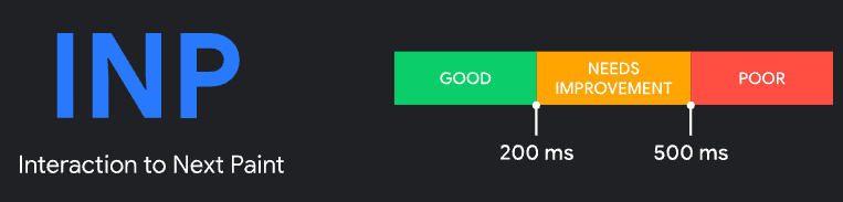
INP is classed as ‘Good’ if the final reported value is less than 200 ms. INP is classed as ‘Needs Improvement’ between 200ms and 500ms. Any measurement above 500 ms is classed as ‘Poor’.
Both FID and INP measure interactivity by measuring delays after user interactions. But INP is more comprehensive than FID. As an example, let’s say a user loads a web page and interacts only once by clicking a button. In this case, FID will capture this interaction by reporting the input delay after the user input. INP will also observe this interaction but it will measure not only the input delay but also the subsequent processing time and the presentation delay. Since this is the only interaction on the web page, INP will observe this as the longest duration within the page view and so will report this duration as the final reported INP value. Already it is clear that with just a single user interaction, INP provides a more comprehensive signal of interactivity because it includes processing time and presentation delay.
But INP also goes beyond the first interaction on the page. It observes all the interactions within a page view and reports the longest interaction of the set (ignoring outliers). This means that web sites need to ensure that all interactions throughout the lifecycle of a page view are under 200ms in order to score a ‘Good’ INP. With FID, web sites only need to focus on optimizing the first interaction’s input delay under 100 ms to score ‘Good’ FID. With INP joining the Core Web Vitals, web sites will need to focus on optimizing all interactions.
Comparing FID with INP across Cloudflare
At Cloudflare, for sites that have enabled Real User Measurements (RUM) via the Web Analytics Product or the Observatory Product, we already collect INP data. This means we have a rich dataset across 850k sites with which to analyze INP against FID.
FID vs INP
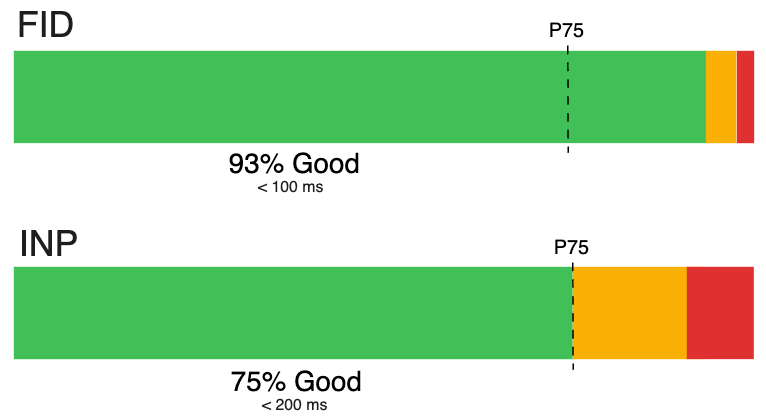
Over the period of a week, across all Cloudflare RUM-enabled sites, we observed over four billion reported FIDs and INPs. 93% of the FID values classify as ‘Good’ (under 100 ms). 75% of the INP values classify as ‘Good’ (under 200 ms). Since these values are sourced from the same set of page views, it is already possible to see at a glance that INP is distributed more lightly in the ‘Good’ range than FID.
Interestingly, the P75 value for FID is just 16 ms. A 0.16 times multiple of the FID ‘Good’ threshold of 100 ms. For INP, the P75 value is 200 ms. A one times multiple of the INP ‘Good’ threshold.
INP across devices
Focusing on INP, when the INP data is segmented by device type, we observe that 88% of desktop INP classify as ‘Good’, but only 67% of mobile INP classify as ‘Good’. This suggests that INP is generally suffering more on mobile devices than on desktop.
The bottom line is that INP is more challenging than FID to ‘get into the Green’. Since INP is a more comprehensive measure of interactivity, web sites are more exposed, and less likely to score favorably.
How to prepare for the change
INP will start affecting Google Search rankings when it becomes a Core Web Vital in March 2024. To get ready, websites need to improve interactivity beyond the initial load of the site.
As always, in order to improve on a metric, a baseline must be drawn by collecting data on the metric. But with INP, this can be challenging because INP is best reported from field data. Field data means that the data comes from real users interacting with web pages on real browsers. With field data, synthetic tools like Google Lighthouse aren’t a great fit. Synthetic tools are not designed to emulate the wide range of users on the wide range of browsers and operating systems that will navigate a web page.
In order to collect real user data from real browsers, websites need to enable a RUM provider. RUM providers collect performance data from real browsers, and process the data so that it can be aggregated and analyzed. It’s worth noting that performance data is anonymous and does not include any personal identifiable information (PII).
So the first step to understanding INP on a website is to enable a RUM provider.
Once a RUM provider is enabled on a website, it is then possible to analyze INP data to understand which web pages are not optimized for interactivity. There can be many possible causes for this. Since INP is composed of input delay, processing time and presentation delay, optimizing INP can be broken down into optimizing these distinct durations.
The best advice for optimizing INP is set out by web.dev. Optimizing INP is not straight-forward – it can involve breaking up JavaScript tasks, reducing DOM interactions and layouts, avoiding use of timers, and limiting third-party code amongst a range of other measures. That’s why it’s best to get started early and learn as much as possible before the change takes place.
How Cloudflare can help
A free RUM provider
Cloudflare offers a free RUM provider which collects INP as part of its dataset. It currently powers Cloudflare Web Analytics and Cloudflare Observatory. By enabling RUM with Cloudflare, you can explore the interactivity of your site’s web pages and start to identify interactivity issues.
Just log onto the Cloudflare Dashboard, and head to your target account. Go to Web Analytics.
Reduce the impact of third-party scripts
One of the contributing causes of degraded INP is JavaScript blocking the main thread after an interaction. Often this can be caused by heavy third-party scripts attaching event listeners to DOM elements. For example, third-party analytics scripts can register listeners on interactive elements of a page to power various forms of analytics. Many sites have dozens, if not hundreds of third-party scripts running, each one potentially degrading INP.
Cloudflare offers a unique product that can entirely remove third-party scripts from the browser. This frees up the main thread, boosting interactivity. If you haven’t come across Cloudflare Zaraz before, check it out in our docs. Not only can it improve INP, but it can also dramatically improve the security posture of your site by reducing (or even entirely removing) the amount of third-party JavaScript that runs on your website.
In this post, we will take you through the advancements we've made in our machine learning capabilities. We'll describe the technical strategies that have enabled us to expand the number of machine learning features and models, all while substantially reducing the processing time for each HTTP request on our network. Let's begin.
Background
For a comprehensive understanding of our evolved approach, it's important to grasp the context within which our machine learning detections operate. Cloudflare, on average, serves over 46 million HTTP requests per second, surging to more than 63 million requests per second during peak times.
Machine learning detection plays a crucial role in ensuring the security and integrity of this vast network. In fact, it classifies the largest volume of requests among all our detection mechanisms, providing the final Bot Score decision for over 72% of all HTTP requests. Going beyond, we run several machine learning models in shadow mode for every HTTP request.
At the heart of our machine learning infrastructure lies our reliable ally, CatBoost. It enables ultra low-latency model inference and ensures high-quality predictions to detect novel threats such as stopping bots targeting our customers' mobile apps. However, it's worth noting that machine learning model inference is just one component of the overall latency equation. Other critical components include machine learning feature extraction and preparation. In our quest for optimal performance, we've continuously optimized each aspect contributing to the overall latency of our system.
Initially, our machine learning models relied on single-request features, such as presence or value of certain headers. However, given the ease of spoofing these attributes, we evolved our approach. We turned to inter-request features that leverage aggregated information across multiple dimensions of a request in a sliding time window. For example, we now consider factors like the number of unique user agents associated with certain request attributes.
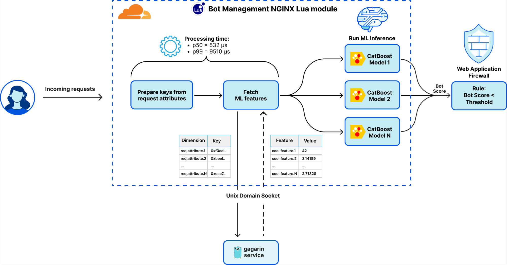
The extraction and preparation of inter-request features were handled by Gagarin, a Go-based feature serving platform we developed. As a request arrived at Cloudflare, we extracted dimension keys from the request attributes. We then looked up the corresponding machine learning features in the multi-layered cache. If the desired machine learning features were not found in the cache, a memcached "get" request was made to Gagarin to fetch those. Then machine learning features were plugged into CatBoost models to produce detections, which were then surfaced to the customers via Firewall and Workers fields and internally through our logging pipeline to ClickHouse. This allowed our data scientists to run further experiments, producing more features and models.
Previous system design for serving machine learning features over Unix socket using Gagarin.
Initially, Gagarin exhibited decent latency, with a median latency around 200 microseconds to serve all machine learning features for given keys. However, as our system evolved and we introduced more features and dimension keys, coupled with increased traffic, the cache hit ratio began to wane. The median latency had increased to 500 microseconds and during peak times, the latency worsened significantly, with the p99 latency soaring to roughly 10 milliseconds. Gagarin underwent extensive low-level tuning, optimization, profiling, and benchmarking. Despite these efforts, we encountered the limits of inter-process communication (IPC) using Unix Domain Socket (UDS), among other challenges, explored below.
Problem definition
In summary, the previous solution had its drawbacks, including:
High tail latency: during the peak time, a portion of requests experienced increased latency caused by CPU contention on the Unix socket and Lua garbage collector.
Suboptimal resource utilization: CPU and RAM utilization was not optimized to the full potential, leaving less resources for other services running on the server.
Machine learning features availability: decreased due to memcached timeouts, which resulted in a higher likelihood of false positives or false negatives for a subset of the requests.
Scalability constraints: as we added more machine learning features, we approached the scalability limit of our infrastructure.
Equipped with a comprehensive understanding of the challenges and armed with quantifiable metrics, we ventured into the next phase: seeking a more efficient way to fetch and serve machine learning features.
Exploring solutions
In our quest for more efficient methods of fetching and serving machine learning features, we evaluated several alternatives. The key approaches included:
Further optimizing Gagarin: as we pushed our Go-based memcached server to its limits, we encountered a lower bound on latency reductions. This arose from IPC over UDS synchronization overhead and multiple data copies, the serialization/deserialization overheads, as well as the inherent latency of garbage collector and the performance of hashmap lookups in Go.
Considering Quicksilver: we contemplated using Quicksilver, but the volume and update frequency of machine learning features posed capacity concerns and potential negative impacts on other use cases. Moreover, it uses a Unix socket with the memcached protocol, reproducing the same limitations previously encountered.
Increasing multi-layered cache size: we investigated expanding cache size to accommodate tens of millions of dimension keys. However, the associated memory consumption, due to duplication of these keys and their machine learning features across worker threads, rendered this approach untenable.
Sharding the Unix socket: we considered sharding the Unix socket to alleviate contention and improve performance. Despite showing potential, this approach only partially solved the problem and introduced more system complexity.
Switching to RPC: we explored the option of using RPC for communication between our front line server and Gagarin. However, since RPC still requires some form of communication bus (such as TCP, UDP, or UDS), it would not significantly change the performance compared to the memcached protocol over UDS, which was already simple and minimalistic.
After considering these approaches, we shifted our focus towards investigating alternative Inter-Process Communication (IPC) mechanisms.
IPC mechanisms
Adopting a first principles design approach, we questioned: "What is the most efficient low-level method for data transfer between two processes provided by the operating system?" Our goal was to find a solution that would enable the direct serving of machine learning features from memory for corresponding HTTP requests. By eliminating the need to traverse the Unix socket, we aimed to reduce CPU contention, improve latency, and minimize data copying.
To identify the most efficient IPC mechanism, we evaluated various options available within the Linux ecosystem. We used ipc-bench, an open-source benchmarking tool specifically designed for this purpose, to measure the latencies of different IPC methods in our test environment. The measurements were based on sending one million 1,024-byte messages forth and back (i.e., ping pong) between two processes.
IPC method
Avg duration, μs
Avg throughput, msg/s
eventfd (bi-directional)
9.456
105,533
TCP sockets
8.74
114,143
Unix domain sockets
5.609
177,573
FIFOs (named pipes)
5.432
183,388
Pipe
4.733
210,369
Message Queue
4.396
226,421
Unix Signals
2.45
404,844
Shared Memory
0.598
1,616,014
Memory-Mapped Files
0.503
1,908,613
Based on our evaluation, we found that Unix sockets, while taking care of synchronization, were not the fastest IPC method available. The two fastest IPC mechanisms were shared memory and memory-mapped files. Both approaches offered similar performance, with the former using a specific tmpfs volume in /dev/shm and dedicated system calls, while the latter could be stored in any volume, including tmpfs or HDD/SDD.
Missing ingredients
In light of these findings, we decided to employ memory-mapped files as the IPC mechanism for serving machine learning features. This choice promised reduced latency, decreased CPU contention, and minimal data copying. However, it did not inherently offer data synchronization capabilities like Unix sockets. Unlike Unix sockets, memory-mapped files are simply files in a Linux volume that can be mapped into memory of the process. This sparked several critical questions:
How could we efficiently fetch an array of hundreds of float features for given dimension keys when dealing with a file?
How could we ensure safe, concurrent and frequent updates for tens of millions of keys?
How could we avert the CPU contention previously encountered with Unix sockets?
How could we effectively support the addition of more dimensions and features in the future?
To address these challenges we needed to further evolve this new approach by adding a few key ingredients to the recipe.
Augmenting the Idea
To realize our vision of memory-mapped files as a method for serving machine learning features, we needed to employ several key strategies, touching upon aspects like data synchronization, data structure, and deserialization.
Wait-free synchronization
When dealing with concurrent data, ensuring safe, concurrent, and frequent updates is paramount. Traditional locks are often not the most efficient solution, especially when dealing with high concurrency environments. Here's a rundown on three different synchronization techniques:
With-lock synchronization: a common approach using mechanisms like mutexes or spinlocks. It ensures only one thread can access the resource at a given time, but can suffer from contention, blocking, and priority inversion, just as evident with Unix sockets.
Lock-free synchronization: this non-blocking approach employs atomic operations to ensure at least one thread always progresses. It eliminates traditional locks but requires careful handling of edge cases and race conditions.
Wait-free synchronization: a more advanced technique that guarantees every thread makes progress and completes its operation without being blocked by other threads. It provides stronger progress guarantees compared to lock-free synchronization, ensuring that each thread completes its operation within a finite number of steps.
We store the synchronization state, which coordinates access to these data copies, in a third memory-mapped file, referred to as "state". This file contains an atomic 64-bit integer, which represents an InstanceVersionand a pair of additional atomic 32-bit variables, tracking the number of active readers for each data copy. The InstanceVersion consists of the currently active data file index (1 bit), the data size (39 bits, accommodating data sizes up to 549 GB), and a data checksum (24 bits).
Zero-copy deserialization
To efficiently store and fetch machine learning features, we needed to address the challenge of deserialization latency. Here, zero-copy deserialization provides an answer. This technique reduces the time and memory required to access and use data by directly referencing bytes in the serialized form.
We turned to rkyv, a zero-copy deserialization framework in Rust, to help us with this task. rkyv implements total zero-copy deserialization, meaning no data is copied during deserialization and no work is done to deserialize data. It achieves this by structuring its encoded representation to match the in-memory representation of the source type.
One of the key features of rkyv that our solution relies on is its ability to access HashMap data structures in a zero-copy fashion. This is a unique capability among Rust serialization libraries and one of the main reasons we chose rkyv for our implementation. It also has a vibrant Discord community, eager to offer best-practice advice and accommodate feature requests.
Leveraging the benefits of memory-mapped files, wait-free synchronization and zero-copy deserialization, we've crafted a unique and powerful tool for managing high-performance, concurrent data access between processes. We've packaged these concepts into a Rust crate named mmap-sync, which we're thrilled to open-source for the wider community.
At the core of the mmap-sync package is a structure named Synchronizer. It offers an avenue to read and write any data expressible as a Rust struct. Users simply have to implement or derive a specific Rust trait surrounding struct definition – a task requiring just a single line of code. The Synchronizer presents an elegantly simple interface, equipped with "write" and "read" methods.
impl Synchronizer {
/// Write a given `entity` into the next available memory mapped file.
pub fn write<T>(&mut self, entity: &T, grace_duration: Duration) -> Result<(usize, bool), SynchronizerError> {
…
}
/// Reads and returns `entity` struct from mapped memory wrapped in `ReadResult`
pub fn read<T>(&mut self) -> Result<ReadResult<T>, SynchronizerError> {
…
}
}
/// FeaturesMetadata stores features along with their metadata
#[derive(Archive, Deserialize, Serialize, Debug, PartialEq)]
#[archive_attr(derive(CheckBytes))]
pub struct FeaturesMetadata {
/// Features version
pub version: u32,
/// Features creation Unix timestamp
pub created_at: u32,
/// Features represented by vector of hash maps
pub features: Vec<HashMap<u64, Vec<f32>>>,
}
A read operation through the Synchronizer performs zero-copy deserialization and returns a "guarded" Result encapsulating a reference to the Rust struct using RAII design pattern. This operation also increments the atomic counter of active readers using the struct. Once the Result is out of scope, the Synchronizer decrements the number of readers.
The synchronization mechanism used in mmap-sync is not only "lock-free" but also "wait-free". This ensures an upper bound on the number of steps an operation will take before it completes, thus providing a performance guarantee.
The data is stored in shared mapped memory, which allows the Synchronizer to “write” to it and “read” from it concurrently. This design makes mmap-sync a highly efficient and flexible tool for managing shared, concurrent data access.
Now, with an understanding of the underlying mechanics of mmap-sync, let's explore how this package plays a key role in the broader context of our Bot Management platform, particularly within the newly developed components: the bliss service and library.
System design overhaul
Transitioning from a Lua-based module that made memcached requests over Unix socket to Gagarin in Go to fetch machine learning features, our new design represents a significant evolution. This change pivots around the introduction of mmap-sync, our newly developed Rust package, laying the groundwork for a substantial performance upgrade. This development led to a comprehensive system redesign and introduced two new components that form the backbone of our Bots Liquidation Intelligent Security System – or BLISS, in short: the bliss service and the bliss library.
Bliss service
The blissservice operates as a Rust-based, multi-threaded sidecar daemon. It has been designed for optimal batch processing of vast data quantities and extensive I/O operations. Among its key functions, it fetches, parses, and stores machine learning features and dimensions for effortless data access and manipulation. This has been made possible through the incorporation of the Tokio event-driven platform, which allows for efficient, non-blocking I/O operations.
Bliss library
Operating as a single-threaded dynamic library, the bliss library seamlessly integrates into each worker thread using the Foreign Function Interface (FFI) via a Lua module. Optimized for minimal resource usage and ultra-low latency, this lightweight library performs tasks without the need for heavy I/O operations. It efficiently serves machine learning features and generates corresponding detections.
In addition to leveraging the mmap-sync package for efficient machine learning feature access, our new design includes several other performance enhancements:
Allocations-free operation: bliss library re-uses pre-allocated data structures and performs no heap allocations, only low-cost stack allocations. To enforce our zero-allocation policy, we run integration tests using the dhat heap profiler.
SIMD optimizations: wherever possible, the bliss library employs vectorized CPU instructions. For instance, AVX2 and SSE4 instruction sets are used to expedite hex-decoding of certain request attributes, enhancing speed by tenfold.
Compiler tuning: We compile both the bliss service and library with the following flags for superior performance:
Benchmarking & profiling: We use Criterion for benchmarking every major feature or component within bliss. Moreover, we are also able to use the Go pprof profiler on Criterion benchmarks to view flame graphs and more:
This comprehensive overhaul of our system has not only streamlined our operations but also has been instrumental in enhancing the overall performance of our Bot Management platform. Stay tuned to witness the remarkable changes brought about by this new architecture in the next section.
Rollout results
Our system redesign has brought some truly "blissful" dividends. Above all, our commitment to a seamless user experience and the trust of our customers have guided our innovations. We ensured that the transition to the new design was seamless, maintaining full backward compatibility, with no customer-reported false positives or negatives encountered. This is a testament to the robustness of the new system.
As the old adage goes, the proof of the pudding is in the eating. This couldn't be truer when examining the dramatic latency improvements achieved by the redesign. Our overall processing latency for HTTP requests at Cloudflare improved by an average of 12.5% compared to the previous system.
This improvement is even more significant in the Bot Management module, where latency improved by an average of 55.93%.
Bot Management module latency, in microseconds.
More specifically, our machine learning features fetch latency has improved by several orders of magnitude:
Latency metric
Before (μs)
After (μs)
Change
p50
532
9
-98.30% or x59
p99
9510
18
-99.81% or x528
p999
16000
29
-99.82% or x551
To truly grasp this impact, consider this: with Cloudflare’s average rate of 46 million requests per second, a saving of 523 microseconds per request equates to saving over 24,000 days or 65 years of processing time every single day!
In addition to latency improvements, we also reaped other benefits from the rollout:
Enhanced feature availability: thanks to eliminating Unix socket timeouts, machine learning feature availability is now a robust 100%, resulting in fewer false positives and negatives in detections.
Improved resource utilization: our system overhaul liberated resources equivalent to thousands of CPU cores and hundreds of gigabytes of RAM – a substantial enhancement of our server fleet's efficiency.
Code cleanup: another positive spin-off has been in our Lua and Go code. Thousands of lines of less performant and less memory-safe code have been weeded out, reducing technical debt.
Upscaled machine learning capabilities: last but certainly not least, we've significantly expanded our machine learning features, dimensions, and models. This upgrade empowers our machine learning inference to handle hundreds of machine learning features and dozens of dimensions and models.
Conclusion
In the wake of our redesign, we've constructed a powerful and efficient system that truly embodies the essence of 'bliss'. Harnessing the advantages of memory-mapped files, wait-free synchronization, allocation-free operations, and zero-copy deserialization, we've established a robust infrastructure that maintains peak performance while achieving remarkable reductions in latency. As we navigate towards the future, we're committed to leveraging this platform to further improve our Security machine learning products and cultivate innovative features. Additionally, we're excited to share parts of this technology through an open-sourced Rust package mmap-sync.
As we leap into the future, we are building upon our platform's impressive capabilities, exploring new avenues to amplify the power of machine learning. We are deploying a new machine learning model built on BLISS with select customers. If you are a Bot Management subscriber and want to test the new model, please reach out to your account team.
Separately, we are on the lookout for more Cloudflare customers who want to run their own machine learning models at the edge today. If you’re a developer considering making the switch to Workers for your application, sign up for our Constellation AI closed beta. If you’re a Bot Management customer and looking to run an already trained, lightweight model at the edge, we would love to hear from you. Let's embark on this path to bliss together.
Cloudflare will deprecate the Railgun product on January 31, 2024. At that time, existing Railgun deployments and connections will stop functioning. Customers have the next eight months to migrate to a supported Cloudflare alternative which will vary based on use case.
Cloudflare first launched Railgun more than ten years ago. Since then, we have released several products in different areas that better address the problems that Railgun set out to solve. However, we shied away from the work to formally deprecate Railgun.
That reluctance led to Railgun stagnating and customers suffered the consequences. We did not invest time in better support for Railgun. Feature requests never moved. Maintenance work needed to occur and that stole resources away from improving the Railgun replacements. We allowed customers to deploy a zombie product and, starting with this deprecation, we are excited to correct that by helping teams move to significantly better alternatives that are now available in Cloudflare’s network.
We know that this will require migration effort from Railgun customers over the next eight months. We want to make that as smooth as possible. Today’s announcement features recommendations on how to choose a replacement, how to get started, and guidance on where you can reach us for help.
What is Railgun?
Cloudflare’s reverse proxy secures and accelerates your applications by placing a Cloudflare data center in over 285+ cities between your infrastructure and your audience. Bad actors attempting to attack your applications hit our network first where products like our WAF and DDoS mitigation service stop them. Your visitors and users connect to our data centers where our cache can serve them content without the need to reach all the way back to your origin server.
For some customers, your infrastructure also runs on Cloudflare’s network in the form of Cloudflare Workers. Others maintain origin servers running on anything from a Raspberry Pi to a hyperscale public cloud. In those cases, Cloudflare needs to connect to that infrastructure to grab new content that our network can serve from our cache to your audience.
However, some content cannot be cached. Dynamically-generated or personalized pages can change for every visitor and every session. Cloudflare Railgun aimed to solve that by determining what was the minimum amount of content that changed and attempting to only send that difference in an efficient transfer – a form of delta compression. By reducing the amount of content that needed to be sent to Cloudflare’s network, we could accelerate page loads for end users.
Railgun accomplishes this goal by running a piece of software inside the customer’s environment, the Railgun listener, and a corresponding service running in Cloudflare’s network, the Railgun sender. The pair establish a permanent TCP connection. The listener keeps track of the most recent version of a page that was requested. When a request arrives for a known page, the listener sends an HTTP request to the origin server, determines what content changed, and then compresses and sends only the delta to the sender in Cloudflare’s network.
Why deprecate a product?
The last major release of Railgun took place eight years ago in 2015. However, products should not be deprecated just because active development stops. We believe that a company should retire a product only when:
the maintenance impacts the ability to focus on solving new problems for customers and
when improved alternatives exist for customers to adopt in replacement.
Hundreds of customers still use Railgun today and the service has continued to run over the last decade without too much involvement from our team. That relative stability deterred us from pushing customers to adopt newer technologies that solved the same problems. As a result, we kept Railgun in a sort of maintenance mode for the last few years.
Why deprecate Railgun now?
Cloudflare’s network has evolved in the eight years since the last Railgun release. We deploy hardware and run services in more than 285 cities around the world, nearly tripling the number of cities since Railgun was last updated. The hardware itself also advanced, becoming more efficient and capable.
The software platform of Cloudflare’s network developed just as fast. Every data center in Cloudflare’s network can run every service that we provide to our customers. These services range from our traditional reverse proxy products to forward proxy services like Zero Trust to our compute and storage platform Cloudflare Workers. Supporting such a broad range of services requires a platform that can adapt to the requirements of the evolving needs of these products.
Maintaining Railgun, despite having better alternatives, creates a burden on our ability to continue investing in new solutions. Some of these tools that power Railgun are themselves approaching an end of life state. Others will likely present security risks that we are not comfortable accepting in the next few years.
We considered several options before deciding on deprecation. First, we could accept the consequences of inaction, leaving our network in a worse state and our Railgun customers in purgatory. Second, we could run Railgun on dedicated infrastructure and silo it from the rest of our network. However, that would violate our principle that every piece of hardware in Cloudflare runs every service.
Third, we could spin up a new engineering team and rebuild Railgun from scratch in a modern way. Doing so would take away from resources we could otherwise invest in newer technologies. We also believe that existing, newer products from Cloudflare solve the same problems that Railgun set out to address. Rebuilding Railgun would take away from our ability to keep shipping and would duplicate better features already released in other products. As a result, we have decided to deprecate Railgun.
What alternatives are available?
Railgun addressed a number of problems for our customers at launch. Today, we have solutions available that solve the same range of challenges in significantly improved ways.
We do not have an exact like-for-like successor for Railgun. The solutions that solve the same set of problems have also evolved with our customers. Different use cases that customers deploy Railgun to address will map to different solutions available in Cloudflare today. We have broken out some of the most common reasons that customers used Railgun and where we recommend they consider migrating.
“I use Railgun to maintain a persistent, secure connection to Cloudflare’s network without the need for a static publicly available IP address.” Customers can deploy Cloudflare Tunnel to connect their infrastructure to Cloudflare’s network without the need to expose a public IP address. Cloudflare Tunnel software runs in your environment, similar to the Railgun listener, and creates an outbound-only connection to Cloudflare’s network. Cloudflare Tunnel is available at no cost.
“I use Railgun to front multiple services running in my infrastructure.” Cloudflare Tunnel can be deployed in this type of bastion mode to support multiple services running behind it in your infrastructure. You can use Tunnel to support services beyond just HTTP servers, and you can deploy replicas of the Cloudflare Tunnel connector for high availability.
“I use Railgun for performance improvements.” Cloudflare has invested significantly in performance upgrades in the eight years since the last release of Railgun. This list is not comprehensive, but highlights some areas where performance can be significantly improved by adopting newer services relative to using Railgun.
Cloudflare Tunnel features Cloudflare’s Argo Smart Routing technology, a service that delivers both “middle mile” and last mile optimization, reducing round trip time by up to 40%. Web assets using Argo perform, on average, 30% faster overall.
Cloudflare Network Interconnect (CNI) gives customers the ability to directly connect to our network, either virtually or physically, to improve the reliability and performance of the connection between Cloudflare’s network and your infrastructure. CNI customers have a dedicated on-ramp to Cloudflare for their origins.
“I use Railgun to reduce the amount of data that egresses from my infrastructure to Cloudflare.” Certain public cloud providers charge egregious egress fees for you to move your own data outside their environment. We believe that degrades an open Internet and locks in customers. We have spent the last several years investing in ways to reduce or eliminate these altogether.
Members of the Bandwidth Alliance mutually agree to waive transfer fees. If your infrastructure runs in Oracle Cloud, Microsoft Azure, Google Cloud, Backblaze and more than a dozen other providers you pay zero cost to send data to Cloudflare.
Cloudflare’s R2 storage product requires customers to pay zero egress fees as well. R2 provides global object storage with an S3-compatible API and easy migration to give customers the ability to build multi-cloud architectures.
What is the timeline?
From the time of this announcement, customers have eight months available to migrate away from Railgun. January 31, 2024, will be the last day that Railgun connections will be supported. Starting on February 1, 2024, existing Railgun connections will stop functioning.
Over the next few days we will prevent new Railgun deployments from being created. Zones with Railgun connections already established will continue to function during the migration window.
How can I get help?
Contract customers can reach out to their Customer Success team to discuss additional questions or migration plans. Each of Cloudflare’s regions has a specialist available to help guide teams who need additional help during the migration.
Customers can also raise questions and provide commentary in this dedicated forum room. We will continue to staff that discussion and respond to questions as customers share them.
What’s next?
Railgun customers will also receive an email notice later today about the deprecation plan and timeline. We will continue sending email notices multiple times over the next eight months leading up to the deprecation.
We are grateful to the Railgun customers who first selected Cloudflare to accelerate the applications and websites that power their business. We are excited to share the latest Cloudflare features with them that will continue to make them faster as they reach their audience.
For developers, performance is everything. If your app is slow, it will get outclassed and no one will use it. In order for your application to be fast, every underlying component and system needs to be as performant as possible. In the past, we’ve shown how our network helps make your apps faster, even in remote places. We’ve focused on how Workers provides the fastest compute, even in regions that are really far away from traditional cloud datacenters.
For Developer Week 2023, we’re going to be looking at one of the newest Cloudflare developer offerings and how it compares to an alternative when retrieving assets from buckets: R2 versus Amazon Simple Storage Service (S3). Spoiler alert: we’re faster than S3 when serving media content via public access. Our test showed that on average, Cloudflare R2 was 20-40% faster than Amazon S3. For this test, we used 95th percentile Response tests, which measures the time it takes for a user to make a request to the bucket, and get the entirety of the response. This test was designed with the goal of measuring end-user performance when accessing content in public buckets.
In this blog we’re going to talk about why your object store needs to be fast, how much faster R2 is, why that is, and how we measured it.
Storage performance is user-facing
Storage performance is critical to a snappy user experience. Storage services are used for many scenarios that directly impact the end-user experience, particularly in the case where the data stored doesn’t end up in a cache (uncacheable or dynamic content). Compute and database services can rely on storage services, so if they’re not fast, the services using them won’t be either. Even the basic content fetching scenarios that use a CDN require storage services to be fast if the asset is either uncacheable or was not cached on the request: if the storage service is slow or far away, users will be impacted by that performance. And as every developer knows, nobody remembers the nine fast API calls if the last call was slow. Users don’t care about API calls, they care about overall experience. One slow API call, one slow image, one slow anything can muck up the works and provide users with a bad experience.
Because there are lots of different ways to use storage services, we’re going to focus on a relatively simple scenario: fetching static images from these services. Let’s talk about R2 and how it compares to one of the alternatives in this scenario: Amazon S3.
Benchmarking storage performance
When looking at uncached raw file delivery for users in North America retrieving content from a bucket in Ashburn, Virginia (US-East) and examining 95th percentile Response, R2 is 38% faster than S3:
Storage Performance: Response in North America (US-East)
95th percentile (ms)
Cloudflare R2
1,262
Amazon S3
2,055
For content hosted in US-East (Ashburn, VA) and only looking at North America-based eyeballs, R2 beats S3 by 30% in response time. When we look at why this is the case, the answer lies in our closeness to users and highly optimized HTTP stacks. Let’s take a look at the TCP connect and SSL times for these tests, which are the times it takes to reach the storage bucket (TCP connect) and the time to complete TLS handshake (SSL time):
Storage Performance: Connect and SSL in North America (US-East)
95th percentile connect (ms)
95th percentile SSL (ms)
Cloudflare R2
32
59
Amazon S3
78
180
Cloudflare’s cumulative connect + SSL time is almost 1/2 of Amazon’s SSL time alone. Being able to be fast on connection establishment gives us an edge right off the bat, especially in North America where cloud and storage providers tend to optimize for performance, and connect times tend to be low because ISPs have good peering with cloud and storage providers. But this isn’t just true in North America. Let’s take a look at Europe (EMEA) and Asia (APAC), where Cloudflare also beats out AWS in 95th percentile response time when we look at eyeballs in region for both regions:
Storage Performance: Response in EMEA (EU-East)
95th percentile (ms)
Cloudflare R2
1,303
Amazon S3
1,729
Cloudflare beats Amazon by 20% in EMEA. And when you look at the SSL times, you’ll see the same trends that were present in North America: faster Connect and SSL times:
Storage Performance: Connect and SSL in EMEA (EU-East)
95th percentile connect (ms)
95th percentile SSL (ms)
Cloudflare R2
57
94
Amazon S3
80
178
Again, the separator is how optimized Cloudflare is at setting up connections to deliver content. This is also true in APAC, where objects stored in Tokyo are served about 1.5 times faster on Cloudflare than for AWS:
Storage Performance: Response in APAC (Tokyo)
95th percentile (ms)
Cloudflare R2
4,057
Amazon S3
6,850
Focus on cross-region
Up until this point, we’ve been looking at scenarios where users are accessing data that is stored in the same region as they are. But what if that isn’t the case? What if a user in Germany is accessing content in Ashburn? In those cases, Cloudflare also pulls ahead. This is a chart showing 95th percentile response times for cases where users outside the United States are accessing content hosted in Ashburn, VA, or US-East:
Storage Performance: Response for users outside of US connecting to US-East
95th percentile (ms)
Cloudflare R2
3,224
Amazon S3
6,387
Cloudflare wins again, at almost 2x faster than S3 at P95. This data shows that not only do our in-region calls win out, but we win across the world. Even if you don’t have the money to buy storage everywhere in the world, R2 can still give you world-class performance because not only is R2 faster cross-region, R2’s default no-region setup ensures your data will be close to your users as often as possible.
Testing methodology
To measure these tests, we set up over 400 Catchpoint backbone nodes embedded in last mile ISPs around the world to retrieve a 1 MB file from R2 and S3 in specific locations: Ashburn, Tokyo, and Frankfurt. We recognize that many users will store larger files than the one we tested with, and we plan to test with larger files next showing that we’re faster delivering larger files as well.
We had these 400 nodes retrieve the file uncached from each storage service every 30 minutes for four days. We configured R2 to disable caching. This allows us to make sure that we aren’t reaping any benefits from our CDN pipeline and are only retrieving uncached files from the storage services.
Finally, we had to fix where the public buckets were stored in R2 to get an equivalent test compared to S3. You may notice that when configuring R2, you aren’t able to select specific datacenter locations like you can in AWS. Instead, you can provide a location hint to a general region. Cloudflare will store data anywhere in that region.
This feature is designed to make it easier for developers to deploy storage that benefits larger ranges of users as opposed to needing to know where specific datacenters are. However, that makes performance comparisons difficult, so for this test we configured R2 to store data in those specific locations (consistent with the S3 placement) on the backend as opposed to in any location in that region to ensure we would get better apples-to-apples results.
Putting the pieces together
Storage services like R2 are only part of the equation. Developers will often use storage services in conjunction with other compute services for a complete end-to-end application experience. Previously, we performed comparisons of Workers and other compute products such as Fastly’s Compute@Edge and AWS’s Lambda@Edge. We’ve rerun the numbers, and for compute times, Workers is still the fastest compute around, beating AWS Lambda@Edge and Fastly’s Compute@Edge for end-to-end performance for Rust hard tests:
Cloudflare is faster than Fastly for both JavaScript and Rust tests, while also being faster than AWS at JavaScript, which is the only test Lambda@Edge supports
To run these tests, we perform two tests against each provider: a complex JavaScript function, and a complex Rust function. These tests run as part of our network benchmarking tests that run from real user browsers around the world. For a more in-depth look at how we collect this data for Workers scenarios, check our previous Developer Week posts.
Here are the functions for both complex functions in JavaScript and Rust:
JavaScript complex function:
function testHardBusyLoop() {
let value = 0;
let offset = Date.now();
for (let n = 0; n < 15000; n++) {
value += Math.floor(Math.abs(Math.sin(offset + n)) * 10);
}
return value;
}
Rust complex function:
fn test_hard_busy_loop() -> i32 {
let mut value = 0;
let offset = Date::now().as_millis();
for n in 0..15000 {
value += (((offset + n) as f64).sin().abs() * 10.0) as i32;
}
value
}
By combining Workers and R2, you get a much simpler developer experience and a much faster user experience than you would get with any of the competition.
Storage, sped up and simplified
R2 is a unique storage service that doesn’t require the knowledge of specific locations, has a more global footprint, and integrates easily with existing Cloudflare Developer Platform products for a simple, performant experience for both users and developers. However, because it’s built on top of Cloudflare, it comes with performance baked in, and that’s evidenced by R2 being faster than its primary alternatives.
At Cloudflare, we believe that developers shouldn’t have to think about performance, you have so many other things to think about. By choosing Cloudflare, you should be able to rest easy knowing that your application will be faster because it’s built on Cloudflare, not because you’re manipulating Cloudflare to be faster for you. And by using R2 and the rest of our developer platform, we’re happy to say that we’re delivering on our vision to make performance easy for you.
A while ago we shared how we replaced NGINX with our in-house proxy, Pingora. We promised to share more technical details as well as our open sourcing plan. This blog post will be the first of a series that shares both the code libraries that power Pingora and the ideas behind them.
Today, we take a look at one of Pingora’s libraries: pingora-limits.
pingora-limits provides the functionality to count inflight events and estimate the rate of events over time. These functions are commonly used to protect infrastructure and services from being overwhelmed by certain types of malicious or misbehaving requests.
For example, when an origin server becomes slow or unresponsive, requests will accumulate on our servers, which adds pressure on both our servers and our customers’ servers. With this library, we are able to identify which origins have issues, so that action can be taken without affecting other traffic.
The problem can be abstracted in a very simple way. The input is a (never ending) stream of different types of events. At any point, the system should be able to tell the number of appearances (or the rate) of a certain type of event.
In a simple example, colors are used as the type of event. The following is one possible example of a sequence of events:
In this example, the system should report that “red” appears three times.
The corresponding algorithms are straightforward to design. One obvious answer is to use a hash table, where the keys are the colors and the values are their corresponding appearances. Whenever a new event appears, the algorithm looks up the hash table and increases the appearance counter. It is not hard to tell that this algorithm’s time complexity is O(1) (per event) and the space complexity O(n) where n is the number of the types of events.
How Pingora does it
The hash table solution is fine in common scenarios, but we believe there are a few things that can be improved.
We observe traffic to millions of different servers when the misbehaving ones are only a few at a given time. It seems a bit wasteful to require space (memory) that holds the counter for all the keys.
Concurrently updating the hash table (especially when adding new keys) requires a lock. This behavior potentially forces all concurrent event processing to go through our system serialized. In other words, when lock contention is severe, the lock slows down the system.
The motivation to improve the above algorithm is even stronger considering such algorithms need to be deployed at scale. This algorithm operates on tens of thousands of machines. It handles more than twenty million requests per second. The benefits of efficiency improvement can be significant.
pingora-limits adopts a different approach: count–min sketch (CM sketch) estimation. CM sketch estimates the counts of events in O(1) (per event) but only using O(log(n)) of space (polylogarithmic, to be precise, more details here). Because of the simplicity of this algorithm, which we will discuss in a bit, it can be implemented without locks. Therefore, pingora-limits runs much faster and more efficiently compared to the hash table approach discussed earlier.
CM sketch
The idea of a CM sketch is similar to a Bloom filter. The mathematical details of the CM sketch can be found in this paper. In this section, we will just illustrate how it works.
A CM sketch data structure takes two parameters, H: number of hashes (rows) and N number of counters (columns) per hash (row). The rows and columns form a matrix. The space they take is H*N. Each row has its own independent hash function (hash_i()).
For this example, we use H=3 and N=4:
0
0
0
0
0
0
0
0
0
0
0
0
When an event, "red", arrives, it is counted by every row independently. Each row will use its own hashing function ( hash_i(“red”) ) to choose a column. The counter of the column is increased without worrying about collisions (see the end of this section).
The table below illustrates a possible state of the matrix after a single “red” event:
0
1
0
0
0
0
1
0
1
0
0
0
Then, let’s assume the event "blue" arrives, and we assume it collides with "red" at row 2: both hash to the third slot:
1
1
0
0
0
0
2
0
1
0
0
1
Let’s say after another series of events, “blue, red, red, red, blue, red”, So far the algorithm observed 5 “red”s and 3 “blue”s in total. Following the algorithm, the estimator eventually becomes:
3
5
0
0
0
0
8
0
5
0
0
3
Now, let’s see how the matrix reports the occurrence of each event. In order to retrieve the count of keys, the estimator just returns the minimal value of all the columns to which that key belongs. So the count of red is min(5, 8, 5) = 5 and blue is min(3, 8, 3) = 3.
This algorithm chooses the cells with the least collisions (via the min() operations). Therefore, collisions between events in single cells are acceptable because as long as there are collision free cells for a given type of event, the counting for that event is accurate.
The estimator can overestimate when two (or more) keys collide on all slots. Assuming there are only two keys, the probability of their total collision is 1/ N^H (1/64 in this example). On the other hand, it never underestimates because it never loses count of any events.
Practical implementation
Because the algorithm only requires hashing, array index and counter increment, it can be implemented in a few lines of code and lock-free.
The following is a code snippet of how it is implemented in Rust.
pub struct Estimator {
estimator: Box<[(Box<[AtomicIsize]>, RandomState)]>,
}
impl Estimator {
/// Increment `key` by the value given. Return the new estimated value as a result.
pub fn incr<T: Hash>(&self, key: T, value: isize) -> isize {
let mut min = isize::MAX;
for (slot, hasher) in self.estimator.iter() {
let hash = hash(&key, hasher) as usize;
let counter = &slot[hash % slot.len()];
let current = counter.fetch_add(value, Ordering::Relaxed);
min = std::cmp::min(min, current + value);
}
min
}
}
Performance
We compare the design above with the two hash table based approaches.
naive: Mutex<HashMap<u32, usize>>. This approach references the simple hash table approach mentioned above. This design requires a lock on every operation.
optimized: DashMap<u32, AtomicUsize>. DashMap leverages multiple hash tables in order to shard the keys to reduce contentions across different keys. We also use atomic counters here so that counting existing keys won't need a write lock.
We have two test cases, one that is single threaded and another that is multi-threaded. In both cases, we have one million keys. We generate 100 million events from the keys. The keys are uniformly distributed among the events.
The results below are performed on Debian VM running on M1 MacBook Pro.
Speed Per event (the incr() function above) timing, lower is better:
pingora-limits
naive
optimized
Single thread
10ns
51ns
43ns
Eight threads
212ns
1505ns
212ns
In the single thread case, where there is no lock contention, our approach is 5x faster than the naive one and 4x faster than the optimized one. With multiple threads, there is a high amount of contention. Our approach is similar to the optimized version. Both are 7x faster than the naive one. The reason the performance of pingora-limits and the optimized hash table are similar is because in both approaches the hot path is just updating the atomic counter.
Memory consumption Lower is better. The numbers are collected only from the single threaded test cases for simplicity.
peak memory bytes
total allocations
total allocated bytes
pingora-limits
26,184
9
26,184
naive
53,477,392
20
71,303,260
optimized
36,211,208
491
71,307,722
Pingora-limits at peak requires 1/2000 of the memory compared to the naive one and 1/1300 of the memory of the optimized one.
From the data above, pingora-limits is both CPU and memory efficient.
The estimator provided by Pingora-limits is a biased estimator because it is possible for it to overestimate the appearance of events.
In the case of accurate counting, where false positives are absolutely unacceptable, pingora-limits can still be very useful. It can work as a first stage filter where only the events beyond a certain threshold are fed to a hash table to perform accurate counting. In this case, the majority of low frequency event types are filtered out by the filter so that the hash table also consumes little memory without losing any accuracy.
How it is used in production
In production, pingora uses this library in a few places. The most common one is the connection limit feature. When our servers try to establish too many connections to a single origin server, in order to protect the server and our infrastructure from becoming overloaded, this feature will start rejecting new requests with 503 errors.
In this feature every incoming request increases a counter, shared by all other requests with the same customer ID, server IP and the server hostname. When the request finishes, the counter decreases accordingly. If the value of the counter is beyond a certain threshold, the request is rejected with a 503 error response. In our production environment we choose the parameters of the library so that a theoretical collision chance between two unrelated customers is about 1 / 2 ^ 52. Additionally, the rejection threshold is significantly higher than what a healthy customer’s traffic would reach. Therefore, even if multiple customers’ counters collide, it is not likely that the overestimated value would reach the threshold. So a false positive on the connection limit is not likely to happen.
Conclusion
Pingora-limits crate is available now on GitHub. Both the core functionality and the performance benchmark performed above can be found there.
In this blog post, we introduced pingora-limits, a library that counts events efficiently. We explained the core idea, which is based on a probabilistic data structure. We also showed through a performance benchmark that the pingora-limits implementation is fast and very efficient for memory consumption.
Not only that, but we will continue introducing and open sourcing Pingora components and libraries because we believe that sharing the idea behind the code is equally important as sharing the code itself.
Interested in joining us to help build a better Internet? Our engineering teams are hiring.
At Netflix, all of our digital media assets (images, videos, text, etc.) are stored in secure storage layers. We built an asset management platform (AMP), codenamed Amsterdam, in order to easily organize and manage the metadata, schema, relations and permissions of these assets. It is also responsible for asset discovery, validation, sharing, and for triggering workflows.
Amsterdam service utilizes various solutions such as Cassandra, Kafka, Zookeeper, EvCache etc. In this blog, we will be focusing on how we utilize Elasticsearch for indexing and search the assets.
Amsterdam is built on top of three storage layers.
The first layer, Cassandra, is the source of truth for us. It consists of close to a hundred tables (column families) , the majority of which are reverse indices to help query the assets in a more optimized way.
The second layer is Elasticsearch, which is used to discover assets based on user queries. This is the layer we’d like to focus on in this blog. And more specifically, how we index and query over 7TB of data in a read-heavy and continuously growing environment and keep our Elasticsearch cluster healthy.
And finally, we have an Apache Iceberg layer which stores assets in a denormalized fashion to help answer heavy queries for analytics use cases.
Elasticsearch Integration
Elasticsearch is one of the best and widely adopted distributed, open source search and analytics engines for all types of data, including textual, numerical, geospatial, structured or unstructured data. It provides simple APIs for creating indices, indexing or searching documents, which makes it easy to integrate. No matter whether you use in-house deployments or hosted solutions, you can quickly stand up an Elasticsearch cluster, and start integrating it from your application using one of the clients provided based on your programming language (Elasticsearch has a rich set of languages it supports; Java, Python, .Net, Ruby, Perl etc.).
One of the first decisions when integrating with Elasticsearch is designing the indices, their settings and mappings. Settings include index specific properties like number of shards, analyzers, etc. Mapping is used to define how documents and their fields are supposed to be stored and indexed. You define the data types for each field, or use dynamic mapping for unknown fields. You can find more information on settings and mappings on Elasticsearch website.
Most applications in content and studio engineering at Netflix deal with assets; such as videos, images, text, etc. These applications are built on a microservices architecture, and the Asset Management Platform provides asset management to those dozens of services for various asset types. Each asset type is defined in a centralized schema registry service responsible for storing asset type taxonomies and relationships. Therefore, it initially seemed natural to create a different index for each asset type. When creating index mappings in Elasticsearch, one has to define the data type for each field. Since different asset types could potentially have fields with the same name but with different data types; having a separate index for each type would prevent such type collisions. Therefore we created around a dozen indices per asset type with fields mapping based on the asset type schema. As we onboarded new applications to our platform, we kept creating new indices for the new asset types. We have a schema management microservice which is used to store the taxonomy of each asset type; and this programmatically created new indices whenever new asset types were created in this service. All the assets of a specific type use the specific index defined for that asset type to create or update the asset document.
Fig 1. Indices based on Asset Types
As Netflix is now producing significantly more originals than it used to when we started this project a few years ago, not only did the number of assets grow dramatically but also the number of asset types grew from dozens to several thousands. Hence the number of Elasticsearch indices (per asset type) as well as asset document indexing or searching RPS (requests per second) grew over time. Although this indexing strategy worked smoothly for a while, interesting challenges started coming up and we started to notice performance issues over time. We started to observe CPU spikes, long running queries, instances going yellow/red in status.
Usually the first thing to try is to scale up the Elasticsearch cluster horizontally by increasing the number of nodes or vertically by upgrading instance types. We tried both, and in many cases it helps, but sometimes it is a short term fix and the performance problems come back after a while; and it did for us. You know it is time to dig deeper to understand the root cause of it.
It was time to take a step back and reevaluate our ES data indexing and sharding strategy. Each index was assigned a fixed number of 6 shards and 2 replicas (defined in the template of the index). With the increase in the number of asset types, we ended up having approximately 900 indices (thus 16200 shards). Some of these indices had millions of documents, whereas many of them were very small with only thousands of documents. We found the root cause of the CPU spike was unbalanced shards size. Elasticsearch nodes storing those large shards became hot spots and queries hitting those instances were timing out or very slow due to busy threads.
We changed our indexing strategy and decided to create indices based on time buckets, rather than asset types. What this means is, assets created between t1 and t2 would go to the T1 bucket, assets created between t2 and t3 would go to the T2 bucket, and so on. So instead of persisting assets based on their asset types, we would use their ids (thus its creation time; because the asset id is a time based uuid generated at the asset creation) to determine which time bucket the document should be persisted to. Elasticsearch recommends each shard to be under 65GB (AWS recommends them to be under 50GB), so we could create time based indices where each index holds somewhere between 16–20GB of data, giving some buffer for data growth. Existing assets can be redistributed appropriately to these precreated shards, and new assets would always go to the current index. Once the size of the current index exceeds a certain threshold (16GB), we would create a new index for the next bucket (minute/hour/day) and start indexing assets to the new index created. We created an index template in Elasticsearch so that the new indices always use the same settings and mappings stored in the template.
We chose to index all versions of an asset in the the same bucket – the one that keeps the first version. Therefore, even though new assets can never be persisted to an old index (due to our time based id generation logic, they always go to the latest/current index); existing assets can be updated, causing additional documents for those new asset versions to be created in those older indices. Therefore we chose a lower threshold for the roll over so that older shards would still be well under 50GB even after those updates.
Fig 2. Indices based on Time Buckets
For searching purposes, we have a single read alias that points to all indices created. When performing a query, we always execute it on the alias. This ensures that no matter where documents are, all documents matching the query will be returned. For indexing/updating documents, though, we cannot use an alias, we use the exact index name to perform index operations.
To avoid the ES query for the list of indices for every indexing request, we keep the list of indices in a distributed cache. We refresh this cache whenever a new index is created for the next time bucket, so that new assets will be indexed appropriately. For every asset indexing request, we look at the cache to determine the corresponding time bucket index for the asset. The cache stores all time-based indices in a sorted order (for simplicity we named our indices based on their starting time in the format yyyyMMddHHmmss) so that we can easily determine exactly which index should be used for asset indexing based on the asset creation time. Without using the time bucket strategy, the same asset could have been indexed into multiple indices because Elasticsearch doc id is unique per index and not the cluster. Or we would have to perform two API calls, first to identify the specific index and then to perform the asset update/delete operation on that specific index.
It is still possible to exceed 50GB in those older indices if millions of updates occur within that time bucket index. To address this issue, we added an API that would split an old index into two programmatically. In order to split a given bucket T1 (which stores all assets between t1 and t2) into two, we choose a time t1.5 between t1 and t2, create a new bucket T1_5, and reindex all assets created between t1.5 and t2 from T1 into this new bucket. While the reindexing is happening, queries / reads are still answered by T1, so any new document created (via asset updates) would be dual-written into T1 and T1.5, provided that their timestamp falls between t1.5 and t2. Finally, once the reindexing is complete, we enable reads from T1_5, stop the dual write and delete reindexed documents from T1.
In fact, Elasticsearch provides an index rollover feature to handle the growing indicex problem https://www.elastic.co/guide/en/elasticsearch/reference/6.0/indices-rollover-index.html. With this feature, a new index is created when the current index size hits a threshold, and through a write alias, the index calls will point to the new index created. That means, all future index calls would go to the new index created. However, this would create a problem for our update flow use case, because we would have to query multiple indices to determine which index contains a particular document so that we can update it appropriately. Because the calls to Elasticsearch may not be sequential, meaning, an asset a1 created at T1 can be indexed after another asset a2 created at T2 where T2>T1, the older asset a1 can end up in the newer index while the newer asset a2 is persisted in the old index. In our current implementation, however, by simply looking at the asset id (and asset creation time), we can easily find out which index to go to and it is always deterministic.
One thing to mention is, Elasticsearch has a default limit of 1000 fields per index. If we index all types to a single index, wouldn’t we easily exceed this number? And what about the data type collisions we mentioned above? Having a single index for all data types could potentially cause collisions when two asset types define different data types for the same field. We also changed our mapping strategy to overcome these issues. Instead of creating a separate Elasticsearch field for each metadata field defined in an asset type, we created a single nested type with a mandatory field called `key`, which represents the name of the field on the asset type, and a handful of data-type specific fields, such as: `string_value`, `long_value`, `date_value`, etc. We would populate the corresponding data-type specific field based on the actual data type of the value. Below you can see a part of the index mapping defined in our template, and an example from a document (asset) which has four metadata fields:
Fig 3. Snippet of the index mappingFig 4. Snippet of nested metadata field on a stored document
As you see above, all asset properties go under the same nested field `metadata` with a mandatory `key` field, and the corresponding data-type specific field. This ensures that no matter how many asset types or properties are indexed, we would always have a fixed number of fields defined in the mapping. When searching for these fields, instead of querying for a single value (cameraId == 42323243), we perform a nested query where we query for both key and the value (key == cameraId AND long_value == 42323243). For more information on nested queries, please refer to this link.
Fig 5. Search/Indexing RPS
After these changes, the indices we created are now balanced in terms of data size. CPU utilization is down from an average of 70% to 10%. In addition, we are able to reduce the refresh interval time on these indices from our earlier setting 30 seconds to 1 sec in order to support use cases like read after write, which enables users to search and get a document after a second it was created
Fig 6. CPU Spike with Old indexing strategyFig 7. CPU Usage with New indexing strategy
We had to do a one time migration of the existing documents to the new indices. Thankfully we already have a framework in place that can query all assets from Cassandra and index them in Elasticsearch. Since doing full table scans in Cassandra is not generally recommended on large tables (due to potential timeouts), our cassandra schema contains several reverse indices that help us query all data efficiently. We also utilize Kafka to process these assets asynchronously without impacting our real time traffic. This infrastructure is used not only to index assets to Elasticsearch, but also to perform administrative operations on all or some assets, such as bulk updating assets, scanning / fixing problems on them, etc. Since we only focused on Elasticsearch indexing in this blog, we are planning to create another blog to talk about this infrastructure later.
In this blog post, we are proud to introduce Oxy – our modern proxy framework, developed using the Rust programming language. Oxy is a foundation of several Cloudflare projects, including the Zero Trust Gateway, the iCloud Private Relay second hop proxy, and the internal egress routing service.
Oxy leverages our years of experience building high-load proxies to implement the latest communication protocols, enabling us to effortlessly build sophisticated services that can accommodate massive amounts of daily traffic.
We will be exploring Oxy in greater detail in upcoming technical blog posts, providing a comprehensive and in-depth look at its capabilities and potential applications. For now, let us embark on this journey and discover what Oxy is and how we built it.
What Oxy does
We refer to Oxy as our “next-generation proxy framework”. But what do we really mean by “proxy framework”? Picture a server (like NGINX, that reader might be familiar with) that can proxy traffic with an array of protocols, including various predefined common traffic flow scenarios that enable you to route traffic to specific destinations or even egress with a different protocol than the one used for ingress. This server can be configured in many ways for specific flows and boasts tight integration with the surrounding infrastructure, whether telemetry consumers or networking services.
Now, take all of that and add in the ability to programmatically control every aspect of the proxying: protocol decapsulation, traffic analysis, routing, tunneling logic, DNS resolution, and so much more. And this is what Oxy proxy framework is: a feature-rich proxy server tightly integrated with our internal infrastructure that’s customizable to meet application requirements, allowing engineers to tweak every component.
This design is in line with our belief in an iterative approach to development, where a basic solution is built first and then gradually improved over time. With Oxy, you can start with a basic solution that can be deployed to our servers and then add additional features as needed, taking advantage of the many extensibility points offered by Oxy. In fact, you can avoid writing any code, besides a few lines of bootstrap boilerplate and get a production-ready server with a wide variety of startup configuration options and traffic flow scenarios.
High-level Oxy architecture
For example, suppose you’d like to implement an HTTP firewall. With Oxy, you can proxy HTTP(S) requests right out of the box, eliminating the need to write any code related to production services, such as request metrics and logs. You simply need to implement an Oxy hook handler for HTTP requests and responses. If you’ve used Cloudflare Workers before, then you should be familiar with this extensibility model.
Similarly, you can implement a layer 4 firewall by providing application hooks that handle ingress and egress connections. This goes beyond a simple block/accept scenario, as you can build authentication functionality or a traffic router that sends traffic to different destinations based on the geographical information of the ingress connection. The capabilities are incredibly rich, and we’ve made the extensibility model as ergonomic and flexible as possible. As an example, if information obtained from layer 4 is insufficient to make an informed firewall decision, the app can simply ask Oxy to decapsulate the traffic and process it with HTTP firewall.
The aforementioned scenarios are prevalent in many products we build at Cloudflare, so having a foundation that incorporates ready solutions is incredibly useful. This foundation has absorbed lots of experience we’ve gained over the years, taking care of many sharp and dark corners of high-load service programming. As a result, application implementers can stay focused on the business logic of their application with Oxy taking care of the rest. In fact, we’ve been able to create a few privacy proxy applications using Oxy that now serve massive amounts of traffic in production with less than a couple of hundred lines of code. This is something that would have taken multiple orders of magnitude more time and lines of code before.
As previously mentioned, we’ll dive deeper into the technical aspects in future blog posts. However, for now, we’d like to provide a brief overview of Oxy’s capabilities. This will give you a glimpse of the many ways in which Oxy can be customized and used.
On-ramps
On-ramp defines a combination of transport layer socket type and protocols that server listeners can use for ingress traffic.
Oxy supports a wide variety of traffic on-ramps:
HTTP 1/2/3 (including various CONNECT protocols for layer 3 and 4 traffic)
TCP and UDP traffic over Proxy Protocol
general purpose IP traffic, including ICMP
With Oxy, you have the ability to analyze and manipulate traffic at multiple layers of the OSI model – from layer 3 to layer 7. This allows for a wide range of possibilities in terms of how you handle incoming traffic.
One of the most notable and powerful features of Oxy is the ability for applications to force decapsulation. This means that an application can analyze traffic at a higher level, even if it originally arrived at a lower level. For example, if an application receives IP traffic, it can choose to analyze the UDP traffic encapsulated within the IP packets. With just a few lines of code, the application can tell Oxy to upgrade the IP flow to a UDP tunnel, effectively allowing the same code to be used for different on-ramps.
The application can even go further and ask Oxy to sniff UDP packets and check if they contain HTTP/3 traffic. In this case, Oxy can upgrade the UDP traffic to HTTP and handle HTTP/3 requests that were originally received as raw IP packets. This allows for the simultaneous processing of traffic at all three layers (L3, L4, L7), enabling applications to analyze, filter, and manipulate the traffic flow from multiple perspectives. This provides a robust toolset for developing advanced traffic processing applications.
Multi-layer traffic processing in Oxy applications
Off-ramps
Off-ramp defines a combination of transport layer socket type and protocols that proxy server connectors can use for egress traffic.
Oxy offers versatility in its egress methods, supporting a range of protocols including HTTP 1 and 2, UDP, TCP, and IP. It is equipped with internal DNS resolution and caching, as well as customizable resolvers, with automatic fallback options for maximum system reliability. Oxy implements happy eyeballs for TCP, advanced tunnel timeout logic and has the ability to route traffic to internal services with accompanying metadata.
Additionally, through collaboration with one of our internal services (which is an Oxy application itself!) Oxy is able to offer geographical egress — allowing applications to route traffic to the public Internet from various locations in our extensive network covering numerous cities worldwide. This complex and powerful feature can be easily utilized by Oxy application developers at no extra cost, simply by adjusting configuration settings.
Tunneling and request handling
We’ve discussed Oxy’s communication capabilities with the outside world through on-ramps and off-ramps. In the middle, Oxy handles efficient stateful tunneling of various traffic types including TCP, UDP, QUIC, and IP, while giving applications full control over traffic blocking and redirection.
Additionally, Oxy effectively handles HTTP traffic, providing full control over requests and responses, and allowing it to serve as a direct HTTP or API service. With built-in tools for streaming analysis of HTTP bodies, Oxy makes it easy to extract and process data, such as form data from uploads and downloads.
In addition to its multi-layer traffic processing capabilities, Oxy also supports advanced HTTP tunneling methods, such as CONNECT-UDP and CONNECT-IP, using the latest extensions to HTTP 3 and 2 protocols. It can even process HTTP CONNECT request payloads on layer 4 and recursively process the payload as HTTP if the encapsulated traffic is HTTP.
Recursive processing of HTTP CONNECT body payload in HTTP pipeline
TLS
The modern Internet is unimaginable without traffic encryption, and Oxy, of course, provides this essential aspect. Oxy’s cryptography and TLS are based on BoringSSL, providing both a FIPS-compliant version with a limited set of certified features and the latest version that supports all the currently available TLS features. Oxy also allows applications to switch between the two versions in real-time, on a per-request or per-connection basis.
Oxy’s TLS client is designed to make HTTPS requests to upstream servers, with the functionality and security of a browser-grade client. This includes the reconstruction of certificate chains, certificate revocation checks, and more. In addition, Oxy applications can be secured with TLS v1.3, and optionally mTLS, allowing for the extraction of client authentication information from x509 certificates.
Oxy has the ability to inspect and filter HTTPS traffic, including HTTP/3, and provides the means for dynamically generating certificates, serving as a foundation for implementing data loss prevention (DLP) products. Additionally, Oxy’s internal fork of BoringSSL, which is not FIPS-compliant, supports the use of raw public keys as an alternative to WebPKI, making it ideal for internal service communication. This allows for all the benefits of TLS without the hassle of managing root certificates.
Gluing everything together
Oxy is more than just a set of building blocks for network applications. It acts as a cohesive glue, handling the bootstrapping of the entire proxy application with ease, including parsing and applying configurations, setting up an asynchronous runtime, applying seccomp hardening and providing automated graceful restarts functionality.
With built-in support for panic reporting to Sentry, Prometheus metrics with a Rust-macro based API, Kibana logging, distributed tracing, memory and runtime profiling, Oxy offers comprehensive monitoring and analysis capabilities. It can also generate detailed audit logs for layer 4 traffic, useful for billing and network analysis.
To top it off, Oxy includes an integration testing framework, allowing for easy testing of application interactions using TypeScript-based tests.
Extensibility model
To take full advantage of Oxy’s capabilities, one must understand how to extend and configure its features. Oxy applications are configured using YAML configuration files, offering numerous options for each feature. Additionally, application developers can extend these options by leveraging the convenient macros provided by the framework, making customization a breeze.
Suppose the Oxy application uses a key-value database to retrieve user information. In that case, it would be beneficial to expose a YAML configuration settings section for this purpose. With Oxy, defining a structure and annotating it with the #[oxy_app_settings] attribute is all it takes to accomplish this:
///Application’s key-value (KV) database settings
#[oxy_app_settings]
pub struct MyAppKVSettings {
/// Key prefix.
pub prefix: Option<String>,
/// Path to the UNIX domain socket for the appropriate KV
/// server instance.
pub socket: Option<String>,
}
Oxy can then generate a default YAML configuration file listing available options and their default values, including those extended by the application. The configuration options are automatically documented in the generated file from the Rust doc comments, following best Rust practices.
Moreover, Oxy supports multi-tenancy, allowing a single application instance to expose multiple on-ramp endpoints, each with a unique configuration. But, sometimes even a YAML configuration file is not enough to build a desired application, this is where Oxy’s comprehensive set of hooks comes in handy. These hooks can be used to extend the application with Rust code and cover almost all aspects of the traffic processing.
To give you an idea of how easy it is to write an Oxy application, here is an example of basic Oxy code:
struct MyApp;
// Defines types for various application extensions to Oxy's
// data types. Contexts provide information and control knobs for
// the different parts of the traffic flow and applications can extend // all of them with their custom data. As was mentioned before,
// applications could also define their custom configuration.
// It’s just a matter of defining a configuration object with
// `#[oxy_app_settings]` attribute and providing the object type here.
impl OxyExt for MyApp {
type AppSettings = MyAppKVSettings;
type EndpointAppSettings = ();
type EndpointContext = ();
type IngressConnectionContext = MyAppIngressConnectionContext;
type RequestContext = ();
type IpTunnelContext = ();
type DnsCacheItem = ();
}
#[async_trait]
impl OxyApp for MyApp {
fn name() -> &'static str {
"My app"
}
fn version() -> &'static str {
env!("CARGO_PKG_VERSION")
}
fn description() -> &'static str {
"This is an example of Oxy application"
}
async fn start(
settings: ServerSettings<MyAppSettings, ()>
) -> anyhow::Result<Hooks<Self>> {
// Here the application initializes various hooks, with each
// hook being a trait implementation containing multiple
// optional callbacks invoked during the lifecycle of the
// traffic processing.
let ingress_hook = create_ingress_hook(&settings);
let egress_hook = create_egress_hook(&settings);
let tunnel_hook = create_tunnel_hook(&settings);
let http_request_hook = create_http_request_hook(&settings);
let ip_flow_hook = create_ip_flow_hook(&settings);
Ok(Hooks {
ingress: Some(ingress_hook),
egress: Some(egress_hook),
tunnel: Some(tunnel_hook),
http_request: Some(http_request_hook),
ip_flow: Some(ip_flow_hook),
..Default::default()
})
}
}
// The entry point of the application
fn main() -> OxyResult<()> {
oxy::bootstrap::<MyApp>()
}
Technology choice
Oxy leverages the safety and performance benefits of Rust as its implementation language. At Cloudflare, Rust has emerged as a popular choice for new product development, and there are ongoing efforts to migrate some of the existing products to the language as well.
Rust offers memory and concurrency safety through its ownership and borrowing system, preventing issues like null pointers and data races. This safety is achieved without sacrificing performance, as Rust provides low-level control and the ability to write code with minimal runtime overhead. Rust’s balance of safety and performance has made it popular for building safe performance-critical applications, like proxies.
We intentionally tried to stand on the shoulders of the giants with this project and avoid reinventing the wheel. Oxy heavily relies on open-source dependencies, with hyper and tokio being the backbone of the framework. Our philosophy is that we should pull from existing solutions as much as we can, allowing for faster iteration, but also use widely battle-tested code. If something doesn’t work for us, we try to collaborate with maintainers and contribute back our fixes and improvements. In fact, we now have two team members who are core team members of tokio and hyper projects.
At the beginning of our journey, we set out to implement a proof-of-concept for an HTTP firewall using Rust for what would eventually become Zero Trust Gateway product. This project was originally part of the WARP service repository. However, as the PoC rapidly advanced, it became clear that it needed to be separated into its own Gateway proxy for both technical and operational reasons.
Later on, when tasked with implementing a relay proxy for iCloud Private Relay, we saw the opportunity to reuse much of the code from the Gateway proxy. The Gateway project could also benefit from the HTTP/3 support that was being added for the Private Relay project. In fact, early iterations of the relay service were forks of the Gateway server.
It was then that we realized we could extract common elements from both projects to create a new framework, Oxy. The history of Oxy can be traced back to its origins in the commit history of the Gateway and Private Relay projects, up until its separation as a standalone framework.
Since our inception, we have leveraged the power of Oxy to efficiently roll out multiple projects that would have required a significant amount of time and effort without it. Our iterative development approach has been a strength of the project, as we have been able to identify common, reusable components through hands-on testing and implementation.
Our small core team is supplemented by internal contributors from across the company, ensuring that the best subject-matter experts are working on the relevant parts of the project. This contribution model also allows us to shape the framework’s API to meet the functional and ergonomic needs of its users, while the core team ensures that the project stays on track.
Although Pingora, another proxy server developed by us in Rust, shares some similarities with Oxy, it was intentionally designed as a separate proxy server with a different objective. Pingora was created to serve traffic from millions of our client’s upstream servers, including those with ancient and unusual configurations. Non-UTF 8 URLs or TLS settings that are not supported by most TLS libraries being just a few such quirks among many others. This focus on handling technically challenging unusual configurations sets Pingora apart from other proxy servers.
The concept of Pingora came about during the same period when we were beginning to develop Oxy, and we initially considered merging the two projects. However, we quickly realized that their objectives were too different to do that. Pingora is specifically designed to establish Cloudflare’s HTTP connectivity with the Internet, even in its most technically obscure corners. On the other hand, Oxy is a multipurpose platform that supports a wide variety of communication protocols and aims to provide a simple way to develop high-performance proxy applications with business logic.
Conclusion
Oxy is a proxy framework that we have developed to meet the demanding needs of modern services. It has been designed to provide a flexible and scalable solution that can be adapted to meet the unique requirements of each project and by leveraging the power of Rust, we made it both safe and fast.
Looking forward, Oxy is poised to play one of the critical roles in our company’s larger effort to modernize and improve our architecture. It provides a solid block in foundation on which we can keep building the better Internet.
As the framework continues to evolve and grow, we remain committed to our iterative approach to development, constantly seeking out new opportunities to reuse existing solutions and improve our codebase. This collaborative, community-driven approach has already yielded impressive results, and we are confident that it will continue to drive the future success of Oxy.
Stay tuned for more tech savvy blog posts on the subject!
The Amazon EMR runtime for Apache Spark is a performance-optimized runtime for Apache Spark that is 100% API compatible with open-source Apache Spark. With Amazon EMR release 6.9.0, the EMR runtime for Apache Spark supports equivalent Spark version 3.3.0.
With Amazon EMR 6.9.0, you can now run your Apache Spark 3.x applications faster and at lower cost without requiring any changes to your applications. In our performance benchmark tests, derived from TPC-DS performance tests at 3 TB scale, we found the EMR runtime for Apache Spark 3.3.0 provides a 3.5 times (using total runtime) performance improvement on average over open-source Apache Spark 3.3.0.
In this post, we analyze the results from our benchmark tests running a TPC-DS application on open-source Apache Spark and then on Amazon EMR 6.9, which comes with an optimized Spark runtime that is compatible with open-source Spark. We walk through a detailed cost analysis and finally provide step-by-step instructions to run the benchmark.
Results observed
To evaluate the performance improvements, we used an open-source Spark performance test utility that is derived from the TPC-DS performance test toolkit. We ran the tests on a seven-node (six core nodes and one primary node) c5d.9xlarge EMR cluster with the EMR runtime for Apache Spark, and a second seven-node self-managed cluster on Amazon Elastic Compute Cloud (Amazon EC2) with the equivalent open-source version of Spark. We ran both the tests with data in Amazon Simple Storage Service (Amazon S3).
Dynamic Resource Allocation (DRA) is a great feature to use for varying workloads. However, for a benchmarking exercise where we compare two platforms purely on performance, and test data volumes don’t change (3 TB in our case), we believe it’s best to avoid variability in order to run an apples-to-apples comparison. In our tests in both open-source Spark and Amazon EMR, we disabled DRA while running the benchmarking application.
The following table shows the total job runtime for all queries (in seconds) in the 3 TB query dataset between Amazon EMR version 6.9.0 and open-source Spark version 3.3.0. We observed that our TPC-DS tests had a total job runtime on Amazon EMR on Amazon EC2 that was 3.5 times faster than that using an open-source Spark cluster of the same configuration.
The per-query speedup on Amazon EMR 6.9 with and without the EMR runtime for Apache Spark is illustrated in the following chart. The horizontal axis shows each query in the 3 TB benchmark. The vertical axis shows the speedup of each query due to the EMR runtime. Notable performance gains are over 10 times faster for TPC-DS queries 24b, 72, 95, and 96.
Cost analysis
The performance improvements of the EMR runtime for Apache Spark directly translate to lower costs. We were able to realize a 67% cost savings running the benchmark application on Amazon EMR in comparison with the cost incurred to run the same application on open-source Spark on Amazon EC2 with the same cluster sizing due to reduced hours of Amazon EMR and Amazon EC2 usage. Amazon EMR pricing is for EMR applications running on EMR clusters with EC2 instances. The Amazon EMR price is added to the underlying compute and storage prices such as EC2 instance price and Amazon Elastic Block Store (Amazon EBS) cost (if attaching EBS volumes). Overall, the estimated benchmark cost in the US East (N. Virginia) Region is $27.01 per run for the open-source Spark on Amazon EC2 and $8.82 per run for Amazon EMR.
Benchmark Job
Runtime (Hour)
Estimated Cost
Total EC2 Instance
Total vCPU
Total Memory (GiB)
Root Device (Amazon EBS)
Open-source Spark on Amazon EC2
(1 primary and 6 core nodes)
2.23
$27.01
7
252
504
20 GiB gp2
Amazon EMR on Amazon EC2
(1 primary and 6 core nodes)
0.63
$8.82
7
252
504
20 GiB gp2
Cost breakdown
The following is the cost breakdown for the open-source Spark on Amazon EC2 job ($27.01):
Total Amazon EC2 cost – (7 * $1.728 * 2.23) = (number of instances * c5d.9xlarge hourly rate * job runtime in hour) = $26.97
Amazon EBS cost – ($0.1/730 * 20 * 7 * 2.23) = (Amazon EBS per GB-hourly rate * root EBS size * number of instances * job runtime in hour) = $0.042
The following is the cost breakdown for the Amazon EMR on Amazon EC2 job ($8.82):
Total Amazon EMR cost – (7 * $0.27 * 0.63) = ((number of core nodes + number of primary nodes)* c5d.9xlarge Amazon EMR price * job runtime in hour) = $1.19
Total Amazon EC2 cost – (7 * $1.728 * 0.63) = ((number of core nodes + number of primary nodes)* c5d.9xlarge instance price * job runtime in hour) = $7.62
Amazon EBS cost – ($0.1/730 * 20 GiB * 7 * 0.63) = (Amazon EBS per GB-hourly rate * EBS size * number of instances * job runtime in hour) = $0.012
Set up OSS Spark benchmarking
In the following sections, we provide a brief outline of the steps involved in setting up the benchmarking. For detailed instructions with examples, refer to the GitHub repo.
For our OSS Spark benchmarking, we use the open-source tool Flintrock to launch our Amazon EC2-based Apache Spark cluster. Flintrock provides a quick way to launch an Apache Spark cluster on Amazon EC2 using the command line.
Prerequisites
Complete the following prerequisite steps:
Have Python 3.7.x or above.
Have Pip3 22.2.2 or above.
Add the Python bin directory to your environment path. The Flintrock binary will be installed in this path.
Run the command flintrock configure, which pops up a default configuration file.
Modify the default config.yaml file based on your needs. Alternatively, copy and paste the config.yaml file content to the default configure file. Then save the file to where it was.
Finally, launch the 7-node Spark cluster on Amazon EC2 via Flintrock.
This should create a Spark cluster with one primary node and six worker nodes. If you see any error messages, double-check the config file values, especially the Spark and Hadoop versions and the attributes of download-source and the AMI.
The OSS Spark cluster doesn’t come with YARN resource manager. To enable it, we need to configure the cluster.
Download the test result file from the output S3 bucket s3://$YOUR_S3_BUCKET/EC2_TPCDS-TEST-3T-RESULT/timestamp=xxxx/summary.csv/xxx.csv. (Replace $YOUR_S3_BUCKET with your S3 bucket name.) You can use the Amazon S3 console and navigate to the output S3 location or use the AWS CLI.
The Spark benchmark application creates a timestamp folder and writes a summary file inside a summary.csv prefix. Your timestamp and file name will be different from the one shown in the preceding example.
The output CSV files have four columns without header names. They are:
Query name
Median time
Minimum time
Maximum time
The following screenshot shows a sample output. We have manually added column names. The way we calculate the geomean and the total job runtime is based on arithmetic means. We first take the mean of the med, min, and max values using the formula AVERAGE(B2:D2). Then we take a geometric mean of the Avg column using the formula GEOMEAN(E2:E105).
Run aws configure to configure your AWS CLI shell to point to the benchmarking account. Refer to Quick configuration with aws configure for instructions.
Configure Amazon EMR with one primary (c5d.9xlarge) and six core (c5d.9xlarge) nodes. Refer to create-cluster for a detailed description of AWS CLI options.
Store the cluster ID from the response. You need this in the next step.
Submit the benchmark job in Amazon EMR using add-steps in the AWS CLI.
Summarize the results
Summarize the results from the output bucket s3://$YOUR_S3_BUCKET/blog/EMRONEC2_TPCDS-TEST-3T-RESULT in the same manner as we did for the OSS results and compare.
Stop the EMR and OSS Spark clusters. You may also delete them if you don’t want to retain the content. You can delete these resources by running the script cleanup-benchmark-env.sh from a terminal in your benchmark environment.
You can run your Apache Spark workloads 3.5 times (based on total runtime) faster and at lower cost without making any changes to your applications by using Amazon EMR 6.9.0.
To keep up to date, subscribe to the Big Data Blog’s RSS feed to learn more about the EMR runtime for Apache Spark, configuration best practices, and tuning advice.
Sekar Srinivasan is a Sr. Specialist Solutions Architect at AWS focused on Big Data and Analytics. Sekar has over 20 years of experience working with data. He is passionate about helping customers build scalable solutions modernizing their architecture and generating insights from their data. In his spare time he likes to work on non-profit projects, especially those focused on underprivileged Children’s education.
Prabu Ravichandran is a Senior Data Architect with Amazon Web Services, focussed on Analytics, data Lake architecture and implementation. He helps customers architect and build scalable and robust solutions using AWS services. In his free time, Prabu enjoys traveling and spending time with family.
At over thirty years old, HTTP is still the foundation of the web and one of the Internet’s most popular protocols—not just for browsing, watching videos and listening to music, but also for apps, machine-to-machine communication, and even as a basis for building other protocols, forming what some refer to as a “second waist” in the classic Internet hourglass diagram.
What makes HTTP so successful? One answer is that it hits a “sweet spot” for most applications that need an application protocol. “Building Protocols with HTTP” (published in 2022 as a Best Current Practice RFC by the HTTP Working Group) argues that HTTP’s success can be attributed to factors like:
– familiarity by implementers, specifiers, administrators, developers, and users; – availability of a variety of client, server, and proxy implementations; – ease of use; – availability of web browsers; – reuse of existing mechanisms like authentication and encryption; – presence of HTTP servers and clients in target deployments; and – its ability to traverse firewalls.
Another important factor is the community of people using, implementing, and standardising HTTP. We work together to maintain and develop the protocol actively, to assure that it’s interoperable and meets today’s needs. If HTTP stagnates, another protocol will (justifiably) replace it, and we’ll lose all the community’s investment, shared understanding and interoperability.
Cloudflare and many others do this by sending engineers to participate in the IETF, where most Internet protocols are discussed and standardised. We also attend and sponsor community events like the HTTP Workshop to have conversations about what problems people have, what they need, and understand what changes might help them.
So what happened at all of those working group meetings, specification documents, and side events in 2022? What are implementers and deployers of the web’s protocol doing? And what’s coming next?
New Specification: HTTP/3
Specification-wise, the biggest thing to happen in 2022 was the publication of HTTP/3, because it was an enormous step towards keeping up with the requirements of modern applications and sites by using the network more efficiently to unblock web performance.
Way back in the 90s, HTTP/0.9 and HTTP/1.0 used a new TCP connection for each request—an astoundingly inefficient use of the network. HTTP/1.1 introduced persistent connections (which were backported to HTTP/1.0 with the `Connection: Keep-Alive` header). This was an improvement that helped servers and the network cope with the explosive popularity of the web, but even back then, the community knew it had significant limitations—in particular, head-of-line blocking (where one outstanding request on a connection blocks others from completing).
That didn’t matter so much in the 90s and early 2000s, but today’s web pages and applications place demands on the network that make these limitations performance-critical. Pages often have hundreds of assets that all compete for network resources, and HTTP/1.1 wasn’t up to the task. After some false starts, the community finally addressed these issues with HTTP/2 in 2015.
However, removing head-of-line blocking in HTTP exposed the same problem one layer lower, in TCP. Because TCP is an in-order, reliable delivery protocol, loss of a single packet in a flow can block access to those after it—even if they’re sitting in the operating system’s buffers. This turns out to be a real issue for HTTP/2 deployment, especially on less-than-optimal networks.
HTTP/3 is the version of HTTP that uses QUIC. While the working group effectively finished it in 2021 along with QUIC, its publication was held until 2022 to synchronise with the publication of other documents (see below). 2022 was also a milestone year for HTTP/3 deployment; Cloudflare saw increasing adoption and confidence in the new protocol.
While there was only a brief gap of a few years between HTTP/2 and HTTP/3, there isn’t much appetite for working on HTTP/4 in the community soon. QUIC and HTTP/3 are both new, and the world is still learning how best to implement the protocols, operate them, and build sites and applications using them. While we can’t rule out a limitation that will force a new version in the future, the IETF built these protocols based upon broad industry experience with modern networks, and have significant extensibility available to ease any necessary changes.
New specifications: HTTP “core”
The other headline event for HTTP specs in 2022 was the publication of its “core” documents — the heart of HTTP’s specification. The core comprises: HTTP Semantics – things like methods, headers, status codes, and the message format; HTTP Caching – how HTTP caches work; HTTP/1.1 – mapping semantics to the wire, using the format everyone knows and loves.
Additionally, HTTP/2 was republished to properly integrate with the Semantics document, and to fix a few outstanding issues.
This is the latest in a long series of revisions for these documents—in the past, we’ve had the RFC 723x series, the (perhaps most well-known) RFC 2616, RFC 2068, and the grandparent of them all, RFC 1945. Each revision has aimed to improve readability, fix errors, explain concepts better, and clarify protocol operation. Poorly specified (or implemented) features are deprecated; new features that improve protocol operation are added. See the ‘Changes from…’ appendix in each document for the details. And, importantly, always refer to the latest revisions linked above; the older RFCs are now obsolete.
Deploying Early Hints
HTTP/2 included server push, a feature designed to allow servers to “push” a request/response pair to clients when they knew the client was going to need something, so it could avoid the latency penalty of making a request and waiting for the response.
After HTTP/2 was finalised in 2015, Cloudflare and many other HTTP implementations soon rolled out server push in anticipation of big performance wins. Unfortunately, it turned out that’s harder than it looks; server push effectively requires the server to predict the future—not only what requests the client will send but also what the network conditions will be. And, when the server gets it wrong (“over-pushing”), the pushed requests directly compete with the real requests that the browser is making, representing a significant opportunity cost with real potential for harming performance, rather than helping it. The impact is even worse when the browser already has a copy in cache, so it doesn’t need the push at all.
As a result, Chrome removed HTTP/2 server push in 2022. Other browsers and servers might still support it, but the community seems to agree that it’s only suitable for specialised uses currently, like the browser notification-specific Web Push Protocol.
That doesn’t mean that we’re giving up, however. The 103 (Early Hints) status code was published as an Experimental RFC by the HTTP Working Group in 2017. It allows a server to send hints to the browser in a non-final response, before the “real” final response. That’s useful if you know that the content is going to include some links to resources that the browser will fetch, but need more time to get the response to the client (because it will take more time to generate, or because the server needs to fetch it from somewhere else, like a CDN does).
Early Hints can be used in many situations that server push was designed for — for example, when you have CSS and JavaScript that a page is going to need to load. In theory, they’re not as optimal as server push, because they only allow hints to be sent when there’s an outstanding request, and because getting the hints to the client and acted upon adds some latency.
In practice, however, Cloudflare and our partners (like Shopify and Google) spent 2022 experimenting with Early Hints and finding them much safer to use, with promising performance benefits that include significant reductions in key web performance metrics.
We’re excited about the potential that Early Hints show; so excited that we’ve integrated them into Cloudflare Pages. We’re also evaluating new ways to improve performance using this new capability in the protocol.
Privacy-focused intermediation
For many, the most exciting HTTP protocol extensions in 2022 focused on intermediation—the ability to insert proxies, gateways, and similar components into the protocol to achieve specific goals, often focused on improving privacy.
The MASQUE Working Group, for example, is an effort to add new tunneling capabilities to HTTP, so that an intermediary can pass the tunneled traffic along to another server.
While CONNECT has enabled TCP tunnels for a long time, MASQUE enabled UDP tunnels, allowing more protocols to be tunneled more efficiently–including QUIC and HTTP/3.
At Cloudflare, we’re enthusiastic to be working with Apple to use MASQUE to implement iCloud Private Relay and enhance their customers’ privacy without relying solely on one company. We’re also very interested in the Working Group’s future work, including IP tunneling that will enable MASQUE-based VPNs. Another intermediation-focused specification is Oblivious HTTP (or OHTTP). OHTTP uses sets of intermediaries to prevent the server from using connections or IP addresses to track clients, giving greater privacy assurances for things like collecting telemetry or other sensitive data. This specification is just finishing the standards process, and we’re using it to build an important new product, Privacy Gateway, to protect the privacy of our customers’ customers.
We and many others in the Internet community believe that this is just the start, because intermediation can partition communication, a valuable tool for improving privacy.
Protocol security
Finally, 2022 saw a lot of work on security-related aspects of HTTP. The Digest Fields specification is an update to the now-ancient `Digest` header field, allowing integrity digests to be added to messages. The HTTP Message Signatures specification enables cryptographic signatures on requests and responses — something that has widespread ad hoc deployment, but until now has lacked a standard. Both specifications are in the final stages of standardisation.
A revision of the Cookie specification also saw a lot of progress in 2022, and should be final soon. Since it’s not possible to get rid of them completely soon, much work has taken place to limit how they operate to improve privacy and security, including a new `SameSite` attribute.
Another set of security-related specifications that Cloudflare has invested in for many years is Privacy Pass also known as “Private Access Tokens.” These are cryptographic tokens that can assure clients are real people, not bots, without using an intrusive CAPTCHA, and without tracking the user’s activity online. In HTTP, they take the form of a new authentication scheme.
While Privacy Pass is still not quite through the standards process, 2022 saw its broad deployment by Apple, a huge step forward. And since Cloudflare uses it in Turnstile, our CAPTCHA alternative, your users can have a better experience today.
At the 2022 HTTP Workshop, the community also talked about what new work we can take on to improve the protocol. Some ideas discussed included improving our shared protocol testing infrastructure (right now we have a few resources, but it could be much better), improving (or replacing) Alternative Services to allow more intelligent and correct connection management, and more radical changes, like alternative, binary serialisations of headers.
There’s also a continuing discussion in the community about whether HTTP should accommodate pub/sub, or whether it should be standardised to work over WebSockets (and soon, WebTransport). Although it’s hard to say now, adjacent work on Media over QUIC that just started might provide an opportunity to push this forward.
Of course, that’s not everything, and what happens to HTTP in 2023 (and beyond) remains to be seen. HTTP is still evolving, even as it stays compatible with the largest distributed hypertext system ever conceived—the World Wide Web.
Amazon Redshift is a fast, scalable, secure, and fully-managed data warehouse that enables you to analyze all of your data using standard SQL easily and cost-effectively. Amazon Redshift Data Sharing allows customers to securely share live, transactionally consistent data in one Amazon Redshift cluster with another Amazon Redshift cluster across accounts and regions without needing to copy or move data from one cluster to another.
Amazon Redshift Data Sharing was initially launched in March 2021, and added support for cross-account data sharing was added in August 2021. The cross-region support became generally available in February 2022. This provides full flexibility and agility to share data across Redshift clusters in the same AWS account, different accounts, or different regions.
Amazon Redshift Data Sharing is used to fundamentally redefine Amazon Redshift deployment architectures into a hub-spoke, data mesh model to better meet performance SLAs, provide workload isolation, perform cross-group analytics, easily onboard new use cases, and most importantly do all of this without the complexity of data movement and data copies. Some of the most common questions asked during data sharing deployment are, “How big should my consumer clusters and producer clusters be?”, and “How do I get the best price performance for workload isolation?”. As workload characteristics like data size, ingestion rate, query pattern, and maintenance activities can impact data sharing performance, a continuous strategy to size both consumer and producer clusters to maximize the performance and minimize cost should be implemented. In this post, we provide a step-by-step approach to help you determine your producer and consumer clusters sizes for the best price performance based on your specific workload.
Generic consumer sizing guidance
The following steps show the generic strategy to size your producer and consumer clusters. You can use it as a starting point and modify accordingly to cater your specific use case scenario.
Size your producer cluster
You should always make sure that you properly size your producer cluster to get the performance that you need to meet your SLA. You can leverage the sizing calculator from the Amazon Redshift console to get a recommendation for the producer cluster based on the size of your data and query characteristic. Look for Help me choose on the console in AWS Regions that support RA3 node types to use this sizing calculator. Note that this is just an initial recommendation to get started, and you should test running your full workload on the initial size cluster and elastic resize the cluster up and down accordingly to get the best price performance.
Size and setup initial consumer cluster
You should always size your consumer cluster based on your compute needs. One way to get started is to follow the generic cluster sizing guide similar to the producer cluster above.
Setup Amazon Redshift data sharing
Setup data sharing from producer to consumer once you have both the producer and consumer cluster setup. Refer to this post for guidance on how to setup data sharing.
Test consumer only workload on initial consumer cluster
Test consumer only workload on the new initial consumer cluster. This can be done by pointing consumer applications, for example ETL tools, BI applications, and SQL clients, to the new consumer cluster and rerunning the workload to evaluate the performance against your requirements.
Test consumer only workload on different consumer cluster configurations
If the initial size consumer cluster meets or exceeds your workload performance requirements, then you can either continue to use this cluster configuration or you can test on smaller configurations to see if you can further reduce the cost and still get the performance that you need.
On the other hand, if the initial size consumer cluster fails to meet your workload performance requirements, then you can further test larger configurations to get the configuration that meets your SLA.
As a rule of thumb, size up the consumer cluster by 2x the initial cluster configuration incrementally until it meets your workload requirements.
Once you plan out what configuration you want to test, use elastic resize to resize the initial cluster to the target cluster configuration. After elastic resize is completed, perform the same workload test and evaluate the performance against your SLA. Select the configuration that meets your price performance target.
Test producer only workload on different producer cluster configurations
Once you move your consumer workload to the consumer cluster with the optimum price performance, there might be an opportunity to reduce the compute resource on the producer to save on costs.
To achieve this, you can rerun the producer only workload on 1/2x of the original producer size and evaluate the workload performance. Resizing the cluster up and down accordingly depends on the result, and then you select the minimum producer configuration that meets your workload performance requirements.
Re-evaluate after a full workload run over time
As Amazon Redshift continues evolving, and there are continuous performance and scalability improvement releases, data sharing performance will continue improving. Furthermore, numerous variables might impact the performance of data sharing queries. The following are just some examples:
Ingestion rate and amount of data change
Query pattern and characteristic
Workload changes
Concurrency
Maintenance activities, for example vacuum, analyze, and ATO
This is why you must re-evaluate the producer and consumer cluster sizing using the strategy above on occasion, especially after a full workload deployment, to gain the new best price performance from your cluster’s configuration.
Automated sizing solutions
If your environment involved more complex architecture, for example with multiple tools or applications (BI, ingestion or streaming, ETL, data science), then it might not feasible to use the manual method from the generic guidance above. Instead, you can leverage solutions in this section to automatically replay the workload from your production cluster on the test consumer and producer clusters to evaluate the performance.
Simple Replay utility will be leveraged as the automated solution to guide you through the process of getting the right producer and consumer clusters size for the best price performance.
Simple Replay is a tool for conducting a what-if analysis and evaluating how your workload performs in different scenarios. For example, you can use the tool to benchmark your actual workload on a new instance type like RA3, evaluate a new feature, or assess different cluster configurations. It also includes enhanced support for replaying data ingestion and export pipelines with COPY and UNLOAD statements. To get started and replay your workloads, download the tool from the Amazon Redshift GitHub repository.
Here we walk through the steps to extract your workload logs from the source production cluster and replay them in an isolated environment. This lets you perform a direct comparison between these Amazon Redshift clusters seamlessly and select the clusters configuration that best meet your price performance target.
The following diagram shows the solution architecture.
Solution walkthrough
Follow these steps to go through the solution to size your consumer and producer clusters.
Size your production cluster
You should always make sure to properly size your existing production cluster to get the performance that you need to meet your workload requirements. You can leverage the sizing calculator from the Amazon Redshift console to get a recommendation on the production cluster based on the size of your data and query characteristic. Look for Help me choose on the console in AWS Regions that support RA3 node types to use this sizing calculator. Note that this is just an initial recommendation to get started. You should test running your full workload on the initial size cluster and elastic resize the cluster up and down accordingly to get the best price performance.
Identify the workload to be isolated
You might have different workloads running on your original cluster, but the first step is to identify the most critical workload to the business that we want to isolate. This is because we want to make sure that the new architecture can meet your workload requirements. This post is a good reference on a data sharing workload isolation use case that can help you decide which workload can be isolated.
Setup Simple Replay
Once you know your critical workload, you must enable audit logging in your production cluster where the critical workload identified above is running to capture query activities and store in Amazon Simple Storage Service (Amazon S3). Note that it may take up to three hours for the audit logs to be delivered to Amazon S3. Once the audit log is available, proceed to setup Simple Replay and then extract the critical workload from the audit log. Note that start_time and end_time could be used as parameters to filter out the critical workload if those workloads run in certain time periods, for example 9am to 11am. Otherwise it will extract all of the logged activities.
Baseline workload
Create a baseline cluster with the same configuration as the producer cluster by restoring from the production snapshot. The purpose of starting with the same configuration is to baseline the performance with an isolated environment.
Once the baseline cluster is available, replay the extracted workload in the baseline cluster. The output from this replay will be the baseline used to compare against subsequent replays on different consumer configurations.
Setup initial producer and consumer test clusters
Create a producer cluster with the same production cluster configuration by restoring from the production snapshot. Create a consumer cluster with the recommended initial consumer size from the previous guidance. Furthermore, setup data sharing between the producer and consumer.
Replay workload on initial producer and consumer
Replay the producer only workload on the initial size producer cluster. This can be achieved using the “Exclude” filter parameter to exclude consumer queries, for example the user that runs consumer queries.
Replay the consumer only workload on the initial size consumer cluster. This can be achieved using the “Include” filter parameter to exclude consumer queries, for example the user that runs consumer queries.
Evaluate the performance of these replays against the baseline and workload performance requirements.
Replay consumer workload on different configurations
If the initial size consumer cluster meets or exceeds your workload performance requirements, then you can either use this cluster configuration or you can follow these steps to test on smaller configurations to see if you can further reduce costs and still get the performance that you need.
Compare initial consumer performance results against your workload requirements:
If the result exceeds your workload performance requirements, then you can reduce the size of the consumer cluster incrementally, starting with 1/2x, retry the replay and evaluate the performance, then resize up or down accordingly based on the result until it meets your workload requirements. The purpose is to get a sweet spot where you’re comfortable with the performance requirements and get the lowest price possible.
If the result fails to meet your workload performance requirements, then you can increase the size of the cluster incrementally, starting with 2x the original size, retry the replay and evaluate the performance until it meets your workload performance requirements.
Replay producer workload on different configurations
Once you split your workloads out to consumer clusters, the load on the producer cluster should be reduced and you should evaluate your producer cluster’s workload performance to seek the opportunity to downsize to save on costs.
The steps are similar to consumer replay. Elastic resize the producer cluster incrementally starting with 1/2x the original size, replay the producer only workload and evaluate the performance, and then further resize up or down until it meets your workload performance requirements. The purpose is to get a sweet spot where you’re comfortable with the workload performance requirements and get the lowest price possible. Once you have the desired producer cluster configuration, retry replay consumer workloads on the consumer cluster to make sure that the performance wasn’t impacted by producer cluster configuration changes. Finally, you should replay both producer and consumer workloads concurrently to make sure that the performance is achieved in a full workload scenario.
Re-evaluate after a full workload run over time
Similar to the generic guidance, you should re-evaluate the producer and consumer clusters sizing using the previous strategy on occasion, especially after full workload deployment to gain the new best price performance from your cluster’s configuration.
Clean up
Running these sizing tests in your AWS account may have some cost implications because it provisions new Amazon Redshift clusters, which may be charged as on-demand instances if you don’t have Reserved Instances. When you complete your evaluations, we recommend deleting the Amazon Redshift clusters to save on costs. We also recommend pausing your clusters when they’re not in use.
Applying Amazon Redshift and data sharing best practices
Proper sizing of both your producer and consumer clusters will give you a good start to get the best price performance from your Amazon Redshift deployment. However, sizing isn’t the only factor that can maximize your performance. In this case, understanding and following best practices are equally important.
General Amazon Redshift performance tuning best practices are applicable to data sharing deployment. Make sure that your deployment follows these best practices.
There numerous data sharing specific best practices that you should follow to make sure that you maximize the performance. Refer to this post for more details.
Summary
There is no one-size-fits-all recommendation on producer and consumer cluster sizes. It varies by workloads and your performance SLA. The purpose of this post is to provide you with guidance for how you can evaluate your specific data sharing workload performance to determine both consumer and producer cluster sizes to get the best price performance. Consider testing your workloads on producer and consumer using simple replay before adopting it in production to get the best price performance.
About the Authors
BP Yau is a Sr Product Manager at AWS. He is passionate about helping customers architect big data solutions to process data at scale. Before AWS, he helped Amazon.com Supply Chain Optimization Technologies migrate its Oracle data warehouse to Amazon Redshift and build its next generation big data analytics platform using AWS technologies.
Sidhanth Muralidhar is a Principal Technical Account Manager at AWS. He works with large enterprise customers who run their workloads on AWS. He is passionate about working with customers and helping them architect workloads for costs, reliability, performance and operational excellence at scale in their cloud journey. He has a keen interest in Data Analytics as well.
Grab’s real-time data platform team, also known as Coban, has been operating large-scale Kafka clusters for all Grab verticals, with a strong focus on ensuring a best-in-class-performance and 99.99% availability.
Security has always been one of Grab’s top priorities and as fraudsters continue to evolve, there is an increased need to continue strengthening the security of our data streaming platform. One of the ways of doing this is to move from a pure network-based access control to state-of-the-art security and zero trust by default, such as:
Authentication: The identity of any remote systems – clients and servers – is established and ascertained first, prior to any further communications.
Authorisation: Access to Kafka is granted based on the principle of least privilege; no access is given by default. Kafka clients are associated with the whitelisted Kafka topics and permissions – consume or produce – they strictly need. Also, granted access is auditable.
Confidentiality: All in-transit traffic is encrypted.
Solution
We decided to use mutual Transport Layer Security (mTLS) for authentication and encryption. mTLS enables clients to authenticate servers, and servers to reciprocally authenticate clients.
Kafka supports other authentication mechanisms, like OAuth, or Salted Challenge Response Authentication Mechanism (SCRAM), but we chose mTLS because it is able to verify the peer’s identity offline. This verification ability means that systems do not need an active connection to an authentication server to ascertain the identity of a peer. This enables operating in disparate network environments, where all parties do not necessarily have access to such a central authority.
We opted for Hashicorp Vault and its PKI engine to dynamically generate clients and servers’ certificates. This enables us to enforce the usage of short-lived certificates for clients, which is a way to mitigate the potential impact of a client certificate being compromised or maliciously shared. We said zero trust, right?
For authorisation, we chose Policy-Based Access Control (PBAC), a more scalable solution than Role-Based Access Control (RBAC), and the Open Policy Agent (OPA) as our policy engine, for its wide community support.
To integrate mTLS and the OPA with Kafka, we leveraged Strimzi, the Kafka on Kubernetes operator. In a previous article, we have alluded to Strimzi and hinted at how it would help with scalability and cloud agnosticism. Built-in security is undoubtedly an additional driver of our adoption of Strimzi.
Server authentication
Figure 1 – Server authentication process for internal cluster communications
We first set up a single Root Certificate Authority (CA) for each environment (staging, production, etc.). This Root CA, in blue on the diagram, is securely managed by the Hashicorp Vault cluster. Note that the color of the certificates, keys, signing arrows and signatures on the diagrams are consistent throughout this article.
To secure the cluster’s internal communications, like the communications between the Kafka broker and Zookeeper pods, Strimzi sets up a Cluster CA, which is signed by the Root CA (step 1). The Cluster CA is then used to sign the individual Kafka broker and zookeeper certificates (step 2). Lastly, the Root CA’s public certificate is imported into the truststores of both the Kafka broker and Zookeeper (step 3), so that all pods can mutually verify their certificates when authenticating one with the other.
Strimzi’s embedded Cluster CA dynamically generates valid individual certificates when spinning up new Kafka and Zookeeper pods. The signing operation (step 2) is handled automatically by Strimzi.
For client access to Kafka brokers, Strimzi creates a different set of intermediate CA and server certificates, as shown in the next diagram.
Figure 2 – Server authentication process for client access to Kafka brokers
The same Root CA from Figure 1 now signs a different intermediate CA, which the Strimzi community calls the Client CA (step 1). This naming is misleading since it does not actually sign any client certificates, but only the server certificates (step 2) that are set up on the external listener of the Kafka brokers. These server certificates are for the Kafka clients to authenticate the servers. This time, the Root CA’s public certificate will be imported into the Kafka Client truststore (step 3).
Client authentication
Figure 3 – Client authentication process
For client authentication, the Kafka client first needs to authenticate to Hashicorp Vault and request an ephemeral certificate from the Vault PKI engine (step 1). Vault then issues a certificate and signs it using its Root CA (step 2). With this certificate, the client can now authenticate to Kafka brokers, who will use the Root CA’s public certificate already in their truststore, as previously described (step 3).
CA tree
Putting together the three different authentication processes we have just covered, the CA tree now looks like this. Note that this is a simplified view for a single environment, a single cluster, and two clients only.
Figure 4 – Complete certificate authority tree
As mentioned earlier, each environment (staging, production, etc.) has its own Root CA. Within an environment, each Strimzi cluster has its own pair of intermediate CAs: the Cluster CA and the Client CA. At the leaf level, the Zookeeper and Kafka broker pods each have their own individual certificates.
On the right side of the diagram, each Kafka client can get an ephemeral certificate from Hashicorp Vault whenever they need to connect to Kafka. Each team or application has a dedicated Vault PKI role in Hashicorp Vault, restricting what can be requested for its certificate (e.g., Subject, TTL, etc.).
Strimzi deployment
We heavily use Terraform to manage and provision our Kafka and Kafka-related components. This enables us to quickly and reliably spin up new clusters and perform cluster scaling operations.
Under the hood, Strimzi Kafka deployment is a Kubernetes deployment. To increase the performance and the reliability of the Kafka cluster, we create dedicated Kubernetes nodes for each Strimzi Kafka broker and each Zookeeper pod, using Kubernetes taints and tolerations. This ensures that all resources of a single node are dedicated solely to either a single Kafka broker or a single Zookeeper pod.
We also decided to go with a single Kafka cluster by Kubernetes cluster to make the management easier.
Client setup
Coban provides backend microservice teams from all Grab verticals with a popular Kafka SDK in Golang, to standardise how teams utilise Coban Kafka clusters. Adding mTLS support mostly boils down to upgrading our SDK.
Our enhanced SDK provides a default mTLS configuration that works out of the box for most teams, while still allowing customisation, e.g., for teams that have their own Hashicorp Vault Infrastructure for compliance reasons. Similarly, clients can choose among various Vault auth methods such as AWS or Kubernetes to authenticate to Hashicorp Vault, or even implement their own logic for getting a valid client certificate.
To mitigate the potential risk of a user maliciously sharing their application’s certificate with other applications or users, we limit the maximum Time-To-Live (TTL) for any given certificate. This also removes the overhead of maintaining a Certificate Revocation List (CRL). Additionally, our SDK stores the certificate and its associated private key in memory only, never on disk, hence reducing the attack surface.
In our case, Hashicorp Vault is a dependency. To prevent it from reducing the overall availability of our data streaming platform, we have added two features to our SDK – a configurable retry mechanism and automatic renewal of clients’ short-lived certificates when two thirds of their TTL is reached. The upgraded SDK also produces new metrics around this certificate renewal process, enabling better monitoring and alerting.
Authorisation
Figure 5 – Authorisation process before a client can access a Kafka record
For authorisation, we set up the Open Policy Agent (OPA) as a standalone deployment in the Kubernetes cluster, and configured Strimzi to integrate the Kafka brokers with that OPA.
OPA policies – written in the Rego language – describe the authorisation logic. They are created in a GitLab repository along with the authorisation rules, called data sources (step 1). Whenever there is a change, a GitLab CI pipeline automatically creates a bundle of the policies and data sources, and pushes it to an S3 bucket (step 2). From there, it is fetched by the OPA (step 3).
When a client – identified by its TLS certificate’s Subject – attempts to consume or produce a Kafka record (step 4), the Kafka broker pod first issues an authorisation request to the OPA (step 5) before processing the client’s request. The outcome of the authorisation request is then cached by the Kafka broker pod to improve performance.
As the core component of the authorisation process, the OPA is deployed with the same high availability as the Kafka cluster itself, i.e. spread across the same number of Availability Zones. Also, we decided to go with one dedicated OPA by Kafka cluster instead of having a unique global OPA shared between multiple clusters. This is to reduce the blast radius of any OPA incidents.
For monitoring and alerting around authorisation, we submitted an Open Source contribution in the opa-kafka-plugin project in order to enable the OPA authoriser to expose some metrics. Our contribution to the open source code allows us to monitor various aspects of the OPA, such as the number of authorised and unauthorised requests, as well as the cache hit-and-miss rates. Also, we set up alerts for suspicious activity such as unauthorised requests.
Finally, as a platform team, we need to make authorisation a scalable, self-service process. Thus, we rely on the Git repository’s permissions to let Kafka topics’ owners approve the data source changes pertaining to their topics.
Teams who need their applications to access a Kafka topic would write and submit a JSON data source as simple as this:
GitLab CI unit tests and business logic checks are set up in the Git repository to ensure that the submitted changes are valid. After that, the change would be submitted to the topic’s owner for review and approval.
What’s next?
The performance impact of this security design is significant compared to unauthenticated, unauthorised, plaintext Kafka. We observed a drop in throughput, mostly due to the low performance of encryption and decryption in Java, and are currently benchmarking different encryption ciphers to mitigate this.
Also, on authorisation, our current PBAC design is pretty static, with a list of applications granted access for each topic. In the future, we plan to move to Attribute-Based Access Control (ABAC), creating dynamic policies based on teams and topics’ metadata. For example, teams could be granted read and write access to all of their own topics by default. Leveraging a versatile component such as the OPA as our authorisation controller enables this evolution.
Join us
Grab is the leading superapp platform in Southeast Asia, providing everyday services that matter to consumers. More than just a ride-hailing and food delivery app, Grab offers a wide range of on-demand services in the region, including mobility, food, package and grocery delivery services, mobile payments, and financial services across 428 cities in eight countries.
Powered by technology and driven by heart, our mission is to drive Southeast Asia forward by creating economic empowerment for everyone. If this mission speaks to you, join our team today!

In one of our previous blogposts, A Microscope on Microservices we outlined three broad domains of observability (or “levels of magnification,” as we referred to them) — Fleet-wide, Microservice and Instance. We described the tools and techniques we use to gain insight within each domain. There is, however, a class of problems that requires an even stronger level of magnification going deeper down the stack to introspect CPU microarchitecture. In this blogpost we describe one such problem and the tools we used to solve it.
The problem
It started off as a routine migration. At Netflix, we periodically reevaluate our workloads to optimize utilization of available capacity. We decided to move one of our Java microservices — let’s call it GS2 — to a larger AWS instance size, from m5.4xl (16 vCPUs) to m5.12xl (48 vCPUs). The workload of GS2 is computationally heavy where CPU is the limiting resource. While we understand it’s virtually impossible to achieve a linear increase in throughput as the number of vCPUs grow, a near-linear increase is attainable. Consolidating on the larger instances reduces the amortized cost of background tasks, freeing up additional resources for serving requests and potentially offsetting the sub-linear scaling. Thus, we expected to roughly triple throughput per instance from this migration, as 12xl instances have three times the number of vCPUs compared to 4xl instances. A quick canary test was free of errors and showed lower latency, which is expected given that our standard canary setup routes an equal amount of traffic to both the baseline running on 4xl and the canary on 12xl. As GS2 relies on AWS EC2 Auto Scaling to target-track CPU utilization, we thought we just had to redeploy the service on the larger instance type and wait for the ASG (Auto Scaling Group) to settle on the CPU target. Unfortunately, the initial results were far from our expectations:
The first graph above represents average per-node throughput overlaid with average CPU utilization, while the second graph shows average request latency. We can see that as we reached roughly the same CPU target of 55%, the throughput increased only by ~25% on average, falling far short of our desired goal. What’s worse, average latency degraded by more than 50%, with both CPU and latency patterns becoming more “choppy.” GS2 is a stateless service that receives traffic through a flavor of round-robin load balancer, so all nodes should receive nearly equal amounts of traffic. Indeed, the RPS (Requests Per Second) data shows very little variation in throughput between nodes:
But as we started looking at the breakdown of CPU and latency by node, a strange pattern emerged:
Although we confirmed fairly equal traffic distribution between nodes, CPU and latency metrics surprisingly demonstrated a very different, bimodal distribution pattern. There is a “lower band” of nodes exhibiting much lower CPU and latency with hardly any variation; and there is an “upper band” of nodes with significantly higher CPU/latency and wide variation. We noticed only ~12% of the nodes fall into the lower band, a figure that was suspiciously consistent over time. In both bands, performance characteristics remain consistent for the entire uptime of the JVM on the node, i.e. nodes never jumped the bands. This was our starting point for troubleshooting.
First attempt at solving it
Our first (and rather obvious) step at solving the problem was to compare flame graphs for the “slow” and “fast” nodes. While flame graphs clearly reflected the difference in CPU utilization as the number of collected samples, the distribution across the stacks remained the same, thus leaving us with no additional insight. We turned to JVM-specific profiling, starting with the basic hotspot stats, and then switching to more detailed JFR (Java Flight Recorder) captures to compare the distribution of the events. Again, we came away empty-handed as there was no noticeable difference in the amount or the distribution of the events between the “slow” and “fast” nodes. Still suspecting something might be off with JIT behavior, we ran some basic stats against symbol maps obtained by perf-map-agent only to hit another dead end.
False Sharing
Convinced we’re not missing anything on the app-, OS- and JVM- levels, we felt the answer might be hidden at a lower level. Luckily, the m5.12xl instance type exposes a set of core PMCs (Performance Monitoring Counters, a.k.a. PMU counters), so we started by collecting a baseline set of counters using PerfSpect:
In the table above, the nodes showing low CPU and low latency represent a “fast node”, while the nodes with higher CPU/latency represent a “slow node”. Aside from obvious CPU differences, we can see that the slow node has almost 3x CPI (Cycles Per Instruction) of the fast node. We also see much higher L1 cache activity combined with 4x higher count of MACHINE_CLEARS. One common cause of these symptoms is so-called “false sharing” — a usage pattern occurring when 2 cores reading from / writing to unrelated variables that happen to share the same L1 cache line. Cache line is a concept similar to memory page — a contiguous chunk of data (typically 64 bytes on x86 systems) transferred to and from the cache. This diagram illustrates it:
Each core in this diagram has its own private cache. Since both cores are accessing the same memory space, caches have to be consistent. This consistency is ensured with so-called “cache coherency protocol.” As Thread 0 writes to the “red” variable, coherency protocol marks the whole cache line as “modified” in Thread 0’s cache and as “invalidated” in Thread 1’s cache. Later, when Thread 1 reads the “blue” variable, even though the “blue” variable is not modified, coherency protocol forces the entire cache line to be reloaded from the cache that had the last modification — Thread 0’s cache in this example. Resolving coherency across private caches takes time and causes CPU stalls. Additionally, ping-ponging coherency traffic has to be monitored through the last level shared cache’s controller, which leads to even more stalls. We take CPU cache consistency for granted, but this “false sharing” pattern illustrates there’s a huge performance penalty for simply reading a variable that is neighboring with some other unrelated data.
Armed with this knowledge, we used Intel vTune to run microarchitecture profiling. Drilling down into “hot” methods and further into the assembly code showed us blocks of code with some instructions exceeding 100 CPI, which is extremely slow. This is the summary of our findings:
Numbered markers from 1 to 6 denote the same code/variables across the sources and vTune assembly view. The red arrow indicates that the CPI value likely belongs to the previous instruction — this is due to the profiling skid in absence of PEBS (Processor Event-Based Sampling), and usually it’s off by a single instruction. Based on the fact that (5) “repne scan” is a rather rare operation in the JVM codebase, we were able to link this snippet to the routine for subclass checking (the same code exists in JDK mainline as of the writing of this blogpost). Going into the details of subtype checking in HotSpot is far beyond the scope of this blogpost, but curious readers can learn more about it from the 2002 publication Fast Subtype Checking in the HotSpot JVM. Due to the nature of the class hierarchy used in this particular workload, we keep hitting the code path that keeps updating (6) the “_secondary_super_cache” field, which is a single-element cache for the last-found secondary superclass. Note how this field is adjacent to the “_secondary_supers”, which is a list of all superclasses and is being read (1) in the beginning of the scan. Multiple threads do these read-write operations, and if fields (1) and (6) fall into the same cache line, then we hit a false sharing use case. We highlighted these fields with red and blue colors to connect to the false sharing diagram above.
Note that since the cache line size is 64 bytes and the pointer size is 8 bytes, we have a 1 in 8 chance of these fields falling on separate cache lines, and a 7 in 8 chance of them sharing a cache line. This 1-in-8 chance is 12.5%, matching our previous observation on the proportion of the “fast” nodes. Fascinating!
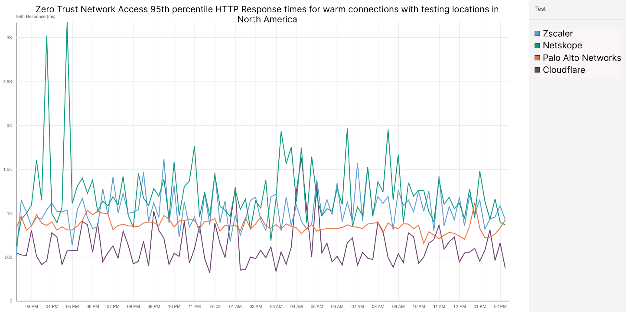
Although the fix involved patching the JDK, it was a simple change. We inserted padding between “_secondary_super_cache” and “_secondary_supers” fields to ensure they never fall into the same cache line. Note that we did not change the functional aspect of JDK behavior, but rather the data layout:
The results of deploying the patch were immediately noticeable. The graph below is a breakdown of CPU by node. Here we can see a red-black deployment happening at noon, and the new ASG with the patched JDK taking over by 12:15:
Both CPU and latency (graph omitted for brevity) showed a similar picture — the “slow” band of nodes was gone!
True Sharing
We didn’t have much time to marvel at these results, however. As the autoscaling reached our CPU target, we noticed that we still couldn’t push more than ~150 RPS per node — well short of our goal of ~250 RPS. Another round of vTune profiling on the patched JDK version showed the same bottleneck around secondary superclass cache lookup. It was puzzling at first to see seemingly the same problem coming back right after we put in a fix, but upon closer inspection we realized we’re dealing with “true sharing” now. Unlike “false sharing,” where 2 independent variables share a cache line, “true sharing” refers to the same variable being read and written by multiple threads/cores. In this case, CPU-enforced memory ordering is the cause of slowdown. We reasoned that removing the obstacle of false sharing and increasing the overall throughput resulted in increased execution of the same JVM superclass caching code path. Essentially, we have higher execution concurrency, causing excessive pressure on the superclass cache due to CPU-enforced memory ordering protocols. The common way to resolve this is to avoid writing to the shared variable altogether, effectively bypassing the JVM’s secondary superclass cache. Since this change altered the behavior of the JDK, we gated it behind a command line flag. This is the entirety of our patch:
And here are the results of running with disabled superclass cache writes:
Our fix pushed the throughput to ~350 RPS at the same CPU autoscaling target of 55%. To put this in perspective, that’s a 3.5x improvement over the throughput we initially reached on m5.12xl, along with a reduction in both average and tail latency.
Future work
Disabling writes to the secondary superclass cache worked well in our case, and even though this might not be a desirable solution in all cases, we wanted to share our methodology, toolset and the fix in the hope that it would help others encountering similar symptoms. While working through this problem, we came across JDK-8180450 — a bug that’s been dormant for more than five years that describes exactly the problem we were facing. It seems ironic that we could not find this bug until we actually figured out the answer. We believe our findings complement the great work that has been done in diagnosing and remediating it.
Conclusion
We tend to think of modern JVMs as highly optimized runtime environments, in many cases rivaling more “performance-oriented” languages like C++. While it holds true for the majority of workloads, we were reminded that performance of certain workloads running within JVMs can be affected not only by the design and implementation of the application code, but also by the implementation of the JVM itself. In this blogpost we described how we were able to leverage PMCs in order to find a bottleneck in the JVM’s native code, patch it, and subsequently realize better than a threefold increase in throughput for the workload in question. When it comes to this class of performance issues, the ability to introspect the execution at the level of CPU microarchitecture proved to be the only solution. Intel vTune provides valuable insight even with the core set of PMCs, such as those exposed by m5.12xl instance type. Exposing a more comprehensive set of PMCs along with PEBS across all instance types and sizes in the cloud environment would pave the way for deeper performance analysis and potentially even larger performance gains.
Today we are excited to talk about Pingora, a new HTTP proxy we’ve built in-house using Rust that serves over 1 trillion requests a day, boosts our performance, and enables many new features for Cloudflare customers, all while requiring only a third of the CPU and memory resources of our previous proxy infrastructure.
As Cloudflare has scaled we’ve outgrown NGINX. It was great for many years, but over time its limitations at our scale meant building something new made sense. We could no longer get the performance we needed nor did NGINX have the features we needed for our very complex environment.
Many Cloudflare customers and users use the Cloudflare global network as a proxy between HTTP clients (such as web browsers, apps, IoT devices and more) and servers. In the past, we’ve talked a lot about how browsers and other user agents connect to our network, and we’ve developed a lot of technology and implemented new protocols (see QUIC and optimizations for http2) to make this leg of the connection more efficient.
Today, we’re focusing on a different part of the equation: the service that proxies traffic between our network and servers on the Internet. This proxy service powers our CDN, Workers fetch, Tunnel, Stream, R2 and many, many other features and products.
Let’s dig in on why we chose to replace our legacy service and how we developed Pingora, our new system designed specifically for Cloudflare’s customer use cases and scale.
Why build yet another proxy
Over the years, our usage of NGINX has run up against limitations. For some limitations, we optimized or worked around them. But others were much harder to overcome.
Architecture limitations hurt performance
The NGINX worker (process) architecture has operational drawbacks for our use cases that hurt our performance and efficiency.
Because of this request-process pinning effect, requests that do CPU heavy or blocking IO tasks can slow down other requests. As those blog posts attest we’ve spent a lot of time working around these problems.
The most critical problem for our use cases is poor connection reuse. Our machines establish TCP connections to origin servers to proxy HTTP requests. Connection reuse speeds up TTFB (time-to-first-byte) of requests by reusing previously established connections from a connection pool, skipping TCP and TLS handshakes required on a new connection.
However, the NGINX connection pool is per worker. When a request lands on a certain worker, it can only reuse the connections within that worker. When we add more NGINX workers to scale up, our connection reuse ratio gets worse because the connections are scattered across more isolated pools of all the processes. This results in slower TTFB and more connections to maintain, which consumes resources (and money) for both us and our customers.
As mentioned in past blog posts, we have workarounds for some of these issues. But if we can address the fundamental issue: the worker/process model, we will resolve all these problems naturally.
Some types of functionality are difficult to add
NGINX is a very good web server, load balancer or a simple gateway. But Cloudflare does way more than that. We used to build all the functionality we needed around NGINX, which is not easy to do while trying not to diverge too much from NGINX upstream codebase.
For example, when retrying/failing over a request, sometimes we want to send a request to a different origin server with a different set of request headers. But that is not something NGINX allows us to do. In cases like this, we spend time and effort on working around the NGINX constraints.
Meanwhile, the programming languages we had to work with didn’t provide help alleviating the difficulties. NGINX is purely in C, which is not memory safe by design. It is very error-prone to work with such a 3rd party code base. It is quite easy to get into memory safety issues, even for experienced engineers, and we wanted to avoid these as much as possible.
The other language we used to complement C is Lua. It is less risky but also less performant. In addition, we often found ourselves missing static typing when working with complicated Lua code and business logic.
And the NGINX community is not very active, and development tends to be “behind closed doors”.
Choosing to build our own
Over the past few years, as we’ve continued to grow our customer base and feature set, we continually evaluated three choices:
Continue to invest in NGINX and possibly fork it to tailor it 100% to our needs. We had the expertise needed, but given the architecture limitations mentioned above, significant effort would be required to rebuild it in a way that fully supported our needs.
Migrate to another 3rd party proxy codebase. There are definitely good projects, like envoy and others. But this path means the same cycle may repeat in a few years.
Start with a clean slate, building an in-house platform and framework. This choice requires the most upfront investment in terms of engineering effort.
We evaluated each of these options every quarter for the past few years. There is no obvious formula to tell which choice is the best. For several years, we continued with the path of the least resistance, continuing to augment NGINX. However, at some point, building our own proxy’s return on investment seemed worth it. We made a call to build a proxy from scratch, and began designing the proxy application of our dreams.
The Pingora Project
Design decisions
To make a proxy that serves millions of requests per second fast, efficient and secure, we have to make a few important design decisions first.
We chose Rust as the language of the project because it can do what C can do in a memory safe way without compromising performance.
Although there are some great off-the-shelf 3rd party HTTP libraries, such as hyper, we chose to build our own because we want to maximize the flexibility in how we handle HTTP traffic and to make sure we can innovate at our own pace.
At Cloudflare, we handle traffic across the entire Internet. We have many cases of bizarre and non-RFC compliant HTTP traffic that we have to support. For example, hyper did not support HTTP status codes greater than 599 until late 2020, three years after people initially raised the issue and repeatedly argued that it was necessary. And we need more than being correct. We need a robust, permissive, customizable HTTP library that can survive the wilds of the Internet. The best way to guarantee that is to implement our own.
The next design decision was around our workload scheduling system. We chose multithreading over multiprocessing in order to share resources, especially connection pools, easily. We also decided that work stealing was required to avoid some classes of performance problems mentioned above. The Tokio async runtime turned out to be a great fit for our needs.
Finally, we wanted our project to be intuitive and developer friendly. What we build is not the final product, and should be extensible as a platform as more features are built on top of it. We decided to implement a “life of a request” event based programmable interface similar to NGINX/OpenResty. For example, the “request filter” phase allows developers to run code to modify or reject the request when a request header is received. With this design, we can separate our business logic and generic proxy logic cleanly. Developers who previously worked on NGINX can easily switch to Pingora and quickly become productive.
Pingora is faster in production
Let’s fast-forward to the present. Pingora handles almost every HTTP request that needs to interact with an origin server (for a cache miss, for example), and we’ve collected a lot of performance data in the process.
First, let’s see how Pingora speeds up our customer’s traffic. Overall traffic on Pingora shows 5ms reduction on median TTFB and 80ms reduction on the 95th percentile. This is not because we run code faster. Even our old service could handle requests in the sub-millisecond range.
The savings come from our new architecture which can share connections across all threads. This means a better connection reuse ratio, which spends less time on TCP and TLS handshakes.
Across all customers, Pingora makes only a third as many new connections per second compared to the old service. For one major customer, it increased the connection reuse ratio from 87.1% to 99.92%, which reduced new connections to their origins by 160x. To present the number more intuitively, by switching to Pingora, we save our customers and users 434 years of handshake time every day.
More features
Having a developer friendly interface engineers are familiar with while eliminating the previous constraints allows us to develop more features, more quickly. Core functionality like new protocols act as building blocks to more products we can offer to customers.
More recently we’ve announced Cache Reserve where Pingora uses R2 storage as a caching layer. As we add more functionality to Pingora, we’re able to offer new products that weren’t feasible before.
More efficient
In production, Pingora consumes about 70% less CPU and 67% less memory compared to our old service with the same traffic load. The savings come from a few factors.
Our Rust code runs more efficiently compared to our old Lua code. On top of that, there are also efficiency differences from their architectures. For example, in NGINX/OpenResty, when the Lua code wants to access an HTTP header, it has to read it from the NGINX C struct, allocate a Lua string and then copy it to the Lua string. Afterwards, Lua has to garbage-collect its new string as well. In Pingora, it would just be a direct string access.
The multithreading model also makes sharing data across requests more efficient. NGINX also has shared memory but due to implementation limitations, every shared memory access has to use a mutex lock and only strings and numbers can be put into shared memory. In Pingora, most shared items can be accessed directly via shared references behind atomic reference counters.
Another significant portion of CPU saving, as mentioned above, is from making fewer new connections. TLS handshakes are expensive compared to just sending and receiving data via established connections.
Safer
Shipping features quickly and safely is difficult, especially at our scale. It’s hard to predict every edge case that can occur in a distributed environment processing millions of requests a second. Fuzzing and static analysis can only mitigate so much. Rust’s memory-safe semantics guard us from undefined behavior and give us confidence our service will run correctly.
With those assurances we can focus more on how a change to our service will interact with other services or a customer’s origin. We can develop features at a higher cadence and not be burdened by memory safety and hard to diagnose crashes.
When crashes do occur an engineer needs to spend time to diagnose how it happened and what caused it. Since Pingora’s inception we’ve served a few hundred trillion requests and have yet to crash due to our service code.
In fact, Pingora crashes are so rare we usually find unrelated issues when we do encounter one. Recently we discovered a kernel bug soon after our service started crashing. We’ve also discovered hardware issues on a few machines, in the past ruling out rare memory bugs caused by our software even after significant debugging was nearly impossible.
Conclusion
To summarize, we have built an in-house proxy that is faster, more efficient and versatile as the platform for our current and future products.
We will be back with more technical details regarding the problems we faced, the optimizations we applied and the lessons we learned from building Pingora and rolling it out to power a significant portion of the Internet. We will also be back with our plan to open source it.
Pingora is our latest attempt at rewriting our system, but it won’t be our last. It is also only one of the building blocks in the re-architecting of our systems.
Since my previous blog about Secondary DNS, Cloudflare’s DNS traffic has more than doubled from 15.8 trillion DNS queries per month to 38.7 trillion. Our network now spans over 270 cities in over 100 countries, interconnecting with more than 10,000 networks globally. According to w3 stats, “Cloudflare is used as a DNS server provider by 15.3% of all the websites.” This means we have an enormous responsibility to serve DNS in the fastest and most reliable way possible.
Although the response time we have on DNS queries is the most important performance metric, there is another metric that sometimes goes unnoticed. DNS Record Propagation time is how long it takes changes submitted to our API to be reflected in our DNS query responses. Every millisecond counts here as it allows customers to quickly change configuration, making their systems much more agile. Although our DNS propagation pipeline was already known to be very fast, we had identified several improvements that, if implemented, would massively improve performance. In this blog post I’ll explain how we managed to drastically improve our DNS record propagation speed, and the impact it has on our customers.
How DNS records are propagated
Cloudflare uses a multi-stage pipeline that takes our customers’ DNS record changes and pushes them to our global network, so they are available all over the world.
The steps shown in the diagram above are:
Customer makes a change to a record via our DNS Records API (or UI).
The change is persisted to the database.
The database event triggers a Kafka message which is consumed by the Zone Builder.
The Zone Builder takes the message, collects the contents of the zone from the database and pushes it to Quicksilver, our distributed KV store.
Quicksilver then propagates this information to the network.
Of course, this is a simplified version of what is happening. In reality, our API receives thousands of requests per second. All POST/PUT/PATCH/DELETE requests ultimately result in a DNS record change. Each of these changes needs to be actioned so that the information we show through our API and in the Cloudflare dashboard is eventually consistent with the information we use to respond to DNS queries.
Historically, one of the largest bottlenecks in the DNS propagation pipeline was the Zone Builder, shown in step 4 above. Responsible for collecting and organizing records to be written to our global network, our Zone Builder often ate up most of the propagation time, especially for larger zones. As we continue to scale, it is important for us to remove any bottlenecks that may exist in our systems, and this was clearly identified as one such bottleneck.
Growing pains
When the pipeline shown above was first announced, the Zone Builder received somewhere between 5 and 10 DNS record changes per second. Although the Zone Builder at the time was a massive improvement on the previous system, it was not going to last long given the growth that Cloudflare was and still is experiencing. Fast-forward to today, we receive on average 250 DNS record changes per second, a staggering 25x growth from when the Zone Builder was first announced.
The way that the Zone Builder was initially designed was quite simple. When a zone changed, the Zone Builder would grab all the records from the database for that zone and compare them with the records stored in Quicksilver. Any differences were fixed to maintain consistency between the database and Quicksilver.
This is known as a full build. Full builds work great because each DNS record change corresponds to one zone change event. This means that multiple events can be batched and subsequently dropped if needed. For example, if a user makes 10 changes to their zone, this will result in 10 events. Since the Zone Builder grabs all the records for the zone anyway, there is no need to build the zone 10 times. We just need to build it once after the final change has been submitted.
What happens if the zone contains one million records or 10 million records? This is a very real problem, because not only is Cloudflare scaling, but our customers are scaling with us. Today our largest zone currently has millions of records. Although our database is optimized for performance, even one full build containing one million records took up to 35 seconds, largely caused by database query latency. In addition, when the Zone Builder compares the zone contents with the records stored in Quicksilver, we need to fetch all the records from Quicksilver for the zone, adding time. However, the impact doesn’t just stop at the single customer. This also eats up more resources from other services reading from the database and slows down the rate at which our Zone Builder can build other zones.
Per-record build: a new build type
Many of you might already have the solution to this problem in your head:
Why doesn’t the Zone Builder just query the database for the record that has changed and propagate just the single record?
Of course this is the correct solution, and the one we eventually ended up at. However, the road to get there was not as simple as it might seem.
Firstly, our database uses a series of functions that, at zone touch time, create a PostgreSQL Queue (PGQ) event that ultimately gets turned into a Kafka event. Initially, we had no distinction for individual record events, which meant our Zone Builder had no idea what had actually changed until it queried the database.
Next, the Zone Builder is still responsible for DNS zone settings in addition to records. Some examples of DNS zone settings include custom nameserver control and DNSSEC control. As a result, our Zone Builder needed to be aware of specific build types to ensure that they don’t step on each other. Furthermore, per-record builds cannot be batched in the same way that zone builds can because each event needs to be actioned separately.
As a result, a brand new scheduling system needed to be written. Lastly, Quicksilver interaction needed to be re-written to account for the different types of schedulers. These issues can be broken down as follows:
Create a new Kafka event pipeline for record changes that contain information about the changed record.
Separate the Zone Builder into a new type of scheduler that implements some defined scheduler interface.
Implement the per-record scheduler to read events one by one in the correct order.
Implement the new Quicksilver interface for the per-record scheduler.
Below is a high level diagram of how the new Zone Builder looks internally with the new scheduler types.
It is critically important that we lock between these two schedulers because it would otherwise be possible for the full build scheduler to overwrite the per-record scheduler’s changes with stale data.
It is important to note that none of this per-record architecture would be possible without the use of Cloudflare’s black lie approach to negative answers with DNSSEC. Normally, in order to properly serve negative answers with DNSSEC, all the records within the zone must be canonically sorted. This is needed in order to maintain a list of references from the apex record through all the records in the zone. With this normal approach to negative answers, a single record that has been added to the zone requires collecting all records to determine its insertion point within this sorted list of names.
Bugs
I would love to be able to write a Cloudflare blog where everything went smoothly; however, that is never the case. Bugs happen, but we need to be ready to react to them and set ourselves up so that next time this specific bug cannot happen.
In this case, the major bug we discovered was related to the cleanup of old records in Quicksilver. With the full Zone Builder, we have the luxury of knowing exactly what records exist in both the database and in Quicksilver. This makes writing and cleaning up a fairly simple task.
When the per-record builds were introduced, record events such as creates, updates, and deletes all needed to be treated differently. Creates and deletes are fairly simple because you are either adding or removing a record from Quicksilver. Updates introduced an unforeseen issue due to the way that our PGQ was producing Kafka events. Record updates only contained the new record information, which meant that when the record name was changed, we had no way of knowing what to query for in Quicksilver in order to clean up the old record. This meant that any time a customer changed the name of a record in the DNS Records API, the old record would not be deleted. Ultimately, this was fixed by replacing those specific update events with both a creation and a deletion event so that the Zone Builder had the necessary information to clean up the stale records.
None of this is rocket surgery, but we spend engineering effort to continuously improve our software so that it grows with the scaling of Cloudflare. And it’s challenging to change such a fundamental low-level part of Cloudflare when millions of domains depend on us.
Results
Today, all DNS Records API record changes are treated as per-record builds by the Zone Builder. As I previously mentioned, we have not been able to get rid of full builds entirely; however, they now represent about 13% of total DNS builds. This 13% corresponds to changes made to DNS settings that require knowledge of the entire zone’s contents.
When we compare the two build types as shown below we can see that per-record builds are on average 150x faster than full builds. The build time below includes both database query time and Quicksilver write time.
From there, our records are propagated to our global network through Quicksilver.
The 150x improvement above is with respect to averages, but what about that 4000x that I mentioned at the start? As you can imagine, as the size of the zone increases, the difference between full build time and per-record build time also increases. I used a test zone of one million records and ran several per-record builds, followed by several full builds. The results are shown in the table below:
Build Type
Build Time (ms)
Per Record #1
6
Per Record #2
7
Per Record #3
6
Per Record #4
8
Per Record #5
6
Full #1
34032
Full #2
33953
Full #3
34271
Full #4
34121
Full #5
34093
We can see that, given five per-record builds, the build time was no more than 8ms. When running a full build however, the build time lasted on average 34 seconds. That is a build time reduction of 4250x!
Given the full build times for both average-sized zones and large zones, it is apparent that all Cloudflare customers are benefitting from this improved performance, and the benefits only improve as the size of the zone increases. In addition, our Zone Builder uses less database and Quicksilver resources meaning other Cloudflare systems are able to operate at increased capacity.
Next Steps
The results here have been very impactful, though we think that we can do even better. In the future, we plan to get rid of full builds altogether by replacing them with zone setting builds. Instead of fetching the zone settings in addition to all the records, the zone setting builder would just fetch the settings for the zone and propagate that to our global network via Quicksilver. Similar to the per-record builds, this is a difficult challenge due to the complexity of zone settings and the number of actors that touch it. Ultimately if this can be accomplished, we can officially retire the full builds and leave it as a reminder in our git history of the scale at which we have grown over the years.
In addition, we plan to introduce a batching system that will collect record changes into groups to minimize the number of queries we make to our database and Quicksilver.
Does solving these kinds of technical and operational challenges excite you? Cloudflare is always hiring for talented specialists and generalists within our Engineering and other teams.
The collective thoughts of the interwebz
Manage Consent
To provide the best experiences, we use technologies like cookies to store and/or access device information. Consenting to these technologies will allow us to process data such as browsing behavior or unique IDs on this site. Not consenting or withdrawing consent, may adversely affect certain features and functions.
Functional
Always active
The technical storage or access is strictly necessary for the legitimate purpose of enabling the use of a specific service explicitly requested by the subscriber or user, or for the sole purpose of carrying out the transmission of a communication over an electronic communications network.
Preferences
The technical storage or access is necessary for the legitimate purpose of storing preferences that are not requested by the subscriber or user.
Statistics
The technical storage or access that is used exclusively for statistical purposes.The technical storage or access that is used exclusively for anonymous statistical purposes. Without a subpoena, voluntary compliance on the part of your Internet Service Provider, or additional records from a third party, information stored or retrieved for this purpose alone cannot usually be used to identify you.
Marketing
The technical storage or access is required to create user profiles to send advertising, or to track the user on a website or across several websites for similar marketing purposes.