Post Syndicated from Harsh Vardhan Singh Gaur original https://aws.amazon.com/blogs/big-data/introducing-pii-data-identification-and-handling-using-aws-glue-databrew/
AWS Glue DataBrew, a visual data preparation tool, can now identify and handle sensitive data by applying advance transformations like redaction, replacement, encryption, and decryption on your personally identifiable information (PII) data. With exponential growth of data, companies are handling huge volumes and a wide variety of data coming into their platform, including PII data. Identifying and protecting sensitive data at scale has become increasingly complex, expensive, and time-consuming. Organizations have to adhere to data privacy, compliance, and regulatory needs such as GDPR and CCPA. They need to identify sensitive data, including PII such as name, SSN, address, email, driver’s license, and more. Even after identification, it’s cumbersome to implement redaction, masking, or encryption of sensitive personal information at scale.
To enable data privacy and protection, DataBrew has launched PII statistics, which identifies PII columns and provide their data statistics when you run a profile job on your dataset. Furthermore, DataBrew has introduced PII data handling transformations, which enable you to apply data masking, encryption, decryption, and other operations on your sensitive data.
In this post, we walk through a solution in which we run a data profile job to identify and suggest potential PII columns present in a dataset. Next, we target PII columns in a DataBrew project and apply various transformations to handle the sensitive columns existing in the dataset. Finally, we run a DataBrew job to apply the transformations on the entire dataset and store the processed, masked, and encrypted data securely in Amazon Simple Storage Service (Amazon S3).
Solution overview
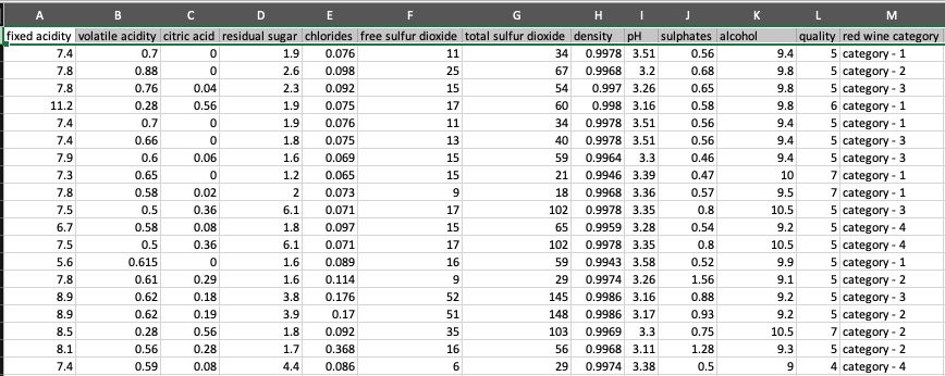
We use a public dataset that is available for download at Synthetic Patient Records with COVID-19. The data hosted within SyntheticMass has been generated by SyntheaTM, an open-source patient population simulation made available by The MITRE Corporation.
Download the zipped file 10k_synthea_covid19_csv.zip for this solution and unzip it locally. The solution uses the dummy data in the file patient.csv to demonstrate data redaction and encryption capability. The file contains 10,000 synthetic patient records in CSV format, including PII columns like driver’s license, birth date, address, SSN, and more.
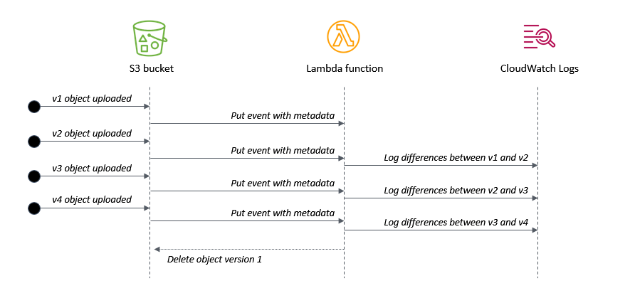
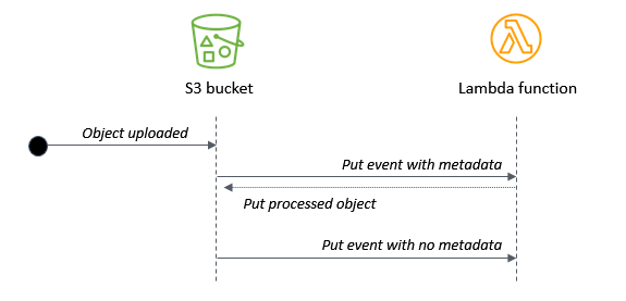
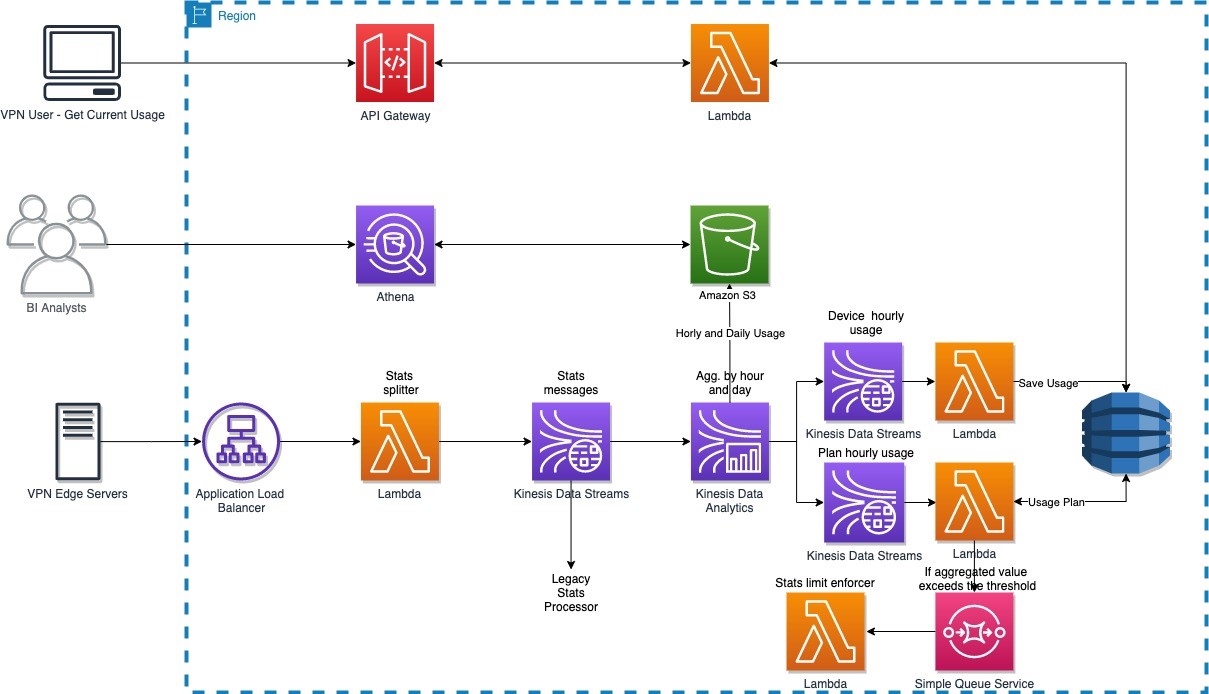
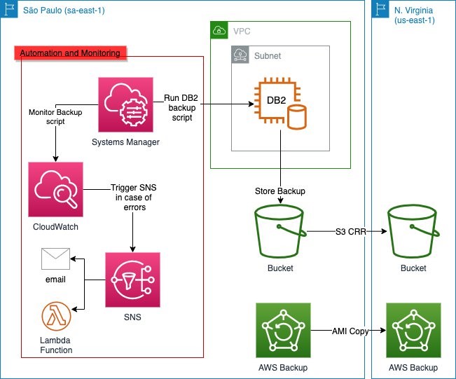
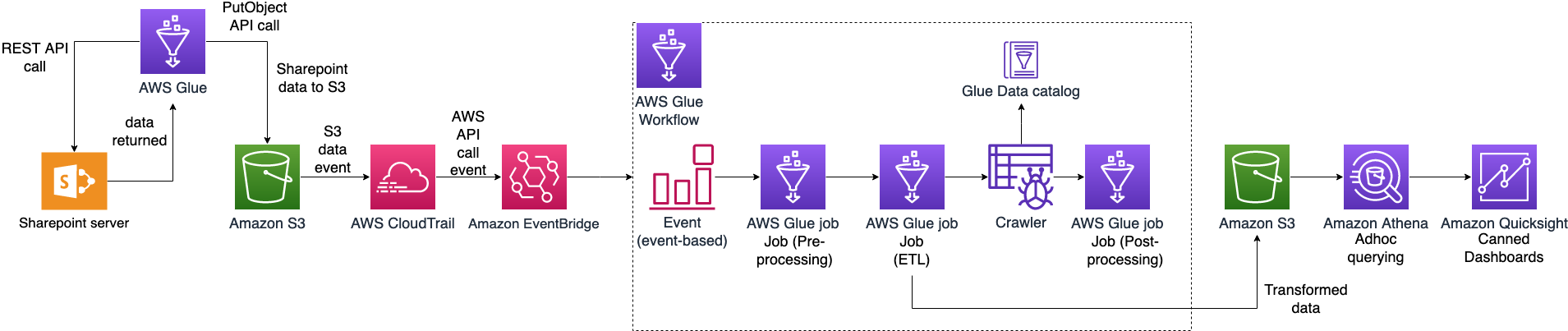
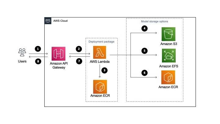
The following diagram illustrates the architecture for our solution.
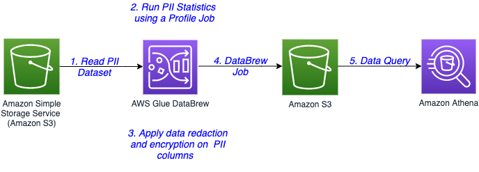
The steps in this solution are as follows:
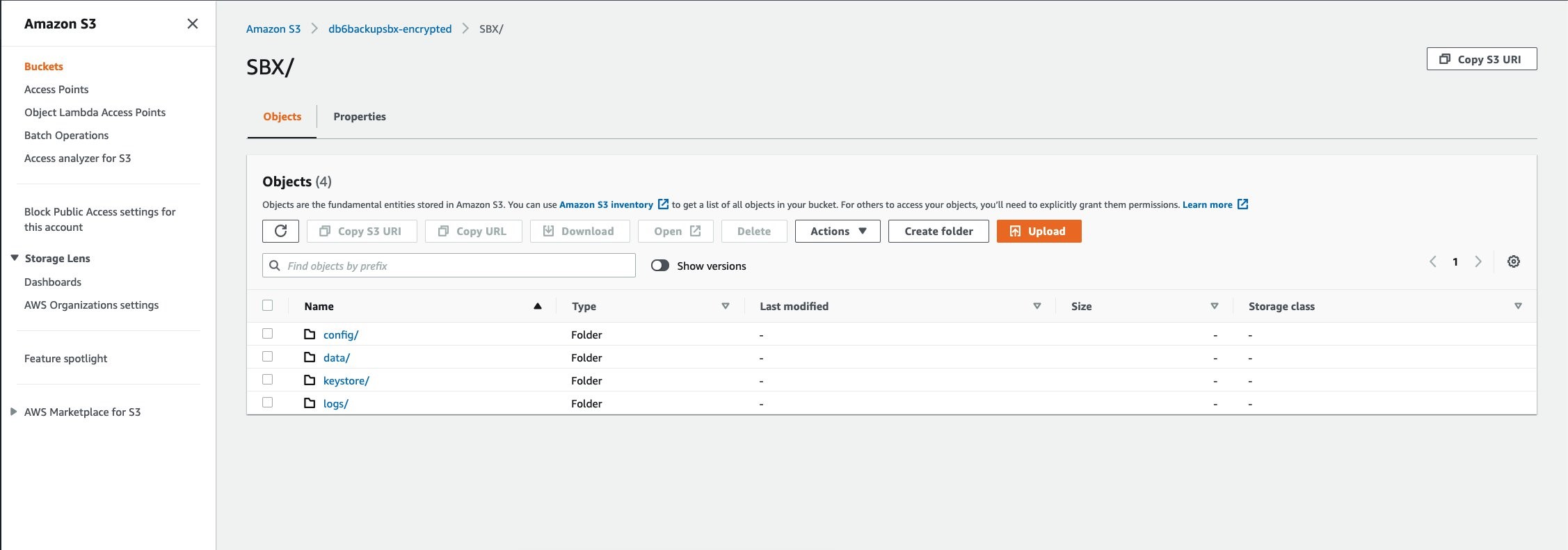
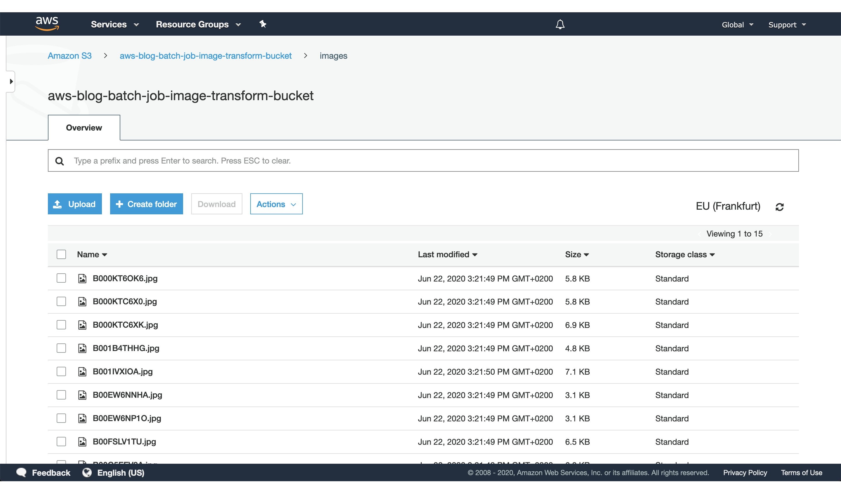
- The sensitive data is stored in an S3 bucket. You create a DataBrew dataset by connecting to the data in Amazon S3.
- Run a DataBrew profile job to identify the PII columns present in the dataset by enabling PII statistics.
- After identification of PII columns, apply transformations to redact or encrypt column values as a part of your recipe.
- A DataBrew job runs the recipe steps on the entire data and generates output files with sensitive data redacted or encrypted.
- After the output data is written to Amazon S3, we create an external table on top in Amazon Athena. Data consumers can use Athena to query the processed and cleaned data.
Prerequisites
For this walkthrough, you need an AWS account. Use us-east-1 as your AWS Region to implement this solution.
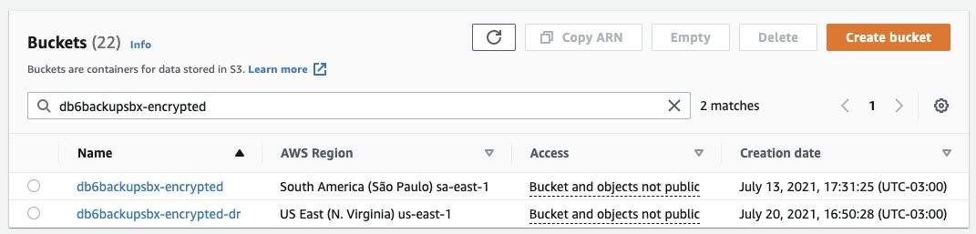
Set up your source data in Amazon S3
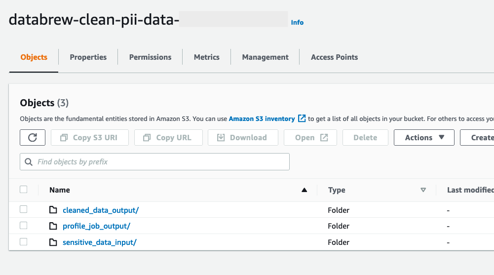
Create an S3 bucket called databrew-clean-pii-data-<Your-Account-ID> in us-east-1 with the following prefixes:
sensitive_data_inputcleaned_data_outputprofile_job_output
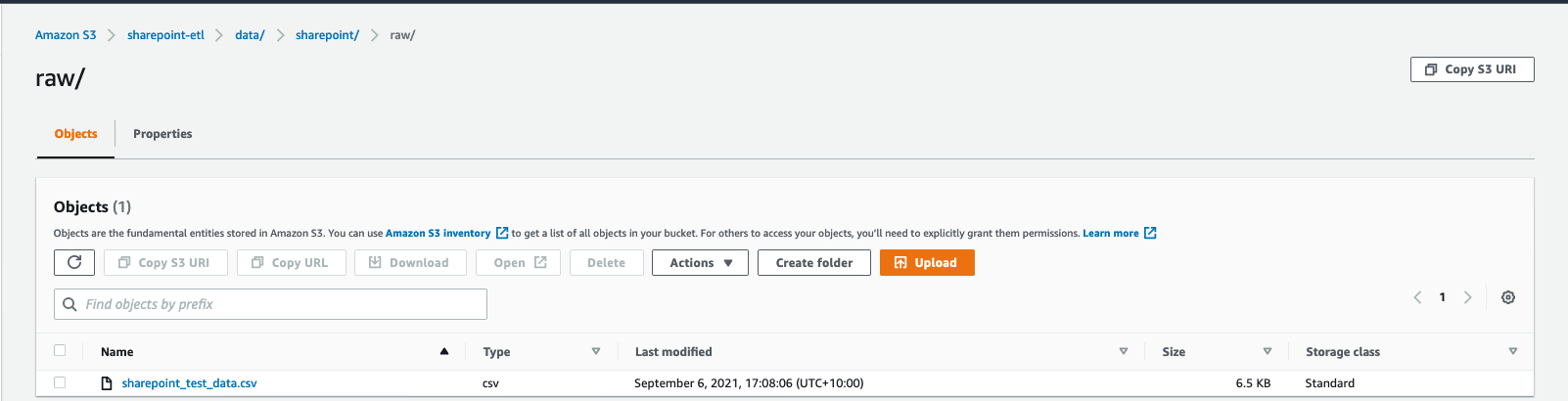
Upload the patient.csv file to the sensitive_data_input prefix.
Create a DataBrew dataset
To create a DataBrew dataset, complete the following steps:
- On the DataBrew console, in the navigation pane, choose Datasets.
- Choose Connect new dataset.
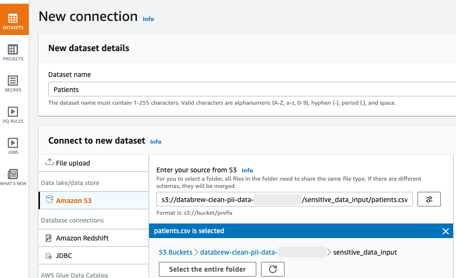
- For Dataset name, enter a name (for this post,
Patients). - Under Connect to new dataset, select Amazon S3 as your source.
- For Enter your source from S3, enter the S3 path to the
patient.csvfile. In our case, this iss3://databrew-clean-pii-data-<Account-ID>/ sensitive_data_input/patients.csv. - Scroll to the bottom of the page and choose Create dataset.
Run a data profile job
You’re now ready to create your profile job.
- In the navigation pane, choose Datasets.
- Select the
Patientsdataset. - Choose Run data profile and choose Create profile job.

- Name the job
Patients - Data Profile Job. - We run the data profile on the entire dataset, so for Data sample, select Full dataset.
- In the Job output settings section, point to the
profile_job_outputS3 prefix where the data profile output is stored when the job is complete.

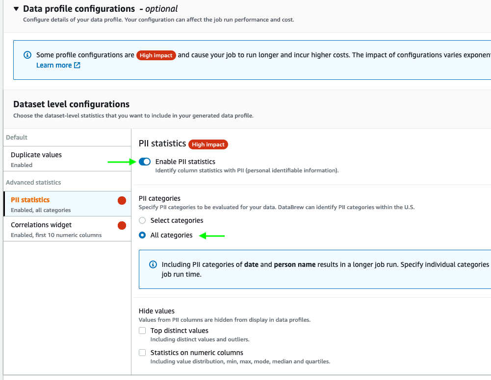
- Expand Data profile configurations, and select Enable PII statistics to identify PII columns when running the data profile job.


This option is disabled by default; you must enable it manually before running the data profile job.
- For PII categories, select All categories.

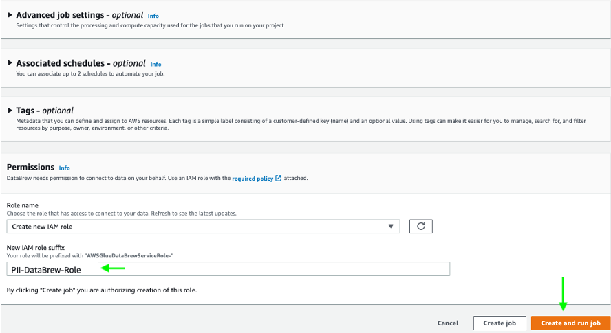
- Keep the remaining settings at their default.
- In the Permissions section, create a new AWS Identity and Access Management (IAM) role that is used by the DataBrew job to run the profile job, and use
PII-DataBrew-Roleas the role suffix. - Choose Create and run job.

The job runs on the sample data and takes a few minutes to complete.
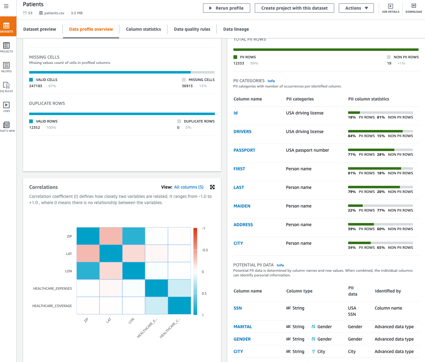
Now that we’ve run our profile job, we can review data profile insights about our dataset by choosing View data profile. We can also review the results of the profile through the visualizations on the DataBrew console and view the PII widget. This section provides a list of identified PII columns mapped to PII categories with column statistics. Furthermore, it suggests potential PII data that you can review.
Create a DataBrew project
After we identify the PII columns in our dataset, we can focus on handling the sensitive data in our dataset. In this solution, we perform redaction and encryption in our DataBrew project using the Sensitive category of transformations.
To create a DataBrew project for handling our sensitive data, complete the following steps:
- On the DataBrew console, choose Projects.
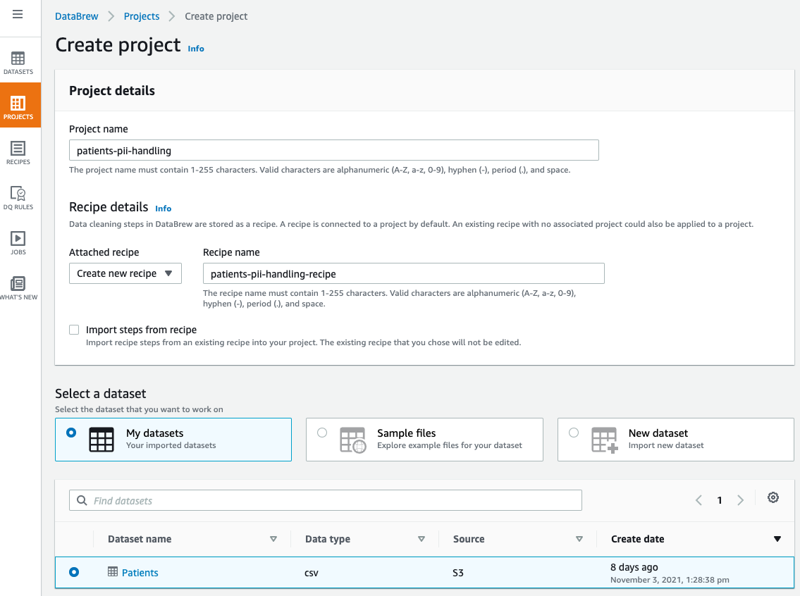
- Choose Create project.
- For Project name, enter a name (for this post,
patients-pii-handling). - For Select a dataset, select My datasets.
- Select the
Patientsdataset.

- Under Permissions, for Role name, choose the IAM role that we created previously for our DataBrew profile job
AWSGlueDataBrewServiceRole-PII-DataBrew-Role. - Choose Create project.


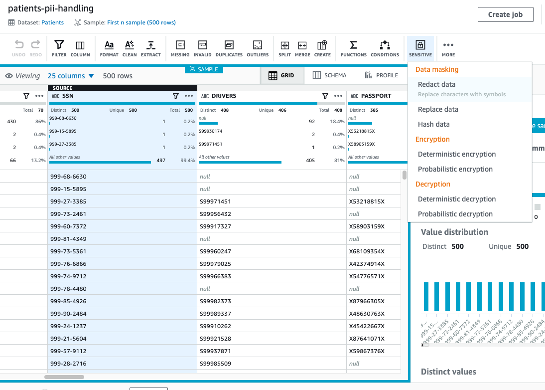
The dataset takes few minutes to load. When the dataset is loaded, we can start performing redactions. Let us start with the column SSN.
- For the
SSNcolumn, on the Sensitive menu, choose Redact data.

- Under Apply redaction, select Full string value.
- We redact all the non-alphanumeric characters and replace them with
#. - Choose Preview changes to compare the redacted values.
- Choose Apply.


On the Sensitive menu, all the data masking transformations—redact, replace, and hash data—are irreversible. After we finalize our recipe and run the DataBrew job, the job output to Amazon S3 is permanently redacted and we can’t recover it.
- Now, let’s apply redaction to multiple columns, assuming the following columns must not be consumed by any downstream users like data analyst, BI engineer, and data scientist:
DRIVERSPASSPORTBIRTHPLACEADDRESSLATLON
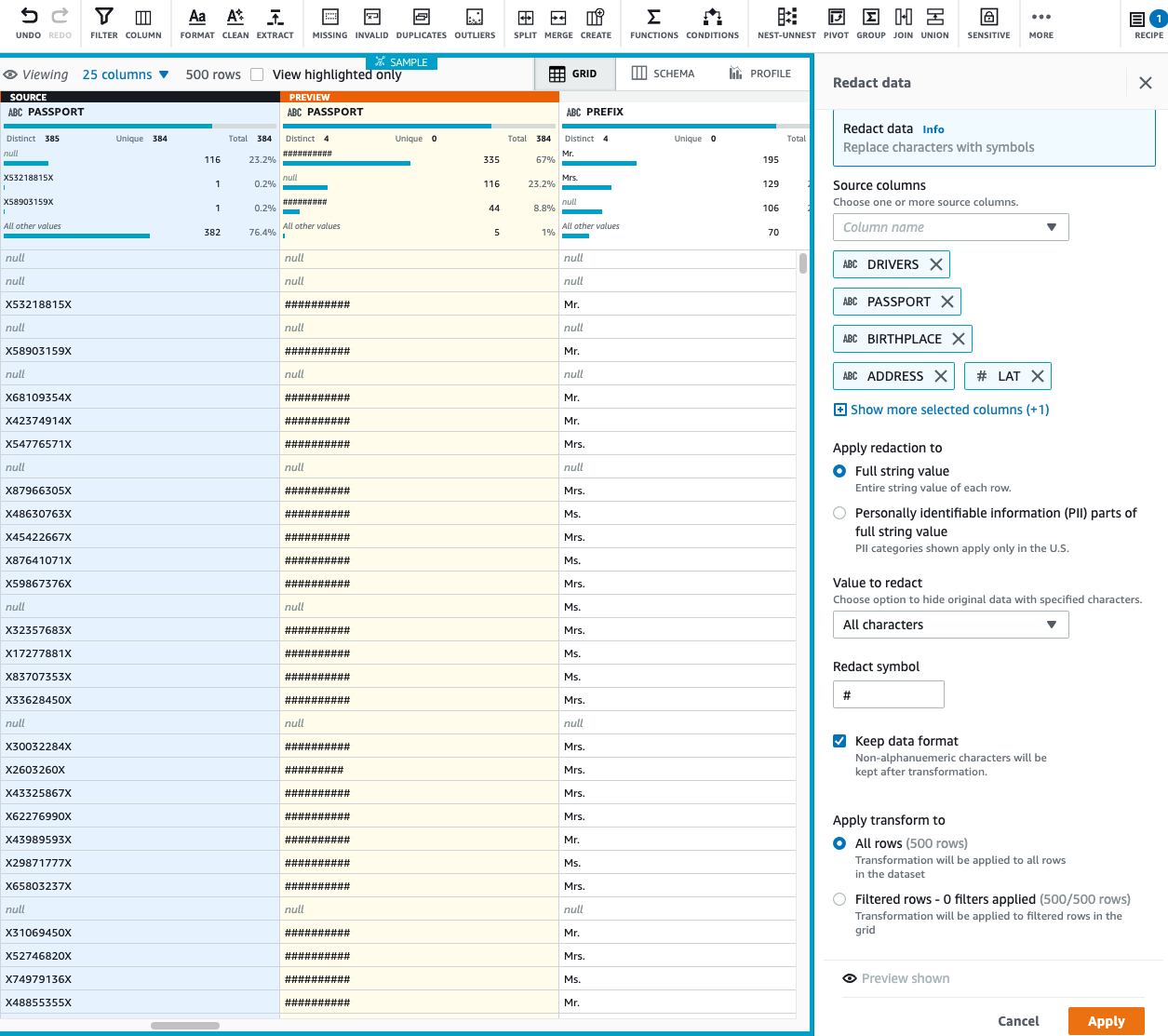
In special cases, when we need to recover our sensitive data, instead of masking, we can encrypt our column values and when needed, decrypt the data to bring it back to its original format. Let’s assume we require a column value to be decrypted by a downstream application; in that case, we can encrypt our sensitive data.
We have two encryption options: deterministic and probabilistic. For use cases when we want to join two datasets on the same encrypted column, we should apply deterministic encryption. It makes sure that the encrypted value of all the distinct values is the same across DataBrew projects as long as we use the same AWS secret key. Additionally, keep in mind that when you apply deterministic encryption on your PII columns, you can only use DataBrew to decrypt those columns.
For our use case, let’s assume we want to perform deterministic encryption on a few of our columns.
- On the Sensitive menu, choose Deterministic encryption.

- For Source columns, select BIRTHDATE, DEATHDATE, FIRST, and LAST.
- For Encryption option, select Deterministic encryption.
- For Select secret, choose the
databrew!defaultAWS secret.

- Choose Apply.
- After you finish applying all your transformations, choose Publish.

- Enter a description for the recipe version and choose Publish.


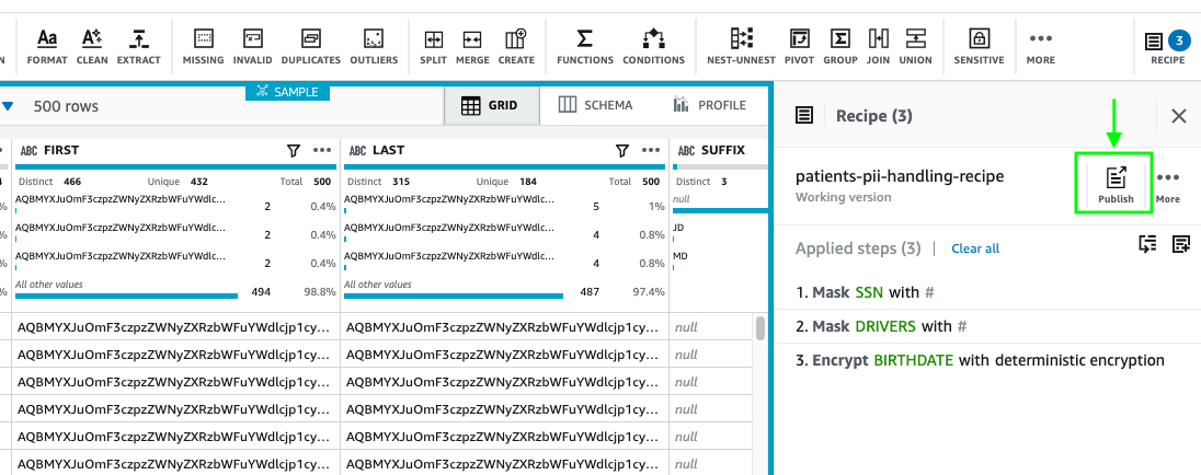

Create a DataBrew job
Now that our recipe is ready, we can create a job to apply the recipe steps to the Patients dataset.
- On the DataBrew console, choose Jobs.
- Choose Create a job.
- For Job name, enter a name (for example,
Patient PII Making and Encryption). - Select the
Patientsdataset and choosepatients-pii-handling-recipeas your recipe. - Under Job output settings¸ for File type, choose your final storage format to be Parquet.
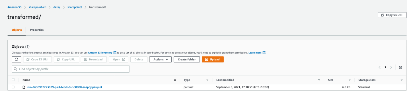
- For S3 location, enter your S3 output as
s3://databrew-clean-pii-data-<Account-ID>/cleaned_data_output/.

- For Compression, choose None.
- For File output storage, select Replace output files for each job run.
- Under Permissions, for Role name¸ choose the same IAM role we used previously.
- Choose Create and run job.

Create an Athena table
You can create tables by writing the DDL statement in the Athena query editor. If you’re not familiar with Apache Hive, you should review Creating Tables in Athena to learn how to create an Athena table that references the data residing in Amazon S3.
To create an Athena table, use the query editor and enter the following DDL statement:
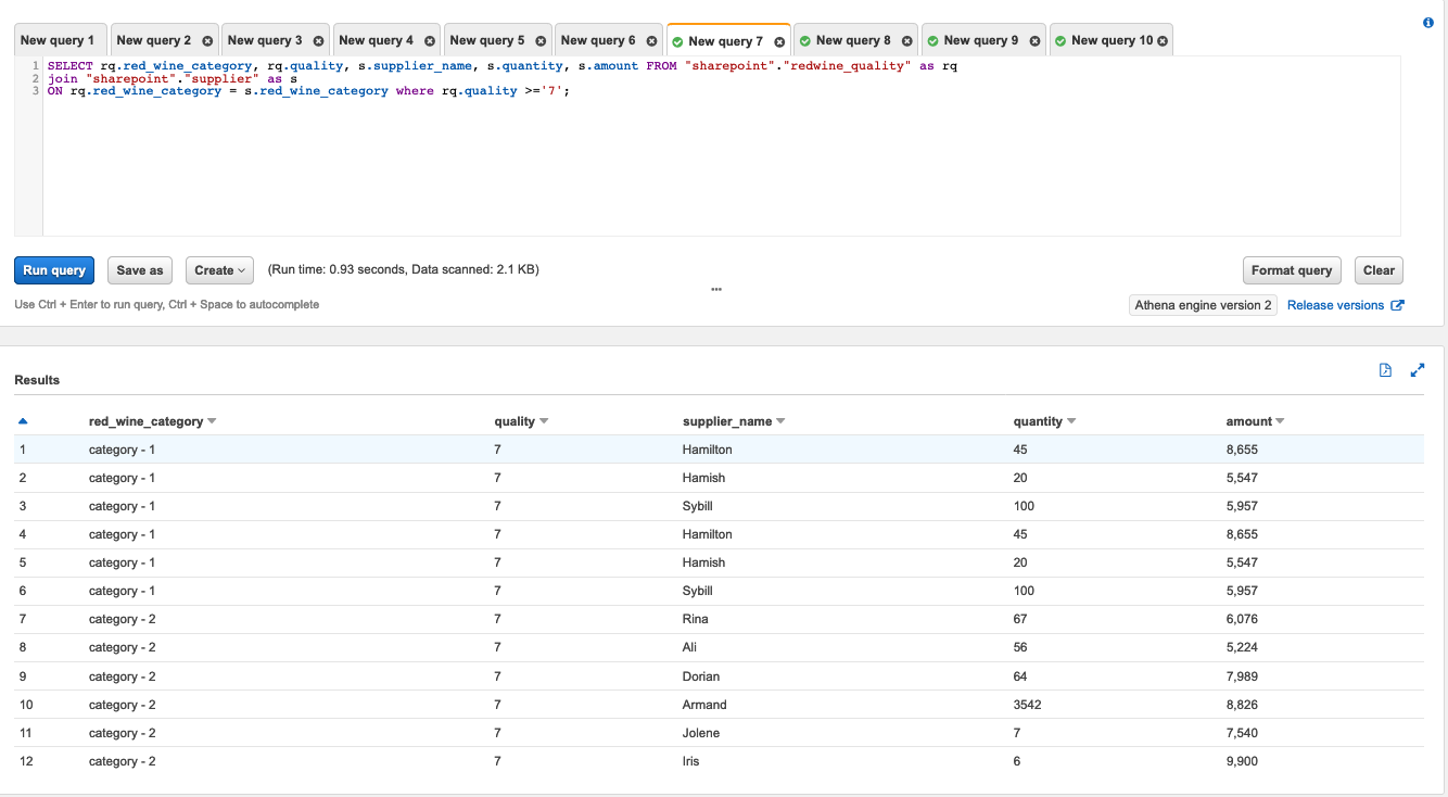
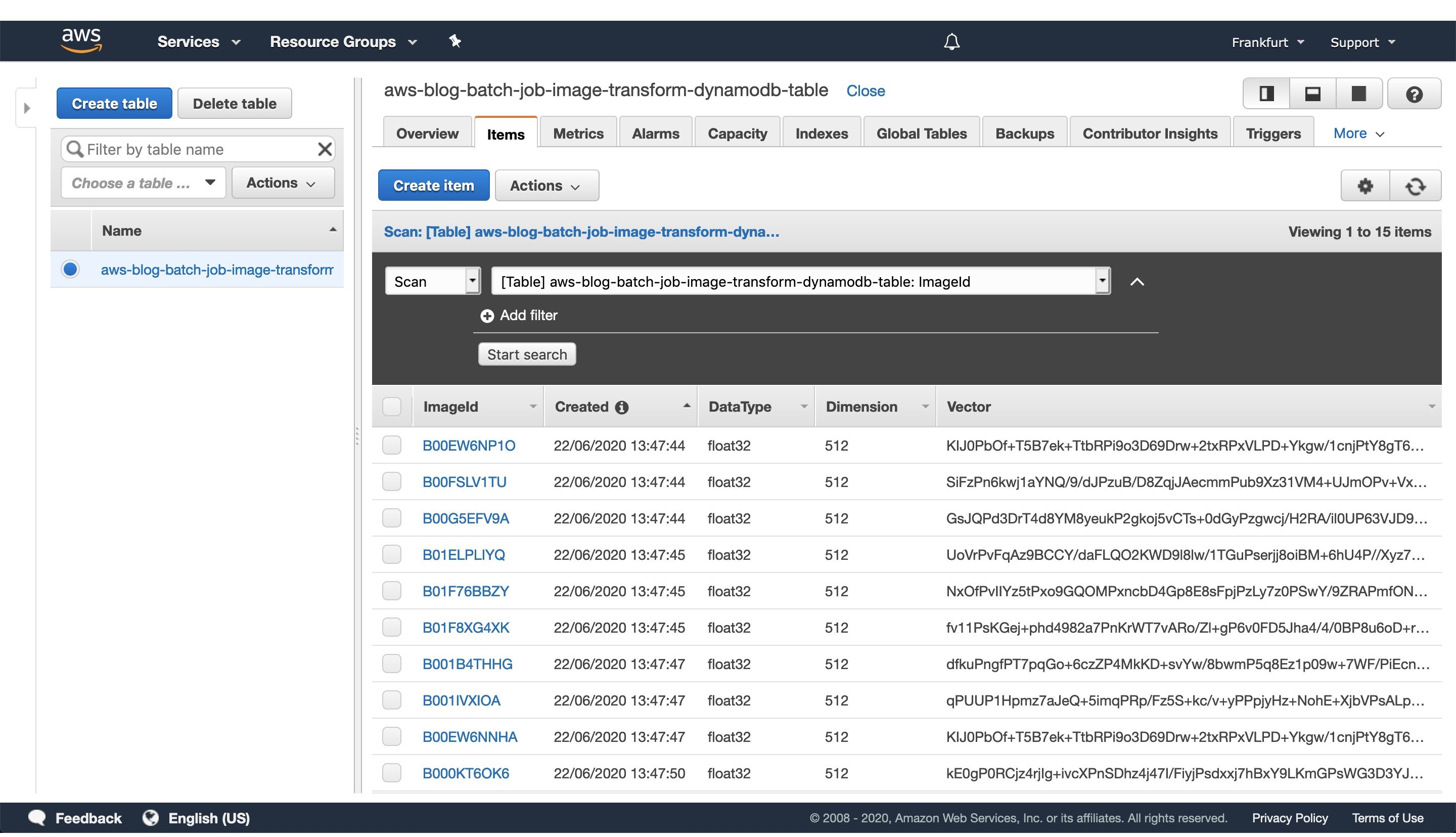
Let’s validate the table output in Athena by running a simple SELECT query. The following screenshot shows the output.
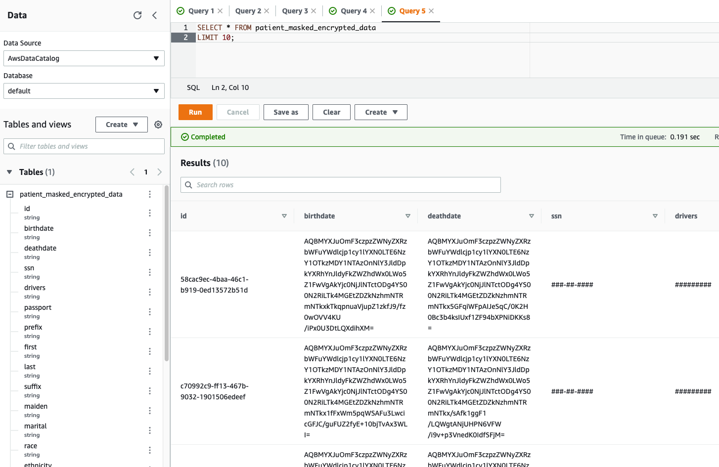
We can clearly see the encrypted and redacted column values in our query output.
Cleaning up
To avoid incurring future charges, delete the resources created during this walkthrough.
Conclusion
As demonstrated in this post, you can use DataBrew to help identify, redact, and encrypt PII data. With these new PII transformations, you can streamline and simplify customer data management across industries such as financial services, government, retail, and much more.
Now that you can protect your sensitive data workloads to meet regulatory and compliance best practices, you can use this solution to build de-identified data lakes in AWS. Sensitive data fields remain protected throughout their lifecycle, whereas non-sensitive data fields remain in the clear. This approach can allow analytics or other business functions to operate on data without exposing sensitive data.
About the Authors
 Harsh Vardhan Singh Gaur is an AWS Solutions Architect, specializing in Analytics. He has over 5 years of experience working in the field of big data and data science. He is passionate about helping customers adopt best practices and discover insights from their data.
 Navnit Shukla is an AWS Specialist Solution Architect, Analytics, and is passionate about helping customers uncover insights from their data. He has been building solutions to help organizations make data-driven decisions.


 Hammad Ausaf is a Sr Solutions Architect in the M&E space. He is a passionate builder and strives to provide the best solutions to AWS customers.
 Andrew Lee is a Solutions Architect on the Snap Account, and is based in Los Angeles, CA.