Tag Archives: Amazon Simple Storage Service (S3)

How to Audit and Report S3 Prefix Level Access Using S3 Access Analyzer

2022-02-11 Somdeb Bhattacharjee

Post Syndicated from Somdeb Bhattacharjee original https://aws.amazon.com/blogs/architecture/how-to-audit-and-report-s3-prefix-level-access-using-s3-access-analyzer/

Data Services teams in all industries are developing centralized data platforms that provide shared access to datasets across multiple business units and teams within the organization. This makes data governance easier, minimizes data redundancy thus reducing cost, and improves data integrity. The central data platform is often built with AWS Simple Storage Service (S3).

A common pattern for providing access to this data is for you to set up cross-account IAM Users and IAM Roles to allow direct access to the datasets stored in S3 buckets. You then enforce the permission on these datasets with S3 Bucket Policies or S3 Access Point policies. These policies can be very granular and you can provide access at the bucket level, prefix level as well as object level within an S3 bucket.

To reduce risk and unintended access, you can use Access Analyzer for S3 to identify S3 buckets within your zone of trust (Account or Organization) that are shared with external identities. Access Analyzer for S3 provides a lot of useful information at the bucket level but you often need S3 audit capability one layer down, at the S3 prefix level, since you are most likely going to organize your data using S3 prefixes.

Common use cases

Many organizations need to ingest a lot of third-party/vendor datasets and then distribute these datasets within the organization in a subscription-based model. Irrespective of how the data is ingested, whether it is using AWS Transfer Family service or other mechanisms, all the ingested datasets are stored in a single S3 bucket with a separate prefix for each vendor dataset. The hierarchy can be represented as:

vendor-s3-bucket
->vendorA-prefix
->vendorA.dataset.csv
->vendorB-prefix
->vendorB.dataset.csv

Based on this design, access is also granted to the data subscribers at the S3 prefix level. Access Analyzer for S3 does not provide visibility at the S3 prefix level so you need to develop custom scripts to extract this information from the S3 policy documents. You also need the information in an easy-to-consume format, for example, a csv file, that can be queried, filtered, readily downloaded and shared across the organization.

To help address this requirement, we show how to implement a solution that builds on the S3 access analyzer findings to generate a csv file on a pre-configured frequency. This solution provides details about:

External Principals outside your trust zone that have access to your S3 buckets
Permissions granted to these external principals (read, write)
List of s3 prefixes these external principals have access to that is configured using S3 bucket policy and/or S3 access point policies.

Architecture Overview

Architecture Diagram showing How to Audit and Report S3 prefix level access using S3 Access Analyzer

Figure 1 – How to Audit and Report S3 prefix level access using S3 Access Analyzer

The solution entails the following steps:

Step 1 – The Access Analyzer ARN and the S3 bucket parameters are passed to an AWS Lambda function via Environment variables.

Step 2 – The Lambda code uses the Access Analyzer ARN to call the list-findings API to retrieve the findings information and store it in the S3 bucket (under json prefix) in JSON format.

Step 3 – The Lambda function then also parses the JSON file to get the required fields and store it as a csv file in the same S3 bucket (under report prefix). It also scans the bucket policy and/or the access point policies to retrieve the S3 prefix level permission granted to the external identity. That information is added to the csv file.

Steps 4 and 5 – As part of the initial deployment, an AWS Glue crawler is provided to discover and create the schema of the csv file and store it in the AWS Glue Data Catalog.

Step 6 – An Amazon Athena query is run to create a spreadsheet of the findings that can be downloaded and distributed for audit.

Prerequisites

For this walkthrough, you should have the following prerequisites:

An AWS account
S3 buckets that are shared with external identities via cross-account IAM roles or IAM users. Follow these instructions in this user guide to set up cross-account S3 bucket access.
IAM Access Analyzer enabled for your AWS account. Follow these instructions to enable IAM Access Analyzer within your account.

Once the IAM Access Analyzer is enabled, you should be able to view the Analyzer findings from the S3 console by selecting the bucket name and clicking on the ‘View findings’ box or directly going to the Access Analyzer findings on the IAM console.

When you select a ‘Finding id’ for an S3 Bucket, a screen similar to the following will appear:

Figure 2 – IAM Console Screenshot

Setup

Now that your access analyzer is running, you can open the link below to deploy the CloudFormation template. Make sure to launch the CloudFormation in the same AWS Region where IAM Access Analyzer has been enabled.

Launch template

Specify a name for the stack and input the following parameters:

ARN of the Access Analyzer which you can find from the IAM Console.
New S3 bucket where your findings will be stored. The Cloudformation template will add a suffix to the bucket name you provide to ensure uniqueness.

Figure 3 – CloudFormation Template screenshot

Select Next twice and on the final screen check the box allowing CloudFormation to create the IAM resources before selecting Create Stack.
It will take a couple of minutes for the stack to create the resources and launch the AWS Lambda function.
Once the stack is in CREATE_COMPLETE status, go to the Outputs tab of the stack and note down the value against the DataS3BucketName key. This is the S3 bucket the template generated. It would be of the format analyzer-findings-xxxxxxxxxxxx. Go to the S3 console and view the contents of the bucket.
There should be two folders archive/ and report/. In the report folder you should have the csv file containing the findings report.
You can download the csv directly and open it in a excel sheet to view the contents. If would like to query the csv based on different attributes, follow the next set of steps.
Go to the AWS Glue console and click on Crawlers. There should be an analyzer-crawler created for you. Select the crawler to run it.
After the crawler runs successfully, you should see a new table, analyzer-report created under analyzerdb Glue database.
Select the tablename to view the table properties and schema.
To query the table, go to the Athena console and select the analyzerdb database. Then you can run a query like “Select * from analyzer-report where externalaccount = <<valid external account>>” to list all the S3 buckets the external account has access to.

Figure 4 – Amazon Athena Console screenshot

The output of the query with a subset of columns is shown as follows:

Figure 5 – Output of Amazon Athena Query

This CloudFormation template also creates a Cloudwatch event rule, testanalyzer-ScheduledRule-xxxxxxx, that launches the Lambda function every Monday to generate a new version of the findings csv file. You can update the rule to set it to a frequency you desire.

Clean Up

To avoid incurring costs, remember to delete the resources you created. First, manually delete the folders ‘archive’ and ‘report’ in the S3 bucket and then delete the CloudFormation stack you deployed at the beginning of the setup.

Conclusion

In this blog, we showed how you can build audit capabilities for external principals accessing your S3 buckets at a prefix level. Organizations looking to provide shared access to datasets across multiple business units will find this solution helpful in improving their security posture. Give this solution a try and share your feedback!

Doing more with less: Moving from transactional to stateful batch processing

2022-02-09 Tom Jin

Post Syndicated from Tom Jin original https://aws.amazon.com/blogs/big-data/doing-more-with-less-moving-from-transactional-to-stateful-batch-processing/

Amazon processes hundreds of millions of financial transactions each day, including accounts receivable, accounts payable, royalties, amortizations, and remittances, from over a hundred different business entities. All of this data is sent to the eCommerce Financial Integration (eCFI) systems, where they are recorded in the subledger.

Ensuring complete financial reconciliation at this scale is critical to day-to-day accounting operations. With transaction volumes exhibiting double-digit percentage growth each year, we found that our legacy transactional-based financial reconciliation architecture proved too expensive to scale and lacked the right level of visibility for our operational needs.

In this post, we show you how we migrated to a batch processing system, built on AWS, that consumes time-bounded batches of events. This not only reduced costs by almost 90%, but also improved visibility into our end-to-end processing flow. The code used for this post is available on GitHub.

Legacy architecture

Our legacy architecture primarily utilized Amazon Elastic Compute Cloud (Amazon EC2) to group related financial events into stateful artifacts. However, a stateful artifact could refer to any persistent artifact, such as a database entry or an Amazon Simple Storage Service (Amazon S3) object.

We found this approach resulted in deficiencies in the following areas:

Cost – Individually storing hundreds of millions of financial events per day in Amazon S3 resulted in high I/O and Amazon EC2 compute resource costs.
Data completeness – Different events flowed through the system at different speeds. For instance, while a small stateful artifact for a single customer order could be recorded in a couple of seconds, the stateful artifact for a bulk shipment containing a million lines might require several hours to update fully. This made it difficult to know whether all the data had been processed for a given time range.
Complex retry mechanisms – Financial events were passed between legacy systems using individual network calls, wrapped in a backoff retry strategy. Still, network timeouts, throttling, or traffic spikes could result in some events erroring out. This required us to build a separate service to sideline, manage, and retry problematic events at a later date.
Scalability – Bottlenecks occurred when different events competed to update the same stateful artifact. This resulted in excessive retries or redundant updates, making it less cost-effective as the system grew.
Operational support – Using dedicated EC2 instances meant that we needed to take valuable development time to manage OS patching, handle host failures, and schedule deployments.

The following diagram illustrates our legacy architecture.

Transactional-based legacy architecture

Evolution is key

Our new architecture needed to address the deficiencies while preserving the core goal of our service: update stateful artifacts based on incoming financial events. In our case, a stateful artifact refers to a group of related financial transactions used for reconciliation. We considered the following as part of the evolution of our stack:

Stateless and stateful separation
Minimized end-to-end latency
Scalability

Stateless and stateful separation

In our transactional system, each ingested event results in an update to a stateful artifact. This became a problem when thousands of events came in all at once for the same stateful artifact.

However, by ingesting batches of data, we had the opportunity to create separate stateless and stateful processing components. The stateless component performs an initial reduce operation on the input batch to group together related events. This meant that the rest of our system could operate on these smaller stateless artifacts and perform fewer write operations (fewer operations means lower costs).

The stateful component would then join these stateless artifacts with existing stateful artifacts to produce an updated stateful artifact.

As an example, imagine an online retailer suddenly received thousands of purchases for a popular item. Instead of updating an item database entry thousands of times, we can first produce a single stateless artifact that summaries the latest purchases. The item entry can now be updated one time with the stateless artifact, reducing the update bottleneck. The following diagram illustrates this process.

Batch visualization

Minimized end-to-end latency

Unlike traditional extract, transform, and load (ETL) jobs, we didn’t want to perform daily or even hourly extracts. Our accountants need to be able to access the updated stateful artifacts within minutes of data arriving in our system. For instance, if they had manually sent a correction line, they wanted to be able to check within the same hour that their adjustment had the intended effect on the targeted stateful artifact instead of waiting until the next day. As such, we focused on parallelizing the incoming batches of data as much as possible by breaking down the individual tasks of the stateful component into subcomponents. Each subcomponent could run independently of each other, which allowed us to process multiple batches in an assembly line format.

Scalability

Both the stateless and stateful components needed to respond to shifting traffic patterns and possible input batch backlogs. We also wanted to incorporate serverless compute to better respond to scale while reducing the overhead of maintaining an instance fleet.

This meant we couldn’t simply have a one-to-one mapping between the input batch and stateless artifact. Instead, we built flexibility into our service so the stateless component could automatically detect a backlog of input batches and group multiple input batches together in one job. Similar backlog management logic was applied to the stateful component. The following diagram illustrates this process.

Batch scalability

Current architecture

To meet our needs, we combined multiple AWS products:

AWS Step Functions – Orchestration of our stateless and stateful workflows
Amazon EMR – Apache Spark operations on our stateless and stateful artifacts
AWS Lambda – Stateful artifact indexing and orchestration backlog management
Amazon ElastiCache – Optimizing Amazon S3 request latency
Amazon S3 – Scalable storage of our stateless and stateful artifacts
Amazon DynamoDB – Stateless and stateful artifact index

The following diagram illustrates our current architecture.

Current architecture

The following diagram shows our stateless and stateful workflow.

Flowchart

The AWS CloudFormation template to render this architecture and corresponding Java code is available in the following GitHub repo.

Stateless workflow

We used an Apache Spark application on a long-running Amazon EMR cluster to simultaneously ingest input batch data and perform reduce operations to produce the stateless artifacts and a corresponding index file for the stateful processing to use.

We chose Amazon EMR for its proven highly available data-processing capability in a production setting and also its ability to horizontally scale when we see increased traffic loads. Most importantly, Amazon EMR had lower cost and better operational support when compared to a self-managed cluster.

Stateful workflow

Each stateful workflow performs operations to create or update millions of stateful artifacts using the stateless artifacts. Similar to the stateless workflows, all stateful artifacts are stored in Amazon S3 across a handful of Apache Spark part-files. This alone resulted in a huge cost reduction, because we significantly reduced the number of Amazon S3 writes (while using the same amount of overall storage). For instance, storing 10 million individual artifacts using the transactional legacy architecture would cost $50 in PUT requests alone, whereas 10 Apache Spark part-files would cost only $0.00005 in PUT requests (based on $0.005 per 1,000 requests).

However, we still needed a way to retrieve individual stateful artifacts, because any stateful artifact could be updated at any point in the future. To do this, we turned to DynamoDB. DynamoDB is a fully managed and scalable key-value and document database. It’s ideal for our access pattern because we wanted to index the location of each stateful artifact in the stateful output file using its unique identifier as a primary key. We used DynamoDB to index the location of each stateful artifact within the stateful output file. For instance, if our artifact represented orders, we would use the order ID (which has high cardinality) as the partition key, and store the file location, byte offset, and byte length of each order as separate attributes. By passing the byte-range in Amazon S3 GET requests, we can now fetch individual stateful artifacts as if they were stored independently. We were less concerned about optimizing the number of Amazon S3 GET requests because the GET requests are over 10 times cheaper than PUT requests.

Overall, this stateful logic was split across three serial subcomponents, which meant that three separate stateful workflows could be operating at any given time.

Pre-fetcher

The following diagram illustrates our pre-fetcher subcomponent.

Prefetcher architecture

The pre-fetcher subcomponent uses the stateless index file to retrieve pre-existing stateful artifacts that should be updated. These might be previous shipments for the same customer order, or past inventory movements for the same warehouse. For this, we turn once again to Amazon EMR to perform this high-throughput fetch operation.

Each fetch required a DynamoDB lookup and an Amazon S3 GET partial byte-range request. Due to the large number of external calls, fetches were highly parallelized using a thread pool contained within an Apache Spark flatMap operation. Pre-fetched stateful artifacts were consolidated into an output file that was later used as input to the stateful processing engine.

Stateful processing engine

The following diagram illustrates the stateful processing engine.

Stateful processor architecture

The stateful processing engine subcomponent joins the pre-fetched stateful artifacts with the stateless artifacts to produce updated stateful artifacts after applying custom business logic. The updated stateful artifacts are written out across multiple Apache Spark part-files.

Because stateful artifacts could have been indexed at the same time that they were pre-fetched (also called in-flight updates), the stateful processor also joins recently processed Apache Spark part-files.

We again used Amazon EMR here to take advantage of the Apache Spark operations that are required to join the stateless and stateful artifacts.

State indexer

The following diagram illustrates the state indexer.

State Indexer architecture

This Lambda-based subcomponent records the location of each stateful artifact within the stateful part-file in DynamoDB. The state indexer also caches the stateful artifacts in an Amazon ElastiCache for Redis cluster to provide a performance boost in the Amazon S3 GET requests performed by the pre-fetcher.

However, even with a thread pool, a single Lambda function isn’t powerful enough to index millions of stateful artifacts within the 15-minute time limit. Instead, we employ a cluster of Lambda functions. The state indexer begins with a single coordinator Lambda function, which determines the number of worker functions that are needed. For instance, if 100 part-files are generated by the stateful processing engine, then the coordinator might assign five part-files for each of the 20 Lambda worker functions to work on. This method is highly scalable because we can dynamically assign more or fewer Lambda workers as required.

Each Lambda worker then performs the ElastiCache and DynamoDB writes for all the stateful artifacts within each assigned part-file in a multi-threaded manner. The coordinator function monitors the health of each Lambda worker and restarts workers as needed.

Distributed Lambda architecture

Orchestration

We used Step Functions to coordinate each of the stateless and stateful workflows, as shown in the following diagram.

Step Function Workflow

Every time a new workflow step ran, the step was recorded in a DynamoDB table via a Lambda function. This table not only maintained the order in which stateful batches should be run, but it also formed the basis of the backlog management system, which directed the stateless ingestion engine to group more or fewer input batches together depending on the backlog.

We chose Step Functions for its native integration with many AWS services (including triggering by an Amazon CloudWatch scheduled event rule and adding Amazon EMR steps) and its built-in support for backoff retries and complex state machine logic. For instance, we defined different backoff retry rates based on the type of error.

Conclusion

Our batch-based architecture helped us overcome the transactional processing limitations we originally set out to resolve:

Reduced cost – We have been able to scale to thousands of workflows and hundreds of million events per day using only three or four core nodes per EMR cluster. This reduced our Amazon EC2 usage by over 90% when compared with a similar transactional system. Additionally, writing out batches instead of individual transactions reduced the number of Amazon S3 PUT requests by over 99.8%.
Data completeness guarantees – Because each input batch is associated with a time interval, when a batch has finished processing, we know that all events in that time interval have been completed.
Simplified retry mechanisms – Batch processing means that failures occur at the batch level and can be retried directly through the workflow. Because there are far fewer batches than transactions, batch retries are much more manageable. For instance, in our service, a typical batch contains about two million entries. During a service outage, only a single batch needs to be retried, as opposed to two million individual entries in the legacy architecture.
High scalability – We’ve been impressed with how easy it is to scale our EMR clusters on the fly if we detect an increase in traffic. Using Amazon EMR instance fleets also helps us automatically choose the most cost-effective instances across different Availability Zones. We also like the performance achieved by our Lambda-based state indexer. This subcomponent not only dynamically scales with no human intervention, but has also been surprisingly cost-efficient. A large portion of our usage has fallen within the free tier.
Operational excellence – Replacing traditional hosts with serverless components such as Lambda allowed us to spend less time on compliance tickets and focus more on delivering features for our customers.

We are particularly excited about the investments we have made moving from a transactional-based system to a batch processing system, especially our shift from using Amazon EC2 to using serverless Lambda and big data Amazon EMR services. This experience demonstrates that even services originally built on AWS can still achieve cost reductions and improve performance by rethinking how AWS services are used.

Inspired by our progress, our team is moving to replace many other legacy services with serverless components. Likewise, we hope that other engineering teams can learn from our experience, continue to innovate, and do more with less.

Find the code used for this post in the following GitHub repository.

Special thanks to development team: Ryan Schwartz, Abhishek Sahay, Cecilia Cho, Godot Bian, Sam Lam, Jean-Christophe Libbrecht, and Nicholas Leong.

About the Authors

Tom Jin is a Senior Software Engineer for eCommerce Financial Integration (eCFI) at Amazon. His interests include building large-scale systems and applying machine learning to healthcare applications. He is based in Vancouver, Canada and is a fan of ocean conservation.

Karthik Odapally is a Senior Solutions Architect at AWS supporting our Gaming Customers. He loves presenting at external conferences like AWS Re:Invent, and helping customers learn about AWS. His passion outside of work is to bake cookies and bread for family and friends here in the PNW. In his spare time, he plays Legend of Zelda (Link’s Awakening) with his 4 yr old daughter.

NEW – Replicate Existing Objects with Amazon S3 Batch Replication

2022-02-09 Marcia Villalba

Post Syndicated from Marcia Villalba original https://aws.amazon.com/blogs/aws/new-replicate-existing-objects-with-amazon-s3-batch-replication/

Starting today, you can replicate existing Amazon Simple Storage Service (Amazon S3) objects and synchronize your buckets using the new Amazon S3 Batch Replication feature.

Amazon S3 Replication supports several customer use cases. For example, you can use it to minimize latency by maintaining copies of your data in AWS Regions geographically closer to your users, to meet compliance and data sovereignty requirements, and to create additional resiliency for disaster recovery planning. S3 Replication is a fully managed, low-cost feature that replicates newly uploaded objects between buckets. The buckets can belong to the same or different accounts. Objects may be replicated to a single destination bucket or to multiple destination buckets. Destination buckets can be in different AWS Regions (Cross-Region Replication) or within the same Region as the source bucket (Same-Region Replication).

But until today, S3 Replication could not replicate existing objects; now you can do it with S3 Batch Replication.

There are many reasons why customers will want to replicate existing objects. For example, customers might want to copy their data to a new AWS Region for a disaster recovery setup. To do that, they will need to populate the new destination bucket with existing data. Another reason to copy existing data comes from organizations that are expanding around the world. For example, imagine a US-based animation company now opens a new studio in Singapore. To reduce latency for their employees, they will need to replicate all the internal ﬁles and in-progress media ﬁles to the Asia Pacific (Singapore) Region. One other common use case we see is customers going through mergers and acquisitions where they need to transfer ownership of existing data from one AWS account to another.

To replicate existing objects between buckets, customers end up creating complex processes. In addition, copying objects between buckets does not preserve the metadata of objects such as version ID and object creation time.

Today we are happy to launch S3 Batch Replication, a new capability offered through S3 Batch Operations that removes the need for customers to develop their own solutions for copying existing objects between buckets. It provides a simple way to replicate existing data from a source bucket to one or more destinations. With this capability, you can replicate any number of objects with a single job.

When to Use Amazon S3 Batch Replication
S3 Batch Replication can be used to:

Replicate existing objects – use S3 Batch Replication to replicate objects that were added to the bucket before the replication rules were configured.
Replicate objects that previously failed to replicate – retry replicating objects that failed to replicate previously with the S3 Replication rules due to insufficient permissions or other reasons.
Replicate objects that were already replicated to another destination – you might need to store multiple copies of your data in separate AWS accounts or Regions. S3 Batch Replication can replicate objects that were already replicated to new destinations.
Replicate replicas of objects that were created from a replication rule – S3 Replication creates replicas of objects in destination buckets. Replicas of objects cannot be replicated again with live replication. These replica objects can only be replicated with S3 Batch Replication.

Get started with S3 Batch Replication
There are many ways to get started with S3 Batch Replication from the S3 console. You can create a job from the Replication configuration page or the Batch Operations create job page. You will also get prompted to replicate existing objects when you create a new replication rule or add a new destination bucket.

For this demo, imagine that you are creating a replication rule in a bucket that has existing objects. When you finish creating the rule, you will get prompted with a message asking you if you want to replicate existing objects.

If you answer yes, then you will be directed to a simplified Create Batch Operations job page. If you want this job to execute automatically after the job is ready, you can leave the default option. If you want to review the manifest or the job details before running the job, select Wait to run the job when it’s ready.

This method of creating the job automatically generates the manifest of objects to replicate. A manifest is a list of objects in a given source bucket to apply the replication rules. The generated manifest report has the same format as an Amazon S3 Inventory Report.

Create a Batch Operations job view

S3 Batch Replication creates a Completion report, similar to other Batch Operations jobs, with information on the results of the replication job. It is highly recommended to select this option and to specify a bucket to store this report.

The final step is to configure permissions for creating this batch job. If you keep the default settings, Amazon S3 will create a new AWS Identity and Access Management (IAM) role for you.

After you save this job, check the status of the job on the Batch Operations page. You will see the job changing status as it progresses, the percentage of files that have been replicated, and the total number of files that have failed the replication.

Keep in mind that existing objects can take longer to replicate than new objects, and the replication speed largely depends on the AWS Regions, size of data, object count, and encryption type.

When the Batch Replication job completes, you can navigate to the bucket where you saved the completion report to check the status of object replication. The reports have the same format as an Amazon S3 Inventory Report.

Pricing and availability
When using this feature, you will be charged replication fees for request and data transfer for cross Region, for the
batch operations, and a manifest generation fee if you opted for it.

Additionally, you will be charged the storage cost of storing the replicated data in the destination bucket and AWS KMS charges if your objects are replicated with AWS KMS. Check the Replication tab on the S3 pricing page to learn all the details.

S3 Batch Replication is available in all AWS Regions, including the AWS GovCloud Regions, the AWS China (Beijing) Region, operated by Sinnet, and the AWS China (Ningxia) Region, operated by NWCD. And you can get started using the Amazon S3 console, CLI, S3 API, or AWS SDKs client.

To learn more about S3 Batch Replication, check out the Amazon S3 User Guide.

— Marcia

Automating Anomaly Detection in Ecommerce Traffic Patterns

2022-02-07 Aditya Pendyala

Post Syndicated from Aditya Pendyala original https://aws.amazon.com/blogs/architecture/automating-anomaly-detection-in-ecommerce-traffic-patterns/

Many organizations with large ecommerce presences have procedures to detect major anomalies in their user traffic. Often, these processes use static alerts or manual monitoring. However, the ability to detect minor anomalies in traffic patterns near real-time can be challenging. Early detection of these minor anomalies in ecommerce traffic (such as website page visits and order completions) helps organizations take corrective actions to address issues. This decreases negative impacts to business key performance indicators (KPIs).

In this blog post, we will demonstrate an artificial intelligence/machine learning (AI/ML) solution using AWS services. We’ll show how Amazon Kinesis and Amazon Lookout for Metrics can be used to detect major and minor anomalies near-real time, based on historical and current traffic trends.

The inconsistency of ecommerce traffic

The ecommerce traffic (and number of orders placed) varies based on season, month, date, and time of day. For example, ecommerce websites experience high traffic during weekday evening hours, compared to morning hours. Similarly, there is a spike in web traffic on weekends, compared to weekdays. However, the ecommerce traffic on holiday events (for example, Black Friday, Cyber Monday) does not follow this trend. Due to such dynamic and varying patterns, detecting minor anomalies in user traffic near-real time becomes difficult.

We need a smart solution that can detect the smallest deviation in user traffic based on historical data (date and time). As you can imagine, programming these trends based on static rules is time-intensive. In the next section, we discuss a solution that can help organizations automate and detect minor (and major) anomalies while still accounting for varying traffic trends.

The components of our anomaly detection solution

The architecture consists of three functional components:

The ecommerce application that customers use for interaction
The data ingesting, transforming, and storage platform
Anomaly detection and notification

This solution automates data ingestion and anomaly detection, and provides a graphical user interface to interact, tweak, and filter anomalies based on severity.

Figure 1 illustrates the architecture of this solution:

Figure 1. Architecture diagram of an anomaly detection solution for ecommerce traffic

Let’s look at the individual components of this architecture before reviewing the overall solution.

The ecommerce application that customers use for interaction

A customer’s journey of purchasing a product online involves user actions that include:

Searching for and viewing the product on the “Product Display Page” (PDP)
Adding to the “cart”
Completing the purchase on the “checkout“ page

The traffic on these pages is broken down into chunks based on time intervals. These serve as the data points that we can use to understand traffic patterns.

The data ingesting, transforming, and storage platform

Ecommerce applications generate data in multiple formats and in different volumes. This data must be fed into a streaming platform that can ingest and collect data continuously. Typically, the data must be transformed and stored for analysis and machine learning purposes. To satisfy these requirements, we will use Amazon Kinesis Data Streams as a streaming platform for data ingestion. Amazon Kinesis Data Firehose with AWS Lambda can transform the data. And we’ll store the data in Amazon Simple Storage Service (S3).

Anomaly detection and notification in near-real time

Once our data is ready, we must analyze it near-real time to identify anomalies. We must notify the concerned team about this anomaly so that they can take necessary corrective actions, if needed. We will use Lookout for Metrics and Amazon Simple Notification Service (SNS) to satisfy these requirements.

Lookout for Metrics can detect and diagnose anomalies in traffic patterns using ML. Amazon Lookout for Metrics accepts feedback on detected anomalies and tunes the results to improve accuracy over time. Lookout for Metrics is also capable of integrating with Amazon SNS, which can send notifications via SMS, mobile push, and emails.

Monitoring ecommerce traffic with Lookout for Metrics

As shown in Figure 1, data from user traffic and user interactions with the ecommerce application is captured as a function of time, and ingested into Kinesis Data Streams. Using Kinesis Data Firehose and Lambda, data is transformed and stored in an S3 bucket. We then create a detector in Lookout for Metrics and use the S3 bucket as the data source. Because of seamless integration between S3 and Lookout for Metrics, data from S3 bucket is automatically ingested into the detector we created.

Once the detector is activated, Lookout for Metrics will start monitoring the data for anomalies, and start identifying the anomalies near-real time. Lookout for Metrics also provides a mechanism to adjust severity threshold on a scale of 0-100, which will help decrease false positives as much as desired. In addition, it integrates with SNS, and can publish notifications to an SNS Topic. An email/ SMS or mobile push subscription can be created on this topic, which will notify users about any current anomalies.

Conclusion

In this post, we discussed how minor anomalies are hard to detect near-real time in ecommerce traffic of organizations. We also discussed the services that can be used to monitor these anomalies, such as Lookout for Metrics. Use this architecture to help you monitor, detect anomalies in near-real time, and reduce any negative impact to your business KPIs.

For further reading:

Automate Amazon Connect Data Streaming using AWS CDK

2022-02-04 Tarik Makota

Post Syndicated from Tarik Makota original https://aws.amazon.com/blogs/architecture/automate-amazon-connect-data-streaming-using-aws-cdk/

Many customers want to provision Amazon Web Services (AWS) cloud resources quickly and consistently with lifecycle management, by treating infrastructure as code (IaC). Commonly used services are AWS CloudFormation and HashiCorp Terraform. Currently, customers set up Amazon Connect data streaming manually, as the service is not available under CloudFormation resource types. Customers may want to extend it to retrieve real-time contact and agent data. Integration is done manually and can result in issues with IaC.

Amazon Connect contact trace records (CTRs) capture the events associated with a contact in the contact center. Amazon Connect agent event streams are Amazon Kinesis Data Streams that provide near real-time reporting of agent activity within the Amazon Connect instance. The events published to the stream include these contact control panel (CCP) events:

Agent login
Agent logout
Agent connects with a contact
Agent status change, such as to available to handle contacts, or on break, or at training.

In this blog post, we will show you how to automate Amazon Connect data streaming using AWS Cloud Development Kit (AWS CDK). AWS CDK is an open source software development framework to define your cloud application resources using familiar programming languages. We will create a custom CDK resource, which in turn uses Amazon Connect API. This can be used as a template to automate other parts of Amazon Connect, or for other AWS services that don’t expose its full functionality through CloudFormation.

Overview of Amazon Connect automation solution

Amazon Connect is an omnichannel cloud contact center that helps you provide superior customer service. We will stream Amazon Connect agent activity and contact trace records to Amazon Kinesis. We will assume that data will then be used by other services or third-party integrations for processing. Here are the high-level steps and AWS services that we are going use, see Figure 1:

Amazon Connect: We will create an instance and enable data streaming
Cloud Deployment Toolkit: We will create custom resource and orchestrate automation
Amazon Kinesis Data Streams and Amazon Kinesis Data Firehose: To stream data out of Connect
AWS Identity and Access Management (IAM): To govern access and permissible actions across all AWS services
Third-party tool or Amazon S3: Used as a destination of Connect data via Amazon Kinesis data

Figure 1. Connect data streaming automation workflow

Walkthrough and deployment tasks

Sample code for this solution is provided in this GitHub repo. The code is packaged as a CDK application, so the solution can be deployed in minutes. The deployment tasks are as follows:

Deploy the CDK app
Update Amazon Connect instance settings
Import the demo flow and data

Custom Resources enables you to write custom logic in your CloudFormation deployment. You implement the creation, update, and deletion logic to define the custom resource deployment.

CDK implements the AWSCustomResource, which is an AWS Lambda backed custom resource that uses the AWS SDK to provision your resources. This means that the CDK stack deploys a provisioning Lambda. Upon deployment, it calls the AWS SDK API operations that you defined for the resource lifecycle (create, update, and delete).

Prerequisites

For this walkthrough, you need the following prerequisites:

An AWS account.
This post uses an AWS CDK stack written in Python; follow the instructions in the CDK Getting Started guide to set up your environment.
An Amazon Connect instance. If you do not have one, you can deploy a Connect instance and claim a phone number, see Set up your Amazon Connect instance.

Deploy and verify

1. Deploy the CDK application.

The resources required for this demo are packaged as a CDK app. Before proceeding, confirm you have command line interface (CLI) access to the AWS account where you would like to deploy your solution.

Open a terminal window and clone the GitHub repository in a directory of your choice:
git clone [email protected]:aws-samples/connect-cdk-blog
Navigate to the cdk-app directory and follow the deployment instructions. The default Region is usually us-east-1. If you would like to deploy in another Region, you can run:
export AWS_DEFAULT_REGION=eu-central-1

2. Create the CloudFormation stack by initiating the following commands.

source .env/bin/activate
pip install -r requirements.txt
cdk synth
cdk bootstrap
cdk deploy --parametersinstanceId={YOUR-AMAZON-CONNECT-INSTANCE-ID}

--parameters ctrStreamName={CTRStream}

--parameters agentStreamName={AgentStream}

Note: By default, the stack will create contact trace records stream [ctrStreamName] as a Kinesis Data Stream. If you want to use an Amazon Kinesis Data Firehose delivery stream instead, you can modify this behavior by going to cdk.json and adding “ctr_stream_type”: “KINESIS_FIREHOSE” as a parameter under “context.”

Once the status of CloudFormation stack is updated to CREATE_COMPLETE, the following resources are created:

Kinesis Data Stream
IAM roles
Lambda

3. Verify the integration.

Kinesis Data Streams are added to the Amazon Connect instance

Figure 2. Screenshot of Amazon Connect with Data Streaming enabled

Cleaning up

You can remove all resources provisioned for the CDK app by running the following command under connect-app directory:

cdk destroy

This will not remove your Amazon Connect instance. You can remove it by navigating to the AWS Management Console -> Services -> Amazon Connect. Find your Connect instance and click Delete.

Conclusion

In this blog, we demonstrated how to maintain Amazon Connect as Infrastructure as Code (IaC). Using a custom resource of AWS CDK, we have shown how to automate setting Amazon Kinesis Data Streams to Data Streaming in Amazon Connect. The same approach can be extended to automate setting other Amazon Connect properties such as Amazon Lex, AWS Lambda, Amazon Polly, and Customer Profiles. This approach will help you to integrate Amazon Connect with your Workflow Management Application in a faster and consistent manner, and reduce manual configuration.

For more information, refer to Enable Data Streaming for your instance.

Build a modern data architecture on AWS with Amazon AppFlow, AWS Lake Formation, and Amazon Redshift: Part 2

2022-02-02 Dr. Yannick Misteli

Post Syndicated from Dr. Yannick Misteli original https://aws.amazon.com/blogs/big-data/part-2-build-a-modern-data-architecture-on-aws-with-amazon-appflow-aws-lake-formation-and-amazon-redshift/

In Part 1 of this post, we provided a solution to build the sourcing, orchestration, and transformation of data from multiple source systems, including Salesforce, SAP, and Oracle, into a managed modern data platform. Roche partnered with AWS Professional Services to build out this fully automated and scalable platform to provide the foundation for their machine learning goals. This post continues the data journey to include the steps undertaken to build an agile and extendable Amazon Redshift data warehouse platform using a DevOps approach.

The modern data platform ingests delta changes from all source data feeds once per night. The orchestration and transformations of the data is undertaken by dbt. dbt enables data analysts and engineers to write data transformation queries in a modular manner without having to maintain the run order manually. It compiles all code into raw SQL queries that run against the Amazon Redshift cluster. It also controls the dependency management within your queries and runs it in the correct order. dbt code is a combination of SQL and Jinja (a templating language); therefore, you can express logic such as if statements, loops, filters, and macros in your queries. dbt also contains automatic data validation job scheduling to measure the data quality of the data loaded. For more information about how to configure a dbt project within an AWS environment, see Automating deployment of Amazon Redshift ETL jobs with AWS CodeBuild, AWS Batch, and DBT.

Amazon Redshift was chosen as the data warehouse because of its ability to seamlessly access data stored in industry standard open formats within Amazon Simple Storage Service (Amazon S3) and rapidly ingest the required datasets into local, fast storage using well-understood SQL commands. Being able to develop extract, load, and transform (ELT) code pipelines in SQL was important for Roche to take advantage of the existing deep SQL skills of their data engineering teams.

A modern ELT platform requires a modern, agile, and highly performant data model. The solution in this post builds a data model using the Data Vault 2.0 standards. Data Vault has several compelling advantages for data-driven organizations:

It removes data silos by storing all your data in reusable source system independent data stores keyed on your business keys.
It’s a key driver for data integration at many levels, from multiple source systems, multiple local markets, multiple companies and affiliates, and more.
It reduces data duplication. Because data is centered around business keys, if more than one system sends the same data, then multiple data copies aren’t needed.
It holds all history from all sources; downstream you can access any data at any point in time.
You can load data without contention or in parallel, and in batch or real time.
The model can adapt to change with minimal impact. New business relationships can be made independently of the existing relationships
The model is well established in the industry and naturally drives templated and reusable code builds.

The following diagram illustrates the high-level overview of the architecture:

Amazon Redshift has several methods for ingesting data from Amazon S3 into the data warehouse cluster. For this modern data platform, we use a combination of the following methods:

We use Amazon Redshift Spectrum to read data directly from Amazon S3. This allows the project to rapidly load, store, and use external datasets. Amazon Redshift allows the creation of external schemas and external tables to facilitate data being accessed using standard SQL statements.
Some feeds are persisted in a staging schema within Amazon Redshift, for example larger data volumes and datasets that are used multiple times in subsequent ELT processing. dbt handles the orchestration and loading of this data in an incremental manner to cater to daily delta changes.

Within Amazon Redshift, the Data Vault 2.0 data model is split into three separate areas:

Raw Data Vault within a schema called raw_dv
Business Data Vault within a schema called business_dv
Multiple Data Marts, each with their own schema

Raw Data Vault

Business keys are central to the success of any Data Vault project, and we created hubs within Amazon Redshift as follows:

CREATE TABLE IF NOT EXISTS raw_dv.h_user
(
 user_pk          VARCHAR(32)   			 
,user_bk          VARCHAR(50)   			 
,load_dts         TIMESTAMP  	 
,load_source_dts  TIMESTAMP  	 
,bookmark_dts     TIMESTAMP  	 
,source_system_cd VARCHAR(10)   				 
) 
DISTSTYLE ALL;

Keep in mind the following:

The business keys from one or more source feeds are written to the reusable _bk column; compound business keys should be concatenated together with a common separator between each element.
The primary key is stored in the _pk column and is a hashed value of the _bk column. In this case, MD5 is the hashing algorithm used.
Load_Dts is the date and time of the insertion of this row.
Hubs hold reference data, which is typically smaller in volume than transactional data, so you should choose a distribution style of ALL for the most performant joining to other tables at runtime.

Because Data Vault is built on a common reusable notation, the dbt code is parameterized for each target. The Roche engineers built a Yaml-driven code framework to parameterize the logic for the build of each target table, enabling rapid build and testing of new feeds. For example, the preceding user hub contains parameters to identify source columns for the business key, source to target mappings, and physicalization choices for the Amazon Redshift target:

name: h_user
    type: hub
    materialized: incremental
    schema: raw_dv
    dist: all
    pk_name: user_pk
    bk:
      name: user_bk
      type: varchar(50)
    sources:
      - name: co_rems_invitee
        schema: re_rems_core
        key:
          - dwh_source_country_cd
          - employee_user_id
        columns:
          - source: "'REMS'"
            alias: source_system_cd
            type: varchar(10)
        load_source_dts: glue_dts
        bookmark_dts: bookmark_dts        
      - name: co_rems_event_users
        schema: re_rems_core
        key:
          - dwh_source_country_cd
          - user_name
        columns:
          - source: "'REMS'"
            alias: source_system_cd
            type: varchar(10)
        load_source_dts: glue_dts
        bookmark_dts: bookmark_dts        
      - name: user
        alias: user_by_id
        schema: roche_salesforce_we_prod
        key:
          - id
        columns:
          - source: "'SFDC_WE'"
            alias: source_system_cd
            type: varchar(10)
        load_source_dts: to_date(appflow_date_str,'YYYYMMDD')
        bookmark_dts: to_date(systemmodstamp,'YYYY-MM-DD HH24.mi.ss')
        where: id > 0 and id <> '' and usertype = 'Standard'
      - name: activity_g__c
        schema: roche_salesforce_we_prod
        key:
          - ownerid
        columns:
          - source: "'SFDC_WE'"
            alias: source_system_cd
            type: varchar(10)
        load_source_dts: to_date(appflow_date_str,'YYYYMMDD')
        bookmark_dts: to_date(systemmodstamp,'YYYY-MM-DD HH24.mi.ss')        
      - name: user_territory_g__c
        schema: roche_salesforce_we_prod
        key:
          - user_ref_g__c
        columns:
          - source: "'SFDC_WE'"
            alias: source_system_cd
            type: varchar(10)
        load_source_dts: to_date(appflow_date_str,'YYYYMMDD')
        bookmark_dts: to_date(systemmodstamp,'YYYY-MM-DD HH24.mi.ss')

On reading the YAML configuration, dbt outputs the following, which is run against the Amazon Redshift cluster:

{# Script generated by dbt model generator #}

{{
	config({
	  "materialized": "incremental",
	  "schema": "raw_dv",
	  "dist": "all",
	  "unique_key": "user_pk",
	  "insert_only": {}
	})
}}

with co_rems_invitee as (

	select
		{{ hash(['dwh_source_country_cd', 'employee_user_id'], 'user_pk') }},
		cast({{ compound_key(['dwh_source_country_cd', 'employee_user_id']) }} as varchar(50)) as user_bk,
		{{ dbt_utils.current_timestamp() }} as load_dts,
		glue_dts as load_source_dts,
		bookmark_dts as bookmark_dts,
		cast('REMS' as varchar(10)) as source_system_cd
	from
		{{ source('re_rems_core', 'co_rems_invitee') }}
	where
		dwh_source_country_cd is not null 
		and employee_user_id is not null

		{% if is_incremental() %}
			and glue_dts > (select coalesce(max(load_source_dts), to_date('20000101', 'yyyymmdd', true)) from {{ this }})
		{% endif %}

), 
co_rems_event_users as (

	select
		{{ hash(['dwh_source_country_cd', 'user_name'], 'user_pk') }},
		cast({{ compound_key(['dwh_source_country_cd', 'user_name']) }} as varchar(50)) as user_bk,
		{{ dbt_utils.current_timestamp() }} as load_dts,
		glue_dts as load_source_dts,
		bookmark_dts as bookmark_dts,
		cast('REMS' as varchar(10)) as source_system_cd
	from
		{{ source('re_rems_core', 'co_rems_event_users') }}
	where
		dwh_source_country_cd is not null 
		and user_name is not null

		{% if is_incremental() %}
			and glue_dts > (select coalesce(max(load_source_dts), to_date('20000101', 'yyyymmdd', true)) from {{ this }})
		{% endif %}

), 
all_sources as (

	select * from co_rems_invitee
	union
	select * from co_rems_event_users

),
unique_key as (

	select
		row_number() over(partition by user_pk order by bookmark_dts desc) as rn,
		user_pk,
		user_bk,
		load_dts,
		load_source_dts,
		bookmark_dts,
		source_system_cd
	from
		all_sources

)
select
	user_pk,
	user_bk,
	load_dts,
	load_source_dts,
	bookmark_dts,
	source_system_cd
from
	unique_key
where
	rn = 1

dbt also has the capability to add reusable macros to allow common tasks to be automated. The following example shows the construction of the business key with appropriate separators (the macro is called compound_key):

{% macro single_key(field) %}
  {# Takes an input field value and returns a trimmed version of it. #}
  NVL(NULLIF(TRIM(CAST({{ field }} AS VARCHAR)), ''), '@@')
{% endmacro %}

{% macro compound_key(field_list,sort=none) %}
  {# Takes an input field list and concatenates it into a single column value.
     NOTE: Depending on the sort parameter [True/False] the input field
     list has to be passed in a correct order if the sort parameter
     is set to False (default option) or the list will be sorted 
     if You will set up the sort parameter value to True #}
  {% if sort %}
    {% set final_field_list = field_list|sort %}
  {%- else -%}
    {%- set final_field_list = field_list -%}
  {%- endif -%}        
  {% for f in final_field_list %}
    {{ single_key(f) }}
    {% if not loop.last %} || '^^' || {% endif %}
  {% endfor %}
{% endmacro %}

{% macro hash(columns=none, alias=none, algorithm=none) %}
    {# Applies a Redshift supported hash function to the input string 
       or list of strings. #}

    {# If single column to hash #}
    {% if columns is string %}
        {% set column_str = single_key(columns) %}
        {{ redshift__hash(column_str, alias, algorithm) }}
    {# Else a list of columns to hash #}
    {% elif columns is iterable %}        
        {% set column_str = compound_key(columns) %}
        {{ redshift__hash(column_str, alias, algorithm) }}
    {% endif %}
   
{% endmacro %}

{% macro redshift__hash(column_str, alias, algorithm) %}
    {# Applies a Redshift supported hash function to the input string. #}

    {# If the algorithm is none the default project configuration for hash function will be used. #}
    {% if algorithm == none or algorithm not in ['MD5', 'SHA', 'SHA1', 'SHA2', 'FNV_HASH'] %}
        {# Using MD5 if the project variable is not defined. #}
        {% set algorithm = var('project_hash_algorithm', 'MD5') %}
    {% endif %}

    {# Select hashing algorithm #}
    {% if algorithm == 'FNV_HASH' %}
        CAST(FNV_HASH({{ column_str }}) AS BIGINT) AS {{ alias }}
    {% elif algorithm == 'MD5' %}
        CAST(MD5({{ column_str }}) AS VARCHAR(32)) AS {{ alias }}
    {% elif algorithm == 'SHA' or algorithm == 'SHA1' %}
        CAST(SHA({{ column_str }}) AS VARCHAR(40)) AS {{ alias }}
    {% elif algorithm == 'SHA2' %}
        CAST(SHA2({{ column_str }}, 256) AS VARCHAR(256)) AS {{ alias }}
    {% endif %}

{% endmacro %}

Historized reference data about each business key is stored in satellites. The primary key of each satellite is a compound key consisting of the _pk column of the parent hub and the Load_Dts. See the following code:

CREATE TABLE IF NOT EXISTS raw_dv.s_user_reine2
(
 user_pk             VARCHAR(32)   			 
,load_dts            TIMESTAMP    	 
,hash_diff           VARCHAR(32)   			 
,load_source_dts     TIMESTAMP  	 
,bookmark_dts        TIMESTAMP    	 
,source_system_cd    VARCHAR(10)				 
,is_deleted          VARCHAR(1)   				 
,invitee_type        VARCHAR(10)   			 
,first_name          VARCHAR(50)   			 
,last_name           VARCHAR(10)   			 
)
DISTSTYLE ALL
SORTKEY AUTO;

CREATE TABLE IF NOT EXISTS raw_dv.s_user_couser
(
 user_pk                VARCHAR(32)   			 
,load_dts               TIMESTAMP  	 
,hash_diff              VARCHAR(32)   			 
,load_source_dts        TIMESTAMP  	 
,bookmark_dts           TIMESTAMP  	 
,source_system_cd       VARCHAR(10)   			 
,name                   VARCHAR(150)   			 
,username               VARCHAR(80)   			 
,firstname              VARCHAR(40)   			 
,lastname               VARCHAR(80)   			 
,alias                  VARCHAR(8)   				 
,community_nickname     VARCHAR(30)   			 
,federation_identifier  VARCHAR(50)   			 
,is_active              VARCHAR(10)   			 
,email                  VARCHAR(130)   			 
,profile_name           VARCHAR(80)   			 
)
DISTSTYLE ALL
SORTKEY AUTO;

Keep in mind the following:

The feed name is saved as part of the satellite name. This allows the loading of reference data from either multiple feeds within the same source system or from multiple source systems.
Satellites are insert only; new reference data is loaded as a new row with an appropriate Load_Dts.
The HASH_DIFF column is a hashed concatenation of all the descriptive columns within the satellite. The dbt code uses it to decide whether reference data has changed and a new row is to be inserted.
Unless the data volumes within a satellite become very large (millions of rows), you should choose a distribution choice of ALL to enable the most performant joins at runtime. For larger volumes of data, choose a distribution style of AUTO to take advantage of Amazon Redshift automatic table optimization, which chooses the most optimum distribution style and sort key based on the downstream usage of these tables.

Transactional data is stored in a combination of link and link satellite tables. These tables hold the business keys that contribute to the transaction being undertaken as well as optional measures describing the transaction.

Previously, we showed the build of the user hub and two of its satellites. In the following link table, the user hub foreign key is one of several hub keys in the compound key:

CREATE TABLE IF NOT EXISTS raw_dv.l_activity_visit
(
 activity_visit_pk         VARCHAR(32)   			 
,activity_pk               VARCHAR(32)   			 
,activity_type_pk          VARCHAR(32)   			
,hco_pk                    VARCHAR(32)   			
,address_pk                VARCHAR(32)   			
,user_pk                   VARCHAR(32)   			
,hcp_pk                    VARCHAR(32)   			
,brand_pk                  VARCHAR(32)   			
,activity_attendee_pk      VARCHAR(32)   			
,activity_discussion_pk    VARCHAR(32)				
,load_dts                  TIMESTAMP  	
,load_source_dts           TIMESTAMP  				
,bookmark_dts              TIMESTAMP  				
,source_system_cd          VARCHAR(10)   				
)
DISTSTYLE KEY
DISTKEY (activity_visit_pk)
SORTKEY (activity_visit_pk);

Keep in mind the following:

The foreign keys back to each hub are a hash value of the business keys, giving a 1:1 join with the _pk column of each hub.
The primary key of this link table is a hash value of all of the hub foreign keys.
The primary key gives direct access to the optional link satellite that holds further historized data about this transaction. The definition of the link satellites is almost identical to satellites; instead of the _pk from the hub being part of the compound key, the _pk of the link is used.
Because data volumes are typically larger for links and link satellites than hubs or satellites, you can again choose AUTO distribution style to let Amazon Redshift choose the optimum physical table distribution choice. If you do choose a distribution style, then choose KEY on the _pk column for both the distribution style and sort key on both the link and any link satellites. This improves downstream query performance by co-locating the datasets on the same slice within the compute nodes and enables MERGE JOINS at run time for optimum performance.

In addition to the dbt code to build all the preceding targets in the Amazon Redshift schemas, the product contains a powerful testing tool that makes assertions on the underlying data contents. The platform continuously tests the results of each data load.

Tests are specified using a YAML file called schema.yml. For example, taking the territory satellite (s_territory), we can see automated testing for conditions, including ensuring the primary key is populated, its parent key is present in the territory hub (h_territory), and the compound key of this satellite is unique:

As shown in the following screenshot, the tests are clearly labeled as PASS or FAILED for quick identification of data quality issues.

Business Data Vault

The Business Data Vault is a vital element of any Data Vault model. This is the place where business rules, KPI calculations, performance denormalizations, and roll-up aggregations take place. Business rules can change over time, but the raw data does not, which is why the contents of the Raw Data Vault should never be modified.

The type of objects created in the Business Data Vault schema include the following:

Type 2 denormalization based on either the latest load date timestamp or a business-supplied effective date timestamp. These objects are ideal as the base for a type 2 dimension view within a data mart.
Latest row filtering based on either the latest load date timestamp or a business-supplied effective date timestamp. These objects are ideal as the base for a type 1 dimension within a data mart.
For hubs with multiple independently loaded satellites, point-in-time (PIT) tables are created with the snapshot date set to one time per day.
Where the data access requirements span multiple links and link satellites, bridge tables are created with the snapshot date set to one time per day.

In the following diagram, we show an example of user reference data from two source systems being loaded into separate satellite targets.

Keep in mind the following:

You should create a separate schema for the Business Data Vault objects
You can build several object types in the Business Data Vault:
- PIT and bridge targets are typically either tables or materialized views can be used for data that incrementally changes due to the auto refresh capabilities
- The type 2 and latest row selections from an underlying satellite are typically views because of the lower data volumes typically found in reference datasets
Because the Raw Data Vault tables are insert only, to determine a timeline of changes, create a view similar to the following:

CREATE OR REPLACE VIEW business_dv.ref_user_type2 AS
SELECT 
  s.user_pk,
  s.load_dts from_dts,
  DATEADD(second,-1,COALESCE(LEAD(s.load_dts) OVER (PARTITION BY s.user_pk ORDER BY s.load_dts),'2200-01-01 00:00:00')) AS to_dts
  FROM raw_dv.s_user_reine2 s
  INNER JOIN raw_dv.h_user h ON h.user_pk = s.user_pk
  WITH NO SCHEMA BINDING;

Data Marts

The work undertaken in the Business Data Vault means that views can be developed within the Data Marts to directly access the data without having to physicalize the results into another schema. These views may apply filters to the Business Vault objects, for example to filter only for data from specific countries, or the views may choose a KPI that has been calculated in the Business Vault that is only useful within this one data mart.

Conclusion

In this post, we detailed how you can use dbt and Amazon Redshift for continuous build and validation of a Data Vault model that stores all data from multiple sources in a source-independent manner while offering flexibility and choice of subsequent business transformations and calculations.

Special thanks go to Roche colleagues Bartlomiej Zalewski, Wojciech Kostka, Michalina Mastalerz, Kamil Piotrowski, Igor Tkaczyk, Andrzej Dziabowski, Joao Antunes, Krzysztof Slowinski, Krzysztof Romanowski, Patryk Szczesnowicz, Jakub Lanski, and Chun Wei Chan for their project delivery and support with this post.

About the Authors

Dr. Yannick Misteli, Roche – Dr. Yannick Misteli is leading cloud platform and ML engineering teams in global product strategy (GPS) at Roche. He is passionate about infrastructure and operationalizing data-driven solutions, and he has broad experience in driving business value creation through data analytics.

Simon Dimaline, AWS – Simon Dimaline has specialised in data warehousing and data modelling for more than 20 years. He currently works for the Data & Analytics team within AWS Professional Services, accelerating customers’ adoption of AWS analytics services.

Matt Noyce, AWS – Matt Noyce is a Senior Cloud Application Architect in Professional Services at Amazon Web Services. He works with customers to architect, design, automate, and build solutions on AWS for their business needs.

Chema Artal Banon, AWS – Chema Artal Banon is a Security Consultant at AWS Professional Services and he works with AWS’s customers to design, build, and optimize their security to drive business. He specializes in helping companies accelerate their journey to the AWS Cloud in the most secure manner possible by helping customers build the confidence and technical capability.

Securely share your data across AWS accounts using AWS Lake Formation

2022-01-19 Yumiko Kanasugi

Post Syndicated from Yumiko Kanasugi original https://aws.amazon.com/blogs/big-data/securely-share-your-data-across-aws-accounts-using-aws-lake-formation/

Data lakes have become very popular with organizations that want a centralized repository that allows you to store all your structured data and unstructured data at any scale. Because data is stored as is, there is no need to convert it to a predefined schema in advance. When you have new business use cases, you can easily build new types of analyses on top of the data lake, at any time.

In real-world use cases, it’s common to have requirements to share data stored within the data lake with multiple companies, organizations, or business units. For example, you may want to provide your data to stakeholders in another company for a co-marketing campaign between the two companies. For any of these use cases, the producer party wants to share data in a secure and effective manner, without having to copy the entire database.

In August 2019, we announced the general availability of AWS Lake Formation, a fully managed service that makes it easy to set up a secure data lake in days. AWS Lake Formation permission management capabilities simplify securing and managing distributed data lakes across multiple AWS accounts through a centralized approach, providing fine-grained access control to the AWS Glue Data Catalog and Amazon Simple Storage Service (Amazon S3) locations.

There are two options to share your databases and tables with another account by using Lake Formation cross-account access control:

Lake Formation tag-based access control (recommended)
Lake Formation named resources

In this post, I explain the differences between these two options, and walk you through the steps to configure cross-account sharing.

Overview of tag-based access control

Lake Formation tag-based access control is an authorization strategy that defines permissions based on attributes. In Lake Formation, these attributes are called LF-tags. You can attach LF-tags to Data Catalog resources and Lake Formation principals. Data lake administrators can assign and revoke permissions on Lake Formation resources using these LF-tags. For more details about tag-based access control, refer to Easily manage your data lake at scale using AWS Lake Formation Tag-based access control.

The following diagram illustrates the architecture of this method.

We recommend tag-based access control for the following use cases:

You have a large number of tables and principals that the data lake administrator has to grant access to
You want to classify your data based on an ontology and grant permissions based on classification
The data lake administrator wants to assign permissions dynamically, in a loosely coupled way

You can also use tag-based access control to share Data Catalog resources (databases, tables, and columns) with external AWS accounts.

Overview of named resources

The Lake Formation named resource method is an authorization strategy that defines permissions for resources. Resources include databases, tables, and columns. Data lake administrators can assign and revoke permissions on Lake Formation resources. See Cross-Account Access: How It Works for details.

The following diagram illustrates the architecture for this method.

We recommend using named resources if the data lake administrator prefers granting permissions explicitly to individual resources.

When you use the named resource method to grant Lake Formation permissions on a Data Catalog resource to an external account, Lake Formation uses AWS Resource Access Manager (AWS RAM) to share the resource.

Now, let’s take a closer look at how to configure cross-account access with these two options. We refer to the account that has the source table as the producer account, and refer to the account that needs access to the source table as consumer account.

Configure Lake Formation Data Catalog settings in the producer account

Lake Formation provides its own permission management model. To maintain backward compatibility with the AWS Identity and Access Management (IAM) permission model, the Super permission is granted to the group IAMAllowedPrincipals on all existing AWS Glue Data Catalog resources by default. Also, Use only IAM access control settings are enabled for new data catalog resources.

In this post, we do fine grained access control using Lake Formation permissions and use IAM policies for coarse grained access control. See Methods for Fine-Grained Access Control for details. Therefore, before you use an AWS CloudFormation template for a quick setup, you need to change Lake Formation Data Catalog settings in the producer account.

This setting affects all newly created databases and tables, so we strongly recommend completing this tutorial in a non-production or new account. Also, if you’re using a shared account (such as your company’s dev account), make sure it doesn’t affect others resources. If you prefer to keep the default security settings, you must complete an extra step when sharing resources to other accounts, in which you revoke the default Super permission from IAMAllowedPrincipals on the database or table. We discuss the details later in this post.

To configure Lake Formation Data Catalog settings in the producer account, complete the following steps:

Sign in to the producer account as an admin user, or a user with Lake Formation PutDataLakeSettings API permission.
On the Lake Formation console, in the navigation pane, under Data catalog, choose Settings.
Deselect Use only IAM access control for new databases and Use only IAM access control for new tables in new databases
Choose Save.

Additionally, you can remove CREATE_DATABASE permissions for IAMAllowedPrincipals under Administrative roles and tasks > Database creators. Only then, who can create a new database is governed through Lake Formation permissions.

Set up resources with AWS CloudFormation

We provide two CloudFormation templates in this post: one for the producer account, and one for the consumer account.

The CloudFormation template for the producer account generates the following resources:

An S3 bucket to serve as our data lake.
A Lambda function (for Lambda-backed AWS CloudFormation custom resources). We use the function to copy sample data files from the public S3 bucket to your S3 bucket.
IAM users and policies:
- DataLakeAdminProducer
An AWS Glue Data Catalog database, table, and partition. Because we introduce two options for sharing resources across AWS accounts, this template creates two separate sets of database and table.
Lake Formation data lake settings and permissions. This includes:
- Defining the Lake Formation data lake administrator in the producer account.
- Registering an S3 bucket as the Lake Formation data lake location (producer account).

The CloudFormation template for the consumer account generates the following resources:

IAM users and policies:
- DataLakeAdminConsumer
- DataAnalyst
An AWS Glue Data Catalog database. We use this database for creating resource links to shared resources.

Launch the CloudFormation stack in the producer account

To launch the CloudFormation stack in the producer account, complete the following steps:

Sign in to the producer account’s AWS CloudFormation console in the target Region.
Choose Launch Stack:
Choose Next.
For Stack name, enter a stack name, such as stack-producer.
For ProducerDatalakeAdminUserName and ProducerDatalakeAdminUserPassword, enter the user name and password you want for the data lake admin IAM user.
For DataLakeBucketName, enter the name of your data lake bucket. This name needs to be globally unique.
For DatabaseName and TableName, leave the default values.
Choose Next.
On the next page, choose Next.
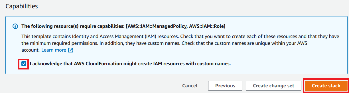
Review the details on the final page and select I acknowledge that AWS CloudFormation might create IAM resources.
Choose Create stack.

Launch the CloudFormation stack in the consumer account

To launch the CloudFormation stack in the consumer account, complete the following steps:

Sign in to the consumer account’s AWS CloudFormation console in the target Region.
Choose Launch Stack:
Choose Next.
For Stack name, enter a stack name, such as stack-consumer.
For ConsumerDatalakeAdminUserName and ConsumerDatalakeAdminUserPassword, enter the user name and password you want for the data lake admin IAM user.
For DataAnalystUserName and DataAnalystUserPassword, enter the user name and password you want for the data analyst IAM user.
For DatabaseName, leave the default values.
For AthenaQueryResultS3BucketName, enter the name of the S3 bucket that stores Amazon Athena query results. If you don’t have one, create an S3 bucket.
Choose Next.
On the next page, choose Next.
Review the details on the final page and select I acknowledge that AWS CloudFormation might create IAM resources.
Choose Create stack.

Stack creation can take about 1 minute.

(Optional) AWS KMS server-side encryption

If the source S3 bucket is encrypted using server-side encryption with an AWS Key Management Service (AWS KMS) customer master key (CMK), make sure the IAM role that Lake Formation uses to access S3 data is registered as the key user for the KMS CMK. By default, the IAM role AWSServiceRoleForLakeFormationDataAccess is used, but you can choose other IAM roles when registering an S3 data lake location. To register the Lake Formation role as the KMS key user, you can use the AWS KMS console, or directly add the permission to the key policy using the KMS PutKeyPolicy API and the AWS Command Line Interface (AWS CLI).

You don’t have to add individual consumer accounts to the key policy. Only the role that Lake Formation uses is required. Also, this step isn’t necessary if the source S3 bucket is encrypted with server-side encryption with Amazon S3, or an AWS managed key.

To add a Lake Formation role as the KMS key user via the console, complete the following steps:

Sign in to the AWS KMS console as the key administrator.
In the navigation pane, under Customer managed keys, choose the key that is used to encrypt the source S3 bucket.
Under Key users, choose Add.
Select AWSServiceRoleForLakeFormationDataAccess and choose Add.

To use the AWS CLI, enter the following command (replace <key-id>, <name-of-key-policy>, and <key-policy> with valid values):

aws kms put-key-policy --key-id <key-id> --policy-name <name-of-key-policy> --policy <key-policy>

For more information, see put-key-policy.

Lake Formation cross-account sharing prerequisites

Before sharing resources with Lake Formation, there are prerequisites for both the tag-based access control method and named resource method.

Tag-based access control cross-account sharing prerequisites

As described in Lake Formation Tag-Based Access Control Cross-Account Prerequisites, before you can use the tag-based access control method to grant cross-account access to resources, you must add the following JSON permissions object to the AWS Glue Data Catalog resource policy in the producer account. This gives the consumer account permission to access the Data Catalog when glue:EvaluatedByLakeFormationTags is true. Also, this condition becomes true for resources on which you granted permission using Lake Formation permission Tags to the consumer’s account. This policy is required for every AWS account that you’re granting permissions to.

The following policy must be within a Statement element. We discuss the full IAM policy later in this post.

{
    "Effect": "Allow",
    "Action": [
        "glue:*"
    ],
    "Principal": {
        "AWS": [
            "<consumer-account-id>"
        ]
    },
    "Resource": [
        "arn:aws:glue:<region>:<account-id>:table/*",
        "arn:aws:glue:<region>:<account-id>:database/*",
        "arn:aws:glue:<region>:<account-id>:catalog"
    ],
    "Condition": {
        "Bool": {
            "glue:EvaluatedByLakeFormationTags": true
        }
    }
}

Named resource method cross-account sharing prerequisites

As described in Managing Cross-Account Permissions Using Both AWS Glue and Lake Formation, if there is no Data Catalog resource policy in your account, the Lake Formation cross-account grants that you make proceed as usual. However, if a Data Catalog resource policy exists, you must add the following statement to it to permit your cross-account grants to succeed if they’re made with the named resource method. If you plan to use only the named resource method, or only the tag-based access control method, you can skip this step. In this post, we evaluate both methods, so we need to add the following policy.

The following policy must be within a Statement element. We discuss the full IAM policy in the next section.

{
    "Effect": "Allow",
    "Action": [
        "glue:ShareResource"
    ],
    "Principal": {
        "Service": [
            "ram.amazonaws.com"
        ]
    },
    "Resource": [
        "arn:aws:glue:<region>:<account-id>:table/*/*",
        "arn:aws:glue:<region>:<account-id>:database/*",
        "arn:aws:glue:<region>:<account-id>:catalog"
    ]
}

Add the AWS Glue Data Catalog resource policy using the AWS CLI

If we grant cross-account permissions by using both the tag-based access control method and named resource method, we must set the EnableHybrid argument to ‘true’ when adding the preceding policies. Because this option isn’t currently supported on the console, we must use the glue:PutResourcePolicy API and AWS CLI.

First, create a policy document (such as policy.json) and add the preceding two policies. Replace <consumer-account-id> with the account ID of the AWS account receiving the grant, <region> with the Region of the Data Catalog containing the databases and tables that you are granting permissions on, and <account-id> with the producer AWS account ID.

{
    "Version": "2012-10-17",
    "Statement": [
        {
            "Effect": "Allow",
            "Principal": {
                "Service": "ram.amazonaws.com"
            },
            "Action": "glue:ShareResource",
            "Resource": [
                "arn:aws:glue:<region>:<account-id>:table/*/*",
                "arn:aws:glue:<region>:<account-id>:database/*",
                "arn:aws:glue:<region>:<account-id>:catalog"
            ]
        },
        {
            "Effect": "Allow",
            "Principal": {
                "AWS": "<consumer-account-id>"
            },
            "Action": "glue:*",
            "Resource": [
                "arn:aws:glue:<region>:<account-id>:table/*/*",
                "arn:aws:glue:<region>:<account-id>:database/*",
                "arn:aws:glue:<region>:<account-id>:catalog"
            ],
            "Condition": {
                "Bool": {
                    "glue:EvaluatedByLakeFormationTags": "true"
                }
            }
        }
    ]
}

Enter the following AWS CLI command. Replace <glue-resource-policy> with the correct values (such as file://policy.json).

aws glue put-resource-policy --policy-in-json <glue-resource-policy> --enable-hybrid TRUE

For more information, see put-resource-policy.

Implement the Lake Formation tag-based access control method

In this section, we walk through the following high-level steps:

Define an LF-tag.
Assign the LF-tag to the target resource.
Grant LF-tag permissions to the consumer account.
Grant data permissions to the consumer account.
Optionally, revoke permissions for IAMAllowedPrincipals on the database, tables, and columns.
Create a resource link to the shared table.
Create an LF-tag and assign it to the target database.
Grant LF-tag data permissions to the consumer account.

Define an LF-tag

If you’re signed in to your producer account, sign out before completing the following steps.

Sign in as the producer account data lake administrator. Use the producer account ID, IAM user name (the default is DatalakeAdminProducer), and password that you specified during CloudFormation stack creation.
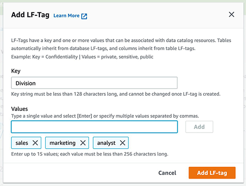
On the Lake Formation console, in the navigation pane, under Permissions, and under Administrative roles and tasks, choose LF-tags.
Choose Add LF-tag.
Specify the key and values. In this post, we create an LF-tag where the key is Confidentiality and the values are private, sensitive, and public.
Choose Add LF-tag.

Assign the LF-tag to the target resource

As a data lake administrator, you can attach tags to resources. If you plan to use a separate role, you may have to grant describe and attach permissions to the separate role.

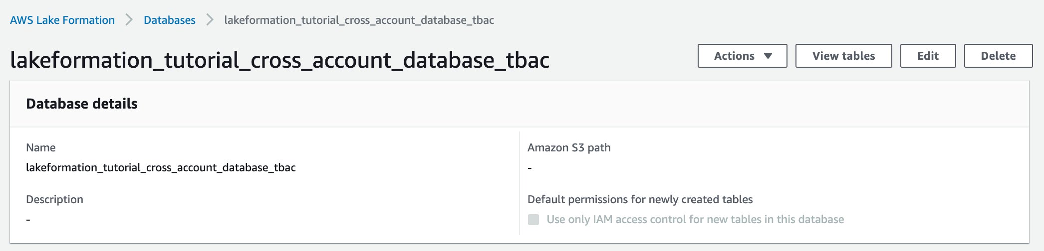
In the navigation pane, under Data catalog, select Databases.
Select the target database (lakeformation_tutorial_cross_account_database_tbac) and on the Actions menu, choose Edit LF-tags.

For this post, we assign an LF-tag to a database, but you can also assign LF-tags to tables and columns.

Choose Assign new LF-Tag.
Add the key Confidentiality and value public.
Choose Save.

Grant LF-tag permission to the consumer account

Still in the producer account, we grant permissions to the consumer account to access the LF-tag.

In the navigation pane, under Permissions, Administrative roles and tasks, LF-tag permissions, choose Grant.
For Principals, choose External accounts.
Enter the target AWS account ID.

AWS accounts within the same organization appear automatically. Otherwise, you have to manually enter the AWS account ID. As of this writing, Lake Formation tag-based access control doesn’t support granting permission to organizations or organization units.

For LF-Tags, choose the key and values of the LF-tag that is being shared with the consumer account (key Confidentiality and value public).
For Permissions, select Describe for LF-tag permissions.

LF-tag permissions are permissions given to the consumer account. Grantable permissions are permissions that the consumer account can grant to other principals.

Choose Grant.

At this point, the consumer data lake administrator should be able to find the policy tag being shared via the consumer account Lake Formation console, under Permissions, Administrative roles and tasks, LF-tags.

Grant data permission to the consumer account

We will now provide data access to the consumer account by specifying an LF-Tag expression and granting the consumer account access to any table or database that matches the expression.

In the navigation pane, under Permissions, Data lake permissions, choose Grant.
For Principals, choose External accounts, and enter the consumer AWS account ID.
For LF-tags or catalog resources, under Resources matched by LF-Tags (recommended), choose Add LF-Tag.
Select the key and values of the tag that is being shared with the consumer account (key Confidentiality and value public).
For Database permissions, select Describe under Database permissions to grant access permissions at the database level.
Select Describe under Grantable permissions so the consumer account can grant database-level permissions to its users.
For Table and column permissions, select Select and Describe under Table permissions.
Select Select and Describe under Grantable permissions.
Choose Grant.

Revoke permission for IAMAllowedPrincipals on the database, tables, and columns (Optional)

At the very beginning of this tutorial, we changed the Lake Formation Data Catalog settings. If you skipped that part, this step is required. If you changed your Lake Formation Data Catalog settings, you can skip this step.

In this step, we have to revoke the default Super permission from IAMAllowedPrincipals on the database or table. See Secure Existing Data Catalog Resources for details.

Before revoking permission for IAMAllowedPrincipals, make sure that you granted existing IAM principals with necessary permission through Lake Formation. This includes two steps:

Add IAM permission to the target IAM user or role with the Lake Formation GetDataAccess action (with IAM policy).
Grant the target IAM user or role with Lake Formation data permissions (alter, select, and so on)

Then, revoke permissions for IAMAllowedPrincipals. Otherwise, after revoking permissions for IAMAllowedPrincipals, existing IAM principals may no longer be able to access the target database or catalog.

Revoking Super permission for IAMAllowedPrincipals is required when you want to apply the Lake Formation permission model (instead of the IAM policy model) to manage user access within a single account or among multiple accounts using the Lake Formation permission model. You don’t have to revoke permission of IAMAllowedPrincipals for other tables where you want to keep the traditional IAM policy model.

At this point, the consumer account data lake administrator should be able to find the database and table being shared via the consumer account Lake Formation console, under Data catalog, Databases. If not, confirm if the following are properly configured:

Make sure the correct policy tag and values are assigned to the target databases and tables
Make sure the correct tag permission and data permission are assigned to the consumer account
Revoke the default super permission from IAMAllowedPrincipals on the database or table

Create a resource link to the shared table

When a resource is shared between accounts, the shared resources are not put in the consumer accounts’ catalog. To make them available, and query the underlying data of a shared table using services like Athena, we need to create a resource link to the shared table. A resource link is a Data Catalog object that is a link to a local or shared database or table. By creating a resource link, you can:

Assign a different name to a database or table that aligns with your Data Catalog resource naming policies
Use services such as Athena and Amazon Redshift Spectrum to query shared databases or tables

To create a resource link, complete the following steps:

If you’re signed in to your consumer account, sign out.
Sign in as the consumer account data lake administrator. Use the consumer account ID, IAM user name (default DatalakeAdminConsumer) and password that you specified during CloudFormation stack creation.
On the Lake Formation console, in the navigation pane, under Data catalog, Databases, choose the shared database lakeformation_tutorial_cross_account_database_tbac.

If you don’t see the database, revisit the previous steps to see if everything is properly configured.

Choose View tables.
Choose the shared table amazon_reviews_table_tbac.
On the Actions menu, choose Create resource link.
For Resource link name, enter a name (for this post, amazon_reviews_table_tbac_resource_link).
Under Database, select the database that the resource link is created in (for this post, the CloudFormation stack created the database lakeformation_tutorial_cross_account_database_consumer).
Choose Create.

The resource link appears under Data catalog, Tables.

Create an LF-tag and assign it to the target database

Lake Formation tags reside in the same catalog as the resources. This means that tags created in the producer account aren’t available to use when granting access to the resource links in the consumer account. You need to create a separate set of LF-tags in the consumer account to use LF tag-based access control when sharing the resource links in the consumer account. Let’s first create the LF-tag. Refer to the previous sections for full instructions.

Define the LF-tag in the consumer account. For this post, we use key Division and values sales, marketing, and analyst.
Assign the LF-tag key Division and value analyst to the database lakeformation_tutorial_cross_account_database_consumer, where the resource link is created in.

Grant LF-tag data permission to the consumer

As a final step, we grant LF-tag data permission to the consumer.

In the navigation pane, under Permissions, Data lake permissions, choose Grant.
For Principals, choose IAM users and roles, and choose the user DataAnalyst.
For LF-tags or catalog resources, choose Resources matched by LF-tags (recommended).
Choose key Division and value analyst.
For Database permissions, select Describe under Database permissions.
For Table and column permissions, select Select and Describe under Table permissions.
Choose Grant.
Repeat these steps for user DataAnalyst, where the LF-tag key is Confidentiality and value is public.

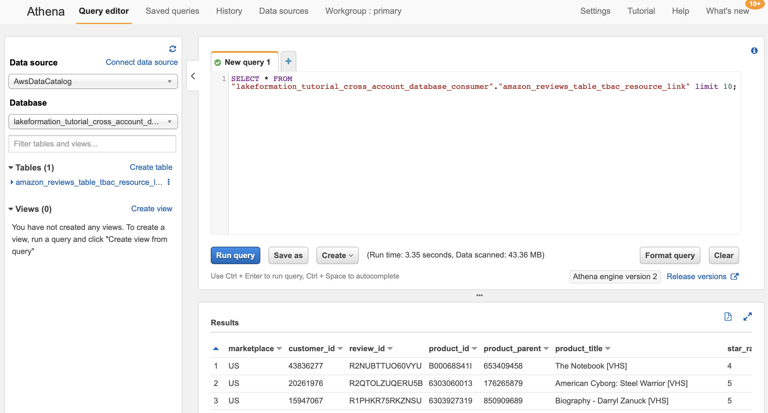
At this point, the data analyst user in the consumer account should be able to find the database and resource link, and query the shared table via the Athena console.

If not, confirm if the following are properly configured:

Make sure the resource link is created for the shared table
Make sure you granted the user access to the LF-tag shared by the producer account
Make sure you granted the user access to the LF-tag associated to the resource link and database that the resource link is created in
Check if you assigned the correct LF-tag to the resource link, and to the database that the resource link is created in

Implement the Lake Formation named resource method

To use the named resource method, we walk through the following high-level steps:

Optionally, revoke permission for IAMAllowedPrincipals on the database, tables, and columns.
Grant data permission to the consumer account.
Accept a resource share from AWS RAM.
Create a resource link for the shared table.
Grant data permission for the shared table to the consumer.
Grant data permission for the resource link to the consumer.

Revoke permission for IAMAllowedPrincipals on the database, tables, and columns (Optional)

At the very beginning of this tutorial, we changed Lake Formation Data Catalog settings. If you skipped that part, this step is required. For instructions, see the optional step in the previous section.

Grant data permission to the consumer account

If you’re signed in to producer account as another user, sign out first.

Sign in as the producer account data lake administrator using the AWS account ID, IAM user name (default is DatalakeAdminProducer), and password specified during CloudFormation stack creation.
In the navigation pane, under Permissions, Data lake permissions, choose Grant.
For Principals, choose External accounts, and enter one or more AWS account IDs or AWS Organizations IDs.

Organizations that the producer account belongs to and AWS accounts within the same organization appear automatically. Otherwise, manually enter the account ID or organization ID.

For LF-tags or catalog resources, choose Named data catalog resources.
Under Databases, choose the database lakeformation_tutorial_cross_account_database_named_resource.
Under Tables, choose All tables.
For Table and column permissions, select Select and Describe under Table permissions.
Select Select and Describe under Grantable permissions.
Optionally, for Data permissions, select Simple column-based access if column-level permission management is required.
Choose Grant.

If you haven’t revoked permission for IAMAllowedPrincipals, you get a Grant permissions failed error.

At this point, you should see the target table being shared via AWS RAM with the consumer account under Permissions, Data permissions.

Accept a resource share from AWS RAM

This step is required only for account ID-based sharing, not for organization-based sharing.

Sign in as the consumer account data lake administrator using the IAM user name (default is DatalakeAdminConsumer) and password specified during CloudFormation stack creation.
On the AWS RAM console, in the navigation pane, under Shared with me, Resource shares, choose the shared Lake Formation resource.

The Status should be Pending.

Confirm the resource details, and choose Accept resource share.

At this point, the consumer account data lake administrator should be able to find the shared resource on the Lake Formation console under Data catalog, Databases.

Create a resource link for the shared table

Follow the instructions detailed earlier to create a resource link for a shared table. Name the resource link amazon_reviews_table_named_resource_resource_link. Create the resource link in the database lakeformation_tutorial_cross_account_database_consumer.

Grant data permission for the shared table to the consumer

To grant data permission for the shared table to the consumer, complete the following steps:

In the navigation pane, under Permissions, Data lake permissions, choose Grant.
For Principals, choose IAM users and roles, and choose the user DataAnalyst.
For LF-tags or catalog resources, choose Named data catalog resources.
Under Databases, choose the database lakeformation_tutorial_cross_account_database_named_resource.

If you don’t see the database on the drop-down list, choose Load more.

Under Tables, choose the table amazon_reviews_table_named_resource.
For Table and column permissions, select Select and Describe under Table permissions.
Choose Grant.

Grant data permission for the resource link to the consumer

In addition to granting the data lake user permission to access the shared table, you also need to grant the data lake user permission to access the resource link.

In the navigation pane, under Permissions, Data lake permissions, choose Grant.
For Principals, choose IAM users and roles, and choose the user DataAnalyst.
For LF-tags or catalog resources, choose Named data catalog resources.
Under Databases, choose the database lakeformation_tutorial_cross_account_database_consumer.
Under Tables, choose the table amazon_reviews_table_named_resource_resource_link.
For Resource link permissions, select Describe under Resource link permissions.
Choose Grant.

At this point, the data analyst user in the consumer account should be able to find the database and resource link, and query the shared table via the Athena console.

If not, confirm if the following are properly configured:

Make sure the resource link is created for the shared table
Make sure you granted the user access to the table shared by the producer account
Make sure you granted the user access to the resource link and database that the resource link is created in

Clean up

To clean up the resources created within this tutorial, delete or change the following resources:

Producer account:
- AWS RAM resource share
- Lake Formation tags
- CloudFormation stack
- Lake Formation settings
- AWS Glue Data Catalog settings
Consumer account:
- Lake Formation tags
- CloudFormation stack

Summary

Lake Formation cross-account sharing enables you to share data across AWS accounts without copying the actual data. Also, it provides both the producer and consumer with control over data permissions in a flexible way. In this post, we introduced two different options to reference catalog data from another account by using the cross-account access features provided by Lake Formation:

Tag-based access control
Named resource

The tag-based access control method is recommended when many resources and entities are involved. Although it seems like this option requires more steps, tag-based access control helps data lake administrators control relationships between each user and table via tags dynamically. The named resource method provides the data lake administrator with a more straightforward way to manage catalog permissions. You can choose the method that best fits your requirement.

About the author

Yumiko Kanasugi is a Solutions Architect with Amazon Web Services Japan, supporting digital native business customers to utilize AWS.

How Ribbon Communications Built a Scalable, Resilient Robocall Mitigation Platform

2022-01-14 Siva Rajamani

Post Syndicated from Siva Rajamani original https://aws.amazon.com/blogs/architecture/how-ribbon-communications-built-a-scalable-resilient-robocall-mitigation-platform/

Ribbon Communications provides communications software, and IP and optical networking end-to-end solutions that deliver innovation, unparalleled scale, performance, and agility to service providers and enterprise.

Ribbon Communications is helping customers modernize their networks. In today’s data-hungry, 24/7 world, this equates to improved competitive positioning and business outcomes. Companies are migrating from on-premises equipment for telephony services and looking for equivalent as a service (aaS) offerings. But these solutions must still meet the stringent resiliency, availability, performance, and regulatory requirements of a telephony service.

The telephony world is inundated with robocalls. In the United States alone, there were an estimated 50.5 billion robocalls in 2021! In this blog post, we describe the Ribbon Identity Hub – a holistic solution for robocall mitigation. The Ribbon Identity Hub enables services that sign and verify caller identity, which is compliant to the ATIS standards under the STIR/SHAKEN framework. It also evaluates and scores calls for the probability of nuisance and fraud.

Ribbon Identity Hub is implemented in Amazon Web Services (AWS). It is a fully managed service for telephony service providers and enterprises. The solution is secure, multi-tenant, automatic scaling, and multi-Region, and enables Ribbon to offer managed services to a wide range of telephony customers. Ribbon ensures resiliency and performance with efficient use of resources in the telephony environment, where load ratios between busy and idle time can exceed 10:1.

Ribbon Identity Hub

The Ribbon Identity Hub services are separated into a data (call-transaction) plane, and a control plane.

Data plane (call-transaction)

The call-transaction processing is typically invoked on a per-call-setup basis where availability, resilience, and performance predictability are paramount. Additionally, due to high variability in load, automatic scaling is a prerequisite.

Figure 1. Data plane architecture

Several AWS services come together in a solution that meets all these important objectives:

Amazon Elastic Container Service (ECS): The ECS services are set up for automatic scaling and span two Availability Zones. This provides the horizontal scaling capability, the self-healing capacity, and the resiliency across Availability Zones.
Elastic Load Balancing – Application Load Balancer (ALB): This provides the ability to distribute incoming traffic to ECS services as the target. In addition, it also offers:
- Seamless integration with the ECS Auto Scaling group. As the group grows, traffic is directed to the new instances only when they are ready. As traffic drops, traffic is drained from the target instances for graceful scale down.
- Full support for canary and linear upgrades with zero downtime. Maintains full-service availability without any changes or even perception for the client devices.
Amazon Simple Storage Service (S3): Transaction detail records associated with call-related requests must be securely and reliably maintained for over a year due to billing and other contractual obligations. Amazon S3 simplifies this task with high durability, lifecycle rules, and varied controls for retention.
Amazon DynamoDB: Building resilient services is significantly easier when the compute processing can be stateless. Amazon DynamoDB facilitates such stateless architectures without compromise. Coupled with the availability of the Amazon DynamoDB Accelerator (DAX) caching layer, the solution can meet the extreme low latency operation requirements.
AWS Key Management Service (KMS): Certain tenant configuration is highly confidential and requires elevated protection. Furthermore, the data is part of the state that must be recovered across Regions in disaster recovery scenarios. To meet the security requirements, the KMS is used for envelope encryption using per-tenant keys. Multi-Region KMS keys facilitates the secure availability of this state across Regions without the need for application-level intervention when replicating encrypted data.
Amazon Route 53: For telephony services, any non-transient service failure is unacceptable. In addition to providing high degree of resiliency through Multi-AZ architecture, Identity Hub also provides Regional level high availability through its multi-Region active-active architecture. Route 53 with health checks provides for dynamic rerouting of requests within minutes to alternate Regions.

Control plane

The Identity Hub control plane is used for customer configuration, status, and monitoring. The API is REST-based. Since this is not used on a call-by-call basis, the requirements around latency and performance are less stringent, though the requirements around high resiliency and dynamic scaling still apply. In this area, ease of implementation and maintainability are key.

Figure 2. Control plane architecture

The following AWS services implement our control plane:

Amazon API Gateway: Coupled with a custom authenticator, the API Gateway handles all the REST API credential verification and routing. Implementation of an API is transformed into implementing handlers for each resource, which is the application core of the API.
AWS Lambda: All the REST API handlers are written as Lambda functions. By using the Lambda’s serverless and concurrency features, the application automatically gains self-healing and auto-scaling capabilities. There is also a significant cost advantage as billing is per millisecond of actual compute time used. This is significant for a control plane where usage is typically sparse and unpredictable.
Amazon DynamoDB: A stateless architecture with Lambda and API Gateway, all persistent state must be stored in an external database. The database must match the resilience and auto-scaling characteristics of the rest of the control plane. DynamoDB easily fits the requirements here.

The customer portal, in addition to providing the user interface for control plane REST APIs, also delivers a rich set of user-customizable dashboards and reporting capability. Here again, the availability of various AWS services simplifies the implementation, and remains non-intrusive to the central call-transaction processing.

Services used here include:

AWS Glue: Enables extraction and transformation of raw transaction data into a format useful for reporting and dashboarding. AWS Glue is particularly useful here as the data available is regularly expanding, and the use cases for the reporting and dashboarding increase.
Amazon QuickSight: Provides all the business intelligence (BI) functionality, including the ability for Ribbon to offer separate author and reader access to their users, and implements tenant-based access separation.

Conclusion

Ribbon has successfully deployed Identity Hub to enable cloud hosted telephony services to mitigate robocalls. Telephony requirements around resiliency, performance, and capacity were not compromised. Identity Hub offers the benefits of a 24/7 fully managed service requiring no additional customer on-premises equipment.

Choosing AWS services for Identity Hub gives Ribbon the ability to scale and meet future growth. The ability to dynamically scale the service in and out also brings significant cost advantages in telephony applications where busy hour traffic is significantly higher than idle time traffic. In addition, the availability of global AWS services facilitates the deployment of services in customer-local geographic locations to meet performance requirements or local regulatory compliance.

Backtest trading strategies with Amazon Kinesis Data Streams long-term retention and Amazon SageMaker

2022-01-14 Sachin Thakkar

Post Syndicated from Sachin Thakkar original https://aws.amazon.com/blogs/big-data/backtest-trading-strategies-with-amazon-kinesis-data-streams-long-term-retention-and-amazon-sagemaker/

Real-time insight is critical when it comes to building trading strategies. Any delay in data insight can cost lot of money to the traders. Often, you need to look at historical market trends to predict future trading pattern and make the right bid. More the historical data you analyze, better trading prediction you get. Back tracking streaming data can be tricky as it requires sophisticated storage and analysis mechanisms.

Amazon Kinesis Data Streams allows our customer to store streaming data for up to one year. Amazon Kinesis Data Streams Long Term Retention (LTR) of streaming data enables to use the same platform for both real-time and older data retained in Amazon Kinesis Data Streams. For example, one can train machine learning algorithms for financial trading, marketing personalization, and recommendation models without moving the data into a different data store or writing a new application. Customers can also satisfy certain data retention regulations, including under HIPAA and FedRAMP, using long term retention. This thus simplifies the data ingestion architecture for our trading use case we will discuss in this post.

In the post Building algorithmic trading strategies with Amazon SageMaker, we demonstrated how to backtest trading strategies with Amazon SageMaker with historical stock price data stored in Amazon Simple Storage Service (Amazon S3). In this post, we expand this solution for streaming data and describe how to use Amazon Kinesis.

In addition, we want to use Amazon SageMaker automatic tuning to find the optimal configuration for a moving average crossover strategy. In this strategy, two moving averages for a slow and a fast time period are calculated, and a trade is executed when a crossover happens. If the fast moving average crosses above the slow moving average, the strategy places a long trade, otherwise the strategy goes short. We find the optimal period length for these moving averages by running multiple backtests with different lengths over a historical dataset.

Finally, we run the optimal configuration for this moving average crossover strategy over a different test dataset and analyze the performance results. If the performance measured in profit and loss (P&L) is positive for the test period, we can consider this trading strategy for a forward test.

To show you how easy and quick it is to get started on AWS, we provide a one-click deployment for an extensible trading backtesting solution that uses Kinesis long-term retention for streaming data.

Solution overview

We use Kinesis Data Streams to store real-time streaming as well as historical market data. We use Jupyter notebooks as our central interface for exploring and backtesting new trading strategies. SageMaker allows you to set up Jupyter notebooks and integrate them with AWS CodeCommit to store different versions of strategies and share them with other team members.

We use Amazon S3 to store model artifacts and backtesting results.

For our trading strategies, we create Docker containers that contain the required libraries for backtesting and the strategy itself. These containers follow the SageMaker Docker container structure in order to run them inside of SageMaker. For more information about the structure of SageMaker containers, see Using the SageMaker Training and Inference Toolkits.

The following diagram illustrates this architecture.

We run the data preparation step from a SageMaker notebook. This copies the historical market data to the S3 bucket.

We use AWS Data Migration Service (AWS DMS) to load the market data to the data stream. The

SageMaker notebook connects with Kinesis Data Streams and runs the trading strategy algorithm via a SageMaker training job. The algorithm uses part of the data for training to find the optimal strategy configuration.

Finally, we run the trading strategy using the previously determined configuration on a test dataset.

Prerequisites

Before getting started, we set up our resources. In this post, we use the us-east-2 Region as an example.

Deploy the AWS resources using the provided AWS CloudFormation template.
For Stack name, enter a name for your stack.
Provide an existing S3 bucket name to store the historical market data.

The data is loaded in Kinesis Data Streams from this S3 bucket. Your bucket needs to be in same Region where your stack is set up.

Accept all the defaults and choose Next.
Acknowledge that AWS CloudFormation might create AWS Identity and Access Management (IAM) resources with custom names.
Choose Create stack.

This creates all the required resources.

Data load to Kinesis Data Streams

To perform the data load, complete the following steps:

On the SageMaker console, under Notebook in the navigation pane, choose Notebook instances.
Locate the notebook instance AlgorithmicTradingInstance-*.
Choose Open Jupyter for this instance.
Go to the algorithmic-trading->4_Kinesis folder and choose Strategy_Kinesis_EMA_HPO.pynb.

You now run the data preparation step in the notebook.

Load the dataset.

Specify the existing bucket where test data is stored. Make sure that the test bucket is in the same Region where you set up the stack.

Run all the steps in the notebook until Step 2 Data Preparation.
On the AWS DMS console, choose Database migration tasks.
Select the AWS DMS task dmsreplicationtask-*.
On the Actions menu, choose Restart/Resume.

This starts the data load from the S3 bucket to the data stream.

Wait until the replication task shows the status Load complete.

Continue the steps in the Jupyter notebook.

Read data from Kinesis long-term retention

We read daily open, high, low, close price, and volume data from the stream’s long-term retention with the AWS SDK for Python (Boto3).

Although we don’t use enhanced fan-out (EFO) in this post, it may be advisable to do so an existing application is already reading from the stream. That way this backtesting app doesn’t interfere with the existing application.

You can visualize your data, as shown in the following screenshot.

Define your trading strategy

In this step, we define our moving average crossover trading strategy.

Build a Docker image

We build our backtesting job as a Docker image and push it to Amazon ECR.

Hyperparameter optimization with SageMaker on training data

For the moving average crossover trading strategy, we want to find the optimal fast period and slow period of this strategy, and we provide a range of days to search for.

We use profit and loss (P&L) of the strategy as the metric to find optimized hyperparameters.

You can see the tuning job recommended a value of 7 and 21 days for the fast and slow period for this trading strategy given the training dataset.

Run the strategy with optimal hyperparameters on test data

We now run this strategy with optimal hyperparameters on the test data.

When the job is complete, the performance results are stored in Amazon S3, and you can review the performance metrics in a chart and analyze the buy and sell orders for your strategy.

Conclusion

In this post, we described how to use the Kinesis Data Streams long-term retention feature to store the historical stock price data and how to use streaming data for backtesting of a trading strategy with SageMaker.

Long-term retention of streaming data enables you to use the same platform for both real-time and older data retained in Kinesis Data Streams. This allows you to use this data stream for financial use cases like backtesting or for machine learning without moving the data into a different data store or writing a new application. You can also satisfy certain data retention regulations, including under HIPAA and FedRAMP, using long-term retention. For more information, see Amazon Kinesis Data Streams enables data stream retention up to one year.

Risk disclaimer

This post is for educational purposes only and past trading performance does not guarantee future performance.

About the Authors

Sachin Thakkar is a Senior Solutions Architect at Amazon Web Services, working with a leading Global System Integrator (GSI). He brings over 22 years of experience as an IT Architect and as Technology Consultant for large institutions. His focus area is on Data & Analytics. Sachin provides architectural guidance and supports the GSI partner in building strategic industry solutions on AWS

Amogh Gaikwad is a Solutions Developer in the Prototyping Team. He specializes in machine learning and analytics and has extensive experience developing ML models in real-world environments and integrating AI/ML and other AWS services into large-scale production applications. Before joining Amazon, he worked as a software developer, developing enterprise applications focusing on Enterprise Resource Planning (ERP) and Supply Chain Management (SCM). Amogh has received his master’s in Computer Science specializing in Big Data Analytics and Machine Learning.

Dhiraj Thakur is a Solutions Architect with Amazon Web Services. He works with AWS customers and partners to provide guidance on enterprise cloud adoption, migration and strategy. He is passionate about technology and enjoys building and experimenting in Analytics and AI/ML space.

Oliver Steffmann is an Enterprise Solutions Architect at AWS based in New York. He brings over 18 years of experience as IT Architect, Software Development Manager, and as Management Consultant for international financial institutions. During his time as a consultant, he leveraged his extensive knowledge of Big Data, Machine Learning and cloud technologies to help his customers get their digital transformation off the ground. Before that he was the head of municipal trading technology at a tier-one investment bank in New York and started his career in his own startup in Germany.

Creating a Multi-Region Application with AWS Services – Part 2, Data and Replication

2022-01-12 Joe Chapman

Post Syndicated from Joe Chapman original https://aws.amazon.com/blogs/architecture/creating-a-multi-region-application-with-aws-services-part-2-data-and-replication/

In Part 1 of this blog series, we looked at how to use AWS compute, networking, and security services to create a foundation for a multi-Region application.

Data is at the center of many applications. In this post, Part 2, we will look at AWS data services that offer native features to help get your data where it needs to be.

In Part 3, we’ll look at AWS application management and monitoring services to help you build, monitor, and maintain a multi-Region application.

Considerations with replicating data

Data replication across the AWS network can happen quickly, but we are still limited by the speed of light. For this reason, data consistency must be considered when building a multi-Region application. Generally speaking, the longer a physical distance is, the longer it will take the data to get there.

When building a distributed system, consider the consistency, availability, partition tolerance (CAP) theorem. This theorem states that an application can only pick 2 out of the 3, and tradeoffs should be considered.

Consistency – all clients always have the same view of data
Availability – all clients can always read and write data
Partition Tolerance – the system will continue to work despite physical partitions

Achieving consistency and availability is common for single-Region applications. For example, when an application connects to a single in-Region database. However, this becomes more difficult with multi-Region applications due to the latency added by transferring data over long distances. For this reason, highly distributed systems will typically follow an eventual consistency approach, favoring availability and partition tolerance.

Replicating objects and files

To ensure objects are in multiple Regions, Amazon Simple Storage Service (Amazon S3) can be set up to replicate objects across AWS Regions automatically with one-way or two-way replication. A subset of objects in an S3 bucket can be replicated with S3 replication rules. If low replication lag is critical, S3 Replication Time Control can help meet requirements by replicating 99.99% of objects within 15 minutes, and most within seconds. To monitor the replication status of objects, Amazon S3 events and metrics will track replication and can send an alert if there’s an issue.

Traditionally, each S3 bucket has its own single, Regional endpoint. To simplify connecting to and managing multiple endpoints, S3 Multi-Region Access Points create a single global endpoint spanning multiple S3 buckets in different Regions. When applications connect to this endpoint, it will route over the AWS network using AWS Global Accelerator to the bucket with the lowest latency. Failover routing is also automatically handled if the connectivity or availability to a bucket changes.

For files stored outside of Amazon S3, AWS DataSync simplifies, automates, and accelerates moving file data across Regions and accounts. It supports homogeneous and heterogeneous file migrations across Elastic File System (Amazon EFS), Amazon FSx, AWS Snowcone, and Amazon S3. It can even be used to sync on-premises files stored on NFS, SMB, HDFS, and self-managed object storage to AWS for hybrid architectures.

File and object replication should be expected to be eventually consistent. The rate at which a given dataset can transfer is a function of the amount of data, I/O bandwidth, network bandwidth, and network conditions.

Copying backups

Scheduled backups can be set up with AWS Backup, which automates backups of your data to meet business requirements. Backup plans can automate copying backups to one or more AWS Regions or accounts. A growing number of services are supported, and this can be especially useful for services that don’t offer real-time replication to another Region such as Amazon Elastic Block Store (Amazon EBS) and Amazon Neptune.

Figure 1 shows how these data transfer services can be combined for each resource.

Figure 1. Storage replication services

Spanning non-relational databases across Regions

Amazon DynamoDB global tables provide multi-Region and multi-writer features to help you build global applications at scale. A DynamoDB global table is the only AWS managed offering that allows for multiple active writers in a multi-Region topology (active-active and multi-Region). This allows for applications to read and write in the Region closest to them, with changes automatically replicated to other Regions.

Global reads and fast recovery for Amazon DocumentDB (with MongoDB compatibility) can be achieved with global clusters. These clusters have a primary Region that handles write operations. Dedicated storage-based replication infrastructure enables low-latency global reads with a lag of typically less than one second.

Keeping in-memory caches warm with the same data across Regions can be critical to maintain application performance. Amazon ElastiCache for Redis offers global datastore to create a fully managed, fast, reliable, and secure cross-Region replica for Redis caches and databases. With global datastore, writes occurring in one Region can be read from up to two other cross-Region replica clusters – eliminating the need to write to multiple caches to keep them warm.

Spanning relational databases across Regions

For applications that require a relational data model, Amazon Aurora global database provides for scaling of database reads across Regions in Aurora PostgreSQL-compatible and MySQL-compatible editions. Dedicated replication infrastructure utilizes physical replication to achieve consistently low replication lag that outperforms the built-in logical replication database engines offer, as shown in Figure 2.

Figure 2. SysBench OLTP (write-only) stepped every 600 seconds on R4.16xlarge

With Aurora global database, one primary Region is designated as the writer, and secondary Regions are dedicated to reads. Aurora MySQL supports write forwarding, which forwards write requests from a secondary Region to the primary Region to simplify logic in application code. Failover testing can happen by utilizing managed planned failover, which will change the active write cluster to another Region while keeping the replication topology intact. All databases discussed in this post employ eventual consistency when used across Regions, but Aurora PostgreSQL has an option to set the maximum a replica lag allowed with managed recovery point objective (managed RPO).

Logical replication, which utilizes a database engine’s built-in replication technology, can be set up for Amazon Relational Database Service (Amazon RDS) for MariaDB, MySQL, Oracle, PostgreSQL, and Aurora databases. A cross-Region read replica will receive these changes from the writer in the primary Region. For applications built on RDS for Microsoft SQL Server, cross-Region replication can be achieved by utilizing the AWS Database Migration Service. Cross-Region replicas allow for quicker local reads and can reduce data loss and recovery times in the case of a disaster by being promoted to a standalone instance.

For situations where a longer RPO and recovery time objective (RTO) are acceptable, backups can be copied across Regions. This is true for all of the relational and non-relational databases mentioned in this post, except for ElastiCache for Redis. Amazon Redshift can also automatically do this for your data warehouse. Backup copy times will vary depending on size and change rates.

A purpose-built database strategy offers many benefits, Figure 3 forms a purpose-built global database architecture.

Figure 3. Purpose-built global database architecture

Summary

Data is at the center of almost every application. In this post, we reviewed AWS services that offer cross-Region data replication to get your data where it needs to be quickly. Whether you need faster local reads, an active-active database, or simply need your data durably stored in a second Region, we have a solution for you. In the 3rd and final post of this series, we’ll cover application management and monitoring features.

Ready to get started? We’ve chosen some AWS Solutions, AWS Blogs, and Well-Architected labs to help you!

Find Public IPs of Resources – Use AWS Config for Vulnerability Assessment

2021-12-22 Gurkamal Deep Singh Rakhra

Post Syndicated from Gurkamal Deep Singh Rakhra original https://aws.amazon.com/blogs/architecture/find-public-ips-of-resources-use-aws-config-for-vulnerability-assessment/

Systems vulnerability management is a key component of your enterprise security program. Its goal is to remediate OS, software, and applications vulnerabilities. Scanning tools can help identify and classify these vulnerabilities to keep the environment secure and compliant.

Typically, vulnerability scanning tools operate from internal or external networks to discover and report vulnerabilities. For internal scanning, the tools use private IPs of target systems in scope. For external scans, the public target system’s IP addresses are used. It is important that security teams always maintain an accurate inventory of all deployed resource’s IP addresses. This ensures a comprehensive, consistent, and effective vulnerability assessment.

This blog discusses a scalable, serverless, and automated approach to discover public IP addresses assigned to resources in a single or multi-account environment in AWS, using AWS Config.

Single account is when you have all your resources in a single AWS account. A multi-account environment refers to many accounts under the same AWS Organization.

Understanding scope of solution

You may have good visibility into the private IPs assigned to your resources: Amazon Elastic Compute Cloud (Amazon EC2), Amazon Elastic Kubernetes Service (EKS) clusters, Elastic Load Balancing (ELB), and Amazon Elastic Container Service (Amazon ECS). But it may require some effort to establish a complete view of the existing public IPs. And these IPs can change over time, as new systems join and exit the environment.

An elastic network interface is a logical networking component in a Virtual Private Cloud (VPC) that represents a virtual network card. The elastic network interface routes traffic to other destinations/resources. Usually, you have to make Describe* API calls for the specific resource with an elastic network interface to get information about its configuration and IP address. This may throttle the resource-specific API calls, and result in higher costs. Additionally, if there are tens or hundreds of accounts, it becomes exponentially more difficult to get the information into a single inventory.

AWS Config enables you to assess, audit, and evaluate the configurations of your AWS resources. The advanced query feature provides a single query endpoint and language to get current resource state metadata for a single account and Region, or multiple accounts and Regions. You can use configuration aggregators to run the same queries from a central account across multiple accounts and AWS Regions.

AWS Config supports a subset of structured query language (SQL) SELECT syntax, which enables you to perform property-based queries and aggregations on the current configuration item (CI) data. Advanced query is available at no additional cost to AWS Config customers in all AWS Regions (except China Regions) and AWS GovCloud (US).

AWS Organizations helps you centrally govern your environment. Its integration with other AWS services lets you define central configurations, security mechanisms, audit requirements, and resource sharing across accounts in your organization.

Choosing scope of advanced queries in AWS Config

When running advanced queries in AWS Config, you must choose the scope of the query. The scope defines the accounts you want to run the query against and is configured when you create an aggregator.

Following are the three possible scopes when running advanced queries:

Single account and single Region
Multiple accounts and multiple Regions
AWS Organization accounts

Single account and single Region

Figure 1. AWS Config workflow for single account and single Region

The use case shown in Figure 1 addresses the need of customers operating within a single account and single Region. With AWS Config enabled for the individual account, you will use AWS Config advanced query feature to run SQL queries. These will give you resource metadata about associated public IPs. You do not require an aggregator for single-account and single Region.

In Figure 1.1, the advanced query returned results from a single account and all Availability Zones within the Region in which the query was run.

Figure 1.1 Advanced query returning results for a single account and single Region

Query for reference

SELECT

resouceId,

resourceName,

resourceType,

configuration.association.publicIp,

availabilityZone,

awsRegion

WHERE

resourceType='AWS::EC2::NetworkInterface'

AND configuration.association.publicIp>'0.0.0.0'

This query is fetching the properties of all elastic network interfaces. The WHERE condition is used to list the elastic network interfaces using the resourceType property and find all public IPs greater than 0.0.0.0. This is because elastic network interfaces can exist with a private IP, in which case there will be no public IP assigned to it. For a list of supported resourceType, refer to supported resource types for AWS Config.

Multiple accounts and multiple Regions

Figure 2. AWS Config monitoring workflow for multiple account and multiple Regions. The figure shows EC2, EKS, and Amazon ECS, but it can be any AWS resource having a public elastic network interface.

AWS Config enables you to monitor configuration changes against multiple accounts and multiple Regions via an aggregator, see Figure 2. An aggregator is an AWS Config resource type that collects AWS Config data from multiple accounts and Regions. You can choose the aggregator scope when running advanced queries in AWS Config. Remember to authorize the aggregator accounts to collect AWS Config configuration and compliance data.

Figure 2.1 Advanced query returning results from multiple Regions (awsRegion column) as highlighted in the diagram

This use case applies when you have AWS resources in multiple accounts (or span multiple organizations) and multiple Regions. Figure 2.1 shows the query results being returned from multiple AWS Regions.

Accounts in AWS Organization

Figure 3. The workflow of accounts in an AWS Organization being monitored by AWS Config. This figure shows EC2, EKS, and Amazon ECS but it can be any AWS resource having a public elastic network interface.

An aggregator also enables you to monitor all the accounts in your AWS Organization, see Figure 3. When this option is chosen, AWS Config enables you to run advanced queries against the configuration history in all the accounts in your AWS Organization. Remember that an aggregator will only aggregate data from the accounts and Regions that are specified when the aggregator is created.

Figure 3.1 Advanced query returning results from all accounts (accountId column) under an AWS Organization

In Figure 3.1, the query is run against all accounts in an AWS Organization. This scope of AWS Organization is accomplished by the aggregator and it automatically accumulates data from all accounts under a specific AWS Organization.

Common architecture workflow for discovering public IPs

Figure 4. High-level architecture pattern for discovering public IPs

The workflow shown in Figure 4 starts with Amazon EventBridge triggering an AWS Lambda function. You can configure an Amazon EventBridge schedule via rate or cron expressions, which define the frequency. This AWS Lambda function will host the code to make an API call to AWS Config that will run an advanced query. The advanced query will check for all elastic network interfaces in your account(s). This is because any public resource launched in your account will be assigned an elastic network interface.

When the results are returned, they can be stored on Amazon S3. These result files can be timestamped (via naming or S3 versioning) in order to keep a history of public IPs used in your account. The result set can then be fed into or accessed by the vulnerability scanning tool of your choice.

Note: AWS Config advanced queries can also be used to query IPv6 addresses. You can use the “configuration.ipv6Addresses” AWS Config property to get IPv6 addresses. When querying IPv6 addresses, remove “configuration.association.publicIp > ‘0.0.0.0’” condition from the preceding sample queries. For more information on available AWS Config properties and data types, refer to GitHub.

Conclusion

In this blog, we demonstrated how to extract public IP information from resources deployed in your account(s) using AWS Config and AWS Config advanced query. We discussed how you can support your vulnerability scanning process by identifying public IPs in your account(s) that can be fed into your scanning tool. This solution is serverless, automated, and scalable, which removes the undifferentiated heavy lifting required to manage your resources.

Learn more about AWS Config best practices:

Modernized Database Queuing using Amazon SQS and AWS Services

2021-12-17 Scott Wainner

Post Syndicated from Scott Wainner original https://aws.amazon.com/blogs/architecture/modernized-database-queuing-using-amazon-sqs-and-aws-services/

A queuing system is composed of producers and consumers. A producer enqueues messages (writes messages to a database) and a consumer dequeues messages (reads messages from the database). Business applications requiring asynchronous communications often use the relational database management system (RDBMS) as the default message storage mechanism. But the increased message volume, complexity, and size, competes with the inherent functionality of the database. The RDBMS becomes a bottleneck for message delivery, while also impacting other traditional enterprise uses of the database.

In this blog, we will show how you can mitigate the RDBMS performance constraints by using Amazon Simple Queue Service (Amazon SQS), while retaining the intrinsic value of the stored relational data.

Problems with legacy queuing methods

Commercial databases such as Oracle offer Advanced Queuing (AQ) mechanisms, while SQL Server supports Service Broker for queuing. The database acts as a message queue system when incoming messages are captured along with metadata. A message stored in a database is often processed multiple times using a sequence of message extraction, transformation, and loading (ETL). The message is then routed for distribution to a set of recipients based on logic that is often also stored in the database.

The repetitive manipulation of messages and iterative attempts at distributing pending messages may create a backlog that interferes with the primary function of the database. This backpressure can propagate to other systems that are trying to store and retrieve data from the database and cause a performance issue (see Figure 1).

Figure 1. A relational database serving as a message queue.

There are several scenarios where the database can become a bottleneck for message processing:

Message metadata. Messages consist of the payload (the content of the message) and metadata that describes the attributes of the message. The metadata often includes routing instructions, message disposition, message state, and payload attributes.

The message metadata may require iterative transformation during the message processing. This creates an inefficient sequence of read, transform, and write processes. This is especially inefficient if the message attributes undergo multiple transformations that must be reflected in the metadata. The iterative read/write process of metadata consumes the database IOPS, and forces the database to scale vertically (add more CPU and more memory).
A new paradigm emerges when message management processes exist outside of the database. Here, the metadata is manipulated without interacting with the database, except to write the final message disposition. Application logic can be applied through functions such as AWS Lambda to transform the message metadata.

Message large object (LOB). A message may contain a large binary object that must be stored in the payload.

Storing large binary objects in the RDBMS is expensive. Manipulating them consumes the throughput of the database with iterative read/write operations. If the LOB must be transformed, then it becomes wasteful to store the object in the database.
An alternative approach offers a more efficient message processing sequence. The large object is stored external to the database in universally addressable object storage, such as Amazon Simple Storage Service (Amazon S3). There is only a pointer to the object that is stored in the database. Smaller elements of the message can be read from or written to the database, while large objects can be manipulated more efficiently in object storage resources.

Message fan-out. A message can be loaded into the database and analyzed for routing, where the same message must be distributed to multiple recipients.

Messages that require multiple recipients may require a copy of the message replicated for each recipient. The replication creates multiple writes and reads from the database, which is inefficient.
A new method captures only the routing logic and target recipients in the database. The message replication then occurs outside of the database in distributed messaging systems, such as Amazon Simple Notification Service (Amazon SNS).

Message queuing. Messages are often kept in the database until they are successfully processed for delivery. If a message is read from the database and determined to be undeliverable, then the message is kept there until a later attempt is successful.

An inoperable message delivery process can create backpressure on the database where iterative message reads are processed for the same message with unsuccessful delivery. This creates a feedback loop causing even more unsuccessful work for the database.
Try a message queuing system such as Amazon MQ or Amazon SQS, which offloads the message queuing from the database. These services offer efficient message retry mechanisms, and reduce iterative reads from the database.

Sequenced message delivery. Messages may require ordered delivery where the delivery sequence is crucial for maintaining application integrity.

The application may capture the message order within database tables, but the sorting function still consumes processing capabilities. The order sequence must be sorted and maintained for each attempted message delivery.
Message order can be maintained outside of the database using a queue system, such as Amazon SQS, with first-in/first-out (FIFO) delivery.

Message scheduling. Messages may also be queued with a scheduled delivery attribute. These messages require an event driven architecture with initiated scheduled message delivery.

The database often uses trigger mechanisms to initiate message delivery. Message delivery may require a synchronized point in time for delivery (many messages at once), which can cause a spike in work at the scheduled interval. This impacts the database performance with artificially induced peak load intervals.
Event signals can be generated in systems such as Amazon EventBridge, which can coordinate the transmission of messages.

Message disposition. Each message maintains a message disposition state that describes the delivery state.

The database is often used as a logging system for message transmission status. The message metadata is updated with the disposition of the message, while the message remains in the database as an artifact.
An optimized technique is available using Amazon CloudWatch as a record of message disposition.

Modernized queuing architecture

Decoupling message queuing from the database improves database availability and enables greater message queue scalability. It also provides a more cost-effective use of the database, and mitigates backpressure created when database performance is constrained by message management.

The modernized architecture uses loosely coupled services, such as Amazon S3, AWS Lambda, Amazon Message Queue, Amazon SQS, Amazon SNS, Amazon EventBridge, and Amazon CloudWatch. This loosely coupled architecture lets each of the functional components scale vertically and horizontally independent of the other functions required for message queue management.

Figure 2 depicts a message queuing architecture that uses Amazon SQS for message queuing and AWS Lambda for message routing, transformation, and disposition management. An RDBMS is still leveraged to retain metadata profiles, routing logic, and message disposition. The ETL processes are handled by AWS Lambda, while large objects are stored in Amazon S3. Finally, message fan-out distribution is handled by Amazon SNS, and the queue state is monitored and managed by Amazon CloudWatch and Amazon EventBridge.

Figure 2. Modernized queuing architecture using Amazon SQS

Conclusion

In this blog, we show how queuing functionality can be migrated from the RDMBS while minimizing changes to the business application. The RDBMS continues to play a central role in sourcing the message metadata, running routing logic, and storing message disposition. However, AWS services such as Amazon SQS offload queue management tasks related to the messages. AWS Lambda performs message transformation, queues the message, and transmits the message with massive scale, fault-tolerance, and efficient message distribution.

Read more about the diverse capabilities of AWS messaging services:

By using AWS services, the RDBMS is no longer a performance bottleneck in your business applications. This improves scalability, and provides resilient, fault-tolerant, and efficient message delivery.

Read our blog on modernization of common database functions:

Migrating a Database Workflow to Modernized AWS Workflow Services

Modernize your Penetration Testing Architecture on AWS Fargate

2021-12-14 Conor Walsh

Post Syndicated from Conor Walsh original https://aws.amazon.com/blogs/architecture/modernize-your-penetration-testing-architecture-on-aws-fargate/

Organizations in all industries are innovating their application stack through modernization. Developers have found that modular architecture patterns, serverless operational models, and agile development processes provide great benefits. They offer faster innovation, reduced risk, and reduction in total cost of ownership.

Security organizations must evolve and innovate as well. But security practitioners often find themselves stuck between using powerful yet inflexible open-source tools with little support, and monolithic software with expensive and restrictive licenses.

This post describes how you can use modern cloud technologies to build a scalable penetration testing platform, with no infrastructure to manage.

The penetration testing monolith

AWS operates under the shared responsibility model, where AWS is responsible for the security of the cloud, and the customer is responsible for securing workloads in the cloud. This includes validating the security of your internal and external attack surface. Following the AWS penetration testing policy, customers can run tests against their AWS accounts, except for denial of service (DoS).

A legacy model commonly involves a central server for running a scanning application among the team. The server must be powerful enough for peak load and likely runs 24/7. Common licensing for scanner software is capped on the number of targets you can scan. This model does not scale, and incurs cost when no assessments are being performed.

Penetration testers must constantly reinvent their toolkit. Many one-off tools or scripts are built during engagements when encountering a unique problem. These tools and their environments are often customized, making standardization between machines and software difficult. Building, maintaining, and testing UI/UX and platform compatibility can be expensive and difficult to scale. This often leads to these tools being discarded and the value lost when the analyst moves on to the next engagement. Later, other analysts may run into the same scenario and need to rebuild the tool all over again, resulting in duplicated effort.

Network security scanning using modern cloud infrastructure

By using modern cloud container technologies, we can redesign this monolithic architecture to one that scales to meet increased demand, yet incurs no cost when idle. Containerization provides flexibility and secure isolation.

Figure 1. Overview of the serverless security scanning architecture

Scanning task flow

This workflow is based on the architecture shown in Figure 1:

User authenticates to Amazon Cognito with their organization’s SSO.
User makes authorized request to Amazon API Gateway.
Request is forwarded to an AWS Lambda function that pulls configuration from Amazon Simple Storage Service (S3).
Lambda function validates parameters, incorporates them into the task definition, and calls Amazon Elastic Container Service (ECS).
ECS orchestrates worker nodes using AWS Fargate compute engine and initiates task.
ECS asynchronously returns the task configuration to Lambda, which sanitizes sensitive data and sends response through API Gateway.
The ECS task launches one or more containers, which run the tool.
Scan results are stored in the ephemeral storage provided by Fargate.
Final container in the ECS task copies the scan report to S3.

Now we’ll describe the different components of the architecture shown in Figure 1. Start by packaging one’s favorite tool into a container, and publish it to Amazon Elastic Container Registry (ECR). ECR provides your containers additional layers of security assurance with built-in dependency vulnerability scans.

AWS Fargate is a serverless compute engine powering Amazon ECS to orchestrate container tasks. Fargate scales up capacity to support the current load, and scales down once complete to reduce cost. By default, Fargate offers 20 GB of ephemeral storage to each ECS task for shared storage between containers as volume mounts.

Task input and output can be processed with custom code running on the serverless computing service AWS Lambda. For multi-stage Lambda functionality, you can use AWS Step Functions.

Amazon API Gateway can forward incoming requests to these Lambda functions. API Gateway provides serverless REST endpoints to handle requests processed by Lambda functions. Amazon Cognito authorizes users through API Gateway or your organization’s single-sign on (SSO) provider.

The final step of the ECS task can upload any resulting files to an Amazon S3 bucket. Amazon S3 offers industry-leading scalability, data availability, security, and performance with integration into other AWS services. This means that the results of your data can be consumed by other AWS services for processing, analytics, machine learning, and security controls.

Amazon CloudWatch Events are used to build an event-based workflow. The S3 upload initiates a CloudWatch Event, which can then invoke a Lambda function to process the file, or launch another ECS task.

This solution is completely serverless. It will scale on demand, yet cost nothing when not in use. This architecture can support anything that can be run in a container, regardless of tool function.

Network Mapper workflow

Figure 2. Network Mapper scanner task workflow

The example in Figure 2 was based on using a tool called Network Mapper, or Nmap. However, a variety of tools can be used, including nslookup/dig, Selenium, Nikto, recon-ng, SpiderFoot, Greenbone Vulnerability Manager (GVM), or OWASP ZAP. You can use anything that runs in a container! With some additional work, findings could be fed into AWS security services like AWS Security Hub, or Amazon GuardDuty. You can also use AWS Partner Network services like Splunk and Datadog, or open source frameworks like Metasploit and DefectDojo. The flexibility to add additional applications that integrate with AWS services means that this architecture can be easily deployed into a variety of AWS environments.

Remember, installation and use of software not included in an AWS-supported Amazon Machine Image (AMI) or container, falls into the customer side of the shared responsibility model. Make sure to do your due diligence in securing any software you decide to use in this or any workload. To reduce blast radius, run this in an isolated account and only provide least privilege access to targets.

Conclusion

In this blog post, we showed how to run a penetration testing workload on a modern platform, powered with serverless, and container-based services. Amazon API Gateway is the entry point for your architecture, which calls on AWS Lambda. Lambda builds a task definition to launch a fully orchestrated, on-demand container workload using AWS Fargate and Amazon ECS. The final stage of the ECS task copies the results of the scan to Amazon S3. This can be accessed by security analysts or other downstream containers, tools, or services.

We encourage you to go build this architecture in your own environment, and begin conducting your own tests! Construct your Nmap container and store it in Amazon ECR or use securecodebox/nmap, a Docker container built for the Open Web Application Security Project® (OWASP) SecureCodeBox project. Make sure to spend time securing this workload, especially when using open-source software you’re not familiar with. Now go get scanning!

Creating a Multi-Region Application with AWS Services – Part 1, Compute and Security

2021-12-08 Joe Chapman

Post Syndicated from Joe Chapman original https://aws.amazon.com/blogs/architecture/creating-a-multi-region-application-with-aws-services-part-1-compute-and-security/

Building a multi-Region application requires lots of preparation and work. Many AWS services have features to help you build and manage a multi-Region architecture, but identifying those capabilities across 200+ services can be overwhelming.

In this 3-part blog series, we’ll explore AWS services with features to assist you in building multi-Region applications. In Part 1, we’ll build a foundation with AWS security, networking, and compute services. In Part 2, we’ll add in data and replication strategies. Finally, in Part 3, we’ll look at the application and management layers.

Considerations before getting started

AWS Regions are built with multiple isolated and physically separate Availability Zones (AZs). This approach allows you to create highly available Well-Architected workloads that span AZs to achieve greater fault tolerance. There are three general reasons that you may need to expand beyond a single Region:

Expansion to a global audience as an application grows and its user base becomes more geographically dispersed, there can be a need to reduce latencies for different parts of the world.
Reducing Recovery Point Objectives (RPO) and Recovery Time Objectives (RTO) as part of disaster recovery (DR) plan.
Local laws and regulations may have strict data residency and privacy requirements that must be followed.

Ensuring security, identity, and compliance

Creating a security foundation starts with proper authentication, authorization, and accounting to implement the principle of least privilege. AWS Identity and Access Management (IAM) operates in a global context by default. With IAM, you specify who can access which AWS resources and under what conditions. For workloads that use directory services, the AWS Directory Service for Microsoft Active Directory Enterprise Edition can be set up to automatically replicate directory data across Regions. This allows applications to reduce lookup latencies by using the closest directory and creates durability by spanning multiple Regions.

Applications that need to securely store, rotate, and audit secrets, such as database passwords, should use AWS Secrets Manager. It encrypts secrets with AWS Key Management Service (AWS KMS) keys and can replicate secrets to secondary Regions to ensure applications are able to obtain a secret in the closest Region.

Encrypt everything all the time

AWS KMS can be used to encrypt data at rest, and is used extensively for encryption across AWS services. By default, keys are confined to a single Region. AWS KMS multi-Region keys can be created to replicate keys to a second Region, which eliminates the need to decrypt and re-encrypt data with a different key in each Region.

AWS CloudTrail logs user activity and API usage. Logs are created in each Region, but they can be centralized from multiple Regions and multiple accounts into a single Amazon Simple Storage Service (Amazon S3) bucket. As a best practice, these logs should be aggregated to an account that is only accessible to required security personnel to prevent misuse.

As your application expands to new Regions, AWS Security Hub can aggregate and link findings to a single Region to create a centralized view across accounts and Regions. These findings are continuously synced between Regions to keep you updated on global findings.

We put these features together in Figure 1.

Figure 1. Multi-Region security, identity, and compliance services

Building a global network

For resources launched into virtual networks in different Regions, Amazon Virtual Private Cloud (Amazon VPC) allows private routing between Regions and accounts with VPC peering. These resources can communicate using private IP addresses and do not require an internet gateway, VPN, or separate network appliances. This works well for smaller networks that only require a few peering connections. However, as the number of peered connections increases, the mesh of peered connections can become difficult to manage and troubleshoot.

AWS Transit Gateway can help reduce these difficulties by creating a central transitive hub to act as a cloud router. A Transit Gateway’s routing capabilities can expand to additional Regions with Transit Gateway inter-Region peering to create a globally distributed private network.

Building a reliable, cost-effective way to route users to distributed Internet applications requires highly available and scalable Domain Name System (DNS) records. Amazon Route 53 does exactly that.

Route 53 routing policies can route traffic to a record with the lowest latency, or automatically fail over a record. If a larger failure occurs, the Route 53 Application Recovery Controller can simplify the monitoring and failover process for application failures across Regions, AZs, and on-premises.

Amazon CloudFront’s content delivery network is truly global, built across 300+ points of presence (PoP) spread throughout the world. Applications that have multiple possible origins, such as across Regions, can use CloudFront origin failover to automatically fail over the origin. CloudFront’s capabilities expand beyond serving content, with the ability to run compute at the edge. CloudFront functions make it easy to run lightweight JavaScript functions, and AWS Lambda@Edge makes it easy to run Node.js and Python functions across these 300+ PoPs.

AWS Global Accelerator uses the AWS global network infrastructure to provide two static anycast IPs for your application. It automatically routes traffic to the closest Region deployment, and if a failure is detected it will automatically redirect traffic to a healthy endpoint within seconds.

Figure 2 brings these features together to create a global network across two Regions.

Figure 2. AWS VPC connectivity and content delivery

Building the compute layer

An Amazon Elastic Compute Cloud (Amazon EC2) instance is based on an Amazon Machine Image (AMI). An AMI specifies instance configurations such as the instance’s storage, launch permissions, and device mappings. When a new standard image needs to be created, EC2 Image Builder can be used to streamline copying AMIs to selected Regions.

Although EC2 instances and their associated Amazon Elastic Block Store (Amazon EBS) volumes live in a single AZ, Amazon Data Lifecycle Manager can automate the process of taking and copying EBS snapshots across Regions. This can enhance DR strategies by providing a relatively easy cold backup-and-restore option for EBS volumes.

As an architecture expands into multiple Regions, it can become difficult to track where instances are provisioned. Amazon EC2 Global View helps solve this by providing a centralized dashboard to see Amazon EC2 resources such as instances, VPCs, subnets, security groups, and volumes in all active Regions.

Microservice-based applications that use containers benefit from quicker start-up times. Amazon Elastic Container Registry (Amazon ECR) can help ensure this happens consistently across Regions with private image replication at the registry level. An ECR private registry can be configured for either cross-Region or cross-account replication to ensure your images are ready in secondary Regions when needed.

We bring these compute layer features together in Figure 3.

Figure 3. AMI and EBS snapshot copy across Regions

Summary

It’s important to create a solid foundation when architecting a multi-Region application. These foundations pave the way for you to move fast in a secure, reliable, and elastic way as you build out your application. In this post, we covered options across AWS security, networking, and compute services that have built-in functionality to take away some of the undifferentiated heavy lifting. We’ll cover data, application, and management services in future posts.

Ready to get started? We’ve chosen some AWS Solutions and AWS Blogs to help you!

Looking for more architecture content? AWS Architecture Center provides reference architecture diagrams, vetted architecture solutions, Well-Architected best practices, patterns, icons, and more!

Enhanced Amazon S3 Integration for Amazon FSx for Lustre

2021-12-01 Sébastien Stormacq

Post Syndicated from Sébastien Stormacq original https://aws.amazon.com/blogs/aws/enhanced-amazon-s3-integration-for-amazon-fsx-for-lustre/

Today, we are announcing two additional capabilities of Amazon FSx for Lustre. First, a full bi-directional synchronization of your file systems with Amazon Simple Storage Service (Amazon S3), including deleted files and objects. Second, the ability to synchronize your file systems with multiple S3 buckets or prefixes.

Lustre is a large scale, distributed parallel file system powering the workloads of most of the largest supercomputers. It is popular among AWS customers for high-performance computing workloads, such as meteorology, life-science, and engineering simulations. It is also used in media and entertainment, as well as the financial services industry.

I had my first hands-on Lustre file systems when I was working for Sun Microsystems. I was a pre-sales engineer and worked on some deals to sell multimillion-dollar compute and storage infrastructure to financial services companies. Back then, having access to a Lustre file system was a luxury. It required expensive compute, storage, and network hardware. We had to wait weeks for delivery. Furthermore, it required days to install and configure a cluster.

Fast forward to 2021, I may create a petabyte-scale Lustre cluster and attach the file system to compute resources running in the AWS cloud, on-demand, and only pay for what I use. There is no need to know about Storage Area Networks (SAN), Fiber Channel (FC) fabric, and other underlying technologies.

Modern applications use different storage options for different workloads. It is common to use S3 object storage for data transformation, preparation, or import/export tasks. Other workloads may require POSIX file-systems to access the data. FSx for Lustre lets you synchronize objects stored on S3 with the Lustre file system to meet these requirements.

When you link your S3 bucket to your file system, FSx for Lustre transparently presents S3 objects as files and lets you to write results back to S3.

Full Bi-Directional Synchronization with Multiple S3 Buckets
If your workloads require a fast, POSIX-compliant file system access to your S3 buckets, then you can use FSx for Lustre to link your S3 buckets to a file system and keep data synchronized between the file system and S3 in both directions. However, until today, there were a couple limitations. First, you had to manually configure a task to export data back from FSx for Lustre to S3. Second, deleted files on S3 were not automatically deleted from the file system. And third, an FSx for Lustre file system was synchronized with one S3 bucket only. We are addressing these three challenges with this launch.

Starting today, when you configure an automatic export policy for your data repository association, files on your FSx for Lustre file system are automatically exported to your data repository on S3. Next, deleted objects on S3 are now deleted from the FSx for Lustre file system. The opposite is also available: deleting files on FSx for Lustre triggers the deletion of corresponding objects on S3. Finally, you may now synchronize your FSx for Lustre file system with multiple S3 buckets. Each bucket has a different path at the root of your Lustre file system. For example your S3 bucket logs may be mapped to /fsx/logs and your other financial_data bucket may be mapped to /fsx/finance.

These new capabilities are useful when you must concurrently process data in S3 buckets using both a file-based and an object-based workflow, as well as share results in near real time between these workflows. For example, an application that accesses file data can do so by using an FSx for Lustre file system linked to your S3 bucket, while another application running on Amazon EMR may process the same files from S3.

Moreover, you may link multiple S3 buckets or prefixes to a single FSx for Lustre file system, thereby enabling a unified view across multiple datasets. Now you can create a single FSx for Lustre file system and easily link multiple S3 data repositories (S3 buckets or prefixes). This is convenient when you use multiple S3 buckets or prefixes to organize and manage access to your data lake, access files from a public S3 bucket (such as these hundreds of public datasets) and write job outputs to a different S3 bucket, or when you want to use a larger FSx for Lustre file system linked to multiple S3 datasets to achieve greater scale-out performance.

How It Works
Let’s create an FSx for Lustre file system and attach it to an Amazon Elastic Compute Cloud (Amazon EC2) instance. I make sure that the file system and instance are in the same VPC subnet to minimize data transfer costs. The file system security group must authorize access from the instance.

I open the AWS Management Console, navigate to FSx, and select Create file system. Then, I select Amazon FSx for Lustre. I am not going through all of the options to create a file system here, you can refer to the documentation to learn how to create a file system. I make sure that Import data from and export data to S3 is selected.

It takes a few minutes to create the file system. Once the status is Available, I navigate to the Data repository tab, and then select Create data repository association.

I choose a Data Repository path (my source S3 bucket) and a file system path (where in the file system that bucket will be imported).

Then, I choose the Import policy and Export policy. I may synchronize the creation of file/objects, their updates, and when they are deleted. I select Create.

When I use automatic import, I also make sure to provide an S3 bucket in the same AWS Region as the FSx for Lustre cluster. FSx for Lustre supports linking to an S3 bucket in a different AWS Region for automatic export and all other capabilities.

Using the console, I see the list of Data repository associations. I wait for the import task status to become Succeeded. If I link the file system to an S3 bucket with a large number of objects, then I may choose to skip Importing metadata from repository while creating the data repository association, and then load metadata from selected prefixes in my S3 buckets that are required for my workload using an Import task.

I create an EC2 instance in the same VPC subnet. Furthermore, I make sure that the FSx for Lustre cluster security group authorizes ingress traffic from the EC2 instance. I use SSH to connect to the instance, and then type the following commands (commands are prefixed with the $ sign that is part of my shell prompt).

# check kernel version, minimum version 4.14.104-95.84 is required 
$ uname -r
4.14.252-195.483.amzn2.aarch64

# install lustre client 
$ sudo amazon-linux-extras install -y lustre2.10
Installing lustre-client
...
Installed:
  lustre-client.aarch64 0:2.10.8-5.amzn2                                                                                                                        

Complete!

# create a mount point 
$ sudo mkdir /fsx

# mount the file system 
$ sudo mount -t lustre -o noatime,flock fs-00...9d.fsx.us-east-1.amazonaws.com@tcp:/ny345bmv /fsx

# verify mount succeeded
$ mount 
...
172.0.0.0@tcp:/ny345bmv on /fsx type lustre (rw,noatime,flock,lazystatfs)

Then, I verify that the file system contains the S3 objects, and I create a new file using the touch command.

I switch to the AWS Console, under S3 and then my bucket name, and I verify that the file has been synchronized.

Using the console, I delete the file from S3. And, unsurprisingly, after a few seconds, the file is also deleted from the FSx file system.

Pricing and Availability
These new capabilities are available at no additional cost on Amazon FSx for Lustre file systems. Automatic export and multiple repositories are only available on Persistent 2 file systems in US East (N. Virginia), US East (Ohio), US West (Oregon), Canada (Central), Asia Pacific (Tokyo), Europe (Frankfurt), and Europe (Ireland). Automatic import with support for deleted and moved objects in S3 is available on file systems created after July 23, 2020 in all regions where FSx for Lustre is available.

You can configure your file system to automatically import S3 updates by using the AWS Management Console, the AWS Command Line Interface (CLI), and AWS SDKs.

Learn more about using S3 data repositories with Amazon FSx for Lustre file systems.

One More Thing
One more thing while you are reading. Today, we also launched the next generation of FSx for Lustre file systems. FSx for Lustre next-gen file systems are built on AWS Graviton processors. They are designed to provide you with up to 5x higher throughput per terabyte (up to 1 GB/s per terabyte) and reduce your cost of throughput by up to 60% as compared to previous generation file systems. Give it a try today!

— seb

PS : my colleague Michael recorded a demo video to show you the enhanced S3 integration for FSx for Lustre in action. Check it out today.

Preview – AWS Backup Adds Support for Amazon S3

2021-12-01 Sébastien Stormacq

Post Syndicated from Sébastien Stormacq original https://aws.amazon.com/blogs/aws/preview-aws-backup-adds-support-for-amazon-s3/

Starting today, you can preview AWS Backup for Amazon Simple Storage Service (Amazon S3).

AWS Backup is a fully managed, policy-based service that lets you to centralize and automate the backup and restore of your applications spanning across 12 AWS services: Amazon Elastic Compute Cloud (Amazon EC2) instances, Amazon Elastic Block Store (EBS) volumes, Amazon Relational Database Service (RDS) databases (including Amazon Aurora clusters), Amazon DynamoDB tables, Amazon Neptune databases, Amazon DocumentDB (with MongoDB compatibility) databases, Amazon Elastic File System (Amazon EFS) file systems, Amazon FSx for Lustre file systems, Amazon FSx for Windows File Server file systems, AWS Storage Gateway volumes, and now Amazon S3 (in preview).

Modern workloads and systems are leveraging different storage options for different functionalities. In the 21st century, it is normal to build applications relying on non-relational and relational databases, shared file storage, and object storage, just to name of few. When operating and managing these applications, you told us that you wanted centralized protection and provable compliance for application data stored in S3 alongside other AWS services for storage, compute, and databases.

I can see three benefits when integrating Amazon Simple Storage Service (Amazon S3) with your data protection policies in AWS Backup.

First, it lets you centrally manage your applications backups: AWS Backup provides an automated solution to centrally configure backup policies, thereby helping you simplify backup lifecycle management. This also makes it easy to ensure that your application data across AWS services (including S3) is centrally backed up.

Second, it lets you easily restore your data: AWS Backup provides a single-click-restore experience for your S3 data. This lets you perform point-in-time restores of your S3 buckets and objects to a new or existing S3 bucket.

Finally, it improves backup compliance: AWS Backup provides built-in dashboards that let you to track backup and restore operations for S3.

AWS Backup for S3 (Preview) lets you create continuous point-in-time backups along with periodic backups of S3 buckets, including object data, object tags, access control lists (ACLs), and user-defined metadata. The first backup is a full snapshot, while subsequent backups are incremental. If there is a data disruption event, then you choose a backup from the backup vault, and restore an S3 bucket (or individual S3 objects) to a new or existing S3 bucket. AWS Backup is integrated with AWS Organizations, which let you use a single policy across AWS accounts (within your Organizations) to automate backup creation and backup access management.

Furthermore, you can turn on AWS Backup Vault Lock to enable delete protection of the data that you protect with AWS Backup, and thereby improving protection of your immutable backups from accidental deletion or malicious re-encryption.

How to Get Started
AWS Backup works with versioned S3 buckets. Before you get started, turn on S3 Versioning on your buckets to backup.

I must enable S3 in AWS Backup Settings when I use this feature for the first time. Using the AWS Management Console, I navigate to AWS Backup, then select Settings and Configure resources. I enable S3, and select Confirm. This is a one-time operation.

For this demo, I already have an existing backup plan, and I want to add an S3 bucket to this plan. If you want to create a new backup plan, then you can refer to AWS Backup‘s technical documentation.

To start including my S3 objects in my backup plan, I open the AWS Management Console, navigate to Backup plans, and select Assign resources.

I give a name to my Resource assignment. I select Include specific resources types, then I select S3 as Resource type and one or several S3 Bucket names. When I am done, I select Assign resources.

Alternatively, I may use tags or resource IDs to assign S3 resources.

If you have thousands of S3 buckets, I recommend using tags to assign the S3 buckets to a backup plan. AWS Backup matches the tags in S3 buckets to the ones assigned to the backup plan, and it centrally backs up the S3 resources along with other AWS services that your application uses.

The other options are not different from what you know already.

The Bucket names list in the previous screenshot only shows the S3 buckets in the same Region.

Alternatively, I may also create on-demand backups. I navigate to the Protected resources section, and select Create on-demand backup.

I select S3 as the Resource type, and select the Bucket name. As per usual, I choose a Backup Window, a Retention period, a Backup vault, and an IAM role. Then, I select Create on-demand backup.

After a while, depending on the size of my bucket, the backup is Completed.

All of the backups are encrypted and stored securely in a backup vault that I selected in the backup plan.

A backup vault (or backup storage vault) is an encrypted logical construct in my AWS account that stores and organizes my backups (recovery points). I may create new backup vaults in every AWS Region where AWS Backup is available. I may enable AWS Backup Vault Lock (delete-protection capability) on the backup vault to avoid accidental deletions and prevent malicious actors from re-encrypting my data. AWS Backup stores my continuous backups and periodic snapshots in the backup vault of my preference, and it lets me browse and restore as per my requirements.

How to Restore Objects
Let’s try to restore this backup.

The restore operation is very flexible. I may restore entire S3 buckets or individual S3 objects. I may restore the backups to the source S3 bucket, or to another existing bucket. Furthermore, I may create a new S3 bucket during restore. The S3 buckets must have Versioning enabled. Also, I may change the encryption key during restore.

I navigate to Backup vaults to restore the S3 bucket I just backed up. In the Backups section, I select the Recovery point ID that I want to restore, and I select Restore from the Actions menu.

Before starting the restore, I may select a few options:

The Restore time: I may restore my continuous backup to a point-in-time in the last 35 days, while I can restore my periodic backups to their original state.
The Restore type: I may choose to restore the entire bucket or a subset of objects within it.
The Restore destination: I may choose to restore on the same bucket, on another one, or create a new bucket during restore.
The Restored object encryption: this lets me select the key I want to use to encrypt the restored objects in the bucket.

I select Restore backup to start the restore.

I can monitor the progress in the Jobs section, under the Restore jobs tab.

When the status turns green to Completed, my objects are ready to use!

Generally, the most comprehensive data-protection strategies include regular testing and validation of your restore procedures before you need them. Testing your restores also helps to prepare and maintain recovery runbooks. In turn, that ensures operational readiness during a disaster recovery exercise, or an actual data loss scenario.

Availability and Pricing
The preview is available in the US West (Oregon) Region only.

During the preview, there are no charges for creating and storing backups. You will pay the AWS charges for underlying resources, such as S3 storage, API usage, and versioning.

Send us an email at [email protected] including your AWS account ID to register for the preview.

Go ahead and apply to the preview program today.

— seb

Amazon S3 Glacier is the Best Place to Archive Your Data – Introducing the S3 Glacier Instant Retrieval Storage Class

2021-12-01 Marcia Villalba

Post Syndicated from Marcia Villalba original https://aws.amazon.com/blogs/aws/amazon-s3-glacier-is-the-best-place-to-archive-your-data-introducing-the-s3-glacier-instant-retrieval-storage-class/

Today we are announcing the Amazon S3 Glacier Instant Retrieval storage class. This new archive storage class delivers the lowest cost storage for long-lived data that is rarely accessed and requires millisecond retrieval.

We are also excited to announce that S3 Intelligent-Tiering now automatically optimizes storage costs for rarely accessed data that needs immediate retrieval with the new Archive Instant Access tier, which is ideal for data with unknown or changing access patterns. For existing customers, this will provide an immediate savings of 68 percent for data that hasn’t been accessed for more than 90 days, with no action needed. The Frequent, Infrequent, and now Archive Instant Access tiers are designed for the same milliseconds access time and high-throughput performance.

In addition, we are announcing the new name for the existing Amazon S3 Glacier storage class and several price reductions.

Amazon S3 Glacier Instant Retrieval
The Amazon S3 Glacier storage classes are extremely low-cost and built for data archiving. They are secure and durable, and they are designed to provide the lowest cost for data that does not require immediate access, with retrieval options from minutes to hours.

Many customers need to store rarely accessed data for several years. However the data must be highly available and immediately accessible. Today, these customers use the S3 Standard-Infrequent Access (S3 Standard-IA) storage class. This storage class offers low cost for storage and allows customers to retrieve their data instantly.

S3 Glacier Instant Retrieval is a new storage class that delivers the fastest access to archive storage, with the same low latency and high-throughput performance as the S3 Standard and S3 Standard-IA storage classes. You can save up to 68 percent on storage costs as compared with using the S3 Standard-IA storage class when you use the S3 Glacier Instant Retrieval storage class and pay a low price to retrieve data. For example, in the US East (N. Virginia) Region, S3 Glacier Instant Retrieval storage pricing is $0.004 per GB-month and data retrieval is $0.03 per GB. Learn more about pricing for your Region.

Media archives, medical images, or user-generated content are just a few examples of ideal use cases for S3 Glacier Instant Retrieval. Once created, this content is rarely accessed, but when it is needed it must be available in milliseconds.

To get started using the new storage class from the Amazon S3 console, upload an object as you would normally, and select the S3 Glacier Instant Retrieval storage class.

This feature is available programmatically from AWS SDKs, AWS Command Line Interface (CLI), and AWS CloudFormation.

In my opinion, the easiest way to store data in S3 Glacier Instant Retrieval is to use the S3 PUT API using the CLI. When using this API, set the storage class to GLACIER_IR.

aws s3api put-object --bucket <bucket-name> --key <object-key> --body <name-file> --storage-class GLACIER_IR

When the object is uploaded to Amazon S3, verify the storage class in the list of objects or on the object details page.

For data that already exists in Amazon S3, you can use S3 Lifecycle to transition data from the S3 Standard and S3 Standard-IA storage classes into S3 Glacier Instant Retrieval.

New Archive Instant Access Tier in S3 Intelligent-Tiering
S3 Intelligent-Tiering is a storage class that automatically moves objects between access tiers to optimize costs. This is the recommended storage class for data with unpredictable or changing access patterns, such as in data lakes, analytics, or user-generated content.

Until today, there were two low latency access tiers optimized for frequent and infrequent access, and two optional archive access tiers designed for asynchronous access optimized for rare access at a low cost.

Beginning today, the Archive Instant Access tier is added as a new access tier in the S3 Intelligent-Tiering storage class. You will start seeing automatic costs savings for your storage in S3 Intelligent-Tiering for rarely accessed objects.

The Archive Instant Access tier joins the group of low latency access tiers. This new tier is optimized for data that is not accessed for months at a time but, when it is needed, is available within milliseconds.

S3 Intelligent-Tiering automatically stores objects in three access tiers that deliver the same performance as the S3 Standard storage class:

Frequent Access tier
Infrequent Access tier
Archive Instant Access (new)

For a small monitoring and automation charge, S3 Intelligent-Tiering monitors access patterns and moves objects between the different access tiers. Objects that have not been accessed for 30 consecutive days are moved from the Frequent Access tier to the Infrequent Access tier for savings of 40 percent. When an object hasn’t been accessed for 90 consecutive days, S3 Intelligent-Tiering will move the object from the Infrequent Access tier to the Archive Instant Access tier, with a savings of 68 percent. If the data is accessed later, it is automatically moved back to the Frequent Access tier. No tiering charges apply when objects are moved between access tiers within the S3 Intelligent-Tiering storage class.

To get started with this new access tier, select Intelligent-Tiering as the storage class for an object when uploading an object using the S3 console. After 90 days of inactivity (30 days in Frequent Access tier and 60 days in Infrequent Access tier), S3 Intelligent-Tiering will automatically move the object to the Archive Instant Access tier. The introduction of the new Archive Instant Access tier has no impact on performance when you retrieve objects.

New name for the Amazon S3 Glacier storage class – S3 Glacier Flexible Retrieval
The existing Amazon S3 Glacier storage class is now named S3 Glacier Flexible Retrieval. This storage class now has free bulk retrievals in 5 to 12 hours, and the storage price has been reduced by 10 percent in all Regions, effective December 1, 2021. S3 Glacier Flexible Retrieval is now even more cost-effective, and the free bulk retrievals make it ideal for retrieving large data volumes.

These are the Amazon S3 archive storage classes:

S3 Glacier Instant Retrieval: The newest storage class is optimized for long-lived data that is rarely accessed (typically once per quarter). However when data is needed, it is available within milliseconds. For example, medical images and news media assets are perfect for this storage class.
S3 Glacier Flexible Retrieval: This newly renamed storage class is optimized for archiving data that can be retrieved in minutes or with free bulk retrievals in 5 to 12 hours. This storage class is ideal for backups and disaster recovery use cases, where you have large amounts of long-term, rarely accessed data, and you don’t want to worry about retrieval costs when you need the data.
S3 Glacier Deep Archive: This storage class is the lowest-cost storage in the cloud and is optimized for archiving data that can be restored in at least 12 hours. It’s great for storing your compliance archives or for digital media preservation.

Amazon S3 has reduced storage prices!
We are excited to announce that Amazon S3 has reduced storage prices of up to 31 percent in the S3 Standard-IA and S3 One Zone-IA storage classes across 9 AWS Regions: US West (N. California), Asia Pacific (Hong Kong), Asia Pacific (Mumbai), Asia Pacific (Osaka), Asia Pacific (Seoul), Asia Pacific (Singapore), Asia Pacific (Sydney), Asia Pacific (Tokyo), and South America (São Paulo). These price reductions are effective December 1, 2021.

Learn more about price reduction details.

Available Now
The new storage class, S3 Glacier Instant Retrieval, and the new Archive Instant Access tier in S3 Intelligent-Tiering are available today (November 30, 2021) in all AWS Regions.

The price cut for S3 Glacier and free bulk retrievals in all AWS Regions, and the S3 Standard-Infrequent Access/One Zone-Infrequent storage class in nine Regions will be effective on December 1, 2021.

Learn more about the storage classes changes and all the storage classes.

— Marcia

New – Simplify Access Management for Data Stored in Amazon S3

2021-12-01 Marcia Villalba

Post Syndicated from Marcia Villalba original https://aws.amazon.com/blogs/aws/new-simplify-access-management-for-data-stored-in-amazon-s3/

Today, we are introducing a couple new features that simplify access management for data stored in Amazon Simple Storage Service (Amazon S3). First, we are introducing a new Amazon S3 Object Ownership setting that lets you disable access control lists (ACLs) to simplify access management for data stored in Amazon S3. Second, the Amazon S3 console policy editor now reports security warnings, errors, and suggestions powered by IAM Access Analyzer as you author your S3 policies.

Since launching 15 years ago, Amazon S3 buckets have been private by default. At first, the only way to grant access to objects was using ACLs. In 2011, AWS Identity and Access Management (IAM) was announced, which allowed the use of policies to define permissions and control access to buckets and objects in Amazon S3. Nowadays, you have several ways to control access to your data in Amazon S3, including IAM policies, S3 bucket policies, S3 Access Points policies, S3 Block Public Access, and ACLs.

ACLs are an access control mechanism in which each bucket and object has an ACL attached to it. ACLs define which AWS accounts or groups are granted access as well as the type of access. When an object is created, the ownership of it belongs to the creator. This ownership information is embedded in the object ACL. When you upload an object to a bucket owned by another AWS account, and you want the bucket owner to access the object, then permissions need to be granted in the ACL. In many cases, ACLs and other kinds of policies are used within the same bucket.

The new Amazon S3 Object Ownership setting, Bucket owner enforced, lets you disable all of the ACLs associated with a bucket and the objects in it. When you apply this bucket-level setting, all of the objects in the bucket become owned by the AWS account that created the bucket, and ACLs are no longer used to grant access. Once applied, ownership changes automatically, and applications that write data to the bucket no longer need to specify any ACL. As a result, access to your data is based on policies. This simplifies access management for data stored in Amazon S3.

With this launch, when creating a new bucket in the Amazon S3 console, you can choose whether ACLs are enabled or disabled. In the Amazon S3 console, when you create a bucket, the default selection is that ACLs are disabled. If you wish to keep ACLs enabled, you can choose other configurations for Object Ownership, specifically:

Bucket owner preferred: All new objects written to this bucket with the bucket-owner-full-controlled canned ACL will be owned by the bucket owner. ACLs are still used for access control.
Object writer: The object writer remains the object owner. ACLs are still used for access control.

For existing buckets, you can view and manage this setting in the Permissions tab.

Before enabling the Bucket owner enforced setting for Object Ownership on an existing bucket, you must migrate access granted to other AWS accounts from the bucket ACL to the bucket policy. Otherwise, you will receive an error when enabling the setting. This helps you ensure applications writing data to your bucket are uninterrupted. Make sure to test your applications after you migrate the access.

Policy validation in the Amazon S3 console
We are also introducing policy validation in the Amazon S3 console to help you out when writing resource-based policies for Amazon S3. This simplifies authoring access control policies for Amazon S3 buckets and access points with over 100 actionable policy checks powered by IAM Access Analyzer.

To access policy validation in the Amazon S3 console, first go to the detail page for a bucket. Then, go to the Permissions tab and edit the bucket policy.

When you start writing your policy, you see that, as you type, different findings appear at the bottom of the screen. Policy checks from IAM Access Analyzer are designed to validate your policies and report security warnings, errors, and suggestions as findings based on their impact to help you make your policy more secure.

You can also perform these checks and validations using the IAM Access Analyzer’s ValidatePolicy API.

Availability
Amazon S3 Object Ownership is available at no additional cost in all AWS Regions, excluding the AWS China Regions and AWS GovCloud Regions. IAM Access Analyzer policy validation in the Amazon S3 console is available at no additional cost in all AWS Regions, including the AWS China Regions and AWS GovCloud Regions.

Get started with Amazon S3 Object Ownership through the Amazon S3 console, AWS Command Line Interface (CLI), Amazon S3 REST API, AWS SDKs, or AWS CloudFormation. Learn more about this feature on the documentation page.

And to learn more and get started with policy validation in the Amazon S3 console, see the Access Analyzer policy validation documentation.

— Marcia

New – Use Amazon S3 Event Notifications with Amazon EventBridge

2021-11-30 Jeff Barr

Post Syndicated from Jeff Barr original https://aws.amazon.com/blogs/aws/new-use-amazon-s3-event-notifications-with-amazon-eventbridge/

We launched Amazon EventBridge in mid-2019 to make it easy for you to build powerful, event-driven applications at any scale. Since that launch, we have added several important features including a Schema Registry, the power to Archive and Replay Events, support for Cross-Region Event Bus Targets, and API Destinations to allow you to send events to any HTTP API. With support for a very long list of destinations and the ability to do pattern matching, filtering, and routing of events, EventBridge is an incredibly powerful and flexible architectural component.

S3 Event Notifications
Today we are making it even easier for you to use EventBridge to build applications that react quickly and efficiently to changes in your S3 objects. This is a new, “directly wired” model that is faster, more reliable, and more developer-friendly than ever. You no longer need to make additional copies of your objects or write specialized, single-purpose code to process events.

At this point you might be thinking that you already had the ability to react to changes in your S3 objects, and wondering what’s going on here. Back in 2014 we launched S3 Event Notifications to SNS Topics, SQS Queues, and Lambda functions. This was (and still is) a very powerful feature, but using it at enterprise-scale can require coordination between otherwise-independent teams and applications that share an interest in the same objects and events. Also, EventBridge can already extract S3 API calls from CloudTrail logs and use them to do pattern matching & filtering. Again, very powerful and great for many kinds of apps (with a focus on auditing & logging), but we always want to do even better.

Net-net, you can now configure S3 Event Notifications to directly deliver to EventBridge! This new model gives you several benefits including:

Advanced Filtering – You can filter on many additional metadata fields, including object size, key name, and time range. This is more efficient than using Lambda functions that need to make calls back to S3 to get additional metadata in order to make decisions on the proper course of action. S3 only publishes events that match a rule, so you save money by only paying for events that are of interest to you.

Multiple Destinations – You can route the same event notification to your choice of 18 AWS services including Step Functions, Kinesis Firehose, Kinesis Data Streams, and HTTP targets via API Destinations. This is a lot easier than creating your own fan-out mechanism, and will also help you to deal with those enterprise-scale situations where independent teams want to do their own event processing.

Fast, Reliable Invocation – Patterns are matched (and targets are invoked) quickly and directly. Because S3 provides at-least-once delivery of events to EventBridge, your applications will be more reliable.

You can also take advantage of other EventBridge features, including the ability to archive and then replay events. This allows you to reprocess events in case of an error or if you add a new target to an event bus.

Getting Started
I can get started in minutes. I start by enabling EventBridge notifications on one of my S3 buckets (jbarr-public in this case). I open the S3 Console, find my bucket, open the Properties tab, scroll down to Event notifications, and click Edit:

I select On, click Save changes, and I’m ready to roll:

Now I use the EventBridge Console to create a rule. I start, as usual, by entering a name and a description:

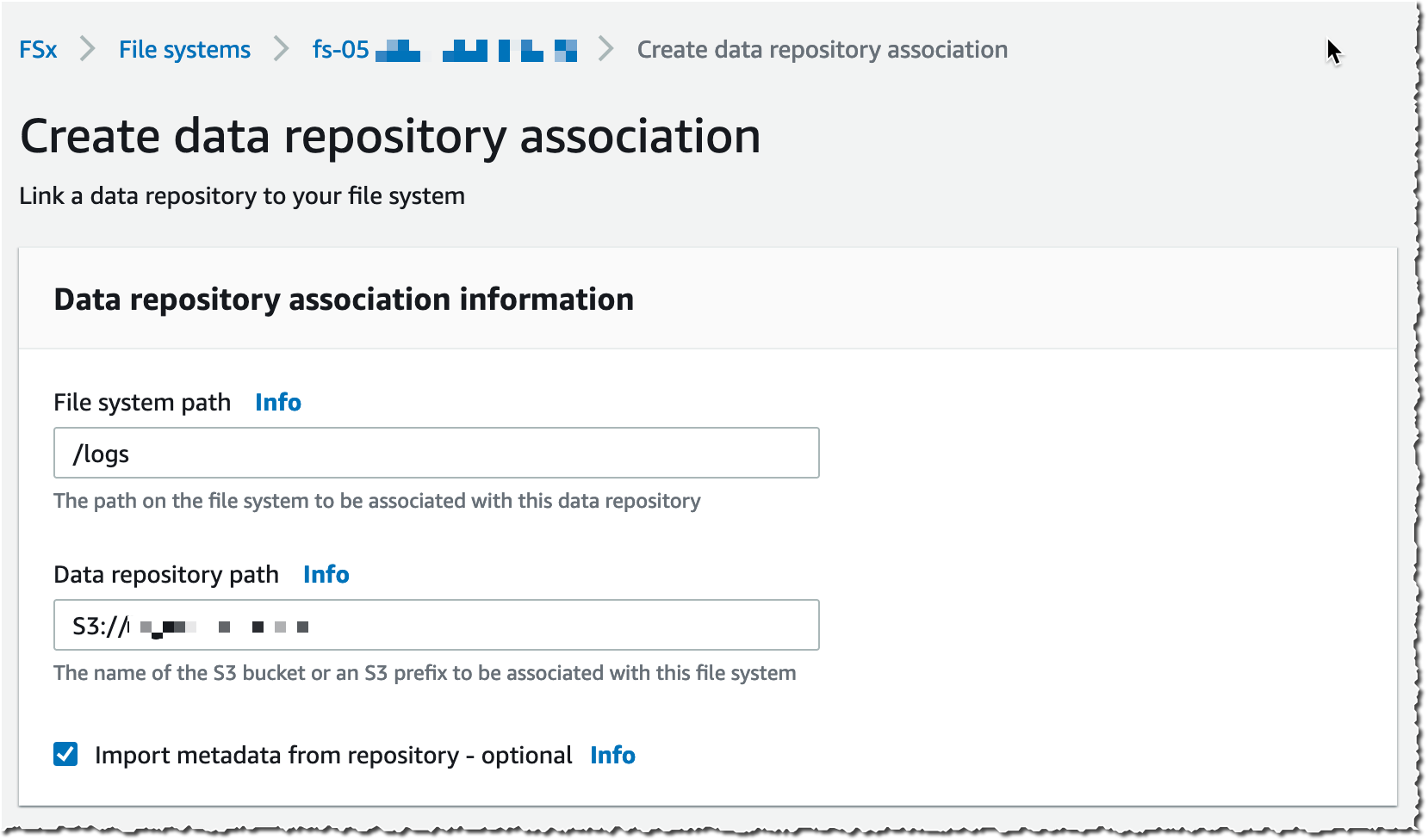
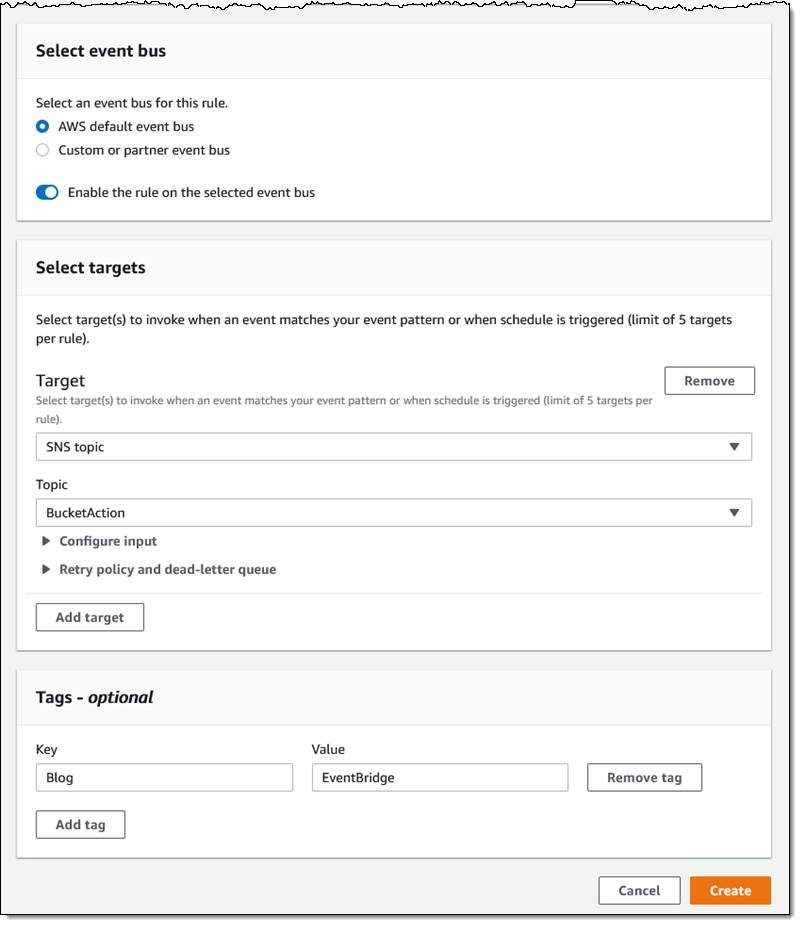
Then I define a pattern that matches the bucket and the events of interest:

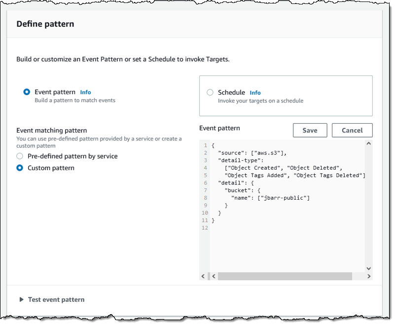One pattern can match one or more buckets and one or more events; the following events are supported:

Object Created
Object Deleted
Object Restore Initiated
Object Restore Completed
Object Restore Expired
Object Tags Added
Object Tags Deleted
Object ACL Updated
Object Storage Class Changed
Object Access Tier Changed

Then I choose the default event bus, and set the target to an SNS topic (BucketAction) which publishes the messages to my Amazon email address:

I click Create, and I am all set. To test it out, I simply upload some files to my bucket and await the messages:

The message contains all of the interesting and relevant information about the event, and (after some unquoting and formatting), looks like this:

{
    "version": "0",
    "id": "2d4eba74-fd51-3966-4bfa-b013c9da8ff1",
    "detail-type": "Object Created",
    "source": "aws.s3",
    "account": "348414629041",
    "time": "2021-11-13T00:00:59Z",
    "region": "us-east-1",
    "resources": [
        "arn:aws:s3:::jbarr-public"
    ],
    "detail": {
        "version": "0",
        "bucket": {
            "name": "jbarr-public"
        },
        "object": {
            "key": "eb_create_rule_mid_1.png",
            "size": 99797,
            "etag": "7a72374e1238761aca7778318b363232",
            "version-id": "a7diKodKIlW3mHIvhGvVphz5N_ZcL3RG",
            "sequencer": "00618F003B7286F496"
        },
        "request-id": "4Z2S00BKW2P1AQK8",
        "requester": "348414629041",
        "source-ip-address": "72.21.198.68",
        "reason": "PutObject"
    }

My initial event pattern was very simple, and matched only the bucket name. I can use content-based filtering to write more complex and more interesting patterns. For example, I could use numeric matching to set up a pattern that matches events for objects that are smaller than 1 megabyte:

{
    "source": [
        "aws.s3"
    ],
    "detail-type": [
        "Object Created",
        "Object Deleted",
        "Object Tags Added",
        "Object Tags Deleted"
    ],

    "detail": {
        "bucket": {
            "name": [
                "jbarr-public"
            ]
        },
        "object" : {
            "size": [{"numeric" :["<=", 1048576 ] }]
        }
    }
}

Or, I could use prefix matching to set up a pattern that looks for objects uploaded to a “subfolder” (which doesn’t really exist) of a bucket:

"object": {
  "key" : [{"prefix" : "uploads/"}]
  }]
}

You can use all of this in conjunction with all of the existing EventBridge features, including Archive/Replay. You can also access the CloudWatch metrics for each of your rules:

Available Now
This feature is available now and you can start using it today in all commercial AWS Regions. You pay $1 for every 1 million events that match a rule; check out the EventBridge Pricing page for more information.

— Jeff;

Enforce customized data quality rules in AWS Glue DataBrew

2021-11-25 Navnit Shukla

Post Syndicated from Navnit Shukla original https://aws.amazon.com/blogs/big-data/enforce-customized-data-quality-rules-in-aws-glue-databrew/

GIGO (garbage in, garbage out) is a concept common to computer science and mathematics: the quality of the output is determined by the quality of the input. In modern data architecture, you bring data from different data sources, which creates challenges around volume, velocity, and veracity. You might write unit tests for applications, but it’s equally important to ensure the data veracity of these applications, because incoming data quality can make or break your application. Incorrect, missing, or malformed data can have a large impact on production systems. Examples of data quality issues include but are not limited to the following:

Missing or incorrect values can lead to failures in the production system that require non-null values
Changes in the distribution of data can lead to unexpected outputs of machine learning (ML) models
Aggregations of incorrect data can lead to wrong business decisions
Incorrect data types have a big impact on financial or scientific institutes

In this post, we introduce data quality rules in AWS Glue DataBrew. DataBrew is a visual data preparation tool that makes it easy to profile and prepare data for analytics and ML. We demonstrate how to use DataBrew to define a list of rules in a new entity called a ruleset. A ruleset is a set of rules that compare different data metrics against expected values.

The post describes the implementation process and provides a step-by-step guide to build data quality checks in DataBrew.

Solution overview

To illustrate our data quality use case, we use a human resources dataset. This dataset contains the following attributes:

Emp ID, Name Prefix, First Name, Middle Initial,Last Name,Gender,E Mail,Father's Name,Mother's Name,Mother's Maiden Name,Date of Birth,Time of Birth,Age in Yrs.,Weight in Kgs.,Date of Joining,Quarter of Joining,Half of Joining,Year of Joining,Month of Joining,Month Name of Joining,Short Month,Day of Joining,DOW of Joining,Short DOW,Age in Company (Years),Salary,Last % Hike,SSN,Phone No. ,Place Name,County,City,State,Zip,Region,User Name,Password

For this post, we downloaded data with 5 million records, but feel free to use a smaller dataset to follow along with this post.

The following diagram illustrates the architecture for our solution.

The steps in this solution are as follows:

Create a sample dataset.
Create a ruleset.
Create data quality rules.
Create a profile job.
Inspect the data quality rules validation results.
Clean the dataset.
Create a DataBrew job.
Validate the data quality check with the updated dataset.

Prerequisites

Before you get started, complete the following prerequisites:

Have an AWS account.
Download the sample dataset.
Extract the CSV file.
Create an Amazon Simple Storage Service (Amazon S3) bucket with three folders: input, output, and profile.
Upload the sample data in input folder to your S3 bucket (for example, s3://<s3 bucket name>/input/).

Create a sample dataset

To create your dataset, complete the following steps:

On the DataBrew console, in the navigation pane, choose Datasets.
Choose Connect new dataset.
For Dataset name, enter a name (for example, human-resource-dataset).
Under Data lake/data store, choose Amazon S3 as your source.
For Enter your source from Amazon S3, enter the S3 bucket location where you uploaded your sample files (for example, s3://<s3 bucket name>/input/).
Under Additional configurations, keep the selected file type CSV and CSV delimiter comma (,).
Scroll to the bottom of the page and choose Create dataset.

The dataset is now available on the Datasets page.

Create a ruleset

We now define data quality rulesets against the dataset created in the previous step.

On the DataBrew console, in the navigation pane, choose DQ Rules.
Choose Create data quality ruleset.
For Ruleset name, enter a name (for example, human-resource-dataquality-ruleset).
Under Associated dataset, choose the dataset you created earlier.

Create data quality rules

To add data quality rules, you can use rules and add multiple rules, and within each rule, you can define multiple checks.

For this post, we create the following data quality rules and data quality checks within the rules:

Row count is correct
No duplicate rows
Employee ID, email address, and SSN are unique
Employee ID and phone number are not be null
Employee ID and employee age in years has no negative values
SSN data format is correct (123-45-6789)
Phone number for string length is correct
Region column only has the specified region
Employee ID is an integer

Row count is correct

To check the total row count, complete the following steps:

Add a new rule.
For Rule name, enter a name (for example, Check total record count).
For Data quality check scope, choose Individual check for each column.
For Rule success criteria, choose All data quality checks are met (AND).
For Data quality checks¸ choose Number of rows.
For Condition, choose Is equals.
For Value, enter 5000000.

No duplicate rows

To check the dataset for duplicate rows, complete the following steps:

Choose Add another rule.
For Rule name, enter a name (for example, Check dataset for duplicate rows).
For Data quality check scope, choose Individual check for each column.
For Rule success criteria, choose All data quality checks are met (AND).
Under Check 1, for Data quality check¸ choose Duplicate rows.
For Condition, choose Is equals.
For Value, enter 0 and choose rows on the drop-down menu.

Employee ID, email address, and SSN are unique

To check that the employee ID, email, and SSN are unique, complete the following steps:

Choose Add another rule.
For Rule name, enter a name (for example, Check dataset for Unique Values).
For Data quality check scope, choose Common checks for selected columns.
For Rule success criteria, choose All data quality checks are met (AND).
For Selected columns, select Selected columns.
Choose the columns Emp ID, e mail, and SSN.
Under Check 1, for Data quality check, choose Unique values.
For Condition, choose Is equals.
For Value, enter 100 and choose %(percent) rows on the drop-down menu.

Employee ID and phone number are not be null

To check that employee IDs and phone numbers aren’t null, complete the following steps:

Choose Add another rule.
For Rule name, enter a name (for example, Check Dataset for NOT NULL).
For Data quality check scope, choose Common checks for selected columns.
For Rule success criteria, choose All data quality checks are met (AND).
For Selected columns, select Selected columns.
Choose the columns Emp ID and Phone No.
Under Check 1, for Data quality check, choose Value is not missing.
For Condition, choose Greater than equals.
For Threshold, enter 100 and choose %(percent) rows on the drop-down menu.

Employee ID and age in years has no negative values

To check the employee ID and age for positive values, complete the following steps:

Choose Add another rule.
For Rule name, enter a name (for example, Check emp ID and age for positive values).
For Data quality check scope, choose Individual check for each column.
For Rule success criteria, choose All data quality checks are met (AND).
Under Check 1, for Data quality check, choose Numeric values.
Choose Emp ID on the drop-down menu.
For Condition, choose Greater than equals.
For Value, select Custom value and enter 0.
Choose Add another quality check and repeat the same steps for age in years.

SSN data format is correct

To check the SSN data format, complete the following steps:

Choose Add another rule.
For Rule name, enter a name (for example, Check dataset format).
For Data quality check scope, choose Individual check for each column.
For Rule success criteria, choose All data quality checks are met (AND).
Under Check 1, for Data quality check, choose String values.
Choose SSN on the drop-down menu.
For Condition, choose Matches (RegEx pattern).
For RegEx value, enter ^[0-9]{3}-[0-9]{2}-[0-9]{4}$.

Phone number string length is correct

To check the length of the phone number, complete the following steps:

Choose Add another rule.
For Rule name, enter a name (for example, Check Dataset Phone no. for string length).
For Data quality check scope, choose Individual check for each column.
For Rule success criteria, choose All data quality checks are met (AND).
Under Check 1, for Data quality check, choose Value string length.
Choose Phone No on the drop-down menu.
For Condition, choose Greater than equals.
For Value, select Custom value and enter 9.
Under Check 2, for Data quality check, choose Value string length.
Choose Phone No on the drop-down menu.
For Condition, choose Less than equals.
For Value¸ select Custom value and enter 12.

Region column only has the specified region

To check the Region column, complete the following steps:

Choose Add another rule.
For Rule name, enter a name (for example, Check Region column only for specific region).
For Data quality check scope, choose Individual check for each column.
For Rule success criteria, choose All data quality checks are met (AND).
Under Check 1, for Data quality check, choose Value is exactly.
Choose Region on the drop-down menu.
For Value, select Custom value.
Choose the values Midwest, South, West, and Northeast.

Employee ID is an integer

To check that the employee ID is an integer, complete the following steps:

Choose Add another rule.
For Rule name, enter a name (for example, Validate Emp ID is an Integer).
For Data quality check scope, choose Individual check for each column.
For Rule success criteria, choose All data quality checks are met (AND).
Under Check 1, for Data quality check, choose String values.
Choose Emp ID on the drop-down menu.
For Condition, choose Matches (RegEx pattern).
For RegEx value, enter ^[0-9]+$.
After you create all the rules, choose Create ruleset.

Your ruleset is now listed on the Data quality rulesets page.

Create a profile job

To create a profile job with your new ruleset, complete the following steps:

On the Data quality rulesets page, select the ruleset you just created.
Choose Create profile job with ruleset.
For Job name, keep the prepopulated name or enter a new one.
For Data sample, select Full dataset.

The default sample size is important for data quality rules validation, because it matters if you validate all the roles or a limited sample.

Under Job output settings, for S3 location, enter the path to the profile bucket.

If you enter a new bucket name, the folder is created automatically.

Keep the default settings for the remaining optional sections: Data profile configurations, Data quality rules, Advanced job settings, Associated schedules, and Tags.

The next step is to choose or create the AWS Identity and Access Management (IAM) role that grants DataBrew access to read from the input S3 bucket and write to the job output bucket.

For Role name, choose an existing role or choose Create a new IAM role and enter an IAM role suffix.
Choose Create and run job.

For more information about configuring and running DataBrew jobs, see Creating, running, and scheduling AWS Glue DataBrew jobs.

Inspect data quality rules validation results

To inspect the data quality rules, we need to let the profile job complete.

On the Jobs page of the DataBrew console, choose the Profile jobs tab.
Wait until the profile job status changes to Succeeded.
When the job is complete, choose View data profile.

You’re redirected to the Data profile overview tab on the Datasets page.

Choose the Data quality rules tab.

Here you can review the status to your data quality rules. As shown in the following screenshot, eight of the nine data quality rules defined were successful, and one rule failed.

Our failed data quality rule indicates that we found duplicate values for employee ID, SSN, and email.

To confirm that the data has duplicate values, on the Column statistics tab, choose the Emp ID column.
Scroll down to the section Top distinct values.

Similarly, you can check the E Mail and SSN columns to find that those columns also have duplicate values.

Now we have confirmed that our data has duplicate values. The next step is to clean up the dataset and rerun the quality rules validation.

Clean the dataset

To clean the dataset, we first need to create a project.

On the DataBrew console, choose Projects.
Choose Create project.
For Project name, enter a name (for this post, human-resource-project-demo).
For Select a dataset, select My datasets.
Select the human-resource-dataset dataset.
Keep the sampling size at its default.
Under Permissions, for Role name, choose the IAM role that we created previously for our DataBrew profile job.
Choose Create project.

The project takes a few minutes to open. When it’s complete, you can see your data.

Next, we delete the duplicate value from the Emp ID column.

Choose the Emp ID column.
Choose the more options icon (three dots) to view all the transforms available for this column.
Choose Remove duplicate values.
Repeat these steps for the SSN and E Mail columns.

You can now see the three applied steps in the Recipe pane.

Create a DataBrew job

The next step is to create a DataBrew job to run these transforms against the full dataset.

On the project details page, choose Create job.
For Job name, enter a name (for example, human-resource-after-dq-check).
Under Job output settings¸ for File type, choose your final storage format to be CSV.
For S3 location, enter your output S3 bucket location (for example, s3://<s3 bucket name>/output/).
For Compression, choose None.
Under Permissions, for Role name¸ choose the same IAM role we used previously.
Choose Create and run job.
Wait for job to complete; you can monitor the job on the Jobs page.

Validate the data quality check with the corrected dataset

To perform the data quality checks with the corrected dataset, complete the following steps:

Follow the steps outlined earlier to create a new dataset, using the corrected data from the previous section.
Choose the Amazon S3 location of the job output.
Choose Create dataset.
Choose DQ Rules and select the ruleset you created earlier.
On the Actions menu, choose Duplicate.
For Ruleset name, enter a name (for example, human-resource-dataquality-ruleset-on-corrected-dataset).
Select the newly created dataset.
Choose Create data quality ruleset.
After the ruleset is created, select it and choose Create profile job with ruleset.
Create a new profile job.
Choose Create and run job.
When the job is complete, repeat the steps from earlier to inspect the data quality rules validation results.

This time, under Data quality rules, all the rules are passed except Check total record count because you removed duplicate values.

On the Column statistics page, under Top distinct values for the Emp ID column, you can see the distinct values.

You can find similar results for the SSN and E Mail columns.

Clean up

To avoid incurring future charges, we recommend you delete the resources you created during this walkthrough.

Conclusion

As demonstrated in this post, you can use DataBrew to help create data quality rules, which can help you identify any discrepancies in your data. You can also use DataBrew to clean the data and validate it going forwards. You can learn more about AWS Glue DataBrew from here and learn around AWS Glue DataBrew pricing here.

About the Authors

Navnit Shukla is an AWS Specialist Solution Architect, Analytics, and is passionate about helping customers uncover insights from their data. He has been building solutions to help organizations make data-driven decisions.

Harsh Vardhan Singh Gaur is an AWS Solutions Architect, specializing in Analytics. He has over 5 years of experience working in the field of big data and data science. He is passionate about helping customers adopt best practices and discover insights from their data.