Post Syndicated from Ajay Vohra original https://aws.amazon.com/blogs/architecture/field-notes-launch-a-fully-configured-aws-deep-learning-desktop-with-nice-dcv/
You want to start quickly when doing deep learning using GPU-activated Elastic Compute Cloud (Amazon EC2) instances in the AWS Cloud. Although AWS provides end-to-end machine learning (ML) in Amazon SageMaker, working at the deep learning frameworks level, the quickest way to start is with AWS Deep Learning AMIs (DLAMIs), which provide preconfigured Conda environments for most of the popular frameworks.
DLAMIs make it straightforward to launch Amazon EC2 instances, but these instances do not automatically provide the high-performance graphics visualization required during deep learning research. Additionally, they are not preconfigured to use AWS storage services or SageMaker. This post explains how you can launch a fully-configured deep learning desktop in the AWS Cloud. Not only is this desktop preconfigured with the popular frameworks such as TensorFlow, PyTorch, and Apache MXNet, but it is also enabled for high-performance graphics visualization. NICE DCV is the remote display protocol used for visualization. In addition, it is preconfigured to use AWS storage services and SageMaker.
Overview of the Solution
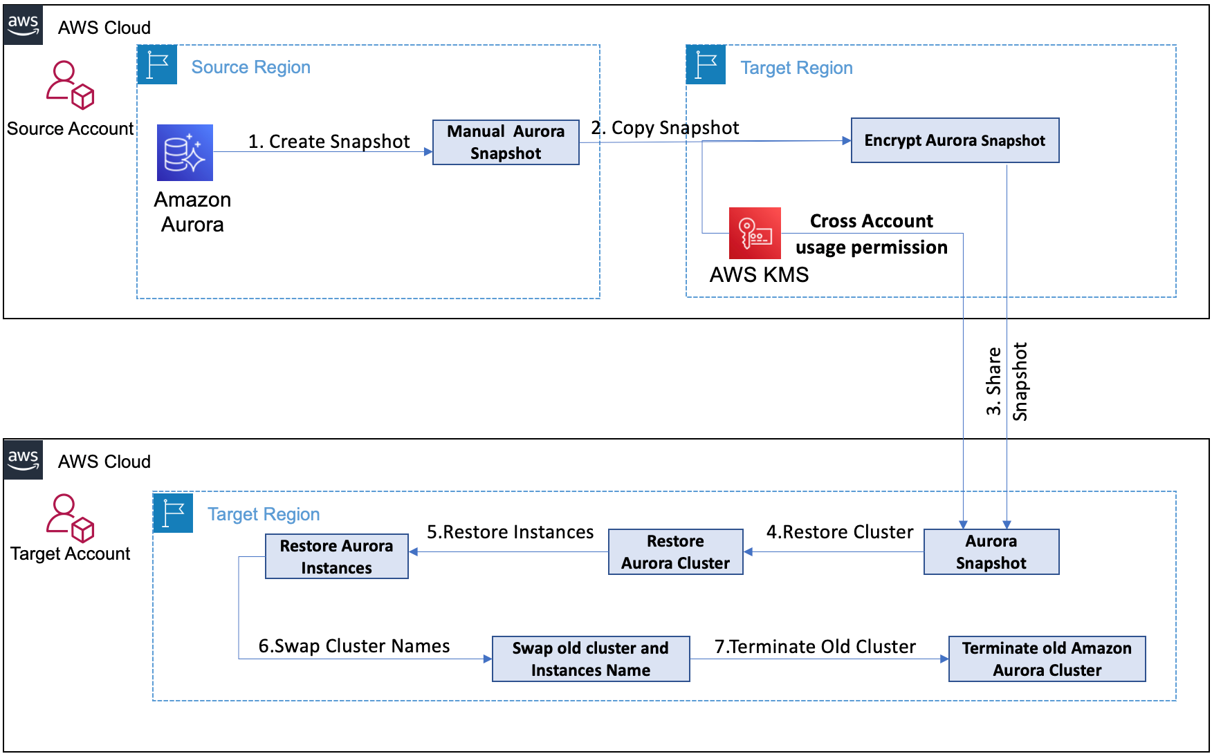
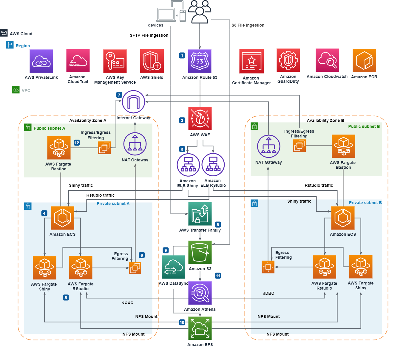
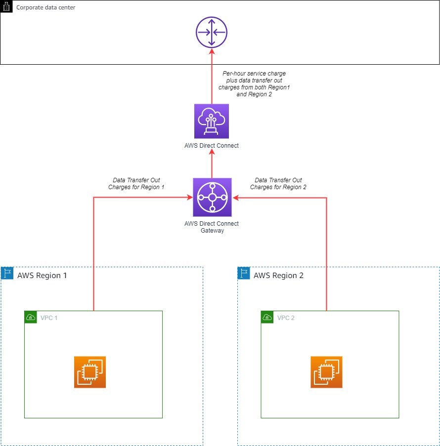
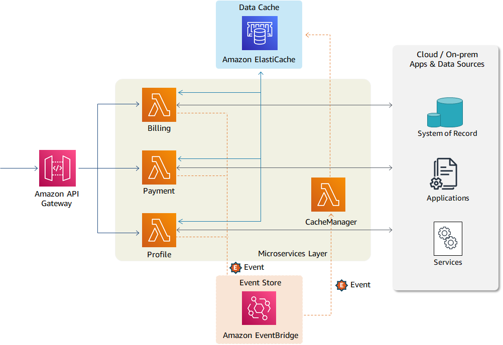
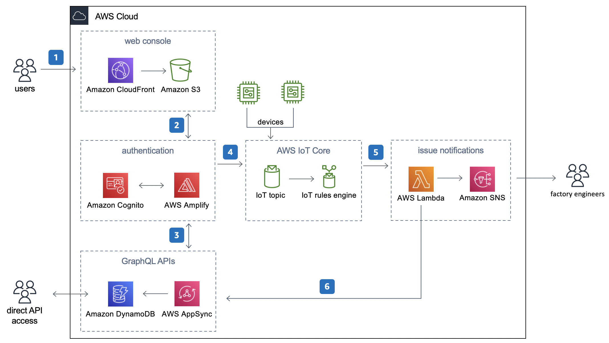
The deep learning desktop described in this solution is ready for research and development of deep neural networks (DNNs) and their visualization. You no longer need to set up low-level drivers, libraries, and frameworks, or configure secure access to AWS storage services and SageMaker. The desktop has preconfigured access to your data in a Simple Storage Service (Amazon S3) bucket, and a shared Amazon Elastic File System (Amazon EFS) is automatically attached to the desktop. It is automatically configured to access SageMaker for ML services, and provides you with the ability to prepare the data needed for deep learning, and to research, develop, build, and debug your DNNs. You can use all the advanced capabilities of SageMaker from your deep learning desktop. The following diagram shows the reference architecture for this solution.

Figure 1 – Architecture overview of the solution to launch a fully configured AWS Deep Learning Desktop with NICE DCV
The deep learning desktop solution discussed in this post is contained in a single AWS CloudFormation template. To launch the solution, you create a CloudFormation stack from the template. Before we provide a detailed walkthrough for the solution, let us review the key benefits.
DNN Research and Development
During the DNN research phase, there is iterative exploration until you choose the preferred DNN architecture. During this phase, you may prefer to work in an isolated environment (for example, a dedicated desktop) with your favorite integrated development environment (IDE) (for example, Visual Studio Code or PyCharm). Developers like the ability to step through code the IDE Debugger. With the increasing support for imperative programming in modern ML frameworks, the ability to step through code in the research phase can accelerate DNN development.
The DLAMIs are preconfigured with NVIDIA GPU drivers, NVIDIA CUDA Toolkit, and low-level libraries such as Deep Neural Network library (cuDNN). Deep learning ML frameworks such as TensorFlow, PyTorch, and Apache MXNet are preconfigured.
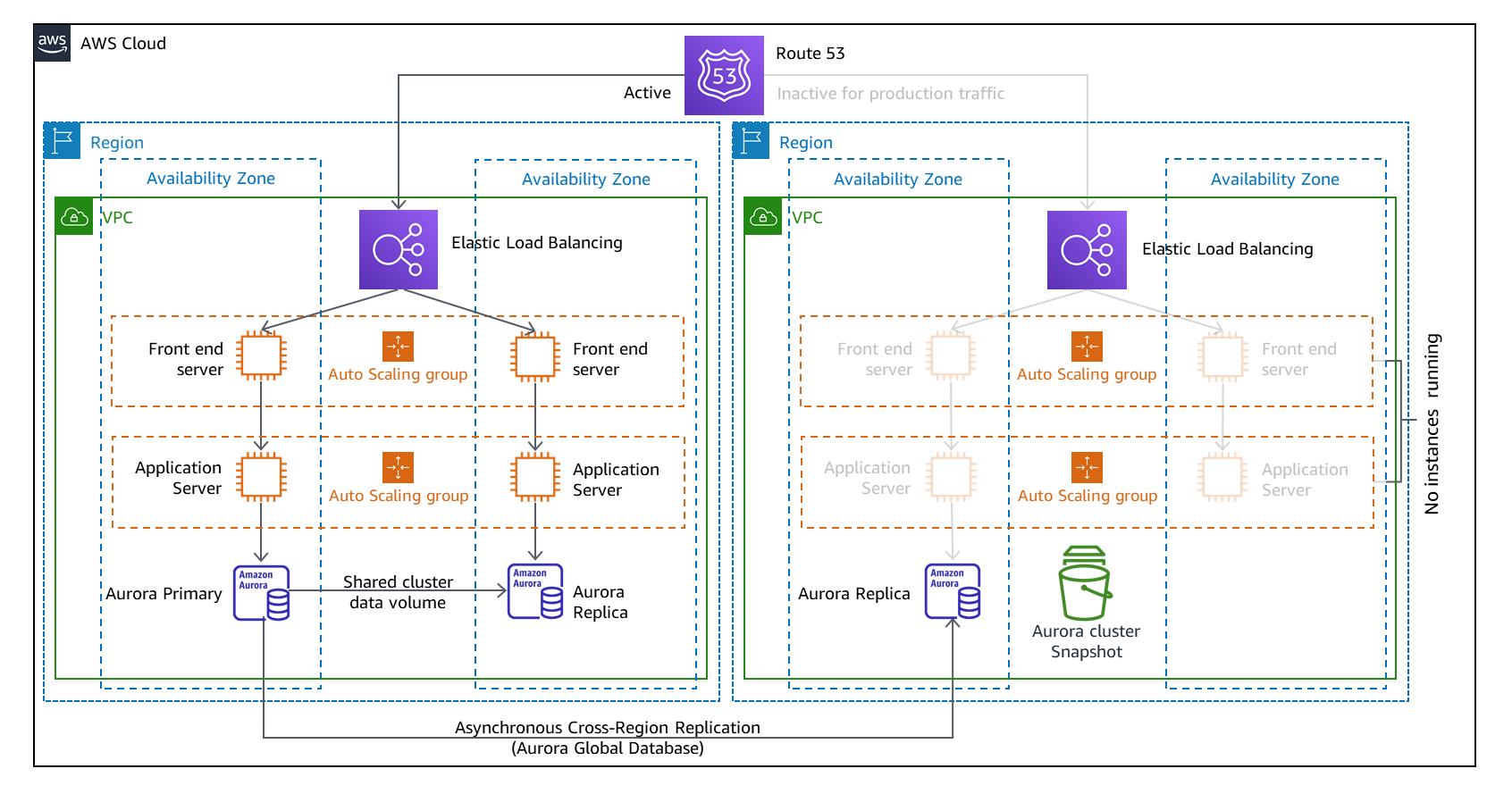
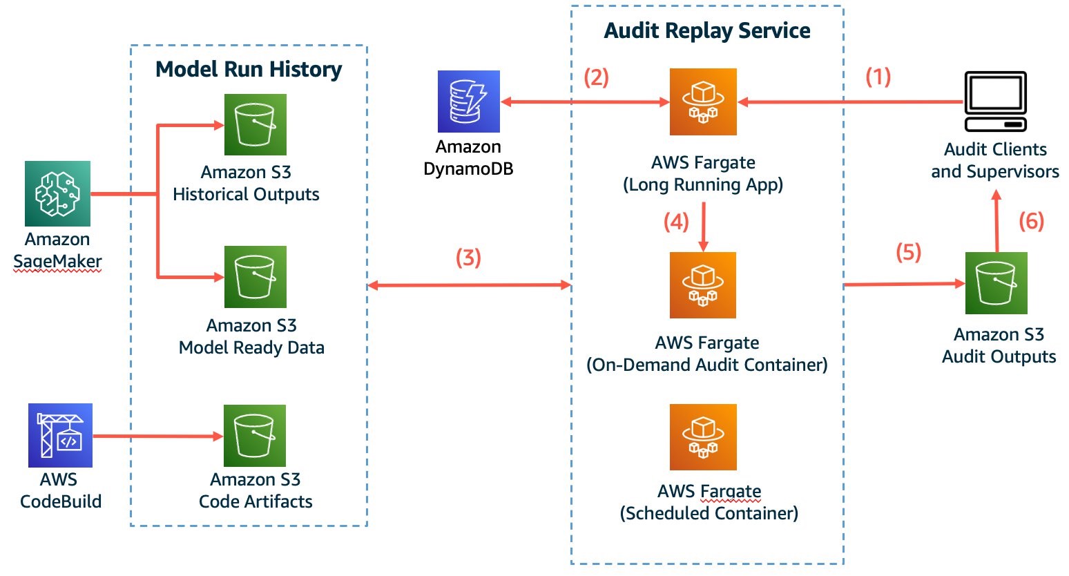
After you launch the deep learning desktop, you need to install and open your favorite IDE, clone your GitHub repository, and you can start researching, developing, debugging, and visualizing your DNN. The acceleration of DNN research and development is the first key benefit for the solution described in this post.
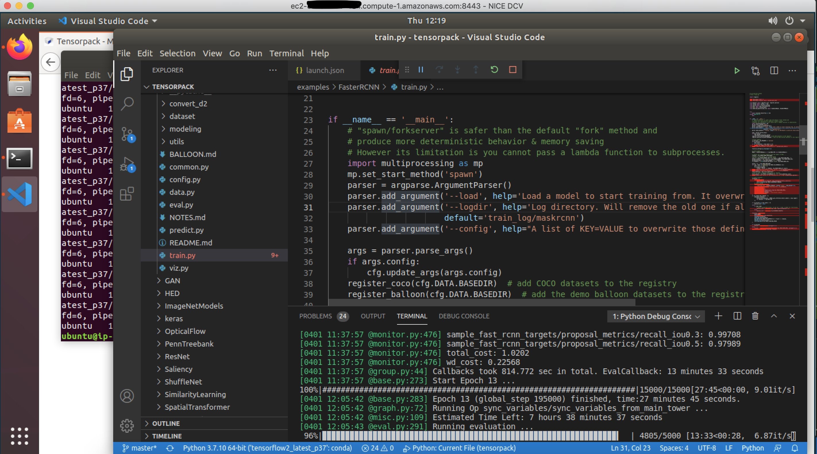
Figure 2 – Developing on deep learning desktop with Visual Studio Code IDE
Elasticity in number of GPUs
During the research phase, you need to debug any issues using a single GPU. However, as the DNN is stabilized, you horizontally scale across multiple GPUs in a single machine, followed by scaling across multiple machines.
Most modern deep learning frameworks support distributed training across multiple GPUs in a single machine, and also across multiple machines. However, when you use a single GPU in an on-premises desktop equipped with multiple GPUs, the idle GPUs are wasted. With the deep learning desktop solution described in this post, you can stop the deep learning desktop instance, change its Amazon EC2 instance type to another compatible type, restart the desktop, and get the exact number of GPUs you need at the moment. The elasticity in the number of GPUs in the deep learning desktop is the second key benefit for the solution described in this post.
Integrated access to storage services
Since the deep learning desktop is running in AWS Cloud, you have access to all of the AWS data storage options, including the S3 object store, the Amazon EFS, and the Amazon FSx file system for Lustre. You can build your favorite data pipeline and it will be supported by one or more data storage options. You can also easily use ML-IO library, which is a high-performance data access library for ML tasks with support for multiple data formats. The integrated access to highly durable and scalable object and file system storage services for accessing ML data is the third key benefit for the solution described in this post.
Integrated access to SageMaker
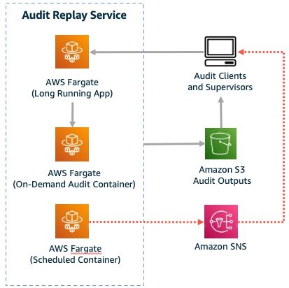
Once you have a stable version of your DNN, you need to find the right hyperparameters that lead to model convergence during training. Having tuned the hyperparameters, you need to run multiple trials over permutations of datasets and hyperparameters to fine-tune your models. Finally, you may need to prune and compile the models to optimize inference. To compress the training time, you may need to do distributed data parallel training across multiple GPUs in multiple machines. For all of these activities, the deep learning desktop is preconfigured to use SageMaker. You can use jupyter-lab notebooks running on the desktop to launch SageMaker training jobs for distributed training in infrastructure automatically managed by SageMaker.
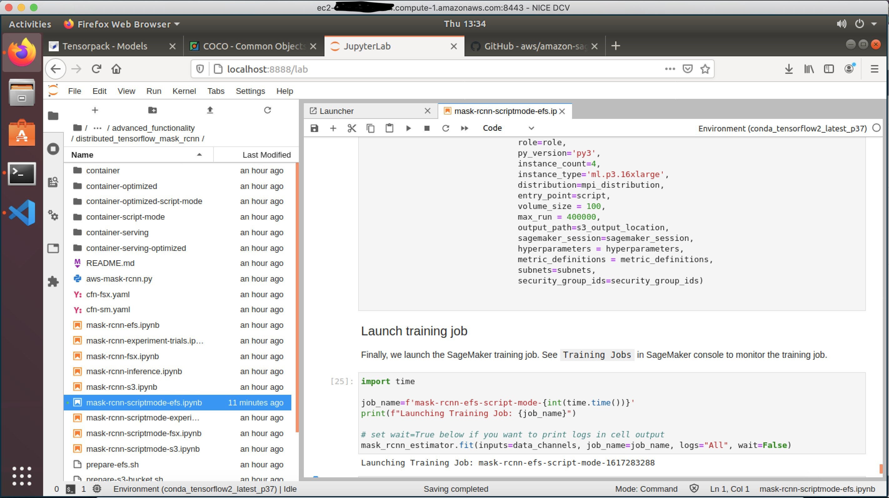
Figure 3 – Submitting a SageMaker training job from deep learning desktop using Jupyter Lab notebook
The SageMaker training logs, TensorBoard summaries, and model checkpoints can be configured to be written to the Amazon EFS attached to the deep learning desktop. You can use the Linux command tail to monitor the logs, or start a TensorBoard server from the Conda environment on the deep learning desktop, and monitor the progress of your SageMaker training jobs. You can use a Jupyter Lab notebook running on the deep learning desktop to load a specific model checkpoint available on the Amazon EFS, and visualize the predictions from the model checkpoint, even while the SageMaker training job is still running.
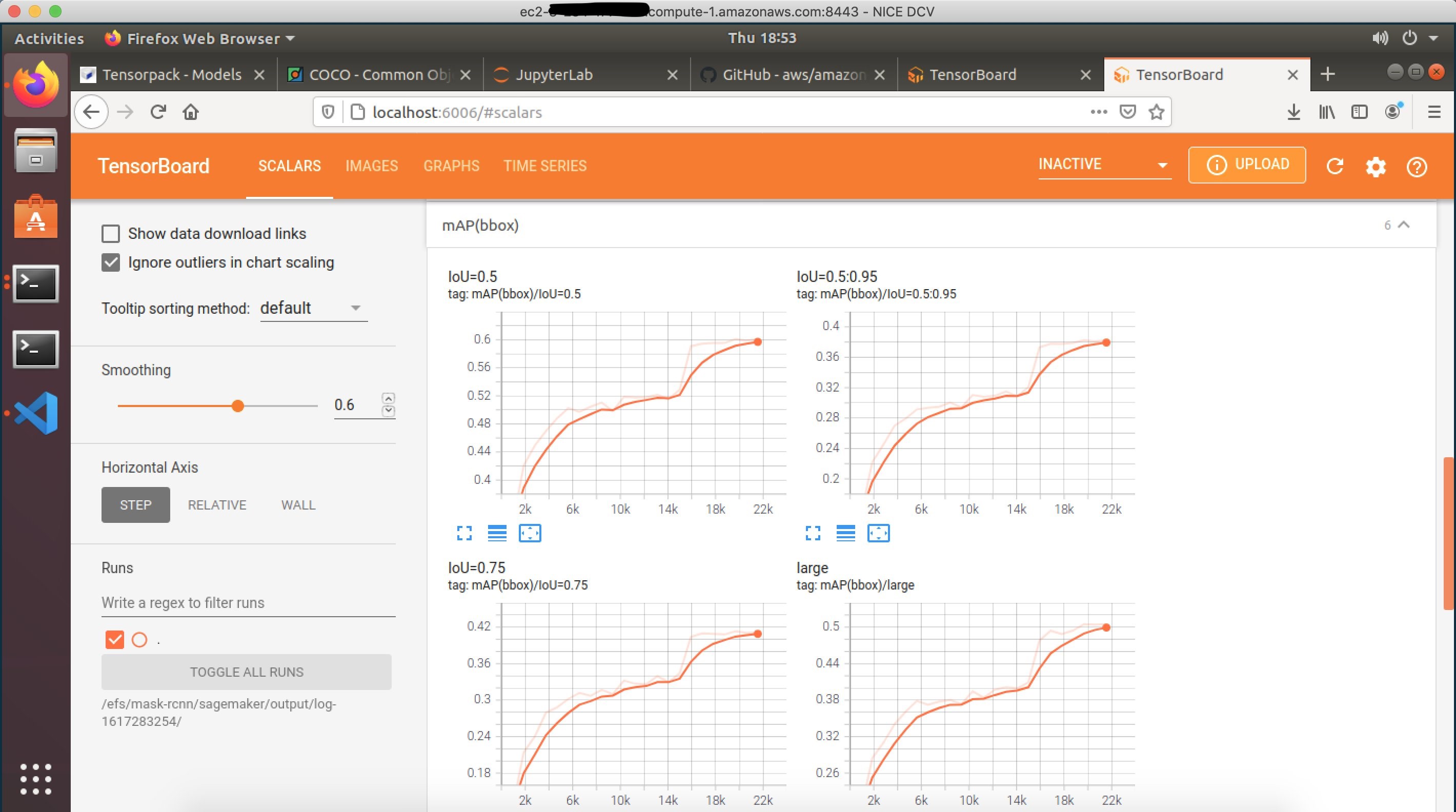
Figure 4 – Locally monitoring the TensorBoard summaries from SageMaker training job
SageMaker offers many advanced capabilities, such as profiling ML training jobs using Amazon SageMaker Debugger, and these services are easily accessible from the deep learning desktop. You can manage the training input data, training model checkpoints, training logs, and TensorBoard summaries of your local iterative development, in addition to the distributed SageMaker training jobs, all from your deep learning desktop. The integrated access to SageMaker services is the fourth key use case for the solution described in this post.
Prerequisites
To get started, complete the following steps:
- If you do not have an AWS Account, create a new AWS account.
- You must have AWS Identity and Access Management (IAM) access consistent with administrator job function.
- In the AWS Management Console, select a supported Region (review the prerequisites in the read me file within the GitHub repository for the list of supported Regions).
- Subscribe to DLAMI (Ubuntu 18.04).
- Create a new Amazon EC2 key pair, or use an existing key pair.
- Create a new S3 bucket in the selected AWS Region, or use an existing bucket. The bucket can be empty.
- Clone the GitHub repository on your laptop using the Git clone command.
Walkthrough
The complete source and reference documentation for this solution is available in the repository accompanying this post. Following is a walkthrough of the steps.
Create a CloudFormation stack
Create a stack on the CloudFormation console in your selected AWS Region using the CloudFormation template in your cloned GitHub repository. This CloudFormation stack creates IAM resources. When you are creating a CloudFormation stack using the console, you must confirm: I acknowledge that AWS CloudFormation might create IAM resources.
To create the CloudFormation stack, you must specify values for the following input parameters (for the rest of the input parameters, default values are recommended):
- DesktopAccessCIDR – Use the public internet address of your laptop as the base value for the CIDR.
- DesktopInstanceType – For deep leaning, the recommended value for this parameter is p3.2xlarge, or larger.
- DesktopVpcId – Select an Amazon Virtual Private Cloud (VPC) with at least one public subnet.
- DesktopVpcSubnetId – Select a public subnet in your VPC.
- DesktopSecurityGroupId – The specified security group must allow inbound access over ports 22 (SSH) and 8443 (NICE DCV) from your DesktopAccessCIDR, and must allow inbound access from within the security group to port 2049 and all network ports required for distributed SageMaker training in your subnet.
- If you leave it blank, the automatically-created security group allows inbound access for SSH, and NICE DCV from your DesktopAccessCIDR, and allows inbound access to all ports from within the security group.
- KeyName – Select your SSH key pair name.
- S3Bucket – Specify your S3 bucket name. The bucket can be empty.
Visit the documentation on all the input parameters.
Connect to the deep learning desktop
- When the status for the stack in the CloudFormation console is CREATE_COMPLETE, find the deep learning desktop instance launched in your stack in the Amazon EC2 console,
- Connect to the instance using SSH as user ubuntu, using your SSH key pair. When you connect using SSH, if you see the message, “Cloud init in progress. Machine will REBOOT after cloud init is complete!!”, disconnect and try again in about 15 minutes.
- The desktop installs the NICE DCV server on first-time startup, and automatically reboots after the install is complete. If instead you see the message, “NICE DCV server is enabled!”, the desktop is ready for use.
- Before you can connect to the desktop using the NICE DCV client, you need to set a new password for user ubuntu using the Bash command:
sudo passwd ubuntu - After you successfully set the new password for user ubuntu, exit the SSH connection. You are now ready to connect to the desktop using a suitable NICE DCV client (a non–web browser client is recommended) using the user ubuntu, and the new password.
- NICE DCV client asks you to specify the server host and port to connect. For the server host, use the public IPv4 DNS address of the desktop Amazon EC2 instance available in Amazon EC2 console.
- You do not need to specify the port, because the desktop is configured to use the default NICE DCV server port of 8443.
- When you first login to the desktop using the NICE DCV client, you will be asked if you would like to upgrade the OS version. Do not upgrade the OS version!
Develop on the deep learning desktop
When you are connected to the desktop using the NICE DCV client, use the Ubuntu Software Center to install Visual Studio Code, or your favorite IDE. To view the available Conda environments containing the popular deep learning frameworks preconfigured on the desktop, open a desktop terminal, and run the Bash command:
conda env listThe deep learning desktop instance has secure access to the S3 bucket you specified when you created the CloudFormation stack. You can verify access to the S3 bucket by running the Bash command (replace ‘your-bucket-name’ following with your S3 bucket name):
aws s3 ls your-bucket-name If your bucket is empty, a successful initiation of the previous command will produce no output, which is normal.
An Amazon Elastic Block Store (Amazon EBS) root volume is attached to the instance. In addition, an Amazon EFS is mounted on the desktop at the value of EFSMountPath input parameter, which by default is /home/ubuntu/efs. You can use the Amazon EFS for staging deep learning input and output data.
Use SageMaker from the deep learning desktop
The deep learning desktop is preconfigured to use SageMaker. To get started with SageMaker examples in a JupyterLab notebook, launch the following Bash commands in a desktop terminal:
mkdir ~/git
cd ~/git
git clone https://github.com/aws/amazon-sagemaker-examples.git
jupyter-lab
This will start a ‘jupyter-lab’ notebook server in the terminal, and open a tab in your web browser. You can explore any of the SageMaker example notebooks. We recommend starting with the example Distributed Training of Mask-RCNN in SageMaker using Amazon EFS found at the following path in the cloned repository:
advanced_functionality/distributed_tensorflow_mask_rcnn/mask-rcnn-scriptmode-efs.ipynbThe preceding SageMaker example requires you to specify a subnet and a security group. Use the preconfigured OS environment variables as follows:
security_group_ids = [ os.environ['desktop_sg_id'] ]
subnets = [ os.environ['desktop_subnet_id' ] ]
Stopping and restarting the desktop
You may safely reboot, stop, and restart the desktop instance at any time. The desktop will automatically mount the Amazon EFS at restart.
Clean Up
When you no longer need the deep learning desktop, you may delete the CloudFormation stack from the CloudFormation console. Deleting the stack will shut down the desktop instance, and delete the root Amazon EBS volume attached to the desktop. The Amazon EFS is not automatically deleted when you delete the stack.
Conclusion
In this post, we showed how to launch a desktop pre-configured with the popular machine learning frameworks for research and development of deep learning neural networks. NICE-DCV was used for high performance visualization related to deep learning. AWS storage services were used for highly scalable access to deep learning data. Finally, Amazon SageMaker was used for the distributed training of deep learning data.


 to the many challenges we face today, and seeking improved methods for future needs.