Post Syndicated from Sudhir Amin original https://aws.amazon.com/blogs/architecture/field-notes-implementing-ha-and-dr-for-microsoft-sql-server-using-always-on-failover-cluster-instance-and-sios-datakeeper/
To ensure high availability (HA) of Microsoft SQL Server in Amazon Elastic Compute Cloud (Amazon EC2), there are two options: Always On Failover Cluster Instance (FCI) and Always On availability groups. With a wide range of networking solutions such as VPN and AWS Direct Connect, you have options to further extend your HA architecture to another AWS Region to also meet your disaster recovery (DR) objectives.
You can also run asynchronous replication between Regions, or a combination of both synchronous replication between Availability Zones and asynchronous replication between Regions.
Choosing the right SQL Server HA solution depends on your requirements. If you have hundreds of databases, or are looking to avoid the expense of SQL Server Enterprise Edition, then SQL Server FCI is the preferred option. If you are looking to protect user-defined databases and system databases that hold agent jobs, usernames, passwords, and so forth, then SQL Server FCI is the preferred option. If you already own SQL Server Enterprise licenses we recommend continuing with that option.
On-premises Always On FCI deployments typically require shared storage solutions such as a fiber channel storage area network (SAN). When deploying SQL Server FCI in AWS, a SAN is not a viable option. Although Amazon FSx for Microsoft Windows is the recommended storage option for SQL Server FCI in AWS, it does not support adding cluster nodes in different Regions. To build a SQL Server FCI that spans both Availability Zones and Regions, you can use a solution such as SIOS DataKeeper.
In this blog post, we will show you how SIOS DataKeeper solves both HA and DR requirements for customers by enabling a SQL Server FCI that spans both Availability Zones and Regions. Synchronous replication will be used between Availability Zones for HA, while asynchronous replication will be used between Regions for DR.
Architecture overview
We will create a three-node Windows Server Failover Cluster (WSFC) with the configuration shown in Figure 1 between two Regions. Virtual private cloud (VPC) peering was used to enable routing between the different VPCs in each Region.
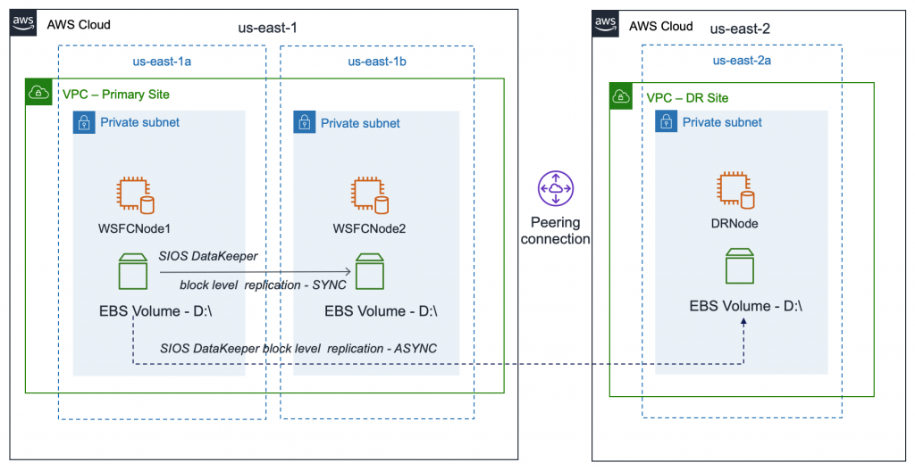
Figure 1 – High-level architecture showing two cluster nodes replicating synchronously between Availability Zones.
Walkthrough
SIOS DataKeeper is a host-based, block-level volume replication solution that integrates with WSFC to enable what is known as a SANLess cluster. DataKeeper runs on each cluster node and has two primary functions: data replication and cluster integration through the DataKeeper volume cluster resource.
The DataKeeper volume resource takes the place of the traditional Cluster Disk resource found in a SAN-based cluster. Upon failover, the DataKeeper volume resource controls the replication direction, ensuring the active cluster node becomes the source of the replication while all the remaining nodes become the target of the replication.
After the SANLess cluster is configured, it is managed through Windows Server Failover Cluster Manager just like its SAN-based counterpart. Configuration of DataKeeper can be done through the DataKeeper UI, CLI, or PowerShell. AWS CloudFormation templates can also be used for automated deployment, as shown in AWS Quick Start.
The following steps explain how to configure a three-node SQL Server SANless cluster with SIOS DataKeeper.
Prerequisites
- IAM permissions to create VPCs and VPC Peering connection between them.
- A VPC that spans two Availability Zones and includes two private subnets to host Primary and Secondary SQL Server.
- Another VPC with single Availability Zone and includes one private subnet to host Tertiary SQL Server Node for Disaster Recovery.
- Subscribe to the SIOS DataKeeper Cluster Edition AMI in the AWS Marketplace, or sign up for FTP download for SIOS Cluster Edition software.
- An existing deployment of Active Directory with networking access to support the Windows Failover Cluster and SQL Deployment. Active Directory can deployed on EC2 with AWS Launch Wizard for Active Directory or through our Quick Start for Active Directory.
- Active Directory Domain administrator account credentials.
Configuring a three-node cluster
Step 1: Configure the EC2 instances
It’s good practice to record the system and network configuration details as shown below[SM1]. Indicate the hostname, volume information, and networking configuration of each cluster node. Each node requires a primary IP address and two secondary IP addresses, one for the core cluster resource and one for the SQL Server client listener.
The example shown in Figure 2 uses a single volume; however, it is completely acceptable to use multiple volumes in your SQL Server FCI.
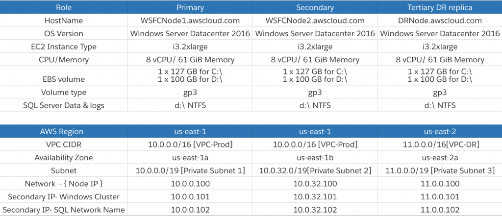
Figure 2 – Shows Storage, Network and AWS Configuration details of all threes cluster nodes
Due to Region and Availability Zone constructs, each cluster node will reside in a different subnet. A cluster that spans multiple subnets is referred to as a multi-subnet failover cluster. Refer to Create a failover cluster and SQL Server Multi-Subnet Clustering to learn more.
Step 2: Join the domain
With properly configured networking and security groups, DNS name resolution, and Active Directory credentials with required permissions, join all the cluster nodes to the domain. You can use AWS Managed Microsoft AD or manage your own Microsoft Active Directory domain controllers.
Step 3: Create the basic cluster
- Install the Failover Clustering feature and its prerequisite software components on all three nodes using PowerShell, shown in the following example.
Install-WindowsFeature -Name Failover-Clustering -IncludeManagementTools - Run cluster validation [CA2] [CA3] using PowerShell, shown in the following example.
Test-Cluster -Node wsfcnode1.awslab.com, wsfcnode2.awslab.com, drnode.awslab.com
NOTE: Windows PowerShell cmdlet Test-Cluster tests the underlying hardware and software, directly and individually, to obtain an accurate assessment of how well Failover Clustering can be supported in a given configuration with the following steps. - Create the cluster using PowerShell, shown in the following example.
New-Cluster -Name WSFCCluster1 -NoStorage -StaticAddress 10.0.0.101, 10.0.32.101, 11.0.0.101 -Node wsfcnode1.awslab.com, wsfcnode2.awslab.com, drnode.awslab.com - For more information using PowerShell for WSFC, view Microsoft’s documentation.
- It is always best practice to configure a file share witness and add it to your cluster quorum. You can use Amazon FSx for Windows to provide a Server Message Block (SMB) share, or you can create a file share on another domain joined server in your environment. See the following for more documentation for more details.
A successful implementation will show all three nodes UP (shown in Figure 3) in the Failover Cluster Manager.
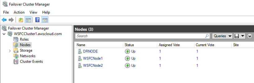
Figure 3 – Shows all three nodes status participating in Windows Failover Cluster
Step 4: Configure SIOS DataKeeper
After the basic cluster is created, you are ready to proceed with the DataKeeper configuration. Below are the basic steps to configure DataKeeper. For more detailed instructions, review the SIOS documentation.
Step 4.1: Install DataKeeper on all three nodes
- After you sign up for a free demo, SIOS provides you with an FTP URL to download the software package of SIOS Datakeeper Cluster edition. Use the FTP URL to download and run the latest software release.

- Choose Next, and read and accept the license terms.

- By Default, both components SIOS Datakeeper Server Components and SIOS DataKeeper User Interface will be selected. Choose Next to proceed.

- Accept the default install location, and choose Next.

- Next, you will be prompted to accept the system configuration changes to add firewall exceptions for the required ports. Choose Yes to enable.

- Enter credentials for SIOS Service account, and choose Next.

- Finally, choose Yes, and then Finish, to restart your system.


Step 4.2: Relocate the intent log (bitmap) file to the ephemeral drive
- Relocate the bitmap file to the ephemeral drive (confirm the ephemeral drive uses Z:\ for its drive letter).
- SIOS DataKeeper uses an intent log (also referred to as a bitmap file) to track changes made to the source, or to target volume during times that the target is unlocked. SIOS recommends to use ephemeral storage as a preferred location for the intent log to minimize the performance impact associated with the intent log. By default, SIOS InstallShield Wizard will store the bitmap at: “C:\Program Files (x86) \SIOS\DataKeeper\Bitmaps”.

- To change the intent log location, make the following registry changes. Edit registry through regedit.
“HKEY_LOCAL_MACHINE\SYSTEM\CurrentControlSet\Services\ExtMirr\Parameter” - Modify the “BitmapBaseDir” parameter by changing to the new location (i.e.s, Z:\), and then reboot your system.

- To ensure the ephemeral drive is reattached upon reboot, specify volume settings in the DriveLetterMappingConfig.json, and save the file under the location.
“C:\ProgramData\Amazon\EC2-Windows\Launch\Config\DriveLetterMappingConfig.json”.{ "driveLetterMapping": [ { "volumeName": "Temporary Storage 0", "driveLetter": "Z" }, { "volumeName": "Data", "driveLetter": "D" } ] } - Next, open Windows PowerShell and use the following command to run the EC2Launch script that initializes the disks:
C:\ProgramData\Amazon\EC2-Windows\Launch\Scripts\InitializeDisks.ps1 -Schedule For more information, see EC2Launch documentation.NOTE: If you are using the SIOS DataKeeper Marketplace AMI, you can skip the previous steps to install SIOS Software and relocating bitmap file, and continue with the following steps.


 For more information, see
 Step 4.3: Create a DataKeeper job
- Open SIOS DataKeeper application. From the right-side Actions panel, select Create Job.

- Enter Job name and Job description, and then choose Create Job.

- A create mirror wizard will open. In this job, we will set up a mirror relationship between WSFCNode1(Primary) and WSFCNode2(Secondary) within us-east-1 using synchronous replication.
Select the source WSFCNode1.awscloud.com and volume D. Choose Next to proceed.

NOTE: The volume on both the source and target systems must be NTFS file system type, and the target volume must be greater than or equal to the size of the source volume. - Choose the target WSFCNODE2.awscloud.com and correctly-assigned volume drive D.

- Now, select how the source volume data should be sent to the target volume.
For our design, choose Synchronous replication for nodes within us-east-1.

- After you choose Done, you will be prompted to register the volume into Windows Failover Cluster as a clustered datakeeper volume as a storage resource. When prompted, choose Yes.

- After you have successfully created the first mirror you will see the status of the mirror job (as shown in Figure 4).
If you have additional volumes, repeat the previous steps for each additional volume.
Figure 4 – Shows the SIOS Datakeeper Job Summary of mirrored volume between WFSCNODE1 & WSFCNODE2
- If you have additional volumes, repeat the previous steps for each additional volume.


Step 4.4: Add another mirror pair to the same job using asynchronous replication between nodes residing in different AWS Regions (us-east-1 and us-east-2)
- Open the create mirror wizard from the right-side action pane.
- Choose the source WSFCNode1.awscloud.com and volume D.
- For Server, enter DRNODE.awscloud.com.

- After you are connected, select the target DRNODE.awscloud.com and assigned volume D.

- For, How should the source volume data be sent to the target volume?, choose Asynchronous replication for nodes between us-east-1 and us-east-2.

- Choose Done to finish, and a pop-up window will provide you with additional information on action to take in the event of failover.

- You configured WSFCNode1.awscloud.com to mirror asynchronously to DRNODE.awscloud.com. However, during the event of failover, WSFCNode2.awscloud.com will become the new owner of the Failover Cluster and therefore own the source volume. This function of SIOS DataKeeper, called switchover, automatically changes the source of the mirror to the new owner of the Windows Failover Cluster. For our example, SIOS DataKeeper will automatically perform a switchover function to create a new mirror pair between WSFCNODE2.awscloud.com and DRNODE.awscloud.com. Therefore, select Asynchronous mirror type, and choose OK. For more information, see Switchover and Failover with Multiple Targets.
- A successfully-configured job will appear under Job Overview.


If you prefer to script the process of creating the DataKeeper job, and adding the additional mirrors, you can use the DataKeeper CLI as described in How to Create a DataKeeper Replicated Volume that has Multiple Targets via CLI.
If you have done everything correctly, the DataKeeper UI will look similar to the following image.

Furthermore, Failover Cluster Manager will show the Datakeeper Volume D, online, registered.

Step 5: Install the SQL Server FCI
- Install SQL Server on WSFCNode1 with the New SQL Server failover cluster installation option in the SQL Server installer.

- Install SQL Server on WSFCNode2 with the Add node to a SQL Server failover cluster option in the SQL Server installer.

- If you are using SQL Server Enterprise Edition, install SQL Server on DRNode using the “Add Node to Existing Cluster” option in the SQL Server installer.
- If you are using SQL Server Standard Edition, you will not be able to add the DR node to the cluster. Follow the SIOS documentation: Accessing Data on the Non-Clustered Disaster Recovery Node.


For detailed information on installing a SQL Server FCI, visit SQL Server Failover Cluster Installation.
At the end of installation, your Failover Cluster Manager will look similar to the following image.

Step 6: Client redirection considerations
When you install SQL Server into a multi-subnet cluster, RegisterAllProvidersIP is set to true. With that setting enabled, your DNS Server will register three Name Records (A), each using the name that you used when you created the SQL Listener during the SQL Server FCI installation. Each Name (A) record will have a different IP address, one for each of the cluster IP addresses that are associated with that cluster name resource.
If your clients are using .NET Framework 4.6.1 or later, the clients will manage the cross-subnet failover automatically. If your clients are using .NET Framework 4.5 through 4.6, then you will need to add MultiSubnetFailover=true to your connection string.
If you have an older client that does not allow you to add the MultiSubnetFailover=true parameter, then you will need to change the way that the failover cluster behaves. First, set the RegisterAllProvidersIP to false, so that only one Name (A) record will be entered in DNS. Each time the cluster fails over the name resource, the Name (A) record in DNS will be updated with the cluster IP address associated with the node coming online. Finally, adjust the TTL of the Name (A) record so that the clients do not have to wait the default 20 minutes before the TTL expires and the IP address is refreshed.
In the following PowerShell, you can see how to change the RegisterAllProvidersIP setting and update the TTL to 30 seconds.
Get-ClusterResource "sql name resource" | Set-ClusterParameter RegisterAllProvidersIP 0
Set-ClusterParameter -Name HostRecordTTL 30
Cleanup
When you are finished, you can terminate all three EC2 instances you launched.
Conclusion
Deploying a SQL Server FCI, that includes both Availability Zones and AWS Regions, is ideal for a solution that includes HA and DR. Although AWS provides the necessary infrastructure in terms of compute and networking, it is the combination of SIOS DataKeeper with WSFC that makes this configuration possible.
The solution described in this blogpost works with all supported versions of Windows Failover Cluster and SQL Server. Other configurations, such as hybrid-cloud and multi-cloud, are also possible. If adequate networking is in place, and Windows Server is running, where the cluster nodes reside is entirely up to you.