Tag Archives: AWS Step Functions

Applying Federated Learning for ML at the Edge

Post Syndicated from Randy DeFauw original https://aws.amazon.com/blogs/architecture/applying-federated-learning-for-ml-at-the-edge/

Federated Learning (FL) is an emerging approach to machine learning (ML) where model training data is not stored in a central location. During ML training, we typically need to access the entire training dataset on a single machine. For purposes of performance scaling, we divide the training data between multiple CPUs, multiple GPUs, or a cluster of machines. But in actuality, the training data is available in a single place. This poses challenges when we gather data from many distributed devices, like mobile phones or industrial sensors. For privacy reasons, we may not be able to collect training data from mobile phones. In an industrial setting, we may not have the network connectivity to push a large volume of sensor data to a central location. In addition, raw sensor data may contain sensitive information about a plant’s operation.

In this blog, we will demonstrate a working example of federated learning on AWS. We’ll also discuss some design challenges you may face when implementing FL for your own use case.

Federated learning challenges

In FL, all data stays on the devices. A training coordinator process invokes a training round or epoch, and the devices update a local copy of the model using local data. When complete, the devices each send their updated copy of the model weights to the coordinator. The coordinator combines these weights using an approach like federated averaging, and sends the new weights to each device. Figures 1 and 2 compare traditional ML with federated learning.

Traditional ML training:

Figure 1. Traditional ML training

Figure 1. Traditional ML training

Federated Learning:

Figure 2. Federated learning. Note that in federated learning, all data stays on the devices, as compared to traditional ML.

Figure 2. Federated learning. Note that in federated learning, all data stays on the devices, as compared to traditional ML.

Compared to traditional ML, federated learning poses several challenges.

Unpredictable training participants. Mobile and industrial devices may have intermittent connectivity. We may have thousands of devices, and the communication with these devices may be asynchronous. The training coordinator needs a way to discover and communicate with these devices.

Asynchronous communication. As previously noted, devices like IoT sensors may use communication protocols like MQTT, and rely on IoT frameworks with asynchronous pub/sub messaging. For example, the training coordinator cannot simply make a synchronous call to a device to send updated weights.

Passing large messages. The model weights can be several MB in size, making them too large for typical MQTT payloads. This can be problematic when network connections are not high bandwidth.

Emerging frameworks. Deep learning frameworks like TensorFlow and PyTorch do not yet fully support FL. Each has emerging options for edge-oriented ML, but they are not yet production-ready, and are intended mostly for simulation work.

Solving for federated learning challenges

Let’s begin by discussing the framework used for FL. This framework should work with any of the major deep learning systems like PyTorch and TensorFlow. It should clearly separate what happens on the training coordinator versus what happens on the devices. The Flower framework satisfies these requirements. In the simplest cases, Flower only requires that a device or client implement four methods: get model weights, set model weights, run a training round, and return metrics (like accuracy). Flower provides a default weight combination strategy, federated averaging, although we could design our own.

Next, let’s consider the challenges of devices and coordinator-to-device communication. Here it helps to have a specific use case in mind. Let’s focus on an industrial use case using the AWS IoT services. The IoT services will provide device discovery and asynchronous messaging tools. Running Flower code in tasks running on Amazon ECS on AWS Fargate containers orchestrated by an AWS Step Functions workflow, bridges the gap between the synchronous training process and the asynchronous device communication.

Devices: Our devices are registered with the AWS IoT Core, which gives access to MQTT communication. We use an AWS IoT Greengrass device, which lets us push AWS Lambda functions on the core device to run the actual ML training code. Greengrass also provides access to other AWS services and provides a streaming capability for pushing large payloads to the AWS Lambdacloud. Devices publish heartbeat messages to an MQTT topic to facilitate device discovery by the training coordinator.

Flower processes: The Flower framework requires a server and one or more clients. The clients communicate with the server synchronously over gRPC, so we cannot directly run the Flower client code on the devices. Rather, we use Amazon ECS Fargate containers to run the Flower server and client code. The client container acts as a proxy and communicates with the devices using MQTT messaging, Greengrass streaming, and direct Amazon S3 file transfer. Since the devices cannot send responses directly to the proxy containers, we use IoT rules to push responses to an Amazon DynamoDB bookkeeping table.

Orchestration: We use a Step Functions workflow to launch a training run. It performs device discovery, launches the server container, and then launches one proxy client container for each Greengrass core.

Metrics: The Flower server and proxy containers emit useful data to logs. We use Amazon CloudWatch log metric filters to collect this information on a CloudWatch dashboard.

Figure 3 shows the high-level design of the prototype.

Figure 3. FL prototype deployed on Amazon ECS Fargate containers and AWS IoT Greengrass cores.

Figure 3. FL prototype deployed on Amazon ECS Fargate containers and AWS IoT Greengrass cores

Production considerations

As you move into production with FL, you must design for a new set of challenges compared to traditional ML.

What type of devices do you have? Mobile and IoT devices are the most common candidates for FL.

How do the devices communicate with the coordinator? Devices come and go, and don’t always support synchronous communication. How will you discover devices that are available for FL and manage asynchronous communication? IoT frameworks are designed to work with large fleets of devices with intermittent connectivity. But mobile devices will find it easier to push results back to a training coordinator using regular API endpoints.

How will you integrate FL into your ML practice? As you saw in this example, we built a working FL prototype using AWS IoT, container, database, and application integration services. A data science team is likely to work in Amazon SageMaker or an equivalent ML environment that provides model registries, experiment tracking, and other features. How will you bridge this gap? (We may need to invent a new term – “MLEdgeOps.”)

Conclusion

In this blog, we gave a working example of federated learning in an IoT scenario using the Flower framework. We discussed the challenges involved in FL compared to traditional ML when building your own FL solution. As FL is an important and emerging topic in edge ML scenarios, we invite you to try our GitHub sample code. Please give us feedback as GitHub issues, particularly if you see additional federated learning challenges that we haven’t covered yet.

Optimize your IoT Services for Scale with IoT Device Simulator

Post Syndicated from Ajay Swamy original https://aws.amazon.com/blogs/architecture/optimize-your-iot-services-for-scale-with-iot-device-simulator/

The IoT (Internet of Things) has accelerated digital transformation for many industries. Companies can now offer smarter home devices, remote patient monitoring, connected and autonomous vehicles, smart consumer devices, and many more products. The enormous volume of data emitted from IoT devices can be used to improve performance, efficiency, and develop new service and business models. This can help you build better relationships with your end consumers. But you’ll need an efficient and affordable way to test your IoT backend services without incurring significant capex by deploying test devices to generate this data.

IoT Device Simulator (IDS) is an AWS Solution that manufacturing companies can use to simulate data, test device integration, and improve the performance of their IoT backend services. The solution enables you to create hundreds of IoT devices with unique attributes and properties. You can simulate data without configuring and managing physical devices.

An intuitive UI to create and manage devices and simulations

IoT Device Simulator comes with an intuitive user interface that enables you to create and manage device types for data simulation. The solution also provides you with a pre-built autonomous car device type to simulate a fleet of connected vehicles. Once you create devices, you can create simulations and generate data (see Figure 1.)

Figure 1. The landing page UI enables you to create devices and simulation

Figure 1. The landing page UI enables you to create devices and simulation

Create devices and simulate data

With IDS, you can create multiple device types with varying properties and data attributes (see Figure 2.) Each device type has a topic where simulation data is sent. The supported data types are object, array, sinusoidal, location, Boolean, integer, float, and more. Refer to this full list of data types. Additionally, you can import device types via a specific JSON format or use the existing automotive demo to pre-populate connected vehicles.

Figure 2. Create multiple device types and their data attributes

Figure 2. Create multiple device types and their data attributes

Create and manage simulations

With IDS, you can create simulations with one device or multiple device types (see Figure 3.) In addition, you can specify the number of devices to simulate for each device type and how often data is generated and sent.

Figure 3. Create simulations for multiple devices

Figure 3. Create simulations for multiple devices

You can then run multiple simulations (see Figure 4) and use the data generated to test your IoT backend services and infrastructure. In addition, you have the flexibility to stop and restart the simulation as needed.

Figure 4. Run and stop multiple simulations

Figure 4. Run and stop multiple simulations

You can view the simulation in real time and observe the data messages flowing through. This way you can ensure that the simulation is working as expected (see Figure 5.) You can stop the simulation or add a new simulation to the mix at any time.

Figure 5. Observe your simulation in real time

Figure 5. Observe your simulation in real time

IoT Device Simulator architecture

Figure 6. IoT Device Simulator architecture

Figure 6. IoT Device Simulator architecture

The AWS CloudFormation template for this solution deploys the following architecture, shown in Figure 6:

  1. Amazon CloudFront serves the web interface content from an Amazon Simple Storage Service (Amazon S3) bucket.
  2. The Amazon S3 bucket hosts the web interface.
  3. Amazon Cognito user pool authenticates the API requests.
  4. An Amazon API Gateway API provides the solution’s API layer.
  5. AWS Lambda serves as the solution’s microservices and routes API requests.
  6. Amazon DynamoDB stores simulation and device type information.
  7. AWS Step Functions include an AWS Lambda simulator function to simulate devices and send messages.
  8. An Amazon S3 bucket stores pre-defined routes that are used for the automotive demo (which is a pre-built example in the solution).
  9. AWS IoT Core serves as the endpoint to which messages are sent.
  10. Amazon Location Service provides the map display showing the location of automotive devices for the automotive demo.

The IoT Device Simulator console is hosted on an Amazon S3 bucket, which is accessed via Amazon CloudFront. It uses Amazon Cognito to manage access. API calls, such as retrieving or manipulating information from the databases or running simulations, are routed through API Gateway. API Gateway calls the microservices, which will call the relevant service.

For example, when creating a new device type, the request is sent to API Gateway, which then routes the request to the microservices Lambda function. Based on the request, the microservices Lambda function recognizes that it is a request to create a device type and saves the device type to DynamoDB.

Running a simulation

When running a simulation, the microservices Lambda starts a Step Functions workflow. First, the request contains information about the simulation to be run, including the unique device type ID. Then, using the unique device type ID, Step Functions retrieves all the necessary information about each device type to run the simulation. Once all the information has been retrieved, the simulator Lambda function is run. The simulator Lambda function uses the device type information, including the message payload template. The Lambda function uses this template to build the message sent to the IoT topic specified for the device type.

When running a custom device type, the simulator generates random information based on the values provided for each attribute. For example, when the automotive simulation is run, the simulation runs a series of calculations to simulate an automobile moving along a series of pre-defined routes. Pre-defined routes are created and stored in an S3 bucket, when the solution is launched. The simulation retrieves the routes at random each time the Lambda function runs. Automotive demo simulations also show a map generated from Amazon Location Service and display the device locations as they move.

The simulator exits once the Lambda function has completed or has reached the fifteen-minute execution limit. It then passes all the necessary information back to the Step Function. Step Functions then enters a choice state and restarts the Lambda function if it has not yet surpassed the duration specified for the simulation. It then passes all the pertinent information back to the Lambda function so that it can resume where it left off. The simulator Lambda function also checks DynamoDB every thirty seconds to see if the user has manually stopped the simulation. If it has, it will end the simulation early. Once the simulation is complete, the Step Function updates the DynamoDB table.

The solution enables you to launch hundreds of devices to test backend infrastructure in an IoT workflow. The solution contains an Import/Export feature to share device types. Exporting a device type generates a JSON file that represents the device type. The JSON file can then be imported to create the same device type automatically. The solution allows the viewing of up to 100 messages while the solution is running. You can also filter the messages by topic and device and see what data each device emits.

Conclusion

IoT Device Simulator is designed to help customers test device integration and IoT backend services more efficiently without incurring capex for physical devices. This solution provides an intuitive web-based graphic user interface (GUI) that enables customers to create and simulate hundreds of connected devices. It is not necessary to configure and manage physical devices or develop time-consuming scripts. Although we’ve illustrated an automotive application in this post, this simulator can be used for many different industries, such as consumer electronics, healthcare equipment, utilities, manufacturing, and more.

Get started with IoT Device Simulator today.

Visualizing AWS Step Functions workflows from the Amazon Athena console

Post Syndicated from James Beswick original https://aws.amazon.com/blogs/compute/visualizing-aws-step-functions-workflows-from-the-amazon-athena-console/

This post is written by Dhiraj Mahapatro, Senior Specialist SA, Serverless.

In October 2021, AWS announced visualizing AWS Step Functions from the AWS Batch console. Now you can also visualize Step Functions from the Amazon Athena console.

Amazon Athena is an interactive query service that makes it easier to analyze Amazon S3 data using standard SQL. Athena is a serverless service and can interact directly with data stored in S3. Athena can process unstructured, semistructured, and structured datasets.

AWS Step Functions is a low-code visual workflow service used to orchestrate AWS services, automate business processes, and build serverless applications. Step Functions workflows manage failures, retries, parallelization, service integrations, and observability so builders can focus on business logic. Athena is one of the service integrations that are available for Step Functions.

This blog walks through Step Functions integration in Amazon Athena console. It shows how you can visualize and operate Athena queries at scale using Step Functions.

Introducing workflow orchestration in Amazon Athena console

AWS customers store large amounts of historical data on S3 and query the data using Athena to get results quickly. They also use Athena to process unstructured data or analyze structured data as part of a data processing pipeline.

Data processing involves discrete steps for ingesting, processing, storing the transformed data, and post-processing, such as visualizing or analyzing the transformed data. Each step involves multiple AWS services. With Step Functions workflow integration, you can orchestrate these steps. This helps to create repeatable and scalable data processing pipelines as part of a larger business application and visualize the workflows in the Athena console.

With Step Functions, you can run queries on a schedule or based on an event by using Amazon EventBridge. You can poll long-running Athena queries before moving to the next step in the process, and handle errors without writing custom code. Combining these two services provides developers with a single method that is scalable and repeatable.

Step Functions workflows in the Amazon Athena console allow orchestration of Athena queries with Step Functions state machines:

Athena console

Using Athena query patterns from Step Functions

Execute multiple queries

In Athena, you run SQL queries in the Athena console against Athena workgroups. With Step Functions, you can run Athena queries in a sequence or run independent queries simultaneously in parallel using a parallel state. Step Functions also natively handles errors and retries related to Athena query tasks.

Workflow orchestration in the Athena console provides these capabilities to run and visualize multiple queries in Step Functions. For example:

UI flow

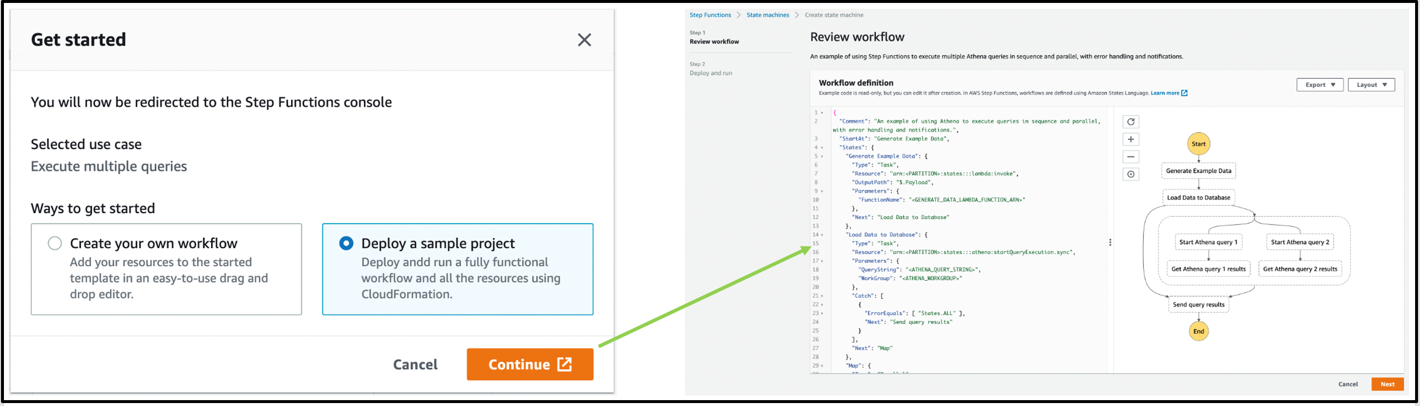
  1. Choose Get Started from Execute multiple queries.
  2. From the pop-up, choose Create your own workflow and select Continue.

A new browser tab opens with the Step Functions Workflow Studio. The designer shows a workflow pattern template pre-created. The workflow loads data from a data source running two Athena queries in parallel. The results are then published to an Amazon SNS topic.

Alternatively, choosing Deploy a sample project from the Get Started pop-up deploys a sample Step Functions workflow.

Get started flow

This option creates a state machine. You then review the workflow definition, deploy an AWS CloudFormation stack, and run the workflow in the Step Functions console.

Deploy and run

Once deployed, the state machine is visible in the Step Functions console as:

State machines

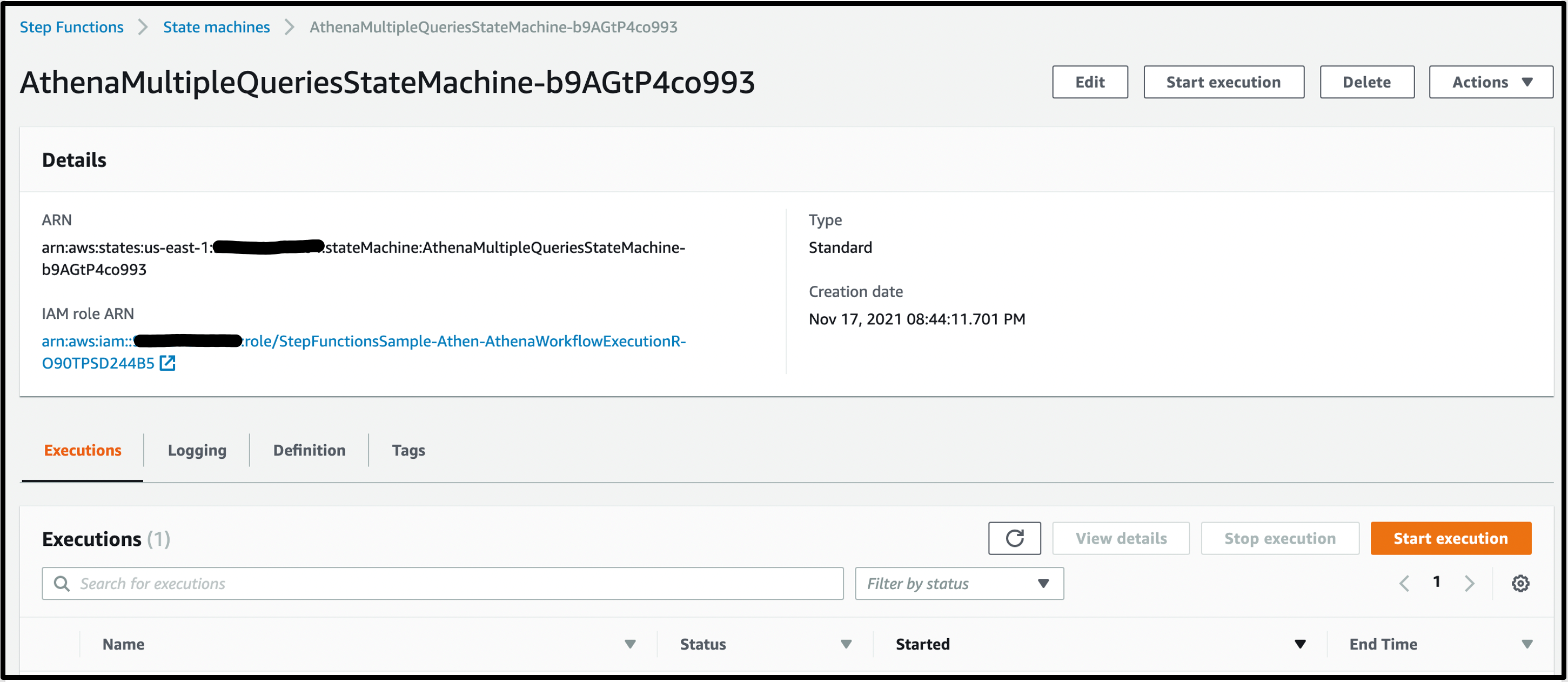
Select the AthenaMultipleQueriesStateMachine to land on the details page:

Details page

The CloudFormation template provisions the required AWS Glue database, S3 bucket, an Athena workgroup, the required AWS Lambda functions, and the SNS topic for query results notification.

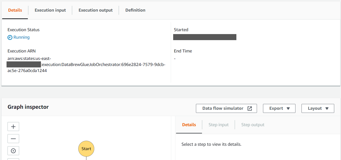
To see the Step Functions workflow in action, choose Start execution. Keep the optional name and input and choose Start execution:

Start execution

The state machine completes the tasks successfully by Executing multiple queries in parallel using Amazon Athena and Sending query results using the SNS topic:

Successful execution

The state machine used the Amazon Athena StartQueryExecution and GetQueryResults tasks. The Workflow orchestration in Athena console now highlights this newly created Step Functions state machine:

Athena console

Any state machine that uses this task in Step Functions in this account is listed here as a state machine that orchestrates Athena queries.

Query large datasets

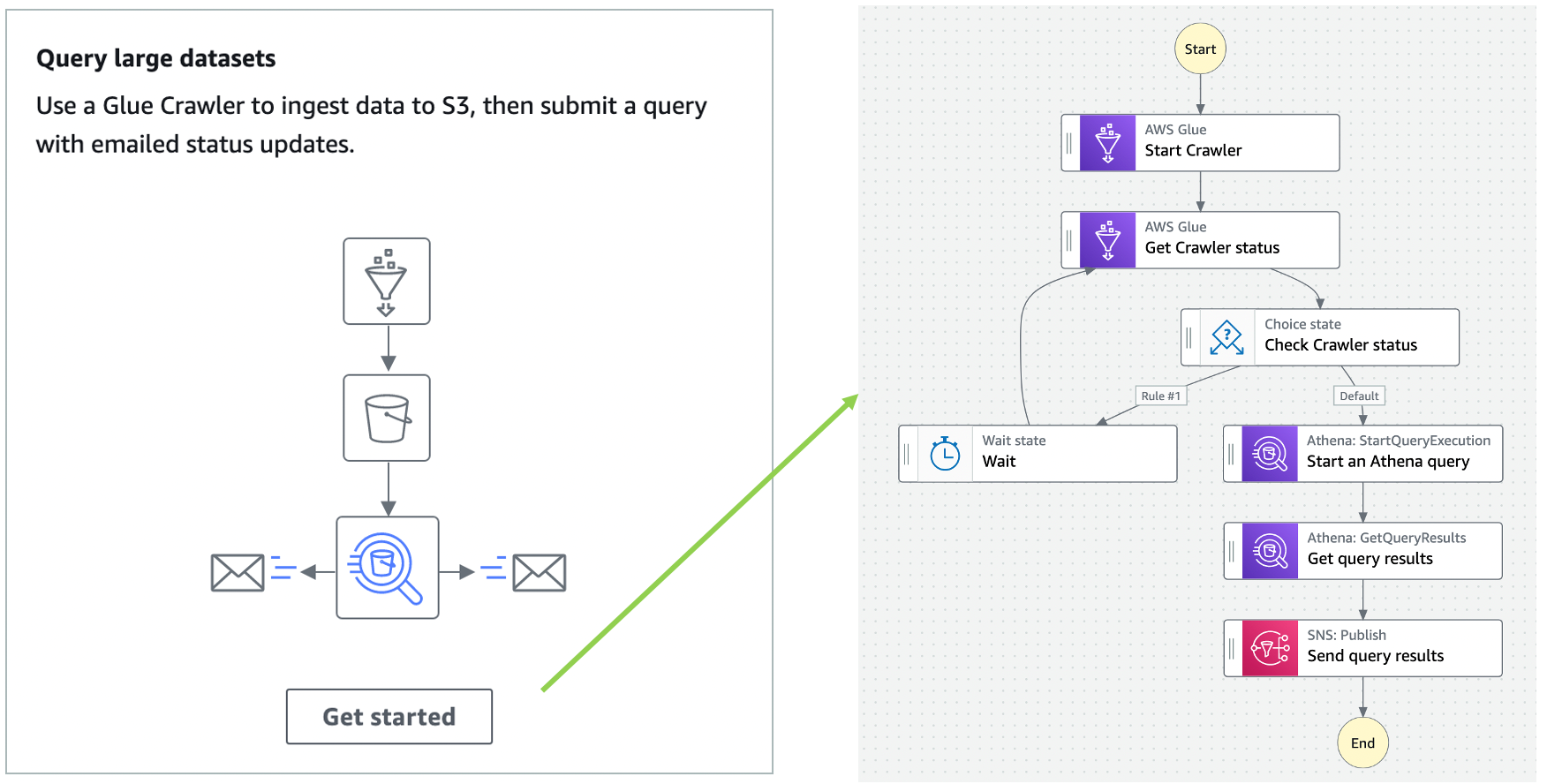
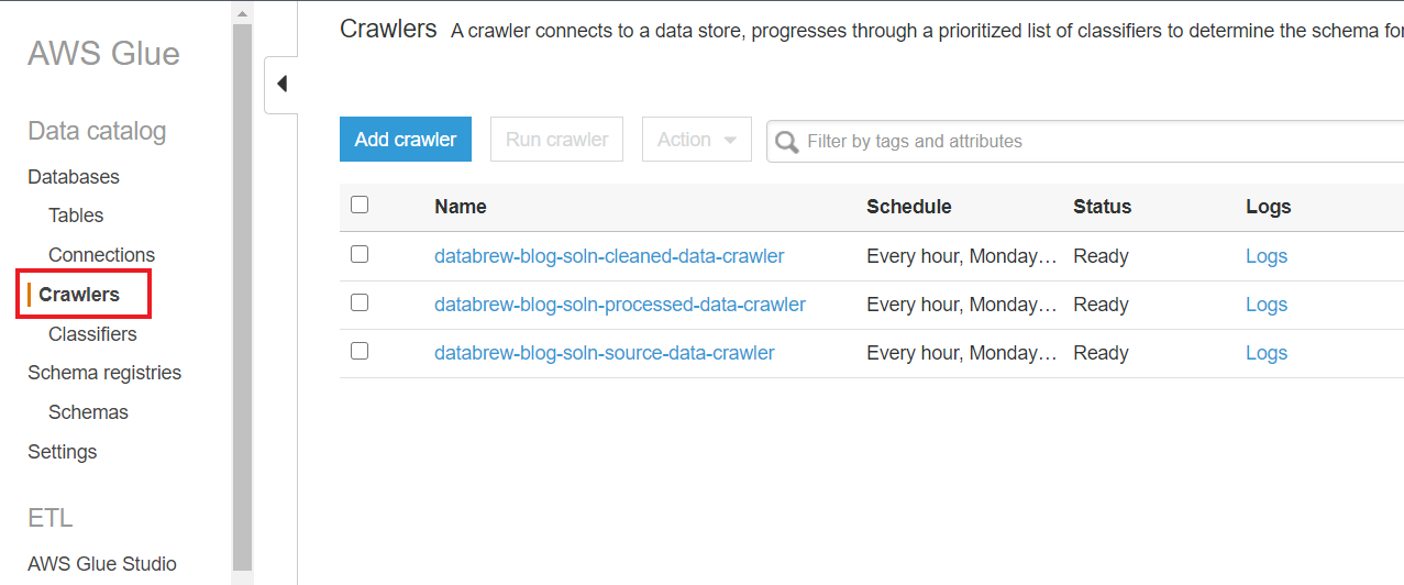
You can also ingest an extensive dataset in Amazon S3, partition it using AWS Glue crawlers, then run Amazon Athena queries against that partition.

Select Get Started from the Query large datasets pop-up, then choose Create your own workflow and Continue. This action opens the Step Functions Workflow studio with the following pattern. The Glue crawler starts and partitions large datasets for Athena to query in the subsequent query execution task:

Query large datasets

Step Functions allows you to combine Glue crawler tasks and Athena queries to partition where necessary before querying and publishing the results.

Keeping data up to date

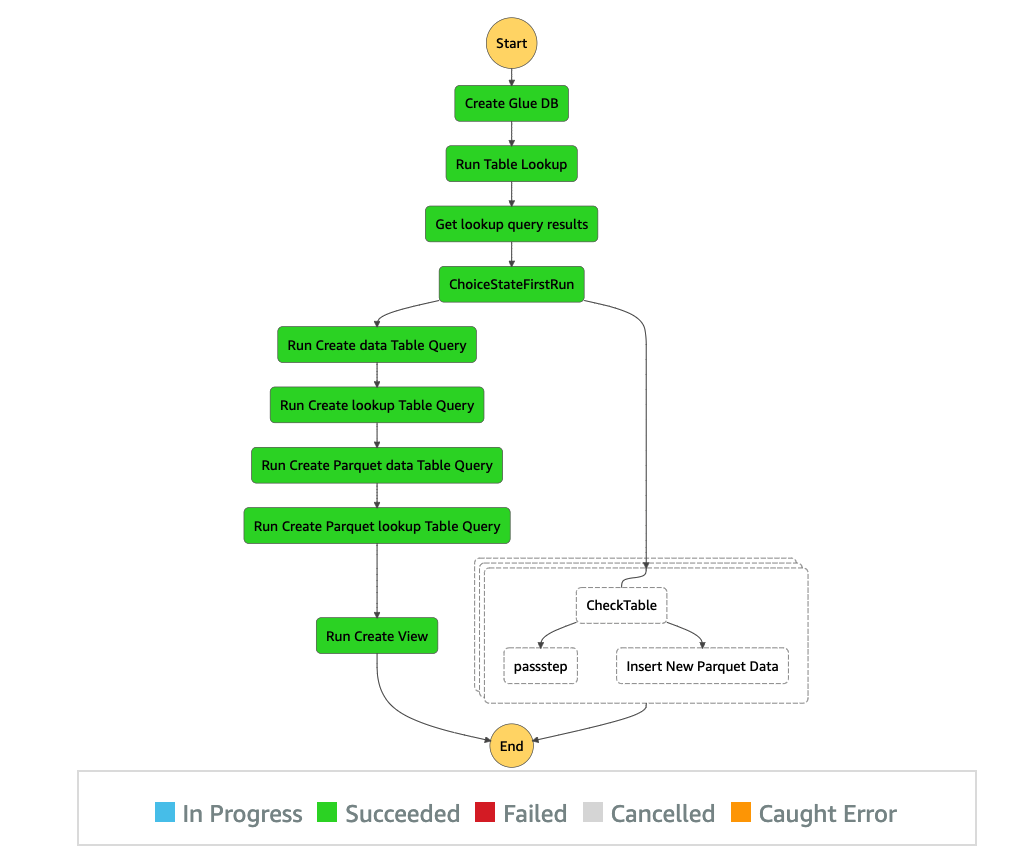
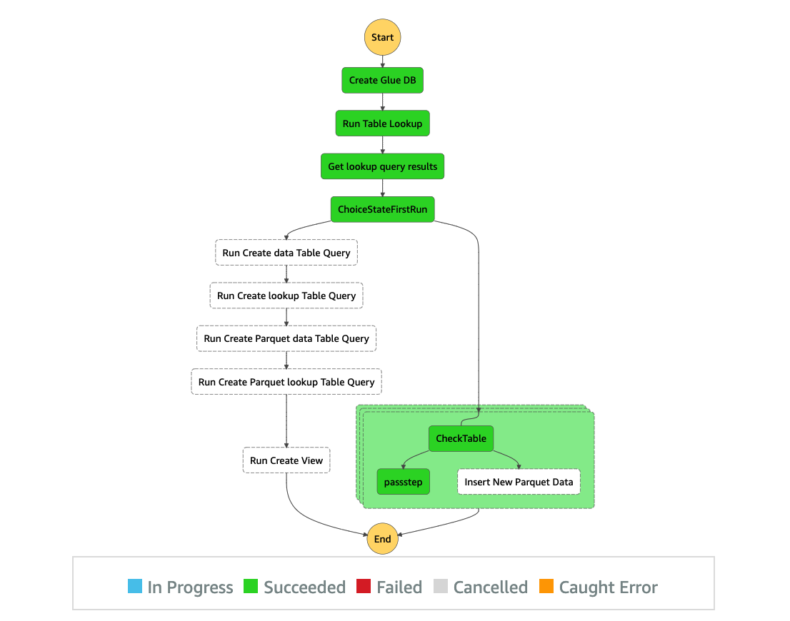
You can also use Athena to query a target table to fetch data, then update it with new data from other sources using Step Functions’ choice state. The choice state in Step Functions provides branching logic for a state machine.

Keep data up to date

You are not limited to the previous three patterns shown in workflow orchestration in the Athena console. You can start from scratch and build Step Functions state machine by navigating to the bottom right and using Create state machine:

Create state machine

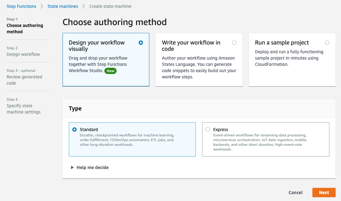
Create State Machine in the Athena console opens a new tab showing the Step Functions console’s Create state machine page.

Choosing authoring method

Refer to building a state machine AWS Step Functions Workflow Studio for additional details.

Step Functions integrates with all Amazon Athena’s API actions

In September 2021, Step Functions announced integration support for 200 AWS services to enable easier workflow automation. With this announcement, Step Functions can integrate with all Amazon Athena API actions today.

Step Functions can automate the lifecycle of an Athena query: Create/read/update/delete/list workGroups; Create/read/update/delete/list data catalogs, and more.

Other AWS service integrations

Step Functions’ integration with the AWS SDK provides support for 200 AWS Services and over 9,000 API actions. Athena tasks in Step Functions can evolve by integrating available AWS services in the workflow for their pre and post-processing needs.

For example, you can read Athena query results that are put to an S3 bucket by using a GetObject S3 task AWS SDK integration in Step Functions. You can combine different AWS services into a single business process so that they can ingest data through Amazon Kinesis, do processing via AWS Lambda or Amazon EMR jobs, and send notifications to interested parties via Amazon SNS or Amazon SQS or Amazon EventBridge to trigger other parts of their business application.

There are multiple ways to decorate around an Amazon Athena job task. Refer to AWS SDK service integrations and optimized integrations for Step Functions for additional details.

Important considerations

Workflow orchestrations in the Athena console only show Step Functions state machines that use Athena’s optimized API integrations. This includes StartQueryExecution, StopQueryExecution, GetQueryExecution, and GetQueryResults.

Step Functions state machines do not show in the Athena console when:

  1. A state machine uses any other AWS SDK Athena API integration task.
  2. The APIs are invoked inside a Lambda function task using an AWS SDK client (like Boto3 or Node.js or Java).

Cleanup

First, empty DataBucket and AthenaWorkGroup to delete the stack successfully. To delete the sample application stack, use the latest version of AWS CLI and run:

aws cloudformation delete-stack --stack-name <stack-name>

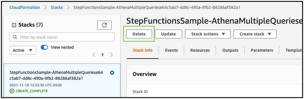
Alternatively, delete the sample application stack in the CloudFormation console by selecting the stack and choosing Delete:

Stack deletion

Conclusion

Amazon Athena console now provides an integration with AWS Step Functions’ workflows. You can use the provided patterns to create and visualize Step Functions’ workflows directly from the Amazon Athena console. Step Functions’ workflows that use Athena’s optimized API integration appear in the Athena console. To learn more about Amazon Athena, read the user guide.

To get started, open the Workflows page in the Athena console. Select Create Athena jobs with Step Functions Workflows to deploy a sample project, if you are new to Step Functions.

For more serverless learning resources, visit Serverless Land.

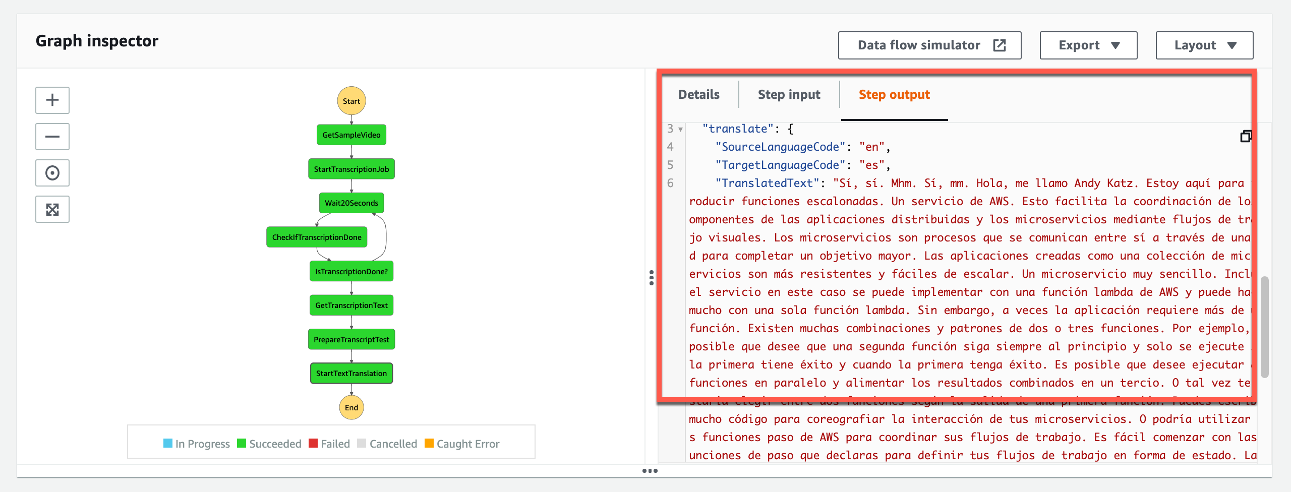
Running a Cost-effective NLP Pipeline on Serverless Infrastructure at Scale

Post Syndicated from Eitan Sela original https://aws.amazon.com/blogs/architecture/running-a-cost-effective-nlp-pipeline-on-serverless-infrastructure-at-scale/

Amenity Analytics develops enterprise natural language processing (NLP) platforms for the finance, insurance, and media industries that extract critical insights from mountains of documents. We provide a scalable way for businesses to get a human-level understanding of information from text.

In this blog post, we will show how Amenity Analytics improved the continuous integration (CI) pipeline speed by 15x. We hope that this example can help other customers achieve high scalability using AWS Step Functions Express.

Amenity Analytics’ models are developed using both a test-driven development (TDD) and a behavior-driven development (BDD) approach. We verify the model accuracy throughout the model lifecycle—from creation to production, and on to maintenance.

One of the actions in the Amenity Analytics model development cycle is backtesting. It is an important part of our CI process. This process consists of two steps running in parallel:

  • Unit tests (TDD): checks that the code performs as expected
  • Backtesting tests (BDD): validates that the precision and recall of our models is similar or better than previous

The backtesting process utilizes hundreds of thousands of annotated examples in each “code build.” To accomplish this, we initially used the AWS Step Functions default workflow. AWS Step Functions is a low-code visual workflow service used to orchestrate AWS services, automate business processes, and build serverless applications. Workflows manage failures, retries, parallelization, service integrations, and observability.

Challenge with the existing Step Functions solution

We found that Step Functions standard workflow has a bucket of 5,000 state transitions with a refill rate of 1,500. Each annotated example has ~10 state transitions. This creates millions of state transitions per code build. Since state transitions are limited and couldn’t be increased to our desired amount, we often faced delays and timeouts. Developers had to coordinate their work with each other, which inevitably slowed down the entire development cycle.

To resolve these challenges, we migrated from Step Functions standard workflows to Step Functions Express workflows, which have no limits on state transitions. In addition, we changed the way each step in the pipeline is initiated, from an async call to a sync API call.

Step Functions Express workflow solution

When a model developer merges their new changes, the CI process starts the backtesting for all existing models.

  • Each model is checked to see if the annotated examples were already uploaded and saved in the Amazon Simple Storage Service (S3) cache. The check is made by a unique key representing the list of items. Once a model is reviewed, the review items will rarely be changed.
  • If the review items haven’t been uploaded yet, it uploads them and initiates an unarchive process. This way the review items can be used in the next phase.
  • When the items are uploaded, an API call is invoked using Amazon API Gateway with the review items keys, see Figure 1.
  • The request is forwarded to an AWS Lambda function. It is responsible for validating the request and sending a job message to an Amazon Simple Queue Service (SQS) queue.
  • The SQS messages are consumed by concurrent Lambda functions, which synchronously invoke a Step Function. The number of Lambda functions are limited to ensure that they don’t exceed their limit in the production environment.
  • When an item is finished in the Step Function, it creates an SQS notification message. This message is inserted into a queue and consumed as a message batch by a Lambda function. The function then sends an AWS IoT message containing all relevant messages for each individual user.
Figure 1. Step Functions Express workflow solution

Figure 1. Step Functions Express workflow solution

Main Step Function Express workflow pipeline

Step Functions Express supports only sync calls. Therefore, we replaced the previous async Amazon Simple Notification Service (SNS) and Amazon SQS, with sync calls to API Gateway.

Figure 2 shows the workflow for a single document in Step Function Express:

  1. Generate a document ID for the current iteration
  2. Perform base NLP analysis by calling another Step Function Express wrapped by an API Gateway
  3. Reformat the response to be the same as all other “logic” steps results
  4. Verify the result by the “Choice” state – if failed go to end, otherwise, continue
  5. Perform the Amenity core NLP analysis in three model invocations: Group, Patterns, and Business Logic (BL)
  6. For each of the model runtime steps:
    • Check if the result is correct
    • If failed, go to end, otherwise continue
  7. Return a formatted result at the end
Figure 2. Workflow for a single document

Figure 2. Workflow for a single document

Base NLP analysis Step Function Express

For our base NLP analysis, we use Spacy. Figure 3 shows how we used it in Step Functions Express:

  1. Confirm if text exists in cache (this means it has been previously analyzed)
  2. If it exists, return the cached result
  3. If it doesn’t exist, split the text to a manageable size (Spacy has text size limitations)
  4. All the texts parts are analyzed in parallel by Spacy
  5. Merge the results into a single, analyzed document and save it to the cache
  6. If there was an exception during the process, it is handled in the “HandleStepFunctionExceptionState”
  7. Send a reference to the analyzed document if successful
  8. Send an error message if there was an exception
Figure 3. Base NLP analysis for a single document

Figure 3. Base NLP analysis for a single document

Results

Our backtesting migration was deployed on August 10, and unit testing migration on September 14. After the first migration, the CI was limited by the unit tests, which took ~25 minutes. When the second migration was deployed, the process time was reduced to ~6 minutes (P95).

Figure 4. Process time reduced from 50 minutes to 6 minutes

Figure 4. Process time reduced from 50 minutes to 6 minutes

Conclusion

By migrating from standard Step Functions to Step Functions Express, Amenity Analytics increased processing speed 15x. A complete pipeline that used to take ~45 minutes with standard Step Functions, now takes ~3 minutes using Step Functions Express. This migration removed the need for users to coordinate workflow processes to create a build. Unit testing (TDD) went from ~25 mins to ~30 seconds. Backtesting (BDD) went from taking more than 1 hour to ~6 minutes.

Switching to Step Functions Express allows us to focus on delivering business value faster. We will continue to explore how AWS services can help us drive more value to our users.

For further reading:

Build workflows for Amazon Forecast with AWS Step Functions

Post Syndicated from James Beswick original https://aws.amazon.com/blogs/compute/build-workflows-for-amazon-forecast-with-aws-step-functions/

This post is written by Péter Molnár, Data Scientist, ML ProServe and Sachin Doshi, Senior Application Architect, ProServe.

This blog builds a full lifecycle workflow for Amazon Forecast to predict household electricity consumption from historic data. Previously, developers used AWS Lambda function to build workflows for Amazon Forecast. You can now use AWS Step Functions with AWS SDK integrations to reduce cost and complexity.

Step Functions recently expanded the number of supported AWS service integrations from 17 to over 200 with AWS API actions from 46 to over 9,000 with AWS SDK service integrations.

Step Functions is a low-code visual workflow service used for workflow automation and service orchestration. Developers use Step Functions with managed services such as artificial intelligence servicesAmazon S3, and AWS Glue.

You can create state machines that use AWS SDK Service Integrations with Amazon States Language (ASL)AWS Cloud Development Kit (AWS CDK), AWS Serverless Application Model (AWS SAM), or visually using AWS Step Function Workflow Studio.

To create workflows for AWS AI services like Forecast, you can use Step Functions AWS SDK service integrations. This approach can be simpler because it allows users to build solutions without writing JavaScript or Python code.

Workflow for Amazon Forecast

The solution includes four components:

Solution architecture

  1. IAM role granting Step Functions control over Forecast.
  2. IAM role granting Forecast access to S3 storage locations.
  3. S3 bucket with input data
  4. Define Step Functions state machine and parameters for Forecast.

The repo provides an AWS SAM template to deploy these resources in your AWS account.

Understanding Amazon Forecast

Amazon Forecast is a fully managed service for time series forecasting. Forecast uses machine learning to combine time series data with additional variables to build forecasts.

Using Amazon Forecast involves steps that may take from minutes to hours. Instead of executing each step and waiting for its completion, you use Step Functions to define the steps of the forecasting process.

These are the individual steps of the Step Functions workflow:

Step Functions workflow

  1. Create a dataset: In Forecast, there are three types of datasets, target time series, related time series, and item metadata. The target time series is required and the others provide additional context with certain algorithms.
  2. Import data: This moves the information from S3 into a storage volume where the data is used for training and validation.
  3. Create a dataset group: This is the large box that isolates models and the data they are trained on from each other.
  4. Train a model: Forecast automates this process for you but you can also select algorithms. You can provide your own hyper parameters or use hyperparameter optimization (HPO) to determine the most performant values.
  5. Export back-test results: this creates a detailed table of the model performance.
  6. Deploy a predictor to deploy the model to use it to generate a forecast.
  7. Export forecast to create future predictions.

For more details, read the documentation of the Forecast APIs.

Example dataset

This example uses the individual household electric power consumption dataset. This dataset is available from the UCI Machine Learning Repository. We have aggregated the usage data to hourly intervals.

The dataset has three columns: the timestamp, value, and item ID. These are the minimum required to generate a forecast with Amazon Forecast.

Read more about the data and parameters in https://github.com/aws-samples/amazon-forecast-samples/tree/master/notebooks/basic/Tutorial.

Step Functions AWS SDK integrations

The AWS SDK integrations of Step Functions reduce the need for Lambda functions that call the Forecast APIs. You can call any AWS SDK-compatible service directly from the ASL. Use the following syntax in the resource field of a Step Functions task:

arn:aws:states:::aws-sdk:serviceName:apiAction.[serviceIntegrationPattern]

The following example compares using Step Functions AWS SDK service integrations with calling the boto3 Python method to create a dataset with a corresponding resource in the state machine definition. This is the ASL of a Step Functions state machine:

"States": {
  "Create-Dataset": {
    "Resource": "arn:aws:states:::aws-sdk:forecast:createDataset",
    "Parameters": {
      "DatasetName": "blog_example",
      "DataFrequency": "H",
      "Domain": "CUSTOM",
      "DatasetType": "TARGET_TIME_SERIES",
      "Schema": {
        "Attributes": [
          {
            "AttributeName": "timestamp",
            "AttributeType": "timestamp"
          },
          {
            "AttributeName": "target_value",
            "AttributeType": "float"
          },
          {
            "AttributeName": "item_id",
            "AttributeType": "string"
          }
        ]
      }
    },
    "ResultPath": "$.createDatasetResult",
    "Next": "Import-Data"
  }

The structure is similar to the corresponding boto3 methods. Compare the Python code with the state machine code – it uses the same parameters as calling the Python API:

forecast = boto3.client('forecast')
response = forecast.create_dataset(
             Domain='CUSTOM',
             DatasetType='TARGET_TIME_SERIES',
             DatasetName='blog_example',
             DataFrequency='H', 
             Schema={
               'Attributes': [
                  {
                    'AttributeName': 'timestamp',
                    'AttributeType': 'timestamp'
                  },
                  {
                    'AttributeName': 'target_value',
                    'AttributeType': 'float'
                  },
                  {
                    'AttributeName': 'item_id',
                    'AttributeType': 'string'
                  }
               ]
             }
           )

Handling asynchronous API calls

Several Forecast APIs run asynchronously, such as createDatasetImportJob and createPredictor. This means that your workflow must wait until the import job is completed.

You can use one of two methods in the state machine: create a wait loop, or allow any following task that depends on the completion of the previous task to retry.

In general, it is good practice to allow any task to retry for a few times. For simplicity this example does not include general error handling. Read the blog Handling Errors, Retries, and adding Alerting to Step Function State Machine Executions to learn more about writing robust state machines.

1. State machine wait loop

Wait loop

To wait for an asynchronous task to complete, use the services’ Describe* API methods to get the status of current job. You can implement the wait loop with the native Step Function tasks Choice and Wait.

Here, the task “Check-Data-Import” calls the describeDatasetImportJob API to receive a status value of the running job:

"Check-Data-Import": {
  "Type": "Task",
  "Resource": "arn:aws:states:::aws-sdk:forecast:describeDatasetImportJob",
  "Parameters": {
    "DatasetImportJobArn.$": "$.createDatasetImportJobResult.DatasetImportJobArn"
   },
   "ResultPath": "$.describeDatasetImportJobResult",
   "Next": "Fork-Data-Import"
 },
 "Fork-Data-Import": {
   "Type": "Choice",
   "Choices": [
     {
       "Variable": "$.describeDatasetImportJobResult.Status",
       "StringEquals": "ACTIVE",
       "Next": "Done-Data-Import"
     }
   ],
   "Default": "Wait-Data-Import"
 },
 "Wait-Data-Import": {
   "Type": "Wait",
   "Seconds": 60,
   "Next": "Check-Data-Import"
 },
 "Done-Data-Import": {
   "Type": "Pass",
   "Next": "Create-Predictor"
 },

2. Fail and retry

Alternatively, use the Retry parameter to specify how to repeat the API call in case of an error. This example shows how the attempt to create the forecast is repeated if the resource that it depends on is not created. In this case, the preceding task of creating the predictor.

The time between retries is set to 180 seconds and the number of retries must not exceed 100. This means that the workflow waits 3 minutes before trying again. The longest time to wait for the ML training is five hours.

With the BackoffRate set to 1, the wait interval of 3 minutes remains constant. Value greater that 1 may reduce the number of retries but may also add increased wait time for training jobs that run for several hours:

"Create-Forecast": {
  "Type": "Task",
  "Resource": "arn:aws:states:::aws-sdk:forecast:createForecast",
  "Parameters": {
    "ForecastName.$": "States.Format('{}_forecast', $.ProjectName)",
    "PredictorArn.$": "$.createPredictorResult.PredictorArn"
   },
   "ResultPath": "$.createForecastResult",
   "Retry": [
     {
       "ErrorEquals": ["Forecast.ResourceInUseException"],
       "IntervalSeconds": 180,
       "BackoffRate": 1.0,
       "MaxAttempts": 100
     }
   ],
   "Next": "Forecast-Export"
 },

Deploying the workflow

The AWS Serverless Application Model Command Line Interface (AWS SAM CLI) is an extension of the AWS CLI that adds functionality for building and testing serverless applications. Follow the instructions to install the AWS SAM CLI.

To build and deploy the application:

  1. Clone the GitHub repo:
    git clone https://github.com/aws-samples/aws-stepfunctions-examples/tree/main/sam/demo-forecast-service-integration
  2. Change directory to cloned repo.
    cd demo-forecast-service-integration
  3. Enable execute permissions for the deployment script
    chmod 700 ./bootstrap_deployment_script.sh
  4. Execute the script with a stack name of your choosing as parameter.
    ./bootstrap_deployment_script.sh <Here goes your stack name>

The script builds the AWS SAM template and deploys the stack under the given name. The AWS SAM template creates the underlying resources like S3 bucket, IAM policies, and Step Functions workflow. The script also copies the data file used for training to the newly created S3 bucket.

Running the workflow

After the AWS SAM Forecast workflow application is deployed, run the workflow to train a forecast predictor for the energy consumption:

  1. Navigate to the AWS Step Functions console.
  2. Select the state machine named “ForecastWorkflowStateMachine-*” and choose New execution.
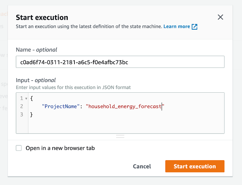
  3. Define the “ProjectName” parameter in form of a JSON structure. The name for the Forecast Dataset group is “household_energy_forecast”.
    Start execution
  4. Choose Start execution.

Viewing resources in the Amazon Forecast console

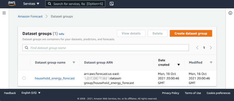
Navigate to the Amazon Forecast console and select the data set group “household_energy_forecast”. You can see the details of the Forecast resource as they are created. The provided state machine executes every step in the workflow and then deletes all resources, leaving the output files in S3.

Amazon Forecast console

You can disable the clean-up process by editing the state machine:

  1. Choose Edit to open the editor.
  2. Find the tasks “Clean-Up” and change the “Next” state from “Delete-Forecast_export” to “SuccessState”.
    "Clean-Up": {
       "Type": "Pass",
       "Next": "SuccessState"
    },
    
  3. Delete all tasks named Delete-*.

Remember to delete the dataset group manually if you bypass the clean-up process of the workflow.

Analyzing Forecast Results

The forecast workflow creates a folder “forecast_results” for all of its output files. In there you find the subfolders “backtestexport” with data produced by Backtest-Export task, and “forecast” with the predicted energy demand forecast produced by the Forecast-Export job.

The “backtestexport” folder contains two tables: “accuracy-metrics-values” with the model performance accuracy metrics, and “forecast-values” with the predicted forecast values of the training set. Read the blog post Amazon Forecast now supports accuracy measurements for individual items for details.

The forecast predictions are stored in the “forecast” folder. The table contains forecasts at three different quantiles: 10%, 50% and 90%.

The data files are partitioned into multiple CSV files. In order to analyze them, first download and merge the files into proper tables. Use the AWS CLI command to download

BUCKET="<your account number>-<your region>-sf-forecast-workflow"
aws s3 cp s3://$BUCKET/forecast_results . –recursive

Alternatively, you may import and analyze the data into Amazon Athena.

Cleaning up

To delete the application that you created, use the AWS SAM CLI.

sam delete --stack-name <Here goes your stack name>

Also delete the data files in the S3 bucket. If you skipped the clean-up tasks in your workflow, you must delete the dataset group from the Forecast console.

Important things to know

Here are things know, that will help you to use AWS SDK service integration:

  • Call AWS SDK services directly from the ASL in the resource field of a task state. To do this, use the following syntax: arn:aws:states:::aws-sdk:serviceName:apiAction.[serviceIntegrationPattern]
  • Use camelCase for apiAction names in the Resource field, such as “copyObject”, and use PascalCase for parameter names in the Parameters field, such as “CopySource”.
  • Step Functions cannot generate IAM policies for most AWS SDK service integrations. You must add those to the IAM role of the state machine explicitly.

Learn more about this new capability by reading its documentation.

Conclusion

This post shows how to create a Step Functions workflow for Forecast using AWS SDK service integrations, which allows you to use over 200 with AWS API actions. It shows two patterns for handling asynchronous tasks. The first pattern queries the describe-* API repeatedly and the second pattern uses the “Retry” option. This simplifies the development of workflows because in many cases they can replace Lambda functions.

For more serveless learning resources, visit Serverless Land.

How Parametric Built Audit Surveillance using AWS Data Lake Architecture

Post Syndicated from Raghavarao Sodabathina original https://aws.amazon.com/blogs/architecture/how-parametric-built-audit-surveillance-using-aws-data-lake-architecture/

Parametric Portfolio Associates (Parametric), a wholly owned subsidiary of Morgan Stanley, is a registered investment adviser. Parametric provides investment advisory services to individual and institutional investors around the world. Parametric manages over 100,000 client portfolios with assets under management exceeding $400B (as of 9/30/21).

As a registered investment adviser, Parametric is subject to numerous regulatory requirements. The Parametric Compliance team conducts regular reviews on the firm’s portfolio management activities. To accomplish this, the organization needs both active and archived audit data to be readily available.

Parametric’s on-premises data lake solution was based on an MS-SQL server. They used an Apache Hadoop platform for their data storage, data management, and analytics. Significant gaps existed with the on-premises solution, which complicated audit processes. They were spending a large amount of effort on system maintenance, operational management, and software version upgrades. This required expensive consulting services and challenges with keeping the maintenance windows updated. This limited their agility, and also impacted their ability to derive more insights and value from their data. In an environment of rapid growth, adoption of more sophisticated analytics tools and processes has been slower to evolve.

In this blog post, we will show how Parametric implemented their Audit Surveillance Data Lake on AWS with purpose-built fully managed analytics services. With this solution, Parametric was able to respond to various audit requests within hours rather than days or weeks. This resulted in a system with a cost savings of 5x, with no data growth. Additionally, this new system can seamlessly support a 10x data growth.

Audit surveillance platform

The Parametric data management office (DMO) was previously running their data workloads using an on-premises data lake, which ran on the Hortonworks data platform of Apache Hadoop. This platform wasn’t up to date, and Parametric’s hardware was reaching end-of-life. Parametric was faced with a decision to either reinvest in their on-premises infrastructure or modernize their infrastructure using a modern data analytics platform on AWS. After doing a detailed cost/benefit analysis, the DMO calculated a 5x cost savings by using AWS. They decided to move forward and modernize with AWS due to these cost benefits, in addition to elasticity and security features.

The PPA compliance team asked the DMO to provide an enterprise data service to consume data from a data lake. This data was destined for downstream applications and ad-hoc data querying capabilities. It was accessed via standard JDBC tools and user-friendly business intelligence dashboards. The goal was to ensure that seven years of audit data would be readily available.

The DMO team worked with AWS to conceptualize an audit surveillance data platform architecture and help accelerate the implementation. They attended a series of AWS Immersion Days focusing on AWS fundamentals, Data Lakes, Devops, Amazon EMR, and serverless architectures. They later were involved in a four-day AWS Data Lab with AWS SMEs to create a data lake. The first use case in this Lab was creating the Audit Surveillance system on AWS.

Audit surveillance architecture on AWS

The following diagram shows the Audit Surveillance data lake architecture on AWS by using AWS purpose-built analytics services.

Figure 1. Audit Surveillance data lake architecture diagram

Figure 1. Audit Surveillance data lake architecture diagram

Architecture flow

  1. User personas: As first step, the DMO team identified three user personas for the Audit Surveillance system on AWS.
    • Data service compliance users who would like to consume audit surveillance data from the data lake into their respective applications through an enterprise data service.
    • Business users who would like to create business intelligence dashboards using a BI tool to audit data for compliance needs.
    • Complaince IT users who would like to perform ad-hoc queries on the data lake to perform analytics using an interactive query tool.
  2. Data ingestion: Data is ingested into Amazon Simple Storage Service (S3) from different on-premises data sources by using AWS Lake Formation blueprints. AWS Lake Formation provides workflows that define the data source and schedule to import data into the data lake. It is a container for AWS Glue crawlers, jobs, and triggers that are used to orchestrate the process to load and update the data lake.
  3. Data storage: Parametric used Amazon S3 as a data storage to build an Audit Surveillance data lake, as it has unmatched 11 nines of durability and 99.99% availability. The existing Hadoop storage was replaced with Amazon S3. The DMO team created a drop zone (raw), an analytics zone (transformed), and curated (enriched) storage layers for their data lake on AWS.
  4. Data cataloging: AWS Glue Data Catalog was the central catalog used to store and manage metadata for all datasets hosted in the Audit Surveillance data lake. The existing Hadoop metadata store was replaced with AWS Glue Data Catalog. AWS services such as AWS Glue, Amazon EMR, and Amazon Athena, natively integrate with AWS Glue Data Catalog.
  5. Data processing: Amazon EMR and AWS Glue process the raw data and places it into analytics zones (transformed) and curated zones (enriched) S3 buckets. Amazon EMR was used for big data processing and AWS Glue for standard ETL processes. AWS Lambda and AWS Step Functions were used to initiate monitoring and ETL processes.
  6. Data consumption: After Audit Surveillance data was transformed and enriched, the data was consumed by various personas within the firm as follows:
    • AWS Lambda and Amazon API Gateway were used to support consumption for data service compliance users.
    • Amazon QuickSight was used to create business intelligence dashboards for compliance business users.
    • Amazon Athena was used to query transformed and enriched data for compliance IT users.
  7. Security: AWS Key Management Service (KMS) customer managed keys were used for encryption at rest, and TLS for encryption at transition. Access to the encryption keys is controlled using AWS Identity and Access Management (IAM) and is monitored through detailed audit trails in AWS CloudTrail. Amazon CloudWatch was used for monitoring, and thresholds were created to determine when to send alerts.
  8. Governance: AWS IAM roles were attached to compliance users that permitted the administrator to grant access. This was only given to approved users or programs that went through authentication and authorization through AWS SSO. Access is logged and permissions can be granted or denied by the administrator. AWS Lake Formation is used for fine-grained access controls to grant/revoke permissions at the database, table, or column-level access.

Conclusion

The Parametric DMO team successfully replaced their on-premises Audit Surveillance Data Lake. They now have a modern, flexible, highly available, and scalable data platform on AWS, with purpose-built analytics services.

This change resulted in a 5x cost savings, and provides for a 10x data growth. There are now fast responses to internal and external audit requests (hours rather than days or weeks). This migration has given the company access to a wider breadth of AWS analytics services, which offers greater flexibility and options.

Maintaining the on-premises data lake would have required significant investment in both hardware upgrade costs and annual licensing and upgrade vendor consulting fees. Parametric’s decision to migrate their on-premises data lake has yielded proven cost benefits. And it has introduced new functions, service, and capabilities that were previously unavailable to Parametric DMO.

You may also achieve similar efficiencies and increase scalability by migrating on-premises data platforms into AWS. Read more and get started on building Data Lakes on AWS.

Creating AWS Serverless batch processing architectures

Post Syndicated from James Beswick original https://aws.amazon.com/blogs/compute/creating-aws-serverless-batch-processing-architectures/

This post is written by Reagan Rosario, AWS Solutions Architect and Mark Curtis, Solutions Architect, WWPS.

Batch processes are foundational to many organizations and can help process large amounts of information in an efficient and automated way. Use cases include file intake processes, queue-based processing, and transactional jobs, in addition to heavy data processing jobs.

This post explains a serverless solution for batch processing to implement a file intake process. This example uses AWS Step Functions for orchestration, AWS Lambda functions for on-demand instance compute, Amazon S3 for storing the data, and Amazon SES for sending emails.

Overview

This post’s example takes a common use-case of a business’s need to process data uploaded as a file. The test file has various data fields such as item ID, order date, order location. The data must be validated, processed, and enriched with related information such as unit price. Lastly, this enriched data may need to be sent to a third-party system.

Step Functions allows you to coordinate multiple AWS services in fully managed workflows to build and update applications quickly. You can also create larger workflows out of smaller workflows by using nesting. This post’s architecture creates a smaller and modular Chunk processor workflow, which is better for processing smaller files.

As the file size increases, the size of the payload passed between states increases. Executions that pass large payloads of data between states can be stopped if they exceed the maximum payload size of 262,144 bytes.

To process large files and to make the workflow modular, I split the processing between two workflows. One workflow is responsible for splitting up a larger file into chunks. A second nested workflow is responsible for processing records in individual chunk files. This separation of high-level workflow steps from low-level workflow steps also allows for easier monitoring and debugging.

Splitting the files in multiple chunks can also improve performance by processing each chunk in parallel. You can further improve the performance by using dynamic parallelism via the map state for each chunk.

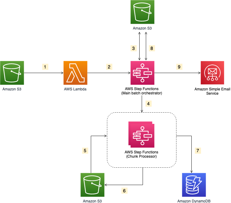
Solution architecture

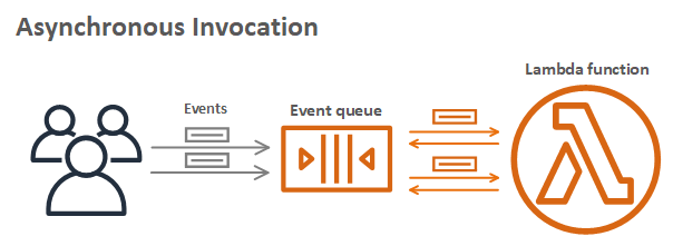
  1. The file upload to an S3 bucket triggers the S3 event notification. It invokes the Lambda function asynchronously with an event that contains details about the object.
  2. Lambda function calls the Main batch orchestrator workflow to start the processing of the file.
  3. Main batch orchestrator workflow reads the input file and splits it into multiple chunks and stores them in an S3 bucket.
  4. Main batch orchestrator then invokes the Chunk Processor workflow for each split file chunk.
  5. Each Chunk processor workflow execution reads and processes a single split chunk file.
  6. Chunk processor workflow writes the processed chunk file back to the S3 bucket.
  7. Chunk processor workflow writes the details about any validation errors in an Amazon DynamoDB table.
  8. Main batch orchestrator workflow then merges all the processed chunk files and saves it to an S3 bucket.
  9. Main batch orchestrator workflow then emails the consolidated files to the intended recipients using Amazon Simple Email Service.

Step Functions workflow

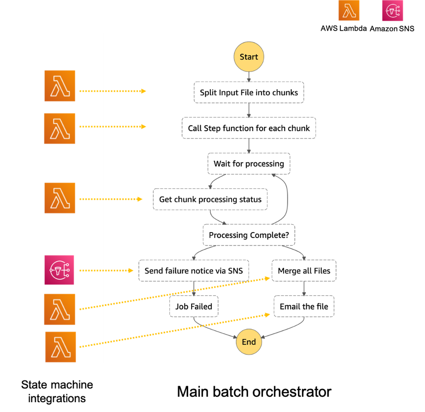
  1. The Main batch orchestrator workflow orchestrates the processing of the file.
    1. The first task state Split Input File into chunks calls a Lambda function. It splits the main file into multiple chunks based on the number of records and stores each chunk into an S3 bucket.
    2. The next task state Call Step Functions for each chunk invokes a Lambda function. It triggers a workflow for each chunk of the file. It passes information such as the name of bucket and the key where the chunk file to be processed is present.
    3. Then we wait for all the child workflow executions to complete.
    4. Once all the child workflows are processed successfully, the next task state is Merge all Files. This combines all the processed chunks into a single file and then stores the file back to the S3 bucket.
    5. The next task state Email the file takes the output file. It generates an S3 presigned URL for the file and sends an email with the S3 presigned URL.Chunk processor workflow
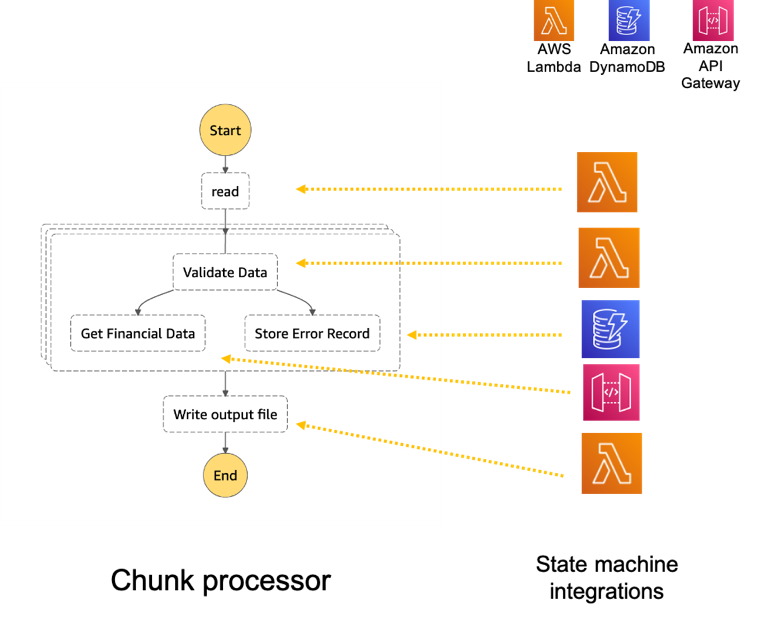
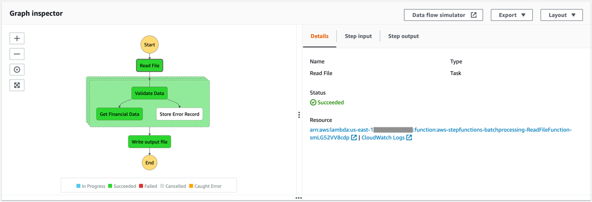
  2. The Chunk processor workflow is responsible for processing each row from the chunk file that was passed.
    1. The first task state Read reads the chunked file from S3 and converts it to an array of JSON objects. Each JSON object represents a row in the chunk file.
    2. The next state is a map state called Process messages (not shown in the preceding visual workflow). It runs a set of steps for each element of an input array. The input to the map state is an array of JSON objects passed by the previous task.
    3. Within the map state, Validate Data is the first state. It invokes a Lambda function that validates each JSON object using the rules that you have created. Records that fail validation are stored in an Amazon DynamoDB table.
    4. The next state Get Financial Data invokes Amazon API Gateway endpoints to enrich the data in the file with data from a DynamoDB table.
    5. When the map state iterations are complete, the Write output file state triggers a task. It calls a Lambda function, which converts the JSON data back to CSV and writes the output object to S3.

Prerequisites

Deploying the application

  1. Clone the repository.
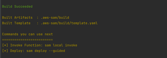
  2. Change to the directory and build the application source:
    sam build
    sam build
  3. Package and deploy the application to AWS. When prompted, input the corresponding parameters as shown below:
    sam deploy –guided
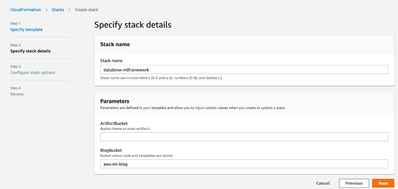
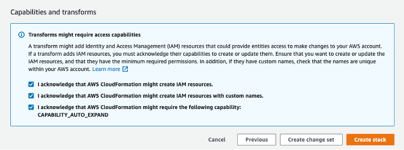
    sam deployNote the template parameters:
    • SESSender: The sender email address for the output file email.
    • SESRecipient: The recipient email address for the output file email.
    • SESIdentityName: An email address or domain that Amazon SES users use to send email.
    • InputArchiveFolder: Amazon S3 folder where the input file will be archived after processing.
    • FileChunkSize: Size of each of the chunks, which is split from the input file.
    • FileDelimiter: Delimiter of the CSV file (for example, a comma).
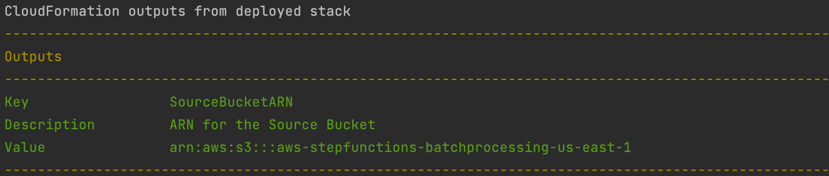
  4. After the stack creation is complete, you see the source bucket created in Outputs.
    Outputs
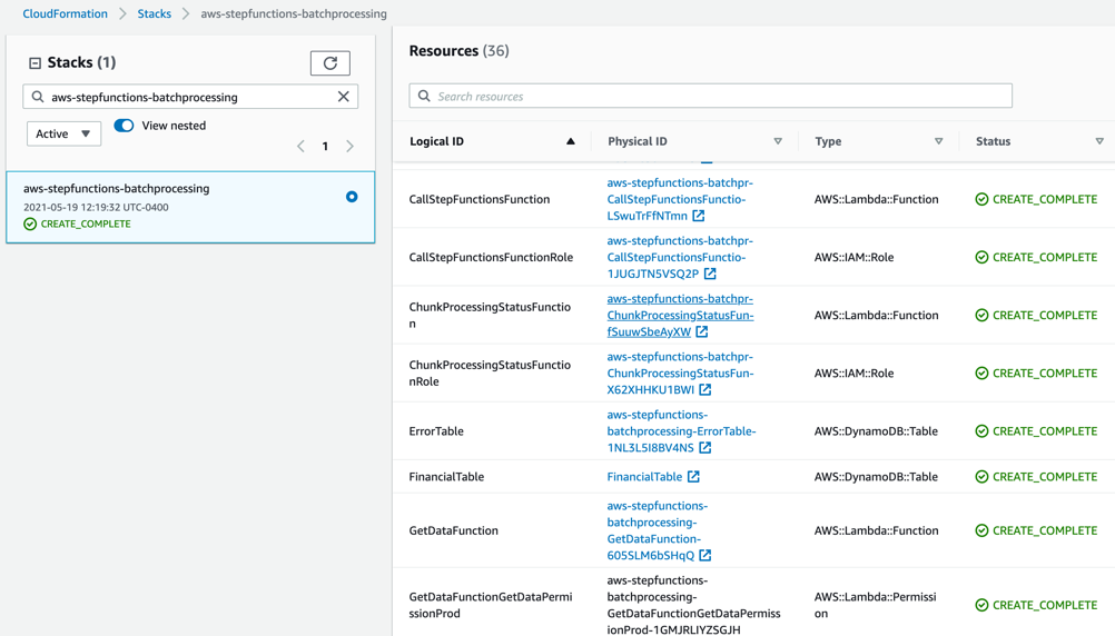
  5. Review the deployed components in the AWS CloudFormation Console.
    CloudFormation console

Testing the solution

  1. Before you can send an email using Amazon SES, you must verify each identity that you’re going to use as a “From”, “Source”, “Sender”, or “Return-Path” address to prove that you own it. Refer Verifying identities in Amazon SES for more information.
  2. Locate the S3 bucket (SourceBucket) in the Resources section of the CloudFormation stack. Choose the physical ID.
    s3 bucket ID
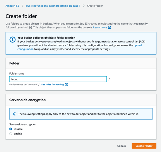
  3. In the S3 console for the SourceBucket, choose Create folder. Name the folder input and choose Create folder.
    Create folder
  4. The S3 event notification on the SourceBucket uses “input” as the prefix and “csv” as the suffix. This triggers the notification Lambda function. This is created as a part of the custom resource in the AWS SAM template.
    Event notification
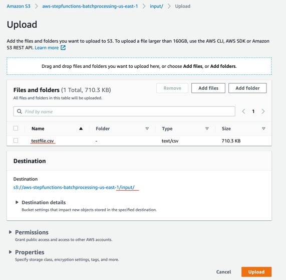
  5. In the S3 console for the SourceBucket, choose the Upload button. Choose Add files and browse to the input file (testfile.csv). Choose Upload.
    Upload dialog
  6. Review the data in the input file testfile.csv.
    Testfile.csv
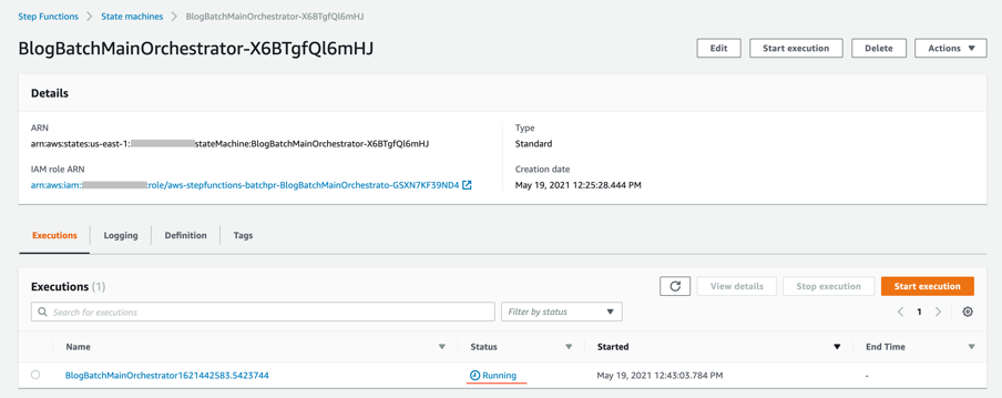
  7. After the object is uploaded, the event notification triggers the Lambda Function. This starts the main orchestrator workflow. In the Step Functions console, you see the workflow is in a running state.
    Step Functions console
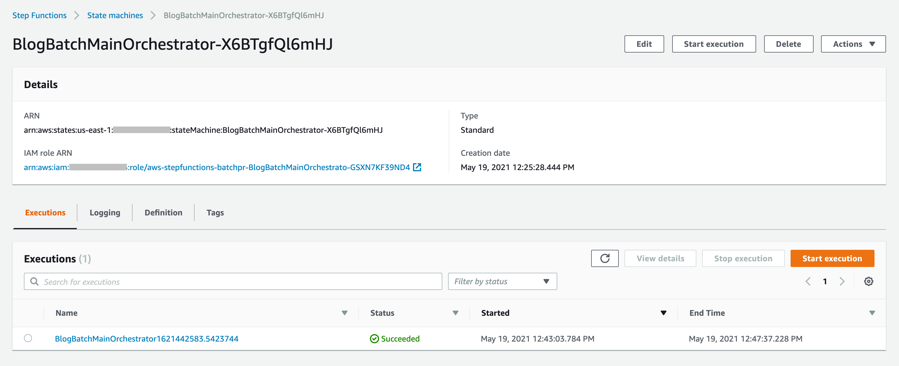
  8. Choose an individual state machine to see additional information.
    State machine
  9. After a few minutes, both BlogBatchMainOrchestrator and BlogBatchProcessChunk workflows have completed all executions. There is one execution for the BlogBatchMainOrchestrator workflow and multiple invocations of the BlogBatchProcessChunk workflow. This is because the BlogBatchMainOrchestrator invokes the BlogBatchProcessChunk for each of the chunked files.
    Workflow #1Workflow #2

Checking the output

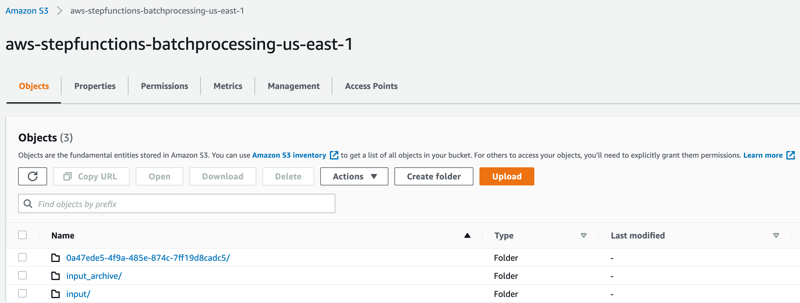
  1. Open the S3 console and verify the folders created after the process has completed.
    S3 folders
    The following subfolders are created after the processing is complete:
    input_archive – Folder for archival of the input object.
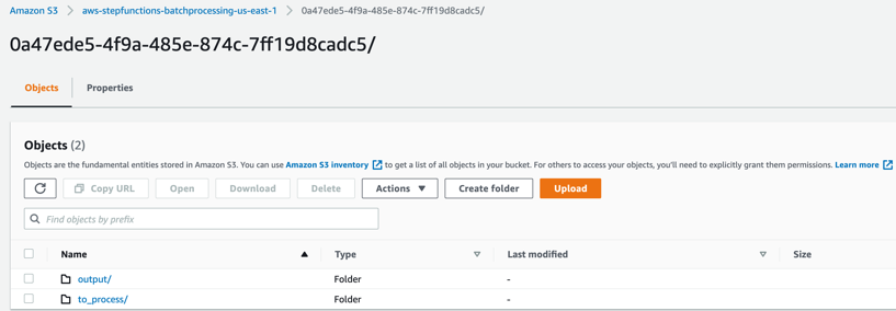
    0a47ede5-4f9a-485e-874c-7ff19d8cadc5 – Subfolder with a unique UUID in the name. This is created for storing the objects generated during batch execution.
  2. Select the folder 0a47ede5-4f9a-485e-874c-7ff19d8cadc5.
    Folder contents
    output – This folder contains the completed output objects, some housekeeping files, and processed chunk objects.
    Output folderto_process – This folder contains all the split objects from the original input file.
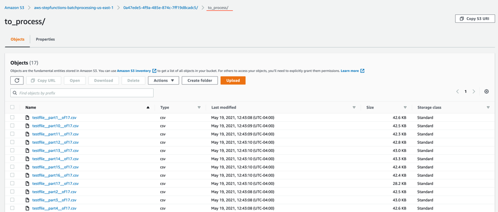
    to_process folder
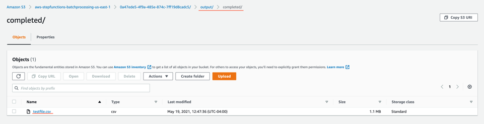
  3. Open the processed object from the output/completed folder.
    Processed object
    Inspect the output object testfile.csv. It is enriched with additional data (columns I through N) from the DynamoDB table fetched through an API call.Output testfile.csv

Viewing a completed workflow

Open the Step Functions console and browse to the BlogBatchMainOrchestrator and BlogBatchProcessChunk state machines. Choose one of the executions of each to locate the Graph Inspector. This shows the execution results for each state.

BlogBatchMainOrchestrator:

BlogBatchMainOrchestrator

BlogBatchProcessChunk:

BlogBatchProcessChunk

Batch performance

For this use case, this is the time taken for the batch to complete, based on the number of input records:

No. of records Time for batch completion
10 k 5 minutes
100 k 7 minutes

The performance of the batch depends on other factors such as the Lambda memory settings and data in the file. Read more about Profiling functions with AWS Lambda Power Tuning.

Conclusion

This blog post shows how to use Step Functions’ features and integrations to orchestrate a batch processing solution. You use two Steps Functions workflows to implement batch processing, with one workflow splitting the original file and a second workflow processing each chunk file.

The overall performance of our batch processing application is improved by splitting the input file into multiple chunks. Each chunk is processed by a separate state machine. Map states further improve the performance and efficiency of workflows by processing individual rows in parallel.

Download the code from this repository to start building a serverless batch processing system.

Additional Resources:

For more serverless learning resources, visit Serverless Land.

Visualizing AWS Step Functions workflows from the AWS Batch console

Post Syndicated from Eric Johnson original https://aws.amazon.com/blogs/compute/visualizing-aws-step-functions-workflows-from-the-aws-batch-console/

This post written by Dhiraj Mahapatro, Senior Specialist SA, Serverless.

AWS Step Functions is a low-code visual workflow service used to orchestrate AWS services, automate business processes, and build serverless applications. Step Functions workflows manage failures, retries, parallelization, service integrations, and observability so builders can focus on business logic.

AWS Batch is one of the service integrations that are available for Step Functions. AWS Batch enables users to more easily and efficiently run hundreds of thousands of batch computing jobs on AWS. AWS Batch dynamically provisions the optimal quantity and compute resource classifications based on the volume and specific resource requirements of the batch jobs submitted. AWS Batch plans, schedules, and runs batch computing workloads across the full range of AWS compute services and features, such as AWS FargateAmazon EC2, and spot instances.

Now, Step Functions is available to AWS Batch users through the AWS Batch console. This feature enables AWS Batch users to augment compute options and have additional orchestration capabilities to manage their batch jobs.

This blog walks through Step Functions integration in AWS Batch console and shows how AWS Batch users can efficiently use Step Functions workflow orchestrators in batch workloads. A sample application also highlights the use of AWS Lambda as a compute option for AWS Batch.

Introducing workflow orchestration in AWS Batch console

Today, AWS users use AWS Batch for high performance computing, post-trade analytics, fraud surveillance, screening, DNA sequencing, and more. AWS Batch minimizes human error, increases speed and accuracy, and reduces costs with automation so that users can refocus on evolving the business.

In addition to using compute-intensive tasks, users sometimes need Lambda for simpler, less intense processing. Users also want to combine the two in a single business process that is scalable and repeatable.

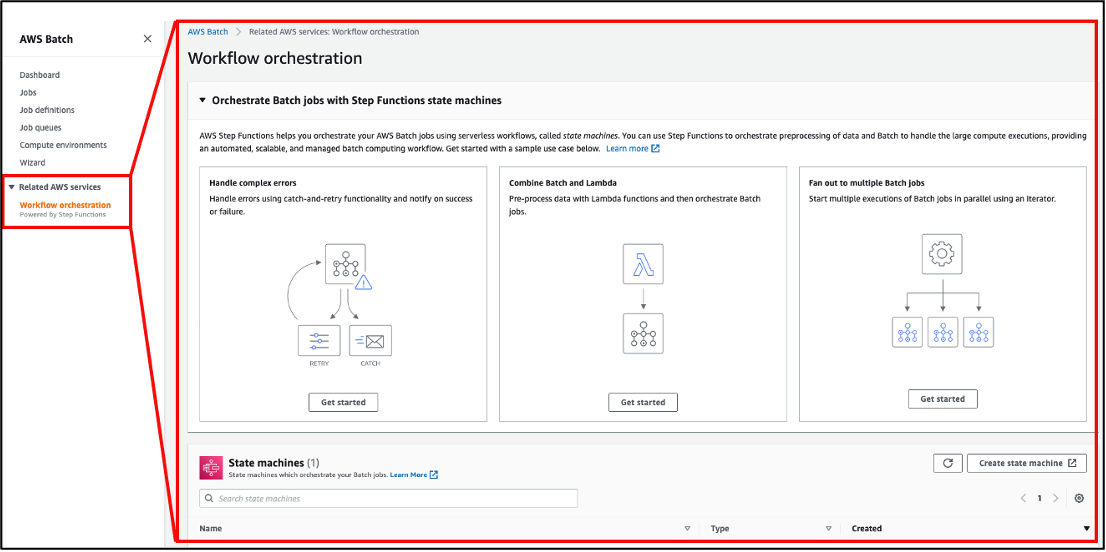
Workflow orchestration (powered by Step Functions) in AWS Batch console allows orchestration of batch jobs with Step Functions state machine:

Workflow orchestration in Batch console

Workflow orchestration in Batch console

Using batch-related patterns from Step Functions

Error handling

Step Functions natively handles errors and retries of its workflows. Users rely on this native error handling mechanism to focus on building business logic.

Workflow orchestration in AWS Batch console provides common batch-related patterns that are present in Step Functions. Handling errors while submitting batch jobs in Step Functions is one of them.

Getting started with orchestration in Batch

Getting started with orchestration in Batch

  1. Choose Get Started from Handle complex errors.
  2. From the pop-up, choose Start from a template and choose Continue.

A new browser tab opens with Step Functions Workflow Studio. The Workflow Studio designer has a workflow pattern template pre-created. Diving deeper into the workflow highlights that the Step Functions workflow submits a batch job and then handles success and error scenarios by sending Amazon SNS notifications, respectively.

Alternatively, choosing Deploy a sample project from the Get Started pop-up deploys a sample Step Functions workflow.

Deploying a sample project

Deploying a sample project

This option allows creating a state machine from scratch, reviewing the workflow definition, deploying an AWS CloudFormation stack, and running the workflow in Step Functions console.

Deploy and run from console

Deploy and run from console

Once deployed, the state machine is visible in the Step Functions console as:

Viewing the state machine in the AWS Step Functions console

Viewing the state machine in the AWS Step Functions console

Select the BatchJobNotificationStateMachine to land on the details page:

View the state machine's details

View the state machine’s details

The CloudFormation template has already provisioned the required batch job in AWS Batch and the SNS topic for success and failure notification.

To see the Step Functions workflow in action, use Start execution. Keep the optional name and input as is and choose Start execution:

Run the Step Function

Run the Step Function

The state machine completes the tasks successfully by Submitting Batch Job using AWS Batch and Notifying Success using the SNS topic:

The successful results in the console

The successful results in the console

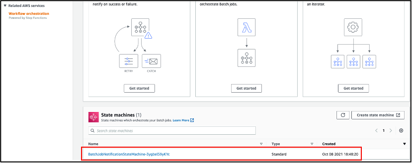
The state machine used the AWS Batch Submit Job task. The Workflow orchestration in AWS Batch console now highlights this newly created Step Functions state machine:

The state machine is listed in the Batch console

The state machine is listed in the Batch console

Therefore, any state machine that uses this task in Step Functions for this account is listed here as a state machine that orchestrates batch jobs.

Combine Batch and Lambda

Another pattern to use in Step Functions is the combination of Lambda and batch job.

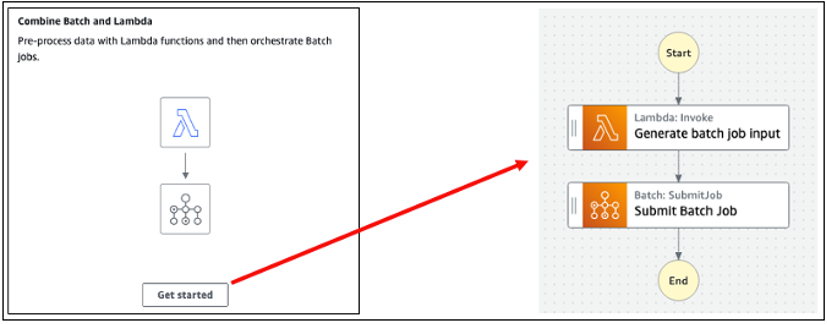
Select Get Started from Combine Batch and Lambda pop-up followed by Start from a template and Continue. This takes the user to Step Functions Workflow studio with the following pattern. The Lambda task generates input for the subsequent batch job task. Submit Batch Job task takes the input and submits the batch job:

Combining AWS Lambda with AWS Step Functions

Combining AWS Lambda with AWS Step Functions

Step Functions enables AWS Batch users to combine Batch and Lambda functions to optimize compute spend while using the power of the different compute choices.

Fan out to multiple Batch jobs

In addition to error handling and combining Lambda with AWS Batch jobs, a user can fan out multiple batch jobs using Step Functions’ map state. Map state in Step Functions provides dynamic parallelism.

With dynamic parallelism, a user can submit multiple batch jobs based on a collection of batch job input data. With visibility to each iteration’s input and output, users can easily navigate and troubleshoot in case of failure.

Easily navigate and troubleshoot in case of failure

Easily navigate and troubleshoot in case of failure

AWS Batch users are not limited to the previous three patterns shown in Workflow orchestration in the AWS Batch console. AWS Batch users can start from scratch and build Step Functions state machine by navigating to the bottom right and using Create state machine:

Create a state machine from the Step Functions console

Create a state machine from the Step Functions console

Create State Machine in AWS Batch console opens a new tab with Step Functions console’s Create state machine page.

Design a workflow visually

Design a workflow visually

Refer building a state machine AWS Step Functions Workflow Studio for additional details.

Deploying the application

The sample application shows fan out to multiple batch jobs pattern. Before deploying the application, you need:

To deploy:

  1. From a terminal window, clone the GitHub repo:
    git clone [email protected]:aws-samples/serverless-batch-job-workflow.git
  2. Change directory:
    cd ./serverless-batch-job-workflow
  3. Download and install dependencies:
    sam build
  4. Deploy the application to your AWS account:
    sam deploy --guided

To run the application using the AWS CLI, replace the state machine ARN from the output of deployment steps:

aws stepfunctions start-execution \
    --state-machine-arn <StepFunctionArnHere> \
    --region <RegionWhereApplicationDeployed> \
    --input "{}"

Step Functions is not limited to AWS Batch’s Submit Job API action

In September 2021, Step Functions announced integration support for 200 AWS Services to enable easier workflow automation. With this announcement, Step Functions is not limited to integrate with AWS Batch’s SubmitJob API but also can integrate with any AWS Batch SDK API today.

Step Functions can automate the lifecycle of an AWS Batch job, starting from creating a compute environment, creating job queues, registering job definitions, submitting a job, and finally cleaning up.

Other AWS service integrations

Step Functions support for 200 AWS Services equates integration with more than 9,000 API actions across these services. AWS Batch tasks in Step Functions can evolve by integrating with available services in the workflow for their pre- and post-processing needs.

For example, batch job input data sanitization can be done inside Lambda and that gets pushed to an Amazon SQS queue or Amazon S3 as an object for auditability purposes.

Similarly, Amazon SNS, Amazon Pinpoint, or Amazon SES can notify once AWS Batch job task is complete.

There are multiple ways to decorate around an AWS Batch job task. Refer to AWS SDK service integrations and optimized integrations for Step Functions for additional details.

Important considerations

Workflow orchestrations in the AWS Batch console only show Step Functions state machines that use AWS Batch’s Submit Job task. Step Functions state machines do not show in the AWS Batch console when:

  1. A state machine uses any other AWS SDK Batch API integration task
  2. AWS Batch’s SubmitJob API is invoked inside a Lambda function task using an AWS SDK client (like Boto3 or Node.js or Java)

Cleanup

The sample application provisions AWS Batch (the job definition, job queue, and ECS compute environment inside a VPC). It also creates subnets, route tables, and an internet gateway. Clean up the stack after testing the application to avoid the ongoing cost of running these services.

To delete the sample application stack, use the latest version of AWS SAM CLI and run:

sam delete

Conclusion

To learn more on AWS Batch, read the Orchestrating Batch jobs section in the Batch developer guide.

To get started, open the workflow orchestration page in the Batch console. Select Orchestrate Batch jobs with Step Functions Workflows to deploy a sample project, if you are new to Step Functions.

This feature is available in all Regions where both Step Functions and AWS Batch are available. View the AWS Regions table for details.

To learn more on Step Functions patterns, visit Serverless Land.

Using JSONPath effectively in AWS Step Functions

Post Syndicated from James Beswick original https://aws.amazon.com/blogs/compute/using-jsonpath-effectively-in-aws-step-functions/

This post is written by Dhiraj Mahapatro, Senior Serverless Specialist SA, Serverless.

AWS Step Functions uses Amazon States Language (ASL), which is a JSON-based, structured language used to define the state machine. ASL uses paths for input and output processing in between states. Paths follow JSONPath syntax.

JSONPath provides the capability to select parts of JSON structures similar to how XPath expressions select nodes of XML documents. Step Functions provides the data flow simulator, which helps in modeling input and output path processing using JSONPath.

This blog post explains how you can effectively use JSONPath in a Step Functions workflow. It shows how you can separate concerns between states by specifically identifying input to and output from each state. It also explains how you can use advanced JSONPath expressions for filtering and mapping JSON content.

Overview

The sample application in this blog is based on a use case in the insurance domain. A new potential customer signs up with an insurance company by creating an account. The customer provides their basic information, and their interests in the types of insurances for shopping later.

The information provided by the potential insurance customer is accepted by the insurance company’s new account application for processing. This application is built using Step Functions, which accepts provided input as a JSON payload and applies the following business logic:

Example application architecture

  1. Verify the identity of the user.
  2. Verify the address of the user.
  3. Approve the new account application if the checks pass.
  4. Upon approval, insert user information into the Amazon DynamoDB Accounts table.
  5. Collect home insurance interests and store in an Amazon SQS queue.
  6. Send email notification to the user about the application approval.
  7. Deny the new account application if the checks fail.
  8. Send an email notification to the user about the application denial.

Deploying the application

Before deploying the solution, you need:

To deploy:

  1. From a terminal window, clone the GitHub repo:
    git clone [email protected]:aws-samples/serverless-account-signup-service.git
  2. Change directory:
    cd ./serverless-account-signup-service
  3. Download and install dependencies:
    sam build
  4. Deploy the application to your AWS account:
    sam deploy --guided
  5. During the guided deployment process, enter a valid email address for the parameter “Email” to receive email notifications.
  6. Once deployed, a confirmation email is sent to the provided email address from SNS. Confirm the subscription by clicking the link in the email.
    Email confirmation

To run the application using the AWS CLI, replace the state machine ARN from the output of deployment steps:

aws stepfunctions start-execution \
  --state-machine-arn <StepFunctionArnHere> \
  --input "{\"data\":{\"firstname\":\"Jane\",\"lastname\":\"Doe\",\"identity\":{\"email\":\"[email protected]\",\"ssn\":\"123-45-6789\"},\"address\":{\"street\":\"123 Main St\",\"city\":\"Columbus\",\"state\":\"OH\",\"zip\":\"43219\"},\"interests\":[{\"category\":\"home\",\"type\":\"own\",\"yearBuilt\":2004},{\"category\":\"auto\",\"type\":\"car\",\"yearBuilt\":2012},{\"category\":\"boat\",\"type\":\"snowmobile\",\"yearBuilt\":2020},{\"category\":\"auto\",\"type\":\"motorcycle\",\"yearBuilt\":2018},{\"category\":\"auto\",\"type\":\"RV\",\"yearBuilt\":2015},{\"category\":\"home\",\"type\":\"business\",\"yearBuilt\":2009}]}}"

Paths in Step Functions

Here is the sample payload structure :

{
  "data": {
    "firstname": "Jane",
    "lastname": "Doe",
    "identity": {
      "email": "[email protected]",
      "ssn": "123-45-6789"
    },
    "address": {
      "street": "123 Main St",
      "city": "Columbus",
      "state": "OH",
      "zip": "43219"
    },
    "interests": [
      {"category": "home", "type": "own", "yearBuilt": 2004},
      {"category": "auto", "type": "car", "yearBuilt": 2012},
      {"category": "boat", "type": "snowmobile", "yearBuilt": 2020},
      {"category": "auto", "type": "motorcycle", "yearBuilt": 2018},
      {"category": "auto", "type": "RV", "yearBuilt": 2015},
      {"category": "home", "type": "business", "yearBuilt": 2009}
    ]
  }
}

The payload has data about the new user (identity and address information) and the user’s interests in the types of insurance.

The Compute Blog post on using data flow simulator elaborates on how to use Step Functions paths. To summarize how paths work:

  1. InputPath – What input does a task need?
  2. Parameters – How does the task need the structure of the input to be?
  3. ResultSelectors – What to choose from the task’s output?
  4. ResultPath – Where to put the chosen output?
  5. OutputPath – What output to send to the next state?

The key idea is that the input of downstream states input depends on the output of previous states. JSONPath expressions help structuring input and output between states.

Using JSONPath inside paths

This is how paths are used in the sample application for each type.

InputPath

The first two main tasks in the Step Functions state machine validate the identity and the address of the user. Since both validations are unrelated, they can work independently by using parallel state.

Each state needs the identity and address information provided by the input payload. There is no requirement to provide interests to those states, so InputPath can help answer “What input does a task need?”.

Inside the Check Identity state:

"InputPath": "$.data.identity"

Inside the Check Address state:

"InputPath": "$.data.address"

Parameters

What should the input of the underlying task look like? Check Identity and Check Address use their respective AWS Lambda functions. When Lambda functions or any other AWS service integration is used as a task, the state machine should follow the request syntax of the corresponding service.

For a Lambda function as a task, the state should provide the FunctionName and an optional Payload as parameters. For the Check Identity state, the parameters section looks like:

"Parameters": {
    "FunctionName": "${CheckIdentityFunctionArn}",
    "Payload.$": "$"
}

Here, Payload is the entire identity JSON object provided by InputPath.

ResultSelector

Once the Check Identity task is invoked, the Lambda function successfully validates the user’s identity and responds with an approval response:

{
  "ExecutedVersion": "$LATEST",
  "Payload": {
    "statusCode": "200",
    "body": "{\"approved\": true,\"message\": \"identity validation passed\"}"
  },
  "SdkHttpMetadata": {
    "HttpHeaders": {
      "Connection": "keep-alive",
      "Content-Length": "43",
      "Content-Type": "application/json",
      "Date": "Thu, 16 Apr 2020 17:58:15 GMT",
      "X-Amz-Executed-Version": "$LATEST",
      "x-amzn-Remapped-Content-Length": "0",
      "x-amzn-RequestId": "88fba57b-adbe-467f-abf4-daca36fc9028",
      "X-Amzn-Trace-Id": "root=1-5e989cb6-90039fd8971196666b022b62;sampled=0"
    },
    "HttpStatusCode": 200
  },
  "SdkResponseMetadata": {
    "RequestId": "88fba57b-adbe-467f-abf4-daca36fc9028"
  },
  "StatusCode": 200
}

The identity validation approval must be provided to the downstream states for additional processing. However, the downstream states only need the Payload.body from the preceding JSON.

You can use a combination of intrinsic function and ResultSelector to choose attributes from the task’s output:

"ResultSelector": {
  "identity.$": "States.StringToJson($.Payload.body)"
}

ResultSelector takes the JSON string $.Payload.body and applies States.StringToJson to convert the string to JSON store in a new attribute named identity:

"identity": {
    "approved": true,
    "message": "identity validation passed"
}

When Check Identity and Check Address states finish their work and exit, the step output from each state is captured as a JSON array. This JSON array is the step output of the parallel state. Reconcile the results from the JSON array using the ResultSelector that is available in parallel state.

"ResultSelector": {
    "identityResult.$": "$[0].result.identity",
    "addressResult.$": "$[1].result.address"
}

ResultPath

After ResultSelector, where should the identity result go to in the initial payload? The downstream states need access to the actual input payload in addition to the results from the previous state. ResultPath provides the mechanism to extend the initial payload to add results from the previous state.

ResultPath: "$.result" informs the state machine that any result selected from the task output (actual output if none specified) should go under result JSON attribute and result should get added to the incoming payload. The output from ResultPath looks like:

{
  "data": {
    "firstname": "Jane",
    "lastname": "Doe",
    "identity": {
      "email": "[email protected]",
      "ssn": "123-45-6789"
    },
    "address": {
      "street": "123 Main St",
      "city": "Columbus",
      "state": "OH",
      "zip": "43219"
    },
    "interests": [
      {"category":"home", "type":"own", "yearBuilt":2004},
      {"category":"auto", "type":"car", "yearBuilt":2012},
      {"category":"boat", "type":"snowmobile","yearBuilt":2020},
      {"category":"auto", "type":"motorcycle","yearBuilt":2018},
      {"category":"auto", "type":"RV", "yearBuilt":2015},
      {"category":"home", "type":"business", "yearBuilt":2009}
    ]
  },
  "result": {
    "identity": {
      "approved": true,
      "message": "identity validation passed"
    }
  }
}

The preceding JSON has results from an operation but also the incoming payload is intact for business logic in downstream states.

This pattern ensures that the previous state keeps the payload hydrated for the next state. Use these combinations of paths across all states to make sure that each state has all the information needed.

As with the parallel state’s ResultSelector, an appropriate ResultPath is needed to hold both the results from Check Identity and Check Address to get the below results JSON object added to the payload:

"results": {
  "addressResult": {
    "approved": true,
    "message": "address validation passed"
  },
  "identityResult": {
    "approved": true,
    "message": "identity validation passed"
  }
}

With this approach for all of the downstream states, the input payload is still intact and the state machine has collected results from each state in results.

OutputPath

To return results from the state machine, ideally you do not send back the input payload to the caller of the Step Functions workflow. You can use OutputPath to select a portion of the state output as an end result. OutputPath determines what output to send to the next state.

In the sample application, the last states (Approved Message and Deny Message) defined OutputPath as:

“OutputPath”: “$.results”

The output from the state machine is:

{
  "addressResult": {
    "approved": true,
    "message": "address validation passed"
  },
  "identityResult": {
    "approved": true,
    "message": "identity validation passed"
  },
  "accountAddition": {
    "statusCode": 200
  },
  "homeInsuranceInterests": {
    "statusCode": 200
  },
  "sendApprovedNotification": {
    "statusCode": 200
  }
}

This response strategy is also effective when using a Synchronous Express Workflow for this business logic.

Advanced JSONPath

You can declaratively use advanced JSONPath expressions to apply logic without writing imperative code in utility functions.

Let’s focus on the interests that the new customer has asked for in the input payload. The Step Functions state machine has a state that focuses on interests in the “home” insurance category. Once the new account application is approved and added to the database successfully, the application captures home insurance interests. It adds home-related detail in an HomeInterestsQueue SQS queue and transitions to the Approved Message state.

The interests JSON array has the information about insurance interests. An effective way to get home-related details is to filter out the interests array based on the category “home”. You can try this in data flow simulator:

Data flow simulator

You can apply additional filter expressions to filter data according to your use case. To learn more, visit the the data flow simulator blog.

Inside the state machine JSON, the Home Insurance Interests task has:

"InputPath": "$..interests[?(@.category==home)]"

It uses advanced JSONPath with $.. notation and [?(@.category==home)] filters.

Using advanced expressions on JSONPath is not limited to home insurance interests and can be extended to other categories and business logic.

Cleanup

To delete the sample application, use the latest version of the AWS SAM CLI and run:

sam delete

Conclusion

This post uses a sample application to highlight effective use of JSONPath and data filtering strategies that can be used in Step Functions.

JSONPath provides the flexibility to work on JSON objects and arrays inside the Step Functions states machine by reducing the amount of utility code. It allows developers to build state machines by separating concerns for states’ input and output data. Advanced JSONPath expressions help writing declarative filtering logic without needing imperative utility code, optimizing cost, and performance.

For more serverless learning resources, visit Serverless Land.

Build and orchestrate ETL pipelines using Amazon Athena and AWS Step Functions

Post Syndicated from Behram Irani original https://aws.amazon.com/blogs/big-data/build-and-orchestrate-etl-pipelines-using-amazon-athena-and-aws-step-functions/

Extract, transform, and load (ETL) is the process of reading source data, applying transformation rules to this data, and loading it into the target structures. ETL is performed for various reasons. Sometimes ETL helps align source data to target data structures, whereas other times ETL is done to derive business value by cleansing, standardizing, combining, aggregating, and enriching datasets. You can perform ETL in multiple ways; the most popular choices being:

  • Programmatic ETL using Apache Spark. Amazon EMR and AWS Glue both support this model.
  • SQL ETL using Apache Hive or PrestoDB/Trino. Amazon EMR supports both these tools.
  • Third-party ETL products.

Many organizations prefer the SQL ETL option because they already have developers who understand and write SQL queries. However, these developers want to focus on writing queries and not worry about setting up and managing the underlying infrastructure.

Amazon Athena is an interactive query service that makes it easy to analyze data in Amazon Simple Storage Service (Amazon S3) using standard SQL. Athena is serverless, so there is no infrastructure to manage, and you pay only for the queries that you run.

This post explores how you can use Athena to create ETL pipelines and how you can orchestrate these pipelines using AWS Step Functions.

Architecture overview

The following diagram illustrates our architecture.

The source data first gets ingested into an S3 bucket, which preserves the data as is. You can ingest this data in Amazon S3 multiple ways:

After the source data is in Amazon S3 and assuming that it has a fixed structure, you can either run an AWS Glue crawler to automatically generate the schema or you can provide the DDL as part of your ETL pipeline. An AWS Glue crawler is the primary method used by most AWS Glue users. You can use a crawler to populate the AWS Glue Data Catalog with tables. A crawler can crawl multiple data stores in a single run. Upon completion, the crawler creates or updates one or more tables in your Data Catalog. Athena uses this catalog to run queries against the tables.

After the raw data is cataloged, the source-to-target transformation is done through a series of Athena Create Table as Select (CTAS) and INSERT INTO statements. The transformed data is loaded into another S3 bucket. The files are also partitioned and converted into Parquet format to optimize performance and cost.

Prepare your data

For this post, we use the NYC taxi public dataset. It has the data of trips taken by taxis and for-hire vehicles in New York City organized in CSV files by each month of the year starting from 2009. For our ETL pipeline, we use two files containing yellow taxi data: one for demonstrating the initial table creation and loading this table using CTAS, and the other for demonstrating the ongoing data inserts into this table using the INSERT INTO statement. We also use a lookup file to demonstrate join, transformation, and aggregation in this ETL pipeline.

  1. Create a new S3 bucket with a unique name in your account.

You use this bucket to copy the raw data from the NYC taxi public dataset and store the data processed by Athena ETL.

  1. Create the S3 prefixes athena, nyctaxidata/data, nyctaxidata/lookup, nyctaxidata/optimized-data, and nyctaxidata/optimized-data-lookup inside this newly created bucket.

These prefixes are used in the Step Functions code provided later in this post.

  1. Copy the yellow taxi data files from the nyc-tlc public bucket described in the NYC taxi public dataset registry for January and February 2020 into the nyctaxidata/data prefix of the S3 bucket you created in your account.
  2. Copy the lookup file into the nyctaxidata/lookup prefix you created.

Create an ETL pipeline using Athena integration with Step Functions

Step Functions is a low-code visual workflow service used to orchestrate AWS services, automate business processes, and build serverless applications. Through its visual interface, you can create and run a series of checkpointed and event-driven workflows that maintain the application state. The output of one step acts as an input to the next. Each step in your application runs in order, as defined by your business logic.

The Step Functions service integration with Athena enables you to use Step Functions to start and stop query runs, and get query results.

For the ETL pipeline in this post, we keep the flow simple; however, you can build a complex flow using different features of Step Functions.

The flow of the pipeline is as follows:

  1. Create a database if it doesn’t already exist in the Data Catalog. Athena by default uses the Data Catalog as its metastore.
  2. If no tables exist in this database, take the following actions:
    1. Create the table for the raw yellow taxi data and the raw table for the lookup data.
    2. Use CTAS to create the target tables and use the raw tables created in the previous step as input in the SELECT statement. CTAS also partitions the target table by year and month, and creates optimized Parquet files in the target S3 bucket.
    3. Use a view to demonstrate the join and aggression parts of ETL.
  3. If any table exists in this database, iterate though the list of all the remaining CSV files and process by using the INSERT INTO statement.

Different use cases may make the ETL pipeline quite complex. You may be getting continuous data from the source either with AWS DMS in batch or CDC mode or by Kinesis in streaming mode. This requires mechanisms in place to process all such files during a particular window and mark it as complete so that the next time the pipeline is run, it processes only the newly arrived files. Instead of manually adding DDL in the pipeline, you can add AWS Glue crawler steps in the Step Functions pipeline to create a schema for the raw data; and instead of a view to aggregate data, you may have to create a separate table to keep the results ready for consumption. Also, many use cases get change data as part of the feed, which needs to be merged with the target datasets. Extra steps in the Step Functions pipeline are required to process such data on a case-by-case basis.

The following code for the Step Functions pipeline covers the preceding flow we described. For more details on how to get started with Step Functions, refer the tutorials. Replace the S3 bucket names with the unique bucket name you created in your account.

{
  "Comment": "An example of using Athena to query logs, get query results and send results through notification.",
  "StartAt": "Create Glue DB",
  "States": {
    "Create Glue DB": {
      "Resource": "arn:aws:states:::athena:startQueryExecution.sync",
      "Parameters": {
        "QueryString": "CREATE DATABASE if not exists nyctaxidb",
        "WorkGroup": "primary",
        "ResultConfiguration": {
          "OutputLocation": "s3://MY-BUCKET/athena/"
        }
      },
      "Type": "Task",
      "Next": "Run Table Lookup"
    },
    "Run Table Lookup": {
      "Resource": "arn:aws:states:::athena:startQueryExecution.sync",
      "Parameters": {
        "QueryString": "show tables in nyctaxidb",
        "WorkGroup": "primary",
        "ResultConfiguration": {
          "OutputLocation": "s3://MY-BUCKET/athena/"
        }
      },
      "Type": "Task",
      "Next": "Get lookup query results"
    },
    "Get lookup query results": {
      "Resource": "arn:aws:states:::athena:getQueryResults",
      "Parameters": {
        "QueryExecutionId.$": "$.QueryExecution.QueryExecutionId"
      },
      "Type": "Task",
      "Next": "ChoiceStateFirstRun"
    },
    "ChoiceStateFirstRun": {
      "Comment": "Based on the input table name, a choice is made for moving to the next step.",
      "Type": "Choice",
      "Choices": [
        {
          "Not": {
            "Variable": "$.ResultSet.Rows[0].Data[0].VarCharValue",
            "IsPresent": true
          },
          "Next": "Run Create data Table Query"
        },
        {
          "Variable": "$.ResultSet.Rows[0].Data[0].VarCharValue",
          "IsPresent": true,
          "Next": "Check All Tables"
        }
      ],
      "Default": "Check All Tables"
    },
    "Run Create data Table Query": {
      "Resource": "arn:aws:states:::athena:startQueryExecution.sync",
      "Parameters": {
        "QueryString": "CREATE EXTERNAL TABLE nyctaxidb.yellowtaxi_data_csv(  vendorid bigint,   tpep_pickup_datetime string,   tpep_dropoff_datetime string,   passenger_count bigint,   trip_distance double,   ratecodeid bigint,   store_and_fwd_flag string,   pulocationid bigint,   dolocationid bigint,   payment_type bigint,   fare_amount double,   extra double,   mta_tax double,   tip_amount double,   tolls_amount double,   improvement_surcharge double,   total_amount double,   congestion_surcharge double) ROW FORMAT DELIMITED   FIELDS TERMINATED BY ',' STORED AS INPUTFORMAT   'org.apache.hadoop.mapred.TextInputFormat' OUTPUTFORMAT   'org.apache.hadoop.hive.ql.io.HiveIgnoreKeyTextOutputFormat' LOCATION  's3://MY-BUCKET/nyctaxidata/data/' TBLPROPERTIES (  'skip.header.line.count'='1')",
        "WorkGroup": "primary",
        "ResultConfiguration": {
          "OutputLocation": "s3://MY-BUCKET/athena/"
        }
      },
      "Type": "Task",
      "Next": "Run Create lookup Table Query"
    },
    "Run Create lookup Table Query": {
      "Resource": "arn:aws:states:::athena:startQueryExecution.sync",
      "Parameters": {
        "QueryString": "CREATE EXTERNAL TABLE nyctaxidb.nyctaxi_lookup_csv(  locationid bigint,   borough string,   zone string,   service_zone string,   latitude double,   longitude double)ROW FORMAT DELIMITED   FIELDS TERMINATED BY ',' STORED AS INPUTFORMAT   'org.apache.hadoop.mapred.TextInputFormat' OUTPUTFORMAT   'org.apache.hadoop.hive.ql.io.HiveIgnoreKeyTextOutputFormat'LOCATION  's3://MY-BUCKET/nyctaxidata/lookup/' TBLPROPERTIES (  'skip.header.line.count'='1')",
        "WorkGroup": "primary",
        "ResultConfiguration": {
          "OutputLocation": "s3://MY-BUCKET/athena/"
        }
      },
      "Type": "Task",
      "Next": "Run Create Parquet data Table Query"
    },
    "Run Create Parquet data Table Query": {
      "Resource": "arn:aws:states:::athena:startQueryExecution.sync",
      "Parameters": {
        "QueryString": "CREATE  table if not exists nyctaxidb.yellowtaxi_data_parquet WITH (format='PARQUET',parquet_compression='SNAPPY',partitioned_by=array['pickup_year','pickup_month'],external_location = 's3://MY-BUCKET/nyctaxidata/optimized-data/') AS SELECT vendorid,tpep_pickup_datetime,tpep_dropoff_datetime,passenger_count,trip_distance,ratecodeid,store_and_fwd_flag,pulocationid,dolocationid,fare_amount,extra,mta_tax,tip_amount,tolls_amount,improvement_surcharge,total_amount,congestion_surcharge,payment_type,substr(\"tpep_pickup_datetime\",1,4) pickup_year, substr(\"tpep_pickup_datetime\",6,2) AS pickup_month FROM nyctaxidb.yellowtaxi_data_csv where substr(\"tpep_pickup_datetime\",1,4) = '2020' and substr(\"tpep_pickup_datetime\",6,2) = '01'",
        "WorkGroup": "primary",
        "ResultConfiguration": {
          "OutputLocation": "s3://MY-BUCKET/athena/"
        }
      },
      "Type": "Task",
      "Next": "Run Create Parquet lookup Table Query"
    },
    "Run Create Parquet lookup Table Query": {
      "Resource": "arn:aws:states:::athena:startQueryExecution.sync",
      "Parameters": {
        "QueryString": "CREATE table if not exists nyctaxidb.nyctaxi_lookup_parquet WITH (format='PARQUET',parquet_compression='SNAPPY', external_location = 's3://MY-BUCKET/nyctaxidata/optimized-data-lookup/') AS SELECT locationid, borough, zone , service_zone , latitude ,longitude  FROM nyctaxidb.nyctaxi_lookup_csv",
        "WorkGroup": "primary",
        "ResultConfiguration": {
          "OutputLocation": "s3://MY-BUCKET/athena/"
        }
      },
      "Type": "Task",
      "Next": "Run Create View"
    },
    "Run Create View": {
      "Resource": "arn:aws:states:::athena:startQueryExecution.sync",
      "Parameters": {
        "QueryString": "create or replace view nyctaxidb.yellowtaxi_data_vw as select a.*,lkup.* from (select  datatab.pulocationid pickup_location ,pickup_month, pickup_year, sum(cast(datatab.total_amount AS decimal(10, 2))) AS sum_fare , sum(cast(datatab.trip_distance AS decimal(10, 2))) AS sum_trip_distance , count(*) AS countrec   FROM nyctaxidb.yellowtaxi_data_parquet datatab WHERE datatab.pulocationid is NOT null  GROUP BY  datatab.pulocationid, pickup_month, pickup_year) a , nyctaxidb.nyctaxi_lookup_parquet lkup where lkup.locationid = a.pickup_location",
        "WorkGroup": "primary",
        "ResultConfiguration": {
          "OutputLocation": "s3://MY-BUCKET/athena/"
        }
      },
      "Type": "Task",
      "End": true
    },
    "Check All Tables": {
      "Type": "Map",
      "InputPath": "$.ResultSet",
      "ItemsPath": "$.Rows",
      "MaxConcurrency": 0,
      "Iterator": {
        "StartAt": "CheckTable",
        "States": {
          "CheckTable": {
            "Type": "Choice",
            "Choices": [
              {
                "Variable": "$.Data[0].VarCharValue",
                "StringMatches": "*data_csv",
                "Next": "passstep"
              },
              {
                "Variable": "$.Data[0].VarCharValue",
                "StringMatches": "*data_parquet",
                "Next": "Insert New Parquet Data"
              }
            ],
            "Default": "passstep"
          },
          "Insert New Parquet Data": {
            "Resource": "arn:aws:states:::athena:startQueryExecution.sync",
            "Parameters": {
              "QueryString": "INSERT INTO nyctaxidb.yellowtaxi_data_parquet select vendorid,tpep_pickup_datetime,tpep_dropoff_datetime,passenger_count,trip_distance,ratecodeid,store_and_fwd_flag,pulocationid,dolocationid,fare_amount,extra,mta_tax,tip_amount,tolls_amount,improvement_surcharge,total_amount,congestion_surcharge,payment_type,substr(\"tpep_pickup_datetime\",1,4) pickup_year, substr(\"tpep_pickup_datetime\",6,2) AS pickup_month FROM nyctaxidb.yellowtaxi_data_csv where substr(\"tpep_pickup_datetime\",1,4) = '2020' and substr(\"tpep_pickup_datetime\",6,2) = '02'",
              "WorkGroup": "primary",
              "ResultConfiguration": {
                "OutputLocation": "s3://MY-BUCKET/athena/"
              }
            },
            "Type": "Task",
            "End": true
          },
          "passstep": {
            "Type": "Pass",
            "Result": "NA",
            "End": true
          }
        }
      },
      "End": true
    }
  }
}

The first time we run this pipeline, it follows the CTAS path and creates the aggregation view.

The second time we run it, it follows the INSERT INTO statement path to add new data into the existing tables.

When to use this pattern

You should use this pattern when the raw data is structured and the metadata can easily be added to the catalog.

Because Athena charges are calculated by the amount of data scanned, this pattern is best suitable for datasets that aren’t very large and need continuous processing.

The pattern is best suitable to convert raw data into columnar formats like Parquet or ORC, and aggregate a large number of small files into larger files or partition and bucket your datasets.

Conclusion

In this post, we showed how to use Step Functions to orchestrate an ETL pipeline in Athena using CTAS and INSERT INTO statements.

As next steps to enhance this pipeline, consider the following:

  • Create an ingestion pipeline that continuously puts data in the raw S3 bucket at regular intervals
  • Add an AWS Glue crawler step in the pipeline to automatically create the raw schema
  • Add extra steps to identify change data and merge this data with the target
  • Add error handling and notification mechanisms in the pipeline
  • Schedule the pipeline using Amazon EventBridge to run at regular intervals

About the Authors

Behram Irani, Sr Analytics Solutions Architect

Dipankar Kushari, Sr Analytics Solutions Architect

Rahul Sonawane, Principal Analytics Solutions Architect

Prepare, transform, and orchestrate your data using AWS Glue DataBrew, AWS Glue ETL, and AWS Step Functions

Post Syndicated from Durga Mishra original https://aws.amazon.com/blogs/big-data/prepare-transform-and-orchestrate-your-data-using-aws-glue-databrew-aws-glue-etl-and-aws-step-functions/

Data volumes in organizations are increasing at an unprecedented rate, exploding from terabytes to petabytes and in some cases exabytes. As data volume increases, it attracts more and more users and applications to use the data in many different ways—sometime referred to as data gravity. As data gravity increases, we need to find tools and services that allow us to prepare and process a large amount of data with ease to make it ready for consumption by a variety of applications and users. In this post, we look at how to use AWS Glue DataBrew and AWS Glue extract, transform, and load (ETL) along with AWS Step Functions to simplify the orchestration of a data preparation and transformation workflow.

DataBrew is a visual data preparation tool that exposes data in spreadsheet-like views to make it easy for data analysts and data scientists to enrich, clean, and normalize data to prepare it for analytics and machine learning (ML) without writing any line of code. With more than 250 pre-built transformations, it helps reduce the time it takes to prepare the data by about 80% compared to traditional data preparation approaches.

AWS Glue is a fully managed ETL service that makes it simple and cost-effective to categorize your data, clean it, enrich it, and move it reliably between various data stores and data streams. AWS Glue consists of a central metadata repository known as the AWS Glue Data Catalog, an ETL engine that automatically generates Python or Scala code, and a flexible scheduler that handles dependency resolution, job monitoring, and retries. AWS Glue is serverless, so there’s no infrastructure to set up or manage.

Step Functions is a serverless orchestration service that makes it is easy to build an application workflow by combining many different AWS services like AWS Glue, DataBrew, AWS Lambda, Amazon EMR, and more. Through the Step Functions graphical console, you see your application’s workflow as a series of event-driven steps. Step Functions is based on state machines and tasks. A state machine is a workflow, and a task is a state in a workflow that represents a single unit of work that another AWS service performs. Each step in a workflow is a state.

Overview of solution

DataBrew is a new service we introduced in AWS Re:invent 2020 in the self-serviced data preparation space and is focused on the data analyst, data scientist, and self-service audience. We understand that some organizations may have use cases where self-service data preparation needs to be integrated with a standard corporate data pipeline for advanced data transformation and operational reasons. This post provides a solution for customers who are looking for a mechanism to integrate data preparation done by analysts and scientists to the standard AWS Glue ETL pipeline using Step Functions. The following diagram illustrates this workflow.

Architecture overview

To demonstrate the solution, we prepare and transform the publicly available New Your Citi Bike trip data to analyze bike riding patterns. The dataset has the following attributes.

Field Name Description
starttime Start time of bike trip
stoptime End time of bike trip
start_station_id Station ID where bike trip started
start_station_name Station name where bike trip started
start_station_latitude Station latitude where bike trip started
start_station_longitude Station longitude where bike trip started
end_station_id Station ID where bike trip ended
end_station_name Station name where bike trip ended
end_station_latitude Station latitude where bike trip ended
end_station_longitude Station longitude where bike trip ended
bikeid ID of the bike used in bike trip
usertype User type (customer = 24-hour pass or 3-day pass user; subscriber = annual member)
birth_year Birth year of the user on bike trip
gender Gender of the user (zero=unknown; 1=male; 2=female)

We use DataBrew to prepare and clean the most recent data and then use Step Functions for advanced transformation in AWS Glue ETL.

For the DataBrew steps, we clean up the dataset and remove invalid trips where either the start time or stop time is missing, or the rider’s gender isn’t specified.

After DataBrew prepares the data, we use AWS Glue ETL tasks to add a new column tripduration and populate it with values by subtracting starttime from endtime.

After we perform the ETL transforms and store the data in our Amazon Simple Storage Service (Amazon S3) target location, we use Amazon Athena to run interactive queries on the data to find the most used bikes to schedule maintenance, and the start stations with the most trips to make sure enough bikes are available at these stations.

We also create an interactive dashboard using Amazon QuickSight to gain insights and visualize the data to compare trip count by different rider age groups and user type.

The following diagram shows our solution architecture.

Prerequisites

To follow along with this walkthrough, you must have an AWS account. Your account should have permission to run an AWS CloudFormation script to create the services mentioned in solution architecture.

Your AWS account should also have an active subscription to QuickSight to create the visualization on processed data. If you don’t have a Quicksight account, you can sign up for an account.

Create the required infrastructure using AWS CloudFormation

To get started, complete the following steps:

  1. Choose Launch Stack to launch the CloudFormation stack to configure the required resources in your AWS account.
  2. On the Create stack page, choose Next.
  3. On the Specify stack details page, enter values for Stack name and Parameters, and choose Next.
  4. Follow the remaining instructions using all the defaults and complete the stack creation.

The CloudFormation stack takes approximately 2 minutes to complete.

  1. When the stack is in the CREATE_COMPLETE state, go to the Resources tab of the stack and verify that you have 18 new resources.

In the following sections, we go into more detail of a few of these resources.

Source data and script files S3 bucket

The stack created an S3 bucket with the name formatted as <Stack name>-<SolutionS3BucketNameSuffix>.

On the Amazon S3 console, verify the creation of the bucket with the following folders:

  • scripts – Contains the Python script for the ETL job to process the cleaned data
  • source – Has the source City Bike data to be processed by DataBrew and the ETL job

DataBrew dataset, project, recipe, and job

The CloudFormation stack also created the DataBrew dataset, project, recipe, and job for the solution. Complete the following steps to verify that these resources are available:

  1. On the DataBrew console, choose Projects to see the list of projects.

You should see a new project, associated dataset, attached recipe, and job in the Projects list.

  1. To review the source data, choose the dataset, and choose View dataset on the resulting popup.

You’re redirected to the Dataset preview page.

DataBrew lets you create a dynamic dataset using custom parameter and conditions. This feature helps you automatically process the latest files available in your S3 buckets with a user-friendly interface. For example, you can choose the latest 10 files or files that are created in the last 24 hours that match specific conditions to be automatically included in your dynamic dataset.

  1. Choose the Data profile overview tab to examine and collect summaries of statistics about your data by running the data profile.
  2. Choose Run data profile to create and run a profile job.
  3. Follow the instructions to create and run the job to profile the source data.

The job takes 2–3 minutes to complete.

When the profiling job is complete, you should see Summary, Correlations, Value distribution, and Column Summary sections with more insight statistics about the data, including data quality, on the Data profile overview tab.

  1. Choose the Column statistics tab to see more detailed statistics on individual data columns.

DataBrew provides a user-friendly way to prepare, profile, and visualize the lineage of the data. Appendix A at the end of this post provides details on some of the widely used data profiling and statistical features provided by DataBrew out of the box.

  1. Choose the Data Lineage tab to see the information on data lineage.
  1. Choose PROJECTS in the navigation pane and choose the project name to review the data in the project and the transformation applied through the recipe.

DataBrew provides over 250 transforms functions to prepare and transform the dataset. Appendix B at the end of this post reviews some of the most commonly used transformations.

We don’t need to run the DataBrew job manually—we trigger it using a Step Function state machine in subsequent steps.

AWS Glue ETL job

The CloudFormation stack also created an AWS Glue ETL job for the solution. Complete the following steps to review the ETL job:

  1. On the AWS Glue console, choose Jobs in the navigation pane to see the new ETL job.
  2. Select the job and on the Script tab, choose Edit script to inspect the Python script for the job.

We don’t need to run the ETL job manually—we trigger it using a Step Function state machine in subsequent steps.

Start the Step Function state machine

The CloudFormation stack created a Step Functions state machine to orchestrate running the DataBrew job and AWS Glue ETL job. A Lambda function starts the state machine whenever the daily data files are uploaded into the source data folder of the S3 bucket. For this post, we start the state machine manually.

  1. On the Step Functions console, choose State machines in the navigation pane to see the list of state machines.
  2. Choose the state machine to see the state machine details.
  3. Choose Start execution to run the state machine.

The details of the state machine run are displayed on the Details tab.

  1. Review the Graph inspector section to observe the different states of the state machine. As each step completes, it turns green.
  1. Choose the Definition tab to review the definition of the state machine.

When the state machine is complete, it should have run the DataBrew job to clean the data and the AWS Glue ETL job to process the cleaned data.

The DataBrew job removed all trips in the source dataset with missing starttime and stoptime, and unspecified gender. It also copied the cleaned data to the cleaned folder of the S3 bucket. We review the cleaned data in subsequent steps with Athena.

The ETL job processed the data in the cleaned folder to add a calculated column tripduration, which is calculated by subtracting the starttime from the stoptime. It also converted the processed data into columnar format (Parquet), which is more optimized for analytical processing, and copied it to the processed folder. We review the processed data in subsequent steps with Athena and also use it with QuickSight to get some insight into rider behavior.

Run an AWS Glue crawler to create tables in the Data Catalog

The CloudFormation stack also added three AWS Glue crawlers to crawl through the data stored in the source, cleaned, and processed folders. A crawler can crawl multiple data stores in a single run. Upon completion, the crawler creates or updates one or more tables in your Data Catalog. Complete the following steps to run these crawlers to create AWS Glue tables for the date in each of the S3 folders.

  1. On the AWS Glue console, choose Crawlers in the navigation pane to see the list of crawlers created by the CloudFormation stack.If you have AWS Lake Formation enabled in the Region in which you’re implementing this solution, you may get insufficient lake formation permissions error. Please follow steps in Appendix C to provide required permission to the IAM role used by Glue Crawler to create table in citibike database.
  2. Select each crawler one by one and choose Run crawler.

After the crawlers successfully run, you should see one table added by each crawler.

We run crawlers manually in this post, but you can trigger the crawlers whenever a new file is added to their respective S3 bucket folder.

  1. To verify the AWS Glue database citibike, created by the CloudFormation script, choose Databases in the navigation pane.
  2. Select the citibike database and choose View tables.

You should now see the three tables created by the crawlers.

Use Athena to run analytics queries

In the following steps, we use Athena for ad-hoc analytics queries on the cleaned and processed data in the processed_citibike table of the Data Catalog. For this post, we find the 20 most used bikes to schedule maintenance for them, and find the top 20 start stations with the most trips to make sure enough bikes are available at these stations.

  1. On the Athena console, for Data source, choose AwsDataCatalog.
  2. For Database, choose citibike.

The three new tables are listed under Tables.

If you haven’t used Athena before in your account, you receive a message to set up a query result location for Athena to store the results of queries.

  1. Run the following query on the New query1 tab to find the find the 20 most used bikes:
SELECT bikeid as BikeID, count(*) TripCount FROM "citibike"."processed_citibike" group by bikeid order by 2 desc limit 20;

If you have AWS Lake Formation enabled in the Region in which you’re implementing this solution, you may get error (similar to below error) in executing queries. To resolve the permission issues, please follow steps in Appendix D to provide “Select” permission to all tables in citibike database to logged in user using Lake Formation.

  1. Run the following query on the New query1 tab to find the top 20 start stations with the most trips:
SELECT start_station_name, count(*) trip_count FROM "citibike"."processed_citibike" group by start_station_name order by 2 desc limit 20;

Visualize the processed data on a QuickSight dashboard

As the final step, we visualize the following data using a QuickSight dashboard:

  • Compare trip count by different rider age groups
  • Compare trip count by user type (customer = 24-hour pass or 3-day pass user; subscriber = annual member)

Your AWS account should also have an active subscription to QuickSight to create the visualization on processed data. If you don’t have a Quicksight account, you can sign up for an account.

  1. On the QuickSight console, create a dataset with Athena as your data source.
  2. Follow the instructions to complete your dataset creation.
  3. Add a calculated filed rider_age using following formula:
dateDiff(parseDate({birth_year},"YYYY"), truncDate( "YYYY", now() ) ,"YYYY")

Your dataset should look like the following screenshot.

Now you can create visualizations to compare weekly trip count by user type and total trip count by rider age group.

Clean up

To avoid incurring future charges, delete the resources created for the solution.

  1. Delete the DataBrew profile job created for profiling the source data.
  2. Delete the CloudFormation stack to delete all the resources created by the stack.

Conclusion

In this post, we discussed how to use DataBrew to prepare your data and then further process the data using AWS Glue ETL to integrate it in a standard operational ETL flow to gather insights from your data.

We also walked through how you can use Athena to perform SQL analysis on the dataset and visualize and create business intelligence reports through QuickSight.

We hope this post provides a good starting point for you to orchestrate your DataBrew job with your existing or new data processing ETL pipelines.

For more details on using DataBrew with Step Functions, see Manage AWS Glue DataBrew Jobs with Step Functions.

For more information on DataBrew jobs, see Creating, running, and scheduling AWS Glue DataBrew jobs.

Appendix A

The following table lists the widely used data profiling and statistical features provided by DataBrew out of the box.

Type Data type of the column
missingValuesCount The number of missing values. Null and empty strings are considered as missing.
distinctValuesCount The number of the value appears at least once.
entropy A measure of the randomness in the information being processed. The higher the entropy, the harder it is to draw any conclusions from that information.
mostCommonValues A list of the top 50 most common values.
mode The value that appears most often in the column.
min/max/range The minimum, maximum, and range values in the column.
mean The mean or average value of the column.
kurtosis A measure of whether the data is heavy-tailed or light-tailed relative to a normal distribution. A dataset with high kurtosis has more outliers compared to a dataset with low kurtosis.
skewness A measure of the asymmetry of the probability distribution of a real-valued random variable about its mean.
Correlation The Pearson correlation coefficient. This is a measure if one column’s values correlate to values of another column.
Percentile95 The element in the list that represents the 95th percentile (95% of numbers fall below this and 5% of numbers fall above it).
interquartileRange The range between the 25th percentile and 75th percentile of numbers.
standardDeviation The unbiased sample standard deviation of values in the column.
min/max Values A list of the five minimum and maximum values in a column.
zScoreOutliersSample A list of the top 50 outliers that have the largest or smallest Z-score. -/+3 is the default threshold.
valueDistribution The measure of the distribution of values by range.

Appendix B

DataBrew provides the ability to prepare and transform your dataset using over 250 transforms. In this section, we discuss some of the most commonly used transformations:

  • Combine datasets – You can combine datasets in the following ways:
    • Join – Combine several datasets by joining them with other datasets using a join type like inner join, outer join, or excluding join.
    • Union operation – Combine several datasets using a union operation.
    • Multiple files for input datasets – While creating a dataset, you can use a parameterized Amazon S3 path or a dynamic parameter and select multiple files.
  • Aggregate data – You can aggregate the dataset using a group by clause and use standard and advanced aggregation functions like Sum, Count, Min, Max, mode, standard deviation, variance, skewness, kurtosis, as well as cumulative functions like cumulative sum and cumulative count.
  • Pivot a dataset – You can pivot the dataset in the following ways:
    • Pivot operation – Convert all rows to columns.
    • Unpivot operation – Convert all columns to rows.
    • Transpose operation – Convert all selected rows to columns and columns to rows.
  • Unnest top level value – You can extract values from arrays into rows and columns into rows. This only operates on top-level values.
  • Outlier detection and handling – This transformation works with outliers in your data and performs advanced transformations on them like flag outliers, rescale outliers, and replace or remover outliers. You can use several strategies like ZScore, modified Z-score, and interquartile range (IQR) to detect outliers.
  • Delete duplicate values – You can delete any row that is an exact match to an earlier row in the dataset.
  • Handle or impute missing values – You have the following options:
    • Remove invalid records – Delete an entire row if an invalid value is encountered in a column of that row.
    • Replace missing values – Replace missing values with custom values, most frequent value, last valid value, or numeric aggregate values.
  • Filter data – You can filter the dataset based on a custom condition, validity of a column, or missing values.
  • Split or merge columns – You can split a column into multiple columns based on a custom delimiter, or merge multiple columns into a single column.
  • Create columns based on functions –You can create new columns using different functions like mathematical functions, aggregated functions, date functions, text functions, windows functions like next and previous, and rolling aggregation functions like rolling sum, rolling count, and rolling mean.

Appendix C

If you have AWS Lake Formation enabled in the Region in which you’re implementing this solution, you may get insufficient lake formation permissions error during Glue Crawler run.


Please provide create table permission in GlueDatabase (citibike) to GlueCrawlersRole (find the ARN from the Cloud Formation Resource section) for the crawler to create required table.

Appendix D

If you have AWS Lake Formation enabled in the Region in which you’re implementing this solution, you may get error similar to below error in running queries on tables in citibike database.

Please provide “Select” permission to all tables in GlueDatabase (citibike) to logged in user in Lake formation to allow the select on tables created by the solution to logged in user.


About the Authors

Photo and bio go here Narendra Gupta is a solutions architect at AWS, helping customers on their cloud journey with focus on AWS analytics services. Outside of work, Narendra enjoys learning new technologies, watching movies, and visiting new places.

Photo and bio go hereDurga Mishra is a solutions architect at AWS. Outside of work, Durga enjoys spending time with family and loves to hike on Appalachian trails and spend time in nature.

Photo and bio go hereJay Palaniappan is a Sr. Analytics Specialist Solutions architect at AWS, helping media & entertainment customers adopt and run AWS Analytics services.

Simplifying B2B integrations with AWS Step Functions Workflow Studio

Post Syndicated from James Beswick original https://aws.amazon.com/blogs/compute/simplifying-b2b-integrations-with-aws-step-functions-workflow-studio/

This post is written by Patrick Guha, Associate Solutions Architect, WWPS, Hamdi Hmimy, Associate Solutions Architect, WWPS, and Madhu Bussa, Senior Solutions Architect, WWPS.

B2B integration helps organizations with disparate technologies communicate and exchange business-critical information. However, organizations typically have few options in building their B2B pipeline infrastructure. Often, they use an out-of-the-box SaaS integration platform that may not meet all of their technical requirements. Other times, they code an entire pipeline from scratch.

AWS Step Functions offers a solution to this challenge. It provides both the code customizability of AWS Lambda with the low-code, visual building experience of Workflow Studio.

This post introduces a customizable serverless architecture for B2B integrations. It explains how the solution works and how it can save you time in building B2B integrations.

Overview

The following diagram illustrates components and interactions of the example application architecture:

Example architecture

This section describes building a configurable B2B integration pipeline with AWS serverless technologies. It walks through the components and discusses the flow of transactions from trading partners to a consolidated database.

Communication

The B2B integration pipeline accepts transactions both in batch (a single file with many transactions) and in real-time (a single transaction) modes. Batch communication is over open standard SFTP protocol, and real-time communication is over the REST/HTTPS protocol.

For batch communication needs, AWS Transfer Family provides managed support for file transfers directly between Amazon Simple Storage Service (S3) or Amazon Elastic File System (EFS). EFS provides a serverless, elastic file system that lets you share file data without provisioning or managing storage.

Amazon EventBridge provides serverless event bus functionality to automate specific actions in the B2B pipeline. In this case, batch transaction uploads from a partner trigger the B2B pipeline. When a file is put in S3 from the Transfer SFTP server, EventBridge captures the event and routes to a target Lambda function.

As batch transactions are saved via AWS Transfer SFTP to Amazon S3, AWS CloudTrail captures the events. It provides the underlying API requests as files are PUT into S3, which triggers the EventBridge rule created previously.

For real-time communication needs, Amazon API Gateway provides an API management layer, allowing you to manage the lifecycle of APIs. Trading partners can send their transactions to this API over the ubiquitous REST API protocol.

Processing

Amazon Simple Queue Service (SQS) is a fully managed queuing service that allows you to decouple applications. In this solution, SQS manages and stores messages to be processed individually.

Lambda is a fully managed serverless compute service that allows you to create business logic functions as needed. In this example, Lambda functions process the data from the pipeline to clean, format, and upload the transactions from SQS.

Step Functions manages the workflow of a B2B transaction. Step Functions is a low-code visual workflow service used to orchestrate AWS services, automate business processes, and build serverless applications. Workflows manage failures, retries, parallelization, service integrations, and observability so developers can focus on higher-value business logic.

API Gateway is used in the processing pipeline of the solution to enrich the transactions coming through the pipeline.

Amazon DynamoDB serves as the database for the solution. DynamoDB is a key-value and document database that can scale to virtually any number of requests. As the pipeline experiences a wide range of transaction throughputs, DynamoDB is a good solution to store processed transactions as they arrive.

Batch transaction flow

  1. A trading partner logs in to AWS Transfer SFTP and uploads a batch transaction file.
  2. An S3 bucket is populated with the batch transaction file.
  3. A CloudTrail data event captures the batch transaction file being PUT into S3.
  4. An EventBridge rule is triggered from the CloudTrail data event.
  5. Lambda is triggered from the EventBridge rule. It processes each message from the batch transaction file and sends individual messages to SQS.
  6. SQS stores each message from the file as it is passed through from Lambda.
  7. Lambda is triggered from each SQS incoming message, then invokes Step Functions to run through the following steps for each transaction.
  8. Lambda accepts and formats the transaction payload.
  9. API Gateway enriches the transaction.
  10. DynamoDB stores the transaction.

Single/real-time transaction flow

  1. A trading partner uploads a single transaction via an API Gateway REST API.
  2. API Gateway sends a single transaction to Lambda SQS writer function via proxy integration.
  3. SQS stores each message from the API POSTs.
  4. Lambda is triggered from each SQS incoming message. It invokes Step Functions to run through the workflow for each transaction.
  5. Lambda accepts and formats the transaction payload.
  6. API Gateway enriches the transaction.
  7. DynamoDB stores the transaction.

Exploring and testing the architecture

To explore and test the architecture, there is an AWS Serverless Application Model (AWS SAM) template. The AWS SAM template creates an AWS CloudFormation stack for you. This can help you save time building your own B2B pipeline, as you can deploy and customize the example application.

To deploy in your own AWS account:

  1. To install AWS SAM, visit the installation page.
  2. To deploy the AWS SAM template, navigate to the directory where the template is located. Run the following bash commands in the terminal:
    git clone https://github.com/aws-samples/simplified-serverless-b2b-application
    cd simplified-serverless-b2b-application
    sam build
    sam deploy --guided --capabilities CAPABILITY_NAMED_IAM

Prerequisites

  1. Create an SSH key pair. To authenticate to the AWS Transfer SFTP server and upload files, you must generate an SSH key pair. Once created, you must copy the contents of the public key to the SshPublicKeyParameter displayed after running the sam deploy command. Follow the instructions to create an SSH key pair for Transfer.
  2. Copy batch and real-time input. The following XML content contains multiple example transactions to be processed in the batch workflow. Create an XML file on your machine with the following content:
    <?xml version="1.0" encoding="UTF-8"?>
    <Transactions>
      <Transaction TransactionID="1">
        <Notes>Transaction made between user 57 and user 732.</Notes>
      </Transaction>
      <Transaction TransactionID="2">
        <Notes>Transaction made between user 9824 and user 2739.</Notes>
      </Transaction>
      <Transaction TransactionID="3">
        <Notes>Transaction made between user 126 and user 543.</Notes>
      </Transaction>
      <Transaction TransactionID="4">
        <Notes>Transaction made between user 5785 and user 839.</Notes>
      </Transaction>
      <Transaction TransactionID="5">
        <Notes>Transaction made between user 83782 and user 547.</Notes>
      </Transaction>
      <Transaction TransactionID="6">
        <Notes>Transaction made between user 64783 and user 1638.</Notes>
      </Transaction>
      <Transaction TransactionID="7">
        <Notes>Transaction made between user 785 and user 7493.</Notes>
      </Transaction>
      <Transaction TransactionID="8">
        <Notes>Transaction made between user 5473 and user 3829.</Notes>
      </Transaction>
      <Transaction TransactionID="9">
        <Notes>Transaction made between user 3474 and user 9372.</Notes>
      </Transaction>
      <Transaction TransactionID="10">
        <Notes>Transaction made between user 1537 and user 9473.</Notes>
      </Transaction>
      <Transaction TransactionID="11">
        <Notes>Transaction made between user 2837 and user 7383.</Notes>
      </Transaction>
    </Transactions>
    

    Similarly, the following content contains a single transaction to be processed in the real-time workflow.

    transactionId=12&transactionMessage= Transaction made between user 687 and user 329.

  3. Download Cyberduck, an SFTP client, to upload the batch transaction file to the B2B pipeline.

Uploading the XML file to Transfer and POST to API Gateway

Use Cyberduck to upload the batch transaction file to the B2B pipeline. Follow the instructions here to upload the preceding transactions XML file. You can find the Transfer server endpoint in both the Transfer console and the Outputs section of the AWS SAM template.

Use the API Gateway console to test the POST method for the single transaction workflow. Navigate to API Gateway in the AWS Management Console and choose the REST API created by the AWS SAM template called SingleTransactionAPI.

In the Resources pane, view the methods. Choose the POST method. Next, choose the client Test bar on the left.

API Gateway console

Copy the single real-time transaction into the Query Strings text box then choose Test. This sends the single transaction and starts the real-time workflow of the B2B pipeline.

Testing in the console

Viewing Step Functions executions

Navigate to the Step Functions console. Choose the state machine created by the AWS SAM template called StepFunctionsStateMachine.

In the Executions tab, you see a number of successful executions. Each transaction represents a Step Functions state machine execution. This means that every time a transaction is submitted by a trading partner to SQS, it is individually processed as a unique Step Functions state machine execution. This granularity is useful for tracking transactions.

Step Functions console

Viewing Workflow Studio

Next, view the Step Functions state machine definition. On the StepFunctionsStateMachine page, choose Edit. You see a code and visual representation of your workflow.

The code version uses Amazon States Language, allowing you to modify the state machine as needed. Choose the Workflow Studio button to get a visual representation of the services and integrations in the workflow.

ASL in Workflow Studio

The Workflow Studio helps you to save time while building a B2B pipeline. There are over 40 different actions you can take on various AWS services and flow states that can provide additional logic to the workflow.

Step Functions Workflow Studio

One of the largest benefits of Workflow Studio are the time-savings possible through built-in integrations to AWS services. This architecture includes two integrations: API Gateway request and DynamoDB PutItem.

Choose the API Gateway request state in the diagram. To make a request to the API Gateway REST API, you update the API Parameters section in Configuration. Previously, you may have used a Lambda function to perform this action, adding extra code to maintain a B2B pipeline.

Updating parameters

The same is true for DynamoDB. Choose the DynamoDB PutItem state to view more. The configuration to put the item is made in the API Parameters section. To connect to any other AWS services via Actions, add Identity and Access Manager (IAM) permissions for Step Functions to access them. These examples include the necessary IAM permissions for Step Functions to both API Gateway and DynamoDB in the AWS SAM template.

PutItem workflow

Cleaning up

To avoid ongoing charges to your AWS account, remove the created resources:

  • Use the CloudFormation console to delete the stack created as part of this demo. Choose the stack, choose Delete, and then choose Delete stack.
  • Navigate to the S3 console and both Empty then Delete S3 buckets created from the stack: [stackName]-cloudtrails3bucket-[uniqueId] and [stackName]-sftpservers3bucket-[uniqueId]
  • Navigate to the CloudWatch console and delete the following log groups created from the stack: /aws/lambda/IntakeSingleTransactionLambdaFunction, /aws/lambda/SingleQueueUploadLambda, and /aws/lambda/TriggerStepFunctionsLambdaFunction.

Conclusion

This post shows an architecture to share your business data with your trading partners using API Gateway, AWS Transfer for SFTP, Lambda, and Step Functions. This architecture enables organizations to quickly on-board partners, build event-driven pipelines, and streamline business processes.

To learn more about B2B pipelines on AWS, read: https://aws.amazon.com/blogs/compute/integrating-b2b-using-event-notifications-with-amazon-sns/.

For more serverless learning resources, visit Serverless Land.

Serverless Architecture for a Structured Data Mining Solution

Post Syndicated from Uri Rotem original https://aws.amazon.com/blogs/architecture/serverless-architecture-for-a-structured-data-mining-solution/

Many businesses have an essential need for structured data stored in their own database for business operations and offerings. For example, a company that produces electronics may want to store a structured dataset of parts. This requires the following properties: color, weight, connector type, and more.

This data may already be available from external sources. In many cases, one source is sufficient. But often, multiple data sources from different vendors must be incorporated. Each data source might have a different structure for the same data field, which is problematic. Achieving one unified structure from variable sources can be difficult, and is a classic data mining problem.

We will break the problem into two main challenges:

  1. Locate and collect data. Collect from multiple data sources and load data into a data store.
  2. Unify the collected data. Since the collected data has no constraints, it might be stored in different structures and file formats. To use the collected data, it must be unified by performing an extract, transform, load (ETL) process. This matches the different data sources and creates one unified data store.

In this post, we demonstrate a pipeline of services, built on top of a serverless architecture that will handle the preceding challenges. This architecture supports large-scale datasets. Because it is a serverless solution, it is also secure and cost effective.

We use Amazon SageMaker Ground Truth as a tool for classifying the data, so that no custom code is needed to classify different data sources.

Data mining and structuring

There are three main steps to explore in order to solve these challenges:

  1. Collect the data – Data mine from different sources
  2. Map the data – Construct a dictionary of key-value pairs without writing code
  3. Structure the collected data – Enrich your dataset with a unified collection of data that was collected and mapped in steps 1 and 2

Following is an example of a use case and solution flow using this architecture:

  • In this scenario, a company must enrich an empty data base with items and properties, see Figure 1.
Figure 1. Company data before data mining

Figure 1. Company data before data mining

  • Data will then be collected from multiple data sources, and stored in the cloud, as shown in Figure 2.
Figure 2. Collecting the data by SKU from different sources

Figure 2. Collecting the data by SKU from different sources

  • To unify different property names, SageMaker Ground Truth is used to label the property names with a list of properties. The results are stored in Amazon DynamoDB, shown in Figure 3.
Figure 3. Mapping the property names to match a unified name

Figure 3. Mapping the property names to match a unified name

  • Finally, the database is populated and enriched by the mapped properties from the different data sources. This can be iterated with new sources to further enrich the data base, see Figure 4.
Figure 4. Company data after data mining, mapping, and structuring

Figure 4. Company data after data mining, mapping, and structuring

1. Collect the data

Using this serverless architecture illustrated in Figure 5, your teams can minimize the effort and cost. You’ll be able to handle large-scale datasets to collect and store the data required for your business.

Figure 5. Serverless architecture for parallel data collection

Figure 5. Serverless architecture for parallel data collection

We use Amazon S3 as it is a highly scalable and durable object storage service, and can store the original dataset. It will initiate an event that will invoke a Lambda function to start a state machine, using the original dataset as its input.

AWS Step Functions are used to orchestrate the process of preparing the dataset for parallel scraping of the items. It will automatically manage the queue of items to be processed when the dataset is large. Step Functions ensures visibility of the process, reports errors, and decouples the compute-intensive scraping operation per item.

The state machine has two steps:

  1. ETL the data to clean and standardize it. Store each item in Amazon DynamoDB, a fast and flexible NoSQL database service for any scale. The ETL function will create an array of all the items identifiers. The identifier is a unique describer of the item, such as manufacturer ID and SKU.
  2. Using the Map functionality of Step Functions, a Lambda function will be invoked for each item. This runs all your scrapers for that item and stores the results in an S3 bucket.

This solution requires custom implementation of only these two functions, according to your own dataset and scraping sources. The ETL Lambda function will contain logic needed to transform your input into an array of identifiers. The scraper Lambda function will contain logic to locate the data in the source and then store it.

Scraper function flow

For each data source, write your own scraper. The Lambda function can run them sequentially.

  1. Use the identifier input to locate the item in each one of the external sources. The data source can be an API, a webpage, a PDF file, or other source.
    • API: Collecting this data will be specific to the interface provided.
    • Webpages: Data is collected with custom code. There are open source libraries that are popular for this task, such as Beautiful Soup.
    • PDF files: Consider using Amazon Textract. Amazon Textract will give you key-value pairs and table analysis.
  2. Transform the response to key-value pairs as part of the scraper logic.
  3. Store the key-value pairs in a sub folder of the scraper responses S3 bucket, and name it after that data source.

2. Mapping the responses

Figure 6. Pipeline for property mapping

Figure 6. Pipeline for property mapping

This pipeline is initiated after the data is collected. It creates a labeling job of Named Entity Recognition, with a pre-defined set of labels. The labeling work will be split among your Workforces. When the job is completed, the output manifest file for named entity recognition is used for the final ETL Lambda. This manually locates the labeling key and values detected by your workforce, and places the results in a reusable mapping table in DynamoDB.

Services used:

Amazon SageMaker Ground Truth is a fully managed data labeling service that helps you build highly accurate training datasets for machine learning (ML). By using Ground Truth, your teams can unify different data sources to match each other, so they can be identified and used in your applications.

Figure 7. Example of one line item being labeled by one of the Workforce team members

Figure 7. Example of one line item being labeled by one of the Workforce team members

3. Structure the collected data

Figure 8. Architecture diagram of entire data collection and classification process

Figure 8. Architecture diagram of entire data collection and classification process

Using another Lambda function (see in Figure 8, populate items properties), we use the collected data (1), and the mapping (2), to populate the unified dataset into the original data DynamoDB table (3).

Conclusion

In this blog, we showed a solution to automatically collect and structure data. We used a serverless architecture that requires minimal effort, to build a reusable asset that can unify different property definitions from different data sources. Minimal effort is involved in structuring this data, as we use Amazon SageMaker Ground Truth to match and reconcile the new data sources.

For further reading:

ICYMI: Serverless Q3 2021

Post Syndicated from James Beswick original https://aws.amazon.com/blogs/compute/icymi-serverless-q3-2021/

Welcome to the 15th edition of the AWS Serverless ICYMI (in case you missed it) quarterly recap. Every quarter, we share all of the most recent product launches, feature enhancements, blog posts, webinars, Twitch live streams, and other interesting things that you might have missed!

Q3 calendar

In case you missed our last ICYMI, check out what happened last quarter here.

AWS Lambda

You can now choose next-generation AWS Graviton2 processors in your Lambda functions. This Arm-based processor architecture can provide up to 19% better performance at 20% lower cost. You can configure functions to use Graviton2 in the AWS Management Console, API, CloudFormation, and CDK. We recommend using the AWS Lambda Power Tuning tool to see how your function compare and determine the price improvement you may see.

All Lambda runtimes built on Amazon Linux 2 support Graviton2, with the exception of versions approaching end-of-support. The AWS Free Tier for Lambda includes functions powered by both x86 and Arm-based architectures.

Create Lambda function with new arm64 option

You can also use the Python 3.9 runtime to develop Lambda functions. You can choose this runtime version in the AWS Management Console, AWS CLI, or AWS Serverless Application Model (AWS SAM). Version 3.9 includes a range of new features and performance improvements.

Lambda now supports Amazon MQ for RabbitMQ as an event source. This makes it easier to develop serverless applications that are triggered by messages in a RabbitMQ queue. This integration does not require a consumer application to monitor queues for updates. The connectivity with the Amazon MQ message broker is managed by the Lambda service.

Lambda has added support for up to 10 GB of memory and 6 vCPU cores in AWS GovCloud (US) Regions and in the Middle East (Bahrain), Asia Pacific (Osaka), and Asia Pacific (Hong Kong) Regions.

AWS Step Functions

Step Functions now integrates with the AWS SDK, supporting over 200 AWS services and 9,000 API actions. You can call services directly from the Amazon States Language definition in the resource field of the task state. This allows you to work with services like DynamoDB, AWS Glue Jobs, or Amazon Textract directly from a Step Functions state machine. To learn more, see the SDK integration tutorial.

AWS Amplify

The Amplify Admin UI now supports importing existing Amazon Cognito user pools and identity pools. This allows you to configure multi-platform apps to use the same user pools with different client IDs.

Amplify CLI now enables command hooks, allowing you to run custom scripts in the lifecycle of CLI commands. You can create bash scripts that run before, during, or after CLI commands. Amplify CLI has also added support for storing environment variables and secrets used by Lambda functions.

Amplify Geo is in developer preview and helps developers provide location-aware features to their frontend web and mobile applications. This uses the Amazon Location Service to provide map UI components.

Amazon EventBridge

The EventBridge schema registry now supports discovery of cross-account events. When schema registry is enabled on a bus, it now generates schemes for events originating from another account. This helps organize and find events in multi-account applications.

Amazon DynamoDB

DynamoDB console

The new DynamoDB console experience is now the default for viewing and managing DynamoDB tables. This makes it easier to manage tables from the navigation pane and also provided a new dedicated Items page. There is also contextual guidance and step-by-step assistance to help you perform common tasks more quickly.

API Gateway

API Gateway can now authenticate clients using certificate-based mutual TLS. Previously, this feature only supported AWS Certificate Manager (ACM). Now, customers can use a server certificate issued by a third-party certificate authority or ACM Private CA. Read more about using mutual TLS authentication with API Gateway.

The Serverless Developer Advocacy team built the Amazon API Gateway CORS Configurator to help you configure cross origin resource scripting (CORS) for REST and HTTP APIs. Fill in the information specific to your API and the AWS SAM configuration is generated for you.

Serverless blog posts

July

August

September

Tech Talks & Events

We hold AWS Online Tech Talks covering serverless topics throughout the year. These are listed in the Serverless section of the AWS Online Tech Talks page. We also regularly deliver talks at conferences and events around the world, speak on podcasts, and record videos you can find to learn in bite-sized chunks.

Here are some from Q3:

Videos

Serverless Land

Serverless Office Hours – Tues 10 AM PT

Weekly live virtual office hours. In each session we talk about a specific topic or technology related to serverless and open it up to helping you with your real serverless challenges and issues. Ask us anything you want about serverless technologies and applications.

July

August

September

DynamoDB Office Hours

Are you an Amazon DynamoDB customer with a technical question you need answered? If so, join us for weekly Office Hours on the AWS Twitch channel led by Rick Houlihan, AWS principal technologist and Amazon DynamoDB expert. See upcoming and previous shows

Still looking for more?

The Serverless landing page has more information. The Lambda resources page contains case studies, webinars, whitepapers, customer stories, reference architectures, and even more Getting Started tutorials.

You can also follow the Serverless Developer Advocacy team on Twitter to see the latest news, follow conversations, and interact with the team.

Now — AWS Step Functions Supports 200 AWS Services To Enable Easier Workflow Automation

Post Syndicated from Marcia Villalba original https://aws.amazon.com/blogs/aws/now-aws-step-functions-supports-200-aws-services-to-enable-easier-workflow-automation/

Today AWS Step Functions expands the number of supported AWS services from 17 to over 200 and AWS API Actions from 46 to over 9,000 with its new capability AWS SDK Service Integrations.

When developers build distributed architectures, one of the patterns they use is the workflow-based orchestration pattern. This pattern is helpful for workflow automation inside a service to perform distributed transactions. An example of a distributed transaction is all the tasks required to handle an order and keep track of the transaction status at all times.

Step Functions is a low-code visual workflow service used for workflow automation, to orchestrate services, and help you to apply this pattern. Developers use Step Functions with managed services such as Artificial Intelligence services, Amazon Simple Storage Service (Amazon S3), and Amazon DynamoDB.

Introducing Step Functions AWS SDK Service Integrations
Until today, when developers were building workflows that integrate with AWS services, they had to choose from the 46 supported services integrations that Step Functions provided. If the service integration was not available, they had to code the integration in an AWS Lambda function. This is not ideal as it added more complexity and costs to the application.

Now with Step Functions AWS SDK Service Integrations, developers can integrate their state machines directly to AWS service that has AWS SDK support.

You can create state machines that use AWS SDK Service Integrations with Amazon States Language (ASL), AWS Cloud Development Kit (AWS CDK), or visually using AWS Step Function Workflow Studio. To get started, create a new Task state. Then call AWS SDK services directly from the ASL in the resource field of a task state. To do this, use the following syntax.

arn:aws:states:::aws-sdk:serviceName:apiAction.[serviceIntegrationPattern]

Let me show you how to get started with a demo.

Demo
In this demo, you are building an application that, when given a video file stored in S3, transcribes it and translates from English to Spanish.

Let’s build this demo with Step Functions. The state machine, with the service integrations, integrates directly to S3, Amazon Transcribe, and Amazon Translate. The API for transcribing is asynchronous. To verify that the transcribing job is completed, you need a polling loop, which waits for it to be ready.

State machine we are going to build

Create the state machine
To follow this demo along, you need to complete these prerequisites:

  • An S3 bucket where you will put the original file that you want to process
  • A video or audio file in English stored in that bucket
  • An S3 bucket where you want the processing to happen

I will show you how to do this demo using the AWS Management Console. If you want to deploy this demo as infrastructure as code, deploy the AWS CloudFormation template for this project.

To get started with this demo, create a new standard state machine. Choose the option Write your workflow in code to build the state machine using ASL. Create a name for the state machine and create a new role.

Creating a state machine

Start a transcription job
To get started working on the state machine definition, you can Edit the state machine.

Edit the state machine definition

The following piece of ASL code is a state machine with two tasks that are using the new AWS SDK Service Integrations capability. The first task is copying the file from one S3 bucket to another, and the second task is starting the transcription job by directly calling Amazon Transcribe.

For using this new capability from Step Functions, the state type needs to be a Task. You need to specify the service name and API action using this syntax: “arn:aws:states:::aws-sdk:serviceName:apiAction.<serviceIntegrationPattern>”. Use camelCase for apiAction names in the Resource field, such as “copyObject”, and use PascalCase for parameter names in the Parameters field, such as “CopySource”.

For the parameters, find the name and required parameters in the AWS API documentation for this service and API action.

{
  "Comment": "A State Machine that process a video file",
  "StartAt": "GetSampleVideo",
  "States": {
    "GetSampleVideo": {
      "Type": "Task",
      "Resource": "arn:aws:states:::aws-sdk:s3:copyObject",
      "Parameters": {
        "Bucket.$": "$.S3BucketName",
        "Key.$": "$.SampleDataInputKey",
        "CopySource.$": "States.Format('{}/{}',$.SampleDataBucketName,$.SampleDataInputKey)"
      },
      "ResultPath": null,
      "Next": "StartTranscriptionJob"
    },
    "StartTranscriptionJob": {
      "Type": "Task",
      "Resource": "arn:aws:states:::aws-sdk:transcribe:startTranscriptionJob",
      "Parameters": {
        "Media": {
          "MediaFileUri.$": "States.Format('s3://{}/{}',$.S3BucketName,$.SampleDataInputKey)"
        },
        "TranscriptionJobName.$": "$$.Execution.Name",
        "LanguageCode": "en-US",
        "OutputBucketName.$": "$.S3BucketName",
        "OutputKey": "transcribe.json"
      },
      "ResultPath": "$.transcription",
      "End": true
    }
  }
}

In the previous piece of code, you can see an interesting use case of the intrinsic functions that ASL provides. You can construct a string using different parameters. Using intrinsic functions in combination with AWS SDK Service Integrations allows you to manipulate data without the needing a Lambda function. For example, this line:

"MediaFileUri.$": "States.Format('s3://{}/{}',$.S3BucketName,$.SampleDataInputKey)"

Give permissions to the state machine
If you start the execution of the state machine now, it will fail. This state machine doesn’t have permissions to access the S3 buckets or use Amazon Transcribe. Step Functions can’t autogenerate IAM policies for most AWS SDK Service Integrations, so you need to add those to the role manually.

Add those permissions to the IAM role that was created for this state machine. You can find a quick link to the role in the state machine details. Attach the “AmazonTranscribeFullAccess” and the “AmazonS3FullAccess” policies to the role.

Link of the IAM role

Running the state machine for the first time
Now that the permissions are in place, you can run this state machine. This state machine takes as an input the S3 bucket name where the original video is uploaded, the name for the file and the name of the S3 bucket where you want to store this file and do all the processing.

For this to work, this file needs to be a video or audio file and it needs to be in English. When the transcription job is done, it saves the result in the bucket you specify in the input with the name transcribe.json.

 {
  "SampleDataBucketName": "<name of the bucket where the original file is>",
  "SampleDataInputKey": "<name of the original file>",
  "S3BucketName": "<name of the bucket where the processing will happen>"
}

As StartTranscriptionJob is an asynchronous call, you won’t see the results right away. The state machine is only calling the API, and then it completes. You need to wait until the transcription job is ready and then see the results in the output bucket in the file transcribe.json.

Adding a polling loop
Because you want to translate the text using your transcriptions results, your state machine needs to wait for the transcription job to complete. For building an API poller in a state machine, you can use a Task, Wait, and Choice state.

  • Task state gets the job status. In your case, it is calling the service Amazon Transcribe and the API getTranscriptionJob.
  • Wait state waits for 20 seconds, as the transcription job’s length depends on the size of the input file.
  • Choice state moves to the right step based on the result of the job status. If the job is completed, it moves to the next step in the machine, and if not, it keeps on waiting.

States of a polling loop

Wait state
The first of the states you are going to add is the Wait state. This is a simple state that waits for 20 seconds.

"Wait20Seconds": {
        "Type": "Wait",
        "Seconds": 20,
        "Next": "CheckIfTranscriptionDone"
      },

Task state
The next state to add is the Task state, which calls the API getTranscriptionJob. For calling this API, you need to pass the transcription job name. This state returns the job status that is the input of the Choice state.

"CheckIfTranscriptionDone": {
        "Type": "Task",
        "Resource": "arn:aws:states:::aws-sdk:transcribe:getTranscriptionJob",
        "Parameters": {
          "TranscriptionJobName.$": "$.transcription.TranscriptionJob.TranscriptionJobName"
        },
        "ResultPath": "$.transcription",
        "Next": "IsTranscriptionDone?"
      },

Choice state
The Choice state has one rule that checks if the transcription job status is completed. If that rule is true, then it goes to the next state. If not, it goes to the Wait state.

 "IsTranscriptionDone?": {
        "Type": "Choice",
        "Choices": [
          {
            "Variable": "$.transcription.TranscriptionJob.TranscriptionJobStatus",
            "StringEquals": "COMPLETED",
            "Next": "GetTranscriptionText"
          }
        ],
        "Default": "Wait20Seconds"
      },

Getting the transcription text
In this step you are extracting only the transcription text from the output file returned by the transcription job. You need only the transcribed text, as the result file has a lot of metadata that makes the file too long and confusing to translate.

This is a step that you would generally do with a Lambda function. But you can do it directly from the state machine using ASL.

First you need to create a state using AWS SDK Service Integration that gets the result file from S3. Then use another ASL intrinsic function to convert the file text from a String to JSON.

In the next state you can process the file as a JSON object. This state is a Pass state, which cleans the output from the previous state to get only the transcribed text.

 "GetTranscriptionText": {
        "Type": "Task",
        "Resource": "arn:aws:states:::aws-sdk:s3:getObject",
        "Parameters": {
          "Bucket.$": "$.S3BucketName",
          "Key": "transcribe.json"
        },
        "ResultSelector": {
          "filecontent.$": "States.StringToJson($.Body)"
        },
        "ResultPath": "$.transcription",
        "Next": "PrepareTranscriptTest"
      },
  
      "PrepareTranscriptTest" : {
        "Type": "Pass",
        "Parameters": {
          "transcript.$": "$.transcription.filecontent.results.transcripts[0].transcript"
        },
        "Next": "TranslateText"
      },

Translating the text
After preparing the transcribed text, you can translate it. For that you will use Amazon Translate API translateText directly from the state machine. This will be the last state for the state machine and it will return the translated text in the output of this state.

"TranslateText": {
        "Type": "Task",
        "Resource": "arn:aws:states:::aws-sdk:translate:translateText",
        "Parameters": {
          "SourceLanguageCode": "en",
          "TargetLanguageCode": "es",
          "Text.$": "$.transcript"
         },
         "ResultPath": "$.translate",
        "End": true
      }

Add the permissions to the state machine to call the Translate API, by attaching the managed policy “TranslateReadOnly”.

Now with all these in place, you can run your state machine. When the state machine finishes running, you will see the translated text in the output of the last state.

Final state machine

Important things to know
Here are some things that will help you to use AWS SDK Service Integration:

  • Call AWS SDK services directly from the ASL in the resource field of a task state. To do this, use the following syntax: arn:aws:states:::aws-sdk:serviceName:apiAction.[serviceIntegrationPattern]
  • Use camelCase for apiAction names in the Resource field, such as “copyObject”, and use PascalCase for parameter names in the Parameters field, such as “CopySource”.
  • Step Functions can’t autogenerate IAM policies for most AWS SDK Service Integrations, so you need to add those to the IAM role of the state machine manually.
  • Take advantage of ASL intrinsic functions, as those allow you to manipulate the data and avoid using Lambda functions for simple transformations.

Get started today!
AWS SDK Service Integration is generally available in the following regions: US East (N. Virginia), US East (Ohio), US West (Oregon), Canada (Central), Europe (Ireland), Europe (Milan), Africa (Cape Town) and Asia Pacific (Tokyo). It will be generally available in all other commercial regions where Step Functions is available in the coming days.

Learn more about this new capability by reading its documentation.

Marcia

Building an API poller with AWS Step Functions and AWS Lambda

Post Syndicated from James Beswick original https://aws.amazon.com/blogs/compute/building-an-api-poller-with-aws-step-functions-and-aws-lambda/

This post is written by Siarhei Kazhura, Solutions Architect.

Many customers have to integrate with external APIs. One of the most common use cases is data synchronization between a customer and their trusted partner.

There are multiple ways of doing this. For example, the customer can provide a webhook that the partner can call to notify the customer of any data changes. Often the customer has to poll the partner API to stay up to date with the changes. Even when using a webhook, a complete synchronization happening on schedule is necessary.

Furthermore, the partner API may not allow loading all the data at once. Often, a pagination solution allows loading only a portion of the data via one API call. That requires the customer to build an API poller that can iterate through all the data pages to fully synchronize.

This post demonstrates a sample API poller architecture, using AWS Step Functions for orchestration, AWS Lambda for business logic processing, along with Amazon API Gateway, Amazon DynamoDB, Amazon SQS, Amazon EventBridge, Amazon Simple Storage Service (Amazon S3), and the AWS Serverless Application Model (AWS SAM).

Overall architecture

Reference architecture

The application consists of the following resources defined in the AWS SAM template:

  • PollerHttpAPI: The front door of the application represented via an API Gateway HTTP API.
  • PollerTasksEventBus: An EventBridge event bus that is directly integrated with API Gateway. That means that an API call results in an event being created in the event bus. EventBridge allows you to route the event to the destination you want. It also allows you to archive and replay events as needed, adding resiliency to the architecture. Each event has a unique id that this solution uses for tracing purposes.
  • PollerWorkflow: The Step Functions workflow.
  • ExternalHttpApi: The API Gateway HTTP API that is used to simulate an external API.
  • PayloadGenerator: A Lambda function that is generating a sample payload for the application.
  • RawPayloadBucket: An Amazon S3 bucket that stores the payload received from the external API. The Step Functions supported payload size is up to 256 KB. For larger payloads, you can store the API payload in an S3 bucket.
  • PollerTasksTable: A DynamoDB table that tracks each poller’s progress. The table has a TimeToLive (TTL) attribute enabled. This automatically discards tasks that exceed the TTL value.
  • ProcessPayoadQueue: Amazon SQS queue that decouples our payload fetching mechanism from our payload processing mechanism.
  • ProcessPayloadDLQ: Amazon SQS dead letter queue is collecting the messages that we are unable to process.
  • ProcessPayload: Lambda function that is processing the payload. The function reports progress of each poller task, marking it as complete when given payload is processed successfully.

Data flow

Data flow

When the API poller runs:

  1. After a POST call is made to PollerHttpAPI /jobs endpoint, an event containing the API payload is put on the PollerTasksEventBus.
  2. The event triggers the PollerWorkflow execution. The event payload (including the event unique id) is passed to the PollerWorkflow.
  3. The PollerWorkflow starts by running the PreparePollerJob function. The function retrieves required metadata from the ExternalHttpAPI. For example, the total number of records to be loaded and maximum records that can be retrieved via a single API call. The function creates poller tasks that are required to fetch the data. The task calculation is based on the metadata received.
  4. The PayloadGenerator function generates random ExternalHttpAPI payloads. The PayloadGenerator function also includes code that simulates random errors and delays.
  5. All the tasks are processed in a fan-out fashion using dynamic-parallelism. The FetchPayload function retrieves a payload chunk from the ExternalHttpAPI, and the payload is saved to the RawPayloadBucket.
  6. A message, containing a pointer to the payload file stored in the RawPayloadBucket, the id of the task, and other task information is sent to the ProcessPayloadQueue. Each message has jobId and taskId attributes. This helps correlate the message with the poller task.
  7. Anytime a task is changing its status (for example, when the payload is saved to S3 bucket, or when a message has been sent to SQS queue) the progress is reported to the PollerTaskTable.
  8. The ProcessPayload function is long-polling the ProcessPayloadQueue. As messages appear on the queue, they are being processed.
  9. The ProcessPayload function is removing an object from the RawPayloadBucket. This is done to illustrate a type of processing that you can do with the payload stored in the S3 bucket.
  10. After the payload is removed successfully, the progress is reported to the PollerTasksTable. The corresponding task is marked as complete.
  11. If the ProcessPayload function experiences errors, it tries to process the message several times. If it cannot process the message, the message is pushed to the ProcessPayloadDLQ. This is configured as a dead-letter queue for the ProcessPayloadQueue.
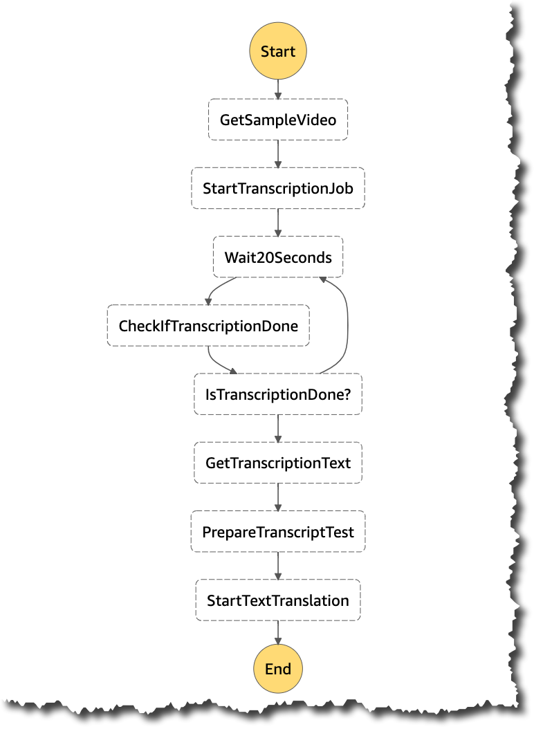
Step Functions state machine

State machine

The Step Functions state machine orchestrates the following workflow:

  1. Fetch external API metadata and create tasks required to fetch all payload.
  2. For each task, report that the task has entered Started state.
  3. Since the task is in the Started state, the next action is FetchPayload
  4. Fetch payload from the external API and store it in an S3 bucket.
  5. In case of success, move the task to a PayloadSaved state.
  6. In case of an error, report that the task is in a failed state.
  7. Report that the task has entered PayloadSaved (or failed) state.
  8. In case the task is in the PayloadSaved state, move to the SendToSQS step. If the task is in a failed state, exit.
  9. Send the S3 object pointer and additional task metadata to the SQS queue.
  10. Move the task to an enqueued state.
  11. Report that the task has entered enqueued state.
  12. Since the task is in the enqueued state, we are done.
  13. Combine the results for a single task execution.
  14. Combine the results for all the task executions.

Prerequisites to implement the solution

The following prerequisites are required for this walk-through:

Step-by-step instructions

You can use AWS Cloud9, or your preferred IDE, to deploy the AWS SAM template. Refer to the cleanup section of this post for instructions to delete the resources to stop incurring any further charges.

  1. Clone the repository by running the following command:
    git clone https://github.com/aws-samples/sam-api-poller.git
  2. Change to the sam-api-poller directory, install dependencies and build the application:
    npm install
    sam build -c -p
  3. Package and deploy the application to the AWS Cloud, following the series of prompts. Name the stack sam-api-poller:
    sam deploy --guided --capabilities CAPABILITY_NAMED_IAM
  4. SAM outputsAfter stack creation, you see ExternalHttpApiUrl, PollerHttpApiUrl, StateMachineName, and RawPayloadBucket in the outputs section.
    CloudFormation outputs
  5. Store API URLs as variables:
    POLLER_HTTP_API_URL=$(aws cloudformation describe-stacks --stack-name sam-api-poller --query "Stacks[0].Outputs[?OutputKey=='PollerHttpApiUrl'].OutputValue" --output text)
    
    EXTERNAL_HTTP_API_URL=$(aws cloudformation describe-stacks --stack-name sam-api-poller --query "Stacks[0].Outputs[?OutputKey=='ExternalHttpApiUrl'].OutputValue" --output text)
  6. Make an API call:
    REQUEST_PYLOAD=$(printf '{"url":"%s/payload"}' $EXTERNAL_HTTP_API_URL)
    EVENT_ID=$(curl -d $REQUEST_PYLOAD -H "Content-Type: application/json" -X POST $POLLER_HTTP_API_URL/jobs | jq -r '.Entries[0].EventId')
    
  7. The EventId that is returned by the API is stored in a variable. You can trace all the poller tasks related to this execution via the EventId. Run the following command to track task progress:
    curl -H "Content-Type: application/json" $POLLER_HTTP_API_URL/jobs/$EVENT_ID
  8. Inspect the output. For example:
    {"Started":9,"PayloadSaved":15,"Enqueued":11,"SuccessfullyCompleted":0,"FailedToComplete":0,"Total":35}%
  9. Navigate to the Step Functions console and choose the state machine name that corresponds to the StateMachineName from step 4. Choose an execution and inspect the visual flow.
    Workflow
  10. Inspect each individual step by clicking on it. For example, for the PollerJobComplete step, you see:
    Step output

Cleanup

  1. Make sure that the `RawPayloadBucket` bucket is empty. In case the bucket has some files, follow emptying a bucket guide.
  2. To delete all the resources permanently and stop incurring costs, navigate to the CloudFormation console. Select the sam-api-poller stack, then choose Delete -> Delete stack.

Cost optimization

For Step Functions, this example uses the Standard Workflow type because it has a visualization tool. If you are planning to re-use the solution, consider switching from standard to Express Workflows. This may be a better option for the type of workload in this example.

Conclusion

This post shows how to use Step Functions, Lambda, EventBridge, S3, API Gateway HTTP APIs, and SQS to build a serverless API poller. I show how you can deploy a sample solution, process sample payload, and store it to S3.

I also show how to perform clean-up to avoid any additional charges. You can modify this example for your needs and build a custom solution for your use case.

For more serverless learning resources, visit Serverless Land.

Speed Up Translation Jobs with a Fully Automated Translation System Assistant

Post Syndicated from Narcisse Zekpa original https://aws.amazon.com/blogs/architecture/speed-up-translation-jobs-with-a-fully-automated-translation-system-assistant/

Like other industries, translation and localization companies face the challenge of providing fast delivery at a low cost. To address this challenge, organizations use Machine Translation (MT) to complement their translator teams. MT is the use of automated software that translates text without the need of human involvement.

One of the most recent advancements is Active Custom Translation (ACT). ACT helps tailor translated text to a specific language style or terminology, per customer specifications. In the past, organizations built custom models to include ACT in their translation system. Amazon Translate has an Active Custom Translation feature, which helps customers integrate configurable MT capabilities into their translation systems, without needing to build it themselves.

This blog describes an end-to-end automated translation flow, including guidelines to manage the data involved in the ACT process. The solution combines Amazon Translate with other Amazon Web Services (AWS) such as AWS DataSync and AWS Lambda. Before exploring this architecture, let’s explain a few basic concepts specific to the translation and localization industry.

Standard translation concepts

Translation Memory. It is common to reuse previously generated outputs as components for machine translation systems. This data is commonly called Translation Memory, and is stored and exchanged according to standardized formats (TMX, TSV, or CSV).

Source Text. Translation input data is commonly exchanged as XML Localization Interchange File Format (XLIFF) documents. Amazon Translate recently added the support of XLIFF documents for batch processing.

Figure 1 illustrates a standard translation flow involving machine translation and translation memory. Once the output has been reviewed and finalized, it is part of the company’s intellectual property (IP). It can then be reincorporated into the flywheel as an input to future translation jobs.

Figure 1: Translation workflow using machine translation

Figure 1: Translation workflow using machine translation

Translation assistant solution walkthrough

When using Amazon Translate in batch mode, you must:

  • Gather together and make translation input data available to the Translation job
  • Monitor the processing and retrieval of the output
  • Implement improvised processes to integrate your Translation Management System (TMS) with AWS, as needed

As you can see, this can involve many manual steps. You must download huge files, upload them into Amazon Simple Storage Service (S3), and configure jobs. The solution shown in Figure 2 illustrates these automation activities.

Figure 2: Automated batch ACT translation solution architecture

Figure 2: Automated batch ACT translation solution architecture

Translation automation activities:

  1. Upload the translation job input data (source files, custom terminology, translation memory files).
  2. Initiate the preprocessing step. Scan input files and identify language pairs.
  3. Create an Amazon Simple Queue Service (SQS) message per language pairs and translation project.
  4. Create S3 buckets and prefixes for each translation job.
  5. Create an Amazon Translate job.
  6. Initiate a post-processing workflow, see Figure 3 (AWS Step Functions).
  7. Copy the Translation output into the output bucket.
  8. Publish an Amazon SNS notification to inform on job completion status.
  9. Download translated files back into customer environment.

In this scenario, translators are operating from their company’s internal infrastructure, although their TMS can also be hosted on the cloud. They first collect the translation input data from their TMS and drop the files onto a shared file server. These files can be XLIFF, TMX, or CSV. We use AWS DataSync to orchestrate and initiate the data transfer from on-premises into an Amazon S3 staging bucket. AWS DataSync provides a few advantages:

  • A low code solution that manages the upload/download of translation data from/to AWS
  • The ability to schedule the synchronization for both upstream and downstream and control the frequency. This allows for batching translation jobs and optimizes usage and cost for Amazon Translate
  • A single point of access to translation data, which reduces the need to manage user accounts and grants access to the data

Once the files are uploaded into the input bucket, DataSync generates an event through Amazon EventBridge. This notification invokes an AWS Lambda function that pushes a message into an Amazon SQS queue. The message contains the list of files to be translated in the current batch. SQS decouples the data upload from the actual processing. Using this workflow provides scalability, service quota limit control, and better error handling.

The queue initiates another Lambda function that creates a file hierarchy in S3 for each translation job. File-naming conventions can be used as a key to separate jobs from each other. The function also prepares translation memory and custom terminology when required. Lastly, it creates and submits the translation job.

The post-processing AWS Step Functions workflow

Amazon Translate is able to generate events into EventBridge upon job completion or failure. We use this capability to invoke a post-processing AWS Step Functions workflow. For instance, some customers must flag machine translated segments within an XLIFF file, so their translators can quickly identify them for manual review.

The flow implemented in the state machine does the following (shown in Figure 3):

  • Verifies output of Amazon Translate. Checks for completeness, confirms all segments successfully translated
  • Enriches the translation data. Flags machine translated segments by comparing input and output
  • Copies output to staging bucket. Prepares for final upload
  • Sends SNS notifications to alert operators. Notifies that the batch is complete
Figure 3: Post-processing Step Functions workflow

Figure 3: Post-processing Step Functions workflow

This solution is entirely serverless, which frees you from maintaining the infrastructure or software platform. You can focus on the core business logic, and what really differentiates you from your competitors.

As the number of translation projects grow overtime, you can also take advantage of Amazon S3 storage classes to optimize document archiving. A translation service provider can define specific rules per customer or per project. These rules can be configured automatically as the data is copied into S3. The result is that files can be transferred to cheaper storage tiers with predefined retention periods.

Conclusion

In this blog, we’ve described a solution that helps you automate the collection and transfer of translation data. It also assists in the scheduling and orchestration of translation jobs. This leads to greater productivity, reduction in cost, and faster time-to-market. Using AWS, you can decrease maintenance, and create a highly scalable and cost-effective solution. Because of the AWS pay-as-you-go model, you can assess the price per project. This information can be used in your pricing model, and be passed along as service options to your own customers.

To get started with Amazon Translate or read more, check out these blogs:

Building well-architected serverless applications: Optimizing application costs

Post Syndicated from Julian Wood original https://aws.amazon.com/blogs/compute/building-well-architected-serverless-applications-optimizing-application-costs/

This series of blog posts uses the AWS Well-Architected Tool with the Serverless Lens to help customers build and operate applications using best practices. In each post, I address the serverless-specific questions identified by the Serverless Lens along with the recommended best practices. See the introduction post for a table of contents and explanation of the example application.

COST 1. How do you optimize your serverless application costs?

Design, implement, and optimize your application to maximize value. Asynchronous design patterns and performance practices ensure efficient resource use and directly impact the value per business transaction. By optimizing your serverless application performance and its code patterns, you can directly impact the value it provides, while making more efficient use of resources.

Serverless architectures are easier to manage in terms of correct resource allocation compared to traditional architectures. Due to its pay-per-value pricing model and scale based on demand, a serverless approach effectively reduces the capacity planning effort. As covered in the operational excellence and performance pillars, optimizing your serverless application has a direct impact on the value it produces and its cost. For general serverless optimization guidance, see the AWS re:Invent talks, “Optimizing your Serverless applications” Part 1 and Part 2, and “Serverless architectural patterns and best practices”.

Required practice: Minimize external calls and function code initialization

AWS Lambda functions may call other managed services and third-party APIs. Functions may also use application dependencies that may not be suitable for ephemeral environments. Understanding and controlling what your function accesses while it runs can have a direct impact on value provided per invocation.

Review code initialization

I explain the Lambda initialization process with cold and warm starts in “Optimizing application performance – part 1”. Lambda reports the time it takes to initialize application code in Amazon CloudWatch Logs. As Lambda functions are billed by request and duration, you can use this to track costs and performance. Consider reviewing your application code and its dependencies to improve the overall execution time to maximize value.

You can take advantage of Lambda execution environment reuse to make external calls to resources and use the results for subsequent invocations. Use TTL mechanisms inside your function handler code. This ensures that you can prevent additional external calls that incur additional execution time, while preemptively fetching data that isn’t stale.

Review third-party application deployments and permissions

When using Lambda layers or applications provisioned by AWS Serverless Application Repository, be sure to understand any associated charges that these may incur. When deploying functions packaged as container images, understand the charges for storing images in Amazon Elastic Container Registry (ECR).

Ensure that your Lambda function only has access to what its application code needs. Regularly review that your function has a predicted usage pattern so you can factor in the cost of other services, such as Amazon S3 and Amazon DynamoDB.

Required practice: Optimize logging output and its retention

Considering reviewing your application logging level. Ensure that logging output and log retention are appropriately set to your operational needs to prevent unnecessary logging and data retention. This helps you have the minimum of log retention to investigate operational and performance inquiries when necessary.

Emit and capture only what is necessary to understand and operate your component as intended.

With Lambda, any standard output statements are sent to CloudWatch Logs. Capture and emit business and operational events that are necessary to help you understand your function, its integration, and its interactions. Use a logging framework and environment variables to dynamically set a logging level. When applicable, sample debugging logs for a percentage of invocations.

In the serverless airline example used in this series, the booking service Lambda functions use Lambda Powertools as a logging framework with output structured as JSON.

Lambda Powertools is added to the Lambda functions as a shared Lambda layer in the AWS Serverless Application Model (AWS SAM) template. The layer ARN is stored in Systems Manager Parameter Store.

Parameters:
  SharedLibsLayer:
    Type: AWS::SSM::Parameter::Value<String>
    Description: Project shared libraries Lambda Layer ARN
Resources:
    ConfirmBooking:
        Type: AWS::Serverless::Function
        Properties:
            FunctionName: !Sub ServerlessAirline-ConfirmBooking-${Stage}
            Handler: confirm.lambda_handler
            CodeUri: src/confirm-booking
            Layers:
                - !Ref SharedLibsLayer
            Runtime: python3.7
…

The LOG_LEVEL and other Powertools settings are configured in the Globals section as Lambda environment variable for all functions.

Globals:
    Function:
        Environment:
            Variables:
                POWERTOOLS_SERVICE_NAME: booking
                POWERTOOLS_METRICS_NAMESPACE: ServerlessAirline
                LOG_LEVEL: INFO 

For Amazon API Gateway, there are two types of logging in CloudWatch: execution logging and access logging. Execution logs contain information that you can use to identify and troubleshoot API errors. API Gateway manages the CloudWatch Logs, creating the log groups and log streams. Access logs contain details about who accessed your API and how they accessed it. You can create your own log group or choose an existing log group that could be managed by API Gateway.

Enable access logs, and selectively review the output format and request fields that might be necessary. For more information, see “Setting up CloudWatch logging for a REST API in API Gateway”.

API Gateway logging

API Gateway logging

Enable AWS AppSync logging which uses CloudWatch to monitor and debug requests. You can configure two types of logging: request-level and field-level. For more information, see “Monitoring and Logging”.

AWS AppSync logging

AWS AppSync logging

Define and set a log retention strategy

Define a log retention strategy to satisfy your operational and business needs. Set log expiration for each CloudWatch log group as they are kept indefinitely by default.

For example, in the booking service AWS SAM template, log groups are explicitly created for each Lambda function with a parameter specifying the retention period.

Parameters:
    LogRetentionInDays:
        Type: Number
        Default: 14
        Description: CloudWatch Logs retention period
Resources:
    ConfirmBookingLogGroup:
        Type: AWS::Logs::LogGroup
        Properties:
            LogGroupName: !Sub "/aws/lambda/${ConfirmBooking}"
            RetentionInDays: !Ref LogRetentionInDays

The Serverless Application Repository application, auto-set-log-group-retention can update the retention policy for new and existing CloudWatch log groups to the specified number of days.

For log archival, you can export CloudWatch Logs to S3 and store them in Amazon S3 Glacier for more cost-effective retention. You can use CloudWatch Log subscriptions for custom processing, analysis, or loading to other systems. Lambda extensions allows you to process, filter, and route logs directly from Lambda to a destination of your choice.

Good practice: Optimize function configuration to reduce cost

Benchmark your function using a different set of memory size

For Lambda functions, memory is the capacity unit for controlling the performance and cost of a function. You can configure the amount of memory allocated to a Lambda function, between 128 MB and 10,240 MB. The amount of memory also determines the amount of virtual CPU available to a function. Benchmark your AWS Lambda functions with differing amounts of memory allocated. Adding more memory and proportional CPU may lower the duration and reduce the cost of each invocation.

In “Optimizing application performance – part 2”, I cover using AWS Lambda Power Tuning to automate the memory testing process to balances performance and cost.

Best practice: Use cost-aware usage patterns in code

Reduce the time your function runs by reducing job-polling or task coordination. This avoids overpaying for unnecessary compute time.

Decide whether your application can fit an asynchronous pattern

Avoid scenarios where your Lambda functions wait for external activities to complete. I explain the difference between synchronous and asynchronous processing in “Optimizing application performance – part 1”. You can use asynchronous processing to aggregate queues, streams, or events for more efficient processing time per invocation. This reduces wait times and latency from requesting apps and functions.

Long polling or waiting increases the costs of Lambda functions and also reduces overall account concurrency. This can impact the ability of other functions to run.

Consider using other services such as AWS Step Functions to help reduce code and coordinate asynchronous workloads. You can build workflows using state machines with long-polling, and failure handling. Step Functions also supports direct service integrations, such as DynamoDB, without having to use Lambda functions.

In the serverless airline example used in this series, Step Functions is used to orchestrate the Booking microservice. The ProcessBooking state machine handles all the necessary steps to create bookings, including payment.

Booking service state machine

Booking service state machine

To reduce costs and improves performance with CloudWatch, create custom metrics asynchronously. You can use the Embedded Metrics Format to write logs, rather than the PutMetricsData API call. I cover using the embedded metrics format in “Understanding application health” – part 1 and part 2.

For example, once a booking is made, the logs are visible in the CloudWatch console. You can select a log stream and find the custom metric as part of the structured log entry.

Custom metric structured log entry

Custom metric structured log entry

CloudWatch automatically creates metrics from these structured logs. You can create graphs and alarms based on them. For example, here is a graph based on a BookingSuccessful custom metric.

CloudWatch metrics custom graph

CloudWatch metrics custom graph

Consider asynchronous invocations and review run away functions where applicable

Take advantage of Lambda’s event-based model. Lambda functions can be triggered based on events ingested into Amazon Simple Queue Service (SQS) queues, S3 buckets, and Amazon Kinesis Data Streams. AWS manages the polling infrastructure on your behalf with no additional cost. Avoid code that polls for third-party software as a service (SaaS) providers. Rather use Amazon EventBridge to integrate with SaaS instead when possible.

Carefully consider and review recursion, and establish timeouts to prevent run away functions.

Conclusion

Design, implement, and optimize your application to maximize value. Asynchronous design patterns and performance practices ensure efficient resource use and directly impact the value per business transaction. By optimizing your serverless application performance and its code patterns, you can reduce costs while making more efficient use of resources.

In this post, I cover minimizing external calls and function code initialization. I show how to optimize logging output with the embedded metrics format, and log retention. I recap optimizing function configuration to reduce cost and highlight the benefits of asynchronous event-driven patterns.

This post wraps up the series, building well-architected serverless applications, where I cover the AWS Well-Architected Tool with the Serverless Lens . See the introduction post for links to all the blog posts.

For more serverless learning resources, visit Serverless Land.


Centralize feature engineering with AWS Step Functions and AWS Glue DataBrew

Post Syndicated from Gayatri Ghanakota original https://aws.amazon.com/blogs/big-data/centralize-feature-engineering-with-aws-step-functions-and-aws-glue-databrew/

One of the key phases of a machine learning (ML) workflow is data preprocessing, which involves cleaning, exploring, and transforming the data. AWS Glue DataBrew, announced in AWS re:Invent 2020, is a visual data preparation tool that enables you to develop common data preparation steps without having to write any code or installation.

In this post, we show how to integrate the standard data preparation steps with training an ML model and running inference on a pre-trained model via DataBrew and AWS Step Functions. The solution is architected with an ML pipeline that trains the publicly available Air Quality Dataset to predict the CO levels in New York City.

Overview of solution

The following architecture diagram shows an overview of the ML workflow, which employs DataBrew for data preparation and scheduling jobs, and uses AWS Lambda and Step Functions to orchestrate ML model training and inference using the AWS Step Functions Data Science SDK. We use Amazon EventBridge to trigger the Step Functions state machine when the DataBrew job is complete.

Scope of Solution

The steps in this solution are as follows:

  1.  Import your dataset to Amazon Simple Storage Service (Amazon S3).
  2.  Launch the AWS CloudFormation stack, which deploys the following:
    1. DataBrew recipes for training and inference data.
    2.  The DataBrew job’s schedule for training and inference.
    3.  An EventBridge rule.
    4. A Lambda function that triggers the Step Functions state machine, which in turn orchestrates the states.
    5. The training state includes the following steps:
      1. Runs an Amazon SageMaker processing job to remove column headers.
      2. Performs SageMaker model training.
      3. Outputs the data to an S3 bucket to store the trained model.
    6. The inference state includes the following steps:
      1. Runs a SageMaker processing job to remove column headers.
      2. Performs a SageMaker batch transform.
      3. Outputs the data to an S3 bucket to store the predictions.

Prerequisites

For this solution, you should have the following prerequisites:

Load the dataset to Amazon S3

In this first step, we load our air quality dataset into Amazon S3.

  1. Download the Outdoor Air Quality Dataset for the years 2018, 2019, and 2020, limiting to the following options:
    1. Pollutant – CO
    2. Geographic Area – New York
    3. Monitor Site – All Sites
  2. For each year of data, split by year, month, and day, and use the data for 2018–2019 to train the model and the 2020 data to run inference.
  3. Run the following script, which stores the output into the NY_XXXX folder:
import os
import pandas as pd

def split_data(root_folder,df):
    # Create year, month and day columns
    df["year"] = pd.DatetimeIndex(df["Date"]).year
    df["month"] = pd.DatetimeIndex(df["Date"]).month
    df["day"] = pd.DatetimeIndex(df["Date"]).day
    if not os.path.exists(root_folder):
        os.mkdir(root_folder)
    for m, x1 in df.groupby(['month']):
        month_dir = os.path.join("{:02}".format(m))
        if not os.path.exists(root_folder+"/"+month_dir):
            os.mkdir(root_folder+"/"+month_dir)
        for d, x2 in x1.groupby(["day"]):
            day_dir = os.path.join("{:02}".format(d))
            if not os.path.exists(root_folder+"/"+month_dir+"/"+day_dir):
                os.mkdir(root_folder+"/"+month_dir+"/"+day_dir)
            p = os.path.join(root_folder+"/"+month_dir+"/"+day_dir, "{:02}.csv".format(d))
            x2.to_csv(p, index=False)

ny_data_2018 = pd.read_csv("<path to downloaded 2018 data  file>")
ny_data_2019 = pd.read_csv("<path to downloaded 2019 data file>")
ny_data_2020 = pd.read_csv("<path to downloaded 2020 data file>") 
 
split_data("NY_2018", ny_data_2018)
split_data("NY_2019", ny_data_2019)
split_data("NY_2020", ny_data_2020)
  1. Create an S3 bucket in the us-east-1 Region and upload the folders NY_2018 and NY_2019 to the path S3://<artifactbucket>/train_raw_data/.

train-raw-data-s3

  1. Upload the folder NY_2020 to S3:// <artifactbucket>/inference_raw_data/.

inference-raw-data-s3

Deploy your resources

For a quick start of this solution, you can deploy the provided AWS CloudFormation stack. This creates all the required resources in your account (us-east-1 Region), including the DataBrew datasets, jobs, projects, and recipes; the Step Functions train and inference state machines (which include SageMaker processing, model training, and batch transform jobs); an EventBridge rule; and the Lambda function to deploy an end-to-end ML pipeline for a predefined S3 bucket.

  1. Launch the following stack:
  2. For ArtifactBucket, enter the name of the S3 bucket you created in the previous step.

enter cloud formation stack details

  1. Select the three acknowledgement check boxes.
  2. Choose Create stack.

Create Cloud Formation Stack

Test the solution

As part of the CloudFormation template, the DataBrew job km-mlframework-trainingfeatures-job was created, which is scheduled to run every Monday at 10:00 AM UTC. This job creates the features required to train the model.

When the template deployment is successfully completed, you can manually activate the training pipeline. For this, navigate to the DataBrew console, select the DataBrew job km-mlframework-trainingfeatures-job, and choose Run job.

Glue DataBrew Run Train Job

The job writes the features to s3://<artifactbucket>/train_features/.

When the job is complete, an EventBridge rule invokes the Lambda function, which orchestrates the SageMaker training jobs via Step Functions.

Step Function Train Job

When the job is complete, the output of the model is stored in s3://<artifactbucket>/artifact-repo/model/.

In the next step, we trigger the DataBrew job km-mlframework-inferencefeatures-job, which is scheduled to run every Tuesday at 10:00 AM UTC. This job creates the inference features that are used to run inference on the trained model.

You can also activate the inference pipeline by manually triggering the DataBrew job on the DataBrew console.

Glue DataBrew Inference Job

The job writes the features to s3://<artifactbucket>/ inference_features/.

When the job is complete, an EventBridge rule invokes the Lambda function, which orchestrates the SageMaker batch transform job via Step Functions.

Inference Step Function

When the job is complete, the predictions are written to s3://<artifactbucket>/predictions/.

For more information on DataBrew steps and building a DataBrew recipe, see Preparing data for ML models using AWS Glue DataBrew in a Jupyter notebook.

Clean up

To avoid incurring future charges, complete the following steps:

  1. Wait for any currently running activity to complete, or manually stop it (DataBrew, Step Functions, SageMaker).
  2. Delete the scheduled DataBrew jobs km-mlframework-trainingfeatures-job and km-mlframework-inferencefeatures-job. This ensures the jobs aren’t started by the schedule.
  3. Delete the S3 bucket created to store data and model artifacts.
  4. Delete the CloudFormation stack created earlier.

Conclusion

DataBrew is designed to support data engineers and data scientists to experiment with data preparation steps via a visual interface. With more than 250 built-in transformations, DataBrew can be a strong tool to accelerate your ML lifecycle for development and production stages.

In this post, we walked through the process of creating an end-to-end ML framework with DataBrew, which you can use to train an ML model as well as run inferences on a schedule. You can use the same framework with your own DataBrew recipe prepared using any dataset.

To learn more on applying the most frequently used transformations from within DataBrew, see 7 most common data preparation transformations in AWS Glue DataBrew.


About the Authors

Gayatri Ghanakota is a Machine Learning Engineer with AWS Professional Services, where she helps customers build machine learning solutions on AWS. She is passionate about developing, deploying, and explaining ML models.

Surbhi Dangi is a product and design leader at Amazon Web Services. She focusses on providing ease of use and rich functionality for her analytics and monitoring on both her products – Amazon CloudWatch Synthetics and AWS Glue DataBrew. When not working, she mentors aspiring product managers, hiking, and traveling the world.

Building well-architected serverless applications: Optimizing application performance – part 2

Post Syndicated from Julian Wood original https://aws.amazon.com/blogs/compute/building-well-architected-serverless-applications-optimizing-application-performance-part-2/

This series of blog posts uses the AWS Well-Architected Tool with the Serverless Lens to help customers build and operate applications using best practices. In each post, I address the serverless-specific questions identified by the Serverless Lens along with the recommended best practices. See the introduction post for a table of contents and explanation of the example application.

PERF 1. Optimizing your serverless application’s performance

This post continues part 1 of this security question. Previously, I cover measuring and optimizing function startup time. I explain cold and warm starts and how to reuse the Lambda execution environment to improve performance. I show a number of ways to analyze and optimize the initialization startup time. I explain how only importing necessary libraries and dependencies increases application performance.

Good practice: Design your function to take advantage of concurrency via asynchronous and stream-based invocations

AWS Lambda functions can be invoked synchronously and asynchronously.

Favor asynchronous over synchronous request-response processing.

Consider using asynchronous event processing rather than synchronous request-response processing. You can use asynchronous processing to aggregate queues, streams, or events for more efficient processing time per invocation. This reduces wait times and latency from requesting apps and functions.

When you invoke a Lambda function with a synchronous invocation, you wait for the function to process the event and return a response.

Synchronous invocation

Synchronous invocation

As synchronous processing involves a request-response pattern, the client caller also needs to wait for a response from a downstream service. If the downstream service then needs to call another service, you end up chaining calls that can impact service reliability, in addition to response times. For example, this POST /order request must wait for the response to the POST /invoice request before responding to the client caller.

Example synchronous processing

Example synchronous processing

The more services you integrate, the longer the response time, and you can no longer sustain complex workflows using synchronous transactions.

Asynchronous processing allows you to decouple the request-response using events without waiting for a response from the function code. This allows you to perform background processing without requiring the client to wait for a response, improving client performance. You pass the event to an internal Lambda queue for processing and Lambda handles the rest. An external process, separate from the function, manages polling and retries. Using this asynchronous approach can also make it easier to handle unpredictable traffic with significant volumes.

Asynchronous invocation

Asynchronous invocation

For example, the client makes a POST /order request to the order service. The order service accepts the request and returns that it has been received, without waiting for the invoice service. The order service then makes an asynchronous POST /invoice request to the invoice service, which can then process independently of the order service. If the client must receive data from the invoice service, it can handle this separately via a GET /invoice request.

Example asynchronous processing

Example asynchronous processing

You can configure Lambda to send records of asynchronous invocations to another destination service. This helps you to troubleshoot your invocations. You can also send messages or events that can’t be processed correctly into a dedicated Amazon Simple Queue Service (SQS) dead-letter queue for investigation.

You can add triggers to a function to process data automatically. For more information on which processing model Lambda uses for triggers, see “Using AWS Lambda with other services”.

Asynchronous workflows handle a variety of use cases including data Ingestion, ETL operations, and order/request fulfillment. In these use-cases, data is processed as it arrives and is retrieved as it changes. For example asynchronous patterns, see “Serverless Data Processing” and “Serverless Event Submission with Status Updates”.

For more information on Lambda synchronous and asynchronous invocations, see the AWS re:Invent presentation “Optimizing your serverless applications”.

Tune batch size, batch window, and compress payloads for high throughput

When using Lambda to process records using Amazon Kinesis Data Streams or SQS, there are a number of tuning parameters to consider for performance.

You can configure a batch window to buffer messages or records for up to 5 minutes. You can set a limit of the maximum number of records Lambda can process by setting a batch size. Your Lambda function is invoked whichever comes first.

For high volume SQS standard queue throughput, Lambda can process up to 1000 concurrent batches of records per second. For more information, see “Using AWS Lambda with Amazon SQS”.

For high volume Kinesis Data Streams throughput, there are a number of options. Configure the ParallelizationFactor setting to process one shard of a Kinesis Data Stream with more than one Lambda invocation simultaneously. Lambda can process up to 10 batches in each shard. For more information, see “New AWS Lambda scaling controls for Kinesis and DynamoDB event sources.” You can also add more shards to your data stream to increase the speed at which your function can process records. This increases the function concurrency at the expense of ordering per shard. For more details on using Kinesis and Lambda, see “Monitoring and troubleshooting serverless data analytics applications”.

Kinesis enhanced fan-out can maximize throughput by dedicating a 2 MB/second input/output channel per second per consumer instead of 2 MB per shard. For more information, see “Increasing stream processing performance with Enhanced Fan-Out and Lambda”.

Kinesis stream producers can also compress records. This is at the expense of additional CPU cycles for decompressing the records in your Lambda function code.

Required practice: Measure, evaluate, and select optimal capacity units

Capacity units are a unit of consumption for a service. They can include function memory size, number of stream shards, number of database reads/writes, request units, or type of API endpoint. Measure, evaluate and select capacity units to enable optimal configuration of performance, throughput, and cost.

Identify and implement optimal capacity units.

For Lambda functions, memory is the capacity unit for controlling the performance of a function. You can configure the amount of memory allocated to a Lambda function, between 128 MB and 10,240 MB. The amount of memory also determines the amount of virtual CPU available to a function. Adding more memory proportionally increases the amount of CPU, increasing the overall computational power available. If a function is CPU-, network- or memory-bound, then changing the memory setting can dramatically improve its performance.

Choosing the memory allocated to Lambda functions is an optimization process that balances performance (duration) and cost. You can manually run tests on functions by selecting different memory allocations and measuring the time taken to complete. Alternatively, use the AWS Lambda Power Tuning tool to automate the process.

The tool allows you to systematically test different memory size configurations and depending on your performance strategy – cost, performance, balanced – it identifies what is the most optimum memory size to use. For more information, see “Operating Lambda: Performance optimization – Part 2”.

AWS Lambda Power Tuning report

AWS Lambda Power Tuning report

Amazon DynamoDB manages table processing throughput using read and write capacity units. There are two different capacity modes, on-demand and provisioned.

On-demand capacity mode supports up to 40K read/write request units per second. This is recommended for unpredictable application traffic and new tables with unknown workloads. For higher and predictable throughputs, provisioned capacity mode along with DynamoDB auto scaling is recommended. For more information, see “Read/Write Capacity Mode”.

For high throughput Amazon Kinesis Data Streams with multiple consumers, consider using enhanced fan-out for dedicated 2 MB/second throughput per consumer. When possible, use Kinesis Producer Library and Kinesis Client Library for effective record aggregation and de-aggregation.

Amazon API Gateway supports multiple endpoint types. Edge-optimized APIs provide a fully managed Amazon CloudFront distribution. These are better for geographically distributed clients. API requests are routed to the nearest CloudFront Point of Presence (POP), which typically improves connection time.

Edge-optimized API Gateway deployment

Edge-optimized API Gateway deployment

Regional API endpoints are intended when clients are in the same Region. This helps you to reduce request latency and allows you to add your own content delivery network if necessary.

Regional endpoint API Gateway deployment

Regional endpoint API Gateway deployment

Private API endpoints are API endpoints that can only be accessed from your Amazon Virtual Private Cloud (VPC) using an interface VPC endpoint. For more information, see “Creating a private API in Amazon API Gateway”.

For more information on endpoint types, see “Choose an endpoint type to set up for an API Gateway API”. For more general information on API Gateway, see the AWS re:Invent presentation “I didn’t know Amazon API Gateway could do that”.

AWS Step Functions has two workflow types, standard and express. Standard Workflows have exactly once workflow execution and can run for up to one year. Express Workflows have at-least-once workflow execution and can run for up to five minutes. Consider the per-second rates you require for both execution start rate and the state transition rate. For more information, see “Standard vs. Express Workflows”.

Performance load testing is recommended at both sustained and burst rates to evaluate the effect of tuning capacity units. Use Amazon CloudWatch service dashboards to analyze key performance metrics including load testing results. I cover performance testing in more detail in “Regulating inbound request rates – part 1”.

For general serverless optimization information, see the AWS re:Invent presentation “Serverless at scale: Design patterns and optimizations”.

Conclusion

Evaluate and optimize your serverless application’s performance based on access patterns, scaling mechanisms, and native integrations. You can improve your overall experience and make more efficient use of the platform in terms of both value and resources.

This post continues from part 1 and looks at designing your function to take advantage of concurrency via asynchronous and stream-based invocations. I cover measuring, evaluating, and selecting optimal capacity units.

This well-architected question will continue in part 3 where I look at integrating with managed services directly over functions when possible. I cover optimizing access patterns and applying caching where applicable.

For more serverless learning resources, visit Serverless Land.