Tag Archives: Intermediate (200)

Keep your firewall rules up-to-date with Network Firewall features

2024-10-01 Salman Ahmed

Post Syndicated from Salman Ahmed original https://aws.amazon.com/blogs/security/keep-your-firewall-rules-up-to-date-with-network-firewall-features/

AWS Network Firewall is a managed firewall service that makes it simple to deploy essential network protections for your virtual private clouds (VPCs) on AWS. Network Firewall automatically scales with your traffic, and you can define firewall rules that provide fine-grained control over network traffic.

When you work with security products in a production environment, you need to maintain a consistent effort to keep the security rules synchronized as you make modifications to your environment. To stay aligned with your organization’s best practices, you should diligently review and update security rules, but this can increase your team’s operational overhead.

Since the launch of Network Firewall, we have added new capabilities that simplify your efforts by using managed rules and automated methods to help keep your firewall rules current. This approach can streamline operations for your team and help enhance security by reducing the risk of failures stemming from manual intervention or customer automation processes. You can apply regularly updated security rules with just a few clicks, enabling a wide range of comprehensive protection measures.

In this blog post, I discuss three features—managed rule groups, prefix lists, and tag-based resource groups—offering an in-depth look at how Network Firewall operates to assist you in keeping your rule sets current and effective.

Prerequisites

If this is your first time using Network Firewall, make sure to complete the following prerequisites. However, if you already created rule groups, a firewall policy, and a firewall, then you can skip this section.

Network Firewall and AWS managed rule groups

AWS managed rule groups are collections of predefined, ready-to-use rules that AWS maintains on your behalf. You can use them to address common security use cases and help protect your environment from various types of threats. This can help you stay current with the evolving threat landscape and security best practices.

AWS managed rule groups are available for no additional cost to customers who use Network Firewall. When you work with a stateful rule group—a rule group that uses Suricata-compatible intrusion prevention system (IPS) specifications—you can integrate managed rules that help provide protection from botnet, malware, and phishing attempts.

AWS offers two types of managed rule groups: domain and IP rule groups and threat signature rule groups. AWS regularly maintains and updates these rule groups, so you can use them to help protect against constantly evolving security threats.

When you use Network Firewall, one of the use cases is to protect your outbound traffic from compromised hosts, malware, and botnets. To help meet this requirement, you can use the domain and IP rule group. You can select domain and IP rules based on several factors, such as the following:

Domains that are generally legitimate but now are compromised and hosting malware
Domains that are known for hosting malware
Domains that are generally legitimate but now are compromised and hosting botnets
Domains that are known for hosting botnets

The threat signature rule group offers additional protection by supporting several categories of threat signatures to help protect against various types of malware and exploits, denial of service attempts, botnets, web attacks, credential phishing, scanning tools, and mail or messaging attacks.

To use Network Firewall managed rules

Update the existing firewall policy that you created as part of the Prerequisites for this post or create a new firewall policy.
Add a managed rule group to your policy and select from Domain and IP rule groups or Threat signature rule groups.

Figure 1 illustrates the use of AWS managed rules. It shows both the domain and IP rule group and the threat signature rule group, and it includes one specific rule or category from each as a demonstration.

Figure 1: Network Firewall deployed with AWS managed rules

As shown in Figure 1, the process for using AWS managed rules has the following steps:

The Network Firewall policy contains managed rules from the domain and IP rule groups and threat signature rule groups.
If the traffic from a protected subnet passes the checks of the firewall policy as it goes to the Network Firewall endpoint, then it proceeds to the NAT gateway and the internet gateway (depicted with the dashed line in the figure).
If traffic from a protected subnet fails the checks of the firewall policy, the traffic is dropped at the Network Firewall endpoint (depicted with the dotted line).

Inner workings of AWS managed rules

Let’s go deeper into the underlying mechanisms and processes that AWS uses for managed rules. After you configure your firewall with these managed rules, you gain the benefits of the up-to-date rules that AWS manages. AWS pulls updated rule content from the managed rules provider on a fixed cadence for domain-based rules and other managed rule groups.

The Network Firewall team operates a serverless processing pipeline powered by AWS Lambda. This processes the rules from the vendor source, first fetching them so that they can be manipulated and transformed into the managed rule groups. Then the rules are mapped to the appropriate category based on their metadata. The final rules are uploaded to Amazon Simple Storage Service (Amazon S3) to prepare for propagation in each AWS Region.

Finally, Network Firewall processes the rule group content Region by Region, updating the managed rule group object associated with your firewall with the new content from the vendor. For threat signature rule groups, subscribers receive an SNS notification, letting them know that the rules have been updated.

AWS handles the tasks associated with this process so you can deploy and secure your workloads while addressing evolving security threats.

Network Firewall and prefix lists

Network Firewall supports Amazon Virtual Private Cloud (Amazon VPC) prefix lists to simplify management of your firewall rules and policies across your VPCs. With this capability, you can define a prefix list one time and reference it in your rules later. For example, with prefix lists, you can group multiple CIDR blocks into a single object instead of managing them at an individual IP level by creating a prefix list for their specific use case.

AWS offers two types of prefix lists: AWS-managed prefix lists and customer-managed prefix lists. In this post, we focus on customer-managed prefix lists. With customer-managed prefix lists, you can define and maintain your own sets of IP address ranges to meet your specific needs. Although you operate these prefix lists and can add and remove IP addresses, AWS controls and maintains the integration of these prefix lists with Network Firewall.

To use a Network Firewall prefix list

Create a prefix list.
Update your existing rule group that you created as part of the Prerequisites for this post or create a new rule group.
Use IP set references in Suricata compatible rule groups. In the IP set references section, select Edit, and in the Resource ID section, select the prefix list that you created.

Figure 2 illustrates Network Firewall deployed with a prefix list.

Figure 2: Network Firewall deployed with prefix list

As shown in Figure 2, we use the same design as in our previous example:

We use a prefix list that is referenced in our rule group.
The traffic from the protected subnet goes through the Network Firewall endpoint and NAT gateway and then to the internet gateway. As it passes through the Network Firewall endpoint, the firewall policy that contains the rule group determines if the traffic is allowed or not according to the policy.

Inner workings of prefix lists

After you configure a rule group that references a prefix list, Network Firewall automatically keeps the associated rules up to date. Network Firewall creates an IP set object that corresponds to this prefix list. This IP set object is how Network Firewall internally tracks the state of the prefix list reference, and it contains both resolved IP addresses from the source and additional metadata that’s associated with the IP set, such as which rule groups reference it. AWS manages these references and uses them to track which firewalls need to be updated when the content of these IP sets change.

The Network Firewall orchestration engine is integrated with prefix lists, and it works in conjunction with Amazon VPC to keep the resolved IPs up to date. The orchestration engine automatically refreshes IPs associated with a prefix list, whether that prefix list is AWS-managed or customer-managed.

When you use a prefix list with Network Firewall, AWS handles a significant portion of the work on your behalf. This managed approach simplifies the process while providing the flexibility that you need to customize the allow or deny list of IP addresses according to your specific security requirements.

Network Firewall and tag-based resource groups

With Network Firewall, you can now use tag-based resource groups to simplify managing your firewall rules. A resource group is a collection of AWS resources that are in the same Region, and that match the criteria specified in the group’s query. A tag-based resource group bases its membership on a query that specifies a list of resource types and tags. Tags are key value pairs that help identify and sort your resources within your organization.

In your stateful firewall rules, you can reference a resource group that you have created for a specific set of Amazon Elastic Compute Cloud (Amazon EC2) instances or elastic network interfaces (ENIs). When these resources change, you don’t have to update your rule group every time. Instead, you can use a tagging policy for the resources that are in your tag-based resource group.

As your AWS environment changes, it’s important to make sure that new resources are using the same egress rules as the current resources. However, managing the changing EC2 instances due to workload changes creates an operational overhead. By using tag-based resource groups in your rules, you can eliminate the need to manually manage the changing resources in your AWS environment.

To use Network Firewall resource groups with a stateful rule group

Create Network Firewall resource groups – Create a resource group for each of two applications. For the example in this blog post, enter the name rg-app-1 for application 1, and rg-app-2 for application 2.
Update your existing rule group that you created as a part of the Prerequisites for this post or create a new rule group. In the IP set references section, select Edit; and in the Resource ID section, choose the resource groups that you created in the previous step (rg-app-1 and rg-app-2).

Now as your EC2 instance or ENIs scale, those resources stay in sync automatically.

Figure 3 illustrates resource groups with a stateful rule group.

Figure 3: Network Firewall deployed with resource groups

As shown in Figure 3, we tagged the EC2 instances as app-1 or app-2. In your stateful rule group, restrict access to a website for app-2, but allow it for app-1:

We use the resource group that is referenced in our rule group.
The traffic from the protected subnet goes through the Network Firewall endpoint and the NAT gateway and then to the internet gateway. As it passes through the Network Firewall endpoint, the firewall policy that contains the rule group referencing the specific resource group determines how to handle the traffic. In the figure, the dashed line shows that the traffic is allowed while the dotted line shows it’s denied based on this rule.

Inner workings of resource groups

For tag-based resource groups, Network Firewall works with resource groups to automatically refresh the contents of the Network Firewall resource groups. Network Firewall first resolves the resources that are associated with the resource group, which are EC2 instances or ENIs that match the tag-based query specified. Then it resolves the IP addresses associated with these resources by calling the relevant Amazon EC2 API.

After the IP addresses are resolved, through either a prefix list or Network Firewall resource group, the IP set is ready for propagation. Network Firewall uploads the refreshed content of the IP set object to Amazon S3, and the data plane capacity (the hardware responsible for packet processing) fetches this new configuration. The stateful firewall engine accepts and applies these updates, which allows your rules to apply to the new IP set content.

By using tag-based resource groups within your workloads, you can delegate a substantial amount of your firewall management tasks to AWS, enhancing efficiency and reducing manual efforts on your part.

Considerations

When you use a managed rule group in your firewall policy, you can edit the following setting: Set rule actions to alert. This will override all rule actions in the rule group to alert which is useful for testing a rule group before using it control your traffic.
Managed rule groups count against the limit of stateful rules for each policy. For more information, see AWS Network Firewall quotas and setting rule group capacity in AWS Network Firewall.
When working with prefix lists and resource groups, make sure that you understand the Limits for IP set references.

Conclusion

In this blog post, you learned how to use Network Firewall managed rule groups, prefix lists, and tag-based resource groups to harness the automation and user-friendly capabilities of Network Firewall. You also learned more detail about how AWS operates these features on your behalf, to help you deploy a simple-to-use and secure solution. Enhance your current or new Network Firewall deployments by integrating these features today.

If you have feedback about this post, submit comments in the Comments section below. If you have questions about this post, contact AWS Support.

Exploring Telemetry Events in Amazon Q Developer

2024-09-30 David Ernst

Post Syndicated from David Ernst original https://aws.amazon.com/blogs/devops/exploring-telemetry-events-in-amazon-q-developer/

As organizations increasingly adopt Amazon Q Developer, understanding how developers use it is essential. Diving into specific telemetry events and user-level data clarifies how users interact with Amazon Q Developer, offering insights into feature usage and developer behaviors. This granular view, accessible through logs, is vital for identifying trends, optimizing performance, and enhancing the overall developer experience. This blog is intended to give visibility to key telemetry events logged by Amazon Q Developer and how to explore this data to gain insights.

To help you get started, the following sections will walk through several practical examples that showcase how to extract meaningful insights from AWS CloudTrail. By reviewing the logs, organizations can track usage patterns, identify top users, and empower them to train and mentor other developers, ultimately fostering broader adoption and engagement across teams.

Although the examples here focus on Amazon Athena for querying logs, the methods can be adapted to integrate with other tools like Splunk or Datadog for further analysis. Through this exploration, readers will learn how to query the log data to understand better how Amazon Q Developer is used within your organization.

Solution Overview

Architecture diagram illustrating the solution using Amazon Q Developer's logs from the IDE and terminal, captured in AWS CloudTrail. The logs are stored in Amazon S3 and queried using Amazon Athena to analyze feature usage, including in-line code suggestions, chat interactions, and security scanning events.

This solution leverages Amazon Q Developer’s logs from the Integrated Development Environment (IDE) and terminal, captured in AWS CloudTrail. The logs will be queried directly using Amazon Athena from Amazon Simple Storage Service (Amazon S3) to analyze feature usage, such as in-line code suggestions, chat interactions, and security scanning events.

Analyzing Telemetry Events in Amazon Q Developer

Amazon Athena is used to query the CloudTrail logs directly to analyze this data. By utilizing Athena, queries can be run on existing CloudTrail records, making it simple to extract insights from the data in its current format.

Ensuring CloudTrail is set up to log the data events.

Navigate to the AWS CloudTrail Console.
Edit an Existing Trail:
- If you have a trail, verify it is configured to log data events for Amazon CodeWhisperer.
- Note: As of 4/30/24, CodeWhisperer has been renamed to Amazon Q Developer. All the functionality previously provided by CodeWhisperer is now part of Amazon Q Developer. However, for consistency, the original API names have been retained.
Click on your existing trail in CloudTrail. Find the Data Events section and click edit.
- For CodeWhisperer:
  - Data event type: CodeWhisperer
  - Log selector template: Log all events
Save your changes.
Note your “Trail log location.” This S3 bucket will be used in our Athena setup.

If you don’t have an existing trail, follow the instructions in the AWS CloudTrail User Guide to set up a new trail.

Below is a screenshot of the data events addition:

Screenshot showing the configuration of data events in AWS CloudTrail. The image illustrates the setup for logging data events for CodeWhisperer, including log selector templates ("Log all events").

Steps to Create an Athena Table from CloudTrail Logs: This step aims to turn CloudTrail events into a queryable Athena table.

1. Navigate to the AWS Management Console > Athena > Editor.

2. Click on the plus to create a query tab.

3. Run the following query to create a database and table. Note to update the location to your S3 bucket.

-- Step 1: Create a new database (if it doesn't exist)
CREATE DATABASE IF NOT EXISTS amazon_q_metrics;

-- Step 2: Create the external table explicitly within the new database
CREATE EXTERNAL TABLE amazon_q_metrics.cloudtrail_logs (

    userIdentity STRUCT<
        accountId: STRING,
        onBehalfOf: STRUCT<
            userId: STRING,
            identityStoreArn: STRING
        >
    >,  
    eventTime STRING,
    eventSource STRING,
    eventName STRING,
    requestParameters STRING,
    requestId STRING,
    eventId STRING,
    resources ARRAY<STRUCT<
        arn: STRING,
        accountId: STRING,
        type: STRING
    >>,
    recipientAccountId STRING

)
ROW FORMAT SERDE 'org.apache.hive.hcatalog.data.JsonSerDe'
STORED AS INPUTFORMAT 'com.amazon.emr.cloudtrail.CloudTrailInputFormat'
OUTPUTFORMAT 'org.apache.hadoop.hive.ql.io.HiveIgnoreKeyTextOutputFormat'
LOCATION 's3://{Insert Bucket Name from CloudTrail}/'
TBLPROPERTIES ('classification'='cloudtrail');

4. Click Run

5. Run a quick query to view the data.

SELECT 
    eventTime,
    userIdentity.onBehalfOf.userId AS user_id,
    eventName,
    requestParameters
FROM 
    amazon_q_metrics.cloudtrail_logs AS logs
WHERE 
    eventName = 'SendTelemetryEvent'
LIMIT 10;

In this section, the significance of the telemetry events captured in the requestParameters field will be explained. The query begins by displaying key fields and their data, offering insights into how users interact with various features of Amazon Q Developer.

Query Breakdown:

eventTime: This field captures the time the event was recorded, providing insights into when specific user interactions took place.
userIdentity.onBehalfOf.userId: This extracts the userId of the user. This is critical for attributing interactions to the correct user, which will be covered in more detail later in the blog.
eventName: The query is filtered on SendTelemetryEvent. Telemetry events are triggered when the user interacts with particular features or when a developer uses the service.
requestParameters: The requestParameters field is crucial because it holds the details of the telemetry events. This field contains a rich set of information depending on the type of interaction and feature the developer uses, which programming languages are used, completion types, or code modifications.

In the context of the SendTelemetryEvent, various telemetry events are captured in the requestParameters field of CloudTrail logs. These events provide insights into user interactions, overall usage, and the effectiveness of Amazon Q Developer’s suggestions. Here are the key telemetry events along with their descriptions:

UserTriggerDecisionEvent
- Description: This event is triggered when a user interacts with a suggestion made by Amazon Q Developer. It captures whether the suggestion was accepted or rejected, along with relevant metadata.
- Key Fields:
  - completionType: Whether the completion was a block or a line.
  - suggestionState: Whether the user accepted, rejected, or discarded the suggestion.
  - programmingLanguage: The programming language associated with the suggestion.
  - generatedLine: The number of lines generated by the suggestion.
CodeScanEvent
- Description: This event is logged when a code scan is performed. It helps track the scope and result of the scan, providing insights into security and code quality checks.
- Key Fields:
  - codeAnalysisScope: Whether the scan was performed at the file level or the project level.
  - programmingLanguage: The language being scanned.
CodeScanRemediationsEvent
- Description: This event captures user interactions with Amazon Q Developer’s remediation suggestions, such as applying fixes or viewing issue details.
- Key Fields:
  - CodeScanRemediationsEventType: The type of remediation action taken (e.g., viewing details or applying a fix).
  - includesFix: A boolean indicating whether the user applied a fix.
ChatAddMessageEvent
- Description: This event is triggered when a new message is added to an ongoing chat conversation. It captures the user’s intent which refers to the purpose or goal the user is trying to achieve with the chat message. The intent can include various actions, such as suggesting alternate implementations of the code, applying common best practices, improving the quality or performance of the code.
- Key Fields:
  - conversationId: The unique identifier for the conversation.
  - messageId: The unique identifier for the chat message.
  - userIntent: The user’s intent, such as improving code or explaining code.
  - programmingLanguage: The language related to the chat message.
ChatInteractWithMessageEvent
- Description: This event captures when users interact with chat messages, such as copying code snippets, clicking links, or hovering over references.
- Key Fields:
  - interactionType: The type of interaction (e.g., copy, hover, click).
  - interactionTarget: The target of the interaction (e.g., a code snippet or a link).
  - acceptedCharacterCount: The number of characters from the message that were accepted.
  - acceptedSnippetHasReference: A boolean indicating if the accepted snippet included a reference.
TerminalUserInteractionEvent
- Description: This event logs user interactions with terminal commands or completions in the terminal environment.
- Key Fields:
  - terminalUserInteractionEventType: The type of interaction (e.g., terminal translation or code completion).
  - isCompletionAccepted: A boolean indicating whether the completion was accepted by the user.
  - terminal: The terminal environment in which the interaction occurred.
  - shell: The shell used for the interaction (e.g., Bash, Zsh).

For a full exploration of all event types and their detailed fields, you can refer to the official schema reference for Amazon Q Developer.

Telemetry events are key to understanding how users engage with Amazon Q Developer. They track interactions such as code completion, security scans, and chat-based suggestions. Analyzing the data in the requestParameters field helps reveal usage patterns and behaviors that offer valuable insights.

By exploring events such as UserTriggerDecisionEvent, ChatAddMessageEvent, TerminalUserInteractionEvent, and others in the schema, organizations can assess the effectiveness of Amazon Q Developer and identify areas for improvement.

Example Queries for Analyzing Developer Engagement

To gain deeper insights into how developers interact with Amazon Q Developer, the following queries can help analyze key telemetry data from CloudTrail logs. These queries track in-line code suggestions, chat interactions, and code-scanning activities. By running these queries, you can uncover valuable metrics such as the frequency of accepted suggestions, the types of chat interactions, and the programming languages most frequently scanned. This analysis helps paint a clear picture of developer engagement and usage patterns, guiding efforts to enhance productivity.

These four examples only cover a sample set of the available telemetry events, but they serve as a starting point for further exploration of Amazon Q Developer’s capabilities.

Query 1: Analyzing Accepted In-Line Code Suggestions

SELECT 
    eventTime,
    userIdentity.onBehalfOf.userId AS user_id,
    eventName,
    json_extract_scalar(requestParameters, '$.telemetryEvent.userTriggerDecisionEvent.suggestionState') AS suggestionState,
    json_extract_scalar(requestParameters, '$.telemetryEvent.userTriggerDecisionEvent.completionType') AS completionType
FROM 
    amazon_q_metrics.cloudtrail_logs
WHERE 
    eventName = 'SendTelemetryEvent'
    AND json_extract(requestParameters, '$.telemetryEvent.userTriggerDecisionEvent') IS NOT NULL
    AND json_extract_scalar(requestParameters, '$.telemetryEvent.userTriggerDecisionEvent.suggestionState') = 'ACCEPT';

Use Case:This use case focuses on how developers interact with in-line code suggestions by analyzing accepted snippets. It helps identify which users are accepting suggestions, the type of snippets being accepted (blocks or lines), and the programming languages involved. Understanding these patterns can reveal how well Amazon Q Developer aligns with the developers’ expectations.

Query Explanation: The query retrieves the event time, user ID, event name, suggestion state (filtered to show only ACCEPT), and completion type. TotalGeneratedLinesBlockAccept and totalGeneratedLinesLineAccept or discarded suggestions are not included, but this gives an idea of the developers using the service for in-line code suggestions and the lines or blocks they have accepted. Additionally, the programming language field can be extracted to see which languages are used during these interactions.

Query 2: Analyzing Chat Interactions

SELECT 
    userIdentity.onBehalfOf.userId AS userId,
    json_extract_scalar(requestParameters, '$.telemetryEvent.chatInteractWithMessageEvent.interactionType') AS interactionType,
    COUNT(*) AS eventCount
FROM 
    amazon_q_metrics.cloudtrail_logs
WHERE 
    eventName = 'SendTelemetryEvent'
    AND json_extract(requestParameters, '$.telemetryEvent.chatInteractWithMessageEvent') IS NOT NULL
GROUP BY 
    userIdentity.onBehalfOf.userId,
    json_extract_scalar(requestParameters, '$.telemetryEvent.chatInteractWithMessageEvent.interactionType')
ORDER BY 
    eventCount DESC;

Use Case: This use case looks at how developers use chat options like upvoting, downvoting, and copying code snippets. Understanding the chat usage patterns shows which interactions are most used and how developers engage with Amazon Q Developer chat. As an organization, this insight can help support other developers in successfully leveraging this feature.

Query Explanation: The query provides insights into chat interactions within Amazon Q Developer by retrieving user IDs, interaction types, and event counts. This query aggregates data based on the interactionType field within chatInteractWithMessageEvent, showcasing various user actions such as UPVOTE, DOWNVOTE, INSERT_AT_CURSOR, COPY_SNIPPET, COPY, CLICK_LINK, CLICK_BODY_LINK, CLICK_FOLLOW_UP, and HOVER_REFERENCE.

This analysis highlights how users engage with the chat feature and the interactions, offering a view of interaction patterns. By focusing on the interactionType field, you can better understand how developers interact with the chat feature of Amazon Q Developer.

Query 3: Analyzing Code Scanning Jobs Across Programming Languages

SELECT 
    userIdentity.onBehalfOf.userId AS userId,
    json_extract_scalar(requestParameters, '$.telemetryEvent.codeScanEvent.programmingLanguage.languageName') AS programmingLanguage,
    COUNT(json_extract_scalar(requestParameters, '$.telemetryEvent.codeScanEvent.codeScanJobId')) AS jobCount
FROM 
    amazon_q_metrics.cloudtrail_logs
WHERE 
    eventName = 'SendTelemetryEvent'
    AND json_extract(requestParameters, '$.telemetryEvent.codeScanEvent') IS NOT NULL
GROUP BY 
    userIdentity.onBehalfOf.userId,
    json_extract_scalar(requestParameters, '$.telemetryEvent.codeScanEvent.programmingLanguage.languageName')
ORDER BY 
    jobCount DESC;

Use Case: Amazon Q Developer includes security scanning, and this section helps determine how the security scanning feature is being used across different users and programming languages within the organization. Understanding these trends provides valuable insights into which users actively perform security scans and the specific languages targeted for these scans.

Query Explanation: The query provides insights into the distribution of code scanning jobs across different programming languages in Amazon Q Developer. It retrieves user IDs and the count of code-scanning jobs by programming language. This analysis focuses on the CodeScanEvent, aggregating data to show the total number of jobs executed per language.

By summing up the number of code scanning jobs per programming language, this query helps to understand which languages are most frequently analyzed. It provides a view of how users are leveraging the code-scanning feature. This can be useful for identifying trends in language usage and optimizing code-scanning practices.

Query 4: Analyzing User Activity across features.

SELECT 
    userIdentity.onBehalfOf.userId AS user_id,
    COUNT(DISTINCT CASE 
        WHEN json_extract(requestParameters, '$.telemetryEvent.userTriggerDecisionEvent') IS NOT NULL 
        THEN eventId END) AS inline_suggestions_count,
    COUNT(DISTINCT CASE 
        WHEN json_extract(requestParameters, '$.telemetryEvent.chatInteractWithMessageEvent') IS NOT NULL 
        THEN eventId END) AS chat_interactions_count,
    COUNT(DISTINCT CASE 
        WHEN json_extract(requestParameters, '$.telemetryEvent.codeScanEvent') IS NOT NULL 
        THEN eventId END) AS security_scans_count,
    COUNT(DISTINCT CASE 
        WHEN json_extract(requestParameters, '$.telemetryEvent.terminalUserInteractionEvent') IS NOT NULL 
        THEN eventId END) AS terminal_interactions_count
FROM 
    amazon_q_metrics.cloudtrail_logs
WHERE 
    eventName = 'SendTelemetryEvent'
GROUP BY 
    userIdentity.onBehalfOf.userId

Use Case:This use case looks at how developers use Amazon Q Developer across different features: in-line code suggestions, chat interactions, security scans, and terminal interactions. By tracking usage, organizations can see overall engagement and identify areas where developers may need more support or training. This helps optimize the use of Amazon Q Developer and helps teams get the most out of the tool.

Query Explanation: Let’s take the other events from the prior queries and additional events to get more detail overall and tie it all together. This expanded query provides a comprehensive view of user activity within Amazon Q Developer by tracking the number of in-line code suggestions, chat interactions, security scans, and terminal interactions performed by each user. By analyzing these events, organizations can gain a better understanding of how developers are using these key features.

By summing up the interactions for each feature, this query helps identify which users are most active in each category, offering insights into usage patterns and areas where additional training or support may be needed.

Enhancing Metrics with Display Names and Usernames

The previous queries had userid as a field; however, many customers would prefer to see a user alias (such as username or display name). The following section illustrates enhancing these metrics by augmenting user IDs with display names and usernames from the AWS IAM Identity Center. This will provide more human-readable user names.

In this example, the export is run locally to enhance user metrics with IAM Identity Center for simplicity. This method works well for demonstrating how to access and work with the data, but it provides a static snapshot of the users at the time of export. In a production environment, an automated solution would be preferable to capture newly added users continuously. For the purposes of this blog, this straightforward approach is used to focus on data access.

To proceed, install Python 3.8+ and Boto3, and configure AWS credentials via the CLI. Then, run the following Python script locally to export the data:

import boto3, csv
# replace this with the region of your IDC instance
RegionName='us-east-1'
# client creation
idstoreclient = boto3.client('identitystore', RegionName)
ssoadminclient = boto3.client('sso-admin', RegionName)

Instances= (ssoadminclient.list_instances()).get('Instances')
InstanceARN=Instances[0].get('InstanceArn')
IdentityStoreId=Instances[0].get('IdentityStoreId')

# query
UserDigestList = []
ListUserResponse = idstoreclient.list_users(IdentityStoreId=IdentityStoreId)
UserDigestList.extend([[user['DisplayName'], user['UserName'], user['UserId']] for user in ListUserResponse['Users']])
NextToken = None
if 'NextToken' in ListUserResponse.keys(): NextToken = ListUserResponse['NextToken']
while NextToken is not None:
    ListUserResponse = idstoreclient.list_users(IdentityStoreId=IdentityStoreId, NextToken=NextToken)
    UserDigestList.extend([[user['DisplayName'], user['UserName'], user['UserId']] for user in ListUserResponse['Users']])
    if 'NextToken' in ListUserResponse.keys(): NextToken = ListUserResponse['NextToken']
    else: NextToken = None

# write the query results to IDCUserInfo.csv
with open('IDCUserInfo.csv', 'w') as CSVFile:
    CSVWriter = csv.writer(CSVFile, quoting=csv.QUOTE_ALL)
    HeaderRow = ['DisplayName', 'UserName', 'UserId']
    CSVWriter.writerow(HeaderRow) 
    for UserRow in UserDigestList:
        CSVWriter.writerow(UserRow)

This script will query the IAM Identity Center for all users and write the results to a CSV file, including DisplayName, UserName, and UserId. After generating the CSV file, upload it to an S3 bucket. Please make note of this S3 location.

Steps to Create an Athena Table from the above CSV output: Create a table in Athena to join the existing table with the user details.

1. Navigate to the AWS Management Console > Athena > Editor.

2. Click on the plus to create a query tab.

3. Run the following query to create our table. Note to update the location to your S3 bucket.

CREATE EXTERNAL TABLE amazon_q_metrics.user_data (
    DisplayName STRING,
    UserName STRING,
    UserId STRING
)
ROW FORMAT SERDE 'org.apache.hadoop.hive.serde2.OpenCSVSerde'
WITH SERDEPROPERTIES (
   'separatorChar' = ',',
   'quoteChar'     = '"'
)
STORED AS TEXTFILE
LOCATION 's3://{Update to your S3 object location}/'  -- Path containing CSV file
TBLPROPERTIES ('skip.header.line.count'='1');

4. Click Run

5. Now, let’s run a quick query to verify the data in the new table.

SELECT * FROM amazon_q_metrics.user_data limit 10;

The first query creates an external table in Athena from user data stored in a CSV file in S3. The user_data table has three fields: DisplayName, UserName, and UserId. To specify the correct parsing of the CSV, separatorChar is specified as a comma and quoteChar as a double quote. Additionally, the TBLPROPERTIES
(‘skip.header.line.count’=’1’) flag skips the header row in the CSV file, ensuring that column names aren’t treated as data.

The user_data table holds key details: DisplayName (full name), UserName (username), and UserId (unique identifier). This table will be joined with the cloudtrail_q_metrics table using the userId field from the onBehalfOf struct, enriching the interaction logs with human-readable user names and display names instead of user IDs.

In the previous analysis of in-line code suggestions, the focus was on retrieving key metrics related to user interactions with Amazon Q Developer. The query below follows a similar structure but now includes a join with the user_data table to enrich insights with additional user details such as DisplayName and Username.

To include a join with the user_data table in the query, it is necessary to define a shared key between the cloudtrail_logs_amazon_q and user_data tables. For this example, user_id will be used.

SELECT 
    logs.eventTime,
    user_data.displayname,  -- Additional field from user_data table
    user_data.username,     -- Additional field from user_data table
    json_extract_scalar(logs.requestParameters, '$.telemetryEvent.userTriggerDecisionEvent.suggestionState') AS suggestionState,
    json_extract_scalar(logs.requestParameters, '$.telemetryEvent.userTriggerDecisionEvent.completionType') AS completionType
FROM 
    amazon_q_metrics.cloudtrail_logs AS logs  -- Specified database for cloudtrail_logs
JOIN 
    amazon_q_metrics.user_data  -- Specified database for user_data
ON 
    logs.userIdentity.onBehalfOf.userId = user_data.userid
WHERE 
    logs.eventName = 'SendTelemetryEvent'
    AND json_extract_scalar(logs.requestParameters, '$.telemetryEvent.userTriggerDecisionEvent.suggestionState') = 'ACCEPT';

This approach allows for a deeper analysis by integrating user-specific information with the telemetry data, helping you better understand how different user roles interact with the in-line suggestions and other features of Amazon Q Developer.

Cleanup

If you have been following along with this workflow, it is important to clean up the resources to avoid unnecessary charges. You can perform the cleanup by running the following query in the Amazon Athena console:

-- Step 1: Drop the tables
DROP TABLE IF EXISTS amazon_q_metrics.cloudtrail_logs;
DROP TABLE IF EXISTS amazon_q_metrics.user_data;

-- Step 2: Drop the database after the tables are removed
DROP DATABASE IF EXISTS amazon_q_metrics CASCADE;

This query removes both the cloudtrail_logs and user_data tables, followed by the amazon_q_metrics database.

Remove the S3 objects used to store the CloudTrail logs and user data by navigating to the S3 console, selecting the relevant buckets or objects, and choosing “Delete.”

If a new CloudTrail trail was created, consider deleting it to stop further logging. For instructions, see Deleting a Trail. If an existing trail was used, remove the CodeWhisperer data events to prevent continued logging of those events.

Conclusion

By tapping into Amazon Q Developer’s logging capabilities, organizations can unlock detailed insights that drive better decision-making and boost developer productivity. The ability to analyze user-level interactions provides a deeper understanding of how the service is used.

Now that you have these insights, the next step is leveraging them to drive improvements. For example, organizations can use this data to identify opportunities for Proof of Concepts (PoCs) and pilot programs that further demonstrate the value of Amazon Q Developer. By focusing on areas where engagement is high, you can support the most engaged developers as champions to advocate for the tool across the organization, driving broader adoption.

The true potential of these insights lies in the “art of the possible.” With the data provided, it is up to you to explore how to query or visualize it further. Whether you’re examining metrics for in-line code suggestions, interactions, or security scanning, this foundational analysis is just the beginning.

As Amazon Q Developer continues to evolve, staying updated with emerging telemetry events is crucial for maintaining visibility into the available metrics. You can do this by regularly visiting the official Amazon Q Developer documentation and the Amazon Q Developer’s Changelog to stay up-to-date latest information and insights.

About the authors:

Apply enterprise data governance and management using AWS Lake Formation and AWS IAM Identity Center

2024-09-27 Manjit Chakraborty

Post Syndicated from Manjit Chakraborty original https://aws.amazon.com/blogs/big-data/apply-enterprise-data-governance-and-management-using-aws-lake-formation-and-aws-iam-identity-center/

In today’s rapidly evolving digital landscape, enterprises across regulated industries face a critical challenge as they navigate their digital transformation journeys: effectively managing and governing data from legacy systems that are being phased out or replaced. This historical data, often containing valuable insights and subject to stringent regulatory requirements, must be preserved and made accessible to authorized users throughout the organization.

Failure to address this issue can lead to significant consequences, including data loss, operational inefficiencies, and potential compliance violations. Moreover, organizations are seeking solutions that not only safeguard this legacy data but also provide seamless access based on existing user entitlements, while maintaining robust audit trails and governance controls. As regulatory scrutiny intensifies and data volumes continue to grow exponentially, enterprises must develop comprehensive strategies to tackle these complex data management and governance challenges, making sure they can use their historical information assets while remaining compliant and agile in an increasingly data-driven business environment.

In this post, we explore a solution using AWS Lake Formation and AWS IAM Identity Center to address the complex challenges of managing and governing legacy data during digital transformation. We demonstrate how enterprises can effectively preserve historical data while enforcing compliance and maintaining user entitlements. This solution enables your organization to maintain robust audit trails, enforce governance controls, and provide secure, role-based access to data.

Solution overview

This is a comprehensive AWS based solution designed to address the complex challenges of managing and governing legacy data during digital transformation.

In this blog post, there are three personas:

Data Lake Administrator (with admin level access)
User Silver from the Data Engineering group
User Lead Auditor from the Auditor group.

You will see how different personas in an organization can access the data without the need to modify their existing enterprise entitlements.

Note: Most of the steps here are performed by Data Lake Administrator, unless specifically mentioned for other federated/user logins. If the text specifies “You” to perform this step, then it assumes that you are a Data Lake administrator with admin level access.

In this solution you move your historical data into Amazon Simple Storage Service (Amazon S3) and apply data governance using Lake Formation. The following diagram illustrates the end-to-end solution.

The workflow steps are as follows:

You will use IAM Identity Center to apply fine-grained access control through permission sets. You can integrate IAM Identity Center with an external corporate identity provider (IdP). In this post, we have used Microsoft Entra ID as an IdP, but you can use another external IdP like Okta.
The data ingestion process is streamlined through a robust pipeline that combines AWS Database Migration service (AWS DMS) for efficient data transfer and AWS Glue for data cleansing and cataloging.
You will use AWS LakeFormation to preserve existing entitlements during the transition. This makes sure the workforce users retain the appropriate access levels in the new data store.
User personas Silver and Lead Auditor can use their existing IdP credentials to securely access the data using Federated access.
For analytics, Amazon Athena provides a serverless query engine, allowing users to effortlessly explore and analyze the ingested data. Athena workgroups further enhance security and governance by isolating users, teams, applications, or workloads into logical groups.

The following sections walk through how to configure access management for two different groups and demonstrate how the groups access data using the permissions granted in Lake Formation.

Prerequisites

To follow along with this post, you should have the following:

An AWS account with IAM Identity Center enabled. For more information, see Enabling AWS IAM Identity Center.
Set up IAM Identity Center with Entra ID as an external IdP.
In this post, we use users and groups in Entra ID. We have created two groups: Data Engineering and Auditor. The user Silver belongs to the Data Engineering and Lead Auditor belongs to the Auditor.

Configure identity and access management with IAM Identity Center

Entra ID automatically provisions (synchronizes) the users and groups created in Entra ID into IAM Identity Center. You can validate this by examining the groups listed on the Groups page on the IAM Identity Center console. The following screenshot shows the group Data Engineering, which was created in Entra ID.

If you navigate to the group Data Engineering in IAM Identity Center, you should see the user Silver. Similarly, the group Auditor has the user Lead Auditor.

You now create a permission set, which will align to your workforce job role in IAM Identity Center. This makes sure that your workforce operates within the boundary of the permissions that you have defined for the user.

On the IAM Identity Center console, choose Permission sets in the navigation pane.
Click Create Permission set. Select Custom permission set and then click Next. In the next screen you will need to specify permission set details.
Provide a permission set a name (for this post, Data-Engineer) while keeping rest of the option values to its default selection.
To enhance security controls, attach the inline policy text described here to Data-Engineer permission set, to restrict the users’ access to certain Athena workgroups. This additional layer of access management makes sure that users can only operate within the designated workgroups, preventing unauthorized access to sensitive data or resources.

For this post, we are using separate Athena workgroups for Data Engineering and Auditors. Pick a meaningful workgroup name (for example, Data-Engineer, used in this post) which you will use during the Athena setup. Provide the AWS Region and account number in the following code with the values relevant to your AWS account.

arn:aws:athena:<region>:<youraccountnumber>:workgroup/Data-Engineer

Edit the inline policy for Data-Engineer permission set. Copy and paste the following JSON policy text, replace parameters for the arn as suggested earlier and save the policy.

{
  "Version": "2012-10-17",
  "Statement": [
    {
      "Effect": "Allow",
      "Action": [
        "athena:ListEngineVersions",
        "athena:ListWorkGroups",
        "athena:ListDataCatalogs",
        "athena:ListDatabases",
        "athena:GetDatabase",
        "athena:ListTableMetadata",
        "athena:GetTableMetadata"
      ],
      "Resource": "*"
    },
    {
      "Effect": "Allow",
      "Action": [
        "athena:BatchGetQueryExecution",
        "athena:GetQueryExecution",
        "athena:ListQueryExecutions",
        "athena:StartQueryExecution",
        "athena:StopQueryExecution",
        "athena:GetQueryResults",
        "athena:GetQueryResultsStream",
        "athena:CreateNamedQuery",
        "athena:GetNamedQuery",
        "athena:BatchGetNamedQuery",
        "athena:ListNamedQueries",
        "athena:DeleteNamedQuery",
        "athena:CreatePreparedStatement",
        "athena:GetPreparedStatement",
        "athena:ListPreparedStatements",
        "athena:UpdatePreparedStatement",
        "athena:DeletePreparedStatement",
        "athena:UpdateNamedQuery",
        "athena:UpdateWorkGroup",
        "athena:GetWorkGroup",
        "athena:CreateWorkGroup"
      ],
      "Resource": [
        "arn:aws:athena:<region>:<youraccountnumber>:workgroup/Data-Engineer"
      ]
    },
    {
      "Sid": "BaseGluePermissions",
      "Effect": "Allow",
      "Action": [
        "glue:CreateDatabase",
        "glue:DeleteDatabase",
        "glue:GetDatabase",
        "glue:GetDatabases",
        "glue:UpdateDatabase",
        "glue:CreateTable",
        "glue:DeleteTable",
        "glue:BatchDeleteTable",
        "glue:UpdateTable",
        "glue:GetTable",
        "glue:GetTables",
        "glue:BatchCreatePartition",
        "glue:CreatePartition",
        "glue:DeletePartition",
        "glue:BatchDeletePartition",
        "glue:UpdatePartition",
        "glue:GetPartition",
        "glue:GetPartitions",
        "glue:BatchGetPartition",
        "glue:StartColumnStatisticsTaskRun",
        "glue:GetColumnStatisticsTaskRun",
        "glue:GetColumnStatisticsTaskRuns"
      ],
      "Resource": [
        "*"
      ]
    },
    {
      "Sid": "BaseQueryResultsPermissions",
      "Effect": "Allow",
      "Action": [
        "s3:GetBucketLocation",
        "s3:GetObject",
        "s3:ListBucket",
        "s3:ListBucketMultipartUploads",
        "s3:ListMultipartUploadParts",
        "s3:AbortMultipartUpload",
        "s3:CreateBucket",
        "s3:PutObject",
        "s3:PutBucketPublicAccessBlock"
      ],
      "Resource": [
        "arn:aws:s3:::aws-athena-query-results-Data-Engineer"
      ]
    },
    {
      "Sid": "BaseSNSPermissions",
      "Effect": "Allow",
      "Action": [
        "sns:ListTopics",
        "sns:GetTopicAttributes"
      ],
      "Resource": [
        "*"
      ]
    },
    {
      "Sid": "BaseCloudWatchPermissions",
      "Effect": "Allow",
      "Action": [
        "cloudwatch:PutMetricAlarm",
        "cloudwatch:DescribeAlarms",
        "cloudwatch:DeleteAlarms",
        "cloudwatch:GetMetricData"
      ],
      "Resource": [
        "*"
      ]
    },
    {
      "Sid": "BaseLakeFormationPermissions",
      "Effect": "Allow",
      "Action": [
        "lakeformation:GetDataAccess"
      ],
      "Resource": [
        "*"
      ]
    }
  ]
}

The preceding inline policy restricts anyone mapped to Data-Engineer permission sets to only the Data-Engineer workgroup in Athena. The users with this permission set will not be able to access any other Athena workgroup.

Next, you assign the Data-Engineer permission set to the Data Engineering group in IAM Identity Center.

Select AWS accounts in the navigation pane and then select the AWS account (for this post, workshopsandbox).
Select Assign users and groups to choose your groups and permission sets. Choose the group Data Engineering from the list of Groups, then select Next. Choose the permission set Data-Engineer from the list of permission sets, then select Next. Finally review and submit.
Follow the previous steps to create another permission set with the name Auditor.
Use an inline policy similar to the preceding one to restrict access to a specific Athena workgroup for Auditor.
Assign the permission set Auditor to the group Auditor.

This completes the first section of the solution. In the next section, we create the data ingestion and processing pipeline.

Create the data ingestion and processing pipeline

In this step, you create a source database and move the data to Amazon S3. Although the enterprise data often resides on premises, for this post, we create an Amazon Relational Database Service (Amazon RDS) for Oracle instance in a separate virtual private cloud (VPC) to mimic the enterprise setup.

Create an RDS for Oracle DB instance and populate it with sample data. For this post, we use the HR schema, which you can find in Oracle Database Sample Schemas.
Create source and target endpoints in AWS DMS:
- The source endpoint demo-sourcedb points to the Oracle instance.
- The target endpoint demo-targetdb is an Amazon S3 location where the relational database will be stored in Apache Parquet format.

The source database endpoint will have the configurations required to connect to the RDS for Oracle DB instance, as shown in the following screenshot.

The target endpoint for the Amazon S3 location will have an S3 bucket name and folder where the relational database will be stored. Additional connection attributes, like DataFormat, can be provided on the Endpoint settings tab. The following screenshot shows the configurations for demo-targetdb.

Set the DataFormat to Parquet for the stored data in the S3 bucket. Enterprise users can use Athena to query the data held in Parquet format.

Next, you use AWS DMS to transfer the data from the RDS for Oracle instance to Amazon S3. In large organizations, the source database could be located anywhere, including on premises.

On the AWS DMS console, create a replication instance that will connect to the source database and move the data.

You need to carefully select the class of the instance. It should be proportionate to the volume of the data. The following screenshot shows the replication instance used in this post.

Provide the database migration task with the source and target endpoints, which you created in the previous steps.

The following screenshot shows the configuration for the task datamigrationtask.

After you create the migration task, select your task and start the job.

The full data load process will take a few minutes to complete.

You have data available in Parquet format, stored in an S3 bucket. To make this data accessible for analysis by your users, you need to create an AWS Glue crawler. The crawler will automatically crawl and catalog the data stored in your Amazon S3 location, making it available in Lake Formation.

When creating the crawler, specify the S3 location where the data is stored as the data source.
Provide the database name myappdb for the crawler to catalog the data into.
Run the crawler you created.

After the crawler has completed its job, your users will be able to access and analyze the data in the AWS Glue Data Catalog with Lake Formation securing access.

On the Lake Formation console, choose Databases in the navigation pane.

You will find mayappdb in the list of databases.

Configure data lake and entitlement access

With Lake Formation, you can lay the foundation for a robust, secure, and compliant data lake environment. Lake Formation plays a crucial role in our solution by centralizing data access control and preserving existing entitlements during the transition from legacy systems. This powerful service enables you to implement fine-grained permissions, so your workforce users retain appropriate access levels in the new data environment.

On the Lake Formation console, choose Data lake locations in the navigation pane.
Choose Register location to register the Amazon S3 location with Lake Formation so it can access Amazon S3 on your behalf.
For Amazon S3 path, enter your target Amazon S3 location.
For IAM role¸ keep the IAM role as AWSServiceRoleForLakeFormationDataAccess.
For the Permission mode, select Lake Formation option to manage access.
Choose Register location.

You can use tag-based access control to manage access to the database myappdb.

Create an LF-Tag data classification with the following values:
- General – To imply that the data is not sensitive in nature.
- Restricted – To imply generally sensitive data.
- HighlyRestricted – To imply that the data is highly restricted in nature and only accessible to certain job functions.
Navigate to the database myappdb and on the Actions menu, choose Edit LF-Tags to assign an LF-Tag to the database. Choose Save to apply the change.

As shown in the following screenshot, we have assigned the value General to the myappdb database.

The database myappdb has 7 tables. For simplicity, we work with the table jobs in this post. We apply restrictions to the columns of this table so that its data is visible to only the users who are authorized to view the data.

Navigate to the jobs table and choose Edit schema to add LF-Tags at the column level.
Tag the value HighlyRestricted to the two columns min_salary and max_salary.
Choose Save as new version to apply these changes.

The goal is to restrict access to these columns for all users except Auditor.

Choose Databases in the navigation pane.
Select your database and on the Actions menu, choose Grant to provide permissions to your enterprise users.
For IAM users and roles, choose the role created by IAM Identity Center for the group Data Engineer. Choose the IAM role with prefix AWSResrevedSSO_DataEngineer from the list. This role is created as a result of creating permission sets in IAM identity Center.
In the LF-Tags section, select option Resources matched by LF-Tags. The choose Add LF-Tag key-value pair. Provide the LF-Tag key data classification and the values as General and Restricted. This grants the group of users (Data Engineer) to the database myappdb as long as the group is tagged with the values General and Restricted.
In the Database permissions and Table permissions sections, select the specific permissions you want to give to the users in the group Data Engineering. Choose Grant to apply these changes.
Repeat these steps to grant permissions to the role for the group Auditor. In this example, choose IAM role with prefix AWSResrevedSSO_Auditor and give the data classification LF-tag to all possible values.
This grant implies that the personas logging in with the Auditor permission set will have access to the data that is tagged with the values General, Restricted, and Highly Restricted.

You have now completed the third section of the solution. In the next sections, we demonstrate how the users from two different groups—Data Engineer and Auditor—access data using the permissions granted in Lake Formation.

Log in with federated access using Entra ID

Complete the following steps to log in using federated access:

On the IAM Identity Center console, choose Settings in the navigation pane.
Locate the URL for the AWS access portal.
Log in as the user Silver.
Choose your job function Data-Engineer (this is the permission set from IAM Identity Center).

Perform data analytics and run queries in Athena

Athena serves as the final piece in our solution, working with Lake Formation to make sure individual users can only query the datasets they’re entitled to access. By using Athena workgroups, we create dedicated spaces for different user groups or departments, further reinforcing our access controls and maintaining clear boundaries between different data domains.

You can create Athena workgroup by navigating to Amazon Athena in AWS console.

Select Workgroups from left navigation and choose Create Workgroup.
On the next screen, provide workgroup name Data-Engineer and leave other fields as default values.
- For the query result configuration, select the S3 location for the Data-Engineer workgroup.
Chose Create workgroup.

Similarly, create a workgroup for Auditors. Choose a separate S3 bucket for Athena Query results for each workgroup. Ensure that the workgroup name matches with the name used in arn string of the inline policy of the permission sets.

In this setup, users can only view and query tables that align with their Lake Formation granted entitlements. This seamless integration of Athena with our broader data governance strategy means that as users explore and analyze data, they’re doing so within the strict confines of their authorized data scope.

This approach not only enhances our security posture but also streamlines the user experience, eliminating the risk of inadvertent access to sensitive information while empowering users to derive insights efficiently from their relevant data subsets.

Let’s explore how Athena provides this powerful, yet tightly controlled, analytical capability to our organization.

When user Silver accesses Athena, they’re redirected to the Athena console. According to the inline policy in the permission set, they have access to the Data-Engineer workgroup only.

After they select the correct workgroup Data-Engineer from the Workgroup drop-down menu and the myapp database, it displays all columns except two columns. The min_sal and max_sal columns that were tagged as HighlyRestricted are not displayed.

This outcome aligns with the permissions granted to the Data-Engineer group in Lake Formation, making sure that sensitive information remains protected.

If you repeat the same steps for federated access and log in as Lead Auditor, you’re similarly redirected to the Athena console. In accordance with the inline policy in the permission set, they have access to the Auditor workgroup only.

When they select the correct workgroup Auditor from the Workgroup dropdown menu and the myappdb database, the job table will display all columns.

This behavior aligns with the permissions granted to the Auditor workgroup in Lake Formation, making sure all information is accessible to the group Auditor.

Enabling users to access only the data they are entitled to based on their existing permissions is a powerful capability. Large organizations often want to store data without having to modify queries or adjust access controls.

This solution enables seamless data access while maintaining data governance standards by allowing users to use their current permissions. The selective accessibility helps balance organizational needs for storage and data compliance. Companies can store data without compromising different environments or sensitive information.

This granular level of access within data stores is a game changer for regulated industries or businesses seeking to manage data responsibly.

Clean up

To clean up the resources that you created for this post and avoid ongoing charges, delete the following:

IAM Identity Center application in Entra ID
IAM Identity Center configurations
RDS for Oracle and DMS replication instances.
Athena workgroups and the query results in Amazon S3
S3 buckets

Conclusion

This AWS powered solution tackles the critical challenges of preserving, safeguarding, and scrutinizing historical data in a scalable and cost-efficient way. The centralized data lake, reinforced by robust access controls and self-service analytics capabilities, empowers organizations to maintain their invaluable data assets while enabling authorized users to extract valuable insights from them.

By harnessing the combined strength of AWS services, this approach addresses key difficulties related to legacy data retention, security, and analysis. The centralized repository, coupled with stringent access management and user-friendly analytics tools, enables enterprises to safeguard their critical information resources while simultaneously empowering sanctioned personnel to derive meaningful intelligence from these data sources.

If your organization grapples with similar obstacles surrounding the preservation and management of data, we encourage you to explore this solution and evaluate how it could potentially benefit your operations.

For more information on Lake Formation and its data governance features, refer to AWS Lake Formation Features.

About the authors

Manjit Chakraborty is a Senior Solutions Architect at AWS. He is a Seasoned & Result driven professional with extensive experience in Financial domain having worked with customers on advising, designing, leading, and implementing core-business enterprise solutions across the globe. In his spare time, Manjit enjoys fishing, practicing martial arts and playing with his daughter.

Neeraj Roy is a Principal Solutions Architect at AWS based out of London. He works with Global Financial Services customers to accelerate their AWS journey. In his spare time, he enjoys reading and spending time with his family.

Evren Sen is a Principal Solutions Architect at AWS, focusing on strategic financial services customers. He helps his customers create Cloud Center of Excellence and design, and deploy solutions on the AWS Cloud. Outside of AWS, Evren enjoys spending time with family and friends, traveling, and cycling.

Achieve cross-Region resilience with Amazon OpenSearch Ingestion

2024-09-24 Muthu Pitchaimani

Post Syndicated from Muthu Pitchaimani original https://aws.amazon.com/blogs/big-data/achieve-cross-region-resilience-with-amazon-opensearch-ingestion/

Cross-Region deployments provide increased resilience to maintain business continuity during outages, natural disasters, or other operational interruptions. Many large enterprises, design and deploy special plans for readiness during such situations. They rely on solutions built with AWS services and features to improve their confidence and response times. Amazon OpenSearch Service is a managed service for OpenSearch, a search and analytics engine at scale. OpenSearch Service provides high availability within an AWS Region through its Multi-AZ deployment model and provides Regional resiliency with cross-cluster replication. Amazon OpenSearch Serverless is a deployment option that provides on-demand auto scaling, to which we continue to bring in many features.

With the existing cross-cluster replication feature in OpenSearch Service, you designate a domain as a leader and another as a follower, using an active-passive replication model. Although this model offers a way to continue operations during Regional impairment, it requires you to manually configure the follower. Additionally, after recovery, you need to reconfigure the leader-follower relationship between the domains.

In this post, we outline two solutions that provide cross-Region resiliency without needing to reestablish relationships during a failback, using an active-active replication model with Amazon OpenSearch Ingestion (OSI) and Amazon Simple Storage Service (Amazon S3). These solutions apply to both OpenSearch Service managed clusters and OpenSearch Serverless collections. We use OpenSearch Serverless as an example for the configurations in this post.

Solution overview

We outline two solutions in this post. In both options, data sources local to a region write to an OpenSearch ingestion (OSI) pipeline configured within the same region. The solutions are extensible to multiple Regions, but we show two Regions as an example as Regional resiliency across two Regions is a popular deployment pattern for many large-scale enterprises.

You can use these solutions to address cross-Region resiliency needs for OpenSearch Serverless deployments and active-active replication needs for both serverless and provisioned options of OpenSearch Service, especially when the data sources produce disparate data in different Regions.

Prerequisites

Complete the following prerequisite steps:

Deploy OpenSearch Service domains or OpenSearch Serverless collections in all the Regions where resiliency is needed.
Create S3 buckets in each Region.
Configure AWS Identity and Access Management (IAM) permissions needed for OSI. For instructions, refer to Amazon S3 as a source. Choose Amazon Simple Queue Service (Amazon SQS) as the method for processing data.

After you complete these steps, you can create two OSI pipelines one in each Region with the configurations detailed in the following sections.

Use OpenSearch Ingestion (OSI) for cross-Region writes

In this solution, OSI takes the data that is local to the Region it’s in and writes it to the other Region. To facilitate cross-Region writes and increase data durability, we use an S3 bucket in each Region. The OSI pipeline in the other Region reads this data and writes to the collection in its local Region. The OSI pipeline in the other Region follows a similar data flow.

While reading data, you have choices: Amazon SQS or Amazon S3 scans. For this post, we use Amazon SQS because it helps provide near real-time data delivery. This solution also facilitates writing directly to these local buckets in the case of pull-based OSI data sources. Refer to Source under Key concepts to understand the different types of sources that OSI uses.

The following diagram shows the flow of data.

The data flow consists of the following steps:

Data sources local to a Region write their data to the OSI pipeline in their Region. (This solution also supports sources directly writing to Amazon S3.)
OSI writes this data into collections followed by S3 buckets in the other Region.
OSI reads the other Region data from the local S3 bucket and writes it to the local collection.
Collections in both Regions now contain the same data.

The following snippets shows the configuration for the two pipelines.

#pipeline config for cross region writes
version: "2"
write-pipeline:
  source:
    http:
      path: "/logs"
  processor:
    - parse_json:
  sink:
    # First sink to same region collection
    - opensearch:
        hosts: [ "https://abcdefghijklmn.us-east-1.aoss.amazonaws.com" ]
        aws:
          sts_role_arn: "arn:aws:iam::1234567890:role/pipeline-role"
          region: "us-east-1"
          serverless: true
        index: "cross-region-index"
    - s3:
        # Second sink to cross region S3 bucket
        aws:
          sts_role_arn: "arn:aws:iam::1234567890:role/pipeline-role"
          region: "us-east-2"
        bucket: "osi-cross-region-bucket"
        object_key:
          path_prefix: "osi-crw/%{yyyy}/%{MM}/%{dd}/%{HH}"
        threshold:
          event_collect_timeout: 60s
        codec:
          ndjson:

The code for the write pipeline is as follows:

#pipeline config to read data from local S3 bucket
version: "2"
read-write-pipeline:
  source:
    s3:
      # S3 source with SQS 
      acknowledgments: true
      notification_type: "sqs"
      compression: "none"
      codec:
        newline:
      sqs:
        queue_url: "https://sqs.us-east-1.amazonaws.com/1234567890/my-osi-cross-region-write-q"
        maximum_messages: 10
        visibility_timeout: "60s"
        visibility_duplication_protection: true
      aws:
        region: "us-east-1"
        sts_role_arn: "arn:aws:iam::123567890:role/pipe-line-role"
  processor:
    - parse_json:
  route:
  # Routing uses the s3 keys to ensure OSI writes data only once to local region 
    - local-region-write: "contains(/s3/key, \"osi-local-region-write\")"
    - cross-region-write: "contains(/s3/key, \"osi-cross-region-write\")"
  sink:
    - pipeline:
        name: "local-region-write-cross-region-write-pipeline"
    - pipeline:
        name: "local-region-write-pipeline"
        routes:
        - local-region-write
local-region-write-cross-region-write-pipeline:
  # Read S3 bucket with cross-region-write
  source:
    pipeline: 
      name: "read-write-pipeline"
  sink:
   # Sink to local-region managed OpenSearch service 
    - opensearch:
        hosts: [ "https://abcdefghijklmn.us-east-1.aoss.amazonaws.com" ]
        aws:
          sts_role_arn: "arn:aws:iam::12345678890:role/pipeline-role"
          region: "us-east-1"
          serverless: true
        index: "cross-region-index"
local-region-write-pipeline:
  # Read local-region write  
  source:
    pipeline: 
      name: "read-write-pipeline"
  processor:
    - delete_entries:
        with_keys: ["s3"]
  sink:
     # Sink to cross-region S3 bucket 
    - s3:
        aws:
          sts_role_arn: "arn:aws:iam::1234567890:role/pipeline-role"
          region: "us-east-2"
        bucket: "osi-cross-region-write-bucket"
        object_key:
          path_prefix: "osi-cross-region-write/%{yyyy}/%{MM}/%{dd}/%{HH}"
        threshold:
          event_collect_timeout: "60s"
        codec:
          ndjson:

To separate management and operations, we use two prefixes, osi-local-region-write and osi-cross-region-write, for buckets in both Regions. OSI uses these prefixes to copy only local Region data to the other Region. OSI also creates the keys s3.bucket and s3.key to decorate documents written to a collection. We remove this decoration while writing across Regions; it will be added back by the pipeline in the other Region.

This solution provides near real-time data delivery across Regions, and the same data is available across both Regions. However, although OpenSearch Service contains the same data, the buckets in each Region contain only partial data. The following solution addresses this.

Use Amazon S3 for cross-Region writes

In this solution, we use the Amazon S3 Region replication feature. This solution supports all the data sources available with OSI. OSI again uses two pipelines, but the key difference is that OSI writes the data to Amazon S3 first. After you complete the steps that are common to both solutions, refer to Examples for configuring live replication for instructions to configure Amazon S3 cross-Region replication. The following diagram shows the flow of data.

The data flow consists of the following steps:

Data sources local to a Region write their data to OSI. (This solution also supports sources directly writing to Amazon S3.)
This data is first written to the S3 bucket.
OSI reads this data and writes to the collection local to the Region.
Amazon S3 replicates cross-Region data and OSI reads and writes this data to the collection.

The following snippets show the configuration for both pipelines.

version: "2"
s3-write-pipeline:
  source:
    http:
      path: "/logs"
  processor:
    - parse_json:
  sink:
    # Write to S3 bucket that has cross region replication enabled
    - s3:
        aws:
          sts_role_arn: "arn:aws:iam::1234567890:role/pipeline-role"
          region: "us-east-2"
        bucket: "s3-cross-region-bucket"
        object_key:
          path_prefix: "pushedlogs/%{yyyy}/%{MM}/%{dd}/%{HH}"
        threshold:
          event_collect_timeout: 60s
          event_count: 2
        codec:
          ndjson:

The code for the write pipeline is as follows:

version: "2"
s3-read-pipeline:
  source:
    s3:
      acknowledgments: true
      notification_type: "sqs"
      compression: "none"
      codec:
        newline:
      # Configure SQS to notify OSI pipeline
      sqs:
        queue_url: "https://sqs.us-east-2.amazonaws.com/1234567890/my-s3-crr-q"
        maximum_messages: 10
        visibility_timeout: "15s"
        visibility_duplication_protection: true
      aws:
        region: "us-east-2"
        sts_role_arn: "arn:aws:iam::1234567890:role/pipeline-role"
  processor:
    - parse_json:
  # Configure OSI sink to move the files from S3 to OpenSearch Serverless
  sink:
    - opensearch:
        hosts: [ "https://abcdefghijklmn.us-east-1.aoss.amazonaws.com" ]
        aws:
          # Role must have access to S3 OpenSearch Pipeline and OpenSearch Serverless
          sts_role_arn: "arn:aws:iam::1234567890:role/pipeline-role"
          region: "us-east-1"
          serverless: true
        index: "cross-region-index"

The configuration for this solution is relatively simpler and relies on Amazon S3 cross-Region replication. This solution makes sure that the data in the S3 bucket and OpenSearch Serverless collection are the same in both Regions.

For more information about the SLA for this replication and metrics that are available to monitor the replication process, refer to S3 Replication Update: Replication SLA, Metrics, and Events.

Impairment scenarios and additional considerations

Let’s consider a Regional impairment scenario. For this use case, we assume that your application is powered by an OpenSearch Serverless collection as a backend. When a region is impaired, these applications can simply failover to the OpenSearch Serverless collection in the other Region and continue operations without interruption, because the entirety of the data present before the impairment is available in both collections.

When the Region impairment is resolved, you can failback to the OpenSearch Serverless collection in that Region either immediately or after you allow some time for the missing data to be backfilled in that Region. The operations can then continue without interruption.

You can automate these failover and failback operations to provide a seamless user experience. This automation is not in scope of this post, but will be covered in a future post.

The existing cross-cluster replication solution, requires you to manually reestablish a leader-follower relationship, and restart replication from the beginning once recovered from an impairment. But the solutions discussed here automatically resume replication from the point where it last left off. If for some reason only Amazon OpenSearch service that is collections or domain were to fail, the data is still available in a local buckets and it will be back filled as soon the collection or domain becomes available.

You can effectively use these solutions in an active-passive replication model as well. In those scenarios, it’s sufficient to have minimum set of resources in the replication Region like a single S3 bucket. You can modify this solution to solve different scenarios using additional services like Amazon Managed Streaming for Apache Kafka (Amazon MSK), which has a built-in replication feature.

When building cross-Region solutions, consider cross-Region data transfer costs for AWS. As a best practice, consider adding a dead-letter queue to all your production pipelines.

Conclusion

In this post, we outlined two solutions that achieve Regional resiliency for OpenSearch Serverless and OpenSearch Service managed clusters. If you need explicit control over writing data cross Region, use solution one. In our experiments with few KBs of data majority of writes completed within a second between two chosen regions. Choose solution two if you need simplicity the solution offers. In our experiments replication completed completely in a few seconds. 99.99% of objects will be replicated within 15 minutes. These solutions also serve as an architecture for an active-active replication model in OpenSearch Service using OpenSearch Ingestion.

You can also use OSI as a mechanism to search for data available within other AWS services, like Amazon S3, Amazon DynamoDB, and Amazon DocumentDB (with MongoDB compatibility). For more details, see Working with Amazon OpenSearch Ingestion pipeline integrations.

About the Authors

Muthu Pitchaimani is a Search Specialist with Amazon OpenSearch Service. He builds large-scale search applications and solutions. Muthu is interested in the topics of networking and security, and is based out of Austin, Texas.

Aruna Govindaraju is an Amazon OpenSearch Specialist Solutions Architect and has worked with many commercial and open source search engines. She is passionate about search, relevancy, and user experience. Her expertise with correlating end-user signals with search engine behavior has helped many customers improve their search experience.

Six tips to improve the security of your AWS Transfer Family server

2024-09-24 John Jamail

Post Syndicated from John Jamail original https://aws.amazon.com/blogs/security/six-tips-to-improve-the-security-of-your-aws-transfer-family-server/

AWS Transfer Family is a secure transfer service that lets you transfer files directly into and out of Amazon Web Services (AWS) storage services using popular protocols such as AS2, SFTP, FTPS, and FTP. When you launch a Transfer Family server, there are multiple options that you can choose depending on what you need to do. In this blog post, I describe six security configuration options that you can activate to fit your needs and provide instructions for each one.

Use our latest security policy to help protect your transfers from newly discovered vulnerabilities

By default, newly created Transfer Family servers use our strongest security policy, but for compatibility reasons, existing servers require that you update your security policy when a new one is issued. Our latest security policy, including our FIPS-based policy, can help reduce your risks of known vulnerabilities such as CVE-2023-48795, also known as the Terrapin Attack. In 2020, we had already removed support for the ChaCha20-Poly1305 cryptographic construction and CBC with Encrypt-then-MAC (EtM) encryption modes, so customers using our later security policies did not need to worry about the Terrapin Attack. Transfer Family will continue to publish improved security policies to offer you the best possible options to help ensure the security of your Transfer Family servers. See Edit server details for instructions on how to update your Transfer Family server to the latest security policy.

Use slashes in session policies to limit access

If you’re using Amazon Simple Storage Service (Amazon S3) as your data store with a Transfer Family server, the session policy for your S3 bucket grants and limits access to objects in the bucket. Amazon S3 is an object store and not a file system, so it has no concept of directories, only prefixes. You cannot, for example, set permissions on a directory the way you might on a file system. Instead, you set session policies on prefixes.

Even though there isn’t a file system, the slash character still plays an important role. Imagine you have a bucket named DailyReports and you’re trying to authorize certain entities to access the objects in that bucket. If your session policy is missing a slash in the Resource section, such as arn:aws:s3:::$DailyReports*, then you should add a slash to make it arn:aws:s3:::$DailyReports/*. Without the slash (/) before the asterisk (*), your session policy might allow access to buckets you don’t intend. For example, if you also have buckets named DailyReports-archive and DailyReports-testing, then a role with permission arn:aws:s3:::$DailyReports* will also grant access to objects in those buckets, which is probably not what you want. A role with permission arn:aws:s3:::$DailyReports/* won’t grant access to objects in your DailyReports-archive bucket, because the slash (/) makes it clear that only objects whose prefix begins with DailyReports/ will match, and all objects in DailyReports-archive will have a prefix of DailyReports-archive/, which won’t match your pattern. To check to see if this is an issue, follow the instructions in Creating a session policy for an Amazon S3 bucket to find your AWS Identity and Access Management (IAM) session policy.

Use scope down policies to back up logical directory mappings

When creating a logical directory mapping with a role that has more access than you intend to give your users, it’s important to use session policies to tailor the access appropriately. This provides an extra layer of protection against accidental changes to your logical directory mapping opening access to files you didn’t intend.

Details on how to construct a session policy for an S3 bucket can be found in Creating a session policy for an Amazon S3 bucket, and Create fine-grained session permissions using IAM managed policies provides additional context. Amazon S3 also offers IAM Access Analyzer to assist with this process.

Don’t place NLBs in front of a Transfer Family server

We’ve spoken with many customers who have configured a Network Load Balancer (NLB) to route traffic to their Transfer Family server. Usually, they’ve done this either because they created their server before we offered a way to access it from both inside their VPC and from the internet, or to support FTP on the internet. This not only increases the cost for the customer, it can cause other issues, which we describe in this section.

If you’re using this configuration, we encourage you to move to a VPC endpoint and use an Elastic IP. Placing an NLB in front of your Transfer Family server removes your ability to see the source IP of your users, because Transfer Family will see only the IP address of your NLB. This not only degrades your ability to audit who is accessing your server, it can also impact performance. Transfer Family uses the source IP to shard your connections across our data plane. In the case of FTPS, this means that instead of being able to have 10,000 simultaneous connections, a Transfer Family server with an NLB in front of it would be limited to only 300 simultaneous connections. If you have a use case that requires you to place an NLB in front of your Transfer Family server, reach out to the Transfer Family Product Management team through AWS Support or discuss issues on AWS re:Post, so we can look for options to help you take full advantage of our service.

Protect your API Gateway instance with WAF

If you’re using the custom identity provider capability of Transfer Family, you connect your identity provider through Amazon API Gateway. As a best practice, Transfer Family recommends use AWS Web Application Firewall (WAF) to help protect your API Gateway. This will allow you to create access control lists (ACLs) for your API Gateway instance to allow access for only AWS and anyone in the ACL. To help protect your API Gateway instance, see Securing AWS Transfer Family with AWS Web Application Firewall and Amazon API Gateway.

FTPS customers should use TLS session resumption

One of the security challenges with FTPS is that it uses two separate ports to process read/write requests. An analogy to this in the physical world would be going through a drive-thru window where you pay for your food and someone else can cut in front of you to receive your order at the second window. For this reason, security measures have been added to the FTPS protocol over time. In a client-server protocol, there are server-side configurations and client-side configurations.

TLS session resumption helps protect client connections as they hand off between the FTPS control port and the data port. The server sends a unique identifier for each session on the control port, and the client is meant to send that same session identifier back on the data port. This gives the server confidence that it’s talking to the same client on the data port that initiated the session on the control port. Transfer Family endpoints provide three options for session resumption:

Disabled – The server ignores whether the client sends a session ID and doesn’t check that it’s correct, if it is sent. This option exists for backward compatibility reasons, but we don’t recommend it.
Enabled – The server will transmit session IDs and will enforce session IDs if the client uses them, but clients who don’t use session IDs are still allowed to connect. We only recommend this as a transitional state to Enforced to verify client compatibility.
Enforced – Clients must support TLS session resumption, or the server won’t transmit data to them. This is our default and recommended setting.

To use the console to see your TLS session resumption settings:

Sign in to the AWS Management Console in the account where your transfer server runs and go to AWS Transfer Family. Be sure to select the correct AWS Region.
To find your Transfer Family server endpoint, find your Transfer Family server in the console and choose Main Server Details.
Select Additional Details.
Under TLS Session Resumption, you will see if your server is enforcing TLS session resumption.
If some of your users don’t have access to modern FTPS clients that support TLS, you can choose Edit to choose a different option.

Conclusion

Transfer Family offers many benefits to help secure your managed file transfer (MFT) solution as the threat landscape evolves. The steps in this post can help you get the most out of Transfer Family to help protect your file transfers. As the requirements for a secure, compliant architecture for file transfers evolve and threats become more sophisticated, Transfer Family will continue to offer optimized solutions and provide actionable advice on how you can use them. For more information, see Security in AWS Transfer Family and take our self-paced security workshop.

If you have feedback about this post, submit comments in the Comments section below. If you have questions about this post, start a new thread on the AWS Transfer Family re:Post or contact AWS Support.

Refine unused access using IAM Access Analyzer recommendations

2024-09-18 Stéphanie Mbappe

Post Syndicated from Stéphanie Mbappe original https://aws.amazon.com/blogs/security/refine-unused-access-using-iam-access-analyzer-recommendations/

As a security team lead, your goal is to manage security for your organization at scale and ensure that your team follows AWS Identity and Access Management (IAM) security best practices, such as the principle of least privilege. As your developers build on AWS, you need visibility across your organization to make sure that teams are working with only the required privileges. Now, AWS Identity and Access Management Analyzer offers prescriptive recommendations with actionable guidance that you can share with your developers to quickly refine unused access.

In this post, we show you how to use IAM Access Analyzer recommendations to refine unused access. To do this, we start by focusing on the recommendations to refine unused permissions and show you how to generate the recommendations and the actions you can take. For example, we show you how to filter unused permissions findings, generate recommendations, and remediate issues. Now, with IAM Access Analyzer, you can include step-by-step recommendations to help developers refine unused permissions quickly.

Unused access recommendations

IAM Access Analyzer continuously analyzes your accounts to identify unused access and consolidates findings in a centralized dashboard. The dashboard helps review findings and prioritize accounts based on the volume of findings. The findings highlight unused IAM roles and unused access keys and passwords for IAM users. For active IAM roles and users, the findings provide visibility into unused services and actions. You can learn more about unused access analysis through the IAM Access Analyzer documentation.

For unused IAM roles, access keys, and passwords, IAM Access Analyzer provides quick links in the console to help you delete them. You can use the quick links to act on the recommendations or use export to share the details with the AWS account owner. For overly permissive IAM roles and users, IAM Access Analyzer provides policy recommendations with actionable steps that guide you to refine unused permissions. The recommended policies retain resource and condition context from existing policies, helping you update your policies iteratively.

Throughout this post, we use an IAM role in an AWS account and configure the permissions by doing the following:

Attaching the AWS managed policy AmazonBedrockReadOnly.
Attaching the AWS managed policy AmazonS3ReadOnlyAccess.
Embedding an inline policy with the permissions described in the following code and named InlinePolicyListLambda.

Content of inline policy InlinePolicyListLambda:

{
    "Version": "2012-10-17",
    "Statement": [
        {
            "Sid": "InlinePolicyLambda",
            "Effect": "Allow",
            "Action": [
                "lambda:ListFunctions",
                "lambda:ListLayers",
                "lambda:ListAliases",
                "lambda:ListFunctionUrlConfigs"
            ],
            "Resource": "*",
            "Condition": {
                "NotIpAddress": {
                    "aws:SourceIp": "1.100.150.200/32"
                }
            }
        }
    ]
}

We use an inline policy to demonstrate that IAM Access Analyzer unused access recommendations are applicable for that use case. The recommendations are also applicable when using AWS managed policies and customer managed policies.

In your AWS account, after you have configured an unused access analyzer, you can select an IAM role that you have used recently and see if there are unused access permissions findings and recommendations.

Prerequisites

Before you get started, you must create an unused access analyzer for your organization or account. Follow the instructions in IAM Access Analyzer simplifies inspection of unused access in your organization to create an unused access analyzer.

Generate recommendations for unused permissions

In this post we explore three options for generating recommendations for IAM Access Analyzer unused permissions findings: the console, AWS CLI, and AWS API.

Generate recommendations for unused permissions using the console

After you have created an unused access analyzer as described in the prerequisites, wait a few minutes to see the analysis results. Then use the AWS Management Console to view the proposed recommendations for the unused permissions.

To list unused permissions findings

Go to the IAM console and under Access Analyzer, choose Unused access from the navigation pane.
Search for active findings with the type Unused permissions in the search box.
1. Select Active from the Status drop-down list.
2. In the search box, select Findings type under Properties.
3. Select Equals as Operators.
4. Select Findings Type = Unused permissions.
5. This list shows the active findings for IAM resources with unused permissions.
Figure 1: Filter on unused permissions in the IAM console
Select a finding to learn more about the unused permissions granted to a given role or user.

To obtain recommendations for unused permissions

On the findings detail page, you will see a list of the unused permissions under Unused permissions.
Following that, there is a new section called Recommendations. The Recommendations section presents two steps to remediate the finding:
1. Review the existing permissions on the resource.
2. Create new policies with the suggested refined permissions and detach the existing policies.
Figure 2: Recommendations section
The generation of recommendations is on-demand and is done in the background when you’re using the console. The message Analysis in progress indicates that recommendations are being generated. The recommendations exclude the unused actions from the recommended policies.
When an IAM principal, such as an IAM role or user, has multiple permissions policies attached, an analysis of unused permissions is made for each of permissions policies:
- If no permissions have been used, the recommended action is to detach the existing permissions policy.
- If some permissions have been used, only the used permissions are kept in the recommended policy, helping you apply the principle of least privilege.
The recommendations are presented for each existing policy in the column Recommended policy. In this example, the existing policies are:
- AmazonBedrockReadOnly
- AmazonS3ReadOnlyAccess
- InlinePolicyListLambda
And the recommended policies are:
- None
- AmazonS3ReadOnlyAccess-recommended
- InlinePolicyListLambda-recommended
Figure 3: Recommended policies
There is no recommended policy for AmazonBedrockReadOnly because the recommended action is to detach it. When hovering over None, the following message is displayed: There are no recommended policies to create for the existing permissions policy.
AmazonS3ReadOnlyAccess and InlinePolicyListLambda and their associated recommended policy can be previewed by choosing Preview policy.

To preview a recommended policy

IAM Access Analyzer has proposed two recommended policies based on the unused actions.

To preview each recommended policy, choose Preview policy for that policy to see a comparison between the existing and recommended permissions.
1. Choose Preview policy for AmazonS3ReadOnlyAccess-recommended.
  1. The existing policy has been analyzed and the broad permissions—s3:Get* and s3:List*—have been scoped down to detailed permissions in the recommended policy.
  2. The permissions s3:Describe*, s3-object-lambda:Get*, and s3-object-lambda:List* can be removed because they weren’t used.
  Figure 4: Preview of the recommended policy for AmazonS3ReadOnlyAccess
2. Choose Preview policy for InlinePolicyListLambda-recommended to see a comparison between the existing inline policy InlinePolicyListLambda and its recommended version.
  1. The existing permissions, lambda:ListFunctions and lambda:ListLayers, are kept in the recommended policy, as well as the existing condition.
  2. The permissions in lambda:ListAliases and lambda:ListFunctionUrlConfigs can be removed because they weren’t used.
  Figure 5: Preview the recommended policy for the existing inline policy InlinePolicyListLambda

To download the recommended policies file

Choose Download JSON to download the suggested recommendations locally.

Figure 6: Download the recommended policies
A .zip file that contains the recommended policies in JSON format will be downloaded.

Figure 7: Downloaded recommended policies as JSON files
The content of the AmazonS3ReadOnlyAccess-recommended-1-2024-07-22T20/08/44.793Z.json file the same as the recommended policy shown in Figure 4.

Generate recommendations for unused permissions using AWS CLI

In this section, you will see how to generate recommendations for unused permissions using AWS Command Line Interface (AWS CLI).

To list unused permissions findings

Use the following code to refine the results by filtering on the type UnusedPermission and selecting only the active findings. Copy the Amazon Resource Name (ARN) of your unused access analyzer and use it to replace the ARN in the following code:

aws accessanalyzer list-findings-v2 \
  --analyzer-arn "arn:aws:access-analyzer:<region>:<123456789012>:analyzer/<analyzer_name>" \
  --region <region> \
  --filter '{"findingType": {"eq": ["UnusedPermission"]}, "status": {"eq": ["ACTIVE"]}}'

You will obtain results similar to the following.

{
    "findings": [
        {
            "analyzedAt": "2024-05-29T07:25:34+00:00",
            "createdAt": "2024-05-23T19:20:59+00:00",
            "id": "0fa3f5a1-bd92-4193-8ca4-aba12cd91370",
            "resource": "arn:aws:iam::123456789012:user/demoIAMUser",
            "resourceType": "AWS::IAM::User",
            "resourceOwnerAccount": "123456789012",
            "status": "ACTIVE",
            "updatedAt": "2024-05-29T07:25:35+00:00",
            "findingType": "UnusedPermission"
        },
        {
            "analyzedAt": "2024-05-29T07:25:34+00:00",
            "createdAt": "2024-05-23T19:20:59+00:00",
            "id": "1e952245-bcf3-48ad-a708-afa460df794b",
            "resource": "arn:aws:iam::123456789012:role/demoIAMRole",
            "resourceType": "AWS::IAM::Role",
            "resourceOwnerAccount": "123456789012",
            "status": "ACTIVE",
            "updatedAt": "2024-05-29T07:25:37+00:00",
            "findingType": "UnusedPermission"
        },
        ...
    ]
}

To generate unused permissions finding recommendations

After you have a list of findings for unused permissions, you can generate finding recommendations.

Run the following, replacing the analyzer ARN and the finding ID to generate the suggested recommendations.

aws accessanalyzer generate-finding-recommendation \
  --analyzer-arn "arn:aws:access-analyzer:<region>:<123456789012>:analyzer/<analyzer_name>" \
  --region <region> \
  --id "ab123456-bcd0-78ab-a012-afa460df794b"

You will get an empty response if your command ran successfully. The process is running in the background.

To obtain the generated recommendations

After the recommendations are generated, you need to make a separate API call to view the recommendations details.

The following command returns the recommended remediation.

aws accessanalyzer get-finding-recommendation \
  --analyzer-arn "arn:aws:access-analyzer:<region>:<123456789012>:analyzer/<analyzer_name>" \
  --region <region> \
  --id "ab123456-bcd0-78ab-a012-afa460df794b"

This command provides the following results. For more information about the meaning and structure of the recommendations, see Anatomy of a recommendation later in this post.

Note: The recommendations consider AWS managed policies, customer managed policies, and inline policies. The IAM conditions in the initial policy are maintained in the recommendations if the actions they’re related to are used.

The remediations suggested are to do the following:

Detach AmazonBedrockReadOnly policy because it is unused: DETACH_POLICY
Create a new recommended policy with scoped down permissions from the managed policy AmazonS3ReadOnlyAccess: CREATE_POLICY
Detach AmazonS3ReadOnlyAccess: DETACH_POLICY
Embed a new recommended policy with scoped down permissions from the inline policy: CREATE_POLICY
Delete the inline policy.

{
    "recommendedSteps": [
        {
            "unusedPermissionsRecommendedStep": {
                "policyUpdatedAt": "2023-12-06T15:48:19+00:00",
                "recommendedAction": "DETACH_POLICY",
                "existingPolicyId": "arn:aws:iam::aws:policy/AmazonBedrockReadOnly"
            }
        },
        {
            "unusedPermissionsRecommendedStep": {
                "policyUpdatedAt": "2023-08-10T21:31:39+00:00",
                "recommendedAction": "CREATE_POLICY",
                "recommendedPolicy": "{\"Version\":\"2012-10-17\",\"Statement\":[{\"Effect\":\"Allow\",\"Action\":[\"s3:GetBucketObjectLockConfiguration\",\"s3:GetBucketOwnershipControls\",\"s3:GetBucketTagging\",\"s3:GetBucketVersioning\",\"s3:GetJobTagging\",\"s3:GetObject\",\"s3:GetObjectAcl\",\"s3:GetObjectLegalHold\",\"s3:GetObjectRetention\",\"s3:GetObjectTagging\",\"s3:GetObjectTorrent\",\"s3:GetObjectVersion*\",\"s3:GetStorage*\",\"s3:ListAllMyBuckets\",\"s3:ListBucket\",\"s3:ListBucketVersions\",\"s3:ListMultipartUploadParts\",\"s3:ListStorageLensGroups\",\"s3:ListTagsForResource\"],\"Resource\":\"*\"}]}",
                "existingPolicyId": "arn:aws:iam::aws:policy/AmazonS3ReadOnlyAccess"
            }
        },
        {
            "unusedPermissionsRecommendedStep": {
                "policyUpdatedAt": "2023-08-10T21:31:39+00:00",
                "recommendedAction": "DETACH_POLICY",
                "existingPolicyId": "arn:aws:iam::aws:policy/AmazonS3ReadOnlyAccess"
            }
        },
        {
            "unusedPermissionsRecommendedStep": {
                "recommendedAction": "CREATE_POLICY",
                "recommendedPolicy": "{\"Version\":\"2012-10-17\",\"Statement\":[{\"Sid\":\"InlinePolicyLambda\",\"Effect\":\"Allow\",\"Action\":[\"lambda:ListFunctions\",\"lambda:ListLayers\"],\"Resource\":\"*\",\"Condition\":{\"NotIpAddress\":{\"aws:SourceIp\":\"1.100.150.200/32\"}}}]}",
                "existingPolicyId": "InlinePolicyListLambda"
            }
        },
        {
            "unusedPermissionsRecommendedStep": {
                "recommendedAction": "DETACH_POLICY",
                "existingPolicyId": "InlinePolicyListLambda"
            }
        }
    ],
    "status": "SUCCEEDED",
    "error": null,
    "completedAt": "2024-07-22T20:40:58.413698+00:00",
    "recommendationType": "UNUSED_PERMISSION_RECOMMENDATION",
    "resourceArn": "arn:aws:iam::123456789012:role/IAMRole_IA2_Blog_EC2Role",
    "startedAt": "2024-07-22T20:40:54+00:00"
}

Generate recommendations for unused permissions using EventBridge and AWS API

We have described how to use AWS CLI and the console to find unused permissions findings and to generate recommendations.

In this section, we show you how to use an Amazon EventBridge rule to find the active unused permissions findings from IAM Access Analyzer. Then we show you how to generate recommendations using two IAM Access Analyzer APIs to generate the finding recommendations and get the finding recommendations.

To create an EventBridge rule to detect unused permissions findings

Create an EventBridge rule to detect new unused permissions findings from IAM Access Analyzer.

Go to the Amazon EventBridge console.
Choose Rules, and then choose Create rule.
Enter a name for your rule. Leave the Event bus value as the default.
Under Rule type, select Rule with an event pattern.
In the Event Source section, select AWS events or EventBridge partner events.
For Creation method, select Use pattern form.
Under Event pattern:
1. For Event source, select AWS services.
2. For AWS service, select Access Analyzer.
3. For Event type, select Unused Access Finding for IAM entities.
Note: There is no event for generated recommendations, only for unused access findings.

Figure 8: Listing unused permissions by filtering events using an EventBridge rule
Configure the Event pattern by changing the default values to the following:
1. resources: Enter the ARN of your unused access analyzer.
2. status: ACTIVE indicates that you are only looking for active findings.
3. findingType: UnusedPermission.
You can select a target Amazon Simple Notification Service (Amazon SNS) to be notified of new active findings for a specific analyzer for unused permissions.

To generate recommendations for unused permissions using the IAM Access Analyzer API

The findings are generated on-demand. For that purpose, IAM Access Analyzer API GenerateFindingRecommendation can be called with two parameters: the ARN of the analyzer and the finding ID.

You can use AWS Software Development Kit (SDK) for Python(boto3) for the API call.

Run the call as follows:

ia2_client = boto3.client('accessanalyzer')
response = ia2_client.generate_finding_recommendation(
    analyzerArn=analyzer,
    id=findingId
    )

To obtain the finding recommendations

After the recommendations are generated, they can be obtained by calling the API GetFindingRecommendation with the same parameters: the ARN of the analyzer and the finding ID.

Use AWS SDK for Python (boto3) for the API call as follows:

ia2_client = boto3.client('accessanalyzer')
response = ia2_client.get_finding_recommendation(
    analyzerArn=analyzer,
    id=findingId
)

Remediate based on the generated recommendations

The recommendations are generated as actionable guidance that you can follow. They propose new IAM policies that exclude the unused actions, helping you rightsize your permissions.

Anatomy of a recommendation

The recommendations are usually presented in the following way:

Date and time: startedAt, completedAt. Respectively when the API call was made and when the analysis was completed and the results were provided.
Resource ARN: The ARN of the resource being analyzed.
Recommended steps: The recommended steps, such as creating a new policy based on the actions used and detaching the existing policy.
Recommendation type: UNUSED_PERMISSION_RECOMMENDATION.
Status: The status of retrieving the finding recommendation. The status values include SUCCEEDED, FAILED, and IN_PROGRESS.

For more information about the structure of recommendations, see the output section of get-finding-recommendation.

Recommended policy review

You must review the recommended policy. The recommended actions depend on the original policy. The original policy will be one of the following:

An AWS managed policy: You need to create a new IAM policy using recommendedPolicy. Attach this newly created policy to your IAM role. Then detach the former policy.
A customer managed policy or an inline policy: Review the policy, verify its scope, consider how often it’s attached to other principals (customer managed policy only), and when you are confident to proceed, use the recommended policy to create a new policy and detach the former policy.

Use cases to consider when reviewing recommendations

During your review process, keep in mind that the unused actions are determined based on the time defined in your tracking period. The following are some use cases you might have where a necessary role or action might be identified as unused (this is not an exhaustive list of use cases). It’s important to review the recommendations based on your business needs. You can also archive some findings related to the use cases such as the ones that follow:

Backup activities: If your tracking period is 28 days and you have a specific role for your backup activities running at the end of each month, you might discover that after 29 days some of the permissions for that backup role are identified as unused.
IAM permissions associated to an infrastructure as code deployment pipeline: You should also consider the permissions associated to specific IAM roles such an IAM for infrastructure as code (IaC) deployment pipeline. Your pipeline can be used to deploy Amazon Simple Storage Service (Amazon S3) buckets based on your internal guidelines. After deployment is complete, the pipeline permissions can become unused after your tracking period, but removing those unused permissions can prevent you from updating your S3 buckets configuration or from deleting it.
IAM roles associated with disaster recovery activities: While it’s recommended to have a disaster recovery plan, the IAM roles used to perform those activities might be flagged by IAM Access Analyzer for having unused permissions or being unused roles.

To apply the suggested recommendations

Of the three original policies attached to IAMRole_IA2_Blog_EC2Role, AmazonBedrockReadOnly can be detached and AmazonS3ReadOnlyAccess and InlinePolicyListLambda can be refined.

Detach AmazonBedrockReadOnly
No permissions are used in this policy, and the recommended action is to detach it from your IAM role. To detach it, you can use the IAM console, the AWS CLI, or the AWS API.

Create a new policy called AmazonS3ReadOnlyAccess-recommended and detach AmazonS3ReadOnlyAccess.

The unused access analyzer has identified unused permissions in the managed policy AmazonS3ReadOnlyAccess and proposed a new policy AmazonS3ReadOnlyAccess-recommended that contains only the used actions. This is a step towards least privilege because the unused actions can be removed by using the recommended policy.

Create a new IAM policy named AmazonS3ReadOnlyAccess-recommended that contains only the following recommended policy or one based on the downloaded JSON file.

{
  "Version": "2012-10-17",
  "Statement": [
    {
      "Effect": "Allow",
      "Action": [
        "s3:getbuckettagging",
        "s3:getjobtagging",
        "s3:getobject",
        "s3:getobjectacl",
        "s3:getobjectlegalhold",
        "s3:getobjectretention",
        "s3:getobjecttagging",
        "s3:getobjecttorrent",
        "s3:getobjectversion",
        "s3:getobjectversionacl",
        "s3:getobjectversionattributes",
        "s3:getobjectversionforreplication",
        "s3:getobjectversiontagging",
        "s3:getobjectversiontorrent",
        "s3:getstoragelensconfigurationtagging",
        "s3:getstoragelensgroup",
        "s3:listbucket",
        "s3:listbucketversions",
        "s3:listmultipartuploadparts",
        "s3:liststoragelensgroups",
        "s3:listtagsforresource"
      ],
      "Resource": "*"
    }
  ]
}

Detach the managed policy AmazonS3ReadOnlyAccess.

Embed a new inline policy InlinePolicyListLambda-recommended and delete InlinePolicyListLambda. This inline policy lists AWS Lambda aliases, functions, layers, and function URLs only when coming from a specific source IP address.
1. Embed the recommended inline policy.
  The recommended policy follows. You can embed an inline policy for the IAM role using the console, AWS CLI, or the AWS API PutRolePolicy.
```
{
  "Version": "2012-10-17",
  "Statement": [
    {
      "Sid": "InlinePolicyLambda",
      "Effect": "Allow",
      "Action": [
        "lambda:ListFunctions",
        "lambda:ListLayers"
      ],
      "Resource": "*",
      "Condition": {
        "NotIpAddress": {
          "aws:SourceIp": "1.100.150.200/32"
        }
      }
    }
  ]
}
```
2. Delete the inline policy.
After updating the policies based on the Recommended policy proposed, the finding Status will change from Active to Resolved.

Figure 9: The finding is resolved

Pricing

There is no additional pricing for using the prescriptive recommendations after you have enabled unused access findings.

Conclusion

As a developer writing policies, you can use the actionable guidance provided in recommendations to continually rightsize your policies to include only the roles and actions you need. You can export the recommendations through the console or set up automated workflows to notify your developers about new IAM Access Analyzer findings.

This new IAM Access Analyzer unused access recommendations feature streamlines the process towards least privilege by selecting the permissions that are used and retaining the resource and condition context from existing policies. It saves an impressive amount of time by the actions used by your principals and guiding you to refine them.

By using the IAM Access Analyzer findings and access recommendations, you can quickly see how to refine the permissions granted. We have shown in this blog post how to generate prescriptive recommendations with actionable guidance for unused permissions using AWS CLI, API calls, and the console.

To learn more about IAM Access Analyzer Unused Access, see Findings for external and unused access.
To learn about the creation of unused access findings, see IAM Access Analyzer simplifies inspection of unused access in your organization.
To learn about the strategies for achieving least privilege at scale, see Strategies for achieving least privilege at scale Part 1 and Part 2.
To practice, use the Refining IAM Permissions Like A Pro the workshop.

If you have feedback about this post, submit comments in the Comments section below. If you have questions about this post, contact AWS Support.

Using Amazon Detective for IAM investigations

2024-09-18 Ahmed Adekunle

Post Syndicated from Ahmed Adekunle original https://aws.amazon.com/blogs/security/using-amazon-detective-for-iam-investigations/

Uncovering AWS Identity and Access Management (IAM) users and roles potentially involved in a security event can be a complex task, requiring security analysts to gather and analyze data from various sources, and determine the full scope of affected resources.

Amazon Detective includes Detective Investigation, a feature that you can use to investigate IAM users and roles to help you determine if a resource is involved in a security event and obtain an in-depth analysis. It automatically analyzes resources in your Amazon Web Services (AWS) environment using machine learning and threat intelligence to identify potential indicators of compromise (IoCs) or suspicious activity. This allows analysts to identify patterns and identify which resources are impacted by security events, offering a proactive approach to threat identification and mitigation. Detective Investigation can help determine if IAM entities have potentially been compromised or involved in known tactics, techniques, and procedures (TTPs) from the MITRE ATT&CK framework, a well adopted framework for security and threat detection. MITRE TTPs are the terms used to describe the behaviors, processes, actions, and strategies used by threat actors engaged in cyberattacks.

In this post, I show you how to use Detective Investigation and how to interpret and use the information provided from an IAM investigation.

Prerequisites

The following are the prerequisites to follow along with this post:

Access to the AWS Management Console with an active AWS account.
Amazon Detective and Amazon GuardDuty enabled in the same AWS account and AWS Region.

Use Detective Investigation to investigate IAM users and roles

To get started with an investigation, sign in to the console. The walkthrough uses three scenarios:

Automated investigations
Investigator persona
Threat hunter persona

In addition to Detective, some of these scenarios also use Amazon GuardDuty, which is an intelligent threat detection service.

Scenario 1: Automated investigations

Automatic investigations are available in Detective. Detective only displays investigation information when you’re running an investigation. You can use the Detective console to see the number of IAM roles and users that were impacted by security events over a set period. In addition to the console, you can use the StartInvestigation API to initiate a remediation workflow or collect information about IAM entities involved or AWS resources compromised.

The Detective summary dashboard, shown in Figure 1, automatically shows you the number of critical investigations, high investigations, and the number of IAM roles and users found in suspicious activities over a period of time. Detective Investigation uses machine learning models and threat intelligence to surface only the most critical issues, allowing you to focus on high-level investigations. It automatically analyzes resources in your AWS environment to identify potential indicators of compromise or suspicious activity.

To get to the dashboard using the Detective console, choose Summary from the navigation pane.

Figure 1: AWS roles and users impacted by a security event

Note: If you don’t have automatic investigations listed in Detective, the View active investigations link won’t display any information. To run a manual investigation, follow the steps in Running a Detective Investigation using the console or API.

If you have an active automatic investigation, choose View active investigations on the Summary dashboard to go to the Investigations page (shown in Figure 2), which shows potential security events identified by Detective. You can select a specific investigation to view additional details in the investigations report summary.

Figure 2: Active investigations that are related to IAM entities

Select a report ID to view its details. Figure 3 shows the details of the selected event under Indicators of compromise along with the AWS role that was involved, period of time, role name, and the recommended mitigation action. The indicators of compromise list includes observed tactics from the MITRE ATT&CK framework, flagged IP addresses involved in potential compromise (if any), impossible travel under the indicators, and the finding group. You can continue your investigation by selecting and reviewing the details of each item from the list of indicators of compromise.

Figure 3: Summary of the selected investigation

Figure 4 shows the lower portion of the selected investigation. Detective maps the investigations to TTPs from the MITRE ATT&CK framework. TTPs are classified according to their severity. The console shows the techniques and actions used. When selecting a specific TTP, you can see the details in the right pane. In this example, the valid cloud credential has IP addresses involved in 34 successful API call attempts.

Figure 4: TTP mappings

Scenario 2: Investigator persona

For this scenario, you have triaged the resources associated with a GuardDuty finding informing you that an IAM user or role has been identified in an anomalous behavior. You need to investigate and analyze the impact this security issue might have had on other resources and ensure that nothing else needs to be remediated.

The example for this use case starts by going to the GuardDuty console and choosing Findings from the navigation pane, selecting a GuardDuty IAM finding, and then choosing the Investigate with Detective link.

Figure 5: List of findings in GuardDuty

Let’s now investigate an IAM user associated with the GuardDuty finding. As shown in Figure 6, you have multiple options for pivoting to Detective, such as the GuardDuty finding itself, the AWS account, the role session, and the internal and external IP addresses.

Figure 6: Options for pivoting to Detective

From the list of Detective options, you can choose Role session, which will help you investigate the IAM role session that was in use when the GuardDuty finding was created. Figure 7 shows the IAM role session page.

Before moving on to the next section, you would scroll down to Resources affected in the GuardDuty finding details panel on the right side of the screen and take note of the Principal ID.

Figure 7: IAM role session page in Detective

A role session consists of an instantiation of an IAM role and the associated set of short-term credentials. A role session involves the following:

The role that is assumed
The entity—IAM user or role, federated user, or Amazon Elastic Compute Cloud (Amazon EC2) instance—that assumes the role

When investigating a role session, consider the following questions:

How long has the role been active?
Is the role routinely used?
Has activity changed over that use?
Was the role assumed by multiple users?
Was it assumed by a large number of users? A narrowly used role session might guide your investigation differently from a role session with overlapping use.

You can use the principal ID to get more in-depth details using the Detective search function. Figure 8 shows the search results of an IAM role’s details. To use the search function, choose Search from the navigation pane, select Role session as the type, and enter an exact identifier or identifier with wildcard characters to search for. Note that the search is case sensitive.

When you select the assumed role link, additional information about the IAM role will be displayed, helping to verify if the role has been involved in suspicious activities.

Figure 8: Results of an IAM role details search

Figure 9 shows other findings related to the role. This information is displayed by choosing the Assumed Role link in the search results.

Now you should see a new screen with information specific to the role entity that you selected. Look through the role information and gather evidence that would be important to you if you were investigating this security issue.

Were there other findings associated to the role? Was there newly observed activity during this time in terms of new behavior? Were there resource interaction associated with the role? What permissions did this role have?

Figure 9: Other findings related to the role

In this scenario, you used Detective to investigate an IAM role session. The information that you have gathered about the security findings will help give you a better understanding of other resources that need to be remediated, how to remediate, permissions that need to be scoped down, and root cause analysis insight to include in your action reports.

Scenario 3: Threat hunter persona

Another use case is to aid in threat hunting (searching) activities. In this scenario, suspicious activity has been detected in your organization and you need to find out what resources (that is, what IAM entities) have been communicating with a command-and-control IP address. You can check from the Detective summary page for roles and users with the highest API call volume, which automatically lists the IAM roles and users that were impacted by security events over a set time scope, as shown in Figure 10.

Figure 10: Roles and users with the highest API call volume

From the list of Principal (role or user) options, choose the user or role that you find interesting based on the data presented. Things to consider when choosing the role or user to examine:

Is there a role with a large amount of failed API calls?
Is there a role with an unusual data trend?

After choosing a role from the DetectiveSummary page, you’re taken to the role overview page. Scroll down to the Overall API call volume section to view the overall volume of API calls issued by the resource during the scope time. Detective presents this information to you in a graphical interface without the need to create complex queries.

Figure 11: Graph showing API call volume

In the Overall API call volume, choose the display details for time scope button at the bottom of the section to search through the observed IP addresses, API method by service, and resource.

Figure 12: <strong>Overall API call volume</strong> during the specified scope time” width=”780″ class=”size-full wp-image-35810″ style=”border: 1px solid #bebebe”></p>
<p id=

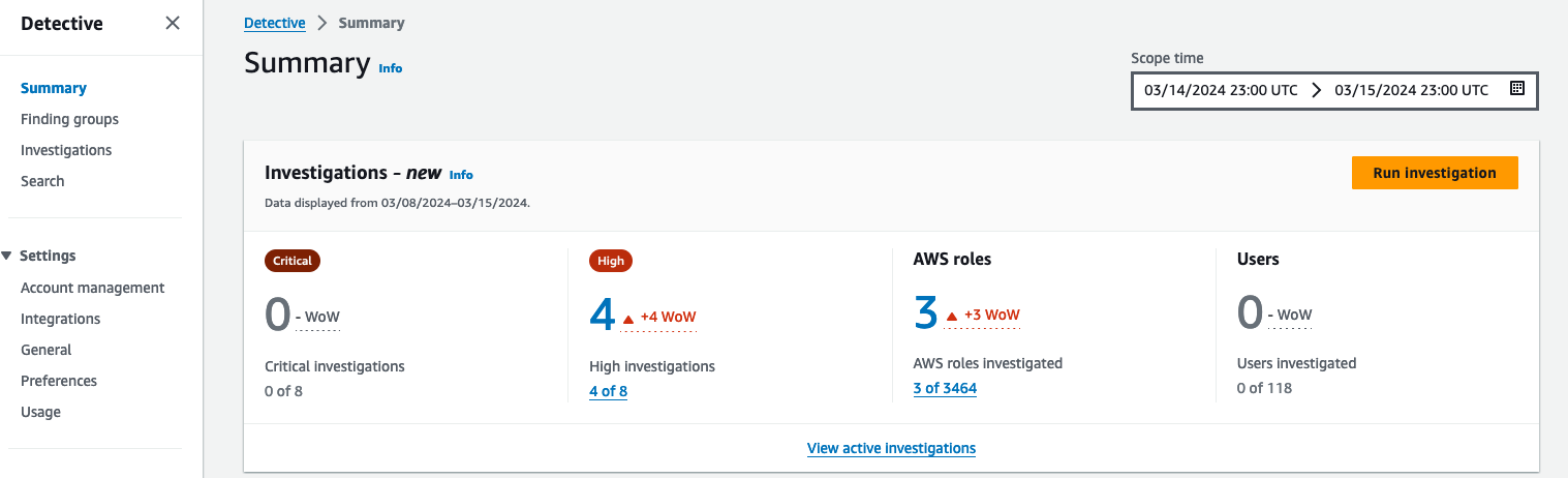
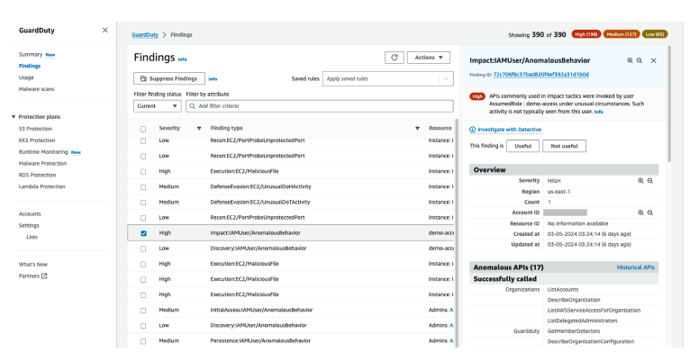
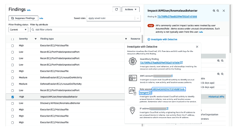
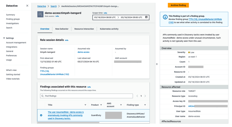
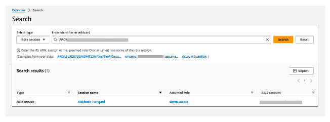
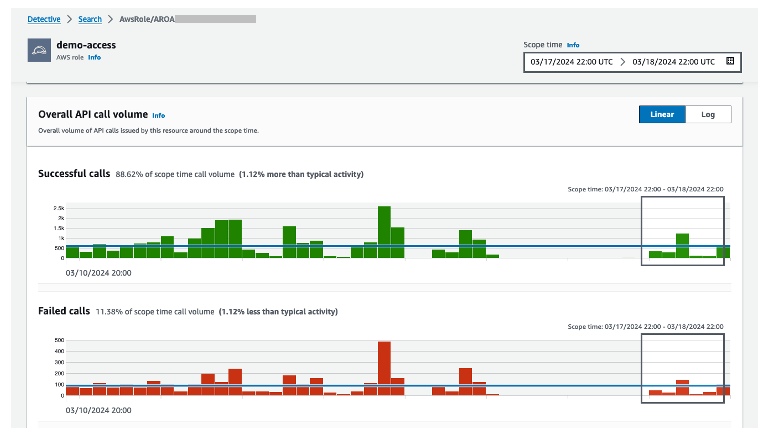
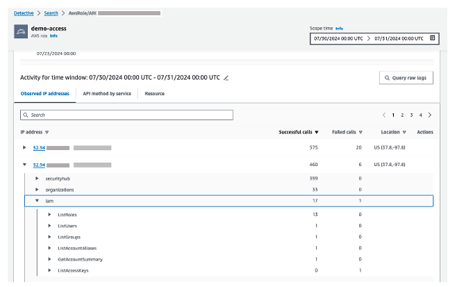
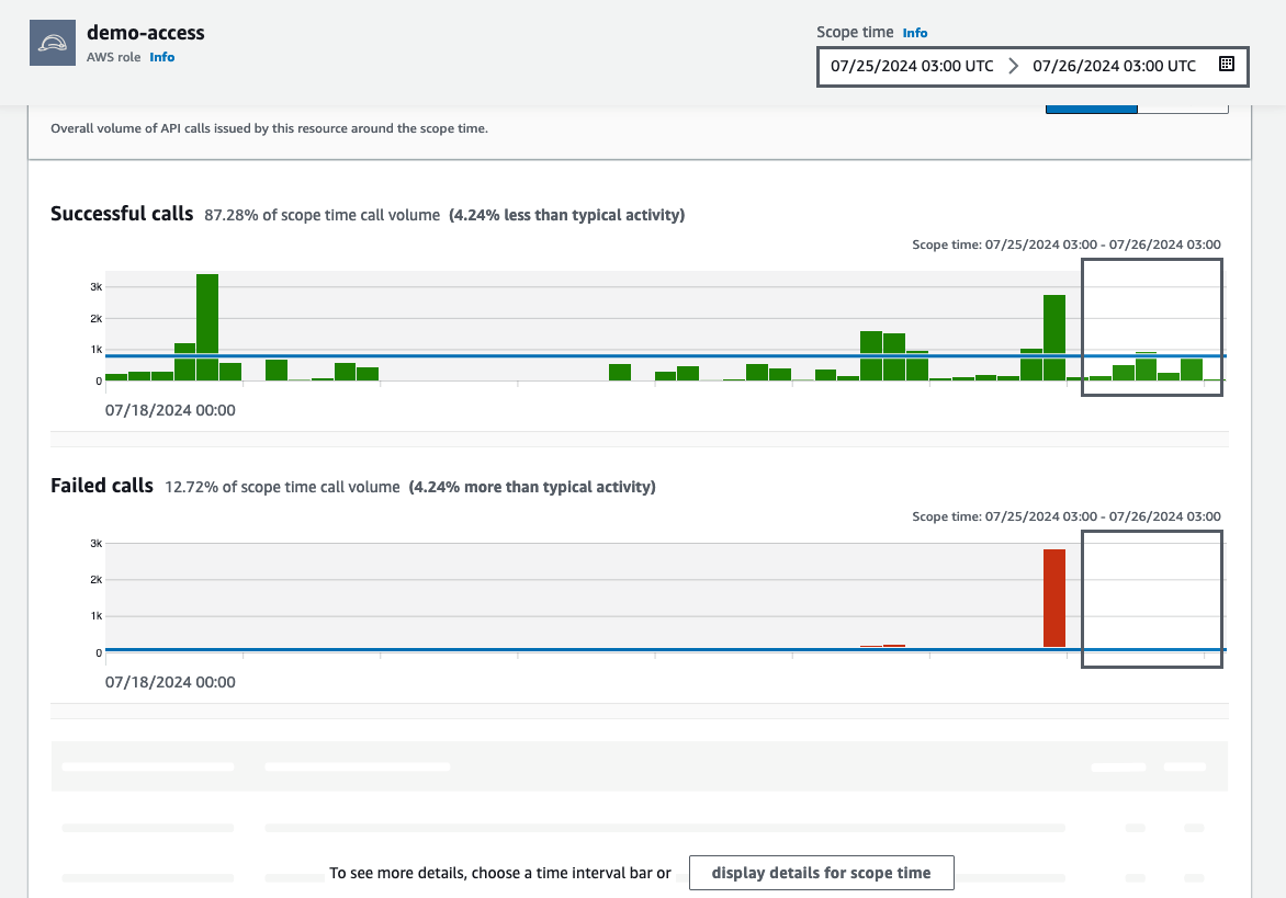
Figure 12: Overall API call volume during the specified scope time

To see the details for a specific IP address, use the Overall API call volume panel to search through different locations and to determine where the failed API calls came from. Select an IP address to get more granular details (as shown in Figure 13). When looking through this information, think about what this might tell you in your own environment.

Do you know who normally uses this role?
What is this role used for?
Should this role be making calls from various geolocations?

Figure 13: Granular details for the selected IP address

In this scenario, you used Detective to review potentially suspicious activity in your environment related to information assumed to be malicious. If adversaries have assumed the same role with different session names, this gives you more information about how this IAM role was used. If you find information related to the suspicious resources in question, you should conduct a formal search according to your internal incident response playbooks.

Conclusion

In this blog post, I walked you through how to investigate IAM entities (IAM users or rules) using Amazon Detective. You saw different scenarios on how to investigate IAM entities involved in a security event. You also learned about the Detective investigations for IAM feature, which you can use to automatically investigate IAM entities for indicators of compromise (IOCs), helping security analysts determine whether IAM entities have potentially been compromised or involved in known TTPs from the MITRE ATT&CK framework.

There’s no additional charge for this capability, and it’s available today for existing and new Detective customers in AWS Regions that support Detective. If you don’t currently use Detective, you can start a free 30-day trial. For more information about Detective investigations, see Detective Investigation.

If you have feedback about this post, submit comments in the Comments section below. If you have questions about this post, contact AWS Support.

Get to know Amazon GuardDuty Runtime Monitoring for Amazon EC2

2024-09-18 Scott Ward

Post Syndicated from Scott Ward original https://aws.amazon.com/blogs/security/get-to-know-amazon-guardduty-runtime-monitoring-for-amazon-ec2/

In this blog post, I take you on a deep dive into Amazon GuardDuty Runtime Monitoring for EC2 instances and key capabilities that are part of the feature. Throughout the post, I provide insights around deployment strategies for Runtime Monitoring and detail how it can deliver security value by detecting threats against your Amazon Elastic Compute Cloud (Amazon EC2) instances and the workloads you run on them. This post builds on the post by Channy Yun that outlines how to enable Runtime Monitoring, how to view the findings that it produces, and how to view the coverage it provides across your EC2 instances.

Amazon Web Services (AWS) launched Amazon GuardDuty at re:Invent 2017 with a focus on providing customers managed threat detection capabilities for their AWS accounts and workloads. When enabled, GuardDuty takes care of consuming and processing the necessary log data. Since its launch, GuardDuty has continued to expand its threat detection capabilities. This expansion has included identifying new threat types that can impact customer environments, identifying new threat tactics and techniques within existing threat types and expanding the log sources consumed by GuardDuty to detect threats across AWS resources. Examples of this expansion include the ability to detect EC2 instance credentials being used to invoke APIs from an IP address that’s owned by a different AWS account than the one that the associated EC2 instance is running in, and the ability to identify threats to Amazon Elastic Kubernetes Services (Amazon EKS) clusters by analyzing Kubernetes audit logs.

GuardDuty has continued to expand its threat detection capabilities beyond AWS log sources, providing a more comprehensive coverage of customers’ AWS resources. Specifically, customers needed more visibility around threats that might occur at the operating system level of their container and compute instances. To address this customer need, GuardDuty released the Runtime Monitoring feature, beginning with support on Amazon Elastic Kubernetes Service (Amazon EKS) workloads. Runtime Monitoring provides operating system insight for GuardDuty to use in detecting potential threats to workloads running on AWS and enabled the operating system visibility that customers were asking for. At re:Invent 2023, GuardDuty expanded Runtime Monitoring to include Amazon Elastic Container Service (Amazon ECS)—including serverless workloads running on AWS Fargate, and previewed support for Amazon EC2, which became generally available earlier this year. The release of EC2 Runtime Monitoring enables comprehensive compute coverage for GuardDuty across containers and EC2 instances, delivering breadth and depth for threat detection in these areas.

Features and functions

GuardDuty EC2 Runtime Monitoring relies on a lightweight security agent that collects operating system events—such as file access, processes, command line arguments, and network connections—from your EC2 instance and sends them to GuardDuty. After the operating system events are received by GuardDuty, they’re evaluated to identify potential threats related to the EC2 instance. In this section, we explore how GuardDuty is evaluating the runtime events it receives and how GuardDuty presents identified threat information.

Command arguments and event correlation

The runtime security agent enables GuardDuty to create findings that can’t be created using the foundational data sources of VPC Flow Logs, DNS logs, and CloudTrail logs. The security agent can collect detailed information about what’s happening at the instance operating system level that the foundational data sources don’t contain.

With the release of EC2 Runtime Monitoring, additional capabilities have been added to the runtime agent and to GuardDuty. The additional capabilities include collecting command arguments and correlation of events for an EC2 instance. These new capabilities help to rule out benign events and more accurately generate findings that are related to activities that are associated with a potential threat to your EC2 instance.

Command arguments

The GuardDuty security agent collects information on operating system runtime commands (curl, systemctl, cron, and so on) and uses this information to generate findings. The security agent now also collects the command arguments that were used as part of running a command. This additional information gives GuardDuty more capabilities to detect threats because of the additional context related to running a command.

For example, the agent will not only identify that systemctl (which is used to manage services on your Linux instance) was run but also which parameters the command was run with (stop, start, disable, and so on) and for which service the command was run. This level of detail helps identify that a threat actor might be changing security or monitoring services to evade detection.

Event correlation

GuardDuty can now also correlate multiple events collected using the runtime agent to identify scenarios that present themselves as a threat to your environment. There might be events that happen on your instance that, on their own, don’t present themselves as a clear threat. These are referred to as weak signals. However, when these weak signals are considered together and the sequence of commands aligns to malicious activity, GuardDuty uses that information to generate a finding. For example, a download of a file would present itself as a weak signal. If that download of a file is then piped to a shell command and the shell command begins to interact with additional operating system files or network configurations, or run known malware executables, then the correlation of all these events together can lead to a GuardDuty finding.

GuardDuty finding types

GuardDuty Runtime Monitoring currently supports 41 finding types to indicate potential threats based on the operating system-level behavior from the hosts and containers in your Amazon EKS clusters on Amazon EC2, Amazon ECS on Fargate and Amazon EC2, and EC2 instances. These findings are based on the event types that the security agent collects and sends to the GuardDuty service.

Five of these finding types take advantage of the new capabilities of the runtime agent and GuardDuty, which were discussed in the previous section of this post. These five new finding types are the following:

Each GuardDuty finding begins with a threat purpose, which is aligned with MITRE ATT&CK tactics. The Execution finding types are focused on observed threats to the actual running of commands or processes that align to malicious activity. The DefenseEvasion finding types are focused on situations where commands are run that are trying to disable defense mechanisms on the instance, which would normally be used to identify or help prevent the activity of a malicious actor on your instance.

In the following sections, I go into more detail about the new Runtime Monitoring finding types and the types of malicious activities that they are identifying.

Identifying suspicious tools and commands

The SuspiciousTool, SuspiciousCommand, and PtraceAntiDebugging finding types are focused on suspicious activities, or those that are used to evade detection. The approach to identify these types of activities is similar. The SuspiciousTool finding type is focused on tools such as backdoor tools, network scanners, and network sniffers. GuardDuty helps to identify the cases where malicious activities related to these tools are occurring on your instance.

The SuspiciousCommand finding type identifies suspicious commands with the threat purposes of DefenseEvasion or Execution. The DefenseEvasion findings are an indicator of an unauthorized user trying to hide their actions. These actions could include disabling a local firewall, modifying local IP tables, or removing crontab entries. The Execution findings identify when a suspicious command has been run on your EC2 instance. The findings related to Execution could be for a single suspicious command or a series of commands, which, when combined with a series of other commands along with additional context, becomes a clearer indicator of suspicious activity. An example of an Execution finding related to combining multiple commands could be when a file is downloaded and is then run in a series of steps that align with a known malicious pattern.

For the PtraceAntiDebugging finding, GuardDuty is looking for cases where a process on your instance has used the ptrace system call with the PTRACE_TRACEME option, which causes an attached debugger to detach from the running process. This is a suspicious activity because it allows a process to evade debugging using ptrace and is a known technique that malware uses to evade detection.

Identifying running malicious files

The updated GuardDuty security agent can also identify when malicious files are run. With the MaliciousFileExecuted finding type, GuardDuty can identify when known malicious files might have been run on your EC2 instance, providing a strong indicator that malware is present on your instance. This capability is especially important because it allows you to identify known malware that might have been introduced since your last malware scan.

Finding details

All of the findings mentioned so far are consumable through the AWS Management Console for GuardDuty, through the GuardDuty APIs, as Amazon EventBridge messages, or through AWS Security Hub. The findings that GuardDuty generates are meant to not only tell you that a suspicious event has been observed on your instance, but also give you enough context to formulate a response to the finding.

The GuardDuty security agent collects a variety of events from the operating system to use for threat detection. When GuardDuty generates a finding based on observed runtime activities, it will include the details of these observed events, which can help with confirmation on what the threat is and provide you a path for possible remediation steps based on the reported threat. The information provided in a GuardDuty runtime finding can be broken down into three main categories:

Information about the impacted AWS resource
Information about the observed processes that were involved in the activity
Context related to the runtime events that were observed

Impacted AWS resources

In each finding that GuardDuty produces, information about the impacted AWS resource will be included. For EC2 Runtime Monitoring, the key information included will be information about the EC2 instance (such as name, instance type, AMI, and AWS Region), tags that are assigned to the instance, network interfaces, and security groups. This information will help guide your response and investigation to the specific instance that’s identified for the observed threat. It’s also useful in assessing key network configurations of the instance that could assist with confirming whether the network configuration of the instance is correct or assessing how the network configuration might factor into the response.

Process details

For each runtime finding, GuardDuty includes the details that were observed about the process attributed to the threat that the finding is for. Common items that you should expect to see include the name of the executable and the path to the executable that resulted in the finding being created, the ID of the operating system process, when the process started, and which operating system user ran the process. Additionally, process lineage is included in the finding. Process lineage helps identify operating system processes that are related to each other and provides insight into the parent processes that were run leading up to the identified process. Understanding this lineage can give you valuable insight into what the root cause of the malicious process identified in the finding might be; for example, being able to identify which other commands were run that ultimately led to the activation of the executable or command identified in the finding. If the process attributed to the finding is running inside a container, the finding also provides container details such as the container ID and image.

Runtime context

Runtime context provides insight on things such as file system type, flags that were used to control the behavior of the event, name of the potentially suspicious tool, path to the script that generated the finding, and the name of the security service that was disabled. The context information in the finding is intended to help you further understand the runtime activity that was identified as a threat and determine its potential impact and what your response might be. For example, a command that is detected by using the systemctl command to disable the apparmor utility would report the process information related to running the systemctl command, and then the runtime context would contain the name of the actual service that was impacted by the systemctl command call and the options used with the command.

See Runtime Monitoring finding details for a full list of the process and context details that might be present in your runtime findings.

Responding to runtime findings

With GuardDuty findings, it’s a best practice to enable an event-based response that can be invoked as soon as the runtime finding is generated. This approach holds true for runtime related findings as well. For every runtime finding that GuardDuty generates, a copy of the finding is sent to EventBridge. If you use Security Hub, a copy of the finding is sent to Security Hub as well. With EventBridge, you can define a rule with a pattern that matches the finding attributes you want to prioritize and respond to. This pattern could be very broad in looking for all runtime-related findings. Or, it could be more specific, only looking for certain finding types, findings of a certain severity, or even certain attributes related to the process or runtime context of a finding.

After the rule pattern is established, you can define a target that the finding should be sent to. This target can be one of over 20 AWS services, which gives you lots of flexibility in routing the finding into the operational tools or processes that are used by your company. The target could be an AWS Lambda function that’s responsible for evaluating the finding, adding some additional data to the finding, and then sending it to a ticketing or chat tool. The target could be an AWS Systems Manager runbook, which would be used on the actual operating system to perform additional forensics or to isolate or disable any processes that are identified in the finding.

Many customers take a stepped approach in their response to GuardDuty findings. The first step might be to make sure that the finding is enriched with as many supporting details as possible and sent to the right individual or team. This helps whoever’s investigating the finding to confirm that the finding is a true positive, further informing the decision on what action to take.

In addition to having an event-based response to GuardDuty findings, you can investigate each GuardDuty runtime finding in the GuardDuty or Security Hub console. Through the console, you can research the details of the finding and use the information to inform the next steps to respond to or remediate the finding.

Speed to detection

With its close proximity to your workloads, the GuardDuty security agent can produce findings more quickly when compared to processing log sources such as VPC Flow Logs and DNS logs. The security agent collects operating system events and forwards them directly to the GuardDuty service, examining events and generating findings more quickly. This helps you to formulate a response sooner so that you can isolate and stop identified threats to your EC2 instances.

Let’s examine a finding type that can be detected by both the runtime security agent and by the foundational log sources of AWS CloudTrail, VPC Flow Logs, and DNS logs. Backdoor:EC2/C&CActivity.B!DNS and Backdoor:Runtime/C&CActivity.B!DNS are the same finding with one coming from DNS logs and one coming from the runtime security agent. While GuardDuty doesn’t have a service-level agreement (SLA) on the time it takes to consume the findings for a log source or the security agent, testing for these finding types reveals that the runtime finding is generated in just a few minutes. Log file-based findings will take around 15 minutes to produce because of the latency of log file delivery and processing. In the end, these two findings mean the same thing, but the runtime finding will arrive faster and with additional process and context information, helping you implement a response to the threat sooner and improve your ability to isolate, contain, and stop the threat.

Runtime data and flow logs data

When exploring the Runtime Monitoring feature and its usefulness for your organization, a key item to understand is the foundational level of protection for your account and workloads. When you enable GuardDuty the foundational data sources of VPC Flow Logs, DNS logs, and CloudTrail logs are also enabled, and those sources cannot be turned off without fully disabling GuardDuty. Runtime Monitoring provides contextual information that allows for more precise findings that can help with targeted remediation compared to the information provided in VPC Flow Logs. When the Runtime Monitoring agent is deployed onto an instance, the GuardDuty service still processes the VPC Flow Logs and DNS logs for that instance. If, at any point in time, an unauthorized user tampers with your security agent or an instance is deployed without the security agent, GuardDuty will continue to use VPC Flow Logs and DNS logs data to monitor for potential threats and suspicious activity, providing you defense in depth to help ensure you have visibility and coverage for detecting threats.

Note: GuardDuty doesn’t charge you for processing VPC Flow Logs while the Runtime Monitoring agent is active on an instance.

Deployment strategies

There are multiple strategies that you can use to install the GuardDuty security agent on an EC2 instance, and it’s important to use the one that fits best based on how you deploy and maintain instances in your environment. The following are agent installation options that cover managed installation, tag-based installation, and manual installation techniques. The managed installation approach is a good fit for most customers, but the manual options are potentially better if you have existing processes that you want to maintain or you want the more fine-grained features provided by agent installation compared to the managed approach.

Note: GuardDuty requires that each VPC, with EC2 instances running the GuardDuty agent, has a VPC endpoint that allows the agent to communicate with the GuardDuty service. You aren’t charged for the cost of these VPC endpoints. When you’re using the GuardDuty managed agent feature, GuardDuty will automatically create and operate these VPC endpoints for you. For the other agent deployment options listed in this section, or other approaches that you take, you must manually configure the VPC endpoint for each VPC where you have EC2 instances that will run the GuardDuty agent. See Creating VPC endpoint manually for additional details.

GuardDuty-managed installation

If you want to use security agents to monitor runtime activity on your EC2 instances but don’t want to manage the installation and lifecycle of the agent on specific instances, then Automated agent configuration is the option for you. For GuardDuty to successfully manage agent installation, each EC2 instance must meet the operating system architectural requirements of the security agent. Additionally, each instance must have the Systems Manager agent installed and configured with the minimal instance permissions that System Manager requires.

In addition to making sure that your instances are configured correctly, you also need to enable automated agent configuration for your EC2 instances in the Runtime Monitoring section of the GuardDuty console. Figure 1 shows what this step looks like.

Figure 1: Enable GuardDuty automated agent configuration for Amazon EC2

After you have enabled automated agent configuration and have your instances correctly configured, GuardDuty will install and manage the security agent for every instance that is configured.

GuardDuty-managed with explicit tagging

If you want to selectively manage installation of the GuardDuty agent but still want automated deployment and updates, you can use inclusion or exclusion tags to control which instances the agent is installed to.

Inclusion tags allow you to specify which EC2 instances the GuardDuty security agent should be installed to without having to enable automated agent configuration. To use inclusion tags, each instance where the security agent should be installed needs to have a key-value pair of GuardDutyManaged/true. While you don’t need to turn on automated agent configuration to use inclusion tags, each instance that you tag for agent installation needs to have the Systems Manager agent installed and the appropriate permissions attached to the instance using an instance role.
Exclusion tags allow you to enable automated agent configuration, and then selectively manage which instances the agent shouldn’t be deployed to. To use exclusion tags, each instance that shouldn’t have an instance installed needs to have a key-value pair of GuardDutyManaged/false.

You can use selective installation for a variety of use cases. If you’re doing a proof of concept with EC2 Runtime Monitoring, you might want to deploy the solution to a subset of your instances and then gradually onboard additional instances. At times, you might want to limit agent installation to instances that are deployed into certain environments or applications that are a priority for runtime monitoring. Tagging resources associated with these workloads helps ensure that monitoring is in place for resources that you want to prioritize for runtime monitoring. This strategy gives you more fine-grained control but also requires more work and planning to help ensure that the strategy is implemented correctly.

With a tag-based strategy it is important to understand who is allowed to add or remove tags to your EC2 instances as this influences when security controls are enabled or disabled. A review of your IAM roles and policies for tagging permissions is recommended to help ensure that the appropriate principals have access to this tagging capability. This IAM document provides an example of how you may limit tagging capabilities within a policy. The approach you take will depend on how you are using policies within your environment.

Manual agent installation options

If you don’t want to run the Systems Manager agent that powers the automated agent configuration, or if you have your own strategy to install and configure software on your EC2 instances, there are other deployment options that are better suited for your situation. The following are multiple approaches that you can use to manually install the GuardDuty agent for Runtime Monitoring. See Installing the security agent manually for general pointers on the recommended manual installation steps. With manual installation, you’re responsible for updating the GuardDuty security agent when new versions of the agent are released. Updating the agent can often be performed using the same techniques as installing the agent.

EC2 Image Builder

Your EC2 deployment strategy might be to build custom Amazon EC2 machine images that are then used as the approved machine images for your organization’s workloads. One option for installing the GuardDuty runtime agent as part of a machine image build is to use EC2 Image Builder. Image Builder simplifies the building, testing, and deployment of virtual machine and container images for use on AWS. With Image Builder, you define an image pipeline that includes a recipe with a build component for installing the GuardDuty Runtime Monitoring RPM. This approach with Image Builder helps ensure that your pre-built machine image includes the necessary components for EC2 Runtime Monitoring so that the necessary security monitoring is in place as soon as your instances are launched.

Bootstrap

Some customers prefer to configure their EC2 instances as they’re launched. This is commonly done through the user data field of an EC2 instance definition. For EC2 Runtime Monitoring agent installation, you would add the steps related to download and install of the runtime RPM as part of your user data script. The steps that you would add to your user data script are outlined in the Linux Package Managers method of Installing the security agent manually.

Other tools

In addition to the preceding steps, there are other tools that you can use when you want to incorporate the installation of the GuardDuty runtime monitoring agent. Tools such as Packer for building EC2 images, and Ansible, Chef, and Puppet for instance automation can be used to run the necessary steps to install the runtime agent onto the necessary EC2 instances. See Installing the security agent manually for guidance on the installation commands you would use with these tools.

Conclusion

Through customer feedback, GuardDuty has enhanced its threat detection capabilities with the Runtime Monitoring feature and you can now use it to deploy the same security agent across different compute services in AWS for runtime threat detection. Runtime monitoring provides an additional level of visibility that helps you achieve your security goals for your AWS workloads.

This post outlined the GuardDuty EC2 Runtime Monitoring feature, how you can implement the feature on your EC2 instances, and the security value that the feature provides. The insight provided in this post is intended to help you better understand how EC2 Runtime Monitoring can benefit you in achieving your security goals related to identifying and responding to threats.

To learn more about GuardDuty and its Runtime Monitoring capabilities, see Runtime Monitoring in GuardDuty.

If you have feedback about this post, submit comments in the Comments section below. If you have questions about this post, contact AWS Support.

Methodology for incident response on generative AI workloads

2024-09-16 Anna McAbee

Post Syndicated from Anna McAbee original https://aws.amazon.com/blogs/security/methodology-for-incident-response-on-generative-ai-workloads/

The AWS Customer Incident Response Team (CIRT) has developed a methodology that you can use to investigate security incidents involving generative AI-based applications. To respond to security events related to a generative AI workload, you should still follow the guidance and principles outlined in the AWS Security Incident Response Guide. However, generative AI workloads require that you also consider some additional elements, which we detail in this blog post.

We start by describing the common components of a generative AI workload and discuss how you can prepare for an event before it happens. We then introduce the Methodology for incident response on generative AI workloads, which consists of seven elements that you should consider when triaging and responding to a security event on a generative AI workload. Lastly, we share an example incident to help you explore the methodology in an applied scenario.

Components of a generative AI workload

As shown in Figure 1, generative AI applications include the following five components:

An organization that owns or is responsible for infrastructure, generative AI applications, and the organization’s private data.
Infrastructure within an organization that isn’t specifically related to the generative AI application itself. This can include databases, backend servers, and websites.
Generative AI applications, which include the following:
- Foundation models – AI models with a large number of parameters and trained on a massive amount of diverse data.
- Custom models – models that are fine-tuned or trained on an organization’s specific data and use cases, tailored to their unique requirements.
- Guardrails – mechanisms or constraints to help make sure that the generative AI application operates within desired boundaries. Examples include content filtering, safety constraints, or ethical guidelines.
- Agents – workflows that enable generative AI applications to perform multistep tasks across company systems and data sources.
- Knowledge bases – repositories of domain-specific knowledge, rules, or data that the generative AI application can access and use.
- Training data – data used to train, fine-tune, or augment the generative AI application’s models, including data for techniques such as retrieval augmented generation (RAG).
  
  Note: Training data is distinct from an organization’s private data. A generative AI application might not have direct access to private data, although this is configured in some environments.
- Plugins – additional software components or extensions that you can integrate with the generative AI application to provide specialized functionalities or access to external services or data sources.
Private data refers to the customer’s privately stored, confidential data that the generative AI resources or applications aren’t intended to interact with during normal operation.
Users are the identities that can interact with or access the generative AI application. They can be human or non-human (such as machines).

Figure 1: Common components of an AI/ML workload

Prepare for incident response on generative AI workloads

You should prepare for a security event across three domains: people, process, and technology. For a summary of how to prepare, see the preparation items from the Security Incident Response Guide. In addition, your preparation for a security event that’s related to a generative AI workload should include the following:

People: Train incident response and security operations staff on generative AI – You should make sure that your staff is familiar with generative AI concepts and with the AI/ML services in use at your organization. AWS Skill Builder provides both free and paid courses on both of these subjects.
Process: Develop new playbooks – You should develop new playbooks for security events that are related to a generative AI workload. To learn more about how to develop these, see the following sample playbooks:
You can use these playbooks as a starting point and modify them to best fit your organization and usage of these services.
Technology: Log generative AI application prompts and invocations – In addition to foundational logs, such as those available in AWS CloudTrail, you should consider logging Amazon Bedrock model invocation logs so that you can analyze the prompts coming into your application and the outputs. To learn more, see Amazon Bedrock model invocation logging. CloudTrail data event logging is also available for Amazon Bedrock, Amazon Q, and Amazon SageMaker. For general guidance, see Logging strategies for security incident response.

Important: Logs can contain sensitive information. To help protect this information, you should set up least privilege access to these logs, like you do for your other security logs. You can also protect sensitive log data with data masking. In Amazon CloudWatch, you can mask data natively through log group data protection policies.

Methodology for incident response on generative AI workloads

After you complete the preparation items, you can use the Methodology for incident response on generative AI workloads for active response, to help you rapidly triage an active security event involving a generative AI application.

The methodology has seven elements, which we detail in this section. Each element describes a method by which the components can interact with another component or a method by which a component can be modified. Consideration of these elements will help guide your actions during the Operations phase of a security incident, which includes detection, analysis, containment, eradication, and recovery phases.

Access – Determine the designed or intended access patterns for the organization that hosts the components of the generative AI application, and look for deviations or anomalies from those patterns. Consider whether the application is accessible externally or internally because that will impact your analysis.
To help you identify anomalous and potential unauthorized access to your AWS environment, you can use Amazon GuardDuty. If your application is accessible externally, the threat actor might not be able to access your AWS environment directly and thus GuardDuty won’t detect it. The way that you’ve set up authentication to your application will drive how you detect and analyze unauthorized access.

If evidence of unauthorized access to your AWS account or associated infrastructure exists, determine the scope of the unauthorized access, such as the associated privileges and timeline. If the unauthorized access involves service credentials—for example, Amazon Elastic Compute Cloud (Amazon EC2) instance credentials—review the service for vulnerabilities.
Infrastructure changes – Review the supporting infrastructure, such as servers, databases, serverless computing instances, and internal or external websites, to determine if it was accessed or changed. To investigate infrastructure changes, you can analyze CloudTrail logs for modifications of in-scope resources, or analyze other operating system logs or database access logs.
AI changes – Investigate whether users have accessed components of the generative AI application and whether they made changes to those components. Look for signs of unauthorized activities, such as the creation or deletion of custom models, modification of model availability, tampering or deletion of generative AI logging capabilities, tampering with the application code, and removal or modification of generative AI guardrails.
Data store changes – Determine the designed or intended data access patterns, whether users accessed the data stores of your generative AI application, and whether they made changes to these data stores. You should also look for the addition or modification of agents to a generative AI application.
Invocation – Analyze invocations of generative AI models, including the strings and file inputs, for threats, such as prompt injection or malware. You can use the OWASP Top 10 for LLM as a starting point to understand invocation related threats, and you can use invocation logs to analyze prompts for suspicious patterns, keywords, or structures that might indicate a prompt injection attempt. The logs also capture the model’s outputs and responses, enabling behavioral analysis to help identify uncharacteristic or unsafe model behavior indicative of a prompt injection. You can use the timestamps in the logs for temporal analysis to help detect coordinated prompt injection attempts over time and collect information about the user or system that initiated the model invocation, helping to identify the source of potential exploits.
Private data – Determine whether the in-scope generative AI application was designed to have access to private or confidential data. Then look for unauthorized access to, or tampering with, that data.
Agency – Agency refers to the ability of applications to make changes to an organization’s resources or take actions on a user’s behalf. For example, a generative AI application might be configured to generate content that is then used to send an email, invoking another resource or function to do so. You should determine whether the generative AI application has the ability to invoke other functions. Then, investigate whether unauthorized changes were made or if the generative AI application invoked unauthorized functions.

The following table lists some questions to help you address the seven elements of the methodology. Use your answers to guide your response.

Topic	Questions to address
Access	Do you still have access to your computing environment? Is there continued evidence of unauthorized access to your organization?
Infrastructure changes	Were supporting infrastructure resources accessed or changed?
AI changes	Were your AI models, code, or resources accessed or changed?
Data store changes	Were your data stores, knowledge bases, agents, plugins, or training data accessed or tampered with?
Invocation	What data, strings, or files were sent as input to the model? What prompts were sent? What responses were produced?
Private data	What private or confidential data do generative AI resources have access to? Was private data changed or tampered with?
Agency	Can the generative AI application resources be used to start computing services in an organization, or do the generative AI resources have the authority to make changes? Were unauthorized changes made?

Example incident

To see how to use the methodology for investigation and response, let’s walk through an example security event where an unauthorized user compromises a generative AI application that’s hosted on AWS by using credentials that were exposed on a public code repository. Our goal is to determine what resources were accessed, modified, created, or deleted.

To investigate generative AI security events on AWS, these are the main log sources that you should review:

CloudTrail
CloudWatch
VPC Flow Logs
Amazon Simple Storage Service (Amazon S3) data events (for evidence of access to an organization’s S3 buckets)
Amazon Bedrock model invocation logs (if your application uses this service)

Access

Analysis of access for a generative AI application is similar to that for a standard three-tier web application. To begin, determine whether an organization has access to their AWS account. If the password for the AWS account root user was lost or changed, reset the password. Then, we strongly recommended that you immediately enable a multi-factor authentication (MFA) device for the root user—this should block a threat actor from accessing the root user.

Next, determine whether unauthorized access to the account persists. To help identify mutative actions logged by AWS Identity and Access Management (IAM) and AWS Security Token Service (Amazon STS), see the Analysis section of the Compromised IAM Credentials playbook on GitHub. Lastly, make sure that access keys aren’t stored in public repositories or in your application code; for alternatives, see Alternatives to long-term access keys.

Infrastructure changes

To analyze the infrastructure changes of an application, you should consider both the control plane and data plane. In our example, imagine that Amazon API Gateway was used for authentication to the downstream components of the generative AI application and that other ancillary resources were interacting with your application. Although you could review control plane changes to these resources in CloudTrail, you would need additional logging to be turned on to review changes made on the operating system of the resource. The following are some common names for control plane events that you could find in CloudTrail for this element:

ec2:RunInstances
ec2:StartInstances
ec2:TerminateInstances
ecs:CreateCluster
cloudformation:CreateStack
rds:DeleteDBInstance
rds:ModifyDBClusterSnapshotAttribute

AI changes

Unauthorized changes can include, but are not limited to, system prompts, application code, guardrails, and model availability. Internal user access to the generative AI resources that AWS hosts are logged in CloudTrail and appear with one of the following event sources:

amazonaws.com
amazonaws.com
amazonaws.com
amazonaws.com

The following are a couple examples of the event names in CloudTrail that would represent generative AI resource log tampering in our example scenario:

bedrock:PutModelInvocationLoggingConfiguration
bedrock:DeleteModelInvocationLoggingConfiguration

The following are some common event names in CloudTrail that would represent access to the AI/ML model service configuration:

bedrock:GetFoundationModelAvailability
bedrock:ListProvisionedModelThroughputs
bedrock:ListCustomModels
bedrock:ListFoundationModels
bedrock:ListProvisionedModelThroughput
bedrock:GetGuardrail
bedrock:DeleteGuardrail

In our example scenario, the unauthorized user has gained access to the AWS account. Now imagine that the compromised user has a policy attached that grants them full access to all resources. With this access, the unauthorized user can enumerate each component of Amazon Bedrock and identify the knowledge base and guardrails that are part of the application.

The unauthorized user then requests model access to other foundation models (FMs) within Amazon Bedrock and removes existing guardrails. The access to other foundation models could indicate that the unauthorized user intends to use the generative AI application for their own purposes, and the removal of guardrails minimizes filtering or output checks by the model. AWS recommends that you implement fine-grained access controls by using IAM policies and resource-based policies to restrict access to only the necessary Amazon Bedrock resources, AWS Lambda functions, and other components that the application requires. Also, you should enforce the use of MFA for IAM users, roles, and service accounts with access to critical components such as Amazon Bedrock and other components of your generative AI application.

Data store changes

Typically, you use and access a data store and knowledge base through model invocation, and for Amazon Bedrock, you include the API call bedrock:InvokeModel.

However, if an unauthorized user gains access to the environment, they can create, change, or delete the data sources and knowledge bases that the generative AI applications integrate with. This could cause data or model exfiltration or destruction, as well as data poisoning, and could create a denial-of-service condition for the model. The following are some common event names in CloudTrail that would represent changes to AI/ML data sources in our example scenario:

bedrock:CreateDataSource
bedrock:GetKnowledgeBase
bedrock:DeleteKnowledgeBase
bedrock:CreateAgent
bedrock:DeleteAgent
bedrock:InvokeAgent
bedrock:Retrieve
bedrock:RetrieveAndGenerate

For the full list of possible actions, see the Amazon Bedrock API Reference.

In this scenario, we have established that the unauthorized user has full access to the generative AI application and that some enumeration took place. The unauthorized user then identified the S3 bucket that was the knowledge base for the generative AI application and uploaded inaccurate data, which corrupted the LLM. For examples of this vulnerability, see the section LLM03 Training Data Poisoning in the OWASP TOP 10 for LLM Applications.

Invocation

Amazon Bedrock uses specific APIs to register model invocation. When a model in Amazon Bedrock is invoked, CloudTrail logs it. However, to determine the prompts that were sent to the generative AI model and the output response that was received from it, you must have configured model invocation logging.

These logs are crucial because they can reveal important information, such as whether a threat actor tried to get the model to divulge information from your data stores or release data that the model was trained or fine-tuned on. For example, the logs could reveal if a threat actor attempted to prompt the model with carefully crafted inputs that were designed to extract sensitive data, bypass security controls, or generate content that violates your policies. Using the logs, you might also learn whether the model was used to generate misinformation, spam, or other malicious outputs that could be used in a security event.

Note: For services such as Amazon Bedrock, invocation logging is disabled by default. We recommend that you enable data events and model invocation logging for generative AI services, where available. However, your organization might not want to capture and store invocation logs for privacy and legal reasons. One common concern is users entering sensitive data as input, which widens the scope of assets to protect. This is a business decision that should be taken into consideration.

In our example scenario, imagine that model invocation wasn’t enabled, so the incident responder couldn’t collect invocation logs to see the model input or output data for unauthorized invocations. The incident responder wouldn’t be able to determine the prompts and subsequent responses from the LLM. Without this logging enabled, they also couldn’t see the full request data, response data, and metadata associated with invocation calls.

Event names in model invocation logs that would represent model invocation logging in Amazon Bedrock include:

bedrock:InvokeModel
bedrock:InvokeModelWithResponseStream
bedrock:Converse
bedrock:ConverseStream

The following is a sample log entry for Amazon Bedrock model invocation logging:

Figure 2: sample model invocation log including prompt and response

Private data

From an architectural standpoint, generative AI applications shouldn’t have direct access to an organization’s private data. You should classify data used to train a generative AI application or for RAG use as data store data and segregate it from private data, unless the generative AI application uses the private data (for example, in the case where a generative AI application is tasked to answer questions about medical records for a patient). One way to help make sure that an organization’s private data is segregated from generative AI applications is to use a separate account and to authenticate and authorize access as necessary to adhere to the principle of least privilege.

Agency

Excessive agency for an LLM refers to an AI system that has too much autonomy or decision-making power, leading to unintended and potentially harmful consequences. This can happen when an LLM is deployed with insufficient oversight, constraints, or alignment with human values, resulting in the model making choices that diverge from what most humans would consider beneficial or ethical.

In our example scenario, the generative AI application has excessive permissions to services that aren’t required by the application. Imagine that the application code was running with an execution role with full access to Amazon Simple Email Service (Amazon SES). This could allow for the unauthorized user to send spam emails on the users’ behalf in response to a prompt. You could help prevent this by limiting permission and functionality of the generative AI application plugins and agents. For more information, see OWASP Top 10 for LLM, evidence of LLM08 Excessive Agency.

During an investigation, while analyzing the logs, both the sourceIPAddress and the userAgent fields will be associated with the generative AI application (for example, sagemaker.amazonaws.com, bedrock.amazonaws.com, or q.amazonaws.com). Some examples of services that might commonly be called or invoked by other services are Lambda, Amazon SNS, and Amazon SES.

Conclusion

To respond to security events related to a generative AI workload, you should still follow the guidance and principles outlined in the AWS Security Incident Response Guide. However, these workloads also require that you consider some additional elements.

You can use the methodology that we introduced in this post to help you address these new elements. You can reference this methodology when investigating unauthorized access to infrastructure where the use of generative AI applications is either a target of unauthorized use, the mechanism for unauthorized use, or both. The methodology equips you with a structured approach to prepare for and respond to security incidents involving generative AI workloads, helping you maintain the security and integrity of these critical applications.

For more information about best practices for designing your generative AI application, see Generative AI for the AWS Security Reference Architecture. For information about tactical mitigations for a common generative AI application, see the Blueprint for secure design and anti-pattern mitigation.

If you have feedback about this post, submit comments in the Comments section below. If you have questions about this post, start a new thread on the AWS Security, Identity, & Compliance re:Post or contact AWS Support.

Harness Zero Copy data sharing from Salesforce Data Cloud to Amazon Redshift for Unified Analytics – Part 2

2024-09-12 Rajkumar Irudayaraj

Post Syndicated from Rajkumar Irudayaraj original https://aws.amazon.com/blogs/big-data/harness-zero-copy-data-sharing-from-salesforce-data-cloud-to-amazon-redshift-for-unified-analytics-part-2/

In the era of digital transformation and data-driven decision making, organizations must rapidly harness insights from their data to deliver exceptional customer experiences and gain competitive advantage. Salesforce and Amazon have collaborated to help customers unlock value from unified data and accelerate time to insights with bidirectional Zero Copy data sharing between Salesforce Data Cloud and Amazon Redshift.

In the Part 1 of this series, we discussed how to configure data sharing between Salesforce Data Cloud and customers’ AWS accounts in the same AWS Region. In this post, we discuss the architecture and implementation details of cross-Region data sharing between Salesforce Data Cloud and customers’ AWS accounts.

Solution overview

Salesforce Data Cloud provides a point-and-click experience to share data with a customer’s AWS account. On the AWS Lake Formation console, you can accept the datashare, create the resource link, mount Salesforce Data Cloud objects as data catalog views, and grant permissions to query the live and unified data in Amazon Redshift. Cross-Region data sharing between Salesforce Data Cloud and a customer’s AWS accounts is supported for two deployment scenarios: Amazon Redshift Serverless and Redshift provisioned clusters (RA3).

Cross-Region data sharing with Redshift Serverless

The following architecture diagram depicts the steps for setting up a cross-Region datashare between a Data Cloud instance in US-WEST-2 with Redshift Serverless in US-EAST-1.

Cross-Region data sharing set up consists of the following steps:

The Data Cloud admin identifies the objects to be shared and creates a Data Share in the data cloud provisioned in the US-WEST-2
The Data Cloud admin links the Data Share with the Amazon Redshift Data Share target. This creates an AWS Glue Data Catalog view and a cross-account Lake Formation resource share using the AWS Resource Access Manager (RAM) with the customer’s AWS account in US-WEST-2.
The customer’s Lake Formation admin accepts the datashare invitation in US-WEST-2 from the Lake Formation console and grants default (select and describe) permissions to an AWS Identity and Access Management (IAM) principal.
The Lake Formation admin switches to US-EAST-1 and creates a resource link pointing to the shared database in the US-WEST-2 Region.
The IAM principal can log in to the Amazon Redshift query editor in US-EAST-1 and creates an external schema referencing the datashare resource link. The data can be queried through these external tables.

Cross-Region data sharing with a Redshift provisioned cluster

Cross-Region data sharing across Salesforce Data Cloud and a Redshift provisioned cluster requires additional steps on top of the Serverless set up. Based on the Amazon Redshift Spectrum considerations, the provisioned cluster and the Amazon Simple Storage Service (Amazon S3) bucket must be in the same Region for Redshift external tables. The following architecture depicts a design pattern and steps to share data with Redshift provisioned clusters.

Steps 1–5 in the set up remain the same across Redshift Serverless and provisioned cluster cross-Region sharing. Encryption must be enabled on both Redshift Serverless and the provisioned cluster. Listed below are the additional steps:

Create a table from datashare data with the CREATE TABLE AS SELECT Create a datashare in Redshift serverless and grant access to the Redshift provisioned cluster.
Create a database in the Redshift provisioned cluster and grant access to the target IAM principals. The datashare is ready for query.

The new table needs to be refreshed periodically to get the latest data from the shared Data Cloud objects with this solution.

Considerations when using data sharing in Amazon Redshift

For a comprehensive list of considerations and limitations of data sharing, refer to Considerations when using data sharing in Amazon Redshift. Some of the important ones for Zero Copy data sharing includes:

Data sharing is supported for all provisioned RA3 instance types (ra3.16xlarge, ra3.4xlarge, and ra3.xlplus) and Redshift Serverless. It isn’t supported for clusters with DC and DS node types.
For cross-account and cross-Region data sharing, both the producer and consumer clusters and serverless namespaces must be encrypted. However, they don’t need to share the same encryption key.
Data Catalog multi-engine views are generally available in commercial Regions where Lake Formation, the Data Catalog, Amazon Redshift, and Amazon Athena are available.
Cross-Region sharing is available in all LakeFormation supported regions.

Prerequisites

The prerequisites remain the same across same-Region and cross-Region data sharing, which are required before proceeding with the setup.

Configure cross-Region data sharing

The steps to create a datashare, create a datashare target, link the datashare target to the datashare, and accept the datashare in Lake Formation remain the same across same-Region and cross-Region data sharing. Refer to Part 1 of this series to complete the setup.

Cross-Region data sharing with Redshift Serverless

If you’re using Redshift Serverless, complete the following steps:

On the Lake Formation console, choose Databases in the navigation pane.
Choose Create database.
Under Database details¸ select Resource link.
For Resource link name, enter a name for the resource link.
For Shared database’s region, choose the Data Catalog view source Region.
The Shared database and Shared database’s owner ID fields are populated manually from the database metadata.
Choose Create to complete the setup.

The resource link appears on the Databases page on the Lake Formation console, as shown in the following screenshot.

Launch Redshift Query Editor v2 for the Redshift Serverless workspace The cross-region data share tables are auto-mounted and appear under awsdatacatalog. To query, run the following command and create an external schema. Specify the resource link as the Data Catalog database, the Redshift Serverless Region, and the AWS account ID.
```
CREATE external SCHEMA cross_region_data_share --<<SCHEMA_NAME>>
FROM DATA CATALOG DATABASE 'cross-region-data-share' --<<RESOURCE_LINK_NAME>>
REGION 'us-east-1' --<TARGET_REGION>
IAM_ROLE 'SESSION' CATALOG_ID '<<aws_account_id>>'; --<<REDSHIFT AWS ACCOUNT ID>>
```
Refresh the schemas to view the external schema created in the dev database
Run the show tables command to check the shared objects under the external database:
```
SHOW TABLES FROM SCHEMA dev.cross_region_data_share --<<schema name>>
```

Query the datashare as shown in the following screenshot.

SELECT * FROM dev.cross_region_data_share.churn_modellingcsv_tableaus3_dlm; --<<change schema name & table name>>

Cross-Region data sharing with Redshift provisioned cluster

This section is a continuation of the previous section with additional steps needed for data sharing to work when the consumer is a provisioned Redshift cluster. Refer to Sharing data in Amazon Redshift and Sharing datashares for a deeper understanding of concepts and the implementation steps.

Create a new schema and table in the Redshift Serverless in the consumer Region:

CREATE SCHEMA customer360_data_share;
CREATE TABLE customer360_data_share. customer_churn as
SELECT * from dev.cross_region_data_share.churn_modellingcsv_tableaus3__dlm;

Get the namespace for the Redshift Serverless (producer) and Redshift provisioned cluster (consumer) by running the following query in each cluster:
```
select current_namespace
```

Create a datashare in the Redshift Serverless (producer) and grant usage to the Redshift provisioned cluster (consumer). Set the datashare, schema, and table names to the appropriate values, and set the namespace to the consumer namespace.

CREATE DATASHARE customer360_redshift_data_share;
ALTER DATASHARE customer360_redshift_data_share ADD SCHEMA customer360_data_share;
ALTER DATASHARE customer360_redshift_data_share ADD TABLE customer360_data_share.customer_churn; 
GRANT USAGE ON DATASHARE customer360_redshift_data_share 
TO NAMESPACE '5709a006-6ac3-4a0c-a609-d740640d3080'; --<<Data Share Consumer Namespace>>

Log in as a superuser in the Redshift provisioned cluster, create a database from the datashare, and grant permissions. Refer to managing permissions for Amazon Redshift datashare for detailed guidance.

The datashare is now ready for query.

You can periodically refresh the table you created to get the latest data from the data cloud based on your business requirement.

Conclusion

Zero Copy data sharing between Salesforce Data Cloud and Amazon Redshift represents a significant advancement in how organizations can use their customer 360 data. By eliminating the need for data movement, this approach offers real-time insights, reduced costs, and enhanced security. As businesses continue to prioritize data-driven decision-making, Zero Copy data sharing will play a crucial role in unlocking the full potential of customer data across platforms.

This integration empowers organizations to break down data silos, accelerate analytics, and drive more agile customer-centric strategies. To learn more, refer to the following resources:

About the Authors

Rajkumar Irudayaraj is a Senior Product Director at Salesforce with over 20 years of experience in data platforms and services, with a passion for delivering data-powered experiences to customers.

Sriram Sethuraman is a Senior Manager in Salesforce Data Cloud product management. He has been building products for over 9 years using big data technologies. In his current role at Salesforce, Sriram works on Zero Copy integration with major data lake partners and helps customers deliver value with their data strategies.

Jason Berkowitz is a Senior Product Manager with AWS Lake Formation. He comes from a background in machine learning and data lake architectures. He helps customers become data-driven.

Ravi Bhattiprolu is a Senior Partner Solutions Architect at AWS. Ravi works with strategic ISV partners, Salesforce and Tableau, to deliver innovative and well-architected products and solutions that help joint customers achieve their business and technical objectives.

Avijit Goswami is a Principal Solutions Architect at AWS specialized in data and analytics. He supports AWS strategic customers in building high-performing, secure, and scalable data lake solutions on AWS using AWS managed services and open source solutions. Outside of his work, Avijit likes to travel, hike, watch sports, and listen to music.

Ife Stewart is a Principal Solutions Architect in the Strategic ISV segment at AWS. She has been engaged with Salesforce Data Cloud over the last 2 years to help build integrated customer experiences across Salesforce and AWS. Ife has over 10 years of experience in technology. She is an advocate for diversity and inclusion in the technology field.

Michael Chess is a Technical Product Manager at AWS Lake Formation. He focuses on improving data permissions across the data lake. He is passionate about enabling customers to build and optimize their data lakes to meet stringent security requirements.

Mike Patterson is a Senior Customer Solutions Manager in the Strategic ISV segment at AWS. He has partnered with Salesforce Data Cloud to align business objectives with innovative AWS solutions to achieve impactful customer experiences. In his spare time, he enjoys spending time with his family, sports, and outdoor activities.

The AWS Glue Data Catalog now supports storage optimization of Apache Iceberg tables

2024-09-12 Sandeep Adwankar

Post Syndicated from Sandeep Adwankar original https://aws.amazon.com/blogs/big-data/the-aws-glue-data-catalog-now-supports-storage-optimization-of-apache-iceberg-tables/

The AWS Glue Data Catalog now enhances managed table optimization of Apache Iceberg tables by automatically removing data files that are no longer needed. Along with the Glue Data Catalog’s automated compaction feature, these storage optimizations can help you reduce metadata overhead, control storage costs, and improve query performance.

Iceberg creates a new version called a snapshot for every change to the data in the table. Iceberg has features like time travel and rollback that allow you to query data lake snapshots or roll back to previous versions. As more table changes are made, more data files are created. In addition, any failures during writing to Iceberg tables will create data files that aren’t referenced in snapshots, also known as orphan files. Time travel features, though useful, may conflict with regulations like GDPR that require permanent data deletion. Because time travel allows accessing data through historical snapshots, additional safeguards are needed to maintain compliance with data privacy laws. To control storage costs and comply with regulations, many organizations have created custom data pipelines that periodically expire snapshots in a table that are no longer needed and remove orphan files. However, building these custom pipelines is time-consuming and expensive.

With this launch, you can enable Glue Data Catalog table optimization to include snapshot and orphan data management along with compaction. You can enable this by providing configurations such as a default retention period and maximum days to keep orphan files. The Glue Data Catalog monitors tables daily, removes snapshots from table metadata, and removes the data files and orphan files that are no longer needed. The Glue Data Catalog honors retention policies for Iceberg branches and tags referencing snapshots. You can now get an always-optimized Amazon Simple Storage Service (Amazon S3) layout by automatically removing expired snapshots and orphan files. You can view the history of data, manifest, manifest lists, and orphan files deleted from the table optimization tab on the AWS Glue Data Catalog console.

In this post, we show how to enable managed retention and orphan file deletion on an Apache Iceberg table for storage optimization.

Solution overview

For this post, we use a table called customer in the iceberg_blog_db database, where data is added continuously by a streaming application—around 10,000 records (file size less than 100 KB) every 10 minutes, which includes change data capture (CDC) as well. The customer table data and metadata are stored in the S3 bucket. Because the data is updated and deleted as part of CDC, new snapshots are created for every change to the data in the table.

Managed compaction is enabled on this table for query optimization, which results in new snapshots being created when compaction rewrites several small files into a few compacted files, leaving the old small files in storage. This results in data and metadata in Amazon S3 growing at a rapid pace, which can become cost-prohibitive.

Snapshots are timestamped versions of an iceberg table. Snapshot retention configurations allow customers to enforce how long to retain snapshots and how many snapshots to retain. Configuring a snapshot retention optimizer can help manage storage overhead by removing older, unnecessary snapshots and their underlying files.

Orphan files are files that are no longer referenced by the Iceberg table metadata. These files can accumulate over time, especially after operations like table deletions or failed ETL jobs. Enabling orphan file deletion allows AWS Glue to periodically identify and remove these unnecessary files, freeing up storage.

The following diagram illustrates the architecture.

architecture

In the following sections, we demonstrate how to enable managed retention and orphan file deletion on the AWS Glue managed Iceberg table.

Prerequisite

Have an AWS account. If you don’t have an account, you can create one.

Set up resources with AWS CloudFormation

This post includes a CloudFormation template for a quick setup. You can review and customize it to suit your needs. The template generates the following resources:

An S3 bucket to store the dataset, Glue job scripts, and so on
Data Catalog database
An AWS Glue job that creates and modifies sample customer data in your S3 bucket with a Trigger every 10 mins
AWS Identity and Access Management (AWS IAM) roles and policies – glueroleoutput

To launch the CloudFormation stack, complete the following steps:

Sign in to the AWS CloudFormation console.
Choose Launch Stack.
Choose Next.
Leave the parameters as default or make appropriate changes based on your requirements, then choose Next.
Review the details on the final page and select I acknowledge that AWS CloudFormation might create IAM resources.
Choose Create.

This stack can take around 5-10 minutes to complete, after which you can view the deployed stack on the AWS CloudFormation console.

CFN

Note down the role glueroleouput value that will be used when enabling optimization setup.

From the Amazon S3 console, note the Amazon S3 bucket and you can monitor how the data will be continuously updated every 10 mins with the AWS Glue Job.

S3 buckets

Enable snapshot retention

We want to remove metadata and data files of snapshots older than 1 day and the number of snapshots to retain a maximum of 1. To enable snapshot expiry, you enable snapshot retention on the customer table by setting the retention configuration as shown in the following steps, and AWS Glue will run background operations to perform these table maintenance operations, enforcing these settings one time per day.

Sign in to the AWS Glue console as an administrator.
Under Data Catalog in the navigation pane, choose Tables.
Search for and select the customer table.
On the Actions menu, choose Enable under Optimization.
Specify your optimization settings by selecting Snapshot retention.
Under Optimization configuration, select Customize settings and provide the following:
1. For IAM role, choose role created as CloudFormation resource.
2. Set Snapshot retention period as 1 day.
3. Set Minimum snapshots to retain as 1.
4. Choose Yes for Delete expire files.
Select the acknowledgement check box and choose Enable.

optimization enable

Alternatively, you can install or update the latest AWS Command Line Interface (AWS CLI) version to run the AWS CLI to enable snapshot retention. For instructions, refer to Installing or updating the latest version of the AWS CLI. Use the following code to enable snapshot retention:

aws glue create-table-optimizer
--catalog-id 112233445566
--database-name iceberg_blog_db
--table-name customer
--table-optimizer-configuration
'{
"roleArn": "arn:aws:iam::112233445566:role/<glueroleoutput>",
"enabled": true,
"retentionConfiguration": {
"icebergConfiguration": {
"snapshotRetentionPeriodInDays": 1,
"numberOfSnapshotsToRetain": 1,
"cleanExpiredFiles": true
}
}
}'
--type retention
--region us-east-1

Enable orphan file deletion

We want to remove metadata and data files that aren’t referenced of snapshots older than 1 day and the number of snapshots to retain a maximum of 1. Complete the steps to enable orphan file deletion on the customer table, and AWS Glue will run background operations to perform these table maintenance operations enforcing these settings one time per day.

Under Optimization configuration, select Customize settings and provide the following:
1. For IAM role, choose role created as CloudFormation resource.
2. Set Delete orphan file period as 1 day.
Select the acknowledgement check box and choose Enable.

Alternatively, you can use the AWS CLI to enable orphan file deletion:

aws glue create-table-optimizer
--catalog-id 112233445566
--database-name iceberg_blog_db
--table-name customer
--table-optimizer-configuration
'{
"roleArn": "arn:aws:iam::112233445566:role/<glueroleoutput>",
"enabled": true,
"orphanFileDeletionConfiguration": {
"icebergConfiguration": {
"orphanFileRetentionPeriodInDays": 1
}
}
}'
--type orphan_file_deletion
--region us-east-1

Based on the optimizer configuration, you will start seeing the optimization history in the AWS Glue Data Catalog

runs

Validate the solution

To validate the snapshot retention and orphan file deletion configuration, complete the following steps:

Sign in to the AWS Glue console as an administrator.
Under Data Catalog in the navigation pane, choose Tables.
Search for and choose the customer table.
Choose the Table optimization tab to view the optimization job run history.

runs

Alternatively, you can use the AWS CLI to verify snapshot retention:

aws glue get-table-optimizer --catalog-id 112233445566 --database-name iceberg_blog_db --table-name customer --type retention

You can also use the AWS CLI to verify orphan file deletion:

aws glue get-table-optimizer --catalog-id 112233445566 --database-name iceberg_blog_db --table-name customer --type orphan_file_deletion

Monitor CloudWatch metrics for Amazon S3

The following metrics show a steep increase in the bucket size as streaming of customer data happens along with CDC, leading to an increase in the metadata and data objects as snapshots are created. When snapshot retention (“snapshotRetentionPeriodInDays“: 1, “numberOfSnapshotsToRetain“: 50) and orphan file deletion (“orphanFileRetentionPeriodInDays“: 1) enabled, there is drop in the total bucket size for the customer prefix and the total number of objects as the maintenance takes place, eventually leading to optimized storage.

metrics

Clean up

To avoid incurring future charges, delete the resources you created in the Glue, Data Catalog, and S3 bucket used for storage.

Conclusion

Two of the key features of Iceberg are time travel and rollbacks, allowing you to query data at previous points in time and roll back unwanted changes to your tables. This is facilitated through the concept of Iceberg snapshots, which are a complete set of data files in the table at a point in time. With these new releases, the Data Catalog now provides storage optimizations that can help you reduce metadata overhead, control storage costs, and improve query performance.

To learn more about using the AWS Glue Data Catalog, refer to Optimizing Iceberg Tables.

A special thanks to everyone who contributed to the launch: Sangeet Lohariwala, Arvin Mohanty, Juan Santillan, Sandya Krishnanand, Mert Hocanin, Yanting Zhang and Shyam Rathi.

About the Authors

Sandeep Adwankar is a Senior Product Manager at AWS. Based in the California Bay Area, he works with customers around the globe to translate business and technical requirements into products that enable customers to improve how they manage, secure, and access data.

Srividya Parthasarathy is a Senior Big Data Architect on the AWS Lake Formation team. She enjoys building data mesh solutions and sharing them with the community.

Paul Villena is a Senior Analytics Solutions Architect in AWS with expertise in building modern data and analytics solutions to drive business value. He works with customers to help them harness the power of the cloud. His areas of interests are infrastructure as code, serverless technologies, and coding in Python.

Differentiate generative AI applications with your data using AWS analytics and managed databases

2024-09-12 Diego Colombatto

Post Syndicated from Diego Colombatto original https://aws.amazon.com/blogs/big-data/differentiate-generative-ai-applications-with-your-data-using-aws-analytics-and-managed-databases/

While the potential of generative artificial intelligence (AI) is increasingly under evaluation, organizations are at different stages in defining their generative AI vision. In many organizations, the focus is on large language models (LLMs), and foundation models (FMs) more broadly. This is just the tip of the iceberg, because what enables you to obtain differential value from generative AI is your data.

Generative AI applications are still applications, so you need the following:

Operational databases to support the user experience for interaction steps outside of invoking generative AI models
Data lakes to store your domain-specific data, and analytics to explore them and understand how to use them in generative AI
Data integrations and pipelines to manage (sourcing, transforming, enriching, and validating, among others) and render data usable with generative AI
Governance to manage aspects such as data quality, privacy and compliance to applicable privacy laws, and security and access controls

LLMs and other FMs are trained on a generally available collective body of knowledge. If you use them as is, they’re going to provide generic answers with no differential value for your company. However, if you use generative AI with your domain-specific data, it can provide a valuable perspective for your business and enable you to build differentiated generative AI applications and products that will stand out from others. In essence, you have to enrich the generative AI models with your differentiated data.

On the importance of company data for generative AI, McKinsey stated that “If your data isn’t ready for generative AI, your business isn’t ready for generative AI.”

In this post, we present a framework to implement generative AI applications enriched and differentiated with your data. We also share a reusable, modular, and extendible asset to quickly get started with adopting the framework and implementing your generative AI application. This asset is designed to augment catalog search engine capabilities with generative AI, improving the end-user experience.

You can extend the solution in directions such as the business intelligence (BI) domain with customer 360 use cases, and the risk and compliance domain with transaction monitoring and fraud detection use cases.

Solution overview

There are three key data elements (or context elements) you can use to differentiate the generative AI responses:

Behavioral context – How do you want the LLM to behave? Which persona should the FM impersonate? We call this behavioral context. You can provide these instructions to the model through prompt templates.
Situational context – Is the user request part of an ongoing conversation? Do you have any conversation history and states? We call this situational context. Also, who is the user? What do you know about user and their request? This data is derived from your purpose-built data stores and previous interactions.
Semantic context – Is there any meaningfully relevant data that would help the FMs generate the response? We call this semantic context. This is typically obtained from vector stores and searches. For example, if you’re using a search engine to find products in a product catalog, you could store product details, encoded into vectors, into a vector store. This will enable you to run different kinds of searches.

Using these three context elements together is more likely to provide a coherent, accurate answer than relying purely on a generally available FM.

There are different approaches to design this type of solution; one method is to use generative AI with up-to-date, context-specific data by supplementing the in-context learning pattern using Retrieval Augmented Generation (RAG) derived data, as shown in the following figure. A second approach is to use your fine-tuned or custom-built generative AI model with up-to-date, context-specific data.

The framework used in this post enables you to build a solution with or without fine-tuned FMs and using all three context elements, or a subset of these context elements, using the first approach. The following figure illustrates the functional architecture.

Technical architecture

When implementing an architecture like that illustrated in the previous section, there are some key aspects to consider. The primary aspect is that, when the application receives the user input, it should process it and provide a response to the user as quickly as possible, with minimal response latency. This part of the application should also use data stores that can handle the throughput in terms of concurrent end-users and their activity. This means predominantly using transactional and operational databases.

Depending on the goals of your use case, you might store prompt templates separately in Amazon Simple Storage Service (Amazon S3) or in a database, if you want to apply different prompts for different usage conditions. Alternatively, you might treat them as code and use source code control to manage their evolution over time.

NoSQL databases like Amazon DynamoDB, Amazon DocumentDB (with MongoDB compatibility), and Amazon MemoryDB can provide low read latencies and are well suited to handle your conversation state and history (situational context). The document and key value data models allow you the flexibility to adjust the schema of the conversation state over time.

User profiles or other user information (situational context) can come from a variety of database sources. You can store that data in relational databases like Amazon Aurora, NoSQL databases, or graph databases like Amazon Neptune.

The semantic context originates from vector data stores or machine learning (ML) search services. Amazon Aurora PostgreSQL-Compatible Edition with pgvector and Amazon OpenSearch Service are great options if you want to interact with vectors directly. Amazon Kendra, our ML-based search engine, is a great fit if you want the benefits of semantic search without explicitly maintaining vectors yourself or tuning the similarity algorithms to be used.

Amazon Bedrock is a fully managed service that makes high-performing FMs from leading AI startups and Amazon available through a unified API. You can choose from a wide range of FMs to find the model that is best suited for your use case. Amazon Bedrock also offers a broad set of capabilities to build generative AI applications with security, privacy, and responsible AI. Amazon Bedrock provides integrations with both Aurora and OpenSearch Service, so you don’t have to explicitly query the vector data store yourself.

The following figure summarizes the AWS services available to support the solution framework described so far.

Catalog search use case

We present a use case showing how to augment the search capabilities of an existing search engine for product catalogs, such as ecommerce portals, using generative AI and customer data.

Each customer will have their own requirements, so we adopt the framework presented in the previous sections and show an implementation of the framework for the catalog search use case. You can use this framework for both catalog search use cases and as a foundation to be extended based on your requirements.

One additional benefit about this catalog search implementation is that it’s pluggable to existing ecommerce portals, search engines, and recommender systems, so you don’t have to redesign or rebuild your processes and tools; this solution will augment what you currently have with limited changes required.

The solution architecture and workflow is shown in the following figure.

The workflow consists of the following steps:

The end-user browses the product catalog and submits a search, in natual language, using the web interface of the frontend catalog application (not shown). The catalog frontend application sends the user search to the generative AI application. Application logic is currently implemented as a container, but it can be deployed with AWS Lambda as required.
The generative AI application connects to Amazon Bedrock to convert the user search into embeddings.
The application connects with OpenSearch Service to search and retrieve relevant search results (using an OpenSearch index containing products). The application also connects to another OpenSearch index to get user reviews for products listed in the search results. In terms of searches, different options are possible, such as k-NN, hybrid search, or sparse neural search. For this post, we use k-NN search. At this stage, before creating the final prompt for the LLM, the application can perform an additional step to retrieve situational context from operational databases, such as customer profiles, user preferences, and other personalization information.
The application gets prompt templates from an S3 data lake and creates the engineered prompt.
The application sends the prompt to Amazon Bedrock and retrieves the LLM output.
The user interaction is stored in a data lake for downstream usage and BI analysis.
The Amazon Bedrock output retrieved in Step 5 is sent to the catalog application frontend, which shows results on the web UI to the end-user.
DynamoDB stores the product list used to display products in the ecommerce product catalog. DynamoDB zero-ETL integration with OpenSearch Service is used to replicate product keys into OpenSearch.

Security considerations

Security and compliance are key concerns for any business. When adopting the solution described in this post, you should always factor in the Security Pillar best practices from the AWS Well-Architecture Framework.

There are different security categories to consider and different AWS Security services you can use in each security category. The following are some examples relevant for the architecture shown in this post:

Data protection – You can use AWS Key Management Service (AWS KMS) to manage keys and encrypt data based on the data classification policies defined. You can also use AWS Secrets Manager to manage, retrieve, and rotate database credentials, API keys, and other secrets throughout their lifecycles.
Identity and access management – You can use AWS Identity and Access Management (IAM) to specify who or what can access services and resources in AWS, centrally manage fine-grained permissions, and analyze access to refine permissions across AWS.
Detection and response – You can use AWS CloudTrail to track and provide detailed audit trails of user and system actions to support audits and demonstrate compliance. Additionally, you can use Amazon CloudWatch to observe and monitor resources and applications.
Network security – You can use AWS Firewall Manager to centrally configure and manage firewall rules across your accounts and AWS network security services, such as AWS WAF, AWS Network Firewall, and others.

Conclusion

In this post, we discussed the importance of using customer data to differentiate generative AI usage in applications. We presented a reference framework (including a functional architecture and a technical architecture) to implement a generative AI application using customer data and an in-context learning pattern with RAG-provided data. We then presented an example of how to apply this framework to design a generative AI application using customer data to augment search capabilities and personalize the search results of an ecommerce product catalog.

Contact AWS to get more information on how to implement this framework for your use case. We’re also happy to share the technical asset presented in this post to help you get started building generative AI applications with your data for your specific use case.

About the Authors

Diego Colombatto is a Senior Partner Solutions Architect at AWS. He brings more than 15 years of experience in designing and delivering Digital Transformation projects for enterprises. At AWS, Diego works with partners and customers advising how to leverage AWS technologies to translate business needs into solutions.

Angel Conde Manjon is a Sr. EMEA Data & AI PSA, based in Madrid. He has previously worked on research related to Data Analytics and Artificial Intelligence in diverse European research projects. In his current role, Angel helps partners develop businesses centered on Data and AI.

Tiziano Curci is a Manager, EMEA Data & AI PDS at AWS. He leads a team that works with AWS Partners (G/SI and ISV), to leverage the most comprehensive set of capabilities spanning databases, analytics and machine learning, to help customers unlock the through power of data through an end-to-end data strategy.

Developer guidance on how to do local testing with Amazon MSK Serverless

2024-09-11 Simon Peyer

Post Syndicated from Simon Peyer original https://aws.amazon.com/blogs/big-data/developer-guidance-on-how-to-do-local-testing-with-amazon-msk-serverless/

Amazon Managed Streaming for Apache Kafka (Amazon MSK) is a fully managed service that makes it easy to build and run Kafka clusters on Amazon Web Services (AWS). When working with Amazon MSK, developers are interested in accessing the service locally. This allows developers to test their application with a Kafka cluster that has the same configuration as production and provides an identical infrastructure to the actual environment without needing to run Kafka locally.

An Amazon MSK Serverless private DNS endpoint is only accessible from Amazon Virtual Private Cloud (Amazon VPC) connections that have been configured to connect. It isn’t directly resolvable from your local development environment. One option is to use AWS Direct Connect or AWS VPN to be able to Connect to Amazon MSK Serverless from your on-premises network. However, building such a solution may incur cost and complexity, and it needs to be set up by a platform team.

This post presents a practical approach to accessing your Amazon MSK environment for development purposes through a bastion host using a Secure Shell (SSH) tunnel (a commonly used secure connection method). Whether you’re working with Amazon MSK Serverless, where public access is unavailable, or with provisioned MSK clusters that are intentionally kept private, this post guides you through the steps to establish a secure connection and seamlessly integrate your local development environment with your MSK resources.

Solution overview

The solution allows you to directly connect to the Amazon MSK Serverless service from your local development environment without using Direct Connect or a VPN. The service is accessed with the bootstrap server DNS endpoint boot-<<xxxxxx>>.c<<x>>.kafka-serverless.<<region-name>>.amazonaws.com on port 9098, then routed through an SSH tunnel to a bastion host, which connects to the MSK Serverless cluster. In the next step, let’s explore how to set up this connection.

The flow of the solution is as follows:

The Kafka client sends a request to connect to the bootstrap server
The DNS query for your MSK Serverless endpoint is routed to a locally configured DNS server
The locally configured DNS server routes the DNS query to localhost.
The SSH tunnel forwards all the traffic on port 9098 from the localhost to the MSK Serverless server through the Amazon Elastic Compute Cloud (Amazon EC2) bastion host.

The following image shows the architecture diagram.

Prerequisites

Before deploying the solution, you need to have the following resources deployed in your account:

An MSK Serverless cluster configured with AWS Identity and Access Management (IAM) authentication.
A bastion host instance with network access to the MSK Serverless cluster and SSH public key authentication.
AWS CLI configured with an IAM user and able to read and create topics on Amazon MSK. Use the IAM policy from Step 2: Create an IAM role in the Getting started using MSK Serverless clusters
For Windows users, install Linux on Windows with Windows Subsystem for Linux 2 (WSL 2) using Ubuntu 24.04. For guidance, refer to How to install Linux on Windows with WSL.

This guide assumes an MSK Serverless deployment in us-east-1, but it can be used in every AWS Region where MSK Serverless is available. Furthermore, we are using OS X as operating system. In the following steps replace msk-endpoint-url with your MSK Serverless endpoint URL with IAM authentication. The MSK endpoint URL has a format like boot-<<xxxxxx>>.c<<x>>.kafka-serverless.<<region-name>>.amazonaws.com.

Solution walkthrough

To access your Amazon MSK environment for development purposes, use the following walkthrough.

Configure local DNS server OSX

Install Dnsmasq as a local DNS server and configure the resolver to resolve the Amazon MSK. The solution uses Dnsmasq because it can compare DNS requests against a database of patterns and use these to determine the correct response. This functionality can match any request that ends in kafka-serverless.us-east-1.amazonaws.com and send 127.0.0.1 in response. Follow these steps to install Dnsmasq:

Update brew and install Dnsmasq using brew
```
brew up
brew install dnsmasq
```
Start the Dnsmasq service
```
sudo brew services start dnsmasq
```

Reroute all traffic for Serverless MSK (kafka-serverless.us-east-1.amazonaws.com) to 127.0.0.1

echo address=/kafka-serverless.us-east-1.amazonaws.com/127.0.0.1 >> $(brew --prefix)/etc/dnsmasq.conf

Reload Dnsmasq configuration and clear cache

sudo launchctl unload /Library/LaunchDaemons/homebrew.mxcl.dnsmasq.plist
sudo launchctl load /Library/LaunchDaemons/homebrew.mxcl.dnsmasq.plist
dscacheutil -flushcache

Configure OS X resolver

Now that you have a working DNS server, you can configure your operating system to use it. Configure the server to send only .kafka-serverless.us-east-1.amazonaws.com queries to Dnsmasq. Most operating systems that are similar to UNIX have a configuration file called /etc/resolv.conf that controls the way DNS queries are performed, including the default server to use for DNS queries. Use the following steps to configure the OS X resolver:

OS X also allows you to configure additional resolvers by creating configuration files in the /etc/resolver/ This directory probably won’t exist on your system, so your first step should be to create it:
```
sudo mkdir -p /etc/resolver
```
Create a new file with the same name as your new top-level domain (kafka-serverless.us-east-1.amazonaws.com) in the /etc/resolver/ directory and add 127.0.0.1 as a nameserver to it by entering the following command.
```
sudo tee /etc/resolver/kafka-serverless.us-east-1.amazonaws.com >/dev/null <<EOF
nameserver 127.0.0.1
EOF
```

Configure local DNS server Windows

In Windows Subsystem for Linux, first install Dnsmasq, then configure the resolver to resolve the Amazon MSK and finally add localhost as the first nameserver.

Update apt and install Dnsmasq using apt. Install the telnet utility for later tests:
```
sudo apt update
sudo apt install dnsmasq
sudo apt install telnet
```

Reroute all traffic for Serverless MSK (kafka-serverless.us-east-1.amazonaws.com) to 127.0.0.1.

echo "address=/kafka-serverless.us-east-1.amazonaws.com/127.0.0.1" | sudo tee -a /etc/dnsmasq.conf

Reload Dnsmasq configuration and clear cache.
```
sudo /etc/init.d/dnsmasq restart
```
Open /etc/resolv.conf and add the following code in the first line.
```
nameserver 127.0.0.1
```
The output should look like the following code.
```
#Some comments
nameserver 127.0.0.1
nameserver <<your_nameservers>>
..
```

Create SSH tunnel

The next step is to create the SSH tunnel, which will allow any connections made to localhost:9098 on your local machine to be forwarded over the SSH tunnel to the target Kafka broker. Use the following steps to create the SSH tunnel:

Replace bastion-host-dns-endpoint with the public DNS endpoint of the bastion host, which comes in the style of <<xyz>>.compute-1.amazonaws.com, and replace ec2-key-pair.pem with the key pair of the bastion host. Then create the SSH tunnel by entering the following command.
```
ssh -i "~/<<ec2-key-pair.pem>>" ec2-user@<<bastion-host-dns-endpoint>> -L 127.0.0.1:9098:<<msk-endpoint-url>>:9098
```
Leave the SSH tunnel running and open a new terminal window.

Test the connection to the Amazon MSK server by entering the following command.

telnet <<msk-endpoint-url>> 9098

The output should look like the following example.

Trying 127.0.0.1...
Connected to boot-<<xxxxxxxx>>.c<<x>>.kafka-serverless.us-east-1.amazonaws.com.
Escape character is '^]'.

Testing

Now configure the Kafka client to use IAM Authentication and then test the setup. You find the latest Kafka installation at the Apache Kafka Download site. Then unzip and copy the content of the Dafka folder into ~/kafka.

Download the IAM authentication and unpack it

cd ~/kafka/libs
wget https://github.com/aws/aws-msk-iam-auth/releases/download/v2.2.0/aws-msk-iam-auth-2.2.0-all.jar
cd ~

Configure Kafka properties to use IAM as the authentication mechanism

cat <<EOF > ~/kafka/config/client-config.properties

# Sets up TLS for encryption and SASL for authN.

security.protocol = SASL_SSL

# Identifies the SASL mechanism to use.

sasl.mechanism = AWS_MSK_IAM

# Binds SASL client implementation.

sasl.jaas.config = software.amazon.msk.auth.iam.IAMLoginModule required;


# Encapsulates constructing a SigV4 signature based on extracted credentials.

# The SASL client bound by "sasl.jaas.config" invokes this class.

sasl.client.callback.handler.class = software.amazon.msk.auth.iam.IAMClientCallbackHandler

EOF

Enter the following command in ~/kafka/bin to create an example topic. Make sure that the SSH tunnel created in the previous section is still open and running.

./kafka-topics.sh --bootstrap-server <<msk-endpoint-url>>:9098 --command-config ~/kafka/config/client-config.properties --create --topic ExampleTopic --partitions 10 --replication-factor 3 --config retention.ms=3600000

Cleanup

To remove the solution, complete the following steps for Mac users:

Delete the file /etc/resolver/kafka-serverless.us-east-1.amazonaws.com
Delete the entry address=/kafka-serverless.us-east-1.amazonaws.com/127.0.0.1 in the file $(brew --prefix)/etc/dnsmasq.conf
Stop the Dnsmasq service sudo brew services stop dnsmasq
Remove the Dnsmasq service sudo brew uninstall dnsmasq

To remove the solution, complete the following steps for WSL users:

Delete the file /etc/dnsmasq.conf
Delete the entry nameserver 127.0.0.1 in the file /etc/resolv.conf
Remove the Dnsmasq service sudo apt remove dnsmasq
Remove the telnet utility sudo apt remove telnet

Conclusion

In this post, I presented you with guidance on how developers can connect to Amazon MSK Serverless from local environments. The connection is done using an Amazon MSK endpoint through an SSH tunnel and a bastion host. This enables developers to experiment and test locally, without needing to setup a separate Kafka cluster.

About the Author

Simon Peyer is a Solutions Architect at Amazon Web Services (AWS) based in Switzerland. He is a practical doer and passionate about connecting technology and people using AWS Cloud services. A special focus for him is data streaming and automations. Besides work, Simon enjoys his family, the outdoors, and hiking in the mountains.

Publish and enrich real-time financial data feeds using Amazon MSK and Amazon Managed Service for Apache Flink

2024-09-09 Rana Dutt

Post Syndicated from Rana Dutt original https://aws.amazon.com/blogs/big-data/publish-and-enrich-real-time-financial-data-feeds-using-amazon-msk-and-amazon-managed-service-for-apache-flink/

Financial data feeds are real-time streams of stock quotes, commodity prices, options trades, or other real-time financial data. Companies involved with capital markets such as hedge funds, investment banks, and brokerages use these feeds to inform investment decisions.

Financial data feed providers are increasingly being asked by their customers to deliver the feed directly to them through the AWS Cloud. That’s because their customers already have infrastructure on AWS to store and process the data and want to consume it with minimal effort and latency. In addition, the AWS Cloud’s cost-effectiveness enables even small and mid-size companies to become financial data providers. They can deliver and monetize data feeds that they have enriched with their own valuable information.

An enriched data feed can combine data from multiple sources, including financial news feeds, to add information such as stock splits, corporate mergers, volume alerts, and moving average crossovers to a basic feed.

In this post, we demonstrate how you can publish an enriched real-time data feed on AWS using Amazon Managed Streaming for Kafka (Amazon MSK) and Amazon Managed Service for Apache Flink. You can apply this architecture pattern to various use cases within the capital markets industry; we discuss some of those use cases in this post.

Apache Kafka is a high-throughput, low-latency distributed event streaming platform. Financial exchanges such as Nasdaq and NYSE are increasingly turning to Kafka to deliver their data feeds because of its exceptional capabilities in handling high-volume, high-velocity data streams.

Amazon MSK is a fully managed service that makes it easy for you to build and run applications on AWS that use Kafka to process streaming data.

Apache Flink is an opensource distributed processing engine, offering powerful programming interfaces for both stream and batch processing, with first-class support for stateful processing, event time semantics, checkpointing, snapshots and rollback. Apache Flink supports multiple programming languages, Java, Python, Scala, SQL, and multiple APIs with different level of abstraction, which can be used interchangeably in the same application.

Amazon Managed Service for Apache Flink is a fully managed, serverless experience in running Apache Flink applications. Customers can easily build real time Flink applications using any of Flink’s languages and APIs.

In this post, we use a real-time stock quotes feed from financial data provider Alpaca and add an indicator when the price moves above or below a certain threshold. The code provided in the GitHub repo allows you to deploy the solution to your AWS account. This solution was built by AWS Partner NETSOL Technologies.

Solution overview

In this solution, we deploy an Apache Flink application that enriches the raw data feed, an MSK cluster that contains the messages streams for both the raw and enriched feeds, and an Amazon OpenSearch Service cluster that acts as a persistent data store for querying the data. In a separate virtual private cloud (VPC) that acts as the customer’s VPC, we also deploy an Amazon EC2 instance running a Kafka client that consumes the enriched data feed. The following diagram illustrates this architecture.

Figure 1 – Solution architecture

The following is a step-by-step breakdown of the solution:

The EC2 instance in your VPC is running a Python application that fetches stock quotes from your data provider through an API. In this case, we use Alpaca’s API.
The application sends these quotes using Kafka client library to your kafka topic on MSK cluster. The kafka topic stores the raw quotes.
The Apache Flink application takes the Kafka message stream and enriches it by adding an indicator whenever the stock price rises or declines 5% or more from the previous business day’s closing price.
The Apache Flink application then sends the enriched data to a separate Kafka topic on your MSK cluster.
The Apache Flink application also sends the enriched data stream to Amazon OpenSearch using a Flink connector for OpenSearch. Amazon Opensearch stores the data, and OpenSearch Dashboards allows applications to query the data at any point in the future.
Your customer is running a Kafka consumer application on an EC2 instance in a separate VPC in their own AWS account. This application uses AWS PrivateLink to consume the enriched data feed securely, in real time.
All Kafka user names and passwords are encrypted and stored in AWS Secrets Manager. The SASL/SCRAM authentication protocol used here makes sure all data to and from the MSK cluster is encrypted in transit. Amazon MSK encrypts all data at rest in the MSK cluster by default.

The deployment process consists of the following high-level steps:

Launch the Amazon MSK cluster, Apache Flink application, Amazon OpenSearch Service domain, and Kafka producer EC2 instance in the producer AWS account. This step usually completes within 45 minutes.
Set up multi-VPC connectivity and SASL/SCRAM authentication for the MSK cluster. This step can take up to 30 minutes.
Launch the VPC and Kafka consumer EC2 instance in the consumer account. This step takes about 10 minutes.

Prerequisites

To deploy this solution, complete the following prerequisite steps:

Create an AWS account if you don’t already have one and log in. We refer to this as the producer account.
Create an AWS Identity and Access Management (IAM) user with full admin permissions. For instructions, refer to Create an IAM user.
Sign out and sign back in to the AWS Management Console as this IAM admin user.
Create an EC2 key pair named my-ec2-keypair in the producer account. If you already have an EC2 key pair, you can skip this step.
Follow the instructions in ALPACA_README to sign up for a free Basic account at Alpaca to get your Alpaca API key and secret key. Alpaca will provide the real-time stock quotes for our input data feed.
Install the AWS Command Line Interface (AWS CLI) on your local development machine and create a profile for the admin user. For instructions, see Set up the AWS Command Line Interface (AWS CLI).
Install the latest version of the AWS Cloud Development Kit (AWS CDK) globally:

 npm install -g aws-cdk@latest

Deploy the Amazon MSK cluster

These steps create a new provider VPC and launch the Amazon MSK cluster there. You also deploy the Apache Flink application and launch a new EC2 instance to run the application that fetches the raw stock quotes.

On your development machine, clone the GitHub repo and install the Python packages:

git clone https://github.com/aws-samples/msk-powered-financial-data-feed.git
cd msk-powered-financial-data-feed
pip install -r requirements.txt

Set the following environment variables to specify your producer AWS account number and AWS Region:
```
export CDK_DEFAULT_ACCOUNT={your_AWS_account_no}
export CDK_DEFAULT_REGION=us-east-1
```

Run the following commands to create your config.py file:

echo "mskCrossAccountId = <Your producer AWS account ID>" > config.py
echo "producerEc2KeyPairName = '' " >> config.py
echo "consumerEc2KeyPairName = '' " >> config.py
echo "mskConsumerPwdParamStoreValue= '' " >> config.py
echo "mskClusterArn = '' " >> config.py

Run the following commands to create your alpaca.conf file:

echo [alpaca] > dataFeedMsk/alpaca.conf
echo ALPACA_API_KEY=your_api_key >> dataFeedMsk/alpaca.conf
echo ALPACA_SECRET_KEY=your_secret_key >> dataFeedMsk/alpaca.conf

Edit the alpaca.conf file and replace your_api_key and your_secret_key with your Alpaca API key.

Bootstrap the environment for the producer account:

cdk bootstrap aws://{your_AWS_account_no}/{your_aws_region}

Using your editor or integrated development environment (IDE), edit the config.py file:
1. Update the mskCrossAccountId parameter with your AWS producer account number.
2. If you have an existing EC2 key pair, update the producerEc2KeyPairName parameter with the name of your key pair.
View the dataFeedMsk/parameters.py file:
1. If you are deploying in a Region other than us-east-1, update the Availability Zone IDs az1 and az2 accordingly. For example, the Availability Zones for us-west-2 would us-west-2a and us-west-2b.
2. Make sure that the enableSaslScramClientAuth, enableClusterConfig, and enableClusterPolicy parameters in the parameters.py file are set to False.
Make sure you are in the directory where the app1.py file is located. Then deploy as follows:
```
cdk deploy --all --app "python app1.py" --profile {your_profile_name}
```
Check that you now have an Amazon Simple Storage Service (Amazon S3) bucket whose name starts with awsblog-dev-artifacts containing a folder with some Python scripts and the Apache Flink application JAR file.

Deploy multi-VPC connectivity and SASL/SCRAM

Complete the following steps to deploy multi-VPC connectivity and SASL/SCRAM authentication for the MSK cluster:

Set the enableSaslScramClientAuth, enableClusterConfig, and enableClusterPolicy parameters in the config.py file to True.
Make sure you’re in the directory where the config.py file is located and deploy the multi-VPC connectivity and SASL/SCRAM authentication for the MSK cluster:

cdk deploy --all --app "python app1.py" --profile {your_profile_name}

This step can take up to 30 minutes.

To check the results, navigate to your MSK cluster on the Amazon MSK console, and choose the Properties

You should see PrivateLink turned on, and SASL/SCRAM as the authentication type.

BDB-3696-multiVPC

Copy the MSK cluster ARN.
Edit your config.py file and enter the ARN as the value for the mskClusterArn parameter, then save the updated file.

Deploy the data feed consumer

Complete the steps in this section to create an EC2 instance in a new consumer account to run the Kafka consumer application. The application will connect to the MSK cluster through PrivateLink and SASL/SCRAM.

Navigate to Parameter Store, a capability of AWS Systems Manager, in your producer account.
Copy the value of the blogAws-dev-mskConsumerPwd-ssmParamStore parameter and update the mskConsumerPwdParamStoreValue parameter in the config.py file.
Check the value of the parameter named blogAws-dev-getAzIdsParamStore and make a note of these two values.
Create another AWS account for the Kafka consumer if you don’t already have one, and log in.
Create an IAM user with admin permissions.
Log out and log back in to the console using this IAM admin user.
Make sure you are in the same Region as the Region you used in the producer account. Then create a new EC2 key pair named, for example, my-ec2-consumer-keypair, in this consumer account.
Update the value of consumerEc2KeyPairName in your config.py file with the name of the key pair you just created.
Open the AWS Resource Access Manager (AWS RAM) console in your consumer account.
Compare the Availability Zone IDs from the Systems Manager parameter store with the Availability Zone IDs shown on the AWS RAM console.
Identify the corresponding Availability Zone names for the matching Availability Zone IDs.
Open the parameters.py file in the dataFeedMsk folder and insert these Availability Zone names into the variables crossAccountAz1 and crossAccountAz2. For example, in Parameter Store, if the values are “use1-az4” and “use1-az6”, then, when you switch to the consumer account’s AWS RAM console and compare, you may find that these values correspond to the Availability Zone names “us-east-1a” and “us-east-1b”. In that case, you need to update the parameters.py file with these Availability Zone names by setting crossAccountAz1 to “us-east-1a” and crossAccountAz2 to “us-east-1b”.
Set the following environment variables, specifying your consumer AWS account ID:

export CDK_DEFAULT_ACCOUNT={your_aws_account_id}
export CDK_DEFAULT_REGION=us-east-1

Bootstrap the consumer account environment. You need to add specific policies to the AWS CDK role in this case.

cdk bootstrap aws://{your_aws_account_id}/{your_aws_region} --cloudformation-execution-policies "arn:aws:iam::aws:policy/AmazonMSKFullAccess,arn:aws:iam::aws:policy/AdministratorAccess" –-profile <your-user-profile>

You now need to grant the consumer account access to the MSK cluster.

On the console, copy the consumer AWS account number to your clipboard.
Sign out and sign back in to your producer AWS account.
On the Amazon MSK console, navigate to your MSK cluster.
Choose Properties and scroll down to Security settings.
Choose Edit cluster policy and add the consumer account root to the Principal section as follows, then save the changes:
```
"Principal": {
    "AWS": ["arn:aws:iam::<producer-acct-no>:root", "arn:aws:iam::<consumer-acct-no>:root"]
},
```

Create the IAM role that needs to be attached to the EC2 consumer instance:

aws iam create-role --role-name awsblog-dev-app-consumerEc2Role --assume-role-policy-document file://dataFeedMsk/ec2ConsumerPolicy.json --profile <your-user-profile>

Deploy the consumer account infrastructure, including the VPC, consumer EC2 instance, security groups, and connectivity to the MSK cluster:
```
cdk deploy --all --app "python app2.py" --profile {your_profile_name}
```

Run the applications and view the data

Now that we have the infrastructure up, we can produce a raw stock quotes feed from the producer EC2 instance to the MSK cluster, enrich it using the Apache Flink application, and consume the enriched feed from the consumer application through PrivateLink. For this post, we use the Flink DataStream Java API for the stock data feed processing and enrichment. We also use Flink aggregations and windowing capabilities to identify insights in a certain time window.

Run the managed Flink application

Complete the following steps to run the managed Flink application:

In your producer account, open the Amazon Managed Service for Apache Flink console and navigate to your application.
To run the application, choose Run, select Run with latest snapshot, and choose Run.
When the application changes to the Running state, choose Open Apache Flink dashboard.

You should see your application under Running Jobs.

BDB-3696-FlinkDashboard

Run the Kafka producer application

Complete the following steps to run the Kafka producer application:

On the Amazon EC2 console, locate the IP address of the producer EC2 instance named awsblog-dev-app-kafkaProducerEC2Instance.

Connect to the instance using SSH and run the following commands:

sudo su
cd environment
source alpaca-script/bin/activate
python3 ec2-script-live.py AMZN NVDA

You need to start the script during market open hours. This will run the script that creates a connection to the Alpaca API. You should see lines of output showing that it is making the connection and subscribing to the given ticker symbols.

View the enriched data feed in OpenSearch Dashboards

Complete the following steps to create an index pattern to view the enriched data in your OpenSearch dashboard:

To find the master user name for OpenSearch, open the config.py file and locate the value assigned to the openSearchMasterUsername parameter.
Open Secrets Manager and click on awsblog-dev-app-openSearchSecrets secret to retrieve the password for OpenSearch.
Navigate to your OpenSearch console and find the URL to your OpenSearch dashboard by clicking on the domain name for your OpenSearch cluster. Click on the URL and sign in using your master user name and password.
In the OpenSearch navigation bar on the left, select Dashboards Management under the Management section.
Choose Index patterns, then choose Create index pattern.
Enter amzn* in the Index pattern name field to match the AMZN ticker, then choose Next step.
Select timestamp under Time field and choose Create index pattern.
Choose Discover in the OpenSearch Dashboards navigation pane.
With amzn selected on the index pattern dropdown, select the fields to view the enriched quotes data.

The indicator field has been added to the raw data by Amazon Managed Service for Apache Flink to indicate whether the current price direction is neutral, bullish, or bearish.

Run the Kafka consumer application

To run the consumer application to consume the data feed, you first need to get the multi-VPC brokers URL for the MSK cluster in the producer account.

On the Amazon MSK console, navigate to your MSK cluster and choose View client information.
Copy the value of the Private endpoint (multi-VPC).

SSH to your consumer EC2 instance and run the following commands:

sudo su
alias kafka-consumer=/kafka_2.13-3.5.1/bin/kafka-console-consumer.sh
kafka-consumer --bootstrap-server {$MULTI_VPC_BROKER_URL} --topic amznenhanced --from-beginning --consumer.config ./customer_sasl.properties

You should then see lines of output for the enriched data feed like the following:

{"symbol":"AMZN","close":194.64,"open":194.58,"low":194.58,"high":194.64,"volume":255.0,"timestamp":"2024-07-11 19:49:00","%change":-0.8784661217630548,"indicator":"Neutral"}
{"symbol":"AMZN","close":194.77,"open":194.615,"low":194.59,"high":194.78,"volume":1362.0,"timestamp":"2024-07-11 19:50:00","%change":-0.8122628778040887,"indicator":"Neutral"}
{"symbol":"AMZN","close":194.82,"open":194.79,"low":194.77,"high":194.82,"volume":1143.0,"timestamp":"2024-07-11 19:51:00","%change":-0.7868000916660381,"indicator":"Neutral"}

In the output above, no significant changes are happening to the stock prices, so the indicator shows “Neutral”. The Flink application determines the appropriate sentiment based on the stock price movement.

Additional financial services use cases

In this post, we demonstrated how to build a solution that enriches a raw stock quotes feed and identifies stock movement patterns using Amazon MSK and Amazon Managed Service for Apache Flink. Amazon Managed Service for Apache Flink offers various features such as snapshot, checkpointing, and a recently launched Rollback API. These features allow you to build resilient real-time streaming applications.

You can apply this approach to a variety of other use cases in the capital markets domain. In this section, we discuss other cases in which you can use the same architectural patterns.

Real-time data visualization

Using real-time feeds to create charts of stocks is the most common use case for real-time market data in the cloud. You can ingest raw stock prices from data providers or exchanges into an MSK topic and use Amazon Managed Service for Apache Flink to display the high price, low price, and volume over a period of time. This is known as aggregates and is the foundation for displaying candlestick bar graphs. You can also use Flink to determine stock price ranges over time.

BDB-3696-real-time-dv

Stock implied volatility

Implied volatility (IV) is a measure of the market’s expectation of how much a stock’s price is likely to fluctuate in the future. IV is forward-looking and derived from the current market price of an option. It is also used to price new options contracts and is sometimes referred to as the stock market’s fear gauge because it tends to spike higher during market stress or uncertainty. With Amazon Managed Service for Apache Flink, you can consume data from a securities feed that will provide current stock prices and combine this with an options feed that provides contract values and strike prices to calculate the implied volatility.

Technical indicator engine

Technical indicators are used to analyze stock price and volume behavior, provide trading signals, and identify market opportunities, which can help in the decision-making process of trading. Although implied volatility is a technical indicator, there are many other indicators. There can be simple indicators such as “Simple Moving Average” that represent a measure of trend in a specific stock price based on the average of price over a period of time. There are also more complex indicators such as Relative Strength Index (RSI) that measures the momentum of a stock’s price movement. RSI is a mathematical formula that uses the exponential moving average of upward movements and downward movements.

Market alert engine

Graphs and technical indicators aren’t the only tools that you can use to make investment decisions. Alternative data sources are important, such as ticker symbol changes, stock splits, dividend payments, and others. Investors also act on recent news about the company, its competitors, employees, and other potential company-related information. You can use the compute capacity provided by Amazon Managed Service for Apache Flink to ingest, filter, transform, and correlate the different data sources to the stock prices and create an alert engine that can recommend investment actions based on these alternate data sources. Examples can range from invoking an action if dividend prices increase or decrease to using generative artificial intelligence (AI) to summarize several correlated news items from different sources into a single alert about an event.

Market surveillance

Market surveillance is the monitoring and investigation of unfair or illegal trading practices in the stock markets to maintain fair and orderly markets. Both private companies and government agencies conduct market surveillance to uphold rules and protect investors.

You can use Amazon Managed Service for Apache Flink streaming analytics as a powerful surveillance tool. Streaming analytics can detect even subtle instances of market manipulation in real time. By integrating market data feeds with external data sources, such as company merger announcements, news feeds, and social media, streaming analytics can quickly identify potential attempts at market manipulation. This allows regulators to be alerted in real time, enabling them to take prompt action even before the manipulation can fully unfold.

Markets risk management

In fast-paced capital markets, end-of-day risk measurement is insufficient. Firms need real-time risk monitoring to stay competitive. Financial institutions can use Amazon Managed Service for Apache Flink to compute intraday value-at-risk (VaR) in real time. By ingesting market data and portfolio changes, Amazon Managed Service for Apache Flink provides a low-latency, high-performance solution for continuous VaR calculations.

This allows financial institutions to proactively manage risk by quickly identifying and mitigating intraday exposures, rather than reacting to past events. The ability to stream risk analytics empowers firms to optimize portfolios and stay resilient in volatile markets.

Clean up

It’s always a good practice to clean up all the resources you created as part of this post to avoid any additional cost. To clean up your resources, complete the following steps:

Delete the CloudFormation stacks from the consumer account.
Delete the CloudFormation stacks from the provider account.

Conclusion

In this post, we showed you how to provide a real-time financial data feed that can be consumed by your customers using Amazon MSK and Amazon Managed Service for Apache Flink. We used Amazon Managed Service for Apache Flink to enrich a raw data feed and deliver it to Amazon OpenSearch. Using this solution as a template, you can aggregate multiple source feeds, use Flink to calculate in real time any technical indicator, display data and volatility, or create an alert engine. You can add value for your customers by inserting additional financial information within your feed in real time.

We hope you found this post helpful and encourage you to try out this solution to solve interesting financial industry challenges.

About the Authors

Rana Dutt is a Principal Solutions Architect at Amazon Web Services. He has a background in architecting scalable software platforms for financial services, healthcare, and telecom companies, and is passionate about helping customers build on AWS.

Amar Surjit is a Senior Solutions Architect at Amazon Web Services (AWS), where he specializes in data analytics and streaming services. He advises AWS customers on architectural best practices, helping them design reliable, secure, efficient, and cost-effective real-time analytics data systems. Amar works closely with customers to create innovative cloud-based solutions that address their unique business challenges and accelerate their transformation journeys.

Diego Soares is a Principal Solutions Architect at AWS with over 20 years of experience in the IT industry. He has a background in infrastructure, security, and networking. Prior to joining AWS in 2021, Diego worked for Cisco, supporting financial services customers for over 15 years. He works with large financial institutions to help them achieve their business goals with AWS. Diego is passionate about how technology solves business challenges and provides beneficial outcomes by developing complex solution architectures.

Amazon Redshift data ingestion options

2024-09-05 Steve Phillips

Post Syndicated from Steve Phillips original https://aws.amazon.com/blogs/big-data/amazon-redshift-data-ingestion-options/

Amazon Redshift, a warehousing service, offers a variety of options for ingesting data from diverse sources into its high-performance, scalable environment. Whether your data resides in operational databases, data lakes, on-premises systems, Amazon Elastic Compute Cloud (Amazon EC2), or other AWS services, Amazon Redshift provides multiple ingestion methods to meet your specific needs. The currently available choices include:

The Amazon Redshift COPY command can load data from Amazon Simple Storage Service (Amazon S3), Amazon EMR, Amazon DynamoDB, or remote hosts over SSH. This native feature of Amazon Redshift uses massive parallel processing (MPP) to load objects directly from data sources into Redshift tables. Further, the auto-copy feature simplifies and automates data loading from Amazon S3 into Amazon Redshift.
Amazon Redshift federated queries run queries using source database compute with the results returned to Amazon Redshift.
Amazon Redshift zero-ETL integrations can load data from Amazon Aurora MySQL-Compatible Edition, Amazon Relational Database Service (Amazon RDS) for MySQL, Amazon RDS for PostgreSQL, and DynamoDB, with the added ability to perform transformations after loading.
The Amazon Redshift integration for Apache Spark combined with AWS Glue or Amazon EMR performs transformations before loading data into Amazon Redshift.
Amazon Redshift streaming supports ingestion of streaming sources, including Amazon Kinesis Data Streams, Amazon Managed Streaming for Apache Kafka (Amazon MSK), and Amazon Data Firehose.
Finally, data can be loaded into Amazon Redshift with popular ETL tools like Informatica, Matillion and DBT Labs.

This post explores each option (as illustrated in the following figure), determines which are suitable for different use cases, and discusses how and why to select a specific Amazon Redshift tool or feature for data ingestion.

Amazon Redshift COPY command

The Redshift COPY command, a simple low-code data ingestion tool, loads data into Amazon Redshift from Amazon S3, DynamoDB, Amazon EMR, and remote hosts over SSH. It’s a fast and efficient way to load large datasets into Amazon Redshift. It uses massively parallel processing (MPP) architecture in Amazon Redshift to read and load large amounts of data in parallel from files or data from supported data sources. This allows you to utilize parallel processing by splitting data into multiple files, especially when the files are compressed.

Recommended use cases for the COPY command include loading large datasets and data from supported data sources. COPY automatically splits large uncompressed delimited text files into smaller scan ranges to utilize the parallelism of Amazon Redshift provisioned clusters and serverless workgroups. With auto-copy, automation enhances the COPY command by adding jobs for automatic ingestion of data.

COPY command advantages:

Performance – Efficiently loads large datasets from Amazon S3 or other sources in parallel with optimized throughput
Simplicity – Straightforward and user-friendly, requiring minimal setup
Cost-optimized – Uses Amazon Redshift MPP at a lower cost by reducing data transfer time
Flexibility – Supports file formats such as CSV, JSON, Parquet, ORC, and AVRO

Amazon Redshift federated queries

Amazon Redshift federated queries allow you to incorporate live data from Amazon RDS or Aurora operational databases as part of business intelligence (BI) and reporting applications.

Federated queries are useful for use cases where organizations want to combine data from their operational systems with data stored in Amazon Redshift. Federated queries allow querying data across Amazon RDS for MySQL and PostgreSQL data sources without the need for extract, transform, and load (ETL) pipelines. If storing operational data in a data warehouse is a requirement, synchronization of tables between operational data stores and Amazon Redshift tables is supported. In scenarios where data transformation is required, you can use Redshift stored procedures to modify data in Redshift tables.

Federated queries key features:

Real-time access – Enables querying of live data across discrete sources, such as Amazon RDS and Aurora, without the need to move the data
Unified data view – Provides a single view of data across multiple databases, simplifying data analysis and reporting
Cost savings – Eliminates the need for ETL processes to move data into Amazon Redshift, saving on storage and compute costs
Flexibility – Supports Amazon RDS and Aurora data sources, offering flexibility in accessing and analyzing distributed data

Amazon Redshift Zero-ETL integration

Aurora zero-ETL integration with Amazon Redshift allows access to operational data from Amazon Aurora MySQL-Compatible (and Amazon Aurora PostgreSQL-Compatible Edition, Amazon RDS for MySQL in preview), and DynamoDB from Amazon Redshift without the need for ETL in near real time. You can use zero-ETL to simplify ingestion pipelines for performing change data capture (CDC) from an Aurora database to Amazon Redshift. Built on the integration of Amazon Redshift and Aurora storage layers, zero-ETL boasts simple setup, data filtering, automated observability, auto-recovery, and integration with either Amazon Redshift provisioned clusters or Amazon Redshift Serverless workgroups.

Zero-ETL integration benefits:

Seamless integration – Automatically integrates and synchronizes data between operational databases and Amazon Redshift without the need for custom ETL processes
Near real-time insights – Provides near real-time data updates, so the most current data is available for analysis
Ease of use – Simplifies data architecture by eliminating the need for separate ETL tools and processes
Efficiency – Minimizes data latency and provides data consistency across systems, enhancing overall data accuracy and reliability

Amazon Redshift integration for Apache Spark

The Amazon Redshift integration for Apache Spark, automatically included through Amazon EMR or AWS Glue, provides performance and security optimizations when compared to the community-provided connector. The integration enhances and simplifies security with AWS Identity and Access Management (IAM) authentication support. AWS Glue 4.0 provides a visual ETL tool for authoring jobs to read from and write to Amazon Redshift, using the Redshift Spark connector for connectivity. This simplifies the process of building ETL pipelines to Amazon Redshift. The Spark connector allows use of Spark applications to process and transform data before loading into Amazon Redshift. The integration minimizes the manual process of setting up a Spark connector and shortens the time needed to prepare for analytics and machine learning (ML) tasks. It allows you to specify the connection to a data warehouse and start working with Amazon Redshift data from your Apache Spark-based applications within minutes.

The integration provides pushdown capabilities for sort, aggregate, limit, join, and scalar function operations to optimize performance by moving only the relevant data from Amazon Redshift to the consuming Apache Spark application. Spark jobs are suitable for data processing pipelines and when you need to use Spark’s advanced data transformation capabilities.

With the Amazon Redshift integration for Apache Spark, you can simplify the building of ETL pipelines with data transformation requirements. It offers the following benefits:

High performance – Uses the distributed computing power of Apache Spark for large-scale data processing and analysis
Scalability – Effortlessly scales to handle massive datasets by distributing computation across multiple nodes
Flexibility – Supports a wide range of data sources and formats, providing versatility in data processing tasks
Interoperability – Seamlessly integrates with Amazon Redshift for efficient data transfer and queries

Amazon Redshift streaming ingestion

The key benefit of Amazon Redshift streaming ingestion is the ability to ingest hundreds of megabytes of data per second directly from streaming sources into Amazon Redshift with very low latency, supporting real-time analytics and insights. Supporting streams from Kinesis Data Streams, Amazon MSK, and Data Firehose, streaming ingestion requires no data staging, supports flexible schemas, and is configured with SQL. Streaming ingestion powers real-time dashboards and operational analytics by directly ingesting data into Amazon Redshift materialized views.

Amazon Redshift streaming ingestion unlocks near real-time streaming analytics with:

Low latency – Ingests streaming data in near real time, making streaming ingestion ideal for time-sensitive applications such as Internet of Things (IoT), financial transactions, and clickstream analysis
Scalability – Manages high throughput and large volumes of streaming data from sources such as Kinesis Data Streams, Amazon MSK, and Data Firehose
Integration – Integrates with other AWS services to build end-to-end streaming data pipelines
Continuous updates – Keeps data in Amazon Redshift continuously updated with the latest information from the data streams

Amazon Redshift ingestion use cases and examples

In this section, we discuss the details of different Amazon Redshift ingestion use cases and provide examples.

Redshift COPY use case: Application log data ingestion and analysis

Ingesting application log data stored in Amazon S3 is a common use case for the Redshift COPY command. Data engineers in an organization need to analyze application log data to gain insights into user behavior, identify potential issues, and optimize a platform’s performance. To achieve this, data engineers ingest log data in parallel from multiple files stored in S3 buckets into Redshift tables. This parallelization uses the Amazon Redshift MPP architecture, allowing for faster data ingestion compared to other ingestion methods.

The following code is an example of the COPY command loading data from a set of CSV files in an S3 bucket into a Redshift table:

COPY myschema.mytable
FROM 's3://my-bucket/data/files/'
IAM_ROLE ‘arn:aws:iam::1234567891011:role/MyRedshiftRole’
FORMAT AS CSV;

This code uses the following parameters:

mytable is the target Redshift table for data load
‘s3://my-bucket/data/files/‘ is the S3 path where the CSV files are located
IAM_ROLE specifies the IAM role required to access the S3 bucket
FORMAT AS CSV specifies that the data files are in CSV format

In addition to Amazon S3, the COPY command loads data from other sources, such as DynamoDB, Amazon EMR, remote hosts through SSH, or other Redshift databases. The COPY command provides options to specify data formats, delimiters, compression, and other parameters to handle different data sources and formats.

To get started with the COPY command, see Using the COPY command to load from Amazon S3.

Federated queries use case: Integrated reporting and analytics for a retail company

For this use case, a retail company has an operational database running on Amazon RDS for PostgreSQL, which stores real-time sales transactions, inventory levels, and customer information data. Additionally, a data warehouse runs on Amazon Redshift storing historical data for reporting and analytics purposes. To create an integrated reporting solution that combines real-time operational data with historical data in the data warehouse, without the need for multi-step ETL processes, complete the following steps:

Set up network connectivity. Make sure your Redshift cluster and RDS for PostgreSQL instance are in the same virtual private cloud (VPC) or have network connectivity established through VPC peering, AWS PrivateLink, or AWS Transit Gateway.
Create a secret and IAM role for federated queries:
1. In AWS Secrets Manager, create a new secret to store the credentials (user name and password) for your Amazon RDS for PostgreSQL instance.
2. Create an IAM role with permissions to access the Secrets Manager secret and the Amazon RDS for PostgreSQL instance.
3. Associate the IAM role with your Amazon Redshift cluster.
Create an external schema in Amazon Redshift:
1. Connect to your Redshift cluster using a SQL client or the query editor v2 on the Amazon Redshift console.
2. Create an external schema that references your Amazon RDS for PostgreSQL instance:

CREATE EXTERNAL SCHEMA postgres_schema
FROM POSTGRES
DATABASE 'mydatabase'
SCHEMA 'public'
URI 'endpoint-for-your-rds-instance.aws-region.rds.amazonaws.com:5432'
IAM_ROLE 'arn:aws:iam::123456789012:role/RedshiftRoleForRDS'
SECRET_ARN 'arn:aws:secretsmanager:aws-region:123456789012:secret:my-rds-secret-abc123';

Query tables in your Amazon RDS for PostgreSQL instance directly from Amazon Redshift using federated queries:

SELECT
    r.order_id,
    r.order_date,
    r.customer_name,
    r.total_amount,
    h.product_name,
    h.category
FROM
    postgres_schema.orders r
    JOIN redshift_schema.product_history h ON r.product_id = h.product_id
WHERE
    r.order_date >= '2024-01-01';

Create views or materialized views in Amazon Redshift that combine the operational data from federated queries with the historical data in Amazon Redshift for reporting purposes:

CREATE MATERIALIZED VIEW sales_report AS
SELECT
    r.order_id,
    r.order_date,
    r.customer_name,
    r.total_amount,
    h.product_name,
    h.category,
    h.historical_sales
FROM
    (
        SELECT
            order_id,
            order_date,
            customer_name,
            total_amount,
            product_id
        FROM
            postgres_schema.orders
    ) r
    JOIN redshift_schema.product_history h ON r.product_id = h.product_id;

With this implementation, federated queries in Amazon Redshift integrate real-time operational data from Amazon RDS for PostgreSQL instances with historical data in a Redshift data warehouse. This approach eliminates the need for multi-step ETL processes and enables you to create comprehensive reports and analytics that combine data from multiple sources.

To get started with Amazon Redshift federated query ingestion, see Querying data with federated queries in Amazon Redshift.

Zero-ETL integration use case: Near real-time analytics for an ecommerce application

Suppose an ecommerce application built on Aurora MySQL-Compatible manages online orders, customer data, and product catalogs. To perform near real-time analytics with data filtering on transactional data to gain insights into customer behavior, sales trends, and inventory management without the overhead of building and maintaining multi-step ETL pipelines, you can use zero-ETL integrations for Amazon Redshift. Complete the following steps:

Set up an Aurora MySQL cluster (must be running Aurora MySQL version 3.05-compatible with MySQL 8.0.32 or higher):
1. Create an Aurora MySQL cluster in your desired AWS Region.
2. Configure the cluster settings, such as the instance type, storage, and backup options.
Create a zero-ETL integration with Amazon Redshift:
1. On the Amazon RDS console, navigate to the Zero-ETL integrations
2. Choose Create integration and select your Aurora MySQL cluster as the source.
3. Choose an existing Redshift cluster or create a new cluster as the target.
4. Provide a name for the integration and review the settings.
5. Choose Create integration to initiate the zero-ETL integration process.
Verify the integration status:
1. After the integration is created, monitor the status on the Amazon RDS console or by querying the SVV_INTEGRATION and SYS_INTEGRATION_ACTIVITY system views in Amazon Redshift.
2. Wait for the integration to reach the Active state, indicating that data is being replicated from Aurora to Amazon Redshift.
Create analytics views:
1. Connect to your Redshift cluster using a SQL client or the query editor v2 on the Amazon Redshift console.
2. Create views or materialized views that combine and transform the replicated data from Aurora for your analytics use cases:

CREATE MATERIALIZED VIEW orders_summary AS
SELECT
    o.order_id,
    o.customer_id,
    SUM(oi.quantity * oi.price) AS total_revenue,
    MAX(o.order_date) AS latest_order_date
FROM
    aurora_schema.orders o
    JOIN aurora_schema.order_items oi ON o.order_id = oi.order_id
GROUP BY
    o.order_id,
    o.customer_id;

Query the views or materialized views in Amazon Redshift to perform near real-time analytics on the transactional data from your Aurora MySQL cluster:

SELECT
	customer_id,
	SUM(total_revenue) AS total_customer_revenue,
	MAX(latest_order_date) AS most_recent_order
FROM
	orders_summary
GROUP BY
	customer_id
ORDER BY
	total_customer_revenue DESC;

This implementation achieves near real-time analytics for an ecommerce application’s transactional data using the zero-ETL integration between Aurora MySQL-Compatible and Amazon Redshift. The data automatically replicates from Aurora to Amazon Redshift, eliminating the need for multi-step ETL pipelines and supporting insights from the latest data quickly.

To get started with Amazon Redshift zero-ETL integrations, see Working with zero-ETL integrations. To learn more about Aurora zero-ETL integrations with Amazon Redshift, see Amazon Aurora zero-ETL integrations with Amazon Redshift.

Integration for Apache Spark use case: Gaming player events written to Amazon S3

Consider a large volume of gaming player events stored in Amazon S3. The events require data transformation, cleansing, and preprocessing to extract insights, generate reports, or build ML models. In this case, you can use the scalability and processing power of Amazon EMR to perform the required data changes using Apache Spark. After it’s processed, the transformed data must be loaded into Amazon Redshift for further analysis, reporting, and integration with BI tools.

In this scenario, you can use the Amazon Redshift integration for Apache Spark to perform the necessary data transformations and load the processed data into Amazon Redshift. The following implementation example assumes gaming player events in Parquet format are stored in Amazon S3 (s3://<bucket_name>/player_events/).

Launch an Amazon EMR (emr-6.9.0) cluster with Apache Spark (Spark 3.3.0) with Amazon Redshift integration with Apache Spark support.
Configure the necessary IAM role for accessing Amazon S3 and Amazon Redshift.
Add security group rules to Amazon Redshift to allow access to the provisioned cluster or serverless workgroup.
Create a Spark job that sets up a connection to Amazon Redshift, reads data from Amazon S3, performs transformations, and writes resulting data to Amazon Redshift. See the following code:

from pyspark.sql import SparkSession
from pyspark.sql.functions import col, lit
import os

def main():

	# Create a SparkSession
	spark = SparkSession.builder \
    		.appName("RedshiftSparkJob") \
    		.getOrCreate()

	# Set Amazon Redshift connection properties
	Redshift_jdbc_url = "jdbc:redshift://<redshift-endpoint>:<port>/<database>"
	redshift_table = "<schema>.<table_name>"
	temp_s3_bucket = "s3://<bucket_name>/temp/"
	iam_role_arn = "<iam_role_arn>"

	# Read data from Amazon S3
	s3_data = spark.read.format("parquet") \
    		.load("s3://<bucket_name>/player_events/")

	# Perform transformations
	transformed_data = s3_data.withColumn("transformed_column", lit("transformed_value"))

	# Write the transformed data to Amazon Redshift
	transformed_data.write \
    		.format("io.github.spark_redshift_community.spark.redshift") \
    		.option("url", redshift_jdbc_url) \
    		.option("dbtable", redshift_table) \
    		.option("tempdir", temp_s3_bucket) \
    		.option("aws_iam_role", iam_role_arn) \
    		.mode("overwrite") \
    		.save()

if __name__ == "__main__":
    main()

In this example, you first import the necessary modules and create a SparkSession. Set the connection properties for Amazon Redshift, including the endpoint, port, database, schema, table name, temporary S3 bucket path, and the IAM role ARN for authentication. Read data from Amazon S3 in Parquet format using the spark.read.format("parquet").load() method. Perform a transformation on the Amazon S3 data by adding a new column transformed_column with a constant value using the withColumn method and the lit function. Write the transformed data to Amazon Redshift using the write method and the io.github.spark_redshift_community.spark.redshift format. Set the necessary options for the Redshift connection URL, table name, temporary S3 bucket path, and IAM role ARN. Use the mode("overwrite") option to overwrite the existing data in the Amazon Redshift table with the transformed data.

To get started with Amazon Redshift integration for Apache Spark, see Amazon Redshift integration for Apache Spark. For more examples of using the Amazon Redshift for Apache Spark connector, see New – Amazon Redshift Integration with Apache Spark.

Streaming ingestion use case: IoT telemetry near real-time analysis

Imagine a fleet of IoT devices (sensors and industrial equipment) that generate a continuous stream of telemetry data such as temperature readings, pressure measurements, or operational metrics. Ingesting this data in real time to perform analytics to monitor the devices, detect anomalies, and make data-driven decisions requires a streaming solution integrated with a Redshift data warehouse.

In this example, we use Amazon MSK as the streaming source for IoT telemetry data.

Create an external schema in Amazon Redshift:
1. Connect to an Amazon Redshift cluster using a SQL client or the query editor v2 on the Amazon Redshift console.
2. Create an external schema that references the MSK cluster:

CREATE EXTERNAL SCHEMA kafka_schema
FROM KAFKA
BROKER 'broker-1.example.com:9092,broker-2.example.com:9092'
TOPIC 'iot-telemetry-topic'
REGION 'us-east-1'
IAM_ROLE 'arn:aws:iam::123456789012:role/RedshiftRoleForMSK';

Create a materialized view in Amazon Redshift:
1. Define a materialized view that maps the Kafka topic data to Amazon Redshift table columns.
2. CAST the streaming message payload data type to the Amazon Redshift SUPER type.
3. Set the materialized view to auto refresh.

CREATE MATERIALIZED VIEW iot_telemetry_view
AUTO REFRESH YES
AS SELECT
    kafka_partition,
    kafka_offset,
    kafka_timestamp_type,
    kafka_timestamp,
    CAST(kafka_value AS SUPER) payload
FROM kafka_schema.iot-telemetry-topic;

Query the iot_telemetry_view materialized view to access the real-time IoT telemetry data ingested from the Kafka topic. The materialized view will automatically refresh as new data arrives in the Kafka topic.

SELECT
    kafka_timestamp,
    payload:device_id,
    payload:temperature,
    payload:pressure
FROM iot_telemetry_view;

With this implementation, you can achieve near real-time analytics on IoT device telemetry data using Amazon Redshift streaming ingestion. As telemetry data is received by an MSK topic, Amazon Redshift automatically ingests and reflects the data in a materialized view, supporting query and analysis of the data in near real time.

To get started with Amazon Redshift streaming ingestion, see Streaming ingestion to a materialized view. To learn more about streaming and customer use cases, see Amazon Redshift Streaming Ingestion.

Conclusion

This post detailed the options available for Amazon Redshift data ingestion. The choice of data ingestion method depends on factors such as the size and structure of data, the need for real-time access or transformations, data sources, existing infrastructure, ease of use, and user skill-sets. Zero-ETL integrations and federated queries are suitable for simple data ingestion tasks or joining data between operational databases and Amazon Redshift analytics data. Large-scale data ingestion with transformation and orchestration benefit from Amazon Redshift integration with Apache Spark with Amazon EMR and AWS Glue. Bulk loading of data into Amazon Redshift regardless of dataset size fits perfectly with the capabilities of the Redshift COPY command. Utilizing streaming sources such as Kinesis Data Streams, Amazon MSK, or Data Firehose are ideal scenarios for utilizing AWS streaming services integration for data ingestion.

Evaluate the features and guidance provided for your data ingestion workloads and let us know your feedback in the comments.

About the Authors

Steve Phillips is a senior technical account manager at AWS in the North America region. Steve has worked with games customers for eight years and currently focuses on data warehouse architectural design, data lakes, data ingestion pipelines, and cloud distributed architectures.

Sudipta Bagchi is a Sr. Specialist Solutions Architect at Amazon Web Services. He has over 14 years of experience in data and analytics, and helps customers design and build scalable and high-performant analytics solutions. Outside of work, he loves running, traveling, and playing cricket.

Amazon Q Developer Code Challenge

2024-09-05 Aaron Sempf

Post Syndicated from Aaron Sempf original https://aws.amazon.com/blogs/devops/amazon-q-developer-code-challenge/

Amazon Q Developer is a generative artificial intelligence (AI) powered conversational assistant that can help you understand, build, extend, and operate AWS applications. You can ask questions about AWS architecture, your AWS resources, best practices, documentation, support, and more.

With Amazon Q Developer in your IDE, you can write a comment in natural language that outlines a specific task, such as, “Upload a file with server-side encryption.” Based on this information, Amazon Q Developer recommends one or more code snippets directly in the IDE that can accomplish the task. You can quickly and easily accept the top suggestions (tab key), view more suggestions (arrow keys), or continue writing your own code.

However, Amazon Q Developer in the IDE is more than just a code completion plugin. Amazon Q Developer is a generative AI (GenAI) powered assistant for software development that can be used to have a conversation about your code, get code suggestions, or ask questions about building software. This provides the benefits of collaborative paired programming, powered by GenAI models that have been trained on billions of lines of code, from the Amazon internal code-base and publicly available sources.

The challenge

At the 2024 AWS Summit in Sydney, an exhilarating code challenge took center stage, pitting a Blue Team against a Red Team, with approximately 10 to 15 challengers in each team, in a battle of coding prowess. The challenge consisted of 20 tasks, starting with basic math and string manipulation, and progressively escalating in difficulty to include complex algorithms and intricate ciphers.

The Blue Team had a distinct advantage, leveraging the powerful capabilities of Amazon Q Developer, the most capable generative AI-powered assistant for software development. With Q Developer’s guidance, the Blue Team navigated increasingly complex tasks with ease, tapping into Q Developer’s vast knowledge base and problem-solving abilities. In contrast, the Red Team competed without assistance, relying solely on their own coding expertise and problem-solving skills to tackle daunting challenges.

As the competition unfolded, the two teams battled it out, each striving to outperform the other. The Blue Team’s efficient use of Amazon Q Developer proved to be a game-changer, allowing them to tackle the most challenging tasks with remarkable speed and accuracy. However, the Red Team’s sheer determination and technical prowess kept them in the running, showcasing their ability to think outside the box and devise innovative solutions.

The culmination of the code challenge was a thrilling finale, with both teams pushing the boundaries of their skills and ultimately leaving the audience in a state of admiration for their remarkable achievements.

Graph of elapsed time of teams in the AWS Sydney Summit code challenge

The graph shows the average completion time in which Team Blue “Q Developer” completed more questions across the board in less time than Team Red “Solo Coder”. Within the 1-hour time limit, Team Blue got all the way to Question 19, whereas Team Red only got to Question 16.

There are some assumptions and validations. People who consider themselves very experienced programmers were encouraged to choose team Red and not use AI, to test themselves against team Blue, those using AI. The code challenges were designed to test the output of applying logic. They were specifically designed to be passable without the use of Amazon Q Developer, to test the optimization of writing logical code with Amazon Q Developer. As a result, the code tasks worked well with Amazon Q Developer due to the nature of and underlying training of Amazon Q Developer models. Many people who attended the event were not Python Programmers (we constrained the challenge to Python only), and walked away impressed at how much of the challenge they could complete.

As an example of one of the more complex questions competitors were given to solve was:

Implement the rail fence cipher.
In the Rail Fence cipher, the message is written downwards on successive "rails" of an imaginary fence, then moving up when we get to the bottom (like a zig-zag). Finally the message is then read off in rows.

For example, using three "rails" and the message "WE ARE DISCOVERED FLEE AT ONCE", the cipherer writes out: 

W . . . E . . . C . . . R . . . L . . . T . . . E
. E . R . D . S . O . E . E . F . E . A . O . C .
. . A . . . I . . . V . . . D . . . E . . . N . .

Then reads off: WECRLTEERDSOEEFEAOCAIVDEN

Given variable a. Use a three-rail fence cipher so that result is equal to the decoded message of variable a.

The questions were both algorithmic and logical in nature, which made them great for testing conversational natural language capability to solve questions using Amazon Q Developer, or by applying one’s own logic to write code to solve the question.

Top scoring individual per team:

	Total Questions Complete	individual time (min)
With Q Developer (Blue Team)	19	30.46
Solo Coder (Red Team)	16	58.06

By comparing the top two competitors, and considering the solo coder was a highly experienced programmer versus the top Q Developer coder, who was a relatively new programmer not familiar with Python, you can see the efficiency gain when using Q Developer as an AI peer programmer. It took the entire 60 minutes for the solo coder to complete 16 questions, whereas the Q Developer coder got to the final question (Question 20, incomplete) in half of the time.

Summary

Integrating advanced IDE features and adopting paired programming have significantly improved coding efficiency and quality. However, the introduction of Amazon Q Developer has taken this evolution to new heights. By tapping into Q Developer’s vast knowledge base and problem-solving capabilities, the Blue Team was able to navigate complex coding challenges with remarkable speed and accuracy, outperforming the unassisted Red Team. This highlights the transformative impact of leveraging generative AI as a collaborative pair programmer in modern software development, delivering greater efficiency, problem-solving, and, ultimately, higher-quality code. Get started with Amazon Q Developer for your IDE by installing the plugin and enabling your builder ID today.

About the authors:

Use the AWS CDK with the Data Solutions Framework to provision and manage Amazon Redshift Serverless

2024-09-04 Jan Michael Go Tan

Post Syndicated from Jan Michael Go Tan original https://aws.amazon.com/blogs/big-data/use-the-aws-cdk-with-the-data-solutions-framework-to-provision-and-manage-amazon-redshift-serverless/

In February 2024, we announced the release of the Data Solutions Framework (DSF), an opinionated open source framework for building data solutions on AWS. DSF is built using the AWS Cloud Development Kit (AWS CDK) to package infrastructure components into L3 AWS CDK constructs on top of AWS services. L3 constructs are implementations of common technical patterns and create multiple resources that are configured to work with each other.

In this post, we demonstrate how to use the AWS CDK and DSF to create a multi-data warehouse platform based on Amazon Redshift Serverless. DSF simplifies the provisioning of Redshift Serverless, initialization and cataloging of data, and data sharing between different data warehouse deployments. Using a programmatic approach with the AWS CDK and DSF allows you to apply GitOps principles to your analytics workloads and realize the following benefits:

You can deploy using continuous integration and delivery (CI/CD) pipelines, including the definitions of Redshift objects (databases, tables, shares, and so on)
You can roll out changes consistently across multiple environments
You can bootstrap data warehouses (table creation, ingestion of data, and so on) using code and use version control to simplify the setup of testing environments
You can test changes before deployment using AWS CDK built-in testing capabilities

In addition, DSF’s Redshift Serverless L3 constructs provide a number of built-in capabilities that can accelerate development while helping you follow best practices. For example:

Running extract, transform, and load (ETL) jobs to and from Amazon Redshift is more straightforward because an AWS Glue connection resource is automatically created and configured. This means data engineers don’t have to configure this resource and can use it right away with their AWS Glue ETL jobs.
Similarly, with discovery of data inside Amazon Redshift, DSF provides a convenient method to configure an AWS Glue crawler to populate the AWS Glue Data Catalog for ease of discovery as well as ease of referencing tables when creating ETL jobs. The configured AWS Glue crawler uses an AWS Identity and Access Management (IAM) role that follows least privilege.
Sharing data between Redshift data warehouses is a common approach to improve collaboration between lines of business without duplicating data. DSF provides convenient methods for the end-to-end flow for both data producer and consumer.

Solution overview

The solution demonstrates a common pattern where a data warehouse is used as a serving layer for business intelligence (BI) workloads on top of data lake data. The source data is stored in Amazon Simple Storage Service (Amazon S3) buckets, then ingested into a Redshift producer data warehouse to create materialized views and aggregate data, and finally shared with a Redshift consumer running BI queries from the end-users. The following diagram illustrates the high-level architecture.

Solution Overview

In the post, we use Python for the example code. DSF also supports TypeScript.

Prerequisites

Because we’re using the AWS CDK, complete the steps in Getting Started with the AWS CDK before you implement the solution.

Initialize the project and provision a Redshift Serverless namespace and workgroup

Let’s start with initializing the project and including DSF as a dependency. You can run this code in your local terminal, or you can use AWS Cloud9:

mkdir dsf-redshift-blog && cd dsf-redshift-blog
cdk init --language python

Open the project folder in your IDE and complete the following steps:

Open the app.py file.
In this file, make sure to uncomment the first env This configures the AWS CDK environment depending on the AWS profile used during the deployment.
Add a configuration flag in the cdk.context.json file at the root of the project (if it doesn’t exist, create the file):
```
{  
    "@data-solutions-framework-on-aws/removeDataOnDestroy": true 
}
```

Setting the @data-solutions-framework-on-aws/removeDataOnDestroy configuration flag to true makes sure resources that have the removal_policy parameter set to RemovalPolicy.DESTROY are destroyed when the AWS CDK stack is deleted. This is a guardrail DSF uses to prevent accidentally deleting data.

Now that the project is configured, you can start adding resources to the stack.

Navigate to the dsf_redshift_blog folder and open the dsf_redshift_blog_stack.py file.

This is where we configure the resources to be deployed.

To get started building the end-to-end demo, add the following import statements at the top of the file, which allows you to start defining the resources from both the AWS CDK core library as well as DSF:

from aws_cdk import (
    RemovalPolicy,
    Stack
)

from aws_cdk.aws_s3 import Bucket
from aws_cdk.aws_iam import Role, ServicePrincipal
from constructs import Construct
from cdklabs import aws_data_solutions_framework as dsf

We use several DSF-specific constructs to build the demo:

DataLakeStorage – This creates three S3 buckets, named Bronze, Silver, and Gold, to represent the different data layers.
S3DataCopy – This manages the copying of data from one bucket to another bucket.
RedshiftServerlessNamespace – This creates a Redshift Serverless namespace where database objects and users are stored.
RedshiftServerlessWorkgroup – This creates a Redshift Serverless workgroup that contains compute- and network-related configurations for the data warehouse. This is also the entry point for several convenient functionalities that DSF provides, such as cataloging of Redshift tables, running SQL statements as part of the AWS CDK (such as creating tables, data ingestion, merging of tables, and more), and sharing datasets across different Redshift clusters without moving data.

Now that you have imported the libraries, create a set of S3 buckets following the medallion architecture best practices with bronze, silver, and gold data layers.

The high-level definitions of each layer are as follows:

Bronze represents raw data; this is where data from various source systems lands. No schema is needed.
Silver is cleaned and potentially augmented data. The schema is enforced in this layer.
Gold is data that’s further refined and aggregated to serve a specific business need.

Using the DataLakeStorage construct, you can create these three S3 buckets with the following best practices:

Encryption at rest through AWS Key Management Service (AWS KMS) is turned on
SSL is enforced
The use of S3 bucket keys is turned on

There’s a default S3 lifecycle rule defined to delete incomplete multipart uploads after 1 day

data_lake = dsf.storage.DataLakeStorage(self,
    'DataLake',
    removal_policy=RemovalPolicy.DESTROY)

After you create the S3 buckets, copy over the data using the S3DataCopy For this demo, we land the data in the Silver bucket because it’s already cleaned:

source_bucket = Bucket.from_bucket_name(self, 
    'SourceBucket', 
    bucket_name='redshift-immersionday-labs')

data_copy = dsf.utils.S3DataCopy(self,
    'SourceData', 
    source_bucket=source_bucket, 
    source_bucket_prefix='data/amazon-reviews/', 
    source_bucket_region='us-west-2', 
    target_bucket=data_lake.silver_bucket, 
    target_bucket_prefix='silver/amazon-reviews/')

In order for Amazon Redshift to ingest the data in Amazon S3, it needs an IAM role with the right permissions. This role will be associated with the Redshift Serverless namespace that you create next.
```
lake_role = Role(self, 
    'LakeRole', 
    assumed_by=ServicePrincipal('redshift.amazonaws.com'))

data_lake.silver_bucket.grant_read(lake_role)
```
To provision Redshift Serverless, configure two resources: a namespace and a workgroup. DSF provides L3 constructs for both:
1. RedshiftServerlessNamespace
2. RedshiftServerlessWorkgroup
Both constructs follow security best practices, including:
- The default virtual private cloud (VPC) uses private subnets (with public access disabled).
- Data is encrypted at rest through AWS KMS with automatic key rotation.
- Admin credentials are stored in AWS Secrets Manager with automatic rotation managed by Amazon Redshift.
- A default AWS Glue connection is automatically created using private connectivity. This can be used by AWS Glue crawlers as well as AWS Glue ETL jobs to connect to Amazon Redshift.
The RedshiftServerlessWorkgroup construct is the main entry point for other capabilities, such as integration with the AWS Glue Data Catalog, Redshift Data API, and Data Sharing API.
1. In the following example, use the defaults provided by the construct and associate the IAM role that you created earlier to give Amazon Redshift access to the data lake for data ingestion:
```
namespace = dsf.consumption.RedshiftServerlessNamespace(self, 
    'Namespace', 
    db_name='defaultdb', 
    name='producer', 
    removal_policy=RemovalPolicy.DESTROY, 
    default_iam_role=lake_role)

workgroup = dsf.consumption.RedshiftServerlessWorkgroup(self, 
    'Workgroup', 
    name='producer', 
    namespace=namespace, 
    removal_policy=RemovalPolicy.DESTROY)
```

Create tables and ingest data

To create a table, you can use the runCustomSQL method in the RedshiftServerlessWorkgroup construct. This method allows you to run arbitrary SQL statements when the resource is being created (such as create table or create materialized view) and when it’s being deleted (such as drop table or drop materialized view).

Add the following code after the RedshiftServerlessWorkgroup instantiation:

create_amazon_reviews_table = workgroup.run_custom_sql('CreateAmazonReviewsTable', 
    database_name='defaultdb', 
    sql='CREATE TABLE amazon_reviews (marketplace character varying(16383) ENCODE lzo, customer_id character varying(16383) ENCODE lzo, review_id character varying(16383) ENCODE lzo, product_id character varying(16383) ENCODE lzo, product_parent character varying(16383) ENCODE lzo, product_title character varying(16383) ENCODE lzo, star_rating integer ENCODE az64, helpful_votes integer ENCODE az64, total_votes integer ENCODE az64, vine character varying(16383) ENCODE lzo, verified_purchase character varying(16383) ENCODE lzo, review_headline character varying(max) ENCODE lzo, review_body character varying(max) ENCODE lzo, review_date date ENCODE az64, year integer ENCODE az64) DISTSTYLE AUTO;', 
    delete_sql='drop table amazon_reviews')

load_amazon_reviews_data = workgroup.ingest_data('amazon_reviews_ingest_data', 
    'defaultdb', 
    'amazon_reviews', 
    data_lake.silver_bucket, 
    'silver/amazon-reviews/', 
    'FORMAT parquet')

load_amazon_reviews_data.node.add_dependency(create_amazon_reviews_table)
load_amazon_reviews_data.node.add_dependency(data_copy)

Given the asynchronous nature of some of the resource creation, we also enforce dependencies between some resources; otherwise, the AWS CDK would try to create them in parallel to accelerate the deployment. The preceding dependency statements establish the following:

Before you load the data, the S3 data copy is complete, so the data exists in the source bucket of the ingestion
Before you load the data, the target table has been created in the Redshift namespace

Bootstrapping example (materialized views)

The workgroup.run_custom_sql() method provides flexibility in how you can bootstrap your Redshift data warehouse using the AWS CDK. For example, you can create a materialized view to improve the queries’ performance by pre-aggregating data from the Amazon reviews:

materialized_view = workgroup.run_custom_sql('MvProductAnalysis',
    database_name='defaultdb',
    sql=f'''CREATE MATERIALIZED VIEW mv_product_analysis AS SELECT review_date, product_title, COUNT(1) AS review_total, SUM(star_rating) AS rating FROM amazon_reviews WHERE marketplace = 'US' GROUP BY 1,2;''',
    delete_sql='drop materialized view mv_product_analysis')

materialized_view.node.add_dependency(load_amazon_reviews_data)

Catalog tables in Amazon Redshift

The deployment of RedshiftServerlessWorkgroup automatically creates an AWS Glue connection resource that can be used by AWS Glue crawlers and AWS Glue ETL jobs. This is directly exposed from the workgroup construct through the glue_connection property. Using this connection, the workgroup construct exposes a convenient method to catalog the tables inside the associated Redshift Serverless namespace. The following an example code:

workgroup.catalog_tables('DefaultDBCatalog', 'mv_product_analysis')

This single line of code creates a database in the Data Catalog named mv_product_analysis and the associated crawler with the IAM role and network configuration already configured. By default, it crawls all the tables inside the public schema in the default database indicated when the Redshift Serverless namespace was created. To override this, the third parameter in the catalogTables method allows you to define a pattern on what to crawl (see the JDBC data store in the include path).

You can run the crawler using the AWS Glue console or invoke it using the SDK, AWS Command Line Interface (AWS CLI), or AWS CDK using AwsCustomResource.

Data sharing

DSF supports Redshift data sharing for both sides (producers and consumers) as well as same account and cross-account scenarios. Let’s create another Redshift Serverless namespace and workgroup to demonstrate the interaction:

namespace2 = dsf.consumption.RedshiftServerlessNamespace(self, 
    "Namespace2", 
    db_name="defaultdb", 
    name="consumer", 
    default_iam_role=lake_role, 
    removal_policy=RemovalPolicy.DESTROY)

workgroup2 = dsf.consumption.RedshiftServerlessWorkgroup(self, 
    "Workgroup2", 
    name="consumer", 
    namespace=namespace2, 
    removal_policy=RemovalPolicy.DESTROY)

For producers

For producers, complete the following steps:

Create the new share and populate the share with the schema or tables:

data_share = workgroup.create_share('DataSharing', 
    'defaultdb', 
    'defaultdbshare', 
    'public', ['mv_product_analysis'])

data_share.new_share_custom_resource.node.add_dependency(materialized_view)

Create access grants:

To grant to a cluster in the same account:

share_grant = workgroup.grant_access_to_share("GrantToSameAccount", 
    data_share, 
    namespace2.namespace_id)

share_grant.resource.node.add_dependency(data_share.new_share_custom_resource)
share_grant.resource.node.add_dependency(namespace2)

To grant to a different account:

workgroup.grant_access_to_share('GrantToDifferentAccount', 
    tpcdsShare, 
    undefined, 
    '<ACCOUNT_ID_OF_CONSUMER>', 
    true)

The last parameter in the grant_access_to_share method allows to automatically authorize the cross-account access on the data share. Omitting this parameter would default to no authorization; which means a Redshift administrator needs to authorize the cross-account share either using the AWS CLI, SDK, or Amazon Redshift console.

For consumers

For the same account share, to create the database from the share, use the following code:

create_db_from_share = workgroup2.create_database_from_share("CreateDatabaseFromShare", 
    "marketing", 
    data_share.data_share_name, 
    data_share.producer_namespace)

create_db_from_share.resource.node.add_dependency(share_grant.resource)
create_db_from_share.resource.node.add_dependency(workgroup2)

For cross-account grants, the syntax is similar, but you need to indicate the producer account ID:

consumerWorkgroup.create_database_from_share('CreateCrossAccountDatabaseFromShare', 
    'tpcds', 
    <PRODUCER_SHARE_NAME>, 
    <PRODUCER_NAMESPACE_ID>, 
    <PRODUCER_ACCOUNT_ID>)

To see the full working example, follow the instructions in the accompanying GitHub repository.

Deploy the resources using the AWS CDK

To deploy the resources, run the following code:

cdk deploy

You can review the resources created, as shown in the following screenshot.

Confirm the changes for the deployment to start. Wait a few minutes for the project to be deployed; you can keep track of the deployment using the AWS CLI or the AWS CloudFormation console.

When the deployment is complete, you should see two Redshift workgroups (one producer and one consumer).

Using Amazon Redshift Query Editor v2, you can log in to the producer Redshift workgroup using Secrets Manager, as shown in the following screenshot.

Producer QEV2 Login

After you log in, you can see the tables and views that you created using DSF in the defaultdb database.

QEv2 Tables

Log in to the consumer Redshift workgroup to see the shared dataset from the producer Redshift workgroup under the marketing database.

Clean up

You can run cdk destroy in your local terminal to delete the stack. Because you marked the constructs with a RemovalPolicy.DESTROY and configured DSF to remove data on destroy, running cdk destroy or deleting the stack from the AWS CloudFormation console will clean up the provisioned resources.

Conclusion

In this post, we demonstrated how to use the AWS CDK along with the DSF to manage Redshift Serverless as code. Codifying the deployment of resources helps provide consistency across multiple environments. Aside from infrastructure, DSF also provides capabilities to bootstrap (table creation, ingestion of data, and more) Amazon Redshift and manage objects, all from the AWS CDK. This means that changes can be version controlled, reviewed, and even unit tested.

In addition to Redshift Serverless, DSF supports other AWS services, such as Amazon Athena, Amazon EMR, and many more. Our roadmap is publicly available, and we look forward to your feature requests, contributions, and feedback.

You can get started using DSF by following our quick start guide.

About the authors

Jan Michael Go Tan is a Principal Solutions Architect for Amazon Web Services. He helps customers design scalable and innovative solutions with the AWS Cloud.

Vincent Gromakowski is an Analytics Specialist Solutions Architect at AWS where he enjoys solving customers’ analytics, NoSQL, and streaming challenges. He has a strong expertise on distributed data processing engines and resource orchestration platform.

Integrate Tableau and Microsoft Entra ID with Amazon Redshift using AWS IAM Identity Center

2024-09-04 Debu Panda

Post Syndicated from Debu Panda original https://aws.amazon.com/blogs/big-data/integrate-tableau-and-microsoft-entra-id-with-amazon-redshift-using-aws-iam-identity-center/

This post is co-written with Sid Wray, Jade Koskela, and Ravi Bhattiprolu from SalesForce.

Amazon Redshift and Tableau empower data analysis. Amazon Redshift is a cloud data warehouse that processes complex queries at scale and with speed. Its advanced query optimization serves results to Tableau. Tableau’s extensive capabilities and enterprise connectivity help analysts efficiently prepare, explore, and share data insights company-wide.

Customers can integrate Amazon Redshift with Tableau using single sign-on (SSO) capabilities enabled by AWS IAM Identity Center integration with trusted identity propagation. You can use this to seamlessly implement authentication with third-party identity providers (IdP) and authorization with Redshift. It positions Amazon Redshift as an AWS managed application, allowing you to take full advantage of the trusted identity propagation feature.

Amazon Web Services (AWS) collaborated with Tableau to enable SSO support for accessing Amazon Redshift from Tableau. Both Tableau Desktop 2023.3.9 and Tableau Server 2023.3.9 releases support trusted identity propagation with IAM Identity Center. This SSO integration is available for Tableau Desktop, Tableau Server, and Tableau Prep.

This blog post provides a step-by-step guide to integrating IAM Identity Center with Microsoft Entra ID as the IdP and configuring Amazon Redshift as an AWS managed application. Additionally, you’ll learn how to set up the Amazon Redshift driver in Tableau, enabling SSO directly within Tableau Desktop.

Solution overview

The following diagram illustrates the architecture of the Tableau SSO integration with Amazon Redshift, IAM Identity Center, and Microsoft Entra ID.

Figure 1: Solution overview for Tableau integration with Amazon Redshift using IAM Identity Center and Microsoft Entra ID

The solution depicted in Figure 1 includes the following steps:

The user configures Tableau to access Amazon Redshift using IAM Identity Center.
On a user sign-in attempt, Tableau initiates a browser-based OAuth flow and redirects the user to the Microsoft Entra ID sign-in page to enter the sign-in credentials.
After successful authentication, Microsoft Entra ID issues authentication tokens (ID and access token) to Tableau.
The Amazon Redshift driver then makes a call to the Amazon Redshift-enabled Identity Center application and forwards the access token.
Amazon Redshift passes the token to IAM Identity Center for validation.
IAM Identity Center first validates the token using the OpenID Connect (OIDC) discovery connection to the trusted token issuer (TTI) and returns an IAM Identity Center generated access token for the same user. In Figure 1, the TTI is the Microsoft Entra ID server.
Amazon Redshift then uses the access token to obtain the user and group membership information from Identity Center.
The Tableau user will be able to connect with Amazon Redshift and access data based on the user and group membership returned from IAM Identity Center.

Prerequisites

Before you begin implementing the solution, you must have the following in place:

Set up IAM Identity Center and Amazon Redshift integration by following the steps in Integrate Identity Provider (IdP) with Amazon Redshift Query Editor V2 using AWS IAM Identity Center for seamless Single Sign-On.
Download and install the latest ODBC 2.X Driver.
Install Tableau Desktop 2023.3.9 or above version.
Install Tableau Server 2023.3.9 or above version. For Tableau Server installation, see Install and Configure Tableau Server.
Use an Entra ID account that has an active subscription. You need an admin role to set up the application on Entra ID. If you don’t have an Entra ID account, you can create an account for free.

Walkthrough

In this walkthrough, you will use the following steps to build the solution:

Set up the Microsoft Entra ID OIDC application
Collect Microsoft Entra ID information
Set up a trusted token issuer in IAM Identity Center
Set up client connections and trusted token issuers
Set up the Tableau OAuth config files for Microsoft Entra ID
Install the Tableau OAuth config file for Tableau Desktop
Set up the Tableau OAuth config file for Tableau Server or Tableau Cloud
Federate to Amazon Redshift from Tableau Desktop
Federate to Amazon Redshift from Tableau Server

Set up the Microsoft Entra ID OIDC application

To create your Microsoft Entra application and service principal, follow these steps:

Sign in to the Microsoft Entra admin center as Cloud Application Administrator (at the least).
Browse to App registrations under Manage, and choose New registration.
Enter a name for the application. For example, Tableau-OIDC-App.
Select a supported account type, which determines who can use the application. For this example, select the first option in the list.
Under Redirect URI, select Web for the type of application you want to create. Enter the URI where the access token is sent to. In this example, you’re using localhost, so enter http://localhost:55556/Callback and http://localhost/auth/add_oauth_token.
Choose Register.
In the navigation pane, choose Certificates & secrets.
Choose New client secret.
Enter a Description and select an expiration for the secret or specify a custom lifetime. For this example, keep the Microsoft recommended default expiration value of 6 months. Choose Add.
Copy the secret value.
Note: It will only be presented one time; after that you cannot read it.
In the navigation pane, under Manage, choose Expose an API.
If you’re setting up for the first time, you can see Set to the right of Application ID URI.
Choose Set, and then choose Save.
After the application ID URI is set up, choose Add a scope.
For Scope name, enter a name. For example, redshift_login.
For Admin consent display name, enter a display name. For example, redshift_login.
For Admin consent description, enter a description of the scope.
Choose Add scope.

For more information about setting up the Microsoft Entra app, see Register a Microsoft Entra app and create a service principal.

Collect Microsoft Entra ID information

To configure your IdP with IAM Identity Center and Amazon Redshift, collect the following parameters from Microsoft Entra ID. If you don’t have these parameters, contact your Microsoft Entra ID admin.

Tenant ID,Client ID and Audience value: To get these values:
1. Sign in to the Azure portal with your Microsoft account.
2. Under Manage, choose App registrations.
3. Choose the application that you created in previous sections.
4. On the left panel, choose Overview, a new page will appear containing the Essentials section. You can find the Tenant ID,Client ID and Audience value (Application ID URI) as shown in the following figure:
  
  Figure 2: Overview section of OIDC application

Scope: To find your scope value:
1. In the navigation pane of the OIDC application, under Manage, choose Expose an API.
2. You will find the value under Scopes as shown in the following figure:
  
  Figure 3: Application scope

Set up a trusted token issuer in IAM Identity Center

At this point, you have finished configurations in the Entra ID console; now you’re ready to add Entra ID as a TTI. You will start by adding a TTI so you can exchange tokens. In this step, you will create a TTI in the centralized management account. To create a TTI, follow these steps:

Open the AWS Management Console and navigate to IAM Identity Center, and then to the Settings
Select the Authentication tab and under Trusted token issuers, choose Create trusted token issuer.
On the Set up an external IdP to issue trusted tokens page, under Trusted token issuer details, do the following:
1. For Issuer URL, enter the OIDC discovery URL of the external IdP that will issue tokens for trusted identity propagation. The URL would be: https://sts.windows.net/<tenantid>/. To find your Microsoft Entra tenant ID, see Collect Microsoft Entra ID information.
2. For Trusted token issuer name, enter a name to identify this TTI in IAM Identity Center and in the application console.
3. Under Map attributes, do the following:
  1. For Identity provider attribute, select an attribute from the list to map to an attribute in the Identity Center identity store. You can choose Email, Object Identifier, Subject, and Other. This example uses Other where we’re specifying the upn (user principal name) as the Identity provider attribute to map with Email from the IAM identity Center attribute.
  2. For IAM Identity Center attribute, select the corresponding attribute for the attribute mapping.
4. Under Tags (optional), choose Add new tag, specify a value for Key, and optionally for Value. For information about tags, see Tagging AWS IAM Identity Center resources.

Figure 4 that follows shows the set up for TTI.

Figure 4: Create a trusted token issuer

Choose Create trusted token issuer.

Set up client connections and trusted token issuers

A third-party application (such as Tableau) that isn’t managed by AWS exchanges the external token (JSON Web Token (JWT) for an IAM Identity Center token before calling AWS services.

The JWT must contain a subject (sub) claim, an audience (aud) claim, an issuer (iss), a user attribute claim, and a JWT ID (JTI) claim. The audience is a value that represents the AWS service that the application will use, and the audience claim value must match the value that’s configured in the Redshift application that exchanges the token.

In this section, you will specify the audience claim in the Redshift application, which you will get from Microsoft Entra ID. You will configure the Redshift application in the member account where the Redshift cluster or serverless instance is.

Select IAM Identity Center connection from Amazon Redshift console menu.

Figure 5: Redshift IAM Identity Center connection

Select the Amazon Redshift application that you created as part of the prerequisites.
Select the Client connections tab and choose Edit.
Choose Yes under Configure client connections that use third-party IdPs.
Select the checkbox for Trusted token issuer that you created in the previous section.
Enter the aud claim value under Configure selected trusted token issuers. For example, api://1230a234-b456-7890-99c9-a12345bcc123. To get the audience value, see Collect Microsoft Entra ID information.
Choose Save.

Figure 6: Adding an audience claim for the TTI

Your IAM Identity Center, Amazon Redshift, and Microsoft Entra ID configuration is complete. Next, you need to configure Tableau.

Set up the Tableau OAuth config files for Microsoft Entra ID

To integrate Tableau with Amazon Redshift using IAM Identity Center, you need to use a custom XML. In this step, you use the following XML and replace the values starting with the $ sign and highlighted in bold. The rest of the values can be kept as they are, or you can modify them based on your use case. For detailed information on each of the elements in the XML file, see the Tableau documentation on GitHub.

Note: The XML file will be used for all the Tableau products including Tableau Desktop, Server, and Cloud. You can use the following XML or you can refer to Tableau’s github.

<?xml version="1.0" encoding="utf-8"?>
<pluginOAuthConfig>
<dbclass>redshift</dbclass>
<!-- For configs embedded in the connector package, don't prefix with "custom_". For external configs, always prefix with "custom_". -->
<oauthConfigId>custom_redshift_azure</oauthConfigId>
<clientIdDesktop>$copy_client_id_from_azure_oidc_app</clientIdDesktop>
<clientSecretDesktop>$copy_client_secret_from_azure_oidc_app</clientSecretDesktop>
<redirectUrisDesktop>http://localhost:55556/Callback</redirectUrisDesktop>
<redirectUrisDesktop>http://localhost:55557/Callback</redirectUrisDesktop>
<redirectUrisDesktop>http://localhost:55558/Callback</redirectUrisDesktop>
<redirectUrisDesktop>http://localhost:55559/Callback</redirectUrisDesktop>
<!-- For multitenant apps use the common endpoint, for single tenant apps use the directory specific endpoint. -->
<authUri>https://login.microsoftonline.com/$azure_tenant_id/oauth2/v2.0/authorize</authUri>
<tokenUri>https://login.microsoftonline.com/$azure_tenant_id/oauth2/v2.0/token</tokenUri>
<scopes>openid</scopes>
<scopes>offline_access</scopes>
<scopes>email</scopes>
<!-- An example with a custom API, which was required at the time of writing for integration with AWS IAM IDC. -->
<scopes>$scope_from_azure_oidc_app</scopes>
<capabilities>
<entry>
<key>OAUTH_CAP_REQUIRES_PROMPT_SELECT_ACCOUNT</key>
<value>true</value>
</entry>
<entry>
<key>OAUTH_CAP_REQUIRE_PKCE</key>
<value>true</value>
</entry>
<entry>
<key>OAUTH_CAP_PKCE_REQUIRES_CODE_CHALLENGE_METHOD</key>
<value>true</value>
</entry>
<entry>
<key>OAUTH_CAP_SUPPORTS_STATE</key>
<value>true</value>
</entry>
<entry>
<key>OAUTH_CAP_CLIENT_SECRET_IN_URL_QUERY_PARAM</key>
<value>false</value>
</entry>
<entry>
<key>OAUTH_CAP_SUPPORTS_GET_USERINFO_FROM_ID_TOKEN</key>
<value>true</value>
</entry>
<!-- Depending on the Azure application, dynamic ports may not be allowed. Enable this if not allowed. -->
<entry>
<key>OAUTH_CAP_FIXED_PORT_IN_CALLBACK_URL</key>
<value>true</value>
</entry>
</capabilities>
<accessTokenResponseMaps>
<entry>
<key>ACCESSTOKEN</key>
<value>access_token</value>
</entry>
<entry>
<key>REFRESHTOKEN</key>
<value>refresh_token</value>
</entry>
<entry>
<key>access-token-issue-time</key>
<value>issued_at</value>
</entry>
<entry>
<key>id-token</key>
<value>id_token</value>
</entry>
<entry>
<key>username</key>
<value>email</value>
</entry>
<entry>
<key>access-token-expires-in</key>
<value>expires_in</value>
</entry>
</accessTokenResponseMaps>
</pluginOAuthConfig>

The following is an example XML file:

<?xml version="1.0" encoding="utf-8"?>
<pluginOAuthConfig>
<dbclass>redshift</dbclass>
<!-- For configs embedded in the connector package, don't prefix with "custom_". For external configs, always prefix with "custom_". -->
<oauthConfigId>custom_redshift_azure</oauthConfigId>
<clientIdDesktop>1230a234-b456-7890-99c9-a12345bcc123</clientIdDesktop>
<clientSecretDesktop>RdQbc~1234559xFX~c65737wOwjsdfdsg123bg2</clientSecretDesktop>
<redirectUrisDesktop>http://localhost:55556/Callback</redirectUrisDesktop>
<redirectUrisDesktop>http://localhost:55557/Callback</redirectUrisDesktop>
<redirectUrisDesktop>http://localhost:55558/Callback</redirectUrisDesktop>
<redirectUrisDesktop>http://localhost:55559/Callback</redirectUrisDesktop>
<!-- For multitenant apps use the common endpoint, for single tenant apps use the directory specific endpoint. -->
<authUri>https://login.microsoftonline.com/e12a1ab3-1234-12ab-12b3-1a5012221d12/oauth2/v2.0/authorize</authUri>
<tokenUri>https://login.microsoftonline.com/e12a1ab3-1234-12ab-12b3-1a5012221d12/oauth2/v2.0/token</tokenUri>
<scopes>openid</scopes>
<scopes>offline_access</scopes>
<scopes>email</scopes>
<!-- An example with a custom API, which was required at the time of writing for integration with AWS IAM IDC. -->
<scopes>api://1230a234-b456-7890-99c9-a12345bcc123/redshift_login</scopes>
<capabilities>
<entry>
<key>OAUTH_CAP_REQUIRES_PROMPT_SELECT_ACCOUNT</key>
<value>true</value>
</entry>
<entry>
<key>OAUTH_CAP_REQUIRE_PKCE</key>
<value>true</value>
</entry>
<entry>
<key>OAUTH_CAP_PKCE_REQUIRES_CODE_CHALLENGE_METHOD</key>
<value>true</value>
</entry>
<entry>
<key>OAUTH_CAP_SUPPORTS_STATE</key>
<value>true</value>
</entry>
<entry>
<key>OAUTH_CAP_CLIENT_SECRET_IN_URL_QUERY_PARAM</key>
<value>false</value>
</entry>
<entry>
<key>OAUTH_CAP_SUPPORTS_GET_USERINFO_FROM_ID_TOKEN</key>
<value>true</value>
</entry>
<!-- Depending on the Azure application, dynamic ports may not be allowed. Enable this if not allowed. -->
<entry>
<key>OAUTH_CAP_FIXED_PORT_IN_CALLBACK_URL</key>
<value>true</value>
</entry>
</capabilities>
<accessTokenResponseMaps>
<entry>
<key>ACCESSTOKEN</key>
<value>access_token</value>
</entry>
<entry>
<key>REFRESHTOKEN</key>
<value>refresh_token</value>
</entry>
<entry>
<key>access-token-issue-time</key>
<value>issued_at</value>
</entry>
<entry>
<key>id-token</key>
<value>id_token</value>
</entry>
<entry>
<key>username</key>
<value>email</value>
</entry>
<entry>
<key>access-token-expires-in</key>
<value>expires_in</value>
</entry>
</accessTokenResponseMaps>
</pluginOAuthConfig>

Install the Tableau OAuth config file for Tableau Desktop

After the configuration XML file is created, it must be copied to a location to be used by Amazon Redshift Connector from Tableau Desktop. Save the file from the previous step as .xml and save it under Documents\My Tableau Repository\OAuthConfigs.

Note: Currently, this integration isn’t supported in macOS because the Redshift ODBC 2.X driver isn’t supported yet for MAC. It will be supported soon.

Set up the Tableau OAuth config file for Tableau Server or Tableau Cloud

To integrate with Amazon Redshift using IAM Identity Center authentication, you must install the Tableau OAuth config file in Tableau Server or Tableau Cloud.

Sign in to the Tableau Server or Tableau Cloud using admin credentials.
Navigate to Settings.
Go to OAuth Clients Registry and select Add OAuth Client
Choose following settings:
1. Connection Type: Amazon Redshift
2. OAuth Provider: Custom_IdP
3. Client Id: Enter your IdP client ID value
4. Client Secret: Enter your client secret value
5. Redirect URL: Enter http://localhost/auth/add_oauth_token. This example uses localhost for testing in a local environment. You should use the full hostname with https.
6. Choose OAuth Config File. Select the XML file that you configured in the previous section.
7. Select Add OAuth Client and choose Save.

Figure 7: Create an OAuth connection in Tableau Server or Cloud

Federate to Amazon Redshift from Tableau Desktop

Now you’re ready to connect to Amazon Redshift from Tableau as an Entra ID federated user. In this step, you create a Tableau Desktop report and publish it to Tableau Server.

Open Tableau Desktop.
Select Amazon Redshift Connector and enter the following values:
1. Server: Enter the name of the server that hosts the database and the name of the database you want to connect to.
2. Port: Enter 5439.
3. Database: Enter your database name. This example uses dev.
4. Authentication: Select OAuth.
5. Federation Type: Select Identity Center.
6. Identity Center Namespace: You can leave this value blank.
7. OAuth Provider: This value should automatically be pulled from your configured XML. It will be the value from the element oauthConfigId.
8. Select Require SSL.
9. Choose Sign in.
  
  Figure 8: Tableau Desktop OAuth connection

Enter your IdP credentials in the browser pop-up window.

Figure 9: Microsoft Entra sign in page
When authentication is successful, you will see the message shown in Figure 10 that follows.

Figure 10: Successful authentication using Tableau

Congratulations! You’re signed in using the IAM Identity Center integration with Amazon Redshift. Now you’re ready to explore and analyze your data using Tableau Desktop.

Figure 11: Successful connection using Tableau Desktop

After signing in, you can create your own Tableau Report on the desktop version and publish it to your Tableau Server. For this example, we created and published a report named SalesReport.

Federate to Amazon Redshift from Tableau Server

After you have published the report from Tableau Desktop to Tableau Server, sign in as a non-admin user and view the published report (SalesReport in this example) using IAM Identity Center authentication.

Sign in to the Tableau Server site as a non-admin user.
Navigate to Explore and go to the folder where your published report is stored.
Select the report and choose Sign In.

Figure 12: User audit in sys_query_history
To authenticate, enter your non-admin Microsoft Entra ID (Azure) credentials in the browser pop-up.

Figure 13: Tableau Server sign In
After your authentication is successful, you can access the report.

Figure 14: Tableau report

Verify user identity from Amazon Redshift

As an optional step, you can audit the federated IAM Identity Center user from Amazon Redshift.

Figure 15 is a screenshot from the Amazon Redshift system table (sys_query_history) showing that user Ethan from Microsoft Entra ID is accessing the sales report.

select distinct user_id, pg.usename as username, trim(query_text) as query_text
from sys_query_history sys
join pg_user_info pg
on sys.user_id=pg.usesysid
where query_id=<query_id> and usesysid=<federateduser_id> and query_type='SELECT'
order by start_time desc
;

Figure 15: User audit in sys_query_history

Clean up

Complete the following steps to clean up your resources:

Delete the IdP applications that you created to integrate with IAM Identity Center.
Delete the IAM Identity Center configuration.
Delete the Amazon Redshift application and the Amazon Redshift provisioned cluster or serverless instance that you created for testing.
Delete the AWS Identity and Access Management (IAM) role and IAM policy that you created as part of the prerequisites for IAM Identity Center and Amazon Redshift integration.
Delete the permission set from IAM Identity Center that you created for Amazon Redshift Query Editor V2 in the management account.

Conclusion

This post explored a streamlined approach to access management for data analytics by using Tableau’s support for OIDC for SSO. The solution facilitates federated user authentication, where user identities from an external IdP are trusted and propagated to Amazon Redshift. You learned how to configure Tableau Desktop and Tableau Server to seamlessly integrate with Amazon Redshift using IAM Identity Center for SSO. By harnessing this integration between a third-party IdP and IAM Identity Center, users can securely access Amazon Redshift data sources within Tableau without managing separate database credentials.

The following are key resources to learn more about Amazon Redshift integration with IAM Identity Center:

About the Authors

Debu Panda is a Senior Manager, Product Management at AWS. He is an industry leader in analytics, application platform, and database technologies, and has more than 25 years of experience in the IT world.

Sid Wray is a Senior Product Manager at Salesforce based in the Pacific Northwest with nearly 20 years of experience in Digital Advertising, Data Analytics, Connectivity Integration and Identity and Access Management. He currently focuses on supporting ISV partners for Salesforce Data Cloud.

Adiascar Cisneros is a Tableau Senior Product Manager based in Atlanta, GA. He focuses on the integration of the Tableau Platform with AWS services to amplify the value users get from our products and accelerate their journey to valuable, actionable insights. His background includes analytics, infrastructure, network security, and migrations.

Jade Koskela is a Principal Software Engineer at Salesforce. He has over a decade of experience building Tableau with a focus on areas including data connectivity, authentication, and identity federation.

Harshida Patel is a Principal Solutions Architect, Analytics with AWS.

Maneesh Sharma is a Senior Database Engineer at AWS with more than a decade of experience designing and implementing large-scale data warehouse and analytics solutions. He collaborates with various Amazon Redshift Partners and customers to drive better integration.

Ravi Bhattiprolu is a Senior Partner Solutions Architect at AWS. He collaborates with strategic independent software vendor (ISV) partners like Salesforce and Tableau to design and deliver innovative, well-architected cloud products, integrations, and solutions to help joint AWS customers achieve their business goals.

Attribute Amazon EMR on EC2 costs to your end-users

2024-08-27 Raj Patel

Post Syndicated from Raj Patel original https://aws.amazon.com/blogs/big-data/attribute-amazon-emr-on-ec2-costs-to-your-end-users/

Amazon EMR on EC2 is a managed service that makes it straightforward to run big data processing and analytics workloads on AWS. It simplifies the setup and management of popular open source frameworks like Apache Hadoop and Apache Spark, allowing you to focus on extracting insights from large datasets rather than the underlying infrastructure. With Amazon EMR, you can take advantage of the power of these big data tools to process, analyze, and gain valuable business intelligence from vast amounts of data.

Cost optimization is one of the pillars of the Well-Architected Framework. It focuses on avoiding unnecessary costs, selecting the most appropriate resource types, analyzing spend over time, and scaling in and out to meet business needs without overspending. An optimized workload maximizes the use of all available resources, delivers the desired outcome at the most cost-effective price point, and meets your functional needs.

The current Amazon EMR pricing page shows the estimated cost of the cluster. You can also use AWS Cost Explorer to get more detailed information about your costs. These views give you an overall picture of your Amazon EMR costs. However, you may need to attribute costs at the individual Spark job level. For example, you might want to know the usage cost in Amazon EMR for the finance business unit. Or, for chargeback purposes, you might need to aggregate the cost of Spark applications by functional area. After you have allocated costs to individual Spark jobs, this data can help you make informed decisions to optimize your costs. For instance, you could choose to restructure your applications to utilize fewer resources. Alternatively, you might opt to explore different pricing models like Amazon EMR on EKS or Amazon EMR Serverless.

In this post, we share a chargeback model that you can use to track and allocate the costs of Spark workloads running on Amazon EMR on EC2 clusters. We describe an approach that assigns Amazon EMR costs to different jobs, teams, or lines of business. You can use this feature to distribute costs across various business units. This can assist you in monitoring the return on investment for your Spark-based workloads.

Solution overview

The solution is designed to help you track the cost of your Spark applications running on EMR on EC2. It can help you identify cost optimizations and improve the cost-efficiency of your EMR clusters.

The proposed solution uses a scheduled AWS Lambda function that operates on a daily basis. The function captures usage and cost metrics, which are subsequently stored in Amazon Relational Database Service (Amazon RDS) tables. The data stored in the RDS tables is then queried to derive chargeback figures and generate reporting trends using Amazon QuickSight. The utilization of these AWS services incurs additional costs for implementing this solution. Alternatively, you can consider an approach that involves a cron-based agent script installed on your existing EMR cluster, if you want to avoid the use of additional AWS services and associated costs for building your chargeback solution. This script stores the relevant metrics in an Amazon Simple Storage Service (Amazon S3) bucket, and uses Python Jupyter notebooks to generate chargeback numbers based on the data files stored in Amazon S3, using AWS Glue tables.

The following diagram shows the current solution architecture.

The workflow consists of the following steps:

A Lambda function gets the following parameters from Parameter Store, a capability of AWS Systems Manager:

{
  "yarn_url": "http://dummy.compute-1.amazonaws.com:8088/ws/v1/cluster/apps",
  "tbl_applicationlogs_lz": "public.emr_applications_execution_log_lz",
  "tbl_applicationlogs": "public.emr_applications_execution_log",
  "tbl_emrcost": "public.emr_cluster_usage_cost",
  "tbl_emrinstance_usage": "public.emr_cluster_instances_usage",
  "emrcluster_id": "j-xxxxxxxxxx",
  "emrcluster_name": "EMR_Cost_Measure",
  "emrcluster_role": "dt-dna-shared",
  "emrcluster_linkedaccount": "xxxxxxxxxxx",
  "postgres_rds": {
    "host": "xxxxxxxxx.amazonaws.com",
    "dbname": "postgres",
    "user": "postgresadmin",
    "secretid": "postgressecretid"
  }
}

The Lambda function extracts Spark application run logs from the EMR cluster using the Resource Manager API. The following metrics are extracted as part of the process: vcore-seconds, memory MB-seconds, and storage GB-seconds.
The Lambda function captures the daily cost of EMR clusters from Cost Explorer.
The Lambda function also extracts EMR On-Demand and Spot Instance usage data using the Amazon Elastic Compute Cloud (Amazon EC2) Boto3 APIs.
Lambda function loads these datasets into an RDS database.
The cost of running a Spark application is determined by the amount of CPU resources it uses, compared to the total CPU usage of all Spark applications. This information is used to distribute the overall cost among different teams, business lines, or EMR queues.

The extraction process runs daily, extracting the previous day’s data and storing it in an Amazon RDS for PostgreSQL table. The historical data in the table needs to be purged based on your use case.

The solution is open source and available on GitHub.

You can use the AWS Cloud Development Kit (AWS CDK) to deploy the Lambda function, RDS for PostgreSQL data model tables, and a QuickSight dashboard to track EMR cluster cost at the job, team, or business unit level.

The following schema show the tables used in the solution which are queried by QuickSight to populate the dashboard.

emr_applications_execution_log_lz or public.emr_applications_execution_log – Storage for daily run metrics for all jobs run on the EMR cluster:
- appdatecollect – Log collection date
- app_id – Spark job run ID
- app_name – Run name
- queue – EMR queue in which job was run
- job_state – Job running state
- job_status – Job run final status (Succeeded or Failed)
- starttime – Job start time
- endtime – Job end time
- runtime_seconds – Runtime in seconds
- vcore_seconds – Consumed vCore CPU in seconds
- memory_seconds – Memory consumed
- running_containers – Containers used
- rm_clusterid – EMR cluster ID
emr_cluster_usage_cost – Captures Amazon EMR and Amazon EC2 daily cost consumption from Cost Explorer and loads the data into the RDS table:
- costdatecollect – Cost collection date
- startdate – Cost start date
- enddate – Cost end date
- emr_unique_tag – EMR cluster associated tag
- net_unblendedcost – Total unblended daily dollar cost
- unblendedcost – Total unblended daily dollar cost
- cost_type – Daily cost
- service_name – AWS service for which the cost incurred (Amazon EMR and Amazon EC2)
- emr_clusterid – EMR cluster ID
- emr_clustername – EMR cluster name
- loadtime – Table load date/time
emr_cluster_instances_usage – Captures the aggregated resource usage (vCores) and allocated resources for each EMR cluster node, and helps identify the idle time of the cluster:
- instancedatecollect – Instance usage collect date
- emr_instance_day_run_seconds – EMR instance active seconds in the day
- emr_region – EMR cluster AWS Region
- emr_clusterid – EMR cluster ID
- emr_clustername – EMR cluster name
- emr_cluster_fleet_type – EMR cluster fleet type
- emr_node_type – Instance node type
- emr_market – Market type (on-demand or provisioned)
- emr_instance_type – Instance size
- emr_ec2_instance_id – Corresponding EC2 instance ID
- emr_ec2_status – Running status
- emr_ec2_default_vcpus – Allocated vCPU
- emr_ec2_memory – EC2 instance memory
- emr_ec2_creation_datetime – EC2 instance creation date/time
- emr_ec2_end_datetime – EC2 instance end date/time
- emr_ec2_ready_datetime – EC2 instance ready date/time
- loadtime – Table load date/time

Prerequisites

You must have the following prerequisites before implementing the solution:

An EMR on EC2 cluster.
The EMR cluster must have a unique tag value defined. You can assign the tag directly on the Amazon EMR console or using Tag Editor. The recommended tag key is cost-center along with a unique value for your EMR cluster. After you create and apply user-defined tags, it can take up to 24 hours for the tag keys to appear on your cost allocation tags page for activation
Activate the tag in AWS Billing. It takes about 24 hours to activate the tag if not done before. To activate the tag, follow these steps:
- On the AWS Billing and Cost Management console, choose Cost allocation tags from navigation pane.
- Select the tag key that you want to activate.
- Choose Activate.
The Spark application’s name should follow the standardized naming convention. It consists of seven components separated by underscores: <business_unit>_<program>_<application>_<source>_<job_name>_<frequency>_<job_type>. These components are used to summarize the resource consumption and cost in the final report. For example: HR_PAYROLL_PS_PSPROD_TAXDUDUCTION_DLY_LD, FIN_CASHRECEIPT_GL_GLDB_MAIN_DLY_LD, or MKT_CAMPAIGN_CRM_CRMDB_TOPRATEDCAMPAIGN_DLY_LD. The application name must be supplied with the spark submit command using the --name parameter with the standardized naming convention. If any of these components don’t have a value, hardcode the values with the following suggested names:
- frequency
- job_type
- Business_unit
The Lambda function should be able to connect to Cost Explorer, connect to the EMR cluster through the Resource Manager APIs, and load data into the RDS for PostgreSQL database. To do this, you need to configure the Lambda function as follows:
- VPC configuration – The Lambda function should be able to access the EMR cluster, Cost Explorer, AWS Secrets Manager, and Parameter Store. If access is not in place already, you can do this by creating a virtual private cloud (VPC) that includes the EMR cluster and create VPC endpoint for Parameter Store and Secrets Manager and attach it to the VPC. Because there is no VPC endpoint available for Cost Explorer and in order to have Lambda connect to Cost Explorer, a private subnet and a route table are required to send VPC traffic to public NAT gateway. If your EMR cluster is in public subnet, you must create a private subnet including a custom route table and a public NAT gateway, which will allow the Cost Explorer connection to flow from the VPC private subnet. Refer to How do I set up a NAT gateway for a private subnet in Amazon VPC? for setup instructions and attach the newly created private subnet to the Lambda function explicitly.
- IAM role – The Lambda function needs to have an AWS Identity and Access Management (IAM) role with the following permissions: AmazonEC2ReadOnlyAccess, AWSCostExplorerFullAccess, and AmazonRDSDataFullAccess. This role will be created automatically during AWS CDK stack deployment; you don’t need to set it up separately.
The AWS CDK should be installed on AWS Cloud9 (preferred) or another development environment such as VSCode or Pycharm. For more information, refer to Prerequisites.
The RDS for PostgreSQL database (v10 or higher) credentials should be stored in Secrets Manager. For more information, refer to Storing database credentials in AWS Secrets Manager.

Create RDS tables

Create the data model tables mentioned in emr-cost-rds-tables-ddl.sql by logging in to postgres rds manually into the public schema.

Use DBeaver or any compatible SQL clients to connect to the RDS instance and validate the tables have been created.

Deploy AWS CDK stacks

Complete the steps in this section to deploy the following resources using the AWS CDK:

Parameter Store to store required parameter values
IAM role for the Lambda function to help connect to Amazon EMR and underlying EC2 instances, Cost Explorer, CloudWatch, and Parameter Store
Lambda function

Clone the GitHub repo:

git clone [email protected]:aws-samples/attribute-amazon-emr-costs-to-your-end-users.git

Update the following the environment parameters in cdk.context.json (this file can be found in the main directory):
1. yarn_url – YARN ResourceManager URL to read job run logs and metrics. This URL should be accessible within the VPC where Lambda would be deployed.
2. tbl_applicationlogs_lz – RDS temp table to store EMR application run logs.
3. tbl_applicationlogs – RDS table to store EMR application run logs.
4. tbl_emrcost – RDS table to capture daily EMR cluster usage cost.
5. tbl_emrinstance_usage – RDS table to store EMR cluster instance usage info.
6. emrcluster_id – EMR cluster instance ID.
7. emrcluster_name – EMR cluster name.
8. emrcluster_tag – Tag key assigned to EMR cluster.
9. emrcluster_tag_value – Unique value for EMR cluster tag.
10. emrcluster_role – Service role for Amazon EMR (EMR role).
11. emrcluster_linkedaccount – Account ID under which the EMR cluster is running.
12. postgres_rds – RDS for PostgreSQL connection details.
13. vpc_id – VPC ID in which the EMR cluster is configured and the cost metering Lambda function would be deployed.
14. vpc_subnets – Comma-separated private subnets ID associated with the VPC.
15. sg_id – EMR security group ID.

The following is a sample cdk.context.json file after being populated with the parameters:

{
  "yarn_url": "http://dummy.compute-1.amazonaws.com:8088/ws/v1/cluster/apps",
  "tbl_applicationlogs_lz": "public.emr_applications_execution_log_lz",
  "tbl_applicationlogs": "public.emr_applications_execution_log",
  "tbl_emrcost": "public.emr_cluster_usage_cost",
  "tbl_emrinstance_usage": "public.emr_cluster_instances_usage",
  "emrcluster_id": "j-xxxxxxxxxx",
  "emrcluster_name": "EMRClusterName",
  "emrcluster_tag": "EMRClusterTag",
  "emrcluster_tag_value": "EMRClusterUniqueTagValue",
  "emrcluster_role": "EMRClusterServiceRole",
  "emrcluster_linkedaccount": "xxxxxxxxxxx",
  "postgres_rds": {
    "host": "xxxxxxxxx.amazonaws.com",
    "dbname": "dbname",
    "user": "username",
    "secretid": "DatabaseUserSecretID"
  },
  "vpc_id": "xxxxxxxxx",
  "vpc_subnets": "subnet-xxxxxxxxxxx",
  "sg_id": "xxxxxxxxxx"
}

You can choose to deploy the AWS CDK stack using AWS Cloud9 or any other development environment according to your needs. For instructions to set up AWS Cloud9, refer to Getting started: basic tutorials for AWS Cloud9.

Go to AWS Cloud9 and choose File and Upload local files upload the project folder.

Deploy the AWS CDK stack with the following code:

cd attribute-amazon-emr-costs-to-your-end-users/
pip install -r requirements.txt
cdk deploy –-all

The deployed Lambda function requires two external libraries: psycopg2 and requests. The corresponding layer needs to be created and assigned to the Lambda function. For instructions to create a Lambda layer for the requests module, refer to Step-by-Step Guide to Creating an AWS Lambda Function Layer.

Creation of the psycopg2 package and layer is tied to the Python runtime version of the Lambda function. Provided that the Lambda function uses the Python 3.9 runtime, complete the following steps to create the corresponding layer package for peycopog2:

Download psycopg2_binary-2.9.9-cp39-cp39-manylinux_2_17_x86_64.manylinux2014_x86_64.whl from https://pypi.org/project/psycopg2-binary/#files.
Unzip and move the contents to a directory named python:
```
zip ‘python’ directory
```
Create a Lambda layer for psycopg2 using the zip file.
Assign the layer to the Lambda function by choosing Add a layer in the deployed function properties.
Validate the AWS CDK deployment.

Your Lambda function details should look similar to the following screenshot.

On the Systems Manager console, validate the Parameter Store content for actual values.

The IAM role details should look similar to the following code, which allows the Lambda function access to Amazon EMR and underlying EC2 instances, Cost Explorer, CloudWatch, Secrets Manager, and Parameter Store:

{
  "Version": "2012-10-17",
  "Statement": [
    {
      "Action": [
        "ce:GetCostAndUsage",
        "ce:ListCostAllocationTags",
        "ec2:AttachNetworkInterface",
        "ec2:CreateNetworkInterface",
        "ec2:DeleteNetworkInterface",
        "ec2:DescribeInstanceTypes",
        "ec2:DescribeInstances",
        "ec2:DescribeNetworkInterfaces",
        "elasticmapreduce:Describe*",
        "elasticmapreduce:List*",
        "ssm:Describe*",
        "ssm:Get*",
        "ssm:List*"
      ],
      "Resource": "*",
      "Effect": "Allow"
    },
    {
      "Action": [
        "logs:CreateLogGroup",
        "logs:CreateLogStream",
        "logs:DescribeLogStreams",
        "logs:PutLogEvents"
      ],
      "Resource": "arn:aws:logs:*:*:*",
      "Effect": "Allow"
    },
    {
      "Action": "secretsmanager:GetSecretValue",
      "Resource": "arn:aws:secretsmanager:*:*:*",
      "Effect": "Allow"
    }
  ]
}

Test the solution

To test the solution, you can run a Spark job that combines multiple files in the EMR cluster, and you can do this by creating separate steps within the cluster. Refer to Optimize Amazon EMR costs for legacy and Spark workloads for more details on how to add the jobs as steps to EMR cluster.

Use the following sample command to submit the Spark job (emr_union_job.py).
It takes in three arguments:
1. <input_full_path> – The Amazon S3 location of the data file that is read in by the Spark job. The path should not be changed. The input_full_path is s3://aws-blogs-artifacts-public/artifacts/BDB-2997/sample-data/input/part-00000-a0885743-e0cb-48b1-bc2b-05eb748ab898-c000.snappy.parquet
2. <output_path> – The S3 folder where the results are written to.
3. <number of copies to be unioned> – By changing the input to the Spark job, you can make sure the job runs for different amounts of time and also change the number of Spot nodes used.

spark-submit --deploy-mode cluster --name HR_PAYROLL_PS_PSPROD_TAXDUDUCTION_DLY_LD s3://aws-blogs-artifacts-public/artifacts/BDB-2997/scripts/emr_union_job.py s3://aws-blogs-artifacts-public/artifacts/BDB-2997/sample-data/input/part-00000-a0885743-e0cb-48b1-bc2b-05eb748ab898-c000.snappy.parquet s3://<output_bucket>/<output_path>/ 6

spark-submit --deploy-mode cluster --name FIN_CASHRECEIPT_GL_GLDB_MAIN_DLY_LD s3://aws-blogs-artifacts-public/artifacts/BDB-2997/scripts/emr_union_job.py s3://aws-blogs-artifacts-public/artifacts/BDB-2997/sample-data/input/part-00000-a0885743-e0cb-48b1-bc2b-05eb748ab898-c000.snappy.parquet s3://<output_bucket>/<output_path>/ 12

The following screenshot shows the log of the steps run on the Amazon EMR console.

Run the deployed Lambda function from the Lambda console. This loads the daily application log, EMR dollar usage, and EMR instance usage details into their respective RDS tables.

The following screenshot of the Amazon RDS query editor shows the results for public.emr_applications_execution_log.

The following screenshot shows the results for public.emr_cluster_usage_cost.

The following screenshot shows the results for public.emr_cluster_instances_usage.

Cost can be calculated using the preceding three tables based on your requirements. In the following SQL query, you calculate the cost based on relative usage of all applications in a day. You first identify the total vcore-seconds CPU consumed in a day and then find out the percentage share of an application. This drives the cost based on overall cluster cost in a day.

Consider the following example scenario, where 10 applications ran on the cluster for a given day. You would use the following sequence of steps to calculate the chargeback cost:

Calculate the relative percentage usage of each application (consumed vcore-seconds CPU by app/total vcore-seconds CPU consumed).
Now you have the relative resource consumption of each application, distribute the cluster cost to each application. Let’s assume that the total EMR cluster cost for that date is $400.

app_id	app_name	runtime_seconds	vcore_seconds	% Relative Usage	Amazon EMR Cost ($)
application_00001	app1	10	120	5%	19.83
application_00002	app2	5	60	2%	9.91
application_00003	app3	4	45	2%	7.43
application_00004	app4	70	840	35%	138.79
application_00005	app5	21	300	12%	49.57
application_00006	app6	4	48	2%	7.93
application_00007	app7	12	150	6%	24.78
application_00008	app8	52	620	26%	102.44
application_00009	app9	12	130	5%	21.48
application_00010	app10	9	108	4%	17.84

A sample chargeback cost calculation SQL query is available on the GitHub repo.

You can use the SQL query to create a report dashboard to plot multiple charts for the insights. The following are two examples created using QuickSight.

The following is a daily bar chart.

The following shows total dollars consumed.

Solution cost

Let’s assume we’re calculating for an environment that runs 1,000 jobs daily, and we run this solution daily:

Lambda costs – One run requires 30 Lambda function invocations per month.
Amazon RDS cost – The total number of records in the public.emr_applications_execution_log table for a 30-day month would be 30,000 records, which translates to 5.72 MB of storage. If we consider the other two smaller tables and storage overhead, the overall monthly storage requirement would be approximately 12 MB.

In summary, the solution cost according to the AWS Pricing Calculator is $34.20/year, which is negligible.

Clean up

To avoid ongoing charges for the resources that you created, complete the following steps:

Delete the AWS CDK stacks:
```
cdk destroy –-all
```
Delete the QuickSight report and dashboard, if created.

Run the following SQL to drop the tables:

drop table public.emr_applications_execution_log_lz;
drop table public.emr_applications_execution_log;
drop table public.emr_cluster_usage_cost;
drop table public.emr_cluster_instances_usage;

Conclusion

With this solution, you can deploy a chargeback model to attribute costs to users and groups using the EMR cluster. You can also identify options for optimization, scaling, and separation of workloads to different clusters based on usage and growth needs.

You can collect the metrics for a longer duration to observe trends on the usage of Amazon EMR resources and use that for forecasting purposes.

If you have any thoughts or questions, leave them in the comments section.

About the Authors

Raj Patel is AWS Lead Consultant for Data Analytics solutions based out of India. He specializes in building and modernising analytical solutions. His background is in data warehouse/data lake – architecture, development and administration. He is in data and analytical field for over 14 years.

Ramesh Raghupathy is a Senior Data Architect with WWCO ProServe at AWS. He works with AWS customers to architect, deploy, and migrate to data warehouses and data lakes on the AWS Cloud. While not at work, Ramesh enjoys traveling, spending time with family, and yoga.

Gaurav Jain is a Sr Data Architect with AWS Professional Services, specialized in big data and helps customers modernize their data platforms on the cloud. He is passionate about building the right analytics solutions to gain timely insights and make critical business decisions. Outside of work, he loves to spend time with his family and likes watching movies and sports.

Dipal Mahajan is a Lead Consultant with Amazon Web Services based out of India, where he guides global customers to build highly secure, scalable, reliable, and cost-efficient applications on the cloud. He brings extensive experience on Software Development, Architecture and Analytics from industries like finance, telecom, retail and healthcare.

Copy and mask PII between Amazon RDS databases using visual ETL jobs in AWS Glue Studio

2024-08-26 Monica Alcalde Angel

Post Syndicated from Monica Alcalde Angel original https://aws.amazon.com/blogs/big-data/copy-and-mask-pii-between-amazon-rds-databases-using-visual-etl-jobs-in-aws-glue-studio/

Moving and transforming data between databases is a common need for many organizations. Duplicating data from a production database to a lower or lateral environment and masking personally identifiable information (PII) to comply with regulations enables development, testing, and reporting without impacting critical systems or exposing sensitive customer data. However, manually anonymizing cloned information can be taxing for security and database teams.

You can use AWS Glue Studio to set up data replication and mask PII with no coding required. AWS Glue Studio visual editor provides a low-code graphic environment to build, run, and monitor extract, transform, and load (ETL) scripts. Behind the scenes, AWS Glue handles underlying resource provisioning, job monitoring, and retries. There’s no infrastructure to manage, so you can focus on rapidly building compliant data flows between key systems.

In this post, I’ll walk you through how to copy data from one Amazon Relational Database Service (Amazon RDS) for PostgreSQL database to another, while scrubbing PII along the way using AWS Glue. You will learn how to prepare a multi-account environment to access the databases from AWS Glue, and how to model an ETL data flow that automatically masks PII as part of the transfer process, so that no sensitive information will be copied to the target database in its original form. By the end, you’ll be able to rapidly build data movement pipelines between data sources and targets, that can hide PII in order to protect individual identities, without needing to write code.

Solution overview

The following diagram illustrates the solution architecture:

The solution uses AWS Glue as an ETL engine to extract data from the source Amazon RDS database. Built-in data transformations then scrub columns containing PII using pre-defined masking functions. Finally, the AWS Glue ETL job inserts privacy-protected data into the target Amazon RDS database.

This solution employs multiple AWS accounts. Having multi-account environments is an AWS best practice to help isolate and manage your applications and data. The AWS Glue account shown in the diagram is a dedicated account that facilitates the creation and management of all necessary AWS Glue resources. This solution works across a broad array of connections that AWS Glue supports, so you can centralize the orchestration in one dedicated AWS account.

It is important to highlight the following notes about this solution:

Following AWS best practices, the three AWS accounts discussed are part of an organization, but this is not mandatory for this solution to work.
This solution is suitable for use cases that don’t require real-time replication and can run on a schedule or be initiated through events.

Walkthrough

To implement this solution, this guide walks you through the following steps:

Enable connectivity from the AWS Glue account to the source and target accounts
Create AWS Glue components for the ETL job
Create and run the AWS Glue ETL job
Verify results

Prerequisites

For this walkthrough, we’re using Amazon RDS for PostgreSQL 13.14-R1. Note that the solution will work with other versions and database engines that support the same JDBC driver versions as AWS Glue. See JDBC connections for further details.

To follow along with this post, you should have the following prerequisites:

Three AWS accounts as follows:
1. Source account: Hosts the source Amazon RDS for PostgreSQL database. The database contains a table with sensitive information and resides within a private subnet. For future reference, record the associated virtual private cloud (VPC) ID, security group, and private subnets associated to the Amazon RDS database.
2. Target account: Contains the target Amazon RDS for PostgreSQL database, with the same table structure as the source table, initially empty. The database resides within a private subnet. Similarly, write down the associated VPC ID, security group ID and private subnets.
3. AWS Glue account: This dedicated account holds a VPC, a private subnet, and a security group. As mentioned in the AWS Glue documentation, the security group includes a self-referencing inbound rule for All TCP and TCP ports (0-65535) to allow AWS Glue to communicate with its components.

The following figure shows a self-referencing inbound rule needed on the AWS Glue account security group.

Make sure the three VPC CIDRs do not overlap with each other, as shown in the following table:

	VPC	Private subnet
Source account	10.2.0.0/16	10.2.10.0/24
AWS Glue account	10.1.0.0/16	10.1.10.0/24
Target account	10.3.0.0/16	10.3.10.0/24

The VPC network attributes enableDnsHostnames and enableDnsSupport are set to true on each VPC. For details, see Using DNS with your VPC.
An AWS Identity and Access Management (IAM) role is used for AWS Glue. For instructions, see Create IAM role for AWS Glue.
A user on the AWS Glue account with access to the AWS Management Console and permissions for AWS Glue Studio. See Set up IAM permissions for AWS Glue Studio for instructions.
An Amazon Simple Storage Service (Amazon S3) endpoint on the AWS Glue account. AWS Glue requires this endpoint to store the ETL script. During the S3 endpoint set up, make sure you associate the endpoint with the route table assigned to the private subnet on the AWS Glue account. For details on creating an S3 endpoint, see Amazon VPC Endpoints for Amazon S3.

The following diagram illustrates the environment with all prerequisites:

To streamline the process of setting up the prerequisites, you can follow the directions in the README file on this GitHub repository.

Database tables

For this example, both source and target databases contain a customer table with the exact same structure. The former is prepopulated with data as shown in the following figure:

The AWS Glue ETL job you will create focuses on masking sensitive information within specific columns. These are last_name, email, phone_number, ssn and notes.

If you want to use the same table structure and data, the SQL statements are provided in the GitHub repository.

Step 1 – Enable connectivity from the AWS Glue account to the source and target accounts

When creating an AWS Glue ETL job, provide the AWS IAM role, VPC ID, subnet ID, and security groups needed for AWS Glue to access the JDBC databases. See AWS Glue: How it works for further details.

In our example, the role, groups, and other information are in the dedicated AWS Glue account. However, for AWS Glue to connect to the databases, you need to enable access to source and target databases from your AWS Glue account’s subnet and security group.

To enable access, first you inter-connect the VPCs. This can be done using VPC peering or AWS Transit Gateway. For this example, we use VPC peering. Alternatively, you can use an S3 bucket as an intermediary storage location. See Setting up network access to data stores for further details.

Follow these steps:

Peer AWS Glue account VPC with the database VPCs
Update the route tables
Update the database security groups

Peer AWS Glue account VPC with database VPCs

Complete the following steps in the AWS VPC console:

On the AWS Glue account, create two VPC peering connections as described in Create VPC peering connection, one for the source account VPC, and one for the target account VPC.
On the source account, accept the VPC peering request. For instructions, see Accept VPC peering connection
On the target account, accept the VPC peering request as well.
On the AWS Glue account, enable DNS Settings on each peering connection. This allows AWS Glue to resolve the private IP address of your databases. For instructions, follow Enable DNS resolution for VPC peering connection.

After completing the preceding steps, the list of peering connections on the AWS Glue account should look like the following figure:
Note that source and target account VPCs are not peered together. Connectivity between the two accounts isn’t needed.

Update subnet route tables

This step will enable traffic from the AWS Glue account VPC to the VPC subnets associate to the databases in the source and target accounts.

Complete the following steps in the AWS VPC console:

On the AWS Glue account’s route table, for each VPC peering connection, add one route to each private subnet associated to the database. These routes enable AWS Glue to establish a connection to the databases and limit traffic from the AWS Glue account to only the subnets associated to the databases.
On the source account’s route table of the private subnets associated to the database, add one route for the VPC peering with the AWS Glue account. This route will allow traffic back to the AWS Glue account.
Repeat step 2 on the target account’s route table.

For instructions on how to update route tables, see Work with route tables.

Update database security groups

This step is required to allow traffic from the AWS Glue account’s security group to the source and target security groups associated to the databases.

For instructions on how to update security groups, see Work with security groups.

Complete the following steps in the AWS VPC console:

On the source account’s database security group, add an inbound rule with Type PostgreSQL and Source, the AWS Glue account security group.
Repeat step 1 from the target account’s database security group.

The following diagram shows the environment with connectivity enabled from the AWS Glue account to the source and target accounts:

Step 2 – Create AWS Glue components for the ETL job

The next task is to create the AWS Glue components to synchronize the source and target database schemas with the AWS Glue Data Catalog.

Follow these steps:

Create an AWS Glue Connection for each Amazon RDS database.
Create AWS Glue Crawlers to populate the Data Catalog.
Run the crawlers.

Create AWS Glue connections

Connections enable AWS Glue to access your databases. The main benefit of creating AWS Glue connections is that connections save time by not making you have to specify all connection details every time you create a job. You can then reuse connections when creating jobs in AWS Glue Studio without having to manually enter connection details each time. This makes the job creation process more consistent and faster.

Complete these steps on the AWS Glue account:

On the AWS Glue console, choose the Data connections link on the navigation pane.
Choose Create connection and follow the instructions in the Create connection wizard:
1. In Choose data source, choose JDBC as data source.
2. In Configure connection:
  - For JDBC URL, enter the JDBC URL for the source database. For PostgreSQL, the syntax is:
```
jdbc:postgresql://database-endpoint:5432/database-name
```
    You can find the database-endpoint on the Amazon RDS console on the source account.
  - Expand Network options. For VPC, Subnet and Security group, select the ones in the centralized AWS Glue account, as shown in the following figure:
3. In Set Properties, for Name enter Source DB connection-Postgresql.
Repeat steps 1 and 2 to create the connection to the target Amazon RDS database. Name the connection Target DB connection-Postgresql.

Now you have two connections, one for each Amazon RDS database.

Create AWS Glue crawlers

AWS Glue crawlers allow you to automate data discovery and cataloging from data sources and targets. Crawlers explore data stores and auto-generate metadata to populate the Data Catalog, registering discovered tables in the Data Catalog. This helps you to discover and work with the data to build ETL jobs.

To create a crawler for each Amazon RDS database, complete the following steps on the AWS Glue account:

On the AWS Glue console, choose Crawlers in the navigation pane.
Choose Create crawler and follow the instructions in the Add crawler wizard:
1. In Set crawler properties, for Name enter Source PostgreSQL database crawler.
2. In Chose data sources and classifiers, choose Not yet.
3. In Add data source, for Data source choose JDBC, as shown in the following figure:
4. For Connection, choose Source DB Connection - Postgresql.
5. For Include path, enter the path of your database including the schema. For our example, the path is sourcedb/cx/% where sourcedb is the name of the database, and cx the schema with the customer table.
6. In Configure security settings, choose the AWS IAM service role created a part of the prerequisites.
7. In Set output and scheduling, since we don’t have a database yet in the Data Catalog to store the source database metadata, choose Add database and create a database named sourcedb-postgresql.
Repeat steps 1 and 2 to create a crawler for the target database:
1. In Set crawler properties, for Name enter Target PostgreSQL database crawler.
2. In Add data source, for Connection, choose Target DB Connection-Postgresql, and for Include path enter targetdb/cx/%.
3. In Add database, for Name enter targetdb-postgresql.

Now you have two crawlers, one for each Amazon RDS database, as shown in the following figure:

Run the crawlers

Next, run the crawlers. When you run a crawler, the crawler connects to the designated data store and automatically populates the Data Catalog with metadata table definitions (columns, data types, partitions, and so on). This saves time over manually defining schemas.

From the Crawlers list, select both Source PostgreSQL database crawler and Target PostgreSQL database crawler, and choose Run.

When finished, each crawler creates a table in the Data Catalog. These tables are the metadata representation of the customer tables.

You now have all the resources to start creating AWS Glue ETL jobs!

Step 3 – Create and run the AWS Glue ETL Job

The proposed ETL job runs four tasks:

Source data extraction – Establishes a connection to the Amazon RDS source database and extracts the data to replicate.
PII detection and scrubbing.
Data transformation – Adjusts and removes unnecessary fields.
Target data loading – Establishes a connection to the target Amazon RDS database and inserts data with masked PII.

Let’s jump into AWS Glue Studio to create the AWS Glue ETL job.

Sign in to the AWS Glue console with your AWS Glue account.
Choose ETL jobs in the navigation pane.
Choose Visual ETL as shown in the following figure:

Task 1 – Source data extraction

Add a node to connect to the Amazon RDS source database:

Choose AWS Glue Data Catalog from the Sources. This adds a data source node to the canvas.
On the Data source properties panel, select sourcedb-postgresql database and source_cx_customer table from the Data Catalog as shown in the following figure:

Task 2 – PII detection and scrubbing

To detect and mask PII, select Detect Sensitive Data node from the Transforms tab.

Let’s take a deeper look into the Transform options on the properties panel for the Detect Sensitive Data node:

First, you can choose how you want the data to be scanned. You can select Find sensitive data in each row or Find columns that contain sensitive data as shown in the following figure. Choosing the former scans all rows for comprehensive PII identification, while the latter scans a sample for PII location at lower cost.

Selecting Find sensitive data in each row allows you to specify fine-grained action overrides. If you know your data, with fine-grained actions you can exclude certain columns from detection. You can also customize the entities to detect for every column in your dataset and skip entities that you know aren’t in specific columns. This allows your jobs to be more performant by eliminating unnecessary detection calls for those entities and perform actions unique to each column and entity combination.

In our example, we know our data and we want to apply fine-grained actions to specific columns, so let’s select Find sensitive data in each row. We’ll explore fine-grained actions further below.

Next, you select the types of sensitive information to detect. Take some time to explore the three different options.

In our example, again because we know the data, let’s select Select specific patterns. For Selected patterns, choose Person’s name, Email Address, Credit Card, Social Security Number (SSN) and US Phone as shown in the following figure. Note that some patterns, such as SSNs, apply specifically to the United States and might not detect PII data for other countries. But there are available categories applicable to other countries, and you can also use regular expressions in AWS Glue Studio to create detection entities to help meet your needs.

Next, select the level of detection sensitivity. Leave the default value (High).
Next, choose the global action to take on detected entities. Select REDACT and enter **** as the Redaction Text.
Next, you can specify fine-grained actions (overrides). Overrides are optional, but in our example, we want to exclude certain columns from detection, scan certain PII entity types on specific columns only, and specify different redaction text settings for different entity types.

Choose Add to specify the fine-grained action for each entity as shown in the following figure:

Task 3 – Data transformation

When the Detect Sensitive Data node runs, it converts the id column to string type and it adds a column named DetectedEntities with PII detection metadata to the output. We don’t need to store such metadata information in the target table, and we need to convert the id column back to integer, so let’s add a Change Schema transform node to the ETL job, as shown in the following figure. This will make these changes for us.

Note: You must select the DetectedEntities Drop checkbox for the transform node to drop the added field.

Task 4 – Target data loading

The last task for the ETL job is to establish a connection to the target database and insert the data with PII masked:

Choose AWS Glue Data Catalog from the Targets. This adds a data target node to the canvas.
On the Data target properties panel, choose targetdb-postgresql and target_cx_customer, as shown in the following figure.

Save and run the ETL job

From the Job details tab, for Name, enter ETL - Replicate customer data.
For IAM Role, choose the AWS Glue role created as part of the prerequisites.
Choose Save, then choose Run.

Monitor the job until it successfully finishes from Job run monitoring on the navigation pane.

Step 4 – Verify the results

Connect to the Amazon RDS target database and verify that the replicated rows contain the scrubbed PII data, confirming sensitive information was masked properly in transit between databases as shown in the following figure:

And that’s it! With AWS Glue Studio, you can create ETL jobs to copy data between databases and transform it along the way without any coding. Try other types of sensitive information for securing your sensitive data during replication. Also try adding and combining multiple and heterogenous data sources and targets.

Clean up

To clean up the resources created:

Delete the AWS Glue ETL job, crawlers, Data Catalog databases, and connections.
Delete the VPC peering connections.
Delete the routes added to the route tables, and inbound rules added to the security groups on the three AWS accounts.
On the AWS Glue account, delete associated Amazon S3 objects. These are in the S3 bucket with aws-glue-assets-account_id-region in its name, where account-id is your AWS Glue account ID, and region is the AWS Region you used.
Delete the Amazon RDS databases you created if you no longer need them. If you used the GitHub repository, then delete the AWS CloudFormation stacks.

Conclusion

In this post, you learned how to use AWS Glue Studio to build an ETL job that copies data from one Amazon RDS database to another and automatically detects PII data and masks the data in-flight, without writing code.

By using AWS Glue for database replication, organizations can eliminate manual processes to find hidden PII and bespoke scripting to transform it by building centralized, visible data sanitization pipelines. This improves security and compliance, and speeds time-to-market for test or analytics data provisioning.

About the Author

Monica Alcalde Angel is a Senior Solutions Architect in the Financial Services, Fintech team at AWS. She works with Blockchain and Crypto AWS customers, helping them accelerate their time to value when using AWS. She lives in New York City, and outside of work, she is passionate about traveling.