Post Syndicated from Venkat Viswanathan original https://aws.amazon.com/blogs/big-data/use-databricks-unity-catalog-open-apis-for-spark-workloads-on-amazon-emr/
This post was written with John Spencer, Sreeram Thoom, and Dipankar Kushari from Databricks.
Organizations need seamless access to data across multiple platforms and business units. A common scenario involves one team using Amazon EMR for data processing while needing to access data that another team manages in Databricks Unity Catalog. Traditionally, this would require data duplication or complex manual setups.
Although both Amazon EMR and Databricks Unity Catalog are powerful tools on their own, integrating them effectively is crucial for maintaining strong data governance, security, and operational efficiency. In this post, we demonstrate how to achieve this integration using Amazon EMR Serverless, though the approach works well with other Amazon EMR deployment options and Unity Catalog OSS.
EMR Serverless makes running big data analytics frameworks straightforward by offering a serverless option that automatically provisions and manages the infrastructure required to run big data applications. Teams can run Apache Spark and other workloads without the complexity of cluster management, while providing cost-effective scaling based on actual workload demands and seamless integration with AWS services and security controls.
Databricks Unity Catalog serves as a unified governance solution for data and AI assets, providing centralized access control and auditing capabilities. It enables fine-grained permissions across workspaces and cloud platforms, while supporting comprehensive metadata management and data discovery across the organization, and can complement governance tools like AWS Lake Formation.
To enable Amazon EMR to process data maintained in Unity Catalog, the data team traditionally copies data products across the platforms to a location accessible by Amazon EMR. The practice of data duplication not only leads to increased storage costs, but also severely impacts data quality and makes it challenging to effectively enforce same governance policies across different systems, track data lineage, enforce data retention policies, and maintain consistent access controls across the organization.
Now using Unity Catalog’s Open REST APIs, Amazon EMR customers can read from and write to Databricks Unity Catalog and Unity Catalog OSS tables using Spark, enabling cross-platform interoperability while maintaining governance and access controls across Amazon EMR and Unity Catalog.
Solution overview
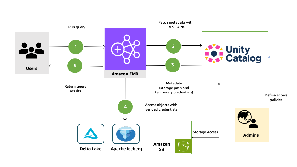
In this post, we will provide an overview of EMR Spark workload integration with Databricks Unity Catalog and walk through the end-to-end process of reading from and writing to Databricks Unity Catalog tables using Amazon EMR and Spark. We show you how to configure EMR Serverless to interact with Databricks Unity Catalog, run an interactive Spark workload to access the data, and run an analysis to derive insights.
The following diagram illustrates the solution architecture.
Prerequisites
You must have the following prerequisites:
- An AWS account and admin user. For instructions, see Set up an AWS account and create an administrator user.
- Storage for EMR Serverless. We use an Amazon Simple Storage Service (Amazon S3) bucket to store output files and logs from the Spark workload that you will run using an EMR Serverless application. For instructions to create a bucket, see Creating a general purpose bucket.
- An EMR Serverless runtime execution AWS Identity and Access Management (IAM) role. For instructions, refer to Job runtime roles for Amazon EMR Serverless, and add access to the storage bucket and storage bucket objects of the Unity Catalog’s storage data.
- A Databricks account. To sign up, see Sign up for Databricks using your existing AWS account.
- Access to a Databricks workspace (on AWS) with Unity Catalog configured. For instructions, see Get started with Unity Catalog.
In the following sections, we walk through the process of reading and writing to Unity Catalog with EMR Serverless.
Enable Unity Catalog for external access
Log in to your workspace as a Databricks admin and complete the following steps to configure external access to read Databricks objects:
- Enable external data access for your metastore. For instructions, see Enable external data access on the metastore.
- Set up a principal that will be configured with Amazon EMR for data access.
- Grant the principal the privilege to configure the integration of the EXTERNAL USE SCHEMA privilege on the schema containing the objects. For instructions, see Grant a principal EXTERNAL USE SCHEMA.
- For this post, we generate a Databricks personal access token (PAT) for the principal and note it down. For instructions, refer to Authorizing access to Databricks resources and Databricks personal access token authentication.
For a production deployment, store the PAT in AWS Secrets Manager. You can use it in a later step to read and write to Unity Catalog with Amazon EMR.
Configure EMR Spark to access Unity Catalog
In this walkthrough, we run PySpark interactive queries through notebooks using EMR Studio. Complete the following steps:
- Open the AWS Management Console with administrator permission.
- Create an EMR Studio to run interactive workloads. To create a workspace, you need to specify the S3 bucket created in the prerequisites and the minimum service role for EMR Serverless. For instructions, see Set up an EMR Studio.
- For this post, we create two EMR Serverless applications. For instructions, see Creating an EMR Serverless application from the EMR Studio console.
- For Iceberg tables, create an EMR Serverless application called dbx-demo-application-iceberg with version 7.8.0 or higher. Make sure to deselect Use AWS Glue Data Catalog as Metastore under Additional Configurations, Metastore configuration. Add the following Spark configuration (see Configure applications). Provide the name of the catalog in Unity Catalog that contains your tables and the URL of the Databricks workspace.
- For Delta tables, create an EMR Serverless application called dbx-demo-application and version 7.8.0 or higher. Make sure to deselect Use AWS Glue Data Catalog as Metastore under Additional Configurations, Metastore configuration. Add the following Spark configuration (see Configure applications). Provide the name of the catalog in Unity Catalog that contains your tables and the URL of the Databricks workspace.
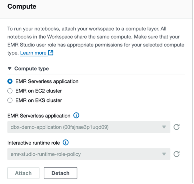
- To set up your interactive workload with a runtime role, see Run interactive workloads with EMR Serverless through EMR Studio.
Read and write to Unity Catalog with Amazon EMR
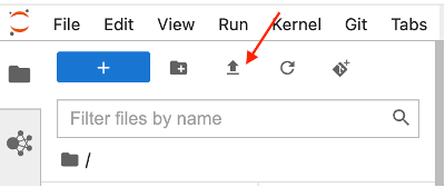
Launch the workspace created in the previous step. Download the notebooks create-delta-table and create-iceberg-table and upload them to the EMR Studio workspace.
The create-delta-table.ipynb notebook configures the metastore properties to work with Delta tables. The create-iceberg-table.ipynb notebook configures the metastore properties to work with Iceberg tables.
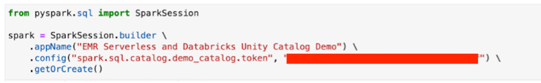
Add the generated token to the session.
For a production deployment, store the PAT in Secrets Manager.
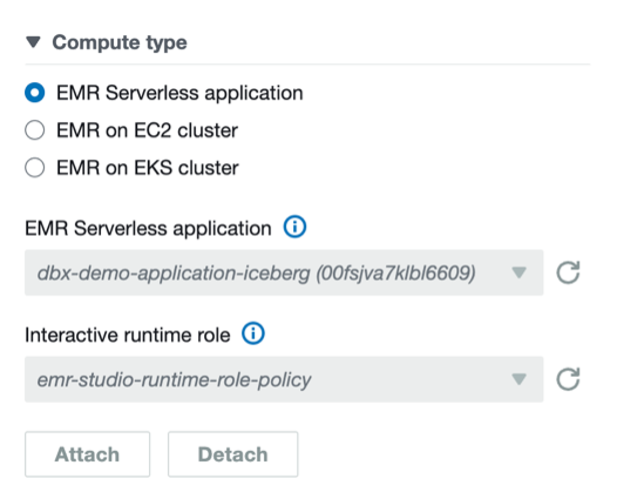
For Iceberg tables, connect to the EMR Serverless application dbx-demo-application-iceberg with the runtime role created in earlier steps under compute and run the notebook (create-iceberg-table). Select PySpark as the kernel and execute each cell in the notebook by choosing the run icon. Refer to Submit a job run or interactive workload for further details about how to run an interactive notebook.
We use the following code to create an external Iceberg table in the catalog:
For Delta tables, connect to the EMR Serverless application dbx-demo-application with the runtime role created in earlier steps and run the notebook (create-delta-table). Select PySpark as the kernel and execute each cell in the notebook by choosing the run icon. Refer to Submit a job run or interactive workload for further details about how to run an interactive notebook.
We use the following code to create an external Delta table in the catalog:
Verify in Databricks for both Iceberg and Delta tables
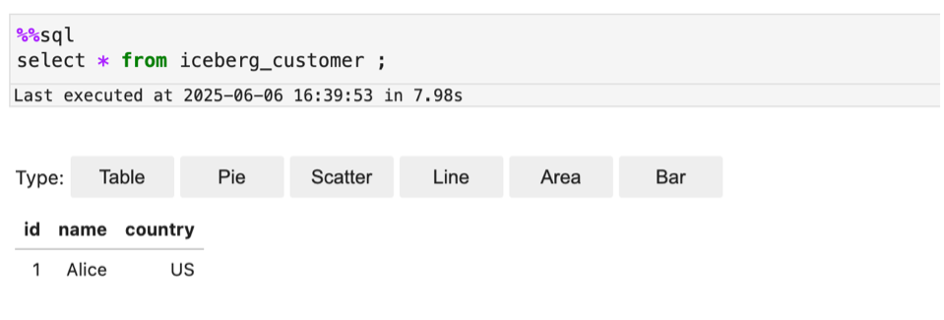
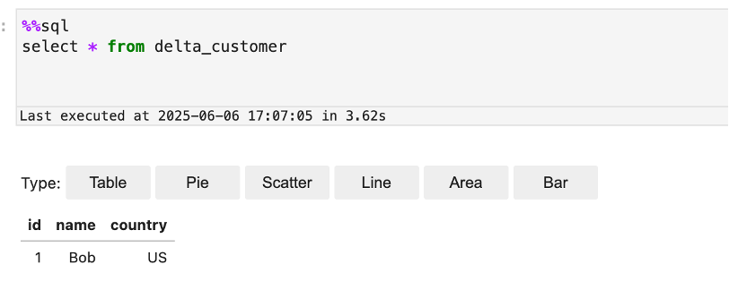
Now you can run queries in Databricks Unity Catalog to show the records inserted into the Iceberg and Delta tables from EMR Serverless:
- Log in to your Databricks workspace.
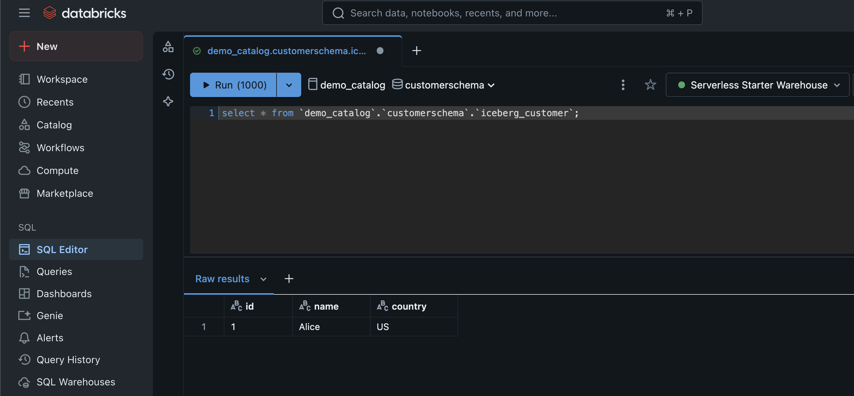
- Choose SQL Editor in the navigation pane.
- Run queries for both Iceberg and Delta tables.
- Verify the results show the same as what you saw in the Jupyter notebook in EMR Studio.
The following screenshot shows an example of querying the Iceberg table.
The following screenshot shows an example of querying the Delta table.

Clean up
Clean up the resources used in this post to avoid additional charges:
- Delete the IAM roles for this post.
- Delete the EMR applications and EMR Studio setup created for this post.
- Delete the resources created in Unity Catalog.
- Empty and then delete the S3 bucket.
Summary
In this post, we demonstrated the powerful interoperability between Amazon EMR and Databricks Unity Catalog by walking through how to enable external access to Unity Catalog, configure EMR Spark to connect seamlessly with Unity Catalog, and perform DML and DDL operations on Unity Catalog tables using EMR Serverless.
To learn more about using EMR Serverless, see Getting started with Amazon EMR Serverless. To learn more about using tools like EMR Spark with Unity Catalog, see Unity Catalog integrations.
About the authors
 Venkatavaradhan (Venkat) Viswanathan is a Global Partner Solutions Architect at Amazon Web Services. Venkat is a Technology Strategy Leader in Data, AI, ML, generative AI, and Advanced Analytics. Venkat is a Global SME for Databricks and helps AWS customers design, build, secure, and optimize Databricks workloads on AWS.
 Srividya Parthasarathy is a Senior Big Data Architect on the AWS Lake Formation team. She works with the product team and customers to build robust features and solutions for their analytical data platform. She enjoys building data mesh solutions and sharing them with the community.
 Ramkumar Nottath is a Principal Solutions Architect at AWS focusing on Analytics services. He enjoys working with various customers to help them build scalable, reliable big data and analytics solutions. His interests extend to various technologies such as analytics, data warehousing, streaming, data governance, and machine learning. He loves spending time with his family and friends.
 John Spencer is a Product Manager at Databricks, dedicated to making Unity Catalog work seamlessly with customers’ ecosystems of tools and platforms so they can easily access, govern, and use their data.
 Sreeram Thoom is a Specialist Solutions Architect at Databricks helping customers design secure, scalable applications on the Data Lakehouse.
 Dipankar Kushari is a specialist solutions architect at Databricks helping customer architect and build secured applications on Data Lakehouse.
 Tom Burns is a Senior Cloud Support Engineer at AWS and is based in the NYC area. He is a subject matter expert in Amazon OpenSearch Service and engages with customers for critical event troubleshooting and improving the supportability of the service. Outside of work, he enjoys playing with his cats, playing board games with friends, and playing competitive games online.
 Ron Miller is a Solutions Architect based out of NYC, supporting transportation and logistics customers. Ron works closely with AWS’s Data & Analytics specialist organization to promote and support OpenSearch. On the weekend, Ron is a shade tree mechanic and trains to complete triathlons.
 Sohaib Katariwala is a Senior Specialist Solutions Architect at AWS focused on Amazon OpenSearch Service based out of Chicago, IL. His interests are in all things data and analytics. More specifically he loves to help customers use AI in their data strategy to solve modern day challenges.
 Mark Twomey is a Senior Solutions Architect at AWS focused on storage and data management. He enjoys working with customers to put their data in the right place, at the right time, for the right cost. Living in Ireland, Mark enjoys walking in the countryside, watching movies, and reading books.
 Sorabh Hamirwasia is a senior software engineer at AWS working on the OpenSearch Project. His primary interest include building cost optimized and performant distributed systems.
 Pallavi Priyadarshini is a Senior Engineering Manager at Amazon OpenSearch Service leading the development of high-performing and scalable technologies for search, security, releases, and dashboards.
 Bobby Mohammed is a Principal Product Manager at AWS leading the Search, GenAI, and Agentic AI product initiatives. Previously, he worked on products across the full lifecycle of machine learning, including data, analytics, and ML features on SageMaker platform, deep learning training and inference products at Intel.
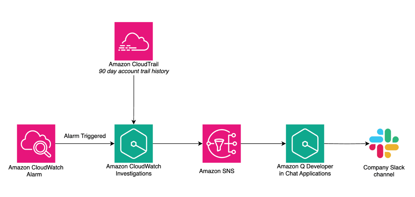
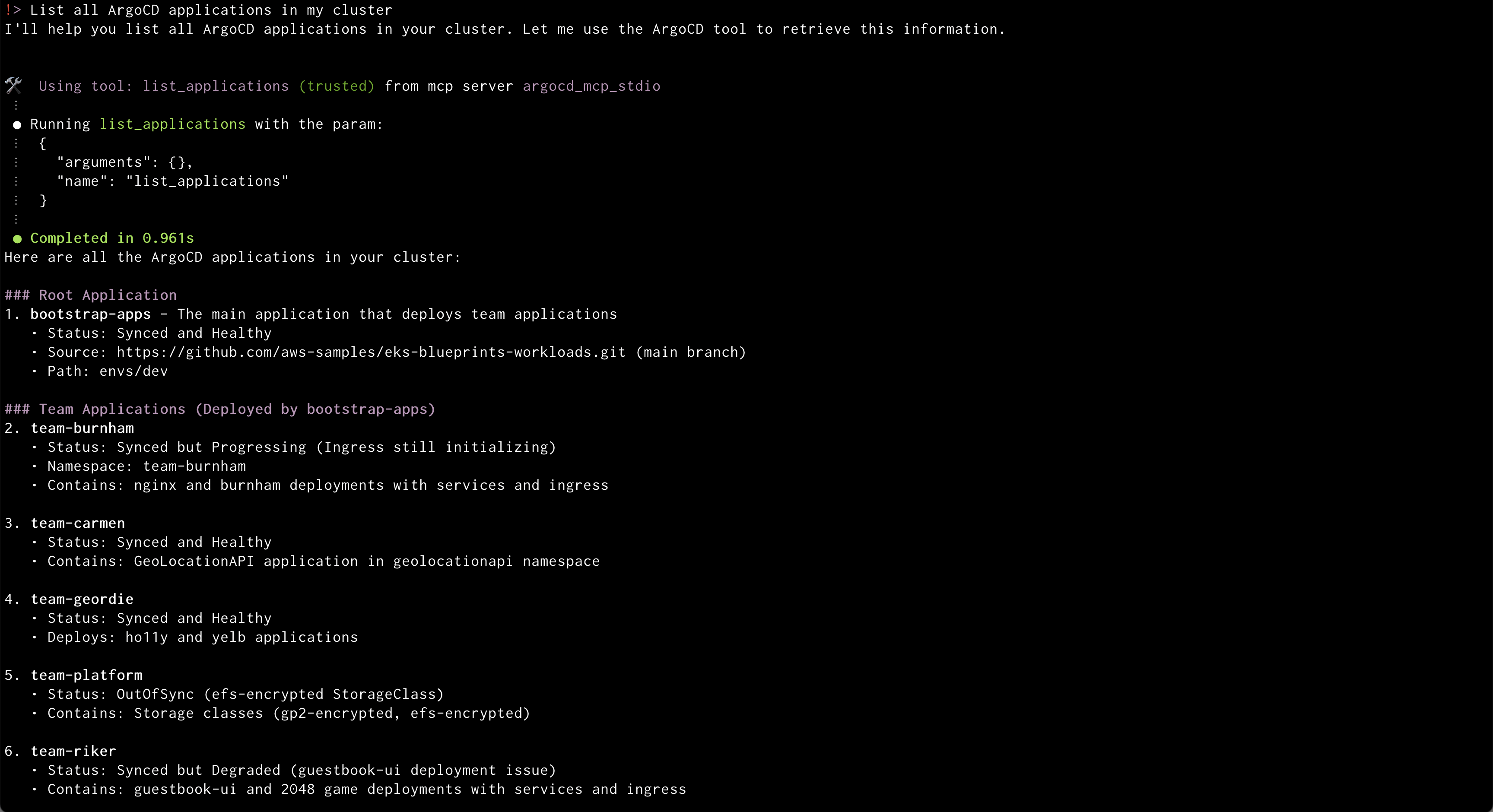 Amazon Q will use the ArgoCD MCP server to retrieve and display all applications
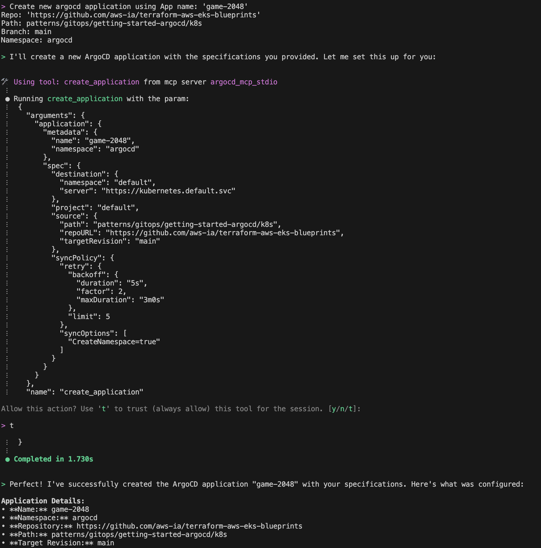 Amazon Q will create a new application from GitRepo information provided
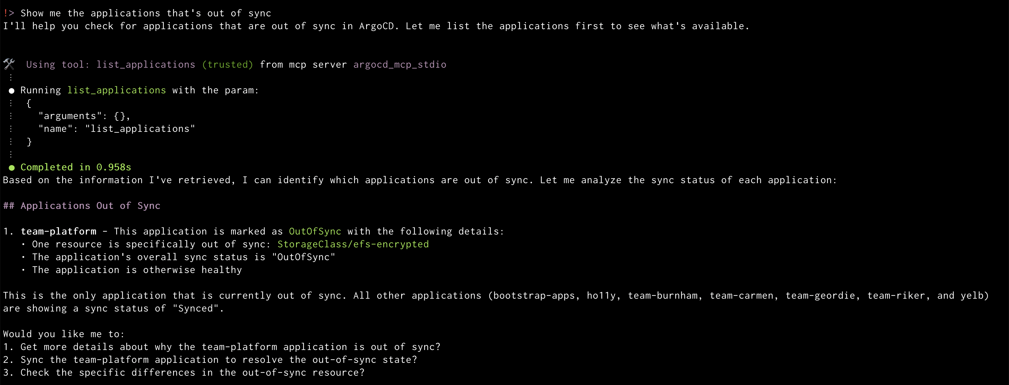 Amazon Q will display the out of sync applications
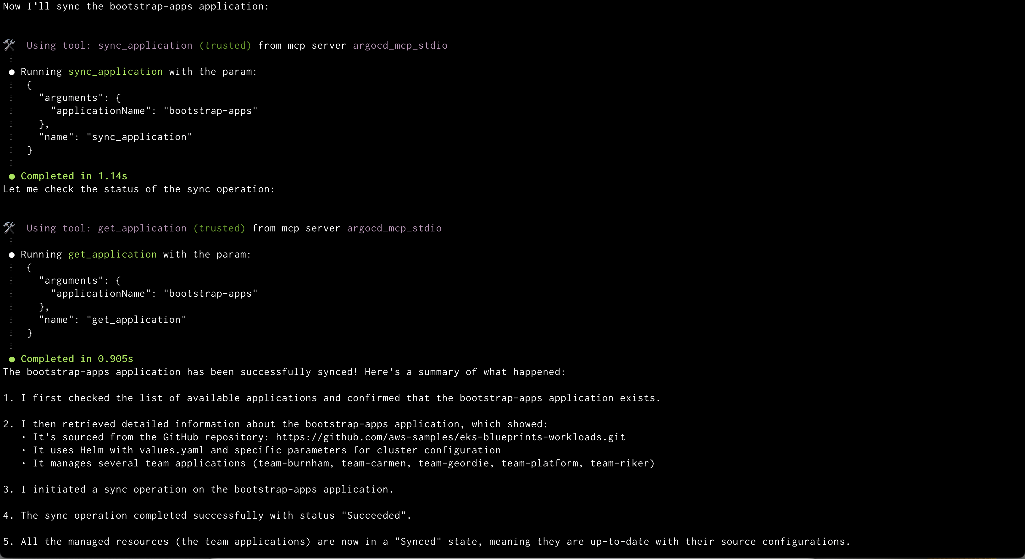 Amazon Q syncing application
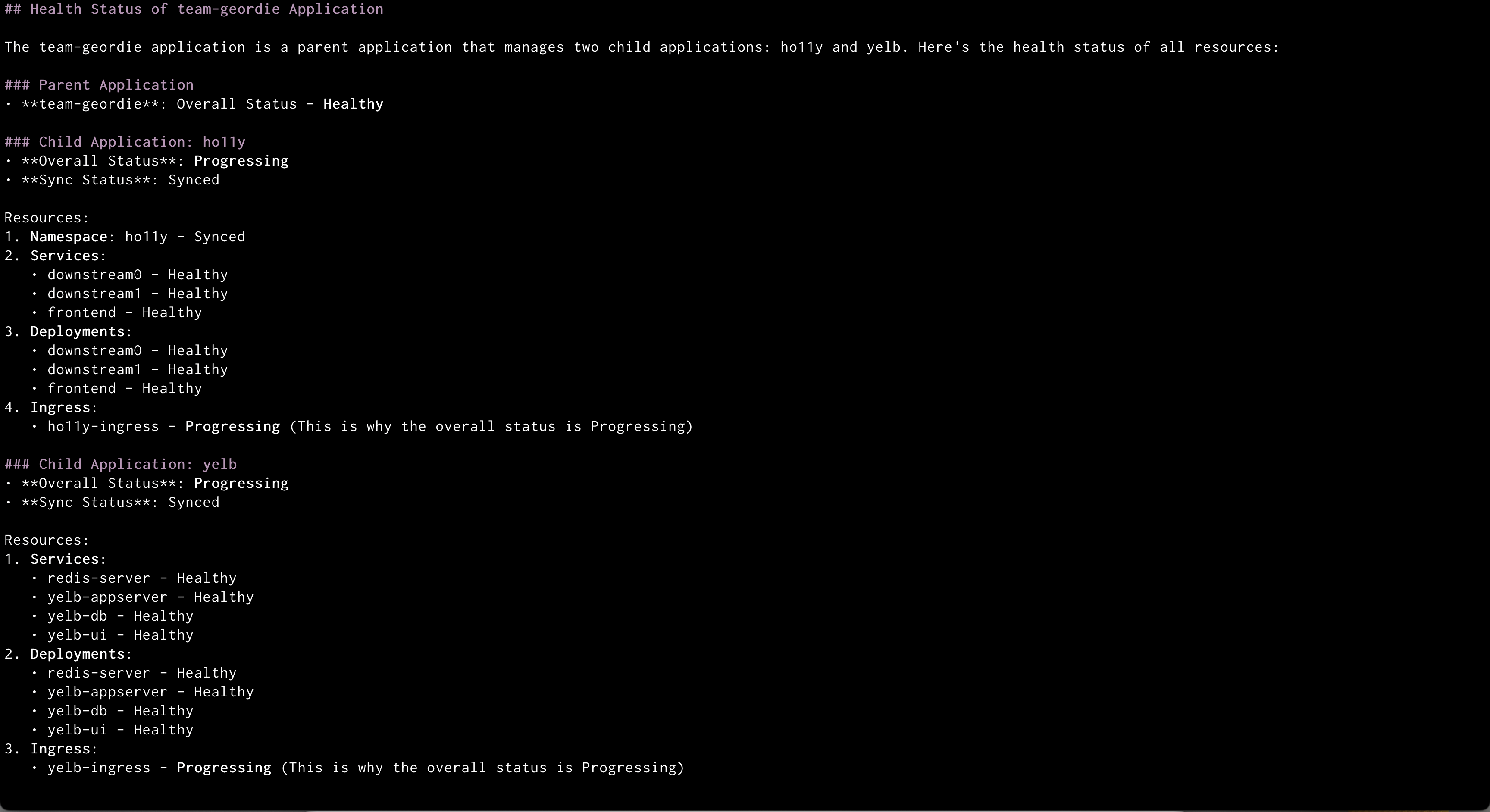 Amazon Q showing health status of all the resources in an application
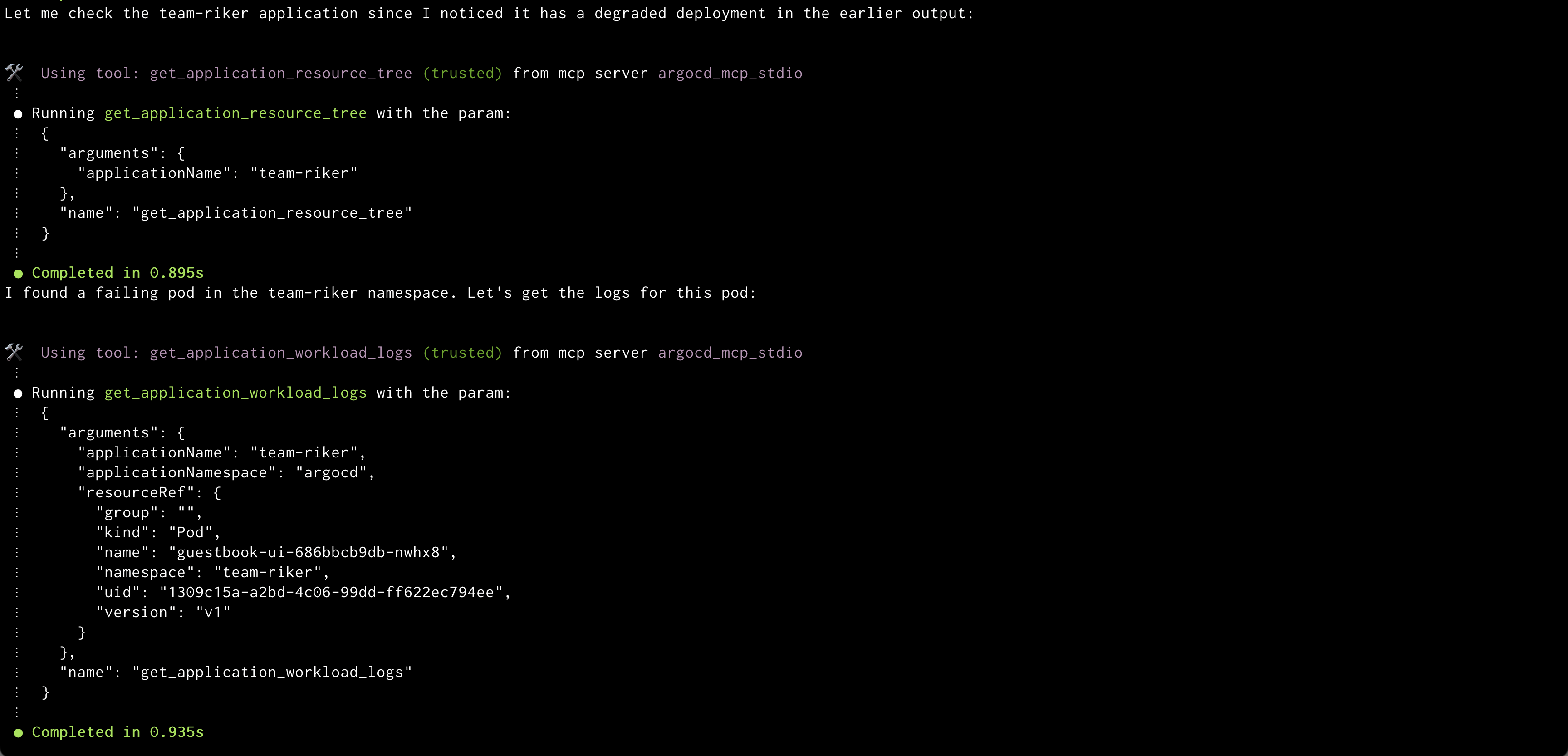 Amazon Q showing logs of problematic pod


 Chiho Sugimoto is a Cloud Support Engineer on the AWS Big Data Support team. She is passionate about helping customers build data lakes using ETL workloads. She loves planetary science and enjoys studying the asteroid Ryugu on weekends.
 Noritaka Sekiyama is a Principal Big Data Architect at the AWS Analytics product team. He’s responsible for designing new features in AWS products, building software artifacts, and providing architecture guidance to customers. In his spare time, he enjoys cycling on his road bike.
 Matt Su is a Senior Product Manager on the AWS Glue team. He enjoys helping customers uncover insights and make better decisions using their data with AWS Analytics services. In his spare time, he enjoys skiing and gardening.


 Naohisa Takahashi is a Senior Cloud Support Engineer on the AWS Support Engineering team. He supports customers resolve technical issues and launch systems. In his spare time, he plays board games with his friends.
 Noritaka Sekiyama is a Principal Big Data Architect with AWS Analytics services. He’s responsible for building software artifacts to help customers. In his spare time, he enjoys cycling on his road bike.
 Iris Tian is a UX designer on the Amazon SageMaker Unified Studio team. She designs intuitive, end-to-end experiences that simplify and streamline workflows across data processing and orchestration. In her spare time, she enjoys snowboarding and visiting museums.
 Regan Baum is a Senior Software Development Engineer on the Amazon SageMaker Unified Studio team. She designs, implements, and maintains features that enable customers to manage their workflows in SageMaker Unified Studio. Outside of work, she enjoys hiking and running.
 Yuhang Huang is a Software Development Manager on the Amazon SageMaker Unified Studio team. He leads the engineering team to design, build, and operate scheduling and orchestration capabilities in SageMaker Unified Studio. In his free time, he enjoys playing tennis.
 Gal Heyne is a Senior Technical Product Manager for AWS Analytics services with a strong focus on AI/ML and data engineering. She is passionate about developing a deep understanding of customers’ business needs and collaborating with engineers to design simple-to-use data products.
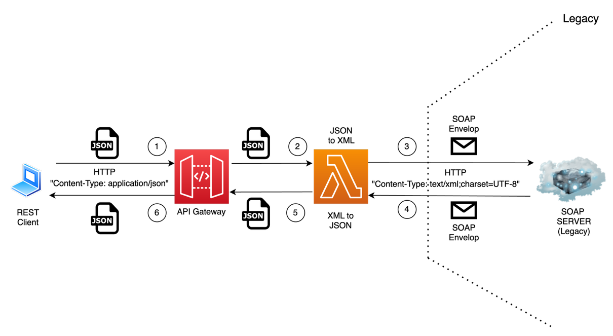


 Jeremy Spell is a Cloud Infrastructure Architect working with Amazon Web Services (AWS) Professional Services. He enjoys architecting and building solutions for customers. In his free time Jeremy makes Texas style BBQ, and spends time with his family and church community.
 Jeff Demuth is a solutions architect who joined Amazon Web Services (AWS) in 2016. He focuses on the geospatial community and is passionate about geographic information systems (GIS) and technology. Outside of work, Jeff enjoys traveling, building Internet of Things (IoT) applications, and tinkering with the latest gadgets.


 The following screenshot shows an example of the Spark UI.
  The following screenshot shows an example of the driver logs.
  The following screenshot shows the Executors tab, which provides access to the driver and executor logs.


 In the following example, we run some TPC-DS SQL statements that are used for performance and benchmarks:


 Amit Maindola is a Senior Data Architect focused on data engineering, analytics, and AI/ML at Amazon Web Services. He helps customers in their digital transformation journey and enables them to build highly scalable, robust, and secure cloud-based analytical solutions on AWS to gain timely insights and make critical business decisions.
 Abhilash is a senior specialist solutions architect at Amazon Web Services (AWS), helping public sector customers on their cloud journey with a focus on AWS Data and AI services. Outside of work, Abhilash enjoys learning new technologies, watching movies, and visiting new places.


 Enrique Salgado Hernández is a Senior Specialist Solutions Architect at AWS with more than 10 years of experience working in the cloud. He specializes in designing and implementing large-scale analytics architectures across various industry sectors. He is passionate about working with customers to solve their problems by supporting them during their cloud journey.
 Angel Conde Manjon is a Senior EMEA Data & AI PSA, based in Madrid. He previously worked on research related to data analytics and AI in diverse European research projects. In his current role, Angel helps partners develop businesses centered on data and AI.


 Srinivas Kandi is a Senior Architect at Stifel focusing on delivering the next generation of cloud data platform on AWS. Prior to joining Stifel, Srini was a delivery specialist in cloud data analytics at AWS helping several customers in their transformational journey into AWS cloud. In his free time, Srini likes to explore cooking, travel and learn new trends and innovations in AI and cloud computing.
 Hossein Johari is a seasoned data and analytics leader with over 25 years of experience architecting enterprise-scale platforms. As Lead and Senior Architect at Stifel Financial Corp. in St. Louis, Missouri, he spearheads initiatives in Data Platforms and Strategic Solutions, driving the design and implementation of innovative frameworks that support enterprise-wide analytics, strategic decision-making, and digital transformation. Known for aligning technical vision with business objectives, he works closely with cross-functional teams to deliver scalable, forward-looking solutions that advance organizational agility and performance.
 Ahmad Rawashdeh is a Senior Architect at Stifel Financial. He supports Stifel and its clients in designing, implementing, and building scalable and reliable data architectures on Amazon Web Services (AWS), with a strong focus on data lake strategies, database services, and efficient data ingestion and transformation pipelines.
 Lei Meng is a data architect at Stifel. His focus is working in designing and implementing scalable and secure data solutions on the AWS and helping Stifel’s cloud migration from on-premises systems.


 Ido Ziv is a DevOps team leader in Kaltura with over 6 years of experience. His hobbies include sailing and Kubernetes (but not at the same time).
 Roi Gamliel is a Senior Solutions Architect helping startups build on AWS. He is passionate about the OpenSearch Project, helping customers fine-tune their workloads and maximize results.
 Yonatan Dolan is a Principal Analytics Specialist at Amazon Web Services. He is located in Israel and helps customers harness AWS analytical services to use data, gain insights, and derive value.