Post Syndicated from Debasis Rath original https://aws.amazon.com/blogs/compute/infrastructure-as-code-translation-for-serverless-using-ai-code-assistants/
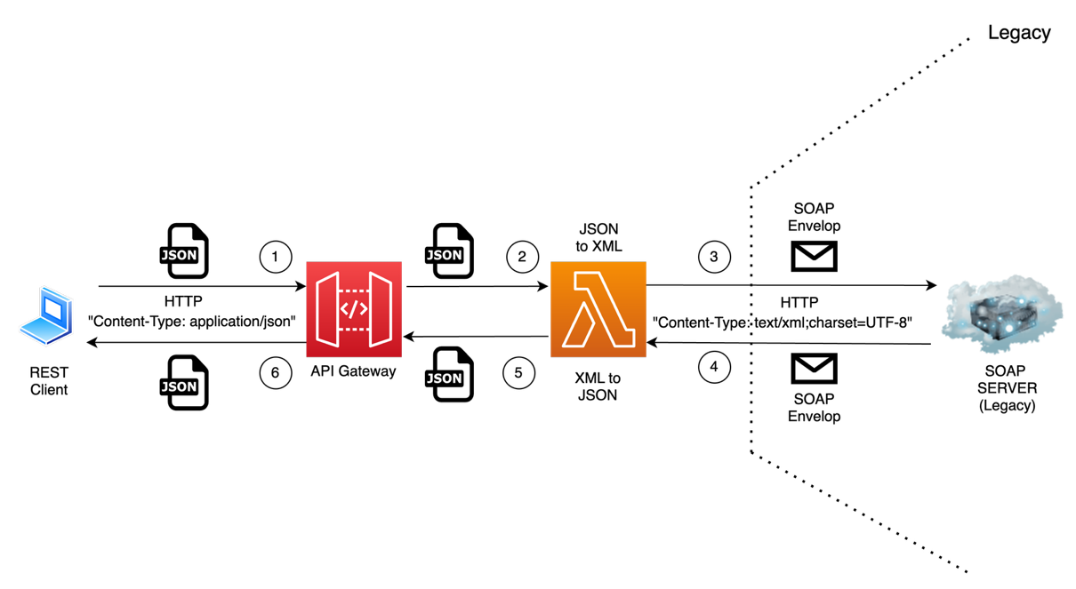
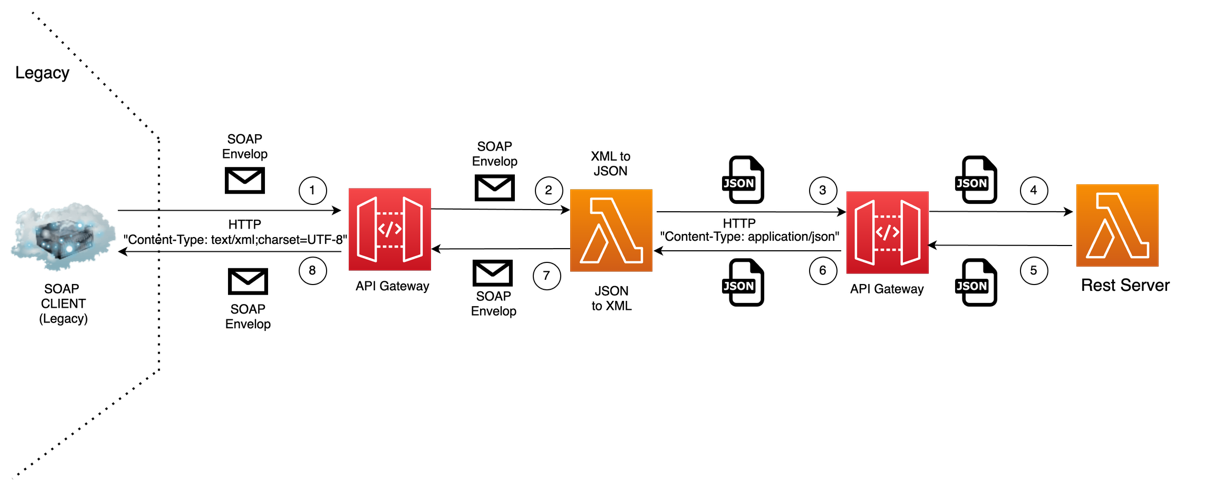
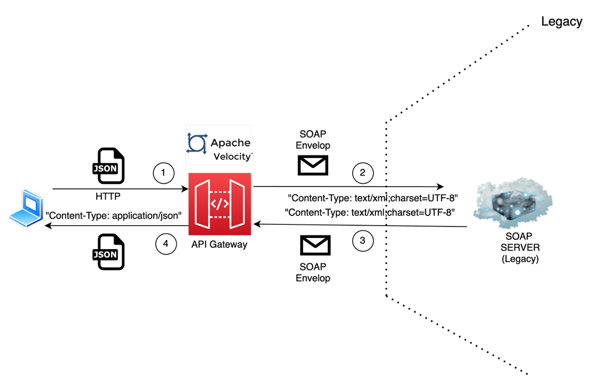
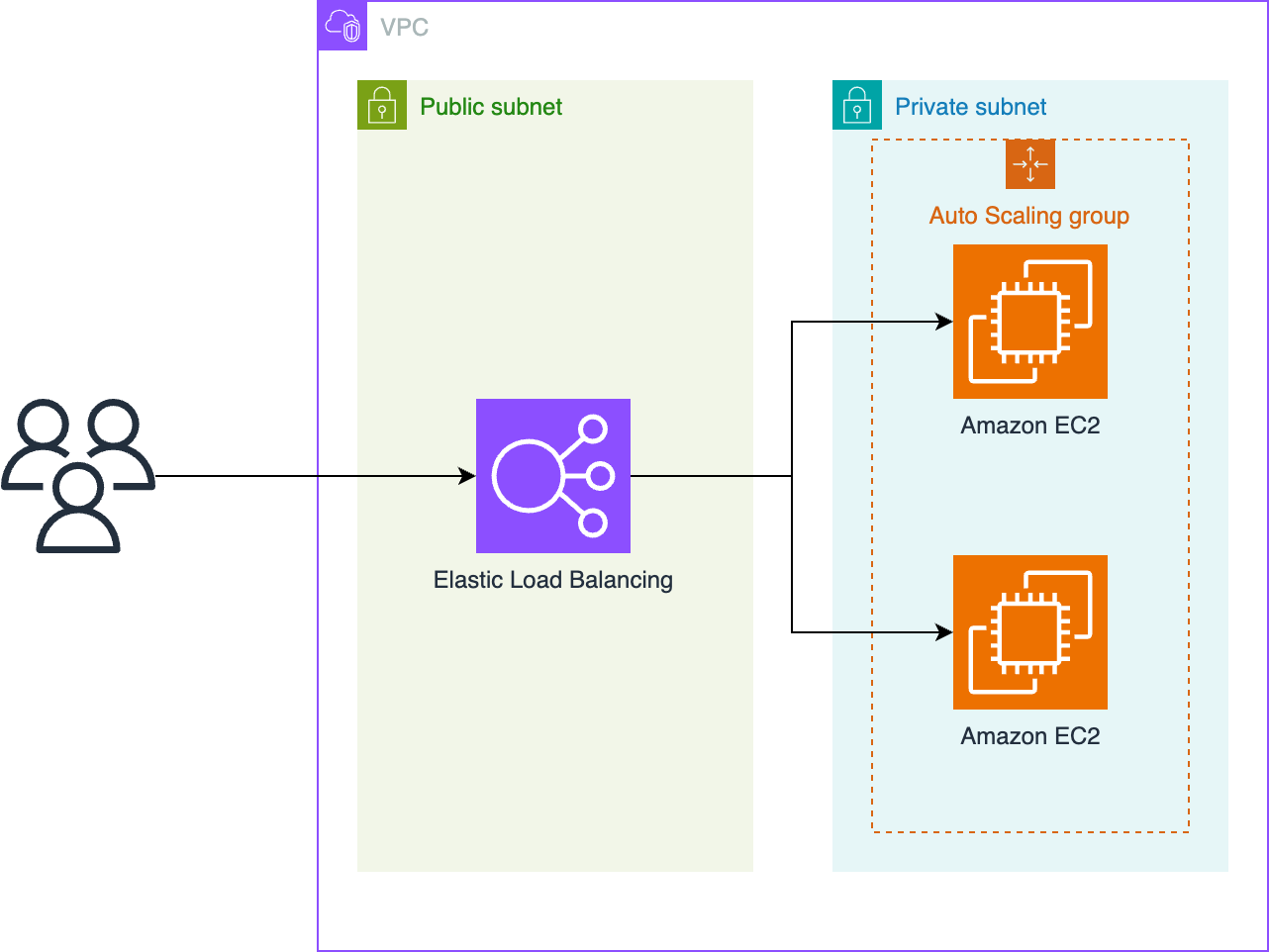
Serverless applications commonly use infrastructure as code (IaC) frameworks to define and manage their cloud resources. Teams choose different IaC tools based on their skills, existing tooling, or compliance needs. As applications grow, the need to shift between IaC formats may arise to adopt new features or align with evolving standards. Developers are rapidly adopting AI-powered coding assistants to help with these evolving demands. In this post, we focus on Amazon Q Developer as an example, but the guidance applies broadly to any coding assistant. Amazon Q Developer is an AI-powered assistant that helps developers with code generation, problem-solving, and development tasks within the Amazon Web Services (AWS) ecosystem. Amazon Q Developer command line interface (CLI) allows developers to convert infrastructure definitions between popular IaC frameworks. This post demonstrates how to use Amazon Q CLI to translate a serverless project from a source IaC such as Serverless Framework version 3 to an IaC framework of choice such as the AWS Serverless Application Model (AWS SAM). To make demonstration more accessible, we have chosen a low-complexity project. However, Amazon Q CLI supports bidirectional translation across multiple IaC formats. We walk through how to migrate a reference architecture to show how the process works, as shown in the following figure.
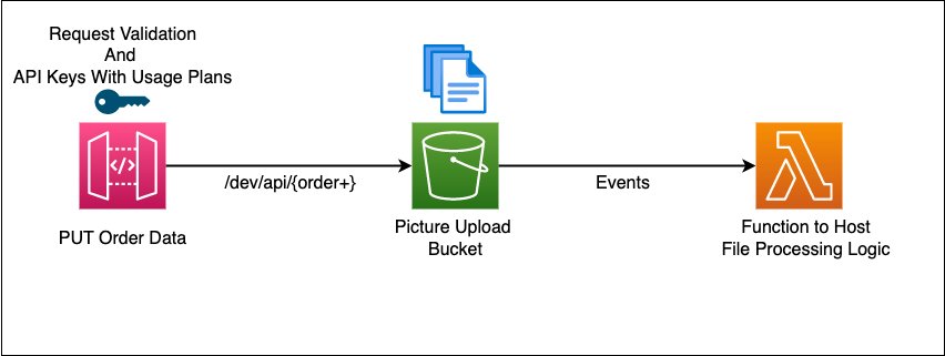
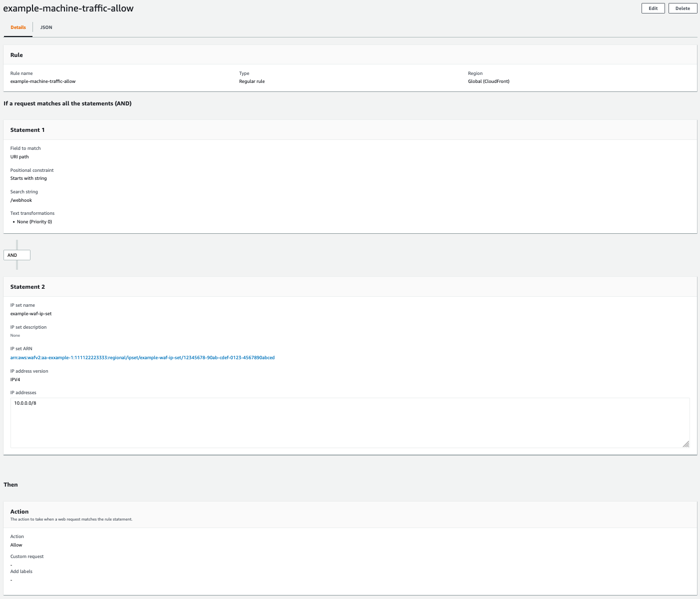
Figure 1. Architecture diagram of example AWS solution to translate
This sample project orchestrates the deployment of a REST API using Amazon API Gateway, acting as an Amazon Simple Storage Service (Amazon S3) proxy for write operations. It includes API-Key setup, basic request validator, AWS Lambda invocation on Amazon S3 events, and enables Amazon CloudWatch Logs and AWS X-Ray tracing for API Gateway and Lambda using the Powertools for Lambda developer toolkit.
Solution overview
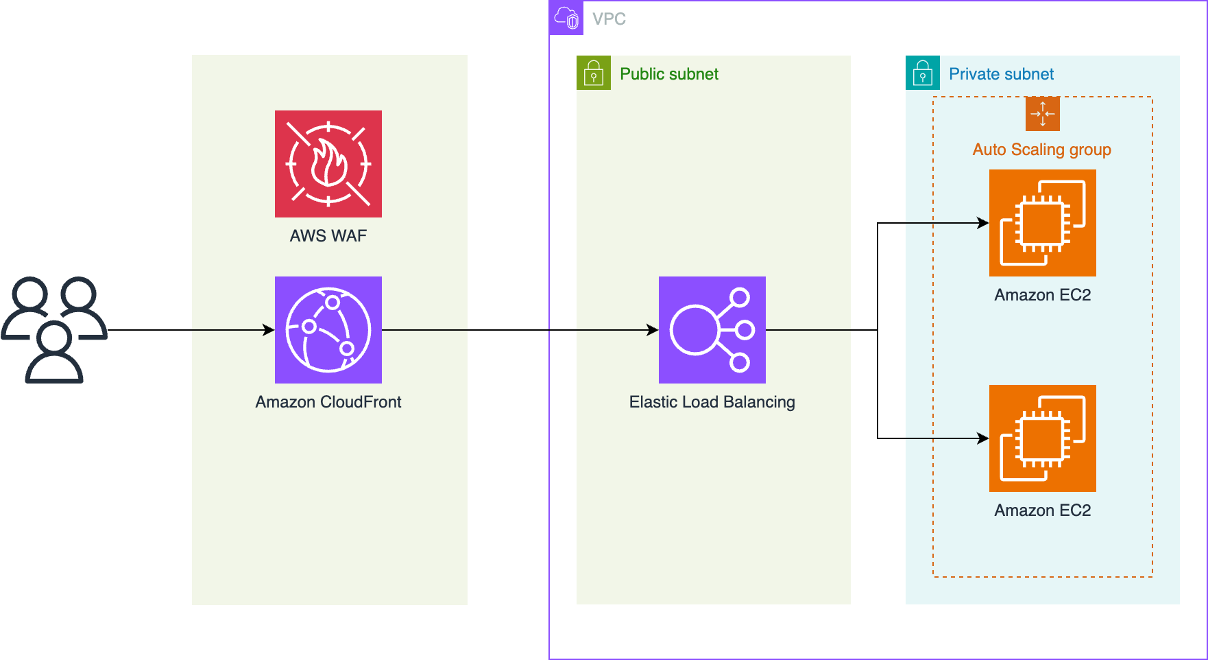
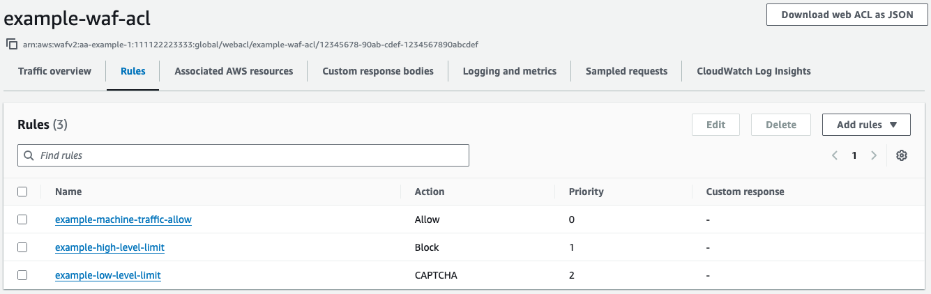
Amazon Q Developer is trained on AWS best practices and provides an AI-powered experience through its CLI. It automates IaC translation by reducing manual effort, minimizing errors, and preserving the original intent across frameworks. The translation process follows four steps: assess, translate, test and refine, and deploy. The following figure shows this workflow.
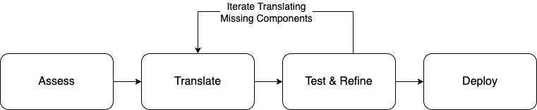
Figure 2. Logical flow for assessment, translation, testing, and deployment
- Assess: Analyze existing Serverless Framework projects for compatibility and readiness.
- Translate: Convert Serverless Framework configuration into AWS SAM templates using Amazon Q Developer CLI.
- Test and refine: Validate and improve translated templates to make sure of functional accuracy and best practices.
- Deploy: Package and deploy the finalized AWS SAM templates to AWS environments.
Prerequisites and considerations
The following prerequisites and considerations are necessary to complete this solution.
Define custom rules to guide automation with Amazon Q Developer
Amazon Q Developer uses a rule-based model to automate tasks that is guided by user-defined rules. These rules encode your team’s standards to make sure that the automation is consistent and repeatable. You can create a library of custom rules to enforce best practices when using Amazon Q in your integrated development environment (IDE) or through the CLI. To help you get started, we’ve included a sample rules file that provides a baseline configuration. This file defines the structure of the output, sequence of the automation steps, and best practices to follow during each phase of the project. You can customize these rules to align with your organization’s architectural guidelines, security policies, or compliance needs.
Understand and categorize project complexity
Serverless projects differ in scale and structure, which directly impacts how you assess them. Smaller projects with minimal configuration and a few functions typically present fewer challenges. Larger, more complex projects can include dozens of Lambda functions, shared layers, and integrations across services such as Amazon Simple Queue Service (Amazon SQS), Amazon DynamoDB, or Amazon EventBridge. Start by categorizing the project as low, medium, or high complexity based on factors such as the number of functions, the diversity of event sources, and the presence of shared configurations. Use this categorization to prioritize and scope your assessment efforts. For complex workloads, assess individual components separately to reduce the surface area for troubleshooting and remediation.
Handle framework-specific tooling and plugins
Plugins or dependencies in different IaC frameworks extend core functionality or introduce custom behaviors. AWS SAM supports similar capabilities but in a different way. For example, you may be able to use AWS SAM, but for capabilities not found in AWS SAM, you can use AWS CloudFormation macros or Lambda-backed custom resources. During assessment, identify all active plugins and document their purpose and integration points. Evaluate whether each plugin’s functionality can be replicated using native AWS services or custom resources in AWS SAM. For common patterns—such as packaging optimizations, function warmers, or custom deploy hooks—consider using the CloudFormation macros and custom resources. When plugin functionality cannot be translated directly, annotate it in your assessment report for manual intervention. Clearly mapping each plugin’s role helps maintain parity and reduces surprises during deployment in the new environment.
With all of this you are ready to start the conversion.
Assess with Amazon Q Developer
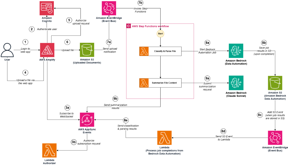
The animated diagrams included in this post offer step-by-step visuals to explain the Amazon Q behavior throughout the workflow. Remember that you have already set rules for Amazon Q for each phase. Now your prompt to Amazon Q is clear. At this point Amazon Q has enough context to get you crisper and deterministic result. Use the following prompt to start the assessment:
Prompt
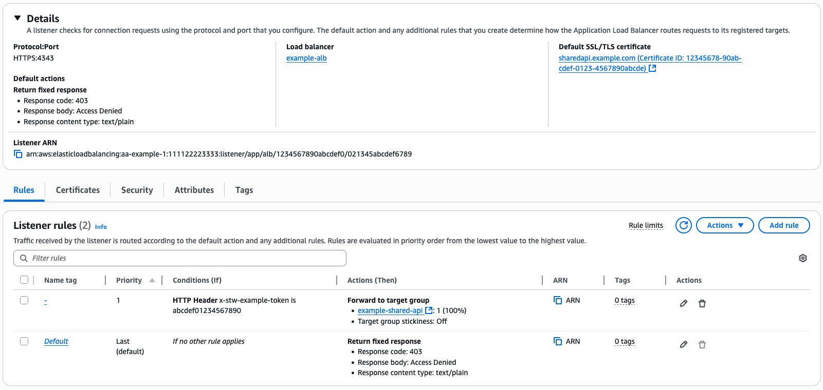
Figure 3. Assessment step using Amazon Q Developer
After the assessment, Amazon Q Developer generates translation recommendations based on AWS best practices. It produces an evaluation_summary.md file with detailed insights, mapping guidance, and technical considerations for converting components to AWS SAM resources. The report serves as the foundation for the next step: automated translation into AWS SAM resources.
Translate using Amazon Q Developer
After completing the assessment, begin the translation using the baseline rules defined in .amazonq/rules/translation_rules.md. These rules guide the conversion and make sure of consistency with the assessment outputs. Amazon Q Developer CLI uses these rules to parse the serverless.yml file, scaffold a new project structure, and generate a complete AWS SAM template. During translation, Amazon Q Developer performs the following actions:
- Converts each Lambda function into an
AWS::Serverless::Function, preserving runtime, handler, memory, timeout, and environment settings. - Translates event sources such as HTTP APIs and Amazon SQS into SAM event definitions.
- Maps AWS Identity and Access Management (IAM) policies and permissions into CloudFormation-compatible resources.
- Removes development-only settings such as the
serverless-offlineplugin.
Serverless Framework v3 often uses CloudFormation orchestration and custom resources to deliver certain capabilities. For example, it may use custom resources to provision S3 bucket notifications. Amazon Q detects these patterns during assessment and translates them into explicit, well-structured AWS SAM resources. This makes sure of functional parity in the target IaC.Use the following prompt to begin the translation:
Prompt
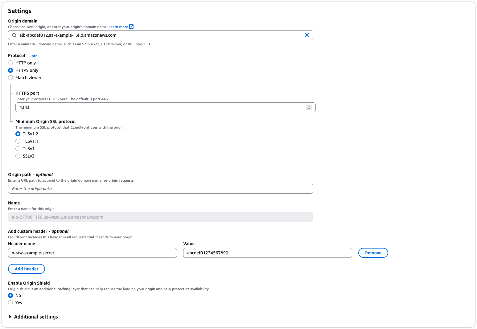
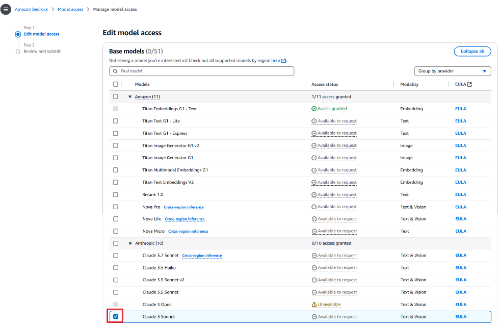
Figure 4. Translation using Amazon Q Developer
After translation, Amazon Q Developer produces a complete AWS SAM project with test scripts and documentation. The project supports local testing, automated deployment, consistent resource management, and native integration with AWS tools. You also receive a development_summary.md file with a structured project overview and step-by-step testing instructions.
Amazon Q Developer replaces resources created implicitly by Serverless Framework plugins (such as Serverless Lift or custom resources for handling circular dependencies) with explicit CloudFormation definitions. To support custom or unsupported plugins, define the translation logic in .amazonq/rules/development_rules.md. Specify mappings or flag resources for manual review. This maximizes automation while highlighting exceptions early in the workflow.
Test and refine using Amazon Q Developer
Validate the translated AWS SAM application using the local testing rules defined in .amazonq/rules/local_testing_rules.md. These rules guide high-fidelity simulation and verification.
Amazon Q Developer generates test commands that use the AWS SAM CLI to replicate real-world behavior. It uses sam local invoke to test Lambda functions and sam local start-api to simulate HTTP API calls. This makes sure of the translated application behaves as expected when compared to the original Serverless Framework project.
To simulate Amazon S3 events, provision temporary S3 buckets, and instruct Amazon Q Developer to reference them during testing, it enables full end-to-end validation by combining real Amazon S3 interactions with a local function execution.Use the following prompt to begin testing:
Figure 5. Testing and refinement step using Amazon Q Developer
Use AWS SAM Accelerate with sam sync to run cloud-based integration tests in a lower environment after completing local validation. This complements early testing and helps catch runtime issues before deployment. Combining Amazon Q Developer automation with AWS SAM CLI allows you to speed up feedback cycles and make sure of functional accuracy in the cloud environment.
Deploy
The translated and tested AWS SAM application is ready, thus the final step is deployment. Using AWS SAM CLI, package and deploy the application to an AWS environment where it becomes fully operational. Begin by running the following:sam build
This command prepares the application for deployment by packaging the Lambda function code, resolving dependencies, and creating build artifacts in the .aws-sam directory.Next, deploy the application using the following:
The --guided flag walks you through the initial configuration, such as stack name, AWS Region, and necessary capabilities such as IAM role creation. When it’s complete, CloudFormation provisions all resources defined in the template.yaml, such as Lambda functions, API Gateway endpoints, SQS queues, and IAM policies. Here is how the output looks from the deployment:
AWS SAM emphasizes explicit definitions such as resource names and parameters. Therefore, using the AWS SAM guided deployment here helps by presenting change set reviews to verify these changes.Now that you’ve translated and tested your AWS SAM application, verify its parity with the original Serverless Framework stack. Compare CloudFormation outputs—API Gateway endpoints, S3 bucket names, Lambda Amazon Resource Names (ARNs), and queue URLs—and automate integration or A/B tests to confirm functional equivalence. Then, deploy the AWS SAM version using a canary release, monitor performance and user metrics, and shift traffic gradually to minimize risk.
Cleaning up
If you no longer need the AWS resources that you created by running this example, then you can remove them by deleting the CloudFormation stack that you deployed.
To delete the CloudFormation stack, use the sam delete command:
Conclusion
In this post you’ve learned how Amazon Q Developer CLI can streamline the translation of IaC by using an example of migrating Serverless Framework to AWS SAM. Using AI-powered conversational interfaces and deep integration with AWS knowledge means that Amazon Q Developer substantially reduces the manual effort and potential errors involved in these translations. Comprehensive assessment, translation, testing, and deployment can be difficult to accelerate, but this can be streamlined with new generative AI tools from AWS.
For more information on Amazon Q, you can check out Amazon Q Developer. For more serverless learning resources, visit Serverless Land. To find more patterns, go directly to the Serverless Patterns Collection.


 Enrique Salgado Hernández is a Senior Specialist Solutions Architect at AWS with more than 10 years of experience working in the cloud. He specializes in designing and implementing large-scale analytics architectures across various industry sectors. He is passionate about working with customers to solve their problems by supporting them during their cloud journey.
 Angel Conde Manjon is a Senior EMEA Data & AI PSA, based in Madrid. He previously worked on research related to data analytics and AI in diverse European research projects. In his current role, Angel helps partners develop businesses centered on data and AI.


 Amit Maindola is a Senior Data Architect focused on data engineering, analytics, and AI/ML at Amazon Web Services. He helps customers in their digital transformation journey and enables them to build highly scalable, robust, and secure cloud-based analytical solutions on AWS to gain timely insights and make critical business decisions.
 Srinivas Kandi is a Senior Architect at Stifel focusing on delivering the next generation of cloud data platform on AWS. Prior to joining Stifel, Srini was a delivery specialist in cloud data analytics at AWS helping several customers in their transformational journey into AWS cloud. In his free time, Srini likes to explore cooking, travel and learn new trends and innovations in AI and cloud computing.
 Hossein Johari is a seasoned data and analytics leader with over 25 years of experience architecting enterprise-scale platforms. As Lead and Senior Architect at Stifel Financial Corp. in St. Louis, Missouri, he spearheads initiatives in Data Platforms and Strategic Solutions, driving the design and implementation of innovative frameworks that support enterprise-wide analytics, strategic decision-making, and digital transformation. Known for aligning technical vision with business objectives, he works closely with cross-functional teams to deliver scalable, forward-looking solutions that advance organizational agility and performance.
 Ahmad Rawashdeh is a Senior Architect at Stifel Financial. He supports Stifel and its clients in designing, implementing, and building scalable and reliable data architectures on Amazon Web Services (AWS), with a strong focus on data lake strategies, database services, and efficient data ingestion and transformation pipelines.
 Lei Meng is a data architect at Stifel. His focus is working in designing and implementing scalable and secure data solutions on the AWS and helping Stifel’s cloud migration from on-premises systems.


 Konstantina Mavrodimitraki is a Senior Solutions Architect at Amazon Web Services, where she assists customers in designing scalable, robust, and secure systems in global markets. With deep expertise in data strategy, data warehousing, and big data systems, she helps organizations transform their data landscapes. A passionate technologist and people person, Konstantina loves exploring emerging technologies and supports the local tech communities. Additionally, she enjoys reading books and playing with her dog.
 Kostas Diamantis is the Head of the Data Warehouse at Skroutz company. With a background in software engineering, he transitioned into data engineering, using his technical expertise to build scalable data solutions. Passionate about data-driven decision-making, he focuses on optimizing data pipelines, enhancing analytics capabilities, and driving business insights.


 Nikos Tragaras is a Principal Software Architect at Nexthink with around two decades of experience in building distributed systems, from traditional architectures to modern cloud-native platforms. He has worked extensively with streaming technologies, focusing on reliability and performance at scale. Passionate about programming, he enjoys building clean solutions to complex engineering problems
 Raphaël Afanyan is a Software Engineer and Tech Lead of the Alerts team at Nexthink. Over the years, he has worked on designing and scaling data processing systems and played a key role in building Nexthink’s alerting platform. He now collaborates across teams to bring innovative product ideas to life, from backend architecture to polished user interfaces.
 Simone Pomata is a Senior Solutions Architect at AWS. He has worked enthusiastically in the tech industry for more than 10 years. At AWS, he helps customers succeed in building new technologies every day.
 Subham Rakshit is a Senior Streaming Solutions Architect for Analytics at AWS based in the UK. He works with customers to design and build streaming architectures so they can get value from analyzing their streaming data. His two little daughters keep him occupied most of the time outside work, and he loves solving jigsaw puzzles with them. Connect with him on
  Lorenzo Nicora works as a Senior Streaming Solutions Architect at AWS, helping customers across EMEA. He has been building cloud-centered, data-intensive systems for over 25 years, working across industries both through consultancies and product companies. He has used open source technologies extensively and contributed to several projects, including Apache Flink.


 Aarthi Srinivasan is a Senior Big Data Architect with Amazon SageMaker Lakehouse. As part of the SageMaker Lakehouse team, she works with AWS customers and partners to architect lake house solutions, enhance product features, and establish best practices for data governance.
 Praveen Kumar is an Analytics Solutions Architect at AWS with expertise in designing, building, and implementing modern data and analytics platforms using cloud-based services. His areas of interest are serverless technology, data governance, and data-driven AI applications.
 Dhananjay Badaya is a Software Developer at AWS, specializing in distributed data processing engines including Apache Spark and Apache Hadoop. As a member of the Amazon EMR team, he focuses on designing and implementing enterprise governance features for EMR Spark.


 Sri Potluri is a Cloud Infrastructure Architect at AWS. He is passionate about solving complex problems and delivering well-structured solutions for diverse customers. His expertise spans across a range of cloud technologies, providing scalable and reliable infrastructures tailored to each project’s unique challenges.
 Suvojit Dasgupta is a Principal Data Architect at AWS. He leads a team of skilled engineers in designing and building scalable data solutions for AWS customers. He specializes in developing and implementing innovative data architectures to address complex business challenges.