Post Syndicated from Shoukat Ghouse original https://aws.amazon.com/blogs/big-data/simplify-data-lake-access-control-for-your-enterprise-users-with-trusted-identity-propagation-in-aws-iam-identity-center-aws-lake-formation-and-amazon-s3-access-grants/
Many organizations use external identity providers (IdPs) such as Okta or Microsoft Azure Active Directory to manage their enterprise user identities. These users interact with and run analytical queries across AWS analytics services. To enable them to use the AWS services, their identities from the external IdP are mapped to AWS Identity and Access Management (IAM) roles within AWS, and access policies are applied to these IAM roles by data administrators.
Given the diverse range of services involved, different IAM roles may be required for accessing the data. Consequently, administrators need to manage permissions across multiple roles, a task that can become cumbersome at scale.
To address this challenge, you need a unified solution to simplify data access management using your corporate user identities instead of relying solely on IAM roles. AWS IAM Identity Center offers a solution through its trusted identity propagation feature, which is built upon the OAuth 2.0 authorization framework.
With trusted identity propagation, data access management is anchored to a user’s identity, which can be synchronized to IAM Identity Center from external IdPs using the System for Cross-domain Identity Management (SCIM) protocol. Integrated applications exchange OAuth tokens, and these tokens are propagated across services. This approach empowers administrators to grant access directly based on existing user and group memberships federated from external IdPs, rather than relying on IAM users or roles.
In this post, we showcase the seamless integration of AWS analytics services with trusted identity propagation by presenting an end-to-end architecture for data access flows.
Solution overview
Let’s consider a fictional company, OkTank. OkTank has multiple user personas that use a variety of AWS Analytics services. The user identities are managed externally in an external IdP: Okta. User1 is a Data Analyst and uses the Amazon Athena query editor to query AWS Glue Data Catalog tables with data stored in Amazon Simple Storage Service (Amazon S3). User2 is a Data Engineer and uses Amazon EMR Studio notebooks to query Data Catalog tables and also query raw data stored in Amazon S3 that is not yet cataloged to the Data Catalog. User3 is a Business Analyst who needs to query data stored in Amazon Redshift tables using the Amazon Redshift Query Editor v2. Additionally, this user builds Amazon QuickSight visualizations for the data in Redshift tables.
OkTank wants to simplify governance by centralizing data access control for their variety of data sources, user identities, and tools. They also want to define permissions directly on their corporate user or group identities from Okta instead of creating IAM roles for each user and group and managing access on the IAM role. In addition, for their audit requirements, they need the capability to map data access to the corporate identity of users within Okta for enhanced tracking and accountability.
To achieve these goals, we use trusted identity propagation with the aforementioned services and use AWS Lake Formation and Amazon S3 Access Grants for access controls. We use Lake Formation to centrally manage permissions to the Data Catalog tables and Redshift tables shared with Redshift datashares. In our scenario, we use S3 Access Grants for granting permission for the Athena query result location. Additionally, we show how to access a raw data bucket governed by S3 Access Grants with an EMR notebook.
Data access is audited with AWS CloudTrail and can be queried with AWS CloudTrail Lake. This architecture showcases the versatility and effectiveness of AWS analytics services in enabling efficient and secure data analysis workflows across different use cases and user personas.
We use Okta as the external IdP, but you can also use other IdPs like Microsoft Azure Active Directory. Users and groups from Okta are synced to IAM Identity Center. In this post, we have three groups, as shown in the following diagram.

User1 needs to query a Data Catalog table with data stored in Amazon S3. The S3 location is secured and managed by Lake Formation. The user connects to an IAM Identity Center enabled Athena workgroup using the Athena query editor with EMR Studio. The IAM Identity Center enabled Athena workgroups need to be secured with S3 Access Grants permissions for the Athena query results location. With this feature, you can also enable the creation of identity-based query result locations that are governed by S3 Access Grants. These user identity-based S3 prefixes let users in an Athena workgroup keep their query results isolated from other users in the same workgroup. The following diagram illustrates this architecture.

User2 needs to query the same Data Catalog table as User1. This table is governed using Lake Formation permissions. Additionally, the user needs to access raw data in another S3 bucket that isn’t cataloged to the Data Catalog and is controlled using S3 Access Grants; in the following diagram, this is shown as S3 Data Location-2.
The user uses an EMR Studio notebook to run Spark queries on an EMR cluster. The EMR cluster uses a security configuration that integrates with IAM Identity Center for authentication and uses Lake Formation for authorization. The EMR cluster is also enabled for S3 Access Grants. With this kind of hybrid access management, you can use Lake Formation to centrally manage permissions for your datasets cataloged to the Data Catalog and use S3 Access Grants to centrally manage access to your raw data that is not yet cataloged to the Data Catalog. This gives you flexibility to access data managed by either of the access control mechanisms from the same notebook.

User3 uses the Redshift Query Editor V2 to query a Redshift table. The user also accesses the same table with QuickSight. For our demo, we use a single user persona for simplicity, but in reality, these could be completely different user personas. To enable access control with Lake Formation for Redshift tables, we use data sharing in Lake Formation.

Data access requests by the specific users are logged to CloudTrail. Later in this post, we also briefly touch upon using CloudTrail Lake to query the data access events.

In the following sections, we demonstrate how to build this architecture. We use AWS CloudFormation to provision the resources. AWS CloudFormation lets you model, provision, and manage AWS and third-party resources by treating infrastructure as code. We also use the AWS Command Line Interface (AWS CLI) and AWS Management Console to complete some steps.
The following diagram shows the end-to-end architecture.

Prerequisites
Complete the following prerequisite steps:
- Have an AWS account. If you don’t have an account, you can create one.
- Have IAM Identity Center set up in a specific AWS Region.
- Make sure you use the same Region where you have IAM Identity Center set up throughout the setup and verification steps. In this post, we use the
us-east-1Region. - Have Okta set up with three different groups and users, and enable sync to IAM Identity Center. Refer to Configure SAML and SCIM with Okta and IAM Identity Center for instructions.
After the Okta groups are pushed to IAM Identity Center, you can see the users and groups on the IAM Identity Center console, as shown in the following screenshot. You need the group IDs of the three groups to be passed in the CloudFormation template.

- For enabling User2 access using the EMR cluster, you need have an SSL certificate .zip file available in your S3 bucket. You can download the following sample certificate to use in this post. In production use cases, you should create and use your own certificates. You need to reference the bucket name and the certificate bundle .zip file in AWS CloudFormation. The CloudFormation template lets you choose the components you want to provision. If you do not intend to deploy the EMR cluster, you can ignore this step.
- Have an administrator user or role to run the CloudFormation stack. The user or role should also be a Lake Formation administrator to grant permissions.
Deploy the CloudFormation stack
The CloudFormation template provided in the post lets you choose the components you want to provision from the solution architecture. In this post, we enable all components, as shown in the following screenshot.

Run the provided CloudFormation stack to create the solution resources. Refer to the following table for a list of important parameters.
| Parameter Group | Description | Parameter Name | Expected Value |
| Choose components to provision. | Choose the components you want to be provisioned. | DeployAthenaFlow |
Yes/No. If you choose No, you can ignore the parameters in the “Athena Configuration” group. |
DeployEMRFlow |
Yes/No. If you choose No, you can ignore the parameters in the “EMR Configuration” group. | ||
DeployRedshiftQEV2Flow |
Yes/No. If you choose No, you can ignore the parameters in the “Redshift Configuration” group. | ||
CreateS3AGInstance |
Yes/No. If you already have an S3 Access Grants instance, choose No. Otherwise, choose Yes to allow the stack create a new S3 Access Grants instance. The S3 Access Grants instance is needed for User1 and User2. | ||
| Identity Center Configuration | IAM Identity Center parameters. | IDCGroup1Id |
Group ID corresponding to Group1 from IAM Identity Center. |
IDCGroup2Id |
Group ID corresponding to Group2 from IAM Identity Center. | ||
IDCGroup3Id |
Group ID corresponding to Group3 from IAM Identity Center. | ||
IAMIDCInstanceArn |
IAM Identity Center instance ARN. You can get this from the Settings section of IAM Identity Center. | ||
| Redshift Configuration |
Redshift parameters. Ignore if you chose |
RedshiftServerlessAdminUserName |
Redshift admin user name. |
RedshiftServerlessAdminPassword |
Redshift admin password. | ||
RedshiftServerlessDatabase |
Redshift database to create the tables. | ||
| EMR Configuration |
EMR parameters. Ignore if you chose parameter |
SSlCertsS3BucketName |
Bucket name where you copied the SSL certificates. |
SSlCertsZip |
Name of SSL certificates file (my-certs.zip) to use the sample certificate provided in the post. | ||
| Athena Configuration |
Athena parameters. Ignore if you chose parameter |
IDCUser1Id |
User ID corresponding to User1 from IAM Identity Center. |
The CloudFormation stack provisions the following resources:
- A VPC with a public and private subnet.
- If you chose the Redshift components, it also creates three additional subnets.
- S3 buckets for data and Athena query results location storage. It also copies some sample data to the buckets.
- EMR Studio with IAM Identity Center integration.
- Amazon EMR security configuration with IAM Identity Center integration.
- An EMR cluster that uses the EMR security group.
- Registers the source S3 bucket with Lake Formation.
- An AWS Glue database named
oktank_tipblog_tempand a table namedcustomerunder the database. The table points to the Amazon S3 location governed by Lake Formation. - Allows external engines to access data in Amazon S3 locations with full table access. This is required for Amazon EMR integration with Lake Formation for trusted identity propagation. As of this writing, Amazon EMR supports table-level access with IAM Identity Center enabled clusters.
- An S3 Access Grants instance.
- S3 Access Grants for Group1 to the User1 prefix under the Athena query results location bucket.
- S3 Access Grants for Group2 to the S3 bucket input and output prefixes. The user has read access to the input prefix and write access to the output prefix under the bucket.
- An Amazon Redshift Serverless namespace and workgroup. This workgroup is not integrated with IAM Identity Center; we complete subsequent steps to enable IAM Identity Center for the workgroup.
- An AWS Cloud9 integrated development environment (IDE), which we use to run AWS CLI commands during the setup.
Note the stack outputs on the AWS CloudFormation console. You use these values in later steps.

Choose the link for Cloud9URL in the stack output to open the AWS Cloud9 IDE. In AWS Cloud9, go to the Window tab and choose New Terminal to start a new bash terminal.
Set up Lake Formation
You need to enable Lake Formation with IAM Identity Center and enable an EMR application with Lake Formation integration. Complete the following steps:
- In the AWS Cloud9 bash terminal, enter the following command to get the Amazon EMR security configuration created by the stack:
- Note the value for
IdcApplicationARNfrom the output. - Enter the following command in AWS Cloud9 to enable the Lake Formation integration with IAM Identity Center and add the Amazon EMR security configuration application as a trusted application in Lake Formation. If you already have the IAM Identity Center integration with Lake Formation, sign in to Lake Formation and add the preceding value to the list of applications instead of running the following command and proceed to next step.
After this step, you should see the application on the Lake Formation console.

This completes the initial setup. In subsequent steps, we apply some additional configurations for specific user personas.
Validate user personas
To review the S3 Access Grants created by AWS CloudFormation, open the Amazon S3 console and Access Grants in the navigation pane. Choose the access grant you created to view its details.
The CloudFormation stack created the S3 Access Grants for Group1 for the User1 prefix under the Athena query results location bucket. This allows User1 to access the prefix under in the query results bucket. The stack also created the grants for Group2 for User2 to access the raw data bucket input and output prefixes.

Set up User1 access
Complete the steps in this section to set up User1 access.
Create an IAM Identity Center enabled Athena workgroup
Let’s create the Athena workgroup that will be used by User1.
Enter the following command in the AWS Cloud9 terminal. The command creates an IAM Identity Center integrated Athena workgroup and enables S3 Access Grants for the user-level prefix. These user identity-based S3 prefixes let users in an Athena workgroup keep their query results isolated from other users in the same workgroup. The prefix is automatically created by Athena when the CreateUserLevelPrefix option is enabled. Access to the prefix was granted by the CloudFormation stack.

Grant access to User1 on the Athena workgroup
Sign in to the Athena console and grant access to Group1 to the workgroup as shown in the following screenshot. You can grant access to the user (User1) or to the group (Group1). In this post, we grant access to Group1.

Grant access to User1 in Lake Formation
Sign in to the Lake Formation console, choose Data lake permissions in the navigation pane, and grant access to the user group on the database oktank_tipblog_temp and table customer.
With Athena, you can grant access to specific columns and for specific rows with row-level filtering. For this post, we grant column-level access and restrict access to only selected columns for the table.

This completes the access permission setup for User1.
Verify access
Let’s see how User1 uses Athena to analyze the data.
- Copy the URL for
EMRStudioURLfrom the CloudFormation stack output. - Open a new browser window and connect to the URL.
You will be redirected to the Okta login page.
- Log in with User1.
- In the EMR Studio query editor, change the workgroup to
AthenaIDCWGand choose Acknowledge. - Run the following query in the query editor:

You can see that the user is only able to access the columns for which permissions were previously granted in Lake Formation. This completes the access flow verification for User1.
Set up User2 access
User2 accesses the table using an EMR Studio notebook. Note the current considerations for EMR with IAM Identity Center integrations.
Complete the steps in this section to set up User2 access.
Grant Lake Formation permissions to User2
Sign in to the Lake Formation console and grant access to Group2 on the table, similar to the steps you followed earlier for User1. Also grant Describe permission on the default database to Group2, as shown in the following screenshot.

Create an EMR Studio Workspace
Next, User2 creates an EMR Studio Workspace.
- Copy the URL for EMR Studio from the
EMRStudioURLvalue from the CloudFormation stack output. - Log in to EMR Studio as User2 on the Okta login page.
- Create a Workspace, giving it a name and leaving all other options as default.
This will open a JupyterLab notebook in a new window.
Connect to the EMR Studio notebook
In the Compute pane of the notebook, select the EMR cluster (named EMRWithTIP) created by the CloudFormation stack to attach to it. After the notebook is attached to the cluster, choose the PySpark kernel to run Spark queries.

Verify access
Enter the following query in the notebook to read from the customer table:

The user access works as expected based on the Lake Formation grants you provided earlier.
Run the following Spark query in the notebook to read data from the raw bucket. Access to this bucket is controlled by S3 Access Grants.

Let’s write this data to the same bucket and input prefix. This should fail because you only granted read access to the input prefix with S3 Access Grants.

The user has access to the output prefix under the bucket. Change the query to write to the output prefix:
The write should now be successful.

We have now seen the data access controls and access flows for User1 and User2.
Set up User3 access
Following the target architecture in our post, Group3 users use the Redshift Query Editor v2 to query the Redshift tables.
Complete the steps in this section to set up access for User3.
Enable Redshift Query Editor v2 console access for User3
Complete the following steps:
- On the IAM Identity Center console, create a custom permission set and attach the following policies:
- AWS managed policy
AmazonRedshiftQueryEditorV2ReadSharing. - Customer managed policy
redshift-idc-policy-tip. This policy is already created by the CloudFormation stack, so you don’t have to create it.
- AWS managed policy
- Provide a name (
tip-blog-qe-v2-permission-set) to the permission set. - Set the relay state as
https://<region-id>.console.aws.amazon.com/sqlworkbench/home(for example,https://us-east-1.console.aws.amazon.com/sqlworkbench/home). - Choose Create.
- Assign Group3 to the account in IAM Identity Center, select the permission set you created, and choose Submit.

Create the Redshift IAM Identity Center application
Enter the following in the AWS Cloud9 terminal:
Enter the following command to get the application details:
Keep a note of the IdcManagedApplicationArn, IdcDisplayName, and IdentityNamespace values in the output for the application with IdcDisplayName TIPBlog_AWSIDC. You need these values in the next step.

Enable the Redshift Query Editor v2 for the Redshift IAM Identity Center application
Complete the following steps:
- On the Amazon Redshift console, choose IAM Identity Center connections in the navigation pane.
- Choose the application you created.
- Choose Edit.
- Select Enable Query Editor v2 application and choose Save changes.
- On the Groups tab, choose Add or assign groups.
- Assign Group3 to the application.

The Redshift IAM Identity Center connection is now set up.
Enable the Redshift Serverless namespace and workgroup with IAM Identity Center
The CloudFormation stack you deployed created a serverless namespace and workgroup. However, they’re not enabled with IAM Identity Center. To enable with IAM Identity Center, complete the following steps. You can get the namespace name from the RedshiftNamespace value of the CloudFormation stack output.
- On the Amazon Redshift Serverless dashboard console, navigate to the namespace you created.
- Choose Query Data to open Query Editor v2.
- Choose the options menu (three dots) and choose Create connections for the workgroup
redshift-idc-wg-tipblog. - Choose Other ways to connect and then Database user name and password.
- Use the credentials you provided for the Redshift admin user name and password parameters when deploying the CloudFormation stack and create the connection.
Create resources using the Redshift Query Editor v2
You now enter a series of commands in the query editor with the database admin user.
- Create an IdP for the Redshift IAM Identity Center application:
- Enter the following command to check the IdP you added previously:
Next, you grant permissions to the IAM Identity Center user.
- Create a role in Redshift. This role should correspond to the group in IAM Identity Center to which you intend to provide the permissions (Group3 in this post). The role should follow the format
<namespace>:<GroupNameinIDC>.
- Run the following command to see role you created. The
external_idcorresponds to the group ID value for Group3 in IAM Identity Center.

- Create a sample table to use to verify access for the Group3 user:
- Grant access to the user on the schema:
- To create a datashare and add the preceding table to the datashare, enter the following statements:
- Grant usage on the datashare to the account using the Data Catalog:
Authorize the datashare
For this post, we use the AWS CLI to authorize the datashare. You can also do it from the Amazon Redshift console.
Enter the following command in the AWS Cloud9 IDE to describe the datashare you created and note the value of DataShareArn and ConsumerIdentifier to use in subsequent steps:
Enter the following command in the AWS Cloud9 IDE to the authorize the datashare:

Accept the datashare in Lake Formation
Next, accept the datashare in Lake Formation.
- On the Lake Formation console, choose Data sharing in the navigation pane.
- In the Invitations section, select the datashare invitation that is pending acceptance.
- Choose Review invitation and accept the datashare.
- Provide a database name (
tip-blog-redshift-ds-db), which will be created in the Data Catalog by Lake Formation. - Choose Skip to Review and Create and create the database.

Grant permissions in Lake Formation
Complete the following steps:
- On the Lake Formation console, choose Data lake permissions in the navigation pane.
- Choose Grant and in the Principals section, choose User3 to grant permissions with the IAM Identity Center-new option. Refer to the Lake Formation access grants steps performed for User1 and User2 if needed.
- Choose the database (
tip-blog-redshift-ds-db) you created earlier and the tablepublic.revenue, which you created in the Redshift Query Editor v2. - For Table permissions¸ select Select.
- For Data permissions¸ select Column-based access and select the
accountandsalesamtcolumns. - Choose Grant.
Mount the AWS Glue database to Amazon Redshift
As the last step in the setup, mount the AWS Glue database to Amazon Redshift. In the Query Editor v2, enter the following statements:

You are now done with the required setup and permissions for User3 on the Redshift table.
Verify access
To verify access, complete the following steps:
- Get the AWS access portal URL from the IAM Identity Center Settings section.
- Open a different browser and enter the access portal URL.
This will redirect you to your Okta login page.
- Sign in, select the account, and choose the tip-blog-qe-v2-permission-set link to open the Query Editor v2.
If you’re using private or incognito mode for testing this, you may need to enable third-party cookies.
- Choose the options menu (three dots) and choose Edit connection for the
redshift-idc-wg-tipblogworkgroup. - Use IAM Identity Center in the pop-up window and choose Continue.
If you get an error with the message “Redshift serverless cluster is auto paused,” switch to the other browser with admin credentials and run any sample queries to un-pause the cluster. Then switch back to this browser and continue the next steps.
- Run the following query to access the table:

You can only see the two columns due to the access grants you provided in Lake Formation earlier.
This completes configuring User3 access to the Redshift table.
Set up QuickSight for User3
Let’s now set up QuickSight and verify access for User3. We already granted access to User3 to the Redshift table in earlier steps.
- Create a new IAM Identity Center enabled QuickSight account. Refer to Simplify business intelligence identity management with Amazon QuickSight and AWS IAM Identity Center for guidance.
- Choose Group3 for the author and reader for this post.
- For IAM Role, choose the IAM role matching the
RoleQuickSightvalue from the CloudFormation stack output.

Next, you add a VPC connection to QuickSight to access the Redshift Serverless namespace you created earlier.
- On the QuickSight console, manage your VPC connections.
- Choose Add VPC connection.
- For VPC connection name, enter a name.
- For VPC ID, enter the value for
VPCIdfrom the CloudFormation stack output. - For Execution role, choose the value for
RoleQuickSightfrom the CloudFormation stack output. - For Security Group IDs, choose the security group for
QSSecurityGroupfrom the CloudFormation stack output.

- Wait for the VPC connection to be AVAILABLE.
- Enter the following command in AWS Cloud9 to enable QuickSight with Amazon Redshift for trusted identity propagation:

Verify User3 access with QuickSight
Complete the following steps:
- Sign in to the QuickSight console as User3 in a different browser.
- On the Okta sign-in page, sign in as User 3.
- Create a new dataset with Amazon Redshift as the data source.
- Choose the VPC connection you created above for Connection Type.
- Provide the Redshift server (the
RedshiftSrverlessWorkgroupvalue from the CloudFormation stack output), port (5439in this post), and database name (devin this post). - Under Authentication method, select Single sign-on.
- Choose Validate, then choose Create data source.
If you encounter an issue with validating using single sign-on, switch to Database username and password for Authentication method, validate with any dummy user and password, and then switch back to validate using single sign-on and proceed to the next step. Also check that the Redshift serverless cluster is not auto-paused as mentioned earlier in Redshift access verification.
- Choose the schema you created earlier (
tipblog_datashare_idc_schema) and the tablepublic.revenue - Choose Select to create your dataset.
You should now be able to visualize the data in QuickSight. You are only able to only see the account and salesamt columns from the table because of the access permissions you granted earlier with Lake Formation.

This finishes all the steps for setting up trusted identity propagation.
Audit data access
Let’s see how we can audit the data access with the different users.
Access requests are logged to CloudTrail. The IAM Identity Center user ID is logged under the onBehalfOf tag in the CloudTrail event. The following screenshot shows the GetDataAccess event generated by Lake Formation. You can view the CloudTrail event history and filter by event name GetDataAccess to view similar events in your account.

You can see the userId corresponds to User2.
You can run the following commands in AWS Cloud9 to confirm this.
Get the identity store ID:
Describe the user in the identity store:

One way to query the CloudTrail log events is by using CloudTrail Lake. Set up the event data store (refer to the following instructions) and rerun the queries for User1, User2, and User3. You can query the access events using CloudTrail Lake with the following sample query:

The following screenshot shows an example of the detailed results with audit explanations.

Clean up
To avoid incurring further charges, delete the CloudFormation stack. Before you delete the CloudFormation stack, delete all the resources you created using the console or AWS CLI:
- Manually delete any EMR Studio Workspaces you created with User2.
- Delete the Athena workgroup created as part of the User1 setup.
- Delete the QuickSight VPC connection you created.
- Delete the Redshift IAM Identity Center connection.
- Deregister IAM Identity Center from S3 Access Grants.
- Delete the CloudFormation stack.
- Manually delete the VPC created by AWS CloudFormation.
Conclusion
In this post, we delved into the trusted identity propagation feature of AWS Identity Center alongside various AWS Analytics services, demonstrating its utility in managing permissions using corporate user or group identities rather than IAM roles. We examined diverse user personas utilizing interactive tools like Athena, EMR Studio notebooks, Redshift Query Editor V2, and QuickSight, all centralized under Lake Formation for streamlined permission management. Additionally, we explored S3 Access Grants for S3 bucket access management, and concluded with insights into auditing through CloudTrail events and CloudTrail Lake for a comprehensive overview of user data access.
For further reading, refer to the following resources:
- Trusted identity propagation overview
- Integrate Amazon EMR with AWS IAM Identity Center
- Managing access with S3 Access Grants
- Connect Redshift with IAM Identity Center to give users a single sign-on experience
- Enabling trusted identity propagation with Amazon Redshift
- Bring your workforce identity to Amazon EMR Studio and Athena
- Use your corporate identities with Amazon EMR and AWS IAM Identity Center
- Integrate Identity Provider (IdP) with Amazon Redshift Query Editor V2 using AWS IAM Identity Center for seamless Single Sign-On
- Simplify business intelligence identity management with Amazon QuickSight and AWS IAM Identity Center
About the Author
 Shoukat Ghouse is a Senior Big Data Specialist Solutions Architect at AWS. He helps customers around the world build robust, efficient and scalable data platforms on AWS leveraging AWS analytics services like AWS Glue, AWS Lake Formation, Amazon Athena and Amazon EMR.


 Raghavarao Sodabathina is a Principal Solutions Architect at AWS, focusing on Data Analytics, AI/ML, and cloud security. He engages with customers to create innovative solutions that address customer business problems and to accelerate the adoption of AWS services. In his spare time, Raghavarao enjoys spending time with his family, reading books, and watching movies.
 Hang Zuo is a Senior Product Manager on the Amazon Kinesis Data Streams team at Amazon Web Services. He is passionate about developing intuitive product experiences that solve complex customer problems and enable customers to achieve their business goals.
 Shwetha Radhakrishnan is a Solutions Architect for AWS with a focus in Data Analytics. She has been building solutions that drive cloud adoption and help organizations make data-driven decisions within the public sector. Outside of work, she loves dancing, spending time with friends and family, and traveling.
 Brittany Ly is a Solutions Architect at AWS. She is focused on helping enterprise customers with their cloud adoption and modernization journey and has an interest in the security and analytics field. Outside of work, she loves to spend time with her dog and play pickleball.


 Noritaka Sekiyama is a Principal Big Data Architect on the AWS Glue team. He is responsible for building software artifacts to help customers. In his spare time, he enjoys cycling with his new road bike.
 Chuhan Liu is a Software Development Engineer on the AWS Glue team. He is passionate about building scalable distributed systems for big data processing, analytics, and management. In his spare time, he enjoys playing tennis.
 XiaoRun Yu is a Software Development Engineer on the AWS Glue team. He is working on building new features for AWS Glue to help customers. Outside of work, Xiaorun enjoys exploring new places in the Bay Area.
 Sean Ma is a Principal Product Manager on the AWS Glue team. He has a track record of more than 18 years innovating and delivering enterprise products that unlock the power of data for users. Outside of work, Sean enjoys scuba diving and college football.
 Mohit Saxena is a Senior Software Development Manager on the AWS Glue team. His team focuses on building distributed systems to enable customers with interactive and simple to use interfaces to efficiently manage and transform petabytes of data seamlessly across data lakes on Amazon S3, databases and data-warehouses on cloud.


 Tony Stricker is a Principal Technologist on the Data Strategy team at AWS, where he helps senior executives adopt a data-driven mindset and align their people/process/technology in ways that foster innovation and drive towards specific, tangible business outcomes. He has a background as a data warehouse architect and data scientist and has delivered solutions in to production across multiple industries including oil and gas, financial services, public sector, and manufacturing. In his spare time, Tony likes to hang out with his dog and cat, work on home improvement projects, and restore vintage Airstream campers.
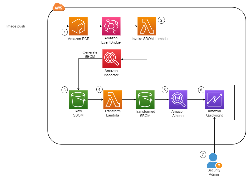


 Venkata Kampana is a Senior Solutions Architect in the AWS Health and Human Services team and is based in Sacramento, CA. In that role, he helps public sector customers achieve their mission objectives with well-architected solutions on AWS.
 Jim Daniel is the Public Health lead at Amazon Web Services. Previously, he held positions with the United States Department of Health and Human Services for nearly a decade, including Director of Public Health Innovation and Public Health Coordinator. Before his government service, Jim served as the Chief Information Officer for the Massachusetts Department of Public Health.


 Arun Sudhir is a Staff Software Engineer at Eightfold AI. He has more than 15 years of experience in design and development of backend software systems in companies like Microsoft and AWS, and has a deep knowledge of database engines like Amazon Aurora PostgreSQL and Amazon Redshift.
 Rohit Bansal is an Analytics Specialist Solutions Architect at AWS. He specializes in Amazon Redshift and works with customers to build next-generation analytics solutions using AWS Analytics services.
 Anjali Vijayakumar is a Senior Solutions Architect at AWS focusing on EdTech. She is passionate about helping customers build well-architected solutions in the cloud.


 Let’s go through each numbered step as outlined in the architecture:
 Philipp Karg is Lead FinOps Engineer at BMW Group and founder of the CLEA platform. He focus on boosting cloud efficiency initiatives and establishing a cost-aware culture within the company to ultimately leverage the cloud in a sustainable way.
 Alex Gutfreund is Head of Product and Technology Integration at the BMW Group. He spearheads the digital transformation with a particular focus on platforms ecosystems and efficiencies. With extensive experience at the interface of business and IT, he drives change and makes an impact in various organizations. His industry knowledge spans from automotive, semiconductor, public transportation, and renewable energies.
 Cizer Pereira is a Senior DevOps Architect at AWS Professional Services. He works closely with AWS customers to accelerate their journey to the cloud. He has a deep passion for Cloud Native and DevOps, and in his free time, he also enjoys contributing to open-source projects.
 Selman Ay is a Data Architect in the AWS Professional Services team. He has worked with customers from various industries such as e-commerce, pharma, automotive and finance to build scalable data architectures and generate insights from the data. Outside of work, he enjoys playing tennis and engaging in outdoor activities.
 Nick McCarthy is a Senior Machine Learning Engineer in the AWS Professional Services team. He has worked with AWS clients across various industries including healthcare, finance, sports, telecoms and energy to accelerate their business outcomes through the use of AI/ML. Outside of work Nick loves to travel, exploring new cuisines and cultures in the process.
 Miguel Henriques is a Cloud Application Architect in the AWS Professional Services team with 4 years of experience in the automotive industry delivering cloud native solutions. In his free time, he is constantly looking for advancements in the web development space and searching for the next great pastel de nata.


 Michael Hamilton is a Sr Analytics Solutions Architect focusing on helping enterprise customers in the south east modernize and simplify their analytics workloads on AWS. He enjoys mountain biking and spending time with his wife and three children when not working.
 Cody Penta is a Solutions Architect at Amazon Web Services and is based out of Charlotte, NC. He has a focus in security and CDK, and enjoys solving the really difficult problems in the technology world. Off the clock, he loves relaxing in the mountains, coding personal projects, and gaming.
 Angus Ferguson is a Solutions Architect at AWS who is passionate about meeting customers across the world, helping them solve their technical challenges. Angus specializes in Data & Analytics with a focus on customers in the financial services industry.


 Gokhul Srinivasan is a Senior Partner Solutions Architect leading AWS Healthcare and Life Sciences (HCLS) Global Startup Partners. Gokhul has over 19 years of Healthcare experience helping organizations with digital transformation, platform modernization, and deliver business outcomes.
 Laks Sundararajan is a seasoned Enterprise Architect helping companies reset, transform and modernize their IT, digital, cloud, data and insight strategies. A proven leader with significant expertise around Generative AI, Digital, Cloud and Data/Analytics Transformation, Laks is a Sr. Solutions Architect with Healthcare and Life Sciences (HCLS).
 Anil Chinnam is a Solutions Architect in the Digital Native Business Segment at Amazon Web Services(AWS). He enjoys working with customers to understand their challenges and solve them by creating innovative solutions using AWS services. Outside of work, Anil enjoys being a father, swimming and traveling.


