Tag Archives: Amazon Redshift

Migrate a large data warehouse from Greenplum to Amazon Redshift using AWS SCT – Part 3

2022-12-12 Jon Roberts

Post Syndicated from Jon Roberts original https://aws.amazon.com/blogs/big-data/part-3-migrate-a-large-data-warehouse-from-greenplum-to-amazon-redshift-using-aws-sct/

In this third post of a multi-part series, we explore some of the edge cases in migrating a large data warehouse from Greenplum to Amazon Redshift using AWS Schema Conversion Tool (AWS SCT) and how to handle these challenges. Challenges include how best to use virtual partitioning, edge cases for numeric and character fields, and arrays.

You can check out the first post of this series for guidance on planning, running, and validating the migration. You can also check out the second post for best practices for choosing the optimal Amazon Redshift cluster, data architecture, converting stored procedures, compatible functions and queries widely used for SQL conversions, and recommendations for optimizing the length of data types for table columns.

Unbounded character data type

Greenplum supports creating columns as text and varchar without specifying the length of the field. This works without an issue in Greenplum but doesn’t work well in migrating to Amazon Redshift. Amazon Redshift stores data in columnar format and gets better compression when using shorter column lengths. Therefore, the Amazon Redshift best practice is to use the smallest character length possible.

AWS SCT will convert these unbounded fields as large objects (LOBs) instead of treating the columns as character fields with a specified length. LOBs are implemented differently in each database product on the market, but in general, a LOB is not stored with the rest of the table data. Instead, there is a pointer to the location of the data. When the LOB is queried, the database reconstitutes the data automatically for you, but this typically requires more resources.

Amazon Redshift doesn’t support LOBs, so AWS SCT resolves this by loading the data into Amazon Simple Storage Service (Amazon S3) and in the column, it stores the S3 URL. When you need to retrieve this data, you have to query the table, get the S3 URL, and then fetch the data from Amazon S3. This isn’t ideal because most of the time, the actual maximum length of the field doesn’t require it to be treated as a LOB, and storing the data remotely means it will take much longer to fetch the data for queries.

The current resolution is to calculate the maximum length of these columns and update the Greenplum tables before converting to Amazon Redshift with AWS SCT.

Note that in a future release of AWS SCT, the collection of statistics will include calculating the maximum length for each column, and the conversion of unbounded varchar and text will set the length in Amazon Redshift automatically.

The following code is an example of an unbounded character data type:

CREATE TABLE public.mytable 
(description1 text NOT NULL PRIMARY KEY, description2 varchar);
CREATE INDEX ON public.mytable (description2);

This table uses a primary key column on an unbounded text column. This needs to be converted to varchar(n), where n is the maximum length found in this column.

Drop unique constraints on affected columns:

ALTER TABLE public.mytable DROP CONSTRAINT mytable_pkey;

Drop indexes on affected columns:

DROP INDEX public.mytable_description2_idx;

Calculate maximum length of affected columns:

select coalesce(max(length(description1)), 10),
coalesce(max(length(description2)), 10) 
from public.mytable;

Note that in this example, the description1 and description2 columns only contain NULL values, or the table doesn’t have any data in it, or the calculated length of the columns is 10.

Alter the length of the affected columns:

ALTER TABLE public.mytable ALTER COLUMN description1 TYPE varchar(10);
ALTER TABLE public.mytable ALTER COLUMN description2 TYPE varchar(10);

You can now proceed with using AWS SCT to convert the Greenplum schema to Amazon Redshift and avoiding using LOBs to store the column values.

GitHub help

If you have many tables to update and want an automated solution, you can use the add_varchar_lengths.sh script found in the GitHub repo to fix all of the unbounded varchar and text columns in a given schema in Greenplum. The script calculates the appropriate maximum length and then alters the Greenplum tables so the varchar data type is bounded by a length.

Please note that the script also will drop any constraints or indexes on the affected columns.

Empty character data

Greenplum and Amazon Redshift support an empty string value in a field that is different from NULL. The behavior is the same between the two databases. However, AWS SCT defaults to convert empty strings to NULL. This simply needs to be disabled to avoid problems.

In AWS SCT, open your project, choose Settings, Project settings, and Data migration.
Scroll to the bottom and find Use empty as null value.
Deselect this so that AWS SCT doesn’t convert empty strings to NULL.

NaN and Infinity numeric data type

Greenplum supports NaN and Infinity in a numeric field to represent an undefined calculation result and infinity. NaN is very uncommon because when using aggregate functions on a column with a NaN row, the result will also be NaN. Infinity is also uncommon and not useful when aggregating data. However, you may encounter these values in a Greenplum database.

Amazon Redshift doesn’t support NaN and Infinity, and AWS SCT doesn’t check for this in your data. If you do encounter this when using AWS SCT, the task will fail with a numeric conversion error.

To resolve this, it’s suggested to use NULL instead of NaN and Infinity. This allows you to aggregate data and get results other than NaN and, importantly, allow you to convert the Greenplum data to Amazon Redshift.

The following code is an example NaN numeric value:

CREATE TABLE public.mytable2 (id int NOT NULL, amount numeric NOT NULL);
INSERT INTO public.mytable2 VALUES (1, 10), (2, 'NaN'), (3, 20);

Drop the NOT NULL constraint:

ALTER TABLE public.mytable2 ALTER COLUMN amount DROP NOT NULL;

Update the table:

UPDATE public.mytable2 SET amount = NULL where amount = 'NaN';

You can now proceed with using AWS SCT to migrate the Greenplum data to Amazon Redshift.

Note that in a future release of AWS SCT, there will be an option to convert NaN and Infinity to NULL so that you won’t have to update your Greenplum data to migrate to Amazon Redshift.

Virtual partitioning on GP_SEGMENT_ID

For large tables, it’s recommended to use virtual partitioning to extract data from Greenplum. Without virtual partitioning, AWS SCT will run a single query to unload data from Greenplum. For example:

SELECT * FROM store_sales;

If this table is very large, it will take a long time to extract the data because this is a single process querying the data. With virtual partitioning, multiple queries are run in parallel so that the extraction of data is completed faster. It also makes it easier to recover if there is an issue with the task.

Virtual partitioning is very flexible, but a simple way to do this in Amazon Redshift is to utilize the Greenplum hidden column gp_segment_id. This column identifies which segment in Greenplum has the data, and each segment should have an equal number of rows. Therefore, creating partitions for each gp_segment_id is an easy way to implement virtual partitioning.

If you’re not familiar with the term segment, it’s similar to an Amazon Redshift slice.

For example:

SELECT * FROM store_sales WHERE gp_segment_id = 0;
SELECT * FROM store_sales WHERE gp_segment_id = 1;
SELECT * FROM store_sales WHERE gp_segment_id = 2;
...

First, determine the number of segments in Greenplum:

SELECT count(*) 
FROM gp_segment_configuration 
WHERE content >= 0 AND preferred_role = 'p';

Now you can configure AWS SCT.

In AWS SCT, go to Data Migration view (other) and choose (right-click) a large table.
Scroll down to Add virtual partitioning.
For the partition type, choose Auto Split and change the column name to GP_SEGMENT_ID.
Use 0 for Start value, the number of segments found in Step 1 as End value, and Interval of 1.

When you create a local task to load this table, the task will have a sub-task for each gp_segment_id value.

Note that in a future release of AWS SCT, there will be an option to automatically virtually partition tables based on GP_SEGMENT_ID. This option will also retrieve the number of segments automatically.

Arrays

Greenplum supports arrays such as bigint[] that are unbounded. Typically, arrays are kept relatively small in Greenplum because arrays consume more memory in Greenplum than using an alternative strategy. However, it’s possible to have a very large array in Greenplum that isn’t supported by Amazon Redshift.

AWS SCT converts a Greenplum array to varchar(65535), but if the converted array is longer than 65,535 characters, then the load will fail.

The following code is an example of a large array:

CREATE TABLE public.sales 
(sales_id int NOT NULL,
customer_id int NOT NULL,
sales_item_ids bigint[]) 
DISTRIBUTED BY (sales_id);

INSERT INTO public.sales values (1, 100, '{1,2,3}'), (2, 100, '{1,2,3}');

In this example, the sales items are stored in an array for each sales_id. If you encounter an error while loading that the length is too long to load this data into Amazon Redshift with AWS SCT, then this is the solution. It’s also a more efficient pattern to store data in both Greenplum and Amazon Redshift!

Create a new sales table that has all columns from the existing sales table, but exclude the array column:

CREATE TABLE public.sales_new 
(sales_id int NOT NULL,
customer_id int NOT NULL) 
DISTRIBUTED BY (sales_id);

Populate the new sales table with the existing data except for the array column:

INSERT INTO public.sales_new (sales_id, customer_id) 
SELECT sales_id, customer_id FROM public.sales;

We create a new table that is a cross-reference of sales IDs with the sales items. Instead of having a single row for this association, now there will be a row for each relationship.

Create a new sales item table:

CREATE TABLE public.sales_items 
(sales_id int NOT NULL, 
sales_item_id bigint NOT NULL) 
DISTRIBUTED BY (sales_id);

To unnest the array, create a row for each array element:

INSERT INTO public.sales_items 
(sales_id, sales_item_id) 
SELECT sales_id, unnest(sales_item_ids) 
FROM public.sales;

Rename the sales tables:

ALTER TABLE public.sales RENAME TO sales_old;
ALTER TABLE public.sales_new RENAME TO sales;

In AWS SCT, refresh the tables and migrate the revised sales and the new sales_items table.

The following are some example queries before and after.

Before:

SELECT s.sales_id, unnest(s.sales_item_ids) 
FROM public.sales s 
WHERE s.sales_id = 1;

After:

SELECT s.sales_id, i.sales_item_id 
FROM public.sales s 
JOIN public.sales_items i ON s.sales_id = i.sales_id 
WHERE s.sales_id = 1;

Before:

SELECT s.sales_id 
FROM public.sales s 
WHERE s.customer_id = 100
AND 10 = ANY(s.sales_item_ids);

After:

SELECT s.sales_id
FROM public.sales s 
JOIN public.sales_items i ON s.sales_id = i.sales_id 
WHERE s.customer_id = 100
AND i.sales_item_id = 10;

VACUUM ANALYZE

Greenplum, like Amazon Redshift, supports the VACUUM command, which reclaims storage space after UPDATE and DELETE commands are run on a table. Greenplum also allows you to add the ANALYZE option to run both statements with a single command.

The following code is the Greenplum command:

VACUUM ANALYZE table;

This is not very common, but you’ll see this from time to time. If you’re just inserting data into a table, there is no need to run VACUUM, but for ease of use, sometimes developers will use VACUUM ANALYZE.

The following are the Amazon Redshift commands:

VACUUM table;
ANALYZE table;

Amazon Redshift doesn’t support adding ANALYZE to the VACUUM command, so instead, this needs to be two different statements. Also note that Amazon Redshift performs VACUUM and ANALYZE automatically for you so in most cases, you can remove these commands from your scripts entirely.

DISTINCT ON query

Greenplum supports an unusual shortcut for eliminating duplicates in a table. This feature keeps the first row for each set of rows based on the order of the data being fetched. It’s easiest to understand by looking at an example:

CREATE TABLE customer 
(customer_name varchar(100) not null, 
customer_address varchar(1000) not null, 
lastupdate timestamp not null);

INSERT INTO customer VALUES
('ACME', '123 Main St', '2022-01-01'), 
('ACME', '456 Market St', '2022-05-01'), 
('ACME', '789 Broadway', '2022-08-01');

SELECT DISTINCT ON (customer_name) customer_name, customer_address 
FROM customer 
ORDER BY customer_name, lastupdate DESC;

We get the following results:

customer_name | customer_address 
---------------+------------------
 ACME          | 789 Broadway

The solution for running this in Amazon Redshift is to use the ANSI standard row_number() analytical function, as shown in the following code:

SELECT sub.customer_name, sub.customer_address 
FROM (SELECT customer_name, customer_address, row_number() over (partition by customer_name ORDER BY lastupdate DESC) AS row_number FROM customer) AS sub 
WHERE sub.row_number = 1;

Clean up

The examples in this post create tables in Greenplum. To remove these example tables, run the following commands:

DROP TABLE IF EXISTS public.mytable;
DROP TABLE IF EXISTS public.mytable2;
DROP TABLE IF EXISTS public.sales;
DROP TABLE IF EXISTS public.sales_new;
DROP TABLE IF EXISTS public.sales_items;
DROP TABLE IF EXISTS public.customer;

Conclusion

In this post, we covered some of the edge cases when migrating Greenplum to Amazon Redshift and how to handle these challenges, including easy virtual partitioning, edge cases for numeric and character fields, and arrays. This is not an exhaustive list of migrating Greenplum to Amazon Redshift, but this series should help you navigate modernizing your data platform by moving to Amazon Redshift.

For additional details, see the Amazon Redshift Getting Started Guide and the AWS SCT User Guide.

About the Authors

Jon Roberts is a Sr. Analytics Specialist based out of Nashville, specializing in Amazon Redshift. He has over 27 years of experience working in relational databases. In his spare time, he runs.

Nelly Susanto is a Senior Database Migration Specialist of AWS Database Migration Accelerator. She has over 10 years of technical experience focusing on migrating and replicating databases along with data warehouse workloads. She is passionate about helping customers in their cloud journey.

Suresh Patnam is a Principal BDM – GTM AI/ML Leader at AWS. He works with customers to build IT strategy, making digital transformation through the cloud more accessible by leveraging Data & AI/ML. In his spare time, Suresh enjoys playing tennis and spending time with his family.

Enable Multi-AZ deployments for your Amazon Redshift data warehouse

2022-12-09 Ranjan Burman

Post Syndicated from Ranjan Burman original https://aws.amazon.com/blogs/big-data/enable-multi-az-deployments-for-your-amazon-redshift-data-warehouse/

November 2023: This post was reviewed and updated with the general availability of Multi-AZ deployments for provisioned RA3 clusters.
Originally published on December 9th, 2022.

Amazon Redshift is a fully managed, petabyte scale cloud data warehouse that enables you to analyze large datasets using standard SQL. Data warehouse workloads are increasingly being used with mission-critical analytics applications that require the highest levels of resilience and availability. Amazon Redshift is a cloud-based data warehouse that supports many recovery capabilities to address unforeseen outages and minimize downtime. Amazon Redshift RA3 instance types store their data in Redshift Managed Storage (RMS), which is backed by Amazon Simple Storage Service (Amazon S3) making it highly available and durable by default. Amazon Redshift also supports automatic backups that can recover a data warehouse, automatically remediate failures and relocates clusters to different AZs without changes to applications. Although many customers benefit from these features, enterprise data warehouse customers require a low Recovery Time Objective (RTO) and higher availability to support their business continuity with minimal impact to applications.

Amazon Redshift just announced the general availability of Multi-AZ deployments for provisioned RA3 clusters that support running your data warehouse in two Availability Zones simultaneously and can continue operating in unforeseen failure scenarios. A Multi-AZ deployment is intended for customers with mission-critical analytics applications that require the highest levels of resilience and availability.

A Redshift Multi-AZ deployment leverages compute resources in two AZs to scale data warehouse workload processing. In situations where there is a high level or concurrency Redshift will automatically leverage the resources in both AZs to scale the workload for both read and write requests.

Our pre-launch tests found that Amazon Redshift Multi-AZ deployments reduce recovery time to under 60 seconds or less in the unlikely case of an AZ failure.

Single-AZ vs. Multi-AZ deployment

Amazon Redshift requires a cluster subnet group to create a cluster in your VPC. The cluster subnet group includes information about the VPC ID and a list of subnets in your VPC. When you launch a cluster, Amazon Redshift either creates a default cluster subnet group automatically or you choose a cluster subnet group of your choice so that Amazon Redshift can provision your cluster in one of the subnets in the VPC. You can configure your cluster subnet group to add subnets from different Availability Zones that you want Amazon Redshift to use for cluster deployment.

All Amazon Redshift clusters today are created and situated in a particular Availability Zone within an AWS Region and thus called Single-AZ deployments. For a Single-AZ deployment, Amazon Redshift selects the subnet from one of the Availability Zones within a Region and deploys the cluster there. You can choose an Availability Zone for deployment, and Amazon Redshift will deploy your cluster in the chosen Availability Zone based on the subnets provided.

On the other hand, a multi-AZ deployment is provisioned in two Availability Zones simultaneously. For a Multi-AZ deployment, Amazon Redshift automatically selects two subnets from two different Availability Zones and deploys an equal number of compute nodes in each Availability Zone. All these compute nodes are utilized via a single endpoint as compute nodes from both Availability Zones are used for workload processing.

As shown in the following diagrams, Amazon Redshift deploys a cluster in a single Availability Zone for Single-AZ deployment, and two Availability Zones for Multi-AZ deployment.

Auto recovery of multi-AZ deployment

In the unlikely event of an Availability Zone failure, Amazon Redshift Multi-AZ deployments continue to serve your workloads by automatically using resources in the other Availability Zone. You are not required to make any application changes to maintain business continuity during unforeseen outages since a multi-AZ deployment is accessed as a single data warehouse with one endpoint. Amazon Redshift Multi-AZ deployments are designed to ensure there is no data loss, and you can query all data committed up until the point of failure.

As shown in the below diagram, if there is an unlikely event that causes compute nodes in AZ1 to fail, then a multi-AZ deployment automatically recovers to use compute resources in AZ2. Amazon Redshift will also automatically provision identical compute nodes in another availability zone (AZ3) to continue operating simultaneously in two Availability zones (AZ2 and AZ3).

Amazon Redshift Multi-AZ deployment is not only used for protection against the possibility of Availability Zone failures, but it can also maximize your data warehouse performance by automatically distributing workload processing across two Availability Zones. A Multi-AZ deployment will always process an individual query using compute resources only from one Availability Zone, but it can automatically distribute processing of multiple simultaneous queries to both Availability Zones to increase overall performance for high concurrency workloads.

It’s a good practice to set up automatic retries in your extract, transform, and load (ETL) processes and dashboards so that they can be reissued and served by the cluster in the secondary Availability Zone when an unlikely failure happens in the primary Availability Zone. If a connection is dropped, it can then be retried or reestablished immediately. In addition, queries and loads that were running in the failed Availability Zone will be aborted. New queries issued at or after a failure occurs may experience run delays while the multi-AZ data warehouse is being recovered to a two AZ setup.

Overview of solution

In this post, we provide a walkthrough of how to create and manage a Multi-AZ deployment for Amazon Redshift using the AWS Management Console. We also test the fault tolerance of an Amazon Redshift Multi-AZ data warehouse and monitor queries in your Multi-AZ deployment.

Create a new Multi-AZ deployment from the console

You can easily create a new multi-AZ deployments through Amazon Redshift console. Amazon Redshift will deploy the same number of nodes in each of the two Availability Zones for a Multi-AZ deployment. All nodes of a multi-AZ deployment can perform read and write workload processing during normal operation. A Multi-AZ deployment is supported only for provisioned RA3 clusters.

Follow these steps to create an Amazon Redshift provisioned cluster in two Availability Zones:

On the Amazon Redshift console, in the navigation pane, choose Clusters.
Click on Create cluster.

For general information about creating clusters, see Creating a cluster.

Choose one of the RA3 node types on the Node type drop-down menu. The Multi-AZ deployment option only becomes available when you choose an RA3 node type.
For Multi-AZ deployment, select Multi-AZ option.
For Number of nodes per AZ, enter the number of nodes that you need for your cluster.

Under the Database configurations, choose Admin user name and Admin user password.
Turn Use defaults on next to Additional configurations to modify the default settings.
Under Network and security, specify the following:
1. For Virtual private cloud (VPC), choose the VPC you want to deploy the cluster in.
2. For VPC security groups, either leave as default or add the security groups of your choice.
3. For Cluster subnet group, either leave as default or add a cluster subnet group of your choice. For a Multi-AZ deployment, a cluster subnet group must include one subnet each from at least three or more different Availability Zones.

For general information about managing cluster subnet groups, see Cluster subnet groups

Under Database configuration, for Database port, you either use the default value 5439 or choose a value from the range of 5431–5455 and 8191–8215.
Under Database configuration, in the Database encryption section, to use a custom AWS Key Management Service (AWS KMS) key other than the default KMS key, choose Customize encryption settings. This option is deselected by default.
Under Choose an AWS KMS key, you can either choose an existing KMS key, or choose Create an AWS KMS key to create a new KMS key.

For more information to create key using KMS, refer to Creating keys.

Choose Create cluster.

When the cluster creation succeeds, you can view the details on the cluster details page.

Under General information, you can see Multi-AZ as Yes.

On the Properties tab, under Network and security settings, you can find the details on the primary and secondary Availability Zone.

Create a new Multi-AZ deployment from the CLI

The following create-cluster AWS CLI command shows how to create a Multi-AZ cluster

aws redshift create-cluster 
--port 5439 
    --master-username master
    --master-user-password ######
    --node-type ra3.4xlarge
    --number-of-nodes 2
    --profile maz-test
    --endpoint-url https://redshift.us-east-1.amazonaws.com
    --region eu-west-1
    --cluster-identifier redshift-cluster-1
    --multi-az 
    --maintenance-track-name CURRENT
    --encrypted

Convert a Single-AZ deployment to Multi-AZ deployment

To convert an existing Single-AZ deployment to a Multi-AZ deployment, you can go to the Redshift console and select your Redshift cluster that currently is Single-AZ setup and navigate to Actions and select Activate Multi-AZ. Your Single-AZ cluster must be encrypted for a successful conversion to Multi-AZ. During conversion to Multi-AZ, Redshift will double the total number of nodes distributing them equally in each AZ. Redshift will not allow you to split existing number of nodes while converting to Multi-AZ to maintain consistent query performance.

Complete the following steps to create a Multi-AZ deployment restored from a snapshot:

On the Amazon Redshift console, in the navigation pane, choose Clusters.
Select your cluster and navigate to the cluster details page.
On the Actions menu, choose Activate Multi-AZ.

Review the modification summary and confirm by choosing Activate Multi-AZ.

Using the below AWS CLI command you can convert a single AZ Redshift data warehouse to Multi-AZ.

aws redshift modify-cluster 
    --profile maz-test
    --endpoint-url https://redshift.eu-west-1.amazonaws.com
    --region eu-west-1
    --cluster-identifier redshift-cluster-1
    --multi-az

Convert a Multi-AZ deployment to Single-AZ deployment

Redshift also supports conversion of a Multi-AZ deployment into Single-AZ. This option provides customers with the flexibility to switch between different deployments with few easy steps as follows:

On the Amazon Redshift console, in the navigation pane, choose Clusters.
Select your cluster and navigate to the cluster details page.
On the Actions menu, choose Deactivate Multi-AZ.
Review the modification summary and confirm by choosing Deactivate Multi-AZ.

Creating a Multi-AZ data warehouse restored from a snapshot

Existing customers can also create a Multi-AZ deployment by restoring a snapshot from an existing Single-AZ deployment. See the required steps as below.

On the Amazon Redshift console, in the navigation pane, choose Clusters.
Select the cluster and navigate to the cluster details page.
Choose the Maintenance
Select a snapshot and choose Restore snapshot, Restore to provisioned cluster.
Review the Cluster configuration and Cluster details values of the new cluster to be created using the snapshot information.
Select Multi-AZ option and update the properties of the new cluster, then choose Restore cluster from snapshot at the bottom of the page.

Resizing a Multi-AZ data warehouse

Redshift Multi-AZ feature also supports resizing Multi-AZ Redshift cluster deployments to change the cluster configuration based on scaling needs. You can change both number and type of nodes as per needs.

On the Amazon Redshift console, in the navigation pane, choose Clusters.
Select your cluster and navigate to the cluster details page.
On the Actions menu, choose
Once selected it will bring into another screen to show cluster resize screen where you can choose type and number of nodes and click on Resize cluster.

Failing over Multi-AZ deployment

In addition to the automatic recovery process, you can also trigger this process manually for your data warehouse using the Failover primary compute option. This approach can be used to manage operational maintenance and other planned operational procedures as per the needs of the respective environment. When the cluster successfully recovers, Multi-AZ deployment becomes available. Your Multi-AZ deployment also automatically provisions new compute nodes in another Availability Zone as soon as it is available.

Let’s manually trigger the Failover of your Redshift Multi-AZ deployment.

On the Amazon Redshift console, choose Clusters in the navigation pane.
Navigate to the cluster detail page
From Actions, choose Failover primary compute.
When prompted, choose Confirm.

After the cluster is back to Available status, you can observe that the primary and secondary Availability Zones have changed.

The following screenshot shows the status before injecting failure.

The following screenshot shows the status after injecting failure.

Restore a table from snapshot

You can restore a single table from a snapshot from your Multi-AZ cluster. When you restore a single table from a snapshot, you specify the source snapshot, database, schema, and table name, and the target database, schema, and a new table name for the restored table.

To restore a table from a snapshot:

On the Amazon Redshift console, in the navigation pane, choose Clusters.
Select your cluster and navigate to the cluster details page.
On the Actions menu, choose Restore table.
Enter the information about which snapshot, source table, and target table to use, and then choose Restore table.

Enable public connections for your Multi-AZ data warehouse

From the navigation menu, choose CLUSTERS.
Choose the Multi-AZ cluster that you want to modify.
Choose Actions.
Choose Turn on Publicly accessible.
Choose Elastic IP address, if you do not choose one, an address will be randomly assigned to you.
Choose Save changes.

Monitor queries for Multi-AZ deployments

A Multi-AZ deployment uses compute resources that are deployed in both Availability Zones and can continue operating in the event that the resources in a given Availability Zone are not available. All the compute resources are used at all times, which allows full operation across two Availability Zones in both read and write operations.

You can query SYS_views in the pg_catalog schema to monitor Multi-AZ query runs. The SYS_views cover query run activities and stats from primary and secondary clusters.

The following are the system tables in the SYS_view list:

Follow these steps to monitor the query run on Multi-AZ deployment from the Amazon Redshift Console:

On the Amazon Redshift console, connect to the database in your Multi-AZ deployment and run queries through the query editor.
Run any sample query on the Multi-AZ Redshift deployment.
For a Multi-AZ deployment, you can identify a query and the Availability Zone where it is being run (running on the primary or secondary availability zone) by using the compute_type column in the SYS_QUERY_HISTORY table. The valid values for the compute type column are as follows:
1. primary – When run on primary availability zone in the Multi-AZ deployment.
2. secondary – When run on secondary availability zone in the Multi-AZ deployment.

The following is a sample query using the compute_type column to monitor a query:

dev=# select (compute_type) as compute_type, left(query_text, 50) query_text from sys_query_history order by start_time desc;

 compute_type | query_text
--------------+----------------------------------------------------
 secondary    | select count(*) from t1;
 primary 	   select count(*) from t2;

You can also access the query history from the console to analyze your query diagnostics.

On the Query monitoring tab, choose Connect to database.

For Connection, choose Create a new connection
For Authentication, choose Temporary credentials
For Database name, enter the database name (for example, dev).
For Database user, enter the database user name (for example, awsuser).
Choose Connect.

After you’re connected, under Query Monitoring, on the Query history tab, you can view all the queries and loads, as shown in the following screenshot.

Under Metric filters, you can use the various filters in the Additional filtering options section to view query history based on Time interval, Users, Databases, or SQL commands.

There are a few limitations when working with Amazon Redshift Multi-AZ in preview mode, refer here for the limitations.

Customer feedback

Janssen Pharmaceuticals, a subsidiary of Johnson & Johnson, researches and manufactures medicines with a focus on the changing needs of patients and the healthcare industry.

“Janssen Pharmaceutical uses Amazon Redshift to enable critical insights that drive important business decisions for our data scientists, data stewards, business users, and external stakeholders. With Amazon Redshift Multi-AZ, we can be confident that our data warehouse will always be available without any disruptions that might delay impact our ability to make critical business decisions.”

– Shyam Mohapatra, Director of Information Technology – Janssen Pharmaceutical Companies of Johnson & Johnson

Stripe is a technology company that builds economic infrastructure for the internet. Stripe’s products power payments for online and in-person retailers, subscriptions businesses, software platforms and marketplaces, and everything in between.

“Millions of companies use Stripe’s software and APIs to accept payments, send payouts, and manage their businesses online. Access to their Stripe data via leading data warehouses like Amazon Redshift has been a top request from our customers. Our customers needed highly available, secure, fast, and integrated analytics at scale without building complex data pipelines or moving and copying data around. With Stripe Data Pipeline for Amazon Redshift, we’re helping our customers set up a direct and reliable data pipeline in a few clicks.

Stripe Data Pipeline enables our customers to automatically share their complete, up-to-date Stripe data with their Amazon Redshift data warehouse, and take their business analytics and reporting to the next level.”

– Brian Brunner, Senior Manager, Engineering at Stripe

Conclusion

This post demonstrated how to configure an Amazon Redshift Multi-AZ deployment in two Availability Zones and test the fault tolerance of your workloads during an unlikely failure of an Availability Zone. Amazon Redshift Multi-AZ deployment also helps improve overall performance of your data warehouse because compute nodes in both Availability Zones are used for read and write operations. Amazon Redshift Multi-AZ data warehouse helps meet the demands of customers with mission critical analytics applications that require the highest levels of availability and resiliency. For more details, refer Configuring Multi-AZ deployment.

About the Authors

Ranjan Burman is an Analytics Specialist Solutions Architect at AWS. He specializes in Amazon Redshift and helps customers build scalable analytical solutions. He has more than 16 years of experience in different database and data warehousing technologies. He is passionate about automating and solving customer problems with cloud solutions.

Saurav Das is part of the Amazon Redshift Product Management team. He has more than 16 years of experience in working with relational databases technologies and data protection. He has a deep interest in solving customer challenges centered around high availability and disaster recovery.

Anusha Challa is a Senior Analytics Specialist Solutions Architect focused on Amazon Redshift. She has helped many customers build large-scale data warehouse solutions in the cloud and on premises. She is passionate about data analytics and data science.

Nita Shah is an Analytics Specialist Solutions Architect at AWS based out of New York. She has been building data warehouse solutions for over 20 years and specializes in Amazon Redshift. She is focused on helping customers design and build enterprise-scale well-architected analytics and decision support platforms.

Suresh Patnam is a Principal BDM – GTM AI/ML Leader at AWS. He works with customers to build IT strategy, making digital transformation through the cloud more accessible by using data and AI/ML. In his spare time, Suresh enjoys playing tennis and spending time with his family.

How Blueshift integrated their customer data environment with Amazon Redshift to unify and activate customer data for marketing

2022-12-08 Vijay Chitoor

Post Syndicated from Vijay Chitoor original https://aws.amazon.com/blogs/big-data/how-blueshift-integrated-their-customer-data-environment-with-amazon-redshift-to-unify-and-activate-customer-data-for-marketing/

This post was co-written with Vijay Chitoor, Co-Founder & CEO, and Mehul Shah, Co-Founder and CTO from the Blueshift team, as the lead authors.

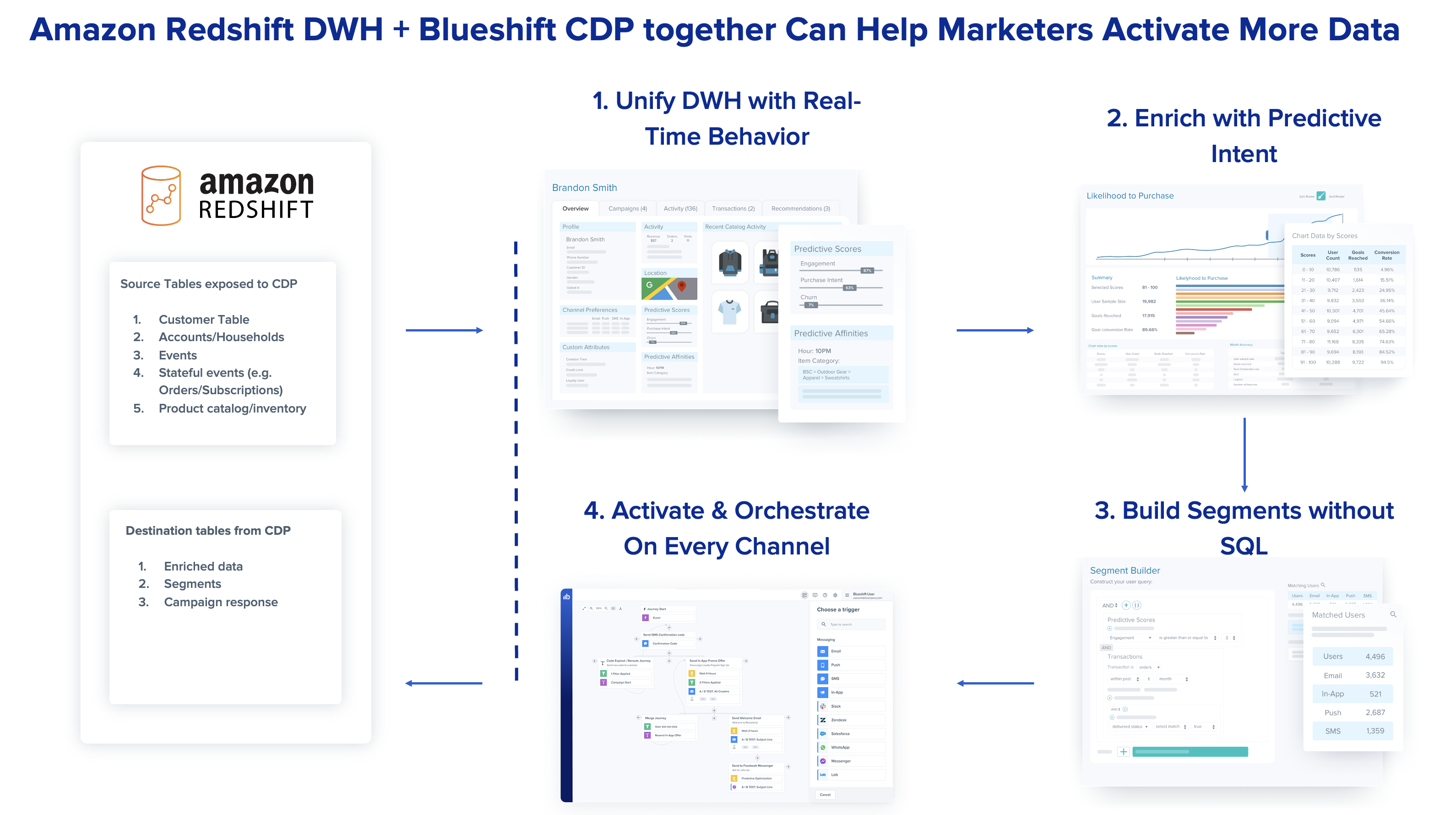
Blueshift is a San Francisco-based startup that helps marketers deliver exceptional customer experiences on every channel, delivering relevant personalized marketing. Blueshift’s SmartHub Customer Data Platform (CDP) empowers marketing teams to activate their first-party customer data to drive 1:1 personalization on owned (email, mobile) and paid (Google, Facebook, and so on) website and customer (CX) channels.

In this post, Blueshift’s founding team discuss how they used Amazon Redshift Data API to integrate data from their customer’s Amazon Redshift data warehouse with their CDP environment to help marketers activate their enterprise data and drive growth for their businesses.

Business need

In today’s omnichannel world, marketing teams at modern enterprises are being tasked with engaging customers on multiple channels. To successfully deliver intelligent customer engagement, marketers need to operate with a 360 degree view of their customers that takes into account various types of data, including customer behavior, demographics, consent and preferences, transactions, data from human assisted and digital interactions, and more. However, unifying this data and making it actionable for marketers is often a herculean task. Now, for the first time, with the integration of Blueshift with Amazon Redshift, companies can use more data than ever for intelligent cross-channel engagement.

Amazon Redshift is a fast, fully managed cloud data warehouse. Tens of thousands of customers use Amazon Redshift as their analytics infrastructure. Users such as data analysts, database developers, and data scientists use SQL to analyze their data in Amazon Redshift data warehouses. Amazon Redshift provides a web-based query editor in addition to supporting connectivity via ODBC/JDBC or the Redshift Data API.

Blueshift aims at empowering business users to unlock data in such data warehouses and activate audiences with personalized journeys for segmentation, 1:1 messaging, website, mobile, and paid media use cases. Moreover, Blueshift can help combine this data in Amazon Redshift data warehouses with real-time website and mobile data for real-time profiles and activation, enabling this data to be used by marketers in these businesses.

Although the data in Amazon Redshift is incredibly powerful, marketers are unable to use it in it’s original form for customer engagement for a variety of reasons. Firstly, querying the data requires knowledge of query languages like SQL, which marketers aren’t necessarily adept at. Furthermore, marketers need to combine the data in the warehouse with additional sources of data that are critical for customer engagement, including real-time events (for example, a website page viewed by a customer), as well as channel-level permissions and identity.

With the new integration, Blueshift customers can ingest multidimensional data tables from Amazon Redshift (for example, a customer table, transactions table, and product catalog table) into Blueshift to build a single customer view that is accessible by marketers. The bi-directional integration also ensures that predictive data attributes computed in Blueshift, as well as campaign engagement data from Blueshift, are written back into Amazon Redshift tables, enabling technology and analytics teams to have a comprehensive view of the data.

In this post, we describe how Blueshift integrates with Amazon Redshift. We highlight the bi-directional integration with data flowing from a customer’s Amazon Redshift data warehouse to Blueshift’s CDP environment and vice versa. These mechanisms are facilitated through the use of the Redshift Data API.

Solution overview

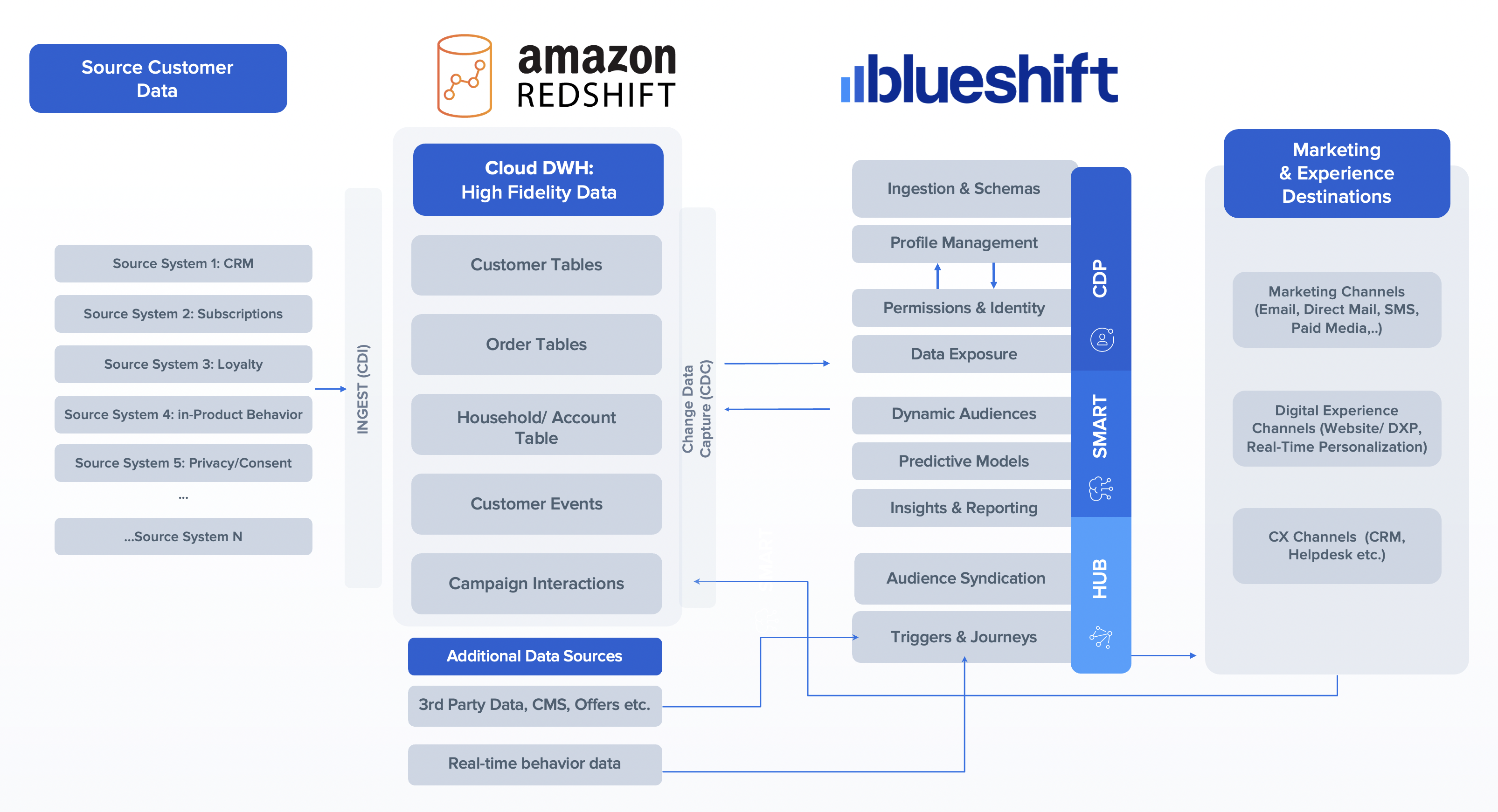
The integration between the two environments is achieved through a connector. We discuss the connector’s core components in this section. Blueshift uses a hybrid approach using Redshift S3 UNLOAD, Redshift S3 COPY, and the Redshift Data API to simplify the integration between Blueshift and Amazon Redshift, thereby facilitating the data needs to empower marketing teams. The following flow diagram shows the overview of the solution.

Blueshift uses container technology to ingest and process data. The data ingestion and egress containers are scaled up and down depending on the amount of data being processed. One of the key design tenets was to simplify the design by not having to manage connections or active connection pools. The Redshift Data API supports a HTTP-based SQL interface without the need for actively managing connections. As depicted in the process flow, the Redshift Data API lets you access data from Amazon Redshift with various types of traditional, cloud-native, containerized, serverless web service-based applications and event-driven applications. The Blueshift application includes a mix of programming languages, including Ruby (for the customer-facing dashboard), Go (for container workloads), and Python (for data science workloads). The Redshift Data API supports bindings in Python, Go, Java, Node.js, PHP, Ruby, and C++, which makes it simple for developer teams to integrate quickly.

With the Redshift Data API integration in place in Blueshift’s application, IT users from Blueshift customers can set up and validate the data connection, and subsequently Blueshift’s business users (marketers) can seamlessly extract value from data by developing insights and putting those insights into action for the customer data housed in AWS Redshift seamlessly. Therefore, the process developed by Blueshift using the Redshift Data API significantly lowers the barrier for entry for new users without needing data warehousing experience or ongoing IT dependencies for the business user.

The solution architecture depicted in the following figure shows how the various components of the CDP environment and Amazon Redshift integrate to provide the the end-to-end solution.

shows how the various components of the CDP environment and Amazon Redshift integrate to provide the the end-to-end solution

Prerequisites

In this section, we describe the requirements of the integration solution between the two infrastructures. A typical data implementation with customers involves data from Amazon Redshift ingesting into the Blueshift CDP environment. This ingestion mechanism must accommodate different data types, such as the following:

Customer CRM data (user identifiers and various CRM fields). A typical range for data volume to be supported for this data type is 50–500 GB ingested once initially.
Real-time behavior or events data (for example, playing or pausing a movie).
Transactions data, such as subscription purchases. Typical data volumes ingested daily for events and transactions are in the 500 GB – 1 TB range.
Catalog content (for example, a list of shows or movies for discovery), which is typically about 1 GB in size ingested daily.

The integration also needs to support Blueshift’s CDP platform environment to export data to Amazon Redshift. This includes data such as campaign activities like emails being viewed, which can run into tens of TB, and segment or user exports to support a list of users that are part of a segment definition, typically 50–500 GB exported daily.

Integrate Amazon Redshift with data applications

Amazon Redshift provides several ways to quickly integrate data applications.

For the initial data loads, Blueshift uses Redshift S3 UNLOAD to dump Amazon Redshift data into Amazon Simple Storage Service (Amazon S3). Blueshift natively uses Amazon S3 as a persistent object store and supports bulk ingestion and export from Amazon S3. Data loads from Amazon S3 are ingested in parallel and cut down on data load times, enabling Blueshift clients to quickly onboard.

For incremental data ingestion, Blueshift data import jobs track the last time an import was run, and import new rows of data that have been added or updated since the previous import ran. Blueshift stays in sync with changes (updates or inserts) to the Amazon Redshift data warehouse using the Redshift Data API. Blueshift uses the last_updated_at column in Amazon Redshift tables to determine new or updated rows and subsequently ingest those using the Redshift Data API. Blueshift’s data integration cron job syncs data in near-real time using the Redshift Data API by polling for updates on a regular cadence (for example, every 10 minutes, hourly, or daily). The cadence can be tuned depending on data freshness requirements.

The following table summarizes the integration types.

Integration type	Integration mechanism	Advantage
Initial data ingestion from Amazon Redshift to Blueshift	Redshift S3 UNLOAD command	Initial data is exported from Amazon Redshift via Amazon S3 to allow faster parallel loads into Blueshift using the Amazon Redshift UNLOAD command.
Incremental data ingestion from Amazon Redshift to Blueshift	Redshift Data API	Incremental data changes are synchronized using the Redshift Data API in near-real time.
Data export from Blueshift to Amazon Redshift	Redshift S3 COPY command	Blueshift natively stores campaign activity and segment data in Amazon S3, which is loaded into Amazon Redshift using the Redshift S3 COPY command.

Redshift supports numerous out-of-the-box mechanisms to provide data access. Blueshift was able to cut down the data onboarding time for clients by using a hybrid approach of integrating with Amazon Redshift with Redshift S3 UNLOAD, the Redshift Data API, and Redshift S3 COPY. Blueshift is able to cut down the initial data load time, as well as be updated in near-real time with changes in Amazon Redshift and vice versa.

Conclusion

In this post, we showed how Blueshift integrated with the Redshift Data API to ingest customer data. This integration was seamless and demonstrated how straightforward the Redshift Data API makes integration with external applications, such as Blueshift’s CDP environment for marketing, with Amazon Redshift. The outlined use cases in this post are just a few examples of how to use the Redshift Data API to simplify interactions between users and Amazon Redshift clusters.

Now go build and integrate Amazon Redshift with Blueshift.

About the authors

Vijay Chittoor is the CEO & co-founder of Blueshift. Vijay has a wealth of experience in AI, marketing technology and e-commerce domains. Vijay was previously the co-founder & CEO of Mertado (acquired by Groupon to become Groupon Goods), and an early team member at Kosmix (acquired by Walmart to become @WalmartLabs). A former consultant with McKinsey & Co., Vijay is a graduate of Harvard Business School’s MBA Program. He also holds Bachelor’s and Master’s degrees in Electrical Engineering from the Indian Institute of Technology, Bombay.

Mehul Shah is co-Founder & CTO at Blueshift. Previously, he was a co-founder & CTO at Mertado, which was acquired by Groupon to become Groupon Goods. Mehul was an early employee at Kosmix that was acquired by Walmart to become @WalmartLabs. Mehul is a Y Combinator alumni and a graduate of University of Southern California. Mehul is a co-inventor of 12+ patents, and coaches a middle school robotics team.

Manohar Vellala is a Senior Solutions Architect at AWS working with digital native customers on their cloud native journey. He is based in San Francisco Bay Area and is passionate about helping customers build modern applications that can take the full advantage of the cloud. Prior to AWS he worked at H2O.ai where he helped customers build ML models. His interests are Storage, Data Analytics and AI/ML.

Prashant Tyagi joined AWS in September 2020, where he now manages the solutions architecture team focused on enabling digital native businesses. Prashant worked previously at ThermoFisher Scientific, and GE Digital where he held roles as Sr. Director for their Digital Transformation initiatives. Prashant has enabled digital transformation for customers in the Life Sciences and other industry verticals. He has experience in IoT, Data Lakes and AI/ML technical domains. He lives in the bay area in California.

How dynamic data masking support in Amazon Redshift helps achieve data privacy and compliance

2022-12-07 Rohit Vashishtha

Post Syndicated from Rohit Vashishtha original https://aws.amazon.com/blogs/big-data/how-dynamic-data-masking-support-in-amazon-redshift-helps-achieve-data-privacy-and-compliance/

Amazon Redshift is a fully managed, petabyte-scale, massively parallel data warehouse that offers simple operations and high performance. It makes it fast, simple, and cost-effective to analyze all your data using standard SQL and your existing business intelligence (BI) tools. Today, Amazon Redshift is the most widely used cloud data warehouse.

Dynamic data masking (DDM) support (preview) in Amazon Redshift enables you to simplify the process of protecting sensitive data in your Amazon Redshift data warehouse. You can now use DDM to protect data based on your job role or permission rights and level of data sensitivity through a SQL interface. DDM support (preview) in Amazon Redshift enables you to hide, obfuscate, or pseudonymize column values within the tables in your data warehouse without incurring additional storage costs. It is configurable to allow you to define consistent, format-preserving, and irreversible masked data values.

DDM support (preview) in Amazon Redshift provides a native feature to support your need to mask data for regulatory or compliance requirements, or to increase internal privacy standards. Compared to static data masking where underlying data at rest gets permanently replaced or redacted, DDM support (preview) in Amazon Redshift enables you to temporarily manipulate the display of sensitive data in transit at query time based on user privilege, leaving the original data at rest intact. You control access to data through masking policies that apply custom obfuscation rules to a given user or role. That way, you can respond to changing privacy requirements without altering the underlying data or editing SQL queries.

With DDM support (preview) in Amazon Redshift, you can do the following:

Define masking policies that apply custom obfuscation policies (for example, masking policies to handle credit card, PII entries, HIPAA or GDPR needs, and more)
Transform the data at query time to apply masking policies
Attach masking policies to roles or users
Attach multiple masking policies with varying levels of obfuscation to the same column in a table and assign them to different roles with priorities to avoid conflicts
Implement cell-level masking by using conditional columns when creating your masking policy
Use masking policies to partially or completely redact data, or hash it by using user-defined functions (UDFs)

Here’s what our customers have to say on DDM support(private beta) in Amazon Redshift:

“Baffle delivers data-centric protection for enterprises via a data security platform that is transparent to applications and unique to data security. Our mission is to seamlessly weave data security into every data pipeline. Previously, to apply data masking to an Amazon Redshift data source, we had to stage the data in an Amazon S3 bucket. Now, by utilizing the Amazon Redshift Dynamic Data Masking capability, our customers can protect sensitive data throughout the analytics pipeline, from secure ingestion to responsible consumption reducing the risk of breaches.”

-Ameesh Divatia, CEO & co-founder of Baffle

“EnergyAustralia is a leading Australian energy retailer and generator, with a mission to lead the clean energy transition for customers in a way that is reliable, affordable and sustainable for all. We enable all corners of our business with Data & Analytics capabilities that are used to optimize business processes and enhance our customers’ experience. Keeping our customers’ data safe is a top priority across our teams. In the past, this involved multiple layers of custom built security policies that could make it cumbersome for analysts to find the data they require. The new AWS dynamic data masking feature will significantly simplify our security processes so we continue to keep customer data safe, while also reducing the administrative overhead.”

-William Robson, Data Solutions Design Lead, EnergyAustralia

Use case

For our use case, a retail company wants to control how they show credit card numbers to users based on their privilege. They also don’t want to duplicate the data for this purpose. They have the following requirements:

Users from Customer Service should be able to view the first six digits and the last four digits of the credit card for customer verification
Users from Fraud Prevention should be able to view the raw credit card number only if it’s flagged as fraud
Users from Auditing should be able to view the raw credit card number
All other users should not be able to view the credit card number

Solution overview

The solution encompasses creating masking policies with varying masking rules and attaching one or more to the same role and table with an assigned priority to remove potential conflicts. These policies may pseudonymize results or selectively nullify results to comply with retailers’ security requirements. We refer to multiple masking policies being attached to a table as a multi-modal masking policy. A multi-modal masking policy consists of three parts:

A data masking policy that defines the data obfuscation rules
Roles with different access levels depending on the business case
The ability to attach multiple masking policies on a user or role and table combination with priority for conflict resolution

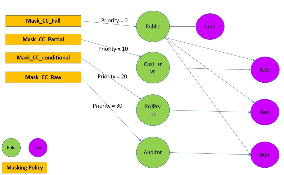
The following diagram illustrates how DDM support (preview) in Amazon Redshift policies works with roles and users for our retail use case.

For a user with multiple roles, the masking policy with the highest attachment priority is used. For example, in the following example, Ken is part of the Public and FrdPrvnt role. Because the FrdPrvnt role has a higher attachment priority, card_number_conditional_mask will be applied.

Prerequisites

To implement this solution, you need to complete the following prerequisites:

Have an AWS account.
Have an Amazon Redshift cluster provisioned with DDM support (preview) or a serverless workgroup with DDM support (preview).
1. Navigate to the provisioned or serverless Amazon Redshift console and choose Create preview cluster.
2. In the create cluster wizard, choose the preview track.
Have Superuser privilege, or the sys:secadmin role on the Amazon Redshift data warehouse created in step 2.

Preparing the data

To set up our use case, complete the following steps:

On the Amazon Redshift console, choose Query editor v2 in Explorer.
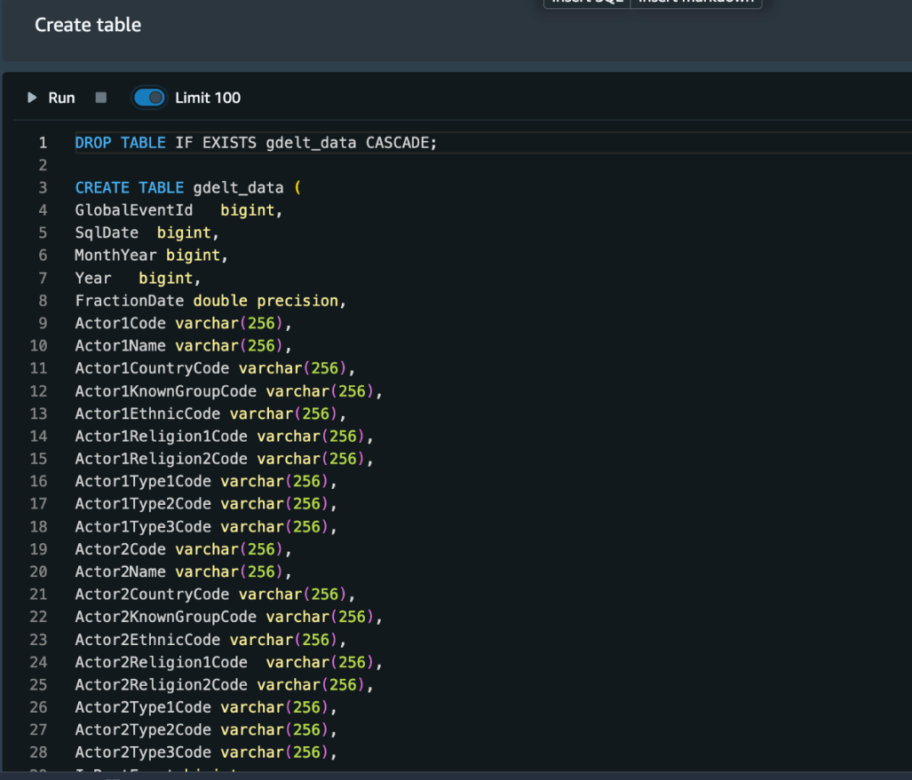
If you’re familiar with SQL Notebooks, you can download the Jupyter notebook for the demonstration, and import it to quickly get started.
Create the table and populate contents.

Create users.

-- 1- Create the credit cards table
CREATE TABLE credit_cards (
customer_id INT,
is_fraud BOOLEAN,
credit_card TEXT
);
-- 2- Populate the table with sample values
INSERT INTO credit_cards
VALUES
(100,'n', '453299ABCDEF4842'),
(100,'y', '471600ABCDEF5888'),
(102,'n', '524311ABCDEF2649'),
(102,'y', '601172ABCDEF4675'),
(102,'n', '601137ABCDEF9710'),
(103,'n', '373611ABCDEF6352')
;
--run GRANT to grant SELECT permission on the table
GRANT SELECT ON credit_cards TO PUBLIC;
--create four users
CREATE USER Kate WITH PASSWORD '1234Test!';
CREATE USER Ken  WITH PASSWORD '1234Test!';
CREATE USER Bob  WITH PASSWORD '1234Test!';
CREATE USER Jane WITH PASSWORD '1234Test!';

Implement the solution

To satisfy the security requirements, we need to make sure that each user sees the same data in different ways based on their granted privileges. To do that, we use user roles combined with masking policies as follows:

Create user roles and grant different users to different roles:

-- 1. Create User Roles
CREATE ROLE cust_srvc_role;
CREATE ROLE frdprvnt_role;
CREATE ROLE auditor_role;
-- note that public role exist by default.

-- Grant Roles to Users
GRANT ROLE cust_srvc_role to Kate;
GRANT ROLE frdprvnt_role  to Ken;
GRANT ROLE auditor_role   to Bob;
-- note that regualr_user is attached to public role by default.

Create masking policies:

-- 2. Create Masking policies

-- 2.1 create a masking policy that fully masks the credit card number
CREATE MASKING POLICY Mask_CC_Full
WITH (credit_card VARCHAR(256))
USING ('XXXXXXXXXXXXXXXX');

--2.2- Create a scalar SQL user-defined function(UDF) that partially obfuscates credit card number, only showing the first 6 digits and the last 4 digits
CREATE FUNCTION REDACT_CREDIT_CARD (text)
  returns text
immutable
as $$
  select left($1,6)||'XXXXXX'||right($1,4)
$$ language sql;


--2.3- create a masking policy that applies the REDACT_CREDIT_CARD function
CREATE MASKING POLICY Mask_CC_Partial
WITH (credit_card VARCHAR(256))
USING (REDACT_CREDIT_CARD(credit_card));

-- 2.4- create a masking policy that will display raw credit card number only if it is flagged for fraud 
CREATE MASKING POLICY Mask_CC_Conditional
WITH (is_fraud BOOLEAN, credit_card VARCHAR(256))
USING (CASE WHEN is_fraud 
                 THEN credit_card 
                 ELSE Null 
       END);

-- 2.5- Create masking policy that will show raw credit card number.
CREATE MASKING POLICY Mask_CC_Raw
WITH (credit_card varchar(256))
USING (credit_card);

Attach the masking policies on the table or column to the user or role:

-- 3. ATTACHING MASKING POLICY
-- 3.1- make the Mask_CC_Full the default policy for all users
--    all users will see this masking policy unless a higher priority masking policy is attached to them or their role

ATTACH MASKING POLICY Mask_CC_Full
ON credit_cards(credit_card)
TO PUBLIC;

-- 3.2- attach Mask_CC_Partial to the cust_srvc_role role
--users with the cust_srvc_role role can see partial credit card information
ATTACH MASKING POLICY Mask_CC_Partial
ON credit_cards(credit_card)
TO ROLE cust_srvc_role
PRIORITY 10;

-- 3.3- Attach Mask_CC_Conditional masking policy to frdprvnt_role role
--    users with frdprvnt_role role can only see raw credit card if it is fraud
ATTACH MASKING POLICY Mask_CC_Conditional
ON credit_cards(credit_card)
USING (is_fraud, credit_card)
TO ROLE frdprvnt_role
PRIORITY 20;

-- 3.4- Attach Mask_CC_Raw masking policy to auditor_role role
--    users with auditor_role role can see raw credit card numbers
ATTACH MASKING POLICY Mask_CC_Raw
ON credit_cards(credit_card)
TO ROLE auditor_role
PRIORITY 30;

Test the solution

Let’s confirm that the masking policies are created and attached.

Check that the masking policies are created with the following code:

-- 1.1- Confirm the masking policies are created
SELECT * FROM svv_masking_policy;

Check that the masking policies are attached:
```
-- 1.2- Verify attached masking policy on table/column to user/role.
SELECT * FROM svv_attached_masking_policy;
```
Now we can test that different users can see the same data masked differently based on their roles.

Test that the Customer Service agents can only view the first six digits and the last four digits of the credit card number:

-- 1- Confirm that customer service agent can only view the first 6 digits and the last 4 digits of the credit card number
SET SESSION AUTHORIZATION Kate;
SELECT * FROM credit_cards;

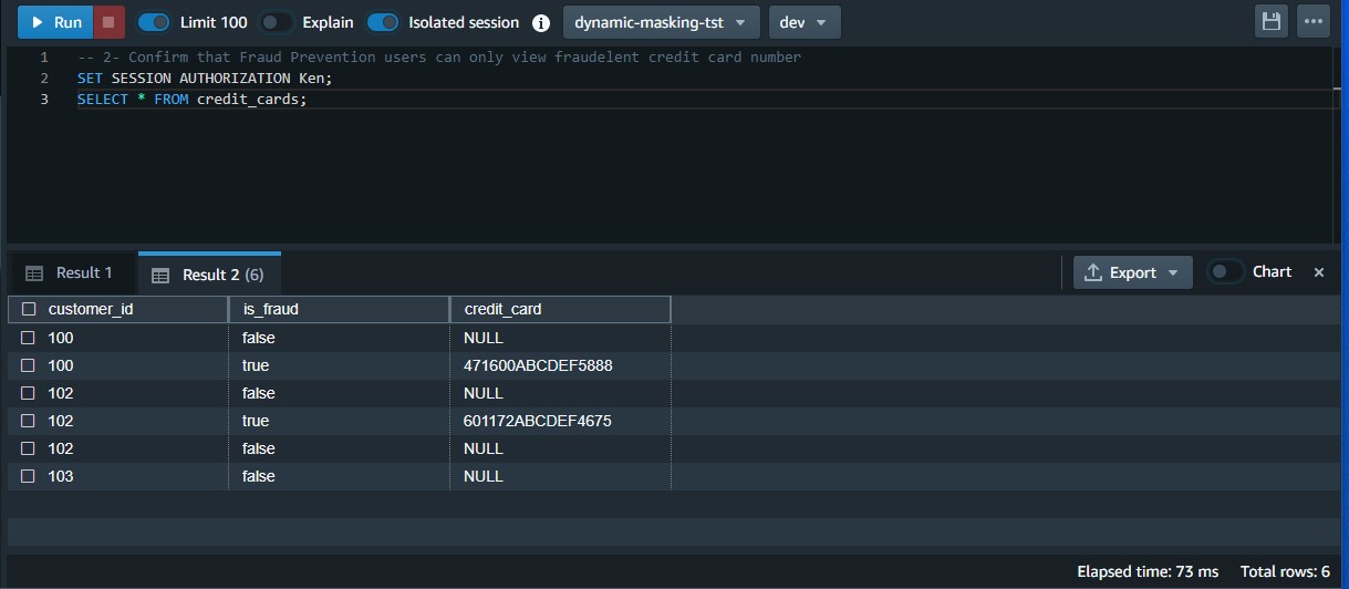
Test that the Fraud Prevention users can only view the raw credit card number when it’s flagged as fraud:

-- 2- Confirm that Fraud Prevention users can only view fraudulent credit card number
SET SESSION AUTHORIZATION Ken;
SELECT * FROM credit_cards;

Test that Auditor users can view the raw credit card number:

-- 3- Confirm the auditor can view RAW credit card number
SET SESSION AUTHORIZATION Bob;
SELECT * FROM credit_cards;

Test that general users can’t view any digits of the credit card number:

-- 4- Confirm that regular users can not view any digit of the credit card number
SET SESSION AUTHORIZATION Jane;
SELECT * FROM credit_cards;

Modify the masking policy

To modify an existing masking policy, you must detach it from the role first and then drop and recreate it.

In our use case, the business changed direction and decided that Customer Service agents should only be allowed to view the last four digits of the credit card number.

Detach and drop the policy:

--reset session authorization to the default
RESET SESSION AUTHORIZATION;
--detach masking policy from the credit_cards table
DETACH MASKING POLICY Mask_CC_Partial
ON                    credit_cards(credit_card)
FROM ROLE             cust_srvc_role;
-- Drop the masking policy
DROP MASKING POLICY Mask_CC_Partial;
-- Drop the function used in masking
DROP FUNCTION REDACT_CREDIT_CARD (TEXT);

Recreate the policy and reattach the policy on the table or column to the intended user or role.Note that this time we created a scalar Python UDF. It’s possible to create a SQL, Python, and Lambda UDF based on your use case.

-- Re-create the policy and re-attach it to role

-- Create a user-defined function that partially obfuscates credit card number, only showing the last 4 digits
CREATE FUNCTION REDACT_CREDIT_CARD (credit_card TEXT) RETURNS TEXT IMMUTABLE AS $$
    import re
    regexp = re.compile("^([0-9A-F]{6})[0-9A-F]{5,6}([0-9A-F]{4})")
    match = regexp.search(credit_card)
    if match != None:
        last = match.group(2)
    else:
        last = "0000"
    return "XXXXXXXXXXXX{}".format(last)
$$ LANGUAGE plpythonu;

--Create a masking policy that applies the REDACT_CREDIT_CARD function
CREATE MASKING POLICY Mask_CC_Partial
WITH (credit_card VARCHAR(256))
USING (REDACT_CREDIT_CARD(credit_card));

-- attach Mask_CC_Partial to the cust_srvc_role role
-- users with the cust_srvc_role role can see partial credit card information
ATTACH MASKING POLICY Mask_CC_Partial
ON credit_cards(credit_card)
TO ROLE cust_srvc_role
PRIORITY 10;

Test that Customer Service agents can only view the last four digits of the credit card number:

-- Confirm that customer service agent can only view the last 4 digits of the credit card number
SET SESSION AUTHORIZATION Kate;
SELECT * FROM credit_cards;

Clean up

When you’re done with the solution, clean up your resources:

Detach the masking policies from the table:

-- Cleanup
--reset session authorization to the default
RESET SESSION AUTHORIZATION;

--1.	Detach the masking policies from table
DETACH MASKING POLICY Mask_CC_Full
ON credit_cards(credit_card)
FROM PUBLIC;
DETACH MASKING POLICY Mask_CC_Partial
ON credit_cards(credit_card)
FROM ROLE cust_srvc_role;
DETACH MASKING POLICY Mask_CC_Conditional
ON credit_cards(credit_card)
FROM ROLE frdprvnt_role;
DETACH MASKING POLICY Mask_CC_Raw
ON credit_cards(credit_card)
FROM ROLE auditor_role;

Drop the masking policies:

-- 2.	Drop the masking policies 
DROP MASKING POLICY Mask_CC_Full;
DROP MASKING POLICY Mask_CC_Partial;
DROP MASKING POLICY Mask_CC_Conditional;
DROP MASKING POLICY Mask_CC_Raw;

Revoke and drop each user and role:

-- 3.	Revoke/Drop - role/user 
REVOKE ROLE cust_srvc_role from Kate;
REVOKE ROLE frdprvnt_role  from Ken;
REVOKE ROLE auditor_role   from Bob;

DROP ROLE cust_srvc_role;
DROP ROLE frdprvnt_role;
DROP ROLE auditor_role;

DROP USER Kate;
DROP USER Ken;
DROP USER Bob;
DROP USER Jane;

Drop the function and table:

-- 4.	Drop function and table 
DROP FUNCTION REDACT_CREDIT_CARD (credit_card TEXT);
DROP TABLE credit_cards;

Considerations and best practices

Consider the following:

Always create a default policy attached to the public user. If you create a new user, they will always have a minimum policy attached. It will enforce the intended security posture.
Remember that DDM policies in Amazon Redshift always follow invoker permissions convention, not definer (for more information, refer to Security and privileges for stored procedures ). That being said, the masking policies are applicable based on the user or role running it.
For best performance, create the masking functions using a scalar SQL UDF, if possible. The performance of scalar UDFs typically goes by the order of SQL to Python to Lambda, in that order. Generally, SQL UDF outperforms Python UDFs and the latter outperforms scalar Lambda UDFs.
DDM policies in Amazon Redshift are applied ahead of any predicate or join operations. For example, if you’re running a join on a masked column (per your access policy) to an unmasked column, the join will lead to a mismatch. That’s an expected behavior.
Always detach a masking policy from all users or roles before dropping it.
As of this writing, the solution has the following limitations:
- You can apply a mask policy on tables and columns and attach it to a user or role, but groups are not supported.
- You can’t create a mask policy on views, materialized views, and external tables.
- The DDM support (preview) in Amazon Redshift is available in following regions: US East (Ohio), US East (N. Virginia), US West (Oregon), Asia Pacific (Tokyo), Europe (Ireland), and Europe (Stockholm).

Performance benchmarks

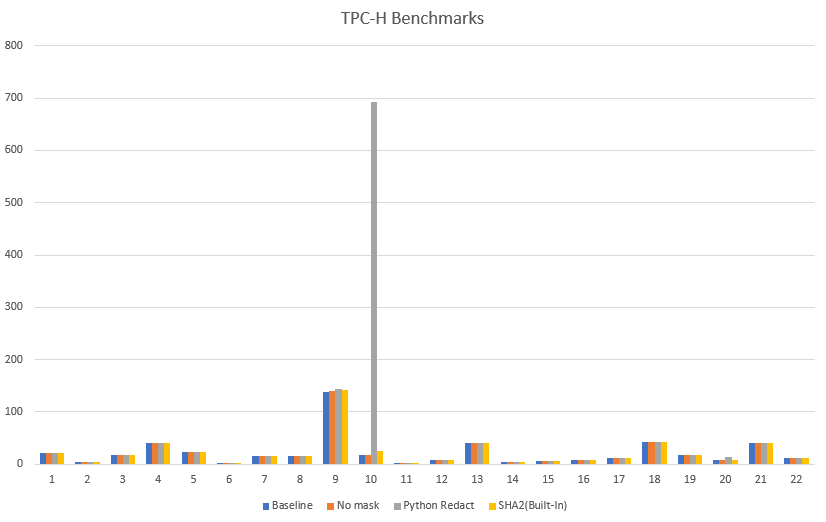
Based on various tests performed on TPC-H datasets, we’ve found built-in functions to be more performant as compared to functions created externally using scalar Python or Lambda UDFs.

Expand the solution

You can take this solution further and set up a masking policy that restricts SSN and email address access as follows:

Customer Service agents accessing pre-built dashboards may only view the last four digits of SSNs and complete email addresses for correspondence
Analysts cannot view SSNs or email addresses
Auditing services may access raw values for SSNs as well as email addresses

For more information, refer to Use DDM support (preview) in Amazon Redshift for E-mail & SSN Masking.

Conclusion

In this post, we discussed how to use DDM support (preview) in Amazon Redshift to define configuration-driven, consistent, format-preserving, and irreversible masked data values. With DDM support (preview) in Amazon Redshift, you can control your data masking approach using familiar SQL language. You can take advantage of the Amazon Redshift role-based access control capability to implement different levels of data masking. You can create a masking policy to identify which column needs to be masked, and you have the flexibility of choosing how to show the masked data. For example, you can completely hide all the information of the data, replace partial real values with wildcard characters, or define your own way to mask the data using SQL expressions, Python, or Lambda UDFs. Additionally, you can apply a conditional masking based on other columns, which selectively protects the column data in a table based on the values in one or more columns.

We encourage you to create your own user defined functions for various use-cases and accomplish desired security posture using dynamic data masking support in Amazon Redshift.

About the Authors

Rohit Vashishtha is a Senior Analytics Specialist Solutions Architect at AWS based in Dallas, TX. He has more than 16 years of experience architecting, building, leading, and maintaining big data platforms. Rohit helps customers modernize their analytic workloads using the breadth of AWS services and ensures that customers get the best price/performance with the utmost security and data governance.

Ahmed Shehata is a Senior Analytics Specialist Solutions Architect at AWS based on Toronto. He has more than two decades of experience helping customers modernize their data platforms. Ahmed is passionate about helping customers build efficient, performant, and scalable analytic solutions.

Variyam Ramesh is a Senior Analytics Specialist Solutions Architect at AWS based in Charlotte, NC. He is an accomplished technology leader helping customers conceptualize, develop, and deliver innovative analytic solutions.

Yanzhu Ji is a Product Manager in the Amazon Redshift team. She has experience in product vision and strategy in industry-leading data products and platforms. She has outstanding skill in building substantial software products using web development, system design, database, and distributed programming techniques. In her personal life, Yanzhu likes painting, photography, and playing tennis.

James Moore is a Technical Lead at Amazon Redshift focused on SQL features and security. His work over the last 10 years has spanned distributed systems, machine learning, and databases. He is passionate about building scalable software that enables customers to solve real-world problems.

Simplify data ingestion from Amazon S3 to Amazon Redshift using auto-copy (preview)

2022-12-07 Jason Pedreza

Post Syndicated from Jason Pedreza original https://aws.amazon.com/blogs/big-data/simplify-data-ingestion-from-amazon-s3-to-amazon-redshift-using-auto-copy-preview/

Amazon Redshift is a fast, scalable, secure, and fully managed cloud data warehouse that makes it simple and cost-effective to analyze all of your data using standard SQL and your existing business intelligence (BI) tools. Tens of thousands of customers today rely on Amazon Redshift to analyze exabytes of data and run complex analytical queries, making it the most widely used cloud data warehouse.

Data ingestion is the process of getting data from the source system to Amazon Redshift. This can be done by using one of many AWS cloud-based ETL tools like AWS Glue, Amazon EMR, or AWS Step Functions, or you can simply load data from Amazon Simple Storage Service (Amazon S3) to Amazon Redshift using the COPY command. A COPY command is the most efficient way to load a table because it uses the Amazon Redshift massively parallel processing (MPP) architecture to read and load data in parallel from a file or multiple files in an S3 bucket.

Now SQL users can easily automate data ingestion from Amazon S3 to Amazon Redshift with a simple SQL command using the Amazon Redshift auto-copy preview feature. COPY statements are triggered and start loading data when Amazon Redshift auto-copy detects new files in the specified Amazon S3 paths. This also ensures end-users have the latest data available in Amazon Redshift shortly after the source data is available.

This post shows you how to easily build continuous file ingestion pipelines in Amazon Redshift using auto-copy when source files are located on Amazon S3 using a simple SQL command. In addition, we show you how to enable auto-copy using copy jobs, how to monitor jobs, considerations, and best practices.

Overview of the auto-copy feature in Amazon Redshift

The auto-copy feature in Amazon Redshift simplifies automatic data loading from Amazon S3 with a simple SQL command. You can enable Amazon Redshift auto-copy by creating copy jobs. A copy job is a database object that stores, automates, and reuses the COPY statement for newly created files that land in the S3 folder.

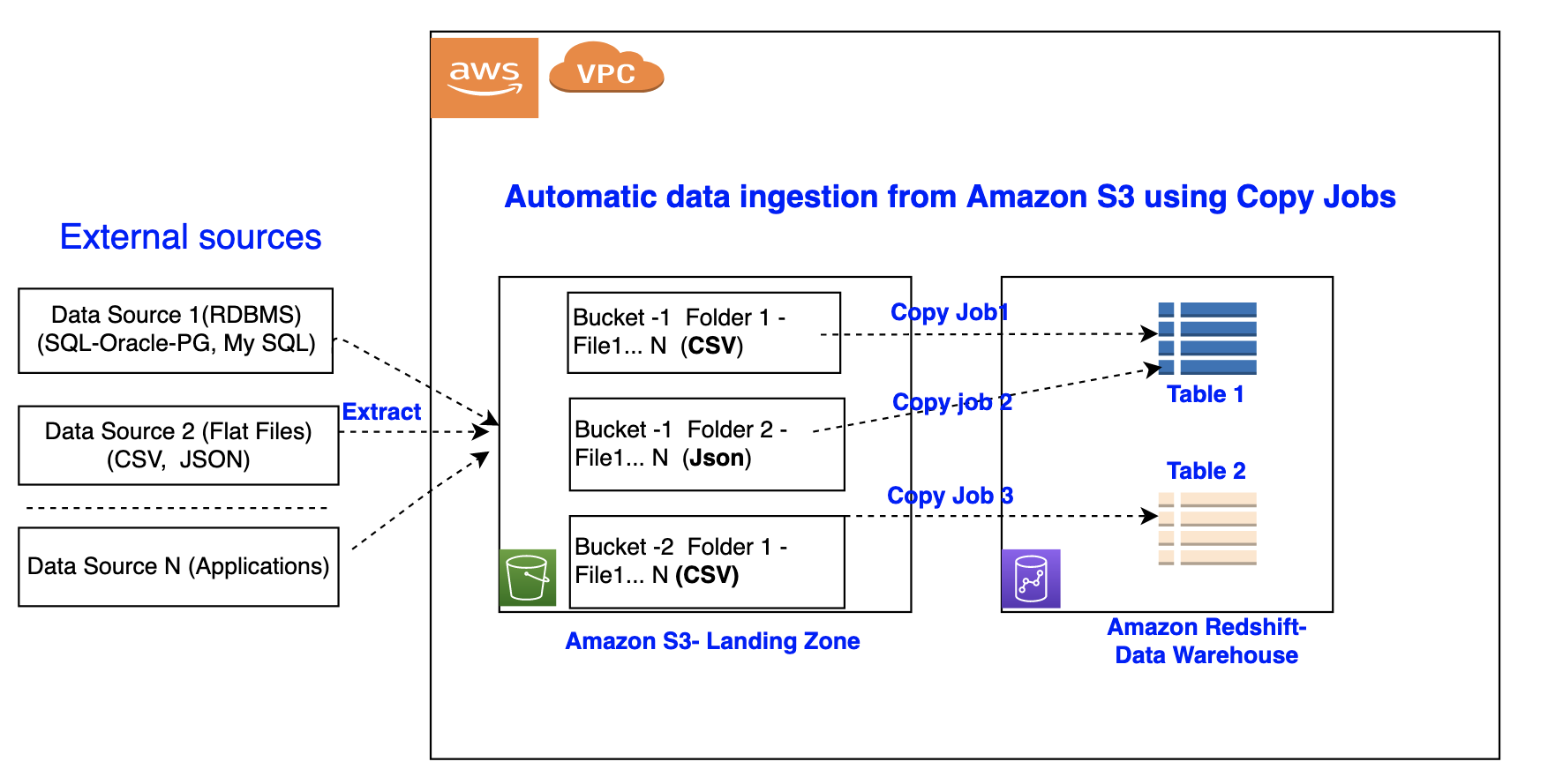
The following diagram illustrates this process.

automatic data ingestion from Amazon S3 using copy jobx

Copy jobs have the following benefits:

SQL users such as data analysts can now load data from Amazon S3 automatically without having to build a pipeline or using an external framework
Copy jobs offer continuous and incremental data ingestion from an Amazon S3 location without the need to implement a custom solution
This functionality comes at no additional cost
Existing COPY statements can be converted into copy jobs by appending the JOB CREATE <job_name> parameter
It keeps track of all loaded files and prevents data duplication
It can be easily set up using a simple SQL statement and any JDBC or ODBC client

Prerequisites

To get started with auto-copy preview, you need the following prerequisites:

An AWS account
An Amazon Redshift cluster with a maintenance track of PREVIEW_AUTOCOPY_2022

The Amazon Redshift auto-copy support from Amazon S3 is available as a preview for provisioned clusters in the following AWS Regions: US East (Ohio), US East (N. Virginia), US West (Oregon), Asia Pacific (Sydney), Europe (Ireland), and Europe (Stockholm). Please note that for the preview track, restore from snapshot is not supported.

You can refer to the SQL notebook redshift-auto-copy-preview-demo-sql-notebook.ipynb for the SQL statements used in this post.

Set up copy jobs

In this section, we demonstrate how to automate data loading of files from Amazon S3 into Amazon Redshift. With the existing COPY syntax, we add the JOB CREATE parameter to perform a one-time setup for automatic file ingestion. See the following code:

COPY <table-name>
FROM 's3://<s3-object-path>'
[COPY PARAMETERS...]
JOB CREATE <job-name> [AUTO ON | OFF];

Auto ingestion is enabled by default on copy jobs.

Automate ingestion from a single data source

With a copy job, you can automate ingestion from a single data source by creating one job and specifying the path to the S3 objects that contain the data. The S3 object path can reference a set of folders that have the same key prefix.

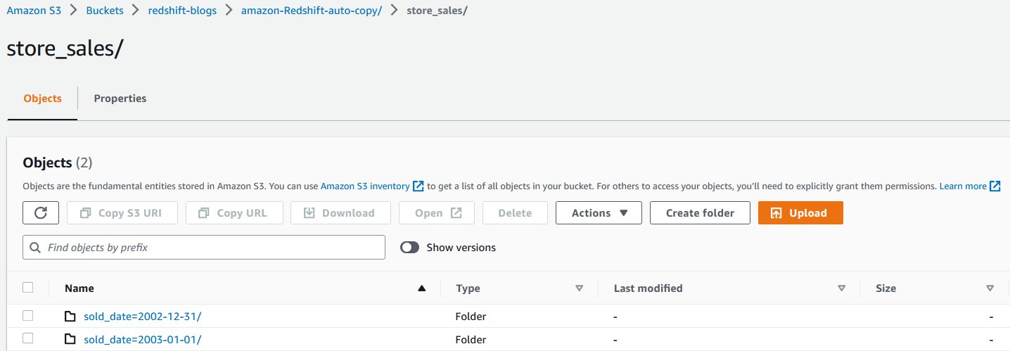
In this example, we have multiple files that are being loaded on a daily basis containing the sales transactions across all the stores in the US. Each day’s sales transactions are loaded to their own folder in Amazon S3.

store_sales

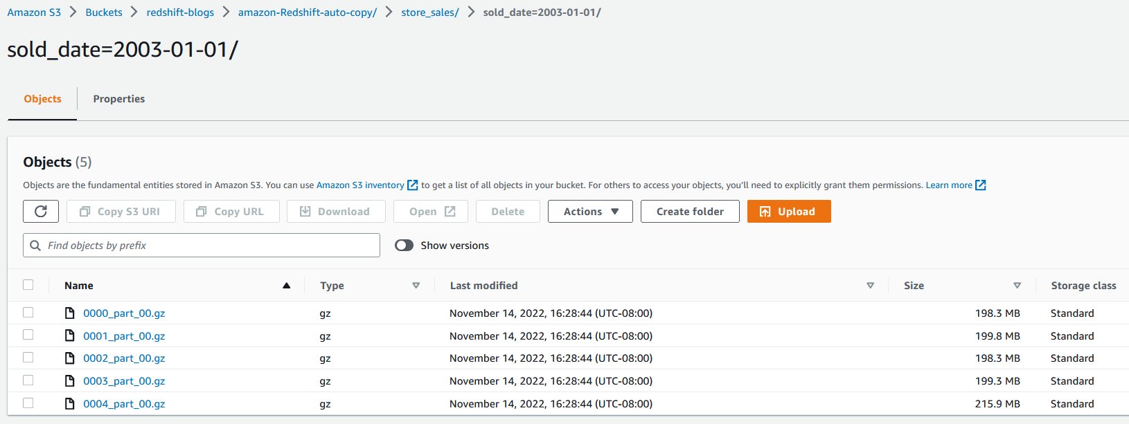
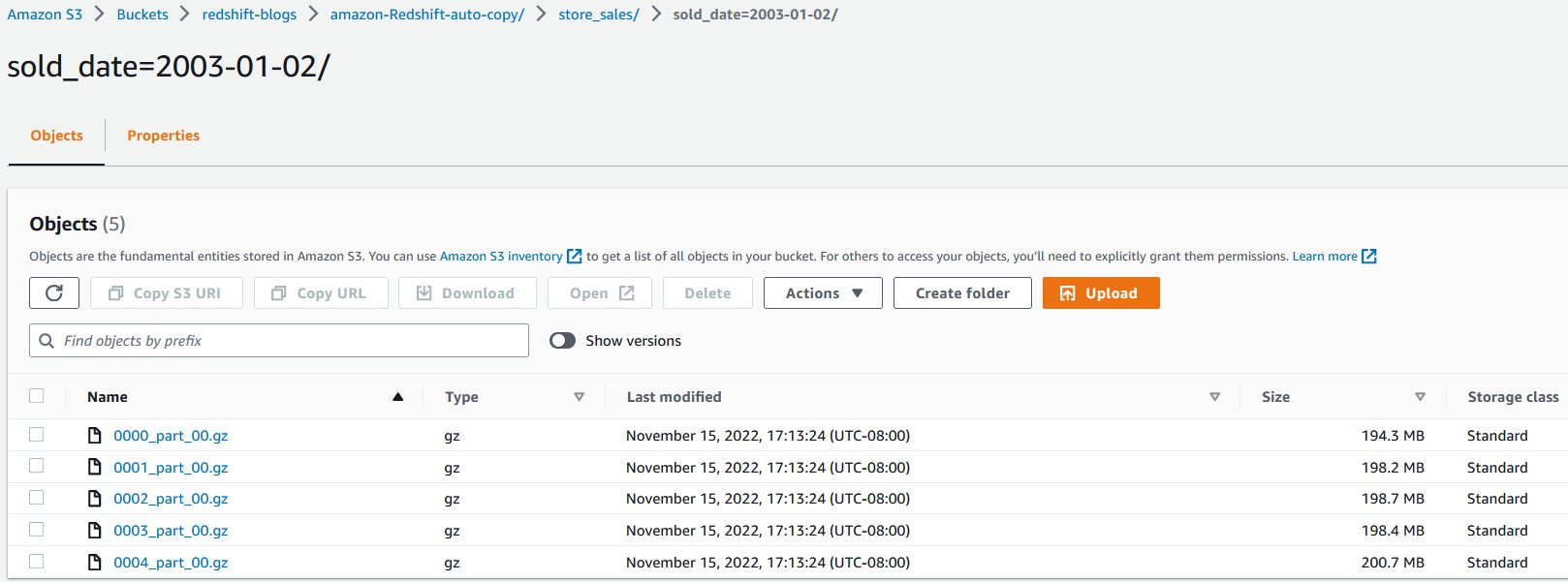
Each folder contains multiple gzip-compressed files.

gzip-compressed files

The following code creates the store_sales table:

DROP TABLE IF EXISTS store_sales;
CREATE TABLE IF NOT EXISTS store_sales
(
  ss_sold_date_sk int4 ,            
  ss_sold_time_sk int4 ,     
  ss_item_sk int4 not null ,      
  ss_customer_sk int4 ,           
  ss_cdemo_sk int4 ,              
  ss_hdemo_sk int4 ,         
  ss_addr_sk int4 ,               
  ss_store_sk int4 ,           
  ss_promo_sk int4 ,           
  ss_ticket_number int8 not null,        
  ss_quantity int4 ,           
  ss_wholesale_cost numeric(7,2) ,          
  ss_list_price numeric(7,2) ,              
  ss_sales_price numeric(7,2) ,
  ss_ext_discount_amt numeric(7,2) ,             
  ss_ext_sales_price numeric(7,2) ,              
  ss_ext_wholesale_cost numeric(7,2) ,           
  ss_ext_list_price numeric(7,2) ,               
  ss_ext_tax numeric(7,2) ,                 
  ss_coupon_amt numeric(7,2) , 
  ss_net_paid numeric(7,2) ,   
  ss_net_paid_inc_tax numeric(7,2) ,             
  ss_net_profit numeric(7,2) ,
  primary key (ss_item_sk, ss_ticket_number)
) DISTKEY (ss_item_sk) 
  SORTKEY(ss_sold_date_sk);

Next, we create the copy job to automatically load the gzip-compressed files into the store_sales table:

COPY store_sales
FROM 's3://redshift-blogs/amazon-Redshift-auto-copy/store_sales'
IAM_ROLE 'arn:aws:iam::**********:role/Redshift-S3'
gzip delimiter '|' EMPTYASNULL
region 'us-east-1'
JOB CREATE job_store_sales AUTO ON;

When the copy job is created, it automatically loads the existing gzip-compressed files located in the S3 object path specified in the command to the store_sales table.

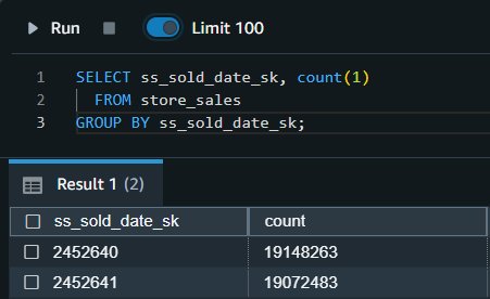
Let’s run a query to get the daily total of sales transactions across all the stores in the US:

SELECT ss_sold_date_sk, count(1)
  FROM store_sales
GROUP BY ss_sold_date_sk;

The output shown comes from the transactions sold on 2002-12-31 and 2003-01-01, respectively.

transactions shown

The following day, incremental sales transactions data are loaded to a new folder in the same S3 object path.

incremental sales transactions

As new files arrive to the same S3 object path, the copy job automatically loads the unprocessed files to the store_sales table in an incremental fashion.

All new sales transactions for 2003-01-02 are automatically ingested, which can be verified by running the following query:

SELECT ss_sold_date_sk, count(1)
  FROM store_sales
GROUP BY ss_sold_date_sk;

Automate ingestion from multiple data sources

We can also load an Amazon Redshift table from multiple data sources. When using a pub/sub pattern where multiple S3 buckets populate data to an Amazon Redshift table, you have to maintain multiple data pipelines for each source/target combination. With new parameters in the COPY command, this can be automated to handle data loads efficiently.

In the following example, the Customer_1 folder has Green Cab Company sales data, and the Customer_2 folder has Red Cab Company sales data. We can use the COPY command with the JOB parameter to automate this ingestion process.

automate this ingestion process

The following screenshot shows sample data stored in files. Each folder has similar data but for different customers.

sample data sored in files

The target for these files in this example is the Amazon Redshift table cab_sales_data.

Define the target table cab_sales_data:

DROP TABLE IF EXISTS cab_sales_data;
CREATE TABLE IF NOT EXISTS cab_sales_data
(
  vendorid                VARCHAR(4),
  pickup_datetime         TIMESTAMP,
  dropoff_datetime        TIMESTAMP,
  store_and_fwd_flag      VARCHAR(1),
  ratecode                INT,
  pickup_longitude        FLOAT4,
  pickup_latitude         FLOAT4,
  dropoff_longitude       FLOAT4,
  dropoff_latitude        FLOAT4,
  passenger_count         INT,
  trip_distance           FLOAT4,
  fare_amount             FLOAT4,
  extra                   FLOAT4,
  mta_tax                 FLOAT4,
  tip_amount              FLOAT4,
  tolls_amount            FLOAT4,
  ehail_fee               FLOAT4,
  improvement_surcharge   FLOAT4,
  total_amount            FLOAT4,
  payment_type            VARCHAR(4),
  trip_type               VARCHAR(4)
)
DISTSTYLE EVEN
SORTKEY (passenger_count,pickup_datetime);

You can define two copy jobs as shown in the following code to handle and monitor ingestion of sales data belonging to different customers , in our case Customer_1 and Customer_2. These jobs monitor the Customer_1 and Customer_2 folders and load any new files that are added here.

COPY cab_sales_data
FROM 's3://redshift-blogs/amazon-Redshift-auto-copy/Customer_1'
IAM_ROLE 'arn:aws:iam::**********:role/Redshift-S3'
DATEFORMAT 'auto'
IGNOREHEADER 1
DELIMITER ','
IGNOREBLANKLINES
REGION 'us-east-1'
JOB CREATE job_green_cab AUTO ON;

COPY cab_sales_data
FROM 's3://redshift-blogs/amazon-Redshift-auto-copy/Customer_2'
IAM_ROLE 'arn:aws:iam::**********:role/Redshift-S3'
DATEFORMAT 'auto'
IGNOREHEADER 1
DELIMITER ','
IGNOREBLANKLINES
REGION 'us-east-1'
JOB CREATE job_red_cab AUTO ON;

Each customer is assigned its own vendorid, as shown in the following output:

SELECT vendorid,
       sum(passenger_count) as total_passengers 
  FROM cab_sales_data
GROUP BY vendorid;

Manually run a copy job

There might be scenarios wherein the copy job needs to be paused, meaning it needs to stop looking for new files, for example, to fix a corrupted data pipeline at the data source.

In that case, either use the COPY JOB ALTER command to set AUTO to OFF or create a new COPY JOB with AUTO OFF. Once this is set, auto copy will no longer look for new files.

If in case required, users can manually invoke COPY JOB which will do the work and ingest if any new files found.

COPY JOB RUN <Copy Job Name>

You can disable “AUTO ON” in the existing copy job using the following command:

COPY JOB ALTER <Copy Job Name> AUTO OFF

The following table compares the syntax and data duplication between a regular copy statement and the new auto-copy job.

.	Copy	Auto-Copy Job (preview)
Syntax	`COPY <table-name> FROM 's3://<s3-object-path>' [COPY PARAMETERS...]`	`COPY <table-name> FROM 's3://<s3-object-path>' [COPY PARAMETERS...] JOB CREATE <job-name>;`
Data Duplication	If it is run multiple times against the same S3 folder, it will load the data again, resulting in data duplication.	It will not load the same file twice, preventing data duplication.

For the copy job preview, support on other data formats will be expanded.

Error handling and monitoring for copy jobs

Copy jobs continuously monitor the S3 folder specified during job creation and perform ingestion whenever new files are created. New files created under the S3 folder are loaded exactly once to avoid data duplication.

By default, if there are any data or format issues with the specific files, the copy job will fail to ingest the files with a load error and log details to the system tables. The copy job will remain AUTO ON with new data files and will continue to ignore previously failed files.

Amazon Redshift provides the following system tables for users to monitor or troubleshoot copy jobs as needed:

List copy jobs – Use SYS_COPY_JOB to list all the copy jobs stored in the database:

SELECT * 
  FROM sys_copy_job;

Get a summary of a copy job – Use the SYS_LOAD_HISTORY view to get the aggregate metrics of a copy job operation by specifying the copy_job_id. It shows the aggregate metrics of all the files that have been processed by a copy job.

SELECT *
  FROM sys_load_history
 WHERE copy_job_id = 105928;

Get details of a copy job – Use STL_LOAD_COMMITS to get the status and details of each file that was processed by a copy job:

SELECT *
  FROM stl_load_commits
 WHERE copy_job_id = 105928
ORDER BY curtime ASC;

Get exception details of a copy job – Use STL_LOAD_ERRORS to get the details of files that failed to ingest from a copy job:

SELECT *
  FROM stl_load_errors
 WHERE copy_job_id = 105939;

Copy job best practices

In a copy job, when a new file is detected and ingested (automatically or manually), Amazon Redshift stores the file name and doesn’t run this specific job when a new file is created with the same file name.

The following are the recommended best practices when working with files using the copy job:

Use unique file names for each file in a copy job (for example, 2022-10-15-batch-1.csv). However, you can use the same file name as long as it’s from different copy jobs:
- job_customerA_sales – s3://redshift-blogs/sales/customerA/2022-10-15-sales.csv
- job_customerB_sales – s3://redshift-blogs/sales/customerB/2022-10-15-sales.csv
Do not update file contents. Do not overwrite existing files. Changes in existing files will not be reflected to the target table. The copy job doesn’t pick up updated or overwritten files, so make sure they’re renamed as new file names for the copy job to pick up.
Run regular COPY statements (not a job) if you need to ingest a file that was already processed by your copy job. (COPY without a copy job doesn’t track loaded files.) For example, this is helpful in scenarios where you don’t have control of the file name and the initial file received failed. The following figure shows a typical workflow in this case.

Delete and recreate your copy job if you want to reset file tracking history and start over.

Copy job considerations

During the preview, here are the main things to consider when using auto-copy:

The copy job must be created using an empty S3 folder (no existing files)
The following features are unsupported:
- MAXERROR parameter
- manifest files
- key-based access control
- columnar data format (Parquet, ORC, RCFile, SequenceFile)
- use of IAM_ROLE default

For additional details on other considerations for auto-copy preview, refer to the AWS documentation.

Customer feedback

GE Aerospace is a global provider of jet engines, components, and systems for commercial and military aircraft. The company has been designing, developing, and manufacturing jet engines since World War I.

“GE Aerospace uses AWS analytics and Amazon Redshift to enable critical business insights that drive important business decisions. With the support for auto-copy from Amazon S3, we can build simpler data pipelines to move data from Amazon S3 to Amazon Redshift. This accelerates our data product teams’ ability to access data and deliver insights to end users. We spend more time adding value through data and less time on integrations.”

– Alcuin Weidus Sr Principal Data Architect at GE Aerospace

Conclusion

This post demonstrated how to automate data load from Amazon S3 to Amazon Redshift using the auto-copy preview feature. This new functionality helps make Amazon Redshift data ingestion easier than ever, and will allow SQL users to get access to the most recent data using a simple SQL command.

As an analysts or SQL users, you can begin ingesting data to Redshift from Amazon S3 with simple SQL commands and gain access to the most up-to-date data without the need for third-party tools or custom implementation.

About the authors

Jason Pedreza is an Analytics Specialist Solutions Architect at AWS with data warehousing experience handling petabytes of data. Prior to AWS, he built data warehouse solutions at Amazon.com. He specializes in Amazon Redshift and helps customers build scalable analytic solutions.

Eren Baydemir, a Technical Product Manager at AWS, has 15 years of experience in building customer-facing products and is currently focusing on data lake and file ingestion topics in the Amazon Redshift team. He was the CEO and co-founder of DataRow, which was acquired by Amazon in 2020.

Eesha Kumar is an Analytics Solutions Architect with AWS. He works with customers to realize the business value of data by helping them build solutions using the AWS platform and tools.

Satish Sathiya is a Senior Product Engineer at Amazon Redshift. He is an avid big data enthusiast who collaborates with customers around the globe to achieve success and meet their data warehousing and data lake architecture needs.

Hangjian Yuan is a Software Development Engineer at Amazon Redshift. He’s passionate about analytical databases and focuses on delivering cutting-edge streaming experiences for customers.

Centrally manage access and permissions for Amazon Redshift data sharing with AWS Lake Formation

2022-11-30 Srividya Parthasarathy

Post Syndicated from Srividya Parthasarathy original https://aws.amazon.com/blogs/big-data/centrally-manage-access-and-permissions-for-amazon-redshift-data-sharing-with-aws-lake-formation/

Today’s global, data-driven organizations treat data as an asset and use it across different lines of business (LOBs) to drive timely insights and better business decisions. Amazon Redshift data sharing allows you to securely share live, transactionally consistent data in one Amazon Redshift data warehouse with another Amazon Redshift data warehouse within the same AWS account, across accounts, and across Regions, without needing to copy or move data from one cluster to another.

Some customers share their data with 50–100 data warehouses in different accounts and do a lot of cross-sharing, making it difficult to track who is accessing what data. They have to navigate to an individual account’s Amazon Redshift console to retrieve the access information. Also, many customers have their data lake on Amazon Simple Storage Service (Amazon S3), which is shared within and across various business units. As the organization grows and democratizes the data, administrators want the ability to manage the datashare centrally for governance and auditing, and to enforce fine-grained access control.

Working backward from customer ask, we are announcing the preview of the following new feature: Amazon Redshift data sharing integration with AWS Lake Formation, which enables Amazon Redshift customers to centrally manage access to their Amazon Redshift datashares using Lake Formation.

Lake Formation has been a popular choice for centrally governing data lakes backed by Amazon S3. Now, with Lake Formation support for Amazon Redshift data sharing, it opens up new design patterns, and broadens governance and security posture across data warehouses. With this integration, you can use Lake Formation to define fine-grained access control on tables and views being shared with Amazon Redshift data sharing for federated AWS Identity and Access Management (IAM) users and IAM roles.

Customers are using the data mesh approach, which provides a mechanism to share data across business units. Customers are also using a modern data architecture to share data from data lake stores and Amazon Redshift purpose-built data stores across business units. Lake Formation provides the ability to enforce data governance within and across business units, which enables secure data access and sharing, easy data discovery, and centralized audit for data access.

United Airlines is in the business of connecting people and uniting the world.

“As a data-driven enterprise, United is trying to create a unified data and analytics experience for our analytics community that will innovate and build modern data-driven applications. We believe we can achieve this by building a purpose-built data mesh architecture using a variety of AWS services like Athena, Aurora, Amazon Redshift, and Lake Formation to simplify management and governance around granular data access and collaboration.”

-Ashok Srinivas, Director of ML Engineering and Sarang Bapat, Director of Data Engineering.

In this post, we show how to centrally manage access and permissions for Amazon Redshift data sharing with Lake Formation.

Solution overview

In this solution, we demonstrate how integration of Amazon Redshift data sharing with Lake Formation for data governance can help you build data domains, and how you can use the data mesh approach to bring data domains together to enable data sharing and federation across business units. The following diagram illustrates our solution architecture.

solution architecture

The data mesh is a decentralized, domain-oriented architecture that emphasizes separating data producers from data consumers via a centralized, federated Data Catalog. Typically, the producers and consumers run within their own account. The details of these data mesh characteristics are as follows:

Data producers – Data producers own their data products and are responsible for building their data, maintaining its accuracy, and keeping their data product up to date. They determine what datasets can be published for consumption and share their datasets by registering them with the centralized data catalog in a central governance account. You might have a producer steward or administrator persona for managing the data products with the central governance steward or administrators team.
Central governance account – Lake Formation enables fine-grained access management on the shared dataset. The centralized Data Catalog offers consumers the ability to quickly find shared datasets, allows administrators to centrally manage access permissions on shared datasets, and provides security teams the ability to audit and track data product usage across business units.
Data consumers – The data consumer obtains access to shared resources from the central governance account. These resources are available inside the consumer’s AWS Glue Data Catalog, allowing fine-grained access on the database and table that can be managed by the consumer’s data stewards and administrators.

The following steps provide an overview of how Amazon Redshift data sharing can be governed and managed by Lake Formation in the central governance pattern of a data mesh architecture:

In the producer account, data objects are created and maintained in the Amazon Redshift producer cluster. A data warehouse admin creates the Amazon Redshift datashare and adds datasets (tables, views) to the share.
The data warehouse admin grants and authorizes access on the datashare to the central governance account’s Data Catalog.
In the central governance account, the data lake admin accepts the datashare and creates the AWS Glue database that points to the Amazon Redshift datashare so that Lake Formation can manage it.
The data lake admin shares the AWS Glue database and tables to the consumer account using Lake Formation cross-account sharing.
In the consumer account, the data lake admin accepts the resource share invitation via AWS Resource Access Manager (AWS RAM) and can view the database listed in the account.
The data lake admin defines the fine-grained access control and grants permissions on databases and tables to IAM users (for this post, consumer1 and consumer2) in the account.
In the Amazon Redshift cluster, the data warehouse admin creates an Amazon Redshift database that points to the Glue database and authorizes usage on the created Amazon Redshift database to the IAM users.
The data analyst as an IAM user can now use their preferred tools like the Amazon Redshift query editor to access the dataset based on the Lake Formation fine-grained permissions.

We use the following account setup for our example in this post:

Producer account – 123456789012
Central account – 112233445566
Consumer account – 665544332211

Prerequisites

Create the Amazon Redshift data share and add datasets

In the data producer account, create an Amazon Redshift cluster using the RA3 node type with encryption enabled. Complete the following steps:

On the Amazon Redshift console, create a cluster subnet group.

For more information, refer to Managing cluster subnet groups using the console.

Choose Create cluster.
For Cluster identifier, provide the cluster name of your choice.
For Preview track, choose preview_2022.

For Node type, choose one of the RA3 node types.

This feature is only supported on the RA3 node type.

For Number of nodes, enter the number of nodes that you need for your cluster.
Under Database configurations, choose the admin user name and admin user password.
Under Cluster permissions, you can select the IAM role and set it as the default.

For more information about the default IAM role, refer to Creating an IAM role as default for Amazon Redshift.

cluster permissions

Turn on the Use defaults option next to Additional configurations to modify the default settings.
Under Network and security, specify the following:
1. For Virtual private cloud (VPC), choose the VPC you would like to deploy the cluster in.
2. For VPC security groups, either leave as default or add the security groups of your choice.
3. For Cluster subnet group, choose the cluster subnet group you created.

additional configurations

Under Database configuration, in the Encryption section, select Use AWS Key Management Service (AWS KMS) or Use a hardware security module (HSM).

Encryption is disabled by default.

For Choose an AWS KMS key, you can either choose an existing AWS Key Management Service (AWS KMS) key, or choose Create an AWS KMS key to create a new key.

For more information, refer to Creating keys.

database configurations

Choose Create cluster.
For this post, create tables and load data into the producer Amazon Redshift cluster using the following script.

Authorize the datashare

Install or update the latest AWS Command Line Interface (AWS CLI) version to run the AWS CLI to authorize the datashare. For instructions, refer to Installing or updating the latest version of the AWS CLI.

Set up Lake Formation permissions

To use the AWS Glue Data Catalog in Lake Formation, complete the following steps in the central governance account to update the Data Catalog settings to use Lake Formation permissions to control catalog resources instead of IAM-based access control:

Sign in to the Lake Formation console as admin.
In the navigation pane, under Data catalog, choose Settings.
Deselect Use only IAM access control for new databases.
Deselect Use only IAM access control for new tables in new databases.
Choose Version 2 for Cross account version settings.
Choose Save.

data catalog settings

Set up an IAM user as a data lake administrator

If you’re using an existing data lake administrator user or role add the following managed policies, if not attached and skip the below setup steps:

AWSGlueServiceRole
AmazonRedshiftFullAccess

Otherwise, to set up an IAM user as a data lake administrator, complete the following steps:

On the IAM console, choose Users in the navigation pane.
Select the IAM user who you want to designate as the data lake administrator.
Choose Add an inline policy on the Permissions tab.
Replace <AccountID> with your own account ID and add the following policy:

{
    "Version": "2012-10-17",
    "Statement": [ {
        "Condition": {"StringEquals": {
            "iam:AWSServiceName":"lakeformation.amazonaws.com"}},
            "Action":"iam:CreateServiceLinkedRole",
            "Resource": "*",
            "Effect": "Allow"},
            {"Action": ["iam:PutRolePolicy"],
            "Resource": "arn:aws:iam::<AccountID>:role/aws-service role/lakeformation.amazonaws.com/AWSServiceRoleForLakeFormationDataAccess",
            "Effect": "Allow"
     },{
                  "Effect": "Allow",
                  "Action": [
                    "ram:AcceptResourceShareInvitation",
                    "ram:RejectResourceShareInvitation",
                    "ec2:DescribeAvailabilityZones",
                    "ram:EnableSharingWithAwsOrganization"
                  ],
                  "Resource": "*"
                }]
}

Provide a policy name.
Review and save your settings.
Choose Add permissions, and choose Attach existing policies directly.
Add the following policies:
1. AWSLakeFormationCrossAccountManager
2. AWSGlueConsoleFullAccess
3. AWSGlueServiceRole
4. AWSLakeFormationDataAdmin
5. AWSCloudShellFullAccess
6. AmazonRedshiftFullAccess
Choose Next: Review and add permissions.

Data consumer account setup

In the consumer account, follow the steps mentioned previously in the central governance account to set up Lake Formation and a data lake administrator.

In the data consumer account, create an Amazon Redshift cluster using the RA3 node type with encryption (refer to the steps demonstrated to create an Amazon Redshift cluster in the producer account).
Choose Launch stack to deploy an AWS CloudFormation template to create two IAM users with policies.

The stack creates the following users under the data analyst persona:

consumer1
consumer2

After the CloudFormation stack is created, navigate to the Outputs tab of the stack.
Capture the ConsoleIAMLoginURL and LFUsersCredentials values.

createiamusers

Choose the LFUsersCredentials value to navigate to the AWS Secrets Manager console.
In the Secret value section, choose Retrieve secret value.

secret value

Capture the secret value for the password.

Both consumer1 and consumer2 need to use this same password to log in to the AWS Management Console.

secret value

Configure an Amazon Redshift datashare using Lake Formation

Producer account

Create a datashare using the console

Complete the following steps to create an Amazon Redshift datashare in the data producer account and share it with Lake Formation in the central account:

On the Amazon Redshift console, choose the cluster to create the datashare.
On the cluster details page, navigate to the Datashares tab.
Under Datashares created in my namespace, choose Connect to database.

connect to database

Choose Create datashare.

create datashare

For Datashare type, choose Datashare.
For Datashare name, enter the name (for this post, demotahoeds).
For Database name, choose the database from where to add datashare objects (for this post, dev).
For Publicly accessible, choose Turn off (or choose Turn on to share the datashare with clusters that are publicly accessible).

datashare information

Under DataShare objects, choose Add to add the schema to the datashare (in this post, the public schema).
Under Tables and views, choose Add to add the tables and views to the datashare (for this post, we add the table customer and view customer_view).

datashare objects

Under Data consumers, choose Publish to AWS Data Catalog.
For Publish to the following accounts, choose Other AWS accounts.
Provide the AWS account ID of the consumer account. For this post, we provide the AWS account ID of the Lake Formation central governance account.
To share within the same account, choose Local account.
Choose Create datashare.

data consumers

After the datashare is created, you can verify by going back to the Datashares tab and entering the datashare name in the search bar under Datashares created in my namespace.
Choose the datashare name to view its details.
Under Data consumers, you will see the consumer status of the consumer data catalog account as Pending Authorization.

data consumers

Choose the checkbox against the consumer data catalog which will enable the Authorize option.

authorize

Click Authorize to authorize the datashare access to the consumer account data catalog, consumer status will change to Authorized.

authorized

Create a datashare using a SQL command

Complete the following steps to create a datashare in data producer account 1 and share it with Lake Formation in the central account:

On the Amazon Redshift console, in the navigation pane, choose Editor, then Query editor V2.
Choose (right-click) the cluster name and choose Edit connection or Create Connection.
For Authentication, choose Temporary credentials.

Refer to Connecting to an Amazon Redshift database to learn more about the various authentication methods.

For Database, enter a database name (for this post, dev).
For Database user, enter the user authorized to access the database (for this post, awsuser).
Choose Save to connect to the database.

Connecting to an Amazon Redshift database

Run the following SQL commands to create the datashare and add the data objects to be shared:

create datashare demotahoeds;
ALTER DATASHARE demotahoeds ADD SCHEMA PUBLIC;
ALTER DATASHARE demotahoeds ADD TABLE customer;
ALTER DATASHARE demotahoeds ADD TABLE customer_view;

Run the following SQL command to share the producer datashare to the central governance account:

GRANT USAGE ON DATASHARE demotahoeds TO ACCOUNT '<central-aws-account-id>' via DATA CATALOG

Run the following SQL command

You can verify the datashare created and objects shared by running the following SQL command:

DESC DATASHARE demotahoeds

DESC DATASHARE demotahoeds

Run the following command using the AWS CLI to authorize the datashare to the central data catalog so that Lake Formation can manage them:

aws redshift authorize-data-share \
--data-share-arn 'arn:aws:redshift:<producer-region>:<producer-aws-account-id>:datashare:<producer-cluster-namespace>/demotahoeds' \
--consumer-identifier DataCatalog/<central-aws-account-id>

The following is an example output:

 {
    "DataShareArn": "arn:aws:redshift:us-east-1:XXXXXXXXXX:datashare:cd8d91b5-0c17-4567-a52a-59f1bdda71cd/demotahoeds",
    "ProducerArn": "arn:aws:redshift:us-east-1:XXXXXXXXXX:namespace:cd8d91b5-0c17-4567-a52a-59f1bdda71cd",
    "AllowPubliclyAccessibleConsumers": false,
    "DataShareAssociations": [{
        "ConsumerIdentifier": "DataCatalog/XXXXXXXXXXXX",
        "Status": "AUTHORIZED",
        "CreatedDate": "2022-11-09T21:10:30.507000+00:00",
        "StatusChangeDate": "2022-11-09T21:10:50.932000+00:00"
    }]
}

You can verify the datashare status on the console by following the steps outlined in the previous section.

Central catalog account

The data lake admin accepts and registers the datashare with Lake Formation in the central governance account and creates a database for the same. Complete the following steps:

Sign in to the console as the data lake administrator IAM user or role.
If this is your first time logging in to the Lake Formation console, select Add myself and choose Get started.
Under Data catalog in the navigation pane, choose Data sharing and view the Amazon Redshift datashare invitations on the Configuration tab.
Select the datashare and choose Review Invitation.

AWS Lake Formation data sharing

A window pops up with the details of the invitation.

Choose Accept to register the Amazon Redshift datashare to the AWS Glue Data Catalog.

accept reject invitation

Provide a name for the AWS Glue database and choose Skip to Review and create.

Skip to Review and create

Review the content and choose Create database.

create database

After the AWS Glue database is created on the Amazon Redshift datashare, you can view them under Shared Databases.

Shared Databases.

You can also use the AWS CLI to register the datashare and create the database. Use the following commands:

Describe the Amazon Redshift datashare that is shared with the central account:

aws redshift describe-data-shares

Accept and associate the Amazon Redshift datashare to Data Catalog:

aws redshift associate-data-share-consumer \
--data-share-arn 'arn:aws:redshift:<producer-region>:<producer-aws-account-id>:datashare:<producer-cluster-namespace>/demotahoeds' \
--consumer-arn arn:aws:glue:us-east-1:<central-aws-account-id>:catalog

The following is an example output:

 {
    "DataShareArn": "arn:aws:redshift:us-east-1:123456789012:datashare:cd8d91b5-0c17-4567-a52a-59f1bdda71cd/demotahoeds",
    "ProducerArn": "arn:aws:redshift:us-east-1:123456789012:namespace:cd8d91b5-0c17-4567-a52a-59f1bdda71cd",
    "AllowPubliclyAccessibleConsumers": false,
    "DataShareAssociations": [
        {
            "ConsumerIdentifier": "arn:aws:glue:us-east-1:112233445566:catalog",
            "Status": "ACTIVE",
            "ConsumerRegion": "us-east-1",
            "CreatedDate": "2022-11-09T23:25:22.378000+00:00",
            "StatusChangeDate": "2022-11-09T23:25:22.378000+00:00"
        }
    ]
}

aws lakeformation register-resource \
--resource-arn arn:aws:redshift:<producer-region>:<producer-aws-account-id>:datashare:<producer-cluster-namespace>/demotahoeds

Create the AWS Glue database that points to the accepted Amazon Redshift datashare:

aws glue create-database --region <central-catalog-region> --cli-input-json '{
    "CatalogId": "<central-aws-account-id>",
    "DatabaseInput": {
        "Name": "demotahoedb",
        "FederatedDatabase": {
            "Identifier": "arn:aws:redshift:<producer-region>:<producer-aws-account-id>:datashare:<producer-cluster-namespace>/demotahoeds",
            "ConnectionName": "aws:redshift"
        }
    }
}'

Now the data lake administrator of the central governance account can view and share access on both the database and tables to the data consumer account using the Lake Formation cross-account sharing feature.

Grant datashare access to the data consumer

To grant the data consumer account permissions on the shared AWS Glue database, complete the following steps:

On the Lake Formation console, under Permissions in the navigation pane, choose Data Lake permissions.
Choose Grant.
Under Principals, select External accounts.
Provide the data consumer account ID (for this post, 665544332211).
Under LF_Tags or catalog resources, select Named data catalog resources.
For Databases, choose the database demotahoedb.
Select Describe for both Database permissions and Grantable permissions.
Choose Grant to apply the permissions.

grant data permissions

To grant the data consumer account permissions on tables, complete the following steps:

On the Lake Formation console, under Permissions in the navigation pane, choose Data Lake permissions.
Choose Grant.
Under Principals, select External accounts.
Provide the consumer account (for this post, we use 665544332211).
Under LF-Tags or catalog resources, select Named data catalog resources.
For Databases, choose the database demotahoedb.
For Tables, choose All tables.
Select Describe and Select for both Table permissions and Grantable permissions.
Choose Grant to apply the changes.

grant the data consumer account permissions on tables

Consumer account

The consumer admin will receive the shared resources from the central governance account and delegate access to other users in the consumer account as shown in the following table.

IAM User	Object Access	Object Type	Access Level
`consumer1`	`public.customer`	Table	All
`consumer2`	`public.customer_view`	View	specific columns: `c_customer_id`, `c_birth_country`, `cd_gender`, `cd_marital_status`, `cd_education_status`

In the data consumer account, follow these steps to accept the resources shared with the account:

Sign in to the console as the data lake administrator IAM user or role.
If this is your first time logging in to the Lake Formation console, select Add myself and choose Get started.
Sign in to the AWS RAM console.
In the navigation pane, under Shared with me, choose Resource shares to view the pending invitations. You will receive 2 invitations.

Choose the pending invitations and accept the resource share.

Choose the pending invitation and accept the resource share

On the Lake formation console, under Data catalog in the navigation pane, choose Databases to view the cross-account shared database.

choose Databases to view the cross-account shared database

Grant access to the data analyst and IAM users using Lake Formation

Now the data lake admin in the data consumer account can delegate permissions on the shared database and tables to users in the consumer account.

Grant database permissions to consumer1 and consumer2

To grant the IAM users consumer1 and consumer2 database permissions, follow these steps:

On the Lake Formation console, under Data catalog in the navigation pane, choose Databases.
Select the database demotahoedb and on the Actions menu, choose Grant.

choose Grant database

Under Principals, select IAM users and roles.
Choose the IAM users consumer1 and consumer2.
Under LF-Tags or catalog resources, demotahoedb is already selected for Databases.
Select Describe for Database permissions.
Choose Grant to apply the permissions.

Choose Grant to apply the permissions

Grant table permissions to consumer1

To grant the IAM user consumer1 permissions on table public.customer, follow these steps:

Under Data catalog in the navigation pane, choose Databases.
Select the database demotahoedb and on the Actions menu, choose Grant.
Under Principals, select IAM users and roles.
Choose IAM user consumer1.
Under LF-Tags or catalog resources, demotahoedb is already selected for Databases.
For Tables, choose public.customer.
Select Describe and Select for Table permissions.
Choose Grant to apply the permissions.

Grant table permissions to consumer1

Grant column permissions to consumer2

To grant the IAM user consumer2 permissions on non-sensitive columns in public.customer_view, follow these steps:

Under Data catalog in the navigation pane, choose Databases.
Select the database demotahoedb and on the Actions menu, choose Grant.
Under Principals, select IAM users and roles.
Choose the IAM user consumer2.
Under LF-Tags or catalog resources, demotahoedb is already selected for Databases.
For Tables, choose public.customer_view.

Grant column permissions to consumer2

Select Select for Table permissions.
Under Data Permissions, select Column-based access.
Select Include columns and choose the non-sensitive columns (c_customer_id, c_birth_country, cd_gender, cd_marital_status, and cd_education_status).
Choose Grant to apply the permissions.

table permissions

Consume the datashare from the data consumer account in the Amazon Redshift cluster

In the Amazon Redshift consumer data warehouse, log in as the admin user using Query Editor V2 and complete the following steps:

Create the Amazon Redshift database from the shared catalog database using the following SQL command:

CREATE DATABASE demotahoedb FROM ARN 'arn:aws:glue:<producer-region>:<producer-aws-account-id>:database/demotahoedb' WITH DATA CATALOG SCHEMA demotahoedb ;

Run the following SQL commands to create and grant usage on the Amazon Redshift database to the IAM users consumer1 and consumer2:

CREATE USER IAM:consumer1 password disable;
CREATE USER IAM:consumer2  password disable;
GRANT USAGE ON DATABASE demotahoedb TO IAM:consumer1;
GRANT USAGE ON DATABASE demotahoedb TO IAM:consumer2;

In order to use a federated identity to enforce Lake Formation permissions, follow the next steps to configure Query Editor v2.

Choose the settings icon in the bottom left corner of the Query Editor v2, then choose Account settings.

identity to enforce Lake Formation permissions

Under Connection settings, select Authenticate with IAM credentials.
Choose Save.

Authenticate with IAM credentials

Query the shared datasets as a consumer user

To validate that the IAM user consumer1 has datashare access from Amazon Redshift, perform the following steps:

Sign in to the console as IAM user consumer1.
On the Amazon Redshift console, choose Query Editor V2 in the navigation pane.
To connect to the consumer cluster, choose the consumer cluster in the tree-view pane.
When prompted, for Authentication, select Temporary credentials using your IAM identity.
For Database, enter the database name (for this post, dev).
The user name will be mapped to your current IAM identity (for this post, consumer1).
Choose Save.

edit connection for redshift

Once you’re connected to the database, you can validate the current logged-in user with the following SQL command:

select current_user;

To find the federated databases created on the consumer account, run the following SQL command:

SHOW DATABASES FROM DATA CATALOG [ACCOUNT '<id1>', '<id2>'] [LIKE 'expression'];

federated databases created on the consumer account

To validate permissions for consumer1, run the following SQL command:

select * from demotahoedb.public.customer limit 10;

As shown in the following screenshot, consumer1 is able to successfully access the datashare customer object.

Now let’s validate that consumer2 doesn’t have access to the datashare tables “public.customer” on the same consumer cluster.

Log out of the console and sign in as IAM user consumer2.
Follow the same steps to connect to the database using the query editor.
Once connected, run the same query:

select * from demotahoedb.public.customer limit 10;

The user consumer2 should get a permission denied error, as in the following screenshot.

should get a permission denied error

Let’s validate the column-level access permissions of consumer2 on public.customer_view view.

Connect to Query Editor v2 as consumer2 and run the following SQL command:

select c_customer_id,c_birth_country,cd_gender,cd_marital_status from demotahoedb.public.customer_view limit 10;

In the following screenshot, you can see consumer2 is only able to access columns as granted by Lake Formation.

access columns as granted by Lake Formation

Conclusion

A data mesh approach provides a method by which organizations can share data across business units. Each domain is responsible for the ingestion, processing, and serving of their data. They are data owners and domain experts, and are responsible for data quality and accuracy. Using Amazon Redshift data sharing with Lake Formation for data governance helps build the data mesh architecture, enabling data sharing and federation across business units with fine-grained access control.

Special thanks to everyone who contributed to launch Amazon Redshift data sharing with AWS Lake Formation:

Debu Panda, Michael Chess, Vlad Ponomarenko, Ting Yan, Erol Murtezaoglu, Sharda Khubchandani, Rui Bi

References

About the Authors

Srividya Parthasarathy is a Senior Big Data Architect on the AWS Lake Formation team. She enjoys building data mesh solutions and sharing them with the community.

Harshida Patel is a Analytics Specialist Principal Solutions Architect, with AWS.

Ranjan Burman is a Analytics Specialist Solutions Architect, with AWS.

Vikram Sahadevan is a Senior Resident Architect on the AWS Data Lab team. He enjoys efforts that focus around providing prescriptive architectural guidance, sharing best practices, and removing technical roadblocks with joint engineering engagements between customers and AWS technical resources that accelerate data, analytics, artificial intelligence, and machine learning initiatives.

Steve Mitchell is a Senior Solution Architect with a passion for analytics and data mesh. He enjoys working closely with customers as they transition to a modern data architecture.

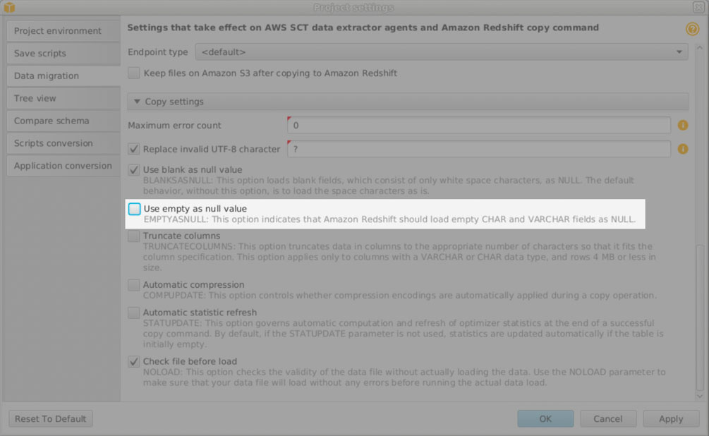
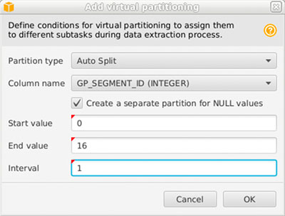
New for Amazon Redshift – Simplify Data Ingestion and Make Your Data Warehouse More Secure and Reliable

2022-11-30 Danilo Poccia

Post Syndicated from Danilo Poccia original https://aws.amazon.com/blogs/aws/new-for-amazon-redshift-simplify-data-ingestion-and-make-your-data-warehouse-more-secure-and-reliable/

When we talk with customers, we hear that they want to be able to harness insights from data in order to make timely, impactful, and actionable business decisions. A common pattern with data-driven organizations is that they have many diﬀerent data sources they need to ingest into their analytics systems. This requires them to build manual data pipelines spanning across their operational databases, data lakes, streaming data, and data within their warehouse. As a consequence of this complex setup, it can take data engineers weeks or even months to build data ingestion pipelines. These data pipelines are costly, and the delays can lead to missed business opportunities. Additionally, data warehouses are increasingly becoming mission critical systems that require high availability, reliability, and security.

Amazon Redshift is a fully managed petabyte-scale data warehouse used by tens of thousands of customers to easily, quickly, securely, and cost-effectively analyze all their data at any scale. This year at re:Invent, Amazon Redshift has announced a number of features to help you simplify data ingestion and get to insights easily and quickly, within a secure, reliable environment.

In this blog, I introduce some of these new features that ﬁt into two main categories:

Simplify data ingestion
- Amazon Redshift now supports auto-copy from Amazon S3 (available in preview). With this new capability, Amazon Redshift automatically loads the files that arrive in an Amazon Simple Storage Service (Amazon S3) location that you specify into your data warehouse. The files can use any of the formats supported by the Amazon Redshift copy command, such as CSV, JSON, Parquet, and Avro. In this way, you don’t need to manually or repeatedly run copy procedures. Amazon Redshift automates file ingestion and takes care of data-loading steps under the hood.
- With Amazon Aurora zero-ETL integration with Amazon Redshift, you can use Amazon Redshift for near real-time analytics and machine learning on petabytes of transactional data stored on Amazon Aurora MySQL databases (available in limited preview). With this capability, you can choose the Amazon Aurora databases containing the data you want to analyze with Amazon Redshift. Data is then replicated into your data warehouse within seconds after transactional data is written into Amazon Aurora, eliminating the need to build and maintain complex data pipelines. You can replicate data from multiple Amazon Aurora databases into the same Amazon Redshift instance to run analytics across multiple applications. With near real-time access to transactional data, you can leverage Amazon Redshift’s analytics and capabilities, such as built-in machine learning (ML), materialized views, data sharing, and federated access to multiple data stores and data lakes, to derive insights from transactional and other data.
- With the general availability of Amazon Redshift Streaming Ingestion, you can now natively ingest hundreds of megabytes of data per second from Amazon Kinesis Data Streams and Amazon MSK into an Amazon Redshift materialized view and query it in seconds. Learn more in this post.
Make your data warehouse more secure and reliable
- You can now improve the availability of your data warehouse by choosing multiple Availability Zone (AZ) deployments. Multi-AZ deployments for your Amazon Redshift clusters are available in preview and reduce recovery times to seconds through automatic recovery. In this way, you can build solutions that are more compliant with the recommendations of the Reliability Pillar of the AWS Well-Architected Framework.
- With dynamic data masking (available in preview), you can protect sensitive information stored in your data warehouse and ensure that only the relevant data is accessible by users based on their roles. You can limit how much identifiable data is visible to users using multiple levels of policies so different users and groups can have different levels of data access without having to create multiple copies of data. Dynamic data masking complements other granular access control capabilities in Amazon Redshift including row-level and column-level security and role-based access controls. In this way, Dynamic Data Masking helps you meet requirements for GDPR, CCPA, and other privacy regulations.
- Amazon Redshift now supports central access controls for data sharing with AWS Lake Formation (available in public preview). You can now use Lake Formation to simplify governance of data shared from Amazon Redshift and centrally manage granular access across all data-sharing consumers.

There have been other interesting news for Amazon Redshift at re:Invent you might have already heard about:

The general availability of Amazon Redshift integration for Apache Spark makes it easy to build and run Spark applications on Amazon Redshift and Redshift Serverless, opening up the data warehouse for a broader set of AWS analytics and machine learning solutions.
AWS Backup now supports Amazon Redshift. AWS Backup allows you to define a central backup policy to manage data protection of your applications and can also protect your Amazon Redshift clusters. In this way, you have a consistent experience when managing data protection across all supported services.

Availability and Pricing
Multi-AZ deployments, central access control for data sharing with AWS Lake Formation, auto-copy from Amazon S3, and dynamic data masking are available in preview in US East (Ohio), US East (N. Virginia), US West (Oregon), Asia Pacific (Tokyo), Europe (Ireland), and Europe (Stockholm).

There is no additional cost for using auto-copy from Amazon S3 and near real-time analytics on transactional data. There is no extra charge for dynamic data masking and central access control for data sharing. For more information, see Amazon Redshift pricing.

These new capabilities take you one step further in analyzing all your data across data sources with simple data ingestion capabilities, while improving the security and reliability of your data warehouse.

— Danilo

New for Amazon Redshift – General Availability of Streaming Ingestion for Kinesis Data Streams and Managed Streaming for Apache Kafka

2022-11-29 Danilo Poccia

Post Syndicated from Danilo Poccia original https://aws.amazon.com/blogs/aws/new-for-amazon-redshift-general-availability-of-streaming-ingestion-for-kinesis-data-streams-and-managed-streaming-for-apache-kafka/

Ten years ago, just a few months after I joined AWS, Amazon Redshift was launched. Over the years, many features have been added to improve performance and make it easier to use. Amazon Redshift now allows you to analyze structured and semi-structured data across data warehouses, operational databases, and data lakes. More recently, Amazon Redshift Serverless became generally available to make it easier to run and scale analytics without having to manage your data warehouse infrastructure.

To process data as quickly as possible from real-time applications, customers are adopting streaming engines like Amazon Kinesis and Amazon Managed Streaming for Apache Kafka. Previously, to load streaming data into your Amazon Redshift database, you’d have to configure a process to stage data in Amazon Simple Storage Service (Amazon S3) before loading. Doing so would introduce a latency of one minute or more, depending on the volume of data.

Today, I am happy to share the general availability of Amazon Redshift Streaming Ingestion. With this new capability, Amazon Redshift can natively ingest hundreds of megabytes of data per second from Amazon Kinesis Data Streams and Amazon MSK into an Amazon Redshift materialized view and query it in seconds.

Streaming ingestion benefits from the ability to optimize query performance with materialized views and allows the use of Amazon Redshift more efficiently for operational analytics and as the data source for real-time dashboards. Another interesting use case for streaming ingestion is analyzing real-time data from gamers to optimize their gaming experience. This new integration also makes it easier to implement analytics for IoT devices, clickstream analysis, application monitoring, fraud detection, and live leaderboards.

Let’s see how this works in practice.

Configuring Amazon Redshift Streaming Ingestion
Apart from managing permissions, Amazon Redshift streaming ingestion can be configured entirely with SQL within Amazon Redshift. This is especially useful for business users who lack access to the AWS Management Console or the expertise to configure integrations between AWS services.

You can set up streaming ingestion in three steps:

Create or update an AWS Identity and Access Management (IAM) role to allow access to the streaming platform you use (Kinesis Data Streams or Amazon MSK). Note that the IAM role should have a trust policy that allows Amazon Redshift to assume the role.
Create an external schema to connect to the streaming service.
Create a materialized view that references the streaming object (Kinesis data stream or Kafka topic) in the external schemas.

After that, you can query the materialized view to use the data from the stream in your analytics workloads. Streaming ingestion works with Amazon Redshift provisioned clusters and with the new serverless option. To maximize simplicity, I am going to use Amazon Redshift Serverless in this walkthrough.

To prepare my environment, I need a Kinesis data stream. In the Kinesis console, I choose Data streams in the navigation pane and then Create data stream. For the Data stream name, I use my-input-stream and then leave all other options set to their default value. After a few seconds, the Kinesis data stream is ready. Note that by default I am using on-demand capacity mode. In a development or test environment, you can choose provisioned capacity mode with one shard to optimize costs.

Now, I create an IAM role to give Amazon Redshift access to the my-input-stream Kinesis data streams. In the IAM console, I create a role with this policy:

{
    "Version": "2012-10-17",
    "Statement": [
        {
            "Effect": "Allow",
            "Action": [
                "kinesis:DescribeStreamSummary",
                "kinesis:GetShardIterator",
                "kinesis:GetRecords",
                "kinesis:DescribeStream"
            ],
            "Resource": "arn:aws:kinesis:*:123412341234:stream/my-input-stream"
        },
        {
            "Effect": "Allow",
            "Action": [
                "kinesis:ListStreams",
                "kinesis:ListShards"
            ],
            "Resource": "*"
        }
    ]
}

To allow Amazon Redshift to assume the role, I use the following trust policy:

{
    "Version": "2012-10-17",
    "Statement": [
        {
            "Effect": "Allow",
            "Principal": {
                "Service": "redshift.amazonaws.com"
            },
            "Action": "sts:AssumeRole"
        }
    ]
}

In the Amazon Redshift console, I choose Redshift serverless from the navigation pane and create a new workgroup and namespace, similar to what I did in this blog post. When I create the namespace, in the Permissions section, I choose Associate IAM roles from the dropdown menu. Then, I select the role I just created. Note that the role is visible in this selection only if the trust policy allows Amazon Redshift to assume it. After that, I complete the creation of the namespace using the default options. After a few minutes, the serverless database is ready for use.

In the Amazon Redshift console, I choose Query editor v2 in the navigation pane. I connect to the new serverless database by choosing it from the list of resources. Now, I can use SQL to configure streaming ingestion. First, I create an external schema that maps to the streaming service. Because I am going to use simulated IoT data as an example, I call the external schema sensors.

CREATE EXTERNAL SCHEMA sensors
FROM KINESIS
IAM_ROLE 'arn:aws:iam::123412341234:role/redshift-streaming-ingestion';

To access the data in the stream, I create a materialized view that selects data from the stream. In general, materialized views contain a precomputed result set based on the result of a query. In this case, the query is reading from the stream, and Amazon Redshift is the consumer of the stream.

Because streaming data is going to be ingested as JSON data, I have two options:

Leave all the JSON data in a single column and use Amazon Redshift capabilities to query semi-structured data.
Extract JSON properties into their own separate columns.

Let’s see the pros and cons of both options.

The approximate_arrival_timestamp, partition_key, shard_id, and sequence_number columns in the SELECT statement are provided by Kinesis Data Streams. The record from the stream is in the kinesis_data column. The refresh_time column is provided by Amazon Redshift.

To leave the JSON data in a single column of the sensor_data materialized view, I use the JSON_PARSE function:

CREATE MATERIALIZED VIEW sensor_data AUTO REFRESH YES AS
    SELECT approximate_arrival_timestamp,
           partition_key,
           shard_id,
           sequence_number,
           refresh_time,
           JSON_PARSE(kinesis_data, 'utf-8') as payload    
      FROM sensors."my-input-stream";
CREATE MATERIALIZED VIEW sensor_data AUTO REFRESH YES AS
SELECT approximate_arrival_timestamp,
partition_key,
shard_id,
sequence_number,
refresh_time,
JSON_PARSE(kinesis_data) as payload 
FROM sensors."my-input-stream";

Because I used the AUTO REFRESH YES parameter, the content of the materialized view is automatically refreshed when there is new data in the stream.

To extract the JSON properties into separate columns of the sensor_data_extract materialized view, I use the JSON_EXTRACT_PATH_TEXT function:

CREATE MATERIALIZED VIEW sensor_data_extract AUTO REFRESH YES AS
    SELECT approximate_arrival_timestamp,
           partition_key,
           shard_id,
           sequence_number,
           refresh_time,
           JSON_EXTRACT_PATH_TEXT(FROM_VARBYTE(kinesis_data, 'utf-8'),'sensor_id')::VARCHAR(8) as sensor_id,
           JSON_EXTRACT_PATH_TEXT(FROM_VARBYTE(kinesis_data, 'utf-8'),'current_temperature')::DECIMAL(10,2) as current_temperature,
           JSON_EXTRACT_PATH_TEXT(FROM_VARBYTE(kinesis_data, 'utf-8'),'status')::VARCHAR(8) as status,
           JSON_EXTRACT_PATH_TEXT(FROM_VARBYTE(kinesis_data, 'utf-8'),'event_time')::CHARACTER(26) as event_time
      FROM sensors."my-input-stream";

Loading Data into the Kinesis Data Stream
To put data in the my-input-stream Kinesis Data Stream, I use the following random_data_generator.py Python script simulating data from IoT sensors:

import datetime
import json
import random
import boto3

STREAM_NAME = "my-input-stream"


def get_random_data():
    current_temperature = round(10 + random.random() * 170, 2)
    if current_temperature > 160:
        status = "ERROR"
    elif current_temperature > 140 or random.randrange(1, 100) > 80:
        status = random.choice(["WARNING","ERROR"])
    else:
        status = "OK"
    return {
        'sensor_id': random.randrange(1, 100),
        'current_temperature': current_temperature,
        'status': status,
        'event_time': datetime.datetime.now().isoformat()
    }


def send_data(stream_name, kinesis_client):
    while True:
        data = get_random_data()
        partition_key = str(data["sensor_id"])
        print(data)
        kinesis_client.put_record(
            StreamName=stream_name,
            Data=json.dumps(data),
            PartitionKey=partition_key)


if __name__ == '__main__':
    kinesis_client = boto3.client('kinesis')
    send_data(STREAM_NAME, kinesis_client)

I start the script and see the records that are being put in the stream. They use a JSON syntax and contain random data.

$ python3 random_data_generator.py

{'sensor_id': 66, 'current_temperature': 69.67, 'status': 'OK', 'event_time': '2022-11-20T18:31:30.693395'}
{'sensor_id': 45, 'current_temperature': 122.57, 'status': 'OK', 'event_time': '2022-11-20T18:31:31.486649'}
{'sensor_id': 15, 'current_temperature': 101.64, 'status': 'OK', 'event_time': '2022-11-20T18:31:31.671593'}
...

Querying Streaming Data from Amazon Redshift
To compare the two materialized views, I select the first ten rows from each of them:

In the sensor_data materialized view, the JSON data in the stream is in the payload column. I can use Amazon Redshift JSON functions to access data stored in JSON format.
In the sensor_data_extract materialized view, the JSON data in the stream has been extracted into different columns: sensor_id, current_temperature, status, and event_time.

Now I can use the data in these views in my analytics workloads together with the data in my data warehouse, my operational databases, and my data lake. I can use the data in these views together with Redshift ML to train a machine learning model or use predictive analytics. Because materialized views support incremental updates, the data in these views can be efficiently used as a data source for dashboards, for example, using Amazon Redshift as a data source for Amazon Managed Grafana.

Availability and Pricing
Amazon Redshift streaming ingestion for Kinesis Data Streams and Managed Streaming for Apache Kafka is generally available today in all commercial AWS Regions.

There are no additional costs for using Amazon Redshift streaming ingestion. For more information, see Amazon Redshift pricing.

It’s never been easier to use low-latency streaming data in your data warehouse and in your data lake. Let us know what you build with this new capability!

— Danilo

New – Amazon Redshift Integration with Apache Spark

2022-11-29 Channy Yun

Post Syndicated from Channy Yun original https://aws.amazon.com/blogs/aws/new-amazon-redshift-integration-with-apache-spark/

Apache Spark is an open-source, distributed processing system commonly used for big data workloads. Spark application developers working in Amazon EMR, Amazon SageMaker, and AWS Glue often use third-party Apache Spark connectors that allow them to read and write the data with Amazon Redshift. These third-party connectors are not regularly maintained, supported, or tested with various versions of Spark for production.

Today we are announcing the general availability of Amazon Redshift integration for Apache Spark, which makes it easy to build and run Spark applications on Amazon Redshift and Redshift Serverless, enabling customers to open up the data warehouse for a broader set of AWS analytics and machine learning (ML) solutions.

With Amazon Redshift integration for Apache Spark, you can get started in seconds and effortlessly build Apache Spark applications in a variety of languages, such as Java, Scala, and Python.

Your applications can read from and write to your Amazon Redshift data warehouse without compromising on the performance of the applications or transactional consistency of the data, as well as performance improvements with pushdown optimizations.

Amazon Redshift integration for Apache Spark builds on an existing open source connector project and enhances it for performance and security, helping customers gain up to 10x faster application performance. We thank the original contributors on the project who collaborated with us to make this happen. As we make further enhancements we will continue to contribute back into the open source project.

Getting Started with Spark Connector for Amazon Redshift
To get started, you can go to AWS analytics and ML services, use data frame or Spark SQL code in a Spark job or Notebook to connect to the Amazon Redshift data warehouse, and start running queries in seconds.

In this launch, Amazon EMR 6.9, EMR Serverless, and AWS Glue 4.0 come with the pre-packaged connector and JDBC driver, and you can just start writing code. EMR 6.9 provides a sample notebook, and EMR Serverless provides a sample Spark Job too.

First, you should set AWS Identity and Access Management (AWS IAM) authentication between Redshift and Spark, between Amazon Simple Storage Service (Amazon S3) and Spark, and between Redshift and Amazon S3. The following diagram describes the authentication between Amazon S3, Redshift, the Spark driver, and Spark executors.

For more information, see Identity and access management in Amazon Redshift in the AWS documentation.

Amazon EMR
If you already have an Amazon Redshift data warehouse and the data available, you can create the database user and provide the right level of grants to the database user. To use this with Amazon EMR, you need to upgrade to the latest version of the Amazon EMR 6.9 that has the packaged spark-redshift connector. Select the emr-6.9.0 release when you create an EMR cluster on Amazon EC2.

You can use EMR Serverless to create your Spark application using the emr-6.9.0 release to run your workload.

EMR Studio also provides an example Jupyter Notebook configured to connect to an Amazon Redshift Serverless endpoint leveraging sample data that you can use to get started quickly.

Here is a Scalar example to build your applications both with Spark Dataframe and Spark SQL. Use IAM-based credentials for connecting to Redshift and use IAM role for unloading and loading data from S3.

// Create the JDBC connection URL and define the Redshift context
val jdbcURL = "jdbc:redshift:iam://<RedshiftEndpoint>:<Port>/<Database>?DbUser=<RsUser>"
val rsOptions = Map (
  "url" -> jdbcURL,
  "tempdir" -> tempS3Dir, 
  "aws_iam_role" -> roleARN,
  )
// Reference the sales table from Redshift 
val sales_df = spark
  .read 
  .format("io.github.spark_redshift_community.spark.redshift") 
  .options(rsOptions) 
  .option("dbtable", "sales") 
  .load() 
sales_df.createOrReplaceTempView("sales") 
// Reference the date table from Redshift using Data Frame 
sales_df.join(date_df, sales_df("dateid") === date_df("dateid"))
  .where(col("caldate") === "2008-01-05")
  .groupBy().sum("qtysold")
  .select(col("sum(qtysold)"))
  .show()

If Amazon Redshift and Amazon EMR are in different VPCs, you have to configure VPC peering or enable cross-VPC access. Assuming both Amazon Redshift and Amazon EMR are in the same virtual private cloud (VPC), you can create a Spark job or Notebook and connect to the Amazon Redshift data warehouse and write Spark code to use the Amazon Redshift connector.

To learn more, see Use Spark on Amazon Redshift with a connector in the AWS documentation.

AWS Glue
When you use AWS Glue 4.0, the spark-redshift connector is available both as a source and target. In Glue Studio, you can use a visual ETL job to read or write to a Redshift data warehouse simply by selecting a Redshift connection to use within a built-in Redshift source or target node.

The Redshift connection contains Redshift connection details along with the credentials needed to access Redshift with the proper permissions.

To get started, choose Jobs in the left menu of the Glue Studio console. Using either of the Visual modes, you can easily add and edit a source or target node and define a range of transformations on the data without writing any code.

Choose Create and you can easily add and edit a source, target node, and the transform node in the job diagram. At this time, you will choose Amazon Redshift as Source and Target.

Once completed, the Glue job can be executed on Glue for the Apache Spark engine, which will automatically use the latest spark-redshift connector.

The following Python script shows an example job to read and write to Redshift with dynamicframe using the spark-redshift connector.

import sys
from awsglue.transforms import *
from awsglue.utils import getResolvedOptions
from pyspark.context import SparkContext
from awsglue.context import GlueContext
from awsglue.job import Job

## @params: [JOB_NAME]
args = getResolvedOptions(sys.argv, ['JOB_NAME'])
sc = SparkContext()
glueContext = GlueContext(sc)
spark = glueContext.spark_session
job = Job(glueContext)
job.init(args['JOB_NAME'], args)

print("================ DynamicFrame Read ===============")
url = "jdbc:redshift://<RedshiftEndpoint>:<Port>/dev"
read_options = {
    "url": url,
    "dbtable": dbtable,
    "redshiftTmpDir": redshiftTmpDir,
    "tempdir": redshiftTmpDir,
    "aws_iam_role": aws_iam_role,
    "autopushdown": "true",
    "include_column_list": "false"
}

redshift_read = glueContext.create_dynamic_frame.from_options(
    connection_type="redshift",
    connection_options=read_options
) 

print("================ DynamicFrame Write ===============")

write_options = {
    "url": url,
    "dbtable": dbtable,
    "user": "awsuser",
    "password": "Password1",
    "redshiftTmpDir": redshiftTmpDir,
    "tempdir": redshiftTmpDir,
    "aws_iam_role": aws_iam_role,
    "autopushdown": "true",
    "DbUser": "awsuser"
}

print("================ dyf write result: check redshift table ===============")
redshift_write = glueContext.write_dynamic_frame.from_options(
    frame=redshift_read,
    connection_type="redshift",
    connection_options=write_options
)

When you set up your job detail, you can only use the Glue 4.0 – Supports spark 3.3 Python 3 version for this integration.

To learn more, see Creating ETL jobs with AWS Glue Studio and Using connectors and connections with AWS Glue Studio in the AWS documentation.

Gaining the Best Performance
In the Amazon Redshift integration for Apache Spark, the Spark connector automatically applies predicate and query pushdown to optimize for performance. You can gain performance improvement by using the default Parquet format for the connector used for unloading with this integration.

As the following sample code shows, the Spark connector will turn the supported function into a SQL query and run the query in Amazon Redshift.

import sqlContext.implicits._val
sample= sqlContext.read
.format("io.github.spark_redshift_community.spark.redshift")
.option("url",jdbcURL )
.option("tempdir", tempS3Dir)
.option("unload_s3_format", "PARQUET")
.option("dbtable", "event")
.load()

// Create temporary views for data frames created earlier so they can be accessed via Spark SQL
sales_df.createOrReplaceTempView("sales")
date_df.createOrReplaceTempView("date")
// Show the total sales on a given date using Spark SQL API
spark.sql(
"""SELECT sum(qtysold)
| FROM sales, date
| WHERE sales.dateid = date.dateid
| AND caldate = '2008-01-05'""".stripMargin).show()

Amazon Redshift integration for Apache Spark adds pushdown capabilities for operations such as sort, aggregate, limit, join, and scalar functions so that only the relevant data is moved from the Redshift data warehouse to the consuming Spark application, thereby improving performance.

Available Now
The Amazon Redshift integration for Apache Spark is now available in all Regions that support Amazon EMR 6.9, AWS Glue 4.0, and Amazon Redshift. You can start using the feature directly from EMR 6.9 and Glue Studio 4.0 with the new Spark 3.3.0 version.

Give it a try, and please send us feedback either in the AWS re:Post for Amazon Redshift or through your usual AWS support contacts.

– Channy

Simplify data loading on the Amazon Redshift console with Informatica Data Loader

2022-11-28 Deepak Rameswarapu

Post Syndicated from Deepak Rameswarapu original https://aws.amazon.com/blogs/big-data/simplify-data-loading-on-the-amazon-redshift-console-with-informatica-data-loader/

Amazon Redshift is the fastest, most widely used, fully managed, petabyte-scale cloud data warehouse. Tens of thousands of customers use Amazon Redshift to process exabytes of data every day to power their analytics workloads. Data engineers, data analysts, and data scientists want to use this data to power analytics workloads such as business intelligence (BI), predictive analytics, machine learning (ML), and real-time streaming analytics.

Informatica Intelligent Data Management Cloud (IDMC) is an AI-powered, metadata-driven, persona-based, cloud-native platform to empower data professionals with a comprehensive and cohesive cloud data management capabilities to discover, catalog, ingest, cleanse, integrate, govern, secure, prepare, and master data. Informatica Data Loader for Amazon Redshift, available on the AWS Management Console, is a zero-cost, serverless IDMC service that enables frictionless data loading to Amazon Redshift.

Customers need to bring data quickly and at scale from various data stores, including on-premises and legacy systems, third-party applications, and AWS services such as Amazon Relational Database Service (Amazon RDS), Amazon DynamoDB, and more. You also need a simple, easy, and cloud-native solution to quickly onboard new data sources or to analyze recent data for actionable insights. Now, with Informatica Data Loader for Amazon Redshift, you can securely connect and load data to Amazon Redshift at scale via a simple and guided interface. You can access Informatica Data Loader directly from the Amazon Redshift console.

This post provides step-by-step instructions to load data into Amazon Redshift using Informatica Data Loader.

Solution overview

You can access Informatica Data Loader directly from the navigation pane on the Amazon Redshift console. The process follows a similar workflow that Amazon Redshift users already use to access the Amazon Redshift query editor to author and organize SQL queries, or create datashares to share live data in read-only mode across clusters.

For this post, we use a Salesforce developer account as the data source. For instructions in importing a sample dataset, see Import Sample Account Data. You can use over 30 pre-built connectors supported by Informatica services to connect to the data source of your choice.

We use Informatica Data Loader to select and load a subset of Salesforce objects to Amazon Redshift in three simple steps:

Connect to the data source.
Connect to the target data source.
Schedule or run the data load.

In addition to object-level filtering, the service also supports full and incremental loads, change data capture (CDC), column-based and row-based filtering, and schema drifts. After the data is loaded, you can run query and generate visualizations using Amazon Redshift Query Editor v2.0.

Prerequisites

Complete the following prerequisites:

Create an Amazon Redshift cluster or workgroup. For more information, refer to Creating a cluster in a VPC or Amazon Redshift Serverless.
Ensure that the cluster can be accessed from Informatica Data Loader. For a private cluster, add an ingress rule to the security group attached to your cluster to allow traffic from Informatica Data Loader. Allow-list the IP address for the cluster to be accessed from Informatica Data Loader. For more information about adding rules to an Amazon Elastic Compute Cloud (Amazon EC2) security group, see Authorize inbound traffic for your Linux instances.
Create an Amazon Simple Storage Service (Amazon S3) bucket in the same Region as the Amazon Redshift cluster. The Informatica Data Loader will stage the data into this bucket before uploading the data to the cluster. Refer to Creating a bucket for more details. Make a note of the access key ID and secret access key for the user with permission to write to the staging S3 bucket.
If you don’t have a Salesforce account, you can sign up for a free developer account.

Now that you have completed the prerequisites, let’s get started.

Launch Informatica Data Loader from the Amazon Redshift console

To launch Informatica Data Loader, complete the following steps:

On the Amazon Redshift console, under AWS Partner Integration in navigation pane, choose Informatica Data Loader.
In the pop-up window Create Informatica integration, choose Complete Informatica integration.
If you’re accessing the free Informatica Data Loader for first time, you’re directed to the Informatica Data Loader for Amazon Redshift to sign up at no cost. You only need your email address to sign up.
After you sign up, you can sign in to your Informatica account.

Connect to a data source

To connect to a data source, complete the following steps:

On the Informatica Data Loader console, choose New in the navigation pane.
Choose New Connection.
Choose Salesforce as your source connection.
Choose Continue.
Under General Properties, enter a name for your connection and an optional description.
Under Salesforce Connection Properties¸ enter the credentials for your Salesforce account and security token.These options may vary depending on the source type, connection type, and authentication method. For guidance, you can use the embedded connection configuration help video.
Make a note of the connection name Salesforce_Source_Connection.
Choose Test to verify the connection.
Choose Add to save your connection details, and continue setting up the data loader.Now that you have connected to the Salesforce data source, you load the sample account information to Amazon Redshift. For this post, we load the Account object containing information on customer type and billing state or province, among other fields.
Ensure that Salesforce_Source_Connection you just created is selected as Connection.
To filter the Account object in Salesforce, select Include some under Define Object.
Choose the plus sign to select the source object Account.
In the pop-up window Select Source Object, search for account and choose Search.
Select Account and choose OK.
For this post, the rest of the following settings are left to their default value:
1. Exclude fields – Exclude source fields from the source data.
2. Define Filter – Filter rows from source data based on one or more specified filters.
3. Define Primary Keys – Configuration to specify or detect the primary key column in the data source.
4. Define Watermark Fields – Configuration to specify or detect the watermark column in the data source.

Connect to the target data source

To connect to the target data source (Amazon Redshift), complete the following steps:

On the Informatica Data Loader, choose Connect Target.
Choose New Connection.
For Connection, choose Redshift (Amazon Redshift v2).
Provide a connection name and optional description.
Under Amazon Redshift Connection Section, enter your access key ID, secret access key, and the JDBC URL or your provisioned cluster or serverless workgroup.
Choose Test to verify connectivity.
After the connection is successful, choose Add.
Optionally, for Target Name Prefix, enter the prefix to which the object name should be appended.
For Path, enter the schema name public in Amazon Redshift where you want to load the data.
For Load to existing tables, select No, create new tables every time.
Choose Advanced Options to enter the name of the staging S3 bucket.
Choose OK.

You have now successfully connected to a target Amazon Redshift cluster.

Schedule or run a data load

You can run your data load by choosing Run or expand the Schedule section to schedule it.

You can also monitor job status on the My Jobs page.

When your job status changes to Success, you can return to the Amazon Redshift console and open Query Editor V2.

In Amazon Redshift Query Editor v2.0, you can verify the loaded data by running the following query:

select * from public.”Account”;

Now we can do some more analysis. Let’s look at customer account by industry:

select 
    case when industry is NULL then 'Other'
    else industry end as Industry,
    case
        when type is NULL then 'Customer-Other'
        when type = '1' then 'Customer-Other'
        when type = '2' then 'Customer-Other'
        else type 
    end as CustomerType,
    count(*) as AggCount
from "dev"."public"."Account"
group by industry, type
order by aggcount desc

Also, we can use the charting capability of Query Editor V2 for visualization.

Simply choose the chart type and the value and label you want to chart.

Conclusion

The post demonstrates the integrated Amazon Redshift console experience of loading data with Informatica Data Loader and querying the data with Amazon Redshift Query Editor. With Informatica Data Loader, Amazon Redshift customers can quickly onboard new data sources in three simple steps and just-in-time bring data at scale to drive data-driven decisions.

You can sign up for Informatica Data Loader for Amazon Redshift and start loading data to Amazon Redshift.

About the authors

Deepak Rameswarapu is a Director of Product Management at Informatica. He is product leader with a strategic focus on new features and product launches, strategic product road map, AI/ML, cloud data integration, and data engineering and integration leadership. He brings 20 years of experience building best-of-breed products and solutions to address end-to-end data management challenges.

Rajeev Srinivasan is a Director of Technical Alliance, Ecosystem at Informatica. He leads the strategic technical partnership with AWS to bring needed and innovative solutions and capabilities into the hands of the customers. Along with customer obsession, he has a passion for data and cloud technologies, and riding his Harley.

Michael Yitayew is a Product Manager for Amazon Redshift based out of New York. He works with customers and engineering teams to build new features that enable data engineers and data analysts to more easily load data, manage data warehouse resources, and query their data. He has supported AWS customers for over 3 years in both product marketing and product management roles.

Phil Bates is a Senior Analytics Specialist Solutions Architect at AWS. He has more than 25 years of experience implementing large-scale data warehouse solutions. He is passionate about helping customers through their cloud journey and using the power of ML within their data warehouse.

Weifan Liang is a Senior Partner Solutions Architect at AWS. He works closely with AWS top strategic data analytics software partners to drive product integration, build optimized architecture, develop long-term strategy, and provide thought leadership. Innovating together with partners, Weifan strives to help customers accelerate business outcomes with cloud-powered digital transformation.

Run queries concurrently and see query history using Amazon Redshift Query Editor v2

2022-11-28 Anusha Challa

Post Syndicated from Anusha Challa original https://aws.amazon.com/blogs/big-data/run-queries-concurrently-and-see-query-history-using-amazon-redshift-query-editor-v2/

Amazon Redshift is a fast, fully managed, petabyte-scale cloud data warehouse. You have the flexibility to choose from provisioned and serverless compute modes. You can start loading and querying large datasets conveniently in Amazon Redshift using Amazon Redshift Query Editor v2, a web-based SQL client application.

Query Editor v2 empowers your technical and business teams by providing several easy-to-use features. The following are some notable actions you can perform:

Browse through multiple database storage and code objects using a hierarchical tree-view panel.
Create databases, schemas, tables, functions, and more using an easy-to-follow GUI.
Load industry standard sample datasets such as tpcds, tpch, and tickit in just a few clicks.
Load data from Amazon Simple Storage Service (Amazon S3). You can query external datasets in Amazon S3 or Amazon Relational Database Service (Amazon RDS) PostgreSQL and MySQL databases.
Create multiple SQL editors and SQL notebooks in separate tabs to author and run queries. This offers the following features:
- Use each tab to run queries on a different provisioned cluster’s database or serverless workgroup’s database. You can choose where to connect or change where you’re connected using a drop-down menu.
- Create charts to visualize the output using the built-in chart wizard. It supports different types of charts, such as histogram, bar chart, area chart, and more.
- Export query results into JSON or CSV formats.
- Turn on explain graph to display a graphical representation of your query’s explain plan.
Save queries and share them to collaborate with your teams.
Use SQL notebooks to organize, annotate, and share multiple SQL queries in a single document. With SQL notebooks, you can present a compelling data story to your stakeholders.
Define session-level variables.

In this post, we describe two of Query Editor v2’s most requested features:

Run multiple queries concurrently
View the query history for an individual tab or consolidated query history for all tabs

Run queries concurrently

With Amazon Redshift Query Editor v2, you can run multiple queries concurrently on a provisioned cluster’s database or serverless workgroup’s database. In the past, you had to wait for query runs on other tabs to complete in order to start a new query run. This is no longer the case in Query Editor v2. You can use multiple editors or notebooks that are using isolated sessions to run multiple queries concurrently.

To run queries in SQL editors or SQL notebooks in Query Editor v2, you start by connecting to a serverless workgroup or provisioned cluster’s database. Then you create a SQL editor tab or SQL notebook tab to author queries and loads. Each tab can either use an isolated session or a shared session. New tabs in Query Editor v2 use an isolated session by default. If a tab uses an isolated session, the queries in other tabs can’t see the session-level changes made by it. For example, a temporary table is valid only within a session. If you create a temporary table using a SQL editor tab that is using an isolated session, the other tabs—even if they’re connected to the same endpoint and database—can’t see this temporary table.

You can change an isolated session to a shared session by turning off the Isolated session option. Tabs using a shared session can see the session-level changes (such as temporary tables) created in other tabs that use shared connections to the same database. A connection is unique to a provisioned cluster’s database or a serverless workgroup’s database. Tabs connected to the same endpoint (provisioned cluster or serverless workgroup) but to different databases can’t share the same connection because the databases they’re connected to are different.

In Query Editor v2, you can run queries concurrently on the same database from tabs that use isolated sessions. Tabs using the shared connection must wait until a query run is complete in other tabs that are sharing the same connection.

Let’s see how you can load data into multiple tables concurrently using Query Editor V2. The tables we loading for this example are orders, supplier, and customer from the tpcds dataset.

Follow these steps to run queries concurrently:

On the Amazon Redshift console, navigate to Amazon Redshift Query Editor v2.
In the tree-view panel, choose the Amazon Redshift provisioned cluster or Amazon Redshift Serverless workgroup you want to connect.

You can navigate through multiple connections and view objects, as shown in the following screenshot.

redshift query v2

Connect by choosing one of the authentication modes.
Choose the plus sign to create as many SQL editors as the concurrent queries you require. Because we’re going to run queries to load three tables concurrently, we created three editors.

Redshift query editor v2

To save SQL queries, choose (double-click) the name and enter a name to describe the query (for example, query1, query2, query3).
You can choose the serverless workgroup or provisioned cluster to connect by using the drop-down menu, as shown in the following screenshot. You can also choose the database to connect. Because we want to run queries to load all three tables on the same database, choose the same compute and database for all SQL editor tabs.

serverless: workgroup

Author queries you want to run concurrently in each SQL editor.
Choose Run on each tab to run the queries concurrently.

Like in SQL editors, you can run queries in multiple SQL notebooks concurrently. After you author the notebooks, choose Run all in each of the notebooks.

run queries in multiple SQL notebooks

Account settings for concurrent connections

By default, you can have three concurrent connections running queries using Query Editor v2. This is an account-level setting that can only be changed by an admin user. In account settings, you can change the maximum concurrent connections value from the default value 3 to a value between 1–10. To open account settings, choose the settings icon and choose Account settings.

account settings

Under Connection settings, choose a number between 1–10 for Maximum concurrent connections and choose Save. It can take up to 10 minutes for the setting change to take effect.

connection settings

This lets you to control the number of queries your users can run concurrently, so that they don’t put a large load on the database. If your users run more than the allowed number of concurrent queries, they receive an error indicating that “The current limit of <<?>> connections has been reached. Close another connection, use a non-isolated session or contact your Query Editor v2 account administrator to adjust the limit.”

View connections

To see connections, choose the settings icon and choose Connections.

connections

For each connection, the cluster or workgroup name, database name, database user, type of session (isolated or shared) and status (busy if a query is actively running, idle if no query is running) are displayed. You can choose Go to tab to navigate to the tab associated with the connection. You can choose Close to close the connection.

close the connection

View query history

You can see the history of the last 1,000 queries that ran in Query Editor v2 in the query history. If you forgot to save your queries, you can retrieve them from the query history. You can also see the duration, status, runtime, and query text of your queries. Queries that ran from all SQL editors and SQL notebooks are available in the query history.

To get started, navigate to the Query history page in Query Editor v2. You can choose to see the last 1,000 queries that ran in the last 3 days, this week, this month, this year, or for all time.

Query history

Search for queries in query history

You can also search for queries. For example, to search for queries that have the word “nation,” enter nation in the search box and press Enter. The query history page refreshes to show queries with the keyword “nation.”

nation

Similarly, you can search for the queries that ran on a provisioned cluster or serverless workgroup. For example, to search for queries that ran on the Amazon Redshift Serverless workgroup that have the phrase “curate” in its name, enter curate in the search box.

curate

You can also search for queries that ran on a database. Enter the name of the database in the search box. For example, the following are the queries that ran on the database sample_data_dev.

sample_data_dev

View query details

For any query in the query history, you can see query details by choosing View query details on the Actions menu for that query.

view query details

For the chosen query, you can see the following details:

Local time when the query run started
Local time when the query run ended
Total query runtime
Query status (Running, Succeeded, Failed, or Canceled)
Cluster or workgroup in which the query ran
Database in which the query ran

query details

From the query details, to go back to the query history, simply choose Back.

Open query in a new tab

You can open a query in a new tab by selecting the query in the query history and choosing Open query in a new tab on the Actions menu.

Open query in a new tab

The query opens in a new untitled SQL editor.

opens in a new untitled SQL editor

Open saved queries, saved notebooks, or the source tab

You can save SQL editors and SQL notebooks authored using Query Editor v2. To see them, you can navigate to the Saved queries and Saved notebooks pages, respectively. If the query you’re seeing from the query history is part of a saved query, the Open saved query option is available on the Actions menu. You can then open the saved query by choosing that option.

Open saved query

If the query you’re seeing in the query history is part of a saved notebook, the Open saved notebook option is available on the Actions menu. You can then open the saved notebook by choosing that option.

Open saved notebook

If you ran your query from an un-saved editor tab, and the tab isn’t closed yet, you can open the source tab used for the query run by choosing the Open source tab option on the Actions menu.

Open source tab

View tab history

In Query Editor v2, in addition to seeing a consolidated query history for all SQL editors and SQL notebooks, you can see the tab-level query run history. Tabs can represent either an editor or a SQL notebook. You can see tab history for both of them.

View tab history for SQL editor tabs

SQL editor tabs are represented by the file icon. To see tab history, choose the options menu (three dots) and choose Tab history.

Tab history

When the tab history opens, you can see the queries that were run in that SQL editor tab and how long ago were they run. You can copy the query, open it in a new SQL editor tab, or see query details by choosing the options menu (three dots) next to each query.

see query details by choosing the options menu

View tab history for notebook tabs

Notebook tabs are represented by the notebook icon. On the notebook tab, to see tab history, choose the options menu (three dots) and choose Tab history.

Tab history 2

When the tab history opens, you can see the queries that were run in that notebook tab and how long ago were they run. You can copy the query, open it in a new SQL editor tab, or see query details by choosing the options menu (three dots) next to each query.

tab history for notebook tabs

Conclusion

In this post, we introduced you to concurrent query runs and query history features of Amazon Redshift Query Editor v2. It has powerful yet easy-to-use features that your teams can use to query and load datasets. If you have any questions or suggestions, please leave a comment.

Happy querying!

About the Authors

Anusha Challa is a Senior Analytics Specialist Solutions Architect focused on Amazon Redshift. She has helped many customers build large scale data warehouses in the cloud and on premises.

Bahadir Özavci is a Senior Software Engineer focused on Amazon Redshift. He primarily works on designing and building features for Amazon Redshift customers to provide a great IDE experience. Outside of work, you can find him cooking or playing roguelike video games.

Mohamed Shaaban is a Senior Software Engineer in Amazon Redshift and is based in Berlin, Germany. He has over 12 years of experience in the software engineering. He is passionate about cloud services and building solutions that delight customers. Outside of work, he is an amateur photographer who loves to explore and capture unique moments.

Erol Murtezaoglu, a Technical Product Manager at AWS, is an inquisitive and enthusiastic thinker with a drive for self-improvement and learning. He has a strong and proven technical background in software development and architecture, balanced with a drive to deliver commercially successful products. Erol highly values the process of understanding customer needs and problems in order to deliver solutions that exceed expectations.

New – Amazon Redshift Support in AWS Backup

2022-11-28 Danilo Poccia

Post Syndicated from Danilo Poccia original https://aws.amazon.com/blogs/aws/new-amazon-redshift-support-in-aws-backup/

With Amazon Redshift, you can analyze data in the cloud at any scale. Amazon Redshift offers native data protection capabilities to protect your data using automatic and manual snapshots. This works great by itself, but when you’re using other AWS services, you have to configure more than one tool to manage your data protection policies.

To make this easier, I am happy to share that we added support for Amazon Redshift in AWS Backup. AWS Backup allows you to define a central backup policy to manage data protection of your applications and can now also protect your Amazon Redshift clusters. In this way, you have a consistent experience when managing data protection across all supported services. If you have a multi-account setup, the centralized policies in AWS Backup let you define your data protection policies across all your accounts within your AWS Organizations. To help you meet your regulatory compliance needs, AWS Backup now includes Amazon Redshift in its auditor-ready reports. You also have the option to use AWS Backup Vault Lock to have immutable backups and prevent malicious or inadvertent changes.

Let’s see how this works in practice.

Using AWS Backup with Amazon Redshift
The first step is to turn on the Redshift resource type for AWS Backup. In the AWS Backup console, I choose Settings in the navigation pane and then, in the Service opt-in section, Configure resources. There, I toggle the Redshift resource type on and choose Confirm.

Now, I can create or update a backup plan to include the backup of all, or some, of my Redshift clusters. In the backup plan, I can define how often these backups should be taken and for how long they should be kept. For example, I can have daily backups with one week of retention, weekly backups with one month of retention, and monthly backups with one year of retention.

I can also create on-demand backups. Let’s see this with more details. I choose Protected resources in the navigation pane and then Create on-demand backup.

I select Redshift in the Resource type dropdown. In the Cluster identifier, I select one of my clusters. For this workload, I need two weeks of retention. Then, I choose Create on-demand backup.

My data warehouse is not huge, so after a few minutes, the backup job has completed.

I now see my Redshift cluster in the list of the resources protected by AWS Backup.

In the Protected resources list, I choose the Redshift cluster to see the list of the available recovery points.

When I choose one of the recovery points, I have the option to restore the full data warehouse or just a table into a new Redshift cluster.

I now have the possibility to edit the cluster and database configuration, including security and networking settings. I just update the cluster identifier, otherwise the restore would fail because it must be unique. Then, I choose Restore backup to start the restore job.

After some time, the restore job has completed, and I see the old and the new clusters in the Amazon Redshift console. Using AWS Backup gives me a simple centralized way to manage data protection for Redshift clusters as well as many other resources in my AWS accounts.

Availability and Pricing
Amazon Redshift support in AWS Backup is available today in the AWS Regions where both AWS Backup and Amazon Redshift are offered, with the exception of the Regions based in China. You can use this capability via the AWS Management Console, AWS Command Line Interface (CLI), and AWS SDKs.

There is no additional cost for using AWS Backup compared to the native snapshot capability of Amazon Redshift. Your overall costs depend on the amount of storage and retention you need. For more information, see AWS Backup pricing.

— Danilo

Optimize your modern data architecture for sustainability: Part 2 – unified data governance, data movement, and purpose-built analytics

2022-11-25 Sam Mokhtari

Post Syndicated from Sam Mokhtari original https://aws.amazon.com/blogs/architecture/optimize-your-modern-data-architecture-for-sustainability-part-2-unified-data-governance-data-movement-and-purpose-built-analytics/

In the first part of this blog series, Optimize your modern data architecture for sustainability: Part 1 – data ingestion and data lake, we focused on the 1) data ingestion, and 2) data lake pillars of the modern data architecture. In this blog post, we will provide guidance and best practices to optimize the components within the 3) unified data governance, 4) data movement, and 5) purpose-built analytics pillars.
Figure 1 shows the different pillars of the modern data architecture. It includes data ingestion, data lake, unified data governance, data movement, and purpose-built analytics pillars.

Figure 1. Modern Data Analytics Reference Architecture on AWS

3. Unified data governance

A centralized Data Catalog is responsible for storing business and technical metadata about datasets in the storage layer. Administrators apply permissions in this layer and track events for security audits.

Data discovery

To increase data sharing and reduce data movement and duplication, enable data discovery and well-defined access controls for different user personas. This reduces redundant data processing activities. Separate teams within an organization can rely on this central catalog. It provides first-party data (such as sales data) or third-party data (such as stock prices, climate change datasets). You’ll only need access data once, rather than having to pull from source repeatedly.

AWS Glue Data Catalog can simplify the process for adding and searching metadata. Use AWS Glue crawlers to update the existing schemas and discover new datasets. Carefully plan schedules to reduce unnecessary crawling.

Data sharing

Establish well-defined access control mechanisms for different data consumers using services such as AWS Lake Formation. This will enable datasets to be shared between organizational units with fine-grained access control, which reduces redundant copying and movement. Use Amazon Redshift data sharing to avoid copying the data across data warehouses.

Well-defined datasets

Create well-defined datasets and associated metadata to avoid unnecessary data wrangling and manipulation. This will reduce resource usage that might result from additional data manipulation.

4. Data movement

AWS Glue provides serverless, pay-per-use data movement capability, without having to stand up and manage servers or clusters. Set up ETL pipelines that can process tens of terabytes of data.

To minimize idle resources without sacrificing performance, use auto scaling for AWS Glue.

You can create and share AWS Glue workflows for similar use cases by using AWS Glue blueprints, rather than creating an AWS Glue workflow for each use case. AWS Glue job bookmark can track previously processed data.

Consider using Glue Flex Jobs for non-urgent or non-time sensitive data integration workloads such as pre-production jobs, testing, and one-time data loads. With Flex, AWS Glue jobs run on spare compute capacity instead of dedicated hardware.

Joins between several dataframes is a common operation in Spark jobs. To reduce shuffling of data between nodes, use broadcast joins when one of the merged dataframes is small enough to be duplicated on all the executing nodes.

The latest AWS Glue version provides more new and efficient features for your workload.

5. Purpose-built analytics

Data Processing modes

Real-time data processing options need continuous computing resources and require more energy consumption. For the most favorable sustainability impact, evaluate trade-offs and choose the optimal batch data processing option.

Identify the batch and interactive workload requirements and design transient clusters in Amazon EMR. Using Spot Instances and configuring instance fleets can maximize utilization.

To improve energy efficiency, Amazon EMR Serverless can help you avoid over- or under-provisioning resources for your data processing jobs. Amazon EMR Serverless automatically determines the resources that the application needs, gathers these resources to process your jobs, and releases the resources when the jobs finish.

Amazon Redshift RA3 nodes can improve compute efficiency. With RA3 nodes, you can scale compute up and down without having to scale storage. You can choose Amazon Redshift Serverless to intelligently scale data warehouse capacity. This will deliver faster performance for the most demanding and unpredictable workloads.

Energy efficient transformation and data model design

Data processing and data modeling best practices can reduce your organization’s environmental impact.

To avoid unnecessary data movement between nodes in an Amazon Redshift cluster, follow best practices for table design.

You can also use automatic table optimization (ATO) for Amazon Redshift to self-tune tables based on usage patterns.

Use the EXPLAIN feature in Amazon Athena or Amazon Redshift to tune and optimize the queries.

The Amazon Redshift Advisor provides specific, tailored recommendations to optimize the data warehouse based on performance statistics and operations data.

Consider migrating Amazon EMR or Amazon OpenSearch Service to a more power-efficient processor such as AWS Graviton. AWS Graviton 3 delivers 2.5–3 times better performance over other CPUs. Graviton 3-based instances use up to 60% less energy for the same performance than comparable EC2 instances.

Minimize idle resources

Use auto scaling features in EMR Clusters or employ Amazon Kinesis Data Streams On-Demand to minimize idle resources without sacrificing performance.

AWS Trusted Advisor can help you identify underutilized Amazon Redshift Clusters. Pause Amazon Redshift clusters when not in use and resume when needed.

Energy efficient consumption patterns

Consider querying the data in place with Amazon Athena or Amazon Redshift Spectrum for one-off analysis, rather than copying the data to Amazon Redshift.

Enable a caching layer for frequent queries as needed. This is in addition to the result caching that comes built-in with services such as Amazon Redshift. Also, use Amazon Athena Query Result Reuse for every query where the source data doesn’t change frequently.

Use materialized views capabilities available in Amazon Redshift or Amazon Aurora Postgres to avoid unnecessary computation.

Use federated queries across data stores powered by Amazon Athena federated query or Amazon Redshift federated query to reduce data movement. For querying across separate Amazon Redshift clusters, consider using Amazon Redshift data sharing feature that decreases data movement between these clusters.

Track and assess improvement for environmental sustainability

The optimal way to evaluate success in optimizing your workloads for sustainability is to use proxy measures and unit of work KPI. This can be GB per transaction for storage, or vCPU minutes per transaction for compute.

In Table 1, we list certain metrics you could collect on analytics services as proxies to measure improvement. These fall under each pillar of the modern data architecture covered in this post.

Pillar	Metrics
Unified data governance	CloudTrail events – for monitoring crawler runs and job runs
Data movement	DPU-hour for AWS Glue jobs
Purpose-built Analytics	Redshift cluster performance data – CPUUtilization, percentage disk space used, read throughput, write throughput, query duration, query throughput Redshift query history (optimize queries) – query runtime, CPUUtilization, storage capacity used Amazon Redshift Spectrum queries – System views: SVL_S3QUERY, SVL_S3QUERY_SUMMARY CloudWatch metrics for Amazon EMR – IsIdle, HDFSUtilization, S3BytesRead, S3BytesWritten CloudWatch metrics for Amazon OpenSearch (Cluster metrics) – CPUUtilization, FreeStorageSpace, ClusterUsedSpace, JVMMemoryPressure, DiskThroughputThrottle CloudWatch metrics for Amazon Athena – ProcessedBytes, QueryQueueTime, TotalExecutionTime CloudWatch metrics for Amazon SageMaker – CPUUtilization, GPUUtilization, GPUMemoryUtilization, MemoryUtilization, and DiskUtilization Kinesis Data Analytics application metrics – CPUUtilization, containerCPUUtilization, containerDiskUtilization, idleTimeMsPerSecond

Table 1. Metrics for the Modern data architecture pillars

Conclusion

In this blog post, we provided best practices to optimize processes under the unified data governance, data movement, and purpose-built analytics pillars of modern architecture.

If you want to learn more, check out the Sustainability Pillar of the AWS Well-Architected Framework and other blog posts on architecting for sustainability.

If you are looking for more architecture content, refer to the AWS Architecture Center for reference architecture diagrams, vetted architecture solutions, Well-Architected best practices, patterns, icons, and more.

Implement row-level access control in a multi-tenant environment with Amazon Redshift

2022-11-23 Siva Bangaru

Post Syndicated from Siva Bangaru original https://aws.amazon.com/blogs/big-data/implement-row-level-access-control-in-a-multi-tenant-environment-with-amazon-redshift/

This is a guest post co-written with Siva Bangaru and Leon Liu from ADP.

ADP helps organizations of all types and sizes by providing human capital management (HCM) solutions that unite HR, payroll, talent, time, tax, and benefits administration. ADP is a leader in business outsourcing services, analytics, and compliance expertise. ADP’s unmatched experience, deep insights, and cutting-edge technology have transformed human resources from a back-office administrative function to a strategic business advantage.

People Analytics powered by ADP DataCloud is an application that provides analytics and enhanced insights to ADP’s clients. It delivers a guided analytics experience that make it easy for you to create, use, and distribute tailored analytics for your organization. ADP People Analytics’s streamlined, configurable dashboards can help you identify potential issues in key areas, like overtime, turnover, compensation, and much more.

ADP provides this analytics experience to thousands of clients today. Securing customers’ data is a top priority for ADP. The company requires the highest security standards when implementing a multi-tenant analytics platform on Amazon Redshift.

ADP DataCloud integrates with Amazon Redshift row-level security (RLS) to implement granular data entitlements and enforce the access restrictions on their tables in Amazon Redshift.

In this post, we discuss how the ADP DataCloud team implemented Amazon Redshift RLS on the foundation of role-based access control (RBAC) to simplify managing privileges required in a multi-tenant environment, and also enabled and enforced access to granular data entitlements in business terms.

The ADP DataCloud team had the following key requirements and challenges:

Support a multi-tenant application to enforce a logical separation of each tenant’s data rows
Support dynamic provisioning of new tenants
Minimal impact on performance

Row-level security in Amazon Redshift

Amazon Redshift is a fully managed, petabyte-scale data warehouse service in the cloud. One of the challenges with security is that enterprises want to provide fine-grained access control at the row level for sensitive data. This can be done by creating views or using different databases and schemas for different users. However, this approach isn’t scalable and becomes complex to maintain over time, especially when supporting multi-tenant environments.

In early 2022, Amazon Redshift released row-level security, which is built on the foundation of role-based access control. RLS allows you to control which users or roles can access specific records of data within tables, based on security policies that are defined at the database object level. This new RLS capability in Amazon Redshift enables you to dynamically filter existing rows of data in a table along with session context variable setting capabilities to dynamically assign the appropriate tenant configuration. This is in addition to column-level access control, where you can grant users permissions to a subset of columns. Now you can combine column-level access control with RLS policies to further restrict access to particular rows of visible columns. Refer to Achieve fine-grained data security with row-level access control in Amazon Redshift for additional details.

Solution overview

As part of ADP’s key requirements to support a multi-tenant data store wherein a single table holds data of multiple tenants, enforcement of security policies to ensure no cross-tenant data access is of paramount importance. One obvious way to ensure this is by creating database users for each tenant and implementing RLS policies to filter a single tenant’s data as per the logged-in user. But this can be tedious and become cumbersome to maintain as the number of tenants grow by the thousands.

This post presents another way to handle this use case by combining session context variables and RLS policies on tables to filter a single tenant’s data, thereby easing the burden of creating and maintaining thousands of database users. In fact, a single database user is all that is needed to connect and query different tenant’s data in different sessions from a multi-tenant table by setting different values to a session context variable in each session, as shown in the following diagram.

Let’s start by covering the high-level implementation steps. Consider there is a database user in Amazon Redshift app_user (which is neither a super user, nor has the sys:secadmin role granted, nor has the IGNORE RLS system privilege granted via another role). The user app_user owns a schema with the same name and all objects in it. The following is a typical multi-tenant table employee in the app_user schema with some sample records shown in the table:

CREATE TABLE app_user.employee (
    tenant_id varchar(50) not null,
    id varchar(50) not null,
    name varchar(200),
    email varchar(200),
    ssn char(9),
    constraint employee_pkey primary key (tenant_id,id)	
);

TENANT_ID	ID	NAME	EMAIL	SSN
T0001	E4646	Andy	.	XXXXXXXXX
T0001	E4689	Bob	.	XXXXXXXXX
T0001	E4691	Christina	.	XXXXXXXXX
T0002	E4733	Peter	.	XXXXXXXXX
T0002	E4788	Quan	.	XXXXXXXXX
T0002	E4701	Rose	.	XXXXXXXXX
T0003	E5699	Diana	.	XXXXXXXXX
T0003	E5608	Emily	.	XXXXXXXXX
T0003	E5645	Florence	.	XXXXXXXXX

To implement that, the following steps are required:

Create a RLS policy on a column using a predicate that is set using a session context variable.
Enable RLS at the table level and attach the RLS policy on the table.
Create a stored procedure that sets the session context variable used in the RLS policy predicate.
Connect and call the stored procedure to set the session context variable and query the table.

Now RLS can be enabled on this table in such a way that whenever app_user queries the employee table, the user will either see no rows or retrieve only rows specific to single tenant despite being the owner of the table.

An administrator, such as app_admin, either a super user or a user that has the sys:secadmin role, can enforce this as follows:

Create a RLS policy that attaches a tenant_id predicate using a session context variable:

create rls policy tenant_policy
with (tenant_id varchar(50))
using (tenant_id = current_setting('app_context.tenant_id'));

Enable RLS and attach the policy on the employee table:

alter table app_user.employee row level security on;

attach rls policy tenant_policy on app_user.employee to public;

Create a stored procedure to set the tenant_id in a session variable and grant access to app_user:

create or replace procedure app_admin.set_app_context
(p_tenant_id in varchar)
	language plpgsql
as $$ 	
declare
		v_tenant_id  varchar(50);
begin
    reset all;   
	v_tenant_id := set_config('app_context.tenant_id',p_tenant_id,false);	
end;
 $$
;

grant execute on app_admin. set_app_context(varchar) to app_user;

Connect to app_user and call the stored procedure to set the session context variable:
```
call app_admin.set_app_context('T0001');
```

When this setup is complete, whenever tenants are connecting to ADP Analytics dashboards, it connects as app_user and runs stored procedures by passing tenant_id, which sets the session context variable using the tenant ID. In this case, when requests come to connect and query the employee table, the user will experience the following scenarios:

No data is retrieved if current_setting('app_context.tenant_id') is not set or is null
Data is retrieved if current_setting('app_context.tenant_id') is set by calling the app_admin.set_app_context(varchar) procedure to a value that exists in the employee table (for example, app_admin.set_app_context(‘T0001’))

No data is retrieved if current_setting('app_context.tenant_id') is set to a value that doesn’t exist in the employee table (for example, app_admin.set_app_context(‘T9999’))

Validate RLS by examining query plans

Now let’s review the preceding scenarios by running an explain plan and observing how RLS works for the test setup. If a query contains a table that is subject to RLS policies, EXPLAIN displays a special RLS SecureScan node. Amazon Redshift also logs the same node type to the STL_EXPLAIN system table. EXPLAIN doesn’t reveal the RLS predicate that applies to the employee table. To view an explain plan with RLS predicate details, the EXPLAIN RLS system privilege is granted to app_user via a role.

In this first scenario, tenant_id wasn’t set by the stored procedure and was passed as a null value, therefore below select statement returns no rows .

=> select count(1),tenant_id from employee group by 2;

count | tenant_id

-------+-------------

(0 rows)

Explain plan output shows the filter as NULL:

=> explain select count(1),tenant_id from employee group by 2;

QUERY PLAN

--------------------------------------------------------------------------------

XN HashAggregate (cost=0.10..0.11 rows=4 width=20)

-> XN RLS SecureScan employee (cost=0.00..0.08 rows=4 width=20)

-> XN Result (cost=0.00..0.04 rows=4 width=20)

One-Time Filter: NULL::boolean

-> XN Seq Scan on employee (cost=0.00..0.04 rows=4 width=20)

(5 rows)

In the second scenario, tenant_id was set by the stored procedure and passed as a value of T0001, therefore returning only corresponding rows as shown in the explain plan output:

Call stored procedure to set the session context variable as ‘T0001’ and then run the select :

=> call app_admin.set_app_context('T0001');

=> select count(1),tenant_id from employee group by 2;
 count |   tenant_id
-------+------------------
     3 | T0001
(1 row)

Explain plan output shows the filter on tenant_id as ‘T0001’

=> explain select count(1),tenant_id from employee group by 2;
                                QUERY PLAN
--------------------------------------------------------------------------
 XN HashAggregate  (cost=0.07..0.07 rows=1 width=20)
   ->  XN RLS SecureScan employee  (cost=0.00..0.06 rows=1 width=20)
         ->  XN Seq Scan on employee  (cost=0.00..0.05 rows=1 width=20)
               Filter: ((tenant_id)::text = 'T0001'::text)
(4 rows)

In the third scenario, a non-existing tenant_id was set by the stored procedure, therefore returning no rows:

=> call app_admin.set_app_context('T9999');

=> select count(1),tenant_id from employee group by 2;
 count | tenant_id
-------+-------------
(0 rows)


=> explain select count(1),tenant_id from employee group by 2;
                                QUERY PLAN
--------------------------------------------------------------------------
 XN HashAggregate  (cost=0.07..0.07 rows=1 width=20)
   ->  XN RLS SecureScan employee  (cost=0.00..0.06 rows=1 width=20)
         ->  XN Seq Scan on employee  (cost=0.00..0.05 rows=1 width=20)
               Filter: ((tenant_id)::text = 'T9999'::text)
(4 rows)

Another key point is that you can apply the same policy to multiple tables as long as they have the column (tenant_id varchar(50)) defined with the same data type, because RLS polices are strongly typed in Amazon Redshift. Similarly, you can combine multiple RLS policies defined using different session context variables or other relevant column predicates and attach them to a single table.

Also, this RLS implementation doesn’t need any changes when a new tenant’s data is added to the table, because it can be queried by simply setting the new tenant’s identifier in the session context variable that is used to define the filter predicate inside the RLS policy. A tenant to its corresponding identifier mapping is typically done during an application’s tenant onboarding process and is generally maintained in a separate metastore, which is also referred to during each tenant’s login to get the tenant’s identifier. With that, thousands of tenants could be provisioned without needing to change any policy in Amazon Redshift. In our testing, we found no performance impact by tenants after RLS was implemented.

Conclusion

In this post, we demonstrated how the ADP DataCloud team implemented row-level security in a multi-tenant environment for thousands of customers using Amazon Redshift RLS and session context variables. For more information about RLS best practices, refer to Amazon Redshift security overview.

Try out RLS for your future Amazon Redshift implementations, and feel free to leave a comment about your use cases and experience.

About the authors

Siva Bangaru is a Database Architect at ADP. He has more than 13 years of experience with technical expertise on design, development, administration, and performance tuning of database solutions for a variety of OLAP and OLTP use cases on multiple database engines like Oracle, Amazon Aurora PostgreSQL, and Amazon Redshift.

Leon Liu is a Chief Architect at ADP. He has over 20 years of experience with enterprise application framework, architecture, data warehouses, and big data real-time processing.

Neha Daudani is a Solutions Architect at AWS. She has 15 years of experience in the data and analytics space. She has enabled clients on various projects on enterprise data warehouses, data governance, data visualization, master data management, data modeling, and data migration for clients to use business intelligence and analytics in business growth and operational efficiency.

Rohit Bansal is an Analytics Specialist Solutions Architect at AWS. He specializes in Amazon Redshift and works with customers to build next-generation analytics solutions using other AWS Analytics services.

How Etleap and Amazon Redshift Serverless optimize costs for ETL

2022-11-22 Caius Brindescu

Post Syndicated from Caius Brindescu original https://aws.amazon.com/blogs/big-data/how-etleap-and-amazon-redshift-serverless-optimize-costs-for-etl/

Amazon Redshift Serverless lets you avoid managing infrastructure while only paying for what you use. Etleap provides data integration software that is natively built on AWS. It’s an AWS Advanced Technology Partner with the AWS Data & Analytics Competency and Amazon Redshift Service Ready designation.

In this post, we share how you can minimize the usage of resources for some workload patterns and maximize savings while seamlessly managing data pipelines. We illustrate an example of how Redshift Serverless and Etleap’s load synchronization feature can reduce active Redshift Serverless time, further optimizing extract, transform, and load (ETL) costs.

Introduction to Redshift Serverless

Redshift Serverless makes it easy to run and scale analytics in seconds without the need to set up and manage data warehouse clusters. With Redshift Serverless, you pay for the compute only when the data warehouse is in use. This is ideal when it’s difficult to predict compute needs such as variable workloads, periodic workloads with idle time, and steady-state workloads with spikes. As your demand evolves with new workloads and more concurrent users, Redshift Serverless automatically provisions the right compute resources, and your data warehouse scales seamlessly and automatically.

You can create a Redshift Serverless data warehouse either using the default settings or custom settings. Redshift Serverless creates a default workgroup and associates that to the default namespace. You can also create multiple Redshift Serverless endpoints per AWS account and Region using namespaces and workgroups.

A namespace is a collection of database objects and users, with properties such as database name and password, permissions, and encryption and security. The following screenshot shows an example of a namespace configuration on the Redshift Serverless console.

A workgroup is a collection of compute resources, which includes network and security settings. Workgroup configuration allows you to create a private or public serverless endpoint that you can use to connect with your applications. The following screenshot shows an example workgroup on the Redshift Serverless console.

When the Redshift Serverless endpoint is available, choose Query data to launch the Amazon Redshift Query Editor v2 to create database objects, load data, and analyze and visualize data. You can also connect to Redshift Serverless endpoints using your preferred SQL client tools via Amazon Redshift JDBC/ODBC drivers.

With Redshift Serverless, you pay separately for the compute and storage you use. Compute capacity is measured in Redshift Processing Units (RPUs), and you pay for the workloads in RPU-hours with a minimum charge of 60 seconds, metered on a per-second basis. Data lake queries are also part of the same RPU-hours, and Redshift Serverless doesn’t charge separately for the per-TB based pricing of Amazon Redshift Spectrum. The default base capacity is 128 RPUs, but you can adjust it from 32 RPUs to 512 RPUs in units of 8 using the Redshift Serverless console. For storage, you pay for data stored in Amazon Redshift-managed storage and storage used for manual snapshots, similar to what you would pay with Amazon Redshift provisioned RA3 instances.

To control your costs, you can specify usage limits and define actions that Amazon Redshift automatically takes if those limits are reached. You can specify usage limits in RPU-hours and associated with a daily, weekly, or monthly duration. Setting higher usage limits can improve the overall throughput of the system, especially for workloads that need to handle high concurrency while maintaining consistently high performance.

Why Etleap customers need Redshift Serverless

Etleap gives customers robust and flexible pipelines without the hassle of coding and managing infrastructure. Redshift Serverless has a similar benefit, letting you run Amazon Redshift without worrying about provisioning and maintaining data warehouse.

With the close Etleap-AWS integration, you can get started working with multiple data sources in Redshift Serverless in minutes.

Redshift Serverless can also reduce users’ costs because it automatically scales data warehouse capacity up and down to match usage and only charges when the serverless instance is active. ETL workloads are often batch-based and characterized by spikes, so the dynamic scaling of Redshift Serverless reduces unnecessary costs.

The following diagram illustrates this solution architecture.

Etleap uses Amazon Database Migration Service (AWS DMS), Amazon EMR, and Amazon Simple Storage Service (Amazon S3) to process data from databases, files, applications, and streams into Redshift Serverless.

Optimize costs for Redshift Serverless

One of the main sources of cost savings when using Redshift Serverless comes from its auto-pausing feature. When a Redshift Serverless instance is idle, it will auto-pause and you aren’t charged during this period of inactivity.

However, high frequency ETL pipelines (such as those from streams or CDC sources) can constantly resume the Redshift Serverless instance, negating the cost benefit. To maximize the advantages of the auto-pausing feature of Redshift Serverless, Etleap provides the option of load synchronization. As shown in the following figure, this reduces the number of load batches, thereby lowering active Redshift Serverless instance time and cost.

It sometimes makes sense to maximize the frequency of data ingestion, but not all use cases justify the higher cost of an always-on Amazon Redshift instance. Etleap users can set their load frequency at a cost-efficient once-per-hour or as frequently as every 5 minutes.

Amazon Redshift users typically run some SQL transformations after data is loaded in the warehouse. Etleap’s models feature lets you define the SQL transformations and their dependencies and control when these transformations are run. As with data loading, however, if these aren’t designed thoughtfully, there is a risk that models will trigger updates that unnecessarily wake up an idle Redshift Serverless instance, negating the cost savings of the Redshift Serverless auto-pausing feature.

To avoid this, Etleap schedules the models to update immediately after all the dependent tables have been updated. This maximizes the instance usage while it’s awake and allows it to pause when the loads and updates have completed.

Cost savings example

Let’s illustrate the cost savings benefits of Redshift Serverless by means of an example. A customer has set a 1-hour load synchronization schedule and has 100 pipelines and 10 models. Although by default Redshift Serverless has a provisioned base capacity of 128 RPUs, a provisioned base capacity of 32 RPUs is sufficient for the load requirements of this example. A typical average load time for Etleap customers into Amazon Redshift is 6 seconds. In Etleap, we perform a maximum of five loads at a time to avoid overloading the Redshift Serverless instance.

Here is an example of how the sequence would work for the pipelines:

When the hourly schedule triggers, Etleap begins the extraction and transformation of source data for all pipelines with new data to process.
After all the pipelines have finished extraction and transformation, Etleap begins to load the data into Amazon Redshift. This resumes the serverless instance. At an average of 6 seconds per load and five loads running in parallel, it takes 120 seconds to load all the pipelines (100 / 5 pipeline cycles * 6 seconds each).
When the load is complete, Etleap triggers the model updates. A typical model in Etleap takes about 130 seconds to update. As with loads, Etleap limits models to five simultaneous updates to reduce the load on the Redshift Serverless instance. Therefore, updating all 10 models takes 260 seconds of total instance run time (130 seconds * 10/5 model cycles).
At this point, you’re being charged for 380 seconds of active workload, and Redshift Serverless will become idle after some time.

Additionally, Etleap runs daily vacuum operations on applicable tables to minimize storage and improve query efficiency. The length of this process depends on the tables and the number of updates and deletes. For a customer with this amount of pipeline volume, 20 minutes is a typical length of time to vacuum the tables, adding that much daily runtime for the instance.

This results in a total daily runtime of 172 minutes ((380 seconds * 24 daily cycles / 60) + 20 minutes), which translates into a cost of $34.40 per day for a 32 RPU serverless instance. This is 88% lower cost than a comparable Amazon Redshift provisioned environment without the benefits of Etleap and Redshift Serverless: an always-on provisioned Amazon Redshift cluster with similar performance (1 year reserved instance pricing for 16 ra3.xlplus nodes running 24 hours/day).

Other ETL optimizations on Etleap using Redshift Serverless

Etleap natively supports Redshift Serverless by updating its ETL solution to ensure you can continue to seamlessly ingest diverse data sources.

Redshift Serverless offers new system views that are used for tracking and managing ingestion, and Etleap utilizes these new system views to natively handle tracking ingestion loads and vacuuming operations in their platform. For example, Etleap uses sys_query_history to determine which loads are in progress or complete, and thereby helps avoid double loading a batch.

Redshift Serverless automatically initiates optimizations such as sort and vacuum in the background and doesn’t charge for these automatic optimizations. As a best practice, after Etleap load synchronization, Etleap periodically runs the vacuum function on applicable tables, which reduces storage and improves query performance. Etleap uses the vacuum_sort_benefit column in svv_table_info, which provides the statistics for each table, informing which would benefit from vacuuming.

Summary

In this post, we described how Redshift Serverless frees you from managing data warehouse infrastructure and reduces costs. In particular, we illustrated a data integration pattern where Etleap can ensure further cost savings through its load synchronization feature by optimally choosing a cost-efficient once-per-hour load frequency. Although this proves to be an optimal solution for uses cases where you prefer cost efficiency over real-time data insights, Etleap also allows you to set the load frequency as low as 5 minutes for use cases where near-real-time data insights are important.

Start using Redshift Serverless to run and scale analytics without having to manage data warehouse infrastructure and take advantage of further cost savings through Etleap’s load synchronization feature. To get started with Etleap, start a free trial or request a tailored demo.

About the Authors

Caius Brindescu is an engineer at Etleap with over 4 years of experience in developing ETL software. In addition to development work, he helps customers make the most out of Etleap and Amazon Redshift. He holds a PhD from Oregon State University and one AWS certification (Big Data – Specialty).

Maneesh Sharma is a Senior Database Engineer at AWS with more than a decade of experience designing and implementing large-scale data warehouse and analytics solutions. He collaborates with various Amazon Redshift Partners and customers to drive better integration.

Sathisan Vannadil is a Senior Partner Solutions Architect at Amazon Web Services (AWS). His primary focus is on helping independent software vendor (ISV) partners design and build solutions at scale on AWS. Prior to AWS, Sathisan held diverse technical positions and has over 20 years of experience in the field of data and analytics.

Get started with data integration from Amazon S3 to Amazon Redshift using AWS Glue interactive sessions

2022-11-21 Vikas Omer

Post Syndicated from Vikas Omer original https://aws.amazon.com/blogs/big-data/get-started-with-data-integration-from-amazon-s3-to-amazon-redshift-using-aws-glue-interactive-sessions/

Organizations are placing a high priority on data integration, especially to support analytics, machine learning (ML), business intelligence (BI), and application development initiatives. Data is growing exponentially and is generated by increasingly diverse data sources. Data integration becomes challenging when processing data at scale and the inherent heavy lifting associated with infrastructure required to manage it. This is one of the key reasons why organizations are constantly looking for easy-to-use and low maintenance data integration solutions to move data from one location to another or to consolidate their business data from several sources into a centralized location to make strategic business decisions.

Most organizations use Spark for their big data processing needs. If you’re looking to simplify data integration, and don’t want the hassle of spinning up servers, managing resources, or setting up Spark clusters, we have the solution for you.

AWS Glue is a serverless data integration service that makes it easy to discover, prepare, and combine data for analytics, ML, and application development. AWS Glue provides both visual and code-based interfaces to make data integration simple and accessible for everyone.

If you prefer a code-based experience and want to interactively author data integration jobs, we recommend interactive sessions. Interactive sessions is a recently launched AWS Glue feature that allows you to interactively develop AWS Glue processes, run and test each step, and view the results.

There are different options to use interactive sessions. You can create and work with interactive sessions through the AWS Command Line Interface (AWS CLI) and API. You can also use Jupyter-compatible notebooks to visually author and test your notebook scripts. Interactive sessions provide a Jupyter kernel that integrates almost anywhere that Jupyter does, including integrating with IDEs such as PyCharm, IntelliJ, and Visual Studio Code. This enables you to author code in your local environment and run it seamlessly on the interactive session backend. You can also start a notebook through AWS Glue Studio; all the configuration steps are done for you so that you can explore your data and start developing your job script after only a few seconds. When the code is ready, you can configure, schedule, and monitor job notebooks as AWS Glue jobs.

If you haven’t tried AWS Glue interactive sessions before, this post is highly recommended. We work through a simple scenario where you might need to incrementally load data from Amazon Simple Storage Service (Amazon S3) into Amazon Redshift or transform and enrich your data before loading into Amazon Redshift. In this post, we use interactive sessions within an AWS Glue Studio notebook to load the NYC Taxi dataset into an Amazon Redshift Serverless cluster, query the loaded dataset, save our Jupyter notebook as a job, and schedule it to run using a cron expression. Let’s get started.

Solution overview

We walk you through the following steps:

Set up an AWS Glue Jupyter notebook with interactive sessions.
Use notebook’s magics, including AWS Glue connection and bookmarks.
Read data from Amazon S3, and transform and load it into Redshift Serverless.
Save the notebook as an AWS Glue job and schedule it to run.

Prerequisites

For this walkthrough, we must complete the following prerequisites:

Upload Yellow Taxi Trip Records data and the taxi zone lookup table datasets into Amazon S3. Steps to do that are listed in the next section.
Prepare the necessary AWS Identity and Access Management (IAM) policies and roles to work with AWS Glue Studio Jupyter notebooks, interactive sessions, and AWS Glue.
Create the AWS Glue connection for Redshift Serverless.

Upload datasets into Amazon S3

Download Yellow Taxi Trip Records data and taxi zone lookup table data to your local environment. For this post, we download the January 2022 data for yellow taxi trip records data in Parquet format. The taxi zone lookup data is in CSV format. You can also download the data dictionary for the trip record dataset.

On the Amazon S3 console, create a bucket called my-first-aws-glue-is-project-<random number> in the us-east-1 Region to store the data.S3 bucket names must be unique across all AWS accounts in all the Regions.
Create folders nyc_yellow_taxi and taxi_zone_lookup in the bucket you just created and upload the files you downloaded.
Your folder structures should look like the following screenshots.

Prepare IAM policies and role

Let’s prepare the necessary IAM policies and role to work with AWS Glue Studio Jupyter notebooks and interactive sessions. To get started with notebooks in AWS Glue Studio, refer to Getting started with notebooks in AWS Glue Studio.

Create IAM policies for the AWS Glue notebook role

Create the policy AWSGlueInteractiveSessionPassRolePolicy with the following permissions:

{
    "Version": "2012-10-17",
    "Statement": [
        {
        "Effect": "Allow",
        "Action": "iam:PassRole",
        "Resource":"arn:aws:iam::<AWS account ID>:role/AWSGlueServiceRole-GlueIS"
        }
    ]
}

This policy allows the AWS Glue notebook role to pass to interactive sessions so that the same role can be used in both places. Note that AWSGlueServiceRole-GlueIS is the role that we create for the AWS Glue Studio Jupyter notebook in a later step. Next, create the policy AmazonS3Access-MyFirstGlueISProject with the following permissions:

{
    "Version": "2012-10-17",
    "Statement": [
        {
            "Effect": "Allow",
            "Action": [
                "s3:GetObject",
                "s3:ListBucket"
            ],
            "Resource": [
                "arn:aws:s3:::<your s3 bucket name>",
                "arn:aws:s3:::<your s3 bucket name>/*"
            ]
        }
    ]
}

This policy allows the AWS Glue notebook role to access data in the S3 bucket.

Create an IAM role for the AWS Glue notebook

Create a new AWS Glue role called AWSGlueServiceRole-GlueIS with the following policies attached to it:

Create the AWS Glue connection for Redshift Serverless

Now we’re ready to configure a Redshift Serverless security group to connect with AWS Glue components.

On the Redshift Serverless console, open the workgroup you’re using.
You can find all the namespaces and workgroups on the Redshift Serverless dashboard.
Under Data access, choose Network and security.
Choose the link for the Redshift Serverless VPC security group.You’re redirected to the Amazon Elastic Compute Cloud (Amazon EC2) console.
In the Redshift Serverless security group details, under Inbound rules, choose Edit inbound rules.
Add a self-referencing rule to allow AWS Glue components to communicate:
1. For Type, choose All TCP.
2. For Protocol, choose TCP.
3. For Port range, include all ports.
4. For Source, use the same security group as the group ID.
Similarly, add the following outbound rules:
1. A self-referencing rule with Type as All TCP, Protocol as TCP, Port range including all ports, and Destination as the same security group as the group ID.
2. An HTTPS rule for Amazon S3 access. The s3-prefix-list-id value is required in the security group rule to allow traffic from the VPC to the Amazon S3 VPC endpoint.

If you don’t have an Amazon S3 VPC endpoint, you can create one on the Amazon Virtual Private Cloud (Amazon VPC) console.

You can check the value for s3-prefix-list-id on the Managed prefix lists page on the Amazon VPC console.

Next, go to the Connectors page on AWS Glue Studio and create a new JDBC connection called redshiftServerless to your Redshift Serverless cluster (unless one already exists). You can find the Redshift Serverless endpoint details under your workgroup’s General Information section. The connection setting looks like the following screenshot.

Write interactive code on an AWS Glue Studio Jupyter notebook powered by interactive sessions

Now you can get started with writing interactive code using AWS Glue Studio Jupyter notebook powered by interactive sessions. Note that it’s a good practice to keep saving the notebook at regular intervals while you work through it.

On the AWS Glue Studio console, create a new job.
Select Jupyter Notebook and select Create a new notebook from scratch.
Choose Create.
For Job name, enter a name (for example, myFirstGlueISProject).
For IAM Role, choose the role you created (AWSGlueServiceRole-GlueIS).
Choose Start notebook job.
After the notebook is initialized, you can see some of the available magics and a cell with boilerplate code. To view all the magics of interactive sessions, run %help in a cell to print a full list. With the exception of %%sql, running a cell of only magics doesn’t start a session, but sets the configuration for the session that starts when you run your first cell of code.For this post, we configure AWS Glue with version 3.0, three G.1X workers, idle timeout, and an Amazon Redshift connection with the help of available magics.

Let’s enter the following magics into our first cell and run it:

%glue_version 3.0
%number_of_workers 3
%worker_type G.1X
%idle_timeout 60
%connections redshiftServerless

We get the following response:

Welcome to the Glue Interactive Sessions Kernel
For more information on available magic commands, please type %help in any new cell.

Please view our Getting Started page to access the most up-to-date information on the Interactive Sessions kernel: https://docs.aws.amazon.com/glue/latest/dg/interactive-sessions.html
Installed kernel version: 0.35 
Setting Glue version to: 3.0
Previous number of workers: 5
Setting new number of workers to: 3
Previous worker type: G.1X
Setting new worker type to: G.1X
Current idle_timeout is 2880 minutes.
idle_timeout has been set to 60 minutes.
Connections to be included:
redshiftServerless

Let’s run our first code cell (boilerplate code) to start an interactive notebook session within a few seconds:

import sys
from awsglue.transforms import *
from awsglue.utils import getResolvedOptions
from pyspark.context import SparkContext
from awsglue.context import GlueContext
from awsglue.job import Job
  
sc = SparkContext.getOrCreate()
glueContext = GlueContext(sc)
spark = glueContext.spark_session
job = Job(glueContext)

We get the following response:

Authenticating with environment variables and user-defined glue_role_arn:arn:aws:iam::xxxxxxxxxxxx:role/AWSGlueServiceRole-GlueIS
Attempting to use existing AssumeRole session credentials.
Trying to create a Glue session for the kernel.
Worker Type: G.1X
Number of Workers: 3
Session ID: 7c9eadb1-9f9b-424f-9fba-d0abc57e610d
Applying the following default arguments:
--glue_kernel_version 0.35
--enable-glue-datacatalog true
--job-bookmark-option job-bookmark-enable
Waiting for session 7c9eadb1-9f9b-424f-9fba-d0abc57e610d to get into ready status...
Session 7c9eadb1-9f9b-424f-9fba-d0abc57e610d has been created

Next, read the NYC yellow taxi data from the S3 bucket into an AWS Glue dynamic frame:

nyc_taxi_trip_input_dyf = glueContext.create_dynamic_frame.from_options(
    connection_type = "s3", 
    connection_options = {
        "paths": ["s3://<your-s3-bucket-name>/nyc_yellow_taxi/"]
    }, 
    format = "parquet",
    transformation_ctx = "nyc_taxi_trip_input_dyf"
)

Let’s count the number of rows, look at the schema and a few rows of the dataset.

Count the rows with the following code:

nyc_taxi_trip_input_df = nyc_taxi_trip_input_dyf.toDF()
nyc_taxi_trip_input_df.count()

We get the following response:

View the schema with the following code:

nyc_taxi_trip_input_df.printSchema()

We get the following response:

root
 |-- VendorID: long (nullable = true)
 |-- tpep_pickup_datetime: timestamp (nullable = true)
 |-- tpep_dropoff_datetime: timestamp (nullable = true)
 |-- passenger_count: double (nullable = true)
 |-- trip_distance: double (nullable = true)
 |-- RatecodeID: double (nullable = true)
 |-- store_and_fwd_flag: string (nullable = true)
 |-- PULocationID: long (nullable = true)
 |-- DOLocationID: long (nullable = true)
 |-- payment_type: long (nullable = true)
 |-- fare_amount: double (nullable = true)
 |-- extra: double (nullable = true)
 |-- mta_tax: double (nullable = true)
 |-- tip_amount: double (nullable = true)
 |-- tolls_amount: double (nullable = true)
 |-- improvement_surcharge: double (nullable = true)
 |-- total_amount: double (nullable = true)
 |-- congestion_surcharge: double (nullable = true)
 |-- airport_fee: double (nullable = true)

View a few rows of the dataset with the following code:

nyc_taxi_trip_input_df.show(5)

We get the following response:

+--------+--------------------+---------------------+---------------+-------------+----------+------------------+------------+------------+------------+-----------+-----+-------+----------+------------+---------------------+------------+--------------------+-----------+
|VendorID|tpep_pickup_datetime|tpep_dropoff_datetime|passenger_count|trip_distance|RatecodeID|store_and_fwd_flag|PULocationID|DOLocationID|payment_type|fare_amount|extra|mta_tax|tip_amount|tolls_amount|improvement_surcharge|total_amount|congestion_surcharge|airport_fee|
+--------+--------------------+---------------------+---------------+-------------+----------+------------------+------------+------------+------------+-----------+-----+-------+----------+------------+---------------------+------------+--------------------+-----------+
|       2| 2022-01-18 15:04:43|  2022-01-18 15:12:51|            1.0|         1.13|       1.0|                 N|         141|         229|           2|        7.0|  0.0|    0.5|       0.0|         0.0|                  0.3|        10.3|                 2.5|        0.0|
|       2| 2022-01-18 15:03:28|  2022-01-18 15:15:52|            2.0|         1.36|       1.0|                 N|         237|         142|           1|        9.5|  0.0|    0.5|      2.56|         0.0|                  0.3|       15.36|                 2.5|        0.0|
|       1| 2022-01-06 17:49:22|  2022-01-06 17:57:03|            1.0|          1.1|       1.0|                 N|         161|         229|           2|        7.0|  3.5|    0.5|       0.0|         0.0|                  0.3|        11.3|                 2.5|        0.0|
|       2| 2022-01-09 20:00:55|  2022-01-09 20:04:14|            1.0|         0.56|       1.0|                 N|         230|         230|           1|        4.5|  0.5|    0.5|      1.66|         0.0|                  0.3|        9.96|                 2.5|        0.0|
|       2| 2022-01-24 16:16:53|  2022-01-24 16:31:36|            1.0|         2.02|       1.0|                 N|         163|         234|           1|       10.5|  1.0|    0.5|       3.7|         0.0|                  0.3|        18.5|                 2.5|        0.0|
+--------+--------------------+---------------------+---------------+-------------+----------+------------------+------------+------------+------------+-----------+-----+-------+----------+------------+---------------------+------------+--------------------+-----------+
only showing top 5 rows

Now, read the taxi zone lookup data from the S3 bucket into an AWS Glue dynamic frame:

nyc_taxi_zone_lookup_dyf = glueContext.create_dynamic_frame.from_options(
    connection_type = "s3", 
    connection_options = {
        "paths": ["s3://<your-s3-bucket-name>/taxi_zone_lookup/"]
    }, 
    format = "csv",
    format_options= {
        'withHeader': True
    },
    transformation_ctx = "nyc_taxi_zone_lookup_dyf"
)

Let’s count the number of rows, look at the schema and a few rows of the dataset.

Count the rows with the following code:

nyc_taxi_zone_lookup_df = nyc_taxi_zone_lookup_dyf.toDF()
nyc_taxi_zone_lookup_df.count()

We get the following response:

View the schema with the following code:

nyc_taxi_zone_lookup_apply_mapping_dyf.toDF().printSchema()

We get the following response:

root
 |-- LocationID: string (nullable = true)
 |-- Borough: string (nullable = true)
 |-- Zone: string (nullable = true)
 |-- service_zone: string (nullable = true)

View a few rows with the following code:

nyc_taxi_zone_lookup_df.show(5)

We get the following response:

+----------+-------------+--------------------+------------+
|LocationID|      Borough|                Zone|service_zone|
+----------+-------------+--------------------+------------+
|         1|          EWR|      Newark Airport|         EWR|
|         2|       Queens|         Jamaica Bay|   Boro Zone|
|         3|        Bronx|Allerton/Pelham G...|   Boro Zone|
|         4|    Manhattan|       Alphabet City| Yellow Zone|
|         5|Staten Island|       Arden Heights|   Boro Zone|
+----------+-------------+--------------------+------------+
only showing top 5 rows

Based on the data dictionary, lets recalibrate the data types of attributes in dynamic frames corresponding to both dynamic frames:

nyc_taxi_trip_apply_mapping_dyf = ApplyMapping.apply(
    frame = nyc_taxi_trip_input_dyf, 
    mappings = [
        ("VendorID","Long","VendorID","Integer"), 
        ("tpep_pickup_datetime","Timestamp","tpep_pickup_datetime","Timestamp"), 
        ("tpep_dropoff_datetime","Timestamp","tpep_dropoff_datetime","Timestamp"), 
        ("passenger_count","Double","passenger_count","Integer"), 
        ("trip_distance","Double","trip_distance","Double"),
        ("RatecodeID","Double","RatecodeID","Integer"), 
        ("store_and_fwd_flag","String","store_and_fwd_flag","String"), 
        ("PULocationID","Long","PULocationID","Integer"), 
        ("DOLocationID","Long","DOLocationID","Integer"),
        ("payment_type","Long","payment_type","Integer"), 
        ("fare_amount","Double","fare_amount","Double"),
        ("extra","Double","extra","Double"), 
        ("mta_tax","Double","mta_tax","Double"),
        ("tip_amount","Double","tip_amount","Double"), 
        ("tolls_amount","Double","tolls_amount","Double"), 
        ("improvement_surcharge","Double","improvement_surcharge","Double"), 
        ("total_amount","Double","total_amount","Double"), 
        ("congestion_surcharge","Double","congestion_surcharge","Double"), 
        ("airport_fee","Double","airport_fee","Double")
    ],
    transformation_ctx = "nyc_taxi_trip_apply_mapping_dyf"
)

nyc_taxi_zone_lookup_apply_mapping_dyf = ApplyMapping.apply(
    frame = nyc_taxi_zone_lookup_dyf, 
    mappings = [ 
        ("LocationID","String","LocationID","Integer"), 
        ("Borough","String","Borough","String"), 
        ("Zone","String","Zone","String"), 
        ("service_zone","String", "service_zone","String")
    ],
    transformation_ctx = "nyc_taxi_zone_lookup_apply_mapping_dyf"
)

Now let’s check their schema:

nyc_taxi_trip_apply_mapping_dyf.toDF().printSchema()

We get the following response:

root
 |-- VendorID: integer (nullable = true)
 |-- tpep_pickup_datetime: timestamp (nullable = true)
 |-- tpep_dropoff_datetime: timestamp (nullable = true)
 |-- passenger_count: integer (nullable = true)
 |-- trip_distance: double (nullable = true)
 |-- RatecodeID: integer (nullable = true)
 |-- store_and_fwd_flag: string (nullable = true)
 |-- PULocationID: integer (nullable = true)
 |-- DOLocationID: integer (nullable = true)
 |-- payment_type: integer (nullable = true)
 |-- fare_amount: double (nullable = true)
 |-- extra: double (nullable = true)
 |-- mta_tax: double (nullable = true)
 |-- tip_amount: double (nullable = true)
 |-- tolls_amount: double (nullable = true)
 |-- improvement_surcharge: double (nullable = true)
 |-- total_amount: double (nullable = true)
 |-- congestion_surcharge: double (nullable = true)
 |-- airport_fee: double (nullable = true)

nyc_taxi_zone_lookup_apply_mapping_dyf.toDF().printSchema()

We get the following response:

root
 |-- LocationID: integer (nullable = true)
 |-- Borough: string (nullable = true)
 |-- Zone: string (nullable = true)
 |-- service_zone: string (nullable = true)

Let’s add the column trip_duration to calculate the duration of each trip in minutes to the taxi trip dynamic frame:

# Function to calculate trip duration in minutes
def trip_duration(start_timestamp,end_timestamp):
    minutes_diff = (end_timestamp - start_timestamp).total_seconds() / 60.0
    return(minutes_diff)

# Transformation function for each record
def transformRecord(rec):
    rec["trip_duration"] = trip_duration(rec["tpep_pickup_datetime"], rec["tpep_dropoff_datetime"])
    return rec
nyc_taxi_trip_final_dyf = Map.apply(
    frame = nyc_taxi_trip_apply_mapping_dyf, 
    f = transformRecord, 
    transformation_ctx = "nyc_taxi_trip_final_dyf"
)

Let’s count the number of rows, look at the schema and a few rows of the dataset after applying the above transformation.

Get a record count with the following code:

nyc_taxi_trip_final_df = nyc_taxi_trip_final_dyf.toDF()
nyc_taxi_trip_final_df.count()

We get the following response:

View the schema with the following code:

nyc_taxi_trip_final_df.printSchema()

We get the following response:

root
 |-- extra: double (nullable = true)
 |-- tpep_dropoff_datetime: timestamp (nullable = true)
 |-- trip_duration: double (nullable = true)
 |-- trip_distance: double (nullable = true)
 |-- mta_tax: double (nullable = true)
 |-- improvement_surcharge: double (nullable = true)
 |-- DOLocationID: integer (nullable = true)
 |-- congestion_surcharge: double (nullable = true)
 |-- total_amount: double (nullable = true)
 |-- airport_fee: double (nullable = true)
 |-- payment_type: integer (nullable = true)
 |-- fare_amount: double (nullable = true)
 |-- RatecodeID: integer (nullable = true)
 |-- tpep_pickup_datetime: timestamp (nullable = true)
 |-- VendorID: integer (nullable = true)
 |-- PULocationID: integer (nullable = true)
 |-- tip_amount: double (nullable = true)
 |-- tolls_amount: double (nullable = true)
 |-- store_and_fwd_flag: string (nullable = true)
 |-- passenger_count: integer (nullable = true)

View a few rows with the following code:

nyc_taxi_trip_final_df.show(5)

We get the following response:

+-----+---------------------+------------------+-------------+-------+---------------------+------------+--------------------+------------+-----------+------------+-----------+----------+--------------------+--------+------------+----------+------------+------------------+---------------+
|extra|tpep_dropoff_datetime|     trip_duration|trip_distance|mta_tax|improvement_surcharge|DOLocationID|congestion_surcharge|total_amount|airport_fee|payment_type|fare_amount|RatecodeID|tpep_pickup_datetime|VendorID|PULocationID|tip_amount|tolls_amount|store_and_fwd_flag|passenger_count|
+-----+---------------------+------------------+-------------+-------+---------------------+------------+--------------------+------------+-----------+------------+-----------+----------+--------------------+--------+------------+----------+------------+------------------+---------------+
|  0.0|  2022-01-18 15:12:51| 8.133333333333333|         1.13|    0.5|                  0.3|         229|                 2.5|        10.3|        0.0|           2|        7.0|         1| 2022-01-18 15:04:43|       2|         141|       0.0|         0.0|                 N|              1|
|  0.0|  2022-01-18 15:15:52|              12.4|         1.36|    0.5|                  0.3|         142|                 2.5|       15.36|        0.0|           1|        9.5|         1| 2022-01-18 15:03:28|       2|         237|      2.56|         0.0|                 N|              2|
|  3.5|  2022-01-06 17:57:03| 7.683333333333334|          1.1|    0.5|                  0.3|         229|                 2.5|        11.3|        0.0|           2|        7.0|         1| 2022-01-06 17:49:22|       1|         161|       0.0|         0.0|                 N|              1|
|  0.5|  2022-01-09 20:04:14| 3.316666666666667|         0.56|    0.5|                  0.3|         230|                 2.5|        9.96|        0.0|           1|        4.5|         1| 2022-01-09 20:00:55|       2|         230|      1.66|         0.0|                 N|              1|
|  1.0|  2022-01-24 16:31:36|14.716666666666667|         2.02|    0.5|                  0.3|         234|                 2.5|        18.5|        0.0|           1|       10.5|         1| 2022-01-24 16:16:53|       2|         163|       3.7|         0.0|                 N|              1|
+-----+---------------------+------------------+-------------+-------+---------------------+------------+--------------------+------------+-----------+------------+-----------+----------+--------------------+--------+------------+----------+------------+------------------+---------------+
only showing top 5 rows

Next, load both the dynamic frames into our Amazon Redshift Serverless cluster:

nyc_taxi_trip_sink_dyf = glueContext.write_dynamic_frame.from_jdbc_conf(
    frame = nyc_taxi_trip_final_dyf, 
    catalog_connection = "redshiftServerless", 
    connection_options =  {"dbtable": "public.f_nyc_yellow_taxi_trip","database": "dev"}, 
    redshift_tmp_dir = "s3://aws-glue-assets-<AWS-account-ID>-us-east-1/temporary/", 
    transformation_ctx = "nyc_taxi_trip_sink_dyf"
)

nyc_taxi_zone_lookup_sink_dyf = glueContext.write_dynamic_frame.from_jdbc_conf(
    frame = nyc_taxi_zone_lookup_apply_mapping_dyf, 
    catalog_connection = "redshiftServerless", 
    connection_options = {"dbtable": "public.d_nyc_taxi_zone_lookup", "database": "dev"}, 
    redshift_tmp_dir = "s3://aws-glue-assets-<AWS-account-ID>-us-east-1/temporary/", 
    transformation_ctx = "nyc_taxi_zone_lookup_sink_dyf"
)

Now let’s validate the data loaded in Amazon Redshift Serverless cluster by running a few queries in Amazon Redshift query editor v2. You can also use your preferred query editor.

First, we count the number of records and select a few rows in both the target tables (f_nyc_yellow_taxi_trip and d_nyc_taxi_zone_lookup):
```
SELECT 'f_nyc_yellow_taxi_trip' AS table_name, COUNT(1) FROM "public"."f_nyc_yellow_taxi_trip"
UNION ALL
SELECT 'd_nyc_taxi_zone_lookup' AS table_name, COUNT(1) FROM "public"."d_nyc_taxi_zone_lookup";
```
The number of records in f_nyc_yellow_taxi_trip (2,463,931) and d_nyc_taxi_zone_lookup (265) match the number of records in our input dynamic frame. This validates that all records from files in Amazon S3 have been successfully loaded into Amazon Redshift.

You can view some of the records for each table with the following commands:
```
SELECT * FROM public.f_nyc_yellow_taxi_trip LIMIT 10;
```
```
SELECT * FROM public.d_nyc_taxi_zone_lookup LIMIT 10;
```

One of the insights that we want to generate from the datasets is to get the top five routes with their trip duration. Let’s run the SQL for that on Amazon Redshift:

SELECT 
    CASE WHEN putzl.zone >= dotzl.zone 
        THEN putzl.zone || ' - ' || dotzl.zone 
        ELSE  dotzl.zone || ' - ' || putzl.zone 
    END AS "Route",
    COUNT(1) AS "Frequency",
    ROUND(SUM(trip_duration),1) AS "Total Trip Duration (mins)"
FROM 
    public.f_nyc_yellow_taxi_trip ytt
INNER JOIN 
    public.d_nyc_taxi_zone_lookup putzl ON ytt.pulocationid = putzl.locationid
INNER JOIN 
    public.d_nyc_taxi_zone_lookup dotzl ON ytt.dolocationid = dotzl.locationid
GROUP BY 
    "Route"
ORDER BY 
    "Frequency" DESC, "Total Trip Duration (mins)" DESC
LIMIT 5;

Transform the notebook into an AWS Glue job and schedule it

Now that we have authored the code and tested its functionality, let’s save it as a job and schedule it.

Let’s first enable job bookmarks. Job bookmarks help AWS Glue maintain state information and prevent the reprocessing of old data. With job bookmarks, you can process new data when rerunning on a scheduled interval.

Add the following magic command after the first cell that contains other magic commands initialized during authoring the code:
```
%%configure
{
    "--job-bookmark-option": "job-bookmark-enable"
}
```
To initialize job bookmarks, we run the following code with the name of the job as the default argument (myFirstGlueISProject for this post). Job bookmarks store the states for a job. You should always have job.init() in the beginning of the script and the job.commit() at the end of the script. These two functions are used to initialize the bookmark service and update the state change to the service. Bookmarks won’t work without calling them.

Add the following piece of code after the boilerplate code:

params = []
if '--JOB_NAME' in sys.argv:
    params.append('JOB_NAME')
args = getResolvedOptions(sys.argv, params)
if 'JOB_NAME' in args:
    jobname = args['JOB_NAME']
else:
    jobname = "myFirstGlueISProject"
job.init(jobname, args)

Then comment out all the lines of code that were authored to verify the desired outcome and aren’t necessary for the job to deliver its purpose:

#nyc_taxi_trip_input_df = nyc_taxi_trip_input_dyf.toDF()
#nyc_taxi_trip_input_df.count()
#nyc_taxi_trip_input_df.printSchema()
#nyc_taxi_trip_input_df.show(5)

#nyc_taxi_zone_lookup_df = nyc_taxi_zone_lookup_dyf.toDF()
#nyc_taxi_zone_lookup_df.count()
#nyc_taxi_zone_lookup_df.printSchema()
#nyc_taxi_zone_lookup_df.show(5)

#nyc_taxi_trip_apply_mapping_dyf.toDF().printSchema()
#nyc_taxi_zone_lookup_apply_mapping_dyf.toDF().printSchema()

#nyc_taxi_trip_final_df = nyc_taxi_trip_final_dyf.toDF()
#nyc_taxi_trip_final_df.count()
#nyc_taxi_trip_final_df.printSchema()
#nyc_taxi_trip_final_df.show(5)

Save the notebook.

You can check the corresponding script on the Script tab.Note that job.commit() is automatically added at the end of the script.Let’s run the notebook as a job.
First, truncate f_nyc_yellow_taxi_trip and d_nyc_taxi_zone_lookup tables in Amazon Redshift using the query editor v2 so that we don’t have duplicates in both the tables:
```
truncate "public"."f_nyc_yellow_taxi_trip";
truncate "public"."d_nyc_taxi_zone_lookup";
```
Choose Run to run the job.
You can check its status on the Runs tab.The job completed in less than 5 minutes with G1.x 3 DPUs.
Let’s check the count of records in f_nyc_yellow_taxi_trip and d_nyc_taxi_zone_lookup tables in Amazon Redshift:
```
SELECT 'f_nyc_yellow_taxi_trip' AS table_name, COUNT(1) FROM "public"."f_nyc_yellow_taxi_trip"
UNION ALL
SELECT 'd_nyc_taxi_zone_lookup' AS table_name, COUNT(1) FROM "public"."d_nyc_taxi_zone_lookup";
```
With job bookmarks enabled, even if you run the job again with no new files in corresponding folders in the S3 bucket, it doesn’t process the same files again. The following screenshot shows a subsequent job run in my environment, which completed in less than 2 minutes because there were no new files to process.

Now let’s schedule the job.
On the Schedules tab, choose Create schedule.
For Name¸ enter a name (for example, myFirstGlueISProject-testSchedule).
For Frequency, choose Custom.
Enter a cron expression so the job runs every Monday at 6:00 AM.
Add an optional description.
Choose Create schedule.

The schedule has been saved and activated. You can edit, pause, resume, or delete the schedule from the Actions menu.

Clean up

To avoid incurring future charges, delete the AWS resources you created.

Delete the AWS Glue job (myFirstGlueISProject for this post).
Delete the Amazon S3 objects and bucket (my-first-aws-glue-is-project-<random number> for this post).
Delete the AWS IAM policies and roles (AWSGlueInteractiveSessionPassRolePolicy, AmazonS3Access-MyFirstGlueISProject and AWSGlueServiceRole-GlueIS).
Delete the Amazon Redshift tables (f_nyc_yellow_taxi_trip and d_nyc_taxi_zone_lookup).
Delete the AWS Glue JDBC Connection (redshiftServerless).
Also delete the self-referencing Redshift Serverless security group, and Amazon S3 endpoint (if you created it while following the steps for this post).

Conclusion

In this post, we demonstrated how to do the following:

Set up an AWS Glue Jupyter notebook with interactive sessions
Use the notebook’s magics, including the AWS Glue connection onboarding and bookmarks
Read the data from Amazon S3, and transform and load it into Amazon Redshift Serverless
Configure magics to enable job bookmarks, save the notebook as an AWS Glue job, and schedule it using a cron expression

The goal of this post is to give you step-by-step fundamentals to get you going with AWS Glue Studio Jupyter notebooks and interactive sessions. You can set up an AWS Glue Jupyter notebook in minutes, start an interactive session in seconds, and greatly improve the development experience with AWS Glue jobs. Interactive sessions have a 1-minute billing minimum with cost control features that reduce the cost of developing data preparation applications. You can build and test applications from the environment of your choice, even on your local environment, using the interactive sessions backend.

Interactive sessions provide a faster, cheaper, and more flexible way to build and run data preparation and analytics applications. To learn more about interactive sessions, refer to Job development (interactive sessions), and start exploring a whole new development experience with AWS Glue. Additionally, check out the following posts to walk through more examples of using interactive sessions with different options:

About the Authors

Vikas Omer is a principal analytics specialist solutions architect at Amazon Web Services. Vikas has a strong background in analytics, customer experience management (CEM), and data monetization, with over 13 years of experience in the industry globally. With six AWS Certifications, including Analytics Specialty, he is a trusted analytics advocate to AWS customers and partners. He loves traveling, meeting customers, and helping them become successful in what they do.

Noritaka Sekiyama is a Principal Big Data Architect on the AWS Glue team. He enjoys collaborating with different teams to deliver results like this post. In his spare time, he enjoys playing video games with his family.

Gal Heyne is a Product Manager for AWS Glue and has over 15 years of experience as a product manager, data engineer and data architect. She is passionate about developing a deep understanding of customers’ business needs and collaborating with engineers to design elegant, powerful and easy to use data products. Gal has a Master’s degree in Data Science from UC Berkeley and she enjoys traveling, playing board games and going to music concerts.

Share and publish your Snowflake data to AWS Data Exchange using Amazon Redshift data sharing

2022-11-17 Raks Khare

Post Syndicated from Raks Khare original https://aws.amazon.com/blogs/big-data/share-and-publish-your-snowflake-data-to-aws-data-exchange-using-amazon-redshift-data-sharing/

Amazon Redshift is a fully managed, petabyte-scale data warehouse service in the cloud. You can start with just a few hundred gigabytes of data and scale to a petabyte or more. Today, tens of thousands of AWS customers—from Fortune 500 companies, startups, and everything in between—use Amazon Redshift to run mission-critical business intelligence (BI) dashboards, analyze real-time streaming data, and run predictive analytics. With the constant increase in generated data, Amazon Redshift customers continue to achieve successes in delivering better service to their end-users, improving their products, and running an efficient and effective business.

In this post, we discuss a customer who is currently using Snowflake to store analytics data. The customer needs to offer this data to clients who are using Amazon Redshift via AWS Data Exchange, the world’s most comprehensive service for third-party datasets. We explain in detail how to implement a fully integrated process that will automatically ingest data from Snowflake into Amazon Redshift and offer it to clients via AWS Data Exchange.

Overview of the solution

The solution consists of four high-level steps:

Configure Snowflake to push the changed data for identified tables into an Amazon Simple Storage Service (Amazon S3) bucket.
Use a custom-built Redshift Auto Loader to load this Amazon S3 landed data to Amazon Redshift.
Merge the data from the change data capture (CDC) S3 staging tables to Amazon Redshift tables.
Use Amazon Redshift data sharing to license the data to customers via AWS Data Exchange as a public or private offering.

The following diagram illustrates this workflow.

Prerequisites

To get started, you need the following prerequisites:

A Snowflake account in the same Region as your Amazon Redshift cluster.
An S3 bucket. Refer to Create your first S3 bucket for more details.
An Amazon Redshift cluster with encryption enabled and an AWS Identity and Access Management (IAM) role with permission to the S3 bucket. See Create a sample Amazon Redshift cluster and Create an IAM role for Amazon Redshift for more details.
A database schema from Snowflake to Amazon Redshift that is migrated using the AWS Schema Conversion Tool (AWS SCT). For more information, refer to Accelerate Snowflake to Amazon Redshift migration using AWS Schema Conversion Tool.
An IAM role and external Amazon S3 stage for Snowflake access to the S3 bucket you created earlier. For instructions, refer to Configuring Secure Access to Amazon S3. Name this external stage unload_to_s3, pointing to the s3-redshift-loader-source folder of the target S3 bucket. It will be referenced in COPY commands later in this post for offloading the data to Amazon S3. Once created, you should see an external stage created as shown in the following screenshot.
You must be a registered provider on AWS Data Exchange. For more information, see Providing data products on AWS Data Exchange.

Configure Snowflake to track the changed data and unload it to Amazon S3

In Snowflake, identify the tables that you need to replicate to Amazon Redshift. For the purpose of this demo, we use the data in the TPCH_SF1 schema’s Customer, LineItem, and Orders tables of the SNOWFLAKE_SAMPLE_DATA database, which comes out of the box with your Snowflake account.

Make sure that the Snowflake external stage name unload_to_s3 created in the prerequisites is pointing to the S3 prefix s3-redshift-loader-sourcecreated in the previous step.
Create a new schema BLOG_DEMO in the DEMO_DB database:CREATE SCHEMA demo_db.blog_demo;

Duplicate the Customer, LineItem, and Orders tables in the TPCH_SF1 schema to the BLOG_DEMO schema:

CREATE TABLE CUSTOMER AS 
SELECT * FROM snowflake_sample_data.tpch_sf1.CUSTOMER;
CREATE TABLE ORDERS AS
SELECT * FROM snowflake_sample_data.tpch_sf1.ORDERS;
CREATE TABLE LINEITEM AS 
SELECT * FROM snowflake_sample_data.tpch_sf1.LINEITEM;

Verify that the tables have been duplicated successfully:

SELECT table_catalog, table_schema, table_name, row_count, bytes
FROM INFORMATION_SCHEMA.TABLES
WHERE TABLE_SCHEMA = 'BLOG_DEMO'
ORDER BY ROW_COUNT;

unload-step-4

Create table streams to track data manipulation language (DML) changes made to the tables, including inserts, updates, and deletes:

CREATE OR REPLACE STREAM CUSTOMER_CHECK ON TABLE CUSTOMER;
CREATE OR REPLACE STREAM ORDERS_CHECK ON TABLE ORDERS;
CREATE OR REPLACE STREAM LINEITEM_CHECK ON TABLE LINEITEM;

Perform DML changes to the tables (for this post, we run UPDATE on all tables and MERGE on the customer table):

UPDATE customer 
SET c_comment = 'Sample comment for blog demo' 
WHERE c_custkey between 0 and 10; 
UPDATE orders 
SET o_comment = 'Sample comment for blog demo' 
WHERE o_orderkey between 1800001 and 1800010; 
UPDATE lineitem 
SET l_comment = 'Sample comment for blog demo' 
WHERE l_orderkey between 3600001 and 3600010;

MERGE INTO customer c 
USING 
( 
SELECT n_nationkey 
FROM snowflake_sample_data.tpch_sf1.nation s 
WHERE n_name = 'UNITED STATES') n 
ON n.n_nationkey = c.c_nationkey 
WHEN MATCHED THEN UPDATE SET c.c_comment = 'This is US based customer1';

Validate that the stream tables have recorded all changes:
```
SELECT * FROM CUSTOMER_CHECK; 
SELECT * FROM ORDERS_CHECK; 
SELECT * FROM LINEITEM_CHECK;
```
For example, we can query the following customer key value to verify how the events were recorded for the MERGE statement on the customer table:

SELECT * FROM CUSTOMER_CHECK where c_custkey = 60027;

We can see the METADATA$ISUPDATE column as TRUE, and we see DELETE followed by INSERT in the METADATA$ACTION column.

Run the COPY command to offload the CDC from the stream tables to the S3 bucket using the external stage name unload_to_s3.In the following code, we’re also copying the data to S3 folders ending with _stg to ensure that when Redshift Auto Loader automatically creates these tables in Amazon Redshift, they get created and marked as staging tables:

COPY INTO @unload_to_s3/customer_stg/
FROM (select *, sysdate() as LAST_UPDATED_TS from demo_db.blog_demo.customer_check)
FILE_FORMAT = (TYPE = PARQUET)
OVERWRITE = TRUE HEADER = TRUE;

COPY INTO @unload_to_s3/customer_stg/
FROM (select *, sysdate() as LAST_UPDATED_TS from demo_db.blog_demo.customer_check)
FILE_FORMAT = (TYPE = PARQUET)
OVERWRITE = TRUE HEADER = TRUE;

COPY INTO @unload_to_s3/lineitem_stg/ 
FROM (select *, sysdate() as LAST_UPDATED_TS from demo_db.blog_demo.lineitem_check) 
FILE_FORMAT = (TYPE = PARQUET) 
OVERWRITE = TRUE HEADER = TRUE;

Verify the data in the S3 bucket. There will be three sub-folders created in the s3-redshift-loader-source folder of the S3 bucket, and each will have .parquet data files.You can also automate the preceding COPY commands using tasks, which can be scheduled to run at a set frequency for automatic copy of CDC data from Snowflake to Amazon S3.
Use the ACCOUNTADMIN role to assign the EXECUTE TASK privilege. In this scenario, we’re assigning the privileges to the SYSADMIN role:
```
USE ROLE accountadmin;
GRANT EXECUTE TASK, EXECUTE MANAGED TASK ON ACCOUNT TO ROLE sysadmin;
```

Use the SYSADMIN role to create three separate tasks to run three COPY commands every 5 minutes: USE ROLE sysadmin;

/* Task to offload Customer CDC table */ 
CREATE TASK sf_rs_customer_cdc 
WAREHOUSE = SMALL 
SCHEDULE = 'USING CRON 5 * * * * UTC' 
AS 
COPY INTO @unload_to_s3/customer_stg/ 
FROM (select *, sysdate() as LAST_UPDATED_TS from demo_db.blog_demo.customer_check) 
FILE_FORMAT = (TYPE = PARQUET) 
OVERWRITE = TRUE 
HEADER = TRUE;

/*Task to offload Orders CDC table */ 
CREATE TASK sf_rs_orders_cdc 
WAREHOUSE = SMALL 
SCHEDULE = 'USING CRON 5 * * * * UTC' 
AS 
COPY INTO @unload_to_s3/orders_stg/ 
FROM (select *, sysdate() as LAST_UPDATED_TS from demo_db.blog_demo.orders_check)
FILE_FORMAT = (TYPE = PARQUET)
OVERWRITE = TRUE HEADER = TRUE;

/* Task to offload Lineitem CDC table */ 
CREATE TASK sf_rs_lineitem_cdc 
WAREHOUSE = SMALL 
SCHEDULE = 'USING CRON 5 * * * * UTC' 
AS 
COPY INTO @unload_to_s3/lineitem_stg/ 
FROM (select *, sysdate() as LAST_UPDATED_TS from demo_db.blog_demo.lineitem_check)
FILE_FORMAT = (TYPE = PARQUET)
OVERWRITE = TRUE HEADER = TRUE;

When the tasks are first created, they’re in a SUSPENDED state.

Alter the three tasks and set them to RESUME state:

ALTER TASK sf_rs_customer_cdc RESUME;
ALTER TASK sf_rs_orders_cdc RESUME;
ALTER TASK sf_rs_lineitem_cdc RESUME;

Validate that all three tasks have been resumed successfully: SHOW TASKS;Now the tasks will run every 5 minutes and look for new data in the stream tables to offload to Amazon S3.As soon as data is migrated from Snowflake to Amazon S3, Redshift Auto Loader automatically infers the schema and instantly creates corresponding tables in Amazon Redshift. Then, by default, it starts loading data from Amazon S3 to Amazon Redshift every 5 minutes. You can also change the default setting of 5 minutes.
On the Amazon Redshift console, launch the query editor v2 and connect to your Amazon Redshift cluster.
Browse to the dev database, public schema, and expand Tables.
You can see three staging tables created with the same name as the corresponding folders in Amazon S3.
Validate the data in one of the tables by running the following query:SELECT * FROM "dev"."public"."customer_stg";

Configure the Redshift Auto Loader utility

The Redshift Auto Loader makes data ingestion to Amazon Redshift significantly easier because it automatically loads data files from Amazon S3 to Amazon Redshift. The files are mapped to the respective tables by simply dropping files into preconfigured locations on Amazon S3. For more details about the architecture and internal workflow, refer to the GitHub repo.

We use an AWS CloudFormation template to set up Redshift Auto Loader. Complete the following steps:

Launch the CloudFormation template.
Choose Next.
For Stack name, enter a name.

Provide the parameters listed in the following table.

CloudFormation Template Parameter	Allowed Values	Description
`RedshiftClusterIdentifier`	Amazon Redshift cluster identifier	Enter the Amazon Redshift cluster identifier.
`DatabaseUserName`	Database user name in the Amazon Redshift cluster	The Amazon Redshift database user name that has access to run the SQL script.
`DatabaseName`	S3 bucket name	The name of the Amazon Redshift primary database where the SQL script is run.
`DatabaseSchemaName`	Database name in Amazon Redshift	The Amazon Redshift schema name where the tables are created.
`RedshiftIAMRoleARN`	Default or the valid IAM role ARN attached to the Amazon Redshift cluster	The IAM role ARN associated with the Amazon Redshift cluster. Your default IAM role is set for the cluster and has access to your S3 bucket, leave it at the default.
`CopyCommandOptions`	Copy option; default is delimiter ‘\|’ gzip	Provide the additional COPY command data format parameters. If InitiateSchemaDetection = Yes, then the process attempts to detect the schema and automatically set the suitable copy command options. In the event of failure on schema detection or when InitiateSchemaDetection = No, then this value is used as the default COPY command options to load data.
`SourceS3Bucket`	S3 bucket name	The S3 bucket where the data is stored. Make sure the IAM role that is associated to the Amazon Redshift cluster has access to this bucket.
`InitiateSchemaDetection`	Yes/No	Set to Yes to dynamically detect the schema prior to file load and create a table in Amazon Redshift if it doesn’t exist already. If a table already exists, then it won’t drop or recreate the table in Amazon Redshift. If schema detection fails, the process uses the default COPY options as specified in `CopyCommandOptions`.

The Redshift Auto Loader uses the COPY command to load data into Amazon Redshift. For this post, set CopyCommandOptions as follows, and configure any supported COPY command options:

delimiter '|' dateformat 'auto' TIMEFORMAT 'auto'

autoloader-input-parameters

Choose Next.
Accept the default values on the next page and choose Next.
Select the acknowledgement check box and choose Create stack.
Monitor the progress of the Stack creation and wait until it is complete.
To verify the Redshift Auto Loader configuration, sign in to the Amazon S3 console and navigate to the S3 bucket you provided.
You should see a new directory s3-redshift-loader-source is created.

Copy all the data files exported from Snowflake under s3-redshift-loader-source.

Merge the data from the CDC S3 staging tables to Amazon Redshift tables

To merge your data from Amazon S3 to Amazon Redshift, complete the following steps:

Create a temporary staging table merge_stg and insert all the rows from the S3 staging table that have metadata_action as INSERT, using the following code. This includes all the new inserts as well as the update.
```
CREATE TEMP TABLE merge_stg 
AS
SELECT * FROM
(
SELECT *, DENSE_RANK() OVER (PARTITION BY c_custkey ORDER BY last_updated_ts DESC
) AS rnk
FROM customer_stg WHERE rnk = 1 AND metadata$action = 'INSERT'
```
The preceding code uses a window function DENSE_RANK() to select the latest entries for a given c_custkey by assigning a rank to each row for a given c_custkey and arrange the data in descending order using last_updated_ts. We then select the rows with rnk=1 and metadata$action = ‘INSERT’ to capture all the inserts.
Use the S3 staging table customer_stg to delete the records from the base table customer, which are marked as deletes or updates:
```
DELETE FROM customer 
USING customer_stg 
WHERE customer.c_custkey = customer_stg.c_custkey;
```
This deletes all the rows that are present in the CDC S3 staging table, which takes care of rows marked for deletion and updates.

Use the temporary staging table merge_stg to insert the records marked for updates or inserts:

INSERT INTO customer 
SELECT c_custkey, c_name, c_address, c_nationkey, c_phone, c_acctbal, c_mktsegment, c_comment 
FROM merge_stg;

Truncate the staging table, because we have already updated the target table:truncate customer_stg;

You can also run the preceding steps as a stored procedure:

CREATE OR REPLACE PROCEDURE merge_customer()
AS $$
BEGIN
/*CREATING TEMP TABLE TO GET THE MOST LATEST RECORDS FOR UPDATES/NEW INSERTS*/
CREATE TEMP TABLE merge_stg AS
SELECT * FROM
(
SELECT *, DENSE_RANK() OVER (PARTITION BY c_custkey ORDER BY last_updated_ts DESC ) AS rnk
FROM customer_stg
)
WHERE rnk = 1 AND metadata$action = 'INSERT';
/* DELETING FROM THE BASE TABLE USING THE CDC STAGING TABLE ALL THE RECORDS MARKED AS DELETES OR UPDATES*/
DELETE FROM customer
USING customer_stg
WHERE customer.c_custkey = customer_stg.c_custkey;
/*INSERTING NEW/UPDATED RECORDS IN THE BASE TABLE*/ 
INSERT INTO customer
SELECT c_custkey, c_name, c_address, c_nationkey, c_phone, c_acctbal, c_mktsegment, c_comment
FROM merge_stg;
truncate customer_stg;
END;
$$ LANGUAGE plpgsql;

For example, let’s look at the before and after states of the customer table when there’s been a change in data for a particular customer.

The following screenshot shows the new changes recorded in the customer_stg table for c_custkey = 74360.
merge-process-new-changes
We can see two records for a customer with c_custkey=74360 one with metadata$action as DELETE and one with metadata$action as INSERT. That means the record with c_custkey was updated at the source and these changes need to be applied to the target customer table in Amazon Redshift.

The following screenshot shows the current state of the customer table before these changes have been merged using the preceding stored procedure:
merge-process-current-state

Now, to update the target table, we can run the stored procedure as follows: CALL merge_customer()The following screenshot shows the final state of the target table after the stored procedure is complete.

Run the stored procedure on a schedule

You can also run the stored procedure on a schedule via Amazon EventBridge. The scheduling steps are as follows:

On the EventBridge console, choose Create rule.
For Name, enter a meaningful name, for example, Trigger-Snowflake-Redshift-CDC-Merge.
For Event bus, choose default.
For Rule Type, select Schedule.
Choose Next.
For Schedule pattern, select A schedule that runs at a regular rate, such as every 10 minutes.
For Rate expression, enter Value as 5 and choose Unit as Minutes.
Choose Next.
For Target types, choose AWS service.
For Select a Target, choose Redshift cluster.
For Cluster, choose the Amazon Redshift cluster identifier.
For Database name, choose dev.
For Database user, enter a user name with access to run the stored procedure. It uses temporary credentials to authenticate.
Optionally, you can also use AWS Secrets Manager for authentication.
For SQL statement, enter CALL merge_customer().
For Execution role, select Create a new role for this specific resource.
Choose Next.
Review the rule parameters and choose Create rule.

After the rule has been created, it automatically triggers the stored procedure in Amazon Redshift every 5 minutes to merge the CDC data into the target table.

Configure Amazon Redshift to share the identified data with AWS Data Exchange

Now that you have the data stored inside Amazon Redshift, you can publish it to customers using AWS Data Exchange.

In Amazon Redshift, using any query editor, create the data share and add the tables to be shared:

CREATE DATASHARE salesshare MANAGEDBY ADX;
ALTER DATASHARE salesshare ADD SCHEMA tpch_sf1;
ALTER DATASHARE salesshare ADD TABLE tpch_sf1.customer;

ADX-step1

On the AWS Data Exchange console, create your dataset.
Select Amazon Redshift datashare.
Create a revision in the dataset.
Add assets to the revision (in this case, the Amazon Redshift data share).
Finalize the revision.

After you create the dataset, you can publish it to the public catalog or directly to customers as a private product. For instructions on how to create and publish products, refer to NEW – AWS Data Exchange for Amazon Redshift

Clean up

To avoid incurring future charges, complete the following steps:

Delete the CloudFormation stack used to create the Redshift Auto Loader.
Delete the Amazon Redshift cluster created for this demonstration.
If you were using an existing cluster, drop the created external table and external schema.
Delete the S3 bucket you created.
Delete the Snowflake objects you created.

Conclusion

In this post, we demonstrated how you can set up a fully integrated process that continuously replicates data from Snowflake to Amazon Redshift and then uses Amazon Redshift to offer data to downstream clients over AWS Data Exchange. You can use the same architecture for other purposes, such as sharing data with other Amazon Redshift clusters within the same account, cross-accounts, or even cross-Regions if needed.

About the Authors

Raks Khare is an Analytics Specialist Solutions Architect at AWS based out of Pennsylvania. He helps customers architect data analytics solutions at scale on the AWS platform.

Ekta Ahuja is a Senior Analytics Specialist Solutions Architect at AWS. She is passionate about helping customers build scalable and robust data and analytics solutions. Before AWS, she worked in several different data engineering and analytics roles. Outside of work, she enjoys baking, traveling, and board games.

Tahir Aziz is an Analytics Solution Architect at AWS. He has worked with building data warehouses and big data solutions for over 13 years. He loves to help customers design end-to-end analytics solutions on AWS. Outside of work, he enjoys traveling
and cooking.

Ahmed Shehata is a Senior Analytics Specialist Solutions Architect at AWS based on Toronto. He has more than two decades of experience helping customers modernize their data platforms, Ahmed is passionate about helping customers build efficient, performant and scalable Analytic solutions.

Optimize your modern data architecture for sustainability: Part 1 – data ingestion and data lake

2022-11-04 Sam Mokhtari

Post Syndicated from Sam Mokhtari original https://aws.amazon.com/blogs/architecture/optimize-your-modern-data-architecture-for-sustainability-part-1-data-ingestion-and-data-lake/

The modern data architecture on AWS focuses on integrating a data lake and purpose-built data services to efficiently build analytics workloads, which provide speed and agility at scale. Using the right service for the right purpose not only provides performance gains, but facilitates the right utilization of resources. Review Modern Data Analytics Reference Architecture on AWS, see Figure 1.

In this series of two blog posts, we will cover guidance from the Sustainability Pillar of the AWS Well-Architected Framework on optimizing your modern data architecture for sustainability. Sustainability in the cloud is an ongoing effort focused primarily on energy reduction and efficiency across all components of a workload. This will achieve the maximum benefit from the resources provisioned and minimize the total resources required.

Modern data architecture includes five pillars or capabilities: 1) data ingestion, 2) data lake, 3) unified data governance, 4) data movement, and 5) purpose-built analytics. In the first part of this blog series, we will focus on the data ingestion and data lake pillars of modern data architecture. We’ll discuss tips and best practices that can help you minimize resources and improve utilization.

Figure 1. Modern Data Analytics Reference Architecture on AWS

1. Data ingestion

The data ingestion process in modern data architecture can be broadly divided into two main categories: batch, and real-time ingestion modes.

To improve the data ingestion process, see the following best practices:

Avoid unnecessary data ingestion

Work backwards from your business needs and establish the right datasets you’ll need. Evaluate if you can avoid ingesting data from source systems by using existing publicly available datasets in AWS Data Exchange or Open Data on AWS. Using these cleaned and curated datasets will help you to avoid duplicating the compute and storage resources needed to ingest this data.

Reduce the size of data before ingestion

When you design your data ingestion pipelines, use strategies such as compression, filtering, and aggregation to reduce the size of ingested data. This will permit smaller data sizes to be transferred over network and stored in the data lake.

To extract and ingest data from data sources such as databases, use change data capture (CDC) or date range strategies instead of full-extract ingestion. Use AWS Database Migration Service (DMS) transformation rules to selectively include and exclude the tables (from schema) and columns (from wide tables, for example) for ingestion.

Consider event-driven serverless data ingestion

Adopt an event-driven serverless architecture for your data ingestion so it only provisions resources when work needs to be done. For example, when you use AWS Glue jobs and AWS Step Functions for data ingestion and pre-processing, you pass the responsibility and work of infrastructure optimization to AWS.

2. Data lake

Amazon Simple Storage Service (S3) is an object storage service which customers use to store any type of data for different use cases as a foundation for a data lake. To optimize data lakes on Amazon S3, follow these best practices:

Understand data characteristics

Understand the characteristics, requirements, and access patterns of your workload data in order to optimally choose the right storage tier. You can classify your data into categories shown in Figure 2, based on their key characteristics.

Figure 2. Data Characteristics

Adopt sustainable storage options

Based on your workload data characteristics, use the appropriate storage tier to reduce the environmental impact of your workload, as shown in Figure 3.

Figure 3. Storage tiering on Amazon S3

Implement data lifecycle policies aligned with your sustainability goals

Based on your data classification information, you can move data to more energy-efficient storage or safely delete it. Manage the lifecycle of all your data automatically using Amazon S3 Lifecycle policies.

Amazon S3 Storage Lens delivers visibility into storage usage, activity trends, and even makes recommendations for improvements. This information can be used to lower the environmental impact of storing information on S3.

Select efficient file formats and compression algorithms

Use efficient file formats such as Parquet, where a columnar format provides opportunities for flexible compression options and encoding schemes. Parquet also enables more efficient aggregation queries, as you can skip over the non-relevant data. Using an efficient way of storage and accessing data is translated into higher performance with fewer resources.

Compress your data to reduce the storage size. Remember, you will need to trade off compression level (storage saved on disk) against the compute effort required to compress and decompress. Choosing the right compression algorithm can be beneficial as well. For instance, ZStandard (zstd) provides a better compression ratio compared with LZ4 or GZip.

Use data partitioning and bucketing

Partitioning and bucketing divides your data and keeps related data together. This can help reduce the amount of data scanned per query, which means less compute resources needed to service the workload.

Track and assess the improvement for environmental sustainability

The best way for customers to evaluate success in optimizing their workloads for sustainability is to use proxy measures and unit of work KPIs. For storage, this is GB per transaction, and for compute, it would be vCPU minutes per transaction. To use proxy measures to optimize workloads for energy efficiency, read Sustainability Well-Architected Lab on Turning the Cost and Usage Report into Efficiency Reports.

In Table 1, we have listed certain metrics to use as a proxy metric to measure specific improvements. These fall under each pillar of modern data architecture covered in this post. This is not an exhaustive list, you could use numerous other metrics to spot inefficiencies. Remember, just tracking one metric may not explain the impact on sustainability. Use an analytical exercise of combining the metric with data, type of attributes, type of workload, and other characteristics.

Pillar	Metrics
Data ingestion	DMS Replication Instance and Task Metrics – CPUAllocated, CPUUtilization, WriteThroughput, ReadThroughput CloudWatch Metrics – Amazon Kinesis – ReadProvisionedThroughputExceeded, WriteProvisionedThroughputExceeded CloudWatch Metrics – Amazon MSK – BurstBalance, CpuIdle, CpuIoWait, KafkaAppLogsDiskUsed, KafkaDataLogsDiskUsed
Data lake	CloudWatch Metrics for Amazon S3 – BucketSizeBytes

Table 1. Metrics for the Modern data architecture pillars

Conclusion

In this post, we have provided guidance and best practices to help reduce the environmental impact of the data ingestion and data lake pillars of modern data architecture.

In the next post, we will cover best practices for sustainability for the unified governance, data movement, and purpose-built analytics and insights pillars.

Further reading:

To learn more, check out the Sustainability Pillar of the AWS Well-Architected Framework and other blog posts on architecting for sustainability.
For more architecture content, refer to AWS Architecture Center for reference architecture diagrams, vetted architecture solutions, Well-Architected best practices, patterns, icons, and more.

Simplify data analysis and collaboration with SQL Notebooks in Amazon Redshift Query Editor V2.0

2022-10-26 Ranjan Burman

Post Syndicated from Ranjan Burman original https://aws.amazon.com/blogs/big-data/simplify-data-analysis-and-collaboration-with-sql-notebooks-in-amazon-redshift-query-editor-v2-0/

Amazon Redshift Query Editor V2.0 is a web-based analyst workbench that you can use to author and run queries on your Amazon Redshift data warehouse. You can visualize query results with charts, and explore, share, and collaborate on data with your teams in SQL through a common interface.

With SQL Notebooks, Amazon Redshift Query Editor V2.0 simplifies organizing, documenting, and sharing of data analysis with SQL queries. The notebook interface enables users such as data analysts, data scientists, and data engineers to author SQL code more easily, organizing multiple SQL queries and annotations on a single document. You can also collaborate with your team members by sharing notebooks. With SQL Notebooks, you can visualize the query results using charts. SQL Notebooks support provides an alternative way to embed all queries required for a complete data analysis in a single document using SQL cells. Query Editor V2.0 simplifies development of SQL notebooks with query versioning and export/import features. You can use the built-in version history feature to track changes in your SQL and markdown cells. With the export/import feature, you can easily move your notebooks from development to production accounts or share with team members cross-Region and cross-account.

In this post, we demonstrate how to use SQL Notebooks using Query Editor V2.0 and walk you through some of the new features.

Use cases for SQL Notebooks

Customers want to use SQL notebooks when they want reusable SQL code with multiple SQL statements and annotations or documentations. For example:

A data analyst might have several SQL queries to analyze data that create temporary tables, and runs multiple SQL queries in sequence to derive insights. They might also perform visual analysis of the results.
A data scientist might create a notebook that creates some training data, creates a model, tests the model, and runs sample predictions.
A data engineer might have a script to create schema and tables, load sample data, and run test queries.

Solution overview

For this post, we use the Global Database of Events, Language, and Tone (GDELT) dataset, which monitors news across the world, and the data is stored for every second of every day. This information is freely available as part of the Registry of Open Data on AWS.

For our use case, a data scientist wants to perform unsupervised learning with Amazon Redshift ML by creating a machine learning (ML) model, and then generate insights from the dataset, create multiple versions of the notebook, visualize using charts, and share the notebook with other team members.

Prerequisites

To use the SQL Notebooks feature, you must add a policy for SQL Notebooks to a principal—an AWS Identity and Access Management (IAM) user or role—that already has one of the Query Editor V2.0 managed policies. For more information, see Accessing the query editor V2.0.

Import the sample notebook

To import the sample SQL notebook in Query Editor V2.0, complete the following steps:

Download the sample SQL notebook.
On the Amazon Redshift console, choose Query Editor V2 in the navigation pane. Query Editor V2.0 opens in a new browser tab.
To connect to a database, choose the cluster or workgroup name.
If prompted, enter your connection parameters. For more information about different authentication methods, refer to Connecting to an Amazon Redshift database.
When you’re connected to the database, choose Notebooks in the navigation pane.
Choose Import to use the SQL notebook downloaded in the first step.
After the notebook is imported successfully, it will be available under My notebooks.
To open the notebook, right-click on the notebook and choose Open notebook, or double-click on the notebook.

Perform data analysis

Let’s explore how you can run different queries from the SQL notebook cells for your data analysis.

Let’s start by creating the table.
Next, we load data into the table using COPY command. Before running the COPY command in the notebook, you need to have a default IAM role attached to your Amazon Redshift cluster, or replace the default keyword with the IAM role ARN attached to the Amazon Redshift cluster:
```
COPY gdelt_data FROM 's3://gdelt-open-data/events/1979.csv'
region 'us-east-1' iam_role 'arn:aws:iam::<account-id>:role/<role-name>' csv delimiter '\t';
```
For more information, refer to Creating an IAM role as default in Amazon Redshift.

Before we create the ML model, let’s examine the training data.
Before you run the cell to create the ML model, replace the <your-amazon-s3-bucket-name> with the S3 bucket of your account to store intermediate results.
Create the ML model.
To check the status of the model, run the notebook cell Show status of the model. The model is ready when the Model State key value is READY.
Let’s identify the clusters associated with each GlobalEventId.
Let’s get insights into the data points assigned to one of the clusters.

In the preceding screenshot, we can observe the data points assigned to the clusters. We see clusters of events corresponding to interactions between the US and China (probably due to the establishment of diplomatic relations), between the US and RUS (probably corresponding to the SALT II Treaty), and those involving Iran (probably corresponding to the Iranian Revolution).

To add text and format the appearance to provide context and additional information for your data analysis tasks, you can add a markdown cell. For example, in our sample notebook, we have provided a description about the query in the markdown cells to make it simpler to understand. For more information on markdown cells, refer to Markdown Cells.

To run all the queries in the SQL notebook at once, choose Run all.

Add new SQL and markdown cells

To add new SQL queries or markdown cells, complete the following steps:

After you open the SQL notebook, hover over the cell and choose Insert SQL to add a SQL cell or Insert markdown to add a markdown cell.
The new cell is added before the cell you selected.
You can also move the new cell after a specific cell by choosing the up or down icon.

Visualize notebook results using charts

Now that you can run the SQL notebook cell and get the results, you can display a graphic visualization of the results by using the chart option in Query Editor V2.0.

Let’s run the following query to get more insights into the data points assigned to one of the cluster’s results and visualize using charts.

To visualize the query results, configure a chart on the Results tab. Choose actor2name for the X-axis and totalarticles for the Y-axis dropdown. By default, the graph type is a bar chart.

Charts can be plotted in every cell, and each cell can have multiple result tables, but only one of them can have a chart. For more information about working with charts in Query Editor V2.0, refer to Visualizing query results.

Versioning in SQL Notebooks

Version control enables easier collaboration with your peers and reduces the risks of any mistakes. You can create multiple versions of the same SQL notebook by using the Save version option in Query Editor V2.0.

In the navigation pane, choose Notebooks.
Choose the SQL notebook that you want to open.
Choose the options menu (three dots) and choose Save version.

SQL Notebooks creates the new version and displays a message that the version has been created successfully.

Now we can view the version history of the notebook.
Choose the SQL notebook for which you created the version (right-click) and choose Version history.

You can see a list of all the versions of the SQL notebook.
To revert to a specific version of the notebook, choose the version you want and choose Revert to version.
To create a new notebook from a version, choose the version you want and choose Create a new notebook from the version.

Duplicate the SQL notebook

While working with your peers, you might need to share your notebook, but you also need to continue making changes in your notebook. To avoid any impact with the shared version, you can duplicate the notebook and keep working on your changes in the duplicate copy of the notebook.

In the navigation pane, choose Notebooks.
Open the SQL notebook.
Choose the options menu (three dots) and choose Duplicate.
Provide the duplicate notebook name.
Choose Duplicate.

Share notebooks

You often need to collaborate with other teams, for example to share the queries for integration testing, deploy the queries from dev to the production account, and more. You can achieve this by sharing the notebook with your team.

A team is defined for a set of users who collaborate and share Query Editor V2.0 resources. An administrator can create a team by adding a tag to an IAM role.

Before you start sharing your notebook with your team, make sure that you have the principal tag sqlworkbench-team set to the same value as the rest of your team members in your account. For example, an administrator might set the value to accounting-team for everyone in the accounting department. To create a team and tag, refer to Permissions required to use the query editor v2.0.

To share a SQL notebook with a team in the same account, complete the following steps:

Open the SQL notebook you want to share.
Choose the options menu (three dots) and choose Share with my team.Notebooks that are shared to the team can be seen in the notebooks panel’s Shared to my team tab, and the notebooks that are shared by the user can be seen in Shared by me tab.You can also use the export/import feature for other use cases. For example, developers can deploy notebooks from lower environments to production, or customers can provide a SAAS solution sharing notebook with their end-users in different accounts or Regions. Complete the following steps to export and import SQL notebooks:
Open the SQL notebook you want to share.
Choose the options menu (three dots) and choose Export. SQL Notebooks saves the notebook in your local desktop as a .ipynb file.
Import the notebook into another account or Region.

Run parameterized queries in a SQL notebook

Database users often need to pass parameters to the queries with different values at runtime. You can achieve this in SQL Notebooks by using parameterized queries. It can be defined in the query as ${parameter_name}, and when the query is run, it prompts to set a value for the parameter.

Let’s look at the following example, in which we pass the events_cluster parameter.

Insert a SQL cell in the SQL notebook and add the following SQL query:

select news_monitoring_cluster ( AvgTone, EventCode, NumArticles, Actor1Geo_Lat, Actor1Geo_Long, Actor2Geo_Lat, Actor2Geo_Long ) as events_cluster, eventcode, actor1name, actor2name, sum(numarticles) as totalarticles
from gdelt_data
where events_cluster = ${events_cluster}
and actor1name <> ' 'and actor2name <> ' '
group by 1,2,3,4
order by 5 desc

When prompted, input the value of the parameter events_cluster, (for this post, we set the value as 4).
Choose Run now to run the query.

The following screenshot shows the query results with the events_cluster parameter value set to 4.

Conclusion

In this post, we introduced SQL Notebooks using the Amazon Redshift Query Editor V2.0. We used a sample notebook to demonstrate how it simplifies data analysis tasks for a data scientist and how you can collaborate using notebooks with your team.

About the Authors

Ranjan Burman is an Analytics Specialist Solutions Architect at AWS. He specializes in Amazon Redshift and helps customers build scalable analytical solutions. He has more than 15 years of experience in different database and data warehousing technologies. He is passionate about automating and solving customer problems with the use of cloud solutions.

Cansu Aksu is a Frontend Engineer at AWS. She has several years of experience in building user interfaces that simplify complex actions and contribute to a seamless customer experience. In her career in AWS, she has worked on different aspects of web application development, including front end, backend, and application security.

Andrei Marchenko is a Full Stack Software Development Engineer at AWS. He works to bring notebooks to life on all fronts—from the initial requirements to code deployment, from the database design to the end-user experience. He uses a holistic approach to deliver the best experience to customers.

Debu Panda is a Senior Manager, Product Management at AWS. He is an industry leader in analytics, application platform, and database technologies, and has more than 25 years of experience in the IT world. Debu has published numerous articles on analytics, enterprise Java, and databases and has presented at multiple conferences such as re:Invent, Oracle Open World, and Java One. He is lead author of the EJB 3 in Action (Manning Publications 2007, 2014) and Middleware Management (Packt, 2009)

Automate Amazon Redshift Serverless data warehouse management using AWS CloudFormation and the AWS CLI

2022-10-19 Ranjan Burman

Post Syndicated from Ranjan Burman original https://aws.amazon.com/blogs/big-data/automate-amazon-redshift-serverless-data-warehouse-management-using-aws-cloudformation-and-the-aws-cli/

Amazon Redshift Serverless makes it simple to run and scale analytics without having to manage the instance type, instance size, lifecycle management, pausing, resuming, and so on. It automatically provisions and intelligently scales data warehouse compute capacity to deliver fast performance for even the most demanding and unpredictable workloads, and you pay only for what you use. Just load your data and start querying right away in the Amazon Redshift Query Editor or in your favorite business intelligence (BI) tool and continue to enjoy the best price performance and familiar SQL features in an easy-to-use, zero administration environment.

Redshift Serverless separates compute and storage and introduces two abstractions:

Workgroup – A workgroup is a collection of compute resources. It groups together compute resources like RPUs, VPC subnet groups, and security groups.
Namespace – A namespace is a collection of database objects and users. It groups together data objects, such as databases, schemas, tables, users, or AWS Key Management Service (AWS KMS) keys for encrypting data.

Some organizations want to automate the creation of workgroups and namespaces for automated infrastructure management and consistent configuration across environments, and provide end-to-end self-service capabilities. You can automate the workgroup and namespace management operations using the Redshift Serverless API, the AWS Command Line Interface (AWS CLI), or AWS CloudFormation, which we demonstrate in this post.

Solution overview

In the following sections, we discuss the automation approaches for various tasks involved in Redshift Serverless data warehouse management using AWS CloudFormation (for more information, see RedshiftServerless resource type reference) and the AWS CLI (see redshift-serverless).

The following are some of the key use cases and appropriate automation approaches to use with AWS CloudFormation:

Enable end-to-end self-service from infrastructure setup to querying
Automate data consumer onboarding for data provisioned through AWS Data Exchange
Accelerate workload isolation by creating endpoints
Create a new data warehouse with consistent configuration across environments

The following are some of the main use cases and approaches for the AWS CLI:

Automate maintenance operations:
- Backup and limits
- Modify RPU configurations
- Manage limits
Automate migration from provisioned to serverless

Prerequisites

To run the operations described in this post, make sure that this user or role has AWS Identity Access and Management (IAM) arn:aws:iam::aws:policy/AWSCloudFormationFullAccess, and either the administrator permission arn:aws:iam::aws:policy/AdministratorAccess or the full Amazon Redshift permission arn:aws:iam::aws:policy/AmazonRedshiftFullAccess policy attached. Refer to Security and connections in Amazon Redshift Serverless for further details.

You should have at least three subnets, and they must span across three Availability Zones.It is not enough if just 3 subnets created in same availability zone. To create a new VPC and subnets, use the following CloudFormation template to deploy in your AWS account.

Create a Redshift Serverless namespace and workgroup using AWS CloudFormation

AWS CloudFormation helps you model and set up your AWS resources so that you can spend less time on infrastructure setup and more time focusing on your applications that run in AWS. You create a template that describes all the AWS resources that you want, and AWS CloudFormation takes care of provisioning and configuring those resources based on the given input parameters.

To create the namespace and workgroup for a Redshift Serverless data warehouse using AWS CloudFormation, complete the following steps:

Choose Launch Stack to launch AWS CloudFormation in your AWS account with a template:
For Stack name, enter a meaningful name for the stack, for example, rsserverless.
Enter the parameters detailed in the following table.

Parameters	Default	Allowed Values	Description
Namespace	.	N/A	The name of the namespace of your choice to be created.
Database Name	dev	N/A	The name of the first database in the Redshift Serverless environment.
Admin User Name	admin	N/A	The administrator’s user name for the Redshift Serverless namespace being create.
Admin User Password	.	N/A	The password associated with the admin user.
Associate IAM Role	.	Comma-delimited list of ARNs of IAM roles	Associate an IAM role to your Redshift Serverless namespace (optional).
Log Export List	userlog, connectionlog, useractivitylog	userlog, connectionlog, useractivitylog	Provide comma-separated values from the list. For example, userlog, connectionlog, useractivitylog. If left blank, LogExport is turned off.
Workgroup	.	N/A	The workgroup name of your choice to be created.
Base RPU	128	Minimum value of 32 and maximum value of 512	The base RPU for the Redshift Serverless workgroup.
Publicly accessible	false	true, false	Indicates if the Redshift Serverless instance is publicly accessible.
Subnet Ids	.	N/A	You must have at least three subnets, and they must span across three Availability Zones.
Security Group Id	.	N/A	The list of security group IDs in your VPC.
Enhanced VPC Routing	false	true, false	The value that specifies whether to enable enhanced VPC routing, which forces Redshift Serverless to route traffic through your VPC.

Pass the parameters provided to the AWS::RedshiftServerless::Namespace and AWS::RedshiftServerless::Workgroup resource types:

Resources:
  RedshiftServerlessNamespace:
    Type: 'AWS::RedshiftServerless::Namespace'
    Properties:
      AdminUsername:
        Ref: AdminUsername
      AdminUserPassword:
        Ref: AdminUserPassword
      DbName:
        Ref: DatabaseName
      NamespaceName:
        Ref: NamespaceName
      IamRoles:
        Ref: IAMRole
      LogExports:
        Ref: LogExportsList        
  RedshiftServerlessWorkgroup:
    Type: 'AWS::RedshiftServerless::Workgroup'
    Properties:
      WorkgroupName:
        Ref: WorkgroupName
      NamespaceName:
        Ref: NamespaceName
      BaseCapacity:
        Ref: BaseRPU
      PubliclyAccessible:
        Ref: PubliclyAccessible
      SubnetIds:
        Ref: SubnetId
      SecurityGroupIds:
        Ref: SecurityGroupIds
      EnhancedVpcRouting:
        Ref: EnhancedVpcRouting        
    DependsOn:
      - RedshiftServerlessNamespace

Perform namespace and workgroup management operations using the AWS CLI

The AWS CLI is a unified tool to manage your AWS services. With just one tool to download and configure, you can control multiple AWS services from the command line and automate them through scripts.

To run the Redshift Serverless CLI commands, you need to install the latest version of AWS CLI. For instructions, refer to Installing or updating the latest version of the AWS CLI.

Now you’re ready to complete the following steps:

Use the following command to create a new namespace:

aws redshift-serverless create-namespace \
    --admin-user-password '<password>' \
    --admin-username cfn-blog-admin \
    --db-name cfn-blog-db \
    --namespace-name 'cfn-blog-ns'

The following screenshot shows an example output.

create-namespace

Use the following command to create a new workgroup mapped to the namespace you just created:

aws redshift-serverless create-workgroup \
    --base-capacity 128 \
    --namespace-name 'cfn-blog-ns' \
    --no-publicly-accessible \
    --security-group-ids "sg-0269bd680e0911ce7" \
    --subnet-ids "subnet-078eedbdd99398568" "subnet-05defe25a59c0e4c2" "subnet-0f378d07e02da3e48"\
    --workgroup-name 'cfn-blog-wg'

The following is an example output.

create workgroup

To allow instances and devices outside the VPC to connect to the workgroup, use the publicly-accessible option in the create-workgroup CLI command.

To verify the workgroup has been created and is in AVAILABLE status, use the following command:

aws redshift-serverless get-workgroup \
--workgroup-name 'cfn-blog-wg' \
--output text \
--query 'workgroup.status'

The following screenshot shows our output.

Regardless of whether your snapshot was made from a provisioned cluster or serverless workgroup, it can be restored into a new serverless workgroup. Restoring a snapshot replaces the namespace and workgroup with the contents of the snapshot.

Use the following command to restore from a snapshot:

aws redshift-serverless restore-from-snapshot \
--namespace-name 'cfn-blog-ns' \
--snapshot-arn arn:aws:redshift:us-east-1:<account-id>:snapshot:<cluster-identifier>/<snapshot-identifier> \
--workgroup-name 'cfn-blog-wg'

The following is an example output.

To check the workgroup status, run the following command:

aws redshift-serverless get-workgroup \
--workgroup-name 'cfn-blog-wg' \
--output text \
--query 'workgroup.status'

To create a snapshot from an existing namespace, run the following command:

aws redshift-serverless create-snapshot \
--namespace-name cfn-blog-ns \
--snapshot-name cfn-blog-snapshot-from-ns \
--retention-period 7

The following is an example output.

Redshift Serverless creates recovery points of your namespace that are available for 24 hours. To keep your recovery point longer than 24 hours, convert it to a snapshot.

To find the recovery points associated to your namespace, run the following command:

aws redshift-serverless list-recovery-points \
--namespace-name cfn-blog-ns \
--no-paginate

The following an example output with the list of all the recovery points.

list recovery points

Let’s take the latest recoveryPointId from the list and convert to snapshot.

To create a snapshot from a recovery point, run the following command:

aws redshift-serverless convert-recovery-point-to-snapshot \
--recovery-point-id f9eaf9ac-a98d-4809-9eee-869ef03e98b4 \
--retention-period 7 \
--snapshot-name cfn-blog-snapshot-from-rp

The following is an example output.

convert-recovery-point

In addition to restoring a snapshot to a serverless namespace, you can also restore from a recovery point.

First, you need to find the recovery point identifier using the list-recovery-points command.
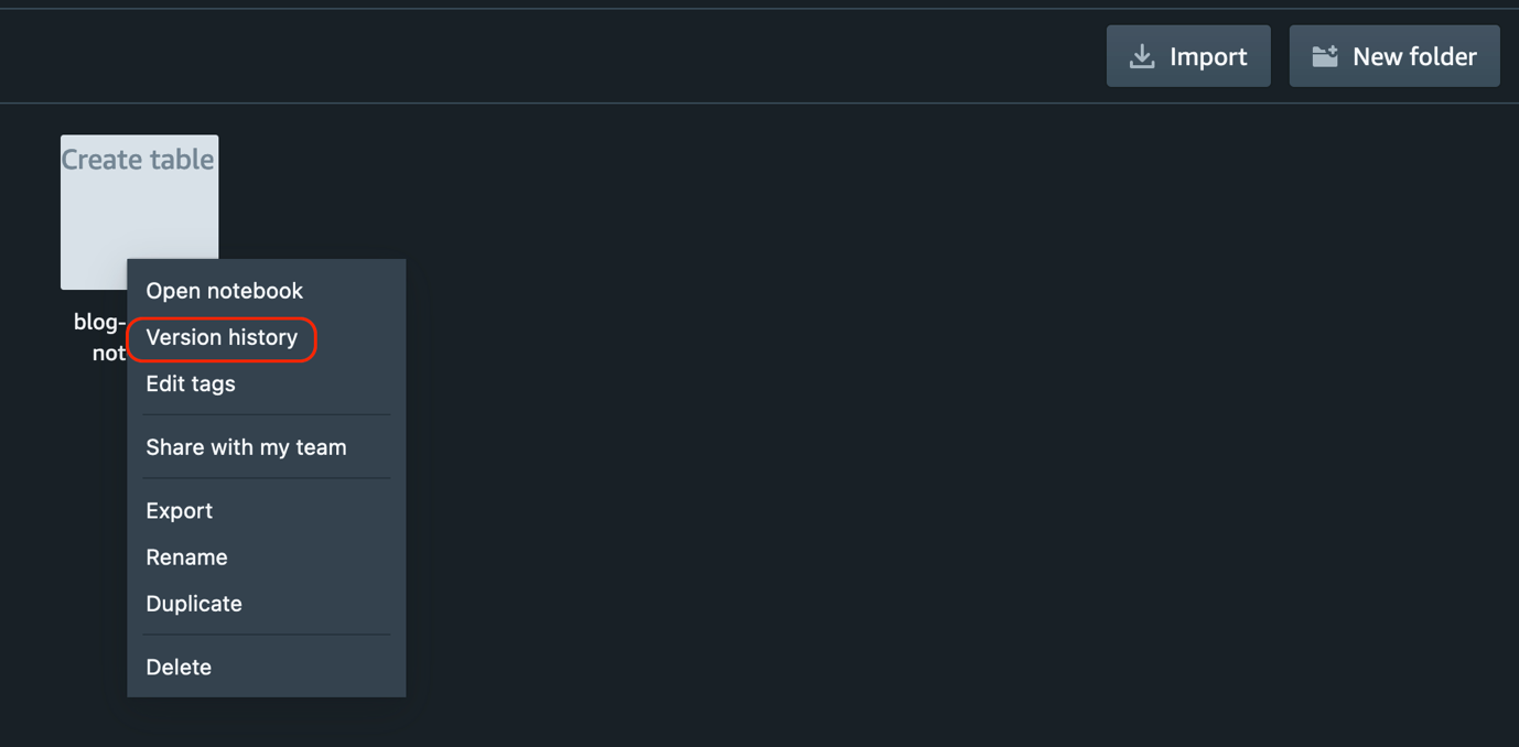
Then use the following command to restore from a recovery point:

aws redshift-serverless restore-from-recovery-point \
--namespace-name cfn-blog-ns \
--recovery-point-id 15c55fb4-d973-4d8a-a8fe-4741e7911137 \
--workgroup-name cfn-blog-wg

The following is an example output.

restore from recovery point

The base RPU determines the starting capacity for your serverless environment.

Use the following command to modify the base RPU based on your workload requirements:

aws redshift-serverless update-workgroup \
--base-capacity 256 \
--workgroup-name 'cfn-blog-wg'

The following is an example output.

Run the following command to verify the workgroup base RPU capacity has been modified to 256:

aws redshift-serverless get-workgroup \
--workgroup-name 'cfn-blog-wg' \
--output text \
--query 'workgroup.baseCapacity'

To keep costs predictable for Redshift Serverless, you can set the maximum RPU hours used per day, per week, or per month. In addition, you can take action when the limit is reached. Actions include: write a log entry to a system table, receive an alert, or turn off user queries.

Use the following command to first get the workgroup ARN:

aws redshift-serverless get-workgroup --workgroup-name 'cfn-blog-wg' \
--output text \
--query 'workgroup.workgroupArn'

The following screenshot shows our output.

Use the workgroupArn output from the preceding command with the following command to set the daily RPU usage limit and set the action behavior to log:

aws redshift-serverless create-usage-limit \
--amount 256 \
--breach-action log \
--period daily \
--resource-arn arn:aws:redshift-serverless:us-east-1:<aws-account-id>:workgroup/1dcdd402-8aeb-432e-8833-b1f78a112a93 \
--usage-type serverless-compute

The following is an example output.

Conclusion

You have now learned how to automate management operations on Redshift Serverless namespaces and workgroups using AWS CloudFormation and the AWS CLI. To automate creation and management of Amazon Redshift provisioned clusters, refer to Automate Amazon Redshift Cluster management operations using AWS CloudFormation.

About the Authors

Ranjan Burman is a Analytics Specialist Solutions Architect at AWS. He specializes in Amazon Redshift and helps customers build scalable analytical solutions. He has more than 15 years of experience in different database and data warehousing technologies. He is passionate about automating and solving customer problems with the use of cloud solutions.

Satesh Sonti is a Sr. Analytics Specialist Solutions Architect based out of Atlanta, specialized in building enterprise data platforms, data warehousing, and analytics solutions. He has over 16 years of experience in building data assets and leading complex data platform programs for banking and insurance clients across the globe.

Urvish Shah is a Senior Database Engineer at Amazon Redshift. He has more than a decade of experience working on databases, data warehousing and in analytics space. Outside of work, he enjoys cooking, travelling and spending time with his daughter.