Tag Archives: announcements

New – Amazon Genomics CLI Is Now Open Source and Generally Available

Post Syndicated from Danilo Poccia original https://aws.amazon.com/blogs/aws/new-amazon-genomics-cli-is-now-open-source-and-generally-available/

Less than 70 years separate us from one of the greatest discoveries of all time: the double helix structure of DNA. We now know that DNA is a sort of a twisted ladder composed of four types of compounds, called bases. These four bases are usually identified by an uppercase letter: adenine (A), guanine (G), cytosine (C), and thymine (T). One of the reasons for the double helix structure is that when these compounds are at the two sides of the ladder, A always bonds with T, and C always bonds with G.

If we unroll the ladder on a table, we’d see two sequences of “letters”, and each of the two sides would carry the same genetic information. For example, here are two series (AGCT and TCGA) bound together:

A – T
G – C
C – G
T – A

These series of letters can be very long. For example, the human genome is composed of over 3 billion letters of code and acts as the biological blueprint of every cell in a person. The information in a person’s genome can be used to create highly personalized treatments to improve the health of individuals and even the entire population. Similarly, genomic data can be use to track infectious diseases, improve diagnosis, and even track epidemics, food pathogens and toxins. This is the emerging field of environmental genomics.

Accessing genomic data requires genome sequencing, which with recent advances in technology, can be done for large groups of individuals, quickly and more cost-effectively than ever before. In the next five years, genomics datasets are estimated to grow and contain more than a billion sequenced genomes.

How Genomics Data Analysis Works
Genomics data analysis uses a variety of tools that need to be orchestrated as a specific sequence of steps, or a workflow. To facilitate developing, sharing, and running workflows, the genomics and bioinformatics communities have developed specialized workflow definition languages like WDL, Nextflow, CWL, and Snakemake.

However, this process generates petabytes of raw genomic data and experts in genomics and life science struggle to scale compute and storage resources to handle data at such massive scale.

To process data and provide answers quickly, cloud resources like compute, storage, and networking need to be configured to work together with analysis tools. As a result, scientists and researchers often have to spend valuable time deploying infrastructure and modifying open-source genomics analysis tools instead of making contributions to genomics innovations.

Introducing Amazon Genomics CLI
A couple of months ago, we shared the preview of Amazon Genomics CLI, a tool that makes it easier to process genomics data at petabyte scale on AWS. I am excited to share that the Amazon Genomics CLI is now an open source project and is generally available today. You can use it with publicly available workflows as a starting point and develop your analysis on top of these.

Amazon Genomics CLI simplifies and automates the deployment of cloud infrastructure, providing you with an easy-to-use command line interface to quickly setup and run genomics workflows on AWS. By removing the heavy lifting from setting up and running genomics workflows in the cloud, software developers and researchers can automatically provision, configure and scale cloud resources to enable faster and more cost-effective population-level genetics studies, drug discovery cycles, and more.

Amazon Genomics CLI lets you run your workflows on an optimized cloud infrastructure. More specifically, the CLI:

  • Includes improvements to genomics workflow engines to make them integrate better with AWS, removing the burden to manually modify open-source tools and tune them to run efficiently at scale. These tools work seamlessly across Amazon Elastic Container Service (Amazon ECS), Amazon DynamoDB, Amazon Elastic File System (Amazon EFS), and Amazon Simple Storage Service (Amazon S3), helping you to scale compute and storage and at the same time optimize your costs using features like EC2 Spot Instances.
  • Eliminates the most time-consuming tasks like provisioning storage and compute capacities, deploying the genomics workflow engines, and tuning the clusters used to execute workflows.
  • Automatically increases or decreases cloud resources based on your workloads, which eliminates the risk of buying too much or too little capacity.
  • Tags resources so that you can use tools like AWS Cost & Usage Report to understand the costs related to your genomics data analysis across multiple AWS services.

The use of Amazon Genomics CLI is based on these three main concepts:

Workflow – These are bioinformatics workflows written in languages like WDL or Nextflow. They can be either single script files or packages of multiple files. These workflow script files are workflow definitions and combined with additional metadata, like the workflow language the definition is written in, form a workflow specification that is used by the CLI to execute workflows on appropriate compute resources.

Context – A context encapsulates and automates time-consuming tasks to configure and deploy workflow engines, create data access policies, and tune compute clusters (managed using AWS Batch) for operation at scale.

Project – A project links together workflows, datasets, and the contexts used to process them. From a user perspective, it handles resources related to the same problem or used by the same team.

Let’s see how this works in practice.

Using Amazon Genomics CLI
I follow the instructions to install Amazon Genomics CLI on my laptop. Now, I can use the agc command to manage genomic workloads. I see the available options with:

$ agc --help

The first time I use it, I activate my AWS account:

$ agc account activate

This creates the core infrastructure that Amazon Genomics CLI needs to operate, which includes an S3 bucket, a virtual private cloud (VPC), and a DynamoDB table. The S3 bucket is used for durable metadata, and the VPC is used to isolate compute resources.

Optionally, I can bring my own VPC. I can also use one of my named profiles for the AWS Command Line Interface (CLI). In this way, I can customize the AWS Region and the AWS account used by the Amazon Genomics CLI.

I configure my email address in the local settings. This wil be used to tag resources created by the CLI:

$ agc configure email [email protected]

There are a few demo projects in the examples folder included by the Amazon Genomics CLI installation. These projects use different engines, such as Cromwell or Nextflow. In the demo-wdl-project folder, the agc-project.yaml file describes the workflows, the data, and the contexts for the Demo project:

---
name: Demo
schemaVersion: 1
workflows:
  hello:
    type:
      language: wdl
      version: 1.0
    sourceURL: workflows/hello
  read:
    type:
      language: wdl
      version: 1.0
    sourceURL: workflows/read
  haplotype:
    type:
      language: wdl
      version: 1.0
    sourceURL: workflows/haplotype
  words-with-vowels:
    type:
      language: wdl
      version: 1.0
    sourceURL: workflows/words
data:
  - location: s3://gatk-test-data
    readOnly: true
  - location: s3://broad-references
    readOnly: true
contexts:
  myContext:
    engines:
      - type: wdl
        engine: cromwell

  spotCtx:
    requestSpotInstances: true
    engines:
      - type: wdl
        engine: cromwell

For this project, there are four workflows (hello, read, words-with-vowels, and haplotype). The project has read-only access to two S3 buckets and can run workflows using two contexts. Both contexts use the Cromwell engine. One context (spotCtx) uses Amazon EC2 Spot Instances to optimize costs.

In the demo-wdl-project folder, I use the Amazon Genomics CLI to deploy the spotCtx context:

$ agc context deploy -c spotCtx

After a few minutes, the context is ready, and I can execute the workflows. Once started, a context incurs about $0.40 per hour of baseline costs. These costs don’t include the resources created to execute workflows. Those resources depend on your specific use case. Contexts have the option to use spot instances by adding the requestSpotInstances flag to their configuration.

I use the CLI to see the status of the contexts of the project:

$ agc context status

INSTANCE spotCtx STARTED true

Now, let’s look at the workflows included in this project:

$ agc workflow list

2021-09-24T11:15:29+01:00 𝒊  Listing workflows.
WORKFLOWNAME haplotype
WORKFLOWNAME hello
WORKFLOWNAME read
WORKFLOWNAME words-with-vowels

The simplest workflow is hello. The content of the hello.wdl file is quite understandable if you know any programming language:

version 1.0
workflow hello_agc {
    call hello {}
}
task hello {
    command { echo "Hello Amazon Genomics CLI!" }
    runtime {
        docker: "ubuntu:latest"
    }
    output { String out = read_string( stdout() ) }
}

The hello workflow defines a single task (hello) that prints the output of a command. The task is executed on a specific container image (ubuntu:latest). The output is taken from standard output (stdout), the default file descriptor where a process can write output.

Running workflows is an asynchronous process. After submitting a workflow from the CLI, it is handled entirely in the cloud. I can run multiple workflows at a time. The underlying compute resources will automatically scale and I will be charged only for what I use.

Using the CLI, I start the hello workflow:

$ agc workflow run hello -c spotCtx

2021-09-24T13:03:47+01:00 𝒊  Running workflow. Workflow name: 'hello', Arguments: '', Context: 'spotCtx'
fcf72b78-f725-493e-b633-7dbe67878e91

The workflow was successfully submitted, and the last line is the workflow execution ID. I can use this ID to reference a specific workflow execution. Now, I check the status of the workflow:

$ agc workflow status

2021-09-24T13:04:21+01:00 𝒊  Showing workflow run(s). Max Runs: 20
WORKFLOWINSTANCE	spotCtx	fcf72b78-f725-493e-b633-7dbe67878e91	true	RUNNING	2021-09-24T12:03:53Z	hello

The hello workflow is still running. After a few minutes, I check again:

$ agc workflow status

2021-09-24T13:12:23+01:00 𝒊  Showing workflow run(s). Max Runs: 20
WORKFLOWINSTANCE	spotCtx	fcf72b78-f725-493e-b633-7dbe67878e91	true	COMPLETE	2021-09-24T12:03:53Z	hello

The workflow has terminated and is now complete. I look at the workflow logs:

$ agc logs workflow hello

2021-09-24T13:13:08+01:00 𝒊  Showing the logs for 'hello'
2021-09-24T13:13:12+01:00 𝒊  Showing logs for the latest run of the workflow. Run id: 'fcf72b78-f725-493e-b633-7dbe67878e91'
Fri, 24 Sep 2021 13:07:22 +0100	download: s3://agc-123412341234-eu-west-1/scripts/1a82f9a96e387d78ae3786c967f97cc0 to tmp/tmp.498XAhEOy/batch-file-temp
Fri, 24 Sep 2021 13:07:22 +0100	*** LOCALIZING INPUTS ***
Fri, 24 Sep 2021 13:07:23 +0100	download: s3://agc-123412341234-eu-west-1/project/Demo/userid/danilop20tbvT/context/spotCtx/cromwell-execution/hello_agc/fcf72b78-f725-493e-b633-7dbe67878e91/call-hello/script to agc-024700040865-eu-west-1/project/Demo/userid/danilop20tbvT/context/spotCtx/cromwell-execution/hello_agc/fcf72b78-f725-493e-b633-7dbe67878e91/call-hello/script
Fri, 24 Sep 2021 13:07:23 +0100	*** COMPLETED LOCALIZATION ***
Fri, 24 Sep 2021 13:07:23 +0100	Hello Amazon Genomics CLI!
Fri, 24 Sep 2021 13:07:23 +0100	*** DELOCALIZING OUTPUTS ***
Fri, 24 Sep 2021 13:07:24 +0100	upload: ./hello-rc.txt to s3://agc-123412341234-eu-west-1/project/Demo/userid/danilop20tbvT/context/spotCtx/cromwell-execution/hello_agc/fcf72b78-f725-493e-b633-7dbe67878e91/call-hello/hello-rc.txt
Fri, 24 Sep 2021 13:07:25 +0100	upload: ./hello-stderr.log to s3://agc-123412341234-eu-west-1/project/Demo/userid/danilop20tbvT/context/spotCtx/cromwell-execution/hello_agc/fcf72b78-f725-493e-b633-7dbe67878e91/call-hello/hello-stderr.log
Fri, 24 Sep 2021 13:07:25 +0100	upload: ./hello-stdout.log to s3://agc-123412341234-eu-west-1/project/Demo/userid/danilop20tbvT/context/spotCtx/cromwell-execution/hello_agc/fcf72b78-f725-493e-b633-7dbe67878e91/call-hello/hello-stdout.log
Fri, 24 Sep 2021 13:07:25 +0100	*** COMPLETED DELOCALIZATION ***
Fri, 24 Sep 2021 13:07:25 +0100	*** EXITING WITH RETURN CODE ***
Fri, 24 Sep 2021 13:07:25 +0100	0

In the logs, I find as expected the Hello Amazon Genomics CLI! message printed by workflow.

I can also look at the content of hello-stdout.log on S3 using the information in the log above:

aws s3 cp s3://agc-123412341234-eu-west-1/project/Demo/userid/danilop20tbvT/context/spotCtx/cromwell-execution/hello_agc/fcf72b78-f725-493e-b633-7dbe67878e91/call-hello/hello-stdout.log -

Hello Amazon Genomics CLI!

It worked! Now, let’s look for at more complex workflows. Before I change project, I destroy the context for the Demo project:

$ agc context destroy -c spotCtx

In the gatk-best-practices-project folder, I list the available workflows for the project:

$ agc workflow list

2021-09-24T11:41:14+01:00 𝒊  Listing workflows.
WORKFLOWNAME	bam-to-unmapped-bams
WORKFLOWNAME	cram-to-bam
WORKFLOWNAME	gatk4-basic-joint-genotyping
WORKFLOWNAME	gatk4-data-processing
WORKFLOWNAME	gatk4-germline-snps-indels
WORKFLOWNAME	gatk4-rnaseq-germline-snps-indels
WORKFLOWNAME	interleaved-fastq-to-paired-fastq
WORKFLOWNAME	paired-fastq-to-unmapped-bam
WORKFLOWNAME	seq-format-validation

In the agc-project.yaml file, the gatk4-data-processing workflow points to a local directory with the same name. This is the content of that directory:

$ ls gatk4-data-processing

MANIFEST.json
processing-for-variant-discovery-gatk4.hg38.wgs.inputs.json
processing-for-variant-discovery-gatk4.wdl

This workflow processes high-throughput sequencing data with GATK4, a genomic analysis toolkit focused on variant discovery.

The directory contains a MANIFEST.json file. The manifest file describes which file contains the main workflow to execute (there can be more than one WDL file in the directory) and where to find input parameters and options. Here’s the content of the manifest file:

{
  "mainWorkflowURL": "processing-for-variant-discovery-gatk4.wdl",
  "inputFileURLs": [
    "processing-for-variant-discovery-gatk4.hg38.wgs.inputs.json"
  ],
  "optionFileURL": "options.json"
}

In the gatk-best-practices-project folder, I create a context to run the workflows:

$ agc context deploy -c spotCtx

Then, I start the gatk4-data-processing workflow:

$ agc workflow run gatk4-data-processing -c spotCtx

2021-09-24T12:08:22+01:00 𝒊  Running workflow. Workflow name: 'gatk4-data-processing', Arguments: '', Context: 'spotCtx'
630e2d53-0c28-4f35-873e-65363529c3de

After a couple of hours, the workflow has terminated:

$ agc workflow status

2021-09-24T14:06:40+01:00 𝒊  Showing workflow run(s). Max Runs: 20
WORKFLOWINSTANCE	spotCtx	630e2d53-0c28-4f35-873e-65363529c3de	true	COMPLETE	2021-09-24T11:08:28Z	gatk4-data-processing

I look at the logs:

$ agc logs workflow gatk4-data-processing

...
Fri, 24 Sep 2021 14:02:32 +0100	*** DELOCALIZING OUTPUTS ***
Fri, 24 Sep 2021 14:03:45 +0100	upload: ./NA12878.hg38.bam to s3://agc-123412341234-eu-west-1/project/GATK/userid/danilop20tbvT/context/spotCtx/cromwell-execution/PreProcessingForVariantDiscovery_GATK4/630e2d53-0c28-4f35-873e-65363529c3de/call-GatherBamFiles/NA12878.hg38.bam
Fri, 24 Sep 2021 14:03:46 +0100	upload: ./NA12878.hg38.bam.md5 to s3://agc-123412341234-eu-west-1/project/GATK/userid/danilop20tbvT/context/spotCtx/cromwell-execution/PreProcessingForVariantDiscovery_GATK4/630e2d53-0c28-4f35-873e-65363529c3de/call-GatherBamFiles/NA12878.hg38.bam.md5
Fri, 24 Sep 2021 14:03:47 +0100	upload: ./NA12878.hg38.bai to s3://agc-123412341234-eu-west-1/project/GATK/userid/danilop20tbvT/context/spotCtx/cromwell-execution/PreProcessingForVariantDiscovery_GATK4/630e2d53-0c28-4f35-873e-65363529c3de/call-GatherBamFiles/NA12878.hg38.bai
Fri, 24 Sep 2021 14:03:48 +0100	upload: ./GatherBamFiles-rc.txt to s3://agc-123412341234-eu-west-1/project/GATK/userid/danilop20tbvT/context/spotCtx/cromwell-execution/PreProcessingForVariantDiscovery_GATK4/630e2d53-0c28-4f35-873e-65363529c3de/call-GatherBamFiles/GatherBamFiles-rc.txt
Fri, 24 Sep 2021 14:03:49 +0100	upload: ./GatherBamFiles-stderr.log to s3://agc-123412341234-eu-west-1/project/GATK/userid/danilop20tbvT/context/spotCtx/cromwell-execution/PreProcessingForVariantDiscovery_GATK4/630e2d53-0c28-4f35-873e-65363529c3de/call-GatherBamFiles/GatherBamFiles-stderr.log
Fri, 24 Sep 2021 14:03:50 +0100	upload: ./GatherBamFiles-stdout.log to s3://agc-123412341234-eu-west-1/project/GATK/userid/danilop20tbvT/context/spotCtx/cromwell-execution/PreProcessingForVariantDiscovery_GATK4/630e2d53-0c28-4f35-873e-65363529c3de/call-GatherBamFiles/GatherBamFiles-stdout.log
Fri, 24 Sep 2021 14:03:50 +0100	*** COMPLETED DELOCALIZATION ***
Fri, 24 Sep 2021 14:03:50 +0100	*** EXITING WITH RETURN CODE ***
Fri, 24 Sep 2021 14:03:50 +0100	0

Results have been written to the S3 bucket created during the account activation. The name of the bucket is in the logs but I can also find it stored as a parameter by AWS Systems Manager. I can save it in an environment variable with the following command:

$ export AGC_BUCKET=$(aws ssm get-parameter \
  --name /agc/_common/bucket \
  --query 'Parameter.Value' \
  --output text)

Using the AWS Command Line Interface (CLI), I can now explore the results on the S3 bucket and get the outputs of the workflow.

Before looking at the results, I remove the resources that I don’t need by stopping the context. This will destroy all compute resources, but retain data in S3.

$ agc context destroy -c spotCtx

Additional examples on configuring different contexts and running additional workflows are provided in the documentation on GitHub.

Availability and Pricing
Amazon Genomics CLI is an open source tool, and you can use it today in all AWS Regions with the exception of AWS GovCloud (US) and Regions located in China. There is no cost for using the AWS Genomics CLI. You pay for the AWS resources created by the CLI.

With the Amazon Genomics CLI, you can focus on science instead of architecting infrastructure. This gets you up and running faster, enabling research, development, and testing workloads. For production workloads that scale to several thousand parallel workflows, we can provide recommended ways to leverage additional Amazon services, like AWS Step Functions, just reach out to our account teams for more information.

Danilo

137 AWS services achieve HITRUST certification

Post Syndicated from Sonali Vaidya original https://aws.amazon.com/blogs/security/137-aws-services-achieve-hitrust-certification/

We’re excited to announce that 137 Amazon Web Services (AWS) services are certified for the Health Information Trust Alliance (HITRUST) Common Security Framework (CSF) for the 2021 cycle.

The full list of AWS services that were audited by a third-party auditor and certified under HITRUST CSF is available on our Services in Scope by Compliance Program page. You can view and download our HITRUST CSF certification on demand through AWS Artifact.

AWS HITRUST CSF certification is available for customer inheritance

You don’t have to assess inherited controls for your HITRUST validated assessment, because AWS already has! You can deploy business solutions into AWS and inherit our HITRUST CSF certification, provided that you use only in-scope services and apply the controls detailed on the HITRUST website that you are responsible for implementing.

With the HITRUST certification, you, as an AWS customer, can tailor your security control baselines to a variety of factors—including, but not limited to, regulatory requirements and organization type. The HITRUST CSF is widely adopted by leading organizations in a variety of industries as part of their approach to security and privacy. Visit the HITRUST website for more information.

As always, we value your feedback and questions and are committed to helping you achieve and maintain the highest standard of security and compliance. Feel free to contact the team through AWS Compliance Contact Us. If you have feedback about this post, submit comments in the Comments section below.

Want more AWS Security how-to content, news, and feature announcements? Follow us on Twitter.

Author

Sonali Vaidya

Sonali is a Security Assurance Manager at AWS. She leads the global HITRUST assurance program within AWS. Sonali considers herself a perpetual student of information security, and holds multiple certifications like CISSP, PCIP, CCSK, CEH, CISA, ISO 27001 Lead Auditor, ISO 22301 Lead Auditor, C-GDPR Practitioner, and ITIL.

New for Amazon Connect: Voice ID, Wisdom, and Outbound Communications

Post Syndicated from Sébastien Stormacq original https://aws.amazon.com/blogs/aws/three-new-capabilities-for-amazon-connect/

During the AWS re:Invent conference last year, I wrote about new capabilities added to Amazon Connect. Today, I am happy to announce the general availability of two of these capabilities, Voice ID and Wisdom, and the launch of a new one. High-volume outbound communications allows, as the name implies, the initiation and management of outbound communications over voice, SMS, or email.

Amazon Connect is an easy-to-use omnichannel cloud contact center that helps you provide customer service at a lower cost. In just a few clicks, you can set up and make changes to your contact center, so agents can begin helping customers right away.

Amazon Connect Wisdom
Wisdom reduces the time agents spend searching for answers. Today, when agents require access to information to help a customer, they lose time trying to navigate different data sources in siloes: FAQ, files, wiki pages, customer call history, knowledge bases, etc.

When using Wisdom, agents simply enter a question or phrase in their agent desktop application, such as “what is the pet policy in hotel rooms”, and Wisdom searches connected repositories and returns the most relevant information and best answer to handle the customer issue.

Amazon Connect Wisdom launch screenshot

Wisdom also uses real-time call transcripts from Contact Lens for Amazon Connect to automatically detect customer issues during calls and to recommend relevant content stored across connected knowledge repositories, without requiring agents to even enter a question.

Wisdom connects to knowledge repositories with built-in connectors for third-party applications including Salesforce and ServiceNow. You can also ingest content from other knowledge stores using the Wisdom ingestion APIs.

Amazon Connect Wisom configure connectors

Amazon Connect Voice ID
How many times have you been through an authentication procedure when calling a contact center? Voice ID simplifies this to make voice interactions faster and more secure. It uses machine learning to provide real-time caller authentication based on the caller’s voice.

To effectively recognize me as “Sébastien”, Voice ID must learn how I talk. This is the enrollment phase. It only requires 30 seconds of voice recording to enroll a caller.

When I call the same contact center again, Voice ID compares the sound of my voice with the one enrolled earlier. This is the verification phase. It only requires between 5 and 10 seconds of my voice to authenticate me. The verification phase generates a confidence score and a status displayed in the agent desktop app.

Amazon Connect Voice ID agent desktop view

Contact Center administrators can use this result to configure different flows depending on the verification outcome. The routing is configured with a simple configuration panel such as this one:Amazon Connect Voice ID Configuration panelTo meet with personal data protection laws, contact center agents capture my consent to use Voice ID.

High-Volume Outbound Communications
Typical contact centers are designed to receive customer calls. However, there is a growing set of use cases where contact centers send outbound communications as well. For example, to call customers back,to inform them about the progress of a case, to confirm an appointment, to renew a subscription, or for telemarketing, just to name a few.

The majority of these outbound communications are phone calls. When doing so, traditional contact center agents dial the number provided by a customer management system and wait for someone to answer. Typically, only 10% of the calls are answered. This process is highly inefficient.

In the Amazon Connect administration console, I select High volume outbound communication, then I select Create Campaign.

Connect High Volume Outbout Communication - Create Campaign

I then configure the details. I give the campaign a name, then I select one of my outbound contact flow and a contact queue associated with an outbound phone number.

Connect High Volume Outbout Communication - Campaign details

The predictive dialer makes more calls than available agents. It uses metrics such as campaign performance, expected pick-up rates, and the number of available agents to adjust the number of calls. When a call is answered, it detects when a human is on the line (vs. an automatic machine, a fax line, etc.). Only calls answered by humans are routed to an available agent. The Amazon Connect agent application shows the call script that was specified during setup, along with relevant customer information.

The progressive dialer is more conservative, it uses a 1:1 ratio between calls and available agents.

Amazon Connect not only adds high-volume outbound communication capabilities for voice, but also for SMS, and email. Amazon Connect comes with pre-built connectors for importing customer contact lists from external systems, such as Salesforce, Zendesk, Marketo, and Amazon Pinpoint. No coding required.

Contact center managers have access to real-time metrics such as contact volume, abandonment rates, average connection times, and minimum ring times to optimize agent efficiency. These metrics help to understand the status of their campaigns and ensure compliance with applicable regulations, such as maximum call abandonment rates. Contact center managers use historical reports of these metrics to understand the effectiveness of all their communications campaigns over time.

To ensure a fair usage of the high-volume outbound communication capability, you must apply for production access to use the predictive dialer as well as SMS and email. You may submit a service request detailing your use cases and business context, which will be used to validate your legitimacy as a sender. Once access is granted, Amazon Connect continuously monitors your usage and the team might revoke access when fraud is suspected.

If you want to try it out yourself, you may apply to the preview by filling out this form.

Pricing and Availability
As usual, there are no upfront costs or minimum usage fees. You pay only what you use: a price per minute of outbound calls and per email or SMS message. The details are up-to-date on the Amazon Connect pricing page.

Regional availability slightly differ for each of these three new capabilities, here is a the list of AWS Regions where they are available:

  • Wisdom: US West (Oregon), US East (N. Virginia), Europe (London), Europe (Frankfurt), Asia Pacific (Tokyo), and Asia Pacific (Sydney).
  • Voice ID: US West (Oregon), US East (N. Virginia), Europe (London), Europe (Frankfurt), Asia Pacific (Tokyo), Asia Pacific (Singapore), and Asia Pacific (Sydney)
  • High volume outbound communication (preview): US East (N. Virginia), Europe (London), and US West (Oregon). More Regions will be added when it will be generally available.

As usual, let us know what you think about these new capabilities and how you use them. Go build your own contact center in the cloud today.

— seb

AWS achieves GSMA security certification for US East (Ohio) Region

Post Syndicated from Janice Leung original https://aws.amazon.com/blogs/security/aws-achieves-gsma-security-certification-for-us-east-ohio-region/

We continue to expand the scope of our assurance programs at Amazon Web Services (AWS) and are pleased to announce that our US East (Ohio) Region (us-east-2) is now certified by the GSM Association (GSMA) under its Security Accreditation Scheme Subscription Management (SAS-SM) with scope Data Center Operations and Management (DCOM). This alignment with GSMA requirements demonstrates our continuous commitment to adhere to the heightened expectations for cloud service providers. AWS customers who provide embedded Universal Integrated Circuit Card (eUICC) for mobile devices can run their remote provisioning applications with confidence in the AWS Cloud in the GSMA-certified US East (Ohio) Region.

As of this writing, 128 services offered in the US East (Ohio) Region are in scope of this certification. For up-to-date information, including when additional services are added, see the AWS Services in Scope by Compliance Program and choose GSMA.

AWS was evaluated by independent third-party auditors chosen by GSMA. The Certificate of Compliance illustrating the AWS GSMA compliance status is available on the GSMA website and through AWS Artifact. AWS Artifact is a self-service portal for on-demand access to AWS compliance reports. Sign in to AWS Artifact in the AWS Management Console, or learn more at Getting Started with AWS Artifact.

To learn more about our compliance and security programs, see AWS Compliance Programs. As always, we value your feedback and questions; reach out to the AWS Compliance team through the Contact Us page.

If you have feedback about this post, submit comments in the Comments section below.

Want more AWS Security how-to content, news, and feature announcements? Follow us on Twitter.

Author

Janice Leung

Janice is a Security Audit Program Manager at AWS, based in New York. She leads various security audit programs across Europe. She previously worked in security assurance and technology risk management in the financial industry for 10 years.

Author

Karthik Amrutesh

Karthik is a Senior Manager, Security Assurance at AWS, based in New York. He leads a team responsible for audits, attestations, and certifications across the European Union. Karthik has previously worked in risk management, security assurance, and technology audits for over 18 years.

Amazon QuickSight Q – Business Intelligence Using Natural Language Questions

Post Syndicated from Jeff Barr original https://aws.amazon.com/blogs/aws/amazon-quicksight-q-business-intelligence-using-natural-language-questions/

Making sense of business data so that you can get value out of it is worthwhile yet still challenging. Even though the term Business Intelligence (BI) has been around since the mid-1800s (according to Wikipedia) adoption of contemporary BI tools within enterprises is still fairly low.

Amazon QuickSight was designed to make it easier for you to put BI to work in your organization. Announced in 2015 and launched in 2016, QuickSight is a scalable BI service built for the cloud. Since that 2016 launch, we have added many new features, including geospatial visualization and private VPC access in 2017, pay-per-session pricing in 2018, additional APIs (data, dashboard, SPICE, and permissions in 2019), embedded authoring of dashboards & support for auto-naratives in 2020, and Dataset-as-a-Source in 2021.

QuickSight Q is Here
My colleague Harunobu Kameda announced Amazon QuickSight Q (or Q for short) last December and gave you a sneak peek. Today I am happy to announce the general availability of Q, and would like to show you how it works!

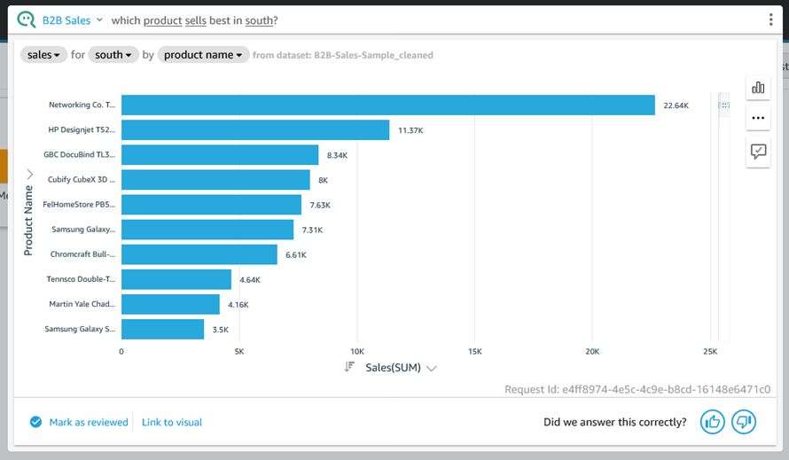
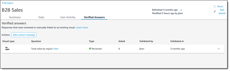
To recap, Q is a natural language query tool for the Enterprise Edition of QuickSight. Powered by machine learning, it makes your existing data more accessible, and therefore more valuable. Think of Q as your personal Business Intelligence Engineer or Data Analyst, one that is on call 24 hours a day and always ready to provide you with quick, meaningful results! You get high-quality results in seconds, always shown in an appropriate form.

Behind the scenes, Q uses Natural Language Understanding (NLU) to discover the intent of your question. Aided by models that have been trained to recognize vocabulary and concepts drawn from multiple domains (sales, marketing, retail, HR, advertising, financial services, health care, and so forth), Q is able to answer questions that refer all data sources supported by QuickSight. This includes data from AWS sources such as Amazon Redshift, Amazon Relational Database Service (RDS), Amazon Aurora, Amazon Athena, and Amazon Simple Storage Service (Amazon S3) as well as third party sources & SaaS apps such as Salesforce, Adobe Analytics, ServiceNow, and Excel.

Q in Action
Q is powered by topics, which are generally created by QuickSight Authors for use within an organization (if you are a QuickSight Author, you can learn more about getting started). Topics represent subject areas for questions, and are created interactively. To learn more about the five-step process that Authors use to create a topic, be sure to watch our new video, Tips to Create a Great Q Topic.

To use Q, I simply select a topic (B2B Sales in this case) and enter a question in the Q bar at the top of the page:

Q query --

In addition to the actual results, Q gives me access to explanatory information that I can review to ensure that my question was understood and processed as desired. For example, I can click on sales and learn how Q handles the field:

Detailed information on the use of the sales field.

I can fine-tune each aspect as well; here I clicked Sorted by:

Changing sort order for sales field.

Q chooses an appropriate visual representation for each answer, but I can fine-tune that as well:

Select a new visual type.

Perhaps I want a donut chart instead:

Now that you have seen how Q processes a question and gives you control over how the question is processed & displayed, let’s take a look at a few more questions, starting with “which product sells best in south?”

Question:

Here’s “what is total sales by region and category?” using the vertical stacked bar chart visual:

Total sales by region and catergory.

Behind the Scenes – Q Topics
As I mentioned earlier, Q uses topics to represent a particular subject matter. I click Topics to see the list of topics that I have created or that have been shared with me:

I click B2B Sales to learn more. The Summary page is designed to provide QuickSight Authors with information that they can use to fine-tune the topic:

Info about the B2B Sales Topic.

I can click on the Data tab and learn more about the list of fields that Q uses to answer questions. Each field can have some synonyms or friendly names to make the process of asking questions simpler and more natural:

List of fields for the B2B Sales topic.

I can expand a field (row) to learn more about how Q “understands” and uses the field. I can make changes in order to exercise control over the types of aggregations that make sense for the field, and I can also provide additional semantic information:

Information about the Product Name field.

As an example of providing additional semantic information, if the field’s Semantic Type is Location, I can choose the appropriate sub-type:

The User Activity tab shows me the questions that users are asking of this topic:

User activirty for the B2B Sales topic.

QuickSight Authors can use this tab to monitor user feedback, get a sense of the most common questions, and also use the common questions to drive improvements to the content provided on QuickSight dashboards.

Finally, the Verified answers tab shows the answers that have been manually reviewed and approved:

Things to Know
Here are a couple of things to know about Amazon QuickSight Q:

Pricing – There’s a monthly fee for each Reader and each Author; take a look at the QuickSight Pricing Page for more information.

Regions – Q is available in the US East (N. Virginia), US West (Oregon), US East (Ohio), Europe (Ireland), Europe (Frankfurt), and Europe (London) Regions.

Supported Languages – We are launching with question support in English.

Jeff;

New for AWS Distro for OpenTelemetry – Tracing Support is Now Generally Available

Post Syndicated from Danilo Poccia original https://aws.amazon.com/blogs/aws/new-for-aws-distro-for-opentelemetry-tracing-support-is-now-generally-available/

Last year before re:Invent, we introduced the public preview of AWS Distro for OpenTelemetry, a secure distribution of the OpenTelemetry project supported by AWS. OpenTelemetry provides tools, APIs, and SDKs to instrument, generate, collect, and export telemetry data to better understand the behavior and the performance of your applications. Yesterday, upstream OpenTelemetry announced tracing stability milestone for its components. Today, I am happy to share that support for traces is now generally available in AWS Distro for OpenTelemetry.

Using OpenTelemetry, you can instrument your applications just once and then send traces to multiple monitoring solutions.

You can use AWS Distro for OpenTelemetry to instrument your applications running on Amazon Elastic Compute Cloud (Amazon EC2), Amazon Elastic Container Service (Amazon ECS), Amazon Elastic Kubernetes Service (EKS), and AWS Lambda, as well as on premises. Containers running on AWS Fargate and orchestrated via either ECS or EKS are also supported.

You can send tracing data collected by AWS Distro for OpenTelemetry to AWS X-Ray, as well as partner destinations such as:

You can use auto-instrumentation agents to collect traces without changing your code. Auto-instrumentation is available today for Java and Python applications. Auto-instrumentation support for Python currently only covers the AWS SDK. You can instrument your applications using other programming languages (such as Go, Node.js, and .NET) with the OpenTelemetry SDKs.

Let’s see how this works in practice for a Java application.

Visualizing Traces for a Java Application Using Auto-Instrumentation
I create a simple Java application that shows the list of my Amazon Simple Storage Service (Amazon S3) buckets and my Amazon DynamoDB tables:

package com.example.myapp;

import software.amazon.awssdk.regions.Region;
import software.amazon.awssdk.services.s3.S3Client;
import software.amazon.awssdk.services.s3.model.*;
import software.amazon.awssdk.services.dynamodb.model.DynamoDbException;
import software.amazon.awssdk.services.dynamodb.model.ListTablesResponse;
import software.amazon.awssdk.services.dynamodb.model.ListTablesRequest;
import software.amazon.awssdk.services.dynamodb.DynamoDbClient;

import java.util.List;

/**
 * Hello world!
 *
 */
public class App {

    public static void listAllTables(DynamoDbClient ddb) {

        System.out.println("DynamoDB Tables:");

        boolean moreTables = true;
        String lastName = null;

        while (moreTables) {
            try {
                ListTablesResponse response = null;
                if (lastName == null) {
                    ListTablesRequest request = ListTablesRequest.builder().build();
                    response = ddb.listTables(request);
                } else {
                    ListTablesRequest request = ListTablesRequest.builder().exclusiveStartTableName(lastName).build();
                    response = ddb.listTables(request);
                }

                List<String> tableNames = response.tableNames();

                if (tableNames.size() > 0) {
                    for (String curName : tableNames) {
                        System.out.format("* %s\n", curName);
                    }
                } else {
                    System.out.println("No tables found!");
                    System.exit(0);
                }

                lastName = response.lastEvaluatedTableName();
                if (lastName == null) {
                    moreTables = false;
                }
            } catch (DynamoDbException e) {
                System.err.println(e.getMessage());
                System.exit(1);
            }
        }

        System.out.println("Done!\n");
    }

    public static void listAllBuckets(S3Client s3) {

        System.out.println("S3 Buckets:");

        ListBucketsRequest listBucketsRequest = ListBucketsRequest.builder().build();
        ListBucketsResponse listBucketsResponse = s3.listBuckets(listBucketsRequest);
        listBucketsResponse.buckets().stream().forEach(x -> System.out.format("* %s\n", x.name()));

        System.out.println("Done!\n");
    }

    public static void listAllBucketsAndTables(S3Client s3, DynamoDbClient ddb) {
        listAllBuckets(s3);
        listAllTables(ddb);
    }

    public static void main(String[] args) {

        Region region = Region.EU_WEST_1;

        S3Client s3 = S3Client.builder().region(region).build();
        DynamoDbClient ddb = DynamoDbClient.builder().region(region).build();

        listAllBucketsAndTables(s3, ddb);

        s3.close();
        ddb.close();
    }
}

I package the application using Apache Maven. Here’s the Project Object Model (POM) file managing dependencies such as the AWS SDK for Java 2.x that I use to interact with S3 and DynamoDB:

<project xmlns="http://maven.apache.org/POM/4.0.0" xmlns:xsi="http://www.w3.org/2001/XMLSchema-instance" xsi:schemaLocation="http://maven.apache.org/POM/4.0.0 http://maven.apache.org/maven-v4_0_0.xsd">
  <modelVersion>4.0.0</modelVersion>
  <properties>
    <project.build.sourceEncoding>UTF-8</project.build.sourceEncoding>
  </properties>
  <groupId>com.example.myapp</groupId>
  <artifactId>myapp</artifactId>
  <packaging>jar</packaging>
  <version>1.0-SNAPSHOT</version>
  <name>myapp</name>
  <dependencyManagement>
    <dependencies>
      <dependency>
        <groupId>software.amazon.awssdk</groupId>
        <artifactId>bom</artifactId>
        <version>2.17.38</version>
        <type>pom</type>
        <scope>import</scope>
      </dependency>
    </dependencies>
  </dependencyManagement>
  <dependencies>
    <dependency>
      <groupId>junit</groupId>
      <artifactId>junit</artifactId>
      <version>3.8.1</version>
      <scope>test</scope>
    </dependency>
    <dependency>
      <groupId>software.amazon.awssdk</groupId>
      <artifactId>s3</artifactId>
    </dependency>
    <dependency>
      <groupId>software.amazon.awssdk</groupId>
      <artifactId>dynamodb</artifactId>
    </dependency>
  </dependencies>
  <build>
    <plugins>
      <plugin>
        <groupId>org.apache.maven.plugins</groupId>
        <artifactId>maven-compiler-plugin</artifactId>
        <version>3.8.1</version>
        <configuration>
          <source>8</source>
          <target>8</target>
        </configuration>
      </plugin>
      <plugin>
        <artifactId>maven-assembly-plugin</artifactId>
        <configuration>
          <archive>
            <manifest>
              <mainClass>com.example.myapp.App</mainClass>
            </manifest>
          </archive>
          <descriptorRefs>
            <descriptorRef>jar-with-dependencies</descriptorRef>
          </descriptorRefs>
        </configuration>
      </plugin>
    </plugins>
  </build>
</project>

I use Maven to create an executable Java Archive (JAR) file that includes all dependencies:

$ mvn clean compile assembly:single

To run the application and get tracing data, I need two components:

In one terminal, I run the AWS Distro for OpenTelemetry Collector using Docker:

$ docker run --rm -p 4317:4317 -p 55680:55680 -p 8889:8888 \
         -e AWS_REGION=eu-west-1 \
         -e AWS_PROFILE=default \
         -v ~/.aws:/root/.aws \
         --name awscollector public.ecr.aws/aws-observability/aws-otel-collector:latest

The collector is now ready to receive traces and forward them to a monitoring platform. By default, the AWS Distro for OpenTelemetry Collector sends traces to AWS X-Ray. I can change the exporter or add more exporters by editing the collector configuration. For example, I can follow the documentation to configure OLTP exporters to send telemetry data using the OLTP protocol. In the documentation, I also find how to configure other partner destinations. [[ It would be great it we had a link for the partner section, I can find only links to a specific partner ]]

I download the latest version of the AWS Distro for OpenTelemetry Auto-Instrumentation Java Agent. Now, I run my application and use the agent to capture telemetry data without having to add any specific instrumentation the code. In the OTEL_RESOURCE_ATTRIBUTES environment variable I set a name and a namespace for the service: [[ Are service.name and service.namespace being used by X-Ray? I couldn’t find them in the service map ]]

$ OTEL_RESOURCE_ATTRIBUTES=service.name=MyApp,service.namespace=MyTeam \
  java -javaagent:otel/aws-opentelemetry-agent.jar \
       -jar myapp/target/myapp-1.0-SNAPSHOT-jar-with-dependencies.jar

As expected, I get the list of my S3 buckets globally and of the DynamoDB tables in the Region.

To generate more tracing data, I run the previous command a few times. Each time I run the application, telemetry data is collected by the agent and sent to the collector. The collector buffers the data and then sends it to the configured exporters. By default, it is sending traces to X-Ray.

Now, I look at the service map in the AWS X-Ray console to see my application’s interactions with other services:

Console screenshot.

And there they are! Without any change in the code, I see my application’s calls to the S3 and DynamoDB APIs. There were no errors, and all the circles are green. Inside the circles, I find the average latency of the invocations and the number of transactions per minute.

Adding Spans to a Java Application
The information automatically collected can be improved by providing more information with the traces. For example, I might have interactions with the same service in different parts of my application, and it would be useful to separate those interactions in the service map. In this way, if there is an error or high latency, I would know which part of my application is affected.

One way to do so is to use spans or segments. A span represents a group of logically related activities. For example, the listAllBucketsAndTables method is performing two operations, one with S3 and one with DynamoDB. I’d like to group them together in a span. The quickest way with OpenTelemetry is to add the @WithSpan annotation to the method. Because the result of a method usually depends on its arguments, I also use the @SpanAttribute annotation to describe which arguments in the method invocation should be automatically added as attributes to the span.

@WithSpan
    public static void listAllBucketsAndTables(@SpanAttribute("title") String title, S3Client s3, DynamoDbClient ddb) {

        System.out.println(title);

        listAllBuckets(s3);
        listAllTables(ddb);
    }

To be able to use the @WithSpan and @SpanAttribute annotations, I need to import them into the code and add the necessary OpenTelemetry dependencies to the POM. All these changes are based on the OpenTelemetry specifications and don’t depend on the actual implementation that I am using, or on the tool that I will use to visualize or analyze the telemetry data. I have only to make these changes once to instrument my application. Isn’t that great?

To better see how spans work, I create another method that is running the same operations in reverse order, first listing the DynamoDB tables, then the S3 buckets:

    @WithSpan
    public static void listTablesFirstAndThenBuckets(@SpanAttribute("title") String title, S3Client s3, DynamoDbClient ddb) {

        System.out.println(title);

        listAllTables(ddb);
        listAllBuckets(s3);
    }

The application is now running the two methods (listAllBucketsAndTables and listTablesFirstAndThenBuckets) one after the other. For simplicity, here’s the full code of the instrumented application:

package com.example.myapp;

import software.amazon.awssdk.regions.Region;
import software.amazon.awssdk.services.s3.S3Client;
import software.amazon.awssdk.services.s3.model.*;
import software.amazon.awssdk.services.dynamodb.model.DynamoDbException;
import software.amazon.awssdk.services.dynamodb.model.ListTablesResponse;
import software.amazon.awssdk.services.dynamodb.model.ListTablesRequest;
import software.amazon.awssdk.services.dynamodb.DynamoDbClient;

import java.util.List;

import io.opentelemetry.extension.annotations.SpanAttribute;
import io.opentelemetry.extension.annotations.WithSpan;

/**
 * Hello world!
 *
 */
public class App {

    public static void listAllTables(DynamoDbClient ddb) {

        System.out.println("DynamoDB Tables:");

        boolean moreTables = true;
        String lastName = null;

        while (moreTables) {
            try {
                ListTablesResponse response = null;
                if (lastName == null) {
                    ListTablesRequest request = ListTablesRequest.builder().build();
                    response = ddb.listTables(request);
                } else {
                    ListTablesRequest request = ListTablesRequest.builder().exclusiveStartTableName(lastName).build();
                    response = ddb.listTables(request);
                }

                List<String> tableNames = response.tableNames();

                if (tableNames.size() > 0) {
                    for (String curName : tableNames) {
                        System.out.format("* %s\n", curName);
                    }
                } else {
                    System.out.println("No tables found!");
                    System.exit(0);
                }

                lastName = response.lastEvaluatedTableName();
                if (lastName == null) {
                    moreTables = false;
                }
            } catch (DynamoDbException e) {
                System.err.println(e.getMessage());
                System.exit(1);
            }
        }

        System.out.println("Done!\n");
    }

    public static void listAllBuckets(S3Client s3) {

        System.out.println("S3 Buckets:");

        ListBucketsRequest listBucketsRequest = ListBucketsRequest.builder().build();
        ListBucketsResponse listBucketsResponse = s3.listBuckets(listBucketsRequest);
        listBucketsResponse.buckets().stream().forEach(x -> System.out.format("* %s\n", x.name()));

        System.out.println("Done!\n");
    }

    @WithSpan
    public static void listAllBucketsAndTables(@SpanAttribute("title") String title, S3Client s3, DynamoDbClient ddb) {

        System.out.println(title);

        listAllBuckets(s3);
        listAllTables(ddb);

    }

    @WithSpan
    public static void listTablesFirstAndThenBuckets(@SpanAttribute("title") String title, S3Client s3, DynamoDbClient ddb) {

        System.out.println(title);

        listAllTables(ddb);
        listAllBuckets(s3);

    }

    public static void main(String[] args) {

        Region region = Region.EU_WEST_1;

        S3Client s3 = S3Client.builder().region(region).build();
        DynamoDbClient ddb = DynamoDbClient.builder().region(region).build();

        listAllBucketsAndTables("My S3 buckets and DynamoDB tables", s3, ddb);
        listTablesFirstAndThenBuckets("My DynamoDB tables first and then S3 bucket", s3, ddb);

        s3.close();
        ddb.close();
    }
}

And here’s the updated POM that includes the additional OpenTelemetry dependencies:

<project xmlns="http://maven.apache.org/POM/4.0.0" xmlns:xsi="http://www.w3.org/2001/XMLSchema-instance" xsi:schemaLocation="http://maven.apache.org/POM/4.0.0 http://maven.apache.org/maven-v4_0_0.xsd">
  <modelVersion>4.0.0</modelVersion>
  <properties>
    <project.build.sourceEncoding>UTF-8</project.build.sourceEncoding>
  </properties>
  <groupId>com.example.myapp</groupId>
  <artifactId>myapp</artifactId>
  <packaging>jar</packaging>
  <version>1.0-SNAPSHOT</version>
  <name>myapp</name>
  <dependencyManagement>
    <dependencies>
      <dependency>
        <groupId>software.amazon.awssdk</groupId>
        <artifactId>bom</artifactId>
        <version>2.16.60</version>
        <type>pom</type>
        <scope>import</scope>
      </dependency>
    </dependencies>
  </dependencyManagement>
  <dependencies>
    <dependency>
      <groupId>junit</groupId>
      <artifactId>junit</artifactId>
      <version>3.8.1</version>
      <scope>test</scope>
    </dependency>
    <dependency>
      <groupId>software.amazon.awssdk</groupId>
      <artifactId>s3</artifactId>
    </dependency>
    <dependency>
      <groupId>software.amazon.awssdk</groupId>
      <artifactId>dynamodb</artifactId>
    </dependency>
    <dependency>
      <groupId>io.opentelemetry</groupId>
      <artifactId>opentelemetry-extension-annotations</artifactId>
      <version>1.5.0</version>
    </dependency>
    <dependency>
      <groupId>io.opentelemetry</groupId>
      <artifactId>opentelemetry-api</artifactId>
      <version>1.5.0</version>
    </dependency>
  </dependencies>
  <build>
    <plugins>
      <plugin>
        <groupId>org.apache.maven.plugins</groupId>
        <artifactId>maven-compiler-plugin</artifactId>
        <version>3.8.1</version>
        <configuration>
          <source>8</source>
          <target>8</target>
        </configuration>
      </plugin>
      <plugin>
        <artifactId>maven-assembly-plugin</artifactId>
        <configuration>
          <archive>
            <manifest>
              <mainClass>com.example.myapp.App</mainClass>
            </manifest>
          </archive>
          <descriptorRefs>
            <descriptorRef>jar-with-dependencies</descriptorRef>
          </descriptorRefs>
        </configuration>
      </plugin>
    </plugins>
  </build>
</project>

I compile my application with these changes and run it again a few times:

$ mvn clean compile assembly:single

$ OTEL_RESOURCE_ATTRIBUTES=service.name=MyApp,service.namespace=MyTeam \
  java -javaagent:otel/aws-opentelemetry-agent.jar \
       -jar myapp/target/myapp-1.0-SNAPSHOT-jar-with-dependencies.jar

Now, let’s look at the X-Ray service map, computed using the additional information provided by those annotations.

Console screenshot.

Now I see the two methods and the other services they invoke. If there are errors or high latency, I can easily understand how the two methods are affected.

In the Traces section of the X-Ray console, I look at the Raw data for some of the traces. Because the title argument was annotated with @SpanAttribute, each trace has the value of that argument in the metadata section.

Console screenshot.

Collecting Traces from Lambda Functions
The previous steps work on premises, on EC2, and with applications running in containers. To collect traces and use auto-instrumentation with Lambda functions, you can use the AWS managed OpenTelemetry Lambda Layers (a few examples are included in the repository).

After you add the Lambda layer to your function, you can use the environment variable OPENTELEMETRY_COLLECTOR_CONFIG_FILE to pass your own configuration to the collector. More information on using AWS Distro for OpenTelemetry with AWS Lambda is available in the documentation.

Availability and Pricing
You can use AWS Distro for OpenTelemetry to get telemetry data from your application running on premises and on AWS. There are no additional costs for using AWS Distro for OpenTelemetry. Depending on your configuration, you might pay for the AWS services that are destinations for OpenTelemetry data, such as AWS X-Ray, Amazon CloudWatch, and Amazon Managed Service for Prometheus (AMP).

To learn more, you are invited to this webinar on Thursday, October 7 at 10:00 am PT / 1:00 pm EDT / 7:00 pm CEST.

Simplify the instrumentation of your applications and improve their observability using AWS Distro for OpenTelemetry today.

Danilo

New Standard Contractual Clauses now part of the AWS GDPR Data Processing Addendum for customers

Post Syndicated from Stéphane Ducable original https://aws.amazon.com/blogs/security/new-standard-contractual-clauses-now-part-of-the-aws-gdpr-data-processing-addendum-for-customers/

Today, we’re happy to announce an update to our online AWS GDPR Data Processing Addendum (AWS GDPR DPA) and our online Service Terms to include the new Standard Contractual Clauses (SCCs) that the European Commission (EC) adopted in June 2021. The EC-approved SCCs give our customers the ability to comply with the General Data Protection Regulation (GDPR) when they transfer personal data subject to GDPR to countries outside the European Economic Area (EEA) that haven’t received an EC adequacy decision (third countries). The new SCCs are now better adapted to how our customers operate their applications or run their workloads in the cloud, because they cover different transfer scenarios, and also provide enhanced safeguards for data transfers.

Achieving compliance with GDPR is critical for hundreds of thousands of AWS customers and AWS. The new SCCs allow all AWS customers that are controllers or processors under GDPR to continue to transfer personal data from their AWS accounts in compliance with GDPR. As part of the online Service Terms, the new SCCs will apply automatically whenever an AWS customer uses AWS services to transfer customer data to third countries.

The updated AWS GDPR DPA incorporating the new SCCs supplements our announcement in February 2021 of strengthened commitments to protect customer data, such as challenging law enforcement requests that conflict with EU law. We have also published the blog post How AWS is helping EU customers navigate the new normal for data protection, and the whitepaper Navigating Compliance with EU Data Transfer Requirements to help AWS customers conduct their data transfer assessments and comply with GDPR, the Schrems II ruling, and the recommendations issued by the European Data Protection Board. AWS is constantly working to ensure that our customers can enjoy the benefits of AWS everywhere they operate, and we welcome the new SCCs because they enable our customers to continue using AWS services in compliance with GDPR. If you have questions or need more information, visit our EU Data Protection page and our GDPR Center.

Want more AWS Security how-to content, news, and feature announcements? Follow us on Twitter.

Author

Stéphane Ducable

Stéphane is Vice President of Public Policy – EMEA at AWS. He is focused on increasing awareness of the benefits of adopting cloud computing technology across the EMEA region.

Introducing Amazon MSK Connect – Stream Data to and from Your Apache Kafka Clusters Using Managed Connectors

Post Syndicated from Danilo Poccia original https://aws.amazon.com/blogs/aws/introducing-amazon-msk-connect-stream-data-to-and-from-your-apache-kafka-clusters-using-managed-connectors/

Apache Kafka is an open-source platform for building real-time streaming data pipelines and applications. At re:Invent 2018, we announced Amazon Managed Streaming for Apache Kafka, a fully managed service that makes it easy to build and run applications that use Apache Kafka to process streaming data.

When you use Apache Kafka, you capture real-time data from sources such as IoT devices, database change events, and website clickstreams, and deliver it to destinations such as databases and persistent storage.

Kafka Connect is an open-source component of Apache Kafka that provides a framework for connecting with external systems such as databases, key-value stores, search indexes, and file systems. However, manually running Kafka Connect clusters requires you to plan and provision the required infrastructure, deal with cluster operations, and scale it in response to load changes.

Today, we’re announcing a new capability that makes it easier to manage Kafka Connect clusters. MSK Connect allows you to configure and deploy a connector using Kafka Connect with a just few clicks. MSK Connect provisions the required resources and sets up the cluster. It continuously monitors the health and delivery state of connectors, patches and manages the underlying hardware, and auto-scales connectors to match changes in throughput. As a result, you can focus your resources on building applications rather than managing infrastructure.

MSK Connect is fully compatible with Kafka Connect, which means you can migrate your existing connectors without code changes. You don’t need an MSK cluster to use MSK Connect. It supports Amazon MSK, Apache Kafka, and Apache Kafka compatible clusters as sources and sinks. These clusters can be self-managed or managed by AWS partners and 3rd parties as long as MSK Connect can privately connect to the clusters.

Using MSK Connect with Amazon Aurora and Debezium
To test MSK Connect, I want to use it to stream data change events from one of my databases. To do so, I use Debezium, an open-source distributed platform for change data capture built on top of Apache Kafka.

I use a MySQL-compatible Amazon Aurora database as the source and the Debezium MySQL connector with the setup described in this architectural diagram:

Architectural diagram.

To use my Aurora database with Debezium, I need to turn on binary logging in the DB cluster parameter group. I follow the steps in the How do I turn on binary logging for my Amazon Aurora MySQL cluster article.

Next, I have to create a custom plugin for MSK Connect. A custom plugin is a set of JAR files that contain the implementation of one or more connectors, transforms, or converters. Amazon MSK will install the plugin on the workers of the connect cluster where the connector is running.

From the Debezium website, I download the MySQL connector plugin for the latest stable release. Because MSK Connect accepts custom plugins in ZIP or JAR format, I convert the downloaded archive to ZIP format and keep the JARs files in the main directory:

$ tar xzf debezium-connector-mysql-1.6.1.Final-plugin.tar.gz
$ cd debezium-connector-mysql
$ zip -9 ../debezium-connector-mysql-1.6.1.zip *
$ cd ..

Then, I use the AWS Command Line Interface (CLI) to upload the custom plugin to an Amazon Simple Storage Service (Amazon S3) bucket in the same AWS Region I am using for MSK Connect:

$ aws s3 cp debezium-connector-mysql-1.6.1.zip s3://my-bucket/path/

On the Amazon MSK console there is a new MSK Connect section. I look at the connectors and choose Create connector. Then, I create a custom plugin and browse my S3 buckets to select the custom plugin ZIP file I uploaded before.

Console screenshot.

I enter a name and a description for the plugin and then choose Next.

Console screenshot.

Now that the configuration of the custom plugin is complete, I start the creation of the connector. I enter a name and a description for the connector.

Console screenshot.

I have the option to use a self-managed Apache Kafka cluster or one that is managed by MSK. I select one of my MSK cluster that is configured to use IAM authentication. The MSK cluster I select is in the same virtual private cloud (VPC) as my Aurora database. To connect, the MSK cluster and Aurora database use the default security group for the VPC. For simplicity, I use a cluster configuration with auto.create.topics.enable set to true.

Console screenshot.

In Connector configuration, I use the following settings:

connector.class=io.debezium.connector.mysql.MySqlConnector
tasks.max=1
database.hostname=<aurora-database-writer-instance-endpoint>
database.port=3306
database.user=my-database-user
database.password=my-secret-password
database.server.id=123456
database.server.name=ecommerce-server
database.include.list=ecommerce
database.history.kafka.topic=dbhistory.ecommerce
database.history.kafka.bootstrap.servers=<bootstrap servers>
database.history.consumer.security.protocol=SASL_SSL
database.history.consumer.sasl.mechanism=AWS_MSK_IAM
database.history.consumer.sasl.jaas.config=software.amazon.msk.auth.iam.IAMLoginModule required;
database.history.consumer.sasl.client.callback.handler.class=software.amazon.msk.auth.iam.IAMClientCallbackHandler
database.history.producer.security.protocol=SASL_SSL
database.history.producer.sasl.mechanism=AWS_MSK_IAM
database.history.producer.sasl.jaas.config=software.amazon.msk.auth.iam.IAMLoginModule required;
database.history.producer.sasl.client.callback.handler.class=software.amazon.msk.auth.iam.IAMClientCallbackHandler
include.schema.changes=true

Some of these settings are generic and should be specified for any connector. For example:

  • connector.class is the Java class of the connector.
  • tasks.max is the maximum number of tasks that should be created for this connector.

Other settings are specific to the Debezium MySQL connector:

  • The database.hostname contains the writer instance endpoint of my Aurora database.
  • The database.server.name is a logical name of the database server. It is used for the names of the Kafka topics created by Debezium.
  • The database.include.list contains the list of databases hosted by the specified server.
  • The database.history.kafka.topic is a Kafka topic used internally by Debezium to track database schema changes.
  • The database.history.kafka.bootstrap.servers contains the bootstrap servers of the MSK cluster.
  • The final eight lines (database.history.consumer.* and database.history.producer.*) enable IAM authentication to access the database history topic.

In Connector capacity, I can choose between autoscaled or provisioned capacity. For this setup, I choose Autoscaled and leave all other settings at their defaults.

Console screenshot.

With autoscaled capacity, I can configure these parameters:

  • MSK Connect Unit (MCU) count per worker – Each MCU provides 1 vCPU of compute and 4 GB of memory.
  • The minimum and maximum number of workers.
  • Autoscaling utilization thresholds – The upper and lower target utilization thresholds on MCU consumption in percentage to trigger auto scaling.

Console screenshot.

There is a summary of the minimum and maximum MCUs, memory, and network bandwidth for the connector.

Console screenshot.

For Worker configuration, you can use the default one provided by Amazon MSK or provide your own configuration. In my setup, I use the default one.

In Access permissions, I create a IAM role. In the trusted entities, I add kafkaconnect.amazonaws.com to allow MSK Connect to assume the role.

The role is used by MSK Connect to interact with the MSK cluster and other AWS services. For my setup, I add:

The Debezium connector needs access to the cluster configuration to find the replication factor to use to create the history topic. For this reason, I add to the permissions policy the kafka-cluster:DescribeClusterDynamicConfiguration action (equivalent Apache Kafka’s DESCRIBE_CONFIGS cluster ACL).

Depending on your configuration, you might need to add more permissions to the role (for example, in case the connector needs access to other AWS resources such as an S3 bucket). If that is the case, you should add permissions before creating the connector.

In Security, the settings for authentication and encryption in transit are taken from the MSK cluster.

Console screenshot.

In Logs, I choose to deliver logs to CloudWatch Logs to have more information on the execution of the connector. By using CloudWatch Logs, I can easily manage retention and interactively search and analyze my log data with CloudWatch Logs Insights. I enter the log group ARN (it’s the same log group I used before in the IAM role) and then choose Next.

Console screenshot.

I review the settings and then choose Create connector. After a few minutes, the connector is running.

Testing MSK Connect with Amazon Aurora and Debezium
Now let’s test the architecture I just set up. I start an Amazon Elastic Compute Cloud (Amazon EC2) instance to update the database and start a couple of Kafka consumers to see Debezium in action. To be able to connect to both the MSK cluster and the Aurora database, I use the same VPC and assign the default security group. I also add another security group that gives me SSH access to the instance.

I download a binary distribution of Apache Kafka and extract the archive in the home directory:

$ tar xvf kafka_2.13-2.7.1.tgz

To use IAM to authenticate with the MSK cluster, I follow the instructions in the Amazon MSK Developer Guide to configure clients for IAM access control. I download the latest stable release of the Amazon MSK Library for IAM:

$ wget https://github.com/aws/aws-msk-iam-auth/releases/download/1.1.0/aws-msk-iam-auth-1.1.0-all.jar

In the ~/kafka_2.13-2.7.1/config/ directory I create a client-config.properties file to configure a Kafka client to use IAM authentication:

# Sets up TLS for encryption and SASL for authN.
security.protocol = SASL_SSL

# Identifies the SASL mechanism to use.
sasl.mechanism = AWS_MSK_IAM

# Binds SASL client implementation.
sasl.jaas.config = software.amazon.msk.auth.iam.IAMLoginModule required;

# Encapsulates constructing a SigV4 signature based on extracted credentials.
# The SASL client bound by "sasl.jaas.config" invokes this class.
sasl.client.callback.handler.class = software.amazon.msk.auth.iam.IAMClientCallbackHandler

I add a few lines to my Bash profile to:

  • Add Kafka binaries to the PATH.
  • Add the MSK Library for IAM to the CLASSPATH.
  • Create the BOOTSTRAP_SERVERS environment variable to store the bootstrap servers of my MSK cluster.
$ cat >> ~./bash_profile
export PATH=~/kafka_2.13-2.7.1/bin:$PATH
export CLASSPATH=/home/ec2-user/aws-msk-iam-auth-1.1.0-all.jar
export BOOTSTRAP_SERVERS=<bootstrap servers>

Then, I open three terminal connections to the instance.

In the first terminal connection, I start a Kafka consumer for a topic with the same name as the database server (ecommerce-server). This topic is used by Debezium to stream schema changes (for example, when a new table is created).

$ cd ~/kafka_2.13-2.7.1/
$ kafka-console-consumer.sh --bootstrap-server $BOOTSTRAP_SERVERS \
                            --consumer.config config/client-config.properties \
                            --topic ecommerce-server --from-beginning

In the second terminal connection, I start another Kafka consumer for a topic with a name built by concatenating the database server (ecommerce-server), the database (ecommerce), and the table (orders). This topic is used by Debezium to stream data changes for the table (for example, when a new record is inserted).

$ cd ~/kafka_2.13-2.7.1/
$ kafka-console-consumer.sh --bootstrap-server $BOOTSTRAP_SERVERS \
                            --consumer.config config/client-config.properties \
                            --topic ecommerce-server.ecommerce.orders --from-beginning

In the third terminal connection, I install a MySQL client using the MariaDB package and connect to the Aurora database:

$ sudo yum install mariadb
$ mysql -h <aurora-database-writer-instance-endpoint> -u <database-user> -p

From this connection, I create the ecommerce database and a table for my orders:

CREATE DATABASE ecommerce;

USE ecommerce

CREATE TABLE orders (
       order_id VARCHAR(255),
       customer_id VARCHAR(255),
       item_description VARCHAR(255),
       price DECIMAL(6,2),
       order_date DATETIME DEFAULT CURRENT_TIMESTAMP
);

These database changes are captured by the Debezium connector managed by MSK Connect and are streamed to the MSK cluster. In the first terminal, consuming the topic with schema changes, I see the information on the creation of database and table:

Struct{source=Struct{version=1.6.1.Final,connector=mysql,name=ecommerce-server,ts_ms=1629202831473,db=ecommerce,server_id=1980402433,file=mysql-bin-changelog.000003,pos=9828,row=0},databaseName=ecommerce,ddl=CREATE DATABASE ecommerce,tableChanges=[]}
Struct{source=Struct{version=1.6.1.Final,connector=mysql,name=ecommerce-server,ts_ms=1629202878811,db=ecommerce,table=orders,server_id=1980402433,file=mysql-bin-changelog.000003,pos=10002,row=0},databaseName=ecommerce,ddl=CREATE TABLE orders ( order_id VARCHAR(255), customer_id VARCHAR(255), item_description VARCHAR(255), price DECIMAL(6,2), order_date DATETIME DEFAULT CURRENT_TIMESTAMP ),tableChanges=[Struct{type=CREATE,id="ecommerce"."orders",table=Struct{defaultCharsetName=latin1,primaryKeyColumnNames=[],columns=[Struct{name=order_id,jdbcType=12,typeName=VARCHAR,typeExpression=VARCHAR,charsetName=latin1,length=255,position=1,optional=true,autoIncremented=false,generated=false}, Struct{name=customer_id,jdbcType=12,typeName=VARCHAR,typeExpression=VARCHAR,charsetName=latin1,length=255,position=2,optional=true,autoIncremented=false,generated=false}, Struct{name=item_description,jdbcType=12,typeName=VARCHAR,typeExpression=VARCHAR,charsetName=latin1,length=255,position=3,optional=true,autoIncremented=false,generated=false}, Struct{name=price,jdbcType=3,typeName=DECIMAL,typeExpression=DECIMAL,length=6,scale=2,position=4,optional=true,autoIncremented=false,generated=false}, Struct{name=order_date,jdbcType=93,typeName=DATETIME,typeExpression=DATETIME,position=5,optional=true,autoIncremented=false,generated=false}]}}]}

Then, I go back to the database connection in the third terminal to insert a few records in the orders table:

INSERT INTO orders VALUES ("123456", "123", "A super noisy mechanical keyboard", "50.00", "2021-08-16 10:11:12");
INSERT INTO orders VALUES ("123457", "123", "An extremely wide monitor", "500.00", "2021-08-16 11:12:13");
INSERT INTO orders VALUES ("123458", "123", "A too sensible microphone", "150.00", "2021-08-16 12:13:14");

In the second terminal, I see the information on the records inserted into the orders table:

Struct{after=Struct{order_id=123456,customer_id=123,item_description=A super noisy mechanical keyboard,price=50.00,order_date=1629108672000},source=Struct{version=1.6.1.Final,connector=mysql,name=ecommerce-server,ts_ms=1629202993000,db=ecommerce,table=orders,server_id=1980402433,file=mysql-bin-changelog.000003,pos=10464,row=0},op=c,ts_ms=1629202993614}
Struct{after=Struct{order_id=123457,customer_id=123,item_description=An extremely wide monitor,price=500.00,order_date=1629112333000},source=Struct{version=1.6.1.Final,connector=mysql,name=ecommerce-server,ts_ms=1629202993000,db=ecommerce,table=orders,server_id=1980402433,file=mysql-bin-changelog.000003,pos=10793,row=0},op=c,ts_ms=1629202993621}
Struct{after=Struct{order_id=123458,customer_id=123,item_description=A too sensible microphone,price=150.00,order_date=1629115994000},source=Struct{version=1.6.1.Final,connector=mysql,name=ecommerce-server,ts_ms=1629202993000,db=ecommerce,table=orders,server_id=1980402433,file=mysql-bin-changelog.000003,pos=11114,row=0},op=c,ts_ms=1629202993630}

My change data capture architecture is up and running and the connector is fully managed by MSK Connect.

Availability and Pricing
MSK Connect is available in the following AWS Regions: Asia Pacific (Mumbai), Asia Pacific (Seoul), Asia Pacific (Singapore), Asia Pacific (Sydney), Asia Pacific (Tokyo), Canada (Central), EU (Frankfurt), EU (Ireland), EU (London), EU (Paris), EU (Stockholm), South America (Sao Paulo), US East (N. Virginia), US East (Ohio), US West (N. California), US West (Oregon). For more information, see the AWS Regional Services List.

With MSK Connect you pay for what you use. The resources used by your connectors can be scaled automatically based on your workload. For more information, see the Amazon MSK pricing page.

Simplify the management of your Apache Kafka connectors today with MSK Connect.

Danilo

AWS IQ expansion: Connect with Experts and Consulting Firms based in the UK and France

Post Syndicated from Alex Casalboni original https://aws.amazon.com/blogs/aws/aws-iq-expansion-experts-uk-france/

AWS IQ launched in 2019 and has been helping customers worldwide engage thousands of AWS Certified third-party experts and consulting firms for on-demand project work. Whether you need to learn about AWS, plan your project, setup new services, migrate existing applications, or optimize your spend, AWS IQ connects you with experts and consulting firms who can help. You can share your project objectives with a description, receive responses within the AWS IQ application, approve permissions and budget, and will be charged directly through AWS billing.

Until yesterday, experts had to reside in the United States to offer their hands-on help on AWS IQ. Today, I’m happy to announce that AWS Certified experts and consulting firms based in the UK and France can participate in AWS IQ.

If you are an AWS customer based in the UK or France and need to connect with local AWS experts, now you can reach out to a wider pool of experts and consulting firms during European business hours. When creating a new project, you can now indicate a preferred expert location.

As an AWS Certified expert you can now view the buyer’s preferred expert location to ensure the right fit. AWS IQ simplifies finding relevant opportunities and it helps you access a customer’s AWS environment securely. It also takes care of billing so more time is spent on solving customer problems, instead of administrative tasks. Your payments will be disbursed by AWS Marketplace in USD towards a US bank account. If you don’t already have a US bank account, you may be able to obtain one through third-party services such as Hyperwallet.

AWS IQ User Interface Update
When you create a new project request, you can select a Preferred expert or firm location: Anywhere, France, UK, or US.

Check out Jeff Barr’s launch article to learn more about the full request creation process.

You can also work on the same project with multiple experts from different locations.

When browsing experts and firms, you will find their location under the company name and reviews.

Available Today
AWS IQ is available for customers anywhere in the world (except China) for all sorts of project work, delivered by AWS experts in the United States, the United Kingdom, and France. Get started by creating your project request on iq.aws.amazon.com. Here you can discover featured experts or browse experts for a specific service such as Amazon Elastic Compute Cloud (EC2) or DynamoDB.

If you’re interested in getting started as an expert, check out AWS IQ for Experts. Your profile will showcase your AWS Certifications as well as the ratings and reviews from completed projects.

I’m excited about the expansion of AWS IQ for experts based in the UK and France, and I’m looking forward to further expansions in the future.

Alex

Amazon Pinpoint achieves HITRUST certification

Post Syndicated from Srini Sekaran original https://aws.amazon.com/blogs/messaging-and-targeting/amazon-pinpoint-achieves-hitrust-certification/

Securing the storage and flow of data is increasingly critical to the healthcare industry. More stringent security and compliance needs, along with mandates like HIPAA, help the industry mitigate risk but navigating multiple frameworks makes the process complex.

The Health Information Trust Alliance Common Security Framework (HITRUST CSF) reduces complexity for organizations by providing a single framework to create a comprehensive set of baseline security and privacy controls. HITRUST CSF leverages nationally and international standards: GDPR, ISO, NIST, PCI, and HIPAA. As a result, many healthcare networks and hospitals view HITRUST as a widely accepted framework to reduce risk.

Today, we’re announcing that Amazon Pinpoint has achieved HITRUST CSF v9.4, helping our customers in the healthcare industry, such as Care Connectors, continue to engage with their constituents at scale—securely.

Using HITRUST certified services means you can take a consistent approach to managing compliance as well as assessing and reporting against multiple sets of requirements. This can also help in getting your own HITRUST certification.

For more information on HITRUST and what it means for your organization, visit https://aws.amazon.com/compliance/hitrust/.

For more on how you can engage with your constituents reliably, securely, and at scale, visit https://aws.amazon.com/pinpoint/.

Optimize costs by up to 70% with new Amazon T3 Dedicated Hosts

Post Syndicated from Emma White original https://aws.amazon.com/blogs/compute/optimize-costs-by-up-to-70-with-new-amazon-t3-dedicated-hosts/

This post is written by Andy Ward, Senior Specialist Solutions Architect, and Yogi Barot, Senior Specialist Solutions Architect.

Customers have been taking advantage of Amazon Elastic Compute Cloud (Amazon EC2) Dedicated Hosts to enable them to use their eligible software licenses from vendors such as Microsoft and Oracle since the feature launched in 2015. Amazon EC2 Dedicated Hosts have gained new features over the years. For example, Customers can launch different-sized instances within the same instance family and use AWS License Manager to track and manage software licenses. Host Resource Groups have enabled customers to take advantage of automated host management. Further, the ability to use license included Windows Server on Dedicated Hosts has opened up new possibilities for cost-optimization.

The ability to bring your own license (BYOL) to Amazon EC2 Dedicated Hosts has been an invaluable cost-optimization tool for customers. Since the introduction of Dedicated Hosts on Amazon EC2, customers have requested additional flexibility to further optimize their ability to save on licensing costs on AWS. We listened to that feedback, and are now launching a new type of Amazon EC2 Dedicated Host to enable additional cost savings.

In this blog post, we discuss how our customers can benefit from the newest member of our Amazon EC2 Dedicated Hosts family – the T3 Dedicated Host. The T3 Dedicated Host is the first Amazon EC2 Dedicated Host to support general-purpose burstable T3 instances, providing the most cost-efficient way of using eligible BYOL software on dedicated hardware.

Introducing T3 Dedicated Hosts

When we talk to our customers about BYOL, we often hear the following:

  • We currently run our workloads on-premises and want to move our workloads to AWS with BYOL.
  • We currently benefit from oversubscribing CPU on our on-premises hosts, and want to retain our oversubscription benefits when bringing our eligible BYOL software to AWS.
  • How can we further cost-optimize our AWS environment, increasing the flexibility and cost effectiveness of our licenses?
  • Some of our virtual servers use minimal resources. How can we use smaller instance sizes with BYOL?

T3 Dedicated Hosts differ from our other EC2 Dedicated Hosts. Where our traditional EC2 Dedicated Hosts provide fixed CPU resources, T3 Dedicated Hosts support burstable instances capable of sharing CPU resources, providing a baseline CPU performance and the ability to burst when needed. Sharing CPU resources, also known as oversubscription, is what enables a single T3 Dedicated Host to support up to 4x more instances than comparable general-purpose Dedicated Hosts. This increase in the number of instances supported can enable customers to save on licensing and infrastructure costs by as much as 70%.

Advantages of T3 Dedicated Hosts

 T3 Dedicated Hosts drive a lower total cost of ownership (TCO) by delivering a higher instance density than any other EC2 Dedicated Host. Burstable T3 instances allow customers to consolidate a higher number of instances with low-to-moderate average CPU utilization on fewer hosts than ever before.

T3 Dedicated Hosts also offer smaller instance sizes, in a greater number of vCPU and memory combinations, than other EC2 Dedicated Hosts. Smaller instance sizes can contribute to lower TCO and help deliver consolidation ratios equivalent to or greater than on-premises hosts.

AWS hypervisor management features provide consistent performance for customer workloads. Customers can choose between a wide selection of instance configurations with different vCPU and memory sizes, mixing and matching instances sizes from t3.nano up to t3.2xlarge

You can use your existing eligible per-socket, per-core, or per-VM software licenses, including licenses for Windows Server, SQL Server, SUSE Linux Enterprise Server and Red Hat Enterprise Linux. As licensing terms often change over time, we recommend checking eligibility for BYOL with your license vendor.

You can track your license usage using your license configuration in AWS License Manager. For more information, see the Track your license using AWS License Manager blog post and the Manage Software Licenses with AWS License Manager video on YouTube.

When to use T3 Dedicated Hosts

T3 Dedicated Hosts are best suited for running instances such as small and medium databases and application servers, virtual desktops, and development and test environments. In common with on-premises hypervisor hosts that allow CPU oversubscription, T3 Dedicated Hosts are less suitable for workloads that experience correlated CPU burst patterns.

T3 Dedicated Hosts support all instance sizes of the T3 family, with a wide variety of CPU and RAM ratios. Additionally, as T3 Dedicated Hosts are powered by the AWS Nitro System, they support multiple instance sizes on a single host. Customers can run up to 192 instances on a single T3 Dedicated Host, each capable of supporting multiple processes. The maximum instance limits are shown in the following table:

Instance Family Sockets Physical Cores nano micro small medium large xlarge 2xlarge
t3 2 48 192 192 192 192 96 48 24


Any combination of T3 instance types can be run, up to the memory limit of the host (768GB). Examples of supported blended instance type combinations are:

  • 132 t3.small and 60 t3.large
  • 128 t3.small and 64 t3.large
  • 24 t3.xlarge and 12 t3.2xlarge

Use Cases

If you are looking for ways to decrease your license costs and host footprint in order to achieve the lowest TCO, then using T3 Dedicated Hosts enables a set of previously unavailable scenarios to help you achieve this goal. The ability to run a greater number of instances per host compared to existing Dedicated Hosts leads directly to lower licensing and infrastructure costs on AWS, for suitable BYOL workloads.

The following three scenarios are typical examples of benefits that can be realized by customers using T3 Dedicated Hosts.

Retaining Existing Server Consolidation Ratios While Migrating to AWS

On-premises, you are taking advantage of the fact that you can easily oversubscribe your physical CPUs on VMware hosts and achieve high-levels of consolidation. As you can license Windows Server on a per-physical-core basis, you only need to license the physical cores of the VMware hosts, and not the vCPUs of the Windows Server virtual machines.

  • You are currently running 7 x 48 core VMware Hosts on-premises.
  • Each host is running 150 x 2 vCPU low average-CPU-utilization Windows Server virtual machines.
  • You have Windows Server Datacenter licenses that are eligible for BYOL to AWS.

In this scenario, T3 Dedicated Hosts enable you to achieve similar, or better, levels of consolidation. Additionally, the number of Windows Server Datacenter licenses required in order to bring your workloads to AWS is reduced from 336 cores to 288 cores – a saving of 14%.

On-Premises VMware Hosts T3 Dedicated Hosts Savings
Physical Servers (48 Cores) 7 6
2 vCPU VMs per Host 150 192
Total number of VMs 1000 1000
Total Windows Server Datacenter Licenses (Per Core) 336 288 14%

Reducing License Requirements While Migrating To AWS

On-premises you are taking advantage of the fact that you can easily oversubscribe your physical CPUs on VMware hosts and achieve high-levels of consolidation. You can now achieve far greater levels of consolidation by moving your virtual machines to T3 Dedicated Hosts, which have double the amount of RAM compared to your current on-premises VMware hosts.

  • You are currently using 10 x 36 core, 384GB RAM VMware Hosts on-premises.
  • Each host is running 96 x 2 vCPU, 4GB RAM low average-CPU-utilization Windows Server virtual machines.

By taking advantage of oversubscription and the increased RAM on T3 Dedicated Hosts, you can now achieve far greater levels of consolidation. Additionally, you are able to reduce the number of Windows Server Datacenter licenses required for BYOL. In this scenario, you can achieve a license reduction from 360 cores to 240 cores – a 33% saving.

On-Premises VMware Hosts T3 Dedicated Hosts Savings
Physical Servers 10 5
Physical Cores per Host 36 48
RAM per Host (GB) 384 768
2 vCPU, 4GB RAM VMs per Host 96 192
Total number of VMs 960 960
Total Windows Server Datacenter Licenses (Per Core) = Number of Servers * Physical Core Count 10 * 36 = 360 5 * 48 = 240 33%

Reducing License and Infrastructure Cost by Migrating from C5 Dedicated Hosts to T3 Dedicated Hosts

In this scenario, you are taking advantage of the fact that you can bring your own eligible Windows Server and SQL Server licenses to AWS for use on Dedicated Hosts. However, as your instances all have low average-CPU-utilization, your current C5 Dedicated Hosts, with fixed CPU resources, are largely underutilized.

  • You are currently using C5 EC2 Dedicated Hosts on AWS with eligible Windows Server Datacenter licenses and SQL Server 2017 Enterprise Edition (BYOL).
  • Each host is running 36 x 2 vCPU low average-CPU-utilization Windows Server virtual machines.

By migrating to T3 Dedicated Hosts, you can achieve a substantial reduction in licensing costs. As the total number of physical cores requiring licensing is reduced, you can benefit from a corresponding reduction in the number of SQL Server Enterprise Edition licenses required – a saving of 71%.

C5 Dedicated Hosts T3 Dedicated Hosts Savings
Total Number of Hosts Required 28 6
2 vCPU, 4GB VMs per Host 36 192
Total number of VMs 1008 1008
Total SQL Server EE Licenses = Number of Servers * Physical Core Count 36 * 28 = 1008 48 * 6 = 288 71%

Conclusion

In this blog post, we described the new T3 Dedicated Hosts and how they help customers benefit from running more instances per host in BYOL scenarios. We showed that heavily oversubscribed on-premises environments can be migrated to T3 Dedicated Hosts on AWS while lowering existing licensing and infrastructure costs. We further showed how significant licensing and infrastructure savings can be realized by moving existing workloads from EC2 Dedicated Hosts with fixed CPU resources to new T3 Dedicated Hosts.

Visit the Dedicated Hosts, AWS License Manager and host resource group pages to get started with saving costs on licensing and infrastructure.

AWS can help you assess how your company can get the most out of cloud. Join the millions of AWS customers that trust us to migrate and modernize their most important applications in the cloud. To learn more on modernizing Windows Server or SQL Server, visit Windows on AWS. Contact us to start your migration journey today.

Apple Mail’s iOS15 Privacy Protection Impact to Senders

Post Syndicated from Matt Strzelecki original https://aws.amazon.com/blogs/messaging-and-targeting/apple-mails-ios15-privacy-protection-impact-to-senders-2/

On June 7th at Apple’s Worldwide Developer’s Conference (WWDC 2021) Apple announced that Apple Mail users can now choose to use Apple Mail Privacy Protection. Apple Mail Privacy Protection will allow iOS to privately load remote message content which will hide recipient’s mail activity information like IP and user agent information, including geolocation and device(s) used to engage with the message. Apple Mail Privacy Protection will eliminate the open as being a reliable metric to evaluate user engagement on the sender’s side as all tracking pixels and images will be cached and fired as it hits Apple Mail. Apple is doing this in order to protect user information and increase privacy while also helping to facilitate a richer user experience as Apple Mail user can confidently open, read and engage with messages without all their email interactions are being tracked through remote images and tracking pixels. This will result in all messages that have the Apple Mail Privacy Protection enabled to register an open regardless of whether the recipient has read the email message or not. The end user will also have more confidence in the security of the message including its links.

When a user starts Apple Mail on their iOS device, emails to that user are initiated for download to their device but are first cached by Apple including all images and pixels, to a proxy server that does not expose individual recipient IP addresses but rather a generic IP of the Apple Cache. This happens regardless of if the user actually opens the mail at that time or not. If the user opens the email it pulls the message from the Apple Cache rather than from the original sending source, typically an email service provider (ESP). As a result, senders will not have open tracking insight as all tracking images and pixels will fire as the messages are downloaded to the Apple Cache.

Apple Mail Privacy Protection will apply to email opened on the Apple Mail app. If a user engages messages through another mail application such as the Gmail app, Apple Mail Privacy Protection will not be applied. Apple Mail Privacy Protection is not enabled by default but as you launch the Apple Mail app in iOS 15 initially, the user will be prompted to enable privacy protection which most users will choose to turn on.

Impact to Marketers

There will be a major impact to marketers who rely heavily on open rates as a conversion metric for user engagement as open data will be skewed as messages containing tracking links will fire regardless of if a recipient actually engages with the message or not. However, other data points and user activity will still be available such as click-through rates, onsite activity, and conversion history. These types of metrics will need to be relied upon to supplement open tracking data. Additionally, email deliverability best practices will be more important than ever to help maintain healthy lists and a responsive user base. Best practices such as confirmed opt-in list building, list maintenance & hygiene, consistent sending patterns and cadence, and honoring opt-outs and complaints will be even more important for marketers to adhere to as they adjust to the new Mail Privacy Protection feature.

While Mail Privacy Protection reduces visibility of open rates there are benefits to the user experience as user trust increases in the messages received through Apple Mail. For example, previous users who chose to receive text-only based messages to protect their privacy will now receive the more rich content of the full message providing a better user experience while engaging with the message. Full load of images and content will be sent to the recipients who will have a much higher sense of security in reading/ingesting/actioning the email and its content. Prior to Apple Mail Privacy Protection there could be skepticism of URLs and links within the messages leading to more deletes or false positive, potentially also resulting in more complaints and/or unsubscribes.

There are other benefits of Apple’s Mail Privacy Protection to marketers such as validation of email addresses. Since emails are cached as the messages are initiated for download to a device, and as a result it is downloaded to the Apple Cache and the tracking image or pixel is fired, it validates the existence of that email address. This does not mean you should use this feature as a validation tool as mailbox providers such as Gmail will still evaluate senders in part on list hygiene and high invalid requests will still lead to negative sender reputation with those providers. Confirmed opt-in practices are going to be even more crucial for managing healthy and long-term lists for marketers than it was prior to Apple Mail Privacy Protection. If a marketer is unsure about opt-in status, look into creating a re-confirmation campaign and only add back in recipients that re-confirm the opt-in by clicking a confirmation link in the message.

Conclusion

Email is still the most used tool to communicate whether that’s business-to-business, business-to-consumer or peer-to-peer, especially when it comes to marketing. Marketers need to continue to evolve and be creative when sending messages to their recipients because email, as it it relates to privacy & security, will continue evolve and leave marketers who don’t keep pace behind. While Apple’s Mail Privacy Protection reduces open rate visibility it does provide its user base with more security and confidence in messages passed to their devices. That confidence can allow marketers to focus on developing richer content for a better user experience and drive conversions rather than just opens.

Developing and managing a list with proper confirmed opt-in methods are crucial to developing long-term email lists and the trust of your recipients. The implementation of Apple Mail Privacy Protection reinforces this principle.

Lastly, email privacy & security will continue to advance forward and marketers along with email service providers should not be trying to “get around” these privacy features, rather they need to understand that these features are intended to help the end user and your customers. Work within the ideology of providing the customers what they want to receive and nothing more or less, and you can help your emails thrive. Stay tuned for more updates as they become available.

17 additional AWS services authorized for DoD workloads in the AWS GovCloud Regions

Post Syndicated from Tyler Harding original https://aws.amazon.com/blogs/security/17-additional-aws-services-authorized-for-dod-workloads-in-the-aws-govcloud-regions/

I’m pleased to announce that the Defense Information Systems Agency (DISA) has authorized 17 additional Amazon Web Services (AWS) services and features in the AWS GovCloud (US) Regions, bringing the total to 105 services and major features that are authorized for use by the U.S. Department of Defense (DoD). AWS now offers additional services to DoD mission owners in these categories: business applications; computing; containers; cost management; developer tools; management and governance; media services; security, identity, and compliance; and storage.

Why does authorization matter?

DISA authorization of 17 new cloud services enables mission owners to build secure innovative solutions to include systems that process unclassified national security data (for example, Impact Level 5). DISA’s authorization demonstrates that AWS effectively implemented more than 421 security controls by using applicable criteria from NIST SP 800-53 Revision 4, the US General Services Administration’s FedRAMP High baseline, and the DoD Cloud Computing Security Requirements Guide.

Recently authorized AWS services at DoD Impact Levels (IL) 4 and 5 include the following:

Business Applications

Compute

Containers

Cost Management

  • AWS Budgets – Set custom budgets to track your cost and usage, from the simplest to the most complex use cases
  • AWS Cost Explorer – An interface that lets you visualize, understand, and manage your AWS costs and usage over time
  • AWS Cost & Usage Report – Itemize usage at the account or organization level by product code, usage type, and operation

Developer Tools

  • AWS CodePipeline – Automate continuous delivery pipelines for fast and reliable updates
  • AWS X-Ray – Analyze and debug production and distributed applications, such as those built using a microservices architecture

Management & Governance

Media Services

  • Amazon Textract – Extract printed text, handwriting, and data from virtually any document

Security, Identity & Compliance

  • Amazon Cognito – Secure user sign-up, sign-in, and access control
  • AWS Security Hub – Centrally view and manage security alerts and automate security checks

Storage

  • AWS Backup – Centrally manage and automate backups across AWS services

Figure 1 shows the IL 4 and IL 5 AWS services that are now authorized for DoD workloads, broken out into functional categories.
 

Figure 1: The AWS services newly authorized by DISA

Figure 1: The AWS services newly authorized by DISA

To learn more about AWS solutions for the DoD, see our AWS solution offerings. Follow the AWS Security Blog for updates on our Services in Scope by Compliance Program. If you have feedback about this blog post, let us know in the Comments section below.

Want more AWS Security how-to content, news, and feature announcements? Follow us on Twitter.

Author

Tyler Harding

Tyler is the DoD Compliance Program Manager for AWS Security Assurance. He has over 20 years of experience providing information security solutions to the federal civilian, DoD, and intelligence agencies.

Welcome to AWS Storage Day 2021

Post Syndicated from Marcia Villalba original https://aws.amazon.com/blogs/aws/welcome-to-aws-storage-day-2021/

Welcome to the third annual AWS Storage Day 2021! During Storage Day 2020 and the first-ever Storage Day 2019 we made many impactful announcements for our customers and this year will be no different. The one-day, free AWS Storage Day 2021 virtual event will be hosted on the AWS channel on Twitch. You’ll hear from experts about announcements, leadership insights, and educational content related to AWS Storage services.

AWS Storage DayThe first part of the day is the leadership track. Wayne Duso, VP of Storage, Edge, and Data Governance, will be presenting a live keynote. He’ll share information about what’s new in AWS Cloud Storage and how these services can help businesses increase agility and accelerate innovation. The keynote will be followed by live interviews with the AWS Storage leadership team, including Mai-Lan Tomsen Bukovec, VP of AWS Block and Object Storage.

The second part of the day is a technical track in which you’ll learn more about Amazon Simple Storage Service (Amazon S3), Amazon Elastic Block Store (EBS), Amazon Elastic File System (Amazon EFS), AWS Backup, Cloud Data Migration, AWS Transfer Family and Amazon FSx.

To register for the event, visit the AWS Storage Day 2021 event page.

Now as Jeff Barr likes to say, let’s get into the announcements.

Amazon FSx for NetApp ONTAP
Today, we are pleased to announce Amazon FSx for NetApp ONTAP, a new storage service that allows you to launch and run fully managed NetApp ONTAP file systems in the cloud. Amazon FSx for NetApp ONTAP joins Amazon FSx for Lustre and Amazon FSx for Windows File Server as the newest file system offered by Amazon FSx.

Amazon FSx for NetApp ONTAP provides the full ONTAP experience with capabilities and APIs that make it easy to run applications that rely on NetApp or network-attached storage (NAS) appliances on AWS without changing your application code or how you manage your data. To learn more, read New – Amazon FSx for NetApp ONTAP.

Amazon S3
Amazon S3 Multi-Region Access Points is a new S3 feature that allows you to define global endpoints that span buckets in multiple AWS Regions. Using this feature, you can now build multi-region applications without adding complexity to your applications, with the same system architecture as if you were using a single AWS Region.

S3 Multi-Region Access Points is built on top of AWS Global Accelerator and routes S3 requests over the global AWS network. S3 Multi-Region Access Points dynamically routes your requests to the lowest latency copy of your data, so the upload and download performance can increase by 60 percent. It’s a great solution for applications that rely on reading files from S3 and also for applications like autonomous vehicles that need to write a lot of data to S3. To learn more about this new launch, read How to Accelerate Performance and Availability of Multi-Region Applications with Amazon S3 Multi-Region Access Points.

Creating a multi-region access point

There’s also great news about the Amazon S3 Intelligent-Tiering storage class! The conditions of usage have been updated. There is no longer a minimum storage duration for all objects stored in S3 Intelligent-Tiering, and monitoring and automation charges for objects smaller than 128 KB have been removed. Smaller objects (128 KB or less) are not eligible for auto-tiering when stored in S3 Intelligent-Tiering. Now that there is no monitoring and automation charge for small objects and no minimum storage duration, you can use the S3 Intelligent-Tiering storage class by default for all your workloads with unknown or changing access patterns. To learn more about this announcement, read Amazon S3 Intelligent-Tiering – Improved Cost Optimizations for Short-Lived and Small Objects.

Amazon EFS
Amazon EFS Intelligent Tiering is a new capability that makes it easier to optimize costs for shared file storage when access patterns change. When you enable Amazon EFS Intelligent-Tiering, it will store the files in the appropriate storage class at the right time. For example, if you have a file that is not used for a period of time, EFS Intelligent-Tiering will move the file to the Infrequent Access (IA) storage class. If the file is accessed again, Intelligent-Tiering will automatically move it back to the Standard storage class.

To get started with Intelligent-Tiering, enable lifecycle management in a new or existing file system and choose a lifecycle policy to automatically transition files between different storage classes. Amazon EFS Intelligent-Tiering is perfect for workloads with changing or unknown access patterns, such as machine learning inference and training, analytics, content management and media assets. To learn more about this launch, read Amazon EFS Intelligent-Tiering Optimizes Costs for Workloads with Changing Access Patterns.

AWS Backup
AWS Backup Audit Manager allows you to simplify data governance and compliance management of your backups across supported AWS services. It provides customizable controls and parameters, like backup frequency or retention period. You can also audit your backups to see if they satisfy your organizational and regulatory requirements. If one of your monitored backups drifts from your predefined parameters, AWS Backup Audit Manager will let you know so you can take corrective action. This new feature also enables you to generate reports to share with auditors and regulators. To learn more, read How to Monitor, Evaluate, and Demonstrate Backup Compliance with AWS Backup Audit Manager.

Amazon EBS
Amazon EBS direct APIs now support creating 64 TB EBS Snapshots directly from any block storage data, including on-premises. This was increased from 16 TB to 64 TB, allowing customers to create the largest snapshots and recover them to Amazon EBS io2 Block Express Volumes. To learn more, read Amazon EBS direct API documentation.

AWS Transfer Family
AWS Transfer Family Managed Workflows is a new feature that allows you to reduce the manual tasks of preprocessing your data. Managed Workflows does a lot of the heavy lifting for you, like setting up the infrastructure to run your code upon file arrival, continuously monitoring for errors, and verifying that all the changes to the data are logged. Managed Workflows helps you handle error scenarios so that failsafe modes trigger when needed.

AWS Transfer Family Managed Workflows allows you to configure all the necessary tasks at once so that tasks can automatically run in the background. Managed Workflows is available today in the AWS Transfer Family Management Console. To learn more, read Transfer Family FAQ.

Storage Day 2021 Join us online for more!
Don’t forget to register and join us for the AWS Storage Day 2021 virtual event. The event will be live at 8:30 AM Pacific Time (11:30 AM Eastern Time) on September 2. The event will immediately re-stream for the Asia-Pacific audience with live Q&A moderators on Friday, September 3, at 8:30 AM Singapore Time. All sessions will be available on demand next week.

We look forward to seeing you there!

Marcia

New – Amazon EFS Intelligent-Tiering Optimizes Costs for Workloads with Changing Access Patterns

Post Syndicated from Channy Yun original https://aws.amazon.com/blogs/aws/new-amazon-efs-intelligent-tiering-optimizes-costs-for-workloads-with-changing-access-patterns/

Amazon Elastic File System (Amazon EFS) offers four storage classes: two Standard storage classes, Amazon EFS Standard and Amazon EFS Standard-Infrequent Access (EFS Standard-IA), and two One Zone storage classes, Amazon EFS One Zone, and Amazon EFS One Zone-Infrequent Access (EFS One Zone-IA). Standard storage classes store data within and across multiple availability zones (AZ). One Zone storage classes store data redundantly within a single AZ, at 47 percent lower price compared to file systems using Standard storage classes, for workloads that don’t require multi-AZ resilience.

The EFS Standard and EFS One Zone storage classes are performance-optimized to deliver lower latency. The Infrequent Access (IA) storage classes are cost-optimized for files that are not accessed every day. With EFS lifecycle management, you can move files that have not been accessed for the duration of the lifecycle policy (7, 14, 30, 60, or 90 days) to the IA storage classes. This will reduce the cost of your storage by up to 92 percent compared to EFS Standard and EFS One Zone storage classes respectively.

Customers love the cost savings provided by the IA storage classes, but they also want to ensure that they won’t get unexpected data access charges if access patterns change and files that have transitioned to IA are accessed frequently. Reading from or writing data to the IA storage classes incurs a data access charge for every access.

Today, we are launching Amazon EFS Intelligent-Tiering, a new EFS lifecycle management feature that automatically optimizes costs for shared file storage when data access patterns change, without operational overhead.

With EFS Intelligent-Tiering, lifecycle management monitors the access patterns of your file system and moves files that have not been accessed for the duration of the lifecycle policy from EFS Standard or EFS One Zone to EFS Standard-IA or EFS One Zone-IA, depending on whether your file system uses EFS Standard or EFS One Zone storage classes. If the file is accessed again, it is moved back to EFS Standard or EFS One Zone storage classes.

EFS Intelligent-Tiering optimizes your costs even if your workload file data access patterns change. You’ll never have to worry about unbounded data access charges because you only pay for data access charges for transitions between storage classes.

Getting started with EFS Intelligent-Tiering
To get started with EFS Intelligent-Tiering, create a file system using the AWS Management Console, enable lifecyle management and set two lifecycle policies.

Choose a Transition into IA option to move infrequently accessed files to the IA storage classes. From the drop down list, you can choose lifecycle policies of 7, 14, 30, 60, or 90 days. Additionally, choose a Transition out of IA option and select On first access to move files back to EFS Standard or EFS One Zone storage classes on access.

For an existing file system, you can click the Edit button on your file system to enable or change lifecycle management and EFS Intelligent-Tiering.

Also, you can use the PutLifecycleConfiguration API action or put-lifecycle-configuration command specifying the file system ID of the file system for which you are enabling lifecycle management and the two policies for EFS Intelligent-Tiering.

$ aws efs put-lifecycle-configuration \
   --file-system-id File-System-ID \
   --lifecycle-policies "[{"TransitionToIA":"AFTER_30_DAYS"},
     {"TransitionToPrimaryStorageClass":"AFTER_1_ACCESS"}]"
   --region us-west-2 \
   --profile adminuser

You get the following response:

{
  "LifecyclePolicies": [
    {
        "TransitionToIA": "AFTER_30_DAYS"
    },
    {
        "TransitionToPrimaryStorageClass": "AFTER_1_ACCESS"
    }
  ]
}

To disable EFS Intelligent-Tiering, set both the Transition into IA and Transition out of IA options to None. This will disable lifecycle management, and your files will remain on the storage class they’re on.

Any files that have already started to move between storage classes at the time that you disabled EFS Intelligent-Tiering will complete moving to their new storage class. You can disable transition policies independently of each other.

For more information, see Amazon EFS lifecycle management in the Amazon EFS User Guide.

Now Available
Amazon EFS Intelligent-Tiering is available in all AWS Regions where Amazon EFS is available. To learn more, join us for the third annual and completely free-to-attend AWS Storage Day 2021 and tune in to our livestream on the AWS Twitch channel today.

You can send feedback to the AWS forum for Amazon EFS or through your usual AWS Support contacts.

Channy

How to Accelerate Performance and Availability of Multi-region Applications with Amazon S3 Multi-Region Access Points

Post Syndicated from Alex Casalboni original https://aws.amazon.com/blogs/aws/s3-multi-region-access-points-accelerate-performance-availability/

Building multi-region applications allows you to improve latency for end users, achieve higher availability and resiliency in case of unexpected disasters, and adhere to business requirements related to data durability and data residency. For example, you might want to reduce the overall latency of dynamic API calls to your backend services . Or you might want to extend a single-region deployment to handle internet routing issues, failures of submarine cables, or regional connectivity issues – and therefore avoid costly downtime. Today, thanks to multi-region data replication functions such as Amazon DynamoDB global tables, Amazon Aurora global database, Amazon ElastiCache global datastore, and Amazon Simple Storage Service (Amazon S3) cross-region replication, you can build multi-region applications across 25 AWS Regions worldwide.

Yet, when it comes to implementing multi-region applications, you often have to make your code region-aware and take care of the heavy lifting of interacting with the correct regional resources, whether it’s the closest or the most available. For example, you might have three S3 buckets with object replication across three AWS Regions. Your application code needs to be aware of how many copies of the bucket exist and where they are located, which bucket is the closest to the caller, and how to fall back to other buckets in case of issues. The complexity grows when you add new regions to your multi-region architecture and redeploy your stack in each region whenever a global configuration changes.

Today, I’m happy to announce the general availability of Amazon S3 Multi-Region Access Points, a new S3 feature that allows you to define global endpoints that span buckets in multiple AWS Regions. With S3 Multi-Region Access Points, you can build multi-region applications with the same simple architecture used in a single region.

S3 Multi-Region Access Points deliver built-in network resilience, building on top AWS Global Accelerator to route S3 requests over the AWS global network. This is especially important to minimize network congestion and overall latency, while maintaining a simple application architecture. AWS Global Accelerator constantly monitors for regional availability and can shift requests to another region within seconds. By dynamically routing your requests to the lowest latency copy of your data, S3 Multi-Region Access Points increase upload and download performance by up to 60%. This is great not just for server-side applications that rely on S3 for reading configuration files or application data, but also for edge applications that need a performant and reliable write-only endpoint, such as IoT devices or autonomous vehicles.

S3 Multi-Region Access Points in Action
To get started, you create an S3 Multi-Region Access Point in the S3 console, via API, or with AWS CloudFormation.

Let me show you how to create one using the S3 console. Each access point needs a name, unique at the account level.

After it’s created, you can access it through its alias, which is generated automatically and globally unique. The alias will look like a random string ending with .mrap – for example, mmqdt41e4bf6x.mrap. It can also be accessed over the internet via https://mmqdt41e4bf6x.mrap.s3-global.amazonaws.com, via VPC, or on-premises using AWS PrivateLink.

Then, you associate multiple buckets (new or existing) to the access point, one per Region. If you need data replication, you’ll need to enable bucket versioning too.

Finally, you configure the Block Public Access settings for the access point. By default, all public access is blocked, which works fine for most cases.

The creation process is asynchronous, you can view the creation status in the Console or by listing the S3 Multi-Region Access Points from the CLI. When it becomes Ready, you can configure optional settings for the access point policy and object replication.

Similar to regular access points, you can customize the access control policy to limit the use of the access point with respect to the bucket’s permission. Keep in mind that both the access point and the underlying buckets must permit a request. S3 Multi-Region Access Points cannot extend the permissions, just limit (or equal) them. You can also use IAM Access Analyzer to verify public and cross-account access for buckets that use S3 Multi-Region Access Points and preview access to your buckets before deploying permissions changes.

Your S3 Multi-Region Access Point access policy might look like this:

{
  "Version": "2012-10-17",
  "Statement": [
    {
      "Sid": "Default",
      "Effect": "Allow",
      "Principal": {
        "AWS": "YOUR_ACCOUNT_ID" 
      },
      "Action": ["s3:GetObject", "s3:PutObject"],
      "Resource": "arn:aws:s3::YOUR_ACCOUNT_ID:accesspoint/YOUR_ALIAS/object/*"
    }
   ]
}

To replicate data between buckets used with your S3 Multi-Region Access Point, you configure S3 Replication. In some cases, you might want to store different content in each bucket, or have a portion of a regional bucket for use with a global endpoint and other portions that aren’t replicated and used only with a regional access point or direct bucket access. For example, an IoT device configuration might include references to other regional API endpoints or regional resources that will be different for each bucket.

The new S3 console provides two basic templates that you can use to easily and centrally create replication rules:

  • Replicate objects from one or more source bucket to one or more destination buckets: This is ideal for ready-only use cases where data is always generated in a specific AWS Region and you want it to be available in all other Regions, too.
  • Replicate objects among all specified buckets: This is ideal for the IoT scenario I mentioned, where you’d define a write-only access point that devices use to upload data to the closest region, and you need this data to be available in all regions.

Of course, thanks to filters and conditions, you can create more sophisticated replication setups. For example, you might want to replicate only certain objects based on a prefix or tags.

Keep in mind that bucket versioning must be enabled for cross-region replication.

The console will take care of creating and configuring the replication rules and IAM roles. Note that to add or remove buckets, you would create a new the S3 Multi-Region Access Point with the revised list.

In addition to the replication rules, here is where you configure replication options such as Replication Time Control (RTC), replication metrics and notifications, and bidirectional sync. RTC allows you to replicate most new objects in seconds, and 99.99% of those objects within 15 minutes, for use cases where replication speed is important; replications metrics allow you to monitor how synchronized are your buckets in terms of object and byte count; bidirectional sync allows you to achieve an active-active configuration for put-heavy use cases in which object metadata needs to be replicated across buckets too.

After replication is configured, you get a very useful visual and interactive summary that allows you to verify which AWS Regions are enabled. You’ll see where they are on the map, the name of the regional buckets, and which replication rules are being applied.

After the S3 Multi-Region Access Point is defined and correctly configured, you can start interacting with it through the S3 API, AWS CLI, or the AWS SDKs. For example, this is how you’d write and read a new object using the CLI (don’t forget to upgrade to the latest CLI version):

# create a new object
aws s3api put-object --bucket arn:aws:s3::YOUR_ACCOUNT_ID:accesspoint/YOUR_ALIAS --key test.png --body test.png
# retrieve the same object
aws s3api get-object --bucket arn:aws:s3::YOUR_ACCOUNT_ID:accesspoint/YOUR_ALIAS --key test.png test.png

Last but not least, you can use bucket metrics in Amazon CloudWatch to keep track of how user requests are distributed across buckets in multiple AWS Regions.

CloudFormation Support at Launch
Today, you can start using two new CloudFormation resources to easily define an S3 Multi-Region Access Point: AWS::S3::MultiRegionAccessPoint and AWS::S3::MultiRegionAccessPointPolicy.

Here is an example:

Resources:
  MyS3MultiRegionAccessPoint:
    Type: AWS::S3::MultiRegionAccessPoint
    Properties:
      Regions:
        - Bucket: regional-bucket-ireland
        - Bucket: regional-bucket-australia
        - Bucket: regional-bucket-us-east
      PublicAccessBlockConfiguration:
        BlockPublicAcls: true
        IgnorePublicAcls: true
        BlockPublicPolicy: true
        RestrictPublicBuckets: true
  MyMultiRegionAccessPointPolicy:
    Type: AWS::S3::MultiRegionAccessPointPolicy
    Properties:
      MrapName: !Ref MyS3MultiRegionAccessPoint
      Policy:
        Version: 2012-10-17
        Statement:
          - Action: '*'
            Effect: Allow
            Resource: !Sub
              - 'arn:aws:s3::${AWS::AccountId}:accesspoint/${mrapalias}/object/*'
              - mrapalias: !GetAtt
                  - MyS3MultiRegionAccessPoint
                  - Alias
            Principal: {"AWS": !Ref "AWS::AccountId"}

The AWS::S3::MultiRegionAccessPoint resource depends only on the S3 bucket names. You don’t need to reference other regional stacks and you can easily centralize the S3 Multi-Region Access Point definition into its own stack. On the other hand, cross-region replication needs to be configured on each S3 bucket.

Cost considerations
When you use an S3 Multi-Region Access Point to route requests within the AWS global network, you pay a data routing cost of $0.0033 per GB processed, in addition to the standard charges for S3 requests, storage, data transfer, and replication. If your applications access the S3 Multi-Region Access Point over the internet, you’re also charged an internet acceleration cost per GB. This cost depends on the transfer type (upload or download) and whether the client and the bucket are in the same or different locations. For details, visit the S3 pricing page and select the data transfer tab.

Let me share a few practical examples:

  • All traffic within an AWS Region: In this simple case, your application runs in US East (N. Virginia) and you configure two S3 buckets in US East (N. Virginia) and US West (Oregon). The application uploads 100GB of data and the lowest latency bucket is in US East(N. Virginia). All the data is routed by your S3 Multi-Region Access Point in the same region and the total cost is $0.33.
  • All traffic across two AWS Regions: In this case, your application runs in US East (N. Virginia) and you configure two S3 buckets in US East (Ohio) and US West (Oregon). The application uploads 100GB of data and the lowest latency bucket is in US East (Ohio). All the data is routed by your S3 Multi-Region Access Point across two AWS Regions. The data routing cost for 100GB is the same of the previous example ($0.33), plus the S3 data transfer cost of $0.01 per GB, resulting in a total cost of $1.33.
  • All traffic over the internet across North America, Europe, and Asia Pacific (download and upload): In this case, your application runs on customer devices in North America, Europe, and Asia, and you configure two S3 buckets in US East (N. Virginia) and Europe (Ireland). One customer in North America uploads 50GB of data, which is routed to the bucket in US East (N. Virginia); a second customer in Europe downloads 50GB of data from the bucket in Europe (Ireland); a third customer in Asia downloads 50GB of data from the bucket in Europe (Ireland). The data routing cost for 150GB is $0.495. Plus the data transfer out from S3 to Europe of $0.09 per GB ($9), the internet acceleration cost from North America to the S3 bucket in US East (N. Virginia) of $0.0025 per GB ($0.125), the internet acceleration cost from the S3 bucket in Europe (Ireland) to Europe of $0.005 per GB ($0.25), and the internet acceleration cost from the S3 bucket in Europe (Ireland) to Asia of $0.05 per GB ($2.5). The total cost is $12.37. Please note that this example is intended to demonstrate how the internet acceleration cost works across continents. Also note that the internet acceleration cost to Asia might be reduced by an order of magnitude with an additional S3 bucket in Asia (see next example).
  • All the traffic over the internet across North America, Europe, and Asia Pacific (only upload): In this case, we consider the same conditions of the previous example. The only difference is that all customers only upload data and that you configure an additional bucket in Asia Pacific (Singapore). The data routing cost is the same ($0.495). Plus the internet acceleration cost from North America to the S3 bucket in US East (N. Virginia) of $0.0025 per GB ($0.125), the internet acceleration cost from Europe to the S3 bucket in Europe (Ireland) of $0.0025 per GB ($0.125), and the internet acceleration cost from Asia to the S3 bucket in Asia Pacific (Singapore) of $0.01 per GB ($0.5). The total cost is $1.24.

In other words, the routing cost is easy to estimate and doesn’t depend on the application type or data access pattern. The internet acceleration cost depends on the access pattern (downloads are more expensive than uploads) and on the client location with respect to the closest AWS Region. For global applications that upload or download data over the internet, you can minimize the internet acceleration cost by configuring at least one S3 bucket in each continent.

Available Today
Amazon S3 Multi-Region Access Points allow you to increase resiliency and accelerate application performance up to 60% when accessing data across multiple AWS Regions. We look forward to feedback about your use cases so that we can iterate quickly and simplify how you design and implement multi-region applications.

You can get started using the S3 API, CLI, SDKs, AWS CloudFormation or the S3 Console. This new functionality is available in 17 AWS Regions worldwide (see the full list of supported AWS Regions).

Learn More

Watch this video to hear more about S3 Multi-Region Access Points and see a short demo.

Check out the technical documentation for S3 Multi-Region Access Points.

Alex

Amazon S3 Intelligent-Tiering – Improved Cost Optimizations for Short-Lived and Small Objects

Post Syndicated from Sean M. Tracey original https://aws.amazon.com/blogs/aws/amazon-s3-intelligent-tiering-further-automating-cost-savings-for-short-lived-and-small-objects/

In 2018, we first launched Amazon S3 Intelligent-Tiering (S3 Intelligent-Tiering). For customers managing data across business units, teams, and products, unpredictable access patterns are often the norm. With the S3 Intelligent-Tiering storage class, S3 automatically optimizes costs by moving data between access tiers as access patterns change.

Today, we’re pleased to announce two updates to further enhance savings.

  • S3 Intelligent-Tiering now has no minimum storage duration period for all objects.
  • Monitoring and automation charges are no longer collected for objects smaller than 128 KB.

How Does this Benefit Customers?
Amazon S3 Intelligent-Tiering can be used to store shared datasets, where data is aggregated and accessed by different applications, teams, and individuals, whether for analytics, machine learning, real-time monitoring, or other data lake use cases.

An image showing how S3 Intelligent-Tiering Optimises costs by moving objects between access tier

With these use cases, it’s common that many users within an organization will store data with a wide range of objects and delete subsets of data in less than 30 days.

To date, S3 Intelligent-Tiering was intended for objects larger than 128 KB stored for a minimum of 30 days. As of today, monitoring and automation charges will no longer be collected for objects smaller than 128 KB — this includes both new and already existing objects in the S3 Intelligent-Tiering storage class. Additionally, objects deleted, transitioned, or overwritten within 30 days will no longer accrue prorated charges.

With these changes, S3 Intelligent-Tiering is the ideal storage class for data with unknown, changing, or unpredictable access patterns, independent of object size or retention period.

How Can I Use This Now?
S3 Intelligent-Tiering can either be applied to objects individually, as they are written to S3 by adding the Intelligent-Tiering header to the PUT request for your object, or through the creation of a lifecycle rule.

One way you can explore the benefits of S3 Intelligent-Tiering is through the Amazon S3 Console.

Once there, select a bucket you wish to upload an object to and store with the S3 Intelligent-Tiering class, then select the Upload button on the object display view. This will take you to a page where you can upload files or folders to S3.

You can drag and drop or use either the Add Files or Add Folders button to upload objects to your bucket. Once selected, you will see a view like the following image.

A screenshot showing the upload of a file into an S3 bucket.

Next, scroll down the page and expand the Properties section. Here, we can select the storage class we wish for our object (or objects) to be stored in. Select Intelligent-Tiering from the storage class options list. Then select the Upload button at the bottom of the page.

Screenshot showing the properties section, choosing Intelligent-Tiering as the storage class

Your objects will now be stored in your S3 bucket utilizing the S3 Intelligent-Tiering storage class, further optimizing costs by moving data between access tiers as access patterns change.

S3 Intelligent-Tiering is available in all AWS Regions, including the AWS GovCloud (US) Regions, the AWS China (Beijing) Region, operated by Sinnet, and the AWS China (Ningxia) Region, operated by NWCD. To learn more, visit the S3 Intelligent-Tiering page.

New – Amazon FSx for NetApp ONTAP

Post Syndicated from Jeff Barr original https://aws.amazon.com/blogs/aws/new-amazon-fsx-for-netapp-ontap/

Back in 2018 I wrote about the first two members of the Amazon FSx family of fully-managed, highly-reliable, and highly-performant file systems, Amazon FSx for Lustre and Amazon FSx for Windows File Server. Both of these services give you the ability to use popular open source and commercially-licensed file systems without having to deal with hardware provisioning, software configuration, patching, backups, and so forth. Since those launches, we have added many new features to both services in response to your requests:

Amazon FSx for Lustre now supports Persistent file systems with SSD- and HDD-based storage for longer-term storage and workloads, storage capacity scaling, crash-consistent backups, data compression, and storage quotas.

Amazon FSx for Windows File Server now supports many enterprise-ready features including Multi-AZ file systems, self-managed Active Directories, fine-grained file restoration, file access auditing, storage size and capacity throughput scaling, and a low cost HDD storage option.

Because these services support the file access and storage paradigms that are already well understood by Lustre and Windows File Server users, it is easy to migrate existing applications and to fine-tune existing operational regimens when you put them to use. While migration is important, so are new applications! All of the Amazon FSx systems make it easy for you to build applications that need high-performance fully managed storage along with the rich set of features provided by the file systems.

Amazon FSx for NetApp ONTAP
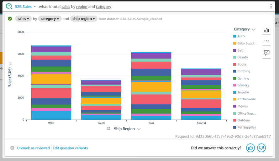
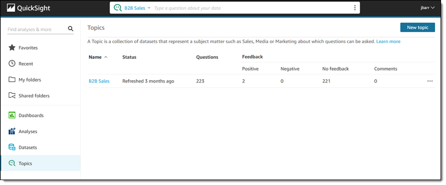
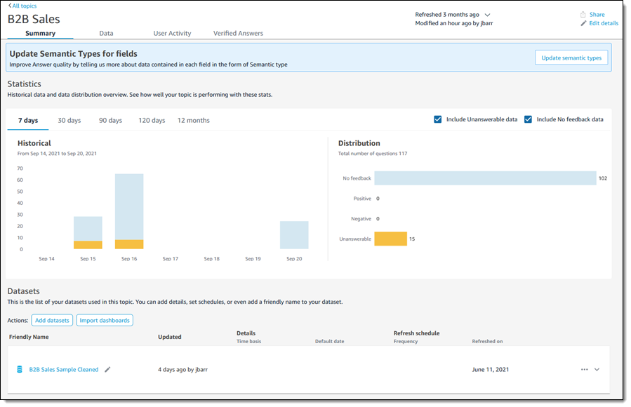
As I often tell you, we are always looking for more ways to meet the needs of our customers. To this end, we are launching Amazon FSx for NetApp ONTAP today. You get the popular features, performance, and APIs of ONTAP file systems with the agility, scalability, security, and resiliency of AWS, making it easier for you to migrate on-premises applications that rely on network-attached storage (NAS) appliances to AWS.

ONTAP (a NetApp product) is an enterprise data management offering designed to provide high-performance storage suitable for use with Oracle, SAP, VMware, Microsoft SQL Server, and so forth. ONTAP is flexible and scalable, with support for multi-protocol access and file systems that can scale up to 176 PiB. It supports a wide variety of features that are designed to make data management cheaper and easier including inline data compression, deduplication, compaction, thin provisioning, replication (SnapMirror), and point-in-time cloning (FlexClone).

FSx for ONTAP is fully managed so you can start to enjoy all of these features in minutes. AWS provisions the file servers and storage volumes, manages replication, installs software updates & patches, replaces misbehaving infrastructure components, manages failover, and much more. Whether you are migrating data from your on-premises NAS environment or building brand-new cloud native applications, you will find a lot to like! If you are migrating, you can enjoy all of the benefits of a fully-managed file system while taking advantage of your existing tools, workflows, processes, and operational expertise. If you are building brand-new applications, you can create a cloud-native experience that makes use of ONTAP’s rich feature set. Either way, you can scale to support hundreds of thousands of IOPS and benefit from the continued, behind-the-scenes evolution of the compute, storage, and networking components.

There are two storage tiers, and you can enable intelligent tiering to move data back and forth between them on an as-needed basis:

Primary Storage is built on high performance solid state drives (SSD), and is designed to hold the part of your data set that is active and/or sensitive to latency. You can provision up to 192 TiB of primary storage per file system.

Capacity Pool Storage grows and shrinks as needed, and can scale to pebibytes. It is cost-optimized and designed to hold data that is accessed infrequently.

Within each Amazon FSx for NetApp ONTAP file system you can create one or more Storage Virtual Machines (SVMs), each of which supports one or more Volumes. Volumes can be accessed via NFS, SMB, or as iSCSI LUNs for shared block storage. As you can see from this diagram, you can access each volume from AWS compute services, VMware Cloud on AWS, and from your on-premises applications:

If your on-premises applications are already making use of ONTAP in your own data center, you can easily create an ONTAP file system in the cloud, replicate your data using NetApp SnapMirror, and take advantage of all that Amazon FSx for NetApp ONTAP has to offer.

Getting Started with Amazon FSx for NetApp ONTAP
I can create my first file system from the command line, AWS Management Console, or the NetApp Cloud Manager. I can also make an API call or use a CloudFormation template. I’ll use the Management Console.

Each file system runs within a Virtual Private Cloud (VPC), so I start by choosing a VPC and a pair of subnets (preferred and standby). Every SVM has an endpoint in the Availability Zones associated with both of the subnets, with continuous monitoring, automated failover, and automated failback to ensure high availability.

I open the Amazon FSx Console, click Create file system, select Amazon FSx for NetApp ONTAP, and click Next:

I can choose Quick create and use a set of best practices, or Standard create and set all of the options myself. I’ll go for the first option, since I can change all of the configuration options later if necessary. I select Quick create, enter a name for my file system (jb-fsx-ontap-1), and set the storage capacity in GiB. I also choose the VPC, and enable ONTAP’s storage efficiency features:

I confirm all of my choices, and note that this option will also create a Storage Virtual Machine (fsx) and a volume (vol1) for me. Then I click Create file system to “make it so”:

The file system Status starts out as Creating, then transitions to Available within 20 minutes or so:

My first SVM transitions from Pending to Created shortly thereafter, and my first volume transitions from Pending to Created as well. I can click on the SVM to learn more about it and to see the full set of management and access endpoints that it provides:

I can click Volumes in the left-side navigation and see all of my volumes. The root volume (fsx_root) is created automatically and represents all of the storage on the SVM:

I can select a volume and click Attach to get customized instructions for attaching it to an EC2 instance running Linux or Windows:

I can select a volume and then choose Update volume from the Action menu to change the volume’s path, size, storage efficiency, or tiering policy:

To learn more about the tiering policy, read about Amazon FSx for NetApp ONTAP Storage.

I can click Create volume and create additional volumes within any of my file systems:

There’s a lot more than I have space to show you, so be sure to open up the Console and try it out for yourself.

Things to Know
Here are a couple of things to know about Amazon FSx for NetApp ONTAP:

Regions – The new file system is available in most AWS regions and in GovCloud; check out the AWS Regional Service list for more information.

Pricing – Pricing is based on multiple usage dimensions including the Primary Storage, Capacity Pool Storage, throughput capacity, additional SSD IOPS, and backup storage consumption; consult the Amazon FSx for NetApp ONTAP Pricing page for more information.

Connectivity – You can use AWS Direct Connect to connect your on-premises applications to your new file systems. You can use Transit Gateway to connect to VPCs in other accounts and/or regions.

Availability – As I mentioned earlier, each file system is powered by AWS infrastructure in a pair of Availability Zones. Amazon FSx for NetApp ONTAP automatically replicates data between the zones and monitors the AWS infrastructure, initiating a failover (typically within 60 seconds), and then replacing infrastructure components as necessary. There’s a 99.99% availability SLA for each file system.

Jeff;

Amazon Managed Grafana Is Now Generally Available with Many New Features

Post Syndicated from Danilo Poccia original https://aws.amazon.com/blogs/aws/amazon-managed-grafana-is-now-generally-available-with-many-new-features/

In December, we introduced the preview of Amazon Managed Grafana, a fully managed service developed in collaboration with Grafana Labs that makes it easy to use the open-source and the enterprise versions of Grafana to visualize and analyze your data from multiple sources. With Amazon Managed Grafana, you can analyze your metrics, logs, and traces without having to provision servers, or configure and update software.

During the preview, Amazon Managed Grafana was updated with new capabilities. Today, I am happy to announce that Amazon Managed Grafana is now generally available with additional new features:

  • Grafana has been upgraded to version 8 and offers new data sources, visualizations, and features, including library panels that you can build once and re-use on multiple dashboards, a Prometheus metrics browser to quickly find and query metrics, and new state timeline and status history visualizations.
  • To centralize the querying of additional data sources within an Amazon Managed Grafana workspace, you can now query data using the JSON data source plugin. You can now also query Redis, SAP HANA, Salesforce, ServiceNow, Atlassian Jira, and many more data sources.
  • You can use Grafana API keys to publish your own dashboards or give programmatic access to your Grafana workspace. For example, this is a Terraform recipe that you can use to add data sources and dashboards.
  • You can enable single sign-on to your Amazon Managed Grafana workspaces using Security Assertion Markup Language 2.0 (SAML 2.0). We have worked with these identity providers (IdP) to have them integrated at launch: CyberArk, Okta, OneLogin, Ping Identity, and Azure Active Directory.
  • All calls from the Amazon Managed Grafana console and code calls to Amazon Managed Grafana API operations are captured by AWS CloudTrail. In this way, you can have a record of actions taken in Amazon Managed Grafana by a user, role, or AWS service. Additionally, you can now audit mutating changes that occur in your Amazon Managed Grafana workspace, such as when a dashboard is deleted or data source permissions are changed.
  • The service is available in ten AWS Regions (full list at the end of the post).

Let’s do a quick walkthrough to see how this works in practice.

Using Amazon Managed Grafana
In the Amazon Managed Grafana console, I choose Create workspace. A workspace is a logically isolated, highly available Grafana server. I enter a name and a description for the workspace, and then choose Next.

Console screenshot.

I can use AWS Single Sign-On (AWS SSO) or an external identity provider via SAML to authenticate the users of my workspace. For simplicity, I select AWS SSO. Later in the post, I’ll show how SAML authentication works. If this is your first time using AWS SSO, you can see the prerequisites (such as having AWS Organizations set up) in the documentation.

Console screenshot.

Then, I choose the Service managed permission type. In this way, Amazon Managed Grafana will automatically provision the necessary IAM permissions to access the AWS Services that I select in the next step.

Console screenshot.

In Service managed permission settings, I choose to monitor resources in my current AWS account. If you use AWS Organizations to centrally manage your AWS environment, you can use Grafana to monitor resources in your organizational units (OUs).

Console screenshot.

I can optionally select the AWS data sources that I am planning to use. This configuration creates an AWS Identity and Access Management (IAM) role that enables Amazon Managed Grafana to access those resources in my account. Later, in the Grafana console, I can set up the selected services as data sources. For now, I select Amazon CloudWatch so that I can quickly visualize CloudWatch metrics in my Grafana dashboards.

Here I also configure permissions to use Amazon Managed Service for Prometheus (AMP) as a data source and have a fully managed monitoring solution for my applications. For example, I can collect Prometheus metrics from Amazon Elastic Kubernetes Service (EKS) and Amazon Elastic Container Service (Amazon ECS) environments, using AWS Distro for OpenTelemetry or Prometheus servers as collection agents.

Console screenshot.

In this step I also select Amazon Simple Notification Service (SNS) as a notification channel. Similar to the data sources before, this option gives Amazon Managed Grafana access to SNS but does not set up the notification channel. I can do that later in the Grafana console. Specifically, this setting adds SNS publish permissions to topics that start with grafana to the IAM role created by the Amazon Managed Grafana console. If you prefer to have tighter control on permissions for SNS or any data source, you can edit the role in the IAM console or use customer-managed permissions for your workspace.

Finally, I review all the options and create the workspace.

After a few minutes, the workspace is ready, and I find the workspace URL that I can use to access the Grafana console.

Console screenshot.

I need to assign at least one user or group to the Grafana workspace to be able to access the workspace URL. I choose Assign new user or group and then select one of my AWS SSO users.

Console screenshot.

By default, the user is assigned a Viewer user type and has view-only access to the workspace. To give this user permissions to create and manage dashboards and alerts, I select the user and then choose Make admin.

Console screenshot.

Back to the workspace summary, I follow the workspace URL and sign in using my AWS SSO user credentials. I am now using the open-source version of Grafana. If you are a Grafana user, everything is familiar. For my first configurations, I will focus on AWS data sources so I choose the AWS logo on the left vertical bar.

Console screenshot.

Here, I choose CloudWatch. Permissions are already set because I selected CloudWatch in the service-managed permission settings earlier. I select the default AWS Region and add the data source. I choose the CloudWatch data source and on the Dashboards tab, I find a few dashboards for AWS services such as Amazon Elastic Compute Cloud (Amazon EC2), Amazon Elastic Block Store (EBS), AWS Lambda, Amazon Relational Database Service (RDS), and CloudWatch Logs.

Console screenshot.

I import the AWS Lambda dashboard. I can now use Grafana to monitor invocations, errors, and throttles for Lambda functions in my account. I’ll save you the screenshot because I don’t have any interesting data in this Region.

Using SAML Authentication
If I don’t have AWS SSO enabled, I can authenticate users to the Amazon Managed Grafana workspace using an external identity provider (IdP) by selecting the SAML authentication option when I create the workspace. For existing workspaces, I can choose Setup SAML configuration in the workspace summary.

First, I have to provide the workspace ID and URL information to my IdP in order to generate IdP metadata for configuring this workspace.

Console screenshot.

After my IdP is configured, I import the IdP metadata by specifying a URL or copying and pasting to the editor.

Console screenshot.

Finally, I can map user permissions in my IdP to Grafana user permissions, such as specifying which users will have Administrator, Editor, and Viewer permissions in my Amazon Managed Grafana workspace.

Console screenshot.

Availability and Pricing
Amazon Managed Grafana is available today in ten AWS Regions: US East (N. Virginia), US East (Ohio), US West (Oregon), Europe (Ireland), Europe (Frankfurt), Europe (London), Asia Pacific (Singapore), Asia Pacific (Tokyo), Asia Pacific (Sydney), and Asia Pacific (Seoul). For more information, see the AWS Regional Services List.

With Amazon Managed Grafana, you pay for the active users per workspace each month. Grafana API keys used to publish dashboards are billed as an API user license per workspace each month. You can upgrade to Grafana Enterprise to have access to enterprise plugins, support, and on-demand training directly from Grafana Labs. For more information, see the Amazon Managed Grafana pricing page.

To learn more, you are invited to this webinar on Thursday, September 9 at 9:00 am PDT / 12:00 pm EDT / 6:00 pm CEST.

Start using Amazon Managed Grafana today to visualize and analyze your operational data at any scale.

Danilo

Inspect Subnet to Subnet traffic with Amazon VPC More Specific Routing

Post Syndicated from Sébastien Stormacq original https://aws.amazon.com/blogs/aws/inspect-subnet-to-subnet-traffic-with-amazon-vpc-more-specific-routing/

Since December 2019, Amazon Virtual Private Cloud (VPC) has allowed you to route all ingress traffic (also known as north – south traffic) to a specific network interface. You might use this capability for a number of reasons. For example, to inspect incoming traffic using an intrusion detection system (IDS) appliance or to route ingress traffic to a firewall.

Since we launched this feature, many of you asked us to provide a similar capability to analyze traffic flowing from one subnet to another inside your VPC, also known as east – west traffic. Until today, it was not possible because a route in a routing table cannot be more specific than the default local route (check the VPC documentation for more details). In plain English, it means that no route can have a destination using a smaller CIDR range than the default local route (which is the CIDR range of the whole VPC). For example, when the VPC range is 10.0.0/16 and a subnet has 10.0.1.0/24, a route to 10.0.1.0/24 is more specific than a route to 10.0.0/16.

Routing tables no longer have this restriction. Routes in a routing table can have routes more specific than the default local route. You can use such more specific route to send all traffic to a dedicated appliance or service to inspect, analyze, or filter all traffic flowing between two subnets (east-west traffic). The route target can be the network interface (ENI) attached to an appliance you built or you acquired, an AWS Gateway Load Balancer (GWLB) endpoint to distribute traffic to multiple appliances for performance or high availability reasons, an AWS Firewall Manager endpoint, or a NAT gateway. It also allows to insert an appliance between a subnet and an AWS Transit Gateway.

It is possible to chain appliances to have more than one type of analysis in between source and destination subnets. For examples, you might want first to filter traffic using a firewall (AWS managed or a third-party firewall appliance), second send the traffic to an intrusion detection and prevention systems, and finally, perform deep packet inspection. You can access virtual appliances from our AWS Partner Network and AWS Marketplace.

When you chain appliances, each appliance and each endpoint have to be in separate subnets.

Let’s get our hands dirty and try this new capability.

How It Works
For the purpose of this blog post, let’s assume I have a VPC with three subnets. The first subnet is public and has a bastion host. It requires access to resources, such as an API or a database in the second subnet. The second subnet is private. It hosts the resources required by the bastion. I wrote a simple CDK script to help you to deploy this setup.

VPC More Specific Routing

For compliance reasons, my company requires that traffic to this private application flows through an intrusion detection system. The CDK script also creates a third subnet, a private one, to host a network appliance. It provides three Amazon Elastic Compute Cloud (Amazon EC2) instances : the bastion host, the application instance and the network analysis appliance. The script also creates a NAT gateway allowing to bootstrap the application instance and to connect to the three instances using AWS Systems Manager Session Manager (SSM).

Because this is a demo, the network appliance is just a regular Amazon Linux EC2 instance configured as an IP router. In real life, you’re most probably going to use either one of the many appliances provided by our partners on the AWS Marketplace, or a Gateway Load Balancer endpoint, or a Network Firewall.

Let’s modify the routing tables to send the traffic through the appliance.

Using either the AWS Management Console, or the AWS Command Line Interface (CLI), I add a more specific route to the 10.0.0.0/24 and 10.0.1.0/24 subnet routing tables. These routes point to eni0, the network interface of the traffic-inspection appliance.

Using the CLI, I first collect the VPC ID, Subnet IDs, routing table IDs, and the ENI ID of the appliance.

VPC_ID=$(aws                                                    \
    --region $REGION cloudformation describe-stacks             \
    --stack-name SpecificRoutingDemoStack                       \
    --query "Stacks[].Outputs[?OutputKey=='VPCID'].OutputValue" \
    --output text)
echo $VPC_ID

APPLICATION_SUBNET_ID=$(aws                                                                      \
    --region $REGION ec2 describe-instances                                                      \
    --query "Reservations[].Instances[] | [?Tags[?Key=='Name' && Value=='application']].NetworkInterfaces[].SubnetId" \
    --output text)
echo $APPLICATION_SUBNET_ID

APPLICATION_SUBNET_ROUTE_TABLE=$(aws                                                             \
    --region $REGION  ec2 describe-route-tables                                                  \
    --query "RouteTables[?VpcId=='${VPC_ID}'] | [?Associations[?SubnetId=='${APPLICATION_SUBNET_ID}']].RouteTableId" \
    --output text)
echo $APPLICATION_SUBNET_ROUTE_TABLE

APPLIANCE_ENI_ID=$(aws                                                                           \
    --region $REGION ec2 describe-instances                                                      \
    --query "Reservations[].Instances[] | [?Tags[?Key=='Name' && Value=='appliance']].NetworkInterfaces[].NetworkInterfaceId" \
    --output text)
echo $APPLIANCE_ENI_ID

BASTION_SUBNET_ID=$(aws                                                                         \
    --region $REGION ec2 describe-instances                                                     \
    --query "Reservations[].Instances[] | [?Tags[?Key=='Name' && Value=='BastionHost']].NetworkInterfaces[].SubnetId" \
    --output text)
echo $BASTION_SUBNET_ID

BASTION_SUBNET_ROUTE_TABLE=$(aws \
 --region $REGION ec2 describe-route-tables \
 --query "RouteTables[?VpcId=='${VPC_ID}'] | [?Associations[?SubnetId=='${BASTION_SUBNET_ID}']].RouteTableId" \
 --output text)
echo $BASTION_SUBNET_ROUTE_TABLE

Next, I add two more specific routes. One route sends traffic from the bastion public subnet to the application private subnet through the appliance network interface.  The second route is in the opposite direction to route replies. It routes more specific traffic from the application private subnet to the bastion public subnet through the appliance network interface.  Confused? Let’s look at the following diagram:

VPC More Specific Routing

First, let’s modify the bastion routing table:

aws ec2 create-route                                  \
     --region $REGION                                 \
     --route-table-id $BASTION_SUBNET_ROUTE_TABLE     \
     --destination-cidr-block 10.0.1.0/24             \
     --network-interface-id $APPLIANCE_ENI_ID

Next, let’s modify the application routing table:

aws ec2 create-route                                  \
    --region $REGION                                  \
    --route-table-id $APPLICATION_SUBNET_ROUTE_TABLE  \
    --destination-cidr-block 10.0.0.0/24              \
    --network-interface-id $APPLIANCE_ENI_ID

I can also use the Amazon VPC Console to make these modifications. I simply choose the “Bastion” routing tables and from the Routes tab and click Edit routes.MSR : Select a routing table

I add a route to send traffic for 10.0.1.0/24 (subnet of the application) to the appliance ENI (eni-055...).MSR : create a route

The next step is to define the opposite route for replies, from the application subnet send traffic to 10.0.0.0/24 to the appliance ENI (eni-05...).  Once finished, the application subnet routing table should look like this:

MSR : Final route table

Configure the Appliance Instance
Finally, I configure the appliance instance to forward all traffic it receives. Your software appliance usually does that for you. No extra step is required when you use AWS Marketplace appliances or the instance created by the CDK script I provided for this demo. If you’re using a plain Linux instance, complete these two extra steps:

1. Connect to the EC2 appliance instance and configure IP traffic forwarding in the kernel:

sysctl -w net.ipv4.ip_forward=1
sysctl -w net.ipv6.conf.all.forwarding=1

2. Configure the EC2 instance to accept traffic for destinations other than itself (known as source/destination check) :

APPLIANCE_ID=$(aws --region $REGION ec2 describe-instances                     \
     --filter "Name=tag:Name,Values=appliance"                                 \
     --query "Reservations[].Instances[?State.Name == 'running'].InstanceId[]" \
     --output text)

aws ec2 modify-instance-attribute --region $REGION     \
                         --no-source-dest-check        \
                         --instance-id $APPLIANCE_ID

Test the Setup
The appliance is now ready to forward traffic to the other EC2 instances.

If you are using the demo setup, there is no SSH key installed on the bastion host. Access is made through AWS Systems Manager Session Manager.

BASTION_ID=$(aws --region $REGION ec2 describe-instances                      \
    --filter "Name=tag:Name,Values=BastionHost"                               \
    --query "Reservations[].Instances[?State.Name == 'running'].InstanceId[]" \
    --output text)

aws --region $REGION ssm start-session --target $BASTION_ID

After you’re connected to the bastion host, issue the following cURL command to connect to the application host:

sh-4.2$ curl -I 10.0.1.239 # use the private IP address of your application host
HTTP/1.1 200 OK
Server: nginx/1.18.0
Date: Mon, 24 May 2021 10:00:22 GMT
Content-Type: text/html
Content-Length: 12338
Last-Modified: Mon, 24 May 2021 09:36:49 GMT
Connection: keep-alive
ETag: "60ab73b1-3032"
Accept-Ranges: bytes

To verify the traffic is really flowing through the appliance, you can enable source/destination check on the instance again. Use the --source-dest-check parameter with the modify-instance-attribute CLI command above. The traffic is blocked when the source/destination check is enabled.

I can also connect to the appliance host and inspect traffic with the tcpdump command.

(on your laptop)
APPLIANCE_ID=$(aws --region $REGION ec2 describe-instances     \
                   --filter "Name=tag:Name,Values=appliance" \
		   --query "Reservations[].Instances[?State.Name == 'running'].InstanceId[]" \
  		   --output text)

aws --region $REGION ssm start-session --target $APPLIANCE_ID

(on the appliance host)
tcpdump -i eth0 host 10.0.0.16 # the private IP address of the bastion host

08:53:22.760055 IP ip-10-0-0-16.us-west-2.compute.internal.46934 > ip-10-0-1-104.us-west-2.compute.internal.http: Flags [S], seq 1077227105, win 26883, options [mss 8961,sackOK,TS val 1954932042 ecr 0,nop,wscale 6], length 0
08:53:22.760073 IP ip-10-0-0-16.us-west-2.compute.internal.46934 > ip-10-0-1-104.us-west-2.compute.internal.http: Flags [S], seq 1077227105, win 26883, options [mss 8961,sackOK,TS val 1954932042 ecr 0,nop,wscale 6], length 0
08:53:22.760322 IP ip-10-0-1-104.us-west-2.compute.internal.http > ip-10-0-0-16.us-west-2.compute.internal.46934: Flags [S.], seq 4152624111, ack 1077227106, win 26847, options [mss 8961,sackOK,TS val 4094021737 ecr 1954932042,nop,wscale 6], length 0
08:53:22.760329 IP ip-10-0-1-104.us-west-2.compute.internal.http > ip-10-0-0-16.us-west-2.compute.internal.46934: Flags [S.], seq 4152624111, ack 1077227106, win 26847, options [mss 

Cleanup
If you used the CDK script I provided for this post, be sure to run cdk destroy when you’re finished so that you’re not billed for the three EC2 instances and the NAT gateway I use for this demo. Running the demo script in us-west-2 costs $0.062 per hour.

Things to Keep in Mind.
There are couple of things to keep in mind when using VPC more specific routes :

  • The network interface or service endpoint you are sending the traffic to must be in a dedicated subnet. It cannot be in the source or destination subnet of your traffic.
  • You can chain appliances. Each appliance must live in its dedicated subnet.
  • Each subnet you’re adding consumes a block of IP addresses.  If you’re using IPv4, be conscious of the number of IP addresses consumed (A /24 subnet consumes 256 addresses from your VPC). The smallest CIDR range allowed in a subnet is /28, it just consumes 16 IP addresses.
  • The appliance’s security group must have a rule accepting incoming traffic on the desired port. Similarly, the application’s security group must authorize traffic coming from the appliance security group or IP address.

This new capability is available in all AWS Regions, at no additional cost.

You can start using it today.