Tag Archives: Technical How-to

Genomics workflows, Part 7: analyze public RNA sequencing data using AWS HealthOmics

2024-06-05 Rostislav Markov

Post Syndicated from Rostislav Markov original https://aws.amazon.com/blogs/architecture/genomics-workflows-part-7-analyze-public-rna-sequencing-data-using-aws-healthomics/

Genomics workflows process petabyte-scale datasets on large pools of compute resources. In this blog post, we discuss how life science organizations can use Amazon Web Services (AWS) to run transcriptomic sequencing data analysis using public datasets. This allows users to quickly test research hypotheses against larger datasets in support of clinical diagnostics. We use AWS HealthOmics and AWS Step Functions to orchestrate the entire lifecycle of preparing and analyzing sequence data and remove the associated heavy lifting.

Use case

In genomics, transcription relates to the process of making a ribonucleic acid (RNA) copy from a gene’s deoxyribonucleic acid (DNA). Usually, RNA is single-stranded, although some RNA viruses are double-stranded. With RNA sequencing (RNA-Seq), scientists isolate the RNA, prepare an RNA library, and use next-generation sequencing technology to decode it. Organizations around the world use RNA-Seq to support clinical diagnostics.

In our use case, life science research teams use workflows written in Nextflow to process RNA-Seq datasets in FASTQ file format. Following their initial RNA-Seq studies on internal datasets, scientists can extend their insights by using public datasets. For example, the Gene Expression Omnibus (GEO) functional genomics data repository is hosted by the National Center for Biotechnology Information (NCBI) and offers multiple download options and formats. Scientists can download datasets in FASTQ format from GEO File Transfer Protocol (FTP) and compress them into the .gz format before further analysis.

Scaling and automating the data ingestion can be challenging. For example, scientists might need to do the following:

Manually download FASTQ files and invoke their analysis pipelines
Monitor the workflow runs, which can span hours, days, or weeks
Manage the infrastructure for performance and scale

This blog post presents a solution that removes this undifferentiated heavy lifting.

Prerequisites

To build this solution, you must be analyzing transcriptomic sequencing data with the Nextflow workflow system and make use of GEO FASTQ datasets. In addition, you must do the following:

Create three Amazon Simple Storage Service (Amazon S3) buckets with the following purposes:
- Uploaded GEO Accession IDs (GEO IDs)
- Ingested FASTQ datasets
- RNA-Seq output files
Create one Amazon DynamoDB table to track the status of data ingestion. This helps with checkpointing and avoids repetitive ingestion jobs so that you can keep data ingestion cost to a minimum.

Solution overview

Using AWS, you can automate the entire RNA-Seq Nextflow pipeline. Users only need to provide the GEO IDs, then the pipeline ingests the corresponding FASTQ sample files and performs the subsequent data analysis.

Our solution, shown in Figure 1, uses a combination of AWS HealthOmics and AWS Step Functions. HealthOmics manages the compute, scalability, scheduling, and orchestration required for processing large RNA-Seq datasets. This helps scientists focus on writing their pipelines in Nextflow while AWS takes care of the underlying infrastructure. Step Functions adds reliability to the workflow from dataset ingestion to output archival. Automating the entire workflow also helps with tracing specific invocations and troubleshooting errors.

This figure visualizes the AWS services involved in each processing step, starting with users uploading CSV files with GEO metadata to Amazon S3, and concluding with AWS HealthOmics performing the RNA-Seq analysis and putting the output data on Amazon S3.

Figure 1. RNA sequencing using HealthOmics

Our solution includes the following:

The scientist creates and uploads a CSV file to the GEO metadata S3 bucket. The CSV file includes a reference to the specific GEO ID that is ingested. An Amazon S3 Event Notification configured on s3:ObjectCreated events (in this case, the CSV file upload) invokes an AWS Lambda function.
The Lambda function first extracts the corresponding Sequence Read Run (SRR) IDs of the GEO ID. Next, it starts a Step Functions state machine with the following input parameters: the SRR IDs, species of the samples, and GEO ID. The state machine uses an AWS Batch job queue for parallel ingestion.
The Lambda function writes the following metadata to a DynamoDB table for future reference:
- Ingested GEO ID and corresponding list of SRR IDs
- Amazon S3 output paths to the ingested FASTQ files
- Overall workflow status
- Ingested species
Upon ingestion completion, the state machine puts the RNA-Seq sample sheet into the FASTQ S3 bucket. This invokes a Lambda function, which launches the RNA-Seq analysis workflow with the following input parameters:
- Sample sheet
- GEO ID
- Other relevant metadata
Our RNA-Seq data analysis is run with HealthOmics and the associated sequence store. We use Step Functions to launch this workflow and ingest the relevant files to the sequence store.
Upon workflow completion, HealthOmics writes the output data (BAM files) to the output S3 bucket.

Implementation considerations

Dataset preparation

The Step Functions state machine orchestrates the ingestion of FASTQ files through the following steps:

The state machine invokes the Map state in Step Functions that uses dynamic parallelism for increased scale, with the SRR IDs array as input. You can now launch multiple AWS Batch jobs in parallel to ingest the FASTQ files that correspond to the SRR ID input.
The state machine checks our ingestion DynamoDB table to see if the corresponding SRR ID has already been processed and has ingested the corresponding FASTQ files. If the SRR ID ingested the files, the state machine writes the sample sheet to the FASTQ S3 bucket and terminates successfully.
The state machine uses the NCBI-provided sra-tools Docker container and fasterq-dump command to ingest the FASTQ files. The state machine generates the set of ingestion commands and starts the AWS Batch job. The ingestion commands are a set of shell commands that interact with NCBI for downloading FASTQ files. These commands compress the files with pigz, and then uploads them to an S3 bucket.
The state machine updates the DynamoDB table with the ingestion status.
1. If the ingestion is successful, then the state machine continues to step 5.
2. If the ingestion isn’t successful, the state machine writes a message to Amazon Simple Notification Service (Amazon SNS) to notify scientists of the failure.
A Lambda function generates the RNA-Seq sample sheet with the combined samples to analyze. This sample sheet is a CSV file containing:
1. The paths to the ingested FASTQ files.
2. The names of each corresponding SRR ID as input to the RNA-Seq workflow.
The state machine notifies that the ingestion job is complete by publishing a message to an Amazon SNS topic before terminating itself.

Figure 2 provides a detailed overview of the state machine.

This Map state definition in AWS Step Functions visualizes the aforementioned steps for FASTQ file ingestion including orchestration of the associated AWS Batch job.

Figure 2. RNA sequencing data ingestion

Dataset analysis

A Lambda function divides the RNA-Seq sample sheet in compliance with the Step Functions service quota. This enables parallel processing using a Map state.

Our transcriptomic analysis workflow does the following:

Checks if samples are single-end (one FASTQ file per sample) or paired-end (two sets of FASTQ files per sample).
Ingests the appropriate set of FASTQ files into the HealthOmics sequence store.
Monitors the status until all files are imported.

In parallel, a Lambda function initiates the HealthOmics RNA-Seq workflow.

Upon successful completion, HealthOmics stores the output data in Amazon S3. Finally, our state machine imports the output BAM files into the HealthOmics sequence store for future use.

Figure 3 provides a detailed overview of our state machine.

This AWS Step Functions workflow visualizes the aforementioned steps for data analysis including orchestration of the associated AWS HealthOmics workflow and FASTQ file ingestion into the HealthOmics Sequence Store.

Figure 3. RNA sequencing workflow

Cleanup (optional)

Delete all AWS resources that you no longer want to maintain.

Conclusion

HealthOmics removes the heavy lifting associated with gaining insights from genomics, transcriptomics, and other omics data. We used RNA-Seq analysis to showcase an example scientific workflow that can benefit from HealthOmics. When using HealthOmics in combination with Step Functions, scientists can automate the entire workflow from initial dataset preparation to archival. To learn more, we encourage you to explore our HealthOmics tutorials on GitHub.

Related information

Optimize write throughput for Amazon Kinesis Data Streams

2024-06-03 Buddhike de Silva

Post Syndicated from Buddhike de Silva original https://aws.amazon.com/blogs/big-data/optimize-write-throughput-for-amazon-kinesis-data-streams/

Amazon Kinesis Data Streams is used by many customers to capture, process, and store data streams at any scale. This level of unparalleled scale is enabled by dividing each data stream into multiple shards. Each shard in a stream has a 1 Mbps or 1,000 records per second write throughput limit. Whether your data streaming application is collecting clickstream data from a web application or recording telemetry data from billions of Internet of Things (IoT) devices, streaming applications are highly susceptible to a varying amount of data ingestion. Sometimes such a large and unexpected volume of data could be the thing we least expect. For instance, consider application logic with a retry mechanism when writing records to a Kinesis data stream. In case of a network failure, it’s common to buffer data locally and write them when connectivity is restored. Depending on the rate that data is buffered and the duration of connectivity issue, the local buffer can accumulate enough data that could saturate the available write throughput quota of a Kinesis data stream.

When an application attempts to write more data than what is allowed, it will receive write throughput exceeded errors. In some instances, not being able to address these errors in a timely manner can result in data loss, unhappy customers, and other undesirable outcomes. In this post, we explore the typical reasons behind write throughput exceeded errors, along with methods to identify them. We then guide you on swift responses to these events and provide several solutions for mitigation. Lastly, we delve into how on-demand capacity mode can be valuable in addressing these errors.

Why do we get write throughput exceeded errors?

Write throughput exceeded errors are generally caused by three different scenarios:

The simplest is the case where the producer application is generating more data than the throughput available in the Kinesis data stream (the sum of all shards).
Next, we have the case where data distribution is not even across all shards, known as hot shard issue.
Write throughout errors can also be caused by an application choosing a partition key to write records at a rate exceeding the throughput offered by a single shard. This situation is somewhat similar to hot shard issue, but as we see later in this post, unlike a hot shard issue, you can’t solve this problem by adding more shards to the data stream. This behavior is commonly known as a hot key issue.

Before we discuss how to diagnose these issues, let’s look at how Kinesis data streams organize data and its relationship to write throughput exceeded errors.

A Kinesis data stream has one or more shards to store data. Each shard is assigned a key range in 128-bit integer space. If you view the details of a data stream using the describe-stream operation in the AWS Command Line Interface (AWS CLI), you can actually see this key range assignment:

$ aws kinesis describe-stream --stream-name my-data-stream
"StreamDescription": {
  "Shards": [
    {
      "ShardId": "shardId-000000000000",
      "HashKeyRange": {
        "StartingHashKey": "0",
        "EndingHashKey": 
        "85070591730234615865843651857942052863"
       }
    },
    {
       "ShardId": "shardId-000000000001",
       "HashKeyRange": {
       "StartingHashKey": 
          "85070591730234615865843651857942052864",
       "EndingHashKey": 
         "170141183460469231731687303715884105727"
       }
    }
  ]
}

When a producer application invokes the PutRecord or PutRecords API, the service calculates a MD5 hash for the PartitionKey specified in the record. The resulting hash is used to determine which shard to store that record. You can take more control over this process by setting the ExplicitHashKey property in the PutRecord request to a hash key that falls within a specific shard’s key range. For instance, setting ExplicitHashKey to 0 will guarantee that record is written to shard ID shardId-0 in the stream described in the preceding code snippet.

How partition keys are distributed across available shards plays a vital role in maximizing the available throughput in a Kinesis data stream. When the partition key being used is repeated frequently in a way that some keys are more frequent than the others, shards storing those records will be utilized more. We also get the same net effect if we use ExplicitHashKey and our logic for choosing the hash key is biased towards a subset of shards.

Imagine you have a fleet of web servers logging performance metrics for each web request served into a Kinesis data stream with two shards and you used a request URL as the partition key. Each time a request is served, the application makes a call to the PutRecord API carrying a 10-bytes record. Let’s say that you have a total of 10 URLs and each receives 10 requests per second. Under these circumstances, total throughput required for the workload is 1,000 bytes per second and 100 requests per second. If we assume perfect distribution of 10 URLs across the two shards, each shard will receive 500 bytes per second and 50 requests per second.

Now imagine one of these URLs went viral and it started receiving 1,000 requests per second. Although the situation is positive from a business point of view, you’re now on the brink of making users unhappy. After the page gained popularity, you’re now counting 1,040 requests per second for the shard storing the popular URL (1000 + 10 * 4). At this point, you’ll receive write throughput exceeded errors from that shard. You’re throttled based on the requests per second quota because even with increased requests, you’re still generating approximately 11 KB of data.

You can solve this problem either by using a UUID for each request as the partition key so that you share the total load across both shards, or by adding more shards to the Kinesis data stream. The method you choose depends on how you want to consume data. Changing the partition key to a UUID would be problematic if you want performance metrics from a given URL to be always processed by the same consumer instance or if you want to maintain the order of records on a per-URL basis.

Knowing the exact cause of write throughout exceeded errors is an important step in remediating them. In the next sections, we discuss how to identify the root cause and remediate this problem.

Identifying the cause of write throughput exceeded errors

The first step in solving a problem is that knowing that it exists. You can use the WriteProvisionedThrougputExceeded metric in Amazon CloudWatch in this case. You can correlate the spikes in the WriteProvisionedThrougputExceeded metric to the IncomingBytes and IncomingRecords metrics to identify whether an application is getting throttled due to the size of data or the number of records written.

Let’s look at a few tests we performed in a stream with two shards to illustrate various scenarios. In this instance, with two shards in our stream, total throughput available to our producer application is either 2 Mbps or 2,000 records per second.

In the first test, we ran a producer to write batches of 30 records, each being 100 KB, using the PutRecords API. As you can see in the graph on the left of the following figure, our WriteProvisionedThroughputExceedded errors count went up. The graph on the right shows that we are reaching the 2 Mbps limit, but our incoming records rate is much lower than the 2,000 records per second limit (Kinesis metrics are published at 1-minute intervals, hence 125.8 and 120,000 as upper limits).

The following figures show how the same three metrics changed when we changed the producer to write batches of 500 records, each being 50 bytes, in the second test. This time, we exceeded the 2,000 records per second throughput limit, but our incoming bytes rate is well under the limit.

Now that we know that problem exists, we should look for clues to see if we’re exceeding the overall throughput available in the stream or if we’re having a hot shard issue due to an imbalanced partition key distribution as discussed earlier. One approach to this is to use enhanced shard-level metrics. Prior to our tests, we enabled enhanced shard-level metrics, and we can see in the following figure that both shards equally reached their quota in our first test.

We have seen Kinesis data streams containing thousands of shards harnessing the power of infinite scale in Kinesis data streams. However, plotting enhanced shard-level metrics on a such large stream may not provide an easy to way to find out which shards are over-utilized. In that instance, it’s better to use CloudWatch Metrics Insights to run queries to view top-n items, as shown in the following code (adjust the LIMIT 5 clause accordingly):

-- Show top 5 shards with highest incoming bytes
SELECT
SUM(IncomingBytes)
FROM "AWS/Kinesis"
GROUP BY ShardId, StreamName
ORDER BY MAX() DESC
LIMIT 5

-- Show top 5 shards with highest incoming records
SELECT
SUM(IncomingRecords)
FROM "AWS/Kinesis"
GROUP BY ShardId, StreamName
ORDER BY MAX() DESC
LIMIT 5

Enhanced shard-level metrics are not enabled by default. If you didn’t enable them and you want to perform root cause analysis after an incident, this option isn’t very helpful. In addition, you can only query the most recent 3 hours of data. Enhanced shard-level metrics also incur additional costs for CloudWatch metrics and it may be cost prohibitive to have it always on in data streams with a lot of shards.

One interesting scenario is when the workload is bursty, which can make the resulting CloudWatch metrics graphs rather baffling. This is because Kinesis publishes CloudWatch metric data aggregated at 1-minute intervals. Consequently, although you can see write throughput exceeded errors, your incoming bytes/records graphs may be still within the limits. To illustrate this scenario, we changed our test to create a burst of writes exceeding the limits and then sleep for a few seconds. Then we repeated this cycle for several minutes to yield the graphs in the following figure, which show write throughput exceeded errors on the left, but the IncomingBytes and IncomingRecords graphs on the right seem fine.

To enhance the process of identifying write throughput exceeded errors, we developed a CLI tool called Kinesis Hot Shard Advisor (KHS). With KHS, you can view shard utilization when shard-level metrics are not enabled. This is particularly useful for investigating an issue retrospectively. It can also show most frequently written keys to a particular shard. KHS reports shard utilization by reading records and aggregating them per second intervals based on the ApproximateArrivalTimestamp in the record. Because of this, you can also understand shard utilization drivers during bursty write workloads.

By running the following command, we can get KHS to inspect the data that arrived in 1 minute during our first test and generate a report:

khs -stream my-data-stream -from "2023-06-22 17:35:00" -to "2023-06-22 17:36:00"

For the given time window, the summary section in the generated report shows the maximum bytes per second rate observed, total bytes ingested, maximum records per second observed, and the total number of records ingested for each shard.

Choosing a shard ID in the first column will display a graph of incoming bytes and records for that shard. This is similar to the graph you get in CloudWatch metrics, except the KHS graph reports on a per-second basis. For instance, in the following figure, we can see how the producer was going through a series of bursty writes followed by a throttling event during our test case.

Running the same command with the -aggregate-key option enables partition key distribution analysis. It generates an additional graph for each shard showing the key distribution, as shown in the following figure. For our test scenario, we can only see each key being used one time because we used a new UUID for each record.

Because KHS reports based on data stored in streams, it creates an enhanced fan-out consumer at startup to prevent using the read throughput quota available for other consumers. When the analysis is complete, it deletes that enhanced fan-out consumer.

Due its nature of reading data streams, KHS can transfer a lot of data during analysis. For instance, assume you have a stream with 100 shards. If all of them are fully utilized during a minute window specified using -from and -to arguments, the host running KHS will receive at least 1 MB * 100 * 60 = 6000 MB = approximately 6 GB data. To avoid this kind of excessive data transfer and speed up the analysis process, we recommend first using the WriteProvisionedThroughoutExceeded CloudWatch metric to identify a time period when you experienced throttling and use a small window (such as 10 seconds) with KHS. You can also run KHS in an Amazon Elastic Compute Cloud (Amazon EC2) instance in the same AWS Region as your Kinesis data stream to minimize network latency during reads.

KHS is designed to run in a single machine to diagnose large-scale workloads. Using a naive in-memory-based counting algorithm (such as a hash map storing the partition key and count) for partition key distribution analysis could easily exhaust the available memory in the host system. Therefore, we use a probabilistic data structure called count-min-sketch to estimate the number of times a key has been used. As a result, the number you see in the report should be taken as an approximate value rather than an absolute value. After all, with this report, we just want to find out if there’s an imbalance in the keys written to a shard.

Now that we understand what causes hot shards and how to identify them, let’s look at how to deal with this in producer applications and remediation steps.

Remediation steps

Having producers retry writes is a step towards making our producers resilient to write throughput exceeded errors. Consider our earlier sample application logging performance metrics data for each web request served by a fleet of web servers. When implementing this retry mechanism, you should remember that records that are not written to the Kinesis stream are going to be in host system’s memory. The first issue with this is, if the host crashes before the records could be written, you’ll experience data loss. Scenarios such as tracking web request performance data might be more forgiving for this type of data loss than scenarios like financial transactions. You should evaluate durability guarantees required for your application and employ techniques to achieve them.

The second issue is that records waiting to be written to the Kinesis data stream are going to consume the host system’s memory. When you start getting throttled and have some retry logic in place, you should notice that your memory utilization is going up. A retry mechanism should have a way to avoid exhausting the host system’s memory.

With the appropriate retry logic in place, if you receive write throughput exceeded errors, you can use the methods we discussed earlier to identify the cause. After you identify the root cause, you can choose the appropriate remediation step:

If the producer application is exceeding the overall stream’s throughput, you can add more shards to the stream to increase its write throughput capacity. When adding shards, the Kinesis data stream makes the new shards available incrementally, minimizing the time that producers experience write throughput exceeded errors. To add shards to a stream, you can use the Kinesis console, the update-shard-count operation in the AWS CLI, the UpdateShardCount API through the AWS SDK, or the ShardCount property in the AWS CloudFormation template used to create the stream.
If the producer application is exceeding the throughput limit of some shards (hot shard issue), pick one of the following options based on consumer requirements:
- If locality of data is required (records with the same partition key are always processed by the same consumer) or an order based on partition key is required, use the split-shard operation in the AWS CLI or the SplitShard API in the AWS SDK to split those shards.
- If locality or order based on the current partition key is not required, change the partition key scheme to increase its distribution.
If the producer application is exceeding the throughput limit of a shard due to a single partition key (hot key issue), change the partition key scheme to increase its distribution.

Kinesis Data Streams also has an on-demand capacity mode. In on-demand capacity mode, Kinesis Data Streams automatically scales streams when needed. Additionally, you can switch between on-demand and provisioned capacity modes without causing an outage. This could be particularly useful when you’re experiencing write throughput exceeded errors but require immediate reaction to keep your application available to your users. In such instances, you can switch a provisioned capacity mode data stream to an on-demand data stream and let Kinesis Data Streams handle the required scale appropriately. You can then perform root cause analysis in the background and take corrective actions. Finally, if necessary, you can change the capacity mode back to provisioned.

Conclusion

You should now have a solid understanding of the common causes of write throughput exceeded errors in Kinesis data streams, how to diagnose them, and what actions to take to appropriately deal with them. We hope that this post will help you make your Kinesis Data Streams applications more robust. If you are just starting with Kinesis Data Streams, we recommend referring to the Developer Guide.

If you have any questions or feedback, please leave them in the comments section.

About the Authors

Buddhike de Silva is a Senior Specialist Solutions Architect at Amazon Web Services. Buddhike helps customers run large scale streaming analytics workloads on AWS and make the best out of their cloud journey.

Nihar Sheth is a Senior Product Manager at Amazon Web Services. He is passionate about developing intuitive product experiences that solve complex customer problems and enable customers to achieve their business goals.

Implement a full stack serverless search application using AWS Amplify, Amazon Cognito, Amazon API Gateway, AWS Lambda, and Amazon OpenSearch Serverless

2024-05-31 Anand Komandooru

Post Syndicated from Anand Komandooru original https://aws.amazon.com/blogs/big-data/implement-a-full-stack-serverless-search-application-using-aws-amplify-amazon-cognito-amazon-api-gateway-aws-lambda-and-amazon-opensearch-serverless/

Designing a full stack search application requires addressing numerous challenges to provide a smooth and effective user experience. This encompasses tasks such as integrating diverse data from various sources with distinct formats and structures, optimizing the user experience for performance and security, providing multilingual support, and optimizing for cost, operations, and reliability.

Amazon OpenSearch Serverless is a powerful and scalable search and analytics engine that can significantly contribute to the development of search applications. It allows you to store, search, and analyze large volumes of data in real time, offering scalability, real-time capabilities, security, and integration with other AWS services. With OpenSearch Serverless, you can search and analyze a large volume of data without having to worry about the underlying infrastructure and data management. An OpenSearch Serverless collection is a group of OpenSearch indexes that work together to support a specific workload or use case. Collections have the same kind of high-capacity, distributed, and highly available storage volume that’s used by provisioned Amazon OpenSearch Service domains, but they remove complexity because they don’t require manual configuration and tuning. Each collection that you create is protected with encryption of data at rest, a security feature that helps prevent unauthorized access to your data. OpenSearch Serverless also supports OpenSearch Dashboards, which provides an intuitive interface for analyzing data.

OpenSearch Serverless supports three primary use cases:

Time series – The log analytics workloads that focus on analyzing large volumes of semi-structured, machine-generated data in real time for operational, security, user behavior, and business insights
Search – Full-text search that powers applications in your internal networks (content management systems, legal documents) and internet-facing applications, such as ecommerce website search and content search
Vector search – Semantic search on vector embeddings that simplifies vector data management and powers machine learning (ML) augmented search experiences and generative artificial intelligence (AI) applications, such as chatbots, personal assistants, and fraud detection

In this post, we walk you through a reference implementation of a full-stack cloud-centered serverless text search application designed to run using OpenSearch Serverless.

Solution overview

The following services are used in the solution:

AWS Amplify is a set of purpose-built tools and features that enables frontend web and mobile developers to quickly and effortlessly build full-stack applications on AWS. These tools have the flexibility to use the breadth of AWS services as your use cases evolve. This solution uses the Amplify CLI to build the serverless movie search web application. The Amplify backend is used to create resources such as the Amazon Cognito user pool, API Gateway, Lambda function, and Amazon S3 storage.
Amazon API Gateway is a fully managed service that makes it straightforward for developers to create, publish, maintain, monitor, and secure APIs at any scale. We use API Gateway as a “front door” for the movie search application for searching movies.
AWS CloudFront accelerates the delivery of web content such as static and dynamic web pages, video streams, and APIs to users across the globe by caching content at edge locations closer to the end-users. This solution uses CloudFront with Amazon S3 to deliver the search application user interface to the end users.
Amazon Cognito makes it straightforward for adding authentication, user management, and data synchronization without having to write backend code or manage any infrastructure. We use Amazon Cognito for creating a user pool so the end-user can log in to the movie search application through Amazon Cognito.
AWS Lambda is a serverless, event-driven compute service that lets you run code for virtually any type of application or backend service without provisioning or managing servers. Our solution uses a Lambda function to query OpenSearch Serverless. API Gateway forwards all requests to the Lambda function to serve up the requests.
Amazon OpenSearch Serverless is a serverless option for OpenSearch Service. In this post, you use common methods for searching documents in OpenSearch Service that improve the search experience, such as request body searches using domain-specific language (DSL) for queries. The query DSL lets you specify the full range of OpenSearch search options, including pagination and sorting the search results. Pagination and sorting are implemented on the server side using DSL as part of this implementation.
Amazon Simple Storage Service (Amazon S3) is an object storage service that offers industry-leading scalability, data availability, security, and performance. The solution uses Amazon S3 as storage for storing movie trailers.
AWS WAF helps protects web applications from attacks by allowing you to configure rules that allow, block, or monitor (count) web requests based on conditions that you define. We use AWS WAF to allow access to the movie search app from only IP addresses on an allow list.

The following diagram illustrates the solution architecture.

The workflow includes the following steps:

The end-user accesses the CloudFront and Amazon S3 hosted movie search web application from their browser or mobile device.
The user signs in with their credentials.
A request is made to an Amazon Cognito user pool for a login authentication token, and a token is received for a successful sign-in request.
The search application calls the search API method with the token in the authorization header to API Gateway. API Gateway is protected by AWS WAF to enforce rate limiting and implement allow and deny lists.
API Gateway passes the token for validation to the Amazon Cognito user pool. Amazon Cognito validates the token and sends a response to API Gateway.
API Gateway invokes the Lambda function to process the request.
The Lambda function queries OpenSearch Serverless and returns the metadata for the search.
Based on metadata, content is returned from Amazon S3 to the user.

In the following sections, we walk you through the steps to deploy the solution, ingest data, and test the solution.

Prerequisites

Before you get started, make sure you complete the following prerequisites:

Install Nodejs latest LTS version.
Install and configure the AWS Command Line Interface (AWS CLI).
Install awscurl for data ingestion.
Install and configure the Amplify CLI. At the end of configuration, you should successfully set up the new user using the amplify-dev user’s AccessKeyId and SecretAccessKey in your local machine’s AWS profile.
Amplify users need additional permissions in order to deploy AWS resources. Complete the following steps to create a new inline AWS Identity and Access Management (IAM) policy and attach it to the user:

- On the IAM console, choose Users in the navigation pane.
- Choose the user amplify-dev.
- On the Permissions tab, choose the Add permissions dropdown menu, then choose Inline policy.
- In the policy editor, choose JSON.

You should see the default IAM statement in JSON format.

- Copy the file contents in AddionalPermissions-Amplify, replacing the tags with your target AWS Region, account, and environment.

This environment name needs to be used when performing amplify init when bringing up the backend. The actions in the IAM statement are largely open (*) but restricted or limited by the target resources; this is done to satisfy the maximum inline policy length (2,048 characters).

- Enter the updated JSON into the policy editor, then choose Next.
- For Policy name, enter a name (for this post, AddionalPermissions-Amplify).
- Choose Create policy.

You should now see the new inline policy attached to the user.

Deploy the solution

Complete the following steps to deploy the solution:

Clone the repository to a new folder on your desktop using the following command:

git clone https://github.com/aws-samples/amazon-opensearchserverless-searchapp.git

Deploy the movie search backend.
Deploy the movie search frontend.

Ingest data

To ingest the sample movie data into the newly created OpenSearch Serverless collection, complete the following steps:

On the OpenSearch Service console, choose Ingestion: Pipelines in the navigation pane.
Choose the pipeline movie-ingestion and locate the ingestion URL.

Replace the ingestion endpoint and Region in the following snippet and run the awscurl command to save data into the collection:

awscurl --service osis --region <region> \
-X POST \
-H "Content-Type: application/json" \
-d "@project_assets/movies-data.json" \
https://<ingest_url>/movie-ingestion/data

You should see a 200 OK response.

On the Amazon S3 console, open the trailer S3 bucket (created as part of the backend deployment.
Upload some movie trailers.

Storage

Make sure the file name matches the ID field in sample movie data (for example, tt1981115.mp4, tt0800369.mp4, and tt0172495.mp4). Uploading a trailer with ID tt0172495.mp4 is used as the default trailer for all movies, without having to upload one for each movie.

Test the solution

Access the application using the CloudFront distribution domain name. You can find this by opening the CloudFront console, choosing the distribution, and copying the distribution domain name into your browser.

Sign up for application access by entering your user name, password, and email address. The password should be at least eight characters in length, and should include at least one uppercase character and symbol.

After you’re logged in, you’re redirected to the Movie Finder home page.

Home Page

You can search using a movie name, actor, or director, as shown in the following example. The application returns results using OpenSearch DSL.

Search Results

If there’s a large number of search results, you can navigate through them using the pagination option at the bottom of the page. For more information about how the application uses pagination, see Paginating search results.

Pagination

You can choose movie tiles to get more details and watch the trailer if you took the optional step of uploading a movie trailer.

Movie Details

You can sort the search results using the Sort by feature. The application uses the sort functionality within OpenSearch.

Sort

There are many more DSL search patterns that allow for intricate searches. See Query DSL for complete details.

Monitoring OpenSearch Serverless

Monitoring is an important part of maintaining the reliability, availability, and performance of OpenSearch Serverless and your other AWS services. AWS provides Amazon CloudWatch and AWS CloudTrail to monitor OpenSearch Serverless, report when something is wrong, and take automatic actions when appropriate. For more information, see Monitoring Amazon OpenSearch Serverless.

Clean up

To avoid unnecessary charges, clean up the solution implementation by running the following command at the project root folder you created using the git clone command during deployment:

amplify delete

You can also clean up the solution by deleting the AWS CloudFormation stack you deployed as part of the setup. For instructions, see Deleting a stack on the AWS CloudFormation console.

Conclusion

In this post, we implemented a full-stack serverless search application using OpenSearch Serverless. This solution seamlessly integrates with various AWS services, such as Lambda for serverless computing, API Gateway for constructing RESTful APIs, IAM for robust security, Amazon Cognito for streamlined user management, and AWS WAF for safeguarding the web application against threats. By adopting a serverless architecture, this search application offers numerous advantages, including simplified deployment processes and effortless scalability, with the benefits of a managed infrastructure.

With OpenSearch Serverless, you get the same interactive millisecond response times as OpenSearch Service with the simplicity of a serverless environment. You pay only for what you use by automatically scaling resources to provide the right amount of capacity for your application without impacting performance and scale as needed. You can use OpenSearch Serverless and this reference implementation to build your own full-stack text search application.

About the Authors

Anand Komandooru is a Principal Cloud Architect at AWS. He joined AWS Professional Services organization in 2021 and helps customers build cloud-native applications on AWS cloud. He has over 20 years of experience building software and his favorite Amazon leadership principle is “Leaders are right a lot“.

Rama Krishna Ramaseshu is a Senior Application Architect at AWS. He joined AWS Professional Services in 2022 and with close to two decades of experience in application development and software architecture, he empowers customers to build well architected solutions within the AWS cloud. His favorite Amazon leadership principle is “Learn and Be Curious”.

Sachin Vighe is a Senior DevOps Architect at AWS. He joined AWS Professional Services in 2020, and specializes in designing and architecting solutions within the AWS cloud to guide customers through their DevOps and Cloud transformation journey. His favorite leadership principle is “Customer Obsession”.

Molly Wu is an Associate Cloud Developer at AWS. She joined AWS Professional Services in 2023 and specializes in assisting customers in building frontend technologies in AWS cloud. Her favorite leadership principle is “Bias for Action”.

Andrew Yankowsky is a Security Consultant at AWS. He joined AWS Professional Services in 2023, and helps customers build cloud security capabilities and follow security best practices on AWS. His favorite leadership principle is “Earn Trust”.

Using Single Sign On (SSO) to manage project teams for Amazon CodeCatalyst

2024-05-31 Divya Konaka Satyapal

Post Syndicated from Divya Konaka Satyapal original https://aws.amazon.com/blogs/devops/using-single-sign-on-sso-to-manage-project-teams-for-amazon-codecatalyst/

Amazon CodeCatalyst is a modern software development service that empowers teams to deliver software on AWS easily and quickly. Amazon CodeCatalyst provides one place where you can plan, code, and build, test, and deploy your container applications with continuous integration/continuous delivery (CI/CD) tools.

CodeCatalyst recently announced the teams feature, which simplifies management of space and project access. Enterprises can now use this feature to organize CodeCatalyst space members into teams using single sign-on (SSO) with IAM Identity Center. You can also assign SSO groups to a team, to centralize your CodeCatalyst user management.
CodeCatalyst space admins can create teams made up any members of the space and assign them to unique roles per project, such as read-only or contributor.

Introduction:

In this post, we will demonstrate how enterprises can enable access to CodeCatalyst with their workforce identities configured in AWS IAM Identity Center, and also easily manage which team members have access to CodeCatalyst spaces and projects. With AWS IAM Identity Center, you can connect a self-managed directory in Active Directory (AD) or a directory in AWS Managed Microsoft AD by using AWS Directory Service. You can also connect other external identity providers (IdPs) like Okta or OneLogin to authenticate identities from the IdPs through the Security Assertion Markup Language (SAML) 2.0 standard. This enables your users to sign in to the AWS access portal with their corporate credentials.

Pre-requisites:

To get started with CodeCatalyst, you need the following prerequisites. Please review them and ensure you have completed all steps before proceeding:

1. Set up an CodeCatalyst space. To join a space, you will need to either:

Create an Amazon CodeCatalyst space that supports identity federation. If you are creating the space, you will need to specify an AWS account ID for billing and provisioning of resources. If you have not created an AWS account, follow the AWS documentation to create one

Figure 1: CodeCatalyst Space Settings
Use an IAM Identity Center instance that is part of your AWS Organization or AWS account to associate with CodeCatalyst space.
Accept an invitation to sign in with SSO to an existing space.

2. Create an AWS Identity and Access Management (IAM) role. Amazon CodeCatalyst will need an IAM role to have permissions to deploy the infrastructure to your AWS account. Follow the documentation for steps how to create an IAM role via the Amazon CodeCatalyst console.

3. Once the above steps are completed, you can go ahead and create projects in the space using the available blueprints or custom blueprints.

Walkthrough:

The emphasis of this post, will be on how to manage IAM identity center (SSO) groups with CodeCatalyst teams. At the end of the post, our workflow will look like the one below:

Figure 2: Architectural Diagram

For the purpose of this walkthrough, I have used an external identity provider Okta to federate with AWS IAM Identity Center to manage access to CodeCatalyst.

Figure 3: Okta Groups from Admin Console

You can also see the same Groups are synced with the IAM Identity Center instance from the figure below. Please note Groups and member management must be done only via external identity providers.

Figure 4: IAM Identity Center Groups created via SCIM synch

Now, if you go to your Okta apps and click on ‘AWS IAM Identity Center’, the AWS account ID and CodeCatalyst space that you created as part of prerequisites should be automatically configured for you via single sign-on. Developers and Administrators of the space can easily login using this integration.

Figure 5: CodeCatalyst Space via SSO

Once you are in the CodeCatalyst space, you can organize CodeCatalyst space members into teams, and configure the default roles for them. You can choose one of the three roles from the list of space roles available in CodeCatalyst that you want to assign to the team. The role will be inherited by all members of the team:

Space administrator – The Space administrator role is the most powerful role in Amazon CodeCatalyst. Only assign the Space administrator role to users who need to administer every aspect of a space, because this role has all permissions in CodeCatalyst. For details, see Space administrator role.
Power user – The Power user role is the second-most powerful role in Amazon CodeCatalyst spaces, but it has no access to projects in a space. It is designed for users who need to be able to create projects in a space and help manage the users and resources for the space. For details, see Power user role.
Limited access – It is the role automatically assigned to users when they accept an invitation to a project in a space. It provides the limited permissions they need to work within the space that contains that project. For details, see Limited access role.

Since you have the space integrated with SSO groups set up in IAM Identity Center, you can use that option to create teams and manage members using SSO groups.

Figure 6: Managing Teams in CodeCatalyst Space

In this example here, if I go into the ‘space-admin’ team, I can view the SSO group associated with it through IAM Identity Center.

Figure 7: SSO Group association with Teams

You can now use these teams from the CodeCatalyst space to help manage users and permissions for the projects in that space. There are four project roles available in CodeCatalyst:

Project administrator — The Project administrator role is the most powerful role in an Amazon CodeCatalyst project. Only assign this role to users who need to administer every aspect of a project, including editing project settings, managing project permissions, and deleting projects. For details, see Project administrator role.
Contributor — The Contributor role is intended for the majority of members in an Amazon CodeCatalyst project. Assign this role to users who need to be able to work with code, workflows, issues, and actions in a project. For details, see Contributor role.
Reviewer — The Reviewer role is intended for users who need to be able to interact with resources in a project, such as pull requests and issues, but not create and merge code, create workflows, or start or stop workflow runs in an Amazon CodeCatalyst project. For details, see Reviewer role.
Read only — The Read only role is intended for users who need to view the resources and status of resources but not interact with them or contribute directly to the project. Users with this role cannot create resources in CodeCatalyst, but they can view them and copy them, such as cloning repositories and downloading attachments to issues to a local computer. For details, see Read only role.

For the purpose of this demonstration, I have created projects from the default blueprints (I chose the modern three-tier web application blueprint) and assigned Teams to it with specific roles. You can also create a project using a default blueprint in CodeCatalyst space if you don’t already have an existing project.

Figure 8: Teams in Project Settings

You can also view the roles assigned to each of the teams in the CodeCatalyst Space settings.

Figure 9: Project roles in Space settings

Clean up your Environment:

If you have been following along with this workflow, you should delete the resources you deployed so you do not continue to incur charges. First, delete the two stacks that CDK deployed using the AWS CloudFormation console in the AWS account you associated when you launched the blueprint. If you had launched the Modern three-tier web application just like I did, these stacks will have names like mysfitsXXXXXWebStack and mysfitsXXXXXAppStack. Second, delete the project from CodeCatalyst by navigating to Project settings and choosing Delete project.

Conclusion:

In this post, you learned how to add Teams to a CodeCatalyst space and projects using SSO Groups. I used Okta for my external identity provider to connect with IAM Identity Center, but you can use your Organizations idP or any other IDP that supports SAML. You also learned how easy it is to maintain SSO group members in the CodeCatalyst space by assigning the necessary roles and restricting access when not necessary.

About the Authors:

Quickly adopt new AWS features with the Terraform AWS Cloud Control provider

2024-05-30 Welly Siauw

Post Syndicated from Welly Siauw original https://aws.amazon.com/blogs/devops/quickly-adopt-new-aws-features-with-the-terraform-aws-cloud-control-provider/

Introduction

Today, we are pleased to announce the general availability of the Terraform AWS Cloud Control (AWS CC) Provider, enabling our customers to take advantage of AWS innovations faster. AWS has been continually expanding its services to support virtually any cloud workload; supporting over 200 fully featured services and delighting customers through its rapid pace of innovation with over 3,400 significant new features in 2023. Our customers use Infrastructure as Code (IaC) tools such as HashiCorp Terraform among others as a best-practice to provision and manage these AWS features and services as part of their cloud infrastructure at scale. With the Terraform AWS CC Provider launch, AWS customers using Terraform as their IaC tool can now benefit from faster time-to-market by building cloud infrastructure with the latest AWS innovations that are typically available on the Terraform AWS CC Provider on the day of launch. For example, AWS customer Meta’s Oculus Studios was able to quickly leverage Amazon GameLift to support their game development. “AWS and Hashicorp have been great partners in helping Oculus Studios standardize how we deploy our GameLift infrastructure using industry best practices.” said Mick Afaneh, Meta’s Oculus Studios Central Technology.

The Terraform AWS CC Provider leverages AWS Cloud Control API to automatically generate support for hundreds of AWS resource types, such as Amazon EC2 instances and Amazon S3 buckets. Since the AWS CC provider is automatically generated, new features and services on AWS can be supported as soon as they are available on AWS Cloud Control API, addressing any coverage gaps in the existing Terraform AWS standard provider. This automated process allows the AWS CC provider to deliver new resources faster because it does not have to wait for the community to author schema and resource implementations for each new service. Today, the AWS CC provider supports 950+ AWS resources and data sources, with more support being added as AWS service teams continue to adopt the Cloud Control API standard.

As a Terraform practitioner, using the AWS CC Provider would feel familiar to the existing workflow. You can employ the configuration blocks shown below, while specifying your preferred region.

terraform {
  required_providers {
    awscc = {
      source  = "hashicorp/awscc"
      version = "~> 1.0"
    }
    aws = {
      source  = "hashicorp/aws"
      version = "~> 5.0"
    }
  }
}

provider "awscc" {
  region = "us-east-1"
}

provider "aws" {
  region = "us-east-1"
}

During Terraform plan or apply, the AWS CC Terraform provider interacts with AWS Cloud Control API to provision the resources by calling its consistent Create, Read, Update, Delete, or List (CRUD-L) APIs.

AWS Cloud Control API

AWS service teams own, publish, and maintain resources on the AWS CloudFormation Registry using a standardized resource model. This resource model uses uniform JSON schemas and provisioning logic that codifies the expected behavior and error handling associated with CRUD-L operations. This resource model enables AWS service teams to expose their service features in an easily discoverable, intuitive, and uniform format with standardized behavior. Launched in September 2021, AWS Cloud Control API exposes these resources through a set of five consistent CRUD-L operations without any additional work from service teams. Using Cloud Control API, developers can manage the lifecycle of hundreds of AWS and third-party resources with consistent resource-oriented API instead of using distinct service-specific APIs. Furthermore, Cloud Control API is up-to-date with the latest AWS resources as soon as they are available on the CloudFormation Registry, typically on the day of launch. You can read more on launch day requirement for Cloud Control API in this blog post. This enables AWS Partners such as HashiCorp to take advantage of consistent CRUD-L API operations and integrate Terraform with Cloud Control API just once, and then automatically access new AWS resources without additional integration work.

History and Evolution of the Terraform AWS CC Provider

The general availability of Terraform AWS CC Provider project is a culmination of 4+ years of collaboration between AWS and HashiCorp. Our teams partnered across the Product, Engineering, Partner, and Customer Support functions in influencing, shaping, and defining the customer experience leading up to the the technical preview announcement of the AWS CC provider in September 2021. At technical preview, the provider supported more than 300 resources. Since then, we have added an additional 600+ resources to the provider, bringing the total to 950+ supported resources at general availability.

Beyond just increasing resource coverage, we gathered additional signals from customer feedback during the technical preview and rolled out several improvements since September 2021. Customers care deeply about the user experience on the providers available on the Terraform registry. Customers sought practical examples in the form of sample HCL configurations for each resource that they could use to immediately test in order to confidently start using the provider. This prompted us to enrich the AWS CC provider with hundreds of practical examples for popular AWS CC provider resources in the Terraform registry. This was made possible by contributions of hundreds of Amazonians who became early adopters of the AWS CC provider. We also published a how-to guide for anyone interested in contributing to AWS CC provider examples. Furthermore, customers also wanted to minimize context switching by moving between Terraform and AWS service documentation on what each attribute of a resource signified and the type of values it needed as part of configuration. This empowered us to prioritize augmenting the provider with rich resource attribute description with information taken from AWS documentation. The documentation provides detailed information of how to use the attributes, enumerations of the accepted attribute values and other relevant information for dozens of popularly used AWS resources.

We also worked with HashiCorp on various bug fixes and feature enhancements for the AWS CC provider, as well as the upstream Cloud Control API dependencies. We improved handling for resources with complex nested attribute schemas, implemented various bug fixes to resolve unintended resource replacement, and refined provider behavior under various conditions to support the idempotency expected by Terraform practitioners. While this are not an exhaustive list of improvements, we continue to listen to customer feedback and iterate on improving the experience. We encourage you to try out the provider and share feedback on the AWS CC provider’s GitHub page.

Using the AWS CC Provider

Let’s take an example of a recently introduced service, Amazon Q Business, a fully managed, generative AI-powered assistant that you can configure to answer questions, provide summaries, generate content, and complete tasks based on your enterprise data. Amazon Q Business resources were available in AWS CC provider shortly after the April 30th 2024 launch announcement. In the following example, we’ll create a demo Amazon Q Business application and deploy the web experience.

data "aws_caller_identity" "current" {}

data "aws_ssoadmin_instances" "example" {}

resource "awscc_qbusiness_application" "example" {
  description                  = "Example QBusiness Application"
  display_name                 = "Demo_QBusiness_App"
  attachments_configuration    = {
    attachments_control_mode = "ENABLED"
  }
  identity_center_instance_arn = data.aws_ssoadmin_instances.example.arns[0]
}

resource "awscc_qbusiness_web_experience" "example" {
  application_id              = awscc_qbusiness_application.example.id
  role_arn                    = awscc_iam_role.example.arn
  subtitle                    = "Drop a file and ask questions"
  title                       = "Demo Amazon Q Business"
  welcome_message             = "Welcome, please enter your questions"
}

resource "awscc_iam_role" "example" {
  role_name   = "Amazon-QBusiness-WebExperience-Role"
  description = "Grants permissions to AWS Services and Resources used or managed by Amazon Q Business"
  assume_role_policy_document = jsonencode({
    Version = "2012-10-17"
    Statement = [
      {
        Sid    = "QBusinessTrustPolicy"
        Effect = "Allow"
        Principal = {
          Service = "application.qbusiness.amazonaws.com"
        }
        Action = [
          "sts:AssumeRole",
          "sts:SetContext"
        ]
        Condition = {
          StringEquals = {
            "aws:SourceAccount" = data.aws_caller_identity.current.account_id
          }
          ArnEquals = {
            "aws:SourceArn" = awscc_qbusiness_application.example.application_arn
          }
        }
      }
    ]
  })
  policies = [{
    policy_name = "qbusiness_policy"
    policy_document = jsonencode({
      Version = "2012-10-17"
      Statement = [
        {
          Sid = "QBusinessConversationPermission"
          Effect = "Allow"
          Action = [
            "qbusiness:Chat",
            "qbusiness:ChatSync",
            "qbusiness:ListMessages",
            "qbusiness:ListConversations",
            "qbusiness:DeleteConversation",
            "qbusiness:PutFeedback",
            "qbusiness:GetWebExperience",
            "qbusiness:GetApplication",
            "qbusiness:ListPlugins",
            "qbusiness:GetChatControlsConfiguration"
          ]
          Resource = awscc_qbusiness_application.example.application_arn
        }
      ]
    })
  }]
}

As you see in this example, you can use both the AWS and AWS CC providers in the same configuration file. This allows you to easily incorporate new resources available in the AWS CC provider into your existing configuration with minimal changes. The AWS CC provider also accepts the same authentication method and provider-level features available in the AWS provider. This means you don’t have to add additional configuration in your CI/CD pipeline to start using the AWS CC provider. In addition, you can also add custom agent information inside the provider block as described in this documentation.

Things to know

The AWS CC provider is unique due to how it was developed and its dependencies with Cloud Control API and AWS resource model in the CloudFormation registry. As such, there are things that you should know before you start using the AWS CC provider.

The AWS CC provider is generated from the latest CloudFormation schemas, and will release weekly containing all new AWS services and enhancements added to Cloud Control API.
Certain resources available in the CloudFormation schema are not compatible with the AWS CC provider due to nuances in the schema implementation. You can find them on the GitHub issue list here. We are actively working to add these resources to the AWS CC provider.
The AWS CC provider requires Terraform CLI version 1.0.7 or higher.
Every AWS CC provider resource includes a top-level attribute `id` that acts as the resource identifier. If the CloudFormation resource schema also has a similarly named top-level attribute `id`, then that property is mapped to a new attribute named `<type>_id`. For example `web_experience_id` for `awscc_qbusiness_web_experience` resource.
If a resource attribute is not defined in the Terraform configuration, the AWS CC provider will honor the default values specified in the CloudFormation resource schema. If the resource schema does not include a default value, AWS CC provider will use attribute value stored in the Terraform state (taken from Cloud Control API GetResponse after resource was created).
In correlation to the default value behavior as stated above, when an attribute value is removed from the Terraform configuration (e.g. by commenting the attribute), the AWS CC provider will use the previous attribute value stored in the Terraform state. As such, no drift will be detected on the resource configuration when you run Terraform plan / apply.
The AWS CC provider data sources are either plural or singular with filters based on `id` attribute. Currently there is no native support for metadata sources such as `aws_region` or `aws_caller_identity`. You can continue to leverage the AWS provider data sources to complement your Terraform configuration.

If you want to dive deeper into AWS CC provider resource behavior, we encourage you to check the documentation here.

Conclusion

The AWS CC provider is now generally available and will be the fastest way for customers to access newly launched AWS features and services using Terraform. We will continue to add support for more resources, additional examples and enriching the schema descriptions. You can start using the AWS CC provider alongside your existing AWS standard provider. To learn more about the AWS CC provider, please check the HashiCorp announcement blog post. You can also follow the workshop on how to get started with AWS CC provider. If you are interested in contributing with practical examples for AWS CC provider resources, check out the how-to guide. For more questions or if you run into any issues with the new provider, don’t hesitate to submit your issue in the AWS CC provider GitHub repository.

Authors

How to issue use-case bound certificates with AWS Private CA

2024-05-30 Chris Morris

Post Syndicated from Chris Morris original https://aws.amazon.com/blogs/security/how-to-issue-use-case-bound-certificates-with-aws-private-ca/

In this post, we’ll show how you can use AWS Private Certificate Authority (AWS Private CA) to issue a wide range of X.509 certificates that are tailored for specific use cases. These use-case bound certificates have their intended purpose defined within the certificate components, such as the Key Usage and Extended Key usage extensions. We will guide you on how you can define your usage by applying your required Key Usage and Extended Key usage values with the IssueCertificate API operation.

Background

With the AWS Private CA service, you can build your own public key infrastructure (PKI) in the AWS Cloud and issue certificates to use within your organization. Certificates issued by AWS Private CA support both the Key Usage and Extended Key Usage extensions. By using these extensions with specific values, you can bind the usage of a given certificate to a particular use case during creation. Binding certificates to their intended use case, such as SSL/TLS server authentication or code signing, provides distinct security benefits such as accountability and least privilege.

When you define certificate usage with specific Key Usage and Extended Key Usage values, this helps your organization understand what purpose a given certificate serves and the use case for which it is bound. During audits, organizations can inspect their certificate’s Key Usage and Extended Key Usage values to determine the certificate’s purpose and scope. This not only provides accountability regarding a certificate’s usage, but also a level of transparency for auditors and stakeholders. Furthermore, by using these extensions with specific values, you will follow the principle of least privilege. You can grant least privilege by defining only the required Key Usage and Extended Key Usage values for your use case. For example, if a given certificate is going to be used only for email protection (S/MIME), you can assign only that extended key usage value to the certificate.

Certificate templates and use cases

In AWS Private CA, the Key Usage and Extended Key Usage extensions and values are specified by using a configuration template, which is passed with the IssueCertificate API operation. The base template provided by AWS handles the most common certificate use cases, such as SSL/TLS server authentication or code signing. However, there are additional use cases for certificates that are not defined in base templates. To issue certificates for these use cases, you can pass blank certificate templates in your IssueCertificate requests, along with your required Key Usage and Extended Key usage values.

Such use cases include, but are not limited to the following:

Certificates for SSL/TLS
- Issue certificates with an Extended Key Usage value of Server Authentication, Client Authentication, or both.
Certificates for email protection (S/MIME)
- Issue certificates with an Extended Key Usage value of E-mail Protection
Certificates for smart card authentication (Microsoft Smart Card Login)
- Issue certificates with an Extended Key Usage value of Smart Card Logon
Certificates for document signing
- Issue certificates with an Extended Key Usage value of Document Signing
Certificates for code signing
- Issue certificates with an Extended Key Usage value of Code Signing
Certificates that conform to the Matter connectivity standard
- Matter-compliant device attestation certificates
- Matter-compliant subordinate CA certificates
- Matter-compliant node operational certificate
- More Matter-compliant certificates

If your certificates require less-common extended key usage values not defined in the AWS documentation, you can also pass object identifiers (OIDs) to define values in Extended Key Usage. OIDs are dotted-string identifiers that are mapped to objects and attributes. OIDs can be defined and passed with custom extensions using API passthrough. You can also define OIDs in a CSR (certificate signing request) with a CSR passthrough template. Such uses include:

Certificates that require IPSec or virtual private network (VPN) related extensions
- Issue certificates with Extended Key Usage values:
  - OID: 1.3.6.1.5.5.7.3.5 (IPSEC_END_SYSTEM)
  - OID: 1.3.6.1.5.5.7.3.6 (IPSEC_TUNNEL)
  - OID: 1.3.6.1.5.5.7.3.7 (IPSEC_USER)
Certificates that conform to the ISO/IEC standard for mobile driving license (mDL)
- Pass the ISO/IEC 18013-5 OID reserved for mDL DS: 1.0.18013.5.1.2 by using custom extensions.

It’s important to note that blank certificate templates aren’t limited to just end-entity certificates. For example, the BlankSubordinateCACertificate_PathLen0_APICSRPassthrough template sets the Basic constraints parameter to CA:TRUE, allowing you to issue a subordinate CA certificate with your own Key Usage and Extended Key Usage values.

Using blank certificate templates

When you browse through the AWS Private CA certificate templates, you may see that base templates don’t allow you to define your own Key Usage or Extended Key Usage extensions and values. They are preset to the extensions and values used for the most common certificate types in order to simplify issuing those types of certificates. For example, when using EndEntityCertificate/V1, you will always get a Key Usage value of Critical, digital signature, key encipherment and an Extended Key Usage value of TLS web server authentication, TLS web client authentication. The following table shows all of the values for this base template.

EndEntityCertificate/V1
X509v3 parameter	Value
Subject alternative name	[Passthrough from certificate signing request (CSR)]
Subject	[Passthrough from CSR]
Basic constraints	CA:`FALSE`
Authority key identifier	[Subject key identifier from CA certificate]
Subject key identifier	[Derived from CSR]
Key usage	Critical, digital signature, key encipherment
Extended key usage	TLS web server authentication, TLS web client authentication
CRL distribution points	[Passthrough from CA configuration]

When you look at blank certificate templates, you will see that there is more flexibility. For one example of a blank certificate template, BlankEndEntityCertificate_APICSRPassthrough/V1, you can see that there are fewer predefined values compared to EndEntityCertificate/V1. You can pass your own values for Extended Key Usage and Key Usage.

BlankEndEntityCertificate_APICSRPassthrough/V1
X509v3 parameter	Value
Subject alternative name	[Passthrough from API or CSR]
Subject	[Passthrough from API or CSR]
Basic constraints	CA:FALSE
Authority key identifier	[Subject key identifier from CA certificate]
Subject key identifier	[Derived from CSR]
CRL distribution points Note: CRL distribution points are included in the template only if the CA is configured with CRL generation enabled.	[Passthrough from CA configuration or CSR]

To specify your desired extension and value, you must pass them in the IssueCertificate API call. There are two ways of doing so: the API Passthrough and CSR Passthrough templates.

API Passthrough – Extensions and their values defined in the IssueCertificate parameter APIPassthrough are copied over to the issued certificate.
CSR Passthrough – Extensions and their values defined in the CSR are copied over to the issued certificate.

To accommodate the different ways of passing these values, there are three varieties of blank certificate templates. If you would like to pass extensions defined only in your CSR file to the issued certificate, you can use the BlankEndEntityCertificate_CSRPassthrough/V1 template. Similarly, if you would like to pass extensions defined only in the APIPassthrough parameter, you can use the BlankEndEntityCertificate_APIPassthrough/V1 template. Finally, if you would like to use a combination of extensions defined in both the CSR and APIPassthrough, you can use the BlankEndEntityCertificate_APICSRPassthrough/V1 template. It’s important to remember these points when choosing your template:

The template definition will always have the higher priority over the values specified in the CSR, regardless of what template variety you use. For example, if the template contains a Key Usage value of digital signature and your CSR file contains key encipherment, the certificate will choose the template definition digital signature.
API passthrough values are only respected when you use an API passthrough or APICSR passthrough template. CSR passthrough is only respected when you use a CSR passthrough or APICSR passthrough template. When these sources of information are in conflict (the CSR contains the same extension or value as what’s passed in API passthrough), a general rule usually applies: For each extension value, the template definition has highest priority, followed by API passthrough values, followed by CSR passthrough extensions. Read more about the template order of operations in the AWS documentation.

How to issue use-case bound certificates in the AWS CLI

To get started issuing certificates, you must have appropriate AWS Identity and Access Management (IAM) permissions as well as an AWS Private CA in an “Active” status. You can verify if your private CA is active by running the aws acm-pca list-certificate-authorities command from the AWS Command Line Interface (CLI). You should see the following:

"Status": "ACTIVE"

After verifying the status, make note of your private CA Amazon Resource Name (ARN).

To issue use-case bound certificates, you must use the Private CA API operation IssueCertificate.

In the AWS CLI, you can call this API by using the command issue-certificate. There are several parameters you must pass with this command:

(--certificate-authority-arn) – The ARN of your private CA.
(--csr) – The CSR in PEM format. It must be passed as a blob , like fileb://.
(--validity) – Sets the “Not After” date (expiration date) for the certificate.
(--signing-algorithm) – The signing algorithm to be used to sign the certificate. The value you choose must match the algorithm family of the private CA’s algorithm (RSA or ECDSA). For example, if the private CA uses RSA_2048, the signing algorithm must be an RSA variant, like SHA256WITHRSA.
You can check your private CA’s algorithm family by referring to its key algorithm. The command aws acm-pca describe-certificate-authority will show the corresponding KeyAlgorithm value.
(--template-arn) – This is where the blank certificate template is defined. The template should be an AWS Private CA template ARN. The full list of AWS Private CA template ARNs are shown in the AWS documentation.

We’ll now demonstrate how to issue use-case bound end-entity certificates by using blank end-entity certificate templates. We will issue two different certificates. One will be bound for email protection, and one will be bound for smart card authentication. Email protection and smart card authentication certificates have specific Extended Key Usage values which are not defined by any base template. We’ll use CSR passthrough to issue the smart card authentication certificate and use API passthrough to issue the email protection certificate.

The certificate templates that we will use are:

For CSR passthrough: BlankEndEntityCertificate_CSRPassthrough/V1
For API Passthrough: BlankEndEntityCertificate_APIPassthrough/V1

Important notes about this demo:

These commands are for demo purposes only. Depending on your specific use case, email protection certificates and smart card authentication certificates may require different extensions than what’s shown in this demo.
You will be generating RSA 2048 private keys. Private keys need to be protected and stored properly and securely. For example, encrypting private keys or storing private keys in a hardware security module (HSM) are some methods of protection that you can use.
We will be using the OpenSSL command line tool, which is installed by default on many operating systems such as Amazon Linux 2023. If you don’t have this tool installed, you can obtain it by using the software distribution facilities of your organization or your operating system, as appropriate.

Use API passthrough

We will now demonstrate how to issue a certificate that is bound for email protection. We’ll specify Key Usage and Extended Key Usage values, and also a subject alternative name through API passthrough. The goal is to have these extensions and values in the email protection certificate.

Extensions:

	X509v3 Key Usage: critical
	Digital Signature, Key Encipherment
	X509v3 Extended Key Usage:
	E-mail Protection
	X509v3 Subject Alternative Name:
	email:[email protected]

To issue a certificate bound for email protection

Use the following command to create your keypair and CSR with OpenSSL. Define your distinguished name in the OpenSSL prompt.
```
openssl req -out csr-demo-1.csr -new -newkey rsa:2048 -nodes -keyout private-key-demo-1.pem
```

Use the following command to issue an end-entity certificate specifying the EMAIL_PROTECTION extended key usage value, the Digital Signature and Key Encipherment Key Usage values, and the subject alternative name [email protected]. We will use the Rfc822Name subject alternative name type, because the value is an email address.

Make sure to replace the data in arn:aws:acm-pca:<region>:<accountID>:certificate-authority/11111111-1111-1111-1111-111111111111 with your private CA ARN, and adjust the signing algorithm according to your private CA’s algorithm. Assuming my PCA is type RSA, I am using SHA256WITHRSA.

aws acm-pca issue-certificate --certificate-authority-arn arn:aws:acm-pca:<region>:<accountID>:certificate-authority/11111111-1111-1111-1111-111111111111 --csr fileb://csr-demo-1.csr --template-arn arn:aws:acm-pca:::template/BlankEndEntityCertificate_APIPassthrough/V1 --signing-algorithm "SHA256WITHRSA" --validity Value=365,Type="DAYS" --api-passthrough "Extensions={ExtendedKeyUsage=[{ExtendedKeyUsageType="EMAIL_PROTECTION"}],KeyUsage={"DigitalSignature"=true,"KeyEncipherment"=true},SubjectAlternativeNames=[{Rfc822Name="[email protected]"}]}"

If the command is successful, then the ARN of the issued certificate is shown as the result:

{
    "CertificateArn": "arn:aws:acm-pca:us-east-1:<accountID>:certificate-authority/11111111-1111-1111-1111-111111111111/certificate/123465789123456789"
}

Proceed to the Retrieve the Certificate section of this post to retrieve the certificate and certificate chain PEM from the CertificateArn.

Use CSR passthrough

We’ll now demonstrate how to issue a certificate that is bound for smart card authentication. We will specify Key Usage, Extended Key Usage, and subject alternative name extensions and values through CSR passthrough. The goal is to have these values in the smart card authentication certificate.

Extensions:

	X509v3 Key Usage: critical
	Digital Signature
	X509v3 Extended Key Usage:
	TLS Web Client Authentication, Microsoft Smartcard Login
	X509v3 Subject Alternative Name:
	othername: UPN::[email protected]

We’ll generate our CSR by requesting these specific extensions and values with OpenSSL. When we call IssueCertificate, the CSR passthrough template will acknowledge the requested extensions and copy them over to the issued certificate.

To issue a certificate bound for smart card authentication

Use the following command to create the private key.

openssl genpkey -algorithm RSA -pkeyopt rsa_keygen_bits:2048 -out private-key-demo-2.pem

Create a file called openssl_csr.conf to define the distinguished name and the requested CSR extensions.

Following is an example of OpenSSL configuration file content. You can copy this configuration to the openssl_csr.conf file and adjust the values to your requirements. You can find further reference on the configuration in the OpenSSL documentation.

[ req ]
default_bits = 2048
prompt = no
default_md = sha256
req_extensions = my_req_ext
distinguished_name = dn

#Specify the Distinguished Name
[ dn ]
countryName                     = US
stateOrProvinceName             = VA 
localityName                    = Test City
organizationName                = Test Organization Inc
organizationalUnitName          = Test Organization Unit
commonName                      = john_doe


#Specify the Extensions
[ my_req_ext ]
keyUsage = critical, digitalSignature
extendedKeyUsage = clientAuth, msSmartcardLogin 

#UPN OtherName OID: "1.3.6.1.4.1.311.20.2.3". Value is ASN1-encoded UTF8 string
subjectAltName = otherName:msUPN;UTF8:[email protected]

In this example, you can specify your Key Usage and Extended Key Usage values in the [ my_req_ext ] section of the configuration. In the extendedKeyUsage line, you may also define extended key usage OIDs, like 1.3.6.1.4.1.311.20.2.2. Possible values are defined in the OpenSSL documentation.

Create the CSR, defining the configuration file.

openssl req -new -key private-key-demo-2.pem -out csr-demo-2.csr -config openssl_csr.conf

(Optional) You can use the following command to decode the CSR to make sure it contains the information you require.

openssl req -in csr-demo-2.csr -noout  -text

The output should show the requested extensions and their values, as follows.

	X509v3 Key Usage: critical
	Digital Signature
	X509v3 Extended Key Usage:
	TLS Web Client Authentication, Microsoft Smartcard Login
	X509v3 Subject Alternative Name:
	othername: UPN:: <your_user_here>

Issue the certificate by using the issue-certificate command. We will use a CSR passthrough template so that the requested extensions and values in the CSR file are copied over to the issued certificate.
Make sure to replace the data in arn:aws:acm-pca:us-east-1:<accountID>:certificate-authority/11111111-1111-1111-1111-111111111111 with your private CA ARN and adjust the signing algorithm and validity to for your use case. Assuming my PCA is type RSA, I am using SHA256WITHRSA.
```
aws acm-pca issue-certificate --certificate-authority-arn arn:aws:acm-pca:us-east-1:<accountID>:certificate-authority/11111111-1111-1111-1111-111111111111 --csr fileb://csr-demo-2.csr --template-arn arn:aws:acm-pca:::template/BlankEndEntityCertificate_CSRPassthrough/V1 --signing-algorithm "SHA256WITHRSA" --validity Value=365,Type="DAYS"
```
If the command is successful, then the ARN of the issued certificate is shown as the result:
```
{
    "CertificateArn": "arn:aws:acm-pca:us-east-1:<accountID>:certificate-authority/11111111-1111-1111-1111-111111111111/certificate/123465789123456789"
}
```

Retrieve the certificate

After using issue-certificate with API passthrough or CSR passthrough, you can retrieve the certificate material in PEM format. Use the get-certificate command and specify the ARN of the private CA that issued the certificate, as well as the ARN of the certificate that was issued:

aws acm-pca get-certificate --certificate-arn arn:aws:acm-pca:us-east-1:<accountID>:certificate-authority/11111111-1111-1111-1111-111111111111/certificate/123465789123456789 --certificate-authority-arn arn:aws:acm-pca:us-east-1:<accountID>:certificate-authority/11111111-1111-1111-1111-111111111111 --output text

You can use the --query command with the AWS CLI to get the certificate and certificate chain in separate files.

Certificate

aws acm-pca get-certificate --certificate-authority-arn  arn:aws:acm-pca:us-east-1:<accountID>:certificate-authority/11111111-1111-1111-1111-111111111111 --certificate-arn arn:aws:acm-pca:us-east-1:<accountID>:certificate-authority/11111111-1111-1111-1111-111111111111/certificate/123465789123456789 --output text --query Certificate > certfile.pem

Certificate chain

aws acm-pca get-certificate --certificate-authority-arn  arn:aws:acm-pca:us-east-1:<accountID>:certificate-authority/11111111-1111-1111-1111-111111111111 --certificate-arn arn:aws:acm-pca:us-east-1:<accountID>:certificate-authority/11111111-1111-1111-1111-111111111111/certificate/123465789123456789 --output text --query CertificateChain > certchain.pem

After you retrieve the certificate, you can decode it with the openssl x509 command. This will allow you to view the details of the certificate, including the extensions and values that you defined.

openssl x509 -in certfile.pem -noout -text

Conclusion

In AWS Private CA, you can implement the security benefits of accountability and least privilege by defining the usage of your certificates. The Key Usage and Extended Key Usage values define the usage of your certificates. Many certificate use cases require a combination of Key Usage and Extended Key Usage values, which cannot be defined with base certificate templates. Some examples include document signing, smart card authentication, and mobile driving license (mDL) certificates. To issue certificates for these specific use cases, you can use blank certificate templates with the IssueCertificate API call. In addition to the blank certificate template, you must also define the specific combination of Key Usage and Extended Key Usage values through CSR passthrough, API passthrough, or both.

If you have feedback about this post, submit comments in the Comments section below. If you have questions about this post, contact AWS Support.

Want more AWS Security news? Follow us on Twitter.

Establishing a data perimeter on AWS: Analyze your account activity to evaluate impact and refine controls

2024-05-29 Achraf Moussadek-Kabdani

Post Syndicated from Achraf Moussadek-Kabdani original https://aws.amazon.com/blogs/security/establishing-a-data-perimeter-on-aws-analyze-your-account-activity-to-evaluate-impact-and-refine-controls/

A data perimeter on Amazon Web Services (AWS) is a set of preventive controls you can use to help establish a boundary around your data in AWS Organizations. This boundary helps ensure that your data can be accessed only by trusted identities from within networks you expect and that the data cannot be transferred outside of your organization to untrusted resources. Review the previous posts in the Establishing a data perimeter on AWS series for information about the security objectives and foundational elements needed to define and enforce each perimeter type.

In this blog post, we discuss how to use AWS logging and analytics capabilities to help accelerate the implementation and effectively operate data perimeter controls at scale.

You start your data perimeter journey by identifying access patterns that you want to prevent and defining what trusted identities, trusted resources, and expected networks mean to your organization. After you define your trust boundaries based on your business and security requirements, you can use policy examples provided in the data perimeter GitHub repository to design the authorization controls for enforcing these boundaries. Before you enforce the controls in your organization, we recommend that you assess the potential impacts on your existing workloads. Performing the assessment helps you to identify unknown data access patterns missed during the initial design phase, investigate, and refine your controls to help ensure business continuity as you deploy them.

Finally, you should continuously monitor your controls to verify that they operate as expected and consistently align with your requirements as your business grows and relationships with your trusted partners change.

Figure 1 illustrates common phases of a data perimeter journey.

Figure 1: Data perimeter implementation journey

The usual phases of the data perimeter journey are:

Examine your security objectives
Set your boundaries
Design data perimeter controls
Anticipate potential impacts
Implement data perimeter controls
Monitor data perimeter controls
Continuous improvement

In this post, we focus on phase 4: Anticipate potential impacts. We demonstrate how to analyze activity observed in your AWS environment to evaluate impact and refine your data perimeter controls. We also demonstrate how you can automate the analysis by using the data perimeter helper open source tool.

You can use the same techniques to support phase 6: Monitor data perimeter controls, where you will continuously monitor data access patterns in your organization and potentially troubleshoot permissions issues caused by overly restrictive or overly permissive policies as new data access paths are introduced.

Setting prerequisites for impact analysis

In this section, we describe AWS logging and analytics capabilities that you can use to analyze impact of data perimeter controls on your environment. We also provide instructions for configuring them.

While you might have some capabilities covered by other AWS tools (for example, AWS Security Lake) or external tools, the proposed approach remains applicable. For instance, if your logs are stored in an external security data lake or your configuration state recording is performed by an external cloud security posture management (CSPM) tool, you can extract and adapt the logic from this post to suit your context. The flexibility of this approach allows you to use the existing tools and processes in your environment while benefiting from the insights provided.

Pricing

Some of the required capabilities can generate additional costs in your environment.

AWS CloudTrail charges based on the number of events delivered to Amazon Simple Storage Service (Amazon S3). Note that the first copy of management events is free. To help control costs, you can use advanced event selectors to select only events that matter to your context. For more details, see CloudTrail pricing.

AWS Config charges based on the number of configuration items delivered, the AWS Config aggregator and advanced queries are included in AWS Config pricing. To help control costs, you can select which resource types AWS Config records or change the recording frequency. For more details, see AWS Config pricing.

Amazon Athena charges based on the number of terabytes of data scanned in Amazon S3. To help control costs, use the proposed optimized tables with partitioning and reduce the time frame of your queries. For more details, see Athena pricing.

AWS Identity and Access Management Access Analyzer doesn’t charge additional costs for external access findings. For more details, see IAM Access Analyzer pricing.

Create a CloudTrail trail to record access activity

The primary capability that you will use is a CloudTrail trail. CloudTrail records AWS API calls and events from your AWS accounts that contain the following information relevant to data perimeter objectives:

API calls performed by your identities or on your resources (record fields: eventSource, eventName)
Identity that performed API calls (record field: userIdentity)
Network origin of API calls (record fields: sourceIPAddress, vpcEndpointId)
Resources API calls are performed on (record fields: resources, requestParameters)

See the CloudTrail record contents page for the description of all available fields.

Data perimeter controls are meant to be applied across a broad set of accounts and resources, therefore, we recommend using a CloudTrail organization trail that collects logs across the AWS accounts in your organization. If you don’t have an organization trail configured, follow these steps or use one of the data perimeter helper templates for deploying prerequisites. If you use AWS services that support CloudTrail data events and want to analyze the associated API calls, enable the relevant data events.

Though CloudTrail provides you information about parameters of an API request, it doesn’t reflect values of AWS Identity and Access Management (IAM) condition keys present in the request. Thus, you still need to analyze the logs to help refine your data perimeter controls.

Create an Athena table to analyze CloudTrail logs

To ease and accelerate logs analysis, use Athena to query and extract relevant data from the log files stored by CloudTrail in an S3 bucket.

To create an Athena table

Open the Athena console. If this is your first time visiting the Athena console in your current AWS Region, choose Edit settings to set up a query result location in Amazon S3.

Next, navigate to the Query editor and create a SQL table by entering the following DDL statement into the Athena console query editor. Make sure to replace s3://<BUCKET_NAME_WITH_PREFIX>/AWSLogs/<ORGANIZATION_ID>/ to point to the S3 bucket location that contains your CloudTrail log data and <REGIONS> with the list of AWS regions where you want to analyze API calls. For example, to analyze API calls made in the AWS Regions Paris (eu-west-3) and North Virginia (us-east-1), use eu-west-3,us-east-1. We recommend that you include us-east-1 to retrieve API calls performed on global resources such as IAM roles.

CREATE EXTERNAL TABLE IF NOT EXISTS cloudtrail_logs (
    eventVersion STRING,
    userIdentity STRUCT<
        type: STRING,
        principalId: STRING,
        arn: STRING,
        accountId: STRING,
        invokedBy: STRING,
        accessKeyId: STRING,
        userName: STRING,
        sessionContext: STRUCT<
            attributes: STRUCT<
                mfaAuthenticated: STRING,
                creationDate: STRING>,
            sessionIssuer: STRUCT<
                type: STRING,
                principalId: STRING,
                arn: STRING,
                accountId: STRING,
                userName: STRING>,
            ec2RoleDelivery: STRING,
            webIdFederationData: MAP<STRING,STRING>>>,
    eventTime STRING,
    eventSource STRING,
    eventName STRING,
    awsRegion STRING,
    sourceIpAddress STRING,
    userAgent STRING,
    errorCode STRING,
    errorMessage STRING,
    requestParameters STRING,
    responseElements STRING,
    additionalEventData STRING,
    requestId STRING,
    eventId STRING,
    readOnly STRING,
    resources ARRAY<STRUCT<
        arn: STRING,
        accountId: STRING,
        type: STRING>>,
    eventType STRING,
    apiVersion STRING,
    recipientAccountId STRING,
    serviceEventDetails STRING,
    sharedEventID STRING,
    vpcEndpointId STRING,
    tlsDetails STRUCT<
        tlsVersion:string,
        cipherSuite:string,
        clientProvidedHostHeader:string
    >
)
PARTITIONED BY (
`p_account` string,
`p_region` string,
`p_date` string
)
ROW FORMAT SERDE 'org.apache.hive.hcatalog.data.JsonSerDe'
STORED AS INPUTFORMAT 'com.amazon.emr.cloudtrail.CloudTrailInputFormat'
OUTPUTFORMAT 'org.apache.hadoop.hive.ql.io.HiveIgnoreKeyTextOutputFormat'
LOCATION 's3://<BUCKET_NAME_WITH_PREFIX>/AWSLogs/<ORGANIZATION_ID>/'
TBLPROPERTIES (
    'projection.enabled'='true',
    'projection.p_date.type'='date',
    'projection.p_date.format'='yyyy/MM/dd', 
    'projection.p_date.interval'='1', 
    'projection.p_date.interval.unit'='DAYS', 
    'projection.p_date.range'='2022/01/01,NOW', 
    'projection.p_region.type'='enum',
    'projection.p_region.values'='<REGIONS>',
    'projection.p_account.type'='injected',
'storage.location.template'='s3://<BUCKET_NAME_WITH_PREFIX>/AWSLogs/<ORGANIZATION_ID>/${p_account}/CloudTrail/${p_region}/${p_date}'
)

Finally, run the Athena query and confirm that the cloudtrail_logs table is created and appears under the list of Tables.

Create an AWS Config aggregator to enrich query results

To further reduce manual steps for retrieval of relevant data about your environment, use the AWS Config aggregator and advanced queries to enrich CloudTrail logs with the configuration state of your resources.

To have a view into the resource configurations across the accounts in your organization, we recommend using the AWS Config organization aggregator. You can use an existing aggregator or create a new one. You can also use one of the data perimeter helper templates for deploying prerequisites.

Create an IAM Access Analyzer external access analyzer

To identify resources in your organization that are shared with an external entity, use the IAM Access Analyzer external access analyzer with your organization as the zone of trust.

You can use an existing external access analyzer or create a new one.

Install the data perimeter helper tool

Finally, you will use the data perimeter helper, an open-source tool with a set of purpose-built data perimeter queries, to automate the logs analysis process.

Clone the data perimeter helper repository and follow instructions in the Getting Started section.

Analyze account activity and refine your data perimeter controls

In this section, we provide step-by-step instructions for using the AWS services and tools you configured to effectively implement common data perimeter controls. We first demonstrate how to use the configured CloudTrail trail, Athena table, and AWS Config aggregator directly. We then show you how to accelerate the analysis with the data perimeter helper.

Example 1: Review API calls to untrusted S3 buckets and refine your resource perimeter policy

One of the security objectives targeted by companies is ensuring that their identities can only put or get data to and from S3 buckets belonging to their organization to manage the risk of unintended data disclosure or access to unapproved data. You can help achieve this security objective by implementing a resource perimeter on your identities using a service control policy (SCP). Start crafting your policy by referring to the resource_perimeter_policy template provided in the data perimeter policy examples repository:

{
  "Version": "2012-10-17",
  "Statement": [
    {
      "Sid": "EnforceResourcePerimeterAWSResourcesS3",
      "Effect": "Deny",
      "Action": [
        "s3:GetObject",
        "s3:PutObject",
        "s3:PutObjectAcl"
      ],
      "Resource": "*",
      "Condition": {
        "StringNotEqualsIfExists": {
          "aws:ResourceOrgID": "<my-org-id>",
          "aws:PrincipalTag/resource-perimeter-exception": "true"
        },
        "ForAllValues:StringNotEquals": {
          "aws:CalledVia": [
            "dataexchange.amazonaws.com",
            "servicecatalog.amazonaws.com"
          ]
        }
      }
    }
  ]
}

Replace the value of the aws:ResourceOrgID condition key with your organization identifier. See the GitHub repository README file for information on other elements of the policy.

As a security engineer, you can anticipate potential impacts by reviewing account activity and CloudTrail logs. You can perform this analysis manually or use the data perimeter helper tool to streamline the process.

First, let’s explore the manual approach to understand each step in detail.

Perform impact analysis without tooling

To assess the effects of the preceding policy before deployment, review your CloudTrail logs to understand on which S3 buckets API calls are performed. The targeted Amazon S3 API calls are recorded as CloudTrail data events, so make sure you enable the S3 data event for this example. CloudTrail logs provide request parameters from which you can extract the bucket names.

Below is an example Athena query to list the targeted S3 API calls made by principals in the selected account within the last 7 days. The 7-day timeframe is set to verify that the query runs quickly, but you can adjust the timeframe later to suit your specific requirements and obtain more realistic results. Replace <ACCOUNT_ID> with the AWS account ID you want to analyze the activity of.

SELECT
  useridentity.sessioncontext.sessionissuer.arn AS principal_arn,
  useridentity.type AS principal_type,
  eventname,
  JSON_EXTRACT_SCALAR(requestparameters, '$.bucketName') AS bucketname,
  resources,
  COUNT(*) AS nb_reqs
FROM "cloudtrail_logs"
WHERE
  p_account = '<ACCOUNT_ID>'
  AND p_date BETWEEN DATE_FORMAT(CURRENT_DATE - INTERVAL '7' day, '%Y/%m/%d') AND DATE_FORMAT(CURRENT_DATE, '%Y/%m/%d')
  AND eventsource = 's3.amazonaws.com'
  -- Get only requests performed by principals in the selected account
  AND useridentity.accountid = '<ACCOUNT_ID>'
  -- Keep only the targeted API calls
  AND eventname IN ('GetObject', 'PutObject', 'PutObjectAcl')
  -- Remove API calls made by AWS service principals - `useridentity.principalid` field in CloudTrail log equals `AWSService`.
  AND useridentity.principalid != 'AWSService'
  -- Remove API calls made by service-linked roles in the selected account
    AND COALESCE(NOT regexp_like(useridentity.sessioncontext.sessionissuer.arn, '(:role/aws-service-role/)'), True)
  -- Remove calls with errors
  AND errorcode IS NULL
GROUP BY
  useridentity.sessioncontext.sessionissuer.arn,
  useridentity.type,
  eventname,
  JSON_EXTRACT_SCALAR(requestparameters, '$.bucketName'),
  resources

As shown in Figure 2, this query provides you with a list of the S3 bucket names that are being accessed by principals in the selected account, while removing calls made by service-linked roles (SLRs) because they aren’t governed by SCPs. In this example, the IAM roles AppMigrator and PartnerSync performed API calls on S3 buckets named app-logs-111111111111, raw-data-111111111111, expected-partner-999999999999, and app-migration-888888888888.

Figure 2: Sample of the Athena query results

The CloudTrail record field resources provides information on the list of resources accessed in an event. The field is optional and can notably contain the resource Amazon Resource Names (ARNs) and the account ID of the resource owner. You can use this record field to detect resources owned by accounts not in your organization. However, because this record field is optional, to scale your approach you can also use the AWS Config aggregator data to list resources currently deployed in your organization.

To know if the S3 buckets belong to your organization or not, you can run the following AWS Config advanced query. This query lists the S3 buckets inventoried in your AWS Config organization aggregator.

SELECT
  accountId,
  awsRegion,
  resourceId
WHERE
  resourceType = 'AWS::S3::Bucket'

As shown in Figure 3, buckets expected-partner-999999999999 and app-migration-888888888888 aren’t inventoried and therefore don’t belong to this organization.

Figure 3: Sample of the AWS Config advanced query results

By combining the results of the Athena query and the AWS Config advanced query, you can now pinpoint S3 API calls made by principals in the selected account on S3 buckets that are not part of your AWS organization.

If you do nothing, your starting resource perimeter policy would block access to these buckets. Therefore, you should investigate with your development teams why your principals performed those API calls and refine your policy if there is a legitimate reason, such as integration with a trusted third party. If you determine, for example, that your principals have a legitimate reason to access the bucket expected-partner-999999999999, you can discover the account ID (<third-party-account-a>) that owns the bucket by reviewing the record field resources in your CloudTrail logs or investigating with your developers and edit the policy as follows:

{
  "Version": "2012-10-17",
  "Statement": [
    {
      "Sid": "EnforceResourcePerimeterAWSResourcesS3",
      "Effect": "Deny",
      "Action": [
        "s3:GetObject",
        "s3:PutObject",
        "s3:PutObjectAcl"
      ],
      "Resource": "*",
      "Condition": {
        "StringNotEqualsIfExists": {
          "aws:ResourceOrgID": "<my-org-id>",
          "aws:ResourceAccount": "<third-party-account-a>",
          "aws:PrincipalTag/resource-perimeter-exception": "true"
        },
        "ForAllValues:StringNotEquals": {
          "aws:CalledVia": [
            "dataexchange.amazonaws.com",
            "servicecatalog.amazonaws.com"
          ]
        }
      }
    }
  ]
}

Now your resource perimeter policy helps ensure that access to resources that belong to your trusted third-party partner aren’t blocked by default.

Automate impact analysis with the data perimeter helper

Data perimeter helper provides queries that perform and combine the results of Athena and AWS Config aggregator queries on your behalf to accelerate policy impact analysis.

For this example, we use the s3_scp_resource_perimeter query to analyze S3 API calls made by principals in a selected account on S3 buckets not owned by your organization or inventoried in your AWS Config aggregator.

You can first add the bucket names of your trusted third-party partners that are already known in the data perimeter helper configuration file (resource_perimeter_trusted_bucket parameter). You then run the data perimeter helper query using the following command. Replace <ACCOUNT_ID> with the AWS account ID you want to analyze the activity of.

data_perimeter_helper --list-account <ACCOUNT_ID> --list-query s3_scp_resource_perimeter

Data perimeter helper performs these actions:

Runs an Athena query to list S3 API calls made by principals in the selected account, filtering out:
- S3 API calls made at the account level (for example, s3:ListAllMyBuckets)
- S3 API calls made on buckets that your organization owns
- S3 API calls made on buckets listed as trusted in the data perimeter helper configuration file (resource_perimeter_trusted_bucket parameter)
- API calls made by service principals and SLRs because SCPs don’t apply to them
- API calls with errors
Gets the list of S3 buckets in your organization using an AWS Config advanced query.
Removes from the Athena query’s results API calls performed on S3 buckets inventoried in your AWS Config aggregator. This is done as a second clean-up layer in case the optional CloudTrail record field resources isn’t populated.

Data perimeter helper exports the results in the selected format (HTML, Excel, or JSON) so that you can investigate API calls that don’t align with your initial resource perimeter policy. Figure 4 shows a sample of results in HTML:

Figure 4: Sample of the s3_scp_resource_perimeter query results

The preceding data perimeter helper query results indicate that the IAM role PartnerSync performed API calls on S3 buckets that aren’t part of the organization, giving you a head start in your investigation efforts. Following the investigation, you can document a trusted partner bucket in the data perimeter helper configuration file to filter out the associated API calls from subsequent queries:

111111111111:
  network_perimeter_expected_public_cidr: [
  ]
  network_perimeter_trusted_principal: [
  ]
  network_perimeter_expected_vpc: [
  ]
  network_perimeter_expected_vpc_endpoint: [
  ]
  identity_perimeter_trusted_account: [
  ]
  identity_perimeter_trusted_principal: [
  ]
  resource_perimeter_trusted_bucket: [
    expected-partner-999999999999
  ]

With a single command line, you have identified for your selected account the S3 API calls crossing your resource perimeter boundaries. You can now refine and implement your controls while lowering the risk of potential impacts. If you want to scale your approach to other accounts, you just need to run the same query against them.

Example 2: Review granted access and API calls by untrusted identities on your S3 buckets and refine your identity perimeter policy

Another security objective pursued by companies is ensuring that their S3 buckets can be accessed only by principals belonging to their organization to manage the risk of unintended access to company data. You can help achieve this security objective by implementing an identity perimeter on your buckets. You can start by crafting your identity perimeter policy using policy samples provided in the data perimeter policy examples repository.

{
  "Version": "2012-10-17",
  "Statement": [
    {
      "Sid": "EnforceIdentityPerimeter",
      "Effect": "Deny",
      "Principal": "*",
      "Action": "s3:*",
      "Resource": [
        "arn:aws:s3:::<my-data-bucket>",
        "arn:aws:s3:::<my-data-bucket>/*"
      ],
      "Condition": {
        "StringNotEqualsIfExists": {
          "aws:PrincipalOrgID": "<my-org-id>",
          "aws:PrincipalAccount": [
            "<load-balancing-account-id>",
            "<third-party-account-a>",
            "<third-party-account-b>"
          ]
        },
        "BoolIfExists": {
          "aws:PrincipalIsAWSService": "false"
        }
      }
    }
  ]
}

Replace values of the aws:PrincipalOrgID and aws:PrincipalAccount condition keys based on what trusted identities mean for your organization and on your knowledge of the intended access patterns you need to support. See the GitHub repository README file for information on elements of the policy.

To assess the effects of the preceding policy before deployment, review your IAM Access Analyzer external access findings to discover the external entities that are allowed in your S3 bucket policies. Then to accelerate your analysis, review your CloudTrail logs to learn who is performing API calls on your S3 buckets. This can help you accelerate the removal of granted but unused external accesses.

Data perimeter helper provides queries that streamline these processes for you:

External access findings: s3_external_access_org_boundary
CloudTrail analysis: s3_bucket_policy_identity_perimeter_org_boundary

Run these queries by using the following command, replacing <ACCOUNT_ID> with the AWS account ID of the buckets you want to analyze the access activity of:

data_perimeter_helper --list-account <ACCOUNT_ID> --list-query s3_external_access_org_boundary s3_bucket_policy_identity_perimeter_org_boundary

The query s3_external_access_org_boundary performs this action:

Extracts IAM Access Analyzer external access findings from either:
- IAM Access Analyzer if the variable external_access_findings in the data perimeter variable file is set to IAM_ACCESS_ANALYZER
- AWS Security Hub if the same variable is set to SECURITY_HUB. Security Hub provides cross-Region aggregation, enabling you to retrieve external access findings across your organization

The query s3_external_access_org_boundary performs this action:

Runs an Athena query to list S3 API calls made on S3 buckets in the selected account, filtering out:
- API calls made by principals in the same organization
- API calls made by principals belonging to trusted accounts listed in the data perimeter configuration file (identity_perimeter_trusted_account parameter)
- API calls made by trusted identities listed in the data perimeter configuration file (identity_perimeter_trusted_principal parameter)

Figure 5 shows a sample of results for this query in HTML:

Figure 5: Sample of the s3_bucket_policy_identity_perimeter_org_boundary and s3_external_access_org_boundary queries results

The result shows that only the bucket my-bucket-open-to-partner grants access (PutObject) to principals not in your organization. Plus, in the configured time frame, your CloudTrail trail hasn’t recorded S3 API calls made by principals not in your organization on buckets that the account 111111111111 owns.

This means that your proposed identity perimeter policy accounts for the access patterns observed in your environment. After reviewing with your developers, if the granted action on the bucket my-bucket-open-to-partner is not needed, you could deploy it on the analyzed account with a reduced risk of impacting business applications.

Example 3: Investigate resource configurations to support network perimeter controls implementation

The blog post Require services to be created only within expected networks provides an example of an SCP you can use to make sure that AWS Lambda functions can only be created or updated if associated with an Amazon Virtual Private Cloud (Amazon VPC).

{
  "Version": "2012-10-17",
  "Statement": [
    {
      "Sid": "EnforceVPCFunction",
      "Action": [
          "lambda:CreateFunction",
          "lambda:UpdateFunctionConfiguration"
       ],
      "Effect": "Deny",
      "Resource": "*",
      "Condition": {
        "Null": {
           "lambda:VpcIds": "true"
        }
      }
    }
  ]
}

Before implementing the preceding policy or to continuously review the configuration of your Lambda functions, you can use your AWS Config aggregator to understand whether there are functions in your environment that aren’t attached to a VPC.

Data perimeter helper provides the referential_lambda_function query that helps you automate the analysis. Run the query by using the following command:

data_perimeter_helper --list-query referential_lambda_function

Figure 6 shows a sample of results for this query in HTML:

Figure 6: Sample of the referential_lambda_function query results

By reviewing the inVpc column, you can quickly identify functions that aren’t currently associated with a VPC and investigate with your development teams before enforcing your network perimeter controls.

Example 4: Investigate access denied errors to help troubleshoot your controls

While you refine your data perimeter controls or after deploying them, you might encounter API calls that fail with an access denied error message. You can use CloudTrail logs to review those API calls and use the record to investigate the root-cause.

Data perimeter helper provides the common_only_denied query, which lists the API calls with access denied errors in the configured time frame. Run the query by using the following command, replacing <ACCOUNT_ID> with your account ID:

data_perimeter_helper --list-account <ACCOUNT_ID> --list-query common_only_denied

Figure 7 shows a sample of results for this query in HTML:

Figure 7: Sample of the common_only_denied query results

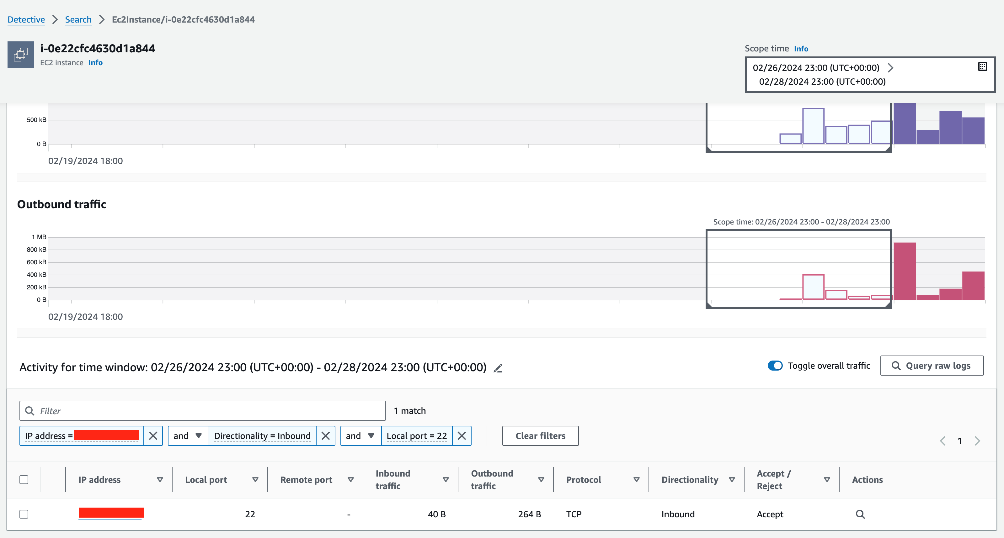
Let’s say you want to review S3 API calls with access denied error messages for one of your developers who uses a role called DevOps. You can update, in the HTML report, the input fields below the principal_arn and eventsource columns to match your lookup.

Then by reviewing the columns principal_arn, eventname, isAssumableBy, and nb_reqs, you learn that the role DevOps is assumable through a SAML provider and performed two GetObject API calls that failed with an access denied error message. By reviewing the sourceipaddress field you discover that the request has been performed from an IP address outside of your network perimeter boundary, you can then advise your developer to perform the API calls again from an expected network.

Data perimeter helper provides several ready-to-use queries and a framework to add new queries based on your data perimeter objectives and needs. See Guidelines to build a new query for detailed instructions.

Clean up

If you followed the configuration steps in this blog only to test the solution, you can clean up your account to avoid recurring charges.

If you used the data perimeter helper deployment templates, use the respective infrastructure as code commands to delete the provisioned resources (for example, for Terraform, terraform destroy).

To delete configured resources manually, follow these steps:

If you created a CloudTrail organization trail:
- Navigate to the CloudTrail console, select the trail your created, and choose Delete.
- Navigate to the Amazon S3 console and delete the S3 bucket you created to store CloudTrail logs from all accounts.
If you created an Athena table:
- Navigate to the Athena console and select Query editor in the left navigation panel.
- Run the following SQL query by replacing <TABLE_NAME> with the name of the created table:
```
DROP TABLE <TABLE_NAME>
```
If you created an AWS Config aggregator:
- Navigate to the AWS Config console and select Aggregators in the left navigation panel.
- Select the created aggregator and select Delete from the Actions drop-down list.
If you installed data perimeter helper:
- Follow the uninstallation steps in the data perimeter helper README file.

Conclusion

In this blog post, we reviewed how you can analyze access activity in your organization by using the CloudTrail logs to evaluate impact of your data perimeter controls and perform troubleshooting. We discussed how the log events data can be enriched using resource configuration information from AWS Config to streamline your analysis. Finally, we introduced the open source tool, data perimeter helper, that provides a set of data perimeter tailored queries to speed up your review process and a framework to create new queries.

For additional learning opportunities, see the Data perimeters on AWS page, which provides additional material such as a data perimeter workshop, blog posts, whitepapers, and webinar sessions.

If you have feedback about this post, submit comments in the Comments section below. If you have questions about this post, start a new thread on the AWS Security, Identity, and Compliance re:Post or contact AWS Support.

Want more AWS Security news? Follow us on X.

Simplify data lake access control for your enterprise users with trusted identity propagation in AWS IAM Identity Center, AWS Lake Formation, and Amazon S3 Access Grants

2024-05-29 Shoukat Ghouse

Post Syndicated from Shoukat Ghouse original https://aws.amazon.com/blogs/big-data/simplify-data-lake-access-control-for-your-enterprise-users-with-trusted-identity-propagation-in-aws-iam-identity-center-aws-lake-formation-and-amazon-s3-access-grants/

Many organizations use external identity providers (IdPs) such as Okta or Microsoft Azure Active Directory to manage their enterprise user identities. These users interact with and run analytical queries across AWS analytics services. To enable them to use the AWS services, their identities from the external IdP are mapped to AWS Identity and Access Management (IAM) roles within AWS, and access policies are applied to these IAM roles by data administrators.

Given the diverse range of services involved, different IAM roles may be required for accessing the data. Consequently, administrators need to manage permissions across multiple roles, a task that can become cumbersome at scale.

To address this challenge, you need a unified solution to simplify data access management using your corporate user identities instead of relying solely on IAM roles. AWS IAM Identity Center offers a solution through its trusted identity propagation feature, which is built upon the OAuth 2.0 authorization framework.

With trusted identity propagation, data access management is anchored to a user’s identity, which can be synchronized to IAM Identity Center from external IdPs using the System for Cross-domain Identity Management (SCIM) protocol. Integrated applications exchange OAuth tokens, and these tokens are propagated across services. This approach empowers administrators to grant access directly based on existing user and group memberships federated from external IdPs, rather than relying on IAM users or roles.

In this post, we showcase the seamless integration of AWS analytics services with trusted identity propagation by presenting an end-to-end architecture for data access flows.

Solution overview

Let’s consider a fictional company, OkTank. OkTank has multiple user personas that use a variety of AWS Analytics services. The user identities are managed externally in an external IdP: Okta. User1 is a Data Analyst and uses the Amazon Athena query editor to query AWS Glue Data Catalog tables with data stored in Amazon Simple Storage Service (Amazon S3). User2 is a Data Engineer and uses Amazon EMR Studio notebooks to query Data Catalog tables and also query raw data stored in Amazon S3 that is not yet cataloged to the Data Catalog. User3 is a Business Analyst who needs to query data stored in Amazon Redshift tables using the Amazon Redshift Query Editor v2. Additionally, this user builds Amazon QuickSight visualizations for the data in Redshift tables.

OkTank wants to simplify governance by centralizing data access control for their variety of data sources, user identities, and tools. They also want to define permissions directly on their corporate user or group identities from Okta instead of creating IAM roles for each user and group and managing access on the IAM role. In addition, for their audit requirements, they need the capability to map data access to the corporate identity of users within Okta for enhanced tracking and accountability.

To achieve these goals, we use trusted identity propagation with the aforementioned services and use AWS Lake Formation and Amazon S3 Access Grants for access controls. We use Lake Formation to centrally manage permissions to the Data Catalog tables and Redshift tables shared with Redshift datashares. In our scenario, we use S3 Access Grants for granting permission for the Athena query result location. Additionally, we show how to access a raw data bucket governed by S3 Access Grants with an EMR notebook.

Data access is audited with AWS CloudTrail and can be queried with AWS CloudTrail Lake. This architecture showcases the versatility and effectiveness of AWS analytics services in enabling efficient and secure data analysis workflows across different use cases and user personas.

We use Okta as the external IdP, but you can also use other IdPs like Microsoft Azure Active Directory. Users and groups from Okta are synced to IAM Identity Center. In this post, we have three groups, as shown in the following diagram.

User1 needs to query a Data Catalog table with data stored in Amazon S3. The S3 location is secured and managed by Lake Formation. The user connects to an IAM Identity Center enabled Athena workgroup using the Athena query editor with EMR Studio. The IAM Identity Center enabled Athena workgroups need to be secured with S3 Access Grants permissions for the Athena query results location. With this feature, you can also enable the creation of identity-based query result locations that are governed by S3 Access Grants. These user identity-based S3 prefixes let users in an Athena workgroup keep their query results isolated from other users in the same workgroup. The following diagram illustrates this architecture.

User2 needs to query the same Data Catalog table as User1. This table is governed using Lake Formation permissions. Additionally, the user needs to access raw data in another S3 bucket that isn’t cataloged to the Data Catalog and is controlled using S3 Access Grants; in the following diagram, this is shown as S3 Data Location-2.

The user uses an EMR Studio notebook to run Spark queries on an EMR cluster. The EMR cluster uses a security configuration that integrates with IAM Identity Center for authentication and uses Lake Formation for authorization. The EMR cluster is also enabled for S3 Access Grants. With this kind of hybrid access management, you can use Lake Formation to centrally manage permissions for your datasets cataloged to the Data Catalog and use S3 Access Grants to centrally manage access to your raw data that is not yet cataloged to the Data Catalog. This gives you flexibility to access data managed by either of the access control mechanisms from the same notebook.

User3 uses the Redshift Query Editor V2 to query a Redshift table. The user also accesses the same table with QuickSight. For our demo, we use a single user persona for simplicity, but in reality, these could be completely different user personas. To enable access control with Lake Formation for Redshift tables, we use data sharing in Lake Formation.

Data access requests by the specific users are logged to CloudTrail. Later in this post, we also briefly touch upon using CloudTrail Lake to query the data access events.

In the following sections, we demonstrate how to build this architecture. We use AWS CloudFormation to provision the resources. AWS CloudFormation lets you model, provision, and manage AWS and third-party resources by treating infrastructure as code. We also use the AWS Command Line Interface (AWS CLI) and AWS Management Console to complete some steps.

The following diagram shows the end-to-end architecture.

Prerequisites

Complete the following prerequisite steps:

Have an AWS account. If you don’t have an account, you can create one.
Have IAM Identity Center set up in a specific AWS Region.
Make sure you use the same Region where you have IAM Identity Center set up throughout the setup and verification steps. In this post, we use the us-east-1 Region.
Have Okta set up with three different groups and users, and enable sync to IAM Identity Center. Refer to Configure SAML and SCIM with Okta and IAM Identity Center for instructions.

After the Okta groups are pushed to IAM Identity Center, you can see the users and groups on the IAM Identity Center console, as shown in the following screenshot. You need the group IDs of the three groups to be passed in the CloudFormation template.

For enabling User2 access using the EMR cluster, you need have an SSL certificate .zip file available in your S3 bucket. You can download the following sample certificate to use in this post. In production use cases, you should create and use your own certificates. You need to reference the bucket name and the certificate bundle .zip file in AWS CloudFormation. The CloudFormation template lets you choose the components you want to provision. If you do not intend to deploy the EMR cluster, you can ignore this step.
Have an administrator user or role to run the CloudFormation stack. The user or role should also be a Lake Formation administrator to grant permissions.

Deploy the CloudFormation stack

The CloudFormation template provided in the post lets you choose the components you want to provision from the solution architecture. In this post, we enable all components, as shown in the following screenshot.

Run the provided CloudFormation stack to create the solution resources. Refer to the following table for a list of important parameters.

Parameter Group	Description	Parameter Name	Expected Value
Choose components to provision.	Choose the components you want to be provisioned.	`DeployAthenaFlow`	Yes/No. If you choose No, you can ignore the parameters in the “Athena Configuration” group.
		`DeployEMRFlow`	Yes/No. If you choose No, you can ignore the parameters in the “EMR Configuration” group.
		`DeployRedshiftQEV2Flow`	Yes/No. If you choose No, you can ignore the parameters in the “Redshift Configuration” group.
		`CreateS3AGInstance`	Yes/No. If you already have an S3 Access Grants instance, choose No. Otherwise, choose Yes to allow the stack create a new S3 Access Grants instance. The S3 Access Grants instance is needed for User1 and User2.
Identity Center Configuration	IAM Identity Center parameters.	`IDCGroup1Id`	Group ID corresponding to Group1 from IAM Identity Center.
		`IDCGroup2Id`	Group ID corresponding to Group2 from IAM Identity Center.
		`IDCGroup3Id`	Group ID corresponding to Group3 from IAM Identity Center.
		`IAMIDCInstanceArn`	IAM Identity Center instance ARN. You can get this from the Settings section of IAM Identity Center.
Redshift Configuration	Redshift parameters. Ignore if you chose `DeployRedshiftQEV2Flow` as No.	`RedshiftServerlessAdminUserName`	Redshift admin user name.
		`RedshiftServerlessAdminPassword`	Redshift admin password.
		`RedshiftServerlessDatabase`	Redshift database to create the tables.
EMR Configuration	EMR parameters. Ignore if you chose parameter `DeployEMRFlow` as No.	`SSlCertsS3BucketName`	Bucket name where you copied the SSL certificates.
EMR Configuration		`SSlCertsZip`	Name of SSL certificates file (my-certs.zip) to use the sample certificate provided in the post.
Athena Configuration	Athena parameters. Ignore if you chose parameter `DeployAthenaFlow` as No.	`IDCUser1Id`	User ID corresponding to User1 from IAM Identity Center.

The CloudFormation stack provisions the following resources:

A VPC with a public and private subnet.
If you chose the Redshift components, it also creates three additional subnets.
S3 buckets for data and Athena query results location storage. It also copies some sample data to the buckets.
EMR Studio with IAM Identity Center integration.
Amazon EMR security configuration with IAM Identity Center integration.
An EMR cluster that uses the EMR security group.
Registers the source S3 bucket with Lake Formation.
An AWS Glue database named oktank_tipblog_temp and a table named customer under the database. The table points to the Amazon S3 location governed by Lake Formation.
Allows external engines to access data in Amazon S3 locations with full table access. This is required for Amazon EMR integration with Lake Formation for trusted identity propagation. As of this writing, Amazon EMR supports table-level access with IAM Identity Center enabled clusters.
An S3 Access Grants instance.
S3 Access Grants for Group1 to the User1 prefix under the Athena query results location bucket.
S3 Access Grants for Group2 to the S3 bucket input and output prefixes. The user has read access to the input prefix and write access to the output prefix under the bucket.
An Amazon Redshift Serverless namespace and workgroup. This workgroup is not integrated with IAM Identity Center; we complete subsequent steps to enable IAM Identity Center for the workgroup.
An AWS Cloud9 integrated development environment (IDE), which we use to run AWS CLI commands during the setup.

Note the stack outputs on the AWS CloudFormation console. You use these values in later steps.

Choose the link for Cloud9URL in the stack output to open the AWS Cloud9 IDE. In AWS Cloud9, go to the Window tab and choose New Terminal to start a new bash terminal.

Set up Lake Formation

You need to enable Lake Formation with IAM Identity Center and enable an EMR application with Lake Formation integration. Complete the following steps:

In the AWS Cloud9 bash terminal, enter the following command to get the Amazon EMR security configuration created by the stack:

aws emr describe-security-configuration --name TIP-EMRSecurityConfig | jq -r '.SecurityConfiguration | fromjson | .AuthenticationConfiguration.IdentityCenterConfiguration.IdCApplicationARN'

Note the value for IdcApplicationARN from the output.
Enter the following command in AWS Cloud9 to enable the Lake Formation integration with IAM Identity Center and add the Amazon EMR security configuration application as a trusted application in Lake Formation. If you already have the IAM Identity Center integration with Lake Formation, sign in to Lake Formation and add the preceding value to the list of applications instead of running the following command and proceed to next step.

aws lakeformation create-lake-formation-identity-center-configuration --catalog-id <Replace with CatalogId value from Cloudformation output> --instance-arn <Replace with IDCInstanceARN value from CloudFormation stack output> --external-filtering Status=ENABLED,AuthorizedTargets=<Replace with IdcApplicationARN value copied in previous step>

After this step, you should see the application on the Lake Formation console.

This completes the initial setup. In subsequent steps, we apply some additional configurations for specific user personas.

Validate user personas

To review the S3 Access Grants created by AWS CloudFormation, open the Amazon S3 console and Access Grants in the navigation pane. Choose the access grant you created to view its details.

The CloudFormation stack created the S3 Access Grants for Group1 for the User1 prefix under the Athena query results location bucket. This allows User1 to access the prefix under in the query results bucket. The stack also created the grants for Group2 for User2 to access the raw data bucket input and output prefixes.

Set up User1 access

Complete the steps in this section to set up User1 access.

Create an IAM Identity Center enabled Athena workgroup

Let’s create the Athena workgroup that will be used by User1.

Enter the following command in the AWS Cloud9 terminal. The command creates an IAM Identity Center integrated Athena workgroup and enables S3 Access Grants for the user-level prefix. These user identity-based S3 prefixes let users in an Athena workgroup keep their query results isolated from other users in the same workgroup. The prefix is automatically created by Athena when the CreateUserLevelPrefix option is enabled. Access to the prefix was granted by the CloudFormation stack.

aws athena create-work-group --cli-input-json '{
"Name": "AthenaIDCWG",
"Configuration": {
"ResultConfiguration": {
"OutputLocation": "<Replace with AthenaResultLocation from CloudFormation stack>"
},
"ExecutionRole": "<Replace with TIPStudioRoleArn from CloudFormation stack>",
"IdentityCenterConfiguration": {
"EnableIdentityCenter": true,
"IdentityCenterInstanceArn": "<Replace with IDCInstanceARN from CloudFormation stack>"
},
"QueryResultsS3AccessGrantsConfiguration": {
"EnableS3AccessGrants": true,
"CreateUserLevelPrefix": true,
"AuthenticationType": "DIRECTORY_IDENTITY"
},
"EnforceWorkGroupConfiguration":true
},
"Description": "Athena Workgroup with IDC integration"
}'

Grant access to User1 on the Athena workgroup

Sign in to the Athena console and grant access to Group1 to the workgroup as shown in the following screenshot. You can grant access to the user (User1) or to the group (Group1). In this post, we grant access to Group1.

Grant access to User1 in Lake Formation

Sign in to the Lake Formation console, choose Data lake permissions in the navigation pane, and grant access to the user group on the database oktank_tipblog_temp and table customer.

With Athena, you can grant access to specific columns and for specific rows with row-level filtering. For this post, we grant column-level access and restrict access to only selected columns for the table.

This completes the access permission setup for User1.

Verify access

Let’s see how User1 uses Athena to analyze the data.

Copy the URL for EMRStudioURL from the CloudFormation stack output.
Open a new browser window and connect to the URL.

You will be redirected to the Okta login page.

Log in with User1.
In the EMR Studio query editor, change the workgroup to AthenaIDCWG and choose Acknowledge.
Run the following query in the query editor:

SELECT * FROM "oktank_tipblog_temp"."customer" limit 10;

You can see that the user is only able to access the columns for which permissions were previously granted in Lake Formation. This completes the access flow verification for User1.

Set up User2 access

User2 accesses the table using an EMR Studio notebook. Note the current considerations for EMR with IAM Identity Center integrations.

Complete the steps in this section to set up User2 access.

Grant Lake Formation permissions to User2

Sign in to the Lake Formation console and grant access to Group2 on the table, similar to the steps you followed earlier for User1. Also grant Describe permission on the default database to Group2, as shown in the following screenshot.

Create an EMR Studio Workspace

Next, User2 creates an EMR Studio Workspace.

Copy the URL for EMR Studio from the EMRStudioURL value from the CloudFormation stack output.
Log in to EMR Studio as User2 on the Okta login page.
Create a Workspace, giving it a name and leaving all other options as default.

This will open a JupyterLab notebook in a new window.

Connect to the EMR Studio notebook

In the Compute pane of the notebook, select the EMR cluster (named EMRWithTIP) created by the CloudFormation stack to attach to it. After the notebook is attached to the cluster, choose the PySpark kernel to run Spark queries.

Verify access

Enter the following query in the notebook to read from the customer table:

spark.sql("select * from oktank_tipblog_temp.customer").show()

The user access works as expected based on the Lake Formation grants you provided earlier.

Run the following Spark query in the notebook to read data from the raw bucket. Access to this bucket is controlled by S3 Access Grants.

spark.read.option("header",True).csv("s3://tip-blog-s3-s3ag/input/*").show()

Let’s write this data to the same bucket and input prefix. This should fail because you only granted read access to the input prefix with S3 Access Grants.

spark.read.option("header",True).csv("s3://tip-blog-s3-s3ag/input/*").write.mode("overwrite").parquet("s3://tip-blog-s3-s3ag/input/")

The user has access to the output prefix under the bucket. Change the query to write to the output prefix:

spark.read.option("header",True).csv("s3://tip-blog-s3-s3ag/input/*").write.mode("overwrite").parquet("s3://tip-blog-s3-s3ag/output/test.part")

The write should now be successful.

We have now seen the data access controls and access flows for User1 and User2.

Set up User3 access

Following the target architecture in our post, Group3 users use the Redshift Query Editor v2 to query the Redshift tables.

Complete the steps in this section to set up access for User3.

Enable Redshift Query Editor v2 console access for User3

Complete the following steps:

On the IAM Identity Center console, create a custom permission set and attach the following policies:
1. AWS managed policy AmazonRedshiftQueryEditorV2ReadSharing.
2. Customer managed policy redshift-idc-policy-tip. This policy is already created by the CloudFormation stack, so you don’t have to create it.
Provide a name (tip-blog-qe-v2-permission-set) to the permission set.
Set the relay state as https://<region-id>.console.aws.amazon.com/sqlworkbench/home (for example, https://us-east-1.console.aws.amazon.com/sqlworkbench/home).
Choose Create.
Assign Group3 to the account in IAM Identity Center, select the permission set you created, and choose Submit.

Create the Redshift IAM Identity Center application

Enter the following in the AWS Cloud9 terminal:

aws redshift create-redshift-idc-application \
--idc-instance-arn '<Replace with IDCInstanceARN value from CloudFormation Output>' \
--redshift-idc-application-name 'redshift-iad-<Replace with CatalogId value from CloudFormation output>-tip-blog-1' \
--identity-namespace 'tipblogawsidc' \
--idc-display-name 'TIPBlog_AWSIDC' \
--iam-role-arn '<Replace with TIPRedshiftRoleArn value from CloudFormation output>' \
--service-integrations '[
  {
    "LakeFormation": [
    {
     "LakeFormationQuery": {
     "Authorization": "Enabled"
    }
   }
  ]
 }
]'

Enter the following command to get the application details:

aws redshift describe-redshift-idc-applications --output json

Keep a note of the IdcManagedApplicationArn, IdcDisplayName, and IdentityNamespace values in the output for the application with IdcDisplayName TIPBlog_AWSIDC. You need these values in the next step.

Enable the Redshift Query Editor v2 for the Redshift IAM Identity Center application

Complete the following steps:

On the Amazon Redshift console, choose IAM Identity Center connections in the navigation pane.
Choose the application you created.
Choose Edit.
Select Enable Query Editor v2 application and choose Save changes.
On the Groups tab, choose Add or assign groups.
Assign Group3 to the application.

The Redshift IAM Identity Center connection is now set up.

Enable the Redshift Serverless namespace and workgroup with IAM Identity Center

The CloudFormation stack you deployed created a serverless namespace and workgroup. However, they’re not enabled with IAM Identity Center. To enable with IAM Identity Center, complete the following steps. You can get the namespace name from the RedshiftNamespace value of the CloudFormation stack output.

On the Amazon Redshift Serverless dashboard console, navigate to the namespace you created.
Choose Query Data to open Query Editor v2.
Choose the options menu (three dots) and choose Create connections for the workgroup redshift-idc-wg-tipblog.
Choose Other ways to connect and then Database user name and password.
Use the credentials you provided for the Redshift admin user name and password parameters when deploying the CloudFormation stack and create the connection.

Create resources using the Redshift Query Editor v2

You now enter a series of commands in the query editor with the database admin user.

Create an IdP for the Redshift IAM Identity Center application:

CREATE IDENTITY PROVIDER "TIPBlog_AWSIDC" TYPE AWSIDC
NAMESPACE 'tipblogawsidc'
APPLICATION_ARN '<Replace with IdcManagedApplicationArn value you copied earlier in Cloud9>'
IAM_ROLE '<Replace with TIPRedshiftRoleArn value from CloudFormation output>';

Enter the following command to check the IdP you added previously:

SELECT * FROM svv_identity_providers;

Next, you grant permissions to the IAM Identity Center user.

Create a role in Redshift. This role should correspond to the group in IAM Identity Center to which you intend to provide the permissions (Group3 in this post). The role should follow the format <namespace>:<GroupNameinIDC>.

Create role "tipblogawsidc:Group3";

Run the following command to see role you created. The external_id corresponds to the group ID value for Group3 in IAM Identity Center.

Select * from svv_roles where role_name = 'tipblogawsidc:Group3';

Create a sample table to use to verify access for the Group3 user:

CREATE TABLE IF NOT EXISTS revenue
(
account INTEGER ENCODE az64
,customer VARCHAR(20) ENCODE lzo
,salesamt NUMERIC(18,0) ENCODE az64
)
DISTSTYLE AUTO
;

insert into revenue values (10001, 'ABC Company', 12000);
insert into revenue values (10002, 'Tech Logistics', 175400);

Grant access to the user on the schema:

-- Grant usage on schema
grant usage on schema public to role "tipblogawsidc:Group3";

To create a datashare and add the preceding table to the datashare, enter the following statements:

CREATE DATASHARE demo_datashare;
ALTER DATASHARE demo_datashare ADD SCHEMA public;
ALTER DATASHARE demo_datashare ADD TABLE revenue;

Grant usage on the datashare to the account using the Data Catalog:

GRANT USAGE ON DATASHARE demo_datashare TO ACCOUNT '<Replace with CatalogId from Cloud Formation Output>' via DATA CATALOG;

Authorize the datashare

For this post, we use the AWS CLI to authorize the datashare. You can also do it from the Amazon Redshift console.

Enter the following command in the AWS Cloud9 IDE to describe the datashare you created and note the value of DataShareArn and ConsumerIdentifier to use in subsequent steps:

aws redshift describe-data-shares

Enter the following command in the AWS Cloud9 IDE to the authorize the datashare:

aws redshift authorize-data-share --data-share-arn <Replace with DataShareArn value copied from earlier command’s output> --consumer-identifier <Replace with ConsumerIdentifier value copied from earlier command’s output >

Accept the datashare in Lake Formation

Next, accept the datashare in Lake Formation.

On the Lake Formation console, choose Data sharing in the navigation pane.
In the Invitations section, select the datashare invitation that is pending acceptance.
Choose Review invitation and accept the datashare.
Provide a database name (tip-blog-redshift-ds-db), which will be created in the Data Catalog by Lake Formation.
Choose Skip to Review and Create and create the database.

Grant permissions in Lake Formation

Complete the following steps:

On the Lake Formation console, choose Data lake permissions in the navigation pane.
Choose Grant and in the Principals section, choose User3 to grant permissions with the IAM Identity Center-new option. Refer to the Lake Formation access grants steps performed for User1 and User2 if needed.
Choose the database (tip-blog-redshift-ds-db) you created earlier and the table public.revenue, which you created in the Redshift Query Editor v2.
For Table permissions¸ select Select.
For Data permissions¸ select Column-based access and select the account and salesamt columns.
Choose Grant.

Mount the AWS Glue database to Amazon Redshift

As the last step in the setup, mount the AWS Glue database to Amazon Redshift. In the Query Editor v2, enter the following statements:

create external schema if not exists tipblog_datashare_idc_schema from DATA CATALOG DATABASE 'tip-blog-redshift-ds-db' catalog_id '<Replace with CatalogId from CloudFormation output>';

grant usage on schema tipblog_datashare_idc_schema to role "tipblogawsidc:Group3";

grant select on all tables in schema tipblog_datashare_idc_schema to role "tipblogawsidc:Group3";

You are now done with the required setup and permissions for User3 on the Redshift table.

Verify access

To verify access, complete the following steps:

Get the AWS access portal URL from the IAM Identity Center Settings section.
Open a different browser and enter the access portal URL.

This will redirect you to your Okta login page.

If you’re using private or incognito mode for testing this, you may need to enable third-party cookies.

Choose the options menu (three dots) and choose Edit connection for the redshift-idc-wg-tipblog workgroup.
Use IAM Identity Center in the pop-up window and choose Continue.

If you get an error with the message “Redshift serverless cluster is auto paused,” switch to the other browser with admin credentials and run any sample queries to un-pause the cluster. Then switch back to this browser and continue the next steps.

Run the following query to access the table:

SELECT * FROM "dev"."tipblog_datashare_idc_schema"."public.revenue";

You can only see the two columns due to the access grants you provided in Lake Formation earlier.

This completes configuring User3 access to the Redshift table.

Set up QuickSight for User3

Let’s now set up QuickSight and verify access for User3. We already granted access to User3 to the Redshift table in earlier steps.

Create a new IAM Identity Center enabled QuickSight account. Refer to Simplify business intelligence identity management with Amazon QuickSight and AWS IAM Identity Center for guidance.
Choose Group3 for the author and reader for this post.
For IAM Role, choose the IAM role matching the RoleQuickSight value from the CloudFormation stack output.

Next, you add a VPC connection to QuickSight to access the Redshift Serverless namespace you created earlier.

On the QuickSight console, manage your VPC connections.
Choose Add VPC connection.
For VPC connection name, enter a name.
For VPC ID, enter the value for VPCId from the CloudFormation stack output.
For Execution role, choose the value for RoleQuickSight from the CloudFormation stack output.
For Security Group IDs, choose the security group for QSSecurityGroup from the CloudFormation stack output.

Wait for the VPC connection to be AVAILABLE.
Enter the following command in AWS Cloud9 to enable QuickSight with Amazon Redshift for trusted identity propagation:

aws quicksight update-identity-propagation-config --aws-account-id "<Replace with CatalogId from CloudFormation output>" --service "REDSHIFT" --authorized-targets "< Replace with IdcManagedApplicationArn value from output of aws redshift describe-redshift-idc-applications --output json which you copied earlier>"

Verify User3 access with QuickSight

Complete the following steps:

Sign in to the QuickSight console as User3 in a different browser.
On the Okta sign-in page, sign in as User 3.
Create a new dataset with Amazon Redshift as the data source.
Choose the VPC connection you created above for Connection Type.
Provide the Redshift server (the RedshiftSrverlessWorkgroup value from the CloudFormation stack output), port (5439 in this post), and database name (dev in this post).
Under Authentication method, select Single sign-on.
Choose Validate, then choose Create data source.

If you encounter an issue with validating using single sign-on, switch to Database username and password for Authentication method, validate with any dummy user and password, and then switch back to validate using single sign-on and proceed to the next step. Also check that the Redshift serverless cluster is not auto-paused as mentioned earlier in Redshift access verification.

Choose the schema you created earlier (tipblog_datashare_idc_schema) and the table public.revenue
Choose Select to create your dataset.

You should now be able to visualize the data in QuickSight. You are only able to only see the account and salesamt columns from the table because of the access permissions you granted earlier with Lake Formation.

This finishes all the steps for setting up trusted identity propagation.

Audit data access

Let’s see how we can audit the data access with the different users.

Access requests are logged to CloudTrail. The IAM Identity Center user ID is logged under the onBehalfOf tag in the CloudTrail event. The following screenshot shows the GetDataAccess event generated by Lake Formation. You can view the CloudTrail event history and filter by event name GetDataAccess to view similar events in your account.

You can see the userId corresponds to User2.

You can run the following commands in AWS Cloud9 to confirm this.

Get the identity store ID:

aws sso-admin describe-instance --instance-arn <Replace with your instance arn value> | jq -r '.IdentityStoreId'

Describe the user in the identity store:

aws identitystore describe-user --identity-store-id <Replace with output of above command> --user-id <User Id from above screenshot>

One way to query the CloudTrail log events is by using CloudTrail Lake. Set up the event data store (refer to the following instructions) and rerun the queries for User1, User2, and User3. You can query the access events using CloudTrail Lake with the following sample query:

SELECT eventTime,userIdentity.onBehalfOf.userid AS idcUserId,requestParameters as accessInfo, serviceEventDetails
FROM 04d81d04-753f-42e0-a31f-2810659d9c27
WHERE userIdentity.arn IS NOT NULL AND eventName='BatchGetTable' or eventName='GetDataAccess' or eventName='CreateDataSet'
order by eventTime DESC

The following screenshot shows an example of the detailed results with audit explanations.

Clean up

To avoid incurring further charges, delete the CloudFormation stack. Before you delete the CloudFormation stack, delete all the resources you created using the console or AWS CLI:

Manually delete any EMR Studio Workspaces you created with User2.
Delete the Athena workgroup created as part of the User1 setup.
Delete the QuickSight VPC connection you created.
Delete the Redshift IAM Identity Center connection.
Deregister IAM Identity Center from S3 Access Grants.
Delete the CloudFormation stack.
Manually delete the VPC created by AWS CloudFormation.

Conclusion

In this post, we delved into the trusted identity propagation feature of AWS Identity Center alongside various AWS Analytics services, demonstrating its utility in managing permissions using corporate user or group identities rather than IAM roles. We examined diverse user personas utilizing interactive tools like Athena, EMR Studio notebooks, Redshift Query Editor V2, and QuickSight, all centralized under Lake Formation for streamlined permission management. Additionally, we explored S3 Access Grants for S3 bucket access management, and concluded with insights into auditing through CloudTrail events and CloudTrail Lake for a comprehensive overview of user data access.

For further reading, refer to the following resources:

About the Author

Shoukat Ghouse is a Senior Big Data Specialist Solutions Architect at AWS. He helps customers around the world build robust, efficient and scalable data platforms on AWS leveraging AWS analytics services like AWS Glue, AWS Lake Formation, Amazon Athena and Amazon EMR.

How to enable one-click unsubscribe email with Amazon Pinpoint

2024-05-29 Zip Zieper

Post Syndicated from Zip Zieper original https://aws.amazon.com/blogs/messaging-and-targeting/how-to-enable-one-click-unsubscribe-email-with-amazon-pinpoint/

Amazon Pinpoint customers who use campaigns, journeys, or the SendMesages API to send more than 5,000 marketing email messages per day are considered “bulk senders”. If your organization meets this criteria, you are now subject to new requirements that were recently established by Google, Yahoo and other large ISPs/ESPs. These providers have mandated these requirements to help protect their user’s inboxes. Detailed information about these requirements is provided in the Amazon Simple Email Service (SES) bulk sender updates blog post.

Per these new requirements, Pinpoint customers that send marketing email messages in bulk must meet all of these criteria:

Fully authenticate their email sending domains with SPF, DKIM and DMARC. See this blog.
Provide a clearly visible unsubscribe link in the body &/or footer of each message.
Enable the “List-Unsubscribe” and “List-Unsubscribe-Post” one-click unsubscribe (the subbect of this blog post). You can learn more about these headers and how they are used in SES in this related blog post.
Honor all unsubscribe POST requests within 48 hours, after which time you shouldn’t be sending emails to the now unsubscribed end-user.
Actively monitor spam complaint rates, and take the steps needed to ensure these rates remain below acceptable levels as defined by the ESPs.

This blog post provides Pinpoint customers with the steps necessary to enable the one-click unsubscribe button via email headers for “List-Unsubscribe” and “List-Unsubscribe-Post” as defined by RFC 2369 and RFC 8058.

Unsubscribe Process Overview

Pinpoint now supports the inclusion of the “List-Unsubscribe” and “List-Unsubscribe-Post” email headers that enable compatible email client apps to render a one-click unsubscribe button when displaying emails from a subscription list. When you include these headers in the emails you send by Pinpoint, those end-users who want to unsubscribe from your emails can do so by simply clicking the unsubscribe button in their email app (see image). Once pressed, the unsubscribe button fires off a POST request to the URL you have defined in the “List-Unsubscribe” header.

You, the Pinpoint customer, are responsible for defining the “List-Unsubscribe” and “List-Unsubscribe-Post” headers, as well as supplying the system or process invoked by the “List-Unsubscribe” and “List-Unsubscribe-Post” email headers. Your system or process must, when activated by the unsubscribe action, update that end-user’s preferences accordingly so that within 48 hours, any end-user who unsubscribes will no longer receive unwanted emails.

If you only use Pinpoint’s campaigns and journeys, you may elect to use the Pinpoint endpoint’s OptOut attribute to store the user’s unsubscribe preferences. Possible values for OptOut are: ALL, the user has opted out and doesn’t want to receive any messages; and, NONE, the user hasn’t opted out and wants to receive all messages. It is important to note, however, that the SendMessages API ignores the Pinpoint endpoint’s OptOut attribute.

If you do not currently offer your recipients the option to unsubscribe to unwanted emails, you will need to develop & deploy a system or process to receive end-user unsubscribe requests to be in compliance with these new requirements. An example solution with sample code to processes email opt-out requests for Pinpoint can be found here. You can read more about this example in this blog post.

REQUIRED: Update the SES IAM role used by Pinpoint

Because Pinpoint uses SES resources for sending email messages, when using campaigns or journeys you must now create (or update) an IAM Orchestration sending role to grant Pinpoint service access to your SES resources. This allows Pinpoint to send emails via SES. To add or update the IAM role, follow the steps outlined in the Pinpoint documentation.

Note – If you are sending emails directly via the SendMesage, API you do not need an IAM Orchestration sending role, but you must have permissions for ses:SendEmail and ses:SendRawEmail.

Add easy unsubscribe email headers:

The steps you need to take to enable one-click unsubscribe in your Pinpoint emails depends on how you send emails, and whether or not you use templates, as shown below:

Decision tree for adding headers

Use `SendMessages` with the AWS SDK or CLI

Using the AWS CLI: add headers for the “List-Unsubscribe” and “List-Unsubscribe-post” as shown in the example below:

aws pinpoint send-messages \
--region us-east-1 \
--application-id ce796be37f32f178af652b26eexample \
--message-request '{
    "Addresses": {
        "[email protected]": {"ChannelType": "EMAIL"},
    },
    "MessageConfiguration": {
        "EmailMessage": {
            "SimpleEmail": {
                "Subject": {"Data":"URL with easy unsubscribe headers", "Charset":"UTF-8"},
                "TextPart": {"Data":"with headers list-unsubscribe and list-unsubscribe-post.\n\nUnsubscribe: <https://www.example.com/preferences>", "Charset":"UTF-8"},
                "HtmlPart": {"Data":"<html><body>with headers list-unsubscribe and list-unsubscribe-post<br><br><a ses:tags=\"unsubscribeLinkTag:optout\" href=\"https://example.com/?address=x&topic=x\">Unsubscribe</a></body></html>", "Charset":"UTF-8"},
                "Headers": [
                    {"Name":"List-Unsubscribe", "Value":"<https://example.com/?address=x&topic=x>, <mailto: [email protected]?subject=TopicUnsubscribe>"},
                    {"Name":"List-Unsubscribe-Post", "Value":"List-Unsubscribe=One-Click"}
                ]
            }
        }
    }
}

Send an email message

Below is an example using the SendMessages API from the AWS SDK for Python (Boto3) that includes the List-Unsubscribe headers. This example assumes that you’ve already installed and updated the SDK for Python (Boto3) to the latest version available. For more information, see Quickstart in the AWS SDK for Python (Boto3) API Reference.

import logging  # Logging library to log messages
import boto3  # AWS SDK for Python
from botocore.exceptions import ClientError  # Exception handling for boto3
import hashlib  # Library to generate unique hashes

# Configure logger
logger = logging.getLogger(__name__)

# Define constants
CHARSET = "UTF-8"
REGION = 'us-east-1'

def send_email_message(
    pinpoint_client,
    project_id, 
    sender,
    to_addresses,
    subject,
    html_message,
    text_message,
):
    """
    Sends an email message with HTML and plain text versions.

    :param pinpoint_client: A Boto3 Pinpoint client.
    :param project_id: The Amazon Pinpoint project ID to use when you send this message.
    :param sender: The "From" address. This address must be verified in
                   Amazon Pinpoint in the AWS Region you're using to send email.
    :param to_addresses: The list of addresses on the "To" line. If your Amazon Pinpoint account
                         is in the sandbox, these addresses must be verified.
    :param subject: The subject line of the email.
    :param html_message: The HTML content of the email.
    :param text_message: The plain text content of the email.
    :return: A dict of to_addresses and their message IDs.
    """
    try:
        # Create a dictionary of addresses with unique unsubscribe URLs
        # The addresses are encoded using the SHA256 hashing algorithm from the hashlib library
        # to create a unique and obfuscated unsubscribe URL for each recipient. This ensures
        # that the unsubscribe link is specific to each individual recipient, preventing
        # potential abuse or unauthorized unsubscribes. The hashed value is appended to the
        # base unsubscribe URL, allowing the email service to identify the intended recipient
        # when the unsubscribe link is clicked, while also protecting the recipient's personal
        # email address from being directly exposed in the URL.
        addresses = {
            address: {
                "ChannelType": "EMAIL",
                "Substitutions": {
                    "unsubscribeURL": [f"https://example.com/unsub/{hashlib.sha256(address.encode()).hexdigest()}"],
                }
            }
            for address in to_addresses
        }
        
        # Send email using Amazon Pinpoint
        response = pinpoint_client.send_messages(
            ApplicationId=project_id,
            MessageRequest={
                "Addresses": addresses,
                "MessageConfiguration": {
                    "EmailMessage": {
                        "FromAddress": sender,
                        "SimpleEmail": {
                            "Subject": {"Charset": CHARSET, "Data": subject},
                            "HtmlPart": {"Charset": CHARSET, "Data": html_message},
                            "TextPart": {"Charset": CHARSET, "Data": text_message},
                            "Headers": [
                                {"Name": "List-Unsubscribe", "Value": "{{unsubscribeURL}}"},
                                {"Name": "List-Unsubscribe-Post", "Value": "List-Unsubscribe=One-Click"}
                            ],
                        },
                    }
                }
            }
        )
    except ClientError as e:
        # Log exception if sending email fails
        logger.exception("Couldn't send email: %s", e)
        raise
    else:
        # Return a dictionary of addresses and their respective message IDs
        return {
            address: message["MessageId"] 
        for address, message in response["MessageResponse"]["Result"].items()
        }

def main():
    # Sample data for sending email
    project_id = "ce796be37f32f178af652b26eexample"  # Amazon Pinpoint project ID
    sender = "[email protected]"  # Verified sender email address
    to_addresses = ["[email protected]", "[email protected]", "[email protected]"]  # Recipient email addresses
    subject = "Amazon Pinpoint Unsubscribe Headers Test (SDK for Python (Boto3))"  # Email subject
    text_message = """Amazon Pinpoint Test (SDK for Python)
    -------------------------------------
    This email was sent with Amazon Pinpoint using the AWS SDK for Python (Boto3).
    For more information, see https://aws.amazon.com/sdk-for-python/
                """  # Plain text message
    html_message = """<html>
    <head></head>
    <body>
      <h1>Amazon Pinpoint Test (SDK for Python (Boto3)</h1>
      <p>This email was sent with
        <a href='https://aws.amazon.com/pinpoint/'>Amazon Pinpoint</a> using the
        <a href='https://aws.amazon.com/sdk-for-python/'>
          AWS SDK for Python (Boto3)</a>.</p>
    </body>
    </html>
                """  # HTML message

    # Create a Pinpoint client
    pinpoint_client = boto3.client("pinpoint", region_name=REGION)

    print("Sending email.")
    # Send email and print message IDs
    try:
        message_ids = send_email_message(
            pinpoint_client,
            project_id,
            sender,
            to_addresses,
            subject,
            html_message,
            text_message,
        )
        print(f"Message sent! Message IDs: {message_ids}")
    except ClientError as e:
        print(f"Failed to send messages: {e}")

# Entry point of the script
if __name__ == "__main__":
    logging.basicConfig(level=logging.INFO)  # Set logging level to INFO
    main()

Send an email message with an existing email template.

If you use message templates to send email messages via AWS SDK for Python (Boto3), you can add the headers for List-Unsubscribe and List-Unsubscribe-post into the template, and then fill those variables with unique values per recipient, as shown in the code example below. First, you would create the template via the UI and add the Headers in the new fields as shown in the image below.

Or you can create the template, with headers, via the AWS CLI:

aws pinpoint create-email-template --template-name MyEmailTemplate \
--email-template-request '{
    "Subject": "Amazon Pinpoint Unsubscribe Headers Test using email template",
    "TextPart": "Hello, welcome to our service. We are glad to have you with us. If you wish to unsubscribe, click here: {{unsubscribeURL}}",
    "HtmlPart": "<html><body><h1>Hello, welcome to our service</h1><p>We are glad to have you with us.</p><p>If you wish to unsubscribe, click <a href=\"{{unsubscribeURL}}\">here</a>.</p></body></html>",
    "DefaultSubstitutions": "{\"unsubscribeURL\": \"https://example.com/unsubscribe\"}",
    "Headers": [
            {"Name": "List-Unsubscribe","Value": "{{unsubscribeURL}}"},
            {"Name": "List-Unsubscribe-Post","Value": "List-Unsubscribe=One-Click"}
        ]
  }

In this next example, we are including the use of a secret Hash key. By using this format, the unsubscribe URL will include the Pinpoint project ID and a hashed value of the email address combined with the secret key. This provides a more secure and customized unsubscribe experience for the recipients.

import logging  # Logging library to log messages
import boto3  # AWS SDK for Python
from botocore.exceptions import ClientError  # Exception handling for boto3
import hashlib  # Library to generate unique hashes

# Configure logger
logger = logging.getLogger(__name__)

# Define constants
REGION = 'us-east-1'
HASH_SECRET_KEY = "my_secret_key"  # Replace with your secret key

def send_templated_email_message(
    pinpoint_client, 
    project_id, 
    sender, 
    to_addresses, 
    template_name, 
    template_version
):
    """
    Sends an email message with HTML and plain text versions.

    :param pinpoint_client: A Boto3 Pinpoint client.
    :param project_id: The Amazon Pinpoint project ID to use when you send this message.
    :param sender: The "From" address. This address must be verified in
                   Amazon Pinpoint in the AWS Region you're using to send email.
    :param to_addresses: The list of addresses on the "To" line. If your Amazon Pinpoint account
                         is in the sandbox, these addresses must be verified.
    :param template_name: The name of the email template to use when sending the message.
    :param template_version: The version number of the message template.

    :return: A dict of to_addresses and their message IDs.
    """
    try:
        # Create a dictionary of addresses with unique unsubscribe URLs
        # The addresses are encoded using the SHA256 hashing algorithm from the hashlib library
        # to create a unique and obfuscated unsubscribe URL for each recipient. This ensures
        # that the unsubscribe link is specific to each individual recipient, preventing
        # potential abuse or unauthorized unsubscribes. The hashed value is appended to the
        # base unsubscribe URL, allowing the email service to identify the intended recipient
        # when the unsubscribe link is clicked, while also protecting the recipient's personal
        # email address from being directly exposed in the URL.
        addresses = {
            address: {
                "ChannelType": "EMAIL",
                "Substitutions": {
                    "unsubscribeURL": [
                        f"https://www.example.com/preferences/index.html?pid={project_id}&h={hashlib.sha256((address + HASH_SECRET_KEY).encode()).hexdigest()}"
                    ]
                }
            }
            for address in to_addresses
        }
        # Send templated email using Amazon Pinpoint
        response = pinpoint_client.send_messages(
            ApplicationId=project_id,
            MessageRequest={
                "Addresses": addresses,
                "MessageConfiguration": {"EmailMessage": {"FromAddress": sender}},
                "TemplateConfiguration": {
                    "EmailTemplate": {
                        "Name": template_name,
                        "Version": template_version,
                    },
                },
            },
        )
    except ClientError as e:
        # Log exception if sending email fails
        logger.exception("Couldn't send email: %s", e)
        raise
    else:
        # Return a dictionary of addresses and their respective message IDs
        return {
            address: message["MessageId"] 
        for address, message in response["MessageResponse"]["Result"].items()
        }


def main():
    # Sample data for sending email
    project_id = "ce796be37f32f178af652b26eexample"  # Amazon Pinpoint project ID
    sender = "[email protected]"  # Verified sender email address
    to_addresses = ["[email protected]", "[email protected]", "[email protected]"]  # Recipient email addresses
    template_name = "MyEmailTemplate"
    template_version = "1"

    # Create a Pinpoint client
    pinpoint_client = boto3.client("pinpoint", region_name=REGION)
    print("Sending email.")
    # Send email and print message IDs
    try:
        message_ids = send_templated_email_message(
            pinpoint_client,
            project_id,
            sender,
            to_addresses,
            template_name,
            template_version,
        ),
        print(f"Message sent! Message IDs: {message_ids}"),
    except ClientError as e:
        print(f"Failed to send messages: {e}")
        
# Entry point of the script
if __name__ == "__main__":
    logging.basicConfig(level=logging.INFO)  # Set logging level to INFO
    main()

Pinpoint Campaigns via API (runtime).

If you send emails using Pinpoint campaigns via the API call (runtime), you can add the headers as described below:

"EmailMessage":{
   "Body": "string", 
   "Title": "string", 
   "HtmlBody": "string", 
    "FromAddress": "string",
   "Headers": [
        {
            "Name": "string", 
            "Value": "string"
        } 
   ]
}

Pinpoint Campaigns & Journeys via AWS Console.

The Pinpoint console enables you to create (or update) your email templates to add support for up to 15 different headers, including the “List-Unsubscribe” and “List-Unsubscribe-Post” headers. Simply open , or create a new, template in the Pinpoint console, scroll to the bottom of the visual message editor, expand the Headers option, and insert the header names and values. Note that if you only use the console UI to send your Campaigns and Journeys, you can store the encoded List-Unsubscribe URL as an attribute in the endpoint, then use that attribute as the value as shown below:

Conclusion.

In this blog, we provide Pinpoint customers with the information and guidance needed to enable a one-click unsubscribe link in their recipients’ compatible email apps via “List-Unsubscribe” and “List-Unsubscribe-Post” email headers. Following this guidance, in conjunction with properly authenticating your email sending domains and monitoring / keeping spam complaints below prescribed thresholds will help ensure high rates of Pinpoint email deliverability.

We welcome your comments on this post below. For additional information, refer to these resources, or contact your AWS account team.

Amazon SES bulk sender updates blog post
Amazon SES unsubscribe headers blog post
Pinpoint Preference Center example code
Pinpoint documentation

About the Authors

Zip

Zip is an Amazon Pinpoint and Amazon Simple Email Service Sr. Specialist Solutions Architect at AWS. Outside of work he enjoys time with his family, cooking, mountain biking and plogging.

Darren Roback

Darren is a Senior Solutions Architect with Amazon Web Services based in St. Louis, Missouri. He has a background in Security and Compliance, Serverless Event-Driven Architecture, and Enterprise Architecture. At AWS, Darren partners with customers to help them solve business challenges with AWS technology. Outside of work, Darren enjoys spending time in his shop working on woodworking projects.

Bruno Giorgini

Bruno Giorgini is a Senior Solutions Architect specializing in Pinpoint and SES. With over two decades of experience in the IT industry, Bruno has been dedicated to assisting customers of all sizes in achieving their objectives. When he is not crafting innovative solutions for clients, Bruno enjoys spending quality time with his wife and son, exploring the scenic hiking trails around the SF Bay Area.

Introducing Amazon EMR on EKS with Apache Flink: A scalable, reliable, and efficient data processing platform

2024-05-28 Kinnar Kumar Sen

Post Syndicated from Kinnar Kumar Sen original https://aws.amazon.com/blogs/big-data/introducing-amazon-emr-on-eks-with-apache-flink-a-scalable-reliable-and-efficient-data-processing-platform/

AWS recently announced that Apache Flink is generally available for Amazon EMR on Amazon Elastic Kubernetes Service (EKS). Apache Flink is a scalable, reliable, and efficient data processing framework that handles real-time streaming and batch workloads (but is most commonly used for real-time streaming). Amazon EMR on EKS is a deployment option for Amazon EMR that allows you to run open source big data frameworks such as Apache Spark and Flink on Amazon Elastic Kubernetes Service (Amazon EKS) clusters with the EMR runtime. With the addition of Flink support in EMR on EKS, you can now run your Flink applications on Amazon EKS using the EMR runtime and benefit from both services to deploy, scale, and operate Flink applications more efficiently and securely.

In this post, we introduce the features of EMR on EKS with Apache Flink, discuss their benefits, and highlight how to get started.

EMR on EKS for data workloads

AWS customers deploying large-scale data workloads are adopting the EMR runtime with Amazon EKS as the underlying orchestrator to benefit from complimenting features. This also enables multi-tenancy and allows data engineers and data scientists to focus on building the data applications, and the platform engineering and the site reliability engineering (SRE) team can manage the infrastructure. Some key benefits of Amazon EKS for these customers are:

The AWS-managed control plane, which improves resiliency and removes undifferentiated heavy lifting
Features like multi-tenancy and resource-based access policies (RBAC), which allow you to build cost-efficient platforms and enforce organization-wide governance policies
The extensibility of Kubernetes, which allows you to install open source add-ons (observability, security, notebooks) to meet your specific needs

The EMR runtime offers the following benefits:

Takes care of the undifferentiated heavy lifting of managing installations, configuration, patching, and backups
Simplifies scaling
Optimizes performance and cost
Implements security and compliance by integrating with other AWS services and tools

Benefits of EMR on EKS with Apache Flink

The flexibility to choose instance types, price, and AWS Region and Availability Zone according to the workload specification is often the main driver of reliability, availability, and cost-optimization. Amazon EMR on EKS natively integrates tools and functionalities to enable these—and more.

Integration with existing tools and processes, such as continuous integration and continuous development (CI/CD), observability, and governance policies, helps unify the tools used and decreases the time to launch new services. Many customers already have these tools and processes for their Amazon EKS infrastructure, which you can now easily extend to your Flink applications running on EMR on EKS. If you’re interested in building your Kubernetes and Amazon EKS capabilities, we recommend using EKS Blueprints, which provides a starting place to compose complete EKS clusters that are bootstrapped with the operational software that is needed to deploy and operate workloads.

Another benefit of running Flink applications with Amazon EMR on EKS is improving your applications’ scalability. The volume and complexity of data processed by Flink apps can vary significantly based on factors like the time of the day, day of the week, seasonality, or being tied to a specific marketing campaign or other activity. This volatility makes customers trade off between over-provisioning, which leads to inefficient resource usage and higher costs, or under-provisioning, where you risk missing latency and throughput SLAs or even service outages. When running Flink applications with Amazon EMR on EKS, the Flink auto scaler will increase the applications’ parallelism based on the data being ingested, and Amazon EKS auto scaling with Karpenter or Cluster Autoscaler will scale the underlying capacity required to meet those demands. In addition to scaling up, Amazon EKS can also scale your applications down when the resources aren’t needed so your Flink apps are more cost-efficient.

Running EMR on EKS with Flink allows you to run multiple versions of Flink on the same cluster. With traditional Amazon Elastic Compute Cloud (Amazon EC2) instances, each version of Flink needs to run on its own virtual machine to avoid challenges with resource management or conflicting dependencies and environment variables. However, containerizing Flink applications allows you to isolate versions and avoid conflicting dependencies, and running them on Amazon EKS allows you to use Kubernetes as the unified resource manager. This means that you have the flexibility to choose which version of Flink is best suited for each job, and also improves your agility to upgrade a single job to the next version of Flink rather than having to upgrade an entire cluster, or spin up a dedicated EC2 instance for a different Flink version, which would increase your costs.

Key EMR on EKS differentiations

In this section, we discuss the key EMR on EKS differentiations.

Faster restart of the Flink job during scaling or failure recovery

This is enabled by task local recovery via Amazon Elastic Block Store (Amazon EBS) volumes and fine-grained recovery support in Adaptive Scheduler.

Task local recovery via EBS volumes for TaskManager pods is available with Amazon EMR 6.15.0 and higher. The default overlay mount comes with 10 GB, which is sufficient for jobs with a lower state. Jobs with large states can enable the automatic EBS volume mount option. The TaskManager pods are automatically created and mounted during pod creation and removed during pod deletion.

Fine-grained recovery support in the adaptive scheduler is available with Amazon EMR 6.15.0 and higher. When a task fails during its run, fine-grained recovery restarts only the pipeline-connected component of the failed task, instead of resetting the entire graph, and triggers a complete rerun from the last completed checkpoint, which is more expensive than just rerunning the failed tasks. To enable fine-grained recovery, set the following configurations in your Flink configuration:

jobmanager.execution.failover-strategy: region
restart-strategy: exponential-delay or fixed-delay

Logging and monitoring support with customer managed keys

Monitoring and observability are key constructs of the AWS Well-Architected framework because they help you learn, measure, and adapt to operational changes. You can enable monitoring of launched Flink jobs while using EMR on EKS with Apache Flink. Amazon Managed Service for Prometheus is deployed automatically, if enabled while installing the Flink operator, and it helps analyze Prometheus metrics emitted for the Flink operator, job, and TaskManager.

You can use the Flink UI to monitor health and performance of Flink jobs through a browser using port-forwarding. We have also enabled collection and archival of operator and application logs to Amazon Simple Storage Service (Amazon S3) or Amazon CloudWatch using a FluentD sidecar. This can be enabled through a monitoringConfiguration block in the deployment customer resource definition (CRD):

monitoringConfiguration:
    s3MonitoringConfiguration:
      logUri: S3 BUCKET
      encryptionKeyArn: CMK ARN FOR S3 BUCKET ENCRYPTION
    cloudWatchMonitoringConfiguration:
      logGroupName: LOG GROUP NAME
      logStreamNamePrefix: LOG GROUP STREAM PREFIX
    sideCarResources:
      limits:
        cpuLimit: 500m
        memoryLimit: 250Mi
    containerLogRotationConfiguration:
        rotationSize: 2Gb
        maxFilesToKeep: 10

Cost-optimization using Amazon EC2 Spot Instances

Amazon EC2 Spot Instances are an Amazon EC2 pricing option that provides steep discounts of up to 90% over On-Demand prices. It’s the preferred choice to run big data workloads because it helps improve throughput and optimize Amazon EC2 spend. Spot Instances are spare EC2 capacity and can be interrupted with notification if Amazon EC2 needs the capacity for On-Demand requests. Flink streaming jobs running on EMR on EKS can now respond to Spot Instance interruption, perform a just-in-time (JIT) checkpoint of the running jobs, and prevent scheduling further tasks on these Spot Instances. When restarting the job, not only will the job restart from the checkpoint, but a combined restart mechanism will provide a best-effort service to restart the job either after reaching target resource parallelism or the end of the current configured window. This can also prevent consecutive job restarts caused by Spot Instances stopping in a short interval and help reduce cost and improve performance.

To minimize the impact of Spot Instance interruptions, you should adopt Spot Instance best practices. The combined restart mechanism and JIT checkpoint is offered only in Adaptive Scheduler.

Integration with the AWS Glue Data Catalog as a metadata store for Flink applications

The AWS Glue Data Catalog is a centralized metadata repository for data assets across various data sources, and provides a unified interface to store and query information about data formats, schemas, and sources. Amazon EMR on EKS with Apache Flink releases 6.15.0 and higher support using the Data Catalog as a metadata store for streaming and batch SQL workflows. This further enables data understanding and makes sure that it is transformed correctly.

Integration with Amazon S3, enabling resiliency and operational efficiency

Amazon S3 is the preferred cloud object store for AWS customers to store not only data but also application JARs and scripts. EMR on EKS with Apache Flink can fetch application JARs and scripts (PyFlink) through deployment specification, which eliminates the need to build custom images in Flink’s Application Mode. When checkpointing on Amazon S3 is enabled, a managed state is persisted to provide consistent recovery in case of failures. Retrieval and storage of files using Amazon S3 is enabled by two different Flink connectors. We recommend using Presto S3 (s3p) for checkpointing and s3 or s3a for reading and writing files including JARs and scripts. See the following code:

...
spec:
  flinkConfiguration:
    taskmanager.numberOfTaskSlots: "2"
    state.checkpoints.dir: s3p://<BUCKET-NAME>/flink-checkpoint/
...
job:
jarURI: "s3://<S3-BUCKET>/scripts/pyflink.py" # Note, this will trigger the artifact download process
entryClass: "org.apache.flink.client.python.PythonDriver"
...

Role-based access control using IRSA

IAM Roles for Service Accounts (IRSA) is the recommended way to implement role-based access control (RBAC) for deploying and running applications on Amazon EKS. EMR on EKS with Apache Flink creates two roles (IRSA) by default for Flink operator and Flink jobs. The operator role is used for JobManager and Flink services, and the job role is used for TaskManagers and ConfigMaps. This helps limit the scope of AWS Identity and Access Management (IAM) permission to a service account, helps with credential isolation, and improves auditability.

Get started with EMR on EKS with Apache Flink

If you want to run a Flink application on recently launched EMR on EKS with Apache Flink, refer to Running Flink jobs with Amazon EMR on EKS, which provides step-by-step guidance to deploy, run, and monitor Flink jobs.

We have also created an IaC (Infrastructure as Code) template for EMR on EKS with Flink Streaming as part of Data on EKS (DoEKS), an open-source project aimed at streamlining and accelerating the process of building, deploying, and scaling data and ML workloads on Amazon Elastic Kubernetes Service (Amazon EKS). This template will help you to provision a EMR on EKS with Flink cluster and evaluate the features as mentioned in this blog. This template comes with the best practices built in, so you can use this IaC template as a foundation for deploying EMR on EKS with Flink in your own environment if you decide to use it as part of your application.

Conclusion

In this post, we explored the features of recently launched EMR on EKS with Flink to help you understand how you might run Flink workloads on a managed, scalable, resilient, and cost-optimized EMR on EKS cluster. If you are planning to run/explore Flink workloads on Kubernetes consider running them on EMR on EKS with Apache Flink. Please do contact your AWS Solution Architects, who can be of assistance alongside your innovation journey.

About the Authors

Kinnar Kumar Sen is a Sr. Solutions Architect at Amazon Web Services (AWS) focusing on Flexible Compute. As a part of the EC2 Flexible Compute team, he works with customers to guide them to the most elastic and efficient compute options that are suitable for their workload running on AWS. Kinnar has more than 15 years of industry experience working in research, consultancy, engineering, and architecture.

Alex Lines is a Principal Containers Specialist at AWS helping customers modernize their Data and ML applications on Amazon EKS.

Mengfei Wang is a Software Development Engineer specializing in building large-scale, robust software infrastructure to support big data demands on containers and Kubernetes within the EMR on EKS team. Beyond work, Mengfei is an enthusiastic snowboarder and a passionate home cook.

Jerry Zhang is a Software Development Manager in AWS EMR on EKS. His team focuses on helping AWS customers to solve their business problems using cutting-edge data analytics technology on AWS infrastructure.

Architectural Patterns for real-time analytics using Amazon Kinesis Data Streams, Part 2: AI Applications

2024-05-28 Raghavarao Sodabathina

Post Syndicated from Raghavarao Sodabathina original https://aws.amazon.com/blogs/big-data/architectural-patterns-for-real-time-analytics-using-amazon-kinesis-data-streams-part-2-ai-applications/

Welcome back to our exciting exploration of architectural patterns for real-time analytics with Amazon Kinesis Data Streams! In this fast-paced world, Kinesis Data Streams stands out as a versatile and robust solution to tackle a wide range of use cases with real-time data, from dashboarding to powering artificial intelligence (AI) applications. In this series, we streamline the process of identifying and applying the most suitable architecture for your business requirements, and help kickstart your system development efficiently with examples.

Before we dive in, we recommend reviewing Architectural patterns for real-time analytics using Amazon Kinesis Data Streams, part 1 for the basic functionalities of Kinesis Data Streams. Part 1 also contains architectural examples for building real-time applications for time series data and event-sourcing microservices.

Now get ready as we embark on the second part of this series, where we focus on the AI applications with Kinesis Data Streams in three scenarios: real-time generative business intelligence (BI), real-time recommendation systems, and Internet of Things (IoT) data streaming and inferencing.

Real-time generative BI dashboards with Kinesis Data Streams, Amazon QuickSight, and Amazon Q

In today’s data-driven landscape, your organization likely possesses a vast amount of time-sensitive information that can be used to gain a competitive edge. The key to unlock the full potential of this real-time data lies in your ability to effectively make sense of it and transform it into actionable insights in real time. This is where real-time BI tools such as live dashboards come into play, assisting you with data aggregation, analysis, and visualization, therefore accelerating your decision-making process.

To help streamline this process and empower your team with real-time insights, Amazon has introduced Amazon Q in QuickSight. Amazon Q is a generative AI-powered assistant that you can configure to answer questions, provide summaries, generate content, and complete tasks based on your data. Amazon QuickSight is a fast, cloud-powered BI service that delivers insights.

With Amazon Q in QuickSight, you can use natural language prompts to build, discover, and share meaningful insights in seconds, creating context-aware data Q&A experiences and interactive data stories from the real-time data. For example, you can ask “Which products grew the most year-over-year?” and Amazon Q will automatically parse the questions to understand the intent, retrieve the corresponding data, and return the answer in the form of a number, chart, or table in QuickSight.

By using the architecture illustrated in the following figure, your organization can harness the power of streaming data and transform it into visually compelling and informative dashboards that provide real-time insights. With the power of natural language querying and automated insights at your fingertips, you’ll be well-equipped to make informed decisions and stay ahead in today’s competitive business landscape.

Build real-time generative business intelligence dashboards with Amazon Kinesis Data Streams, Amazon QuickSight, and Amazon Qtreaming & inferencing pipeline with AWS IoT & Amazon SageMaker

The steps in the workflow are as follows:

We use Amazon DynamoDB here as an example for the primary data store. Kinesis Data Streams can ingest data in real time from data stores such as DynamoDB to capture item-level changes in your table.
After capturing data to Kinesis Data Streams, you can ingest the data into analytic databases such as Amazon Redshift in near-real time. Amazon Redshift Streaming Ingestion simplifies data pipelines by letting you create materialized views directly on top of data streams. With this capability, you can use SQL (Structured Query Language) to connect to and directly ingest the data stream from Kinesis Data Streams to analyze and run complex analytical queries.
After the data is in Amazon Redshift, you can create a business report using QuickSight. Connectivity between a QuickSight dashboard and Amazon Redshift enables you to deliver visualization and insights. With the power of Amazon Q in QuickSight, you can quickly build and refine the analytics and visuals with natural language inputs.

For more details on how customers have built near real-time BI dashboards using Kinesis Data Streams, refer to the following:

Real-time recommendation systems with Kinesis Data Streams and Amazon Personalize

Imagine creating a user experience so personalized and engaging that your customers feel truly valued and appreciated. By using real-time data about user behavior, you can tailor each user’s experience to their unique preferences and needs, fostering a deep connection between your brand and your audience. You can achieve this by using Kinesis Data Streams and Amazon Personalize, a fully managed machine learning (ML) service that generates product and content recommendations for your users, instead of building your own recommendation engine from scratch.

With Kinesis Data Streams, your organization can effortlessly ingest user behavior data from millions of endpoints into a centralized data stream in real time. This allows recommendation engines such as Amazon Personalize to read from the centralized data stream and generate personalized recommendations for each user on the fly. Additionally, you could use enhanced fan-out to deliver dedicated throughput to your mission-critical consumers at even lower latency, further enhancing the responsiveness of your real-time recommendation system. The following figure illustrates a typical architecture for building real-time recommendations with Amazon Personalize.

Build real-time recommendation systems with Kinesis Data Streams and Amazon Personalize

The steps are as follows:

Create a dataset group, schemas, and datasets that represent your items, interactions, and user data.
Select the best recipe matching your use case after importing your datasets into a dataset group using Amazon Simple Storage Service(Amazon S3), and then create a solution to train a model by creating a solution version. When your solution version is complete, you can create a campaign for your solution version.
After a campaign has been created, you can integrate calls to the campaign in your application. This is where calls to the GetRecommendations or GetPersonalizedRanking APIs are made to request near-real-time recommendations from Amazon Personalize. Your website or mobile application calls a AWS Lambda function over Amazon API Gateway to receive recommendations for your business apps.
An event tracker provides an endpoint that allows you to stream interactions that occur in your application back to Amazon Personalize in near-real time. You do this by using the PutEvents API. You can build an event collection pipeline using API Gateway, Kinesis Data Streams, and Lambda to receive and forward interactions to Amazon Personalize. The event tracker performs two primary functions. First, it persists all streamed interactions so they will be incorporated into future retrainings of your model. This is also how Amazon Personalize cold starts new users. When a new user visits your site, Amazon Personalize will recommend popular items. After you stream in an event or two, Amazon Personalize immediately starts adjusting recommendations.

To learn how other customers have built personalized recommendations using Kinesis Data Streams, refer to the following:

Real-time IoT data streaming and inferencing with AWS IoT Core and Amazon SageMaker

From office lights that automatically turn on as you enter the room to medical devices that monitors a patient’s health in real time, a proliferation of smart devices is making the world more automated and connected. In technical terms, IoT is the network of devices that connect with the internet and can exchange data with other devices and software systems. Many organizations increasingly rely on the real-time data from IoT devices, such as temperature sensors and medical equipment, to drive automation, analytics, and AI systems. It’s important to choose a robust streaming solution that can achieve very low latency and handle high volumes of data throughputs to power the real-time AI inferencing.

With Kinesis Data Streams, IoT data across millions of devices can simultaneously write to a centralized data stream. Alternatively, you can use AWS IoT Core to securely connect and easily manage the fleet of IoT devices, collect the IoT data, and then ingest to Kinesis Data Streams for real-time transformation, analytics, and event-driven microservices. Then, you can use integrated services such as Amazon SageMaker for real-time inference. The following diagram depicts the high-level streaming architecture with IoT sensor data.

Build real-time IoT data streaming & inferencing pipeline with AWS IoT & Amazon SageMaker

The steps are as follows:

Data originates in IoT devices such as medical devices, car sensors, and industrial IoT sensors. This telemetry data is collected using AWS IoT Greengrass, an open source IoT edge runtime and cloud service that helps your devices collect and analyze data closer to where the data is generated.
Event data is ingested into the cloud using edge-to-cloud interface services such as AWS IoT Core, a managed cloud platform that connects, manages, and scales devices effortlessly and securely. You can also use AWS IoT SiteWise, a managed service that helps you collect, model, analyze, and visualize data from industrial equipment at scale. Alternatively, IoT devices could send data directly to Kinesis Data Streams.
AWS IoT Core can stream ingested data into Kinesis Data Streams.
The ingested data gets transformed and analyzed in near real time using Amazon Managed Service for Apache Flink. Stream data can further be enriched using lookup data hosted in a data warehouse such as Amazon Redshift. Managed Service for Apache Flink can persist streamed data into Amazon Redshift after the customer’s integration and stream aggregation (for example, 1 minute or 5 minutes). The results in Amazon Redshift can be used for further downstream BI reporting services, such as QuickSight. Managed Service for Apache Flink can also write to a Lambda function, which can invoke SageMaker models. After the ML model is trained and deployed in SageMaker, inferences are invoked in a microbatch using Lambda. Inferenced data is sent to Amazon OpenSearch Service to create personalized monitoring dashboards using OpenSearch Dashboards. The transformed IoT sensor data can be stored in DynamoDB. You can use AWS AppSync to provide near real-time data queries to API services for downstream applications. These enterprise applications can be mobile apps or business applications to track and monitor the IoT sensor data in near real time.
The streamed IoT data can be written to an Amazon Data Firehose delivery stream, which microbatches data into Amazon S3 for future analytics.

To learn how other customers have built IoT device monitoring solutions using Kinesis Data Streams, refer to:

Conclusion

This post demonstrated additional architectural patterns for building low-latency AI applications with Kinesis Data Streams and its integrations with other AWS services. Customers looking to build generative BI, recommendation systems, and IoT data streaming and inferencing can refer to these patterns as the starting point of designing your cloud architecture. We will continue to add new architectural patterns in the future posts of this series.

For detailed architectural patterns, refer to the following resources:

If you want to build a data vision and strategy, check out the AWS Data-Driven Everything (D2E) program.

About the Authors

Raghavarao Sodabathina is a Principal Solutions Architect at AWS, focusing on Data Analytics, AI/ML, and cloud security. He engages with customers to create innovative solutions that address customer business problems and to accelerate the adoption of AWS services. In his spare time, Raghavarao enjoys spending time with his family, reading books, and watching movies.

Hang Zuo is a Senior Product Manager on the Amazon Kinesis Data Streams team at Amazon Web Services. He is passionate about developing intuitive product experiences that solve complex customer problems and enable customers to achieve their business goals.

Shwetha Radhakrishnan is a Solutions Architect for AWS with a focus in Data Analytics. She has been building solutions that drive cloud adoption and help organizations make data-driven decisions within the public sector. Outside of work, she loves dancing, spending time with friends and family, and traveling.

Brittany Ly is a Solutions Architect at AWS. She is focused on helping enterprise customers with their cloud adoption and modernization journey and has an interest in the security and analytics field. Outside of work, she loves to spend time with her dog and play pickleball.

Accelerate incident response with Amazon Security Lake

2024-05-28 Jerry Chen

Post Syndicated from Jerry Chen original https://aws.amazon.com/blogs/security/accelerate-incident-response-with-amazon-security-lake/

This blog post is the first of a two-part series that will demonstrate the value of Amazon Security Lake and how you can use it and other resources to accelerate your incident response (IR) capabilities. Security Lake is a purpose-built data lake that centrally stores your security logs in a common, industry-standard format. In part one, we will first demonstrate the value Security Lake can bring at each stage of the National Institute of Standards and Technology (NIST) SP 800-61 Computer Security Incident Handling Guide. We will then demonstrate how you can configure Security Lake in a multi-account deployment by using the AWS Security Reference Architecture (AWS SRA).

In part two of this series, we’ll walk through an example to show you how to use Security Lake and other AWS services and tools to drive an incident to resolution.

At Amazon Web Services (AWS), security is our top priority. When security incidents occur, customers need the right capabilities to quickly investigate and resolve them. Security Lake enhances your capabilities, especially during the detection and analysis stages, which can reduce time to resolution and business impact. We also cover incident response specifically in the security pillar of the AWS Well-Architected Framework, provide prescriptive guidance on preparing for and handling incidents, and publish incident response playbooks.

Incident response life cycle

NIST SP 800-61 describes a set of steps you use to resolve an incident. These include preparation (Stage 1), detection and analysis (Stage 2), containment, eradication and recovery (Stage 3), and finally post-incident activities (Stage 4).

Figure 1 shows the workflow of incident response defined by NIST SP 800-61. The response flows from Stage 1 through Stage 4, with Stages 2 and 3 often being an iterative process. We will discuss the value of Security Lake at each stage of the NIST incident response handling process, with a focus on preparation, detection, and analysis.

Figure 1: NIST 800-61 incident response life cycle. Source: NIST 800-61

Stage 1: Preparation

Preparation helps you ensure that tools, processes, and people are prepared for incident response. In some cases, preparation can also help you identify systems, networks, and applications that might not be sufficiently secure. For example, you might determine you need certain system logs for incident response, but discover during preparation that those logs are not enabled.

Figure 2 shows how Security Lake can accelerate the preparation stage during the incident response process. Through native integration with various security data sources from both AWS services and third-party tools, Security Lake simplifies the integration and concentration of security data, which also facilitates training and rehearsal for incident response.

Figure 2: Amazon Security Lake data consolidation for IR preparation

Some challenges in the preparation stage include the following:

Insufficient incident response planning, training, and rehearsal – Time constraints or insufficient resources can slow down preparation.
Complexity of system integration and data sources – An increasing number of security data sources and integration points require additional integration effort, or increase risk that some log sources are not integrated.
Centralized log repository for mixed environments – Customers with both on-premises and cloud infrastructure told us that consolidating logs for those mixed environments was a challenge.

Security Lake can help you deal with these challenges in the following ways:

Simplify system integration with security data normalization
- Security Lake provides a central repository to store your security log data from various data sources with less integration effort.
- Security Lake uses the Open Cybersecurity Schema Framework (OCSF) standard to ingest log data in a common format, regardless of the source. This common format eases integration with custom data sources and simplifies integration with data subscribers.
Streamline data consolidation across mixed environments
- Security Lake supports multiple log sources, including AWS native services and custom sources, which include third-party partner solutions, other cloud platforms and your on-premises log sources. For example, see this blog post to learn how to ingest Microsoft Azure activity logs into Security Lake.
Facilitate IR planning and testing
- Security Lake reduces the undifferentiated heavy lifting needed to get security data into tooling so teams spend less time on configuration and data extract, transform, and load (ETL) work and more time on preparedness.
- With a purpose-built security data lake and data retention policies that you define, security teams can integrate data-driven decision making into their planning and testing, answering questions such as “which incident handling capabilities do we prioritize?” and running Well-Architected game days.

Stages 2 and 3: Detection and Analysis, Containment, Eradication and Recovery

The Detection and Analysis stage (Stage 2) should lead you to understand the immediate cause of the incident and what steps need to be taken to contain it. Once contained, it’s critical to fully eradicate the issue. These steps form Stage 3 of the incident response cycle. You want to ensure that those malicious artifacts or exploits are removed from systems and verify that the impacted service has recovered from the incident.

Figure 3 shows how Security Lake can enable effective detection and analysis. Doing so enables teams to quickly contain, eradicate, and recover from the incident. Security Lake natively integrates with other AWS analytics services, such as Amazon Athena, Amazon QuickSight, and Amazon OpenSearch Service, which makes it easier for your security team to generate insights on the nature of the incident and to take relevant remediation steps.

Figure 3: Amazon Security Lake accelerates IR Detection and Analysis, Containment, Eradication, and Recovery

Common challenges present in stages 2 and 3 include the following:

Challenges generating insights from disparate data sources
- Inability to generate insights from security data means teams are less likely to discover an incident, as opposed to having the breach revealed to them by a third party (such as a threat actor).
- Breaches disclosed by a threat actor might involve higher costs than incidents discovered by the impacted organizations themselves, because typically the unintended access has progressed for longer and impacted more resources and data than if the impacted organization discovered it sooner.
Inconsistency of data visibility and data siloing
- Security log data silos may slow IR data analysis because it’s challenging to gather and correlate the necessary information to understand the full scope and impact of an incident. This can lead to delays in identifying the root cause, assessing the damage, and taking remediation steps.
- Data silos might also mean additional permissions management overhead for administrators.
Disparate data sources add barriers to adopting new technology, such as AI-driven security analytics tools
- AI-driven security analysis requires a large amount of security data from various data sources, which might be in disparate formats. Without a centralized security data repository, you might need to make additional effort to ingest and normalize data for model training.

Security Lake offers native support for log ingestion for a range of AWS security services, including AWS CloudTrail, AWS Security Hub, and VPC Flow Logs. Additionally, you can configure Security Lake to ingest external sources. This helps enrich findings and alerts.

Security Lake addresses the preceding challenges as follows:

Unleash security detection capability by centralizing detection data
- With a purpose-built security data lake with a standard object schema, organizations can centrally access their security data—AWS and third-party—using the same set of IR tools. This can help you investigate incidents that involve multiple resources and complex timelines, which could require access logs, network logs, and other security findings. For example, use Amazon Athena to query all your security data. You can also build a centralized security finding dashboard with Amazon QuickSight.
Reduce management burden
- With Security Lake, permissions complexity is reduced. You use the same access controls in AWS Identity and Access Management (IAM) to make sure that only the right people and systems have access to sensitive security data.

See this blog post for more details on generating machine learning insights for Security Lake data by using Amazon SageMaker.

Stage 4: Post-Incident Activity

Continuous improvement helps customers to further develop their IR capabilities. Teams should integrate lessons learned into their tools, policies, and processes. You decide on lifecycle policies for your security data. You can then retroactively review event data for insight and to support lessons learned. You can also share security telemetry at levels of granularity you define. Your organization can then establish distributed data views for forensic purposes and other purposes, while enforcing least privilege for data governance.

Figure 4 shows how Security Lake can accelerate the post-incident activity stage during the incident response process. Security Lake natively integrates with AWS Organizations to enable data sharing across various OUs within the organization, which further unleashes the power of machine learning to automatically create insights for incident response.

Figure 4: Security Lake accelerates post-incident activity

Having covered some advantages of working with your data in Security Lake, we will now demonstrate best practices for getting Security Lake set up.

Setting up for success with Security Lake

Most of the customers we work with run multiple AWS accounts, usually with AWS Organizations. With that in mind, we’re going to show you how to set up Security Lake and related tooling in line with guidance in the AWS Security Reference Architecture (AWS SRA). The AWS SRA provides guidance on how to deploy AWS security services in a multi-account environment. You will have one AWS account for security tooling and a different account to centralize log storage. You’ll run Security Lake in this log storage account.

If you just want to use Security Lake in a standalone account, follow these instructions.

Set up Security Lake in your logging account

Most of the instructions we link to in this section describe the process using either the console or AWS CLI tools. Where necessary, we’ve described the console experience for illustrative purposes.

The AmazonSecurityLakeAdministrator AWS managed IAM policy grants the permissions needed to set up Security Lake and related services. Note that you may want to further refine permissions, or remove that managed policy after Security Lake and the related services are set up and running.

To set up Security Lake in your logging account

Note down the AWS account number that will be your delegated administrator account. This will be your centralized archive logs account. In the AWS Management Console, sign in to your Organizations management account and set up delegated administration for Security Lake.
Sign in to the delegated administrator account, go to the Security Lake console, and choose Get started. Then follow these instructions from the Security Lake User Guide. While you’re setting this up, note the following specific guidance (this will make it easier to follow the second blog post in this series):
Define source objective: For Sources to ingest, we recommend that you select Ingest the AWS default sources. However, if you want to include S3 data events, you’ll need to select Ingest specific AWS sources and then select CloudTrail – S3 data events. Note that we use these events for responding to the incident in blog post part 2, when we really drill down into user activity.

Figure 5 shows the configuration of sources to ingest in Security Lake.

Figure 5: Sources to ingest in Security Lake

We recommend leaving the other settings on this page as they are.

Define target objective: We recommend that you choose Add rollup Region and add multiple AWS Regions to a designated rollup Region. The rollup Region is the one to which you will consolidate logs. The contributing Region is the one that will contribute logs to the rollup Region.

Figure 6 shows how to select the rollup regions.

Figure 6: Select rollup Regions

You now have Security Lake enabled, and in the background, additional services such as AWS Lake Formation and AWS Glue have been configured to organize your Security Lake data.

Now you need to configure a subscriber with query access so that you can query your Security Lake data. Here are a few recommendations:

Subscribers are specific to a Region, so you want to make sure that you set up your subscriber in the same Region as your rollup Region.
You will also set up an External ID. This is a value you define, and it’s used by the IAM role to prevent the confused deputy problem. Note that the subscriber will be your security tooling account.
You will select Lake Formation for Data access, which will create shares in AWS Resource Access Manager (AWS RAM) that will be shared with the account that you specified in Subscriber credentials.
If you’ve already set up Security Lake at some time in the past, you should select Specific log and event sources and confirm the source and version you want the subscriber to access. If it’s a new implementation, we recommend using version 2.0 or greater.
There’s a note in the console that says the subscribing account will need to accept the RAM resource shares. However, if you’re using AWS Organizations, you don’t need to do that; the resource share will already list a status of Active when you select the Shared with me >> Resource shares in the subscriber (security tooling) account RAM console.

Note: If you prefer a visual guide, you can refer to this video to set up Security Lake in AWS Organizations.

Set up Amazon Athena and AWS Lake Formation in the security tooling account

If you go to Athena in your security tooling account, you won’t see your Security Lake tables yet because the tables are shared from the Security Lake account. Although services such as Amazon Athena can’t directly access databases or tables across accounts, the use of resource links overcomes this challenge.

To set up Athena and Lake Formation

Go to the Lake Formation console in the security tooling account and follow the instructions to create resource links for the shared Security Lake tables. You’ll most likely use the Default database and will see your tables there. The table names in that database start with amazon_security_lake_table. You should expect to see about eight tables there.
Figure 7 shows the shared tables in the Lake Formation service console.

Figure 7: Shared tables in Lake Formation

You will need to create resource links for each table, as described in the instructions from the Lake Formation Developer Guide.

Figure 8 shows the resource link creation process.

Figure 8: Creating resource links
Next, go to Amazon Athena in the same Region. If Athena is not set up, follow the instructions to get it set up for SQL queries. Note that you won’t need to create a database—you’re going to use the “default” database that already exists. Select it from the Database drop-down menu in the Query editor view.
In the Tables section, you should see all your Security Lake tables (represented by whatever names you gave them when you created the resource links in step 1, earlier).

Get your incident response playbooks ready

Incident response playbooks are an important tool that enable responders to work more effectively and consistently, and enable the organization to get incidents resolved more quickly. We’ve created some ready-to-go templates to get you started. You can further customize these templates to meet your needs. In part two of this post, you’ll be using the Unintended Data Access to an Amazon Simple Storage Service (Amazon S3) bucket playbook to resolve an incident. You can download that playbook so that you’re ready to follow it to get that incident resolved.

Conclusion

This is the first post in a two-part series about accelerating security incident response with Security Lake. We highlighted common challenges that decelerate customers’ incident responses across the stages outlined by NIST SP 800-61 and how Security Lake can help you address those challenges. We also showed you how to set up Security Lake and related services for incident response.

In the second part of this series, we’ll walk through a specific security incident—unintended data access—and share prescriptive guidance on using Security Lake to accelerate your incident response process.

If you have feedback about this post, submit comments in the Comments section below. If you have questions about this post, contact AWS Support.

Want more AWS Security news? Follow us on Twitter.

In-place version upgrades for applications on Amazon Managed Service for Apache Flink now supported

2024-05-23 Jeremy Ber

Post Syndicated from Jeremy Ber original https://aws.amazon.com/blogs/big-data/in-place-version-upgrades-for-applications-on-amazon-managed-service-for-apache-flink-now-supported/

For existing users of Amazon Managed Service for Apache Flink who are excited about the recent announcement of support for Apache Flink runtime version 1.18, you can now statefully migrate your existing applications that use older versions of Apache Flink to a more recent version, including Apache Flink version 1.18. With in-place version upgrades, upgrading your application runtime version can be achieved simply, statefully, and without incurring data loss or adding additional orchestration to your workload.

Apache Flink is an open source distributed processing engine, offering powerful programming interfaces for both stream and batch processing, with first-class support for stateful processing and event time semantics. Apache Flink supports multiple programming languages, Java, Python, Scala, SQL, and multiple APIs with different level of abstraction, which can be used interchangeably in the same application.

Managed Service for Apache Flink is a fully managed, serverless experience in running Apache Flink applications, and now supports Apache Flink 1.18.1, the latest released version of Apache Flink at the time of writing.

In this post, we explore in-place version upgrades, a new feature offered by Managed Service for Apache Flink. We provide guidance on getting started and offer detailed insights into the feature. Later, we deep dive into how the feature works and some sample use cases.

This post is complemented by an accompanying video on in-place version upgrades, and code samples to follow along.

Use the latest features within Apache Flink without losing state

With each new release of Apache Flink, we observe continuous improvements across all aspects of the stateful processing engine, from connector support to API enhancements, language support, checkpoint and fault tolerance mechanisms, data format compatibility, state storage optimization, and various other enhancements. To learn more about the features supported in each Apache Flink version, you can consult the Apache Flink blog, which discusses at length each of the Flink Improvement Proposals (FLIPs) incorporated into each of the versioned releases. For the most recent version of Apache Flink supported on Managed Service for Apache Flink, we have curated some notable additions to the framework you can now use.

With the release of in-place version upgrades, you can now upgrade to any version of Apache Flink within the same application, retaining state in between upgrades. This feature is also useful for applications that don’t require retaining state, because it makes the runtime upgrade process seamless. You don’t need to create a new application in order to upgrade in-place. In addition, logs, metrics, application tags, application configurations, VPCs, and other settings are retained between version upgrades. Any existing automation or continuous integration and continuous delivery (CI/CD) pipelines built around your existing applications don’t require changes post-upgrade.

In the following sections, we share best practices and considerations while upgrading your applications.

Make sure your application code runs successfully in the latest version

Before upgrading to a newer runtime version of Apache Flink on Managed Service for Apache Flink, you need to update your application code, version dependencies, and client configurations to match the target runtime version due to potential inconsistencies between application versions for certain Apache Flink APIs or connectors. Additionally, there may have been changes within the existing Apache Flink interface between versions that will require updating. Refer to Upgrading Applications and Flink Versions for more information about how to avoid any unexpected inconsistencies.

The next recommended step is to test your application locally with the newly upgraded Apache Flink runtime. Make sure the correct version is specified in your build file for each of your dependencies. This includes the Apache Flink runtime and API and recommended connectors for the new Apache Flink runtime. Running your application with realistic data and throughput profiles can prevent issues with code compatibility and API changes prior to deploying onto Managed Service for Apache Flink.

After you have sufficiently tested your application with the new runtime version, you can begin the upgrade process. Refer to General best practices and recommendations for more details on how to test the upgrade process itself.

It is strongly recommended to test your upgrade path on a non-production environment to avoid service interruptions to your end-users.

Build your application JAR and upload to Amazon S3

You can build your Maven projects by following the instructions in How to use Maven to configure your project. If you’re using Gradle, refer to How to use Gradle to configure your project. For Python applications, refer to the GitHub repo for packaging instructions.

Next, you can upload this newly created artifact to Amazon Simple Storage Service (Amazon S3). It is strongly recommended to upload this artifact with a different name or different location than the existing running application artifact to allow for rolling back the application should issues arise. Use the following code:

aws s3 cp <<artifact>> s3://<<bucket-name>>/path/to/file.extension

The following is an example:

aws s3 cp target/my-upgraded-application.jar s3://my-managed-flink-bucket/1_18/my-upgraded-application.jar

Take a snapshot of the current running application

It is recommended to take a snapshot of your current running application state prior to starting the upgrade process. This enables you to roll back your application statefully if issues occur during or after your upgrade. Even if your applications don’t use state directly in the case of windows, process functions, or similar, they may still use Apache Flink state in the case of a source like Apache Kafka or Amazon Kinesis, remembering the position in the topic or shard it last left off before restarting. This helps prevent duplicate data entering the stream processing application.

Some things to keep in mind:

Stateful downgrades are not compatible and will not be accepted due to snapshot incompatibility.
Validation of the state snapshot compatibility happens when the application attempts to start in the new runtime version. This will happen automatically for applications in RUNNING mode, but for applications that are upgraded in READY state, the compatibility check will only happen when the application starts by calling the RunApplication action.
Stateful upgrades from an older version of Apache Flink to a newer version are generally compatible with rare exceptions. Make sure your current Flink version is snapshot-compatible with the target Flink version by consulting the Apache Flink state compatibility table.

Begin the upgrade of a running application

After you have tested your new application, uploaded the artifacts to Amazon S3, and taken a snapshot of the current application, you are now ready to begin upgrading your application. You can upgrade your applications using the UpdateApplication action:

aws kinesisanalyticsv2 update-application \ --region ${region} \ --application-name ${appName} \ --current-application-version-id 1 \ --runtime-environment-update "FLINK-1_18" \ --application-configuration-update '{ "ApplicationCodeConfigurationUpdate": { "CodeContentTypeUpdate": "ZIPFILE", "CodeContentUpdate": { "S3ContentLocationUpdate": { "BucketARNUpdate": "'${bucketArn}'", "FileKeyUpdate": "1_18/amazon-msf-java-stream-app-1.0.jar" } } } }'

This command invokes several processes to perform the upgrade:

Compatibility check – The API will check if your existing snapshot is compatible with the target runtime version. If compatible, your application will transition into UPDATING status, otherwise your upgrade will be rejected and resume processing data with unaffected application.
Restore from latest snapshot with new code – The application will then attempt to start using the most recent snapshot. If the application starts running and behavior appears in-line with expectations, no further action is needed.
Manual intervention may be required – Keep a close watch on your application throughout the upgrade process. If there are unexpected restarts, failures, or issues of any kind, it is recommended to roll back to the previous version of your application.

When the application is in RUNNING status in the new application version, it is still recommended to closely monitor the application for any unexpected behavior, state incompatibility, restarts, or anything else related to performance.

Unexpected issues while upgrading

In the event of encountering any issues with your application following the upgrade, you retain the ability to roll back your running application to the previous application version. This is the recommended approach if your application is unhealthy or unable to take checkpoints or snapshots while upgrading. Additionally, it’s recommended to roll back if you observe unexpected behavior out of the application.

There are several scenarios to be aware of when upgrading that may require a rollback:

An app stuck in UPDATING state for any reason can use the RollbackApplication action to trigger a rollback to the original runtime
If an application successfully upgrades to a newer Apache Flink runtime and switches to RUNNING status, but exhibits unexpected behavior, it can use the RollbackApplication function to revert back to the prior application version
An application fails via the UpgradeApplication command, which will result in the upgrade not taking place to begin with

Edge cases

There are several known issues you may face when upgrading your Apache Flink versions on Managed Service for Apache Flink. Refer to Precautions and known issues for more details to see if they apply to your specific applications. In this section, we walk through one such use case of state incompatibility.

Consider a scenario where you have an Apache Flink application currently running on runtime version 1.11, using the Amazon Kinesis Data Streams connector for data retrieval. Due to notable alterations made to the Kinesis Data Streams connector across various Apache Flink runtime versions, transitioning directly from 1.11 to 1.13 or higher while preserving state may pose difficulties. Notably, there are disparities in the software packages employed: Amazon Kinesis Connector vs. Apache Kinesis Connector. Consequently, this difference will lead to complications when attempting to restore state from older snapshots.

For this specific scenario, it’s recommended to use the Amazon Kinesis Connector Flink State Migrator, a tool to help migrate Kinesis Data Streams connectors to Apache Kinesis Data Stream connectors without losing state in the source operator.

For illustrative purposes, let’s walk through the code to upgrade the application:

aws kinesisanalyticsv2 update-application \ --region ${region} \ --application-name ${appName} \ --current-application-version-id 1 \ --runtime-environment-update "FLINK-1_13" \ --application-configuration-update '{ "ApplicationCodeConfigurationUpdate": { "CodeContentTypeUpdate": "ZIPFILE", "CodeContentUpdate": { "S3ContentLocationUpdate": { "BucketARNUpdate": "'${bucketArn}'", "FileKeyUpdate": "1_13/new-kinesis-application-1-13.jar" } } } }'

This command will issue an update command and run all compatibility checks. Additionally, the application may even start, displaying the RUNNING status on the Managed Service for Apache Flink console and API.

However, with a closer inspection into your Apache Flink Dashboard to view the fullRestart metrics and application behavior, you may find that the application has failed to start due to the state from the 1.11 version of the application’s state being incompatible with the new application due changing the connector as described previously.

You can roll back to the previous running version, restoring from the successfully taken snapshot, as shown in the following code. If the application has no snapshots, Managed Service for Apache Flink will reject the rollback request.

aws kinesisanalyticsv2 rollback-application --application-name ${appName} --current-application-version-id 2 --region ${region}

After issuing this command, your application should be running again in the original runtime without any data loss, thanks to the application snapshot that was taken previously.

This scenario is meant as a precaution, and a recommendation that you should test your application upgrades in a lower environment prior to production. For more details about the upgrade process, along with general best practices and recommendations, refer to In-place version upgrades for Apache Flink.

Conclusion

In this post, we covered the upgrade path for existing Apache Flink applications running on Managed Service for Apache Flink and how you should make modifications to your application code, dependencies, and application JAR prior to upgrading. We also recommended taking snapshots of your application prior to the upgrade process, along with testing your upgrade path in a lower environment. We hope you found this post helpful and that it provides valuable insights into upgrading your applications seamlessly.

To learn more about the new in-place version upgrade feature from Managed Service for Apache Flink, refer to In-place version upgrades for Apache Flink, the how-to video, the GitHub repo, and Upgrading Applications and Flink Versions.

About the Authors

Jeremy Ber

Jeremy Ber boasts over a decade of expertise in stream processing, with the last four years dedicated to AWS as a Streaming Specialist Solutions Architect. With a robust ten-year career background, Jeremy’s commitment to stream processing, notably Apache Flink, underscores his professional endeavors. Transitioning from Software Engineer to his current role, Jeremy prioritizes assisting customers in resolving complex challenges with precision. Whether elucidating Amazon Managed Streaming for Apache Kafka (Amazon MSK) or navigating AWS’s Managed Service for Apache Flink, Jeremy’s proficiency and dedication ensure efficient problem-solving. In his professional approach, excellence is maintained through collaboration and innovation.

Krzysztof Dziolak is Sr. Software Engineer on Amazon Managed Service for Apache Flink. He works with product team and customers to make streaming solutions more accessible to engineering community.

Get started with AWS Glue Data Quality dynamic rules for ETL pipelines

2024-05-23 Prasad Nadig

Post Syndicated from Prasad Nadig original https://aws.amazon.com/blogs/big-data/get-started-with-aws-glue-data-quality-dynamic-rules-for-etl-pipelines/

Hundreds of thousands of organizations build data integration pipelines to extract and transform data. They establish data quality rules to ensure the extracted data is of high quality for accurate business decisions. These rules assess the data based on fixed criteria reflecting current business states. However, when the business environment changes, data properties shift, rendering these fixed criteria outdated and causing poor data quality.

For example, a data engineer at a retail company established a rule that validates daily sales must exceed a 1-million-dollar threshold. After a few months, daily sales surpassed 2 million dollars, rendering the threshold obsolete. The data engineer couldn’t update the rules to reflect the latest thresholds due to lack of notification and the effort required to manually analyze and update the rule. Later in the month, business users noticed a 25% drop in their sales. After hours of investigation, the data engineers discovered that an extract, transform, and load (ETL) pipeline responsible for extracting data from some stores had failed without generating errors. The rule with outdated thresholds continued to operate successfully without detecting this issue. The ordering system that used the sales data placed incorrect orders, causing low inventory for future weeks. What if the data engineer had the ability to set up dynamic thresholds that automatically adjusted as business properties changed?

We are excited to talk about how to use dynamic rules, a new capability of AWS Glue Data Quality. Now, you can define dynamic rules and not worry about updating static rules on a regular basis to adapt to varying data trends. This feature enables you to author dynamic rules to compare current metrics produced by your rules with your historical values. These historical comparisons are enabled by using the last(k) operator in expressions. For example, instead of writing a static rule like RowCount > 1000, which might become obsolete as data volume grows over time, you can replace it with a dynamic rule like RowCount > min(last(3)) . This dynamic rule will succeed when the number of rows in the current run is greater than the minimum row count from the most recent three runs for the same dataset.

This is part 7 of a seven-part series of posts to explain how AWS Glue Data Quality works. Check out the other posts in the series:

Part 1: Getting started with AWS Glue Data Quality from the AWS Glue Data Catalog
Part 2: Getting started with AWS Glue Data Quality for ETL Pipelines
Part 3: Set up data quality rules across multiple datasets using AWS Glue Data Quality
Part 4: Set up alerts and orchestrate data quality rules with AWS Glue Data Quality
Part 5: Visualize data quality score and metrics generated by AWS Glue Data Quality
Part 6: Measure performance of AWS Glue Data Quality for ETL pipelines
Part 7: Get started with AWS Glue Data Quality dynamic rules for ETL pipelines

Previous posts explain how to author static data quality rules. In this post, we show how to create an AWS Glue job that measures and monitors the data quality of a data pipeline using dynamic rules. We also show how to take action based on the data quality results.

Solution overview

Let’s consider an example data quality pipeline where a data engineer ingests data from a raw zone and loads it into a curated zone in a data lake. The data engineer is tasked with not only extracting, transforming, and loading data, but also identifying anomalies compared against data quality statistics from historical runs.

In this post, you’ll learn how to author dynamic rules in your AWS Glue job in order to take appropriate actions based on the outcome.

The data used in this post is sourced from NYC yellow taxi trip data. The yellow taxi trip records include fields capturing pickup and dropoff dates and times, pickup and dropoff locations, trip distances, itemized fares, rate types, payment types, and driver-reported passenger counts. The following screenshot shows an example of the data.

Set up resources with AWS CloudFormation

This post includes an AWS CloudFormation template for a quick setup. You can review and customize it to suit your needs.

The CloudFormation template generates the following resources:

An Amazon Simple Storage Service (Amazon S3) bucket (gluedataqualitydynamicrules-*)
An AWS Lambda which will create the following folder structure within the above Amazon S3 bucket:
- raw-src/
- landing/nytaxi/
- processed/nytaxi/
- dqresults/nytaxi/
AWS Identity and Access Management (IAM) users, roles, and policies. The IAM role GlueDataQuality-* has AWS Glue run permission as well as read and write permission on the S3 bucket.

To create your resources, complete the following steps:

Sign in to the AWS CloudFormation console in the us-east-1 Region.
Choose Launch Stack:
Select I acknowledge that AWS CloudFormation might create IAM resources.
Choose Create stack and wait for the stack creation step to complete.

Upload sample data

Download the dataset to your local machine.
Unzip the file and extract the Parquet files into a local folder.
Upload parquet files under prefix raw-src/ in Amazon s3 bucket (gluedataqualitydynamicrules-*)

Implement the solution

To start configuring your solution, complete the following steps:

On the AWS Glue Studio console, choose ETL Jobs in the navigation pane and choose Visual ETL.
Navigate to the Job details tab to configure the job.
For Name, enter GlueDataQualityDynamicRules
For IAM Role, choose the role starting with GlueDataQuality-*.
For Job bookmark, choose Enable.

This allows you to run this job incrementally. To learn more about job bookmarks, refer to Tracking processed data using job bookmarks.

Leave all the other settings as their default values.
Choose Save.
After the job is saved, navigate to the Visual tab and on the Sources menu, choose Amazon S3.
In the Data source properties – S3 pane, for S3 source type, select S3 location.
Choose Browse S3 and navigate to the prefix /landing/nytaxi/ in the S3 bucket starting with gluedataqualitydynamicrules-*.
For Data format, choose Parquet and choose Infer schema.

On the Transforms menu, choose Evaluate Data Quality.

You now implement validation logic in your process to identify potential data quality problems originating from the source data.

To accomplish this, specify the following DQDL rules on the Ruleset editor tab:

CustomSql "select vendorid from primary where passenger_count > 0" with threshold > 0.9,
Mean "trip_distance" < max(last(3)) * 1.50,
Sum "total_amount" between min(last(3)) * 0.8 and max(last(3)) * 1.2,
RowCount between min(last(3)) * 0.9 and max(last(3)) * 1.2,
Completeness "fare_amount" >= avg(last(3)) * 0.9,
DistinctValuesCount "ratecodeid" between avg(last(3))-1 and avg(last(3))+2,
DistinctValuesCount "pulocationid" > avg(last(3)) * 0.8,
ColumnCount = max(last(2))

Select Original data to output the original input data from the source and add a new node below the Evaluate Data Quality node.
Choose Add new columns to indicate data quality errors to add four new columns to the output schema.
Select Data quality results to capture the status of each rule configured and add a new node below the Evaluate Data Quality node.

With rowLevelOutcomes node selected, choose Amazon S3 on the Targets menu.
Configure the S3 target location to /processed/nytaxi/ under the bucket name starting with gluedataqualitydynamicrules-* and set the output format to Parquet and compression type to Snappy.

With the ruleOutcomes node selected, choose Amazon S3 on the Targets menu.
Configure the S3 target location to /dqresults/ under the bucket name starting with gluedataqualitydynamicrules-*.
Set the output format to Parquet and compression type to Snappy.
Choose Save.

Up to this point, you have set up an AWS Glue job, specified dynamic rules for the pipeline, and configured the target location for both the original source data and AWS Glue Data Quality results to be written on Amazon S3. Next, let’s examine dynamic rules and how they function, and provide an explanation of each rule we used in our job.

Dynamic rules

You can now author dynamic rules to compare current metrics produced by your rules with their historical values. These historical comparisons are enabled by using the last() operator in expressions. For example, the rule RowCount > max(last(1)) will succeed when the number of rows in the current run is greater than the most recent prior row count for the same dataset. last() takes an optional natural number argument describing how many prior metrics to consider; last(k) where k >= 1 will reference the last k metrics. The rule has the following conditions:

If no data points are available, last(k) will return the default value 0.0
If fewer than k metrics are available, last(k) will return all prior metrics

For example, if values from previous runs are (5, 3, 2, 1, 4), max(last (3)) will return 5.

AWS Glue supports over 15 types of dynamic rules, providing a robust set of data quality validation capabilities. For more information, refer to Dynamic rules. This section demonstrates several rule types to showcase the functionality and enable you to apply these features in your own use cases.

CustomSQL

The CustomSQL rule provides the capability to run a custom SQL statement against a dataset and check the return value against a given expression.

The following example rule uses a SQL statement wherein you specify a column name in your SELECT statement, against which you compare with some condition to get row-level results. A threshold condition expression defines a threshold of how many records should fail in order for the entire rule to fail. In this example, more than 90% of records should contain passenger_count greater than 0 for the rule to pass:

CustomSql "select vendorid from primary where passenger_count > 0" with threshold > 0.9

Note: Custom SQL also supports Dynamic rules, below is an example of how to use it in your job

CustomSql "select count(*) from primary" between min(last(3)) * 0.9 and max(last(3)) * 1.2

Mean

The Mean rule checks whether the mean (average) of all the values in a column matches a given expression.

The following example rule checks that the mean of trip_distance is less than the maximum value for the column trip distance over the last three runs times 1.5:

Mean "trip_distance" < max(last(3)) * 1.50

Sum

The Sum rule checks the sum of all the values in a column against a given expression.

The following example rule checks that the sum of total_amount is between 80% of the minimum of the last three runs and 120% of the maximum of the last three runs:

Sum "total_amount" between min(last(3)) * 0.8 and max(last(3)) * 1.2

RowCount

The RowCount rule checks the row count of a dataset against a given expression. In the expression, you can specify the number of rows or a range of rows using operators like > and <.

The following example rule checks if the row count is between 90% of the minimum of the last three runs and 120% of the maximum of last three runs (excluding the current run). This rule applies to the entire dataset.

RowCount between min(last(3)) * 0.9 and max(last(3)) * 1.2

Completeness

The Completeness rule checks the percentage of complete (non-null) values in a column against a given expression.

The following example rule checks if the completeness of the fare_amount column is greater than or equal to the 90% of the average of the last three runs:

Completeness "fare_amount" >= avg(last(3)) * 0.9

DistinctValuesCount

The DistinctValuesCount rule checks the number of distinct values in a column against a given expression.

The following example rules checks for two conditions:

If the distinct count for the ratecodeid column is between the average of the last three runs minus 1 and the average of the last three runs plus 2

If the distinct count for the pulocationid column is greater than 80% of the average of the last three runs

DistinctValuesCount "ratecodeid" between avg(last(3))-1 and avg(last(3))+2,
DistinctValuesCount "pulocationid" > avg(last(3)) * 0.8

ColumnCount

The ColumnCount rule checks the column count of the primary dataset against a given expression. In the expression, you can specify the number of columns or a range of columns using operators like > and <.

The following example rule check if the column count is equal to the maximum of the last two runs:

ColumnCount = max(last(2))

Run the job

Now that the job setup is complete, we are prepared to run it. As previously indicated, dynamic rules are determined using the last(k) operator, with k set to 3 in the configured job. This implies that data quality rules will be evaluated using metrics from the previous three runs. To assess these rules accurately, the job must be run a minimum of k+1 times, requiring a total of four runs to thoroughly evaluate dynamic rules. In this example, we simulate an ETL job with data quality rules, starting with an initial run followed by three incremental runs.

First job (initial)

Complete the following steps for the initial run:

Navigate to the source data files made available under the prefix /raw-src/ in the S3 bucket starting with gluedataqualitydynamicrules-*.
To simulate the initial run, copy the day one file 20220101.parquet under /raw-src/ to the /landing/nytaxi/ folder in the same S3 bucket.

On the AWS Glue Studio console, choose ETL Jobs in the navigation pane.
Choose GlueDataQualityDynamicRule under Your jobs to open it.
Choose Run to run the job.

You can view the job run details on the Runs tab. It will take a few minutes for the job to complete.

After job successfully completes, navigate to the Data quality -updated tab.

You can observe the Data Quality rules, rule status, and evaluated metrics for each rule that you set in the job. The following screenshot shows the results.

The rule details are as follows:

CustomSql – The rule passes the data quality check because 95% of records have a passenger_count greater than 0, which exceeds the set threshold of 90%.
Mean – The rule fails due to the absence of previous runs, resulting in a default value of 0.0 when using last(3), with an overall mean of 5.94, which is greater than 0. If no data points are available, last(k) will return the default value of 0.0.
Sum – The rule fails for the same reason as the mean rule, with last(3) resulting in a default value of 0.0.
RowCount – The rule fails for the same reason as the mean rule, with last(3) resulting in a default value of 0.0.
Completeness – The rule passes because 100% of records are complete, meaning there are no null values for the fare_amount column.
DistinctValuesCount “ratecodeid” – The rule fails for the same reason as the mean rule, with last(3) resulting in a default value of 0.0.
DistinctValuesCount “pulocationid” – The rule passes because the distinct count of 205 for the pulocationid column is higher than the set threshold, with a value of 0.00 because avg(last(3))*0.8 results in 0.
ColumnCount – The rule fails for the same reason as the mean rule, with last(3) resulting in a default value of 0.0.

Second job (first incremental)

Now that you have successfully completed the initial run and observed the data quality results, you are ready for the first incremental run to process the file from day two. Complete the following steps:

Navigate to the source data files made available under the prefix /raw-src/ in the S3 bucket starting with gluedataqualitydynamicrules-*.
To simulate the first incremental run, copy the day two file 20220102.parquet under /raw-src/ to the /landing/nytaxi/ folder in the same S3 bucket.
On the AWS Glue Studio console, repeat Steps 4–7 from the first (initial) run to run the job and validate the data quality results.

The following screenshot shows the data quality results.

On the second run, all rules passed because each rule’s threshold has been met:

CustomSql – The rule passed because 96% of records have a passenger_count greater than 0, exceeding the set threshold of 90%.
Mean – The rule passed because the mean of 6.21 is less than 9.315 (6.21 * 1.5, meaning the mean from max(last(3)) is 6.21, multiplied by 1.5).
Sum – The rule passed because the sum of the total amount, 1,329,446.47, is between 80% of the minimum of the last three runs, 1,063,557.176 (1,329,446.47 * 0.8), and 120% of the maximum of the last three runs, 1,595,335.764 (1,329,446.47 * 1.2).
RowCount – The rule passed because the row count of 58,421 is between 90% of the minimum of the last three runs, 52,578.9 (58,421 * 0.9), and 120% of the maximum of the last three runs, 70,105.2 (58,421 * 1.2).
Completeness – The rule passed because 100% of the records have non-null values for the fare amount column, exceeding the set threshold of the average of the last three runs times 90%.
DistinctValuesCount “ratecodeid” – The rule passed because the distinct count of 8 for the ratecodeid column is between the set threshold of 6, which is the average of the last three runs minus 1 ((7)/1 = 7 – 1), and 9, which is the average of the last three runs plus 2 ((7)/1 = 7 + 2).
DistinctValuesCount “pulocationid” – The rule passed because the distinct count of 201 for the pulocationid column is greater than 80% of the average of the last three runs, 160.8 (201 * 0.8).
ColumnCount – The rule passed because the number of columns, 19, is equal to the maximum of the last two runs.

Third job (second incremental)

After the successful completion of the first incremental run, you are ready for the second incremental run to process the file from day three. Complete the following steps:

Navigate to the source data files under the prefix /raw-src/ in the S3 bucket starting with gluedataqualitydynamicrules-*.
To simulate the second incremental run, copy the day three file 20220103.parquet under /raw-src/ to the /landing/nytaxi/ folder in the same S3 bucket.
On the AWS Glue Studio console, repeat Steps 4–7 from the first (initial) job to run the job and validate data quality results.

The following screenshot shows the data quality results.

Similar to the second run, the data file from the source didn’t contain any data quality issues. As a result, all of the defined data validation rules were within the set thresholds and passed successfully.

Fourth job (third incremental)

Now that you have successfully completed the first three runs and observed the data quality results, you are ready for the final incremental run for this exercise, to process the file from day four. Complete the following steps:

Navigate to the source data files under the prefix /raw-src/ in the S3 bucket starting with gluedataqualitydynamicrules-*.
To simulate the third incremental run, copy the day four file 20220104.parquet under /raw-src/ to the /landing/nytaxi/ folder in the same S3 bucket.
On the AWS Glue Studio console, repeat Steps 4–7 from the first (initial) job to run the job and validate the data quality results.

The following screenshot shows the data quality results.

In this run, there are some data quality issues from the source that were caught by the AWS Glue job, causing the rules to fail. Let’s examine each failed rule to understand the specific data quality issues that were detected:

CustomSql – The rule failed because only 80% of the records have a passenger_count greater than 0, which is lower than the set threshold of 90%.
Mean – The rule failed because the mean of trip_distance is 71.74, which is greater than 1.5 times the maximum of the last three runs, 11.565 (7.70 * 1.5).
Sum – The rule passed because the sum of total_amount is 1,165,023.73, which is between 80% of the minimum of the last three runs, 1,063,557.176 (1,329,446.47 * 0.8), and 120% of the maximum of the last three runs, 1,816,645.464 (1,513,871.22 * 1.2).
RowCount – The rule failed because the row count of 44,999 is not between 90% of the minimum of the last three runs, 52,578.9 (58,421 * 0.9), and 120% of the maximum of the last three runs, 88,334.1 (72,405 * 1.2).
Completeness – The rule failed because only 82% of the records have non-null values for the fare_amount column, which is lower than the set threshold of the average of the last three runs times 90%.
DistinctValuesCount “ratecodeid” – The rule failed because the distinct count of 6 for the ratecodeid column is not between the set threshold of 6.66, which is the average of the last three runs minus 1 ((8+8+7)/3 = 7.66 – 1), and 9.66, which is the average of the last three runs plus 1 ((8+8+7)/3 = 7.66 + 2).
DistinctValuesCount “pulocationid” – The rule passed because the distinct count of 205 for the pulocationid column is greater than 80% of the average of the last three runs, 165.86 ((216+201+205)/3 = 207.33 * 0.8).
ColumnCount – The rule passed because the number of columns, 19, is equal to the maximum of the last two runs.

To summarize the outcome of the fourth run: the rules for Sum and DistinctValuesCount for pulocationid, as well as the ColumnCount rule, passed successfully. However, the rules for CustomSql, Mean, RowCount, Completeness, and DistinctValuesCount for ratecodeid failed to meet the criteria.

Upon examining the Data Quality evaluation results, further investigation is necessary to identify the root cause of these data quality issues. For instance, in the case of the failed RowCount rule, it’s imperative to ascertain why there was a decrease in record count. This investigation should delve into whether the drop aligns with actual business trends or if it stems from issues within the source system, data ingestion process, or other factors. Appropriate actions must be taken to rectify these data quality issues or update the rules to accommodate natural business trends.

You can expand this solution by implementing and configuring alerts and notifications to promptly address any data quality issues that arise. For more details, refer to Set up alerts and orchestrate data quality rules with AWS Glue Data Quality (Part 4 in this series).

Clean up

To clean up your resources, complete the following steps:

Delete the AWS Glue job.
Delete the CloudFormation stack.

Conclusion

AWS Glue Data Quality offers a straightforward way to measure and monitor the data quality of your ETL pipeline. In this post, you learned about authoring a Data Quality job with dynamic rules, and how these rules eliminate the need to update static rules with ever-evolving source data in order to keep the rules current. Data Quality dynamic rules enable the detection of potential data quality issues early in the data ingestion process, before downstream propagation into data lakes, warehouses, and analytical engines. By catching errors upfront, organizations can ingest cleaner data and take advantage of advanced data quality capabilities. The rules provide a robust framework to identify anomalies, validate integrity, and provide accuracy as data enters the analytics pipeline. Overall, AWS Glue dynamic rules empower organizations to take control of data quality at scale and build trust in analytical outputs.

To learn more about AWS Glue Data Quality, refer to the following:

About the Authors

Prasad Nadig is an Analytics Specialist Solutions Architect at AWS. He guides customers architect optimal data and analytical platforms leveraging the scalability and agility of the cloud. He is passionate about understanding emerging challenges and guiding customers to build modern solutions. Outside of work, Prasad indulges his creative curiosity through photography, while also staying up-to-date on the latest technology innovations and trends.

Mahammadali Saheb is a Data Architect at AWS Professional Services, specializing in Data Analytics. He is passionate about helping customers drive business outcome via data analytics solutions on AWS Cloud.

Tyler McDaniel is a software development engineer on the AWS Glue team with diverse technical interests including high-performance computing and optimization, distributed systems, and machine learning operations. He has eight years of experience in software and research roles.

Rahul Sharma is a Senior Software Development Engineer at AWS Glue. He focuses on building distributed systems to support features in AWS Glue. He has a passion for helping customers build data management solutions on the AWS Cloud. In his spare time, he enjoys playing the piano and gardening.

Edward Cho is a Software Development Engineer at AWS Glue. He has contributed to the AWS Glue Data Quality feature as well as the underlying open-source project Deequ.

Use AWS Data Exchange to seamlessly share Apache Hudi datasets

2024-05-22 Saurabh Bhutyani

Post Syndicated from Saurabh Bhutyani original https://aws.amazon.com/blogs/big-data/use-aws-data-exchange-to-seamlessly-share-apache-hudi-datasets/

Apache Hudi was originally developed by Uber in 2016 to bring to life a transactional data lake that could quickly and reliably absorb updates to support the massive growth of the company’s ride-sharing platform. Apache Hudi is now widely used to build very large-scale data lakes by many across the industry. Today, Hudi is the most active and high-performing open source data lakehouse project, known for fast incremental updates and a robust services layer.

Apache Hudi serves as an important data management tool because it allows you to bring full online transaction processing (OLTP) database functionality to data stored in your data lake. As a result, Hudi users can store massive amounts of data with the data scaling costs of a cloud object store, rather than the more expensive scaling costs of a data warehouse or database. It also provides data lineage, integration with leading access control and governance mechanisms, and incremental ingestion of data for near real-time performance. AWS, along with its partners in the open source community, has embraced Apache Hudi in several services, offering Hudi compatibility in Amazon EMR, Amazon Athena, Amazon Redshift, and more.

AWS Data Exchange is a service provided by AWS that enables you to find, subscribe to, and use third-party datasets in the AWS Cloud. A dataset in AWS Data Exchange is a collection of data that can be changed or updated over time. It also provides a platform through which a data producer can make their data available for consumption for subscribers.

In this post, we show how you can take advantage of the data sharing capabilities in AWS Data Exchange on top of Apache Hudi.

Benefits of AWS Data Exchange

AWS Data Exchange offers a series of benefits to both parties. For subscribers, it provides a convenient way to access and use third-party data without the need to build and maintain data delivery, entitlement, or billing technology. Subscribers can find and subscribe to thousands of products from qualified AWS Data Exchange providers and use them with AWS services. For providers, AWS Data Exchange offers a secure, transparent, and reliable channel to reach AWS customers. It eliminates the need to build and maintain data delivery, entitlement, and billing technology, allowing providers to focus on creating and managing their datasets.

To become a provider on AWS Data Exchange, there are a few steps to determine eligibility. Providers need to register to be a provider, make sure their data meets the legal eligibility requirements, and create datasets, revisions, and import assets. Providers can define public offers for their data products, including prices, durations, data subscription agreements, refund policies, and custom offers. The AWS Data Exchange API and AWS Data Exchange console can be used for managing datasets and assets.

Overall, AWS Data Exchange simplifies the process of data sharing in the AWS Cloud by providing a platform for customers to find and subscribe to third-party data, and for providers to publish and manage their data products. It offers benefits for both subscribers and providers by eliminating the need for complex data delivery and entitlement technology and providing a secure and reliable channel for data exchange.

Solution overview

Combining the scale and operational capabilities of Apache Hudi with the secure data sharing features of AWS Data Exchange enables you to maintain a single source of truth for your transactional data. Simultaneously, it enables automatic business value generation by allowing other stakeholders to use the insights that the data can provide. This post shows how to set up such a system in your AWS environment using Amazon Simple Storage Service (Amazon S3), Amazon EMR, Amazon Athena, and AWS Data Exchange. The following diagram illustrates the solution architecture.

Set up your environment for data sharing

You need to register as a data producer before you create datasets and list them in AWS Data Exchange as data products. Complete the following steps to register as a data provider:

Sign in to the AWS account that you want to use to list and manage products on AWS Data Exchange.
As a provider, you are responsible for complying with these guidelines and the Terms and Conditions for AWS Marketplace Sellers and the AWS Customer Agreement. AWS may update these guidelines. AWS removes any product that breaches these guidelines and may suspend the provider from future use of the service. AWS Data Exchange may have some AWS Regional requirements; refer to Service endpoints for more information.
Open the AWS Marketplace Management Portal registration page and enter the relevant information about how you will use AWS Data Exchange.
For Legal business name, enter the name that your customers see when subscribing to your data.
Review the terms and conditions and select I have read and agree to the AWS Marketplace Seller Terms and Conditions.
Select the information related to the types of products you will be creating as a data provider.
Choose Register & Sign into Management Portal.

If you want to submit paid products to AWS Marketplace or AWS Data Exchange, you must provide your tax and banking information. You can add this information on the Settings page:

Choose the Payment information tab.
Choose Complete tax information and complete the form.
Choose Complete banking information and complete the form.
Choose the Public profile tab and update your public profile.
Choose the Notifications tab and configure an additional email address to receive notifications.

You’re now ready to configure seamless data sharing with AWS Data Exchange.

Upload Apache Hudi datasets to AWS Data Exchange

After you create your Hudi datasets and register as a data provider, complete the following steps to create the datasets in AWS Data Exchange:

Sign in to the AWS account that you want to use to list and manage products on AWS Data Exchange.
On the AWS Data Exchange console, choose Owned data sets in the navigation pane.
Choose Create data set.
Select the dataset type you want to create (for this post, we select Amazon S3 data access).
Choose Choose Amazon S3 locations.
Choose the Amazon S3 location where you have your Hudi datasets.

After you add the Amazon S3 location to register in AWS Data Exchange, a bucket policy is generated.

Copy the JSON file and update the bucket policy in Amazon S3.
After you update the bucket policy, choose Next.
Wait for the CREATE_S3_DATA_ACCESS_FROM_S3_BUCKET job to show as Completed, then choose Finalize data set.

Publish a product using the registered Hudi dataset

Complete the following steps to publish a product using the Hudi dataset:

On the AWS Data Exchange console, choose Products in the navigation pane.
Make sure you’re in the Region where you want to create the product.
Choose Publish new product to start the workflow to create a new product.
Choose which product visibility you want to have: public (it will be publicly available in AWS Data Exchange catalog as well as the AWS Marketplace websites) or private (only the AWS accounts you share with will have access to it).
Select the sensitive information category of the data you are publishing.
Choose Next.
Select the dataset that you want to add to the product, then choose Add selected to add the dataset to the new product.
Define access to your dataset revisions based on time. For more information, see Revision access rules.
Choose Next.
Provide the information for a new product, including a short description.
One of the required fields is the product logo, which must be in a supported image format (PNG, JPG, or JPEG) and the file size must be 100 KB or less.
Optionally, in the Deﬁne product section, under Data dictionaries and samples, select a dataset and choose Edit to upload a data dictionary to the product.
For Long description, enter the description to display to your customers when they look at your product. Markdown formatting is supported.
Choose Next.
Based on your choice of product visibility, configure the offer, renewal, and data subscription agreement.
Choose Next.
Review all the products and offer information, then choose Publish to create the new private product.

Manage permissions and access controls for shared datasets

Datasets that are published on AWS Data Exchange can only be used when customers are subscribed to the products. Complete the following steps to subscribe to the data:

On the AWS Data Exchange console, choose Browse catalog in the navigation pane.
In the search bar, enter the name of the product you want to subscribe to and press Enter.
Choose the product to view its detail page.
On the product detail page, choose Continue to Subscribe.
Choose your preferred price and duration combination, choose whether to enable auto-renewal for the subscription, and review the offer details, including the data subscription agreement (DSA).
The dataset is available in the US East (N. Virginia) Region.
Review the pricing information, choose the pricing offer and, if you and your organization agree to the DSA, pricing, and support information, choose Subscribe.

After the subscription has gone through, you will be able to see the product on the Subscriptions page.

Create a table in Athena using an Amazon S3 access point

Complete the following steps to create a table in Athena:

Open the Athena console.
If this is the first time using Athena, choose Explore Query Editor and set up the S3 bucket where query results will be written:
Athena will display the results of your query on the Athena console, or send them through your ODBC/JDBC driver if that is what you are using. Additionally, the results are written to the result S3 bucket.
1. Choose View settings.
2. Choose Manage.
3. Under Query result location and encryption, choose Browse Amazon S3 to choose the location where query results will be written.
4. Choose Save.
5. Choose a bucket and folder you want to automatically write the query results to.
  Athena will display the results of your query on the Athena console, or send them through your ODBC/JDBC driver if that is what you are using. Additionally, the results are written to the result S3 bucket.
Complete the following steps to create a workgroup:
1. In the navigation pane, choose Workgroups.
2. Choose Create workgroup.
3. Enter a name for your workgroup (for this post, data_exchange), select your analytics engine (Athena SQL), and select Turn on queries on requester pay buckets in Amazon S3.
  This is important to access third-party datasets.
4. In the Athena query editor, choose the workgroup you created.
5. Run the following DDL to create the table:

Now you can run your analytical queries using Athena SQL statements. The following screenshot shows an example of the query results.

Enhanced customer collaboration and experience with AWS Data Exchange and Apache Hudi

AWS Data Exchange provides a secure and simple interface to access high-quality data. By providing access to over 3,500 datasets, you can use leading high-quality data in your analytics and data science. Additionally, the ability to add Hudi datasets as shown in this post allows you to enable deeper integration with lakehouse use cases. There are several potential use cases where having Apache Hudi datasets integrated into AWS Data Exchange can accelerate business outcomes, such as the following:

Near real-time updated datasets – One of Apache Hudi’s defining features is the ability to provide near real-time incremental data processing. As new data flows in, Hudi allows that data to be ingested in real time, providing a central source of up-to-date truth. AWS Data Exchange supports dynamically updated datasets, which can keep up with these incremental updates. For downstream customers that rely on the most up-to-date information for their use cases, the combination of Apache Hudi and AWS Data Exchange means that they can subscribe to a dataset in AWS Data Exchange and know that they’re getting incrementally updated data.
Incremental pipelines and processing – Hudi supports incremental processing and updates to data in the data lake. This is especially valuable because it enables you to only update or process any data that has changed and materialized views that are valuable for your business use case.

Best practices and recommendations

We recommend the following best practices for security and compliance:

Enable AWS Lake Formation or other data governance systems as part of creating the source data lake
To maintain compliance, you can use the guides provided by AWS Artifact

For monitoring and management, you can enable Amazon CloudWatch logs on your EMR clusters along with CloudWatch alerts to maintain pipeline health.

Conclusion

Apache Hudi enables you to bring to life massive amounts of data stored in Amazon S3 for analytics. It provides full OLAP capabilities, enables incremental processing and querying, along with maintaining the ability to run deletes to remain GDPR compliant. Combining this with the secure, reliable, and user-friendly data sharing capabilities of AWS Data Exchange means that the business value unlocked by a Hudi lakehouse doesn’t need to remain limited to the producer that generates this data.

For more use cases about using AWS Data Exchange, see Learning Resources for Using Third-Party Data in the Cloud. To learn more about creating Apache Hudi data lakes, refer to Build your Apache Hudi data lake on AWS using Amazon EMR – Part 1. You can also consider using a fully managed lakehouse product such as Onehouse.

About the Authors

Saurabh Bhutyani is a Principal Analytics Specialist Solutions Architect at AWS. He is passionate about new technologies. He joined AWS in 2019 and works with customers to provide architectural guidance for running generative AI use cases, scalable analytics solutions and data mesh architectures using AWS services like Amazon Bedrock, Amazon SageMaker, Amazon EMR, Amazon Athena, AWS Glue, AWS Lake Formation, and Amazon DataZone.

Ankith Ede is a Data & Machine Learning Engineer at Amazon Web Services, based in New York City. He has years of experience building Machine Learning, Artificial Intelligence, and Analytics based solutions for large enterprise clients across various industries. He is passionate about helping customers build scalable and secure cloud based solutions at the cutting edge of technology innovation.

Chandra Krishnan is a Solutions Engineer at Onehouse, based in New York City. He works on helping Onehouse customers build business value from their data lakehouse deployments and enjoys solving exciting challenges on behalf of his customers. Prior to Onehouse, Chandra worked at AWS as a Data and ML Engineer, helping large enterprise clients build cutting edge systems to drive innovation in their organizations.

How to implement single-user secret rotation using Amazon RDS admin credentials

2024-05-21 Adithya Solai

Post Syndicated from Adithya Solai original https://aws.amazon.com/blogs/security/how-to-implement-single-user-secret-rotation-using-amazon-rds-admin-credentials/

You might have security or compliance standards that prevent a database user from changing their own credentials and from having multiple users with identical permissions. AWS Secrets Manager offers two rotation strategies for secrets that contain Amazon Relational Database Service (Amazon RDS) credentials: single-user and alternating-user.

In the preceding scenario, neither single-user rotation nor alternating-user rotation would meet your security or compliance standards. Single-user rotation uses database user credentials in the secret to rotate itself (assuming the user has change-password permissions). Alternating-user rotation uses Amazon RDS admin credentials from another secret to create and update a _clone user credential, which means there are two valid user credentials with identical permissions.

In this post, you will learn how to implement a modified alternating-user solution that uses Amazon RDS admin user credentials to rotate database credentials while not creating an identical _clone user. This modified rotation strategy creates a short lag between when the password in the database changes and when the secret is updated. During this brief lag before the new password is updated, database calls using the old credentials might be denied. Test this in your environment to determine if the lag is within an acceptable range.

Walkthrough

In this walkthrough, you will learn how to implement the modified rotation strategy by modifying the existing alternating-user rotation template. To accomplish this, you need to complete the following:

Configure alternating-user rotation on the database credential secret for which you want to implement the modified rotation strategy.
Modify your AWS Lambda rotation function template code to implement the modified rotation strategy.
Test the modified rotation strategy on your database credential secret and verify that the secret was rotated while also not creating a _clone user.

To configure alternating-user rotation on the database credential secret

Follow this AWS Security Blog post to set up alternating-user rotation on an Amazon RDS instance.
When configuring rotation for the database user secret in the Secrets Manager console, clear the checkbox for Rotate immediately when the secret is stored. The next rotation will begin on your schedule in the Rotation schedule tab. Make sure that no _clone user is created by the default alternating-user rotation code through your database’s user tables.

Figure 1: Clear the checkbox for Rotate immediately when the secret is stored

To modify your Lambda function rotation Lambda template to implement the modified rotation strategy

In the Secrets Manager console, select the Secrets menu from the left pane. Then, select the new database user secret’s name from the Secret name column.

Figure 2: Select the new database user secret
Select the Rotation tab on the Secrets page, and then choose the link under Lambda rotation function.

Figure 3: Select the Lambda rotation function
From the rotation Lambda menu, Download select Download function code.zip.

Figure 4: Select Download function code .zip from Download

Unzip the .zip file. Open the lambda_function.py file in a code editor and make the following code changes to implement the modified rotation strategy.

The following code changes show how to modify a rotation function for the MySQL alternating-user rotation code template. You must make similar changes in the CreateSecret and SetSecret steps of the alternating-user rotation code template for your database’s engine type.

To make the needed changes, remove the lines of code that are in grey italic and add the lines of code that are bold.

Consider using AWS Lambda function versions to enable reverting your Lambda function to previous iterations in case this modified rotation strategy goes wrong.

In create_secret()

The following code suggestion removes the creation of _clone-suffixed usernames.

Remove:

-- # Get the alternate username swapping between the original user and the user with _clone appended to it
-- current_dict['username'] = get_alt_username(current_dict['username'])

In set_secret()

The following code suggestions remove the creation of _clone-suffixed usernames and subsequent checks for such usernames in conditional logic.

Keep:

# Get username character limit from environment variable
username_limit = int(os.environ.get('USERNAME_CHARACTER_LIMIT', '16'))

Remove:

-- # Get the alternate username swapping between the original user and the user with _clone appended to it
-- current_dict['username'] = get_alt_username(current_dict['username'])

Keep:

# Check that the username is within correct length requirements for version

Remove:

-- if current_dict['username'].endswith('_clone') and len(current_dict['username']) > username_limit:

Add:

++ if len(current_dict[‘username’]) > username_limit:

Keep:

raise ValueError("Unable to clone user, username length with _clone appended would exceed %s character
s" % username_limit)
# Make sure the user from current and pending match

Remove:

-- if get_alt_username(current_dict['username']) != pending_dict['username']:

Add:

++ if current_dict['username'] != pending_dict['username']:

Remove:

-- def get_alt_username(current_username):
--   """Gets the alternate username for the current_username passed in
--
--   This helper function gets the username for the alternate user based on the passed in current username.
--
--   Args:
--       current_username (client): The current username
--
--   Returns:
--      AlternateUsername: Alternate username
--
--   Raises:
--      ValueError: If the new username length would exceed the maximum allowed
--
--   """
--   clone_suffix = "_clone"
--   if current_username.endswith(clone_suffix):
--       return current_username[:(len(clone_suffix) * -1)]
--   else:
--       return current_username + clone_suffix
--

The following code suggestions remove the logic of creating a new _clone user within the database, and rotates the existing user’s password.

Keep:

with conn.cursor() as cur:

Remove:

--   cur.execute("SELECT User FROM mysql.user WHERE User = %s", pending_dict['username'])
--   # Create the user if it does not exist
--   if cur.rowcount == 0:
--      cur.execute("CREATE USER %s IDENTIFIED BY %s", (pending_dict['username'], pending_dict['password']))
-- 
--   # Copy grants to the new user
--   cur.execute("SHOW GRANTS FOR %s", current_dict['username'])
--   for row in cur.fetchall():
--       grant = row[0].split(' TO ')
--       new_grant_escaped = grant[0].replace('%', '%%')  # % is a special character in Python format strings.
--       cur.execute(new_grant_escaped + " TO %s", (pending_dict['username'],))

Keep:

    # Get the version of MySQL
    cur.execute("SELECT VERSION()")
    ver = cur.fetchone()[0]

Remove:

--   # Copy TLS options to the new user
--   escaped_encryption_statement = get_escaped_encryption_statement(ver)
--   cur.execute("SELECT ssl_type, ssl_cipher, x509_issuer, x509_subject FROM mysql.user WHERE User = %s", current_dict['username'])
--   tls_options = cur.fetchone()
--   ssl_type = tls_options[0]
--   if not ssl_type:
--       cur.execute(escaped_encryption_statement + " NONE", pending_dict['username'])
--   elif ssl_type == "ANY":
--       cur.execute(escaped_encryption_statement + " SSL", pending_dict['username'])
--   elif ssl_type == "X509":
--       cur.execute(escaped_encryption_statement + " X509", pending_dict['username'])
--   else:
--       cur.execute(escaped_encryption_statement + " CIPHER %s AND ISSUER %s AND SUBJECT %s", (pending_dict['username'], tls_options[1], tls_options[2], tls_options[3]))

Keep:

    # Set the password for the user and commit
    password_option = get_password_option(ver)
    cur.execute("SET PASSWORD FOR %s = " + password_option, (pending_dict['username'], pending_dict['password']))
    conn.commit()
    logger.info("setSecret: Successfully set password for %s in MySQL DB for secret arn %s." % (pending_dict['username'], arn))

Re-zip the folder with the local code changes. From the rotation Lambda menu, under the Code tab, choose Upload from and select .zip file. Upload the new .zip file.

Figure 5: Use Upload from to upload the new .zip file as the Code source

To test the modified rotation strategy

During the next scheduled rotation for the new database user secret, the modified rotation code will run. To test this immediately, select the Rotation tab within the Secrets menu and choose Rotate secret immediately in the Rotation configuration section.

Figure 6: Choose Rotate secret immediately to test the new rotation strategy
To verify that the modified rotation strategy worked, verify the sign-in details in both the secret and the database itself.
1. To verify the Secrets Manager secret, select the Secrets menu in the Secrets Manager console and choose Retrieve secret value under the Overview tab. Verify that the username doesn’t have a _clone suffix and that there is a new password. Alternatively, make a get-secret-value call on the secret through the AWS Command Line Interface (AWS CLI) and verify the username and password details.
  
  Figure 7: Use the secret details page for the database user secret to verify that the value of the username key is unchanged
2. To verify the sign-in details in the database, sign in to the database with admin credentials. Run the following database command to verify that no users with a _clone suffix exist: SELECT * FROM mysql.user;. Make sure to use the commands appropriate for your database engine type.
3. Also, verify that the new sign-in credentials in the secret work by signing in to the database with the credentials.

Clean up the resources

Follow the Clean up the resources section from the AWS Security Blog post used at the start of this walkthrough.

Conclusion

In this post, you’ve learned how to configure rotation of Amazon RDS database users using a modified alternating-users rotation strategy to help meet more specific security and compliance standards. The modified strategy ensures that database users don’t rotate themselves and that there are no duplicate users created in the database.

You can start implementing this modified rotation strategy through the AWS Secrets Manager console and Amazon RDS console. To learn more about Secrets Manager, see the Secrets Manager documentation.

If you have feedback about this post, submit comments in the Comments section below. If you have questions about this post, start a new thread on AWS Secrets Manager re:Post or contact AWS Support.

Want more AWS Security news? Follow us on X.

Integrating AWS Verified Access with Jamf as a device trust provider

2024-05-20 Mayank Gupta

Post Syndicated from Mayank Gupta original https://aws.amazon.com/blogs/security/integrating-aws-verified-access-with-jamf-as-a-device-trust-provider/

In this post, we discuss how to architect Zero Trust based remote connectivity to your applications hosted within Amazon Web Services (AWS). Specifically, we show you how to integrate AWS Verified Access with Jamf as a device trust provider. This post is an extension of our previous post explaining how to integrate AWS Verified Access with CrowdStrike. In this post, we also look at how to troubleshoot Verified Access policies and integration issues for when a user with valid access receives access denied or unauthorized error messages.

Verified Access is a networking service that is built on Zero Trust principles and provides secured access to corporate applications without needing a virtual private network (VPN). This enables your corporate users to be able to access their applications from anywhere with a complaint device. Verified Access reduces IT operations overhead because it is built on an open environment and integrates with your existing trust providers and lets you use your existing implementations.

Verified Access lets you centrally define access policies for your applications with additional context beyond only IP address, using claims from user identity and user device coming from the trust providers. Using these access policies, Verified Access evaluates each access request at scale in real time and records each access request centrally, making it easier and quicker for you to respond to security incidents or audit requests.

Jamf is an Apple mobile device management (MDM) software and security provider. Organizations can use Jamf to manage their corporate devices and maintain security posture. Jamf’s Zero Trust product—Jamf Trust—monitors device security posture and reports it back to the administrators on the Jamf Protect console. It monitors the device’s OS settings, patch level, and device settings against an organization’s defined policy and calculates device posture from secure to high risk.

Verified Access integrates with third-party device management providers such as Jamf to gather additional security claims from the device in addition to user identity to either allow or deny access.

Solution overview

In this example, you will set up remote access to a sales application and an HR application. Through the solution, you want to make sure only users from the sales group can access the sales application, and only users from the HR group are able to access the HR application.

You will onboard the applications to Verified Access, and access policies will be defined based on the security requirements using Cedar as the policy language. After you have onboarded the applications and have defined the access policies, engineers and users will be able to access the application from anywhere using the Verified Access endpoint without needing a VPN.

You will also use the claims coming from the device in the access policies to make sure that device is managed by Jamf and is secure—for example, that the device is at the right patch level or there are no security vulnerabilities—before granting user access to the respective application.

Figure 1: High-level solution architecture

Prerequisites

To integrate Verified Access with Jamf device trust provider, you need to have the following prerequisites.

Verified Access:

Enable AWS IAM Identity Center for your entire AWS Organization. If you don’t have it enabled, follow the steps to enable AWS IAM Identity Center
Have users created and mapped to respective groups under AWS IAM Identity Center
Apple device (EC2 Mac for this demo)
Subscription with Jamf Pro and Jamf Security (RADAR)
Jamf tenant ID

Jamf:

Managed devices with Jamf Pro
Volume purchasing for app deployment
MacOS 12 or later

Walkthrough

For this demo, you will use Amazon Elastic Compute Cloud (Amazon EC2) Mac instances, which will be enrolled and managed by Jamf. Because EC2 Mac instances don’t come with MDM capabilities out of the box, you can use the following steps to enroll an EC2 Mac instance with Jamf.

Enroll EC2 Mac instance with Jamf

To start, you need to create some credentials and store them in AWS Secrets Manager. These credentials are Jamf endpoint, Jamf user and password with enrollment privileges, and the EC2 Mac instance local admin and the password. We have used AWS Secrets Manager for this demo, but if desired, you could use Parameter Store, a capability of AWS Systems Manager. You can find AWS CloudFormation and Terraform templates for both Secrets Manager and Systems Manager at our sample code on GitHub.

The CloudFormation template will create:

jamfServerDomain – This is your organization’s Jamf URL, the endpoint for your device to get the enrollment from.
jamfEnrollmentUser – This is the authorized user within Jamf with device enrollment permissions.
jamfEnrollmemtPassword – This is the password for the enrollment user provided in number 2.
localAdmin – This is the admin user on your EC2 Mac instance, with the permissions to install required profiles and apply changes.
localAdminPassword – This is the password for the admin user on your EC2 Mac instance provided in number 4.

The CloudFormation template also creates a Secrets Manager secret, an AWS Identity and Access Management (IAM) policy, a role, and an instance profile.

To allocate a Dedicated Host and launch an EC2 Mac instance

After you complete deploying the CloudFormation template, allocate an Amazon EC2 Dedicated Host for Mac and launch an EC2 Mac instance on the host. On the Launch an instance screen, after providing the basic details, expand the Advanced details section and select the IAM instance profile that was created as part of CloudFormation deployment.

Figure 2: Advanced details pane showing the selected IAM instance profile

To configure the instance:

Connect to your EC2 Mac instance using Secure Shell (SSH).

Figure 3: The steps for connecting to the instance using SSH client

Enable screen sharing and set the admin password to the one you used when creating credentials. Use the following command:

sudo /usr/bin/dscl . -passwd /Users/ec2-user 'l0c4l3x4mplep455w0rd' ; sudo launchctl enable system/com.apple.screensharing ; sudo launchctl load -w /System/Library/LaunchDaemons/com.apple.screensharing.plist

After screen sharing is enabled, connect to the EC2 Mac instance using VNC Viewer or a similar tool and enable automatic login from System Settings – > Users & Groups
Place the AppleScript provided on the GitHub in /Users/Shared:
1. You can either download the script to your local machine and then copy it over or download the script directly to the EC2 Mac instance.
2. If you are using VNC Viewer to connect to the instance, you should be able to drag and drop the file from your local machine to the EC2 Mac instance.
Edit and update the AppleScript with the secret ID from Secrets Manager for the MMSecret variable:
1. MMSecret is the secret from the Secrets Manager that was created as part of the CloudFormation template deployment. Copy the secret Amazon Resource Name (ARN) from the Secrets Manager console or use the AWS Command Line Interface (AWS CLI) to get the ARN and update it in the AppleScript.
Run the AppleScript using the following command and allow access to Accessibility, App Management, and Disk Access permissions for the script. While the script is running, the screen might flash a few times.
```
osascript /Users/Shared/enroll-ec2-mac.scpt --setup
```
After you see the Successful message, choose OK and restart the instance. After the instance has restarted, sign in to the instance and the enrollment will proceed.

The enrollment will take a few minutes and your EC2 Mac instance will receive the profiles and policies from the Jamf instance as configured by your administrator.

Jamf end setup for Verified Access

In this section, you will be working on your Jamf security portal, RADAR, to integrate Verified Access with Jamf, and then onboard your applications to Verified Access and define access policies. You begin this walkthrough by enabling Verified Access on Jamf first.

Jamf Protect and Jamf Trust are the components that collect device claims and share them with Verified Access. The following section illustrates how to make Jamf ready to send claims over to Verified Access. This section needs to be completed on Jamf Security and Jamf Pro Portals. Jamf UI can differ depending on the Jamf Pro version used.

To enable Verified Access profile and deploy Jamf Trust and Verified Access browser extensions

Create an AWS Verified Access activation profile:
1. Go to Jamf RADAR portal -> Devices -> Activation profiles.
2. Choose Create profile. If presented with an option, choose Jamf Trust.
3. Select Device identity from the options available and choose Next.
4. Select Without identity provider and Assign random identifier and choose Next.
5. Leave the following sections as they are and continue to choose Next until you reach the review screen.
6. Choose Save and Create.
Download the manifest files:
1. Select the profile created in Step 1.
2. Select your UEM (Jamf Pro in our case).
3. Select your OS (macOS in our case).
4. Download Configuration profiles and Browser manifests.
Deploy Jamf Trust using Jamf Pro:
1. For Jamf Trust, go to the App Store apps in your Jamf Pro instance.
2. Search for and add Jamf Trust for deployment.
3. For deployment method, select Install Automatically.
4. Define scope for target computers and save.
Deploy configuration profiles using Jamf Pro:
1. Navigate to Configuration Profiles.
2. Choose Upload and select the configuration file downloaded from the RADAR portal and upload it.
3. In the General payload configuration tab, select basic settings and distribution method.
4. Define scope for target computers and choose Save.
Deploy browser extensions using Jamf Pro:
1. Navigate to Settings -> computer management, choose Packages, and choose New.
2. Use the general pane to define basic settings.
3. Select Choose File and select the Verified Access PKG file downloaded from the RADAR portal to upload and choose Save.
4. Navigate to Policies under Computers and choose New to create a new policy and use the general pane to define basic settings.
5. Select Packages and choose Configure.
6. Choose Add for the package you want to install and choose Install under Actions.
7. Define scope for target computers and choose Save.
Create and deploy Verified Access browser extensions (Google Chrome):
1. In Jamf Pro, at the top of the sidebar, select Computers. In the sidebar, select Configuration Profiles and choose New.
2. In General, use the default basic settings, including the level at which to apply the profile and the distribution method.
3. Select the Application & Custom Settings, and then choose External Applications and choose Add.
4. In the Source section, from the Choose source pop-up menu, choose Jamf Repository.
5. In the Application Domain section, choose com.google.chrome. Select the default options for version and variant choices.
6. Choose Add/Remove properties and deselect the Cloud Management Enrollment Token and, in the Custom Property field, enter ExtensionInstallForcelist, then choose Add and choose Apply.
7. In the ExtensionInstallForcelist pop-up menu, select Array. For item 1, select String from the pop-up menu, and enter the following ID for the Google Chrome browser extension: aepkkaojepmbeifpjmonopnjcimcjcbd.
8. Select the Scope tab and configure the scope of the profile and choose Save.
Create and deploy Verified Access browser extensions (Firefox):
1. In Jamf Pro, at the top of the sidebar, select Computers.
2. Select Configuration Profiles in the sidebar and choose New.
3. In General, use the default basic settings, including the level at which to apply the profile and the distribution method.
4. Select the Application & Custom Settings payload, choose External Applications > Upload, and choose Add.
5. In the Preference Domain field, enter org.mozilla.firefox.
6. Use the following code to create the desired policies for browser extension behavior. Key-value pairs in the following sample PLIST can be modified to match desired policy options.
```
<dict>
<key>EnterprisePoliciesEnabled</key>
<true/>
<key>ExtensionSettings</key>
<dict>
<key>verified-access@amazonaws</key>
<dict>
<key>install_url</key>
<string>https://addons.mozilla.org/firefox/downloads/latest/aws-verified-access/latest.xpi</string>
<key>installation_mode</key>
<string>normal_installed</string>
</dict>
</dict>
</dict>
```
7. Select the Scope tab and configure the scope of the profile and choose Save.

To obtain your Jamf tenant ID for integrating with Verified Access:

Navigate to your Jamf Security console.
Navigate to Integrations and choose Access providers.
Choose Verified Access and choose the connection name.
Your Jamf Customer ID is your tenant ID you’ll use during the setup of integration.

Figure 4: Jamf tenant ID

To review your managed device posture within the Jamf security console:

Navigate to your Jamf Security console.
Navigate to Reports -> Security -> Device view to review current device posture of your managed devices.

Figure 5: Device posture within Jamf

Verified Access setup

There are four steps to onboard your applications to Verified Access:

Onboard Verified Access trust providers.
Create a Verified Access instance.
Create one or more Verified Access groups.
Onboard your application and create Verified Access endpoints.

The following steps explain in detail how to onboard your applications to Verified Access.

Step 1: Onboard Verified Access trust providers

Create a user trust provider

Open the Amazon VPC console. In the navigation pane, choose Verified Access trust providers, and then Create Verified Access trust provider.
Provide a Name and Description. The screenshot shows identitycenter-trust-provider as the name and Identity Center as trust provider as the description.
Provide a Policy Reference name that you will use later while defining policies. This screenshot shows idcpolicy as the policy reference name.
Select User Trust Provider.
Select IAM Identity Center.
Provide additional tags.
Choose Create Verified Access trust provider.

Figure 6: This screenshot shows that user identity trust providers have been created

Create a device trust provider

Open the Amazon VPC console. In the navigation pane, choose Verified Access trust providers, and then Create Verified Access trust provider.
Provide a Name and Description. The screenshot shows device-trust-provider as the name and Jamf as device trust provider as the description.
Provide a Policy Reference name that you will use later while defining policies. The screenshot shows jamfpolicy as the policy reference name.
Select Device trust provider.
In Device details, provide the Jamf tenant ID that you obtained from the Jamf Security console.
Provide additional tags.
Choose Create Verified Access trust provider.

Figure 7: This screenshot shows the device trust provider has been created

Step 2: Create a Verified Access instance

Open the Amazon VPC console. In the navigation pane, choose Verified Access instances, and then Create Verified Access instance. Provide a Name and Description.
From the dropdown list, select one of the trust providers you created in Step 1. You can only select one trust provider at the time of instance creation.
Provide additional tags and choose Create Verified Access instance.
After the instance is created, select the instance and choose Actions.
Choose Attach Verified Access trust provider.
Select the other trust provider from the dropdown list and choose Attach Verified Access trust provider.

Figure 8: The Verified Access instance has been created with both trust providers attached

Step 3: Create Verified Access groups

Open the Amazon VPC console. In the navigation pane, choose Verified Access groups, and then Create Verified Access group.
Provide a Name and Description. The screenshot shows hr-group for the name and AVA Group for HR application as the description.
Select the Verified Access instance from the dropdown list that you created in Step 2.
Leave policy empty for now. You will define the access policy later.
Choose Create Verified Access group.

You need to repeat the preceding steps for HR applications, creating two groups, one for each application.

Figure 9: HR group successfully created

Step 4: Create Verified Access endpoints

Before proceeding with the endpoint creation, make sure you have your application deployed with an internal Application Load Balancer, and you have requested an ACM certificate for your public domain that your users will use to access the application.

Open the Amazon VPC console. In the navigation pane, choose Verified Access endpoints and then Create Verified Access endpoint.
Provide a Name and Description. The example has hr-endpoint for name and AVA endpoint for HR application as the description.
Select the HR Group that you created in Step 3 from the dropdown list.
Under Application Domain, provide the public DNS name for your application and then select the public TLS certificate created and stored to the ACM. For example: hr.xxxxx.people.aws.dev.
1. Verified Access supports wildcard certificates, which means that you can use a wildcard certificate for all your endpoints, but it doesn’t support wildcard endpoints, which means you cannot have a single endpoint mapping to multiple hostnames.
For attachment type, select VPC.
Select the Security group to be used for the endpoint. Traffic from the endpoint that enters your load balancer is associated with this security group.
For Endpoint type, choose Load balancer. Select the HTTP, port 80, load balancer ARN, and subnet.
Choose Create Verified Access Endpoint.

Repeat the same steps to create an endpoint for the HR application.

It can take a few minutes for the endpoint to become active. Your endpoints are active when you see Active in the Status field.

Figure 10: The HR application endpoint has been created

Create Verified Access policies using trust data from user and device trust providers

Before you make the application available on your public domain for your users, define the access policies for your applications.

Verified Access policies are written in Cedar, an AWS policy language. Review the Verified Access policies documentation for details on policy syntax. The context that is available to use in policies varies based on the trust provider. You can review Trust data from trust providers to learn more about the available trust data for supported trust providers.

To Create or modify group level policy:

You now need to define an access policy for your applications at the group level.

In the Amazon VPC console, select Verified Access groups.
Select one of the groups you created earlier for your application.
From Actions, choose Modify Verified Access Group Policy.

In the policy document, provide the following policy:

permit(principal,action,resource)
when {
    context.idcpolicy.groups has "d6e20264-4081-7021-48df-def4276a19fe" &&
    context.idcpolicy.user.email.address like "*@example.com" &&
    context has "jamfpolicy" &&
    context.jamfpolicy has "risk" &&
    ["LOW","SECURE"].contains(context.jamfpolicy.risk)
};

Choose Modify Verified Access group policy.

The policy checks for claims received from the user trust provider (IAM Identity Center) and the device trust provider (Jamf). Based on these claims, it makes a decision whether the user is authorized to access the application. In the preceding policy, you check whether the user who is trying to access this application belongs to a certain group and has an email ending with example.com in IAM Identity Center by referencing to the idcpolicy context, which you defined while creating the user trust provider. Similarly, you use the jamfpolicy to reference the context coming from Jamf to validate whether the device used for accessing this application is secure or not. If access criteria aren’t matched, the user will receive a 403 Unauthorized error.

You need to repeat the preceding steps for the other group, defining the access policy with relevant group ID and claims for the application.

Amazon Route 53 configuration

After you complete your Verified Access setup and have defined your access policies, you will make your application public for your users to be able to access from anywhere, without a VPN and in a secure manner. For that, you will update your Amazon Route 53 records with the endpoints you created in Step 4: Create Verified Access endpoints.

In the Amazon VPC console, select Verified Access endpoints.
Select one of the endpoints you created earlier for your application.
From the Details section, make a note of the Endpoint domain. Repeat these two steps for the other endpoint as well and make a note of the endpoint domain.
Go to the Amazon Route53 console and in your hosted zone, choose Click Record.
Provide a Record name. This is the subdomain your users will use to access the application.
For Record type select CNAME.
In the Value section, provide the endpoint domain that you copied from Verified Access endpoints. Leave everything else as the default settings and choose Create records. Repeat these steps for the other endpoint and provide the relevant subdomain and value to the record.

Figure 11: The Route 53 record has been created

And that’s it. You have finished integrating Jamf Trust and Jamf Pro with Verified Access, and your users can now access their applications using the above CNAMES from their managed computers.

Test the solution

To test, use your browser (Firefox or Chrome) on one of your Jamf managed computers with the Verified Access extension installed to access one or both applications. The user will first be directed to the IAM Identity Center sign-in screen to sign in to the application. Then Verified Access will evaluate the user and the device posture before either granting or denying access to the user.

Figure 12: Access has been granted to the user based on identity and device posture

If the user meets the requirements, they will be presented with the application page. If the user doesn’t meet the requirements, they will receive a 403 Unauthorized error.

Figure 13: Access has been denied to the user based on identity and device posture

Troubleshooting on EC2 Mac

During testing or later, if your users receive a 403 Unauthorized error or the Verified Access extension isn’t forwarding the request, use the following steps to verify the browser extension being used and installed on the device is correct.

To verify the extension using Google Chrome:

Verify that the browser extension is installed and is the latest version. If not, update the browser extension.
Verify that Jamf Trust is installed and your device has the corresponding profiles for Jamf Trust. If not, install Jamf Trust and push the Jamf Trust profile to the device.
If the problem persists, verify your local Jamf JSON configuration file and validate that the Chrome extension ID is correct. Follow these steps:
1. Go to Chrome and select Manage Extensions.
2. Enable Developer mode.
3. Check the value of ID for your installed Verified Access browser extension.
4. Open your terminal.
5. Use the following command to change your directory to /Library/Google/Chrome/NativeMessagingHosts
```
cd /Library/Google/Chrome/NativeMessagingHosts
```
6. Verify that the value for chrome-extension matches the ID of the installed browser extension.

To verify the extension using Firefox:

Verify that the browser extension is installed and is the latest version. If not, update the browser extension.
Verify that Jamf Trust is installed and your device has the corresponding profiles for Jamf Trust. If not, install Jamf Trust and push the Jamf Trust profile to the device.
If the problem persists, verify your local Jamf JSON configuration file and validate that it points to the correct Verified Access Firefox browser extension deployment.
1. Open your terminal.
2. Use the following command to change your directory to /Library/Application\ Support/Mozilla/NativeMessagingHosts:
```
cd /Library/Application\ Support/Mozilla/NativeMessagingHosts
```
3. Verify that the value for allowed_extensions is pointing to verified-access@amazonaws.

Conclusion

In this blog post, you learned how to use additional claims from a device trust provider such as Jamf in addition to user identity to provide access to corporate applications with AWS Verified Access. The access policies defined at Verified Access level consider the user identity and the device posture to determine and grant access to a user. Verified Access aligns with the principles of Zero Trust and evaluates each access request at scale in real time for user identity and device posture. Verified Access helps you keep your applications hosted in AWS securely without relying solely on a network perimeter for protection. To get started with Verified Access, visit the Amazon VPC console.

If you have feedback about this post, submit comments in the Comments section below. If you have questions about this post, contact AWS Support.

Want more AWS Security news? Follow us on Twitter.

How to set up SAML federation in Amazon Cognito using IdP-initiated single sign-on, request signing, and encrypted assertions

2024-05-16 Vishal Jakharia

Post Syndicated from Vishal Jakharia original https://aws.amazon.com/blogs/security/how-to-set-up-saml-federation-in-amazon-cognito-using-idp-initiated-single-sign-on-request-signing-and-encrypted-assertions/

When an identity provider (IdP) serves multiple service providers (SPs), IdP-initiated single sign-on provides a consistent sign-in experience that allows users to start the authentication process from one centralized portal or dashboard. It helps administrators have more control over the authentication process and simplifies the management.

However, when you support IdP-initiated authentication, the SP (Amazon Cognito in this case) can’t verify that it has solicited the SAML response that it receives from IdP because there is no SAML request initiated from the SP. To accept unsolicited SAML assertions in your user pool, you must consider its effect on your app security. Although your user pool can’t verify an IdP-initiated sign-in session, Amazon Cognito validates your request parameters and SAML assertions.

Amazon Cognito has recently enhanced support for the SAML 2.0 protocol by adding support to IdP-initiated single sign-on (SSO), SAML request signing and accepting encrypted SAML responses.

Amazon Cognito acts as the SP representing your application and generates a token after federation that can be used by the application to access protected backends. The SAML provider acts as an IdP, where the user identities and credentials are stored, and is responsible for authenticating the user.

This post describes the steps to integrate a SAML IdP, Microsoft Entra ID, with an Amazon Cognito user pool and use SAML IdP-initiated SSO flow. It also describes steps to enable signing authentication requests and accepting encrypted SAML responses.

IdP-initiated authentication flow using SAML federation

Figure 1: High-level diagram for SAML IdP-initiated authentication flow in a web or mobile app

As shown in Figure 1, the high-level flow diagram of an application with federated authentication typically involves the following steps:

An enterprise user opens their SSO portal and signs in. This usually opens a portal with several applications that the user has access to. When the user selects an Amazon Cognito protected application from their SSO portal, an IdP-initiated SSO flow is initiated.
When the user launches an application from the SSO portal, Entra ID sends a SAML assertion to the Cognito endpoint to federate the user.
Amazon Cognito validates the SAML assertion and creates the user in Cognito if this is first-time federation for the user or updates the user’s record if user has signed in before from this IdP. Cognito then generates an authorization code and redirects the user to the application URL with this authorization code. The application exchanges the authorization code for tokens from the Cognito token endpoint.
After the application has tokens, it uses them to authorize access within the application stack as needed.

The SAML response contains claims or assertions that contain user-specific data. The SAML response is transferred over HTTPS to protect confidentiality of the data, but you can also enable encryption to further protect the confidentiality of transferred user information. This enables trusted parties who have the decryption key to decrypt the data. It protects the confidentiality of the data after it’s received by the SP.

Setting up SAML federation between Amazon Cognito and Entra ID

To set up SAML federation and use IdP-initiated SSO, you will complete the following steps:

Create an Amazon Cognito user pool.
Create an app client in the Cognito user pool.
Add Cognito as an enterprise application in Entra ID.
Add Entra ID as the SAML IdP and enable IdP-initiated SSO in Cognito.
Add the newly created SAML IdP to your user pool app client.
Enable encrypting the SAML response.
Add RelayState in Entra ID SAML SSO.

Prerequisites

To implement the solution, you must have the necessary permissions to perform these tasks in Azure portal and in your AWS account.

Step 1: Create an Amazon Cognito user pool

Create a new user pool in Amazon Cognito with the default settings. Make a note of the user pool ID, for example, us-east-1_abcd1234. You will need this value for the next steps.

Add a domain name to user pool

The Cognito user pool’s hosted UI can be used as the OAuth 2.0 authorization server with a customizable web interface for sign-up and sign-in. Cognito OAuth 2.0 endpoints are accessible from a domain name that must be added to the user pool. There are two options for adding a domain name to a user pool. You can either use a Cognito domain or a domain name that you own. This solution uses a Cognito domain, which will look like the following:

https://<yourDomainPrefix>.auth.<aws-region>.amazoncognito.com

To add a domain name to a user pool:

In the AWS Management Console for Amazon Cognito, navigate to the App integration tab for your user pool.
On the right side of the pane, choose Actions and select Create Cognito domain.

Figure 2: Create a Cognito domain
Enter an available domain prefix (for example example-corp-prd) to use with the Cognito domain.

Figure 3: Add a domain prefix
Choose Create Cognito domain.

Step 2: Create an app client in the Cognito user pool

Before you can use Amazon Cognito in your web application, you must register your app with Amazon Cognito as an app client. The IdP-initiated SAML flow can’t be enabled on one app client with the other SP-initiated authentication SAML IdPs or social IdPs. IdP-initiated SAML introduces additional risks that other SSO providers aren’t subject to. For example, it’s not possible to add a state parameter, which is usually used for cross-site request forgery (CSRF) mitigation. Because of this, you can’t add IdPs that aren’t SAML, including the user pool itself, to an app client that uses a SAML provider with IdP-initiated SSO.

To create an app client:

In the Amazon Cognito console, navigate to the App integration tab for the same user pool and locate App clients. Choose Create an app client.
Select an Application type. For this example, create a public client.
Enter an App client name.
Choose Don’t generate client secret.
Keep the rest of the settings as default.
Under Hosted UI settings, add Allowed callback URLs for your app client. This is where you will be directed after authentication.
Choose Authorization code grant for OAuth 2.0 grant types.
You can keep the remaining configuration as default and choose Create app client.

After the app client is successfully created, capture the app client ID from the App integration tab of the user pool.

Prepare information for the Entra ID setup

Prepare the Identifier (Entity ID) and Reply URL, which are required to add Amazon Cognito as an enterprise application in Entra ID (Step 3).

Create values for Identifier (Entity ID) and Reply URL according to the following formats:

For Identifier (Entity ID), the format is:
urn:amazon:cognito:sp:<yourUserPoolID>

For example: urn:amazon:cognito:sp:us-east-1_abcd1234

For Reply URL, the format is:
https://<yourDomainPrefix>.auth.<aws-region>.amazoncognito.com/saml2/idpresponse

For example: https://example-corp-prd.auth.us-east-1.amazoncognito.com/saml2/idpresponse

The reply URL is the endpoint where Entra ID will send the SAML assertion to Amazon Cognito during user authentication.

For more information, see Adding SAML identity providers to a user pool.

Step 3: Add Amazon Cognito as an enterprise application in Entra ID

With the user pool and app client created and the information for Entra ID prepared, you can add Amazon Cognito as an application in Entra ID. To complete this step, you will add Cognito as an enterprise application and set up SSO.

To add Cognito as an enterprise application

Sign in to the Azure portal.
In the search box, search for the service Microsoft Entra ID.
In the left sidebar, select Enterprise applications.
Choose New application.
On the Browse Microsoft Entra Gallery page, choose Create your own application.

Figure 4: Create an application in Entra ID
Under What’s the name of your app?, enter a name for your application and select Integrate any other application you don’t find in the gallery (Non-gallery), as shown in Figure 4. Choose Create.
It will take few seconds for the application to be created in Entra ID, and then you should be redirected to the Overview page for the newly added application.

To set up SSO using SAML:

On the Getting started page, in the Set up single sign on tile, choose Get started, as shown in Figure 5.

Figure 5: Choose Set up single sign-on in Getting Started
On the next screen, select SAML.
In the middle pane under Set up Single Sign-On with SAML, in the Basic SAML Configuration section, choose the edit icon.
In the right pane under Basic SAML Configuration, replace the default Identifier ID (Entity ID) with the identifier (entity ID) you created in Step 2. Replace Reply URL (Assertion Consumer Service URL) with the reply URL you created in Step 2.

Figure 6: Add the identifier (entity ID) and reply URL
Now go to Attributes & Claims and note the claims, as shown in Figure 7. You’ll need these when creating attribute mapping in Amazon Cognito.

Figure 7: Entra ID Attributes & Claims
Scroll down to the SAML Certificates section and copy the App Federation Metadata Url by choosing the copy into clipboard icon. Make a note of this URL to use in the next step.

Figure 8: Copy SAML metadata URL from Entra ID

Step 4: Add Entra ID as SAML IdP in Amazon Cognito

In this step, you’ll add Entra ID as a SAML IdP to your user pool and download the signing and encryption certificates.

To add the SAML IdP:

In the Amazon Cognito console, navigate to the Sign-in experience tab of the same user pool. Locate Federated identity provider sign-in and choose Add an Identity provider.
Choose a SAML IdP.
Enter a Provider name, for example, EntraID.
Under IdP-initiated SAML sign-in, choose Accept SP-initiated and IdP-initiated SAML assertions.
Under Metadata document source, enter the metadata document endpoint URL you captured in Step 3.
(Optional) Under SAML signing and encryption, select Require encrypted SAML assertion from this provider.
Enable Required encrypted SAML assertion from this provider only if you can turn on token encryption in the Entra ID application. See Step 6.
Under Map attributes between your SAML provider and your user pool to map SAML provider attributes to the user profile in your user pool. Include your user pool required attributes in your attribute map.
For example, when you choose User pool attribute email, enter the SAML attribute name as it appears in the SAML assertion from your IdP. In our case it will be http://schemas.xmlsoap.org/ws/2005/05/identity/claims/emailaddress.

Figure 9: Enter the SAML attribute name
Choose Add identity provider.

After the IdP has been created, you can navigate to the recently added EntraID IdP in the user pool for downloading the SAML signing and encryption certificate. These certificates must be imported into the Entra ID enterprise application.

To download the certificates

To download the SAML signing certificate, Choose View signing certificate and Download as .crt
To download the SAML encryption certificate, Choose View encryption certificate and Download as .crt.

Step 5: Add the newly created SAML IdP to your user pool app client

Before you can use Amazon Cognito in your web application, you must add the SAML IdP created in Step 4 to your app client.

To add the SAML IdP:

In the Amazon Cognito console, navigate to the App integration tab for the same user pool and locate App clients.
Choose the app client you created in Step 2.
Locate the Hosted UI section and choose Edit.
Under Identity providers, select the identity provider you created in Step 4 and choose Save changes.

Figure 10: Enabling the Entra ID SAML identity provider in the Cognito app client

At this stage, the Amazon Cognito OAuth 2.0 server is up and running and the web interface is accessible and ready to use. You can access the Cognito hosted UI from your app client using the Cognito console to test it further.

Step 6: Enable encrypting the SAML response in EntraID

For additional security and privacy of user data, enable encrypting the SAML response. Amazon Cognito and your IdP can establish confidentiality in SAML responses when users sign in and sign out. Cognito assigns a public-private RSA key pair and a certificate to each external SAML provider that you configure in your user pool. You will use the SAML encryption certificate downloaded in step 4.

To enable encrypting the SAML response:

Navigate to your Enterprise application in Entra ID and in the left menu, under Security, select Token encryption.
Import the SAML encryption certificate you have already downloaded in step 4.

Figure 11: Import the Cognito encryption certificate to Entra ID
After the certificate is imported, it’s inactive by default. To activate it, right-click on the certificate and select Activate token encryption certificate. This enables the encrypted SAML response.

Figure 12: Activate the token encryption certificate in Entra ID

Step 7: Add RelayState in Entra ID SAML SSO

A RelayState parameter is required when using SAML IdP-initiated authentication flow. Set this up in Entra ID for the Amazon Cognito user pool and the enabled app client ID.

To add RelayState in Entra ID SAML SSO:

Sign in to the Azure portal and open the enterprise application created in Step 3.
In the left sidebar, choose Single sign-on.
In the middle pane under Set up Single Sign-On with SAML, in the Basic SAML Configuration section, choose the edit icon.
In the right pane under Basic SAML Configuration, apply the value as the format below to the Relay State (Optional) field.
```
identity_provider=<IDProviderName>&client_id=<ClientId>&redirect_uri=<callbackURL>&response_type=code&scope=openid+email+phone
```
1. Replace <IDProviderName> with the name you previously used for ID provider.
2. Replace <ClientId> with the app client’s ClientID created in Step 2.
3. Replace <ecallbackURL> with the URL of your web application that will receive the authorization code. It must be an HTTPS endpoint, except for in a local development environment where you can use http://localhost:PORT_NUMBER.
For example:
```
identity_provider=EntraID&client_id=abcd1234567&redirect_uri=https://example.com&response_type=code&scope=openid+email+phone
```
Figure 13: Set RelayState in Entra ID single sign-on

Test the IdP-initiated flow

Next, do a quick test to check if everything is configured properly.

Sign in to the Azure portal and open the Enterprise application created in Step 3.
In the left sidebar, choose Users and groups.
On the right side, choose Add user/group. This will show the Add Assignment page.
From the left side of the page, choose None Selected .
Select a user from the right of the screen and follow the prompt to assign the user for this application.
Once the user is assigned successfully, open https://www.microsoft365.com/apps and sign in as the assigned user.
After you are signed in, choose the application icon registered as the IdP-initiated SSO.

Figure 14: Testing IdP-initiated SSO from an Office 365 application
The application will start the IdP-initiated authentication flow and the user will be redirected to the application as a signed-in user.

Signing an authentication request in case of SP-initiated flow

The preceding authentication flow that you tested uses IdP-initiated SSO. If you’re using an SP-initiated flow, you can enable signing of the SAML request that is sent from the SP (Amazon Cognito) to the IdP (Entra ID) for additional security and integrity of communication between them.

You can enable the authentication request signing in Cognito while creating the IdP or by updating your existing IdP.

To enable signing of the SAML request:

In the Amazon Cognito console, when you create or edit your SAML identity provider, under SAML signing and encryption, select the box Sign SAML requests to this provider and choose Save changes.

Figure 15: Enabling signing SAML request
Sign in to the Azure portal and access your Entra ID enterprise application. Go to Set up single sign on and edit Verification certificates (optional).
Select the checkbox Require verification certificates and upload the Cognito user pool SAML signing certificate already downloaded in Step 4 with a .cer file extension. You must convert the .crt file to a .cer file because Entra ID requires a verification certificate in a .cer extension.

To convert the .crt certificate extension to .cer:

Right-click the .crt file and choose Open.
Navigate to the Details tab.
Select Copy to File… and choose Next.
Select Base-64 encoded X.509 (.CER) and choose Next.
Give your export file a name (for example, Entra ID.cer) and choose Save.
Choose Next.
Confirm the details and choose Finish.

Test the SP-initiated flow

Next, do a quick test to check if everything is configured properly.

In the Amazon Cognito console, navigate to the App integration tab for the same user pool and locate App clients.
Choose the app client you created in Step 2.
Locate the Hosted UI section and choose View Hosted UI.
From the hosted UI, authenticate yourself using Entra ID as the identity provider.
After authentication is completed successfully, you will be redirected to the callback URL you configured in your app client with the authorization code.

If you capture the SAML request, you will see that Amazon Cognito is sending a cryptographic signature with the signing certificate in the SAML request to the IdP, and the IdP will match the cryptographic signature with the uploaded certificate to ensure the integrity of the request.

Conclusion

In this post, you learned the benefits of using IdP-initiated single sign-on. It helps centralize administration and lowers dependency on service provider applications. Also, you learned how to integrate an Amazon Cognito user pool with Microsoft Entra ID as an external SAML IdP using IdP-initiated SSO so your users can use their corporate ID to sign in to web or mobile applications. Also, you learned about how to enable signed authentication requests when using an SP-initiated flow and encrypting SAML responses for additional security between Cognito and the SAML IdP.

If you have feedback about this post, submit comments in the Comments section below. If you have questions about this post, contact AWS Support.

Want more AWS Security news? Follow us on Twitter.

Investigating lateral movements with Amazon Detective investigation and Security Lake integration

2024-05-15 Yue Zhu

Post Syndicated from Yue Zhu original https://aws.amazon.com/blogs/security/investigating-lateral-movements-with-amazon-detective-investigation-and-security-lake-integration/

According to the MITRE ATT&CK framework, lateral movement consists of techniques that threat actors use to enter and control remote systems on a network. In Amazon Web Services (AWS) environments, threat actors equipped with illegitimately obtained credentials could potentially use APIs to interact with infrastructures and services directly, and they might even be able to use APIs to evade defenses and gain direct access to Amazon Elastic Compute Cloud (Amazon EC2) instances. To help customers secure their AWS environments, AWS offers several security services, such as Amazon GuardDuty, a threat detection service that monitors for malicious activity and anomalous behavior, and Amazon Detective, an investigation service that helps you investigate, and respond to, security events in your AWS environment.

After the service is turned on, Amazon Detective automatically collects logs from your AWS environment to help you analyze and investigate security events in-depth. At re:Invent 2023, Detective released Detective Investigations, a one-click investigation feature that automatically investigates AWS Identity and Access Management (IAM) users and roles for indicators of compromise (IoC), and Security Lake integration, which enables customers to retrieve log data from Amazon Security Lake to use as original evidence for deeper analysis with access to more detailed parameters.

In this post, you will learn about the use cases behind these features, how to run an investigation using the Detective Investigation feature, and how to interpret the contents of investigation reports. In addition, you will also learn how to use the Security Lake integration to retrieve raw logs to get more details of the impacted resources.

Triage a suspicious activity

As a security analyst, one of the common workflows in your daily job is to respond to suspicious activities raised by security event detection systems. The process might start when you get a ticket about a GuardDuty finding in your daily operations queue, alerting you that suspicious or malicious activity has been detected in your environment. To view more details of the finding, one of the options is to use the GuardDuty console.

In the GuardDuty console, you will find more details about the finding, such as the account and AWS resources that are in scope, the activity that caused the finding, the IP address that caused the finding and information about its possible geographic location, and times of the first and last occurrences of the event. To triage the finding, you might need more information to help you determine if it is a false positive.

Every GuardDuty finding has a link labeled Investigate with Detective in the details pane. This link allows you to pivot to the Detective console based on aspects of the finding you are investigating to their respective entity profiles. The finding Recon:IAMUser/MaliciousIPCaller.Custom that’s shown in Figure 1 results from an API call made by an IP address that’s on the custom threat list, and GuardDuty observed it made API calls that were commonly used in reconnaissance activity, which commonly occurs prior to attempts at compromise. To investigate this finding, because it involves an IAM role, you can select the Role session link and it will take you to the role session’s profile in the Detective console.

Figure 1: Example finding in the GuardDuty console, with Investigate with Detective pop-up window

Within the AWS Role session profile page, you will find security findings from GuardDuty and AWS Security Hub that are associated with the AWS role session, API calls the AWS role session made, and most importantly, new behaviors. Behaviors that deviate from expectations can be used as indicators of compromises to give you more information to determine if the AWS resource might be compromised. Detective highlights new behaviors first observed during the scope time of the events related to the finding that weren’t observed during the Detective baseline time window of 45 days.

If you switch to the New behavior tab within the AWS role session profile, you will find the Newly observed geolocations panel (Figure 2). This panel highlights geolocations of IP addresses where API calls were made from that weren’t observed in the baseline profile. Detective determines the location of requests using MaxMind GeoIP databases based on the IP address that was used to issue requests.

Figure 2: Detective’s Newly observed geolocations panel

If you choose Details on the right side of each row, the row will expand and provide details of the API calls made from the same locations from different AWS resources, and you can drill down and get to the API calls made by the AWS resource from a specific geolocation (Figure 3). When analyzing these newly observed geolocations, a question you might consider is why this specific AWS role session made API calls from Bellevue, US. You’re pretty sure that your company doesn’t have a satellite office there, nor do your coworkers who have access to this role work from there. You also reviewed the AWS CloudTrail management events of this AWS role session, and you found some unusual API calls for services such as IAM.

Figure 3: Detective’s Newly observed geolocations panel expanded on details

You decide that you need to investigate further, because this role session’s anomalous behavior from a new geolocation is sufficiently unexpected, and it made unusual API calls that you would like to know the purpose of. You want to gather anomalous behaviors and high-risk API methods that can be used by threat actors to make impacts. Because you’re investigating an AWS role session rather than investigating a single role session, you decide you want to know what happened in other role sessions associated with the AWS role in case threat actors spread their activities across multiple sessions. To help you examine multiple role sessions automatically with additional analytics and threat intelligence, Detective introduced the Detective Investigation feature at re:Invent 2023.

Run an IAM investigation

Amazon Detective Investigation uses machine learning (ML) models and AWS threat intelligence to automatically analyze resources in your AWS environment to identify potential security events. It identifies tactics, techniques, and procedures (TTPs) used in a potential security event. The MITRE ATT&CK framework is used to classify the TTPs. You can use this feature to help you speed up the investigation and identify indicators of compromise and other TTPs quickly.

To continue with your investigation, you should investigate the role and its usage history as a whole to cover all involved role sessions at once. This addresses the potential case where threat actors assumed the same role under different session names. In the AWS role session profile page that’s shown in Figure 4, you can quickly identify and pivot to the corresponding AWS role profile page under the Assumed role field.

Figure 4: Detective’s AWS role session profile page

After you pivot to the AWS role profile page (Figure 5), you can run the automated investigations by choosing Run investigation.

Figure 5: Role profile page, from which an investigation can be run

The first thing to do in a new investigation is to choose the time scope you want to run the investigation for. Then, choose Confirm (Figure 6).

Figure 6: Setting investigation scope time

Next, you will be directed to the Investigations page (Figure 7), where you will be able to see the status of your investigation. Once the investigation is done, you can choose the hyperlinked investigation ID to access the investigation report.

Figure 7: Investigations page, with new report

Another way to run an investigation is to choose Investigations on the left menu panel in the Detective console, and then choose Run investigation. You will then be taken to the page where you will specify the AWS role Amazon Resource Number (ARN) you’re investigating, and the scope time (Figure 8). Then you can choose Run investigation to commence an investigation.

Figure 8: Configuring a new investigation from scratch rather than from an existing finding

Detective also offers StartInvestigation and GetInvestigation APIs for running Detective Investigations and retrieving investigation reports programmatically.

Interpret the investigation report

The investigation report (Figure 9) includes information on anomalous behaviors, potential TTP mappings of observed CloudTrail events, and indicators of compromises of the resource (in this example, an IAM principal) that was investigated.

At the top of the report, you will find a severity level computed based on the observed behaviors during the scope window, as well as a summary statement to give you a quick understanding of what was found. In Figure 9, the AWS role that was investigated engaged in the following unusual behaviors:

Seven tactics showing that the API calls made by this AWS role were mapped to seven tactics of the MITRE ATT&CK framework.
Eleven cases of impossible travel representing API calls made from two geolocations that are too far apart for the same user to have physically travelled between them to make the calls from both, within the time span involved.
Zero flagged IP addresses. Detective would flag IP addresses that are considered suspicious according to its threat intelligence sources.
Two new Autonomous System Organizations (ASOs) which are entities with assigned Autonomous System Numbers (ASNs) as used in Border Gateway Protocol (BGP) routing.
Nine new user agents were used to make API calls that weren’t observed in the 45 days prior to the events being investigated.

These indicators of compromise represent unusual behaviors that have either not been observed before in the AWS account involved or that are intrinsically considered high risk. The following summary panel includes the report that shows a detailed breakdown of the investigation results.

Unusual activities are important factors that you should look for during investigations, and sudden behavior change can be a sign of compromise. When you’re investigating an AWS role that can be assumed by different users from different AWS Regions, you are likely to need to examine activity at the granularity of the specific AWS role session that made the APIs calls. Within the report, you can do this by choosing the hyperlinked role name in the summary panel, and it will take you to the AWS role profile page.

Figure 9: Investigation report summary page

Further down on the investigation report is the TTP Mapping from CloudTrail Management Events panel. Detective Investigations maps CloudTrail events to the MITRE ATT&CK framework to help you understand how an API can be used by threat actors. For each mapped API, you can see the tactics, techniques, and procedures it can be used for. In Figure 10, at the top there is a summary of TTPs with different severity levels. At the bottom is a breakdown of potential TTP mappings of observed CloudTrail management events during the investigation scope time.

When you select one of the cards, a side panel appears on the right to give you more details about the APIs. It includes information such as the IP address that made the API call, the details of the TTP the API call was mapped to, and if the API call succeeded or failed. This information can help you understand how these APIs can potentially be used by threat actors to modify your environment, and whether or not the API call succeeded tells you if it might have affected the security of your AWS resources. In the example that’s shown in Figure 10, the IAM role successfully made API calls that are mapped to Lateral Movement in the ATT&CK framework.

Figure 10: Investigation report page with event ATT CK mapping

The report also includes additional indicators of compromise (Figure 11). You can find these if you select the Indicators tab next to Overview. Within this tab, you can find the indicators identified during the scope time, and if you select one indicator, details for that indicator will appear on the right. In the example in Figure 11, the IAM role made API calls with a user agent that wasn’t used by this IAM role or other IAM principals in this account, and indicators like this one show sudden behavior change of your IAM principal. You should review them and identify the ones that aren’t expected. To learn more about indicators of compromise in Detective Investigation, see the Amazon Detective User Guide.

Figure 11: Indicators of compromise identified during scope time

At this point, you’ve analyzed the new and unusual behaviors the IAM role made and learned that the IAM role made API calls using new user agents and from new ASOs. In addition, you went through the API calls that were mapped to the MITRE ATT&CK framework. Among the TTPs, there were three API calls that are classified as lateral movements. These should attract attention for the following reasons: first, the purpose of these API calls is to gain access to the EC2 instance involved; and second, ec2-instance-connect:SendSSHPublicKey was run successfully.

Based on the procedure description in the report, this API would grant threat actors temporary SSH access to the target EC2 instance. To gather original evidence, examine the raw logs stored in Security Lake. Security Lake is a fully managed security data lake service that automatically centralizes security data from AWS environments, SaaS providers, on-premises sources, and other sources into a purpose-built data lake stored in your account.

Retrieve raw logs

You can use Security Lake integration to retrieve raw logs from your Security Lake tables within the Detective console as original evidence. If you haven’t enabled the integration yet, you can follow the Integration with Amazon Security Lake guide to enable it. In the context of the example investigation earlier, these logs include details of which EC2 instance was associated with the ec2-instance-connect:SendSSHPublicKey API call. Within the AWS role profile page investigated earlier, if you scroll down to the bottom of the page, you will find the Overall API call volume panel (Figure 12). You can search for the specific API call using the Service and API method filters. Next, choose the magnifier icon, which will initiate a Security Lake query to retrieve the raw logs of the specific CloudTrail event.

Figure 12: Finding the CloudTrail record for a specific API call held in Security Lake

You can identify the target EC2 instance the API was issued against from the query results (Figure 13). To determine whether threat actors actually made an SSH connection to the target EC2 instance as a result of the API call, you should examine the EC2 instance’s profile page:

Figure 13: Reviewing a CloudTrail log record from Security Lake

From the profile page of the EC2 instance in the Detective console, you can go to the Overall VPC flow volume panel and filter the Amazon Virtual Private Cloud (Amazon VPC) flow logs using the attributes related to the threat actor identified as having made the SSH API call. In Figure 14, you can see the IP address that tried to connect to 22/tcp, which is the SSH port of the target instance. It’s common for threat actors to change their IP address in an attempt to evade detection, and you can remove the IP address filter to see inbound connections to port 22/tcp of your EC2 instance.

Figure 14: Examining SSH connections to the target instance in the Detective profile page

Iterate the investigation

At this point, you’ve made progress with the help of Detective Investigations and Security Lake integration. You started with a GuardDuty finding, and you got to the point where you were able to identify some of the intent of the threat actors and uncover the specific EC2 instance they were targeting. Your investigation shouldn’t stop here because you’ve successfully identified the EC2 instance, which is the next target to investigate.

You can reuse this whole workflow by starting with the EC2 instance’s New behavior panel, run Detective Investigations on the IAM role attached to the EC2 instance and other IAM principals you think are worth taking a closer look at, then use the Security Lake integration to gather raw logs of the APIs made by the EC2 instance to identify the specific actions taken and their potential consequences.

Conclusion

In this post, you’ve seen how you can use the Amazon Detective Investigation feature to investigate IAM user and role activity and use the Security Lake integration to determine the specific EC2 instances a threat actor appeared to be targeting.

The Detective Investigation feature is automatically enabled for both existing and new customers in AWS Regions that support Detective where Detective has been activated. The Security Lake integration feature can be enabled in your Detective console. If you don’t currently use Detective, you can start a free 30-day trial. For more information on Detective Investigation and Security Lake integration, see Investigating IAM resources using Detective investigations and Security Lake integration.

If you have feedback about this post, submit comments in the Comments section below. If you have questions about this post, contact AWS Support.

Want more AWS Security news? Follow us on X.

Governing and securing AWS PrivateLink service access at scale in multi-account environments

2024-05-14 Anandprasanna Gaitonde

Post Syndicated from Anandprasanna Gaitonde original https://aws.amazon.com/blogs/security/governing-and-securing-aws-privatelink-service-access-at-scale-in-multi-account-environments/

Amazon Web Services (AWS) customers have been adopting the approach of using AWS PrivateLink to have secure communication to AWS services, their own internal services, and third-party services in the AWS Cloud. As these environments scale, the number of PrivateLink connections outbound to external services and inbound to internal services increase and are spread out across multiple accounts in virtual private clouds (VPCs). While AWS Identity and Access Management (IAM) policies allow you to control access to individual PrivateLink services, customers want centralized governance for the use of PrivateLink in adherence with organizational standards and security needs.

This post provides an approach for centralized governance for PrivateLink based services across your multi-account environment. It provides a way to create preventative controls through the use of service control policies (SCPs) and detective controls through event-driven automation. This allows your application teams to consume internal and external services while adhering to organization policies and provides a mechanism for centralized control as your AWS environment grows.

Scenarios faced by customers

Figure 1 shows an example customer environment comprising a multi-account structure created through AWS Organizations or using AWS Control Tower. There are separate organizational units (OUs) pertaining to different business units (BUs) with respective accounts. The business services’ account hosts several backend services that are utilized by consuming applications for their functionality. Since these services provide functionality to more than one internal application and will require access across VPC and account boundaries, these are exposed through AWS PrivateLink. One such service is shown in the business services account.

The customer has partners that provide services for integration with the customer’s application stack. The approved partner account provides a service that is approved for use by the cloud administration team. The NotApproved partner account provides services that are not approved within the customer’s organization. The customer has another OU dedicated to application teams. The application 1 account has an application that consumes the business service of the approved partner account. It is also planning to use the service from the NotApproved partner, which should be blocked. The application in the application 2 account is planning on using AWS services through interface endpoints as well as the approved partner account through PrivateLink integration.

Note: Throughout this post, “organization” is used to refer to an organization that you create and manage through AWS Organizations.

Figure 1: A multi-account customer environment

Current challenges

Access to individual PrivateLink connections can be controlled through IAM policies. At scale, however, different teams use and adopt PrivateLink for incoming and outgoing connections, and the number of VPC endpoint policies to create and manage increases. As mentioned in the problem statement presented in the introduction, as the customer environment scales and the number of PrivateLink connections increases, customers want centralized guardrails to manage PrivateLink resources at scale. For our example, the customer would like to put the following controls in place:

Preventative controls:

Use case 1:

Allow creation of VPC endpoints and allow access only to PrivateLink enabled AWS services.
Allow creation of VPC endpoints and initiating connection only to approved PrivateLink enabled third-party services.
Allow creation of VPC endpoints and initiating connection only to internal business services owned by accounts in the same organization.

Use case 2:

Allow only a cloud admin role to add permissions to connect to an endpoint service to prevent connections from external clients to internal VPC endpoint services.

Detective controls:

Use case 3:

Detect if connections are made to PrivateLink services exposed by AWS accounts not belonging to the customer’s organization.

Use case 4:

Detect if connections are made by external AWS accounts (not belonging to the customer’s organization) to PrivateLink services exposed for internal use by the customer’s AWS accounts.

This post presents a solution that uses SCPs, AWS CloudTrail, and AWS Config to achieve governance. When the solution is deployed in your account, the following components are created as part of the architecture, as shown in Figure 2.

Figure 2: Resources deployed in the customer environment by the solution

The following architecture is now in place:

SCPs to provide preventative controls for the PrivateLink connections.
Amazon EventBridge rules that are configured to trigger based on events from API calls captured by CloudTrail in specified accounts within specified OUs.
EventBridge rules in member accounts to send events to the event bus in the Audit account, and a central EventBridge rule in that account to trigger an AWS Lambda function based on PrivateLink related API calls.
A Lambda function that receives the events and validates if the VPC endpoint API call is allowed for the PrivateLink service and notifies a cloud administrator if a policy is violated.
An AWS Config rule that checks if PrivateLink enabled VPC endpoint services created within your AWS accounts have enabled auto accept of client connections and disabled notifications.

Use cases and solution approach

This section walks through each use case and how the solution components are used to address each use case.

Preventative control

Use case 1: Allowing the creation of a VPC endpoint connection to only AWS services and approved internal and third-party PrivateLink services

This solution allows creating a VPC endpoint for only approved partner PrivateLink services, PrivateLink services internal to the organization, and AWS services. This is implemented using an SCP and can be enforced at the individual account or OU. The approved partner services as well as the internal accounts that can host allowed PrivateLink services can be specified during the solution deployment. Application teams operating in AWS accounts within the customer environment can then create VPC endpoints to PrivateLink services of approved partners or AWS services. However, they will not be able to create a VPC endpoint to an unapproved PrivateLink service, for example. This is shown in Figure 3.

Figure 3: Allowed and disallowed paths in PrivateLink connections by SCP

The SCP that allows you to do this preventative control is shown in the following code snippet. In this example SCP policy, AllowedPrivateLinkPartnerService-ServiceName refers to the service name of the allowed partner PrivateLink. Also, the SCP allows the creation of VPC endpoints to internal PrivateLink services that are hosted in AllowedPrivateLinkAccount. Make sure that this SCP does not interfere with the other policies you created within your organization. The solution currently uses ec2:VpceServiceName and ec2:VpceServiceOwner conditions to identify the PrivateLink service of AWS services or a third-party partner. These conditions can be used in an SCP to control the creation of VPC endpoints:

{
  "Version": "2012-10-17",
  "Statement": [
    {
      "Condition": {
        "StringNotEquals": {
          "ec2:VpceServiceName": [
            "AllowedPrivateLinkPartnerService-ServiceName",
          ],
          "ec2:VpceServiceOwner": [
            "AllowedPrivateLinkAccount",
            "amazon"
          ]
        }
      },
      "Action": [
        "ec2:CreateVpcEndpoint"
      ],
      "Resource": "arn:aws:ec2:*:*:vpc-endpoint/*",
      "Effect": "Deny",
      "Sid": "SCPDenyPrivateLink"
    }
  ]
}

Use case 2: Allow only a cloud admin role to add permissions to connect to an endpoint service

This solution makes sure that PrivateLink services that are owned and created in AWS accounts of the customer cannot be connected to consumers unless it is allowed by the cloud administrator role. The cloud administrator can then make sure that only legitimate internal AWS accounts are allowed access to that service and restrict access from other accounts outside of the customer’s organization. This is achieved through the use of a service control policy that will restrict modifications of permissions of the PrivateLink endpoint service. This makes sure that individual teams are not able to use the Allow principals configuration to open access to other entities directly, and only a cloud administrator role with the right permissions can make that change.

{
  "Version": "2012-10-17",
  "Statement": [
  
      "Sid": "Statement1",
      "Effect": "Deny",
      "Action": [
        "ec2:ModifyVpcEndpointServicePermissions"
      ],
      "Resource": [
        "*"
      ],
      "Condition": {
        "StringNotEquals": {
          "aws:PrincipalArn": [
            "arn:aws:iam::*:role/CloudNetworkAdmin"
          ]
        }
      }
    }
  ]
}

This policy can help in achieving the access control, as shown in Figure 4. The cloud administrator uses the Allow principals configuration of the business services PrivateLink service to provide access only to the application 1 account. The SCP allows only the cloud administrator to make the modification and does not allow another member of the team from bypassing that process and adding a nonapproved client application account to access the internal PrivateLink service.

Figure 4: Centralized control on access to the internal PrivateLink service to the customer’s own accounts

Detective controls

For detective controls, we discuss two use cases that are deployed as part of the solution and can be enabled and disabled based on the test that you want to perform.

Use case 3: Detecting if connections are made by external AWS accounts (not belonging to the customer’s organization) to PrivateLink services exposed by the customer’s AWS accounts

In this use case, the customer would like to detect if connections are made to their business services from accounts outside of its organization. The solution uses individual member account trails for capturing API calls across the multi-account structure and cross-account EventBridge integration. CloudTrail events from member accounts capture events when a PrivateLink service connection is accepted through the API call event AcceptVPCConnectionEndpoint and sent to the event bus in the audit account. This triggers a Lambda function that then captures the information of the entity requesting the connection and details of the PrivateLink service and sends a notification to the cloud administrator. This is shown in Figure 5.

Figure 5: Detecting the creation of a VPC endpoint or accepting a PrivateLink service connection using CloudTrail events in EventBridge

Custom AWS Config rule for detective control

This detective control mechanism works in cases where PrivateLink services are configured to manually accept client connections. If the endpoint is configured to automatically accept connections, CloudTrail will not generate an event when a connection is accepted. AWS PrivateLink allows customers to configure connection notifications to send connection notification events to an Amazon Simple Notification Service (Amazon SNS) topic. Cloud administrators can get the notifications if they are subscribed to the SNS topic. However, if the notification configuration is removed by the member account, there is no way for the cloud administrator to have visibility for new connections and effectively apply governance requirements.

This solution employs an AWS Config rule to detect if PrivateLink services are created with the Auto Accept Connections setting enabled or without a connection notification configuration and flag it as noncompliant.

This is depicted in Figure 6.

Figure 6: Custom AWS Config rule and SNS notification deployed as part of the solution

When a PrivateLink service is created by one of the business services teams, an AWS Config organization rule in the audit account will detect the event, and the custom Lambda function will check if the connection notification configuration is present. If not, then the AWS Config rule will flag the resource as noncompliant. Cloud administrators can view these in the AWS Config dashboard or receive notifications configured through AWS Config.

Use case 4: Detecting if connections are made to PrivateLink services exposed by AWS accounts not belonging to the customer’s organization.

Using the same approach as presented in use case 3, connections made to PrivateLink services exposed by AWS accounts outside of the customer’s organization can be detected through the API call event from CloudTrail CreateVPCEndpoint. This event is sent to the centralized event bus and the Lambda function to check against the criteria and provide notifications to the cloud administrator.

Deploy and test the solution

This section walks through how to deploy and test our recommended solution.

Prerequisites

To deploy the solution, first follow these steps.

In your AWS Organizations multi-account environment, go to the management account and enable trusted access for AWS CloudFormation, enable trusted access for AWS Config, and enable trusted access for CloudTrail.
Identify an account in your organization to serve as the audit account and set it up as a delegated administrator for CloudFormation, AWS Config, and CloudTrail. Follow these steps to perform this step:
1. Register a delegated administrator for CloudFormation.
2. Perform the steps mentioned in step 1 of this post to register a delegated administrator for AWS Config.
3. Register a delegated admin for CloudTrail.
The solution uses the deployment of CloudFormation StackSets with self-managed permissions to set up the resources in the audit account. In order to enable this, create AWSCloudFormationStackSetAdministrationRole in the management account and AWSCloudFormationStackSetExecutionRole in the audit account by using the steps in the topic Grant self-managed permissions.
In a separate AWS account that is different than your multi-account environment, create two PrivateLink VPC endpoint services as explained in the documentation. You can use this template to create a test PrivateLink VPC endpoint service. These will serve as two partner services, one of which is allowed, and another is untrusted and not allowed. Make note of their service names.

Figure 7: Simulated partner services (approved and not approved) in a separate test account

Deploying the solution

Go to the management account of your AWS Organizations multi-account environment and use this CloudFormation template to deploy the solution, or choose the following Launch Stack button:

CloudFormation stacks can be deployed using the AWS CloudFormation console or using the AWS CLI.
This initially displays the Create stack page. Leave the details entered by default, and then choose Next.

On the Specify stack details page, enter the details for the input parameters for this solution. The following table shows the details that you will provide when setting up the CloudFormation template on the Specify stack details page on the CloudFormation console.

AWSOrganizationsId	Identifier for your organization. This can be obtained from your management account as described in the AWS Organizations User Guide.
AdminRoleArn	Role of the persona who is allowed to modify PrivateLink endpoint permissions.
AllowedPrivateLinkAccounts	AWS account IDs of accounts in your OU that host PrivateLink services.
AllowedPrivateLinkPartnerServices	Specify the service name of the approved PrivateLink services from partners. If you want to test with a simulated partner PrivateLink, take the service name of PrivateLink services created in Step 4 of the prerequisites as the partner services to which connections should be allowed. The unique service name of the partner’s PrivateLink service is provided by the partner to the customer so that they can connect to it.
AuditAccountId	AWS account ID of the audit account in your multi-account environment.
PLOrganizationUnit	OU identifier for the organizational unit where the solution will perform preventative and detective control.

Figure 8: CloudFormation template input parameters for the solution as it appears on the console

Choose Next and keep the defaults for the rest of the fields. Then, on the Review and create page, choose Submit to finish deploying the solution.

Testing the solution

Once the solution is deployed successfully, follow these steps to test the solution:

For an account specified in the AllowedPrivateLinkAccounts parameter, create a VPC endpoint service as explained in the topic Create a service powered by AWS PrivateLink. Instead of creating this manually, use this CloudFormation template to create a test VPC endpoint service.
Sign in to a member account within the OU that you specified in the CloudFormation template.
From the member account, create a VPC endpoint connection to the internal PrivateLink service created in the account from Step 1. This connection will set up successfully because it is internal to the organization and therefore allowed by the SCP policy, and is not flagged to the cloud administrator as violating organization policy.
From the member account, create a VPC endpoint connection to the AWS service that is supporting PrivateLink, such as AWS Key Management Service (AWS KMS). This connection will set up successfully because it is internal to the organization and therefore allowed by the SCP policy, and is not flagged to the cloud administrator as violating organization policy.
From the member account, create a VPC endpoint connection to the PrivateLink service created in Step 4 of the prerequisites. This connection will set up successfully because it is internal to the organization and therefore allowed by the SCP policy, and is not flagged to the cloud administrator as violating organization policy.
From the member account, create a VPC endpoint connection to the PrivateLink service created in Step 4 of the prerequisites and that is not an allowed partner service. This connection will fail because it is not allowed by the SCP policy.
From an account outside of your organization, create a VPC endpoint connection to the internal PrivateLink service created in Step 1. The connection setup is successful, but the cloud administrator will see the internal PrivateLink service as NOT COMPLIANT because the connection from external clients is considered to be not compliant with organization requirements in this solution. This information allows the cloud admin to quickly find the noncompliant resource and work with the PrivateLink service owner team to remediate the issue.
From the member account, create another VPC endpoint service without configuring the notification configuration, and leave the Acceptance required field unchecked. Navigate to the AWS Config console in the audit account and go to Aggregator->Rules. Check the evaluation of the rule starting with “OrgConfigRule-pl-governance-rule….” Once the evaluation is complete, it will indicate that this VPC endpoint service is NOT COMPLIANT, whereas the service created in Step 1 will show as COMPLIANT.

Considerations

The solution described here takes the approach of allowing all VPC endpoint connections from within a customer’s organization to the PrivateLink services in specified accounts and detecting and notifying all external ones. This can be modified based on your specific use cases and requirements.
The solution uses AWS Config rules that are applied to specific accounts of your organization, even though the solution is applied at an OU level. The AWS Config rules created in this solution are scoped to evaluate VPC endpoint services and should incur charges accordingly. Refer to the AWS Config pricing page to understand usage-based pricing for the service.
Other services, such AWS Lambda and Amazon EventBridge, also incur usage-based charges. Please verify that these are deleted to prevent incurring unnecessary charges.
SCP policies only affect member accounts. They do not apply to the management account, so actions denied through an SCP policy multi-account will still be allowed in the management account.

Cleanup

You can delete the solution by following these steps to avoid unnecessary charges:

Delete the CloudFormation stack created as part of Step 4 of the prerequisites.
Delete the CloudFormation stack of the main solution deployed in the management account as part of the Deploying the solution section.
Delete the CloudFormation stack created as part of Step 1 of Testing the solution.

Summary

As customers adopt AWS PrivateLink throughout their environment, the mechanisms discussed in this post provide a way for administrators to govern and secure their PrivateLink services at scale. This approach can help you create a scalable solution where interconnections are aligned to the organization’s guidelines and security requirements. While this solution presents an approach to governance, customers can tailor this solution to their unique organizational requirements.

If you have feedback about this post, submit comments in the Comments section below. If you have questions about this post, contact AWS Support.

Want more AWS Security news? Follow us on Twitter.