Post Syndicated from Nigel Brittain original https://aws.amazon.com/blogs/security/modern-web-application-authentication-and-authorization-with-amazon-vpc-lattice/
When building API-based web applications in the cloud, there are two main types of communication flow in which identity is an integral consideration:
- User-to-Service communication: Authenticate and authorize users to communicate with application services and APIs
- Service-to-Service communication: Authenticate and authorize application services to talk to each other
To design an authentication and authorization solution for these flows, you need to add an extra dimension to each flow:
- Authentication: What identity you will use and how it’s verified
- Authorization: How to determine which identity can perform which task
In each flow, a user or a service must present some kind of credential to the application service so that it can determine whether the flow should be permitted. The credentials are often accompanied with other metadata that can then be used to make further access control decisions.
In this blog post, I show you two ways that you can use Amazon VPC Lattice to implement both communication flows. I also show you how to build a simple and clean architecture for securing your web applications with scalable authentication, providing authentication metadata to make coarse-grained access control decisions.
The example solution is based around a standard API-based application with multiple API components serving HTTP data over TLS. With this solution, I show that VPC Lattice can be used to deliver authentication and authorization features to an application without requiring application builders to create this logic themselves. In this solution, the example application doesn’t implement its own authentication or authorization, so you will use VPC Lattice and some additional proxying with Envoy, an open source, high performance, and highly configurable proxy product, to provide these features with minimal application change. The solution uses Amazon Elastic Container Service (Amazon ECS) as a container environment to run the API endpoints and OAuth proxy, however Amazon ECS and containers aren’t a prerequisite for VPC Lattice integration.
If your application already has client authentication, such as a web application using OpenID Connect (OIDC), you can still use the sample code to see how implementation of secure service-to-service flows can be implemented with VPC Lattice.
VPC Lattice configuration
VPC Lattice is an application networking service that connects, monitors, and secures communications between your services, helping to improve productivity so that your developers can focus on building features that matter to your business. You can define policies for network traffic management, access, and monitoring to connect compute services in a simplified and consistent way across instances, containers, and serverless applications.
For a web application, particularly those that are API based and comprised of multiple components, VPC Lattice is a great fit. With VPC Lattice, you can use native AWS identity features for credential distribution and access control, without the operational overhead that many application security solutions require.
This solution uses a single VPC Lattice service network, with each of the application components represented as individual services. VPC Lattice auth policies are AWS Identity and Access Management (IAM) policy documents that you attach to service networks or services to control whether a specified principal has access to a group of services or specific service. In this solution we use an auth policy on the service network, as well as more granular policies on the services themselves.
User-to-service communication flow
For this example, the web application is constructed from multiple API endpoints. These are typical REST APIs, which provide API connectivity to various application components.
The most common method for securing REST APIs is by using OAuth2. OAuth2 allows a client (on behalf of a user) to interact with an authorization server and retrieve an access token. The access token is intended to be presented to a REST API and contains enough information to determine that the user identified in the access token has given their consent for the REST API to operate on their data on their behalf.
Access tokens use OAuth2 scopes to indicate user consent. Defining how OAuth2 scopes work is outside the scope of this post. You can learn about scopes in Permissions, Privileges, and Scopes in the AuthO blog.
VPC Lattice doesn’t support OAuth2 client or inspection functionality, however it can verify HTTP header contents. This means you can use header matching within a VPC Lattice service policy to grant access to a VPC Lattice service only if the correct header is included. By generating the header based on validation occurring prior to entering the service network, we can use context about the user at the service network or service to make access control decisions.

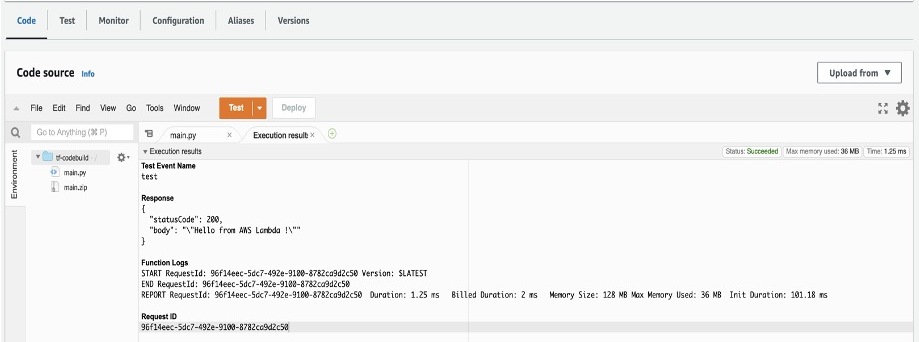
Figure 1: User-to-service flow
The solution uses Envoy, to terminate the HTTP request from an OAuth 2.0 client. This is shown in Figure 1: User-to-service flow.
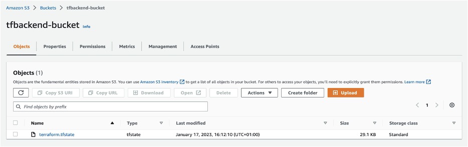
Envoy (shown as (1) in Figure 2) can validate access tokens (presented as a JSON Web Token (JWT) embedded in an Authorization: Bearer header). If the access token can be validated, then the scopes from this token are unpacked (2) and placed into X-JWT-Scope-<scopename> headers, using a simple inline Lua script. The Envoy documentation provides examples of how to use inline Lua in Envoy. Figure 2 – JWT Scope to HTTP shows how this process works at a high level.

Figure 2: JWT Scope to HTTP headers
Following this, Envoy uses Signature Version 4 (SigV4) to sign the request (3) and pass it to the VPC Lattice service. SigV4 signing is a native Envoy capability, but it requires the underlying compute that Envoy is running on to have access to AWS credentials. When you use AWS compute, assigning a role to that compute verifies that the instance can provide credentials to processes running on that compute, in this case Envoy.
By adding an authorization policy that permits access only from Envoy (through validating the Envoy SigV4 signature) and only with the correct scopes provided in HTTP headers, you can effectively lock down a VPC Lattice service to specific verified users coming from Envoy who are presenting specific OAuth2 scopes in their bearer token.
To answer the original question of where the identity comes from, the identity is provided by the user when communicating with their identity provider (IdP). In addition to this, Envoy is presenting its own identity from its underlying compute to enter the VPC Lattice service network. From a configuration perspective this means your user-to-service communication flow doesn’t require understanding of the user, or the storage of user or machine credentials.
The sample code provided shows a full Envoy configuration for VPC Lattice, including SigV4 signing, access token validation, and extraction of JWT contents to headers. This reference architecture supports various clients including server-side web applications, thick Java clients, and even command line interface-based clients calling the APIs directly. I don’t cover OAuth clients in detail in this post, however the optional sample code allows you to use an OAuth client and flow to talk to the APIs through Envoy.
Service-to-service communication flow
In the service-to-service flow, you need a way to provide AWS credentials to your applications and configure them to use SigV4 to sign their HTTP requests to the destination VPC Lattice services. Your application components can have their own identities (IAM roles), which allows you to uniquely identify application components and make access control decisions based on the particular flow required. For example, application component 1 might need to communicate with application component 2, but not application component 3.
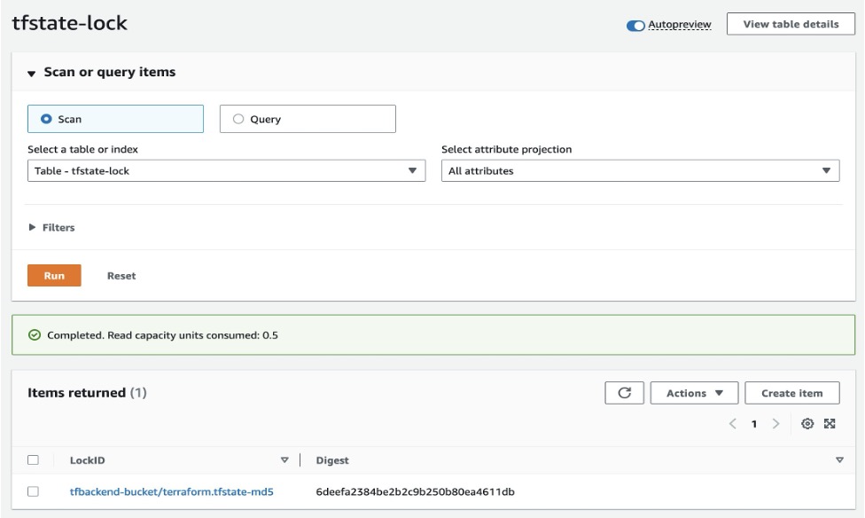
If you have full control of your application code and have a clean method for locating the destination services, then this might be something you can implement directly in your server code. This is the configuration that’s implemented in the AWS Cloud Development Kit (AWS CDK) solution that accompanies this blog post, the app1, app2, and app3 web servers are capable of making SigV4 signed requests to the VPC Lattice services they need to communicate with. The sample code demonstrates how to perform VPC Lattice SigV4 requests in node.js using the aws-crt node bindings. Figure 3 depicts the use of SigV4 authentication between services and VPC Lattice.

Figure 3: Service-to-service flow
To answer the question of where the identity comes from in this flow, you use the native SigV4 signing support from VPC Lattice to validate the application identity. The credentials come from AWS STS, again through the native underlying compute environment. Providing credentials transparently to your applications is one of the biggest advantages of the VPC Lattice solution when comparing this to other types of application security solutions such as service meshes. This implementation requires no provisioning of credentials, no management of identity stores, and automatically rotates credentials as required. This means low overhead to deploy and maintain the security of this solution and benefits from the reliability and scalability of IAM and the AWS Security Token Service (AWS STS) — a very slick solution to securing service-to-service communication flows!
VPC Lattice policy configuration
VPC Lattice provides two levels of auth policy configuration — at the VPC Lattice service network and on individual VPC Lattice services. This allows your cloud operations and development teams to work independently of each other by removing the dependency on a single team to implement access controls. This model enables both agility and separation of duties. More information about VPC Lattice policy configuration can be found in Control access to services using auth policies.
Service network auth policy
This design uses a service network auth policy that permits access to the service network by specific IAM principals. This can be used as a guardrail to provide overall access control over the service network and underlying services. Removal of an individual service auth policy will still enforce the service network policy first, so you can have confidence that you can identify sources of network traffic into the service network and block traffic that doesn’t come from a previously defined AWS principal.
The preceding auth policy example grants permissions to any authenticated request that uses one of the IAM roles app1TaskRole, app2TaskRole, app3TaskRole or EnvoyFrontendTaskRole to make requests to the services attached to the service network. You will see in the next section how service auth policies can be used in conjunction with service network auth policies.
Service auth policies
Individual VPC Lattice services can have their own policies defined and implemented independently of the service network policy. This design uses a service policy to demonstrate both user-to-service and service-to-service access control.
The preceding auth policy is an example that could be attached to the app1 VPC Lattice service. The policy contains two statements:
- The first (labelled “Sid”: “UserToService”) provides user-to-service authorization and requires requiring the caller principal to be EnvoyFrontendTaskRole and the request headers to contain the header x-jwt-scope-test.all: true when calling the app1 VPC Lattice service.
- The second (labelled “Sid”: “ServiceToService”) provides service-to-service authorization and requires the caller principal to be app2TaskRole when calling the app1 VPC Lattice service.
As with a standard IAM policy, there is an implicit deny, meaning no other principals will be permitted access.
The caller principals are identified by VPC Lattice through the SigV4 signing process. This means by using the identities provisioned to the underlying compute the network flow can be associated with a service identity, which can then be authorized by VPC Lattice service access policies.
Distributed development
This model of access control supports a distributed development and operational model. Because the service network auth policy is decoupled from the service auth policies, the service auth policies can be iterated upon by a development team without impacting the overall policy controls set by an operations team for the entire service network.
Solution overview
I’ve provided an aws-samples AWS CDK solution that you can deploy to implement the preceding design.

Figure 4: CDK deployable solution
The AWS CDK solution deploys four Amazon ECS services, one for the frontend Envoy server for the client-to-service flow, and the remaining three for the backend application components. Figure 4 shows the solution when deployed with the internal domain parameter application.internal.
Backend application components are a simple node.js express server, which will print the contents of your request in JSON format and perform service-to-service calls.
A number of other infrastructure components are deployed to support the solution:
- A VPC with associated subnets, NAT gateways and an internet gateway. Internet access is required for the solution to retrieve JSON Web Key Set (JWKS) details from your OAuth provider.
- An Amazon Route53 hosted zone for handling traffic routing to the configured domain and VPC Lattice services.
- An Amazon ECS cluster (two container hosts by default) to run the ECS tasks.
- Four Application Load Balancers, one for frontend Envoy routing and one for each application component.
- All application load balancers are internally facing.
- Application component load balancers are configured to only accept traffic from the VPC Lattice managed prefix List.
- The frontend Envoy load balancer is configured to accept traffic from any host.
- Three VPC Lattice services and one VPC Lattice network.
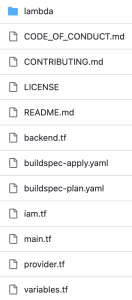
The code for Envoy and the application components can be found in the lattice_soln/containers directory.
AWS CDK code for all other deployable infrastructure can be found in lattice_soln/lattice_soln_stack.py.
Prerequisites
Before you begin, you must have the following prerequisites in place:
- An AWS account to deploy solution resources into. AWS credentials should be available to the AWS CDK in the environment or configuration files for the CDK deploy to function.
- Python 3.9.6 or higher
- Docker or Finch for building containers. If using Finch, ensure the Finch executable is in your path and instruct the CDK to use it with the command export CDK_DOCKER=finch
- Enable elastic network interface (ENI) trunking in your account to allow more containers to run in VPC networking mode:
[Optional] OAuth provider configuration
This solution has been tested using Okta, however any OAuth compatible provider will work if it can issue access tokens and you can retrieve them from the command line.
The following instructions describe the configuration process for Okta using the Okta web UI. This allows you to use the device code flow to retrieve access tokens, which can then be validated by the Envoy frontend deployment.
Create a new app integration
- In the Okta web UI, select Applications and then choose Create App Integration.
- For Sign-in method, select OpenID Connect.
- For Application type, select Native Application.
- For Grant Type, select both Refresh Token and Device Authorization.
- Note the client ID for use in the device code flow.
Create a new API integration
- Still in the Okta web UI, select Security, and then choose API.
- Choose Add authorization server.
- Enter a name and audience. Note the audience for use during CDK installation, then choose Save.
- Select the authorization server you just created. Choose the Metadata URI link to open the metadata contents in a new tab or browser window. Note the jwks_uri and issuer fields for use during CDK installation.
- Return to the Okta web UI, select Scopes and then Add scope.
- For the scope name, enter test.all. Use the scope name for the display phrase and description. Leave User consent as implicit. Choose Save.
- Under Access Policies, choose Add New Access Policy.
- For Assign to, select The following clients and select the client you created above.
- Choose Add rule.
- In Rule name, enter a rule name, such as Allow test.all access
- Under If Grant Type Is uncheck all but Device Authorization. Under And Scopes Requested choose The following scopes. Select OIDC default scopes to add the default scopes to the scopes box, then also manually add the test.all scope you created above.
During the API Integration step, you should have collected the audience, JWKS URI, and issuer. These fields are used on the command line when installing the CDK project with OAuth support.
You can then use the process described in configure the smart device to retrieve an access token using the device code flow. Make sure you modify scope to include test.all — scope=openid profile offline_access test.all — so your token matches the policy deployed by the solution.
Installation
You can download the deployable solution from GitHub.
Deploy without OAuth functionality
If you only want to deploy the solution with service-to-service flows, you can deploy with a CDK command similar to the following:
Deploy with OAuth functionality
To deploy the solution with OAuth functionality, you must provide the following parameters:
- jwt_jwks: The URL for retrieving JWKS details from your OAuth provider. This would look something like https://dev-123456.okta.com/oauth2/ausa1234567/v1/keys
- jwt_issuer: The issuer for your OAuth access tokens. This would look something like https://dev-123456.okta.com/oauth2/ausa1234567
- jwt_audience: The audience configured for your OAuth protected APIs. This is a text string configured in your OAuth provider.
- app_domain: The domain to be configured in Route53 for all URLs provided for this application. This domain is local to the VPC created for the solution. For example application.internal.
The solution can be deployed with a CDK command as follows:
Security model
For this solution, network access to the web application is secured through two main controls:
- Entry into the service network requires SigV4 authentication, enforced by the service network policy. No other mechanisms are provided to allow access to the services, either through their load balancers or directly to the containers.
- Service policies restrict access to either user- or service-based communication based on the identity of the caller and OAuth subject and scopes.
The Envoy configuration strips any x- headers coming from user clients and replaces them with x-jwt-subject and x-jwt-scope headers based on successful JWT validation. You are then able to match these x-jwt-* headers in VPC Lattice policy conditions.
Solution caveats
This solution implements TLS endpoints on VPC Lattice and Application Load Balancers. The container instances do not implement TLS in order to reduce cost for this example. As such, traffic is in cleartext between the Application Load Balancers and container instances, and can be implemented separately if required.
How to use the solution
Now for the interesting part! As part of solution deployment, you’ve deployed a number of Amazon Elastic Compute Cloud (Amazon EC2) hosts to act as the container environment. You can use these hosts to test some of the flows and you can use the AWS Systems Manager connect function from the AWS Management console to access the command line interface on any of the container hosts.
In these examples, I’ve configured the domain during the CDK installation as application.internal, which will be used for communicating with the application as a client. If you change this, adjust your command lines to match.
[Optional] For examples 3 and 4, you need an access token from your OAuth provider. In each of the examples, I’ve embedded the access token in the AT environment variable for brevity.
Example 1: Service-to-service calls (permitted)
For these first two examples, you must sign in to the container host and run a command in your container. This is because the VPC Lattice policies allow traffic from the containers. I’ve assigned IAM task roles to each container, which are used to uniquely identify them to VPC Lattice when making service-to-service calls.
To set up service-to service calls (permitted):
- Sign in to the Amazon ECS console. You should see at least three ECS services running.

Figure 5: Cluster console
- Select the app2 service LatticeSolnStack-app2service…, then select the Tasks tab.
Under the Container Instances heading select the container instance that’s running the app2 service.
Figure 6: Container instances
- You will see the instance ID listed at the top left of the page.
Figure 7: Single container instance
- Select the instance ID (this will open a new window) and choose Connect. Select the Session Manager tab and choose Connect again. This will open a shell to your container instance.


The policy statements permit app2 to call app1. By using the path app2/call-to-app1, you can force this call to occur.
Test this with the following commands:
You should see the following output:
Example 2: Service-to-service calls (denied)
The policy statements don’t permit app2 to call app3. You can simulate this in the same way and verify that the access isn’t permitted by VPC Lattice.
To set up service-to-service calls (denied)
You can change the curl command from Example 1 to test app2 calling app3.
[Optional] Example 3: OAuth – Invalid access token
If you’ve deployed using OAuth functionality, you can test from the shell in Example 1 that you’re unable to access the frontend Envoy server (application.internal) without a valid access token, and that you’re also unable to access the backend VPC Lattice services (app1.application.internal, app2.application.internal, app3.application.internal) directly.
You can also verify that you cannot bypass the VPC Lattice service and connect to the load balancer or web server container directly.
[Optional] Example 4: Client access
If you’ve deployed using OAuth functionality, you can test from the shell in Example 1 to access the application with a valid access token. A client can reach each application component by using application.internal/<componentname>. For example, application.internal/app2. If no component name is specified, it will default to app1.
This will fail when attempting to connect to app3 using Envoy, as we’ve denied user to service calls on the VPC Lattice Service policy
Summary
You’ve seen how you can use VPC Lattice to provide authentication and authorization to both user-to-service and service-to-service flows. I’ve shown you how to implement some novel and reusable solution components:
- JWT authorization and translation of scopes to headers, integrating an external IdP into your solution for user authentication.
- SigV4 signing from an Envoy proxy running in a container.
- Service-to-service flows using SigV4 signing in node.js and container-based credentials.
- Integration of VPC Lattice with ECS containers, using the CDK.
All of this is created almost entirely with managed AWS services, meaning you can focus more on security policy creation and validation and less on managing components such as service identities, service meshes, and other self-managed infrastructure.
Some ways you can extend upon this solution include:
- Implementing different service policies taking into consideration different OAuth scopes for your user and client combinations
- Implementing multiple issuers on Envoy to allow different OAuth providers to use the same infrastructure
- Deploying the VPC Lattice services and ECS tasks independently of the service network, to allow your builders to manage task deployment themselves
I look forward to hearing about how you use this solution and VPC Lattice to secure your own applications!
Additional references
- Authorisation policy capabilities in VPC Lattice
- Sample code for creating SigV4 signed requests
- AWS Request Signing filter configuration for Envoy Proxy
If you have feedback about this post, submit comments in the Comments section below. If you have questions about this post, contact AWS Support.


 Sebastian Vlad is a Senior Partner Solutions Architect with Amazon Web Services, with a passion for data and analytics solutions and customer success. Sebastian works with enterprise customers to help them design and build modern, secure, and scalable solutions to achieve their business outcomes.
 Sharad Pai is a Lead Technical Consultant at AWS. He specializes in streaming analytics and helps customers build scalable solutions using Amazon MSK and Amazon Kinesis. He has over 16 years of industry experience and is currently working with media customers who are hosting live streaming platforms on AWS, managing peak concurrency of over 50 million. Prior to joining AWS, Sharad’s career as a lead software developer included 9 years of coding, working with open source technologies like JavaScript, Python, and PHP.


 Michael Greenshtein is an Analytics Specialist Solutions Architect for the Public Sector.
 Gonzalo Herreros is a Senior Big Data Architect on the AWS Glue team.


 Swapna Bandla is a Senior Solutions Architect in the AWS Analytics Specialist SA Team. Swapna has a passion towards understanding customers data and analytics needs and empowering them to develop cloud-based well-architected solutions. Outside of work, she enjoys spending time with her family.
 Indira Balakrishnan is a Principal Solutions Architect in the AWS Analytics Specialist SA Team. She is passionate about helping customers build cloud-based analytics solutions to solve their business problems using data-driven decisions. Outside of work, she volunteers at her kids’ activities and spends time with her family.


 Stefano Sandona is a Senior Big Data Solution Architect at AWS. He loves data, distributed systems and security. He helps customers around the world architecting secure, scalable and reliable big data platforms.
 Adnan Hemani is a Software Development Engineer at AWS working with the EMR team. He focuses on the security posture of applications running on EMR clusters. He is interested in modern Big Data applications and how customers interact with them.
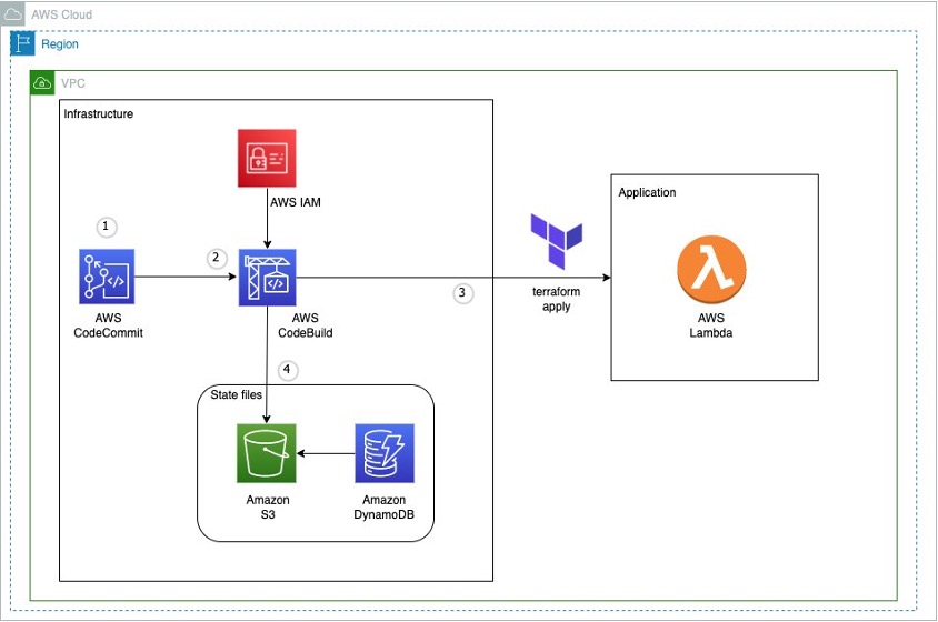


 Ryan Waldorf is a Senior Product Manager at Amazon Redshift. Ryan focuses on features that enable customers to define and scale compute including data sharing and concurrency scaling.
 Harshida Patel is a Analytics Specialist Principal Solutions Architect, with Amazon Web Services (AWS).


 Kanwar Bajwa is an Enterprise Support Lead at AWS who works with customers to optimize their use of AWS services and achieve their business objectives.


 Tamer Soliman is a Senior Solutions Architect at AWS. He helps Independent Software Vendor (ISV) customers innovate, build, and scale on AWS. He has over two decades of industry experience, and is an inventor with three granted patents. His experience spans multiple technology domains including telecom, networking, application integration, data analytics, AI/ML, and cloud deployments. He specializes in AWS Networking and has a profound passion for machine leaning, AI, and Generative AI.


 Venkata Kampana is a Senior Solutions Architect in the AWS Health and Human Services team and is based in Sacramento, CA. In that role, he helps public sector customers achieve their mission objectives with well-architected solutions on AWS.
 Jim Daniel is the Public Health lead at Amazon Web Services. Previously, he held positions with the United States Department of Health and Human Services for nearly a decade, including Director of Public Health Innovation and Public Health Coordinator. Before his government service, Jim served as the Chief Information Officer for the Massachusetts Department of Public Health.


 Durga Prasad is a Sr Lead Consultant enabling customers build their Data Analytics solutions on AWS. He is a coffee lover and enjoys playing badminton.
 Murali Reddy is a Lead Consultant at Amazon Web Services (AWS), helping customers build and implement data analytics solution. When he’s not working, Murali is an avid bike rider and loves exploring new places.
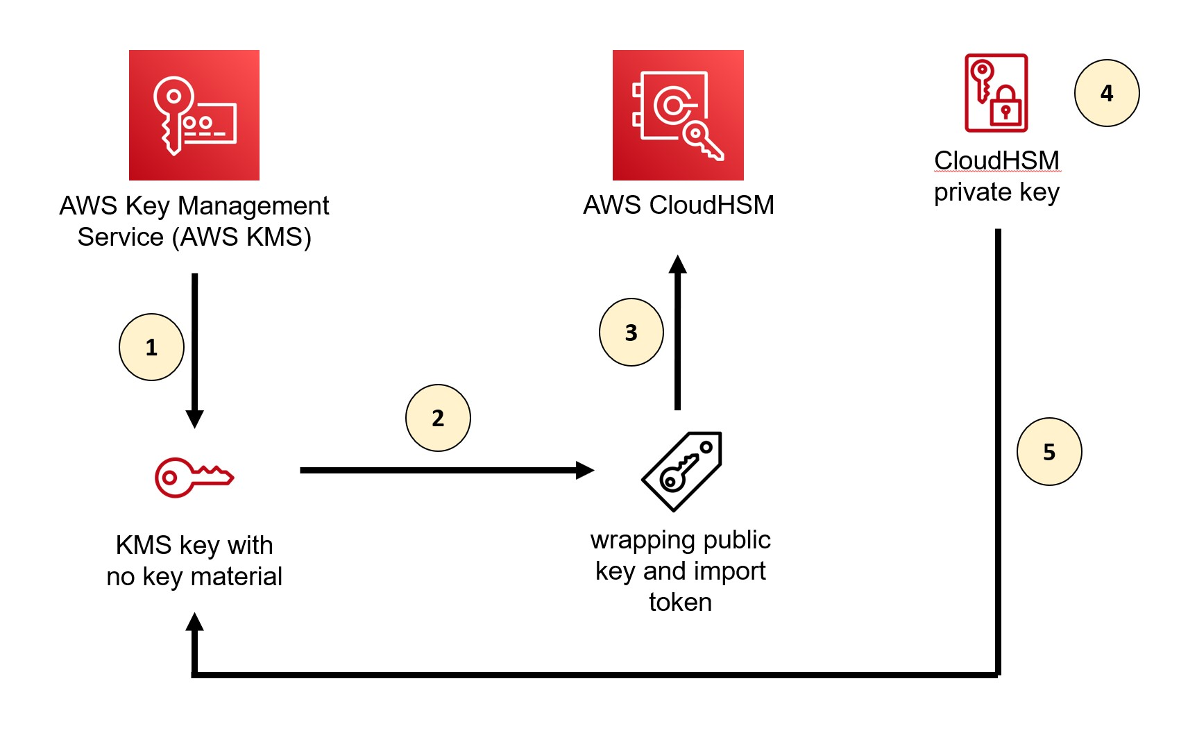


 Satesh Sonti is a Sr. Analytics Specialist Solutions Architect based out of Atlanta, specialized in building enterprise data platforms, data warehousing, and analytics solutions. He has over 18 years of experience in building data assets and leading complex data platform programs for banking and insurance clients across the globe.
 Alket Memushaj works as a Principal Architect in the Financial Services Market Development team at AWS. Alket is responsible for technical strategy for capital markets, working with partners and customers to deploy applications across the trade lifecycle to the AWS Cloud, including market connectivity, trading systems, and pre- and post-trade analytics and research platforms.
 Ruben Falk is a Capital Markets Specialist focused on AI and data & analytics. Ruben consults with capital markets participants on modern data architecture and systematic investment processes. He joined AWS from S&P Global Market Intelligence where he was Global Head of Investment Management Solutions.
 Jeff Wilson is a World-wide Go-to-market Specialist with 15 years of experience working with analytic platforms. His current focus is sharing the benefits of using Amazon Redshift, Amazon’s native cloud data warehouse. Jeff is based in Florida and has been with AWS since 2019.