Tag Archives: Technical How-to

How to deploy AWS Network Firewall to help protect your network from malware

Post Syndicated from Ajit Puthiyavettle original https://aws.amazon.com/blogs/security/how-to-deploy-aws-network-firewall-to-help-protect-your-network-from-malware/

Protecting your network and computers from security events requires multi-level strategies, and you can use network level traffic filtration as one level of defense. Users need access to the internet for business reasons, but they can inadvertently download malware, which can impact network and data security. This post describes how to use custom Suricata Rules with AWS Network Firewall to add protections that prevent users from downloading malware. You can use your own internal list, or a list from commercial or open-source threat intelligence feeds.

Network Firewall is a managed service that makes it easy to deploy essential network protection for all of your Amazon Virtual Private Cloud (Amazon VPC) Infrastructure. Network Firewall’s flexible rules engine lets you define firewall rules, giving you fine-grained control over network traffic, such as blocking outbound requests to prevent the spread of potential malware.

Features of Network Firewall

This section describes features of Network Firewall that help improve the overall security of your network.

Network Firewall:

  • Is a managed Amazon Web Services (AWS) service, so you don’t have to build and maintain the infrastructure to host the network firewall.
  • Integrates with AWS Firewall Manager, which allows you to centrally manage security policies and automatically enforce mandatory security policies across existing and newly created accounts and virtual private clouds (VPCs).
  • Protects application availability by filtering inbound internet traffic using tools such as access control list (ACL) rules, stateful inspection, protocol detection, and intrusion prevention.
  • Provides URL, IP address, and domain-based outbound traffic filtering to help you meet compliance requirements, stop potential data leaks, and block communication with known malware hosts.
  • Gives you control and visibility of VPC-to-VPC traffic to logically separate networks that host sensitive applications or line-of-business resources.
  • Complements existing network and application security services on AWS by providing control and visibility to layer 3 through 7 network traffic for your entire VPC.

Automating deployment of Network Firewall and management of Network Firewall rules support management at-scale and help in timely response, as Network Firewall is designed to block access to insecure sites before they impact your resources. For the solution in this blog post, you’ll use an AWS CloudFormation template to deploy the network architecture with Network Firewall.

Solution architecture

Figure 1 shows a sample architecture to demonstrate how users are able to download malware files, and how you can prevent this using network firewall rules.

Network Firewall is deployed in a single VPC architecture, where it is placed in line with the traffic to and from the internet.

Figure 1. Network architecture diagram

Figure 1. Network architecture diagram

The network architecture shown in Figure 1 includes three subnets:

  1. A network firewall subnet
    Hosts the Network Firewall endpoint interface. All outbound traffic from this network goes through the internet gateway.
  2. A public subnet
    Hosts a NAT gateway. The next hop from the public subnet is the Network Firewall endpoint, where all traffic can be inspected before being forwarded to the internet.
  3. A private network subnet
    Used to host the client instances. All outbound traffic from this network goes to the NAT gateway endpoint.

In the network architecture shown in Figure 1, only one AZ is shown for simplicity, but best practices recommend deploying infrastructure across multiple AZs

To run the CloudFormation deployment template

  1. To set up the architecture shown in Figure 1, launch the provided CloudFormation deployment template using the Launch stack button in step 2 below.
    This CloudFormation template:

    • Sets up VPCs and appropriate subnets as required by the network architecture.
    • Creates a route table with appropriate routes and attaches it to the appropriate subnet (i.e. private subnet, firewall subnet, public subnet).
    • Creates a test instance with appropriate security groups.
    • Deploys Network Firewall with firewall policy.
    • Creates a Rule Group SampleStatefulRulegroupName with Suricata rules, which is not attached to a firewall policy
  2. To launch the stack, click the Launch Stack button below.
  3. Select the Launch Stack button to launch the template

  4. Name the newly created stack (for example, nfw-stack).
  5. The template will also install two sample rules that will be used to protect against accessing two sample malware site URLs, but it will not automatically attach them to a firewall policy
  6. You can see that Network Firewall with firewall policy was deployed as part of the basic CloudFormation deployment. It also created Suricata rules in rule groups, but is not yet attached to the firewall policy.

    Note: Unless you attach the rule to the Network Firewall, it will not provide the required protection.

Example: confirming vulnerability

We have identified two sample URLs that contain malware to use for demonstration.

In the example screen shot below, we tested vulnerability by logging into test instance using AWS Session Manager. and at the shell prompt, used wget to access and download a malware file.

Figure 2 that follows is a screenshot of how a user could access and download two different malware files.

Note: Since these URLs contain malware files, we do not recommend users perform this test, but are providing a screenshot as a demonstration. If you wish to actually test ability to download files, use URLs you know are safe for testing.

Figure 2. Insecure URL access

Figure 2. Insecure URL access

Network Firewall policies

Before the template creates the Network Firewall rule group, it creates a Network Firewall policy and attaches it to the Network Firewall. An AWS Network Firewall firewall policy defines the monitoring and protection behavior for a firewall. The details of the behavior are defined in the rule groups that you add to your policy.

Network Firewall rules

A Network Firewall rule group is a reusable set of criteria for inspecting and handling network traffic. You can add one or more rule groups to a firewall policy as part of policy configuration. The included template does this for you.

Network Firewall rule groups are either stateless or stateful. Stateless rule groups evaluate packets in isolation, while stateful rule groups evaluate them in the context of their traffic flow. Network Firewall uses a Suricata rules engine to process all stateful rules.

Suricata rules can be used to create a Network Firewall stateful rule to prevent insecure URL access. Figure 3 shows the Suricata rules that the template adds and attaches to the Network Firewall policy in order to block access to the sample malware URLs used in the previous example.

Figure 3. Suricata rules in a Network Firewall rule group

Figure 3. Suricata rules in a Network Firewall rule group

Attach the rule group to the Network Firewall policy

When you launched the CloudFormation template, it automatically created these rules in the rule group. You will now be attaching this rule group to the firewall policy in order to enable the protection. You will need similar rules to block the test URLs that are used for your testing.

Figure 3 shows two Suricata rules that have been configured to block the insecure malware URLs.

To add Suricata rules to Network Firewall

To improve site security and protect against downloading malware, you can add Suricata rules to Network Firewall to secure your site. You’ll do this by:

  1. Creating and attaching a firewall policy to the Network Firewall.
  2. Creating rules as part of rule groups, which are attached to the firewall policy
  3. Testing to verify that access to malware URLs from the instance is blocked.

Let’s review Suricata Rules that are created, which can be attached to Network Firewall.

Suricata rule parts

Each Suricata rule has three parts:

  1. Action
  2. drop action that should be taken

  3. Header
  4. http this is the traffic protocol

    $HOME_NET anywhere $HOME_NET is a Suricata variable. By default it is set to the CIDR range of the VPC where Network Firewall is deployed and any refers to any source port

    $EXTERNAL_NET 80 where $EXTERNAL_NET 80 is a Suricata standard variable that refers to traffic destination, and 80 refers to the destination port

    -> is the direction that tells in which direction the signature has to match

  5. Options
  6. msg “MALWARE custom solution” – gives textual information about the signature and the possible alert

    flow to_server,established – it is used to match on the direction of the flow and established refers to match on established connections

    classtype trojan-activity – gives information about the classification of rules and alerts

    sid:xxxxx gives every signature its own id

    content “xxxx” – This keyword is very important and it identifies the pattern that your signature should match.

    http_uri is a content modifier that helps you match specifically and only on the request URI

    rev:xxx this goes along with sid keyword. It represents the version of the signature

The signatures in the Suricate rule shown in Figure 3 will block traffic that matches the http_uri contents /data/js_crypto_miner.html and /data/java_jre17_exec.html when the traffic is initiated from the VPC to the public network.

To attach a rule group to an existing Network Firewall

In Figure 4, the Network Firewall has a policy attached. but it does not have a rule group

Figure 4. A policy is attached, but not a rule group

Figure 4. A policy is attached, but not a rule group

  1. As shown in Figure 5, choose Add rule group to start adding your Suricata rule to the Network Firewall.
  2. Choose Add from existing stateful rule groups to attach an already created Suricata rule group.
  3. Figure 5. Choose Add rule group

    Figure 5. Choose Add rule group

  4. Figure 6 shows the Suriacata rule groups that are already created. SampleStatefulRulegroupName is the rule group created by the CloudFormation template.
  5. Select the rule group and choose Add stateful rule group to finish adding the rule group to Network Firewall.
  6. Figure 6. Review the rule groups that are already created

    Figure 6. Review the rule groups that are already created

  7. Figure 7 shows that the rule group SampleStatefulRulegroupName is now part of the Stateful rule group section of Network Firewall screen, which completes adding Suricata rules to Network Firewall.
  8. Figure 7. Shows the new rule group is now added

    Figure 7. Shows the new rule group is now added

Example: validating the solution

Your Network Firewall is now configured to block malware URLs that are defined in the rulegroup SampleStatefulRulegroupName.

As in the example above where we confirmed vulnerability, Figure 8 shows how to validate that the solution is now protecting your users from accessing malware sites.

Figure 8 shows a user trying to access the same insecure URLs we tested earlier and shows that the URLs are now blocked and the attempted connection times out.

Note: Since these URLs contain malware files, we do not recommend users perform this test, but are providing a screenshot as a demonstration. If you wish to actually test ability to download files, use URLs you know are safe for testing.

Figure 8. Insecure URL access blocked

Figure 8. Insecure URL access blocked

Validating blocking access helps your security team ensure that users or applications on your network cannot download malware. You can add similar rules for any URLs you identify as insecure. SOC operators are typically not familiar with updating CloudFormation templates, but you can use a deployment pipeline where the data required for the rule is stored in Amazon DynamoDB and use AWS Lambda functions to automate updating rules.

Now that you have an example running, you should implement a complete rule set that meets your requirement from a publicly available malware list such as CISSECURITY MALWARE LIST.

Cleanup

AWS resources created for testing can result in additional costs. Since this environment used a CloudFormation template, you can remove all AWS resources associated with the solution by deleting the CloudFormation stack you named previously (for example, nfw-stack).

Conclusion

This blog describes an approach for preventing users from downloading malware. The solution presented uses AWS Network Firewall to secure your environment by blocking access to the specified malware URLs. The supplied CloudFormation template can be used to automate this protection, and to easily set up a test environment to simulate the scenario.

For additional best practice information, see:

If you have feedback about this post, submit comments in the Comments section below. If you have questions about this post, contact AWS Support.

.

Want more AWS Security news? Follow us on Twitter.

Author

Ajit Puthiyavettle

Ajit is a Solution Architect working with enterprise clients, architecting solutions to achieve business outcomes. He is passionate about solving customer challenges with innovative solutions. His experience is with leading DevOps and security teams for enterprise and SaaS (Software as a Service) companies.

Deploy and Manage Gitlab Runners on Amazon EC2

Post Syndicated from Sylvia Qi original https://aws.amazon.com/blogs/devops/deploy-and-manage-gitlab-runners-on-amazon-ec2/

Gitlab CI is a tool utilized by many enterprises to automate their Continuous integration, continuous delivery and deployment (CI/CD) process. A Gitlab CI/CD pipeline consists of two major components: A .gitlab-ci.yml file describing a pipeline’s jobs, and a Gitlab Runner, an application that executes the pipeline jobs.

Setting up the Gitlab Runner is a time-consuming process. It involves provisioning the necessary infrastructure, installing the necessary software to run pipeline workloads, and configuring the runner. For enterprises running hundreds of pipelines across multiple environments, it is essential to automate the Gitlab Runner deployment process so as to be deployed quickly in a repeatable, consistent manner.

This post will guide you through utilizing Infrastructure-as-Code (IaC) to automate Gitlab Runner deployment and administrative tasks on Amazon EC2. With IaC, you can quickly and consistently deploy the entire Gitlab Runner architecture by running a script. You can track and manage changes efficiently. And, you can enforce guardrails and best practices via code. The solution presented here also offers autoscaling so that you save costs by terminating resources when not in use. You will learn:

  • How to deploy Gitlab Runner quickly and consistently across multiple AWS accounts.
  • How to enforce guardrails and best practices on the Gitlab Runner through IaC.
  • How to autoscale Gitlab Runner based on workloads to ensure best performance and save costs.

This post comes from a DevOps engineer perspective, and assumes that the engineer is familiar with the practices and tools of IaC and CI/CD.

Overview of the solution

The following diagram displays the solution architecture. We use AWS CloudFormation to describe the infrastructure that is hosting the Gitlab Runner. The main steps are as follows:

  1. The user runs a deploy script in order to deploy the CloudFormation template. The template is parameterized, and the parameters are defined in a properties file. The properties file specifies the infrastructure configuration, as well as the environment in which to deploy the template.
  2. The deploy script calls CloudFormation CreateStack API to create a Gitlab Runner stack in the specified environment.
  3. During stack creation, an EC2 autoscaling group is created with the desired number of EC2 instances. Each instance is launched via a launch template, which is created with values from the properties file. An IAM role is created and attached to the EC2 instance. The role contains permissions required for the Gitlab Runner to execute pipeline jobs. A lifecycle hook is attached to the autoscaling group on instance termination events. This ensures graceful instance termination.
  4. During instance launch, CloudFormation uses a cfn-init helper script to install and configure the Gitlab Runner:
    1. cfn-init installs the Gitlab Runner software on the EC2 instance.
    2. cfn-init configures the Gitlab Runner as a docker executor using a pre-defined docker image in the Gitlab Container Registry. The docker executor implementation lets the Gitlab Runner run each build in a separate and isolated container. The docker image contains the software required to run the pipeline workloads, thereby eliminating the need to install these packages during each build.
    3. cfn-init registers the Gitlab Runner to Gitlab projects specified in the properties file, so that these projects can utilize the Gitlab Runner to run pipelines.
  1. The user may repeat the same steps to deploy Gitlab Runner into another environment.

Architecture diagram previously explained in post.

Walkthrough

This walkthrough will demonstrate how to deploy the Gitlab Runner, and how easy it is to conduct Gitlab Runner administrative tasks via this architecture. We will walk through the following tasks:

  • Build a docker executor image for the Gitlab Runner.
  • Deploy the Gitlab Runner stack.
  • Update the Gitlab Runner.
  • Terminate the Gitlab Runner.
  • Add/Remove Gitlab projects from the Gitlab Runner.
  • Autoscale the Gitlab Runner based on workloads.

The code in this post is available at https://github.com/aws-samples/amazon-ec2-gitlab-runner.git

Prerequisites

For this walkthrough, you need the following:

  • A Gitlab account (all tiers including Gitlab Free self-managed, Gitlab Free SaaS, and higher tiers). This demo uses gitlab.com free tire.
  • A Gitlab Container Registry.
  • A Git client to clone the source code provided.
  • An AWS account with local credentials properly configured (typically under ~/.aws/credentials).
  • The latest version of the AWS CLI. For more information, see Installing, updating, and uninstalling the AWS CLI.
  • Docker is installed and running on the localhost/laptop.
  • Nodejs and npm installed on the localhost/laptop.
  • A VPC with 2 private subnets and that is connected to the internet via NAT gateway allowing outbound traffic.
  • The following IAM service-linked role created in the AWS account: AWSServiceRoleForAutoScaling
  • An Amazon S3 bucket for storing Lambda deployment packages.
  • Familiarity with Git, Gitlab CI/CD, Docker, EC2, CloudFormation and Amazon CloudWatch.

Build a docker executor image for the Gitlab Runner

The Gitlab Runner in this solution is implemented as docker executor. The Docker executor connects to Docker Engine and runs each build in a separate and isolated container via a predefined docker image. The first step in deploying the Gitlab Runner is building a docker executor image. We provided a simple Dockerfile in order to build this image. You may customize the Dockerfile to install your own requirements.

To build a docker image using the sample Dockerfile:

  1. Create a directory where we will store our demo code. From your terminal run:
mkdir demo-repos && cd demo-repos
  1. Clone the source code repository found in the following location:
git clone https://github.com/aws-samples/amazon-ec2-gitlab-runner.git
  1. Create a new project on your Gitlab server. Name the project any name you like.
  2. Clone your newly created repo to your laptop. Ignore the warning about cloning an empty repository.
git clone <your-repo-url>
  1. Copy the demo repo files into your newly created repo on your laptop, and push it to your Gitlab repository. You may customize the Dockerfile before pushing it to Gitlab.
cp -r amazon-ec2-gitlab-runner/* <your-repo-dir>
cd <your-repo-dir>
git add .
git commit -m “Initial commit”
git push
  1. On the Gitlab console, go to your repository’s Package & Registries -> Container Registry. Follow the instructions provided on the Container Registry page in order to build and push a docker image to your repository’s container registry.

Deploy the Gitlab Runner stack

Once the docker executor image has been pushed to the Gitlab Container Registry, we can deploy the Gitlab Runner. The Gitlab Runner infrastructure is described in the Cloudformation template gitlab-runner.yaml. Its configuration is stored in a properties file called sample-runner.properties. A launch template is created with the values in the properties file. Then it is used to launch instances. This architecture lets you deploy Gitlab Runner to as many environments as you like by utilizing the configurations provided in the appropriate properties files.

During the provisioning process, utilize a cfn-init helper script to run a series of commands to install and configure the Gitlab Runner.

          commands:
            01InstallDocker:
              command: sudo yum -y install docker
            02StartDocker:
              command: sudo service docker start
            03DownloadGitlabRunner:
              command: sudo wget -O /usr/bin/gitlab-runner https://gitlab-runner-downloads.s3.amazonaws.com/latest/binaries/gitlab-runner-linux-amd64
            04ChmodGitlabRunner:
              command: sudo chmod a+x /usr/bin/gitlab-runner
            05AddUser:
              command: sudo useradd --comment 'GitLab Runner' --create-home gitlab-runner --shell /bin/bash
            06InstallGitlabRunner:
              command: sudo gitlab-runner install --user=gitlab-runner --working-directory=/home/gitlab-runner
            07SetRegion:
              command: !Sub 'aws configure set default.region ${AWS::Region}'
            08ConfigureDockerExecutor:
              command: !Sub 
                - |
                  for GitlabGroupToken in `aws ssm get-parameters --names /${AWS::StackName}/ci-tokens --query 'Parameters[0].Value' | sed -e "s/\"//g" | sed "s/,/ /g"`;do
                      sudo gitlab-runner register \
                      --non-interactive \
                      --url "${GitlabServerURL}" \
                      --registration-token $GitlabGroupToken \
                      --executor "docker" \
                      --docker-image "${DockerImagePath}" \
                      --description "Gitlab Runner with Docker Executor" \
                      --locked="${isLOCKED}" --access-level "${ACCESS}" \
                      --docker-volumes "/var/run/docker.sock:/var/run/docker.sock" \
                      --tag-list "${RunnerEnvironment}-${RunnerVersion}-docker"
                  done
                - isLOCKED: !FindInMap [GitlabRunnerRegisterOptionsMap, !Ref RunnerEnvironment, isLOCKED]
                  ACCESS: !FindInMap [GitlabRunnerRegisterOptionsMap, !Ref RunnerEnvironment, ACCESS]                              
            09StartGitlabRunner:
              command: sudo gitlab-runner start

The helper script ensures that the Gitlab Runner setup is consistent and repeatable for each deployment. If a configuration change is required, users simply update the configuration steps and redeploy the stack. Furthermore, all changes are tracked in Git, which allows for versioning of the Gitlab Runner.

To deploy the Gitlab Runner stack:

  1. Obtain the runner registration tokens of the Gitlab projects that you want registered to the Gitlab Runner. Obtain the token by selecting the project’s Settings > CI/CD and expand the Runners section.
  2. Update the sample-runner.properties file parameters according to your own environment. Refer to the gitlab-runner.yaml file for a description of these parameters. Rename the file if you like. You may also create an additional properties file for deploying into other environments.
  3. Run the deploy script to deploy the runner:
cd <your-repo-dir>
./deploy-runner.sh <properties-file> <region> <aws-profile> <stack-name> 

<properties-file> is the name of the properties file.

<region> is the region where you want to deploy the stack.

<aws-profile> is the name of the CLI profile you set up in the prerequisites section.

<stack-name> is the name you chose for the CloudFormation stack.

For example:

./deploy-runner.sh sample-runner.properties us-east-1 dev amazon-ec2-gitlab-runner-demo

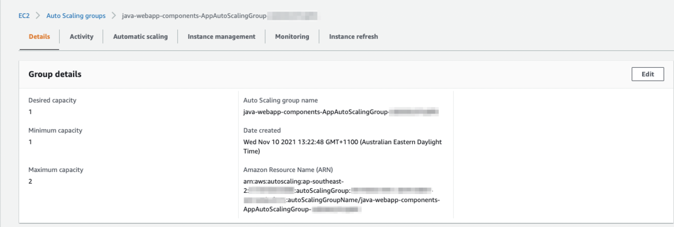
After the stack is deployed successfully, you will see the Gitlab Runner autoscaling group created in the EC2 console:

After the stack is deployed successfully, you will see the Gitlab Runner autoscaling group created in the EC2 console.

Under your Gitlab project Settings > CICD > Runners > Available specific runners, you will see the fully configured Gitlab Runner. The green circle indicates that the Gitlab Runner is ready for use.

Now go to your Gitlab project Settings  CICD  Runners  Available specific runners, you will see the fully configured Gitlab Runner. The green circle indicates that the Gitlab Runner is ready for use.

Updating the Gitlab Runner

There are times when you would want to update the Gitlab Runner. For example, updating the instance VolumeSize in order to resolve a disk space issue, or updating the AMI ID when a new AMI becomes available.

Utilizing the properties file and launch template makes it easy to update the Gitlab Runner. Simply update the Gitlab Runner configuration parameters in the properties file. Then, run the deploy script to udpate the Gitlab Runner stack. To ensure that the changes take effect immediately (e.g., existing instances are replaced by new instances with the new configuration), we utilize an AutoscalingRollingUpdate update policy to automatically update the instances in the autoscaling group.

    UpdatePolicy:
      AutoScalingRollingUpdate:
        MinInstancesInService: !Ref MinInstancesInService
        MaxBatchSize: !Ref MaxBatchSize
        PauseTime: "PT5M"
        WaitOnResourceSignals: true
        SuspendProcesses:
          - HealthCheck
          - ReplaceUnhealthy
          - AZRebalance
          - AlarmNotification
          - ScheduledActions

The policy tells CloudFormation that when changes are detected in the launch template, update the instances in batch size of MaxBatchSize, while keeping a number of instances (specified in MinInstanceInService) in service during the update.

Below is an example of updating the Gitlab Runner instance type.

To update the instance type of the runner instance:

  1. Update the “InstanceType” parameter in the properties file.

InstanceType=t2.medium

  1. Run the deploy-runner.sh script to update the CloudFormation stack:
cd <your-repo-dir>
./deploy-runner.sh <properties-file> <region> <aws-profile> <stack-name> 

In the CloudFormation console, you will see that the launch template is updated first, then a rolling update is initiated. The instance type update requires a replacement of the original instance, so a temporary instance was launched and put in service. Then, the temporary instance was terminated when the new instance was launched successfully.

In the CloudFormation console, you will see that the launch template is updated first, then a rolling update is initiated. The instance type update requires a replacement of the original instance, so a temporary instance was launched and put in service. Then, the temporary instance was terminated when the new instance was launched successfully.

After the update is complete, you will see that on the Gitlab project’s console, the old Gitlab Runner, ez_5x8Rv, is replaced by the new Gitlab Runner, N1_UQ7yc.

After the update is complete, you will see that on the Gitlab project’s console, the old Gitlab Runner, ez_5x8Rv, is replaced by the new Gitlab Runner, N1_UQ7yc.

Terminate the Gitlab Runner

There are times when an autoscaling group instance must be terminated. For example, during an autoscaling scale-in event, or when the instance is being replaced by a new instance during a stack update, as seen previously. When terminating an instance, you must ensure that the Gitlab Runner finishes executing any running jobs before the instance is terminated, otherwise your environment could be left in an inconsistent state. Also, we want to ensure that the terminated Gitlab Runner is removed from the Gitlab project. We utilize an autoscaling lifecycle hook to achieve these goals.

The lifecycle hook works like this: A CloudWatch event rule actively listens for the EC2 Instance-terminate events. When one is detected, the event rule triggers a Lambda function. The Lambda function calls SSM Run Command to run a series of commands on the EC2 instances, via a SSM Document. The commands include stopping the Gitlab Runner gracefully when all running jobs are finished, de-registering the runner from Gitlab projects, and signaling the autoscaling group to terminate the instance.

The lifecycle hook works like this: A CloudWatch event rule actively listens for the EC2 Instance-terminate events. When one is detected, the event rule triggers a Lambda function. The Lambda function calls SSM Run Command to run a series of commands on the EC2 instances, via a SSM Document. The commands include stopping the Gitlab Runner gracefully when all running jobs are finished, de-registering the runner from Gitlab projects, and signaling the autoscaling group to terminate the instance.

There are also times when you want to terminate an instance manually. For example, when an instance is suspected to not be functioning properly. To terminate an instance from the Gitlab Runner autoscaling group, use the following command:

aws autoscaling terminate-instance-in-auto-scaling-group \
    --instance-id="${InstanceId}" \
    --no-should-decrement-desired-capacity \
    --region="${region}" \
    --profile="${profile}"

The above command terminates the instance. The lifecycle hook ensures that the cleanup steps are conducted properly, and the autoscaling group launches another new instance to replace the old one.

Note that if you terminate the instance by using the “ec2 terminate-instance” command, then the autoscaling lifecycle hook actions will not be triggered.

Add/Remove Gitlab projects from the Gitlab Runner

As new projects are added to your enterprise, you may want to register them to the Gitlab Runner, so that those projects can utilize the Gitlab Runner to run pipelines. On the other hand, you would want to remove the Gitlab Runner from a project if it no longer wants to utilize the Gitlab Runner, or if it qualifies to utilize the Gitlab Runner. For example, if a project is no longer allowed to deploy to an environment configured by the Gitlab Runner. Our architecture offers a simple way to add and remove projects from the Gitlab Runner. To add new projects to the Gitlab Runner, update the RunnerRegistrationTokens parameter in the properties file, and then rerun the deploy script to update the Gitlab Runner stack.

To add new projects to the Gitlab Runner:

  1. Update the RunnerRegistrationTokens parameter in the properties file. For example:
RunnerRegistrationTokens=ps8RjBSruy1sdRdP2nZX,XbtZNv4yxysbYhqvjEkC
  1. Update the Gitlab Runner stack. This updates the SSM parameter which stores the tokens.
cd <your-repo-dir>
./deploy-runner.sh <properties-file> <region> <aws-profile> <stack-name> 
  1. Relaunch the instances in the Gitlab Runner autoscaling group. The new instances will use the new RunnerRegistrationTokens value. Run the following command to relaunch the instances:
./cycle-runner.sh <runner-autoscaling-group-name> <region> <optional-aws-profile>

To remove projects from the Gitlab Runner, follow the steps described above, with just one difference. Instead of adding new tokens to the RunnerRegistrationTokens parameter, remove the token(s) of the project that you want to dissociate from the runner.

Autoscale the runner based on custom performance metrics

Each Gitlab Runner can be configured to handle a fixed number of concurrent jobs. Once this capacity is reached for every runner, any new jobs will be in a Queued/Waiting status until the current jobs complete, which would be a poor experience for our team. Setting the number of concurrent jobs too high on our runners would also result in a poor experience, because all jobs leverage the same CPU, memory, and storage in order to conduct the builds.

In this solution, we utilize a scheduled Lambda function that runs every minute in order to inspect the number of jobs running on every runner, leveraging the Prometheus Metrics endpoint that the runners expose. If we approach the concurrent build limit of the group, then we increase the Autoscaling Group size so that it can take on more work. As the number of concurrent jobs decreases, then the scheduled Lambda function will scale the Autoscaling Group back in an effort to minimize cost. The Scaling-Up operation will ignore the Autoscaling Group’s cooldown period, which will help ensure that our team is not waiting on a new instance, whereas the Scale-Down operation will obey the group’s cooldown period.

Here is the logical sequence diagram for the work:

Sequence diagram

For operational monitoring, the Lambda function also publishes custom CloudWatch Metrics for the count of active jobs, along with the target and actual capacities of the Autoscaling group. We can utilize this information to validate that the system is working properly and determine if we need to modify any of our autoscaling parameters.

For operational monitoring, the Lambda function also publishes custom CloudWatch Metrics for the count of active jobs, along with the target and actual capacities of the Autoscaling group. We can utilize this information to validate that the system is working properly and determine if we need to modify any of our autoscaling parameters.

Congratulations! You have completed the walkthrough. Take some time to review the resources you have deployed, and practice the various runner administrative tasks that we have covered in this post.

Troubleshooting

Problem: I deployed the CloudFormation template, but no runner is listed in my repository.

Possible Cause: Errors have been encountered during cfn-init, causing runner registration to fail. Connect to your runner EC2 instance, and check /var/log/cfn-*.log files.

Cleaning up

To avoid incurring future charges, delete every resource provisioned in this demo by deleting the CloudFormation stack created in the “Deploy the Gitlab Runner stack” section.

Conclusion

This article demonstrated how to utilize IaC to efficiently conduct various administrative tasks associated with a Gitlab Runner. We deployed Gitlab Runner consistently and quickly across multiple accounts. We utilized IaC to enforce guardrails and best practices, such as tracking Gitlab Runner configuration changes, terminating the Gitlab Runner gracefully, and autoscaling the Gitlab Runner to ensure best performance and minimum cost. We walked through the deploying, updating, autoscaling, and terminating of the Gitlab Runner. We also saw how easy it was to clean up the entire Gitlab Runner architecture by simply deleting a CloudFormation stack.

About the authors

Sylvia Qi

Sylvia is a Senior DevOps Architect focusing on architecting and automating DevOps processes, helping customers through their DevOps transformation journey. In her spare time, she enjoys biking, swimming, yoga, and photography.

Sebastian Carreras

Sebastian is a Senior Cloud Application Architect with AWS Professional Services. He leverages his breadth of experience to deliver bespoke solutions to satisfy the visions of his customer. In his free time, he really enjoys doing laundry. Really.

How to use tokenization to improve data security and reduce audit scope

Post Syndicated from Tim Winston original https://aws.amazon.com/blogs/security/how-to-use-tokenization-to-improve-data-security-and-reduce-audit-scope/

Tokenization of sensitive data elements is a hot topic, but you may not know what to tokenize, or even how to determine if tokenization is right for your organization’s business needs. Industries subject to financial, data security, regulatory, or privacy compliance standards are increasingly looking for tokenization solutions to minimize distribution of sensitive data, reduce risk of exposure, improve security posture, and alleviate compliance obligations. This post provides guidance to determine your requirements for tokenization, with an emphasis on the compliance lens given our experience as PCI Qualified Security Assessors (PCI QSA).

What is tokenization?

Tokenization is the process of replacing actual sensitive data elements with non-sensitive data elements that have no exploitable value for data security purposes. Security-sensitive applications use tokenization to replace sensitive data, such as personally identifiable information (PII) or protected health information (PHI), with tokens to reduce security risks.

De-tokenization returns the original data element for a provided token. Applications may require access to the original data, or an element of the original data, for decisions, analysis, or personalized messaging. To minimize the need to de-tokenize data and to reduce security exposure, tokens can retain attributes of the original data to enable processing and analysis using token values instead of the original data. Common characteristics tokens may retain from the original data are:

Format attributes

Length for compatibility with storage and reports of applications written for the original data
Character set for compatibility with display and data validation of existing applications
Preserved character positions such as first 6 and last 4 for credit card PAN

Analytics attributes

Mapping consistency where the same data always results in the same token
Sort order

Retaining functional attributes in tokens must be implemented in ways that do not defeat the security of the tokenization process. Using attribute preservation functions can possibly reduce the security of a specific tokenization implementation. Limiting the scope and access to tokens addresses limitations introduced when using attribute retention.
Why tokenize? Common use cases

I need to reduce my compliance scope

Tokens are generally not subject to compliance requirements if there is sufficient separation of the tokenization implementation and the applications using the tokens. Encrypted sensitive data may not reduce compliance obligations or scope. Such industry regulatory standards as PCI DSS 3.2.1 still consider systems that store, process, or transmit encrypted cardholder data as in-scope for assessment; whereas tokenized data may remove those systems from assessment scope. A common use case for PCI DSS compliance is replacing PAN with tokens in data sent to a service provider, which keeps the service provider from being subject to PCI DSS.

I need to restrict sensitive data to only those with a “need-to-know”

Tokenization can be used to add a layer of explicit access controls to de-tokenization of individual data items, which can be used to implement and demonstrate least-privileged access to sensitive data. For instances where data may be co-mingled in a common repository such as a data lake, tokenization can help ensure that only those with the appropriate access can perform the de-tokenization process and reveal sensitive data.

I need to avoid sharing sensitive data with my service providers

Replacing sensitive data with tokens before providing it to service providers who have no access to de-tokenize data can eliminate the risk of having sensitive data within service providers’ control, and avoid having compliance requirements apply to their environments. This is common for customers involved in the payment process, which provides tokenization services to merchants that tokenize the card holder data, and return back to their customers a token they can use to complete card purchase transactions.

I need to simplify data lake security and compliance

A data lake centralized repository allows you to store all your structured and unstructured data at any scale, to be used later for not-yet-determined analysis. Having multiple sources and data stored in multiple structured and unstructured formats creates complications for demonstrating data protection controls for regulatory compliance. Ideally, sensitive data should not be ingested at all; however, that is not always feasible. Where ingestion of such data is necessary, tokenization at each data source can keep compliance-subject data out of data lakes, and help avoid compliance implications. Using tokens that retain data attributes, such as data-to-token consistency (idempotence) can support many of the analytical capabilities that make it useful to store data in the data lake.

I want to allow sensitive data to be used for other purposes, such as analytics

Your organization may want to perform analytics on the sensitive data for other business purposes, such as marketing metrics, and reporting. By tokenizing the data, you can minimize the locations where sensitive data is allowed, and provide tokens to users and applications needing to conduct data analysis. This allows numerous applications and processes to access the token data and maintain security of the original sensitive data.

I want to use tokenization for threat mitigation

Using tokenization can help you mitigate threats identified in your workload threat model, depending on where and how tokenization is implemented. At the point where the sensitive data is tokenized, the sensitive data element is replaced with a non-sensitive equivalent throughout the data lifecycle, and across the data flow. Some important questions to ask are:

  • What are the in-scope compliance, regulatory, privacy, or security requirements for the data that will be tokenized?
  • When does the sensitive data need to be tokenized in order to meet security and scope reduction objectives?
  • What attack vector is being addressed for the sensitive data by tokenizing it?
  • Where is the tokenized data being hosted? Is it in a trusted environment or an untrusted environment?

For additional information on threat modeling, see the AWS security blog post How to approach threat modeling.

Tokenization or encryption consideration

Tokens can provide the ability to retain processing value of the data while still managing the data exposure risk and compliance scope. Encryption is the foundational mechanism for providing data confidentiality.

Encryption rarely results in cipher text with a similar format to the original data, and may prevent data analysis, or require consuming applications to adapt.

Your decision to use tokenization instead of encryption should be based on the following:

Reduction of compliance scope As discussed above, by properly utilizing tokenization to obfuscate sensitive data you may be able to reduce the scope of certain framework assessments such as PCI DSS 3.2.1.
Format attributes Used for compatibility with existing software and processes.
Analytics attributes Used to support planned data analysis and reporting.
Elimination of encryption key management A tokenization solution has one essential API—create token—and one optional API—retrieve value from token. Managing access controls can be simpler than some non-AWS native general purpose cryptographic key use policies. In addition, the compromise of the encryption key compromises all data encrypted by that key, both past and future. The compromise of the token database compromises only existing tokens.

Where encryption may make more sense

Although scope reduction, data analytics, threat mitigation, and data masking for the protection of sensitive data make very powerful arguments for tokenization, we acknowledge there may be instances where encryption is the more appropriate solution. Ask yourself these questions to gain better clarity on which solution is right for your company’s use case.

Scalability If you require a solution that scales to large data volumes, and have the availability to leverage encryption solutions that require minimal key management overhead, such as AWS Key Management Services (AWS KMS), then encryption may be right for you.
Data format If you need to secure data that is unstructured, then encryption may be the better option given the flexibility of encryption at various layers and formats.
Data sharing with 3rd parties If you need to share sensitive data in its original format and value with a 3rd party, then encryption may be the appropriate solution to minimize external access to your token vault for de-tokenization processes.

What type of tokenization solution is right for your business?

When trying to decide which tokenization solution to use, your organization should first define your business requirements and use cases.

  1. What are your own specific use cases for tokenized data, and what is your business goal? Identifying which use cases apply to your business and what the end state should be is important when determining the correct solution for your needs.
  2. What type of data does your organization want to tokenize? Understanding what data elements you want to tokenize, and what that tokenized data will be used for may impact your decision about which type of solution to use.
  3. Do the tokens need to be deterministic, the same data always producing the same token? Knowing how the data will be ingested or used by other applications and processes may rule out certain tokenization solutions.
  4. Will tokens be used internally only, or will the tokens be shared across other business units and applications? Identifying a need for shared tokens may increase the risk of token exposure and, therefore, impact your decisions about which tokenization solution to use.
  5. How long does a token need to be valid? You will need to identify a solution that can meet your use cases, internal security policies, and regulatory framework requirements.

Choosing between self-managed tokenization or tokenization as a service

Do you want to manage the tokenization within your organization, or use Tokenization as a Service (TaaS) offered by a third-party service provider? Some advantages to managing the tokenization solution with your company employees and resources are the ability to direct and prioritize the work needed to implement and maintain the solution, customizing the solution to the application’s exact needs, and building the subject matter expertise to remove a dependency on a third party. The primary advantages of a TaaS solution are that it is already complete, and the security of both tokenization and access controls are well tested. Additionally, TaaS inherently demonstrates separation of duties, because privileged access to the tokenization environment is owned by the tokenization provider.

Choosing a reversible tokenization solution

Do you have a business need to retrieve the original data from the token value? Reversible tokens can be valuable to avoid sharing sensitive data with internal or third-party service providers in payments and other financial services. Because the service providers are passed only tokens, they can avoid accepting additional security risk and compliance scope. If your company implements or allows de-tokenization, you will need to be able to demonstrate strict controls on the management and use of de-tokenization privilege. Eliminating the implementation of de-tokenization is the clearest way to demonstrate that downstream applications cannot have sensitive data. Given the security and compliance risks of converting tokenized data back into its original data format, this process should be highly monitored, and you should have appropriate alerting in place to detect each time this activity is performed.

Operational considerations when deciding on a tokenization solution

While operational considerations are outside the scope of this post, they are important factors for choosing a solution. Throughput, latency, deployment architecture, resiliency, batch capability, and multi-regional support can impact the tokenization solution of choice. Integration mechanisms with identity and access control and logging architectures, for example, are important for compliance controls and evidence creation.

No matter which deployment model you choose, the tokenization solution needs to meet security standards, similar to encryption standards, and must prevent determining what the original data is from the token values.

Conclusion

Using tokenization solutions to replace sensitive data offers many security and compliance benefits. These benefits include lowered security risk and smaller audit scope, resulting in lower compliance costs and a reduction in regulatory data handling requirements.

Your company may want to use sensitive data in new and innovative ways, such as developing personalized offerings that use predictive analysis and consumer usage trends and patterns, fraud monitoring and minimizing financial risk based on suspicious activity analysis, or developing business intelligence to improve strategic planning and business performance. If you implement a tokenization solution, your organization can alleviate some of the regulatory burden of protecting sensitive data while implementing solutions that use obfuscated data for analytics.

On the other hand, tokenization may also add complexity to your systems and applications, as well as adding additional costs to maintain those systems and applications. If you use a third-party tokenization solution, there is a possibility of being locked into that service provider due to the specific token schema they may use, and switching between providers may be costly. It can also be challenging to integrate tokenization into all applications that use the subject data.

In this post, we have described some considerations to help you determine if tokenization is right for you, what to consider when deciding which type of tokenization solution to use, and the benefits. disadvantages, and comparison of tokenization and encryption. When choosing a tokenization solution, it’s important for you to identify and understand all of your organizational requirements. This post is intended to generate questions your organization should answer to make the right decisions concerning tokenization.

You have many options available to tokenize your AWS workloads. After your organization has determined the type of tokenization solution to implement based on your own business requirements, explore the tokenization solution options available in AWS Marketplace. You can also build your own solution using AWS guides and blog posts. For further reading, see this blog post: Building a serverless tokenization solution to mask sensitive data.

If you have feedback about this post, submit comments in the Comments section below. If you have questions about this post, start a new thread on the Amazon Security Assurance Services or contact AWS Support.

Want more AWS Security news? Follow us on Twitter.

Author

Tim Winston

Tim is a Senior Assurance Consultant with AWS Security Assurance Services. He leverages more than 20 years’ experience as a security consultant and assessor to provide AWS customers with guidance on payment security and compliance. He is a co-author of the “Payment Card Industry Data Security Standard (PCI DSS) 3.2.1 on AWS”.

Author

Kristine Harper

Kristine is a Senior Assurance Consultant and PCI DSS Qualified Security Assessor (QSA) with AWS Security Assurance Services. Her professional background includes security and compliance consulting with large fintech enterprises and government entities. In her free time, Kristine enjoys traveling, outdoor activities, spending time with family, and spoiling her pets.

Author

Michael Guzman

Michael is an Assurance Consultant with AWS Security Assurance Services. Michael is a PCI QSA and HITRUST CCSFP, along with holding several AWS certifications. His background is in Financial Services IT Operations and Administrations, with over 20 years experience within that industry. In his spare time Michael enjoy’s spending time with his family, continuing to improve his golf skills and perfecting his Tri-Tip recipe.

Migrating AWS Lambda functions to Arm-based AWS Graviton2 processors

Post Syndicated from Julian Wood original https://aws.amazon.com/blogs/compute/migrating-aws-lambda-functions-to-arm-based-aws-graviton2-processors/

AWS Lambda now allows you to configure new and existing functions to run on Arm-based AWS Graviton2 processors in addition to x86-based functions. Using this processor architecture option allows you to get up to 34% better price performance. This blog post highlights some considerations when moving from x86 to arm64 as the migration process is code and workload dependent.

Functions using the Arm architecture benefit from the performance and security built into the Graviton2 processor, which is designed to deliver up to 19% better performance for compute-intensive workloads. Workloads using multithreading and multiprocessing, or performing many I/O operations, can experience lower invocation time, which reduces costs.

Duration charges, billed with millisecond granularity, are 20 percent lower when compared to current x86 pricing. This also applies to duration charges when using Provisioned Concurrency. Compute Savings Plans supports Lambda functions powered by Graviton2.

The architecture change does not affect the way your functions are invoked or how they communicate their responses back. Integrations with APIs, services, applications, or tools are not affected by the new architecture and continue to work as before.

The following runtimes, which use Amazon Linux 2, are supported on Arm:

  • Node.js 12 and 14
  • Python 3.8 and 3.9
  • Java 8 (java8.al2) and 11
  • .NET Core 3.1
  • Ruby 2.7
  • Custom runtime (provided.al2)

Lambda@Edge does not support Arm as an architecture option.

You can create and manage Lambda functions powered by Graviton2 processor using the AWS Management Console, AWS Command Line Interface (AWS CLI), AWS CloudFormation, AWS Serverless Application Model (AWS SAM), and AWS Cloud Development Kit (AWS CDK). Support is also available through many AWS Lambda Partners.

Understanding Graviton2 processors

AWS Graviton processors are custom built by AWS. Generally, you don’t need to know about the specific Graviton processor architecture, unless your applications can benefit from specific features.

The Graviton2 processor uses the Neoverse-N1 core and supports Arm V8.2 (include CRC and crypto extensions) plus several other architectural extensions. In particular, Graviton2 supports the Large System Extensions (LSE), which improve locking and synchronization performance across large systems.

Migrating x86 Lambda functions to arm64

Many Lambda functions may only need a configuration change to take advantage of the price/performance of Graviton2. Other functions may require repackaging the Lambda function using Arm-specific dependencies, or rebuilding the function binary or container image.

You may not require an Arm processor on your development machine to create Arm-based functions. You can build, test, package, compile, and deploy Arm Lambda functions on x86 machines using AWS SAM and Docker Desktop. If you have an Arm-based system, such as an Apple M1 Mac, you can natively compile binaries.

Functions without architecture-specific dependencies or binaries

If your functions don’t use architecture-specific dependencies or binaries, you can switch from one architecture to the other with a single configuration change. Many functions using interpreted languages such as Node.js and Python, or functions compiled to Java bytecode, can switch without any changes. Ensure you check binaries in dependencies, Lambda layers, and Lambda extensions.

To switch functions from x86 to arm64, you can change the Architecture within the function runtime settings using the Lambda console.

Edit AWS Lambda function Architecture

Edit AWS Lambda function Architecture

If you want to display or log the processor architecture from within a Lambda function, you can use OS specific calls. For example, Node.js process.arch or Python platform.machine().

When using the AWS CLI to create a Lambda function, specify the --architectures option. If you do not specify the architecture, the default value is x86-64. For example, to create an arm64 function, specify --architectures arm64.

aws lambda create-function \
    --function-name MyArmFunction \
    --runtime nodejs14.x \
    --architectures arm64 \
    --memory-size 512 \
    --zip-file fileb://MyArmFunction.zip \
    --handler lambda.handler \
    --role arn:aws:iam::123456789012:role/service-role/MyArmFunction-role

When using AWS SAM or CloudFormation, add or amend the Architectures property within the function configuration.

MyArmFunction:
  Type: AWS::Lambda::Function
  Properties:
    Runtime: nodejs14.x
    Code: src/
    Architectures:
  	- arm64
    Handler: lambda.handler
    MemorySize: 512

When initiating an AWS SAM application, you can specify:

sam init --architecture arm64

When building Lambda layers, you can specify CompatibleArchitectures.

MyArmLayer:
  Type: AWS::Lambda::LayerVersion
  Properties:
    ContentUri: layersrc/
    CompatibleArchitectures:
      - arm64

Building function code for Graviton2

If you have dependencies or binaries in your function packages, you must rebuild the function code for the architecture you want to use. Many packages and dependencies have arm64 equivalent versions. Test your own workloads against arm64 packages to see if your workloads are good migration candidates. Not all workloads show improved performance due to the different processor architecture features.

For compiled languages like Rust and Go, you can use the provided.al2 custom runtime, which supports Arm. You provide a binary that communicates with the Lambda Runtime API.

When compiling for Go, set GOARCH to arm.

GOOS=linux GOARCH=arm go build

When compiling for Rust, set the target.

cargo build --release -- target-cpu=neoverse-n1

The default installation of Python pip on some Linux distributions is out of date (<19.3). To install binary wheel packages released for Graviton, upgrade the pip installation using:

sudo python3 -m pip install --upgrade pip

The Arm software ecosystem is continually improving. As a general rule, use later versions of compilers and language runtimes whenever possible. The AWS Graviton Getting Started GitHub repository includes known recent changes to popular packages that improve performance, including ffmpeg, PHP, .Net, PyTorch, and zlib.

You can use https://pkgs.org/ as a package repository search tool.

Sometimes code includes architecture specific optimizations. These can include code optimized in assembly using specific instructions for CRC, or enabling a feature that works well on particular architectures. One way to see if any optimizations are missing for arm64 is to search the code for __x86_64__ ifdefs and see if there is corresponding arm64 code included. If not, consider alternative solutions.

For additional language-specific considerations, see the links within the GitHub repository.

The Graviton performance runbook is a performance profiling reference by the Graviton to benchmark, debug, and optimize application code.

Building functions packages as container images

Functions packaged as container images must be built for the architecture (x86 or arm64) they are going to use. There are arm64 architecture versions of the AWS provided base images for Lambda. To specify a container image for arm64, use the arm64 specific image tag, for example, for Node.js 14:

  • public.ecr.aws/lambda/nodejs:14-arm64
  • public.ecr.aws/lambda/nodejs:latest-arm64
  • public.ecr.aws/lambda/nodejs:14.2021.10.01.16-arm64

Arm64 Images are also available from Docker Hub.

You can also use arbitrary Linux base images in addition to the AWS provided Amazon Linux 2 images. Images that support arm64 include Alpine Linux 3.12.7 or later, Debian 10 and 11, Ubuntu 18.04 and 20.04. For more information and details of other supported Linux versions, see Operating systems available for Graviton based instances.

Migrating a function

Here is an example of how to migrate a Lambda function from x86 to arm64 and take advantage of newer software versions to improve price and performance. You can follow a similar approach to test your own code.

I have an existing Lambda function as part of an AWS SAM template configured without an Architectures property, which defaults to x86_64.

  Imagex86Function:
    Type: AWS::Serverless::Function
    Properties:
      CodeUri: src/
      Handler: app.lambda_handler
      Runtime: python3.9

The Lambda function code performs some compute intensive image manipulation. The code uses a dependency configured with the following version:

{
  "dependencies": {
    "imagechange": "^1.1.1"
  }
}

I duplicate the Lambda function within the AWS SAM template using the same source code and specify arm64 as the Architectures.

  ImageArm64Function:
    Type: AWS::Serverless::Function
    Properties:
      CodeUri: src/
      Handler: app.lambda_handler
      Runtime: python3.9
      Architectures:
        - arm64

I use AWS SAM to build both Lambda functions. I specify the --use-container flag to build each function within its architecture-specific build container.

sam build –use-container

I can use sam local invoke to test the arm64 function locally even on an x86 system.

AWS SAM local invoke

AWS SAM local invoke

I then use sam deploy to deploy the functions to the AWS Cloud.

The AWS Lambda Power Tuning open-source project runs your functions using different settings to suggest a configuration to minimize costs and maximize performance. The tool allows you to compare two results on the same chart and incorporate arm64-based pricing. This is useful to compare two versions of the same function, one using x86 and the other arm64.

I compare the performance of the X86 and arm64 Lambda functions and see that the arm64 Lambda function is 12% cheaper to run:

Compare x86 and arm64 with dependency version 1.1.1

Compare x86 and arm64 with dependency version 1.1.1

I then upgrade the package dependency to use version 1.2.1, which has been optimized for arm64 processors.

{
  "dependencies": {
    "imagechange": "^1.2.1"
  }
}

I use sam build and sam deploy to redeploy the updated Lambda functions with the updated dependencies.

I compare the original x86 function with the updated arm64 function. Using arm64 with a newer dependency code version increases the performance by 30% and reduces the cost by 43%.

Compare x86 and arm64 with dependency version 1.2.1

Compare x86 and arm64 with dependency version 1.2.1

You can use Amazon CloudWatch,to view performance metrics such as duration, using statistics. You can then compare average and p99 duration between the two architectures. Due to the Graviton2 architecture, functions may be able to use less memory. This could allow you to right-size function memory configuration, which also reduces costs.

Deploying arm64 functions in production

Once you have confirmed your Lambda function performs successfully on arm64, you can migrate your workloads. You can use function versions and aliases with weighted aliases to control the rollout. Traffic gradually shifts to the arm64 version or rolls back automatically if any specified CloudWatch alarms trigger.

AWS SAM supports gradual Lambda deployments with a feature called Safe Lambda deployments using AWS CodeDeploy. You can compile package binaries for arm64 using a number of CI/CD systems. AWS CodeBuild supports building Arm based applications natively. CircleCI also has Arm compute resource classes for deployment. GitHub Actions allows you to use self-hosted runners. You can also use AWS SAM within GitHub Actions and other CI/CD pipelines to create arm64 artifacts.

Conclusion

Lambda functions using the Arm/Graviton2 architecture provide up to 34 percent price performance improvement. This blog discusses a number of considerations to help you migrate functions to arm64.

Many functions can migrate seamlessly with a configuration change, others need to be rebuilt to use arm64 packages. I show how to migrate a function and how updating software to newer versions may improve your function performance on arm64. You can test your own functions using the Lambda PowerTuning tool.

Start migrating your Lambda functions to Arm/Graviton2 today.

For more serverless learning resources, visit Serverless Land.

Continuous compliance monitoring using custom audit controls and frameworks with AWS Audit Manager

Post Syndicated from Deenadayaalan Thirugnanasambandam original https://aws.amazon.com/blogs/security/continuous-compliance-monitoring-using-custom-audit-controls-and-frameworks-with-aws-audit-manager/

For most customers today, security compliance auditing can be a very cumbersome and costly process. This activity within a security program often comes with a dependency on third party audit firms and robust security teams, to periodically assess risk and raise compliance gaps aligned with applicable industry requirements. Due to the nature of how audits are now performed, many corporate IT environments are left exposed to threats until the next manual audit is scheduled, performed, and the findings report is presented.

AWS Audit Manager can help you continuously audit your AWS usage and simplify how you assess IT risks and compliance gaps aligned with industry regulations and standards. Audit Manager automates evidence collection to reduce the “all hands-on deck” manual effort that often happens for audits, while enabling you to scale your audit capability in the cloud as your business grows. Customized control frameworks help customers evaluate IT environments against their own established assessment baseline, enabling them to discern how aligned they are with a set of compliance requirements tailored to their business needs. Custom controls can be defined to collect evidence from specific data sources, helping rate the IT environment against internally defined audit and compliance requirements. Each piece of evidence collected during the compliance assessment becomes a record that can be used to demonstrate compliance with predefined requirements specified by a control.

In this post, you will learn how to leverage AWS Audit Manager to create a tailored audit framework to continuously evaluate your organization’s AWS infrastructure against the relevant industry compliance requirements your organization needs to adhere to. By implementing this solution, you can simplify yet accelerate the detection of security risks present in your AWS environment, which are relevant to your organization, while providing your teams with the information needed to remedy reported compliance gaps.

Solution overview

This solution utilizes an event-driven architecture to provide agility while reducing manual administration effort.

  • AWS Audit Manager–AWS Audit Manager helps you continuously audit your AWS usage to simplify how you assess risk and compliance with regulations and industry standards.
  • AWS Lambda–AWS Lambda is a serverless compute service that lets you run code without provisioning or managing servers, in response to events such as changes in data, application state or user actions.
  • Amazon Simple Storage Service (Amazon S3) –Amazon S3 is object storage built to store and retrieve any amount of data from anywhere, that offers industry leading availability, performance, security, and virtually unlimited scalability at very low costs.
  • AWS Cloud Development Kit (AWS CDK)–AWS Cloud Development Kit is a software development framework for provisioning your cloud infrastructure in code through AWS CloudFormation.

Architecture

This solution enables automated controls management using event-driven architecture with AWS Services such as AWS Audit Manager, AWS Lambda and Amazon S3, in integration with code management services like GitHub and AWS CodeCommit. The Controls owner can design, manage, monitor and roll out custom controls in GitHub with a simple custom controls configuration file, as illustrated in Figure 1. Once the controls configuration file is placed in an Amazon S3 bucket, the on-commit event of the file triggers a control pipeline to load controls in audit manager using a Lambda function. 

Figure 1: Solution workflow

Figure 1: Solution workflow

Solution workflow overview

  1. The Control owner loads the controls as code (Controls and Framework) into an Amazon S3 bucket.
  2. Uploading the Controls yaml file into the S3 bucket triggers a Lambda function to process the control file.
  3. The Lambda function processes the Controls file, and creates a new control (or updates an existing control) in the Audit Manager.
  4. Uploading the Controls Framework yaml file into the S3 bucket triggers a Lambda function to process the Controls Framework file.
  5. The Lambda function validates the Controls Framework file, and updates the Controls Framework library in Audit Manager

This solution can be extended to create custom frameworks based on the controls, and to run an assessment framework against the controls.

Prerequisite steps

  1. Sign in to your AWS Account
  2. Login to the AWS console and choose the appropriate AWS Region.
  3. In the Search tab, search for AWS Audit Manager
  4. Figure 2. AWS Audit Manager

    Figure 2. AWS Audit Manager

  5. Choose Set up AWS Audit Manager.

Keep the default configurations from this page, such as Permissions and Data encryption. When done choose Complete setup.

Before deploying the solution, please ensure that the following software packages and their dependencies are installed on your local machine:

Node.js v12 or above https://nodejs.org/en/
AWS CLI version 2 https://docs.aws.amazon.com/cli/latest/userguide/install-cliv2.html
AWS CDK https://docs.aws.amazon.com/cdk/latest/guide/getting_started.html
jq https://stedolan.github.io/jq/
git https://git-scm.com/
AWS CLI configuration https://docs.aws.amazon.com/cli/latest/userguide/cli-configure-quickstart.html

Solution details

To provision the enterprise control catalog with AWS Audit Manager, start by cloning the sample code from the aws-samples repository on GitHub, followed by running the installation script (included in this repository) with sample controls and framework from your AWS Account.

To clone the sample code from the repository

On your development terminal, git clone the source code of this blog post from the AWS public repository:

git clone [email protected]:aws-samples/enterprise-controls-catalog-via-aws-audit-manager.git

To bootstrap CDK and run the deploy script

The CDK Toolkit Stack will be created by cdk bootstrap and will manage resources necessary to enable deployment of Cloud Applications with AWS CDK.

cdk bootstrap aws://<AWS Account Number>/<Region> # Bootstrap CDK in the specified account and region

cd audit-manager-blog

./deploy.sh

Workflow

Figure 3 illustrates the overall deployment workflow. The deployment script triggers the NPM package manager, and invokes AWS CDK to create necessary infrastructure using AWS CloudFormation. The CloudFormation template offers an easy way to provision and manage lifecycles, by treating infrastructure as code.
 

Figure 3: Detailed workflow lifecycle

Figure 3: Detailed workflow lifecycle

Once the solution is successfully deployed, you can view two custom controls and one custom framework available in AWS Audit Manager. The custom controls use a combination of manual and automated evidence collection, using compliance checks for resource configurations from AWS Config.

To verify the newly created custom data security controls

  1. In the AWS console, go to AWS Audit Manager and select Control library
  2. Choose Custom controls to view the controls DataSecurity-DatainTransit and DataSecurity-DataAtRest
Figure 4. View custom controls

Figure 4. View custom controls

To verify the newly created custom framework

  1. In the AWS console, go to AWS Audit Manager and select Framework library.
  2. Choose Custom frameworks to view the following framework:
Figure 5. Custom frameworks list

Figure 5. Custom frameworks list

You have now successfully created the custom controls and framework using the proposed solution.

Next, you can create your own controls and add to your frameworks using a simple configuration file, and let the implemented solution do the automated provisioning.

To set up error reporting

Before you begin creating your own controls and frameworks, you should complete the error reporting configuration. The solution automatically sets up the error reporting capability using Amazon SNS, a web service that enables sending and receiving notifications from the cloud.

  1. In the AWS Console, go to Amazon SNS > Topics > AuditManagerBlogNotification
  2. Select Create subscription and choose Email as your preferred endpoint to subscribe.
  3. This will trigger an automated email on subscription confirmation. Upon confirmation, you will begin receiving any error notifications by email.

To create your own custom control as code

Follow these steps to create your own controls and frameworks:

  1. Create a new control file named example-control.yaml with contents as shown below. This creates a custom control to check whether all public access to data in Amazon S3 is prohibited:
  2. name:
    DataSecurity-PublicAccessProhibited

    description:
    Information and records (data) are managed consistent with the organization’s risk strategy to protect the confidentiality, integrity, and availability of information.

    actionPlanTitle:
    All public access block settings are enabled at account level

    actionPlanInstructions:
    Ensure all Amazon S3 resources have public access prohibited

    testingInformation:
    Test attestations – preventive and detective controls for prohibiting public access

    tags:
    ID: PRDS-3Subcategory: Public-Access-Prohibited
    Category: Data Security-PRDS
    CIS: CIS17
    COBIT: COBIT 5 APO07-03
    NIST: NIST SP 800-53 Rev 4

    datasources:
    sourceName: Config attestation
    sourceDescription: Config attestation
    sourceSetUpOption: System_Controls_Mapping
    sourceType: AWS_Config

    sourceKeyword:
    keywordInputType: SELECT_FROM_LIST
    keywordValue: S3_ACCOUNT_LEVEL_PUBLIC_ACCESS_BLOCKS

  3. Go to AWS Console > AWS CloudFormation > Stacks. Select AuditManagerBlogStack and choose Outputs.
  4. Make note of the bucketOutput name that starts with auditmanagerblogstack-
  5. Upload the example-control.yaml file into the auditmanagerblogstack- bucket noted in step 3, inside the controls folder
  6. The event-driven architecture is deployed as part of the solution. Uploading the file to the Amazon S3 bucket triggers an automated event to create the new custom control in AWS Audit Manager.

To validate your new custom control is automatically provisioned in AWS Audit Manager

  1. In the AWS console, go to AWS Audit Manager and select Control library
  2. Choose Custom controls to view the following controls:
Figure 6. Audit Manager custom controls are listed as Custom controls

Figure 6. Audit Manager custom controls are listed as Custom controls

To create your own custom framework as code

  1. Create a new framework file named example-framework.yaml with contents as shown below:
  2. name:
    Sample DataSecurity Framework

    description:
    A sample data security framework to prohibit public access to data

    complianceType:
    NIST

    controlSets:
    – name: Prohibit public access
    controls:
    – DataSecurity-PublicAccessProhibited

    tags:
    Tag1: DataSecurity
    Tag2: PublicAccessProhibited

  3. Go to AWS Console > AWS CloudFormation > Stacks. Select AuditManagerBlogStack and choose Outputs.
  4. Make note of the bucketOutput name that starts with auditmanagerblogstack-
  5. Upload the example-framework.yaml file into the bucket noted in step 3 above, inside the frameworks folder
  6. The event driven architecture is deployed as part of the blog. The file upload to Amazon S3 triggers an automated event to create the new custom framework in AWS Audit Manager.

To validate your new custom framework automatically provisioned in AWS Audit Manager

  1. Go to AWS Audit Manager in the AWS console and select Control library
  2. Click Custom controls and you should be able to see the following controls:
Figure 7. View custom controls created via custom repo

Figure 7. View custom controls created via custom repo

Congratulations, you have successfully created your new custom control and framework using the proposed solution.

Next steps

An Audit Manager assessment is based on a framework, which is a grouping of controls. Using the framework of your choice as a starting point, you can create an assessment that collects evidence for the controls in that framework. In your assessment, you can also define the scope of your audit. This includes specifying which AWS accounts and services you want to collect evidence for. You can create an assessment from a custom framework  you build yourself, using steps from the Audit Manager documentation.
Conclusion

The solution provides the dynamic ability to design, develop and monitor capabilities that can be extended as a standardized enterprise IT controls catalogue for your company. With AWS Audit Manager, you can build compliance controls as code, with capability to audit your environment on a daily, weekly, or monthly basis. You can use this solution to improve the dynamic nature of assessments with AWS Audit Manager’s compliance audit, on time with reduced manual effort. To learn more about our standard frameworks to assist you, see Supported frameworks in AWS Audit Manager which provides prebuilt frameworks based on AWS best practices.

Author

Deenadayaalan Thirugnanasambandam

Deenadayaalan is a Solution Architect at Amazon Web Services. He provides prescriptive architectural guidance and consulting that enable and accelerate customers’ adoption of AWS.

Author

Hu Jin

Hu is a Software Development Engineer at AWS. He helps customers build secure and scalable solutions on AWS Cloud to realise business value faster.

Author

Vinodh Shankar

Vinodh is a Sr. Specialist SA at Amazon Web Services. He helps customers with defining their transformation road map, assessing readiness, creating business case and mapping future state business transformation on cloud.

Author

Hafiz Saadullah

Hafiz is a Senior Technical Product Manager with AWS focused on AWS Solutions.

Configure AWS SSO ABAC for EC2 instances and Systems Manager Session Manager

Post Syndicated from Rodrigo Ferroni original https://aws.amazon.com/blogs/security/configure-aws-sso-abac-for-ec2-instances-and-systems-manager-session-manager/

In this blog post, I show you how to configure AWS Single Sign-On to define attribute-based access control (ABAC) permissions to manage Amazon Elastic Compute Cloud (Amazon EC2) instances and AWS Systems Manager Session Manager for federated users. This combination allows you to control access to specific Amazon EC2 instances based on users’ attributes. I show you how defined AWS SSO identity source attributes like login and department can be used, and how custom attributes like SSMSessionRunAs can be used to pass these attributes into Amazon Web Services (AWS) from an external identity provider (IdP) using  SAML 2.0 assertion.

AWS SSO added support for ABAC to enable you to create fine-grained permissions for your workforce in AWS using user attributes. Using user attributes as tags in AWS helps you simplify the process of creating fine-grained permissions in AWS and enables you to ensure that your workforce has access only to the AWS resources with matching tags.

The new feature works with any supported AWS SSO identity source. This post walks you through the steps to enable attributes for access control, create permission sets and manage assignments when using a supported external IdP as your identity source.

Solution overview

The following architecture diagram—Figure 1—presents an overview of the solution.

Figure 1: Solution architecture diagram

Figure 1: Solution architecture diagram

In the example in Figure 1, Alice and Bob are users who each have the attributes
login
, department, and SSMSessionRunAs. These attributes are created and updated in the external directory—Okta in this example—under those users’ profiles. The first two attributes are automatically synchronized by using System for Cross-domain Identity Management (SCIM) protocol between AWS SSO and Okta and configured within AWS SSO settings. The third custom attribute is passed directly from Okta into the AWS accounts as a new SAML assertion.

Both users are using the same AWS SSO custom permission set that allows them to launch a new Amazon EC2 instance with proper tags enforcement. Based on those tags, they can start, stop, and restart the EC2 instance if they are in the same department, and to terminate it if they are the owner. Also, they can connect using Session Manager if they’re in the same department. Users can sign in to those instances using the Linux OS user defined in the attribute SSMSessionRunAs.

Prerequisites

To perform the steps to use AWS SSO attributes for ABAC, you must already have deployed AWS SSO for your AWS Organizations and have connected with an external identity source using SAML and SCIM protocols. For more information, see Checklist: Configuring ABAC in AWS using AWS SSO.

You need two test users for implementing and testing the solution. You can use two existing users, or create new users named Alice and Bob to match the solution and testing described in the following sections.

Implement the solution

The basic steps to implement the solution are:

  1. Confirm in AWS SSO settings that you have defined an external IdP, authentication via SAML 2.0, and provisioning via SCIM protocol.
  2. Enable attributes for access control and define the two supported attributes: login and department.
  3. Create a new user attribute in the Okta Directory.
  4. Edit and confirm the users’ attributes defined in the Okta Directory profile.
  5. Configure the SAML attribute statement in the Okta AWS SSO application.
  6. Create a new permission set using an ABAC policy.
  7. Create an AWS account assignment to the users using the permission set created in the previous step.

Confirm AWS SSO configuration

In this first step, you confirm that AWS SSO has been properly configured. Go to AWS SSO console SSO settings to check that the configuration of your identity source, authentication, and provisioning is as follows:

Identity source: External Identity Provider
Authentication: SAML 2.0
Provisioning: SCIM

  1. Confirm authentication is working as expected, by going to your user portal URL in a new browser instance (to ensure your user authentication doesn’t overwrite your existing authentication). The user portal offers a single place to access all the assigned AWS accounts, roles, and applications. For example, it should look like https://exampledomain.awsapps.com/start. Once you access it, the process automatically redirects the request to your external provider for authentication, and then returns the user to the AWS SSO user portal.
  2. To confirm provisioning, go to the AWS SSO console and choose Users from the right panel. You should see your Okta users assigned to the AWS SSO application being synchronized by SCIM protocol. Select any user to see the Created by SCIM and Updated by SCIM information for that user.

Enable AWS SSO attributes for access control

In this step, you enable ABAC and then configure AWS SSO attributes. This solution uses the Attributes for access control page in the AWS Management Console to enter the key and value pairs.

To enable attributes for access control

  1. Open the AWS SSO console.
  2. Choose Settings.
  3. On the Settings page, under Identity source, next to Attributes for access control, select Enable. As shown in Figure 2.
Figure 2: Attributes for access control settings (enable ABAC)

Figure 2: Attributes for access control settings (enable ABAC)

Once ABAC is enabled, you can select the attributes to be synchronized. For this use case, select login and department.

To select your attributes using the AWS SSO console

  1. Open the AWS SSO console.
  2. Choose Settings.
  3. On the Settings page, under Identity source, next to Attributes for access control, choose View details.
  4. On the Attributes for access control page, notice the Key and Value columns. This is where you will be mapping the attribute from your identity source to an attribute that AWS SSO passes as a session tag. Set the first key and value pair by entering login as the key and ${path:userName} as the value. Set the second key and value pair to department and ${path:enterprise.department}. The settings are shown in Figure 3 below.

    Figure 3: Map attributes using the Attributes for access control page

    Figure 3: Map attributes using the Attributes for access control page

  5. Choose Save changes.

Create a new attribute in Okta Directory

In this third step, you create the new custom attribute SSMSessionRunAs.

To create a new user attribute

  1. Open the Okta console.
  2. Under Directory, choose Profile Editor.
  3. Choose Edit Profile for Okta User (default).
  4. Under Attributes, choose Add Attribute as follows:
    Data type: Select String
    Display Name: Enter SSMSessionRunAs
    Variable Name: Enter SSMSessionRunAs
    Attribute Length: Select Less than and enter 10 (max).
  5. Choose Save.

Edit and confirm users’ attributes defined in Okta Directory profile

Now that you have the new attribute SSMSessionRunAs created, go to the users’ profiles to enter the Department and SSMSessionRunAs values for both users.

To edit and confirm users’ attributes

  1. Open the Okta console.
  2. Under Directory, choose People.
  3. Select user Bob.
  4. Under Profile tab choose Edit as follows:

    For the key Department, enter blue as the value.

    For the key SSMSessionRunAs, enter bob as the value.

  5. Choose Save.
  6. Repeat steps 1 through 5 for Alice. For the key Department, enter amber as the value and for SSMSessionRunAs, enter alice as the value.
  7. Confirm that the attributes of both users are defined in the external directory as follows:Username (login): [email protected]
    First name (firstName): Bob
    Last name (lastName): Rodriguez
    Display name (displayName): Bob
    Department (department): blue
    SSMSessionRunAs (SSMSessionRunAs): bob

    Username (login): [email protected]
    First name (firstName): Alice
    Last name (lastName): Rosalez
    Display name (displayName): Alice
    Department (department): amber
    SSMSessionRunAs (SSMSessionRunAs): alice

Configure SAML attribute statement in Okta AWS SSO application

The attribute SSMSessionRunAs isn’t available as an attribute within AWS SSO. However, you can include it by defining SAML attribute statements, which are inserted into the SAML assertions.

To create a new SAML attribute

  1. Open the Okta Application console.
  2. Choose AWS Single Sign-on application.
  3. On the Sign On tab, choose Edit Settings.
  4. Under SAML 2.0 Attributes Statements enter the following:
    • For Name, enter https://aws.amazon.com/SAML/Attributes/AccessControl:SSMSessionRunAs
    • For Name format, select URI Reference
    • For Value, enter user.SSMSessionRunAs
  5. Choose Save.

Create a new permission set using an ABAC policy

In this step, you create a permissions policy that determines who can access your AWS resources based on the configured attribute value. When you enable ABAC and specify attributes, AWS SSO passes the attribute value of the authenticated user into AWS Identity and Access Management (IAM) for use in policy evaluation.

To create a permission set

  1. Open the AWS SSO console.
  2. Choose AWS accounts.
  3. Select the Permission sets tab.
  4. Choose Create permission set.
  5. On the Create new permission set page, choose Create a custom permission set.
    1. Choose Next: Details.
    2. Under Create a custom permission set, enter a name that will identify this permission set in AWS SSO. This name will also appear as an IAM role in the user portal for any users who have access to it. For this solution, name it myCustomPermissionSetEC2SSM.
    3. Choose Create a custom permissions policy and paste in the following ABAC policy document:
      {
        "Version": "2012-10-17",
        "Statement": [
          {
            "Sid": "AllowDescribeList",
            "Action": [
              "ec2:Describe*",
              "ssm:Describe*",
              "ssm:Get*",
              "ssm:List*",
              "iam:ListInstanceProfiles",
              "cloudwatch:DescribeAlarms"
            ],
            "Effect": "Allow",
            "Resource": "*"
          },
          {
            "Sid": "AllowRunInstancesResources",
            "Effect": "Allow",
            "Action": "ec2:RunInstances",
            "Resource": [
              "arn:aws:ec2:*::image/*",
              "arn:aws:ec2:*::snapshot/*",
              "arn:aws:ec2:*:*:subnet/*",
              "arn:aws:ec2:*:*:key-pair/*",
              "arn:aws:ec2:*:*:security-group/*",
              "arn:aws:ec2:*:*:network-interface/*"
            ]
          },
          {
            "Sid": "AllowRunInstancesConditions",
            "Effect": "Allow",
            "Action": "ec2:RunInstances",
            "Resource": [
              "arn:aws:ec2:*:*:instance/*",
              "arn:aws:ec2:*:*:volume/*",
              "arn:aws:ec2:*:*:network-interface/*"
            ],
            "Condition": {
              "StringLike": {
                "aws:RequestTag/Name": "*"
              },
              "StringEquals": {
                "aws:RequestTag/Owner": "${aws:PrincipalTag/login}",
                "aws:RequestTag/Department": "${aws:PrincipalTag/department}"
              },
              "ForAllValues:StringEquals": {
                "aws:TagKeys": [
                  "Name",
                  "Owner",
                  "Department"
                ]
              }
            }
          },
          {
            "Sid": "AllowCreateTagsOnRunInstance",
            "Effect": "Allow",
            "Action": "ec2:CreateTags",
            "Resource": [
              "arn:aws:ec2:*:*:volume/*",
              "arn:aws:ec2:*:*:instance/*",
              "arn:aws:ec2:*:*:network-interface/*"
            ],
            "Condition": {
              "StringEquals": {
                "ec2:CreateAction": "RunInstances"
              }
            }
          },
          {
            "Sid": "AllowPassRoleSpecificRole",
            "Effect": "Allow",
            "Action": "iam:PassRole",
            "Resource": "arn:aws:iam::*:role/EC2UbuntuSSMRole"
          },
          {
            "Sid": "AllowEC2ActionsConditions",
            "Effect": "Allow",
            "Action": [
              "ec2:StartInstances",
              "ec2:StopInstances",
              "ec2:RebootInstances"
            ],
            "Resource": "*",
            "Condition": {
              "StringEquals": {
                "ec2:ResourceTag/Department": "${aws:PrincipalTag/department}"
              }
            }
          },
          {
            "Sid": "AllowTerminateConditions",
            "Effect": "Allow",
            "Action": [
              "ec2:TerminateInstances"
            ],
            "Resource": "*",
            "Condition": {
              "StringEquals": {
                "ec2:ResourceTag/Owner": "${aws:PrincipalTag/login}"
              }
            }
          },
          {
            "Sid": "AllowStartSessionConditions",
            "Effect": "Allow",
            "Action": [
              "ssm:StartSession"
            ],
            "Resource": "*",
            "Condition": {
              "StringEquals": {
                "ssm:resourceTag/Department": "${aws:PrincipalTag/department}"
              }
            }
          },
          {
            "Sid": "AllowTerminateSessionConditions",
            "Effect": "Allow",
            "Action": [
              "ssm:TerminateSession"
            ],
            "Resource": [
              "arn:aws:ssm:*:*:session/${aws:PrincipalTag/login}-*"
            ]
          }
        ]
      }
      

    4. Choose Next: Tags.
    5. Review the selections you made, and then choose Create.

The policy described above uses SAML session tags for the ABAC to define permissions based on attributes. These attributes are the tags passed in the AssumeRoleWithSAML operation when the SAML-based federation occurs.

A combination of global (aws:TagKeys, aws:PrincipalTag, aws:RequestTag) and service (ec2:ResourceTag, ec2:CreateAction, ssm:resourceTag) condition keys is used to assign the permissions.

To learn more about AWS global and service conditions keys, see AWS global condition context keys and The condition keys table for AWS services.

Assign users to an AWS account

In this step, you use the permission set created in the previous step to assign access to the users for a specified AWS account.

To assign access to users

  1. Open the AWS SSO console.
  2. Choose AWS accounts.
  3. Under the AWS organization tab, in the list of AWS accounts, select one or more accounts to which you want to assign access.
  4. Choose Assign users.
  5. On the Select users or groups page, select both test users from the list of users as shown in Figure 4.

    Note: You can use the search box to look for specific users.

    Figure 4: Select users to assign to AWS accounts

    Figure 4: Select users to assign to AWS accounts

  6. Choose Next: Permission sets.
  7. On the Select permission sets page, select the permission sets that you created in step 5 to apply to the users from the table as shown in Figure 5.

    Figure 5: Select permissions sets

    Figure 5: Select permissions sets

  8. Choose Finish to start the configuration of your AWS account. When configuration is complete, a message is displayed stating that you have successfully configured your AWS account as shown in Figure 6.

    Figure 6: Confirmation that configuration is complete

    Figure 6: Confirmation that configuration is complete

Test the solution

Now that you have everything in place, let’s test the solution. To test the solution, you’ll log in to AWS SSO, access the AWS account and check the event logs, and test the Amazon EC2 operations.

Log in to AWS SSO as Bob through your external IdP

Enter the user portal URL in a browser window and log in to AWS SSO as Bob. AWS SSO redirects to the external provider for the log in process. After successful authentication, the external provider redirects to the AWS SSO portal, which shows you a list of the AWS accounts that you have access to. In this case, Bob has access to one AWS account as shown in Figure 7.

Figure 7: AWS SSO showing AWS accounts that the user has access to

Figure 7: AWS SSO showing AWS accounts that the user has access to

Access the AWS account using the permission set and confirm the event logs

Select the Management console link for the AWS account that has the myCustomPermissionSetEC2SSM permission set that you created earlier. This action federates into the AWS account and is logged in to AWS CloudTrail with the API AssumeRoleWithSAML. To confirm that the SAML session tags are being passed in the session, look at the API event log in the CloudTrail Event history console. In the following example, you can check the principalTags keys and their values under requestParameters.

{
     "eventVersion": "1.08",
     "userIdentity": {
          "type": "SAMLUser",
          "principalId": "d/UbWH0ijLBmlakaboZwi5CA/30=:[email protected]",
          "userName": "[email protected]",
          "identityProvider": "d/UbWH0ijLBmlakaboZwi5CA/30="
},
     "eventTime": "2021-05-13T16:08:48Z",
     "eventSource": "sts.amazonaws.com",
     "eventName": "AssumeRoleWithSAML",
     ...
     "requestParameters": {
        "sAMLAssertionID": "_5072d119-64f5-4341-aeed-30d9b7c24b5b",
        "roleSessionName": "[email protected]",
        "principalTags": {
            "SSMSessionRunAs": "bob",
            "department": "blue",
            "login": "[email protected]"
        },
        "durationSeconds": 3600,
        "roleArn": "arn:aws:iam::555555555555:role/aws-reserved/sso.amazonaws.com/AWSReservedSSO_myCustomPermissionSetEC2SSM_9e80ec498218bbea",
        "principalArn": "arn:aws:iam::555555555555:saml-provider/AWSSSO_5f872b6782a0507a_DO_NOT_DELETE"
    },
     "responseElements": {
     ...

Test EC2 operations

  1. Open the Amazon EC2 console:
    For this example, when opening the Amazon EC2 console there are already three running EC2 instances to test the ABAC policy that have been created with proper tags explained in the following step. From the top menu, you can also confirm the federated login AWSReservedSSO_myCustomPermissionSetEC2SSM_9e80ec498218bbea/[email protected] that represents the AWS SSO managed role and the user as shown in Figure 8.

    Figure 8: EC2 instances and user information

    Figure 8: EC2 instances and user information

  2. Launch a new EC2 instance:
    Start testing the ABAC policy by launching a new EC2 instance. This action is authorized only when you fill in the three required tags: Name, Owner, and Department.

    1. From the Amazon EC2 console, choose Launch Instances.
    2. Set the AMI, for this example select an Ubuntu-based OS.
    3. Set the Instance Type, a t2.micro will work.
    4. Configure the EC2 instance. Choose an IAM role to allow Systems Manager to manage the new EC2 instance. In this case, you have to create the IAM role EC2UbuntuSSMRole with the AWS managed policy AmazonEC2RoleforSSM attached in advanced with proper IAM permissions since the user Bob is not allow to do so. Then, you must use the user data to create the OS Ubuntu user—Bob—that you need to log in to the EC2 instance by using Session Manager. You can copy and paste the following to create the user “Bob”:#!/bin/bash
      sudo useradd -m bob
    5. Add storage using the default settings.
    6. Add tags. From the ABAC policy previously created, you can confirm that tag key Name can be anything as the condition StringLike is indicated with a wildcard (*). The tag keys Owner and Department have to match the principal session tags passed through federation. In this case, enter [email protected] as the key Owner, and enter blue as the Department, as shown in Figure 9.

      Figure 9: EC2 tags describing key value pairs

      Figure 9: EC2 tags describing key value pairs

    7. Configure security groups. When configuring security groups, you can choose an existing security group that doesn’t allow any inbound traffic to the SSH port. Since when using Session Manager you connect to the EC2 instance through an API that is going to be an outbound connection. This way you can safely leave the security group inbound rules close.
    8. Review and launch. It will ask you about selecting or creating a key pair. You don’t need one, because you’re using Session Manager. Proceed without selecting or creating a new SSH key pair. When launching the EC2 instance with the correct tag keys and values, you get the success message shown in Figure 10.
      Figure 10: EC2 success message launching an instance with the correct tags

      Figure 10: EC2 success message launching an instance with the correct tags

      If there are any missing tag keys or the values aren’t correct, the action will be denied as shown in Figure 11. For more information, you can decode the authorization error message using the API DecodeAuthorizationMessage.

      Figure 11: EC2 failed message launching an instance with incorrect tags

      Figure 11: EC2 failed message launching an instance with incorrect tags

  3. Stop, reboot, and terminate EC2 instances.
    The next tests are to be stop, reboot, and terminate the EC2 instances. In the ABAC policy you defined that only users who have the same department value as the resource can perform the first two actions. You can terminate and EC2 instance only if you are an owner. To stop, reboot, and terminate instances, open the EC2 Console, choose Instances, and select the instance you want to affect. Choose Instance state and choose the action you want to test: Stop instance, Reboot instance or Terminate instance.

    Trying to stop the EC2 instance amber-instance where Department is amber is shown in Figure 12.

    Figure 12: EC2 console showing how to stop an instance

    Figure 12: EC2 console showing how to stop an instance

    The action should fail as shown in Figure 13.

    Figure 13: EC2 instance failure message stopping an instance with wrong tags

    Figure 13: EC2 instance failure message stopping an instance with wrong tags

    Only when the department value of the EC2 instance is blue is it possible to stop or reboot the instance as shown in Figure 14.

    Figure 14: EC2 success message stopping an instance with correct tags

    Figure 14: EC2 success message stopping an instance with correct tags

    Only when the owner who launched the EC2 instance matches with the federated login is it possible to terminate the instance. Trying to terminate an EC2 instance that was launched by anyone other than the owner will lead to a failed action as shown in Figure 15.

    Figure 15: EC2 failed message terminating an instance with incorrect tags

    Figure 15: EC2 failed message terminating an instance with incorrect tags

  4. Try to modify tags. Because ABAC policies rely on tags, you cannot modify tags after the resources have been created. This is set in the ABAC policy statement AllowCreateTagsOnRunInstance in Create a new permission set using an ABAC policy. If you try to modify any tag keys or values on existing resources, the changes will be denied. For example, if you try to modify the owner of a tag on an existing EC2 instance, you get the “Failed to update tags” error message as shown in Figure 16.

    Figure 16: Failed message when attempting to modify tags

    Figure 16: Failed message when attempting to modify tags

  5. Connect to the EC2 instance using Session Manager.
    1. Test logging in to the EC2 instance by choosing the new instance and choosing Connect as shown in Figure 17.

      Figure 17: EC2 console selecting an instance to connect

      Figure 17: EC2 console selecting an instance to connect

    2.  Then choose the Session Manager tab and choose Connect as shown in Figure 18.
      Figure 18: EC2 console selecting Session Manager to connect

      Figure 18: EC2 console selecting Session Manager to connect

      This will open a new tab in the browser redirecting to a Systems Manager session where you can confirm that the Ubuntu OS user is Bob as shown in Figure 19.

      Figure 19: Systems Manager session started confirming Ubunto OS user

      Figure 19: Systems Manager session started confirming Ubunto OS user

      Note: By default, sessions are launched using the credentials of a system-generated account named ssm-user that is created on a managed instance. However, you can instead launch sessions using any OS user by enabling the run as feature in SSM. To learn more about this, see Enable run as support for Linux and macOS instances in the Systems Manager Session Manager user guide.

    3. Performing the same action in an EC2 instance with a different Department tag will lead to a denied action as shown in Figure 20. This is because the ABAC policy allows the StartSession action only when the Department key matches the Department value in the EC2 instance.

      Figure 20: Systems Manager StartSession failed message

      Figure 20: Systems Manager StartSession failed message

Conclusion

In this blog post, you learned how to use AWS SSO with the two methods of passing attributes to AWS account using session tags for ABAC. You also learned how to build policies with tags as conditions to simplify and reuse custom permission sets. You have seen working examples with services like EC2, and Systems Manager Session Manager. To learn more about ABAC policies, SAML session tags, and how to pass session tags in federation, see IAM tutorial: Use SAML session tags for ABAC and Passing session tags using AssumeRoleWithSAML.

If you have feedback about this post, submit comments in the Comments section below.

Want more AWS Security news? Follow us on Twitter.

Author

Rodrigo Ferroni

Rodrigo Ferroni is a senior Security Specialist at AWS Enterprise Support. He is certified in CISSP, AWS Security Specialist, and AWS Solutions Architect Associate. He enjoys helping customers to continue adopting AWS security services to improve their security posture in the cloud. Outside of work, he loves to travel as much as he can. In every winter he enjoys snowboarding with his friends.

Detect Real-Time Anomalies and Failures in Industrial Processes Using Apache Flink

Post Syndicated from Hubert Asamer original https://aws.amazon.com/blogs/architecture/detect-real-time-anomalies-and-failures-in-industrial-processes-using-apache-flink/

For a long time, industrial control systems were the heart of the manufacturing process which allows collecting, processing, and acting on data from the shop floor. Process manufacturers used a distributed control system (DCS) to do the automated control and operation of an industrial process or plant.

With the convergence of operational technology and information technology (IT), customers such as Yara are integrating their DCS with additional intelligence from the IT side. This provides customers with a holistic view of the different data sources to make more complex decisions with advanced analytics.

In this blog post, we show how to start with advanced analytics on streaming data coming from the shop floor. The sensor data, such as pressure and temperature, is typically published by a DCS. It is then ingested with a local edge gateway and streamed to the cloud with streaming and industrial internet of things (IoT) technology. Analytics on the streaming data is typically done before all data points are stored in the data layer. Figure 1 shows how the data flow can be modeled and visualized with AWS services.

Figure 1: High-level ingestion and analytics architecture

Figure 1: High-level ingestion and analytics architecture

In this example, we are concentrating on the streaming analytics part in the Cloud. We will generate data from a simulated DCS to Amazon Kinesis Data Streams where you have a gateway such as AWS IoT Greengrass and maybe other IoT services in-between.

For the simulated process that the DCS is controlling, we use a well-documented industrial process for creating a chemical compound (acetic anhydride) called the Tennesee Eastman process (TEP). There are several simulations available as open source. We demonstrate how to use this data as a constant stream with more than 30 real-time measurement parameters, ingest to Kinesis Data Streams, and run in-stream analytics using Apache Flink. Within Apache Flink, data is grouped and mapped to the respective stages and parts of the industrial process, and constantly analyzed by calculating anomalies of all process stages. All raw data, plus the derived anomalies and failure patterns, are then ingested from Apache Flink to Amazon Timestream for further use in near real-time dashboards.

Overview of solution

Note: Refer to steps 1 to 6 in Figure 2.

As a starting point for a realistic and data intensive measurement source, we use an already existing (TEP) simulation framework written in C++ originally created from National Institute of Standards and Technology, and published as open source. The GitHub Blog repository contains a small patch which adds AWS connectivity with the software development kits (SDKs) and modifications to the command line arguments. The programs provided by this framework are (step 1) a simulation process starter with configurable starting conditions and timestep configurations and a real-time client (step 2) which connects to the simulation and sends the simulation output data to the AWS Cloud.

Tennesee Eastman process (TEP) background

A paper by Downs & Vogel, A plant-wide industrial process control problem, from 1991 states:

“This chemical standard process consists of a reactor/separator/recycle arrangement involving two simultaneous gas-liquid exothermic reactions.”

“The process produces two liquid products from four reactants. Also present are an inert and a byproduct making a total of eight components. Two additional byproduct reactions also occur. The process has 12 valves available for manipulation and 41 measurements available for monitoring or control.“

The simulation framework used can control all of the 12 valve settings and produces 41 measurement variables with varying sampling frequency.

Data ingestion

The 41 measurement variables, named xmeas_1 to xmeas_41, are emitted by the real-time client (step 2) as key-value JSON messages. The client code is configured to produce 100 messages per second. A built-in C++ Kinesis SDK allows the real-time client to directly stream JSON messages to a Kinesis data stream (step 3).

Figure 2: Detailed system architecture

Figure 2 – Detailed system architecture

Stream processing with Apache Flink

Messages sent to Amazon Kinesis Data Stream are processed in configurable batch sizes by an Apache Flink application, deployed in Amazon Kinesis Data Analytics. Apache Flink is an open-source stream processing framework, written and usable in Java or Scala. As described in Figure 3, it allows the definition of various data sources (for example, a Kinesis data stream) and data sinks for storing processing results. In-between data can be processed by a range of operators—typically mapping and reducing functions (step 4).

In our case, we use a mapping operator where each batch of incoming messages is processed. In Code snippet 1, we apply a custom mapping function to the raw data stream. For rapid and iterative development purposes it’s possible to have the complete stream processing pipeline running in a local Java or Scala IDE such as Maven, Eclipse, or IntelliJ.

Figure 3: Flink execution plan (green: streaming data sources; yellow: data sinks)

Figure 3: Flink execution plan (green: streaming data sources; yellow: data sinks)

public class StreamingJob extends AnomalyDetector {
---
  public static DataStream<String> createKinesisSource
    (StreamExecutionEnvironment env, 
     ParameterTool parameter)
    {
    // create Stream
    return kinesisStream;
  }
---
  public static void main(String[] args) {
    // set up the execution environment
    final StreamExecutionEnvironment env = 
      StreamExecutionEnvironment.getExecutionEnvironment();
---
    DataStream<List<TimestreamPoint>> mainStream =
      createKinesisSource(env, parameter)
      .map(new AnomalyJsonToTimestreamPayloadFn(parameter))
      .name("MaptoTimestreamPayload");
---
    env.execute("Amazon Timestream Flink Anomaly Detection Sink");
  }
}

Code snippet 1: Flink application main class

In-stream anomaly detection

Within the Flink mapping operator, a statistical outlier detection (anomaly detection) is implemented. Flink allows the inclusion of custom libraries within its operators. The library used here is published by AWS—a Random Cut Forest implementation available from GitHub. Random Cut Forest is a well understood statistical method which can operate on batches of measurements. It then calculates an anomaly score for each new measurement by comparing a new value with a cached pool (=forest) of older values.

The algorithm allows the creation of grouped anomaly scores, where a set of variables is combined to calculate a single anomaly score. In the simulated chemical process (TEP), we can group the measurement variables into three process stages:

  1. reactor feed analysis
  2. purge gas analysis
  3. product analysis.

Each group consists of 5–10 measurement variables. We’re getting anomaly scores for a, b, and c. In Code snippet 2 we can learn how an anomaly detector is created. The class AnomalyDetector is instantiated and extended then three times (for our three distinct process stages) within the mapping function as described in Code snippet 3.

Flink distributes this calculation across its worker nodes and handles data deduplication processes within its system.

---
public class AnomalyDetector {
    protected final ParameterTool parameter;
    protected final Function<RandomCutForest, LineTransformer> algorithmInitializer;
    protected LineTransformer algorithm;
    protected ShingleBuilder shingleBuilder;
    protected double[] pointBuffer;
    protected double[] shingleBuffer;
    public AnomalyDetector(
      ParameterTool parameter,
      Function<RandomCutForest,LineTransformer> algorithmInitializer)
    {
      this.parameter = parameter;
      this.algorithmInitializer = algorithmInitializer;
    }
    public List<String> run(Double[] values) {
            if (pointBuffer == null) {
                prepareAlgorithm(values.length);
            }
      return processLine(values);
    }
    protected void prepareAlgorithm(int dimensions) {
---
      RandomCutForest forest = RandomCutForest.builder()
        .numberOfTrees(Integer.parseInt(
          parameter.get("RcfNumberOfTrees", "50")))
        .sampleSize(Integer.parseInt(
          parameter.get("RcfSampleSize", "8192")))
        .dimensions(shingleBuilder.getShingledPointSize())
        .lambda(Double.parseDouble(
          parameter.get("RcfLambda", "0.00001220703125")))
        .randomSeed(Integer.parseInt(
          parameter.get("RcfRandomSeed", "42")))
      .build();
---
    algorithm = algorithmInitializer.apply(forest);
  }

Code snippet 2: AnomalyDetector base class, which gets extended by the streaming applications main class

public class AnomalyJsonToTimestreamPayloadFn extends 
    RichMapFunction<String, List<TimestreamPoint>> {
  protected final ParameterTool parameter;
  private final Logger logger = 

  public AnomalyJsonToTimestreamPayloadFn(ParameterTool parameter) {
    this.parameter = parameter;
  }

  // create new instance of StreamingJob for running our Forest
  StreamingJob overallAnomalyRunner1;
  StreamingJob overallAnomalyRunner2;
  StreamingJob overallAnomalyRunner3;
---

  // use `open`method as RCF initialization
  @Override
  public void open(Configuration parameters) throws Exception {
    overallAnomalyRunner1 = new StreamingJob(parameter);
    overallAnomalyRunner2 = new StreamingJob(parameter);
    overallAnomalyRunner3 = new StreamingJob(parameter);
  super.open(parameters);
}
---

Code snippet 3: Mapping Function uses the Flink RichMapFunction open routine to initialize three distinct Random Cut Forests

Data persistence – Flink data sinks

After all anomalies are calculated, we can decide where to send this data. Flink provides various ready-to-use data sinks. In these examples, we fan out all (raw and processed) data to Amazon Kinesis Data Firehose for storing in Amazon Simple Storage Service (Amazon S3) (long term) (step 5) and to Amazon Timestream (short term) (step 5). Kinesis Data Firehose is configured with a small AWS Lambda function to reformat data from JSON to CSV, and data is stored with automated partitioning to Amazon S3. A Timestream data sink does not come pre-bundled with Flink. A custom Timestream ingestion code is used in these examples. Flink provides extensible operator interfaces for the creation of custom map and sink functions.

Timeseries handling

Timestream, in combination with Grafana, is used for near real-time monitoring. Grafana comes bundled with a Timestream data source plugin and can constantly query and visualize Timestream data (step 6).

Walkthrough

Our architecture is available as a deployable AWS CloudFormation template. The simulation framework comes packed as a docker image, with an option to install it locally on a linux host.

Prerequisites

To implement this architecture, you will need:

  • An AWS account
  • Docker (CE) Engine v18++
  • Java JDK v11++
  • maven v3.6++

We recommend running a local and recent Linux environment. It is assumed that you are using AWS Cloud9, deployed with CloudFormation, within your AWS account.

Steps

Follow these steps to deploy the solution and play with the simulation framework. At the end, detected anomalies derived from Flink are stored next to all raw data in Timestream and presented in Grafana. We’re using AWS Cloud9 and its Linux terminal capabilities here to fire up a Grafana instance, then manually run the simulation to ingest data to Kinesis and optionally manually start the Flink app from the console using Maven.

Deploy stack

After you’re logged in to the AWS Management console you can deploy the CloudFormation stack. This stack creates a fully configured AWS Cloud9 environment with the related GitHub Repo already in place, a Kinesis data stream, Kinesis Data Firehose delivery stream, Kinesis Data Analytics with Flink app deployed, Timestream database, and an S3 bucket.

launch stack button

After successful deployment, record two important facts from the CloudFormation console: the chosen stack name and the attribute 03Cloud9EnvUrl displayed in the Output Section of the stack. The attribute’s URL will take you directly to our deployed AWS Cloud9 environment.

Run post install step within AWS Cloud9

The deployed stack created an AWS Cloud9 environment and an AWS Identity and Access Management (IAM) instance profile. We apply this instance profile to AWS Cloud9 to interact with Kinesis, Timestream, and Amazon S3 throughout the next steps. The used script also configures and installs other required tools.

1.       Open a terminal window.

$ cd flinkAnomalySteps/deployment
$ source c9-postInstall.sh
---SETTING UP IAM INSTANCE PROFILE
Please enter cloudformation stack name (default: flink-rcf-app):
# enter your stack name

Start a Grafana development server

In this section we are starting a Grafana server using docker. Cloud 9 allows us to expose web applications (for demo & development purposes) on container port 8080.

1.       Open a terminal window.

$ cd ../src/grafana-dashboard
$ docker volume create grafana-storage
# this creates a docker volume for persisting your Grafana settings
$./start-grafana.sh
# this starts a recent Grafana using docker with Timestream plugin and a pre-configured dashboard in place

2.       Open the preview panel by selecting Preview, and then select Preview Running Application.

Cloud9 screenshot

3.       Next, in the preview pane, select Pop out into new Window.

Cloud9 screenshot2

4.       A new browser tab with Grafana opens.

5.       Choose any username and password combination.

6.       In Grafana use the “Search dashboards” icon on the left and choose “TEP-SIM-DEV”. This pre-configured dashboard displays data from Amazon Timestream (see step “Open Grafana”).

TEP simulation procedure

Within your local or AWS Cloud9 Linux environment, fetch the simulation docker image from the public AWS container registry, or build the simulation binaries locally, for building manually check the GitHub repo.

Start simulation (in separate terminal)

# starts container and switch into the container-shell
$ docker run -it --rm \
  --network host \
  --name tesim-runner \
  tesim-runner:01 \
 /bin/bash
# then inside container
$ ./tesim --simtime 100  --external-ctrl
# simulation started…

Manipulate simulation (in separate terminal)

Follow the steps here for a basic process disturbance task. Review the aspects of influencing the simulation in the GitHub-Repo. The rtclient program has a range of commands to use for introducing disturbances.

# first switch into running simulation container
$ docker exec -it tesim-runner /bin/bash
# now we can access the shared storage of the simulation process…
$ ./rtclient –setidv 6
# this enables one of the built in process disturbances (1-20)
$ ./rtclient –setidv 7
$ ./rtclient –setidv 8
$ …

Stream Simulation data to Amazon Kinesis DataStream (in separate terminal)

The client has a built-in record frequency of 50 messages per second. One message contains more than 50 measurements, so we have approximately 2,500 measurements per second.

$ ./rtclient -k

AWS libcrypto resolve: found static libcrypto 1.1.1 HMAC symbols
AWS libcrypto resolve: found static libcrypto 1.1.1 EVP_MD symbols
{"xmeas_1": 3649.739476,"xmeas_2": 4451.32071,"xmeas_3": 9.223142558,"xmeas_4": 32.39290913,"xmeas_5": 47.55975621,"xmeas_6": 2798.975688,"xmeas_7": 64.99582601,"xmeas_8": 122.8987929,"xmeas_9": 0.1978264656,…}
# Messages in JSON sent to Kinesis DataStream visible via stdout

Compile and start Flink Application (optional step)

If you want deeper insights into the Flink Application, we can start this as well from the AWS Cloud9 instance. Note: this is only appropriate in development.

$ cd flinkAnomalySteps/src
$ cd flink-rcf-app
$ mvn clean compile
# the Flink app gets compiled
$ mvn exec:java -Dexec.mainClass= \
    "com.amazonaws.services.kinesisanalytics.StreamingJob"
# Flink App is started with default settings in place…
…

Open Grafana dashboard (from the step Start a Grafana development server)

Process anomalies are visible instantly after you start the simulation. Use Grafana to drill down into the data as needed.

/**example - simplest possible Timestream query used for Viz:**/

SELECT CREATE_TIME_SERIES(time, measure_value::double) as anomaly_stream6 FROM "kdaflink"."kinesisdata1"

    WHERE measure_name='anomaly_score_stream6' AND

    time between ago(15m) and now()

Code snippet 4: Timestream SQL example; Timestream database is `kdaflink` – table is `kinesisdata1`

Figure 4 - Grafana dashboard showing near real-time simulation data

Figure 4 – Grafana dashboard showing near real-time simulation data, three anomalies, mapped to the TEP process, are constantly calculated by Flink

S3 raw metrics bucket

For the sake of completeness and potential usefulness, the Flink Application emits all raw data in an intermediate step to Kinesis Data Firehose. The service converts all JSON data to CSV format by using a small AWS Lambda function.

$ aws s3 ls flink-rcf-app-rawmetricsbucket-<CFN-UUID>/tep-raw-csv/2021/11/26/19/

Cleaning up

Delete the deployed CloudFormation stack. All resources (excluding S3 buckets) are permanently deleted.

Conclusion

In this blog post, we learned that in-stream anomaly detection and constant measurement data insights can work together. The Apache Flink framework offers a ready-to-use platform that is mission critical for future adoption across manufacturing and other industries. Other applications of the presented Flink pattern can run on capable edge compute devices. Integration with AWS IoT Greengrass and AWS Greengrass Stream Manager are part of the GitHub Blog repository.

Another extension includes measurement data pattern detection routines, which can coexist with in-stream anomaly detection and can detect specific failure patterns over time using time-windowing features of the Flink framework. You can refer to the GitHub repo which accompanies this blog post. Give it a try and let us know your feedback in the comments!

Monitor AWS resources created by Terraform in Amazon DevOps Guru using tfdevops

Post Syndicated from Harish Vaswani original https://aws.amazon.com/blogs/devops/monitor-aws-resources-created-by-terraform-in-amazon-devops-guru-using-tfdevops/

This post was written in collaboration with Kapil Thangavelu, CTO at Stacklet


Amazon DevOps Guru is a machine learning (ML) powered service that helps developers and operators automatically detect anomalies and improve application availability. DevOps Guru utilizes machine learning models, informed by years of Amazon.com and AWS operational excellence to identify anomalous application behavior (e.g., increased latency, error rates, resource constraints) and surface critical issues that could cause potential outages or service disruptions. DevOps Guru’s anomaly detectors can also proactively detect anomalous behavior even before it occurs, helping you address issues before they happen; insights provide recommendations to mitigate anomalous behavior.

When you enable DevOps Guru, you can configure its coverage to determine which AWS resources you want to analyze. As an option, you can define the coverage boundary by selecting specific AWS CloudFormation stacks. For each stack you choose, DevOps Guru analyzes operational data from the supported resources to detect anomalous behavior. See Working with AWS CloudFormation stacks in DevOps Guru for more details.

For Terraform users, Stacklet developed an open-source tool called tfdevops, which converts Terraform state to an importable CloudFormation stack, which allows DevOps Guru to start monitoring the encapsulated AWS resources. Note that tfdevops is not a tool to convert Terraform into CloudFormation. Instead, it creates the CloudFormation stack containing the imported resources that are specified in the Terraform module and enables DevOps Guru to monitor the resources in that CloudFormation stack.

In this blog post, we will explain how you can configure and use tfdevops, to easily enable DevOps Guru for your existing AWS resources created by Terraform.

Solution overview

tfdevops performs the following steps to import resources into Amazon DevOps Guru:

  • It translates terraform state into an AWS CloudFormation template with a retain deletion policy
  • It creates an AWS CloudFormation stack with imported resources
  • It enrolls the stack into Amazon DevOps Guru

For illustration purposes, we will use a sample serverless application that includes some of the components DevOps Guru and tfdevops supports. This application consists of an Amazon Simple Queue Service (SQS) queue, and an AWS Lambda function that processes messages in the SQS queue. It also includes an Amazon DynamoDB table that the Lambda function uses to persist or to read data, and an Amazon Simple Notification Service (SNS) topic to where the Lambda function publishes the results of its processing. The following diagram depicts our sample application:

The architecture diagram shows a sample application containing an Amazon SQS queue, an AWS Lambda function, an Amazon SNS topic and an Amazon DynamoDB table.

Prerequisites

Before getting started, make sure you have these prerequisites:

Walkthrough

Follow these steps to monitor your AWS resources created with Terraform templates by using tfdevops:

  1. Install tfdevops following the instructions on GitHub
  2. Create a Terraform module with the resources supported by tfdevops
  3. Deploy the Terraform to your AWS account to create the resources in your account

Below is a sample Terraform module to create a sample AWS Lambda function, an Amazon DynamoDB table, an Amazon SNS topic and an Amazon SQS queue.

# IAM role for the lambda function
resource "aws_iam_role" "lambda_role" {
 name   = "iam_role_lambda_function"
 assume_role_policy = <<EOF
{
  "Version": "2012-10-17",
  "Statement": [
    {
      "Action": "sts:AssumeRole",
      "Principal": {
        "Service": "lambda.amazonaws.com"
      },
      "Effect": "Allow",
      "Sid": ""
    }
  ]
}
EOF
}

# IAM policy for logging from the lambda function
resource "aws_iam_policy" "lambda_logging" {

  name         = "iam_policy_lambda_logging_function"
  path         = "/"
  description  = "IAM policy for logging from a lambda"
  policy = <<EOF
{
  "Version": "2012-10-17",
  "Statement": [
    {
      "Action": [
        "logs:CreateLogGroup",
        "logs:CreateLogStream",
        "logs:PutLogEvents"
      ],
      "Resource": "arn:aws:logs:*:*:*",
      "Effect": "Allow"
    }
  ]
}
EOF
}

# Policy attachment for the role
resource "aws_iam_role_policy_attachment" "policy_attach" {
  role        = aws_iam_role.lambda_role.name
  policy_arn  = aws_iam_policy.lambda_logging.arn
}

# Generates an archive from the source
data "archive_file" "default" {
  type        = "zip"
  source_dir  = "${path.module}/src/"
  output_path = "${path.module}/myzip/python.zip"
}

# Create a lambda function
resource "aws_lambda_function" "basic_lambda_function" {
  filename                       = "${path.module}/myzip/python.zip"
  function_name                  = "basic_lambda_function"
  role                           = aws_iam_role.lambda_role.arn
  handler                        = "index.lambda_handler"
  runtime                        = "python3.8"
  depends_on                     = [aws_iam_role_policy_attachment.policy_attach]
}

# Create a DynamoDB table
resource "aws_dynamodb_table" "sample_dynamodb_table" {
  name           = "sample_dynamodb_table"
  hash_key       = "sampleHashKey"
  billing_mode   = "PAY_PER_REQUEST"

  attribute {
    name = "sampleHashKey"
    type = "S"
  }
}

# Create an SQS queue
resource "aws_sqs_queue" "sample_sqs_queue" {
  name          = "sample_sqs_queue"
}

# Create an SNS topic
resource "aws_sns_topic" "sample_sns_topic" {
  name = "sample_sns_topic"
}
  1. Run tfdevops to convert to CloudFormation template, deploy the stack and enable DevOps Guru

The following command generates a CloudFormation template locally from a Terraform state file:

tfdevops cfn -d ~/path/to/terraform/module --template mycfn.json --resources importable-ids.json

The following command deploys the CloudFormation template, creates a CloudFormation stack, imports resources, and activates DevOps Guru on the stack:

tfdevops deploy --template mycfn.json --resources importable-ids.json
  1. After tfdevopsfinishes the deployment, you can already see the stack in the CloudFormation dashboard.

CloudFormation dashboard showing the stack, GuruStack, created by tfdevops

tfdevops imports the existing resources in the Terraform module into AWS CloudFormation. Note, that these are not new resources and would have no additional cost implications for the resources itself. See Bringing existing resources into CloudFormation management to learn more about importing resources into CloudFormation.

Resources view for GuruStack listing the imported resources in GuruStack

  1. Your stack also appears at the DevOps Guru dashboard, indicating that DevOps Guru is monitoring your resources, and will alarm in case it detects anomalous behavior. Insights are co-related sequence of events and trails, grouped together to provide you with prescriptive guidance and recommendations to root-cause and resolve issues more quickly. See Working with insights in DevOps Guru to learn more about DevOps Guru insights.

Amazon DevOps Guru Dashboard displays the system health summary and system health overview of each CloudFormation stack. GuruStack is marked as healthy with 0 reactive insights and 0 proactive insights.

Note that when you use the tfdevops tool, it automatically enables DevOps Guru on the imported stack.

Amazon DevOps Guru Analyze resources displays the analysis coverage option selected. GuruStack is the selected stack for analysis

  1. Clean up – delete the stack

CloudFormation Stacks menu showing GuruStack as selected. The stack can be deleted by pressing the Delete button.

Conclusion

This blog post demonstrated how to enable DevOps Guru to monitor your AWS resources created by Terraform. Using the Stacklet’s tfdevops tool, you can create a CloudFormation stack from your Terraform state, and use that to define the coverage boundary for DevOps Guru. With that, if your resources have unexpected or unusual behavior, DevOps Guru will notify you and provide prescriptive recommendations to help you quickly fix the issue.

If you want to experiment DevOps Guru, AWS offers a free tier for the first three months that includes 7,200 AWS resource hours per month for free on each resource group A and B. Also, you can Estimate Amazon DevOps Guru resource analysis costs from the AWS Management Console. This feature scans selected resources to automatically generate a monthly cost estimate. Furthermore, refer to Gaining operational insights with AIOps using Amazon DevOps Guru to learn more about how DevOps Guru helps you increase your applications’ availability, and check out this workshop for a hands-on walkthrough of DevOps Guru’s main features and capabilities. To learn more about proactive insights, see Generating DevOps Guru Proactive Insights for Amazon ECS. To learn more about anomaly detection, see Anomaly Detection in AWS Lambda using Amazon DevOps Guru’s ML-powered insights.

About the authors

Harish Vaswani

Harish Vaswani is a Senior Cloud Application Architect at Amazon Web Services. He specializes in architecting and building cloud native applications and enables customers with best practices in their cloud journey. He is a DevOps and Machine Learning enthusiast. Harish lives in New Jersey and enjoys spending time with this family, filmmaking and music production.

Rafael Ramos

Rafael is a Solutions Architect at AWS, where he helps ISVs on their journey to the cloud. He spent over 13 years working as a software developer, and is passionate about DevOps and serverless. Outside of work, he enjoys playing tabletop RPG, cooking and running marathons.

Define application boundary using AWS resources tags in Amazon DevOps Guru

Post Syndicated from Suneel Joshi original https://aws.amazon.com/blogs/devops/define-application-boundary-using-aws-resources-tags-in-amazon-devops-guru/

Amazon DevOps Guru is an ML powered service that makes it easy to improve an application’s operational performance and availability. By analyzing application metrics, logs, events and traces, DevOps Guru identifies behaviors that deviate from normal operating patterns and creates insights that you can use to improve your application.

At re:Invent 2021, we announced a new tagging feature in DevOps Guru. This feature allows you to organize resources into logical applications, using AWS resources tags so that you can have more control over how applications are defined. Well-defined applications enable DevOps Guru to group related anomalies together to better identify problems and to provide more meaningful recommendations. A tag is a label consisting of a user-defined key and a value. Previously, the coverage boundary consisted of an entire AWS account or specific resources defined by AWS CloudFormation stacks.

Getting Started

Define Resources to analyze using AWS resources tags

An AWS resource tag is a label that consists of a key and a value. A key-value pair can create useful grouping of resources into different applications. For DevOps Guru, you specify one tag key across all your applications. Resources with the same tag value are grouped together into a logical application. The tag key needs to be prefixed with the string “devops-guru-”. Note that the prefix string is not case sensitive. The tag value can be any value you define. The next section describes how you can use tag values to define coverage boundary for your applications.

You can add tags to your resources using the AWS service to which each resource belongs, or use the Tag Editor. To manage tags using your resource’s service, you can use the console, AWS CLI or SDK of the service.

Define Application boundary using AWS resources tag values

For DevOps Guru, we define an application as a group of instantiated AWS resources (Amazon EC2, AWS Lambda, Amazon RDS, etc.) that your workload is running on. You assign the same tag value to all resources that make up your application. DevOps Guru will analyze each resource separately, and will also look at metrics and events across all resources in your application to detect anomalies and generate insights. For example, see the diagram below.

You can have one tag key across all your applications. For each application, assign a different tag value. All resources that make up an application should have the same tag value.

App 1 consists of 2 different resources for a database application – an EC2 instance and a database instance. Assigning the same tag value of RDS to both of the resources. I have another serverless application in App 2, which has a Lambda function and a DynamoDB instance. I assign a different tag value of serverless-app-1 to both of the App 2 resources.

Example Test Scenario

I am going to create a test scenario with an application server running in an EC2 instance. The application server is connected to an Aurora MySQL-Compatible database instance. I will instrument my application to introduce a misbehaving SQL query to create a performance anomaly.

In my example below, I tagged my EC2 instance and database instance with the tag value of RDS. I am interested in detecting performance issues in my Database instance and I want DevOps Guru to provide recommendations to fix those issues.

Manage DevOpsGuru Analysis Coverage

Next, I define the coverage boundary in DevOps Guru Console. In the Settings options in navigation pane, I select Analyzed resources and choose Edit.

To define coverage boundary in the DevOps Guru Console, select the “Settings” option in navigation pane, select “Analyzed resources“ and choose Edit.

Next, I select the “devops-guru-applications” as tag key from the dropdown menu. I am going to select RDS as the tag value, since I am interested in looking at performance issues in my Amazon Aurora database instance.

In the “Edit analyzed resources” screen, choose your tag key in the “Tag key” dropdown menu. Next, press the radio button for choosing specific tag values and then select the tag values to define the coverage boundary of your application.

Filter insights by tags

Next, I created my test scenario. Once DevOps Guru generated an insight, I am able to filter the insights by tag key or tag values. To display insights for my database instance, I select “Affected applications” from the search menu bar on insights page as shown below:

Insights generated by DevOps Guru can be filtered based on the tag values. Select “Affected applications” in the search menu bar in insights page.

Next, I select “Affected applications” as RDS in the above dropdown menu. Below is the Insight overview screen that gets displayed.

The metrics section of the Insights page provides a summary of the Anomaly detected. It also displays a graphical representation of the time window when the anomaly was detected as well as the detailed metric the anomaly was based upon.

The insights generated by DevOps Guru for my Amazon Aurora instances are enabled by Amazon DevOps Guru for RDS, a new feature we announced at re:Invent 2021. It allows developers to easily detect, diagnose, and resolve performance and operational issues in Amazon Aurora. For more information on Amazon DevOps Guru for RDS, see a related news blog written by my colleague, Marcia Villalba.

The insight summary indicates that there is high DB load, ten times above baseline. DevOps Guru for RDS uses anomaly detection on the database load (DB load) performance metric to detect issues. DB load is measured in units of Average Active Sessions (AAS). DB load measures the level of activity in your database, making it a great metric to understand the health of your database.

If you continue scrolling on the DevOps Guru for RDS analysis page, you can discover the cause for the problem and some recommendations to fix it. DevOps Guru for RDS detected there was a high load of wait events, and one SQL query was found to require further investigation. You can even see the exact SQL query if you click on the SQL digest IDs. The insight’s analysis and recommendation section is full of information on how to investigate further and fix the issue.

The easy-to-understand recommendations made by DevOps Guru for RDS means that as a DevOps engineer, you do not need to rely on a database administrator (DBA) or use any third party tools.

DevOps Guru for RDS provides specific recommendations to fix the performance issues detected. In this example, specific wait events contributing to high DB load were identified and specific SQL query ID was identified as a major contributor

Conclusion

AWS resources tags give you one more way to specify the resource analysis coverage boundary, in addition to existing methods of an entire AWS account or specific AWS CloudFormation stacks. AWS tags allows you to better isolate the applications you want DevOps Guru to analyze. In this post, we used AWS tags to define the coverage boundary for a database application. We reduced unrelated and unnecessary resource coverage from our analysis, thereby controlling our resource analysis costs.  Visit the DevOps Guru documentation to learn more about how to use tags to identify resources in your DevOps Guru applications.

About the author

Suneel Joshi

Suneel is an Enterprise Support Lead at Amazon Web Services. He provides advocacy and guidance to customers in their cloud journey as they plan and build cloud solutions. He is a DevOps and Machine Learning enthusiast. Among other things, he helps customers build intelligence in their applications using AI services.

Optimize Cost by Automating the Start/Stop of Resources in Non-Production Environments

Post Syndicated from Ashutosh Pateriya original https://aws.amazon.com/blogs/architecture/optimize-cost-by-automating-the-start-stop-of-resources-in-non-production-environments/

Co-authored with Nirmal Tomar, Principal Consultant, Infosys Technologies Ltd.

Ease of creating on-demand resources on AWS can sometimes lead to over-provisioning or under-utilization of AWS resources like Amazon EC2 and Amazon RDS. This can lead to higher costs that can often be avoided with proper planning and monitoring.  Non-critical environments, like development and test are often not monitored on a regular basis and can result in under-utilization of AWS resources.

In this blog, we discuss a common AWS cost optimization strategy, which is an automated and deployable solution to schedule the start/stop of AWS resources. For this example, we are considering non-production environments because in most scenarios these do not need to be available at all time. By following this solution, cloud architects can automate the start/stop of services per their usage pattern and can save up to 70% of costs while running their non-production environment.

The solution outlined here is designed to automatically stop and start the following AWS services based on your needs; Amazon RDS, Amazon Aurora, Amazon EC2, Auto Scaling groups, AWS Beanstalk, and Amazon EKS. The solution is automated using AWS Step functions, AWS Lambda, AWS Cloud​Formation Templates, Amazon EventBridge and AWS Identity and Access Management (IAM).

In this solution, we also provide an option to exclude specific Amazon Resource Names (ARNs) of the aforementioned services. This helps cloud architects to exclude the start/stop function for various use cases like in a QA environment when they don’t want to stop Aurora or they want to start RDS in a Development environment. The solution can be used to start/stop the services mentioned previously on a scheduled interval but can also be used for other applicable services like Amazon ECS, Amazon SageMaker Notebook Instances, Amazon Redshift and many more.

Note – Don’t set up this solution in a production or other environment where you require continuous service availability.

Prerequisites

For this walkthrough, you should have the following prerequisites:

  • An AWS account with permission to spin up required resources.
  • A running Amazon Aurora instance in the source AWS account.

Walkthrough

To set up this solution, proceed with the following two steps:

  1. Set up the step function workflow to stop services using a CloudFormation template. On a scheduled interval, this workflow will run and stop the chosen services.
  2. Set up the step function workflow to start services using a  CloudFormation template. On a scheduled interval, this workflow will run and start services as configured during the CloudFormation setup.

1. Stop Services using the Step Function workflow for a predefined duration

Figure 1 – Architecture showing the AWS Step Functions Workflow to stop services

Figure 1 – Architecture showing the AWS Step Functions Workflow to stop services

The AWS Lambda functions involved in this workflow:

  • StopAuroraCluster:  This Lambda function will stop all Aurora Cluster setup across Region including read replica.
  • StopRDSInstances:  This Lambda function will stop all RDS Instances except the Aurora setup across the Region.
  • ScaleDownEKSNodeGroups: This Lambda function will downsize all nodegroups to zero instance across the Region.
  • ScaleDownASG: This Lambda function will downsize all Auto Scaling groups including the Elastic Beanstalk Auto Scaling group to zero instance across Region. We can edit CloudFormation templates to include the custom value.
  • StopEC2Instances: This Lambda function will stop all EC2 instances set up across the Region.

Using the following AWS CloudFormation Template, we set up the required services and workflow:

a. Launch the template in the source account and source Region:

Launch Stack

Specify stack details screenshot

b.     Fill out the preceding form with the following details and select Next.

Stack name:  Stack Name which you want to create.

ExcludeAuroraClusterArnListInCommaSeprated: Comma separated Aurora clusters ARN which enterprises don’t want to stop, keep the default value if there is no exclusion list.

e.g.  arn:aws:rds:us-east-1:111111111111:cluster:aurorcluster1, arn:aws:rds:us-east-2:111111111111:cluster:auroracluster2

ExcludeRDSDBInstancesArnListInCommaSeprated: Comma separated DB instances ARN which enterprises don’t want to stop, keep the default value if there is no exclusion list.

e.g.   arn:aws:rds:us-east-1:111111111111:db:rds-instance-1, arn:aws:rds:us-east-2:111111111111:db:rds-instance-2

ExcludeEKSClusterNodeGroupsArnListInCommaSeprated: Comma separated EKS Clusters ARN which enterprises don’t want to stop, leave it with default value if there is no exclusion list.

e.g.   arn:aws:eks:us-east-2:111111111111:cluster/testcluster

ExcludeAutoScalingGroupIncludingBeanstalkListInCommaSeprated: Comma separated Beanstalk and other Auto Clusters groups ARN (except Amazon EKS) which enterprises don’t want to stop, keep the default value if there is no exclusion list.

e.g.  arn:aws:autoscaling:us-east-1:111111111111:autoScalingGroup:6d5af669-eb3b-4530-894b-e314a667f2e7:autoScalingGroupName/test-0-ASG

ExcludeEC2InstancesIdListInCommaSeprated: Comma separated EC2 instance ID’s which you don’t want to stop, keep the default value if there is no exclusion list.

e.g.  i-02185df0872f0f852, 0775f7e39513c50dd

ScheduleExpression: Schedule a cron expression when you want to run this workflow. Sample expressions are available in this guide, Schedule expressions using rate or cron.

c.     Select IAM role to launch this template.  As a best practice, select the AWS CloudFormation service role to manage AWS services and resources  available to each user.

Permissions screenshot

d.     Acknowledge that you want to create various resources including IAM roles/policies and select Create Stack.

d. Acknowledge to create various resources including IAM roles/policies and select Create Stack.

2. Start Services using the Step Function workflow in pre-configured time

Figure 2 – Architecture showing the AWS Step Functions Workflow to start services

Figure 2 – Architecture showing the AWS Step Functions Workflow to start services

The  Lambda functions involved in this workflow:

  • StartAuroraCluster:  This Lambda function will start all Aurora Cluster setup across Region including read-replica.
  • StartRDSInstances:  This Lambda function will start all RDS Instances except for the Aurora setup across the Region.
  • ScaleUpEKSNodeGroups: This Lambda function will upsize all nodegroups to minimum 2 and maximum 4 instances across Region. We can edit CloudFormation templates for custom value.
  • ScaleUpASG: This Lambda function will Scale up all Auto Scaling group including Elastic Beanstalk Auto Scaling group to minimum 2 and maximum 4 instances across the Region. We can edit CloudFormation templates for custom value.
  • StartEC2Instances: This Lambda function will start all EC2 instances setup across the Region.

Using the following AWS CloudFormation template, we set up the required services and workflow:

a. Launch the template in the source account and source Region:

Launch Stack

b. Fill out the preceding form with the following details and select Next.

Stack details screenshot

Stack name:  Stack Name which you want to create.

ExcludeAuroraClusterArnListInCommaSeprated: Comma separated Aurora clusters the ARN which you don’t want to start, keep the default value if there is no exclusion list.

For example:  arn:aws:rds:us-east-1:111111111111:cluster:aurorcluster1, arn:aws:rds:us-east-2:111111111111:cluster:auroracluster2

ExcludeRDSDBInstancesArnListInCommaSeprated: Comma separated databaseinstances ARN which you don’t want to start, keep default value if there is no exclusion list.

For example:   arn:aws:rds:us-east-1:111111111111:db:rds-instance-1, arn:aws:rds:us-east-2:111111111111:db:rds-instance-2

ExcludeEKSClusterNodeGroupsArnListInCommaSeprated: Comma separated EKS Clusters ARN which you don’t want to start, keep the default value if there is no exclusion list.

For example:   arn:aws:eks:us-east-2:111111111111:cluster/testcluster

ExcludeAutoScalingGroupIncludingBeanstalkListInCommaSeprated: Comma separated Beanstalk and other Auto Clusters groups ARN (except EKS) which you don’t want to start, keep the default value if there is no exclusion list.

For example:  arn:aws:autoscaling:us-east-1:111111111111:autoScalingGroup:6d5af669-eb3b-4530-894b-e314a667f2e7:autoScalingGroupName/test-0-ASG

ExcludeEC2InstancesIdListInCommaSeprated: Comma separated EC2 instance ID s you  don’t want to start, keep the default value if there is no exclusion list.

For example:  i-02185df0872f0f852, 0775f7e39513c50dd

ScheduleExpression: Schedule a cron expression when you want to run this workflow. Sample expressions are available in this guide, Schedule expressions using rate or cron.

c.     Select IAM role to launch this template.  As a best practice, select the AWS CloudFormation service role to manage AWS services and resources available to each user.

Permissions screenshot

d. Acknowledge that you want to create various resources including IAM roles and policies and select Create Stack.

Acknowledgement screenshot

Cleaning up

Delete any unused resources to avoid incurring future charges.

Conclusion

In this blog post, we outlined a solution to help you optimize cost by automating the stop/start of AWS services in non-production environments. Cost Optimization and Cloud Financial Management are ongoing initiatives. We hope you found this solution helpful and encourage you to explore additional ways to optimize cost on the AWS Architecture Center.

Nirmal Tomar

Nirmal Tomar

Nirmal is a principal consultant with Infosys, assisting vertical industries on application migration and modernization to the public cloud. He is the part of the Infosys Cloud CoE team and leads various initiatives with AWS. Nirmal has a keen interest in industry and cloud trends, and in working with hyperscalers to build differentiated offerings. Nirmal also specializes in cloud native development, managed containerization solutions, data analytics, data lakes, IoT, AI, and machine learning solutions.

Ingesting Automotive Sensor Data using DXC RoboticDrive Ingestor on AWS

Post Syndicated from Bryan Berezdivin original https://aws.amazon.com/blogs/architecture/ingesting-automotive-sensor-data-using-dxc-roboticdrive-ingestor-on-aws/

This post was co-written by Pawel Kowalski, a Technical Product Manager for DXC RoboticDrive and Dr. Max Böhm, a software and systems architect and DXC Distinguished Engineer.

To build the first fully autonomous vehicle, L5 standard per SAE, auto-manufacturers collected sensor data from test vehicle fleets across the globe in their testing facilities and driving circuits. It wasn’t easy collecting, ingesting and managing massive amounts of data, and that’s before it’s used for any meaningful processing, and training the AI self-driving algorithms. In this blog post, we outline a solution using DCX RoboticDrive Ingestor to address the following challenges faced by automotive original equipment manufacturers (OEMs) when ingesting sensor data from the car to the data lake:

  • Each test drive alone can gather hundreds of terabytes of data per fleet. A few vehicles doing test fleets can produce petabyte(s) worth of data in a day.
  • Vehicles collect data from all the sensors into local storage with fast disks. Disks must offload data to a buffer station and then to a data lake as soon as possible to be reused in the test drives.
  • Data is stored in binary file formats like ROSbag, ADTF or MDF4, that are difficult to read for any pre-ingest checks and security scans.
  • On-premises (ingest location) to Cloud data ingestion requires a hybrid solution with reliable connectivity to the cloud.
  • Ingesting process depositing files into a data lake without organizing them first can cause discovery and read performance issues later in the analytics phase.
  • Orchestrating and scaling an ingest solution can involve several steps, such as copy, security scans, metadata extraction, anonymization, annotation, and more.

Overview of the RoboticDrive Ingestor solution

The DXC RoboticDrive Ingestor (RDI) solution addresses the core requirements as follows:

  • Cloud ready:  Implements a recommended architectural pattern where data from globally located logger copy stations are ingested into the cloud data lake in one or more AWS Regions over AWS Direct Connect or Site-to-Site VPN connections.
  • Scalable: Runs multiple steps as defined in an Ingest Pipeline, containerized on Amazon EKS based Amazon EC2 compute nodes that can auto-scale horizontally and vertically on AWS. Steps can be for example, Virus Scan, Copy to Amazon S3, Quality Check, Metadata Extraction, and others.
  • Performant: Uses the Apache Spark-based DXC RoboticDrive Analyzer component to process large amounts of sensor data files efficiently in parallel, which will be described in a future blog post. Analyzer can read and processes native automotive file formats, extract and prepare metadata, and populate metadata into the DXC RoboticDrive Meta Data Store. The maximum throughput of network and disk is leveraged and data files are placed on the data lake following a hierarchical prefix domain model, that aligns with the best practices around S3 performance.
  • Operations ready: Containerized deployment, custom monitoring UI, visual workflow management with MWAA, Amazon CloudWatch based monitoring for virtual infrastructure and cloud native services.
  • Modular: Programmatically add or customize steps into the managed Ingest Pipeline DAG, defined in Amazon Managed Workflows for Apache Airflow (MWAA).
  • Security: IAM based access policy and technical roles, Amazon Cognito based UI authentication, virus scan, and an optional data anonymization step.

The ingest pipeline copies new files to S3 followed by user configurable steps, such as Virus Scan or Integrity Checks. When new files have been uploaded, cloud native S3 event notifications generate messages in an Amazon SQS queue. These are then consumed by serverless AWS Lambda functions or by containerized workloads in the EKS cluster, to asynchronously perform metadata extraction steps.

Walkthrough

There are two main areas of the ingest solution:

  1. On-Premises devices – these are dedicated copy stations in the automotive OEM’s data center where data cartridges are physically connected. Copy stations are easily configurable devices that automatically mount inserted data cartridges and share its content via NFS. At the end of the mounting process, they call an HTTP post API to trigger the ingest process.
  2. Managed Ingest Pipeline – this is a Managed service in the cloud to orchestrate the ingest process. As soon as a cartridge is inserted into the Copy Station, mounted and shared via NFS, the ingest process can be started.
Figure 1 - Architecture showing the DXC RoboticDrive Ingestor (RDI) solution

Figure 1 – Architecture showing the DXC RoboticDrive Ingestor (RDI) solution

Depending on the customer’s requirements, the ingest process may differ. It can be easily modified using predefined Docker images. A configuration file defines what features from the Ingest stack should be used. It can be a simple copy from the source to the cloud but we can easily extend it with additional steps, such as a virus scan, special data partitioning, data quality checks on even scripts provided by the automotive OEM.

The ingest process is orchestrated by a dedicated MWAA pipeline built dynamically from the configuration file. We can easily track the progress, see the logs and, if required, stop or restart the process. Progress is tracked at a detailed level, including the number and volume of data uploaded, remaining files, estimated finish time, and ingest summary, all visualized in a dedicated ingest UI.

Prerequisites

Ingest pipeline

To build an MWAA pipeline, we need to choose from prebuilt components of the ingestor and add them into the JSON configuration, which is stored in an Airflow variable:

{
    "tasks" : [
        {
            "name" : "Virus_Scan",
            "type" : "copy",
            "srcDir" : "file:///mnt/ingestor/CopyStation1/",
            "quarantineDir" : "s3a://k8s-ingestor/CopyStation1/quarantine/”
        },
        {
            "name" : "Copy_to_S3",
            "type" : "copy",
            "srcDir" : "file:///mnt/ingestor/car01/test.txt",
            "dstDir" : "s3a://k8s-ingestor/copy_dest/",
            "integrity_check" : false
        },
        {
            "name" : "Quality_Check",
            "type" : "copy",
            "srcDir" : "file:///mnt/ingestor/car01/test.txt",
            "InvalidFilesDir" : "s3a://k8s-ingestor/CopyStation1/invalid/",
        }
    ]
}

The final ingest pipeline, a Directed Acyclic Graph (DAG), is built automatically from the configuration and changes are visible within seconds:

Figure 2 - Screenshot showing the final ingest pipeline, a Directed Acyclic Graph (DAG)

Figure 2 – Screenshot showing the final ingest pipeline, a Directed Acyclic Graph (DAG)

If required, external tools or processes can also call ingest components using the Ingest API, which is shown in the following screenshot:

Figure 3 - Screenshot showing a tool being used to call ingest components using the Ingest API

Figure 3 – Screenshot showing a tool being used to call ingest components using the Ingest API

The usual ingest process consists of the following steps:

  1. Ingest data source (cartridge) into the Copy Station

2. Wait for Copy Station to report proper cartridge mounting. In case a dedicated device (Copy Station) is not used, and you want to use an external disc as your data source, it can be mounted manually:

mount -o ro /dev/sda /media/disc

Here, /dev/sda is the disc containing your data and /media/disc is the mountpoint, which must also be added to /etc/exports.

3. Every time the MWAA ingest pipeline (DAG) is triggered, a Kubernetes job is created through a Helm template and Helm values which add the above data source as a persistent volume (PV) mount inside the job.

Helm template is as follows:

apiVersion: v1

kind: PersistentVolume

metadata:

 name: {{ .name }}

 namespace: {{ .Values.namespace }}

spec:

 capacity:

  storage: {{ .storage }}

 accessModes:

  - {{ .accessModes }}

nfs:

 server: {{ .server }}

 path: {{ .path }}

Helm values:

name: "YourResourceName"

server: 10.1.1.44

path: "/cardata"

mountPath: "/media/disc"

storage: 100Mi

accessModes: ReadOnlyMany

4.  Trigger ingest manually from MWAA UI – this can also be automatically triggered from a Copy Station by calling MWAA API:

curl -X POST "https://roboticdrive/api/v1/dags/ingest_dag/dagRuns" -H "accept: application/json" -H "Content-Type: application/json" -d "{\"dag_run_id\":\"IngestDAG\"}"

5.  Watch ingest progress – this can be omitted as the ingest results, such as success, failure, can be notified by email or reported to a ticketing system.

6.  Once successfully uploaded, turn off the Copy Station manually or it can be the last task of a flow in the following ingest DAG:

(…)

def ssh_operator(task_identifier: str, cmd: str):

    return SSHOperator(task_id=task_identifier,

                       command=cmd + ' ',

                       remote_host=CopyStation,

                       ssh_hook=sshHook,

                       trigger_rule=TriggerRule.NONE_FAILED,

                       do_xcom_push=True,

                       dag= IngestDAG)

host_shutdown = ssh_operator(task_identifier='host_shutdown', \

                             cmd='sudo shutdown –h +5 &')

When launched, you can track the progress and basic KPIs on the Monitoring UI:

Figure 5 - Screenshot basic KPIs on the Monitoring UI

Figure 4 – Screenshot basic KPIs on the Monitoring UI

Conclusion

In this blog post, we showed how to set up the DXC RoboticDrive Ingestor. This solution was designed to overcome several data ingestion challenges and resulted in the following positive results:

  • Time-to-Analyze KPI decreased by 30% in our tests, local offload steps become obsolete, and data offloaded from cars were accessible on a globally accessible data-lake (S3) for further processing and analysis.
  • MWAA integrated with EKS made the solution flexible, fault tolerant, as well as easy to manage and maintain.
  • Autoscaling the compute capacity as needed for any pre-processing steps within ingestion, helped with boosting performance and productivity.
  • On-premises to AWS cloud connectivity options provided flexibility in configuring and scaling (up and down), and provides optimal performance and bandwidth.

We hope you found this solution insightful and look forward to hearing your feedback in the comments!

Dr. Max Böhm

Dr. Max Böhm

Dr. Max Böhm is a software and systems architect and DXC Distinguished Engineer with over 20 years’ experience in the IT industry and 9 years of research and teaching at universities. He advises customers across industries on their digital journeys, and has created innovative solutions, including real-time management views for global IT infrastructures and data correlation tools that simplify consumption-based billing. He currently works as a solution architect for DXC Robotic Drive. Max has authored or co-authored over 20 research papers and four patents. He has participated in key industry-research collaborations including projects at CERN.

Pawel Kowalski

Pawel Kowalski

Pawel Kowalski is a Technical Product Manager for DXC RoboticDrive where he leads the Data Value Services stream. His current area of focus is to drive solution development for large-scale (PB) end-to-end data ingestion use cases, ensuring performance and reliability. With over 10 years of experience in Big Data Analytics & Business Intelligence, Pawel has designed and delivered numerous customer tailored solutions.

Serverless Scheduling with Amazon EventBridge, AWS Lambda, and Amazon DynamoDB

Post Syndicated from Peter Grman original https://aws.amazon.com/blogs/architecture/serverless-scheduling-with-amazon-eventbridge-aws-lambda-and-amazon-dynamodb/

Many applications perform scheduled tasks. For instance, you might want to automatically publish an article at a given time, change prices for offers which were defined weeks in advance, or notify customers 8 hours before a flight. These might be one-off tasks, or recurring ones.

On Unix-like operating systems, you might have opted for the cron utility. There are also similar alternatives for many web application frameworks, as well as advanced libraries, to schedule future one-off tasks. In a single server environment, this might seem like a simple solution. However, when you run dozens of instances of your application server, it gets harder to rely on those libraries to schedule tasks reliably at least once, without taking up too many resources. If you decide to build a serverless application, you need a new approach all together.

This post shows how you can build a scalable serverless job scheduler. You can use this method to scale to thousands, or even millions, of distributed jobs per minute. Because you are using serverless technologies, the underlying infrastructure is fully managed by AWS and you only pay for what you use. You can use this solution as an addition to your existing applications, regardless if they already use serverless technologies.

Similarly to a cron job running on a single instance, this solution uses an Amazon EventBridge rule, which starts new events periodically on a schedule. For recurring jobs, you would use this capability to start specific actions directly. This will work if you have only a few dozen periodic tasks, whose execution cycle can be defined as a cron expression. However, remember that there are limits to how many rules can be defined per event bus, and rules with a scheduled expression can only be defined on the default event bus. This post describes a method to multiplex a single Amazon EventBridge rule via an AWS Lambda function and Amazon DynamoDB, to scale beyond thousands of jobs. While this example focuses on one-off tasks, you can use the same approach for recurring jobs as well.

Overview of solution

The following diagram shows the architecture of the serverless scheduling solution.

Figure 1 - Architecture diagram showing Serverless Scheduling with Amazon EventBridge, AWS Lambda, and Amazon DynamoDB

Figure 1 – Architecture diagram showing Serverless Scheduling with Amazon EventBridge, AWS Lambda, and Amazon DynamoDB

Amazon EventBridge with scheduled expressions periodically starts an AWS Lambda function. An Amazon DynamoDB table stores the future jobs. The Lambda function queries the table for due jobs and distributes them via Amazon EventBridge to the workers.

The following services are used:

Amazon EventBridge: to initiate the serverless scheduling solution. Amazon EventBridge is a serverless event bus that makes it easier to build event-driven applications at scale. It can also schedule events based on time intervals or cron expressions.

In this solution, you’ll use EventBridge for two things:

  1. to periodically start the AWS Lambda function, which checks for new jobs to be executed, and
  2. to distribute those jobs to the workers.

Here, you can control the granularity of your job executions. The fastest rate possible is once every minute. But if you don’t need a 1-minute precision, you can also opt for once every 5 minutes, or even once every hour. Remember that you cannot control at which second the event is started. It might be at the beginning of the minute, in the middle, or at the end.

AWS Lambda: to execute the scheduler logic. AWS Lambda is a serverless, event-driven compute service that lets you run code without provisioning or managing servers. The Lambda function queries the jobs from DynamoDB and distributes them via EventBridge. Based on your requirements, you can adjust this to use different mechanisms to notify the workers about the jobs, such as HTTP APIs, gRPC calls, or AWS services like Amazon Simple Notification Service (SNS) or Amazon Simple Queue Service (SQS).

Amazon DynamoDB: to store scheduled jobs. Amazon DynamoDB is a fully managed, serverless, key-value NoSQL database designed to run high-performance applications at any scale. Defining the right data model is important to be able to scale to thousands or even millions of scheduled and processed jobs per minute. The DynamoDB table in this solution has a partition key “pk” and a sort key “sk”. For the Lambda function, to be able to query all due jobs quickly and efficiently, jobs must be partitioned. For this, they are grouped together based on their scheduled times in intervals of 5 minutes. This value is the partition key “pk”. How to calculate this value is explained in detail, when you will test the solution.

The sort key “sk” contains the precise execution time concatenated with a unique identifier, such as a job ID, because the combination of “pk” and “sk” must be unique. To schedule a job in this example, you write it manually into the DynamoDB table. In your production code you can abstract the synchronous DynamoDB access, by implementing it in a shared library, or using Amazon API Gateway. You could also schedule jobs from a Lambda function reacting to events in your system.

Amazon EventBridge: to distribute the jobs. The Lambda function uses Amazon EventBridge as an example to distribute the jobs. The workers which should receive the jobs, must configure the corresponding rules upfront. For testing purposes, this solution comes with a rule which logs all events from the Lambda function into Amazon CloudWatch Logs.

Walkthrough

In this section, you will deploy the solution and test it.

Deploying the solution

To deploy it in your account:

1.  Select Launch Stack.

Launch Stack

2. Select the Region where you want to launch your serverless scheduler.

3. Define a name for your stack. Leave the parameters with the default values for now and select Next.

parameters table

4. At the bottom of the page, acknowledge the required Capabilities and select Create stack.

5.  Wait until the status of the stack is CREATE_COMPLETE, this can take a minute or two.

Testing the solution

In this section, you test the serverless scheduler. First, you’ll schedule a job for some time in the near future. Afterwards you will check that the job has been logged in CloudWatch Logs at the time, it was scheduled.

1. In the AWS Management Console, navigate to the DynamoDB service and select the Items sub-menu on the left side, between Tables and PartiQL editor.

2. Select the JobsTable which you created via the CloudFormation Stack; it should be empty for now:

Jobstable

3. Select Create item. Make sure you switch to the JSON editor at the top, and disable View DynamoDB JSON. Now copy this item into the editor:

{
  "pk": "j#2015-03-20T09:45",
  "sk": "2015-03-20T09:46:47.123Z#564ade05-efda-4a2e-a7db-933ad3c89a83",
  "detail": {
    "action": "send-reminder",
    "userId": "16f3a019-e3a5-47ed-8c46-f668347503d1",
    "taskId": "6d2f710d-99d8-49d8-9f52-92a56d0c6b81",
    "params": {
      "can_skip": false,
      "reminder_volume": 0.5
    }
  },
  "detail_type": "job-reminder"
}

Create table DynamoDB table

This is a sample job definition. You will need to adjust it, to be started a few minutes from now. For this you need to adjust the first 2 attributes, the partition key “pk” and the sort key “sk”. Start with “sk”, this is the UTC timestamp for the due date of the job in ISO 8601 format (YYYY-MM-DDTHH:MM:SS), followed by a separator (“#”) and a unique identifier, to make sure that multiple jobs can have the same due timestamp.

Afterwards adjust “pk”. The “pk” looks like the ISO 8601 timestamp in the “sk” reduced to date and time in hours and minutes. The minutes for the partition key must be an integer multiple of 5. This value represents the grouping of the jobs, so they can be queried quickly and efficiently by the Lambda function. For instance, for me 2021-11-26T13:31:55.000Z is in the future and the corresponding partition would be 2021-11-26T13:30.

Note: your local time zone might not be UTC. You can get the current UTC time on timeanddate.com.

You can find in the following table for every “sk” minute the corresponding “pk” minute:

SK and PK table

The corresponding python code would be:

f'{(sk_minutes – sk_minutes % 5):02d}'

Create table DynamoDB table

4. Now that you defined your event in the near future, you can optionally adjust the content of the “detail” and “detail_type” attributes. These are forwarded to EventBridge as “detail” and “detail-type” and should be used by your workers to understand which task they are supposed to perform. You can find more details on EventBridge event structure in our documentation. After you configured the job correctly, select Create item.
5. It is time to navigate to CloudWatch Log groups and wait for the item to be due and to show up in the debug logs.

CloudWatch log groups

For now, the log streams should be empty:

Log streams sceenshot

After the item was due, you should see a new log stream with the item “detail” and “detail_type” attributes logged.

If you don’t see a new log stream with the item, check back in your DynamoDB table, if the “sk” is in the UTC time zone and the minutes of the “pk” are a multiple of 5. You can consult the table at the end of step 3, to check for the correct “pk” minutes based on your “sk” minutes.

Log events screenshot

You might notice that the timestamp of the message is within a minute after the job was scheduled. In my example, I scheduled the job for 2021-11-26T13:31:55.000Z and it was put into EventBridge at 2021-11-26T13:32:33Z. The delay comes from the Lambda function only starting once per minute. As I mentioned in the beginning, the function also isn’t started at second 00 but at a random second within that minute.

Exploring the Lambda function

Now, let’s have a look at the core logic. For this, navigate to AWS Lambda in the AWS Management console and open the SchedulerFunction.

AWS Lambda screenshot

In the function configuration, you can see that it is triggered by EventBridge via a scheduled expression at the rate, which was defined in the CloudFormation Stack.

Function Configuration in Cloudformation Stack

When you open the Code tab, you can see that it is less than 100 lines of python code. The main part is the lambda_handler function:

def lambda_handler(event, context):
    event_time_in_utc = event['time']
    previous_partition, current_partition = get_partitions(event_time_in_utc)

    previous_jobs = query_jobs(previous_partition, event_time_in_utc)
    current_jobs = query_jobs(current_partition, event_time_in_utc)
    all_jobs = previous_jobs + current_jobs

    print('dispatching {} jobs'.format(len(all_jobs)))

    put_all_jobs_into_event_bridge(all_jobs)
    delete_all_jobs(all_jobs)

    print('dispatched and deleted {} jobs'.format(len(all_jobs)))

The function starts by calculating the current and previous partitions. This is done to ensure that no jobs stay unprocessed in the old partition, when a new one starts. Afterwards, jobs from these partitions are queried up to the current time, so no future jobs will be fetched from the current partition. Lastly, all jobs are put into EventBridge and deleted from the table.

Instead of pushing the jobs into EventBridge, they could be started via HTTP(S), gRPC, or pushed into other AWS services, like Amazon Simple Notification Service (SNS) or Amazon Simple Queue Service (SQS). Also remember that the communication with other AWS services is synchronous and does not use batching options when putting jobs into EventBridge or deleting them from the DynamoDB table. This is to keep the function simpler and easier to understand. When you plan to distribute thousands of jobs per minute, you’d want to adjust this, to improve the throughput of the Lambda function.

Cleaning up

To avoid incurring future charges, delete the CloudFormation Stack and all resources you created.

Conclusion

In this post, you learned how to build a serverless scheduling solution. Using only serverless technologies which scale automatically, don’t require maintenance, and offer a pay as you go pricing model, this scheduler solution can be implemented for use cases with varying throughput requirements for their scheduled jobs. These could range from publishing articles at a scheduled time to notifying hundreds of passengers per minute about their upcoming flight.

You can adjust the Lambda function to distribute the jobs with a technology more fitting to your application, as well as to handle recurring tasks. The grouping interval of 5 minutes for the partition key, can be also adjusted based on your throughput requirements. It’s important to note that for this solution to work, the interval by which the jobs are grouped must be longer than the rate at which the Lambda function is started.

Give it a try and let us know your thoughts in the comments!

Introducing new features for Amazon Redshift COPY: Part 1

Post Syndicated from Dipankar Kushari original https://aws.amazon.com/blogs/big-data/part-1-introducing-new-features-for-amazon-redshift-copy/

Amazon Redshift is a fast, scalable, secure, and fully managed cloud data warehouse that makes it simple and cost-effective to analyze all your data using standard SQL. Amazon Redshift offers up to three times better price performance than any other cloud data warehouse. Tens of thousands of customers use Amazon Redshift to process exabytes of data per day and power analytics workloads such as high-performance business intelligence (BI) reporting, dashboarding applications, data exploration, and real-time analytics.

Loading data is a key process for any analytical system, including Amazon Redshift. Loading very large datasets can take a long time and consume a lot of computing resources. How your data is loaded can also affect query performance. You can use many different methods to load data into Amazon Redshift. One of the fastest and most scalable methods is to use the COPY command. This post dives into some of the recent enhancements made to the COPY command and how to use them effectively.

Overview of the COPY command

A best practice for loading data into Amazon Redshift is to use the COPY command. The COPY command loads data in parallel from Amazon Simple Storage Service (Amazon S3), Amazon EMR, Amazon DynamoDB, or multiple data sources on any remote hosts accessible through a Secure Shell (SSH) connection.

The COPY command reads and loads data in parallel from a file or multiple files in an S3 bucket. You can take maximum advantage of parallel processing by splitting your data into multiple files, in cases where the files are compressed. The COPY command appends the new input data to any existing rows in the target table. The COPY command can load data from Amazon S3 for the file formats AVRO, CSV, JSON, and TXT, and for columnar format files such as ORC and Parquet.

Use COPY with FILLRECORD

In situations when the contiguous fields are missing at the end of some of the records for data files being loaded, COPY reports an error indicating that there is mismatch between the number of fields in the file being loaded and the number of columns in the target table. In some situations, columnar files (such as Parquet) that are produced by applications and ingested into Amazon Redshift via COPY may have additional fields added to the files (and new columns to the target Amazon Redshift table) over time. In such cases, these files may have values absent for certain newly added fields. To load these files, you previously had to either preprocess the files to fill up values in the missing fields before loading the files using the COPY command, or use Amazon Redshift Spectrum to read the files from Amazon S3 and then use INSERT INTO to load data into the Amazon Redshift table.

With the FILLRECORD parameter, you can now load data files with a varying number of fields successfully in the same COPY command, as long as the target table has all columns defined. The FILLRECORD parameter addresses ease of use because you can now directly use the COPY command to load columnar files with varying fields into Amazon Redshift instead of achieving the same result with multiple steps.

With the FILLRECORD parameter, missing columns are loaded as NULLs. For text and CSV formats, if the missing column is a VARCHAR column, zero-length strings are loaded instead of NULLs. To load NULLs to VARCHAR columns from text and CSV, specify the EMPTYASNULL keyword. NULL substitution only works if the column definition allows NULLs.

Use FILLRECORD while loading Parquet data from Amazon S3

In this section, we demonstrate the utility of FILLRECORD by using a Parquet file that has a smaller number of fields populated than the number of columns in the target Amazon Redshift table. First we try to load the file into the table without the FILLRECORD parameter in the COPY command, then we use the FILLRECORD parameter in the COPY command.

For the purpose of this demonstration, we have created the following components:

  • An Amazon Redshift cluster with a database, public schema, awsuser as admin user, and an AWS Identity and Access Management (IAM) role, used to perform the COPY command to load the file from Amazon S3, attached to the Amazon Redshift cluster. For details on authorizing Amazon Redshift to access other AWS services, refer to Authorizing Amazon Redshift to access other AWS services on your behalf.
  • An Amazon Redshift table named call_center_parquet.
  • A Parquet file already uploaded to an S3 bucket from where the file is copied into the Amazon Redshift cluster.

The following code is the definition of the call_center_parquet table:

DROP TABLE IF EXISTS public.call_center_parquet;
CREATE TABLE IF NOT EXISTS public.call_center_parquet
(
	cc_call_center_sk INTEGER NOT NULL ENCODE az64
	,cc_call_center_id varchar(100) NOT NULL  ENCODE lzo
	,cc_rec_start_date VARCHAR(50)   ENCODE lzo
	,cc_rec_end_date VARCHAR(50)   ENCODE lzo
	,cc_closed_date_sk varchar (100)   ENCODE lzo
	,cc_open_date_sk INTEGER   ENCODE az64
	,cc_name VARCHAR(50)   ENCODE lzo
	,cc_class VARCHAR(50)   ENCODE lzo
	,cc_employees INTEGER   ENCODE az64
	,cc_sq_ft INTEGER   ENCODE az64
	,cc_hours VARCHAR(20)   ENCODE lzo
	,cc_manager VARCHAR(40)   ENCODE lzo
	,cc_mkt_id INTEGER   ENCODE az64
	,cc_mkt_class VARCHAR(50)   ENCODE lzo
	,cc_mkt_desc VARCHAR(100)   ENCODE lzo
	,cc_market_manager VARCHAR(40)   ENCODE lzo
	,cc_division INTEGER   ENCODE az64
	,cc_division_name VARCHAR(50)   ENCODE lzo
	,cc_company INTEGER   ENCODE az64
	,cc_company_name VARCHAR(50)   ENCODE lzo
	,cc_street_number INTEGER   ENCODE az64
	,cc_street_name VARCHAR(60)   ENCODE lzo
	,cc_street_type VARCHAR(15)   ENCODE lzo
	,cc_suite_number VARCHAR(10)   ENCODE lzo
	,cc_city VARCHAR(60)   ENCODE lzo
	,cc_county VARCHAR(30)   ENCODE lzo
	,cc_state CHAR(2)   ENCODE lzo
	,cc_zip INTEGER   ENCODE az64
	,cc_country VARCHAR(20)   ENCODE lzo
	,cc_gmt_offset NUMERIC(5,2)   ENCODE az64
	,cc_tax_percentage NUMERIC(5,2)   ENCODE az64
)
DISTSTYLE ALL
;
ALTER TABLE public.call_center_parquet OWNER TO awsuser;

The table has 31 columns.

The Parquet file doesn’t contain any value for the cc_gmt_offset and cc_tax_percentage fields. It has 29 columns. The following screenshot shows the schema definition for the Parquet file located in Amazon S3, which we load into Amazon Redshift.

We ran the COPY command two different ways: with or without the FILLRECORD parameter.

We first tried to load the Parquet file into the call_center_parquet table without the FILLRECORD parameter:

COPY call_center_parquet
FROM 's3://*****************/parquet/part-00000-d9a3ab22-9d7d-439a-b607-2ddc2d39c5b0-c000.snappy.parquet'
iam_role 'arn:aws:iam::**********:role/RedshiftAttachedRole'
FORMAT PARQUET;

It generated an error while performing the copy.

Next, we tried to load the Parquet file into the call_center_parquet table and used the FILLRECORD parameter:

COPY call_center_parquet
FROM 's3://*****************/parquet/part-00000-d9a3ab22-9d7d-439a-b607-2ddc2d39c5b0-c000.snappy.parquet'
iam_role 'arn:aws:iam::**********:role/RedshiftAttachedRole'
FORMAT PARQUET FILLRECORD;

The Parquet data was loaded successfully in the call_center_parquet table, and NULL was entered into the cc_gmt_offset and cc_tax_percentage columns.

Split large text files while copying

The second new feature we discuss in this post is automatically splitting large files to take advantage of the massive parallelism of the Amazon Redshift cluster. A best practice when using the COPY command in Amazon Redshift is to load data using a single COPY command from multiple data files. This loads data in parallel by dividing the workload among the nodes and slices in the Amazon Redshift cluster. When all the data from a single file or small number of large files is loaded, Amazon Redshift is forced to perform a much slower serialized load, because the Amazon Redshift COPY command can’t utilize the parallelism of the Amazon Redshift cluster. You have to write additional preprocessing steps to split the large files into smaller files so that the COPY command loads data in parallel into the Amazon Redshift cluster.

The COPY command now supports automatically splitting a single file into multiple smaller scan ranges. This feature is currently supported only for large uncompressed delimited text files. More file formats and options, such as COPY with CSV keyword, will be added in the near future.

This helps improve performance for COPY queries when loading a small number of large uncompressed delimited text files into your Amazon Redshift cluster. Scan ranges are implemented by splitting the files into 64 MB chunks, which get assigned to each Amazon Redshift slice. This change addresses ease of use because you don’t need to split large uncompressed text files as an additional preprocessing step.

With Amazon Redshift’s ability to split large uncompressed text files, you can see performance improvements for the COPY command with a single large file or a few files with significantly varying relative sizes (for example, one file 5 GB in size and 20 files of a few KBs). Performance improvements for the COPY command are more significant as the file size increases even with keeping the same Amazon Redshift cluster configuration. Based on tests done, we observed a more than 1,500% performance improvement for the COPY command for loading a 6 GB uncompressed text file when the auto splitting feature became available.

There are no changes in the COPY query or keywords to enable this change, and splitting of files is automatically applied for the eligible COPY commands. Splitting isn’t applicable for the COPY query with the keywords CSV, REMOVEQUOTES, ESCAPE, and FIXEDWIDTH.

For the test, we used a single 6 GB uncompressed text file and the following COPY command:

COPY store_sales
FROM 's3://*****************/text/store_sales.txt'
iam_role 'arn:aws:iam::**********:role/RedshiftAttachedRole';

The Amazon Redshift cluster without the auto split option took 102 seconds to copy the file from Amazon S3 to the Amazon Redshift store_sales table. When the auto split option was enabled in the Amazon Redshift cluster (without any other configuration changes), the same 6 GB uncompressed text file took just 6.19 seconds to copy the file from Amazon S3 to the store_sales table.

Summary

In this post, we showed two enhancements to the Amazon Redshift COPY command. First, we showed how you can add the FILLRECORD parameter in the COPY command in order to successfully load data files even when the contiguous fields are missing at the end of some of the records, as long as the target table has all the columns. Secondly, we described how Amazon Redshift auto splits large uncompressed text files into 64 MB chunks before copying the files into the Amazon Redshift cluster to enhance COPY performance. This automatic split of large files allows you to use the COPY command on large uncompressed text files—Amazon Redshift auto splits the file without needing you to add a preprocessing step to the split the large files yourself. Try these features to make your data loading to Amazon Redshift much simpler by removing custom preprocessing steps.

In Part 2 of this series, we will discuss additional new features of Amazon Redshift COPY command and demonstrate how you can take benefits of those to optimize your data loading process.


About the Authors

Dipankar Kushari is a Senior Analytics Solutions Architect with AWS.

Cody Cunningham is a Software Development Engineer with AWS, working on data ingestion for Amazon Redshift.

Joe Yong is a Senior Technical Product Manager on the Amazon Redshift team and a relentless pursuer of making complex database technologies easy and intuitive for the masses. He has worked on database and data management systems for SMP, MPP, and distributed systems. Joe has shipped dozens of features for on-premises and cloud-native databases that serve IoT devices through petabyte-sized cloud data warehouses. Off keyboard, Joe tries to onsight 5.11s, hunt for good eats, and seek a cure for his Australian Labradoodle’s obsession with squeaky tennis balls.

Anshul Purohit is a Software Development Engineer with AWS, working on data ingestion and query processing for Amazon Redshift.

How to customize behavior of AWS Managed Rules for AWS WAF

Post Syndicated from Madhu Kondur original https://aws.amazon.com/blogs/security/how-to-customize-behavior-of-aws-managed-rules-for-aws-waf/

AWS Managed Rules for AWS WAF provides a group of rules created by AWS that can be used help protect you against common application vulnerabilities and other unwanted access to your systems without having to write your own rules. AWS Threat Research Team updates AWS Managed Rules to respond to an ever-changing threat landscape in order to protect your applications.

Recently, AWS WAF launched four new features that are centered on rule customization:

  • Labels – Metadata that can be added to web requests when a rule is matched. Labels can be used to alter the behavior or default action of managed rules.
  • Version management – You can select a specific version of a managed rule group. Versioning can be used to return to previously tested versions.
  • Scope-down statements – Use to narrow the scope of the requests that a rule group evaluates.
  • Custom responses – Send a custom HTTP response back to the client from AWS WAF when a rule blocks a connection request.

In this blog, we go through four use cases to demonstrate how you can use these features to improve your security posture by customizing managed rules.

Case 1: Control automatic updates for a managed rule group by selecting a specific version

By default, managed rule groups are updated automatically as updates become available. This ensures you have the latest protection as soon as it’s available. With the version management feature, you can choose to stay on a specific version, meaning that it won’t update until you explicitly move to a newer version. This allows you to test a new version and promote it to your web ACL when you’re ready, and to return to a previously tested version if necessary.

Note: It’s recommended that you use a version as close as possible to the latest.

To select a managed rule group version

  1. In your AWS WAF console, navigate to the web ACL where you’ve added a managed rule group.
  2. Select the managed rule group whose version you want to set, and choose Edit.
  3. In the Version selection drop down, select the version you want to use. You’ll remain on this version until the version expires or you select another version—you’ll learn how to manage version expiration later in this post.

Note: If you want to receive updates automatically, select Default as the version.

  1. Choose Save Rule to save the configuration.

Figure 1: Console screenshot showing the AWS Managed Rules version drop downFigure 1: Console screenshot showing the AWS Managed Rules version drop down

Set up notifications

You can use Amazon Simple Notification Service (Amazon SNS) to get notifications of updates to a managed rule group. You can subscribe to the SNS topic using the ARN of the managed rule group. Every SNS notification for AWS Managed Rules updates uses the same message format, which enables you to consume these updates programmatically. For more details on the SNS notification message format, see Getting notified of new versions and updates to a managed rule group.

To set up email notifications on new rule updates through Amazon SNS

  1. In your AWS WAF console, navigate to the web ACL where you added the managed rule group.
  2. Select the managed rule group that you want to receive notifications for, and choose Edit.
  3. On the Core rule set page, look for the Amazon SNS topic ARN. Select the link to go to the Amazon SNS console. Make a note of the topic ARN to use in step 4.

Figure 2: Console screenshot highlighting the SNS topic ARNFigure 2: Console screenshot highlighting the SNS topic ARN

  1. On the Create subscription page, enter the following information:
    Topic ARN: Enter the SNS topic ARN from step 3.
    Protocol: Select Email.
    Endpoint: Enter the email address where you want notifications sent.

Figure 3: SNS Create subscription console screenshotFigure 3: SNS Create subscription console screenshot

  1. Choose Create subscription.
  2. Watch for a confirmation email from Amazon SNS. Choose the confirm subscription link in the email to complete the subscription.

Set up a version expiration alert using a CloudWatch alarm

When you stay on a specific version of managed rule group for a long time, there is a risk that you may miss important updates. To ensure you do not stay on a stale version for long time, you should set up an alarm to alert you when a version is close to expiring. When a version expires, the managed rule group automatically switches to the default version. To be notified when a version is about to expire, set up an alert using an Amazon CloudWatch alarm based on DaysToExpiry. You can use the following procedure to set up a notification 60 days before a specific version of the rule set you’re using expires.

To set up a CloudWatch alarm

This will notify you 60 days before a specific version of a rule set expires

  1. Navigate to the CloudWatch console.
  2. Select All metrics from the left navigation pane, and then select WAFV2 from the list of namespaces.
  3. Choose ManagedRuleGroup, Region, Vendor, Version.
  4. Select the managed rule group whose expiration you want to monitor. This example uses AWSManagedRulesCommonRuleSet and Version_1.0.
  5. Select Graphed metric and select the bell alarm icon on the lower right, under Actions. Selecting this icon will take you to the CloudWatch alarms console.

Figure 4: CloudWatch Graphed metrics tabFigure 4: CloudWatch Graphed metrics tab

  1. Configure the CloudWatch alarm with the following details, and then choose Next:
    Statistic: Select Minimum
    Period: Select 5 minutes
    Threshold Type: Select Static
    Operator: Select Lower/Equal (<=threshold)
    Threshold: Enter the value as 60
    Datapoints to alarm: Enter the lower value as 1 and higher value as 1
    Missing data treatment: Select Treat missing data as good (not breaching threshold)
  2. Select the SNS topic that you want to be launched when the configured alarm goes to ALARM state and choose Next.
  3. Enter a name and description for the Alarm. Choose Next to preview the configuration and choose Create Alarm to complete the CloudWatch alarm creation process.

Additional tips

  • If the version of a managed rule group that you’re using has expired, AWS WAF will prevent any configuration change to the web ACL until you select a valid version. You should move onto the newest version as soon as possible so you are covered against the latest threats.
  • You will only receive the DaysToExpiry metric when there is traffic flowing through your web ACL.
  • You can use two different versions of a managed rule group in a web ACL. This can be useful if you want to test two different versions simultaneously to see how they will affect your traffic once deployed—for example, have one version in count mode and the other in block mode.

Note: This workflow is supported through the JSON rule editor and API, but not through the console.

Case 2: Use labels to mitigate false positives caused by a rule in a managed rule group

A label is metadata that a rule can add to matching web requests, regardless of the action associated with the rule. The latest version of AWS Managed Rules supports labels. By creating custom rules that match requests that have labels, you can change the behavior or default action of rules inside a managed rule group.

For example, if you have a rule that’s causing a false positive in a managed rule group, you can mitigate it by overriding the managed rule to Count and writing a custom rule with logic similar to the following:

IF (Statement 1) AND NOT (Statement 2) THEN Block
Statement 1 matches on the label generated from the rule causing a false positive.
Statement 2 contains exception conditions for when you don’t want the rule to evaluate because it’s causing false positives.

Consider a scenario where redirection requests to your application are blocked due to the rule GenericRFI_QUERYARGUMENTS in the managed rule group you’re using. This rule inspects the value of all query parameters and blocks requests that attempt to exploit remote file inclusion (RFI) in web applications, such as :// embedded midway through a URL. An example of a legitimate redirection request that could be blocked due to the characters :// present in the query argument scope could be as follows:

https://ourdomain.com/sso/complete?scope=email profile https://www.redirect-domain.com/auth/email https://www.redirect-domain.com/auth/profile

To prevent similar legitimate requests from being blocked, you can write a custom rule to match based on the label.

Step 1: Set the specific managed rule group to count mode

The first step is to set the specific managed rule to count mode, so that labels are added to the matching requests. Next, the priority of the managed rule must be set higher than the priority of the custom rule.

To set the specific managed rule group to count mode

  1. In your AWS WAF console, navigate to your web ACL and select the Rules tab. Choose Add Rule, and then select Add managed rule groups.
  2. Select AWS managed rule groups.
  3. Under Free rule groups, look for Core rule set and add it to your web ACL by selecting the toggle Add to web ACL.
  4. Choose Edit.
  5. From the list of rules, set the rule generating false positives to the Count action, by selecting the Count toggle beside the rule. This example changes the action for the rule GenericRFI_QUERYARGUMENTS to Count. This ensures that all the matching requests are sent to the subsequent WAF rules in order of priority and adds the label awswaf:managed:aws:commonruleset:GenericRFI_QueryArguments whenever there’s a matching request.
  6. Choose on Save rule.
  7. Choose Add rules again to go to the next window where you can set the rule priority. The managed rule must have a higher priority than the custom rule that you will create in the next steps.
  8. Choose Save to save the configuration.

Step 2: Add a custom rule to the web ACL with lower priority than the managed rule

Create a custom rule in the web ACL that blocks requests if it has the label that you are looking for and doesn’t have the exception condition that caused the false positive. The priority of this custom rule should be set lower than the managed rule.

To add a custom rule with lower priority than the managed rule

  1. In your AWS WAF console, navigate to your web ACL Rules tab and choose Add Rule and select Add my own rules and rule groups.
  2. Select Rule Builder for the rule type.
  3. Enter a Rule Name and select Regular Rule as the Type.
  4. Use the If a request drop down to select matches all the statements (AND).
  5. Statement 1 checks if the request has the label that you’re looking for. In this example it is configured with the following details:
    Inspect: Select Has a label
    Labels: Select Label
    Match key: Select awswaf:managed:aws:commonruleset:GenericRFI_QueryArguments
  6. All subsequent statements must be negated so that the requests don’t match the statement criteria and will be treated as legitimate requests. In this example, we set NOT Statement 2, that checks if the request contains https://www.redirect-domain.com/ in its query string:
    Enable: Select Negate statement results
    Inspect: Select All query parameters
    Match type: Select Contains string
    String to Match: Enter https://www.redirect-domain.com/
    Text transformation: Select None
  7. Under Action, select Block and choose Add rule.
  8. In the Set rule Priority window, set the rule priority of your custom rule to lower than the AWS Managed Rules rule.
  9. Choose Save.

Case 3: Use a scope-down statement to narrow the scope of traffic matching a managed rule group

A scope-down statement can be added to any rule group to narrow the scope of the requests that a rule group evaluates. This allows you to either filter in the requests that you want the rule group to inspect or filter out any requests that doesn’t meet the criteria.

Consider a case where you have a list of trusted IP address that you don’t want to be evaluated against AmazonIPReputationList. You can avoid blocking these trusted IP addresses by using a scope-down statement to exclude the traffic from evaluation.

Step 1: Create the IP set for allowed list of IPs

The first step is to create an IP set that contains the allowed list of IPs. The IP set can be created for a particular AWS Region, or can be global if the web ACL is associated with an Amazon CloudFront distribution.

To create an IP set

  1. Choose IP sets in the AWS WAF console and then choose Create IP set.
  2. In IP set name enter Allowed IPs. Enter the IPs that you want to allow in IP addresses. Choose Create IP set when done.

Figure 5: Console screenshot creating an IP setFigure 5: Console screenshot creating an IP set

Step 2: Add a scope-down statement to the managed rule group

Once you have created the IP set, you can add a scope down statement in your managed rule group so that traffic originating from the IPs in the IP set aren’t evaluated against the rules in the managed rule group.

To add a scope-down statement

  1. On the Rules tab of you your web ACL, choose Add Rule and select Add managed rule groups.
  2. Select AWS managed rule groups.
  3. Under Free rule groups, turn on Amazon IP reputation list to add it to the web ACL and choose Edit.
  4. Select Enable scope-down statement.

Figure 6: Console screenshot showing enabling the scope-down statementFigure 6: Console screenshot showing enabling the scope-down statement

  1. Add the condition so that only the requests that don’t originate from the allowed IPs list created earlier are evaluated for this rule group. Use the If a request drop down to select doesn’t match the statements (NOT).
    Inspect: Select Originates from an IP address in
    IP set: Select Allowed-IPs
    IP address to use as the originating address: Select Source IP address

Figure 7: Scope down statement configuration console screenshotFigure 7: Scope down statement configuration console screenshot

  1. Choose Save rule to add this rule to your web ACL.

Case 4: Use custom responses to change the default block action for a managed rule group

AWS WAF sends back response code 403 (forbidden) when it blocks an incoming request. You can use the custom response feature to instead send a custom HTTP response back to the client when the rule blocks access. Using the custom response, you can customize the status code, response headers, and response body.

Let’s say you want to respond back to a client who might be connecting to your application over VPN. You want to use a custom response to inform the user that this behavior is discouraged, by sending error code 400 (Bad Request) and a static body message (“Please don’t try to connect over a VPN”). To do this, you can use the AWS Managed Rule group AWSManagedRulesAnonymousIpList and then set up custom rules using the label awswaf:managed:aws:anonymous-ip-list:AnonymousIPList.

Step 1: Create a custom response body

The first step in creating a custom response is to create a custom response body. This is the message that will be shown when the custom response is sent.

To create a custom response body

  1. In the AWS WAF console, open your web ACL and select the Custom response bodies tab.
  2. Choose Create custom response body.
  3. In Response body object name, enter a name for this response—for example, Custom-body-IP-list.
  4. Choose a Content type for the response body.
  5. In Response body, enter the response that you want to send back to the client.
  6. Choose Save.

Figure 8: Custom response body creation on the AWS WAF consoleFigure 8: Custom response body creation on the AWS WAF console

Step 2: Override the actions of the managed rule group

The rule you use to send your custom response should be in count mode. This will ensure that all the matching requests are sent to the subsequent WAF rules in priority order. In the following example, the rule AnonymousIPList in the managed rule group AWSManagedRulesAnonymousIpList is set to count mode. For more details on how to override the action of a managed rule group, see Overriding the actions of a rule group or its rules.

Figure 9: console screenshot overriding an AWS Managed Rules ruleFigure 9: console screenshot overriding an AWS Managed Rules rule

Step 3: Create a rule to block the request and send a custom response back to the client

You’ll use the AWS WAF labels feature for this step. As explained in Case 2 above, you need to create a custom rule that matches the label generated by the managed rule. In this case the, custom rule should be configured to send your custom response.

To create a custom rule

  1. Expand the Custom response section and select Enable.
  2. Under Response code, enter the custom HTTP status code you want to send back to the client.
  3. (Optional) Use the Response headers section if you wish to add a custom response header
  4. Under Choose how you would like to specify the response body, select the custom response body you created in Step 1.
  5. (Optional) If you wish to generate additional labels to track activity in logs, you can use Add label.
  6. Choose Add rule.
  7. Set the rule priority of your custom rule to lower than the AWS Managed Rules rule.
  8. Choose Save.

Figure 10: Console screenshot configuring a custom response body for a ruleFigure 10: Console screenshot configuring a custom response body for a rule

Summary

In this post, we demonstrated how the new AWS WAF features such as labels, version management, scope-down statements, and custom responses can help you customize the behavior of AWS Managed Rules to protect your web applications and minimize risk. You can use these features in various ways, such as customizing AWS Managed Rules by combining labels and request properties to allow or block requests, and using labels to help filter logs.

You can learn more about AWS WAF in other AWS WAF–related Security Blog posts.

 
If you have feedback about this post, submit comments in the Comments section below.

Want more AWS Security news? Follow us on Twitter.

Madhu Kondur

Madhu Kondur

Madhu is a cloud support engineer at AWS. He’s passionate about helping customers solve their AWS issues. He specializes in network security and enjoys helping customers get the best cloud experience possible through AWS.

Venugopal Pai

Venugopal Pai

Venugopal is a solutions architect at AWS. He lives in Bengaluru, India, and helps customers scale and optimize their applications in AWS.

Field Notes: Building an Industrial Data Platform to Gather Insights from Operational Data

Post Syndicated from Shailaja Suresh original https://aws.amazon.com/blogs/architecture/field-notes-building-an-industrial-data-platform-to-gather-insights-from-operational-data/

Co-authored with Russell de Pina, former Sr. Partner Solutions Architect at AWS

Manufacturers looking to achieve greater operational efficiency need actionable insights from their operational data. Traditionally, operational technology (OT) and enterprise information technology (IT) existed in silos with various manual processes to clean and process data. Leveraging insights at a process level requires converging data across silos and abstracting the right data for the right use case in a scalable fashion.

The AWS Industrial Data Platform (IDP) facilitates the convergence of enterprise and operational data for gathering insights that lead to overall operational efficiency of the plant. In this blog, we demonstrate a sample AWS IDP architecture along with the steps to gather data across multiple data sources on the shop floor.

Overview of solution

With the IDP Reference Architecture as the backdrop, let us walk through the steps to implement this solution. Let us say we have gas compressors being used in our factory. The Operations Team has identified an anomaly in the wear of the bearings used in some of these compressors. Currently the bearings are supplied by two manufacturers, ABC and XYZ.

The graphs in Figures 1 and 2 show the expected and actual performance data of the bearings with respect to the vibration (actual and expected) against time. The points represent a cluster of plots which are represented as single dots here. The Mean Time Between Maintenance (MTBM) per the manufacturer for these bearings is five years. The factory has detected that for ABC bearings, the actual vibrations detected during its half-life is much more than the normal (expected) as shown. This clearly requires further analysis to identify the root cause for this discrepancy to prevent compressor breakdowns, unplanned downtime and cost.

ABC Bearings Anomoly

Figure 1 – ABC Bearings Anomaly

XYZ Bearings Vibration

Figure 2 – XYZ Bearings Vibration

Although the deviation observed from expected is much less in XYZ bearings, there is still a deviation which needs to be understood. This blog provides an overview of how the various AWS services of the IDP architecture help with this analysis. Figure 3, shows the AWS architecture used for this specific use case.

IDP AWS Architecture to solve for the Bearings Anomaly 

Figure 3 – IDP AWS Architecture to solve for the Bearings Anomaly

Tracking Anomaly Data

The sensors on the compressor bearings send the vibration/chatter data to AWS through AWS IoT core. Amazon Lookout for Equipment is configured as detailed out in the user guide with the necessary data formatting guidelines.

The raw sensor data from IoT Core which is in a JSON format is converted into a CSV format with the necessary headers to match the schema (one schema for each sensor) in Figure 7 using AWS Lambda. This CSV conversion is needed for the data to be processed by Amazon Lookout for Equipment. A sample sensor data from the ABC sensor, the AWS Lambda code snippet to convert this JSON to CSV and the output CSV which is to be ingested into Lookout for Equipment are shown in Figure 4,5 and 6 respectively. For detailed steps on how a dataset is created to be ingested into Lookout For Equipment, please refer the user guide.

Figure 4: Sample Sensor Data from ABC Bearings’ Sensor

Figure 4: Sample Sensor Data from ABC Bearings’ Sensor

import boto3
import botocore
import csv
import json

def lambda_handler(event, context):
    BUCKET_NAME = 'L4EData' 
    OUTPUT_KEY = 'csv/ABCSensor.csv' # OUTPUT FILE 
    INPUT_KEY = 'ABCSensor.json'# INPUT FILE 
    s3client = boto3.client('s3')
    s3 = boto3.resource('s3') 
    
    obj = s3.Object(BUCKET_NAME, INPUT_KEY)
    data = obj.get()['Body'].read().decode('utf-8')
    json_data = json.loads(data)
    print(json_data)

    
    output_file_path = "/tmp/data.csv"
    
    with open(output_file_path, "w") as file:
        csv_file = csv.writer(file)
        csv_file.writerow(['TIMESTAMP', 'Sensor'])
        for item in json_data:
            csv_file.writerow([item.get('TIMESTAMP'),item.get('Sensor')])
    
    csv_binary = open(output_file_path, 'rb').read()
    
    
    try:
        obj = s3.Object(BUCKET_NAME, OUTPUT_KEY)
        obj.put(Body=csv_binary)
    except botocore.exceptions.ClientError as e:
        if e.response['Error']['Code'] == "404":
            print("The object does not exist.")
        else:
            raise
    
    try:
        download_url = s3client.generate_presigned_url(
                         'get_object',
                          Params={
                              'Bucket': BUCKET_NAME,
                              'Key': OUTPUT_KEY
                              },
                          ExpiresIn=3600
        )
        return json.dumps(download_url)
    except Exception as e:
        raise utils_exception.ErrorResponse(400, e, Log)

Figure 5 –  AWS Lambda Python Code snippet to Convert CSV to JSON

Figure 6: Output CSV from AWS Lambda with Timestamp and Vibration values from Sensor

Figure 6 – Output CSV from AWS Lambda with Timestamp and Vibration values from Sensor

Figure 7: Data Schema used for Dataset Ingestion in Amazon Lookout for Equipment for ABC Vibration Sensor

Figure 7 – Data Schema used for Dataset Ingestion in Amazon Lookout for Equipment for ABC Vibration Sensor

Once the model is trained the anomaly is detected on bearing ABC as already stated.

Analyze Factory Environment Data

For our analysis, it is important to factor in the factory environment conditions. There are variables like factory humidity, machine temperature, bearing lubrication levels that could attribute to increased vibration. We have all the environment data gathered from factory sensors made available through AWS IoT Core as shown in Figure 3. Since the number of parameters measured through the factory sensors can change over time, the architecture uses a no-SQL database, Amazon DynamoDB, to persist this data for downstream analysis.

Since we only need sensor events that exceed a particular threshold, we set rules under AWS IoT Core to capture those events that could potentially cause increased vibration on the bearings. For example, we just want only those events that exceed a temperature threshold, say anything above 75-degree Fahrenheit along with the timestamp in Amazon DynamoDB. This is beyond the normal operating temperature for the bearings and certainly demands our interest.

So, we set a rule trigger as shown in Figure 8 in the Rule query statement while defining an action under IoT Core. The flow of events from an IoT sensor to Amazon DynamoDB is illustrated in Figure 9.

Figure 8 - Define a Rule in IoT Core

Figure 8 – Define a Rule in IoT Core

The events are received on a minute basis. So, if there are 3 records inserted in Amazon DynamoDB on a day, it means that there has been a temperature threshold breach for a maximum of 3 minutes.

We set up similar rules and actions to DynamoDB for humidity and compressor lubrication levels.

Figure 9: Event from IoT factory sensor to Amazon DynamoDB

Figure 9: Event from IoT factory sensor to Amazon DynamoDB

1)      Factory Data Storage

It is required to factor in both the factory data like machine id, shift number, shop floor and the operator data like the operator name, machine-operator relationships, operator’s shift, etc., for this analysis since we are drilling down to the granular details of which operators where working on the machines which have ABC bearings. Since this data is relational, it is stored in Amazon Aurora. We opt for the serverless option of the Aurora database since the operations team requires a database that is fully managed.

The  data of the vendors who supply ABC and XYZ bearings and their contracts  are stored in Amazon S3. We also have the operators’ performance scores pre-calculated and stored in Amazon S3.

2)      Querying the Data Lake

Now that we have data ingested and stored in various channels – Amazon S3, AWS IoT Core, Amazon DynamoDB and Amazon Aurora, it is required that we collate this data for further analysis and querying. We use Athena Federated Query  under Amazon Athena for querying across these multiple data sources and store the results in Amazon S3 as shown in Figure 10. It is required that we create a workgroup and configure connectors to set up Amazon S3, Amazon DynamoDB and Amazon Aurora as the data sources under Amazon Athena. The detailed steps to create and connect the data sources are provided in the user guide.

Figure 10: Athena Federated Query across Data Sources

Figure 10: Athena Federated Query across Data Sources

We are now interested to gather some insights across the three different data sources. Let us find all those machines and their corresponding operators with performance scores in factory shop floor 1 which have the lubrication levels as demonstrated in Figure 11.

Figure 11: Query to Determine Operators and their Performance

Figure 11: Query to Determine Operators and their Performance

From the output in Table 1, we see that operators on these machines which have the machine temperature levels of above the threshold to be having good scores (above 5, which is the average) based on past performance. Hence, we could conclude for now that they have been operating these machines under the normal expected conditions with the right controls and settings.

Table 1: Operators and their Scores

Table 1: Operators and their Scores

We would then want to find all those machines which have ABC Bearings and the vendors who supplied them as demonstrated in Figure 12.

Figure 12: Vendors Supplying ABC Bearings

Figure 12: Vendors Supplying ABC Bearings

Table 2: Names of Vendors Who Supply ABC Bearings

Table 2: Names of Vendors Who Supply ABC Bearings

As a next step, we would want to reach out to the vendors, Jane Doe Enterprises and Scott Inc.(see Table 2) to report the issue with ABC Bearings. The next step is to potentially modify the supply contracts and purchase only from XYZ manufacturer and/or to look for other bearing manufacturers in the vendor supply chain.

Conclusion

In this blog, we covered a sample use case to demonstrate how the AWS Industrial Data Platform can help gather actionable insights from factory floor data to gain operation efficiencies. We also did a walkthrough of a sample use case to demonstrate how the various AWS services can be used to build a scalable data platform for seamless querying and processing of data coming in with various formats.

Field Notes: Building a Data Service for Autonomous Driving Systems Development using Amazon EKS

Post Syndicated from Ajay Vohra original https://aws.amazon.com/blogs/architecture/field-notes-building-a-data-service-for-autonomous-driving-systems-development-using-amazon-eks/

Many aspects of autonomous driving (AD) system development are based on data that capture real-life driving scenarios. Therefore, research and development professionals working on AD systems need to handle an ever-changing array of interesting datasets composed from the real-life driving data.  In this blog post, we address a key problem in AD system development, which is how to dynamically compose interesting datasets from real-life driving data and serve them at scale in near real-time.

The first challenge in composing large interesting datasets is high latency. If you have to wait for the entire dataset to be composed before you can start consuming the dataset, you may have to wait for several minutes, or even hours. This latency slows down AD system research and development. The second challenge is creating a data service that can cost-efficiently serve the dynamically composed datasets at scale. In this blog post, we propose solutions to both these challenges.

For the challenge of high latency, we propose dynamically composing the data sets as chunked data streams, and serving them using a Amazon FSx for Lustre high-performance file-system. Chunked data streams immediately solve the latency issue, because you do not need to compose the entire stream before it can be consumed. For the challenge of cost-efficiently serving the datasets at scale, we propose using Amazon EKS with auto-scaling features.

Overview of the Data Service Architecture

The data service described in this post dynamically composes and serves data streams of selected sensor modalities for a specified drive scene selected from the A2D2 driving dataset. The data stream is dynamically composed from the extracted A2D2 drive scene data stored in Amazon S3 object data store, and the accompanying meta-data stored in an Amazon Redshift data warehouse. While the data service described in this post uses the Robot Operating System (ROS), the data service can be easily adapted for use with other robotic systems.

The data service runs in Kubernetes Pods in an Amazon EKS cluster configured to use a Horizontal Pod Autoscaler and EKS Cluster Autoscaler. An Amazon Managed Service For Apache Kafka (MSK) cluster provides the communication channel between the data service, and the data clients. The data service implements a request-response paradigm over Apache Kafka topics. However, the response data is not sent back over the Kafka topics. Instead, the data service stages the response data in Amazon S3, Amazon FSx for Lustre, or Amazon EFS, as specified in the data client request, and only the location of the staged response data is sent back to the data client over the Kafka topics. The data client directly reads the response data from its staged location.

The data client running in a ROS enabled Amazon EC2 instance plays back the received data stream into ROS topics, whereby it can be nominally consumed by any ROS node subscribing to the ROS topics. The solution architecture diagram for the data service is shown in Figure 1.

Figure 1. Data service solution architecture with default configuration

Figure 1 – Data service solution architecture with default configuration

Data Client Request

Imagine the data client wants to request drive scene data in ROS bag file format from A2D2 autonomous driving dataset for vehicle id a2d2, drive scene id 20190401145936, starting at timestamp 1554121593909500 (microseconds) , and stopping at timestamp 1554122334971448 (microseconds). The data client wants the response to include data only from the camera/front_left sensor encoded in sensor_msgs/Image ROS data type, and the lidar/front_left  sensor encoded in sensor_msgs/PointCloud2 ROS data type. The data client wants the response data to be streamed back chunked in series of rosbag files, each file spanning 1000000 microseconds of the drive scene. The data client wants the chunked response rosbag files to be staged on a shared Amazon FSx for Lustre file system.

Finally, the data client wants the camera/front_left sensor data to be played back on /a2d2/camera/front_left ROS topic, and the lidar/front_left  sensor data to be played back on /a2d2/lidar/front_left ROS topic.

The data client can encode such a data request using the following JSON object, and send it to the Kafka bootstrap servers  b-1.msk-cluster-1:9092,b-2.msk-cluster-1:9092 on the Apache Kafka topic named a2d2.

{
 "servers": "b-1.msk-cluster-1:9092,b-2.msk-cluster-1:9092",
 "requests": [{
    "kafka_topic": "a2d2", 
    "vehicle_id": "a2d2",
    "scene_id": "20190401145936",
    "sensor_id": ["lidar/front_left", "camera/front_left"],
    "start_ts": 1554121593909500, 
    "stop_ts": 1554122334971448,
    "ros_topic": {"lidar/front_left": "/a2d2/lidar/front_left", 
    "camera/front_left": "/a2d2/camera/front_left"},
    "data_type": {"lidar/front_left": "sensor_msgs/PointCloud2",
    "camera/front_left": "sensor_msgs/Image"},
    "step": 1000000,
    "accept": "fsx/multipart/rosbag",
    "preview": false
 }]
}

At any given time, one or more EKS pods in the data service are listening for messages on the Kafka topic a2d2. The EKS pod that picks the request message responds to the request by composing the requested data as a series of rosbag files, and staging them on FSx for Lustre, as requested in the  "accept": "fsx/multipart/rosbag" field.

Each rosbag in the response is dynamically composed from the drive scene data stored in Amazon S3, using the meta-data stored in Amazon Redshift. Each rosbag contains drive scene data for a single time step. In the preceding example, the time step is specified as "step": 1000000 (microseconds).

Visualizing the Data Service Response

If a human is interested in visualizing the data response, one can use any ROS visualization tool. One such tool is rviz. This tool can be run on the ROS desktop. In the following screenshot, we show the visualization of the response using rviz tool for the example data request shown previously.

Figure 2. Visualization of response using rviz tool

Figure 2 – Visualization of response using rviz tool

Dynamically Transforming the Coordinate Frames

The data service supports dynamically transforming the composed data from one coordinate frame to another frame. A typical use case is to transform the data from a sensor specific coordinate frame to AV (ego) coordinate frame. Such transformation request can be included in the data client request.

For example, imagine the data client wants to compose a data stream from all the LiDAR sensors, and transform the point cloud  data into the vehicle’s coordinate frame. The example configuration c-config-lidar.json allows you to do that. Following is a visualization of the LiDAR point cloud data transformed to the vehicle coordinate frame and visualized in the rviz tool  from a top-down perspective.

Figure 3. Top-down rviz visualization of point-cloud data transformed to ego vehicle view

Figure 3 –  Top-down rviz visualization of point-cloud data transformed to ego vehicle view

Walkthrough

In this walkthrough, we use the A2D2 autonomous driving dataset. The complete code for this walk-through and reference documentation is available in the associated Github repository. So before we get into the walk-through, clone the  Github repository on your laptop using the Git clone command. Next, ensure these prerequisites are satisfied.

The approximate cost of the walk-through of this tutorial with default configuration is US $2,000. The actual cost may vary considerably based on actual configuration, and the duration used for the walk-through.

Configure the data service

To configure the data service, we need to create a new AWS CloudFormation stack in the AWS console using the cfn/mozart.yml template from the cloned repository on your laptop.

This template creates AWS Identity and Access Management (IAM) resources, so when you create the CloudFormation Stack using the console, in the review step, you must check I acknowledge that AWS CloudFormation might create IAM resources. The stack input parameters you must specify are the following:

Parameter Name table

For all other stack input parameters, default values are recommended during the first walkthrough. Review the complete list of all the template input parameters in the Github repository reference.

  • Once the stack status in CloudFormation console is CREATE_COMPLETE, find the ROS desktop instance launched in your stack in the Amazon EC2 console, and connect to the instance using SSH as user ubuntu, using your SSH key pair. The ROS desktop instance is named as <name-of-stack>-desktop.
  • When you connect to the ROS desktop using SSH, and you see the message "Cloud init in progress. Machine will REBOOT after cloud init is complete!!", disconnect and try later after about 20 minutes. The desktop installs the NICE DCV server on first-time startup, and reboots after the install is complete.
  • If the message NICE DCV server is enabled!appears, run the command sudo passwd ubuntu to set a new strong password for user ubuntu. Now you are ready to connect to the desktop using the NICE DCV client.
  • Download and install the NICE DCV client on your laptop.
  • Use the NICE DCV Client to login to the desktop as user ubuntu
  • When you first login to the desktop using the NICE DCV client, you may be asked if you would like to upgrade the OS version. Do not upgrade the OS version.

Now you are ready to proceed with the following steps. For all the commands in this blog, we assume the working directory to be ~/amazon-eks-autonomous-driving-data-service on the ROS desktop.

If you used an IAM role to create the stack above, you must manually configure the credentials associated with the IAM role in the ~/.aws/credentials file with the following fields:

aws_access_key_id=

aws_secret_access_key=

aws_session_token=

If you used an IAM user to create the stack, you do not have to manually configure the credentials. In the working directory, run the command:

    ./scripts/configure-eks-auth.sh

When successfully running this command, the following confirmation appears AWS Credentials Removed.

Configure the EKS cluster environment

In this step, we configure the EKS cluster environment by running the command:

    ./scripts/setup-dev.sh

This step also builds and pushes the data service container image into Amazon ECR.

Prepare the A2D2 data

Before we can run the A2D2 data service, we need to extract the raw A2D2 data into your S3 bucket, extract the metadata from the raw data, and upload the metadata into the Redshift cluster. We execute these three steps using an AWS Step Functions state machine. To create and run the AWS Step Functions state machine, run the following command in the working directory:

    ./scripts/a2d2-etl-steps.sh

Note the executionArn of the state machine execution in the output of the previous command. To check the status of the execution, use following command, replacing executionArn below with your value:

The state machine execution time depends on many variable factors, and may take anywhere from 4 – 24 hours, or possibly longer. All the AWS Batch jobs started as part of the state machine automatically reattempt in case of failure.

Run the data service

The data service is deployed using a Helm Chart, and runs as a kubernetes deployment in EKS. To start the data service, execute the following command in the working directory:

    kubectl get pods -n a2d2

Run the data service client

To visualize the response data requested by the A2D2 data client, we will use the rviz tool on the ROS desktop. Open a terminal on the desktop, and run rviz.

In the rviz tool, use File>Open Config to select /home/ubuntu/amazon-eks-autonomous-driving-data-service/a2d2/config/a2d2.rviz as the rviz config. You should notice that the rviz tool is now configured with two areas, one for visualizing image data, and the other for visualizing point cloud data.

To run the data client, open a new terminal on the desktop, and execute the following command in the root directory of the cloned Github repository on the ROS desktop:

python ./a2d2/src/data_client.py --config ./a2d2/config/c-config-ex1.json 1>/tmp/a.out 2>&1 & 

After a brief delay, you should be able to preview the response data in the rviz tool. You can set "preview": false in the data client config file, ./a2d2/config/c-config-ex1.json, and rerun the preceding command to view the complete response. For maximum performance, pre-load S3 data to FSx for Lustre.

Hard reset of the data service

This step is for reference purposes. If at any time you need to do a hard reset of the data service, you can do so by executing:

    helm delete a2d2-data-service

This will delete all data service EKS pods immediately. All in-flight service responses will be aborted. Because the connection between the data client and data service is asynchronous, the data clients may wait indefinitely, and you may need to cleanup the data client processes manually on the ROS desktop using operating system tools. Note, each data client instance spawns multiple Python processes. You may also want to cleanup /fsx/rosbag directory.

Clean Up

When you no longer need the data service,  delete the AWS CloudFormation stack from the AWS CloudFormation console. Deleting the stack will shut down the desktop instance, and delete the EFS and FSx for Lustre file-systems created in the stack. The Amazon S3 bucket is not deleted.

Conclusion

In this post, we demonstrated how to build a data service that can dynamically compose near real-time chunked data streams at scale using EKS, Redshift, MSK, and FSx for Lustre. By using a data service, you increase agility, flexibility and cost-efficiency in AD system research and development.

Related reading: Field Notes: Deploy and Visualize ROS Bag Data on AWS using rviz and Webviz for Autonomous Driving

Field Notes provides hands-on technical guidance from AWS Solutions Architects, consultants, and technical account managers, based on their experiences in the field solving real-world business problems for customers.

Field Notes: Monitor IBM Db2 for Errors Using Amazon CloudWatch and Send Notifications Using Amazon SNS

Post Syndicated from Sai Parthasaradhi original https://aws.amazon.com/blogs/architecture/field-notes-monitor-ibm-db2-for-errors-using-amazon-cloudwatch-and-send-notifications-using-amazon-sns/

Monitoring a is crucial function to be able to detect any unanticipated or unknown access to your data in an IBM Db2 database running on AWS.  You also need to monitor any specific errors which might have an impact on the system stability and get notified immediately in case such an event occurs. Depending on the severity of the events, either manual or automatic intervention is needed to avoid issues.

While it is possible to access the database logs directly from the Amazon EC2 instances on which the database is running, you may need additional privilege to access the instance, in a production environment. Also, you need to write custom scripts to extract the required information from the logs and share with the relevant team members.

In this post, we use Amazon CloudWatch log Agent to export the logs to Amazon CloudWatch Logs and monitor the errors and activities in the Db2 database. We provide email notifications for the configured metric alerts which may need attention using Amazon Simple Notification Service (Amazon SNS).

Overview of solution

This solution covers the steps to configure a Db2 Audit policy on the database to capture the SQL statements which are being run on a particular table. This is followed by installing and configuring Amazon CloudWatch log Agent to export the logs to Amazon CloudWatch Logs. We set up metric filters to identify any suspicious activity on the table like unauthorized access from a user or permissions being granted on the table to any unauthorized user. We then use Amazon Simple Notification Service (Amazon SNS) to notify of events needing attention.

Similarly, we set up the notifications in case of any critical errors in the Db2 database by exporting the Db2 Diagnostics Logs to Amazon CloudWatch Logs.

Solution Architecture diagram

Figure 1 – Solution Architecture

Prerequisites

You should have the following prerequisites:

  • Ensure you have access to the AWS console and CloudWatch
  • Db2 database running on Amazon EC2 Linux instance. Refer to the Db2 Installation methods from the IBM documentation for more details.
  • A valid email address for notifications
  • A SQL client or Db2 Command Line Processor (CLP) to access the database
  • Amazon CloudWatch Logs agent installed on the EC2 instances

Refer to the Installing CloudWatch Agent documentation and install the agent. The setup shown in this post is based on a RedHat Linux operating system.  You can run the following commands as a root user to install the agent on the EC2 instance, if your OS is also based on the RedHat Linux operating system.

cd /tmp
wget https://s3.amazonaws.com/amazoncloudwatch-agent/redhat/amd64/latest/amazon-cloudwatch-agent.rpm
sudo rpm -U ./amazon-cloudwatch-agent.rpm
  • Create an IAM role with policy CloudWatchAgentServerPolicy.

This IAM role/policy is required to run CloudWatch agent on EC2 instance. Refer to the documentation CloudWatch Agent IAM Role for more details. Once the role is created, attach it to the EC2 instance profile.

Setting up a Database audit

In this section, we set up and activate the db2 audit at the database level. In order to run the db2audit command, the user running it needs SYSADM authority on the database.

First, let’s configure the path to store an active audit log where the main audit file will be created, and archive path where it will be archived using the following commands.

db2audit configure datapath /home/db2inst1/dbaudit/active/
db2audit configure archivepath /home/db2inst1/dbaudit/archive/

Now, let’s set up the static configuration audit_buf_sz size to write the audit records asynchronously in 64 4K pages. This will ensure that the statement generating the corresponding audit record does not wait until the record is written to disk.

db2 update dbm cfg using audit_buf_sz 64

Now, create an audit policy on the WORKER table, which contains sensitive employee data to log all the SQL statements being executed against the table and attach the policy to the table as follows.

db2 connect to testdb
db2 "create audit policy worktabpol categories execute status both error type audit"
db2 "audit table sample.worker using policy worktabpol"

Finally, create an audit policy to audit and log the SQL queries run by the admin user authorities. Attach this policy to dbadm, sysadm and secadm authorities as follows.

db2 "create audit policy adminpol categories execute status both,sysadmin status both error type audit"
db2 "audit dbadm,sysadm,secadm using policy adminpol"
db2 terminate

The following SQL statement can be issued to verify if the policies are created and attached to the WORKER table and the admin authorities properly.

db2 "select trim(substr(p.AUDITPOLICYNAME,1,10)) AUDITPOLICYNAME, EXECUTESTATUS, ERRORTYPE,substr(OBJECTSCHEMA,1,10) as OBJECTSCHEMA, substr(OBJECTNAME,1,10) as OBJECTNAME from SYSCAT.AUDITPOLICIES p,SYSCAT.AUDITUSE u where p.AUDITPOLICYNAME=u.AUDITPOLICYNAME and p.AUDITPOLICYNAME in ('WORKTABPOL','ADMINPOL')"
Figure 2. Audit policy setup in the database

Figure 2. Audit policy setup in the database

Once the audit setup is complete, you need to extract the details into a readable file. This contains all the execution logs whenever the WORKER table is accessed by any user from any SQL statement. You can run the following bash script periodically using CRON scheduler. This identifies events where the WORKER table is being accessed as part of any SQL statement by any user to populate worker_audit.log file which will be in a readable format.

#!/bin/bash
. /home/db2inst1/sqllib/db2profile
cd /home/db2inst1/dbaudit/archive
db2audit flush
db2audit archive database testdb
if ls db2audit.db.TESTDB.log* 1> /dev/null 2>&1; then
latest_audit=`ls db2audit.db.TESTDB.log* | tail -1`
db2audit extract file worker_audit.log from files $latest_audit
rm -f db2audit.db.TESTDB.log*
fi

Publish database audit and diagnostics Logs to CloudWatch Logs

The CloudWatch Log agent uses a JSON configuration file located at /opt/aws/amazon-cloudwatch-agent/bin/config.json. You can edit the JSON configuration as a root user and provide the following configuration details manually.  For more information, refer to the CloudWatch Agent configuration file documentation. Based on the setup in your environment, modify the file_path location in the following configuration along with any custom values for the log group and log stream names which you specify.

{
     "agent": {
         "run_as_user": "root"
     },
     "logs": {
         "logs_collected": {
             "files": {
                 "collect_list": [
                     {
                         "file_path": "/home/db2inst1/dbaudit/archive/worker_audit.log",
                         "log_group_name": "db2-db-worker-audit-log",
                         "log_stream_name": "Db2 - {instance_id}"
                     },
                   {
                       "file_path": "/home/db2inst1/sqllib/db2dump/DIAG0000/db2diag.log",
                       "log_group_name": "db2-diagnostics-logs",
                       "log_stream_name": "Db2 - {instance_id}"
                   }
                 ]
             }
         }
     }
 }

This configuration specifies the file path which needs to be published to CloudWatch Logs along with the CloudWatch Logs group and stream name details as provided in the file. We publish the audit log which was created earlier as well as the Db2 Diagnostics log which gets generated on the Db2 server, generally used to troubleshoot database issues. Based on the config file setup, we publish the worker audit log file with log group name db2-db-worker-audit-log and the Db2 diagnostics log with db2-diagnostics-logs log group name respectively.

You can now run the following command to start the CloudWatch Log agent which was installed on the EC2 instance as part of the Prerequisites.

sudo /opt/aws/amazon-cloudwatch-agent/bin/amazon-cloudwatch-agent-ctl -a fetch-config -m ec2 -c file:/opt/aws/amazon-cloudwatch-agent/bin/config.json -s

Create SNS Topic and subscription

To create an SNS topic, complete the following steps:

  • On the Amazon SNS console, choose Topics in the navigation pane.
  • Choose Create topic.
  • For Type, select Standard.
  • Provide the Topic name and other necessary details as per your requirements.
  • Choose Create topic.

After you create your SNS topic, you can create a subscription. Following are the steps to create the subscription.

  • On the Amazon SNS console, choose Subscriptions in the navigation pane.
  • Choose Create subscription.
  • For Topic ARN, choose the SNS topic you created earlier.
  • For Protocol, choose Email. Other options are available, but for this post we create an email notification.
  • For Endpoint, enter the email address to receive event notifications.
  • Choose Create subscription. Refer to the following screenshot for an example:
Figure 3. Create SNS subscription

Figure 3. Create SNS subscription

Create metric filters and CloudWatch alarm

You can use a metric filter in CloudWatch to create a new metric in a custom namespace based on a filter pattern.  Create a metric filter for db2-db-worker-audit-log log using the following steps.

To create a metric filter for the db2-db-worker-audit-log log stream:

  • On the CloudWatch console, under CloudWatch Logs, choose Log groups.
  • Select the Log group db2-db-worker-audit-log.
  • Choose Create metric filter from the Actions drop down as shown in the following screenshot.
Figure 4. Create Metric filter

Figure 4. Create Metric filter

  • For Filter pattern, enter “worker – appusr” to filter any user access on the WORKER table in the database except the authorized user appusr.

This means that only appusr user is allowed to query WORKER table to access the data. If there is an attempt to grant permissions on the table to any other user or access is being attempted by any other user, these actions are monitored. Choose Next to navigate to Assign metric step as shown in the following screenshot.

Figure 5. Define Metric filter

Figure 5. Define Metric filter

  • Enter Filter name, Metric namespace, Metric name and Metric value as provided and choose Next as shown in the following screenshot.
Figure 6. Assign Metric

Figure 6. Assign Metric

  • Choose Create Metric Filter from the next page.
  • Now, select the new Metric filter you just created from the Metric filters tab and choose Create alarm as shown in the following screenshot.
Figure 7. Create alarm

Figure 7. Create alarm

  • Choose Minimum under Statistic, Period as per your choice, say 10 seconds and Threshold value as 0 as shown in the following screenshot.
Figure 8. Configure actions

Figure 8. Configure actions

  • Choose Next and under Notification screen. select In Alarm under Alarm state trigger option.
  • Under Send a notification to search box, select the SNS Topic you have created earlier to send notifications and choose Next.
  • Enter the Filter name and choose Next and then finally choose Create alarm.

To create metric filter for db2-diagnostics-logs log stream:

Follow the same steps as earlier to create the Metric filter and alarm for the CloudWatch Log group db2-diagnostics-logs. While creating the Metric filter, enter the Filter pattern “?Error?Severe” to monitor Log level that are ‘Error’ or ‘Severe’ in nature from the diagnostics file and get notified during such events.

Testing the solution

Let’s test the solution by running a few commands and validate if notifications are being sent appropriately.

To test audit notifications, run the following grant statement against the WORKER table as system admin user or database admin user or the security admin user, depending on the user authorization setup in your environment. For this post, we use db2inst1 (system admin) to run the commands. Since the WORKER table has sensitive data, the DBA does not issue grants against the table to any other user apart from the authorized appusr user.

Alternatively, you can also issue a SELECT SQL statement against the WORKER table from any user other than appusr for testing.

db2 "grant select on table sample.worker to user abcuser, role trole"
Figure 9. Email notification for audit monitoring

Figure 9. Email notification for audit monitoring

To test error notifications, we can simulate db2 database manager failure by issuing db2_kill from the instance owner login.

Figure 10. Issue db2_kill on the database server

Figure 10. Issue db2_kill on the database server

Figure 11. Email notification for error monitoring

Figure 11. Email notification for error monitoring

Clean up

Shut down the Amazon EC2 instance which was created as part of the setup outlined in this blog post to avoid any incurring future charges.

Conclusion

In this post, we showed you how to set up Db2 database auditing on AWS and set up metric alerts and alarms to get notified in case of any unknown access or unauthorized actions. We used the audit logs and monitor errors from Db2 diagnostics logs by publishing to CloudWatch Logs.

If you have a good understanding on specific error patterns in your system, you can use the solution to filter out specific errors and get notified to take the necessary action. Let us know if you have any comments or questions. We value your feedback!

Field Notes provides hands-on technical guidance from AWS Solutions Architects, consultants, and technical account managers, based on their experiences in the field solving real-world business problems for customers.

Insulating AWS Outposts Workloads from Amazon EC2 Instance Size, Family, and Generation Dependencies

Post Syndicated from Emma White original https://aws.amazon.com/blogs/compute/insulating-aws-outposts-workloads-from-amazon-ec2-instance-size-family-and-generation-dependencies/

This post is written by Garry Galinsky, Senior Solutions Architect.

AWS Outposts is a fully managed service that offers the same AWS infrastructure, AWS services, APIs, and tools to virtually any datacenter, co-location space, or on-premises facility for a truly consistent hybrid experience. AWS Outposts is ideal for workloads that require low-latency access to on-premises systems, local data processing, data residency, and application migration with local system interdependencies.

Unlike AWS Regions, which offer near-infinite scale, Outposts are limited by their provisioned capacity, EC2 family and generations, configured instance sizes, and availability of compute capacity that is not already consumed by other workloads. This post explains how Amazon EC2 Fleet can be used to insulate workloads running on Outposts from EC2 instance size, family, and generation dependencies, reducing the likelihood of encountering an error when launching new workloads or scaling existing ones.

Product Overview

Outposts is available as a 42U rack that can scale to create pools of on-premises compute and storage capacity. When you order an Outposts rack, you specify the quantity, family, and generation of Amazon EC2 instances to be provisioned. As of this writing, five EC2 families, each of a single generation, are available on Outposts (m5, c5, r5, g4dn, and i3en). However, in the future, more families and generations may be available, and a given Outposts rack may include a mix of families and generations. EC2 servers on Outposts are partitioned into instances of homogenous or heterogeneous sizes (e.g., large, 2xlarge, 12xlarge) based on your workload requirements.

Workloads deployed through AWS CloudFormation or scaled through Amazon EC2 Auto Scaling generally assume that the required EC2 instance type will be available when the deployment or scaling event occurs. Although in the Region this is a reasonable assumption, the same is not true for Outposts. Whether as a result of competing workloads consuming the capacity, the Outpost having been configured with limited capacity for a given instance size, or an Outpost update resulting in instances being replaced with a newer generation, a deployment or scaling event tied to a specific instance size, family, and generation may encounter an InsufficentInstanceCapacity error (ICE). And this may occur even though sufficient unused capacity of a different size, family, or generation is available.

EC2 Fleet

Amazon EC2 Fleet simplifies the provisioning of Amazon EC2 capacity across different Amazon EC2 instance types and Availability Zones, as well as across On-Demand, Amazon EC2 Reserved Instances (RI), and Amazon EC2 Spot purchase models. A single API call lets you provision capacity across EC2 instance types and purchase models in order to achieve the desired scale, performance, and cost.

An EC2 Fleet contains a configuration to launch a fleet, or group, of EC2 instances. The LaunchTemplateConfigs parameter lets multiple instance size, family, and generation combinations be specified in a priority order.

This feature is commonly used in AWS Regions to optimize fleet costs and allocations across multiple deployment strategies (reserved, on-demand, and spot), while on Outposts it can be used to eliminate the tight coupling of a workload to specific EC2 instances by specifying multiple instance families, generations, and sizes.

Launch Template Overrides

The EC2 Fleet LaunchTemplateConfigs definition describes the EC2 instances required for the fleet. A specific parameter of this definition, the Overrides, can include prioritized and/or weighted options of EC2 instances that can be launched to satisfy the workload. Let’s investigate how you can use Overrides to decouple the EC2 size, family, and generation dependencies.

Overriding EC2 Instance Size

Let’s assume our Outpost was provisioned with an m5 server. The server is the equivalent of an m5.24xlarge, which can be configured into multiple instances. For example, the server can be homogeneously provisioned into 12 x m5.2xlarge, or heterogeneously into 1 x m5.8xlarge, 3 x m5.2xlarge, 8 x m5.xlarge, and 4 x m5.large. Let’s assume the heterogeneous configuration has been applied.

Our workload requires compute capacity equivalent to an m5.4xlarge (16 vCPUs, 64 GiB memory), but that instance size is not available on the Outpost. Attempting to launch this instance would result in an InsufficentInstanceCapacity error. Instead, the following LaunchTemplateConfigs override could be used:

"Overrides": [
    {
        "InstanceType": "m5.4xlarge",
        "WeightedCapacity": 1.0,
        "Priority": 1.0
    },
    {
        "InstanceType": "m5.2xlarge",
        "WeightedCapacity": 0.5,
        "Priority": 2.0
    },
    {
        "InstanceType": "m5.8xlarge",
        "WeightedCapacity": 2.0,
        "Priority": 3.0
    }
]

The Priority describes our order of preference. Ideally, we launch a single m5.4xlarge instance, but that’s not an option. Therefore, in this case, the EC2 Fleet would move to the next priority option, an m5.2xlarge. Given that an m5.2xlarge (8 vCPUs, 32 GiB memory) offers only half of the resource of the m5.4xlarge, the override includes the WeightedCapacity parameter of 0.5, resulting in two m5.2xlarge instances launching instead of one.

Our overrides include a third, over-provisioned and less preferable option, should the Outpost lack two m5.2xlarge capacity: launch one m5.8xlarge. Operating within finite resources requires tradeoffs, and priority lets us optimize them. Note that had the launch required 2 x m5.4xlarge, only one instance of m5.8xlarge would have been launched.

Overriding EC2 Instance Family

Let’s assume our Outpost was provisioned with an m5 and a c5 server, homogeneously partitioned into 12 x m5.2xlarge and 12 x c5.2xlarge instances. Our workload requires compute capacity equivalent to a c5.2xlarge instance (8 vCPUs, 16 GiB memory). As our workload scales, more instances must be launched to meet demand. If we couple our workload to c5.2xlarge, then our scaling will be blocked as soon as all 12 instances are consumed. Instead, we use the following LaunchTemplateConfigs override:

"Overrides": [
    {
        "InstanceType": "c5.2xlarge",
        "WeightedCapacity": 1.0,
        "Priority": 1.0
    },
    {
        "InstanceType": "m5.2xlarge",
        "WeightedCapacity": 1.0,
        "Priority": 2.0
    }
]

The Priority describes our order of preference. Ideally, we scale more c5.2xlarge instances, but when those are not an option EC2 Fleet would launch the next priority option, an m5.2xlarge. Here again the outcome may result in over-provisioned memory capacity (32 vs 16 GiB memory), but it’s a reasonable tradeoff in a finite resource environment.

Overriding EC2 Instance Generation

Let’s assume our Outpost was provisioned two years ago with an m5 server. Since then, m6 servers have become available, and there’s an expectation that m7 servers will be available soon. Our single-generation Outpost may unexpectedly become multi-generation if the Outpost is expanded, or if a hardware failure results in a newer generation replacement.

Coupling our workload to a specific generation could result in future scaling challenges. Instead, we use the following LaunchTemplateConfigs override:

"Overrides": [
    {
        "InstanceType": "m6.2xlarge",
        "WeightedCapacity": 1.0,
        "Priority": 1.0
    },
    {
        "InstanceType": "m5.2xlarge",
        "WeightedCapacity": 1.0,
        "Priority": 2.0
    },
    {
        "InstanceType": "m7.2xlarge",
        "WeightedCapacity": 1.0,
        "Priority": 3.0
    }

]

Note the Priority here, our preference is for the current generation m6, even though it’s not yet provisioned in our Outpost. The m5 is what would be launched now, given that it’s the only provisioned generation. However, we’ve also future-proofed our workload by including the yet unreleased m7.

Deploying an EC2 Fleet

To deploy an EC2 Fleet, you must:

  1. Create a launch template, which streamlines and standardizes EC2 instance provisioning by simplifying permission policies and enforcing best practices across your organization.
  2. Create a fleet configuration, where you set the number of instances required and specify the prioritized instance family/generation combinations.
  3. Launch your fleet (or a single EC2 instance).

These steps can be codified through AWS CloudFormation or executed through AWS Command Line Interface (CLI) commands. However, fleet definitions cannot be implemented by using the AWS Console. This example will use CLI commands to conduct these steps.

Prerequisites

To follow along with this tutorial, you should have the following prerequisites:

Create a Launch Template

Launch templates let you store launch parameters so that you do not have to specify them every time you launch an EC2 instance. A launch template can contain the Amazon Machine Images (AMI) ID, instance type, and network settings that you typically use to launch instances. For more details about launch templates, reference Launch an instance from a launch template .

For this example, we will focus on these specifications:

  • AMI image ImageId
  • Subnet (the SubnetId associated with your Outpost)
  • Availability zone (the AvailabilityZone associated with your Outpost)
  • Tags

Create a launch template configuration (launch-template.json) with the following content:

{
    "ImageId": "<YOUR-AMI>",
    "NetworkInterfaces": [
        {
            "DeviceIndex": 0,
            "SubnetId": "<YOUR-OUTPOST-SUBNET>"
        }
    ],
    "Placement": {
        "AvailabilityZone": "<YOUR-OUTPOST-AZ>"
    },
    "TagSpecifications": [
        {
            "ResourceType": "instance",
            "Tags": [
                {
                    "Key": "<YOUR-TAG-KEY>",
                    "Value": "<YOUR-TAG-VALUE>"
                }
            ]
        }
    ]
}

Create your launch template using the following CLI command:

aws ec2 create-launch-template \
  --launch-template-name <YOUR-LAUNCH-TEMPLATE-NAME> \
  --launch-template-data file://launch-template.json

You should see a response like this:

{
    "LaunchTemplate": {
        "LaunchTemplateId": "lt-010654c96462292e8",
        "LaunchTemplateName": "<YOUR-LAUNCH-TEMPLATE-NAME>",
        "CreateTime": "2021-07-12T15:55:00+00:00",
        "CreatedBy": "arn:aws:sts::<YOUR-AWS-ACCOUNT>:assumed-role/<YOUR-AWS-ROLE>",
        "DefaultVersionNumber": 1,
        "LatestVersionNumber": 1
    }
}

The value for LaunchTemplateId is the identifier for your newly created launch template. You will need this value lt-010654c96462292e8 in the subsequent step.

Create a Fleet Configuration

Refer to Generate an EC2 Fleet JSON configuration file for full documentation on the EC2 Fleet configuration.

For this example, we will use this configuration to override a mix of instance size, family, and generation. The override includes three EC2 instance types:

  • m5.large, the instance family and generation currently available on the Outpost.
  • m6.large, a forthcoming family and generation not yet available for Outposts.
  • m7.large, a potential future family and generation.

Create an EC2 fleet configuration (ec2-fleet.json) with the following content (note that the LaunchTemplateId was the value returned in the prior step):

{
    "TargetCapacitySpecification": {
        "TotalTargetCapacity": 1,
        "OnDemandTargetCapacity": 1,
        "SpotTargetCapacity": 0,
        "DefaultTargetCapacityType": "on-demand"
    },
    "OnDemandOptions": {
        "AllocationStrategy": "prioritized",
        "SingleInstanceType": true,
        "SingleAvailabilityZone": true,
        "MinTargetCapacity": 1
    },
    "LaunchTemplateConfigs": [
        {
            "LaunchTemplateSpecification": {
                "LaunchTemplateId": "lt-010654c96462292e8",
                "Version": "1"
            },
            "Overrides": [
                {
                    "InstanceType": "m6.2xlarge",
                    "WeightedCapacity": 1.0,
                    "Priority": 1.0
                },
                {
                    "InstanceType": "c5.2xlarge",
                    "WeightedCapacity": 1.0,
                    "Priority": 2.0
                },
                {
                    "InstanceType": "m5.large",
                    "WeightedCapacity": 0.25,
                    "Priority": 3.0
                },
                {
                    "InstanceType": "m5.2xlarge",
                    "WeightedCapacity": 1.0,
                    "Priority": 4.0
                },
                {
                    "InstanceType": "r5.2xlarge",
                    "WeightedCapacity": 1.0,
                    "Priority": 5.0
                }


            ]
        }
    ],
    "Type": "instant"
}

Launch the Single Instance Fleet

To launch the fleet, execute the following CLI command (this will launch a single instance, but a similar process can be used to launch multiple):

aws ec2 create-fleet \
  --cli-input-json file://ec2-fleet.json

You should see a response like this:

{
    "FleetId": "fleet-dc630649-5d77-60b3-2c30-09808ef8aa90",
    "Errors": [
        {
            "LaunchTemplateAndOverrides": {
                "LaunchTemplateSpecification": {
                    "LaunchTemplateId": "lt-010654c96462292e8",
                    "Version": "1"
                },
                "Overrides": {
                    "InstanceType": "m6.2xlarge",
                    "WeightedCapacity": 1.0,
                    "Priority": 1.0
                }
            },
            "Lifecycle": "on-demand",
            "ErrorCode": "InvalidParameterValue",
            "ErrorMessage": "The instance type 'm6.2xlarge' is not supported in Outpost 'arn:aws:outposts:us-west-2:111111111111:outpost/op-0000ffff0000fffff'."
        },
        {
            "LaunchTemplateAndOverrides": {
                "LaunchTemplateSpecification": {
                    "LaunchTemplateId": "lt-010654c96462292e8",
                    "Version": "1"
                },
                "Overrides": {
                    "InstanceType": "c5.2xlarge",
                    "WeightedCapacity": 1.0,
                    "Priority": 2.0
                }
            },
            "Lifecycle": "on-demand",
            "ErrorCode": "InsufficientCapacityOnOutpost",
            "ErrorMessage": "There is not enough capacity on the Outpost to launch or start the instance."
        }
    ],
    "Instances": [
        {
            "LaunchTemplateAndOverrides": {
                "LaunchTemplateSpecification": {
                    "LaunchTemplateId": "lt-010654c96462292e8",
                    "Version": "1"
                },
                "Overrides": {
                    "InstanceType": "m5.large",
                    "WeightedCapacity": 0.25,
                    "Priority": 3.0
                }
            },
            "Lifecycle": "on-demand",
            "InstanceIds": [
                "i-03d6323c8a1df8008",
                "i-0f62593c8d228dba5",
                "i-0ae25baae1f621c15",
                "i-0af7e688d0460a60a"
            ],
            "InstanceType": "m5.large"
        }
    ]
}

Results

Navigate to the EC2 Console where you will find new instances running on your Outpost. An example is shown in the following screenshot:

EC2 running instances, AWS console, network view, filtered by tag

Although multiple instance size, family, and generation combinations were included in the Overrides, only the c5.large was available on the Outpost. Instead of launching one m6.2xlarge, four c5.large were launched in order to compensate for their lower WeightedCapacity. From the fleet-create response, the overrides were clearly evaluated in priority order with the error messages explaining why the top two overrides were ignored.

Clean up

AWS CLI EC2 commands can be used to create fleets but can also be used to delete them.

To clean up the resources created in this tutorial:

    1. Note the FleetId values returned in the create-fleet command.
    2. Run the following command for each fleet created:
aws ec2 delete-fleets \
  --fleet-ids  \
  --terminate-instances
  1. Note the launch-template-name used in the create-launch-template command.
  2. Run the following command for each fleet created:
{
    "SuccessfulFleetDeletions": [
        {
            "CurrentFleetState": "deleted_terminating",
            "PreviousFleetState": "active",
            "FleetId": "fleet-dc630649-5d77-60b3-2c30-09808ef8aa90"
        }
    ],
    "UnsuccessfulFleetDeletions": []
}
  1. Clean up any resources you created for the prerequisites.

Conclusion

This post discussed how EC2 Fleet can be used to decouple the availability of specific EC2 instance sizes, families, and generation from the ability to launch or scale workloads. On an Outpost provisioned with multiple families of EC2 instances (say m5 and c5) and different sizes (say m5.large and m5.2xlarge), EC2 Fleet can be used to satisfy a workload launch request even if the capacity of the preferred instance size, family, or generation is unavailable.

To learn more about AWS Outposts, check out the Outposts product page. To see a full list of pre-defined Outposts configurations, visit the Outposts pricing page

Setting up EC2 Mac instances as shared remote development environments

Post Syndicated from Rick Armstrong original https://aws.amazon.com/blogs/compute/setting-up-ec2-mac-instances-as-shared-remote-development-environments/

This post is written by: Michael Meidlinger, Solutions Architect 

In December 2020, we announced a macOS-based Amazon Elastic Compute Cloud (Amazon EC2) instance. Amazon EC2 Mac instances let developers build, test, and package their applications for every Apple platform, including macOS, iOS, iPadOS, tvOS, and watchOS. Customers have been utilizing these instances in order to automate their build pipelines for the Apple platform and integrate their native build tools, such as Jenkins and GitLab.

Aside from build automation, more and more customers are looking to utilize EC2 Mac instances for interactive development. Several advantages exist when utilizing remote development environments over installations on local developer machines:

  • Light-weight process for rolling out consistent, up-to-date environments for every developer without having to install software locally.
  • Solve cross-platform issues by having separate environments for different target platforms, all of which are independent of the developer’s local setup.
  • Consolidate access to source code and internal build tools, as they can be integrated with the remote development environment rather than local developer machines.
  • No need for specialized or powerful developer hardware.

On top of that, this approach promotes cost efficiency, as it enables EC2 Mac instances to be shared and utilized by multiple developers concurrently. This is particularly relevant for EC2 Mac instances, as they run on dedicated Mac mini hosts with a minimum tenancy of 24 hours. Therefore, handing out full instances to individual developers is not practical most often.

Interactive remote development environments are also facilitated by code editors, such as VSCode, which provide a modern GUI based experience on the developer’s local machine while having source code files and terminal sessions for testing and debugging in the remote environment context.

This post will demonstrate how EC2 Mac instances can be setup as remote development servers that can be accessed by multiple developers concurrently in order to compile and run their code interactively via command line access. The proposed setup features centralized user management based on AWS Directory Service and shared network storage utilizing Amazon Elastic File System (Amazon EFS), thereby decoupling those aspects from the development server instances. As a result, new instances can easily be added when needed, and existing instances can be updated to the newest OS and development toolchain version without affecting developer workflow.

Architecture

The following diagram shows the architecture rolled out in the context of this blog.

Architecture Diagram. A detailed description is featured in the blog text.

Compute Layer

The compute layer consists of two EC2 Mac instances running in isolated private subnets in different Availability Zones. In a production setup, these instances are provisioned with every necessary tool and software needed by developers to build and test their code for Apple platforms. Provisioning can be accomplished by creating custom Amazon Machine Images (AMIs) for the EC2 Mac instances or by bootstrapping them with setup scripts. This post utilizes Amazon provided AMIs with macOS BigSur without custom software. Once setup, developers gain command line access to the instances via SSH and utilize them as remote development environments.

Storage Layer

The architecture promotes the decoupling of compute and storage so that EC2 Mac instances can be updated with new OS and/or software versions without affecting the developer experience or data. Home directories reside on a highly available Amazon EFS file system, and they can be consistently accessed from all EC2 Mac instances. From a user perspective, any two EC2 Mac instances are alike, in that the user experiences the same configuration and environment (e.g., shell configurations such as .zshrc, VSCode remote extensions .vscode-server, or other tools and configurations installed within the user’s home directory). The file system is exposed to the private subnets via redundant mount target ENIs and persistently mounted on the Mac instances.

Identity Layer

For centralized user and access management, all instances in the architecture are part of a common Active Directory domain based on AWS Managed Microsoft AD. This is exposed via redundant ENIs to the private subnets containing the Mac instances.

To manage and configure the Active Directory domain, a Windows Instance (MGMT01) is deployed. For this post, we will connect to this instance for setting up Active Directory users. Note: other than that, this instance is not required for operating the solution, and it can be shut down both for reasons of cost efficiency and security.

Access Layer

The access layer constitutes the entry and exit point of the setup. For this post, it is comprised of an internet-facing bastion host connecting authorized Active Directory users to the Mac instances, as well as redundant NAT gateways providing outbound internet connectivity.

Depending on customer requirements, the access layer can be realized in various ways. For example, it can provide access to customer on-premises networks by using AWS Direct Connect or AWS Virtual Private Network (AWS VPN), or to services in different Virtual Private Cloud (VPC) networks by using AWS PrivateLink. This means that you can integrate your Mac development environment with pre-existing development-related services, such as source code and software repositories or build and test services.

Prerequisites

We utilize AWS CloudFormation to automatically deploy the entire setup in the preceding description. All templates and code can be obtained from the blog’s GitHub repository. To complete the setup, you need

Warning: Deploying this example will incur AWS service charges of at least $50 due to the fact that EC2 Mac instances can only be released 24 hours after allocation.

Solution Deployment

In this section, we provide a step-by-step guide for deploying the solution. We will mostly rely on AWS CLI and shell scripts provided along with the CloudFormation templates and use the AWS Management Console for checking and verification only.

1. Get the Code: Obtain the CloudFormation templates and all relevant scripts and assets via git:

git clone https://github.com/aws-samples/ec2-mac-remote-dev-env.git
cd ec2-mac-remote-dev-env
git submodule init 
git submodule update

2. Create an Amazon Simple Storage Service (Amazon S3) deployment bucket and upload assets for deployment: CloudFormation templates and other assets are uploaded to this bucket in order to deploy them. To achieve this, run the upload.sh script in the repository root, accepting the default bucket configuration as suggested by the script:

./upload.sh

3. Create an SSH Keypair for admin Access: To access the instances deployed by CloudFormation, create an SSH keypair with name mac-admin, and then import it with EC2:

ssh-keygen -f ~/.ssh/mac-admin
aws ec2 import-key-pair \
    --key-name "mac-admin" \
    --public-key-material fileb://~/.ssh/mac-admin.pub

4. Create CloudFormation Parameters file: Initialize the json file by copying the provided template parameters-template.json :

cp parameters-template.json parameters.json

Substitute the following placeholders:

a. <YourS3BucketName>: The unique name of the S3 bucket you created in step 2.

b. <YourSecurePassword>: Active Directory domain admin password. This must be 8-32 characters long and can contain numbers, letters and symbols.

c. <YourMacOSAmiID>: We used the latest macOS BigSur AMI at the time of writing with AMI ID ami-0c84d9da210c1110b in the us-east-2 Region. You can obtain other AMI IDs for your desired AWS Region and macOS version from the console.

d. <MacHost1ID> and <MacHost2ID>: See the next step 5. on how to allocate Dedicated Hosts and obtain the host IDs.

5. Allocate Dedicated Hosts: EC2 Mac Instances run on Dedicated Hosts. Therefore, prior to being able to deploy instances, Dedicated Hosts must be allocated. We utilize us-east-2 as the target Region, and we allocate the hosts in the Availability Zones us-east-2b and us-east-2c:

aws ec2 allocate-hosts \
    --auto-placement off \
    --region us-east-2 \
    --availability-zone us-east-2b \
    --instance-type mac1.metal \
    --quantity 1 \
    --tag-specifications 'ResourceType=dedicated-host,Tags=[{Key=Name,Value=MacHost1}]'

aws ec2 allocate-hosts \
    --auto-placement off \
    --region us-east-2 \
    --availability-zone us-east-2c \
    --instance-type mac1.metal \
    --quantity 1 \
    --tag-specifications 'ResourceType=dedicated-host,Tags=[{Key=Name,Value=MacHost2}]'

Substitute the host IDs returned from those commands in the parameters.json file as instructed in the previous step 5.

6. Deploy the CloudFormation Stack: To deploy the stack with the name ec2-mac-remote-dev-env, run the provided sh script as follows:

./deploy.sh ec2-mac-remote-dev-env

Stack deployment can take up to 1.5 hours, which is due to the Microsoft Managed Active Directory, the Windows MGMT01 instance, and the Mac instances being created sequentially. Check the CloudFormation Console to see whether the stack finished deploying. In the console, under Stacks, select the stack name from the preceding code (ec2-mac-remote-dev-env), and then navigate to the Outputs Tab. Once finished, this will display the public DNS name of the bastion host, as well as the private IPs of the Mac instances. You need this information in the upcoming section in order to connect and test your setup.

Solution Test

Now you can log in and explore the setup. We will start out by creating a developer account within Active Directory and configure an SSH key in order for it to grant access.

Create an Active Directory User

Create an SSH Key for the Active Directory User and configure SSH Client

First, we create a new SSH key for the developer Active Directory user. Utilize OpenSSH CLI,

ssh-keygen -f ~/.ssh/mac-developer

Furthermore, utilizing the connection information from the CloudFormation output, setup your ~/.ssh/config to contain the following entries, where $BASTION_HOST_PUBLIC_DNS, $MAC1_PRIVATE_IP and $MAC2_PRIVATE_IP must be replaced accordingly:

Host bastion
  HostName $BASTION_HOST_PUBLIC_DNS
  User ec2-user
  IdentityFile ~/.ssh/mac-admin

Host bastion-developer
  HostName $BASTION_HOST_PUBLIC_DNS
  User developer
  IdentityFile ~/.ssh/mac-developer

Host macos1
  HostName $MAC1_PRIVATE_IP
  ProxyJump %r@bastion-developer
  User developer
  IdentityFile ~/.ssh/mac-developer

Host macos2
  HostName $MAC2_PRIVATE_IP
  ProxyJump %r@bastion-developer
  User developer
  IdentityFile ~/.ssh/mac-developer

As you can see from this configuration, we set up both SSH keys created during this blog. The mac-admin key that you created earlier provides access to the privileged local ec2-user account, while the mac-developer key that you just created grants access to the unprivileged AD developer account. We will create this next.

Login to the Windows MGMT Instance and setup a developer Active Directory account

Now login to the bastion host, forwarding port 3389 to the MGMT01 host in order to gain Remote Desktop Access to the Windows management instance:

ssh -L3389:mgmt01:3389 bastion

While having this connection open, launch your Remote Desktop Client and connect to localhost with Username admin and password as specified earlier in the CloudFormation parameters. Once connected to the instance, open Control Panel>System and Security>Administrative Tools and click Active Directory Users and Computers. Then, in the appearing window, enable View>Advanced Features. If you haven’t changed the Active Directory domain name explicitly in CloudFormation, then the default domain name is example.com with corresponding NetBIOS Name example. Therefore, to create a new user for that domain, select Active Directory Users and Computers>example.com>example>Users, and click Create a new User. In the resulting wizard, set the Full name and User logon name fields to developer, and proceed to set a password to create the user. Once created, right-click on the developer user, and select Properties>Attribute Editor. Search for the altSecurityIdentities property, and copy-paste the developer public SSH key (contained in ~/.ssh/mac-developer.pub) into the Value to add field, click Add, and then click OK. In the Properties window, save your changes by clicking Apply and OK. The following figure illustrates the process just described:

Screenshot from the Windows Management instance depicting the creation of the Active Directory user. A detailed description of this process is contained in the blog text.

Connect to the EC2 Mac instances

Now that the developer account is setup, you can connect to either of the two EC2 Mac instances from your local machine with the Active Directory account:

ssh macos1

When you connect via the preceding command, your local machine first establishes an SSH connection to the bastion host which authorizes the request against the key we just stored in Active Directory. Upon success, the bastion host forwards the connection to the macos1 instance, which again authorizes against Active Directory and launches a  terminal session upon success. The following figure illustrates the login with the macos1 instances, showcasing both the integration with AD (EXAMPLE\Domain Users group membership) as well as with the EFS share, which is mounted at /opt/nfsshare and symlinked to the developer’s home directory.

Screenshot from a terminal window after logging into the macos1 instance. Instructions for doing this are included in the blog text.

Likewise, you can create folders and files in the developer’s home directory such as the test-project folder depicted in the screenshot.

Lastly, let’s utilize VS Code’s remote plugin and connect to the other macos2 instance. Select the Remote Explorer on the left-hand pane and click to open the macos2 host as shown in the following screenshot:

Screenshot depicting how to connect to the macos2 instance using the VSCode Remote SSH extension.

A new window will be opened with the context of the remote server, as shown in the next figure. As you can see, we have access to the same files seen previously on the macos1 host.

Screenshot showing VSCode UI once connected to the macos2 instance.

Cleanup

From the repository root, run the provided destroy.sh script in order to destroy all resources created by CloudFormation, specifying the stack name as input parameter:

./destroy.sh ec2-mac-remote-dev-env

Check the CloudFormation Console to confirm that the stack and its resources are properly deleted.

Lastly, in the EC2 Console, release the dedicated Mac Hosts that you allocated in the beginning. Notice that this is only possible 24 hours after allocation.

Summary

This post has shown how EC2 Mac instances can be set up as remote development environments, thereby allowing developers to create software for Apple platforms regardless of their local hardware and software setup. Aside from increased flexibility and maintainability, this setup also saves cost because multiple developers can work interactively with the same EC2 Mac instance. We have rolled out an architecture that integrates EC2 Mac instances with AWS Directory Services for centralized user and access management as well as Amazon EFS to store developer home directories in a durable and highly available manner. This has resulted in an architecture where instances can easily be added, removed, or updated without affecting developer workflow. Now, irrespective of your client machine, you are all set to start coding with your local editor while leveraging EC2 Mac instances in the AWS Cloud to provide you with a macOS environment! To get started and learn more about EC2 Mac instances, please visit the product page.

Field Notes: Building On-Demand Disaster Recovery for IBM DB2 on AWS

Post Syndicated from João Bozelli original https://aws.amazon.com/blogs/architecture/field-notes-building-on-demand-disaster-recovery-for-ibm-db2-on-aws/

With the increased adoption of critical applications running in the cloud, customers often find themselves revisiting traditional strategies that were adopted for on-premises workloads. When it comes to IBM DB2, one of the first decisions to make is to decide what backup and restore method will be used.

In this blog post, we will show you how IT architects, database administrators, and cloud administrators can use AWS services such as Amazon Machine Images (AMIs) and Amazon Simple Storage Service (Amazon S3) to build on-demand disaster recovery. This is useful for organizations who are flexible in their Recovery Time Objective (RTO) to reduce cost by only provisioning the target environment when needed.

Architecture overview

Figure 1. Architecture of AWS services used in this blog post

Figure 1 shows the Amazon Elastic Compute Cloud (Amazon EC2) instance running the DB2 database in the primary Region (São Paulo, in this example) and performing backups to Amazon S3 by a script initiated by AWS Systems Manager. The backups in Amazon S3 are then replicated to the secondary Region (N. Virginia, in this example) by the S3 Cross-Region Replication (CRR) feature of Amazon S3.

AWS Backup provides automation by performing the AMI copy and in a similar fashion to the database backups, the AMIs are copied to the secondary Region as well. You can further enhance the backup mechanism by activating monitoring through Amazon CloudWatch and using Amazon Simple Notification Service (Amazon SNS) to send out alerts in the event of failures. The architectural considerations will be outlined in detail.

Configuring IBM DB2 native data backup to Amazon S3

Database backups are stored in Amazon S3, which replicates the backups inside a Region by default and can be replicated to another Region using CRR. Since version 11.1, IBM DB2 running on Linux natively supports data backups to Amazon S3. To create this architecture, follow these steps:

  1. Log in to the Linux server and create a PKCS keystore to store the key and create a secret access key that will be used to transfer the data to Amazon S3. The remote storage credentials will be stored in this keystore.
cd /db2/db2<sid>/
mkdir .keystore
gsk8capicmd_64 -keydb -create -db "/db2/db2<sid>/.keystore/db6-s3.p12" -pw "<password>" -type pkcs12 -stash
  1. Configure IBM DB2 to use the keystore with the KEYSTORE_LOCATION and KEYSTORE_TYPE parameters.
db2 "update dbm cfg using keystore_location /db2/db2<sid>/.keystore/db6-s3.p12 keystore_type pkcs12"
  1. Validate that the parameters were successfully updated.
db2 get dbm cfg |grep -i KEYSTORE
 Keystore type                           (KEYSTORE_TYPE) = PKCS12
 Keystore location                   (KEYSTORE_LOCATION) = /db2/db2<sid>/.keystore/db6-s3.p12
  1. Create an S3 bucket in the same Region where your EC2 instance running the IBM DB2 database is located. Ensure that all security best practices are followed for the creation of the bucket. This bucket will store the backup images. You can create different folders to store different objects. For example, you can store the configuration files in a different path, or separate backups from different IBM DB2 instances by folders inside one bucket.

Figure 2. Example bucket for storing backups

In this example, the primary folder for this database is SBX. The folder data will store the data backups, the folder config will store the configuration parameters, the folder keystore will store the backup of the keystore, and the folder logs will store the database logs.

  1. A user with programmatic access is required, because the only method of authentication available is using an access key (access key ID and secret access key). Create the user with the proper S3 permissions (the best practice is to use the principle of least privilege) and note the access key ID and secret access key. Then, create an IBM DB2 storage access alias using the following syntax:
db2 "catalog storage access alias <alias_name> vendor S3 server <S3 endpoint> user '<access_key>' password '<secret_access_key>' container '<bucket_name>'"
  1. Set the staging path to where the backups will be stored before moving to Amazon S3. This is done by defining the environment variable. Ensure this is set to avoid that the backup is written to an unwanted path.
db2set DB2_OBJECT_STORAGE_LOCAL_STAGING_PATH=/backup/staging/data
  1. To validate if variable was properly set, check that the IBM DB2 variable DB2_OBJECT_STORAGE_LOCAL_STAGING_PATH is set as follows:
db2set |grep -i STAGING

DB2_OBJECT_STORAGE_LOCAL_STAGING_PATH=/backup/staging/data
  1. Initiate the database backup either by the following command or with your backup script.

Note: make sure that the target is DB2REMOTE as follows:

db2 BACKUP DATABASE <instance> TO DB2REMOTE://<alias>//<path>/<additional path> compress without prompting

While the backup is running, you will see data being stored in the staging directory (for this example: /backup/staging/data), and then uploaded to Amazon S3.

The backup script can be integrated with AWS Systems Manager maintenance windows to run on schedule to allow control and visibility. When combined with Amazon SNS, you can send out notifications in case of success, failures, or both.

Set log and DB2 config backup to Amazon S3

There are different options when it comes to storing the database logs into Amazon S3. In this example, we’re using a very simple script initiated by AWS Systems Manager to sync the logs from the staging disk to Amazon S3. This, combined with CRR, increases the durability of the backup by replicating the logs to another Region of your choice. The same backup method for the logs is applied to the IBM DB2 configuration files (parameters and variables) and the keystore. Figure 3 shows the CRR configured on the target bucket, which is then automatically replicating the data to a secondary Region (us-east-1).

Figure 3. Example buckets for IBM DB2 backup and disaster recovery, respectively

Figure 4. Amazon S3 Replication rules configured from sa-east-1 to us-east-1 (São Paulo to N. Virginia)

Figure 5. IBM DB2 logs backed up in São Paulo (sa-east-1) and replicated to N. Virginia (us-east-1)

Amazon S3 Lifecycle policy

For this use case, we have defined a lifecycle policy to maintain the objects (full and log backups) stored as Amazon S3 Standard for 30 days, afterwards they will be moved from Amazon S3 Standard to Amazon S3 Standard-IA. After 30 days, any objects stored as Amazon S3 Standard-IA will be deleted. When used in the context of a database, this allows you to automatically manage the lifecycle of your backups. If you have compliance needs to store specific backups with longer retention times, you can backup to a separate folder (prefix) with a different lifecycle rule.

Figure 6. Amazon S3 Lifecycle policy configure for buckets in São Paulo (sa-east-1) and N. Virginia (us-east-1)

AMI to aid with automation

Up to this point, this blog post has covered how you can manage the backups for a better Recovery Point Objective (RPO). However, let’s consider what happens in case of a disaster or if you have issues with the server running the IBM DB2 database. The Recovery Time Objective (RTO) will be higher because you will have to launch an EC2 instance, prepare the server, install the IBM DB2 database, and restore the full data and log backups.

To reduce your RTO, we recommend using automated AMI backups for your EC2 instance. AWS Backup helps you generate automated AMIs based on tags and resource IDs. AWS Backup can ship the AMI backup generated from your instance to another Region, for a multi-Region disaster recovery strategy.

In this example, we have created an AWS Backup plan to run twice a day and to ship a copy of the AMI from São Paulo (sa-east-1) to N. Virginia (sa-east-1).

Figure 7. Automated AMIs copied from São Paulo (sa-east-1) to N. Virginia (us-east-1) by AWS Backup

Performance considerations

It is important to discuss the factors that impact overall backup and restore performance, and ultimately the RTO.

We recommend using VPC endpoints to ensure that the traffic from your EC2 to Amazon S3 does not traverse the internet, and to provide improved throughput for data upload. Another important factor is the type of EBS volumes used for storing the IBM DB2 data files. In this example, to cover a 170 GB database, the disk used was GP2 not striped in Logical Volume Manager (LVM). Because the degree of parallelism (number of tablespaces read in parallel by the IBM DB2 backup process) can increase CPU usage, caution is warranted when running online backups so as not to cause too much overhead on your database server. When considering optimization for EBS volumes, note the maximum throughput and IOPS that can be reached by instance type.

A test was run using AWS Command Line Interface to sync 100 GB of logs (100 files of 1 GB) from Amazon S3 to the newly created instance. It took 16 minutes. The amount of logs will vary depending on the backup schedule implemented. The Amazon S3 costs will vary depending on the lifecycle policies implemented. For further details, refer to Amazon S3 pricing.

Results

In our tests, the backup time for a 170 GB database took 38 minutes, with a restore time of 14 minutes.

The restore time can vary depending on the backup size, the amount of logs to roll forward, and disk type (mentioned previously in the Performance considerations section).

With the results of this test, the RTO was the restore time plus the time taken to launch the new server based off the AMI backup taken.

Table 1. Recovery test
Disk Type DB Size Instance Type (Backup) Parallel Channels (Backup) Backup Time Instance Type (Restore) Parallel Channels (Restore) Restore Time
GP2 170 GB m5.4xlarge 12 38 Minutes m5.4xlarge 12 14 Minutes

Conclusion

To summarize, in this blog post we described how to configure IBM DB2 backups to Amazon S3, to build an on-demand strategy for backup and disaster recovery. By following these architecture design principles, you will continue to develop resilient business continuity. Let us know if you have any comments or questions. We value your feedback!

Field Notes provides hands-on technical guidance from AWS Solutions Architects, consultants, and technical account managers, based on their experiences in the field solving real-world business problems for customers.