As your data and machine learning (ML) assets grow, tracking which assets lack documentation or monitoring asset registration trends becomes challenging without custom reporting infrastructure. You need visibility into your catalog’s health, without the overhead of managing ETL jobs. The metadata feature of Amazon SageMaker provides this capability to users. Converting catalog asset metadata into Apache Iceberg tables stored in Amazon S3 Tables removes the need to build and maintain custom ETL pipelines. Your team can then query asset metadata directly using standard SQL tools. You can now answer governance questions like asset registration trends, classification status, and metadata completeness using standard SQL queries through tools like Amazon Athena, Amazon SageMaker Unified Studio notebooks, and BIsystems.
This automated approach reduces ETL development time and gives your team visibility into catalog health, compliance gaps, and asset lifecycle patterns. The exported tables include technical metadata, business metadata, project ownership details, and timestamps, partitioned by snapshot date to enable time travel queries and historical analysis. Teams can use this capability to proactively monitor catalog health, identify gaps in documentation, track asset lifecycle patterns, and make sure that governance policies are consistently applied.
How metadata export works
After you enable the metadata export feature, it runs automatically on a daily schedule:
SageMaker Catalog creates the infrastructure — An Amazon Simple Storage Service (Amazon S3) table bucket named aws-sagemaker-catalog is created with an asset_metadata namespace and an empty asset table.
Daily snapshots are captured — A scheduled job runs once per day around midnight (local time per AWS Region) to export updated asset metadata.
Metadata is structured and partitioned — The export captures technical metadata (resource_id, resource_type), business metadata (asset_name, business_description), project ownership details, and timestamps, partitioned by snapshot_date for query performance.
Data becomes queryable — Within 24 hours, the asset table appears in Amazon SageMaker Unified Studio under the aws-sagemaker-catalog bucket and becomes accessible through Amazon Athena, Studio notebooks, or external BI tools.
Teams query using standard SQL — Data teams can now answer questions like “How many assets were registered last month?” or “Which assets lack business descriptions?” without building custom ETL pipelines.
The export evaluates catalog assets and their metadata properties in the domain, converting them into Apache Iceberg table format. The data flows into downstream analytics operations immediately, with no separate ETL or batch processes to maintain. The exported metadata becomes part of a queryable data lake that supports time-travel queries and historical analysis.
In this post, we demonstrate how to use the metadata export capability in Amazon SageMaker Catalog and perform analytics on these tables. We explore the following specific use-cases.
Audit historical changes to investigate what an asset looked like at a specific point in time.
Monitor asset growth view how the data catalog has grown over the last 30 days.
Track metadata improvements to see which assets gained descriptions or ownership over time.
Solution overview
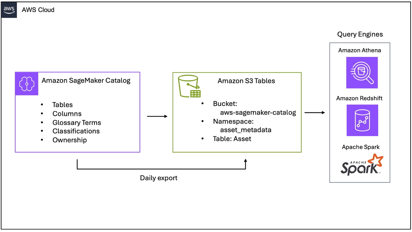
Figure 1 – SageMaker catalog export to S3 Tables
The architecture consists of three key components:
Amazon SageMaker Catalog exports asset metadata daily to Amazon S3.
S3 Tables stores metadata as Apache Iceberg tables in the aws-sagemaker-catalog bucket with ACID compliance and time travel.
Query engines (Amazon Athena, Amazon Redshift, and Apache Spark) access metadata using standard SQL from the asset_metadata.asset table.
What metadata is exposed?
SageMaker Catalog exports metadata in the asset_metadata.asset table:
Metadata Type
Fields
Description
Technical metadata
resource_id, resource_type_enum, account_id, region
Resource identifiers (ARN), types (GlueTable, RedshiftTable, S3Collection), and location
An Amazon SageMaker project for publishing assets.
For SageMaker Unified Studio domain setup instructions, refer to the SageMaker Unified Studio Getting started guide.
After you complete the prerequisites, complete the following steps.
Add this policy to our IAM user or role to enable metadata export. If using SageMaker Unified Studio to query the catalog, add this policy to the AmazonSageMakerAdminIAMExecutionRole managed role.
Grant describe and select permissions for SageMaker Catalog with AWS Lake Formation. This step can be performed in the AWS Lake Formation console.
Select Permissions -> Data permissions and choose Grant.
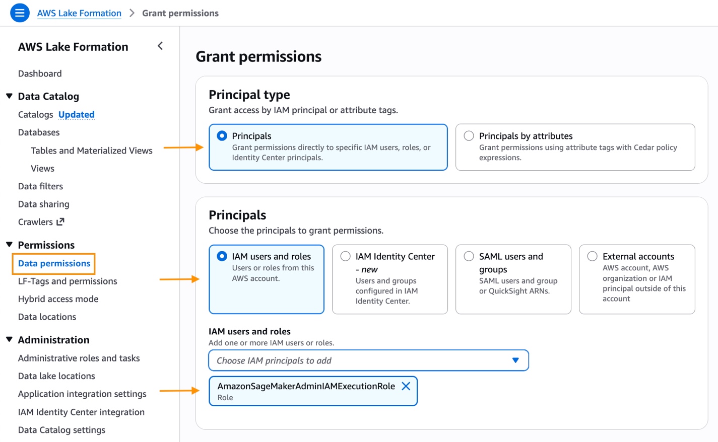
Figure 2 – AWS Lake Formation grant permission
Under Principal type, select Principals, IAM users and roles and the AWS managed AmazonSageMakerAdminIAMExecutionRole execution role.
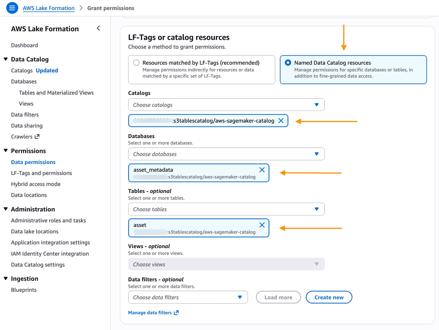
Choose Named Data Catalog resources.
Under Catalogs, search for and select <account-id>:s3tablecatalog/aws-sagemaker-catalog.
Under Databases, select asset_metadata database.
Figure 3 – AWS Lake Formation catalog, database, and table
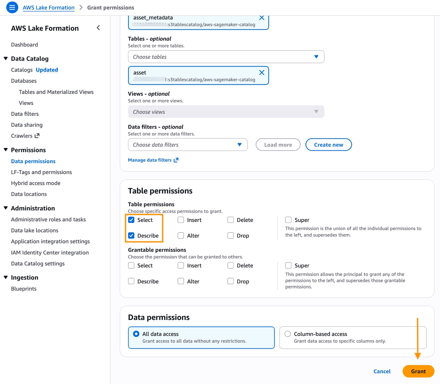
Figure 4 – AWS Lake Formation grant permission
For Table, select asset.
Under Table permissions, check Select and Describe.
Choose Grant to save the permissions.
Enable data export using the AWS CLI
Configure metadata export using the PutDataExportConfiguration API. The Amazon DataZone service automatically creates an S3 table bucket named aws-sagemaker-catalog with an asset_metadata namespace, and schedules a daily export job. Asset metadata is exported once daily around midnight local time per AWS Region.
The SageMaker Domain identifier is available on domain detail page in the AWS Management Console. Accessing the asset table through the S3 Tables console or the Data tab in SageMaker Unified Studio can require up to 24 hours.
AWS CLI command to enable SageMaker catalog export:
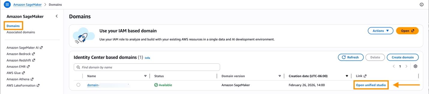
Navigate to Amazon SageMaker Domains in the AWS Management Console.
Select your domain and select Open.
Figure 5 – Open Amazon SageMaker Unified Studio
In SageMaker Unified Studio, choose a project from the Select a project dropdown list.
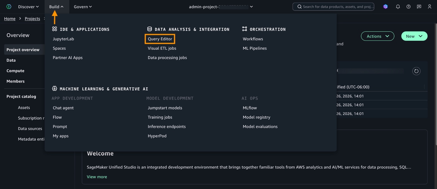
To query SageMaker catalog data, select Build in the menu bar and then choose Query Editor. To create a new project, follow the instructions in the Amazon SageMaker Unified Studio User Guide.
Figure 6 – Open SageMaker Unified Studio Query Editor
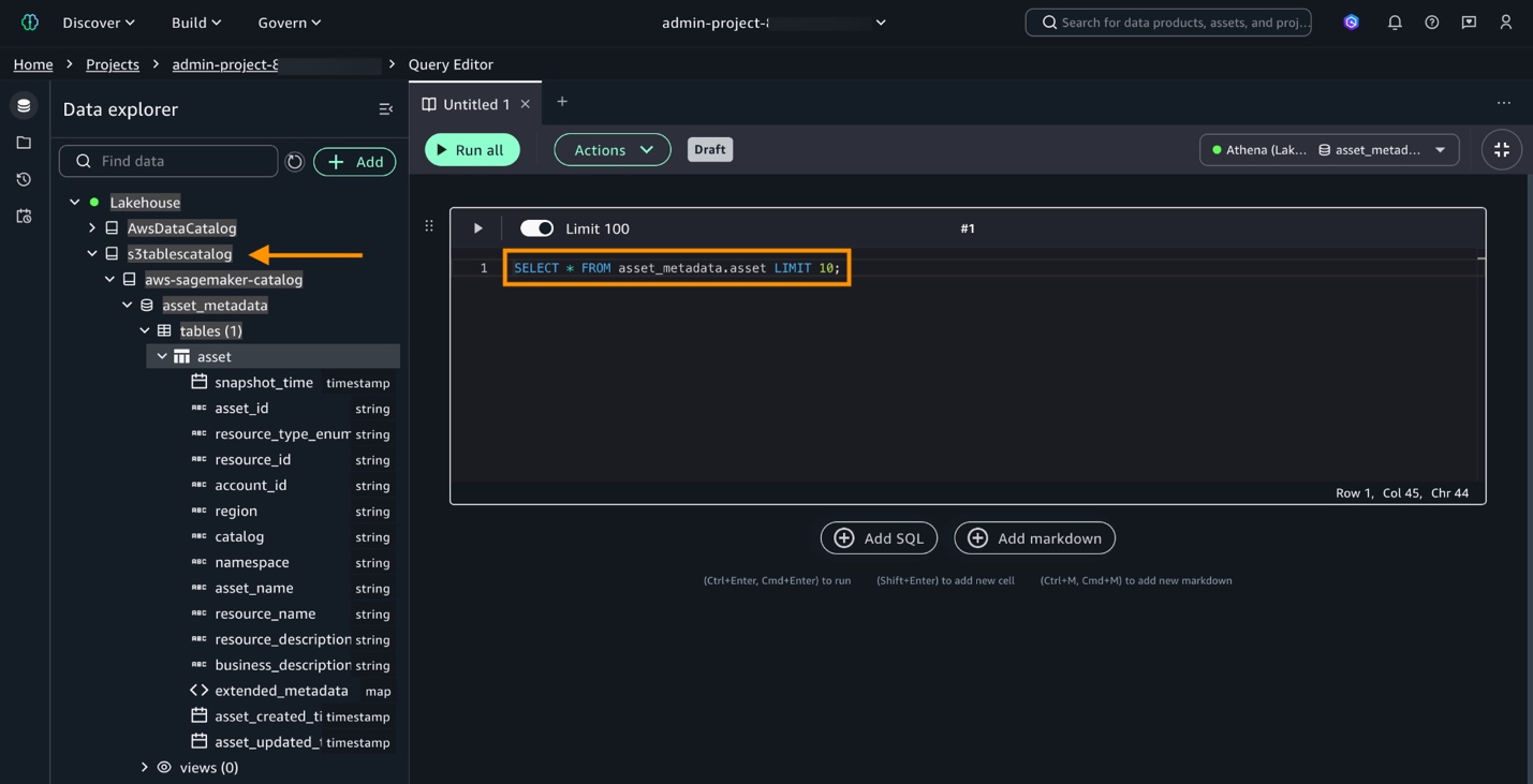
The asset_metadata.asset table is available in Data explorer. Use Data explorer to view the schema and query data to perform analytics from.
Expand Catalogs in Data explorer. Then, select and expand s3tablecatalog, aws-sagemaker-catalog, asset_metadata, and asset.
Test querying the catalog with SELECT * FROM asset_metadata.asset LIMIT 10;.
Figure 7 – Query SageMaker catalog
Queries for observability and analytics
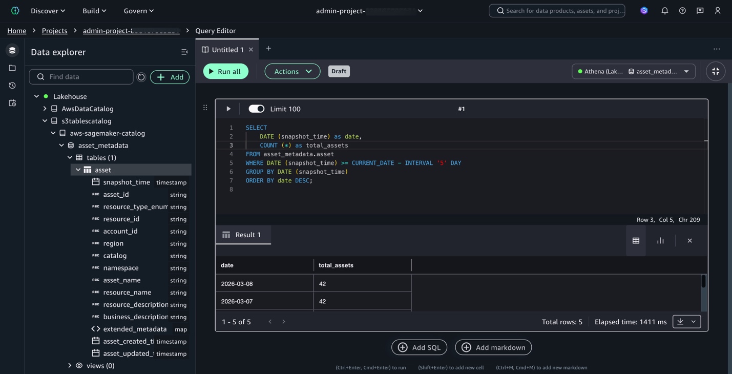
With setup complete, execute queries to gain insights on catalog usage and changes. To monitor asset growth, and view how the data catalog has grown over the last five days:
SELECT
    DATE (snapshot_time) as date,
    COUNT (*) as total_assets
FROM asset_metadata.asset
WHERE
     DATE (snapshot_time) >= CURRENT_DATE - INTERVAL '5' DAY
GROUP BY DATE (snapshot_time)
ORDER BY date DESC;
Figure 8 – Query asset growth
Use the catalog to track metadata changes to determine which assets gained descriptions or ownership over time. Use this query to identify assets that gained business descriptions over the past five days by comparing today’s snapshot with the earlier snapshot.
SELECT
    t.asset_id,
    t.resource_name,
    p.business_description as description_before,
    t.business_description as description_now
FROM asset_metadata.asset t
JOIN asset_metadata.asset p ON t.asset_id = p.asset_id
WHERE DATE(t.snapshot_time) = CURRENT_DATE
    AND DATE(p.snapshot_time) = CURRENT_DATE - INTERVAL '5' DAY
    AND p.business_description IS NULL
    AND t.business_description IS NOT NULL;
Investigate asset values at a specific point in time using this query to retrieve metadata from any snapshot date.
SELECT
     asset_id,
     resource_name,
     business_description,
     extended_metadata['owningEntityId'] as owner,
     snapshot_time
FROM asset_metadata.asset
WHERE asset_id = 'your-asset-id'
     AND DATE(snapshot_time) = DATE('2025-11-26');
Clean up resources
To avoid ongoing charges, clean up the resources created in this walkthrough:
Disable metadata export:
Disable the daily metadata export to stop new snapshots:
Optionally, delete the S3 Tables namespace containing the exported metadata to remove historical snapshots and stop storage charges. For instructions on how to delete S3 tables, see Deleting an Amazon S3 table in the Amazon Simple Storage Service User Guide.
Conclusion
In this post, you enabled the metadata export feature of SageMaker Catalog and used SQL queries to gain visibility into your asset inventory. The feature converts asset metadata into Apache Iceberg tables partitioned by snapshot date, so you can perform time-travel queries, monitor catalog growth, track metadata completeness, and audit historical asset states. This provides a repeatable, low-overhead way to maintain catalog health and meet governance requirements over time.
You can process real-time data from your data lake with Amazon Managed Service for Apache Flink without maintaining two separate pipelines. Yet many teams do exactly that, and the cost adds up fast. In this post, you build a unified pipeline using Apache Iceberg and Amazon Managed Service for Apache Flink that replaces the dual-pipeline approach. This walkthrough is for intermediate AWS users who are comfortable with Amazon Simple Storage Service (Amazon S3) and AWS Glue Data Catalog but new to streaming from Apache Iceberg tables.
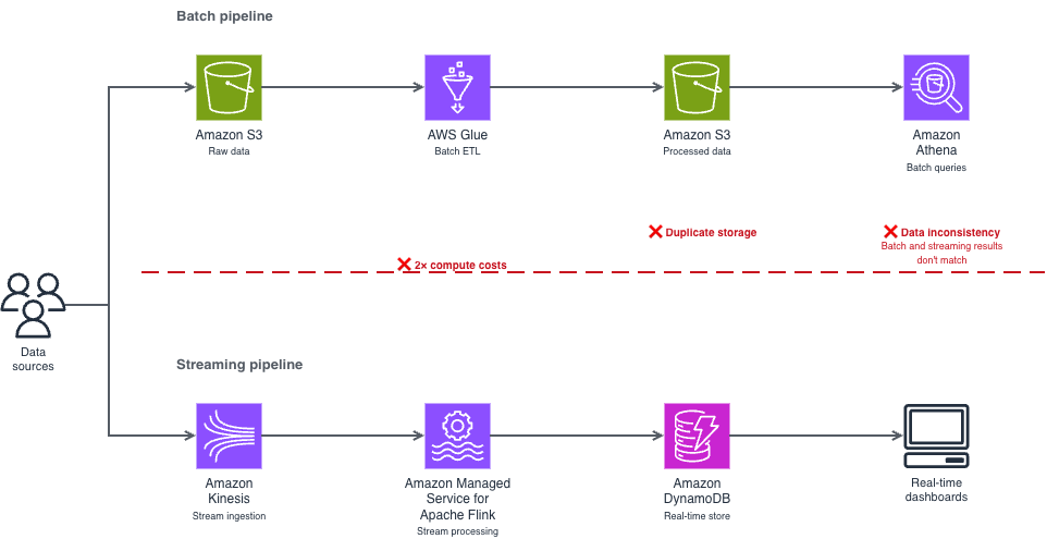
The dual-pipeline problem
This dual-pipeline approach creates three problems:
Double the infrastructure costs. You run and pay for two separate compute environments, two storage layers, and two sets of monitoring. For example, if you’re spending $10,000/month on separate streaming and batch infrastructure, a meaningful portion of that spend is pure duplication.
Data synchronization issues. Your batch and streaming consumers read from different copies of the data, processed at different times. When a transaction shows up in your real-time dashboard but not in your batch report (or vice versa), debugging the inconsistency takes hours.
Operational complexity. Two pipelines mean two deployment processes, two failure modes to monitor, and two sets of schema evolution to manage. Your team spends time reconciling systems instead of building features.
Where this pattern fits
Before diving into the implementation, consider whether streaming from your data lake is the right approach for your use case.
Streaming from Apache Iceberg tables works well when you need data available within seconds to minutes and you query recent data frequently, multiple times per hour. Common scenarios include:
Operational data stores — Stream customer profile updates to serve downstream applications like recommendation engines. When a customer updates their preferences, those changes reach your operational data store within seconds.
Fraud detection — Stream transactions for immediate analysis. Start with a 3-second monitor interval and adjust based on your detection accuracy needs.
Live dashboards — Power real-time analytics directly from your lake. This is the strongest starting point if you’re evaluating the approach for the first time, because the feedback loop is immediate and straightforward to validate.
Event-driven architectures — Trigger downstream processes based on data changes in your Apache Iceberg tables.
Batch processing remains more cost-effective when you process data once per day or less, or you primarily query historical data. Batch queries on Apache Iceberg tables cost less because they don’t require a continuous Apache Flink runtime.
How Apache Iceberg solves this
Apache Iceberg’s snapshot-based architecture removes the need for a separate streaming pipeline. Think of snapshots like Git commits for your data. Each time you write data to your Iceberg table, Iceberg creates a new snapshot that points to the new data files while preserving references to existing files. Apache Flink reads only the changes between snapshots (the new files that arrived after the last checkpoint), rather than scanning the entire table. Atomicity, Consistency, Isolation, Durability (ACID) transactions prevent your concurrent reads and writes from producing partial or inconsistent results. For example, if your batch extract, transform, and load (ETL) job is writing 10,000 records while your Flink application is reading, ACID transactions mean that your streaming query sees either the complete batch of 10,000 records or none of them, not a partial set that could skew your analytics.
The result is a single pipeline that handles both real-time and batch access from the same data, through the same storage layer, with the same schema.
Solution architecture
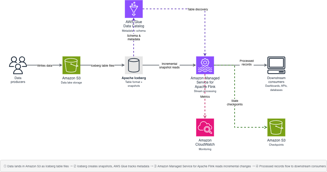
Your architecture uses four AWS services and one open source table format working together. The following diagram shows how these components connect, replacing the dual-pipeline pattern shown earlier with a single unified flow.
Your source data lands in Amazon S3 as Apache Iceberg table files. AWS Glue Data Catalog tracks the metadata and schema. When new data arrives, Apache Iceberg creates a new snapshot that your application detects. Your Flink application monitors these snapshots and processes new records incrementally, reading only the files that arrived after the last checkpoint, not the entire table.
You use four main components:
Amazon S3 — Foundational storage layer for your data lake
Data Catalog — Metadata and schema management for Apache Iceberg tables
Apache Iceberg — Table format with snapshot-based streaming capabilities
Amazon Managed Service for Apache Flink — Stream processing and incremental consumption
Important notices
Before implementing this solution, evaluate these risks for your environment:
Data security: Streaming from data lakes exposes data to additional processing systems. Classify your data before implementation—customer profile updates and transaction data typically contain personally identifiable information (PII) and treat them as confidential. Apply encryption at rest and in transit for confidential data. Key risks include unauthorized data access through misconfigured Amazon S3 bucket policies or overly permissive IAM roles. Mitigations: use the resource-scoped IAM policy and TLS-enforcing bucket policy provided in the Security section.
Data integrity: Misconfigured checkpoints or schema changes during streaming can lead to data inconsistency. Mitigations: enable exactly-once processing semantics and test schema evolution in a non-production environment first.
Compliance: Verify that real-time data processing meets your regulatory requirements. For workloads subject to HIPAA, confirm that you use HIPAA Eligible Services and have a Business Associate Agreement (BAA) with AWS. For PCI-DSS or GDPR workloads, review the relevant compliance documentation on the AWS Compliance page. Implement data retention policies that comply with your regulatory framework.
Cost: Nearly continuous streaming incurs ongoing compute costs. Monitor usage to avoid unexpected charges. Cost estimates in this post are based on pricing as of March 2026 and might change. Verify current pricing on the relevant AWS service pricing pages.
Operational: Pipeline failures might impact downstream systems. Implement monitoring and alerting before running in production.
Prerequisites
Before you begin, make sure that you have the following in place. This walkthrough assumes intermediate Python skills (comfortable with functions, error handling, and environment variables), basic Apache Flink concepts (streaming compared to batch processing), and basic AWS Identity and Access Management (AWS IAM) knowledge (creating roles and attaching policies). Plan for approximately 90–120 minutes, including setup, implementation, and testing. First-time setup might take longer as you download dependencies and configure AWS resources. Expected AWS costs: approximately $5–10 if you complete the walkthrough within 2 hours and clean up resources immediately afterward. The primary cost driver is Amazon Managed Service for Apache Flink runtime ($0.11/hour per Kinesis Processing Unit (KPU)). You can minimize costs by stopping your application when not in use.
An AWS account with AWS IAM permissions for: s3:GetObject, s3:PutObject, s3:ListBucket on your data bucket; glue:GetDatabase, glue:GetTable for catalog access; and flink:CreateApplication, flink:StartApplication for Amazon Managed Service for Apache Flink
You need multiple JAR files because your Flink application coordinates between different systems—Amazon S3 for storage, AWS Glue for metadata, Hadoop for file operations, and Apache Iceberg for the table format. Each JAR handles a specific part of this integration. Missing even one causes ClassNotFoundException errors at runtime.
iceberg-flink-runtime-1.19-1.6.1.jar — Core Apache Iceberg integration with Apache Flink
iceberg-aws-bundle-1.6.1.jar — AWS-specific Apache Iceberg functionality for Amazon S3 and AWS Glue
flink-s3-fs-hadoop-1.19.1.jar — Provides Apache Flink read and write access to Amazon S3
flink-sql-connector-hive-3.1.3_2.12-1.19.1.jar — Hive metastore connector for catalog compatibility
hadoop-common-3.4.0.jar — Core Hadoop libraries required by Apache Iceberg
flink-shaded-hadoop-2-uber-2.8.3-10.0.jar — Repackaged Hadoop dependencies that avoid version conflicts with Apache Flink
hadoop-hdfs-client-3.4.0.jar — Hadoop Distributed File System (HDFS) client libraries for file system operations
flink-json-1.19.1.jar — JSON format support for Apache Flink
hadoop-aws-3.4.0.jar — Hadoop integration with AWS services
hadoop-client-3.4.0.jar — Hadoop client libraries
aws-java-sdk-bundle-1.12.261.jar — AWS SDK for authentication and service access
The sample code in this post is available under the MIT-0 license.This section walks you through building the streaming pipeline step by step. You create a single Python file, iceberg_streaming.py, with three functions that run in sequence. Your main() function calls them in order: set up the Apache Flink environment, register the Data Catalog, then start the streaming query.
Set up your Apache Flink environment
To prepare your Apache Flink environment:
Download the required JAR files listed in the prerequisites section.
Place the JAR files in a lib directory in your project folder.
Configure your HADOOP_CLASSPATH environment variable to point to the lib directory.
Create your streaming execution environment by adding the following function to iceberg_streaming.py:
Verify your environment by running flink –version. If the command isn’t found, confirm that Apache Flink 1.19.1 is installed and that your PATH includes the Flink bin directory.
Configure AWS Glue Data Catalog
To connect your Flink application to Data Catalog:
Open your iceberg_streaming.py file.
Add the create_iceberg_source() function shown in the following section.
Replace the placeholder values with your actual AWS resources before running. These values are static configuration strings, not user input — do not construct them from external or untrusted sources at runtime.
Save the file.
def create_iceberg_source(t_env):
    """Register the AWS Glue Data Catalog as an Iceberg catalog."""
    try:
        catalog_sql = """
        CREATE CATALOG glue_catalog WITH (
            'type'='iceberg',
            'catalog-impl'='org.apache.iceberg.aws.glue.GlueCatalog',
            'warehouse'='s3://<example-data-lake-bucket>',
            'io-impl'='org.apache.iceberg.aws.s3.S3FileIO',
            'aws.region'='us-east-1',
            'hadoop-conf.fs.s3a.aws.credentials.provider'=
                'com.amazonaws.auth.DefaultAWSCredentialsProviderChain',
            'hadoop-conf.fs.s3a.endpoint'='s3.amazonaws.com',
            'property-version'='1'
        )
        """
        t_env.execute_sql(catalog_sql)
        t_env.use_catalog("glue_catalog")
        t_env.use_database("streaming_db")
    except Exception as e:
        print(f"Failed to configure Iceberg catalog: {e}")
        raise
Set up streaming logic
This function configures Apache Flink to monitor your Apache Iceberg table continuously and process new records as they arrive. Checkpointing runs every 10 seconds to track progress—if the job restarts, it resumes from the last checkpoint rather than reprocessing the entire table.Notice the monitor-interval parameter, it controls how frequently Apache Flink checks for new Apache Iceberg snapshots. A 3-second interval provides near real-time processing but generates approximately 1,200 Amazon S3 LIST API calls per hour (at $0.005 per 1,000 requests, roughly $0.04/month per table based on pricing as of March 2026). For less time-sensitive workloads, increase this to 30s to reduce API costs by 90%.Replace customer_events with the name of your Apache Iceberg table in Data Catalog:
def process_record(row):
    """Validate and process each record from the stream."""
    try:
        if row is None:
            raise ValueError("Received null row")
        required_fields = ["event_type", "timestamp"]
        for field in required_fields:
            if field not in row:
                raise ValueError(f"Missing required field: {field}")
        # Validate field types and content
        if not isinstance(row.get("event_type"), str) or len(row["event_type"]) > 256:
            raise ValueError("event_type must be a string under 256 characters")
        if not isinstance(row.get("timestamp"), (str, int)):
            raise ValueError("timestamp must be a string or integer")
        # Replace with your business logic
        print(f"Processing record: {row}")
    except ValueError as e:
        print(f"Validation error for record {row}: {e}")
    except Exception as e:
        print(f"Error processing record {row}: {e}")
def stream_data(t_env):
    """Start the streaming query and process results."""
    try:
        configuration = t_env.get_config().get_configuration()
        configuration.set_string("table.dynamic-table-options.enabled", "true")
        configuration.set_string("execution.checkpointing.interval", "10000")
        query = """
        SELECT * FROM customer_events /*+ OPTIONS(
            'streaming'='true',
            'monitor-interval'='3s',
            'table.exec.iceberg.cell-based-snapshot'='true'
        ) */
        """
        table_result = t_env.execute_sql(query)
        with table_result.collect() as results:
            for row in results:
                process_record(row)
    except Exception as e:
        print(f"Streaming query failed: {e}")
        raise
Putting it together
Your main() function calls the three steps in order:
Run the pipeline locally:python iceberg_streaming.pyPackage the application and submit it to Amazon Managed Service for Apache Flink using the console or the AWS Command Line Interface (AWS CLI).
Running in production
Moving from a local test to a production deployment requires tuning four areas: performance, monitoring, cost, and security. This section covers the key decisions for each.
Performance tuning
Determine your latency requirements before tuning. For fraud detection, you need subsecond processing. For daily reporting dashboards, you can tolerate minutes of delay.
Partition pruning reduces the amount of data scanned per query. Proper partitioning can significantly reduce query times for time series data partitioned by date. To implement, create your Apache Iceberg table with partition columns (PARTITIONED BY (date_column) in your CREATE TABLE statement), then include partition filters in your WHERE clause: WHERE date_column >= CURRENT_DATE - INTERVAL '7' DAY.
Parallel processing matches your data volume and throughput requirements. For most workloads under 10,000 records per second, a parallelism of 1–4 is sufficient. Scale up incrementally and monitor backpressure metrics (indicators that data arrives faster than your pipeline processes it, causing queuing) to find the right setting.
Checkpoint tuning balances reliability and latency. Consider how much data you can afford to reprocess after a failure. If you process 1,000 records per second with 10-second checkpoints, a failure means reprocessing up to 10,000 records. When that’s acceptable, 10 seconds works well. For faster recovery or higher volumes, reduce to 5 seconds.
Resource allocation — Right-size your Apache Flink cluster to avoid over-provisioning. Monitor CPU and memory utilization during your initial runs and adjust task manager resources accordingly.
Monitoring
Configure your production deployment with the following checkpoint settings. These work well for moderate data volumes (up to 10,000 records per second), providing exactly-once processing semantics. This means that the pipeline processes each record exactly once, even if your application restarts. Adjust the checkpoint interval based on your latency requirements. Add this to your setup_environment() function after creating the table environment.
Use Amazon CloudWatch to track checkpoint duration, records processed per second, and backpressure metrics. A 10-second checkpoint interval means writing state to Amazon S3 360 times per hour. For a 1 MB state size, that’s approximately 8.6 GB per day in checkpoint storage—at Amazon S3 Standard pricing of $0.023/GB, roughly $0.20/day or $6/month per application based on current pricing. If the checkpoint duration exceeds 50% of your interval, increase the interval or add parallelism.
Cost management
Use Amazon S3 Intelligent-Tiering for your Apache Iceberg data files, which typically have predictable access patterns after initial processing. Configure Apache Iceberg’s table expiration to automatically clean up early snapshots. This can reduce storage costs by an estimated 20–30%, though your results vary depending on write frequency and retention policies.
Right-size your Apache Flink resources based on actual throughput needs. Start with a minimal configuration and scale up based on observed backpressure and checkpoint duration metrics. Use Amazon Elastic Compute Cloud (Amazon EC2) Spot Instances where workload interruptions are acceptable, for example, in development and testing environments.
Set data retention policies on both your Apache Iceberg tables and checkpoint storage to avoid storing data longer than necessary.
Security
Security is a shared responsibility between you and AWS. AWS is responsible for the security of the cloud, including the hardware, software, networking, and facilities that run AWS services. You are responsible for security in the cloud, configuring access controls, encrypting data, and managing your application security. Apply these controls in priority order.
AWS IAM roles — Use AWS IAM roles with least-privilege access, scoped to specific resources. The following example policy restricts permissions to your data lake bucket and AWS Glue catalog:
Scoping permissions to specific Amazon S3 buckets, AWS Glue databases, and AWS Key Management Service (AWS KMS) keys restrict access to only the resources your pipeline requires. Review IAM policies quarterly using the IAM Access Analyzer to identify and remove unused permissions.
Encryption — Configure server-side encryption with AWS Key Management Service (AWS KMS) customer managed keys (SSE-KMS) for your Amazon S3 buckets. Using customer managed keys requires additional review from your security team. Confirm your key management policies, rotation procedures, and access controls before implementation. Enable automatic key rotation annually. For encryption in transit, enforce TLS by adding a bucket policy that denies non-HTTPS access:
Enable versioning on buckets that store critical data and checkpoints to protect against accidental deletion. For production environments with sensitive data, consider enabling MFA Delete on versioned buckets. Enable S3 server access logging to track requests for security auditing.
Access logging – Enable AWS CloudTrail data events to log Amazon S3 object-level API calls (GetObject, PutObject) and Data Catalog API calls. Store logs in a separate Amazon S3 bucket with restricted access and enable log file integrity validation. Run regular compliance checks using AWS Config.
Operational practices
Set up a continuous integration and continuous deployment (CI/CD) pipeline to automate deployment and testing. Use version control to track schema and code changes. With Apache Iceberg’s schema evolution support, you can add columns without rewriting existing data files. Establish rollback procedures using Apache Iceberg’s snapshot-based architecture, so you can roll back to a previous table state if a bad write corrupts your data.
Troubleshooting
If you run into issues during setup or execution, use the following table to diagnose common errors.
Error
Cause
Solution
ClassNotFoundException
Missing JAR files
Check the dependencies in your lib directory and confirm HADOOP_CLASSPATH points to the correct path
Table not found
Database name mismatch
Check that the database name in t_env.use_database() matches the AWS Glue database where you registered your table
Checkpoint failures
Amazon S3 permissions
Check that your Amazon S3 bucket policy grants s3:PutObject for the checkpoint location
AWS credential errors
Missing AWS IAM configuration
Check that the AWS IAM role attached to your Apache Flink application has glue:GetTable, glue:GetDatabase, and s3:GetObject permissions on the relevant resources
Snapshot not found
Table modified during query
Increase monitor-interval or implement retry logic in your process_record() function
Schema mismatch
Table schema changed between snapshots
Review Apache Iceberg schema evolution settings and confirm backward compatibility
Clean up
To avoid ongoing charges, delete the resources that you created during this walkthrough.
Stop your Amazon Managed Service for Apache Flink application. Open the Amazon Managed Service for Apache Flink console, choose your application name, choose Stop, and confirm the action. Or use the AWS CLI:
If you created an Amazon VPC or Amazon VPC endpoints for testing, delete those resources.
Conclusion
Maintaining separate streaming and batch pipelines doubles your infrastructure costs, creates data synchronization issues, and adds operational complexity that slows your team down. In this post, you replaced that dual-pipeline architecture with a single system built on Apache Iceberg and Amazon Managed Service for Apache Flink. You configured a Flink environment with the required JAR dependencies, connected it to Data Catalog, and implemented streaming queries that read new records incrementally with exactly-once processing semantics. The same data, the same storage layer, the same schema—accessible to both your real-time and batch consumers.
To extend this solution, try these next steps based on your use case:
If you’re processing high volumes (>10,000 records/sec): Start with partition pruning. Add PARTITIONED BY (date_column) to your table definition, this typically reduces query times by 60–80%.
If you need production monitoring: Implement custom Amazon CloudWatch metrics. Track checkpoint duration, records processed per second, and backpressure to catch issues before they impact your pipeline.
Security logs capture essential security-related activities, such as user sign-ins, file access, network traffic, and application usage. These logs are important for monitoring, detecting, and responding to potential security events. The Open Cybersecurity Schema Framework (OCSF) addresses this challenge by providing a standardized format to represent security events, ensuring consistent and efficient data handling across various systems. OCSF enhances interoperability, streamlines analysis, simplifies compliance reporting, and reduces vendor lock-in, fostering greater flexibility and efficiency in security operations.
However, manually transforming diverse security logs into OCSF format at scale can be complex and time-consuming. Amazon Security Lake simplifies this process by automatically centralizing security data from AWS services such as AWS CloudTrail management and data events (Amazon Simple Storage Service (Amazon S3) and AWS Lambda), Amazon Elastic Kubernetes Service (Amazon EKS) audit logs, Amazon Route 53 resolver query logs, AWS Security Hub findings, Amazon Virtual Private Cloud (Amazon VPC) Flow Logs, and AWS WAF logs. It also centralizes security logs from software as a service (SaaS) providers, on-premises, and cloud sources into a purpose-built data lake stored in your account. It uses the OCSF format to standardize and normalize this data, ensuring consistency and simplifying analysis. By integrating with analytics tools such as Amazon Athena and Amazon Quick Sight, Security Lake simplifies threat detection, improves security posture monitoring, and streamlines compliance reporting, making it an essential tool for modern security operations.
In this post, we show you how to transform custom security logs into OCSF format after you have the OCSF mappings ready, using a configuration-driven extract, transform, load (ETL) solution.
Accelerating OCSF adoption with AWS ProServe ETL solution
Amazon Security Lake stores security data in OCSF format and so customers looking to use custom log sources in Security Lake must transform their logs into OCSF format. To facilitate this process, the AWS Professional Services (ProServe) team built an ETL solution accelerator that converts custom security logs into OCSF format. This solution bridges existing log formats with the OCSF version 1.1 standard, streamlining data onboarding into Security Lake or other data lakes of security logs coming from multiple security tools.
Prerequisites
To implement this solution, you must have the following resources:
This solution uses serverless AWS services including Amazon S3, Lambda, DynamoDB, Step Functions, and either AWS Glue or Amazon EMR Serverless for ETL. Costs depend on data volume and processing frequency. Key expenses are storage (Amazon S3 and DynamoDB), compute (Lambda, AWS Glue, and Amazon EMR), and orchestration services. The architecture is cost-optimized through serverless components and pay-per-use pricing. Use AWS Pricing Calculator to estimate costs for your specific log volume and retention needs.
Solution overview
The solution uses two input files: a mapping file and a configuration file. These files guide the transformation of source logs into OCSF-compliant Parquet format, which is then partitioned by location/region=region/accountId=accountID/eventDay=yyyyMMdd/ and stored in an Amazon S3 location provided by Security Lake.
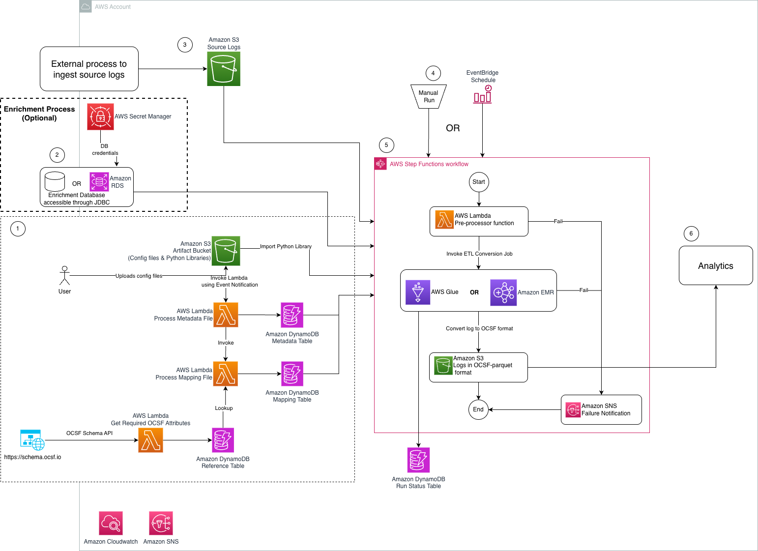
The following diagram shows the key architecture components of this solution and data flow between them.
Figure 1: Architecture diagram of ETL solution to transform security logs into OCSF format
The steps mentioned below walks you through the architecture diagram:
Preprocessing steps:
User uploads a mapping file in CSV format that maps custom security logs into OCSF class.
User uploads a metadata file in CSV format that is passed to the solution to transform custom security logs into OCSF format.
An Amazon S3artifact bucket stores the metadata, source-to-target mapping, and Python libraries required for OCSF conversion.
An Amazon S3 event notification invokes the Lambda function that writes the metadata to the asl-etl-framework-ocsf-attribute-metadata DynamoDB table when the metadata files are created or updated.
Metadata and mapping Lambda functions process the respective configuration files and store the required information in DynamoDB tables.
The Reference Lambda function extracts the required OCSF attributes using an API call and stores the results in a DynamoDB table.
Optional enrichment process: The solution reads data from an enrichment database stored on Amazon RDS or an external on-premises database that’s accessible through a JDBC connection from either Amazon EMR or AWS Glue. The credentials of this enrichment database are stored in Secrets Manager.
Source log files are delivered to an S3 bucket by an external process.
An EventBridge schedule or manual invoke initiates the Step Functions workflow, responsible for log conversion.
A Step Functions workflow performs the following tasks:
The preprocessor Lambda function performs checkpointing and invokes the required number of ETL jobs in parallel.
The ETL job converts the source log files to the OCSF-Parquet format using the custom Python libraries stored in the artifact bucket and the mapping information defined in the DynamoDB table.
A separate target S3 bucket stores the converted log data.
An Amazon SNS topic is used to notify users if the Step Functions workflow fails during checkpointing or the ETL process.
Analytics are performed on the converted data.
Deployment
You can find the required resources to deploy this solution in this GitHub repository. It provides detailed instructions in the README on how to deploy the solution. After you have the prerequisites mentioned earlier, see the Environment Setup portion of the repository.
Solution walkthrough
In this section, we walk you through steps to deploy this solution.
Map source log files into OCSF format
Before you start mapping the security logs into OCSF format, check if there are existing mappings available on OCSF mappings Github.
Mapping security logs into the OCSF format typically involves several steps. Here are the high-level steps:
Understand OCSF schema: Familiarize yourself with the OCSF schema, which defines the structure and format for organizing security log data into event classes and attributes. In OCSF, events are organized into event classes, each of which comprises a set of attributes designed to offer comprehensive semantics for the event.
Identify log sources: Determine your security log sources, such as firewalls, intrusion detection systems, or antivirus software. Each log source might have its own format (CSV, JSON, and so on) and structure.
Identify OCSF categories and classes: Analyze the log content and match security events to the appropriate OCSF categories and classes for standardized data organization.
Map fields to OCSF schema: Map the source log data fields in the OCSF schema. Ensure that each field from your logs is mapped to the appropriate field in the OCSF format. If a field in the source log schema isn’t mapped to any OCSF field, you might need to consider mapping it to unmapped object.
Enrichment: Enrich data with additional contextual information, such as standardizing timestamps, converting IP addresses to a common format, or adding supplementary data for better analysis. The enrichment column is added to the final dataset. Each category in OCSF has an optional enrichment column that provides more information about a column. For example, the Authentication OCSF category contains an optional enrichment column that provides more details about the IP addresses. .
Test and validate: Validate mapped log data against the OCSF schema to ensure compliance and accuracy. Test the mapping process with sample log data from different sources to identify any inconsistencies or errors. You can use this open source utility to validate your generated OCSF version 1.1 output file based on mapping.
Contribute OCSF Mapping to the OCSF community: Submit the OCSF mapping to the Github repository and raise a pull request to contribute it to the OCSF community. Iterate on the mapping procedure to improve accuracy, efficiency, and compatibility with the OCSF schema based on the pull request feedback.
By following these steps, you can effectively map security logs into the OCSF format, enabling better interoperability, analysis, and collaboration across security tools and platforms. AWS ProServe has helped many customers map their security logs to OCSF format. If you need guidance to map and transform security logs into OCSF format and want to use AWS ProServe, reach out to your account executive.
Create and transform mapping files
The ETL solution requires a CSV mapping file that maps the custom security log attributes into standardized OCSF attributes based on the specified OCSF class. For detailed instructions on generating this mapping file, see the Solution Usage section, bullet 2, in the README of the code repository. To follow the instructions in this post, you can enable Amazon S3 server access logging to publish source logs to Amazon S3. The following is a sample S3 server access log record:
Because the sample record uses spaces as delimiters and contains an extra space before +0000, you need to wrap each attribute in quotes. Here’s a sample Python code implementation that handles this requirement:
import re
def format_s3_access_log(log_line):
    def quote_field(field):
        """Add quotes around a field and handle special cases"""
        if field is None or field.strip() == '':
            return '"-"'
        # If field is already quoted, return as is
        if field.startswith('"') and field.endswith('"'):
            return field
        return f'"{field}"'
    try:
        # First, protect quoted strings and bracketed content by temporarily replacing them
        protected_line = log_line
        protected_parts = re.findall(r'(\[.*?\]|".*?")', log_line)
        for i, part in enumerate(protected_parts):
            protected_line = protected_line.replace(part, f"PROTECTED_{i}_PART")
        # Split the protected line
        parts = protected_line.split()
        # Restore protected parts
        restored_parts = []
        for part in parts:
            if part.startswith('PROTECTED_') and part.endswith('_PART'):
                index = int(part.split('_')[1])
                restored_parts.append(protected_parts[index])
            else:
                restored_parts.append(part)
        # Quote each field
        quoted_fields = [quote_field(field) for field in restored_parts]
        # Join with spaces
        return ' '.join(quoted_fields)
    except Exception as e:
        print(f"Error processing line: {e}")
        return None

# Example usage
if __name__ == "__main__":
    # Example input log line
    log_line = '''90de84bb542adb54766fec66ee554475b7e1a56a9d8b30e3598230f9ef6d6ac7 azv-asl-src-logs [29/May/2025:04:35:45 +0000] - arn:aws:sts::768196192565:assumed-role/AwsSecurityAudit/Palisade QS8DSY4SGF8M8SD7 REST.GET.BUCKETPOLICY - "GET /?policy HTTP/1.1" 200 - 255 - 39 - "-" "-" - N9XclJkv6hw/y4yApPyDII2sRoMNbqJqBEXdnmzFndcvhQOpdcc3PNQNQX7NhQaPJ5FKSVPh6hLB0GqsSN4apcbBUHi3rNcPRqa6rFLAYU4= SigV4 TLS_AES_128_GCM_SHA256 AuthHeader azv-asl-src-logs.s3.amazonaws.com TLSv1.3 - -'''
    # Process the log line
    formatted_output = format_s3_access_log(log_line)
    print(formatted_output)
This sample code demonstrates how to wrap quotes around each attribute. You can extend this code to read source Amazon S3 server access log files from an S3 location and write the modified logs to another location. After these logs are available in an S3 bucket in your AWS account, you need to map the S3 server access logs to OCSF format. The following is an example of an S3 server access log CSV mapping file:
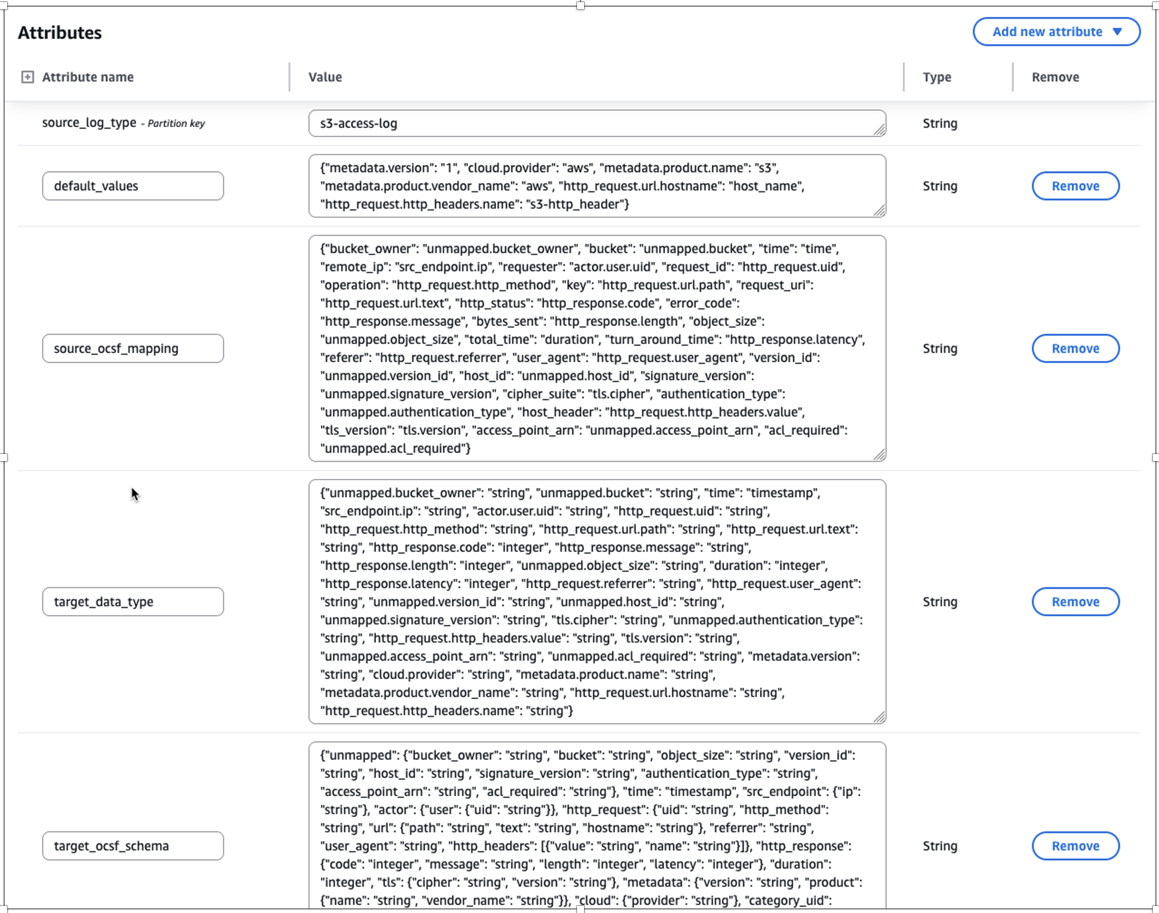
Upload the mapping CSV file to the S3 artifact location s3://secure-datalake-artifacts-<account_number>-<aws_region>/config/mapping/. The Lambda function asl-etl-framework_update-mapping-ddb ingests this mapping CSV file, processes its entries, and converts them into the required DynamoDB format. This Lambda function writes the results to the asl-etl-framework-ocsf-attribute-mapping DynamoDB table, which stores the schema and mapping information for all source log files processed by this solution. You can find an example of an S3 server access log CSV metadata file in the GitHub repository.
Upload the completed mapping CSV file into an S3 artifact location s3://secure-datalake-artifacts-<account_number>-<aws_region>/config/metadata/. An upload of a metadata CSV file to S3 invokes a Lambda function asl-etl-framework_insert_metadata_ddb, which stores the configuration in the asl-etl-framework-source-ocsf-metadata DynamoDB table. The following image shows the configuration in DynamoDB table.
Figure 2: Screenshot of metadata configuration in the asl-etl-framework-source-ocsf-metadata DynamoDB table for S3 Access Logs
After inserting the metadata into the asl-etl-framework-source-ocsf-metadata DynamoDB table, the Lambda function asl-etl-framework_update-mapping-ddb is invoked to read the mapping CSV file and inserts mappings into the asl-etl-framework-ocsf-attribute-mapping DynamoDB table. The following image shows the mapping in DynamoDB table.
Figure 3: Screenshot of transformed mapping in the asl-etl-framework-ocsf-attribute-mapping DynamoDB table for S3 Access Logs
Historical load
The ETL solution offers a historical load capability that processes logs from specified date or year ranges based on metadata file inputs. After being converted to OCSF format in Parquet file format, these logs can be integrated into Amazon Security Lake or be used to create a custom data lake. The solution includes checkpointing functionality to handle potential failures during historical data processing.
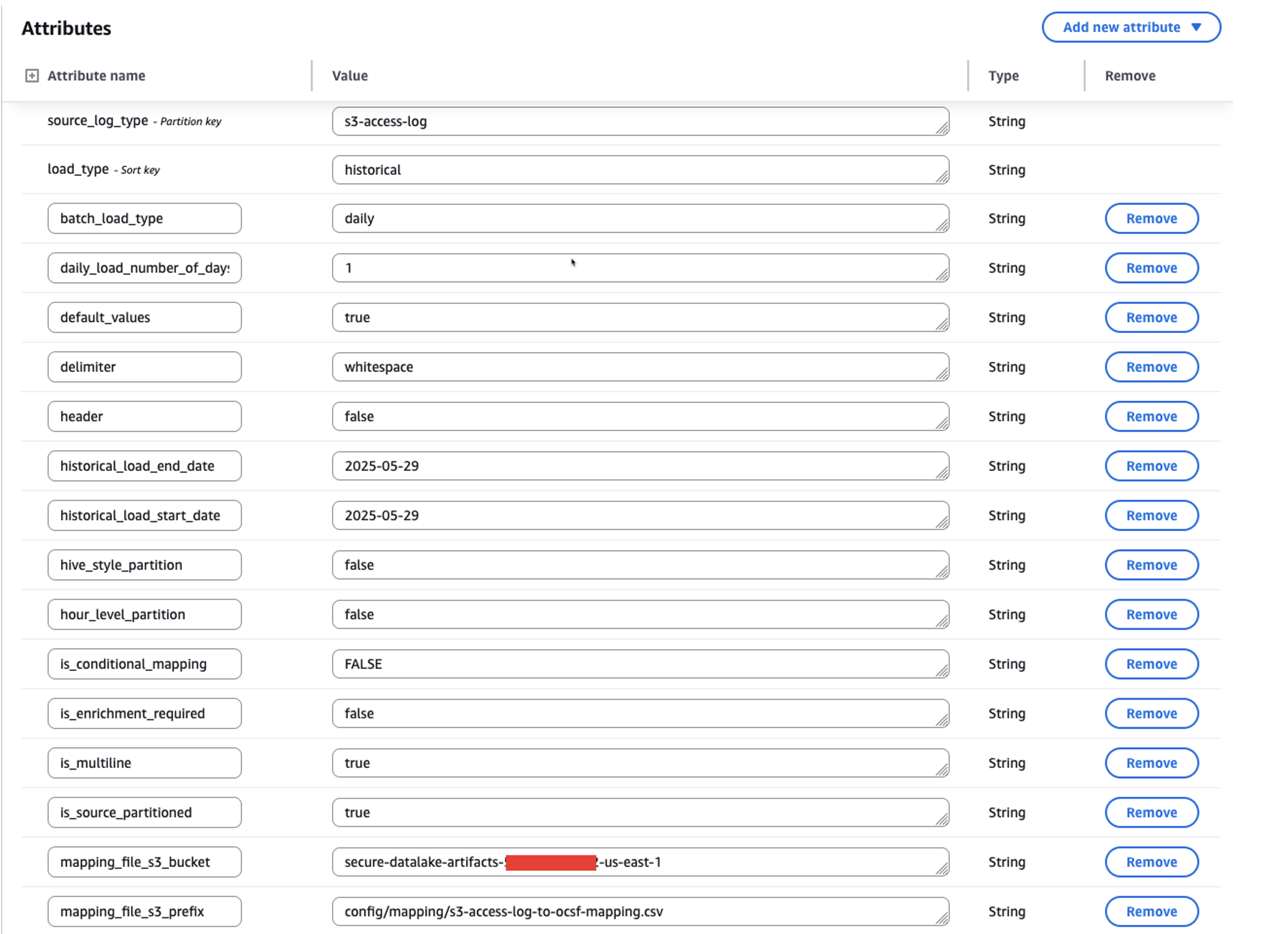
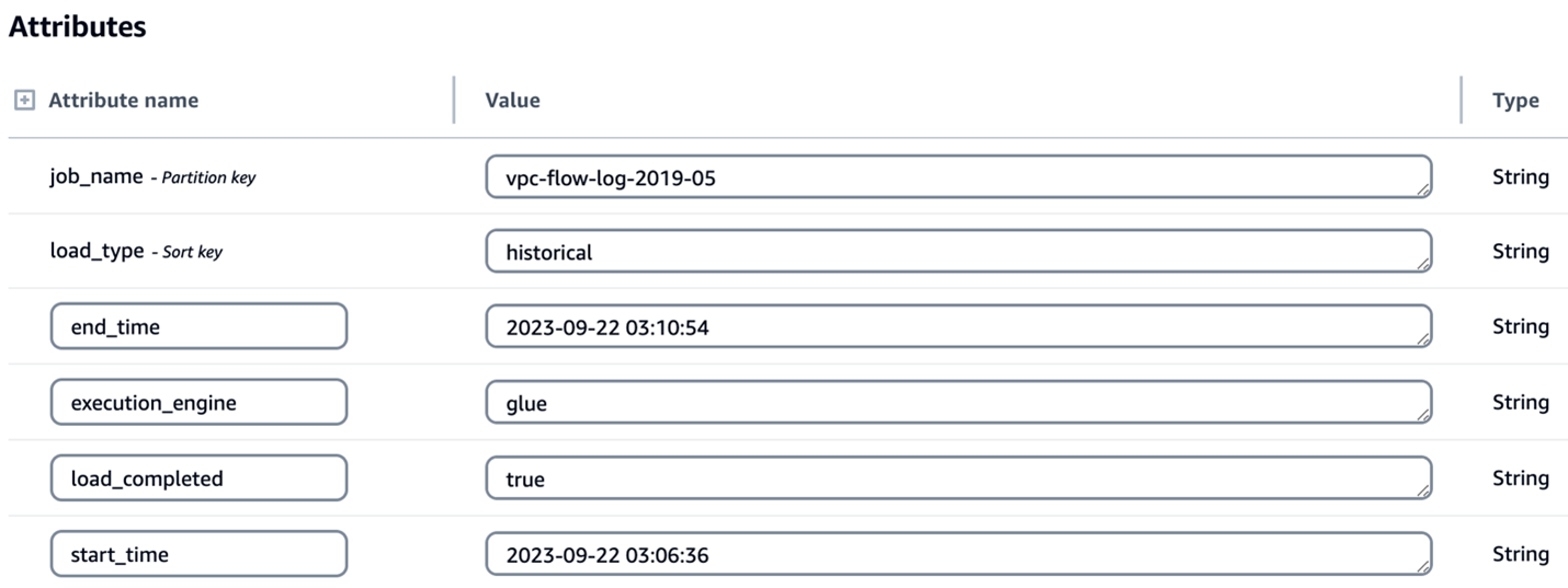
The checkpointing feature provides process resilience by tracking conversion progress in the asl-etl-framework-ocsf-run-status DynamoDB table. If a conversion process fails during multi-year historical processing, the solution resumes from the point of failure rather than reprocessing previously converted data. For example, if conversion fails while processing the second year’s data, the solution will resume from that point, preserving the first year’s successful conversion. While this feature is enabled by default, you can disable it, in which case any process restart will begin from the initial specified date. The following image shows the load_type as historical along with start_time and end_time for the period you want to transform the logs.
Figure 4: Screenshot of configuration for historical load attributes in the asl-etl-framework-source-ocsf-metadata DynamoDB table
Enrichment
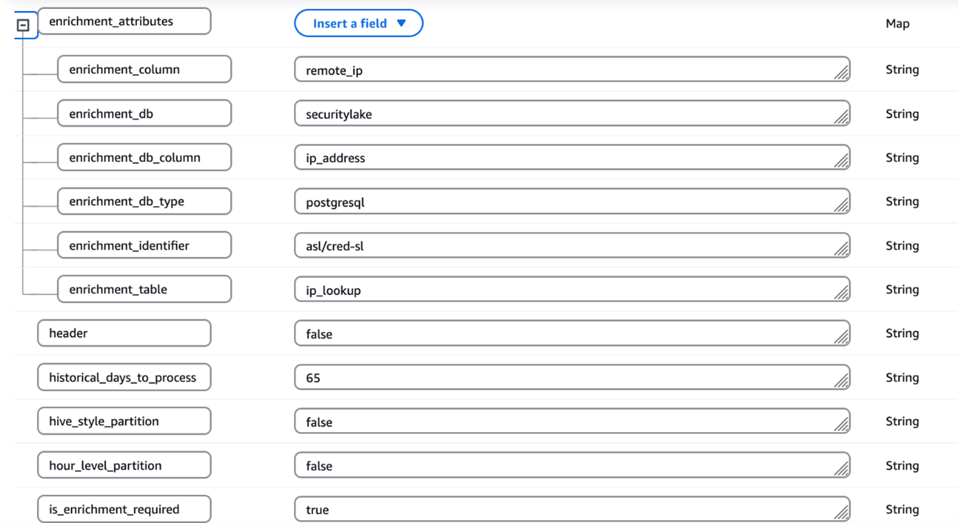
Enterprises often possess valuable contextual data that can enhance their security logs through enrichment. By correlating existing data with security logs and appending relevant information, you can create more comprehensive datasets for advanced analytics and deeper security insights. After the logs are converted to OCSF, you might want to know more about specific columns or attributes so that you can extract meaningful information. To support this, the solution has an option for enrichment. For example, if you want to get additional information, such as the geolocation of each IP address in the logs, you can provide the source database information in the metadata CSV file of the solution. It connects to the source database through a JDBC connection, extracts the requested information associated with the IP address to enrich the dataset, and adds the extracted information as new columns to the converted OCSF log output. In this way, you can have detailed information about each IP address in the converted OCSF log. The following screenshot shows parameters for enabling enrichment by setting the is_enrichment_required flag as true and adding necessary enrichment_attributes to the metadata table.
Figure 5: Screenshot of configuration for enrichment attributes in the asl-etl-framework-source-ocsf-metadata DynamoDB table
ETL transformation using AWS Glue or EMR Serverless
You can use the engine of your choice for the transformation by providing the engine name during the deployment steps as mentioned in the Pre-Deployment Configuration section of the ReadMe. Based on this, the solution uses either AWS Glue or EMR Serverless as mentioned in the Orchestration using Step Functions section.
The process includes the following steps:
The user enters the metadata and mapping information in the respective CSV files and uploads the files to Amazon S3.
A process (Lambda job) converts the metadata and mapping files to a DynamoDB schema and stores them in corresponding DynamoDB tables (metadata and mapping tables).
A preprocessor job is invoked that takes the metadata from the DynamoDB table asl-etl-framework-source-ocsf-metadata and, based on the input parameters passed for the Step Functions workflow shown in the Orchestration using Step Functions section, the Step Functions workflow generates the input arguments for the transformation job (AWS Glue or EMR Serverless based on the user’s choice).
The transformation job (AWS Glue or Amazon EMR based on the user’s choice) is invoked and reads the metadata and mapping tables and converts the data into OCSF format.
The converted OCSF log files are stored to an Amazon S3 location in Parquet format, which is defined in the DynamoDB table asl-etl-framework-source-ocsf-metadata. These custom OCSF logs on S3 can be integrated with Security Lake.
Orchestration using Step Functions
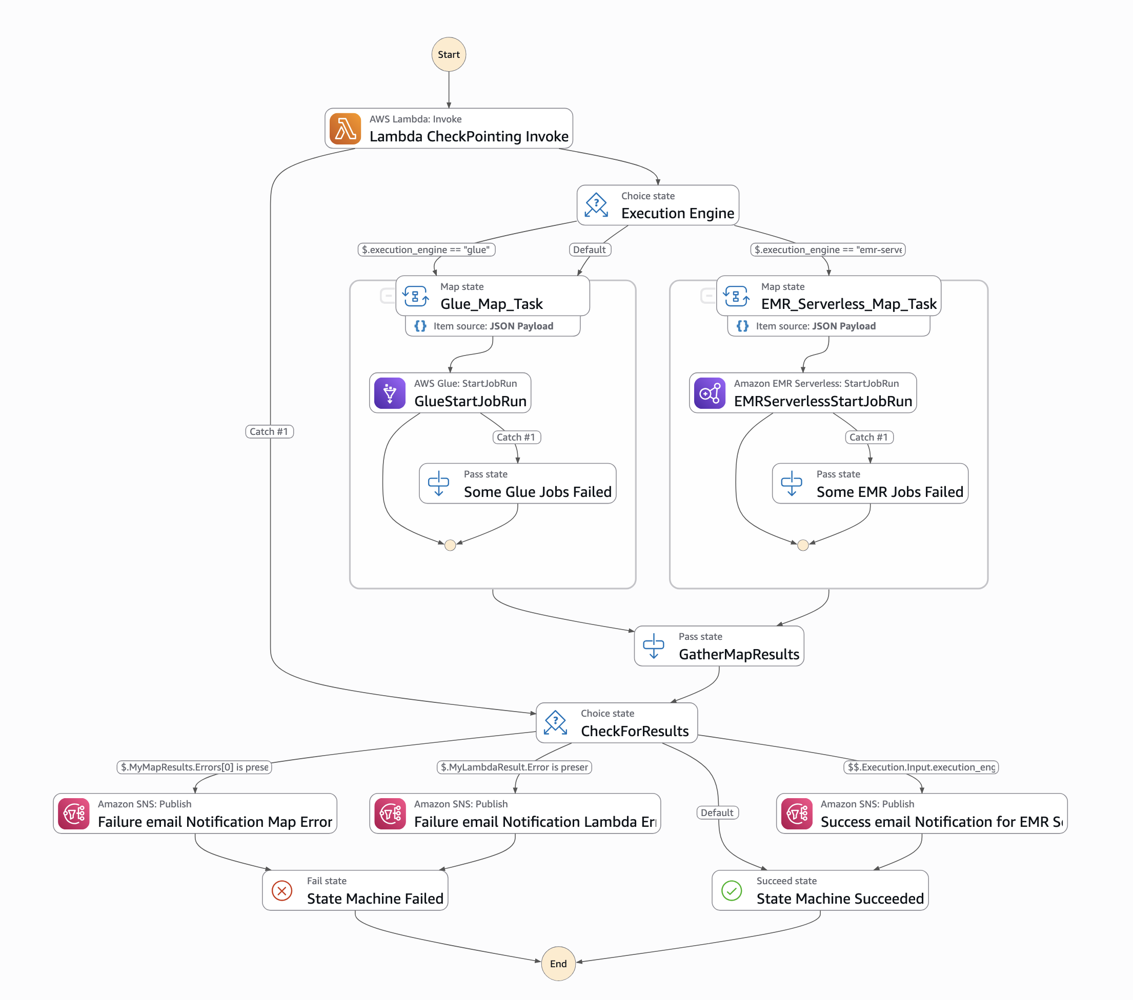
This solution is orchestrated using Step Functions and offers two execution engine options: AWS Glue or EMR Serverless, depending on the services allow-listed in your enterprise. For processing historical loads, we recommend using EMR Serverless; however, AWS Glue is suitable for historical loads less than 100 GB. When invoking the Step Functions workflow, specify the execution engine as either emr-serverless or glue in the input parameters passed using EventBridge.
Figure 6: Screenshot of Step Functions workflow orchestration
To run the workflow, an input must be passed through an EventBridge schedule. The input parameters are as follows:
It’s a best practice to ensure that the generated Parquet files properly map to the various schema definitions specified within the Open Cybersecurity Schema Framework (OCSF). Validating the mapping helps to maintain data integrity and allows the security data to be effectively analyzed and processed by downstream applications and tools, such as Security Lake. You can use OCSF Schema Validator, which was built to provide supplementary validation for Security Lake. Performing this validation step helps detect any schema misalignments or data quality issues early in the process, leading to more reliable and trustworthy security analytics.
If validation of the transformed OCSF Schema fails using the OCSF Schema Validator, you need to validate if your mappings are aligned with the respective OCSF category. Adjust your mappings, rerun the solution, and validate the transformed OCSF logs using OCSF Schema Validator until you get a valid OCSF schema.
When discovering incorrect OCSF mappings or format inconsistencies in converted logs, begin by conducting a thorough validation against OCSF schema specifications to identify specific discrepancies. Update the mappings with correct field mappings, ensuring proper data type conversions and mandatory field requirements are met. Test these corrections using sample data to verify OCSF compliance using the above mentioned tool and data integrity before implementing in production.
Conclusion
In this post, we showed you how the ETL solution accelerator transforms custom security logs into the standardized OCSF format, enabling enhanced security analytics capabilities. This solution, developed by AWS Professional Services (AWS ProServe), addresses common challenges in security log standardization and streamlines the adoption of Amazon Security Lake. While the solution is available as an open source project, engaging with AWS ProServe provides significant advantages, including proven implementation expertise, best practices guidance, and accelerated deployment timelines. Our ProServe team brings extensive experience in security log standardization and can help customize the solution to your specific requirements while ensuring optimal integration with Security Lake. To begin your journey toward standardized security analytics using OCSF, contact your AWS account team to discuss how AWS ProServe can help implement this solution in your environment.
This post is co-authored with Gil Irizarry, Mae Wells-Kress and Craig Harmon from Babel Street.
Can your system tell “John Smith” apart from “John Smith”?
Organizations requiring identity intelligence increasingly face challenges due to complexity of matching names and entities across vast, multilingual, and constantly evolving datasets. Whether helping border security, combating financial crimes, or maintaining regulatory compliance, the accuracy of identity and entity resolution directly determines whether threats are detected, investigations succeed, and regulatory requirements are met. Yet, linguistic diversity, transliterations, inconsistent data formats, and legacy system limitations continue to create friction, leading to false positives, missed matches, and costly manual reviews. As customers ingest and analyze petabytes of unstructured and structured data in Amazon OpenSearch Service, the need for intelligent, scalable, and multilingual matching becomes increasingly important. This is where the integration of Babel Street (an AWS Partner) with OpenSearch Service provides a solution that helps organizations enhance precision, reduce noise, and accelerate insights from their high-volume data environments.
This post explores how combining Babel Street Match with OpenSearch Service provides a solution that helps your organization to handle large-scale, multilingual data.
The growing complexity of identity and entity resolution
As organizations ingest and analyze massive volumes of multilingual and inconsistently formatted data, accurately matching names and entities becomes increasingly difficult. Variations in spelling, transliterations, semantic differences, cultural naming conventions, and incomplete or noisy records can contribute to mismatches. These challenges are compounded by legacy systems, fragmented data pipelines, operational inefficiencies, and evolving regulatory requirements—especially in sectors where precision is a requirement.
Evaluating and enhancing identity in high-volume enterprise environments
Amazon OpenSearch Service is a fully managed, scalable search and analytics service that enables organizations to ingest, search, visualize, and analyze massive volumes of data in near real time. Built to handle structured and unstructured information from diverse sources, it powers use cases ranging from security analytics and log monitoring to enterprise search and advanced analytical applications.
Babel Street delivers risk intelligence trusted by organizations across government, defense, and the private sector. The offering combines access to vast volumes of multilingual data with advanced analytics to uncover hidden identities, secure vendor networks, and identify emerging risks with precision, speed, and scale. From national security to regulatory compliance and enterprise resilience, Babel Street provides the strategic advantage needed to stay ahead of risk, safeguard operations, and protect missions.
Babel Street Match, an offering from Babel Street incorporates advanced identity risk intelligence capabilities, which enhance the precision and reliability of screening processes. This advanced solution uses sophisticated matching techniques to verify identities and identify variations in personal data—including aliases, alternate spellings, and differences in biographical details, helping organizations separate legitimate individuals from potential threats. The ability to screen names, addresses, dates, and other identifiers across different scripts and languages helps reduce false positives and negatives, helps accurately detect critical risks with transparent scoring to meet compliance and audit requirements. Further, Babel Street Match streamlines screening workflows, reduces the burden of manual reviews, and elevates the accuracy of threat detection.
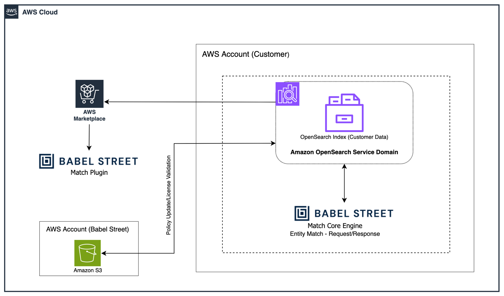
The following diagram shows the details of OpenSearch Service and Babel Street Match Plugin integration.
Babel Street Match integrates directly with the OpenSearch Service domain through a lightweight plugin that runs inside your own AWS account where you have full control of your data. The Match plugin sends encrypted match requests to Babel Street’s fully managed Match engine, where the core matching engine performs the entity-resolution logic. The results return to you in real time, enhancing your existing OpenSearch Service workflows with advanced name- and entity-matching capabilities. Meanwhile, Babel Street’s control plane handles licensing, monitoring, and AWS Marketplace integration behind the scenes, provides continuous validation, automated updates, and a seamless operational experience.
Example use cases
The solution combines enterprise-scale search and analytics with AI-powered, multilingual identity intelligence. This section showcases example use cases where integration has enhanced organizations’ capabilities.
Border Screening: Help agencies identify high-risk travelers, cargo, and networks to strengthen point-of-entry security with faster, automated risk assessment.
Financial Services Compliance: Help Financial institutions and the FinTechs that serve them by offering AI-driven solutions for name screening, adverse media monitoring, and know your customer (KYC)/know your vendor (KYV) due diligence.
Identity and Organization Screening: Help businesses needing identity and organization screening by providing AI, analytics, and advanced matching technologies to assist in addressing complex screening challenges.
Customer and Vendor Onboarding: Help governments and financial institutions by providing research, analytics, and advanced matching technologies needed to quickly and confidently onboard customers and vendors at scale.
Customer Success Stories
Here’s how leading organizations are leveraging Babel Street Match and Amazon OpenSearch Service to solve real-world identity challenges:
A European online brokerage faced AML (anti-money laundering) compliance challenges with its outdated name-matching system, which produced excessive false positives and couldn’t process longer multilingual names. After implementing Babel Street Match on OpenSearch Service, the firm achieved up to 70% better accuracy across 25 languages—significantly reducing manual work and speeding customer payments. Babel Street Match Improves FI’s Name-Matching Accuracy by Up to 70% on OpenSearch
A major border agency struggled with an outdated screening system that flagged 15% of travelers as potential watchlist matches—overwhelming agents and creating long queues. After implementing Babel Street Match, false positives dropped dramatically (from 80,000 to just 100 in one test), hardware needs fell by 70%, and travelers with common names can now pass through faster. As one stakeholder put it: “Name matching is not our biggest problem anymore.” Enabling Stronger, Safer Borders with AI-powered Screening by Babel Street Match
Getting Started with Babel Street Match for Amazon OpenSearch Service
Amazon OpenSearch Service supports third-party plugins like Babel Street Match for OpenSearch. This plugin is supported on OpenSearch version 2.15 or higher and licenses can be obtained through AWS Marketplace.
Installing Babel Street Match for Amazon OpenSearch Service
Prerequisites: Obtain the license file from Babel Street and upload it to an S3 bucket in the same AWS Region as your OpenSearch domain.
Installation Steps:
Create packages – In the OpenSearch Service console, create a package for your license file and select the Babel Street Match plugin from the available options
Associate packages – Link both the license and plugin packages to your OpenSearch domain
Verify – Monitor the domain update and confirm the plugin is active
Together, Babel Street Match and OpenSearch Service help organizations cut through false positives and catch true matches faster. The result? Greater precision, efficiency, and speed—whether protecting entities, maintaining compliance, or securing supply chains. That’s business-critical identity intelligence in action.
Explore how Babel Street Match on Amazon OpenSearch Service can elevate your organization’s identity intelligence capabilities and transform the screening operations through an interactive or customized demo on Babel Street’s website. Portions of this content describing Babel Street products and services are provided by Babel Street. AWS is not responsible for the accuracy of third-party product information.
In this post, we demonstrate how Notebooks in Amazon SageMaker Unified Studio help you get to insights faster by simplifying infrastructure configuration. You’ll see how to analyze housing price data, create scalable data tables, run distributed profiling, and train machine learning (ML) models within a single notebook environment.
Data scientists and analysts often spend days configuring infrastructure and managing authentication across multiple data sources before they can begin analysis. When working with data across Amazon Simple Storage Service (Amazon S3), Amazon Redshift, Snowflake, and local files, teams face repeated authentication setup, manual compute scaling decisions, and tool-switching overhead that delays insights.
Notebooks in Amazon SageMaker Unified Studio provide instant access to 12+ data sources, compute scaling from local to distributed processing, and AI-powered code generation within a single browser-based environment. You’ll learn to use polyglot programming, multi-engine compute, and AI-assisted development to accelerate your path from question to insight.
What are Notebooks in Amazon SageMaker Unified Studio?
Notebooks in Amazon SageMaker Unified Studio provide an interactive environment for data analysis, exploration, engineering, and machine learning workflows. It delivers five integrated capabilities:
Polyglot programming: Write code in Python and SQL interchangeably within the same notebook environment
Unified data access: Connect instantly to data stored in Amazon S3, AWS Glue Data Catalog, Apache Iceberg tables, and third-party sources like Snowflake and BigQuery
Native visualization: Create charts directly from Python and SQL results for immersive data analytics
AI-powered development: Generate code through natural language prompts using SageMaker Data Agent, with an intelligent chat interface for data analytics, data science, and ML tasks
Flexible compute: Scale from basic instances to GPU-powered environments as your needs grow
Architecture
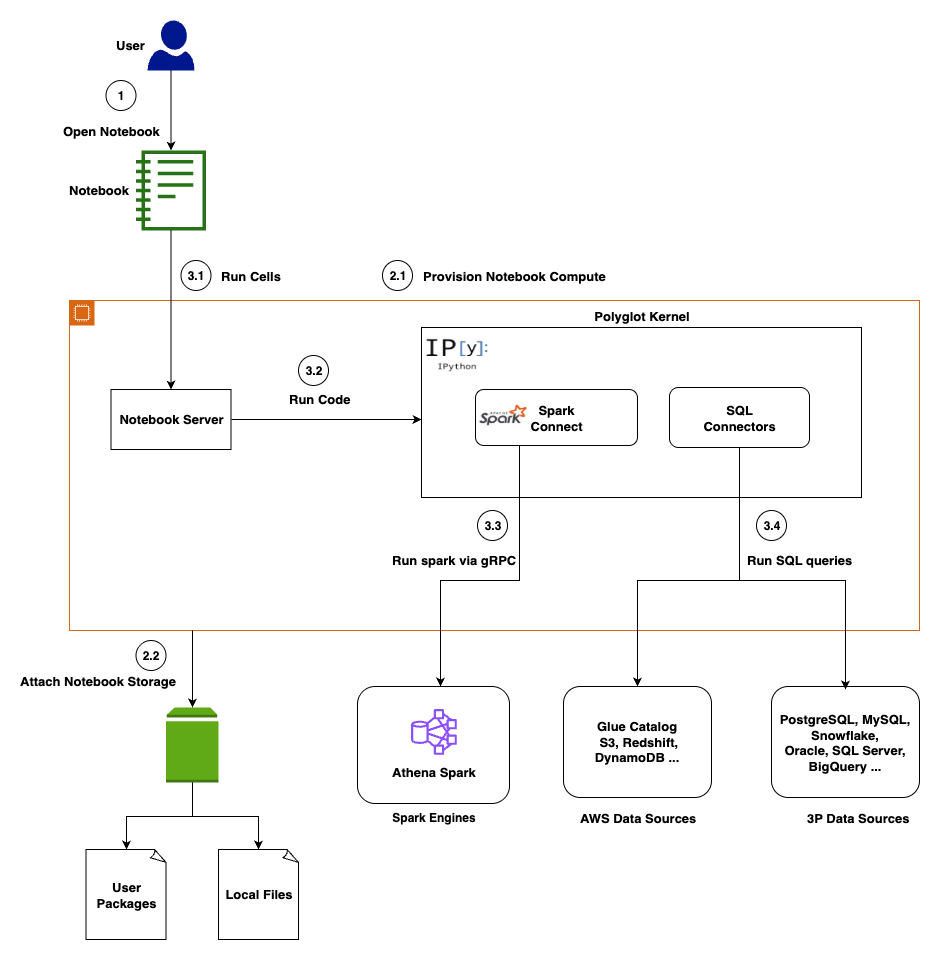
This section covers the architecture of Notebooks, which delivers enterprise-scale analytics with browser-based simplicity through a cloud-native architecture that integrates multiple compute engines, diverse data sources, and AI-powered assistance.
Presentation layer
You access the notebook interface through Amazon SageMaker Unified Studio, interacting with a familiar interface featuring code cells for execution, markdown cells for documentation, and visualization cells for charts and tables.
Compute layer
A dedicated notebook server manages your kernel lifecycle and session state. Key components include a Language Server for code completion, a Python 3.11 runtime with pre-loaded data science libraries, and a Polyglot Kernel that handles your Python, PySpark, and SQL execution within the same notebook. Persistent Amazon Elastic Block Store (Amazon EBS) storage backs each notebook you create.
Execution layer
Notebooks support multiple execution engines, automatically routing your code to the optimal processing engine. In-memory execution handles your smaller datasets and rapid prototyping. Apache Spark via Amazon Athena provides distributed processing for your large-scale analytics via Spark Connect. Native connectivity to Amazon Athena (Trino), Amazon Redshift, Snowflake, and BigQuery processes your SQL queries.
Data Integration
You get unified access to 12+ data sources including AWS-native (Amazon S3, AWS Glue, Amazon Athena, Amazon Redshift) and third-party (Snowflake, BigQuery, PostgreSQL, MySQL) data sources. For the latest supported data sources, see Connect to data sources .
Security is embedded throughout the architecture to protect your work. Data access respects your AWS Identity and Access Management (AWS IAM) permissions. The notebook and the agent can only access data sources you’re authorized to use. Communication between components uses encrypted channels, and your notebook storage is encrypted at rest. The AI agent includes built-in guardrails to help prevent destructive operations and logs interactions for your compliance and auditing purposes.
Prerequisites
Before you begin, you need:
An AWS account with appropriate permissions to create Amazon SageMaker Unified Studio resources. See Set up IAM-based domains for complete permission requirements.
Basic familiarity with Python programming and SQL queries
Understanding of data analysis concepts and ML workflows
Access to the sample housing dataset (provided in the walkthrough)
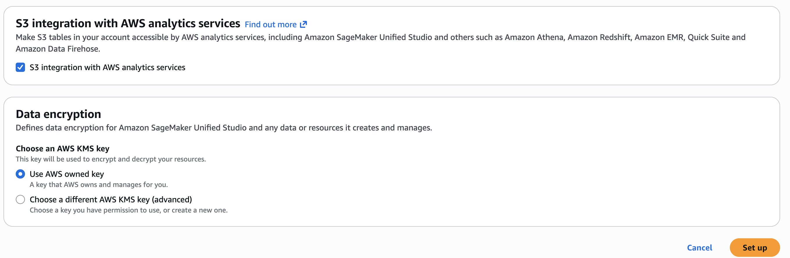
You will be prompted either to select an existing AWS Identity and Access Management (AWS IAM) role that has access to your data and compute, or to create a new role. For this walkthrough, choose Create a new role and leave the other options at their defaults.
Choose Set up. It takes a few minutes to complete your environment.
Use case
In this post, you’ll use a Notebook and the SageMaker Data Agent to perform the following:
Working with dataset: Upload sample dataset housing.csv and explore with data explorer
Polyglot programming: Query dataframes with SQL via DuckDB
Multi-engine access via AWS Glue: Create an AWS Glue table to unlock Athena SQL/Spark engines for distributed processing
Advanced analytics: Use Athena Spark for data profiling
AI-assisted development: Generate profiling and ML code with Data Agent
ML workflow: Train Random Forest model and evaluate results
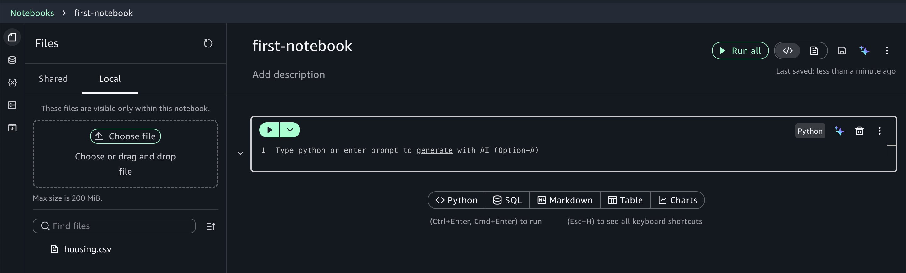
First, let’s walk through the interface and explore its core capabilities.
Understanding the interface
The Notebooks interface follows familiar notebook conventions with cells for code execution and markdown for documentation. Within the notebook, you’ll see your current programming environment (such as Python 3.11) and compute profile specifications. The interface allows you to:
Access your data by browsing files, exploring data catalogs, and managing third-party connections
Monitor variables created within your notebook context
Scale compute resources on demand by adjusting virtual CPUs and RAM based on your workload requirements, even scaling up to GPU instances
Manage packages by installing and configuring Python packages as needed
Working with the dataset
For this walkthrough, you’ll use the housing.csv sample dataset which you can download from this page. (the file is named canvas-sample-housing.csv on the linked page). Choose the Files icon in the left panel and choose the Local tab. Upload the CSV file to the notebook on the Local tab.
Notebooks provide you with instant access to your data assets. Using the data explorer, you can browse your AWS Glue Data Catalog, Amazon S3 table catalogs, Amazon S3 buckets, and configured third-party connections.
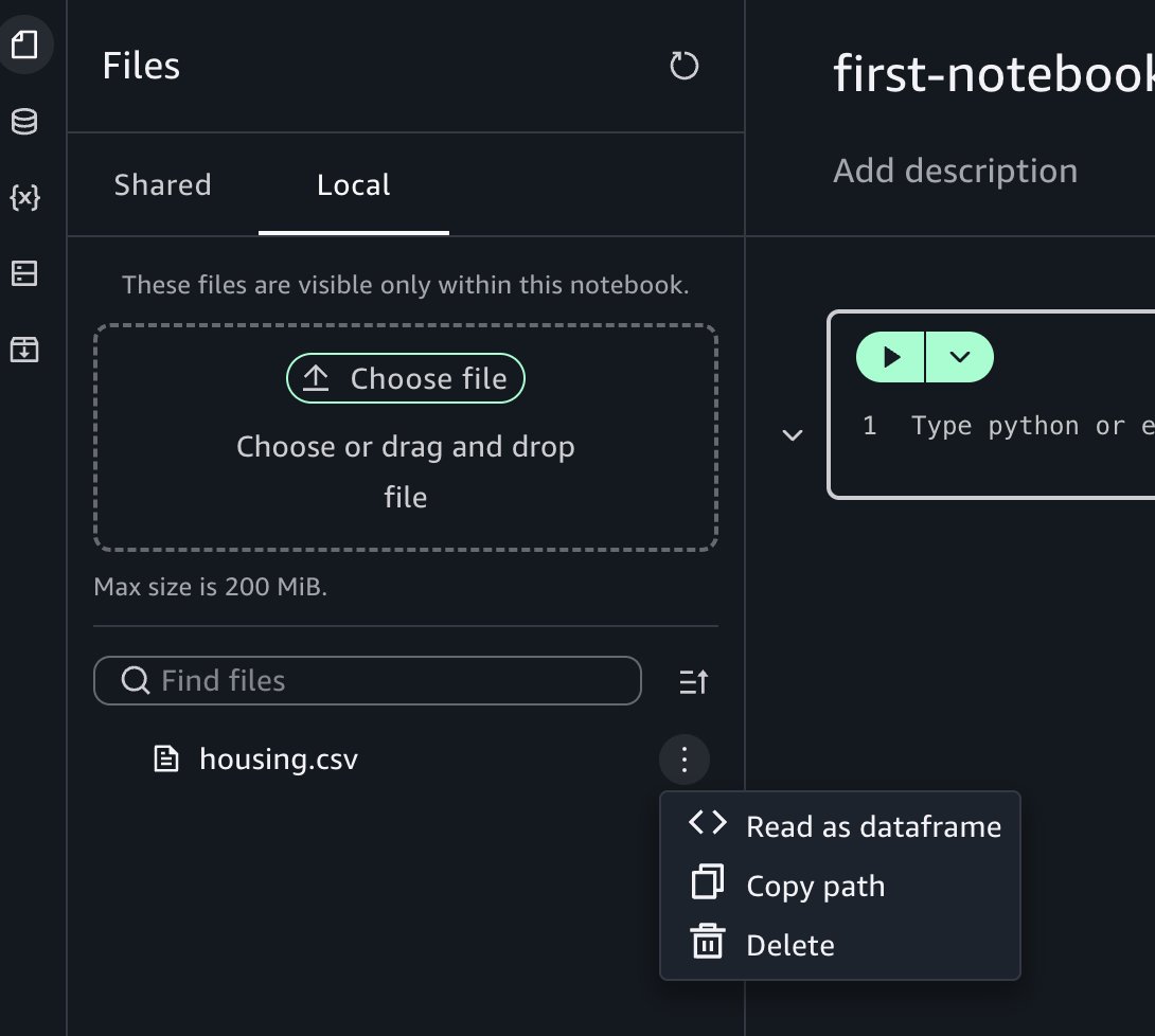
Choose the three-dot options menu.
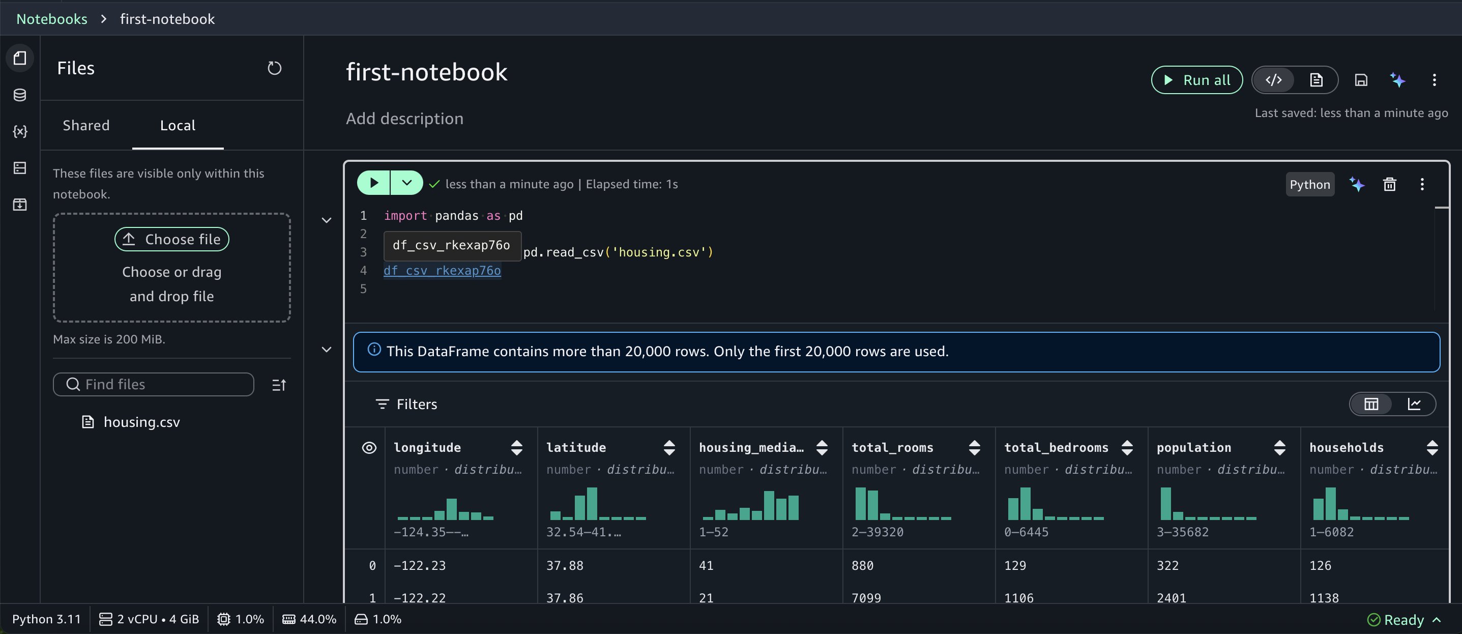
Choose Read as dataframe, then run the inserted cell in the notebook to view the results.
import pandas as pd
<<df_csv_xxxx>> = pd.read_csv('housing.csv')
<<df_csv_xxxx>>
When you return a dataframe, Notebooks render it in a rich table format with automatic data profiling.
Polyglot programming: Python and SQL together
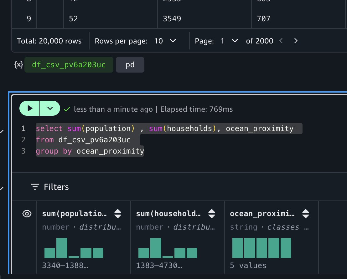
One of the most powerful features in Notebooks is the interoperability between Python and SQL. After you load data into a Python dataframe, you can immediately query it using SQL. For example, to calculate total population and household by ocean proximity, you can run:
select sum(population) ,sum(households),ocean_proximity
from<<df_csv_xxxx>>
group byocean_proximity
The notebook’s autocomplete functionality recognizes dataframes in your context, making SQL queries intuitive.
This SQL query runs on DuckDB (an in-memory SQL database engine), which requires no separate installation or server maintenance on your part. DuckDB’s lightweight design integrates into Python, Java, and other environments, making it ideal for your rapid interactive data analysis. For distributed processing needs, you can use engines such as Apache Spark or Trino after creating an AWS Glue table for this dataset.
Create an AWS Glue table for the dataset
After you create an AWS Glue table, you can query the dataset using various AWS Glue catalog-compatible engines, including Amazon Athena SQL (Trino) and Amazon Athena Spark. These engines deliver optimal price-performance for your specific workload requirements.
Start by creating an AWS Glue database. To do that, create a new cell in the notebook by choosing SQL and selecting Amazon Athena (SQL).
Run this SQL to create a database: create database demo;
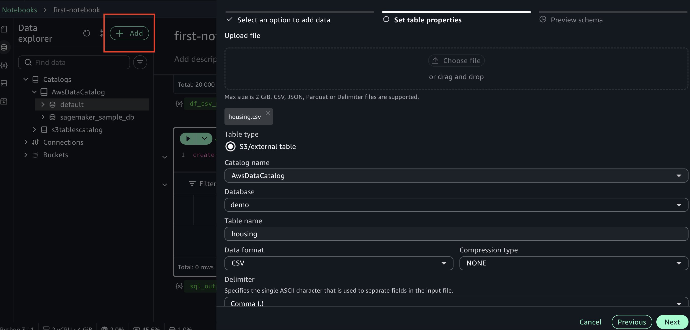
Next, go to data explorer and choose +Add on the top left, then choose Create table. Choose the database you created earlier and enter a name for the table. Upload the housing.csv dataset file used earlier. Continue by choosing Next in the side panel to create the table.
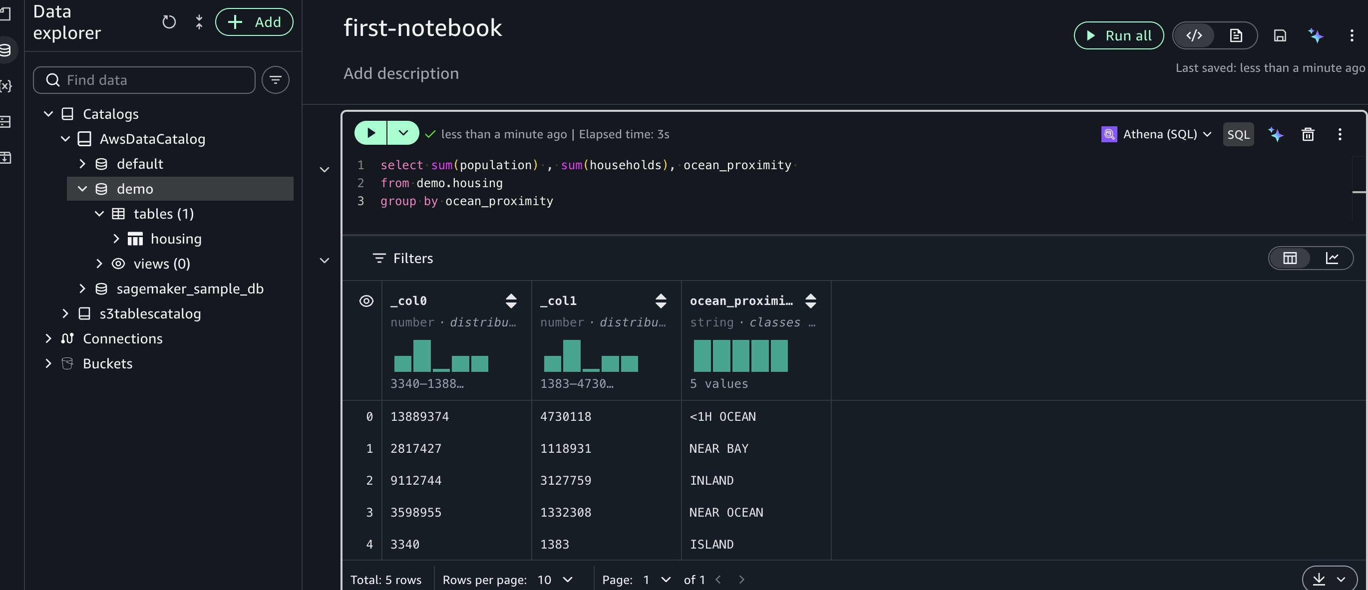
Next, let’s run a sample SQL query in a new cell using Amazon Athena SQL:
select sum(population) , sum(households), ocean_proximity
fromdemo.housing
group by ocean_proximity
Advanced capabilities with Athena Spark
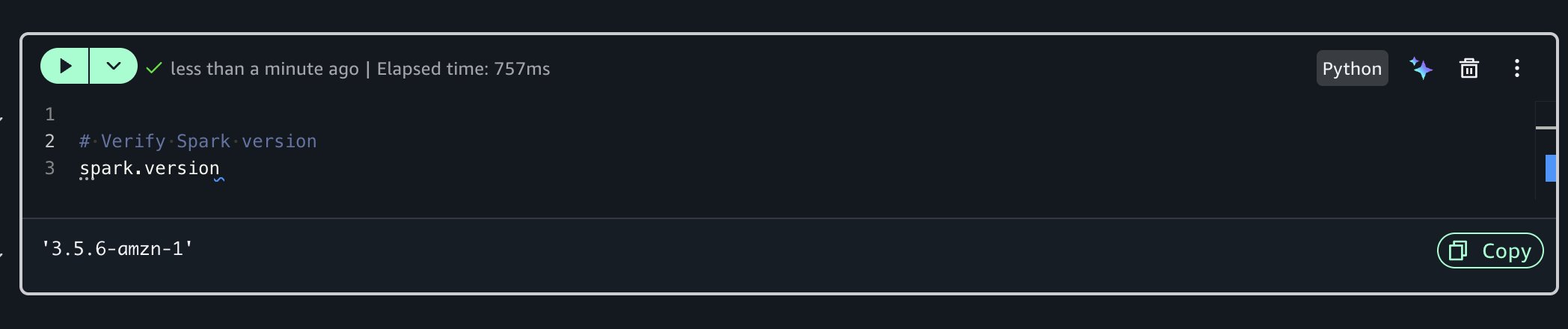
Before you can build an ML model to predict house prices, let’s analyze the dataset further and run data profiling for additional insights. For advanced exploration, you can use Amazon Athena Spark within your notebook.To do that, you’ll create a new Python cell which has a built-in Spark session. Run the following code to check the Spark version:
# Verify Spark version
spark.version
Using the SageMaker Data Agent for data profiling
Instead of writing boilerplate code manually, you can use the built-in generative AI capability.
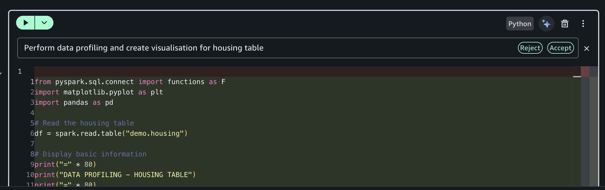
Prompt: “Perform data profiling and create visualization for housing table”
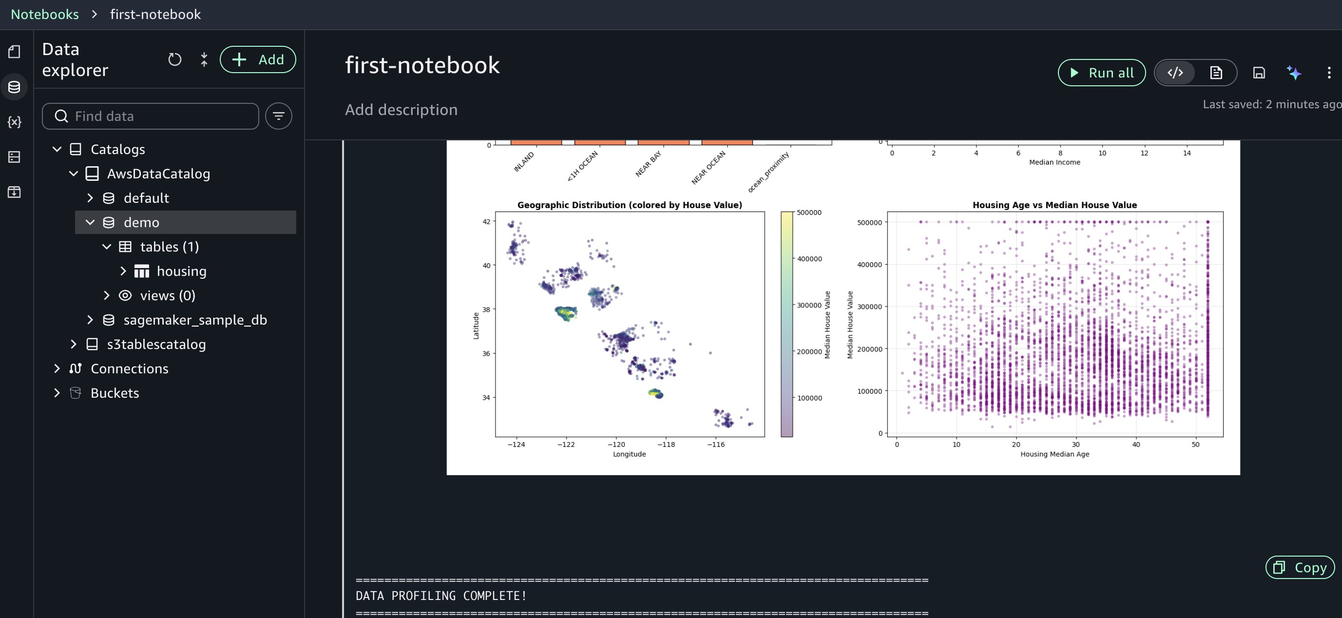
The AI assistant generates comprehensive profiling code for you, including basic statistics calculation, column-level profiling, data type analysis, and missing value detection.
The agent accessed your AWS Glue Data Catalog, understood your housing table structure, and generated profiling code tailored to your specific columns and data types. This context awareness reduces the trial-and-error cycle you’d normally face when adapting generic code snippets to your environment. Review the generated code and run it. The fast response times help you iterate on your analysis efficiently.
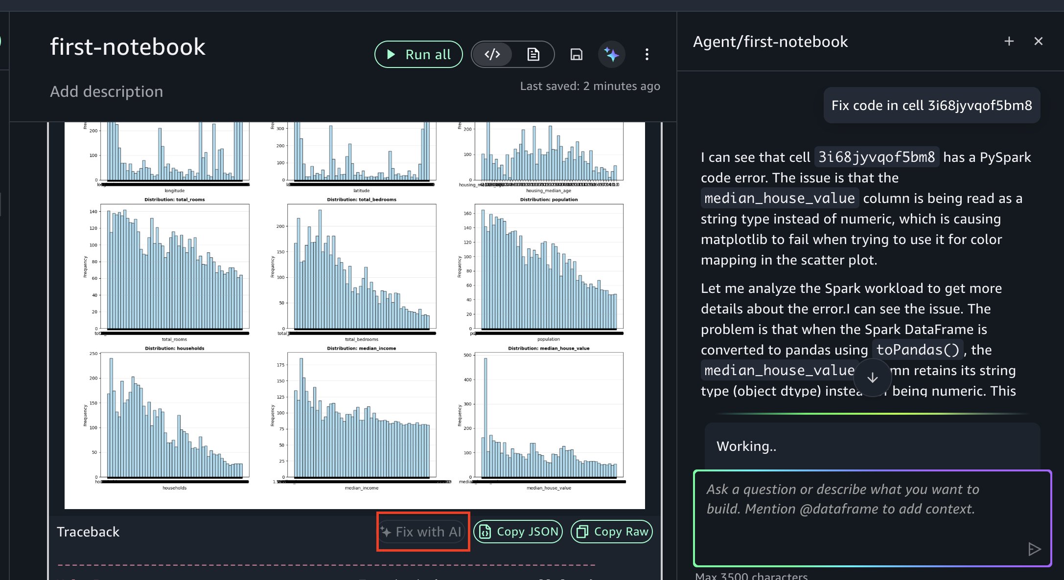
If you encounter an error, you can resolve it using Fix with AI as shown in the following figure. When errors occur during execution, the “Fix with AI” feature analyzes the traceback, diagnoses the root cause, and generates corrected code, so you can keep your analysis moving forward.
Training ML models
Next, you’ll use the data agent to generate code for training a model that predicts housing prices.
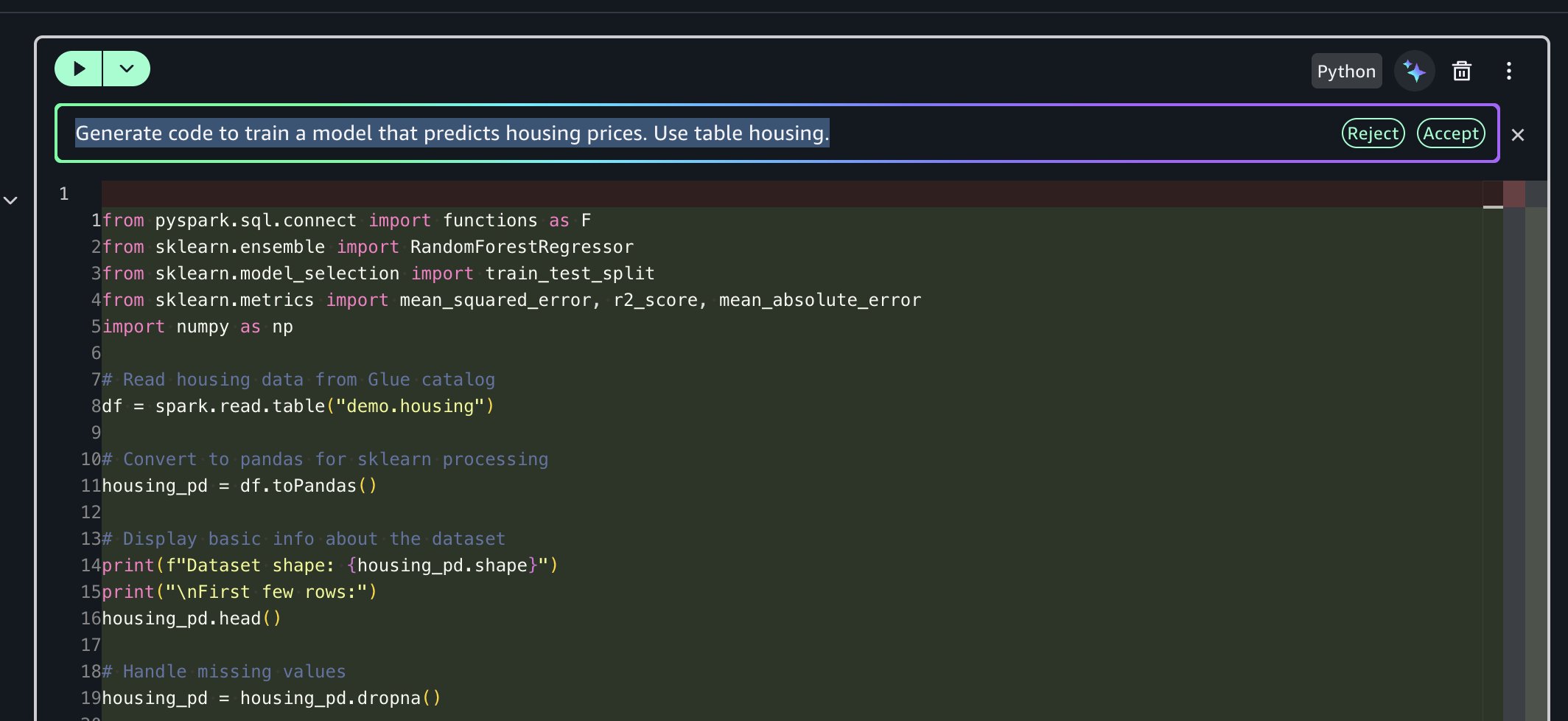
Prompt: “Generate code to train a model that predicts housing prices. Use table housing.”
The AI assistant generates end-to-end code for you that:
Reads housing data from AWS Glue catalog using Amazon Athena Spark and converts to pandas
Converts string columns to numeric, encodes using one-hot encoding and removes missing values
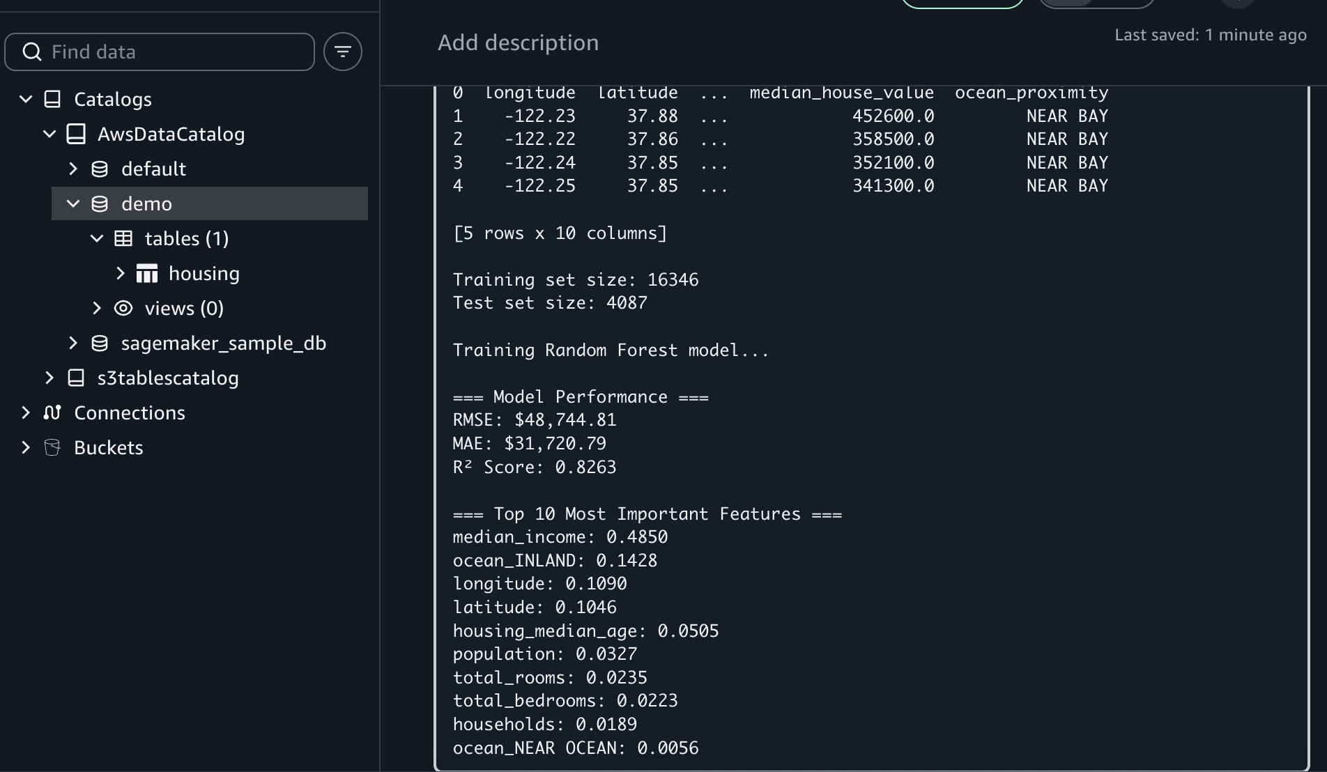
Trains a Random Forest model to predict median house values
Evaluates model performance (RMSE, MAE, R-square)
Displays top 10 most important features for predictions
This multi-step orchestration saves you hours of development time by handling the entire workflow from data access to model evaluation.
If you encounter an error, you can resolve it using Fix with AI available in the results traceback section.
This workflow showcased Notebooks’ unified capabilities: you uploaded files locally, created AWS Glue tables for multi-engine access, used Amazon Athena Spark for distributed profiling, and used AI-assisted ML development to predict housing prices. All of this happened within a single notebook environment without switching tools.
Key benefits and best practices
Notebooks in Amazon SageMaker Unified Studio deliver several advantages:
Faster time to insights: With traditional environments, you might spend hours on configuration before analysis begins. Notebooks bypass this overhead, so you can start work immediately.
Improved collaboration: You can share notebooks with consistent environments, supporting reproducibility and reducing “works on my machine” issues.
Reduced complexity: You can access multiple data sources and compute engines from one interface rather than navigating separate tools for each data source or processing engine.
AI-accelerated development: Generate task-specific code and receive intelligent suggestions, reducing time spent on repetitive coding tasks.
Scalable performance: Handle datasets from megabytes to petabytes with appropriate compute resources. The system scales automatically as data volumes grow.
Best practices
Start with appropriate compute profiles by beginning with smaller instances and scaling up as your needs grow.
Use AI assistance with natural language prompts for your repetitive tasks and complex operations.
Combine engines strategically by using Amazon Athena Spark for your large-scale processing, Amazon Redshift for data warehousing and other specialized engines for your specific workloads.
Document your work using markdown cells to create living documentation alongside your code.
Organize using multiple cells by breaking the complex workflows into logical steps for better readability and debugging.
Cleaning up
To avoid incurring future charges, delete the resources you created in this walkthrough:
In the Amazon SageMaker Unified Studio console, navigate to the Notebook page
Delete the notebook
Delete the demo database and housing table from the AWS Glue Data Catalog
Delete Amazon SageMaker Unified Studio domain created during this walkthrough
If you created a new IAM role specifically for this walkthrough, delete it from the IAM console
Conclusion
In this post, we demonstrated how Notebooks in Amazon SageMaker Unified Studio help you work more efficiently and deliver insights more quickly. By combining familiar notebook interfaces with enterprise-scale compute, multi-engine support, and generative AI assistance, teams can streamline data and AI workflows.
The integration of Python and SQL, instant access to diverse data sources, and intelligent code generation capabilities make Notebooks a valuable tool for modern data teams. Teams can perform exploratory data analysis, build complex data pipelines, or train ML models with the flexibility and power needed within a single, intuitive environment.
Amazon Athena recently added support for reading Parquet Column Indexes in Apache Iceberg tables on November 21, 2025. With this optimization, Athena can perform page-level data pruning to skip unnecessary data within Parquet row groups, potentially reducing the amount of data scanned and improving query runtime for queries with selective filters. For data teams, this may help enable faster insights and help reduce costs when analyzing large-scale data lakes.
Data teams building data lakes often choose Apache Iceberg for its ACID transactions, schema evolution, and metadata management capabilities. Athena is a serverless query engine that allows you to query Amazon S3-based data lakes using SQL, and you don’t need to manage infrastructure. Based on the type of data and query logic, Athena can apply multiple query optimizations to improve performance and reduce costs.
In this blog post, we use Athena and Amazon SageMaker Unified Studio to explore Parquet Column Indexes and demonstrate how they can improve Iceberg query performance. We explain what Parquet Column Indexes are, demonstrate their performance benefits, and show you how to use them in your applications.
Overview of Parquet Column Indexes
Parquet Column Indexes store metadata that query engines can use to skip irrelevant data with greater precision than row group statistics alone. To understand how they work, consider how data is structured within Parquet files and how engines like Athena process them.
Parquet files organize data hierarchically by dividing data into row groups (typically 128-512 MB each) and further subdividing them into pages (typically 1 MB each). Traditionally, Parquet maintains metadata on the contents of each row group level in the form of min/max statistics, allowing engines like Athena to skip row groups that don’t satisfy query predicates. Although this approach reduces the bytes scanned and query runtime, it has limitations. If even a single page within a row group overlaps with the values you are searching for, Athena scans all pages within the row group.
Parquet Column Indexes help address this problem by storing page-level min/max statistics in the Parquet file footer. Row group statistics provide coarse-grained filtering, but Parquet Column Indexes enable finer-grained filtering by allowing query engines like Athena to skip individual pages within a row group. Consider a Parquet file with a single row group containing 5 pages for a column. The row group has min/max statistics of (1, 20), and each page for that column has the following min/max statistics.
When Athena runs a query filtering for values equal to 2, it first checks the row group statistics and confirms that 2 falls within the range (1, 20). Athena will then plan to scan the pages within that row group. Without Parquet Column Indexes, Athena scans each of the 5 pages in the row group. With Parquet Column Indexes, Athena examines the page-level statistics and determines that only page-0 and page-1 need to be read, skipping the remaining 3 pages.
How to use Parquet Column Indexes with Athena
Athena uses Parquet Column Indexes based on table type:
Amazon S3 Tables: Athena automatically uses Parquet Column Indexes by default when they are present.
Iceberg tables in S3 general purpose buckets: Athena does not use Parquet Column Indexes by default. To allow Athena to use Parquet Column Indexes, add an AWS Glue table property named use_iceberg_parquet_column_index and set it to true. Use the AWS Glue console or AWS Glue UpdateTable API to perform these actions.
Measuring Athena performance gains when using Parquet Column Indexes
Now that we understand what Parquet Column Indexes are, we’ll demonstrate the performance benefits of using Parquet Column Indexes by analyzing the catalog_sales table from a 3TB TPC-DS dataset. This table contains ecommerce transaction data including order dates, sales amounts, customer IDs, and product information. This dataset is a good proxy for the types of business analysis that you might perform on your own data, such as identifying sales trends, analyzing customer purchasing patterns, and calculating revenue metrics. We compare query execution statistics with and without Parquet Column Indexes to quantify the performance improvement.
Prerequisites
Before you begin, you must have the following resources:
A SageMaker Unified Studio IAM-based domain.
An Execution IAM Role configured within the SageMaker Unified Studio IAM-based domain with access to S3, AWS Glue Data Catalog, and Athena.
An S3 bucket in your account to store Iceberg table data and Athena query results.
Create catalog_sales Iceberg table
Complete the following steps using SageMaker Unified Studio notebooks. There, you can use SageMaker Unified Studio’s multi-dialect notebook functionality to work with your data using the Athena SQL and Spark engines. To create a catalog_sales Iceberg table in your account, follow these steps:
Navigate to Amazon SageMaker in the AWS Management Console and choose Open under Get started with Amazon SageMaker Unified Studio.
From the side navigation, select Notebooks and choose Create Notebook. The subsequent steps in this post will execute scripts in this notebook.
Create a new SQL cell in the notebook and set the connection type to Athena (Spark). Execute the following query to create a database for the tables in this post.
CREATE DATABASE parquet_column_index_blog;
Create a new SQL cell in the notebook and verify the connection type is Athena (Spark). Execute the following query to create a Hive table pointing to the location of the TPC-DS catalog_sales table data at the public S3 bucket.
Create a new SQL cell in the notebook and verify the connection type is Athena (Spark). Execute the following query to add the Hive partitions to the AWS Glue metadata.
Create a new SQL cell in the notebook and verify the connection type is Athena (Spark). Replace s3://amzn-s3-demo-bucket/athena_parquet_column_index_blog/catalog_sales/ with the S3 URI where you want to store your Iceberg table data, then execute the following query to create the catalog_sales Iceberg table from the Hive table.
CREATE TABLE parquet_column_index_blog.catalog_sales
	USING iceberg
	PARTITIONED BY (cs_sold_date_sk)
	LOCATION 's3://amzn-s3-demo-bucket/athena_parquet_column_index_blog/catalog_sales/'
	AS
	SELECT * FROM parquet_column_index_blog.catalog_sales_hive;
Create a new SQL cell in the notebook and verify the connection type is Athena (Spark). Execute the following query to delete the catalog_sales_hive table, which was only needed to create the catalog_sales Iceberg table.
DROP TABLE parquet_column_index_blog.catalog_sales_hive;
Run an Athena query without Parquet Column Indexes
After creating the catalog_sales Iceberg table in the preceding steps, we run a simple query that analyzes shipping delays of the top 10 most ordered items. This type of analysis could be critical for ecommerce and retail operations. By identifying which popular items experience the greatest delays, fulfillment teams can focus resources where they matter most. For example, you can adjust inventory placement, change warehouse assignments, or address carrier issues. Additionally, popular items with significant shipping delays are more likely to result in order cancellations or returns, so proactively identifying these issues helps protect revenue.
SELECT cs_item_sk,
    SUM(cs_quantity) as total_orders,
    AVG(cs_ship_date_sk - cs_sold_date_sk) as avg_ship_delay_days,
    MIN(cs_ship_date_sk - cs_sold_date_sk) as min_ship_delay,
    MAX(cs_ship_date_sk - cs_sold_date_sk) as max_ship_delay,
    SUM(
        CASE
            WHEN cs_ship_date_sk - cs_sold_date_sk > 7 THEN 1 ELSE 0
        END
    ) as late_shipments,
    SUM(
        CASE
            WHEN cs_ship_date_sk - cs_sold_date_sk > 7 THEN 1 ELSE 0
        END
    ) * 100.0 / COUNT(*) as late_shipment_pct,
    AVG(cs_ext_ship_cost) as avg_shipping_cost
FROM parquet_column_index_blog.catalog_sales
WHERE cs_item_sk IN (
        SELECT cs_item_sk
        FROM parquet_column_index_blog.catalog_sales
        WHERE cs_item_sk IS NOT NULL
        GROUP BY cs_item_sk
        ORDER BY SUM(cs_quantity) DESC
        LIMIT 10
    )
    AND cs_ship_date_sk IS NOT NULL
    AND cs_sold_date_sk IS NOT NULL
GROUP BY cs_item_sk
ORDER BY avg_ship_delay_days DESC;
Additionally, this query is a good candidate for demonstrating the effectiveness of using Parquet Column Indexes because it has a selective filter predicate on a single column cs_item_sk. When Athena executes this query, it first identifies row groups whose min/max ranges overlap with the top 10 most ordered items. Without using Parquet Column Indexes, Athena has to scan every page of data within those matched row groups. However, when using Parquet Column Indexes, Athena can prune data further by skipping individual pages within those row groups whose min/max ranges do not overlap with the ids. Complete the following steps to establish baseline query performance when Athena does not use Parquet Column Indexes during the query.
Create a new Python cell in the notebook. Replace s3://amzn-s3-demo-bucket/athena_parquet_column_index_blog/query_results/ with the S3 URI where you want to store your Athena query results, then execute the following script. Note the runtime and bytes scanned that will be printed. The script will run the query five times with query result reuse disabled and chooses the minimum runtime and the corresponding bytes scanned among those iterations. See our numbers in the Run Athena query with Parquet Column Indexes section.
import boto3
import time

# Configuration
DATABASE = "parquet_column_index_blog"
OUTPUT_LOCATION = "s3://amzn-s3-demo-bucket/athena_parquet_column_index_blog/query_results/"

def run_athena_query(query: str, database: str, output_location: str):
    athena_client = boto3.client('athena')

    response = athena_client.start_query_execution(
        QueryString=query,
        QueryExecutionContext={'Database': database},
        ResultConfiguration={'OutputLocation': output_location}
    )

    query_execution_id = response['QueryExecutionId']

    while True:
        result = athena_client.get_query_execution(QueryExecutionId=query_execution_id)
        state = result['QueryExecution']['Status']['State']

        if state in ['SUCCEEDED', 'FAILED', 'CANCELLED']:
            break

        time.sleep(5)

    if state != 'SUCCEEDED':
        raise Exception(f"Query failed with state: {state}")

    stats = result['QueryExecution']['Statistics']

    return {
        'execution_time_sec': stats['EngineExecutionTimeInMillis'] / 1000,
        'data_scanned_gb': stats['DataScannedInBytes'] / (1024 ** 3)
    }


def benchmark_query(query: str, database: str, output_location: str, num_runs: int = 5):
    results = []

    for i in range(num_runs):
        stats = run_athena_query(query, database, output_location)
        results.append(stats)

    best_run = min(results, key=lambda r: r['execution_time_sec'])

    execution_time = round(best_run['execution_time_sec'], 1)
    data_scanned = round(best_run['data_scanned_gb'], 1)

    print(f"Execution time: {execution_time} sec")
    print(f"Data scanned: {data_scanned} GB")


QUERY = """
SELECT cs_item_sk,
    SUM(cs_quantity) as total_orders,
    AVG(cs_ship_date_sk - cs_sold_date_sk) as avg_ship_delay_days,
    MIN(cs_ship_date_sk - cs_sold_date_sk) as min_ship_delay,
    MAX(cs_ship_date_sk - cs_sold_date_sk) as max_ship_delay,
    SUM(
        CASE
            WHEN cs_ship_date_sk - cs_sold_date_sk > 7 THEN 1 ELSE 0
        END
    ) as late_shipments,
    SUM(
        CASE
            WHEN cs_ship_date_sk - cs_sold_date_sk > 7 THEN 1 ELSE 0
        END
    ) * 100.0 / COUNT(*) as late_shipment_pct,
    AVG(cs_ext_ship_cost) as avg_shipping_cost
FROM parquet_column_index_blog.catalog_sales
WHERE cs_item_sk IN (
        SELECT cs_item_sk
        FROM parquet_column_index_blog.catalog_sales
        WHERE cs_item_sk IS NOT NULL
        GROUP BY cs_item_sk
        ORDER BY SUM(cs_quantity) DESC
        LIMIT 10
    )
    AND cs_ship_date_sk IS NOT NULL
    AND cs_sold_date_sk IS NOT NULL
GROUP BY cs_item_sk
ORDER BY avg_ship_delay_days DESC;
"""

# Run benchmark
benchmark_query(QUERY, DATABASE, OUTPUT_LOCATION, num_runs=5)
Sort the catalog_sales table
Before rerunning the query with Athena using Parquet Column Indexes, you need to sort the catalog_sales table by the cs_item_sk column. In the preceding query, there is a dynamic filter as a subquery on the cs_item_sk column:
cs_item_sk IN (
        SELECT cs_item_sk
        FROM parquet_column_index_blog.catalog_sales
        WHERE cs_item_sk IS NOT NULL
        GROUP BY cs_item_sk
        ORDER BY SUM(cs_quantity) DESC
        LIMIT 10
    )
When executing this query, Athena pushes down the filter predicate to the data source level, fetching only rows that match the top 10 most ordered items. To maximize page pruning with Parquet Column Indexes, rows with the same cs_item_sk values should be stored near each other in the Parquet file. Without sorting, matching values could be scattered across many pages, forcing Athena to read more data. Sorting the table by cs_item_sk clusters similar values together, enabling Athena to read fewer pages.
Let’s examine the Parquet Column Indexes in one of the Parquet files to understand how the data in the catalog_sales table is currently organized. First, download the Parquet file from the cs_sold_date_sk = 2450815 partition and install the open-source parquet-cli tool on your local machine. Replace <local-path-to-parquet-file> with the path to the downloaded Parquet file, then run the following command on your local machine:
parquet column-index <local-path-to-parquet-file>
This displays Parquet Column Indexes for all columns. For brevity, only the first 11 pages of the cs_item_sk column from the first row group are shown in the following example:
Notice that nearly every page contains a wide range of values. This overlap means Athena cannot eliminate pages when filtering with Parquet Column Indexes on cs_item_sk. For example, searching for cs_item_sk = 100 requires scanning each of the 11 pages because the value 100 falls within every page’s min/max range. With this overlap, enabling Athena to use Parquet Column Indexes would provide no performance benefit. Sorting the data by cs_item_sk eliminates this overlap, creating distinct, non-overlapping ranges for each page. To make Parquet Column Indexes more effective, sort the table by completing the following step:
Create a new SQL cell in the notebook and verify the connection type is Athena (Spark). Execute the query to sort the cs_item_sk column values of the catalog_sales table in ascending order and to put all the null values in the last few Parquet pages. New Iceberg data files will be generated from this query.
Running the parquet column-index command on the sorted data file from the cs_sold_date_sk = 2450815 partition shows that the Parquet Column Indexes are now sorted and have non-overlapping ranges. The first 11 pages of the cs_item_sk column from the first row group are shown in the following example:
Now when searching for cs_item_sk = 100, Athena only needs to read page-0, skipping the remaining 10 pages entirely.
Run Athena query with Parquet Column Indexes
Now that the data is sorted to eliminate overlapping pages within the row groups for the cs_item_sk column, we run two experiments on the sorted data. The first measures the impact of sorting alone, and the second measures the combined effect of sorting with Parquet Column Indexes.
Create a new Python cell in the notebook. Execute the same script in the section Run Athena query without Parquet Column Indexes and take note of the query runtime and bytes scanned results. This measures the performance of querying sorted data without using Parquet Column Indexes.
Create a new Python cell in the notebook. Execute the following Python script to set the use_iceberg_parquet_column_index table property to true for the catalog_sales table in the AWS Glue Data Catalog.
import boto3

def add_iceberg_parquet_column_index(database_name: str, table_name: str):
    glue_client = boto3.client('glue')

    # Get current table definition
    response = glue_client.get_table(DatabaseName=database_name, Name=table_name)
    table = response['Table']

    # Build TableInput with only allowed fields
    table_input = {'Name': table['Name']}

    allowed_fields = [
        'Description', 'Owner', 'LastAccessTime', 'LastAnalyzedTime',
        'Retention', 'StorageDescriptor', 'PartitionKeys', 'ViewOriginalText',
        'ViewExpandedText', 'TableType', 'Parameters', 'TargetTable'
    ]

    for field in allowed_fields:
        if field in table:
            table_input[field] = table[field]

    # Add the property
    if 'Parameters' not in table_input:
        table_input['Parameters'] = {}
    table_input['Parameters']['use_iceberg_parquet_column_index'] = 'true'

    # Update the table
    glue_client.update_table(DatabaseName=database_name, TableInput=table_input)

# Usage
add_iceberg_parquet_column_index("parquet_column_index_blog", "catalog_sales")
Create a new Python cell in the notebook. Execute the same script in the section Run Athena query without Parquet Column Indexes and take note of the query runtime and bytes scanned results. This measures the performance of querying sorted data using Parquet Column Indexes.
Athena query time and bytes scanned improvement
The following table summarizes the results from each experiment. The percentage improvements for the sorted experiments are measured against the unsorted baseline.
Experiment
Runtime (sec)
Bytes Scanned (GB)
Unsorted without Parquet Column Indexes
20.6
45.2
Sorted without Parquet Column Indexes
15.4 (25.2% faster)
27.8 (38.5% fewer bytes)
Sorted with Parquet Column Indexes
10.3 (50.0% faster)
13.0 (71.2% fewer bytes)
Recommendations
To maximize Athena’s ability to use Parquet Column Indexes and achieve optimal query performance, we recommend the following.
Sort data by frequently filtered columns. This allows Athena to efficiently read Parquet Column Indexes and skip irrelevant pages, potentially reducing scan time. When data is sorted by a filter column, similar values are clustered together within pages. Because Parquet Column Indexes store min/max values for each page, Athena can quickly determine which pages contain matching values and skip the rest.
Sort data by high-cardinality columns. This creates distinct value ranges between pages, maximizing the opportunity for Athena to skip pages during query execution. High-cardinality (many distinct values) columns produce non-overlapping min/max ranges across pages, allowing Athena to more effectively filter out irrelevant pages. In contrast, low-cardinality columns such as boolean or status fields result in overlapping ranges across many pages, reducing the number of skipped pages.
Clean up
When you have finished the steps in this post, complete the following cleanup actions to avoid incurring ongoing charges:
Create a new SQL cell in the notebook and set the connection type to Athena (Spark). Execute the following command to drop the parquet_column_index_blog database and the catalog_sales table.
DROP DATABASE parquet_column_index_blog CASCADE;
Delete the Iceberg table data and the Athena query results from your S3 bucket.
Delete the SageMaker Unified Studio IAM-based domain if it is no longer needed.
Conclusion
In this post, we showed you how Athena uses Parquet Column Indexes to speed up queries and reduce the number of bytes scanned. By using Parquet Column Indexes, Athena can skip irrelevant data pages to improve query performance, especially for queries with selective filters on sorted data. Refer to Optimize Iceberg tables to learn more about this feature and try it out on your own queries.
Developers working with Amazon Managed Streaming for Apache Kafka (Amazon MSK) regularly need to make decisions that require deep operational context—choosing the right instance type, diagnosing consumer lag, or planning for a traffic spike. Answering these questions means piecing together documentation, metrics, and operational know-how.
What if your IDE could guide you through that workflow with built-in domain expertise and tooling? Kiro is an AI-powered agentic IDE that lets you describe what you need in natural language. Whether it’s infrastructure configuration or operational troubleshooting, Kiro guides you through the solution.
In this post, we’ll show you how to use Kiro powers, a new capability that equips Kiro with contextual knowledge and tooling. You can simplify your MSK cluster management, from initial setup to diagnosing common issues, all through natural language conversations.
Challenges operating your MSK Express broker cluster
Amazon MSK Express Brokers are a fully managed offering where AWS handles much of the underlying infrastructure. However, platform teams still need to correctly size clusters based on throughput requirements. They also need to understand the right Amazon CloudWatch metrics during performance issues and investigate when CPU usage or replication lag is higher than expected. MSK best practices documentation spans multiple AWS guides. This makes it time-consuming to find relevant information during production incidents. New team members face a learning curve with MSK operations and can repeat common sizing and configuration mistakes.
Although Express Brokers simplify infrastructure management, you still face operational challenges that require deep Kafka expertise across three areas:
Cluster creation and sizing: You must still select the right instance type, configure networking, and choose authentication methods. These decisions impact cost and performance from day one.
Observability and troubleshooting: Effective operations require correlating broker, partition, and client metrics. Troubleshooting lag or replication issues still requires a solid understanding of Express Brokers’ architecture.
Capacity management: You must monitor CPU usage, understand per-broker throughput limits, and scale before hitting throttling thresholds.
These challenges mean that setting up an MSK cluster, analyzing slow-running clients, or investigating high-CPU load requires pulling together documentation, configuration details, CLI tooling, and operational know-how, which is often spread across multiple sources. Kiro powers address these challenges by bringing best practices, guided workflows, and tooling directly into your IDE, reducing the expertise barrier and the time spent context-switching between documentation, consoles, and the CLI.
Kiro powers
Kiro powers is a feature that combines best practices, specialized context, and tool integrations into a single capability. You can install powers with one click in the Kiro IDE or add them from a public GitHub URL. Each Power combines the following components:
Model Context Protocol (MCP) servers give your Kiro agent direct access to your infrastructure. The AWS MSK MCP server, for example, exposes tools to create clusters, monitor health, and optimize configurations.
Steering files provide persistent knowledge and workflow guides that Kiro loads based on the user’s task, such as monitoring best practices or troubleshooting workflows.
Optional hooks run automated actions when IDE events occur, such as validating configurations before deployment.
The key advantage of Kiro powers is that they load context dynamically based on the user’s task. Instead of configuring every MCP server upfront and re-providing context in each conversation, powers activate the right tools and knowledge on demand. This keeps your agent’s context focused and relevant. In the next section, we look at how these components work together specifically for MSK Express Broker operations.
The MSK Express broker power
The MSK Express broker power packages the AWS MSK MCP server with targeted streaming operations guidance, giving your Kiro agent expertise for MSK Express Broker operations and cluster management. You can use it to build Kafka-based streaming applications through Kiro while maintaining Express broker best practices throughout the development lifecycle.
For cluster operations, you can create Express broker clusters, monitor health metrics, and manage configurations through natural language. You can retrieve cluster metadata, check broker endpoints, and verify replication status. The Power also supports operational monitoring. You can track CPU utilization, throughput limits, partition distribution, and AWS Identity and Access Management (IAM) connection metrics.
To see how this works in practice, here’s what happens when you interact with the Power: When you ask Kiro to create an MSK cluster, the Power recommends appropriate instance sizes based on your throughput requirements. When you’re troubleshooting, it knows to check LeaderCount before diving into network metrics. When you’re troubleshooting authentication failures, it recommends client settings like reconnect.backoff.ms and group.instance.id to resolve connection churn and rebalancing issues against Express broker limits. Use cases include:
Cluster sizing and creation: Describe your throughput requirements (for example, “50 MBps ingress with 3x fan-out”) and the Power calculates the right instance type and broker count, then walks through cluster creation.
Proactive health monitoring: Ask Kiro to review your cluster. It checks CPU against the 60% threshold, compares throughput to instance limits, and flags partition imbalances and throughput bottlenecks before they become incidents.
Incident troubleshooting: Consumer lag spiking? The Power checks the relevant metrics, identifies the root cause (like skewed partition leadership), and guides you through resolution.
Capacity planning: Preparing for a traffic spike? The Power analyzes current utilization against instance limits and recommends whether to scale up or add brokers.
The MSK Express broker power brings together documentation, metrics, and operational context so your Kiro agent can correlate findings and help identify root causes specific to your infrastructure.
Getting started with the MSK Express broker power
Starting with Kiro powers takes only a few clicks in the Kiro IDE. You can install from the built-in marketplace or import from a public GitHub URL. Kiro packages all components and makes them available to the Kiro agent.
To set up the MSK Express broker power, follow these steps:
Choose the Powers icon in the Kiro sidebar
In the AVAILABLE panel, scroll down to Build and Operate MSK Express Broker
The MSK Express broker power streamlines Kafka operations by combining Model Context Protocol (MCP) servers with operational guidance. With natural language interactions, you can create clusters, monitor health, optimize configurations, and troubleshoot issues without reviewing extensive documentation.
Performance issues in analytics environments often remain invisible until they disrupt dashboards, delay ETL jobs, or impact business decisions. For teams running Amazon Redshift Serverless, unmonitored query queues, long-running queries, or unexpected spikes in compute capacity can degrade performance and increase costs if left undetected.
Amazon Redshift Serverless streamlines running analytics at scale by removing the need to provision or manage infrastructure. However, even in a serverless environment, maintaining visibility into performance and usage is essential for efficient operation and predictable costs. While Amazon Redshift Serverless provides advanced built-in dashboards for monitoring performance metrics, delivering notifications directly to platforms like Slack, brings another level of agility. Real-time alerts in the team’s workflow enable faster response times and more informed decision-making without requiring constant dashboard monitoring.
In this post, we show you how to build a serverless, low-cost monitoring solution for Amazon Redshift Serverless that proactively detects performance anomalies and sends actionable alerts directly to your selected Slack channels. This approach helps your analytics team identify and address issues early, often before your users notice a problem.
Solution overview
The solution presented in this post uses AWS services to collect key performance metrics from Amazon Redshift Serverless, evaluate them against thresholds that you can flexibly configure, and notify you when anomalies are detected.
The workflow operates as follows:
Scheduled execution – An Amazon EventBridge rule triggers an AWS Lambda function on a configurable schedule (by default, every 15 minutes during business hours).
Metric collection – The AWS Lambda function gathers metrics including queued queries, running queries, compute capacity (RPUs), data storage usage, table count, database connections, and slow-running queries using Amazon CloudWatch and the Amazon Redshift Data API.
Threshold evaluation – Collected metrics are compared against your predefined thresholds that reflect acceptable performance and usage limits.
Alerting – When a threshold is exceeded, the Lambda function publishes a notification to an Amazon SNS topic.
Observability – Lambda execution logs are stored in Amazon CloudWatch Logs for troubleshooting and auditing.
This architecture is fully serverless and requires no changes to your existing Amazon Redshift Serverless workloads. To simplify deployment, we provide an AWS CloudFormation template that provisions all required resources.
Prerequisites
Before deploying this solution, you must collect information about your existing Amazon Redshift Serverless workgroup and namespace that you want to monitor. To identify your Amazon Redshift Serverless resources:
Provide details for your existing Amazon Redshift Serverless environment. These values connect the monitoring solution to your Redshift environment. Some parameters come with the default values that you can replace with your actual configuration.
Parameter
Default value
Description
Amazon Redshift Workgroup Name
Your Amazon Redshift Serverless workgroup name.
Amazon Redshift Namespace Name
Your Amazon Redshift Serverless namespace name.
Amazon Redshift Workgroup ID
Workgroup ID (UUID) of the Amazon Redshift Serverless workgroup to monitor. Must follow the UUID format: xxxxxxxx-xxxx-xxxx-xxxx-xxxxxxxxxxxx (lowercase hexadecimal with hyphens).
Namespace ID (UUID) of the Amazon Redshift Serverless namespace. Must follow the UUID format: xxxxxxxx-xxxx-xxxx-xxxx-xxxxxxxxxxxx (lowercase hexadecimal with hyphens).
Database Name
dev
Target Amazon Redshift database for SQL-based diagnostic and monitoring queries.
Monitoring schedule
The default schedule runs diagnostic SQL queries every 15 minutes during business hours, balancing responsiveness and cost efficiency. Running more frequently might increase costs, while less frequent monitoring could delay detection of performance issues. You can adjust this schedule to your actual need.
Parameter
Default value
Description
Schedule Expression
cron(0/15 8-17 ? * MON-FRI *)
EventBridge schedule expression for Lambda function execution. Default runs every 15 minutes, Monday through Friday, 8 AM to 5 PM UTC.
Threshold configuration
Thresholds should be tuned based on your workload characteristics.
Parameter
Default value
Description
Queries Queued Threshold
20
Alerts threshold for queued queries.
Queries Running Threshold
20
Alerts threshold for running queries.
Compute Capacity Threshold (RPUs)
64
Alert threshold for compute capacity (RPUs).
Data Storage Threshold (MB)
5242880
Threshold for data storage in MB (default 5 TB).
Table Count Threshold (MB)
1000
Alerts threshold for total table count.
Database Connections Threshold
50
Alert threshold for database connections.
Slow Query Threshold (seconds)
10
Thresholds in seconds for slow query detection.
Query Timeout (Seconds)
30
Timeout for SQL diagnostics queries.
Tip: Start with conservative thresholds and refine them after observing baseline behavior for one to two weeks.
Lambda configuration
Configure the AWS Lambda function settings. The selected default values are appropriate for most monitoring scenarios. You may want to change them only in case of troubleshooting.
If your organization has network isolation requirements, you can optionally enable VPC deployment for the Lambda function. When enabled, the Lambda function runs within your specified VPC subnets, providing network isolation and allowing access to VPC-only resources.
Parameter
Default value
Description
VPC ID
VPC ID for Lambda deployment (required if EnableVPC is true). The Lambda function will be deployed in this VPC. Ensure that the VPC has appropriate routing (NAT Gateway or VPC Endpoints) to allow Lambda to access AWS services like CloudWatch, Amazon Redshift, and Amazon SNS.
VPC Subnet IDs
Comma-separated list of subnet IDs for Lambda deployment (required if EnableVPC is true).
Security Group IDs
Comma-separated list of security group IDs for Lambda (optional). If not provided and EnableVPC is true, a default security group will be created with outbound HTTPS access. Custom security groups must allow outbound HTTPS (port 443) to AWS service endpoints.
Note that VPC deployment might increase cold start times and requires an NAT Gateway or VPC endpoints for AWS service access. We recommend provisioning interface VPC endpoints (through AWS PrivateLink) for the five services the Lambda function calls which keeps all traffic private without the recurring cost of a NAT Gateway.
Security configuration – Encryption
If your organization requires encryption of data at rest, you can optionally enable AWS Key Management Service (AWS KMS) encryption for the Lambda function’s environment variables, CloudWatch Logs, and SNS topic. When enabled, the template encrypts each resource using the AWS KMS keys that you provide, either a single shared key for all three services, or individual keys for granular key management and audit separation.
Parameter
Default value
Description
Shared KMS Key ARN
AWS KMS key ARN to use for all encryption (Lambda, Logs, and SNS) unless service-specific keys are provided. This streamlines key management by using a single key for all services. The key policy must grant encrypt/decrypt permissions to Lambda, CloudWatch Logs, and SNS.
Lambda KMS Key ARN
AWS KMS key ARN for Lambda environment variable encryption (optional, overrides SharedKMSKeyArn). Use this for separate key management per service. The key policy must grant decrypt permissions to the Lambda execution role. If not provided, SharedKMSKeyArn will be used when EnableKMSEncryption is true.
CloudWatch Logs KMS Key ARN
AWS KMS key ARN for CloudWatch Logs encryption (optional, overrides SharedKMSKeyArn). Use this for separate key management per service. The key policy must grant encrypt/decrypt permissions to the CloudWatch Logs service. If not provided, SharedKMSKeyArn will be used when EnableKMSEncryption is true.
SNS Topic KMS Key ARN
AWS KMS key ARN for SNS topic encryption (optional, overrides SharedKMSKeyArn). Use this for separate key management per service. The key policy must grant encrypt/decrypt permissions to SNS service and the Lambda execution role. If not provided, SharedKMSKeyArn will be used when EnableKMSEncryption is true.
Enable Dead Letter Queue
False
Optionally enable Dead Letter Queue (DLQ) for failed Lambda invocations to improve reliability and security monitoring. When enabled, events that fail after all retry attempts will be sent to an SQS queue for investigation and potential replay. This helps prevent data loss, provides visibility into failures, and enables security audit trails for monitoring anomalies. The DLQ retains messages for 14 days.
Note that AWS KMS encryption requires the key policy to grant appropriate permissions to each consuming service (Lambda, CloudWatch Logs, and SNS).
On the review page, select I acknowledge that AWS CloudFormation might create IAM resources with custom names.
Choose Submit.
Resources created
The CloudFormation stack creates the following resources:
EventBridge rule for scheduled execution
AWS Lambda function (Python 3.12 runtime)
Amazon SNS topic for alerts
IAM role with permissions for CloudWatch, Amazon Redshift Data API, and SNS
CloudWatch Log Group for Lambda logs
Note: CloudFormation deployment typically takes 10–15 minutes to complete. You can monitor progress in real time under the Events tab of your CloudFormation stack.
Post-deployment configuration
After the CloudFormation stack has been successfully created, complete the following steps.
Note the values for LambdaRoleArn and SNSTopicArn. You will need these in subsequent steps.
Step 2: Grant Amazon Redshift permissions
Grant permissions to the Lambda function to query Amazon Redshift system tables for monitoring data. Complete the following steps to grant the necessary access:
In the left navigation pane, choose Query Editor V2.
Connect to your Amazon Redshift Serverless workgroup.
Execute the following SQL commands, replacing <IAM Role ARN> with the LambdaRoleArn value from your CloudFormation outputs:
CREATE USER "IAMR:<IAM Lambda Role>" WITH PASSWORD DISABLE;

GRANT ROLE "sys:monitor" TO "IAMR:<IAM Role>";
These commands create an AmazonRedshift user associated with the Lambda IAM role and grant it the sys:monitor Amazon Redshift role. This role provides read-only access to catalog and system tables without granting permissions to user data tables.
Step 3: Configure Slack notifications
Amazon Q Developer in chat applications provides native AWS integration and managed authentication, removing custom webhook code and reducing setup complexity. To receive alerts in Slack, configure Amazon Q Developer in Chat Applications to connect your SNS topic to your preferred Slack channel:
When configuring the Slack channel, ensure that you select the correct AWS Region where you deployed the CloudFormation stack.
In the Notifications section, select the SNS topic created by your CloudFormation stack (refer to the SNSTopicArn output value).
Keep the default IAM read-only permissions for the channel configuration.
After configured, alerts automatically appear in Slack whenever thresholds are exceeded.
Cost considerations
With the default configuration, this solution incurs minimal ongoing costs. The Lambda function executes approximately 693 times per month (every 15 minutes during an 8-hour business day, Monday through Friday), resulting in a monthly cost of approximately $0.33 USD. This includes Lambda compute costs ($0.26) and CloudWatch GetMetricData API calls ($0.07). All other services (EventBridge, SNS, CloudWatch Logs, and Amazon Redshift Data API). The Amazon Redshift Data API has no additional charges beyond the minimal Amazon Redshift Serverless RPU consumption for the Amazon Redshift Serverless system table query execution. You can reduce costs by decreasing the monitoring frequency (such as, every 30 minutes) or increase responsiveness by running more frequently (such as, every 5 minutes) with a proportional cost increase.
All costs are estimates and may vary based on your environment. Variations often occur because queries scanning system tables may take longer or require additional resources depending on the system complexity
Security best practices
This solution implements the following security controls:
IAM policies scoped to specific resource ARNs for the Amazon Redshift workgroup, namespace, SNS topic, and log group.
Data API statement access restricted to the Lambda function’s own IAM user ID.
Read-only sys:monitor database role for operational metadata access. Limit to the role created by the CloudFormation template.
Reserved concurrent executions capped at five.
To further strengthen your security posture, consider the following enhancements:
Enable EnableKMSEncryption to encrypt environment variables, logs, and SNS messages at rest.
Enable EnableVPC to deploy the function within a VPC for network isolation.
Audit access through AWS CloudTrail.
Important: This is sample code for non-production usage. Work with your security and legal teams to meet your organizational security, regulatory, and compliance requirements before deployment. This solution demonstrates monitoring capabilities but requires additional security hardening for production environments, including encryption configuration, IAM policy scoping, VPC deployment, and comprehensive testing.
Clean up
To remove all resources and avoid ongoing charges if you don’t want to use the solution anymore:
Remove the Slack integration from Amazon Q Developer in chat applications.
Troubleshooting
If no metrics or incomplete SQL diagnostics are returned, verify that the Amazon Redshift Serverless workgroup is active with recent query activity, and ensure the database user has the sys:monitor role (GRANT ROLE sys:monitor TO <user>) in the query editor. Without this role, queries execute successfully but only return data visible to that user’s permissions rather than the full cluster activity.
For VPC-deployed functions that fail to reach AWS services, confirm that VPC endpoints or a NAT Gateway are configured for CloudWatch, Amazon Redshift Data API, Amazon Redshift Serverless, SNS, and CloudWatch Logs.
If the Lambda function times out, increase the LambdaTimeout and QueryTimeoutSeconds parameters. The default timeout of 240 seconds accommodates most workloads, but clusters with many active queries may require additional time for SQL diagnostics to complete.
Conclusion
In this post, we showed how you can build a proactive monitoring solution for Amazon Redshift Serverless using AWS Lambda, Amazon CloudWatch, and Amazon SNS with Slack integration. By automatically collecting metrics, evaluating thresholds, and delivering alerts in near real time to Slack or your preferred collaborative platform, this solution helps detect performance and cost issues early. Because the solution itself is serverless, it aligns with the operational simplicity goals of Amazon Redshift Serverless—scaling automatically, requiring minimal maintenance, and delivering high value at low cost. You can extend this foundation with additional metrics, diagnostic logic, or alternative notification channels to meet your organization’s needs.
To learn more, see the Amazon Redshift documentation on monitoring and performance optimization.
Amazon SageMaker HyperPod offers an end-to-end experience supporting the full lifecycle of AI development—from interactive experimentation and training to inference and post-training workflows. The SageMaker HyperPod Inference Operator is a Kubernetes controller that manages the deployment and lifecycle of models on HyperPod clusters, offering flexible deployment interfaces (kubectl, Python SDK, SageMaker Studio UI, or HyperPod CLI), advanced autoscaling with dynamic resource allocation, and comprehensive observability that tracks critical metrics like time-to-first-token, latency, and GPU utilization.
Deploying inference workloads on Kubernetes-native infrastructure has traditionally required AI teams to navigate a maze of Helm charts, IAM role configurations, dependency management, and manual upgrades — often taking hours before a single model can serve predictions. Today, we’re announcing the Amazon SageMaker HyperPod Inference Operator as a native EKS add-on, enabling one-click installation and managed upgrades directly from the SageMaker console. This eliminates the need for manual Helm charts, complex IAM configuration tweaks, and downtime during upgrades.
In this post, we walk through the new installation experience, demonstrate three deployment methods (console, CLI, and Terraform), and show how features like multi-instance-type deployment and native node affinity give you fine-grained control over inference scheduling
Simplified installation experience
The new installation experience addresses three key customer scenarios with streamlined workflows:
New HyperPod clusters: Automatic installation
When creating new HyperPod clusters through the SageMaker console’s Quick Setup or Custom Setup workflows, the Inference Operator along with necessary dependencies is now installed through EKS add-on automatically as part of the cluster creation process. This eliminates the need for post-deployment configuration and ensures your cluster is ready for model deployments immediately upon creation along with one click upgrades.
Existing clusters: One-click installation
For existing HyperPod clusters, customers can install the Inference Operator with a single click through the SageMaker console. The installation automatically:
Creates required IAM roles with appropriate trust relationships and permissions
The EKS add-on integration provides standardized version management with one-click upgrades through the AWS console or CLI. This ensures customers can easily adopt new features and security updates without complex manual procedures.
The below prerequisite resources are needed to be setup before installing the Inference operator add-on. These prerequisites will be setup if SageMaker AI console is used to setup Inference operator. However, if EKS cli or console is used, these prerequisites will need to be created manually and passed to the add-on through configuration parameters. We discuss these approaches in Installation Methods.
The SageMaker console provides the most streamlined experience with two installation options:
Quick install: Automatically creates all required resources with optimized defaults, including IAM roles, S3 buckets, and dependency add-ons. This option is ideal for getting started quickly with minimal configuration decisions.
Custom install: Provides flexibility to specify existing resources or customize configurations while maintaining the one-click experience. Customers can choose to reuse existing IAM roles, S3 buckets, or dependency add-ons based on their organizational requirements.
Prerequisites
An existing Amazon SageMaker HyperPod cluster with EKS orchestration
IAM permissions for EKS cluster administration
kubectl configured for cluster access
Installation steps
Navigate to the SageMaker Console: Go to HyperPod Clusters → Cluster Management
Select Your Cluster: Choose the cluster where you want to install the Inference Operator
Choose Installation Type: Navigate to Inference tab. Select Quick Install for automated setup or Custom Install for configuration flexibility
Configure Options: If choosing Custom Install, specify existing resources or customize settings as needed
Install: Choose Install to begin the automated installation process
Verify: Check the installation status through the console, or by running kubectl get pods -n hyperpod-inference-system, or by checking the add-on status with aws eks describe-addon --cluster-name CLUSTER-NAME --addon-name amazon-sagemaker-hyperpod-inference --region REGION
Method 2: Install SageMaker HyperPod Inference add-on through EKS APIs
For customers preferring command-line workflows, the Inference Operator can be installed directly using the EKS CLI. Note that all prerequisite resources (IAM roles, S3 buckets, VPC endpoints) and dependency add-ons must be created manually before installing the Inference Operator add-on. For detailed setup instructions, see the installation guide.
Method 3: Install SageMaker HyperPod Inference add-on through Terraform deployment
Organizations utilizing Terraform for Infrastructure as Code (IaC) can deploy HyperPod clusters using the provided modules in the awesome-distributed-training GitHub repository.
To enable the HyperPod inference operator, set the create_hyperpod_inference_operator_module variable to true within your custom.tfvars file, as shown below:
The HyperPod inference operator includes several additional dependencies, which are enabled by default but can be toggled off if they already exist on your EKS cluster:
Teams can now deploy their first inference endpoint within minutes of cluster creation, compared to the previous multi-hour setup process. This acceleration enables faster experimentation and reduces the barrier to adoption for new teams.
Reduced complexity
The new installation experience eliminates the need to manually create and configure multiple AWS resources. Previously, customers needed to create IAM roles, policies, S3 buckets, VPC endpoints, and install multiple Kubernetes operators. Now, a single action handles all these requirements automatically.
Consistent configuration
Automated resource creation ensures consistent, secure configurations across environments. The installation process follows AWS best practices for IAM permissions, network security, and resource naming conventions.
Simplified upgrades
EKS Add-on integration provides standardized upgrade paths with rollback capabilities. Customers can confidently adopt new features and security updates through the familiar AWS console or CLI interfaces.
Advanced features integration
The simplified installation experience seamlessly integrates with advanced HyperPod inference capabilities:
Managed tiered KV cache
During installation, customers can optionally enable managed tiered KV cache with intelligent memory allocation based on instance types. This feature can reduce inference latency by up to 40% for long-context workloads while optimizing memory utilization across the cluster.
Intelligent routing
The installation automatically configures intelligent routing capabilities with multiple strategies (prefix-aware, KV-aware, round-robin) to maximize cache efficiency and minimize inference latency based on workload characteristics.
Observability integration
Built-in integration with HyperPod Observability provides immediate visibility into inference metrics, cache performance, and routing efficiency through Amazon Managed Grafana dashboards.
Deploying your first model
Once the add-on is installed, you can deploy models using the InferenceEndpointConfig or JumpStart models custom resources. Here’s an example configuration for deploying a Llama model:
Multi-Instance Type Deployment HyperPod Inference supports multi-instance type deployment, enhancing deployment reliability and resource utilization. You can specify a prioritized list of instance types in your deployment configuration, and the system automatically selects from available alternatives when your preferred instance type lacks capacity. The Kubernetes scheduler evaluates instance types in priority order using node affinity rules based scheduling, seamlessly placing workloads on the highest-priority available instance type. In the example below, when deploying a model from S3, ml.p4d.24xlarge has the highest priority and will be selected first if memory capacity is available. If ml.p4d.24xlarge is unavailable, the scheduler automatically falls back to ml.g5.24xlarge, and finally to ml.g5.8xlarge as the last resort.
This is implemented using Kubernetes node affinity rules with requiredDuringSchedulingIgnoredDuringExecution to restrict scheduling to the specified instance types, and preferredDuringSchedulingIgnoredDuringExecution with descending weights to enforce priority ordering.
Node affinity For scenarios requiring more granular scheduling control — such as excluding spot instances, preferring specific availability zones, or targeting nodes with custom labels — HyperPod Inference exposes Kubernetes’ native nodeAffinity directly in the InferenceEndpointConfig spec. This gives you the full expressiveness of Kubernetes scheduling primitives.
To clean up your environment after completing this walkthrough, follow these steps to remove the deployed models and uninstall the Inference Operator add-on from your HyperPod cluster.
Removing Inference Operator add-on
Through the SageMaker console:
Navigate to SageMaker Console → HyperPod Clusters → Cluster Management
Select your cluster and go to the Inference tab
Choose Remove to uninstall the Inference Operator add-on and associated resources
Automated migration script is hosted in public GitHub that transitions the HyperPod Inference Operator from Helm to EKS add-on with built-in rollback capabilities if add-on installation fails. Backup files are stored in /tmp/hyperpod-migration-backup-<timestamp>/ for manual rollback if needed.
Key features
Auto-Discovery: Derives configuration from existing Helm deployment (roles, buckets, dependencies)
Safe Migration: Scales down Helm deployments before add-on installation, validates prerequisites
Dependency Handling: Migrates S3/FSx CSI drivers, cert-manager, and metrics-server to add-ons
Rollback Support: Preserves original resources and restores on failure
IAM Roles created
Execution Role (Inference Operator + S3 TLS access)
JumpStart Gated Model Role
ALB Controller Role
KEDA Operator Role
Examples for running the script
# to follow step by step guide
./helm_to_addon.sh --cluster-name <my-cluster> --region us-east-1

# no prompts needed except for initiating rollback in case of failure
./helm_to_addon.sh --cluster-name <my-cluster> --region us-east-1 --auto-approve

# To skip the dependencies FSX, S3, Metricsserver, cert manager migration from Inference operator helm to respective add-ons
./helm_to_addon.sh --cluster-name my-cluster —region us-east-1 --skip-dependencies-migration
Migration flow
Validate existing Helm installation
Auto-derive configuration and create new IAM roles
Tag resources (ALBs, ACM certs, S3 objects) with CreatedBy: HyperPodInference
Scale down Helm deployments for ALB, KEDA and Inference operator
Install Inference Operator add-on with OVERWRITE flag
Clean up old Helm resources
Migrate Helm-installed dependencies that are installed through Inference operator main chart to add-ons. To skip this step provide --skip-dependencies flag.
Benefits
Simplified management through EKS console/APIs
Automated updates via EKS add-on mechanisms
Native EKS integration
Zero downtime migration with rollback safety
Conclusion
The streamlined Inference Operator installation experience for Amazon SageMaker HyperPod eliminates infrastructure complexity and accelerates time to value for machine learning teams. With one-click installation, automated resource management, and seamless upgrade capabilities, teams can focus on deploying and optimizing their inference workloads rather than managing underlying infrastructure.
The EKS Add-on integration provides enterprise-grade lifecycle management while maintaining the flexibility to customize configurations for specific organizational requirements. Combined with advanced features like managed tiered KV cache and intelligent routing, this simplified installation experience makes high-performance inference deployment accessible to teams of all sizes.
Get started today by creating a new HyperPod cluster with the Inference Operator pre-installed, or add it to your existing clusters with a single click through the SageMaker console. For detailed add-on installation instructions and configuration options see this guide and for troubleshooting see this guide.
Traditional business intelligence (BI) integration with enterprise data warehouses has been the established pattern for years. With generative AI, you can now modernize BI workloads with capabilities like interactive chat agents, automated business processes, and using natural language to generate dashboards.
In this post, we provide implementation guidance for building integrated analytics solutions that combine the generative BI features of Amazon Quick with Amazon Redshift and Amazon Athena SQL analytics capabilities. Use this post as a reference for proof-of-concept implementations, production deployment planning, or as a learning resource for understanding Quick integration patterns with Amazon Redshift and Athena.
Common use cases
You can use this integrated approach across several scenarios. The following are some of the most common use cases.
Traditional BI reporting benefits from bundled data warehouse and BI tool pricing, making generative BI the primary use case with significant cost advantages.
Insurance: Automates Solvency II and IFRS 17 regulatory reporting, replacing manual spreadsheet consolidation.
Banking: Accelerates FDIC call report generation and capital adequacy dashboards, cutting month-end close from days to hours.
Interactive dashboards with contextual chat agents give BI teams conversational interfaces alongside their visual metrics.
Gaming: Live ops teams query player retention and monetization KPIs in plain English—no SQL needed.
Financial Services: Trading analysts chat with real-time P&L dashboards to surface anomalies and drill into positions on demand.
Domain-specific analytics workspaces democratize enterprise data exploration through Quick Spaces and natural language queries.
Insurance: Actuarial and underwriting teams query claims and risk data without waiting on data engineering.
Banking: Risk and compliance teams explore credit, market, and operational data through a single natural language interface.
Workflow automation removes repetitive tasks and accelerates self-service analytics.
Financial Services: Automated AR reconciliation flows replace manual ledger matching, shrinking close cycle effort significantly.
Gaming: Telemetry ingestion pipelines trigger reporting refreshes automatically, freeing data engineers from routine work.
Let us examine an end-to-end solution combining these technologies.
Solution flow
AWS offers two native SQL analytics engines for building analytics workloads. Amazon Redshift provides a fully managed data warehouse with columnar storage and massively parallel processing. Amazon Athena delivers serverless interactive query capabilities directly against data in Amazon S3.
You can use either Amazon Redshift or Amazon Athena as a SQL engine while implementing the steps in this post. The following are the steps involved in building an end-to-end solution.
Figure1: Solution steps to integrate SQL Analytics engines with Amazon Quick
Set up your SQL analytics engines: Amazon Redshift or Amazon Athena.
Load data and create business views designed for analytics workloads.
Configure integration between SQL analytics engines and Amazon Quick.
Create data sources in Amazon Quick.
Create datasets and dashboards for visual analytics.
Use Topics and Spaces to provide natural language interfaces to your data.
Deploy chat agents to deliver conversational AI experiences for business users.
Implement business flows to automate repetitive workflows and processes.
Let’s start by walking through steps 1–4 for Amazon Redshift. We then describe the same four steps for Amazon Athena before explaining the Amazon Quick steps 5–8.
Configure and create datasets in Amazon Redshift
Amazon Redshift offers two deployment options to meet your data warehousing needs. Provisioned clusters provide traditional deployment where you manage compute resources by selecting node types and cluster size. Serverless automatically scales compute capacity based on workload demands with pay-per-use pricing. Both options are supported by Amazon Quick. For this walkthrough, we use Redshift Serverless.
Set up SQL analytics engine
To create a Redshift Serverless namespace and workgroup:
On the left navigation pane, select Redshift Serverless.
Follow the steps described in the Creating a workgroup with a namespace documentation page to create a workgroup and a namespace. Note the username and password provided. You will use these details for configuring connections in Amazon Redshift and Quick.
You should see the status as Available for both the workgroup and namespace in the Serverless dashboard.
Figure 2: Amazon Redshift Serverless Workgroup and NamespacesThe deployment will be completed in approximately 3–5 minutes.
Load data and create business views
Now you can load data using the industry-standard TPC-H benchmark dataset, which provides realistic customer, order, and product data for analytics workloads.To load data into Amazon Redshift:
Run the following COPY commands to load data from the public S3 bucket: s3://redshift-downloads/TPC-H/.
Ensure that the IAM role attached to the namespace is set as the default IAM role. If you didn’t set up the default IAM role at the time of namespace creation, you can refer to the Creating an IAM role as default for Amazon Redshift documentation page to set it now.
copy customer from 's3://redshift-downloads/TPC-H/2.18/100GB/customer/' iam_role default delimiter '|' region 'us-east-1';

copy orders from 's3://redshift-downloads/TPC-H/2.18/100GB/orders/' iam_role default delimiter '|' region 'us-east-1';

copy lineitem from 's3://redshift-downloads/TPC-H/2.18/100GB/lineitem/' iam_role default delimiter '|' region 'us-east-1';
Run the following query to validate load status. The status column should show as completed. You can also review the information in other columns to see details about the loads such as record counts, duration, and data source.
select * from SYS_LOAD_HISTORY Where table_name in ('customer','orders','lineitem');
Figure 3: Output of SYS_LOAD_HISTORY showing successful completion of COPY Jobs
Create a materialized view to improve query performance:
Run the following SQL to create a materialized view that pre-compute results set for customer revenues and order volumes by market segment.
CREATE MATERIALIZED VIEW mv_customer_revenue AS
SELECT
c.c_custkey,
c.c_name,
c.c_mktsegment,
SUM(l.l_extendedprice * (1 - l.l_discount)) as total_revenue,
COUNT(DISTINCT o.o_orderkey) as order_count
FROM customer c
JOIN orders o ON c.c_custkey = o.o_custkey
JOIN lineitem l ON o.o_orderkey = l.l_orderkey
GROUP BY c.c_custkey, c.c_name, c.c_mktsegment;
Run the following SQL to review the data in the materialized view.
select * from mv_customer_revenue limit 10;
Configure integration with Amazon Quick
Amazon Quick auto discovers the Amazon Redshift provisioned clusters that are associated with your AWS account. These resources must be in the same AWS Region as your Amazon Quick account. For Amazon Redshift clusters in other accounts or Amazon Redshift Serverless, we recommend that you add a VPC connection following the steps in Enabling access to an Amazon Redshift cluster in a VPC documentation. Usually, these steps are performed by your organization’s cloud security administration team.
For serverless, you will apply the same steps in the workgroup instead of the cluster. You can find the VPC and Security Group settings in the Data Access tab of a workgroup.
Figure 4: Amazon Redshift Serverless workgroup VPC and Security groups
To create a dataset connecting to Amazon Redshift, complete the following steps.
In the Quick left navigation pane, go to Datasets.
Choose the Data sources tab and select Create data source.
Select Amazon Redshift and enter the following:
Data Source Name: Provide customer-rev-datasource as data source name.
Connection type: Select the VPC connection created in the previous step.
Database server: Enter the Amazon Redshift workgroup endpoint (for example, quick-demo-wg.123456789.us-west-2.redshift-serverless.amazonaws.com).
Port: 5439 (default).
Database: dev.
Username/Password: Amazon Redshift credentials with access to the database.
Choose Validateconnection. The validation should be successful.
Figure 5: Amazon Redshift data source configuration
Choose Create Data Source to create a data source.
Now let’s explore how to perform all these four steps to configure Athena in Amazon Quick.
Configure and create datasets in Amazon Athena
Amazon Athena provides immediate query capabilities against petabytes of data with automatic scaling to handle concurrent users. Let’s go through the steps to configure connections between Amazon Quick and Amazon Athena.
For Query result configuration, select Athena managed.
Choose Create workgroup.
Your workgroup is ready immediately for querying data.
Load data and create business views
For Athena, you create tables using the TPC-H benchmark dataset that AWS provides in a public S3 bucket. This approach gives you 1.5 million customer records already optimized in Parquet format without requiring data loading.
To create tables and views in Athena:
Open the Athena Query Editor from the console.
Create a database for your analytics (create S3 bucket if it exists already):
CREATE DATABASE IF NOT EXISTS athena_demo_db
COMMENT 'Analytics database for customer insights'
LOCATION 's3://my-analytics-data-lake-[account-id]/';
Create an external table pointing to the TPC-H public dataset:
CREATE EXTERNAL TABLE IF NOT EXISTS athena_demo_db.customer_csv (
  C_CUSTKEY INT,
  C_NAME STRING,
  C_ADDRESS STRING,
  C_NATIONKEY INT,
  C_PHONE STRING,
  C_ACCTBAL DOUBLE,
  C_MKTSEGMENT STRING,
  C_COMMENT STRING
)

ROW FORMAT DELIMITED
FIELDS TERMINATED BY '|'
STORED AS TEXTFILE
LOCATION 's3://redshift-downloads/TPC-H/2.18/100GB/customer/'
Create a business-friendly view for analytics:
Run the following SQL to create a view that aggregates customer account balances grouped by market segments.
CREATE VIEW athena_demo_db.customer_deep_analysis AS
SELECT
    c_custkey AS customer_id,
    c_name AS customer_name,
    c_mktsegment AS market_segment,
    c_nationkey,
    ROUND(c_acctbal, 2) AS account_balance,
    CASE
        WHEN c_acctbal < 0    THEN 'At-Risk'
        WHEN c_acctbal < 2500 THEN 'Low'
        WHEN c_acctbal < 5000 THEN 'Mid'
        WHEN c_acctbal < 8000 THEN 'High'
        ELSE 'Premium'
    END
AS balance_tier,

    ROUND(AVG(c_acctbal) OVER (PARTITION BY c_mktsegment), 2)        AS segment_avg,
    ROUND(c_acctbal - AVG(c_acctbal) OVER (PARTITION BY c_mktsegment), 2) AS vs_segment_avg,
    ROUND((c_acctbal - AVG(c_acctbal) OVER (PARTITION BY c_mktsegment))
          / NULLIF(STDDEV(c_acctbal) OVER (PARTITION BY c_mktsegment), 0), 2) AS segment_z_score,
    RANK() OVER (PARTITION BY c_mktsegment ORDER BY c_acctbal DESC)  AS rank_in_segment,
    NTILE(5) OVER (ORDER BY c_acctbal DESC)                          AS global_quintile

FROM athena_demo_db.customer_csv
ORDER BY c_acctbal DESC;
Verify your view from Athena with:
SELECT * FROM athena_demo_db.customer_deep_analysis limit 5;
In the top-right corner, choose your profile icon, then select Manage account.
Under Permissions, choose AWS resources. Figure 7: AWS resource permissions
Enable Athena Access
Under Quick access to AWS services, choose Manage.
Locate Amazon Athena in the list of AWS services.
If Athena is already selected but access issues persist, clear the checkbox and re-select it to re-enable Athena.
Under Amazon S3, select S3 buckets.
Check the boxes next to each S3 bucket that Amazon Quick needs to access—including buckets used for Athena query results and any Redshift COPY source buckets.
Enable Write permission for Athena Workgroup to allow Amazon Quick to write Athena query results to S3 and choose Finish.
Choose Save to update the configuration.
The final step is to grant your Amazon Quick author permissions to query your database, Athena tables, and views. Configuration depends on whether AWS Lake Formation is enabled.
If AWS Lake Formation is not enabled
Permissions are managed at the Quick service role level through standard IAM-based S3 access control. Ensure that the Quick service role (for example, aws-quick-service-role-v0) has the appropriate IAM permissions for the relevant S3 buckets and Athena resources. No additional Lake Formation configuration is required.
If AWS Lake Formation is enabled
Lake Formation acts as the central authorization layer, overriding standard IAM-based S3 permissions. Grant permissions directly to the Amazon Quick author or IAM role.
Choose Permissions, then Data permissions, then Grant.
Select the IAM user or role.
Choose the required databases, tables, and columns.
Grant SELECT at minimum; add DESCRIBE for dataset creation.
Repeat for each user or role that requires access.
Create data source
Follow these steps to create an Athena data source on Amazon Quick.
In the Amazon Quick console, navigate to Datasets and choose Data sources tab.
Choose Create data source, then select the Amazon Athena card.
Enter a Data source name (you can give any name of your choice), select your Athena workgroup (like quick-demo), and choose Validate connection.
Figure 8: Athena data source creation
Choose Create data source.
Your Athena data source is now available for building datasets, dashboards, and Topics.
Use Amazon Quick generative AI features
The next steps, from 5–8, demonstrate Amazon Quick generative AI capabilities using Amazon Redshift as a data source. While we use Amazon Redshift in this example, you can substitute with Amazon Athena based on your specific requirements.
Create dashboards
Let’s start by creating datasets from the Amazon Redshift data source.
In the left navigation pane, choose Datasets.
On the Datasets page, choose Create Dataset.
For the data source, select Amazon Redshift data source customer-rev-datasource.
From the menu, choose mv_customer_revenue.
Figure 9: Select table to visualize
You can choose one of the following query modes. For this post, select Directly query your data option and choose Visualize.
Import to SPICE for quicker analytics – Quick loads a snapshot into its in-memory engine for faster dashboard performance.
Directly queryyour data– Quick runs queries on demand against your query engine.
Select Build icon to open a chat window. Enter “Show me orders by market segments” as the prompt. Note that you need Author Pro access to use this feature.
Figure 10: Build visualization using generative BI feature
You can change the visual type to a pie chart and add it to the analysis.
Choose Publish dashboard. Your dashboard is now available for viewing and sharing.
Create topics and spaces
To fully maximize enterprise data with AI, we must provide the right structure and context. That’s where Topics and Spaces come in. Topics act as natural language interfaces to your structured datasets, automatically analyzing your data, mapping fields, and adding synonyms. Business users can ask “What are total revenues by market segment?” and receive instant, visualized answers without writing a single line of SQL. Spaces bring together all of your related assets into a single collaborative workspace that democratizes data access, reduces context-switching, accelerates team onboarding, so everyone is working from the same trusted, AI-ready data sources.
To create a Quick topic
From the Amazon Quick homepage, choose Topics, then choose Create topic.
Enter a name for your topic. For this post, use Customer Revenue Analytics.
Enter a description. For example:
The Customer Revenue Analytics topic is designed for business users (including analysts, sales operations teams, finance, and market segment owners who need to explore customer and revenue data without SQL expertise. It serves as a natural language interface over the mv_customer_revenue Amazon Redshift dataset, allowing users to ask plain-English questions like “What are total revenues by market segment?” and receive instant, visualized answers. By automatically mapping business language to the underlying schema, it democratizes access to revenue insights across the organization.
Under Dataset, select mv_customer_revenue.
Choose Create. The topic can take 15–30 minutes to enable depending on the data. During this time, Amazon Quick automatically analyzes your data, selects relevant fields, and adds synonyms.
After the topic is enabled, take a few minutes to review and enrich it. The following are some example enrichments.
Add column descriptions to clarify field meaning for business users.
Define preferred aggregations (for example, sum compared to average for revenue fields).
Confirm which fields are Dimensions and which are Measures.
(Optional) To further refine how your topic interprets and responds to queries, add multiple datasets (for example, a customer CSV combined with a database view), custom instructions, filters, and calculated fields.
After your topic is created, its columns are available to add to a Space or to an Agent by selecting it as a data source.
Figure 11: Create a Quick Topic
Create a Space for your team
Spaces bring together dashboards, topics, datasets, documents, and other resources into organized, collaborative workspaces. By centralizing related assets in a single workspace, Spaces reduce context-switching, accelerate onboarding, so everyone is working from the same trusted data sources.
What to include in your Quick Space
Dashboard – Add the dashboard Market Segment Dashboard published from your mv_customer_revenue analysis. This gives team members instant access to visualizations such as revenue by market segment, top customers by order volume, and revenue distribution.
Topic – Connect the Customer Revenue Analytics (built on the mv_customer_revenue materialized view) to enable natural language queries directly against your Amazon Redshift data.
Optionally, you can upload supporting context to ground your team’s analysis:
Data dictionary or field definitions for mv_customer_revenue
Business rules for revenue calculation (for example, how discounts are applied in the TPC-H model)
This implementation guide, so new team members can onboard quickly
To create the Quick Space
From the left navigation menu, choose Spaces, then choose Create space.
Enter a name, for example, Customer Revenue & Segmentation.
Enter a description. For example:
Centralized workspace for customer revenue analysis powered by Amazon Redshift includes interactive dashboards, natural language query access to customer and segment data, and supports documentation for the TPC-H revenue model.
Add knowledge by connecting the Market Segment Dashboard and topic Customer Revenue Analytics.
You can invite team members, such as finance, sales operations, and segment owners, and set appropriate permissions.
Your Space is now ready for collaborative data exploration.
Figure 12: Create a Quick Space
Build chat agents
A custom chat agent delivers conversational AI experiences that understand business context and provide intelligent, grounded responses to user queries. These agents go beyond question-and-answer interactions. They synthesize knowledge from your dashboards, topics, datasets, and documents to explain trends, surface anomalies, guide users through complex analytics workflows, and recommend next steps.
Rather than requiring users to navigate multiple tools or write SQL queries, agents serve as a single conversational interface to your entire analytics environment. Agents can also connect to Actions, pre-built integrations with enterprise tools such as Slack, Microsoft Teams, Outlook, and SharePoint, enabling them to answer questions and trigger real-world workflows, send notifications, create tasks, and interact with external systems directly from the conversation. Custom agents can be tailored to specific business domains, teams, or use cases so that responses align with organizational terminology, data definitions, and business processes. After created, agents can be shared across teams, enabling consistent, actionable, AI-powered data access at scale. For teams working with the mv_customer_revenue dataset, we recommend creating a dedicated Customer Revenue Analysis Agent. This is a purpose-built conversational assistant grounded in your Amazon Redshift data, dashboards, and the Customer Revenue & Segmentation Space.
Create a Quick chat agent
There are two ways that you can use Amazon Quick to create a Quick agent. You can use the navigation menu or directly from Space. The following steps walk you through creating one from the navigation menu.
To create a Quick chat agent
From the left navigation menu, choose Agents, then choose Create agent.
Enter a name for your agent, for example, Customer Revenue Analyst.
Enter a description. For example:
An AI assistant for analyzing customer revenue, market segment performance, and order trends using our Amazon Redshift or data warehouse.
Under Knowledge Sources, add the Customer Revenue & Segmentation Space as a data source. This gives your agent access to the dashboards, topics, and reference documents you’ve already built.
(Optional) Define custom persona instructions to align the agent’s responses with your business context. For example, specifying preferred terminology, response style, or the types of questions it should prioritize.
Choose Launch chat agent.
Start having a conversation with your data. You are welcome to ask any questions. The following are some examples.
Which market segment generated most revenue?
Show me order trends
Figure 13: Create a Quick Chat agent
To share your Quick chat agent
After your agent is published, choose Share and invite team members or share it across your organization. Custom agents can be tailored to specific business contexts so that different teams can get AI assistance that speaks their language, without needing to configure anything themselves.
Create Quick Flows
Quick Flows automate repetitive tasks and orchestrate multi-step workflows across your entire analytics environment. This removes manual effort, reducing human error, and ensuring consistent execution of critical business processes. Flows can be triggered on a schedule or launched on demand, giving you flexible control over when and how automation runs.
You can build flows that span the full analytics lifecycle: monitoring data quality and flagging anomalies, generating and distributing scheduled reports to stakeholders, and triggering downstream actions in integrated systems such as Slack, Outlook. Amazon Quick gives you three ways to create a flow, so whether you prefer a no-code conversation or a visual step-by-step builder, there’s an option that fits how you work.
To create a flow from chat
While conversing with My Assistant or a custom agent, describe the workflow that you want to automate in plain English.
Amazon Quick generates the flow and offers to create it directly from your conversation — no configuration screens required.
To create a flow from a natural language description
From the left navigation menu, choose Flows, then choose Create flow.
Enter a plain-English description of your workflow. For example:
” Query revenue data by market segments. Filter by order count and all dates. Search web for comparable relevant market trends. Generate formatted summary reports providing market summary and look ahead per segment. ”
Amazon Quick automatically generates the complete workflow with all the necessary steps.
Optionally, you can add additional steps.
Choose Run Mode to test the Flow.
After your flow is created, share it with team members or publish it to your organization’s flow library, so everyone benefits from the same automation without having to rebuild it independently.
Figure 14: Create a Quick Flow to generate summaries and publish dashboards
For more complex flow, review weekly customer revenue summary flow as an example.
Queries the mv_customer_revenue materialized view in Amazon Redshift for the latest weekly revenue figures by market segment.
Compares results against the prior week to calculate segment-level variance.
Generates a formatted summary report and publishes it to the Customer Revenue & Segmentation Space.
Sends a notification through email or Slack to finance, sales operations, and segment owners with a direct link to the updated dashboard.
Flags any segment where revenue has declined more than a defined threshold, routing an alert to the appropriate owner for follow-up.
This flow transforms what might otherwise be a manual, multi-step reporting process into a fully automated pipeline, so stakeholders receive consistent, timely revenue insights without analyst intervention and saving analysts an estimated 3–5 hours per week. For detailed guidance on creating and managing flows, see Using Amazon Quick Flows. Also review Create workflows for routine tasks demo.
Cleanup
Consider deleting the following resources created while following this post to avoid incurring costs. We encourage you to use the trials at no cost as much as possible to familiarize yourself with the features described.
Delete the Amazon Quick account used while following this post. If you used an existing account, delete the data sets, dashboards, topics, spaces, agents and flows created.
Conclusion
This integrated approach to business intelligence combines the power of AWS SQL analytics engines with Amazon Quick generative AI capabilities to deliver comprehensive analytics solutions. By following these implementation steps, you establish a foundation for traditional BI reporting, interactive dashboards, natural language data exploration, and intelligent workflow automation. The architecture scales from proof-of-concept implementations to production deployments, transforming how organizations access and act on data insights. For more information about Amazon Quick features and capabilities, see the Amazon Quick documentation. To learn more about Amazon Redshift, visit the Amazon Redshift product page. For Amazon Athena details, see the Amazon Athena product page.
Learn how you can use AWS services like AWS Backup and AWS Elastic Disaster Recovery (AWS DRS), along with AWS Resilience Competency Partner solutions like Arpio to implement powerful and comprehensive Disaster Recovery solutions.
Resilience is the ability of your application to keep running even when “bad stuff” happens. A critical part of your resilience strategy is Disaster Recovery (DR). DR is what protects you against less frequent, but bigger faults like natural disasters, technical faults, and bad actors. To maintain critical business continuity, disaster recovery requires recovering your workload to a new site, such as a different AWS Region or AWS account.
AWS provides powerful tools for all aspects of resilience. However, achieving a comprehensive Disaster Recovery solution for your cloud workloads using native AWS services requires planning and engineering effort. This is because, as the Shared Responsibility Model for Resiliency states, resilience is a shared responsibility between AWS and the customer. This blog post will help you understand your responsibilities and show you how to reduce the work required to access the powerful DR capabilities of AWS.
In this blog post, we take a building blocks approach. Starting with the tools like AWS Backup to protect your data, we then add protection for Amazon Elastic Compute Cloud (Amazon EC2) compute using AWS Elastic Disaster Recovery (AWS DRS). Finally, we show how to use the full capabilities of AWS to restore your entire workload—data, infrastructure, networking, and configuration, using Arpio disaster recovery automation.
Your recovery site
For DR, your recovery site is usually going to be a different AWS Region (cross-Region) or a different AWS account (cross-account) than where your workload runs.
Cross-Region backup and recovery are essential for disaster recovery. This helps to keep your workloads protected if an event causes your source Region to be unable to run your workload. AWS Regions are strong fault isolation boundaries, so the event in your source is highly unlikely to affect your recovery Region.
Cross-account backup is a critical security measure to enable recovery from malware and ransomware. By storing copies of your data in a separate clean room recovery account with distinct credentials, you create an isolated environment that can’t be accessed, even if the source account is compromised.
Protecting your data
We start with your data—your data is the foundation of your workload.
Figure 1. AWS Backup and replication for Amazon RDS
AWS Backup takes this further, tying together many of these disparate backup technologies, giving a single plane of glass to configure data backup plans across resources. AWS Backup also added backup capabilities for AWS resources that previously didn’t have them such as Amazon Elastic File System (Amazon EFS) and Amazon FSx. It also provides the ability to back up your data to a different AWS Region or AWS account. It even enabled cross-Region backup for services like Amazon DynamoDB, which previously didn’t have that capability.
AWS Backup is a powerful tool for protecting your data. With your data protected, you will then need additional automation to get to a fully recovered workload. If you want to build this yourself, AWS offers the tools to do this. In this prior blog post on Backup and Restore, we go more into detail about adding automation using Amazon EventBridge and AWS Lambda functions for automated recovery. For more information, see figures 6 and 7.
With its ability to create vaults for secure storage, define policies for governance, and set schedules for automation, AWS Backup centralizes and streamlines the backup process. Instead of managing backups service by service, you can enforce consistent protection across resources, reduce manual effort, and streamline recovery when it matters most.
Protecting your Amazon EC2 compute
As important as data is, only restoring your data isn’t a complete solution to recovering from disaster. You must also restore your compute resources.
For static Amazon EC2 instances, you can create snapshots of your instances as Amazon Machine Images (AMIs), or use AWS Backup to manage this for you. By static instances, we mean those you create directly and maintain, as opposed to those created by Amazon EC2 Auto Scaling. Such a strategy can deliver a Recovery Points Objective (RPO) and Recovery Time Objective (RTO) of minutes to hours. The size (and growth in size) of your EC2 instances determines the time to back them up. Their size and launch time determines the time to restore them.
If you need real-time RPO (near-zero data loss) and RTO (recovery) in minutes or less, then AWS DRS is the solution here. AWS DRS provides a nearly continuous block-level replication, recovery orchestration, and automated server conversion capabilities. With these, you to achieve a crash-consistent recovery point objective of seconds, and a recovery time objective typically ranging between 5–20 minutes. You can also use AWS DRS to configure your recovery Amazon Virtual Private Cloud (Amazon VPC). So, with the right settings, you can get your EC2 networking to look like your primary environment.
Protecting everything in your entire workload
Restoring data and static EC2 instances is only part of the disaster recovery solution that you need. Modern workloads often rely on a broader range of compute services, including EC2 Auto Scaling, AWS Lambda, Amazon ECS, and Amazon Elastic Kubernetes Service (Amazon EKS). For ECS and EKS, you can run on EC2 instances or go serverless with AWS Fargate. You will need a solution that can restore either of these.
The challenge with these services is making sure that they are recreated with the right configuration and metadata. For example, EC2 instance types and volume sizes, EC2 user data, or AWS Lambda function code, and not everything here is stateless. Both ECS and EKS can rely on persistent Amazon EBS volumes or Amazon Elastic File System (Amazon EFS). In those cases, recovery requires restoring the data and reattaching volumes restored from backup to the correct ECS tasks or EKS pods.
You can build automation to do all of this, or you can rely on an AWS Resilience Software Competency Partner solution to take care of this for you. Arpio is a software as a service (SaaS) product focused on discovering and backing up everything it takes to run your workload on AWS, and recovering it cross-Region and cross-account as a fully functional workload.
Figure 2 illustrates how AWS tools (left) establish a powerful foundation for robust workload recovery. Beyond these foundational building blocks, full recovery requires additional resources (right), including AWS compute options as discussed. Furthermore, complex networking (potentially spanning VPCs and accounts), infrastructure, and IAM principals are critical. Arpio uses and extends AWS Backup, AWS DRS, and other AWS service capabilities to back up and restore a functional AWS workload, including all its necessary components. This unburdens you from the undifferentiated heavy lifting of building your own automation. You still have responsibilities in the shared responsibility model, but Arpio takes on most of the work of getting you backed up and recovered.
Figure 2. AWS tools on the left provide a powerful foundation for full recovery on the right
Even with data, compute, networking, infrastructure, and IAM principals restored, there is another requirement to achieve full recovery: translation of your configuration. For example, an application that accesses the Amazon RDS database requires configuration information about the DB endpoint and credentials. When restoring your RDS instance into your recovery environment, it will have a new endpoint. Arpio addresses this using a two-fold strategy. First Arpio will find all references to the early database endpoint name and translate them to the new database endpoint name. Next, Arpio will also create an Amazon Route 53 private hosted zone in the recovered VPC, mapping the early endpoint to the new one using a CNAME record. This way, applications still using the early name still connect to the newly recovered database. Arpio also securely backs up the credentials in your recovery account, for every database backup taken, ready to be recovered for the point in time that you recover your database from. Figure 3 shows how your recovered application can seamlessly access your restored database.
Figure 3. Arpio automation ensures your applications can access your restored database in the recovery environment
Figure 4 shows a sample AWS workload protected by Arpio. In the standby state, you can see how Arpio is coordinating multiple AWS services. When a disaster or ransomware event occurs, you can launch a recovery. This will create a fully recovered workload as seen in the recovery stage on the right.
Figure 4. Sample AWS workload protected by Arpio
Arpio does all of this in your accounts, on your behalf. To enable this, Arpio applies AWS Well-Architected Tool (AWS WA Tool) best practices for security, using only IAM roles with least-privilege permissions. For example, the IAM role used to access your source AWS account is incapable of changing or mutating your source workload and is explicitly denied from reading or exfiltrating any data.
With its ability to back up over 140 AWS resources and restore them as fully functioning AWS workloads in a cross-Region cross-account recovery environment, Arpio builds on top of the powerful AWS tooling to streamline your complete workload recovery.
Conclusion
Disaster recovery (DR) is essential for a robust resilience strategy. By using the powerful tools offered by AWS and complementing them with AWS Resilience Competency Partner solutions like Arpio, organizations can significantly streamline access to comprehensive and powerful disaster recovery capabilities for their AWS workloads.
Amazon Managed Workflows for Apache Airflow (Amazon MWAA) provides robust orchestration capabilities for data workflows, but managing DAG permissions at scale presents significant operational challenges. As organizations grow their workflow environments and teams, manually assigning and maintaining user permissions becomes a bottleneck that can impact both security and productivity.
Traditional approaches require administrators to manually configure role-based access control (RBAC) for each DAG, leading to:
Inconsistent permission assignments across teams
Delayed access provisioning for new team members
Increased risk of human error in permission management
Significant operational overhead that doesn’t scale
There is another way of doing it by defining custom RBAC roles as mentioned in this Amazon MWAA User Guide. However, it doesn’t use Airflow tags to do so.
In this post, we show you how to use Apache Airflow tags to systematically manage DAG permissions, reducing operational burden while maintaining robust security controls that complement infrastructure-level security measures.
Prerequisites
To implement this solution, you need:
AWS resources:
An Amazon MWAA environment (version 2.7.2 or later, not supported in Airflow 3.0)
IAM roles configured for Amazon MWAA access with appropriate trust relationships
Amazon Simple Storage Service (Amazon S3) bucket for Amazon MWAA DAG storage with proper permissions
Permissions:
IAM permissions to create and modify Amazon MWAA web login tokens
Amazon MWAA execution role with permissions to access the Apache Airflow metadata database
Administrative access to configure Apache Airflow roles and permissions
Solution overview
The automated permission management system consists of four key components that work together to provide scalable, secure access control.The following diagram shows the workflow of how the solution works.
IAM integration layer – AWS IAM roles map directly to Apache Airflow roles. Then, users authenticate through AWS IAM and are automatically assigned corresponding Airflow roles. This supports both individual user roles and group-based access patterns. Note:
IAM Based access control to Amazon MWAA works for Apache Airflow default roles. For custom roles, the Admin user can assign the custom role using the Apache Airflow UI as mentioned in the Knowledge Center post and in the Amazon MWAA User Guide.
If using other authenticators, the tag-based DAG permissions continue to work as stated in the AWS Big Data Blog post.
Tag-based configuration – Apache Airflow tags defined in DAGs are used to declare access requirements. It supports read-only, edit, and delete permissions.
Automated synchronization engine – Scheduled DAG scans all active DAGs for permission tags based on CRON schedule. It then processes tags and updates Apache Airflow RBAC permissions accordingly. Then, it provides a configuration based to control the clean-up of existing permissions.
Role-based access control enforcement – Apache Airflow RBAC enforces the configured permissions by storing on Apache Airflow role and permissions metadata tables. Users see only the DAGs that they have access to. They have granular control over read compared to edit permissions.
Data flow
Amazon MWAA User assumes an IAM role to access the Amazon MWAA UI.
DAG developer adds relevant tags to the DAG definition.
manage_dag_permissions DAG deployed to the Amazon MWAA environment runs on a CRON schedule, for example, daily.
The DAG updates the respective role permissions to the DAG by updating the Apache Airflow metadata on the Apache Airflow DB.
Users gain or lose access based on their assigned roles.
Our solution builds upon the existing IAM integration of Amazon MWAA, while extending functionality through custom automation:
Authentication and role mapping – Users authenticate through AWS IAM roles that map directly to corresponding Airflow roles.
Automated user creation – Upon first login, users are automatically created in the Apache Airflow metadata database with appropriate role assignments.
Tag-based permission control – Each Apache Airflow role contains specific DAG permissions based on tags defined in the DAGs.
Automated synchronization – A scheduled script maintains permissions as DAGs are added or modified.
Step 1: Configure IAM to Airflow role mapping
First, establish the mapping between your IAM principals and Apache Airflow roles. To grant permission using the AWS Management Console, complete the following steps:
Sign in to your AWS account and open the IAM console.
In the left navigation pane, choose Users, then choose your Amazon MWAA IAM user from the users table.
On the user details page, under Summary, choose the Permissions tab, then choose Permissions policies to expand the card and choose Add permissions.
In the Grant permissions section, choose Attach existing policies directly, then choose Create policy to create and attach your own custom permissions policy.
On the Create policy page, choose JSON, then copy and paste the following JSON permissions policy in the policy editor. This policy grants web server access to the user with the default Public Apache Airflow role.
Step 2: Create the automated permission management DAG
Now, create a DAG that will automatically manage permissions based on tags.
from airflow import DAG, settings
from airflow.operators.python import PythonOperator
from sqlalchemy import text
import pendulum
import logging

dag_id = "manage_dag_permissions"

class Constants:
    """
    Constants class to hold constant values used throughout the code.
    """
    AB_VIEW_MENU = "ab_view_menu"
    AB_PERMISSION = "ab_permission"
    AB_ROLE = "ab_role"
    AB_PERMISSION_VIEW = "ab_permission_view"
    AB_PERMISSION_VIEW_ROLE = "ab_permission_view_role"
    DAG_TAG = "dag_tag"

    CAN_READ = "can_read"
    CAN_EDIT = "can_edit"
    CAN_DELETE = "can_delete"


def _execute_query(sql_text, params=None, fetch=True):
    """
    Execute a parameterized SQL query against the Airflow metadata DB.
    All queries use SQLAlchemy text() with bind parameters to prevent SQL injection.

    Parameters:
        sql_text: SQL string with :named bind parameters
        params: dict of parameter values
        fetch: If True, return list of first-column values; if False, commit and return None
    Returns:
        List of values (first column) if fetch=True, else None
    Raises:
        Re-raises any exception after rollback and logging
    """
    session = settings.Session()
    try:
        stmt = text(sql_text)
        if fetch:
            result = session.execute(stmt, params or {}).fetchall()
            return [row[0] for row in result]
        else:
            session.execute(stmt, params or {})
            session.commit()
            return None
    except Exception as e:
        session.rollback()
        logging.error(f"DB query error (fetch={fetch}): {type(e).__name__}: {e}")
        raise
    finally:
        session.close()

def fetch_airflow_role_id(role_name):
    """
    Fetch role id of a given role name using parameterized query.
    """
    result = _execute_query(
        "SELECT id FROM ab_role WHERE name = :role_name",
        {"role_name": role_name},
    )
    if not result:
        raise ValueError(f"Airflow role not found: {role_name}")
    logging.info("Fetched role ID successfully")
    return result[0]

def fetch_airflow_permission_id(permission_name):
    """
    Fetch permission id of a given permission using parameterized query.
    """
    result = _execute_query(
        "SELECT id FROM ab_permission WHERE name = :perm_name",
        {"perm_name": permission_name},
    )
    if not result:
        raise ValueError(f"Airflow permission not found: {permission_name}")
    logging.info("Fetched permission ID successfully")
    return result[0]

def fetch_airflow_menu_object_ids(dag_names):
    """
    Fetch view_menu IDs for a list of DAG resource names.
    Uses parameterized IN-clause via individual bind params.

    Parameters:
        dag_names: list of DAG resource names (e.g. ['DAG:my_dag1', 'DAG:my_dag2'])
    Returns:
        list of view_menu IDs
    """
    if not dag_names:
        return []
    # Build parameterized IN clause: :p0, :p1, :p2, ...
    param_names = [f":p{i}" for i in range(len(dag_names))]
    params = {f"p{i}": name for i, name in enumerate(dag_names)}
    in_clause = ", ".join(param_names)
    result = _execute_query(
        f"SELECT id FROM ab_view_menu WHERE name IN ({in_clause})",
        params,
    )
    logging.info(f"Fetched {len(result)} view menu IDs")
    return result

def fetch_perms_obj_association_ids(perm_id, view_menu_ids):
    """
    Fetch permission_view IDs for a permission and list of view_menu IDs.
    Uses parameterized query.
    """
    if not view_menu_ids:
        return []
    param_names = [f":vm{i}" for i in range(len(view_menu_ids))]
    params = {f"vm{i}": vm_id for i, vm_id in enumerate(view_menu_ids)}
    params["perm_id"] = perm_id
    in_clause = ", ".join(param_names)
    result = _execute_query(
        f"SELECT id FROM ab_permission_view WHERE permission_id = :perm_id AND view_menu_id IN ({in_clause})",
        params,
    )
    logging.info(f"Fetched {len(result)} permission-view association IDs")
    return result

def fetch_dag_ids_by_tag(tag_name):
    """
    Fetch DAG IDs with a given tag name using parameterized query.
    """
    result = _execute_query(
        "SELECT DISTINCT dag_id FROM dag_tag WHERE name = :tag_name",
        {"tag_name": tag_name},
    )
    logging.info(f"Fetched {len(result)} DAG IDs for tag")
    return result

def associate_permission_to_object(perm_id, view_menu_ids):
    """
    Associate permission to view_menu objects (DAGs) using parameterized INSERT.
    """
    session = settings.Session()
    try:
        for vm_id in view_menu_ids:
            session.execute(
                text(
                    "INSERT INTO ab_permission_view (permission_id, view_menu_id) "
                    "VALUES (:perm_id, :vm_id) "
                    "ON CONFLICT (permission_id, view_menu_id) DO NOTHING"
                ),
                {"perm_id": perm_id, "vm_id": vm_id},
            )
        session.commit()
        logging.info(f"Associated permission to {len(view_menu_ids)} view menus")
    except Exception as e:
        session.rollback()
        logging.error(f"Error associating permission to objects: {type(e).__name__}: {e}")
        raise
    finally:
        session.close()

def associate_permission_to_role(permission_view_ids, role_id):
    """
    Associate permission_view entries to a role using parameterized INSERT.
    """
    session = settings.Session()
    try:
        for pv_id in permission_view_ids:
            session.execute(
                text(
                    "INSERT INTO ab_permission_view_role (permission_view_id, role_id) "
                    "VALUES (:pv_id, :role_id) "
                    "ON CONFLICT (permission_view_id, role_id) DO NOTHING"
                ),
                {"pv_id": pv_id, "role_id": role_id},
            )
        session.commit()
        logging.info(f"Associated {len(permission_view_ids)} permissions to role")
    except Exception as e:
        session.rollback()
        logging.error(f"Error associating permissions to role: {type(e).__name__}: {e}")
        raise
    finally:
        session.close()

def validate_if_permission_granted(permission_view_ids, role_id):
    """
    Validate if given permissions are associated to given role using parameterized query.
    """
    if not permission_view_ids:
        return []
    param_names = [f":pv{i}" for i in range(len(permission_view_ids))]
    params = {f"pv{i}": pv_id for i, pv_id in enumerate(permission_view_ids)}
    params["role_id"] = role_id
    in_clause = ", ".join(param_names)
    result = _execute_query(
        f"SELECT id FROM ab_permission_view_role "
        f"WHERE permission_view_id IN ({in_clause}) AND role_id = :role_id",
        params,
    )
    logging.info(f"Validated {len(result)} permission grants")
    return result

def clean_up_existing_dag_permissions_for_role(role_id):
    """
    Clean up existing DAG permissions for a given role using parameterized query.
    Note: this creates a brief window where the role has no DAG permissions.
    """
    _execute_query(
        "DELETE FROM ab_permission_view_role WHERE id IN ("
        "  SELECT pvr.id"
        "  FROM ab_permission_view_role pvr"
        "  INNER JOIN ab_permission_view pv ON pvr.permission_view_id = pv.id"
        "  INNER JOIN ab_view_menu vm ON pv.view_menu_id = vm.id"
        "  WHERE pvr.role_id = :role_id AND vm.name LIKE :dag_prefix"
        ")",
        {"role_id": role_id, "dag_prefix": "DAG:%"},
        fetch=False,
    )
    logging.info("Cleaned up existing DAG permissions for role")

def sync_permission(config_data):
    """
    Sync permissions based on the config.

    Parameters:
        config_data: dict with keys:
            - airflow_role_name: name of the custom Airflow role
            - managed_dags: list of DAG IDs to grant full management permissions on
              (can_read, can_edit, can_delete)
            - do_cleanup: if True, remove all existing DAG:* permissions first
    """
    # Get the role ID for role name
    role_id = fetch_airflow_role_id(config_data["airflow_role_name"])

    # Clean up existing DAG level permissions if requested
    if config_data.get("do_cleanup", False):
        clean_up_existing_dag_permissions_for_role(role_id)

    managed_dags = config_data.get("managed_dags", [])
    if not managed_dags:
        logging.info("No managed DAGs found, skipping permission sync")
        return

    # Determine which permissions to grant (default: can_read only)
    permissions = config_data.get("permissions", [Constants.CAN_READ])

    # Build DAG resource names (e.g. ["DAG:my_dag1", "DAG:my_dag2"])
    dag_resource_names = [f"DAG:{dag.strip()}" for dag in managed_dags]

    # Get IDs for DAG view_menu objects
    vm_ids = fetch_airflow_menu_object_ids(dag_resource_names)
    if not vm_ids:
        logging.info("No view_menu entries found for managed DAGs")
        return

    # Grant the configured permissions on each managed DAG
    all_perm_view_ids = []
    for perm_name in permissions:
        perm_id = fetch_airflow_permission_id(perm_name)
        associate_permission_to_object(perm_id, vm_ids)
        all_perm_view_ids += fetch_perms_obj_association_ids(perm_id, vm_ids)

    # Associate permission_view entries with the role and validate
    if all_perm_view_ids and role_id:
        associate_permission_to_role(all_perm_view_ids, role_id)
        validate_if_permission_granted(all_perm_view_ids, role_id)

def sync_permissions_with_tags(role_mappings):
    """
    For each role mapping, fetch DAG IDs by tag and sync permissions.
    """
    for role_map in role_mappings:
        username = list(role_map.keys())[0]
        airflow_role = role_map[username]["airflow_role"]
        edit_tag_name = role_map[username]["airflow_edit_tag"]

        config_data = {
            "airflow_role_name": airflow_role,
            "managed_dags": fetch_dag_ids_by_tag(edit_tag_name),
            "permissions": role_map[username].get("permissions", [Constants.CAN_READ]),
            "do_cleanup": role_map[username].get("do_cleanup", True),
        }
        logging.info(f"Syncing permissions for airflow role")
        sync_permission(config_data)
        logging.info("Completed permission sync for role")

"""
    Add new roles and permissions here.
    Format:
    {
       "<role_key>": {
            "airflow_role": <Custom Airflow role name to grant permissions to>,
            "airflow_edit_tag": <Airflow Tag Name - DAGs with this tag will be managed>,
            "permissions": <List of permissions to grant on each tagged DAG.
                Options: "can_read", "can_edit", "can_delete"
                Default: ["can_read"] if omitted>,
            "do_cleanup": <Set to True (recommended) to clean up existing DAG permissions>
        }
    },

    IMPORTANT - ROLE SETUP:
    When creating a new custom role (e.g. "analytics_reporting", "marketing_analyst")
    in the Airflow UI (Security > List Roles), you MUST copy the Viewer role's
    permissions into the new role. The Viewer permissions provide base UI access
    (browse DAGs, view logs, menu access, etc.). --or-- Assign the viewer role as well.
    Without them, users assigned to
    the custom role will not be able to log in to the Airflow UI.

    This DAG manages DAG-level permissions on DAG:xxx resources.
    Which permissions are granted is controlled by the "permissions" list
    in each config entry (options: can_read, can_edit, can_delete).
    It does NOT manage base UI permissions — those must be set up manually
    when creating the role.

    Steps to create a new custom role:
    1. Go to Security > List Roles > + (Add)
    2. Name it to match the "airflow_role" value in the config below
    3. Copy all permissions from the "Viewer" role into the new role
    4. Save — this DAG will then automatically add DAG-specific permissions
       (as configured in the "permissions" list) for each tagged DAG
"""
role_mappings = [
    {
        "analytics_reporting": {
            "airflow_role": "analytics_reporting",
            "airflow_edit_tag": "analytics_reporting_edit",
            "permissions": ["can_read", "can_edit", "can_delete"],
            "do_cleanup": True,
        }
    },
    {
        "marketing_analyst": {
            "airflow_role": "marketing_analyst",
            "airflow_edit_tag": "marketing_analyst_edit",
            "permissions": ["can_read", "can_edit", "can_delete"],
            "do_cleanup": True,
        },
    },
]

with DAG(
    dag_id=dag_id,
    schedule="*/15 * * * *",
    catchup=False,
    start_date=pendulum.datetime(2026, 1, 1, tz="UTC"),
) as dag:
    sync_dag_permissions_task = PythonOperator(
        task_id="sync_dag_permissions",
        python_callable=sync_permissions_with_tags,
        op_kwargs={"role_mappings": role_mappings},
    )
Step 3: Tag your DAGs for access control
Add appropriate tags to your DAGs to specify which roles should have access. Tags are used to define which roles have access to tagged DAGs.
# Example DAG for analytics_reporting
with DAG(
    "analytics_reporting_dag",
    description="Daily analytics reporting pipeline",
    schedule_interval="@daily",
    start_date=pendulum.datetime(2023, 1, 1, tz="UTC"),
    catchup=False,
    tags=["reporting", "analytics", "analytics_reporting_edit"]
) as dag:
    # DAG tasks here
    pass


# Example DAG for marketing_analyst
with DAG(
    "marketing_analyst_dag",
    description="Daily marketing lead analysis pipeline",
    schedule_interval="@daily",
    start_date=pendulum.datetime(2023, 1, 1, tz="UTC"),
    catchup=False,
    tags=["marketing", "analytics", "marketing_analyst_edit"]
) as dag:
    # DAG tasks here
    pass
In this example:
The analytics_reporting custom role will have read, edit, and delete access to the DAG analytics_reporting_dag (and other DAGs tagged with analytics_reporting_edit)
The marketing_analyst custom role will have read, edit, and delete access to the DAG marketing_analyst_dag (and other DAGs tagged with marketing_analyst_edit)
The exact permissions granted (can_read, can_edit, can_delete) are configurable per role in the role_mappings config inside the permission management DAG:
Note: Before this DAG can manage permissions for a custom role, the role must be created manually in the Apache Airflow UI (Security > List Roles) with the Viewer role’s permissions copied in. See Step 2 for details.
Step 4: Deploy and test
Upload both the permission management DAG and your tagged DAGs to your Amazon MWAA environment’s S3 bucket.
Wait for Amazon MWAA to detect and process the new DAGs.
Verify that the permission management DAG runs successfully.
Test access with different user roles to confirm proper permission enforcement.
In this section, we cover some common issues and how to troubleshoot them.
Permission sync failures
Symptom: Permission sync DAG fails with database errors.
Cause: Insufficient permissions on MWAA execution role.
Solution: Ensure that the execution role has airflow:CreateWebLoginToken permission and database access.
Tags not being processed
Symptom: DAG tags are present but permissions aren’t updated.
Solution: Check that DAG is active and parsed successfully – Review permission sync DAG logs for processing errors.
Users cannot access expected DAGs
Symptom: Users with correct IAM roles cannot see DAGs
Solution: Confirm that IAM to Apache Airflow role mapping is correct. Verify that the permission sync DAG has run successfully. Check Amazon CloudWatch Logs for permission assignment errors.
Performance issues
Symptom: Permission sync takes too long or times out.
Solution: Reduce sync frequency for large environments. Consider batching permission updates. Monitor DAG execution time and optimize accordingly.
Debugging steps
Check Amazon MWAA environment health and connectivity
Review permission sync DAG execution logs
Verify IAM role configurations and trust relationships
Test with a single DAG to isolate issues
Monitor CloudWatch Logs for detailed error messages
Benefits and considerations
Automated permission management offers you significant operational advantages while enhancing your security. You will benefit from reduced administrative overhead as manual permission assignments are removed, so you can scale seamlessly without additional burden. Your security improves through consistent application of least-privilege principles and reduced human error. You will enhance your developer experience with automatic access provisioning that shortens onboarding time, while your system supports environments with over 500 DAGs without performance degradation.
When you implement these systems, you must adhere to key security practices. You should apply the principle of least privilege, validate tags to make sure that you’re only processing authorized tags, and establish comprehensive audit mechanisms including CloudTrail logging. Your access control measures should restrict permission management functions to administrators while you utilize appropriate role separation for different user personas.
You will need to consider several technical limitations during your implementation. IAM-based access control to Amazon MWAA works only with Apache Airflow default roles, not custom ones, though your tag-based permissions function with alternative authenticators. Permission changes propagate based on DAG schedules, potentially causing delays. You should establish approval processes for your production changes, maintain version control for permissions, and document your rollback procedures to ensure your system’s resilience and security.
Update the IAM role policy or delete the IAM role if not needed.
Conclusion
In this post, you learned how to automate DAG permission management in Amazon MWAA using Apache Airflow’s tagging system. You saw how to implement tag-based access control that scales efficiently, reduces manual errors, and maintains least-privilege security principles across hundreds of DAGs. You also explored the key security practices and technical considerations that you need to keep in mind during implementation.
Try out this solution in your Amazon MWAA environment to streamline your permission management. Start by implementing the tagging system in a development environment, then gradually roll it out to production as your team becomes comfortable with the approach.
High-performance applications such as CPU-intensive processing, memory-heavy analytics, and steady-state data pipelines often require more predictable compute resources than standard AWS Lambda configurations provide. AWS Lambda Managed Instances (LMI) addresses this by letting you run Lambda functions on selected Amazon EC2 instance types while preserving the Lambda programming model. You can choose over 400 Amazon Elastic Compute Cloud (Amazon EC2) instance types from general purpose, compute optimized, or memory optimized instance families to match workload requirements. AWS Lambda continues to manage infrastructure operations such as instance lifecycle management, operating system patching, runtime updates, request routing, and automatic scaling. This approach gives your teams greater control over compute characteristics, EC2 pricing model and reduces operational overhead of managing servers or clusters.
In this post, you will learn how to configure AWS Lambda Managed Instances by creating a Capacity Provider that defines your compute infrastructure, associating your Lambda function with that provider, and publishing a function version to provision the execution environments. We will conclude with production best practices including scaling strategies, thread safety, and observability for reliable performance.
Figure 1. Creating Function on LMI
Creating Capacity Providers
A Capacity Provider defines the infrastructure blueprint for running LMI functions on Amazon EC2. It specifies instance types, network placement, and scaling behavior. To create a Capacity Provider, you need two parameters: an IAM role (Capacity Provider Operator Role) granting Lambda permissions to launch and manage instances and your VPC configuration with subnets and security groups. Create this role in your account with the AWSLambdaManagedEC2ResourceOperator managed policy following the Principle of Least Privilege (granting only the minimum permissions necessary).
This command creates a Capacity Provider with instance types and scaling configuration:
This command returns a Capacity Provider ARN that you’ll use to create your LMI function. Your functions behavior depends on four main configurations in the capacity provider:
Instance selection
Lambda currently supports three Amazon EC2 instance families (.large and up): C (compute optimized) for CPU-heavy work, M (general purpose) for balanced workloads, and R (memory optimized) for large datasets. Choose x86 (Intel/AMD) or ARM (Graviton) architectures. If you don’t specify instance types, Lambda defaults to appropriate instances based on your function’s memory and CPU configuration. This is the recommended starting point unless you have specific performance requirements. When you need more control, use AllowedInstanceTypes to specify only the instance types that Lambda can use or use ExcludedInstanceTypes to exclude specific types while allowing all other instance types. You can’t use both parameters together.
VPC and networking
Configure multiple subnets across Availability Zones. Lambda creates a minimum Amazon EC2 fleet of three instances distributed across your configured Availability Zones to maintain availability and resiliency. Egress traffic from functions, including Amazon CloudWatch Logs, transits through the Amazon EC2 instance’s network interface in your Amazon Virtual Private Cloud (Amazon VPC). As functions send logs and metrics to CloudWatch, you will need internet access through a NAT Gateway or VPC endpoints with AWS PrivateLink for Amazon CloudWatch. This only affects egress traffic; function invoke requests don’t flow through your VPC. Security groups attached to your instances should allow only the traffic your function code needs. With LMI, configure VPC once at the Capacity Provider level instead of per function, simplifying management for multiple LMI functions. Standard Lambda functions continue to use their own VPC configurations. This Capacity Provider VPC configuration applies only to LMI functions.
Figure 2. LMI Networking
Scaling configuration
Set MaxVCpuCount to cap compute capacity and control costs. New invocations throttle when you reach this limit until capacity frees up. Lambda monitors CPU utilization and scales instances automatically. Choose automatic scaling mode where Lambda tunes thresholds based on load patterns, or manual mode where you set a target CPU utilization percentage. Multiple functions can share the same Capacity Provider to reduce costs through better resource utilization, though you might want separate providers for functions with different performance or isolation requirements.
You create an LMI function similarly to creating a standard Lambda function. You package your code, set your runtime, assign an execution role, and configure memory. The difference is specifying a CapacityProviderConfig to tell Lambda which Capacity Provider to use and how to size each execution environment. Specify CapacityProviderConfig during function creation with the Capacity Provider ARN and configure two execution environment settings. ExecutionEnvironmentMemoryGiBPerVCpu sets the memory-to-vCPU ratio (2:1, 4:1, or 8:1) based on your workload type and PerExecutionEnvironmentMaxConcurrency defines how many concurrent requests share each execution environment. This table shows how memory and vCPU allocation maps across supported execution environment ratio.
2:1 Ratio(Compute optimized)
4:1 Ratio(General purpose)
8:1 Ratio(Memory optimized)
Memory (GB)
vCPU(s)
Memory (GB)
vCPU(s)
Memory (GB)
vCPU(s)
2
1
4
1
8
1
4
2
8
2
16
2
6
3
12
3
24
3
8
4
16
4
32
4
10
5
20
5
12
6
24
6
14
7
28
7
16
8
32
8
…
…
32
16
Function Memory-to-CPU configuration
Set the function’s memory size (up to 32 GB for LMI) and ExecutionEnvironmentMemoryGiBPerVCpu ratio. The default ratio is 2:1. A 2:1 ratio map to compute optimized instances for CPU-intensive tasks like video encoding, 4:1 map to a general purpose for balanced workloads, and 8:1 maps to a memory optimized instances for large in-memory datasets or caching. You must set memory in multiples of the ratio. LMI requires a 2 GB minimum as execution environments need sufficient memory to handle multiple concurrent requests. LMI supports up to 32 GB memory per execution environment.
Multi-Concurrency settings
LMI supports multiple concurrent invocations sharing the same execution environment, reducing cost per invocation by maximizing vCPU utilization. This is particularly effective for I/O-bound workloads, where invocations waiting on database queries or API calls yield vCPU usage to other invocations during idle periods. Lambda defaults to max concurrency per execution environment based on your runtime: Node.js (64 per vCPU), Java, and .NET (32 per vCPU), Python (16 per vCPU). Use PerExecutionEnvironmentMaxConcurrency to set a lower limit based on your workload’s resource needs. Decrease it if you’re experiencing memory pressure or CPU contention. When environments reach their configured max concurrency, new invocations throttle until capacity frees up at the execution environment level. This table captures the maximum concurrency per vCPU for each supported programming language.
Language
Default Max Concurrency
Node.js
64 per vCPU
Java
32 per vCPU
.NET
32 per vCPU
Python
16 per vCPU
This command creates a Lambda function and associates it with your Capacity Provider:
Important: publish a function version before invoking an LMI function. Publishing triggers Lambda to provision Amazon EC2 instances and initialize execution environments, so that the configured baseline capacity is ready before you start invoking. Expect a brief delay before your code goes live as Lambda provisions and launches Amazon EC2 instances. With LMI, execution environments pre-warm after publishing and remain invoke-ready, without cold starts for published versions. Standard Lambda environments initialize on first invoke (cold starts).
This command publishes a Lambda function version and provisions capacity:
After publishing, the function works with standard invocation methods including direct invokes, event source mappings, and service integrations with Amazon API Gateway, Amazon Simple Storage Service (Amazon S3), Amazon DynamoDB Streams, and Amazon EventBridge.
Figure 3. LMI Invocation from event sources
Scaling LMI Functions
Lambda monitors CPU utilization at Capacity Provider level. When CPU utilization reaches the target threshold, Lambda automatically provisions additional EC2 instances, and creates more execution environments on those instances, up to the MaxVCpuCount limit you configured for your capacity provider. As demand decreases, Lambda consolidates workloads onto fewer EC2 instances. You can choose automatic scaling mode (Lambda adjusts thresholds based on your patterns) or manual mode (you set a target CPU percentage). Automatic mode works for variable traffic patterns or when getting started. Manual mode fits when you have predictable patterns and want precise control over scaling thresholds for cost optimization.
Min and max execution environments
Control scaling at the function level with min and max execution environments. The default minimum is 3 execution environments to maintain high availability across Availability Zones. Your total function concurrency equals the number of execution environments multiplied by PerExecutionEnvironmentMaxConcurrency. For example, with min set to 3 and PerExecutionEnvironmentMaxConcurrency of 10, you have provided capacity for 30 concurrent invocations. With max set to 20, you can scale up to 200 concurrent invocations with incoming traffic, based on CPU utilization or concurrency saturation per execution environment. Set max to cap total concurrency and prevent noisy neighbor issues when multiple functions share a Capacity Provider. LMI maintains a minimum number of execution environments with a minimum Amazon EC2 fleet, while standard Lambda scales to zero when idle. Set both min and max to 0 to deactivate a function without deleting it.
Figure 4. LMI Scaling
This command updates the minimum and maximum execution environments for your function:
We’ll cover scaling patterns and throughput optimization strategies in depth in a separate blog post.
Best Practices and Production Considerations
Thread Safety
Since LMI supports multiple invocations sharing execution environments, your code must be thread-safe. Code that isn’t thread-safe causes data corruption, security issues, or unpredictable behavior under concurrent load.
Thread safety essentials
Avoid mutating shared objects or global variables. Use thread-local storage for request-specific data. Initialize shared clients (AWS SDK, database connections) outside the function handler and verify that configurations remain immutable during invocations. Write to /tmp using request-specific file names to prevent concurrent writes.
Runtime-specific guidance
Java applications should use immutable objects, thread-safe collections, and proper synchronization. Node.js applications should use async context for request isolation. Python applications run separate processes per execution environment. So, focus on interprocess coordination and file locking for /tmp access.
Workload Optimization
I/O-bound workloads perform better with higher concurrency per environment. Use asynchronous patterns and non-blocking I/O to maximize efficiency. CPU-bound workloads get no benefit from concurrency greater than one per vCPU. Instead, configure more vCPUs per function for true parallelism for compute-heavy tasks like data transformation or image processing.
Testing
Validate your code under concurrent execution. Test with multiple simultaneous invocations to detect race conditions and shared state issues before production deployment. You can use LocalStack for local emulation of LMI. Learn more about LocalStack’s LMI support in their announcement blog.
Compatibility
Tools like Powertools for AWS work with LMI without code changes. However, if you’re reusing existing Lambda function code, layers, or packaged dependencies on LMI, test for thread safety and compatibility with the multi-concurrent execution model before production deployment.
Observability
LMI automatically publishes CloudWatch metrics at two levels: capacity provider (CPU, memory, network, and disk utilization across your Amazon EC2 fleet) and execution environment (concurrency, CPU, and memory per function). Monitor CPUUtilization to understand scaling headroom and right-size your MaxVCpuCount. Track ExecutionEnvironmentConcurrency against ExecutionEnvironmentConcurrencyLimit to catch throttling before it impacts users. Lambda publishes metrics at 5-minute intervals. Use CloudWatch alarms to stay ahead of capacity limits in production.
Conclusion
AWS Lambda Managed Instances combines serverless simplicity with compute flexibility, helping you run high-performance workloads with reduced operational complexity. You maintain the familiar programming model of Lambda while accessing the diverse instance types of Amazon EC2 and predictable pricing, making it well-suited for data processing pipelines, compute intensive operations and cost-sensitive steady-state applications.
Ready to get started with LMI? Deploy our Monte Carlo risk simulation example from GitHub to see LMI in action with a real compute-intensive workload. The sample includes complete infrastructure code and walks you through capacity provider configuration, function setup, and performance optimization.
We want to hear from you. Share your feedback, questions, and use cases on re:Post.
If you’re architecting cloud systems for AI development on AWS, you’ve likely discovered that traditional architectures create friction for AI agents. Many cloud teams are experimenting with AI coding assistants but quickly discover a gap between what these tools promise and what their architectures allow. When an AI agent generates code, it often takes minutes—or hours—before you can validate whether that change actually works. Slow deployment cycles, tightly coupled services, and opaque code bases turn every iteration into a high-friction exercise. As a result, AI agents struggle to operate autonomously, and developers are forced back into manual validation loops.
This article is written for cloud architects who want to remove that friction. It focuses on agentic development, a model where an AI agent does more than suggest snippets—it writes, tests, deploys, and refines code through rapid feedback cycles. To make that possible, both your system architecture and your code base architecture must be designed to support fast validation, safe iteration, and clear intent.
In this post, we demonstrate how to architect AWS systems that enable AI agents to iterate rapidly through design patterns for both system architecture and code base structure. We first examine the architectural problems that limit agentic development today. We then walk through system architecture patterns that support rapid experimentation, followed by codebase patterns that help AI agents understand, modify, and validate your applications with confidence.
Why traditional architectures hinder agentic AI
Most cloud architectures were designed for human-driven development. They assume long-lived environments, manual testing, and infrequent deployments. In an agentic workflow, those assumptions break down.
AI agents must validate changes continuously. When every test requires provisioning cloud resources, waiting for pipelines, or debugging deployment-only failures, feedback loops become too slow. Tight coupling between business logic and cloud services further complicates local testing, while inconsistent project structures make it difficult for an agent to understand where changes belong.
Without architectural support, agentic AI produces more risk than value. The solution is not better prompts, it’s an architecture that treats fast feedback and clear boundaries as first-class concerns. This architectural friction isn’t only inconvenient, it fundamentally limits AI agent effectiveness. Here’s how to redesign your architecture to help unlock the potential of agentic AI.
System architecture for fast agentic feedback loops
Agentic development depends on feedback speed. The faster an agent can observe the impact of a change, the more effectively it can refine its output. System architecture plays a decisive role here.
Figure 1: High-level architecture enabling agentic development: local test loops, ephemeral test stack, and continuous integration and continuous delivery (CI/CD) pipeline triggered by AI
Local emulation as the default feedback path
Whenever possible, your architecture should allow AI agents to test changes locally before touching cloud resources. AWS provides several tools that make this practical.
For example, serverless applications built with AWS Lambda and Amazon API Gateway can be emulated locally using the AWS Serverless Application Model (AWS SAM). With the sam local start-api command, an AI agent can invoke Lambda functions through a locally emulated API Gateway, observe responses immediately, and iterate in seconds rather than minutes.
Containers offer similar benefits for services that run on Amazon Elastic Container Service (Amazon ECS) or AWS Fargate. By building and running the same container images locally, an agent can validate application behavior before deploying to the cloud. For data persistence, Amazon DynamoDB Local allows the agent to test create, read, update, and delete (CRUD) operations against a local database that mirrors the DynamoDB API.
Note: Local emulation reduces iteration time, allowing AI-generated code to be validated in seconds and potentially reducing the cost and risk of experimentation.
Offline development for data and analytics workloads
Many workloads fit neatly into request-response testing, but data processing pipelines often involve large datasets and distributed execution. Even here, agentic workflows benefit from local feedback.
AWS Glue provides Docker images that allow AWS Glue jobs to run locally with the AWS Glue ETL libraries. An AI agent can validate transformations against sample datasets, inspect intermediate results, and only move to the cloud for scale testing. The same pattern applies to other data and machine learning (ML) workloads: isolate logic, test locally with reduced data, and promote validated code to managed services later.
Note: Offline development shortens feedback loops for data workloads and reduces unnecessary cloud runs during early iteration.
Hybrid testing with lightweight cloud resources
Some AWS services cannot be fully emulated locally. In these cases, the goal is not to avoid the cloud, but to keep cloud feedback lightweight.
For event-driven systems using Amazon Simple Notification Service (Amazon SNS) or Amazon Simple Queue Service (Amazon SQS), you can define minimal development stacks using infrastructure as code (IaC) tools such as AWS CloudFormation or the AWS Cloud Development Kit (AWS CDK). An AI agent can deploy small, isolated resources, invoke them through the AWS SDK, and validate behavior without provisioning full environments.
This hybrid approach treats the cloud as another test dependency—used sparingly and predictably.
Note: Hybrid testing confirms real service behavior early while keeping cloud usage focused and controlled.
Preview environments and contract-first design
Fast feedback does not stop at local testing. End-to-end validation still matters, especially when multiple services interact.
Preview environments are short-lived stacks deployed on demand for validation. Defined through IaC, they allow an AI agent to deploy a complete application, run smoke tests, and tear everything down when finished. When combined with contract-first design—where APIs are defined upfront using OpenAPI specifications—agents can validate integrations even before all services are implemented.
Note: Preview environments can reduce integration risk and allow AI-generated changes to be validated safely before reaching production.
Code base architecture for AI-friendly development
System architecture accelerates feedback, but code base architecture determines whether an AI agent can make sense of what it is changing.
Domain-driven structure with explicit boundaries
We recommend agentic development when your repository reflects clear architectural intent. A domain-driven structure inspired by Domain-Driven Design (DDD) separates core business logic from application orchestration and infrastructure concerns.
In practice, this often means organizing code into predictable layers such as /domain, /application, and /infrastructure. The domain layer contains business rules with no Amazon dependencies. Infrastructure code handles integrations with services such as Amazon DynamoDB or Amazon SNS. This separation allows AI agents to modify business logic and validate it locally without touching cloud-specific code.
Patterns like hexagonal architecture reinforce this separation by treating external systems as adapters rather than dependencies.
Note: Clear boundaries can reduce unintended side effects and make AI-generated changes more straightforward to reason about and test.
For example, a rule might state that database access must go through repository classes in the infrastructure layer. The agent consults these rules automatically, reducing the need to restate constraints in every prompt and helping to keep generated code aligned with your architecture.
Note: Project rules reduce architectural drift and help maintain consistency as AI agents operate more autonomously.
Tests as executable specifications
In agentic workflows, tests do more than catch regressions, they define acceptable behavior. A layered testing strategy works particularly well:
Unit tests validate domain logic in isolation and run quickly, making them ideal for frequent AI-driven iterations.
Smoke tests run against deployed environments to surface configuration or permission issues that only appear at runtime, such as missing AWS Identity and Access Management (IAM) permissions.
Well-written tests also act as documentation. When a test fails, the agent can infer what behavior is expected and refine its changes accordingly.
Note: Tests provide fast, objective validation of AI-generated code and reduce the risk of subtle integration failures.
Monorepos and machine-readable documentation
AI agents work more effectively when they have broad context. A monorepo allows the agent to navigate across services, understand shared patterns, and evaluate the impact of changes system-wide. Within that repository, concise and structured documentation is essential. Files such as AGENT.md can explain architectural principles and constraints, while RUNBOOK.md and CONTRIBUTING.md describe operational and development workflows. Machine-readable formats, such as YAML or configuration files, are more straightforward for agents to interpret than lengthy prose.
Kiro can use foundational steering documents—summaries of structure, technology, and product guidelines—to help the agent maintain situational awareness as the project evolves.
Note: Shared context improves the quality of AI-generated changes and reduces the need for manual correction.
Integrating agents safely into delivery pipelines
As AI agents become more capable, governance remains essential. Continuous integration and continuous deliver (CI/CD) pipelines should include guardrails such as required test execution, automated reviews, and branch protections. Over time, as confidence grows, you can expand the agent’s autonomy while keeping humans in the loop for high-impact decisions. This balance allows AI to accelerate routine work without increasing operational risk.
Conclusion
Agentic AI development does not succeed by accident. It requires architectures that prioritize fast feedback, clear boundaries, and explicit intent. Combining local emulation, lightweight cloud testing, and preview environments with domain-driven structure, layered testing, and machine-readable documentation creates an environment where AI agents can operate effectively and safely. Tools like Kiro help bridge the gap between human design decisions and autonomous AI execution. When architecture aligns with agentic workflows, AI agents become true force multipliers, handling iterative development at speed while your team focuses on higher-level design and innovation.
To learn more about how AWS can help your organization implement agentic solutions, visit AWS Agentic AI.
AWS Lambda durable functions extend the Lambda programming model to build fault-tolerant multi-step applications and AI workflows using familiar programming languages. They preserve progress despite interruptions and execution can suspend for up to one year, for human approvals, scheduled delays, or other external events, without incurring compute charges for on-demand functions.
This post walks through a fraud detection system built with durable functions. It also highlights the best practices that you can apply to your own production workflows, from approval processes to data pipelines to AI agent orchestration. You will learn how to handle concurrent notifications, wait for customer responses, and recover from failures without losing progress. If you are new to durable functions, check out the Introduction to Durable Functions blog post first.
Fraud detection with human-in-the-loop
Consider a credit card fraud detection system, which uses an AI agent to analyze incoming transactions and assign risk scores. For ambiguous cases (medium-risk scores), the system needs human approval before authorizing a transaction. The workflow branches based on risk:
Low risk (score < 3): Authorize immediately
High risk (score ≥ 5): Send to the fraud department immediately
Medium risk (score 3–4): Suspend transaction, send SMS and email to cardholder, wait up to 24 hours for confirmation (wait time is customizable)
Figure 1. Agentic Fraud Detection with durable Lambda functions
With human-in-the-loop workflows, response times can vary from minutes to hours. These delays introduce the need to durably preserve the state without consuming compute resources while waiting. With financial systems, we must also implement idempotency to guard against duplicate messages (invocations) and recover from failures without reprocessing completed work. To address these requirements, developers implement polling patterns with external state stores like Amazon DynamoDB or Amazon Simple Storage Service (Amazon S3) to manage idempotency, pay for idle compute while waiting for callbacks, introduce external orchestration components, or build asynchronous message-driven systems to handle long-processing tasks.
Lambda durable functions provide a new alternative to address these challenges through durable execution, a pattern that uses checkpoints (saved state snapshots) to preserve progress and replays from saved state to recover from failures or resume after waiting. With checkpointing capabilities, you no longer need to pay Lambda compute charges while waiting, whether for callbacks, scheduled delays, or external events. Learn how to implement durable functions using the complete fraud detection implementation at this GitHub repository. You can deploy it to your AWS account and experiment with the code as you read. The repository includes deployment instructions, sample data, and helper functions for testing.
As we walk through the code, we’ll focus on best practices for designing workflows with durable execution and how to apply these patterns correctly in production workflows.
Design steps to be idempotent
Durable execution is designed to preserve progress through checkpoints and replay, but that reliability model means step logic can execute more than once. When steps retry, how do you prevent duplicate actions like charges to the credit card or repeated customer SMS or email notifications?
Durable functions use at-least-once execution by default, executing each step at least one time, potentially more if failures occur. When a step fails, it retries. There are two strategies to design idempotent steps that prevent duplicate side effects: using external API idempotency keys and using the at-most-once step semantics built into durable functions.
idempotency_key in API call: If the step retries, the payment processor recognizes it’s a duplicate request and returns the original result
Defense in depth: Two layers of protection: Lambda checkpointing and external API idempotency
Each layer provides independent protection. If Lambda’s checkpoint fails, the external API prevents duplicate charges. For legacy systems without idempotency support, where it’s critical that an operation is not executed more than once, use at-most-once semantics:
Strategy B: Use At-Most-Once Semantics
For legacy systems without idempotency support, use at-most-once execution, a delivery feature that executes each step zero or one time, never more:
This checkpoints before step execution, preventing the step from re-execution on retries. The tradeoff? If the step fails, you must decide whether to retry (risking duplicates) or fail the entire workflow.
Use idempotency for critical side effects like payment processing, database writes, external API calls, state transitions, and resource provisioning. Read more about idempotency here.
Prevent duplicate executions with DurableExecutionName
Idempotent steps prevent duplicate side effects within a single execution, but what about duplicate workflow executions running concurrently? For example, duplicate messages in the queue, users clicking “Submit” multiple times in the UI, or the same event arriving via multiple channels like webhook and API. Without protection, each invocation creates a separate durable execution, potentially running the fraud check multiple times, sending duplicate notifications, and creating confusion about which execution is authoritative. Durable functions provide DurableExecutionName to help ensure only one concurrent execution per unique name.
// Invoke fraud detection function with execution name
await lambda.invoke({
  FunctionName: 'fraud-detection',
  InvocationType: 'Event',
  DurableExecutionName: `tx-${transactionId}`,
  Payload: JSON.stringify({
    id: transactionId,
    amount: 6500,
    location: 'New York, NY',
    vendor: 'Amazon.com'
  })
});
Notice the configuration:
DurableExecutionName: tx-${transactionId}: Uses the transaction ID as a unique execution identifier
One execution per transaction: If three invocations arrive with the same transaction ID, only the first creates an execution. Subsequent requests with the same execution name and payload receive an idempotent response returning the existing execution’s ARN, rather than creating a new execution.
Lambda durable functions work with Lambda event sources, including event source mappings (ESM) such as Amazon Simple Queue Service (Amazon SQS), Amazon Kinesis, and DynamoDB Streams. ESMs invoke durable functions synchronously and inherit Lambda’s 15-minute invocation limit. Therefore, like direct Request/Response invocations, durable functions executions using event source mappings cannot exceed 15 minutes.
For workflows exceeding 15 minutes, use an intermediary Lambda function between the event source mapping and durable function:
// Intermediary function for SQS -> Durable function
export const handler = async (event) => {
  for (const record of event.Records) {
    const transaction = JSON.parse(record.body);
    await lambda.invoke({
      FunctionName: process.env.FRAUD_DETECTION_FUNCTION,
      InvocationType: 'Event',
      DurableExecutionName: `tx-${transaction.id}`,
      Payload: JSON.stringify(transaction)
    });
  }
};
This removes the 15-minute limit, allows executions up to one year, and enables custom execution name parameters for idempotency. Use Powertools for AWS Lambda to prevent duplicate invocations of the durable function when the event source mapping retries the intermediary function. Additionally, configure failure handling for your event source to capture failed invocations for future redrive or replay. For example, dead letter queues for SQS, or on-failure destinations for other event sources.
Match timeouts to invocation type
One important configuration detail ties these patterns together: matching your timeout settings to your invocation type. Lambda synchronous invocations (RequestResponse) have a hard 15-minute timeout limit. If you configure a durable execution to run for 24 hours but invoke it synchronously, the synchronous invocation fails immediately with an exception. Durable functions support workflows up to one year when invoked asynchronously.
Timeout: 300: Lambda function timeout (5 minutes in this example, up to a maximum of 15 minutes). This defines the maximum duration for each active execution phase, including the initial invocation and any subsequent replays. Set this to cover the longest expected active processing time in your workflow.
ExecutionTimeout: { hours: 25 }: Durable execution timeout covers the workflow’s expected total duration including suspension periods. Set this slightly above the longest wait timeout to avoid edge cases.
InvocationType: ‘Event’: Asynchronous invocation removes the 15-minute limit and enables executions up to one year.
The Lambda function timeout applies to active execution phases (AI calls, notification sending). During suspension (waiting for callbacks), the function isn’t running, so this timeout doesn’t apply. Setting the durable execution timeout to a meaningful boundary prevents workflows from running longer than expected. Without an explicit timeout, executions can run up to the maximum lifetime of one year.
Synchronous (RequestResponse)
Asynchronous (Event)
Total duration
Under 15 minutes
Up to 1 year
Caller needs result
Yes
No
Idempotency support
Yes
Yes
Waits with suspension
Yes
Yes
Execute Concurrent Operations with context.parallel()
In the fraud detection workflow, the system notifies the cardholder through multiple channels such as SMS and email. Preserving business logic when executing parallel workflows introduces code complexities such as managing execution state across branches, handling synchronization, and coordinating branch completion. Durable functions simplify parallel workflow implementation using context.parallel(), which executes branches concurrently while maintaining durable checkpoints for each branch and provides configurable options to handle partial completions. By checkpointing and managing the state internally, durable functions help make sure that the state is preserved even if there are retries or failures. Note that context.parallel() manages the internal execution state for each branch. If your branches interact with a shared external state (such as a database), you’re responsible for managing concurrent access to that external state.
maxConcurrency: 2: Both notifications sent at the same time
minSuccessful: 1: We only need one channel to succeed, whichever responds first wins
Each parallel branch waits for its callback independently, and the durable execution checkpoints each branch as part of the execution state. Using the minSuccessful parameter, you control the minimum number of successful branch executions required for the parallel operation to complete. In this example, only one of the two branches needs to succeed. Verifications through SMS or email are both valid, and the workflow resumes as soon as either channel completes successfully. We call this the first-response-wins pattern. This pattern works well when you only need a single successful result from any parallel branch and want the remaining branches to stop blocking progress.
But what happens if neither channel responds? Without timeouts, this workflow could remain suspended for up to the configured execution lifetime.
Always configure callback timeouts
Let’s add timeout protection to the parallel verification from the previous section. context.waitForCallback() accepts a timeout option that bounds how long each branch waits before throwing an exception. By wrapping the parallel call in a try/catch, you can implement fallback logic when users don’t respond in time.
// Enhanced: parallel verification with timeout and error handling
let verified;
try {
  verified = await context.parallel("human-verification", [
    (ctx) => ctx.waitForCallback("SendVerificationEmail",
      async (callbackId) => sendCustomerNotification(callbackId, 'email', tx),
      { timeout: { days: 1 } }  // Wait up to 1 day for email response
    ),
    (ctx) => ctx.waitForCallback("SendVerificationSMS",
      async (callbackId) => sendCustomerNotification(callbackId, 'sms', tx),
      { timeout: { days: 1 } }  // Wait up to 1 day for SMS response
    )
  ], {
    maxConcurrency: 2,
    completionConfig: {
      minSuccessful: 1
    }
  });
} catch (error) {
  const isTimeout = error.message?.includes("timeout");
  if (isTimeout) {
    context.logger.warn("Customer verification timeout", { error, txId: tx.id });
    // Fallback: escalate to fraud department
    return await context.step("sendToFraudDepartment", async () =>
      sendToFraudDepartment(tx, true)
    );
  }
  throw error; // Re-throw non-timeout errors
}
Notice what changed from the previous section:
timeout: { days: 1 }: Each callback branch now has a maximum wait time of 1 day. If neither the email nor SMS callback arrives within that window, a timeout exception is thrown.
try/catch with timeout detection: The catch block distinguishes between timeout errors and other exceptions. When a timeout occurs, the workflow implements fallback logic by escalating the transaction to the fraud department, while non-timeout errors are re-thrown to be handled by the durable execution retry mechanism.
Without this error handling, the entire execution fails unhandled. The timeout also works with the minSuccessful configuration: if one branch times out but the other succeeds, the parallel operation still completes successfully since only one successful result is required.
For advanced use cases where the callback handler performs long-running work, you can also configure a heartbeatTimeout to detect stalled callbacks before the main timeout expires. See the Lambda Developer Guide for details.
Use callback timeouts for human approvals, external API callbacks, asynchronous processing, and third-party integrations.
Putting it all together: complete fraud detection implementation
Now let’s see how all the best practices work together in the complete fraud detection workflow:
Notice how the best practices work together: context.parallel() sends SMS and email concurrently, resuming when either channel responds. Both callbacks configure 1-day timeouts with try/catch handling that escalates on timeout. The DurableExecutionName: tx-${transactionId} parameter (specified at invocation time, shown in the following CLI example) provides execution-level deduplication, while idempotency keys in the authorization steps prevent duplicate charges at the application layer. Asynchronous invocation (InvocationType: 'Event') enables the 24-hour wait period.
Once deployed, invoke the function asynchronously with a sample transaction to see it in action:
Upon successful invocation, you can view the execution state in the Lambda console’s durable operations view. The execution shows a suspended state, waiting for customer response:
Figure 2: Suspended execution state
Notice the fraudCheck and suspendTransaction steps show as succeeded with checkpointed results. The human-verification parallel operation shows that both SMS and email branches started. The timeline shows the function in a suspended state. Simulate a customer response by sending a callback success through the console, AWS Command Line Interface (AWS CLI) or Lambda API:
Figure 3: Completed execution with customer approval
After receiving the customer’s approval, the durable execution resumes from its checkpoint, authorizes the transaction, and completes. The execution spanned hours but consumed only seconds of compute time.
Conclusion
With durable functions, Lambda extends beyond single-event processing to power core business processes and long-running workflows, while retaining the operational simplicity, reliability, and scale that define Lambda. You can build applications that run for days or months, survive failures, and resume where they left off, all within the familiar event-driven programming model.
In this post, we show you how Amazon Managed Streaming for Apache Kafka (Amazon MSK) Express brokers brokers streamline the end-to-end activities for Kafka administration. Apache Kafka has become the de facto standard for real-time data streaming, powering mission-critical applications across industries worldwide. Its popularity stems from its ability to handle high-throughput, fault-tolerant data pipelines at scale. Given its central role in modern data architectures, managing Apache Kafka with high resilience and reliability is essential for business success.
To maintain this level of resilience, administrators need to handle several important operational tasks. Apache Kafka is a distributed stateful system, whose state management requires constant communication and data movement in dynamic cloud environments. Administrators need to carefully size clusters by calculating complex compute, storage, and network requirements. They must provision storage volumes upfront and monitor utilization constantly to avoid disruptions. When workloads grow, scaling the cluster requires hours or days of effort using multiple tools to provision capacity and rebalance load.
With these operational requirements in mind, many administrators ask: is there an easier way to manage Apache Kafka at scale while maintaining the high resilience their applications demand?
Amazon MSK Express addresses these challenges directly. In this post, we show you how MSK Express brokers streamline the end-to-end activities for Kafka administration, including:
Sizing Kafka clusters for optimal performance and cost
Scaling cluster storage up and down with workload changes
Scaling cluster compute in and out over time
Monitoring cluster health
Managing cluster security
Ensuring high availability with fast and automatic broker recovery
What are Amazon MSK Express brokers?
Amazon MSK Express brokers are a transformative breakthrough for customers needing high-throughput Kafka clusters that scale faster and cost less. Express brokers reimagine Kafka’s compute and storage, decoupling to unlock performance and elasticity benefits. Express brokers deliver performance improvements that directly impact your operations:
Up to 3x more throughput per broker, allowing you to handle more data with fewer resources and lower costs
Rebalance partitions across brokers 180x faster, reducing scaling from hours to minutes
Scale up to 20x faster, enabling you to respond to demand spikes without lengthy planning cycles
Recover 90% quicker compared to standard Apache Kafka brokers, minimizing workload disruption and maintaining business continuity
Let’s explore how MSK Express brokers simplify Apache Kafka management.
Sizing an Express cluster
Sizing a traditional Apache Kafka cluster is complex. Working backwards from your ingress and egress load, you need to consider every dimension of your cluster compute, storage, and network limitations. Each node must be carefully sized to handle:
Ingress and egress traffic from your clients
Internal Kafka operations like replication and rebalancing (the process of redistributing partitions across brokers to maintain balance)
High availability with node and Availability Zone failures
Client operations like backfill procedures when reading historical data
These activities impact your cluster storage I/O limits, network ingress/egress limits, and CPU and memory constraints. Beyond this, you need to consider the number of partitions required and determine whether your cluster can scale to handle partition management for your use case.
MSK Express brokers simplify this calculus. Rather than considering these complex variables, you can focus on what matters:
Notice we did not discuss storage in sizing an Express cluster. That is because storage in Express scales nearly infinitely. You pay for storage as you go rather than sizing storage up front.
Scaling Express cluster storage
With sizing simplified by focusing on throughput and partitions, storage management becomes the next operational consideration.
Normally, Apache Kafka clusters need storage volumes pre-provisioned to handle all retained data. You must allocate all storage up-front and pay for that storage no matter what your actual data retention is.
Example: If you store 7 days of data at 1 MB/sec ingress, that’s 600+ GB of storage. This does not include data replication across nodes and buffers for growth and workload variability. This workload requires over 3 TB of storage, allocated up-front, to handle replicas and storage buffers.
As your workload evolves, careful monitoring of storage utilization becomes essential. Adding storage capacity prevents workload disruptions. Often, you cannot reclaim this storage. Once you increase the volume size, you continue paying for additional storage even if your workload scales down and no longer requires additional capacity.
With Express brokers, there is no need for sizing and provisioning storage volumes. You pay for what you use with no provisioning: the data ingested to the cluster and data stored in the cluster per-GB-per-hour. All data stored in the cluster is replicated across 3 Availability Zones for high availability. This pay-as-you-go model eliminates wasted capacity costs and reduces your total infrastructure spend.
As workloads scale up, the cluster uses more storage with no changes needed from you
When workloads scale down, the cluster uses less storage, reducing storage charges automatically
Storage management for Apache Kafka becomes simpler with Express. You focus on ensuring that your per-topic retention is right-sized for each use case. That is the only consideration. Once you set up topic retention, MSK Express automatically manages and cost-optimizes storage on your behalf.
Storage management in MSK Express brokers is far simpler than in a traditional Apache Kafka cluster. So is scaling the compute capacity for an Express-based cluster.
Scaling Express cluster compute
Just as storage scales automatically with your workload, compute capacity can also adapt to changing demands.
As your workload grows and changes, you may find that you exceed your initial sizing estimates. For a traditional Apache Kafka cluster, scaling the cluster capacity is a significant event. Scaling takes effort to provision capacity and rebalance load, it requires using multiple tools to manage the scaling process (compute, storage, DNS, rebalancing, client configs, and more). The scaling process can take hours or days to complete, which can exacerbate application impact. This means you need to plan well ahead to ensure your Kafka cluster is prepared for any load changes.
With MSK Express clusters, this process becomes much simpler and requires little to no upfront planning. It has near zero disruption to your existing workload, allowing your team to focus on building features rather than managing infrastructure.
To scale up an MSK Express cluster, you simply add brokers to the cluster. Once new brokers come online, Express Intelligent Rebalancing automatically rebalances topic partitions to the new nodes. Thanks to the Express storage architecture, the new nodes automatically have almost all the data they need. There is no significant inter-broker communication for rebalancing. This causes no disruption to existing brokers.
The cluster then elects new broker leaders for each partition, enabling producers to direct traffic to the new nodes. The same applies to consumer groups.
Express broker DNS design keeps this in mind. Express broker connection strings abstract away from the nodes themselves. Clients connect to the active broker nodes with one connection string. No changes to DNS, load balancing, or client configurations are needed.
Deciding when to scale in an Express cluster is also simpler than in a traditional Apache Kafka cluster. The simplified Express architecture means less to monitor and manage for long-term cluster operations.
Monitoring Express clusters
With simplified scaling decisions comes simplified monitoring. Express brokers reduce the number of metrics you need to track for cluster health. The below image demonstrates a dashboard which highlights the key metrics for monitoring MSK Express broker health.
In a traditional Apache Kafka cluster, you need to consider dozens of metrics to understand overall cluster health. Express brokers simplify this operational process. They highlight ingress and egress throughput as two critical metrics for workload sizing and scaling. This streamlined monitoring approach reduces the expertise required to operate Kafka clusters and allows smaller teams to manage larger deployments effectively.
Other factors, like poorly designed clients, can incur additional overhead on a cluster. This can cause symptoms such as high CPU utilization without high ingress throughput. It is still important to monitor a variety of metrics with MSK Express brokers.
For Express brokers, the following table shows the critical metrics you must monitor and alert on for cluster health:
Beyond monitoring, cluster management is another area where MSK Express brokers reduce operational complexity.
Express brokers simplify the internal management of Kafka clusters. In a traditional Kafka environment, you use schemes like SASL/SCRAM (username and password-based authentication) or mutual TLS (certificate-based authentication) for client authentication. Once authenticated, you configure complex Kafka ACLs (Access Control Lists—permissions that define who can access which topics) inside the Kafka cluster to authorize client access to topics and data.
These paradigms require you to manage all topics, authentication, and authorization inside Apache Kafka. This includes credential management, rotation, and other operational activities surrounding cluster access.
MSK simplifies this process by integrating with AWS Identity and Access Management (IAM) for access control. Clients can use IAM Roles that clearly specify cluster access boundaries. They also provide topic-level authorization to read and write data to a cluster with Kafka APIs.
Finally, clients can use MSK APIs to directly manage Kafka cluster configurations and Kafka topics, including creating new topics, updating topic configurations and partition counts, and deleting topics. Configurations and topics can be managed with the AWS Console, AWS CLI, and AWS SDK. For more information, refer to Amazon MSK simplifies Kafka topic management with new APIs and console integration.
You can focus only on your existing enterprise standards for IAM access controls, and your existing AWS CloudFormation and AWS CDK automation to manage your cluster with Infrastructure as Code (IaC). This integration reduces the operational overhead of cluster management and accelerates your time to production by leveraging existing security infrastructure.
MSK also supports using SASL/SCRAM and mutual TLS authentication modes alongside IAM access control. This gives you the flexibility to authorize applications outside of AWS. You can also provide access to legacy applications without the need for code changes.
With security simplified through IAM integration, high availability is the final piece of the operational puzzle.
Many of the same considerations we discussed in scaling Express cluster compute align with high availability considerations for MSK Express brokers.
Based on internal testing, MSK Express broker storage improvements enable faster recovery when broker nodes fail—90% faster than standard brokers. The new node can simply start up with almost no disruption to the rest of the cluster without needing to perform significant rebalancing. This contrasts with standard Kafka clusters, where the cluster needs to rebalance partitions to new nodes after recovery.
In addition to these improvements, MSK Express brokers are highly available by default. The service manages critical cluster and topic configurations for high availability and performance on your behalf. This eliminates the need for managing most cluster configurations.
Express fully manages configurations like min.insync.replicas, num.io.threads, and others described in Express brokers’ read-only configurations. This gives you a highly available and performant cluster out of the box.
You no longer need to worry about most cluster-level configurations of an Apache Kafka cluster. You can simply:
Start an MSK Express cluster
Configure topics and retention
Proceed without the fine tuning normally needed to ensure a highly available cluster
Conclusion
In this post, we showed how MSK Express brokers simplify cluster operations for Apache Kafka clusters. They lower the Total Cost of Ownership (TCO) of running an Apache Kafka cluster by simplifying sizing, storage management, compute management, high availability, and access control, while providing high performance, reliability, and cost-efficiency. These simplifications reduce the specialized expertise needed for cluster administration and accelerate your deployment timeline.
With this in mind, we recommend MSK Express brokers for almost all MSK workloads. If you are starting out with a new Kafka cluster or optimizing an existing one, MSK Express brokers provide a strong combination of simplicity, performance, and cost-efficiency.
Ready to simplify your Kafka operations? Get started using Amazon MSK to create your first Express cluster today. You can provision a fully managed, highly available Kafka cluster in minutes and start experiencing the operational benefits immediately. For pricing details, see Amazon MSK pricing.
Finding the right data assets in large enterprise catalogs can be challenging, especially when thousands of datasets are cataloged with organization-specific metadata. Amazon SageMaker Unified Studio now supports custom metadata search filters. You can filter catalog assets using your own metadata form fields like therapeutic area, data sensitivity, or geographic region rather than relying only on free-text search. Custom metadata forms are structured templates that define additional attributes that can be attached to catalog assets.
In this post, you learn how to create custom metadata forms, publish assets with metadata values, and use structured filters to discover those assets. We explore a healthcare and life sciences use case. A research organization catalogs metrics in Amazon SageMaker Catalog using custom metadata forms with fields such as Therapeutic Area and Sample Size. Researchers building Machine learning models can now search datasets based on custom filters across hundreds of cataloged assets to identify the best datasets to train their models.
Key capabilities
Custom metadata search filters in SageMaker Unified Studio offer the following key capabilities:
Custom metadata form filters – You can filter search results using any custom metadata form fields defined in their catalog. For example, a researcher can filter by Therapeutic Area = Oncology and Data Sensitivity = Confidential to locate specific datasets.
Name and description filters – You can add filters that target asset names or descriptions using a text search operator, enabling targeted discovery without scanning full search results.
Date range filters – You can filter assets by date using on, before, after, and between operators, making it straightforward to locate recently updated or historically relevant assets.
Combinable filters – You can combine multiple filters to construct precise queries. For example, filtering by AWS Region = US AND Classification = PII AND Updated after 2026-01-01 returns only assets matching all three criteria.
Persistent filter selections – You can filter configurations stored in your browser and are not shared across devices or other users. You can later return to the catalog and find your previously defined filters.
Solution overview
In the following sections, we demonstrate how to set up custom metadata forms, publish assets with metadata values, and use custom metadata search filters to discover those assets.We complete the following three steps for the demonstration.
For instructions on setting up a domain and project, see the Getting started guide.
To create a custom metadata form
Complete the following steps to create a custom metadata form with filterable fields:
In SageMaker Unified Studio, choose Project overview from the navigation pane.
Under Project catalog, choose Metadata entities.
Choose Create metadata form.
To create a new metadata form ‘research_metadata’ use the following details, then choose Create metadata form.
Define the form fields. For this demo, we add the following fields:
Create first field Therapeutic Area (String) – Mark as Searchable
Create second field Subject Count (Integer) – Mark as Filterable by range
Mark the form as ‘Enabled’ so the form is visible and can be used.
Create and publish with metadata
In this section, you create a custom asset and attach the research_metadata form created in the previous step.
Under Project catalog in the navigation pane, choose Metadata entities. Choose the ‘ASSET TYPES’ tab and select “CREATE ASSET TYPE’.
Create a new asset type and attach the metadata form that we created in the previous step. A new asset type ‘metric’ is created.
Next, we will create two metrics. Under Project catalog in the navigation pane, choose Assets. On the Asset page, choose CREATE, and then choose Create asset from the menu.
In this demo, you create two metrics.
For the first metric ‘drug_1_treatment’, provide the following asset name and description.
Add the following values for the metadata form.
Validate all fields and choose CREATE.
Publish the asset to the catalog.
Next, we will create the second metric ‘drug_1_treatment’. Repeat the steps from the previous procedure and enter the values shown.
Subject Count = 450
Therapeutic Area = Oncology
Use custom metadata search filters
After publishing assets with custom metadata, go to the Browse Assets page to use the filters.
To browse assets and view filters
In SageMaker Unified Studio, choose Discover from the navigation bar, then select Catalog, Browse Assets.
The search page displays with the filter sidebar on the left. You can see the existing system filters (Data type, Glossary terms, Asset type, Owning project, Source Region, Source account, Domain unit) along with the new Date range and Add Filter sections.
Add a custom filter
Choose + Add Filter at the bottom of the filter sidebar. For Filter type, select Metadata form. For Metadata form, select research_metadata and add a filter as shown in the following image. Choose Apply when you’re done. The search results update to show only assets where ‘subject_count’ is greater than 50.
To combine multiple filters
Choose + Add Filter again. For Filter type, select Metadata form. For Metadata form, select research_metadata and add a filter as shown in the following image. Choose Apply when you’re done.
Manage custom filters
Filter configurations are stored in the user’s browser and are not shared across devices or users.
To customize search, you could:
Toggle filters – Use the checkboxes next to each custom filter to enable or disable them without deleting.
Edit or delete – Choose the kebab menu (⋮) next to any custom filter to edit its values or delete it.
Clear all – Choose CLEAR next to the Custom filters header to deselect all custom filters at once.
Persistence – Your custom filters persist across browser sessions. When you return to the Browse Assets page, your previously defined filters are still listed in the sidebar, ready to be activated.
Using the SearchListings API
To search catalog assets programmatically, you can use the SearchListings API in Amazon DataZone, which supports the same filtering capabilities as the SageMaker Unified Studio UI. The following example filters assets where a custom string field contains a specific value and a numeric field is within a range:
Consider the following best practices when using custom metadata search filters:
Define your metadata forms before publishing assets at scale. If you publish assets before the forms are finalized, you might need to re-tag existing assets, which is a time-consuming process in large catalogs.
Define metadata forms aligned with your organization’s discovery needs (therapeutic areas, data classifications, geographic regions) before publishing assets at scale.
Use specific, consistent values in metadata fields to get precise filter results. For example, use standardized values (for example, use “Oncology” consistently rather than “oncology” or “Onc”) across all assets.
Combine multiple filters to narrow results efficiently rather than scanning through broad result sets.
Use the date range filter alongside custom metadata filters to locate assets within specific time windows.
Custom metadata search filters in Amazon SageMaker Unified Studio give data consumers the ability to find exact assets using structured filters based on their organization’s own metadata fields. By combining multiple filters across custom metadata forms, asset names, descriptions, and date ranges, data consumers can construct precise queries that surface the right datasets without scanning through broad search results. Filter persistence across browser sessions further streamlines repeated discovery workflows.
Custom metadata search filters are now available in AWS Regions where Amazon SageMaker is supported.
This is a guest post by Alex Rabinovich, Anindya Dasgupta, and Vijesh Chandran from Vanguard, Financial Advisor Services division, in partnership with AWS.
Vanguard stands as one of the world’s leading investment companies, serving more than 50 million investors globally. The company offers an extensive selection of low-cost mutual funds and ETFs with over 450 funds/ETFs along with comprehensive investment advice and related financial services. With a workforce of approximately 20,000 crew members, Vanguard has built its reputation on providing low-cost, high-quality investment solutions that help investors achieve their long-term financial goals.
Within this massive organization, Vanguard’s Financial Advisor Services (FAS) division stands as one of the most prominent B2B operations in the financial services industry. Operating at an extraordinary scale, FAS oversees a broad range and diverse range of assets through the intermediary channel while supporting a vast network of advisory firms and financial advisors across the country. This division delivers a full suite of investment products, model portfolios, research capabilities, and technology-driven support services designed to help financial advisors serve their clients more effectively.
Business use cases and initial architecture
The scale and complexity of FAS operations generate enormous amounts of data that require sophisticated analytics capabilities to drive business insights, regulatory compliance, and operational efficiency. To address this, Vanguard launched the FAS 360 initiative. This initiative aims to empower Financial Advisor Services (FAS) with a centralized cloud data warehouse that integrates both internal and external data sources into a unified, intelligent system.
Key business use cases:
Business operations – Enables sales goal setting, tracking, and compensation management to drive operational excellence. It delivers insights on product usage patterns across financial advisor clients.
Data science – Powers customer segmentation models and call transcription analytics to drive strategic insights. It also supports marketing campaign preparation and customer insights for sales call preparation.
Exploratory analytics – Enables ad-hoc leadership questions, what-if scenario analysis, and sales trend analysis for channel managers competitor comparative analysis.
By consolidating these use cases into a centralized system, FAS 360 enables consistent reporting and data-driven decision-making across Vanguard’s Financial Advisor Services division.
Centralized data warehouse FAS 360:
Vanguard’s first wave of modernization established FAS 360 as a centralized enterprise data warehouse, migrating from a fragmented “data swamp” of Parquet files on Amazon Simple Storage Service (Amazon S3) to a structured, unified system.
The following architecture diagram leverages Amazon S3 for raw data storage with Amazon Redshift serving as the core processing engine, providing integrated access for BI tools, analyst exploration, and data science workloads.
Here are the key benefits achieved with this architecture:
Single source of truth – Consolidated fragmented data sources into a unified system, minimizing multiple versions of truth and establishing consistent reporting practices across the organization
10x faster query performance – Dramatically improved query response times compared to the previous solution, helping enhance analyst productivity and enabling more complex analytical workloads
Seamless data lake integration – Maintained connectivity with the broader data lake environment while providing structured warehouse capabilities
Enhanced business agility – Increased trust in metrics and unlocked new use cases that were previously untenable, directing the new migration efforts toward the FAS360 system
This centralized architecture successfully addressed the limitations of Vanguard’s previous approach, where data was scattered across individuals with limited governance, and established a foundation for their subsequent architectural evolution.
Significant growth and expanding use cases
Vanguard FAS experienced remarkable growth in their data analytics requirements over a two-year period, demonstrating the rapid evolution of modern data needs:
Initial State:
20 AWS Glue ETL jobs processing daily data loads
Approximately 100 tables in their data warehouse
20 Tableau dashboards serving business users
Around 60 analysts accessing the system
Two Years Later:
20 TB in data volume in Amazon Redshift and another 150 TB in S3 data lake
600+ AWS Glue ETL jobs (a 30x increase) handling complex data transformations
300+ tables (3x growth) storing diverse business data
Over 500 Tableau dashboards (25x expansion) serving various business functions
500,000+ user queries/months
This exponential growth reflected FAS’s increasing reliance on data-driven decision making across the business functions, from risk management and compliance to client service optimization and operational efficiency improvements.
Resource contention and performance bottlenecks
As Vanguard FAS’s data environment expanded, their initial architecture, a single Amazon Redshift provisioned cluster with 2 nodes (ra3.4xlarge), began experiencing severe performance challenges that threatened business operations:
ETL performance issues:
Frequent ETL SLA failures disrupting critical business processes
Tableau extract failures resulting in stale dashboard data
Resource conflicts between data ingestion and transformation workloads
End-user experience degradation:
Poor query performance during peak usage periods
Table and object locking issues preventing concurrent access
Frustrated analysts unable to perform deep data exploration
Limited ability to run long-running analytical queries
Operational challenges:
Resource contention between ETL workloads and interactive analytics
Inability to scale compute resources independently for different workload types
Single point of failure affecting the data operations
Difficulty in workload prioritization and resource allocation
These challenges were fundamentally limiting FAS’s ability to leverage their data assets effectively, impacting everything from daily operational reporting to strategic business analysis.
Solution overview
To address these critical challenges, Vanguard FAS implemented following multi-warehouse architecture that leverages the advanced data sharing capabilities of Amazon Redshift for workload isolation and independent scaling.
Producer – Amazon Redshift Provisioned Cluster
The central hub consists of the original Amazon Redshift provisioned cluster with RA3 nodes, optimized for consistent, predictable workloads:
Dedicated ETL processing: Handles data ingestion, transformation, and loading operations
Write workload optimization: Manages data writes and updates without interference
Cost optimization: Utilizes reserved instances for predictable, steady-state workloads
Data governance: Serves as the single source of truth for the enterprise data
Consumer – Amazon Redshift Serverless Workgroups
Multiple Amazon Redshift Serverless instances serve as specialized consumer endpoints which auto-scales compute resources based on demand:
Analyst Exploration: Dedicated environment for analyst data discovery and experimentation
BI Tools: Instance optimized specifically for Tableau dashboard and visualization workloads
Data Science: For complex and long running machine learning workloads in completely isolated environment
The solution leverages the native data sharing capabilities of Amazon Redshift to enable secure connectivity between the producer and consumers instances. Consumer clusters can access live data from the producer without data movement, providing real-time access to the most current information available. This zero-copy sharing approach alleviates the need for data duplication or complex synchronization processes, helping reduce both storage costs and operational complexity.
Results
The implementation of the multi-warehouse architecture delivered significant improvements across the key performance indicators:
Predictable Performance
Nightly ETL cycles now consistently complete before the 9 AM SLA, eliminating the previous SLA failures that disrupted business operations and ensuring fresh data is available for morning business activities. Dashboards and reports now reflect the most current data available, providing teams with up-to-date insights for decision-making.
Improved Analyst Productivity and Experience
The new architecture removed the restrictive 10-minute query timeout that previously prevented deep ad hoc exploratory queries. Analysts can now run complex analytical workloads exceeding 30 minutes in a fully isolated environment without impacting other users or ETL processes. This change, combined with significantly faster query response times, has led to higher analyst satisfaction and productivity across the team.
New Analytical Capabilities
The architecture introduced a dedicated “Data Lab” environment where analysts have write access to experiment with data using CREATE TABLE AS SELECT (CTAS) commands. Each workload type can now scale independently based on demand, with different consumer clusters optimized for specific use cases, enabling more sophisticated analytical approaches.
Operational Excellence
The separation of workloads enabled efficient utilization of compute resources across different patterns, leading to better cost control through appropriate sizing, serverless pay-as-you-go pricing, and reserved instance usage. The cleaner separation of concerns between ETL and analytics workloads has simplified overall management of the data platform.
Ongoing modernization: Evolution toward data mesh architecture
As Vanguard’s data environment matured and their success with the multi-warehouse architecture enabled broader adoption across the organization, they recognized an opportunity to evolve their architecture to match their organizational growth. The expanding portfolio of data products and increasing number of teams leveraging the system created new opportunities for innovation.
As Vanguard’s data environment grew, three key challenges emerged:
Centralized ownership bottleneck – Single-team data ownership couldn’t scale with the growing number of data products
Write workload contention – Resource contention persisted for write operations on shared endpoints
Cross-domain dependencies – Data object interdependencies across business domains slowed data product development
Rationale for Data Mesh
Vanguard’s decision to adopt Data Mesh was driven by the need to:
Decentralize data ownership by establishing data domains with dedicated stewards
Remove write contention by isolating each domain’s data loads to separate endpoints
Enable autonomous development allowing stewards to own the complete data product lifecycle and governance
Leverage modern data lake capabilities using AWS Glue and Apache Iceberg format for data product curation
This evolution supports Vanguard’s ability to scale organizationally while building on the technical foundation and operational excellence achieved with their multi-warehouse architecture. Building on the success of their Amazon Redshift multi-warehouse implementation, Vanguard FAS is now exploring on the next phase of their data architecture evolution, implementing following data mesh approach.
This new data mesh architecture has several key components that work together to enable scalable, domain-oriented data management.
Domain-Oriented Data Ownership
Vanguard is establishing distinct data domains aligned with business functions and assigning dedicated data stewards to each domain for clear ownership and accountability. This strategy shifts from centralized data management to a decentralized model where data ownership and responsibility can be distributed across business domains, enabling teams closer to the data to make informed decisions about their domain-specific needs.
Distributed Data Architecture
The new architecture isolates domain-specific data loads to separate compute endpoints and creates independent data processing pipelines for each domain. This approach helps reduce cross-domain dependencies and conflicts that previously slowed development cycles, allowing teams to iterate and deploy changes without waiting for coordination across the entire organization.
Data Product Approach
Vanguard is curating data products on the data lake using Apache Iceberg format and leveraging AWS Glue for metrics computation and data lake integration. This approach treats data as products with defined SLAs and quality metrics, helping facilitate reliable, high-quality data delivery that downstream consumers can depend on with confidence.
Self-Service Analytics
The implementation enables domain teams to manage their complete data product lifecycle independently while maintaining enterprise governance standards. Vanguard provides comprehensive tools and systems for independent data management, allowing teams to innovate quickly without compromising data quality or security, ultimately accelerating time-to-insight across the organization.This evolution represents a natural progression from centralized data warehouse to multi-warehouse architecture, and finally to a fully distributed, domain-oriented data mesh that can scale with Vanguard’s continued growth.
Conclusion
Vanguard Financial Advisor Services’ journey demonstrates that scaling analytics is no longer about scaling a single warehouse bigger, but about architecting for workload isolation, independent scaling, and organizational growth.
By evolving from a single 2-node RA3 provisioned cluster to a multi-warehouse architecture using Amazon Redshift Serverless and Provisioned, Vanguard achieved measurable, production-grade outcomes:
500,000+ monthly queries supported without ETL or dashboard contention
100% ETL SLA adherence, with nightly pipelines completing before 9 AM
25x growth in BI consumption (20 → 500+ Tableau dashboards) without performance degradation
8x growth in analyst population (60 → 500+) enabled through workload isolation
30x increase in ETL pipelines (20 → 600+) without re-architecting ingestion logic
Zero-copy Amazon Redshift data sharing across producer and consumer warehouses, minimizing data duplication and synchronization costs
Removal of 10-minute query limits, unlocking advanced exploratory and long-running analytics
Critically, these gains were not achieved by over-provisioning compute, but by right-sizing and specializing compute per workload, reserving capacity where demand was predictable (ETL) and using Amazon Redshift Serverless auto-scaling where demand was bursty (BI and ad-hoc analysis).
As Vanguard now progresses toward a domain-oriented data mesh, their experience reinforces a key lesson: Multi-warehouse architecture is a foundational enabler for organizational scale, data product ownership, and autonomous analytics.For organizations experiencing exciting growth in their data analytics requirements, Vanguard’s approach showcases the tremendous possibilities that await. With the right architecture and the help of AWS services, organizations can transform their data infrastructure to achieve remarkable improvements in performance, significant cost reductions, and unlock powerful new analytical capabilities that accelerate business value creation.
AWS encourages you to connect with your AWS Account Team to engage an AWS analytics specialist who can provide expert architectural guidance and tailored recommendations to help you achieve your data transformation goals.
This is a guest post by Satoru Ishikawa, Solutions Architect at Classmethod in partnership with AWS.
In April 2025, AWS announced the deprecation of Amazon Redshift DC2 instances, guiding users to migrate to either Redshift RA3 instances or Redshift Serverless. Redshift RA3 instances and Serverless adopt a design that separates storage and compute, offers new features such as data sharing, concurrency scaling for writes, zero-ETL , and cluster relocation.
In this post, we share insights from one of our customers’ migration from DC2 to RA3 instances. The customer, a large enterprise in the retail industry, operated a 16-node dc2.8xlarge cluster for business intelligence (BI) and ETL workloads. Facing growing data volumes and disk capacity limitations, they successfully migrated to RA3 instances using a Blue-Green deployment approach, achieving improved ETL query performance and expanded storage capacity while maintaining cost efficiency.
Amazon Redshift architecture types
Amazon Redshift offers two deployment options: Provisioned mode, where you choose the instance type and number of nodes and manage resizing as needed, and Redshift Serverless, which automatically provisions data warehouse capacity and intelligently scales the underlying resources. The following diagram compares these two architecture types.
Provisioned clusters require you to determine cluster size in advance, but you can optimize costs by purchasing Reserved Instances (RI) or scheduling pause and resume actions. Serverless automatically provisions resources as needed, with a pay-per-use model where you only pay for compute resources consumed. Both services support migration between each other and offer the same features including SQL, zero-ETL, and Federated Query capabilities. For specific pricing details, see Amazon Redshift pricing.
This section describes the customer’s migration from Amazon Redshift DC2 to RA3 instance types. The migration used a Blue-Green deployment approach that minimized downtime while achieving both cost optimization and performance improvement.
The customer’s workload had the following characteristics:
Use cases
The customer had the following key use cases for their Amazon Redshift deployment:
Query via BI tool during business hours
High volume of read queries
Peak access during Mondays and beginning of months
Data processing in early morning
Concentrated write queries for data loading and transformation
Steady-state workload characteristics
Run queries more than 16 hours daily
Requirements
The customer had the following key requirements for their Amazon Redshift migration:
Performance
Use auto-scaling (such as concurrency scaling) during peak access periods
Data size
Disk capacity expansion needed
Cost Management
Easy budget prediction and management
Utilize discount services for long-term usage
Compatibility
Maintain compatibility with existing applications and BI tools
Avoid endpoint changes
Availability
Maximum downtime of 8 hours acceptable during migration
Network
Do not modify the existing 2-Availability Zone (AZ) subnet configuration
When to migrate
To be conducted during low-load days and hours
Planned downtime possible within 8 hours
Key considerations in system design, implementation, and operation included extended operation hours, ease of budget prediction and management, cost optimization through Reserved Instances (RI), and maintaining compatibility with existing systems (avoiding endpoint changes). The customer evaluated Amazon Redshift Serverless, which offered attractive features such as a pay-per-use model, automatic scaling capabilities, and the potential for better price performance for variable workloads. While both Redshift Serverless and provisioned clusters could effectively support their workload patterns, the customer chose the provisioned model with RA3 nodes, leveraging their years of operational experience with provisioned environments, existing RI strategy, and established capacity planning approach.
Features of RA3 instance type
Built on the AWS Nitro System, RA3 instances with managed storage adopt an architecture that separates computing and storage, allowing independent scaling and separate billing for each component. These instances use high-performance SSDs for hot data and Amazon S3 for cold data, providing ease of use, cost-effective storage, and fast query performance. For more details, refer to Amazon Redshift RA3 instances with managed storage.
Migration prerequisites
The customer had the following migration prerequisites in place:
The customer used a Redshift cluster with 16 nodes of dc2.8xlarge configuration.
The customer chose a Blue-Green deployment approach for migration, where they would restore from a snapshot to RA3 instance type, enabling quick rollback if necessary.
The customer implemented cluster switching and rollback through endpoint switching using cluster identifier rotation.
Amazon Redshift’s Classic Resize functionality had been enhanced, for resizing to RA3 instance types, significantly reducing the write-unavailable period. Based on PoC testing, after initiating the resize, the cluster’s status was modifying for 16 minutes before it became available. Based on these results, the customer proceeded with the Classic Resize approach.
Cluster sizing
Sizing involved determining the instance type and number of nodes for the migration target. Sizing points considered workload characteristics such as CPU-intensive (queries using high CPU), I/O-intensive (queries with high data read/write), or both.When migrating from DC2 instance types, additional nodes might be required depending on workload requirements. Nodes were added or removed based on the computing requirements for necessary query performance.
For this migration, the customer proceeded with a cost-efficient 6-node ra3.16xlarge cluster to stay within existing budget constraints. However, since this node count could face throughput limitations during certain times, they enabled concurrent scaling for the RA3 instance type to handle spike access.
Concurrency scaling provides up to 1 hour of free credits per day for each active cluster, accumulating up to 30 hours. On-demand usage fees apply when exceeding this free tier.While the customer chose to implement concurrency scaling, Elastic Resize to temporarily increase nodes during peak loads was also considered but rejected due to on-demand costs for additional nodes and the brief disconnection period during switching.
Managed storage cost
RA3 instances use Redshift Managed Storage (RMS), which is charged at a fixed GB-month rate. The customer’s approximately 2 TB of data required including storage costs in the estimates. For pricing details, see Amazon Redshift pricing.
Migration step from DC2 to RA3
After creating an RA3 cluster from the DC2 cluster’s snapshot, the customer swapped the cluster identifiers. The following diagram shows this process.
Take a snapshot of the current DC2 cluster.
Restore RA3 cluster from the snapshot with a different cluster identifier (Classic Resize)
Swap the cluster identifiers between the current DC2 cluster and the new RA3 cluster.
If any issues arise after the cluster switch, you can quickly roll back by returning the original DC2 cluster to its original cluster identifier.
Note: Restore from a snapshot
Running the restore operation using CLI commands is recommended to minimize operational errors and ensure reproducibility. The following is a sample command.
The time required for the restore and classic resize steps can vary significantly depending on data volume and target cluster specifications. The customer conducted a rehearsal beforehand to measure the actual required time.
Test results
Before the production migration, the customer created a test cluster by restoring a snapshot to the RA3 instance type. While Redshift Test Drive is typically useful for workload testing, this customer faced unique constraints: enabling audit logging in their production cluster would require configuration changes, cluster restarts, and complex approval processes under their strict change management policies. To address this, they developed a custom load testing tool that captured workload patterns using Amazon Redshift system views (SYS_QUERY_HISTORY and SYS_QUERY_TEXT), which maintain 7 days of query history. The tool replayed 55,755 historical queries with 50-way parallelism against both DC2 and RA3 clusters, comparing metrics including query execution time, CPU utilization, and disk I/O. Query result caching was disabled during testing to ensure accurate comparisons.
BI query performance
BI queries were tested using the custom load testing tool. The results represent the average execution time from 15 test runs of 55,755 queries executed with 50-way parallelism. Without concurrency scaling, the dc2.8xlarge 16-node cluster averaged 45.82 seconds per query, while the ra3.16xlarge 6-node cluster averaged 91.30 seconds. This indicated that RA3 instances showed longer execution times for short and medium queries in a direct migration without optimizations. However, enabling concurrency scaling improved RA3 performance progressively. With concurrency scaling enabled at maximum 2 clusters, the ra3.16xlarge 6-node cluster achieved an average of 72.48 seconds per query, a 21% improvement over the non-scaled configuration.
Node Type / Number of nodes
Average Query Time
ra3.16xlarge 6-node cluster
72.48 seconds
ETL query performance comparison
For long-running ETL queries (execution time greater than 10 minutes), the RA3 cluster demonstrated better performance than DC2. These results represented a direct migration of the customer’s workload with no optimizations applied.
For the Large-scale data load workload 1, the ra3.16xlarge cluster completed the query 28% faster than the dc2.8xlarge cluster (41 minutes vs. 57 minutes).
For the Complex transformation workload 1, the ra3.16xlarge cluster was 23% faster (1 hour 1 minute vs. 1 hour 20 minutes).
These results indicated that the RA3 node type was more performant for time-intensive data loading and transformation tasks. The higher CPU utilization values for RA3 suggested more effective compute resource usage.
Node Type / Number of nodes
Average Query Time
MAXCPU%
ra3.16xlarge 6-node cluster
41 mins 09 seconds
11:45
dc2.8xlarge 16-node cluster
57 mins 07 seconds
10:85
Node Type / Number of nodes
Average Query Time
MAXCPU%
ra3.16xlarge 6-node cluster
1 hour 01 mins 33 seconds
74:23
dc2.8xlarge 16-node cluster
1 hour 20 mins 36 seconds
53:58
Performance tuning
Based on the test results, the customer identified that RA3 showed longer execution times for short and medium BI queries but faster performance for long-running ETL queries compared to DC2. To optimize overall performance, they focused on identifying slow queries and frequently referenced tables, prioritizing optimizations with the highest impact.
Performance tuning strategy
The customer considered several optimization strategies to leverage RA3’s architectural advantages. One key strategy involved pre-processing ad-hoc short and medium query workloads during low-load periods, creating pre-processed tables or materialized views for queries that repeatedly performed joins, aggregations, filters, and projections. RA3’s separated compute and storage architecture, with cost-effective large-scale storage, supported this approach.
Converting regular views to materialized views
Analysis of slow queries revealed the use of joins in views, and frequently referenced tables were being accessed multiple times through these views. As a countermeasure, the customer replaced frequently used regular views with materialized views, removing unnecessary data ranges and redundant columns.
Amazon Redshift supports incremental updates of materialized view contents via the REFRESH MATERIALIZED VIEW command, enabling efficient data updates.
Materialized views and query rewrite
By converting regular views to materialized views, existing queries may be automatically optimized through the “query rewrite” feature provided by the query planner. For more details, refer to “Automatic query rewriting to use materialized views“.
Automatic tuning with AutoMV
On the DC2 cluster, disk utilization consistently exceeded 80%, which disabled the AutoMV feature due to insufficient disk space. With RA3’s expanded storage, automatic tuning through AutoMV became possible, leading to further performance improvements. For more details about AutoMV, refer to Automated materialized views.
Performance tuning results
After applying these optimizations, the customer achieved the following results:
Maintained existing performance while controlling cost increases
Achieved higher CPU utilization while maintaining throughput
Enhanced dynamic throughput during peak load periods using concurrency scaling’s automatic scaling
Conclusion
In this post, you learned how a large retail enterprise successfully migrated from Amazon Redshift DC2 to RA3 instances. The Blue-Green deployment approach enabled a safe migration with quick rollback capability, while the separated compute and storage architecture of RA3 provided flexibility to handle growing data volumes. Although RA3 showed different performance characteristics for short BI queries compared to DC2, the customer achieved significant improvements in long-running ETL query performance (up to 28% faster for data loads and 23% faster for complex transformations). By leveraging RA3-specific features such as materialized views and AutoMV, they optimized overall query performance while maintaining cost efficiency through Reserved Instances and concurrency scaling.
Amazon Kinesis Data Streams is a serverless streaming data service that helps you capture, process, and store streaming data at any scale. On November 4, 2025, Amazon Kinesis Data Streams introduced On-demand Advantage mode, a capability that enables on-demand streams to handle instant throughput increases at scale and cost optimization for consistent streaming workloads. Historically, you had to choose between provisioned mode, which required managing stream capacity, and on-demand mode, which automatically scaled capacity, but this new offering removes the need to think about stream type at all.
In this post, we show three real-world scenarios comparing different usage patterns and demonstrate how On-demand Advantage mode can optimize your streaming costs while maintaining performance and flexibility. To have a meaningful comparison, we ran simulations in two separate AWS accounts: one with On-demand Standard mode and another with On-demand Advantage mode enabled at the account level. Both deployments maintained identical stream configurations, shard allocations, and ingest patterns, providing a comparison of the billing impact for all of the following scenarios.
All prices displayed in this post are from the us-east-1 Region.
Breaking down On-demand Advantage savings
Now let’s go into more details. In the first post, we talked about the warm throughput feature and how you can use it to warm streams to handle gigabytes or millions of records per second with On-demand Advantage mode. Next, we illustrate how different streaming use cases operate most cost efficiently with the On-demand Advantage mode, while maintaining performance and flexibility.
Enabling On-demand Advantage mode in the account level gives you cost savings across many dimensions compared to On-demand Standard, here are some notable ones:
Provides at least 60% savings by committing to an account to stream at least 25 MiBps usage in the AWS Region. The minimum commitment is about $100 a day based on AWS N. Virginia Regions’ public pricing.
Enhanced Fan Out consumers usage is priced 68% lower and you can have up to 50 per stream, compared to 20 per stream without On-demand Advantage.
Extended retention usage is priced 77% lower when using data storage beyond 24 hours.
No minimum per-stream fixed charge, so you can use as many streams as you need without incurring a higher cost.
We evaluated Amazon Kinesis Data Streams On-demand using both Standard and Advantage modes by deploying 10 streams and generating a sustained ingest throughput of 100 MiBps across all streams. This scenario models an ecommerce company streaming user clickstream data to generate real-time insights. The simulation was run over two days in two separate AWS accounts with the different modes. On day one, we maintained a steady ingestion rate of 100 MiBps. On day two, in anticipation of a holiday sales event, we increased the warm throughput capacity by 10X across all 10 streams while keeping the actual ingest rate constant at 100 MiBps. Each stream is ingesting 10 MiBps with a total of 100 MiBps across all On-demand streams.
On the second day, we enabled warm throughput of 100 MiBps in an account with On-demand Advantage mode configured. With warm throughput, you can proactively pre-scale your streams when expecting a traffic surge.
On-demand Standard Cost Explorer:
On-demand Advantage Mode Cost Explorer:
This use case is cost effective in On-demand Advantage because of the consistent data throughput traffic and the need to use multiple streams. You can see zero stream hour charges in Advantage mode but in On-demand Standard mode there is a $0.04 charge per stream hour. Additionally, the incoming bytes charge for Advantage mode is $0.032 per GB and On-demand Standard is $0.08 per GB. The On-demand Standard configuration generated total costs of $2,071.75 over the 48-hour period, which comes out to $1,037 per day, which is $378,505 annually. The identical workload running with On-demand Advantage mode costs $823.44 for the same 48-hour period, approximately $412 per day resulting in an annual cost of $150,380. There is also no additional cost for warm throughput in On-demand Advantage. This translates to a 60% cost reduction, which means annual savings of $228,125 for this single workload.
Scenario 2: 15 MiBps throughput and extended retention across 10 streams in one account
A healthcare company requires a two-day data retention period to ensure continuous replay-ability, and regulatory requirements mandate that different types of data be stored in separate streams. To emulate this scenario, we deployed 10 Amazon Kinesis Data Streams configured in both On-demand Standard and Advantage modes, each with an extended 48-hour retention period. The extended retention allows downstream systems to reprocess data and recover from transient failures. This use case is also expected to be cost-efficient in On-demand Advantage mode due to the need for multiple streams and retention, a point we explore further in the following cost breakdown image.
We generated consistent ingest traffic of 15 MiBps distributed across 10 streams for 48 hours to evaluate costs. On-demand Standard Mode:
On-demand Advantage Mode enabled:
The Cost Explorer screenshot gives us a side-by-side view of the pricing between On-demand Standard and Advantage modes. On-demand Standard came out to a daily cost of $176, annually becoming $64,240. For On-demand Advantage, the daily cost was $104 with an annual cost of $37,960. As a result, we achieve a 41% savings with Advantage mode despite operating with 15 MiBps throughput and implementing extended retention. Standard mode has an additional cost of $0.10 per GB of data stored beyond 24 hours, up to 7 days. Advantage mode costs an additional $0.023 per GB month (beyond 24 hours, up to 365 days) resulting in cost optimization for data storage. This scenario shows how Advantage mode delivers cost benefits across a broader range of workloads. When enabling Advantage mode, you commit to paying for usage at a minimum of 25 MiBps. However, in our simulation with 15 MiBps throughput, we found that customers still achieved significant cost savings. With Advantage mode, as long as you’re ingesting 10 MiBps or more, you will experience lower costs compared to Standard mode, even when committing to the 25 MiBps threshold.
Scenario 3: 1 Kinesis Data Stream with 10 enhanced fan-out consumers
In a microservices architecture, multiple services might need to read from the same data stream concurrently and with low latency. As the system evolves, additional Enhanced Fan-Out (EFO) consumers might be added to support new analytics use cases and derive deeper insights from the streaming data pipeline.
Next, we evaluate the cost comparison of using EFO consumers with On-demand Advantage mode in a microservices architecture. Over a 24-hour period, we tested a single Amazon Kinesis Data Stream with standard 24-hour retention, connected to 10 AWS Lambda functions configured as EFO consumers.
To assess the cost impact of multiple EFO consumers accessing the same stream simultaneously, we generated a consistent ingest rate of 25 MiBps throughout the evaluation period. The following chart shows a Kinesis Data Stream with Enhanced Fan-Out Consumers with 25MiBps payload.
The following charts show the cost difference between On-demand Standard mode vs On-demand Advantage mode enabled:
Our Cost Explorer analysis demonstrates that even with multiple EFO consumers, the On-demand Advantage mode resulted in lower overall costs compared to the On-demand Standard mode. The On-demand Standard cost was $1,266 while the Advantage mode cost was $419. For the same workload characteristics, we observed approximately 67% savings with annual savings of $309,155. This is especially important for organizations building event-driven architectures where multiple services need independent, real-time access to streaming data. Enhanced fanout data retrievals are $0.016 per GB per consumer in Advantage mode compared to the $0.05 of Standard mode. Now that we’ve discussed which workloads we recommend for Kinesis On-demand Advantage, let’s turn to workloads that we recommend for On-demand Standard mode. Highly spiky, unpredictable workloads with low sustained throughput (under 10 MiBps) are recommended candidates for On-demand Standard. With these workloads, customers can let the stream automatically scale throughput capacity without committing to a consistent throughput usage.
On-demand Advantage compared to Provisioned mode:
With both On-demand Standard and On-demand Advantage modes available, customers no longer need to rely on Provisioned mode. Instead of continuously managing capacity to balance performance and cost, on-demand streams offer a streamlined pricing model and greater ease of use. Additionally, customers running provisioned workloads that operate many streams or use features such as Extended Retention and Enhanced Fan-Out should strongly consider migrating to On-demand Advantage. Data streams use the same underlying infrastructure, regardless of which mode you choose, so there is no difference in availability or reliability between On-demand Advantage and provisioned.
For ensuring streams can support instant scaling at no extra cost and can reactively scale when needed, On-demand Advantage is a better fit than Provisioned mode, because warm throughput doesn’t incur an additional cost.
Even at a large scale (Gbps), On-demand Advantage’s pay-for-actual-data-usage billing is competitive.
On-demand Advantage has a much lower cost to use EFO (for high fanout needs like microservices) and Extended Retention.
To help you compare, you can use the Kinesis console to check if your account’s top 200 provisioned streams are a good fit to use On-demand Advantage instead.
Conclusion
In this post, we explored three real-world scenarios demonstrating how Amazon Kinesis Data Streams On-demand Advantage mode delivers significant cost savings while maintaining performance and flexibility. On-demand Advantage provides you with the best performance at scale, and together with On-demand Standard, Kinesis Data Streams offers you a streamlined way to use and most cost-effective streaming solution for any streaming use case. If your workloads consistently stream at least 10 MBps, fan out to two or more consumers, retain data for more than 24 hours, or operate hundreds of streams, On-demand Advantage is the most cost-effective mode. For all your other workloads, On-demand Standard mode is a great fit. Whether you’re streaming millions of records or gigabytes of data per second from diverse producers to consumers, Kinesis Data Streams has you covered. We look forward to hearing how you and your teams take advantage of Kinesis Data Streams On-demand Advantage to bring real-time insights to your organizations and processes.
About the authors
The collective thoughts of the interwebz
Manage Consent
To provide the best experiences, we use technologies like cookies to store and/or access device information. Consenting to these technologies will allow us to process data such as browsing behavior or unique IDs on this site. Not consenting or withdrawing consent, may adversely affect certain features and functions.
Functional
Always active
The technical storage or access is strictly necessary for the legitimate purpose of enabling the use of a specific service explicitly requested by the subscriber or user, or for the sole purpose of carrying out the transmission of a communication over an electronic communications network.
Preferences
The technical storage or access is necessary for the legitimate purpose of storing preferences that are not requested by the subscriber or user.
Statistics
The technical storage or access that is used exclusively for statistical purposes.The technical storage or access that is used exclusively for anonymous statistical purposes. Without a subpoena, voluntary compliance on the part of your Internet Service Provider, or additional records from a third party, information stored or retrieved for this purpose alone cannot usually be used to identify you.
Marketing
The technical storage or access is required to create user profiles to send advertising, or to track the user on a website or across several websites for similar marketing purposes.