Businesses around the world use WhatsApp as a primary channel to connect with customers. It’s familiar, trusted, and effective for everything from booking confirmations to customer support. But most of these conversations are still text-only. For many customers, text is fast and efficient. Yet there are times when typing is inconvenient, slow, or less effective at conveying nuance. In those moments, voice messages can transform the interaction — making it faster, more inclusive, and more human.
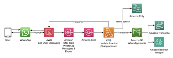
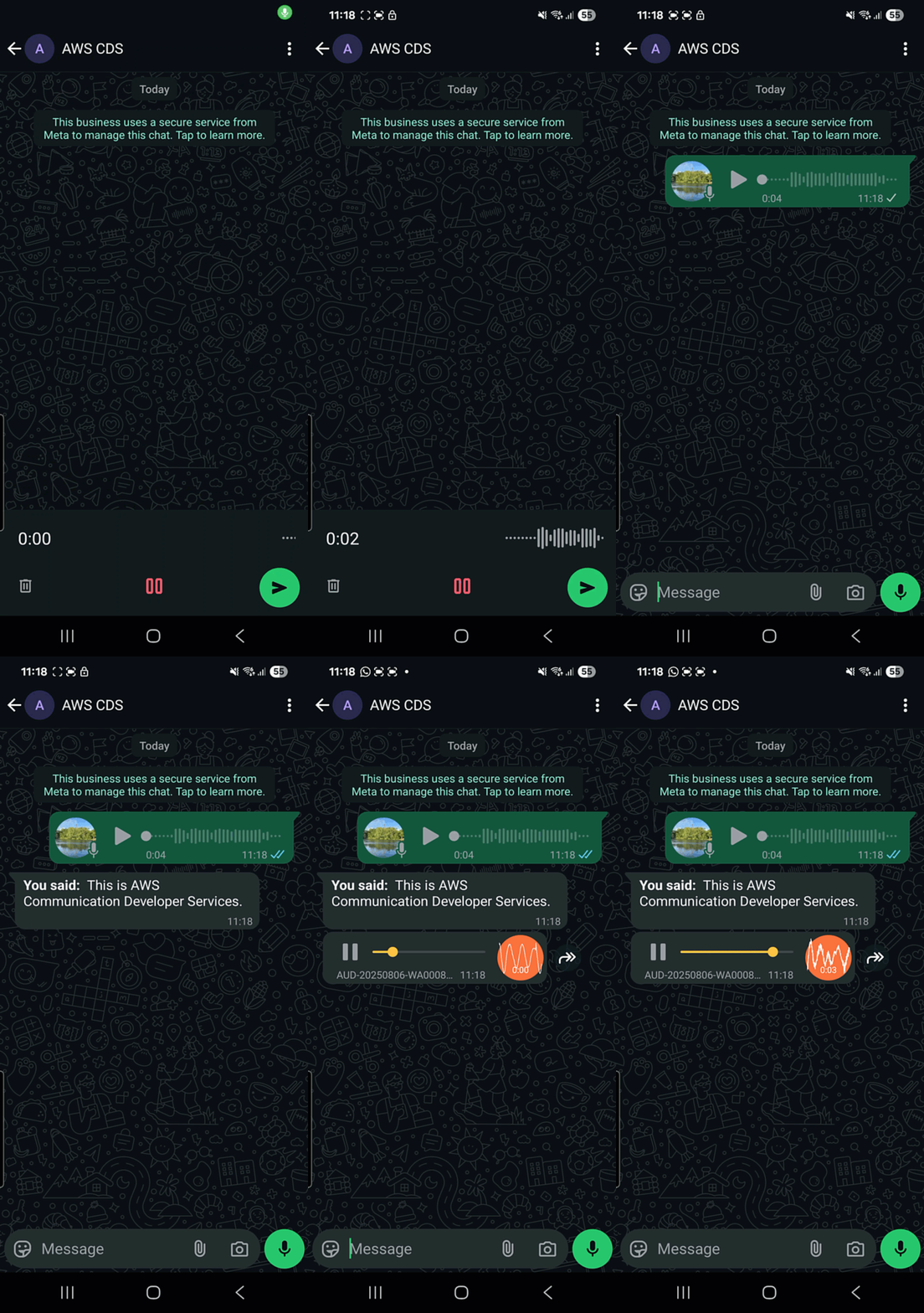
With AWS End User Messaging, businesses can now enable both voice note input and voice note responses on WhatsApp. Customers send a voice note, and a bot can respond with a natural-sounding voice note reply. Note: This solution processes asynchronous voice notes (recorded audio messages), not real-time voice calls. In this blog post, we explore why voice notes matter, where they make a difference, and how AWS helps you enable them through a sample voice note messaging solution.
Text remains essential, but research shows that voice notes adds unique advantages:
Richer communication: Voice carries tone, urgency, and emotion — reducing misunderstandings and helping businesses respond more appropriately (Preply survey).
Natural and fast: Speaking is up to three times faster than typing on mobile devices, especially when users are on the go (Sherry Ruan, Jacob O. Wobbrock, Kenny Liou, Andrew Ng, and James A. Landay. 2018. Comparing Speech and Keyboard Text Entry for Short Messages in Two Languages on Touchscreen Phones. Proc. ACM Interact. Mob. Wearable Ubiquitous Technol. 1, 4, Article 159 (December 2017), 23 pages. https://doi.org/10.1145/3161187).
Accessibility and inclusivity: Voice lowers barriers for people with limited literacy or visual impairments. Elderly customers or those with difficulty reading long text messages benefit significantly.
Context-driven preference: A YouGov study across 17 markets found that while text is still preferred overall, a notable share of users choose both text and audio depending on situation (YouGov survey).
Where voice notes make a difference
Voice messaging is especially useful when speaking feels more natural than typing—helping customers communicate in ways that fit their situation and needs.
Elderly customers – easier to listen than to read.
Field workers or drivers – easier to speak than to type while working.
Healthcare – patients can describe symptoms naturally by voice.
Hospitality and reservations – “Book a table for 7 pm” is faster to say than to navigate online calendar.
Customer support escalation – complex issues are often resolved more quickly with a voice exchange.
Voice notes don’t replace text. It complements it — giving customers the flexibility to communicate in the way that best suits their context.
AWS End User Messaging and WhatsApp
AWS End User Messaging is a managed AWS service that enables businesses to send and receive messages across multiple channels, including WhatsApp, SMS, MMS (US only), outbound voice, and push notifications.
When you use AWS End User Messaging for WhatsApp, you benefit from AWS’s global scale, resilience, and security. Inbound WhatsApp messages are automatically published to an Amazon SNS topic, enabling the integration with other AWS services such as Amazon SQS queues, AWS Lambda functions or Amazon Bedrock for downstream processing.
This flexibility is also what makes voice-to-voice messaging possible. Businesses can process inbound voice messages with Lambda, apply speech-to-text and text-to-speech services like Amazon Transcribe and Amazon Polly, or integrate third-party models such as Whisper through the AWS Marketplace for Amazon Bedrock.
git clone https://github.com/aws-samples/sample-whatsapp-voice-to-voice-messaging
cd sample-whatsapp-voice-to-voice-messaging
npm install
Before deploying, you’ll need to configure your WhatsApp phone number ID in the CDK context or parameters. The deployment will prompt you for this configuration, or you can set it in the cdk.json file. Once configured, deploy with:
cdk deploy
The CDK stack automatically provisions all required AWS resources including Lambda functions, SNS topics, S3 buckets, and IAM roles.
Clean up
To remove all resources and avoid ongoing charges:
cdk destroy
For detailed architecture diagrams, configuration options, and step-by-step setup instructions, visit the GitHub repository.
Conclusion
Customers are already using voice notes in their personal WhatsApp conversations. Bringing that same option into business communication makes customer interactions more natural, inclusive, and efficient.
With AWS End User Messaging and its WhatsApp channel, you can add voice alongside text without changing how customers connect to you. And with the sample CDK project, you can try it out today, experiment, and extend it for your own business needs.
Amazon OpenSearch Service is a fully managed service that reduces operational overhead, provides enterprise-grade security, high availability, and scalability, and enables you to quickly deploy real-time search, analytics, and generative AI applications. OpenSearch itself is an open-source, distributed search and analytics suite that supports a wide range of use cases, including real-time monitoring, log analytics, and full-text search. OpenSearch Service offers zero-ETL integrations with other Amazon Web Service (AWS) services, enabling seamless data access and analysis without the need for maintaining complex data pipelines.
Zero-ETL refers to a set of integrations designed to minimize or eliminate the need to build traditional extract, transform, load (ETL) pipelines. Traditional ETL processes can be time-consuming and difficult to develop, maintain, and scale. In contrast, zero-ETL integrations allow direct, point-to-point data movement and can also support querying across data silos without physically moving the data.
In this post, we explore various zero-ETL integrations available with OpenSearch Service that can help you accelerate innovation and improve operational efficiency. We cover following types of integrations, their key features, architecture, benefits, pricing, limitation and some general best practices.
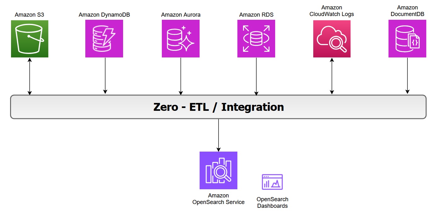
The following diagram illustrates the zero-ETL integration architecture in AWS, showing how various AWS services feed data into OpenSearch Service and its associated dashboards:
Zero-ETL integration with Amazon S3
Amazon OpenSearch Service direct queries with Amazon S3 provides a zero-ETL integration to reduce the operational complexity of duplicating data or managing multiple analytics tools by enabling you to directly query their operational data, reducing costs and time to action.
Key features of this integration include:
In-place querying: You can use rich analytics capabilities of OpenSearch Service SQL and PPL directly on infrequently-queried data stored outside of OpenSearch Service in Amazon S3.
Selective data ingestion: You can choose which data to bring into OpenSearch Service for detailed analysis, optimizing costs and speeding up queries with indexes like skipping or covering indexes.
In log analytics use cases, we categorize operational log data into two types:
Primary data includes the most recent and frequently accessed logs used for real-time monitoring and analysis.
Secondary data consists of historical logs that are accessed less frequently but retained for compliance or trend analysis.
You can offload infrequently queried data, such as archival or compliance data, to Amazon S3. With direct query, you can analyze analytics from Amazon S3 without data movement or duplication. However, query performance in OpenSearch Service might slow down when you’re accessing external data sources due to factors like network latency, data transformation, or large data volumes. You can optimize your query performance by using OpenSearch indexes, such as a skipping index, covering index, or materialized view.
While Amazon S3 direct query integration with OpenSearch Service provides on-demand access to data stored in Amazon S3, it is important to remember that OpenSearch’s alerting, monitoring, anomaly detection, and security analytics capabilities can only operate on data that has been explicitly ingested into OpenSearch Service indices. These capabilities would not work with direct query with Amazon S3. However, it will work if the data is indexed with covering or materialized index.
Benefits
With direct queries with Amazon S3, you no longer need to build complex ETL pipelines or incur the expense of duplicating data in both OpenSearch Service and Amazon S3 storage. You also save time and effort by not having to move back and forth between different tools during your analysis.
Pricing
OpenSearch Service separately charges for the compute needed to query your external data in addition to maintaining indexes in OpenSearch Service. Costs for Direct Query is based on the data volume scanned, query execution time, query frequency and frequency with which the indexed data in OpenSearch is kept updated. For more information, see Amazon OpenSearch Service Pricing.
Considerations
In case you are using OpenSearch service to query directly data on Amazon S3, consider the limitations with Direct Query.
Use the COALESCE SQL function to handle missing columns and ensure results are returned.
Use limits on your queries to ensure you aren’t pulling too much data back.
If you plan to analyze the same dataset many times, create an indexed view to fully ingest and index the data into OpenSearch Service and drop it when you have completed the analysis.
Drop acceleration jobs and indexes when they’re no longer needed.
Ingest data into Amazon S3 using partition formats of year, month, day, hour to speed up queries.
When you build skipping indexes, use Bloom filters for fields with high cardinality and min/max indexes for fields with large value ranges. Bloom filters are a space efficient probabilistic data structure that lets you quickly check whether an item is possibly in a set. For high-cardinality fields, consider using a value-based approach to improve query efficiency.
Use Index State Management to maintain storage for materialized views and covering indexes.
Zero-ETL integration with Amazon CloudWatch Logs
Amazon CloudWatch Logs serves as a centralized monitoring and storage solution for log files generated across various AWS services. This unified logging service offers a highly scalable platform where all your logging data converges into one manageable system. It provides comprehensive functionality for log management, including real-time viewing, pattern searching, field-based filtering, and secure archival capabilities. By presenting all logs chronologically in a unified stream, CloudWatch Logs eliminates the complexity of managing multiple log sources, transforming diverse logging data into a coherent, time-ordered sequence of events.
The zero-ETL integration between Amazon CloudWatch and Amazon OpenSearch Service enables direct log analysis and visualization while avoiding data redundancy, thereby reducing both technical complexity and costs. You can now leverage two additional query languages alongside the existing CloudWatch Logs Insights QL when using CloudWatch Logs, while as an OpenSearch user, you gain the ability to query CloudWatch logs directly.
The enhanced CloudWatch Logs Insights console now incorporates OpenSearch PPL and SQL functionality. Users can perform complex log analysis using SQL JOIN operations and various functions (including JSON, mathematical, datetime, and string operations). The PPL option provides additional data filtering and analysis capabilities.
The integration offers ready-to-use dashboards for various AWS services like Amazon Virtual Private Cloud (VPC), AWS CloudTrail, and AWS Web Application Firewall (WAF). These pre-configured visualizations enable quick insights into metrics such as flow patterns, top users, data transfer volumes, and temporal analysis, without requiring manual dashboard configuration.
You can now analyze CloudWatch logs through OpenSearch UI Discover and execute SQL and PPL queries. At the writing of this post, the query execution is limited to 50 log groups.
The direct access and analysis of CloudWatch data within OpenSearch Service removes the need for traditional ETL processes, eliminates separate data ingestion pipelines and avoids data duplication. This streamlined approach significantly reduces both storage expenses and operational complexity. It delivers a more efficient data management solution that simplifies the entire workflow while maintaining cost-effectiveness.
Pricing
When you use OpenSearch Service direct queries, you incur separate charges for OpenSearch Service and the resource used to process and store your data on Amazon CloudWatch Logs. As you run direct queries, you see charges for OpenSearch Compute Units (OCUs) per hour, listed as DirectQuery OCU usage type on your bill.
For interactive queries, OpenSearch Service handles each query with a separate pre-warmed job, without maintaining an extended session.
For indexed view queries, the indexed data is stored in an OpenSearch Serverless collection where you are charged for data indexed (IndexingOCU), data searched (SearchOCU), and data stored in GB.
In addition to the OpenSearch Service “direct queries” general limitations, if you are direct querying data in CloudWatch Logs, the following limitations apply:
The direct query integration with CloudWatch Logs is only available on OpenSearch Service collections and the OpenSearch user interface.
OpenSearch Serverless collections have networked payload limitations of 100 MiB.
CloudWatch Logs supports VPC Flow Logs, CloudTrail, and AWS WAF dashboard integrations installed from the console.
Best practices
Besides the general recommendations of OpenSearch Service direct querying, when using OpenSearch Service to direct query data in CloudWatch Logs, the following is recommended:
Specify the log group names within logGroupIdentifier in logGroups command to query multiple log groups in one query, see Multi-log group functions.
Enclose certain fields in backticks to successfully query them when using SQL or PPL commands. Backticks are needed for fields with special characters, such as `@SessionToken` or `LogGroup-A` (non-alphabetic and non-numeric). Refer to CloudWatch Logs Recommendations to see an example.
Zero-ETL integration with Amazon DynamoDB
Amazon DynamoDB zero-ETL integration with OpenSearch Service lets you perform a search on your DynamoDB data by automatically replicating and transforming it without custom code or infrastructure. This zero-ETL integration uses Amazon OpenSearch Ingestion to synchronize data between Amazon DynamoDB and OpenSearch Service cluster or OpenSearch Serverless collection within seconds of it being available.
It uses DynamoDB export to Amazon S3 to create an initial snapshot to load into OpenSearch Service. After the snapshot has been loaded, the plugin uses DynamoDB Streams to replicate any further changes in near real time. Turn on point-in-time recovery (PITR) for export and the DynamoDB Streams feature for ongoing replication.
This feature allows you to capture item-level changes in your table and push the changes to a stream. Every item in tables is processed as an event in OpenSearch Ingestion and can be modified with processors. You can also specify index mapping templates within ingestion pipelines to ensure that your Amazon DynamoDB fields are mapped to the correct fields in your OpenSearch indices.
When configuring zero-ETL between DynamoDB and OpenSearch Service, consider the differences between the data models. You have the following options with data layout:
Passthrough: Each item in DynamoDB table is directly mapped to one document in OpenSearch Index.
Routing: A single DynamoDB table mapped to multiple OpenSearch Service indices. In DynamoDB, it is common to store denormalized data in one table to optimize for access patterns. For example, a single DynamoDB table containing both customer profiles and order information can be routed to separate OpenSearch Service indices:
Merge: In some use cases, you need to combine data from multiple DynamoDB tables into a single OpenSearch index. You can use AWS Lambda integration with OpenSearch Ingestion to perform lookups on other DynamoDB tables and merge data from multiple DynamoDB tables.
Pricing
There is no additional cost to use this feature apart from the cost of the existing underlying components, including OpenSearch Ingestion charges OpenSearch Compute Units (OCUs) which is used to replicate data between Amazon DynamoDB and OpenSearch Service. Furthermore, this feature uses Amazon DynamoDB Streams for the change data capture (CDC), and you incur the standard costs for Amazon DynamoDB Streams.
Considerations
Consider the following limitations when you set up an OpenSearch Ingestion pipeline for DynamoDB:
At the writing of this post, the OpenSearch Ingestion integration with DynamoDB doesn’t support cross-Region and cross-account ingestion.
An OpenSearch Ingestion pipeline supports only one DynamoDB table as its source.
Amazon RDS and Amazon Aurora integration with OpenSearch Service eliminates complex data pipelines and enables near real-time data synchronization between Amazon Aurora and Amazon RDS databases (including RDS for MySQL and RDS for PostgreSQL) with advanced search capabilities on transactional databases. You can use an OpenSearch Ingestion pipeline with Amazon RDS or Amazon Aurora to export existing data and stream changes (such as create, update, and delete) to OpenSearch Service domains and collections. The OpenSearch Ingestion pipeline incorporates change data capture (CDC) infrastructure to provide a high-scale, low-latency way to continuously stream data from Amazon RDS or Amazon Aurora.
This automated process keeps your data consistently up to date in OpenSearch Service, making it readily available for search and analysis purpose. The pipeline ensures data consistency by continuously polling or receiving changes from the Amazon Aurora cluster or Amazon RDS and updating the corresponding documents in the OpenSearch index. OpenSearch Ingestion supports end-to-end acknowledgement to ensure data durability. An OpenSearch Ingestion pipeline also maps incoming event actions into corresponding bulk indexing actions to help ingest documents. This keeps data consistent, so that every data change in Amazon RDS is reconciled with the corresponding document changes in OpenSearch.
There is no additional charge for using this feature beyond the cost of your existing underlying resources, such as OpenSearch Service, OpenSearch Ingestion pipelines (OCUs), and Amazon RDS or Amazon Aurora. Additional costs may include storage used for enabling enhanced binlogs for MySQL and WAL logs for PostgreSQL for change data capture. You also incur storage costs for snapshot exports from your database to Amazon S3 used for the initial data.
Considerations
Consider the following limitations when you set up the integration for Amazon RDS or Amazon Aurora:
Requires same-Region and same-account deployment, primary keys for optimal synchronization, and currently has no data definition language (DDL) statement support.
The integration only supports one Aurora PostgreSQL database per pipeline.
The existing pipeline configuration can’t be updated to ingest data from a different database and/or a different table. To update the database and/or table name of a pipeline, stop the pipeline and restart it with an updated configuration or create a new pipeline.
Ensure that the Amazon Aurora or Amazon RDS cluster has authentication enabled using AWS Secrets Manager, which is the only supported authentication mechanism.
Best practices
The following are some best practices to follow while setting up the integration with OpenSearch Service:
If a mapping template is not specified in OpenSearch, it automatically assigns field types using dynamic mapping based on the first document received. However, it is always recommended to define field types explicitly by creating a mapping template that suits your requirements.
To maintain data consistency, the primary and foreign keys of tables remain unchanged.
You can configure the dead-letter queues (DLQ) in your OpenSearch Ingestion pipeline. If you’ve configured the queue, OpenSearch Service sends all failed documents that can’t be ingested due to dynamic mapping failures to the queue.
Amazon Document DB is a fully managed database service built for JSON data management at scale. It offers built-in text and vector search functionalities. By leveraging OpenSearch Service, you can execute search analytics, including features like fuzzy matching, synonym detection, cross-collection queries, and multilingual search capabilities on DocumentDB data.
The zero-ETL integration initiates the process with a full historical data extraction to OpenSearch using an ingestion pipeline. After the initial data load is completed, the pipelines read from Amazon DocumentDB change streams ensuring near real-time data consistency between the two systems. OpenSearch organizes the incoming data into indexes, with flexibility to either consolidate data from a DocumentDB collection into a single index or partition data across multiple indices. The ingestion pipelines synchronize all create, update, and delete operations from the DocumentDB collection, maintaining corresponding document modifications in OpenSearch. This ensures both data systems remain synchronised.
The pipelines offer configurable routing options, allowing data from a single collection to be written to one index or conditionally route to multiple indexes. Users can configure ingestion pipelines to stream data from Amazon DocumentDB to OpenSearch Service through three primary modes namely full load only, streaming change events without initial full load and full load followed by change streams. You can also monitor the state of ingestion pipelines in the OpenSearch service console. Additionally, you can use Amazon Cloudwatch to provide real-time metrics and logs and setting up alerts.
Pricing
There is no additional charge for using this feature apart from the cost of your existing underlying resources, including OpenSearch Service, OpenSearch Ingestion pipelines (OCUs), and Amazon DocumentDB. The integration performs an initial full load of Amazon DocumentDB data and continuously streams ongoing changes to OpenSearch Service using change streams. The change streams feature is disabled by default and does not incur any additional charges until the feature is enabled. Using change streams on a DocumentDB cluster incurs additional read and write input/output (I/O), as well as storage costs.
AWS Secrets Manager is the only supported authentication mechanism.
You can’t update an existing pipeline configuration to ingest data from a different database and/or a different collection. To update the database and/or collection name of a pipeline, create a new pipeline.
Best practices
The following are some best practices to follow while setting up the DocumentDB zero-ETL with OpenSearch Service:
Configure dead-letter queues (DLQ) to handle any failed document ingestion.
Configure AWS Secrets Manager and enable secrets rotation to provide the pipeline secure access.
If you’re using change streams in DocumentDB, it’s important to extend the retention period to up to 7 days. This ensures you don’t lose any data changes during the ingestion process.
With zero-ETL integrations, you can use the powerful search and analytics features of OpenSearch Service directly on your latest database data. These include full-text search, fuzzy search, auto-complete, and vector search for machine learning (ML) workloads—enabling intelligent, real-time experiences that enhance your applications and improve user satisfaction. This integration uses change streams to automate the synchronisation of transactional data from Amazon Aurora, Amazon RDS, Amazon DynamoDB and Amazon DocumentDB to OpenSearch Service without manual intervention. Once the data is available in OpenSearch Service, you can perform real-time searches to quickly retrieve relevant results for your applications.This eliminates the need for manual Extract-Transform-Load (ETL) processes, reduces operational complexity, and accelerates time-to-insight for real-time dashboards, search, and analytics.
Conclusion
In this post, you learned that zero-ETL integrations represent a significant advancement in simplifying data analytics workflows and reducing operational complexity. As you’ve explored throughout this post, these integrations offer several advantages such as elimination of complex ETL pipelines and reduced infrastructure and operational costs by removing the need for intermediate storage and processing that enhance developer productivity.
It is time to accelerate your analytics journey with OpenSearch Service zero ETL – where your data flows seamlessly, eliminating complex pipelines and delivering real-time insights. Get started with Amazon OpenSearch Service or learn more about integrations with other services and applications in the AWS documentation.
This is a guest post by Edijs Drezovs, CEO and Founder of GOStack, Viesturs Kols, Data Architect at GOStack, and Krisjanis Beitans, Senior Data Engineer at GOStack, in partnership with AWS.
Yggdrasil Gaming develops and publishes casino games globally, processing massive amounts of real-time gaming data for game performance analytics, player behavior insights, and industry intelligence. As Yggdrasil’s system grew, managing dual-cloud environments created operational overhead and limited their ability to implement advanced analytics initiatives. This challenge became critical ahead of the launch of the Game in a Box solution on AWS Marketplace, which generates increases in data volume and complexity.
Yggdrasil Gaming reduced multi-cloud complexity and built a scalable analytics foundation by migrating from Google BigQuery to AWS analytics services. In this post, you’ll discover how Yggdrasil Gaming transformed their data architecture to meet growing business demands. You will learn practical strategies for migrating from proprietary systems to open table formats such as Apache Iceberg while maintaining business continuity.
Yggdrasil worked with GOStack, an AWS Partner, to migrate to an Apache Iceberg-based lakehouse architecture. The migration helped reduce operational complexity and enabled real-time gaming analytics and machine learning.
Challenges
Yggdrasil faced several critical challenges that prompted their migration to AWS:
Multi-cloud operational complexity: Managing infrastructure across AWS and Google Cloud created significant operational overhead, reducing agility and increasing maintenance costs. The data team had to maintain expertise in both environments and coordinate data movement between clouds.
Architecture limitations: The existing setup couldn’t effectively support advanced analytics and AI initiatives. More critically, the launch of Yggdrasil’s Game in a Box solution required a modernized, scalable data environment capable of handling increased data volumes and enabling advanced analytics.
Scalability constraints: The architecture lacked the unified data foundation with open standards and automation required to scale efficiently. As data volumes grew, costs increased proportionally, and the team needed an environment designed for modern analytics at scale.
Solution overview
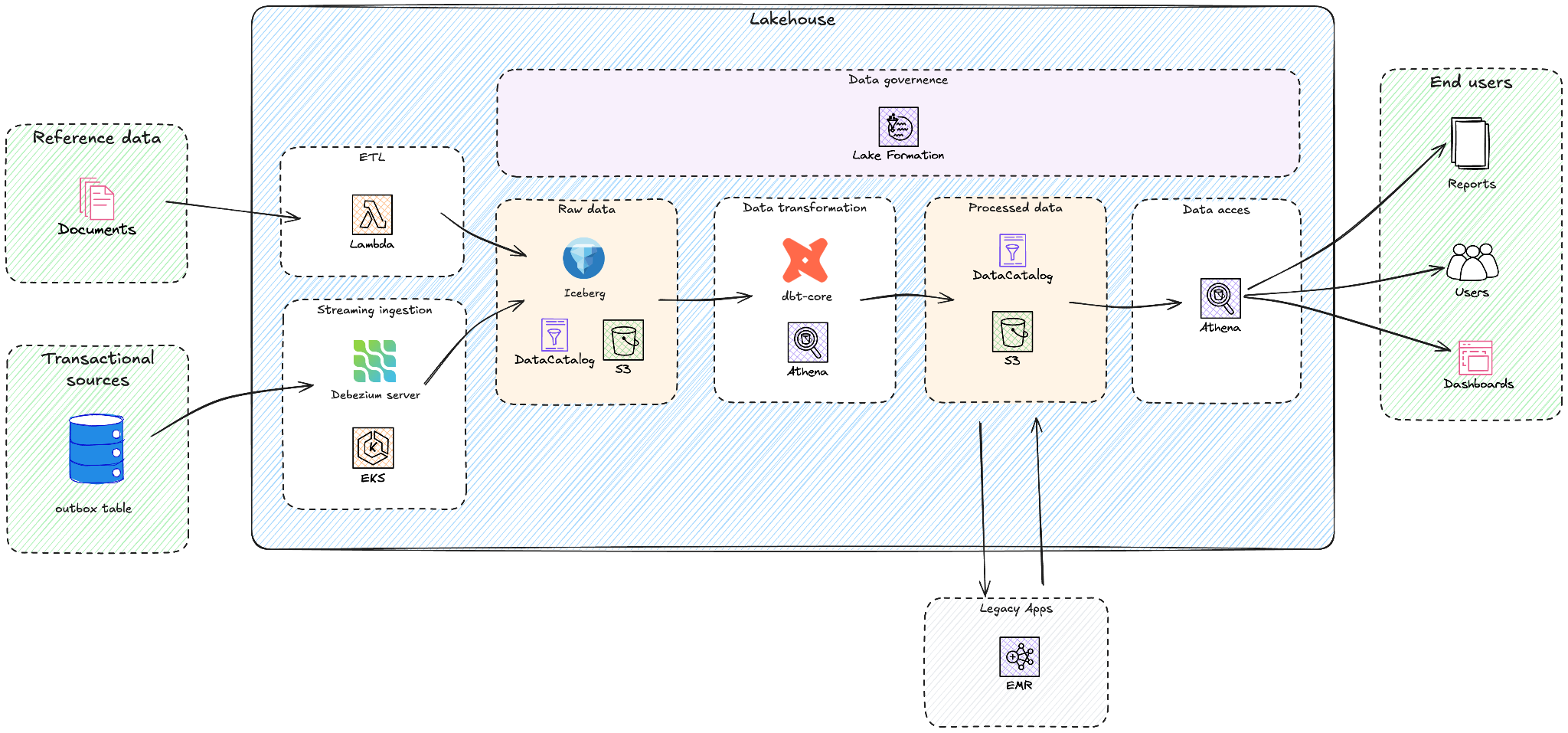
Yggdrasil worked with GOStack, an AWS APN partner, to design their new lakehouse architecture. The following diagram shows the high level overview of this architecture.
The combination of Amazon S3, Apache Iceberg, and Amazon Athena allowed Yggdrasil to move away from provisioned, always-on compute models. The Amazon Athena pay-per-query pricing charges only for data scanned, removing idle compute costs during off-peak periods. Internal cost modeling performed during the evaluation phase indicated that this architecture could reduce analytics system costs by 30–50% compared to compute-based warehouse pricing models of other solutions, particularly for bursty workloads driven by game launches, tournaments, and seasonal traffic. By adopting AWS-native analytics services, Yggdrasil reduced operational complexity through native integration with AWS Identity and Access Management (AWS IAM), Amazon EKS, and AWS Lambda, helping simplify security, governance, and automation across the analytics system.
The solution centers on a modern lakehouse architecture built on Amazon S3, which provides durable and cost-efficient storage for Iceberg tables in Apache Parquet format. Apache Iceberg table format provides ACID transactions, schema evolution, and time travel capabilities while maintaining an open standard. AWS Glue Data Catalog serves as the central technical metadata repository, while Amazon Athena acts as the serverless query engine used by dbt-athena and for ad-hoc data exploration. Amazon EMR runs Yggdrasil’s legacy Apache Spark application in a fully managed environment, and AWS Lake Formation provides centralized security and governance for data lakes, allowing fine-grained access control at database, table, column, and row levels.
The migration followed a phased approach:
Establish lakehouse foundation – Set up Apache Iceberg-based architecture with Amazon S3 with AWS Glue Data Catalog
Implement real-time data ingestion – Deploy Debezium connectors for real-time change data capture from EKS and Google Kubernetes Engine (GKE) clusters
Migrate processing pipelines – Re-system ETL pipelines using AWS Lambda, and legacy data applications re-systemed on Amazon EMR
Modernizing the transformation layer – Implement dbt with Amazon Athena for modular, reusable models
Enable governance – Configure AWS Lake Formation for comprehensive data governance
Establish lakehouse foundation
The first phase of the migration focused on building a solid foundation for the new data lakehouse architecture on AWS. The goal was to create a scalable, secure, and cost-efficient environment that could support analytical workloads with open data formats and serverless query capabilities.
GOStack provisioned an Amazon S3-based data lake as the central storage layer, providing virtually unlimited scalability and fine-grained cost control. This storage-compute separation enables teams to decouple ingestion, transformation, and analytics processes, with each component scaling independently using the most appropriate compute engine.
To establish dataset interoperability and discoverability, the team adopted AWS Glue Data Catalog as the unified metadata repository. The catalog stores Iceberg table definitions and makes schemas accessible across services such as Amazon Athena and Apache Spark workloads on Amazon EMR. Most datasets, both batch and streaming, are registered here, enabling consistent metadata visibility across the lakehouse.
The data is stored in Apache Iceberg tables on Amazon S3, selected for its open table format, ACID transaction support, and powerful schema evolution features. Yggdrasil required ACID transactions for consistent financial reporting and fraud detection, schema evolution to accommodate rapidly changing gaming data models, and time travel queries to align with regulatory audit requirements.
GOStack built a custom schema conversion and table registration service. This internal tool converts source-system Avro schemas into Iceberg table definitions and manages the creation and evolution of raw-layer tables. By controlling schema translation and table registration directly, the team makes sure that metadata stays consistent with the source systems and provides predictable, versioned schema evolution aligned with ingestion needs.
The initial setup made the following components:
Amazon S3 bucket structure design: Implemented a multi-layer layout (raw, curated, and analytics zones) aligned with data lifecycle best practices.
AWS Glue Data Catalog integration: Defined database and table schemas with partitioning strategies optimized for Athena performance.
Iceberg configuration: Enabled versioning and metadata retention policies to balance storage efficiency and query flexibility.
Security and compliance: Configured encryption at rest using AWS Key Management Service (AWS KMS), helped enforce access controls via AWS IAM and Lake Formation, and implemented Amazon S3 bucket policies following the principle of least privilege.
The redesign of the previous GCP setup helped deliver price-performance improvements. Yggdrasil reduced ingestion and processing costs by approximately 60% while also lowering operational overhead through a more direct, event-driven pipeline.
Implement real-time data ingestion
After establishing the lakehouse architecture, the next step focused on enabling real-time data ingestion from Yggdrasil’s operational databases into the raw data layer of the lakehouse. The objective was to capture and deliver transactional changes as they occur, making sure that downstream analytics and reporting reflect the most up-to-date information.
To achieve this, GOStack deployed Debezium Server Iceberg, an open-source project that integrates change data capture (CDC) directly with Apache Iceberg tables. It was deployed as Argo CD applications on Amazon EKS and used Argo’s GitOps-based model for reproducibility, scalability, and seamless rollouts.
This architecture provides an efficient ingestion pathway – streaming data changes directly from the source system’s outbox tables into the Apache Iceberg tables registered in the AWS Glue Data Catalog and physically stored on Amazon S3, bypassing the need for intermediate brokers or staging services. By writing data in the Iceberg table format, the ingestion layer maintained transactional guarantees and immediate query availability through Amazon Athena.
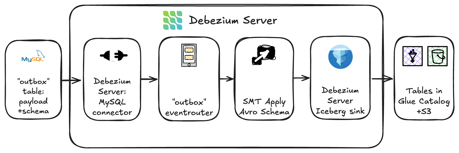
Because Yggdrasil’s source systems emitted outbox events containing Avro records, the team implemented a custom outbox-to-Avro transformation within Debezium. The outbox table stored two key components:
The Avro schema definition
The JSON-encoded payload of each record
The custom transformation module combined these elements into valid Avro records before persisting them into the target Iceberg tables. This approach preserved schema fidelity and verified compatibility with downstream processing tools.
To dynamically route incoming change events, the team leveraged Debezium’s event router configuration. Each record was routed to the appropriate Apache Iceberg table (backed by Amazon S3) based on topic and metadata rules, while table schemas and partitioning were governed on the AWS Glue side to maintain stability and alignment with the lakehouse’s data organization standards.
This setup helped deliver low-latency ingestion with end-to-end streaming from database outbox to S3-based Iceberg tables in near real time. The team managed operations end to end on Amazon EKS using Helm charts deployed via Argo CD in a GitOps model for fully declarative, version-controlled operations. ACID-compliant Iceberg writes verified that partially written data could not corrupt downstream analytics. The modular transformation logic allowed future expansion to new source systems or event formats without rearchitecting the ingestion pipeline.
This Debezium Server solution provides fast, real-time data ingestion. GOStack considers it an interim architecture. In the long term, the ingestion pipeline will evolve to use Amazon Managed Streaming for Apache Kafka (Amazon MSK) as the central event backbone. Debezium connectors will act as producers, publishing change events to Apache Kafka topics, while Apache Flink applications will consume, process, and write data into Iceberg tables.
This planned evolution toward a Kafka-based streaming architecture verifies Yggdrasil’s lakehouse remains not only scalable and cost-efficient today, but also future-ready – capable of supporting richer streaming analytics and broader data integration scenarios as the organization grows.
Migrate processing pipelines
Once real-time data ingestion was established, GOStack turned its focus to modernizing the data transformation layer. The goal was to simplify the transformation logic, reduce operational overhead, and unify the orchestration of analytical workloads within the new AWS-based lakehouse.
GOStack adopted a lift-and-shift approach for some of Yggdrasil’s data pipelines to support a fast and low-risk transition away from GCP. The lightweight Cloud Run functions that previously handled extraction tasks – pulling data from file shares, SharePoint, Google Sheets, and various third-party APIs – were re-implemented using AWS Lambda. These Lambda functions now integrate with the same external systems and write data directly into Iceberg tables.
For more complex processing, previous Apache Spark applications running on Dataproc were migrated to Amazon EMR with minimal code changes. This allowed it to preserve the existing transformation logic while benefiting from the managed scaling capabilities of EMR and improved cost control on AWS.
Over time, these processes will be gradually refactored and consolidated into containerized workflows on the EKS cluster, fully orchestrated by Argo Workflows. This phased migration allows Yggdrasil to move workloads to AWS quickly and decommission GCP resources sooner, while still leaving room for continuous improvement and modernization of the data system over time.
Finally, a lot of analytical transformations that previously lived as BigQuery stored procedures and scheduled queries, that were now rebuilt as modular dbt models executed with dbt-athena. This shift made transformation logic more transparent, maintainable, and version-controlled, improving both developer experience and long-term governance.
Modernizing the transformation layer
With the ingestion pipelines migrated to AWS, GOStack turned its focus to simplifying and modernizing Yggdrasil’s analytical transformations. Rather than replicating the previous stored-procedure–driven approach, the team rebuilt the transformation layer using dbt to help improve maintainability, lineage visibility, orchestration, and long-term governance.As part of this redesign, several data models were reshaped to fit the new lakehouse architecture. The most significant effort involved rewriting a critical Spark-based financial transformation into a set of SQL-driven dbt models. This shift not only aligned the logic with the lakehouse design but also removed the need for long-running Spark clusters, helping generate operational and cost savings.For the curated data layers, replacing the legacy warehouse, GOStack consolidated numerous scheduled queries and stored procedures into structured dbt models. This provides standardized, version-controlled transformations and clear lineage across the analytical stack.
Orchestration was simplified as well. Previously, coordination was split between Apache Airflow for Spark workloads and scheduled queries analytical transformations, creating operational friction and dependency risks. In the new architecture, Argo Workflows on Amazon EKS orchestrates dbt models centrally, consolidating the transformation logic within a single workflow engine. While most transformations still run on time-based schedules today, the system now supports event-driven execution through Argo Events, giving the opportunity to progressively adopt trigger-based workflows as the transformation layer evolves.
This unified orchestration framework can bring multiple benefits:
Consistency: One orchestration layer for data workflows across ingestion and transformation.
Automation: Event-driven dbt runs help remove manual scheduling and reduce operational overhead.
Scalability: Argo Workflows scales with the EKS cluster, handling concurrent dbt jobs seamlessly.
Observability: Centralized logging and workflow visualization help improve visibility into job dependencies and data freshness.
Through this transformation, Yggdrasil successfully unified its data lakes and warehouses into a modern lakehouse architecture, powered by open data formats, serverless query engines, and modular transformation logic. The move to dbt and Athena not only simplified operations but also helped pave the way for faster iteration, simpler governance, and greater developer productivity across the data environment.
Lakehouse performance optimizations
While performance tuning is an ongoing journey, as part of the transformation redesign, GOStack made few performance-oriented tweaks to make sure Athena queries can be fast and cost-efficient. The Apache Iceberg tables were stored in Parquet with ZSTD compression, providing strong read performance and reducing the amount of data scanned by Athena.
Partitioning strategies were also aligned to actual access patterns using Iceberg’s native partitioning. Raw data zones were partitioned by ingestion timestamp, enabling efficient incremental processing. Curated data used business-driven partition keys, such as player or game identifiers and date dimensions, to help optimize analytical queries. These designs made sure Athena could prune unneeded data and consistently scan only the relevant partitions.
Iceberg’s native partitioning features, including transforms such as bucketing and time slicing, replace traditional Hive partitioning patterns. Because Iceberg manages partitions internally in its metadata layer, not all Glue or Athena partition constructs apply. Relying on Iceberg’s native partitioning helps provide predictable pruning and consistent performance across the lakehouse without introducing legacy Hive behaviors.
To handle the high volume of small files produced by real-time ingestion, GOStack enabled AWS Glue Iceberg compaction. This automatically merges small Parquet files into larger segments, helping improve query performance and reduce metadata overhead without manual intervention.
Enable governance
The team adopted AWS Lake Formation as the primary governance layer for the curated zone of the lakehouse, leveraging Lake Formation hybrid access mode to manage fine-grained permissions alongside existing IAM-based access patterns. This hybrid mode provides an incremental and flexible pathway to adopt Lake Formation without forcing a full migration of legacy permissions or internal pipeline roles, making it an ideal fit for Yggdrasil’s phased modernization strategy.
Lake Formation offers centralized authorization, supporting database, table, column, and, critically for Yggdrasil, row-level permissions. These capabilities are essential because of the company’s multi-tenant operating model:
Game development partners require access to data and reports pertaining only to their own games, facilitating both security and compliance alignment with partner agreements.
iGaming operators integrating with Yggdrasil’s system must receive operational and financial insights exclusively for their own data, enforced automatically through reporting tools backed by curated Iceberg tables.
With Lake Formation hybrid access mode, tenant-specific row-level access policies are consistently enforced across Amazon Athena, AWS Glue, and Amazon EMR, without introducing breaking changes to existing IAM-based workloads. This allowed Yggdrasil to implement strong governance for external consumers while keeping internal operations stable and predictable.
Internally, Lake Formation is also used to grant the Analytics team and BI tools targeted access to curated datasets, straightforward but centrally managed to maintain consistency and reduce administrative overhead.
For ingestion and transformation workloads, the team continues to rely on IAM roles and policies. Services such as Debezium, dbt, and Argo Workflows require broad but controlled access to raw and intermediate storage layers, and IAM provides a straightforward, least-privilege mechanism for granting those permissions without involving Lake Formation in the internal pipeline path.
By adopting Lake Formation in hybrid access mode and combining it with IAM for internal services, Yggdrasil established a governance model that can balance strong security with operational flexibility – enabling the lakehouse to scale securely as the business grows.
Results and business impact
The new lakehouse, built on Amazon Athena, Amazon S3, and AWS Glue Data Catalog, now underpins advanced analytics and AI/ML use cases such as player behavior modeling, predictive game recommendations, and fraud detection.
The optimized lakehouse design allows Yggdrasil to rapidly onboard new analytics workloads and business use cases, helping deliver measurable outcomes:
Reduced operational complexity through consolidation on AWS analytics services
Cost optimization with a 60% reduction in data processing costs
Improved data freshness with 75% lower latency for analytics results (from 2 hours to 30 minutes)
Enhanced governance using the AWS Lake Formation fine-grained controls
Future-ready architecture leveraging open formats and serverless analytics
Conclusion
Yggdrasil Gaming’s migration journey illustrates how organizations can successfully transition from proprietary analytics systems to an open, flexible lakehouse architecture. By following a phased approach guided by AWS Well-Architected Framework principles, Yggdrasil maintained business continuity while establishing a modern foundation for their data needs.
Based on this experience, several lessons emerged to help guide your own move to an AWS-based lakehouse:
Assess your current state: Identify pain points in your existing data architecture and establish clear objectives for modernization.
Start small: Begin with a pilot project using AWS analytics services to validate the lakehouse approach for your specific use cases.
Design for openness: Leverage open table formats like Apache Iceberg to maintain flexibility and avoid vendor lock-in.
Implement gradually: Follow a phased migration strategy similar to Yggdrasil’s, prioritizing high-value workloads.
Optimize continuously: Use performance tuning techniques for Amazon Athena to help maximize efficiency and minimize costs.
Over the past year, Amazon Redshift has introduced capabilities that simplify operations and enhance productivity. Building on this momentum, we’re addressing another common operational challenge that data engineers face daily: managing repetitive data loading operations with similar parameters across multiple data sources. This intermediate-level post introduces AWS Redshift Templates, a new feature that you can use to create reusable command patterns for the COPY command, reducing redundancy and improving consistency across your data operations.
The challenge: Managing repetitive data operations at scale
Meet AnyCompany, a fictional data aggregation company that processes customer transaction data from over 50 retail clients. Each client sends daily delimited text files with similar structures:
While the data format is largely consistent across clients (pipe-delimited files with headers, UTF-8 encoding), the sheer volume of COPY commands required to load this data has become a development and maintenance overhead.
Their data engineering team faces several pain points:
Repetitive parameter specification: Each COPY command requires specifying the same parameters for delimiter, encoding, error handling, and compression settings
Inconsistency risks: With multiple team members writing COPY commands, slight variations in parameters lead to data ingestion failures
Maintenance overhead: When they need to adjust error thresholds or encoding settings, they must update hundreds of individual COPY commands across their extract, transform, and load (ETL) pipelines
Onboarding complexity: New team members struggle to remember all the required parameters and their optimal values
Additionally, a few clients send data in slightly different formats. Some use comma delimiters instead of pipes or have different header configurations. The team needs flexibility to handle these exceptions without completely rewriting their data loading logic.
Introducing Redshift Templates
You can address these challenges by using Redshift Templates to store commonly used parameters for COPY commands as reusable database objects. Think of templates as blueprints for your data operations where you can define your parameters once, then reference them across multiple COPY commands.
Template management best practices
Before exploring implementation scenarios, let’s establish best practices for template management to ensure your templates remain maintainable and secure.
-- Grant specific permissions to roles
GRANT USAGE FOR TEMPLATES IN SCHEMA analytics TO ROLE data_engineers;
GRANT ALTER FOR TEMPLATES IN SCHEMA reporting TO ROLE senior_analysts;
-- Revoke broad permissions
REVOKE ALL ON TEMPLATE analytics.csv_load FROM PUBLIC;
Query the system view to track template usage:
SELECT database_name, schema_name, template_name,
       create_time, last_modified_time
FROM sys_redshift_template;
Document each template, including:
Purpose and use cases
Parameter explanations
Ownership and contact information
Change history
Solution overview
Let’s explore how AnyCompany uses Redshift Templates to streamline their data loading operations.
Scenario 1: Standardizing client data ingestion
AnyCompany receives transaction files from multiple retail clients with consistent formatting. They create a template that encapsulates their standard loading parameters:
-- Create a reusable template for standard client data loads
CREATE TEMPLATE data_ingestion.standard_client_load
FOR COPY
AS
DELIMITER '|'
IGNOREHEADER 1
ENCODING UTF8
MAXERROR 100
COMPUPDATE OFF
STATUPDATE ON
ACCEPTINVCHARS
TRUNCATECOLUMNS;
This template defines their standard approach:
DELIMITER '|' specifies pipe-delimited files
IGNOREHEADER 1 skips the header row
ENCODING UTF8 facilitates proper character encoding
MAXERROR 100 allows up to 100 errors before failing, providing resilience for minor data quality issues
COMPUPDATE OFF helps prevent automatic compression analysis during loading for faster performance
STATUPDATE ON keeps table statistics current for query optimization
ACCEPTINVCHARS replaces invalid UTF-8 characters rather than failing
TRUNCATECOLUMNS truncates data that exceeds column width rather than failing
Now, loading data from a standard client becomes remarkably straightforward:
-- Load transaction data from Client A
COPY transactions_client_a
FROM 's3://amzn-s3-demo-bucket/client-a/transactions/'
IAM_ROLE default
USING TEMPLATE data_ingestion.standard_client_load;
-- Load transaction data from Client B
COPY transactions_client_b
FROM 's3://amzn-s3-demo-bucket/client-b/transactions/'
IAM_ROLE default
USING TEMPLATE data_ingestion.standard_client_load;
-- Load product catalog from Client C
COPY products_client_c
FROM 's3:// amzn-s3-demo-bucket/client-c/products/'
IAM_ROLE default
USING TEMPLATE data_ingestion.standard_client_load;
Notice how clean and maintainable these commands are. Each COPY statement specifies only:
The complex formatting and error handling parameters are neatly encapsulated in the template, facilitating consistency across the data loads.
Scenario 2: Handling client-specific variations with parameter overrides
AnyCompany has two clients (Client D, and E) who send comma-delimited files instead of pipe-delimited files. Rather than creating an entirely separate template, they can override specific parameters while still using the template’s other settings:
-- Load data from Client D with comma delimiter (overriding template)
COPY transactions_client_d
FROM 's3://amzn-s3-demo-bucket/client-d/transactions/'
IAM_ROLE default
DELIMITER ','  -- Override the template's pipe delimiter
USING TEMPLATE data_ingestion.standard_client_load;
-- Load data from Client E with comma delimiter and no header
COPY transactions_client_e
FROM 's3://amzn-s3-demo-bucket/client-e/transactions/'
IAM_ROLE default
DELIMITER ','      -- Override delimiter
IGNOREHEADER 0     -- Override header setting
USING TEMPLATE data_ingestion.standard_client_load;
This demonstrates the Redshift Templates parameter hierarchy:
Command-specific parameters (highest priority): Parameters explicitly specified in your COPY command take precedence
Template parameters (medium priority): Parameters defined in the template are used when not overridden
Amazon Redshift default parameters (lowest priority): Default values apply when neither command nor template specifies a value
This three-tier approach provides the perfect balance between standardization and flexibility. You maintain consistency where it matters while retaining the ability to handle exceptions gracefully.
Scenario 3: Simplified template maintenance
Six months after implementing templates, AnyCompany’s data quality team recommends increasing the error threshold from 100 to 500 to better handle occasional data quality issues from upstream systems. With templates, this change is trivial:
-- Update the template to increase error tolerance
ALTER TEMPLATE data_ingestion.standard_client_load
SET MAXERROR TO 500;
This single command instantly updates the error handling behavior for the future COPY operations using this template without needing to hunt through hundreds of ETL scripts or risking missing updates in some pipelines. They can also add new parameters as their requirements evolve:
-- Add compression parameter to improve load performance
ALTER TEMPLATE data_ingestion.standard_client_load
ADD GZIP;
To remove a template when it’s no longer needed:
DROP TEMPLATE data_ingestion.standard_client_load;
Scenario 4: Environment-specific templates for development and production
AnyCompany maintains separate templates for development and production environments, with different error tolerance levels:
-- Development template with lenient error handling
CREATE TEMPLATE data_ingestion.dev_client_load
FOR COPY
AS
DELIMITER '|'
IGNOREHEADER 1
ENCODING UTF8
MAXERROR 1000        -- More lenient for testing
COMPUPDATE OFF
STATUPDATE OFF;      -- Skip stats updates in dev
-- Production template with strict error handling
CREATE TEMPLATE data_ingestion.prod_client_load
FOR COPY
AS
DELIMITER '|'
IGNOREHEADER 1
ENCODING UTF8
MAXERROR 50          -- Stricter for production
COMPUPDATE OFF
STATUPDATE ON;       -- Keep stats current in prod
This approach helps ensure that data quality issues are caught early in production while allowing flexibility during development and testing.
Key benefits
The key benefits of using templates include:
Consistency and standardization: Templates help maintain consistency across different operations by making sure that the same set of parameters and configurations are used every time. This is particularly valuable in large organizations where multiple users work on the same data pipelines.
Ease of use and timesaving: Instead of manually specifying the parameters for each command execution, users can reference a pre-defined template. This saves time and reduces the chances of errors caused by manual input.
Flexibility with parameter overrides: While templates provide standardization, they don’t sacrifice flexibility. You can override a template parameter directly in your COPY command when handling exceptions or special cases.
Simplified maintenance: When changes need to be made to parameters or configurations, updating the corresponding template propagates the changes across the instances where the template is used. This significantly reduces maintenance effort compared to manually updating each command individually.
Collaboration and knowledge sharing: Templates serve as a knowledge base, capturing best practices and optimized configurations developed by experienced users. This facilitates knowledge sharing and onboarding of new team members, reducing the learning curve and facilitating consistent usage of proven configurations.
Additional use cases across industries
Templates can be used across industries.
Financial services: Standardizing regulatory data loads
A financial institution needs to load transaction data from multiple branches with consistent formatting requirements:
-- Create template for branch transaction loads
CREATE TEMPLATE compliance.branch_transaction_load
FOR COPY
AS
FORMAT CSV
DELIMITER ','
IGNOREHEADER 1
ENCODING UTF8
DATEFORMAT 'YYYY-MM-DD'
TIMEFORMAT 'YYYY-MM-DD HH:MI:SS'
MAXERROR 0           -- Zero tolerance for compliance data
COMPUPDATE OFF;
-- Load data from different branches
COPY branch_transactions_east
FROM 's3://amzn-s3-demo-source-bucket/east-branch/transactions/'
IAM_ROLE default
USING TEMPLATE compliance.branch_transaction_load;
COPY branch_transactions_west
FROM 's3://amzn-s3-demo-source-bucket/west-branch/transactions/'
IAM_ROLE default
USING TEMPLATE compliance.branch_transaction_load;
Healthcare: Loading patient data with strict standards
A healthcare analytics company standardizes their patient data ingestion across multiple hospital systems:
-- Create template for HIPAA-compliant data loads
CREATE TEMPLATE healthcare.patient_data_load
FOR COPY
AS
FORMAT CSV
DELIMITER '|'
IGNOREHEADER 1
ENCODING UTF8
ACCEPTINVCHARS
TRUNCATECOLUMNS
MAXERROR 10
COMPUPDATE OFF;
-- Apply to different hospital systems
COPY hospital_a_patients
FROM 's3://amzn-s3-demo-destination-bucket/hospital-a/patients/'
IAM_ROLE default
USING TEMPLATE healthcare.patient_data_load;
COPY hospital_b_patients
FROM 's3://amzn-s3-demo-destination-bucket/hospital-b/patients/'
IAM_ROLE default
USING TEMPLATE healthcare.patient_data_load;
Retail: JSON data loading standardization
A retail company processes JSON-formatted product catalogs from various suppliers:
-- Create template for JSON product data
CREATE TEMPLATE retail.json_product_load
FOR COPY
AS
FORMAT JSON 'auto'
TIMEFORMAT 'auto'
ENCODING UTF8
MAXERROR 100
COMPUPDATE OFF;
-- Load from different suppliers
COPY products_supplier_a
FROM 's3://amzn-s3-demo-logging-bucket/supplier-a/products/'
IAM_ROLE default
USING TEMPLATE retail.json_product_load;
COPY products_supplier_b
FROM 's3://amzn-s3-demo-logging-bucket/supplier-b/products/'
IAM_ROLE default
USING TEMPLATE retail.json_product_load;
Conclusion
In this post, we introduced Redshift Templates and showed examples of how they can standardize and simplify your data loading operations across different scenarios. By encapsulating common COPY command parameters into reusable database objects, templates help remove repetitive parameter specifications, facilitate consistency across teams, and centralize maintenance. When requirements evolve, a single template update propagates quickly across the operations, reducing operational overhead while maintaining flexibility to override parameters for use cases.
Start using Redshift Templates to transform your data ingestion workflows. Create your first template for your most common data loading pattern, then gradually expand coverage across your pipelines. Your team will immediately benefit from cleaner code, faster onboarding, and simplified maintenance. To learn more about Redshift Templates and explore additional configuration options, see the Amazon Redshift documentation.
This is a guest post by Aakash Pradeep, Principal Software Engineer, and Venkatram Bondugula, Software Engineer at Twilio, in partnership with AWS.
Twilio is a cloud communications platform that provides programmable APIs and tools for developers to easily integrate voice, messaging, email, video, and other communication features into their applications and customer engagement workflows.
In this blog series we discuss how we built a multi-engine query platform at Twilio. The first part introduces the use case that led us to build a new platform and why we selected Amazon Athena alongside our open-source Presto implementation. This second part discusses how Twilio’s query infrastructure platform integrates with AWS Lake Formation to provide fine-grained access control to all their data.
At Twilio, we faced critical challenges in managing our multi-engine query platform across a complex data mesh architecture spanning multiple AWS accounts and Lines of Business. We needed a unified permissions model that could work consistently across different query engines like OSS Presto and Amazon Athena, eliminating the fragmented authentication experiences in our infrastructure. The growing demand for secure cross-account data sharing required moving beyond manual, multi-step provisioning processes that depended heavily on human intervention. Additionally, Twilio’s compliance and data stewardship requirements demanded fine-grained access controls at row, column, and cell levels, necessitating a scalable and flexible approach to permission management. By adopting the AWS Glue Data Catalog as our managed metastore and AWS Lake Formation for governance, we implemented Tag-Based Access Control (LF-TBAC) to simplify access management, enabled data sharing through automated workflows, and established a centralized governance framework that provided uniform permissions management across all AWS services.
Transitioning to a managed metastore and governance solutions
We discussed in part 1, how we were looking to move to managed services to alleviate us of the burden of managing the underlying infrastructure of a query platform. Along with our decision to adopt Amazon Athena, we also began to evaluate the adoption of Amazon EMR Serverless for our Spark workloads, which made us aware of the fact that we needed to migrate to a managed solution for our Apache Hive metastore.
We selected the AWS Glue Data Catalog as our managed metastore repository to support our enterprise-wide data mesh architecture. For managing permissions to the Data Catalog assets, we chose AWS Lake Formation, a service that enables data governance and security at scale using familiar database-like permissions. Lake Formation provides a unified permissions model as well as support for enabling data mesh architecture that we were seeking.
Lake Formation’s support for row, column, and cell-level access controls provides the fine-grained access control (FGAC) capabilities required by our compliance and data stewardship policies. Additionally, Lake Formation’s tag-based access control (LF-TBAC) feature allows us to define FGAC permissions based on tags attached to the Data Catalog resources, enabling flexible and scalable permission management.
Integrating Odin with AWS Lake Formation
Odin, our Presto-based gateway, serves as a central hub for query processing, managing authentication, routing, and the complete workflow throughout a query’s lifecycle. As the primary interface, Odin enables users to connect through JDBC or APIs from various BI tools, SQL IDEs, and other applications.
Beyond its core routing capabilities, Odin utilizes local caches implemented using Google’s Guava caching library to optimize performance across the platform. Guava delivers efficient in-memory caching for Java applications by storing data locally within the application instance, resulting in significantly faster retrieval times. Odin employs multiple Guava caching layers across various modules to ensure optimal response times for frequently accessed data and metadata.
Building on this performance foundation, Odin implements authentication and authorization layers to ensure secure and controlled access to data across multiple query engines. These security components work together to verify user identities and enforce data access policies, providing a unified security framework that abstracts away the complexities of individual engine implementations while maintaining strict governance standards.
The authentication layer
Different query engines like OSS Presto and Amazon Athena each implement their own authentication mechanisms. To create a consistent user experience, Odin provides a unified authentication layer that shields users from these underlying differences. Currently, Odin’s pluggable authentication system supports LDAP integration, with plans to expand this capability to include Okta authentication using IAM Identity center in the future.
The authorization layer
For data consumers using AWS Analytics services such as AWS Glue, Amazon EMR, and Athena through an IAM federated role-based access, AWS Lake Formation provided critical authorization capabilities for data governance through their existing integrations. However, we needed to extend its capabilities to integrate with OSS Presto. Additionally, our users for the query infrastructure platform were not mapped to an IAM user so would need to build a custom authorization layer in Odin to verify permissions and integrate with Lake Formation. Our challenge was creating a consistent way to control data access across all our query engines.
When a user runs a query, Odin’s authorization layer checks three key pieces of information:
Table details: which database and table the query is accessing
User permissions: what data tags the user has access to
Resource tags: what security tags are attached to the requested table
We store user permissions in Amazon DynamoDB, which allows us to quickly look up what each user can access. By matching the user’s tags with the table’s Lake Formation tags, we can determine if the query should be allowed. To keep things fast, we cache this information temporarily, allowing us to expedite authorization for recent requests.
How the authorization works:
Initial check: First, we see if this user recently ran a similar successful query (within the last 5 minutes).
Gather information: We collect the table details, user permissions, and security tags—first checking our cache, then fetching from AWS Glue Data Catalog and Lake Formation if needed.
Match permissions: We compare the user’s access tags stored in a DynamoDB table against the table’s security tags in Lake Formation.
Make decision: If the user’s permissions match what’s required for their query action (like SELECT or INSERT), access is granted.
This approach allows us to make use of Lake Formation tag-based access control while keeping our authorization logic separate from the individual query engines. By using smart caching and efficient lookups, we can verify permissions in just milliseconds.
Building a data mesh
At Twilio, we have multiple line of business (LoBs) each managing their own data platform infrastructure. The individual platforms are spread across multiple AWS accounts, and primarily store data on Amazon S3 in variety of open table formats, such as Apache Hudi,Apache Iceberg, and Delta Lake. Each platform independently supports analytics and machine learning use cases, however, there was a growing need for secure sharing of data across LoBs. Additionally, we needed to enable self-service discovery and provisioning of access to the data with a centralized governance framework.
Data consumers bring their own AWS accounts and choice of tools, which include not only AWS services such as Amazon Athena, AWS Glue ETL jobs (Spark), and Amazon EMR, but also AWS partner solutions. To improve the process of access fulfillment, data auditability and lowering the operational overhead involved, we needed an automated framework in place that had minimal human intervention and oversight.
Implementing a data subscription workflow
Previously, consumers requiring access to specific data sets would need to go through multiple steps to secure access, which involved several dependencies and manual actions. To simplify this process and provide a self-service capability, we decided to build a custom integration solution between ServiceNow and AWS Lake Formation. At Twilio, ServiceNow is used extensively to automate workflows and build custom applications to connect disparate systems and improve operational efficiency.
We automated key parts of the data access process using Twilio’s standard tools: Git for version control, Terraform for infrastructure management, and custom scripts to execute the necessary AWS actions.
We automated three main use cases:
1. Sharing data between accounts
When one team needs to share data with another team or with our central governance account, the process starts with a Git pull request (PR). This triggers our custom Lake Formation automation tool, which:
Connects to the source AWS account with admin permissions
Sets up data sharing using the security tags (LF-Tags) specified in a YAML configuration file
Creates resource links in the target account so the data appears in their catalog
Updates ServiceNow with the newly shared database and table information
2. Granting permissions to user roles
When users request access to data, our automation tool grants tag-based permissions directly to their IAM roles in Lake Formation. This happens after approval of either a Git PR or ServiceNow ticket.
3. Granting access to individual users
For individual user access requests:
Users submit a request in ServiceNow for specific tables
After approval, ServiceNow calls our internal API that checks relevant Lake Formation tags
A consumer service processes the request, updates the user’s permissions in our DynamoDB table (which Odin uses for authorization checks), and includes retry logic for reliability
Once complete, the service updates the ServiceNow ticket to notify the user
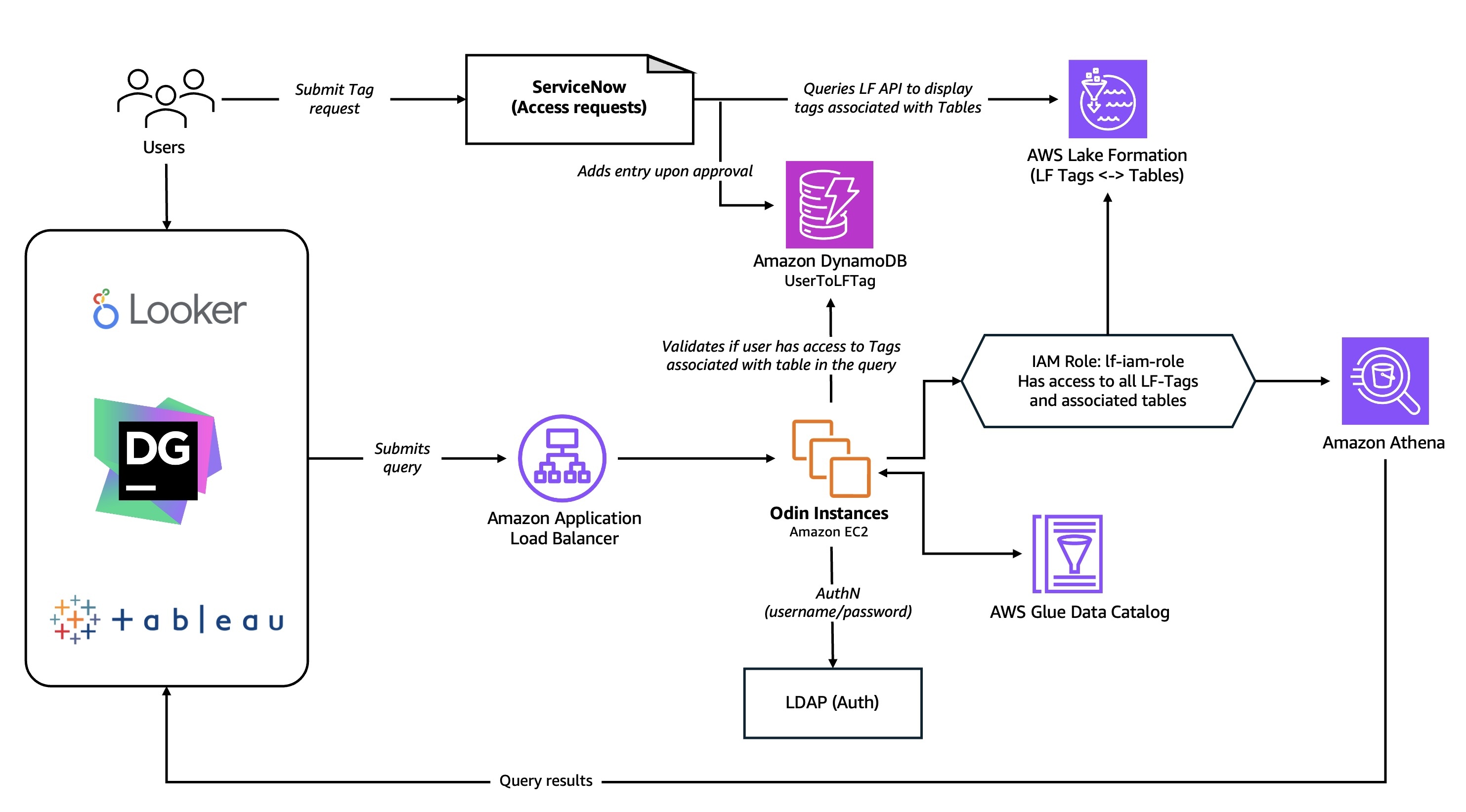
The overall subscription and authorization flow is as shown in the diagram below:
Users submit a request in ServiceNow for access to a database, table, or LF-Tag
The system retrieves the relevant LF-Tags from Lake Formation through our API integration
Upon approval, the automation procedure adds the user to the User-To-Tag DynamoDB table, grants IAM role permissions in Lake Formation, and sets up cross-account sharing via RAM as needed
Users submit SQL query to the Odin presto gateway
Odin authorizes the user through LDAP
Odin parsers the SQL query to identify the tables involved and the action being performed (SELECT, DDL, and more)
Odin validates permissions using the User to LF-Tag mapping and Lake formation grants to authorize the SQL query based on granted permissions
If authorized, Odin routes the query to Amazon Athena or Presto
Using standardized tools and processes to provide self-service capabilities to the users helped us scale the governance framework and support broader use cases. Important capabilities in Lake Formation, such as Tag-based access control (TBAC) and cross-account sharing of data, simplified developing automations and our overall approach to governance.
Lessons learned- Cache is king
“By adopting AWS Glue Data Catalog as our managed metastore and AWS Lake Formation for Tag-Based Access Control, we simplified access management and enabled data sharing by reducing auth overhead to just 6-10 milliseconds through caching and targeted scaling.”
As Odin began handling queries at scale, we encountered performance bottlenecks in our customized authorization process as we had to retrieve information from multiple services, particularly with complex queries spanning multiple tables. The authorization checks involved in the performance bottleneck frequently caused query timeouts which impacted overall system reliability. The root of the problem lay in our sequential authorization workflow: our system first had to parse each query to identify all tables requiring identity verification, then make separate API calls to the AWS Glue Data Catalog and Lake Formation for each table’s permissions. It became clear that we needed to optimize this authentication process to reduce response times and improve the overall query experience.
We also recognized there were different caching needs between our POST operations and GET/DELETE HTTP calls, so we decided to separate them into two different Application Load Balancer (ALB) target groups. For POST requests, which required Lake Formation authentication, we found that concentrating traffic through just 2-3 target instances distributed across multiple Availability Zones (AZ) was more efficient. This approach allowed authentication information to be effectively cached locally on these dedicated instances, dramatically reducing the volume of API calls to the Lake Formation service.
GET and DELETE requests follow a more simplified workflow. Since users have already completed initial authorization, there is no need to continue to perform authorization checks. Although they follow a simpler workflow, these requests have much higher volume with requests numbering into the 10s of millions per hour. Due to this scale, we opted to implement horizontal scaling to scale the target ALB to 10 Amazon EC2 instances to fetch the query history from the DynamoDB table. These EC2 instances make use of local LRU caching with a 5-minute expiration policy for authentication data.
By implementing authentication caching and adopting specialized approaches for different HTTP request types with targeted scaling groups, we successfully reduced Odin’s overall overhead to a maximum of 6-10 milliseconds for both authentication and authorization.
Conclusion and what’s next
In this post, we explored how we enhanced Odin, our unified multi-engine query platform, with authentication and authorization capabilities using AWS Lake Formation and a custom authorization workflow. By using AWS services including Lake Formation, AWS Glue Data Catalog, and Amazon DynamoDB alongside Twilio’s existing infrastructure, we created a scalable self-service governance framework that streamlines user access management, simplifies auditing, and enables seamless data sharing across our complex cloud environment. With this workflow automation, we eliminated operational overhead while building a secure, robust platform that serves as the foundation for Twilio’s data mesh architecture.
Going forward, we are focusing on strengthening our authentication and authorization framework by enabling trusted federation with an identity provider(IdP) through AWS IAM Identity Center, which integrates directly with Lake Formation. Using Trusted Identity Propagation capabilities supported by IAM IDC will allow us to establish a consistent governance flow based on a user identity and will allow us to unlock the full capabilities of AWS Lake Formation such as fine-grained access control with data filters.
Today, we’re excited to announce the general availability of the collection groups feature for Amazon OpenSearch Serverless. With this feature you can reduce compute costs for multi-tenant workloads while creating secure tenant boundaries through per-tenant encryption, giving you the flexibility to balance cost efficiency with the exact level of isolation and security your applications requires.
Amazon OpenSearch Serverless is a serverless deployment option for Amazon OpenSearch Service, that eliminates the complexity of infrastructure management for running search and analytics workloads at scale. It automatically provisions and scales resources to deliver fast data ingestion rates and millisecond response times, even as usage patterns change. For organizations that are managing multi-tenant environments, data isolation, where the tenant’s data must be encrypted and protected (often with their own encryption keys), is a compliance requirement.
Previously, OpenSearch Serverless provided maximum security through physical isolation: each AWS Key Management Service key (KMS key) required dedicated OpenSearch Compute Units (OCUs) to maintain complete physical data separation. While this architecture provided the highest level of protection, it created challenges for multi-tenant deployments at scale. For customers managing multiple tenants with shared encryption keys, OCU resources are efficiently pooled, making the economics favorable. However, customers managing large numbers of smaller tenants, each requiring their own KMS key for data isolation, faced a challenge with higher cost. With dedicated OCU resources needed per unique key, the infrastructure costs could become prohibitive when individual tenants required only a fraction of an OCU’s capacity. This particularly impacted service providers wanting to offer bring your own key (BYOK) capabilities to their customers, forcing them to either absorb unsustainable costs or limit their service offerings.
OpenSearch Serverless has always provided flexible capacity management with maximum OCU settings to help you control costs. For most workloads, this model works seamlessly capacity scales up and down in response to demand, so you only pay for what you use. However, some workload patterns are simply better served by having a guaranteed baseline of compute ready to go from the start. Workloads with sudden traffic spikes, high-speed data ingestion pipelines, or load testing scenarios benefit from having capacity pre-allocated, so that the first requests are handled with the same responsiveness as any other. Similarly, multi-tenant architectures and time-sensitive operations often require predictable, consistent performance from the moment a collection becomes active.
Flexible controls with collection groups
Collection groups give you flexible control over security boundaries and resource allocation. Instead of forcing a one-size-fits-all approach, you can now tailor your architecture to match your specific security and cost requirements. Here’s how it works:
Define your security boundary that matches your need: Collection groups is a logical security construct for related collections. Each collection groups maintains strong isolation with physically separated memory, CPU and disk from other collection groups, ensuring robust security boundaries between different security constructs.
Share resources across encryption keys: Allocate collections to your collection groups regardless of whether they share KMS keys or use separate ones. Collections with different encryption keys can now share OCU resources within the same security boundary, dramatically reducing costs while maintaining full encryption protection and logical separation for each tenant.
Deploy with flexible network access: Collection groups support collections with different network access types, allowing you to combine collections with public endpoints and VPC endpoints within the same group. This flexibility lets you match your security and connectivity requirements while benefiting from shared resource management across all collections in the group.
Control cost and performance: Set maximum OCUs to cap spending and minimum OCUs to guarantee baseline performance. This dual control gives you a defined resource envelope for each collection groups, eliminating cost surprises while ensuring consistent performance.
Optimize with insights: Access detailed CloudWatch metrics showing resource consumption, relative usage patterns, and latency across collection groups. These insights help you right-size allocations, identify optimization opportunities, and tune performance based on actual workload behavior.
With collection groups, you now have full control over resource allocation through both minimum and maximum OCU settings
Maximum OCUs: Cost control
Set an upper limit on resources to prevent runaway scaling and control costs per collection groups. This helps ensure you never exceed your budget, even during unexpected traffic spikes. Collection groups capacity limits operate independently from account-level limits. Account-level maximum OCU settings apply only to collections not associated with any collection groups, while collection groups maximum OCU settings apply to collections within that specific group. The sum of (Max OCUs across all your collection groups + Max OCU setting at the account level) should be less than your Service Quota Max OCUs allowed for your account. This separation gives you granular cost control across different security contexts.
Minimum OCUs: Performance guarantees
Define the baseline compute resources that will always be allocated to your collection groups, for consistent performance and resource availability. These OCUs are reserved exclusively for your collection groups and provide:
Instant availability with no cold starts: Your collections benefit from instant availability without scaling delays. Resources are always warm and ready, eliminating scaling delays when traffic arrives.
Guaranteed capacity: Resources are always available, even during periods of low activity or when competing with other collection groups, ensuring predictable performance even during low-traffic periods.
Predictable costs: Minimum OCUs are charged continuously, providing you with reserved capacity in exchange for predictable billing giving you cost certainty in exchange for guaranteed performance. This reserved baseline serves as the foundation for auto-scaling, which expands capacity up to your maximum limit as demand increases.
This combination gives you the flexibility to balance cost optimization with performance guarantees based on your specific requirements.
Multi-tenant cost economics with collection groups
Managing costs in multi-tenant architectures has always required balancing isolation, performance, and efficiency often at the expense of one another. Collection groups change that equation by enabling shared capacity across collections without sacrificing security boundaries. The following details how this plays out when you work with collection groups or without.
Before collection groups: Consider a customer with 10 tenants, each requiring their own KMS key for data isolation. Most of these tenants have modest data requirements typically 10-100GB, with the majority on the smaller end of that range. Managing dedicated resources for each tenant’s encryption key, regardless of their actual capacity needs, created operational complexity and cost challenges at scale.
With collection groups: The same customer can now group their tenants with similar security requirements into the collection groups, sharing OCU resources across collections. Tenants requiring only a small portion of OCU capacity no longer force the allocation of dedicated resources, reducing costs by up to 90% for large number of smaller tenant workloads.
With minimum OCU configuration: Premium tenants can be placed in collection groups with minimum OCUs set to guarantee performance, while standard tenants use collection groups with lower minimum thresholds for cost efficiency.
The following table illustrates how these cost savings play out across different tenant configurations, comparing infrastructure costs with and without collection groups across varying data sizes and query loads.
Number of tenants with unique KMS keys
Data size and query parameters
Cost with complete data isolation (without collection groups)
Cost with collection groups
Additional comments
10
Data size: 60GB or less
Query: Not needing more than base OCU (1 for redundant collection) compute
$3,500
$350
10x Savings in cost.
10
Data size: 60GB or less
Query: More than base OCU (1 for redundant collection) compute during peak times (For example – 5 additional OCUs per tenant without collection groups & 40 OCUs across all tenants based with collection groups due to benefit of shared infra).
$3500 + Peak time scale out per tenant ($8650)
$350+ Peak time scale out ($6912).
The system will scale up when there is additional query load, additional OCUs are deployed during this time. However when the load scales back, the system will scale-in to base OCU’s.
10
Data size: Sample data size in GB per tenant [3, 5, 7, 8, 10, 15, 18, 25, 28, 150]
Query: Can handle queries upto certain level with minimum OCU for the data size and then scales out on load.
For the sample data sizes, minimum OCU requirement will be [2, 2, 2, 2, 2, 2, 2, 2, 2, 8] = 26 OCUs [$4492] + Peak time scale out per tenant
Minimum cost is determine by the number of OCUs required to hold the data across all tenants (120GB per OCU *2) + Peak time scale out.For the sample data sizes, 8 OCUs [$1382] + Peak time scale out per tenant
The system will scale up when there is additional query load, additional OCUs are deployed during this time. However when the load scales back, the system will scale-in to minimum number of OCU required to hold the data.
Note: Above calculations are made with assumption for redundant enabled collections. For non-redundant mode it will be half the above calculations.
Getting started with collection groups
Collection groups and minimum OCU configuration are available in all AWS Regions where OpenSearch Serverless is offered, at no additional charge. Collection groups offers a new organizational feature to create collection groups and add new collections directly to these groups for enhanced management capabilities. While your existing collections will continue to operate unchanged and remain independent of any collection groups, you can immediately start using collection groups for new collections to benefit from improved organization and workflow management.
Currently, only newly created collections can be associated with collection groups, and all collections within a group must be of the same type (search, time series, or vector search). Existing collections continue to operate independently with their current capacity management settings, and you cannot mix different collection types within a single collection groups. You can use the AWS Management Console, AWS CLI, AWS CloudFormation, or AWS CDK to create the collection groups. In the following section we will show you how you can create the collection groups using the OpenSearch Service console.
In the left navigation pane, choose Serverless, then choose Collection groups.
Choose Create collection groups.
For collection groups name, enter a name for your collection groups. The name must be 3-32 characters long, start with a lowercase letter, and contain only lowercase letters, numbers, and hyphens.
(Optional) For Description, enter a description for your collection groups.
In the Capacity management section, configure the OCU limits:
Maximum indexing capacity – The maximum number of indexing OCUs that collections in this group can scale up to.
Maximum search capacity – The maximum number of search OCUs that collections in this group can scale up to.
Minimum indexing capacity – The minimum number of indexing OCUs to maintain for consistent performance.
Minimum search capacity – The minimum number of search OCUs to maintain for consistent performance.
(Optional) In the Tags section, add tags to help organize and identify your collection groups.
In the left navigation pane, choose Serverless, then choose Collections.
Choose Create collection.
For Collection name, enter a name for your collection. The name must be 3-28 characters long, start with a lowercase letter, and contain only lowercase letters, numbers, and hyphens.
(Optional) For Description, enter a description for your collection.
In the Collection groups section, select the collection groups you want the collection to be assigned to. A collection can only belong to one collection groups at a time. (Optional) You can also choose to Create a new group. This will navigate you to the Create collection groups workflow. After you finish creating the collection groups, return to the step 1 of this procedure to begin creating your new collection.
Continue through the workflow to create the collection.
Managing collection groups
Once you’ve created your collection groups, you can update their settings as your architecture evolves. The Amazon OpenSearch Serverless documentation provides step-by-step guidance on how to edit and delete collection groups, including updating OCU limits and modifying group configurations using the AWS Management Console, CLI, and CloudFormation.
Conclusion
OpenSearch Serverless collection groups transform how you can architect multi-tenant deployments by offering flexible deployment modes that balance security requirements with operational efficiency. You can now choose the collection groups where you define logical security boundaries that allow collections, regardless of whether they share the same KMS key or use different KMS keys to share OCU resources.
This flexibility directly addresses the cost challenges that previously made multi-tenant deployments prohibitive. By consolidating collections within collection groups, you can reduce infrastructure costs while maintaining robust encryption and tenant isolation. Configuring both minimum and maximum OCUs for each collection groups solves the cold-start and capacity guarantee challenges: minimum OCUs ensure your collections maintain ready compute resources to handle high-speed ingestion, sudden traffic spikes, and load testing without performance degradation. Maximum OCUs provide cost predictability and spending controls. This dual configuration gives you a defined resource envelope that eliminates both the uncertainty of cold starts and the risk of runaway costs.
If you’ve ever shopped on Amazon, you’ve used Your Orders. This feature maintains your complete order history dating back to 1995, so you can track and manage every purchase you’ve made. The order history search feature lets you find your past purchases by entering keywords in the search bar. Beyond just finding items, it provides a straightforward way to repurchase the same or similar items, saving you time and effort.
Various features across Amazon’s shopping experience, such as Rufus and Alexa, use order history search to help you find your past purchases. Therefore, it’s important that order history search can locate your past purchased items as accurately and quickly as possible.
In this post, we show you how the Your Orders team improved order history search by introducing semantic search capabilities on top of our existing lexical search system, using Amazon OpenSearch Service and Amazon SageMaker.
Limitations of lexical search
Order history search uses lexical matching to find items from the entire order history of a customer that match at least one word of the search keywords. For example, if a customer searches for “orange juice,” the system retrieves all orange juice items as well as fresh oranges and other fruit juices the customer had previously ordered. Although lexical matching can provide a high recall of items with terms matching the search keywords precisely, it doesn’t work well for related or generic search keywords, like “health drinks” in this example.
Since the launch of Rufus, Amazon’s AI-enabled shopping assistant, a growing number of customers are experiencing a streamlined and richer shopping journey, including searching for their previous purchases with Rufus. Customers can now ask “Show me healthy drinks” without worrying about using lengthy, more precise terms like “kombucha”, “green tea”, and “protein shakes”. This makes the search experience more conversational and intent-based, presenting an opportunity to make item discovery more intuitive. For Rufus to answer order history searches with the same intuitive experience such as “Show me the healthy drinks I bought last year”, the underlying order history data store (“Your Orders”) needs semantic search capability to understand the underlying semantics of search keywords beyond the conventional lexical matching.
Challenges implementing semantic search
Implementing semantic search at our scale presented several technical challenges:
Scale – We needed to enable semantic search across billions of records corresponding to customers’ order history globally.
Zero downtime – We needed to keep the system 100% available while making changes on the backend to introduce semantic search.
Preventing search quality degradation – Semantic search is intended to improve the quality of search results. However, in some cases, it can reduce search quality. For example, if a customer remembers their item name exactly and wants to find only items matching that name, surfacing similar items in addition to the exactly matching items will increase crowding in results and make it harder to find the relevant item. Similarly, semantic search will not work for cases where the customer intends to search by identifier values, like order ID, which lack an inherent semantic meaning. For these scenarios, we use lexical search only.
Solution overview
Semantic search is powered by large language models (LLMs), which are mostly trained on human languages. These models can be adapted to take a piece of text in any language they were trained in and emit an embedding vector of a fixed length, irrespective of the input text length. By design, embedding vectors capture the semantic meaning of input text such that two semantically similar text strings have high cosine similarity computed on their respective embedding vectors. For semantic search on order history, the input text subject to embedding generation and similarity computation are the customer search phrases and the product text of purchased items.
We divide our solution into two parts:
Improving system scalability and resiliency for handling requests at scale – Before implementing semantic search, we needed to ensure our infrastructure could handle the increased computational load, leading us to adopt a cell-based architecture. This step is not needed for every use case, but systems with very high scale in terms of request or data volume can benefit a lot from its use before implementing a resource-intensive use case like semantic search.
Implementing semantic search – We began by evaluating the available embedding models, using the offline evaluation capabilities of Amazon Bedrock to test different models. After we selected our model, we could establish the infrastructure for generating embedding vectors.
Improving system scalability and resiliency
We used the cell-based architecture design pattern for improving our scalability and resiliency. A cell-based design entails partitioning the system into identical, smaller, self-contained chunks, or cells, which handle only a part of the overall traffic received by the system. The following diagram shows a high-level representation of a cell-based design for order history search.
Each cell serves a defined subset of our customers. Cells don’t need to communicate with one another to serve a customer request. Each customer is assigned to a cell and each request from that customer is routed to that cell. The OpenSearch Service domain in each cell holds data only for the subset customers that it is supposed to serve. The number of cells (N) and distribution of data among those cells depends on the business use case, but the goal is to achieve as even a distribution of data and traffic as possible.
The routing logic can be kept as simple or as sophisticated as the use case requires it to be. The cell assignment values can either be computed at runtime for each request, or they can be computed one time and written to a cache or persistent data store like Amazon DynamoDB, from where cell assignment values can be fetched for subsequent requests. For order history search, the logic was simple and quick enough to be executed at runtime for each request. Looking up cell assignment from a persistent data store is especially useful for cases where there is a risk of some cells becoming “heavier” than others over time. In such cases, it becomes easier to redistribute the heavy cell’s data by simply overriding cell assignment values for specific keys in the data store, instead of having to change the partitioning logic immediately, which might have an impact on data distribution across all the cells.
As the system’s load grows, the number of cells in the system can be increased to handle the additional traffic. Even without increasing the number of cells in the system, we can redistribute current data among the existing N cells by reassigning some keys from one or more heavily populated cells to different lightly populated cells to spread out the load more evenly across all the cells and make more efficient use of the infrastructure.
A cell-based architecture also helps make the system more resilient. For example, if we lose one cell, our capacity is diminished only by 1/N, instead of 100%. This arrangement can also be improved to reduce the capacity loss even further by assigning partitioning keys to two or more cells such that they get written to two or more cells. In such cases, loss of a single cell does not result in data loss.
Implementing semantic search
Implementing semantic search for our order history search required several key decisions and technical steps. We began by evaluating the available embedding models, using the offline evaluation capabilities of Amazon Bedrock to test different models against our specific business domain requirements. This evaluation process helped us identify which model would deliver the best performance for our use case. After we selected our model, we needed to establish the infrastructure for generating embedding vectors. We containerized our embedding model and registered it in Amazon Elastic Container Registry (Amazon ECR), then deployed it using SageMaker inference endpoints to handle the actual vector computation at scale.
For the search infrastructure itself, we chose OpenSearch Service to implement our semantic search capabilities. OpenSearch Service provided both the vector storage we needed and the search algorithms required to deliver relevant results to our users.
One of our biggest challenges was updating our historical data to support semantic search on existing orders. We built a data processing pipeline using AWS Step Functions to orchestrate the workflow and AWS Lambda functions to handle the actual vector generation for our legacy data, so we could provide semantic search for all the records we wanted to.
The following diagram illustrates the high-level architecture.
Model evaluation and selection
Order history search uses an embedding model trained on Amazon-specific data. Domain-specific training is critical because the generated embedding vectors must work well for the business context to return quality results.
We used an LLM-as-a-judge methodology with Anthropic’s Claude on Amazon Bedrock to evaluate candidate models. Anthropic’s Claude received prompts containing anonymized item text and search phrases from customer order history, then filtered and ranked items by relevance. These results served as ground truth for comparison.
We evaluated models using standard ranking metrics:
Normalized Discounted Cumulative Gain (NDCG) – Measures ranking quality against ideal order
Mean Reciprocal Rank (MRR) – Considers position of first relevant item
Precision – Rates accuracy of retrieved results
Recall – Rates ability to retrieve all relevant items
Search only through the requesting customer’s order history – We don’t want items from one customer’s order history showing up in search results for another customer
Search all of that customer’s history – We don’t want to miss showing an item that would have been relevant for the customer’s search phrase just because the search algorithm missed evaluating it for some reason
Our approach involves using OpenSearch Service to retrieve all items for the customer who issued the search query, calculating relevance scores for each of them against the search phrase, sorting by score, and returning top K results. This provides comprehensive results coverage for each customer.
Vector storage with OpenSearch Service
We used two OpenSearch Service features for efficient vector storage and search:
knn_vector datatype – Built-in support for storing embedding vectors. Existing domains can add this field type without reindexing, enabling exact kNN search across all records. We didn’t need approximate kNN because the number of records for most customers was small enough for exact kNN to scale.
Hybrid search refers to combining the results of lexical and semantic search to benefit from the strengths of each. The hybrid query capabilities of OpenSearch Service simplify implementing hybrid search by letting clients specify both types of queries in a single request. OpenSearch Service runs both queries in parallel, merges their results, normalizes the relevance scores of the sub-queries, and sorts results by the provided sort order (relevance score by default) before returning them to clients.
This gives clients the best of both types of searches. For example, there are certain scenarios where the search phrase doesn’t make much sense semantically, like when customers search by their orderId values. Semantic search is not designed for such cases; these are best served using keyword matching.
The hybrid search functionality helped save implementation effort and potential latency increase for order history search.
Updating historical data
After the infrastructure has been set up, newly ingested records are persisted with the relevant embedding vectors and support semantic search on those records. However, when customers search, they typically search for products they had purchased earlier. Therefore, the system might not help improve customer experience much unless the older records are updated to include the relevant embeddings. The approach to populate this data depends on the scale of the problem at hand.
Releasing the change to minimize potential customer impact
Our final step was to release the change to clients in a manner such that the impact of any potential problems is as small as possible. There are multiple ways to do that, including:
Implementing semantic search in a manner such that any transient issues in the semantic search flow make the logic fall back to lexical-only search, instead of failing the request completely. Even if semantic search doesn’t execute, the system should still be able to return results of lexical search to the client, instead of empty results.
Gating the change such that the default behavior remains lexical-only search and clients who need the semantic search feature must pass an additional flag in the request, for example, which executes the semantic or hybrid flow only for those requests.
Keeping the new flow behind a feature flag during the initial period such that it could be turned off completely if some critical problem is detected.
Examples of improved customer experience
The following are some examples of customer interactions with Rufus that required Rufus to query the respective customer’s order history to answer their question and give them the required pieces of information.
The following screenshots show how semantic search picks up wooden spoons for a “sustainable utensils” query and different kinds of chargers despite not having the keyword “charger” in the title description, in the case of the wall connector.
The following screenshots show how semantic search picks up relevant results even though the title description doesn’t include the queried keywords.
The semantic search feature of order history search helped Rufus fetch them and show to the customers. Before semantic search, Rufus wasn’t able to show any results to customers for such queries.
Business impact
Our solution resulted in the following key business impacts:
Customer experience improvements – The solution achieved 10% improvement in query recall, increasing the percentage of searches that return relevant results. It also reduced customer service contacts for issues related to locating past orders.
Partner integration success – The solution strengthened natural language processing capabilities for Alexa and Rufus, enhancing their ability to interpret order history queries. It also reduced the need for reranking and postprocessing by partner teams. We improved query success rate by 20%, meaning more customer searches now return at least one relevant item. We also observed enhanced result coverage by 48%, with semantic search consistently surfacing additional relevant matches that lexical search would have missed.
Conclusion
In this post, we showed you how we evolved Amazon order history search to support semantic search capabilities. This transition involved using cutting-edge AI technology while working within existing infrastructure limitations to develop solutions that avoided disruption and maintained SLAs during the feature upgrade. The implementation also involved backfilling, where billions of documents were processed at rates multiple times higher than normal ingestion to compute embedding vectors for previously purchased items. This operation required careful engineering and took advantage of the resilience OpenSearch Service offers even under extreme load.
Beyond the immediate implementation, this foundation enables continued innovation in search technology. The embedding vectors framework can incorporate improved models as they become available, and the architecture supports expansion into new capabilities such as personalization and multi-modal search.
You can get started with exact k-NN search today following the instructions in Exact k-NN search. If you’re looking for a managed solution for your OpenSearch cluster, check out Amazon OpenSearch Service.
This post is co-written with Srinivasa Are, Principal Cloud Architect, and Karthick Shanmugam, Head of Architecture Verisk EES (Extreme Event Solutions).
Verisk, a catastrophe modeling SaaS provider serving insurance and reinsurance companies worldwide, cut processing time from hours to minutes-level aggregations while reducing storage costs by implementing a lakehouse architecture with Amazon Redshift and Apache Iceberg. If you’re managing billions of catastrophe modeling records across hurricanes, earthquakes, and wildfires, this approach eliminates the traditional compute-versus-cost trade-off by separating storage from processing power.
In this post, we examine Verisk’s lakehouse implementation, focusing on four architectural decisions that delivered measurable improvements:
Execution performance: Sub-hour aggregations across billions of records replaced long batch process
Storage efficiency: Columnar Parquet compression reduced costs without sacrificing response time
Multi-tenant security: Schema-level isolation enforced complete data separation between insurance clients
Schema flexibility: Apache Iceberg support column additions and historical data access without downtime
The architecture separates compute (Amazon Redshift) from storage (Amazon S3), demonstrating how to scale from billions to trillions of records without proportional cost increases.
Current state and challenges
In Verisk’s world of risk analytics, data volumes grow at exponential rates. Every day, risk modeling systems generate billions of rows of structured and semi-structured data. Each record captures a micro-slice of exposure, event probability, or loss correlation. To convert this raw information into actionable insights at scale, experts need a data engine designed for high-volume analytical workloads.
Each Verisk model run produces detailed, high-granularity outputs that include billions of simulated risk factors and event-level results, multi-year loss projections across thousands of perils, and deep relational joins across exposure, policy, and claims datasets.
Running meaningful aggregations (such as, loss by region, peril, or occupancy type) over such high volumes created performance challenges.
Verisk needed to build a SQL service that could aggregate at scale in the fastest time possible and integrate into their broader AWS solutions, requiring a serverless, open, and performant SQL engine capable of handling billions of records efficiently.
Prior to this cloud-based release, Verisk’s risk analytics infrastructure operated on an on-premises architecture centered around relational database clusters. Processing nodes shared access to centralized storage volumes through dedicated interconnect networks. This architecture required capital investment in server hardware, storage arrays, and networking equipment. The deployment model required manual capacity planning and provisioning cycles, limiting the organization’s ability to respond to fluctuating workload demands. Database operations depended on batch-oriented processing windows, with analytical queries competing for shared compute resources.
Amazon Redshift and lakehouse architecture
Lakehouse architecture on AWS combines data lake storage scalability with data warehouse analytical performance in a unified architecture. This architecture stores vast amounts of structured and semi-structured data in cost-effective Amazon S3 storage while maintaining Amazon Redshift’s massively parallel SQL analytics.
Amazon Redshift is a fully managed, petabyte-scale cloud data warehouse service that delivers fast query performance using massively parallel processing (MPP) and columnar storage. Amazon Redshift eliminates the complexity of provisioning hardware, installing software, and managing infrastructure, keeping focus on deriving insights from their data rather than maintaining systems.
To meet their challenge, Verisk designed a hybrid data lakehouse architecture that combines the storage scalability of Amazon S3 with the compute power of Amazon Redshift. The following diagram shows the foundational compute and storage architecture that powers Verisk’s analytical solution.
Architecture Overview
The architecture processes risk and loss data through three distinct stages within the lakehouse architecture, with comprehensive multi-tenant delivery capabilities to maintain isolation between insurance clients.
Amazon Redshift allows retrieving data directly from S3 using standard SQL for background processing. This solution collects detailed result outputs, join them with internal reference data, and executes aggregations over billions of rows. Concurrency scaling guarantees that hundreds of background analyses using multiple serverless clusters can run simultaneous aggregation queries.
The following diagram shows the architecture designed by Verisk
Data ingestion and storage foundation
Verisk stores risk model outputs, location level losses, exposure tables, and model data in columnar Parquet format within Amazon S3. An AWS Glue crawler extracts metadata from S3 and feeds it into the lakehouse processing pipeline.
For versioned datasets like exposure tables, Verisk adopted Apache Iceberg, an open table format that addresses schema evolution and historical versioning requirements. Apache Iceberg provides transactional consistency through atomicity, consistency, isolation, durability ACID-compliant operations that maintain consistent snapshots during concurrent updates. Snapshot-based time travel allows data retrieval at previous points in time for regulatory compliance, audit trails, and model comparison with rollback capabilities. Schema evolution supports adding, dropping, or renaming columns without downtime or dataset rewrites. Incremental processing uses metadata tracking to process only changed data, reducing refresh times. Hidden partitioning and file-level statistics reduce I/O operations, improving aggregation performance. Engine interoperability allows accessing the same tables across Amazon Redshift, Amazon Athena, Spark, and other engines without data duplication.
Verisk built a foundation that combines S3’s cost-effectiveness with data management by adopting Apache Iceberg as open table format for this solution.
Three-stage processing pipeline
This pipeline orchestrates data flow from raw inputs to analytical outputs through three sequential stages. Pre-processing prepares and cleanses data, modeling applies risk calculations and analytics, and post-processing aggregates results for delivery.
Stage 1: Pre-processing transforms raw data into structured formats using Iceberg Tables and Parquet files, then processes it through Amazon Redshift Serverless for initial data cleaning and transformation.
Stage 2: Modeling takes place with a process built on AWS Batch the pre-processed data and applies advanced analytics and feature engineering. Results are stored in Iceberg Tables and Parquet files.
Stage 3: Aggregated Results are obtained during post-processing using Amazon Redshift Serverless, it produces the final analytical outputs in Parquet files, ready for consumption by end users.
Multi-tenant delivery system
The architecture delivers results to multiple insurance clients (tenants) through a secure, isolated delivery system that includes:
Amazon Quick Sight dashboards for visualization and business intelligence
Amazon Redshift as the data warehouse for querying aggregated results
Tenant Roles implementing role-based access control to provide data isolation between clients
Summarized results are exposed through Amazon Quick Sight dashboards or downstream APIs to underwriting teams.
Multi-tenant security architecture
A critical requirement for Verisk’s SaaS solution was supporting comprehensive data and compute isolation between different insurance and reinsurance clients. Verisk implemented a comprehensive multi-tenant security model that provides isolation while maintaining operational efficiency.
Our solution implements an isolation strategy in two layers combining logical and physical separation. At the logical layer, each client’s data resides in dedicated schemas with access controls that prevent cross-tenant operations. Amazon Redshift Metadata security restricts tenants from discovering or accessing other clients’ schemas, tables, or database objects through system catalogs. At the physical layer, for larger deployments, dedicated Amazon Redshift clusters provide workload separation at the compute level, preventing one tenant’s analytical operations from impacting another’s performance. This dual approach meets regulatory requirements for data isolation in the insurance industry through schema-level isolation within clusters for standard deployments and complete compute separation across dedicated clusters for larger-scale implementations.
The implementation uses stored procedures to automate security configuration, maintaining consistent application of access controls across tenants. This defense-in-depth approach combines schema-level isolation, system catalog lockdown, and selective permission grants to create a security model.
Verisk’s architecture reveals three decision points for companies building similar systems.
When to adopt open table formats
Apache Iceberg proved essential for datasets requiring schema evolution and historical versioning. Data engineers should evaluate open table formats when analytical workloads span multiple engines (Amazon Redshift, Amazon Athena, Spark) or when regulatory requirements demand point-in-time data reconstruction.
Multi-tenant isolation strategy
Schema-level separation combined with metadata security prevented cross-tenant data discovery without performance overhead. This approach scales more efficiently than database-per-tenant architectures while meeting insurance industry compliance requirements. Security experts should implement isolation controls during initial deployment rather than retrofitting them later.
Stored procedures or application logic
Redshift stored procedures standardized aggregation calculations across teams and constructed dynamic SQL queries. This approach works best when business logic changes frequently or when multiple teams need different aggregation dimensions on the same datasets.
Conclusion
Verisk’s implementation of Amazon Redshift Serverless with Apache Iceberg and lakehouse architecture shows how separating compute from storage addresses enterprise analytics challenges at billion-record scale. By combining cost-effective Amazon S3 storage with Redshift’s massively parallel SQL compute, Verisk achieved aggregations across billions of catastrophe modeling records, reduced storage costs through efficient parquet compression, and eliminated ingestion delays. Now underwriting teams can run ad-hoc analyses during business hours rather than waiting for long-running batch jobs. The combination of open standards like Apache Iceberg, serverless compute with Amazon Redshift, and multi-tenant security provides the scalability, performance, and cost efficiency needed for modern analytics workloads.
Verisk’s journey has positioned them to scale confidently into the future, processing not just billions, but potentially trillions of records as their model resolution increases.
In e-commerce, delivering fast, relevant search results helps users find products quickly and accurately, improving satisfaction and increasing sales. OpenSearch is a distributed search engine that offers advanced search capabilities including advanced full-text and faceted search, customizable analyzers and tokenizers, and auto-complete to help customers quickly find the products they want. It scales to handle millions of products, catalogs and traffic surge. Amazon OpenSearch Service is a managed service that lets users build search workloads balancing search quality, performance at scale and cost. Designing and sizing an Amazon OpenSearch Service cluster correctly is required to meet these demands.
While general sizing guidelines for OpenSearch Service domains are covered in detail in OpenSearch Service documentation, in this post we specifically focus on T-shirt-sizing OpenSearch Service domains for e-commerce search workloads. T-shirt sizing simplifies complex capacity planning by categorizing workloads into sizes like XS, S, M, L, XL based on key workload parameters such as data volume and query concurrency. For e-commerce search, where data growth is moderate and read-heavy queries predominate, this approach offers a flexible, scalable way to allocate the resources without overprovisioning or underestimating needs.
How OpenSearch Service stores indexes and performs queries
E-commerce search platforms handle vast amounts of data and daily data ingestion is typically relatively small and incremental, reflecting catalog changes, price updates, inventory status and user activities like clicks and reviews. Efficiently managing this data and organizing it per OpenSearch Service best practices is crucial in achieving optimal performance. The workload is read-heavy, consisting of user queries with advanced filtering and faceting, especially during sales or seasonal spikes that require elasticity in compute and storage resources.
You ingest product and catalog updates (inventory, listings, pricing) into OpenSearch using bulk APIs or real-time streaming. You index data into logical indexes. How you create and organize indexes in e-commerce has a significant impact on search, scalability and flexibility. The approach depends on the size, diversity and operational needs of the catalog. Small to medium-sized e-commerce platforms commonly use a single, comprehensive product index that stores all product information with product category. Additional indexes may exist for orders, users, reviews and promotions depending on search requirements and data separation needs. Large, diverse catalogs may split products into category-specific indexes for tailored mappings and scaling. You split each index into primary shards, each storing a portion of the documents. To ensure high availability and enhance query throughput, you configure each primary shard with at least one replica shard stored on different data nodes.
Diagram 1. How primary and replica shards are distributed among nodes
This diagram shows two indexes (Products and Reviews), each split into two primary shards with one replica. OpenSearch distributes these shards across cluster nodes to ensure that primary and replica shards for the same data do not reside on the same node. OpenSearch runs search requests using a scatter-gather mechanism. When an application submits a request, any node in the cluster can receive it. This receiving node becomes the coordinating node for that specific query. The coordinating node determines which indices and shards can serve the query. It forwards the query to either primary or replica shards and orchestrates the different phases of the search operation and returns the response. This process ensures efficient distribution and execution of search requests across the OpenSearch cluster.
Diagram 2. Tracing a Search query: “blue running shoes”This diagram walks through how a search query–for example, “blue running shoes”flows through your OpenSearch Service domain .
Request: The application sends the search for “blue running shoes” to the domain. One data node acts as the coordinating node.
Scatter: The coordinator broadcasts the query to either the primary or replica shard for each of the shards in the ‘Products’ index (Nodes 1, 2, and 3 in this case).
Gather: Each data node searches its local shards(s) for “blue running shoes” and returns its own top results (e.g. Node 1 returns its best matches from P0).
Final results: The coordinator merges these partial lists, sorts them into single definitive list of the most relevant shoes, and sends the result back to the app.
Understanding T-Shirt Sizing for E-commerce OpenSearch Service Cluster
Storage planning
Storage impacts both performance and cost. OpenSearch Service offers two main storage options based on query latency requirements and data persistence needs. Selecting the appropriate storage type in a managed OpenSearch Service improves both performance and optimizes cost of the domain. You can choose between Amazon Elastic Block Store( EBS) storage volumes and instance storage volumes (local storage) for your data nodes.
Amazon EBS gp3 volumes offer high throughput, whereas the local NVMe SSD volumes, for example, on the r8gd, i3, or i4i instance families, offer low latency, fast indexing performance and high-speed storage, making them ideal for scenarios where real time data updates and high search throughput are critical for search operations. For search workloads that require a balance between performance and cost, instances backed with EBS GP3 SSD volumes provide a reliable option. This SSD storage offers input/output operations per second (IOPS) that are well-suited for general-purpose search workloads. It also allows users to provision additional IOPS and storage as needed.
When sizing an OpenSearch cluster, start by estimating total storage needs based on catalog size and expected growth. For example, if the catalog contains 500,000 stock keeping units (SKUs), averaging 50KB each; the raw data sums to about 25GB. The size of the raw data, however, is just one aspect of the storage requirements. Also consider the Replica count, indexing overhead (10%), Linux reserves (5%), and OpenSearch Service reserves (20% up to 20GB) per instance while calculating the required storage.
In summary,if you have 25GB of data at any given time who want one replica, the minimum storage requirement is closer to 25 * 2 * 1.1 / 0.95 / 0.8 = 72.5 GB. This calculation can be generalized as follows:
Storage requirement = Raw data * (1 + number of replicas) * 1.45
This helps ensure disk space headroom on all data nodes, preventing shard failures and maintaining search performance. Provisioning storage slightly beyond this minimum is recommended to accommodate future growth and cluster rebalancing.
Data nodes:
For search workloads, compute-optimized instances (C8g) are well-suited for central processing unit (CPU)-intensive operations like nested queries and joins. However, general-purpose instances like M8g offer a better balance between CPU and memory. Memory-optimized instances (R8g, R8gd) are recommended for memory-intensive operations like KNN search, where larger memory footprint is required. In large, complex deployments, compute-optimized instances like c8g or general-purpose m8g, handle CPU-intensive tasks, providing efficient query processing and balanced resource allocation. The balance between CPU and memory, makes them ideal for managing complex search operations for large-scale data processing. For extremely large search workloads (tens of TB) where latency is not a primary concern, consider using the new Amazon OpenSearch Service Writable warm which supports write operations on warm indices.
Instance Class
Best for users who…
Examples (AWS)
Characteristics
General Purpose
have moderate search traffic and want a well-balanced, entry-level setup
M family (M8g)
Balanced CPU & memory, EBS storage. Good starting point for small to medium-sized catalogs.
Compute Optimized
have high queries per second (QPS) search traffic or queries involve scoring scripts or complex filtering
C family (C8)
High CPU-to-memory ratio. Ideal for CPU-bound workloads like many concurrent queries.
Memory Optimized
work with large catalogs, need fast aggregations, or cache a lot in memory
R family (R8g)
More memory per core. Holds large indices in memory to speed up searches and aggregations.
Storage Optimized
update inventory frequently or have so much data that disk access slows things down
I family (I3, I4g), Im4gn
NVMe SSD and SSD local storage. Best for I/O-heavy operations like constant indexing or large product catalogs hitting disk frequently.
Cluster manager nodes:
For production workloads, it is recommended to add dedicated cluster manager nodes to increase the cluster stability and offload cluster management tasks from the data nodes. To choose the right instance type for your cluster manager nodes, review the service recommendations based on the OpenSearch version and number of shards in the cluster.
Sharding strategy
Once storage requirements are understood, you can investigate the indexing strategy. You create shards in OpenSearch Service to distribute an index evenly across the nodes in a cluster. AWS recommends single product index with category facets for simplicity or partition indexes by category for large or distributed catalogs. The size and number of shards per index play a vital role in OpenSearch Service performance and scalability. The right configuration ensures balanced data distribution, avoids hot spotting, and minimizes coordination overhead on nodes for use cases that prioritizes query speed and data freshness.
For read-heavy workloads like e-commerce, where search latency is the key performance objective, maintain shard sizes between 10-30GB. To achieve this, calculate the number of primary shards by dividing your total index size by your target shard size. For example, if you have a 300GB index and want 20GB shards, configure 15 primary shards (300GB ÷ 20GB = 15 shards). Monitor shard sizes using the _cat/shards API and adjust the shard count during reindexing if shards grow beyond the optimal range.
Add replica shards to improve search query throughput and fault tolerance. The minimum recommendation is to have one replica; you can add more replicas for high query throughput requirements. In OpenSearch Service, a shard processes operations like querying single-threaded, meaning one thread handles a shard’s tasks at a time. Replica shards can serve read requests by distributing them across multiple threads and nodes, enabling parallel processing.
T-shirt sizing for an e-commerce workload
In an OpenSearch T-shirt sizing table, each size label (XSmall, Small, Medium, Large, XLarge) represents a generalized cluster scale category that can help teams translate technical requirements into simple, actionable capacity planning. Each size allows architects to quickly align their catalog size, storage requirements, shard planning, CPU and AWS instance choices to the cluster resources provisioned, making it easier to scale infrastructure as business grows.
By referring to this table, teams can select the category similar to their current workload and use the T-shirt size as a starting point while continuing to refine configuration as they monitor and optimize real-world performance. For example, XSmall is suited for small catalogs with hundreds of thousands of products and minimal search traffic. Small clusters are designed for growing catalogs with millions of SKUs, supporting moderate query volumes and scaling up during busy periods. Medium corresponds to mid-size e-commerce operations handling millions of products and higher search demands, while Large fits large online businesses with tens of millions of SKUs, requiring robust infrastructure for fast, reliable search. XLarge is intended for major marketplaces or global platforms with twenty million or more SKUs, enormous data storage needs, and massive concurrent usage.
T-shirt size
Number of Products
Catalog Size
Storage needed
Primary Shard Count
Active Shard Count
Data Nodes Instance Type
Cluster Manager Node instanceType
XSmall
500K
50 GB
145 GB
2
4
[2] r8g.xlarge
[3] m8g.large
Small
2M
200 GB
580 GB
8
16
[2] c8g.4xlarge
[3] m8g.large
Medium
5M
500 GB
1.45 TB
20
40
[2] c8g.8xlarge
[3] m8g.large
Large
10M
1 TB
2.9 TB
40
80
[4] c8g.8xlarge
[3] m8g.large
XLarge
20M
2 TB
5.8 TB
80
160
[4] c8g.16xlarge
[3] m8g.large
T-shirt size: Represents the scale of the cluster, ranging from XS up to XL for high-volume workloads.
Number of products: The estimated count of SKUs in the e-commerce catalog, which drives the data volume.
Catalog size: The total estimated disk size of all indexed product data, based on typical SKU document size.
Storage needed: The actual storage required after accounting for replicas and overhead, ensuring enough room for safe and efficient operation.
Primary shard count: The number of main index shards chosen to balance parallel processing and resource management.
Active shard count: The total number of live shards (primary with one replica), indicating how many shards need to be distributed for availability and performance.
Data node instance type: The recommended instance type to use for data nodes, selected for memory, CPU, and disk throughput.
Cluster manager node instance type: The recommended instance type for lightweight, dedicated master nodes which manage cluster stability and coordination.
Scaling strategies for e-commerce workloads
E-commerce platforms continually face challenges with unpredictable traffic surges and growing product catalogs. To address these challenges, OpenSearch Service automatically publishes critical performance metrics to Amazon CloudWatch, enabling users to monitor when individual nodes reach resource limits. These metrics include CPU utilization exceeding 80%, JVM memory pressure above 75%, frequent garbage collection pauses, and thread pool rejections.
OpenSearch Service also provides robust scaling solutions that maintain consistent search performance across varying workload demands. Use the vertical scaling strategy to upgrade instance types from smaller to larger configurations, such as m6g.large to m6g.2xlarge. While vertical scaling triggers a blue-green deployment, scheduling these changes during off-peak hours minimizes impact on operations.
Use the horizontal scaling strategy to add more data nodes for distributing indexing and search operations. This approach proves particularly effective when scaling for traffic growth or increasing dataset size. In domains with cluster manager nodes, adding data nodes proceeds smoothly without triggering a blue-green deployment. CloudWatch metrics guide horizontal scaling decisions by monitoring thread pool rejections across nodes, indexing latency, and cluster-wide load patterns. Though the process requires shard rebalancing and may temporarily impact performance, it effectively distributes workload across the cluster.
Temporary replicas provide a flexible solution for managing high-traffic periods. By increasing replica shards through the _settings API, read throughput can be boosted when needed. This approach offers a dynamic response to changing traffic patterns without requiring more substantial infrastructure changes.
Monitoring key performance CloudWatch metrics is essential to ensure a well-optimised OpenSearch service domain. One of the key factors is maintaining CPU utilization on data nodes under 80% to prevent query slowdowns. Another metric is ensuring that JVM memory pressure is maintained below 75% on data nodes to prevent garbage collection (GC) pauses that can affect search response time. OpenSearch service publishes these metrics to CloudWatch at 1 minute interval and users can create alarms on these metrics for alerts on the production workloads. Please refer recommended CloudWatch alarms for OpenSearch Service
P95 query latency should be monitored to identify slow queries and optimize performance. Another important indicator is thread pool rejections. A high number of thread pool rejections can result in failed search requests, and affecting user experience. By continuously monitoring these CloudWatch metrics, users can proactively scale resources, optimise queries, and prevent performance bottlenecks.
Conclusion
In this post, we showed how to right-size Amazon OpenSearch Service domains for e-commerce workloads using a T-shirt sizing approach. We explored key factors including storage optimization, sharding strategies, scaling methods, and essential Amazon CloudWatch metrics for monitoring performance.
To build a performant search experience, start with a smaller deployment and iterate as your business scales. Get started with these five steps:
Evaluate your workload requirements in terms of storage, search throughput, and search performance
Select your initial T-shirt size based on your product catalog size and traffic patterns
Deploy the recommended sharding strategy for your catalog scale
Load test your cluster using OpenSearch benchmark and re-iterate until performance requirements are reached
Configure Amazon CloudWatch monitoring and alarms, then continue to monitor your production domain
Many of you choose serverless services for your analytics workloads because of its simplicity and elasticity. But many of you running mission-critical queries face a common challenge: ensuring your high-priority workloads run when needed and without interference from other queries in your account.
Amazon Athena is a serverless interactive query service that makes it simple to analyze data using SQL. Capacity Reservations is a feature of Athena that addresses the need to run critical workloads by providing dedicated serverless capacity for the workloads you specify. With Capacity Reservations, you request capacity in the form of Data Processing Units (DPU) and you assign them to your workloads.
In this post, we highlight three new capabilities that make Capacity Reservations more flexible and easier to manage: reduced minimums for fine-grained capacity adjustments, an autoscaling solution for dynamic workloads, and capacity cost and performance controls.
Now available: 1-minute reservations and 4 DPU minimum
Yesterday, we announced a big change for Capacity Reservations: you can now reserve as few as 4 DPU (down from 24 DPU) for as little as 1 minute (down from 60 minutes). This update lets you make frequent, fine-grained capacity adjustments to closely match your workload patterns and hold less capacity, with savings up to 95% for workloads that complete in under an hour.
We’ve optimized Athena for interactive queries that need a quick response, but many of you use Athena for non-interactive queries as well. For example, you may have queries that run on a schedule to prepare data for downstream analysis or perform updates to Apache Iceberg tables. These queries often process larger volumes of data and run for longer than interactive queries. If you’re using Athena’s scan-based pricing option, all your queries count towards your account-level quota. This means that your latency sensitive interactive queries can sometimes end up queued behind non-interactive queries that are running in your account.
Capacity Reservations addresses prioritization problems like this by making it possible to assign dedicated capacity to Athena workgroups. For example, Twilio operates a query platform that serves 1,500+ users who run over 2.5 million queries per month. They use Capacity Reservations for important workloads that need to have dedicated capacity to run optimally and avoid competing with other workloads.
Capacity Reservations have worked well when your workloads have been large and predictable. For example, users accessing dashboards at the start of the workday, or data processing jobs that run continuously 24/7. However, you’ve told us that you wanted more flexibility to update your reservations more frequently, to better match changes in demand.
With Athena’s new 4 DPU and 1-minute minimums, you’re now able to adjust capacity more frequently and match demand more closely than before. We’re excited to see how these updates benefit your mission-critical query workloads.
Autoscaling for dynamic workloads
The reduced minimums enable frequent capacity adjustments, but making those adjustments requires effort. Consider a business intelligence workload that peaks in the morning as executives review dashboards but decreases throughout the day. You want this workload isolated so that high-priority queries aren’t queued behind less important queries.
With 1-minute minimums, you can now adjust capacity to closely track these patterns. However, manually adjusting capacity this frequently is tedious—you need to monitor utilization, decide when to scale, and periodically adjust DPU.
We recently launched an autoscaling solution that uses AWS Step Functions to orchestrate capacity adjustments. It monitors capacity utilization metrics that Athena emits to Amazon CloudWatch at 1-minute granularity, analyzes utilization signal over configurable intervals, then conditionally adds or removes DPU so you can maintain consistent performance even during traffic spikes.
We have made this available as a 1-click deployment from the Athena console: just click Set up autoscaling on the details page for your reservation. When you do, a AWS CloudFormation template sets up all the resources you need. Among the resources set up is the Step Functions state machine, which you can view by opening Athena’s left-side navigation menu and clicking Workflows.
You can also find the template and information on the configurable autoscaling parameters in our documentation. See Automatically adjust capacity in the Athena User Guide.
We chose Step Functions for this solution to enable extensibility and customization. Step Functions integrates tightly with AWS services and allows you to define sophisticated state machines in Amazon States Language, a JSON-based language for serverless workflows. This makes it straightforward to add conditional logic, integrate additional services, or modify the workflow to match your specific requirements.
Control DPU usage at the workgroup and query levels
Part of the ease of use and simplicity of Athena is that it allocates capacity to queries automatically based on their complexity. However, sometimes preventing a single query from using too much capacity or operating at a required level of concurrency is more important than individual query performance. We recently released new DPU cost and performance controls so you can set constraints on Athena’s capacity allocation behavior when you’re using Capacity Reservations.
You can control DPU allocation in two places: workgroup-level controls that apply to all queries in that workgroup, or per query using the StartQueryExecution API. Both approaches set a type of budget that Athena adheres to when planning queries and determining how much capacity to allocate.
You can set minimum and maximum DPU limits from 4 to 124 DPU in increments of 4. Setting a maximum prevents Athena from allocating more DPU than specified. When you set a minimum, you instruct Athena to allocate at least the specified DPU. This can be beneficial when you know that a specific query requires a specific number of DPU to run optimally for your use case. Set both to create a range. For example, a minimum of 4 and maximum of 16 lets Athena start with 4 DPU and scale to 16 if needed. Setting them to the same value forces queries to run on an exact number of DPU.
Controls that you set at the workgroup-level are visible in the workgroup details page and the reservation that the workgroup has been added to.
Last but not least: every query you run on reserved capacity now reports its DPU usage in the Athena console and GetQueryExecution / BatchGetQueryExecution APIs, giving you complete visibility into capacity utilization.
Moving to Capacity Reservations
Getting started with Capacity Reservations involves creating a reservation with your desired DPU count, then assigning workgroups to that reservation. For end users, nothing changes. You continue running queries as usual and no SQL changes are needed. For administrators, you create a Capacity Reservation with your desired DPU count, then assign workgroups to that reservation. Athena automatically routes queries from assigned workgroups to your reserved capacity, isolated from other queries in your account and no impact to your account-level concurrency quota.
Conclusion
These updates to Capacity Reservations give you greater flexibility and control over your Athena workloads. The reduced minimums let you adjust capacity in smaller increments and shorter time windows, allowing you to match your usage patterns more closely than before. Autoscaling eliminates the work of making those adjustments manually. And DPU controls give you fine-grained influence over how individual queries consume capacity. Together, these capabilities help you optimize costs, manage concurrency, and deliver predictable performance for your most critical workloads—all while preserving Athena’s serverless benefits.
Source – Input component that specifies how the pipeline ingests the data. Each pipeline has a single source which can be either push-based and pull-based.
Processors – Intermediate processing units that can filter, transform, and enrich records before delivery.
Sink – Output component that specifies the destination(s) to which the pipeline publishes data. It can publish records to one or more destinations.
Buffer – It is the layer between the source and the sink. It serves as temporary storage for events, decoupling the source from the downstream processors and sinks. Amazon OpenSearch Ingestion also offers a persistent buffer option for push-based sources
Dead-letter queues (DLQs) – Configures Amazon Simple Storage Service (Amazon S3) to capture records that fail to write to the sink, enabling error handling and troubleshooting.
This end-to-end data ingestion service can help you collect, process, and deliver data to your OpenSearch environments without the need to manage underlying infrastructure.
This post provides an in-depth look at setting up Amazon CloudWatch alarms for OpenSearch Ingestion pipelines. It goes beyond our recommended alarms to help identify bottlenecks in the pipeline, whether that’s in the sink, the OpenSearch clusters data is being sent to, the processors, or the pipeline not pulling or accepting enough from the source. This post will help you proactively monitor and troubleshoot your OpenSearch Ingestion pipelines.
Overview
Monitoring your OpenSearch Ingestion pipelines is crucial for catching and addressing issues early. By understanding the key metrics and setting up the right alarms, you can proactively manage the health and performance of your data ingestion workflows. In the following sections, we provide details about alarm metrics for different sources, monitors, and sinks. The specific values for the threshold, period, and datapoints to alarm used for alarms can vary based on the individual use case and requirements.
You can enable logging for OpenSearch Ingestion Pipeline, which captures various log messages during pipeline operations and ingestion activity, including errors, warnings, and informational messages. For details on enabling and monitoring pipeline logs, refer to Monitoring pipeline logs
Sources
The entry point of your pipeline is often where monitoring should begin. By setting appropriate alarms for source components, you can quickly identify ingestion bottlenecks or connection issues. The following table summarizes key alarm metrics for different sources.
Source
Alarm
Description
Recommended Action
HTTP/ OpenTelemetry
requestsTooLarge.count Threshold: >0 Statistic: SUM Period: 5 minutes Datapoints to alarm: 1 out 1
The request payload size of the client (data producer) is greater than the maximum request payload size, resulting in the status code HTTP 413. The default maximum request payload size is 10 MB for HTTP sources and 4 MB for OpenTelemetry sources. The limit for the HTTP sources can be increased for the pipelines with persistent buffer enabled.
The chunk size for the client can be reduced so that the request payload doesn’t exceed the maximum size. You can examine the distribution of payload sizes of incoming requests using the payloadSize.sum metric.
HTTP
requestsRejected.count Threshold: >0 Statistic: SUM Period: 5 minutes Datapoints to alarm: 1 out 1
The request was sent to the HTTP endpoint of the OpenSearch Ingestion pipeline by the client (data producer), but the request wasn’t accepted by the pipeline, and it rejected the request with the status code 429 in the response.
For persistent issues, consider increasing the minimum OCUs for the pipeline to allocate additional resources for request processing.
Amazon S3
s3ObjectsFailed.count Threshold: >0 Statistic: SUM Period: 5 minutes Datapoints to alarm: 1 out 1
The pipeline is unable to read some objects from the Amazon S3 source.
Refer to REF-003 in Reference Guide below.
Amazon DynamoDB
Difference for totalOpenShards.max - activeShardsInProcessing.value Threshold: >0 Statistic: Maximum (totalOpenShards.max) and Sum (activeShardsInProcessing.value) Datapoints to Alarm: 3 out of 3.Additional Note: refer REF-004 for more details on configuring this specific alarm.
It monitors alignment between total open shards that should be processed by the pipeline and active shards currently in processing. The activeShardsInProcessing.value will go down periodically as shards close but should never misalign from ‘totalOpenShards.max’ for longer than a couple of minutes.
If the alarm is triggered, you can consider stopping and starting the pipeline, this option resets the pipeline’s state, and the pipeline will restart with a new full export. It is non-destructive, so it does not delete your index or any data in DynamoDB. If you don’t create a fresh index before you do this, you might see a high number of errors from version conflicts because the export tries to insert older documents than the current _version in the index. You can safely ignore these errors. For root cause analysis on the misalignment, you can reach out to AWS Support
Amazon DynamoDB
dynamodb.changeEventsProcessingErrors.count Threshold: >0 Statistic: SUM Period: 5 minutes Datapoints to alarm: 1 out 1
The number of processing errors for change events for a pipeline with stream processing for DynamoDB.
If the metrics report increasing values, refer to REF-002 in Reference Guide below
Amazon DocumentDB
documentdb.exportJobFailure.count Threshold: >0 Statistic: SUM Period: 5 minutes Datapoints to alarm: 1 out 1
The attempt to trigger an export to Amazon S3 failed.
Review ERROR-level logs in the pipeline logs for entries beginning with “Received an exception during export from DocumentDB, backing off and retrying.” These logs contain the complete exception details indicating the root cause of the failure.
Amazon DocumentDB
documentdb.changeEventsProcessingErrors.count Threshold: >0 Statistic: SUM Period: 5 minutes Datapoints to alarm: 1 out 1
The number of processing errors for change events for a pipeline with stream processing for Amazon DocumentDB.
Refer to REF-002 in Reference Guide below
Kafka
kafka.numberOfDeserializationErrors.count Threshold: >0 Statistic: SUM Period: 5 minutes Datapoints to alarm: 1 out 1
The OpenSearch Ingestion pipeline encountered deserialization errors while consuming a record from Kafka.
Review WARN-level logs in the pipeline logs and verify serde_format is configured correctly in the pipeline configuration and the pipeline role has access to the AWS Glue Schema Registry (if used).
OpenSearch
opensearch.processingErrors.count Threshold: >0 Statistic: SUM Period: 5 minutes Datapoints to alarm: 1 out 1
Processing errors were encountered while reading from the index. Ideally, the OpenSearch Ingestion pipeline would retry automatically, but for unknown exceptions, it might skip processing.
Refer to REF-001 or REF-002 in Reference Guide below, to get the exception details that resulted in processing errors.
Amazon Kinesis Data Streams
kinesis_data_streams.recordProcessingErrors.count Threshold: >0 Statistic: SUM Period: 5 minutes Datapoints to alarm: 1 out 1
The OpenSearch Ingestion pipeline encountered an error while processing the records.
If the metrics report increasing values, refer to REF-002 in Reference Guide below, which can help in identifying the cause.
Amazon Kinesis Data Streams
kinesis_data_streams.acknowledgementSetFailures.count Threshold: >0 Statistic: SUM Period: 5 minutes Datapoints to alarm: 1 out 1
The pipeline encountered a negative acknowledgment while processing the streams, causing it to reprocess the stream.
Refer to REF-001 or REF-002 in Reference Guide below.
Confluence
confluence.searchRequestsFailed.count Threshold: >0 Statistic: SUM Period: 5 minutes Datapoints to alarm: 1 out 1
While trying to fetch the content, the pipeline encountered the exception.
Review ERROR-level logs in the pipeline logs for entries beginning with “Error while fetching content.” These logs contain the complete exception details indicating the root cause of the failure.
Confluence
confluence.authFailures.count Threshold: >0 Statistic: SUM Period: 5 minutes Datapoints to alarm: 1 out 1
The number of UNAUTHORIZED exceptions received while establishing the connection
Although the service should automatically renew tokens, if the metrics show an increasing value, review ERROR-level logs in the pipeline logs to identify why the token refresh is failing.
Jira
jira.ticketRequestsFailed.count Threshold: >0 Statistic: SUM Period: 5 minutes Datapoints to alarm: 1 out 1
While trying to fetch the issue, the pipeline encountered an exception.
Review ERROR-level logs in the pipeline logs for entries beginning with “Error while fetching issue.” These logs contain the complete exception details indicating the root cause of the failure.
Jira
jira.authFailures.count Threshold: >0 Statistic: SUM Period: 5 minutes Datapoints to alarm: 1 out 1
The number of UNAUTHORIZED exceptions received while establishing the connection.
Although the service should automatically renew tokens, if the metrics show an increasing value, review ERROR-level logs in the pipeline logs to identify why the token refresh is failing.
Processors
The following table provides details about alarm metrics for different processors.
Processor
Alarm
Description
Recommended Action
AWS Lambda
aws_lambda_processor.recordsFailedToSentLambda.count Threshold: >0 Statistic: SUM Period: 5 minutes Datapoints to alarm: 1 out 1
Some of the records could not be sent to Lambda.
In the case of high values for this metric, refer to REF-002 in Reference Guide below.
AWS Lambda
aws_lambda_processor.numberOfRequestsFailed.count Threshold: >0 Statistic: SUM Period: 5 minutes Datapoints to alarm: 1 out 1
The pipeline was unable to invoke the Lambda function.
Although this situation should not occur under normal conditions, if it does, review Lambda logs and refer to REF-002 in Reference Guide below.
AWS Lambda
aws_lambda_processor.requestPayloadSize.max Threshold: >= 6292536 Statistic: MAXIMUM Period: 5 minutes Datapoints to alarm: 1 out 1
The payload size is exceeding the 6 MB limit, so the Lambda function can’t be invoked.
Consider revisiting the batching thresholds in the pipeline configuration for the aws_lambda processor.
Grok
grok.grokProcessingMismatch.count Threshold: >0 Statistic: SUM Period: 5 minutes Datapoints to alarm: 1 out 1
The incoming data doesn’t match the Grok pattern defined in the pipeline configuration.
In the case of high values for this metric, review the Grok processor configurations and make sure the defined pattern matches according to the incoming data.
Grok
grok.grokProcessingErrors.count Threshold: >0 Statistic: SUM Period: 5 minutes Datapoints to alarm: 1 out 1
The pipeline encountered an exception when extracting the information from the incoming data according to the defined Grok pattern.
In the case of high values for this metric, refer to REF-002 in Reference Guide below.
Grok
grok.grokProcessingTime.max Threshold: >= 1000 Statistic: MAXIMUM Period: 5 minutes Datapoints to alarm: 1 out 1
The maximum amount of time that each individual record takes to match against patterns from the match configuration option.
If the time taken is equal to or more than 1 second, check the incoming data and the Grok pattern. The maximum amount of time during which matching occurs is 30,000 milliseconds, which is controlled by the timeout_millis parameter.
Sinks and DLQs
The following table contains details about alarm metrics for different sinks and DLQs.
Sink
Alarm
Description
Recommended Action
OpenSearch
opensearch.bulkRequestErrors.count Threshold: >0 Statistic: SUM Period: 5 minutes Datapoints to alarm: 1 out 1
The number of errors encountered while sending a bulk request.
Refer to REF-002 in Reference Guide below which can help to identify the exception details.
OpenSearch
opensearch.bulkRequestFailed.count Threshold: >0 Statistic: SUM Period: 5 minutes Datapoints to alarm: 1 out 1
The number of errors received after sending the bulk request to the OpenSearch domain.
Refer to REF-001 in Reference Guide below which can help to identify the exception details.
Amazon S3
s3.s3SinkObjectsFailed.count Threshold: >0 Statistic: SUM Period: 5 minutes Datapoints to alarm: 1 out 1
The OpenSearch Ingestion pipeline encountered a failure while writing the object to Amazon S3.
Verify that the pipeline role has the necessary permissions to write objects to the specified S3 key. Review the pipeline logs to identify the specific keys where failures occurred. Monitor the s3.s3SinkObjectsEventsFailed.count metric for granular details on the number of failed write operations.
Amazon S3 DLQ
s3.dlqS3RecordsFailed.count Threshold: >0 Statistic: SUM Period: 5 minutes Datapoints to alarm: 1 out 1
For a pipeline with DLQ enabled, the records are either sent to the sink or to the DLQ (if they are unable to send to the sink). This alarm indicates the pipeline was unable to send the records to the DLQ due to some error.
Refer to REF-002 in Reference Guide below which can help to identify the exception details.
Buffer
The following table contains details about alarm metrics for buffers.
Buffer
Alarm
Description
Recommended Action
BlockingBuffer
BlockingBuffer.bufferUsage.value Threshold: >80 Statistic: AVERAGE Period: 5 minutes Datapoints to alarm: 1 out 1
The percent usage, based on the number of records in the buffer.
To investigate further, check if the Pipeline is bottlenecked due to processors or sink by comparing timeElapsed.max metrics and analyzing bulkRequestLatency.max
Persistent
persistentBufferRead.recordsLagMax.value Threshold: > 5000 Statistic: AVERAGE Period: 5 minutes Datapoints to alarm: 1 out 1
The maximum lag in terms of number of records stored in the persistent buffer.
If the value for bufferUsage is low, increase the maximum OCUs. If bufferUsage is also high [>80], investigate if pipeline is bottlenecked by processors or sink.
Reference Guide
The following provide guidance for resolving common pipeline issues along with general reference.
REF-001: WARN-level Log Review
Review WARN-level logs in the pipeline logs to identify the exception details.
REF-002: ERROR-level Log Review
Review ERROR-level logs in the pipeline logs to identify the exception details.
REF-003: S3 Objects Failed
When troubleshooting increasing s3ObjectsFailed.count values, monitor these specific metrics to narrow down the root cause:
s3ObjectsAccessDenied.count – This metric increments when the pipeline encounters Access Denied or Forbidden errors while reading S3 objects. Common causes include:
Insufficient permissions in the pipeline role.
Restrictive S3 bucket policy not allowing the pipeline role access.
For cross-account S3 buckets, incorrectly configured bucket_owners mapping.
s3ObjectsNotFound.count – This metric increments when the pipeline receives Not Found errors while attempting to read S3 objects.
For further assistance with the recommended actions, contact AWS support.
REF-004: Configuring Alarm for difference in totalOpenShards.max and activeShardsInProcessing.value for Amazon DynamoDB source.
Let’s review couple of scenarios based on the above metrics.
Scenario 1 – Understand and Lower Pipeline Latency
Latency within a pipeline is built up of three main components:
The time it takes to send documents via bulk requests to OpenSearch,
the time it takes for data to go through the pipeline processors, and
the time that data sits in the pipeline buffer
Bulk requests and processors (last two items in the previous list) are the root causes for why the buffer builds up and leads to latency.
To monitor how much data is being stored in the buffer, monitor the bufferUsage.value metric. The only way to lower latency within the buffer is to optimize the pipeline processors and sink bulk request latency, depending on which of those is the bottleneck.
The bulkRequestLatency metric measures the time taken to execute bulk requests, including retries, and can be used to monitor write performance to the OpenSearch sink. If this metric reports an unusually high value, it indicates that the OpenSearch sink may be overloaded, causing increased processing time. To troubleshoot further, review the bulkRequestNumberOfRetries.count metric to confirm whether the high latency is due to rejections from OpenSearch that are leading to retries, such as throttling (429 errors) or other reasons. If document errors are present, examine the configured DLQ to identify the failed document details. Additionally, the max_retries parameter can be configured in the pipeline configuration to limit the number of retries. However, if the documentErrors metric reports zero, the bulkRequestNumberOfRetries.count is also zero, and the bulkRequestLatency remains high, it is likely an indicator that the OpenSearch sink is overloaded. In this case, review the destination metrics for additional details.
If the bulkRequestLatency metric is low (for example, less than 1.5 seconds) and the bulkRequestNumberOfRetries metric is reported as 0, then the bottleneck is likely within the pipeline processors. To monitor the performance of the processors, review the <processorName>.timeElapsed.avg metric. This metric reports the time taken for the processor to complete processing of a batch of records. For example, if a grok processor is reporting a much higher value than other processors for timeElapsed, it may be due to a slow grok pattern that can be optimized or even replaced with a more performant processor, depending on the use case.
Scenario 2 – Understanding and Resolving Document Errors to OpenSearch
The documentErrors.count metric tracks the number of documents that failed to be sent by bulk requests. The failure can happen due to various reasons such as mapping conflicts, invalid data formats, or schema mismatches. When this metric reports a non-zero value, it indicates that some documents are being rejected by OpenSearch. To identify the root cause, examine the configured Dead Letter Queue (DLQ), which captures the failed documents along with error details. The DLQ provides information about why specific documents failed, enabling you to identify patterns such as incorrect field types, missing required fields, or data that exceeds size limits. For example, find the sample DLQ objects for common issues below:
Mapper parsing exception:
{"dlqObjects": [{
        "pluginId": "opensearch",
        "pluginName": "opensearch",
        "pipelineName": "<PipelineName>",
        "failedData": {
            "index": "<IndexName>",
            "indexId": null,
            "status": 400,
            "message": "failed to parse field [<fieldname>] of type [integer] in document with id '<DocumentId>'. Preview of field's value: 'N/A' caused by For input string: \"N/A\"",
            "document": {<OriginalDocument>}
        },
        "timestamp": "…"
    }]}
Here, OpenSearch cannot store the text string “N/A” in a field that is only for numbers, so it rejects the document and stores it in the DLQ.
Limit of total fields exceeded:
{"dlqObjects": [{
        "pluginId": "opensearch",
        "pluginName": "opensearch",
        "pipelineName": "<PipelineName>",
        "failedData": {
            "index": "<IndexName>",
            "indexId": null,
            "status": 400,
            "message": "Limit of total fields [<field limit>] has been exceeded",
            "document": {<OriginalDocument>}
        },
        "timestamp": "…"
    }]}
The index.mapping.total_fields.limit setting is the parameter that controls the maximum number of fields allowed in an index mapping, and exceeding this limit will cause indexing operations to fail. You can check if all those fields are required or leverage various processors provided by OpenSearch Ingestion to transform the data.
Once these issues are identified, you can either correct the source data, adjust the pipeline configuration to transform the data appropriately, or modify the OpenSearch index mapping to accommodate the incoming data format.
Clean up
When setting up alarms for monitoring your OpenSearch Ingestion pipelines, it’s important to be mindful of the potential costs involved. Each alarm you configure will incur charges based on the CloudWatch pricing model.
To avoid unnecessary expenses, we recommend carefully evaluating your alarm requirements and configuring them accordingly. Only set up the alarms that are essential for your use case, and regularly review your alarm configurations to identify and remove unused or redundant alarms.
Conclusion
In this post, we explored the comprehensive monitoring capabilities for OpenSearch Ingestion pipelines through CloudWatch alarms, covering key metrics across various sources, processors, and sinks. Although this post highlights the most critical metrics, there’s more to discover. For a deeper dive, refer to the following resources:
Organizations operating across multiple jurisdictions need to consider the impact of regulatory changes or geopolitical events on their access to cloud infrastructure. This post explains how to design failover architectures that span AWS partitions—including the AWS European Sovereign Cloud, AWS GovCloud (US) and other AWS Regions in the global infrastructure — so workloads can continue operating when sovereignty requirements shift.
Although the AWS European Sovereign Cloud is designed to help customers with operational autonomy and data residency requirements, it can also be used to address broader geopolitical and sovereignty risks. This post explores the architectural patterns, challenges, and best practices for building cross-partition failover, covering network connectivity, authentication, and governance. By understanding these constraints, you can design resilient cloud-native applications that balance regulatory compliance with operational continuity.
Understanding sovereignty risks
Digital sovereignty entails managing digital dependencies — deciding how data, technologies, and infrastructure are used, and reducing the risk of loss of access, control, or connectivity. As with any disaster recovery strategy, there are several means to provide continuity for the systems to be designed. Most of them involve some form of failover architecture, i.e. providing a second set of infrastructure to be used when the disaster incapacitates the original infrastructure. What differs for sovereign disaster recovery are the control mechanics and structures of the target to fail over to. Incorporating the AWS European Sovereign Cloud into your workload design adds failover capabilities that help you to reestablish or maintain enhanced sovereignty if the primary environment becomes unavailable.
As regulatory requirements evolve, modern failover architectures must account for sovereign environments such as the AWS European Sovereign Cloud, AWS GovCloud (US), and multi-vendor deployments. This post focuses on three core areas for incorporating sovereignty requirements into failover design: failover strategy, network connectivity across isolated partitions, and authentication and authorization in cross-partition architectures. These patterns apply to both short regional outages and long-term partition failures.
Understanding AWS partitions
As a global cloud provider, AWS operates multiple infrastructure partitions tailored to meet specific operational and regulatory requirements. In addition to its AWS global infrastructure, AWS offers specialized partitions such as AWS GovCloud for US government agencies, the AWS China Regions, and the AWS European Sovereign Cloud for customers that require stringent data residency and control within the EU.
Each partition is a logically isolated group of AWS Regions with its own set of resources, including AWS Identity and Access Management (IAM). Because of this separation, partitions act as hard boundaries. Credentials don’t carry over, and services such as Amazon S3 and features like S3 Cross-Region Replication or AWS Transit Gateway inter-region peering cannot function across partitions. These limitations are intentional, providing operational isolation. AWS GovCloud (US), launched in 2011, supports US public sector customers with compliance needs such as FedRAMP and ITAR. The AWS China regions are operated through local partnerships to meet Chinese data sovereignty laws. Similarly, the AWS European Sovereign Cloud is a partition built entirely within the EU, launched in 2026.
These partitions provide enhanced data control and physical infrastructure isolation, making them essential if you operate in regulated sensitive sectors and need to satisfy strict compliance requirements.
Key benefits of AWS partitions
AWS introduced partitions for several reasons. They are key to helping customers meet country-specific compliance and regulatory requirements, whether in AWS GovCloud (US), AWS China, or the AWS European Sovereign Cloud. This is underpinned by multiple safeguards and controls, including physical, logical, and operational separation of the cloud infrastructure between partitions. This directly corresponds to the security aspects of partitions. Partitions allow AWS to provide a complete isolation of resources, which helps manage security, especially for architectures running sensitive workloads.
Another important point to keep in mind when talking about partitions is service availability. Not all AWS services are available in every partition. To learn more about the AWS services available by Region, refer to AWS Capabilities by Region.
Cross-partition architectures
A cross-partition architecture enables partition failover by deploying resources and infrastructure across multiple isolated AWS partitions. Because partitions are fully separated by identity, networking, and service boundaries, failover can’t simply switch between them as within a single partition or region. Instead, environments must be pre-provisioned and kept in sync through internal or external tooling. Without such an architecture, failover between partitions is impractical. Cross-partition architectures make failover possible but require duplicate infrastructure, separate identity systems, and custom data synchronization.
Figure 1: Different reasons for failover and their possible locations
When designing cross-Region or cross-partition failover strategies, the choice of Regions depends on the type of disaster you want to mitigate:
Natural disasters – select Regions in different geographic zones or with distinct geographic features.
Technical disasters – separate workloads across independent parts of the global technical infrastructure, such as power grids, networks, and other shared resources.
Human-driven disasters – consider political, socioeconomic, and legal factors that might affect operations.
Figure 2: Active-active failover scenario including a sovereign failover option
Partition failover
Cross-partition workloads arise from industry needs to maintain continuity across sovereign domains while meeting regional regulations. Examples include military and defense connecting specialized clouds (such as AWS GovCloud (US)) with commercial environments, and emergency response systems requiring secure partition isolation combined with unified management (a single pane of glass approach). Control planes managing workloads across partitions are critical for handling multi-tenant structures, enabling centralized metrics, log aggregation, onboarding, security management and more.
However, cross-partition connections increase operational complexity, security and compliance overhead, costs, and governance challenges. These factors make it important to implement such architectures only when they are truly required. Standard cloud resilience models range from simple backups to multi-site setups, and can be implemented across multiple Availability Zones as well as multiple Regions. The same concept equally applies across multiple partitions. We can move backups into a second partition to be able to recover into that partition. Equally we can run an application pilot light in another partition. This greatly reduces the cost of the infrastructure required in the second partition because it will only be built up when needed. Finally, warm standby or multi-site active-active setups mainly differ in the need for more complex network synchronization across partitions.
Figure 3: Different types of disaster recovery scenarios
You might also consider vendor independence as an additional sovereignty requirement when planning failover. One way to achieve vendor independence is to use another cloud provider. However, failing over to another AWS partition is simpler than switching cloud providers because you can reuse your infrastructure as code templates across partitions.
Reasons to connect partitions
Although partitions are designed for isolation, some workloads within a partition might need to communicate with workloads in less regulated partitions or with external systems accessible over the public internet. For such instances several architectural strategies and the corresponding architectural decisions should be considered. There might be use cases where you need AWS Services to communicate across partitions and orchestrate actions spanning multiple partitions, such as:
Cross-domain applications
Feature parity and service availability
Cost-optimization while meeting security demands
Infrastructure consolidations
Control plane patterns
Implementing these use cases requires a deeper look into the technical aspects of connecting partitions from both a network standpoint and a security standpoint.
Regional connections vs. connected partitions
Regional connections let you link AWS Regions within the same partition using features like S3 Cross-Region Replication and Transit Gateway peering, facilitating relatively seamless workload distribution and failover within the partition’s global infrastructure. Understanding the distinction between regional connections and connected partitions is crucial for designing resilient, compliant architectures that meet both operational and regulatory demands.
Connecting partition networks
You can connect AWS partitions in three ways: internet connectivity secured by TLS, IPsec Site-to-Site VPN over the internet, or through an AWS Direct Connect gateway to on-premises routers or using Direct Connect point of presence (PoP) partner connections to another Direct Connect PoP. Each approach offers different trade-offs in terms of security complexity and recovery. For more information about connectivity patterns between AWS GovCloud (US) and the global AWS infrastructure, see Connectivity patterns between AWS GovCloud (US) and AWS commercial partition. In addition to the customer gateway solution shown previously, partners located in Direct Connect PoPs can provide cross-partition connectivity services. These services can move traffic from one Direct Connect PoP to another. Such a setup enables dedicated lines between the AWS European Sovereign Cloud Direct Connect PoPs and the Direct Connect locations in other partitions.
Because IAM credentials don’t work across partitions, you need to create separate roles or use external identity providers. Common approaches include using IAM roles with trust relationships and external IDs, AWS Security Token Service (AWS STS) regional endpoints, resource-based policies, or cross-account roles managed through AWS Organizations. A modern best practice is to federate identities from a single, centralized identity provider to multiple partitions, avoiding the need for IAM users wherever possible. If IAM users are still used, credentials can be stored in AWS Secrets Manager, rotated using Lambda, and a backup user can improve availability. These patterns are often combined with standard access controls, such as Amazon API Gateway with authorizers, to secure cross-partition interactions. For a deeper dive into cross-partition authentication and authorization with AWS IAM, see IAM Identity Center for AWS environments spanning AWS GovCloud (US) and standard Regions.
When securing communication between AWS partitions, certificate-based approaches present both opportunities and challenges. Because AWS Certificate Manager (ACM) certificates and AWS Private Certificate Authority (AWS Private CA) are bound to individual partitions, you must typically deploy and manage separate public key infrastructure (PKI) infrastructures in each environment, including dedicated root CAs and manual handling of private key transfers. To establish secure cross-partition communication, a more advanced solution involves using double-signed certificates, where root CAs in each partition cross-sign each other’s certificates, creating a bidirectional chain of trust. Implementing this requires setting up root CAs with AWS Certificate Manager Private CA, establishing cross-signing agreements, managing trust stores across partitions, and handling complex certificate validation and revocation checks. You must also comply with differing regulatory requirements and maintain detailed audit trails. Although this approach adds operational complexity, it is essential for enabling authenticated, encrypted communication across isolated partitions, particularly in regulated environments where security and compliance are paramount.
Managing AWS Organizations across partitions
Setting up AWS European Sovereign Cloud accounts within your AWS Organization must be done in a completely separate organization. In the AWS GovCloud (US) partition, accounts can be paired into a commercial organization, as described in Inviting Accounts into an Organization for AWS GovCloud. With sovereignty as the main goal, failing over to an AWS European Sovereign Cloud-only state is simpler if the AWS Organizations setup is separate from the start. This doesn’t require starting from scratch. Instead, you can manage the same organizational units (OUs) and policies for the AWS European Sovereign Cloud by reusing your existing deployment automation.
Ideally, AWS Organizations account structures should be separated to make it straightforward to use the AWS landscape within the AWS European Sovereign Cloud without relying on the other partitions.
Figure 4: connectivity and service distribution across AWS partitions like the AWS European Sovereign Cloud
Security controls should be tailored per partition using distinct Service Control Policies (SCPs), with AWS Control Tower managing the commercial side. Networking requires isolated Transit Gateways, separate Amazon Route 53 DNS zones, and secure cross-partition communication using AWS PrivateLink. For monitoring, AWS Config aggregators and AWS Security Hub instances must be configured separately in each partition, while consolidated billing can be managed through Organizations. It’s important to consider limitations (for example, AWS Control Tower can’t directly manage AWS GovCloud (US) or AWS European Sovereign Cloud accounts), and the limited availability of some AWS Organizations features in these partitions. Overall, this approach supports governance, security, and operational clarity across partitions.
Conclusion
Navigating sovereignty-driven cloud architectures requires a strategy that addresses partition isolation, network connectivity, and secure cross-partition authentication. Prioritizing sovereignty in failover design adds complexity, but it might be worth the trade-off if your workloads need protection against geopolitical risks or regulatory changes. Start by identifying the disaster scenarios that matter most to your business, then select the simplest architecture that addresses those risks. By designing proactively for evolving regulations, you can maintain both compliance and resilience in the cloud.
To support cloud applications that increasingly depend on rich contextual data, AWS has raised the maximum payload size from 256 KB to 1 MB for asynchronous AWS Lambda function invocations, Amazon Simple Queue Service (Amazon SQS), and Amazon EventBridge. Developers can use this enhancement to build and maintain context-rich event-driven systems and reduce the need for complex workarounds such as data chunking or external large object storage.
Overview
Modern cloud applications rely on context-rich, structured data to drive intelligent behavior. Large language model (LLM) prompts, telemetry signals, personalization data, machine learning (ML) outputs, and user interaction logs are no longer simple strings. Instead, they’re typically complex, nested JSON or YAML objects carrying meaningful context. Previously, developers working with serverless services such as Amazon SQS, Lambda (asynchronous invocations and Amazon SQS event-source mapping), or EventBridge had to carefully manage their data to fit within the 256 KB payload size limit. This commonly meant chunking larger payloads, externalizing payloads to object stores such as Amazon S3, or using data compression. These workarounds added complexity and latency, creating edge cases that were difficult to monitor and debug.
With the recent launches, you can now transmit payloads up to 1 MB, significantly reducing the need for complex data chunking and architectural workarounds. This increased capacity streamlines design patterns, reduces operational overhead, and makes event-driven systems more intuitive to build and maintain. Developers can now include richer data in single payloads—from detailed LLM prompts and full system states to comprehensive context and complete transaction histories.
The new 1 MB payload size limit applies to asynchronous Lambda function invocations, whether you trigger them using either SQS event-source mapping, AWS Command Line Interface (AWS CLI), AWS SDKs, Lambda Invoke API, or AWS services such as EventBridge. The increased limit also extends to all messages and events flowing through Amazon SQS queues and EventBridge Event Buses.
Getting started
There’s nothing you need to do to get started. This enhancement is automatically applied to all new and existing Lambda functions, SQS queues, and EventBridge Event Buses.
If you were previously chunking data at 256KB (or lower) threshold, then you might need to make changes to your service configurations or business logic code to start using the new limit. For example, if you’ve explicitly set Amazon SQS MaximumMessageSize attribute, then you might need to adjust it to a new desired value. Larger payloads might also result in higher costs, as described in the following section.
Real-world example: rich event context in agentic event-driven architectures
Event-driven architectures allow services to operate independently without centralized coordination. In these systems, comprehensive event context is essential. With the increased 1 MB payload limit, events can now carry more comprehensive data—from user profiles and order details to historical interactions. This enables services such as inventory, shipping, and notifications to act autonomously.
Consider the following example. In hospitality and quick-service industries, customer satisfaction depends on timely, thoughtful service recovery. When a guest submits negative feedback through a survey, review, or complaint form, service teams must gather context, interpret the issue, and craft a response. Traditionally, this meant manually piecing together visit logs, loyalty data, and prior complaints. Now, this can be fully automated using an AI agent powered by AWS serverless services and Amazon Bedrock, as shown in the following figure.
Figure 1: Customer feedback processing pipeline
The workflow:
Receive: A new review is submitted through the Review application and emitted as an event to EventBridge Event Bus.
Detect: Event Bus delivers the event to downstream Feedback analysis agent. The agent running in a Lambda function recognizes the review as low-rating or complaint.
Enrich: The agent collects the guest’s visit metadata, booking details, loyalty activity, and complaint history using attached MCP tools into a single structured JSON payload (up to 1 MB).
Queue: The payload is sent to an SQS queue for further asynchronous processing by downstream components.
Generate: A separate Lambda function polls messages from Amazon SQS and invokes an Amazon Bedrock model to analyze the full complaint context, draft a personalized response, suggest a gesture (such as a refund or credit), and classify issue severity.
Deliver: The message is logged and sent to the customer, and to the service team for further analysis.
This use case demonstrates the importance of having a rich context: current and previous visits details, loyalty tier, prior interactions, and feedback history. Previously, teams had to offload pieces of context to Amazon S3 and reference them externally, adding latency and architectural complexity. The new 1 MB payload size means that all this information can be transported together, improving the serverless agentic workflow efficiency and streamlining maintenance.
Best practices when using large payloads
The following sections outline best practices that you should apply when using larger payloads.
Performance considerations
Monitor Lambda function memory usage carefully when working with larger payloads, because parsing and processing complex JSON objects can increase memory usage and execution duration. Test your systems thoroughly under load, especially for high-throughput applications, by benchmarking with realistic payload sizes and traffic patterns. Although the payload limit has increased to 1 MB, the Lambda 15-minute timeout and memory limits remain unchanged. When applicable, you can use compression to process even larger datasets efficiently, but remember to account for the added CPU overhead of compression and decompression in your performance calculations. Read the Monitoring best practices for event delivery with Amazon EventBridge post for more best practices to tune your event-driven architectures performances.
Operational guidelines
Configure dead-letter-queues (DLQ) to make sure that failed messages are retained for inspection and troubleshooting. This becomes especially important with larger payloads, because debugging complex data structures necessitates access to the complete message context. Implement robust error handling and retries to manage transient failures, particularly when processing rich payload content that may contain nested structures or complex relationships.
To further optimize throughput, you can batch similar smaller events together into a single payload. However, avoid mixing unrelated events and maintain clear boundaries between different business domains and processes.
Always make sure that your downstream dependencies are capable of handling larger payloads.
When to use external storage
Even with the increased 1 MB payload limit, there are scenarios where patterns such as claim check remain a sound architectural choice. These patterns involve storing a full payload in an external system, such as Amazon S3, and passing a lightweight reference through your event stream. This approach continues to provide value when payloads exceed the new limit, when data needs to be reused by multiple consumers, or when strict governance, traceability, and security requirements are involved. For example, audit logs, image metadata, or large ML inference inputs may still surpass the 1 MB boundary, even when compressed. Instead of risking truncation or fragmentation, a claim check enables consistent, scalable access to the complete data set.
Although larger payloads enable richer context in your applications, logging full payloads can increase storage and processing costs. Services such as CloudWatch Logs charge based on data volume, thus implementing selective logging, payload truncation, or sampling becomes crucial for high-volume events. Consider logging only essential fields or implementing smart sampling strategies based on business importance.
For full payload archival and retention, evaluate cost-effective storage solutions such as Amazon S3 with appropriate lifecycle policies. This can include moving older logs to cheaper storage tiers or implementing automated cleanup procedures for non-critical data. Balance your retention needs with cost optimization by defining clear policies for what data needs to be kept and for how long.
The increase in maximum payload size from 256 KB to 1 MB enables developers to build more efficient distributed architectures. You can use this enhancement to transport richer context in event and message payloads, reducing the need for complex workarounds that previously added architectural complexity and operational overhead. This added room to transmit rich context means that you can streamline your workflows, improve observability, and reduce architectural complexity whether using choreography or orchestration patterns.
Customers need solutions to track inventory data such as files and software across Amazon Elastic Compute Cloud (Amazon EC2) instances, detect unauthorized changes, and integrate alerts into their existing security workflows.
In this blog post, I walk you through a highly scalable serverless file integrity monitoring solution. It uses AWS Systems Manager Inventory to collect file metadata from Amazon EC2 instances. The metadata is sent through the Systems Manager Resource Data Sync feature to a versioned Amazon Simple Storage Service (Amazon S3) bucket, storing one inventory object for each EC2 instance. Each time a new object is created in Amazon S3, an Amazon S3 Event Notification triggers a custom AWS Lambda function. This Lambda function compares the latest inventory version with the previous one to detect file changes. If a file that isn’t expected to change has been created, modified, or deleted, the function creates an actionable finding in AWS Security Hub. Findings are then ingested by Amazon Security Lake in a standard OCSF format, which centralizes and normalizes the data. Finally, the data can be analyzed using Amazon Athena for one-time queries, or by building visual dashboards with Amazon QuickSight and Amazon OpenSearch Service. Figure 1 summarizes this flow:
Figure 1: File integrity monitoring workflow
This integration offers an alternative to the default AWS Config and Security Hub integration, which relies on limited data (for example, no file modification timestamps). The solution presented in this post provides control and flexibility to implement custom logic tailored to your operational needs and support security-related efforts.
This flexible solution can also be used with other Systems Manager Inventory metadata, such as installed applications, network configurations, or Windows registry entries, enabling custom detection logic across a wide range of operational and security use cases.
Now let’s build the file integrity monitoring solution.
Prerequisites
Before you get started, you need an AWS account with permissions to create and manage AWS resources such as Amazon EC2, AWS Systems Manager, Amazon S3, and Lambda.
Step 1: Start an EC2 instance
Start by launching an EC2 instance and creating a file that you will later modify to simulate an unauthorized change.
Open the AWS Management Console and go to IAM, choose Roles from the navigation pane, and then choose Create role.
Under Trusted entity type, select AWS service, select EC2 as the use case, and choose Next.
On the Add permissions page, search for and select the AmazonSSMManagedInstanceCore IAM policy, then choose Next.
Enter SSMAccessRole as the role name and choose Create role.
The new SSMAccessRole should now appear in your list of IAM roles:
Figure 2: Create an IAM role for communication with Systems Manager
Start an EC2 instance:
Open the Amazon EC2 console and choose Launch Instance.
Enter a Name, keep the default Linux Amazon Machine Image (AMI), and select an Instance type (for example, t3.micro).
Under Advanced details:
IAM instance profile, select the previously created SSMAccessRole
Create a fictitious payment application configuration file in the /etc/paymentapp/ folder on the EC2 instance. Later, you will modify it to demonstrate a file-change event for integrity monitoring. To create this file during EC2 startup, copy and paste the following script into User data.
Figure 3: Adding the application configuration file
Leave the remaining settings as default, choose Proceed without key pair, and then select Launch Instance. A key pair isn’t required for this demo because you use Session Manager for access.
Step 2: Enable Security Hub and Security Lake
If Security Hub and Security Lake are already enabled, you can skip to Step 3. To start, enable Security Hub, which collects and aggregates security findings. AWS Security Hub CSPM adds continuous monitoring and automated checks against best practices.
Open the Security Hub console.
Choose Security Hub CSPM from the navigation pane and then select Enable AWS Security Hub CSPM and choose Enable Security Hub CSPM at the bottom of the page.
Note: For this demo, you don’t need the Security standards options and can clear them.
Figure 4: Enable Security Hub CSP
Next, activate Security Lake to start collecting actionable findings from Security Hub:
Open the Amazon Security Lake console and choose Get Started.
Under Data sources, select Ingest specific AWS sources.
Under Log and event sources, select Security Hub (you will use this only for this demo):
Figure 5: Select log and event sources
Under Select Regions, choose Specific Regions and make sure you select the AWS Region that you’re using.
Use the default option to Create and use a new service role.
Choose Next and Next again, then choose Create.
Step 3: Configure Systems Manager Inventory and sync to Amazon S3
With Security Hub and Security Lake enabled, the next step is to enable Systems Manager Inventory to collect file metadata and configure a Resource Data Sync to export this data to S3 for analysis.
After you created the bucket, enable versioning in the Amazon S3 console by opening the bucket’s Properties tab, choosing Edit under Bucket Versioning, selecting Enable, and saving your changes. Versioning causes each new inventory snapshot to be saved as a separate version, so that you can track file changes over time.
The next step is to enable Systems Manager Inventory and set up the resource data sync:
In the Systems Manager console, go to Fleet Manager, choose Account management, and select Set up inventory.
Keep the default values but deselect every inventory type except File. Set a Path to limit collection to the files relevant for this demo and your security requirements. Under File, set the Path to: /etc/paymentapp/.
Figure 6: Set the parameters and path
Choose Setup Inventory.
In Fleet Manager, choose Account management and select Resource Data Syncs.
Choose Create resource data sync, enter a Sync name, and enter the name of the versioned S3 bucket you created earlier.
Select This Region and then choose Create.
Step 4: Implement the Lambda function
Next, complete the setup to detect changes and create findings. Each time Systems Manager Inventory writes a new object to Amazon S3, an S3 Event Notification triggers a Lambda function that compares the latest and previous object versions. If it finds created, modified, or deleted files, it creates a security finding. To accomplish this, you will create the Lambda function, set its environment variables, add the helper layer, and attach the required permissions.
The following is an example finding generated in AWS Security Finding Format (ASFF) and sent to Security Hub. In this example, you see a notification about a file change on the EC2 instance listed under the Resources section.
This function detects file changes, reports findings, and removes unused Amazon S3 object versions to reduce costs.
Open the Lambda console and choose Create function in the navigation pane.
For Function Name enter fim-change-detector.
Select Author from scratch, enter a function name, select the latest Python runtime, and choose Create function.
On the Code tab, paste the following main function and choose Deploy.
import boto3, os, json, re
from datetime import datetime, UTC
from urllib.parse import unquote_plus
from helpers import is_critical, load_file_metadata, is_modified, extract_instance_id

s3 = boto3.client('s3')
securityhub = boto3.client('securityhub')

CRITICAL_FILE_PATTERNS = os.environ["CRITICAL_FILE_PATTERNS"].split(",")
SEVERITY_LABEL = os.environ["SEVERITY_LABEL"]

def lambda_handler(event, context):
	# Safe event handling
	if "Records" not in event or not event["Records"]:
		return

	# Extract S3 event
	record = event['Records'][0]
	bucket = record['s3']['bucket']['name']
	key = unquote_plus(record['s3']['object']['key'])
	current_version = record['s3']['object'].get('versionId')
	if not current_version:
		return

	# Fetching the region name
	account_id = context.invoked_function_arn.split(":")[4]
	region = boto3.session.Session().region_name

	# Get object versions (latest first)
	versions = s3.list_object_versions(Bucket=bucket, Prefix=key).get('Versions', [])
	versions = sorted(versions, key=lambda v: v['LastModified'], reverse=True)

	# Find previous version
	idx = next((i for i,v in enumerate(versions) if v["VersionId"] == current_version), None)
	if idx is None or idx + 1 >= len(versions):
		return
	prev_version = versions[idx+1]["VersionId"]

	# Load both versions
	current = load_file_metadata(bucket, key, current_version)
	previous = load_file_metadata(bucket, key, prev_version)

	# Compare
	created = {p for p in set(current) - set(previous) if is_critical(p)}
	deleted = {p for p in set(previous) - set(current) if is_critical(p)}
	modified = {p for p in set(current) & set(previous) if is_critical(p) and is_modified(p, current, previous)}

	# Report if changes were found
	if created or deleted or modified:
		instance_id = extract_instance_id(bucket, key, current_version)
		now = datetime.now(UTC).isoformat(timespec='milliseconds').replace('+00:00', 'Z')
		finding = {
			"SchemaVersion": "2018-10-08",
			"Id": f"fim-{instance_id}-{now}",
			"ProductArn": f"arn:aws:securityhub:{region}:{account_id}:product/{account_id}/default",
			"AwsAccountId": account_id,
			"GeneratorId": "ssm-inventory-fim",
			"CreatedAt": now,
			"UpdatedAt": now,
			"Types": ["Software and Configuration Checks/File Integrity Monitoring"],
			"Severity": {"Label": SEVERITY_LABEL},
			"Title": "File changes detected via SSM Inventory",
			"Description": (
				f"{len(created)} created, {len(modified)} modified, "
				f"{len(deleted)} deleted file(s) on instance {instance_id}"
			),
			"Resources": [{"Type": "AwsEc2Instance", "Id": instance_id}]
		}
		securityhub.batch_import_findings(Findings=[finding])

	# No change – delete older S3 version
	else:
		if prev_version != current_version:
			try:
				s3.delete_object(Bucket=bucket, Key=key, VersionId=prev_version)
			except Exception as e:
				print(f"Delete previous S3 object version failed: {e}")
Configure the two required environment variables in the Lambda console. These two variables (one for critical paths to monitor and one for security finding severity) must be set or the function will fail.
Open the Lambda console and choose Configuration and then select Environment variables.
Choose Edit and then choose Add environment variable.
Under Key, choose CRITICAL_FILE_PATTERNS
Enter ^/etc/paymentapp/config.*$ as the value.
Set the SEVERITY_LABEL to MEDIUM.
Figure 7: CRITICAL_FILE_PATTERNS and SEVERITY_LABEL configuration
Set up permissions
The next step is to attach permissions to the Lambda function
In your Lambda function, choose Configuration and then select Permissions.
Under Execution role, select the role name that will lead to the role in IAM.
Paste the following policy, and make sure to replace <bucket-name> with the name of your S3 bucket, and you also update <region> and <account-id> with your AWS Region and Account ID:
To finalize, enter a Policy name and choose Create policy.
Add functions to the Lambda layer
For better modularity, add some helper functions to a Lambda layer. These functions are already referenced in the import section of the preceding Lambda function’s Python code. The helper functions check critical paths, load file metadata, compare modification times, and extract the EC2 instance ID.
Open AWS CloudShell from the top-right corner of the AWS console header, then copy and paste the following script and press Enter. It creates the helper layer and attaches it to your Lambda function.
#!/bin/bash
set -e
FUNCTION_NAME="fim-change-detector"
LAYER_NAME="fim-change-detector-layer"

mkdir -p python
cat > python/helpers.py << 'EOF'
import json, re, os
from dateutil.parser import parse as parse_dt
import boto3
s3 = boto3.client('s3')
CRITICAL_FILE_PATTERNS = os.environ.get("CRITICAL_FILE_PATTERNS", "").split(",")

def is_critical(path):
	return any(re.match(p.strip(), path) for p in CRITICAL_FILE_PATTERNS if p.strip())

def load_file_metadata(bucket, key, version_id):
	obj = s3.get_object(Bucket=bucket, Key=key, VersionId=version_id)
	data = {}
	for line in obj['Body'].read().decode().splitlines():
		if line.strip():
			i = json.loads(line)
			n, d, m = i.get("Name","").strip(), i.get("InstalledDir","").strip(), i.get("ModificationTime","").strip()
			if n and d and m: data[f"{d.rstrip('/')}/{n}"] = m
	return data

def is_modified(path, current, previous):
	try: return parse_dt(current[path]) != parse_dt(previous[path])
	except: return current[path] != previous[path]

def extract_instance_id(bucket, key, version_id):
	obj = s3.get_object(Bucket=bucket, Key=key, VersionId=version_id)
	for line in obj['Body'].read().decode().splitlines():
		if line.strip():
			r = json.loads(line)
			if "resourceId" in r: return r["resourceId"]
	return None
EOF

zip -r helpers_layer.zip python >/dev/null
LAYER_VERSION_ARN=$(aws lambda publish-layer-version \
	--layer-name "$LAYER_NAME" \
	--description "Helper functions for File Integrity Monitoring" \
	--zip-file fileb://helpers_layer.zip \
	--compatible-runtimes python3.13 \
	--query 'LayerVersionArn' \
	--output text)

aws lambda update-function-configuration \
	--function-name "$FUNCTION_NAME" \
	--layers "$LAYER_VERSION_ARN" >/dev/null
echo "Layer created and attached to the Lambda function."
Step 5: Set up S3 Event Notifications
Finally, set up S3 Event Notifications to trigger the Lambda function when new inventory data arrives.
Open the S3 console and select the Systems Manager Inventory bucket that you created.
Choose Properties and select Event notifications.
Choose Create event notification.
Enter an Event name.
In the Prefix field, enter AWS%3AFile/ to limit Lambda triggers to file inventory objects only. Note: The prefix contains a : character, which must be URL-encoded as %3A.
Under Event types, select Put.
At the bottom, select your newly created Lambda function, and choose Save changes.
In this example, inventory collection runs every 30 minutes (48 times each day) but can be adjusted based on security requirements to optimize costs. The Lambda function is triggered once for each instance whenever a new inventory object is created. You can further reduce event volume by filtering EC2 instances through S3 Event Notification prefixes, enabling focused monitoring of high-value instances.
Step 6: Test the file change detection flow
Now that the EC2 instance is running and the sample configuration file /etc/paymentapp/config.yaml has been initialized, you’re ready to simulate an unauthorized change to test the file integrity monitoring setup.
Open the Systems Manager console.
Go to Session Manager and choose Start session.
Select your EC2 instance and choose Start Session.
Run the following command to modify the file:
echo “db_password=hacked456" | sudo tee /etc/paymentapp/config.yaml
This simulates a configuration tampering event. During the next Systems Manager Inventory run, the updated metadata will be saved to Amazon S3.
To manually trigger this:
Open the Systems Manager consoleand choose State Manager.
Select your association and choose Apply association now to start the inventory update.
After the association status changes to Success, check your SSM Inventory S3 bucket in the AWS:File folder and review the inventory object and its versions.
Open the Security Hub console and choose Findings. After a short delay, you should see a new finding like the one shown in Figure 8:
Figure 8: View file change findings
Step 7: Query and visualize findings
While Security Hub provides a centralized view of findings, you can deepen your analysis using Amazon Athena to run SQL queries directly on the normalized Security Lake data in Amazon S3. This data follows the Open Cybersecurity Schema Framework (OCSF), which is a vendor-neutral standard that simplifies integration and analysis of security data across different tools and services.
The following is an example Athena query:
SELECT
	finding_info.desc AS description,
	class_uid AS class_id,
	severity AS severity_label,
	type_name AS finding_type,
	time_dt AS event_time,
	region,
	accountid
FROM amazon_security_lake_table_us_east_1_sh_findings_2_0
Note: Be sure to adjust the FROM clause for other Regions. Security Lake processes findings before they appear in Athena, so expect a short delay between ingestion and data availability. You will see a similar result for the preceding query, shown in Figure 9:
Figure 9: Athena query result in the Amazon Athena query editor
When processing data at scale, many organizations use Apache Spark on Amazon EMR to run shared clusters that handle workloads across tenants, business units, or classification levels. In such multi-tenant environments, different datasets often require distinct AWS Key Management Service (AWS KMS) keys to enforce strict access controls and meet compliance requirements. At the same time, operational efficiency might drive these organizations to consolidate their data pipelines. Instead of running separate Spark jobs for each dataset, it could be more efficient to run a single job on Amazon EMR that processes inputs once and writes multiple outputs to Amazon Simple Storage Service (Amazon S3), each encrypted with its own KMS key.
Although consolidating multiple datasets in one Spark job reduces orchestration overhead and simplifies code maintenance, you might encounter challenges with encryption configurations. By default, the EMRFS and S3A file system clients cache their settings, which can cause encryption keys to persist incorrectly across writes. This means if you change the encryption key between writes to Amazon S3 in an Apache Hadoop environment, some output files can end up encrypted with unintended keys, leading to possible security and compliance concerns.
In this post, we show how to securely write data to Amazon S3 from Spark jobs running on Amazon EMR, while dynamically managing different KMS keys for encryption. We discuss three approaches to solve this challenge and how to choose the right solution for your use case.
Amazon S3 server-side encryption options with Amazon EMR
When writing data to Amazon S3 from Amazon EMR, you can choose from multiple server-side encryption options. The two most commonly used options are:
Server-side encryption with Amazon S3 managed keys (SSE-S3) – Amazon S3 manages the encryption keys for you
Server-side encryption with KMS keys (SSE-KMS) – AWS KMS manages the keys, and you can use custom KMS keys with fine-grained access control
When running Spark jobs on Amazon EMR, data writes to Amazon S3 occur through one of the following file system implementations:
EMRFS – The default implementation for Amazon EMR versions below 7.10.0
S3A – The default implementation starting from Amazon EMR 7.10.0
Both implementations provide configuration properties to control server-side encryption. The following tables show how to specify the KMS key for SSE-KMS encryption.
For EMRFS (default in Amazon EMR versions below 7.10.0), refer to the following table.
Property
Description
fs.s3.enableServerSideEncryption
Enables server-side encryption. Defaults to SSE-S3 if no KMS key is provided.
fs.s3.serverSideEncryption.kms.keyId
Specifies the KMS key ID or ARN for SSE-KMS encryption.
For S3A (default in Amazon EMR starting from 7.10.0), refer to the following table.
Property
Description
fs.s3a.encryption.algorithm
Specifies the encryption algorithm.
fs.s3a.encryption.key
Specifies the KMS key ID or ARN for SSE-KMS encryption.
Starting from the Amazon EMR 7.10.0 release, the S3A file system has replaced EMRFS as the default EMR S3 connector. For more information, refer to Migration Guide: EMRFS to S3A Filesystem.
Challenges to prevent encryption key reuse due to file system caching
In practice, a unified Spark job might write outputs for multiple tenants or classifications in a single run. In this situation, applying the correct encryption key for each output is critical to maintaining compliance and enforcing isolation in multi-tenant S3 buckets without the complexity of managing separate Spark jobs for each dataset.
When Spark executors write to Amazon S3, they use a file system (EMRFS or S3A) client that is cached and reused for performance optimization. The problem is that each file system instance keeps the encryption settings it was first created with. Each executor’s Java Virtual Machine (JVM) creates and caches a file system (and its underlying S3 client) for a given S3 bucket. This cached instance, along with its encryption configuration, persists throughout the executor’s lifecycle. If you change the encryption key in Spark after some data has been written, the existing cached client can’t pick up the new key.
For example, the following PySpark code first creates a Spark session with S3 server-side encryption enabled. It then writes a DataFrame to two different folders within the same S3 bucket amzn-s3-demo-bucket1, but with different KMS keys. The first write operation writes the data to folder1 using kmsKey1 for encryption, and the second write operation writes to folder2 using kmsKey2.
# Pseudo-code: setting different keys for successive writes to different folders within the same S3 bucket

spark = SparkSession.builder \
.appName("Write data to S3 with KMS") \
.config("spark.hadoop.fs.s3.enableServerSideEncryption", "true") \
.getOrCreate()

df.write.option('fs.s3.serverSideEncryption.kms.keyId', kmsKey1).save("s3://amzn-s3-demo-bucket1/folder1/")
df.write.option('fs.s3.serverSideEncryption.kms.keyId', kmsKey2).save("s3://amzn-s3-demo-bucket1/folder2/")
You might expect files in folder1/ to use kmsKey1 and files in folder2/ to use kmsKey2. But due to caching, the second write can still use the client configured with kmsKey1. This leads to mixed or incorrect encryption key usage across outputs.
Solution overview
Our objective is to achieve correct encryption of each output S3 object with its intended KMS key, even when a single Spark job writes multiple outputs. To implement this, you can use one of the following approaches:
Disable file system cache – Turn off S3 client caching so a new client is created for each write, picking up the current key
Separate Spark applications or sessions – Run a separate Spark application (or session) for each distinct encryption key, so each client is initialized fresh
Use S3 bucket default encryption – Configure bucket-level SSE-KMS with the desired key so Amazon S3 automatically applies the correct encryption key
Each method offers a different balance of implementation complexity, performance, and flexibility. The following sections provide detailed implementation steps and considerations for each approach.
Method 1: Disable file system cache
Disabling the file system cache forces Spark to create a new S3 client for each write, which applies the updated encryption settings. This can be done using a Spark configuration or EMR cluster settings.
The property name for disabling the cache depends on your URI scheme (s3:// or s3a://), not on your choice of file system (EMRFS or S3A). The following table summarizes which configuration property name you should use to disable the cache.
Properties for s3:// URI scheme
Properties for s3a:// URI scheme
fs.s3.impl.disable.cache
fs.s3a.impl.disable.cache
spark.hadoop.fs.s3.impl.disable.cache
spark.hadoop.fs.s3a.impl.disable.cache
To use this method, complete the following steps:
Disable the file system cache in Spark configuration. For s3:// scheme, you can manually set spark.hadoop.fs.s3.impl.disable.cache=true, for example (PySpark):
# PySpark example for "s3://"
# Create Spark session
spark = SparkSession.builder \
.appName("Write data to S3 with KMS") \
.config("spark.hadoop.fs.s3.impl.disable.cache", "true") \
.getOrCreate()
Alternatively, you can use the following spark-defaults configuration classification:
For s3a:// scheme, you can manually set spark.hadoop.fs.s3a.impl.disable.cache=true, for example (PySpark):
# PySpark example for "s3a://"
# Create Spark session
spark = SparkSession.builder \
.appName("Write data to S3 with KMS") \
.config("spark.hadoop.fs.s3a.impl.disable.cache", "true") \
.getOrCreate()
Alternatively, you can use the following spark-defaults configuration classification:
Instead of disabling the cache specifically for Spark applications, you can optionally configure the EMR cluster’s core-site.xml to disable the file system cache globally at cluster level. You must configure the /etc/hadoop/conf/core-site.xml file on the primary nodes of your EMR cluster. For example, when creating or modifying the cluster, use the following configuration. For s3:// scheme:
Enable SSE-KMS encryption. For EMRFS, set spark.hadoop.fs.s3.enableServerSideEncryption=true for Spark applications only or use the following configuration to enable encryption at cluster level:
For S3A, set spark.hadoop.fs.s3a.encryption.algorithm=SSE-KMS for Spark applications only or use the following configuration to enable encryption at cluster level:
When using EMRFS with fs.s3.impl.disable.cache=true, you must also disable the EMRFS S3-optimized committer to avoid errors. You can do this by either manually setting spark.sql.parquet.fs.optimized.committer.optimization-enabled=false or using the following spark-defaults configuration classification:
Use this method when you need to write data to an S3 bucket using multiple KMS keys within a single Spark application. This is a quick, straightforward implementation that works well for the following use cases:
Testing environments and debugging sessions
Proof-of-concept demonstrations
Low-volume or one-time jobs where write performance is not critical
Workloads that frequently switch encryption keys to write data to different S3 prefixes within the same bucket
Before implementation, consider the following performance impacts:
Increased latency for each write
Additional S3 API operations
Extra connection overhead
Although this method provides a pragmatic solution when splitting work into separate Spark applications isn’t feasible, we don’t recommend it for high-throughput or latency-sensitive production workloads. The increased API traffic can lead to higher costs and potential throttling. For production implementations, consider Method 2 and Method 3.
Method 2: Use separate Spark applications or sessions
When writing data with multiple encryption keys, use a separate Spark application (or Spark session) for each distinct key. The file system needs to be initialized with the correct encryption key in a fresh JVM context when writing data with different keys. You can achieve this by either submitting a separate Spark application or starting a new Spark session. This enables the S3 client to be created with the intended encryption key.
Complete the following steps:
Divide the write tasks by KMS key. For example, prepare separate DataFrames or filter logic for each key.
Submit separate jobs. Choose either of the following options:
# For EMRFS
for kmsKey in [kmsKey1, kmsKey2]:
    spark = SparkSession.builder \
        .appName("Write data to S3 with KMS") \
        .config("spark.hadoop.fs.s3.enableServerSideEncryption", "true") \
        .config("spark.hadoop.fs.s3.serverSideEncryption.kms.keyId", kmsKey) \
        .getOrCreate()
    write_df_for_key(kmsKey)  # Pseudocode for writing data for this key
    spark.stop()

# For S3A
for kmsKey in [kmsKey1, kmsKey2]:
    spark = SparkSession.builder \
        .appName("Write data to S3 with KMS") \
        .config("spark.hadoop.fs.s3a.encryption.algorithm", "SSE-KMS") \
        .config("spark.hadoop.fs.s3a.encryption.key", kmsKey) \
        .getOrCreate()
    write_df_for_key(kmsKey)  # Pseudocode for writing data for this key
    spark.stop()
Use your preferred workflow (such as AWS Step Functions, Apache Airflow, or a wrapper script) to launch jobs in sequence or parallel.
Considerations
Use this method when you need a production-grade solution for applying different KMS keys at scale. This approach maintains file system caching benefits and works well for the following use cases:
High-throughput or latency-sensitive workloads with frequent write operations
Scenarios requiring strong isolation between different KMS keys
Multi-tenant environments with separate compliance boundaries
This method creates fresh S3 clients with each new Spark application or session. Compared to Method 1, it offers several advantages:
Enforces credential boundaries between workloads and improves operational and compliance isolation by assigning each Spark application or session a dedicated key
Before implementation, consider the following trade-offs:
Requires orchestration of multiple Spark applications and sessions or clusters
Involves higher resource overhead
Increases operational complexity
Choose this method when performance, cost predictability, and security isolation are more important than single-process simplicity.
On the Amazon S3 console or using the AWS Command Line Interface (AWS CLI), enable default SSE-KMS for the bucket with the desired key. For instructions on enabling SSE-KMS for S3 buckets, refer to Configuring default encryption.
With default encryption enabled for the S3 bucket, you can write without specifying a KMS key in Spark. Amazon S3 can encrypt each object with the bucket’s key. Your Spark code only needs standard write operations.
Considerations
Use this method when your workloads can use a single KMS key per bucket. This approach works well for the following use cases:
Production environments prioritizing operational simplicity
Workloads where all data in a bucket shares the same security requirements
Scenarios where encryption configuration should be managed at the bucket level
Use cases that map naturally to per-bucket separation
This method provides several advantages:
Alleviates the need to configure encryption in Spark applications
Automatically applies the default KMS key for all writes
Simplifies encryption management
Before implementation, consider the following limitations:
You must have all data in one bucket to use the same encryption key
You can’t apply different keys to different prefixes within the same bucket
Choose this method when you need a simple, reliable approach that provides strong security while simplifying operational management.
Choosing the right approach
Choose the method based on your workload’s security requirements, performance needs, and operational constraints:
Method 1 – Use when you need to apply multiple KMS keys within a single Spark job and can accept some performance impact
Method 2 – Use for production workloads that require different encryption keys within the same bucket and need optimal performance
Method 3 – Use when a single KMS key per bucket meets your encryption requirements and you want simplified operations
Conclusion
In this post, we demonstrated how to handle multiple KMS keys when writing to Amazon S3 from Spark jobs on Amazon EMR. When encrypting multiple outputs with different encryption keys in a single Spark application, it’s important to consider the file system caching behavior. We presented several practical solutions with their respective trade-offs. You can start implementing these solutions in your environment by first testing the file system cache-disable method, which provides a straightforward approach to handling multiple encryption keys. As your workload grows, consider evolving to separate Spark sessions or S3 bucket default encryption based on your specific requirements. After implementing a solution, verify that each S3 object’s SSE-KMS key is the intended one (for example, by checking S3 object metadata). We also recommend measuring job performance and S3 API usage, especially for the cache-disable approach.
Organizations increasingly depend on trusted, high-quality data to drive analytics, regulatory reporting, and operational decision-making. When data quality issues go undetected, they can lead to inaccurate insights, stalled initiatives, and compliance gaps that directly affect business outcomes. As data volumes grow and pipelines become more distributed, maintaining consistent data quality across teams and data domains becomes progressively more challenging.
You can address these challenges with AWS Glue Data Quality by providing automated, rule-based data validation across datasets in the AWS Glue Data Catalog and within AWS Glue ETL pipelines. With the Data Quality Definition Language (DQDL), you can author both straightforward and advanced validation rules to detect data quality issues early in the lifecycle, before they reach downstream applications or analytics environments.
In this post, we highlight the new DQDL labels feature, which enhances how you organize, prioritize, and operationalize your data quality efforts at scale. We show how labels such as business criticality, compliance requirements, team ownership, or data domain can be attached to data quality rules to streamline triage and analysis. You’ll learn how to quickly surface targeted insights (for example, “all high-priority customer data failures owned by marketing” or “GDPR-related issues from our Salesforce ingestion pipeline”) and how DQDL labels can help teams improve accountability and accelerate remediation workflows.
Managing complex data quality rules across teams and use cases
As organizations advance in their data quality programs, a few rules often grow into hundreds or thousands maintained across many teams and business domains. Take the example of AnyCompany, a large retail organization with multiple data teams managing customer, product, and sales data across different business units. These teams run a variety of data quality rules, including weekly customer checks, daily product validations, frequent sales checks, and monthly compliance reviews, with different naming patterns, schedules, and response processes. This creates a fragmented, hard-to-navigate system where teams operate in isolation and data quality practices become inconsistent.
The challenge lies in the volume of rules and the lack of organizational context around them. When dozens of data quality rules pass or fail, teams still lack clarity on ownership, urgency, or business impact. This slows incident response, limits executive insight, and complicates resource planning. To move from technical monitoring to strategic value, organizations need a unified structure that connects data quality rules to teams, domains, and priorities, bringing essential business context to data quality operations.
Metadata-driven rule organization
AWS Glue DQDL labels address organizational challenges because you can attach custom metadata to data quality rules, transforming anonymous validations into contextually rich, business-aware checks. Labels work as key-value pairs attached to individual rules or entire rule sets, and you can organize quality operations around business dimensions such as team ownership, criticality, frequency, and regulatory requirements, as in the case of the AnyCompany example. When a rule fails, you immediately identify what failed, who should respond, how urgent it is, and which business area is affected, whether it’s the marketing department tracking email completeness with daily frequency tags, compliance teams monitoring age verification with regulation labels, or the finance team validating payment data with high-criticality markers.
Labels integrate with existing DQDL syntax without requiring changes to current rule definitions, working consistently across AWS Glue Data Quality execution contexts. The feature’s flexibility supports organizational taxonomies from cost centers and geographic regions to data sensitivity levels and service-level agreement (SLA) requirements with single rules carrying multiple labels simultaneously for sophisticated filtering and analysis. Labels appear in the outputs, including rule outcomes, row-level results, and API responses, so organizational context travels with quality results whether you’re troubleshooting failures, analyzing trends in Amazon Athena, or building executive dashboards in Amazon Quick Sight.
Getting started: Writing your first labeled data quality rules
Let’s walk through creating your first labeled data quality rules using AnyCompany’s customer data scenario. We’ll use their customer demographics dataset, which contains customer information that multiple teams need to validate with different priorities and frequencies.
DQDL labels follow a straightforward key-value pair syntax that integrates naturally with existing rule definitions. The basic syntax supports two approaches: default labels that apply to the rules in a rule set, and rule-specific labels that apply to individual rules. Rule-specific labels can override default labels when using the same key, providing fine-grained control over your labeling strategy.
When implementing DQDL labels, keep the following constraints in mind:
Maximum of 10 labels per rule
Label keys are limited to 128 characters and can’t be empty
Label values are limited to 256 characters and can’t be empty
Both keys and values are case-sensitive
Rule-specific labels override default labels when using the same key
Using this labeling approach, you can organize and manage data quality rules efficiently across different teams and validation requirements.
Best practices for label naming conventions
Here are some proven labeling strategies that scale across enterprise environments:
Establish a complete standardized taxonomy upfront – Define label keys in DefaultLabels with sensible defaults such as regulation=none or sla=24h to provide rules with identical keys for cross-team queries.
Use consistent key naming patterns – Establish standard keys such as team, criticality, sla, impact, and regulation across rule sets to maintain query consistency.
Implement hierarchical values – Use formats such as team=marketing-analytics to support both broad and specific filtering while keeping key structure consistent.
Include operational metadata in defaults – Define labels such as sla, escalation-level, or notification-channel as defaults to drive automated response workflows.
Plan for reporting dimensions – Include keys such as cost-center, region, or business-unit in your default taxonomy to support meaningful business analytics.
Use standardized value patterns – Establish consistent formats such as criticality=high/medium/low or sla=15m/1h/1d for predictable filtering and sorting.
These are guidelines rather than requirements but following them from the start enables powerful cross-team analytics and reduces future refactoring effort.
Customer data validation hands-on example
This post assumes you’re familiar with AWS Glue Data Quality and ETL operations. Using the following hands-on walkthrough, you’ll learn how to implement DQDL labels for organizational data quality management.
Start by establishing default labels that automatically apply to every rule in the rule set, providing consistent organizational context:
DefaultLabels provide a foundational taxonomy that automatically propagates across your entire rule set, creating uniformity and reducing configuration overhead. By defining default values at the organizational level, such as team=data-team, criticality=medium, regulation=none, sla=24h, and impact=medium, every rule inherits these standardized attributes without requiring explicit declaration. This inheritance model promotes consistency while maintaining the flexibility individual teams need to address their unique operational contexts.
Individual teams can selectively override inherited defaults to reflect their specific requirements. For example, examine the following complete rule set:
Notice how the compliance team changes regulation from 'none' to 'age21' for age verification rules and analytics elevates criticality to 'high' for business-critical checks. Unspecified labels automatically inherit the default values, providing consistency while maintaining team-level flexibility.
Applying labeled rules against the dataset
Now let’s see DQDL labels in action by applying AnyCompany’s rule set to actual data through an AWS Glue ETL pipeline. This section assumes you’re familiar with AWS Glue EvaluateDataQuality transform and basic extract, transform, and load (ETL) job creation.
We use AWS Glue EvaluateDataQuality transform within an ETL job to process our customer dataset and apply our labeled rule set. The transform generates two types of outputs: rule-level outcomes that show which rules passed or failed with their associated labels and row-level results that identify specific records and the labeled rules they violated.
By default, labels are excluded from row-level results. However, by enabling them you can analyze data quality results at both the individual record level and across organizational dimensions such as teams and criticality levels.
To enable labels in row-level results, you must configure the additionalOptions parameter in your EvaluateDataQuality transform. The key setting is "rowLevelConfiguration.ruleWithLabels":"ENABLED", which instructs AWS Glue to include label metadata for each rule evaluation at the individual record level.
Here’s how to implement an ETL pipeline that applies our AnyCompany’s rule set with labels enabled:
To run this example, update the s3_bucket variable with your own Amazon Simple Storage Service (Amazon S3) bucket name, then create and execute the ETL job in AWS Glue.
After the job is completed, you’ll find:
Rule-level and row-level results stored in your S3 bucket
Two new tables automatically created in your default database: dqrulelevel and dqrowlevel
In the next section, we query these tables using Amazon Athena to analyze the labeled data quality outcomes and extract actionable insights.
Analyzing data quality results by labels using Amazon Athena
We’ve stored our labeled data quality results in Amazon S3 and as a table in the AWS Glue data catalog. Now, we can use Amazon Athena to analyze these results across the organizational dimensions captured in your labels. The labeled metadata transforms raw data quality outcomes into actionable business intelligence that drives targeted remediation and strategic decision-making.
Querying row-level results
With labels stored alongside row-level outcome, you can query specific records that failed data quality checks based on label criteria. For example, the following query identifies individual customer records that failed high criticality compliance rules. You can use it to quickly locate and remediate problematic data for regulatory or business-critical use cases:
SELECT
c_customer_id,
c_age,
failed_rule
FROM (
SELECT *
FROM dqrowlevel
WHERE dataqualityevaluationresult = 'Failed'
)
CROSS JOIN UNNEST(dataqualityrulesfail) AS t(failed_rule)
WHERE failed_rule LIKE '%criticality"="high"%'
AND failed_rule LIKE '%team"="compliance"%'
LIMIT 5;
You can see the query results above showing failed records filtered by 'high' criticality and 'compliance' team labels.
Querying rule-level results
Now that we have stored rule-level outcomes with labels, we can run aggregation queries to analyze failures across different dimensions. For example, the following query groups failed rules by criticality and team to identify which teams have the most high-severity failures. You can use it to prioritize remediation efforts and allocate resources effectively:
SELECT
    labels['team'] AS team,
    labels['criticality'] AS criticality,
    COUNT(*) AS failed_count
FROM dqrulelevel
WHERE outcome = 'Failed'
GROUP BY labels['criticality'], labels['team']
ORDER BY failed_count DESC;
The following screenshot shows aggregated failure counts grouped by team and criticality level.
Viewing data quality results using AWS CLI
Beyond querying results in Athena, you can also retrieve data quality outcomes directly using the AWS Command Line Interface (AWS CLI). This is useful for automation, scripting, and integrating data quality checks into continuous integration and continuous delivery (CI/CD) pipelines.
To list data quality results for your ETL job, enter the following:
The output includes a Labels object for each rule in the RuleResults array, containing the label key-value pairs you defined. This provides programmatic access to the same labeled data quality results, which can be useful for automation and scripting workflows.
Cleanup
To avoid incurring ongoing charges, delete the resources created in this post:
To delete the S3 folders containing the data quality results, follow the directions at Deleting Amazon S3 objects.
To delete the ETL job you created for the test, follow the directions at Delete jobs in the AWS Glue User Guide.
To delete the AWS Glue Data Catalog dqrulelevel and dqrowlevel tables, follow the directions at DeleteTable in the AWS Glue Web API Reference.
Conclusion
AWS Glue DQDL labels add organizational context to data quality management by attaching business metadata directly to validation rules. This helps teams identify rule ownership, prioritize failures, and coordinate remediation efforts more effectively.Throughout this post, we’ve seen how AnyCompany moved from managing hundreds of generic rules to implementing a labeled system where data quality results include team ownership and business context. Marketing teams can identify their email validation failures, compliance teams can focus on regulatory violations, and finance teams can address payment-related issues without manual coordination.To implement DQDL Labels in your organization:
Start simple – Begin with basic organizational dimensions such as team ownership, criticality levels, and SLA requirements. Expand your labeling approach as needed.
Establish standards – Define your label taxonomy up front, including default values for unused dimensions. This consistency supports analytics across teams.
Integrate gradually – Add labels to existing rule sets during routine maintenance.
Use analytics – Apply the Athena query patterns from this post to build tools such as dashboards and alerting workflows.
Build smart automation – Explore creating alerts and notifications tailored to your business criticality and SLA definitions. For example, configure immediate notifications for high-criticality compliance failures while batching low-priority marketing issues into daily reports.
We look forward to seeing how you implement DQDL labels in your organization and expand beyond the examples we’ve covered here. To dive into the AWS Glue Data Quality APIs, refer to Data Quality API documentation. To learn more about AWS Glue Data Quality, check out AWS Glue Data Quality.
Amazon Redshift Serverless removes infrastructure management and manual scaling requirements from data warehousing operations. Amazon Redshift Serverless queue-based query resource management, helps you protect critical workloads and control costs by isolating queries into dedicated queues with automated rules that prevent runaway queries from impacting other users. You can create dedicated query queues with customized monitoring rules for different workloads, providing granular control over resource usage. Queues let you define metrics-based predicates and automated responses, such as automatically aborting queries that exceed time limits or consume excessive resources.
Different analytical workloads have distinct requirements. Marketing dashboards need consistent, fast response times. Data science workloads might run complex, resource-intensive queries. Extract, transform, and load (ETL) processes might execute lengthy transformations during off-hours.
As organizations scale analytics usage across more users, teams, and workloads, ensuring consistent performance and cost control becomes increasingly challenging in a shared environment. A single poorly optimized query can consume disproportionate resources, degrading performance for business-critical dashboards, ETL jobs, and executive reporting. With Amazon Redshift Serverless queue-based Query Monitoring Rules (QMR), administrators can define workload-aware thresholds and automated actions at the queue level—a significant improvement over previous workgroup-level monitoring. You can create dedicated queues for distinct workloads such as BI reporting, ad hoc analysis, or data engineering, then apply queue-specific rules to automatically abort, log, or restrict queries that exceed execution-time or resource-consumption limits. By isolating workloads and enforcing targeted controls, this approach protects mission-critical queries, improves performance predictability, and prevents resource monopolization—all while maintaining the flexibility of a serverless experience.
In this post, we discuss how you can implement your workloads with query queues in Redshift Serverless.
Queue-based vs. workgroup-level monitoring
Before query queues, Redshift Serverless offered query monitoring rules (QMRs) only at the workgroup level. This meant the queries, regardless of purpose or user, were subject to the same monitoring rules.
Queue-based monitoring represents a significant advancement:
Granular control – You can create dedicated queues for different workload types
Role-based assignment – You can direct queries to specific queues based on user roles and query groups
Independent operation – Each queue maintains its own monitoring rules
Solution overview
In the following sections, we examine how a typical organization might implement query queues in Redshift Serverless.
Architecture Components
Workgroup Configuration
The foundational unit where query queues are defined
Contains the queue definitions, user role mappings, and monitoring rules
Queue Structure
Multiple independent queues operating within a single workgroup
Each queue has its own resource allocation parameters and monitoring rules
User/Role Mapping
Directs queries to appropriate queues based on:
User roles (e.g., analyst, etl_role, admin)
Query groups (e.g., reporting, group_etl_inbound)
Query group wildcards for flexible matching
Query Monitoring Rules (QMRs)
Define thresholds for metrics like execution time and resource usage
Specify automated actions (abort, log) when thresholds are exceeded
Prerequisites
To implement query queues in Amazon Redshift Serverless, you need to have the following prerequisites:
Redshift Serverless environment:
Active Amazon Redshift Serverless workgroup
Associated namespace
Access requirements:
AWS Management Console access with Redshift Serverless permissions
AWS CLI access (optional for command-line implementation)
Administrative database credentials for your workgroup
Required permissions:
IAM permissions for Redshift Serverless operations (CreateWorkgroup, UpdateWorkgroup)
Ability to create and manage database users and roles
Identify workload types
Begin by categorizing your workloads. Common patterns include:
Interactive analytics – Dashboards and reports requiring fast response times
Data science – Complex, resource-intensive exploratory analysis
ETL/ELT – Batch processing with longer runtimes
Administrative – Maintenance operations requiring special privileges
Define queue configuration
For each workload type, define appropriate parameters and rules. For a practical example, let’s assume we want to implement three queues:
Dashboard queue – Used by analyst and viewer user roles, with a strict runtime limit set to stop queries longer than 60 seconds
ETL queue – Used by etl_role user roles, with a limit of 100,000 blocks on disk spilling (query_temp_blocks_to_disk) to control resource usage during data processing operations
Admin queue – Used by admin user roles, without a query monitoring limit enforced
On the Redshift Serverless console, go to your workgroup.
On the Limits tab, under Query queues, choose Enable queues.
Configure each queue with appropriate parameters, as shown in the following screenshot.
Each queue (dashboard, ETL, admin_queue) is mapped to specific user roles and query groups, creating clear boundaries between query rules. The query monitoring rules implement automated resource governance—for example, the dashboard queue automatically stops queries exceeding 60 seconds (short_timeout) while allowing ETL processes longer runtimes with different thresholds. This configuration helps prevent resource monopolization by establishing separate processing lanes with appropriate guardrails, so critical business processes can maintain necessary computational resources while limiting the impact of resource-intensive operations.
In the following example, we create a new workgroup named test-workgroup within an existing namespace called test-namespace. This makes it possible to create queues and establish associated monitoring rules for each queue using the following command:
Start simple – Begin with a minimal set of queues and rules
Align with business priorities – Configure queues to reflect critical business processes
Monitor and adjust – Regularly review queue performance and adjust thresholds
Test before production – Validate query metrics behavior in a test environment before applying to production
Clean up
To clean up your resources, delete the Amazon Redshift Serverless workgroups and namespaces. For instructions, see Deleting a workgroup.
Conclusion
Query queues in Amazon Redshift Serverless bridge the gap between serverless simplicity and fine-grained workload control by enabling queue-specific Query Monitoring Rules tailored to different analytical workloads. By isolating workloads and enforcing targeted resource thresholds, you can protect business-critical queries, improve performance predictability, and limit runaway queries, helping minimize unexpected resource consumption and better control costs, while still benefiting from the automatic scaling and operational simplicity of Redshift Serverless.
At Slack, our data platform processes terabytes of data each day using Apache Spark on Amazon EMR on Amazon Elastic Compute Cloud (Amazon EC2), powering the insights that drive strategic decision-making across the organization.
As our data volume expanded, so did our performance challenges. With traditional monitoring tools, we couldn’t effectively manage our systems when Spark jobs slowed down or costs spiraled out of control. We were stuck searching through cryptic logs, making educated guesses about resource allocation, and watching our engineering teams spend hours on manual tuning that should have been automated. That’s why we built something better: a detailed metrics framework designed specifically for Spark’s unique challenges. This is a visibility system that gives us granular insights into application behavior, resource usage, and job-level performance patterns we never had before. We’ve achieved 30–50% cost reductions and 40–60% faster job completion times. This is real operational efficiency that directly translates to better service for our users and significant savings for our infrastructure budget. In this post, we walk you through exactly how we built this framework, the key metrics that made the difference, and how your team can implement similar monitoring to transform your own Spark operations.
Why comprehensive Spark monitoring matters
In enterprise environments, poorly optimized Spark jobs can waste thousands of dollars in cloud compute costs, block critical data pipelines affecting downstream business processes, create cascading failures across interconnected data workflows, and impact service level agreement (SLA) compliance for time-sensitive analytics.
The monitoring framework we’re examining captures over 40 distinct metrics across five key categories, providing the granular insights needed to prevent these issues.
How we ingest, process, and act on Spark metrics
To address the challenges of managing Spark at scale, we developed a custom monitoring and optimization pipeline—from metric collection to AI-assisted tuning. It begins with our in-house Spark listener framework, which captures over 40 metrics in real time across Spark applications, jobs, stages, and tasks while pulling critical operational context from tools such as Apache Airflow and Apache Hadoop YARN.
An Apache Airflow-orchestrated Spark SQL pipeline transforms this data into actionable insights, surfacing performance bottlenecks and failure points. To integrate these metrics into the developer tuning workflow, we expose a metrics tool and a custom prompt through our internal analytics model context protocol (MCP) server. This enables seamless integration with AI-assisted coding tools such as Cursor or Claude Code.
The following is the list of tools used for our Spark monitoring solution, which includes metric collection to AI-assisted tuning:
The result is fast, reliable, deterministic Spark tuning without the guesswork. Developers get environment-aware recommendations, automated configuration updates, and ready-to-review pull requests.
Deep dive into Spark metrics collection
At the center of our real-time monitoring solution lies a custom Spark listener framework that captures thorough telemetry across the Spark lifecycle. Spark’s built-in metrics are often coarse, short‑lived, and scattered across the user interface (UI) and logs, which leaves four critical gaps:
Consistent historical record
Weak linkage from applications to jobs to stages to tasks
Limited context (user, cluster, team)
Poor visibility into patterns such as skew, spill, and retries
Our expanded listener framework closes these gaps by unifying and enriching telemetry with environment and configuration tags, building a durable, queryable history, and correlating events across the execution graph. It explains why tasks fail, pinpoints where memory or CPU pressure occurs, compares intended configurations to actual usage, and produces clear, repeatable tuning recommendations so teams can baseline behavior, minimize waste, and resolve issues faster. The following architecture diagram illustrates the flow of the Spark metrics collection pipeline.
Spark listener
Our listener framework captures Spark metrics at four distinct levels:
Application metrics: Overall application success/failure rates, total runtime, and resource allocation
Job-level metrics: Individual job duration and status tracking within an application
Stage-level metrics: Stage execution details, shuffle operations, and memory usage per stage
Task-level metrics: Individual task performance for deep debugging scenarios
The following Scala example code shows the SparkTaskListener extends the class SparkListener to capture detailed task-level metrics:
class SparkTaskListener(conf: SparkConf) extends SparkListener {
 val taskToStageId = new mutable.HashMap[Long, Int]()
 val stageToJobID = new mutable.HashMap[Int, Int]()
 private val emitter: Emitter = getEmitter(conf)
  override def onTaskStart(taskStart: SparkListenerTaskStart): Unit = {
   taskToStageId += taskStart.taskInfo.taskId -> taskStart.stageId
 }
 override def onTaskEnd(taskEnd: SparkListenerTaskEnd): Unit = {
   val taskInfo = taskEnd.taskInfo
   val taskMetrics = taskEnd.taskMetrics
   val jobId = stageToJobID.apply(taskToStageId.apply(taskInfo.taskId))
   val metrics = Map[String, Any](
     "event_type" -> "task_metric",
     "job_id" -> jobId,
     "task_id" -> taskInfo.taskId,
     "duration" -> taskInfo.duration,
     "executor_run_time" -> taskMetrics.executorRunTime,
     "memory_bytes_spilled" -> taskMetrics.memoryBytesSpilled,
     "bytes_read" -> taskMetrics.inputMetrics.bytesRead,
     "records_read" -> taskMetrics.inputMetrics.recordsRead
     // additional metrics.....
   )
   emitter.report(convertToJson(metrics))
 }
}
Real-time streaming to Kafka
These metrics are streamed in real time to Kafka as JSON-formatted telemetry using a flexible emitter system:
class KafkaEmitter(conf: SparkConf) extends Emitter {
     private val broker = conf.get("spark.custom.listener.kafkaBroker", "<broker_address>")
     private val topic = conf.get("spark.custom.listener.kafkaTopic", "<topic_name>")
     private var producer: Producer[String, Array[Byte]] = _
     override def report(str: String): Unit = {
         val message = str.getBytes(StandardCharsets.UTF_8)
         producer.send(new ProducerRecord[String, Array[Byte]](topic, message))
     }
}
From Kafka, a downstream pipeline ingests these records into an Apache Iceberg table.
Context-rich observability
Beyond standard Spark metrics, our framework captures essential operational context:
Airflow integration: DAG metadata, task IDs, and execution timestamps
Environment context: Cluster identification, user tracking, and Spark configurations
Failure analysis: Detailed error messages and task failure root causes
The combination of thorough metrics collection and real-time streaming has redefined Spark monitoring at scale, laying the groundwork for powerful insights.
Deep dive into Spark metrics processing
When raw metrics—often containing millions of records—are ingested from various sources, a Spark SQL pipeline transforms this high-volume data into actionable insights. It aggregates the data into a single row per application ID, significantly reducing complexity while preserving key performance signals.
For consistency in how teams interpret and act on this data, we apply the Five Pillars of Spark Monitoring, a structured framework that turns raw telemetry into clear diagnostics and repeatable optimization strategies, as shown in the following table.
Pillar
Metrics
Key purpose/insight
Driving event
Application metadata and orchestration details
YARN metadata (app, attempt, allocated memory, compute cluster, final job status, run duration)
Airflow metadata (DAG, task, owner)
Correlate performance patterns with teams and infrastructure to identify inefficiencies and ownership.
Compare configuration as opposed to actual performance to detect over- and under-provisioning and optimizing costs. This is where significant cost savings often hide.
Spark event:
app_metric
Performance insights
Maximum skew ratio (75th percentile as opposed to max shuffle_total_bytes_read by Spark tasks per stage)
Total spill
Spark stage/task retry/failure
This is where the real diagnostic power lies. These metrics identify the three primary stoppers of Spark performance: skew, spill, and failures.
Spark event:
task_metric
stage_metric
Execution insights
Spark job/stage/task count
Spark job/stage/task duration
Understand runtime distribution, identify bottlenecks, and highlight execution outliers.
Spark event:
task_metric
stage_metric
job_metric
Resource usage and system health
Peak JVM heap memory
Max GC overhead %
Reveal memory inefficiencies and JVM-related pressure for cost and stability improvements. Comparing these against given configs helps identify waste and optimize resources.
Spark event:
task_metric
stage_metric
executor_metric
AI-powered Spark tuning
The following architecture diagram illustrates the use of agentic AI tools to analyze the aggregated Spark metrics.
To integrate these metrics into a developer’s tuning workflow, we build a custom Spark metrics tool and a custom prompt that any agent can use. We use our existing analytics service, a homegrown web application that users can query our data warehouse with, build dashboards, and share insights. The backend is written in Python using FastAPI, and we expose an MCP server from the same service by using FastMCP. By exposing the Spark metrics tool and custom prompt through the MCP server, we make it possible for developers to connect their preferred assisted coding tools (Cursor, Claude Code, and more) and use data to guide their tuning.
Because the data exposed by the analytics MCP server might be sensitive, we use Amazon Bedrock in our Amazon Web Services (AWS) account to provide the foundation models to our MCP clients. This keeps our data more secure and facilitates compliance because it never leaves our AWS environment.
Custom prompt
To create our custom prompt for AI-driven Spark tuning, we design a structured, rule-based format that encourages more deterministic and standardized output. The prompt defines the required sections (application overview, current Spark configuration, job health summary, resource recommendations, and summary) for consistency across analyses. We include detailed formatting rules, such as wrapping values in backticks, avoiding line breaks, and enforcing strict table structures to maintain clarity and machine readability. The prompt also embeds explicit guidance for interpreting Spark metrics and mapping them to recommended tuning actions based on best practices, with clear criteria for status flags and impact explanations. The prompt means that the AI’s recommendations can be traced, reproduced, and actioned based on the provided data by tightly controlling the input-output flow and attempting to prevent hallucinations.
Final results
The screenshots in this section show how our tool performed the analysis and provided recommendations. The following is a performance analysis for an existing application.
The following is a recommendation to reduce resource waste.
The impact
Our AI-powered framework has fundamentally changed how Spark is monitored and managed at Slack. We’ve transformed Spark tuning from a high-expertise, trial-and-error process into an automated, data-backed standard by moving beyond traditional log-diving and embracing a structured, AI-driven approach. The results speak for themselves, as shown in the following table.
Metric
Before
After
Improvement
Compute cost
Non-deterministic
Optimized resource use
Up to 50% lower
Job completion time
Non-deterministic
Optimized
Over 40% faster
Developer time on tuning
Hours per week
Minutes per week
>90% reduction
Configuration waste
Frequent over-provisioning
Precise resource allocation
Near-zero waste
Conclusion
At Slack, our experience with Spark monitoring shows that you don’t need to be a performance expert to achieve exceptional results. We’ve shifted from reacting to performance issues to preventing them by systematically applying five key metric categories.
The numbers speak for themselves: 30–50% cost reductions and 40–60% faster job completion times represent operational efficiency that directly impacts our ability to serve millions of users worldwide. These improvements compound over time as teams build confidence in their data infrastructure and can focus on innovation rather than troubleshooting.
Your organization can achieve similar outcomes. Start with the basics: implement comprehensive monitoring, establish baseline metrics, and commit to continuous optimization. Spark performance doesn’t require expertise in every parameter, but it does require a strong monitoring foundation and a disciplined approach to analysis.
Acknowledgments
We want to give our thanks to all the people who have contributed to this incredible journey: Johnny Cao, Nav Shergill, Yi Chen, Lakshmi Mohan, Apun Hiran, and Ricardo Bion.
A new version of AWS Security Hub, is now generally available, introducing new ways for organizations to manage and respond to security findings. The enhanced Security Hub helps you improve your organization’s security posture and simplify cloud security operations by centralizing security management across your Amazon Web Services (AWS) environment. The new Security Hub transforms how organizations handle security findings through advanced automation capabilities with real-time risk analytics, automated correlation, and enriched context that you can use to prioritize critical issues and reduce response times. Automation also helps ensure consistent response procedures and helps you meet compliance requirements.
AWS Security Hub CSPM (cloud security posture management) is now an integral part of the detection engines for Security Hub. Security Hub provides centralized visibility across multiple AWS security services to give you a unified view of your cloud environment, including risk-based prioritization views, attack path visualization, and trend analytics that help you understand security patterns over time.
This is the third post in our series on the new Security Hub capabilities. In our first post, we discussed how Security Hub unifies findings across AWS services to streamline risk management. In the second post, we shared the steps to conduct a successful Security Hub proof of concept (PoC).
We walk through the setup and configuration of automation rules, share best practices for creating effective response workflows, and provide real-world examples of how these tools can be used to automate remediation, escalate high-severity findings, and support compliance requirements.
Security Hub automation enables automatic response to security findings to help ensure critical findings reach the right teams quickly, so that they can reduce manual effort and response time for common security incidents while maintaining consistent remediation processes.
Note: Automation rules evaluate new and updated findings that Security Hub generates or ingests after you create them, not historical findings. These automation capabilities help ensure critical findings reach the right teams quickly.
Why automation matters in cloud security
Organizations often operate across hundreds of AWS accounts, multiple AWS Regions, and diverse services—each producing findings that must be triaged, investigated, and acted upon. Without automation, security teams face high volumes of alerts, duplication of effort, and the risk of delayed responses to critical issues.
Manual processes can’t keep pace with cloud operations; automation helps solve this by changing your security operations in three ways. Automation filters and prioritizes findings based on your criteria, showing your team only relevant alerts. When issues are detected, automated responses trigger immediately—no manual intervention needed.
If you’re managing multiple AWS accounts, automation applies consistent policies and workflows across your environment through centralized management, shifting your security team from chasing alerts to proactively managing risk before issues escalate.
Designing routing strategies for security findings
With Security Hub configured, you’re ready to design a routing strategy for your findings and notifications. When designing your routing strategy, ask whether your existing Security Hub configuration meets your security requirements. Consider whether Security Hub automations can help you meet security framework requirements like NIST 800-53 and identify KPIs and metrics to measure whether your routing strategy works.
Security Hub automation rules and automated responses can help you meet the preceding requirements, however it’s important to understand how your compliance teams, incident responders, security operations personnel, and other security stakeholders operate on a day-to-day basis. For example, do teams use the AWS Management Console for AWS Security Hub regularly? Or do you need to send most findings downstream to an IT systems management (ITSM) tool (such as Jira or ServiceNow) or third-party security orchestration, automation, and response (SOAR) platforms for incident tracking, workflow management, and remediation?
Next, create and maintain an inventory of critical applications. This helps you adjust finding severity based on business context and your incident response playbooks.
Consider the scenario where Security Hub identifies a medium-severity vulnerability on an Elastic Compute Cloud instance. In isolation, this might not trigger immediate action. When you add business context—such as strategic objectives or business criticality—you might discover that this instance hosts a critical payment processing application, revealing the true risk. By implementing Security Hub automation rules with enriched context, this finding can be upgraded to critical severity and automatically routed to ServiceNow for immediate tracking. In addition, by using Security Hub automation with Amazon EventBridge, you can trigger an AWS Systems Manager Automation document to isolate the EC2 instance for security forensics work to then be carried out.
Because Security Hub offers OCSF format and schema, you can use the extensive schema elements that OCSF offers you to target findings for automation and help your organization meet security strategy requirements.
Example use cases
Security Hub automation supports many use cases. Talk with your teams to understand which fit your needs and security objectives. The following are some examples of how you can use security hub automation:
Automated finding remediation
Use automated finding remediation to automatically fix security issues as they’re detected.
Supporting patterns:
Direct remediation: Trigger AWS Lambda functions to fix misconfigurations
Resource tagging: Add tags to non-compliant resources for tracking
Configuration correction: Update resource configurations to match security policies
Step 2: Create automation rules to update finding details and third-party integration
After Security Hub collects findings you can create automation rules to update and route the findings to the appropriate teams. The steps to create automation rules that update finding details or to a set up a third-party integration—such as Jira or ServiceNow—based on criteria you define can be found in Creating automation rules in Security Hub.
With automation rules, Security Hub evaluates findings against the defined rule and then makes the appropriate finding update or calls the APIs to send findings to Jira or ServiceNow. Security Hub sends a copy of every finding to Amazon EventBridge so that you can also implement your own automated response (if needed) for use cases outside of using Security Hub automation rules.
In addition to sending a copy of every finding to EventBridge, Security Hub classifies and enriches security findings according to business context, then delivers them to the appropriate downstream services (such as ITSM tools) for fast response.
Best practices
AWS Security Hub automation rules offer capabilities for automatically updating findings and integrating with other tools. When implementing automation rules, follow these best practices:
Centralized management: Only the Security Hub administrator account can create, edit, delete, and view automation rules. Ensure proper access control and management of this account.
Regional deployment: Automation rules can be created in one AWS Region and then applied across configured Regions. When using Region aggregation, you can only create rules in the home Region. If you create an automation rule in an aggregation Region, it will be applied in all included Regions. If you create an automation rule in a non-linked Region, it will be applied only in that Region. For more information, see Creating automation rules in Security Hub.
Define specific criteria: Clearly define the criteria that findings must match for the automation rule to apply. This can include finding attributes, severity levels, resource types, or member account IDs.
Understand rule order: Rule order matters when multiple rules apply to the same finding or finding field. Security Hub applies rules with a lower numerical value first. If multiple findings have the same RuleOrder, Security Hub applies a rule with an earlier value for the UpdatedAt field first (that is, the rule which was most recently edited applies last). For more information, see Updating the rule order in Security Hub.
Provide clear descriptions: Include a detailed rule description to provide context for responders and resource owners, explaining the rule’s purpose and expected actions.
Use automation for efficiency: Use automation rules to automatically update finding fields (such as severity and workflow status), suppress low-priority findings, or create tickets in third-party tools such as Jira or ServiceNow for findings matching specific attributes.
Consider EventBridge for external actions: While automation rules handle internal Security Hub finding updates, use EventBridge rules to trigger actions outside of Security Hub, such as invoking Lambda functions or sending notifications to Amazon Simple Notification Service (Amazon SNS) topics based on specific findings. Automation rules take effect before EventBridge rules are applied. For more information, see Automation rules in EventBridge.
Manage rule limits: This is a maximum limit of 100 automation rules per administrator account. Plan your rule creation strategically to stay within this limit.
Regularly review and refine: Periodically review automation rules, especially suppression rules, to ensure they remain relevant and effective, adjusting them as your security posture evolves.
Conclusion
You can use Security Hub automation to triage, route, and respond to findings faster through a unified cloud security solution with centralized management. In this post, you learned how to create automation rules that route findings to ticketing systems integrations and upgrade critical findings for immediate response. Through the intuitive and flexible approach to automation that Security Hub provides, your security teams can make confident, data-driven decisions about Security Hub findings that align with your organization’s overall security strategy.
With Security Hub automation features, you can centrally manage security across hundreds of accounts while your teams focus on critical issues that matter most to your business. By implementing the automation capabilities described in this post, you can streamline response times at scale, reduce manual effort, and improve your overall security posture through consistent, automated workflows.
re:Invent 2025 showcased the bold Amazon Web Services (AWS) vision for the future of analytics, one where data warehouses, data lakes, and AI development converge into a seamless, open, intelligent platform, with Apache Iceberg compatibility at its core. Across over 18 major announcements spanning three weeks, AWS demonstrated how organizations can break down data silos, accelerate insights with AI, and maintain robust governance without sacrificing agility.
Amazon SageMaker: Your data platform, simplified
AWS introduced a faster, simpler approach to data platform onboarding for Amazon SageMaker Unified Studio. The new one-click onboarding experience eliminates weeks of setup, so teams can start working with existing datasets in minutes using their current AWS Identity and Access Management (IAM) roles and permissions. Accessible directly from Amazon SageMaker, Amazon Athena, Amazon Redshift, and Amazon S3 Tables consoles, this streamlined experience automatically creates SageMaker Unified Studio projects with existing data permissions intact. At its core is a powerful new serverless notebook that reimagines how data professionals work. This single interface combines SQL queries, Python code, Apache Spark processing, and natural language prompts, backed by Amazon Athena for Apache Spark to scale from interactive exploration to petabyte-scale jobs. Data engineers, analysts, and data scientists no longer need to context-switch between different tools based on workload—they can explore data with SQL, build models with Python, and use AI assistance, all in one place.
The introduction of Amazon SageMaker Data Agent in the new SageMaker notebooks marks a pivotal moment in AI-assisted development for data builders. This built-in agent doesn’t only generate code, it understands your data context, catalog information, and business metadata to create intelligent execution plans from natural language descriptions. When you describe an objective, the agent breaks down complex analytics and machine learning (ML) tasks into manageable steps, generates the required SQL and Python code, and maintains awareness of your notebook environment throughout the entire process. This capability transforms hours of manual coding into minutes of guided development, which means teams can focus on gleaning insights rather than repetitive boilerplate.
Embracing open data with Apache Iceberg
One significant theme across this year’s launches was the widespread adoption of Apache Iceberg across AWS analytics, transforming how organizations manage petabyte-scale data lakes. Catalog federation to remote Iceberg catalogs through the AWS GlueData Catalog addresses a critical challenge in modern data architectures. You can now query remote Iceberg tables, stored in Amazon Simple Storage Service (Amazon S3) and catalogued in remote Iceberg catalogs, using preferred AWS analytics services such as Amazon Redshift, Amazon EMR, Amazon Athena, AWS Glue, and Amazon SageMaker, without moving or copying tables. Metadata synchronizes in real time, providing query results that reflect the current state. Catalog federation supports both coarse-grained access control and fine-grained access permissions through AWS Lake Formation enabling cross-account sharing and trusted identity propagation while maintaining consistent security across federated catalogs.
Amazon Redshift now writes directly to Apache Iceberg tables, enabling true open lakehouse architectures where analytics seamlessly span data warehouses and lakes. Apache Spark on Amazon EMR 7.12, AWS Glue, Amazon SageMaker notebooks, Amazon S3 Tables, and the AWS Glue Data Catalog now support Iceberg V3’s capabilities, including deletion vectors that mark deleted rows without expensive file rewrites, dramatically reducing pipeline costs and accelerating data modifications and row lineage. V3 automatically tracks every record’s history, creating audit trails essential for compliance and has table-level encryption that helps organizations meet stringent privacy regulations. These innovations mean faster writes, lower storage costs, comprehensive audit trails, and efficient incremental processing across your data architecture.
Governance that scales with your organization
Data governance received substantial attention at re:Invent with major enhancements to Amazon SageMaker Catalog. Organizations can now curate data at the column level with custom metadata forms and rich text descriptions, indexed in real time for immediate discoverability. New metadata enforcement rules require data producers to classify assets with approved business vocabulary before publication, providing consistency across the enterprise. The catalog uses Amazon Bedrocklarge language models (LLMs) to automatically suggest relevant business glossary terms by analyzing table metadata and schema information, bridging the gap between technical schemas and business language. Perhaps most importantly, SageMaker Catalog now exports its entire asset metadata as queryable Apache Iceberg tables through Amazon S3 Tables. This way, teams can analyze catalog inventory with standard SQL to answer questions like “which assets lack business descriptions?” or “how many confidential datasets were registered last month?” without building custom ETL infrastructure.
As organizations adopt multi-warehouse architectures to scale and isolate workloads, the new Amazon Redshift federated permissions capability eliminates governance complexity. Define data permissions one time from a Amazon Redshift warehouse, and they automatically enforce them across the warehouses in your account. Row-level, column-level, and masking controls apply consistently regardless of which warehouse queries originate from, and new warehouses automatically inherit permission policies. This horizontal scalability means organizations can add warehouses without increasing governance overhead, and analysts immediately see the databases from registered warehouses.
Accelerating AI innovation with Amazon OpenSearch Service
Amazon OpenSearch Service introduced powerful new capabilities to simplify and accelerate AI application development. With support for OpenSearch 3.3, agentic search enables precise results using natural language inputs without the need for complex queries, making it easier to build intelligent AI agents. The new Apache Calcite-powered PPL engine delivers query optimization and an extensive library of commands for more efficient data processing.
As seen in Matt Garman’s keynote, building large-scale vector databases is now dramatically faster with GPU acceleration and auto-optimization. Previously, creating large-scale vector indexes required days of building time and weeks of manual tuning by experts, which slowed innovation and prevented cost-performance optimizations. The new serverless auto-optimize jobs automatically evaluate index configurations—including k-nearest neighbors (k-NN) algorithms, quantization, and engine settings—based on your specified search latency and recall requirements. Combined with GPU acceleration, you can build optimized indexes up to ten times faster at 25% of the indexing cost, with serverless GPUs that activate dynamically and bill only when providing speed boosts. These advancements simplify scaling AI applications such as semantic search, recommendation engines, and agentic systems, so teams can innovate faster by dramatically reducing the time and effort needed to build large-scale, optimized vector databases.
Performance and cost optimization
Also announced in the keynote, Amazon EMR Serverless now eliminates local storage provisioning for Apache Spark workloads, introducing serverless storage that reduces data processing costs by up to 20% while preventing job failures from disk capacity constraints. The fully managed, auto scaling storage encrypts data in transit and at rest with job-level isolation, allowing Spark to release workers immediately when idle rather than keeping them active to preserve temporary data. Additionally, AWS Glue introduced materialized views based on Apache Iceberg, storing precomputed query results that automatically refresh as source data changes. Spark engines across Amazon Athena, Amazon EMR, and AWS Glue intelligently rewrite queries to use these views, accelerating performance by up to eight times while reducing compute costs. The service handles refresh schedules, change detection, incremental updates, and infrastructure management automatically.
The new Apache Spark upgrade agent for Amazon EMR transforms version upgrades from months-long projects into week-long initiatives. Using conversational interfaces, engineers express upgrade requirements in natural language while the agent automatically identifies API changes and behavioral modifications across PySpark and Scala applications. Engineers review and approve suggested changes before implementation, maintaining full control while the agent validates functional correctness through data quality checks. Currently supporting upgrades from Spark 2.4 to 3.5, this capability is available through SageMaker Unified Studio, Kiro CLI, or an integrated development environment (IDE) with Model Context Protocol compatibility.
For workflow optimization, AWS introduced a new Serverless deployment option for Amazon Managed Workflows for Apache Airflow (Amazon MWAA), which eliminates the operational overhead of managing Apache Airflow environments while optimizing costs through serverless scaling. This new offering addresses key challenges of operational scalability, cost optimization, and access management that data engineers and DevOps teams face when orchestrating workflows. With Amazon MWAA Serverless, data engineers can focus on defining their workflow logic rather than monitoring for provisioned capacity. They can now submit their Airflow workflows for execution on a schedule or on demand, paying only for the actual compute time used during each task’s execution.
Looking forward
These launches collectively represent more than incremental improvements. They signal a fundamental shift in how organizations are approaching analytics. By unifying data warehousing, data lakes, and ML under a common framework built on Apache Iceberg, simplifying access through intelligent interfaces powered by AI, and maintaining robust governance that scales effortlessly, AWS is giving organizations the tools to focus on insights rather than infrastructure. The emphasis on automation, from AI-assisted development to self-managing materialized views and serverless storage, reduces operational overhead while improving performance and cost efficiency. As data volumes continue to grow and AI becomes increasingly central to business operations, these capabilities position AWS customers to accelerate their data-driven initiatives with unprecedented simplicity and power. To view the Re:Invent 2025 Innovation Talk on analytics, visit Harnessing analytics for humans and AI on YouTube.
About the authors
The collective thoughts of the interwebz
Manage Consent
To provide the best experiences, we use technologies like cookies to store and/or access device information. Consenting to these technologies will allow us to process data such as browsing behavior or unique IDs on this site. Not consenting or withdrawing consent, may adversely affect certain features and functions.
Functional
Always active
The technical storage or access is strictly necessary for the legitimate purpose of enabling the use of a specific service explicitly requested by the subscriber or user, or for the sole purpose of carrying out the transmission of a communication over an electronic communications network.
Preferences
The technical storage or access is necessary for the legitimate purpose of storing preferences that are not requested by the subscriber or user.
Statistics
The technical storage or access that is used exclusively for statistical purposes.The technical storage or access that is used exclusively for anonymous statistical purposes. Without a subpoena, voluntary compliance on the part of your Internet Service Provider, or additional records from a third party, information stored or retrieved for this purpose alone cannot usually be used to identify you.
Marketing
The technical storage or access is required to create user profiles to send advertising, or to track the user on a website or across several websites for similar marketing purposes.