Tag Archives: serverless

From virtual machine to Kubernetes to serverless: How dacadoo saved 78% on cloud costs and automated operations

2025-03-26 Andreas Gehrig

Post Syndicated from Andreas Gehrig original https://aws.amazon.com/blogs/architecture/from-virtual-machine-to-kubernetes-to-serverless-how-dacadoo-saved-78-on-cloud-costs-and-automated-operations/

dacadoo is a global Swiss-based technology company that develops solutions for digital health engagement and health risk quantification. Their products include a software-as-a-service (SaaS)-based digital health engagement platform that uses behavioral science, AI, and gamification to help end users improve their health outcomes.

The company embarked on a journey to modernize an API to quantify health and lifestyle data plus a risk engine to calculate mortality and morbidity probabilities based on years of scientific research data.

To transform a virtual machine–based API service into a globally redundant, scalable health score and risk calculation solution dacadoo chose Amazon Web Services (AWS) technology. The service handles highly sensitive health data from a global customer base and must comply with regional regulations.

The result is a cost reduction of 78% and an infrastructure maintenance effort of less than an hour per year , allowing dacadoo to deliver and operate more AWS infrastructure without scaling its site reliability engineering (SRE) team, thanks to a high level of automation and an agile mindset.

In this post, we walk you step-by-step through dacadoo’s journey of embracing managed services, highlighting their architectural decisions as we go.

Background

The solution architecture went through a three-stage journey:

Incubation – Single virtual machine on premises with disaster recovery (DR) in Switzerland
Global and scalable – Multiple global Kubernetes clusters
Operational excellence – Fully serverless and geo-redundant on AWS

Stage 1: Incubation with a virtual machine

After years of scientific research and development, the service was launched, running on a single on-premises virtual machine that used hypervisor technology to provide disaster recovery (DR). However, it had no high availability (HA) capability and it required manual recovery.

The application serving the API requests and the NoSQL database were both running on the same host. Software deployment and operating system maintenance were performed manually using Secure Shell (SSH)—a typical low-automation setup that also included downtime.

The following architecture diagram shows a virtual machine encompassing the monolithic application and its database.

Monolithic architecture

Challenges

A single virtual machine was quick to set up and inexpensive to operate, but it had considerable shortcomings. The health API was only available in Switzerland, infrastructure maintenance was performed manually, and software deployment was handled manually. Additionally, database backups were done using virtual machine snapshots, uptime monitoring only, and testing was conducted on the developer workstation.

Stage 2: Global and scalable with Kubernetes

At that time, dacadoo made a strategic decision to heavily invest in Kubernetes for managing containerized workloads on a global scale. As part of this technology rollout, the health score and risk service were migrated to Kubernetes.

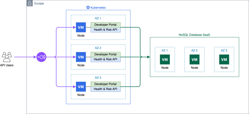
Due to the geographically distributed customer base and low latency requirements, three Kubernetes clusters were deployed, one on each continent. The NoSQL database was hosted in proximity to the workload to reduce service latency and keep the migration effort low.

To reduce the operational maintenance, the NoSQL database was integrated as a SaaS offering, and monitoring was centralized using Datadog.

All cloud infrastructure was provisioned exclusively with Terraform, covering the Kubernetes cluster, NoSQL database , and integration with GitLab and Datadog.

dacadoo containerized the API service and used Gitlab continuous integration and continuous deployment (CI/CD) pipelines to deploy multiple environments and clusters on a global hyperscaler.

In retrospect, this was a typical replatform modernization project from virtual machine to Kubernetes, with a high level of automation and a SaaS-first approach.

The following diagram is the architecture for the container solution with managed NoSQL database.

Containers architecture

Challenges

The service faced several challenges, including increased costs from deploying three regional Kubernetes clusters across three environments, resulting in 27 cluster nodes and additional expenses from managing NoSQL database SaaS instances for each cluster. The complexity of CI/CD pipelines for multi-environment multi-cluster deployments added to the difficulty. Significant operational effort was required to keep infrastructure and Kubernetes components up to date.

Stage 3: Operational excellence with serverless

The Kubernetes-based architecture met the requirements, but some features in the dacadoo API service backlog needed to fit better with the application architecture at the time.

This was the right moment to take a holistic view of the infrastructure and software architecture and refactor the solution according to the latest AWS technologies and best practices, the next frontier for dacadoo’s engineering team.

Solution requirements

Requirements for the solution refactoring were as follows:

Keep the functionality of the API unmodified
Constrain data processing to a region of choice for compliance with local data protection laws
Avoid weekly patch cycles by exclusively using managed serverless services
Reduce costs by choosing services with a pay-as-you-go billing model
Delegate authentication to a dedicated service
Use an established web framework with an extensive ecosystem

Refactoring the apps

The API service has two components: a developer portal and the health score and risk calculations API. The database is only required for API keys, algorithm parameters, quotas, and usage statistics. Health data is processed regionally by the compute layer but not persisted, opening the door for a distributed database: Amazon DynamoDB global tables is the perfect fit for the solution. Writes are distributed to all connected Regions, whereas reads are local, providing low latency for complying with dacadoo service level agreements (SLAs).

The developer portal is a web UI with API documentation and API key management features. AWS Lambda is a great fit because it scales automatically and has a pay-per-request billing model.

The health and risk API uses algorithms implemented in the C programming language for short bursting, compute-intense simulations. These calls are wrapped by a REST API using the Python FastAPI framework. These characteristics make AWS Lambda a great fit.

Serverless architecture

HTTP requests are routed to the Lambda functions using Amazon API Gateway with AWS WAF for protection from malicious requests and attacks. Static assets are served from an Amazon Simple Storage Service (Amazon S3) bucket through API Gateway. The additional features of Amazon CloudFront aren’t required, and Amazon S3 reduces the complexity.

Amazon Route 53 provides a powerful feature known as latency-based routing, which allows it to direct DNS queries to the endpoint that offers the lowest latency for the requester.

This feature provides Regional high availability for API users without data processing location requirements. Alternatively, the user can call specific Regional endpoints to make sure requests are processed in the desired Region.

API authorization is HTTP header-based and is performed in the application with data stored in Amazon DynamoDB.

The following diagram is the architecture for a geo-redundant fully serverless solution.

Serverless architecture

With a dacadoo SRE team proficient in Python, they opted for Pulumi for its advanced features such as programming language flow control constructs, powerful configuration capabilities, and multi-cloud support.

For continuous integration, GitLab CI compiles the algorithm library, tests the FastAPI applications and packages everything. The application deployment is just an update of the AWS Lambda, a simple and reliable workflow.

Summary

The solution evolved from a managed infrastructure setup, where the customer held most of the responsibility, to an AWS managed service architecture.

Infrastructure provisioning evolved from manual, error-prone processes to powerful code-driven workflows in Pulumi. The SRE needed to enhance their software engineering skills to adopt Pulumi, transitioning from configuration-based approaches to designing and maintaining an infrastructure code base using object-oriented Python. This was part of dacadoo’s investment in the SRE team and broader modernization efforts. The serverless architecture enabled a GitOps engineering culture focused on productivity.

The transformation maximized scalability and availability while reducing costs and operational effort:

Virtual machine

Scalability: Low
Availability: Best effort
Infrastructure costs: Low
Maintenance effort: High

Kubernetes

Scalability: High
Availability: 99.95%
Infrastructure costs: High
Maintenance effort: Medium

Serverless

Scalability: Very high
Availability: 99.999% (with failover to another AWS Region)
Infrastructure costs: Low
Maintenance effort: Very low

The global redundancy elevates availability to an impressive 99.999% while keeping the costs low.

Conclusion

Migrating from a virtual machine to Kubernetes and ultimately to AWS Lambda demonstrates the progression of cloud engineering toward enhanced efficiency and scalability.

Each step in this journey reduced the complexity of managing resources while increasing flexibility and automation. Transitioning dacadoo’s API service to a fully serverless, geo-redundant architecture not only advanced the platform but also upskilled engineers, maintained a lean SRE team, and kept infrastructure costs low. Get started with your own AWS serverless solution.

About the Authors

Optimizing network footprint in serverless applications

2025-03-21 Chris McPeek

Post Syndicated from Chris McPeek original https://aws.amazon.com/blogs/compute/optimizing-network-footprint-in-serverless-applications/

This post is authored by Anton Aleksandrov, Principal Solution Architect, AWS Serverless and Daniel Abib, Senior Specialist Solutions Architect, AWS

Serverless application developers may commonly encounter scenarios where they need to transport large payloads, especially when building modern cloud applications that need rich data. Examples include analytics services with detailed reports, e-commerce platforms with extensive product catalogs, healthcare applications transmitting patient records, or financial services aggregating transactional data.

Many serverless services have a well-defined maximum payload size. For example, AWS Lambda maximum request/response payload size is 6 MB, and Amazon Simple Queue Service (Amazon SQS) and Amazon EventBridge maximum message size is 256 KB. In this post, you will learn how to use data compression techniques to reduce your network footprint and transport larger payloads under existing constraints.

Overview

Cloud applications evolve continuously and need to be adjusted frequently for new requirements, such as new business features or new Service Level Objectives (SLO) for higher throughput and lower latency. As new use cases and data patterns are added, it is common to see request and response payload sizes increase. At some point, you might hit the maximum service payload size limits, such as 6 MB for synchronous Lambda function invokes, 10 MB for Amazon API Gateway, and 256 KB for Amazon SQS, EventBridge, and asynchronous Lambda invokes.

There are several techniques you can apply when dealing with large payloads. If your payloads are tens of MBs or more, or you need to transport large binary objects with API Gateway, you can store the payload on Amazon Simple Storage Service (Amazon S3) and use pre-signed URLs for clients to directly upload and download from S3.

Figure 1. A sample of architecture for handling large payloads

Lambda function URLs response streaming supports up to 20 MB responses. For handling large messages with services such as SQS or EventBridge, you can store the message in S3 and pass a reference. The downstream consumer will use the reference to download the message directly from S3. One common characteristic of these techniques is that they introduce architectural complexity and may necessitate modifications to your existing solution architecture and data flow patterns.

Furthermore, as your payloads grow in size, you will see increased data transfer costs, especially if your solution is transporting data through Amazon Virtual Private Cloud (VPC) NAT Gateways, VPC endpoints, or sending data across AWS Regions. For example, it is common for VPC-based solutions to have Lambda functions in their architecture. A container running on Amazon Elastic Kubernetes Service (Amazon EKS) might need to invoke a Lambda function, or a VPC-attached Lambda function might need to reach out to the public internet.

Figure 2. Examples of using virtual network appliances with serverless applications

Both NAT Gateway and VPC Endpoint are billed per GB of data processed, which makes data compression a valuable optimization technique. Go to NAT Gateway pricing and VPC Endpoint pricing for details.

The following sections explore data compression techniques and demonstrate how to apply them in your serverless applications. You can learn how to send larger payloads within the existing payload size boundaries and reduce your network footprint without significant architectural changes. This post discusses compression techniques in the context of Lambda and API Gateway, but the same principles can be applied to other services, such as SQS, EventBridge, and AWS AppSync. Understanding compression concepts better equips you to optimize your application’s data-handling capabilities.

What is data compression?

Compression is a widely used approach to reduce data size in order to improve cost-effectiveness and performance for data storage and transmission. Many tools and frameworks incorporate data compression techniques, such as gzip or zstd. It is thoroughly documented in the official IANA specification and IETF RFC 9110. Browsers such as Chrome and Firefox, HTTP toolkits such as curl and Postman, and runtimes such as Node.js and Python natively handle compression, often without user involvement.

Consider HTTP protocol. When a client wants to send a compressed payload, it specifies it in the Content-Type header. To receive a compressed response, the client specifies supported compression methods in the Accept-Encoding request header.

Figure 3. Accept-Encoding request header specifying supported compression methods

The server compresses the response payload using one of the supported methods and uses the Content-Encoding response header to indicate the method to the client.

Figure 4. Content-Encoding response header specifying compression method

This mechanism can accelerate client-server communications by reducing the number of bytes transmitted over the network. Compression efficiency depends on the data type. Text-based formats like JSON, XML, HTML, and YAML compress well, while binary data such as PDF and JPEG generally compress less effectively.

Data compression with API Gateway

API Gateway provides built-in compression support. Use the minimumCompressionSize configuration to set the smallest payload size to compress automatically. The value can be between 0 bytes to 10 MB. Compressing very small payloads might actually increase the final payload size, and you should always test with your real payload patterns to determine the optimal threshold.

Figure 5. Handling data compression in API Gateway

API Gateway enables clients to interact with your API using compressed payloads through supported content encodings. The compression mechanism works bi-directionally. For JSON payloads, API Gateway seamlessly handles compression and decompression, maintaining compatibility with mapping templates. It decompresses incoming payloads before applying request mapping templates and compresses outgoing responses after applying response mapping templates. This automated compression optimizes data transfer:

When sending compressed data, clients supply the appropriate Content-Encoding header. API Gateway handles the decompression and applies configured mapping templates before forwarding the request to the integration.
When API Gateway receives an integration response and compression is enabled, it compresses the response payload and returns it to the client, provided that the client has included a matching Accept-Encoding header.

A sample test using the compression technique with API Gateway and JSON payload yielded the following results.

Compression disabled. Response size = 1 MB, response latency = 660 ms
Compression enabled. Response size = 220 KB, response latency = 550 ms

Compressing data resulted in 78% network footprint reduction and improved latency by 110 ms.

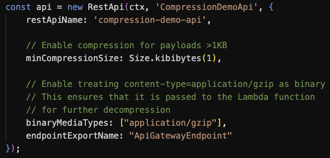
This configuration-based technique uses the API Gateway native compression. However, payloads are decompressed before being delivered to downstream integrations, thus they still remain subject to Lambda’s 6 MB max payload size. To address this, you can configure binaryMediaTypes in the API Gateway to pass compressed payloads to Lambda directly, enabling the function to handle decompression.

Figure 6. CDK code to configure API Gateway for data compression and binary data passthrough

Handling compressed data in Lambda functions

The Lambda Invoke API supports payloads in plain-text formats, such as JSON. The maximum payload size is 6 MB for synchronous invocations and 256 KB for asynchronous. Although the Invoke API supports uncompressed text-based payloads, you can introduce data compression in your function code and use API Gateway or Function URLs to facilitate content conversion, as illustrated in the following figure.

Figure 7. Transporting compressed payloads in a serverless applications

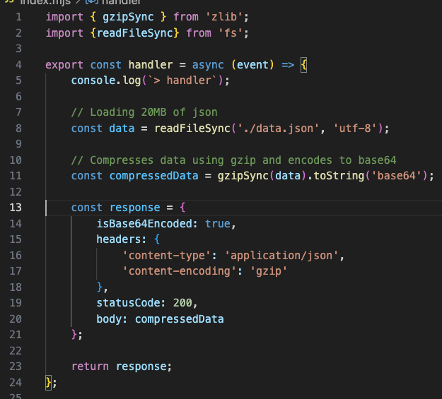
Handling data compression in your Lambda function code can be done through libraries commonly embedded in the runtime. The following code snippet shows the compressing response payload using Node.js. Similar techniques can be applied to other runtimes.

Figure 8. Sample code implementing response payload compression in a Lambda function

Line 1: Import gzip functionality from the zlib module.
Lines 11: Compress and Base64-encode data. Gzip compression, similar to many other compression methods, produces a binary stream. Base64 encoding converts it to the text-based format expected by the Lambda service
Lines 13-21: Response object is created with isBase64Encoded=true and response headers telling the client that the response is a gzip-encoded JSON object.

The following screenshot shows the result: 20 MB uncompressed JSON returned from a Lambda function as a 2.5 MB compressed response body. Network footprint reduced by over 80%.

Figure 9. A screenshot from Postman showing the original and compressed payload size

Using this technique, you can reduce your network footprint and transport payload sizes several times higher than the Lambda maximum payload size.

Using Function URLs with compressed payloads

Transporting compressed payloads through Lambda Function URLs doesn’t necessitate any extra configuration. For handler responses, your code needs to compress and Base64-encode the data as shown in the preceding figure. For invocation requests, the Function URL endpoint recognizes the incoming compressed payload as binary and passes it to your handler as a Base64 encoded string in the event body.

Figure 10. Sample code implementing request payload decompression in a Lambda function

Trade-offs and testing results

Compressing data in function code is a CPU-intensive activity, potentially increasing invocation duration and, as a result, function cost. This, however, can be balanced by the benefits of data compression. As you’ve seen in previous sections, while compressing data adds compute latency, transporting smaller payloads over the network reduces network latency. The following section summarizes a series of tests performed to estimate the impact of data compression on Lambda function invocation duration, Lambda function invocation cost, and data transfer savings with both NAT Gateway and VPC Endpoint. The tests were performed with several assumptions and randomly generated JSON data. You can see full testing results in the sample GitHub.com repo.

Test results demonstrated that the impact on function latency and cost primarily depends on two key factors: payload size and allocated memory (which determines vCPU capacity). Using a Node.js runtime with ARM architecture as an example, compressing a 1 MB JSON object in a function with 1 GB of allocated memory resulted in 124 ms of added processing time on average. For 10 million invocations, this extra processing time adds approximately $16. At the same time, the compression yielded a 70% reduction in payload size. With the same number of invocations, this translates to approximately $300 in savings when using NAT Gateway and $70 in savings when using VPC Endpoints (depending on the number of Availability Zones (AZs)).

AWS Service pricing is updated regularly, you should always consult the respective pricing pages for the latest information. Moreover, you should conduct your own performance and cost estimates using payloads that represent your workloads. Compression effectiveness varies significantly depending on the data type: payloads with low compression rates might not benefit from this technique.

Sample application

Follow the instructions in this GitHub repository to provision the sample in your AWS account. The project creates two Lambda functions to demonstrate receiving and returning compressed JSON using Function URLs and API Gateway.

The sample shows how to GET and POST JSON payloads using gzip compression to reduce the network footprint by over 80%.

Figure 11. A screenshot from Postman showing the original and compressed payload size

Conclusion

Data compression enables larger payload transfers and reduces network footprint. It can help to lower network latencies and optimize data transfer costs. When implementing compression within Lambda functions, it is important to consider its CPU-bound nature, which may increase function duration and costs. You should always evaluate the added compute cost against potential data transfer savings to make sure the technique benefits your use case.

Compression is most effective for handling large text-based payloads and when a slight increase in compute latency balanced by reduced network latency is acceptable.

To learn more about Serverless architectures and asynchronous Lambda invocation patterns, see Serverless Land.

Build a data lakehouse in a hybrid Environment using Amazon EMR Serverless, Apache DolphinScheduler, and TiDB

2025-03-20 Shiyang Wei

Post Syndicated from Shiyang Wei original https://aws.amazon.com/blogs/big-data/build-a-data-lakehouse-in-a-hybrid-environment-using-amazon-emr-serverless-apache-dolphinscheduler-and-tidb/

While helping our customers build systems on AWS, we found out that a large number of enterprise customers who pay great attention to data security and compliance, such as B2C FinTech enterprises, build data-sensitive applications on premises and use other applications on AWS to take advantage AWS managed services. Using AWS managed services can greatly simplify daily operation and maintenance, as well as help you achieve optimized resource utilization and performance.

This post discusses a decoupled approach of building a serverless data lakehouse using AWS Cloud-centered services, including Amazon EMR Serverless, Amazon Athena, Amazon Simple Storage Service (Amazon S3), Apache DolphinScheduler (an open source data job scheduler) as well as PingCAP TiDB, a third-party data warehouse product that can be deployed either on premises or on the cloud or through a software as a service (SaaS).

Solution overview

For our use case, an enterprise data warehouse with business data is hosted on an on-premises TiDB platform, an AWS Global Partner that is also available on AWS through AWS Marketplace.

The data is then processed by an Amazon EMR Serverless Job to achieve data lakehouse tiering logic. Different tiering data are stored in separate S3 buckets or separate S3 prefixes under the same S3 bucket. Typically, there are four layers in terms of data warehouse design.

Operational data store layer (ODS) – This layer stores raw data of the data warehouse
Data warehouse stage layer (DWS) – This layer is a temporary staging area within the data warehousing architecture where data from various sources is loaded, cleaned, transformed, and prepared before being loaded into the data warehouse database layer;
Data warehouse database layer (DWD) – This layer is the central repository in a data warehousing environment where data from various sources is integrated, transformed, and stored in a structured format for analytical purposes;
Analytical data store (ADS) – This layer is a subset of the data warehousing that is specifically designed and optimized for a particular business function, department, or analytical purpose.

For this post, we only use ODS and ADS layers to demonstrate the technical feasibility.

The schema of this data is managed through the AWS Glue Data Catalog, and can be queried using Athena. The EMR Serverless Jobs are orchestrated using Apache DolphinScheduler deployed in cluster mode on Amazon Elasctic Compute Cloud (Amazon EC2) instances, with meta data stored in an Amazon Relational Database Service (Amazon RDS) for MySQL instance.

Using DolphinScheduler as the data lakehouse job orchestrator offers the following advantages:

Its distributed architecture allows for better scalability, and the visual DAG designer makes workflow creation more intuitive for team members with varying technical expertise
It provides more granular task-level controls and supports a wider range of task types out-of-the-box, including Spark, Flink, and machine learning (ML) workflows, without requiring additional plugin installations;
Its multi-tenancy feature enables better resource isolation and access control across different teams within an organization.

However, DolphinScheduler requires more initial setup and maintenance effort, making it more suitable for organizations with strong DevOps capabilities and a desire for complete control over their workflow infrastructure.

The following diagram illustrates the solution architecture.

Prerequisites

You need to create an AWS account and set up an AWS Identity and Access Management (IAM) user as a prerequisite for the following implementation. Complete the following steps:

For AWS account signing up, please follow up the actions guided per page link.

Create an AWS account.
Sign in to the account using the root user for the first time.
One the IAM console, create an IAM user with AdministratorAccess Policy.
Use this IAM user to log in AWS Management Console rather the root user.
On the IAM console, choose Users in the navigation pane.
Navigate to your user, and on the Security credentials tab, create an access key.
Store the access key and secret key in a secure place and use them for further API access of the resources of this AWS account.

Set up DolphinScheduler, IAM configuration, and the TiDB Cloud table

In this section, we walk through the steps to install DolphinScheduler, complete additional IAM configurations to enable the EMR Serverless job, and provision the TiDB Cloud table.

Install DolphinScheduler on an EC2 instance with an RDS for MySQL instance storing DolphinScheduler metadata. The production deployment mode of DolphinScheduler is cluster mode. In this blog, we use pseudo cluster mode which has the same installation steps as cluster mode, and could achieve resource economy. We name the EC2 instance ds-pseudo.

Make sure the inbound rule of the security group attached to the EC2 instance allows port 12345’s TCP traffic. Then complete the following steps:

sudo dnf install java-1.8.0-amazon-corretto
java -version

Switch to dir /usr/local/src:
```
cd /usr/local/src
```

Install Apache Zookeeper:

wget https://archive.apache.org/dist/zookeeper/zookeeper-3.8.0/apache-zookeeper-3.8.0-bin.tar.gz
tar -zxvf apache-zookeeper-3.8.0-bin.tar.gz
cd apache-zookeeper-3.8.0-bin/conf
cp zoo_sample.cfg zoo.cfg
cd ..
nohup bin/zkServer.sh start-foreground &> nohup_zk.out &
bin/zkServer.sh status

Check the Python version:
```
python3 --version
```
The version should be 3.9 or above. It is recommended that you use Amazon Linux 2023 or later as the Amazon EC2 operating system (OS); Python version 3.9 meets the requirement. For detail information, refer to Python in AL2023.

Install Dolphinscheduler

Download the dolphinscheduler package:

cd /usr/local/src
wget https://dlcdn.apache.org/dolphinscheduler/3.1.9/apache-dolphinscheduler-3.1.9-bin.tar.gz
tar -zxvf apache-dolphinscheduler-3.1.9-bin.tar.gz
mv apache-dolphinscheduler-3.1.9-bin apache-dolphinscheduler

Download the mysql connector package:

wget https://downloads.mysql.com/archives/get/p/3/file/mysql-connector-j-8.0.31.tar.gz
tar -zxvf mysql-connector-j-8.0.31.tar.gz

Copy specific mysql connector JAR file to the following destinations:

cp mysql-connector-j-8.0.31/mysql-connector-j-8.0.31.jar ./apache-dolphinscheduler/api-server/libs/
cp mysql-connector-j-8.0.31/mysql-connector-j-8.0.31.jar ./apache-dolphinscheduler/alert-server/libs/
cp mysql-connector-j-8.0.31/mysql-connector-j-8.0.31.jar ./apache-dolphinscheduler/master-server/libs/
cp mysql-connector-j-8.0.31/mysql-connector-j-8.0.31.jar ./apache-dolphinscheduler/worker-server/libs/
cp mysql-connector-j-8.0.31/mysql-connector-j-8.0.31.jar ./apache-dolphinscheduler/tools/libs/

Add the user dolphinscheduler, and make sure the directory apache-dolphinscheduler and the files under it are owned by the user dolphinscheduler:

useradd dolphinscheduler
echo "dolphinscheduler" | passwd --stdin dolphinscheduler
sed -i '$adolphinscheduler ALL=(ALL) NOPASSWD: NOPASSWD: ALL' /etc/sudoers
sed -i 's/Defaults   requirett/#Defaults requirett/g' /etc/sudoers
chown -R dolphinscheduler:dolphinscheduler apache-dolphinscheduler

Install the mysql client:

sudo dnf update -y 
sudo dnf install mariadb105

On the Amazon RDS console, provision an RDS for MySQL instance with the following configurations:
1. For Database Creation Method, select Standard create.
2. For Engine options, choose MySQL.
3. For Edition: choose MySQL 8.0.35.
4. For Templates: select Dev/Test.
5. For Availability and durability, select Single DB instance.
6. For Credentials management, select Self-managed.
7. For Connectivity, select Connect to an EC2 compute resource, and choose the EC2 instance created earlier.
8. For Database Authentication: choose Password Authentication.
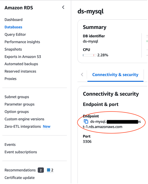
Navigate to the ds- mysql database details page, and under Connectivity & security, copy the RDS for MySQL endpoint.

Configure the intance:

mysql -h <RDS for mysql Endpoint> -u admin -p
mysql> CREATE DATABASE dolphinscheduler DEFAULT CHARACTER SET utf8 DEFAULT COLLATE utf8_general_ci;
mysql> exit;

Configure the dolphinscheduler configuration file:
```
cd /usr/local/src/apache-dolphinscheduler/
```

Revise dolphinscheduler_env.sh:

vim bin/env/dolphinscheduler_env.sh
export DATABASE=${DATABASE:-mysql}
export SPRING_PROFILES_ACTIVE=${DATABASE}
export SPRING_DATASOURCE_URL="jdbc:mysql://ds-mysql.cq**********.us-east-1.rds.amazonaws.com/dolphinscheduler?useUnicode=true&amp;characterEncoding=UTF-8&amp;useSSL=false"
export SPRING_DATASOURCE_USERNAME="admin"
export SPRING_DATASOURCE_PASSWORD="<your password>"

On the Amazon EC2 console, navigate to the instance details page and copy the private IP address.

Revise install_env.sh:

vim bin/env/install_env.sh
ips=${ips:-"<private ip address of ds-pseudo EC2 instance>"}
masters=${masters:-"<private ip address of ds-pseudo EC2 instance>"}
workers=${workers:-" private ip address of ds-pseudo EC2 instance:default"}
alertServer=${alertServer:-" private ip address of ds-pseudo EC2 instance "}
apiServers=${apiServers:-" private ip address of ds-pseudo EC2 instance "}
installPath=${installPath:-"~/dolphinscheduler"}
export JAVA_HOME=${JAVA_HOME:-/usr/lib/jvm/jre-1.8.0-openjdk}
export PYTHON_HOME=${PYTHON_HOME:-/bin/python3}

Configure the dolphinscheduler configuration file:

cd /usr/local/src/apache-dolphinscheduler/
bash tools/bin/upgrade-schema.sh

Install DolphinScheduler:

cd /usr/local/src/apache-dolphinscheduler/
su dolphinscheduler
bash ./bin/install.sh

Start DolphinScheduler after installation:

cd /usr/local/src/apache-dolphinscheduler/
su dolphinscheduler
bash ./bin/start-all.sh

Open the DolphinScheduler console:

http://<ec2 ip address>:12345/dolphinscheduler/ui/login

After input the initial username and password, press Login button to enter into the dashboard shown as below.

initial user/password admin/dolphinscheduler123

Configure IAM role to enable the EMR serverless job

The EMR serverless job role needs to have permission to access a specific S3 bucket to read job scripts and potentially write results, and also have permission to access AWS Glue to read the Data Catalog which stores the tables’ meta data. For detailed guidance, please refer to Grant permission to use EMR Serverless or EMR Serverless Samples.

The following screenshot shows the IAM role configured with the trust policy attached.

The IAM role should have the following permissions policies attached, as shown in the following screenshot.

Provision the TiDB Cloud table

To provision the TiDB Cloud table, complete the following steps:
1. Register for TiDB Cloud.
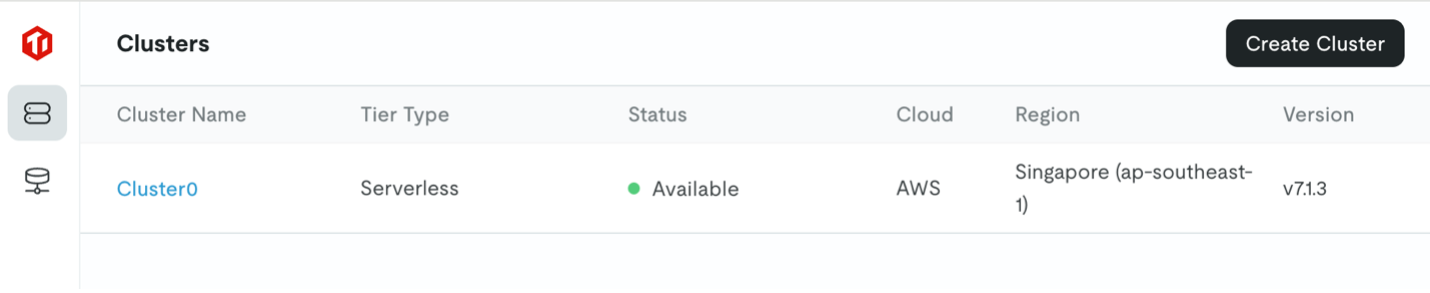
2. Create a serverless cluster, as shown in the following screenshot. For this post, we name the cluster Cluster0.

Choose Cluster0, then choose SQL Editor to create a database named test:

create table testtable (id varchar(255));
insert into testtable values (1);
insert into testtable values (2);
insert into testtable values (3);

Synchronize data between on-premises TiDB and AWS

In this section, we discuss how to synchronize historical data as well as incremental data between TiDB and AWS.

Use TiDB Dumpling to sync historical data from TiDB to Amazon S3

Use the commands in this section to dump data stored in TiDB as CSV files into a S3 bucket. For full details on how to achieve a data sync from on-premises TiDB to Amazon S3, see Export data to Amazon S3 cloud storage. For this post, we use TiDB tool Dumpling. Complete the following steps:

Run the following command to install TiUP:

curl --proto '=https' --tlsv1.2 -sSf https://tiup-mirrors.pingcap.com/install.sh | sh

cd /root
source .bash_profile

tiup --version

Run the following command to install Dumpling:
```
tiup install dumpling
```

Run the following command to achieve target database table dumpling to the specific S3 bucket.

tiup dumpling -u <prefix.root> -P 4000 -h <tidb serverless endpoint/host> -r 200000 -o "s3://<specific s3 bucket>" --sql "select * from <target database>.<target table>" --ca "/etc/pki/tls/certs/ca-bundle.crt" --password <tidb serverless password>

To acquire the TiDB serverless connection information, navigate to the TiDB Cloud console and choose Connect.

You can collect the specific connection information of test database from the following screenshot.

Yan can view the data stored in the S3 bucket on the Amazon S3 console.

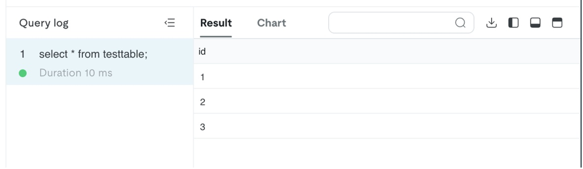
You can use Amazon S3 Select to query the data and get results similar to the following screenshot, confirming that the data has been ingested into testtable.

Use TiDB Dumpling with a self-managed checkpoint to sync incremental data from TiDB to Amazon S3

To achieve incremental data synchronization using TiDB Dumpling, it’s essential to self-manage the check point of the target synchronized data. One recommended way is to store the ID of the final ingested record into a certain media (such as Amazon ElastiCache for Redis, Amazon DynamoDB) to achieve a self-managing checkpoint when running the shell/Python job that trigges TiDB Dumpling. The prerequisite for implementing this is that the target table has a monotonically increasing id field as its primary key.

You can use the following TiDB Dumpling command to filter the exported data:

tiup dumpling -u <prefix.root> -P 4000 -h <tidb serverless endpoint/host> -r 200000 -o "s3://<specific s3 bucket>" --sql "select * from <target database>.<target table> where id > 2" --ca "/etc/pki/tls/certs/ca-bundle.crt" --password <tidb serverless password>

Use the TiDB CDC connector to sync incremental data from TiDB to Amazon S3

The advantage of using TiDB CDC connector to achieve incremental data synchronization from TiDB to Amazon S3 is that there is built-in change data capture (CDC) mechanism, and because the backend engine is Flink, the performance is fast. However, there is one trade-off: you need to create several Flink tables to map the ODS tables on AWS.

For instructions to implement the TiDB CDC connector, refer to TiDB CDC.

Use an EMR serverless job to sync historical and incremental data from a Data Catalog table to the TiDB table

Data usually flows from on premises to the AWS Cloud. However, in some cases, the data might flow from the AWS Cloud to your on-premises database.

After landing on AWS, the data will be wrapped up and managed by the Data Catalog by created Athena tables with the specific tables’ schema. The table DDL script is as follows:

CREATE EXTERNAL TABLE IF NOT EXISTS `testtable`(
  `id` string
) 
ROW FORMAT SERDE 'org.apache.hadoop.hive.serde2.OpenCSVSerde'
LOCATION 's3://<bucket_name>/<prefix_name>/';

The screenshot below showcases the DDL running result using Athena console.

The data stored in testtable table is queried using select * from testable SQL. The query result is shown as follows:

In this case, an EMR serverless spark job can accomplish the work of synchronizing data from an AWS Glue table to your on premises table.

If the Spark job is written in Scala, the sample code is as below:

package com.example
import org.apache.spark.sql.{DataFrame, SparkSession}

object Main  {

  def main(args: Array[String]): Unit = {

    val spark = SparkSession.builder()
      .appName("<specific app name>")
      .enableHiveSupport()
      .getOrCreate()

    spark.sql("show databases").show()
    spark.sql("use default")
    var df=spark.sql("select * from testtable")

    df.write
      .format("jdbc")
      .option("driver","com.mysql.cj.jdbc.Driver")
      .option("url", "jdbc:mysql://<tidbcloud_endpoint>:4000/namespace")
      .option("dbtable", "<table_name>")
      .option("user", "<user_name>")
      .option("password", "<password_string>")
      .save()

    spark.close()
  }
}

You can acquire the TiDB serverless endpoint connection information on the TiDB console by choosing Connect, as shown earlier in this post.

After you have wrapped the Scala code as JAR file using SBT, you can submit the job to EMR Serverless with the following AWS Command Line Interface (AWS CLI) command:

export applicationId=00fev6mdk***

export job_role_arn=arn:aws:iam::<aws account id>:role/emr-serverless-job-role

aws emr-serverless start-job-run \
    --application-id $applicationId \
    --execution-role-arn $job_role_arn \
    --job-driver '{
        "sparkSubmit": {
            "entryPoint": "<s3 object url for the wrapped jar file>",
            "sparkSubmitParameters": "--conf spark.hadoop.hive.metastore.client.factory.class=com.amazonaws.glue.catalog.metastore.AWSGlueDataCatalogHiveClientFactory --conf spark.driver.cores=1 --conf spark.driver.memory=3g --conf spark.executor.cores=4 --conf spark.executor.memory=3g --jars s3://spark-sql-test-nov23rd/mysql-connector-j-8.2.0.jar"
        }
    }'

If the Spark job is written in PySpark, the sample code is as follows:

import os
import sys
import pyspark.sql.functions as F
from pyspark.sql import SparkSession

if __name__ == "__main__":

    spark = SparkSession\
        .builder\
        .appName("app1")\
        .enableHiveSupport()\
        .getOrCreate()

    df=spark.sql(f"select * from {str(sys.argv[1])}")

    df.write.format("jdbc").options(
        driver="com.mysql.cj.jdbc.Driver",
        url="jdbc:mysql://tidbcloud_endpoint:4000/namespace ",
        dbtable="table_name",
        user="use_name",
        password="password_string").save()

    spark.stop()

You can submit the job to EMR Serverless using the following AWS CLI command:

export applicationId=00fev6mdk***

export job_role_arn=arn:aws:iam::<aws account id>:role/emr-serverless-job-role

aws emr-serverless start-job-run \
    --application-id $applicationId \
    --execution-role-arn $job_role_arn \
    --job-driver '{
        "sparkSubmit": {
            "entryPoint": "<s3 object url for the python script file>",
            "entryPointArguments": ["testspark"],
            "sparkSubmitParameters": "--conf spark.hadoop.hive.metastore.client.factory.class=com.amazonaws.glue.catalog.metastore.AWSGlueDataCatalogHiveClientFactory --conf spark.driver.cores=1 --conf spark.driver.memory=3g --conf spark.executor.cores=4 --conf spark.executor.memory=3g --jars s3://spark-sql-test-nov23rd/mysql-connector-j-8.2.0.jar"
        }
    }'

The preceding PySpark code and AWS CLI command achieves outbound parameter input as well: the table name (specifically testspark) is ingested into the SQL sentence when submitting the job.

EMR Serverless job pperation essentials

An EMR Serverless application is a resource pool concept. An application holds a certain capacity of compute, memory, and storage resources for jobs running on it to use. You can configure the resource capacity using AWS CLI or the console. Because it’s a resource pool, EMR Serverless application creation is usually a one-time action with the initial capacity and maximum capacity being configured.

An EMR Serverless job is a working unit that actually processes the compute task. In order for a job to work, you need to set the EMR Serverless application ID, the execution IAM role (discussed previously), and the specific application configuration (the resources the job is planning to use). Although you can create the EMR Serverless job on the console, it’s recommended to create the EMR Serverless job using the AWS CLI for further integration with the scheduler and scripts.

For more details on EMR Serverless application creation and EMR Serverless job provisioning, refer to EMR Serverless Hive query or EMR Serverless PySpark job

DolphinScheduler integration and job orchestration

DolphinScheduler is a modern data orchestration platform. It’s agile to create high- performance workflows with low code. It also provides a powerful UI, dedicated to solving complex task dependencies in the data pipeline and providing various types of jobs out of the box.

DolphinScheduler is developed and maintained by WhaleOps, and available in AWS Marketplace as WhaleStudio.

DolphinScheduler has been natively integrated with Hadoop: DolphinScheduler cluster mode is by default recommended to be deployed on a Hadoop cluster (usually on HDFS data nodes), and the HQL scripts uploaded to DolphinScheduler Resource Manager are stored by default on HDFS, and can be orchestrated using the following native Hive shell command:

Hive -f example.sql

Moreover, for specific case in which the orchestration DAGs are quite complicated, each DAG consists of several jobs (for example, more than 300), and almost all the jobs are HQL scripts stored in DolphinScheduler Resource Manager.

Complete the steps listed in this section to achieve a seamless integration between DolphinScheduler and EMR Serverless.

Switch the storage layer of DolphinScheduler Resource Center from HDFS to Amazon S3

Edit the common.properties files under directories /usr/local/src/apache-dolphinscheduler/api-server/ and directory /usr/local/src/apache-dolphinscheduler/worker-server/conf. The following code snippet shows the part of the file that needs to be revised:

# resource storage type: HDFS, S3, OSS, NONE
#resource.storage.type=NONE
resource.storage.type=S3
# resource store on HDFS/S3 path, resource file will store to this base path, self configuration, please make sure the directory exists on hdfs and have read write permissions. "/dolphinscheduler" is recommended
resource.storage.upload.base.path=/dolphinscheduler

# The AWS access key. if resource.storage.type=S3 or use EMR-Task, This configuration is required
resource.aws.access.key.id=AKIA************
# The AWS secret access key. if resource.storage.type=S3 or use EMR-Task, This configuration is required
resource.aws.secret.access.key=lAm8R2TQzt*************
# The AWS Region to use. if resource.storage.type=S3 or use EMR-Task, This configuration is required
resource.aws.region=us-east-1
# The name of the bucket. You need to create them by yourself. Otherwise, the system cannot start. All buckets in Amazon S3 share a single namespace; ensure the bucket is given a unique name.
resource.aws.s3.bucket.name=dolphinscheduler-shiyang
# You need to set this parameter when private cloud s3. If S3 uses public cloud, you only need to set resource.aws.region or set to the endpoint of a public cloud such as S3.cn-north-1.amazonaws.com.cn
resource.aws.s3.endpoint=s3.us-east-1.amazonaws.com

After editing and saving the two files, restart the api-server and worker-server by running the following commands, under folder path /usr/local/src/apache-dolphinscheduler/

bash ./bin/stop-all.sh
bash ./bin/start-all.sh
bash ./bin/status-all.sh

You can validate whether switching the storage layer to Amazon S3 was successful by uploading a script using DolphinScheduler Resource Center Console, check if the file appears in relevant S3 bucket folder.

Before verifying that Amazon S3 is now the storage location of DolphinScheduler, you need to create a tenant on the DolphinScheduler console and bundle the admin user with the tenant, as illustrated in the following screenshots:

After that, you can create a folder on the DolphinScheduler console, and check whether the folder is visible on the Amazon S3 console.

Make sure the job scripts uploaded from Amazon S3 are available in the DolphinScheduler Resource Center

After accomplishing the first task, you can upload the scripts from the DolphinScheduler Resource Center console, and confirm that the scripts are stored in Amazon S3. However, in practice, you need to migrate all scripts directly to Amazon S3. You can find and modify the scripts stored in Amazon S3 using DolphinScheduler Resource Center console. To do so, you can revise the metadata table t_ds_resources by inserting all the scripts’ metadata. The table schema of table t_ds_resources is shown in the following screenshot.

The insert command is as follows:

insert into t_ds_resources values(6, 'count.java', ' count.java','',1,1,0,'2024-11-09 04:46:44', '2024-11-09 04:46:44', -1, 'count.java',0);

Now there are two records in the table t_ds_resoruces.

You can access relevant records on the DolphinScheduler console.

The following screenshot shows the files on the Amazon S3 console.

Make the DolphinScheduler DAG orchestrator aware of the jobs’ status so the DAG can move forward or take relevant actions

As mentioned earlier, DolphinScheduler is natively integrated with the Hadoop ecosystem, and the HQL scripts can be orchestrated by the DolphinScheduler DAG orchestrator via Hive -f xxx.sql command. As a result, when the scripts changed to shell scripts or Python scripts (EMR Severless jobs needs to be orchestrated via shell scripts or Python scripts rather than the simple Hive command), the DAG orchestrator can start the job, but can’t get the real time status of the job, and therefore can’t continue the workflow to further steps. Because the DAGs in this case are very complicated, it’s not feasible to amend the DAGs; instead we follow a lift-and-shift strategy.

We use the following scripts to capture jobs’ status and take appropriate actions.

Persist the application ID list with the following code:

var=$(cat applicationlist.txt|grep appid1)
applicationId=${var#* }
echo $applicationId

Enable the DolphinScheduler step status auto-check using a Linux shell:

app_state
{
  response2=$(aws emr-serverless get-application --application-id $applicationId)
  application=$(echo $response1 | jq -r '.application')
  state=$(echo $application | jq -r '.state')
  echo $state
}

job_state
{
  response4=$(aws emr-serverless get-job-run --application-id $applicationId --job-run-id $JOB_RUN_ID)
  jobRun=$(echo $response4 | jq -r '.jobRun')
  JOB_RUN_ID=$(echo $jobRun | jq -r '.jobRunId')
  JOB_STATE=$(echo $jobRun | jq -r '.state')
  echo $JOB_STATE
}

state=$(job_state)

while [ $state != "SUCCESS" ]; do
  case $state in
    RUNNING)
         state=$(job_state)
         ;;
    SCHEDULED)
         state=$(job_state)
         ;;
    PENDING)
         state=$(job_state)
         ;;
    FAILED)
         break
         ;;
   esac
done

if [ $state == "FAILED" ]
then
  false
else
  true
fi

Clean up

To clean up your resources, we recommend using APIs through the following steps:

Delete the EC2 instance:
1. Find the instance using the following command:
```
aws ec2 describe-instances 
```
2. Delete the instance using the following command:
```
aws ec2 terminate-instances –instance-ids <specific instance id>
```
Delete the RDS instance:
1. Find the instance using the following command:
```
aws rds describe-db-instances
```
2. Delete the instance using the following command:
```
aws rds delete-db-instances –db-instance-identifier <speficic rds instance id>
```
Delete the EMR Serverless application
1. Find the EMR Serverless application using the following command:
```
aws emr-serverless list-applications 
```
2. Delete the EMR Serverless application using the following command:
```
 aws emr-serverless delete-application –application-id <specific application id>
```

Conclusion

In this post, we discussed how EMR Serverless, as AWS managed serverless big data compute engine, integrates with popular OSS products like TiDB and DolphinScheduler. We discussed how to achieve data synchronization between TiDB and the AWS Cloud, and how to use DolphineScheduler to orchestrate EMR Serverless jobs.

Try out the solution with your own use case, and share your feedback in the comments.

About the Author

Shiyang Wei is Senior Solutions Architect at Amazon Web Services. He is specializing in cloud system architecture and solution design for the financial industry. Particularly, he focused on big data and machine learning applications in finance, as well as the impact of regulatory compliance on cloud architecture design in the financial sector. He has over 10 years of experience in data domain development and architectural design.

Handling billions of invocations – best practices from AWS Lambda

2025-03-17 Chris McPeek

Post Syndicated from Chris McPeek original https://aws.amazon.com/blogs/compute/handling-billions-of-invocations-best-practices-from-aws-lambda/

This post is written by Anton Aleksandrov, Principal Solution Architect, AWS Serverless and Rajesh Kumar Pandey, Principal Engineer, AWS Lambda

AWS Lambda is a highly scalable and resilient serverless compute service. With over 1.5 million monthly active customers and tens of trillions of invocations processed, scalability and reliability are two of the most important service tenets. This post provides recommendations and insights for implementing highly distributed applications based on the Lambda service team’s experience building its robust asynchronous event processing system. It dives into challenges you might face, solution techniques, and best practices for handling noisy neighbors.

Overview

Developers building serverless applications create Lambda functions to run their code in the cloud. After uploading the code, the functions are invoked using synchronous or asynchronous mode.

Synchronous invocations are commonly used for interactive applications that expect immediate responses, such as web APIs. The Lambda service receives the invocation request, invokes the function handler, waits for the handler response, and returns it in response to the original request. With synchronous invocations, the client waits for the function handler to return, and is responsible for managing timeouts and retries for failed invocations.

Figure 1. Synchronous invocation sequence diagram

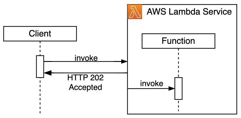
Asynchronous invocations enable decoupled function executions. Clients submit payloads for processing without expecting immediate responses. This is used for scenarios like asynchronous data processing or order/job submissions. The Lambda service immediately returns a confirmation for accepted invocation and proceeds to manage further handler invocation, timeouts, and retries asynchronously.

Figure 2. Asynchronous invocation sequence diagram

Asynchronous invocations under-the-hood

To accommodate asynchronous invocations, the Lambda service places requests into its internal queue and immediately returns HTTP 202 back to the client. After that, a separate internal poller component reads messages from the queue and synchronously invokes the function.

Figure 3. Asynchronous invocations workflow high-level topology

The same system also takes care of timeouts and retries in case of handler exceptions. When code execution completes, the system sends handler response to either onSuccess or onFailure destination, if configured.

Figure 4. Asynchronous invocations workflow detailed sequence diagram

Scaling highly distributed systems for billions of asynchronous requests presents unique challenges, such as managing noisy neighbors and potential traffic spikes to prevent system overload. Solutions vary by scale – what works for millions of requests may not suite billions. As workload size increases, solutions typically become more complex and costly, so right-sizing the approach is critical and should evolve with changing needs.

Simple queueing

A simple implementation of an asynchronous architecture can start with a single shared queue. This is a common approach for many asynchronous systems, particularly in early stages. It is effective when you’re not concerned about tenant isolation and when capacity planning indicates that a single queue can handle estimated incoming traffic efficiently.

Figure 5. Asynchronous workflow with a single queue

Even with this simple setup, it is critical to instrument your solution for observability to detect potential issues as soon as possible. You should monitor key metrics like queue backlog size, processing time, and errors, to indicate insufficient processing capacity early. Periods of unexpected traffic spikes and degraded performance may be a signal you have noisy neighbors impacting other tenants.Top of FormBottom of Form

To address this, you can scale your solution horizontally. You can implement random request placement across multiple queues to spread the load. Using a serverless service like Amazon SQS allows you to easily add and remove queues on-demand. One notable benefit of this approach is its simplicity – you do not need to introduce any complex routing mechanisms; requests are evenly spread across the queues. The downside is that you still do not have tenant boundaries. As your system grows, high-volume tenants and noisy neighbors can potentially affect all queues, thus impacting all tenants.

Figure 6. Asynchronous workflow with multiple queues and random request placement

Intelligent partitioning with consistent hashing

In order to further reduce potential impact, you can partition your tenants using sticky tenant-to-partition assignment with a hashing technique such as consistent hashing. This method uses a hash function to assign each tenant to a queue on a consistent hash ring.

Figure 7. Asynchronous workflow with multiple queues and consistent hashing placement

This technique ensures individual tenants stay in their queue partitions without the risk of disturbing the whole system. It helps to solve the problem where a few noisy neighbors have the potential to overflow all queues and as such impact all other tenants.

The consistent hashing approach proved to be efficient and enabled Lambda to offer robust asynchronous invocation performance to customers. As the volume of traffic and number of customers continued to grow, the Lambda service team came up with an innovative shuffle-sharding technique to further optimize the experience, and proactively eliminate any potential noisy-neighbor issues.

Shuffle-sharding

Drawing inspiration from the “The Power of Two Random Choices” paper, the Lambda team explored the shuffle-sharding technique for its asynchronous invocations processing. Using this technique, you shuffle-shard tenants into several randomly assigned queues. Upon receiving an asynchronous invocation, you place the message in the queue with the smallest backlog to optimize load distribution. This approach helps to minimize the likelihood of assigning tenants to a busy queue.

Figure 8. Asynchronous workflow with multiple queues and shuffle-sharding placement

To illustrate the benefit of this approach, consider a scenario where you’re using а 100 queues. The following formula helps to calculate the number of unique queue shards (combinations), where n is the total number of queues and r is the shard size (the number of queues you’re assigning per tenant).

With n=100, r=2 (each tenant is assigned randomly to 2 out of 100 queues), you get 4,950 unique combinations (shards). The probability of two tenants assigned to exactly the same shard is 0.02%. In case of r=3, the number of combinations spikes to 161,700. The probability of two tenants assigned to exactly the same shard drops to 0.0006%.

The shuffle-sharding technique proved remarkably effective. By distributing tenants across shards, the approach ensures that only a very small subset of tenants could be affected by a noisy neighbor. The potential impact is also minimized since each affected tenant maintains access to unaffected queues. As your workloads grow, increasing the number of queues enhances resilience and further reduces the probability of multiple tenants being assigned to the same shard. This significantly lowers the risk of a single point of failure, making shuffle sharding a robust strategy for workload isolation and fault tolerance.

Proactive detection, automated isolation, sidelining

Many distributed services will have a cohort of tenants with legitimate spiky asynchronous invocation traffic. This can be driven by seasonal factors, such as holiday shopping, or periodical batch processing. Recognizing these as real business needs, not malicious actions, you want to improve service quality for these tenants as well, while maintaining the overall system stability. For example, you can further improve solution performance by continuously monitoring queue depth to detect traffic spikes and route traffic to dynamically allocated dedicated queues. When you use Lambda asynchronous invocations, this internal complexity is managed for you by the service, ensuring seamless consumption experience.

Figure 9. Tenant D is automatically reallocated to a dedicated queue

Resilience and failure handling

“Everything fails, all the time” is a famous quote from Amazon’s Chief Technology Officer Werner Vogels. Lambda’s distributed and resilient architecture is built to withstand potential outages of its dependencies and internal components to limit the fallout for customers. Specifically for asynchronous invocation processing, the frontend service builds a processing backlog during an outage, allowing the backend to gradually recover without losing any in-flight messages.

Figure 10. Lambda service maintains resilience during component outage

Upon recovery, the service gradually ramps up the traffic to process the accumulated backlog. During this time, automated mechanisms are in place to coordinate between system components, preventing inadvertently DDoSing itself.

To further improve the recovery ramp-up process and provide a smooth restoration of normal operations, the Lambda service uses load-shedding technique to ensure fair resource allocation during recovery. While trying to drain the backlog as fast as possible, the service ensures that no single customer ends up consuming an outsized share of the available resources. Adopting such techniques can help you to improve your mean-time-to-recovery (MTTR).

Observability for asynchronous invocations processing

When using the Lambda service for asynchronous processing, you want to monitor your invocations for situational awareness and potential slowdowns. Use metrics such as AsyncEventReceived, AsyncEventAge, and AsyncEventDropped to get insights about internal processing.

AsyncEventReceived tracks the number of async invocations the Lambda service was able to successfully queue for processing. A drop in this metric indicates that invocations are not being delivered to the Lambda service and you should check your invocation source. Potential issues include misconfigurations, invalid access permissions, or throttling. Check your invocation source configuration, logs, and the function resource policy for further analysis.

AsyncEventAge tracks how long has a message spent in the internal queue before being processed by a function. This metric increases when async invocations processing is delayed due to insufficient concurrency, execution failures, or throttles. Increase your function concurrency to process more asynchronous invocations at a time and optimize function performance for better throughput, i.e. by increasing memory allocation to add more vCPU capacity. Experiment with adjusting batch size to enable functions to process more messages at a time. Use invocation logs to identify whether the problem is caused by function code throwing exceptions. Check Throttles and Errors metrics for further analysis.

AsyncEventDropped tracks the number of messages in the internal queue that were dropped because Lambda could not process them. This can be due to throttling, exceeding number of retries, exceeding maximum message age, or function code throwing an exception. Configure OnFailure destination or a dead-letter queue to avoid losing data and save dropped messages for re-processing. Use function logs and metrics described above to investigate whether you can address the issue by increasing function concurrency or allocating more memory.

By monitoring these metrics and addressing the underlying issues, you can ensure that your Lambda functions run smoothly, with minimal event processing delays and failures. You can also enable AWS X-Ray tracing to capture Lambda service traces. The AWS::Lambda trace segment captures the breakdown of the time that Lambda service spends routing requests to internal queues, the time a message spends in a queue, and the time before a function is invoked. This is a powerful tool to get insights into Lambda’s internal processing.

Conclusion

AWS Lambda processes tens of trillions of monthly invocations across more than 1.5 million active customers, demonstrating its exceptional scalability and resilience. Gaining an understanding of the underlying mechanisms of AWS services like Lambda enables you to proactively address potential challenges in your own applications. By learning how these services handle traffic, manage resources, and recover from failures, you can incorporate similar capabilities into your own solutions. For instance, leveraging Lambda’s asynchronous invocation metrics allows you to optimize workflow performance. This knowledge empowers you to implement strategies such as automated scaling, proactive monitoring, and graceful recovery during outages.

See below resources to learn about using queues and shuffle sharding at scale at Amazon

To learn more about Serverless architectures and asynchronous Lambda invocation patterns, see Serverless Land.

Build an enterprise API management solution using Amazon API Gateway

2025-03-11 Roger Zhang

Post Syndicated from Roger Zhang original https://aws.amazon.com/blogs/architecture/build-an-enterprise-api-management-solution-using-amazon-api-gateway/

Enterprises face many challenges when they build and manage application programming interfaces (APIs). These challenges include security controls, version management, traffic control, and usage analytics. As digital businesses expand, a mature API management (APIM) solution is crucial for ensuring scalability, security, and operational efficiency.

This blog post shows how you can use Amazon API Gateway—along with AWS Lambda, Amazon DynamoDB, and other AWS services—to create a comprehensive and customizable APIM solution. This solution addresses the complex requirements of large enterprises managing APIs at scale.

Core features of APIM

API Management (APIM) centralizes the management and publishing of APIs for the entire enterprise, acting as a hub between clients, applications, and administrators on one side, and internal services, external systems, and large language models (LLMs) on the other, as shown in the following figure.

APIM capabilities

The key features of APIM include:

Security and governance
- Authentication, authorization, rate limiting, and security policy enforcement.
- Helps ensure APIs meet organizational or industry standards.
Monitoring and logging
- Provides monitoring, alarms, and logging to track API performance and troubleshoot issues quickly.
Customization and transformation
- Offers protocol and field transformations, plus orchestration and aggregation.
- Makes it easier to integrate with different systems and meet various client needs.
API lifecycle management
- Publishing, rollback, version control, and documentation.
- Streamlines development and maintenance throughout the API lifecycle.
Developer and business tools
- Portals for developers, business owners, and administrators to manage documentation, billing, and analytics.
Integration with LLMs
- Specialized adapters, proxy configurations, and switching to integrate AI models seamlessly.
Flexible deployment options
- Canary releases, pipeline automation, and other advanced release strategies.
- Helps ensure stable, controlled API updates.

Unified management of multiple API gateways

API Gateway enforces resource limits of 300 resources per gateway, with a hard limit of 600. For enterprises that require more resources, managing multiple gateways individually can be time-consuming and error prone. APIM simplifies this by integrating API Gateway, Lambda, and DynamoDB; creating a centralized platform for managing APIs across multiple gateways. This integration streamlines the process, making it easier to scale and maintain APIs.

API lifecycle management

Managing API versions, publishing updates, and maintaining documentation often requires separate tools and manual processes, leading to inefficiencies. APIM centralizes these tasks in one portal, offering version control, publishing workflows, and rollback options. This streamlines the API lifecycle, ensuring consistency and reducing the chances for errors.

Enhanced security

Enterprises often need to implement different authentication strategies for various clients. These configurations typically require custom Lambda logic and database lookups, adding complexity and cost. APIM introduces configurable security policies that allow client-specific authentication without the need for additional custom code, reducing both complexity and operational overhead.

Customization and transformation

Enterprises frequently handle diverse client requests that involve different formats and protocols. Traditional API management approaches might struggle to support such variations. APIM allows for seamless protocol and field transformations, enabling integrations that meet a wide range of client requirements without additional development effort.

Developer portal

Developers need clear documentation, easy testing environments, and efficient API key management to work effectively. Traditional systems often lack these features, slowing down adoption. APIM provides a developer portal that consolidates API documentation, offers sandbox environments for testing, and simplifies API key management, reducing onboarding time and improving the developer experience.

Logging and monitoring

Log management is key to maintaining API performance, diagnosing issues, and gaining insights into usage. APIM uses API Gateway custom access logging, allowing teams to define logs based on business needs; whether creating separate CloudWatch metrics for each API path or exporting data to external platforms like ELK or Grafana.

Architecture overview

The APIM architecture, shown in the following figure, includes a management state (represented by numbers) and a runtime state (represented by letters). Both parts use a serverless paradigm.

APIM Architecture

Management state

The management state includes the following elements:

Administrator portal access: Administrators access the APIM solution through a secured web portal.
API Requests to APIM Lambda: Requests from the administrator’s API go through API Gateway, which then invokes the APIM Lambda function. This function handles logic related to configuration changes and other administrative actions.

In the following example, we show you how the APIM Lambda function dynamically applies different middleware based on the route configuration. This approach allows for flexible handling of authentication, client access restrictions, and request/response transformations. Here’s a quick breakdown of the key elements:

// If the route requires OIDC (OpenID Connect) authentication,
// add the OIDC authentication middleware to the route.
if route.Auth == "OIDC" {
    r.Use(middleware.OidcAuthenticator)
}
// If the route configuration specifies a list of allowed clients
// and the list is not empty, add a middleware to restrict access
// to only the specified clients.
if route.Allow.Clients != nil && len(route.Allow.Clients) != 0 {
    r.Use(middleware.AllowClients(route.Allow.Clients, cfg.Clients))
}
// Remove specific headers injected by the API Gateway
// to reduce exposure of internal details to downstream systems.
r.Use(middleware.RemoveGatewayHeaders)

// Add additional middleware for handling outbound logic.
// This could include retries, logging, or other outbound-specific functionality.
r.Use(outboundMiddlewares)
// Dynamically constructs and applies a chain of middlewares 
// based on the outbound configuration associated with the current request.
func outboundMiddlewares(next http.Handler) http.Handler {
    return http.HandlerFunc(func(w http.ResponseWriter, r *http.Request) {
        // Retrieve the outbound configuration from the request context.
        outbound, _ := r.Context().Value(selectedOutboundContext).(config.Outbound)

        // Initialize a slice to store the middlewares to be applied.
        middlewares := []func(http.Handler) http.Handler{}

        // Middleware to rewrite the HTTP request based on the outbound configuration.
        middlewares = append(middlewares, middleware.ProxyRequestRewrite(&outbound))

        // Add a middleware for mapping request data if specified in the outbound configuration.
        if len(outbound.Convert.Request) != 0 {
            middlewares = append(middlewares, middleware.RequestDataMapping(outbound.Convert.Request))
        }

        // Middleware to log the outbound response for monitoring or debugging purposes.
        middlewares = append(middlewares, middleware.OutboundResponseLog)

        // Add a middleware for mapping response data if specified in the outbound configuration.
        if len(outbound.Convert.Response) != 0 {
            middlewares = append(middlewares, middleware.ResponseDataMapping(outbound.Convert.Response))
        }

        // Add a middleware for modifying the response if a modification function is defined.
        if outbound.ModifyResponse != "" {
            f, ok := system.MODIFY[outbound.ModifyResponse]
            if ok {
                middlewares = append(middlewares, f())
            }
        }

        // Chain the constructed middlewares together and apply them to the request.
        chain := chi.Chain(middlewares...)
        chain.Handler(next).ServeHTTP(w, r)
    })
}

By using a middleware chain, you can customize how each request and response is processed on a per-route basis. This architecture not only keeps your code organized but also makes the API Gateway-integrated Lambda function far more adaptable to changing requirements. You can add or remove configurations from APIM portal as new use cases emerge—such as data transformations, custom logging, or additional security checks—without rewriting core logic.

Configuration management: Administrators set up server-side and client-side settings, such as API Gateway parameters, authentication requirements, transformations, and more.
Persistence: DynamoDB stores these configurations, providing persistent data storage and auditing capabilities.
Asynchronous resource provisioning: After administrators save configurations and release them from the APIM portal, APIM creates or updates AWS resources—such as API Gateway, Lambda functions, and AWS Identity and Access Management (IAM). Lambda runs these updates in the background, so administrators can continue working uninterrupted.

Runtime state

The runtime state includes the following elements:

A. Client request: Clients send requests to the APIM endpoint.

B. Routing to the correct gateway: APIM uses the URI prefix in the API mappings associated with custom domain names to route requests to the appropriate API gateway, as shown in the following figure. Each mapping defines a specific API, stage, and an optional path. When a request arrives, APIM checks the path and directs the request to the correct stage and API if it matches. Unmatched requests default to the mapping with no path defined.

C. APIM core processing: A Lambda function (APIM CORE) uses DynamoDB configurations to handle authentication, authorization, protocol conversion, field transformation, and routing.

D. Downstream service call: APIM forwards each request to the configured internal or external endpoint.

E. Logging and monitoring: API Gateway access logs and custom logs track requests in detail.

F. Alarm: Metrics and alarms detect anomalies and notify stakeholders. Use Amazon CloudWatch or self-hosted solutions such as ELK to enable real-time monitoring and alerting.

api-mapping

Conclusion

In this post, we’ve demonstrated how to build an enterprise API management (APIM) solution using Amazon API Gateway, AWS Lambda, Amazon DynamoDB, and other AWS services. We’ve also shown how APIM centralizes critical features—such as version management, security policies, and request/response transformations—to accommodate large-scale enterprise requirements.

You can use the APIM portal to store and manage configurations in DynamoDB, dynamically applying these settings to multiple API gateways without rewriting code. This approach ensures consistent governance across diverse client types and business scenarios, helping to keep APIs both secure and flexible.

Finally, you’ve seen how the APIM architecture unifies the management state and runtime state, streamlines administrative tasks, and provides end-to-end monitoring and alerting. By adopting these best practices, your enterprise can establish a robust, scalable, and secure API management foundation, all within a serverless paradigm.

About the Authors

Introducing an enhanced local IDE experience for AWS Step Functions

2025-03-06 Chris McPeek

Post Syndicated from Chris McPeek original https://aws.amazon.com/blogs/compute/introducing-an-enhanced-local-ide-experience-for-aws-step-functions/

This post written by Ben Freiberg, Senior Solutions Architect.

AWS Step Functions introduces an enhanced local IDE experience to simplify building state machines. Workflow Studio is now available within Visual Studio Code (VS Code) through the AWS Toolkit extension. With this integration, developers can author and edit state machines in their local IDE using the same powerful visual authoring experience found in the AWS Console.

Step Functions is a visual workflow service that helps developers use AWS services to build distributed applications, automate processes, orchestrate microservices, and create data and machine learning (ML) pipelines.

Customers choose Step Functions to build workflows that involve multiple services such as AWS Lambda, AWS Fargate, Amazon Bedrock, and HTTP API integrations. Developers create these workflows as state machines through the AWS Console using Workflow Studio or as code using Amazon States Language (ASL), a JSON-based domain specific language. Developers maintain their workflows definitions alongside the application and Infrastructure as code (IaC) code. Now, builders have even more capabilities to build and test their workflow in VS Code that matches the same experience as in AWS console.

Simplifying local workflow development

The integrated Workflow Studio provides developers with a seamless experience for building Step Functions workflows within their local IDE. You’ll use the same canvas used in the AWS Console to drag and drop states to build your workflows. As you modify the workflow visually, the ASL definition updates automatically, so you can focus on business logic rather than syntax. The Workflow Studio integration offers the same intuitive and visual approach to designing state machines as the AWS Console, without switching context.

Getting started

To use the updated IDE experience, verify that you have the AWS Toolkit with at least version 3.49.0 installed as a VS Code Extension.

Figure 1: AWS Toolkit update available

After installing the AWS Toolkit extension, you can start building with Workflow Studio by opening a state machine definition. You can use a definition file from your local workspace or use AWS Explorer to download an existing state machine definition from the cloud. VS Code integration supports ASL definitions in JSON and YAML formats. (Note: Files must end in .asl.json, asl.yml or .asl.yaml for Workflow Studio to automatically open the file.) While working with YAML files, Workflow Studio converts the definition to JSON for editing, then converts back to YAML before saving.

Figure 2: Design mode in Workflow Studio

Workflow Studio in VS Code supports both the Design and Code mode. Design mode provides a graphical interface to build and inspect your workflows. In Code mode, you can use an integrated code editor to view and edit the Amazon States Language (ASL) definition of your workflows. You can always switch back to text-based editing by selecting the Return to Default Editor link at the top right of Workflow Studio, as shown in the following screen.

Figure 3: Code mode in Workflow Studio

To open Workflow Studio in VS Code manually, you can use the “Open with Workflow Studio” action at the top of a workflow definition file or the icon in the top right of the editor pane. Both options are highlighted in the following screen. Additionally, you can use the file context-menu to open Workflow Studio from the file explorer pane.

Figure 4: Integrations of Workflow Studio into the editor

Edits you make in Workflow Studio are automatically synced to the underlying file as unsaved changes. To persist your changes, you must either save the changes from Workflow Studio or the file editor. Similarly, any changes you make to the local file are synced to Workflow Studio on save.

Workflow Studio is aware of Definition Substitutions, so you can even edit workflows which have been integrated with your IaC tooling like AWS CloudFormation or the AWS Cloud Development Kit (CDK). Definition Substitutions is a feature of CloudFormation that lets you add dynamic references in your workflow definition to a value that you provide in your IaC template.

AWSTemplateFormatVersion: "2010-09-09"
Description: "State machine with Definition Substitutions"
Resources:
  MyStateMachine:
    Type: AWS::StepFunctions::StateMachine
    Properties:
      StateMachineName: HelloWorld-StateMachine
      DefinitionS3Location:
        Bucket: amzn-s3-demo-bucket
        Key: state-machine-definition.json
      DefinitionSubstitutions:
        TableName: DemoTable

You can then use the Definition Substitutions in the definition of your state machine.

"Write message to DynamoDB": {
  "Type": "Task",
  "Resource": "arn:aws:states:::dynamodb:putItem",
  "Next": "Remove message from SQS queue",
  "Arguments": {
    "TableName": "${TableName}",
    "Item": {
      ... omitted for brevity ...
     }
  },
  "Output": "{% $states.input %}"
}

The code defines a Step Functions task state that writes a message to DynamoDB using the putItem operation. The ${TableName} substitution syntax allows for a dynamic DynamoDB table name that can be passed as a parameter when the state machine is executed.

Testing and Deployment

Workflow Studio integration supports testing a single state through Step Functions TestState API. With the TestState API, you can test a state in the cloud from your local IDE without creating a state machine or updating an existing state machine. With the power of localized granular testing, you can build and debug changes for individual states without needing to invoking the entire state machine. For example, you can refine the input or output processing, or update the conditional logic in a choice state without ever leaving your IDE.

Testing a state

Open any state machine definition file in Workflow Studio
Select a state from the canvas or the code tab
Open the Inspector panel on the right side if not already open
Figure 5: Arguments of an Individual state
Select Test state button at the top
Select your IAM role and add the input. Make sure that the role has the necessary permissions for using TestState API
If your state contains any Definition Substitutions, you’ll see an additional section where you can replace them with your specific values.
Select Start Test

Figure 6: TestState configuration with a Definition Substitution

After the test succeeds, you can publish your workflow from the IDE using the AWS Toolkit. You can also use IaC tools such as AWS Serverless Application Model, AWS CDK, or CloudFormation to deploy your state machine.

Conclusion

Step Functions is introducing an enhanced local IDE experience to simplify the development of workflows using the VS Code IDE and AWS Toolkit. This streamlines the code-test-deploy-debug cycle and offers developers a seamless integration of Workflow Studio. By combining visual workflow design with the power of a full-featured IDE, developers can now build Step Functions workflows more efficiently.

To get started, install the AWS Toolkit for Visual Studio Code and visit the user guide on Workflow Studio integration. Find hands-on examples, best practices, and useful resources for AWS serverless at Serverless Land.

WellRight modernizes to an event-driven architecture to manage bursty and unpredictable traffic

2025-02-24 John Lee

Post Syndicated from John Lee original https://aws.amazon.com/blogs/architecture/wellright-modernizes-to-an-event-driven-architecture-to-manage-bursty-and-unpredictable-traffic/

WellRight is a leading comprehensive corporate wellness platform provider that helps organizations and employees drive meaningful outcomes through personalized wellness programs. The platform increases engagement and benefit utilization by delivering engaging challenges across multiple dimensions of wellness, from physical activities like step tracking to mental health initiatives and team-building exercises.

In this post, we share how WellRight optimized the cost and performance of their application through a ground-up modernization to an event-driven architecture.

The challenge

WellRight’s infrastructure often experiences bursty and unpredictable traffic patterns. For instance, clients can upload bulk user data at any time, which can impact tens of thousands of users, which then cascade into millions of changes. WellRight’s legacy monolithic infrastructure had several challenges when faced with such traffic:

Multiple processes such as registration, progress calculation, and reward distribution relied on a single server, leading to a noisy neighbor problem.
Certain core services were isolated to avoid the noisy neighbor problem, but with high burst workloads, auto scaling didn’t react fast enough to meet the demand. This led to queues backing up with millions of requests. In addition, the database also had to be overprovisioned to avoid throttling, adding to the overall cost.
Parts of the application were not designed with auto scaling in mind, leading to overprovisioning of resources.

The following figure shows the Number of Messages Received metric from a sample Amazon Simple Queue Service (Amazon SQS) queue. WellRight would often receive burst of events at an unpredictable time.

A line graph showing the number of messages received in an SQS queue, with a sharp spike amid otherwise zero activity.

Solution overview

To address the challenges, WellRight made the strategic decision to transition to an event-driven architecture using fully managed AWS services. WellRight’s platform is driven by asynchronous state changes that propagate through multiple wellness programs, which is well suited for an event-driven architecture and can be broken down into microservices. Managed services such as AWS Lambda, Amazon SQS, and Amazon DynamoDB were appealing because they would eliminate the need to manage servers and allow WellRight to focus on core business logic and reduce the operational burden to their engineering team. It also has the added benefit of avoiding overprovisioning of infrastructure or continuously right-sizing resources. Each microservice would scale automatically as needed with no manual efforts, minimizing costs. The loosely coupled architecture would allow the WellRight team to be flexible, being able to add or make modifications to existing programs without affecting existing workflows.

Design

WellRight’s initial event-driven architecture was centered around using serverless and fully managed services. DynamoDB was used as a primary data store for user information. For instance, when a user makes progress on their step challenge, the update in the DynamoDB table would propagate through DynamoDB Streams to Amazon EventBridge. Then, the event would be routed to the appropriate SQS queue, which functions as a buffer and provides fault tolerance to the events. A Lambda function would then process individual user metrics and update the Programs table. The Programs table uses DynamoDB Streams to send out updates using Amazon Simple Notification Service (Amazon SNS), keeping users informed about their progress and rankings.

The following diagram illustrates the flow of an event after a user update.

The first iteration of the event-driven architecture fared better than the monolithic legacy application, but the bursty nature of the traffic was still an issue. Lambda functions triggered by SQS queues scaled rapidly, handling requests in under 15 minutes that previously required 30 servers and took hours to process. Lambda provided WellRight the scalability that they needed, but the rapid scaling introduced a new challenge. This resulted in the throttling of DynamoDB and reaching Lambda concurrency limits during times of extremely high load, which led to many unprocessed messages in the dead-letter queue (DLQ).

Maximum concurrency solution

In January 2023, AWS introduced the maximum concurrency feature for Lambda functions using Amazon SQS as an event source. This new feature allowed WellRight to control the concurrency of their Lambda functions for each SQS queue. Prior to this launch, Lambda functions would continue to scale as long as there were messages in the SQS queue. At times, Lambda functions would scale to its concurrency limits, resulting in it throttling itself. However, with this feature in place, the scaling Lambda functions would not exceed the set maximum concurrency value. This provided WellRight fine-grained control over the overall throughput of the system. WellRight would adjust the maximum concurrency value as needed to protect downstream processes from being overwhelmed, while responding to customer requests in a timely manner.

The following screenshot of the Lambda console shows the maximum concurrency for the function is set to 100 for an SQS trigger.

An AWS Lambda configuration screen showing a trigger from an SQS progress-calculation-queue with maximum concurrency set to 100, alongside a diagram illustrating the SQS to Lambda connection.

WellRight converted all Amazon SQS to Lambda integrations to use this feature. This provided WellRight with full control over the throughput of customer requests while preventing overloading the system. With the maximum concurrency feature, WellRight reduced failed processed messages by 99%, and eliminated DynamoDB throttling events. The feature was enabled for all Amazon SQS and Lambda integrations, including those without scaling issues, as a safeguard for potential future scaling demands.

Performance and cost savings

WellRight’s event-driven architecture significantly improved their ability to handle bursty and unpredictable traffic patterns. The managed serverless services can scale instantaneously to handle these traffic spikes, providing a seamless experience for their clients. With their previous legacy architecture, clients experienced lags in challenge progress, leaderboards, and reward processing.

Now, clients continue to upload updates with over 1 million entries at any time, and WellRight can maintain up-to-the-minute leaderboards and reward processing. The transition to the new architecture has also yielded significant cost savings for WellRight. Prior to the serverless architecture, their baseline architecture required several large Amazon Elastic Compute Cloud (Amazon EC2) instances to handle the initial burst of traffic. After implementing the event-driven architecture, WellRight reduced their costs by 70% on the progress calculation service.

Future plans

WellRight is currently in the process of rolling out the new event-driven architecture to the remaining clients. By the end of 2024, WellRight plans to retire the majority of their remaining servers, further reducing their infrastructure costs.

Conclusion

WellRight’s transition to an event-driven architecture on AWS has been a successful endeavor. By using fully managed services such as Lambda, Amazon SQS, and DynamoDB, they have been able to handle bursty and unpredictable traffic patterns efficiently, while providing a seamless experience for their clients. The introduction of maximum concurrency for Lambda functions has been a game changer, allowing WellRight to control the throughput of their Lambda functions and avoid overwhelming downstream resources.

Overall, the event-driven architecture has enabled WellRight to scale efficiently, improve performance, and reduce costs of their progress calculation service by over 70%. As they continue to optimize their serverless architecture and migrate remaining clients, WellRight is well-positioned to further enhance their platform and provide an exceptional experience to their customers.

To learn more about building event-driven architectures, including key concepts, best practices, AWS services, and getting started resources, visit Serverless Land.

About the authors

Create a serverless custom retry mechanism for stateless queue consumers

2025-02-11 Kaizad Wadia

Post Syndicated from Kaizad Wadia original https://aws.amazon.com/blogs/architecture/create-a-serverless-custom-retry-mechanism-for-stateless-queue-consumers/

Serverless queue processors like AWS Lambda often exist in architectures where they pull messages from queues such as Amazon Simple Queue Service (Amazon SQS) and interact with downstream services or external APIs in a distributed architecture. Robust retry approaches are necessary to provide reliable message processing due to the susceptibility of these downstream services to short-term outages or throttling. This often requires implementing special retry logic with features like dead-letter queues (DLQs) and exponential backoff to handle these cases gracefully, making sure that the downstream systems don’t get overwhelmed by too many retries.

In this post, we propose a solution that handles serverless retries when the workflow’s state isn’t managed by an additional service.

Solution overview

Some custom retry logic is required when Lambda functions interact with downstream services after consuming messages from SQS queues. This strategy involves the usage of Amazon EventBridge Scheduler and code in Lambda. The core concept is to implement a robust retry mechanism for handling failed message processing attempts using an EventBridge scheduler. When a Lambda function encounters a problem while processing a message, it triggers a specific error. Upon catching this error in a catch block, the function generates an EventBridge schedule. As a result, the message is sent back to the SQS queue and will be available for processing again at a specified future time.

In this approach, the retry mechanism can have a fine-grained level of control over the retry timing that might also support various techniques, including exponential backoff and linear retry intervals. This approach separates the retry logic from the code to process the message itself, making the Lambda function performant. Along with handling messages when all retries are exhausted, this solution interfaces with a DLQ to keep such messages separate from the main queue.

The following diagram illustrates the solution architecture.

The error handling and retry choice logic in the Lambda function code form the basis for how this custom retry mechanism is implemented. If there is an error while processing the message, the function raises a specific exception. Raising the exception then initiates the retry flow. A try-catch block catches this exception and calls a function that interfaces with the EventBridge Scheduler API to build a custom schedule. To configure the schedule, we include the destination SQS queue and the intended timestamp when the message is meant to be retried. We can change the delay with some code modifications depending on a number of parameters, such as error type, number of prior retries, or other custom backoff schemes.

As part of this approach, we use SQS message attributes for idempotency and to track retries. On each retry, the function adds the new timestamp to an array in the message body. If the function consumes the message more times than the maximum retry limit (determined by the array of retry attempts) it sends the message to the DLQ without rescheduling.

The solution also involves the integration of a DLQ so that it doesn’t keep messages in the main processing queue and be retried forever. The Lambda function will register messages with the DLQ in case of either exceeding the maximum retry limit or when certain error scenarios require it to stop early. This queue keeps all communications that have failed until such a time they can be manually reviewed, reprocessed, or even corrected.

Considerations and best practices

There are a few key factors to keep in mind while putting this custom retry system into practice. One aspect is handling partial failures, that is, processing where only part of the steps are complete. In such cases, we could use some form of compensating action or rollback to maintain consistency in data and avoid discrepancies downstream of the queue consumer.

Another crucial factor is controlling retry limits. Although the system design allows for variable retry limits, we must balance resource usage and resilience. Too many retries might cause higher costs and lead to slowdowns or service degradation. That is why we recommend that appropriate retry limits are set, considering probable failure rates, SLAs, and business consequences of failures.

We must also consider that EventBridge Scheduler has a granularity of 1 minute, and there is additional latency between the queue and the function, so the mechanism will not be completely precise. In principle, the scheduler sets the minimum time before which the message can be processed, making sure the Lambda function adheres to the rate limits at a minimum. This could also result in additional delays, so the mechanism would need to be adjusted for time-sensitive applications to account for these delays.

Because the solution might deal with variable volumes of messages and processing loads, scaling issues are also important. For example, the Lambda concurrency and retention period for the queue represent resource configurations we should monitor and adjust for optimal performance and cost.

Finally, we need to consider security as part of the solution. If the downstream service runs in a virtual private cloud (VPC), we would also need to place the Lambda function in the VPC. In this case, we would need to access EventBridge Scheduler through AWS PrivateLink, which enables secure and performant access to services from within a VPC.

Additionally, it is important to implement the AWS Identity and Access Management (IAM) roles (mainly the Lambda function role) with the principal of least privilege, which gives it access to create the EventBridge schedule (and iam:PassRole to give the scheduler the required permissions) as well as pass the scheduler’s IAM role to it. The scheduler’s role only needs permission to place a message into the source queue. We also need to give the function access to place a message in the DLQ and receive messages from the source queue.

Monitoring and troubleshooting

The custom retry mechanism demands efficient monitoring and debugging. With that in mind, we might view various behaviors of the system and identify potential problems by using Amazon CloudWatch logs and metrics.

The number of invocations of Lambda functions, related error rates, runtimes, and use of DLQ are the key indicators that we should monitor. It would be worth setting up alarms in CloudWatch to send an alert or initiate automated actions when the Lambda function’s metrics surpass certain predetermined thresholds. By doing this, we proactively detect and resolve certain issues pertaining to the function.

Also, we can examine logs of the Lambda function for certain error situations, retry patterns, or problems with the downstream services or with the retry logic itself. We can place logging lines judiciously in the function code to record pertinent information, including message attributes, retry attempts, and error details.

Future enhancements

There are some improvements we could consider to enhance the capabilities and flexibility of the suggested approach even further, which provides a foundation to customize retry mechanisms.

A possible improvement would be to introduce dynamic retry intervals depending on the conditions of a downstream service or kinds of errors. Instead of being based on predefined backoff schemes, the system might dynamically adjust the retry intervals based on specific error types detected or in-service health monitoring in real time. This concept’s principal disadvantage is additional complexity, which might cause the failure of the retry process itself.

Another potential enhancement is the integration of the system with external configuration services such as Amazon DynamoDB or Parameter Store, a capability of AWS Systems Manager. That way, we can handle the retry configurations centrally and dynamically to provide ease of maintenance and modification in retry strategies without having to redeploy the Lambda function code.

It would also be possible to build in advanced error analysis and reporting into the system. The system would then have the potential to provide key insights for root cause analysis and proactive remediation through comprehensive reporting, patterns of errors analyzed, and failures correlated with downstream service health.

Conclusion

It is often challenging to build scalable, robust serverless applications that might need to talk with external services. However, the proposed solution using Lambda, Amazon SQS, and EventBridge Scheduler brings a simple yet effective solution to implement customized retry mechanisms. It gives the developer fine-grained control over the retry interval, supports scenarios such as exponential backoff, and works seamlessly with DLQs for persisting failures and EventBridge Scheduler for delayed retries of messages. The mechanism can also be reused more broadly for stateless queue consumers, not only for Lambda functions. This pattern enables developers to implement robust, fault-tolerant serverless systems that handle disruptions in downstream services gracefully.

About the Author

Amazon Redshift Serverless adds higher base capacity of up to 1024 RPUs

2025-02-10 Ricardo Serafim

Post Syndicated from Ricardo Serafim original https://aws.amazon.com/blogs/big-data/amazon-redshift-serverless-adds-higher-base-capacity-of-up-to-1024-rpus/

In the rapidly evolving world of data and analytics, organizations are constantly seeking new ways to optimize their data infrastructure and unlock valuable insights. Amazon Redshift is changing the game for thousands of businesses every day by making analytics straightforward and more impactful. Fully managed, AI powered, and using parallel processing, Amazon Redshift helps companies uncover insights faster than ever. Whether you’re a small startup or a big player, Amazon Redshift helps you make smart decisions quickly and with the best price-performance at scale. Amazon Redshift Serverless is a pay-per-use serverless data warehousing service that eliminates the need for manual cluster provisioning and management. This approach is a game changer for organizations of all sizes with predictable or unpredictable workloads.

The key innovation of Redshift Serverless is its ability to automatically scale compute up or down based on your workload demands, maintaining optimal performance and cost-efficiency without manual intervention. Redshift Serverless allows you to specify the base data warehouse capacity the service uses to handle your queries for a steady level of performance on a well-known workload or use a price-performance target (AI-driven scaling and optimization), better suited in scenarios with fluctuating demands, optimizing costs while maintaining performance. The base capacity is measured in Redshift Processing Units (RPUs), where one RPU provides 16 GB of memory. Redshift Serverless defaults to a robust 128 RPUs, capable of analyzing petabytes of data, allowing you to scale up for more power or down for cost optimization, making sure that your data warehouse is optimally sized for your unique needs. By setting a higher base capacity, you can improve the overall performance of your queries, especially for data processing jobs that tend to consume a lot of compute resources. The more RPUs you allocate as the base capacity, the more memory and processing power Redshift Serverless will have available to tackle your most demanding workloads. This setting gives you the flexibility to optimize Redshift Serverless for your specific needs. If you have a lot of complex, resource-intensive queries, increasing the base capacity can help make sure those queries are executed efficiently, with little to no bottlenecks or delays.

In this post, we explore the new higher base capacity of 1024 RPUs in Redshift Serverless, which doubles the previous maximum of 512 RPUs. This enhancement empowers you to get high performance for your workload containing highly complex queries and write-intensive workloads, with concurrent data ingestion and transformation tasks that require high throughput and low latency with Redshift Serverless. Redshift Serverless also offers scale up to 10 times the base capacity. The focus is on helping you find the right balance between performance and cost to meet your organization’s unique data warehousing needs. By adjusting the base capacity, you can fine-tune Redshift Serverless to deliver the perfect combination of speed and efficiency for your workloads.

The need for 1024 RPUs

Data warehousing workloads are increasingly demanding high-performance computing resources to meet the challenges of modern data processing requirements. The need for 1024 RPUs is driven by several key factors. First, many data warehousing use cases involve processing petabyte-sized historical datasets, whether for initial data loading or periodic reprocessing and querying. This is particularly prevalent in industries like healthcare, financial services, manufacturing, retail, and engineering, where third-party data sources can deliver petabytes of information that must be ingested in a timely manner. Additionally, the seasonal nature of many business processes, such as month-end or quarter-end reporting, creates periodic spikes in computational needs that require substantial scalable resources.

The complexity of the queries and analytics run against data warehouses has also grown exponentially, with many workloads now scanning and processing multi-petabyte datasets. This level of complex data processing requires substantial memory and parallel processing capabilities that can be effectively provided by a 1024 RPU configuration. Furthermore, the increasing integration of data warehouses with data lakes and other distributed data sources adds to the overall computational burden, necessitating high-performing, scalable solutions.

Also, many data warehousing environments are characterized by heavy write-intensive workloads, with concurrent data ingestion and transformation tasks that require a high-throughput, low-latency processing architecture. For workloads requiring access to extremely large volumes of data with complex joins, aggregations, and numerous columns that necessitate substantial memory usage, the 1024 RPU configuration can deliver the necessary performance to help meet demanding service level agreements (SLAs) and provide timely data availability for downstream business intelligence and decision-making processes. And for the control of costs, we can set the maximum capacity (on the Limits tab at the workgroup configuration) to cap the usage of resources to a maximum. The following screenshot shows an example.

MaxCapacity

During the tests discussed later in this post, we compare using maximum capacity of 1024 RPUs vs. 512 RPUs.

When to consider using 1024 RPUs

Consider using 1024 RPUs in the following scenarios:

Complex and long-running queries – Large warehouses provide the compute power needed to process complex queries that involve multiple joins, aggregations, and calculations. For workloads analyzing terabytes or petabytes of data, the 1024 RPU capacity can significantly improve query completion times.
Data lake queries scanning large datasets – Queries that scan extensive data in external data lakes benefit from the additional compute resources. This provides faster processing and reduced latency, even for large-scale analytics.
High-memory queries – Queries requiring substantial memory—such as those with many columns, large intermediate results, or temporary tables—perform better with the increased capacity of a larger warehouse.
Accelerated data loading – Large capacity warehouses improve the performance of data ingestion tasks, such as loading massive datasets into the data warehouse. This is particularly beneficial for workloads involving frequent or high-volume data loads.
Performance-critical use cases – For applications or systems that demand low latency and high responsiveness, a 1024 RPU warehouse provides smooth operation by allocating sufficient compute resources to handle peak loads efficiently.

Balancing performance and cost

Choosing the right warehouse size requires evaluating your workload’s complexity and performance requirements. A larger warehouse size, such as 1024 RPUs, excels at handling computationally intensive tasks but should be balanced against cost-effectiveness. Consider testing your workload on different base capacities or using the Redshift Serverless price-performance slider to find the optimal setting.

When to avoid larger base capacity

Although larger warehouses offer powerful performance benefits, they might not always be the most cost-effective solution. Consider the following scenarios where a smaller base capacity might be more suitable:

Basic or small queries – Simple queries that process small datasets or involve minimal computation don’t require the high capacity of a 1024 RPU warehouse. In such cases, smaller warehouses can handle the workload effectively, avoiding unnecessary costs.
Cost-sensitive workloads – For workloads with predictable and moderate complexity, a smaller warehouse can deliver sufficient performance while keeping costs under control. Selecting a larger capacity might lead to overspending without proportional performance gains.

Comparison and cost-effectiveness

The previous maximum of 512 RPUs should suffice for most use cases, but there can be situations that need more. At 512 RPUs, you get 8 TB of memory on your workgroup; with 1024 RPU, it’s doubled to 16 TB. Consider a scenario where you are ingesting large volumes of data with the COPY command and there are healthcare datasets that go into the 30 TB (or more) range.

To illustrate, we ingested the TPC-H 30TB datasets available at AWS Labs Github repository amazon-redshift-utils on the 512 RPU workgroup and the 1024 RPU workgroup.

The following graph provides detailed runtimes. We see an overall 44% performance improvement on 1024 RPUs vs. 512 RPUs. You will notice that the larger ingestion workloads show a greater performance improvement.

Ingestion

The cost for running 6,809 seconds at 512 RPUs in the US East (Ohio) AWS Region at $0.36 per RPU-hour is calculated as 6809 * 512 * 0.36 / 60 / 60 = $348.62.

The cost for running 3,811 seconds at 1024 RPUs in the US East (Ohio) Region at $0.36 per RPU-hour is calculated as 3811 * 1024 * 0.36 / 60 / 60 = $390.25.

1024 RPUs is able to ingest the 30 TB of data 44% faster at a 12% higher cost compared to 512 RPUs.

Next, we ran the 22 TPC-H queries available at AWS Samples Github repository redshift-benchmarks on the same two workgroups to compare query performance.

The following graph provides detailed runtimes for each of the 22 TPC-H queries. We see an overall 17% performance improvement on 1024 RPUs vs. 512 RPUs for a single session sequential query execution, even though performance improved for some and deteriorated for others.

Queries

When running 20 sessions concurrently, we see 62% performance improvement, from 6,903 seconds on 512 RPUs down to 2,592 seconds on 1024 RPUs, with each concurrent session running the 22 TPC-H queries in a different order.

Notice the stark difference in performance improvement seen for concurrent execution (62%) vs. serial execution (17%). The concurrent executions represent a typical production system where multiple concurrent sessions are running queries against the database. It’s important to base your proof of concept decisions on production-like scenarios with concurrent executions, and not only on sequential executions, which typically come from a single user running the proof of concept. The following table compares both tests.

	512 RPU	1024 RPU
Sequential (seconds)	1276	1065
Concurrent executions (seconds)	6903	2592
Total (seconds)	8179	3657
Total ($)	$418.76	$374.48

The total ($) is calculated by seconds * RPUs * 0.36 / 60 / 60.

1024 RPUs are able to run the TPC-H queries against 30 TB benchmark data 55% faster, and at 11% lower cost compared to 512 RPUs.

Amazon Redshift offers system metadata views and system views, which are useful for tracking resource utilization. We analyzed additional metrics from the sys_query_history and sys_query_detail tables to identify which specific parts of query execution experienced performance improvements or declines. Notice that 1024 RPUs with 16 TB of memory is able to hold a larger number of data blocks in-memory, thereby needing to fetch 35% fewer SSD blocks compared to 512 RPUs with 8 TB of memory. It is able to run the larger workloads better by needing to fetch remote Amazon S3 blocks 71% less compared to 512 RPUs. Finally, local disk spill to SSD (when a query can’t be allocated more memory) was reduced by 63% and remote disk spill to S3 (when the SSD cache is fully occupied) was completely eliminated on 1024 RPUs compared to 512 RPUs.

Metric	Improvement (percentage)
Elapsed time	60%
Queue time	23%
Runtime	59%
Compile time	-8%
Planning time	64%
Lockwait time	-31%
Local SSD blocks read	35%
Remote S3 blocks read	71%
Local disk spill to SSD	63%
Remote disk spill to S3	100%

The following are some run characteristic graphs captured from the Amazon Redshift console. To find these, choose Query and database monitoring and Resource monitoring under Monitoring in the navigation pane.

Thanks to the performance enhancement, queries completed sooner with 1024 RPUs than with 512 RPUs, resulting on connections ending faster.

The following graph illustrates the database connection with 512 RPUs.

Database Connections - 512 RPUs

The following graph illustrates the database connection with 1024 RPUs.

Database Connections - 1024 RPUs

Regarding query classification, there are three categories: short queries (less than 10 seconds), medium queries (10 seconds to 10 minutes), and long queries (more than 10 minutes). We observed that due to performance improvements, the 1024 RPU configuration resulted in fewer long queries compared to the 512 RPU configuration.

The following graph illustrates the queries duration with 512 RPUs. Duration of Queries (512 RPUs)

The following graph illustrates the queries duration with 1024 RPUs.

Duration of Queries (1024 RPUs)

Due to the better performance, we noticed that the number of queries handled per second is higher on 1024 RPUs.

The following graph illustrates the queries completed per second with 512 RPUs.

Queries Per Second (512 RPUs)

The following graph illustrates the queries completed per second with 1024 RPUs.

Queries Per Second (1024 RPUs)

In the following graphs, we see that although the number of queries running looks similar, the 1024 RPU endpoint ends the queries faster, which means a smaller window to run the same number of queries.

The following graph illustrates the queries running with 512 RPUs.

Queries running (512 RPUs)

The following graph illustrates the queries running with 1024 RPUs.

Queries running (1024 RPUs)

There was no queuing when we compared both tests.

The following graph illustrates the queries queued with 512 RPUs.

Queries queued (512 RPUs)

The following graph illustrates the queries queued with 1024 RPUs.

Queries queued (1024 RPUs)

The following graph illustrates the query runtime breakdown with 512 RPUs.

Query Breakdown (512 RPUs)

The following graph illustrates the query runtime breakdown with 1024 RPUs.

Query Breakdown (1024 RPUs)

Queuing was largely avoided due to the automatic scaling feature offered by Redshift Serverless. By dynamically adding more resources, we can keep queries running and match the expected performance levels, even during usage peaks. You are able to set a maximum capacity to help prevent automatic scaling from exceeding your desired resource limits.

The following graph illustrates workgroup scaling with 512 RPUs. Redshift Serverless automatically scaled to 2x/1024 RPUs and peaked at 2.5x/1280 RPUs.

Workgroup Scaling With 512 RPUs

The following graph illustrates workgroup scaling with 1024 RPUs. Redshift Serverless automatically scaled to 2x/2048 RPUs and peaked at 3x/3072 RPUs.

Workgroup Scaling With 1024 RPUs

The following graph illustrates compute consumed with 512 RPUs.

Compute Consumed - 512 RPUs

The following graph illustrates compute consumed with 1024 RPUs.

Compute Consumed - 1024 RPUs

Conclusion

The introduction of the 1024 RPUs capacity for Redshift Serverless marks a significant advancement in data warehousing capabilities, offering substantial benefits for organizations handling large-scale, complex data processing tasks. Redshift Serverless ingestion scan scales up the ingestion performance with higher capacity. As evidenced by the benchmark tests in this post using the TPC-H dataset, this higher base capacity not only accelerates processing times, but can also prove more cost-effective for workloads as described in this post, demonstrating improvements such as 44% faster data ingestion, 62% better performance in concurrent query execution, and overall cost savings of 11% for combined workloads.

Given these impressive results, it’s crucial for organizations to evaluate their current data warehousing needs and consider running a proof of concept with the 1024 RPU configuration. Analyze your workload patterns using the Amazon Redshift monitoring tools, optimize your configurations accordingly, and don’t hesitate to engage with AWS experts for personalized advice. If your company is covered by an account team, ask them for a meeting. If not, post your analysis and question to the Re:Post forum.

By taking these steps and staying informed about future developments, you can make sure that your organization fully takes advantage of Redshift Serverless, potentially unlocking new levels of performance and cost-efficiency in your data warehousing operations.

About the authors

Ricardo Serafim is a Senior Analytics Specialist Solutions Architect at AWS.

Harshida Patel is a Analytics Specialist Principal Solutions Architect, with AWS.

Milind Oke is a Data Warehouse Specialist Solutions Architect based out of New York. He has been building data warehouse solutions for over 15 years and specializes in Amazon Redshift.

Introducing JSONL support with Step Functions Distributed Map

2025-02-08 Eric Johnson

Post Syndicated from Eric Johnson original https://aws.amazon.com/blogs/compute/introducing-jsonl-support-with-step-functions-distributed-map/

This post written by Uma Ramadoss, Principal Specialist SA, Serverless and Vinita Shadangi, Senior Specialist SA, Serverless.

Today, AWS Step Functions is expanding the capabilities of Distributed Map by adding support for JSON Lines (JSONL) format. JSONL, a highly efficient text-based format, stores structured data as individual JSON objects separated by newlines, making it particularly suitable for processing large datasets.

This new capability enables you to process large collection of items stored in JSONL format directly through Distribtued Map and optionally exports the output of the Distributed Map as JSONL file. The enhancement also introduces support for additional delimited file formats, including semicolon and tab-delimited files, providing greater flexibility in data source options. Furthermore, new flexible output transformations gives developers more control over result formatting, enabling better integration with downstream processes for efficient data handling.

Overview

Distributed Map enables parallel processing of large-scale data by concurrently running the same processing steps for millions of entries in a dataset at the maximum scale of 10000. This is particularly useful for use cases like large scale payroll processing, image conversion, document processing and data migrations. Previously, the dataset can come from state input, JSON/CSV files in S3 and collection of S3 objects. With this new feature, the dataset can be a JSONL file in Amazon S3.

The AWS Step Functions workflow

Consider an example of end-to-end GenAI batch inferencing using Amazon Bedrock. Batch inference helps you process a large number of requests efficiently by bundling them as single request and storing the results in an S3 bucket. Since both input and output are handled as JSONL files, the blog uses the scenario as an example to demonstrate the new capabilities of Distributed Map.

The diagram below shows the end-to-end flow –

Step Functions workflow (Batch inference input generation worfklow) uses Distributed Map to build and bundle AI prompts for a collection of product review data. Workflow then invokes the Amazon Bedrock batch inference API.
Amazon Bedrock stores the results in S3 as JSONL file when the batch inference is completed.
An S3 object created event invokes the second Step Functions workflow (Batch inference output processing workflow) that processes the JSONL file and loads the results into an Amazon DynamoDB table.

Diagram showing the overall architecture for the end to end flow

Batch inferencing workflow

Introducing new output transformations through batch inference input generation workflow

The batch inference input generation workflow processes product review data in S3 using Distributed Map. Distributed Map spins multiple child workflows that generate AI prompts for sentiment analysis of each product review and exports the results of the child workflows to S3 as a JSONL file. The workflow calls Amazon Bedrock batch inference API (CreateModelInvocationJob) with the JSONL file as input upon completion of the Distributed Map state. Since the inference API operates asynchronously, the workflow completes immediately after receiving a successful response from the API.

Diagram of the AWS Step Function workflow that creates the batch process

Batch inference input generation workflow

Each child workflow receives a batch of product reviews as an array. It operates on the array using Pass state to create an array of AI prompts, one for each item. The Pass state manipulates the input using JSONata expressions, generates unique recordId using JSONata numeric functions, and outputs the results in a format Amazon Bedrock expects.

JSONata transformation to generate prompts

Once all child workflows are complete, Distributed Map uses the new output transformations to export the outputs from child workflows to S3.

Using the new output transformations to export in JSONL format

Distributed Map now offers more flexible output handling through an optional writer configuration. While it traditionally exports child workflow execution results to three separate JSON files (successful, failed, and pending), the new writer configuration streamlines the output and supports JSONL format in addition to JSON format.
The previous export option included comprehensive execution details – metadata, child workflow inputs, and outputs. The new configuration allows you to streamline output to include only the child workflow execution results, which are valuable for map/reduce patterns, where the output from one Distributed Map needs to feed directly into another without the need for additional transformation steps.

JSON structure showing the ASL for Step Functions

Output writer config for JSONL

Writer config also allows you to flatten the output array. When a child workflow processes batches of the input, it produces an array of results which will eventually become an array of arrays when the Distributed Map aggregates the outputs from all child workflows. With the new output transformation called FLATTEN, you can choose to flatten the array without additional code.

JSON examples showing the multiple arrays being flattened

Flattening output in JSONL

Introducing the new ItemReader for JSONL using batch inference output processing workflow

The second workflow processes output of the batch inference job by launching multiple child workflows using Distributed Map. Each child workflow processes batches of items, examining them for error objects and separating successful inferences from errors. The workflow then loads all successful inferences into a DynamoDB table while sending errors to a dead letter queue for subsequent analysis.

AWS Step Functions workflow architecture

Processing inference results

Using the new InputType to read the JSONL inference results

The Distributed Map in the batch inference results processing workflow uses the newly supported ItemReader-InputType, JSONL. Previously, the InputType only accepted CSV, JSON, and MANIFEST, which is an S3 Inventory manifest file.

AWS Step Functions ASL showing how to read the JSONL file

Reading JSONL file

There is no other change to how Distributed Map processes and shares data with child workflows. The Pass state in the child workflow receives batches of Items from the Map, and uses JSONata expressions to separate the errors from successful items.

AWS Step Functions ASL showing JSONata to separate processing for errors

Separating successful processing from errors

The following shows the input received by the Pass state and the output generated by the state using the above JSONata expression.

Resulting JSON showing processed records

Sample successful processing records

Using S3 events as connective tissue between the workflows

When Amazon Bedrock completes the batch inference job, it stores the output in the S3 location specified in the API request. An EventBridge rule triggers the batch inference results processing workflow using S3 event notifications. The rule looks for “Object Created” event from the specified S3 bucket and a wildcard pattern for JSONL file extension. When the rule matches the incoming event, it triggers the workflow.

EventBridge rule

You can detect failed batch inference jobs by setting up EventBridge rules that listen to Amazon Bedrock status events. Since failed jobs don’t create output files in S3, monitoring status events directly ensures you catch and handle job failures.

Key considerations

The new output transformations do not change the information in the FAILED execution results file in order to help you analyze the reasons for failures. To learn more about the output transformation configurations, visit the documentation.
The new transformation mode FLATTEN, COMPACT stores only the output of the execution results. To inspect the results for fact checking or troubleshooting, use the default transformation.
As a best practice, when implementing code changes, it’s advised to use the versioning and aliasing feature for gradual deployment of changes to production.
When using Distributed Map, there is an option to configure the child workflow as either Standard or Express. Express is the recommended choice if each iteration (child workflow) can be completed within 5 minutes, and batching items will help optimize costs. To learn more about optimizations for Distributed Map, visit the workshop.

Conclusion

Step Functions Distributed Map is a powerful feature that enables developers to create large-scale data processing solutions with ease, eliminating concerns about operational aspects and software challenges like batching, concurrency, and failure handling. The addition of JSONL support for both input and output expands workload capabilities and minimizes additional effort through transformations by natively deserializing and flattening the output. This blog demonstrated the new feature’s capabilities through a practical example of building large-scale data processing applications using Distributed Map.

For more information on Distributed Map and how to use it with JSONL files, refer to the user guide.

To explore generative AI samples with Step Functions, visit the the GitiHub repo.

To expand your serverless knowledge, visit Serverless Land.

Introducing cross-account targets for Amazon EventBridge Event Buses

2025-01-21 Chris McPeek

Post Syndicated from Chris McPeek original https://aws.amazon.com/blogs/compute/introducing-cross-account-targets-for-amazon-eventbridge-event-buses/

This post is written by Anton Aleksandrov, Principal Solutions Architect, Serverless and Alexander Vladimirov, Senior Solutions Architect, Serverless

Today, Amazon EventBridge is announcing support for cross-account targets for Event Buses. This new capability allows you to send events directly to targets, such as Amazon Simple Queue Service (Amazon SQS), AWS Lambda, and Amazon Simple Notification Service (Amazon SNS), located in other accounts.

Previously, EventBridge supported cross-account event delivery from an event bus in one account to an event bus in another account. This launch extends that capability and allows you to configure the source event bus to deliver events directly to all EventBridge supported targets in other accounts, not just event buses. This removes the need for an additional event bus in the target account.

Overview

Event-driven architectures built with EventBridge allow you to create solutions spanning many company departments and business domains, while remaining asynchronous and loosely coupled. As solutions grow, you may need to send events across account boundaries.

For example, you may have a set of event buses hosted in multiple accounts that are dispatching security-related events to an Amazon SQS queue hosted in a centralized account for further asynchronous processing and analysis.

Previously, EventBridge rules allowed you to define targets in the same account. The only target type that supported cross-account event delivery was another event bus. If you wanted to send events across account boundaries, you had to create event buses in both source and target accounts. After, you would configure a rule on the source event bus to send events to the target bus, and another rule on the target event bus to deliver the event to a desired target in the target account. Alternatively, a Lambda function or SNS topic could be used as a bridging mechanism to send events across accounts.

The following diagram illustrates what an architecture of cross-account event delivery looked like before the new capability. A “bridging” component, like another event bus, SNS topic, or Lambda function, was required to send events from one account to another.

Figure 1: Delivering cross-account events from source bus to target bus

With this new EventBridge feature, you can deliver events from the source event bus to the desired targets in different accounts directly. This simplifies the architecture and persmission model. It also reduces latency in your event-driven solutions by having fewer components processing events along the path from source to targets.

Figure 2: Delivering cross-account events to target directly

Configuring EventBridge delivery rule targets for cross-account event delivery

Enabling cross-account event delivery should be done with security in mind. You must establish mutual trust between the source and the target. Source event bus rules must have an AWS Identity and Access Management (IAM) role that allows them to send events to specific targets. This is achieved by attaching an execution role to the delivery rule targets.

Event delivery targets hosted in different accounts must have a resource access policy attached that explicitly allows receiving events from the execution role used in the source account. Due to this requirement, you can enable cross-account event delivery only for targets that support resource access policies, such as Amazon SQS queues, Amazon SNS topics, and AWS Lambda functions.

Having both an IAM role in the source account and resource policy in the target account allows you to have fine-grained control over which principals are allowed to use the PutEvents action and under which conditions. You can define service control policies (SCPs) to set organizational boundaries determining who can send and receive events in your organization.

As illustrated in the following diagram, consider Team A owns the source account (Account A). Team A is responsible for setting up the source event bus, its execution role, rules, and targets. Teams B and C own the target accounts (Account B and Account C, accordingly). Both teams manage their respective target accounts. For example, creating delivery targets, such as SQS queues, and granting permissions to accept events from the event bus in the source account. This approach enables Team A to manage the centralized source event bus for other teams, and Teams B and C to control who can send events to their targets. It provides high degree of overall control and governance.

Figure 3: A cross-team collaboration sending events from source account to target account targets

The following example describes setting up cross-account event delivery to an SQS queue. You can apply the same technique to other target types as well, such as Lambda functions or SNS topics.

See the following diagram for a conceptual architectural layout and resource creation order.

Figure 4: Permissions required for cross-account event delivery

Assuming the source event bus already exists, there are three general steps in setting up cross-account event delivery:

Target account – create the delivery target, such as an SQS queue.
Source account – configure a rule for cross-account event delivery. Set the target SQS queue ARN as rule target, and attach an execution role with permissions to send messages to the target SQS Queue.
Target account – apply a resource policy to the target SQS queue allowing the source event bus execution role to send events.

Showing cross-account delivery in action

Follow the instructions in this GitHub repository for provisioning the sample in your AWS accounts using AWS Serverless Application Model (AWS SAM). An event bus rule in the source account sends events directly to an SQS queue, a Lambda function, and an SNS topic in a target account. You must have two accounts for the sample to work.

Figure 5: The sample project architecture, delivering events cross-account to Lambda, SQS, and SNS.

Make sure you enter a valid email address as SnsSubscriptionEmail value and confirm your email subscription once target stack is deployed.

After deployment, open the EventBridge console in the source account. Navigate to the newly created event bus, which has “SourceEventBus” in its name. Use the Send Events functionality to publish sample events, as shown in the following screenshot. Make sure that the Source of your events is set to “test”.

Figure 6: Sending test event

Validate that the events are successfully delivered to all three cross-account targets. Open the target account in a different browser or an incognito window:

Navigate to the SQS console. Open the newly created queue, which has “TargetSqsQueue” in its name.
Choose Send and Receive messages then choose Poll for messages. You can see the events sent in the previous step.Figure 7: Receiving test event with SQS
Navigate to Amazon CloudWatch Logs. Open the Log Group for the newly created Lambda function, which has “TargetLambdaFunction” in its name. It shows events sent in the previous step.
Figure 8: Receiving test event with Lambda
Check your email. If you have confirmed the SNS topic subscription during the sample code deployment, it shows the events sent in the previous step.Figure 9: Receiving test event with SNS

Conclusion

The new EventBridge capability allows you to deliver events directly to targets across account boundaries. This capability helps to simplify your event-driven architectures, as well as improve latency by reducing the number of components processing your events as they travel from event buses to their destinations.

Refer to the EventBridge pricing page to learn more about cross-account events delivery costs.

For additional documentation, refer to Amazon EventBridge documentation. Get the sample code used in this blog from this GitHub repository.

For more serverless learning resources, visit Serverless Land.

Serverless ICYMI Q4 2024

2025-01-16 Eric Johnson

Post Syndicated from Eric Johnson original https://aws.amazon.com/blogs/compute/serverless-icymi-q4-2024/

Welcome to the 27^th edition of the AWS Serverless ICYMI (in case you missed it) quarterly recap. At the end of a quarter, we share the most recent product launches, feature enhancements, blog posts, webinars, live streams, and other interesting things that you might have missed!

In case you missed our last ICYMI, check out what happened in Q2 here.

Calendar showing October through December 2024

2024 Q4 calender

Serverless at re:Invent 2024

AWS re:Invent 2024 had 60,000 in-person attendees and 400,000 online viewers for the keynotes. The conference delivered 1,900 sessions from 3,500 speakers and included 546 AWS service and feature announcements.

The serverless content consisted of two tracks: Serverless (SVS) and App Integration (API). These tracks included 70 unique sessions and attracted nearly 11,000 attendees. Serverlesspresso, the coffee shop powered by serverless technology, operated in two locations during the event: the Expo Hall and the certification lounge.

Crowd of people standing around the AWS reI:nvent expo hall waiting to order coffee at the Serverlesspresso booth.

Serverlesspresso booth in the expo hall

Videos are available on Serverless Land YouTube.

AWS Lambda and Amazon Elastic Container Service (Amazon ECS) 10-year anniversary.

AWS marked significant milestones in serverless computing, celebrating 10 years of AWS Lambda and Amazon ECS. Lambda now serves over 1.5 million monthly customers and processes tens of trillions of requests each month. Amazon ECS launches more than 2.4 billion container tasks weekly and is used by over 65% of new AWS container customers.

AWS is commemorating this anniversary with insights from AWS Serverless Heroes, product leads, principal engineers, and AWS leadership sharing their perspectives on serverless evolution and future directions. These stories and insights are available at https://aws.amazon.com/serverless/10th-anniversary/.

AWS Lambda

The AWS Lambda team has spent a significant amount of time improving the Lambda development experience. Several enhancements have been made in the console as well as the local development experience.

Code-OSS as the new AWS Lambda inline editor

Lambda has launched a significant upgrade to its console by integrating Code-OSS, the open-source version of Visual Studio Code, delivering a familiar development experience directly in the cloud. The new Lambda Code Editor supports viewing larger function packages up to 50 MB, features a split-screen interface for simultaneous code editing and testing, and includes built-in Amazon Q Developer AI assistance for real-time coding suggestions. This enhancement comes at no additional cost and prioritizes accessibility with features like screen reader support and keyboard navigation. The update bridges the gap between cloud and local development by simplifying the process of downloading function code and AWS SAM templates, ultimately providing developers with a more streamlined and familiar serverless development experience. Watch the video explaining the changes in detail.

Additionally, the Lambda console enhances developer experience with two new features: a built-in CloudWatch Metrics Insights dashboard that surfaces key function metrics, and CloudWatch Logs Live Tail support for real-time log streaming and analysis, enabling faster troubleshooting without leaving the Lambda environment.

Top 10 Functions

Lambda now supports native JSON structured logging for .NET managed runtime applications, improving log searchability and analysis capabilities without requiring manual configuration of logging libraries.

Lambda has expanded its runtime support by adding Python 3.13 and Node.js 22 as both managed runtimes and container base images, providing access to the latest language features and ensuring long-term support through October 2029 and April 2027, respectively.

Lambda SnapStart capability is now available for Python and .NET runtimes, delivering sub-second startup performance for latency-sensitive applications by caching initialized execution environments.

Diagram of how SnapStart works compared to not having SnapStart

SnapStart support comparison

New CloudWatch metrics for Lambda Event Source Mappings provide enhanced visibility into event processing states for Amazon Simple Queue Service (SQS), Amazon Kinesis, and Amazon DynamoDB event sources, helping customers monitor and troubleshoot event processing issues.

Lambda introduces Provisioned Mode for Kafka event source mappings, allowing customers to optimize throughput by configuring dedicated event polling resources for applications with stringent performance requirements.

Finally, Lambda introduces an enhanced local development experience through the AWS Toolkit for Visual Studio Code, streamlining the serverless application development workflow. The update features a new Application Builder interface that guides developers through environment setup, offers sample applications, and provides quick-action buttons for common tasks like build, deploy, and invoke operations. Developers can now efficiently iterate on their code with features such as configurable build settings, step-through debugging, and the ability to sync local changes quickly to the cloud or perform full deployments. The toolkit integrates with AWS Infrastructure Composer for visual application building and includes comprehensive local testing capabilities with shareable test events. This enhancement simplifies the Lambda development process by enabling developers to author, test, debug, and deploy serverless applications without leaving their preferred IDE environment.

Screen capture of the getting started experience for serverless in a local IDE

Local IDE getting started

Amazon ECS and AWS Fargate

AWS enhances observability for containerized applications with CloudWatch Application Signals for Amazon ECS, adding infrastructure metrics correlation to existing traces and logs monitoring, enabling operators to identify and resolve performance issues across their application stack.

Amazon ECS adds service revision and deployment history tracking, allowing customers to monitor changes, track ongoing deployments, and debug deployment failures for long-running applications deployed after October 25, 2024.

A graph explaining the flow for service order and history

Service revisions and deployment history

Amazon ECS expands testing capabilities by supporting network fault injection experiments on AWS Fargate through AWS Fault Injection Service, enabling developers to verify application resilience using six different types of fault injection actions, including network disruptions and resource stress testing.

Amazon EventBridge

Amazon EventBridge announces significant performance improvements, reducing end-to-end latency by up to 94% from 2,235ms to 129.33ms at P99, enabling faster event processing for time-sensitive applications like fraud detection and gaming.

Amazon EventBridge and AWS Step Functions now integrate with private APIs through AWS PrivateLink and Amazon VPC Lattice, enabling secure connectivity between cloud and on-premises applications without custom networking code.

Screen capture of the Amazon EventBridge create connection screen showing the new Private option

Connections to Private APIs

EventBridge API destinations introduces proactive OAuth token refresh for public and private authorization endpoints, helping prevent delays and errors by automatically refreshing tokens before expiration.

AWS Step Functions

AWS Step Functions introduces the ability to export workflows as CloudFormation or SAM templates directly from the AWS console, enabling repeatable provisioning across accounts. Developers can export and customize templates from existing workflows, and use AWS Infrastructure Composer to visually connect workflows with other AWS resources.

Step Functions also adds Variables and JSONata support to enhance workflow development. Variables allow data assignment and reference between states, simplifying payload management, while JSONata provides advanced data transformation capabilities, including date formatting and mathematical operations. These features reduce the need for custom code and intermediate states, making it easier to build distributed serverless applications. Watch the in depth video to learn more.

JSONata and variables

Amazon Kinesis

Amazon Kinesis introduces significant updates to its client libraries. The new Kinesis Client Library (KCL) 3.0 reduces compute costs by up to 33% through enhanced load balancing, while the Kinesis Producer Library (KPL) 1.0 improves performance and security. Both libraries now support AWS SDK for Java 2.x and eliminate dependencies on SDK for Java 1.x, enabling seamless upgrades without requiring application code changes.

KCL 3.0 metrics

Amazon MQ

Amazon MQ adds support for AWS PrivateLink, enabling customers to access Amazon MQ API endpoints directly from their VPC through interface VPC endpoints, eliminating the need for internet access and providing enhanced security through AWS’s internal network infrastructure.

Amazon Finch

AWS announces general availability of Linux support for Finch, an open source container development tool that simplifies building, running, and publishing Linux containers across all major operating systems. The release includes support for the Finch Daemon with Docker API compatibility and is available through RPM packages for Amazon Linux 2 and Amazon Linux 2023.

Amazon Simple Queue Service (SQS)

Amazon SQS increases the in-flight message limit for FIFO queues from 20,000 to 120,000 messages, enabling higher concurrent message processing. This enhancement allows customers to scale their receivers and process up to six times more messages simultaneously, provided they have sufficient publish throughput.

Amazon Managed Streaming for Apache Kafka(Amazon MSK)

Amazon MSK now introduces Managed Streaming for Apache Flink blueprints to simplify real-time AI application development. The service enables vector-embedding generation through Amazon Bedrock, streamlining the integration of streaming data with generative AI models. Using a straightforward configuration process, users can generate and index vector embeddings in Amazon OpenSearch, while leveraging LangChain’s data chunking capabilities for enhanced data retrieval efficiency. The service handles all integration aspects between MSK, embedding models, and Amazon OpenSearch vector stores.

AWS Amplify

AWS Amplify launches the Amplify AI kit for Amazon Bedrock, providing fullstack developers with tools to integrate AI capabilities into web applications. The kit includes a customizable React UI component, secure Bedrock access, and context-sharing features, enabling developers to implement chat, search, and summarization functionalities without machine learning expertise.

AWS AppSync

AWS AppSync launches AppSync Events, enabling developers to broadcast real-time data to multiple subscribers through serverless WebSocket APIs. The service eliminates the need to build and manage WebSocket infrastructure while providing secure, scalable event broadcasting capabilities. Developers can create APIs that automatically scale and integrate with services like Amazon EventBridge. The system supports features such as channel namespaces, event handlers, and multiple authorization modes, and is available in all regions where AWS AppSync operates. Users only pay for API operations and real-time connection minutes used.

Creating an AppSunc Event API

Amazon API Gateway

Amazon API Gateway released a significant enhancement to Amazon API Gateway, enabling customers to manage private REST APIs using custom private DNS names. This highly requested feature allows API providers to use user-friendly domain names like private.example.com, while maintaining TLS encryption for security. The implementation process involves creating a private custom domain, configuring certificates through AWS Certificate Manager (ACM), mapping private APIs, and setting resource policies. The feature supports cross-account sharing through AWS Resource Access Manager (AWS RAM) and is now available in all AWS Regions, including AWS GovCloud (US).

Serverless blog posts

October

November

Serverless Office Hours

Serverless office hours videos

October

Oct 1 – Fullstack apps with Amplify Gen 2
Oct 8 – Step Functions + containers
Oct 22 – GraphQL fun with AppSync
Oct 29 – Serverless testing with Pawel Zubkiewicz

November

Still looking for more?

The Serverless landing page has more information. The Lambda resources page contains case studies, webinars, whitepapers, customer stories, reference architectures, and even more Getting Started tutorials.

You can also follow the Serverless Developer Advocacy team on X (formerly Twitter) to see the latest news, follow conversations, and interact with the team.

Eric Johnson: @edjgeek
Julian Wood: @julian_wood
Marcia Villalba: @mavi888uy
Romain Jourdan: @rjourdan_net

And finally, visit the Serverless Land for all your serverless needs.

Jumia builds a next-generation data platform with metadata-driven specification frameworks

2024-12-20 Ramon Diez Lejarazu

Post Syndicated from Ramon Diez Lejarazu original https://aws.amazon.com/blogs/big-data/jumia-builds-a-next-generation-data-platform-with-metadata-driven-specification-frameworks/

Jumia is a technology company born in 2012, present in 14 African countries, with its main headquarters in Lagos, Nigeria. Jumia is built around a marketplace, a logistics service, and a payment service. The logistics service enables the delivery of packages through a network of local partners, and the payment service facilitates the payments of online transactions within Jumia’s ecosystem. Jumia is present in NYSE and has a market cap of $554 million.

In this post, we share part of the journey that Jumia took with AWS Professional Services to modernize its data platform that ran under a Hadoop distribution to AWS serverless based solutions. Some of the challenges that motivated the modernization were the high cost of maintenance, lack of agility to scale computing at specific times, job queuing, lack of innovation when it came to acquiring more modern technologies, complex automation of the infrastructure and applications, and the inability to develop locally.

Solution overview

The basic concept of the modernization project is to create metadata-driven frameworks, which are reusable, scalable, and able to respond to the different phases of the modernization process. These phases are: data orchestration, data migration, data ingestion, data processing, and data maintenance.

This standardization for each phase was considered as a way to streamline the development workflows and minimize the risk of errors that can arise from using disparate methods. This also enabled migration of different kinds of data following a similar approach regardless of the use case. By adopting this approach, the data handling is consistent, more efficient, and more straightforward to manage across different projects and teams. In addition, although the use cases have autonomy in their domain from a governance perspective, on top of them is a centralized governance model that defines the access control in the shared architectural components. Importantly, this implementation emphasizes data protection by enforcing encryption across all services, including Amazon Simple Storage Service (Amazon S3) and Amazon DynamoDB. Furthermore, it adheres to the principle of least privilege, thereby enhancing overall system security and reducing potential vulnerabilities.

The following diagram describes the frameworks that were created. In this design, the workloads in the new data platform are divided by use case. Each use case requires the creation of a set of YAML files for each phase, from data migration to data flow orchestration, and they are basically the input of the system. The output is a set of DAGs that run the specific tasks.

Overview

In the following sections, we discuss the objectives, implementation, and learnings of each phase in more detail.

Data orchestration

The objective of this phase is to build a metadata-driven framework to orchestrate the data flows along the whole modernization process. The orchestration framework provides a robust and scalable solution that has the following capacities: dynamically create DAGs, integrate natively with non-AWS services, allow the creation of dependencies based on past executions, and add an accessible metadata generation per each execution. Therefore, it was decided to use Amazon Managed Workflows for Apache Airflow (Amazon MWAA), which, through the Apache Airflow engine, provides these functionalities while abstracting users from the management operation.

The following is the description of the metadata files that are provided as part of the data orchestration phase for a given use case that performs the data processing using Spark on Amazon EMR Serverless:

owner: # Use case owner
dags: # List of DAGs to be created for this use case
  - name: # Use case name
    type: # Type of DAG (could be migration, ingestion, transformation or maintenance)
    tags: # List of TAGs
    notification: # Defines notificacions for this DAGs
      on_success_callback: true
      on_failure_callback: true
    spark: # Spark job information 
      entrypoint: # Spark script 
      arguments: # Arguments required by the Spark script
      spark_submit_parameters: # Spark submit parameters.

The idea behind all the frameworks is to build reusable artifacts that enable the development teams to accelerate their work while providing reliability. In this case, the framework provides the capabilities to create DAG objects within Amazon MWAA based on configuration files (YAML files).

This particular framework is built on layers that add different functionalities to the final DAG:

DAGs – The DAGs are built based on the metadata information provided to the framework. The data engineers don’t have to write Python code in order to create the DAGs, they are automatically created and this module is in charge of performing this dynamic creation of DAGs.
Validations – This layer handles YAML file validation in order to prevent corrupted files from affecting the creation of other DAGs.
Dependencies – This layer handles dependencies among different DAGs in order to handle complex interconnections.
Notifications – This layer handles the type of notifications and alerts that are part of the workflows.

Orchestration

One aspect to consider when using Amazon MWAA is that, being a managed service, it requires some maintenance from the users, and it’s important to have a good understanding of the number of DAGs and processes that you’re expected to have in order to fine-tune the instance and obtain the desired performance. Some of the parameters that were fine-tuned during the engagement were core.dagbag_import_timeout, core.dag_file_processor_timeout, core.min_serialized_dag_update_interval, core.min_serialized_dag_fetch_interval, scheduler.min_file_process_interval, scheduler.max_dagruns_to_create_per_loop, scheduler.processor_poll_interval, scheduler.dag_dir_list_interval, and celery.worker_autoscale.

One of the layers described in the preceding diagram corresponds to validation. This was an important component for the creation of dynamic DAGs. Because the input to the framework consists of YML files, it was decided to filter out corrupted files before attempting to create the DAG objects. Following this approach, Jumia could avoid undesired interruptions of the whole process. The module that actually builds DAGs only receives configuration files that follow the required specifications to successfully create them. In case of corrupted files, information regarding the actual issues is logged into Amazon CloudWatch so that developers can fix them.

Data migration

The objective of this phase is to build a metadata-driven framework for migrating data from HDFS to Amazon S3 with Apache Iceberg storage format, which involves the least operational overhead, provides scalability capacity during peak hours, and guarantees data integrity and confidentiality.

The following diagram illustrates the architecture.

Migration

During this phase, a metadata-driven framework built in PySpark receives a configuration file as input so that some migration tasks can run in an Amazon EMR Serverless job. This job uses the PySpark framework as the script location. Then the orchestration framework described previously is used to create a migration DAG that runs the following tasks:

The first task creates the DDLs in Iceberg format in the AWS Glue Data Catalog using the migration framework within an Amazon EMR Serverless job.
After the tables are created, the second task transfers HDFS data to a landing bucket in Amazon S3 using AWS DataSync to sync customer data. This process brings data from all the different layers of the data lake.
When this process is complete, a third task converts data to Iceberg format from the landing bucket to the destination bucket (raw, process, or analytics) using again another option of the migration framework embedded in an Amazon EMR Serverless job.

Data transfer performance is better when the size of the files to be transferred is around 128–256 MB, so it’s recommended to compress the files at the source. By reducing the number of files, metadata analysis and integrity phases are reduced, speeding up the migration phase.

Data ingestion

The objective of this phase is to implement another framework based on metadata that responds to the two data ingestion models. A batch mode is responsible for extracting data from different data sources (such as Oracle or PostgreSQL) and a micro-batch-based mode extracts data from a Kafka cluster that, based on configuration parameters, has the capacity to run native streams in streaming.

The following diagram illustrates the architecture for the batch and micro-batch and streaming approach.

Ingestion

During this phase, a metadata-driven framework builds the logic to bring data from Kafka, databases, or external services, that will be run using an ingestion DAG deployed in Amazon MWAA.

Spark Structured Streaming was used to ingest data from Kafka topics. The framework receives configuration files in YAML format that indicate which topics to read, what extraction processes should be performed, whether it should be read in streaming or micro-batch, and in which destination table the information should be saved, among other configurations.

For batch ingestion, a metadata-driven framework written in Pyspark was implemented. In the same way as the previous one, the framework received a configuration in YAML format with the tables to be migrated and their destination.

One of the aspects to consider in this type of migration is the synchronization of data from the ingestion phase and the migration phase, so that there is no loss of data and that data is not reprocessed unnecessarily. To this end, a solution has been implemented that saves the timestamps of the last historical data (per table) migrated in a DynamoDB table. Both types of frameworks are programmed to use this data the first time they are run. For micro-batching use cases, which use Spark Structured Streaming, Kafka data is read by assigning the value stored in DynamoDB to the startingTimeStamp parameter. For all other executions, priority will be given to the metadata in the checkpoint folder. This way, you can make sure ingestion is synchronized with the data migration.

Data processing

The objective in this phase was to be able to handle updates and deletions of data in an object-oriented file system, so Iceberg is a key solution that was adopted throughout the project as delta lake files because of its ACID capabilities. Although all phases use Iceberg as delta files, the processing phase makes extensive use of Iceberg’s capabilities to do incremental processing of data, creating the processing layer using UPSERT using Iceberg’s ability to run MERGE INTO commands.

The following diagram illustrates the architecture.

Processing

The architecture is similar to the ingestion phase, with just changes to the data source to be Amazon S3. This approach speeds up the delivery phase and maintains quality with a production-ready solution.

By default, Amazon EMR Serverless has the spark.dynamicAllocation.enabled parameter set to True. This option scales up or down the number of executors registered within the application, based on the workload. This brings a lot of advantages when dealing with different types of workloads, but it also brings considerations when using Iceberg tables. For instance, while writing data into an Iceberg table, the Amazon EMR Serverless application can use a large number of executors in order to speed up the task. This can result in reaching Amazon S3 limits, specifically the number of requests per second per prefix. For this reason, it’s important to apply good data partitioning practices.

Another important aspect to consider in these cases is the object storage file layout. By default, Iceberg uses the Hive storage layout, but it can be set to use ObjectStoreLocationProvider. By setting this property, a deterministic hash is generated for each file, with a hash appended directly after write.data.path. This can considerably minimize throttle requests based on object prefix, as well as maximize throughput for Amazon S3 related I/O operations, because the files written are equally distributed across multiple prefixes.

Data maintenance

When working with data lake table formats such as Iceberg, it’s essential to engage in routine maintenance tasks to optimize table metadata file management, preventing a large number of unnecessary files from accumulating and promptly removing any unused files. The objective of this phase was to build another framework that can perform these types of tasks on the tables within the data lake.

The following diagram illustrates the architecture.

Maintenance

The framework, as well as the other ones, receives a configuration file (YAML files) indicating the tables and the list of maintenance tasks with their respective parameters. It was built on PySpark so that it could run as an Amazon EMR Serverless job and could be orchestrated using the orchestration framework just like the other frameworks built as part of this solution.

The following maintenance tasks are supported by the framework:

Expire snapshots – Snapshots can be used for rollback operations as well as time traveling queries. However, they can accumulate over time and can lead to performance degradation. It’s highly recommended to regularly expire snapshots that are no longer needed.
Remove old metadata files – Metadata files can accumulate over time just like snapshots. Removing them regularly is also recommended, especially when dealing with streaming or micro-batching operations, which was one of the cases of the overall solution.
Compact files – As the number of data files increases, the number of metadata stored in the manifest files also increases, and small data files can lead to less efficient queries. Because this solution uses a streaming and micro-batching application writing into Iceberg tables, the size of the files tends to be small. For this reason, a method to compact files was imperative to enhance the overall performance.
Hard delete data – One of the requirements was to be able to perform hard deletes in the data older than a certain period of time. This implies removing expiring snapshots and removing metadata files.

The maintenance tasks were scheduled with different frequencies depending on the use case and the specific task. For this reason, the schedule information for this tasks is defined in each of the YAML files of the specific use case.

At the time this framework was implemented, there was no any automatic maintenance solution on top of Iceberg tables. At AWS re:Invent 2024, Amazon S3 Tables functionality has been released to automatize the maintenance of Iceberg Tables . This functionality automates file compaction, snapshot management, and unreferenced file removal.

Conclusion

Building a data platform on top of standarized frameworks that use metadata for different aspects of the data handling process, from data migration and ingestion to orchestration, enhances the visibility and control over each of the phases and significantly speeds up implementation and development processes. Furthermore, by using services such as Amazon EMR Serverless and DynamoDB, you can bring all the benefits of serverless architectures, including scalability, simplicity, flexible integration, improved reliability, and cost-efficiency.

With this architecture, Jumia was able to reduce their data lake cost by 50%. Furthermore, with this approach, data and DevOps teams were able to deploy complete infrastructures and data processing capabilities by creating metadata files along with Spark SQL files. This approach has reduced turnaround time to production and reduced failure rates. Additionally, AWS Lake Formation provided the capabilities to collaborate and govern datasets on various storage layers on the AWS platform and externally.

Leveraging AWS for our data platform has not only optimized and reduced our infrastructure costs but also standardized our workflows and ways of working across data teams and established a more trustworthy single source of truth for our data assets. This transformation has boosted our efficiency and agility, enabling faster insights and enhancing the overall value of our data platform.

– Hélder Russa, Head of Data Engineering at Jumia Group.

Take the first step towards streamlining the data migration process now, with AWS.

About the Authors

Ramón Díez is a Senior Customer Delivery Architect at Amazon Web Services. He led the project with the firm conviction of using technology in service of the business.

Paula Marenco is a Data Architect at Amazon Web Services, she enjoys designing analytical solutions that bring light into complexity, turning intricate data processes into clear and actionable insights. Her work focuses on making data more accessible and impactful for decision-making.

Hélder Russa is the Head of Data Engineering at Jumia Group, contributing to the strategy definition, design, and implementation of multiple Jumia data platforms that support the overall decision-making process, as well as operational features, data science projects, and real-time analytics.

Pedro Gonçalves is a Principal Data Engineer at Jumia Group, responsible for designing and overseeing the data architecture, emphasizing on AWS Platform and datalakehouse technologies to ensure robust and agile data solutions and analytics capabilities.

Efficient satellite imagery supply with AWS Serverless at BASF Digital Farming GmbH

2024-12-06 Kevin S. Ridolfi

Post Syndicated from Kevin S. Ridolfi original https://aws.amazon.com/blogs/architecture/efficient-satellite-imagery-supply-with-aws-serverless-at-basf-digital-farming-gmbh/

This post was co-written with Dr. Jan Melchior at BASF Digital Farming GmbH and xarvio Digital Farming Solutions.

BASF Digital Farming’s mission is to support farmers worldwide with cutting-edge digital agronomic decision advice by using its main crop optimization platform, xarvio FIELD MANAGER. This necessitates providing the most recent satellite imagery available as quickly as possible. This blog post describes the serverless architecture developed by BASF Digital Farming for efficiently downloading and supplying satellite imagery from various providers to support its xarvio platform.

Figure 1. Screenshot showing the xarvio Field Manager platform

Architecture

Figure 2 shows the serverless architecture implemented with AWS services for downloading and processing satellite imagery. The subscription management components handle subscription creation, updates, and deletions, while the actual data downloading and processing occurs in AWS Step Functions.

Figure 2. Serverless implementation of the new imagery service

Subscriptions are created using Amazon API Gateway for external API access, which provides request throttling and can be used to manage API request authorizations.
An AWS Lambda API function manages subscriptions. It implements common create, read, update, and delete operations with request validations and provides an endpoint for replaying failed requests. Subscriptions contain geometry, data provider, as well as start and end date and other parameters, which are stored in the subscription database (Step 7) before a message is sent out for processing.
Notice that the entire architecture is serverless and thus allows for theoretically unbounded scaling. In case of a bug, this can lead to severe cost impacts, so we implemented a safety buffer, which enables us to prioritize and limit the number of Step Functions executions of the processing pipeline.
All requests (such as the initial request for imagery when a subscription is created) are sent to the Amazon Simple Queue Service (Amazon SQS) processing queue first, which functions as a processing buffer and allows for request prioritization.
Subsequently, Amazon EventBridge Pipes connects the processing buffer with AWS Step Functions. It handles pipe-internal errors automatically; for example, when the Step Functions concurrency limit is reached, the invocation will be retired automatically. This does not handle exceptions raised within Step Functions, such as runtime errors.
AWS Step Functions then performs the actual downloading, processing, and ingestion to the STAC catalog of satellite data from different providers. In case of failure, the request message with error description is sent to the failure queue.
Step Functions uploads the data to Amazon Simple Storage Service (Amazon S3), which stores satellite imagery data.
Following this, Step Functions updates the subscriptions in the Amazon DynamoDB-based subscription database, which stores relevant metadata, such as start and end date, boundary, provider, collection, and last update.
A notification is sent out to inform the user that new data is available through Amazon Simple Notification Service (Amazon SNS), which informs users and services about any updates on a subscription, such as new data being available or subscriptions having been created, deleted, updated, or having failed.
Next, the data is published to our internal STAC catalog, which registers the satellite imagery and makes it directly accessible for subsequent processing.
In case of failed Step Functions execution in Step 5, the Amazon SQS-based failure queue buffers failed executions. Failure messages contain the error message and request body. Depending on error reasons, they can be replayed using the corresponding API endpoint, enabling reprocessing through the replay endpoint on the API Lambda function. The endpoint also allows users to filter messages based on their failure type and to delete messages that cannot be replayed.
An update checker, built on AWS Lambda, regularly checks whether a subscription can be updated. It is triggered in conjunction with an event scheduler every 5 minutes, checks the database for subscriptions that can be updated, and sends update request messages to the processing buffer. Besides actively checking resources, such as API endpoints and STAC catalogs, it also sends out an update message if a notification was received, for example, through an external notification service.
Finally, a delete checker, also built on AWS Lambda, identifies subscriptions that can be deleted. It is triggered in conjunction with an event scheduler every 12 hours. It regularly checks the database for subscriptions that can be deleted and removes them from the database, the S3 bucket, and the STAC catalog. As a safety mechanism, a subscription will first be marked for deletion for 6 months before it gets deleted.

Imagery step function

The actual downloading and processing of data from different providers is handled by the imagery function, illustrated for two different providers (Public and Planet) in Figure 3.

Figure 3. Diagram showing detail state machine for the Imagery Step Function

When a request arrives, the provider choice state determines the provider from the request body, depending on which the Step Functions flow routes to different Lambda states.
In case a public provider is selected (for example, Earth Search), the Public_Provider Lambda function downloads the data from STAC-based open data providers and directly uploads it to the S3 data bucket, as shown in Figure 2.
In case Planet data is selected, the data retrieval involves an asynchronous call to an external API: First, the Planet_Requester sends an order to the Planet API, together with a task token for pausing Step Functions and the URL of the Planet_Webhook Lambda function.
The Planet_Webhook function is invoked by Planet when the requested order is available for downloading. Given the transmitted task token, Step Functions is resumed with the next state.
Subsequently, the Planet_Provider Lambda function downloads and processes the Planet data.
For both public providers and Planet, the subsequent Public_Provider Lambda function updates the subscription database entries, as shown in Figure 2 (for example, with the latest available timestamp), and adds the download and processed data to the internal STAC catalog, before it ends in the Success state.
If an error occurs in any of the Lambda functions (2, 3, 5, 6), an error message is prepared in the Error_Parsing If an unknown provider is handed in, an error message, including the request body, is prepared in the Error_Provider_Unknown state. In both cases, the error message is pushed to the Failure_Queue (refer to #10 of Figure 2), before it ends in the Failure state.

Conclusion

BASF Digital Farming GmbH developed a serverless architecture on AWS for efficiently downloading and supplying satellite imagery for use by its xarvio platform. This architecture led to a 5x faster delivery rate, an 80% cost reduction through on-demand data downloading, and a 3x accelerated development cycle. Future work will include optimizing the architecture, exploring additional AWS services, and onboarding more satellite imagery providers. Similar serverless architectures using AWS services like AWS Step Functions, AWS Lambda, and Amazon API Gateway can enhance flexibility, scalability, and cost efficiency in imagery provisioning. Learn more about AWS serverless offerings at aws.amazon.com/serverless.

Let’s Architect! Serverless developer experience in AWS

2024-12-03 Luca Mezzalira

Post Syndicated from Luca Mezzalira original https://aws.amazon.com/blogs/architecture/lets-architect-serverless-developer-experience-in-aws/

Are you a developer approaching serverless for the first time, or even an experienced one looking for a better way to accelerate your feedback loop from code to production? This collection of resources is perfect for you!

There are plenty of developer goodies available on AWS to streamline your code creation and achieve a faster flow in your development lifecycle. Let us share a few examples with you.

What if I told you that you could have an assistant to create your tests? Or that you could review the schema of DynamoDB tables without logging into the AWS Console? Get ready to discover some game-changing tools and techniques that will revolutionize your serverless development process.

And if you want to know more, check out the AWS developer center for more content dedicated to your developer experience on AWS.

Enjoy the journey!

Introducing an enhanced local IDE experience for AWS Lambda developers

We’re excited to announce significant enhancements to the AWS Toolkit, designed to streamline the AWS Lambda development experience. These new features bring the power of Lambda directly to your local development environment, allowing you to work more efficiently within your preferred IDE.

With this update, you can now create, test, and debug Lambda functions locally with unprecedented ease. The toolkit supports local invocation of Lambda functions, enabling real-time testing and debugging without cloud deployment. We’ve also incorporated intelligent code completion and inline documentation for AWS SDK calls, reducing errors and accelerating your coding process.

These improvements offer substantial benefits: faster iteration cycles, deeper insights into Lambda function behavior, and the ability to deliver high-quality serverless applications more rapidly. Whether you’re new to serverless or an experienced Lambda developer, this enhanced local development experience provides a more intuitive and productive environment for building cloud-native solutions.

Figure 1. AWS Toolkit offers the possibility to retrieve real-time the logs of your AWS Lambda functions directly inside your IDE

Take me to this blog

Test Driven Development with Amazon Q Developer

Amazon Q for developers is a versatile AI-powered assistant designed to enhance various aspects of the software development lifecycle. This innovative tool can help streamline numerous tasks, from writing code and documentation to generating unit tests, effectively reducing the time spent on common development activities. By embracing Amazon Q Developer, developers can boost their productivity and focus more on creative problem-solving, with capabilities like test generation serving as just one example of how it can accelerate the development process and improve code quality.

In this example, you will discover how Amazon Q Developer can help out to embrace test-driven development (TDD) in your projects.

Figure 2. Amazon Q Developer in action! As you can see you can choose the right recommendation for your code

Take me to this blog

Stop guesstimating the Lambda functions memory size

Optimizing Lambda function performance is crucial for both cost efficiency and user experience, yet many developers still rely on guesswork when setting memory allocations. This approach often leads to suboptimal configurations, resulting in either wasted resources or underperforming functions. Here is where AWS Lambda Power Tuning comes in. By automatically testing your Lambda function with various memory configurations, you can identify the optimal balance between performance and cost. This data-driven approach ensures your functions run at peak efficiency, potentially reducing costs and improving response times. Moreover, as your application evolves, regular power tuning can help you adapt to changing requirements and usage patterns.

The output of running Lambda Power Tuning with your code is a diagram that shows you the best memory size based on your goals. Either optimized for cost or response time or you can choose a more balanced approach

Figure 3. The output of running Lambda Power Tuning with your code is a diagram that shows you the best memory size based on your goals. Either optimized for cost or response time or you can choose a more balanced approach

Take me to this tool

NoSQL Workbench for Amazon DynamoDB

Developers working with Amazon DynamoDB have a powerful ally in their local development toolkit: NoSQL Workbench for Amazon DynamoDB. This intuitive, graphical tool changes the way you interact with DynamoDB tables, offering a fast and efficient feedback loop right on your laptop. With NoSQL Workbench, you can visually design, create, and modify your DynamoDB table structures without the need to constantly access the AWS Console. The tool’s data modeler allows you to experiment with different schemas, ensuring optimal design before deployment. Need to populate your tables for testing? NoSQL Workbench has you covered with its data visualization and manipulation features, enabling quick data insertion and querying. Moreover, its ability to generate sample data and visualize query results in real-time accelerates the development and debugging process.

Figure 4. Visualizing single table design helps you to understand how to structure your serverless applications

Take me to the documentation

Instrument observability for Lambda functions with Powertools

AWS Lambda Powertools is your go-to open source project when you want to instrument observability and beyond for AWS Lambda functions. Available for multiple programming languages including Python, Node.js, Java, and .NET, Powertools empowers developers to build production-ready Lambda functions with ease. At its core, it provides comprehensive observability features, enabling structured logging, creating custom metrics, and implementing distributed tracing with minimal overhead. But Powertools doesn’t stop there – it also includes utilities for parameter store and secrets management, making it simpler to handle configuration and sensitive data. The suite offers idempotency helpers to ensure reliable execution of your functions, even in the face of retries or duplicates. With its event handler functions, Powertools streamlines the processing of various AWS events, reducing boilerplate code and potential errors. By adopting Powertools, developers can significantly reduce the time spent on implementing best practices, allowing them to focus on building business logic while ensuring their Lambda functions are performant, secure, and easily maintainable.

Figure 5. Powertools for Python goes over and beyond just observability as you can see by the list on the left of this screenshot

Take me to this tool

AWS Serverless developer experience workshop

The AWS Serverless Developer Experience workshop is an hands-on guide that brings together all the cutting-edge tools and techniques we’ve discussed, offering developers a holistic approach to building serverless applications. This free, self-paced workshop is designed to elevate your serverless development skills, regardless of your experience level. It covers a wide range of topics, from implementing best practices with AWS Lambda Powertools, to optimizing your functions using AWS Lambda Power Tuning. The workshop also delves into CI/CD practices, showing you how to automate your deployment pipeline for faster, more reliable releases.

Figure 6. The serverless developer experience architecture you will work on during the workshop

Take me to the workshop

See you next time!

Thanks for reading! This is the last post of the year, thank you so much for being with us for the 3rd year in a row. To revisit any of our previous posts or explore the entire series, visit the Let’s Architect! page.

Introducing Provisioned Mode for Kafka Event Source Mappings with AWS Lambda

2024-11-26 Chris McPeek

Post Syndicated from Chris McPeek original https://aws.amazon.com/blogs/compute/introducing-provisioned-mode-for-kafka-event-source-mappings-with-aws-lambda/

This post is written by Tarun Rai Madan, Principal Product Manager, Serverless Compute and Rajesh Kumar Pandey, Principal Software Engineer, Serverless Compute

AWS is announcing the general availability of Provisioned Mode for AWS Lambda Event Source Mappings (ESMs) that subscribe to Apache Kafka event sources including Amazon MSK and self-managed Kafka. Provisioned Mode allows you to optimize the throughput of your Kafka ESM by provisioning event polling resources that remain ready to handle sudden spikes in traffic. Controlling the throughput of your ESM helps you build highly responsive and scalable event-driven Kafka applications with stringent performance requirements.

Overview

When you build modern applications using Event-Driven Architectures (EDAs), your event producers publish events, which are then processed by event source connectors like an ESM, and routed to serverless compute consumers like Lambda functions. Apache Kafka is a popular open-source platform for building real-time streaming data applications using Lambda functions as consumers. AWS Lambda’s fully-managed MSK ESM or self-managed Kafka ESM reads events from Kafka as an event source, performs operations like filtering and batching, and invokes Lambda functions. Both ESMs offer built-in integrations with event sources, auto-scaling, and features like batching and filtering. When a Kafka ESM is created, Lambda ESM allocates one event poller to start polling for messages in a Kafka topic. The ESM then evaluates the message backlog – using the OffsetLag metric – for all partitions in the topic, and auto-scales event pollers to process messages efficiently.

Many real-time applications using Kafka are sensitive to sudden spikes in traffic, which could lead to noticeable delays in your end users’ experience. Previously, there were no controls to optimize the throughput for performance-sensitive workloads when using Kafka ESMs. This forced you to explore alternative solutions for workloads with strict performance requirements, which added architectural complexity. To harness the power of Lambda for such performance-sensitive applications, you need to be able to control your Kafka ESM’s throughput and ensure responsive auto-scaling behavior.

What’s new

Provisioned Mode for ESM is a feature that helps you control the throughput of your ESM, and achieve an enhanced performance profile for performance-sensitive applications, particularly ones that see sudden spikes in traffic. You can use Provisioned Mode for Kafka ESM with a range of Kafka or Kafka-compatible streaming data platform providers like Amazon MSK, Confluent, Redpanda, and self-managed Kafka. Key benefits include:

Controls to optimize throughput: You can now fine-tune the throughput of your ESM by configuring a minimum and maximum number of resources called “event pollers”. An event poller (or a “poller”) represents a compute resource that underpins an ESM in the Provisioned Mode, and allocates up to 5 MB/s throughput.
Responsive auto-scaling: With Provisioned Mode, your Kafka ESM detects the increase in OffsetLag metric for all partitions in your Kafka topic, and auto-scales event pollers in a responsive manner. During idle periods, your ESM automatically scales down to the minimum event pollers set by you.
Simplified networking experience and charges: Previously, you were required to configure AWS PrivateLink or NAT Gateway to enable Lambda to poll messages from Kafka clusters in your VPC and invoke Lambda functions. With Provisioned Mode, you are no longer required to configure PrivateLink or NAT Gateway. This approach reduces overhead and improves the developer experience, allowing you to focus on building applications rather than managing networking setup. Consequently, you are not charged for PrivateLink VPC endpoints when using Kafka as an event source with Lambda in the Provisioned Mode for ESM, which reduces your networking charges.

Activating Provisioned Mode for ESM

To activate Provisioned Mode for a new or existing Kafka ESM, you can configure the minimum event pollers, the maximum event pollers, or both for your ESM. The allowed values range from 1 to 200 for minimum event pollers, and from 1 to 2000 for maximum event pollers.

Note that you must configure at least one of minimum or maximum event pollers to activate Provisioned Mode. When you configure only the minimum number of event pollers (‘Min-only’), your ESM allocates this minimum quantity and can dynamically scale up to a maximum. This maximum is determined by the OffsetLag and is limited by either the number of partitions or the default maximum event pollers, whichever is lower. When you configure only the maximum number of event pollers (“Max-only”), your ESM starts with one minimum poller by default, and can scale up to the maximum event pollers or number of partitions, whichever is lower. When you configure both the minimum and maximum number of event pollers (“Min and Max”), your ESM can auto-scale between this range of minimum and maximum event pollers configured.

Activating using AWS CLI

You can activate Provisioned Mode for ESM during creation of a new ESM, or by updating an existing ESM. Specify the –provisioned-poller-config parameter.

aws lambda create-event-source-mapping \
    --region <region-name> \
    --function-name <function-name> \
    --event-source-arn <event-source-arn> \
    --provisioned-poller-config '{"MinimumPollers":<number>, "MaximumPollers":<number>}'

Activating using AWS Lambda Console

Select Configure provisioned mode to activate Provisioned Mode when creating a new ESM, or updating an existing one.

Figure 1: Activating Provisioned Mode for ESM in Console

Provisioned Mode for Kafka ESM in action

To see the performance profile with Provisioned Mode for Kafka ESM, deploy a Lambda function that subscribes to an Amazon MSK topic. Use the reference pattern on Serverless Land and see this blog post outlining steps to configure MSK ESM for a Lambda function. In this case, a producer writes 20 million messages, each with 1KB payload size to an MSK topic – distributed evenly across 100 partitions. Use a batch size of 100, with function duration at 100ms, and set the StartingPosition to TRIM_HORIZON to process from the beginning of the stream.

Note the baseline performance profile observed with the default On-Demand mode. Then analyze two configurations with the Provisioned Mode activated.

Scenario 1 uses different configurations for minimum event pollers
Scenario 2 uses the default minimum event pollers and lets Lambda manage the event pollers through autoscaling.

Baseline performance profile for Kafka ESM On-demand

With Provisioned Mode disabled, Lambda takes approximately 20 minutes to drain the backlog of 20 million messages. It takes 4 minutes to reach the maximum concurrent executions. Use this result as a baseline to compare against Provisioned Mode for ESM.

Figure 2: Baseline performance without Provisioned Mode for ESM

Scenario 1: Configuring minimum event pollers, and auto-scaling

To optimize the ESM throughput for this workload and reduce the time to drain the message backlog, configure the minimum event pollers. Select values of 10 and 100 for minimum event pollers, and observe the results.

Configuring 10 minimum event pollers

Lambda drains the backlog of 20 million messages in approximately 11 minutes with minimum pollers set to 10. This is 45% faster than the baseline without Provisioned Mode. It takes approximately 6 minutes to reach maximum concurrent executions.

Figure 3: Performance profile with minimum event pollers set to 10

Configuring 100 minimum event pollers

To further improve the processing performance, configure the minimum event pollers to 100. Lambda now takes 6 minutes to drain the backlog of 20 million messages, which is 70% faster than the baseline. It instantly reaches the maximum concurrent executions.

Figure 4: Performance profile with minimum event pollers set to 100

Scenario 2: Default minimum event pollers, and auto-scaling

In some cases, the workload may not be as performance-sensitive. With the same volume of 20M messages in your Kafka topic, activate Provisioned Mode for ESM. Start with the default minimum event pollers (set to 1) and let Lambda auto-scale the event pollers based on incoming traffic.

Lambda automatically scales up your event pollers to process the incoming messages, and scales them down as the backlog is cleared. With the default minimum and maximum event pollers, Lambda takes approximately 12 minutes to clear the backlog of 20 million messages, which is 40% faster than the baseline. Lambda takes 7 minutes to reach maximum concurrent executions.

Figure 5: Performance profile with minimum event pollers set to 1

The following table summarizes the performance improvement for the analyzed workload using Provisioned Mode for ESM.

ESM Mode	Time to drain message backlog	Percentage improvement
On-demand Mode	20 minutes	Baseline
Provisioned Mode: Scenario 1 (fine-tuned minimum event pollers)
Minimum event pollers = 10	11 minutes	45%
Minimum event pollers = 100	6 minutes	70%
Provisioned Mode: Scenario 2 (default minimum event pollers)
Minimum event pollers = 1	12 minutes	40%

Table: Performance profile for reference test case before and after activating Provisioned Mode for ESM

Observability and Pricing

You can observe the usage of event pollers by monitoring the ProvisionedPollers Amazon CloudWatch metric, which measures the number of event pollers that actively processed at least one event in the last 5-minute window.

Pricing is based on the provisioned minimum event pollers and the number of event pollers consumed during automatic scaling. Provisioned Mode introduces a billing unit called Event Poller Unit (EPU). Each EPU supports up to 20 MB/s of throughput for event polling. The number of event pollers allocated on an EPU depends on the throughput consumed by each event poller. You pay for the number of EPUs used and the duration they run for, measured in Event Poller Unit hours. For details, refer to AWS Lambda pricing.

Best practices and considerations

The optimal configuration of minimum and maximum event pollers for your Kafka Event Source Mapping (ESM) depends on your application’s performance requirements. Start with the default minimum event pollers to baseline the performance profile, and adjust event pollers based on observed message processing patterns and your application’s performance requirements. For workloads with spiky traffic and strict performance needs, increase the minimum event pollers to handle sudden surges. You can fine-tune the minimum required event pollers by evaluating your desired throughput, your observed throughput – which depends on factors like the ingested messages per second and average payload size, and using the throughput capacity of one event poller (up to 5 MB/s) as reference. Note that to maintain ordered processing within a partition, Lambda caps the maximum event pollers at the number of partitions in the topic.

Update your network settings to remove PrivateLink VPC endpoints and associated permissions for existing ESMs when you activate Provisioned Mode.

Conclusion

Provisioned Mode for Lambda ESM allows you to fine-tune the throughput for your Kafka ESMs by configuring a minimum and maximum number of event pollers. This provides a responsive auto-scaling behavior for Kafka applications that have stringent performance requirements and see unpredictable and spiky traffic. You can fine-tune your configured event pollers based on your requirements and monitor usage via CloudWatch metrics. Provisioned Mode also simplifies network configuration by removing the requirement to configure PrivateLink.

For more serverless learning resources, visit Serverless Land.

Implementing transactions using JMS2.0 in Amazon MQ for ActiveMQ

2024-11-25 Chris McPeek

Post Syndicated from Chris McPeek original https://aws.amazon.com/blogs/compute/implementing-transactions-using-jms2-0-in-amazon-mq-for-activemq/

This post is written by Paras Jain, Senior Technical Account Manager and Vinodh Kannan Sadayamuthu, Senior Specialist Solutions Architect

This post describes the transactional capabilities of the ActiveMQ broker in Amazon MQ by using a producer client application written using the Java Messaging System(JMS) 2.0 API. The JMS 2.0 APIs are easier to use and have fewer interfaces than the previous version. To learn about ActiveMQ’s JMS 2.0 support, refer to the ActiveMQ documentation on JMS2.0. Also check out What’s New in JMS 2.0 to learn more about features in JMS2.0.

Amazon MQ now supports ActiveMQ 5.18. Amazon MQ also introduces a new semantic versioning system that displays the minor version (e.g., 5.18) and keeps your broker up-to-date with new patches (e.g., 5.18.4) within the same minor version. ActiveMQ 5.18 adds support for JMS 2.0, Spring 5.3.x, and several dependency updates and bug fixes. For the complete details, see release notes for the Active MQ 5.18.x release series.

Overview

Messaging Patterns in Distributed Systems

Implementing messaging in a message-broker based distributed messaging often involves a fire-and-forget mechanism. Message producers send the messages to the broker and it is message broker’s responsibility to ensure that the messages are delivered to the consumers. In non-transactional use cases, the messages are independent of each other. However, in some situations, a group of messages needs to be delivered to consumers as part of a single transaction. This means either all the messages in the group are to be delivered to the consumer or none of those messages are delivered.

ActiveMQ 5.18 provides two levels of transaction support — JMS transactions and XA transactions.

JMS transactions are used when multiple messages need to be sent to the ActiveMQ broker as a single atomic unit. This transactional behavior is enabled by invoking the commit() and rollback() methods on a Session (for JMS 1.x) or JMSContext (for JMS 2.0) object. If all the messages are successfully sent, the transaction can be committed, ensuring that the messages are processed as a unit. If any issues occur during the sending process, the transaction can be rolled back, preventing the partial delivery of messages. This transactional capability is crucial when maintaining data integrity and ensuring that complex messaging operations are executed reliably. See ActiveMQ FAQ – How Do Transactions work FAQ for more details on how transactions work in ActiveMQ.

XA transactions are used when two or more messages need to be sent to ActiveMQ brokers and other distributed resources in a transactional manner. This is achieved by using an XA Session, which acts as an XA resource. See ActiveMQ FAQ – Should I use XA transactions FAQ for more details on XA transactions.

Transactional use case in an Order Management System

The example in this blog post shows the transactional capabilities in an Order Management System (OMS) application, using ActiveMQ as the message broker. Upon receiving an order, the OMS application sends a message (message 1) to the warehouse queue to start the packing process. Then the application runs an internal business process. If this process is successful, the application sends another message (message 2) to the shipping queue to start the package pickup process. In the event of internal business process failure, it is necessary to prevent message 2 from being sent to the shipping queue and rollback message 1 from the warehouse queue.

The flowchart below illustrates the logic behind the transactional use case featured in this example.

Flowchart describing transactional use case.

The JMS client stores both messages in-memory until the transaction is committed or rolled back. The client achieves this by maintaining a Transacted Session between the message producer client and the broker. A transacted session is a session that uses transactions to ensure message delivery. In our example, transacted session is created using the following statement.

JMSContext jmsContext = connectionFactory.createContext(adminUsername, adminPassword, Session.SESSION_TRANSACTED);

In the example for this post, we have shown a transacted session between the message producer and the broker. We are not showing transactions between the broker and the message consumer. You can implement it using the similar pattern.

Creating ActiveMQ broker

The following prerequisites are required to create and configure ActiveMQ broker in Amazon MQ.

Prerequisites:

Install the AWS Command Line Interface(CLI).
Install Java 11 or above.
Configure AWS CLI with the IAM Principal(user/role) with AmazonMQFullAccess permission attached.

To create a broker (AWS CLI):

Run the following command to create the broker. This creates a publicly accessible broker for testing only. When creating brokers for production use, adhere to the Security best practices for Amazon MQ.
```
aws mq create-broker \
    --broker-name <broker-name> \
    --engine-type activemq \
    --engine-version 5.18 \
    --deployment-mode SINGLE_INSTANCE \
    --host-instance-type mq.t3.micro \
    --auto-minor-version-upgrade \
    --publicly-accessible \
    --users Username=<username>,Password=<password>,ConsoleAccess=true
```
Replace <broker-name> with the name you want to give to the broker. Replace <username> and <password> as per the create-broker CLI documentation. After the successful execution of the command the BrokerArn and the BrokerId is displayed on the command line. Note down these values.Creation of the broker takes about 15 minutes.
Run the following command to get the status
```
aws mq describe-broker --broker-id <BrokerId> --query 'BrokerState'
```
Proceed to next step once the broker state is Running.
Get the console URL and other broker endpoints by running the following command
```
aws mq describe-broker --broker-id <BrokerId> --query 'BrokerInstances[0]’
```
Note the ConsoleURL and ssl endpoint from the output.

Configuring the message producer client

The sample code in this post uses a sample message producer client written using JMS 2.0 API to send messages to the ActiveMQ broker.

In case of a successful transaction, the producer client sends a message to the first queue and waits for 15 seconds. Then it sends the message to the second queue and waits for another 15 seconds. Finally, it commits the transaction.
In case of a failed transaction, the producer client sends the first message and waits for 15 seconds. Then the code introduces an artificial failure, causing the transaction rollback.The 15 seconds wait time provides you the opportunity to verify the number of messages at broker side as the program progresses through the transaction flow. Until the producer client commits the transaction, none of the messages are sent to the broker, even for a successful transaction.

To download and configure the sample client:

Get the Amazon MQ Transactions Sample Jar from the GitHub repository.
To run the sample client, use the java command with -jar option which runs the program encapsulated in a jar file. The syntax for running the sample client is:
```
java -jar <path-to-jar-file>/<jar-filename> <username> <password> <ssl-endpoint> <first-queue> <second-queue> <message> <is-transaction-successful> 
```
Usage:
<path-to-jar-file> – path in your local machine where you have downloaded the jar file.
<jar-filename> – name of the jar file.
<username> – username you selected while creating the broker.
<password> – password you selected while creating the broker.
<ssl-endpoint> – ssl endpoint you noted down in the step above.
<first-queue> – name of the first queue in the transaction.
<second-queue> – name of the second queue in the transaction.
<message> – message text.
<is-transaction-successful> – flag to tell the producer client if the transaction has to be successful or not.

Testing successful transactions

Following are the steps to test successful transactions with ActiveMQ:

List queues and message counts in ActiveMQ console
1. Navigate to the Amazon MQ console and choose your ActiveMQ broker.
2. Login to ActiveMQ Web Console from URLs in Connections panel.
3. Click on Manage ActiveMQ broker.
4. Provide username and password used for the user created when you created the broker.
5. Click on Queues on the top navigation bar.
6. Check warehouse-queue and shipping-queue are not listed.
Run the following command to send messages for order1 to both the queues successfully:
```
java -jar <path-to-jar-file>/<jar-filename> <username> <password> <ssl-endpoint> warehouse-queue shipping-queue order1 true
```
Replace the placeholders as mentioned in the command instructions above.With this command, the example producer client sends the first message to the warehouse-queue and prints the following message to the console and waits for 15 seconds.
```
Sending message: order1 to the warehouse-queue
Message: order1 is sent to the queue: warehouse-queue but not yet committed.
```
During the 15 seconds wait, refresh the browser and verify that the warehouse-queue is now listed but has no pending or enqueued messages.

After 15 seconds, the producer client sends the second message to the shipping-queue and prints the following message to the console and waits for 15 more seconds.
```
Sending message: order1 to the shipping-queue
Message: order1 is sent to the queue: shipping-queue but not yet committed.
```
During this 15-second wait, refresh the browser window again and verify that the shipping-queue is now listed, but like the warehouse-queue, it has no pending or enqueued messages.

Finally, the producer client commits both the messages and prints:
```
Committing
Transaction for Message: order1 is now completely committed.
```
Refresh the browser and verify warehouse-queue and shipping-queue have 1 pending and enqueued message each. The list will look like below:Image showing the shipping and warehouse queues

Repeat this process for testing more successful transactions.

Testing failed transactions

Note down the beginning number of pending and enqueued messages in each of the queues.
Run the following command and pass false for <is-transaction-successful> to introduce an artificial failure.
```
java -jar <path-to-jar-file>/<jar-filename> <username> <password> <ssl-endpoint> warehouse-queue shipping-queue failedorder1 false
```
Replace the placeholders as mentioned in the initial command instructions above.With this command, the example producer client sends the first message to the warehouse-queue and prints the following message to the console and waits for 15 seconds.
```
Sending message: failedorder1 to the warehouse-queue
Message: failedorder1 is sent to the queue: warehouse-queue but not yet committed.
```
During the 15 seconds wait, refresh the browser and verify that the counts in the warehouse-queue and shipping-queue are unchanged.

Finally, the client artificially introduces a failure and rolls back the transaction and prints:
```
Message: failedorder1 cannot be delivered because of an unknown error. Hence the transaction is rolled back.
```
Refresh the browser to confirm that the counts for both the queues are unchanged. This example starts with 1 message each in each queue which remained unchanged after the failed transaction.Image showing shipping and warehouse queues with unchanged counts.

Note that for both the successful and unsuccessful scenarios, the messages that are sent to the queues as part of a transaction are stored in-memory at the client side. These messages are sent to the broker only when the transaction is committed.

Cleanup

Delete the broker by running the following command
```
aws mq delete-broker --broker-id <BrokerId>
```

Conclusion

In this post, you created an Amazon MQ broker for ActiveMQ for version 5.18. You also learned about the new semantic versioning introduced by Amazon MQ. ActiveMQ 5.18.x brings support for JMS 2.0, Spring 5.3.x and dependency updates. Finally, you created a sample application using JMS 2.0 API showing transactional capabilities of the ActiveMQ 5.18.x broker.

To learn more about Amazon MQ, visit https://aws.amazon.com/amazon-mq/.

Automating event validation with Amazon EventBridge Schema Discovery

2024-11-25 Chris McPeek

Post Syndicated from Chris McPeek original https://aws.amazon.com/blogs/compute/automating-event-validation-with-amazon-eventbridge-schema-discovery/

This post is written by Kurt Tometich, Senior Solutions Architect, and Giedrius Praspaliauskas, Senior Solutions Architect, Serverless

Event-driven architectures face challenges with event validation due to unique domains, varying event formats, frequencies, and governance levels. Events are constantly evolving, requiring a balanced approach between speed and governance. This blog post describes approaches to consumer and producer event validation, focusing on automated solutions for producer validation using Amazon EventBridge and Amazon API Gateway.

Consumer and Producer Event Validation

In an event-driven system, events should be validated by both producers and consumers to maintain data integrity. The producers’ job is to create and send valid events before they are routed to consumers. Failing to do so can lead to data inconsistencies, downstream errors in processing and unnecessary costs. As a consumer, even if events come from a trusted source, validation should still be applied. Producers may change data format over time, data may become corrupt, or interfaces between the producer and consumer may alter it.

A common way to manage and route events is through an event bus. EventBridge is a serverless event bus that can perform discovery, versioning and consumption of event schemas. When schema discovery is enabled on an event bus, new schema versions are generated when the event structure changes. These schemas can be used to perform validation on events.

The EventBridge Schema registry stores schemas in OpenAPI or JSONSchema formats. Schemas can be added to the registry automatically through schema discovery or by manually uploading your schema to the registry through the AWS console or programmatically. Schema discovery automates the process of finding schemas and adding them to your registry. Schemas for AWS events are automatically added to the registry.

Once a schema is added to the registry, you can generate a code binding for the schema. This allows you to represent the event as a strongly typed object in your code. Code bindings are available for Golang, Java, Python, or TypeScript programming languages. If preferred language-specific bindings are not available, schemas can be downloaded and validated using third-party schema validation libraries. For example, Ajv for JavaScript or the jsonschema library for Python.

If using code bindings, you can download them using the console, API, or within a supported IDE using the AWS Toolkit. Code bindings can be used like other code artifacts. If an AWS Lambda function is used as a consumer, add the code binding as a layer dependency. Bindings are not automatically synced to any artifact repositories, such as AWS CodeArtifact. The Lambda function code in this solution can be extended to automate binding uploads to your artifact repository.

The following diagram depicts a common producer (left) and consumer (right) event architecture on AWS. Producers send events through API Gateway or directly to an EventBridge event bus. It’s common to use API Gateway as a front door to provide authorization, validation and pre-processing of incoming events. Events going directly to EventBridge may also come from SaaS Partner Integrations (Salesforce, Jira, ServiceNow, etc.) or an application running in a private subnet using the AWS private network to connect to EventBridge. For these events, you can use third-party libraries to validate events prior to them arriving on EventBridge.

Common Architecture for Producer and Consumer Event Validation

Workflow steps:

Producers send events through API Gateway or directly to EventBridge. API Gateway provides request validation, parses and sends events to EventBridge if they pass validation. Invalid events that do not match the schema in API Gateway will be rejected before reaching EventBridge. Events going directly to EventBridge are validated using third party schema validation libraries (e.g. Ajv for JavaScript and jsonschema library for Python).
With schema discovery enabled on a custom event bus, that bus will receive the event from an application and generate a new schema version in the registry. New schema versions are only created when the event structure changes. When new schema versions are created, a schema version created event is automatically emitted on the default EventBridge event bus. The default bus automatically receives AWS events. EventBridge rules can be configured to match all schema version changes or by filtering on schema name, type and other fields available on the event.
Consumers define EventBridge rules to react to schema version change events. Consumers download the schema or code bindings from EventBridge and perform validation and parsing.
Producers define EventBridge rules to react to schema version change events. The new schema is retrieved from the registry and either used in local development with third-party schema validation libraries, or a model in API Gateway is updated with the new schema directly. This step doesn’t exist as a native feature of EventBridge. The solution later in this post will demonstrate how to automate this step.

To scale this architecture to multiple event sources and API endpoints, you can create different models in API Gateway for each event schema. A model in API Gateway is a data schema that defines the structure and format of data for request and response payloads. Those models are then applied to different resources and methods defined on your APIs. The solutions below will demonstrate how event schemas can be automatically synced to models in API Gateway.

Solution Walkthrough

The following solutions use API Gateway to perform request validation and EventBridge schema discovery to automatically generate up-to-date schema versions. Both can be extended or modified to fit unique use cases. These solutions build upon the general producer and consumer validation architecture covered previously by incorporating automated solutions to downloading, processing and applying new schemas to API Gateway. Refer to the README.md file in the AWS Samples GitHub repository for pre-requisites, deployment instructions and testing.

Lambda Driven Schema Updater

The following architecture uses EventBridge schema discovery to generate new schema versions, download, process and post the schema to an API Gateway model for request validation. The Lambda schema updater function will trigger on schema version changes. The function trigger can be enabled or disabled by updating the rule in EventBridge console.

This solution is a good fit for quick updates with minimal processing. If complex testing and validation is required before updating a new schema, see the CI/CD driven schema updater solution covered later in this post. The rule in this solution triggers when a new schema version is added to the registry. To filter further, the rule can be modified or additional processing can be applied to the Lambda function. This provides flexibility in handling multiple domains or event types.

Architecture for Lambda Driven Schema Updater

Workflow Steps:

Producers send events to API Gateway endpoint or directly to EventBridge.
API Gateway performs request validation on the body, modifies the event format and sends to EventBridge. If the event does not match the schema, API Gateway will reject the request.
A custom event bus will receive the event and an optional rule based on source can log all events for tracking and troubleshooting.
With schema discovery enabled on custom event bus, new event structures generate schema versions that are stored in the registry. If a new schema version is generated, consumers can download latest schema and code bindings from the registry.
The schema version creation rule will invoke the Lambda function.
The function will download, process and update the API Gateway model with the new schema. A new schema version is only generated if the structure of the event changes.

CI/CD Driven Schema Updater

The alternative approach uses a CI/CD pipeline to control schema changes. Instead of the Lambda function directly applying the new schema to the API Gateway model, it downloads, processes, and stores the schema in a repository. The CI/CD pipeline references the stored schema, performing additional tests and checks before the schema is promoted and enforced. This provides more control over the schema update process, though it introduces some additional complexity. The following diagram describes the CI/CD driven update process. The solution can be adapted to other artifact repositories and CI/CD systems.

Architecture for CI/CD Driven Schema Updater

Workflow steps:

Producers send events to API Gateway endpoint or directly to EventBridge.
API Gateway will perform request validation against the body, modify the event format and send to EventBridge.
A custom event bus will receive event and an optional rule based on source can log all events for tracking and troubleshooting.
With discovery enabled on the custom event bus, schema versions are produced and stored in the registry.
The schema version creation rule will invoke the Lambda function.
The function will download, process and store the new schema in a repository of choice (i.e. S3, Git, Artifact Repository).
The CI/CD pipeline updates the model in API Gateway and runs any necessary tests.
The consumer downloads schema and code bindings from appropriate repositories.

Conclusion

Event validation can be challenging, but leveraging schema discovery and request validation minimizes custom logic and overhead. EventBridge can discover new schemas from events, while API Gateway validates incoming requests. This approach streamlines validation, improves data quality, and reduces the maintenance burden of manual validation.

For more information on event driven architectures, you can view additional resources on AWS Samples and Serverless Land.

Simplifying developer experience with variables and JSONata in AWS Step Functions

2024-11-22 Chris McPeek

Post Syndicated from Chris McPeek original https://aws.amazon.com/blogs/compute/simplifying-developer-experience-with-variables-and-jsonata-in-aws-step-functions/

This post is written by Uma Ramadoss, Principal Specialist SA, Serverless and Dhiraj Mahapatro, Principal Specialist SA, Amazon Bedrock

AWS Step Functions is introducing variables and JSONata data transformations. Variables allow developers to assign data in one state and reference it in any subsequent steps, simplifying state payload management without the need to pass data through multiple intermediate states. With JSONata, an open source query and transformation language, you now perform advanced data manipulation and transformation, such as date and time formatting and mathematical operations.

This blog post explores the powerful capabilities of these new features, delving deep into simplifying data sharing across states using variables and reducing data manipulation complexity through advanced JSONata expressions.

Overview

Customers choose Step Functions to build complex workflows that involve multiple services such as AWS Lambda, AWS Fargate, Amazon Bedrock, and HTTP API integrations. Within these workflows, you build states to interface with these various services, passing input data and receiving responses as output. While you can use Lambda functions for date, time, and number manipulations beyond Step Functions’ intrinsic capabilities, these methods struggle with increasing complexity, leading to payload restrictions, data conversion burdens, and more state changes. This affects the overall cost of the solution. You use variables and JSONata to address this.

To illustrate these new features, consider the same business use case from the JSONPath blog, a customer onboarding process in the insurance industry. A potential customer provides basic information, including names, addresses, and insurance interests, while signing up. This Know-Your-Customer (KYC) process starts a Step Functions workflow with a payload containing these details. The workflow decides the customer’s approval or denial, followed by sending a notification.

{
  "data": {
    "firstname": "Jane",
    "lastname": "Doe",
    "identity": {
      "email": "[email protected]",
      "ssn": "123-45-6789"
    },
    "address": {
      "street": "123 Main St",
      "city": "Columbus",
      "state": "OH",
      "zip": "43219"
    },
    "interests": [
      {"category": "home", "type": "own", "yearBuilt": 2004, "estimatedValue": 800000},
      {"category": "auto", "type": "car", "yearBuilt": 2012, "estimatedValue": 8000},
      {"category": "boat", "type": "snowmobile", "yearBuilt": 2020, "estimatedValue": 15000},
      {"category": "auto", "type": "motorcycle", "yearBuilt": 2018, "estimatedValue": 25000},
      {"category": "auto", "type": "RV", "yearBuilt": 2015, "estimatedValue": 102000},
      {"category": "home", "type": "business", "yearBuilt": 2009, "estimatedValue": 500000}
    ]
  }
}

The original workflow diagram illustrates the workflow without new features, while the new workflow diagram shows the workflow built by applying variables and JSONata. Access the workflows in the GitHub repository from the main (original workflow) and jsonata-variables (new workflow) branches.

Figure 1: Original Workflow

Figure 2: New Workflow

Setup

Follow the steps in the README to create this state machine and cleanup once testing is complete.

Simplifying data sharing with variables

Variables allow you to instantiate or assign state results to a variable that is referenced in future states. In a single state, you assign multiple variables with different values, including static data, results of a state, JSONPath or JSONata expressions, and intrinsic functions. The following diagram illustrates how variables are assigned and used inside a state machine:

Figure 3: Variable assignment and scope

Variable scope

In Step Functions, variables have a scope similar to programming languages. You define variables at different levels, with inner scope and outer scope. Inner scope variables are defined inside map, parallel, or nested workflows and these variables are only accessible within their specific scope. Alternatively, you set outer scope variables at the top level. Once assigned, these variables can be accessed from any downstream state irrespective of their order of execution in the future. However, as of the release of this blog, distributed map state cannot reference variables in outer scopes. The user guide on variable scope elaborates on these edge cases.

Variable assignment and usage
To set a variable’s value, use the special field Assign. The JSONata part of this blog post further down explains the purpose of {%%}.

"Assign": {
  "inputPayload": "{% $states.context.Execution.Input %}",
  "isCustomerValid": "{% $states.result.isIdentityValid and $states.result.isAddressValid %}"
}

Use a variable by writing a dollar sign ($) before its name.

{
  "TableName": "AccountTable",
  "Item": {
    "email": {
      "S": "{% $inputPayload.data.email %}"
    },
    "firstname": {
      "S": "{% $inputPayload.data.firstname %}"
    },....
}

Simplifying data manipulations with JSONata

JSONata is a lightweight query and transformation language for Json data. JSONata offers more capabilities compared to JSONPath within Step Functions.

Setting QueryLanguage to “JSONata” and using {%%} tags for JSONata expressions allows you to leverage JSONata within a state machine. Apply this configuration at the top level of the state machine or at each task level. JSONata at the task level gives you fine-grained control of choosing JSONata vs JSONPath. This approach is valuable for complex workflows where you want to simplify a subset of states with JSONata and continue to use JSONPath for the rest. JSONata provides you with more functions and operators than JSONPath and intrinsic functions in Step Functions. Activating the QueryLanguage attribute as JSONata at the state machine level disables JSONPath, therefore, restricting the use of InputPath, Parameters, ResultPath, ResultSelector, and OutputPath. Instead of these JSONPath parameters, JSONata uses Arguments and Output.

Optimizing simple states

One of the first things to notice in the new state machine is that the Verification process does not use Lambda functions anymore as seen in the following comparison:

Figure 4: Lambda functions replaced with Pass states

In the previous approach, a Lambda function is used to validate email and SSN using regular expressions:

const ssnRegex = /^\d{3}-?\d{2}-?\d{4}$/;
const emailRegex = /^[a-zA-Z0-9._-]+@[a-zA-Z0-9.-]+\.[a-zA-Z]{2,4}$/;

exports.lambdaHandler = async event => {
  const { ssn, email } = event;
  const approved = ssnRegex.test(ssn) && emailRegex.test(email);

  return {
    statusCode: 200,
    body: JSON.stringify({ 
      approved,
      message: `identity validation ${approved ? 'passed' : 'failed'}`
    })
  }
};

With JSONata, you define regular expressions directly in the state machine’s Amazon States Language (ASL). You use a Pass state and $match() from JSONata to validate the email and the SSN.

{
  "StartAt": "Check Identity",
   "States": {
    "Check Identity": {
      "Type": "Pass",
      "QueryLanguage": "JSONata",
      "End": true,
      "Output": {
        "isIdentityValid": "{% $match($states.input.data.identity.email, /^[a-zA-Z0-9._%+-]+@[a-zA-Z0-9.-]+\\.[a-zA-Z]{2,}$/) and $match($states.input.data.identity.ssn, /^(\\d{3}-?\\d{2}-?\\d{4}|XXX-XX-XXXX)$/) %}"
      }
    }
   }
}

The same applies to validate the address inside a Pass state using sophisticated JSONata string functions like $length, $trim, $each, and $not from JSONata:

{
  "StartAt": "Check Address",
  "States": {
    "Check Address": {
      "Type": "Pass",
      "QueryLanguage": "JSONata",
      "End": true,
      "Output": {
        "isAddressValid": "{% $not(null in $each($states.input.data.address, function($v) { $length($trim($v)) > 0 ? $v : null })) %}"
      }
    }
  }
}

When using JSONata, $states becomes a reserved variable.

Result aggregation

Previously with JSONPath, using an expression outside of a Choice state was not available. That is not the case anymore with JSONata. The parallel state, in the example, gathers identity and address verification results from each sub-step. You merge the results into a boolean variable isCustomerValid.

"Verification": {
  "Type": "Parallel",
  "QueryLanguage": "JSONata",
  ...
  "Assign": {
    "inputPayload": "{% $states.context.Execution.Input %}",
    "isCustomerValid": "{% $states.result.isIdentityValid and $states.result.isAddressValid %}"
  },
  "Next": "Approve or Deny?"
}

The crucial part to note here is the access to results via $states.result and use of AND boolean-operator inside {%%}. This ultimately makes the downstream Choice state, which uses this variable, simpler. Operators in JSONata give you flexibility to write expressions like these wherever possible, which reduces the need of a compute layer to process simple data transformations.

Additionally, the Choice state becomes simpler to use with flexible JSONata operators and expressions, as long as the expressions within {%%} result in a true or false value.

"Approve or Deny?": {
  "Type": "Choice",
  "QueryLanguage": "JSONata",
  "Choices": [
    {
      "Next": "Add Account",
      "Condition": "{% $isCustomerValid %}"
    }
  ],
  "Default": "Deny Message"
}

Intrinsic functions as JSONata functions

Step Functions provides built-in JSONata functions to enable parity with Step Functions’ intrinsic functions. The DynamoDB putItem step shows how you use $uuid() that has the same functionality as States.UUID() intrinsic function. You also get JSONata specific functions on date and time. The following state shows the use of $now() to get the current timestamp as ISO-8601 as a string before inserting this item to the DynamoDB table.

"Add Account": {
  "Type": "Task",
  "QueryLanguage": "JSONata",
  "Resource": "arn:aws:states:::dynamodb:putItem",
  "Arguments": {
    "TableName": "AccountTable",
    "Item": {
      "PK": {
        "S": "{% $uuid() %}"
      },
      "email": {
        "S": "{% $inputPayload.data.identity.email %}"
      },
      "name": {
        "S": "{% $inputPayload.data.firstname & ' ' & $inputPayload.data.lastname  %}"
      },
      "address": {
        "S": "{% $join($each($inputPayload.data.address, function($v) { $v }), ', ') %}"
      },
      "timestamp": {
        "S": "{% $now() %}"
      }
    }
  },
  "Next": "Interests"
}

Notice that you don’t apply the .$ notation in S.$ anymore as JSONata expressions reduces developer pain while building state machine ASL. Explore the additional JSONata functions accessible within Step Functions.

Advanced JSONata

JSONata’s flexibility stems from its pre-built functions, higher-order functions support, and functional programming constructs. With JSONPath, you used the advanced expressions "InputPath": "$..interests[?(@.category==home)]" to filter Home insurance related interests from the interests array. JSONata does much more than filtering. For example, you look for home insurance interests, totalAssetValue of the category type as home, and refer to existing fields like name and email as JSONata variables:

(
    $e := data.identity.email;
    $n := data.firstname & ' ' & data.lastname;
    
    data.interests[category = 'home']{
      'customer': $n,
      'email': $e,
      'totalAssetValue': $sum(estimatedValue),
      category: {type: yearBuilt}
    }
)

The result JSON will be:

{
  "customer": "Jane Doe",
  "email": "[email protected]",
  "totalAssetValue": 1400000,
  "home": {
    "own": 2004,
    "business": 2009
  }
}

By following these steps, you ascend one level by collecting all of the insurance interests and their aggregated results. Notice that the category filter is no longer present.

(
    $e := data.identity.email;
    $n := data.firstname & ' ' & data.lastname;
    
    data.interests{
      'customer': $n,
      'email': $e,
      'totalAssetValue': $sum(estimatedValue),
      category: {type: yearBuilt}
    }
)

which results in:

{
  "customer": "Jane Doe",
  "email": "[email protected]",
  "totalAssetValue": 1549000,
  "home": {
    "own": 2004,
    "business": 2009
  },
  "auto": {
    "car": 2012,
    "motorcycle": 2018,
    "RV": 2015
  },
  "boat": {
    "snowmobile": 2020
  }
}

Discovering complex expressions

Use the JSONata playground with your sample data to discover detailed and complex expressions that fit your requirements. The following is an example of using the JSONata playground:

Figure 5: JSONata playground

Considerations

Variable Size

The maximum size of a single variable is 256Kib. This limit helps you bypass the Step Functions payload size restriction by letting you store state outputs in separate variables. While each individual variable can be up to 256Kib in size, the total size of all variables within a single Assign field cannot exceed 256Kib. Use Pass states to workaround this limitation, however, the total size of all stored variables cannot exceed 10MiB per execution.

Variable visibility

Variables are a powerful mechanism to simplify the data sharing across states. Prefer them over ResultPath, OutputPath or JSONata’s Output fields because of their ease of use and flexibility. There are two situations where you might still use Output. First, you can’t access inner-scoped variables in the outer scope. In these cases, fields in Output can help share data between different workflow levels. Second, when sending a response from the final state of the workflow, you may need to use fields in Output fields. The following transition diagram from JSONPath to JSONata provides additional details:

Figure 6: Transition from JSONPath to JSONata

Additionally, variables assigned to a specific state are not accessible in that same state:

"Assign Variables": {
  "Type": "Pass",
  "Next": "Reassign Variables",
  "Assign": {
    "x": 1,
    "y": 2
  }
},
"Reassign Variables": {
  "Type": "Pass",
  "Assign": {
    "x": 5,
    "y": 10,
      ## The assignment will fail unless you define x and y in a prior state.
      ## otherwise, the value of z will be 3 instead of 15.
    "z": "{% $x+$y %}"
  },
  "Next": "Pass"
}

Best practices

Step Functions’ validation API provides semantic checks for workflows, allowing for early problem identification. To ensure safe workflow updates, it’s best to combine the validation API with versioning and aliases for incremental deployment.

Multi-line expressions in JSONata are not valid JSON. Therefore, use a single line as string delimited by a semicolon “;” where the last line returns the expression.

Mutually exclusive

Use of QueryLanguage type is mutually exclusive. Do not mix JSONPath/intrinsic functions and JSONata during variable assignments. For example, the below task fails because the variable b uses JSONata, whereas c uses an intrinsic function.

"Store Inputs": {
  "Type": "Pass",
  "QueryLanguage": "JSONata"
  "Assign": {
    "inputs": {
      "a": 123,
      "b": "{% $states.input.randomInput %}",
      "c.$": "States.MathRandom($.start, $.end)"
    }
  },
  "Next": "Average"
}

To use variables with JSONPath, set the QueryLanguage to JSONPath or remove this attribute from the task definition.

Conclusion

With variables and JSONata, AWS Step Functions now elevates the developer’s experience to write elegant workflows with simpler code in Amazon States Language (ASL) that matches with the normal programming paradigm. Developers can now build faster and write cleaner code by cutting out extra data transformation steps. These capabilities can be used in both new and existing workflows, giving you the flexibility to upgrade from JSONPath to JSONata and variables.

Variables and JSONata are available at no additional cost to customers in all the AWS regions where AWS Step Functions is available. For more information, refer to the user guide for JSONata and variables, as well as the sample application in the jsonata-variables branch.

To expand your serverless knowledge, visit Serverless Land.