Tag Archives: Technical How-to

Simplify your query performance diagnostics in Amazon Redshift with Query profiler

Post Syndicated from Raks Khare original https://aws.amazon.com/blogs/big-data/simplify-your-query-performance-diagnostics-in-amazon-redshift-with-query-profiler/

Amazon Redshift is a fast, scalable, secure, and fully managed cloud data warehouse that lets you analyze your data at scale. Amazon Redshift Serverless lets you access and analyze data without the usual configurations of a provisioned data warehouse. Resources are automatically provisioned and data warehouse capacity is intelligently scaled to deliver fast performance for even the most demanding and unpredictable workloads. If you prefer to manage your Amazon Redshift resources manually, you can create provisioned clusters for your data querying needs. For more information, refer to Amazon Redshift clusters.

Amazon Redshift provides performance metrics and data so you can track the health and performance of your provisioned clusters, serverless workgroups, and databases. The performance data you can use on the Amazon Redshift console falls into two categories:

  • Amazon CloudWatch metrics – Helps you monitor the physical aspects of your cluster or serverless, such as resource utilization, latency, and throughput.
  • Query and load performance data – Helps you monitor database activity, inspect and diagnose query performance problems.

Amazon Redshift has introduced a new feature called the Query profiler. The Query profiler is a graphical tool that helps users analyze the components and performance of a query. This feature is part of the Amazon Redshift console and provides a visual and graphical representation of the query’s run order, execution plan, and various statistics. The Query profiler makes it easier for users to understand and troubleshoot their queries.

In this post, we cover two common use cases for troubleshooting query performance. We show you step-by-step how to analyze and troubleshoot long-running queries using the Query profiler.

Overview

For Amazon Redshift Serverless, the Query profiler can be accessed by going to the Serverless console. Choose Query and database monitoring, select a query, and then navigate to the Query plan tab. If a query plan is available, you will observe a list of child queries. Choose a query to view it in Query profiler.

For Amazon Redshift provisioned, the Query profiler can be accessed by going to the provisioned clusters dashboard. Choose Query and loads, and choose a query. Navigate to the Query plan tab. If a query plan is available, you will observe a list of child queries. Choose a query to view it in Query profiler.

Prerequisites

  • You can use the following sample AWS Identity and Access Management (IAM) policy to configure your IAM user or role with minimum privileges to access Query profiler from the AWS console. If your IAM user or role already has access to Query and loads section of Redshift provisioned cluster dashboard or Query and database monitoring section of Redshift serverless dashboard, then no additional permissions are needed:
{
    "Version": "2012-10-17",
    "Statement": [
        {
            "Effect": "Allow",
            "Action": [
                "redshift:DescribeClusters",
                "redshift-serverless:ListNamespaces",
                "redshift-serverless:ListWorkgroups",
                "redshift-data:ExecuteStatement",
                "redshift-data:DescribeStatement",
                "redshift-data:GetStatementResult"
            ],
            "Resource": [
                "arn:aws:redshift-serverless:<your-namespace>",
                "arn:aws:redshift-serverless:<your-workgroupname>",
                "arn:aws:redshift:<your-clustername>"
            ]
        }
    ]
}
  • You can choose to use Query profiler in your account with an existing Amazon Redshift data warehouse and queries. However, if you would like to implement this demo in your existing Amazon Redshift data warehouse, download Redshift query editor v2 notebook, Redshift Query profiler demo, and refer to the Data Loading section later in this post.
  • You must connect to the cluster using database credentials and grant the sys:operator or sys:monitor role to the database user to view queries run by users.

Data loading

Amazon Redshift Query Editor v2 comes with sample data that can be loaded into a sample database and corresponding schema. To test Query profiler against the sample data, load the tpcds sample data and run queries.

  1. To load the tpcds sample data, launch Redshift query editor v2 and expand the database sample_data_dev.
  2. Choose the icon associated with the tpcds.
  3. The query editor v2 then loads the data into a schema tpcds in the database sample_data_dev.

The following screenshot shows these steps.
Load Data

  1. Verify the data by running the following sample query, as shown in the following screenshot.
select count(*) from sample_data_dev.tpcds.customer;

Verify Data

Use cases

In this post, we describe two common uses cases around query performance and how to use Query profiler to troubleshoot the performance issues:

  1. Nested loop joins – This join type is the slowest of the possible join types. Nested loop joins are the cross-joins without a join condition that result in the Cartesian product of two tables.
  2. Suboptimal data distribution – If data distribution is suboptimal, you might notice a large broadcast or redistribution of data across compute nodes when two large tables are joined together.

Use case 1: Nested loop joins

To troubleshoot performance issues with nest loop joins using Query profiler, follow these steps:

  1. Import notebook downloaded previously in prerequisites section of the blog into Redshift query editor v2.
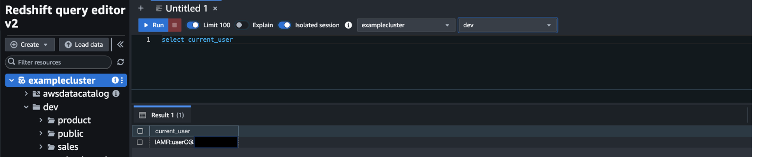
  2. Set the context of database to sample_data_dev in Query Editor v2, as shown in the following screenshot.
    Set the database context
  3. Run cell #3 from demo notebook to diagnose a query performance issue related to nested loop joins.
    Step 3

The query takes around 12 seconds to run, as shown in the Query Editor v2 results panel in the following screenshot.

Step 4 results

  1. Run cell #5 to capture the query id from the SYS_QUERY_HISTORY system view filtering based on the query label you set in the preceding step.Cell 5
  2. On the Amazon Redshift console, in the navigation pane, select Query and loads and choose the cluster name where the query was originally executed, as shown in the following screenshot.
    Query and loads
  3. This will open the new Query profiler. Under the Query history section, choose Connect to database.After successful connection to the database, you will observe the Status showing as Connected and displaying the query history, as shown in the following screenshot.
    Connec to database
  4. You can find your queries either by Query ID or Process ID. Enter the Query ID captured in the preceding step to filter the long-running query for further analysis and choose the corresponding Query ID, as shown in the following screenshot.
    Search query
  5. Under the Query plan section, choose Child query 1, as shown in the following screenshot. If there are multiple child queries, you will have to inspect each one for performance issues.
    Child queryThis will open the query plan in a tree view along with additional metrics on the side panel. This allows you to quickly analyze the query streams, segments and steps. For more information about streams, segments, and steps, refer to Query planning and execution workflow in the Amazon Redshift Database Developer Guide.
  6. Turn on View streams and, in the Streams side panel, investigate and identify which stream has the highest execution time. In this case, Streams ID 5 is where the query spends the majority of time, as shown in the following screenshot
    Enable view stream
  7. In the Streams side panel, under ID, select 5 to focus on Stream 5 for further analysis. Stream 5 shows a step of Nestloop, as shown in the following screenshot.
    Nestloop step
  8. Choose the Nestloop step to further analyze. The side panel will change with step details and additional metrics about the nested loop join.
  9. By looking at Step details – nestloop, we can inspect the Input rows and compare that with the Output rows, as shown in the following screenshot. In this case, due to the cross-joining with the Store_returns table, 287,514 input rows explodes to 950,233,770 rows, thus causing our query to run slower.
    Nestloop step details
  10. Fix the query by introducing a join condition between the store_sales and store_returns. Run cell #7 from Query editor v2 demo notebook.The re-written query runs in just 307 milliseconds.Cell 7

Use case 2: Suboptimal data distribution

  1. To demonstrate suboptimal data distribution, change the distribution style of tables web_sales and web_returns to EVEN by running cell #10 of Query editor v2 demo notebook.Cell 10
  1. Run cell #12. The query takes 409 milliseconds to run, as shown by the elapsed time in the following screenshot of the Query editor v2.Cell 12
  2. Follow steps 3–10 from use case 1 to locate the query_id and to open the Query profiler view for the preceding query.
  3. On the Query profiler page for the preceding query, turn on View streams. In the Streams side panel, investigate and identify which stream has the highest execution time. In this case, Stream ID 6 is where the query spends a majority of the time, as shown in the following screenshot.
    View streams
  4. Under ID, select 6 from the Streams side panel for further analysis.
    Streams side panel

Stream 6 shows a step of hash join, which involves a hash join of two tables that are both redistributed. This can be inferred from Hash Right Join DS_DIST_BOTH under Explain plan node information in the following screenshot. Usually, these redistributions occur because the tables aren’t joined on their distribution keys, or they don’t have the correct distribution style. In the case of large tables, these redistributions can lead to significant performance degradation and, hence, it is important to identify and fix such steps to optimize query performance.

Hashjoin step

  1. Fix this suboptimal data distribution pattern by choosing the appropriate distribution keys on the tables involved: web_sales and web_returns. To change the distribution styles, run cell #14 of demo notebook to alter table commands.
    Cell 14
  2. After the preceding commands finish running, run cell #16 to re-execute the select query. As shown in the Query Editor in the following screenshot, now the same query finished in 244 milliseconds after updating the distribution style to key for tables web_sales and web_returns.
    Cell 16

  3. In the Query profiler view, turn on View streams and notice that Streams 5 now took the most time. It took 8 milliseconds to finish, as compared to 13 milliseconds in the preceding step.
    View streams
  4. In the Streams side panel, under ID, select 5 to drill down further, then choose the Hashjoin As the following screenshot shows, after changing the distribution style to key for both web_sales and web_return tables, none of the tables need to be redistributed at the query runtime, resulting in optimized performance.
    Hashjoin step

Considerations

Consider the following details while using Query profiler:

  1. Query profiler displays information returned by the SYS_QUERY_HISTORY, SYS_QUERY_EXPLAIN, SYS_QUERY_DETAIL, and SYS_CHILD_QUERY_TEXT views.
  2. Query profiler only displays query information for queries that have recently run on the database. If a query completes using a prepopulated resultset cache, Query profiler won’t have information about it because Amazon Redshift doesn’t generate a query plan for such queries.
  3. Queries run by Query profiler to return the query information run on the same data warehouse as the user-defined queries.

Clean Up

To avoid unexpected costs, complete the following action to delete the resources you created:

Drop all the tables in the sample_data_dev under tpcds schema.

Conclusion

In this post, we discussed how to use Amazon Redshift Query profiler to monitor and troubleshoot long-running queries. We demonstrated a step-by-step approach to analyze query performance by examining the query execution plan and statistics and identifying the root cause of query slowness. Try this feature in your environment and share your feedback with us.


About the Authors

Raks KhareRaks Khare is a Senior Analytics Specialist Solutions Architect at AWS based out of Pennsylvania. He helps customers across varying industries and regions architect data analytics solutions at scale on the AWS platform. Outside of work, he likes exploring new travel and food destinations and spending quality time with his family.

Blessing Bamiduro is part of the Amazon Redshift Product Management team. She works with customers to help explore the use of Amazon Redshift ML in their data warehouse. In her spare time, Blessing loves travels and adventures.

Ekta Ahuja is an Amazon Redshift Specialist Solutions Architect at AWS. She is passionate about helping customers build scalable and robust data and analytics solutions. Before AWS, she worked in several different data engineering and analytics roles. Outside of work, she enjoys landscape photography, traveling, and board games.

Apache HBase online migration to Amazon EMR

Post Syndicated from Dalei Xu original https://aws.amazon.com/blogs/big-data/apache-hbase-online-migration-to-amazon-emr/

Apache HBase is an open source, non-relational distributed database developed as part of the Apache Software Foundation’s Hadoop project. HBase can run on Hadoop Distributed File System (HDFS) or Amazon Simple Storage Service (Amazon S3), and can host very large tables with billions of rows and millions of columns.

The followings are some typical use cases for HBase:

  • In an ecommerce scenario, when retrieving detailed product information based on the product ID, HBase can provide a quick and random query function.
  • In security assessment and fraud detection cases, the evaluation dimensions for users vary. HBase’s non-relational architectural design and ability to freely scale columns help cater to the complex needs.
  • In a high-frequency, real-time trading platform, HBase can support highly concurrent reads and writes, resulting in higher productivity and business agility.

Recommended HBase deployment mode

Starting with Amazon EMR 5.2.0, you have the option to run Apache HBase on Amazon S3.

Running HBase on Amazon S3 has several added benefits, including lower costs, data durability, and easier scalability. And during HBase migration, you can export the snapshot files to S3 and use them for recovery.

Recommended HBase migration mode

For existing HBase clusters (including self-built based on open source HBase or provided by vendors or other cloud service providers), we recommend using HBase snapshot and replication technologies to migrate to Apache HBase on Amazon EMR without significant downtime of service.

This blog post introduces a set of typical HBase migration solutions with best practices based on real-world customers’ migration case studies. Additionally, we deep dive into some key challenges faced during migrations, such as:

  • Using HBase snapshots to implement initial migration and HBase replication for real-time data migration.
  • HBase provided by other cloud platforms doesn’t support snapshots.
  • A single table with large amounts of data, for example more than 50 TB.
  • Using BucketCache to improve read performance after migration.

HBase snapshots allow you to take a snapshot of a table without too much impact on region servers, snapshots, clones, and restore operations don’t involve data copying. Also, exporting a snapshot to another cluster has little impact on the region servers.

HBase replication is a way to copy data between HBase clusters. It allows you to keep one cluster’s state synchronized with that of another cluster, using the write-ahead log (WAL) of the source cluster to propagate changes. It can work as a disaster recovery solution and also provides higher availability in the architecture.

Prerequisites

To implement HBase migration, you must have the following prerequisites:

Solution summary

In this example, we walk through a typical migration solution, which is from the source HBase on HDFS cluster (Cluster A) to the target Amazon EMR HBase on S3 (Cluster B). The following diagram illustrates the solution architecture.

Solution architecture

To demonstrate the best practice recommended to the HBase migration process, the following are the detailed steps we will walk through, as shown in the preceding diagram.

Step Activity Description Estimated time
1

Configure cluster A

(Source HBase)

Modify the configuration of the source HBase cluster to prepare for subsequent snapshot exports Less than 5 minutes
2

Create cluster B

(Amazon EMR HBase on S3)

Create an EMR cluster with HBase on Amazon S3 as the migration target cluster Less than 10 minutes
3 Configure replication Configure replication from the source HBase cluster to Amazon EMR HBase, but do not start Less than 1 minute
4 Pause service Pause the service of the source HBase cluster Less than 1 minute
5 Create snapshot Create a snapshot for each table on the source HBase cluster Less than 5 minutes
6 Resume service Resume the service of the source HBase cluster Less than 1 minute
7 Snapshot export and restore Use snapshot to migrate data from the source HBase cluster to the Amazon EMR HBase cluster Depends on the size of the table data volume
8 Start replication Start the replication of the source HBase cluster to Amazon EMR HBase and synchronize incremental data Depends on the size of the data accumulated during the snapshot export restore.
9 Test and verify Test the and verify the Amazon EMR HBase

Solution walkthrough

In the preceding diagram and table, we have listed the operational steps of the solution. Next, we will elaborate the specific operations for each step shown in the preceding table.

1. Configure cluster A (source HBase)

When exporting a snapshot from the source HBase cluster to the Amazon EMR HBase cluster, you must modify the following settings on the source cluster to ensure the performance and stability of data transmission.

Configuration classification Configuration item Suggested value Comment
core-site fs.s3.awsAccessKeyId Your AWS access key ID The snapshot export takes a relatively long time. Without an access key and secret key, the snapshot export to Amazon S3 will encounter errors such as com.amazon.aws.emr.hadoop.fs.shaded.com. amazonaws.SdkClientException: Unable to load AWS credentials from any provider in the chain.
core-site fs.s3.awsSecretAccessKey Your AWS secret access key
yarn-site yarn.nodemanager.resource.memory-mb Half of a single core node RAM The amount of physical memory, in MB, that can be allocated for containers.
yarn-site yarn.scheduler.maximum-allocation-mb Half of a single core node RAM The maximum allocation for every container request at the ResourceManager in MB. Because snapshot export runs in the YARN Map Reduce task, it’s necessary to allocate sufficient memory to YARN to ensure transmission speed.

These values are set depending on the cluster resource, workload, and table data volume. The modification can be done using a web UI if available or by suing a standard configuration XML file. Restart the HBase service after the change is complete.

2. Create cluster B (EMR HBase on S3)

Use the following recommend settings to launch an EMR cluster:

Configuration classification Configuration item Suggested value Comment
yarn-site yarn.nodemanager.resource.memory-mb 20% of a single core node RAM Amount of physical memory, in MB, that can be allocated for containers.
yarn-site yarn.scheduler.maximum-allocation-mb 20% of a single core node RAM The maximum allocation for every container request at the ResourceManager in MB. Because snapshot restore runs in the HBase, it’s necessary to allocate a small amount of small memory to YARN and leave sufficient memory to HBase to ensure restore.
hbase-env.export HBASE_MASTER_OPTS 70% of a single core node RAM Set the Java heap size for the primary HBase.
hbase-env.export HBASE_REGIONSERVER_OPTS 70% of a single core node RAM Set the Java heap size for the HBase region server.
hbase hbase.emr.storageMode S3 Indicates that HBase uses S3 to store data.
hbase-site hbase.rootdir <Your-HBase-Folder-on-S3> Your HBase data folder on S3.

See Configure HBase for more details. Additionally, the default YARN configuration on Amazon EMR for each Amazon EC2 instance type can be found in Task configuration.

The configuration of our example is as shown in the following figure.

Instance group configurations

3. Config replication

Next, we configure the replication peer from the source HBase to the EMR cluster.

The operations include:

  • Create a peer.
  • Because the snapshot migration hasn’t been done, we start by disabling the peer.
  • Specify the table that requires replication for the peer.
  • Enable table replication.

Let’s use the table usertable as an example. The shell script is as follows:

MASTER_IP="<Master-IP>"
TABLE_NAME="usertable"
cat << EOF | sudo -u hbase hbase shell 2>/dev/null
add_peer 'PEER_$TABLE_NAME', CLUSTER_KEY => '$MASTER_IP:2181:/hbase'
disable_peer 'PEER_$TABLE_NAME'
enable_table_replication '$TABLE_NAME'
EOF

The result will like the following text.

hbase:001:0> add_peer 'PEER_usertable', CLUSTER_KEY => '<Master-IP>:2181:/hbase'
Took 13.4117 seconds 
hbase:002:0> disable_peer 'PEER_usertable'
Took 8.1317 seconds 
hbase:003:0> enable_table_replication 'usertable'
The replication of table 'usertable' successfully enabled
Took 168.7254 seconds

In this experiment, we’re using the table usertable as an example. If we have many tables that need to be configured for replication, we can use the following code:

MASTER_IP="<Master-IP>"

# Get all tables
TABLE_LIST=$(echo 'list' | sudo -u hbase hbase shell 2>/dev/null | sed -e '1,/TABLE/d' -e '/seconds/,$d' -e '/row/,$d')
# Iterate each table
for TABLE_NAME in $TABLE_LIST; do
# Add the operation
cat << EOF | sudo -u hbase hbase shell 2>/dev/null
add_peer 'PEER_$TABLE_NAME', CLUSTER_KEY => '$MASTER_IP:2181:/hbase'
disable_peer 'PEER_$TABLE_NAME'
enable_table_replication '$TABLE_NAME'
EOF
done

In the scripts of following steps, if you need to apply the operations for all tables, you can refer to the preceding code sample.

At this point, the status of the peer is Disabled, so replication won’t be started. And the data that needs to be synchronized from the source to the target EMR cluster will be backlogged at the source HBase cluster and won’t be synchronized to HBase on the EMR cluster.

After the snapshot restore (step 7) is completed on the HBase on Amazon EMR cluster, we can enable the peer to start synchronizing data.

If the source HBase version is 1.x, you must run the set_peer_tableCFs function. See HBase Cluster Replication.

4. Pause the service

To pause the service of the source HBase cluster, disable the HBase tables. You can use the following script:

sudo -u hbase bash /usr/lib/hbase/bin/disable_all_tables.sh 2>/dev/null

The result is shown in the following figure.

Disable all tables

After disabling all tables, observe the HBase UI to ensure that no background tasks are being run, and then stop any services accessing the source HBase. This will take 5-10 minutes.

The HBase UI is as shown in the following figure.

Check background tasks

5. Create a snapshot

Make sure the tables in the source HBase are disabled. Then, you can create a snapshot of the source. This process will take 1-5 minutes.

Let’s use the table usertable as an example. The shell script is as follows:

DATE=`date +"%Y%m%d"`
TABLE_NAME="usertable"
sudo -u hbase hbase snapshot create -n "${TABLE_NAME/:/_}-$DATE" -t ${TABLE_NAME} 2>/dev/null

You can check the snapshot with a script:

sudo -u hbase hbase snapshot info -list-snapshots 2>/dev/null

And the result is as shown in the following figure.

Create snapshot

6. Resume service

After the snapshot is successfully created on the source HBase, you can enable the tables and resume the services that access the source HBase. These operations take several minutes, so the total data unavailability time on the source HBase during the implementation (steps 3 to step 6) will be approximately 10 minutes.

The command to enable the table is as follows:

TABLE_NAME="usertable"
echo -e "enable '$TABLE_NAME'" | sudo -u hbase hbase shell 2>/dev/null

The result is shown in the following figure.

Enable table

At this point, you can write data to the source HBase, because the status of the replication peer is disabled, so the incremental data won’t be synchronized to the target cluster.

7. Snapshot export and restore

After the snapshot created in the source HBase, it’s time to export the snapshot to the HBase data directory on the target EMR cluster. The example script is as follows:

DATE=`date +"%Y%m%d"`
TABLE_NAME="usertable"
TARGET_BUCKET="<Your-HBase-Folder-on-S3>"
nohup sudo -u hbase hbase snapshot export -snapshot ${TABLE_NAME/:/_}-$DATE -copy-to $TARGET_BUCKET &> ${TABLE_NAME/:/_}-$DATE-export.log &

Exporting the snapshot will take from 10 minute to several hours to complete, depending on the amount of data to be exported. So we run it in the background. You can check the progress by using the yarn application -list command, as shown in the following figure.

Exporting snapshot process

As an example, if you’re using an HBase cluster with 20 r6g.4xlarge core nodes, it will take about 3 hours for 50 TB of data to be exported to Amazon S3 in same AWS Region.

After the snapshot export is completed at the source HBase, you can check the snapshot in the target EMR cluster using the following script:

sudo -u hbase hbase snapshot info -list-snapshots 2>/dev/null

The result is shown in the following figure.

Check snapshot

Confirm the snapshot name—for example, usertable-20240710 and run snapshot restore on the target EMR cluster using the following script.

TABLE_NAME="usertable"
SNAPSHOT_NAME="usertable-20240710"
cat << EOF | nohup sudo -u hbase hbase shell &> restore-snapshot.out &
disable '$TABLE_NAME'
restore_snapshot '$SNAPSHOT_NAME'
enable '$TABLE_NAME'
EOF

The snapshot restore will take from 10 minute to several hours to complete, depending on the amount of data to be restored, so we run it in the background. The result is as shown in the following figure.

Restore snapshot

You can check the progress of the restore through The Amazon EMR web interface for HBase, as shown in the following figure.

Check snapshot restore

From the Amazon EMR web interface for HBase, you can found it takes about 2 hours to run Clone Snapshot for a sample table with 50 TB of data, and then 1 additional hour to run . After these two stages, the snapshot restore is completed.

8. Start replication

After the snapshot restore is completed on the EMR cluster and the status of the table is set to enabled, you can enable HBase replication in the source HBase. The incremental data will be synchronized to the target EMR cluster.

In the source HBase, the example script is as follows:

TABLE_NAME="usertable"
echo -e "enable_peer 'PEER_$TABLE_NAME'" | sudo -u hbase hbase shell 2>/dev/null

The result is as shown in the following figure.

Enable peer

Wait for the incremental data to be synchronized from the source HBase to the HBase on EMR cluster. The time taken depends on the amount of data accumulated in the source HBase during the snapshot export and restore. In our example, it took about 10 minutes to complete the data synchronization.

You can check the replication status with scripts:

echo -e "status 'replication'" | sudo -u hbase hbase shell 2>/dev/null

The result is shown in the following figure.

Replication status

9. Test and verify

After incremental data synchronization is complete, you can start testing and verifying the results. You can use the same HBase API to access both the source and the target HBase clusters and compare the results.

To guarantee the data integrity, you can check the number of HBase table region and store files for the replicated tables from the Amazon EMR web interface for HBase, as shown in the following figure.

Check hbase region and store files

For small tables, we recommend using the HBase command to verify the number of records. After signing in to the primary node of the Amazon EMR using SSH, you can run the following command:

sudo -u hbase hbase org.apache.hadoop.hbase.mapreduce.RowCounter 'usertable'

Then, in the hbase.log file of the HBase log directory, find the number of records for the table usertable.

For large tables, you can use the HBase Java API to validate the row count in a range of row keys.

We provided sample Java code to implement this functionality. For example, we imported the demo data to usertable using the following script:

java -classpath hbase-utils-1.0-SNAPSHOT-jar-with-dependencies.jar HBaseAccess <Your-Zookeeper-IP> put 1000 20

The result is shown in the following figure.

Put demo data into HBase table

You can run the script multiple times to import enough demo data into the table, then you can use the following script to count the number of records where the value of Row Key is between user1000 and user5000, and the value of the column family:field0 is value0

java -classpath hbase-utils-1.0-SNAPSHOT-jar-with-dependencies.jar HBaseRowCounter <Your-Zookeeper-IP> usertable "user1000" "user1100" "family:field0" "value0"

The result is shown in the following figure.

HBase table row counter

You can run the same code on both the source HBase and the target Amazon EMR HBase to verify that the results are consistent. See complete code.

After these steps are complete, you can switch from the source HBase to the target Amazon EMR Hbase, completing the migration.

Clean up

After you’re done with the solution walkthrough, complete the following steps to clean up your resources:

  1. Stop the Amazon EMR on EC2 cluster.
  2. Delete the S3 bucket that stores the HBase data.
  3. Stop the source HBase cluster, and release its related resource, for example, the Amazon EC2 cluster or resources provided by other vendors or cloud service providers.

Key challenges in HBase migration

In the previous sections, we have detailed the steps to implement HBase online migration through snapshots and replication for general scenario. Many customers’ scenarios may have some differences from the general scenario, and you need to make some modifications to the process steps in order to accomplish the migration.

HBase in the cloud doesn’t support snapshot

Many cloud providers have made modifications to the open source version of HBase, resulting in these versions of HBase not providing snapshot and replication functions. However, these cloud providers will provide data transfer tools for HBase, such as Lindorm Tunnel Service, that can be used to transfer HBase data to an HBase cluster with data on HDFS.

To deploy HBase on Amazon S3, you should follow the previous migration process as the best practice, using snapshot and replication techniques to migrate to an Amazon EMR environment. To solve the problem of HBase versions that don’t support snapshots and replication, you can create an HBase on HDFS as a jump or relay cluster, which can be used to synchronize the data from a source HBase to an HDFS-based HBase cluster, then migrate from the middle cluster to the target HBase on S3.

The following diagram illustrates the solution architecture.

Solution architecture for HBase in the cloud doesn’t support snapshot

You need to add three more steps in addition to the migration steps described previously.

Step Activity Description Estimated time
1

Create Cluster B

(EMR HBase on HDFS)

Create an EMR cluster with HBase on HDFS as the relay cluster. Less than 10 minutes
2 Configure data transfer Configure the data transfer from the outer HBase cluster to Amazon EMR HBase on HDFS and start the data transfer. Less than 5 minutes
3

HBase migration

(snapshot and replication)

Treat the outer HBase cluster as an application which writes data into the Amazon EMR HBase cluster, then you can use the steps in the previous scenario to complete the migration to Amazon EMR HBase on Amazon S3.

Single table with large amounts of data

During the migration process, if the amount of data in a single table in the source HBase (Cluster A) is too large—such as 10 TB or even 50TB—you must modify the target Amazon EMR HBase cluster (Cluster B) configuration to ensure that there are no interruptions during the migration process, especially during the snapshot restore on the Amazon EMR HBase cluster. After the snapshot restore is complete, you can rebuild the Amazon EMR HBase cluster (Cluster C).

The following diagram illustrates the solution architecture for handling a very large table.

Solution architecture for handling a very large table

The following are the steps.

Step Activity Description Estimated time
1 Create Cluster B (EMR HBase on S3 for restore) Create an EMR cluster with the required configuration for a large table snapshot restore. Less than 10 minutes
2

HBase migration

(snapshot and replication)

Consider the Amazon EMR HBase on Amazon S3 as the target cluster, then you can use the steps in the first scenario to complete the migration from the source HBase to the Amazon EMR HBase on S3.
3

Recreate Cluster C

(EMR HBase on S3 for production)

After the migration is complete, Cluster B needs to be changed back to its previous configuration before migration. If it’s inconvenient to modify the parameters, you can use the previous configuration to recreate the EMR cluster (Cluster C). Less than 15 minutes
4 Rebuild replication After recreating the EMR cluster, if replication is still needed to synchronize the data, the replication from the source HBase cluster to the new EMR HBase cluster must be rebuilt. Before building the new EMR cluster, the write service on the source HBase cluster should be paused to avoid data loss on the Amazon EMR HBase. Less than 1 minute

In Step 1, create cluster B (EMR HBase on S3 for restore), use the following configuration for snapshot restore. All time values are in milliseconds.

Configuration classification Configuration item Default value Suggested value Explanation
emrfs-site fs.s3.maxConnections 1000 50000 The number of concurrent Amazon S3 connections that your applications need. The default value is 1000 and must be increased to avoid errors such as com. amazon. ws. emr. hadoop. fs. shaded. com. amazonaws. SdkClientException: Unable to execute HTTP request: timeout waiting for connection from pool.
hbase-site hbase.client.operation.timeout 300000 18000000 Operation timeout is a top-level restriction that makes sure a blocking operation in a table will not be blocked for longer than the timeout.
hbase-site hbase.master.cleaner.interval 60000 18000000 The default is to run HBase Clearer in 60,000 milliseconds, which will clear some files in the archive, resulting in an error that HFile cannot be found.
hbase-site hbase.rpc.timeout 60000 18000000 This property limits how long a single RPC call can run before timing out.
hbase-site hbase.snapshot.master.timeout.millis 300000 18000000 Timeout for the primary HBase for the snapshot procedure.
hbase-site hbase.snapshot.region.timeout 300000 18000000 Timeout for region servers to keep threads in a snapshot request pool waiting.
hbase-site hbase.hregion.majorcompaction 604800000 0

Default is 604,800,000 ms (1 week). Set to 0 to disable automatic triggering of compaction. Note that because of the change to manual triggering, you must make compaction one of the daily operation and maintenance tasks, and run it during periods of low activity to avoid impacting production. The following is the compaction script:

echo -e "major_compact '$TABLE_NAME'" | sudo -u hbase hbase shell

Adjust the suggested values based on the amount of table data, which requires conducting some experiments to determine the values to be used in the final migration plan.

Before you recreate a new EMR cluster in the production environment, disable the HBase table on the active EMR cluster. The command line is as follows:

sudo -u hbase bash /usr/lib/hbase/bin/disable_all_tables.sh 2>/dev/null
echo -e "flush 'hbase:meta'" | sudo -u hbase hbase shell 2>/dev/null

Wait for the command to execute successfully and terminate the current EMR cluster (Cluster B). Now the HBase data is kept in Amazon S3; create a new EMR cluster (Cluster C) with the previous configuration before migration, and specify HBase date folder on S3 to be the same as Cluster B.

Using Bucket Cache to improve read performance

To enhance HBase’s read performance, one of most effective method involves caching data. HBase uses BlockCache to implement caching mechanisms for the region server. Currently, HBase provides two different BlockCache implementations to cache data read from HDFS: the default on-heap LruBlockCache and the BucketCache, which is usually off-heap. Bucket cache is the most used method.

BucketCache can be deployed in offheap, file, or mmaped file mode. These three working modes are the same in terms of memory logical organization and caching process; however, the final storage media corresponding to these three working modes are different, that is, the IOEngine is different.

We recommend that customers use BucketCache in file mode, because the default storage type of Amazon Elastic Block Store (Amazon EBS) in Amazon EMR is SSD. You can put all hot data into BucketCache, which is on Amazon EBS. You can then determine the file size used by BucketCache based on the volume of hot data.

The following are the HBase configurations for BucketCache.

Configuration classification Configuration item Suggested value Explanation
emrfs-site hbase.bucketcache.ioengine files:/mnt1/hbase/cache_01.data Where to store the contents of the bucket cache. You can use offheap, file, files, mmap, or pmem. If a file or files, set it to files. Note that some earlier Amazon EMR versions can only support using one file per core node.
hbase-site hbase.bucketcache.persistent.path file:/mnt1/hbase/cache.meta The path to store the metadata of the bucket cache, used to recover the cache during startup.
hbase-site hbase.bucketcache.size Depends on the hot data volume be cached The capacity in MBs of BucketCache for each core node. If you use multiple cache files, then this size is the sum of the capacities of multiple files.
hbase-site hbase.rs.prefetchblocksonopen TRUE Whether the server should asynchronously load all the blocks when a store file is opened (data, metadata, and index). Note that enabling this property contributes to the time the region server takes to open a region and therefore initialize.
hbase-site hbase.rs.cacheblocksonwrite TRUE Whether an HFile block should be added to the block cache when the block is finished.
hbase-site hbase.rs.cachecompactedblocksonwrite TRUE Whether to cache compressed blocks during writing.

More configuration instructions for BucketCache would refer to Configuration properties.

We provided sample Java code to test HBase read performance. In the Java code, we use the putDemoData method to write test data to the table usertable, ensuring that the data is evenly distributed across HBase table regions, and then use the getDemoData method to read the data.

We tested three scenarios: HBase data stored on HDFS, on Amazon S3 without using BucketCache, and on S3 using BucketCache. To ensure that the written data isn’t cached in the first two scenarios, the cache can be cleared by restarting the the region servers.

We tested on the EMR HBase cluster, which has 10 r6g. 2xlarge core nodes. The command is as follows:

java -classpath hbase-utils-1.0-SNAPSHOT-jar-with-dependencies.jar HBaseAccess <Your-Zookeeper-IP> get 20 100

The result is shown in the following figure.

Read HBase table

Benchmark results and key learning

For the three scenarios, we use 100 HBase record row keys as input, ensure these row keys distributed evenly in HBase table regions, we call the API consecutively with 20 times, 50 times, and 100 times, and we got the time cost result as the following figure. We found the read latency is the shortest when the data is on S3 and using BucketCache.

Read performance

Above, we introduced four migration scenarios. In migration processes in production, we’ve gained invaluable knowledge and experience. We’re sharing the results here for you to use as best practices and a recommended run book.

Configuration parameters

In the configurations provided earlier, some are necessary for BucketCache settings while others mitigate known errors to reduce the snapshot duration. For example, the parameter hbase.snapshot.master.timeout.millis is related to the HBASE-14680 issue. It’s advisable to retain these configurations as much as possible throughout the migration process.

Version choice

When migrating to Amazon EMR and choosing a suitable HBase version, it is recommended to select a more recent minor version and patch version, while keeping the major version unchanged. That is to say:

  • If the source HBase is version 1.x, we recommend using EMR 5.36.1, whose HBase version is 1.4.13, because the HBase 1.x API is compatible and won’t require you to make code changes.
  • If the source HBase is version 2.x, we recommend using EMR 6.15.0, which has an HBase of 2.4.17.

The HBase API under the same major version can be universal. See HBase Version to learn more.

Allocating enough space

HDFS needs to leave enough space when exporting snapshots, it depends on the data volume. Data will be moved to the archive, causing double storage is needed for the table.

Replication

At present, there is compatibility problem if replication and WAL compression are used together. If you are using replication, set the hbase.regionserver.wal.enablecompression property to false. See HBASE-26849 for more information.

By default, replication in HBase is asynchronous, as the write-ahead log (WAL) is sent to another cluster in the background. This implies that when using replication for data recovery, some data loss may occur. Additionally, there is a potential for data overwrite conflicts when concurrently writing the same record within a short time frame. However, HBase v2.x introduces synchronous replication as a solution to this issue. For more details, refer to the Serial Replication documentation.

Disk type for BucketCache

Because BucketCache uses a portion of Amazon EBS IO and throughput to synchronize data, it’s recommended to choose Amazon EBS gp3 volumes for their higher IOPS and throughput.

Response latency when accessing to HBase

Users sometimes face the issue of high response latency from their Hbase on EMR clusters using API calls or the HBase shell tool.

In our testing, we found that the communication between HMaster and RegionServer takes an unusually long time to resolve through DNS. You can reduce latency by adding the host name and IP mapping to the /etc/hosts file in the HBase client host.

Conclusion

In this post, we used the results of real-world migration cases to introduce the process of migrating HBase to Amazon EMR HBase using HBase snapshot and replication and the deployment mode of HBase on Amazon S3. We included how to resolve challenges, such as how to configure the cluster to make the migration process smoother when migrating a single large table, or how to use BucketCache to improve reading performance. We also described techniques for testing performance.

We encourage you to migrate HBase to Amazon EMR HBase. For more information about HBase migration, see Amazon EMR HBase best practices.


About the Authors

Dalei XuDalei Xu is a Analytics Specialist Solution Architect at Amazon Web Services, responsible for consulting, designing, and implementing AWS data analytics solutions. With over 20 years of experience in data-related work, proficient in data development, migration to AWS, architecture design, and performance optimization. Hoping to promote AWS data analytics services to more customers, achieving a win-win situation and mutual growth with customers.

Zhiyong Su is a Migration Specialist Solution Architect at Amazon Web Services, primarily responsible for cloud migration or cross-cloud migration for enterprise-level clients. Has held positions such as R&D Engineer, Solutions Architect, and has years of practical experience in IT professional services and enterprise application architecture.

Shijian TangShijian Tang is a Analytics Specialist Solution Architect at Amazon Web Services.

Infor’s Amazon OpenSearch Service Modernization: 94% faster searches and 50% lower costs

Post Syndicated from Allan Pienaar original https://aws.amazon.com/blogs/big-data/infors-amazon-opensearch-service-modernization-94-faster-searches-and-50-lower-costs/

This post is cowritten by Arjan Hammink from Infor.

Robust storage and search capabilities are critical components of Infor’s enterprise business cloud software. Infor’s Intelligent Open Network (ION) OneView platform provides real-time reporting, dashboards, and data visualization to help customers access and analyze information across their organization. To enhance the search functionality within ION OneView, Infor used Amazon OpenSearch Service to improve their software products and offer better service to their customers by providing real-time visibility. By modernizing their use of OpenSearch Service, Infor has been able to deliver a 94% improvement in search performance for customers, along with a 50% reduction in storage costs.

In this post, we’ll explore Infor’s journey to modernize its search capabilities, the key benefits they achieved, and the technologies that powered this transformation. We’ll also discuss how Infor’s customers are now able to more effectively search through business messages, documents, and other critical data within the ION OneView platform.

Where Infor started

Infor’s ION OneView was built on top of Elasticsearch v5.x on Amazon OpenSearch Service, hosted across eight AWS Regions. This architecture enabled users to track business documents from a consolidated view, search using various criteria, and correlate messages while viewing content based on user roles. Over time, Infor expanded its functionality to include “Enrich” and “Archive” capabilities, which added significant complexity. The Enrich process would build searchable messages by aggregating related events, requiring constant document updates to the OpenSearch indices. The Archive process would then move these messages and events to Amazon Simple Storage Service (Amazon S3), while using a delete_by_query to remove the corresponding documents from OpenSearch Service. These read-update-write-delete workloads, coupled with large all-encompassing indices with shard sizes of over 100GB, resulted in high volumes of deleted documents and exponential data growth that the system struggled to keep up with. To address increasing performance needs, Infor continually horizontally scaled out their OpenSearch Service domain.

Challenges 

The key challenges Infor faced underscored the need for a more scalable, resilient, and cost-effective search capability that could seamlessly integrate with their cloud environment. These included the inability to effectively archive data because of high ingestion rates, resulting in longer upgrade and recovery times. Escalating costs from scaling the solution and the need for custom development to enable newer OpenSearch Service features created significant operational burdens. Additionally, Infor was seeing increasing search latency, with CPU utilization peaking at 75% and occasionally spiking above 90% (as shown in the following figures), demonstrating the performance limitations of Infor’s existing infrastructure. Collectively, these issues drove Infor’s need for a modernized search solution.

SearchLatency Pre-Modernization

Screenshot shows CloudWatch metric SearchLatency before Modernization

CPUUtilization Pre-Modernization

Screenshot shows CloudWatch metric CPUUtilization before Modernization

Infor’s journey to modernize search with OpenSearch Service

To address the growing challenges with ION OneView, Infor partnered with AWS to undertake a comprehensive modernization effort. This involved optimizing operational processes, storage configurations, and instance selections, while also upgrading to the later versions within OpenSearch Service.

Operational review and enhancements

As a collaborative effort between Infor and AWS, a comprehensive operational review of Infor’s OpenSearch Service cluster was undertaken. With the help of slow logs and adjusting the logging thresholds, the review was able to identify long-running queries and the archival process consuming the largest amount of CPU capacity. Infor rewrote the long-running queries that used high cardinality fields, reducing the average query time.

Next, the team turned their attention to redesigning Infor’s archival process to reduce stress on the CPU. Instead of a single large index, we implemented independent indices based on customer license types. This improved delete performance by allowing the team to target old indices, using index aliases to manage the transition. We also replaced the delete_by_query approach where a query is sent to locate documents prior to a delete with a standard delete passing document IDs directly, because all the document IDs to be archived were known ahead of time. This reduced round-trip time and CPU stress compared to the sequential search requests performed by delete_by_query. This was followed by the tuning of the refresh interval based on the workload requirements, improving the indexing performance, and memory and CPU utilization.

Storage optimization

The team switched from GP2 to GP3 storage, provisioning additional input/output operations per second (IOPS) and throughput only when needed. This resulted in a 9% reduction in storage costs for most of Infor’s workloads. In all use cases where IOPS was a bottleneck, the team was able to provision additional IOPS and throughput independent of the volume size using GP3, further reducing Infor’s overall storage costs. Additionally, we implemented a shard size-based rollover strategy that provided a sharding strategy where total shards were divisible by the number of nodes to reduce the shard size to the recommended number of less than 50 GiB. This helped ensure an even distribution of data and workloads across the nodes for each index, and the performance improvements indicated that more vCPU would be beneficial given the thread pool queues and latencies. Appropriate master and data node instance types were chosen based on the new storage requirements. To support the reindexing process, the team also temporarily scaled up the storage and compute resources.

Upgrading OpenSearch Service

After optimizing the storage and compute configurations based on best practices, the Infor ION team turned their attention to using the latest features of OpenSearch Service. With the shards now at an appropriate boundary and the memory and CPU utilization at the right levels, the team was able to seamlessly upgrade from Elasticsearch version 5.x to 6.x and then to 7.x in OpenSearch Service. Each major version upgrade required careful testing and client-side code changes to make sure that the appropriate compatible client libraries were used, and the team took the necessary time after each upgrade to thoroughly validate the system and provide a smooth transition for Infor’s customers. This commitment to a methodical upgrade process allowed Infor to take advantage of the latest OpenSearch Service features, such as Graviton support, performance improvements, bug fixes, and security posture improvements, while minimizing disruption to their users.

Optimizing instance selection for performance

In collaboration with the AWS team, Infor carefully evaluated local non-volatile memory express (NVMe)-backed instance types for their ION OneView search cluster, comparing options such as i3 and R6gd instances to balance memory, latency, and storage requirements. For write-heavy workloads, the team found that using NVMe storage provided better performance and price compared to Amazon Elastic Block Store (Amazon EBS) volumes because of the high IOPS requirement of the workload, allowing them to be less reliant on off-heap memory usage. By selecting the most appropriate instance types, the ION OneView search cluster was able to resize and scale down the number of data nodes by 63% while still achieving improved throughput and reduced latency. Staying on the latest AWS instance families was also a key consideration, and the team further optimized costs by purchasing Reserved Instances after establishing a good baseline for their performance and compute consumption, with discounts ranging from 30% to 50% depending on the commitment term.

Results

The following figures show the improvements of the modernization.

New indices with the correct shard size can be seen in the increase in shards, shown in the following figure.

Figure showing increase in shards with new indices and correct shard size

The updated shard strategy combined with a version upgrade led to a ten-fold increase in the volume of traffic and efficient archiving as shown in the following figure.

Figure illustrates 10x increase in traffic volume and improved archiving due to updated shard strategy and version upgrade

The SearchRate increase is shown in the following figure.

Figure shows increase in SearchRate

The following figure shows that the CPU increase was minimal compared to the traffic increase.

Figure demonstrates CPU increase was minimal compared to traffic increase

The SearchLatency reduction post upgrade and implementation of the new indexing and shard strategy is shown in the following figure.

Figure illustrates reduction in CloudWatch metric SearchLatency after upgrade and new indexing/shard strategy implementation

The following figure shows the monthly spend over the past 4 quarters for two Infor ION products.

Figure shows the monthly spend over 4 quarters for two Infor ION products.

Conclusion

Through their careful modernization of the OpenSearch Service infrastructure, Infor was able to achieve 50% reduction in infrastructure costs coupled with a 94% improvement in cluster performance. The optimized clusters are now healthier and more resilient, enabling faster blue/green deployments to process even greater data volumes.

This successful transformation was driven by Infor’s close collaboration with the AWS team, using deep technical expertise and best practices to accelerate the optimization process and unlock the full potential of OpenSearch Service. Infor’s OpenSearch Service modernization has empowered the company to provide an improved, high-performing search experience for their customers at a significantly lower cost, positioning their ION OneView platform for continued growth and success.

Every workload is unique, with its own distinct characteristics. While the best practices outlined in the Amazon OpenSearch Service developer guide serve as a valuable guide, the most important step is to deploy, test, and continuously tune your own domains to find the optimal configuration, stability, and cost for your specific needs.


About the Authors

Author image of Allan PiennarAllan Pienaar is an OpenSearch SME and Customer Success Engineer at AWS. He works closely with enterprise customers in ensuring operational excellence, maintaining production stability and optimizing cost using the Amazon OpenSearch Service.

Author image of Gokul Sarangaraju Gokul Sarangaraju is a Senior Solutions Architect at AWS. He helps customers adopt AWS services and provides guidance in AWS cost and usage optimization. His areas of expertise include building scalable and cost-effective data analytics solutions using AWS services and tools.

Author image of Arjan Hammink Arjan Hammink is a Senior Director of Software Development at Infor, bringing over 25 years of expertise in software development and team management. He currently oversees Infor ION, a project he has been integral to since its inception in 2010 when he began as a Software Engineer. Infor ION is a robust middleware designed to streamline software integration, a key component of Infor OS, Infor’s cloud technology platform.

How to use interface VPC endpoints to meet your security objectives

Post Syndicated from Joaquin Manuel Rinaudo original https://aws.amazon.com/blogs/security/how-to-use-interface-vpc-endpoints-to-meet-your-security-objectives/

Amazon Virtual Private Cloud (Amazon VPC) endpoints—powered by AWS PrivateLink—enable customers to establish private connectivity to supported AWS services, enterprise services, and third-party services by using private IP addresses. There are three types of VPC endpoints: interface endpoints, Gateway Load Balancer endpoints, and gateway endpoints. An interface VPC endpoint, in particular, allows customers to design applications that connect to AWS services privately, including the more than 130 AWS services that are available over AWS PrivateLink. For a complete list of services that integrate with PrivateLink, see the documentation for VPC endpoints.

The decision regarding when to use interface VPC endpoints to further secure your AWS infrastructure depends on your need for additional security controls or your preferred architecture patterns. In this blog post, we present four security objectives that VPC endpoints help you achieve. It’s important to note that other non-security benefits, such as reduced latency and cost management, are not covered in this post. For more information on those benefits, see these topics:

Background

By default, network packets that originate in the AWS network with a destination on the AWS network (for example, public endpoints for AWS services) stay in the AWS network, except traffic to and from AWS China Regions. In addition, all data flowing across the AWS global network that interconnects AWS data centers and Regions is automatically encrypted at the physical layer before it leaves AWS secured facilities.

AWS PrivateLink VPC endpoints enable customers to further enhance the security posture of their applications by establishing private connectivity to supported AWS services, enterprise services, and third-party services by using a private IP address. You can find patterns for how to use the different types of endpoints in the Securely Access Services Over AWS PrivateLink whitepaper.

An interface VPC endpoint is a collection of one or more elastic network interfaces with private IP addresses. These endpoints can serve as an entry point for traffic destined to a supported AWS service in the same AWS Region as the VPC, without requiring an internet gateway, NAT device, VPN connection, AWS Direct Connect connection, or a public IP. Customers can then use interface VPC endpoints to help meet multiple security objectives, such as the following:

  1. Implement networks that are isolated from the internet
  2. Implement a data perimeter by using VPC endpoint policies
  3. Enable private connectivity to AWS service API endpoints for on-premises environments
  4. Align with specific compliance requirements

In the rest of this post, we’ll discuss each of these objectives in detail and how interface VPC endpoints can help you implement them.

Security objective 1: Implementing networks that are isolated from the internet

If you operate sensitive workloads, you might require that they run in private subnets that are isolated from the internet. In this scenario, the subnets in the network don’t have routes to an internet gateway and won’t be able to either send packets to the internet or receive packets from it.

In this case, you can use interface VPC endpoints to connect your VPC to AWS services in the same Region as if they were in your VPC, without configuring an internet gateway, NAT instance, or route tables. For information on how to configure a cross-Region VPC interface endpoint by using VPC peering, see this guidance.

Figure 1 shows an example architecture with an Amazon Elastic Compute Cloud (Amazon EC2) instance running in an isolated network and using interface VPC endpoints to send messages to Amazon Simple Queue Service (Amazon SQS).

Figure 1

Figure 1: Isolated subnet for EC2 server sending messages to Amazon SQS

Security objective 2: Implement a data perimeter using VPC endpoint policies

A data perimeter is a set of guardrails to help ensure that only your trusted identities are accessing trusted resources from expected networks. Learn more about data perimeters on AWS.

You can use VPC endpoint policies to implement a data perimeter by allowing access to only trusted entities and resources from your network, helping to prevent unintended access. This enables you to take advantage of the power of AWS Identity and Access Management (IAM) policy and flexibility to control access to your resources at a granular level.

In the VPC diagram in Figure 2, EC2 instance traffic flows out through a firewall endpoint, NAT gateway, and internet gateway to reach the S3 public API endpoint, remaining within the AWS network. However, this setup does not allow the implementation of a logical data perimeter to control the specific resources that the EC2 instance can access.

Figure 2

Figure 2: Before implementing a data perimeter

In contrast, in the diagram in Figure 3, you can see how VPC interface endpoints enable the use of VPC endpoint policies to enforce a data perimeter, such as only allowing certain S3 buckets to be accessed by the EC2 instance.

Figure 3

Figure 3: After implementing a data perimeter

For example, you can attach a policy, similar to the one below, to an Amazon S3 interface or gateway VPC endpoint to restrict access from the VPC to only S3 buckets that are owned by the same AWS Organizations organization. Make sure to replace <MY-ORG-ID> with your own information.

{
    "Version": "2012-10-17",
        "Statement": [
        {
            "Effect": "Allow",
            "Principal": "*",
            "Action": "s3:*",
            "Resource": "*",
            "Condition": { "StringEquals": { "aws:ResourceOrgID": <MY-ORG-ID>}}
        }
    ]
}

As a further example, the following policy shows how you can limit access to only trusted identities. You can attach this policy to an S3 interface VPC endpoint to permit access only to principals from your organization, to help mitigate the risk of unintended disclosure through non-corporate credentials. Make sure to replace <MY-ORG-ID> with your own information.

{    "Version": "2012-10-17",
        "Statement": [
        {
            "Effect": "Allow",
            "Principal": "*",
            "Action": "s3:*",
            "Resource": "*",
            "Condition": { "StringEquals": { "aws:PrincipalOrgID": "<MY-ORG-ID>"}}
        }
    ]
}

Finally, you can create resource policies for your resources to restrict access to only VPC interface endpoints. For example, you can use the following policy from our Amazon S3 User Guide for S3 buckets. Make sure to replace <MY-VPCE-ID> and <MY-BUCKET> with your own information.

 {  "Version": "2012-10-17",
        "Statement": [
        {
            "Effect": "Deny",
            "Principal": "*",
            "Action": "s3:*",
            "Resource": ["arn:aws:s3::<MY-BUCKET>", "arn:aws:s3::<MY-BUCKET>/*"]
            "Condition": { "StringNotEquals": { "aws:SourceVpce": "<MY-VPCE-ID>"}}
        }
    ]
}

For more information on the use of these condition keys and how to implement a data perimeter, see this blog post.

Security objective 3: Enable private connectivity to AWS service API endpoints for on-premises environments

You might be required to run private connectivity to AWS only from your on-premises environments, such as when your on-premises firewalls are configured to limit the connectivity to the internet, including AWS public endpoints.

In this case, you can use interface VPC endpoints with Direct Connect private virtual interfaces (VIFs) or Site-to-Site VPN to extend private connectivity to your on-premises networks. With this setup, you can also enforce data perimeter rules like those shown earlier in this post.

For example, customers can use interface VPC endpoints from Amazon CloudWatch agents running on on-premises servers to CloudWatch through a private connection, as demonstrated in this blog post.

In the diagram in Figure 4, we show how you can extend this approach to include other services, such as Amazon S3, in a single VPC setup. To implement this pattern, you need to set up conditional forwarding on your on-premises DNS resolver to forward queries for amazonaws.com to an Amazon Route 53 Resolver’s inbound endpoint IPs.

The flow in this scenario is as follows:

  1. The DNS query for your S3 endpoint from your on-premises host is routed to the locally configured on-premises DNS server.
  2. The on-premises DNS server performs conditional forwarding to an Amazon Route 53 inbound resolver endpoint IP address.
  3. The inbound resolver returns the IP address of the interface VPC endpoint, which allows the on-premises host to establish private connectivity through AWS VPN or AWS Direct Connect.
Figure 4

Figure 4: On-premises private connectivity to Amazon S3 and Amazon CloudWatch

You can extend this architecture to support a cross-Region and multi-VPC setup by using AWS Transit Gateway and Amazon Route 53 private hosted zones, as described in the Building a Scalable and Secure Multi-VPC AWS Network Infrastructure whitepaper. Keep in mind that a distributed VPC endpoint approach (one that uses one endpoint per VPC) will allow you to implement least-privilege policies in VPC endpoints. A centralized approach, while more cost-effective, can increase the complexity of maintaining least privilege in a single policy and increase the scope of impact of a security event.

Security objective 4: Align with specific compliance requirements

In certain cases, customers operating in industries such as financial services or healthcare need to maintain compliance with regulations or standards such as HIPAA, the EU-US Data Privacy Framework, and PCI DSS. Although all communication between instances and services hosted in AWS use the AWS private network, using an interface VPC endpoint can help prove to auditors that you’re applying a defense-in-depth approach. This approach includes designing your workloads to run in networks that are isolated from the internet or implementing additional conditions such as the example VPC endpoint policies shown earlier in this post.

You can use AWS Audit Manager to get started mapping your compliance requirements to industry and geographic frameworks, such as NIST SP 800-53 Rev. 5, FedRAMP, and PCI DSS, and to automate evidence collection for controls such as the use of VPC endpoints. If you also have custom compliance requirements, you can create your own custom controls by using the Configure Amazon Virtual Private Cloud (VPC) service endpoints core control in the AWS Audit Manager control library console.

If you want to know how the use of VPC endpoints can help you align with compliance requirements for your specific workload and require assistance beyond what is provided in the public documentation on the AWS Compliance Programs webpage, you can consult with AWS Security Assurance Services (AWS SAS). AWS SAS has expert consultants and advisors who can help you design your systems to achieve, maintain, and automate compliance in the cloud.

Conclusion

In this blog post, we presented four security objectives to consider when deciding whether to use AWS interface VPC endpoints. You can use this information when you design your architecture or create a threat model to help implement secure architectures for your AWS hosted workloads. If you want to learn more about AWS PrivateLink and interface endpoints, see the AWS PrivateLink documentation. If you’re interested in learning more about implementing data perimeter concepts by using VPC endpoints, we suggest this workshop.

If you have feedback about this post, submit comments in the Comments section below. If you have questions about this post, contact AWS Support.

Jonathan-Jenkyn

Jonathan-Jenkyn

Jonathan (“JJ”) is a Senior Security and Compliance Consultant with AWS Privacy, Security, and Assurance. He’s an active member of the People with Disabilities affinity group and has built several Amazon initiatives supporting charities and social responsibility causes. Since 1998, he has been involved in IT Security and Compliance at many levels, from implementation of cryptographic primitives to managing enterprise security governance. He also enjoys running, cycling, swimming, fundraising for the BHF and Ipswich Hospital Charity, and spending time with his wife and five children.

Andrea_Di_Fabio

Andrea Di Fabio

Andrea is a Senior Security Assurance Consultant with the AWS Professional Services Security Risk and Compliance team. In this role, Andrea uses a risk-based approach to help enterprise customers improve business agility as they operationalize the shared responsibility model throughout their technology transformation journey in AWS.

Zaur _Molotnikov

Zaur Molotnikov

Zaur is a Security Consultant at AWS Professional Services, specializing in complex application security code reviews for top global companies. With a passion for security management, he uses his expertise to help companies achieve robust protection measures. Outside work, Zaur enjoys the thrill of motorcycle riding and the creativity of working with power tools on construction projects.

Joaquin-Manuel-Rinaudo

Joaquin Manuel Rinaudo

Joaquin is a Principal Security Architect with AWS Professional Services. He is passionate about building solutions that help developers improve their software quality. Before joining AWS, he worked across multiple domains in the security industry, from mobile security to cloud- and compliance-related topics. In his free time, Joaquin enjoys spending time with family and reading science fiction novels

Instant Well-Architected CDK Resources with Solutions Constructs Factories

Post Syndicated from Biff Gaut original https://aws.amazon.com/blogs/devops/instant-well-architected-cdk-resources-with-solutions-constructs-factories/

For several years, AWS Solutions Constructs have helped thousands of AWS Cloud Development Kit (CDK) users accelerate their creation of well-architected workloads by providing small, composable patterns linking two or more AWS services, such as an Amazon S3 bucket triggering an AWS Lambda function. Over this time, customers with use cases that don’t match an existing Solutions Construct have expressed a desire to create individual well-architected resources directly. Solutions Constructs Factories allow clients to create well-architected individual resources using the same internal code that Solutions Constructs use when composing larger patterns. While deploying a single AWS resource using the AWS CDK is often a trivial task, deploying that resource following all the best practices requires more knowledge and effort. For instance, a properly configured S3 bucket should include versioning, encryption, access logging, bucket policies allowing only TLS calls, and lifecycle policies. The AWS Solutions Constructs S3BucketFactory()method implements a fully well-architected CDK S3 bucket with all the best practices configured, including an additional bucket to hold S3 Access Logs. At the same time, every aspect of each resource can be overridden to satisfy any unique requirements for your use case. Best of all, the resources created are all standard CDK L2 constructs that integrate with any CDK stack.

Solutions Constructs Factories are a new feature of AWS Solutions Constructs, a library of common architectural patterns built on top of the AWS CDK. These multi-service patterns allow you to deploy multiple resources with a single CDK Construct. Solutions Constructs follow best practices by default – both for the configuration of the individual resources as well as their interaction. While each Solutions Construct implements a very small architectural pattern, they are designed so that multiple constructs can be combined by sharing a common resource. For instance, a Solutions Construct that implements an S3 bucket invoking a Lambda function can be deployed along with a second Solutions Construct that deploys a Lambda function that writes to an Amazon SQS queue by sharing the same Lambda function between the two constructs. There are currently over 70 Solutions Constructs available, covering Amazon API Gateway, Amazon Simple Storage Service (S3), Amazon SNS, Amazon Simple Queue Service (SQS), AWS Lambda, AWS Secrets Manager, IoT, Amazon ElasticCache, AWS Step Functions, AWS Fargate, AWS WAF, Application Load Balancers, Amazon Kinesis, Amazon Data Firehose, Amazon Sagemaker, AWS Elemental Mediastore, and more.

The AWS CDK provides a programming model above the static AWS CloudFormation template, representing all AWS resources with instantiated objects in a high-level programming language. When you instantiate CDK objects in your Typescript (or other language) code, the CDK “compiles” those objects into a JSON template, then deploys that template with CloudFormation. The use of programming languages such as Typescript or Python rather than the declarative YAML or JSON allows much more flexibility in defining your infrastructure. If you are not yet familiar with the AWS CDK you should check it out.

Visual representation of how AWS Solutions Constructs build abstractions upon the AWS CDK, which is then compiled into static CloudFormation templates. Solutions Constructs Factories are a feature found within AWS Solutions Constructs

Infrastructure as Code Abstraction Layers

How Constructs Factories Work

This demo will guide you through building a small CDK stack that uses one of the new Solutions Constructs Factories. The app will use a factory to create an S3 bucket that fully implements all the recommended best practices with a single function call.

First, create a Typescript CDK app and install the Solutions Constructs libraries:

md factories-blog
cd factories-blog
cdk init -l=typescript
npm install @aws-solutions-constructs/aws-constructs-factories

Next, open lib/factories-blog-stack.ts, delete the comments and add the indicated new lines of code:

import * as cdk from 'aws-cdk-lib';
import { Construct } from 'constructs';
// Add this import statement:
import { ConstructsFactories } from '@aws-solutions-constructs/aws-constructs-factories';

export class FactoriesBlogStack extends cdk.Stack {
  constructor(scope: Construct, id: string, props?: cdk.StackProps) {
    super(scope, id, props);

    // Add these two lines
    const factories = new ConstructsFactories(this, 'constructs-factories');
    const response = factories.s3BucketFactory('default-bucket', {});
  }
}

Now build and deploy the app:

npm run build
cdk deploy

A key consideration for Constructs Factories is that the resources they create integrate seamlessly with the rest of your CDK stack. That’s why factories are implemented as methods that return standard AWS CDK L2 constructs rather than L3 constructs. Instantiating the ConstructsFactories object gives you access to the factory methods, but on its own adds nothing to your stack. In this case you called s3BucketFactory(), passing two arguments: a string id upon which all resource names will be based, and an empty S3BucketFactoryProps object. The method added 4 resources to your CDK stack. You can explore everything this app just deployed either in the console or through the synthesized template in ./cdk.out. Here’s a synopsis of what you’ll find:

  • An S3 bucket for storage (the goal of the call), with the following configuration:
    • AES-256 server side encryption
    • All public ACLs and policies blocked
    • Versioning enabled
    • A bucket policy blocking all access not via aws:SecureTransport (TSL)
    • Access logging enabled to a separate bucket
    • A lifecycle rule transitioning non-current versions to Glacier after 90 days
  • A second S3 bucket to contain the access logs, with a similar configuration:
    • AES-256 server side encryption
    • All public ACLs and policies blocked
    • Versioning enabled
    • A bucket policy blocking all access not via aws:SecureTransport (TSL)

A single call has deployed two resources with all best practices configured by default! As most workloads have some unique requirements, all of these resources can be customized to integrate into the overall stack. Diving a little deeper, recall the empty S3BucketFactoryProps object you passed to the factory call. The S3BucketFactoryProps argument allows you to send any properties to override the default settings for the main bucket and the logging bucket. For instance, if you need the bucket to send notifications to EventBridge you can enable that through the properties:

const response = factories.s3BucketFactory('customized-bucket', {
  bucketProps: {
    eventBridgeEnabled:true
  }
});

Second, the factory call returned an S3FactoryResponse object, which exposes standard CDK L2 Bucket constructs for both the main and logging buckets (you can also access the new BucketPolicies through these Bucket constructs).

const arn = response.s3Bucket.bucketArn;

Available Factories

The first release of Solutions Constructs Factories focuses on services where configuring a resource according to best practices requires the launch of additional resources, or other additional complexity. We currently support 3 different resources:

S3 Buckets

The s3BucketFactory() function will create an S3 bucket with:

  • TLS access required
  • Access logging enabled (to an additional log bucket by default)
  • Versioning enabled
  • All public ACLs and policies blocked
  • AWS managed server side encryption
  • Lifecycle policies that transition non-current versions to S3 Glacier after 90 days

Step Functions State Machines

The stateMachineFactory() function will create a Step Functions state machine with:

  • CloudWatch logs names prefixed with /aws/vendedlogs/ and unique to your stack, avoiding any issues with resource policy size without risk of name collisions in your account.
  • CloudWatch alarms for:
    • 1 or more failed executions
    • 1 or more throttled executions
    • 1 or more aborted executions

SQS Queues

The sqsQueueFactory() function will create an SQS queue with:

  • KMS managed encryption
  • A DLQ configured to accept messages that can’t be processed
  • A resource policy ensuring that only the queue owner can perform operations on the queue

Conclusion

A single call to an AWS Solutions Constructs Factory deploys a resource with all best practice settings, as well as any additional infrastructure required to make the resource part of a well-architected application. Since the factories return standard AWS CDK L2 constructs, you can use them in any new or existing CDK stack. The first Solutions Constructs Factories were launched earlier this year and more will be added soon. If you have factories you’d like to see implemented, enter an Issue on the Solutions Constructs github page. The next time you launch any of these three resources in a stack, try using a Constructs factory – you may never directly instantiate a CDK construct again.

Five ways to optimize code with Amazon Q Developer

Post Syndicated from Karthik Chemudupati original https://aws.amazon.com/blogs/devops/five-ways-to-optimize-code-with-amazon-q-developer/

Practical improvement and optimization of software quality requires expert-level knowledge across various subjects. As such, in this blog we shall look at how Amazon Q Developer can help improve your development team productivity and application stability by enabling automation around code optimization by improving your code’s quality, performance, application infrastructure specifications.

The blog will also look at sample prompts that can be used to discover optimization options, control the scope of modifications, choose improvements and iterate through code changes. Being a generative AI–powered software development assistant that integrates with your integrated development environment (IDE), Amazon Q Developer supports in code explanation, code generation, and code improvements such as debugging and optimization. Amazon Q Developer can be configured for IDEs such as Visual Studio Code or Jet Brains IDEs, using AWS Identity and Access Management (IAM) Identity Center or AWS Builder ID.

To illustrate the optimization techniques, we will use the quant-trading sample application from the github aws-samples repo, to look at optimizations across the following domains – 1) Portability 2) Complexity 3) Code Performance 4) Infrastructure 5) Architecture and non-functionals 6) Running on AWS

Please note that as Amazon Q Developer continues to evolve, and due to the non-deterministic nature of Generative AI, the outputs you see when trying this yourself may differ from the examples shown in this blog post.

Amazon Q Developer can assess your code, provide recommendations, and generate an optimized version based on your prompts. A prompt is a natural language text that requests the generative AI to perform a specific task. Among areas you can optimize are portability and complexity.

Portability optimization

To assess portability of your code base, Let us use Portfolio Generator python code from quant-trading sample.

  • In the Integrated development environment (IDE), select the entire code in the file, open Amazon Q Chat and type your prompt: “Is the selected code portable?”

Amazon Q Developer will generate an assessment of portability of your code, as shown in Figure 1. Any specific improvements possible will also be specified.

This image shows two side-by-side screenshots of an Amazon Q chat interface discussing code portability. The left panel displays a question "Is the selected code portable?" followed by a detailed response outlining factors affecting code portability, including use of relative imports, hard-coded paths, external libraries, and AWS SDK integration. The right panel continues the discussion with suggestions on how to make the code more portable, including using absolute imports, avoiding hard-coded paths, isolating dependencies, and separating AWS-specific functionality. The interface has a dark theme with white text on a black background. At the bottom, there are suggested follow-up questions and a note about the AWS Responsible AI Policy.

Figure 1: Optimize code quality. Assessment and recommendations

  • Add code snippets directly to the prompt as context, for further response improvements by:
    1. Right click on the IDE
    2. choose “Send to Amazon Q”
    3. Select “Send to Prompt”.

Now, the context includes the code, its portability assessment and recommendations for further improvements.

  • Ask – “Rewrite code for maximum portability”

However, such a generic prompt would likely result in numerous code modifications chosen by Amazon Q Developer, as shown in Figure 2. To achieve a more specific and higher quality output, in addition to enriched context, the prompt must be more precise and targeted.

This image shows three side-by-side panels of code and explanations in an Amazon Q chat interface. The left panel displays Python code with various import statements and function definitions. The middle panel contains a summary of key changes made to improve code portability, including the use of environment variables, absolute imports, argument parsing, decimal usage, error handling, and formatting. The right panel shows more detailed Python code with import statements, function definitions, and file path configurations. All panels have a dark theme with light-colored text on a dark background. The interface includes options for asking questions or accessing quick actions at the bottom of each panel.

Figure 2: Specific optimization – externalizing config.

  • Ask Amazon Q Developer to perform optimization addressing only hardcoded path values in a specific way.
    • “Rewrite this code to be more portable. Move hardcoded file paths into a separate JSON configuration file under the node “file-paths”. Leave the rest of the file unchanged.”

Amazon Q Developer will now rewrite a few lines of the code and externalized configuration into a JSON file, as shown in Figure 3.

This image shows three panels of an Amazon Q chat interface discussing code portability improvement. The left panel displays a request to rewrite code for better portability by moving hardcoded file paths to a JSON configuration file. It then shows the rewritten Python code with import statements and a highlighted section for loading file paths from the configuration file. The middle panel contains some Python code and an example of the JSON configuration file with "file-paths" node. It explains how the rewritten code loads file paths from the config.json file, making the code more portable and easier to modify for different environments. The right panel shows more detailed Python code, including import statements and function definitions. A section of this code is highlighted, showing sys.path.append() statements that are likely the target of the portability improvement. All panels have a dark theme with colorful syntax highlighting for the code. The interface includes options for asking questions or accessing quick actions at the bottom of each panel.

    Figure 3: Specific optimization – externalizing config.

Note: Dialogue with Amazon Q Developer can span several iterations, allowing you to analyze and narrow down to a very specific aspect of your code. This approach will appear in line with pair programming, iteratively collaborating on a better solution.

  • Continue iterating for optimizations per your code. Examples are – ask “Use YAML format for config.” or “Use path names in config similar to their original values.” or “Add error handling when working with files.”

Such an iterative approach will allow you to gradually apply modifications while preserving control over the scope of changes.

Complexity Optimization

Now let’s analyze and reduce the complexity of the write_portfolio method:

  1. Ask either:
    • “Can the selected code be simplified?”
    • “How can I reduce complexity of the selected code?”
  2. Drill down into a specific, scoped optimization.
    • “Simplify loops, conditions and variables of the selected code.”

Be specific about the kind of optimizations you want Amazon Q Developer to apply (see Figure 4). Example, ask direct prompts such as – “Replace portfolio dictionary with JSON.”

This image shows two panels of an Amazon Q chat interface discussing code simplification. The left panel displays a request to "Simplify loops, conditions and variables of the selected code" followed by a simplified Python function called write_portfolio. The function creates a portfolio dictionary with various keys and values, and includes simplified logic for selecting tickers and creating a positions list using list comprehension. The right panel shows the original Python code that is being simplified. This code includes the write_portfolio function definition with similar structure but more verbose implementation. The file path at the top indicates this is from a file named portfolio_generator.py. Both panels use a dark theme with syntax highlighting in various colors for better code readability. The interface includes an option to ask questions or enter commands at the bottom of the left panel.

Figure 4: Simplify code example

Code Performance optimization

To improve code performance, we shall leverage Amazon Q Developer’s “Optimize” feature. It initiates a dialogue for code performance optimization via the right-click menu or key shortcut (see Figure 5).

This image shows two main panels of an Amazon Q chat interface discussing code optimization. The left panel displays a request to optimize a specific part of the code, followed by suggestions for improvement. These suggestions include using generator expressions instead of list comprehensions, avoiding unnecessary conversions, using conditional assignment, and considering NumPy or Pandas for large numerical datasets. Each suggestion is accompanied by a code snippet demonstrating the optimization. The right panel shows the original Python code in a file editor, with the function calculate_weights highlighted. This appears to be the function targeted for optimization. The editor interface includes various options like "Go to Definition", "Find All References", and "Optimize" visible in a dropdown menu. Both panels use a dark theme with syntax highlighting in various colors for better code readability. The interface includes tabs at the top for different files or chat sessions, and an option to ask questions or enter commands at the bottom of the left panel.

Figure 5: IDE “built-in” feature for code improvement. Amazon Q -> Optimize

The selected code is sent to Amazon Q Developer, which then provides recommendations and generates optimized code.

Let’s now look at how we can use Amazon Q Developer to improve the calculate_weights method.

As shown in Figure 5, Amazon Q Developer explains step-by-step every optimization it suggests. You can further follow-up with a more precise prompt, targeting a specific optimization for a specific code block. For instance, “Optimize only selected method and only avoid unnecessary type conversions. Leave the rest of code unchanged.”

A screenshot of a code editor displaying Python code with a dark background theme. The image shows multiple functions and methods, including 'calculate_weights', 'get_final_payload', and 'add_parameter'. On the left side, there's a blue banner with instructions to optimize a selected method and avoid unnecessary type conversions. Below this, an explanation of the optimized 'calculate_weights' method is provided, highlighting changes made to improve performance. The code is syntax-highlighted, making different elements like functions, variables, and comments easily distinguishable.

Figure 6: Follow-up with a more specific prompt for performance optimization

You can copy-paste newly generated code or insert it directly at the cursor by choosing “Insert code”.

To achieve even higher precision, include in your prompt what not to do or to avoid.

Infrastructure optimization

Amazon Q Developer also supports Infrastructure as Code (IaC) out of the box, providing expert advice and code generation for CloudFormation, CDK, and Terraform. This allows you to leverage code optimization techniques and patterns for your infrastructure.

As a demonstration, let’s improve portability of the CDK code in lambda.ts by introducing environment variables to inject configurations into the runtime.

To begin,

  1. Start a new chat with a broad question – “Could you recommend techniques to inject system variables into a Lambda container function?” Amazon Q Developer will generally provide options to inject environment variables into an AWS Lambda function.
  2. Send function code to the prompt and ask Amazon Q Developer. This generates the code for injecting environment variables through Lambda runtime by using prompt – “Could you add some deployment variables into the tradingStartStopFunction function?”
This image shows three side-by-side screenshots of an Amazon Q chat interface and code editor. The left panel displays a conversation about injecting system variables into a Lambda container function, listing five techniques. The middle panel shows a code snippet for a 'tradingStartStopFunction' with a question about adding deployment variables. The right panel displays more detailed code for Lambda functions related to trading operations. All three panels have a dark theme with syntax-highlighted code in various colors.

Figure 7: Optimizing infrastructure code by introducing environment variables in a Lambda function

Architecture and non-functional optimization

With Amazon Q Developer, you can go beyond code and enhance your system architecture. Let’s consider lambda_function.py which interacts with Amazon DynamoDB and AWS Systems Manager Parameter Store.

  • Send the entire function to the prompt and ask the following in sequence.
    • “What are the architecture implications if I call this lambda function daily?”
    • “How do I optimize this function to be called daily.”
    • Then, follow up with –“How do I optimize this function to be called every 1 second.”
A split-screen image showing two chat conversations and a code editor. The left panel discusses architectural implications of calling a Lambda function daily, covering topics like concurrency, idempotency, error handling, separation of concerns, monitoring, and security. The middle panel offers optimization strategies for calling a Lambda function every 1 second, including separating concerns, caching, batching, and scaling. The right panel shows Python code for a Lambda function, including imports and a function definition dealing with DynamoDB operations.A split-screen image showing two chat conversations and a code editor. The left panel discusses architectural implications of calling a Lambda function daily, covering topics like concurrency, idempotency, error handling, separation of concerns, monitoring, and security. The middle panel offers optimization strategies for calling a Lambda function every 1 second, including separating concerns, caching, batching, and scaling. The right panel shows Python code for a Lambda function, including imports and a function definition dealing with DynamoDB operations.

Figure 8: NFRs and business rules impact architecture enhancements

  • Compare Amazon Q’s outputs to see how each use case impacts the architectural recommendations, such as introducing caching, batch processing, queues, or concurrency mechanisms.

Following the techniques discussed earlier, you can dive in more specific implementations of suggested architecture enhancements. For example, ask “Implement a mechanism to execute only one instance of lambda function at any given moment of time. Implement cache for SSM Parameter store value, but not for Portfolio table.”

Optimize code to run on AWS

As a versatile developer assistant, Amazon Q Developer excels at helping you adhere to AWS best practices and recommendations.

Let’s examine if our sample – IntradayMomentum Lambda function handler can be improved.

  • Send the code to the Amazon Q Developer prompt and ask – “Is this lambda handler following AWS recommended best practices?”
This image shows a split-screen view of an Amazon Q chat interface on the left and a code editor on the right. The left side displays a conversation about AWS Lambda function best practices, listing 9 points of improvement for the provided code, including separation of concerns, environment variables usage, logging, error handling, dependency management, performance optimization, security, idempotency, and testing. The right side shows Python code for a Lambda function. The code includes a lambda_handler function with various operations like getting symbols, calculating updates and weights, and interacting with a DynamoDB table. The code is syntax-highlighted, indicating it's being viewed in a code editor. At the top of the code editor, there are tab names suggesting multiple files are open, including "lambda_function.py" and "portfolio_generator.py". The overall theme of the interface is dark, suggesting a dark mode IDE or development environment.

Figure 9: Optimize code to run on AWS. AWS-recommended best practices for the Lambda handler

The analysis generated by Amazon Q Developer is based on AWS code, best practices and documentation. Not only does it suggest improvements, but also highlights what’s been done correctly, reinforcing best practices.

  • Following an iterative technique described earlier, continue asking Amazon Q developer for further recommendations with more specific prompts. For example – “Add exception handling to the code.”
This image shows a split-screen interface with an Amazon Q chat on the left and a code editor on the right, both using a dark theme. The left side displays a chat conversation about adding exception handling to the code. It shows Python code for a Lambda function with newly added exception handling, including imports for logging and a try-except block. The right side shows the original Python code for the Lambda function in a code editor. The code includes functions for handling portfolio updates, interacting with DynamoDB, and processing various data elements. At the top of the screen, there are multiple tabs open in the code editor, including "lambda_function.py", "portfolio_generator.py", and "deploy_portfolio.py". The image demonstrates the process of improving the Lambda function code by adding error handling based on the chat conversation's recommendations.

Figure 10: Rewrite code with Best Practices in place. Adding Exception Handling.

Conclusion

In this blog post, we discussed approaches for code optimization with the help of Amazon Q Developer. We explored code optimization from various perspectives, such as code quality, performance, application infrastructure, following best practices, and enhancing architecture. We saw the importance of prompt engineering and context when optimizing code with Amazon Q Developer – a generative AI coding assistant. Starting with open, generic prompts helps build the necessary context and discover optimization options. In contrast, precise and specific follow-up prompts help define the scope of changes and incrementally generate optimized code.

It has never been easier for developers to have a development assistant and start improving code with the help of natural language dialogue, provided by Amazon Q.

About the authors

Roman Martynenko is a Senior Solutions Architect at Amazon Web Services with over 20 years of experience in Software Engineering, Architecture and Cloud technologies. Roman is helping Canadian public sector customers with their cloud journey. He focuses on next-generation developer experience, helping organizations re-imagine the entire Software Development Lifecycle. Outside of work, he enjoys hiking, home automation, and DIY projects.

Karthik Chemudupati is a Principal Technical Account Manager (TAM) with AWS, focused on helping customers achieve cost optimization and operational excellence. He has more than 20 years of IT experience in software engineering, cloud operations and automations. Karthik joined AWS in 2016 as a TAM and worked with more than dozen Enterprise Customers across US-West. Outside of work, he enjoys spending time with his family.

Shardul Vaidya is a Worldwide Partner Solutions Architect with AWS, focused on helping partners and customers build and effectively use Generative AI powered developer experiences. Shardul joined AWS in 2020 as part of their early career talent Solutions Architect team and worked with over a hundred modernization and DevOps partners across the world. Outside of work, he’s a music lover and collects records.

Take manual snapshots and restore in a different domain spanning across various Regions and accounts in Amazon OpenSearch Service

Post Syndicated from Madhan Kumar Baskaran original https://aws.amazon.com/blogs/big-data/take-manual-snapshots-and-restore-in-a-different-domain-spanning-across-various-regions-and-accounts-in-amazon-opensearch-service/

Snapshots are crucial for data backup and disaster recovery in Amazon OpenSearch Service. These snapshots allow you to generate backups of your domain indexes and cluster state at specific moments and save them in a reliable storage location such as Amazon Simple Storage Service (Amazon S3).

Snapshots play a critical role in providing the availability, integrity and ability to recover data in OpenSearch Service domains. By implementing a robust snapshot strategy, you can mitigate risks associated with data loss, streamline disaster recovery processes and maintain compliance with data management best practices.

This post provides a detailed walkthrough about how to efficiently capture and manage manual snapshots in OpenSearch Service. It covers the essential steps for taking snapshots of your data, implementing safe transfer across different AWS Regions and accounts, and restoring them in a new domain. This guide is designed to help you maintain data integrity and continuity while navigating complex multi-Region and multi-account environments in OpenSearch Service.

Refer to this developer guide to understand more about index snapshots

Understanding manual snapshots

Manual snapshots are point-in-time backups of your OpenSearch Service domain that are initiated by the user. Contrary to automated snapshots, which are taken on a regular basis in accordance with the specified retention policy by OpenSearch Service, manual snapshots give you the ability to take backups whenever required, whether for the full cluster or for individual indices. This is particularly useful when you want to preserve a specific state of your data for future reference or before implementing significant changes to your domain.

Snapshots are not instantaneous. They take time to complete and don’t represent perfect point-in-time views of the domain. While a snapshot is in progress, you can still index documents and make other requests to the domain, but new documents and updates to existing documents generally aren’t included in the snapshot. The snapshot includes primary shards as they existed when you initiate the snapshot process.

The following are some scenarios where manual snapshots play an important role:

  • Data recovery – The primary purpose of snapshots, whether manual or automated, is to provide a means of data recovery in the event of a failure or data loss. If something goes wrong with your domain, you can restore it to a previous state using a snapshot.
  • Migration – Manual snapshots can be useful when you want to migrate data from one domain to another. You can create a snapshot of the source domain and then restore it on the target domain.
  • Testing and development – You can use snapshots to create copies of your data for testing or development purposes. This allows you to experiment with your data without affecting the production environment.
  • Backup control – Manual snapshots give you more control over your backup process. You can choose exactly when to create a snapshot, which can be useful if you have specific requirements that are not met by automated snapshots.
  • Long-term archiving – Manual snapshots can be kept for as long as you want, which can be useful for long-term archiving of data. Automated snapshots, on the other hand, are often deleted after a certain period of time.

Solution overview

The following sections outline the procedure for taking a manual snapshot and then restoring it in a different domain, spanning across various Regions and accounts. The high-level steps are as follows:

  1. Create an AWS Identity and Access Management (IAM) role and user.
  2. Register a manual snapshot repository.
  3. Take manual snapshots.
  4. Set up S3 bucket replication.
  5. Create an IAM role and user in the target account.
  6. Add a bucket policy.
  7. Register the repository and restore snapshots in the target domain.

Prerequisite

This post assumes you have the following resources set up:

  • An active and running OpenSearch Service domain.
  • An S3 bucket to store the manual snapshots of your OpenSearch Service domain. The bucket has to be in the same Region where the OpenSearch Service domain is hosted.

Create an IAM role and user

Complete the following steps to create your IAM role and user:

  1. Create an IAM role to grant permissions to OpenSearch Service. For this post, we name the role TheSnapshotRole.
  2. Create a new policy using the following code and attach it to the role to allow access to the S3 bucket.
{
  "Version": "2012-10-17",
  "Statement": [
    {
      "Action": [
        "s3:ListBucket"
      ],
      "Effect": "Allow",
      "Resource": [
        "arn:aws:s3:::s3-bucket-name"
      ]
    },
    {
      "Action": [
        "s3:GetObject",
        "s3:PutObject",
        "s3:DeleteObject",
        "iam:PassRole"
      ],
      "Effect": "Allow",
      "Resource": [
        "arn:aws:s3:::s3-bucket-name/*"
      ]
    }
  ]
}
  1. Edit the trust relationship of TheSnapshotRole to specify OpenSearch Service in the Principal statement, as shown in the following example. Under the Condition block, we recommend that you use the aws:SourceAccount and aws:SourceArn condition keys to protect yourself against the confused deputy problem. The source account is the owner and the source ARN is the ARN of the OpenSearch Service domain.
{
  "Version": "2012-10-17",
  "Statement": [
    {
      "Sid": "",
      "Effect": "Allow",
      "Principal": {
        "Service": "es.amazonaws.com"
      },
      "Action": "sts:AssumeRole",
      "Condition": {
        "StringEquals": {
          "aws:SourceAccount": "account-id"
        },
        "ArnLike": {
          "aws:SourceArn": "arn:aws:es:region:account-id:domain/domain-name"
        }
      }
    }
  ]
}
  1. Generate an IAM user to register the snapshot repository. For this post, we name the user TheSnapUser.
  2. To register a snapshot repository, you need to pass TheSnapshotRole to OpenSearch Service. You also need access to the es:ESHttpPut To grant both of these permissions, attach the following policy to the IAM role whose credentials are being used to sign the request.
{
  "Version": "2012-10-17",
  "Statement": [
    {
      "Effect": "Allow",
      "Action": "iam:PassRole",
      "Resource": "arn:aws:iam::123456789012:role/TheSnapshotRole"
    },
    {
      "Effect": "Allow",
      "Action": "es:ESHttpPut",
      "Resource": "arn:aws:es:region:123456789012:domain/domain-name/*"
    }
  ]
}

Register a manual snapshot repository

Complete the following steps to map the snapshot role and the user in OpenSearch Dashboards (if using fine-grained access control):

  1. Navigate to the OpenSearch Dashboards endpoint connected to your OpenSearch Service domain.
  2. Sign in with the admin user or a user with the security_manager role
  3. From the main menu, choose Security, Roles, and select the manage_snapshots role
  4. Choose Mapped users, then choose Manage mapping.
  5. Add the ARN of TheSnapshotRole for Backend role and the ARN of TheSnapUser for User:
    1. arn:aws:iam::123456789123:role/TheSnapshotRole
    2. arn:aws:iam::123456789123:user/TheSnapUser
  6. Choose Map and confirm the user and role shows up under Mapped users.
  7. To register a snapshot repository, send a PUT request to the OpenSearch Service domain endpoint through an API platform like Postman or Insomnia. For more details, see Registering a manual snapshot repository.

Note: While using Postman or Insomnia to run the API calls mentioned throughout this blog, choose AWS IAM v4 as the authentication method and input your IAM credentials in the Authorization section. Ensure you use the credentials of an OpenSearch user who has the ‘all_access’ OpenSearch role assigned on the domain.

curl -XPUT domain-endpoint/_snapshot/my-snapshot-repo-name
{
  "type": "s3",
  "settings": {
    "bucket": "s3-bucket-name",
    "region": "region",
    "role_arn": "arn:aws:iam::123456789012:role/TheSnapshotRole"
  }
}

If your domain resides within a virtual private cloud (VPC), you must be connected to the VPC for the request to successfully register the snapshot repository. Accessing a VPC varies by network configuration, but likely involves connecting to a VPN or corporate network. To check that you can reach the OpenSearch Service domain, navigate to https://<your-vpc-domain.region>.es.amazonaws.com in a web browser and verify that you receive the default JSON response.

Take manual snapshots

Taking a snapshot isn’t possible if another snapshot is currently in progress. The Ultrawarm storage tier migration process also utilizes snapshots to move data between hot and warm storage, running this process in the background. Additionally, automated snapshots are taken based on the schedule configured for the cluster by the service. See Protecting data with encryption for protecting your Amazon S3 data.

  1. To verify, run the following command
curl -XGET 'domain-endpoint/_snapshot/_status
  1. After you confirm no snapshot is running, run the following command to take a manual snapshot
curl -XPUT 'domain-endpoint/_snapshot/repository-name/snapshot-name

  1. Run the following command to verify the state of all snapshots of your domain
curl -XGET 'domain-endpoint/_snapshot/repository-name/_all?pretty

Set up S3 bucket replication

Before you start, have the following in place:

  1. Locate the destination bucket where the data will be replicated. If you don’t have one, create a new S3 bucket in a distinct region, separate from the region of the source bucket.
  2. To allow access to objects in this bucket by other AWS accounts (because the destination OpenSearch Service domain is in a different account), you need to enable access control lists (ACLs) on the bucket. ACLs will be used to specify and manage access permissions for the bucket and its objects.

Complete the following steps to set up S3 bucket replication. For more information, see Walkthroughs: Examples for configuring replication.

  1. On the Amazon S3 console, choose Buckets in the navigation pane.
  2. Choose the bucket you want to replicate (the source bucket with snapshots).
  3. On the Management tab, choose Create replication rule.
  4. Replication requires versioning to be enabled for the source bucket, so choose Enable bucket versioning and enable versioning.
  5. Specify the following details:
    1. For Rule ID, enter a name for your rule.
    2. For Status, choose Enabled.
    3. For Rule scope, specify the data to be replicated.
    4. For Destination S3 bucket, enter the target bucket name where the data will be replicated.
    5. For IAM role, choose Create new role.
  6. Choose Save.
  7. In the Replicate existing objects pop-up window, select Yes, replicate existing objects to start replication.
  8. Choose Submit.

You will see a new active replication rule in the replication table on the Management tab of the source S3 bucket.

Create an IAM role and user in the target account

Complete the following steps to create your IAM role and user in the target account.

  1. Create an IAM role to grant permissions to the target OpenSearch Service. For this post, name the role DestinationSnapshotRole.
  2. Create a new policy using the following code and attach it to the role DestinationSnapshotRole to allow access to the target S3 bucket
{
  "Version": "2012-10-17",
  "Statement": [
    {
      "Action": [
        "s3:ListBucket"
      ],
      "Effect": "Allow",
      "Resource": [
        "arn:aws:s3:::s3-bucket-name" -> Replicated s3 bucket
      ]
    },
    {
      "Action": [
        "s3:GetObject",
        "s3:PutObject",
        "s3:DeleteObject",
        "iam:PassRole"
      ],
      "Effect": "Allow",
      "Resource": [
        "arn:aws:s3:::s3-bucket-name/*" -> Replicated s3 bucket 
      ]
    }
  ]
}
  1. Edit the trust relationship of DestinationSnapshotRole to specify OpenSearch Service in the Principal statement as shown in the following example.
{
  "Version":"2012-10-17",
  "Statement":[
    {
      "Sid":"",
      "Effect":"Allow",
      "Principal":{
        "Service":"es.amazonaws.com"
      },
      "Action":"sts:AssumeRole",
      "Condition":{
        "StringEquals":{
          "aws:SourceAccount":"account-id" -> Target Account
        },
        "ArnLike":{
          "aws:SourceArn":"arn:aws:es:region:account-id:domain/domain-name/*" -> Target OpenSearch Domain
        }
      }
    }
  ]
}
  1. Generate an IAM user to register the snapshot repository. For this post, name the user DestinationSnapUser.
  2. To register a snapshot repository, you need to pass DestinationSnapshotRole to OpenSearch Service. You also need access to the es:ESHttpPut To grant both of these permissions, attach the following policy to the IAM role whose credentials are being used to sign the request
{
  "Version":"2012-10-17",
  "Statement":[
    {
      "Effect":"Allow",
      "Action":"iam:PassRole",
      "Resource":"arn:aws:iam::123456789012:role/DestinationSnapshotRole"
    },
    {
      "Effect":"Allow",
      "Action":"es:ESHttpPut",
      "Resource":"arn:aws:es:region:123456789012:domain/domain-name/*" -> Target OpenSearch Domain
    }
  ]
}

Complete the following steps to map the snapshot role and user in the target OpenSearch Dashboards (if using fine-grained access control).

  1. Navigate to the OpenSearch Dashboard’s endpoint connected with your OpenSearch Service domain.
  2. Sign in with the admin user or a user with the security_manager role
  3. From the main menu, choose Security, Roles, and choose the manage_snapshots role
  4. Choose Mapped users, then choose Manage mapping.
  5. Add the ARN of TheSnapshotRole for Backend role and the ARN of TheSnapUser for User:
    1. arn:aws:iam::123456789123:role/DestinationSnapshotRole
    2. arn:aws:iam::123456789123:user/DestinationSnapUser
  6. Choose Map and confirm the user and role shows up under Mapped users.

Add a bucket policy

In the destination S3 bucket details page, on the Permissions tab, choose Edit, then add the following bucket policy. This policy allows the target OpenSearch Service domain from another AWS account to access the snapshot created by a different AWS account.

{
  "Version":"2012-10-17",
  "Id":"Policy1568001010746",
  "Statement":[
    {
      "Sid":"Stmt1568000712531",
      "Effect":"Allow",
      "Principal":{
        "AWS":"arn:aws:iam::Account B:role/cross" -> DestinationSnapshotRole
      },
      "Action":"s3:*",
      "Resource":"arn:aws:s3:::snapshot"
    },
    {
      "Sid":"Stmt1568001007239",
      "Effect":"Allow",
      "Principal":{
        "AWS":"arn:aws:iam::Account B:role/cross" -> DestinationSnapshotRole
      },
      "Action":[
        "s3:GetObject",
        "s3:PutObject",
        "s3:DeleteObject"
      ],
      "Resource":"arn:aws:s3:::snapshot/*"
    }
  ]
}

Register the repository and restore snapshots in the target domain

To complete this step, you need an active and running OpenSearch Service domain in the target account.

Identify the snapshot you want to restore. Make sure all settings for this index, such as custom analyzer packages or allocation requirement settings, and data are compatible with the domain. Then complete the following steps

  1. To register the repository in the target OpenSearch Service domain, run the following command.
curl -XPUT domain-endpoint/_snapshot/my-snapshot-repo-name
{
  "type": "s3",
  "settings": {
    "bucket": "s3-bucket-name",
    "region": "region",
    "role_arn": "arn:aws:iam::123456789012:role/DestinationSnapshotRole"
  }
}
  1. After you register the repository, run the following command to see all snapshots.
curl -XGET 'domain-endpoint/_snapshot/repository-name/_all?pretty
  1. To restore a snapshot, run the following command.
curl -XPOST 'domain-endpoint/_snapshot/repository-name/snapshot-name/_restore
  1. Alternately, you might want to restore all indexes except the dashboards and fine-grained access control indexes.
curl -XPOST 'domain-endpoint/_snapshot/repository-name/snapshot-name/_restore' \
-d '{"indices": "-.kibana*,-.opendistro*"}' \
-H 'Content-Type: application/json'
  1. Sign in to OpenSearch Dashboards connected to the target OpenSearch Service domain and run the following command to check if the data is getting restored.
curl -XGET _cat/indices?v
  1. Run the following recovery command to check the progress of the restore operation.
curl -XGET _cat/recovery?v

Troubleshooting

This re:Post article addresses the majority of common errors that arise when attempting to restore a manual snapshot, along with effective solutions to resolve them.

Conclusion

In this post, we presented a procedure for taking manual snapshots and restoring them in OpenSearch Service. With manual snapshots, you have the power to manage your data backups, preserving key moments in time, confidently experimenting with domain modifications, and protecting against any data loss. Additionally, being able to restore snapshots across various domains, Regions, and accounts enables a new degree of data portability and flexibility, giving you the freedom to better manage and optimize your domains.

With great data protection comes great innovation. Now that you’re equipped with this knowledge, you can explore the endless possibilities that OpenSearch Service offers, confident in your ability to secure, restore, and thrive in the dynamic world of cloud-based data analytics and management.

See blog post to understand how to use snapshot management policies to manage automated snapshot in OpenSearch Service.

If you have feedback about this post, submit it in the comments section. If you have questions about this post, start a new thread on the Amazon OpenSearch Service forum or contact AWS Support.

Stay tuned for more exciting updates and new features in Amazon OpenSearch Service.


About the authors

Madhan Kumar Baskaran works as a Search Engineer at AWS, specializing in Amazon OpenSearch Service. His primary focus involves assisting customers in constructing scalable search applications and analytics solutions. Based in Bellevue, Washington, Madhan has a keen interest in data engineering and DevOps.

Priyanshi Omer is a Customer Success Engineer at AWS OpenSearch, based in Bengaluru. Her primary focus involves assisting customers in constructing scalable search applications and analytics solutions. She works closely with customers to help them migrate their workloads and aids existing customers in fine-tuning their clusters to achieve better performance and cost savings. Outside of work, she enjoys spending time with her cats and playing video games

Perform data parity at scale for data modernization programs using AWS Glue Data Quality

Post Syndicated from Himanshu Sahni original https://aws.amazon.com/blogs/big-data/perform-data-parity-at-scale-for-data-modernization-programs-using-aws-glue-data-quality/

Today, customers are embarking on data modernization programs by migrating on-premises data warehouses and data lakes to the AWS Cloud to take advantage of the scale and advanced analytical capabilities of the cloud. Customers are migrating their on-premises data warehouse solutions built on databases like Netezza, PostgreSQL, Greenplum, and Teradata to AWS based modern data platforms using services like Amazon Simple Storage Service (Amazon S3) and Amazon Redshift. AWS based modern data platforms help you break down data silos and enable analytics and machine learning (ML) use cases at scale.

During migration, you might want to establish data parity checks between on-premises databases and AWS data platform services. Data parity is a process to validate that data was migrated successfully from source to target without any errors or failures. A successful data parity check means that data in the target platform has the equivalent content, values, and completeness as that of the source platform.

Data parity can help build confidence and trust with business users on the quality of migrated data. Additionally, it can help you identify errors in the new cloud-based extract, transform, and load (ETL) process.

Some customers build custom in-house data parity frameworks to validate data during migration. Others use open source data quality products for data parity use cases. These options involve a lot of custom code, configurations, and installation, and have scalability challenges. This takes away important person hours from the actual migration effort into building and maintaining a data parity framework.

In this post, we show you how to use AWS Glue Data Quality, a feature of AWS Glue, to establish data parity during data modernization and migration programs with minimal configuration and infrastructure setup. AWS Glue Data Quality enables you to automatically measure and monitor the quality of your data in data repositories and AWS Glue ETL pipelines.

Overview of solution

In large data modernization projects of migrating from an on-premises database to an Amazon S3 based data lake, it’s common to have the following requirements for data parity:

  • Compare one-time historical data from the source on-premises database to the target S3 data lake.
  • Compare ongoing data that is replicated from the source on-premises database to the target S3 data lake.
  • Compare the output of the cloud-based new ETL process with the existing on-premises ETL process. You can plan a period of parallel runs, where the legacy and new systems run in parallel, and the data is compared daily.
  • Use functional queries to compare high-level aggregated business metrics between the source on-premises database and the target data lake.

In this post, we use an example of PostgreSQL migration from an on-premises database to an S3 data lake using AWS Glue Data Quality.

The following diagram illustrates this use case’s historical data migration architecture.

The architecture shows a common pattern for on-premises databases (like PostgreSQL) to Amazon S3 based data lake migration. The workflow includes the following steps:

  1. Schemas and tables are stored in an on-premises database (PostgreSQL), and you want to migrate to Amazon S3 for storage and AWS Glue for compute.
  2. Use AWS Database Migration Service (AWS DMS) to migrate historical data from the source database to an S3 staging bucket.
  3. Use AWS Glue ETL to curate data from the S3 staging bucket to an S3 curated bucket. In the curated bucket, AWS Glue tables are created using AWS Glue crawlers or an AWS Glue ETL job.
  4. Use an AWS Glue connection to connect AWS Glue with the on-premises PostgreSQL database.
  5. Use AWS Glue Data Quality to compare historical data from the source database to the target S3 bucket and write results to a separate S3 bucket.

The following diagram illustrates the incremental data migration architecture.

After historical data is migrated and validated, the workflow proceeds to the following steps:

  1. Ingest incremental data from the source systems to the S3 staging bucket. This is done using an ETL ingestion tool like AWS Glue.
  2. Curate incremental data from the S3 staging bucket to the S3 curated bucket using AWS Glue ETL.
  3. Compare the incremental data using AWS Glue Data Quality.

In the next sections, we demonstrate how to use AWS Glue Data Quality to establish data parity between source (PostgreSQL) and target (Amazon S3). We cover the following scenarios:

  • Establish data parity for historical data migration – Historical data migration is defined as a one-time bulk data migration of historical data from legacy on-premises databases to the AWS Cloud. The data parity process maintains the validity of migrated historical data.
  • Establish data parity for incremental data – After the historical data migration, incremental data is loaded to Amazon S3 using the new cloud-based ETL process. The incremental data is compared between the legacy on-premises database and the AWS Cloud.
  • Establish data parity using functional queries – We perform business- and functional-level checks using SQL queries on migrated data.

Prerequisites

You need to set up the following prerequisite resources:

Establish data parity for historical data migration

For historical data migration and parity, we’re assuming that setting up a PostgreSQL database, migrating data to Amazon S3 using AWS DMS, and data curation have been completed as a prerequisite to perform data parity using AWS Glue Data Quality. For this use case, we use an on-premises PostgreSQL database with historical data loaded on Amazon S3 and AWS Glue. Our objective is to compare historical data between the on-premises database and the AWS Cloud.

We use the following tables in the on-premises PostgreSQL database. These have been migrated to the AWS Cloud using AWS DMS. As part of data curation, the following three additional columns have been added to the test_schema.sample_data table in the curated layer: id, etl_create_ts, and etl_user_id.

  1. Create sample_data with the following code:
create table test_schema.sample_data
(
    job              text,
    company          text,
    ssn              text,
    residence        text,
    current_location text,
    website          text,
    username         text,
    name             text,
    gender_id        integer,
    blood_group_id   integer,
    address          text,
    mail             text,
    birthdate        date,
    insert_ts        timestamp with time zone,
    update_ts        timestamp with time zone
);
  1. Create gender with the following code (contains gender details for lookup):
create table test_schema.gender
(
    gender_id integer,
    value     varchar(1)
);
  1. Create blood_group with the following code (contains blood group information for lookup):
create table test_schema.blood_group
(
    blood_group_id integer,
    value          varchar(10)
);

We’re assuming that the preceding tables have been migrated to the S3 staging bucket using AWS DMS and curated using AWS Glue. For detailed instructions on how to set up AWS DMS to replicate data, refer to the appendix at the end of this post.

In the following sections, we showcase how to configure an AWS Glue Data Quality job for comparison.

Create an AWS Glue connection

AWS Glue Data Quality uses an AWS Glue connection to connect to the source PostgreSQL database. Complete the following steps to create the connection:

  1. On AWS Glue console, under Data Catalog in the navigation pane, choose Connections.
  2. Choose Create connection.
  3. Set Connector type as JDBC.
  4. Add connection details like the connection URL, credentials, and networking details.

Refer to AWS Glue connection properties for additional details.

AWS Glue 4.0 uses PostgreSQL JDBC driver 42.3.6. If your PostgreSQL database requires a different version JDBC driver, download the JDBC driver corresponding to your PostgreSQL version.

Create an AWS Glue data parity job for historical data comparison

As part of the preceding steps, you used AWS DMS to pull historical data from PostgreSQL to the S3 staging bucket. You then used an AWS Glue notebook to curate data from the staging bucket to the curated bucket and created AWS Glue tables. As part of this step, you use AWS Glue Data Quality to compare data between PostgreSQL and Amazon S3 to confirm the data is valid. Complete the following steps to create an AWS Glue job using the AWS Glue visual editor to compare data between PostgreSQL and Amazon S3:

  1. Set the source as the PostgreSQL table sample_data.
  2. Set the target as the AWS Glue table sample_data.

  1. In the curated layer, we added a few additional columns: id, etl_create_ts, and etl_user_id. Because these columns are newly created, we use a transformation to drop these columns for comparison.
  2. Additionally, the birth_date column is a timestamp in AWS Glue, so we change it to date format prior to comparison.

  1. Choose Evaluate Data Quality in Transformations.
  2. Specify the AWS Glue Data Quality rule as DatasetMatch, which checks if the data in the primary dataset matches the data in a reference dataset.
  3. Provide the unique key (primary key) information for source and target. In this example, the primary key is a combination of columns job and username.

  1. For Data quality transform output, specify your data to output:
    1. Original data – This output includes all rows and columns in original data. In addition, you can select Add new columns to indicate data quality errors. This option adds metadata columns for each row that can be used to identify valid and invalid rows and the rules that failed validation. You can further customize row-level output to select only valid rows or convert the table format based on the use case.
    2. Data quality results – This is a summary output grouped by a rule. For our data parity example, this output will have one row with a summary of the match percentage.

  1. Configure the Amazon S3 targets for ruleOutcomes and rowLevelOutcomes to write AWS Glue Data Quality output in the Amazon S3 location in Parquet format.

  1. Save and run the AWS Glue job.
  2. When the AWS Glue job is complete, you can run AWS Glue crawler to automatically create rulesummary and row_level_output tables and view the output in Amazon Athena.

The following is an example of rule-level output. The screenshot shows the DatasetMatch value as 1.0, which implies all rows between the source PostgreSQL database and target data lake matched.

The following is an example of row-level output. The screenshot shows all source rows along with additional columns that confirm if a row has passed or failed validation.

Let’s update a few records in PostgreSQL to simulate a data issue during the data migration process:

update test_schema.sample_data set residence = null where blood_group_id = 8
Records updated 1,272

You can rerun the AWS Glue job and observe the output in Athena. In the following screenshot, the new match percentage is 87.27%. With this example, you were able to capture the simulated data issue with AWS Glue Data Quality successfully.

If you run the following query, the output will match the record count with the preceding screenshot:

SELECT count(*) FROM "gluedqblog"."rowleveloutput" where dataqualityevaluationresult='Failed'

Establish data parity for incremental data

After the initial historical migration, the next step is to implement a process to validate incremental data between the legacy on-premises database and the AWS Cloud. For incremental data validation, data output from the existing ETL process and the new cloud-based ETL process is compared daily. You can add a filter to the preceding AWS Glue data parity job to select data that has been modified for a given day using a timestamp column.

Establish data parity using functional queries

Functional queries are SQL statements that business analysts can run in the legacy system (for this post, an on-premises database) and the new AWS Cloud-based data lake to compare data metrics and output. To make sure the consumer applications work correctly with migrated data, it’s imperative to validate data functionally. The previous examples are primarily technical validation to make sure there is no data loss in the target data lake after data ingestion from both historical migration and change data capture (CDC) context. In a typical data warehouse migration use case, the historical migration pipeline often pulls data from a data warehouse, and the incremental or CDC pipeline integrates the actual source systems, which feed the data warehouse.

Functional data parity is the third step in the overall data validation framework, where you have the flexibility to continue similar business metrics validation driven by an aggregated SQL query. You can construct your own business metrics validation query, preferably working with subject matter experts (SMEs) from the business side. We have noticed that agility and perfection matter for a successful data warehouse migration, therefore reusing the time-tested and business SME-approved aggregated SQL query from the legacy data warehouse system with minimal changes can fast-track the implementation as well as maintain business confidence. In this section, we demonstrate how to implement a sample functional parity for a given dataset.

In this example, we use a set of source PostgreSQL tables and target S3 data lake tables for comparison. We use an AWS Glue crawler to create Data Catalog tables for the source tables, as described in the first example.

The sample functional validation compares the distribution count of gender and blood group for each company. This could be any functional query that joins facts and dimension tables and performs aggregations.

You can use a SQL transformation to generate an aggregated dataset for both the source and target query. In this example, the source query uses multiple tables. Apply SQL functions on the columns and required filter criteria.

The following screenshot illustrates the Source Functional Query transform.

The following screenshot illustrates the Target Functional Query transform.

The following screenshot illustrates the Evaluate Data Quality transform. You can apply the DatasetMatch rule to achieve a 100% match.

After the job runs, you can find the job run status on AWS Glue console.

The Data quality tab displays the data quality results.

AWS Glue Data Quality provides row- and rule-level outputs, as described in the previous examples.

Check the rule-level output in the Athena table. The outcome of the DatasetMatch rule shows a 100% match between the PostgreSQL source dataset and target data lake.

Check the row-level output in the Athena table. The following screenshot displays the row-level output with data quality evaluation results and rule status.

Let’s change the company value for Spencer LLC to Spencer LLC – New to simulate the impact on the data quality rule and overall results. This creates a gap in the count of records for the given company name while comparing source and target.

By rerunning the job and checking the AWS Glue Data Quality results, you will discover that the data quality rule has failed. This is due to the difference in company name between the source and target dataset because the data quality rule evaluation is tracking a 100% match. You can reduce the match percentage in the data quality expression based on the required threshold.

Next, revert the changes made for the data quality rule failure simulation.


If you rerun the job and validate the AWS Glue Data Quality results, you can find the data quality score is back to 100%.


Clean up

If you no longer want to keep the resources you created as part of this post in your AWS account, complete the following steps:

  1. Delete the AWS Glue notebook and visual ETL jobs.
  2. Remove all data and delete the staging and curated S3 buckets.
  3. Delete the AWS Glue connection to the PostgreSQL database.
  4. Delete the AWS DMS replication task and instance.
  5. Delete the Data Catalog.

Conclusion

In this post, we discussed how you can use AWS Glue Data Quality to build a scalable data parity pipeline for data modernization programs. AWS Glue Data Quality enables you to maintain the quality of your data by automating many of the manual tasks involved in data quality monitoring and management. This helps prevent bad data from entering your data lakes and data warehouses. The examples in this post provided an overview on how to set up historical, incremental, and functional data parity jobs using AWS Glue Data Quality.

To learn more about AWS Glue Data Quality, refer to Evaluating data quality with AWS Glue Studio and AWS Glue Data Quality. To dive into the AWS Glue Data Quality APIs, see Data Quality API.

Appendix

In this section, we demonstrate how to set up AWS DMS and replicate data. You can use AWS DMS to copy one-time historical data from the PostgreSQL database to the S3 staging bucket. Complete the following steps:

  1. On the AWS DMS console, under Migrate data in the navigation pane, choose Replication instances.
  2. Choose Create a replication instance.
  3. Choose a VPC that has connectivity to the PostgreSQL instance.

After the instance is created, it should appear with the status as Available on the AWS DMS console.

  1. 4. Based on our solution architecture, you now create an S3 staging bucket for AWS DMS to write replicated output. For this post, the staging bucket name is gluedq-blog-dms-staging-bucket.
  2. Under Migrate data in the navigation pane, choose Endpoints.
  3. Create a source endpoint for the PostgreSQL connection.

  1. After you create the source endpoint, choose Test endpoint to make sure it’s connecting successfully to the PostgreSQL Instance.
  2. Similarly, create a target endpoint with the S3 staging bucket as a target and test the target endpoint.

  1. We’ll be writing replicated output from PostgreSQL in CSV format. the addColumnName=true; property in the AWS DMS configuration to make sure the schema information is written as headers in CSV output.

Now you’re ready to create the migration task.

  1. Under Migrate data in the navigation pane, choose Database migration tasks.
  2. Create a new replication task.
  3. Specify the source and target endpoints you created and choose the table that needs to be replicated.

After the replication task is created, it will start replicating data automatically.

When the status shows as Load complete, data should appear in the following S3 locations (the bucket name in this example is a placeholder):

  • s3://<gluedq-blog-dms-staging-bucket>/staging_layer/test_schema/sample_data/
  • s3://<gluedq-blog-dms-staging-bucket>/staging_layer/test_schema/gender/
  • s3://<gluedq-blog-dms-staging-bucket>/staging_layer/test_schema/blood_group/

About the Authors

Himanshu Sahni is a Senior Data Architect in AWS Professional Services. Himanshu specializes in building Data and Analytics solutions for enterprise customers using AWS tools and services. He is an expert in AI/ ML and Big Data tools like Spark, AWS Glue and Amazon EMR. Outside of work, Himanshu likes playing chess and tennis.

Arunabha Datta is a Senior Data Architect at AWS Professional Services. He collaborates with customers and partners to create and execute modern data architecture using AWS Analytics services. Arunabha’s passion lies in assisting customers with digital transformation, particularly in the areas of data lakes, databases, and AI/ML technologies. Besides work, his hobbies include photography and he likes to spend quality time with his family.

Charishma Ravoori is an Associate Data & ML Engineer at AWS Professional Services. She focuses on developing solutions for customers that include building out data pipelines, developing predictive models and generating ai chatbots using AWS/Amazon tools. Outside of work, Charishma likes to experiment with new recipes and play the guitar.

Accelerate Serverless Streamlit App Deployment with Terraform

Post Syndicated from Kevon Mayers original https://aws.amazon.com/blogs/devops/accelerate-serverless-streamlit-app-deployment-with-terraform/

Image depicting the HashiCorp Terraform and Amazon Web Services (AWS) logos. Underneath the AWS logo are AWS service logos for Amazon Elastic Container Service (ECS), AWS CodePipeline, AWS CodeBuild, and Amazon CloudFront

Graphic created by Kevon Mayers.

Introduction

As customers increasingly seek to harness the power of generative AI (GenAI) and machine learning to deliver cutting-edge applications, the need for a flexible, intuitive, and scalable development platform has never been greater. In this landscape, Streamlit has emerged as a standout tool, making it easy for developers to prototype, build, and deploy GenAI-powered apps with minimal friction. It is an open-source Python framework designed to simplify the development of custom web applications for data science, machine learning, and GenAI projects. With Streamlit, developers can quickly transform Python scripts into interactive dashboards, LLM-powered chatbots, and web apps, using just a few lines of code. Its unique combination of simplicity, interactivity, and speed is the perfect complement to the rapid advancements in AI.

When deploying Streamlit applications, customers often face the challenge of ensuring their applications are highly available and can scale to meet a variable amount of demand. To achieve these goals, customers are looking at serverless approaches to deploying their Streamlit apps. With a serverless application, you only pay for the resources required and do not want have to worry about managing servers or capacity planning.

In this post, we will walk you through deploying containerized, serverless Streamlit applications automatically via HashiCorp Terraform, an Infrastructure as Code (IaC) tool that enables users to define and provision infrastructure across cloud platforms.

Solution Overview

For this solution, we have the Streamlit app running on an Amazon Elastic Container Service (ECS) cluster across multiple availability zones (AZs), using AWS Fargate to manage the compute. Fargate is a serverless, pay-as-you-go compute engine that lets you focus on building apps without managing servers. Using Fargate helps reduce the undifferentiated heavy lifting that can come with building and maintaining web applications. It is also often desirable to use a Content Delivery Network (CDN) to ensure low latency for users globally by caching the content at edge locations closer to where the users are geographically located.

Let’s zoom in on the two architectures – the Streamlit App hosting architecture, and the Streamlit App deployment pipeline.

Streamlit app hosting

Image depicting the AWS data flow architecture for the solution. The architecture shows an Amazon Elastic Container Service (ECS) cluster that spans across two availability zones. Within each availability zone are a public and private subnet. A NAT gateway is within the public subnet, and an ECS Cluster with AWS Fargate deployment type is in the private subnet. An Internet Gateway (IGW) is used to allow traffic to flow through the NAT Gateway out to the internet.An Application Load Balancer (ALB) is used to distribute the load to the ECS cluster. Amazon CloudFront is used as the content delivery network (CDN).

In the above architecture, the following flow applies:

  1. Users access the Streamlit App using the public DNS endpoint for an Amazon CloudFront distribution.
  2. Using an Internet Gateway (IGW), user requests are routed to a public-facing Application Load Balancer (ALB).
  3. This ALB has target groups which map to ECS task nodes that are part of an ECS cluster running in two AZs (us-east-1a and us-east-1b in this example).
  4. Fargate will automatically scale the underlying compute nodes in the ECS cluster based on the demand.

Streamlit app deployment pipeline

Image depicting the Streamlit app deployment pipeline architecture. Within it, a developer uploads a .zip file called streamlit-app-assets.zip to an Amazon S3 Bucket. This upload event is processed by Amazon EventBridge, which in turn invokes an AWS CodePipeline to run. Related artifacts are stored in a connected CodePipeline S3 bucket. CodePipeline orchestrates an AWS CodeBuild project that creates a new Docker image using the .zip file that was uploaded, and stores in an Amazon Elastic Container Registry (ECR) repository. This image upload triggers a new Amazon Elastic Container Service (ECS) deployment. Terraform then creates a Amazon CloudFront invalidation to serve the new version of the application to customers.

In the above architecture, the following flow applies:

  1. User develops a local Streamlit App and defines the path of these assets in the module configuration, then runs terraform apply to generate a local .zip file comprised of the Streamlit App directory, and upload this to an Amazon S3 bucket (Streamlit Assets) with versioning enabled, which is configured to trigger the Streamlit CI/CD pipeline to run.
  2. AWS CodePipeline (Streamlit CI/CD pipeline) begins running. The pipeline copies the .zip file from the Streamlit Assets S3 Bucket, stores the contents in a connected CodePipeline Artifacts S3 bucket, and passes the asset to the AWS CodeBuild project that is also part of the pipeline.
  3. CodeBuild (Streamlit CodeBuild Project) configures a compute/build environment and fetches a Python Docker Image from a public Amazon ECR repository. CodeBuild uses Docker to build a new Streamlit App image based on what is defined in the Dockerfile within the .zip file, and pushes the new image to a private ECR repository. It tags the image with latest, an app_version (user-defined in Terraform), as well as the S3 Version ID of the .zip file and pushes the image to ECR.
  4. ECS has a task definition that references the image in ECR based on the S3 Version ID tag which will always be a unique value, as it is generated whenever a new version of the file is created. This also serves as data lineage so versions of the Streamlit App .zip files in S3 can be linked to versions of the image stored in ECR. Once a new image is pushed to ECR (with a unique image tag), the task definition is updated and the ECS service begins a new deployment using the new version of the Streamlit App.
  5. When a new image is pushed to ECR, the Terraform Module is configured to use the local-exec provisioner to run an AWS CLI command that creates a CloudFront invalidation. This enables users of the Streamlit app to use the new version without waiting for the time-to-live (TTL) of the cached file to expire on the edge locations (default is 24 hours).
    Both of these pipelines are built and packaged into a Terraform module that can be reused efficiently with only a few lines of code.

Both of these pipelines are built and packaged into a Terraform module that can be reused efficiently with only a few lines of code.

Prerequisites

This solution requires the following prerequisites:

  • An AWS account. If you don’t have an account, you can sign up for one.
  • Terraform v1.0.0 or newer installed.
  • python v3.8 or newer installed.
  • A Streamlit app. If you don’t have a Streamlit project already, you can download this app directory as a sample Streamlit app for this post and save it to a local folder.

Your folder structure will look something like this:

terraform_streamlit_folder
├── README.md
└── app                 # Streamlit app directory
    ├── home.py         # Streamlit app entry point
    ├── Dockerfile      # Dockerfile
     └── pages/          # Streamlit pages

Create and initialize a Terraform project

In the same folder where you have the your Streamlit app saved, in the above example in the terraform_streamlit_folder, you will create and initialize a new Terraform project.

  1.  In your preferred terminal, create a new file named main.tf by running the following command on Unix/Linux machines, or an equivalent command on Windows machines:
    touch main.tf
  2. Open up the main.tf file and add the following code to it:
    module "serverless-streamlit-app" {
      source          = "aws-ia/serverless-streamlit-app/aws"
      app_name        = "streamlit-app"
      app_version     = "v1.1.0" 
      path_to_app_dir = "./app" # Replace with path to your app
    }

    This code utilizes a module block with a source pointing to the Terraform module, and the appropriate input variables passed in. When Terraform encounters a module block, it loads and processes that module’s configuration files using the source. The Serverless Streamlit App Terraform module has many optional input variables. If you have existing resources, such as an existing VPC, subnets, and security groups that you’d like to reuse instead of deploying new ones, you can use the module’s input variables to reference your existing resources. However, in this post, we’re deploying all of the resources in the above architecture from scratch. Here, we simply define the source that references the module hosted in the Terraform Registry, provide an app_name that will be used as a prefix for naming your resources, the app_version that is used for tracking changes to your app, and the path_to_app_dir which is the path to the local directory where the assets for your Streamlit app are stored.

  3. Save the file.
  4. To initialize the Terraform working directory, run the following command in your terminal:
    terraform init

    The output will contain a successful message like the following:

    "Terraform has been successfully initialized"

Output the CloudFront URL

To be able to easily access the Cloudfront URL of the deployed Streamlit application, you can add the URL as a Terraform output.

  1. In your terminal, create a new file named outputs.tf by running the following command on Unix/Linux machines, or an equivalent command on Windows machines:
    touch outputs.tf
  2. Open up the outputs.tf file and add the following code to it:
    output "streamlit_cloudfront_distribution_url" {
      value = module.serverless-streamlit-app.streamlit_cloudfront_distribution_url
    }
  3. Save the file.
    Now, your folder structure will look like:

    terraform_streamlit_folder
    ├── README.md
    ├── app                 # Streamlit app directory
    │   ├── home.py         # Streamlit app entry point
    │   ├── Dockerfile      # Dockerfile
    │   └── pages/          # Streamlit pages
    │     
    ├── main.tf             # Terraform Code (where you call the module) 
    └── outputs.tf          # Outputs definition

Deploy the solution

Now you can use Terraform to deploy the resources defined in your main.tf file.

  1. In your terminal, run the following command to apply to deploy the infrastructure. This includes the hosting for your Streamlit application using ECS and CloudFront, as well as the pipeline that is used to push updates.
    terraform apply

    When the apply command finishes running, you’ll see the Terraform outputs displayed in the terminal.

  2. Navigate to the streamlit_cloudfront_distribution_url to see your Streamlit application that is hosted on AWS.
  3. When you make changes to your Streamlit codebase, you can go ahead and re-run terraform apply to push your new changes to your cloud environment.

When updating the Streamlit codebase, the CodePipeline and CodeBuild processes kick off to automatically update your new changes, which get reflected on your Streamlit application. CodePipeline automates the entire software release process, managing stages like source retrieval, building, testing, and deployment. It integrates with AWS services and third-party tools (such as GitHub and Jenkins) to enhance automation, speed, and security. CodeBuild focuses on automating code compilation, testing, and packaging, supporting multiple languages and custom Docker environments, while integrating with CodePipeline for scalable, secure builds. With this CI/CD pipeline, when you make changes to your code, all you need to run is terraform apply to update your cloud environment. For an example buildspec, see the example in the repo.

You can find full examples of deploying the infrastructure with and without existing resources in the GitHub repository.

Clean up

When you no longer need the resources deployed in this post, you can clean up the resources by using the Terraform destroy command. Simply run terraform destroy . This will remove all of the resources you have deployed in this post with Terraform.

Conclusion

Building serverless Streamlit applications with Terraform on AWS offers a powerful combination of scalability, efficiency, and automation. As you continue to build and refine your Streamlit applications, Terraform’s flexibility ensures that your infrastructure can evolve seamlessly, supporting rapid innovation and agile development. With Streamlit and Terraform, you have the tools to create dynamic, serverless applications that scale effortlessly and operate reliably in the cloud.

Authors

Image depicting Kevon Mayers, a Solutions Architect at AWS

Kevon Mayers

Kevon Mayers is a Solutions Architect at AWS. Kevon is a Terraform Contributor and has led multiple Terraform initiatives within AWS. Prior to joining AWS he was working as a DevOps Engineer and Developer, and before that was working with the GRAMMYs/The Recording Academy as a Studio Manager, Music Producer, and Audio Engineer. He also owns a professional production company, MM Productions.

Image depicting Alexa Perlov, a Prototyping Architect at AWS

Alexa Perlov

Alexa Perlov is a Prototyping Architect with the Prototyping Acceleration team at AWS. She helps customers build with emerging technologies by open sourcing repeatable projects. She is currently based out of Pittsburgh, PA.

Image depicting Shravani Malipeddi, a Solutions Architect at AWS

Shravani Malipeddi

Shravani Malipeddi is a Solutions Architect at AWS who came out of the TechU Program. She currently supports strategic accounts and is based out of San Francisco, CA. .

Securing communications at the edge with AWS Wickr

Post Syndicated from Erik Iwanski original https://aws.amazon.com/blogs/messaging-and-targeting/securing-communications-at-the-edge-with-aws-wickr/

Organizations that are looking to establish secure communication networks at the edge often encounter challenges. The use of disparate collaboration tools on personal and government-issued devices can make it difficult to protect sensitive data and avoid communication gaps.

This blog post highlights four common communication issues that customers encounter when operating in disconnected (or intermittently connected) environments, and how end-to-end encrypted messaging and collaboration service AWS Wickr can help you address them.

Issue 1: Seamless communication—multiple agencies and partners need to collaborate effectively.

Federal, state, and local organizations tend to use different means and mechanisms to communicate both internally and externally with third parties, which often leads to interoperability challenges. They need to seamlessly coordinate and connect with mission partners—including government agencies, military teams, medical professionals, and first responders—even in disconnected environments in order to work together effectively.

Issue 2: Out-of-band communication—teams need a way to ensure that communication is possible when primary channels are down or compromised.

Network disruptions, security events, and system failures can impact communication channels. The use of a separate, secure, out-of-band communication tool that can be used as a backup when primary channels are unavailable or compromised is critical to protecting sensitive information, maintaining business continuity, and coordinating incident response activities.

Issue 3: Data retention—messages and files need to be retained to help meet recordkeeping requirements, and facilitate after-action reports.

Virtually all federal, state, and local government agencies must adhere to various data retention and records management policies, regulations, and laws. Many are subject to Federal Records Act (FRA) and National Archives and Records Administration (NARA) regulations that require them to collect, store, and manage federal records that are created, received, and used in daily operations. For those subject to Freedom of Information Act (FOIA) requests and U.S. Department of Defense (DOD) Instruction 8170.01—which prescribes procedures for the collection, distribution, storage, and processing of DOD information through electronic messaging services—effectively retaining messages is about more than supporting security and compliance; it’s about maintaining public trust.

Issue 4: Security and control—communications must be adequately protected and administrative control must be maintained, no matter the environment.

The transmission of sensitive and mission-critical data through messaging apps and collaboration tools that lack critical encryption and security protocols increases the likelihood of a security incident. Popular consumer messaging apps don’t provide controls that allow for individual devices or accounts to be suspended or removed, increasing the threat of data exposure stemming from a lost or stolen device. Enterprise collaboration apps lack the advanced security provided by end-to-end encryption.

How AWS Wickr can help

AWS Wickr is a secure messaging and collaboration service that protects one-to-one and group messaging, voice and video calling, file sharing, screen sharing, and location sharing with 256-bit encryption.

Wickr combines the security and privacy of end-to-end encryption with the data retention and administrative controls you need to accelerate collaboration, even in disconnected environments.

Wickr provides the following capabilities to help you address common communication challenges:

  • Seamless communication: Federation and guest access features allow you to exchange sensitive information with mission partners, without the need to connect to a virtual private network (VPN). You can assign groups of users to specific federation rules, restrict access to select agencies and partners, and allow or disable the guest user access feature for individual security groups.
  • Out-of-band communication: Wickr provides a communication channel outside of existing systems that can help you keep teams connected and protect sensitive information, even when primary channels are down or compromised. The user interface is intuitive; response teams can simply open the application on their device and start collaborating, without special software or training.
  • Data retention: Wickr network administrators can configure and apply data retention to both internal and external communications in a Wickr network. This includes conversations with guest users, external teams, and other partner networks, so you can retain messages and files sent to and from the organization to help meet requirements. Data retention is implemented as an always-on recipient that is added to conversations, similar to the blind carbon copy (BCC) feature in email. The data retention process can run anywhere Docker workloads are supported: on-premises, on an Amazon Elastic Compute Cloud (Amazon EC2) virtual machine, or at a location of your choice.
  • Security and control: With Wickr, each message gets a unique Advanced Encryption Standard (AES) private encryption key, and a unique Elliptic-curve Diffie–Hellman (ECDH) public key to negotiate the key exchange with recipients. Message content—including text, files, audio, or video—is encrypted on the sending device using the message-specific AES key. This key is then exchanged via the ECDH key exchange mechanism so that no one other than intended recipients can decrypt the content (not even AWS). Fine-grained administrative controls allow you to organize users into security groups with restricted access to features and content at their level. You can apply policies to each group that are custom-tailored to meet desired outcomes. Wickr app data can be deleted remotely both by administrators, and end users.

Communicating at the edge

Wickr is available in two deployment models: cloud-native AWS Wickr and AWS WickrGov, which are available through the AWS Management Console, and self-hosted Wickr Enterprise. Wickr Enterprise offers the same secure collaboration features as AWS Wickr and AWS WickrGov, but can be self-hosted on any private on-premises infrastructure (such as an AWS Outpost or Snowball Edge device), private cloud infrastructure, or in a multi-cloud deployment. Wickr Enterprise can maintain secure communications when internet access (via broadband, mobile, 5G, or satellite) to cloud-based networks fails. You can run Wickr Enterprise without any internet connectivity and it supports architectural resiliency, such as deploying a fully managed network backhaul that is capable of federating with AWS Wickr users when internet connectivity is available.

Figure 1 illustrates a hybrid architecture that combines AWS Wickr and Wickr Enterprise. The Snowball Edge device running Wickr allows disconnected communications at the edge between Wickr Enterprise users. When internet connectivity becomes available, Wickr Enterprise users can federate with AWS Wickr users and send data retention logs to Amazon S3 or any customer-defined storage.

Figure 1: Hybrid of Wickr Enterprise self-hosted on Snowball Edge and AWS Wickr in the Cloud. A hybrid solution federates AWS Wickr in the cloud with a local deployment of Wickr Enterprise for extended resilience and redundancy.

Collaborate with confidence

Securing communications at the edge is critical to protecting sensitive data and maintaining operational resilience. AWS Wickr offers a secure, simple-to-use, reliable solution that can help you address common challenges and collaborate effectively, even in the harshest environments. By choosing the features and deployment options that meet your needs, you can facilitate secure and compliant communications everywhere, and seamlessly collaborate with mission partners.

AWS Wickr has been authorized for Department of Defense Cloud Computing Security Requirements Guide Impact Level 4 and 5 (DoD CC SRG IL4 and IL5) in the AWS GovCloud (US-West) Region. It is also Federal Risk and Authorization Management Program (FedRAMP) authorized at the Moderate impact level in the AWS US East (N. Virginia) Region, FedRamp High authorized in the AWS GovCloud (US-West) Region, and meets compliance programs and standards such as Health Insurance Portability and Accountability Act (HIPAA) eligibility, International Organization for Standardization (ISO) 27001, and System and Organization Controls (SOC) 1,2, and 3.

For more information, please visit the AWS Wickr webpage, or email [email protected].

About the Authors

Erik Iwanski

Erik is a Principal Worldwide Go-to-Market (GTM) Specialist for Amazon Web Services (AWS) and is based in Montana. He focuses on global customers and leads the global GTM plan for AWS Wickr. Erik has 15-plus years of experience working across industries from national security, federal/SLED sales, healthcare, and technology. He holds a master’s degree in microbiology from California State University Long Beach and a bachelor’s degree in Biological Sciences from the University of California Irvine.
Anne Grahn

Anne is a Senior Worldwide Security GTM Specialist at AWS, based in Chicago. She has more than 13 years of experience in the security industry, and focuses on effectively communicating cybersecurity risk. She maintains a Certified Information Systems Security Professional (CISSP) certification.


Access private code repositories for installing Python dependencies on Amazon MWAA

Post Syndicated from Tim Wilhoit original https://aws.amazon.com/blogs/big-data/access-private-code-repositories-for-installing-python-dependencies-on-amazon-mwaa/

Customers who use Amazon Managed Workflows for Apache Airflow (Amazon MWAA) often need Python dependencies that are hosted in private code repositories. Many customers opt for public network access mode for its ease of use and ability to make outbound Internet requests, all while maintaining secure access. However, private code repositories may not be accessible via the Internet. It’s also a best practice to only install Python dependencies where they are needed. You can use Amazon MWAA startup scripts to selectively install Python dependencies required for running code on workers, while avoiding issues due to web server restrictions.

This post demonstrates a method to selectively install Python dependencies based on the Amazon MWAA component type (web server, scheduler, or worker) from a Git repository only accessible from your virtual private cloud (VPC).

Solution overview

This solution focuses on using a private Git repository to selectively install Python dependencies, although you can use the same pattern demonstrated in this post with private Python package indexes such as AWS CodeArtifact. For more information, refer to Amazon MWAA with AWS CodeArtifact for Python dependencies.

The Amazon MWAA architecture allows you to choose a web server access mode to control whether the web server is accessible from the internet or only from your VPC. You can also control whether your workers, scheduler, and web servers have access to the internet through your customer VPC configuration. In this post, we demonstrate an environment such as the one shown in the following diagram, where the environment is using public network access mode for the web servers, and the Apache Airflow workers and schedulers don’t have a route to the internet from your VPC.

mwaa-architecture

There are up to four potential networking configurations for an Amazon MWAA environment:

  • Public routing and public web server access mode
  • Private routing and public web server access mode (pictured in the preceding diagram)
  • Public routing and private web server access mode
  • Private routing and private web server access mode

We focus on one networking configuration for this post, but the fundamental concepts are applicable for any networking configuration.

The solution we walk through relies on the fact that Amazon MWAA runs a startup script (startup.sh) during startup on every individual Apache Airflow component (worker, scheduler, and web server) before installing requirements (requirements.txt) and initializing the Apache Airflow process. This startup script is used to set an environment variable, which is then referenced in the requirements.txt file to selectively install libraries.

The following steps allow us to accomplish this:

  1. Create and install the startup script (startup.sh) in the Amazon MWAA environment. This script sets the environment variable for selectively installing dependencies.
  2. Create and install global Python dependencies (requirements.txt) in the Amazon MWAA environment. This file contains the global dependencies required by all Amazon MWAA components.
  3. Create and install component-specific Python dependencies in the Amazon MWAA environment. This step involves creating separate requirements files for each component type (worker, scheduler, web server) to selectively install the necessary dependencies.

Prerequisites

For this walkthrough, you should have the following prerequisites:

  • An AWS account
  • An Amazon MWAA environment deployed with public access mode for the web server
  • Versioning enabled for your Amazon MWAA environment’s Amazon Simple Storage Service (Amazon S3) bucket
  • Amazon CloudWatch logging enabled at the INFO level for worker and web server
  • A Git repository accessible from within your VPC

Additionally, we upload a sample Python package to the Git repository:

git clone https://github.com/scrapy/scrapy
git clone https://git-codecommit.us-east-1.amazonaws.com/v1/repos/scrapy scrapylocal
rm -rf ./scrapy/.git*
cp -r ./scrapy/* ./scrapylocal
cd scrapylocal
git add --all
git commit -m "first commit"
git push

Create and install the startup script in the Amazon MWAA environment

Create the startup.sh file using the following example code:

#!/bin/sh

echo "Printing Apache Airflow component"
echo $MWAA_AIRFLOW_COMPONENT

if [[ "${MWAA_AIRFLOW_COMPONENT}" != "webserver" ]]
then
sudo yum -y install libaio
fi
if [[ "${MWAA_AIRFLOW_COMPONENT}" == "webserver" ]]
then
echo "Setting extended python requirements for webservers"
export EXTENDED_REQUIREMENTS="webserver_reqs.txt"
fi

if [[ "${MWAA_AIRFLOW_COMPONENT}" == "worker" ]]
then
echo "Setting extended python requirements for workers"
export EXTENDED_REQUIREMENTS="worker_reqs.txt"
fi

if [[ "${MWAA_AIRFLOW_COMPONENT}" == "scheduler" ]]
then
echo "Setting extended python requirements for schedulers"
export EXTENDED_REQUIREMENTS="scheduler_reqs.txt"
fi

Upload startup.sh to the S3 bucket for your Amazon MWAA environment:

aws s3 cp startup.sh s3://[mwaa-environment-bucket]
aws mwaa update-environment --startup-script-s3-path s3://[mwaa-environment-bucket]/startup.sh

Browse the CloudWatch log streams for your workers and view the worker_console log. Notice the startup script is now running and setting the environment variable.

log-startup-script

Create and install global Python dependencies in the Amazon MWAA environment

Your requirements file must include a –constraint statement to make sure the packages listed in your requirements are compatible with the version of Apache Airflow you are using. The statement beginning with -r references the environment variable you set in your startup.sh script based on the component type.

The following code is an example of the requirements.txt file:

--constraint https://raw.githubusercontent.com/apache/airflow/constraints-2.8.1/constraints-3.11.txt
-r /usr/local/airflow/dags/${EXTENDED_REQUIREMENTS}

Upload the requirements.txt file to the Amazon MWAA environment S3 bucket:

aws s3 cp requirements.txt s3://[mwaa-environment-bucket]

Create and install component-specific Python dependencies in the Amazon MWAA environment

For this example, we want to install the Python package scrapy on workers and schedulers from our private Git repository. We also want to install pprintpp on the web server from the public Python packages indexes. To accomplish that, we need to create the following files (we provide example code):

  • webserver_reqs.txt:
prettyprint
  • worker_reqs.txt:
git+https://[user]:[password]@git-codecommit.us-east-1.amazonaws.com/v1/repos/scrapy#egg=scrapy
  • scheduler_reqs.txt:
git+https://[user]:[password]@git-codecommit.us-east-1.amazonaws.com/v1/repos/scrapy#egg=scrapy

Upload webserver_reqs.txt, scheduler_reqs.txt, and worker_reqs.txt to the DAGs folder for the Amazon MWAA environment:

aws s3 cp webserver_reqs.txt s3://mwaa-environment/dags
aws s3 cp scheduler_reqs.txt s3://mwaa-environment/dags
aws s3 cp worker_reqs.txt s3://mwaa-environment/dags

Update the environment for the new requirements file and observe the results

Get the latest object version for the requirements file:

aws s3api list-object-versions --bucket [mwaa-environment-bucket]

Update the Amazon MWAA environment to use the new requirements.txt file:

aws mwaa update-environment --name [mwaa-environment-name] --requirements-s3-object-version [s3-object-version]

Browse the CloudWatch log streams for your workers and view the requirements_install log. Notice the startup script is now running and setting the environment variable.

log-requirements

log-git

Conclusion

In this post, we demonstrated a method to selectively install Python dependencies based on the Amazon MWAA component type (web server, scheduler, or worker) from a Git repository only accessible from your VPC.

We hope this post provided you with a better understanding of how startup scripts and Python dependency management work in an Amazon MWAA environment. You can implement other variations and configurations using the concepts outlined in this post, depending on your specific network setup and requirements.


About the Author

Tim Wilhoit is a Sr. Solutions Architect for the Department of Defense at AWS. Tim has over 20 years of enterprise IT experience. His areas of interest are serverless computing and ML/AI. In his spare time, Tim enjoys spending time at the lake and rooting on the Oklahoma State Cowboys. Go Pokes!

Improve security incident response times by using AWS Service Catalog to decentralize security notifications

Post Syndicated from Cheng Wang original https://aws.amazon.com/blogs/security/improve-security-incident-response-times-by-using-aws-service-catalog-to-decentralize-security-notifications/

Many organizations continuously receive security-related findings that highlight resources that aren’t configured according to the organization’s security policies. The findings can come from threat detection services like Amazon GuardDuty, or from cloud security posture management (CSPM) services like AWS Security Hub, or other sources. An important question to ask is: How, and how soon, are your teams notified of these findings?

Often, security-related findings are streamed to a single centralized security team or Security Operations Center (SOC). Although it’s a best practice to capture logs, findings, and metrics in standardized locations, the centralized team might not be the best equipped to make configuration changes in response to an incident. Involving the owners or developers of the impacted applications and resources is key because they have the context required to respond appropriately. Security teams often have manual processes for locating and contacting workload owners, but they might not be up to date on the current owners of a workload. Delays in notifying workload owners can increase the time to resolve a security incident or a resource misconfiguration.

This post outlines a decentralized approach to security notifications, using a self-service mechanism powered by AWS Service Catalog to enhance response times. With this mechanism, workload owners can subscribe to receive near real-time Security Hub notifications for their AWS accounts or workloads through email. The notifications include those from Security Hub product integrations like GuardDuty, AWS Health, Amazon Inspector, and third-party products, as well as notifications of non-compliance with security standards. These notifications can better equip your teams to configure AWS resources properly and reduce the exposure time of unsecured resources.

End-user experience

After you deploy the solution in this post, users in assigned groups can access a least-privilege AWS IAM Identity Center permission set, called SubscribeToSecurityNotifications, for their AWS accounts (Figure 1). The solution can also work with existing permission sets or federated IAM roles without IAM Identity Center.

Figure 1: IAM Identity Center portal with the permission set to subscribe to security notifications

Figure 1: IAM Identity Center portal with the permission set to subscribe to security notifications

After the user chooses SubscribeToSecurityNotifications, they are redirected to an AWS Service Catalog product for subscribing to security notifications and can see instructions on how to proceed (Figure 2).

Figure 2: AWS Service Catalog product view

Figure 2: AWS Service Catalog product view

The user can then choose the Launch product utton and enter one or more email addresses and the minimum severity level for notifications (Critical, High, Medium, or Low). If the AWS account has multiple workloads, they can choose to receive only the notifications related to the applications they own by specifying the resource tags. They can also choose to restrict security notifications to include or exclude specific security products (Figure 3).

Figure 3: Service Catalog security notifications product parameters

Figure 3: Service Catalog security notifications product parameters

You can update the Service Catalog product configurations after provisioning by doing the following:

  1. In the Service Catalog console, in the left navigation menu, choose Provisioned products.
  2. Select the provisioned product, choose Actions, and then choose Update.
  3. Update the parameters you want to change.

For accounts that have multiple applications, each application owner can set up their own notifications by provisioning an additional Service Catalog product. You can use the Filter findings by tag parameters to receive notifications only for a specific application. The example shown in Figure 3 specifies that the user will receive notifications only from resources with the tag key app and the tag value BigApp1 or AnotherApp.

After confirming the subscription, the user starts to receive email notifications for new Security Hub findings in near real-time. Each email contains a summary of the finding in the subject line, the account details, the finding details, recommendations (if any), the list of resources affected with their tags, and an IAM Identity Center shortcut link to the Security Hub finding (Figure 4). The email ends with the raw JSON of the finding.

Figure 4: Sample email showing details of the security notification

Figure 4: Sample email showing details of the security notification

Choosing the link in the email takes the user directly to the AWS account and the finding in Security Hub, where they can see more details and search for related findings (Figure 5).

Figure 5: Security Hub finding detail page, linked from the notification email

Figure 5: Security Hub finding detail page, linked from the notification email

Solution overview

We’ve provided two deployment options for this solution; a simpler option and one that is more advanced.

Figure 6 shows the simpler deployment option of using the requesting user’s IAM permissions to create the resources required for notifications.

Figure 6: Architecture diagram of the simpler configuration of the solution

Figure 6: Architecture diagram of the simpler configuration of the solution

The solution involves the following steps:

  1. Create a central Subscribe to AWS Security Hub notifications Service Catalog product in an AWS account which is shared with the entire organization in AWS Organizations or with specific organizational units (OUs). Configure the product with the names of IAM roles or IAM Identity Center permission sets that can launch the product.
  2. Users who sign in through the designated IAM roles or permission sets can access the shared Service Catalog product from the AWS Management Console and enter the required parameters such as their email address and the minimum severity level for notifications.
  3. The Service Catalog product creates an AWS CloudFormation stack, which creates an Amazon Simple Notification Service (Amazon SNS) topic and an Amazon EventBridge rule that filters new Security Hub finding events that match the user’s parameters, such as minimum severity level. The rule then formats the Security Hub JSON event message to make it human-readable by using native EventBridge input transformers. The formatted message is then sent to SNS, which emails the user.

We also provide a more advanced and recommended deployment option, shown in Figure 7. This option involves using an AWS Lambda function to enhance messages by doing conversions from UTC to your selected time zone, setting the email subject to the finding summary, and including an IAM Identity Center shortcut link to the finding. To not require your users to have permissions for creating Lambda functions and IAM roles, a Service Catalog launch role is used to create resources on behalf of the user, and this role is restricted by using IAM permissions boundaries.

Figure 7: Architecture diagram of the solution when using the calling user’s permissions

Figure 7: Architecture diagram of the solution when using the calling user’s permissions

The architecture is similar to the previous option, but with the following changes:

  1. Create a CloudFormation StackSet in advance to pre-create an IAM role and an IAM permissions boundary policy in every AWS account. The IAM role is used by the Service Catalog product as a launch role. It has permissions to create CloudFormation resources such as SNS topics, as well as to create IAM roles that are restricted by the IAM permissions boundary policy that allows only publishing SNS messages and writing to Amazon CloudWatch Logs.
  2. Users who want to subscribe to security notifications require only minimal permissions; just enough to access Service Catalog and to pass the pre-created role (from the preceding step) to Service Catalog. This solution provides a sample AWS Identity Center permission set with these minimal permissions.
  3. The Service Catalog product uses a Lambda function to format the message to make it human-readable. The stack creates an IAM role, limited by the permissions boundary, and the role is assumed by the Lambda function to publish the SNS message.

Prerequisites

The solution installation requires the following:

  1. Administrator-level access to AWS Organizations. AWS Organizations must have all features
  2. Security Hub enabled in the accounts you are monitoring.
  3. An AWS account to host this solution, for example the Security Hub administrator account or a shared services account. This cannot be the management account.
  4. One or more AWS accounts to consume the Service Catalog product.
  5. Authentication that uses AWS IAM Identity Center or federated IAM role names in every AWS account for users accessing the Service Catalog product.
  6. (Optional, only required when you opt to use Service Catalog launch roles) CloudFormation StackSet creation access to either the management account or a CloudFormation delegated administrator account.
  7. This solution supports notifications coming from multiple AWS Regions. If you are operating Security Hub in multiple Regions, for a simplified deployment evaluate the Security Hub cross-Region aggregation feature and enable it for the applicable Regions.

Walkthrough

There are four steps to deploy this solution:

  1. Configure AWS Organizations to allow Service Catalog product sharing.
  2. (Optional, recommended) Use CloudFormation StackSets to deploy the Service Catalog launch IAM role across accounts.
  3. Service Catalog product creation to allow users to subscribe to Security Hub notifications. This needs to be deployed in the specific Region you want to monitor your Security Hub findings in, or where you enabled cross-Region aggregation.
  4. (Optional, recommended) Provision least-privileged IAM Identity Center permission sets.

Step 1: Configure AWS Organizations

Service Catalog organizations sharing in AWS Organizations must be enabled, and the account that is hosting the solution must be one of the delegated administrators for Service Catalog. This allows the Service Catalog product to be shared to other AWS accounts in the organization.

To enable this configuration, sign in to the AWS Management Console in the management AWS account, launch the AWS CloudShell service, and enter the following commands. Replace the <Account ID> variable with the ID of the account that will host the Service Catalog product.

# Enable AWS Organizations integration in Service Catalog
aws servicecatalog enable-aws-organizations-access

# Nominate the account to be one of the delegated administrators for Service Catalog
aws organizations register-delegated-administrator --account-id <Account ID> --service-principal servicecatalog.amazonaws.com

Step 2: (Optional, recommended) Deploy IAM roles across accounts with CloudFormation StackSets

The following steps create a CloudFormation StackSet to deploy a Service Catalog launch role and permissions boundary across your accounts. This is highly recommended if you plan to enable Lambda formatting, because if you skip this step, only users who have permissions to create IAM roles will be able to subscribe to security notifications.

To deploy IAM roles with StackSets

  1. Sign in to the AWS Management Console from the management AWS account, or from a CloudFormation delegated administrator
  2. Download the CloudFormation template for creating the StackSet.
  3. Navigate to the AWS CloudFormation page.
  4. Choose Create stack, and then choose With new resources (standard).
  5. Choose Upload a template file and upload the CloudFormation template that you downloaded earlier:SecurityHub_notifications_IAM_role_stackset.yaml. Then choose Next.
  6. Enter the stack name SecurityNotifications-IAM-roles-StackSet.
  7. Enter the following values for the parameters:
    1. AWS Organization ID: Start AWS CloudShell and enter the command provided in the parameter description to get the organization ID.
    2. Organization root ID or OU ID(s): To deploy the IAM role and permissions boundary to every account, enter the organization root ID using CloudShell and the command in the parameter description. To deploy to specific OUs, enter a comma-separated list of OU IDs. Make sure that you include the OU of the account that is hosting the solution.
    3. Current Account Type: Choose either Management account or Delegated administrator account, as needed.
    4. Formatting method: Indicate whether you plan to use the Lambda formatter for Security Hub notifications, or native EventBridge formatting with no Lambda functions. If you’re unsure, choose Lambda.
  8. Choose Next, and then optionally enter tags and choose Submit. Wait for the stack creation to finish.

Step 3: Create Service Catalog product

Next, run the included installation script that creates the CloudFormation templates that are required to deploy the Service Catalog product and portfolio.

To run the installation script

  1. Sign in to the console of the AWS account and Region that will host the solution, and start the AWS CloudShell service.
  2. In the terminal, enter the following commands:
    git clone https://github.com/aws-samples/improving-security-incident-response-times-by-decentralizing-notifications.git
    
    cd improving-security-incident-response-times-by-decentralizing-notifications
    
    ./install.sh

The script will ask for the following information:

  • Whether you will be using the Lambda formatter (as opposed to the native EventBridge formatter).
  • The timezone to use for displaying dates and times in the email notifications, for example Australia/Melbourne. The default is UTC.
  • The Service Catalog provider display name, which can be your company, organization, or team name.
  • The Service Catalog product version, which defaults to v1. Increment this value if you make a change in the product CloudFormation template file.
  • Whether you deployed the IAM role StackSet in Step 2, earlier.
  • The principal type that will use the Service Catalog product. If you are using IAM Identity Center, enter IAM_Identity_Center_Permission_Set. If you have federated IAM roles configured, enter IAM role name.
  • If you entered IAM_Identity_Center_Permission_Set in the previous step, enter the IAM Identity Center URL subdomain. This is used for creating a shortcut URL link to Security Hub in the email. For example, if your URL looks like this: https://d-abcd1234.awsapps.com/start/#/, then enter d-abcd1234.
  • The principals that will have access to the Service Catalog product across the AWS accounts. If you’re using IAM Identity Center, this will be a permission set name. If you plan to deploy the provided permission set in the next step (Step 4), press enter to accept the default value SubscribeToSecurityNotifications. Otherwise, enter an appropriate permission set name (for example AWSPowerUserAccess) or IAM role name that users use.

The script creates the following CloudFormation stacks:

After the script finishes the installation, it outputs the Service Catalog Product ID, which you will need in the next step. The script then asks whether it should automatically share this Service Catalog portfolio with the entire organization or a specific account, or whether you will configure sharing to specific OUs manually.

(Optional) To manually configure sharing with an OU

  1. In the Service Catalog console, choose Portfolios.
  2. Choose Subscribe to AWS Security Hub notifications.
  3. On the Share tab, choose Add a share.
  4. Choose AWS Organization, and then select the OU. The product will be shared to the accounts and child OUs within the selected OU.
  5. Select Principal sharing, and then choose Share.

To expand this solution across Regions, enable Security Hub cross-Region aggregation. This results in the email notifications coming from the linked Regions that are configured in Security Hub, even though the Service Catalog product is instantiated in a single Region. If cross-Region aggregation isn’t enabled and you want to monitor multiple Regions, you must repeat the preceding steps in all the Regions you are monitoring.

Step 4: (Optional, recommended) Provision IAM Identity Center permission sets

This step requires you to have completed Step 2 (Deploy IAM roles across accounts with CloudFormation StackSets).

If you’re using IAM Identity Center, the following steps create a custom permission set, SubscribeToSecurityNotifications, that provides least-privileged access for users to subscribe to security notifications. The permission set redirects to the Service Catalog page to launch the product.

To provision Identity Center permission sets

  1. Sign in to the AWS Management Console from the management AWS account, or from an IAM Identity Center delegated administrator
  2. Download the CloudFormation template for creating the permission set.
  3. Navigate to the AWS CloudFormation page.
  4. Choose Create stack, and then choose With new resources (standard).
  5. Choose Upload a template file and upload the CloudFormation template you downloaded earlier: SecurityHub_notifications_PermissionSets.yaml. Then choose Next.
  6. Enter the stack name SecurityNotifications-PermissionSet.
  7. Enter the following values for the parameters:
    1. AWS IAM Identity Center Instance ARN: Use the AWS CloudShell command in the parameter description to get the IAM Identity Center ARN.
    2. Permission set name: Use the default value SubscribeToSecurityNotifications.
    3. Service Catalog product ID: Use the last output line of the install.sh script in Step 3, or alternatively get the product ID from the Service Catalog console for the product account.
  8. Choose Next. Then optionally enter tags and choose Next Wait for the stack creation to finish.

Next, go to the IAM Identity Center console, select your AWS accounts, and assign access to the SubscribeToSecurityNotifications permission set for your users or groups.

Testing

To test the solution, sign in to an AWS account, making sure to sign in with the designated IAM Identity Center permission set or IAM role. Launch the product in Service Catalog to subscribe to Security Hub security notifications.

Wait for a Security Hub notification. For example, if you have the AWS Foundational Security Best Practices (FSBP) standard enabled, creating an S3 bucket with no server access logging enabled should generate a notification within a few minutes.

Additional considerations

Keep in mind the following:

Cleanup

To remove unneeded resources after testing the solution, follow these steps:

  1. In the workload account or accounts where the product was launched:
    1. Go to the Service Catalog provisioned products page and terminate each associated provisioned product. This stops security notifications from being sent to the email address associated with the product.
  2. In the AWS account that is hosting the directory:
    1. In the Service Catalog console, choose Portfolios, and then choose Subscribe to AWS Security Hub notifications. On the Share tab, select the items in the list and choose Actions, then choose Unshare.
    2. In the CloudFormation console, delete the SecurityNotifications-Service-Catalog stack.
    3. In the Amazon S3 console, for the two buckets starting with securitynotifications-sc-bucket, select the bucket and choose Empty to empty the bucket.
    4. In the CloudFormation console, delete the SecurityNotifications-SC-Bucket stack.
  3. If applicable, go to the management account or the CloudFormation delegated administrator account and delete the SecurityNotifications-IAM-roles-StackSet stack.
  4. If applicable, go to the management account or the IAM Identity Center delegated administrator account and delete the SecurityNotifications-PermissionSet stack.

Conclusion

This solution described in this blog post enables you to set up a self-service standardized mechanism that application or workload owners can use to get security notifications within minutes through email, as opposed to being contacted by a security team later. This can help to improve your security posture by reducing the incident resolution time, which reduces the time that a security issue remains active.

 
If you have feedback about this post, submit comments in the Comments section below. If you have questions about this post, contact AWS Support.
 

Cheng Wang
Cheng Wang

Cheng is a Solutions Architect at AWS in Melbourne, Australia. With a strong consulting background, he leverages his cloud infrastructure expertise to support enterprise customers in designing and deploying cloud architectures that drive efficiency and innovation.
Karthikeyan KM
Karthikeyan KM

KM is a Senior Technical Account Manager who supports enterprise users at AWS. He has over 18 years of IT experience, and he enjoys building reliable, scalable, and efficient solutions.
Randy Patrick
Randy Patrick

Randy is a Senior Technical Account Manager who supports enterprise customers at AWS. He has 20 years of IT experience, which he uses to build secure, resilient, and optimized solutions. In his spare time, Randy enjoys tinkering in home theater, playing guitar, and hiking trails at the park.

Contributor

Special thanks to Rizvi Rahim, who made significant contributions to this post.

Customer compliance and security during the post-quantum cryptographic migration

Post Syndicated from Panos Kampanakis original https://aws.amazon.com/blogs/security/customer-compliance-and-security-during-the-post-quantum-cryptographic-migration/

Amazon Web Services (AWS) prioritizes the security, privacy, and performance of its services. AWS is responsible for the security of the cloud and the services it offers, and customers own the security of the hosts, applications, and services they deploy in the cloud. AWS has also been introducing quantum-resistant key exchange in common transport protocols used by our customers in order to provide long-term confidentiality. In this blog post, we elaborate how customer compliance and security configuration responsibility will operate in the post-quantum migration of secure connections to the cloud. We explain how customers are responsible for enabling quantum-resistant algorithms or having these algorithms enabled by default in their applications that connect to AWS. We also discuss how AWS will honor and choose these algorithms (if they are supported on the server side) even if that means the introduction of a small delay to the connection.

Secure connectivity

Security and compliance is a shared responsibility between AWS and the customer. This Shared Responsibility Model can help relieve the customer’s operational burden as AWS operates, manages, and controls the components from the host operating system and virtualization layer down to the physical security of the facilities in which the service operates. The customer assumes responsibility and management of the guest operating system and other associated application software, as well as the configuration of the AWS provided security group firewall. AWS has released Customer Compliance Guides (CCGs) to support customers, partners, and auditors in their understanding of how compliance requirements from leading frameworks map to AWS service security recommendations.

In the context of secure connectivity, AWS makes available secure algorithms in encryption protocols (for example, TLS, SSH, and VPN) for customers that connect to its services. That way AWS is responsible for enabling and prioritizing modern cryptography in connections to the AWS Cloud. Customers, on the other hand, use clients that enable such algorithms and negotiate cryptographic ciphers when connecting to AWS. It is the responsibility of the customer to configure or use clients that only negotiate the algorithms the customer prefers and trusts when connecting.

Prioritizing quantum-resistance or performance?

AWS has been in the process of migrating to post-quantum cryptography in network connections to AWS services. New cryptographic algorithms are designed to protect against a future cryptanalytically relevant quantum computer (CRQC) which could threaten the algorithms we use today. Post-quantum cryptography involves introducing post-quantum (PQ) hybrid key exchanges in protocols like TLS 1.3 or SSH/SFTP. Because both classical and PQ-hybrid exchanges need to be supported for backwards compatibility, AWS will prioritize PQ-hybrid exchanges for clients that support it and classical for clients that have not been upgraded yet. We don’t want to switch a client to classical if it advertises support for PQ.

PQ-hybrid key establishment leverages quantum-resistant key encapsulation mechanisms (KEMs) used in conjunction with classical key exchange. The client and server still do an ECDH key exchange, which gets combined with the KEM shared secret when deriving the symmetric key. For example, clients could perform an ECDH key exchange with curve P256 and post-quantum Kyber-768 from NIST’s PQC Project Round 3 (TLS group identifier X25519Kyber768Draft00) when connecting to AWS Certificate Manager (ACM), AWS Key Management Service (AWS KMS), and AWS Secrets Manager. This strategy combines the high assurance of a classical key exchange with the quantum-resistance of the proposed post-quantum key exchanges, to help ensure that the handshakes are protected as long as the ECDH or the post-quantum shared secret cannot be broken. The introduction of the ML-KEM algorithm adds more data (2.3 KB) to be transferred and slightly more processing overhead. The processing overhead is comparable to the existing ECDH algorithm, which has been used in most TLS connections for years. As shown in the following table, the total overhead of hybrid key exchanges has been shown to be immaterial in typical handshakes over the Internet. (Sources: Blog posts How to tune TLS for hybrid post-quantum cryptography with Kyber and The state of the post-quantum Internet)

Data transferred (bytes) CPU processing (thousand ops/sec)
Client Server
ECDH with P256 128 17 17
X25519 64 31 31
ML-KEM-768 2,272 13 25

The new key exchanges introduce some unique conceptual choices that we didn’t have before, which could lead to the peers negotiating classical-only algorithms. In the past, our cryptographic protocol configurations involved algorithms that were widely trusted to be secure. The client and server configured a priority for their algorithms of choice and they picked the more appropriate ones from their negotiated prioritized order. Now, the industry has two families of algorithms, the “trusted classical” and the “trusted post-quantum” algorithms. Given that a CRQC is not available, both classical and post-quantum algorithms are considered secure. Thus, there is a paradigm shift that calls for a decision in the priority vendors should enforce on the client and server configurations regarding the “secure classical” or “secure post-quantum” algorithms.

Figure 1 shows a typical PQ-hybrid key exchange in TLS.

Figure 1: A typical TLS 1.3 handshake

Figure 1: A typical TLS 1.3 handshake

In the example in Figure 1, the client advertises support for PQ-hybrid algorithms with ECDH curve P256 and quantum-resistant ML-KEM-768, ECDH curve P256 and quantum-resistant Kyber-512 Round 3, and classical ECDH with P256. The client also sends a Keyshare value for classical ECDH with P256 and for PQ-hybrid P256+MLKEM768. The Keyshare values include the client’s public keys. The client does not include a Keyshare for P256+Kyber512, because that would increase the size of the ClientHello unnecessarily and because ML-KEM-768 is the ratified version of Kyber Round 3, and so the client chose to only generate and send a P256+MLKEM768 public key. Now let’s say that the server supports ECDH curve P256 and PQ-hybrid P256+Kyber512, but not P256+MLKEM768. Given the groups and the Keyshare values the client included in the ClientHello, the server has the following two options:

  1. Use the client P256 Keyshare to negotiate a classical key exchange, as shown in Figure 1. Although one might assume that the P256+Kyber512 Keyshare could have been used for a quantum-resistant key exchange, the server can pick to negotiate only classical ECDH key exchange with P256, which is not resistant to a CRQC.
  2. Send a Hello Retry Request (HRR) to tell the client to send a PQ-hybrid Keyshare for P256+Kyber512 in a new ClientHello (Figure 2). This introduces a round trip, but it also forces the peers to negotiate a quantum-resistant symmetric key.

Note: A round-trip could take 30-50 ms in typical Internet connections.

Previously, some servers were using the Keyshare value to pick the key exchange algorithm (option 1 above). This generally allowed for faster TLS 1.3 handshakes that did not require an extra round-trip (HRR), but in the post-quantum scenario described earlier, it would mean the server does not negotiate a quantum-resistant algorithm even though both peers support it.

Such scenarios could arise in cases where the client and server don’t deploy the same version of a new algorithm at the same time. In the example in Figure 1, the server could have been an early adopter of the post-quantum algorithm and added support for P256+Kyber512 Round 3. The client could subsequently have upgraded to the ratified post-quantum algorithm with ML-KEM (P256+MLKEM768). AWS doesn’t always control both the client and the server. Some AWS services have adopted the earlier versions of Kyber and others will deploy ML-KEM-768 from the start. Thus, such scenarios could arise while AWS is in the post-quantum migration phase.

Note: In these cases, there won’t be a connection failure; the side-effect is that the connection will use classical-only algorithms although it could have negotiated PQ-hybrid.

These intricacies are not specific to AWS. Other industry peers have been thinking about these issues, and they have been a topic of discussion in the Internet Engineering Task Force (IETF) TLS Working Group. The issue of potentially negotiating a classical key exchange although the client and server support quantum-resistant ones is discussed in the Security Considerations of the TLS Key Share Prediction draft (draft-davidben-tls-key-share-prediction). To address some of these concerns, the Transport Layer Security (TLS) Protocol Version 1.3 draft (draft-ietf-tls-rfc8446bis), which is the draft update of TLS 1.3 (RFC 8446), introduces text about client and server behavior when choosing key exchange groups and the use of Keyshare values in Section 4.2.8. The TLS Key Share Prediction draft also tries to address the issue by providing DNS as a mechanism for the client to use a proper Keyshare that the server supports.

Prioritizing quantum resistance

In a typical TLS 1.3 handshake, the ClientHello includes the client’s key exchange algorithm order of preferences. Upon receiving the ClientHello, the server responds by picking the algorithms based on its preferences.

Figure 2 shows how a server can send a HelloRetryRequest (HRR) to the client in the previous scenario (Figure 1) in order to request the negotiation of quantum-resistant keys by using P256+Kyber512. This approach introduces an extra round trip to the handshake.

Figure 2: An HRR from the server to request the negotiation of mutually supported quantum-resistant keys with the client

Figure 2: An HRR from the server to request the negotiation of mutually supported quantum-resistant keys with the client

AWS services that terminate TLS 1.3 connections will take this approach. They will prioritize quantum resistance for clients that advertise support for it. If the AWS service has added quantum-resistant algorithms, it will honor a client-supported post-quantum key exchange even if that means that the handshake will take an extra round trip and the PQ-hybrid key exchange will include minor processing overhead (ML-KEM is almost performant as ECDH). A typical round trip in regionalized TLS connections today is usually under 50 ms and won’t have material impact to the connection performance. In the post-quantum transition, we consider clients that advertise support for quantum-resistant key exchange to be clients that take the CRQC risk seriously. Thus, the AWS server will honor that preference if the server supports the algorithm.

Pull Request 4526 introduces this behavior in s2n-tls, the AWS open source, efficient TLS library built over other crypto libraries like OpenSSL libcrypto or AWS libcrypto (AWS-LC). When built with s2n-tls, s2n-quic handshakes will also inherit the same behavior. s2n-quic is the AWS open source Rust implementation of the QUIC protocol.

What AWS customers can do to verify post-quantum key exchanges

AWS services that have already adopted the behavior described in this post include AWS KMS, ACM, and Secrets Manager TLS endpoints, which have been supporting post-quantum hybrid key exchange for a few years already. Other endpoints that will deploy quantum-resistant algorithms will inherit the same behavior.

AWS customers that want to take advantage of new quantum-resistant algorithms introduced in AWS services are expected to enable them on the client side or the server side of a customer-managed endpoint. For example, if you are using the AWS Common Runtime (CRT) HTTP client in the AWS SDK for Java v2, you would need to enable post-quantum hybrid TLS key exchanges with the following.

SdkAsyncHttpClient awsCrtHttpClient = AwsCrtAsyncHttpClient.builder()
            .postQuantumTlsEnabled(true)
            .build();

The AWS KMS and Secrets Manager documentation includes more details for using the AWS SDK to make HTTP API calls over quantum-resistant connections to AWS endpoints that support post-quantum TLS.

To confirm that a server endpoint properly prioritizes and enforces the PQ algorithms, you can use an “old” client that sends a PQ-hybrid Keyshare value that the PQ-enabled server does not support. For example, you could use s2n-tls built with AWS-LC (which supports the quantum-resistant KEMs). You could use a client TLS policy (PQ-TLS-1-3-2023-06-01) that is newer than the server’s policy (PQ-TLS-1-0-2021-05-24). That will lead the server to request the client by means of an HRR to send a new ClientHello that includes P256+MLKEM768, as shown following.

./bin/s2nd -c PQ-TLS-1-0-2021-05-24 localhost 4444
sudo tcpdump port 4444 -w hrr-capture.pcap
./bin/s2nc localhost 4444 -c PQ-TLS-1-3-2023-06-01 -i

The hrr-capture.pcap packet capture will show the negotiation and the HRR from the server.

To confirm that a server endpoint properly implements the post-quantum hybrid key exchanges, you can use a modern client that supports the key exchange and connect against the endpoint. For example, using the s2n-tls client built with AWS-LC (which supports the quantum-resistant KEMs), you could try connecting to a Secrets Manager endpoint by using a post-quantum TLS policy (for example, PQ-TLS-1-2-2023-12-15) and observe the PQ hybrid key exchange used in the output, as shown following.

./bin/s2nc -c PQ-TLS-1-2-2023-12-15 secretsmanager.us-east-1.amazonaws.com 443
CONNECTED:
Handshake: NEGOTIATED|FULL_HANDSHAKE|MIDDLEBOX_COMPAT
Client hello version: 33
Client protocol version: 34
Server protocol version: 34
Actual protocol version: 34
Server name: secretsmanager.us-east-1.amazonaws.com
Curve: NONE
KEM: NONE
KEM Group: SecP256r1Kyber768Draft00
Cipher negotiated: TLS_AES_128_GCM_SHA256
Server signature negotiated: RSA-PSS-RSAE+SHA256
Early Data status: NOT REQUESTED
Wire bytes in: 6699
Wire bytes out: 1674
s2n is ready
Connected to secretsmanager.us-east-1.amazonaws.com:443

An alternative would be using the Open Quantum Safe (OQS) for OpenSSL client to do the same.

As another example, if you want to transfer a file over a quantum-resistant SFTP connection with AWS Transfer Family, you would need to configure a PQ cryptography SSH security policy on your AWS File Transfer SFTP endpoint (for example, TransferSecurityPolicy-2024-01) and enable quantum-resistant SSH key exchange in the SFTP client. Note that in SSH/SFTP, although the AWS server side will advertise the quantum-resistant schemes as higher priority, the client picks the key exchange algorithm. So, a client that supports PQ cryptography would need to have the PQ algorithms configured with higher priority (as described in the Shared Responsibility Model). For more details, refer to the AWS Transfer Family documentation.

Conclusion

Cryptographic migrations can introduce intricacies to cryptographic negotiations between clients and servers. During the migration phase, AWS services will mitigate the risks of these intricacies by prioritizing post-quantum algorithms for customers that advertise support for these algorithms—even if that means a small slowdown in the initial negotiation phase. While in the post-quantum migration phase, customers who choose to enable quantum resistance have made a choice which shows that they consider the CRQC risk as important. To mitigate this risk, AWS will honor the customer’s choice, assuming that quantum resistance is supported on the server side.

If you have feedback about this post, submit comments in the Comments section below. If you have questions about this post, start a new thread on the AWS Security, Identity, & Compliance re:Post or contact AWS Support. For more details regarding AWS PQC efforts, refer to our PQC page.
 

Panos Kampanakis
Panos Kampanakis

Panos is a Principal Security Engineer at AWS. He has experience with cybersecurity, applied cryptography, security automation, and vulnerability management. He has coauthored publications on cybersecurity and participated in various security standards bodies to provide common interoperable protocols and languages for security information sharing, cryptography, and public-key infrastructure. Currently, he works with engineers and industry standards partners to provide cryptographically secure tools, protocols, and standards.
Alex Weibel
Alex Weibel

Alex is a Senior Software Development Engineer on the AWS Crypto Algorithms team. He’s a contributor to Amazon’s TLS Library s2n-tls, the Amazon Corretto Crypto Provider (ACCP), and AWS LibCrypto. Previously, Alex worked on TLS termination and request proxying for S3 and the Elastic Load Balancing Service, developing new features for customers. Alex holds a Bachelor of Science degree in Computer Science from the University of Texas at Austin.

How to perform a proof of concept for automated discovery using Amazon Macie

Post Syndicated from Jason Stone original https://aws.amazon.com/blogs/security/proof-of-concept-for-automated-discovery-using-amazon-macie/

Amazon Web Services (AWS) customers of various sizes across different industries are pursuing initiatives to better classify and protect the data they store in Amazon Simple Storage Service (Amazon S3). Amazon Macie helps customers identify, discover, monitor, and protect sensitive data stored in Amazon S3. However, it’s important that customers evaluate and test the capabilities of Macie to verify that they can meet their specific data identification and protection goals. In this post, we show you how to define and run a proof of concept (POC) to validate using Macie and automated discovery to enhance your current data protection strategies. The POC steps demonstrate how you can use Macie to detect and alert you to sensitive data discovered in your AWS environment and help you determine the value of using Macie to enhance your current data protection strategies.

Note: This POC uses some features that offer a 30-day free trial and other features that will incur minimal charges during the POC phase. We highlight and summarize these throughout this post.

Data security business challenges

Data security is a broad concept that revolves around protecting digital information from unauthorized access, corruption, theft, and other forms of malicious activity throughout its lifecycle. There’s an exponential growth of digital data and organizations are grappling with not only managing it but also determining where their sensitive data exists. Additionally, many organizations have compliance requirements from government regulators and industry standards, such as PCI DSS or HIPAA. Organizations want to move fast, which means giving developers the tools to build quickly to stay ahead, while making sure that the correct data classification policies are defined and enforced.

Macie features

Amazon Macie is a data security service that discovers sensitive data using machine learning and pattern matching, provides visibility into data security risks, and enables automated protection against those risks. The following is a summary of the key features of Macie, many of which will be used in this POC. The core capabilities of Macie are focused on the security of your S3 buckets and helping to identify sensitive data including financial data, personal data, and credentials as well as sensitive data that’s unique to your organization, such as intellectual property.

S3 bucket security

Customers use Amazon S3 for a variety of use cases and store various types of data in S3 buckets, including sensitive data. Continuously monitoring these buckets for the presence of sensitive data is a vital part of a data protection strategy. Macie gives you visibility into your S3 bucket inventory and the security and access controls associated with your buckets. This visibility includes if the bucket is publicly accessible, the encryption level of the bucket, and if the bucket is shared with other accounts. Whenever the security posture of one of your buckets is reduced, Macie generates a finding about the change, enabling you to respond. These findings are consumable through the AWS Management Console for Macie, through Macie APIs, as Amazon EventBridge messages, or through AWS Security Hub.

Sensitive data discovery jobs

Sensitive data discovery jobs provide a way to target a specific S3 bucket or group of buckets to do a deep analysis of the objects in those buckets and identify if sensitive data is present in the objects and if so, the type of data. These jobs can run on a daily, weekly, or monthly basis for new or changed data or once for on-demand analysis.

Automated data discovery

Macie offers an automated data discovery feature that can continually discover sensitive data within your S3 buckets. This feature is intended to help customers who have large amounts of S3 buckets and data better understand where sensitive data might be stored without having to scan all their data. By using automated data discovery, you can focus your resources on deeper investigations of the security of buckets identified to have sensitive data. Macie selects samples of the objects within S3 buckets and inspects them for the presence of sensitive data daily, providing insight into where sensitive data might reside in your overall Amazon S3 data estate.

POC overview

This POC is intended to help you gain an understanding of what Macie is capable of and how you can use it to achieve your data discovery goals. The POC in this post includes the following tasks in Macie:

  • Reviewing managed data identifiers
  • Defining custom data identifiers
  • Staging POC data
  • Running a sensitive data discovery job
  • Reviewing the output of the discovery job
  • Enabling and reviewing the output of automated data discovery

Note: The amount of time required for each task depends on your preparation and analysis for each stage. Note that, in the automated data discovery phase, it will take 24–48 hours for Macie to perform the first scan after the feature is enabled.

Enable Macie

Macie must be enabled before you can proceed with the POC. If you haven’t yet enabled Macie, see Enable Macie for instructions.

Note: When you enable Macie and the 30-day free trial for S3, monitoring S3 bucket security and privacy is automatically enabled. There’s also a 30-day free trial for automated data discovery, which is covered later in this post. There is no free trial for running targeted data discovery jobs. Review the Macie pricing page for details.

Review managed data identifiers

A successful POC of Macie includes understanding what data Macie can detect. Macie comes with over 150 managed data identifiers that are designed to identify sensitive data in your S3 objects. It’s important to first understand the available managed data identifiers and which ones align with the use cases you want to address. Examples of Macie managed data identifiers include credit card numbers, AWS secret access keys, and national identification numbers. Macie offers a default collection of recommend managed data identifiers to use for detecting general categories and types of sensitive data while optimizing data discovery results and reducing noise.

Keywords are an important component for Macie to be able to detect sensitive data. Many managed data identifiers require keywords to be in proximity of the data for Macie to be able to detect findings. Understanding the keywords that are used as part of sensitive data detection is important when it comes to building test data for a POC.

Prior to beginning your POC, review the list of managed data identifiers and determine which ones you feel will be necessary to use for your data discovery requirements. Additionally, identify which managed data identifiers, which are applicable to your POC, fall outside of the default list of identifiers.

Define custom data identifiers

Macie covers a wide number of use cases with its managed data identifiers, but some use cases need custom data identifiers for data types that aren’t included in the managed data identifiers. For example, customers might need to identify sensitive data that’s specific to their company, such as an employee ID or project number. Other customers might operate in industries that have data types unique to that industry, such as a known traveler number in the airline industry. If your requirements for identifying sensitive data include detecting sensitive data that isn’t part of the current list of managed data identifiers, then you can create custom data identifiers for those data types. For a POC, you might not want to create a custom data identifier for every additional detection. Instead, you can create a few to help confirm that you can use custom data identifiers for sensitive data detection and that Macie can support your data discovery goals. Building custom data identifiers has a thorough explanation of how to define a custom data identifier. Similar to managed data identifiers, custom data identifiers have keyword requirements. Defining detection criteria for custom data identifiers provides details for the types of data that require keywords.

Stage POC data

After reviewing the managed data identifiers provided by Macie and creating the custom data identifiers needed for your POC, it’s time to stage data sets that will help demonstrate the capabilities of these identifiers and better understand how Macie identifies sensitive data. We recommend that you stage data sets that contain sensitive data as well as data sets that do not to gain a full understanding of how Macie detects and reports on each of these situations. You can stage a variety of data sets to use for your POC using just a few GB of data to help keep your initial POC scans’ cost low. Staged data must be in file formats that Macie supports.

When preparing data to stage, keep in mind the keyword requirements for many of the Macie managed data identifiers. To determine which managed data identifiers have keyword requirements, see Managed data identifiers by type. When you’re staging your data, reference the keywords that are supported for the managed data identifiers you are using to help ensure that the data can be identified in your POC tests.

We recommend staging the data in one S3 bucket that’s dedicated to the POC and to use S3 server-side encryption on the bucket. If you want to use a customer managed AWS KMS key to encrypt the S3 data at rest, follow the instructions in Allowing Macie to use a customer managed AWS KMS key to give Macie access to decrypt the data in the bucket. You should also follow best practices for the S3 bucket related to not allowing public access and implementing least privilege access.

You can use one or more of the following approaches to identify and stage data for your POC:

  • Stage data files created by synthetic data generator tools with sensitive data included. There are many tools available for generating sensitive data. The following are two that you can use to generate test data.
  • Stage data files from public data repositories. There are various repositories staged with information that could be used for sensitive data detection. These repositories are often comprised of publicly available data sets or were created to help with testing machine learning models or sensitive data detection.
  • Stage data files of your own data with sensitive information. Because the goal is to use Macie to identify sensitive information in your S3 buckets, including examples of your own data that contains sensitive information can be helpful to test the capabilities of Macie.
  • Stage data files that don’t contain sensitive information. This can help you understand how Macie handles data that you believe doesn’t contain sensitive information. With the managed data identifiers that Macie offers, you should stage data files that you believe don’t contain information that aligns to the managed data identifiers. The staged data files could be log files, documents, or data sets that meet the criteria of this step.
  • Stage data that contains information that’s representative of data that you would want to detect using custom data identifiers.

Run a data classification job

Now that you’ve reviewed the managed data identifiers, defined custom data identifiers, and staged sample data, it’s time to run a sensitive data discovery job. When configuring the job scope, we recommend the following:

  1. A specific S3 bucket where the POC data is staged.
  2. The scope is set to be a one-time job.
  3. Leave the sampling depth at 100 percent. Most customers leave this value at 100 percent, but some will lower it if they want a smaller random sample scan of their data. Most customers use automated data discovery to get sample scans instead of adjusting the sampling depth for individual jobs.
  4. Select the recommended managed data identifiers. If your testing requires that Macie identify additional sensitive data types that are offered as managed data identifiers but aren’t part of the recommended list, choose the Custom option and select the managed data identifiers that you need. Make sure that the recommended managed data identifiers are part of the custom list that you construct.
  5. Choose the custom data identifiers that you want to be used in the job.

After you configure your job, give it a name, review the final configuration, and then submit the job to run. A job that uses a data set of a few GB should complete within 30 minutes.

Review the findings from your job

After the job completes, it’s time to review what Macie found in the data. Objects that Macie found with sensitive data will be presented as Findings in the Macie console. From the Jobs screen, choose the job you submitted. In the right-hand window, you will see the overview information for the job. From the overview window you can choose Show results menu and then select Show findings to view a list of the findings that were generated by the job.

Figure 1: Viewing Macie job findings

Figure 1: Viewing Macie job findings

Each object where Macie found sensitive data will be listed as a single finding. If there were multiple types of sensitive data found in the object, each type of sensitive data and a count will be included in the details. Choose each of the findings that was produced and review the details to confirm what sensitive data was identified and if the sensitive data was discovered as you expected. Additionally, confirm that you don’t have findings for objects that you staged that were not supposed to have sensitive data so that you can confirm how Macie handles these types of objects. If you created custom data identifiers, review findings for the objects that included the custom data that you detect to confirm that the data was detected.

Enable automated discovery

Now that you understand how to use Macie to discover sensitive data, the next step in the POC is to enable automated discovery and use Macie to discover sensitive data across a larger collection of your existing S3 data.

You will be enabling automated discovery in Macie as a 30-day free trial. For the free trial, the scope of total data storage to be evaluated will be 150 GB. Use the following steps to guide your setup of the automated discovery feature:

  1. To use automated discovery, ensure that you have a delegated administrator account defined for Macie. See Integrating and configuring an organization in Macie for steps on how to configure your delegated administrator account for Macie.
  2. After your delegated administrator account is configured, enable automated discovery. As part of enabling automated discovery, pay extra attention to the following items:
    • Set managed data identifiers. Ideally, choose the recommended data identifiers to help reduce noise. If there are specific managed data identifiers that you really want to see, then choose Custom to choose the ones you want.
    • Include custom data identifiers that you want to be used to evaluate your sensitive data.
    • Exclude buckets that you don’t want included in the scope for identifying sensitive data.
    • Include or exclude specific accounts that should be part of the POC. Step 5 of Enable automated discovery covers how to enable it for specific accounts.

You will see the first set of results 24 to 48 hours after you enable automated discovery. After that, you will see updates to the automated discovery results every 24 hours.

After automated discovery starts producing results, you will start seeing data in the Automated Discovery section of the Macie summary page in the console. The summary includes metrics for the total number of buckets eligible for discovery, counts for the number of buckets where sensitive data was or was not found, and how many of these buckets are public.

Figure 2: Example automated discovery summary metrics

Figure 2: Example automated discovery summary metrics

Choosing a link for one of the counts will take you to the S3 buckets view with the appropriate filters applied.

After reviewing the summary screen, choose S3 buckets from the navigation pane to see a heatmap that shows each account and the buckets within each account.

Figure 3: S3 bucket heatmap view in Macie

Figure 3: S3 bucket heatmap view in Macie

The heatmap provides point-in-time insights into the data that Macie has scanned, and in which buckets sensitive data has been identified or no sensitive data has been found.

Over time, this heatmap might change as automated data discovery continues sampling the data in each bucket. The heatmap view provides information on each organizational member account and insight about sensitive data within each bucket in the account.

The console displays the results as a set of colored squares for each account. Each square represents a bucket in that account and the color of the square indicates whether sensitive data was discovered in that bucket. Red indicates that some type of sensitive data has been found in the bucket, while blue indicates no sensitive data has been identified. If a bucket is blue, that means only that automated data discovery hasn’t identified sensitive data up to the point in time of the last scan, not that there is no sensitive data in the bucket.

Hover over each bucket to see a summary of the sensitivity score of the bucket along with statistics about the data in the bucket. Choosing a bucket in the heatmap will open a window that provides more information about the bucket. This information includes the sensitivity score of the bucket, a summary of the types of sensitive data found in the bucket, which objects within the bucket have been sampled, statistics related to the data that has been scanned and data that is still to be scanned, and other information about the bucket.

Figure 4: S3 bucket sensitivity information in Macie

Figure 4: S3 bucket sensitivity information in Macie

As part of your POC, it’s recommended that you investigate buckets that are reported to contain sensitive data. For your investigation, validate if the data identified is sensitive based on your organization’s data classification policy. Each Macie finding contains not only the details on the types of sensitive data identified, but also the location within the file where the sensitive data is located so that you can confirm the identified data is sensitive. The following is an example of a Macie finding in an Excel file where bank account numbers were found. This example shows the row and column where the sensitive data was found.

{
  "count": 3,
  "occurrences": {
    "cells": [
      {
        "cellReference": "B2",
        "column": 2,
        "columnName": "Bank Account Number",
        "row": 2
      },
      {
        "cellReference": "C2",
        "column": 3,
        "columnName": "checking account",
        "row": 2
      },
      {
        "cellReference": "B3",
        "column": 2,
        "columnName": "Bank Account Number",
        "row": 3
      }
    ]
  },
  "type": "BANK_ACCOUNT_NUMBER"
}

Investigating sensitive data with findings has detailed guidance around locating sensitive data from Macie findings, retrieving the sensitive data, and the schema for sensitive data locations. If the findings are true positives, make sure that the bucket has the right level of security configurations and permissions based on the data stored in the bucket.

In addition to reviewing the bucket level statistics that are generated by automated discovery, you can view the individual findings that were generated for each S3 object that was identified as having sensitive data. You can view the findings through the Findings tab in Macie or by choosing the sensitive data type when looking at the summary detections for a bucket.

Next steps

With the preceding POC, you should now have a more complete understanding of how Macie identifies sensitive data and how you can use the information that Macie provides about that data identified. As you complete your POC, there are a few next steps that other customers have taken after completing their POC with Macie.

Operationalize Macie output

In the POC steps, we outlined how to view the findings and the insights that the automated discovery provides. Before you proceed with Macie, you should have a plan for how you will operationalize the Macie output. This will help ensure that the remediation steps for identified sensitive data are directed to the correct parties.

Depending on what operational tools you have in place, the steps that you take to operationalize the output of Macie will vary. Many customers implement operational processes that cover the following areas:

  • The privacy or security team that’s responsible for Macie does an initial triage on the findings to confirm if there are true positives.
  • The privacy or security team defines their operational processes related to the summary dashboard and bucket sensitivity information that’s provided by automated discovery.
  • The team that owns the bucket where the sensitive data is located is provided the information needed to investigate the identified data and provide a response. Responses will vary but could include removal of the data, correcting the application that is writing the data, or applying additional security to the bucket.

A key part of operationalizing Macie output is also how you are getting and reviewing the signals related to Macie findings. As outlined in this post, you can view and investigate findings in the Macie console. At a steady state, customers find it beneficial to consume Macie findings using Amazon EventBridge, through Macie APIs, or through the integration of Macie with AWS Security Hub. These options can be used to incorporate the findings that are reported by Macie into the operational workflows and tools that work best for your organization and allow you to consume and address findings at scale. Monitoring and processing findings provides more insight into these integration approaches.

Store and retain sensitive data discovery results

As you move forward with Macie, it’s important to enable logging for each of the S3 objects that Macie has scanned. Macie creates an analysis record for each S3 object that’s in scope for a data discovery job or an automated discovery scan. These records are an audit of every object that Macie attempted to scan, including objects that didn’t contain sensitive data. Data discovery results are written to an S3 bucket that you own and where you control the data retention. These data discovery results can assist with analysis of records over time or to get a broader sense of what data Macie has scanned and which objects had sensitive data and which did not.

The data discovery scan results are stored as JSON Lines files. You can use multiple approaches to analyze and query these log files. The Amazon Macie Results Analytics GitHub repository provides instructions on how to configure Amazon Athena with tables that allow you to query the results of Macie discovery scan files.

Define the scope for Macie use

After a POC with Macie, you can set the scope of how you will use Macie in production by deciding which buckets don’t need to be evaluated and so can be excluded, such as buckets used for AWS logs and buckets deemed not in scope for sensitive data identification.

You can also refine the managed data identifiers that are required for detecting sensitive data. Based on what they learned from the POC. You can create custom data identifiers to help meet your data detection needs if necessary.

As you identify the sensitive data discovery jobs to run as part of your production use of Macie, keep in mind that these jobs are immutable. To edit an existing scheduled job, you must create a copy of the job with the updated configuration and cancel the original job for changes to take effect. Depending on the updated criteria for your job, you must do one of the following to help avoid re-scanning objects that were covered by the previous job:

  • Clear include existing objects when setting the scope. This will cause the new job to schedule only objects that were created between when it was first created and when it was run for the first time.
  • When setting the job scope, set the object attributes so that the object last modified date is the date of the last time the previous job ran. This helps ensure that when the new scheduled job runs, it evaluates only objects that weren’t covered by the previous job.

Clean up

To avoid incurring additional charges, disable Macie while you evaluate the value of the additional data protection provided. If S3 buckets were created for this POC, those should also be deleted.

Call to action

After the POC is complete, evaluate the results to determine how much using Macie can strengthen your organization’s data protection program. Based on that evaluation, you can identify how and where to use Macie for maximum effectiveness. Also consider how the information provided can be factored into operational workflows to get additional value from Macie.

Conclusion

This post outlined how you can use a POC to better understand how Amazon Macie can help meet your data discovery and classification needs. A well thought-out and implemented POC can provide valuable early insights and help you develop a more thorough understanding of what your data discovery and classification strategy should be. Planning your POC using the guidance in this post can help you determine more quickly if Macie is a fit for your company.

 
If you have feedback about this post, submit comments in the Comments section below. If you have questions about this post, contact AWS Support.
 

Jason Stone
Jason Stone

Jason is a Senior Security Consultant for AWS Professional Services. He is an experienced cybersecurity expert with over 10 years in the field, specializing in data protection and vulnerability management. Passionate about safeguarding information, Jason has supported diverse sectors including public utilities, FinTech, healthcare, and manufacturing. He is dedicated to enhancing security and ensuring robust defenses against evolving threats.
Scott Ward
Scott Ward

Scott is a Principal Solutions Architect with the Security Services product team and has been with Amazon for over 20 years. Scott provides technical guidance to customers on how to use security services to help protect their AWS environments. Past roles include technical lead for the AWS Security Partner segment and member of the technical team for Amazon.com global financial systems.

Exploring Telemetry Events in Amazon Q Developer

Post Syndicated from David Ernst original https://aws.amazon.com/blogs/devops/exploring-telemetry-events-in-amazon-q-developer/

As organizations increasingly adopt Amazon Q Developer, understanding how developers use it is essential. Diving into specific telemetry events and user-level data clarifies how users interact with Amazon Q Developer, offering insights into feature usage and developer behaviors. This granular view, accessible through logs, is vital for identifying trends, optimizing performance, and enhancing the overall developer experience. This blog is intended to give visibility to key telemetry events logged by Amazon Q Developer and how to explore this data to gain insights.

To help you get started, the following sections will walk through several practical examples that showcase how to extract meaningful insights from AWS CloudTrail. By reviewing the logs, organizations can track usage patterns, identify top users, and empower them to train and mentor other developers, ultimately fostering broader adoption and engagement across teams.

Although the examples here focus on Amazon Athena for querying logs, the methods can be adapted to integrate with other tools like Splunk or Datadog for further analysis. Through this exploration, readers will learn how to query the log data to understand better how Amazon Q Developer is used within your organization.

Solution Overview 

Architecture diagram illustrating the solution using Amazon Q Developer's logs from the IDE and terminal, captured in AWS CloudTrail. The logs are stored in Amazon S3 and queried using Amazon Athena to analyze feature usage, including in-line code suggestions, chat interactions, and security scanning events.

This solution leverages Amazon Q Developer’s logs from the Integrated Development Environment (IDE) and terminal, captured in AWS CloudTrail. The logs will be queried directly using Amazon Athena from Amazon Simple Storage Service (Amazon S3) to analyze feature usage, such as in-line code suggestions, chat interactions, and security scanning events.

Analyzing Telemetry Events in Amazon Q Developer

Amazon Athena is used to query the CloudTrail logs directly to analyze this data. By utilizing Athena, queries can be run on existing CloudTrail records, making it simple to extract insights from the data in its current format.

Ensuring CloudTrail is set up to log the data events.

  1. Navigate to the AWS CloudTrail Console.
  2. Edit an Existing Trail:
    • If you have a trail, verify it is configured to log data events for Amazon CodeWhisperer.
    • Note: As of 4/30/24, CodeWhisperer has been renamed to Amazon Q Developer. All the functionality previously provided by CodeWhisperer is now part of Amazon Q Developer. However, for consistency, the original API names have been retained. 
  3. Click on your existing trail in CloudTrail. Find the Data Events section and click edit.
    • For CodeWhisperer:
      • Data event type: CodeWhisperer
      • Log selector template: Log all events
  4. Save your changes.
  5. Note your “Trail log location.” This S3 bucket will be used in our Athena setup.

If you don’t have an existing trail, follow the instructions in the AWS CloudTrail User Guide to set up a new trail.

Below is a screenshot of the data events addition:

Screenshot showing the configuration of data events in AWS CloudTrail. The image illustrates the setup for logging data events for CodeWhisperer, including log selector templates ("Log all events").

Steps to Create an Athena Table from CloudTrail Logs: This step aims to turn CloudTrail events into a queryable Athena table.

 1. Navigate to the AWS Management Console > Athena > Editor.

 2. Click on the plus to create a query tab.

 3. Run the following query to create a database and table. Note to update the location to your S3 bucket.

-- Step 1: Create a new database (if it doesn't exist)
CREATE DATABASE IF NOT EXISTS amazon_q_metrics;

-- Step 2: Create the external table explicitly within the new database
CREATE EXTERNAL TABLE amazon_q_metrics.cloudtrail_logs (

    userIdentity STRUCT<
        accountId: STRING,
        onBehalfOf: STRUCT<
            userId: STRING,
            identityStoreArn: STRING
        >
    >,  
    eventTime STRING,
    eventSource STRING,
    eventName STRING,
    requestParameters STRING,
    requestId STRING,
    eventId STRING,
    resources ARRAY<STRUCT<
        arn: STRING,
        accountId: STRING,
        type: STRING
    >>,
    recipientAccountId STRING

)
ROW FORMAT SERDE 'org.apache.hive.hcatalog.data.JsonSerDe'
STORED AS INPUTFORMAT 'com.amazon.emr.cloudtrail.CloudTrailInputFormat'
OUTPUTFORMAT 'org.apache.hadoop.hive.ql.io.HiveIgnoreKeyTextOutputFormat'
LOCATION 's3://{Insert Bucket Name from CloudTrail}/'
TBLPROPERTIES ('classification'='cloudtrail');

 4. Click Run

 5. Run a quick query to view the data.

SELECT 
    eventTime,
    userIdentity.onBehalfOf.userId AS user_id,
    eventName,
    requestParameters
FROM 
    amazon_q_metrics.cloudtrail_logs AS logs
WHERE 
    eventName = 'SendTelemetryEvent'
LIMIT 10;

In this section, the significance of the telemetry events captured in the requestParameters field will be explained. The query begins by displaying key fields and their data, offering insights into how users interact with various features of Amazon Q Developer.

Query Breakdown:

  1. eventTime: This field captures the time the event was recorded, providing insights into when specific user interactions took place.
  2. userIdentity.onBehalfOf.userId: This extracts the userId of the user. This is critical for attributing interactions to the correct user, which will be covered in more detail later in the blog.
  3. eventName: The query is filtered on SendTelemetryEvent. Telemetry events are triggered when the user interacts with particular features or when a developer uses the service.
  4. requestParameters: The requestParameters field is crucial because it holds the details of the telemetry events. This field contains a rich set of information depending on the type of interaction and feature the developer uses, which programming languages are used, completion types, or code modifications.

In the context of the SendTelemetryEvent, various telemetry events are captured in the requestParameters field of CloudTrail logs. These events provide insights into user interactions, overall usage, and the effectiveness of Amazon Q Developer’s suggestions. Here are the key telemetry events along with their descriptions:

  1. UserTriggerDecisionEvent
    • Description: This event is triggered when a user interacts with a suggestion made by Amazon Q Developer. It captures whether the suggestion was accepted or rejected, along with relevant metadata.
    • Key Fields:
      • completionType: Whether the completion was a block or a line.
      • suggestionState: Whether the user accepted, rejected, or discarded the suggestion.
      • programmingLanguage: The programming language associated with the suggestion.
      • generatedLine: The number of lines generated by the suggestion.
  2. CodeScanEvent
    • Description: This event is logged when a code scan is performed. It helps track the scope and result of the scan, providing insights into security and code quality checks.
    • Key Fields:
      • codeAnalysisScope: Whether the scan was performed at the file level or the project level.
      • programmingLanguage: The language being scanned.
  3. CodeScanRemediationsEvent
    • Description: This event captures user interactions with Amazon Q Developer’s remediation suggestions, such as applying fixes or viewing issue details.
    • Key Fields:
      • CodeScanRemediationsEventType: The type of remediation action taken (e.g., viewing details or applying a fix).
      • includesFix: A boolean indicating whether the user applied a fix.
  4. ChatAddMessageEvent
    • Description: This event is triggered when a new message is added to an ongoing chat conversation. It captures the user’s intent which refers to the purpose or goal the user is trying to achieve with the chat message. The intent can include various actions, such as suggesting alternate implementations of the code, applying common best practices, improving the quality or performance of the code.
    • Key Fields:
      • conversationId: The unique identifier for the conversation.
      • messageId: The unique identifier for the chat message.
      • userIntent: The user’s intent, such as improving code or explaining code.
      • programmingLanguage: The language related to the chat message.
  5. ChatInteractWithMessageEvent
    • Description: This event captures when users interact with chat messages, such as copying code snippets, clicking links, or hovering over references.
    • Key Fields:
      • interactionType: The type of interaction (e.g., copy, hover, click).
      • interactionTarget: The target of the interaction (e.g., a code snippet or a link).
      • acceptedCharacterCount: The number of characters from the message that were accepted.
      • acceptedSnippetHasReference: A boolean indicating if the accepted snippet included a reference.
  6. TerminalUserInteractionEvent
    • Description: This event logs user interactions with terminal commands or completions in the terminal environment.
    • Key Fields:
      • terminalUserInteractionEventType: The type of interaction (e.g., terminal translation or code completion).
      • isCompletionAccepted: A boolean indicating whether the completion was accepted by the user.
      • terminal: The terminal environment in which the interaction occurred.
      • shell: The shell used for the interaction (e.g., Bash, Zsh).

For a full exploration of all event types and their detailed fields, you can refer to the official schema reference for Amazon Q Developer.

Telemetry events are key to understanding how users engage with Amazon Q Developer. They track interactions such as code completion, security scans, and chat-based suggestions. Analyzing the data in the requestParameters field helps reveal usage patterns and behaviors that offer valuable insights.

By exploring events such as UserTriggerDecisionEvent, ChatAddMessageEvent, TerminalUserInteractionEvent, and others in the schema, organizations can assess the effectiveness of Amazon Q Developer and identify areas for improvement.

Example Queries for Analyzing Developer Engagement

To gain deeper insights into how developers interact with Amazon Q Developer, the following queries can help analyze key telemetry data from CloudTrail logs. These queries track in-line code suggestions, chat interactions, and code-scanning activities. By running these queries, you can uncover valuable metrics such as the frequency of accepted suggestions, the types of chat interactions, and the programming languages most frequently scanned. This analysis helps paint a clear picture of developer engagement and usage patterns, guiding efforts to enhance productivity.

These four examples only cover a sample set of the available telemetry events, but they serve as a starting point for further exploration of Amazon Q Developer’s capabilities.

Query 1: Analyzing Accepted In-Line Code Suggestions

SELECT 
    eventTime,
    userIdentity.onBehalfOf.userId AS user_id,
    eventName,
    json_extract_scalar(requestParameters, '$.telemetryEvent.userTriggerDecisionEvent.suggestionState') AS suggestionState,
    json_extract_scalar(requestParameters, '$.telemetryEvent.userTriggerDecisionEvent.completionType') AS completionType
FROM 
    amazon_q_metrics.cloudtrail_logs
WHERE 
    eventName = 'SendTelemetryEvent'
    AND json_extract(requestParameters, '$.telemetryEvent.userTriggerDecisionEvent') IS NOT NULL
    AND json_extract_scalar(requestParameters, '$.telemetryEvent.userTriggerDecisionEvent.suggestionState') = 'ACCEPT';

Use Case:This use case focuses on how developers interact with in-line code suggestions by analyzing accepted snippets. It helps identify which users are accepting suggestions, the type of snippets being accepted (blocks or lines), and the programming languages involved. Understanding these patterns can reveal how well Amazon Q Developer aligns with the developers’ expectations.

Query Explanation: The query retrieves the event time, user ID, event name, suggestion state (filtered to show only ACCEPT), and completion type. TotalGeneratedLinesBlockAccept and totalGeneratedLinesLineAccept or discarded suggestions are not included, but this gives an idea of the developers using the service for in-line code suggestions and the lines or blocks they have accepted. Additionally, the programming language field can be extracted to see which languages are used during these interactions.

Query 2: Analyzing Chat Interactions

SELECT 
    userIdentity.onBehalfOf.userId AS userId,
    json_extract_scalar(requestParameters, '$.telemetryEvent.chatInteractWithMessageEvent.interactionType') AS interactionType,
    COUNT(*) AS eventCount
FROM 
    amazon_q_metrics.cloudtrail_logs
WHERE 
    eventName = 'SendTelemetryEvent'
    AND json_extract(requestParameters, '$.telemetryEvent.chatInteractWithMessageEvent') IS NOT NULL
GROUP BY 
    userIdentity.onBehalfOf.userId,
    json_extract_scalar(requestParameters, '$.telemetryEvent.chatInteractWithMessageEvent.interactionType')
ORDER BY 
    eventCount DESC;

Use Case: This use case looks at how developers use chat options like upvoting, downvoting, and copying code snippets. Understanding the chat usage patterns shows which interactions are most used and how developers engage with Amazon Q Developer chat. As an organization, this insight can help support other developers in successfully leveraging this feature.

Query Explanation: The query provides insights into chat interactions within Amazon Q Developer by retrieving user IDs, interaction types, and event counts. This query aggregates data based on the interactionType field within chatInteractWithMessageEvent, showcasing various user actions such as UPVOTE, DOWNVOTE, INSERT_AT_CURSOR, COPY_SNIPPET, COPY, CLICK_LINK, CLICK_BODY_LINK, CLICK_FOLLOW_UP, and HOVER_REFERENCE.

This analysis highlights how users engage with the chat feature and the interactions, offering a view of interaction patterns. By focusing on the interactionType field, you can better understand how developers interact with the chat feature of Amazon Q Developer.

Query 3: Analyzing Code Scanning Jobs Across Programming Languages

SELECT 
    userIdentity.onBehalfOf.userId AS userId,
    json_extract_scalar(requestParameters, '$.telemetryEvent.codeScanEvent.programmingLanguage.languageName') AS programmingLanguage,
    COUNT(json_extract_scalar(requestParameters, '$.telemetryEvent.codeScanEvent.codeScanJobId')) AS jobCount
FROM 
    amazon_q_metrics.cloudtrail_logs
WHERE 
    eventName = 'SendTelemetryEvent'
    AND json_extract(requestParameters, '$.telemetryEvent.codeScanEvent') IS NOT NULL
GROUP BY 
    userIdentity.onBehalfOf.userId,
    json_extract_scalar(requestParameters, '$.telemetryEvent.codeScanEvent.programmingLanguage.languageName')
ORDER BY 
    jobCount DESC;

Use Case: Amazon Q Developer includes security scanning, and this section helps determine how the security scanning feature is being used across different users and programming languages within the organization. Understanding these trends provides valuable insights into which users actively perform security scans and the specific languages targeted for these scans.

Query Explanation: The query provides insights into the distribution of code scanning jobs across different programming languages in Amazon Q Developer. It retrieves user IDs and the count of code-scanning jobs by programming language. This analysis focuses on the CodeScanEvent, aggregating data to show the total number of jobs executed per language.

By summing up the number of code scanning jobs per programming language, this query helps to understand which languages are most frequently analyzed. It provides a view of how users are leveraging the code-scanning feature. This can be useful for identifying trends in language usage and optimizing code-scanning practices.

Query 4: Analyzing User Activity across features.

SELECT 
    userIdentity.onBehalfOf.userId AS user_id,
    COUNT(DISTINCT CASE 
        WHEN json_extract(requestParameters, '$.telemetryEvent.userTriggerDecisionEvent') IS NOT NULL 
        THEN eventId END) AS inline_suggestions_count,
    COUNT(DISTINCT CASE 
        WHEN json_extract(requestParameters, '$.telemetryEvent.chatInteractWithMessageEvent') IS NOT NULL 
        THEN eventId END) AS chat_interactions_count,
    COUNT(DISTINCT CASE 
        WHEN json_extract(requestParameters, '$.telemetryEvent.codeScanEvent') IS NOT NULL 
        THEN eventId END) AS security_scans_count,
    COUNT(DISTINCT CASE 
        WHEN json_extract(requestParameters, '$.telemetryEvent.terminalUserInteractionEvent') IS NOT NULL 
        THEN eventId END) AS terminal_interactions_count
FROM 
    amazon_q_metrics.cloudtrail_logs
WHERE 
    eventName = 'SendTelemetryEvent'
GROUP BY 
    userIdentity.onBehalfOf.userId

Use Case:This use case looks at how developers use Amazon Q Developer across different features: in-line code suggestions, chat interactions, security scans, and terminal interactions. By tracking usage, organizations can see overall engagement and identify areas where developers may need more support or training. This helps optimize the use of Amazon Q Developer and helps teams get the most out of the tool.

Query Explanation: Let’s take the other events from the prior queries and additional events to get more detail overall and tie it all together. This expanded query provides a comprehensive view of user activity within Amazon Q Developer by tracking the number of in-line code suggestions, chat interactions, security scans, and terminal interactions performed by each user. By analyzing these events, organizations can gain a better understanding of how developers are using these key features.

By summing up the interactions for each feature, this query helps identify which users are most active in each category, offering insights into usage patterns and areas where additional training or support may be needed.

Enhancing Metrics with Display Names and Usernames

The previous queries had userid as a field; however, many customers would prefer to see a user alias (such as username or display name). The following section illustrates enhancing these metrics by augmenting user IDs with display names and usernames from the AWS IAM Identity Center. This will provide more human-readable user names.

In this example, the export is run locally to enhance user metrics with IAM Identity Center for simplicity. This method works well for demonstrating how to access and work with the data, but it provides a static snapshot of the users at the time of export. In a production environment, an automated solution would be preferable to capture newly added users continuously. For the purposes of this blog, this straightforward approach is used to focus on data access.

To proceed, install Python 3.8+ and Boto3, and configure AWS credentials via the CLI. Then, run the following Python script locally to export the data:

import boto3, csv
# replace this with the region of your IDC instance
RegionName='us-east-1'
# client creation
idstoreclient = boto3.client('identitystore', RegionName)
ssoadminclient = boto3.client('sso-admin', RegionName)

Instances= (ssoadminclient.list_instances()).get('Instances')
InstanceARN=Instances[0].get('InstanceArn')
IdentityStoreId=Instances[0].get('IdentityStoreId')

# query
UserDigestList = []
ListUserResponse = idstoreclient.list_users(IdentityStoreId=IdentityStoreId)
UserDigestList.extend([[user['DisplayName'], user['UserName'], user['UserId']] for user in ListUserResponse['Users']])
NextToken = None
if 'NextToken' in ListUserResponse.keys(): NextToken = ListUserResponse['NextToken']
while NextToken is not None:
    ListUserResponse = idstoreclient.list_users(IdentityStoreId=IdentityStoreId, NextToken=NextToken)
    UserDigestList.extend([[user['DisplayName'], user['UserName'], user['UserId']] for user in ListUserResponse['Users']])
    if 'NextToken' in ListUserResponse.keys(): NextToken = ListUserResponse['NextToken']
    else: NextToken = None

# write the query results to IDCUserInfo.csv
with open('IDCUserInfo.csv', 'w') as CSVFile:
    CSVWriter = csv.writer(CSVFile, quoting=csv.QUOTE_ALL)
    HeaderRow = ['DisplayName', 'UserName', 'UserId']
    CSVWriter.writerow(HeaderRow) 
    for UserRow in UserDigestList:
        CSVWriter.writerow(UserRow)

This script will query the IAM Identity Center for all users and write the results to a CSV file, including DisplayName, UserName, and UserId. After generating the CSV file, upload it to an S3 bucket. Please make note of this S3 location.

Steps to Create an Athena Table from the above CSV output: Create a table in Athena to join the existing table with the user details.

 1. Navigate to the AWS Management Console > Athena > Editor.

 2. Click on the plus to create a query tab.

 3. Run the following query to create our table. Note to update the location to your S3 bucket.

CREATE EXTERNAL TABLE amazon_q_metrics.user_data (
    DisplayName STRING,
    UserName STRING,
    UserId STRING
)
ROW FORMAT SERDE 'org.apache.hadoop.hive.serde2.OpenCSVSerde'
WITH SERDEPROPERTIES (
   'separatorChar' = ',',
   'quoteChar'     = '"'
)
STORED AS TEXTFILE
LOCATION 's3://{Update to your S3 object location}/'  -- Path containing CSV file
TBLPROPERTIES ('skip.header.line.count'='1');

 4. Click Run

 5. Now, let’s run a quick query to verify the data in the new table.

SELECT * FROM amazon_q_metrics.user_data limit 10;  

The first query creates an external table in Athena from user data stored in a CSV file in S3. The user_data table has three fields: DisplayName, UserName, and UserId. To specify the correct parsing of the CSV, separatorChar is specified as a comma and quoteChar as a double quote. Additionally, the TBLPROPERTIES
(‘skip.header.line.count’=’1’) flag skips the header row in the CSV file, ensuring that column names aren’t treated as data.

The user_data table holds key details: DisplayName (full name), UserName (username), and UserId (unique identifier). This table will be joined with the cloudtrail_q_metrics table using the userId field from the onBehalfOf struct, enriching the interaction logs with human-readable user names and display names instead of user IDs.

In the previous analysis of in-line code suggestions, the focus was on retrieving key metrics related to user interactions with Amazon Q Developer. The query below follows a similar structure but now includes a join with the user_data table to enrich insights with additional user details such as DisplayName and Username.

To include a join with the user_data table in the query, it is necessary to define a shared key between the cloudtrail_logs_amazon_q and user_data tables. For this example, user_id will be used.

SELECT 
    logs.eventTime,
    user_data.displayname,  -- Additional field from user_data table
    user_data.username,     -- Additional field from user_data table
    json_extract_scalar(logs.requestParameters, '$.telemetryEvent.userTriggerDecisionEvent.suggestionState') AS suggestionState,
    json_extract_scalar(logs.requestParameters, '$.telemetryEvent.userTriggerDecisionEvent.completionType') AS completionType
FROM 
    amazon_q_metrics.cloudtrail_logs AS logs  -- Specified database for cloudtrail_logs
JOIN 
    amazon_q_metrics.user_data  -- Specified database for user_data
ON 
    logs.userIdentity.onBehalfOf.userId = user_data.userid
WHERE 
    logs.eventName = 'SendTelemetryEvent'
    AND json_extract_scalar(logs.requestParameters, '$.telemetryEvent.userTriggerDecisionEvent.suggestionState') = 'ACCEPT';

This approach allows for a deeper analysis by integrating user-specific information with the telemetry data, helping you better understand how different user roles interact with the in-line suggestions and other features of Amazon Q Developer.

Cleanup

If you have been following along with this workflow, it is important to clean up the resources to avoid unnecessary charges. You can perform the cleanup by running the following query in the Amazon Athena console:

-- Step 1: Drop the tables
DROP TABLE IF EXISTS amazon_q_metrics.cloudtrail_logs;
DROP TABLE IF EXISTS amazon_q_metrics.user_data;

-- Step 2: Drop the database after the tables are removed
DROP DATABASE IF EXISTS amazon_q_metrics CASCADE;

This query removes both the cloudtrail_logs and user_data tables, followed by the amazon_q_metrics database.

Remove the S3 objects used to store the CloudTrail logs and user data by navigating to the S3 console, selecting the relevant buckets or objects, and choosing “Delete.”

If a new CloudTrail trail was created, consider deleting it to stop further logging. For instructions, see Deleting a Trail. If an existing trail was used, remove the CodeWhisperer data events to prevent continued logging of those events.

Conclusion

By tapping into Amazon Q Developer’s logging capabilities, organizations can unlock detailed insights that drive better decision-making and boost developer productivity. The ability to analyze user-level interactions provides a deeper understanding of how the service is used.

Now that you have these insights, the next step is leveraging them to drive improvements. For example, organizations can use this data to identify opportunities for Proof of Concepts (PoCs) and pilot programs that further demonstrate the value of Amazon Q Developer. By focusing on areas where engagement is high, you can support the most engaged developers as champions to advocate for the tool across the organization, driving broader adoption.

The true potential of these insights lies in the “art of the possible.” With the data provided, it is up to you to explore how to query or visualize it further. Whether you’re examining metrics for in-line code suggestions, interactions, or security scanning, this foundational analysis is just the beginning.

As Amazon Q Developer continues to evolve, staying updated with emerging telemetry events is crucial for maintaining visibility into the available metrics. You can do this by regularly visiting the official Amazon Q Developer documentation and the Amazon Q Developer’s Changelog to stay up-to-date latest information and insights.

About the authors:

David Ernst

David Ernst is an AWS Sr. Solution Architect with a DevOps and Generative AI background, leveraging over 20 years of IT experience to drive transformational change for AWS’s customers. Passionate about leading teams and fostering a culture of continuous improvement, David excels in architecting and managing cloud-based solutions, emphasizing automation, infrastructure as code, and continuous integration/delivery.

Joe Miller

Joseph Miller is a AWS Software Engineer working to illuminate Q usage insights. He specializes in Distributed Systems and Big Data applications. Joseph is passionate about high performance distributed computing, and is proficient in C++, Java and Python. In his free time, he skis and rock climbs.

How to implement relationship-based access control with Amazon Verified Permissions and Amazon Neptune

Post Syndicated from Henry Ho original https://aws.amazon.com/blogs/security/how-to-implement-relationship-based-access-control-with-amazon-verified-permissions-and-amazon-neptune/

Externalized authorization for custom applications is a security approach where access control decisions are managed outside of the application logic. Instead of embedding authorization rules within the application’s code, these rules are defined as policies, which are evaluated by a separate system to make an authorization decision. This separation enhances an application’s security posture by aligning with Zero Trust principles of continual real-time authorization, simplifies the management of security policies, and enables consistent policy enforcement across multiple applications. Amazon Verified Permissions is a scalable permissions management and fine-grained authorization service that you can use to externalize application authorization.

Two common access control models that you might consider when implementing your authorization system are role-based access control (RBAC) and attribute-based access control (ABAC). RBAC grants permissions to users based on their assigned roles within an organization, simplifying the management of access by grouping permissions into roles that correspond to job functions. ABAC grants permissions based on a set of attributes associated with users, resources, and the context, allowing for more fine-grained and dynamic authorization decisions. However, as systems become more complex and have more interconnected data—especially in environments like social networks, collaborative environments, and multi-tenant applications—the limitations of RBAC and ABAC become apparent. These models often fail to effectively capture the relationships between entities. Relationship-based access control (ReBAC) offers a more nuanced approach by using the relationships between users and resources to make decisions about permitted actions, thus addressing scenarios more efficiently than other models.

In this blog post, we show you how to implement ReBAC using Verified Permissions and Amazon Neptune, a managed, serverless graph database on AWS.

What is relationship-based access control?

The core principle of ReBAC is that authorization decisions are based on the relationships between the principal requesting access and the resource being accessed. These relationships can be of several types—ownership, collaboration, or membership relationships—that form hierarchical structures. Examples of ReBAC can be found in multiple domains, including social media sites, project management tools, and content management systems. For example, in a social media application, ReBAC can be used to control who can view, comment, or share a post based on the relationships between the poster, their connections, and the content itself.
Conceptually, roles are types of relationships, and relationships are subsets of attributes.
Benefits of ReBAC

In some types of applications, relationships change dynamically. For example, in a collaborative or social media application, relationships such as contributor or co-owner are continually being established between individual users and resources. Compared to traditional access control models, ReBAC offers the following benefits in these use cases.
  • Fine-grained access control – ReBAC grants access at the level of an individual resource based on a user’s relationship with that resource. For example, a user can update individual photo albums with which they have a contributor relationship.
  • Scalability and adaptability – Relationships can change dynamically. Access permissions are updated automatically when a relationship changes. For example, when the contributor relationship is removed, the user no longer has access.
  • Support for hierarchies – ReBAC can handle hierarchical relationships. For example, the contributor relationship can be inherited down through an album hierarchy, permitting the user to update photo albums that are members of the album with which they have the relationship.

Common relationship models in ReBAC

Here are some common relationship models, also shown in Figure 1, for consideration when building the application and its authorization system:

  • Resource ownership – Permissions to access or manipulate a resource are granted based on whether a user owns that resource. For example, you can delete a GitHub repository if you are the owner of the repository.
  • Resource hierarchies – Permissions to access or manipulate a resource are granted based on the permissions that a principal has for the parent resource. For example, a GitHub repository contributor can close issues that belong to that repository.
  • User hierarchies – These are similar to AWS Identity and Access Management (IAM) user groups. Principals that belong to a group will have the permissions granted to that group.

Figure 1: Common relationship models in ReBAC

Figure 1: Common relationship models in ReBAC

In a relationship model, direct relationships represent clear, explicit links between users and resources, such as an employee owns their expense reports or a file is a member of a folder. These connections are straightforward and simply definable.

However, relationship models often extend beyond these direct links to include hierarchical structures. These create indirect relationships that are more complex in nature. For example, team managers might have access to all expense reports filed by their subordinates, even though they don’t directly own these reports. Similarly, folder owners might have access to all files within their subfolders, regardless of who created those files.

These indirect relationships are derived from a series of direct relationships. They form a relationship chain that, while not explicitly defined, is implied by the hierarchical structure. Because of their complexity and potential for far-reaching implications, these indirect relationships require careful consideration when designing an authorization system.

In this blog post, we focus on the implementation of the relationship models that use resource ownership and resource hierarchies, and relationship hierarchies in these models.

Example scenario

Consider a video application that allows users to manage and share videos of their pets. Alice and Bob are individual users within the environment and so they only have access permissions to their own directory or videos. Because Alice and Bob directly own their resources, they have direct OWNER relationships to these resources, represented as solid lines in Figure 2. aliceCatVideo.mp4 is a video resource stored in the aliceVideoDirectory directory. There is a MemberOf relationship between these resources.

Figure 2: Alice has direct relationship to resources that she has direct ownership

Figure 2: Alice has direct relationship to resources that she has direct ownership

Charlie has direct OWNER relationship to the root directory petVideosDirectory. Because aliceVideoDirectory is a subdirectory of petVideosDirectory, Charlie inherits an OWNER relationship to aliceVideoDirectory and the video resource aliceCatVideo.mp4 inside. This indirect OWNER relationship is inherited through the MemberOf relationship between resources and is represented as dotted lines in Figure 3.

Figure 3: Charlie has indirect relationship to resources that inherited from the MemberOf relationship

Figure 3: Charlie has indirect relationship to resources that inherited from the MemberOf relationship

When implementing access control for this scenario, both RBAC and ABAC offer distinct approaches. In RBAC, you might define roles such as OWNER and VIEWER, and grant Charlie full access to each resource through the OWNER role. While initially straightforward, this method can become inflexible as the application grows, potentially leading to role proliferation. For example, you might want to have separate roles to manage different resources (such as photos or videos) for each type of pet (such as cats or dogs). In ABAC, you might assign attributes such as OWNER and VIEWER and grant each user permissions to resources with specific attributes. This approach offers more flexibility, but fine-grained control can be more complex to set up and manage. As the application’s hierarchy becomes more intricate, both models face challenges in maintaining scalability while maintaining proper access control.

ReBAC addresses these limitations by implementing an access control model that uses direct and indirect relationships between principals and resources. In the example scenario, when Charlie requests access to the video resource aliceCatVideo.mp4, the application traverses the relationship graph in Neptune to retrieve the inherited OWNER relationship through the MemberOf relationship and make the authorization decision.

Overview of a ReBAC application

In this solution, relationship data is stored in Neptune. Prior to requesting an authorization decision from Verified Permissions, the application runs a Neptune query that traverses the relationship graph to retrieve the set of principals that have a specific relationship with the resource. The application then constructs an authorization request for Verified Permissions, using the results of this query to populate the entity data in the request.

In the Cedar schema, the resource has an attribute—named for the relationship—that contains the set of principals that have that relationship with the resource. In our sample application, entities of type Video have an attribute called OWNER, which contains the set of users that have an owner relationship, directly or indirectly, with a video. Each potential relationship is represented by a distinct resource attribute and requires a dedicated query to fetch the set of principals that have that relationship.

See the GitHub repository for the step-by-step walkthrough. In this post, we focus on the key concepts of the solution.

Architecture

Figure 4: Solution architecture

Figure 4: Solution architecture

The solution architecture, as shown in Figure 4, includes the following:

  1. The user authenticates with Amazon Cognito and obtains an access token and an ID token.
  2. The user accesses the application through Amazon API Gateway with the provided token.
  3. An application AWS Lambda function traverses the relationship graph in Neptune and returns the set of principals that have a specific relationship with the resource.
  4. The application Lambda function constructs the requests by putting relationship data in the entities field and passes the requests to Verified Permissions. Verified Permissions acts as the policy decision point (PDP) and evaluates the Cedar policies to arrive at an authorization decision.
  5. The application Lambda function acts as the policy enforcement point (PEP) to enforce the authorization decision returned by Verified Permissions by allowing or denying access to the API.

Data modelling and queries in Neptune

Relationships between entities are created and stored in Neptune as a property graph. A property graph is a set of vertices and edges with respective properties (key-value pairs). The vertices represent entities such as User, Directory, and Video in our example, and the edges represent directional relationships between vertices. Each edge has a label that denotes the type of relationship.

Neptune supports multiple graph query languages, including Gremlin, openCypher, and SPARQL, to access a graph. In this solution, we use Gremlin as the graph query language. For more information about Gremlin, see the documentation from Apache TinkerPop. You can use Neptune graph notebooks to work with a Neptune graph.

You can visualize the relationship graph (Figure 5) using the following query. We use elementMap() to include attributes to represent a vertex or an edge.

# Visualizing the relationship graph and extracting the attributes of each vertex and edge
%%gremlin -p v,oute,inv
g.V().outE().inV().path().by(elementMap('name','directoryId','videoId','ownerName','ownerId','userId','isPublic').order().by(keys))
Figure 5: Relationship graph in Neptune

Figure 5: Relationship graph in Neptune

The following code snippet shows how to add a vertex for entity and an edge for relationship in a relationship graph. Static attributes such as ownerId, ownerName, and isPublic are defined as properties of a vertex. In our example, we will define two relationships—MEMBEROF and OWNER—to denote the direct relationships between resources-to-resources and resources-to-users respectively.

# Adding video vertices (eg. aliceCatVideo_vertex)
g.addV('video').property('name', 'aliceCatVideo.mp4').property('videoId', aliceCatVideo_id).property('ownerId', alice_id).property('ownerName', 'alice').property('isPublic', False)

# Adding relationship edges
g.V(aliceCatVideo_vertex).addE('MEMBEROF').to(aliceVideosDir_vertex)
g.V(alice_vertex).addE('OWNER').to(aliceCatVideo_vertex)

It’s a best practice to assign universally unique identifiers (UUIDs) for all principal and resource identifiers. Another best practice is to not include personally identifying, confidential, or sensitive information as part of the unique identifier for your principals or resources.

To traverse the relationship graph to obtain the owner vertex of a resource vertex, you can use the following query. This query returns the vertex that has a direct OWNER relationship to the resource vertex aliceCatVideo.mp4.

# Retrieve the direct owner of a specific video
g.V().hasLabel('video').has('name', 'aliceCatVideo.mp4').in('OWNER').values(‘name’)

You can use the following query to discover inherited OWNER relationships through MemberOf relationships between resources. The query traverses the relationship graph starting from a video vertex and return the OWNER vertex of each resource vertex along the path to the root directory petVideosDirectory. It outputs the set of owners after deduplication. This query discovers the inherited OWNER in the file system hierarchy and includes them in the entities list of authorization requests.

# Retrieve the direct and transitive owners of a specific video
g.V().hasLabel('video').has('videoId',video_id).union(in('OWNER'),repeat(out('MEMBEROF')).until(has('name', 'petVideosDirectory')).in('OWNER')).dedup().values('userId').toList()

Cedar policy design

Verified Permissions uses the Cedar policy language to define fine-grained permissions. The default decision for an authorization response is DENY. The first policy permits a principal to perform actions in the action group OwnerActions on resources in petVideosDirectory only when the same principal is included in the set of resource owners.

// Resource owner and related persons can access the resources
permit (
	principal,
	action in [PetVideosApp::Action::"OwnerActions"],
	resource in PetVideosApp::Directory::<petVideosDirectory_UUID> ) 
when { 
	resource has owner && 
	principal in resource.owner };

The second policy is an ABAC policy that permits a principal to perform actions in the action group PublicActions on resources in petVideosDirectory only when the resource has the static attribute isPublic and its value is true.

// Allow public access to the resources
permit (
	principal,
	action in [PetVideosApp::Action::"PublicActions"], 
	resource in PetVideosApp::Directory::<petVideosDirectory_UUID> ) 
when { 
	resource has isPublic &&
	resource.isPublic == true };

Implementing ReBAC using this Cedar design pattern in conjunction with a relationship graph requires the careful construction of queries. Verified Permissions will validate that the Cedar policies are correct, based on the Cedar schema, but cannot validate that the Neptune queries correctly traverse the graph to return the correct set of principals with the referenced relationship.

When designing your policies and queries, take account of the following guidelines.

  • Each Cedar policy governs the behaviors of a specific relationship, in this case OWNER. Use a distinct Cedar policy for each relationship in your use cases.
  • Define action groups for each relationship in your use cases.
  • Each new relationship referenced in a Cedar policy requires its own query, and the application needs to run this query if the relationship is relevant to the authorization request. Policy writers must collaborate closely with the application developer to help ensure that the application fetches all data that’s relevant to the authorization request.
  • Indirect relationships can be hard to intuit and prone to errors. The example here of an OWNER relationship inherited through the MEMBEROF relationship is relatively intuitive. However, we recommend avoiding policies that rely on indirect relationships that are derived from multiple different types of direct relationship.
  • Indirect relationships can be over-permissive when there is no permission boundary defined. In our example, the boundary for inherited relationship is defined at the root level of the directory (petVideosDirectory). Follow the least privilege principle to limit inherited relationship within a clearly defined permission boundary.
  • Use MEMBEROF to denote the parent relationship in your graph to align with Cedar policy terminology. However, remember that Verified Permissions cannot auto-discover the Neptune graph, so your queries will still need to be designed to traverse it correctly.

Authorization request to Verified Permissions

The following example shows the structure of an authorization request made to Verified Permissions. In the example, Amazon Cognito is used as the identity source of the Verified Permissions policy store. Cognito user ID claims are mapped to the user entity PetVideosApp::User. Tokens issued by Cognito are mapped to a principal ID in the format <user pool ID>|<sub> by Verified Permissions.

The following request was made for action ViewVideo to the video resource entity with UUID 878c101a-ca0e-4733-904d-af3f252abf50 (the video ID of aliceCatVideo.mp4) using the ID token of alice. The user IDs for alice and charlie were returned after traversing the relationship graph in Neptune to fetch users with the OWNER relationship and include these in the owner attribute in the entities field. The entities field is an array of attributes that Verified Permissions can examine when evaluating the policies. The resource hierarchy of this video resource was shown by including the parent directories (petVideosDirectory and aliceVideosDirectory) as the parent entities in the authorization request.

With reference to the Cedar policy <Resource owner and related persons can access the resources>, the following authorization request returns an ALLOW decision.

{
    "policyStoreId": "HhuNNuHBJJYJd4MfEhAZzD",
    "identityToken": [ID Token Redacted],
    "action": {
        "actionType": "PetVideosApp::Action",
        "actionId": "ViewVideo"
    },
    "resource": {
        "entityType": "PetVideosApp::Video",
        "entityId": "878c101a-ca0e-4733-904d-af3f252abf50"
    },
    "entities": {
        "entityList": [
            {
                "identifier": {
                    "entityType": "PetVideosApp::Video",
                    "entityId": "878c101a-ca0e-4733-904d-af3f252abf50"
                },
                "attributes": {
                    "owner": {
                        "set": [
                            {
                                "entityIdentifier": {
                                    "entityType": "PetVideosApp::User",
                                    "entityId": "ap-southeast-2_K9khoza7q|696e7428-e021-708d-7996-2d322fcf4b29"
                                }
                            },
                            {
                                "entityIdentifier": {
                                    "entityType": "PetVideosApp::User",
                                    "entityId": "ap-southeast-2_K9khoza7q|f91eb468-2001-7080-b860-eff8e20c333c"
                                }
                            }
                        ]
                    },
                    "isPublic": {
                        "boolean": false
                    }
                },
                "parents": [
                    {
                        "entityType": "PetVideosApp::Directory",
                        "entityId": "8e46133a-18da-47dc-bb7c-5e8640f45043"
                    },
                    {
                        "entityType": "PetVideosApp::Directory",
                        "entityId": "5e732639-692b-4fb0-8b69-d305926144fe"
                    }
                ]
            }
        ]
    }
}

Combining ReBAC policies with ABAC policies

ReBAC policies are a great fit when you want to create access based on a relationship between the principal and the resource. However, there can be cases where an ABAC policy is a more intuitive expression of a business rule. For example, in the sample application, you might want to grant all principals permission to view any public resource.

With ReBAC, you would need to create a vertex public in the relationship graph, create MEMBEROF relationships between all public resources and this vertex, and then create a VIEWER relationship between all principals and the vertex public.

With Cedar, you can create a policy store that is a mix of ReBAC and ABAC policies, enabling you to express this access rule with a single ABAC policy that allows public access to resources, as described in the section Cedar Policy Design. This policy grants broad access on resources with the attribute isPublic set to true.

You can use the following Gremlin query to modify the static property isPublic of the video resource vertex bobDogVideo.mp4 to true.

# Set the property "isPublic" to "true" for a specific video
g.V().hasLabel('video').has('name','bobDogVideo.mp4').property(single,'isPublic',true)

You can verify the value of property isPublic of bobDogVideo.mp4 with the following Gremlin query.

# Verify the value of property "isPublic" of a specific video
g.V().hasLabel('video').has('name','bobDogVideo.mp4').values('isPublic')

The following authorization request is made to Verified Permissions using the principal alice after you have set the isPublic property of the video resource bobDogVideo.mp4. In the entities field, there is the attribute isPublic with true as the value.

With reference to the Cedar policy <Allow public access to the resources>, the following authorization request returns ALLOW.

{
    "policyStoreId": "HhuNNuHBJJYJd4MfEhAZzD",
    "identityToken": [ID Token Redacted], ,
    "action": {
        "actionType": "PetVideosApp::Action",
        "actionId": "ViewVideo"
    },
    "resource": {
        "entityType": "PetVideosApp::Video",
        "entityId": "8646429e-dca1-4229-aa26-9afcf75f053b"
    },
    "entities": {
        "entityList": [
            {
                "identifier": {
                    "entityType": "PetVideosApp::Video",
                    "entityId": "8646429e-dca1-4229-aa26-9afcf75f053b"
                },
                "attributes": {
                    "owner": {
                        "set": [
                            {
                                "entityIdentifier": {
                                    "entityType": "PetVideosApp::User",
                                    "entityId": "ap-southeast-2_K9khoza7q|b99ee448-f081-7078-5343-826a680f781f"
                                }
                            },
                            {
                                "entityIdentifier": {
                                    "entityType": "PetVideosApp::User",
                                    "entityId": "ap-southeast-2_K9khoza7q|f91eb468-2001-7080-b860-eff8e20c333c"
                                }
                            }
                        ]
                    },
                    "isPublic": {
                        "boolean": true
                    }
                },
                "parents": [
                    {
                        "entityType": "PetVideosApp::Directory",
                        "entityId": "b1551923-838e-43dc-946c-9fc63a85f445"
                    },
                    {
                        "entityType": "PetVideosApp::Directory",
                        "entityId": "5e732639-692b-4fb0-8b69-d305926144fe"
                    }
                ]
            }
        ]
    }
}

Conclusion

In this post, we showed you what ReBAC is and its benefits and demonstrated the implementation of ReBAC using Amazon Verified Permissions and Amazon Neptune. We also reviewed Cedar policy design patterns and considerations, in addition to the authorization request structure for a ReBAC application. You also saw how to combine ReBAC policies with ABAC policies.

To learn more about this solution and the source code, visit the GitHub repository. For more information, see Cedar Policies, Amazon Verified Permissions, and Amazon Neptune.

 
If you have feedback about this post, submit comments in the Comments section below. If you have questions about this post, contact AWS Support.
 

Henry Ho
Henry Ho

Henry is a Senior Solutions Architect at AWS, dedicated to serving enterprise customers in Hong Kong. He specializes in cybersecurity and works with customers from different segments to establish secure landing zones on AWS, elevate their cloud security postures, and advocate cloud security.
Christine Chan
Christine Chan

Christine is an Enterprise Support Technical Account Manager (TAM) based in Hong Kong. She focuses on serving large customers from different industries, using her expertise to provide guidance and technical support. She assists in delivering scalable, resilient, and cost-effective solutions. Apart from work, she also enjoys doing sports.

Securing Your Software Supply Chain with Amazon CodeCatalyst and Amazon Inspector

Post Syndicated from Piyush Mattoo original https://aws.amazon.com/blogs/devops/securing-your-software-supply-chain-with-amazon-codecatalyst-and-amazon-inspector/

Amazon CodeCatalyst is a unified service that streamlines the entire software development lifecycle, empowering teams to build, deliver, and scale applications on AWS.

DevSecOps is the practice of integrating security into all stages of software development. Rather than prioritizing features, it injects security into an earlier phase of the development process – baking it into design, coding, testing, deployment, and operations from the start. Extensive automation like policy checks, scanning, and more proactively uncovers risks.

Amazon Inspector Scan is a CodeCatalyst Action, a logical unit of work to be performed during a workflow run, which leverages software bill of materials (SBOM) generator (sbomgen) to produce a SBOM and ScanSbom to scan a provided CycloneDX 1.5 SBOM and report on any vulnerabilities discovered in that SBOM. An SBOM inventories third-party and open-source components in an application, documenting names, versions, licenses, dependencies, and more. It enables vital DevSecOps initiatives, such as checking an SBOM against CVE databases to rapidly identify vulnerable libraries needing remediation.

Introduction

This blog talks about the benefits of DevSecOps in general and the SBOM in particular. It provides a walkthrough of adding SBOM generation and scanning as a CodeCatalyst Action to an existing CodeCatalyst Workflow. A workflow is an automated procedure that describes how to build, test, and deploy your code as part of a CI/CD system. First, you will create a new Amazon CodeCatalyst project in the CodeCatalyst console. Next, you will modify the workflow to add the Amazon Inspector Scan action. Lastly, you will run the workflow and view the SBOM and vulnerabilities report.

Pre-requisites

Walkthrough

First, you will create a project using CodeCatalyst Blueprints. Blueprints setup a code repository with a working sample app, define cloud infrastructure and run pre-configured CI/CD workflows for your project.

Create a project from a blueprint

Go to your space by clicking your space name in the CodeCatalyst console. From your space, click Create Project. Upon selecting Start with a blueprint, you will select the Single-page application blueprint and click Next as shown in figure 1.

This diagram shows the Amazon CodeCatalyst Create Project screen where you can create the project using a specific blueprint

Figure 1 Amazon CodeCatalyst Create Project screen

You will then pick a suitable name for your project, for this post I will use SafeWebShip. Select the AWS IAM role associated with the space and account connection, then click on Create Project.

Next, you will take a look at the current workflow and add the Amazon Inspector Scan action to identify the packages and libraries that make up a software application and scan for vulnerabilities from the associated packages and libraries.

Review the current workflow

A workflow defines a series of steps, or actions, to take during a workflow run and can be assembled using YAML or a visual editor. Actions which require interaction with AWS resources like creation, modification, reading, and deletion occur in the customer’s AWS account, such as creating an Amazon Inspector task to scan an SBOM report.

Add SBOM generation and scanning to the workflow

To add the Amazon Inspector Scan action to the workflow:

  • Navigate to the CI/CD menu on the left side of your screen, and then click Workflows
  • Click on the onPushToMainPipeline workflow
  • Click the edit button to make changes to the workflow
  • Ensure the Visual tab is selected, then add a CodeCatalyst Action by clicking Actions at the top left of the screen
  • In the new Actions catalog pop-up, search Amazon Inspector Scan. Click the + at the bottom right of the action card as shown in figure 2

This diagram shows an Amazon CodeCatalyst Actions Catalog where the results are filtered based on your search. You can search for the "Amazon Inspect Scan" to be able to integrate that action into your Amazon CodeCatalyst workflow

Figure 2 Amazon CodeCatalyst Actions Catalog

  • Click the Configuration tab of the action and rename the action to inspector_sbom by clicking the pencil under action name
  • Select the environment from the Environment dropdown, AWS account connection and the Role you created earlier in the pre-requisite
  • Scroll down to Path and ensure it is “./” which represents the root of the source repository. The tool will traverse all of the directories of the source repository for supported manifest files to scan
  • The Scan Source should be REPO. The action can scan directories or source repository and a container image. For the purpose of this blog, you will be scanning an existing source repository
  • The tool can be configured to run scanners that will inspect container images, packages, archive, directory, and binary scanners. For the purpose of this blog, you will be using javascript-nodejs scanner. You can skip the rest of the scanners. You can read the action’s documentation from the action’s catalog page for a full list of supported scanners
  • Scroll down to Severity Threshold, type medium to fail the action if a vulnerability of medium or greater is found
  • Skip Files determines the files to skip and should be public/ since you are scanning a public repository
  • Depth specifies the depth of directory traversal when generating the SBOM. You should pick Depth as 1 to scan all the files in the root directory of the public repository. Other inputs that are relevant to container images can be ignored as the source repository is only being scanned
  • The action produces two files, the SBOM in CycloneDX v1.5 format from sbomgen and the vulnerability report from ScanSbom. Click the Outputs tab of the action, under Artifacts click Add artifact
  • Name the Build artifact name as SBOM
  • Paste the Files produced by build with the followinginspector_sbom_report.json
  • Click Add artifact again
  • Name the Build artifact name as SBOM_VULNERABILITIES
  • Paste the Files produced by build with the following

inspector_scan_report.json

This diagram show the Amazon CodeCatalyst Workflow Screen with input options pre-filled. The inputs depend on whether you want to scan a local application or a container image

Figure 3 Amazon CodeCatalyst Workflow Screen

As a best practice, you don’t want to build your project unless it has passed the security scan.

Do the following:

  • From the visual diagram of the workflow, click the Build action
  • With new menu pop-up to the right, in the pre-loaded inputs tab, and under Depends on – optional, select the Add actions dropdown menu and select the inspector_sbom action
  • Click x next to the action name to leave the action input menu

Finally, in order to save our changes to the workflow do the following:

  • Click Validate
  • Once you see a banner at the top of the page that says the workflow definition is valid, click Commit then click Commit once more to publish the changes to the workflow.

Run the workflow and view artifacts

After committing your changes to the workflow. There should be a new workflow run automatically as the trigger to the workflow is a code push.

Currently, SBOM CycloneDX v1.5 is not supported via CodeCatalyst Reports. Therefore, the report can not be visualized under the Reports feature of Amazon CodeCatalyst. However, the SBOM in CycloneDX v1.5 and the scan report are provided as artifacts for you to download and are stored as part of a workflow run.

To access the reports, do the following:

  • Navigate to the CI/CD menu on the left side of your screen, and then click Workflows
  • Click on the onPushToMainPipeline workflow
  • The current view is the Latest state, Click Runs
  • When the workflow, or CI/CD pipeline, runs, it is referred to as a run. Runs that are in progress are under Active runs and Runs history contains all previous workflow runs. Click the Run ID under latest run
  • Once the workflow run page loads, click Artifacts
  • On the Artifacts page, you should notice SBOM, CycloneDX v1.5, and SBOM_VULNERABILITIES, scan of the SBOM for vulnerabilities as shown in figure 4. Both of these artifacts can be downloaded and viewed on your local machine

This diagram show the Amazon CodeCatalyst Workflow Artifact Screen showing the two artifacts resulting from the Amazon CodeCatalyst workflow execution

Figure 4 Amazon CodeCatalyst Workflow Artifact Screen

The SBOM report will be downloaded as inspector_sbom_report.json. In the SBOM report, all the components that make up the software application are available to view. Each listed component is identified by its name and version as shown in figure 5.

This diagram shows the Amazon Inspector Scan SBOM Artifact listing all the components that make up the software application.

Figure 5 Amazon Inspector Scan SBOM Artifact

The scan of the SBOM report for vulnerabilities will be downloaded as inspector_scan_report.json. In the scan report example below, there are 41 medium vulnerabilities and 32 high vulnerabilities. Since the threshold was set to “medium,” the build failed so these vulnerabilities can be addressed.

This diagram shows the Amazon Inspector Scan Vulnerability Artifact. You can see that there are 41 medium vulnerabilities and 32 high vulnerabilities.

Figure 6 Amazon Inspector Scan Vulnerability Artifact

The scan report details the vulnerabilities, links to the affected components, and contains information on the vulnerability like description and CVE reference identifier as shown in figure 6 and figure 7.

This diagram is a continuation of the Amazon Inspector Scan Vulnerability Artifact. The scan report details the vulnerabilities, links to the affected components, and contains information on the vulnerability like description and CVE reference identifier

Figure 7 Amazon Inspector Scan Vulnerability Artifact continued

Clean Up

If you have been following along with building this workflow, you should delete the resources you deployed so you do not continue to incur charges.

First, delete the stack titled DevelopmentFrontendStack-* that has been deployed from the AWS CloudFormation console in the AWS account you associated when you launched the blueprint. Second, delete the project from CodeCatalyst by navigating to Project settings and clicking the Delete project button

Conclusion

In this blog, we demonstrated how you can integrate security practices into a development pipeline using Amazon CodeCatalyst and Amazon Inspector. You created a project from a blueprint that came pre-configured with a workflow. Next, you modified the workflow to add DevSecOps practices to the pipeline through SBOM generation and scanning. Finally, you ran the workflow and viewed the SBOM and vulnerabilities report. It is essential to secure application dependencies during modern software development. For improved software supply chain security, Amazon CodeCatalyst and Amazon Inspector connect effortlessly. Add this action to your existing or new workflows to improve code security. This is necessary in today’s circumstances to protect your software supply chain. Learn more about Amazon CodeCatalyst and get started today!

Piyush Mattoo

Piyush Mattoo is a Senior Solution Architect for Financial Services Data Provider segment at Amazon Web Services. He is a software technology leader with over a decade long experience building scalable and distributed software systems to enable business value through the use of technology. He has an educational background in Computer Science with a Masters degree in Computer and Information Science from University of Massachusetts. He is based out of Southern California and current interests include outdoor camping and nature walks.

Omar Faruk

Omar Faruk is a Partner Solutions Architect at Amazon Web Services. He helps long-tail technology and consulting partners to design, build and operate their and shared customers’ workloads in AWS. He is passionate about serverless and DevOps. Outside work, he enjoys family time and travel.

Jeff Graham

Jeff Graham is a Partner Solutions Architect at Amazon Web Services. He helps MSP partners design, implement, and optimize scalable, secure, and cost-effective solutions on AWS while providing technical guidance and enablement. He is passionate about serverless and front-end technologies. Outside work, he enjoys travel and working out.

James Rehfeld

James Rehfeld is a Senior Cloud Application Architect within ProServe at Amazon Web Services. He helps customers design and build applications that tackle complex business challenges. He is passionate about automation and well-architected solutions. Outside work, he enjoys running, video games and traveling with his family.

Leverage IAM Roles for email sending via SES from EC2 and eliminate a common credential risk

Post Syndicated from Zip Zieper original https://aws.amazon.com/blogs/messaging-and-targeting/leverage-iam-roles-for-email-sending-via-ses-from-ec2-and-eliminate-a-common-credential-risk/

Sending automated transactional emails, such as account verifications and password resets, is a common requirement for web applications hosted on Amazon EC2 instances. Amazon SES provides multiple interfaces for sending emails, including SMTP, API, and the SES console itself. The type of SES credential you use with Amazon SES depends on the method through which you are sending the emails.

In this blog post, we describe how to leverage IAM roles for EC2 instances to securely send emails via the Amazon SES API, without the need to embed IAM credentials directly in the application code, link to a shared credentials file, or manage IAM credentials within the EC2 instance. By adopting the approach outlined in this blog, you can enhance security by eliminating the risk of credential exposure and simplify credential management for your web applications.

Solution Overview

Below we provide step-by-step instructions to configure an IAM role with SES permissions to use on your EC2 instance. This allows the EC2 hosted web application to securely send emails via Amazon SES without storing or managing IAM credentials within the EC2 instance. We present an option for running EC2 and SES in the same AWS account, as well as an option to accommodate running EC2 and SES in different AWS accounts. Both options offer a way to enhance security and simplify credential management.

Either option begins with creating an IAM role with SES permissions. Next, the IAM role is attached to your EC2 instance, providing it with the necessary permissions for SES without needing to embed IAM credentials in your application code or on a file in the EC2 instance. In option 2, we’ll add cross-account permissions that allow the code on the EC2 instance in account “A” to send email via the SES API in account “B”. We also provide a sample Python script that demonstrates how to send an email from your EC2 instance using the attached IAM role.

Option 1 – SES and EC2 are in a single AWS account

In a typical scenario where an EC2 instance is operating in the same AWS account as SES, the process of using an IAM role to send emails via SES is straightforward. In the steps below, you’ll configure and attach an IAM role to the EC2 instance. You’ll then update a sample Python script to use the permissions provided by the attached IAM role to send emails via SES. This direct access simplifies the SES sending process, as no explicit credential management is required in the code, nor do you need to include a shared credentials file on the EC2 instance.

Option_1-Single_AWS_Account

EC2 & SES in the same AWS Account

Prerequisites – single AWS account for EC2 and SES

  • A single AWS account in a region that supports SES
  • Verified domain or email identity in Amazon SES.
    • Make note of a verified sending email address here: ___________
  • EC2 instance (Linux) in running state
    • If you don’t have a EC2 instance create one (Linux)
  • Administrative Access to Amazon SES, IAM and EC2 consoles.
  • Access to a recipient email address to receive test emails from the python script.
    • Make note of a SES verified recipient email address to send test emails here: ___________

Step 1 – Create IAM Role for EC2 instance with SES Permissions

To start, create an IAM role that grants the necessary permissions to send emails using Amazon SES by following these steps:

  • Sign in to the AWS Management Console and open the IAM console.
  • In the navigation pane, choose “Roles,” and then choose “Create role.”
  • Choose the trusted entity type as “AWS service” and select “EC2” as the service that will use this role, then click ‘Next’
  • Search for and select the “AmazonSESFullAccess” policy from the list (or create a custom policy with the necessary SES permissions), then click ‘Next’.
  • Provide a name for your role (e.g., EC2_SES_SendEmail_Role).
  • Click “Create role“.

Step 2 – Attach the IAM Role to EC2 instance.

Next, attach the IAM role to your EC2 instance:

  • Open the EC2 Management Console.
  • In the navigation pane, choose “Instances,” and select the running EC2 instance to which you want to attach the IAM role.
  • With the instance selected, choose “Actions,” then “Security,” and “Modify IAM role.“
  • Choose the IAM role you created (EC2_SES_SendEmail_Role) from the drop-down menu and click “Update IAM role.”

Step 3 – Create a sample python script that sends emails from the EC2 instance with the attached role.

  • Now that your EC2 instance is configured with the necessary permissions, you can set up an example Python script to send emails via Amazon SES using the IAM Role. Here, we’re using the AWS SDK for Python (Boto3), a powerful and versatile library to interact with the SES API endpoint. Before running the example script, ensure that Python, pip (the package installer for Python), and the Boto3 library are installed on your EC2 instance:
    • Run the ‘python3 –version‘ command to check if Python is installed on your EC2 instance. If Python is installed, the version will be displayed, otherwise you’ll receive a ‘command not found’ or similar error message.
      • If python is not installed, run the command ‘sudo yum install python3 -y‘
    • Run the ‘pip3 --version‘ command to check if pip is installed on your EC2 instance. If pip3 is installed, is installed, the version will be displayed, otherwise you’ll receive a ‘command not found’ or similar error message.
      • If pip3 is not installed, run the command ‘sudo yum install python3-pip‘
    • Install the Boto3 Library which allows Python scripts to interact with AWS services including SES. Run the command ‘pip3 install boto3‘ to install (or update) Boto3 using pip.
  • Save the code below as a Python file named ‘sesemail.py‘ on your EC2 instance.
  • Edit 'sesemail.py‘ and replace the placeholder values of SENDER, RECIPIENT, and AWS_REGION with your values (see prerequisites). Do not modify any “” marks.

[copy]

import boto3
from botocore.exceptions import ClientError

SENDER = "[email protected]"
RECIPIENT = "[email protected]"
#CONFIGURATION_SET = "ConfigSet"
AWS_REGION = "us-west-2"
SUBJECT = "Amazon SES Test Email (SDK for Python) using IAM Role"
BODY_TEXT = ("Amazon SES Test (Python)\r\n"
             "This email was sent with Amazon SES using the "
             "AWS SDK for Python (Boto)."
            )
            
BODY_HTML = """<html>
<head></head>
<body>
  <h1>Amazon SES Test (SDK for Python) using IAM Role</h1>
  <p>This email was sent with
    <a href='https://aws.amazon.com/ses/'>Amazon SES</a> using the
    <a href='https://aws.amazon.com/sdk-for-python/'>
      AWS SDK for Python (Boto)</a>.</p>
</body>
</html>
            """            

CHARSET = "UTF-8"

client = boto3.client('ses',region_name=AWS_REGION)

try:
    response = client.send_email(
        Destination={
            'ToAddresses': [
                RECIPIENT,
            ],
        },
        Message={
            'Body': {
                'Html': {
                    'Charset': CHARSET,
                    'Data': BODY_HTML,
                },
                'Text': {
                    'Charset': CHARSET,
                    'Data': BODY_TEXT,
                },
            },
            'Subject': {
                'Charset': CHARSET,
                'Data': SUBJECT,
            },
        },
        Source=SENDER,
    )   
except ClientError as e:
    print(e.response['Error']['Message'])
else:
    print("Email sent! Message ID:"),
    print(response['MessageId'])
  • Run ‘python3 sesmail.py‘ to execute the Python script.
  • When ‘python3 sesmail.py‘ runs successfully, an email is sent to the RECIPIENT(check the inbox), and the command line will display the sent Message ID.


Option 2 – SES and EC2 are in different AWS accounts

In some scenarios, your EC2 instance might operate in a different AWS account than SES. Let’s call the EC2 AWS account “A” and SES AWS account “B”. Because the AWS resources in account A don’t automatically have permission to access AWS resources account B, we need some way to allow the code on EC2 to assume a role in the SES Account using the AWS Security Token Service (STS). This involves a method that generates temporary credentials that include an access key, secret access key, and session token, which are only valid for a limited time.

option-2

EC2 & SES in different AWS Accounts

In the steps below, you’ll configure and attach an IAM role to the EC2 instance in account “A” such that it can run an example Python script. This Python script can use the permissions provided by the attached IAM role to send emails via SES in account “B”. This approach leverages cross-account access and simplifies sending email from the EC2 in account A via SES in account B. As with Option 1, no explicit credential management is required in the code running on EC2, nor do you need to include a shared credentials file on the Ec2 instance.

Prerequisites – different AWS accounts for EC2 and SES (use cross-account access)

  • An AWS account “A” with:
    • EC2 instance (Linux) in running state. (If you don’t have a EC2 instance, create one using Amazon Linux)
    • Administrative Access to Amazon IAM and EC2 consoles.
    • Make note of your “A” AWS account ID here: ________________
  • An AWS account “B” with:
    • Verified domain (or email identity for testing only) in Amazon SES
      • Make note of a verified sending email address here: ___________
    • Administrative Access to Amazon SES and IAM consoles.
      • Make note of your “B” AWS account ID here: ________________
    • In the steps below, you will create a “SES_Role_for_account_A” role.
      • Make note of the ARN of the “SES_Role_for_account_A” role here: ___________
    • Access to a recipient email address to receive test emails from the python script.
      • Make note of a SES verified recipient email address to send test emails here: ___________

Step 1 – Create IAM Role in the SES “B” account

  • Sign in to the SES “B” account via the AWS Management Console and open the IAM console.
  • In the navigation pane, choose “Roles,” and then choose “Create role“.
  • Choose the trusted entity type as ‘AWS account’ and select ‘Another AWS account’.
  • Add the AWS account ID where your EC2 instance resides (AWS account “A” in the prerequisites) and click ‘Next’.
  • Search for and select the “AmazonSESFullAccess” policy or create a custom policy with the necessary SES permissions, then click ‘Next’.
  • Provide a name for your role (e.g., ‘SES_Role_for_account_A').
  • Click “Create role“.
  • Copy the arn for the new SES_Role_for_account_A (you’ll need the arn in the next step).

Step 2 – Create a IAM policy in the EC2 “A” account that allows this role to assume the SES_Role_for_account_A role you just created in the SES “B” Account.

  • Sign in to the EC2 “A” account via the AWS Management Console and open the IAM console.
  • In the navigation pane, choose “Policies,” and then choose “Create Policy”.
  • Choose the service as ‘EC2’ and select policy editor as JSON.
  • Copy the policy below, and in the policy editor, replace the Resource with the arn of theSES_Role_for_account_A in the SES account “B” (you created this in step 1).

[copy, paste into policy editor & replace the arn with SES_Role_for_account_A]

{
"Version": "2012-10-17",
"Statement": [
{
"Effect": "Allow",
"Action": "sts:AssumeRole",
"Resource": "arn:aws:iam::<SES_Account_ID>:role/<Role_Name>"
}
]
}

  • Click ‘Next’ and provide a name for your role (e.g., EC2_Policy_for_account_B).
  • Click ‘Create the Policy’

Step 3 – Create an IAM role in the EC2 “A” account, and attach the previously created IAM policy (EC2_Policy_for_account_B) to it.

  • In the EC2 “A” account IAM console navigation pane, choose “Roles,” and then choose “Create role.”
  • Choose the trusted entity type as “AWS service” and select “EC2” as the service, then click ‘Next’.

  • Filter by type “customer managed”, search for (EC2_Policy_for_account_B) and select that policy and ‘Next’ (note – if you are using AWS Session Manger to remotely connect to your EC2 instance, you may need to add the “AmazonSSMManagedInstanceCore” policy to the role).

  • Provide a name for your role (e.g., EC2_SES_in_account_B_role).
  • Click “Create role“.

Step 4 – Attach the IAM Role (EC2_SES_in_account_B_role) to the EC2 instance in AWS account “A”.

  • Open the EC2 Management Console in AWS account “A”
  •  In the navigation pane, choose “Instances,” and select the instance to which you want to attach the EC2_SES_in_account_B_role IAM role.
  • With the instance selected, choose “Actions,” then “Security,” and “Modify IAM role.”

  • Choose the IAM role you created (EC2_SES_in_account_B_role) from the drop-down menu.
  • Click “Update IAM role.”

Step 5 – Create a sample python script that sends emails via SES in AWS account “B” from the EC2 instance in AWS account “A” using the EC2 attached role.

  1. Now that your EC2 instance is configured with the necessary permissions, you can set up an example Python script to send emails via Amazon SES in AWS Account “B” using the IAM Role on EC2 in AWS Account “A”. We’ll use the AWS SDK for Python (Boto3), a powerful and versatile library to interact with the SES API endpoint. Before running the example script, ensure that Python, pip (the package installer for Python), and the Boto3 library are installed on your EC2 instance:
    • Run the ‘python3 –version‘ command to check if Python is installed on your EC2 instance. If Python is installed, the version will be displayed, otherwise you’ll receive a ‘command not found’ or similar error message.
      • If python is not installed, run the command ‘sudo yum install python3 -y‘
    • Run the ‘pip3 --version‘ command to check if pip is installed on your EC2 instance. If pip3 is installed, is installed, the version will be displayed, otherwise you’ll receive a ‘command not found’ or similar error message.
      • If pip3 is not installed, run the command ‘sudo yum install python3-pip‘
    • Install the Boto3 Library which allows Python scripts to interact with AWS services including SES. Run the command ‘pip3 install boto3‘ to install (or update) Boto3 using pip.
  1. Save the code below as a Python file named cross_sesemail.py on your EC2 instance.
    4b. Edit cross_sesemail.py and replace the placeholder values of the ROLE_ARN with ARN of the SES_Role_for_account_A you created in SES Account “B” (see prerequisites), SENDER, RECIPIENT, and AWS_REGION with your values (see prerequisites). Do not modify any “” marks.

[copy, edit & replace the ROLE_ARN]

import boto3
from botocore.exceptions import ClientError

# Replace with your role ARN in SES Account
ROLE_ARN = "arn:aws:iam::<Account_ID>:role/<Role_Name>"

# Create an STS client
sts_client = boto3.client('sts')

# Assume the role
assumed_role = sts_client.assume_role(
    RoleArn=ROLE_ARN,
    RoleSessionName="SESSession"
)

# Extract the temporary credentials
credentials = assumed_role['Credentials']

# Create an SES client using the assumed role credentials
ses_client = boto3.client(
    'ses',
    region_name='us-west-2',
    aws_access_key_id=credentials['AccessKeyId'],
    aws_secret_access_key=credentials['SecretAccessKey'],
    aws_session_token=credentials['SessionToken']
)

# Email parameters
SENDER = "[email protected]"
RECIPIENT = "[email protected]"
SUBJECT = "Amazon SES Test (SDK for Python) using cross-account IAM Role"
BODY_TEXT = ("Amazon SES Test (Python)\r\n"
             "This email was sent with Amazon SES using the "
             "AWS SDK for Python (Boto) using IAM Role."
            )
BODY_HTML = """<html>
<head></head>
<body>
  <h1>Amazon SES Test (SDK for Python) using IAM Role</h1>
  <p>This email was sent with
    <a href='https://aws.amazon.com/ses/'>Amazon SES</a> using the
    <a href='https://aws.amazon.com/sdk-for-python/'>
      AWS SDK for Python (Boto)</a> using IAM Role.</p>
</body>
</html>
            """
CHARSET = "UTF-8"

# Send the email
try:
    response = ses_client.send_email(
        Destination={
            'ToAddresses': [RECIPIENT],
        },
        Message={
            'Body': {
                'Html': {
                    'Charset': CHARSET,
                    'Data': BODY_HTML,
                },
                'Text': {
                    'Charset': CHARSET,
                    'Data': BODY_TEXT,
                },
            },
            'Subject': {
                'Charset': CHARSET,
                'Data': SUBJECT,
            },
        },
        Source=SENDER,
    )
except ClientError as e:
    print(e.response['Error']['Message'])
else:
    print("Email sent! Message ID:"),
    print(response['MessageId'])
  • Run the python script python3 cross_sesemail.py. When the email is sent successfully, the command line output will display the message ID of the sent email, and the recipient will receive an email.


Conclusion:

By implementing IAM roles for EC2 instances with SES permissions, you can securely send emails via the SES APIs from your web applications without the need to store or manage IAM credentials within the EC2 instance or application code. This approach not only enhances security by eliminating the risk of credential exposure, but also simplifies the management of credentials. With the step-by-step guide provided in this blog post, you can easily configure IAM roles for your EC2 instances and start sending emails via the Amazon SES API in a secure and efficient manner, regardless of whether your EC2 and SES resources reside in the same or different AWS accounts.

Next Steps:

  1. Sign up for the AWS Free Tier and try out Amazon SES with IAM roles for EC2 instances as demonstrated in this blog post.
  2. Consult the AWS documentation on IAM Roles for Amazon EC2 and Amazon SES for more detailed instructions and best practices.
  3. Join the AWS Community Forums to ask questions, share experiences, and learn from other AWS users who have implemented similar solutions for secure email sending from their web applications.

About the Authors

Manas Murali M

Manas Murali M

Manas Murali M is a Cloud Support Engineer II at AWS and subject matter expert in Amazon Simple Email Service (SES) and Amazon CloudFront. With over 5 years of experience in the IT industry, he is passionate about resolving technical issues for customers. In his free time, he enjoys spending time with friends, traveling, and exploring emerging technologies.

zip

Zip

Zip is an Amazon Pinpoint and Amazon Simple Email Service Sr. Specialist Solutions Architect at AWS. Outside of work he enjoys time with his family, cooking, mountain biking and plogging.
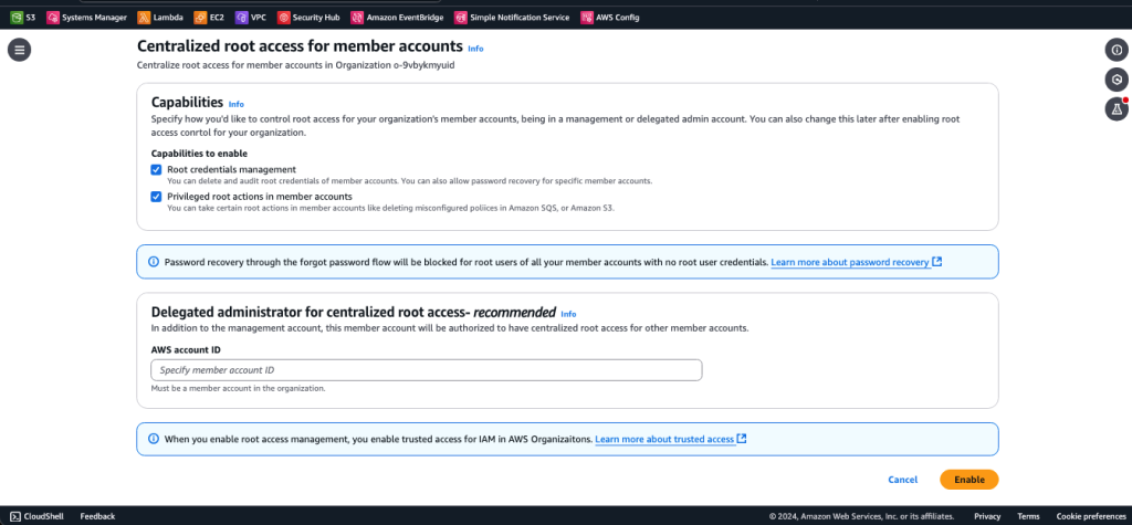
Enrich your serverless data lake with Amazon Bedrock

Post Syndicated from Dave Horne original https://aws.amazon.com/blogs/big-data/enrich-your-serverless-data-lake-with-amazon-bedrock/

Organizations are collecting and storing vast amounts of structured and unstructured data like reports, whitepapers, and research documents. By consolidating this information, analysts can discover and integrate data from across the organization, creating valuable data products based on a unified dataset. For many organizations, this centralized data store follows a data lake architecture.  Although data lakes provide a centralized repository, making sense of this data and extracting valuable insights can be challenging. End-users often struggle to find relevant information buried within extensive documents housed in data lakes, leading to inefficiencies and missed opportunities.

Surfacing relevant information to end-users in a concise and digestible format is crucial for maximizing the value of data assets. Automatic document summarization, natural language processing (NLP), and data analytics powered by generative AI present innovative solutions to this challenge. By generating concise summaries of large documents, performing sentiment analysis, and identifying patterns and trends, end-users can quickly grasp the essence of the information without the need to sift through vast amounts of raw data, streamlining information consumption and enabling more informed decision-making.

This is where Amazon Bedrock comes into play. Amazon Bedrock is a fully managed service that offers a choice of high-performing foundation models (FMs) from leading AI companies like AI21 Labs, Anthropic, Cohere, Meta, Mistral AI, Stability AI, and Amazon through a single API, along with a broad set of capabilities to build generative AI applications with security, privacy, and responsible AI. This post shows how to integrate Amazon Bedrock with the AWS Serverless Data Analytics Pipeline architecture using Amazon EventBridge, AWS Step Functions, and AWS Lambda to automate a wide range of data enrichment tasks in a cost-effective and scalable manner.

Solution overview

The AWS Serverless Data Analytics Pipeline reference architecture provides a comprehensive, serverless solution for ingesting, processing, and analyzing data. At its core, this architecture features a centralized data lake hosted on Amazon Simple Storage Service (Amazon S3), organized into raw, cleaned, and curated zones. The raw zone stores unmodified data from various ingestion sources, the cleaned zone stores validated and normalized data, and the curated zone contains the final, enriched data products.

Building upon this reference architecture, this solution demonstrates how enterprises can use Amazon Bedrock to enhance their data assets through automated data enrichment. Specifically, it showcases the integration of the powerful FMs available in Amazon Bedrock for generating concise summaries of unstructured documents, enabling end-users to quickly grasp the essence of information without sifting through extensive content.

The enrichment process begins when a document is ingested into the raw zone, invoking an Amazon S3 event that initiates a Step Functions workflow. This serverless workflow orchestrates Lambda functions to extract text from the document based on its file type (text, PDF, Word). A Lambda function then constructs a payload with the document’s content and invokes the Amazon Bedrock Runtime service, using state-of-the-art FMs to generate concise summaries. These summaries, encapsulating key insights, are stored alongside the original content in the curated zone, enriching the organization’s data assets for further analysis, visualization, and informed decision-making. Through this seamless integration of serverless AWS services, enterprises can automate data enrichment, unlocking new possibilities for knowledge extraction from their valuable unstructured data.

The serverless nature of this architecture provides inherent benefits, including automatic scaling, seamless updates and patching, comprehensive monitoring capabilities, and robust security measures, enabling organizations to focus on innovation rather than infrastructure management.

The following diagram illustrates the solution architecture.

Let’s walk through the architecture chronologically for a closer look at each step.

Initiation

The process is initiated when an object is written to the raw zone. In this example, the raw zone is a prefix, but it could also be a bucket. Amazon S3 emits an object created event and matches an EventBridge rule. The event invokes a Step Functions state machine. The state machine runs for each object in parallel, so the architecture scales horizontally.

Workflow

The Step Functions state machine provides a workflow to handle different file types for text summarization.  Files are first preprocessed based on the file extension and corresponding Lambda function.  Next, the files are processed by another Lambda function that summarizes the preprocessed content. If the file type is not supported, the workflow fails with an error. The workflow consists of the following states:

  • CheckFileType – The workflow starts with a Choice state that checks the file extension of the uploaded object. Based on the file extension, it routes the workflow to different paths:
    • If the file extension is .txt, it goes to the IngestTextFile state.
    • If the file extension is .pdf, it goes to the IngestPDFFile state.
    • If the file extension is .docx, it goes to the IngestDocFile state.
    • If the file extension doesn’t match any of these options, it goes to the UnsupportedFileType state and fails with an error.
  • IngestTextFile, IngestPDFFile, and IngestDocFile – These are Task states that invoke their respective Lambda functions to ingest (or process) the file based on its type. After ingesting the file, the job moves to the SummarizeTextFile state.
  • SummarizeTextFile – This is another Task state that invokes a Lambda function to summarize the ingested text file. The function takes the source key (object key) and bucket name as input parameters. This is the final state of the workflow.

You can extend this code sample to account for different types of files, including audio, pictures, and video files, by using services like Amazon Transcribe or Amazon Rekognition.

Preprocessing

Lambda enables you to run code without provisioning or managing servers. This solution contains a Lambda function for each file type. These three functions are part of a larger workflow that processes different types of files (Word documents, PDFs, and text files) uploaded to an S3 bucket. The functions are designed to extract text content from these files, handle any encoding issues, and store the extracted text as new text files in the same S3 bucket with a different prefix. The functions are as follows:

  • Word document processing function:
    • Downloads a Word document (.docx) file from the S3 bucket
    • Uses the python-docx library to extract text content from the Word document by iterating over its paragraphs
    • Stores the extracted text as a new text file (.txt) in the same S3 bucket with a cleaned prefix
  • PDF processing function:
    • Downloads a PDF file from the S3 bucket
    • Uses the PyPDF2 library to extract text content from the PDF by iterating over its pages
    • Stores the extracted text as a new text file (.txt) in the same S3 bucket with a cleaned prefix
  • Text file processing function:
    • Downloads a text file from the S3 bucket
    • Uses the chardet library to detect the encoding of the text file
    • Decodes the text content using the detected encoding (or UTF-8 if encoding can’t be detected)
    • Encodes the decoded text content as UTF-8
    • Stores the UTF-8 encoded text as a new text file (.txt) in the same S3 bucket with a cleaned prefix

All three functions follow a similar pattern:

  1. Download the source file from the S3 bucket.
  2. Process the file to extract or convert the text content.
  3. Store the extracted and converted text as a new text file in the same S3 bucket with a different prefix.
  4. Return a response indicating the success of the operation and the location of the output text file.

Processing

After the content has been extracted to the cleaned prefix, the Step Functions state machine initiates the Summarize_text Lambda function. This function acts as an orchestrator in a workflow designed to generate summaries for text files stored in an S3 bucket. When it’s invoked by a Step Functions event, the function retrieves the source file’s path and bucket location, reads the text content using the Boto3 library, and generates a concise summary using Anthropic Claude 3 on Amazon Bedrock. After obtaining the summary, the function encapsulates the original text, generated summary, model details, and a timestamp into a JSON file, which is uploaded back to the same S3 bucket with a specified prefix, providing organized storage and accessibility for further processing or analysis.

Summarization

Amazon Bedrock provides a straightforward way to build and scale generative AI applications with FMs. The Lambda function sends the content to Amazon Bedrock with directions to summarize it. The Amazon Bedrock Runtime service plays a crucial role in this use case by enabling the Lambda function to integrate with the Anthropic Claude 3 model seamlessly. The function constructs a JSON payload containing the prompt, which includes a predefined prompt stored in an environment variable and the input text content, along with parameters like maximum tokens to sample, temperature, and top-p. This payload is sent to the Amazon Bedrock Runtime service, which invokes the Anthropic Claude 3 model and generates a concise summary of the input text. The generated summary is then received by the Lambda function and incorporated into the final JSON file.

If you use this solution for your own use case, you can customize the following parameters:

  • modelId – The model you want Amazon Bedrock to run. We recommend testing your use case and data with different models. Amazon Bedrock has a lot of models to offer, each with their own strengths. Models also vary by context window, which is how much data you can send with a single prompt.
  • prompt – The prompt that you want Anthropic Claude 3 to complete. Customize the prompt for your use case. You can set the prompt in the initial deployment steps as described in the following section.
  • max_tokens_to_sample – The maximum number of tokens to generate before stopping. This sample is currently set at 300 to manage cost, but you will likely want to increase it.
  • Temperature – The amount of randomness injected into the response.
  • top_p – In nucleus sampling, Anthropic’s Claude 3 computes the cumulative distribution over all the options for each subsequent token in decreasing probability order and cuts it off when it reaches a particular probability specified by top_p.

The best way to determine the best parameters for a specific use case is to prototype and test. Fortunately, this can be a quick process by using the following code example or the Amazon Bedrock console. For more details about models and parameters available, refer to Anthropic Claude Text Completions API.

AWS SAM template

This sample is built and deployed with AWS Serverless Application Model (AWS SAM) to streamline development and deployment. AWS SAM is an open source framework for building serverless applications. It provides shorthand syntax to express functions, APIs, databases, and event source mappings. You define the application you want with just a few lines per resource and model it using YAML. In the following sections, we guide you through the process of a sample deployment using AWS SAM that exemplifies the reference architecture.

Prerequisites

For this walkthrough, you should have the following prerequisites:

Set up the environment

This walkthrough uses AWS CloudShell to deploy the solution. CloudShell is a browser-based shell environment provided by AWS that allows you to interact with and manage your AWS resources directly from the AWS Management Console. It offers a pre-authenticated command line interface with popular tools and utilities pre-installed, such as the AWS Command Line Interface (AWS CLI), Python, Node.js, and git. CloudShell eliminates the need to set up and configure your local development environments or manage SSH keys, because it provides secure access to AWS services and resources through a web browser. You can run scripts, run AWS CLI commands, and manage your cloud infrastructure without leaving the AWS console. CloudShell is free to use and comes with 1 GB of persistent storage for each AWS Region, allowing you to store your scripts and configuration files. This tool is particularly useful for quick administrative tasks, troubleshooting, and exploring AWS services without the need for additional setup or local resources.

Complete the following steps to set up the CloudShell environment:

  1. Open the CloudShell console.

If this is your first time using CloudShell, you may see a “Welcome to AWS CloudShell” page.

  1. Choose the option to open an environment in your Region (the Region listed may vary based on your account’s primary Region).

It may take several minutes for the environment to fully initialize if this is your first time using CloudShell.

The display resembles a CLI suitable for deploying AWS SAM sample code.

Download and deploy the solution

This code sample is available on Serverless Land and GitHub. Deploy it according to the directions in the GitHub README on the CloudShell console:

git clone https://github.com/aws-samples/step-functions-workflows-collection

cd step-functions-workflows-collection/s3-sfn-lambda-bedrock

sam build

sam deploy –-guided

For the guided deployment process, use the default values. Also, enter a stack name. AWS SAM will deploy the sample code.

Run the following code to set up the required prefix structure:

bucket=$(aws s3 ls | grep sam-app | cut -f 3 -d ' ') && for each in raw cleaned curated; do aws s3api put-object --bucket $bucket --key $each/; done

The sample application has now been deployed and you’re ready to begin testing.

Test the solution

In this demo, we can initiate the workflow by uploading documents to the raw prefix. In our example, we use PDF files from the AWS Prescriptive Guidance portal. Download the article Prompt engineering best practices to avoid prompt injection attacks on modern LLMs and upload it to the raw prefix.

EventBridge will monitor for new file additions to the raw S3 bucket, invoking the Step Functions workflow.

You can navigate to the Step Functions console and view the state machine. You can observe the status of the job and when it’s complete.

The Step Functions workflow verifies the file type, subsequently invoking the appropriate Lambda function for processing or raising an error if the file type is unsupported. Upon successful content extraction, a second Lambda function is invoked to summarize the content using Amazon Bedrock.

The workflow employs two distinct functions: the first function extracts content from various file types, and the second function processes the extracted information with the assistance of Amazon Bedrock, receiving data from the initial Lambda function.

Upon completion, the processed data is stored back in the curated S3 bucket in JSON format.

The process creates a JSON file with the original_content and summary fields.  The following screenshot shows an example of the process using the Containers On AWS whitepaper.  Results can vary depending on the large language model (LLM) and prompt strategies selected.

Clean up

To avoid incurring future charges, delete the resources you created. Run sam delete from CloudShell.

Solution benefits

Integrating Amazon Bedrock into the AWS Serverless Data Analytics Pipeline for data enrichment offers numerous benefits that can drive significant value for organizations across various industries:

  • Scalability – This serverless approach inherently scales resources up or down as data volumes and processing requirements fluctuate, providing optimal performance and cost-efficiency. Organizations can handle spikes in demand seamlessly without manual capacity planning or infrastructure provisioning.
  • Cost-effectiveness – With the pay-per-use pricing model of AWS serverless services, organizations only pay for the resources consumed during data enrichment. This avoids upfront costs and ongoing maintenance expenses of traditional deployments, resulting in substantial cost savings.
  • Ease of maintenance – AWS handles the provisioning, scaling, and maintenance of serverless services, reducing operational overhead. Organizations can focus on developing and enhancing data enrichment workflows rather than managing infrastructure.
  • Across industries, this solution unlocks numerous use cases:
  • Research and academia – Summarizing research papers, journals, and publications to accelerate literature reviews and knowledge discovery
  • Legal and compliance – Extracting key information from legal documents, contracts, and regulations to support compliance efforts and risk management
    • Healthcare – Summarizing medical records, studies, and patient reports for better patient care and informed decision-making by healthcare professionals
    • Enterprise knowledge management – Enriching internal documents and repositories with summaries, topic modeling, and sentiment analysis to facilitate information sharing and collaboration
  • Customer experience management – Analyzing customer feedback, reviews, and social media data to identify sentiment, issues, and trends for proactive customer service
  • Marketing and sales – Summarizing customer data, sales reports, and market analysis to uncover insights, trends, and opportunities for optimized campaigns and strategies

With Amazon Bedrock and the AWS Serverless Data Analytics Pipeline, organizations can unlock their data assets’ potential, driving innovation, enhancing decision-making, and delivering exceptional user experiences across industries.

The serverless nature of the solution provides scalability, cost-effectiveness, and reduced operational overhead, empowering organizations to focus on data-driven innovation and value creation.

Conclusion

Organizations are inundated with vast information buried within documents, reports, and complex datasets. Unlocking the value of these assets requires innovative solutions that transform raw data into actionable insights.

This post demonstrated how to use Amazon Bedrock, a service providing access to state-of-the-art LLMs, within the AWS Serverless Data Analytics Pipeline. By integrating Amazon Bedrock, organizations can automate data enrichment tasks like document summarization, named entity recognition, sentiment analysis, and topic modeling. Because the solution utilizes a serverless approach, it handles fluctuating data volumes without manual capacity planning, paying only for resources consumed during enrichment and avoiding upfront infrastructure costs.

This solution empowers organizations to unlock their data assets’ potential across industries like research, legal, healthcare, enterprise knowledge management, customer experience, and marketing. By providing summaries, extracting insights, and enriching with metadata, you efficiency add innovative features that provide differentiated user experiences.

Explore the AWS Serverless Data Analytics Pipeline reference architecture and take advantage of the power of Amazon Bedrock. By embracing serverless computing and advanced NLP, organizations can transform data lakes into valuable sources of actionable insights.


About the Authors

Dave Horne is a Sr. Solutions Architect supporting Federal System Integrators at AWS. He is based in Washington, DC, and has 15 years of experience building, modernizing, and integrating systems for public sector customers. Outside of work, Dave enjoys playing with his kids, hiking, and watching Penn State football!

Robert Kessler is a Solutions Architect at AWS supporting Federal Partners, with a recent focus on generative AI technologies. Previously, he worked in the satellite communications segment supporting operational infrastructure globally. Robert is an enthusiast of boats and sailing (despite not owning a vessel), and enjoys tackling house projects, playing with his kids, and spending time in the great outdoors.