Amazon Inspector is an automated vulnerability management service that continually scans Amazon Web Services (AWS) workloads for software vulnerabilities. The vulnerability management capabilities of Amazon Inspector are powered by an asset inventory engine known as the Amazon Inspector SBOM Generator (inspector-sbomgen), a standalone command-line tool that produces a software bill of materials (SBOM) from container images, directories, archives, local systems, compiled binaries, and more. Over the past two years, we’ve expanded inspector-sbomgen’s coverage across dozens of programming language ecosystems, operating systems, and widely deployed applications.
We’re pleased to announce a new capability for builders using inspector-sbomgen: a plugin system for writing your own custom package collectors that you can use right away, without requiring source code compilation nor waiting for an official release.
In this post, we walk you through what the inspector-sbomgen plugin system does, why we built it, and how you can write your first plugin in a few minutes. Along the way, we also cover how plugin-generated package components integrate with Amazon Inspector for vulnerability scanning, and we explore the plugin safety model, which helps ensure security-hardened and predictable plugin behavior.
Why we built a plugin system
Software ecosystems are dynamic. New language package managers, lockfile formats, and end user applications ship constantly, and many are adopted quickly, in some cases with little security scrutiny. That leaves security teams with a visibility gap: production workloads running software that their SBOM tooling doesn’t yet recognize. Customers have asked us to inventory many of these ecosystems directly, and until recently, the only path to support was to open a feature request and wait for the inspector-sbomgen team to onboard the ecosystem and deploy a new release.
The inspector-sbomgen plugin system changes that. With plugins, you can:
Onboard ecosystems that inspector-sbomgen doesn’t support out of the box. New open source ecosystems, niche or fast-moving package formats, and internal or proprietary tooling can all be inventoried without modifying inspector-sbomgen.
Prototype detection for an ecosystem quickly. We designed a plugin system that is friendly to developers and AI coding assistants alike. Plugins are written in Lua, loaded at runtime, and require no Go toolchain nor compilation. You can use the built in test harness to iterate on a plugin and see results immediately.
Build on a stable foundation. The plugin API abstracts away artifact-type differences, so you write your detection logic once and it works seamlessly across container images, archives, local systems, and more. And because plugins stay decoupled from the internals of sbomgen, the core tool’s regression surface stays small.
Internally, we’ve used the plugin system to ship new ecosystem coverage faster than before. In our 1.13 release, more than 20 ecosystems that were previously implemented in Go, including Apache Tomcat, NGINX, MySQL, Redis, WordPress, and the OpenSSH toolchain, are now embedded as plugins inside the sbomgen binary. The same release also added more than ten brand-new ecosystems as plugins, including Apache Cassandra, Apache Struts, Conda, Swift packages, and AI-agent collectors (Amazon Q Developer, Kiro CLI, Claude Code, GitHub Copilot, and Ollama).
How inspector-sbomgen plugins work
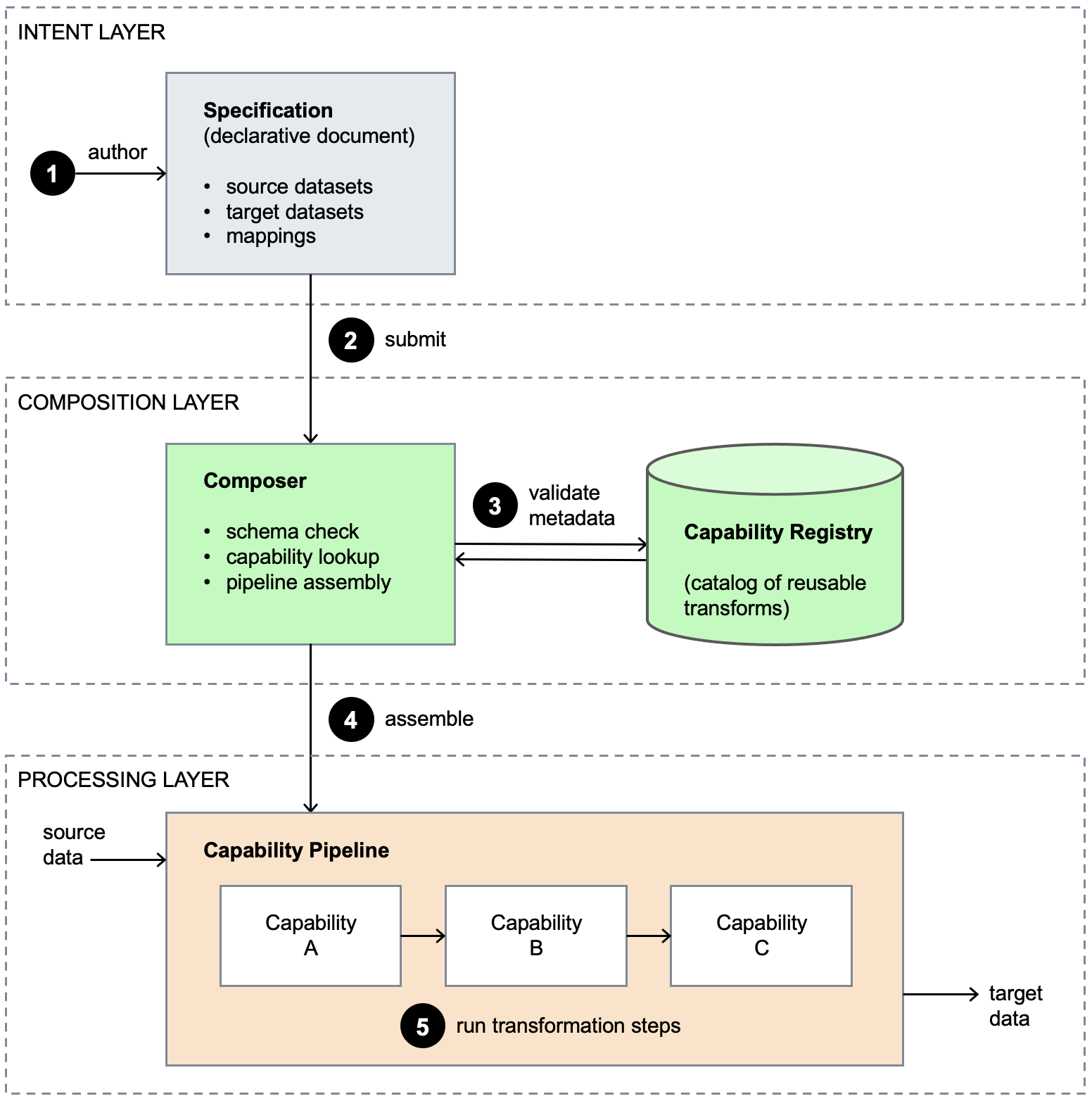
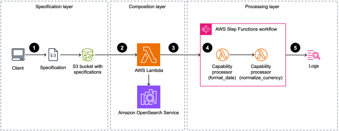
Sbomgen plugins follow a two-step pipeline:
Discovery – Scan the artifact’s file system to identify files that contain installed package metadata.
Collection –Open each discovered file, parse file contents, and publish findings into the SBOM.
Under the hood, an event bus connects discovery and collection plugins. Discovery plugins publish events listing discovered files, and one or more collection plugins subscribe to these events, triggering package collection. Developers might recognize this behavior as the observer pattern.
This decoupling lets a single discovery plugin feed multiple collectors, for example, one extracting package metadata, another scanning for secrets, and another checking policy. Each collection plugin works from the same file list without re-walking the artifact filesystem, a computationally expensive operation.
Write your first plugin in 5 minutes
Inspector-sbomgen makes it straightforward to bootstrap a plugin environment. The plugin new command tells sbomgen to create a new plugin workspace, and the —-with-example flag populates the workspace with a discovery-collection plugin pair, that you can run immediately.
inspector-sbomgen plugin new --with-example
After invoking the preceding command, you will be prompted to provide a plugin name and a directory that will contain your plugin workspace. You can provide custom values or use the default values:
Plugin name (identifies the software ecosystem your plugin will inventory, e.g. debian-dpkg, rhel-rpm, python-pip, cmake) [my-custom-ecosystem]: <enter>
Project directory [my-sbomgen-plugins]: <enter>

Created plugin "my-custom-ecosystem" in my-sbomgen-plugins/
Note that you can skip interactive prompts by specifying the plugin name and directory using the corresponding command line interface (CLI) arguments:
After creating your plugin workspace, inspector-sbomgen will display a next steps screen, which guides developers and AI code assistants to the source files they need to change and to supporting documentation:
Next steps:

  Get started:
    1. Open plugin folder in a code editor (VS Code recommended)
    2. Add test files that your plugin will discover and parse
       (e.g., config files, lockfiles, binaries, etc.):
       my-sbomgen-plugins/discovery/cross-platform/extra-ecosystems/my-custom-ecosystem/_testdata/

  Develop:
    3. Edit discovery:    my-sbomgen-plugins/discovery/cross-platform/extra-ecosystems/my-custom-ecosystem/init.lua
    4. Edit collection:   my-sbomgen-plugins/collection/cross-platform/extra-ecosystems/my-custom-ecosystem/init.lua

  Test:
    5. Write unit tests:  my-sbomgen-plugins/discovery/cross-platform/extra-ecosystems/my-custom-ecosystem/init_test.lua
    6. Run unit tests:    inspector-sbomgen plugin test --path my-sbomgen-plugins

  Deploy:
    7. Distribute your plugin directory wherever you run inspector-sbomgen:
       inspector-sbomgen <arguments> --plugin-dir /path/to/my-sbomgen-plugins

       Example:
       inspector-sbomgen container --image alpine:latest -o /tmp/sbom.json --plugin-dir /path/to/my-sbomgen-plugins

For code completion, install the VS Code Lua language server extension:
  https://luals.github.io/#vscode-install

For more information:
  - Plugin guide:    my-sbomgen-plugins/docs/sbomgen-plugin-developer-guide.md
  - Testing guide:   my-sbomgen-plugins/docs/sbomgen-plugin-testing-guide.md
  - API reference:   my-sbomgen-plugins/docs/sbomgen-plugin-api-reference.md
  - Documentation:   https://docs.aws.amazon.com/inspector/latest/user/sbom-generator.html
Now that you have a plugin workspace, let’s explore its contents in greater detail:
The scaffolded project includes a working discovery and collection plugin pair, passing unit tests with test fixtures under _testdata/, a .vscode/settings.json for integrated development environment (IDE) integration, and a local copy of the developer documentation.
The scaffolding is deliberately succinct and complete, so it reads well for both humans and AI coding assistants. Every file has clear comments that explain what each function does and what the plugin author needs to fill in.
To test a plugin, you first need something to scan, such as a package lock file or a compiled binary. The example plugin inventories a fictional example.lock with the following contents:
The provided discovery plugin knows how to look for instances of example.lock within the artifact file system:
-- my-custom-ecosystem discovery plugin
-- Discovers example.lock files in the artifact file list.

function discover()
    return sbomgen.find_files_by_name({"example.lock"})
end
And the provided collection plugin knows how to parse the contents of example.lock and publish package findings to the output SBOM.
-- my-custom-ecosystem collection plugin
-- Parses example.lock files and extracts package name and version.

function collect(file_path)
    local content = sbomgen.read_file(file_path)
    if content == nil then
        return
    end

    for line in content:gmatch("[^\n]+") do
        local name, ver = line:match("^(.+)==(.+)$")
        if name and ver then
            sbomgen.push_package({
                name = name,
                version = ver,
                purl_type = "generic",
                namespace = "my-custom-ecosystem",
                component_type = sbomgen.component_types.APPLICATION,
            })
        end
    end
end
Run the tests
Plugins ship with a built-in test framework so you can validate your logic before scanning a real artifact. Tests are written in Lua, live next to the plugin in init_test.lua, and reference fixture data in _testdata/:
function test_discovers_packages()
    local result = testing.scan_directory("_testdata")
    testing.assert_equals(3, #result.findings)
    testing.assert_equals("my-package-alpha", result.findings[1].name)
    testing.assert_equals("1.0.0", result.findings[1].version)
end

function test_no_findings_for_empty_directory()
    local result = testing.scan_directory("_testdata/empty")
    testing.assert_equals(0, #result.findings)
end
Run the tests with the following command:
inspector-sbomgen plugin test --path my-sbomgen-plugins -v

=== RUN   my-custom-ecosystem/discovery/init_test/test_discovers_packages
--- PASS: my-custom-ecosystem/discovery/init_test/test_discovers_packages (0.04s)
=== RUN   my-custom-ecosystem/discovery/init_test/test_no_findings_for_empty_directory
--- PASS: my-custom-ecosystem/discovery/init_test/test_no_findings_for_empty_directory (0.04s)
ok    2 tests passed
This is the tightest development loop we could design: no Go toolchain, no rebuild, no container spin-up. Write a test, run it, iterate.
Scan a real artifact
For plugins to produce findings, inspector-sbomgen needs an artifact that contains the files your plugin looks for. For the example plugin, any directory with an example.lock file works. The fixture we generated earlier is a good stand-in:
The --plugin-dir flag tells inspector-sbomgen where to load your Lua plugins from. The resulting SBOM contains a CycloneDX component for each of the three packages in example.lock, for example:
Every plugin-generated component carries an amazon:inspector:sbom_generator:source_path property that records the file the component was collected from, so you can always trace a component back to the artifact that produced it.
Vulnerability scanning with Amazon Inspector
Plugin-generated findings are first-class SBOM components. They work with every downstream consumer that reads CycloneDX SBOMs, including Amazon Inspector. To send an SBOM to Amazon Inspector for vulnerability analysis, add the --scan-sbom flag (this requires an active AWS account):
An important caveat when you onboard a brand-new ecosystem: Plugin authors can inventory arbitrary ecosystems, but Amazon Inspector can only report vulnerabilities for components it has advisories for. When you point Amazon Inspector at a component whose ecosystem isn’t in its advisory feeds yet, Inspector will return the component with a property, Component skipped: no supported rules found. For example:
This is expected behavior, not an error. The SBOM is still generated correctly, the component is still tracked, and the source_path tells you exactly which file produced it. If and when Amazon Inspector adds advisory coverage for the ecosystem, the same SBOM will start producing vulnerability findings without any change to your plugin. For ecosystems Inspector already supports, plugin-generated components are indistinguishable from components produced by built-in scanners.
First class IDE support
We care about productivity and efficiency when writing plugins. Writing Lua without modern conveniences such as autocomplete isn’t fun, so every plugin project scaffolded with the plugin new command ships with a library/sbomgen.lua definition file and a .vscode/settings.json that automatically wires it up to the Lua Language Server extension for VS Code.
For code completion and IDE support, first install the sumneko.lua extension, open your plugin project in VS Code, and every sbomgen.* function will get:
Parameter hints with types.
Hover documentation.
Autocomplete for constants (sbomgen.component_types.*, sbomgen.groups.*, sbomgen.platform.*).
Type checking on function calls.
Inline warnings when required fields are missing from push_package().
The same definition file makes plugin development work well with AI coding assistants. The types and documentation are embedded in a form that tools can read, so assistants can generate correct plugin code with far less monitoring than writing against a raw language would require.
A safe foundation
Plugins run real code inside the same process as inspector-sbomgen, so we designed the execution environment to keep that code stable and security-hardened. Every Lua plugin runs in an isolated sandbox. Every Lua virtual machine (VM) has access to a restricted subset of the Lua standard library to ensure only safe operations are permitted:
No direct filesystem access. The Lua io library isn’t loaded. All file operations go through sbomgen.* functions, which route through sbomgen’s internals so your plugin behaves identically whether it’s scanning a directory on disk, a container image, a compressed archive, or a mounted volume.
No subprocess execution or environment mutation. The Lua os library is blocked, so plugins can’t spawn processes, modify environment variables, or touch files outside the artifact.
No VM introspection. The Lua debug library is blocked.
No unbounded code loading.dofile, loadfile, and loadstring are removed. require() is available but restricted to the plugin’s own directory tree, so plugins can share helper modules with themselves but cannot load code from other plugins or system paths.
If a plugin raises an unhandled Lua error, inspector-sbomgen logs a warning and continues with the next file or plugin; one faulty plugin does not prevent other plugins from running. Plugins never override inspector-sbomgen’s built-in package collectors. Every plugin must declare a unique name. If a custom plugin uses a name that’s already claimed by an official built-in plugin, the custom plugin is skipped with a warning. Built-in plugins always take precedence, so a custom plugin can never silently replace or shadow the tool’s own detection behavior.
Whether you’re adding support for an internal lockfile format, prototyping detection for a new open source ecosystem, or replacing a home-grown scanner with something your whole organization can run at scale, the plugin system is designed to make the path from idea to working SBOM as short as possible. We can’t wait to see what you build with it. If you have feedback about this post, submit comments in the Comments section below. If you have questions about this post, contact AWS Support.
For legal and compliance teams, auditing a repository of thousands of contracts for a single regulatory obligation shouldn’t take weeks. But with keyword search, it often does. A search for “inadvertent access notification” returns exact matches while missing functionally equivalent clauses such as “security incident disclosure” or “unauthorized access reporting.” This creates two problems:
Discovery gap: Critical risk exposure goes undetected because keyword search cannot match semantically equivalent terms across different contracts.
Review latency: After finding relevant contracts, legal counsel must manually scan lengthy documents to locate the specific clauses that matter. This process can stretch from minutes to hours per document.
Amazon OpenSearch Service is a fully managed search and analytics service that configures, manages, and scales OpenSearch clusters in the AWS Cloud. It supports use cases from log analytics and application monitoring to full-text search and real-time security analytics. It also supports AI-powered semantic search.
Amazon OpenSearch Service addresses both problems through two capabilities:
Semantic search retrieves contracts based on meaning rather than exact keyword matches, closing the discovery gap.
Semantic highlighting pinpoints the exact clauses within retrieved contracts that answer the query, reducing review time from hours of manual scanning to seconds of targeted reading.
In this post, you build a contract compliance search system that combines semantic search with semantic highlighting in Amazon OpenSearch Service. You deploy the solution using two AWS CloudFormation stacks, test it with synthetic contract documents, and see how a single query surfaces both the right contracts and the right clauses within them.
Solution overview
The solution uses a two-stage retrieval and extraction pipeline. First, semantic search identifies relevant contracts across the repository. Then, semantic highlighting marks the specific clauses within those contracts that match the query intent.
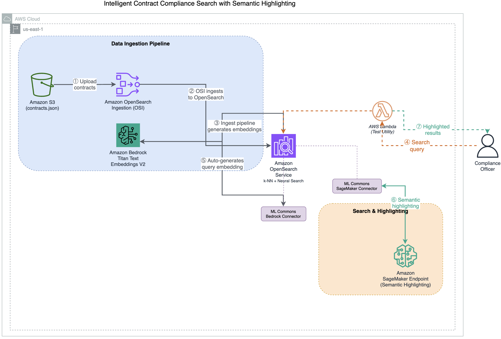
The following diagram illustrates the solution architecture:
Upload contracts toAmazon Simple Storage Service (Amazon S3) – Contract documents (JSON format) are uploaded to an Amazon S3 bucket, which serves as the centralized document repository.
Amazon OpenSearch Ingestion (OSI)reads from S3 – A serverless OSI pipeline detects new documents in the S3 bucket and reads them for processing.
OpenSearch ingest pipeline generates embeddings through Amazon Bedrock – As documents arrive, the ingest pipeline’s text_embedding processor invokes Amazon Titan Text Embeddings V2 through an ML Commons Bedrock connector. This converts contract text into 1024-dimension vector representations, stored in a k-NN index that uses the faiss engine.
User submits a search query – A user queries the system with natural language (for example, “data protection regulations”) through a test AWS Lambda function that forwards the request to OpenSearch using the neural query type.
OpenSearch generates the query embedding – OpenSearch converts the user’s natural language query into a vector embedding using the same machine learning (ML) Commons Amazon Bedrock connector and Amazon Titan V2 model.
Amazon OpenSearch Service performs semantic search – OpenSearch uses k-NN vector similarity to retrieve contracts that are semantically relevant to the query, even when exact terminology differs.
Amazon SageMaker AI performs semantic highlighting – The opensearch-semantic-highlighter-v1 model, hosted on an Amazon SageMaker AI GPU endpoint, scores sentence relevance using cross-encoder inference and wraps the matching clauses in <em> tags for targeted reading.
How semantic search and semantic highlighting work together
The system processes queries in two steps:
Step 1 – Semantic search (document discovery): You query the contract corpus using natural language. The system retrieves contracts with semantically similar concepts, even when exact terminology differs. For example, searching for “force majeure” returns contracts discussing “natural disasters” or “unforeseeable circumstances” because the system understands these concepts are related.
Step 2 – Semantic highlighting (clause identification): After relevant contracts are retrieved, semantic highlighting automatically marks the clauses that semantically match your search intent. Instead of scanning pages of legal text, you immediately see the specific paragraphs that answer your question.
Keyword highlighting wraps individual matching words: <em>termination</em> and <em>rights</em>.
Semantic highlighting wraps entire relevant clauses: <em>Upon termination, the consultant must return all confidential information and proprietary materials within 15 business days.</em>.
This reduces false positives, cuts review time, and provides explainability for why each document was retrieved.
Semantic highlighting model deployment
Before the system can highlight clauses based on meaning, the opensearch-semantic-highlighter-v1 model must be deployed to an Amazon SageMaker AI GPU endpoint and registered with the OpenSearch ML Commons plugin through a remote connector.
Stack 2 of the CloudFormation deployment automates this process. It performs the following steps:
Downloads the model artifact from an AWS-managed source and deploys it to an Amazon SageMaker AI endpoint (ml.g5.xlarge).
Creates a remote ML Commons connector in OpenSearch that points to the SageMaker endpoint.
Registers the model with the QUESTION_ANSWERING function so that OpenSearch can use the model’s cross-encoder capabilities to score sentence relevance at query time.
The equivalent manual registration call (handled automatically by the stack) is:
You don’t need to run this manually. The deployment script and CloudFormation stack handle model registration end-to-end. The resulting model ID is automatically passed to the query Lambda function for use in semantic highlighting requests.
Index configuration
The index uses a k-NN vector field with 1024 dimensions (matching the Amazon Titan V2 output) and the faiss engine with HNSW method. The mapping includes both a knn_vector field for semantic retrieval and a standard text field for keyword matching and highlighting. When you search for “liability limits,” OpenSearch first retrieves documents through vector similarity, then uses the Amazon SageMaker AI model to identify and wrap the specific relevant sentences in <em> tags.
This section walks you through deploying the solution using two AWS CloudFormation stacks and two shell scripts. You first set up the core infrastructure (OpenSearch, ingestion pipeline, and ML Commons Bedrock connector), then deploy the semantic highlighting model on Amazon SageMaker AI.
Prerequisites
To deploy this solution, you need:
An active AWS account with permissions to create Amazon S3 buckets, AWS Lambda functions, Amazon SageMaker AI endpoints, Amazon Bedrock model access, Amazon OpenSearch Ingestion pipelines, Amazon OpenSearch Service domains, and AWS Identity and Access Management (IAM) roles (including iam:PassRole and sts:AssumeRole). For the exact least-privilege policy, see iam-deployer-policy.json in the repository. Both CloudFormation stacks require the CAPABILITY_NAMED_IAM acknowledgement.
Amazon Bedrock model access enabled for Amazon Titan Text Embeddings V2 (amazon.titan-embed-text-v2:0).
Estimated deployment time: approximately 35 minutes.
Estimated cost: approximately USD $ 2.00–3.00 for a quick demo. Delete the stacks promptly after testing.
This post uses US East (N. Virginia) as the deployment AWS Region. Verify service availability in your preferred Region before deploying.
Deploy the solution
The solution deploys using two AWS CloudFormation stacks and two shell scripts. The demo includes synthetic contract documents covering common contract types including software licenses, data processing agreements, managed services, and software as a service (SaaS) subscriptions.
Clone the repository and run the deployment script:
git clone https://github.com/aws-samples/sample-contract-compliance-search-amazon-opensearch.git
cd sample-contract-compliance-search-amazon-opensearch
./deploy.sh
The deployment script creates the following resources across two stacks:
Stack 1:
An Amazon OpenSearch Service domain with fine-grained access control.
An Amazon OpenSearch Ingestion (OSI) pipeline that reads contracts from S3 and sends them to OpenSearch for indexing.
An ML Commons Bedrock connector and ingest pipeline that automatically generates 1024-dimension vector embeddings through Amazon Titan Text Embeddings V2 during document indexing.
A test Lambda function for querying the OpenSearch index using keyword, neural, or hybrid search with semantic highlighting support.
An S3 bucket for storing contract documents.
IAM roles for Lambda functions, the OSI pipeline, and OpenSearch access.
Stack 2:
An Amazon SageMaker AI endpoint hosting the semantic highlighting model.
A Lambda function that creates an ML Commons remote connector in OpenSearch and registers the highlighting model.
After both stacks deploy, the script automatically configures OpenSearch (role mappings, Amazon Bedrock connector, embedding model, k-NN index), ingests the sample contract data, and registers the semantic highlighting model.
The total deployment takes approximately 35 minutes to complete.
(Optional) Automated deployment with Claude Code CLI
If you have Claude Code CLI installed, you can deploy the solution using an AI-assisted workflow that creates a least-privilege IAM role scoped to this demo before deploying:
git clone https://github.com/aws-samples/sample-contract-compliance-search-amazon-opensearch.git
cd sample-contract-compliance-search-amazon-opensearch
./scripts/create-deployer-role.sh
export OS_DEMO_DEPLOYER_ROLE=arn:aws:iam::<ACCOUNT_ID>:role/os-demo-deployer-role
export AWS_DEFAULT_REGION=us-east-1
claude "Deploy the OpenSearch semantic search demo following README.md"
Claude Code reads the repository instructions, assumes the deployer role, deploys both CloudFormation stacks in order, runs the setup scripts, and verifies the deployment end-to-end. The deployer role restricts actions to resources prefixed with os-demo-*, following the principle of least privilege.
Test the solution
After the deployment succeeds, follow these steps to test the solution.
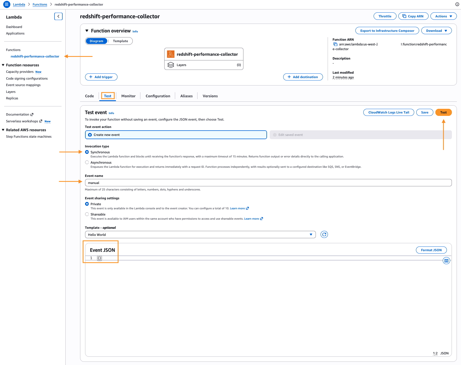
On the Lambda console, choose Functions in the navigation pane.
Choose the function that has os-demo-query in its name.
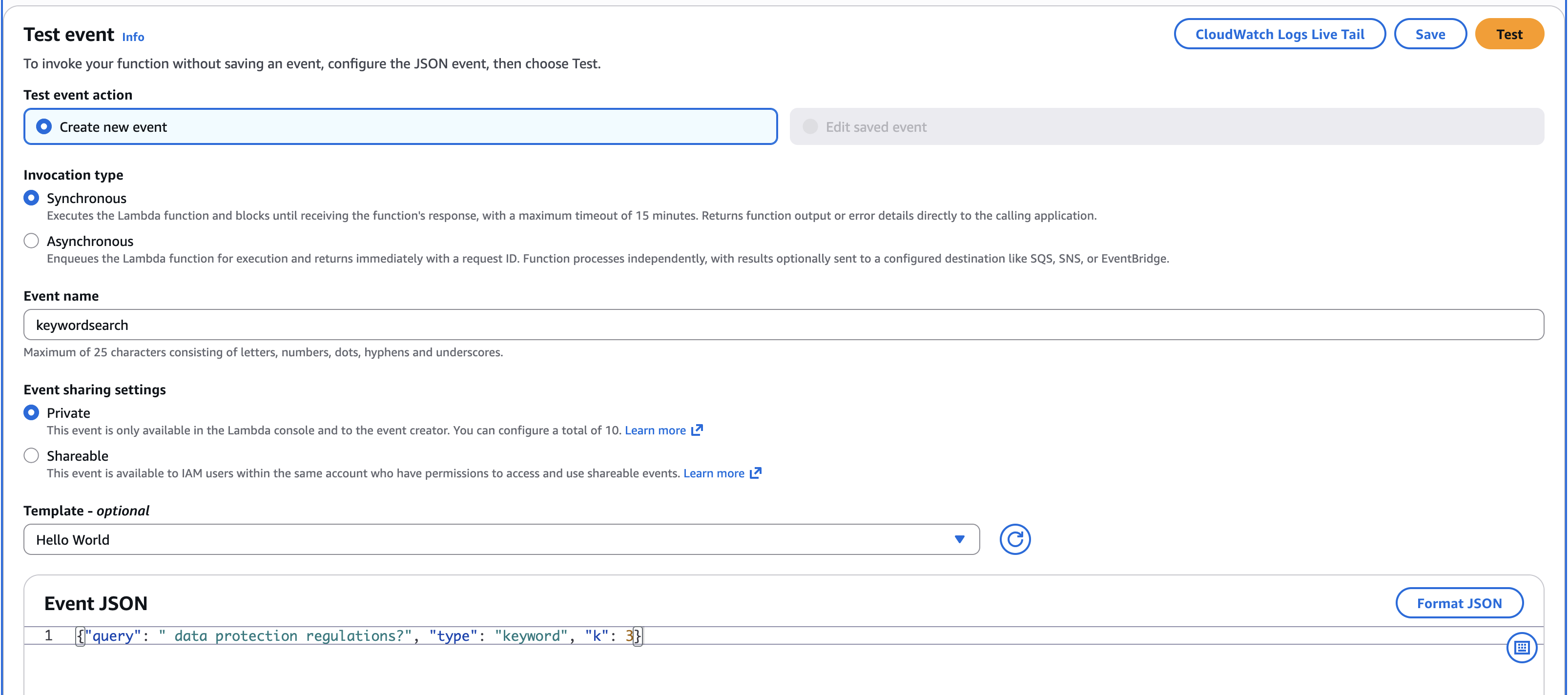
On the Test tab, in the Event JSON paste this keyword search query {"query": "data protection regulations?", "type": "keyword", "k": 3}
Choose Test to run the Lambda function.
The following screenshot shows the Lambda function test configuration on the AWS Management Console with the keyword search query.
The function processes the query in two ways depending on the search type:
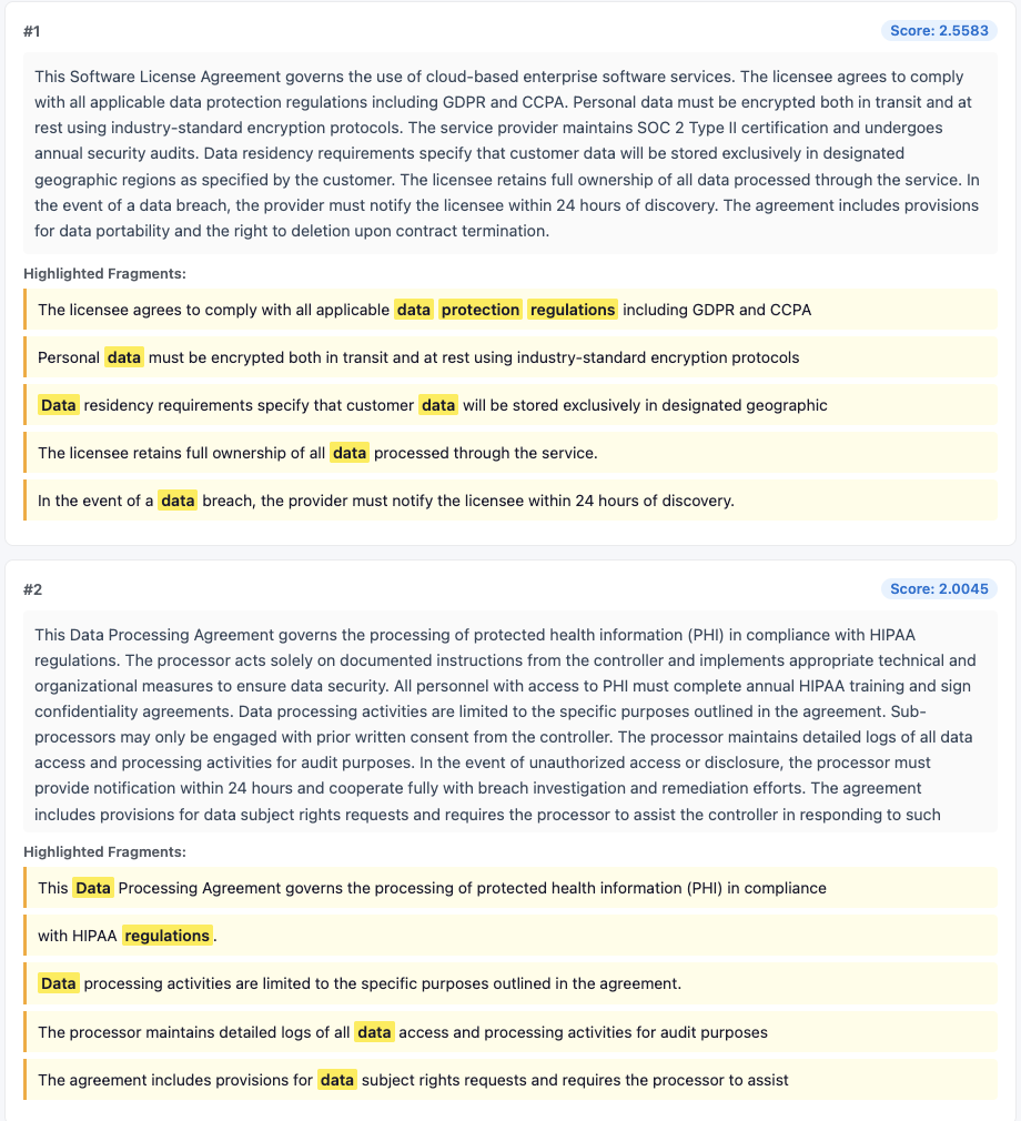
For keyword search (enter: keyword): The function sends a standard match query to OpenSearch, which returns documents containing the exact query terms. The highlight fragments wrap individual matching words like <em>termination</em> and <em>rights</em>.
For neural search (enter: neural): The function sends a hybrid query to OpenSearch combining k-NN (semantic similarity) with keyword matching. OpenSearch automatically generates the query embedding through the ML Commons Amazon Bedrock connector using the same Amazon Titan V2 model. This returns semantically related documents even if they don’t contain the exact query terms. The SageMaker endpoint powers the semantic highlighting, identifying the most relevant clauses within each retrieved document. It wraps entire passages like <em>Upon termination, the consultant must return all confidential information and proprietary materials within 15 business days.</em>.
Download the highlight viewer HTML file and open it in the browser. This file helps you view the highlighted text.
Copy the entire execution output of the Lambda execution, paste it into the placeholder in the HTML file, and then choose Load Results.
The following screenshot shows that only the matching keywords are highlighted.
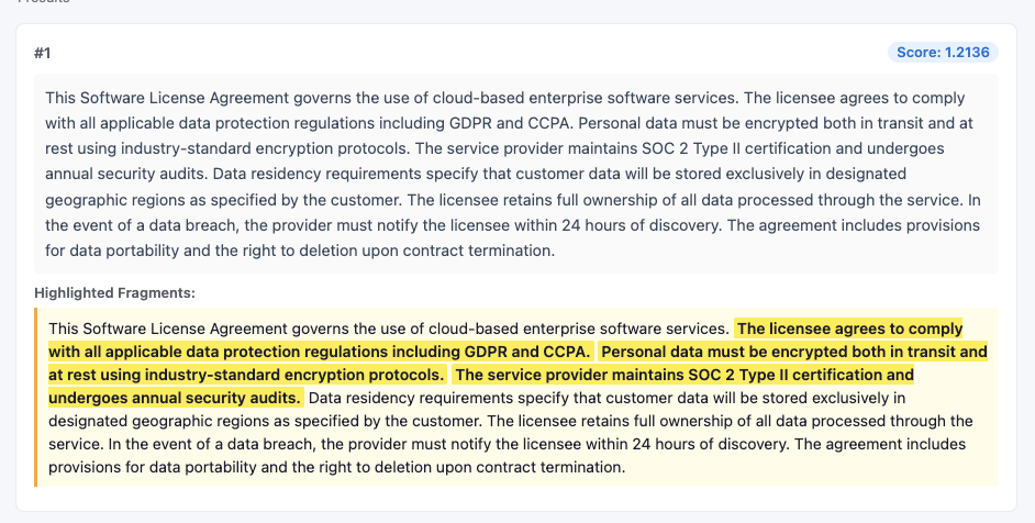
Next, paste the neural search query as input to the Lambda function to see how semantic highlighting works: {"query": "data protection regulations", "type": "neural", "k": 1}
Choose Test to run, and then paste the entire output into the HTML viewer.
The viewer now displays entire sentences highlighted instead of individual keywords.
Optimizing for scale: batch semantic highlighting
In a standard search, a query might return dozens of relevant contracts. Using the default single inference mode, OpenSearch makes a separate ML call for every document in the result set. For a compliance officer reviewing 50 contracts, this sequential processing introduces noticeable latency.
OpenSearch 3.3 introduced batch inference mode to address this. Batch inference collects the matching documents and processes them in a single ML inference call. In the contract compliance use case, this shifts the performance characteristic from multiple sequential roundtrips to a single parallel execution on the Amazon SageMaker AI GPU.
To enable batch inference, first configure the cluster setting:
PUT _cluster/settings
{
  "persistent": {
    "search.pipeline.enabled_system_generated_factories": ["semantic-highlighter"]
  }
}
Then add batch_inference: true to your highlight options. The following query searches for data privacy clauses across the contracts and highlights the top 10 results using a single batch call:
Follow these recommendations to optimize performance, security, and cost-efficiency when deploying the contract compliance search system in production.
Experiment with overlapping chunk sizes (for example, 500 characters with a 10 percent overlap) in your OSI pipeline to verify that context is preserved for long indemnification or liability clauses.
Verify that your Amazon S3 buckets and OpenSearch domains are encrypted using AWS Key Management Service (AWS KMS). For production workloads containing sensitive data, make sure that all traffic stays within your virtual private cloud (VPC) through interface endpoints.
This demo uses simplified configurations for learning purposes. For production deployments, implement VPC isolation, AWS KMS encryption with customer-managed keys, and multi-AZ OpenSearch clusters.
Clean up resources
To avoid ongoing charges, delete the AWS CloudFormation stacks and associated resources:
On the AWS CloudFormation console, choose Stacks in the navigation pane.
Select the os-demo-highlighting stack (Stack 2) and choose Delete. Wait for deletion to complete.
Select the os-demo-search stack (Stack 1) and choose Delete. Stack deletion takes approximately 10–15 minutes to complete.
The stack deletion will automatically remove:
OpenSearch domain.
SageMaker model and endpoint.
Lambda functions.
IAM roles and policies.
After both stacks are deleted, manually delete the S3 bucket (opensearch-cfn-semantic-highlighting-us-east-1-<ACCOUNT_ID>) created for model artifacts. This bucket is provisioned at deploy time and is not managed by CloudFormation. Replace <ACCOUNT_ID> with your AWS account ID in the bucket name.
Conclusion
In this post, you built a contract compliance search system that combines semantic search with semantic highlighting in Amazon OpenSearch Service. The system helps close the discovery gap by retrieving contracts based on meaning rather than exact keywords, and it reduces review latency by highlighting the specific clauses that answer your query.
While we focused on legal agreements, the architecture described here is a blueprint for domains requiring high-stakes document discovery, including:
Regulatory filings: Identifying specific compliance mandates in financial reports.
Technical documentation: Pinpointing troubleshooting steps across massive product manuals.
Research and academia: Isolating specific methodologies within thousands of scientific papers.
Internal knowledge bases: Empowering employees to find exact policy language instantly.
Last week I had the privilege of spending three days in São Paulo with technical builders from across Latin America, brought together for a regional tech event full of deep-dive sessions, hands-on workshops, and conversations with customers and partners. What struck me most wasn’t any single session, it was the energy of a technical community that so rarely gets to be in the same room. People traded architecture ideas over coffee, sketched out solutions on whiteboards, and left with a longer list of things to try than they arrived with. It’s a good reminder that, for all the tooling we build, the community around it is what makes the technology stick.
That community spirit connects nicely to the week’s biggest infrastructure news, which is all about bringing AWS closer to where builders actually are.
Now, let’s get into this week’s AWS news…
Headlines AWS Local Zone in Athens, Greece: AWS has opened a new Local Zone in Athens, Greece, the second Local Zone in EMEA with support for Amazon S3 and Amazon EBS Local Snapshots, so you can store and process data within Greece to help meet local data residency requirements. The Athens Local Zone supports Amazon EC2 (C7i, M7i, and R7i instances), Amazon S3 with the One Zone-Infrequent Access storage class, Amazon EBS, and Amazon ECS.
AWS Local Zones place AWS infrastructure much closer to large population and industry hubs, enabling applications that require single-digit millisecond latency, such as real-time gaming, media production, and financial services, to run where end users actually are. For builders in Greece, you can now run latency-sensitive workloads locally while connecting seamlessly to the nearest AWS Region for services that don’t require low latency, giving you the flexibility to architect hybrid, latency-optimized applications without managing your own data center infrastructure. To learn more, visit AWS Global Infrastructure and Sustainability Blog post.
Last week’s launches Here are some launches and updates from this past week that caught my attention:
Claude Opus 5 on AWS: You can use Anthropic’s Claude Opus 5, the most advanced Opus model yet, matching Claude Fable 5’s top-tier intelligence in many domains at Opus-tier pricing. Amazon Bedrock offers Claude Opus 5 with zero data retention (ZDR) enabled by default, giving you Opus’ top-tier intelligence while meeting your data governance requirements unlike Claude Fable 5. You have two ways to access Claude Opus 5: Amazon Bedrock and Claude Platform on AWS. To learn more, visit the deep dive blog post.
AWS Lambda durable execution SDK for .NET is now generally available: You can now build resilient, long-running workflows in C# using Lambda durable functions, without implementing custom progress tracking or integrating an external orchestration service. The SDK is a natural fit for multi-step applications like payment processing pipelines, AI agent orchestration, and human-in-the-loop approvals, it checkpoints progress automatically and can pause execution for up to a year. If you’re a .NET developer building serverless workflows, this removes a lot of the plumbing you used to write by hand.
Amazon Bedrock AgentCore now delivers unified observability with traces and logs in a single log group: Amazon Bedrock AgentCore now delivers agent traces and prompts to the same Amazon CloudWatch log group as your agent’s logs. Previously, telemetry was split across destinations, trace spans went to a shared log group while prompts, inputs, and outputs went to a separate one, so debugging a single agent invocation meant searching in multiple places. You can now debug an invocation in one place, and apply fine-grained access control and customer-managed key (CMK) encryption at the individual agent level.
Amazon Connect delivers more natural agentic voice experiences: Amazon Connect now supports more natural, human-sounding agentic voice experiences across 50+ languages, including Portuguese, Spanish, French, Italian, Japanese, Korean, and Thai, with over 100 new voice options and conversational improvements that make AI interactions sound more fluid. Connect’s agentic self-service lets AI agents understand, reason, and take action across voice and digital channels, adapting to a customer’s tone and sentiment. You can now build contact center experiences that feel natural to callers in far more of the languages your customers actually speak.
Amazon SageMaker Unified Studio now supports Amazon OpenSearch: You can now query and analyze your search and log analytics data from Amazon OpenSearch directly alongside other data assets in Amazon SageMaker Unified Studio. With this connection, you can combine operational search data in OpenSearch with data from sources like Amazon Redshift, Amazon S3, and relational databases, all within a single, governed environment. It’s especially useful when you need to correlate analytical and operational workloads, such as joining application logs with transactional data to uncover insights.
Amazon CloudWatch announces coding agent insights: Amazon CloudWatch now gives engineering leaders visibility into how AI coding tools are driving value across their organization. Coding agent insights integrates with the Claude apps gateway for AWS to collect telemetry from Claude Code without additional instrumentation, and also supports agents like Codex and GitHub Copilot. As teams scale AI coding adoption, you can now measure the return on that investment with metrics built on OpenTelemetry, no custom instrumentation required.
For a full list of AWS announcements, be sure to keep an eye on the What’s New with AWS page.
Other AWS news Here are some additional posts and resources that you might find interesting:
Evaluating AI Agents: A production blueprint with Strands and AgentCore: A practical guide to evaluating AI agents before and after they reach production, using Strands Agents and Amazon Bedrock AgentCore. If you’re moving agents from prototype to production, this post is a great companion to the AgentCore observability update above, it walks through how to measure agent quality systematically rather than by gut feel.
Upcoming AWS events Check your calendar and sign up for upcoming AWS events:
AWS Summits: AWS Summits are free events that bring the cloud and AI community together to connect, learn, and explore the latest technologies. Browse the full calendar to find a Summit near you in the second half of 2026.
AWS Community Days: Community-led conferences where content is planned, sourced, and delivered by community leaders. If you’re in Latin America, don’t miss AWS Community Day Belo Horizonte on August 22, registration is open at awscommunityday.com.br.
Join the AWS Builder Center to connect with builders, share solutions, and access content that supports your development. Browse here for upcoming AWS-led in-person and virtual events and developer-focused events.
That’s all for this week. Check back next Monday for another Weekly Roundup!
This post is part of our Weekly Roundup series. Check back each week for a quick roundup of interesting news and announcements from AWS!
When an administrator introduces a rule change in AWS Network Firewall and network connectivity is disrupted, pinpointing the cause requires inspecting multiple points in the traffic path. The firewall gives you stateless and stateful rule engines, domain rules, and routing to the firewall endpoint inside your Amazon Virtual Private Cloud (Amazon VPC). A network drop looks the same from the workload no matter where it started. Isolating the cause means correlating the alert and flow logs with the firewall configuration, route tables, and recent API calls in AWS CloudTrail that might have changed them. That manual correlation is exactly where AWS DevOps Agent helps, accelerating root cause analysis so you can restore connectivity in minutes instead of hours.
AWS DevOps Agent does that correlation for you. As your always-available operations teammate, it resolves and proactively prevents operational issues across AWS, multicloud, and on-premises environments. When an Amazon CloudWatch alarm triggers, it reaches the agent through a webhook. The agent then reads the firewall configuration and logs through AWS APIs, ties the drop to recent API activity, and returns a root cause with a mitigation plan you review before you apply it.
This post connects CloudWatch monitoring to DevOps Agent. It walks through three Network Firewall failures from end to end. The first is a domain deny list blocking a legitimate endpoint. The second is a stateless rule priority misconfiguration. The third is an asymmetric cross Availability Zone (AZ) routing drop. Each maps to a different layer, so each leads down a different investigation path. An AWS Cloud Development Kit (AWS CDK) app deploys the whole environment in your own account so you can reproduce each failure and follow along.
The sample workload
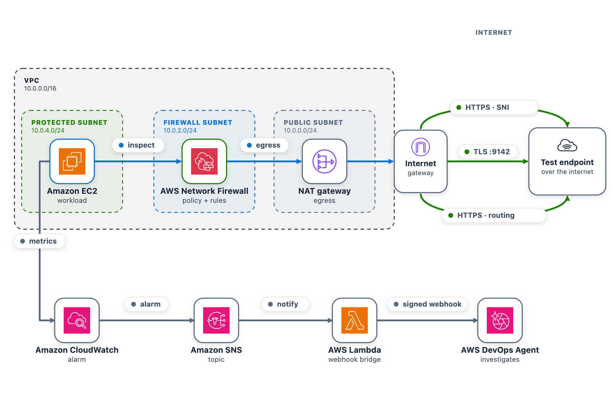
As part of this blog post, we provide a CDK stack that deploys both the AWS DevOps Agent Space and a sample workload used to walk through three separate troubleshooting scenarios. A single t3.micro instance in a protected subnet checks its connectivity to a test endpoint on a continuous loop and publishes results to CloudWatch. Traffic takes the internet egress path through Network Firewall, the NAT gateway, and the internet gateway, so the firewall can intercept or drop it. After completing the walkthrough, you can apply the same troubleshooting techniques with DevOps Agent against your own Network Firewall deployments.
The test endpoint runs in a separate VPC deployed by the same CDK app. It serves HTTPS on port 443 and TCP on port 9142, giving each scenario a different protocol layer to exercise: Scenario 1 targets a TLS connection on 443 (matched by Server Name Indication), Scenario 2 targets a TCP connection on 9142, and Scenario 3 exercises the whole egress path.
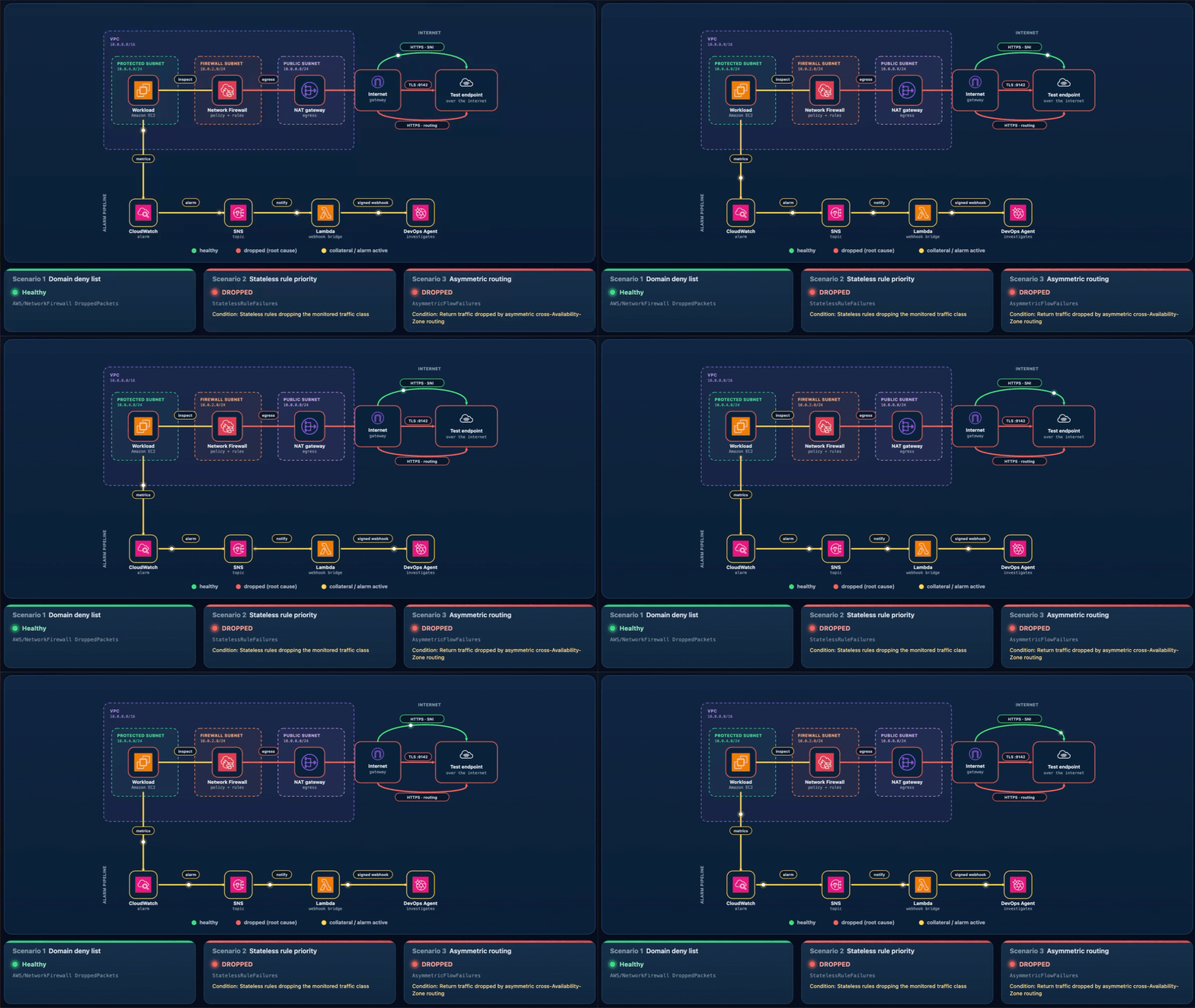
A live status page shows one card per scenario plus the network topology. The whole stack deploys from a single CDK app across two Availability Zones, each with a firewall endpoint and NAT gateway, which is what makes Scenario 3 possible.
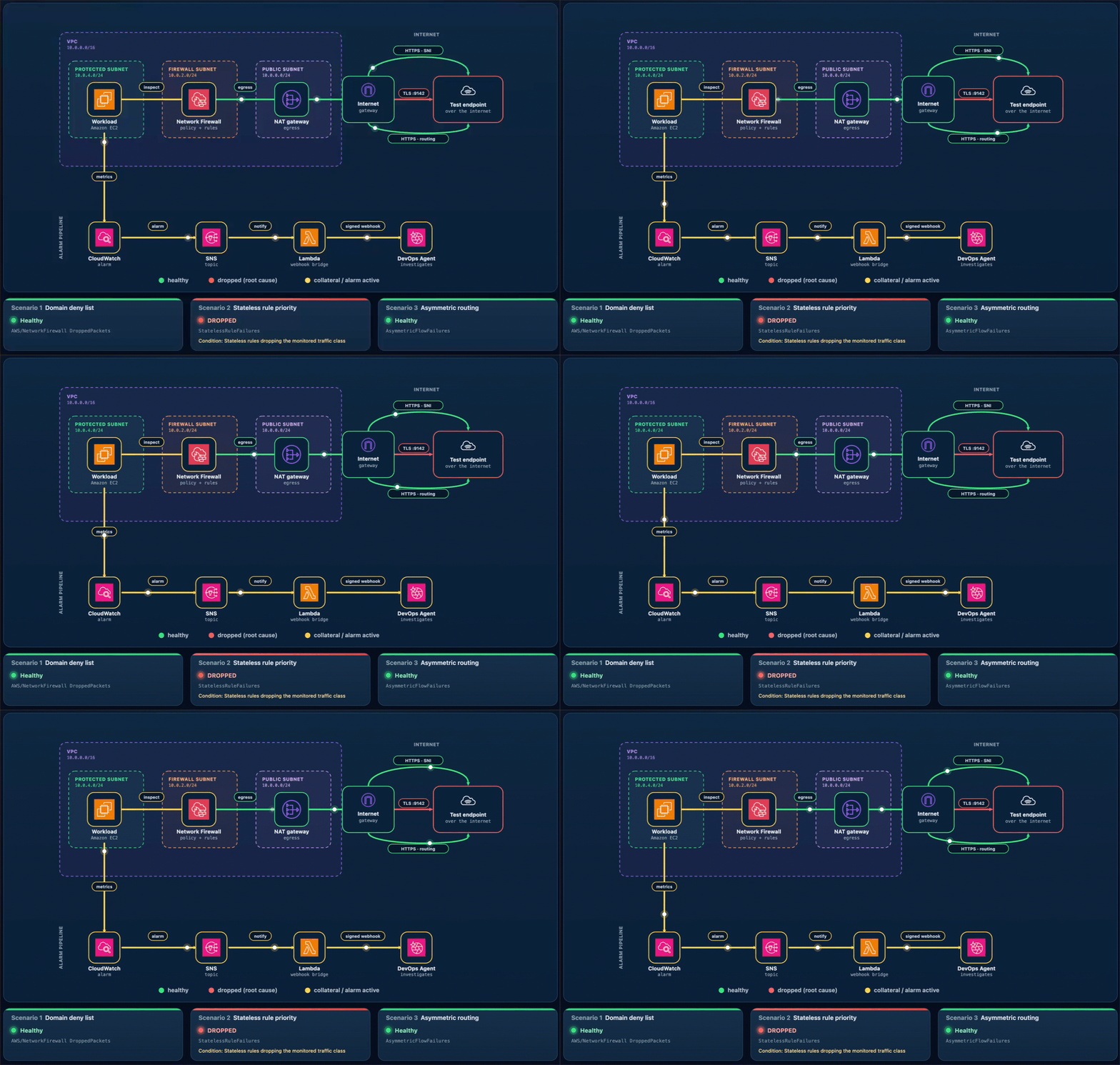
As shown in the following figure, the egress data path runs from the workload through Network Firewall and the NAT and internet gateways to the test endpoint. The alarm pipeline runs from CloudWatch through Amazon Simple Notification Service (Amazon SNS) and the webhook AWS Lambda function to DevOps Agent.
Figure 1: The sample workload
To use this with your own workload, you need a CloudWatch alarm that detects the connectivity problem and the webhook pipeline (SNS topic and Lambda function) that delivers it to DevOps Agent. The agent reads your firewall configuration, logs, and CloudTrail through AWS APIs, so no additional instrumentation is needed on the firewall side.
AWS CDK 2.x is required. You can use it through the project’s npx dependency, or install it globally:
npm install -g aws-cdk
Deploy the sample workload
Clone the project and deploy it into us-east-1 with one command (set awsRegion to use another AWS Region).
git clone https://github.com/aws-samples/sample-accelerating-aws-network-firewall-troubleshooting-with-aws-devops-agent.git
cd sample-accelerating-aws-network-firewall-troubleshooting-with-aws-devops-agent
bash scripts/deploy.sh
The script checks prerequisites, installs dependencies, compiles and tests, and bootstraps the CDK if needed. It then deploys all the stacks from a clean baseline and prints the outputs, including the status-page URL and sign-in details.
Open the status-page link (an https://<random-id>.cloudfront.net address).
Sign in using the username and password provided from the CDK output and confirm all three cards show the green Healthy status.
Keep the page open while you run the scenarios.
Connect AWS DevOps Agent
To connect AWS DevOps Agent to the alarm pipeline
In the AWS DevOps Agent console, open the nf-devops-agent-space Agent Space created by the CDK deployment.
On the status page, choose Configure webhook, paste the URL and signing secret, and save. The page writes them to the nf-devops-agent-webhook-credentialsAWS Secrets Manager secret, so there is no AWS CLI or console step. Until you set it, the bridge Lambda function sees a placeholder and skips delivery.
Verify the path before you run a scenario. In the Lambda console, open nf-devops-agent-webhook and use the Test tab with this event.
{
  "Records": [
    {
      "Sns": {
        "Message": "{\"AlarmName\":\"TEST-webhook-verification\",\"AlarmDescription\":\"[TEST] Webhook integration test - not a real alarm.\",\"NewStateValue\":\"ALARM\",\"NewStateReason\":\"[TEST] Manual webhook connectivity test. Safe to ignore.\",\"Region\":\"us-east-1\"}"
      }
    }
  ]
}
A 200 response confirms the path, and a test investigation appears in the DevOps Agent Operator Web App view.
How the alarm pipeline works
Every scenario reaches DevOps Agent the same way. A CloudWatch alarm moves to ALARM and notifies the SNS topic. Amazon SNS invokes a Lambda function. The function reads the webhook URL and signing secret from Secrets Manager, signs an alarm payload, and POSTs it to the DevOps Agent webhook (as shown in Figure 1). Amazon SNS also provides delivery retries, fan-out to other subscribers, and cross-account publishing.
Prebuilt Network Firewall metric (Scenario 1) – Alarm-1 watches the DroppedPackets metric, summed across the stateful streams, and triggers when drops rise above a baseline threshold. This requires no workload or custom metric and works on an already-deployed firewall. However, it only tells you that the firewall is dropping packets, not which rule is responsible.
Application health metric (Scenarios 2 and 3) – Alarm-2 and Alarm-3 watch a custom metric from a connectivity check. Use this for an alarm tied to user-facing impact or to tell one traffic path from another, which requires running a component that emits the metric.
Alarm
Source
Triggers when
Alarm-1
Native AWS/NetworkFirewall DroppedPackets
The firewall’s dropped-packet count rises above the baseline
Alarm-2
Custom application health metric
The port 9142 (TCP) connectivity check to the test endpoint is being dropped
Alarm-3
Custom application health metric
The cross Availability Zone connectivity check is being dropped
Run the scenarios
Work through each of the scenarios one at a time, following the same cycle. Interrupt network connectivity, watch the alarm trigger, let DevOps Agent investigate, apply the recommended fix, and confirm recovery before moving on.
The status-page cards follow the live CloudWatch alarm state. A card shows a green dot and the word Healthy when its alarm is clear, and a red dot and the word DROPPED when its alarm triggers. In the DROPPED state the card also adds a Condition: line describing what’s being dropped, which isn’t shown when the card is healthy. Network Firewall applies changes to new flows, so a change shows within a minute or two. Recovery comes from the mitigation DevOps Agent recommends, which you review and apply.
Scenario 1. Domain deny list blocking a legitimate endpoint
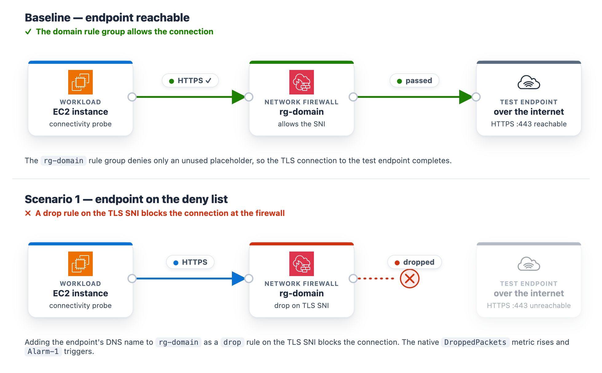
At baseline, the rg-domain Suricata domain rule group denies only an unused placeholder, so the test endpoint stays reachable. The rule group inspects the TLS Server Name Indication (SNI) on each outbound connection and drops any that matches a denied domain. The exact rule syntax and console steps follow.
In the navigation pane, under Network Firewall, choose Network Firewall rule groups.
Choose the rg-domain rule group to open its details page.
In the Rules section, choose Edit.
The rules box already contains two baseline placeholder rules (they match blocked.placeholder.invalid, so nothing real is denied). Leave those in place. Find the <app-endpoint-dns> value for Scenario 1 in the deployment script output (a Nework Load Balancer (NLB) DNS name such as NfTest-AppNl-a1b2C3dEf4G5-1234abcd5678efgh.elb.us-east-1.amazonaws.com). On a new line below the existing rules, add a drop rule that matches that DNS name on the TLS SNI, then choose Save.
drop tls $HOME_NET any -> $EXTERNAL_NET any (ssl_state:client_hello; tls.sni; content:"<app-endpoint-dns>"; startswith; nocase; endswith; msg:"S1 domain denylist"; flow:to_server, established; sid:2000002; rev:1;)
After saving, the rules box holds all three lines. The two placeholders remain, plus the new drop rule for the endpoint DNS name (note the distinct sid 2000002).
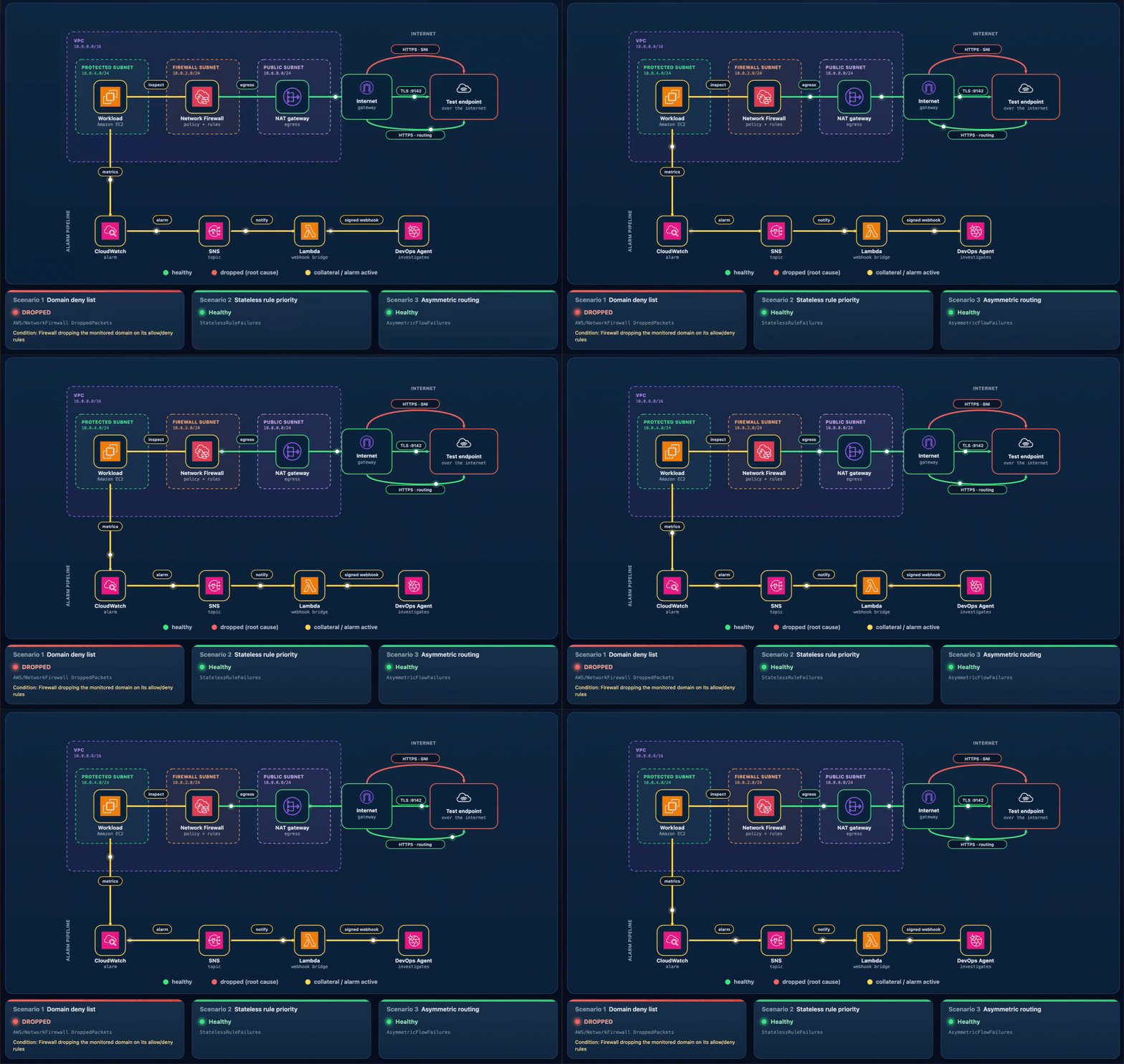
What happens. The workload’s HTTPS check to the test endpoint times out, the “AWS/NetworkFirewall DroppedPackets metric climbs above baseline, and Alarm-1 moves to ALARM. The Scenario 1 card reads DROPPED (with the condition Firewall dropping the monitored domain on its allow/deny rules), while the Scenario 2 and Scenario 3 cards stay Healthy (Figure 3). On the topology, the alarm pipeline from CloudWatch through Amazon SNS and Lambda to DevOps Agent and the workload-to-firewall inspect lines both turn amber, which the legend defines as collateral / alarm active, because the packets are now dropped at the firewall. To demonstrate the resulting failure, the HTTPS · SNI line from the internet gateway to the test endpoint is shown in red, which the legend defines as dropped (root cause).
Figure 3: Scenario 1 active – Traffic blocked at the firewall
Let DevOps Agent investigate. The agent runs several lines of investigation in parallel and correlates them:
Reads the DroppedPackets metric and correlates the spike with a simultaneous drop in passed packets, confirming the firewall is actively blocking traffic.
Reads the ALERT log and finds the workload’s TLS connections to the test endpoint blocked by the S1 domain denylist rule.
Compares the current state against a baseline window, where the same endpoint was reachable with no alerts, which shows the block is new.
Searches CloudTrail and surfaces the UpdateRuleGroup call that added the deny rule, identifying the user, role, and timestamp approximately one minute before the drops began.
Reports the root cause as that manual rule-group change. Recommends removing the deny entry or adding an allow exception and enabling FirewallPolicyChangeProtection to prevent unauthorized changes.
Presents this as a plan you review and apply, not an automatic change.
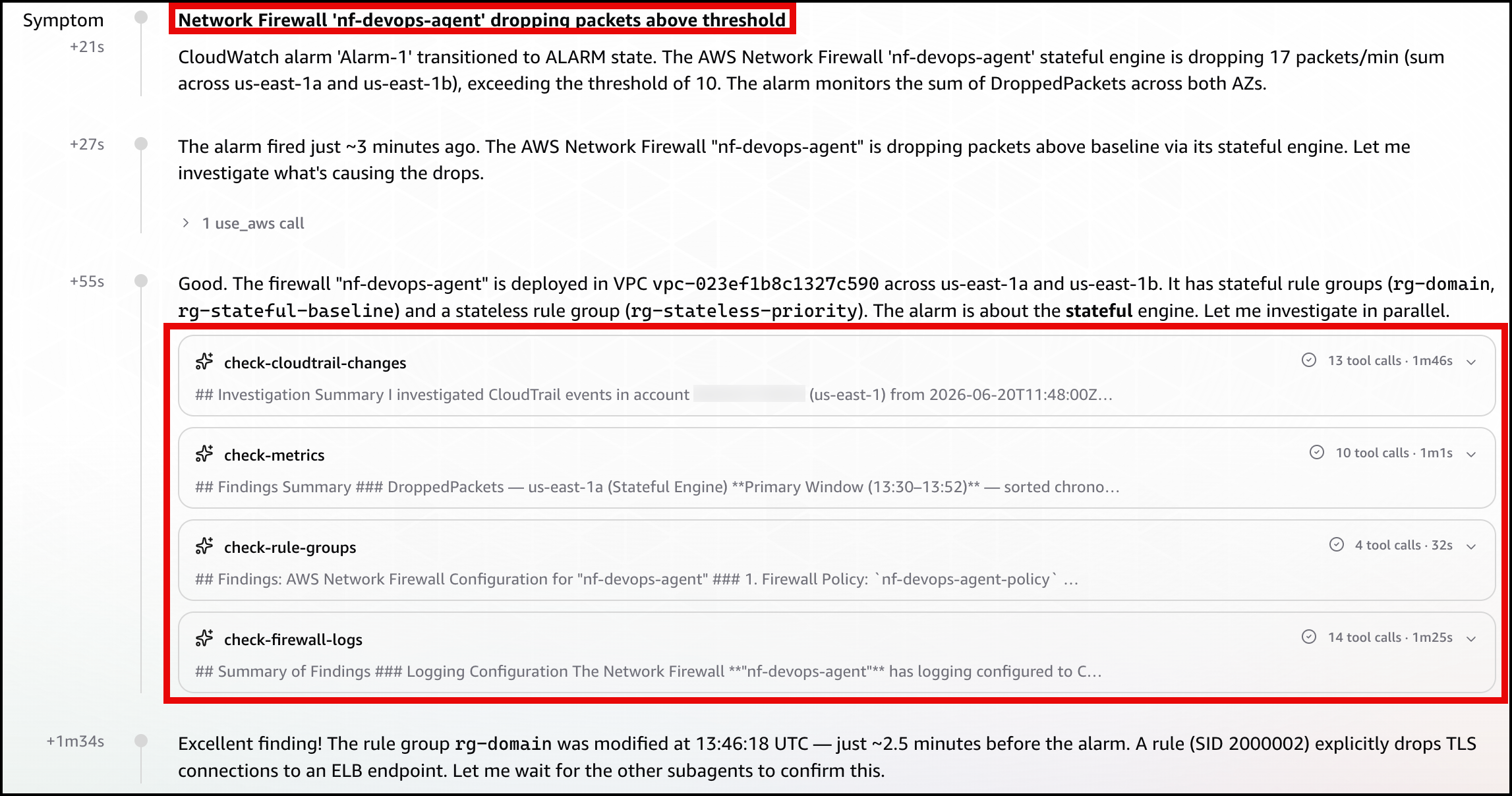
In the DevOps Agent Operator Web App view, the agent first restates the Alarm-1 trigger and confirms the firewall is dropping packets above the threshold (Figure 4).
Figure 4: Scenario 1 – The symptom
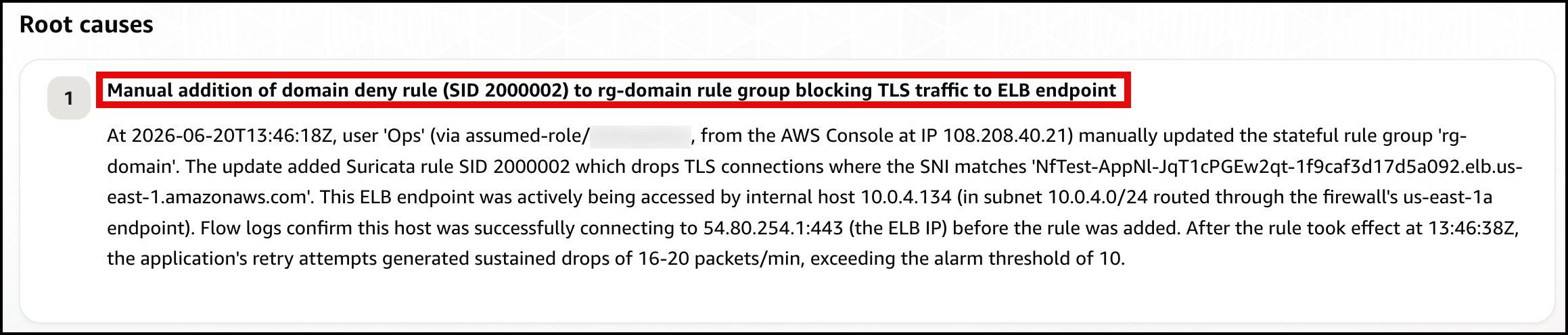
Next, the agent identifies the root cause: a manual update to the rg-domain rule group that added a domain deny rule (SID 2000002) shortly before the alarm fired, blocking TLS connections to the ELB endpoint (Figure 5).
Figure 5: Scenario 1 – The root cause
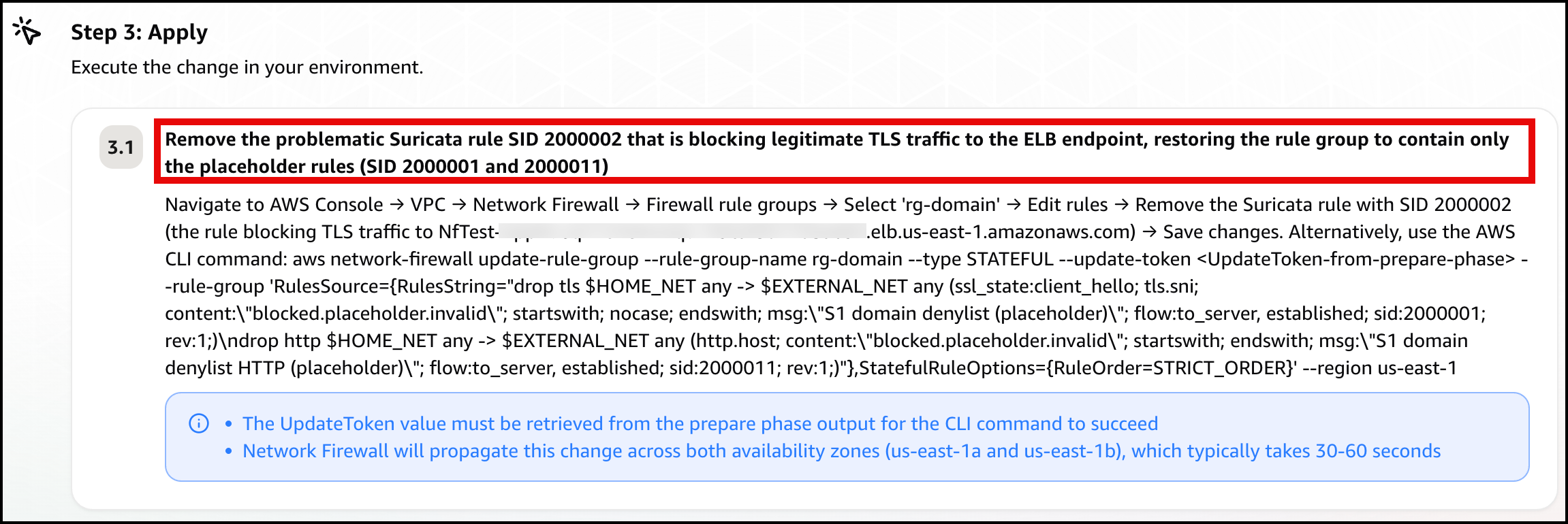
Finally, the agent presents a mitigation plan, recommending you remove the problematic deny rule (SID 2000002) to restore connectivity (Figure 6).
Figure 6: Scenario 1 – The mitigation plan
Note: In a real-world environment, this type of rule typically exists for a reason. Before removing it, verify whether it was intentional but scoped too broadly. If so, refine the rule to block only unauthorized endpoints rather than removing it entirely.
Confirm recovery. Apply the change the agent recommends. After the deny entry is gone, DroppedPackets falls back to baseline, Alarm-1 clears, and the card returns to green. Move on to Scenario 2.
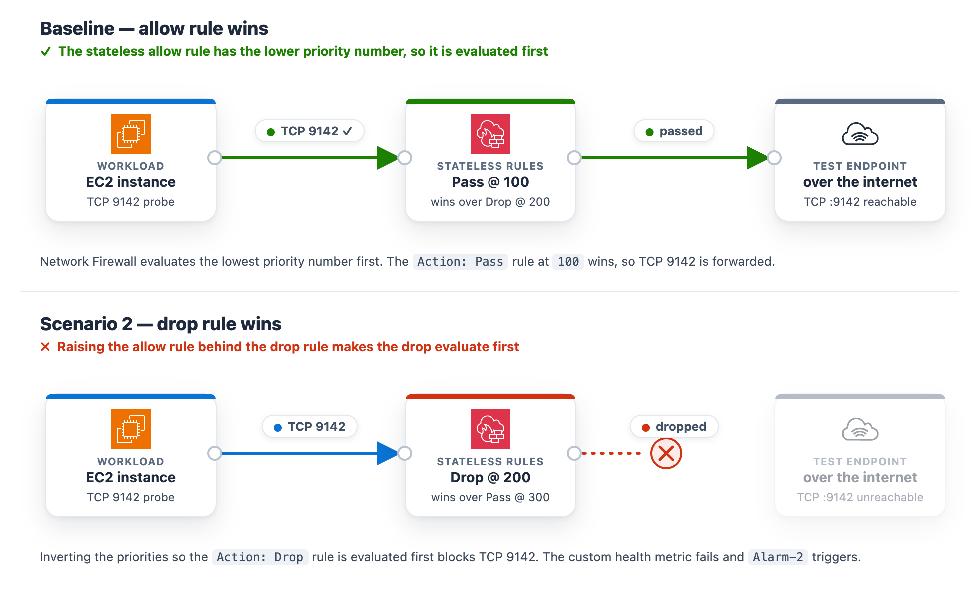
At baseline, the rg-stateless-priority stateless rule group keeps the allow rule at priority 100 and the drop rule at 200 for the test class, TCP destination port 9142. The workload opens a TCP connection to the test endpoint on this port. Lower priority numbers evaluate first, so the allow rule wins. This scenario uses port 9142 instead of 443 to demonstrate a stateless rule, which matches on the packet’s 5-tuple (protocol, ports, addresses) rather than application content.
Introduce the change. Invert the two rule priorities so the drop rule evaluates before the allow rule. This is the kind of change a rushed rule edit can introduce.
In the navigation pane, under Network Firewall, choose Network Firewall rule groups.
Choose the rg-stateless-priority rule group to open its details page.
In the Rules section, choose Edit.
Raise the (Action: Pass) rule’s priority number so it sits after the (Action: Drop) rule, then choose Save. For example, change the (Action: Pass) rule from 100 to 300 (any number higher than the drop rule’s 200 works). You only need to move one rule, and using 300 avoids a clash with the drop rule that already sits at 200. Network Firewall evaluates the lowest priority number first, so the (Action: Drop) rule at 200 now wins for this traffic class, ahead of the (Action: Pass) rule at 300.
Figure 7: Scenario 2 – Rule priority change blocking the traffic class
What happens. The drop rule now wins, the TCP connection to the test endpoint on port 9142 times out, the StatelessRuleFailures metric climbs above baseline, and Alarm-2 moves to ALARM. The Scenario 2 card reads DROPPED (with the condition Stateless rules dropping the monitored traffic class), while the Scenario 1 and Scenario 3 cards stay Healthy (Figure 8). On the topology, the alarm pipeline from CloudWatch through Amazon SNS and Lambda to DevOps Agent and the workload-to-firewall inspect lines both turn amber, which the legend defines as collateral / alarm active, because the packets are now dropped at the firewall. To demonstrate the resulting failure, the TLS :9142 line from the internet gateway to the test endpoint is shown in red, which the legend defines as dropped (root cause).
Figure 8: Scenario 2 active
Let DevOps Agent investigate. A stateless drop happens before traffic reaches the stateful inspection engine, so it produces no ALERT log entries. The agent turns to configuration and flow logs instead:
Reads the stateless rule group state and finds the drop rule at the lower priority number, ahead of the pass rule, so the drop evaluates first.
Reads the flow logs and sees passed packets drop to zero within a minute of the change.
Searches CloudTrail and surfaces the UpdateRuleGroup call that inverted the priorities, identifying the user, role, and timestamp about a minute before the alarm.
Reports the root cause as that priority inversion. Recommends removing the redundant drop rule and managing the rule group through infrastructure-as-code (IaC) to prevent manual misconfigurations.
Presents this as a plan you review and apply, not an automatic change.
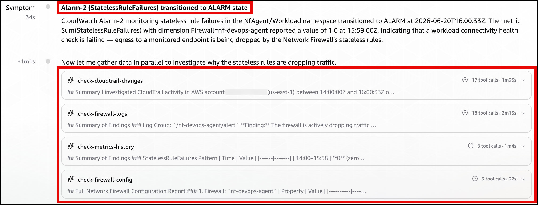
In the DevOps Agent Operator Web App view, the agent first restates the Alarm-2 trigger and confirms that a workload connectivity health check is failing because the firewall’s stateless rules are dropping egress (Figure 9).
Figure 9: Scenario 2 – The symptom
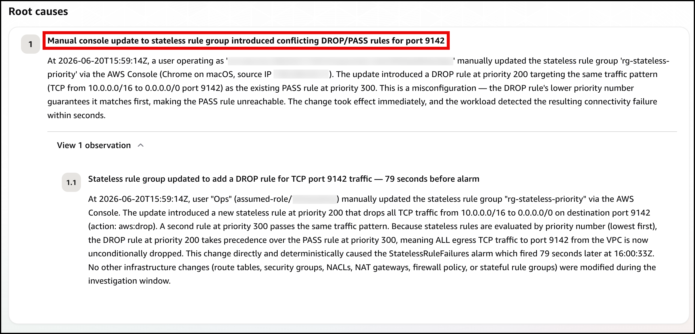
Next, the agent identifies the root cause, using the rule-group state and CloudTrail to pinpoint the conflicting DROP/PASS rules, where the new DROP rule’s lower priority number makes it match first (Figure 10).
Figure 10: Scenario 2 – The root cause
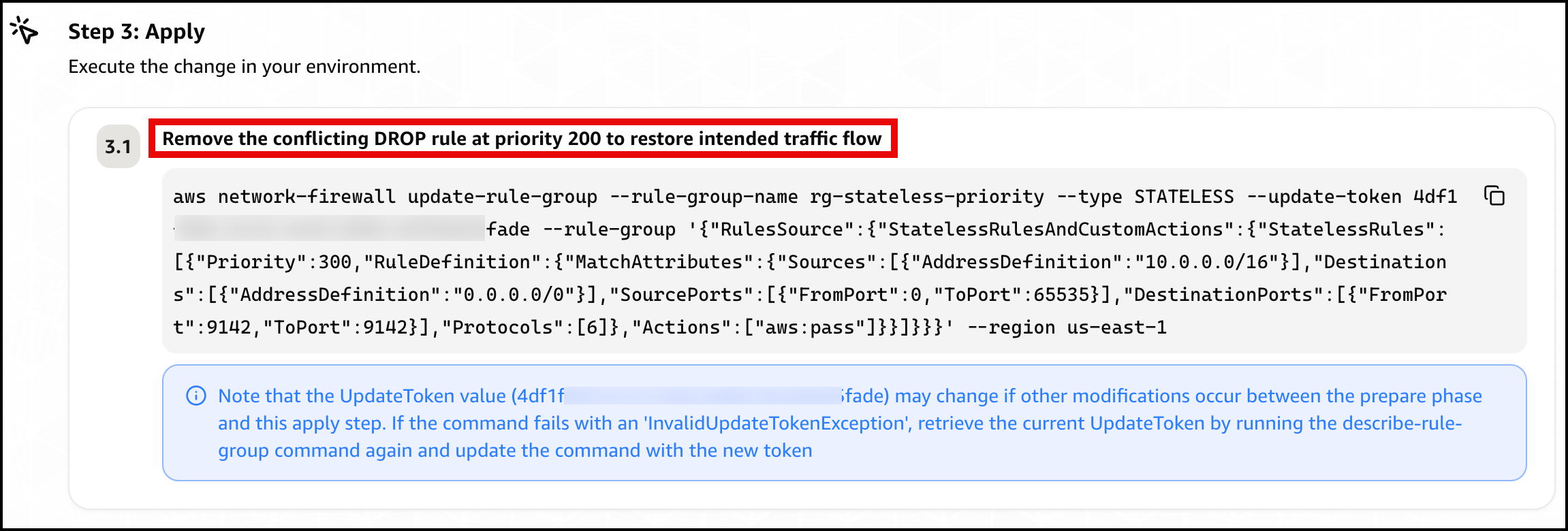
Finally, the agent presents a mitigation plan, recommending you remove the conflicting DROP rule at priority 200 to restore traffic flow (Figure 11).
Figure 11: Scenario 2 – The mitigation plan
Confirm recovery. Apply the change the agent recommends. After the allow rule is ahead of the drop rule again, Alarm-2 clears and the card returns to green. Move on to Scenario 3.
Scenario 3. Asymmetric cross Availability Zone routing drop
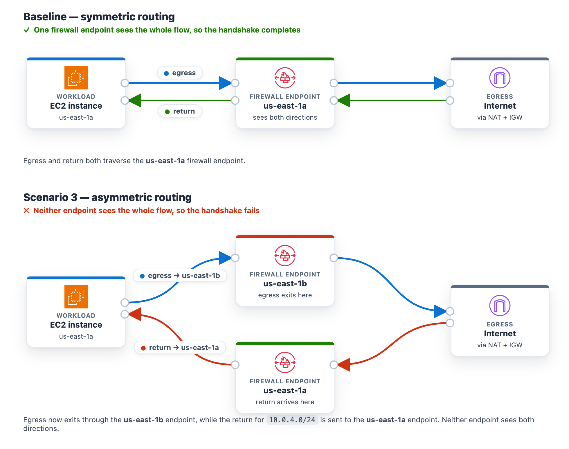
At baseline, the protected subnet in each Availability Zone routes its egress through the firewall endpoint in that same Availability Zone , and the matching return route uses that same endpoint. One endpoint sees both directions of the flow, so the stateful engine completes the handshake. The workload runs in the protected subnet in us-east-1a (CIDR 10.0.4.0/24), so at baseline its egress and its return both use the us-east-1a firewall endpoint.
Introduce the change. Make the flow asymmetric by sending egress out one Availability Zone endpoint while the return comes back through the other. This takes two route edits, and both are required. With only the first edit the flow can still complete, so the alarm will not trigger until both are saved. It makes no firewall-policy change, mirroring a real multi-Availability-Zone routing mistake.
To create asymmetric cross Availability Zone routing
Go to the Amazon VPC console and choose Route tables in the navigation pane.
Flip the egress. Select the NfNetworkStack/SampleVpc/protectedSubnet1 route table (the us-east-1a protected subnet, where the workload runs). On the Routes tab, choose Edit routes. Its 0.0.0.0/0 route currently targets the us-east-1a firewall endpoint. For the target, choose Gateway Load Balancer Endpoint and select the us-east-1b firewall endpoint, then choose Save changes.
Move the return. Select the NfNetworkStack/SampleVpc/publicSubnet2 route table (the us-east-1b public subnet, where egress now exits). Choose Edit routes, then Add route. For the destination enter the workload CIDR 10.0.4.0/24. For the target, choose Gateway Load Balancer Endpoint and select the us-east-1a firewall endpoint. Choose Save changes.
After both edits, a flow’s egress leaves through the us-east-1b endpoint while its return is directed to the us-east-1a endpoint. Neither endpoint sees the whole flow.
Figure 12: Scenario 3 routing change breaking the flow’s symmetry
What happens. A new connection leaves through one endpoint. Its return arrives at the other endpoint, which never saw the connection open, so the handshake fails. Unlike Scenarios 1 and 2, this affects the whole subnet, so all egress stops and Alarm-2 and Alarm-3 both move to ALARM. The AWS/NetworkFirewall DroppedPackets alarm (Alarm-1) stays quiet because no endpoint is making a drop decision. The flow is lost to asymmetric routing rather than counted as a firewall drop. This is why monitoring application connectivity matters. A routing fault is invisible to the firewall’s own drop counter. On the status page, the Scenario 2 card reads DROPPED (with the condition “Stateless rules dropping the monitored traffic class”) and the Scenario 3 card reads DROPPED (with the condition Return traffic dropped by asymmetric cross-Availability-Zone routing), while the Scenario 1 card stays Healthy (Figure 13). On the topology, the alarm pipeline from CloudWatch through Amazon SNS and Lambda to DevOps Agent and the workload-to-firewall inspect lines both turn amber, which the legend defines as collateral / alarm active, while the egress path from the firewall through the NAT gateway and the TLS :9142 and HTTPS · routing lines to the test endpoint turn red, which the legend defines as dropped (root cause).
Figure 13: Scenario 3 – The status page during a path-wide outage
Let DevOps Agent investigate. Both Alarm-2 and Alarm-3 fire in the same datapoint. DevOps Agent recognizes them as linked and merges them into a single investigation:
Reads the flow logs and sees bidirectional TLS connections stop abruptly, with only one-way traffic remaining and no flows reaching the established state.
Reads the firewall metrics and sees received and passed packets shift from one Availability Zone to the other at the moment of the change.
Calls DescribeRouteTables and finds the egress route pointing at one Availability Zone firewall endpoint while the return route points at the other.
Searches CloudTrail and surfaces the ReplaceRoute and CreateRoute calls by the same user, about a minute before both alarms fired.
Reports the root cause as that asymmetric routing change. Recommends restoring symmetric same-Availability-Zone routing so egress and return traverse the same endpoint.
Presents this as a plan you review and apply, not an automatic change.
A mitigation plan is a recommendation you review, not an automatic change, and the right fix depends on the intended design. Restoring symmetric routing can mean sending the workload subnet’s egress back through its own-Availability-Zone firewall endpoint (this sample’s architecture) or, in a design that doesn’t inspect this path, back through a NAT gateway. The agent infers a plausible target from what it can observe, so review the specific route it proposes against your intended topology before you apply it. (Connecting your pipeline or infrastructure-as-code, covered in the next section, lets the agent recommend the target that matches your design.)
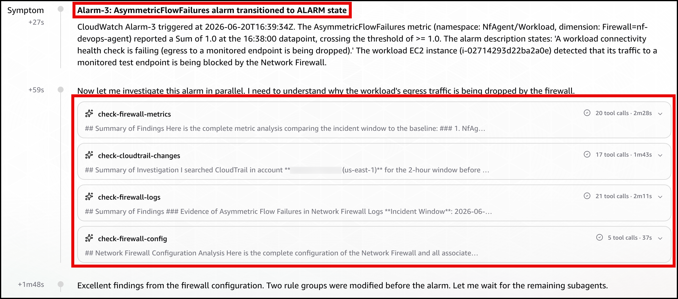
In the DevOps Agent Operator Web App view, the agent restates the Alarm-3 (AsymmetricFlowFailures) trigger and confirms the workload’s egress to a monitored endpoint is being blocked by the Network Firewall (Figure 14).
Figure 14: Scenario 3 – The symptom
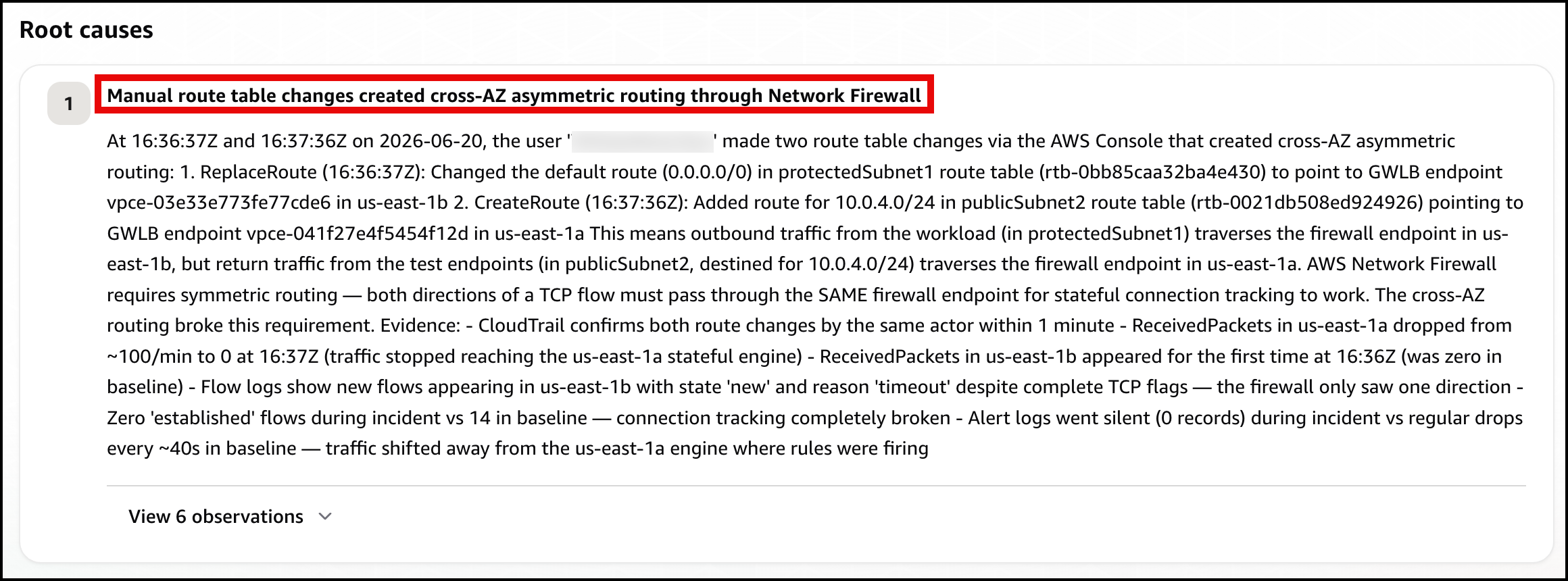
Next, the agent identifies the root cause: manual route table changes that created cross-AZ asymmetric routing through the network firewall, breaking its symmetric routing requirement (Figure 15)
Figure 15: Scenario 3 – The root cause
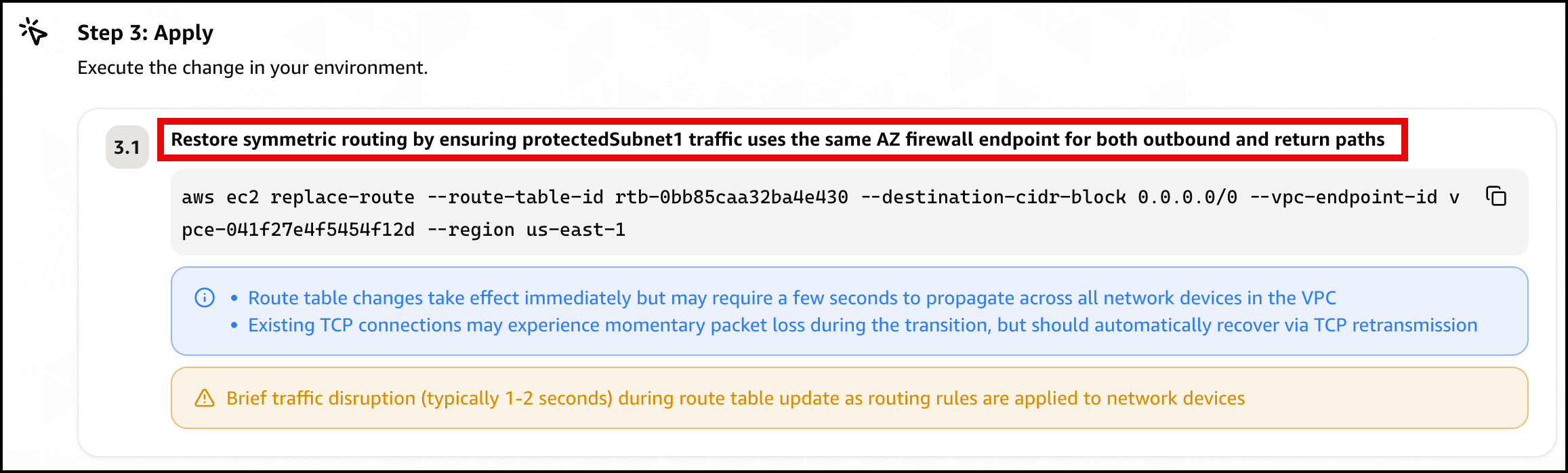
Finally, the agent presents a mitigation plan, recommending you restore symmetric routing by pointing protectedSubnet1‘s default route back to the same Availability Zone firewall endpoint, so one endpoint sees both directions of the flow again (Figure 16).
Figure 16: Scenario 3 – The mitigation plan
Confirm recovery. Apply the change the agent recommends, after checking the route target matches your intended design. After the workload subnet’s egress and return use the same Availability Zone firewall endpoint again, the control probe recovers, the alarms clear, and every card returns to green.
Further considerations
In production a single change can trigger several alarms at the same time, as Scenario 3 shows. DevOps Agent links related investigations and works them as one, so you review a single root cause. You can validate the linked findings or unlink an alarm to investigate it independently. If you would rather collapse alarms before they reach the agent, you can add correlation logic in the bridge Lambda function, buffering and grouping by firewall. You can also add email, Amazon Simple Queue Service (Amazon SQS), or HTTP subscribers to the SNS topic, or add the webhook Lambda function to a topic you already run. DevOps Agent produces a mitigation plan but does not change your environment on its own.
You can also give the agent more to work with. DevOps Agent connects to source repositories and CI/CD pipelines, integrating with GitHub (including GitHub Enterprise Server and GitLab Self-Managed through a private connection). It can associate AWS resources with deployments of AWS CloudFormation, AWS CDK, Amazon Elastic Container Registry (Amazon ECR) images, and Terraform. With deployed configuration and recent deployment events in view, the agent correlates the disruption against the change that introduced it and recommends a fix matching your intended design. For this sample, that means recommending the workload subnet’s own Availability Zone firewall endpoint rather than a generic symmetric path.
DevOps Agent also supports proactive incident prevention. It analyzes patterns across past investigations and delivers recommendations to prevent similar issues from recurring, including governance recommendations that strengthen deployment processes and pipeline controls. For Network Firewall rule changes, this means the agent can recommend guardrails for your CI/CD pipeline based on the classes of misconfigurations it has already resolved. You can access these recommendations through the Improvements page in the DevOps Agent Operator Web App.
Clean up
Clean up the environment with one command.
bash scripts/destroy.sh
It reverts any active scenario, runs cdk destroy for all stacks, and sweeps for stragglers by the Project = nf-devops-agent tag. The main cost drivers are the two Network Firewall endpoints, the NAT gateways (one in the main VPC for each Availability Zone, one in the test-endpoint VPC), and the test endpoint’s load balancers. Each of these bills at an hourly rate for as long as it’s provisioned, whether or not traffic is flowing, so a stack left running continues to accrue charges around the clock even while idle. Running the scenarios and tearing the stack down the same day limits the cost to a few active hours rather than days of idle hourly charges.
Conclusion
In this post, we showed you how AWS DevOps Agent accelerates troubleshooting for three common network firewall connectivity issues. The first was a domain deny list. The second was a stateless priority inversion. The third was an asymmetric cross-AZ routing drop. For each one, DevOps Agent investigated the drop and returned a root cause with a mitigation plan you approve before applying. The first scenario triggered on a prebuilt Network Firewall metric, and the other two on application health metrics. That shows both ways to alarm on a firewall problem through one pipeline.
According to Siemens’ 2024 report The True Cost of Downtime, Fortune 500 companies lose an estimated $1.4 trillion annually because of unplanned downtime. This downtime is often worsened by a lack of skills to detect and resolve issues quickly. Generative AI offers a promising path to address this, but deploying these capabilities in industrial environments introduces a distinct architectural challenge: how do you bring the power of large-scale AI to locations where cloud connectivity is unreliable or unavailable?
The answer lies in an offline-first architecture, one that moves AI inference to the edge while using cloud services for model customization, deployment orchestration, and continuous improvement. This pattern requires careful coordination across multiple AWS services spanning artificial intelligence and machine learning (AI/ML), Internet of Things (IoT), and storage, and demands deliberate trade-offs between model capability, hardware constraints, and operational complexity.
The following are a few potential use cases that could benefit smart applications at the edge:
Maintenance crews struggle to correlate real-time log feeds with relevant machine manuals, and analyze situations in-hand.
Offshore platforms, remote drilling sites, and pipeline maintenance crews operating in areas with limited satellite connectivity requiring instant access to safety procedures, equipment manuals, and regulatory compliance documentation.
Remote agricultural facilities with precision farming equipment requiring access to machinery manuals, crop management protocols, and safety procedures.
In this post, we walk through a reference architecture for building and deploying a generative AI application at the edge using AWS services. We cover the end-to-end pattern, from model customization in the cloud using Amazon Bedrock and Amazon SageMaker AI, to edge deployment using AWS IoT Greengrass, to local inference orchestrated by Strands Agents. Along the way, we highlight the key architectural decisions and service integration patterns that make this approach work.
This post describes a reference architecture. It is not intended for direct production use. Perform a security review and implement controls appropriate to your workload before deploying to production.
Architectural decisions for offline-first AI
Designing an offline-first AI architecture starts with a critical decision: how to customize a language model for your domain while keeping it small enough to run on edge hardware. The model must fit within the compute and memory constraints of site-level devices (typically GPUs with 16 GB or more of VRAM), which means working with small language models (SLMs). The customization strategy you choose directly affects your architecture’s complexity, cost, and data pipeline requirements.
The following strategies represent increasing levels of architectural complexity, each with different infrastructure requirements and expected outcomes:
Model fine-tuning (FT): A relatively lightweight process to adapt a pre-trained model for specialized tasks. For example, you could fine-tune a model to answer troubleshooting questions about specific equipment using labeled Q&A pairs from maintenance tickets. Fine-tuning excels at teaching a model the format, style, and structure of the outputs you want. However, it’s less effective at injecting new domain knowledge that wasn’t in the base model’s original training data.
Continued pre-training (CPT): A more resource-intensive process that extends the base model’s training with domain-specific unlabeled data to embed new knowledge. For example, you could continue training on technical manuals, repair logs, and engineering documentation to teach the model equipment-specific terminology, failure patterns, and diagnostic procedures. This approach effectively injects domain knowledge into model parameters but requires significant computational resources and larger datasets compared to fine-tuning.
Hybrid approach (FT + RAG): Retrieval Augmented Generation (RAG) enhances model responses by retrieving relevant documents at inference time, which provides accurate, up-to-date answers with source citations and reduces hallucinations. For our edge implementation, we use ChromaDB (SQLite + HNSW defaults) with a sentence-transformer embedding model (384 dimensions) running on CPU. Documents are chunked at 512 tokens with 50-token overlap. With a dataset up to 5 GB, retrieval latency stays under 50 ms. The entire RAG pipeline lives on CPU/SSD with zero GPU VRAM consumption, keeping the full 16 GB dedicated to the large language model (LLM).
Hybrid approach (CPT + RAG + FT): Combines continued pre-training of the embedding model with fine-tuning of the language model to optimize the entire RAG pipeline. Through continuing training your embedding model on domain-specific queries to better understand domain-specific terminology and jargon, while fine-tuning your language model on Q&A pairs for the format and tone you want. For example, when an operator asks about the state of a cookie machine, they expect to get the application to check current state, throughput per minute, and visual quality of Cookies! This dual optimization ensures both accurate retrieval and high-quality responses, ideal for knowledge-intensive applications.
To decide on the right strategy for your application, you need to work backward from the use case requirements and expected outcomes.
Reference architecture
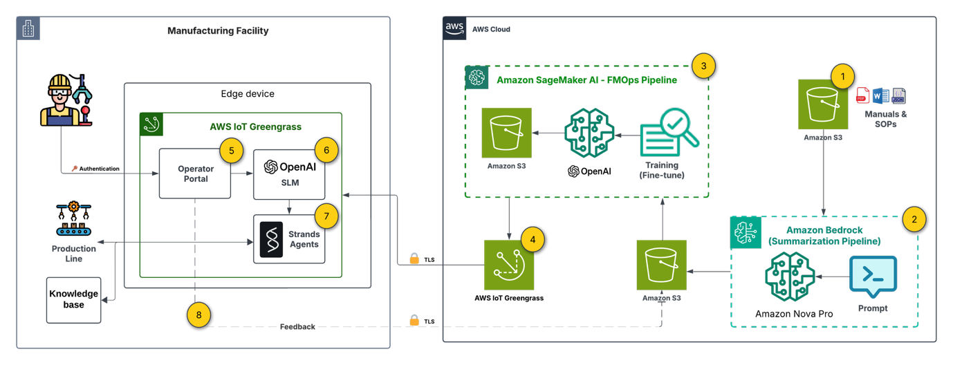
Let’s examine a reference architecture for an edge-deployed generative AI solution built on AWS. This architecture addresses a manufacturing use case where operators need instant access to equipment documentation, log correlation, and troubleshooting guidance, all without depending on cloud connectivity. We chose the hybrid approach (FT + RAG) because it balances two architectural concerns: keeping the on-device model compact through fine-tuning for task-specific behavior, while using RAG to provide up-to-date knowledge retrieval without retraining. The following diagram depicts the end-to-end architecture:
Note: The architecture spans two trust domains. On the cloud side, each service (Amazon Simple Storage Service (Amazon S3), Amazon Bedrock, SageMaker AI, IoT Greengrass) operates under a dedicated least-privilege AWS Identity and Access Management (IAM) role. All cloud-to-edge communication uses mutual TLS using IoT Greengrass device certificates. The operator portal requires authentication. On the edge device, the operator.
The architecture is organized into three layers: cloud-side preparation (steps 1–3), deployment orchestration (step 4), and edge-side inference (steps 5–9). Each layer uses specific AWS services chosen for their integration capabilities.
1. Document base setup
Technical manuals and Standard Operating Procedures (SOPs) are stored in Amazon S3, serving as the single source of truth for both the cloud-side training pipeline and the edge-side RAG knowledge base. The integration of Amazon S3 with both SageMaker AI and IoT Greengrass makes it the natural choice for artifacts that must flow between cloud and edge.
2. Preparing labeled data
Using Amazon Nova Pro on Amazon Bedrock, we process raw documentation into structured question-answer-context pairs for fine-tuning. This is a key architectural decision: rather than manually curating training data, we use a large foundation model (FM) in the cloud to generate high-quality labeled data at scale. The serverless inference of Amazon Bedrock keeps this step cost-effective, and the output feeds directly into the SageMaker AI pipeline.
3. Model customization (FMOps pipeline)
Amazon SageMaker AI Pipelines orchestrates an automated FMOps pipeline that fine-tunes gpt-oss-20b (Mixture of Experts (MoE) architecture: 21B total parameters, 3.6B active per token, 32 experts, 128k context length) on the domain-specific Q&A pairs. The pipeline pattern here is deliberate: it enables repeatable, versioned model customization that can be triggered whenever new documentation is added. The pipeline trains the model to understand equipment-specific terminology and response formats, then stores the customized model artifact in S3 for downstream deployment.
4. Edge deployment
The edge device (in our case, a g4dn.12xlarge with 4× NVIDIA T4 GPUs, 16 GiB each, 64 GiB total accelerator memory, 48 vCPUs, and 129 GiB system RAM) provides the GPU compute necessary for local inference. The hardware selection is an important architectural constraint that directly influences model viability and serving strategy. With gpt-oss-20b occupying 13 GB per T4 GPU, two deployment strategies are available depending on your throughput and latency priorities:
Model Replication — a full model copy on each of the four GPUs, which supports four concurrent client requests without queuing. This maximizes throughput at the cost of using 81 percent of each GPU’s memory for model weights alone.
Tensor Parallelism — the model is sharded across all four GPUs at 3.2 GB per GPU, leaving approximately 12.8 GB available on each GPU. This remaining memory serves as KV cache, supporting the full 128K context window for long-form interactions.
The choice between these strategies depends on your workload profile: replication suits high-concurrency, short-query environments, while tensor parallelism suits fewer concurrent users with longer, more complex interactions.
5. Edge device (manufacturing facility)
The edge device (in our case, NVIDIA Jetson Xavier) provides the GPU compute necessary for local inference. The hardware selection is an important architectural constraint: you need sufficient VRAM (16 GB or more) to run the quantized SLM, which directly influences which models are viable for your deployment.
6. User interface (Flask operator portal)
A Flask-based web interface running locally on the device allows maintenance operators and technicians to submit queries about equipment issues, safety procedures, or maintenance tasks. Running the UI on-device eliminates any dependency on external connectivity for the user-facing layer.
7. Off-cloud generative AI
The fine-tuned SLM runs on-premises using Ollama as the inference runtime. Ollama provides a lightweight, container-friendly serving layer that supports quantized model formats (GGUF) for efficient inference within the device’s memory constraints. This decouples the model serving infrastructure from any cloud dependency.
8. Generative AI orchestration
Strands Agents provides the orchestration layer that coordinates the query processing workflow. It routes requests to the appropriate tools: querying the on-site RAG knowledge base, collecting device telemetry data. This agent-based pattern provides extensibility. You can add new tools and data sources without modifying the core inference pipeline.
9. Continuous improvement (feedback loop)
When connectivity is available, user interactions and feedback flow back to the cloud, enabling ongoing model refinement through the FMOps pipeline. This creates a virtuous cycle: edge usage data improves the next model version, which Greengrass deploys back to the device. The architecture is designed to be resilient to connectivity gaps. Feedback is queued locally and synchronized opportunistically.
Prerequisites
To be able to implement a similar solution, you need:
An AWS account. If you don’t already have an AWS account, you can create one.
Your access to the AWS account must have IAM permissions to services including Amazon SageMaker AI, Amazon Bedrock, AWS IoT Greengrass, and Amazon S3.
A hardware device preferably with a GPU that has a sufficient VRAM (>16 GB) to run an SLM.
Implementation overview
This section summarizes the key implementation steps. Each component uses standard AWS service configurations:
Data preparation – Amazon Nova Pro on Amazon Bedrock generates structured Q&A pairs from raw documentation, producing training data for the SageMaker AI fine-tuning pipeline.
Model fine-tuning – SageMaker AI Pipelines runs a QLoRA fine-tuning job on gpt-oss-20b using the generated dataset, then stores the customized model artifact in S3.
Edge deployment – AWS IoT Greengrass (or AWS Systems Manager) transfers the quantized model (GGUF format) to the edge device.
Local inference – Ollama serves the fine-tuned model with a domain-specific system prompt constraining responses to equipment-relevant answers.
Orchestration – Strands Agents coordinates the workflow, routing queries to the RAG knowledge base or telemetry tools as needed.
For the fine-tuning notebook, refer to this example notebook for fine-tuning an SLM using Amazon SageMaker AI.
Security considerations
Moving inference to the edge shifts the security perimeter. In a cloud-native deployment, AWS manages much of the infrastructure security. At the edge, you own the full stack, which spans physical device access through application-layer controls. This section outlines the security controls to implement when adapting this architecture for your environment.
Authentication and access control. The Flask operator portal runs on an isolated device, but physical proximity doesn’t replace authentication. Integrate with your organization’s identity provider (SAML/OIDC) or implement certificate-based mutual TLS. Enforce role-based access so that operators, administrators, and maintenance personnel each see only the interfaces relevant to their function.
Encryption at rest. Model artifacts and the ChromaDB vector database contain proprietary knowledge. Encrypt the edge device’s storage volume using full-disk encryption (for example, LUKS on Linux or BitLocker on Windows). Manage encryption keys through AWS IoT Greengrass secret manager or a hardware Trusted Platform Module (TPM) on the device.
Encryption in transit. All communication between the edge device and AWS (including the IoT Greengrass deployment channel and the feedback synchronization loop) must use TLS 1.2 or later. For internal communication between edge components (Flask portal to Ollama, Strands Agents to ChromaDB), enforce TLS even on the loopback interface to prevent local interception.
Input validation and prompt guardrails. The Strands Agents orchestration layer accepts natural language input from operators. Apply input validation to reject malformed or excessively long queries. Implement prompt guardrails to detect and block prompt injection attempts. On the output side, apply content filtering to prevent the model from surfacing sensitive information outside its intended scope.
Network segmentation. Separate edge components into distinct network zones: the operator-facing portal in a perimeter network, the inference runtime in a restricted zone, and the cloud sync channel on an isolated outbound-only interface. Use firewall rules to enforce that only the expected traffic flows between zones.
IAM least privilege. On the cloud side, each AWS service in the pipeline should operate with its own IAM role scoped to minimum required permissions. The IoT Greengrass core device role should only access the specific S3 prefixes and IoT topics it needs. SageMaker pipeline execution roles shouldn’t have access to production S3 buckets.
Logging and monitoring. Enable AWS CloudTrail and Amazon CloudWatch for all cloud-side services. On the edge device, log all operator queries, model responses, and sync events locally. When connectivity is available, forward edge logs to Amazon CloudWatch Logs or Amazon S3 for centralized analysis. Set up alerts for anomalous patterns such as unexpected query volumes, repeated authentication failures, or unauthorized access attempts.
Results
We evaluated the fine-tuned gpt-oss-20b model against the base model using 30 domain-specific question-answer pairs. Both configurations use the full RAG pipeline (ChromaDB + sentence-transformer embedding model) as the retrieval layer. The variable being tested is whether fine-tuning the language model improves generation quality when given the same retrieved context. Three LLM judges (Claude 4.5 Haiku and Claude 4.5 Sonnet using Amazon Bedrock, and Amazon Nova Pro) scored responses on a 12-point scale across accuracy, completeness, and relevance.
LLM Evaluator
SLM
Average score
Claude 4.5 Haiku
Fine-tuned gpt-oss-20b + RAG
10.20/12 (85%)
Base gpt-oss-20b + RAG
8.20/12 (68.3%)
Claude 4.5 Sonnet
Fine-tuned gpt-oss-20b + RAG
9.20/12 (76.7%)
Base gpt-oss-20b + RAG
7.49/12 (61.7%)
Nova Pro
Fine-tuned gpt-oss-20b + RAG
9.90/12 (82.5%)
Base gpt-oss-20b +RAG
8.70/12 (72.5%)
These results support the hybrid approach (FT + RAG) outlined in our solution architecture, demonstrating that even with a relatively small fine-tuning dataset, significant performance improvements can be achieved for domain-specific applications at the edge.
Cleanup
The AWS services used in this architecture are fully managed services that follow a pay-as-you-go pricing model, meaning you only pay for actual invocations. Exception for this can be the storage costs for the labeled data and the finetuned model in Amazon S3 which you can consider to delete if not in use.
Conclusion
This post presents a reference architecture for deploying generative AI at the edge using AWS services. The key architectural patterns demonstrated include:
Cloud-side model factory – Using Amazon Bedrock for automated training data generation and Amazon SageMaker AI Pipelines for repeatable, versioned model customization, creating a scalable FMOps workflow that decouples model preparation from deployment.
Managed cloud-to-edge bridge – AWS IoT Greengrass provides the deployment orchestration layer, handling model packaging, versioning, and lifecycle management without requiring persistent connectivity to target devices.
Self-contained edge inference stack – A lightweight runtime (Ollama) combined with an agent-based orchestration framework (Strands Agents) supports local AI inference with extensible tool integration, all operating independently of cloud availability.
Feedback-driven continuous improvement – An asynchronous feedback loop synchronizes usage data back to the cloud when connectivity permits, for iterative model refinement without disrupting edge operations.
These patterns are applicable beyond manufacturing. Any environment with intermittent connectivity, strict latency requirements, or data locality constraints (offshore energy, remote agriculture, transportation, defense) can benefit from this architectural approach. The critical design decisions will vary by use case: selecting the right model customization strategy, sizing edge hardware to model requirements, and choosing between RAG and fine-tuning. The overall integration pattern remains consistent.
As with any reference architecture, we recommend that you conduct a security review before production deployment.
To explore this pattern, consider identifying a use case with clear connectivity constraints and working backward from your edge hardware requirements to select a model customization strategy. The hybrid (FT + RAG) approach described in this post offers the right balance of capability and complexity. Expand it as you validate operational improvements.
Ready to explore more? Join us at re:Invent for related sessions: Real-time insights for smart manufacturing with AWS Serverless (CNS375) and Implement Agentic AI at the edge for industrial automation (HMC317).
In this 33rd quarterly recap post, discover the most impactful AWS serverless launches, features, and resources from Q2 2026 that you might have missed. Stay current with the latest serverless innovations that can improve your applications.
In case you missed our last ICYMI, read about what happened in Q1 2026.
AWS Lambda MicroVMs
AWS Lambda MicroVMs is a new serverless compute primitive for running user or AI-generated code in isolated, stateful execution environments. Built on the same Firecracker virtualization that powers over 15 trillion monthly Lambda invocations, MicroVMs give you VM-level isolation with near-instant launch and resume. Each MicroVM runs in its own Linux environment with no shared kernel or resources between sessions. This isolation makes it a useful solution for AI coding assistant sandboxes, interactive code or multi-tenant development environments, CI/CD build environments, data analytics platforms, vulnerability scanners, and game servers that run user-supplied scripts.
Standard Lambda functions are best for event-driven, request-response workloads which have a 15-minute timeout. MicroVMs are purpose-built for single end user or session workloads and can preserve state for up to 8 hours. You get full lifecycle controls including launch, suspend, resume, and terminate. You can suspend them during the 8 hours if you don’t need them active. MicroVMs retain memory and disk state for the length of the session, even while suspended. They can auto resume when you need to use them again.
Amazon S3 Files makes your S3 buckets accessible as high-performance file systems. S3 files is a fully featured, POSIX-compatible file system to access to your data with approximately 1ms latency.
For serverless workloads, the Lambda integration with S3 Files lets your functions mount an S3 bucket as a local file system. Your function reads and writes files at a local mount path like /mnt/data, and the file system handles synchronization with S3 automatically. You can avoid downloading objects to /tmp from S3 within your function and work directly with files. Applications that assume a file system can now run on Lambda without rewriting their I/O layer. Use cases include sharing data between functions, ML model loading, document processing, media transcoding, or any pipeline that treats data as files rather than objects.
AWS Lambda durable functions
The Lambda durable functions SDK for Java is now generally available, joining Python and TypeScript. This allows Java developers to build multi-step workflows with automatic checkpointing and recovery without adding external orchestration. Durable functions is also now available in 16 additional AWS Regions. Learn how to build fault-tolerant multi-agent AI workflows to coordinate multiple AI agents that call tools, make decisions, and hand off work. There is automatic recovery if any agent fails mid-task. Voice analytics with Amazon Bedrock shows building a pipeline that processes call recordings through transcription, sentiment analysis, and summarization with durable checkpoints between each stage. For best practices, AI patterns, and futures, view the live stream.
AWS Lambda Managed Instances
Lambda Managed Instances now allows you to build memory-intensive apps with up to 32 GB (3x more than standard Lambda). This allows use cases like in-memory caching, large dataset analytics, and ML inference that previously required considering other services.
Scheduled scaling lets you pre-warm capacity for predictable traffic patterns with Amazon EventBridge Scheduler. This helps reduce cold start latency during known demand spikes. Tag propagation automatically applies your function tags to the underlying Amazon EC2 instances, Amazon Elastic Block Store volumes, and network interfaces. This helps finance teams with cost allocation visibility without manual tag management.
Other Lambda updates
Response streaming is now available in all commercial AWS Regions, bringing full regional parity for progressively streaming data back to clients. This is useful for LLM-powered applications where users expect to see tokens as they generate rather than waiting for a complete response.
If you have a fleet of functions on older runtimes, you can now upgrade runtimes at scale using AWS Transform custom. This uses AI to analyze your function code, identify breaking changes for the target runtime version, and generate the code modifications needed. This can help teams save manual migration effort across many functions. The Serverless Office Hours live stream has more information.
AWS Serverless Application Model (AWS SAM) CLI now supports BuildKit for building container images from Dockerfiles. This allows faster multi-stage builds with better caching, cross-architecture image builds, and Docker secrets to keep credentials out of final image layers.
Containers with Mama J
Serverless with Mama J
Mama J is back in the second video of a series where Eric Johnson explains what he does all day at work to his mother. Previously, they talked serverless and Lambda. This time it’s containers, what they are, why they exist, and how AWS manages them at scale. Eric goes through the “it works on my machine” problem, how Docker builds images, container orchestration and how containers differ from Lambda.
AWS Step Functions has an Amazon Bedrock AgentCore-powered agentic reasoning step. You can embed AI agent reasoning directly inside a workflow as a native step type. This bridges structured orchestration with autonomous agent behavior. Your workflow handles the deterministic parts such as branching, retries, timeouts, parallel execution, while the agentic step handles the parts that require flexible reasoning.
The Amazon BedrockAgentCore harness reached general availability. Two API calls give you a running agent in seconds which runs in its own isolated environment with a filesystem and shell. It can read files, run commands, and write code safely.
AgentCore Payments (preview) allows agents to autonomously access and pay for APIs and MCP servers, opening up agent-to-agent commerce. AgentCore Memory has metadata for long-term memory so agents retain and recall context across sessions. Web Search on AgentCore grounds agents in current, cited web knowledge. The Runtime now supports bring-your-own file systems from S3 Files and Amazon Elastic File System, and Node.js for direct code deployment.
Strands Agents SDK
The open source Strands Agents SDK shipped three capabilities. Context management that cuts token costs in half by intelligently pruning what goes into the model context window, Strands Shell for sandboxed agent code execution, and Strands Evals 1.0 with chaos testing and adversarial red teaming. This can reduce costs to help make production agent workloads cheaper without sacrificing quality. A Serverless Office Hours live stream covered the new features in depth.
The Agent Toolkit for AWS became generally available with three plugins (aws-core, aws-agents, aws-data-analytics), over 30 curated skills, and the AWS MCP Server. View this video for an introduction. This gives AI coding agents such as Kiro, Claude Code, and Cursor expert AWS knowledge which helps to reduce errors and lower token costs. For more information on the serverless tools available when using AI, see this Serverless Land resources page.
Serverless Office Hours ran a live stream series finding out how experts use AI to build serverless applications. Hear from:
Kiro launched Kiro Pro Max and an iOS mobile app for approving and monitoring agentic coding sessions from your phone. Amazon Q Developer IDE plugins are transitioning to Kiro. The Kiro power for AWS DevOps Agent connects your IDE directly to production intelligence. You can investigate incidents and generate fixes without context switching.
Join our live stream every Tuesday at 11 AM PT for live discussions, Q&A sessions, and deep dives into serverless technologies. View episodes on-demand at serverlessland.com/office-hours.
The Serverless landing page has overall information about building serverless applications. The Lambda resources page contains case studies, webinars, whitepapers, customer stories, reference architectures, and even more Getting Started tutorials.
You can also follow the Developer Advocacy team to get the latest news, follow conversations, and interact with the team.
Last week, my team visited Seoul to meet AWS Korea User Group (AWSKRUG) leaders. AWSKRUG is the largest cloud developer community in Korea, with 20 meetup groups organized by topic and area that collectively host over 100 events each year, primarily in Seoul.
My team regularly visits countries across the Asia-Pacific region, listens to feedback from user group leaders, and works to support their communities. At this meeting, leaders honestly shared what they did well in the first half of the year, what needs improvement, and what they asked of AWS Developer Experience team. We also enjoyed a pleasant conversation during our Chimaek time together.
Now, let’s take a closer look at key launches of last week.
A one-click Lambda setup prompt for coding agents caught my eye most last week. This prompt configures your agent with AWS Serverless skills and the Serverless Model Context Protocol (MCP) server, embedding serverless best practices from the start. This prompt references the Lambda agent setup guide, which includes installation commands for Claude Code, Kiro, Cursor, GitHub Copilot, Codex, Devin Desktop, and OpenCode.
To get started, choose the Copy agent prompt button on the Lambda console screen or copy fetch https://docs.aws.amazon.com/lambda/latest/dg/samples/aws-lambda-agent-setup.md directly, and paste this URL in your preferred AI agent.
You can also use Agent Toolkit for AWS to give your coding agent current AWS knowledge and safe resource access. Use fetch https://raw.githubusercontent.com/aws/agent-toolkit-for-aws/refs/heads/main/setup-instructions/setup.md for installing AWS MCP Server.
Last week’s launches Here are last week’s launches that caught my attention:
OpenAI GPT-5.6 Sol, Terra, and Luna on Amazon Bedrock: You can use the smartest family of models from OpenAI yet on Bedrock’s next-generation inference engine built for high performance, security, and reliability. The three models span capability tiers from flagship reasoning (Sol) to balanced performance (Terra) to fast, cost-efficient inference (Luna), all accessible through the Responses API on Amazon Bedrock.
Same-day transitions to Amazon S3 Standard-IA and S3 One Zone-IA: You can now transition objects to S3 Standard-Infrequent Access (S3 Standard-IA) and S3 One Zone-Infrequent Access (S3 One Zone-IA) as soon as the day they are created, without the previous 30-day minimum retention period in S3 Standard. These storage classes offer up to 40% lower storage costs than S3 Standard while still providing millisecond access when needed, making them ideal for backups, log analytics, and compliance workloads where data becomes cold within hours or days.
Self-managed code storage on AWS Lambda: With self-managed Amazon S3 buckets for code storage, you can reference source code directly from your own S3 buckets without Lambda creating intermediate copies. This eliminates code storage limits and reduces function activation time after function creates and updates by removing the copy step.
Importing users with password hashes on Amazon Cognito: You can now import users with password hashes in CSV user imports. Previously, imported users had to reset their passwords on first sign-in. Now, you can include password hashes in the CSV import, enabling users to sign in immediately with their existing credentials. When creating a CSV import, you specify the password hashing algorithm used by your source system.
For a full list of AWS announcements, be sure to keep an eye on the What’s New with AWS page.
Additional updates Here are some additional news items that you might find interesting:
Open Protocols with the Strands Agents SDK: Learn how open AI protocols such as MCP, A2A, UTCP, AG-UI, and x402 work together using Strands Agents SDK for building AI agents as an example implementation, though the patterns apply to any agent framework.
Open source Bulk Executor for Amazon DynamoDB: Performing bulk operations against all items in a DynamoDB table has historically required custom coding. The Bulk Executor for DynamoDB simplifies bulk tasks like these. You can use this feature to invoke commands like count, find, delete, or update. No coding is required, even when running at large scale.
Transform AWS Support Case Workflows with Kiro CLI: Explore how Kiro CLI’s MCP integration accelerates support case workflows by combining investigation, documentation lookup, and case creation into a single conversational interface across three real-world scenarios: AWS Glue job failures, AWS Lambda cold start investigation, and AWS WAF false positive analysis.
For a full list of AWS blog posts, be sure to keep an eye on the AWS Blogs page.
Finally, some customers experienced an issue with Cost Explorer displaying inaccurate estimated billing data in last weekend. They may have received erroneous budget and cost anomaly detection alerts, and observed inflated estimated cost and usage data. The issue has been resolved, and all AWS services are operating normally. We apologize for the concern this incident caused our customers and are conducting a thorough retrospective to prevent events like this from reoccurring, as well as improving our response when billing incidents occur. For more information, visit the AWS Health Dashboard.
That’s all for this week. Check back next Monday for another Weekly Roundup!
If you manage Lambda functions at scale, you’ve likely hit the 75 GB code storage limit or explained to your security team why deployment artifacts live in an S3 bucket you don’t control. Today, we’re announcing self-managed Amazon S3 buckets for AWS Lambda deployment packages. Lambda reads your code directly from your bucket, eliminating quota pressure and giving you full security control.
Previously, the default AWS-managed code storage created three challenges at scale. First, all copies count toward your 75 GB code storage quota. Second, you cannot apply your own encryption, access controls, or compliance tags to the internal bucket. Third, the copy cannot be incorporated into your disaster recovery strategies.
With self-managed S3 buckets, Lambda reads your function code directly from your bucket. No copy, no duplication. Your S3 object becomes the single source of truth for your functions. Deployment packages no longer count against your account’s code storage limit. You manage the bucket’s security and compliance posture: choosing the encryption, defining the access policies, managing lifecycle transitions, and maintaining the audit trail. And because you own the bucket, you can use S3 Cross-Region Replication to maintain fallback copies of your code in a secondary Region, so that your functions remain deployable even if your primary Region experiences an issue. Using self-managed S3 buckets also results in a faster time to first invoke for new functions and after function updates, because Lambda no longer needs to copy your zip package to a Lambda-managed S3 bucket.
You can use this feature today in all AWS standard regions where Lambda is available, at no additional charge beyond your standard Amazon S3 storage and request costs. Let’s look at some use cases, how it works, and how to use it at scale.
Use cases
Here are a few patterns where owning your deployment bucket makes a real difference.
CI/CD pipelines and artifact management
With self-managed storage, your CI/CD pipeline uploads once, and Lambda references the same object. One set of lifecycle rules and access controls covers all artifacts, and rollbacks mean pointing the function to a previous S3 object version.
Multi-account and multi-team architectures
Organizations using AWS Organizations often separate workloads into multiple accounts: a development account, a staging account, and a production account. They centralize shared resources in a tooling or shared-services account.
Self-managed buckets integrate naturally with this pattern:
Store all deployment artifacts in a central “artifact account” bucket.
Grant cross-account s3:GetObject access to Lambda execution roles in each workload account through bucket policies.
Maintain a single inventory of what code is deployed where, managed by your platform or DevOps team.
Enforce consistent encryption, versioning, and retention policies from one place.
Disaster recovery and business continuity
Because your deployment artifacts live in a bucket you own, you can use the built-in replication features of S3, Cross-Region Replication (CRR) or Same-Region Replication (SRR), to maintain copies of your code artifacts in backup locations. Combined with S3 Versioning and Object Lock, this gives you a durable, tamper-proof code archive that supports rapid recovery if a deployment is accidentally corrupted or deleted.
How it worked before
When you deploy a Lambda function using a .zip deployment package stored in Amazon S3, the process has traditionally worked like this:
You upload your .zip deployment package to your S3 bucket.
You call CreateFunction or UpdateFunctionCode, specifying the S3 bucket and S3 key.
Lambda copies the .zip artifact from your bucket into an internal, service-managed bucket.
Lambda uses this copy to create the optimized version of your function that runs at invocation time.
The copied artifact counts toward your account’s 75 GB code storage quota.
Figure 1 — Standard Lambda deployment
This model is straightforward and works well for most workloads. However, it creates three friction points at scale:
Storage quota pressure: Every deployment package copy counts toward your account’s 75 GB total code storage limit. Organizations with hundreds of functions and multiple published versions can exhaust this quota.
No control over stored artifacts: You cannot configure encryption (beyond the service default), access logging, lifecycle policies, Object Lock, or compliance tags on the internal bucket.
Redundant storage: Your original artifact remains in your bucket while a copy lives in the Lambda bucket used for provisioning new instances of your Lambda function.
What’s new: REFERENCE mode
This launch introduced a new function configuration setting, S3ObjectStorageMode. The default value is COPY, which provides the existing behavior described in the preceding section. To enable self-managed S3 buckets, set S3ObjectStorageMode to REFERENCE when creating or updating a function. In this mode, Lambda no longer copies your deployment package. Instead, it stores a reference to your S3 object and reads the code directly from your bucket when needed. If you do not specify S3ObjectStorageMode, Lambda still takes a copy by default.
Figure 2 — Lambda deployment with self-managed storage
This gives you:
No quota consumption. Deployment packages in your bucket don’t count against the 75 GB Function and layer storage account limit.
Improved performance. Lambda no longer copies the code to an internal bucket, so function creation and updates are faster.
Full security and compliance control. Apply your own bucket policies, encryption, Object Lock, versioning, access logging, and compliance tags.
Single source of truth. Your S3 object is the canonical artifact with no additional copies and no drift.
Disaster recovery options. Use S3 Cross-Region Replication to maintain fallback copies in a secondary Region.
How it works
To use this feature, specify the S3ObjectStorageMode parameter when creating or updating your function.
We recommend including the aws:SourceArn condition key scoped to your specific function ARN to allow for least-privileged access. Note the Resource is scoped to the exact S3 key rather than a wildcard prefix. This follows least-privilege and matches how the aws:SourceArn condition locks down which function can access which object.
Bucket requirements
Your S3 bucket must meet the following requirements:
Versioning (required). You must enable S3 versioning to make sure that Lambda references a specific, immutable artifact and to protect against accidental overwrites.
Encryption. The following encryption types are supported: SSE-S3, SSE-KMS (including customer-managed KMS keys), and DSSE-KMS. If you use SSE-KMS, the Lambda principal must have kms:Decrypt permission on the key.
Object Lock. Supported. You can apply Object Lock in Compliance or Governance mode to prevent accidental deletion of deployment artifacts.
Access logging. You can enable S3 server access logging or AWS CloudTrail data events to audit every time Lambda reads your code.
What happens when the object is unavailable
Lambda periodically accesses the source object from your S3 bucket to reoptimize your function code. You must maintain access to the source object for your function to remain active.
If Lambda loses access to the source object for a function, the function transitions to the Inactive state. To restore the function, restore access to the source object and then update the function.
Performance considerations
Lambda functions with self-managed code storage behave the same as standard Lambda functions with one difference during function creation and update. Lambda does not copy your deployment package to a Lambda-managed S3 bucket. In our testing with a 200MB Python 3.13 function, functions using self-managed storage showed function creation times approximately 5s less than the default COPY mode. Reading directly from your S3 bucket without an intermediate copy step can provide a modest advantage, particularly for larger deployment packages.
Getting started with infrastructure as code
Self-managed code storage can be implemented using infrastructure-as-code tooling with either the AWS CLI or AWS CloudFormation today.
Once you adopt self-managed S3 buckets for your Lambda deployment packages, your artifact bucket grows over time as you deploy new versions of your functions. This section covers strategies for managing that growth efficiently, keeping your versions organized, and planning for cross-Region deployments.
Managing artifact lifecycle with S3 lifecycle policies
Every time you update a function’s code, S3 creates a new object version in your bucket. The previous objects don’t disappear. They accumulate. Without a cleanup strategy, your storage grows indefinitely and old artifacts clutter your bucket.
S3 Lifecycle policies let you automate this entirely. You define rules that transition or delete objects based on age, and S3 executes them on your behalf: no scripts, no cron jobs, no manual intervention.
Strategy 1: Archive old versions to Glacier
If compliance or audit requirements mandate that you retain all historical deployment packages, but you rarely need to access them, transition old object versions to a lower-cost storage class:
This rule transitions any non-current object version to S3 Glacier Flexible Retrieval after 30 days. Your active deployment packages remain in S3 Standard for fast access, while historical versions move to archival storage at a fraction of the cost.
For artifacts you need to retain for years but will rarely access again, consider a tiered approach: moving to Glacier Flexible Retrieval first, then to Deep Archive:
This rule keeps the 2 most recent non-current versions of each object (giving you a rollback path) and deletes anything older than 14 days beyond that. This aligns well with a deployment strategy where you want the ability to quickly roll back to your previous one or two releases, but don’t need to retain anything older.
Tracking object and function versions
With REFERENCE mode, there is a direct relationship between your S3 object version and your Lambda function version. We recommend the following practices:
Tag your objects with metadata from your CI/CD pipeline (commit SHA, build ID, pipeline run ID) so you can trace any deployed function back to the exact source that produced it.
Document the mapping between Lambda function versions (or aliases) and S3 object version IDs. This makes rollbacks straightforward: update the function to reference the previous object version.
Cross-account considerations
How you organize your artifact buckets across AWS accounts depends on your operational model:
Centralized artifact account: A single bucket in a shared-services or tooling account, with bucket policies granting cross-account s3:GetObject access to Lambda execution roles in workload accounts. This gives your platform team a single inventory of all deployment artifacts with consistent lifecycle, encryption, and access policies.
Per-account buckets: Each workload account owns its own artifact bucket. Requires less effort to set up, but harder to enforce consistent governance across many accounts.
Either pattern works with self-managed storage. Choose based on how your organization balances centralized control against team autonomy.
Cross-Region considerations
With REFERENCE mode, your S3 object is the authoritative copy for your function. Self-managed code storage supports cross-Region function creation within a partition for all default Regions (non-opt-in Regions). You can store your code packages in one Region and deploy your functions in another. This makes cross-Region planning critical. There are four factors to balance:
Disaster recovery
This is the most critical consideration. Because your S3 object is the single source of truth in REFERENCE mode, you do not want all your deployment artifacts in a single Region with no fallback. A recommended pattern:
Primary Region: Your main artifact bucket where CI/CD pipelines deposit new deployment packages.
Fallback Region: A secondary bucket populated via S3 Cross-Region Replication (CRR). If your primary Region becomes unavailable, you can update your Lambda functions to reference the replicated objects in the fallback Region.
Weigh replication + storage costs against per-deploy cross-Region data transfer. If you deploy frequently, storing replicated copies in each target Region is usually cheaper. For infrequent deployments, a one-time transfer may suffice.
Governance and data residency
Some organizations, particularly in regulated industries, have strict requirements about where code artifacts can reside. Before configuring cross-Region replication, confirm that your data is permitted to leave its current Region. Certain regulatory frameworks (for example, data sovereignty laws, FedRAMP boundaries) may restrict replication to specific Region pairs.
Performance
If your workload requires fast function creation and activation times, for example, in a CI/CD pipeline where deployment speed is critical, keep your S3 objects in the same Region where you are creating your Lambda functions. Cross-Region reads add latency to the initial code download, which directly impacts how quickly a new function version becomes active after deployment.
For workloads where creation speed is less critical (for example, batch processing functions that are updated infrequently), the latency of a cross-Region read might be acceptable and can simplify your architecture.
Things to know
Before adopting self-managed S3 buckets for your Lambda functions, keep the following in mind:
Availability: You can use this feature today in all AWS standard regions where Lambda is supported.
Pricing: There is no additional Lambda charge. You pay standard S3 costs for storage, and any cross-Region data transfer.
Maximum deployment package size: The existing limits apply: 250 MB unzipped.
Supported runtimes: All Lambda runtimes that support .zip deployment packages are compatible. Container image deployments are not affected by this feature.
Migration: You can switch an existing function from service-managed to self-managed storage by calling UpdateFunctionCode with the --s3-object-storage-mode REFERENCE parameter. Lambda recreates the function by referencing the object in your S3 bucket and deletes the saved copy.
Reverting: You can switch back to service-managed storage at any time by updating the function with --s3-object-storage-mode COPY. Lambda resumes copying the artifact to its internal bucket.
Object availability is your responsibility: In REFERENCE mode, Lambda depends on your S3 object being accessible. If the object is deleted, the bucket policy changes, or the KMS key is disabled, new invocations requiring a cold start will fail.
Conclusion
In this post, we showed how self-managed S3 buckets for Lambda give you more capacity, more control, and simpler compliance, all without changing how you write or invoke your functions. Your deployment packages no longer count against account quotas, your security team can apply the same policies to code artifacts that they apply everywhere else, and your disaster recovery story is as strong as the replication capabilities of S3.
Amazon Redshift continuously innovates to deliver improved performance and advanced features. In some releases, Amazon Redshift patches might introduce behavior changes. Testing patches in a non-production environment confirms that production workloads continue to function and you can maintain your applications’ service level agreements. As a best practice, keep Dev/QA clusters on the Current patch track and Production on the Trailing track. Test on Dev/QA when a patch lands, allowing 1–6 weeks of review before the scheduled production deployment.
In this post, we demonstrate an automated test suite that validates your Amazon Redshift cluster automatically after any patch, reboot, or modification. It uses standard drivers against real workload patterns to provide a verified gate between a patch landing and that patch reaching production.
Architecture
The solution uses native AWS services to create an automated validation pipeline.
Test Execution: A Docker container runs a comprehensive test suite in four phases:
JDBC Driver Tests – Validates the official Amazon Redshift JDBC driver, testing DatabaseMetaData API calls, connection handling, and queries that tools like SQL Workbench/J depend on.
ODBC Driver Tests – Validates the PostgreSQL ODBC driver with SQLTables, SQLColumns, and other ODBC API calls that RStudio and similar tools use.
Catalog SQL Queries – Runs approximately 35 queries against pg_catalog, information_schema, and svv_* views, organized by client (SQL Workbench, DBeaver, RStudio, JDBC metadata API).
Performance Benchmarks – Executes your custom workload queries and compares execution time against known baselines, flagging regressions. For convenience, the solution includes sample queries to be replaced with performance validation queries from your workloads.
Reporting: Detailed JSON results land in Amazon Simple Storage Service (Amazon S3) for historical analysis. An Amazon Simple Notification Service (Amazon SNS) notification sends your team an email immediately with a pass/fail summary. Full JSON results are written to Amazon S3 with timing data for every individual query, row counts, error details, and the Amazon EventBridge event that triggered the run. If tests fail, you have specific, actionable evidence (which queries broke, which drivers failed, which benchmarks regressed) to open a support case requesting a rollback and defer maintenance until the case is resolved. When tests succeed, you can move forward with confidence to production.
For real-time feedback while the tests are running, a quick command tells you the current state:
The test suite covers two critical areas: client tool compatibility and query performance.
Client compatibility queries
The test suite replicates the connection behavior of popular SQL clients by issuing the same metadata API calls and queries they perform when connecting to your cluster.
ODBC-specific catalog queries, column type mapping
JDBC Metadata API
getTables(), getColumns(), getPrimaryKeys(), and other DatabaseMetaData method equivalents
The package contains the exact queries these clients execute upon connection.
Performance regression detection
The benchmark phase of the suite automatically detects whether it has been run before. On the first execution, it captures baseline query execution times as the “known good” state for your pre-patch environment. On every subsequent run, it compares current query timings against the stored baseline and flags any regressions. If a query that previously completed in 2 seconds now takes 15, the report calls it out immediately. This phase is designed to test your most performance-sensitive queries.
Prerequisites
Before deploying, make sure your environment meets the following requirements:
Amazon Redshift cluster reachable from the private subnets.
An AWS Secrets Manager secret with your Amazon Redshift credentials (created automatically with managed clusters).
Docker installed. Consider building the image with AWS CloudShell, which comes with Docker pre-installed. You can do this either by uploading the customized repo to Amazon S3 and then downloading it to AWS CloudShell, or by cloning and customizing the repo directly within AWS CloudShell.
Getting started
The full solution is available on GitHub. It includes the AWS CloudFormation template, Docker build scripts, test suite, and documentation.
Clone the GitHub repo, customize it for your workload, deploy it against a Dev/QA cluster.
Detailed instructions are included in the package README.md. Reference those for deployment.
Step 2: Customize the scripts for your environment
The test suite ships with comprehensive default queries. After cloning and before deployment, edit the scripts as described in the following sections for each phase.
Add your performance-critical queries
Edit bundle/run_tests.py and replace the example queries with queries where performance is critical:
BENCHMARK_QUERIES = {
    "daily_patient_summary": """
SELECT department, COUNT(DISTINCT patient_id), AVG(los_days)
FROM clinical.encounters
WHERE admit_date >= CURRENT_DATE - 30
GROUP BY 1
""",
    "revenue_rollup": """
SELECT payer_type, SUM(total_charges)
FROM billing.claims
WHERE service_date >= DATE_TRUNC('month', CURRENT_DATE)
GROUP BY 1
""",
}
Add client-specific catalog queries
If your team uses custom views or schemas, add them to bundle/client_catalog_queries.py:
"custom_view_check": {
    "description": "Verify our reporting view works after patching",
    "sql": "SELECT * FROM analytics.monthly_kpis LIMIT 10",
},
Step 3: Build the Docker image
Execute build-image.sh, which creates an Amazon ECR repository, builds the Docker image (with JDBC and ODBC drivers bundled), and pushes it, outputting the image URI for the next step.
# Upload project to S3, then build in CloudShell
./build-image.sh --stack-name my-redshift-tests
Step 4: Deploy the stack
Use the AWS Command Line Interface (AWS CLI) to deploy the AWS CloudFormation stack with your environment-specific parameters. The stack creates the required components: Amazon Elastic Container Service (Amazon ECS) cluster, AWS Fargate task definition, security groups, VPC endpoints (to keep AWS Secrets Manager and Amazon SNS traffic off the NAT gateway), Amazon S3 bucket, Amazon SNS topic, AWS Lambda trigger, and Amazon EventBridge rules.
Here are the core principles that make automated patch testing effective:
Dev/QA on Current track, Production on Trailing: This separation creates the buffer window between when a patch is available and when it reaches production. Without it, there’s no opportunity to catch regressions before they affect users.
Automate the validation: The track split is most effective if the test suite runs after every patch. Event-driven automation helps confirm no patch goes untested during the buffer window.
Test with real drivers: Simulated queries aren’t sufficient. The test suite exercises the Amazon Redshift JDBC and PostgreSQL ODBC drivers that your SQL clients depend on. This validates the same code paths your tools use in production.
Event-driven, not scheduled: Tests run the moment a patch is applied. They don’t run on a fixed cron schedule. Patch applied, then test executed, then results delivered in minutes.
Low operational overhead, minimal cost: The entire solution is serverless (AWS Lambda and AWS Fargate). There are no instances to manage and no agents to install. The Fargate task spins up only when a patch event fires, runs the test suite, and shuts down. You pay only for the compute each test run consumes.
Clean up
When you no longer need the automated test suite, delete the associated resources so you don’t incur ongoing costs.
Delete any created prerequisites, if not needed.
Amazon Redshift cluster (removes the managed secret).
Automated patch testing ensures consistent and predictable performance of your production workloads. By deploying Dev/QA clusters on the Current track with event-driven validation, you gain weeks of advance notice before patches reach production. The solution presented here provides comprehensive testing of JDBC drivers, ODBC drivers, catalog queries, and performance benchmarks. It requires zero manual intervention. Deploy it once, customize it for your workload, and gain confidence that the next Amazon Redshift patch will be validated before it matters.
To learn more about Amazon Redshift, explore the following resources:
A single cold start can push your Java Lambda function’s response time from milliseconds to seconds, enough to violate your p99 SLA, timeout a downstream service, and page your on-call. The Java Virtual Machine (JVM) performs best in long-running processes. Its Just-In-Time (JIT) compiler progressively optimizes code over thousands of invocations. Standard serverless execution environments recycle before the JVM reaches peak performance. This creates a tradeoff for latency-sensitive applications between cold-start penalties and runtime optimizations. For production services with p99 service level agreement (SLA) requirements, a single 14-second cold start spike can violate response time guarantees. It triggers downstream timeouts and degrades customer experience.
AWS Lambda Managed Instances changes this equation. As a capability of AWS Lambda, Managed Instances runs your functions on managed Amazon Elastic Compute Cloud (Amazon EC2) instances in your account and maintains JVM persistence across invocations. Connection pools, class hierarchies, and heap state persist across thousands of requests. This allows the JIT C2 compiler to complete optimizations like method inlining, escape analysis, and loop unrolling. The result: 18 to 30% better median latency and 3 to 30x better tail latency compared to Standard Lambda, as the benchmarks in this post demonstrate.
This post benchmarks four Java deployment modes across three workload types using 240,000 requests. The modes compared are Standard Lambda, AWS Lambda SnapStart, GraalVM Native Image, and Lambda Managed Instances. The workload types are CPU-bound, I/O + computation, and I/O-bound. This post presents benchmark results demonstrating Managed Instances delivering 30% better median latency and removing multi-second cold-start spikes on CPU-bound work after JIT warmup. It explains why these gains occur, maps each deployment mode to specific traffic patterns and cold-start tolerance requirements, and provides a decision framework for selecting the right approach for your workload.
Benchmarking setup
The benchmark runs all four deployment modes with identical Spring Boot 4.0.6 applications on Java 25 and AWS SDK v2. This configuration verifies fair comparison across modes. We tested three workloads: UC1 (PDF generation, CPU-bound), UC2 (data aggregation, I/O + computation), and UC3 (API orchestration, I/O-bound). The benchmark sends 240,000 requests using Artillery load testing at 33 RPS. Standard Lambda, SnapStart, and Native Lambda use 1024 MB (1 vCPU). Managed Instances uses c7i.xlarge instances with 2048 MB memory. Concurrency is tuned per workload (UC1=3, UC2=5, UC3=10) based on load testing to avoid thread contention. The benchmark measures p50, p99, and maximum latency across 10 runs of 2,000 requests each, with 5-minute cool-down between runs. The benchmark tracks JIT compilation metrics via Amazon CloudWatch Embedded Metrics Format. You can validate these results against Amazon API Gateway access logs, which confirm a <0.1% error rate. The GitHub repository contains complete source code, AWS Serverless Application Model (AWS SAM) templates, load scripts, and raw data. Performance claims in this post reference data from this benchmark methodology.
Figure 1 presents the architecture for all four deployment modes running in parallel against shared backend services.
To reproduce these benchmarks or deploy the sample applications, refer to the GitHub repository. The repository contains complete SAM templates, Artillery load configurations, deployment instructions, and cleanup commands. This post focuses on benchmark results and analysis. The benchmark used the following tools and services:
Managed Instances removes the extreme tail spikes characteristic of cold starts. Managed Instances delivers 27x faster maximum latency on CPU-bound workloads (UC1: 489 ms vs. 13,270 ms Standard). Mixed I/O + compute workloads see a 3x improvement (UC2: 3,644 ms vs. 11,174 ms Standard). I/O-bound workloads improve 30x (UC3: 309 ms vs. 9,237 ms Standard). We measured all results using the methodology described in Benchmarking setup.
The Standard Lambda 13-second maximum on UC1 represents a full cold start. That cold start includes JVM boot, Spring context initialization, Amazon DynamoDB client setup, and the first PDF render. SnapStart reduces this to under 3 seconds by restoring from a Firecracker microVM snapshot. However, the restore process plus re-initialization of resources that cannot be checkpointed (network connections, random number generators) still adds latency. GraalVM Native starts in under 2 seconds because the ahead-of-time (AOT) compiled binary skips JVM boot entirely. The Managed Instances maximum of 487 ms is not a cold start; it’s the slowest warm request across 20,000 invocations. For production SLAs, a 14-second cold start spike on Standard Lambda violates most requirements, while Managed Instances removes that spike entirely.
Observing median latency (p50)
Lambda Managed Instances delivered the lowest median latency across all three workloads. Results demonstrate 30% faster median latency on CPU-bound workloads (UC1: 97 ms vs. 139 ms Standard). Mixed I/O + compute achieves a 19% improvement (UC2: 184 ms vs. 228 ms Standard). I/O-bound workloads improve 18% (UC3: 76 ms vs. 93 ms Standard).
The improvement scales with CPU intensity because the JIT C2 compiler on persistent Managed Instances optimizes hot code paths that short-lived serverless environments never reach. On CPU-bound workloads (UC1), the JIT compiler has more opportunity to optimize tight loops in PDF rendering. On I/O-bound workloads (UC3), network latency to Amazon DynamoDB, Amazon SQS, and Amazon SNS dominates the request duration, so JIT optimization provides smaller gains.
Observing tail latency (p99)
Managed Instances showed even larger improvements at the tail of the latency distribution. The p99 improves 36% on CPU-bound workloads (UC1: 225 ms vs. 353 ms Standard). Mixed I/O + compute achieves a 41% improvement (UC2: 1,883 ms vs. 3,201 ms Standard). I/O-bound workloads improve 27% (UC3: 193 ms vs. 265 ms Standard).
UC2 showed the largest p99 improvement (41%) because data aggregation combines DynamoDB queries, returning hundreds of records with in-memory statistical computation and Amazon S3 uploads. Standard Lambda environments that haven’t fully warmed their JIT produce significantly slower responses at the tail. The persistent JIT optimization (-Xms512m -Xmx1408m) with G1 garbage collection (GC) and explicit heap sizing on Managed Instances both contribute to tighter tail latency distribution. For services with SLAs on p99 response time, this reliability improvement matters more than median performance. For workloads with significant heap pressure, tuning -XX:MaxGCPauseMillis and monitoring GC logs can further tighten tail latency.
Why Lambda Managed Instances is faster: JIT compilation
The JVM’s Just-In-Time compiler works in tiers. The C1 compiler performs initial compilation quickly with basic optimizations. The C2 compiler profiles execution over hundreds of invocations and then applies aggressive optimizations: method inlining (eliminating function call overhead), escape analysis (allocating objects on the stack instead of the heap), loop unrolling (reducing branch overhead), and vectorization (processing multiple data elements in a single CPU instruction).
The following table presents JIT warmup progression using java.lang.management.
CompilationMXBean emitted through Amazon CloudWatch Embedded Metrics Format. We collected this data from a 1,500-request sustained load test on UC1 (PDF generation):
Phase
Invocation
Avg Latency
What’s Happening
First requests (application init)
1
~2,400ms
JVM boot, spring context creation, SDK client setup
Early requests (C1 compiled)
2-100
~145ms
C1 compiler active. App is functional, but not optimized
Steady state (C2 optimized)
1000+
~38ms
C2 optimizations completed
The first invocation includes one-time application start costs: class loading, Spring context initialization, and DynamoDB client construction. These costs are unrelated to JIT compilation and occur on any deployment mode.
Once C1 compilation stabilizes during early invocations, latency reaches approximately 145ms. This is the baseline compiled performance. Over the next several hundred invocations, the C2 compiler profiles hot code paths and applies optimizations. By invocation 1,000, latency drops to 38ms. This represents a 3.8x improvement from JIT optimization alone.
Standard Lambda environments typically recycle before C2 completes its optimization passes. On Managed Instances, concurrent requests share the same JVM. This accelerates JIT profiling: three concurrent requests generate three times the method invocation data for the C2 compiler to optimize. The C2 compiler profiles execution patterns across all concurrent requests. It identifies hot code paths faster and applies optimizations sooner than single-concurrency environments.
What this means: CPU-bound workloads see the largest gains (30% faster median latency on UC1) because the JIT compiler has more opportunity to optimize tight loops and method calls. I/O-bound workloads see smaller gains (18% faster on UC3) because network latency to DynamoDB, SQS, and SNS dominates request duration. The JIT compiler still optimizes your code, but the network time remains constant across all deployment modes.
Choosing the right mode
No single mode wins in every scenario. The right choice depends on your traffic pattern, cold-start tolerance, team expertise, and operational complexity budget.
Lambda Managed Instances is ideal for steady-state traffic patterns above 5 requests per second with low cold-start tolerance (p99 SLA under 500 ms). Best for workloads with predictable, sustained traffic that need low latency with zero cold starts. Managed Instances excels at CPU-bound workloads where JIT optimization compounds.
SnapStart works well for variable traffic patterns where cold-start reduction matters. Choose this as the default for Java Lambda functions. SnapStart reduces cold starts with minimal code changes (add CRaC priming). You have no additional infrastructure to manage. Works with the existing Lambda scaling model.
GraalVM Native Image works well for bursty traffic patterns with strict cold-start tolerance (sub-second cold starts required). Ideal if your team can invest in AOT compatibility (reflection configuration, build pipeline). This mode offers a smaller memory footprint. Requires testing for SDK compatibility.
Standard Lambda is the baseline for low-traffic or burst workloads where cold starts of 6-14 seconds are acceptable. Works well when invocation frequency is low enough that per-request billing is cheaper than fixed instance costs, or when operational simplicity is the top priority.
For example, if you run a Spring Boot API handling 100 requests per second with a 400 ms p99 SLA, Lambda Managed Instances reduces your p99 from 353 ms (cutting it close) to 225 ms (comfortable margin) and removes the multi-second cold start spikes that violate your SLA entirely.
Dimension
Standard
SnapStart
Native
Managed Instances
Cold start
6-14 s
2-7 s
800 ms – 2 s
None
Warm p50 (CPU-bound)
139 ms
127 ms
107 ms
97 ms
Tail latency
Worst
Better
Good
Fastest
Error rate
Low
Low
Higher (SDK compat)
Low
Operational complexity
Lowest
Low
High (build pipeline)
Medium (VPC, sizing)
Burst scaling
Fastest
Fastest
Fastest
Slower (capacity provider)
Migration effort
None
Low (add CRaC priming)
High (AOT compat, reflection configuration)
Medium (capacity provider, VPC, thread safety)
Memory efficiency
Good
Good
Lowest
(125-154 MB)
Fixed per instance
Lambda Managed Instances supports Graviton4 (arm64) instances, which offer approximately 20% better price-performance based on AWS published Graviton4 benchmarks. These benchmarks use x86_64 for consistency across all four modes (GraalVM native cross-compilation to arm64 adds complexity). The arm64 parallelization characteristics could shift the performance curves for longer-lived deployment modes like Managed Instances in ways worth exploring in a future post.
Cost considerations
Lambda Managed Instances uses instance-based pricing rather than per-invocation billing. For steady-state workloads above approximately 9 requests per second, the fixed instance cost is lower than equivalent Standard Lambda GB-second charges. You can use the official pricing calculator to compare Managed Instances and standard Lambda costs.
Try it with your runtime version
These benchmarks use Java 25 with Spring Boot 4.0.6. The GitHub repository also includes configurations for Java 21 with Spring Boot 3.x. The repository README walks you through deployment, load testing, and collecting your own metrics.
Conclusion
This post demonstrates how Lambda Managed Instances solves a fundamental Java-on-serverless mismatch. The JVM’s JIT compiler needs time to optimize hot code paths. Standard Lambda recycles environments before the JVM reaches peak optimization. Managed Instances keeps the JVM alive across invocations, allowing the C2 compiler to reach peak optimization. The benchmarks show the impact. In these benchmarks, Managed Instances delivered 18 to 30% faster p50 latency than Standard Lambda. Tail latency improved 27 to 41% at p99. Maximum response times dropped 3 to 30x on CPU-bound workloads. The 3.8x improvement from JIT optimization alone shows what’s possible when the runtime has time to complete its work.
For more information, refer to the Lambda Managed Instances documentation. The GitHub repository contains the complete benchmark code, SAM templates, and deployment instructions. Share your results in the comments and let the community know how Managed Instances performs on your workloads. To delete all benchmark resources and avoid ongoing charges, run the cleanup commands documented in the GitHub repository README.
We recently announced the launch of AWS Lambda MicroVMs, a new serverless compute primitive that provides VM-level isolation, near-instant startup performance, and state retention. You can now give each user or job their own execution environment to securely run just-in-time code – either user or AI generated – without managing virtualization infrastructure or choosing between isolation, speed, and state retention. Lambda MicroVMs are powered by Firecracker virtualization, the technology underpinning AWS Lambda. You can use Lambda MicroVMs to build data analytics applications, AI sandboxes, vulnerability scanners, and interactive development environments.
Evolution of serverless compute
When we launched AWS Lambda in 2014, the premise was simple: give developers a way to run code without thinking about servers. Upload a handler, configure a trigger, and let the service handle infrastructure provisioning, scaling, patching, and availability. Over the past decade, Lambda has grown to process tens of trillions of requests each month for over 1.5 million customers. Under the hood, those invocations run inside a Lambda-managed Firecracker microVM – a lightweight virtual machine that combines hardware-level virtualization and near-instant startup speed. With Lambda SnapStart, we used Firecracker’s snapshotting capabilities to accelerate startup times by resuming execution environments from pre-initialized snapshots (carrying memory and disk state) rather than cold-booting them.
Today, a growing class of applications need to run code supplied by users or AI agents just-in-time – and need Firecracker’s core capabilities directly: hardware isolation, near-instant startup, and state retention over extended periods. Achieving this today often requires building custom infrastructure that diverts teams from core application development. We’ve been hearing this theme from customers across use cases and industry verticals:
Interactive code environments like browser-based IDEs, notebooks, and vibe-coding platforms need to deploy and execute user-generated code in per-user environments that start within seconds and retain state – like installed packages, generated files, and running processes – across interactions.
Data analytics platforms run user-supplied or LLM-generated queries and notebooks in isolated environments that retain large working sets over long durations – such as an 8-hour workday – with the ability to resume quickly after periods of inactivity.
AI coding assistants and agents run LLM-generated code iteratively, while retaining context between iterations, and rapidly launching and shutting down environments to evaluate alternative code paths, such as for reinforcement learning.
IT security scanners execute vulnerability assessments in compute environments that are strongly isolated from one another, can scale to handle bursts of concurrent scan requests, and support elevated operating system privileges.
CI/CD platforms need ephemeral, isolated build and test environments that start quickly and can be discarded after each run.
Introducing Lambda MicroVMs
Now, with AWS Lambda MicroVMs, developers can directly use the isolation, speed, and state snapshotting of Firecracker MicroVM as a primitive, while keeping the serverless simplicity of AWS Lambda. Lambda MicroVMs provide these key capabilities.
Snapshot-based, near-instant startup: To optimize startup speed, MicroVMs are launched from MicroVM images, which are pre-initialized Firecracker snapshots of your application’s memory and disk state. When you create a MicroVM image, the service executes your Dockerfile, initializes your application, and snapshots the MicroVM. Lambda starts MicroVMs from this snapshot with your dependencies loaded.
Direct HTTPS connectivity: Each MicroVM exposes a dedicated HTTPS endpoint for inbound connectivity to individual ports. You can connect to applications running within your MicroVM using standard HTTPS clients, WebSocket connections, or gRPC – exactly as you would with a container or VM.
Lifecycle control with state retention: Lambda MicroVMs allow you to control the lifecycle of each execution environment, enabling you to support interactions that last a few minutes to sessions that span 8 hours.
Vertical and horizontal scaling: Each MicroVM starts with a configurable baseline — 2 GB memory and 1 vCPU by default (up to 8 GB and 4 vCPUs), with CPU allocated in a 2:1 ratio to memory. From that baseline, MicroVMs scale vertically by up to 4x automatically, meeting peak resource demands for each user or session without any action on your part. MicroVMs also scale horizontally — you can launch several hundred within a minute during traffic spikes. For details on service limits, refer to Lambda service quotas.
Internet and VPC access: By default, Lambda MicroVMs support outbound connectivity to the public internet without additional configuration. For private VPC connectivity to resources such as databases or internal APIs, you can use a Lambda Network Connector (LNC). LNC is a new Lambda resource that provides managed, configurable network connectivity between your MicroVMs and your private VPC.
Building with Lambda MicroVMs
Lambda MicroVMs introduces two core resource types: a MicroVM image – a versioned artifact containing your runtime environment and application code, and MicroVMs – individual instances launched on demand from a MicroVM image.
Let’s make this concrete with an example. You are a cloud architect building a data analytics application which under the hood, manages compute environments to generate insights for data analysts within your organization. Analysts load multi-gigabyte datasets and generate visualizations in sessions that last hours with idle gaps when they switch to other tasks. When analysts return, they expect to pick up exactly where they left off. Here’s how you can use MicroVMs for this workload:
Step 1: Define your environment
Write a Dockerfile that installs your data science stack. This runs once at MicroVM image build time – every analyst’s MicroVM starts with these dependencies already loaded. This Dockerfile builds a notebook server that accepts code execution requests, runs them in-process (so state accumulates across requests), and returns results. Your customer-facing UI calls this notebook server for each analyst.
FROM public.ecr.aws/lambda/microvms:al2023-minimal

# Install Python 3.12 and pip
RUN dnf install -y python3.12 python3.12-pip && dnf clean all

RUN pip3.12 install --no-cache-dir \
    pandas numpy scipy scikit-learn matplotlib seaborn \
    fastapi uvicorn boto3 pyarrow

COPY notebook_server.py /app/notebook_server.py
WORKDIR /app
EXPOSE 8080

CMD ["python3.12", "notebook_server.py"]
Next, package and upload your application artifacts and Dockerfile to S3.
When you create a MicroVM image, Lambda executes your Dockerfile, starts your application, and takes a Firecracker snapshot of the fully initialized environment with the libraries imported, and notebook server listening. Every MicroVM launched from this image skips this initialization step, and provides near-instant startup.
Step 2: Launch a MicroVM when an analyst starts their session
Once your MicroVM image is ready, you can start a new MicroVM for each analyst session. The idle policy encodes your business logic: auto-suspend after 5 minutes of inactivity, retain the suspended state for up to 8 hours (covers a full workday), and auto-resume when the analyst’s next request arrives. Within seconds, the analyst has a dedicated environment with their own filesystem, and a dedicated HTTPS endpoint.
aws lambda-microvms run-microvm \
    --image-identifier arn:aws:lambda:us-east-1:123456789012:microvm-image:analytics-notebook \
    --image-version 1.0 \
    --idle-policy '{"maxIdleDurationSeconds":300,"suspendedDurationSeconds":28800,"autoResumeEnabled":true}' \
    --maximum-duration-in-seconds 28800 \
    --execution-role-arn arn:aws:iam::123456789012:role/notebook-exec-role \
    --region us-east-1

# MicroVM endpoint url is returned by the run-microvm API call
ENDPOINT="https://a1b2c3d4-e5f6-7890-abcd-1234567890ef.lambda-microvm.us-east-1.on.aws"
When a data analyst submits a query, it is submitted as an HTTPS request to their assigned MicroVM. You can test this using curl on the MicroVM endpoint.
Notice that you can separate the build-time IAM role from the execution-time IAM role for finer-grained control over each tenant’s permissions.
Step 3: Suspend and resume during idle periods
After 5 minutes of inactivity, the MicroVM is automatically suspended based on the configured idle policy. When the MicroVM is suspended, its memory and disk state is preserved.
Two hours later, the analyst returns and sends the next query. The MicroVM auto-resumes within seconds. The memory and disk state are restored exactly as the analyst left them – no re-computation or re-loading required.
Analysts can also suspend and resume their MicroVMs directly using the APIs.
If your data lives in a private VPC, for example, Amazon Redshift clusters or RDS databases, you can use a Lambda Network Connector (LNC) to give your analysts MicroVMs access to this data. Create a network connector once:
To recap, with MicroVMs we build an image once, launch isolated MicroVMs per user or job, interact over HTTPS, suspend when idle, and terminate when done. This pattern applies broadly, across use cases. For instance, an IT security platform scanning customer repositories has similar requirements: an isolated environment per scan, the ability to run with elevated operating system privileges, and rapid horizontal scaling to hundreds of concurrent scans. Similarly, an AI coding assistant needs per-developer sandboxes that retain installed packages and generated files across iterative code-write-test cycles, with suspend/resume preserving context when developers switch tasks. In each case, the workflow is the same.
Building MicroVMs with Agent Toolkit for AWS
In the previous section, we demonstrated Lambda MicroVMs core API operations. You can also use your preferred Agentic development tools to start developing with Lambda MicroVMs. Simply install the AWS Lambda MicroVMs skill from the Lambda MicroVMs console, or use the Agent Toolkit for AWS.
To get started in the AWS Lambda console, choose the highlighted button to access the MicroVMs agent instructions as in Figure 1:
Figure 1: Access MicroVM agent instructions
Next, copy the agent installation instructions and paste it in your terminal to begin developing.
Figure 2: Copy agent instructions
The following screenshot demonstrates the skill in action in an AI coding assistant. Using the skill, the coding assistant agent generates a detailed plan to build the analytics notebook solution, executes the plan, and validates correct execution.
Figure 3 continued: Agent-driven development with MicroVMs
Lambda MicroVMs as sandboxes for Claude Managed Agents
You can also use AWS Lambda MicroVMs as a managed sandbox provider for Claude Managed Agents self-hosted sandboxes. This pattern keeps the orchestration within your Anthropic environment, which hosts the agent loop and Claude model, but moves tool execution into AWS Lambda MicroVMs, so the agent’s code, filesystem, and network egress never leave the infrastructure you control. You control the execution environment – what is installed, what network access is available, and what resources the agent can reach. For integration details, refer to the Lambda MicroVMs developer guide.
Snapshot compatibility considerations
Lambda MicroVMs are started from snapshots of pre-initialized memory and disk state. This has a few implications for how you build applications:
Uniqueness: Content generated and retained within a MicroVM image is shared across all MicroVMs started from that image. To maintain uniqueness for content such as unique IDs, secrets, or random seeds, generate these values after each MicroVM is started. If your application code uses OpenSSL, use the AWS-provided base container image from public.ecr.aws/lambda/microvms:al2023-minimal to build your MicroVM image.
Ephemeral credentials and network connections: Credentials and connections established during MicroVM image creation – or before a MicroVM is suspended – may expire or terminate by the time the MicroVM starts or resumes. Design your application to refresh these credentials and re-establish connections on startup. AWS SDK clients re-establish connections automatically in most cases.
Lambda MicroVMs provides lifecycle hooks that are executed when a MicroVM is started or resumed. Use these hooks to restore uniqueness and to re-establish network connections or ephemeral credentials. For more details, refer to the Working with snapshots section in the Lambda MicroVMs developer guide.
Pricing
Lambda MicroVMs pricing comprises compute, snapshots, and data transfer (at standard AWS rates, including data transferred to your VPC). You have two cost management levers: baseline-plus-consumption billing and idle-suspension. With baseline-plus-consumption billing, your bill tracks closer to your actual resource usage rather than peak resource usage. You configure your MicroVM’s baseline resource allocation to match your workload’s average resource utilization – not peak. During peak activity, your MicroVM can vertically scale up to 4x of the configured baseline automatically and resource usage above the baseline is only billed during active use. You configure the baseline by setting memory, and CPU is allocated in a 2:1 memory-to-CPU ratio – the default is 2GB / 1vCPU, with a corresponding peak of 8 GB / 4 vCPU. Supported baseline and peak values are shown in Figure 4.
Figure 4: Baseline and peak resource configuration
During extended idle periods, you can suspend your MicroVM to preserve memory and disk state at storage-only rates, resuming near-instantly when needed – no compute charges while suspended. For full pricing details, see AWS Lambda pricing.
Conclusion
Lambda MicroVMs extends the serverless compute model beyond invocation-based functions to long-running, stateful environments that execute code supplied by end users or AI. Development teams can focus on core application development while Lambda provides secure isolation and near-instant startup performance. Whether you’re building an AI coding assistant, an interactive development platform, an IT security platform, or a data analytics workload, the pattern is the same: define your environment in a Dockerfile, build a MicroVM Image once, launch isolated MicroVMs on demand, interact over HTTPS, and terminate when done.
Development teams building serverless applications with AI coding agents face the question of how to let those agents generate and execute code without losing control over governance. Agent-generated code needs a secure environment to execute, isolated from production systems and the developer’s local environment. Addressing this requires three things working together: a secure execution sandbox, domain expertise to build correctly, and governance over what agents are allowed to do. This post shows how you can use AWS Lambda MicroVMs, the Agent Toolkit for AWS, and Policy in Amazon Bedrock AgentCore to let AI coding agents build, test, and deploy serverless applications safely with granular governance controls.
Overview
AI coding agents like Claude Code, Kiro, and Cursor accelerate serverless development by generating code, installing dependencies, running tests, and deploying infrastructure on behalf of developers. But today, most of that work executes with whatever permissions and access the developer has. If the agent acts outside its intended scope, whether by mistake or through prompt manipulation, there is no boundary between the agent’s actions and the rest of the environment.
Moving from proof-of-concept (PoC) to production requires isolating agent-generated code into a contained environment where it can execute freely without affecting the host environment or other tenants. It requires embedded domain expertise so agents produce production-grade output rather than improvising from general training data. And it requires deterministic governance that controls what agents are allowed to do regardless of how they are prompted.
Each of these requirements maps to a specific layer in the stack. Lambda MicroVMs provide an isolated, ephemeral compute environment where agents write, build, test, and run code. The Agent Toolkit for AWS provides validated procedures and best practices that guide agents toward production-quality output. Policy in AgentCore enforces deterministic authorization over agent-to-tool interactions at the boundary.
Each layer solves a problem the other two cannot. Without expertise embedded in the workflow, agents running in isolation still produce code that fails in production. Without governance, even well-guided agents can overstep their boundaries. And without execution isolation, governance policies can be circumvented at the runtime level. The three layers work as a unit.
Figure 1 Three-layer stack for secure code execution for AI agents
Layer 1: Execution (Lambda MicroVMs)
Code generated by AI agents needs a secure environment to execute, isolated from production systems, other tenants, and the host environment. Lambda MicroVMs provide a Firecracker-based compute environment with its own kernel, its own filesystem, and its own network namespace. This is the same isolation foundation that has powered Lambda since 2018, now available as a standalone compute substrate. Inside a MicroVM, agents can perform the same operations a developer would on their local machine, such as installing packages, running shell commands, executing build toolchains, and running tests. The difference lies in containment. If the agent generates destructive code, whether through hallucination or prompt injection, the impact is limited to a single ephemeral environment.
Each MicroVM provides operating system access with configurable vCPU, memory, and disk. Agents can run user sessions for up to 8 hours, with configurable network access (public or virtual private cloud (VPC)-only). MicroVMs can be suspended and resumed with their state preserved, giving agents state retention across sessions without sacrificing isolation between tenants.
Layer 2: Expertise (Agent Toolkit for AWS)
Execution isolation alone is not enough. An agent that runs in a MicroVM but improvises from general training data is unlikely to produce production-grade output. For example, it might generate Lambda functions with overly broad IAM permissions, skip observability configuration, or deploy without safe rollback patterns. The Agent Toolkit for AWS gives coding agents validated, up-to-date procedures for AWS tasks. Instead of improvising, agents using the Agent Toolkit follow curated skills that encode how an experienced engineer actually builds on serverless. The toolkit encodes least-privilege IAM by default, observability wired in from the start, and deployment patterns that reflect production best practices.
For Claude Code and Cursor, the Agent Plugin for AWS Serverless packages these skills as a plugin. In Kiro and other tools that support agent skills, they are available directly. These skills dynamically load relevant guidance throughout the development lifecycle, from project initialization through deployment and troubleshooting. This includes a dedicated Lambda MicroVMs skill that gives agents the procedures to provision, configure, and use MicroVM environments directly.
Layer 3: Governance (Policy in AgentCore)
Expertise without governance can produce correct code with no boundaries on what actions the agent can perform. For example, an agent following best practices can still deploy to production, overwrite existing infrastructure, or access data outside its scope. Policy in AgentCore intercepts every tool call at the Amazon Bedrock AgentCore Gateway and evaluates it against Cedar policies before allowing execution. Cedar is an open-source authorization language purpose-built for fine-grained permissions. Its policies are human-readable, analyzable by machines, and evaluate deterministically regardless of how the agent was prompted. The gateway exposes the available tools to the agent. Cedar can inspect tool input parameters, the identity of the user the agent is acting on behalf of, and the specific tool being invoked. A policy can permit an agent to call a deploy tool but deny it when the environment parameter is production.
The enforcement operates entirely outside the agent’s reasoning loop, so policy decisions are not influenced by the model’s context or prompt. Actions that would always be denied are omitted from the agent’s tool list entirely, so the agent never even attempts them. A log-only mode supports incremental rollout, and every enforcement decision is logged to Amazon CloudWatch for audit.
The agentic serverless stack in action
The following walkthrough shows an AI coding agent building and deploying an order processing API using the three layers working together. The same approach applies to any serverless workload, whether it is an event pipeline, a data transform, or a webhook handler. The developer prompts the agent to build the API. The agent uses the Lambda MicroVMs skill to provision its execution environment, then works autonomously within it. It follows Agent Toolkit skills for production best practices, and invokes deployment tools through the AgentCore Gateway under a Cedar policy that controls what it is allowed to do.
Figure 2 End-to-end workflow from developer prompt to governed deployment
Step 1: Write and test inside the MicroVM. The agent starts inside a MicroVM. It scaffolds the application, installs dependencies, and runs the test suite until all tests pass. The agent’s actions are contained to the MicroVM, with no impact to the host environment or any other tenant.
Figure 3 Agent executing the test suite inside a Lambda MicroVM
Step 2: Scaffold with toolkit skills. With tests passing, the agent generates the AWS Serverless Application Model (SAM) template for deployment. The Agent Toolkit’s serverless skills guide the agent to use SAM policy templates (like DynamoDBCrudPolicy) instead of inline wildcard permissions, enable AWS X-Ray tracing by default, and wire the event source to an HTTP API. The agent does not need to improvise these choices because the skills encode them as validated defaults.
Figure 4 SAM template generated using Agent Toolkit serverless skills
Step 3: Deploy through the governed gateway. The agent has built and tested the application inside its MicroVM. To deploy, it invokes a deployment tool through the AgentCore Gateway. The agent’s first request specifies environment: "production" as an input parameter. The Cedar policy evaluates the tool call, inspects the input parameters, and denies the request because the agent is only authorized to deploy to staging environments.
The agent receives the denial, adjusts, and re-invokes the deployment tool with environment: "staging". The policy permits this request, and the deployment succeeds. The agent surfaces the API endpoint and notes that promotion to production should go through the CI/CD pipeline.
Figure 5 Policy in AgentCore denying production and permitting staging deployment
The Cedar policy did not require changes to the agent’s code or prompting. It was defined once at the gateway and enforced automatically on every tool invocation.
Best practices and considerations
To successfully implement this three-layer architecture, align the configuration of each layer to the security and operational requirements of your workload. Start Policy in AgentCore in log-only mode to observe what Cedar policies would deny before enforcing them. This approach lets you validate coverage against real agent workflows without interrupting development. Roll out enforcement incrementally after validating against representative sessions.
Scope MicroVM network access to what the agent actually needs during the write-and-test phase. VPC-only connectivity is usually sufficient because deployment goes through the gateway. Route all agent tool access through the AgentCore Gateway. Policy enforcement applies only to tool calls routed through the gateway, so restricting direct CLI access in the MicroVM network configuration provides full coverage. Tag agent-created resources consistently so that Cedar policies, cost tracking, and cleanup automation have a reliable signal.
Treat Cedar policies as code. Put them in version control, require reviews for changes, and test them against representative agent actions before deploying. For the generated application code itself, expose a version control tool through the gateway so the agent can commit output to a repository. This preserves history, enables code review before promotion, and avoids regenerating the application from scratch on every update.
Conclusion
This post introduced a three-layer architecture for secure code execution by AI coding agents on AWS serverless. Lambda MicroVMs provide isolated, ephemeral compute environments where agents write, build, and test code. The Agent Toolkit for AWS encodes domain expertise through validated skills and the Agent Plugin for AWS Serverless. Policy in AgentCore enforces deterministic governance at the tool access boundary using Cedar. Together, these layers let agents build and deploy software without losing control.
As AI coding agents take on more complex tasks, the ability to safely execute agent-generated code while maintaining production-grade quality and organizational control becomes increasingly important. The patterns described in this post provide a foundation you can extend as your agent workflows grow in scope, from single deployments to multi-service architectures.
Specification-driven composition addresses a common scalability bottleneck in data pipelines. Data pipelines often start as simple scripts, but as they grow, you duplicate transformation logic and small changes cascade across multiple workflows. Copying and modifying data transformation logic across scripts leads to workflows that become difficult to manage at scale. Tracking what each pipeline does becomes harder because workflow intent is embedded in code. This lack of visibility complicates governance, especially in regulated environments such as healthcare, finance, and life sciences.
Many implementations combine orchestration, transformation logic, and validation rules in the same scripts. Supporting new datasets requires modifying and redeploying code, while validation often happens only during processing. As a result, issues surface late in the lifecycle which increases the operational risk. Specification-driven composition separates workflow intent from implementation so you can build flexible data workflows.
You can separate workflow intent from processing logic with specification-driven composition. This approach reduces duplication, shortens the time required to onboard new datasets, and improves consistency across workflows. Instead of embedding logic in scripts, the system describes workflow intent in a structured specification, validates the specification before processing, and dynamically assembles a processing pipeline.
This approach moves pipeline configuration outside application code and composes pipelines from reusable processing components. To separate concerns, it organizes a workflow into three layers, as shown in Figure 1. The intent layer defines workflow behavior using specifications. The composition layer validates specifications and assembles pipelines. The processing layer runs the pipeline of transformation steps.
Specification-driven composition provides several practical benefits when you manage multiple pipelines. First, it improves governance because specifications provide a clear, traceable description of workflow behavior that you can review and validate before invocation. In regulated industries, this traceability shortens audit preparation time and reduces the review burden for new dataset submissions.
Second, the pattern supports reusable transformations. You implement transformation logic once and reuse it across multiple workflows. This reduces duplication and improves consistency. In practice, teams adopting this pattern report being able to onboard new datasets in days rather than weeks because most required capabilities already exist in the registry.
Third, specification-driven composition enables flexible pipeline design. You define new specifications to create pipelines supporting new datasets and use cases without modifying application code and registering new system release.
Fourth, the pattern separates business intent from execution artifacts. The specification expresses what the workflow should do in domain terms, while the generated state machine remains a system artifact. This separation matters in regulated environments (for example, GxP) where business users author intent but are not allowed to author or modify execution code directly.
Finally, the declarative representation of workflows lets AI tools assist with capability discovery, specification authoring, and pipeline analysis, while runtime behavior stays predictable as it relies on validated capabilities.
Core components
You work with four key components to define, validate, and run workflows.
Specification
A specification is a structured document, typically JSON or YAML, that describes datasets, mappings, and transformations. It defines what the workflow should do without including processing logic. Because specifications are explicit and versioned, they provide a clear record of workflow intent.
Composer
The composer converts specifications into runnable steps, so workflows run consistently without embedding transformation logic in application code. It checks that referenced capabilities exist, retrieves metadata, and builds a workflow that can run on the processing layer. The composer does not perform transformations. It only assembles the workflow. In practice, the composer compiles business intent expressed in the specification into a code artifact such as an Amazon States Language (ASL) definition. This abstraction lets domain users author specifications without producing runnable code, which is important in environments with strict separation of duties.
Capability registry
The registry stores metadata about reusable transformation functions. This includes identifiers, input/output formats, invocation details, and permission boundaries. The composer uses the registry to validate specifications and locate capabilities. Treat this registry as a governed artifact rather than a manually edited lookup table. Capability definitions live in version control, and your CI/CD pipeline validates metadata and runs tests before you publish new versions. Specification authors include explicit capability version references in the specifications to support reproducible workflow runs. In regulated systems, you must validate new capabilities and obtain approval through a separate workflow before you register them.
Capability pipeline
Once assembled, the pipeline runs a sequence of transformation steps. Each step performs a specific operation such as formatting, validation, or enrichment. Because these steps are reusable, you can apply them across many workflows.
Technical implementation
Let’s walk through a technical implementation of this pattern using serverless AWS services. In this example, workflow specifications are uploaded to an S3 bucket. An AWS Lambda composer retrieves and validates the specification, looking up capability metadata in Amazon OpenSearch Service. The composer then assembles the workflow in AWS Step Functions, which orchestrates the workflow and invokes AWS Lambda capability processors. Each processor emits traces to Amazon CloudWatch Logs.
Figure 2 shows the architecture.
Figure 2. AWS implementation of Specification-Driven Composition
Interpreting the workflow specification
The workflow specification defines datasets and transformation logic using a structured format (in this example, JSON). A specification is a declarative document that describes what the pipeline should produce rather than how to produce it. Your composer reads the specification, validates it against a schema, and uses it to construct the pipeline.
The following example maps source fields to target fields using reusable capabilities (Figure 3). It takes data from a source dataset (‘raw_orders’), maps specific fields (‘order_date’, ‘amount’) and applies reusable transformation capabilities such as ‘format_date’ and ‘normalize_currency’. Each mapping explicitly links a source field to a target field and references a capability that performs the transformation. Source dataset(s) are listed under the ‘source’ section of the JSON document, target datasets under the ‘target’ section, and mappings ‘mappings’. You can define your own specification structure and build custom validation logic in your composer to make sure specifications are valid.
You can model preprocessing steps such as column standardization, numeric casting, or unit conversion as first-class capabilities and reference them earlier in the specification (for example, in a dedicated ‘preprocessing’ section) before downstream mappings run. This way, preparation logic uses the same metadata, versioning, validation, and observability model as the rest of the workflow, which simplifies lineage and review.
In this example, an S3 event notification invokes the composer Lambda function when you upload a specification. In practice, the same composer can be invoked through several mechanisms depending on the use case: S3 events for new specifications, an Amazon EventBridge schedule for recurring runs, an API or UI action for on-demand invocation, a direct Step Functions StartExecution call, or an upstream pipeline. This flexibility lets you re-run an approved specification against refreshed data without re-authoring or re-approving the workflow.
The composer parses the specification and validates the referenced capabilities by querying Amazon OpenSearch Service to retrieve capability metadata such as Amazon Resource Names (ARNs). OpenSearch Service is used here because the composer does more than direct-key lookups. It supports capability discovery through full-text and semantic search over capability metadata such as capability descriptions, input/output schemas, and tags. This lets data authors and AI tools find reusable capabilities by intent rather than by exact identifier. After validation, the composer assembles and starts an AWS Step Functions state machine which invokes each capability in sequence. Each capability runs independently, making the pipeline modular and reusable.
Securing sensitive data flows
This pattern suits regulated workloads, so handle security as part of the design. Use SSE-KMS with a customer managed key on the specification and data S3 buckets and enable encryption at rest on the Amazon OpenSearch Service domain. Enforce HTTPS (TLS) access with an S3 bucket policy (aws:SecureTransport) and enable node-to-node encryption on Amazon OpenSearch Service. AWS Step Functions and Lambda calls use TLS by default. Each capability processor receives only the fields its mapping references, and you can apply IAM policy at the source bucket to restrict access. Processors emit traces to Amazon CloudWatch Logs.
For data classification, you can tag sensitive fields in the specification (example: "sensitivity": "PHI") and declare the sensitivity of each capability in the registry: a direct-move capability preserves the source classification, a date-of-birth-to-age capability clears it, and an enrichment that introduces sensitive data sets it. The composer combines the source tag with the capability’s behavior to derive the target field’s sensitivity, validating that the combination resolves clearly before assembling the pipeline. It then generates the masking artifact for the output (for example, AWS Lake Formation column grants) so consumers get correct masking without a separate masking specification or manual effort.
Recognizing the pattern
This approach works well when you describe workflows using structured specifications, reuse transformation logic across pipelines, require validation before invocation, and require workflows to be deterministic and auditable. You are likely to recognize the pattern in regulated data pipelines for the submission of tabular datasets to oversight agencies.
Consider clinical trial reporting as a concrete example. Data analysts collect raw data from clinical sites and must transform it into a standard submission format such as the Study Data Tabulation Model (SDTM) before submission to agencies such as the US Food and Drug Administration. With specification-driven composition, data analysts define specifications that map collected data about adverse events, demographics, and vital signs to the standard target variables, and the validated output feeds downstream systems such as patient safety and medical monitoring.
That said, this pattern might add unnecessary complexity for simple, one-time data transformations or pipelines with fewer than three to five workflows. Evaluate this pattern’s impact by tracking the reduction in duplicated transformation logic across pipelines, the time required to onboard new datasets, and the number of workflows you can create without modifying application code.
Conclusion
Script-based data pipelines accumulate hidden costs as they grow, including duplicated logic across files and late-breaking validation failures. Specification-driven composition separates workflow intent from processing so you can manage data workflows more consistently at scale. The result is faster dataset onboarding, stronger governance, and pipelines that are transparent enough to trust in regulated environments.
This pattern is especially valuable for regulated reporting pipelines, multi-source data integration, and reusable ETL frameworks where traceability and flexibility matter. By investing a small set of reusable capabilities and a disciplined specification format, you can reduce the engineering effort for new pipelines by treating them more as configuration tasks which may be delegated to system users.
For a practical first use case, try applying the pattern to a reporting pipeline you maintain today that has three or more variants such as monthly finance reports generated from different source systems. Replace the duplicated scripts with a single composer and a shared capability library, and measure the onboarding time for the next variant. As you expand your capability library, you can apply the same pattern across additional workflows and standardize how transformations are defined and run.
If you’re building multi-agent AI systems, you need to prevent authorization scope from silently expanding as agents delegate tasks through multi-hop chains. Without proper controls, an agent can potentially act beyond what the originating user authorized, even when role-based access control (RBAC) policies are in place. The OWASP Top 10 for Agentic Applications classifies this risk as ASI03: Identity & Privilege Abuse.
This post shows you how to address the potential risk using a three-layer policy model built with Cedar, an open source authorization policy language, deployed on Amazon Web Services (AWS). The reference implementation uses OAuth 2.0 for authentication and Cedar for authorization. A trusted identity provider authenticates the originating user, then Cedar policies enforce authorization across three layers using verified token claims.
Reference implementation overview
To enforce authorization at each hop in a multi-agent delegation chain, the reference implementation uses two AWS Lambda functions in sequence. A Model Context Protocol (MCP) adapter Lambda function normalizes inbound requests and cryptographically signs the originating user context. This prevents downstream tampering. A Cedar evaluator Lambda function evaluates three independent policy layers sequentially, halting on the first deny.
Table 1: Three-layer Cedar policy evaluation model
Layer
What it checks
Principal to resource
L1 – Agent-to-tool
Whether the invoking agent has a sufficient trust score (1–5), belongs to the correct namespace (for example, payments), and is in the production lifecycle stage
Agent to tool
L2 – Agent-to-agent delegation
Whether the delegation hop count is within the hard limit of five, and whether requested tasks are a subset of the target agent’s registered capabilities
Agent to agent
L3 – Originating user authorization
Whether the human who initiated the chain has the required role (for example, admin), has completed MFA, and is within the allowed delegation depth
Agent to tool (user in context)
Architecture
Cedar evaluates authorization but doesn’t establish identity. Before Cedar can evaluate context.originating_user.role or context.originating_user.mfa_verified, a trusted authentication layer must establish the user’s identity and produce verifiable claims. Steps 1–3 handle authentication; steps 4–10 handle authorization. The architecture shown in Figure 1 is described in the following lists:
Authentication (steps 1–3)
The originating user authenticates with an OIDC-compliant identity provider (in this reference implementation, Amazon Cognito with TOTP multi-factor authentication (MFA)). The identity provider (IdP) issues a signed JSON Web Token (JWT) containing claims such as sub, role, amr (authentication methods), and session_id.
Amazon Cognito returns the signed JWT to the user.
The user passes the JWT and task request to the AI agent (MCP client). The agent carries the originating user context in the MCP _meta envelope.
Authorization pipeline (steps 4–10)
The AI agent sends a Model Context Protocol (MCP) request to AWS WAF, which filters using CommonRuleSet, SQLiRuleSet, rate limiting, and body size constraints.
Amazon API Gateway (with Amazon Cognito authorizer) verifies the JWT signature against the user pool’s public keys and rejects invalid or expired tokens. Valid requests are forwarded to the MCP protocol adapter Lambda function, which applies Amazon Bedrock Guardrails content filtering.
The adapter extracts verified claims from the token and maps them to Cedar context attributes:
JWT role claim : context.originating_user.role
JWT amr includes MFA method: context.originating_user.mfa_verified = true
JWT sub: context.originating_user.user_id
JWT sid: context.originating_user.session_id
JWT amr claim: context.originating_user.authentication_method
The adapter then computes an HMAC-SHA256 signature over the user context (user_id, role, mfa_verified, authentication_method, and session_id in canonical order) using a key from AWS Secrets Manager.
The adapter constructs a signed request envelope and invokes the Cedar evaluator Lambda function.
The evaluator verifies the HMAC-SHA256 signature, retrieves L2 and L3 Cedar policies from Amazon Verified Permissions, and evaluates all three layers (L1, L2, and L3), halting on the first deny.
Two mechanisms work together to protect identity across hops:
Hash-based Message Authentication Code (HMAC-SHA256) ensures integrity and authenticity. Every downstream evaluator verifies this signature before trusting the context.
OAuth 2.0 Token Exchange (RFC 8693) sets delegation scope using the on-behalf-of (OBO) pattern. When the orchestrator delegates to a downstream agent (data-bot), it exchanges the original token for a scoped OBO token that records who’s acting on behalf of whom and with what authority. The Cedar policies (detailed in Step 2: Three-layer policies) then check whether that scoped delegation is permitted and verify the originating user claims carried in the OBO token. Token exchange limits each downstream agent to only the delegated task’s scope instead of passing through the full original token. For enterprise deployments, use token exchange alongside HMAC. OAuth tracks who is acting on behalf of whom and with what scope. HMAC verifies that the context hasn’t been tampered with and came from a trusted source.
Prerequisites
The following prerequisites are needed to deploy the reference implementation. Before you begin, clone the repository:
git clone https://github.com/aws-samples/sample-cedar-agentic-ai-authorization.git
cd sample-cedar-agentic-ai-authorization
In this walkthrough, you define the Cedar entity schema and policies, deploy the infrastructure with AWS CDK, and integrate your identity provider.
To define the Cedar entity schema
In this step, you define a schema with two entity types (Agent and Tool) and two actions (invoke_tool and delegate_task) in the AgentAuthz namespace. Notice that there is no User entity. Instead, you carry the originating user’s identity in the evaluation context record, which is a structured data object passed alongside each authorization request.
This schema is deployed to an Amazon Verified Permissions policy store by the VerifiedPermissionsStack CDK stack. In the reference implementation, the schema file is located at cedar-entity-schema.json.
Agent topology and attributes
The following tables show the agents and tools registered in this reference implementation, along with the attributes the Cedar evaluator function retrieves from the entity store. The test scenarios that follow trace requests through this topology.
Table 2: Agent attributes
Entity
Type
trust_level
namespace
lifecycle_stage
registered_capabilities
orchestrator
Agent
5
orchestration
production
delegate_task
route_request
finance-agent
Agent
3
payments
production
process_payment
refund
data-bot
Agent
4
data
production
query_records
delete_records
Table 3: Tool attributes
Tool
namespace
risk_level
process_payment
payments
medium
delete_records
data
high
query_records
data
low
The orchestrator can delegate to both data-bot and finance-agent. Each agent can only invoke tools within its registered capabilities. The test scenarios below trace requests through these delegation paths.
To create three-layer Cedar policies
The following policies are deployed to the same Verified Permissions policy store. In the reference implementation, policy files are located under cedar/policies/ organized by layer: layer1-agent-to-tool/, layer2-agent-to-agent/, and layer3-originating-user-auth/.
Layer 1 (agent-to-tool): This policy permits the finance-agent to invoke the process_payment tool only when three conditions are met: the agent’s trust score is at least 3, it belongs to the payments namespace, and it’s deployed in the production lifecycle stage. If any condition fails, the request is denied. The agent’s trust_level, namespace, and lifecycle_stage aren’t self-reported in a production deployment. Instead, the evaluator retrieves these attributes from the Verified Permissions entity store using the agent_id as a lookup key.
Important: The reference implementation accepts these values from the request payload for simplicity. Production deployments must validate agent attributes against an authoritative source to prevent a compromised agent from escalating its own trust.
The trust_level attribute uses a 1–5 integer scale that represents an agent’s verified maturity: 1 for newly registered and untested agents, 3 for agents that have passed integration testing and security review, and 5 for agents with a proven production track record. Organizations assign trust levels through their agent promotion pipeline, not through self-declaration. The lifecycle_stage attribute (development, staging, production) prevents pre-production agents from invoking production tools, even if they have the correct namespace and trust score.
Layer 2 (agent-to-agent delegation) enforces depth limits and capability constraints. The orchestrator agent delegates tasks to data-bot only when the delegation chain is three hops or fewer and the requested capabilities are a subset of data-bot’s registered capabilities. A separate forbid policy (L2-004) enforces a hard system-wide limit of five hops regardless of which agents are involved.
// L2-002: Orchestrator can delegate to data agent
permit(
  principal == AgentAuthz::Agent::"orchestrator",
  action == AgentAuthz::Action::"delegate_task",
  resource == AgentAuthz::Agent::"data-bot"
) when {
  context.delegation_depth <= 3 &&
  context.target_capabilities.containsAll(context.requested_capabilities)
};
Layer 3 (originating user authorization) keeps the agent as the principal, but the policy evaluates context.originating_user to validate the human who initiated the request. data-bot invokes the delete_records tool only when the originating user has the admin role, has verified MFA, and the delegation chain is at most two hops deep. Without this layer, an agent with the right capabilities could invoke destructive tools regardless of who initiated the request.
Key design point: The principal remains the agent, not a user entity. The user’s role and MFA status are checked through context attributes, keeping the schema to two entity types and two actions.
Integrate your IdP
The reference implementation uses Amazon Cognito with TOTP MFA, but most OIDC-compliant providers (Okta, Microsoft Entra ID, Auth0, or AWS IAM Identity Center) work with this pattern. The authentication-to-signing flow is described in the preceding Authentication before authorization section. To use a different IdP, replace the Cognito authorizer on API Gateway with a Lambda or JWT authorizer for your IdP’s issuer URL. Cedar policies remain unchanged.
Deploy the infrastructure with AWS CDK
The reference implementation deploys five CloudFormation stacks: KmsStack, VerifiedPermissionsStack, LambdaStack, SecurityLakeStack, and MonitoringStack. The following commands deploy the stacks in dependency order:
The end-to-end tests cover the three scenarios described in the following sections. Each test sends a request through the deployed API and validates the per-layer authorization decisions.
Scenario A: Layer 3 enforcement
A support-role user (no MFA) requests record deletion through orchestrator and data-bot.
Layer
Decision
Reason
L1: Agent-to-tool
PERMIT
data-bot has trust level 4, namespace data, and lifecycle production
L2: Agent-to-agent
PERMIT
orchestrator is authorized to delegate to data-bot, depth within limits
L3: Originating user
DENY
User role is support, not admin; MFA not verified
Overall
DENY
Denying layer: L3
Without Layer 3, this request would have been permitted based on agent capabilities alone, demonstrating why originating user authorization is essential.
Scenario B: Authorized admin request
An admin user with MFA requests the same operation through the same chain.
Layer
Decision
Reason
L1
PERMIT
Agent attributes match
L2
PERMIT
Delegation path authorized
L3
PERMIT
Role is admin, MFA verified, depth is less than or equal to 2
Overall
PERMIT
All three layers permit
Scenario C: Delegation depth limit
An admin with MFA requests the same operation, but the delegation chain has six hops. This scenario tests the Layer 2 depth constraint independently of user authorization.
Layer
Decision
Reason
L1
PERMIT
Agent attributes match
L2
DENY
Depth of six exceeds the hard limit of five
Overall
DENY
Denying layer: L2 (L3 not evaluated – halt)
Even an authorized admin can’t bypass the delegation depth constraint.
Alignment with the security principles for agentic AI
Property-based testing (Hypothesis) for adversarial input fuzzing, Cedar policy formal verification with strict schema validation, end-to-end scenarios testing policy bypass and privilege escalation paths, and infrastructure-as-code (IaC) with AWS CDK.
Traditional security controls remain applicable
AWS WAF, Amazon VPC isolation, AWS Key Management Service (AWS KMS) encryption, Amazon Cognito MFA, and Secrets Manager; NIST SP 800-53 control mapping.
Deterministic external controls (security box)
Three-layer Cedar evaluation runs outside the agent’s reasoning loop in a separate Lambda function. HMAC-signed context prevents tampering. Verified Permissions (the managed Cedar evaluation service) enforces L2 and L3 at the infrastructure level.
Greater autonomy earned through evaluation
trust_level and lifecycle_stage policy attributes calibrate agent capabilities; OCSF 99001 audit events and Amazon CloudWatch dashboards provide the evidence base for expanding autonomy.
Monitoring and audit compliance
Each evaluation produces an OCSF 99001 audit event with request ID, user identity, delegation chain, per-layer decisions, and latency.
The following table maps this implementation to NIST SP 800-53 Rev. 5 controls. Customers are responsible for evaluating whether it meets their compliance requirements.
NIST control
Control name
How the reference implementation addresses it
AC-4
Information Flow Enforcement
User context flows immutably through HMAC-signed envelopes
AC-6
Least Privilege
Three-layer evaluation requires both agent capability and user role
AC-6(1)
Authorize Access to Security Functions
MFA required for high-risk tools in Layer 3
AC-6(5)
Privileged Accounts
Destructive operations restricted to admin with MFA verified
AU-2
Event Logging
Each evaluation is logged as OCSF 99001
AU-3
Content of Audit Records
Events include identity, chain, action, resource, decisions, and latency
SI-10
Information Input Validation
HMAC verified before evaluation; Amazon Bedrock Guardrails on inbound
IA-2(1)
Multi-factor Authentication
Layer 3 enforces MFA for high-risk operations
SC-12
Cryptographic Key Management
Signing key in Secrets Manager with rotation
SC-28
Protection of Information at Rest
Policies in Verified Permissions with STRICT validation
Scaling to multi-account environments
Deploy the Cedar policy store in a central security account and use cross-account IAM roles for workload accounts to call verifiedpermissions:IsAuthorized. Use AWS Organizations service control policies (SCPs) to prevent workload accounts from creating their own policy stores. For standardizing user identity attributes across the organization, consider IAM Identity Center or a centralized OIDC provider that issues consistent claims to your workload accounts. This helps ensure that the context.originating_user attributes are uniform across accounts and agents.
Multi-agent AI systems need authorization boundaries at every delegation hop. The three-layer Cedar policy model with OAuth 2.0 authentication provides that protection while maintaining least-privilege access. Combining a trusted IdP (AuthN) with Cedar policy evaluation (AuthZ) creates an authorization boundary around each tool invocation, verifying agent capability (L1), delegation path (L2), and originating user authority (L3). The pattern works with an OIDC-compliant IdP and a compute platform that can call Amazon Verified Permissions. Clone the reference implementation and adapt the Cedar policies to your organization’s requirements. For more information, see the Cedar policy language documentation and the Amazon Verified Permissions User Guide.
Modern Data Architecture Accelerator (MDAA) is an open source framework that replaces infrastructure code with concise YAML configuration, so your team can deploy a governed, production-ready data architecture, reducing deployment time from months to weeks (depending on complexity and team experience).
Organizations building modern data architecture on AWS face a critical challenge: deploying production-ready, governed infrastructure traditionally requires 6–12 months of custom development, thousands of lines of infrastructure code, and continuous remediation cycles to maintain security and compliance. Governance is often added incrementally, treated as an afterthought that creates compliance gaps and engineering rework.
MDAA addresses this by replacing infrastructure code with concise YAML configuration, achieving up to 97.6 percent code reduction (from approximately 1,800 lines of AWS CloudFormation to 45 lines of MDAA YAML) while embedding governance from the start. The complete Governed Lakehouse Starter Kit deploys 491 AWS resources across 12 stacks from approximately 450 lines of YAML configuration, representing a 66x verbosity ratio where each line automatically expands into production-ready infrastructure.
In this post, we explore how MDAA transforms data architecture development from months of manual coding to production-ready deployment through configuration-driven infrastructure and embedded governance, examine a real customer transformation, and provide a clear implementation pathway for your own data modernization journey.
Customer use case and challenge
A university system office needed to modernize its analytics architecture across 17 campuses while managing sensitive educational data. Their third-party dependency created bottlenecks that slowed feature implementation from weeks to months, and their IT team lacked the cloud skillsets to build modern infrastructure independently.
With MDAA, they achieved:
95 percent reduction in time-to-value for dashboard and feature implementation (from weeks to hours).
17 campuses integrated into a unified, secure architecture.
7.2TB of data and over 8,000 dashboards migrated successfully.
Significant cost savings by removing third-party dependencies and reducing license costs.
Enhanced security posture for external stakeholders accessing sensitive educational data.
The team used MDAA to implement a modernization strategy with continuous integration and continuous delivery (CI/CD) for automated deployment. The architecture now supports rapid response to stakeholder requests while maintaining strict data governance through AWS Lake Formation.
Their transformation demonstrates what becomes possible when governance is embedded from launch rather than added incrementally, moving from months-long manual development to weeks of production-ready deployment through configuration-driven infrastructure.
Solution: MDAA and its value propositions
MDAA’s capabilities stem from its modular, composable architecture. The accelerator provides over 40 pre-built modules that encapsulate AWS best practices for security, governance, and operational excellence. Organizations describe the outcomes they want in MDAA-specific YAML configuration files (not CloudFormation or Terraform YAML) and the accelerator automatically translates these configurations into AWS Cloud Development Kit (AWS CDK) constructs, which then deploy via CloudFormation with embedded governance.
Configuration over code. The MDAA framework takes a fundamentally different approach: describe the outcomes you want in YAML, and the accelerator deploys production-ready infrastructure with embedded governance. Consider deploying a governed data lake where fraud detection teams need write access to transaction data, while marketing analytics teams require read-only access to customer behavior data. Traditional approaches require over 1,800 lines of CloudFormation across Amazon Simple Storage Service (Amazon S3) buckets, AWS Key Management Service (AWS KMS) keys, AWS Identity and Access Management (IAM) policies, and Lake Formation permissions. With MDAA, the same governed data lake is expressed in 45 lines of configuration, a 97.6 percent reduction, while helping you apply encryption, least-privilege access, and cross-account governance as built-in defaults.
The configuration deploys multi-zone S3 storage with KMS encryption, Lake Formation permissions with tag-based access control (TBAC) enabled, Amazon SageMaker Unified Studio for data product discovery, and encrypted AWS Glue Data Catalog with automated crawlers. All permissions flow through Lake Formation rather than individual IAM policies.
Embedded governance from day one. Governance is declared in YAML and deployed alongside infrastructure from the first run. Fine-grained access controls, encrypted data catalogs, data quality validation, audit trails, and sensitive data classification are all part of the same configuration. MDAA’s Governed Lakehouse starter kit defines an entire governed data architecture in roughly 450 lines of YAML, which produces approximately 29,700 lines of CloudFormation across 12 stacks (a 98.5 percent reduction in infrastructure code).
Modular, composable architecture. Each module is purpose-built to handle a specific capability within the data architecture. Modules communicate through AWS Systems Manager Parameter Store, passing resource identifiers (Amazon Resource Names (ARNs), IDs, and names) between stacks. This approach removes hardcoded dependencies. A KMS key created in one module can be referenced by another through parameter resolution, with all dependencies resolved automatically at deployment time.
The diagram illustrates the deployed architecture and team-level access flow that MDAA generates from the 45-line configuration.
Progressive architecture patterns. MDAA provides four reference architecture patterns that align to progressive stages of data infrastructure maturity:
Basic Data Lake deploys a governed data lake with built-in security controls, data quality checks, centralized metadata management using AWS Lake Formation and AWS Glue.
Data Science Platform extends the data lake with Amazon SageMaker notebooks, feature stores, and machine learning (ML) pipelines so data science teams can experiment and train models on governed data.
SageMaker Unified Studio adds a single interface for analytics and ML collaboration, connecting data engineers, analysts, and data scientists in one workspace.
Generative AI Platform layers Amazon Bedrock and Retrieval Augmented Generation (RAG) capabilities on top of your existing data foundation, so teams can build generative AI applications grounded in enterprise data.
Each pattern builds the one before it. You can start with the Basic Data Lake and adopt additional patterns as your team’s needs grow. MDAA’s modular design means you add capabilities without rearchitecting what you already deployed.
The infrastructure is versioned through GitHub, repeatable across environments, and auditable through comprehensive AWS CloudTrail logging. Data engineers focus on data pipelines and business logic while MDAA manages infrastructure complexity and governance integration. This represents the fundamental shift: from writing infrastructure code to describing the outcomes you want through configuration, with governance embedded from the start.
Use case of MDAA: Governed data architecture
DataOps teams spend significant time on governance tasks, including permissions management, compliance validation, and access control, rather than building pipelines and analytics. These aren’t data problems, they’re governance problems that consume engineering capacity meant for higher-value work. MDAA addresses this at the architectural level. Governance is declared in YAML and deployed alongside infrastructure from the first run.
The following sections walk through how each governance module works in practice.
Publish, discover, subscribe, and consume data products between business units: SageMaker Unified Studio
Amazon SageMaker Unified Studio provides a governed data catalog where data producers publish data products, and consumers discover and subscribe to them. Your deployment with MDAA includes a pre-configured domain, blueprints (managed and custom), projects, and environment profiles, all defined in a single configuration file:
Behind this configuration, MDAA deploys an Amazon SageMaker Unified Studio domain with dedicated KMS keys, execution and provisioning roles, and single sign-on group profiles for team access. Data producers tag and publish assets with metadata, ownership, and classification. Consumers browse a searchable catalog, see only authorized assets, and request access through a governed workflow. Cross-account and cross-business-unit data sharing flows through a subscription model, ensuring every access grant is tracked, auditable, and revocable.
Use case of MDAA: Restricting access to cardholder data using Lake Formation
AWS Lake Formation provides fine-grained access control at database and table levels, removing manual IAM policy management. MDAA deploys AWS Lake Formation with pre-configured settings that disable IAMAllowedPrincipals, the critical governance setting that ensures all permissions flow through centralized governance:
That last flag is the single most important governance setting in the platform. Without it, an IAM principal with glue:GetTable can read tables in the catalog, bypassing the entire access control model. Most manual setups miss this or defer it.
With the data lake configuration, you declare roles and access policies in YAML where admins get full control, engineers get read access to curated data, extract, transform, and load (ETL) roles get scoped write access, and MDAA compiles them into the correct S3 bucket policies and Lake Formation registrations.
Use case of MDAA: Ensuring data integrity with AWS Glue Data Quality
AWS Glue Data Quality runs automated validation rulesets continuously as part of the pipeline, not as periodic batch checks. MDAA’s data quality module supports over 15 built-in rule types, from completeness and uniqueness checks to statistical thresholds and data freshness validation:
Quality metrics flow into Amazon CloudWatch for real-time alerting. If anomalies are detected, automated workflows quarantine affected records and alert data engineering teams before issues reach downstream consumers.
Protecting metadata at rest: AWS Glue Data Catalog encryption
Table schemas, column names, and partition structures can reveal sensitive information about an organization’s data architecture, even without access to the underlying data. AWS Glue Catalog Encryption secures metadata at rest using AWS KMS-managed keys. MDAA configures catalog encryption by default, so schema definitions and connection passwords are encrypted from initial deployment without requiring manual key management setup. Access to catalog metadata follows the same Lake Formation governance controls applied to the data itself, so teams see only the schemas that they’re authorized to query.
Auditing every data access event: CloudTrail integration
Every data access event must be logged and attributable to a specific identity. Without a complete audit trail, demonstrating compliance during a regulatory review becomes a manual, error-prone process. AWS CloudTrail captures API-level activity across the data infrastructure, recording who accesses what data, when, and from which service. MDAA configures CloudTrail integration by default, so audit logging is active from initial deployment rather than added retroactively. Log data flows into a centralized, tamper-resistant store, giving compliance teams a single location to query access history across all business units and accounts.
Identifying sensitive data automatically: Macie integration
In large environments, sensitive information spreads across dozens of S3 buckets through pipelines, transforms, and ad hoc data drops, and self-reporting data owners consistently produce gaps. Amazon Macie uses machine learning to automatically discover and classify sensitive data in S3, surfacing findings at the object level without manual tagging. MDAA configures Macie across your S3 buckets during deployment, routing findings to Amazon EventBridge where automated workflows can alert owners or trigger remediation.
Together, these controls form a layered defense: Lake Formation governs access to cataloged data, Glue Data Quality validates integrity on arrival, and Macie identifies sensitive data that lands outside governed pipelines to reduce compliance risk.
Multi-account data mesh
MDAA provides extensive support for multi-account data mesh setups, with decentralized data ownership across business units and centralized governance. The data mesh starter kit supports cross-account data product publishing and consumption, allowing organizations to scale data sharing while maintaining consistent security and compliance controls.
Technical implementation
Ready to deploy your modern data architecture? Here are the resources to get started:
MDAA Implementation Guide provides detailed instructions for deploying all starter packages, including architecture patterns, configuration examples, security best practices, and troubleshooting guidance.
MDAA Hands-on Workshop offers step-by-step guided implementation with AWS experts. The workshop covers configuration management best practices, implementation patterns, hands-on labs with real-world scenarios, and cleanup instructions.
Organizations approach MDAA from different starting points. Some modernize existing data architectures, migrating from on-premises infrastructure or legacy cloud architectures. Others build new architectures for artificial intelligence and machine learning (AI/ML) initiatives or generative AI applications. Financial services organizations require PCI-DSS compliance from day one. Healthcare organizations need controls that can help support HIPAA. Each journey benefits from MDAA’s configuration-driven approach and embedded governance.
Conclusion
MDAA transforms data architecture development from months of manual coding to production-ready deployment. Configuration-driven infrastructure reduces development time by 40–60 percent while embedding governance from the start. The university system’s 95 percent reduction in time-to-value demonstrates the outcome: organizations deploy secure, compliant, governed data architectures in weeks rather than months.
Financial services organizations can deploy architectures to help them align with PCI-DSS compliance requirements using Lake Formation access controls, Glue Data Quality validation, SageMaker Unified Studio data discovery, comprehensive CloudTrail audit trails, and automated Macie data classification, all inherited from configuration rather than built manually.
Data architecture journeys need not follow six-month timelines with governance added incrementally. MDAA provides an alternative: describe the outcomes you want through YAML configuration, inherit pre-validated security controls, and deploy production-ready infrastructure with comprehensive governance from initial deployment.
Security and compliance is a shared responsibility between AWS and the customer. For more information, see the AWS Shared Responsibility Model.
Need help or have questions? Contact AWS ProServe for personalized guidance on selecting the right package and deployment strategy for your organization.
Data platform teams running Amazon Redshift collect performance telemetry across system views like SYS_QUERY_HISTORY, SVV_TABLE_INFO, and SVV_ALTER_TABLE_RECOMMENDATIONS, plus Amazon CloudWatch metrics for capacity, query execution, and storage. The challenge is interpretation. Correlating a spike in QueryRuntimeBreakdown commit time with hundreds of small INSERT statements, or connecting high disk spill with undersized compute, takes deep expertise and hours of manual analysis.
In this post, you learn how to build an AI-powered solution that collects the telemetry, pre-computes performance signals, correlates them with CloudWatch, and uses Amazon Bedrock to generate prioritized recommendations. The source code is in the accompanying GitHub repository: sample-ai-performance-advisor-for-amazon-redshift.
The signal-based design is what makes this solution produce precise recommendations rather than generic advice. Instead of dumping raw system view output into the large language model (LLM) prompt, the collector pre-computes boolean and threshold-based findings, pairs them with CloudWatch correlations, and hands the model a structured context. The model then cross-references specific query IDs, table names, and metric values in its output.
The collector Lambda runs 13 diagnostic SQL queries against Amazon Redshift Serverless and reads the workgroup’s Workload Management (WLM) configuration. It also collects CloudWatch metrics across capacity, query execution, WLM, connections, and storage. From these inputs, it computes the performance signals. Finally, it writes a telemetry JSON file to Amazon Simple Storage Service (Amazon S3).
The analyzer Lambda reads the telemetry from Amazon S3, builds a structured prompt with inline CloudWatch-to-signal correlations. Using the correlations, the analyzer calls Amazon Bedrock (Anthropic Claude Sonnet 4.6), and writes the resulting recommendations JSON back to Amazon S3.
Before deploying the solution, make sure the following are in place.
An Amazon Redshift Serverless workgroup with a database and query history.
An Amazon Redshift database administrator user (superuser). The collector reads views that only a superuser can query (SVV_TABLE_INFO, SVV_ALTER_TABLE_RECOMMENDATIONS, SVV_MV_INFO, SYS_SERVERLESS_USAGE, SYS_AUTO_TABLE_OPTIMIZATION). Store the admin credentials in AWS Secrets Manager and pass the secret ARN to the collector. Alternatively, have an existing superuser run ALTER USER "IAMR:redshift-performance-recommendations-role" CREATEUSER; once to grant the Lambda role superuser privileges.
Amazon Bedrock model access for the model of choice. For this solution, a us.anthropic.claude-* model is recommended for multi-region inference. The solution doesn’t depend on a single model.
Choose Next, enter redshift-performance-admin as the secret name, then choose Next, Next, and Store.
Copy the secret Amazon Resource Name (ARN) from the secret detail page. You pass it to the collector in a later step.
Figure 3 – Create secret
Create the IAM role and attach the policy
The repository includes a trust policy in iam/trust-policy.json (allowing lambda.amazonaws.com to assume the role) and the least-privilege permission policy in iam/lambda-role-policy.json. Replace the <ACCOUNT_ID>, <REGION>, <YOUR_BUCKET>, and SNS topic ARN placeholders in the permission policy with your values, then create the role in the AWS Management Console or with this AWS CLI command:
aws iam create-role --role-name redshift-performance-recommendations-role \
    --assume-role-policy-document file://iam/trust-policy.json

aws iam put-role-policy --role-name redshift-performance-recommendations-role \
    --policy-name redshift-performance-policy \
    --policy-document file://iam/lambda-role-policy.json
The permission policy grants the Amazon Redshift Data API, Amazon S3, Amazon SNS, Amazon Bedrock, AWS Lambda invoke, AWS Secrets Manager, and Amazon CloudWatch Logs permissions that both Lambda functions require.
Deploy the Lambda functions
The collector source is in lambda/collector.py and it loads the SQL files in sql/ at runtime. The deployment package must contain both.
Package the collector
Open a terminal or shell window and execute a command to copy the collector code, supporting SQL into a folder and archive.
Using the AWS Management Console, navigate to AWS Lambda.
Choose Create function.
Figure 4 – Create AWS Lambda function
Select Author from scratch, enter redshift-performance-collector as the name, and select Python 3.14.
Expand Custom settings, toggle Custom execution role, choose an existing role, select redshift-performance-recommendations-role, and choose Save.
On the function page, choose Upload from, .zip file, and upload build/collector.zip.
In Runtime settings, select Edit, and set the Handler to collector.lambda_handler.
Figure 5 – Set AWS Lambda handler
Choose Configuration, Edit, set timeout to 5 minutes, and memory to 256 MB.
Figure 6 – Set AWS Lambda timeout and memory
Under Configuration, select Environment variables, and add the following keys:
WORKGROUP: your Amazon Redshift Serverless workgroup name.
NAMESPACE_NAME: the namespace the workgroup belongs to.
DATABASE: dev (or your target database).
BUCKET: the Amazon S3 bucket name you created earlier.
SECRET_ARN: the AWS Secrets Manager secret ARN you copied earlier.
ANALYZER_FN: redshift-performance-analyzer.
Package and create the analyzer
Repeat the same steps for the analyzer, using lambda/analyzer.py with a 15-minute timeout:
(cd lambda && zip -q ../build/analyzer.zip analyzer.py)
Use the Lambda console to create redshift-performance-analyzer with handler analyzer.lambda_handler, timeout 15 minutes, memory 256 MB, the same execution role, and these environment variables:
BUCKET: the same Amazon S3 bucket.
SNS_TOPIC: the SNS topic ARN.
MODEL_ID: us.anthropic.claude-sonnet-4-6.
The analyzer creates the Amazon Bedrock client with read_timeout=600 and max_tokens=16384 to handle large prompts and long responses. Anthropic Claude inference on a full telemetry payload typically takes 2–4 minutes.
How the signals and the prompt work
You don’t write any custom code for signal computation or prompt construction. Both computation and construction live in the repository.
The compute_signals() function in lambda/collector.py scans the telemetry for Boolean and threshold-based anti-patterns. At the table level, it looks for row skew, ghost rows, stale statistics, unsorted data, sub-optimal sort or distribution keys, and oversized VARCHAR columns. It also flags runtime and workload issues such as disk spill, small-insert bursts, high Data Definition Language (DDL) executions, and unoptimized COPY file size. Beyond that, it catches Amazon Redshift Spectrum queries that fail to prune partitions and data sharing materialized views doing full refresh. It also flags WLM configurations that lack Query Monitoring Rules (QMR), such as limits on blocks spilled to disk and query execution time. The full set of signals and thresholds is defined inline in the function. To tune a threshold or add a custom signal, edit this function and redeploy.
The build_prompt() function in lambda/analyzer.py constructs the Amazon Bedrock prompt in four sections. The first section lists the triggered signals. The second adds CloudWatch metrics, annotated with >> CORRELATION lines that pair each signal with its supporting metric. The third includes the filtered supporting data, limited to the table and query rows that triggered a signal. The fourth gives explicit instructions to return a pipe delimited text where every recommendation references specific table names, query IDs, and metric values. This structure is why the model produces targeted output rather than generic best-practice advice.
Schedule daily runs
Use the Amazon EventBridge console to trigger the collector every 24 hours.
Open the EventBridge console and choose Schedules under Scheduler, Create schedule.
Enter the name redshift-performance-daily for Schedule name, toggle Recurring schedule and Rate-based schedule.
Under Rate expression, enter 24 and select hours.
For Flexible time window, choose Off, and select Next.
Figure 7 – Create Amazon EventBridge schedule
On the Select target page, choose AWS Lambda, select the redshift-performance-collector function, and choose Next.
Accept the defaults for Settings and select Next. EventBridge automatically adds a resource-based permission on the Lambda function so the rule can invoke it.
Choose Create schedule.
Run it once and review the output
Invoke the collector manually to confirm the pipeline works end-to-end.
In the Lambda console, open the redshift-performance-collector function and choose Test. Create a test event named manual with the body {} and choose Test.
Figure 9 – Test end-to-end workflow
The function completes in under a minute. Check the Monitor tab for the invocation log via the CloudWatch live logs link.
In the Amazon S3 console, open your bucket. Confirm that the telemetry/ prefix contains a JSON file with the current timestamp.
Within 2–4 minutes, the analyzer publishes a message to the SNS topic. Check the email address you subscribed for the summary with the top 10 recommendations. Confirm that the recommendations/ prefix in Amazon S3 contains the full JSON.
Each recommendation has a priority (critical, high, medium, low) and a category (query_optimization, table_design, capacity, wlm, maintenance, or ingestion). It also includes a signal_source that names the signals and CloudWatch metrics that triggered it, a plain-language explanation, a specific SQL or configuration action, and an expected impact estimate.
Figure 10 – Sample analyzer emailed output
Best practices
Tune thresholds to your workload. The default thresholds in compute_signals() come from the Amazon Redshift operational review playbook. For high-velocity ingestion or small-cluster environments, consider lowering the small-insert threshold, widening the stale-statistics window, or adding custom signals for your own tables.
Keep the signal-to-metric correlations current. When you add a signal, also add a matching correlation in build_correlations(). The inline >> CORRELATION lines are what make the model connect an infrastructure metric to an application-level symptom.
Review recommendations before you act. The analyzer produces prioritized suggestions, but VACUUM, ANALYZE, and ALTER TABLE actions change table state. Read the explanation and action on each recommendation, validate the SQL against your schema, and run it during a maintenance window.
Cleaning up
To avoid ongoing charges, delete the resources you created for this solution:
The two AWS Lambda functions: redshift-performance-collector and redshift-performance-analyzer.
The Amazon EventBridge rule: redshift-performance-daily.
The Amazon SNS topic and its email subscription: redshift-performance-recommendations.
The Amazon S3 bucket, including the telemetry/ and recommendations/ objects.
The AWS Secrets Manager secret: redshift-performance-admin.
The IAM role and its inline policy: redshift-performance-recommendations-role.
Conclusion
You now have a daily performance review for Amazon Redshift Serverless that runs entirely on AWS Lambda, stores every run in Amazon S3, and delivers prioritized recommendations by email. The signal-based prompt pattern keeps the Amazon Bedrock cost low and the recommendations specific to your workload.
Agentic AI workflows coordinate multiple agents that reason, plan, and act across multi-step processes. Each step is expensive, non-deterministic, and unpredictable in latency. Human review gates can pause execution for days. Transient failures are expected, and restarting a half-finished workflow wastes time and money. Duplicate actions, like charging a payment twice or sending the same request again, create financial and compliance risk. Until now, solving these problems meant building custom infrastructure such as state machines, queues, checkpoint stores before writing a single line of business logic.
Prior authorization is one of the most time-consuming steps in healthcare delivery. A provider must get approval from an insurer before certain treatments or medications are covered. The insurer evaluates whether the care is medically necessary, safe, and cost-effective.
Agentic AI is transforming this process. What previously took days — extracting clinical data, evaluating medical necessity, checking payer-specific criteria, and getting physician sign-off — can now be handled by AI agents that pull records, apply guidelines, and draft justification letters automatically.
This post shows how AWS Lambda durable functions can orchestrate an agentic healthcare prior authorization workflow. The pipeline coordinates multiple AI agents, a human review gate, and an external payer submission into a single fault-tolerant function. Using two key patterns — callbacks for human-in-the-loop approvals and asynchronous agent invocations, and polling for long-running external tasks — Lambda durable functions let you focus on the clinical workflow rather than building custom state machines, retry logic, and checkpoint infrastructure.
Overview of AWS Lambda durable functions
Lambda durable functions extend the standard Lambda programming model with a checkpoint and replay mechanism. You wrap your handler with the durable execution SDK, which enhances the Lambda context with durable operations such as context.step(), context.waitForCallback(), and context.waitForCondition(). These operations checkpoint progress, handle failures, and suspend execution during wait periods. If a failure occurs or the function resumes after being suspended, Lambda invokes your function again. It restores the previous state by replaying the event handler from the start and skipping over previously completed durable operations. Lambda durable functions offer additional patterns such as parallel execution, durable invocations, and saga-style compensations. Refer to the AWS Durable Execution SDK Developer Guide for the full set of capabilities.
Agentic AI workflows are a natural fit for durable functions because each agent invocation is typically expensive, slow, and prone to transient failures, which are exactly the properties that benefit from automatic checkpointing and replay. Beyond orchestrating agent steps, durable functions can pause the workflow execution for external input. You can suspend the execution until a human approval arrives, or poll an external system for completion with configurable backoff. For on-demand functions, you don’t incur compute charges while execution is suspended (see Lambda pricing for details).
The healthcare prior authorization pipeline
The prior authorization workflow orchestrator coordinates four AI agents, a human review gate, and a payer submission.
Clinical extraction agent (step). Extracts relevant clinical data (diagnosis codes, procedure history, lab results) from the patient’s medical records.
Medical necessity agent (step). Evaluates whether the procedure meets clinical guidelines based on the extracted data.
Payer criteria agent (step). Checks the specific payer’s authorization requirements and identifies any missing documentation.
Justification generation agent (step). Produces the prior authorization justification letter using the outputs of the previous three agents.
Physician review (callback). The orchestrator suspends and waits for a physician to review and approve the generated justification. Because this uses waitForCallback(), the function incurs no compute charges while the physician takes minutes, hours, or days to respond.
Payer submission and adjudication (polling). Once approved, the orchestrator submits the authorization request to the payer system using an idempotent step with a clientRequestToken (shown in the code below) to help prevent duplicate submissions. It then polls the payer’s adjudication status using waitForCondition() with exponential backoff, suspending between each check.
Figure 2. The six-stage prior authorization pipeline, orchestrated by a single Lambda durable function.
Putting it together in code
The entire pipeline, from agent steps to human review to payer submission and polling, lives in a single function that reads top to bottom:
The orchestrator is designed to handle the failure modes that come up in real workflows:
An agent step fails. If the medical necessity agent fails after the clinical extraction agent has completed, Lambda durable function replays the handler, skips the extraction step which was already checkpointed, and retries only the failed step. This helps avoid re-incurring the time, cost, and token spend of completed steps.
The physician rejects the justification. The callback returns approved: false, the orchestrator returns a REJECTED status, and no payer submission occurs.
Payer adjudication exceeds the max attempts.waitForCondition() raises a timeout error after the configured attempt limit, which you can catch and route to a manual review queue or compensating action.
The submit step retries after a transient failure. Because the submission carries a clientRequestToken derived from the execution ID, retries against the payer are idempotent at the payer API level, which helps prevent duplicate authorization requests.
The callback pattern
The callback pattern allows the orchestrator to suspend execution and wait for an external signal before resuming. When the durable function reaches a context.waitForCallback(), it sends a unique callbackId to an external system and then suspends. When the external system completes its work, it calls the Lambda API with SendDurableExecutionCallbackSuccess (or SendDurableExecutionCallbackFailure) to resume the orchestrator from where it left off.
In the prior authorization pipeline, this is how the physician review step works. After the justification generation agent produces a letter, the orchestrator emits a callback ID to the clinical review system and suspends. The physician receives the draft in their review queue, reads it, and either approves or rejects it through the review UI. The UI calls the Lambda callback API with the result, and the orchestrator resumes with the approval decision.
Because the function is fully suspended, it incurs no compute charges during the review window, whether that’s 10 minutes or 3 days.
Figure 3. The callback flow for the physician review step. The orchestrator emits a callback ID to the clinical review system and suspends. When the physician approves or rejects, the review system calls SendDurableExecutionCallbackSuccess to resume the orchestrator with the decision.
The callback pattern is appropriate when:
A human needs to review and approve a result (hours to days).
An external agent is invoked asynchronously and the orchestrator should resume when it finishes.
A webhook or third-party system signals completion.
The polling pattern
When an external system cannot send a callback, for example a payer API that offers no webhook support, the polling pattern provides an alternative. The orchestrator monitors the long-running task by periodically checking its status using context.waitForCondition().
It runs a check function periodically as configured by a wait strategy and evaluates the result. If the task isn’t complete, suspends for a configurable delay before checking again. The function incurs no compute charges during each wait interval. Each poll result is automatically checkpointed, so on replay the orchestrator skips previously completed checks.
In the prior authorization pipeline, this is how the payer adjudication step works. Most payer APIs accept a submission and return a tracking ID, but don’t push a completion signal back. The orchestrator calls waitForCondition() with the payer’s status API, an exponential backoff strategy (30 seconds to 5 minutes), and a maximum attempt count that covers the payer’s typical adjudication window.
Lambda durable functions provide waitForCondition() with built-in support for configurable backoff strategies, maximum attempt limits, and timeouts, which can help reduce the need for separate polling infrastructure such as scheduled rules, state machines, or custom retry logic.
Figure 4. The polling flow for the payer adjudication step
Polling is appropriate when:
An async job does not support callbacks.
An external API or system exposes only a status or Describe endpoint.
The orchestrator waits for a resource to become available.
Cost and operational concerns
Here are a few implications when using orchestration of agentic workflows with Lambda durable functions:
Retries don’t re-run completed agents. If the fourth agent fails, the first three are not re-invoked, so the organization does not pay token costs twice for the same work.
Idempotency tokens help prevent duplicate payer submissions. A retry that crosses the submission step reuses the clientRequestToken, which helps the payer deduplicate on their side. This is an important property when duplicate authorization requests can trigger compliance issues.
Replay-aware logger streamlines logging. The SDK’s logger (context.logger) is replay-aware, meaning that it automatically suppresses duplicate log lines during replay.
Operational visibility is consolidated. Instead of stitching together logs from a state machine, a queue, a checkpoint table, and a poller, the entire workflow is one function with one execution history. Lambda publishes durable-execution-specific Amazon CloudWatch metrics, including ApproximateRunningDurableExecutions, DurableExecutionDuration, and DurableExecutionFailed, so you can track running workflows, detect failures, and set alarms at the execution level. Lambda also publishes durable execution status change events to Amazon EventBridge (RUNNING, SUCCEEDED, FAILED, TIMED_OUT) for triggering notifications or downstream workflows, and you can enable AWS X-Ray for distributed tracing across the entire execution. For more details, see Monitoring durable functions in the Lambda developer guide.
Using coding agents to build and test durable functions
To accelerate building agentic workflow orchestration with Lambda durable functions, you can use the Kiro power for Lambda durable functions or the Agent Plugin for AWS Serverless, which is available in any AI coding assistant tool that supports agent plugins such as Claude Code and Cursor. You can also install agent skills from the plugin individually in any AI coding assistant tool that supports agent skills. This helps your coding agents such as Kiro to:
Scaffold an orchestrator function from a prose description of the workflow, wiring up context.step(), wait_for_callback(), and wait_for_condition() calls based on the described stages.
Generate unit tests that exercise the replay behavior, including tests that inject failures at specific steps to confirm that completed checkpoints are skipped on retry.
Generate integration tests that simulate callback delivery and polling responses so you can validate end-to-end behavior without a full external system.
Conclusion
Agentic AI workflows can be non-deterministic, long-running, and failure-prone. Lambda durable functions can help address these challenges by adding checkpointing, replay, and suspension to the Lambda programming model, so completed work is skipped on retry and failures resume exactly where they occurred.
In this post, we walked through a healthcare prior authorization pipeline to illustrate two patterns: Callbacks for human-in-the-loop approvals and asynchronous agent invocations, and polling for monitoring long-running external tasks.
Beyond these two patterns, Lambda durable functions offer additional capabilities for building resilient workflows such as parallel execution, child contexts for isolated execution context for grouping operations, and saga-style compensations. Refer to the Lambda durable functions Developer Guide for the full set of capabilities. For pricing of on-demand and provisioned-concurrency functions, see the Lambda pricing page.
Contact centers handle millions of voice interactions monthly, but transforming raw call recordings into actionable insights remains a manual and fragile process. With voice analytics workflows, you can decrease the average handle time of a voice call from minutes to seconds and increase the efficiency and productivity of your support agents.
Today, these workflows often require custom code to handle non-functional requirements such as retry logic, state management and failure handling across multiple services. In addition, as the selection/determination of insights is derived from specific business objectives, it often needs to be customized for each organization.
In this post, we show a solution using AWS Lambda durable functions to create the following insights: summarization, sentiment analytics and key topics. AWS Lambda durable functions is a capability of AWS Lambda, that simplifies building multi-step applications and AI workflows. It lets you write sequential code with automatic checkpointing, built-in retries, and simplified error handling, so you can focus on the business logic rather than managing the orchestration.
The solution also simplifies the visualization of the conversation transcriptions and insights, with a web application.
Solution overview
In this post, we provide an operational overview of the solution, and then describe how to set it up with the following services:
Amazon Bedrock to generate insights from voice transcriptions.
Amazon Cognito to implement an identity service (user directory and authorization management) for the web application.
Amazon DynamoDB to store the voice transcriptions and its insights.
Amazon Kinesis Streams to create a broker between the producer of voice transcriptions and the consumer of the voice transcriptions. The producer can be either an external system or Amazon Connect Contact Lens.
Amazon API Gateway and AWS Lambda to create an API with an authentication layer. AWS Lambda is also used to interact with Amazon DynamoDB and Amazon Kinesis Streams.
The solution architecture is illustrated in the following diagram:
Step 1 (Option 1): Transcription segments are sent by an external system. The segments are stored in a stream (Amazon Kinesis Streams).
Step 1 (Option 2): Voice calls are sent by an external system to the Contact Lens Connector in AWS. The voice calls are then transcribed using Amazon Connect Contact Lens, to generate transcriptions and send these transcriptions to the stream.
Step 1a: The external system sends a copy of the voice call to a Contact Lens Connector.
Step 1b: The Contact Lens Connector routes the voice call to Amazon Connect Contact Lens.
Step 1c: Amazon Connect Contact Lens generates transcriptions from a voice call.
Step 1d: The transcription segments are stored in a stream (Amazon Kinesis Streams).
Step 2: A transcription processor function (AWS Lambda function) consumes transcription segments from the stream.
Step 3: The transcription processor function (AWS Lambda function) stores transcription segments in a transcription table in Amazon DynamoDB.
Step 4: A durable function (AWS Lambda Durable function) is triggered when new transcription segments are stored in the transcription table (the trigger is implemented using Amazon DynamoDB Streams). It orchestrates the processing of transcriptions in 5 steps.
Step 4a: The durable function fetches the segments received for a given transcription. If all the segments of voice call are available, the processing continues to Step 4b. Otherwise, the Lambda function is stopped (since the transcription is not complete yet).
Step 4b: The durable function summarizes the voice transcription using Amazon Bedrock.
Step 4c: The durable function generates sentiment analytics for the voice transcription using Amazon Bedrock.
Step 4d: The durable function extracts key topics from the voice transcription using Amazon Bedrock.
Step 4e: The durable function stores the conversational insights in an analytics table in Amazon DynamoDB.
Step 5 and 6: The user accesses the web application and authenticates.
Step 7: Amazon Cognito validates the authentication details.
Step 8: Once the user is logged in, the web application sends a request to an API (Amazon API Gateway) to fetch the voice transcriptions and conversational insights.
Step 9: The API calls a Lambda authorizer to confirm that the user is authorized to retrieve the voice transcriptions and conversational insights.
Step 10: The request is sent from the API to a retriever function (AWS Lambda function to retrieve transcriptions from the transcription table and conversational insights from the analytics table).
Step 11: The Lambda function retrieves transcriptions from the transcription table and conversational insights from the analytics table.
After Step 11, the user can now consult the transcriptions and conversational insights from the web application.
Prerequisites
An AWS account.
A Unix based device (or Windows device with WSL setup to run bash scripts) with access to your AWS account with the following tools/libraries installed:
Node.js and npm installed.
Python 3.12 installed.
Docker (for front-end containerization).
AWS Command Line Interface (AWS CLI) configured with appropriate permissions.
Note: Replace us-west-2 with your deployment region.
Deploy the web application:
cdk deploy ScaWebAppStack
Deploy CloudFront Access stack (optional). This stack adds public subnets, an internet gateway, and an Amazon CloudFront distribution.Important note: This stack allows access to the web application from a public endpoint using an Amazon CloudFront distribution. You can use this stack if you currently cannot access a web application behind a private ALB with an existing private connection (virtual private network (VPN), AWS Direct Connect, etc.).
If your web application is private, the application is deployed behind a private ALB. Access it from within the VPC using the ALB DNS name:
aws cloudformation describe-stacks --stack-name ScaWebAppStack --query 'Stacks[0].Outputs[?OutputKey==`AlbDnsName`].OutputValue' --output text
If your web application is public, the application is deployed behind an Amazon CloudFront distribution. You can access it using the CloudFront distribution URL:
aws cloudformation describe-stacks --stack-name ScaCloudFrontAccessStack --query 'Stacks[0].Outputs[?OutputKey==`CloudFrontUrl`].OutputValue' --output text
Configure the Amazon Cognito user pool
In this section, we create a user in our Amazon Cognito user pool. This user will log in to our web application.
Run the script setup-test-user.sh to create the user (make sure to provide your email address):
After you create the user, you should receive an email with a temporary password in this format: “Your username is #your-email-address# and temporary password is #temporary-password#.”
Keep note of these login details (email address and temporary password) to use later when testing the web application.
Test the solution
In this section, we test the solution by ingesting a transcription in the stream (Amazon Kinesis Data Streams) and visualize the results in the web application.
Run the script ingest-transcriptions.sh to ingest a sample transcription in the stream:
Open the URL of the web application in your web browser (either CloudFront distribution URL or ALB DNS name as mentioned in previous section).
Enter your login information (your email and the temporary password you received earlier while configuring the user pool in Amazon Cognito) and choose Sign in.
When prompted, enter a new password and choose Change Password.
You should now be able to see a web interface with a transcription as illustrated in the following screenshot:
Select a transcription to visualize the conversational insights as shown in the following screenshot.
If you want to explore an alternative option by placing a voice call using Amazon Connect (with Amazon Connect Contact Lens to generate the transcriptions):
Create an Amazon Connect instance following instructions in the GitHub repository (Step 8 of the Deployment section).
To make sure that no additional cost is incurred, remove the resources provisioned in your account. Make sure you’re in the correct AWS account before deleting the resources.
Important note: You should exercise caution when performing the preceding steps. Make sure you are deleting the resources in the correct AWS account.
You can navigate to the AWS CloudFormation console to delete the CloudFormation stacks associated to the resources provisioned.
You can also destroy the stacks using cdk destroy in reverse dependency order:
If you deployed the optional CloudFront access stack:
In this post, we walked through a solution to create a web application to visualize voice transcriptions and related conversational insights. First, we created network and backend resources. Then we created the web application. We also configured a user pool to grant a user access to the web application. Finally, we tested solution by ingesting transcriptions then visualize them in the web application.
Learn how Amazon S3 Files simplifies Lambda functions by eliminating transfer code and /tmp constraints. See three modernization patterns with code examples for image processing, ETL pipelines, and multi-agent AI workloads.
AWS Lambda functions that interact with Amazon Simple Storage Service (Amazon S3) typically follow a familiar pattern: download an object to /tmp, process it locally, and upload the result back to S3. This pattern is well-understood and reliable, but it requires you to write code for managing transfers, monitoring /tmp capacity, and cleaning up ephemeral storage alongside your actual processing logic.
Amazon S3 Files changes this by letting your Lambda function mount an S3 bucket as a file system. Your function reads and writes files at a local mount path (such as /mnt/data), and the file system handles synchronization with S3 automatically. The transfer and storage management code goes away, and what remains is your processing logic working directly with files.
In this post, we walk through three common Lambda + S3 workloads and show how to modernize each one by using S3 Files. You will see how the code gets shorter, the /tmp size constraint disappears, and the developer experience improves.
Walkthrough
Prerequisites
Before you begin, make sure you have:
An AWS account with permissions to create Lambda functions, S3 file systems, and VPC resources.
An existing VPC with private subnets and appropriate security groups.
Getting started
To integrate a Lambda function with S3 Files, you can follow these three steps:
Add the file system configuration to your Lambda function. Specify the access point ARN and local mount path (for example, /mnt/data). Your function must be in a VPC with access to the mount target. For optimal throughput on large files, configure your function with 512 MB or more of memory to enable direct reads from S3.
If you are modernizing your existing Lambda function’s code, replace boto3 transfer code with file paths. Change s3.download_file(bucket, key, '/tmp/file') to open('/mnt/data/' + key) and remove upload and cleanup logic.
Your function’s execution role needs s3files:ClientMount and s3files:ClientWritepermissions (included in the AmazonS3FilesClientReadWriteAccess managed policy). For direct S3 reads on large files, also add s3:GetObject and s3:GetObjectVersion.
Pattern 1: Multi-agent shared workspace
Agentic AI workloads, where multiple autonomous agents collaborate on a task, require shared mutable state. Agents need to read each other’s outputs, write intermediate artifacts, and coordinate without tight coupling. With Lambda today, this typically means serializing state to S3 objects or Amazon DynamoDB between every step, adding latency and code for each handoff.
S3 Files gives multiple Lambda functions a shared file system. Agents communicate through the file system itself, with no S3 API calls and no serialization overhead.
Example: Collaborative research agents
Three Lambda functions mount the same S3 bucket at /mnt/workspace. An orchestrator prepares the task, research agents work in parallel, and a synthesis agent combines their findings:
import os
import json

WORKSPACE = "/mnt/workspace"

# --- Orchestrator Agent ---
def orchestrator_handler(event, context):
    session_id = event["session_id"]
    session_dir = f"{WORKSPACE}/sessions/{session_id}"

    os.makedirs(f"{session_dir}/research", exist_ok=True)
    os.makedirs(f"{session_dir}/output", exist_ok=True)

    # Write task assignments directly to shared workspace
    with open(f"{session_dir}/manifest.json", "w") as f:
        json.dump({
            "query": event["research_query"],
            "agents": ["market_analysis", "technical_review", "competitor_scan"],
            "status": "in_progress"
        }, f)

    return {"session_dir": session_dir}


# --- Research Agent (one of many, running in parallel) ---
def research_agent_handler(event, context):
    session_dir = event["session_dir"]
    agent_name = event["agent_name"]

    # Read task from shared workspace (no S3 GET call)
    manifest = json.load(open(f"{session_dir}/manifest.json"))

    # Perform research (invoke Amazon Bedrock, search, etc.)
    # TODO: Implement perform_research() for your use case
    findings = perform_research(manifest["query"], agent_name)

    # Write results to shared workspace (no S3 PUT call)
    with open(f"{session_dir}/research/{agent_name}.json", "w") as f:
        json.dump(findings, f, indent=2)

    return {"status": "complete", "agent": agent_name}


# --- Synthesis Agent ---
def synthesis_handler(event, context):
    session_dir = event["session_dir"]

    # Read all research outputs from shared directory
    all_findings = {}
    for f in os.listdir(f"{session_dir}/research"):
        with open(f"{session_dir}/research/{f}") as fh:
            all_findings[f.replace(".json", "")] = json.load(fh)

    # Synthesize and write final report
    # TODO: Implement synthesize_findings() for your use case
    report = synthesize_findings(all_findings)
    with open(f"{session_dir}/output/report.md", "w") as f:
        f.write(report)

    return {"report_path": f"{session_dir}/output/report.md"}
In the traditional approach, each agent would need to call s3.get_object() to read the manifest, s3.put_object() to write findings, and the synthesis agent would need to call s3.list_objects() then s3.get_object() for each result. That’s eight or more S3 API calls per workflow run replaced by file I/O.
What the shared workspace pattern gives you:
Agents discover each other’s outputs by listing a directory (no coordination logic needed).
Sessions, agents, and outputs map to directories, not flat object key conventions.
Close-to-open consistency means that when an agent closes a file after writing, the next agent to open it sees the complete content.
No need to marshal state into S3 PutObject calls between steps.
Pattern 2: Image thumbnail generation
The S3 thumbnail generator is a common Lambda + S3 pattern. An image is uploaded to S3, a Lambda function is triggered, it downloads the image, resizes it with Pillow, and uploads the thumbnail to a destination bucket.
The traditional approach
import boto3
import os
import uuid
from urllib.parse import unquote_plus
from PIL import Image

s3_client = boto3.client('s3')

def resize_image(image_path, resized_path):
    with Image.open(image_path) as image:
        image.thumbnail(tuple(x / 2 for x in image.size))
        image.save(resized_path)

def handler(event, context):
    for record in event['Records']:
        bucket = record['s3']['bucket']['name']
        key = unquote_plus(record['s3']['object']['key'])
        tmpkey = key.replace('/', '')
        download_path = '/tmp/{}{}'.format(uuid.uuid4(), tmpkey)
        upload_path = '/tmp/resized-{}'.format(tmpkey)

        s3_client.download_file(bucket, key, download_path)
        resize_image(download_path, upload_path)
        s3_client.upload_file(
            upload_path, '{}-resized'.format(bucket), 'resized-{}'.format(key)
        )
What this approach requires you to manage beyond the core resize logic:
Transfer orchestration: Downloading the source, uploading the result, and handling partial transfer failures.
Storage capacity: Both the source and resized image must fit in /tmp simultaneously.
Ephemeral storage cleanup: If the function fails mid-execution or is reused across invocations, orphaned files can accumulate in /tmp.
Redundant downloads: If the same image triggers a retry, it must be downloaded again.
With the file system approach
import os
from urllib.parse import unquote_plus
from PIL import Image

MOUNT = "/mnt/images"

def resize_image(image_path, resized_path):
    with Image.open(image_path) as image:
        image.thumbnail(tuple(x / 2 for x in image.size))
        image.save(resized_path)

def handler(event, context):
    for record in event['Records']:
        key = unquote_plus(record['s3']['object']['key'])
        input_path = f"{MOUNT}/source/{key}"
        output_path = f"{MOUNT}/resized/resized-{os.path.basename(key)}"

        os.makedirs(os.path.dirname(output_path), exist_ok=True)
        resize_image(input_path, output_path)
What changed
The function moves from a download-process-upload pipeline to direct file I/O. No boto3 client, no /tmp management, no upload step. The resize_image function is unchanged because it always worked with file paths. The difference is that those paths now point to a mounted S3 file system instead of ephemeral local storage.
You still handle errors in your processing logic (for example, invalid image formats). What you no longer need to handle are transfer-specific failure modes like partial downloads, failed uploads, or /tmp capacity checks.
Metric
Traditional
S3 Files
Lines of code (non-blank)
22
15
S3 API calls per invocation
2 (GET + PUT)
0
Max image size
Source + output files share /tmp
No /tmp constraint
boto3 dependency
Required
Not needed
Pattern 3: CSV-to-Parquet ETL pipeline
Another commonly used serverless ETL pattern is an S3 event triggers a Lambda function when CSV files land in a bucket. The function downloads the CSV, transforms it to Parquet by using pandas and pyarrow, and uploads the result.
The traditional approach
import boto3
import pandas as pd
import os

s3 = boto3.client("s3")
BUCKET = "data-pipeline-bucket"

def handler(event, context):
    key = event["Records"][0]["s3"]["object"]["key"]
    filename = os.path.basename(key)
    local_input = f"/tmp/{filename}"
    local_output = f"/tmp/{filename.replace('.csv', '.parquet')}"

    try:
        # Download from S3
        s3.download_file(BUCKET, key, local_input)

        # Check /tmp space (10 GB limit)
        tmp_usage = sum(
            os.path.getsize(f"/tmp/{f}")
            for f in os.listdir("/tmp") if os.path.isfile(f"/tmp/{f}")
        )
        if tmp_usage > 9 * 1024**3:  # 9 GB safety margin
            raise RuntimeError("Approaching /tmp storage limit")

        # Transform
        df = pd.read_csv(local_input)
        df["processed_at"] = pd.Timestamp.now()
        df.to_parquet(local_output, engine="pyarrow", compression="snappy")

        # Upload result back to S3
        output_key = key.replace("raw/", "processed/").replace(".csv", ".parquet")
        s3.upload_file(local_output, BUCKET, output_key)

        return {"status": "success", "output_key": output_key}

    finally:
        # Clean up /tmp
        for f in [local_input, local_output]:
            if os.path.exists(f):
                os.remove(f)
What this approach requires you to manage beyond the core transform logic:
With this change, a developer reading this code sees only the transform logic (read CSV, add column, write Parquet). The storage mechanics are handled by the file system.
Metric
Traditional
S3 Files
Lines of code (non-blank)
33
14
S3 API calls per invocation
2 (GET + PUT)
0
Max file size
Source + output share /tmp
No /tmp constraint
Cleanup logic required
Yes
No
/tmp space monitoring
Yes
No
Choosing the right approach: file system mounts vs. traditional access
Use case
Recommendation
Lambda reads/writes files from S3
S3 Files (eliminates transfer boilerplate)
Multiple functions share data
S3 Files (shared mount replaces API coordination)
Files > 10 GB
S3 Files (no /tmp size constraint)
Event-driven processing (trigger on upload)
S3 Files (S3 event triggers still work, function reads from mount)
Direct S3 API features (presigned URLs, S3 Select, multipart upload)
Traditional (these require the S3 API)
Functions outside a VPC
Traditional (S3 Files requires VPC connectivity)
Cleaning up
If you created resources while following along with this post, delete them to avoid incurring future costs. Start by removing the file system configuration from your Lambda function settings. Next, remove the S3 file system, which also deletes its associated mount targets and access points. Then delete the S3 buckets used for source and output data, along with the Lambda functions created for the examples. Finally, remove the IAM roles and policies created for Lambda execution or, if you added the S3 Files permissions (s3files:ClientMount, s3files:ClientWrite, s3:GetObject, s3:GetObjectVersion) to an existing role, remove these permissions. Additionally, If you created a new VPC for this tutorial, delete the VPC, which will also remove the associated private subnets, security groups, and route tables. If you used an existing VPC, remove the security groups and subnets created for this testing.
Warning: Deletion of an S3 bucket and its contents permanently deletes all objects in the buckets and cannot be undone. Make sure you have backed up any data you need to retain before proceeding.
Conclusion
In this post, we demonstrated how to modernize three common Lambda + S3 workloads by using Amazon S3 Files. Across image thumbnail generation, ETL pipelines, and multi-agent AI workloads, the migration follows the same principle: replace S3 API transfer logic with native file I/O and let the file system handle synchronization.
The improvements are consistent:
Less code: Transfer and cleanup logic goes away, leaving only your processing logic.
No /tmp size constraint: Process large files without local storage limits.
Zero S3 API calls for data access: Reads and writes go through the file system mount.
Fewer failure modes to handle: Transfer-specific issues (partial downloads, failed uploads, orphaned temp files) no longer apply.
For teams running Lambda + S3 workloads today, S3 Files isn’t a new architecture to learn. It’s transfer code you can remove. To learn more, see the S3 Files section in the Lambda documentation. To track upcoming features on the AWS Lambda roadmap, you can refer to the AWS Lambda roadmap.
Getting your Short Message Service (SMS) short code production-ready requires you to configure the Amazon Web Services (AWS) infrastructure that controls how your messages are sent, monitored, and protected. You have provisioned your short code, and it is active on carrier networks. In this post, we walk through that setup using AWS End User Messaging SMS, covering 12 configuration steps from compliance through phased traffic migration. Total estimated time is 2 to 4 hours of configuration plus 1 to 3 business days for limit increase approvals.mess
The guide to SMS short codes with AWS End User Messaging covers the application and registration process up through provisioning. This post picks up from that point and provides an operational readiness walkthrough that takes you from “Active” status to confidently sending your first production message, including a final validation step to confirm readiness.
The following diagram shows the end-to-end message flow and event routing architecture covered in this walkthrough.
Prerequisites
You need the following to follow along with this walkthrough:
Your approved registration documentation, including the service name, keyword responses, and message templates submitted to carriers.
Step 1: Verify your short code is active and delivering
Navigate to the AWS End User Messaging SMS console, choose Phone numbers, and locate your provisioned short code. Confirm that the status shows Active, then send a test message to a phone number you control using the SendTextMessage API or the console test feature. Verify delivery on your handset.
Carrier-side activation can take up to 24 to 48 hours to fully propagate across all networks after provisioning finishes. If the console shows Active but your test message does not arrive, submit a support case so the team can verify propagation status with the carrier.
You can also verify using the AWS CLI:
aws pinpoint-sms-voice-v2 send-text-message \
    --destination-phone-number "+15555550100" \
    --origination-identity "12345" \
    --message-body "Test message from short code" \
    --message-type TRANSACTIONAL \
    --configuration-set-name "prod-otp-shortcode"
# Replace +15555550100 with your test phone number, 12345 with your short
# code, and prod-otp-shortcode with your configuration set name from Step 3.
Step 2: Configure keywords and verify message compliance
US carriers require every short code to respond to HELP and STOP keywords. You defined these during your registration, and this step confirms they are configured correctly in your account.
In the SMS console, choose Phone numbers, select your short code, and choose the Keywords tab. Verify that STOP returns the opt-out response you submitted during registration, and that HELP returns your support contact response (which must include a phone number or email). Add any custom keywords your use case requires, such as YES for double opt-in confirmation flows. You can manage keywords programmatically using the PutKeyword API.
To add or update a keyword programmatically:
aws pinpoint-sms-voice-v2 put-keyword \
    --origination-identity "12345" \
    --keyword "YES" \
    --keyword-message "You have confirmed your subscription to Acme Health Alerts. Msg&data rates may apply. Reply STOP to opt out." \
    --keyword-action AUTOMATIC_RESPONSE
# Replace 12345 with your short code, YES with your custom keyword, and the
# keyword-message text with your approved response.
To verify your current keyword configuration:
aws pinpoint-sms-voice-v2 describe-keywords \
    --origination-identity "12345"
# Replace 12345 with your short code.
Beyond keyword configuration, carrier compliance does not end at registration approval. The content you send in production must stay aligned with what carriers reviewed and approved. Here is what to keep consistent.
Use the exact brand or program name from your approved registration across all keyword responses, confirmation messages, and outbound templates. If carriers approved your registration under “Acme Health Alerts,” every message your short code sends should reference that name. Mixing variations creates inconsistencies that auditors flag during reviews. For example, do not use the company name in one message and the product name in another.
Your HELP, STOP, and confirmation responses must match the templates submitted during registration. Do not add or remove opt-out language, change frequency disclosures, or alter customer care contact details post-approval without updating the registration through a support case. If your organization operates multiple domains, use the domain documented in the registration. For example, you might have one domain for the application and another for marketing. Carrier reviewers cross-reference message content, opt-in screenshots, and privacy policy URLs with what was submitted.
Humans conduct carrier reviews, and message content that is concise and limited to the essentials is reviewed consistently. All messages must remain under 160 characters.
Step 3: Create a configuration set with event destinations
A configuration set controls where your SMS delivery events are streamed and which event types are captured. Without one, you are limited to the basic events that AWS End User Messaging SMS sends to Amazon EventBridge by default. These default events omit recipient details and full carrier response context.
Create a configuration set with a descriptive name such as prod-otp-shortcode or marketing-sc-us. Then create at least one event destination. The three main options are Amazon CloudWatch Logs (for operational monitoring and alarming), Amazon SNS (for real-time event fanout to downstream systems), and Amazon Data Firehose (for durable archival and analytics).
# Create the configuration set
aws pinpoint-sms-voice-v2 create-configuration-set \
    --configuration-set-name "prod-otp-shortcode"

# Add a CloudWatch Logs event destination
aws pinpoint-sms-voice-v2 create-event-destination \
    --configuration-set-name "prod-otp-shortcode" \
    --event-destination-name "otp-delivery-logs" \
    --matching-event-types TEXT_DELIVERED TEXT_FAILED TEXT_QUEUED TEXT_CARRIER_UNREACHABLE TEXT_TTL_EXPIRED \
    --cloud-watch-logs-destination '{
        "IamRoleArn": "arn:aws:iam::123456789012:role/SMSEventsToCloudWatch",
        "LogGroupArn": "arn:aws:logs:us-east-1:123456789012:log-group:/aws/sms/prod-otp-shortcode"
    }'
# Replace prod-otp-shortcode with your configuration set name, otp-delivery-logs
# with a descriptive destination name, and the ARN values with your IAM role ARN
# (must have logs:PutLogEvents permission) and CloudWatch Log Group ARN.
Important: When sending messages with SendTextMessage, always specify your ConfigurationSetName parameter so events route to the appropriate destination.
Required event types
Event type
Description
TEXT_DELIVERED
Message successfully delivered to recipient handset.
Step 4: Create a phone pool and associate your short code
A pool is a logical container that groups origination identities and controls routing behavior. Creating one gives you deterministic control over which number sends your messages and how opt-outs are enforced.
# Create the pool
aws pinpoint-sms-voice-v2 create-pool \
    --origination-identity "12345" \
    --iso-country-code "US" \
    --message-type TRANSACTIONAL

# Disable shared routes so only your short code is used
aws pinpoint-sms-voice-v2 update-pool \
    --pool-id "pool-1234567890abcdef0" \
    --shared-routes-enabled false
# Replace 12345 with your short code, US with your destination country code,
# and pool-1234567890abcdef0 with the Pool ID returned by create-pool.
Configuration parameters
Parameter
Recommended value
Rationale
Pool name
us-otp-pool
Descriptive, environment-prefixed.
SharedRoutesEnabled
False
Prevents fallback to shared routes; only your short code is used.
Opt-out list
Associate one
Manages opt-out state per use case.
IsoCountryCode
US
Restricts to destination country your short code serves.
If you operate multiple use cases on separate short codes, create a dedicated pool for each. For example, use one short code for one-time password (OTP) traffic and another for transactional notifications. This isolation means a recipient opting out of marketing messages does not lose access to authentication codes.
Step 5: Request your throughput increase
Short codes start at a default of 100 messages per second (MPS). If your production volume will exceed this, request an increase before your launch date rather than after traffic is flowing.
Create a case in the AWS Support Center, choose Service limit increase, then choose End User Messaging SMS. Provide your short code phone number, requested MPS, use case description, and expected peak volume. Allow 1 to 3 business days for processing.
To estimate your required MPS:
Required MPS = (Peak hourly volume / 3,600) x 2
Short codes support scaling to thousands of MPS, so start with a value that covers your expected peak and request further increases as traffic grows.
Step 6: Request a spending limit increase
AWS accounts have a default monthly SMS spending limit. To keep delivery uninterrupted at your expected volume, request an increase that accommodates your projected monthly spend before you begin sending.
Create a support case under Service limit increase > End User Messaging SMS > Account Spend Threshold. Provide your estimated monthly spend, use case description, and website URL.
If your short code serves a single country (US-only, for example), restrict sending to that country. This protects your account from artificially inflated traffic (SMS pumping). In pumping attacks, messages are routed to international premium-rate numbers, generating significant charges.
In the SMS console, navigate to Account settings, then choose Countries and keep only the countries you intend to send to. The pool-level IsoCountryCode restriction from Step 4 provides an additional enforcement layer at the sending path. Combining account-level country restrictions with pool-level country codes gives you two independent controls that both must be satisfied before a message is sent internationally.
Amazon EventBridge rule on TEXT_CARRIER_UNREACHABLE
Route to Amazon SNS topic or AWS Lambda.
Build a CloudWatch dashboard showing messages sent per minute, success versus failure breakdown, and spend accumulation over time.
You can also configure Amazon EventBridge to notify you of registration status changes. AWS End User Messaging SMS publishes events for statuses including REQUIRES_UPDATES, REVIEWING, and PROVISIONING, which is useful if a carrier requests changes during a proactive audit after your short code is already active.
If your short code delivers OTP or two-factor authentication (2FA) codes, track end-to-end verification success in addition to carrier delivery receipts. A “delivered” status at the carrier level does not confirm the end user received and entered the code.
Tracking verification rates gives you insight into latency patterns when codes expire before arrival, geographic delivery trends, and opportunities to improve conversion. Some use cases involve asynchronous processing where several minutes of computation occur before the SMS is sent. For these, measure the full round-trip from the triggering action to message delivery. This separates application-side latency from carrier-side delivery latency.
SMS costs include AWS charges plus per-message carrier surcharges. Setting up cost visibility from day one lets you track spend trends, catch anomalies early, and optimize over time.
Start by activating AWS Cost Explorer and creating a cost allocation tag for your SMS workload. Then configure an AWS Budget with threshold alerts. For example, you might notify at 80% of projected monthly spend. This gives you advance warning of unexpected cost increases, whether from traffic spikes, retry loops, or blocked-country leakage.
Step 11: Plan your traffic migration
A phased rollout validates delivery performance at each stage before you increase volume.
Start with a canary phase (Day 1 to 3) where you route 5 to 10% of traffic to the short code and monitor delivery rates, latency, and event logs. Move to a ramp phase (Day 3 to 7) at 50%, validating throughput and carrier-level delivery across your recipient base. Finish the full migration (Day 7+) at 100%. Decommission your previous origination identity only after confirming stability for at least 48 hours.
Step 12: Validate production readiness and send
Before declaring your short code production-ready, run through the following validation checks:
Confirm your CloudWatch dashboard shows events flowing for TEXT_DELIVERED and TEXT_FAILED (from Step 3).
Send a test message that triggers your STOP keyword. Verify the correct opt-out response is returned and the phone number appears in your opt-out list.
Send a test message that triggers your HELP keyword. Verify the response matches your approved registration.
Check your MPS quota in the support case response (from Step 5). Confirm it matches or exceeds your calculated peak.
Review your country restrictions (from Step 7). Attempt to send a message to a blocked country and confirm it is rejected.
Verify your CloudWatch alarm fires by temporarily lowering the threshold, or by checking that the alarm state is not INSUFFICIENT_DATA.
After all six checks pass, you are ready to begin your phased migration (Step 11) and scale to full production traffic. At this point, your short code is configured, monitored, compliant, and protected.
Automate with a validation script
You can use an AI coding assistant such as Kiro to generate a validation script tailored to your environment. Try a prompt like: “Write a boto3 script that validates my SMS short code is production-ready by checking Active status, HELP/STOP keywords, configuration set existence, and pool association using the pinpoint-sms-voice-v2 client.”
Refine the prompt with specifics from the following reference implementation, such as exact API names, filter parameters, and output format, to match your requirements.
The following script is an example of what that output looks like:
import boto3
import sys

SHORT_CODE = "12345"  # TODO: Replace with your short code (e.g., "67890")
POOL_ID = "pool-1234567890abcdef0"  # TODO: Replace with your pool ID from Step 4
CONFIG_SET_NAME = "prod-otp-shortcode"  # TODO: Replace with your configuration set name from Step 3

client = boto3.client("pinpoint-sms-voice-v2")

# Note: For accounts with many resources, implement NextToken pagination
# on describe_* calls. This script assumes results fit in a single page.


def check_short_code_active():
    """Step 1: Verify short code is Active."""
    response = client.describe_phone_numbers(
        Filters=[
            {"Name": "status", "Values": ["ACTIVE"]},
            {"Name": "number-type", "Values": ["SHORT_CODE"]}
        ]
    )
    numbers = [
        n for n in response["PhoneNumbers"]
        if n["PhoneNumber"] == SHORT_CODE
    ]
    assert len(numbers) > 0, f"Short code {SHORT_CODE} not found or not Active"
    print(f"[PASS] Short code {SHORT_CODE} is Active")


def check_keywords_configured():
    """Step 2: Verify HELP and STOP keywords exist."""
    response = client.describe_keywords(OriginationIdentity=SHORT_CODE)
    keyword_names = [kw["Keyword"].upper() for kw in response["Keywords"]]
    assert "STOP" in keyword_names, "STOP keyword not configured"
    assert "HELP" in keyword_names, "HELP keyword not configured"
    print("[PASS] HELP and STOP keywords configured")


def check_configuration_set():
    """Step 3: Verify configuration set exists."""
    response = client.describe_configuration_sets(
        ConfigurationSetNames=[CONFIG_SET_NAME]
    )
    assert len(response["ConfigurationSets"]) > 0, f"Configuration set {CONFIG_SET_NAME} not found"
    print(f"[PASS] Configuration set '{CONFIG_SET_NAME}' exists")


def check_pool_association():
    """Step 4: Verify pool exists and short code is associated to it."""
    response = client.describe_pools(PoolIds=[POOL_ID])
    assert len(response["Pools"]) > 0, f"Pool {POOL_ID} not found"

    # Verify short code is associated to the pool
    assoc_response = client.list_pool_origination_identities(PoolId=POOL_ID)
    identities = [
        oi["OriginationIdentity"]
        for oi in assoc_response["OriginationIdentities"]
    ]
    assert any(SHORT_CODE in oi for oi in identities), \
        f"Short code {SHORT_CODE} not associated with pool {POOL_ID}"
    print(f"[PASS] Pool '{POOL_ID}' exists and short code is associated")


if __name__ == "__main__":
    checks = [
        check_short_code_active,
        check_keywords_configured,
        check_configuration_set,
        check_pool_association,
    ]
    for check in checks:
        try:
            check()
        except Exception as e:
            print(f"[FAIL] {check.__doc__} - {e}")
            sys.exit(1)
    print("\nAll validation checks passed. Ready for production traffic.")
Cleaning up
If you created test resources while following this walkthrough, you can delete them through the AWS End User Messaging SMS console or with the API to avoid confusion with your production configuration. This includes a test configuration set, test pool, or test event destinations used for validation. Do not delete your production configuration set, pool, or keyword settings.
If you requested a test-level MPS increase or spending limit for validation, update these to your production values through a new support case before going live.
Quick reference checklist
Step
Action
Key API / Service
1
Verify short code is Active and test delivery
SendTextMessage
2
Configure keywords and verify message compliance
PutKeyword
3
Create configuration set with event destinations
CreateConfigurationSet
4
Create pool and associate short code
CreatePool, AssociateOriginationIdentity
5
Request MPS increase for expected throughput
AWS Support
6
Request spending limit increase
AWS Support
7
Restrict destination countries
Console / UpdateAccount
8
Set up CloudWatch alarms and dashboards
Amazon CloudWatch
9
Track OTP verification success (if applicable)
SMS Feedback events
10
Set up cost visibility
AWS Cost Explorer, AWS Budgets
11
Plan phased traffic migration
Application-level routing
12
Validate production readiness and send
All of the preceding
Conclusion
In this post, we walked through how to configure a newly provisioned SMS short code for production use with AWS End User Messaging SMS. The 12 steps cover keyword verification, message compliance, event monitoring, throughput planning, country restrictions, cost visibility, phased traffic migration, and a final production validation.
To provide the best experiences, we use technologies like cookies to store and/or access device information. Consenting to these technologies will allow us to process data such as browsing behavior or unique IDs on this site. Not consenting or withdrawing consent, may adversely affect certain features and functions.
Functional
Always active
The technical storage or access is strictly necessary for the legitimate purpose of enabling the use of a specific service explicitly requested by the subscriber or user, or for the sole purpose of carrying out the transmission of a communication over an electronic communications network.
Preferences
The technical storage or access is necessary for the legitimate purpose of storing preferences that are not requested by the subscriber or user.
Statistics
The technical storage or access that is used exclusively for statistical purposes.The technical storage or access that is used exclusively for anonymous statistical purposes. Without a subpoena, voluntary compliance on the part of your Internet Service Provider, or additional records from a third party, information stored or retrieved for this purpose alone cannot usually be used to identify you.
Marketing
The technical storage or access is required to create user profiles to send advertising, or to track the user on a website or across several websites for similar marketing purposes.