Post Syndicated from Chris McPeek original https://aws.amazon.com/blogs/compute/implementing-custom-domain-names-for-private-endpoints-with-amazon-api-gateway/
This post is written by Heeki Park, Principal Solutions Architect
Amazon API Gateway is introducing custom domain name support for private REST API endpoints. Customers choose private REST API endpoints when they want endpoints that are only callable from within their Amazon VPC. Custom domain names are simpler and more intuitive URLs that you can use with your applications and were previously only supported with public REST API endpoints. Now you can use custom domain names to map to private REST APIs and share those custom domain names across accounts using AWS Resource Access Manager (AWS RAM).
Overview of API Gateway connectivity
When considering network connectivity with API Gateway, two aspects are important to keep in mind: the integration type and the connectivity type. The following diagram shows examples of those considerations.

Figure 1: Overall architecture
The first aspect is the distinction between frontend integrations and backend integrations. Frontend integrations are how API clients like mobile devices, web browsers, or client applications connect to the API endpoint. Backend integrations are the API services to which your API Gateway endpoint proxies requests, like applications running on Amazon Elastic Compute Cloud (EC2) instances, Amazon Elastic Kubernetes Service (EKS) or Amazon Elastic Container Service (ECS) containers, or as AWS Lambda functions. The second aspect is whether that connectivity is via the public internet or via your private VPC.
Calling private REST API endpoints
In order to send requests to a private REST API endpoint, clients must operate within a VPC that is configured with a VPC endpoint. Once a VPC endpoint is configured, a client has three different options within the VPC for connecting to the API endpoint, depending on how the VPC and the VPC endpoint are configured.
If the VPC endpoint has private DNS enabled, the client can send requests to the standard endpoint URL: https://{api-id}.execute-api.{region}.amazonaws.com/{stage}. These requests resolve to the VPC endpoint, which then get routed to the appropriate API Gateway endpoint.

Figure 2: VPC endpoint configured with private DNS names enabled
Alternatively, if the VPC endpoint has private DNS disabled, the client can send requests to the VPC endpoint URL: https://{vpce-id}.execute-api.{region}.amazonaws.com/{stage}. One of the following headers also needs to be sent along with that request.
Host: {api-id}.execute-api.us-east-1.amazonaws.com
x-apigw-api-id: {api-id}
Finally, if the VPC endpoint has private DNS disabled and the private REST API endpoint is associated with the VPC endpoint, the client can send requests to the following URL: https://{api-id}-{vpce-id}.execute-api.{region}.amazonaws.com/{stage}. To associate a VPC endpoint with a private API, the following property configures that association.
You can see that configuration in the console, as follows.

Figure 3: Optional VPC endpoint configuration with private REST API endpoints
To simplify access to your private REST API endpoints, you can now also configure custom domain names, which functions as a stable vanity URL for your private APIs.
Implementing custom domain names for private endpoints
Before setting up a custom domain name for your private REST API endpoints, a VPC endpoint for API Gateway, an AWS Certificate Manager (ACM) certificate, an Amazon Route 53 private hosted zone, and one or more private REST API endpoints need to be configured.
Once those pre-requisites are set up, a custom domain name can be setup with the following steps:
- In the API provider account, create a custom domain name and base path mapping.
- In the provider account, use AWS RAM to create a resource share for the custom domain name. In the consumer account, accept the resource share request. This step is only required if the provider and consumer are in different AWS accounts.
- In the consumer account, associate the custom domain name to a VPC endpoint.
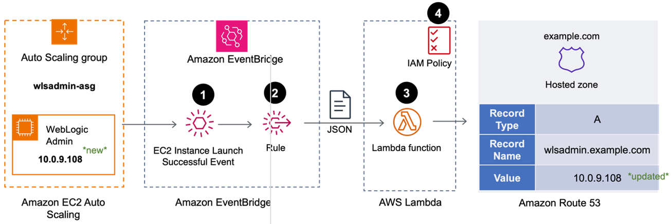
- In the consumer account, create a Route 53 alias to map the custom domain to the VPC endpoint.
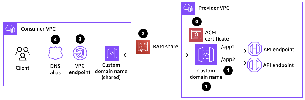
Figure 4: Components for configuring a custom domain name
Step 1: Creating a private custom domain name
When configuring a custom domain name, two policies are used to manage permissions to the private custom domain name resource. Management policies specify which principals are allowed to associate a private custom domain name to a VPC endpoint. Resource-based policies specify which API consumers are allowed to invoke your private custom domain name.
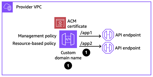
Figure 5: Creating a private custom domain name
This is an example CloudFormation definition for a private custom domain name.
In this example, the management policy specifies that the account 123456789012 is allowed to associate a private custom domain name with a VPC endpoint. The resource-based policy then denies any request that does not come from a particular VPC endpoint and only allows invoke requests that come from that same account 123456789012.
The private custom domain name then needs to be mapped to a private REST API.
In this example, the BasePath is set to app1. If the Stage is set as dev, then the private endpoint can be accessed via https://api.internal.example.com/app1/dev. The domain id is the identifier for the private custom domain name.
Note that with public custom domain names, the domain name has to be unique in the region, since they are resolved publicly. With private custom domain names, since they are resolved within a VPC, a private custom domain name with the same name can be created in different accounts. The private custom domain name is then resolved to the VPC endpoint in that account’s VPC.
Step 2: Sharing the private custom domain name using AWS RAM
In order for API consumers to access the private custom domain name from another account, the custom domain name needs to be shared with the consumer accounts using RAM. If the API provider and API consumer are in the same account, this step with RAM can be skipped.
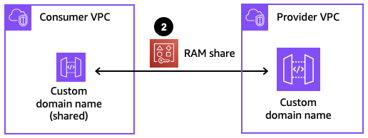
Figure 6: Sharing the private custom domain name
The following CloudFormation definition creates a resource share in the provider account.
The allowed Principals for the resource share specifies the consumer account ids. The ResourceArns specify the ARN of the private custom domain name.
In the consumer account, an administrator receives a notification to accept the resource share. This request must be accepted to allow the consumer account to see the private custom domain name. This handshake acts as a mutual agreement between the accounts to allow the private custom domain name to be exposed from the provider account to the consumer account. If the provider and consumer accounts are in the same AWS Organization, the share is automatically accepted on behalf of consumers.
Step 3: Associating the private custom domain name to a VPC endpoint
The private custom domain name is now visible in the consumer account. Next, associate the private custom domain name with a VPC endpoint in the consumer account and in the VPC where the client applications reside.

Figure 7: Associating the private custom domain name to a VPC endpoint
The AccessAssociationSource is the VPC endpoint id, and the DomainNameArn is the same ARN that is used in the RAM resource share.
Step 4: Creating a Route 53 alias for the custom domain name
The final step before being able to test the custom domain name in the consumer account is setting up a Route 53 alias. That alias is configured in a private hosted zone that is associated with the VPC where the VPC endpoint and client applications reside. The alias resolves the fully qualified domain name (FQDN) to the VPC endpoint DNS name.

Figure 8: Creating a Route 53 alias
The following CloudFormation definition creates that alias.
The ResourceRecords point to the FQDN of the VPC endpoint to which our private custom domain name is associated. Once this alias is created, your client applications can test if it can successfully send requests to the private custom domain name.
Optional: Cleaning up the resources
If you’ve configured a test environment with these resources, you can clean up the deployment by following the steps in reverse order.
- In the consumer account, delete the Route 53 alias.
- In the consumer account, delete the association.
- In both the consumer and provider account, remove the RAM resource share.
- In the provider account, delete the custom domain name and base path mapping.
Conclusion
In this post, you learned about how clients can connect to private REST API endpoints with API Gateway. With custom domain names, your applications connect to stable URLs that can forward requests to many different private API backends. Furthermore, your application teams can deploy resources in separate line of business AWS accounts and access the private custom domain name as a central shared resource, using AWS RAM resource sharing. This allows your application teams to build secure, private API applications and expose them to API consumers securely and across multiple AWS accounts.
For more details, refer to the API Gateway documentation and check out patterns with API Gateway on Serverless Land.


 On November 9, 2004, Jeff Barr published


 AWS re:Invent – You can still


 Boon Lee Eu is a Senior Technical Account Manager at Amazon Web Services (AWS). He works closely and proactively with Enterprise Support customers to provide advocacy and strategic technical guidance to help plan and achieve operational excellence in AWS environment based on best practices. Based in Singapore, Boon Lee has over 20 years of experience in IT & Telecom industries.
 Kyara Labrador is a Sr. Analytics Specialist Solutions Architect at Amazon Web Services (AWS) Philippines, specializing in big data and analytics. She helps customers in designing and implementing scalable, secure, and cost-effective data solutions, as well as migrating and modernizing their big data and analytics workloads to AWS. She is passionate about empowering organizations to unlock the full potential of their data.
 Vikas Omer is the Head of Data & AI Solution Architecture for ASEAN at Amazon Web Services (AWS). With over 15 years of experience in the data and AI space, he is a seasoned leader who leverages his expertise to drive innovation and expansion in the region. Vikas is passionate about helping customers and partners succeed in their digital transformation journeys, focusing on cloud-based solutions and emerging technologies.


 Graviton-4-powered, memory-optimized X8g instances are now available in ten virtual sizes and two bare metal sizes, with up to 3 TiB of DDR5 memory and up to 192 vCPUs. The X8g instances are our most energy efficient to date, with the best price performance and scale-up capability of any comparable EC2 Graviton instance to date. With a 16 to 1 ratio of memory to vCPU, these instances are designed for Electronic Design Automation, in-memory databases & caches, relational databases, real-time analytics, and memory-constrained microservices. The instances fully encrypt all high-speed physical hardware interfaces and also include additional


