Tag Archives: Amazon EC2

New – Amazon EC2 Hpc7g Instances Powered by AWS Graviton3E Processors Optimized for High Performance Computing Workloads

Post Syndicated from Channy Yun original https://aws.amazon.com/blogs/aws/new-amazon-ec2-hpc7g-instances-powered-by-aws-graviton3e-processors-optimized-for-high-performance-computing-workloads/

At AWS re:Invent 2022, Adam Selipsky, CEO of AWS, explained high performance computing (HPC) workloads typically can either be compute-intensive, compute- and networking-intensive, or data- and memory-intensive in his keynote.

Compute workloads include weather forecasting, computational fluid dynamics, and financial options pricing. To help with this, you have Amazon EC2 Hpc6a instances, which deliver up to 65 percent better price performance over comparable compute optimized x86-based instances.

Other HPC workloads require modeling the performance of complex structures—things like wind turbines, concrete buildings, and industrial equipment. Without enough data and memory, these models can take days or weeks to run in a cost-effective way. The Amazon EC2 Hpc6id instance is designed to deliver leading price performance for data and memory-intensive HPC workloads with higher memory bandwidth per core, faster local solid-state drive (SSD) storage, and enhanced networking with Elastic Fabric Adapter (EFA).

Announcing Amazon EC2 Hpc7g Instances
Compute-intensive HPC workloads such as weather forecasting, computational fluid dynamics, and financial options pricing also require more network performance, even better price performance, and greater energy efficiency.

Today we are announcing the general availability of Amazon EC2 Hpc7g instances, a new purpose-built instance type for tightly coupled compute and network-intensive HPC workloads.

Hpc7g instances are powered by AWS Graviton3E processors that provide up to two times better floating-point performance and 200 Gbps dedicated EFA bandwidth than EC2 C6gn instances powered by AWS Graviton2 processors and are up to 60 percent more energy efficient than comparable x86 instances.

Here’s a quick infographic that shows you how the Hpc7g instances and the Graviton3E processors compare to previous instances and processors:

Hpc7g instances feature sizes of up to 64 cores of the latest AWS custom Graviton3E CPUs with 128 GiB RAM. Here are the detailed specs:

Instance Name
CPUs RAM (GiB)
EFA Network Bandwidth (Gbps) Attached Storage
hpc7g.4xlarge 16 128 Up to 200 EBS Only
hpc7g.8xlarge 32 128 Up to 200 EBS Only
hpc7g.16xlarge 64 128 Up to 200 EBS Only

Hpc7g instances are the most cost-efficient option to scale your HPC clusters on AWS. If you are considering migrating your largest HPC workloads requiring tens of thousands of cores at scale to AWS, you can take advantage of up to 200 Gbps EFA bandwidth to reduce the latency and run message passing interface (MPI) applications on parallel computing architectures while ensuring minimized power consumption on Hpc7g instances.

You can choose to use smaller sizes of Hpc7g instances to pick a lower number of cores and evenly distribute memory and network resources across the remaining cores to increase per-core performance to help reduce software licensing costs.

You can also use Hpc7g instances with AWS ParallelCluster to offer a complete HPC run-time environment that spans both x86 and arm64 instance types, giving you the flexibility to run different workload types within the same HPC cluster. You can compare and contrast performance, thus making it easier to find out what’s best for you and enabling easier porting of your workload.

Customer Story
The Water Institute is an independent, non-profit applied research organization that works across disciplines to advance science and develop integrated methods used to solve complex environmental and societal challenges.

They benchmarked the Hpc7g instances with 200 Gbps EFA using the Advanced Circulation (ADCIRC) model. ADCIRC is deployed throughout many US government agencies to simulate the movement of water due to astronomic tides, riverine flows, and atmospheric forces, including hurricanes and it is often used for real-time forecasting applications and design studies.

The model run for this application is targeted at Southern Louisiana and is the basis for most of the analysis conducted there including levee design, planning studies, and real-time hurricane storm surge forecasting applications. The left graphic above shows the full extent of the domain, while to the right of that, the high-resolution area targeted at Southern Louisiana shows flooding around the levees in New Orleans during a simulation of Hurricane Katrina.

The model contains 1.6 million vertices and 3 million elements. It’s these parameters that affect the computational complexity of the simulations. The simulations depict 18 days of astronomic tide, river inflows, and atmospheric wind and pressure forcing.

The Water Institute benchmarked against many of the instance types that would be useful for their workload types at AWS, including c6gn.16xlarge, hpc7g.16xlarge, hpc6a.48xlarge, and hpc6id.36xlarge.

The Hpc7g instance shows more than 40 percent better performance than the C6gn instance and has comparable performance to other high performance x86 instance types but with a better price-to-performance ratio. With Hpc7g instances, the Water Institute can lower its costs while maintaining the performance levels they expect.

RIKEN, who has built the powerful supercomputer, FUGAKU using arm64, is collaborating with AWS to create a virtual Fugaku using Hpc7g with Graviton3E to support Japanese manufacturers’ increasing demand for compute power. RIKEN has already confirmed that multiple Fugaku applications provide excellent performance on the AWS Graviton3E processor in the AWS cloud environment.

Also, Siemens has optimized the scalability of Simcenter STAR-CCM+ across a broad range of CPU and GPU instances on AWS. This technology is supported on Linux and available through Arm-based EC2 instances or the Fugaku supercomputer.

To hear more voices of customers and partners such as Ansys, Arup, CERFACS, ESI, Jij, ParTec, Rescale, and TotalCAE, see the Hpc7g instances page.

Now Available
Amazon EC2 Hpc7g instances are now generally available in the US East (N. Virginia) Region for purchase in On-Demand, Reserved Instance, and Savings Plan form.

To learn more, see the Amazon EC2 Hpc7g instances page. Give it a try, and please send feedback to AWS re:Post for High Performance Compute or through your usual AWS support contacts.

Channy

New Amazon EC2 C7gn Instances: Graviton3E Processors and Up To 200 Gbps Network Bandwidth

Post Syndicated from Jeff Barr original https://aws.amazon.com/blogs/aws/new-amazon-ec2-c7gn-instances-graviton3e-processors-and-up-to-200-gbps-network-bandwidth/

The C7gn instances that we previewed last year are now available and you can start using them today. The instances are designed for your most demanding network-intensive workloads (firewalls, virtual routers, load balancers, and so forth), data analytics, and tightly-coupled cluster computing jobs. They are powered by AWS Graviton3E processors and support up to 200 Gbps of network bandwidth.

Here are the specs:

Instance Name vCPUs
Memory
Network Bandwidth
EBS Bandwidth
c7gn.medium 1 2 GiB up to 25 Gbps up to 10 Gbps
c7gn.large 2 4 GiB up to 30 Gbps up to 10 Gbps
c7gn.xlarge 4 8 GiB up to 40 Gbps up to 10 Gbps
c7gn.2xlarge 8 16 GiB up to 50 Gbps up to 10 Gbps
c7gn.4xlarge 16 32 GiB 50 Gbps up to 10 Gbps
c7gn.8xlarge 32 64 GiB 100 Gbps up to 20 Gbps
c7gn.12xlarge 48 96 GiB 150 Gbps up to 30 Gbps
c7gn.16xlarge 64 128 GiB 200 Gbps up to 40 Gbps

The increased network bandwidth is made possible by the new 5th generation AWS Nitro Card. As another benefit, these instances deliver the lowest Elastic Fabric Adapter (EFA) latency of any current EC2 instance.

Here’s a quick infographic that shows you how the C7gn instances and the Graviton3E processors compare to previous instances and processors:

As you can see, the Graviton3E processors deliver substantially higher memory bandwidth and compute performance than the Graviton2 processors, along with higher vector instruction performance than the Graviton3 processors.

C7gn instances are available in the US East (Ohio, N. Virginia), US West (Oregon), and Europe (Ireland) AWS Regions in On-Demand, Reserved Instance, Spot, and Savings Plan form. Dedicated Instances and Dedicated Hosts are also available.

Jeff;

AWS Week in Review – Amazon EC2 Instance Connect Endpoint, Detective, Amazon S3 Dual Layer Encryption, Amazon Verified Permission – June 19, 2023

Post Syndicated from Sébastien Stormacq original https://aws.amazon.com/blogs/aws/aws-week-in-review-amazon-ec2-instance-connect-endpoint-detective-amazon-s3-dual-layer-encryption-amazon-verified-permission-june-19-2023/

This week, I’ll meet you at AWS partner’s Jamf Nation Live in Amsterdam where we’re showing how to use Amazon EC2 Mac to deploy your remote developer workstations or configure your iOS CI/CD pipelines in the cloud.Mac in an instant

Last Week’s Launches
While I was traveling last week, I kept an eye on the AWS News. Here are some launches that got my attention.

Amazon EC2 Instance Connect Endpoint. Endpoint for EC2 Instance Connect allows you to securely access Amazon EC2 instances using their private IP addresses, making the use of bastion hosts obsolete. Endpoint for EC2 Instance Connect is by far my favorite launch from last week. With EC2 Instance Connect, you use AWS Identity and Access Management (IAM) policies and principals to control SSH access to your instances. This removes the need to share and manage SSH keys. We also updated the AWS Command Line Interface (AWS CLI) to allow you to easily connect or open a secured tunnel to an instance using only its instance ID. I read and contributed to a couple of threads on social media where you pointed out that AWS Systems Manager Session Manager already offered similar capabilities. You’re right. But the extra advantage of EC2 Instance Connect Endpoint is that it allows you to use your existing SSH-based tools and libraries, such as the scp command.

Amazon Inspector now supports code scanning of AWS Lambda functions. This expands the existing capability to scan Lambda functions and associated layers for software vulnerabilities in application package dependencies. Amazon Detective also extends finding groups to Amazon Inspector. Detective automatically collects findings from Amazon Inspector, GuardDuty, and other AWS security services, such as AWS Security Hub, to help increase situational awareness of related security events.

Amazon Verified Permissions is generally available. If you’re designing or developing business applications that need to enforce user-based permissions, you have a new option to centrally manage application permissions. Verified Permissions is a fine-grained permissions management and authorization service for your applications that can be used at any scale. Verified Permissions centralizes permissions in a policy store and helps developers use those permissions to authorize user actions within their applications. Similarly to the way an identity provider simplifies authentication, a policy store lets you manage authorization in a consistent and scalable way. Read Danilo’s post to discover the details.

Amazon S3 Dual-Layer Server-Side Encryption with keys stored in AWS Key Management Service (DSSE-KMS). Some heavily regulated industries require double encryption to store some type of data at rest. Amazon Simple Storage Service (Amazon S3) offers DSSE-KMS, a new free encryption option that provides two layers of data encryption, using different keys and different implementation of the 256-bit Advanced Encryption Standard with Galois Counter Mode (AES-GCM) algorithm. My colleague Irshad’s post has all the details.

AWS CloudTrail Lake Dashboards provide out-of-the-box visibility and top insights from your audit and security data directly within the CloudTrail Lake console. CloudTrail Lake features a number of AWS curated dashboards so you can get started right away – with no required detailed dashboard setup or SQL experience.

AWS IAM Identity Center now supports automated user provisioning from Google Workspace. You can now connect your Google Workspace to AWS IAM Identity Center (successor to AWS Single Sign-On) once and manage access to AWS accounts and applications centrally in IAM Identity Center.

AWS CloudShell is now available in 12 additional regions. AWS CloudShell is a browser-based shell that makes it easier to securely manage, explore, and interact with your AWS resources. The list of the 12 new Regions is detailed in the launch announcement.

For a full list of AWS announcements, be sure to keep an eye on the What’s New at AWS page.

Other AWS News
Here are some other updates and news that you might have missed:

  • AWS Extension for Stable Diffusion WebUI. WebUI is a popular open-source web interface that allows you to easily interact with Stable Diffusion generative AI. We built this extension to help you to migrate existing workloads (such as inference, train, and ckpt merge) from your local or standalone servers to the AWS Cloud.
  • GoDaddy developed a multi-Region, event-driven system. Their system handles 400 millions events per day. They plan to scale it to process 2 billion messages per day in a near future. My colleague Marcia explains the detail of their architecture in her post.
  • The Official AWS Podcast – Listen each week for updates on the latest AWS news and deep dives into exciting use cases. There are also official AWS podcasts in several languages. Check out the podcasts in FrenchGermanItalian, and Spanish.
  • AWS Open Source News and Updates – This is a newsletter curated by my colleague Ricardo to bring you the latest open source projects, posts, events, and more.

Upcoming AWS Events
Check your calendars and sign up for these AWS events:

  • AWS Silicon Innovation Day (June 21) – A one-day virtual event that will allow you to better understand AWS Silicon and how you can use the Amazon EC2 chip offerings to your benefit. My colleague Irshad shared the details in this post. Register today.
  • AWS Global Summits – There are many AWS Summits going on right now around the world: Milano (June 22), Hong Kong (July 20), New York (July 26), Taiwan (Aug 2 & 3), and Sao Paulo (Aug 3).
  • AWS Community Day – Join a community-led conference run by AWS user group leaders in your region: Manila (June 29–30), Chile (July 1), and Munich (September 14).
  • AWS User Group Perú Conf 2023 (September 2023). Some of the AWS News blog writer team will be present: Marcia, Jeff, myself, and our colleague Startup Developer Advocate Mark. Save the date and register today.
  • CDK Day CDK Day is happening again this year on September 29. The call for papers for this event is open, and this year we’re also accepting talks in Spanish. Submit your talk here.

That’s all for this week. Check back next Monday for another Week in Review!

This post is part of our Week in Review series. Check back each week for a quick roundup of interesting news and announcements from AWS!
— seb

Deploying an automated Amazon CloudWatch dashboard for AWS Outposts using AWS CDK

Post Syndicated from Sheila Busser original https://aws.amazon.com/blogs/compute/deploying-an-automated-amazon-cloudwatch-dashboard-for-aws-outposts-using-aws-cdk/

This post is written by Enrico Liguori, Networking Solutions Architect, Hybrid Cloud and Sumeeth Siriyur, Sr. Hybrid Cloud Solutions Architect.

AWS Outposts is a fully managed service that brings the same AWS infrastructure, services, APIs, and tools to virtually any data center, colocation space, manufacturing floor, or on-premises facility where it might be needed. With Outposts, you can run some AWS services on-premises and connect to a broad range of services available in the local AWS Region. Outposts supports workloads requiring low latency, local data processing, data residency, and application migration.

Outposts capacity is driven as per your compute and storage requirements to run workloads. You can monitor Outposts resources using metrics gathered by Amazon CloudWatch. Using these metrics, you can effectively monitor and manage the Outposts resources as they would in the Region, levereging cloud native tools such as CloudWatch dashboards. Check the Monitoring best practices for AWS Outposts blog post to dive deep into the available monitoring options for Outposts.

CloudWatch dashboards are customizable home pages in the CloudWatch console that can be used to monitor resources running on Outposts in a single view. For example, you can monitor in a single pane the number Amazon EC2 instances used per EC2 instance type, the available capacity of Amazon EBS volumes and Amazon S3 buckets, and the operational status of the service link of Outposts.

As a you start deploying additional Outposts resources as a part of their capacity expansion, they must all be integrated and visualized within CloudWatch in an automated way. Traditionally CloudWatch dashboards are built manually and may be time consuming to tune. This post provides also an overview of building CloudWatch dashboards in an automated way using AWS Cloud Development Kit (AWS CDK).

Overview

CloudWatch metrics available to monitor Outposts resources and capacity

CloudWatch metrics for Outposts are available to customers in all public AWS Regions and AWS GovCloud (US) at no additional cost. We can classify the available metrics in two main categories:

To identify the metrics published under the service specific namespaces, we can leverage metadata in the form of tags. A tag is a label that you assign to an AWS resource and consists of a key and an optional value. For the purpose of the monitoring strategy described in this post, we use a tag that contains the OutpostID of the Outpost where the resource is deployed. In this way, we can easily filter the CloudWatch metrics that we would like to show in our dashboard.

To enforce the assignment of tags to our resources we can implement a tagging strategy using AWS tag Policies and Service Control Policies (SCPs).

The following sections describe two different methods to build a CloudWatch dashboard that includes the different types of metrics described so far. In both cases, we see how particularly useful the presence of tags is to identify the service-specific metrics.

Manual approach to building a CloudWatch dashboard for Outposts

This section describes a manual (i.e., non-automated) approach to building a dashboard that could summarize both the capacity utilization metrics and the service specific metrics for your resources running on Outposts.

The benefit of this approach is that we can implement a fully operational dashboard directly from the CloudWatch console. However, it will simultaneously require more effort to properly tune the dashboard to satisfy your monitoring requirements.

You can start creating the dashboard opening the CloudWatch console and following the steps listed in the public documentation.

To display a metric under AWS/Outposts namespace we can choose any of the widgets available. Based on the nature of the data, we can choose different types of Widgets such as Number, Line, Gauge, Explorer, or you can even build your own custom widget.

Together with the Widget type, we must select Outposts namespace in the metric graph dialog box and then navigate to the specific metric of interest.

In case we are creating the dashboard in a different account than the Outposts owner, we must select the right account in the View data drop-down menu to see the Outposts metric in which we are interested.

View data drop-down menu

After selecting one or more metrics we can select Create widget button.

For the service specific metrics, we recommend using the explorer widget. In this way, we can utilize the tagging strategy described earlier to automatically identify the metrics belonging to the resources running on Outposts. Check the documentation page for a step-by-step guide for creating an explorer widget based on tags.

Automated outpost dashboard

After we’ve seen how to build a dashboard manually from the console, in this secton we describe an automated approach to deploy a dashboard for Outposts through AWS CDK.

AWS CDK is an open source software development framework to model and provision your cloud application resources using familiar programming languages, including TypeScript, JavaScript, Python, C#, and Java. For the solution in this post, we use Python.

Architecture overview

The AWS CDK stack described in this post, assumes that the resources running on Outposts (EC2 instances, S3 buckets, Application Load Balancers (ALBs), and RDS instances) are tagged using the tagging strategy described earlier.

Specifying a tag name and a tag value in a configuration file automatically discovers the resources with that tag and adds the related metrics to the CloudWatch dashboard.

Together with the service specific metrics, it creates a series of widgets that we can use to monitor the capacity available and utilized in each Outpost that belongs to the account where the script is running.

The workflow is made of the following phases:

  1. The AWS CDK stack creates an AWS CodeCommit repository and uploads its own code into it. The code contains a series of modules, one for each section of the CloudWatch dashboard. A section of the dashboard contains one or more widgets showing the metrics of a specific service.
  2. To maintain the CloudWatch dashboard always up-to-date with the resources matching the tag, it creates a pipeline in AWS CodePipeline that can dynamically create and or update the dashboard. The pipeline runs the code in the CodeCommit repository and is made of two stages. In the first one, the build stage, it builds the dependencies needed by the AWS CDK stack. In the second stage, the Deploy stage, it loads and runs the modules used to build the dashboard.
  3. Each module contains the code to automatically discover the tagged resources of a specific service. This discovery phase uses standard AWS APIs called through the Python SDK Boto3.
  4. Based on the results of the discovery phase, AWS CDK produces an AWS CloudFormation template containing the definition of the CloudWatch dashboard sections. The template is submitted to CloudFormation.
  5. CloudFormation creates or, if already defined, updates the CloudWatch dashboard.
  6. Together with the dashboard, the AWS CDK script also contains the definition of a CloudWatch Event that, once deployed, triggers the pipeline each time a resource tagged with the specified tag is created or destroyed.

Prerequisites

To implement the solution presented in this post, you must configure:

  1. git as distributed version control system.
  2. In case it is the first time that you’re using AWS CDK in this account and region, you must:

a. Install the AWS CDK, and its prerequisites, following these instructions.

b. Go through the AWS CDK bootstrapping process. This is required only for the first time that we use AWS CDK in a specific AWS environment (an AWS environment is a combination of an AWS account and Region).

How to install

Step 1: Clone the AWS CDK code hosted on GitHub with:

$ git clone https://github.com/aws-samples/automated-cloudwatch-dashboard.git

Step 2: enter the directory using the following:

$ cd  automated-cloudwatch-dashboard/

Step 3: Install the needed Python dependencies with:

$ pip install -r requirements.txt

Step 4: Modify the configuration file

Before deploying the stack, we must modify the configuration file to specify the tag we use for identifying our resources running on Outposts. Open the file with the name config.yaml with your preferred text editor and specify:

      • A name for the dashboard. The default name used is Automated-CloudWatch-Dashboard.
      • Replace <tag_name> placeholder following the tag_name variable with the tag name used to tag the resources that you want to include in the dashboard.
      • Replace <tag_value> placeholder under tag_values variable with the tag value that you used.

Here is an example config.yaml configuration file:

dashboard_name: Automated-CloudWatch-Dahsboard
tag_name: OutpostID
tag_values:
  - op-1234567890abcdefg 

Stack deployment

We can deploy the stack with the following:

$ cdk deploy

At the end of the deployment process, the pipeline that creates the dashboard is provisioned. You can now go to your CloudWatch console to view it.

Automated Outposts dashboard overview

Now that we have built our dashboard, let’s review each section:

  1. Outpost capacity

Outpost Capacity diagram

The AWS CDK stacks define a capacity section for each Outpost available to the AWS account where the script runs.

In this section, we find four widgets showing metrics published under the AWS/Outpost namespace. The first widget shows for each EC2 instance type available on the Outposts the number of instances utilized and available for that instance type. In the second row, we can visualize the available capacity for the Amazon EBS volumes and for the S3 buckets. The last widget shows the operational status of the service link of Outposts.

2. EC2 instances

CPU, Network, and Disk Utilization for an EC2 instance diagram

In this section of the dashboard, we find the metrics showing the CPU, Network, and Disk Utilization for an EC2 instance. It has defined a section of this type for each EC2 instance with a tag assigned matching the name and the value specified in the configuration file of the script.

3. Application Load Balancer

The ALB section aggregates metrics showing the operational status of a load balancer hosted on Outposts

The ALB section aggregates metrics showing the operational status of a load balancer hosted on Outposts. A section of this type is defined for each ALB with an assigned tag matching the one specified in the configuration file.

4. S3 buckets

The S3 buckets section diagram

The S3 buckets section is defined only once and aggregates the utilization metrics for all S3 buckets with an assigned tag.

5. AutoScaling group

The AutoScaling group section diagram

The AutoScaling group section can be used to monitor the number of instances in service in a specific AS group with a tag assigned. This section is defined once and can aggregate the metrics for multiple AutoScaling groups.

Clean up

To terminate the resources that we created in this post, run the following:

$ cdk destroy

Then, go to the Cloudformation console and delete the stack with the name “Deploy-AutomatedCloudWatchDashboard”.

Conclusion

In conclusion, this post demonstrates a manual way of creating CloudWatch Metrics dashboard using the CloudWatch console and an automated way using AWS CDK. The automated approach is also scalable by automatically discovering any new resources added to the existing Outposts in the your environment without any changes to the code.

Secure Connectivity from Public to Private: Introducing EC2 Instance Connect Endpoint

Post Syndicated from Sheila Busser original https://aws.amazon.com/blogs/compute/secure-connectivity-from-public-to-private-introducing-ec2-instance-connect-endpoint-june-13-2023/

This blog post is written by Ariana Rahgozar, Solutions Architect, and Kenneth Kitts, Sr. Technical Account Manager, AWS.

Imagine trying to connect to an Amazon Elastic Compute Cloud (Amazon EC2) instance within your Amazon Virtual Private Cloud (Amazon VPC) over the Internet. Typically, you’d first have to connect to a bastion host with a public IP address that your administrator set up over an Internet Gateway (IGW) in your VPC, and then use port forwarding to reach your destination.

Today we launched Amazon EC2 Instance Connect (EIC) Endpoint, a new feature that allows you to connect securely to your instances and other VPC resources from the Internet. With EIC Endpoint, you no longer need an IGW in your VPC, a public IP address on your resource, a bastion host, or any agent to connect to your resources. EIC Endpoint combines identity-based and network-based access controls, providing the isolation, control, and logging needed to meet your organization’s security requirements. As a bonus, your organization administrator is also relieved of the operational overhead of maintaining and patching bastion hosts for connectivity. EIC Endpoint works with the AWS Management Console and AWS Command Line Interface (AWS CLI). Furthermore, it gives you the flexibility to continue using your favorite tools, such as PuTTY and OpenSSH.

In this post, we provide an overview of how the EIC Endpoint works and its security controls, guide you through your first EIC Endpoint creation, and demonstrate how to SSH to an instance from the Internet over the EIC Endpoint.

EIC Endpoint product overview

EIC Endpoint is an identity-aware TCP proxy. It has two modes: first, AWS CLI client is used to create a secure, WebSocket tunnel from your workstation to the endpoint with your AWS Identity and Access Management (IAM) credentials. Once you’ve established a tunnel, you point your preferred client at your loopback address (127.0.0.1 or localhost) and connect as usual. Second, when not using the AWS CLI, the Console gives you secure and seamless access to resources inside your VPC. Authentication and authorization is evaluated before traffic reaches the VPC. The following figure shows an illustration of a user connecting via an EIC Endpoint:

Figure 1 shows a user connecting to private EC2 instances within a VPC through an EIC Endpoint

Figure 1. User connecting to private EC2 instances through an EIC Endpoint

EIC Endpoints provide a high degree of flexibility. First, they don’t require your VPC to have direct Internet connectivity using an IGW or NAT Gateway. Second, no agent is needed on the resource you wish to connect to, allowing for easy remote administration of resources which may not support agents, like third-party appliances. Third, they preserve existing workflows, enabling you to continue using your preferred client software on your local workstation to connect and manage your resources. And finally, IAM and Security Groups can be used to control access, which we discuss in more detail in the next section.

Prior to the launch of EIC Endpoints, AWS offered two key services to help manage access from public address space into a VPC more carefully. First is EC2 Instance Connect, which provides a mechanism that uses IAM credentials to push ephemeral SSH keys to an instance, making long-lived keys unnecessary. However, until now EC2 Instance Connect required a public IP address on your instance when connecting over the Internet. With this launch, you can use EC2 Instance Connect with EIC Endpoints, combining the two capabilities to give you ephemeral-key-based SSH to your instances without exposure to the public Internet. As an alternative to EC2 Instance Connect and EIC Endpoint based connectivity, AWS also offers Systems Manager Session Manager (SSM), which provides agent-based connectivity to instances. SSM uses IAM for authentication and authorization, and is ideal for environments where an agent can be configured to run.

Given that EIC Endpoint enables access to private resources from public IP space, let’s review the security controls and capabilities in more detail before discussing creating your first EIC Endpoint.

Security capabilities and controls

Many AWS customers remotely managing resources inside their VPCs from the Internet still use either public IP addresses on the relevant resources, or at best a bastion host approach combined with long-lived SSH keys. Using public IPs can be locked down somewhat using IGW routes and/or security groups. However, in a dynamic environment those controls can be hard to manage. As a result, careful management of long-lived SSH keys remains the only layer of defense, which isn’t great since we all know that these controls sometimes fail, and so defense-in-depth is important. Although bastion hosts can help, they increase the operational overhead of managing, patching, and maintaining infrastructure significantly.

IAM authorization is required to create the EIC Endpoint and also to establish a connection via the endpoint’s secure tunneling technology. Along with identity-based access controls governing who, how, when, and how long users can connect, more traditional network access controls like security groups can also be used. Security groups associated with your VPC resources can be used to grant/deny access. Whether it’s IAM policies or security groups, the default behavior is to deny traffic unless it is explicitly allowed.

EIC Endpoint meets important security requirements in terms of separation of privileges for the control plane and data plane. An administrator with full EC2 IAM privileges can create and control EIC Endpoints (the control plane). However, they cannot use those endpoints without also having EC2 Instance Connect IAM privileges (the data plane). Conversely, DevOps engineers who may need to use EIC Endpoint to tunnel into VPC resources do not require control-plane privileges to do so. In all cases, IAM principals using an EIC Endpoint must be part of the same AWS account (either directly or by cross-account role assumption). Security administrators and auditors have a centralized view of endpoint activity as all API calls for configuring and connecting via the EIC Endpoint API are recorded in AWS CloudTrail. Records of data-plane connections include the IAM principal making the request, their source IP address, the requested destination IP address, and the destination port. See the following figure for an example CloudTrail entry.

Figure 2 shows a sample cloud trail entry for SSH data-plane connection for an IAMUser. Specific entry:  Figure 2. Partial CloudTrail entry for an SSH data-plane connection

EIC Endpoint supports the optional use of Client IP Preservation (a.k.a Source IP Preservation), which is an important security consideration for certain organizations. For example, suppose the resource you are connecting to has network access controls that are scoped to your specific public IP address, or your instance access logs must contain the client’s “true” IP address. Although you may choose to enable this feature when you create an endpoint, the default setting is off. When off, connections proxied through the endpoint use the endpoint’s private IP address in the network packets’ source IP field. This default behavior allows connections proxied through the endpoint to reach as far as your route tables permit. Remember, no matter how you configure this setting, CloudTrail records the client’s true IP address.

EIC Endpoints strengthen security by combining identity-based authentication and authorization with traditional network-perimeter controls and provides for fine-grained access control, logging, monitoring, and more defense in depth. Moreover, it does all this without requiring Internet-enabling infrastructure in your VPC, minimizing the possibility of unintended access to private VPC resources.

Getting started

Creating your EIC Endpoint

Only one endpoint is required per VPC. To create or modify an endpoint and connect to a resource, a user must have the required IAM permissions, and any security groups associated with your VPC resources must have a rule to allow connectivity. Refer to the following resources for more details on configuring security groups and sample IAM permissions.

The AWS CLI or Console can be used to create an EIC Endpoint, and we demonstrate the AWS CLI in the following. To create an EIC Endpoint using the Console, refer to the documentation.

Creating an EIC Endpoint with the AWS CLI

To create an EIC Endpoint with the AWS CLI, run the following command, replacing [SUBNET] with your subnet ID and [SG-ID] with your security group ID:

aws ec2 create-instance-connect-endpoint \
    --subnet-id [SUBNET] \
    --security-group-id [SG-ID]

After creating an EIC Endpoint using the AWS CLI or Console, and granting the user IAM permission to create a tunnel, a connection can be established. Now we discuss how to connect to Linux instances using SSH. However, note that you can also use the OpenTunnel API to connect to instances via RDP.

Connecting to your Linux Instance using SSH

With your EIC Endpoint set up in your VPC subnet, you can connect using SSH. Traditionally, access to an EC2 instance using SSH was controlled by key pairs and network access controls. With EIC Endpoint, an additional layer of control is enabled through IAM policy, leading to an enhanced security posture for remote access. We describe two methods to connect via SSH in the following.

One-click command

To further reduce the operational burden of creating and rotating SSH keys, you can use the new ec2-instance-connect ssh command from the AWS CLI. With this new command, we generate ephemeral keys for you to connect to your instance. Note that this command requires use of the OpenSSH client. To use this command and connect, you need IAM permissions as detailed here.

Once configured, you can connect using the new AWS CLI command, shown in the following figure:
Figure 3 shows the AWS CLI view if successfully connecting to your instance using the one-click command. When running the command, you are prompted to connect and can access your instance.

Figure 3. AWS CLI view upon successful SSH connection to your instance

To test connecting to your instance from the AWS CLI, you can run the following command where [INSTANCE] is the instance ID of your EC2 instance:

aws ec2-instance-connect ssh --instance-id [INSTANCE]

Note that you can still use long-lived SSH credentials to connect if you must maintain existing workflows, which we will show in the following. However, note that dynamic, frequently rotated credentials are generally safer.

Open-tunnel command

You can also connect using SSH with standard tooling or using the proxy command. To establish a private tunnel (TCP proxy) to the instance, you must run one AWS CLI command, which you can see in the following figure:

Figure 4 shows the AWS CLI view after running the aws ec2-instance-connect open-tunnel command and connecting to your instance.Figure 4. AWS CLI view after running new SSH open-tunnel command, creating a private tunnel to connect to our EC2 instance

You can run the following command to test connectivity, where [INSTANCE] is the instance ID of your EC2 instance and [SSH-KEY] is the location and name of your SSH key. For guidance on the use of SSH keys, refer to our documentation on Amazon EC2 key pairs and Linux instances.

ssh ec2-user@[INSTANCE] \
    -i [SSH-KEY] \
    -o ProxyCommand='aws ec2-instance-connect open-tunnel \
    --instance-id %h'

Once we have our EIC Endpoint configured, we can SSH into our EC2 instances without a public IP or IGW using the AWS CLI.

Conclusion

EIC Endpoint provides a secure solution to connect to your instances via SSH or RDP in private subnets without IGWs, public IPs, agents, and bastion hosts. By configuring an EIC Endpoint for your VPC, you can securely connect using your existing client tools or the Console/AWS CLI. To learn more, visit the EIC Endpoint documentation.

Discover How AWS Designed Silicon Fuels Customer Outcomes at AWS Silicon Innovation Day

Post Syndicated from Irshad Buchh original https://aws.amazon.com/blogs/aws/discover-how-aws-designed-silicon-fuels-customer-outcomes-at-aws-silicon-innovation-day/

We hope you will join us on Wednesday, June 21, for a free-to-attend online event, AWS Silicon Innovation Day. AWS will stream the event simultaneously across multiple platforms, including LinkedIn Live, Twitter, YouTube, and Twitch.

AWS Silicon Innovation Day is a one-day virtual event on June 21, 2023, that will allow you to better understand AWS Silicon and how you can use AWS’s unique Amazon EC2 chip offerings to your benefit. AWS has designed and developed purpose-built silicon specifically for the cloud.

During this event, you will have the opportunity to hear directly from senior leaders at AWS. Our panel of lead architects, engineers, customers, and analysts will provide insights into our silicon journey. Through deep dives into our cutting-edge silicon design and customer success stories, the panel will provide insights on security enhancements and cost-saving opportunities. Here are some of the highlights you can expect from this event.

Leadership session – To kick off the day, we have a Leadership session featuring Dave Brown, VP of Amazon EC2 and Dr. Ruba Borno, VP of WW Channels and Alliances joining us on stage. Dave will engage in a discussion with Ruba about how you can benefit from the innovation AWS delivers with its silicon technology.

AI/ML session – Gary Szilagyi, VP of Annapurna Labs will discuss with Nafea Bshara, co-founder of Annapurna Labs the utilization of chipset development by his team to create specialized chips for Generative AI, CPU, and the AWS Nitro system. He will highlight how you can harness the Annapurna mindset to develop not only CPUs but also tailor-made chips with specific purposes in mind.

Customer session – Jeff Barr, VP of AWS Evangelism, and Tiffany Wissner, Director of Product Marketing, will delve into insights from our customers. They will share anecdotes and experiences gathered from various sources, such as re:Invent, summits, and developer events, where you have expressed how you harnessed AWS silicon to drive your own remarkable innovations.

Networking session – JR Rivers, Senior Principal Engineer, and Madhura Kale, Senior Product Manager will shed light on the impact of silicon innovation, not only on the benefits you experience using our CPUs, GPUs, or Nitro System, but also on the transformation of AWS’s network infrastructure. They will delve into the realm of networking advancements, showcasing some of the latest innovations and highlighting the instrumental role played by AWS silicon in powering these developments.

Arm and Nitro Innovation sessionAnthony Liguori, VP and Fellow, Nitro System architecture will be joined by Ali Saidi, Director of Annapurna Labs to discuss harnessing the power of hardware and software in tandem to drive the development of cutting-edge silicon technologies.

Analyst and Executive sessionRaj Pai, VP of Amazon EC2 Product Management will engage in a conversation with an analyst, delving into the realm of silicon innovation in the cloud.

Join us for Silicon Innovation Day Wednesday June 21 9:00am - 4:00pm PDT

No advance registration is needed to participate in AWS Silicon Innovation Day, but you can add an event reminder to your calendar by registering on the event page. We sincerely hope that you will join us in embracing the excitement and seizing the valuable learning opportunities at this new event!

Meet you there.

— Irshad

Disaster Recovery for Oracle Database on Amazon EC2 with Fast-Start Failover

Post Syndicated from Harshad Gohil original https://aws.amazon.com/blogs/architecture/disaster-recovery-for-oracle-database-on-amazon-ec2-with-fast-start-failover/

High availability is non-negotiable for organizations today to prevent business-critical application disruptions. Enterprises must prioritize database scalability and availability to avoid downtime in their databases, network, servers, or storage environments.

For organizations that want to avoid required application changes, Oracle Real Application Clusters (RAC) is an option for providing high availability and scalability to the Oracle database. While the RAC feature is not supported by Oracle databases on Amazon Elastic Compute Cloud (Amazon EC2), Oracle Active Data Guard helps achieve high availability on AWS cloud.

The Oracle Data Guard feature helps customers survive disasters and data corruption while creating, maintaining, and managing one or more synchronized standby databases. But further, configuring Oracle Data Guard Fast-Start Failover (FSFO) helps achieve high availability.

In this blog post, we provide an architectural solution to achieve database high availability when running Oracle Database on Amazon EC2 with Oracle Data Guard along with Fast-Start Failover to address Availability Zones (AZs) or Amazon EC2 instance failures. We also introduce the steps you can take to make database failover happen without manual intervention, and offer recommendations for cross-Region disaster recovery.

Solution overview

Let’s explore this solution by discussing the architecture and two alternate options for securing high availability using Oracle Data Guard, along with the advantages and limitations of each. We will then offer a walkthrough of steps to make database failover happen without manual intervention.

Oracle high availability using Oracle Data Guard with multi-AZ and multi-Region with multi-AZ setup

This architecture is recommended to maintain high availability for Oracle databases on Amazon EC2 with protection against Amazon EC2 service outages in a Region. A disaster recovery environment and higher resiliency are provided after an Amazon EC2 service outage. This protects against Amazon EC2 service outages in an AWS Region and maintains resiliency due to the multi-AZ setup in a secondary Region.

In this architecture, Oracle Data Guard Fast Sync replication exists between the Primary database in AZ 1 in Region A, with standbys in AZ 2 Region A (Fast Sync), AZ1 in Region B (ASYNC), and AZ2 in Region B (ASYNC). There is an asynchronous cascading replication setup between standby databases to avoid network latency issues across regions.

Should Region A experience an Amazon EC2 service outage, the Oracle observer, a client software that monitors Oracle Data Guard and initiate failover to the Standby database in Region B. Applications can continue to connect to the database resulting in high availability with limited/minimal data loss based on the data change rate amount, as in Figure 1.

Oracle with cascading standby databases across regions

Figure 1. Oracle with cascading standby databases across regions

Using Oracle RedoRoutes, the default behavior of Data guard can be controlled and it can be set using the following example during setup.

Oracle RedoRoutes setup example:

dgmgrl > edit database DB_1A set property RedoRoutes= ‘ (LOCAL: DB_1B FASTSYNC PRIORITY=1, DB_2A ASYNC PRIORITY=2,DB_2B ASYNC PRIORITY=3)) (DB_1B: (DB_2A ASYNC PRIORITY=1, DB_2B ASYNC PRIORITY=2)) (DB_2A: DB_1B ASYNC) (DB_2B: DB_1B ASYNC)’

dgmgrl > edit database DB_1B set property RedoRoutes= ‘(LOCAL: (DB_1A FASTSYNC PRIORITY=1, DB_2A ASYNC PRIORITY=2,DB_2B ASYNC PRIORITY=3))(DB_1A: (DB_2A ASYNC PRIORITY=1, DB_2B ASYNC PRIORITY=2)) ‘

dgmgrl > edit database DB_1B set property RedoRoutes= ‘(LOCAL: (DB_2B FASTSYNC PRIORITY=1, DB_1A ASYNC PRIORITY=2, DB_1B ASYNC PRIORITY=3))(DB_2B: (DB_1A ASYNC PRIORITY=1, DB_1B ASYNC PRIORITY=2)) (DB_1A: DB_2B ASYNC)(DB_1B: DB_2B ASYNC )’

dgmgrl > edit database DB_1B set property RedoRoutes= ‘(LOCAL: (DB_2A FASTSYNC PRIORITY=1, DB_1A ASYNC PRIORITY=2, DB_1B ASYNC PRIORITY=3))(DB_2A: (DB_1A ASYNC PRIORITY=1, DB_1B ASYNC PRIORITY=2))’

For more information on Oracle RedoRoutes setup for Oracle Cascading Standby, refer to this step-by-step configuration documentation.

Database failover with Amazon Route 53 and Oracle Data Guard

The following walkthrough defines the steps you can take to make database failover happen without manual intervention using Amazon Route 53 and Oracle Data Guard.

Prerequisites

Before getting started, review the following prerequisites for this solution:

Walkthrough

Step 1. Create Oracle Database Service

For applications to connect without manual intervention on event of failure, we recommend creating an Oracle database service using the Oracle DBMS_Package called DBMS_SERVICE.

exec dbms_service.CREATE_SERVICE(SERVICE_NAME=>'DB_SERVICE_FOR_APP', NETWORK_NAME=>'DB_SERVICE_FOR_APP');

exec dbms_service.START_SERVICE('DB_SERVICE_FOR_APP');

Step 2. Network configuration

Applications can connect to the database seamlessly without manual intervention in an event of a failover from the Primary database to Standby using the Oracle Transparent Application Failover (TAF) approach, though TAF requires updating application connection strings in case of a host IP change.

The following approach using Amazon Route 53 is recommended for added flexibility and scalability. Route 53 has DNS A records that map to the database instance IPs and CNAME records that can redirect DNS queries to A records. The following depicts the DNS mapping. The CNAME, along with the database service name, can be used by the application in its network configuration.

Database_Name =
 (DESCRIPTION =
    (ADDRESS_LIST =
       (ADDRESS = (PROTOCOL = TCP)(HOST = <db_cname>)(PORT = 1521))
   (connect_data = 
       (service_name = <db_service_name>)
   )) )

To update the CNAME in Route 53 to map to the Primary host automatically in the event of failure, follow these steps.

Step 3. Route 53 setup

Create a script named route53update.sh and place it on the database hosts using the following code.

#!/bin/bash

export ORACLE_HOME="<<change>> "

export LD_LIBRARY_PATH=$ORACLE_HOME/lib

export PATH=$ORACLE_HOME/bin:$PATH:/usr/local/bin:/usr/bin

LOG_FILE="/tmp/switch_dns_$$.log"

DNS_DOMAIN="<<change>> "

ACTIVE_DB_CNAME="<<change>> "

HOSTED_ZONE_ID="<<change>> "

TTL="<<change>> "

update_dns () {

TMPFILE="/tmp/route53_dns_$$.log"

 cat > ${TMPFILE} << EOF

    {

      "Comment":"Updating DNS of record ${1}.${DNS_DOMAIN}",

      "Changes":[

        {

          "Action":"UPSERT",

          "ResourceRecordSet":{

            "ResourceRecords":[

              {

                "Value":"$2"

              }

            ],

            "Name":"${1}.${DNS_DOMAIN}.",

            "Type":"CNAME",

            "TTL":$TTL

          }

        }

      ]

    }

EOF

  /usr/local/bin/aws route53 change-resource-record-sets \

        --hosted-zone-id $HOSTED_ZONE_ID \

        --change-batch file://"$TMPFILE" >> "$LOG_FILE"

}

prim_uniq_sid=`$ORACLE_HOME/bin/sqlplus -s  / as sysdba <<EOF

set feedback off echo off lines 2000 head off

select upper(db_unique_name) from  v\\$dataguard_config where DEST_ROLE='PRIMARY DATABASE';

EOF`

prim_uniq_sid=`echo $prim_uniq_sid| sed 's/^[ \t]*//;s/[ \t]*$//'`

host_current=`$ORACLE_HOME/bin/tnsping ${prim_uniq_sid}|sed -n 's/\(.*Host\)\([^)]*\)\(.*\)/\2/pi' |sed 's/=//g'|sed 's/^[ \t]*//;s/[ \t]*$//'`

dns_current_host=`/usr/local/bin/aws route53 list-resource-record-sets --hosted-zone-id $HOSTED_ZONE_ID --query  "ResourceRecordSets[?Name == '${ACTIVE_DB_CNAME}.${DNS_DOMAIN}.'].ResourceRecords" --output text`

if [ "$host_current" != "$dns_current_host" ]; then

        update_dns ${ACTIVE_DB_CNAME} $host_current

fi

Step 4. Database job setup

Create a job in the Oracle Primary database to execute the shell script just introduced to initiate in the event of failover using the following code.

begin
  dbms_scheduler.create_job
  (
    job_name             => 'route53update',
    job_type             => 'executable',
    number_of_arguments  => 0,
    job_action           => '/<<location of script>>/ route53update.sh',
    auto_drop            => false
  );

  dbms_scheduler.enable('route53update');
end;
/

Step 5. Database trigger setup

In an event of a failure, the Primary will failover and the Standby starts up as the new Primary. A trigger needs to be created on the Primary database to execute the job on any failover to update the Route53 CNAME using the following code.

create or replace trigger SYS.Update_Route53_Record
AFTER STARTUP ON DATABASE
DECLARE
db_role varchar2(16);
db_mode varchar2(20);BEGIN
select database_role, open_mode into db_role, db_mode from v$database;
if db_role = 'PRIMARY' then
dbms_scheduler.run_job('route53update') ;
END IF;
END;
/

Alternate Option 1: Single Region with multi-AZ

This option is a minimum recommended configuration to maintain high availability for Oracle databases on Amazon EC2 for customers who do not have a multi-region setup.

  • Advantage: Protects against Amazon EC2 service outage in a single AZ.
  • Limitation: Does not protect against Amazon EC2 service outages in a single Region.

In this architecture, Oracle Data Guard Fast Sync replication exists between the Oracle database instance in a multi-AZ setup with the Primary database (Read Write) in AZ 1 and the Standby database (Read Only) in AZ 2.

If the primary database is unreachable due to any failure, the observer will failover to the standby database in a different AZ. Applications can continue to connect to the database with zero data loss due to synchronous replication between AZ using the Maximum Availability/Maximum Protection mode setup in Oracle Data Guard. If the primary database is in us-east-1a and standby in us-east-1b, the RedoRoutes property can be defined as follows.

Oracle RedoRoutes setup example:

dgmgrl> edit database DB_1A set property RedoRoutes= '(LOCAL: (DB_1B FASTSYNC)'

dgmgrl>  edit database DB_1B set property RedoRoutes= '(LOCAL: (DB_1A FASTSYNC)'

For more information on how disaster recovery works in the AWS Cloud, visit the Disaster recovery is different in the cloud section of the AWS Well-Architected Framework. For more on Oracle RedoRoutes setup, refer to the Oracle Redo Routing Rules documentation.

Alternate Option 2: Multi-AZ with multi-Region with single AZ

This option is recommended to maintain high availability for an Oracle database on Amazon EC2 for customers who need multi-region availability. It provides protection against the rare unavailability of Amazon EC2 instances in the primary Region, in which case a disaster recovery environment is provided.

  • Advantage: Protects against Amazon EC2 service outages in a 2 AZ or AWS Region.
  • Limitation: Decreased resiliency without high availability on Amazon EC2 service outage in an entire Region

In this architecture, Oracle Data Guard Fast Sync replication exists between the Oracle database instance in multi-AZ within the single Region, with the Primary database in AZ 1 in Region A and Standby database in AZ 2 in Region A. There is an asynchronous replication setup between the Standby database cross-Region.

Asynchronous replication is recommended between Region replication to avoid network latency issue. A cascading standby setup ensures there is no additional performance impact on the primary database to send data to multiple standbys.

If the primary database is unreachable, failover happens between AZs in Region A. In the event of an Amazon EC2 service outage in a Region, failover occurs to Region B, resulting in high availability with minimal data loss based on the data change rate amount. If the primary database is in us-east-1a and standby in us-east-1b (Fast Sync) and us-east-2a (Async), the RedoRoutes property can be defined as follows.

Oracle RedoRoutes setup example:

dgmgrl > edit database DB_1A set property RedoRoutes= '(LOCAL: (DB_1B FASTSYNC PRIORITY=1, DB_2A ASYNC PRIORITY=2))(DB_1B: DB_2A ASYNC)(DB_2A: DB_1B ASYNC)'

dgmgrl > edit database DB_1B set property RedoRoutes= '(LOCAL: (DB_1A FASTSYNC PRIORITY=1, DB_2A ASYNC  PRIORITY=2)) (DB_1A: DB_2A ASYNC)'

dgmgrl > edit database DB_1B set property RedoRoutes= '(LOCAL: (DB_1A FASTSYNC PRIORITY=1, DB_1B ASYNC  PRIORITY=2))'

Cleaning up

The services involved in this solution incur costs. When you’re done using this solution, clean up the following resources:

  • Amazon EC2 instances – Stop or delete (terminate) the Amazon EC2 instances that you provisioned.
  • Route53 – Delete the hosted Zone ID and A records/CNAMEs created.

Conclusion

This blog post demonstrates how high availability and disaster recovery can be achieved for an Oracle database on an Amazon EC2 instance using Oracle Data Guard. Using the architectures in this post, you can achieve zero data loss with the Oracle Fast-Start Failover option within the same Region or cross-Region on Amazon EC2.

You can also use this architecture to replicate data from an Oracle database on Amazon EC2 to an Oracle database hosted outside of the AWS cloud. With Oracle Cascading Standby and Oracle RedoRoutes, you can remove high dependency on the Primary database to improve overall performance.

Selecting cost effective capacity reservations for your business-critical workloads on Amazon EC2

Post Syndicated from Sheila Busser original https://aws.amazon.com/blogs/compute/selecting-cost-effective-capacity-reservations-for-your-business-critical-workloads-on-amazon-ec2/

This blog post is written by Sarath Krishnan, Senior Solutions Architect and Navdeep Singh, Senior Customer Solutions Manager.

Amazon CTO Werner Vogels famously said, “everything fails all the time.” Designing your systems for failure is important for ensuring availability, scalability, fault tolerance and business continuity. Resilient systems scale with your business demand changes, prevent data loss, and allow for seamless recovery from failures. There are many strategies and architectural patterns to build resilient systems on AWS. Building resiliency often involves running duplicate workloads and maintaining backups and failover mechanisms. However, these additional resources may translate into higher costs. It is important to balance the cost of implementing resiliency measures against the potential cost of downtime and the associated risks to the organization.

In addition to the resilient architectural patterns, if your business-critical workloads are running on Amazon Elastic Compute Cloud (Amazon EC2) instances, it is imperative to understand different EC2 capacity reservation options available in AWS. Capacity reservations ensure that you always have access to Amazon EC2 capacity when you need it. For instance, Multi-AZ deployment is one of the architectural patterns to build highly resilient systems on AWS. In a Multi-AZ deployment, you spread your workload across multiple Availability Zones (AZs) with an Auto Scaling group. In an unlikely event of an AZ failure, the Auto Scaling group will try to bring up your instance in another AZ. In a rare scenario, the other AZ may not have the capacity at that time for your specific instance type, hence capacity reservations are important for your crucial workloads.

While implementing capacity reservations, it is important to understand how to control costs for your capacity reservations. In this post, we describe different EC2 capacity reservation and cost savings options available at AWS.

Amazon EC2 Purchase Options

Before we dive into the capacity reservation options, it is important to understand different EC2 instance purchase options available on AWS. EC2 On-Demand purchase option enables you to pay by the second for the instance you launch. Spot Instances purchase option allows you to request unused EC2 capacity for a steep discount. Savings Plans enable you to reduce cost through one- or three-year usage commitments.

Dedicated Hosts and Dedicated Instances allow you to run EC2 instances on single-tenant hardware. But only the On-Demand Capacity Reservations and zonal reservations can reserve capacity for your EC2 instances..

On-Demand Capacity Reservations Deep Dive

On-Demand Capacity Reservations enable you to reserve compute capacity for your Amazon EC2 instances in a specific AZ for any duration. On-Demand Capacity Reservations ensure On-Demand capacity allocation during capacity constraints without entering into a long-term commitment. With On-Demand Capacity Reservations, you pay on-demand price irrespective of your instance running or not. If your business needs capacity reservations only for a shorter duration, like a holiday season, or for a critical business event, such as large streaming event held once a quarter, On-Demand Capacity Reservations is the right fit for your needs. However, if you need capacity reservations for your business-critical workloads for a longer period consistently, we recommend combining On-Demand Capacity Reservations with Savings Plans to achieve capacity reservations and cost savings.

Savings Plans

Savings Plans is a flexible pricing model that can help you reduce your bill by up to 72% compared to On-Demand prices, in exchange for a one – or three-year hourly spend commitment. AWS offers three types of Savings Plans: Compute Savings Plans, EC2 Instance Savings Plans, and Amazon SageMaker Savings Plans.

With EC2 Instance Savings Plans, you can make an hourly spend commitment for instance family and region (e.g. M5 usage in N. Virginia) for one- or three-year terms. Savings are automatically applied to the instances launched in the selected instance family and region irrespective of size, tenancy and operating system. EC2 Instance Savings Plans also give you the flexibility to change your usage between instances within a family in that region. For example, you can move from c5.xlarge running Windows to c5.2xlarge running Linux and automatically benefit from the Savings Plans prices. EC2 Instance Savings Plans gets you the maximum discount of up to 72%.

Compute Savings Plans offer great flexibility as you can change the instance types, migrate workloads between regions, or move workloads to AWS Fargate or AWS Lambda and automatically continue to pay the discounted Savings Plans price. If you are an EC2 customer today, and planning to modernize your applications by leveraging AWS Fargate or AWS Lambda, evaluating Compute Savings Plans is recommended. This plan offers great flexibility so that your commercial agreements support your long-term changing architectural needs and offer cost savings of up to 66%. For example, with Compute Savings Plans, you can change from C4 to M5 instances, shift a workload from EU (Ireland) to EU (London), or move a workload from EC2 to Fargate or Lambda at any time and automatically continue to pay the Savings Plans price. Combining On-Demand Capacity Reservations with Compute Savings Plans give the capacity reservations, significant discounts and maximum flexibility.

We recommend utilizing Savings Plans for discounts due to its flexibility. However, some of the AWS customers might still have older Reserved Instances. If you have already purchased Reserved Instances and want to ensure capacity reservations, you can combine On-Demand Capacity Reservations with Reserved Instances to get the capacity reservations and the discounts. As your Reserved Instances expire, we recommend to sign up for Savings Plans as they offer the same savings as Reserved Instances, but with additional flexibility.

You may find Savings Plans pricing discount examples explained in the Savings Plans documentation.

Zonal Reservations

Zonal reservations offer reservation of capacity in a specific AZ. Zonal reservation requires one- or three- years commitment and reservation applies to a pre-defined instance family. Zonal reservation provides less flexibility as compared to Savings Plans. With zonal reservations, you do not have flexibility to change the instance family and its size. Zonal reservation also does not support queuing your purchase for a future date. We recommend to consider Savings Plans and On-Demand Capacity Reservations over zonal Reserved Instances so that you can get similar discounts and you get much better flexibility. If you are already on a zonal reservation, as your plan expires, we recommend you sign up for Savings Plans and On-Demand Capacity Reservations .

Working with Capacity Reservations and Savings Plans

You may provision capacity reservations using AWS console, Command Line Interface(CLI), and Application Programming Interface (API).

Work with capacity reservations documentation explains the steps to provision the On-Demand Capacity Reservations using AWS console and CLI in detail. You may find the steps to purchase the Savings Plans explained in the documentation.

Conclusion

In this post, we discussed different options for capacity reservations and cost control for your mission-critical workloads on EC2. For most flexibility and value, we recommend using On-Demand Capacity Reservations with Savings Plans. If you have a steady EC2 workloads which are not suitable candidates for modernization, EC2 Savings Plans is recommended. If you are looking for more flexibility of changing the instance types, migrate workloads between regions or planning to modernize your workloads leveraging AWS Fargate or AWS Lambda, consider Compute Savings Plans. Zonal reservations are not the preferred capacity reservation approach due to its lack of flexibility. If you need the capacity reservation for a short period of time, you may leverage the flexibility of On-Demand Capacity Reservations to book and cancel the reservations anytime.

You may refer to the blog to implement Reserving EC2 Capacity across Availability Zones by utilizing On Demand Capacity Reservations.

Reserving EC2 Capacity across Availability Zones by utilizing On Demand Capacity Reservations (ODCRs)

Post Syndicated from Sheila Busser original https://aws.amazon.com/blogs/compute/reserving-ec2-capacity-across-availability-zones-by-utilizing-on-demand-capacity-reservations-odcrs/

This post is written by Johan Hedlund, Senior Solutions Architect, Enterprise PUMA.

Many customers have successfully migrated business critical legacy workloads to AWS, utilizing services such as Amazon Elastic Compute Cloud (Amazon EC2), Auto Scaling Groups (ASGs), as well as the use of Multiple Availability Zones (AZs), Regions for Business Continuity, and High Availability.

These critical applications require increased levels of availability to meet strict business Service Level Agreements (SLAs), even in extreme scenarios such as when EC2 functionality is impaired (see Advanced Multi-AZ Resilience Patterns for examples). Following AWS best practices such as architecting for flexibility will help here, but for some more rigid designs there can still be challenges around EC2 instance availability.

In this post, I detail an approach for Reserving Capacity for this type of scenario to mitigate the risk of the instance type(s) that your application needs being unavailable, including code for building it and ways of testing it.

Baseline: Multi-AZ application with restrictive instance needs

To focus on the problem of Capacity Reservation, our reference architecture is a simple horizontally scalable monolith. This consists of a single executable running across multiple instances as a cluster in an Auto Scaling group across three AZs for High Availability.

Architecture diagram featuring an Auto Scaling Group spanning three Availability Zones within one Region for high availability.

The application in this example is both business critical and memory intensive. It needs six r6i.4xlarge instances to meet the required specifications. R6i has been chosen to meet the required memory to vCPU requirements.

The third-party application we need to run, has a significant license cost, so we want to optimize our workload to make sure we run only the minimally required number of instances for the shortest amount of time.

The application should be resilient to issues in a single AZ. In the case of multi-AZ impact, it should failover to Disaster Recovery (DR) in an alternate Region, where service level objectives are instituted to return operations to defined parameters. But this is outside the scope for this post.

The problem: capacity during AZ failover

In this solution, the Auto Scaling Group automatically balances its instances across the selected AZs, providing a layer of resilience in the event of a disruption in a single AZ. However, this hinges on those instances being available for use in the Amazon EC2 capacity pools. The criticality of our application comes with SLAs which dictate that even the very low likelihood of instance types being unavailable in AWS must be mitigated.

The solution: Reserving Capacity

There are 2 main ways of Reserving Capacity for this scenario: (a) Running extra capacity 24/7, (b) On Demand Capacity Reservations (ODCRs).

In the past, another recommendation would have been to utilize Zonal Reserved Instances (Non Zonal will not Reserve Capacity). But although Zonal Reserved Instances do provide similar functionality as On Demand Capacity Reservations combined with Savings Plans, they do so in a less flexible way. Therefore, the recommendation from AWS is now to instead use On Demand Capacity Reservations in combination with Savings Plans for scenarios where Capacity Reservation is required.

The TCO impact of the licensing situation rules out the first of the two valid options. Merely keeping the spare capacity up and running all the time also doesn’t cover the scenario in which an instance needs to be stopped and started, for example for maintenance or patching. Without Capacity Reservation, there is a theoretical possibility that that instance type would not be available to start up again.

This leads us to the second option: On Demand Capacity Reservations.

How much capacity to reserve?

Our failure scenario is when functionality in one AZ is impaired and the Auto Scaling Group must shift its instances to the remaining AZs while maintaining the total number of instances. With a minimum requirement of six instances, this means that we need 6/2 = 3 instances worth of Reserved Capacity in each AZ (as we can’t know in advance which one will be affected).

Illustration of number of instances required per Availability Zone, in order to keep the total number of instances at six when one Availability Zone is removed. When using three AZs there are two instances per AZ. When using two AZs there are three instances per AZ.

Spinning up the solution

If you want to get hands-on experience with On Demand Capacity Reservations, refer to this CloudFormation template and its accompanying README file for details on how to spin up the solution that we’re using. The README also contains more information about the Stack architecture. Upon successful creation, you have the following architecture running in your account.

Architecture diagram featuring adding a Resource Group of On Demand Capacity Reservations with 3 On Demand Capacity Reservations per Availability Zone.

Note that the default instance type for the AWS CloudFormation stack has been downgraded to t2.micro to keep our experiment within the AWS Free Tier.

Testing the solution

Now we have a fully functioning solution with Reserved Capacity dedicated to this specific Auto Scaling Group. However, we haven’t tested it yet.

The tests utilize the AWS Command Line Interface (AWS CLI), which we execute using AWS CloudShell.

To interact with the resources created by CloudFormation, we need some names and IDs that have been collected in the “Outputs” section of the stack. These can be accessed from the console in a tab under the Stack that you have created.

Example of outputs from running the CloudFormation stack. AutoScalingGroupName, SubnetForManuallyAddedInstance, and SubnetsToKeepWhenDroppingASGAZ.

We set these as variables for easy access later (replace the values with the values from your stack):

export AUTOSCALING_GROUP_NAME=ASGWithODCRs-CapacityBackedASG-13IZJWXF9QV8E
export SUBNET_FOR_MANUALLY_ADDED_INSTANCE=subnet-03045a72a6328ef72
export SUBNETS_TO_KEEP=subnet-03045a72a6328ef72,subnet-0fd00353b8a42f251

How does the solution react to scaling out the Auto Scaling Group beyond the Capacity Reservation?

First, let’s look at what happens if the Auto Scaling Group wants to Scale Out. Our requirements state that we should have a minimum of six instances running at any one time. But the solution should still adapt to increased load. Before knowing anything about how this works in AWS, imagine two scenarios:

  1. The Auto Scaling Group can scale out to a total of nine instances, as that’s how many On Demand Capacity Reservations we have. But it can’t go beyond that even if there is On Demand capacity available.
  2. The Auto Scaling Group can scale just as much as it could when On Demand Capacity Reservations weren’t used, and it continues to launch unreserved instances when the On Demand Capacity Reservations run out (assuming that capacity is in fact available, which is why we have the On Demand Capacity Reservations in the first place).

The instances section of the Amazon EC2 Management Console can be used to show our existing Capacity Reservations, as created by the CloudFormation stack.

Listing of consumed Capacity Reservations across the three Availability Zones, showing two used per Availability Zone.

As expected, this shows that we are currently using six out of our nine On Demand Capacity Reservations, with two in each AZ.

Now let’s scale out our Auto Scaling Group to 12, thus using up all On Demand Capacity Reservations in each AZ, as well as requesting one extra Instance per AZ.

aws autoscaling set-desired-capacity \
--auto-scaling-group-name $AUTOSCALING_GROUP_NAME \
--desired-capacity 12

The Auto Scaling Group now has the desired Capacity of 12:

Group details of the Auto Scaling Group, showing that Desired Capacity is set to 12.

And in the Capacity Reservation screen we can see that all our On Demand Capacity Reservations have been used up:

Listing of consumed Capacity Reservations across the three Availability Zones, showing that all nine On Demand Capacity Reservations are used.

In the Auto Scaling Group we see that – as expected – we weren’t restricted to nine instances. Instead, the Auto Scaling Group fell back on launching unreserved instances when our On Demand Capacity Reservations ran out:

Listing of Instances in the Auto Scaling Group, showing that the total count is 12.

How does the solution react to adding a matching instance outside the Auto Scaling Group?

But what if someone else/another process in the account starts an EC2 instance of the same type for which we have the On Demand Capacity Reservations? Won’t they get that Reservation, and our Auto Scaling Group will be left short of its three instances per AZ, which would mean that we won’t have enough reservations for our minimum of six instances in case there are issues with an AZ?

This all comes down to the type of On Demand Capacity Reservation that we have created, or the “Eligibility”. Looking at our Capacity Reservations, we can see that they are all of the “targeted” type. This means that they are only used if explicitly referenced, like we’re doing in our Target Group for the Auto Scaling Group.

Listing of existing Capacity Reservations, showing that they are of the targeted type.

It’s time to prove that. First, we scale in our Auto Scaling Group so that only six instances are used, resulting in there being one unused capacity reservation in each AZ. Then, we try to add an EC2 instance manually, outside the target group.

First, scale in the Auto Scaling Group:

aws autoscaling set-desired-capacity \
--auto-scaling-group-name $AUTOSCALING_GROUP_NAME \
--desired-capacity 6

Listing of consumed Capacity Reservations across the three Availability Zones, showing two used reservations per Availability Zone.

Listing of Instances in the Auto Scaling Group, showing that the total count is six

Then, spin up the new instance, and save its ID for later when we clean up:

export MANUALLY_CREATED_INSTANCE_ID=$(aws ec2 run-instances \
--image-id resolve:ssm:/aws/service/ami-amazon-linux-latest/amzn2-ami-hvm-x86_64-gp2 \
--instance-type t2.micro \
--subnet-id $SUBNET_FOR_MANUALLY_ADDED_INSTANCE \
--query 'Instances[0].InstanceId' --output text) 

Listing of the newly created instance, showing that it is running.

We still have the three unutilized On Demand Capacity Reservations, as expected, proving that the On Demand Capacity Reservations with the “targeted” eligibility only get used when explicitly referenced:

Listing of consumed Capacity Reservations across the three Availability Zones, showing two used reservations per Availability Zone.

How does the solution react to an AZ being removed?

Now we’re comfortable that the Auto Scaling Group can grow beyond the On Demand Capacity Reservations if needed, as long as there is capacity, and that other EC2 instances in our account won’t use the On Demand Capacity Reservations specifically purchased for the Auto Scaling Group. It’s time for the big test. How does it all behave when an AZ becomes unavailable?

For our purposes, we can simulate this scenario by changing the Auto Scaling Group to be across two AZs instead of the original three.

First, we scale out to seven instances so that we can see the impact of overflow outside the On Demand Capacity Reservations when we subsequently remove one AZ:

aws autoscaling set-desired-capacity \
--auto-scaling-group-name $AUTOSCALING_GROUP_NAME \
--desired-capacity 7

Then, we change the Auto Scaling Group to only cover two AZs:

aws autoscaling update-auto-scaling-group \
--auto-scaling-group-name $AUTOSCALING_GROUP_NAME \
--vpc-zone-identifier $SUBNETS_TO_KEEP

Give it some time, and we see that the Auto Scaling Group is now spread across two AZs, On Demand Capacity Reservations cover the minimum six instances as per our requirements, and the rest is handled by instances without Capacity Reservation:

Network details for the Auto Scaling Group, showing that it is configured for two Availability Zones.

Listing of consumed Capacity Reservations across the three Availability Zones, showing two Availability Zones using three On Demand Capacity Reservations each, with the third Availability Zone not using any of its On Demand Capacity Reservations.

Listing of Instances in the Auto Scaling Group, showing that there are 4 instances in the eu-west-2a Availability Zone.

Cleanup

It’s time to clean up, as those Instances and On Demand Capacity Reservations come at a cost!

  1. First, remove the EC2 instance that we made:
    aws ec2 terminate-instances --instance-ids $MANUALLY_CREATED_INSTANCE_ID
  2. Then, delete the CloudFormation stack.

Conclusion

Using a combination of Auto Scaling Groups, Resource Groups, and On Demand Capacity Reservations (ODCRs), we have built a solution that provides High Availability backed by reserved capacity, for those types of workloads where the requirements for availability in the case of an AZ becoming temporarily unavailable outweigh the increased cost of reserving capacity, and where the best practices for architecting for flexibility cannot be followed due to limitations on applicable architectures.

We have tested the solution and confirmed that the Auto Scaling Group falls back on using unreserved capacity when the On Demand Capacity Reservations are exhausted. Moreover, we confirmed that targeted On Demand Capacity Reservations won’t risk getting accidentally used by other solutions in our account.

Now it’s time for you to try it yourself! Download the IaC template and give it a try! And if you are planning on using On Demand Capacity Reservations, then don’t forget to look into Savings Plans, as they significantly reduce the cost of that Reserved Capacity..

AWS Week in Review – AWS Documentation Updates, Amazon EventBridge is Faster, and More – May 22, 2023

Post Syndicated from Danilo Poccia original https://aws.amazon.com/blogs/aws/aws-week-in-review-aws-documentation-updates-amazon-eventbridge-is-faster-and-more-may-22-2023/

AWS Data Hero Anahit Pogosova keynote at CloudConf 2023Here are your AWS updates from the previous 7 days. Last week I was in Turin, Italy for CloudConf, a conference I’ve had the pleasure to participate in for the last 10 years. AWS Hero Anahit Pogosova was also there sharing a few serverless tips in front of a full house. Here’s a picture I took from the last row during her keynote.

On Thursday, May 25, I’ll be at the AWS Community Day in Dublin to celebrate the 10 years of the local AWS User Group. Say hi if you’re there!

Last Week’s Launches
Last week was packed with announcements! Here are the launches that got my attention:

Amazon SageMakerGeospatial capabilities are now generally available with security updates and more use case samples.

Amazon DetectiveSimplify the investigation of AWS Security Findings coming from new sources such as AWS IAM Access Analyzer, Amazon Inspector, and Amazon Macie.

Amazon EventBridge – EventBridge now delivers events up to 80% faster than before, as measured by the time an event is ingested to the first invocation attempt. No change is required on your side.

AWS Control Tower – The service has launched 28 new proactive controls that allow you to block non-compliant resources before they are provisioned for services such as AWS OpenSearch Service, AWS Auto Scaling, Amazon SageMaker, Amazon API Gateway, and Amazon Relational Database Service (Amazon RDS). Check out the original posts from when proactive controls were launched.

Amazon CloudFront – CloudFront now supports two new control directives to help improve performance and availability: stale-while-revalidate (to immediately deliver stale responses to users while it revalidates caches in the background) and the stale-if-error cache (to define how long stale responses should be reused if there’s an error).

Amazon Timestream – Timestream now enables to export query results to Amazon S3 in a cost-effective and secure manner using the new UNLOAD statement.

AWS Distro for OpenTelemetryThe tail sampling and the group-by-trace processors are now generally available in the AWS Distro for OpenTelemetry (ADOT) collector. For example, with tail sampling, you can define sampling policies such as “ingest 100% of all error cases and 5% of all success cases.”

AWS DataSync – You can now use DataSync to copy data to and from Amazon S3 compatible storage on AWS Snowball Edge Compute Optimized devices.

AWS Device Farm – Device Farm now supports VPC integration for private devices, for example, when an unreleased version of an app is accessing a staging environment and tests are accessing internal packages only accessible via private networking. Read more at Access your private network from real mobile devices using AWS Device Farm.

Amazon Kendra – Amazon Kendra now helps you search across different content repositories with new connectors for Gmail, Adobe Experience Manager Cloud, Adobe Experience Manager On-Premise, Alfresco PaaS, and Alfresco Enterprise. There is also an updated Microsoft SharePoint connector.

Amazon Omics – Omics now offers pre-built bioinformatic workflows, synchronous upload capability, integration with Amazon EventBridge, and support for Graphical Processing Units (GPUs). For more information, check out New capabilities make it easier for healthcare and life science customers to get started, build applications, and scale-up on Amazon Omics.

Amazon Braket – Braket now supports Aria, IonQ’s largest and highest fidelity publicly available quantum computing device to date. To learn more, read Amazon Braket launches IonQ Aria whith built-in error mitigation.

For a full list of AWS announcements, be sure to keep an eye on the What’s New at AWS page.

Other AWS News
A few more news items and blog posts you might have missed:

AWS Documentation home page screenshot.AWS Documentation – The AWS Documentation home page has been redesigned. Leave your feedback there to let us know what you think or to suggest future improvements. Last week we also announced that we are retiring the AWS Documentation GitHub repo to focus our resources to directly improve the documentation and the website.

Peloton case studyPeloton embraces Amazon Redshift to unlock the power of data during changing times.

Zoom case studyLearn how Zoom implemented streaming log ingestion and efficient GDPR deletes using Apache Hudi on Amazon EMR.

Nice solutionIntroducing an image-to-speech Generative AI application using SageMaker and Hugging Face.

For AWS open-source news and updates, check out the latest newsletter curated by Ricardo to bring you the most recent updates on open-source projects, posts, events, and more.

Upcoming AWS Events
Here are some opportunities to meet and learn:

AWS Data Insights Day (May 24) – A virtual event to discover how to innovate faster and more cost-effectively with data. This event focuses on customer voices, deep-dive sessions, and best practices of Amazon Redshift. You can register here.

AWS Silicon Innovation Day (June 21) – AWS has designed and developed purpose-built silicon specifically for the cloud. Join to learn AWS innovations in custom-designed Amazon EC2 chips built for high performance and scale in the cloud. Register here.

AWS re:Inforce (June 13–14) – You can still register for AWS re:Inforce. This year it is taking place in Anaheim, California.

AWS Global Summits – Sign up for the AWS Summit closest to where you live: Hong Kong (May 23), India (May 25), Amsterdam (June 1), London (June 7), Washington, DC (June 7-8), Toronto (June 14), Madrid (June 15), and Milano (June 22). If you want to meet, I’ll be at the one in London.

AWS Community Days – Join these community-led conferences where event logistics and content is planned, sourced, and delivered by community leaders: Dublin, Ireland (May 25), Shenzhen, China (May 28), Warsaw, Poland (June 1), Chicago, USA (June 15), and Chile (July 1).

That’s all from me for this week. Come back next Monday for another Week in Review!

Danilo

This post is part of our Week in Review series. Check back each week for a quick roundup of interesting news and announcements from AWS!

AWS Week in Review – New Open-Source Updates for Snapchange, Cedar, and Jupyter Community Contributions – May 15, 2023

Post Syndicated from Channy Yun original https://aws.amazon.com/blogs/aws/aws-week-in-review-new-open-source-updates-for-snapchange-cedar-and-jupyter-community-contributions-may-15-2023/

A new week has begun. Last week, there was a lot of news related to AWS. I have compiled a few announcements you need to know. Let’s get started right away!

Last Week’s Launches
Let’s take a look at some launches from the last week that I want to remind you of:

New Amazon EC2 I4g Instances – Powered by AWS Graviton2 processors, Amazon Elastic Compute Cloud (Amazon EC2) I4g instances improve real-time storage performance up to 2x compared to prior generation storage-optimized instances. Based on AWS Nitro SSDs that are custom-built by AWS and reduce both latency and latency variability, I4g instances are optimized for workloads that perform a high mix of random read/write and require very low I/O latency, such as transactional databases and real-time analytics. To learn more, see Jeff’s post.

Amazon Aurora I/O-Optimized – You can now choose between two storage configurations for Amazon Aurora DB clusters: Aurora Standard or Aurora I/O-Optimized. For applications with low-to-moderate I/Os, Aurora Standard is a cost-effective option.

For applications with high I/Os, Aurora I/O-Optimized provides improved price performance, predictable pricing, and up to 40 percent costs savings. To learn more, see my full blog post.

AWS Management Console Private Access – This is a new security feature that allows you to limit access to the AWS Management Console from your Virtual Private Cloud (VPC) or connected networks to a set of trusted AWS accounts and organizations. It is built on VPC endpoints, which use AWS PrivateLink to establish a private connection between your VPC and the console.

https://docs.aws.amazon.com/images/awsconsolehelpdocs/latest/gsg/images/console-private-access-verify.png

AWS Management Console Private Access is useful when you want to prevent users from signing in to unexpected AWS accounts from within your network. To learn more, see the AWS Management Console getting started guide.

One-Click Security Protection on the Amazon CloudFront Console – You can now secure your web applications and APIs with AWS WAF with a single click on the Amazon CloudFront console. CloudFront handles creating and configuring AWS WAF for you with out-of-the-box protections recommended by AWS and this simple and convenient way to protect applications at the time you create or edit your distribution.

You may continue to select a preconfigured AWS WAF web access control list (ACL) when you prefer to use an existing web ACL. To learn more, see Using AWS WAF to control access to your content in the AWS documentation.

Tracing AWS Lambda SnapStart Functions with AWS X-Ray – You can use AWS X-Ray traces to gain deeper visibility into your function’s performance and execution lifecycle, helping you identify errors and performance bottlenecks for your latency-sensitive Java applications built using SnapStart-enabled functions.

With X-Ray support for SnapStart-enabled functions, you can now see trace data about the restoration of the execution environment and execution of your function code. You can enable X-Ray for Java-based SnapStart-enabled Lambda functions running on Amazon Corretto 11 or 17. To learn more about X-Ray for SnapStart-enabled functions, visit the Lambda Developer Guide or read Marcia’s blog post.

For a full list of AWS announcements, be sure to keep an eye on the What’s New at AWS page.

Open Source Updates
Last week, we introduced new open-source projects and significant roadmap contributions to the Jupyter community.

Snapchange – Snapchange is a new open-source project to make fuzzing of a memory snapshot easier using KVM written by Rust. Snapchange enables a target binary to be fuzzed with minimal modifications, providing useful introspection that aids in fuzzing. Snapchange utilizes the features of the Linux kernel’s built-in virtual machine manager known as kernel virtual machine or KVM. To learn more, see the announcement post and GitHub repository.

Cedar – Cedar is a new open-source language for defining permissions as policies, which describes who should have access to what, and evaluating those policies. You can use Cedar to control access to resources such as photos in a photo-sharing app, compute nodes in a microservices cluster, or components in a workflow automation system. Cedar is also authorization-policy language used by the Amazon Verified Permissions, a scalable, fine-grained permissions management and authorization service for custom applications and AWS Verified Access managed services to validate each application request before granting access. To learn more, see the announcement post , Amazon Science blog post and Cedar playground to test sample policies.

Jupyter Community Contributions – We announced new contributions to Jupyter community to democratize generative artificial intelligence (AI) and scale machine learning (ML) workloads. We contributed two Jupyter extensions – Jupyter AI to bring generative AI to Jupyter notebooks and Amazon CodeWhisperer Jupyter extension to generate code suggestions for Python notebooks in JupyterLab. We also contributed three new capabilities to help you scale ML development faster: notebooks scheduling, SageMaker open-source distribution, and Amazon CodeGuru Jupyter extension. To learn more, see the announcement post and Jupyter on AWS.

To learn about weekly updates for open source at AWS, check out the latest AWS open source newsletter by Ricardo.

Upcoming AWS Events
Check your calendars and sign up for these AWS-led events:

AWS Serverless Innovation Day on May 17 – Join us for a free full-day virtual event to learn about AWS Serverless technologies and event-driven architectures from customers, experts, and leaders. Marcia outlined the agenda and main topics of this event in her post. You can register on the event page.

AWS Data Insights Day on May 24 – Join us for another virtual event to discover ways to innovate faster and more cost-effectively with data. Whether your data is stored in operational data stores, data lakes, streaming engines, or within your data warehouse, Amazon Redshift helps you achieve the best performance with the lowest spend. This event focuses on customer voices, deep-dive sessions, and best practices of Amazon Redshift. You can register on the event page.

AWS Silicon Innovation Day on June 21 – Join AWS leaders and experts showcasing AWS innovations in custom-designed EC2 chips built for high performance and scale in the cloud. AWS has designed and developed purpose-built silicon specifically for the cloud. You can understand AWS Silicons and how they can use AWS’s unique EC2 chip offerings to their benefit. You can register on the event page.

AWS re:Inforce 2023 – You can still register for AWS re:Inforce, in Anaheim, California, June 13–14.

AWS Global Summits – Sign up for the AWS Summit closest to your city: Hong Kong (May 23), India (May 25), Amsterdam (June 1), London (June 7), Washington DC (June 7-8), Toronto (June 14), Madrid (June 15), and Milano (June 22).

AWS Community Day – Join community-led conferences driven by AWS user group leaders closest to your city: Chicago (June 15), and Philippines (June 29–30).

You can browse all upcoming AWS-led in-person and virtual events, and developer-focused events such as AWS DevDay.

That’s all for this week. Check back next Monday for another Week in Review!

Channy

This post is part of our Week in Review series. Check back each week for a quick roundup of interesting news and announcements from AWS!

Best practices to optimize your Amazon EC2 Spot Instances usage

Post Syndicated from Sheila Busser original https://aws.amazon.com/blogs/compute/best-practices-to-optimize-your-amazon-ec2-spot-instances-usage/

This blog post is written by Pranaya Anshu, EC2 PMM, and Sid Ambatipudi, EC2 Compute GTM Specialist.

Amazon EC2 Spot Instances are a powerful tool that thousands of customers use to optimize their compute costs. The National Football League (NFL) is an example of customer using Spot Instances, leveraging 4000 EC2 Spot Instances across more than 20 instance types to build its season schedule. By using Spot Instances, it saves 2 million dollars every season! Virtually any organization – small or big – can benefit from using Spot Instances by following best practices.

Overview of Spot Instances

Spot Instances let you take advantage of unused EC2 capacity in the AWS cloud and are available at up to a 90% discount compared to On-Demand prices. Through Spot Instances, you can take advantage of the massive operating scale of AWS and run hyperscale workloads at a significant cost saving. In exchange for these discounts, AWS has the option to reclaim Spot Instances when EC2 requires the capacity. AWS provides a two-minute notification before reclaiming Spot Instances, allowing workloads running on those instances to be gracefully shut down.

In this blog post, we explore four best practices that can help you optimize your Spot Instances usage and minimize the impact of Spot Instances interruptions: diversifying your instances, considering attribute-based instance type selection, leveraging Spot placement scores, and using the price-capacity-optimized allocation strategy. By applying these best practices, you’ll be able to leverage Spot Instances for appropriate workloads and ultimately reduce your compute costs. Note for the purposes of this blog, we will focus on the integration of Spot Instances with Amazon EC2 Auto Scaling groups.

Pre-requisites

Spot Instances can be used for various stateless, fault-tolerant, or flexible applications such as big data, containerized workloads, CI/CD, web servers, high-performance computing (HPC), and AI/ML workloads. However, as previously mentioned, AWS can interrupt Spot Instances with a two-minute notification, so it is best not to use Spot Instances for workloads that cannot handle individual instance interruption — that is, workloads that are inflexible, stateful, fault-intolerant, or tightly coupled.

Best practices

  1. Diversify your instances

The fundamental best practice when using Spot Instances is to be flexible. A Spot capacity pool is a set of unused EC2 instances of the same instance type (for example, m6i.large) within the same AWS Region and Availability Zone (for example, us-east-1a). When you request Spot Instances, you are requesting instances from a specific Spot capacity pool. Since Spot Instances are spare EC2 capacity, you want to base your selection (request) on as many spare pools of capacity as possible in order to increase your likelihood of getting Spot Instances. You should diversify across instance sizes, generations, instance types, and Availability Zones to maximize your savings with Spot Instances. For example, if you are currently using c5a.large in us-east-1a, consider including c6a instances (newer generation of instances), c5a.xl (larger size), or us-east-1b (different Availability Zone) to increase your overall flexibility. Instance diversification is beneficial not only for selecting Spot Instances, but also for scaling, resilience, and cost optimization.

To get hands-on experience with Spot Instances and to practice instance diversification, check out Amazon EC2 Spot Instances workshops. And once you’ve diversified your instances, you can leverage AWS Fault Injection Simulator (AWS FIS) to test your applications’ resilience to Spot Instance interruptions to ensure that they can maintain target capacity while still benefiting from the cost savings offered by Spot Instances. To learn more about stress testing your applications, check out the Back to Basics: Chaos Engineering with AWS Fault Injection Simulator video and AWS FIS documentation.

  1. Consider attribute-based instance type selection

We have established that flexibility is key when it comes to getting the most out of Spot Instances. Similarly, we have said that in order to access your desired Spot Instances capacity, you should select multiple instance types. While building and maintaining instance type configurations in a flexible way may seem daunting or time-consuming, it doesn’t have to be if you use attribute-based instance type selection. With attribute-based instance type selection, you can specify instance attributes — for example, CPU, memory, and storage — and EC2 Auto Scaling will automatically identify and launch instances that meet your defined attributes. This removes the manual-lift of configuring and updating instance types. Moreover, this selection method enables you to automatically use newly released instance types as they become available so that you can continuously have access to an increasingly broad range of Spot Instance capacity. Attribute-based instance type selection is ideal for workloads and frameworks that are instance agnostic, such as HPC and big data workloads, and can help to reduce the work involved with selecting specific instance types to meet specific requirements.

For more information on how to configure attribute-based instance selection for your EC2 Auto Scaling group, refer to Create an Auto Scaling Group Using Attribute-Based Instance Type Selection documentation. To learn more about attribute-based instance type selection, read the Attribute-Based Instance Type Selection for EC2 Auto Scaling and EC2 Fleet news blog or check out the Using Attribute-Based Instance Type Selection and Mixed Instance Groups section of the Launching Spot Instances workshop.

  1. Leverage Spot placement scores

Now that we’ve stressed the importance of flexibility when it comes to Spot Instances and covered the best way to select instances, let’s dive into how to find preferred times and locations to launch Spot Instances. Because Spot Instances are unused EC2 capacity, Spot Instances capacity fluctuates. Correspondingly, it is possible that you won’t always get the exact capacity at a specific time that you need through Spot Instances. Spot placement scores are a feature of Spot Instances that indicates how likely it is that you will be able to get the Spot capacity that you require in a specific Region or Availability Zone. Your Spot placement score can help you reduce Spot Instance interruptions, acquire greater capacity, and identify optimal configurations to run workloads on Spot Instances. However, it is important to note that Spot placement scores serve only as point-in-time recommendations (scores can vary depending on current capacity) and do not provide any guarantees in terms of available capacity or risk of interruption.  To learn more about how Spot placement scores work and to get started with them, see the Identifying Optimal Locations for Flexible Workloads With Spot Placement Score blog and Spot placement scores documentation.

As a near real-time tool, Spot placement scores are often integrated into deployment automation. However, because of its logging and graphic capabilities, you may find it to be a valuable resource even before you launch a workload in the cloud. If you are looking to understand historical Spot placement scores for your workload, you should check out the Spot placement score tracker, a tool that automates the capture of Spot placement scores and stores Spot placement score metrics in Amazon CloudWatch. The tracker is available through AWS Labs, a GitHub repository hosting tools. Learn more about the tracker through the Optimizing Amazon EC2 Spot Instances with Spot Placement Scores blog.

When considering ideal times to launch Spot Instances and exploring different options via Spot placement scores, be sure to consider running Spot Instances at off-peak hours – or hours when there is less demand for EC2 Instances. As you may assume, there is less unused capacity – Spot Instances – available during typical business hours than after business hours. So, in order to leverage as much Spot capacity as you can, explore the possibility of running your workload at hours when there is reduced demand for EC2 instances and thus greater availability of Spot Instances. Similarly, consider running your Spot Instances in “off-peak Regions” – or Regions that are not experiencing business hours at that certain time.

On a related note, to maximize your usage of Spot Instances, you should consider using previous generation of instances if they meet your workload needs. This is because, as with off-peak vs peak hours, there is typically greater capacity available for previous generation instances than current generation instances, as most people tend to use current generation instances for their compute needs.

  1. Use the price-capacity-optimized allocation strategy

Once you’ve selected a diversified and flexible set of instances, you should select your allocation strategy. When launching instances, your Auto Scaling group uses the allocation strategy that you specify to pick the specific Spot pools from all your possible pools. Spot offers four allocation strategies: price-capacity-optimized, capacity-optimized, capacity-optimized-prioritized, and lowest-price. Each of these allocation strategies select Spot Instances in pools based on price, capacity, a prioritized list of instances, or a combination of these factors.

The price-capacity-optimized strategy launched in November 2022. This strategy makes Spot Instance allocation decisions based on the most capacity at the lowest price. It essentially enables Auto Scaling groups to identify the Spot pools with the highest capacity availability for the number of instances that are launching. In other words, if you select this allocation strategy, we will find the Spot capacity pools that we believe have the lowest chance of interruption in the near term. Your Auto Scaling groups then request Spot Instances from the lowest priced of these pools.

We recommend you leverage the price-capacity-optimized allocation strategy for the majority of your workloads that run on Spot Instances. To see how the price-capacity-optimized allocation strategy selects Spot Instances in comparison with lowest-price and capacity-optimized allocation strategies, read the Introducing the Price-Capacity-Optimized Allocation Strategy for EC2 Spot Instances blog post.

Clean-up

If you’ve explored the different Spot Instances workshops we recommended throughout this blog post and spun up resources, please remember to delete resources that you are no longer using to avoid incurring future costs.

Conclusion

Spot Instances can be leveraged to reduce costs across a wide-variety of use cases, including containers, big data, machine learning, HPC, and CI/CD workloads. In this blog, we discussed four Spot Instances best practices that can help you optimize your Spot Instance usage to maximize savings: diversifying your instances, considering attribute-based instance type selection, leveraging Spot placement scores, and using the price-capacity-optimized allocation strategy.

To learn more about Spot Instances, check out Spot Instances getting started resources. Or to learn of other ways of reducing costs and improving performance, including leveraging other flexible purchase models such as AWS Savings Plans, read the Increase Your Application Performance at Lower Costs eBook or watch the Seven Steps to Lower Costs While Improving Application Performance webinar.

Enable transparent connectivity to Oracle Data Guard environments using Amazon Route 53 CNAME records

Post Syndicated from Sudip Acharya original https://aws.amazon.com/blogs/architecture/enable-transparent-connectivity-to-oracle-data-guard-environments-using-amazon-route-53-cname-records/

Customers choose AWS for running their Oracle database workload to help increase resiliency, performance, and scalability of the database layer. A high availability (HA) solution for the database stack is an important aspect to consider when migrating or deploying Oracle databases in AWS to help ensure that the architecture can meet the service level agreement (SLA) of the application. Customers who run their Oracle databases on Amazon Elastic Compute Cloud (Amazon EC2) commonly choose Oracle Data Guard physical standby databases to help meet the HA and disaster recovery (DR) for their Oracle database workloads.

As discussed in this Oracle documentation, role-based services with multiple listener endpoints in the connection URL or tnsnames.ora entry is the preferred way to transparently connect to the database layer that is part of a Data Guard configuration. However, some application components and driver configurations don’t support multiple hostnames in the connection URL. Those applications require a single hostname or IP for the clients to connect to the Data Guard environment.

This post talks about the concept of using an Amazon Route 53 CNAME record in a Data Guard environment on EC2 and lists the artifacts to automatically route the connection between primary and standby environments in a Data Guard configuration based on the database role.

Solution overview

To help avoid the manual efforts to update DNS entries or tnsnames.ora file after a failover or switchover operation in a Data Guard environment, the solution uses an AFTER DB_ROLE_CHANGE trigger to automate the DNS failover process. This trigger runs a shell script on the database host, which in turn updates the CNAME record in Route 53 to point the CNAME records to reflect the role transition. The following diagram illustrates the solution architecture (Figure 1).

Figure 1. Solution architecture

Figure 1. Solution architecture

The solution discussed in this post covers routing new database connection requests to the right database post a Data Guard switchover activity. However, other factors such as application/client TTL settings and behavior of the connection pool to invalidate the connection handles created prior to the switchover activity can cause the application to connect to the database with a different role (like read-write workloads are connected to standby after switchover) and can generate errors, such as ORA-16000: database or pluggable database open for read-only access. It is a best practice to verify the database role before using the connection handles for transactions to verify that the application is connected to the database with the expected role.

The following workflow depicts the sequence of events that happens during a failover or switchover activity in a Data Guard environment to enable seamless connectivity for the application:

  1. A role transition event occurs in the Data Guard environment.
  2. The event triggers the AFTER DB_ROLE_CHANGE trigger.
  3. The trigger runs the shell script on the EC2 instance using a scheduler job.
  4. The shell script updates Route 53 to point the CNAME records to reflect the role transition.

Prerequisites

This post assumes the following prerequisites:

  • You should have an existing Data Guard configuration with one primary and one standby DB instance within a single VPC. Refer to the Oracle quick start template to deploy a Data Guard environment on Amazon EC2.
  • The steps discussed here are for self-managed Data Guard configuration on Amazon EC2 with Red Hat Linux AMI.
  • The scenario discussed in the post involves one primary and one standby database in the Data Guard configuration. For any other configurations, the scripts shown in this example require additional changes.
  • A private or public Route 53 hosted zone should be configured in the VPC where the DB environment exists.
  • The shell script uses the instance profile of the EC2 instance to run the AWS Command Line Interface (AWS CLI) commands. Make sure that the instance profile of the EC2 instances hosting the primary and standby databases has a policy attached that allows changing the record set in the hosted zone such as the following:
{
"Version": "2012-10-17",
"Statement": [
{
"Sid": "DBCnameFlipPloicy",
"Effect": "Allow",
"Action": [
"route53:ChangeResourceRecordSets",
"route53:ListResourceRecordSets"
],
"Resource": "arn:aws:route53:::hostedzone/<<YourHostedZoneId>>"
}
]
}
  • Nslookup, jq, and curl utilities must be installed on all of the DB hosts. If not installed, you can install the utility on RHEL Linux using the following command:
yum install -y bind-utils
yum install -y curl
yum install -y jq

Environment details

This post assumes a Data Guard configuration with two instances within a single VPC, one primary and one standby, with the following details and naming conventions:

  • Oracle database version – 19.10 configured in maximum performance mode with Active Data Guard
  • Route 53 domain name – mydbdomain
  • Database name – orcl
  • DB_UNIQUE_NAME – orcl_a and orcl_b
  • Instance names – orcl
  • Route 53 A record for the host in AZ1 – orcl-a-db.mydbdomain
  • Route 53 A record for the host in AZ2 – orcl-b-db.mydbdomain

Route 53 configuration

Two A records are created in Route 53 to point to the IPs of the primary and standby hosts. Two CNAME records are also created in Route 53, which are automatically updated during the Data Guard switchover and failover scenarios. The CNAME record orcl-rw.mydbdomain points to the instance in the primary role that can accept read/write transactions, and orcl-ro.mydbdomain points to the instance in the standby role that accepts read-only queries.

The A records configuration is as follows:

  • DB host IP in AZ1 (10.0.0.5 in this example) – orcl-a-db.mydbdomain
  • DB host IP in AZ2 (10.0.32.5 in this example) – orcl-b-db.mydbdomain

The CNAME records configuration is as follows:

  • orcl-a-db.mydbdomain – orcl-rw.mydbdomain
  • orcl-b-db.mydbdomain – orcl-ro.mydbdomain

The following screenshot shows the Route 53 console view of the domain mydbdomain.

The Route 53 console view of the domain mydbdomain

Figure 2. The Route 53 console view of the domain mydbdomain

TNS configuration

The following tnsnames.ora file entries show how connections can be made to primary and standby databases using the CNAME records without a dependency on the actual IP address of the EC2 instances that host primary and standby databases. The entry orcl_a always points to the instance on orcl-a-db.mydbdomain, and orcl_b always points to the instance on orcl-b-db.mydbdomain, regardless of their roles. The entries orclrw and orclro direct the connection to the databases playing primary and standby roles, respectively.

orcl_a =
(description =
(address = (protocol = tcp)(host = orcl-a-db.mydbdomain)(port = 1525))
(connect_data =
(server = dedicated)
(service_name = orcl_a)
)
)

orcl_b =
(description =
(address = (protocol = tcp)(host = orcl-b-db.mydbdomain)(port = 1525))
(connect_data =
(server = dedicated)
(service_name = orcl_b)
)
)

orclrw =
(description =
(address = (protocol = tcp)(host = orcl-rw.mydbdomain)(port = 1525))
(connect_data =
(server = dedicated)
(service_name = orcl)
)
)

orclro =
(description =
(address = (protocol = tcp)(host = orcl-ro.mydbdomain)(port = 1525))
(connect_data =
(server = dedicated)
(service_name = orcl)
)
)

To enable connectivity using orclrw and orclro TNS entries, you can use either a role-based service or a static listener registration entry in both the primary and standby listener, as shown in the following code:

SID_DESC =
      (GLOBAL_DBNAME = orcl)
      (ORACLE_HOME = /opt/oracle/product/19c/dbhome_1)
      (SID_NAME = orcl)
    )

Implement the solution

To implement an automated DNS update during an Oracle switchover or failover, we use an Oracle database trigger and a shell script. The following are the high-level steps for the entire workflow:

  1. Create a DB_ROLE_CHANGE ON DATABASE trigger on the primary database
  2. The trigger in turn creates a DBMS job that calls a shell script with the cname_switch.sh.
  3. The shell script updates the Route 53 CNAME entries.

Database trigger

Use the following code for the database trigger:

CREATE OR REPLACE TRIGGER sys.cname_flip_post_role_change 
AFTER DB_ROLE_CHANGE ON DATABASE
DECLARE
  v_db_name VARCHAR2(9);
  v_db_role VARCHAR2(16);
BEGIN
  SELECT DATABASE_ROLE  INTO v_db_role FROM V$DATABASE;
  SELECT DB_UNIQUE_NAME INTO v_db_name FROM V$DATABASE;

  IF v_db_role = 'PRIMARY' THEN
    BEGIN
      dbms_scheduler.drop_job('RW_CNAME_FLIP');
    EXCEPTION
      WHEN OTHERS THEN NULL;
    END;

    dbms_scheduler.create_job(
      job_name   => 'RW_CNAME_FLIP',
      job_type   => 'EXECUTABLE',
      number_of_arguments => 1,
      job_action => '/home/oracle/admin/bin/cname_switch.sh',
      enabled    => false,
      auto_drop  => true);

    dbms_scheduler.set_job_argument_value(
      job_name          => 'RW_CNAME_FLIP',
      argument_position => 1,
      argument_value    => v_db_name);

    BEGIN
      dbms_scheduler.run_job('RW_CNAME_FLIP');
    EXCEPTION
    WHEN OTHERS THEN
      raise_application_error(-20101, 'CNAME flip failed, check script error');
    END;

  END IF;

EXCEPTION
  WHEN OTHERS THEN
    raise_application_error(-20102, 'CNAME flip failed due to error: ' || SQLERR
M);
END;
/

Shell script

This script determines the current CNAME, identifies the dependent A records, and maps the CNAME to the correct A records accordingly. This shell script is provided for reference assuming the naming conventions for db_name and db_unique_name as used in the sample configuration. You should review and modify the script to meet your specific requirements and organization standards.

As per the example shown earlier, the shell script is placed in the location /home/oracle/admin/bin/cname_switch.sh.

Note: it’s common to see production databases that are restored or cloned to lower environments.

If the script is run in those environments, it can potentially change the CNAME entries unexpectedly. To mitigate this, the shell script has the function restore_safeguard. This function checks that the IP assigned to the EC2 instance is actually matching with the A records configured for this database in Route 53. If no match is found, this will not perform CNAME failover.

#! /bin/bash
#set -x
​
# Variables may need to be changed to suit your environment
​
DB_NAME=$1
DB_IN=$1
echo "Orginal Input : ${DB_NAME}"
DB_NAME=`echo "${DB_NAME::-2}"`  # removing last 2 characters from DB_UNIQUE_NAME
DB_NAME=`echo "${DB_NAME}" | tr '[:upper:]' '[:lower:]'`
echo "Modified Input : ${DB_NAME}"
​
DB_DOMAIN=<<YOUR_AWS_ROUTE53_DOMAIN_NAME>>    # Update as per your AWS Route53 domian name
ZONE_ID=<<YOUR_AWS_ROUTE53_HOSTED_ZONE_ID>>   # Update as per your AWS Route53 hosted zone ID
EC2_METADATA='http://169.254.169.254/latest/dynamic/instance-identity/document'
​
# CNAME and A-Records related varables :
​
RW_CNAME=`echo "${DB_NAME}-rw.${DB_DOMAIN}"`
RO_CNAME=`echo "${DB_NAME}-ro.${DB_DOMAIN}"`
A_CNAME=`echo "${DB_NAME}-a-db.${DB_DOMAIN}"`
B_CNAME=`echo "${DB_NAME}-b-db.${DB_DOMAIN}"`
​
REGION=`curl -s ${EC2_METADATA}|grep region|awk -F\" '{print $4}'`
​
# Logfile configuration and file initilization
​
TS=`date +%Y%m%d_%H%M%S`
LOG_DIR=/tmp
CHANGE_SET_FILE=`echo "${LOG_DIR}/${DB_NAME}-CnameFlip-${TS}.json"`
LOG_FILE=`echo "${LOG_DIR}/${DB_NAME}-CnameFlip-${TS}.log"`
CONF_FILE=`echo "file://${CHANGE_SET_FILE}"`
​
# Function to check if current host IP matching with Route 53 configuration
​
IS_SAFE='Unsafe'
​
function restore_safeguard()
{
    AWS_TOKEN=`curl -X PUT "http://169.254.169.254/latest/api/token" -H "X-aws-ec2-metadata-token-ttl-seconds: 21600"`
    LOCAL_IPV4=`curl -sH "X-aws-ec2-metadata-token: $AWS_TOKEN" -v http://169.254.169.254/latest/meta-data/local-ipv4`
    PUBLIC_IPV4=`curl -sH "X-aws-ec2-metadata-token: $AWS_TOKEN" -v http://169.254.169.254/latest/meta-data/public-ipv4`
    NOT_FOUND=`echo ${PUBLIC_IPV4} | grep '404 - Not Found' | wc -l`
​
    if [ ${NOT_FOUND} == 1 ]; then
       PUBLIC_IPV4='No Public IP Assigned'
    fi
​
    A_IP=$(aws route53 list-resource-record-sets --hosted-zone-id ${ZONE_ID} \
           --query 'ResourceRecordSets[?Type==`A`].{Name: Name, Value:ResourceRecords[0].Value}' | \
           jq -cr --arg DB_NAME "${DB_NAME}-a" '.[] | select( .Name | contains($DB_NAME)).Value')
​
    B_IP=$(aws route53 list-resource-record-sets --hosted-zone-id ${ZONE_ID} \
           --query 'ResourceRecordSets[?Type==`A`].{Name: Name, Value:ResourceRecords[0].Value}' | \
           jq -cr --arg DB_NAME "${DB_NAME}-b" '.[] | select( .Name | contains($DB_NAME)).Value')
​
    PREVIOUS_RW_ID=$(aws route53 list-resource-record-sets --hosted-zone-id ${ZONE_ID} \
           --query 'ResourceRecordSets[?Type==`CNAME`].{Name: Name, Value:ResourceRecords[0].Value}' | \
           jq -cr --arg DB_NAME "${DB_NAME}-rw" '.[] | select( .Name | contains($DB_NAME)).Value' | cut -d'-' -f2)
​
    if [ ${PREVIOUS_RW_ID} == 'a' ]; then
       RW_NODE_IP=${A_IP}
       RO_NODE_IP=${B_IP}
    else
       RW_NODE_IP=${B_IP}
       RO_NODE_IP=${A_IP}
    fi
​
    # Looging Input values
​
    echo "Orginal Input   : ${DB_IN}"          | tee -a ${LOG_FILE}
    echo "Modified Input  : ${DB_NAME}"        | tee -a ${LOG_FILE}
    echo "Current RW ID   : ${PREVIOUS_RW_ID}" | tee -a ${LOG_FILE}
    echo "Host Private IP : ${LOCAL_IPV4}"     | tee -a ${LOG_FILE}
    echo "Host Public IP  : ${PUBLIC_IPV4}"    | tee -a ${LOG_FILE}
    echo "A Node IP       : ${A_IP}"           | tee -a ${LOG_FILE}
    echo "A Node IP       : ${B_IP}"           | tee -a ${LOG_FILE}
    echo "RW Node IP      : ${RW_NODE_IP}"     | tee -a ${LOG_FILE}
    echo "RO Node IP      : ${RO_NODE_IP}"     | tee -a ${LOG_FILE}
​
    if [ "${LOCAL_IPV4}" == "${RO_NODE_IP}" -o "${PUBLIC_IPV4}" == "${RO_NODE_IP}" ]; then
       IS_SAFE='Safe'
    else
       IS_SAFE='Unsafe'
    fi
}
​
restore_safeguard
​
if [ ${IS_SAFE} == 'Safe' ]; then
   echo "Safe for CNAME faliover..." | tee -a ${LOG_FILE}
else
   echo "Unsafe for CNAME faliover..." | tee -a ${LOG_FILE}
   echo "Aborting..."
   exit 1
fi
​
PRI_DB_ID=`nslookup ${RW_CNAME}|grep "canonical name"|cut -d'=' -f2|cut -d'-' -f2`
​
# Looging Input values :
echo "Orginal Input      : ${DB_IN}"     | tee    ${LOG_FILE}
echo "Modified Input     : ${DB_NAME}"   | tee -a ${LOG_FILE}
echo "Current RW host ID : ${PRI_DB_ID}" | tee -a ${LOG_FILE}
​
echo -e "\nChange to be done : \n" | tee -a ${LOG_FILE}
​
if [ ${PRI_DB_ID} == 'a' ]; then
   echo "Changing ${RW_CNAME} from ${A_CNAME} to ${B_CNAME}" | tee -a ${LOG_FILE}
   echo "Changing ${RO_CNAME} from ${B_CNAME} to ${A_CNAME}" | tee -a ${LOG_FILE}
   TO_BE_RW_CNAME=${B_CNAME}
   TO_BE_RO_CNAME=${A_CNAME}
else
   echo "Changing ${RW_CNAME} from ${B_CNAME} to ${A_CNAME}" | tee -a ${LOG_FILE}
   echo "Changing ${RO_CNAME} from ${A_CNAME} to ${B_CNAME}" | tee -a ${LOG_FILE}
   TO_BE_RW_CNAME=${A_CNAME}
   TO_BE_RO_CNAME=${B_CNAME}
fi
​
R53_CHANGE=`echo -e "
{
  \"Comment\": \"Flip CNAMEs\",
  \"Changes\": [
    {
      \"Action\" : \"UPSERT\",
      \"ResourceRecordSet\" : {
        \"Name\" : \"${RW_CNAME}.\",
        \"Type\" : \"CNAME\",
        \"TTL\"  : 60,
        \"ResourceRecords\" : [{ \"Value\": \"${TO_BE_RW_CNAME}.\" }]
      }
    },
    {
      \"Action\" : \"UPSERT\",
      \"ResourceRecordSet\" : {
        \"Name\" : \"${RO_CNAME}\",
        \"Type\" : \"CNAME\",
        \"TTL\"  : 60,
        \"ResourceRecords\" : [{ \"Value\": \"${TO_BE_RO_CNAME}.\" }]
      }
    }
  ]
}
"`
​
echo -e "\nRoute53 Change Set :\n" | tee -a ${LOG_FILE}
echo ${R53_CHANGE} | tee -a ${LOG_FILE}
echo ${R53_CHANGE} > ${CHANGE_SET_FILE}
​
echo -e "\nCommand to Execute : " | tee -a ${LOG_FILE}
echo -e "\naws route53 change-resource-record-sets --hosted-zone-id ${ZONE_ID} \
         --change-batch ${CONF_FILE} \n" | tee -a ${LOG_FILE}
​
echo -e "\nExecution Result :\n"
aws route53 change-resource-record-sets --hosted-zone-id ${ZONE_ID} \
--change-batch ${CONF_FILE} | tee -a ${LOG_FILE}
​
echo -e "\nAfter Change :\n "
aws route53 list-resource-record-sets --hosted-zone-id ${ZONE_ID} | tee -a ${LOG_FILE}

Test the solution

The following screenshot shows the Route 53 console view of the domain mydbdomain before the switchover. The primary database is running on orcl-a-db.mydomain because orcl-rw.mydomain is pointing to that.

Route 53 console view of the domain mydbdomain before the switchover

Figure 3. Route 53 console view of the domain mydbdomain before the switchover

The following SQL displays the current role of both primary and standby databases and host_name they are currently running on.

[oracle@ip-10-0-0-5 sql]$ cat db_info.sql

ALTER SESSION SET NLS_DATE_FORMAT='YYYY-MM-DD:HH24:MI';
set lines 150 pages 200
col HOST_NAME for a30 trunc

select d.NAME, d.db_unique_name, d.DATABASE_ROLE, d.OPEN_MODE, i.INSTANCE_NAME, 
i.HOST_NAME, i.STARTUP_TIME
from v$instance i, v$database d;

[oracle@ip-10-0-0-5 sql]$ sqlplus system@orclrw

SQL> @db_info

NAME  DB_UNIQUE_NAME DATABASE_ROLE OPEN_MODE INSTANCE_NAME HOST_NAME STARTUP_TIME
------ ---------------- -------------- ---------------- ------------------------------ ----------------
ORCL orcl_a PRIMARY READ WRITE orcl ip-10-0-0-5.us-west-2.compute. 2020-05-24:01:47

[oracle@ip-10-0-0-5 sql]$ sqlplus system@orclro

SQL> @db_info

NAME DB_UNIQUE_NAME DATABASE_ROLE OPEN_MODE INSTANCE_NAME HOST_NAME STARTUP_TIME
------ ---------------- -------------------- -------------- ------------------------------- ----------------
ORCL orcl_b PHYSICAL STANDBY READ ONLY WITH APPLY orcl ip-10-0-32-5.us-west-2.compute. 2020-05-24:05:50

Let’s initiate the switchover:

[oracle@ip-10-0-0-5 sql]$ dgmgrl /
DGMGRL for Linux: Release 12.2.0.1.0 - Production on Wed May 27 06:42:51 2020

Copyright (c) 1982, 2017, Oracle and/or its affiliates.  All rights reserved.

Welcome to DGMGRL, type "help" for information.
Connected to "orcl_a"
Connected as SYSDG.
DGMGRL> show configuration;

Configuration - awsguard

  Protection Mode: MaxPerformance
  Members:
  orcl_a - Primary database
    orcl_b - Physical standby database

Fast-Start Failover: DISABLED

Configuration Status:
SUCCESS   (status updated 39 seconds ago)

DGMGRL> switchover to orcl_b;
Performing switchover NOW, please wait...
Operation requires a connection to database "orcl_b"
Connecting ...
Connected to "orcl_b"
Connected as SYSDBA.
New primary database "orcl_b" is opening...
Oracle Clusterware is restarting database "orcl_a" ...
Switchover succeeded, new primary is "orcl_b"
DGMGRL>
DGMGRL> show configuration;

Configuration - awsguard

  Protection Mode: MaxPerformance
  Members:
  orcl_b - Primary database
    orcl_a - Physical standby database

Fast-Start Failover: DISABLED

Configuration Status:
SUCCESS   (status updated 67 seconds ago)

DGMGRL>

Now that the switchover is complete, let’s connect to the database using the orclrw and orclro TNS entries using the following code:

[oracle@ip-10-0-0-5 sql]$ sqlplus system@orclrw

SQL> @db_info

NAME DB_UNIQUE_NAME  DATABASE_ROLE  OPEN_MODE     INSTANCE_NAME  HOST_NAME                      STARTUP_TIME
----- -------------- ------------- -------------- ------------------------------ ----------------
ORCL  orcl_b PRIMARY        READ WRITE    orcl          ip-10-0-32-5.us-west-2.compute 2020-05-24:05:50


[oracle@ip-10-0-0-5 sql]$ sqlplus system@orclro

SQL> @db_info

NAME  DATABASE_ROLE     OPEN_MODE            INSTANCE_NAME  HOST_NAME            STARTUP_TIME
----- ----------------- -------------------- -------------- ------------------------------ ----------------
ORCL orcl_a PHYSICAL STANDBY  READ ONLY WITH APPLY orcl          ip-10-0-0-5.us-west-2.compute. 2020-05-27:06:43

The following screenshot shows the Route 53 console view of the domain mydbdomain after the switchover. The primary database is now running on orcl-b-db.mydomain because orcl-rw.mydomain is pointing to that.

Route 53 console view of the domain mydbdomain after the switchover

Figure 4. Route 53 console view of the domain mydbdomain after the switchover

Conclusion

Application connectivity to a Data Guard environment can be challenging, especially when the application configuration doesn’t support multiple hostnames or listener endpoints. In this post, we discussed step-by-step details to enable seamless connectivity to Data Guard environments using Route 53 CNAME records, a database trigger, and a shell script. You can use these artifacts to direct the DB connections to the database with the right role seamlessly without application changes. If you are using Data Guard Observer for automated failover, another blog, Setup a high availability design for Oracle Data Guard (Fast-Start Failover) using Amazon Route 53 discusses an alternate mechanism to achieve the same result.

New Storage-Optimized Amazon EC2 I4g Instances: Graviton Processors and AWS Nitro SSDs

Post Syndicated from Jeff Barr original https://aws.amazon.com/blogs/aws/new-storage-optimized-amazon-ec2-i4g-instances-graviton-processors-and-aws-nitro-ssds/

Today we are launching I4g instances powered by AWS Graviton2 processors that deliver up to 15% better compute performance than our other storage-optimized instances.

With up to 64 vCPUs, 512 GiB of memory, and 15 TB of NVMe storage, one of the six instance sizes is bound to be a great fit for your storage-intensive workloads: relational and non-relational databases, search engines, file systems, in-memory analytics, batch processing, streaming, and so forth. These workloads are generally very sensitive to I/O latency, and require plenty of random read/write IOPS along with high CPU performance.

Here are the specs:

Instance Name vCPUs
Memory
Storage
Network Bandwidth
EBS Bandwidth
i4g.large 2 16 GiB 468 GB up to 10 Gbps up to 40 Gbps
i4g.xlarge 4 32GiB 937 GB up to 10 Gbps up to 40 Gbps
i4g.2xlarge 8 64 GiB 1.875 TB up to 12 Gbps up to 40 Gbps
i4g.4xlarge 16 128 GiB 3.750 TB up to 25 Gbps up to 40 Gbps
i4g.8xlarge 32 256 GiB 7.500 TB
(2 x 3.750 TB)
18.750 Gbps 40 Gbps
i4g.16xlarge 64 512 GiB 15.000 TB
(4 x 3.750 TB)
37.500 Gbps 80 Gbps

The I4g instances make use of AWS Nitro SSDs (read AWS Nitro SSD – High Performance Storage for your I/O-Intensive Applications to learn more) for NVMe storage. Each storage volume can deliver the following performance (all measured using 4 KiB blocks):

  • Up to 800K random write IOPS
  • Up to 1 million random read IOPS
  • Up to 5600 MB/second of sequential writes
  • Up to 8000 MB/second of sequential reads

Torn Write Protection is supported for 4 KiB, 8 KiB, and 16 KiB blocks.

Available Now
I4g instances are available today in the US East (Ohio, N. Virginia), US West (Oregon), and Europe (Ireland) AWS Regions in On-Demand, Spot, Reserved Instance, and Savings Plan form.

Jeff;

AWS Nitro System gets independent affirmation of its confidential compute capabilities

Post Syndicated from Sheila Busser original https://aws.amazon.com/blogs/compute/aws-nitro-system-gets-independent-affirmation-of-its-confidential-compute-capabilities/

This blog post was written By Anthony Liguori, VP/Distinguished Engineer, EC2 AWS.

Customers around the world trust AWS to keep their data safe, and keeping their workloads secure and confidential is foundational to how we operate. Since the inception of AWS, we have relentlessly innovated on security, privacy tools, and practices to meet, and even exceed, our customers’ expectations.

The AWS Nitro System is the underlying platform for all modern AWS compute instances which has allowed us to deliver the data isolation, performance, cost, and pace of innovation that our customers require. It’s a pioneering design of specialized hardware and software that protects customer code and data from unauthorized access during processing.

When we launched the Nitro System in 2017, we delivered a unique architecture that restricts any operator access to customer data. This means no person or even service from AWS, can access data when it is being used in an Amazon EC2 instance. We knew that designing the system this way would present several architectural and operational challenges for us. However, we also knew that protecting customers’ data in this way was the best way to support our customer’s needs.

When AWS made its Digital Sovereignty Pledge last year, we committed to providing greater transparency and assurances to customers about how AWS services are designed and operated, especially when it comes to handling customer data. As part of that increased transparency, we engaged NCC Group, a leading cybersecurity consulting firm based in the United Kingdom, to conduct an independent architecture review of the Nitro System and the security assurances we make to our customers. NCC has now issued its rand affirmed our claims.

The report states, “As a matter of design, NCC Group found no gaps in the Nitro System that would compromise [AWS] security claims.” Specifically, the report validates the following statements about our Nitro System production hosts:

  1. There is no mechanism for a cloud service provider employee to log in to the underlying host.
  2. No administrative API can access customer content on the underlying host.
  3. There is no mechanism for a cloud service provider employee to access customer content stored on instance storage and encrypted EBS volumes.
  4. There is no mechanism for a cloud service provider employee to access encrypted data transmitted over the network.
  5. Access to administrative APIs always requires authentication and authorization.
  6. Access to administrative APIs is always logged.
  7. Hosts can only run tested and signed software that is deployed by an authenticated and authorized deployment service. No cloud service provider employee can deploy code directly onto hosts.

The report details NCC’s analysis for each of these claims. You can also find additional details about the scope, methodology, and steps that NCC used to evaluate the claims.

How Nitro System protects customer data

At AWS, we know that our customers, especially those who have sensitive or confidential data, may have worries about putting that data in the cloud. That’s why we’ve architected the Nitro System to ensure that your confidential information is as secure as possible. We do this in several ways:

There is no mechanism for any system or person to log in to Amazon EC2 servers, read the memory of EC2 instances, or access any data on encrypted Amazon Elastic Block Store (EBS) volumes.

If any AWS operator, including those with the highest privileges, needs to perform maintenance work on the EC2 server, they can do so only by using a strictly limited set of authenticated, authorized, and audited administrative APIs. Critically, none of these APIs have the ability to access customer data on the EC2 server. These restrictions are built into the Nitro System itself, and no AWS operator can circumvent these controls and protections.

The Nitro System also protects customers from AWS system software through the innovative design of our lightweight Nitro Hypervisor, which manages memory and CPU allocation. Typical commercial hypervisors provide administrators with full access to the system, but with the Nitro System, the only interface operators can use is a restricted API. This means that customers and operators cannot interact with the system in unapproved ways and there is no equivalent of a “root” user. This approach enhances security and allows AWS to update systems in the background, fix system bugs, monitor performance, and even perform upgrades without impacting customer operations or customer data. Customers are unaffected during system upgrades, and their data remains protected.

Finally, the Nitro System can also provide customers an extra layer of data isolation from their own operators and software. AWS created  , which allow for isolated compute environments, which is ideal for organizations that need to process personally identifiable information, as well as healthcare, financial, and intellectual property data within their compute instances. These enclaves do not share memory or CPU cores with the customer instance. Further, Nitro Enclaves have cryptographic attestation capabilities that let customers verify that all of the software deployed has been validated and not compromised.

All of these prongs of the Nitro System’s security and confidential compute capabilities required AWS to invest time and resources into building the system’s architecture. We did so because we wanted to ensure that our customers felt confident entrusting us with their most sensitive and confidential data, and we have worked to continue earning that trust. We are not done and this is just one step AWS is taking to increase the transparency about how our services are designed and operated. We will continue to innovate on and deliver unique features that further enhance our customers’ security without compromising on performance.

Learn more:

Watch Anthony speak about AWS Nitro System Security here.

Optimizing Amazon EC2 Spot Instances with Spot Placement Scores

Post Syndicated from Sheila Busser original https://aws.amazon.com/blogs/compute/optimizing-amazon-ec2-spot-instances-with-spot-placement-scores/

This blog post is written by Steve Cole, Principal Specialist SA, and Robert McCone, Sr. Specialist SA.

Getting the compute resources you need, even vCPUS numbering in the millions, and completing a workload using Amazon EC2 Spot Instances is just a configuration away. In this post you will learn how to use Spot placement scores to reduce interruptions, acquire greater capacity, and identify optimal configurations, times, and locations to run workloads on Spot Instances. Amazon EC2 Spot Instances let you take advantage of unused EC2 capacity in the AWS cloud and are available at up to a 90% discount compared to On-Demand prices. Spot placement scores is a feature that many customers use to identify optimal instance types or to choose the best Availability Zone (AZ) for ephemeral work like data analytics or high-performance computing. As a real-time tool, Spot placement scores are often integrated into deployment automation. However, because of its logging and graphic capabilities, you may find it be a valuable resource even before you launch a workload into the cloud. Now available through AWS Labs, a Github repository hosting tools for customers, the Spot placement score tracker tackles the undifferentiated heavy lifting and can do this for any customer.

About Spot placement score

Spot placement scores are a feature available through AWS APIs – also implemented in the Amazon EC2 Spot requests console – that uses internal capacity and interruption data to scrutinize the size and shape of a Spot Instance request and responds with a “likelihood of success” rating of 1 to imply lower likelihood of success and 10 to imply higher likelihood of success. The score represents confidence in being able to acquire the desired capacity (size) using the instance configuration (shape) for the next few hours. The shape of the request can be a list of specific instances or can be requirements-based with attribute-based instance type selection. The size of the request can be instance count, number of vCPUs, or GB of RAM. It’s based on known capacity, allocation strategies, and the trending of capacities over time.

Before the release of Spot placement score, customers could track the trends of their existing workloads and configurations. This might have helped them to anticipate capacity constraints over time, but the ability to do something more meaningful when assessing configurations was something customers requested often. With the launch of Spot placement score, that capability was delivered and enabled customers to receive guidance on how a configuration change might affect the effectiveness of Spot Instances in a workload.

Customers immediately recognized the power of this new feature and started writing tooling around their workloads to incorporate the new functionality provided by Spot placement scores. For examples, customers leveraged Spot placement scores to find the highest scoring AZ in a region for work that requires low latency within a cluster. Customers running data analytics with services like Amazon EMR could more confidently launch clusters on Spot Instances. This reduces costs and the time necessary to process data because of fewer interruptions. Financial customers, health care and life sciences, and high tech were some of the early adopters of this strategy.

Benefits of Spot placement scores

One specific customer used tools like the Spot instance advisor and Spot pricing history tools to make decisions about what instances to run every night. If the customer’s analytics workload received too many interruptions, then it would inevitably be relaunched using On-Demand Instances, increasing costs and time-to-complete. The addition of Spot placement scores to the customer’s tooling allowed for more informed decisions about which configurations worked best and, more specifically, which AZ(s) to use. Ultimately, this led not only to higher confidence in using Spot instances, but also to significant cost savings over time.

Other customers tracked Spot placement scores over time with regular queries stored in time series databases to identify not only the best configuration or location, but also the best time-of-day or day-of-week to run their workloads. Different configurations of instance types were queried through automation and the results were logged into a time series database that could then be presented as graphs. These graphs were scrutinized, configurations were tuned, and ultimately these customers could take greater advantage of the cost optimization that Spot instances offer through fewer interruptions by running their workloads where and when scores were higher.

AWS was interested in how this solved problems for customers, and after some more research with customers and design ideation, led to the creation of an OSS tool that AWS has recently released: Spot placement score tracker. Spot placement score tracker helps customers evaluate different configurations against multiple times and locations. It’s an AWS-native solution that leverages the Spot placement score API along with AWS Lambda and Amazon CloudWatch to create a dashboard that enables any AWS customer to benefit from this model without having to write it themselves.

How to use the Spot placement score tracker

The project provides Infrastructure as Code (IaC) automation using the AWS Cloud Development Kit (AWS CDK) to deploy the infrastructure and permissions required to run Lambda. This gets executed every five minutes to collect the placement scores of as many diversified configurations as defined.

Architectural diagram: CDK building connections between EventBridge, Lambda, S3, and CloudWatch to generate dashboards

After installing the CloudWatch dashboard, and given some time to collect and record data, you will be provided valuable insights in an intuitive graph such as those in the following example.

Sample CloudWatch dashboard with four graphs showing Spot placement score results over time for different configurations

Insights available through the Spot placement score tracker

The first thing you may notice by observing data over time is that instance diversification is the primary driver of high placement scores. This has always been a best practice for the use of Spot Instances, and it extends to On-Demand Instances as well. In short, if you can only run on one instance type, then the likelihood of experiencing interruptions is far greater than if you can run on six or twelve. Sometimes the simple inclusion of -a, -d, and -n instance types (e.g. m5.large, m5a.large, m5d.large, m5d.large), previous generations (e.g., m5.large, m4.large), different sizes in a container environment (e.g., m5.large, m5.xlarge, m5.2xlarge), and even the inclusion of AWS Graviton will have a material impact on placement scores, which equates to fewer interruptions. This ultimately leads to more efficient use of resources through less restarted processes, resulting in increased efficiency and reduced costs.

The second insight that you can realize through the use of placement scores over time is identifying the optimal AZ in which an ephemeral process can be placed. Perhaps the best use case for this type of insight is data analytics clusters that are launched to complete many calculations overnight. This is common in financial institutions for various reasons including risk analysis and compliance, but could apply to medical research examining results of experiments during the day as well as other situations where a 24/7 presence isn’t required by the workload. These customers are typically using a single AZ to allow for faster communication between nodes and to reduce data transfer costs. Therefore, the ability for Spot placement scores to provide different scores for different AZs is highly advantageous.

Third, with access to placement scores over time, it becomes possible to identify exactly how large a workload’s footprint can be. By submitting identical configurations to Spot placement scores but with different sizes, you can surface the ideal workload size. Not too small, where perhaps the job takes too long to complete, but also not so large that the interruptions are too frequent and cause restarts too often. This can benefit not only ephemeral workloads, but also persistent clusters or fleets by understanding what the lowest score would be over time and giving you solid information regarding what they can expect from Spot Instances and where. This might inform you to be ready to launch On-Demand Instances to compensate when Spot Instance availability is lower. This can also help to forecast pricing and inform decisions about the consideration of AWS Savings Plans or On-Demand Capacity Reservations.

Finally, analyzing Spot placement scores over time can provide regional scoring. Through this lens it’s possible for you to identify entire regions that they may have overlooked without the knowledge that Spot Instances outside the your primary region(s) might offer lower interruptions during daylight hours due to them being off-peak. When it’s possible to place a workload in another region, unconstrained by local data access requirements, it’s quite possible to harness the compute of a significant footprint in locations that are otherwise un(der)-utilized. Workloads that require less data transfer and more compute can benefit tremendously from access to Spot Instances in other regions. For example, things like build servers might run extraordinarily well in Europe during North American business hours and the reduction in compute cost might offset the data transfer to complete the job.

Conclusion

Spot placement scores can be used to make decisions about how, when, and where Spot Instances can be most efficiently utilized to deliver business needs, and at greatly reduced prices. We’re very excited to release this tool to enable you to tap into information which was previously unavailable and make data-driven decisions for your business. The information in this post, combined with the output of placement scores over time, is a significant evolution.

Install the Spot placement score tracker today, configure it to match an existing Spot workload, and see how you might perform at different times or different locations.  Explore more robust options and discover greater capacity and lower interruptions. Or investigate how On-Demand workloads could migrate to Spot Instances.

Optimizing GPU utilization for AI/ML workloads on Amazon EC2

Post Syndicated from Sheila Busser original https://aws.amazon.com/blogs/compute/optimizing-gpu-utilization-for-ai-ml-workloads-on-amazon-ec2/

­­­­This blog post is written by Ben Minahan, DevOps Consultant, and Amir Sotoodeh, Machine Learning Engineer.

Machine learning workloads can be costly, and artificial intelligence/machine learning (AI/ML) teams can have a difficult time tracking and maintaining efficient resource utilization. ML workloads often utilize GPUs extensively, so typical application performance metrics such as CPU, memory, and disk usage don’t paint the full picture when it comes to system performance. Additionally, data scientists conduct long-running experiments and model training activities on existing compute instances that fit their unique specifications. Forcing these experiments to be run on newly provisioned infrastructure with proper monitoring systems installed might not be a viable option.

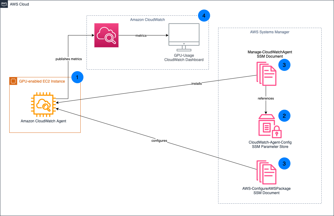
In this post, we describe how to track GPU utilization across all of your AI/ML workloads and enable accurate capacity planning without needing teams to use a custom Amazon Machine Image (AMI) or to re-deploy their existing infrastructure. You can use Amazon CloudWatch to track GPU utilization, and leverage AWS Systems Manager Run Command to install and configure the agent across your existing fleet of GPU-enabled instances.

Overview

First, make sure that your existing Amazon Elastic Compute Cloud (Amazon EC2) instances have the Systems Manager Agent installed, and also have the appropriate level of AWS Identity and Access Management (IAM) permissions to run the Amazon CloudWatch Agent. Next, specify the configuration for the CloudWatch Agent in Systems Manager Parameter Store, and then deploy the CloudWatch Agent to our GPU-enabled EC2 instances. Finally, create a CloudWatch Dashboard to analyze GPU utilization.

Architecture Diagram depicting the integration between AWS Systems Manager with RunCommand Arguments stored in SSM Parameter Store, your Amazon GPU enabled EC2 instance with installed Amazon CloudWatch Agen­t, and Amazon CloudWatch Dashboard that aggregates and displays the ­reported metrics.

  1. Install the CloudWatch Agent on your existing GPU-enabled EC2 instances.
  2. Your CloudWatch Agent configuration is stored in Systems Manager Parameter Store.
  3. Systems Manager Documents are used to install and configure the CloudWatch Agent on your EC2 instances.
  4. GPU metrics are published to CloudWatch, which you can then visualize through the CloudWatch Dashboard.

Prerequisites

This post assumes you already have GPU-enabled EC2 workloads running in your AWS account. If the EC2 instance doesn’t have any GPUs, then the custom configuration won’t be applied to the CloudWatch Agent. Instead, the default configuration is used. For those instances, leveraging the CloudWatch Agent’s default configuration is better suited for tracking resource utilization.

For the CloudWatch Agent to collect your instance’s GPU metrics, the proper NVIDIA drivers must be installed on your instance. Several AWS official AMIs including the Deep Learning AMI already have these drivers installed. To see a list of AMIs with the NVIDIA drivers pre-installed, and for full installation instructions for Linux-based instances, see Install NVIDIA drivers on Linux instances.

Additionally, deploying and managing the CloudWatch Agent requires the instances to be running. If your instances are currently stopped, then you must start them to follow the instructions outlined in this post.

Preparing your EC2 instances

You utilize Systems Manager to deploy the CloudWatch Agent, so make sure that your EC2 instances have the Systems Manager Agent installed. Many AWS-provided AMIs already have the Systems Manager Agent installed. For a full list of the AMIs which have the Systems Manager Agent pre-installed, see Amazon Machine Images (AMIs) with SSM Agent preinstalled. If your AMI doesn’t have the Systems Manager Agent installed, see Working with SSM Agent for instructions on installing based on your operating system (OS).

Once installed, the CloudWatch Agent needs certain permissions to accept commands from Systems Manager, read Systems Manager Parameter Store entries, and publish metrics to CloudWatch. These permissions are bundled into the managed IAM policies AmazonEC2RoleforSSM, AmazonSSMReadOnlyAccess, and CloudWatchAgentServerPolicy. To create a new IAM role and associated IAM instance profile with these policies attached, you can run the following AWS Command Line Interface (AWS CLI) commands, replacing <REGION_NAME> with your AWS region, and <INSTANCE_ID> with the EC2 Instance ID that you want to associate with the instance profile:

aws iam create-role --role-name CloudWatch-Agent-Role --assume-role-policy-document  '{"Statement":{"Effect":"Allow","Principal":{"Service":"ec2.amazonaws.com"},"Action":"sts:AssumeRole"}}'
aws iam attach-role-policy --role-name CloudWatch-Agent-Role --policy-arn arn:aws:iam::aws:policy/service-role/AmazonEC2RoleforSSM
aws iam attach-role-policy --role-name CloudWatch-Agent-Role --policy-arn arn:aws:iam::aws:policy/AmazonSSMReadOnlyAccess
aws iam attach-role-policy --role-name CloudWatch-Agent-Role --policy-arn arn:aws:iam::aws:policy/CloudWatchAgentServerPolicy
aws iam create-instance-profile --instance-profile-name CloudWatch-Agent-Instance-Profile
aws iam add-role-to-instance-profile --instance-profile-name CloudWatch-Agent-Instance-Profile --role-name CloudWatch-Agent-Role
aws ec2 associate-iam-instance-profile --region <REGION_NAME> --instance-id <INSTANCE_ID> --iam-instance-profile Name=CloudWatch-Agent-Instance-Profile

Alternatively, you can attach the IAM policies to your existing IAM role associated with an existing IAM instance profile.

aws iam attach-role-policy --role-name <ROLE_NAME> --policy-arn arn:aws:iam::aws:policy/service-role/AmazonEC2RoleforSSM
aws iam attach-role-policy --role-name <ROLE_NAME> --policy-arn arn:aws:iam::aws:policy/AmazonSSMReadOnlyAccess
aws iam attach-role-policy --role-name <ROLE_NAME> --policy-arn arn:aws:iam::aws:policy/CloudWatchAgentServerPolicy
aws ec2 associate-iam-instance-profile --region <REGION_NAME> --instance-id <INSTANCE_ID> --iam-instance-profile Name=<INSTANCE_PROFILE>

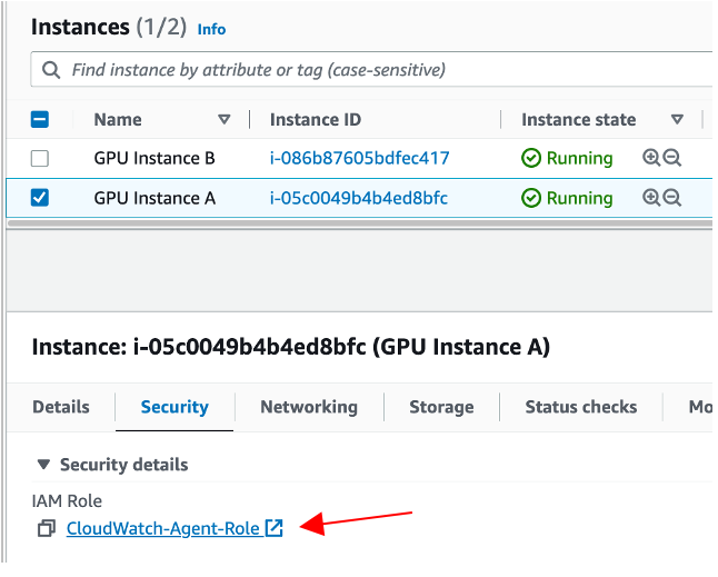
Once complete, you should see that your EC2 instance is associated with the appropriate IAM role.

An Amazon EC2 Instance with the CloudWatch-Agent-Role IAM Role attached

This role should have the AmazonEC2RoleforSSM, AmazonSSMReadOnlyAccess and CloudWatchAgentServerPolicy IAM policies attached.

The CloudWatch-Agent-Role IAM Role’s attached permission policies, Amazon EC2 Role for SSM, CloudWatch Agent Server ¬Policy, and Amazon SSM Read Only Access

Configuring and deploying the CloudWatch Agent

Before deploying the CloudWatch Agent onto our EC2 instances, make sure that those agents are properly configured to collect GPU metrics. To do this, you must create a CloudWatch Agent configuration and store it in Systems Manager Parameter Store.

Copy the following into a file cloudwatch-agent-config.json:

{
    "agent": {
        "metrics_collection_interval": 60,
        "run_as_user": "cwagent"
    },
    "metrics": {
        "aggregation_dimensions": [
            [
                "InstanceId"
            ]
        ],
        "append_dimensions": {
            "AutoScalingGroupName": "${aws:AutoScalingGroupName}",
            "ImageId": "${aws:ImageId}",
            "InstanceId": "${aws:InstanceId}",
            "InstanceType": "${aws:InstanceType}"
        },
        "metrics_collected": {
            "cpu": {
                "measurement": [
                    "cpu_usage_idle",
                    "cpu_usage_iowait",
                    "cpu_usage_user",
                    "cpu_usage_system"
                ],
                "metrics_collection_interval": 60,
                "resources": [
                    "*"
                ],
                "totalcpu": false
            },
            "disk": {
                "measurement": [
                    "used_percent",
                    "inodes_free"
                ],
                "metrics_collection_interval": 60,
                "resources": [
                    "*"
                ]
            },
            "diskio": {
                "measurement": [
                    "io_time"
                ],
                "metrics_collection_interval": 60,
                "resources": [
                    "*"
                ]
            },
            "mem": {
                "measurement": [
                    "mem_used_percent"
                ],
                "metrics_collection_interval": 60
            },
            "swap": {
                "measurement": [
                    "swap_used_percent"
                ],
                "metrics_collection_interval": 60
            },
            "nvidia_gpu": {
                "measurement": [
                    "utilization_gpu",
                    "temperature_gpu",
                    "utilization_memory",
                    "fan_speed",
                    "memory_total",
                    "memory_used",
                    "memory_free",
                    "pcie_link_gen_current",
                    "pcie_link_width_current",
                    "encoder_stats_session_count",
                    "encoder_stats_average_fps",
                    "encoder_stats_average_latency",
                    "clocks_current_graphics",
                    "clocks_current_sm",
                    "clocks_current_memory",
                    "clocks_current_video"
                ],
                "metrics_collection_interval": 60
            }
        }
    }
}

Run the following AWS CLI command to deploy a Systems Manager Parameter CloudWatch-Agent-Config, which contains a minimal agent configuration for GPU metrics collection. Replace <REGION_NAME> with your AWS Region.

aws ssm put-parameter \
--region <REGION_NAME> \
--name CloudWatch-Agent-Config \
--type String \
--value file://cloudwatch-agent-config.json

Now you can see a CloudWatch-Agent-Config parameter in Systems Manager Parameter Store, containing your CloudWatch Agent’s JSON configuration.

CloudWatch-Agent-Config stored in Systems Manager Parameter Store

Next, install the CloudWatch Agent on your EC2 instances. To do this, you can leverage Systems Manager Run Command, specifically the AWS-ConfigureAWSPackage document which automates the CloudWatch Agent installation.

  1. Run the following AWS CLI command, replacing <REGION_NAME> with the Region into which your instances are deployed, and <INSTANCE_ID> with the EC2 Instance ID on which you want to install the CloudWatch Agent.
aws ssm send-command \
--query 'Command.CommandId' \
--region <REGION_NAME> \
--instance-ids <INSTANCE_ID> \
--document-name AWS-ConfigureAWSPackage \
--parameters '{"action":["Install"],"installationType":["In-place update"],"version":["latest"],"name":["AmazonCloudWatchAgent"]}'

2. To monitor the status of your command, use the get-command-invocation AWS CLI command. Replace <COMMAND_ID> with the command ID output from the previous step, <REGION_NAME> with your AWS region, and <INSTANCE_ID> with your EC2 instance ID.

aws ssm get-command-invocation --query Status --region <REGION_NAME> --command-id <COMMAND_ID> --instance-id <INSTANCE_ID>

3.Wait for the command to show the status Success before proceeding.

$ aws ssm send-command \
	 --query 'Command.CommandId' \
    --region us-east-2 \
    --instance-ids i-0123456789abcdef \
    --document-name AWS-ConfigureAWSPackage \
    --parameters '{"action":["Install"],"installationType":["Uninstall and reinstall"],"version":["latest"],"additionalArguments":["{}"],"name":["AmazonCloudWatchAgent"]}'

"5d8419db-9c48-434c-8460-0519640046cf"

$ aws ssm get-command-invocation --query Status --region us-east-2 --command-id 5d8419db-9c48-434c-8460-0519640046cf --instance-id i-0123456789abcdef

"Success"

Repeat this process for all EC2 instances on which you want to install the CloudWatch Agent.

Next, configure the CloudWatch Agent installation. For this, once again leverage Systems Manager Run Command. However, this time the AmazonCloudWatch-ManageAgent document which applies your custom agent configuration is stored in the Systems Manager Parameter Store to your deployed agents.

  1. Run the following AWS CLI command, replacing <REGION_NAME> with the Region into which your instances are deployed, and <INSTANCE_ID> with the EC2 Instance ID on which you want to configure the CloudWatch Agent.
aws ssm send-command \
--query 'Command.CommandId' \
--region <REGION_NAME> \
--instance-ids <INSTANCE_ID> \
--document-name AmazonCloudWatch-ManageAgent \
--parameters '{"action":["configure"],"mode":["ec2"],"optionalConfigurationSource":["ssm"],"optionalConfigurationLocation":["/CloudWatch-Agent-Config"],"optionalRestart":["yes"]}'

2. To monitor the status of your command, utilize the get-command-invocation AWS CLI command. Replace <COMMAND_ID> with the command ID output from the previous step, <REGION_NAME> with your AWS region, and <INSTANCE_ID> with your EC2 instance ID.

aws ssm get-command-invocation --query Status --region <REGION_NAME> --command-id <COMMAND_ID> --instance-id <INSTANCE_ID>

3. Wait for the command to show the status Success before proceeding.

$ aws ssm send-command \
    --query 'Command.CommandId' \
    --region us-east-2 \
    --instance-ids i-0123456789abcdef \
    --document-name AmazonCloudWatch-ManageAgent \
    --parameters '{"action":["configure"],"mode":["ec2"],"optionalConfigurationSource":["ssm"],"optionalConfigurationLocation":["/CloudWatch-Agent-Config"],"optionalRestart":["yes"]}'

"9a4a5c43-0795-4fd3-afed-490873eaca63"

$ aws ssm get-command-invocation --query Status --region us-east-2 --command-id 9a4a5c43-0795-4fd3-afed-490873eaca63 --instance-id i-0123456789abcdef

"Success"

Repeat this process for all EC2 instances on which you want to install the CloudWatch Agent. Once finished, the CloudWatch Agent installation and configuration is complete, and your EC2 instances now report GPU metrics to CloudWatch.

Visualize your instance’s GPU metrics in CloudWatch

Now that your GPU-enabled EC2 Instances are publishing their utilization metrics to CloudWatch, you can visualize and analyze these metrics to better understand your resource utilization patterns.

The GPU metrics collected by the CloudWatch Agent are within the CWAgent namespace. Explore your GPU metrics using the CloudWatch Metrics Explorer, or deploy our provided sample dashboard.

  1. Copy the following into a file, cloudwatch-dashboard.json, replacing instances of <REGION_NAME> with your Region:
{
    "widgets": [
        {
            "height": 10,
            "width": 24,
            "y": 16,
            "x": 0,
            "type": "metric",
            "properties": {
                "metrics": [
                    [{"expression": "SELECT AVG(nvidia_smi_utilization_gpu) FROM SCHEMA(\"CWAgent\", InstanceId) GROUP BY InstanceId","id": "q1"}]
                ],
                "view": "timeSeries",
                "stacked": false,
                "region": "<REGION_NAME>",
                "stat": "Average",
                "period": 300,
                "title": "GPU Core Utilization",
                "yAxis": {
                    "left": {"label": "Percent","max": 100,"min": 0,"showUnits": false}
                }
            }
        },
        {
            "height": 7,
            "width": 8,
            "y": 0,
            "x": 0,
            "type": "metric",
            "properties": {
                "metrics": [
                    [{"expression": "SELECT AVG(nvidia_smi_utilization_gpu) FROM SCHEMA(\"CWAgent\", InstanceId)", "label": "Utilization","id": "q1"}]
                ],
                "view": "gauge",
                "stacked": false,
                "region": "<REGION_NAME>",
                "stat": "Average",
                "period": 300,
                "title": "Average GPU Core Utilization",
                "yAxis": {"left": {"max": 100, "min": 0}
                },
                "liveData": false
            }
        },
        {
            "height": 9,
            "width": 24,
            "y": 7,
            "x": 0,
            "type": "metric",
            "properties": {
                "metrics": [
                    [{ "expression": "SEARCH(' MetricName=\"nvidia_smi_memory_used\" {\"CWAgent\", InstanceId} ', 'Average')", "id": "m1", "visible": false }],
                    [{ "expression": "SEARCH(' MetricName=\"nvidia_smi_memory_total\" {\"CWAgent\", InstanceId} ', 'Average')", "id": "m2", "visible": false }],
                    [{ "expression": "SEARCH(' MetricName=\"mem_used_percent\" {CWAgent, InstanceId} ', 'Average')", "id": "m3", "visible": false }],
                    [{ "expression": "100*AVG(m1)/AVG(m2)", "label": "GPU", "id": "e2", "color": "#17becf" }],
                    [{ "expression": "AVG(m3)", "label": "RAM", "id": "e3" }]
                ],
                "view": "timeSeries",
                "stacked": false,
                "region": "<REGION_NAME>",
                "stat": "Average",
                "period": 300,
                "yAxis": {
                    "left": {"min": 0,"max": 100,"label": "Percent","showUnits": false}
                },
                "title": "Average Memory Utilization"
            }
        },
        {
            "height": 7,
            "width": 8,
            "y": 0,
            "x": 8,
            "type": "metric",
            "properties": {
                "metrics": [
                    [ { "expression": "SEARCH(' MetricName=\"nvidia_smi_memory_used\" {\"CWAgent\", InstanceId} ', 'Average')", "id": "m1", "visible": false } ],
                    [ { "expression": "SEARCH(' MetricName=\"nvidia_smi_memory_total\" {\"CWAgent\", InstanceId} ', 'Average')", "id": "m2", "visible": false } ],
                    [ { "expression": "100*AVG(m1)/AVG(m2)", "label": "Utilization", "id": "e2" } ]
                ],
                "sparkline": true,
                "view": "gauge",
                "region": "<REGION_NAME>",
                "stat": "Average",
                "period": 300,
                "yAxis": {
                    "left": {"min": 0,"max": 100}
                },
                "liveData": false,
                "title": "GPU Memory Utilization"
            }
        }
    ]
}

2. run the following AWS CLI command, replacing <REGION_NAME> with the name of your Region:

aws cloudwatch put-dashboard \
    --region <REGION_NAME> \
    --dashboard-name My-GPU-Usage \
    --dashboard-body file://cloudwatch-dashboard.json

View the My-GPU-Usage CloudWatch dashboard in the CloudWatch console for your AWS region..

An example CloudWatch dashboard, My-GPU-Usage, showing the GPU usage metrics over time.

Cleaning Up

To avoid incurring future costs for resources created by following along in this post, delete the following:

  1. My-GPU-Usage CloudWatch Dashboard
  2. CloudWatch-Agent-Config Systems Manager Parameter
  3. CloudWatch-Agent-Role IAM Role

Conclusion

By following along with this post, you deployed and configured the CloudWatch Agent across your GPU-enabled EC2 instances to track GPU utilization without pausing in-progress experiments and model training. Then, you visualized the GPU utilization of your workloads with a CloudWatch Dashboard to better understand your workload’s GPU usage and make more informed scaling and cost decisions. For other ways that Amazon CloudWatch can improve your organization’s operational insights, see the Amazon CloudWatch documentation.

AWS Week in Review: New Service for Generative AI and Amazon EC2 Trn1n, Inf2, and CodeWhisperer now GA – April 17, 2023

Post Syndicated from Antje Barth original https://aws.amazon.com/blogs/aws/aws-week-in-review-new-service-for-generative-ai-and-amazon-ec2-trn1n-inf2-and-codewhisperer-now-ga-april-17-2023/

I could almost title this blog post the “AWS AI/ML Week in Review.” This past week, we announced several new innovations and tools for building with generative AI on AWS. Let’s dive right into it.

Last Week’s Launches
Here are some launches that got my attention during the previous week:

Announcing Amazon Bedrock and Amazon Titan models Amazon Bedrock is a new service to accelerate your development of generative AI applications using foundation models through an API without managing infrastructure. You can choose from a wide range of foundation models built by leading AI startups and Amazon. The new Amazon Titan foundation models are pre-trained on large datasets, making them powerful, general-purpose models. You can use them as-is or privately to customize them with your own data for a particular task without annotating large volumes of data. Amazon Bedrock is currently in limited preview. Sign up here to learn more.

Building with Generative AI on AWS

Amazon EC2 Trn1n and Inf2 instances are now generally availableTrn1n instances, powered by AWS Trainium accelerators, double the network bandwidth (compared to Trn1 instances) to 1,600 Gbps of Elastic Fabric Adapter (EFAv2). The increased bandwidth delivers even higher performance for training network-intensive generative AI models such as large language models (LLMs) and mixture of experts (MoE). Inf2 instances, powered by AWS Inferentia2 accelerators, deliver high performance at the lowest cost in Amazon EC2 for generative AI models, including LLMs and vision transformers. They are the first inference-optimized instances in Amazon EC2 to support scale-out distributed inference with ultra-high-speed connectivity between accelerators. Compared to Inf1 instances, Inf2 instances deliver up to 4x higher throughput and up to 10x lower latency. Check out my blog posts on Trn1 instances and Inf2 instances for more details.

Amazon CodeWhisperer, free for individual use, is now generally availableAmazon CodeWhisperer is an AI coding companion that generates real-time single-line or full-function code suggestions in your IDE to help you build applications faster. With GA, we introduce two tiers: CodeWhisperer Individual and CodeWhisperer Professional. CodeWhisperer Individual is free to use for generating code. You can sign up with an AWS Builder ID based on your email address. The Individual Tier provides code recommendations, reference tracking, and security scans. CodeWhisperer Professional—priced at $19 per user, per month—offers additional enterprise administration capabilities. Steve’s blog post has all the details.

Amazon GameLift adds support for Unreal Engine 5Amazon GameLift is a fully managed solution that allows you to manage and scale dedicated game servers for session-based multiplayer games. The latest version of the Amazon GameLift Server SDK 5.0 lets you integrate your Unreal 5-based game servers with the Amazon GameLift service. In addition, the latest Amazon GameLift Server SDK with Unreal 5 plugin is built to work with Amazon GameLift Anywhere so that you can test and iterate Unreal game builds faster and manage game sessions across any server hosting infrastructure. Check out the release notes to learn more.

Amazon Rekognition launches Face Liveness to deter fraud in facial verification – Face Liveness verifies that only real users, not bad actors using spoofs, can access your services. Amazon Rekognition Face Liveness analyzes a short selfie video to detect spoofs presented to the camera, such as printed photos, digital photos, digital videos, or 3D masks, as well as spoofs that bypass the camera, such as pre-recorded or deepfake videos. This AWS Machine Learning Blog post walks you through the details and shows how you can add Face Liveness to your web and mobile applications.

For a full list of AWS announcements, be sure to keep an eye on the What’s New at AWS page.

Other AWS News
Here are some additional news items and blog posts that you may find interesting:

Updates to the AWS Well-Architected Framework – The most recent content updates and improvements focus on providing expanded guidance across the AWS service portfolio to help you make more informed decisions when developing implementation plans. Services that were added or expanded in coverage include AWS Elastic Disaster Recovery, AWS Trusted Advisor, AWS Resilience Hub, AWS Config, AWS Security Hub, Amazon GuardDuty, AWS Organizations, AWS Control Tower, AWS Compute Optimizer, AWS Budgets, Amazon CodeWhisperer, and Amazon CodeGuru. This AWS Architecture Blog post has all the details.

Amazon releases largest dataset for training “pick and place” robots – In an effort to improve the performance of robots that pick, sort, and pack products in warehouses, Amazon has publicly released the largest dataset of images captured in an industrial product-sorting setting. Where the largest previous dataset of industrial images featured on the order of 100 objects, the Amazon dataset, called ARMBench, features more than 190,000 objects. Check out this Amazon Science Blog post to learn more.

AWS open-source news and updates – My colleague Ricardo writes this weekly open-source newsletter in which he highlights new open-source projects, tools, and demos from the AWS Community. Read edition #153 here.

Upcoming AWS Events
Check your calendars and sign up for these AWS events:

Build On AWS - Generative AI#BuildOn Generative AI – Join our weekly live Build On Generative AI Twitch show. Every Monday morning, 9:00 US PT, my colleagues Emily and Darko take a look at aspects of generative AI. They host developers, scientists, startup founders, and AI leaders and discuss how to build generative AI applications on AWS.

In today’s episode, Emily walks us through the latest AWS generative AI announcements. You can watch the video here.

Dot Net Developer Day.NET Developer Day.NET Enterprise Developer Day EMEA 2023 (April 25) is a free, one-day virtual event providing enterprise developers with the most relevant information to swiftly and efficiently migrate and modernize their .NET applications and workloads on AWS.

AWS Developer Innovation DayAWS Developer Innovation DayAWS Developer Innovation Day (April 26) is a new, free, one-day virtual event designed to help developers and teams be productive and collaborate from discovery to delivery, to running software and building applications. Get a first look at exciting product updates, technical deep dives, and keynotes.

AWS Global Summits – Check your calendars and sign up for the AWS Summit close to where you live or work: Tokyo (April 20–21), Singapore (May 4), Stockholm (May 11), Hong Kong (May 23), Tel Aviv (May 31), Amsterdam (June 1), London (June 7), Washington, DC (June 7–8), Toronto (June 14), Madrid (June 15), and Milano (June 22).

You can browse all upcoming AWS-led in-person and virtual events and developer-focused events such as Community Days.

That’s all for this week. Check back next Monday for another Week in Review!

— Antje

This post is part of our Week in Review series. Check back each week for a quick roundup of interesting news and announcements from AWS!

Streaming Android games from cloud to mobile with AWS Graviton-based Amazon EC2 G5g instances

Post Syndicated from Sheila Busser original https://aws.amazon.com/blogs/compute/streaming-android-games-from-cloud-to-mobile-with-aws-graviton-based-amazon-ec2-g5g-instances/

This blog post is written by Vincent Wang, GCR EC2 Specialist SA, Compute.

Streaming games from the cloud to mobile devices is an emerging technology that allows less powerful and less expensive devices to play high-quality games with lower battery consumption and less storage capacity. This technology enables a wider audience to enjoy high-end gaming experiences from their existing devices, such as smartphones, tablets, and smart TVs.

To load games for streaming on AWS, it’s necessary to use Android environments that can utilize GPU acceleration for graphics rendering and optimize for network latency. Cloud-native products, such as the Anbox Cloud Appliance or Genymotion available on the AWS Marketplace, can provide a cost-effective containerized solution for game streaming workloads on Amazon Elastic Compute Cloud (Amazon EC2).

For example, Anbox Cloud’s virtual device infrastructure can run games with low latency and high frame rates. When combined with the AWS Graviton-based Amazon EC2 G5g instances, which offer a cost reduction of up to 30% per-game stream per-hour compared to x86-based GPU instances, it enables companies to serve millions of customers in a cost-efficient manner.

In this post, we chose the Anbox Cloud Appliance to demonstrate how you can use it to stream a resource-demanding game called Genshin Impact. We use a G5g instance along with a mobile phone to run the streamed game inside of a Firefox browser application.

Overview

Graviton-based instances utilize fewer compute resources than x86-based instances due to the 64-bit architecture of Arm processors used in AWS Graviton servers. As shown in the following diagram, Graviton instances eliminate the need for cross-compilation or Android emulation. This simplifies development efforts and reduces time-to-market, thereby lowering the cost-per-stream. With G5g instances, customers can now run their Android games natively, encode CPU or GPU-rendered graphics, and stream the game over the network to multiple mobile devices.

Architecture difference when running Android on X86-based instance and Graviton-based instance.

Figure 1: Architecture difference when running Android on X86-based instance and Graviton-based instance.

Real-time ray-traced rendering is required for most modern games to deliver photorealistic objects and environments with physically accurate shadows, reflections, and refractions. The G5g instance, which is powered by AWS Graviton2 processors and NVIDIA T4G Tensor Core GPUs, provides a cost-effective solution for running these resource-intensive games.

Architecture

Architecture of Android Streaming Game.

Figure 2: Architecture of Android Streaming Game.

When streaming games from a mobile device, only input data (touchscreen, audio, etc.) is sent over the network to the game streaming server hosted on a G5g instance. Then, the input is directed to the appropriate Android container designated for that particular client. The game application running in the container processes the input and updates the game state accordingly. Then, the resulting rendered image frames are sent back to the mobile device for display on the screen. In certain games, such as multiplayer games, the streaming server must communicate with external game servers to reflect the full game state. In these cases, additional data is transferred to and from game servers and back to the mobile client. The communication between clients and the streaming server is performed using the WebRTC network protocol to minimize latency and make sure that users’ gaming experience isn’t affected.

The Graviton processor handles compute-intensive tasks, such as the Android runtime and I/O transactions on the streaming server. However, for resource-demanding games, the Nvidia GPU is utilized for graphics rendering. To scale effortlessly, the Anbox Cloud software can be utilized to manage and execute several game sessions on the same instance.

Prerequisites

First, you need an Ubuntu single sign-on (SSO) account. If you don’t have one yet, you may create one from Ubuntu One website. Then you need an Android mobile phone with Firefox or Chrome browser installed to play the streaming games.

Setup

We can install Anbox Cloud Appliance in the AWS Marketplace. Select the Arm variant so that it works on Graviton-based instances. If the subscription doesn’t work on the first try, then you receive an email which guides you to a page where you can try again.

Figure 3: Subscribe Anbox Cloud Appliance in AWS Marketplace.

Figure 3: Subscribe Anbox Cloud Appliance in AWS Marketplace.

In this demonstration, we select G5g.xlarge in the Instance type section and leave all settings with default values, except the storage as per the following:

  1. A root disk with minimum 50 GB (required)
  2. An additional Amazon Elastic Block Store (Amazon EBS) volume with at least 100 GB (recommended)

For the Genshin Impact demo, we recommend a specific amount of storage. However, when deploying your Android applications, you must select an appropriate storage size based on the package size. Additionally, you should choose an instance size based on the resources that you plan to utilize for your gaming sessions, such as CPU, memory, and networking. In our demo, we launched only one session from a single mobile device.

Launch the instance and wait until it reaches running status. Then you can secure shell (SSH) to the instance to configure the Android environment.

Install Anbox cloud

To make sure of the security and reliability of some of the package repositories used, we update the CUDA Linux GPG Repository Key. View this Nvidia blog post for more details on this procedure.

$ sudo apt-key del 7fa2af80

$ wget

https://developer.download.nvidia.com/compute/cuda/repos/ubuntu2004/sbsa/cuda keyring_1.0-1_all.deb

$ sudo dpkg -i cuda-keyring_1.0-1_all.deb

As the Android in Anbox Cloud Appliance is running in an LXD container environment, upgrade LXD to the latest version.

  $ sudo snap refresh –channel=5.0/stable lxd

Install the Anbox Cloud Appliance software using the following command and selecting the default answers:

  $ sudo anbox-cloud-appliance init

Watch the status page at https://$(ec2_public_DNS_name) for progress information.

Figure 4: The status of deploying Anbox Cloud.

Figure 4: The status of deploying Anbox Cloud.

The initialization process takes approximately 20 minutes. After it’s complete, register the Ubuntu SSO account previously created, then follow the instructions provided to finalize the process.

  $ anbox-cloud-appliance dashboard register <your Ubuntu SSO email address>

Stream an Android game application

Use the sample from the following repo to setup the service on the streaming server:

  $ git clone https://github.com/anbox-cloud/cloud-gaming-demo.git

Build the Flutter web UI:

$ sudo snap install flutter –classic

$ cd cloud-gaming-demo/ui && flutter build web && cd ..

$ mkdir -p backend/service/static

$ cp -av ui/build/web/* backend/service/static

Then build the backend service which processes requests and interacts with the Anbox Stream Gateway to create instances of game applications. Start by preparing the environment:

$ sudo apt-get install python3-pip

$ sudo pip3 install virtualenv

$ cd backend && virtualenv venv

Create the configuration file for the backend service so that it can access the Anbox Stream Gateway. There are two parameters to set: gateway-URL and gateway-token. The gateway token can be obtained from the following command:

$ anbox-cloud-appliance gateway account create <account-name>

Create a file called config.yaml that contains the two values:

gateway-url: https:// <EC2 public DNS name>

gateway-token: <gateway_token>

Add the following line to the activate hook in the backend/venv/bin/ directory so that the backend service can read config.yaml on its startup:

$ export CONFIG_PATH=<path_to_config_yaml>

Now we can launch the backend service which will be served by default on TCP port 8002.

$./run.sh

In the next steps, we download a game and build it via Anbox Cloud. We need an Android APK and a configuration file. Create a folder under the HOME directory and create a manifest.yaml file in the folder. In this example, we must add the following details in the file. You can refer to the Anbox Cloud documentation for more information on the format.

name: genshin

instance-type: g10.3

resources:

cpus: 10

memory: 25GB

disk-size: 50GB

gpu-slots: 15

features: [“enable_virtual_keyboard”]

Select an APK for the arm64-v8a architecture which is natively supported on Graviton. In this example, we download Genshin Impact, an action role-playing game developed and published by miHoYo. You must supply your own Android APK if you want to try these steps. Download the APK into the folder and rename it to app.apk. Overall, the final layout of the game folder should look as follows:

.

├── app.apk

└── manifest.yaml

Run the following command from the folder to create the application:

$ amc application create  .

Wait until the application status changes to ready. You can monitor the status with the following command:

$ amc application ls

Edit the following:

  1. Update the gameids variable defined in the ui/lib/homepage.dart file to include the name of the game (as declared in the manifest file).
  2. Insert a new key/value pair to the static appNameMap and appDesMap variables defined in the lib/api/application.dart file.
  3. Provide a screenshot of the game (in jpeg format), rename it to <game-name>.jpeg, and put it into the ui/lib/assets directory.

Then, re-build the web UI, copy the contents from the ui/build/web folder to the backend/service/static directory, and refresh the webpage.

Test the game

Using your mobile phone, open the Firefox browser or another browser that supports WebRTC. Type the public DNS name of the G5g instance with the 8002 TCP port, and you should see something similar to the following:

Figure 5: The webpage of the Android streaming game portal.

Figure 5: The webpage of the Android streaming game portal.

Select the Play now button, wait a moment for the application to be setup on the server side, and then enjoy the game.

Figure 6: The screen capture of playing Android streaming game.

Figure 6: The screen capture of playing Android streaming game.

Clean-up

Please cancel the subscription of the Anbox Cloud Appliance in the AWS Marketplace, you can follow the AWS Marketplace Buyer Guide for more details, then terminate the G5g.xlarge instance to avoid incurring future costs.

Conclusion

In this post, we demonstrated how a resource-intensive Android game runs natively on a Graviton-based G5g instance and is streamed to an Arm-based mobile device. The benefits include better price-performance, reduced development effort, and faster time-to-market. One way to run your games efficiently on the cloud is through software available on the AWS Marketplace, such as the Anbox Cloud Appliance, which was showcased as an example method.

To learn more about AWS Graviton, visit the official product page and the technical guide.

Amazon EC2 Inf2 Instances for Low-Cost, High-Performance Generative AI Inference are Now Generally Available

Post Syndicated from Antje Barth original https://aws.amazon.com/blogs/aws/amazon-ec2-inf2-instances-for-low-cost-high-performance-generative-ai-inference-are-now-generally-available/

Innovations in deep learning (DL), especially the rapid growth of large language models (LLMs), have taken the industry by storm. DL models have grown from millions to billions of parameters and are demonstrating exciting new capabilities. They are fueling new applications such as generative AI or advanced research in healthcare and life sciences. AWS has been innovating across chips, servers, data center connectivity, and software to accelerate such DL workloads at scale.

At AWS re:Invent 2022, we announced the preview of Amazon EC2 Inf2 instances powered by AWS Inferentia2, the latest AWS-designed ML chip. Inf2 instances are designed to run high-performance DL inference applications at scale globally. They are the most cost-effective and energy-efficient option on Amazon EC2 for deploying the latest innovations in generative AI, such as GPT-J or Open Pre-trained Transformer (OPT) language models.

Today, I’m excited to announce that Amazon EC2 Inf2 instances are now generally available!

Inf2 instances are the first inference-optimized instances in Amazon EC2 to support scale-out distributed inference with ultra-high-speed connectivity between accelerators. You can now efficiently deploy models with hundreds of billions of parameters across multiple accelerators on Inf2 instances. Compared to Amazon EC2 Inf1 instances, Inf2 instances deliver up to 4x higher throughput and up to 10x lower latency. Here’s an infographic that highlights the key performance improvements that we have made available with the new Inf2 instances:

Performance improvements with Amazon EC2 Inf2

New Inf2 Instance Highlights
Inf2 instances are available today in four sizes and are powered by up to 12 AWS Inferentia2 chips with 192 vCPUs. They offer a combined compute power of 2.3 petaFLOPS at BF16 or FP16 data types and feature an ultra-high-speed NeuronLink interconnect between chips. NeuronLink scales large models across multiple Inferentia2 chips, avoids communication bottlenecks, and enables higher-performance inference.

Inf2 instances offer up to 384 GB of shared accelerator memory, with 32 GB high-bandwidth memory (HBM) in every Inferentia2 chip and 9.8 TB/s of total memory bandwidth. This type of bandwidth is particularly important to support inference for large language models that are memory bound.

Since the underlying AWS Inferentia2 chips are purpose-built for DL workloads, Inf2 instances offer up to 50 percent better performance per watt than other comparable Amazon EC2 instances. I’ll cover the AWS Inferentia2 silicon innovations in more detail later in this blog post.

The following table lists the sizes and specs of Inf2 instances in detail.

Instance Name
vCPUs AWS Inferentia2 Chips Accelerator Memory NeuronLink Instance Memory Instance Networking
inf2.xlarge 4 1 32 GB N/A 16 GB Up to 15 Gbps
inf2.8xlarge 32 1 32 GB N/A 128 GB Up to 25 Gbps
inf2.24xlarge 96 6 192 GB Yes 384 GB 50 Gbps
inf2.48xlarge 192 12 384 GB Yes 768 GB 100 Gbps

AWS Inferentia2 Innovation
Similar to AWS Trainium chips, each AWS Inferentia2 chip has two improved NeuronCore-v2 engines, HBM stacks, and dedicated collective compute engines to parallelize computation and communication operations when performing multi-accelerator inference.

Each NeuronCore-v2 has dedicated scalar, vector, and tensor engines that are purpose-built for DL algorithms. The tensor engine is optimized for matrix operations. The scalar engine is optimized for element-wise operations like ReLU (rectified linear unit) functions. The vector engine is optimized for non-element-wise vector operations, including batch normalization or pooling.

Here is a short summary of additional AWS Inferentia2 chip and server hardware innovations:

  • Data Types – AWS Inferentia2 supports a wide range of data types, including FP32, TF32, BF16, FP16, and UINT8, so you can choose the most suitable data type for your workloads. It also supports the new configurable FP8 (cFP8) data type, which is especially relevant for large models because it reduces the memory footprint and I/O requirements of the model. The following image compares the supported data types.AWS Inferentia2 Supported Data Types
  • Dynamic Execution, Dynamic Input Shapes – AWS Inferentia2 has embedded general-purpose digital signal processors (DSPs) that enable dynamic execution, so control flow operators don’t need to be unrolled or executed on the host. AWS Inferentia2 also supports dynamic input shapes that are key for models with unknown input tensor sizes, such as models processing text.
  • Custom Operators – AWS Inferentia2 supports custom operators written in C++. Neuron Custom C++ Operators enable you to write C++ custom operators that natively run on NeuronCores. You can use standard PyTorch custom operator programming interfaces to migrate CPU custom operators to Neuron and implement new experimental operators, all without any intimate knowledge of the NeuronCore hardware.
  • NeuronLink v2 – Inf2 instances are the first inference-optimized instance on Amazon EC2 to support distributed inference with direct ultra-high-speed connectivity—NeuronLink v2—between chips. NeuronLink v2 uses collective communications (CC) operators such as all-reduce to run high-performance inference pipelines across all chips.

The following Inf2 distributed inference benchmarks show throughput and cost improvements for OPT-30B and OPT-66B models over comparable inference-optimized Amazon EC2 instances.

Amazon EC2 Inf2 Benchmarks

Now, let me show you how to get started with Amazon EC2 Inf2 instances.

Get Started with Inf2 Instances
The AWS Neuron SDK integrates AWS Inferentia2 into popular machine learning (ML) frameworks like PyTorch. The Neuron SDK includes a compiler, runtime, and profiling tools and is constantly being updated with new features and performance optimizations.

In this example, I will compile and deploy a pre-trained BERT model from Hugging Face on an EC2 Inf2 instance using the available PyTorch Neuron packages. PyTorch Neuron is based on the PyTorch XLA software package and enables the conversion of PyTorch operations to AWS Inferentia2 instructions.

SSH into your Inf2 instance and activate a Python virtual environment that includes the PyTorch Neuron packages. If you’re using a Neuron-provided AMI, you can activate the preinstalled environment by running the following command:

source aws_neuron_venv_pytorch_p37/bin/activate

Now, with only a few changes to your code, you can compile your PyTorch model into an AWS Neuron-optimized TorchScript. Let’s start with importing torch, the PyTorch Neuron package torch_neuronx, and the Hugging Face transformers library.

import torch
import torch_neuronx from transformers import AutoTokenizer, AutoModelForSequenceClassification
import transformers
...

Next, let’s build the tokenizer and model.

name = "bert-base-cased-finetuned-mrpc"
tokenizer = AutoTokenizer.from_pretrained(name)
model = AutoModelForSequenceClassification.from_pretrained(name, torchscript=True)

We can test the model with example inputs. The model expects two sentences as input, and its output is whether or not those sentences are a paraphrase of each other.

def encode(tokenizer, *inputs, max_length=128, batch_size=1):
    tokens = tokenizer.encode_plus(
        *inputs,
        max_length=max_length,
        padding='max_length',
        truncation=True,
        return_tensors="pt"
    )
    return (
        torch.repeat_interleave(tokens['input_ids'], batch_size, 0),
        torch.repeat_interleave(tokens['attention_mask'], batch_size, 0),
        torch.repeat_interleave(tokens['token_type_ids'], batch_size, 0),
    )

# Example inputs
sequence_0 = "The company Hugging Face is based in New York City"
sequence_1 = "Apples are especially bad for your health"
sequence_2 = "Hugging Face's headquarters are situated in Manhattan"

paraphrase = encode(tokenizer, sequence_0, sequence_2)
not_paraphrase = encode(tokenizer, sequence_0, sequence_1)

# Run the original PyTorch model on examples
paraphrase_reference_logits = model(*paraphrase)[0]
not_paraphrase_reference_logits = model(*not_paraphrase)[0]

print('Paraphrase Reference Logits: ', paraphrase_reference_logits.detach().numpy())
print('Not-Paraphrase Reference Logits:', not_paraphrase_reference_logits.detach().numpy())

The output should look similar to this:

Paraphrase Reference Logits:     [[-0.34945598  1.9003887 ]]
Not-Paraphrase Reference Logits: [[ 0.5386365 -2.2197142]]

Now, the torch_neuronx.trace() method sends operations to the Neuron Compiler (neuron-cc) for compilation and embeds the compiled artifacts in a TorchScript graph. The method expects the model and a tuple of example inputs as arguments.

neuron_model = torch_neuronx.trace(model, paraphrase)

Let’s test the Neuron-compiled model with our example inputs:

paraphrase_neuron_logits = neuron_model(*paraphrase)[0]
not_paraphrase_neuron_logits = neuron_model(*not_paraphrase)[0]

print('Paraphrase Neuron Logits: ', paraphrase_neuron_logits.detach().numpy())
print('Not-Paraphrase Neuron Logits: ', not_paraphrase_neuron_logits.detach().numpy())

The output should look similar to this:

Paraphrase Neuron Logits: [[-0.34915772 1.8981738 ]]
Not-Paraphrase Neuron Logits: [[ 0.5374032 -2.2180378]]

That’s it. With just a few lines of code changes, we compiled and ran a PyTorch model on an Amazon EC2 Inf2 instance. To learn more about which DL model architectures are a good fit for AWS Inferentia2 and the current model support matrix, visit the AWS Neuron Documentation.

Available Now
You can launch Inf2 instances today in the AWS US East (Ohio) and US East (N. Virginia) Regions as On-Demand, Reserved, and Spot Instances or as part of a Savings Plan. As usual with Amazon EC2, you pay only for what you use. For more information, see Amazon EC2 pricing.

Inf2 instances can be deployed using AWS Deep Learning AMIs, and container images are available via managed services such as Amazon SageMaker, Amazon Elastic Kubernetes Service (Amazon EKS), Amazon Elastic Container Service (Amazon ECS), and AWS ParallelCluster.

To learn more, visit our Amazon EC2 Inf2 instances page, and please send feedback to AWS re:Post for EC2 or through your usual AWS Support contacts.

— Antje