Post Syndicated from Maneesh Sharma original https://aws.amazon.com/blogs/big-data/simplify-enterprise-data-access-using-the-amazon-redshift-integration-with-amazon-s3-access-grants/

Scaling data access securely while maintaining operational efficiency is a critical challenge for organizations. Access rights are often fragmented across various AWS services, as different business units own and manage different data stores, such as Amazon Simple Storage Service (Amazon S3) and Amazon Redshift. As data grows, modeling access in AWS Identity and Access Management (IAM) policies becomes challenging for data owners, as they try to manage access for different groups and users across accounts in the organization. Managing these distributed access rights requires substantial overhead, because security teams and data owners must collaborate to update and monitor permissions to make sure data is only accessible to authorized users.

Recognizing this challenge, the Amazon S3 Access Grants integration with Amazon Redshift allows centralized user authentication through AWS IAM Identity Center, providing unified identity across the organization. S3 Access Grants allows specific IAM Identity Center users or groups to access registered Amazon S3 locations through a grant. Creating a grant with a group as grantee lets the group members access only the S3 bucket, prefix, or object within the grant’s scope. This means that access can be managed by simply creating a grant for a group and adding or removing the user from the group, reducing administrative overhead.

In this post, we show how to grant Amazon S3 permissions to IAM Identity Center users and groups using S3 Access Grants. We also test the integration using an IAM Identity Center federated user to unload data from Amazon Redshift to Amazon S3 and load data from Amazon S3 to Amazon Redshift.

Solution overview

This post covers a use case where a large organization manages thousands of corporate users across multiple business units through their identity provider (IdP). These users regularly interact with vast amounts of data stored across numerous S3 buckets, frequently performing extract, transform, and load (ETL) operations through Amazon Redshift. Their goal is to have a simpler ETL process of data loading and unloading operations in Amazon Redshift without managing multiple IAM roles and policies for Amazon S3 access. Also, they want a centralized access management solution that seamlessly integrates their corporate identities from existing IdP with AWS services.

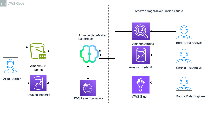
For this solution, AWS Organizations is enabled and IAM Identity Center is configured in the delegated administration account. The organization has two member accounts: Member Account 1 runs analytical workloads on Amazon Redshift, with all the services enabled with trusted identity propagation, and Member Account 2 manages data stored in Amazon S3; here you will set up S3 Access Grants. Amazon Redshift will load the user-specific data from Amazon S3 stored in Member Account 2 using access control based on IAM Identity Center users and groups. This improves the user experience maintaining a single authentication mechanism within an organization, retaining access control, and resource separation using AWS accounts as a boundary per business units.

The following diagram illustrates the solution architecture.

Figure 1: Architecture showing the solution

To run this solution in a single account, configure Amazon Redshift and S3 Access Grants with account instances of IAM Identity Center. Review When to use account instances for more information.

The solution workflow includes the following steps:

1. The user configures and connects with their respective clients (such as Amazon Redshift Query Editor v2 or a SQL client) to access Amazon Redshift using IAM Identity Center.
2. A new browser windows opens and is redirected to the login page of the IdP.
3. The user logs in with their IdP user name and password.
4. After the login is successful, the user is redirected to the client application, such as the Amazon Redshift Query Editor.
5. When the user tries to access data in Amazon S3 using the LOAD or UNLOAD SQL command, Amazon Redshift in Member Account 1 will request credentials from the S3 Access Grants instance from Member Account 2, where the Amazon S3 data is stored. This request will contain the user context.
6. S3 Access Grants will then evaluate the request against the grants it has, matching the identity specified in the grant with the one received in the request. If there is a match, the requestor will receive temporary access to the Amazon S3 locations specified in the grant’s scope.

To implement the solution, we walk you through the following steps:

1. Enable S3 Access Grants in your Amazon Redshift managed application.
2. Update IAM role permissions used in the application.
3. Create a bucket for S3 Access Grants.
4. Create an IAM policy and role for S3 Access Grants.
5. Set up S3 Access Grants.
6. Allow cross-account access of resources.
7. Create Redshift tables.
8. Unload and load data in Amazon Redshift.

Prerequisites

You should have the following prerequisites already set up:

• IAM Identity Center is enabled with a delegated administration account. For more information, see Enable IAM Identity Center and Register a member account. Keep the IAM Identity Center instance ID and the IAM Identity Center delegated administrator account number.
• Connect IAM Identity Center with your preferred IdP and sync users and groups. For instructions, refer to IAM Identity Center identity source tutorials.
• Two member accounts:
  • One with an existing Redshift cluster and managed application (Member Account 1). To set up a Redshift cluster with IAM Identity Center integration enabled, refer to Integrate Identity Provider (IdP) with Amazon Redshift Query Editor V2 using AWS IAM Identity Center for seamless Single Sign-On.
  • The second account for Amazon S3 (Member Account 2). You will set up Amazon S3 and S3 Access Grants later in this post.
• Resource sharing enabled in your organization with AWS Resource Access Manager (AWS RAM). For instructions, refer to Enable resource sharing within AWS Organizations.

Enable S3 Access Grants from the Amazon Redshift managed application

After you have created your Redshift application in IAM Identity Center, you need to perform the following steps to enable S3 Access Grants in the account where Amazon Redshift exists. For this post, we use Member Account 1:

1. Log in to the AWS Management Console as admin.
2. On the Amazon Redshift console, choose IAM Identity Center connection in the navigation pane.
3. Select the managed Redshift application and choose Edit.
4. Choose Amazon S3 access grants in Trusted identity propagation.
5. Choose Save changes.

The following screenshot shows the updated configuration.

Figure 2: Redshift managed application

Update the IAM role permission attached to the Amazon Redshift managed application

The Amazon Redshift managed application has an IAM role attached (in the preceding screenshot, you can see the role called IAMIDCRedshiftRole under IAM role for IAM Identity Center access. We now need to modify the policy on this role and add permissions to allow interaction with Amazon S3. Edit the role and add s3:GetAccessGrantsInstanceForPrefix and s3:GetDataAccess as shown in the following policy:

{
    "Version": "2012-10-17",
    "Statement": [
        {
            "Sid": "AllowGetRedsfhitInformation",
            "Effect": "Allow",
            "Action": [
                "redshift-serverless:ListNamespaces",
                "redshift-serverless:ListWorkgroups",
                "redshift:DescribeQev2IdcApplications",
                "redshift-serverless:GetWorkgroup"
            ],
            "Resource": "*"
        },
        {
            "Sid": "AllowDescribeIdentityCenter",
            "Effect": "Allow",
            "Action": [
                "sso:DescribeApplication",
                "sso:DescribeInstance"
            ],
            "Resource": [
                "arn:aws:sso:::instance/<IAM Identity Center Instance ID>",
                "arn:aws:sso::<Delegated Adminstration AWS Account ID>:application/<IAM Identity Center Instance ID>/*"
            ]
        },
        {
            "Sid": "RetrieveAGinstanceforParticularPrefix",
            "Effect": "Allow",
            "Action": 
                      "s3:GetAccessGrantsInstanceForPrefix",
            "Resource": "*"
        },
        {
            "Sid": "CrossAccountAccessGrantsPolicy",
            "Effect": "Allow",
            "Action": [
                "s3:GetDataAccess"
            ],
            "Resource": "arn:aws:s3:<region>:<AWS Account of S3 Access Grant>:access-grants/default"
        }
    ]
}

Replace <IAM Identity Center Instance ID> with your IAM Identity Center instance ID and <Delegated Adminstration AWS Account ID> with the account ID where IAM Identity Center is set up. You also need to replace the resource in CrossAccountAccessGrantscasePolicy with your S3 Access Grants instance information.

Create an S3 bucket for S3 Access Grants

In this step, you create a S3 bucket that you want to grant access to or use an existing bucket. For this post, we create a bucket called amzn-s3-demo-bucket. You can choose another appropriate name. For more information, see Creating a general purpose bucket.

The bucket must be located in the same AWS Region as your S3 Access Grants instance and IAM Identity Center.

Next, create two folders in the newly created S3 bucket. If you’re using an existing S3 bucket, identify two folders to use for this walkthrough. For this blog post, we create two folders: awssso-sales and awssso-finance, under a bucket named amzn-s3-demo-bucket. The purpose of creating two folders is so that users from different groups have access only to their respective folder.

Create an IAM policy and role for S3 Access Grants

Complete the following steps to create an IAM policy to scope the permissions for a specific access grant:

1. Create an IAM policy with the following permissions. For more information on creating IAM policy, see Create IAM policies. To get additional information on the following specific policy, refer to Register a location.

   {
       "Version": "2012-10-17",
       "Statement": [
           {
               "Sid": "ObjectLevelReadPermissions",
               "Effect": "Allow",
               "Action": [
                   "s3:GetObject",
                   "s3:GetObjectVersion",
                   "s3:GetObjectAcl",
                   "s3:GetObjectVersionAcl",
                   "s3:ListMultipartUploadParts"
               ],
               "Resource": "arn:aws:s3:::<bucket-name>/*",
               "Condition": {
                   "StringEquals": {
                       "aws:ResourceAccount": "<AWS Account of S3 Access Grant>"
                   },
                   "ArnEquals": {
                       "s3:AccessGrantsInstanceArn": [
                           "arn:aws:s3:<region>:<AWS Account of S3 Access Grant>:access-grants/default"
                       ]
                   }
               }
           },
           {
               "Sid": "ObjectLevelWritePermissions",
               "Effect": "Allow",
               "Action": [
                   "s3:PutObject",
                   "s3:PutObjectAcl",
                   "s3:PutObjectVersionAcl",
                   "s3:DeleteObject",
                   "s3:DeleteObjectVersion",
                   "s3:AbortMultipartUpload"
               ],
               "Resource": "arn:aws:s3:::<bucket-name>/*",
               "Condition": {
                   "StringEquals": {
                       "aws:ResourceAccount": "<AWS Account of S3 Access Grant>"
                   },
                   "ArnEquals": {
                       "s3:AccessGrantsInstanceArn": "arn:aws:s3:<region>:<AWS Account of S3 Access Grant>:access-grants/default"
                   }
               }
           },
           {
               "Sid": "BucketLevelReadPermissions",
               "Effect": "Allow",
               "Action": [
                   "s3:ListBucket"
               ],
               "Resource": "arn:aws:s3:::<bucket-name>",
               "Condition": {
                   "StringEquals": {
                       "aws:ResourceAccount": "<AWS Account of S3 Access Grant>"
                   },
                   "ArnEquals": {
                       "s3:AccessGrantsInstanceArn": "arn:aws:s3:<region>:<AWS Account of S3 Access Grant>:access-grants/default"
                   }
               }
           }
       ]
   }

2. Create an IAM role that has permission to access your S3 data in the Region. For more information, see IAM role creation. In this example, we create an IAM role called iamidcs3accessgrant. You need to attach the preceding policy to the IAM role.
3. Use the following trust policy for the IAM role:

   {
       "Version": "2012-10-17",
       "Statement": [
           {
               "Sid": "ForAccessGrants",
               "Effect": "Allow",
               "Principal": {
                   "Service": "access-grants.s3.amazonaws.com"
               },
               "Action": [
                   "sts:AssumeRole",
                   "sts:SetContext",
                   "sts:SetSourceIdentity"
               ],
               "Condition": {
           "StringEquals": {
             "aws:SourceAccount":"<accountId>",
             "aws:SourceArn":"arn:aws:s3:<region>:<accountId>:access-grants/default"
           }
         }
           }
       ]
   }

Set up S3 Access Grants

The S3 Access Grants instance serves as the container for your S3 Access Grants resources, which include registered locations and grants. You can create only one S3 Access Grants instance per Region per account. You can associate this S3 Access Grants instance to your corporate directory with your IAM Identity Center instance. After you’ve done so, you can create grants for your corporate users and groups. S3 Access Grants requires registering a location to map an S3 bucket or prefix to an IAM role, enabling secure access by providing temporary credentials to grantees for that specific location.

Complete the following steps to set up S3 Access Grants:

1. On the Amazon S3 console, choose your preferred Region.
2. In the navigation pane, choose Access Grants.
3. Choose Create S3 Access Grants instance.
4. Select Add IAM Identity Center instance in <region> and enter the IAM Identity Center instance Amazon Resource Name (ARN). For this post, we use the delegated administration account IAM Identity Center ARN.
5. Choose Next.
   

   Figure 3: S3 Access Grants instance

6. After you create an Amazon S3 Access Grants instance in a Region in your account, you register an Amazon S3 location in that instance. For Location scope, choose Browse S3 or enter the S3 URI path to the location that you want to register. After you enter a URI, you can choose View to browse the location. In this example, we provide the scope as s3://amzn-s3-demo-bucket.
7. For IAM role, select Choose from existing IAM roles and choose the IAM role you previously created (iamidcs3accessgrant).
8. Choose Next.

This will register a location in your S3 Access Grants instance.

Figure 4: S3 Access Grants instance location scope

9. You will now create a grant.
   1. If you selected the default Amazon S3 location, use the Subprefix box to narrow the scope of the access grant. For more information, see Working with grants in S3 Access Grants.
   2. If you’re granting access only to an object, select Grant scope is an object. In our example, we register the location as s3://amzn-s3-demo-bucket and then for the subprefix, we specify the folder name followed by an asterisk (awssso-sales/*).
10. Under Permissions and access, select the Permission level, either Read, Write, or both. In this example, we select both because we will first unload from Amazon S3 to Amazon Redshift and then copy from the same bucket to Amazon Redshift.
11. For Grantee type, choose Directory identity from IAM Identity Center.
12. For Directory identity type, you can choose either User or Group. In this example, we choose Group.
13. For IAM Identity Center group ID, enter the group ID from IAM Identity Center where user and group information belongs.

To get this value, open the IAM Identity Center console and choose Groups in the navigation pane, then choose one of the groups you want to provide access and copy the value under Group ID. In the following example, we collect the group ID information from the delegated administration account.

Figure 5: IAM Identity Center group information

15. Choose Next.
    

    Figure 6: S3 Access Grants instance permissions and access

16. Choose Finish.
    

    Figure 7: S3 Access Grants instance review information page

You can view the details of the access grant on the Amazon S3 console, as shown in the following screenshot. For more information, see View a grant.

Figure 8: S3 Access Grants grants

Similarly, you can get the details of a location that’s registered in your S3 Access Grants instance. For more information, see View the details of a registered location.

Figure 9: S3 Access Grants locations

Allow cross-account access of resources and create initial tables

Now we want to share resources to make our cross-account scenario work. This step is only needed if your Amazon Redshift and Amazon S3 resources are in different accounts. This should be done in the account where Amazon S3 is set up. Complete the following steps:

1. On the AWS RAM console, in the navigation pane, choose Resource shares.
2. Choose Create resource share.
3. For Name, enter a descriptive name for the resource share (for example, s3accessgrant).
4. For Resources – optional, choose S3 Access Grants. The S3 Access Grants instance you created will be shown; select the default S3 Access Grant instance ARN.
5. Choose Next.
6. Under Managed permission for s3:AccessGrants, you can choose to associate a managed permission created by AWS with the resource type, choose an existing customer managed permission, or create your own customer managed permission for supported resource types. In this post, we choose the existing permission named AWSRAMPermissionAccessGrantsData.
7. Choose Next.
8. For Grant access to principals, choose Allow sharing only within your organization and enter the account ID where the Redshift instance exists.
9. Choose Add.
10. Choose Next.
11. Choose Create resource share.

The following screenshot shows the new resource share details.

Figure 10: AWS RAM – create resource share wizard

Create tables in Amazon Redshift

As an Amazon Redshift admin user, you need to first create the tables you will use to unload data. In the following code, we create a new store_sales_s3access table:

CREATE TABLE IF NOT EXISTS 
sales_schema.store_sales_s3access ( 
ID INTEGER ENCODE az64, 
Product varchar(20), 
Sales_Amount INTEGER ENCODE az64 
) 
DISTSTYLE AUTO ;

Also make sure the following permissions are applied on the respective IAM Identity Center group; this group is represented in Amazon Redshift as a Redshift role. For this post, we grant permissions to the awssso-sales group:

grant usage on schema sales_schema to role "awsidc:awssso-sales";
grant select,insert  for tables in schema sales_schema to role "awsidc:awssso-sales";

As an Amazon Redshift admin user, you have created a Redshift table and assigned relevant permissions to the Redshift database role awsidc:awssso-sales. Now when an authenticated user that belongs to the group awssso-sales runs a query in Amazon Redshift to access Amazon S3 (such as a COPY, UNLOAD, or Amazon Redshift Spectrum operation), Amazon Redshift retrieves temporary Amazon S3 access credentials scoped to that IAM Identity Center user from S3 Access Grants. Amazon Redshift then uses the retrieved temporary credentials to access the authorized Amazon S3 locations for that query.

Unload and load data in Amazon Redshift

In this step, we log in to the Amazon Redshift Query Editor using IAM Identity Center authentication and run an UNLOAD command to unload data from the table created earlier into the S3 bucket. After that, we run the COPY command to copy information from Amazon S3 into the same table in the same directory we unloaded the data from.

Complete the following steps to access the Amazon Redshift Query Editor with an IAM Identity Center user:

1. On the Amazon Redshift console, open the Amazon Redshift Query Editor.
2. Choose (right-click) your Redshift instance and choose Create connection.
3. Choose IAM Identity Center as your authentication method.
4. A pop-up will appear. Because your IdP credentials are already cached, it uses the same credentials and connects to the Amazon Redshift Query Editor using IAM Identity Center authentication.

Now you’re ready to run the SQL queries in Amazon Redshift.

Unload data

As a federated user, you will first run an unload command from the table store_sales in the bucket s3://amzn-s3-demo-bucket/awssso-sales/.

In this post, we run an UNLOAD command as a federated IAM Identity Center user (Ethan), where we will be unloading the data from a Redshift table. Replace the S3 bucket name with the one you created.

UNLOAD ('SELECT * FROM "dev"."sales_schema"."store_sales"')
TO 's3://amzn-s3-demo-bucket/awssso-sales/';

The preceding command doesn’t include an IAM role ARN. This simplified syntax not only makes your code more readable, but also reduces the potential for configuration errors. The underlying permissions are handled automatically through S3 Access Grants and trusted identity propagation, maintaining robust security while simplifying permissions management.

Load data

Now we demonstrate a common data workflow using the same federated IAM Identity Center user (Ethan), where we will be running the COPY command accessing the same Amazon S3 location where we previously unloaded our data. Use to following command to load data into a separate table called store_sales_s3access:

copy dev.sales_schema.store_sales_s3access 
from 's3://amzn-s3-demo-bucket/awssso-sales/' delimiter '|'

If user Ethan tries to unload "sales_schema"."store_sales" in sales_schema to a different folder in the S3 bucket (awssso-finance), they get a permission denied error. This is because access is controlled by S3 Access Grants, and this user doesn’t have a grant to the awssso-finance folder. Use the following command to test the access denied use case:

UNLOAD ('SELECT * FROM "dev"."sales_schema"."store_sales"')
TO 's3://amzn-s3-demo-bucket/awssso-finance/';

Figure 11: QEv2 query result error

IAM Identity Center related operations are automatically captured and logged in AWS CloudTrail, offering enhanced visibility and comprehensive audit capabilities. To view detailed error information on the CloudTrail console, choose Event history in the navigation pane, then specify s3.amazonaws.com as the event source and open GetDataAccess.

The following screenshot shows the snippet from the CloudTrail logs showing that user access is denied.

Figure 12: Amazon CloudTrail

Clean up

Complete the following steps to clean up your resources:

1. Delete the IdP applications that you created to integrate with IAM Identity Center.
2. Delete the IAM Identity Center configuration.
3. Delete the Redshift application and the Amazon Redshift provisioned cluster or serverless instance that you created for testing.
4. Delete the IAM role and IAM policies that you created in this post.
5. Delete the permission set from IAM Identity Center that you created for the Amazon Redshift Query Editor in the management account.
6. Delete the S3 bucket and associated S3 Access Grants instance.

Conclusion

In this post, we explored how to integrate Amazon Redshift with S3 Access Grants using IAM Identity Center. We established cross-account access to enable centralized user authentication through IAM Identity Center in the delegated administrator account, while keeping Amazon Redshift and Amazon S3 isolated by business unit in separate member accounts. We also showed simplified versions of running COPY and UNLOAD commands as a federated IAM Identity Center user without using an IAM role ARN. This setup creates a robust and secure analytics environment that streamlines data access for business users.

For additional guidance and detailed documentation, refer to the following key resources:

• Connect Redshift with AWS IAM Identity Center for a single sign-on experience
• Integrate Identity Provider (IdP) with Amazon Redshift Query Editor V2 and SQL Client using AWS IAM Identity Center for seamless Single Sign-On
• Set up cross-account AWS Glue Data Catalog access using AWS Lake Formation and AWS IAM Identity Center with Amazon Redshift and Amazon QuickSight
• Integrate Tableau and Microsoft Entra ID with Amazon Redshift using AWS IAM Identity Center
• Integrate ThoughtSpot with Amazon Redshift using AWS IAM Identity Center

About the Authors

Maneesh Sharma is a Senior Database Engineer at AWS with more than a decade of experience designing and implementing large-scale data warehouse and analytics solutions. He collaborates with various Amazon Redshift Partners and customers to drive better integration.

Laura is an Identity Solutions Architect at AWS, where she thrives on helping customers overcome security and identity challenges. In her free time, she enjoys wreck diving and traveling around the world.

Praveen Kumar Ramakrishnan is a Senior Software Engineer at AWS. He has nearly 20 years of experience spanning various domains including filesystems, storage virtualization and network security. At AWS, he focuses on enhancing the Redshift data security.

Yanzhu Ji is a Product Manager in the Amazon Redshift team. She has experience in product vision and strategy in industry-leading data products and platforms. She has outstanding skill in building substantial software products using web development, system design, database, and distributed programming techniques. In her personal life, Yanzhu likes painting, photography, and playing tennis.